Post Syndicated from Sid Chatterjee original http://blog.cloudflare.com/how-we-decreased-pages-latency/


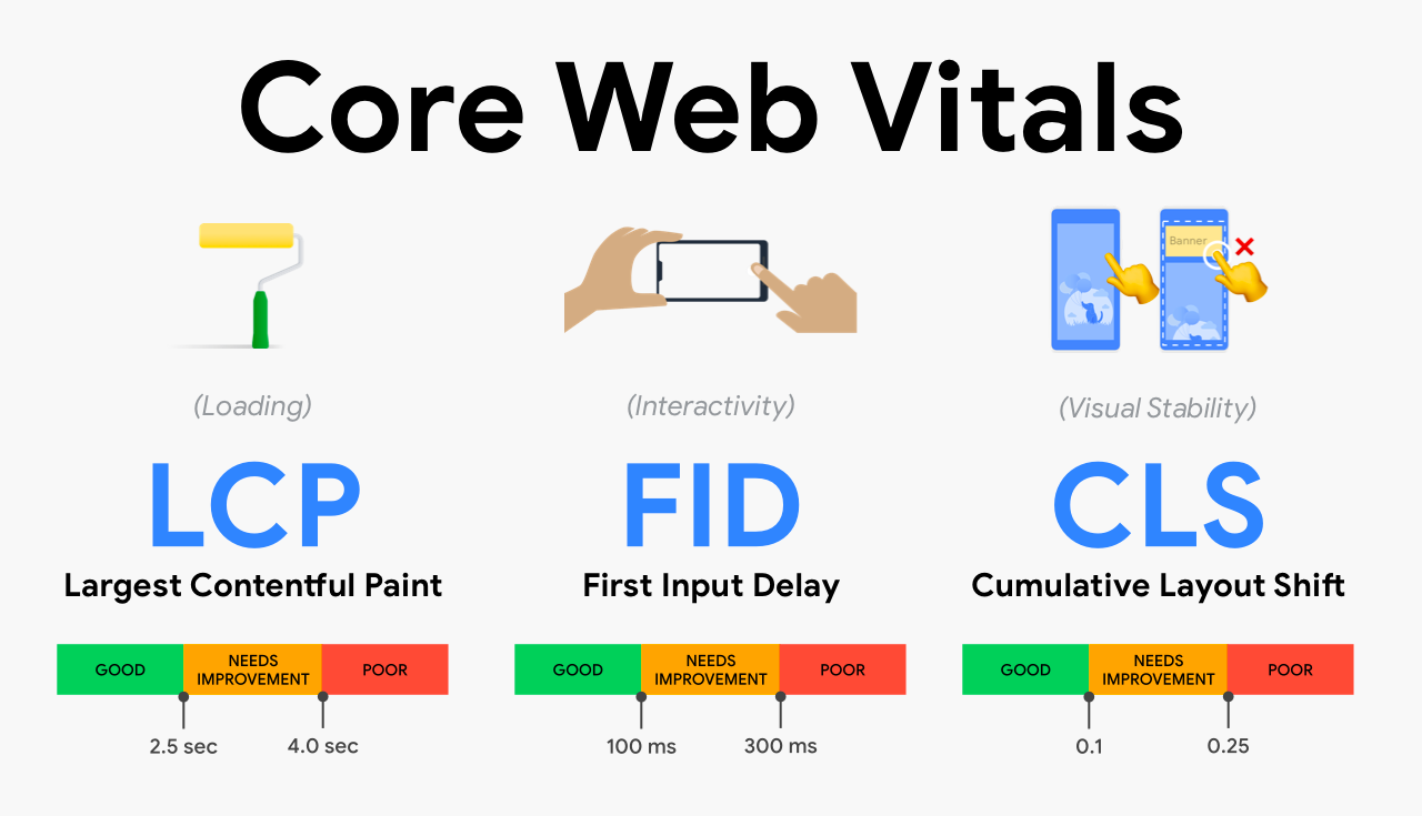
In an era where visitors expect instant gratification and content on-demand, every millisecond counts. If you’re a web application developer, it’s an excellent time to be in this line of business, but with great power comes great responsibility. You’re tasked with creating an experience that is not only intuitive and delightful but also quick, reactive and responsive – sometimes with the two sides being at odds with each other. To add to this, if your business completely runs on the internet (say ecommerce), then your site’s Core Web Vitals could make or break your bottom line.
You don’t just need fast – you need magic fast. For the past two years, Cloudflare Pages has been serving up performant applications for users across the globe, but this week, we’re showing off our brand new, lightning fast architecture, decreasing the TTFB by up to 10X when serving assets.
And while a magician never reveals their secrets, this trick is too good to keep to ourselves. For all our application builders, we’re thrilled to share the juicy technical details on how we adopted Workers for Platforms — our extension of Workers to build SaaS businesses on top of — to make Pages one of the fastest ways to serve your sites.
The problem
When we launched Pages in 2021, we didn’t anticipate the exponential growth we would experience for our platform in the months and years to come. As our users began to adopt Pages into their development workflows, usage of our platform began to skyrocket. However, while riding the high of Pages’ success, we began to notice a problem – a rather large one. As projects grew in size, with every deployment came a pinch more latency, slowly affecting the end users visiting the Pages site. Customers with tens of thousands of deployments were at risk of introducing latency to their site – a problem that needed to be solved.
Before we dive into our technical solution, let’s first explore further the setup of Pages and the relationship between number of deployments and the observed latency.
How could this be?
Built on top of Cloudflare Workers, Pages serves static assets through a highly optimised Worker. We refer to this as the Asset Server Worker.
Users can also add dynamic content through Pages Functions which eventually get compiled into a separate Worker. Every single Pages deployment corresponds to unique instances of these Workers composed in a pipeline.
When a request hits Cloudflare we need to look up which pipeline to execute. As you’d expect, this is a function of the hostname in the URL.
If a user requested https://2b469e16.example.pages.dev/index.html, the hostname is 2b469e16.example.pages.dev which is unique across all deployments on Pages — 2b469e16 is typically the commit hash and example in this case refers to the name of the project.
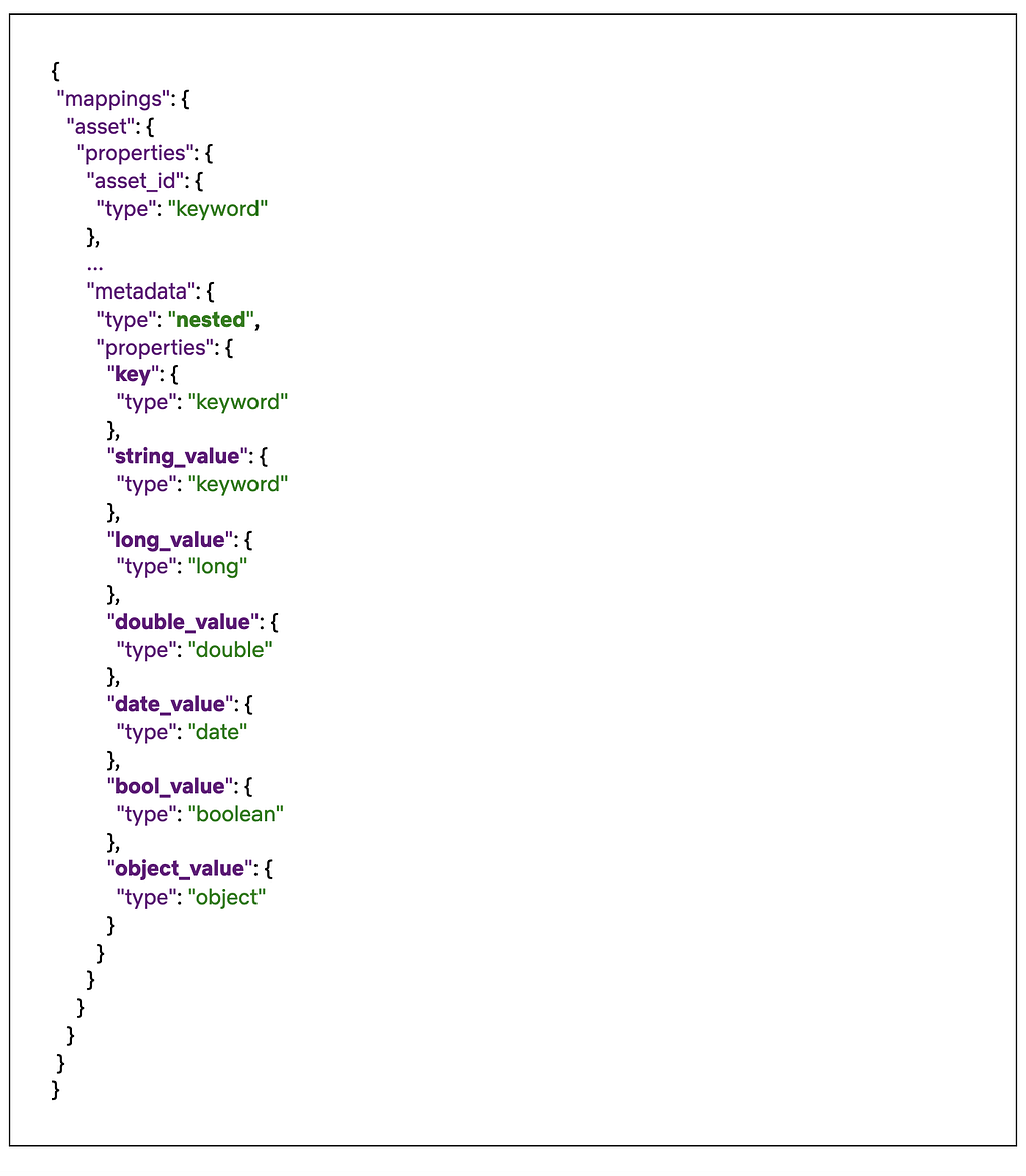
Every Pages project has its own routing table which is used to look up the pipeline to execute. The routing table happens to be a JSON object with a list of regexes for possible paths in that project (in our case, one for every deployment) and their corresponding pipelines.
The script_hash in the example below refers to the pipeline identifier. Naming is hard indeed.
{
 "filters": [
   {
     "pattern": "^(?:2b469e16.example.pages.dev(?:[:][0-9]+)?\\/(?<p1>.*))$",
     "script_hash": "..."
   },
   {
     "pattern": "^(?:example.pages.dev(?:[:][0-9]+)?\\/(?<p1>.*))$",
     "script_hash": "..."
   },
   {
     "pattern": "^(?:test.example.com(?:[:][0-9]+)?\\/(?<p1>.*))$",
     "script_hash": "..."
   }
 ],
 "v": 1
}
So to look up the pipeline in question, we would: download this JSON object from Quicksilver, parse it, and then iterate through this until it finds a regex that matches the current request.
Unsurprisingly, this is expensive. Let’s take a look at a quick real world example to see how expensive.
In one realistic case, it took us 107ms just to parse the JSON. The larger the JSON object gets, the more compute it takes to parse it — with tens of thousands of deployments (not unusual for very active projects that deploy immutable preview deployments for every git commit), this JSON could be several megabytes in size!
It doesn’t end there though. After parsing this, it took 29ms to then iterate and test several regexes to find the one that matched the current request.
To summarise, every single request to this project would take 136ms to just pick the right pipeline to execute. While this was the median case for projects with 10,000 deployments on average, we’ve seen projects with seconds in added latency making them unusable after 50,000 deployments, punishing users for using our platform.
Given most web sites load more than one asset for a page, this leads to timeouts and breakage leading to an unstable and unacceptable user experience.
The secret sauce is Workers for Platforms
We launched Workers for Platforms last year as a way to build ambitious platforms on top of Workers. Workers for Platforms lets one build complex pipelines where a request may be served by a Worker built and maintained by you but could then dispatch to a Worker written by a user of your platform. This allows your platform’s users to write their own Worker like they’ve been used to but while you control how and when they are executed.
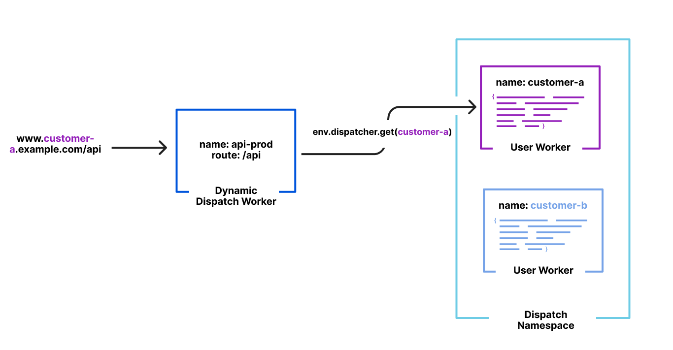
This isn’t very different from what we do with Pages. Users write their Pages functions which compile into a Worker. Users also upload their own static assets which are then bound to our special Asset Server Worker in unique pipelines for each of their deployments. And we control how and when which Worker gets executed based on a hostname in their URL.
Runtime lookups shouldn’t be O(n) though but O(1). Because Workers for Platforms was designed to build entire platforms on top of, lookups when trying to dispatch to a user’s Worker were designed as O(1) ensuring latency wasn’t a function of number of Workers in an account.
The solution
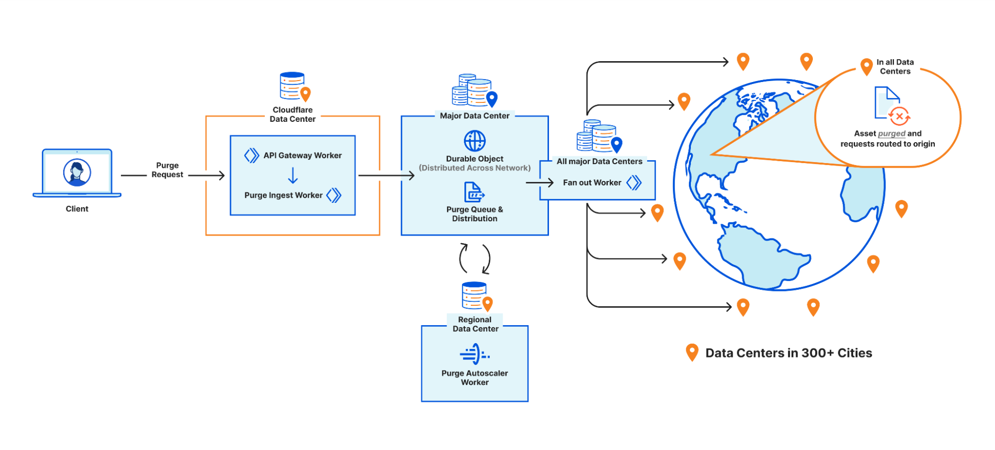
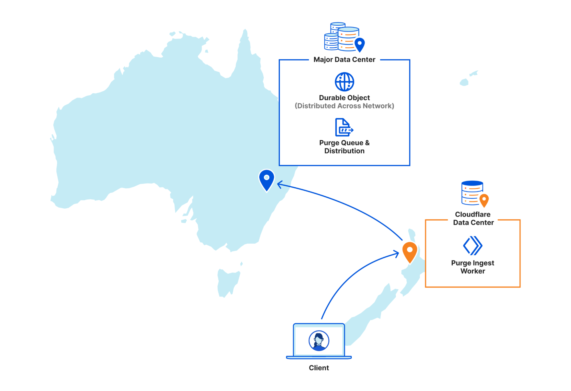
By default, Workers for Platforms hashes the name of the Worker with a secret and uses that for lookups at runtime. However, because we need to dispatch by hostname, we had a different idea. At deployment time, we could hash the pipeline for the deployment by its hostname — 2b469e16.example.pages.dev, for example.
When a request comes in, we hash the hostname from the URL with our predefined secret and then use that value to look up the pipeline to execute. This entirely removes the necessity to fetch, parse and traverse the routing table JSON from before, now making our lookup O(1).
Once we were happy with our new setup from internal testing we wanted to onboard a real user. Our Developer Docs have been running on Pages since the start of 2022 and during that time, we’ve dogfooded many different features and experiments. Due to the great relationship between our two teams and them being a sizable customer of ours we wanted to bring them onto our new Workers for Platform routing.
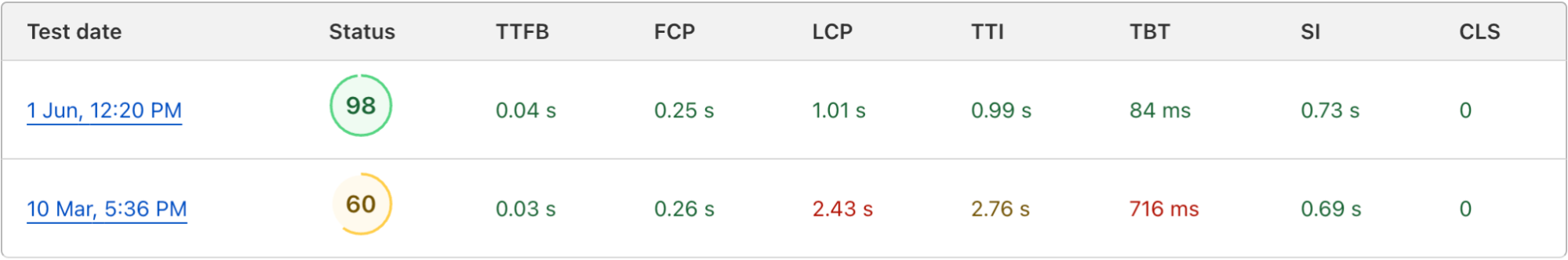
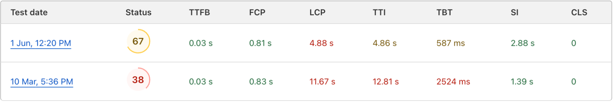
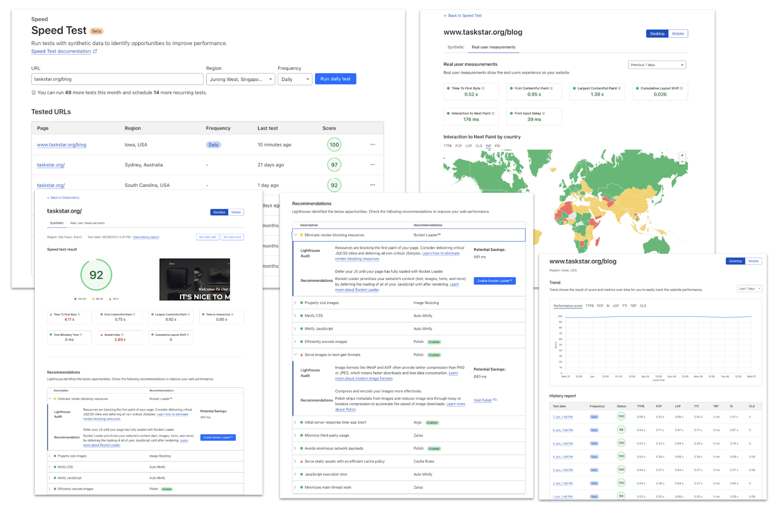
Before opting them in, TTFB was averaging at about 600ms.
After opting them in, TTFB is now 60ms. Web Analytics shows a noticeable drop in entire page load time as a result.
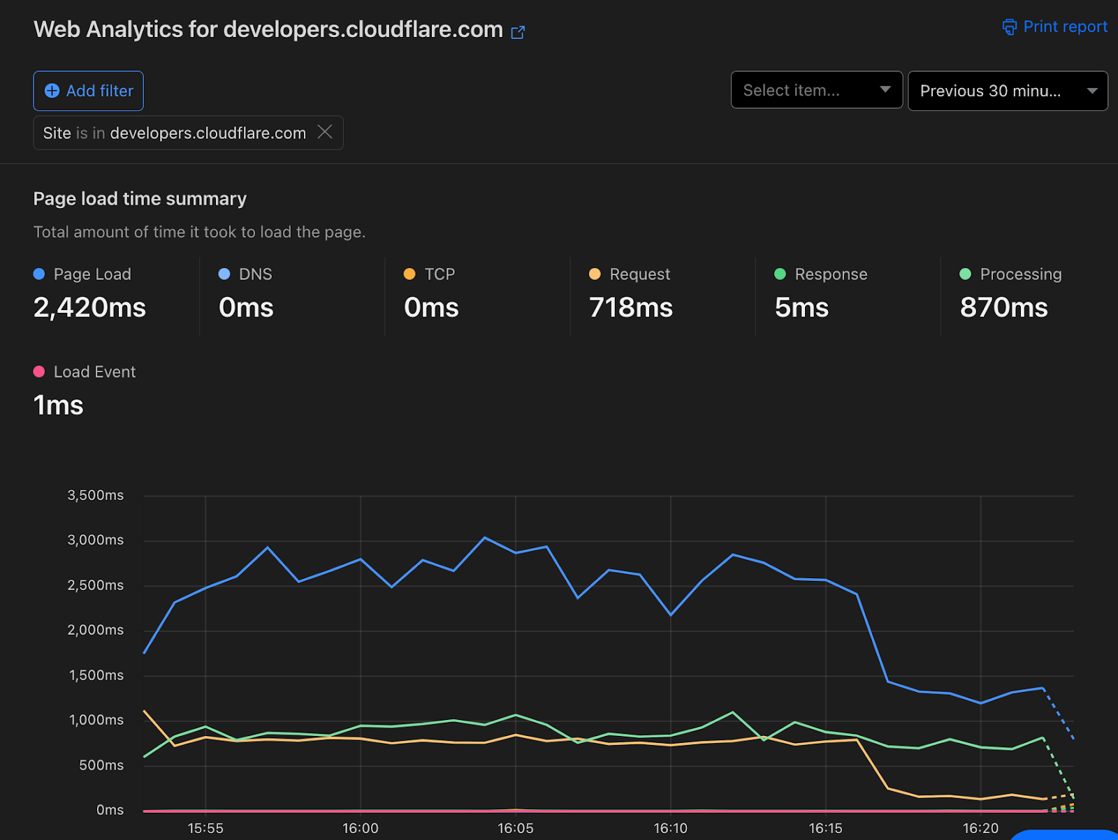
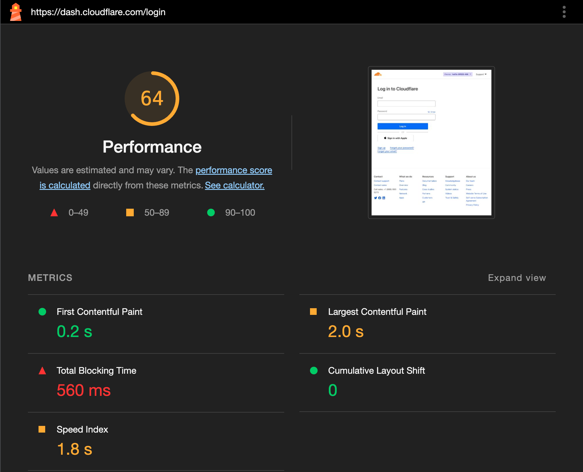
This improvement was also visible through Lighthouse scores now approaching a perfect score of 100 instead of 78 which was the average we saw previously.
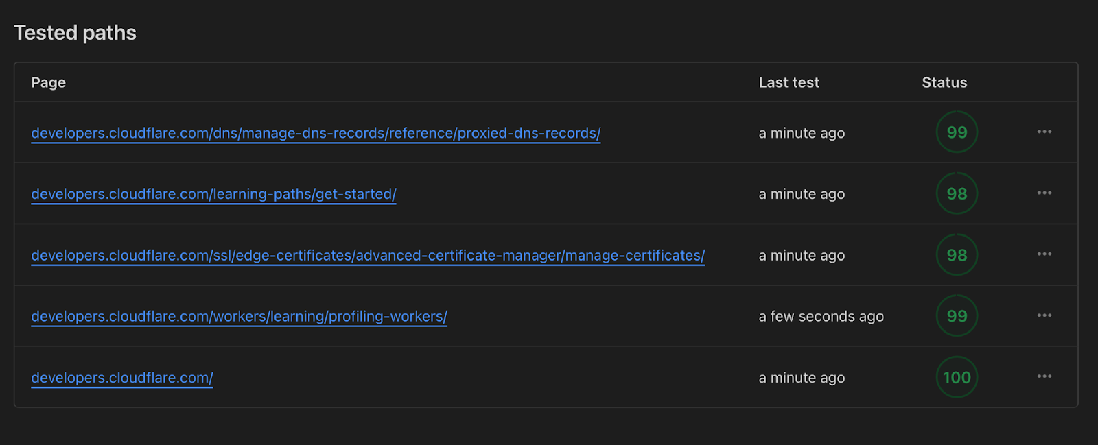
The team was ecstatic about this especially given all of this happened under the hood with no downtime or required engineering team on their end. Not only is https://developers.cloudflare.com/ faster, we’re using less compute to serve it to all of you.
The big migration
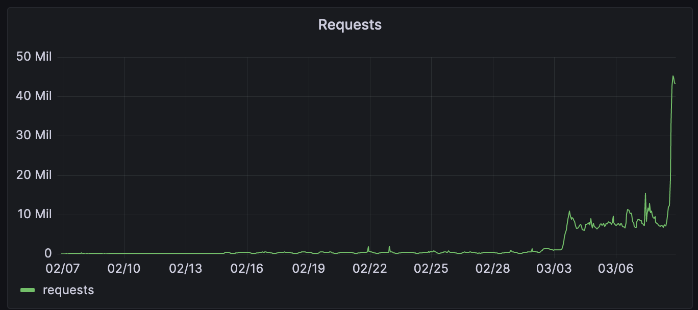
Migrating developers.cloudflare.com was a big milestone for us and meant our new infrastructure was capable of handling traffic at scale. But a goal we were very certain of was migrating every Pages deployment ever created. We didn’t want to leave any users behind.
Turns out, that wasn’t a small number. There’d been over 14 million deployments so far over the years. This was about to be one of the biggest migrations we’d done to runtime assets and the risk was that we’d take down someone’s site.
We approached this migration with some key goals:
- Customer impact in terms of downtime was a no go, all of this needed to happen under the hood without anyone’s site being affected;
- We needed the ability to A/B test the old and new setup so we could revert on a per site basis if something went wrong or was incompatible;
- Migrations at this scale have the ability to cause incidents because they exceed the typical request capacity of our APIs in a short window so they need to run slowly;
- Because this was likely to be a long running migration, we needed the ability to look at metrics and retry failures.
The first step to all of this was to add the ability to A/B test between the legacy setup and the new one. To ensure we could A/B between the legacy setup and new one at any time, we needed to deploy both a regular pipeline (and updated routing table) and new Workers for Platforms hashed one for every deployment.
We also added a feature flag that allowed us to route to either the legacy setup or the new one per site or per data centre with the ability to explicitly opt out a site when an edgecase didn’t work.
With this setup, we started running our long running migration behind the scenes that duplicated every single deployment to the new Workers for Platforms enabled pipelines.
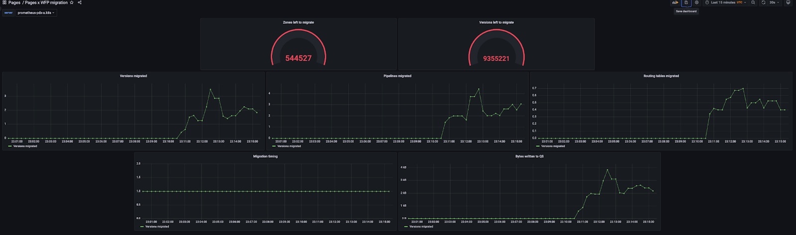
Duplicating them instead of replacing them meant that risk was low and A/B would be possible with the tradeoff of more cleanup after we finished but we picked that with reliability for users in mind.
A few days in after all 14 million deployments had finished migrating over, we started rollout to the new infrastructure with a percentage based rollout. This was a great way for us to find issues and ensure we were ready to serve all runtime traffic for Pages without the risk of an incident.
Feeding three birds with one scone
Alongside the significant latency improvements for Pages projects, this change also gave improvements in other areas:
- Lower CPU usage – Since we no longer need to parse a huge JSON blob and do potentially thousands of regex matches, we saved a nice amount of CPU time across thousands of machines across our data centres.
- Higher LRU hit rate – We have LRU caches for things we fetch from Quicksilver this is to reduce load on Quicksilver and improve performance. However, with the large routing tables we had previously, we could easily fill up this cache with one or just a few routing tables. Now that we have turned this into tiny single entry JSONs, we have improved the cache hit rate for all Workers.
- Quicksilver storage reduction – We also reduced the storage we take up with our routing tables by 92%. This is a reduction of approximately 12 GiB on each of our hundreds of data centres.
We’re just getting started
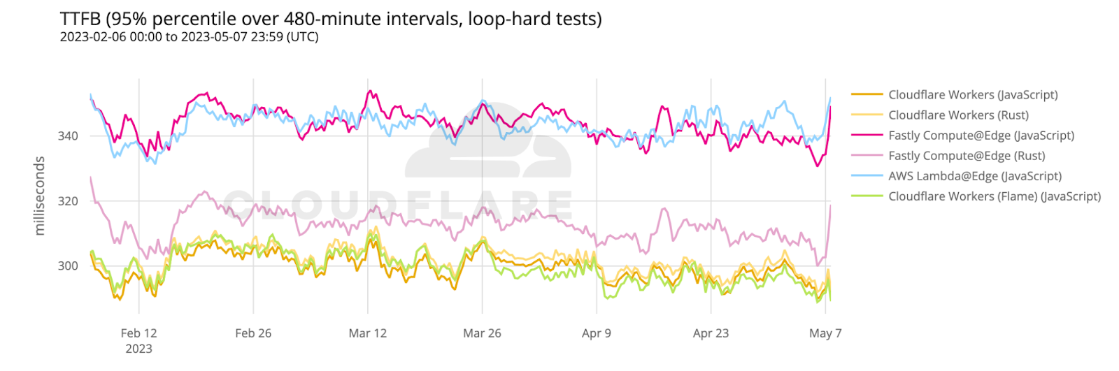
Pages is now the fastest way to serve your sites across Netlify, Vercel and many others and we’re so proud.
But it’s going to get even faster. With projects like Flame, we can’t wait to shave off many more milliseconds to every request a user makes to your site.
To a faster web for all of us.


 Sekar Srinivasan is a Sr. Specialist Solutions Architect at AWS focused on Big Data and Analytics. Sekar has over 20 years of experience working with data. He is passionate about helping customers build scalable solutions modernizing their architecture and generating insights from their data. In his spare time he likes to work on non-profit projects, especially those focused on underprivileged Children’s education.
 Prabu Ravichandran is a Senior Data Architect with Amazon Web Services, focussed on Analytics, data Lake architecture and implementation. He helps customers architect and build scalable and robust solutions using AWS services. In his free time, Prabu enjoys traveling and spending time with family.