Zabbix is an open-source monitoring tool designed to oversee multiple IT infrastructure components, including networks, servers, virtual machines, and cloud services. It operates using both agent-based and agentless monitoring methods. Agents can be installed on monitored devices to collect performance data and report back to a centralized Zabbix server.
Zabbix provides comprehensive integration capabilities for monitoring VMware environments, including ESXi hypervisors, vCenter servers, and virtual machines (VMs). This integration allows administrators to effectively track performance metrics and resource usage across their VMware infrastructure.
In this post, I will show you how to set up Zabbix monitoring with a VMware vSphere infrastructure.
Table of Contents
Requirements:
Zabbix server
Access to the VMware vCenter Server
Step one: Create a Zabbix service user in the vCenter
First things first, let’s create a service user on the vCenter that will be used by the Zabbix server to collect data. To make life easier, in my lab setup the user [email protected] will have full Administrator privileges. Read-only permissions should be enough, however.
1. In the vSphere Client, choose Menu -> Administration -> Users and Groups. From the Users tab, select Domain vsphere.local, and click the ADD button to add a new user.
2. Type a username and password. Click ADD to create a new user.
3. Change the tab to Groups and select the Administrators group.
4. Find a new user zabbix, click on it and save. The user is added to the Administrators group.
5. From the Host and Clusters view, choose vCenter name and go to the Permissions tab. Click the Add button.
6. Choose a proper domain (vsphere.local), find the user zabbix, set the role to Administrator, and check Propagate to children. Click OK to give those permissions.
Step two: Make changes on the Zabbix server
Next, we need to edit zabbix_server.conf. In this file we need to enable the vmware collector process. It’s necessary to start VMware monitoring. FYI, I have installed Zabbix server in version 7.0.4.
1. Edit a configuration file zabbix_server.conf
vim /etc/zabbix/zabbix_server.conf
2. Find the StartVMwareCollectors parameter, delete “#” before it and change the value from 0 to at least 2. Save the file and exit.
Except for StartVMwareCollectors which is mandatory, it’s possible to enable and modify additional VMware parameters. You can find more details about them HERE. VMwareCacheSize VMwareFrequency VMwarePerfFrequency VMwareTimeout
3. Restart the zabbix-server service.
systemctl restart zabbix-server
Step three: Configure the VMware template on Zabbix
1.Log in to the Zabbix server via GUI – http://zabbix_server/zabbix. Go to the Hosts section under the Monitoring tab.
2. Create a new “Host.” Click Create Host in the right upper corner.
3. In the Host tab provide the following details:
Host name – type the name of the system that we want to monitor – here it is VMware Infrastructure. Templates – type/find template name “VMware”, more info about VMware template you can find HERE. Host groups – find/type “VMware(new)” host group.
At this point, go to the Macros tab.
4. In the Macros tab you need to provide 3 values/macros. These macros describes data that is needed to connect Zabbix to the VMware vCenter:
{$VMWARE.URL} – VMware service (vCenter or ESXi hypervisor) SDK URL (https://servername/sdk) that we want to connect. {$VMWARE.USERNAME} – VMware service username created in the 1 section. {$VMWARE.PASSWORD} – VMware service user password created in the 1 section.
Click the Add button.
5. A new Host was created and data collection is in progress.
6. Depending on the size of the infrastructure, data collection takes different amounts of time. Once configured, Zabbix will automatically discover VMs and begin collecting performance data. You can find an overview of the latest data in the Dashboard screen.
7. More specific and detailed data can be found in Latest data under the Monitoring tab.
In Host groups or Hosts choose the name of the item you are looking for (you can also click the “Select” button). Select the name of the ESXi host, the virtual machine, the vCenter name, the datastore, or all VMware information.
Zabbix can collect multiple metrics from VMware using its built-in templates. These metrics include:
– CPU usage
– Memory consumption
– Disk I/O statistics
– Network traffic
– Datastore capacity
In conclusion
Integrating Zabbix with VMware provides a robust solution for monitoring virtualized environments and enhancing visibility into system performance and resource utilization, while enabling timely alerts and responses to operational issues.
When Baselime joined Cloudflare in April 2024, our architecture had evolved to hundreds of AWS Lambda functions, dozens of databases, and just as many queues. We were drowning in complexity and our cloud costs were growing fast. We are now building Baselime and Workers Observability on Cloudflare and will save over 80% on our cloud compute bill. The estimated potential Cloudflare costs are for Baselime, which remains a stand-alone offering, and the estimate is based on the Workers Paid plan. Not only did we achieve huge cost savings, we also simplified our architecture and improved overall latency, scalability, and reliability.
Daily Cost
Before (AWS)
After (Cloudflare)
Compute
$650 – AWS Lambda
$25 – Cloudflare Workers
CDN
$140 – Cloudfront
$0 – Free
Data Stream + Analytics database
$1,150 – Kinesis Data Stream + EC2
$300 – Workers Analytics Engine
Total
$1,940
$325 (83% cost reduction)
Table 1: Daily Costs Comparison ($USD)
When we joined Cloudflare, we immediately saw a surge in usage, and within the first week following the announcement, we were processing over a billion events daily and our weekly active users tripled.
As the platform grew, so did the challenges of managing real-time observability with new scalability, reliability, and cost considerations. This drove us to rebuild Baselime on the Cloudflare Developer Platform, where we could innovate quickly while reducing operational overhead.
Initial architecture — all on AWS
Our initial architecture was all on Amazon Web Services (AWS). We’ll focus here on the data pipeline, which covers ingestion, processing, and storage of tens of billions of events daily.
This pipeline was built on top of AWS Lambda, Cloudfront, Kinesis, EC2, DynamoDB, ECS, and ElastiCache.
Figure1: Initial data pipeline architecture
The key elements are:
Data receptors: Responsible for receiving telemetry data from multiple sources, including OpenTelemetry, Cloudflare Logpush, CloudWatch, Vercel, etc. They cover validation, authentication, and transforming data from each source into a common internal format. The data receptors were deployed either on AWS Lambda (using function URLs and Cloudfront) or ECS Fargate depending on the data source.
Kinesis Data Stream: Responsible for transporting the data from the receptors to the next step: data processing.
Processor: A single AWS Lambda function responsible for enriching and transforming the data for storage. It also performed real-time error tracking and detecting patterns in logs.
ClickHouse cluster: All the telemetry data was ultimately indexed and stored in a self-hosted ClickHouse cluster on EC2.
In addition to these key elements, the existing stack also included orchestration with Firehose, S3 buckets, SQS, DynamoDB and RDS for error handling, retries, and storing metadata.
While this architecture served us well in the early days, it started to show major cracks as we scaled our solution to more and larger customers.
Handling retries at the interface between the data receptors and the Kinesis Data Stream was complex, requiring introducing and orchestrating Firehose, S3 buckets, SQS, and another Lambda function.
Self-hosting ClickHouse also introduced major challenges at scale, as we continuously had to plan our capacity and update our setup to keep pace with our growing user base whilst attempting to maintain control over costs.
Costs began scaling unpredictably with our growing workloads, especially in AWS Lambda, Kinesis, and EC2, but also in less obvious ways, such as in Cloudfront (required for a custom domain in front of Lambda function URLs) and DynamoDB. Specifically, the time spent on I/O operations in AWS Lambda was a particularly costly piece. At every step, from the data receptors to the ClickHouse cluster, moving data to the next stage required waiting for a network request to complete, accounting for over 70% of wall time in the Lambda function.
In a nutshell, we were continuously paged by our alerts, innovating at a slower pace, and our costs were out of control.
Additionally, the entire solution was deployed in a single AWS region: eu-west-1. As a result, all developers located outside continental Europe were experiencing high latency when emitting logs and traces to Baselime.
Modern architecture — transitioning to Cloudflare
The shift to the Cloudflare Developer Platform enabled us to rethink our architecture to be exceptionally fast, globally distributed, and highly scalable, without compromising on cost, complexity, or agility. This new architecture is built on top of Cloudflare primitives.
Figure 2: Modern data pipeline architecture
Cloudflare Workers: the core of Baselime
Cloudflare Workers are now at the core of everything we do. All the data receptors and the processor run in Workers. Workers minimize cold-start times and are deployed globally by default. As such, developers always experience lower latency when emitting events to Baselime.
Additionally, we heavily use JavaScript-native RPC for data transfer between steps of the pipeline. It’s low-latency, lightweight, and simplifies communication between components. This further simplifies our architecture, as separate components behave more as functions within the same process, rather than completely separate applications.
Code Block 1: Simplified data receptor using JavaScript-native RPC to execute the processor.
Workers also expose a Rate Limiting binding that enables us to automatically add rate limiting to our services, which we previously had to build ourselves using a combination of DynamoDB and ElastiCache.
Moreover, we heavily use ctx.waitUntil within our Worker invocations, to offload data transformation outside the request / response path. This further reduces the latency of calls developers make to our data receptors.
Durable Objects: stateful data processing
Durable Objects is a unique service within the Cloudflare Developer Platform, as it enables building stateful applications in a serverless environment. We use Durable Objects in the data pipelines for both real-time error tracking and detecting log patterns.
For instance, to track errors in real-time, we create a durable object for each new type of error, and this durable object is responsible for keeping track of the frequency of the error, when to notify customers, and the notification channels for the error. This implementation with a single building block removes the need for ElastiCache, Kinesis, and multiple Lambda functions to coordinate protecting the RDS database from being overwhelmed by a high frequency error.
Durable Objects gives us precise control over consistency and concurrency of managing state in the data pipeline.
In addition to the data pipeline, we use Durable Objects for alerting. Our previous architecture required orchestrating EventBridge Scheduler, SQS, DynamoDB and multiple AWS Lambda functions, whereas with Durable Objects, everything is handled within the alarm handler.
Workers Analytics Engine: high-cardinality analytics at scale
Though managing our own ClickHouse cluster was technically interesting and challenging, it took us away from building the best observability developer experience. With this migration, more of our time is spent enhancing our product and none is spent managing server instances.
Workers Analytics Engine lets us synchronously write events to a scalable high-cardinality analytics database. We built on top of the same technology that powers Workers Analytics Engine. We also made internal changes to Workers Analytics Engine to natively enable high dimensionality in addition to high cardinality.
Moreover, Workers Analytics Engine and our solution leverages Cloudflare’s ABR analytics. ABR stands for Adaptive Bit Rate, and enables us to store telemetry data in multiple tables with varying resolutions, from 100% to 0.0001% of the data. Querying the table with 0.0001% of the data will be several orders of magnitudes faster than the table with all the data, with a corresponding trade-off in accuracy. As such, when a query is sent to our systems, Workers Analytics Engine dynamically selects the most appropriate table to run the query, optimizing both query time and accuracy. Users always get the most accurate result with optimal query time, regardless of the size of their dataset or the timeframe of the query. Compared to our previous system, which was always running queries on the full dataset, the new system now delivers faster queries across our entire user base and use cases.
In addition to these core services (Workers, Durable Objects, Workers Analytics Engine), the new architecture leverages other building blocks from the Cloudflare Developer Platform. Queues for asynchronous messaging, decoupling services and enabling an event-driven architecture; D1 as our main database for transactional data (queries, alerts, dashboards, configurations, etc.); Workers KV for fast distributed storage; Hono for all our APIs, etc.
How did we migrate?
Baselime is built on an event-driven architecture, where every user action triggers an event. It operates on the principle that every user action is recorded as an event and emitted to the rest of the system — whether it’s creating a user, editing a dashboard, or performing any other action. Migrating to Cloudflare involved transitioning our event-driven architecture without compromising uptime and data consistency. Previously, this was powered by AWS EventBridge and SQS, and we moved entirely to Cloudflare Queues.
We followed the strangler fig pattern to incrementally migrate the solution from AWS to Cloudflare. It consists of gradually replacing specific parts of the system with newer services, with minimal disruption to the system. Early in the process, we created a central Cloudflare Queue which acted as the backbone for all transactional event processing during the migration. Every event, whether a new user signup or a dashboard edit, was funneled into this Queue. From there, events were dynamically routed, each event to the relevant part of the application. User actions were synced into D1 and KV, ensuring that all user actions were mirrored across both AWS and Cloudflare during the transition.
This syncing mechanism enabled us to maintain consistency and ensure that no data was lost as users continued to interact with Baselime.
Here’s an example of how events are processed:
export default {
  async queue(batch, env) {
    for (const message of batch.messages) {
      try {
        const event = message.body;
        switch (event.type) {
          case "WORKSPACE_CREATED":
            await workspaceHandler.create(env, event.data);
            break;
          case "QUERY_CREATED":
            await queryHandler.create(env, event.data);
            break;
          case "QUERY_DELETED":
            await queryHandler.remove(env, event.data);
            break;
          case "DASHBOARD_CREATED":
            await dashboardHandler.create(env, event.data);
            break;
          //
          // Many more events...
          //
          default:
            logger.info("Matched no events", { type: event.type });
        }
        message.ack();
      } catch (e) {
        if (message.attempts < 3) {
          message.retry({ delaySeconds: Math.ceil(30 ** message.attempts / 10), });
        } else {
          logger.error("Failed handling event - No more retrys", { event: message.body, attempts: message.attempts }, e);
        }
      }
    }
  },
} satisfies ExportedHandler<Env, InternalEvent>;
Code Block 2: Simplified internal events processing during migration.
We migrated the data pipeline from AWS to Cloudflare with an outside-in method: we started with the data receptors and incrementally moved the data processor and the ClickHouse cluster to the new architecture. We began writing telemetry data (logs, metrics, traces, wide-events, etc.) to both ClickHouse (in AWS) and to Workers Analytics Engine simultaneously for the duration of the retention period (30 days).
The final step was rewriting all of our endpoints, previously hosted on AWS Lambda and ECS containers, into Cloudflare Workers. Once those Workers were ready, we simply switched the DNS records to point to the Workers instead of the existing Lambda functions.
Despite the complexity, the entire migration process, from the data pipeline to all re-writing API endpoints, took our then team of 3 engineers less than three months.
We ended up saving over 80% on our cloud bill
Savings on the data receptors
After switching the data receptors from AWS to Cloudflare in early June 2024, our AWS Lambda cost was reduced by over 85%. These costs were primarily driven by I/O time the receptors spent sending data to a Kinesis Data Stream in the same region.
Figure 4: Baselime daily AWS Lambda cost [note: the gap in data is the result of AWS Cost Explorer losing data when the parent organization of the cloud accounts was changed.]
Moreover, we used Cloudfront to enable custom domains pointing to the data receptors. When we migrated the data receptors to Cloudflare, there was no need for Cloudfront anymore. As such, our Cloudfront cost was reduced to $0.
Figure 5: Baselime daily Cloudfront cost [note: the gap in data is the result of AWS Cost Explorer losing data when the parent organization of the cloud accounts was changed.]
If we were a regular Cloudflare customer, we estimate that our daily Cloudflare Workers bill would be around \$25 after the switch, against \$790 on AWS: over 95% cost reduction. These savings are primarily driven by the Workers pricing model, since Workers charge for CPU time, and the receptors are primarily just moving data, and as such, are mostly I/O bound.
Savings on the ClickHouse cluster
To evaluate the cost impact of switching from self-hosting ClickHouse to using Workers Analytics Engine, we need to take into account not only the EC2 instances, but also the disk space, networking, and the Kinesis Data Stream cost.
We completed this switch in late August, achieving over 95% cost reduction in both the Kinesis Data Stream and all EC2 related costs.
Figure 6: Baselime daily Kinesis Data Stream cost [note: the gap in data is the result of AWS Cost Explorer losing data when the parent organization of the cloud accounts was changed.]
Figure 7: Baselime daily EC2 cost [note: the gap in data is the result of AWS Cost Explorer losing data when the parent organization of the cloud accounts was changed.]
If we were a regular Cloudflare customer, we estimate that our daily Workers Analytics Engine cost would be around \$300 after the switch, compared to \$1150 on AWS, a cost reduction of over 70%.
Not only did we significantly reduce costs by migrating to Cloudflare, but we also improved performance across the board. Responses to users are now faster, with real-time event ingestion happening across Cloudflare’s network, closer to our users. Responses to users querying their data are also much faster, thanks to Cloudflare’s deep expertise in operating ClickHouse at scale.
Most importantly, we’re no longer bound by limitations in throughput or scale. We launched Workers Logs on September 26, 2024, and our system now handles a much higher volume of events than before, with no sacrifices in speed or reliability.
These cost savings are outstanding as is, and do not include the total cost of ownership of those systems. We significantly simplified our systems and our codebase, as the platform is taking care of more for us. We’re paged less, we spend less time monitoring infrastructure, and we can focus on delivering product improvements.
Conclusion
Migrating Baselime to Cloudflare has transformed how we build and scale our platform. With Workers, Durable Objects, Workers Analytics Engine, and other services, we now run a fully serverless, globally distributed system that’s more cost-efficient and agile. This shift has significantly reduced our operational overhead and enabled us to iterate faster, delivering better observability tooling to our users.
You can start observing your Cloudflare Workers today with Workers Logs. Looking ahead, we’re excited about the features we will deliver directly in the Cloudflare Dashboard, including real-time error tracking, alerting, and a query builder for high-cardinality and dimensionality events. All coming by early 2025.
At Netflix, the Analytics and Developer Experience organization, part of the Data Platform, offers a product called Workbench. Workbench is a remote development workspace based on Titus that allows data practitioners to work with big data and machine learning use cases at scale. A common use case for Workbench is running JupyterLab Notebooks.
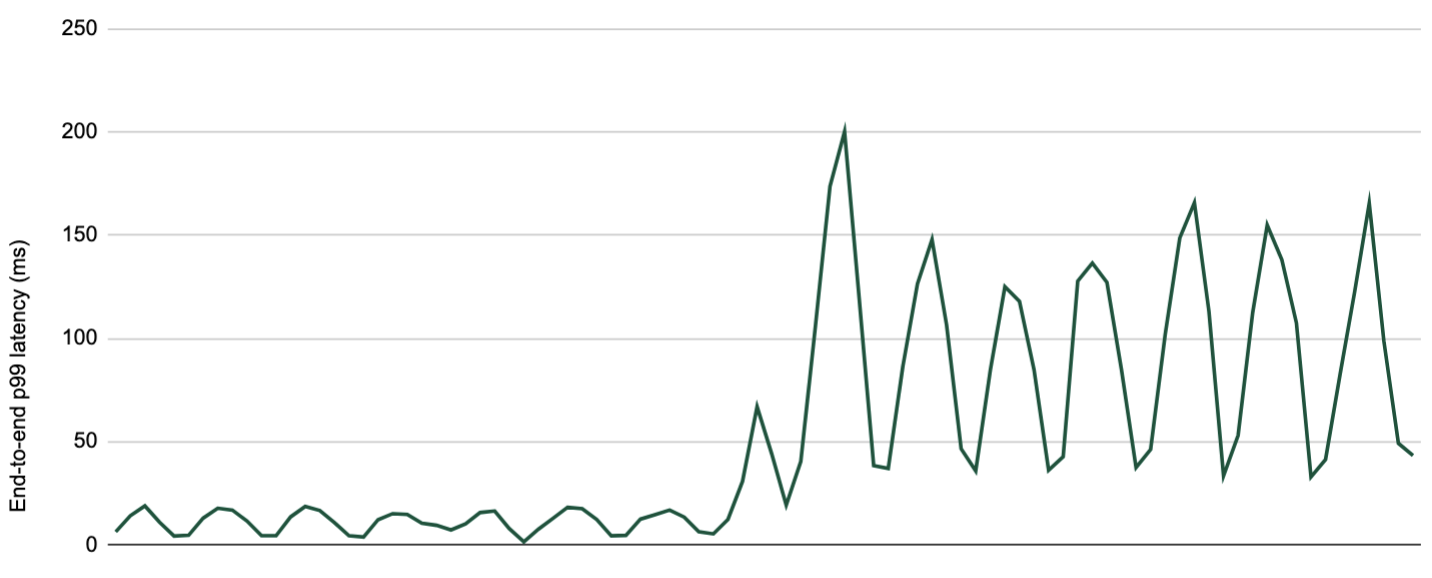
Recently, several users reported that their JupyterLab UI becomes slow and unresponsive when running certain notebooks. This document details the intriguing process of debugging this issue, all the way from the UI down to the Linux kernel.
Symptom
Machine Learning engineer Luca Pozzi reported to our Data Platform team that their JupyterLab UI on their workbench becomes slow and unresponsive when running some of their Notebooks. Restarting the ipykernel process, which runs the Notebook, might temporarily alleviate the problem, but the frustration persists as more notebooks are run.
Quantify the Slowness
While we observed the issue firsthand, the term “UI being slow” is subjective and difficult to measure. To investigate this issue, we needed a quantitative analysis of the slowness.
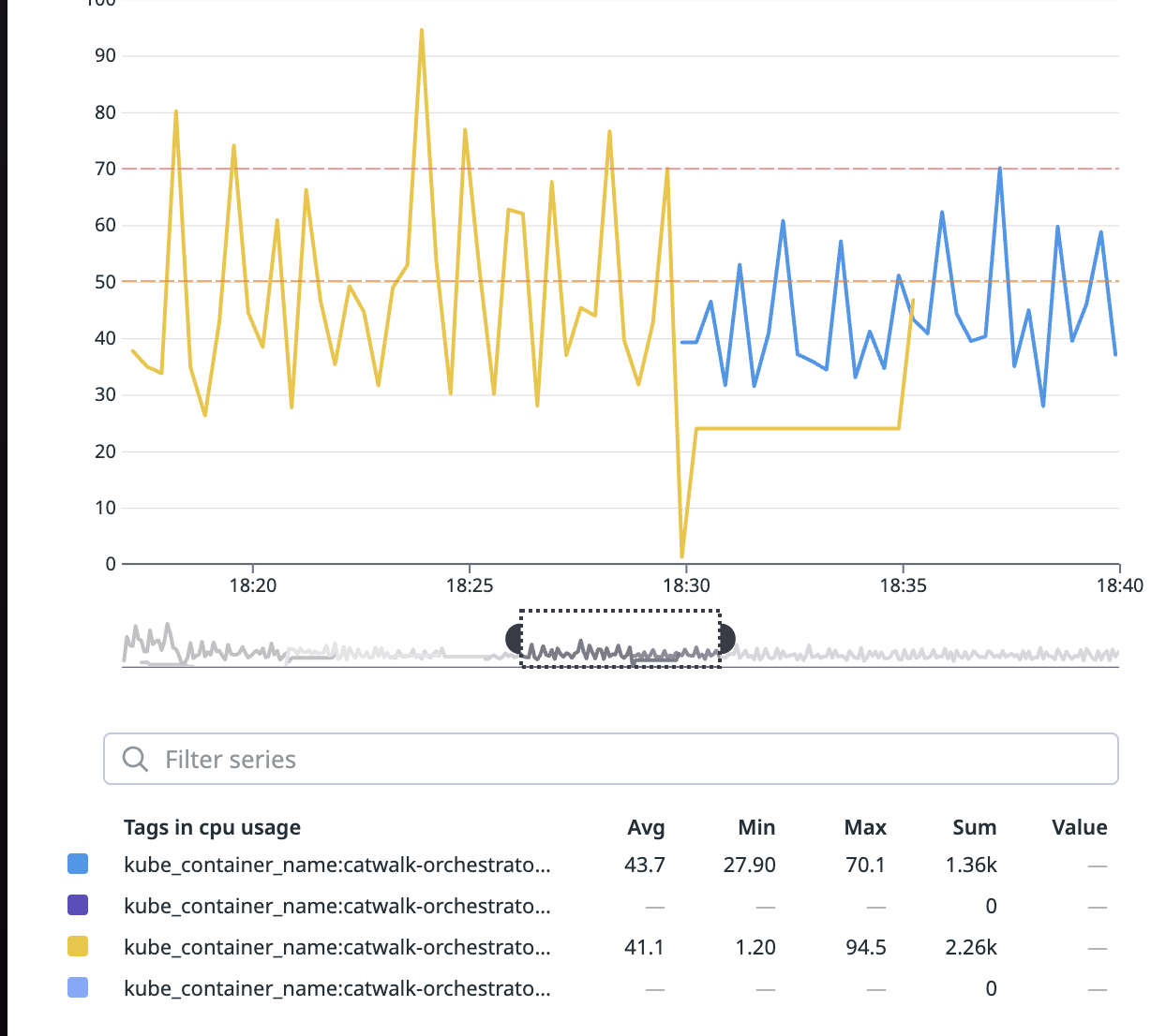
Itay Dafna devised an effective and simple method to quantify the UI slowness. Specifically, we opened a terminal via JupyterLab and held down a key (e.g., “j”) for 15 seconds while running the user’s notebook. The input to stdin is sent to the backend (i.e., JupyterLab) via a WebSocket, and the output to stdout is sent back from the backend and displayed on the UI. We then exported the .har file recording all communications from the browser and loaded it into a Notebook for analysis.
Using this approach, we observed latencies ranging from 1 to 10 seconds, averaging 7.4 seconds.
Blame The Notebook
Now that we have an objective metric for the slowness, let’s officially start our investigation. If you have read the symptom carefully, you must have noticed that the slowness only occurs when the user runs certain notebooks but not others.
Therefore, the first step is scrutinizing the specific Notebook experiencing the issue. Why does the UI always slow down after running this particular Notebook? Naturally, you would think that there must be something wrong with the code running in it.
Upon closely examining the user’s Notebook, we noticed a library called pystan , which provides Python bindings to a native C++ library called stan, looked suspicious. Specifically, pystan uses asyncio. However, because there is already an existing asyncio event loop running in the Notebook process and asyncio cannot be nested by design, in order for pystan to work, the authors of pystanrecommend injecting pystan into the existing event loop by using a package called nest_asyncio, a library that became unmaintained because the author unfortunately passed away.
Given this seemingly hacky usage, we naturally suspected that the events injected by pystan into the event loop were blocking the handling of the WebSocket messages used to communicate with the JupyterLab UI. This reasoning sounds very plausible. However, the user claimed that there were cases when a Notebook not using pystan runs, the UI also became slow.
Moreover, after several rounds of discussion with ChatGPT, we learned more about the architecture and realized that, in theory, the usage of pystan and nest_asyncio should not cause the slowness in handling the UI WebSocket for the following reasons:
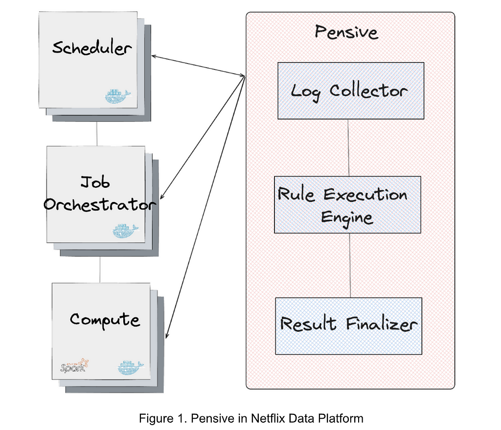
Even though pystan uses nest_asyncio to inject itself into the main event loop, the Notebook runs on a child process (i.e., the ipykernel process) of the jupyter-lab server process, which means the main event loop being injected by pystan is that of the ipykernel process, not the jupyter-server process. Therefore, even if pystan blocks the event loop, it shouldn’t impact the jupyter-lab main event loop that is used for UI websocket communication. See the diagram below:
In other words, pystan events are injected to the event loop B in this diagram instead of event loop A. So, it shouldn’t block the UI WebSocket events.
You might also think that because event loop A handles both the WebSocket events from the UI and the ZeroMQ socket events from the ipykernel process, a high volume of ZeroMQ events generated by the notebook could block the WebSocket. However, when we captured packets on the ZeroMQ socket while reproducing the issue, we didn’t observe heavy traffic on this socket that could cause such blocking.
A stronger piece of evidence to rule out pystan was that we were ultimately able to reproduce the issue even without it, which I’ll dive into later.
Blame Noisy Neighbors
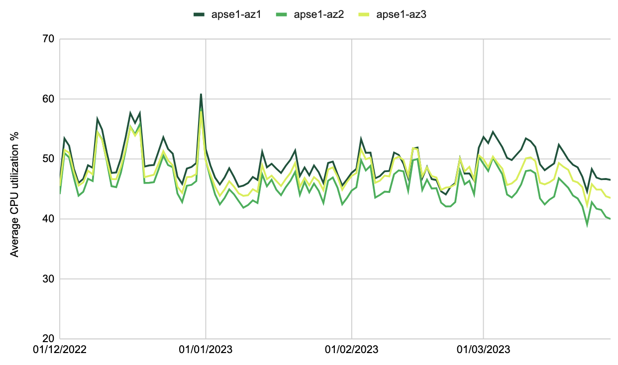
The Workbench instance runs as a Titus container. To efficiently utilize our compute resources, Titus employs a CPU oversubscription feature, meaning the combined virtual CPUs allocated to containers exceed the number of available physical CPUs on a Titus agent. If a container is unfortunate enough to be scheduled alongside other “noisy” containers — those that consume a lot of CPU resources — it could suffer from CPU deficiency.
However, after examining the CPU utilization of neighboring containers on the same Titus agent as the Workbench instance, as well as the overall CPU utilization of the Titus agent, we quickly ruled out this hypothesis. Using the top command on the Workbench, we observed that when running the Notebook, the Workbench instance uses only 4 out of the 64 CPUs allocated to it. Simply put, this workload is not CPU-bound.
Blame The Network
The next theory was that the network between the web browser UI (on the laptop) and the JupyterLab server was slow. To investigate, we captured all the packets between the laptop and the server while running the Notebook and continuously pressing ‘j’ in the terminal.
When the UI experienced delays, we observed a 5-second pause in packet transmission from server port 8888 to the laptop. Meanwhile, traffic from other ports, such as port 22 for SSH, remained unaffected. This led us to conclude that the pause was caused by the application running on port 8888 (i.e., the JupyterLab process) rather than the network.
The Minimal Reproduction
As previously mentioned, another strong piece of evidence proving the innocence of pystan was that we could reproduce the issue without it. By gradually stripping down the “bad” Notebook, we eventually arrived at a minimal snippet of code that reproduces the issue without any third-party dependencies or complex logic:
import time
import os
from multiprocessing import Process

N = os.cpu_count()

def launch_worker(worker_id):
  time.sleep(60)

if __name__ == '__main__':
  with open('/root/2GB_file', 'r') as file:
    data = file.read()
    processes = []
    for i in range(N):
      p = Process(target=launch_worker, args=(i,))
      processes.append(p)
      p.start()

    for p in processes:
      p.join()
The code does only two things:
Read a 2GB file into memory (the Workbench instance has 480G memory in total so this memory usage is almost negligible).
Start N processes where N is the number of CPUs. The N processes do nothing but sleep.
There is no doubt that this is the most silly piece of code I’ve ever written. It is neither CPU bound nor memory bound. Yet it can cause the JupyterLab UI to stall for as many as 10 seconds!
Questions
There are a couple of interesting observations that raise several questions:
We noticed that both steps are required in order to reproduce the issue. If you don’t read the 2GB file (that is not even used!), the issue is not reproducible. Why using 2GB out of 480GB memory could impact the performance?
When the UI delay occurs, the jupyter-lab process CPU utilization spikes to 100%, hinting at contention on the single-threaded event loop in this process (event loop A in the diagram before). What does the jupyter-lab process need the CPU for, given that it is not the process that runs the Notebook?
The code runs in a Notebook, which means it runs in the ipykernel process, that is a child process of the jupyter-lab process. How can anything that happens in a child process cause the parent process to have CPU contention?
The workbench has 64CPUs. But when we printed os.cpu_count(), the output was 96. That means the code starts more processes than the number of CPUs. Why is that?
Let’s answer the last question first. In fact, if you run lscpu and nproc commands inside a Titus container, you will also see different results — the former gives you 96, which is the number of physical CPUs on the Titus agent, whereas the latter gives you 64, which is the number of virtual CPUs allocated to the container. This discrepancy is due to the lack of a “CPU namespace” in the Linux kernel, causing the number of physical CPUs to be leaked to the container when calling certain functions to get the CPU count. The assumption here is that Python os.cpu_count() uses the same function as the lscpu command, causing it to get the CPU count of the host instead of the container. Python 3.13 has a new call that can be used to get the accurate CPU count, but it’s not GA’ed yet.
It will be proven later that this inaccurate number of CPUs can be a contributing factor to the slowness.
More Clues
Next, we used py-spy to do a profiling of the jupyter-lab process. Note that we profiled the parent jupyter-lab process, not the ipykernel child process that runs the reproduction code. The profiling result is as follows:
As one can see, a lot of CPU time (89%!!) is spent on a function called __parse_smaps_rollup. In comparison, the terminal handler used only 0.47% CPU time. From the stack trace, we see that this function is inside the event loop A, so it can definitely cause the UI WebSocket events to be delayed.
The stack trace also shows that this function is ultimately called by a function used by a Jupyter lab extension called jupyter_resource_usage. We then disabled this extension and restarted the jupyter-lab process. As you may have guessed, we could no longer reproduce the slowness!
But our puzzle is not solved yet. Why does this extension cause the UI to slow down? Let’s keep digging.
Root Cause Analysis
From the name of the extension and the names of the other functions it calls, we can infer that this extension is used to get resources such as CPU and memory usage information. Examining the code, we see that this function call stack is triggered when an API endpoint /metrics/v1 is called from the UI. The UI apparently calls this function periodically, according to the network traffic tab in Chrome’s Developer Tools.
Now let’s look at the implementation starting from the call get(jupter_resource_usage/api.py:42) . The full code is here and the key lines are shown below:
for p in all_processes: info = p.memory_full_info()
Basically, it gets all children processes of the jupyter-lab process recursively, including both the ipykernel Notebook process and all processes created by the Notebook. Obviously, the cost of this function is linear to the number of all children processes. In the reproduction code, we create 96 processes. So here we will have at least 96 (sleep processes) + 1 (ipykernel process) + 1 (jupyter-lab process) = 98 processes when it should actually be 64 (allocated CPUs) + 1 (ipykernel process) + 1 (jupyter-lab process) = 66 processes, because the number of CPUs allocated to the container is, in fact, 64.
This is truly ironic. The more CPUs we have, the slower we are!
At this point, we have answered one question: Why does starting many grandchildren processes in the child process cause the parent process to be slow? Because the parent process runs a function that’s linear to the number all children process recursively.
However, this solves only half of the puzzle. If you remember the previous analysis, starting many child processes ALONE doesn’t reproduce the issue. If we don’t read the 2GB file, even if we create 2x more processes, we can’t reproduce the slowness.
So now we must answer the next question: Why does reading a 2GB file in the child process affect the parent process performance, especially when the workbench has as much as 480GB memory in total?
To answer this question, let’s look closely at the function __parse_smaps_rollup. As the name implies, this function parses the file /proc/<pid>/smaps_rollup.
def _parse_smaps_rollup(self):
  uss = pss = swap = 0
  with open_binary("{}/{}/smaps_rollup".format(self._procfs_path, self.pid)) as f:
  for line in f:
    if line.startswith(b”Private_”):
    # Private_Clean, Private_Dirty, Private_Hugetlb
      s uss += int(line.split()[1]) * 1024
    elif line.startswith(b”Pss:”):
      pss = int(line.split()[1]) * 1024
    elif line.startswith(b”Swap:”):
      swap = int(line.split()[1]) * 1024
return (uss, pss, swap)
Naturally, you might think that when memory usage increases, this file becomes larger in size, causing the function to take longer to parse. Unfortunately, this is not the answer because:
Second, this is a special file in the /proc filesystem, which should be seen as a kernel interface instead of a regular file on disk. In other words, I/O operations of this file are handled by the kernel rather than disk.
This file was introduced in this commit in 2017, with the purpose of improving the performance of user programs that determine aggregate memory statistics. Let’s first focus on the handler of open syscall on this /proc/<pid>/smaps_rollup.
Following through the single_openfunction, we will find that it uses the function show_smaps_rollup for the show operation, which can translate to the read system call on the file. Next, we look at the show_smaps_rollupimplementation. You will notice a do-while loop that is linear to the virtual memory area.
This perfectly explains why the function gets slower when a 2GB file is read into memory. Because the handler of reading the smaps_rollup file now takes longer to run the while loop. Basically, even though smaps_rollup already improved the performance of getting memory information compared to the old method of parsing the /proc/<pid>/smaps file, it is still linear to the virtual memory used.
More Quantitative Analysis
Even though at this point the puzzle is solved, let’s conduct a more quantitative analysis. How much is the time difference when reading the smaps_rollup file with small versus large virtual memory utilization? Let’s write some simple benchmark code like below:
import os

def read_smaps_rollup(pid):
  with open("/proc/{}/smaps_rollup".format(pid), "rb") as f:
    for line in f:
      pass

if __name__ == “__main__”:
  pid = os.getpid()

  read_smaps_rollup(pid)

  with open(“/root/2G_file”, “rb”) as f:
    data = f.read()

  read_smaps_rollup(pid)
This program performs the following steps:
Reads the smaps_rollup file of the current process.
Reads a 2GB file into memory.
Repeats step 1.
We then use strace to find the accurate time of reading the smaps_rollup file.
As you can see, both times, the read syscall returned 670, meaning the file size remained the same at 670 bytes. However, the time it took the second time (i.e., 0.027698 seconds) is 100x the time it took the first time (i.e., 0.000259 seconds)! This means that if there are 98 processes, the time spent on reading this file alone will be 98 * 0.027698 = 2.7 seconds! Such a delay can significantly affect the UI experience.
Solution
This extension is used to display the CPU and memory usage of the notebook process on the bar at the bottom of the Notebook:
We confirmed with the user that disabling the jupyter-resource-usage extension meets their requirements for UI responsiveness, and that this extension is not critical to their use case. Therefore, we provided a way for them to disable the extension.
Summary
This was such a challenging issue that required debugging from the UI all the way down to the Linux kernel. It is fascinating that the problem is linear to both the number of CPUs and the virtual memory size — two dimensions that are generally viewed separately.
Overall, we hope you enjoyed the irony of:
The extension used to monitor CPU usage causing CPU contention.
An interesting case where the more CPUs you have, the slower you get!
If you’re excited by tackling such technical challenges and have the opportunity to solve complex technical challenges and drive innovation, consider joining our Data Platform teams. Be part of shaping the future of Data Security and Infrastructure, Data Developer Experience, Analytics Infrastructure and Enablement, and more. Explore the impact you can make with us!
Amazon Redshift enables you to efficiently query and retrieve structured and semi-structured data from open format files in Amazon S3 data lake without having to load the data into Amazon Redshift tables. Amazon Redshift extends SQL capabilities to your data lake, enabling you to run analytical queries. Amazon Redshift supports a wide variety of tabular data formats like CSV, JSON, Parquet, ORC and open tabular formats like Apache Hudi, Linux foundation Delta Lake and Apache Iceberg.
You create Redshift external tables by defining the structure for your files, S3 location of the files and registering them as tables in an external data catalog. The external data catalog can be AWS Glue Data Catalog, the data catalog that comes with Amazon Athena, or your own Apache Hive metastore.
Over the last year, Amazon Redshift added several performance optimizations for data lake queries across multiple areas of query engine such as rewrite, planning, scan execution and consuming AWS Glue Data Catalog column statistics. To get the best performance on data lake queries with Redshift, you can use AWS Glue Data Catalog’s column statistics feature to collect statistics on Data Lake tables. For Amazon Redshift Serverless instances, you will see improved scan performance through increased parallel processing of S3 files and this happens automatically based on RPUs used.
In this post, we highlight the performance improvements we observed using industry standard TPC-DS benchmarks. Overall execution time of TPC-DS 3 TB benchmark improved by 3x. Some of the queries in our benchmark experienced up to 12x speed up.
Performance Improvements
Several performance optimizations were done over the last year to improve performance of data lake queries including the following.
Consume AWS Glue Data Catalog column statistics and tuning of Redshift optimizer to improve quality of query plans
Utilize bloom filters for partition columns
Improved scan efficiency for Amazon Redshift Serverless instances through increased parallel processing of files
Novel query rewrite rules to merge similar scans
Faster retrieval of metadata from AWS Glue Data Catalog
To understand the performance gains, we tested the performance on the industry-standard TPC-DS benchmark using 3 TB data sets and queries which represents different customer use cases. Performance was tested on a Redshift serverless data warehouse with 128 RPU. In our testing, the dataset was stored in Amazon S3 in Parquet format and AWS Glue Data Catalog was used to manage external databases and tables. Fact tables were partitioned on the date column, and each fact table consisted of approximately 2,000 partitions. All of the tables had their row count table property, numRows, set as per the spectrum query performance guidelines.
We did a baseline run on Redshift patch version (patch 172) from last year. Later, we ran all TPC-DS queries on latest patch version (patch 180) that includes all performance optimizations added over last year. Then we used AWS Glue Data Catalog’s column statistics feature to compute statistics for all the tables and measured improvements with the presence of AWS Glue Data Catalog column statistics.
Our analysis revealed that the TPC-DS 3TB Parquet benchmark saw substantial performance gains with these optimizations. Specifically, partitioned Parquet with our latest optimizations achieved 2x faster runtimes compared to the previous implementation. Enabling AWS Glue Data Catalog column statistics further improved performance by 3x versus last year. The following graph illustrates these runtime improvements for the full benchmark (all TPC-DS queries) over the past year, including the additional boost from using AWS Glue Data Catalog column statistics.
Figure 1: Improvement in total runtime of TPC-DS 3T workload
The following graph presents the top queries from the TPC-DS benchmark with the greatest performance improvement over the last year with and without AWS Glue Data Catalog column statistics. You can see that performance improves a lot when statistics exist on AWS Glue Data Catalog (for details on how to get statistics for your Data Lake tables, please refer to optimizing query performance using AWS Glue Data Catalog column statistics). Specifically, multi-join queries will benefit the most from AWS Glue Data Catalog column statistics because the optimizer uses statistics to choose the right join order and distribution strategy.
Figure 2: Speed-up in TPC-DS queries
Let’s discuss some of the optimizations that contributed to improved query performance.
Optimizing with table-level statistics
Amazon Redshift’s design enables it to handle large-scale data challenges with superior speed and cost-efficiency. Its massively parallel processing (MPP) query engine, AI-powered query optimizer, auto-scaling capabilities, and other advanced features allow Redshift to excel at searching, aggregating, and transforming petabytes of data.
However, even the most powerful systems can experience performance degradation if they encounter anti-patterns like grossly inaccurate table statistics, such as the row count metadata.
Without this crucial metadata, Redshift’s query optimizer may be limited in the number of possible optimizations, especially those related to data distribution during query execution. This can have a significant impact on overall query performance.
To illustrate this, consider the following simple query involving an inner join between a large table with billions of rows and a small table with only a few hundred thousand rows.
select small_table.sellerid, sum(large_table.qtysold)
from large_table, small_table
where large_table.salesid = small_table.listid
 and small_table.listtime > '2023-12-01'
 and large_table.saletime > '2023-12-01'
group by 1 order by 1
If executed as-is, with the large table on the right-hand side of the join, the query will lead to sub-optimal performance. This is because the large table will need to be distributed (broadcast) to all Redshift compute nodes to perform the inner join with the small table, as shown in the following diagram.
Figure 3: Inaccurate table statistics lead to limited optimizations and large amounts of data broadcast among compute nodes for a simple inner join
Now, consider a scenario where the table statistics, such as the row count, are accurate. This allows the Amazon Redshift query optimizer to make more informed decisions, such as determining the optimal join order. In this case, the optimizer would immediately rewrite the query to have the large table on the left-hand side of the inner join, so that it is the small table that is broadcast across the Redshift compute nodes, as illustrated in the following diagram.
Figure 4: Accurate table statistics lead to high degree of optimizations and very little data broadcast among compute nodes for a simple inner join
Fortunately, Amazon Redshift automatically maintains accurate table statistics for local tables by running the ANALYZE command in the background. For external tables (data lake tables), however, AWS Glue Data Catalog column statistics are recommended for use with Amazon Redshift as we will discuss in the next section. For more general information on optimizing queries in Amazon Redshift, please refer to the documentation on factors affecting query performance, data redistribution, and Amazon Redshift best practices for designing queries.
Improvements with AWS Glue Data Catalog column statistics
AWS Glue Data Catalog has a feature to compute column level statistics for Amazon S3 backed external tables. AWS Glue Data Catalog can compute column level statistics such as NDV, Number of Nulls, Min/Max and Avg. column width for the columns without the need for additional data pipelines. Amazon Redshift cost-based optimizer utilizes these statistics to come up with better quality query plans. In addition to consuming statistics, we also made several improvements in cardinality estimations and cost tuning to get high quality query plans thereby improving query performance.
TPC-DS 3TB dataset showed 40% improvement in total query execution time when these AWS Glue Data Catalog column statistics were provided. Individual TPC-DS queries showed up to 5x improvements in query execution time. Some of the queries that had greater impact in execution time are Q85, Q64, Q75, Q78, Q94, Q16, Q04, Q24 and Q11.
We will go through an example where cost-based optimizer generated a better query plan with statistics and how it improved the execution time.
Let’s consider following simpler version of TPC-DS Q64 to showcase the query plan differences with statistics.
select i_product_name product_name
,i_item_sk item_sk
,ad1.ca_street_number b_street_number
,ad1.ca_street_name b_street_name
,ad1.ca_city b_city
,ad1.ca_zip b_zip
,d1.d_year as syear
,count(*) cnt
,sum(ss_wholesale_cost) s1
,sum(ss_list_price) s2
,sum(ss_coupon_amt) s3
FROM   tpcds_3t_alls3_pp_ext.store_sales
,tpcds_3t_alls3_pp_ext.store_returns
,tpcds_3t_alls3_pp_ext.date_dim d1
,tpcds_3t_alls3_pp_ext.customer
,tpcds_3t_alls3_pp_ext.customer_address ad1
,tpcds_3t_alls3_pp_ext.item
WHERE
ss_sold_date_sk = d1.d_date_sk AND
ss_customer_sk = c_customer_sk AND

ss_addr_sk = ad1.ca_address_sk and
ss_item_sk = i_item_sk and
ss_item_sk = sr_item_sk and
ss_ticket_number = sr_ticket_number and
i_color in ('firebrick','papaya','orange','cream','turquoise','deep') and
i_current_price between 42 and 42 + 10 and
i_current_price between 42 + 1 and 42 + 15
group by i_product_name
,i_item_sk
,ad1.ca_street_number
,ad1.ca_street_name
,ad1.ca_city
,ad1.ca_zip
,d1.d_year
Without Statistics
Following figure represents the logical query plan of Q64. You can observe that cardinality estimation of joins is not accurate. With inaccurate cardinalities, optimizer produces a sub-optimal query plan leading to higher execution time.
With Statistics
Following figure represents the logical query plan after consuming AWS Glue Data Catalog column statistics. Based on the highlighted changes, you can observe that the cardinality estimations of JOIN improved by many magnitudes helping the optimizer to choose a better join order and join strategy (broadcast DS_BCAST_INNER vs. distribute DS_DIST_BOTH). Switching the customer_address and customer table from inner to outer table and making join strategies as distribute has major impact because this reduces the data movement between the nodes and avoids spilling from hash table.
Figure 5: Logical query plan of Q64 without statistics
Figure 6: Logical query plan of Q64 after consuming AWS Glue Data Catalog column statistics
This change in query plan improved the query execution time of Q64 from 383s to 81s.
Given the greater benefits with AWS Glue Data Catalog column statistics for the optimizer, you should consider collecting stats for your data lake using AWS Glue. If your workload is a JOIN heavy workload, then collecting stats will show greater improvement on your workload. Refer to generating AWS Glue Data Catalog column statistics for instructions on how to collect statistics in AWS Glue Data Catalog.
Query rewrite optimization
We introduced a new query rewrite rule which combines scalar aggregates over the same common expression using slightly different predicates. This rewrite resulted in performance improvements on TPC-DS queries Q09, Q28, and Q88. Let’s focus on Q09 as a representative of these queries, given by the following fragment:
SELECT CASE
WHEN (SELECT COUNT(*)
FROM store_sales
WHERE ss_quantity BETWEEN 1 AND 20) > 48409437
THEN (SELECT AVG(ss_ext_discount_amt)
FROM store_sales
WHERE ss_quantity BETWEEN 1 AND 20)
ELSE (SELECT AVG(ss_net_profit)
FROM store_sales
WHERE ss_quantity BETWEEN 1 AND 20) END
AS bucket1,
<<4 more variations of the CASE expression above>>
FROM reason
WHERE r_reason_sk = 1
In total, there are 15 scans of the fact table store_sales, each one returning various aggregates over different subsets of data. The engine first performs subquery removal and transforms the various expressions in the CASE statements into relational subtrees connected via cross products, and then they are fused into one subquery handling all scalar aggregates. The resulting plan for Q09, described below using SQL for clarity, is given by:
SELECT CASE WHEN v1 > 48409437 THEN t1 ELSE e1 END,
<4 more variations>
FROM (SELECT COUNT(CASE WHEN b1 THEN 1 END) AS v1,
AVG(CASE WHEN b1 THEN ss_ext_discount_amt END) AS t1,
AVG(CASE WHEN b1 THEN ss_net_profit END) AS e1,
<4 more variations>
FROM reason,
(SELECT *,
ss_quantity BETWEEN 1 AND 20 AS b1,
<4 more variations>
FROM store_sales
WHERE ss_quantity BETWEEN 1 AND 20 OR
<4 more variations>))
WHERE r_reason_sk = 1)
In general, this rewrite rule results in the largest improvements both in latency (from 3x to 8x improvements) and bytes read from Amazon S3 (from 6x to 8x reduction in scanned bytes and, consequently, cost).
Bloom filter for partition columns
Amazon Redshift already uses Bloom filters on data columns of external tables in Amazon S3 to enable early and effective data filtering. Last year, we extended this support for partition columns as well. A Bloom filter is a probabilistic, memory-efficient data structure that accelerates join queries at scale by filtering rows that do not match the join relation, significantly reducing the amount of data transferred over the network. Amazon Redshift automatically determines what queries are suitable for leveraging Bloom filters at query runtime.
This optimization resulted in performance improvements on TPC-DS queries Q05, Q17 and Q54. This optimization resulted in large improvements in both latency (from 2x to 3x improvement) and bytes read from S3 (from 9x to 15x reduction in scanned bytes and, consequently cost).
Following is the subquery of Q05 which showcased improvements with runtime filter.
select s_store_id,
sum(sales_price) as sales,
sum(profit) as profit,
sum(return_amt) as returns,
sum(net_loss) as profit_loss
from
( select  ss_store_sk as store_sk,
ss_sold_date_sk  as date_sk,
ss_ext_sales_price as sales_price,
ss_net_profit as profit,
cast(0 as decimal(7,2)) as return_amt,
cast(0 as decimal(7,2)) as net_loss
from tpcds_3t_alls3_pp_ext.store_sales
union all
select sr_store_sk as store_sk,
sr_returned_date_sk as date_sk,
cast(0 as decimal(7,2)) as sales_price,
cast(0 as decimal(7,2)) as profit,
sr_return_amt as return_amt,
sr_net_loss as net_loss
from tpcds_3t_alls3_pp_ext.store_returns
) salesreturnss,
tpcds_3t_alls3_pp_ext.date_dim,
tpcds_3t_alls3_pp_ext.store
where date_sk = d_date_sk
and d_date between cast('1998-08-13' as date)
and (cast('1998-08-13' as date) +  14)
and store_sk = s_store_sk
group by s_store_id
Without bloom filter support on partition columns
Following figure is the logical query plan for sub-query of Q05. This appends two large fact tables store_sales (8B rows) and store_returns (863M rows) and then joins with very selective dimension tables date_dim and then with dimension table store. You can observe that join with date_dim table reduces the number of rows from 9B to 93M rows.
With bloom filter support on partition columns
With support of bloom filter on partition columns, we now create bloom filter for d_date_sk column of date_dim table and push down the bloom filters to store_sales and store_returns table. These bloom filters help to filter out the partitions in both store_sales and store_returns table because join happens on partition column (number of partitions processed reduces by 10x).
Figure 7: Logical query plan for sub-query of Q05 without bloom filter support on partition columns
Figure 8: Logical query plan for sub-query of Q05 with bloom filter support on partition columns
Overall, bloom filter on partition column will reduce the number of partitions processed resulting in reduced S3 listing calls and lesser number of data files to be read (reduction in scanned bytes). You can see that we only scan 89M rows from store_sales and 4M rows from store_returns because of the bloom filter. This reduced number of rows to process at JOIN level and helped in improving the overall query performance by 2x and scanned bytes by 9x.
Conclusion
In this post, we covered new performance optimizations in Amazon Redshift data lake query processing and how AWS Glue Data Catalog statistics helps to enhance quality of query plans for data lake queries in Amazon Redshift. These optimizations together improved TPC-DS 3 TB benchmark by 3x. Some of the queries in our benchmark benefited up to 12x speed up.
In summary, Amazon Redshift now offers enhanced query performance with optimizations such as AWS Glue Data Catalog column statistics, bloom filters on partition columns, new query rewrite rules and faster retrieval of metadata. These optimizations are enabled by default and Amazon Redshift users will benefit with better query response times for their workloads. For more information, please reach out to your AWS technical account manager or AWS account solutions architect. They will be happy to provide additional guidance and support.
About the authors
Kalaiselvi Kamaraj is a Sr. Software Development Engineer with Amazon. She has worked on several projects within Redshift Query processing team and currently focusing on performance related projects for Redshift Data Lake.
Mark Lyons is a Principal Product Manager on the Amazon Redshift team. He works on the intersection of data lakes and data warehouses. Prior to joining AWS, Mark held product leadership roles with Dremio and Vertica. He is passionate about data analytics and empowering customers to change the world with their data.
Asser Moustafa is a Principal Worldwide Specialist Solutions Architect at AWS, based in Dallas, Texas, USA. He partners with customers worldwide, advising them on all aspects of their data architectures, migrations, and strategic data visions to help organizations adopt cloud-based solutions, maximize the value of their data assets, modernize legacy infrastructures, and implement cutting-edge capabilities like machine learning and advanced analytics. Prior to joining AWS, Asser held various data and analytics leadership roles, completing an MBA from New York University and an MS in Computer Science from Columbia University in New York. He is passionate about empowering organizations to become truly data-driven and unlock the transformative potential of their data.
2024 marks Cloudflare’s 14th birthday. Birthday Week each year is packed with major announcements and the release of innovative new offerings, all focused on giving back to our customers and the broader Internet community. Birthday Week has become a proud tradition at Cloudflare and our culture, to not just stay true to our mission, but to always stay close to our customers. We begin planning for this week of celebration earlier in the year and invite everyone at Cloudflare to participate.
Months before Birthday Week, we invited teams to submit ideas for what to announce. We were flooded with submissions, from proposals for implementing new standards to creating new products for developers. Our biggest challenge is finding space for it all in just one week — there is still so much to build. Good thing we have a birthday to celebrate each year, but we might need an extra day in Birthday Week next year!
In case you missed it, here’s everything we announced during 2024’s Birthday Week:
Customers using Cloudflare to manage DNS can create a whole batch of records, enable proxying on many records, update many records to point to a new target at the same time, or even delete all of their records.
Taking the next step in advancing security with Ephemeral IDs, a new feature that generates a unique short-lived ID, without relying on any network-level information.
Speed Brain, our latest leap forward in speed, uses the Speculation Rules API to prefetch content for users’ likely next navigations — downloading web pages before they navigate to them and making pages load 45% faster.
Instant Purge invalidates cached content in under 150ms, offering the industry’s fastest cache purge with global latency for purges by tags, hostnames, and prefixes.
Next generation servers focused on exceptional performance and security, enhanced support for AI/ML workloads, and significant strides in power efficiency.
More powerful GPUs, expanded model support, enhanced logging and evaluations in AI Gateway, and Vectorize GA with larger index sizes and faster queries.
Persistent and queryable Workers logs, Node.js compatibility GA, improved Next.js support via OpenNext, built-in CI/CD for Workers, Gradual Deployments, Queues, and R2 Event Notifications GA, and more — making building on Cloudflare easier, faster, and more affordable.
Using new optimization techniques such as KV cache compression and speculative decoding, we’ve made large language model (LLM) inference lightning-fast on the Cloudflare Workers AI platform.
We’ve been working on something new — a platform for running containers across Cloudflare’s network. We already use it in production, for AI inference and more.
Extending our AI Assistant capabilities to help you build new WAF rules, added new AI bot and crawler traffic insights to Radar, and new AI bot blocking capabilities.
Our free plan is here to stay, and we reaffirm that commitment this week with 15 releases that make the Free plan even better.
One more thing…
Cloudflare serves millions of customers and their millions of domains across nearly every country on Earth. However, as a global company, the payment landscape can be complex — especially in regions outside of North America. While credit cards are very popular for online purchases in the US, the global picture is quite different. 60% of consumers across EMEA, APAC and LATAM choose alternative payment methods. For instance, European consumers often opt for SEPA Direct Debit, a bank transfer mechanism, while Chinese consumers frequently use Alipay, a digital wallet.
At Cloudflare, we saw this as an opportunity to meet customers where they are. Today, we’re thrilled to announce that we are expanding our payment system and launching a closed beta for a new payment method called Stripe Link. The checkout experience will be faster and more seamless, allowing our self-serve customers to pay using saved bank accounts or cards with Link. Customers who have saved their payment details at any business using Link can quickly check out without having to reenter their payment information.
These are the first steps in our efforts to expand our payment system to support global payment methods used by customers around the world.We’ll be rolling out new payment methods gradually, ensuring a smooth integration and gathering feedback from our customers every step of the way.
Until next year
That’s all for Birthday Week 2024. However, the innovation never stops at Cloudflare. Continue to follow the Cloudflare Blog all year long as we launch more products and features that help build a better Internet.
Speed is a critical factor that dictates Internet behavior. Every additional millisecond a user spends waiting for your web page to load results in them abandoning your website. The old adage remains as true as ever: faster websites result in higher conversion rates. And with such outcomes tied to Internet speed, we believe a faster Internet is a better Internet.
Customers often use Workers KV to provide Workers with key-value data for configuration, routing, personalization, experimentation, or serving assets. Many of Cloudflare’s own products rely on KV for just this purpose: Pages stores static assets, Access stores authentication credentials, AI Gateway stores routing configuration, and Images stores configuration and assets, among others. So KV’s speed affects the latency of every request to an application, throughout the entire lifecycle of a user session.
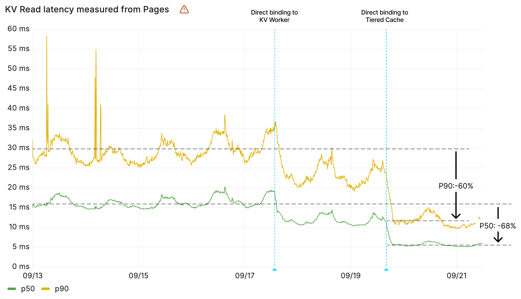
Today, we’re announcing up to 3x faster KV hot reads, with all KV operations faster by up to 20ms. And we want to pull back the curtain and show you how we did it.
Workers KV read latency (ms) by percentile measured from Pages
Optimizing Workers KV’s architecture to minimize latency
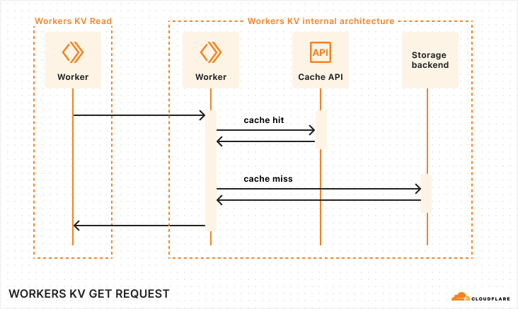
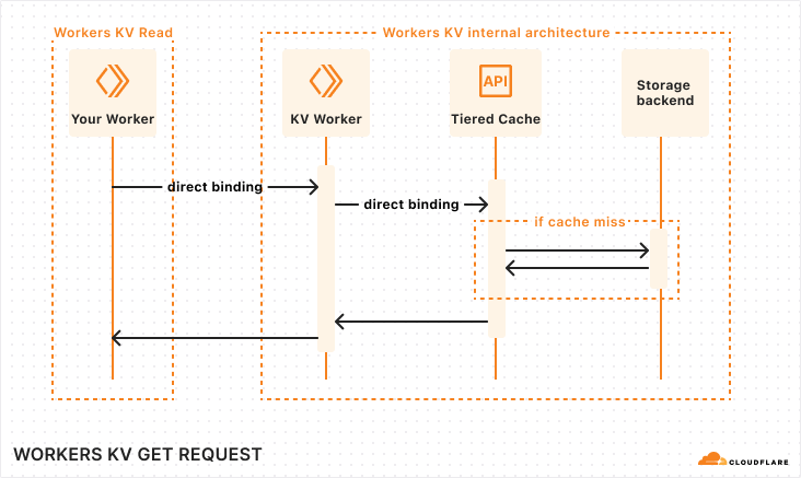
At a high level, Workers KV is itself a Worker that makes requests to central storage backends, with many layers in between to properly cache and route requests across Cloudflare’s network. You can rely on Workers KV to support operations made by your Workers at any scale, and KV’s architecture will seamlessly handle your required throughput.
Sequence diagram of a Workers KV operation
When your Worker makes a read operation to Workers KV, your Worker establishes a network connection within its Cloudflare region to KV’s Worker. The KV Worker then accesses the Cache API, and in the event of a cache miss, retrieves the value from the storage backends.
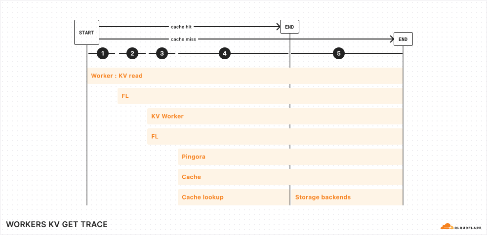
Let’s look one level deeper at a simplified trace:
Simplified trace of a Workers KV operation
From the top, here are the operations completed for a KV read operation from your Worker:
Your Worker makes a connection to Cloudflare’s network in the same data center. This incurs ~5 ms of network latency.
Upon entering Cloudflare’s network, a service called Front Line (FL) is used to process the request. This incurs ~10 ms of operational latency.
FL proxies the request to the KV Worker. The KV Worker does a cache lookup for the key being accessed. This, once again, passes through the Front Line layer, incurring an additional ~10 ms of operational latency.
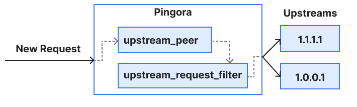
Cache is stored in various backends within each region of Cloudflare’s network. A service built upon Pingora, our open-sourced Rust framework for proxying HTTP requests, routes the cache lookup to the proper cache backend.
Finally, if the cache lookup is successful, the KV read operation is resolved. Otherwise, the request reaches our storage backends, where it gets its value.
Looking at these flame graphs, it became apparent that a major opportunity presented itself to us: reducing the FL overhead (or eliminating it altogether) and reducing the cache misses across the Cloudflare network would reduce the latency for KV operations.
Bypassing FL layers between Workers and services to save ~20ms
A request from your Worker to KV doesn’t need to go through FL. Much of FL’s responsibility is to process and route requests from outside of Cloudflare — that’s more than is needed to handle a request from the KV binding to the KV Worker. So we skipped the Front Line altogether in both layers.
Reducing latency in a Workers KV operation by removing FL layers
To bypass the FL layer from the KV binding in your Worker, we modified the KV binding to connect directly to the KV Worker within the same Cloudflare location. Within the Workers host, we configured a C++ subpipeline to allow code from bindings to establish a direct connection with the proper routing configuration and authorization loaded.
The KV Worker also passes through the FL layer on its way to our internal Pingora service. In this case, we were able to use an internal Worker binding that allows Workers for Cloudflare services to bind directly to non-Worker services within Cloudflare’s network. With this fix, the KV Worker sets the proper cache control headers and establishes its connection to Pingora without leaving the network.
Together, both of these changes reduced latency by ~20 ms for every KV operation.
Implementing tiered cache to minimize requests to storage backends
We also optimized KV’s architecture to reduce the amount of requests that need to reach our centralized storage backends. These storage backends are further away and incur network latency, so improving the cache hit rate in regions close to your Workers significantly improves read latency.
Workers KV uses Tiered Cache to resolve operations closer to your users
To accomplish this, we used Tiered Cache, and implemented a cache topology that is fine-tuned to the usage patterns of KV. With a tiered cache, requests to KV’s storage backends are cached in regional tiers in addition to local (lower) tiers. With this architecture, KV operations that may be cache misses locally may be resolved regionally, which is especially significant if you have traffic across an entire region spanning multiple Cloudflare data centers.
This significantly reduced the amount of requests that needed to hit the storage backends, with ~30% of requests resolved in tiered cache instead of storage backends.
KV’s new architecture
As a result of these optimizations, KV operations are now simplified:
When you read from KV in your Worker, the KV binding binds directly to KV’s Worker, saving 10 ms.
The KV Worker binds directly to the Tiered Cache service, saving another 10 ms.
Tiered Cache is used in front of storage backends, to resolve local cache misses regionally, closer to your users.
Sequence diagram of KV operations with new architecture
In aggregate, these changes significantly reduced KV’s latency.
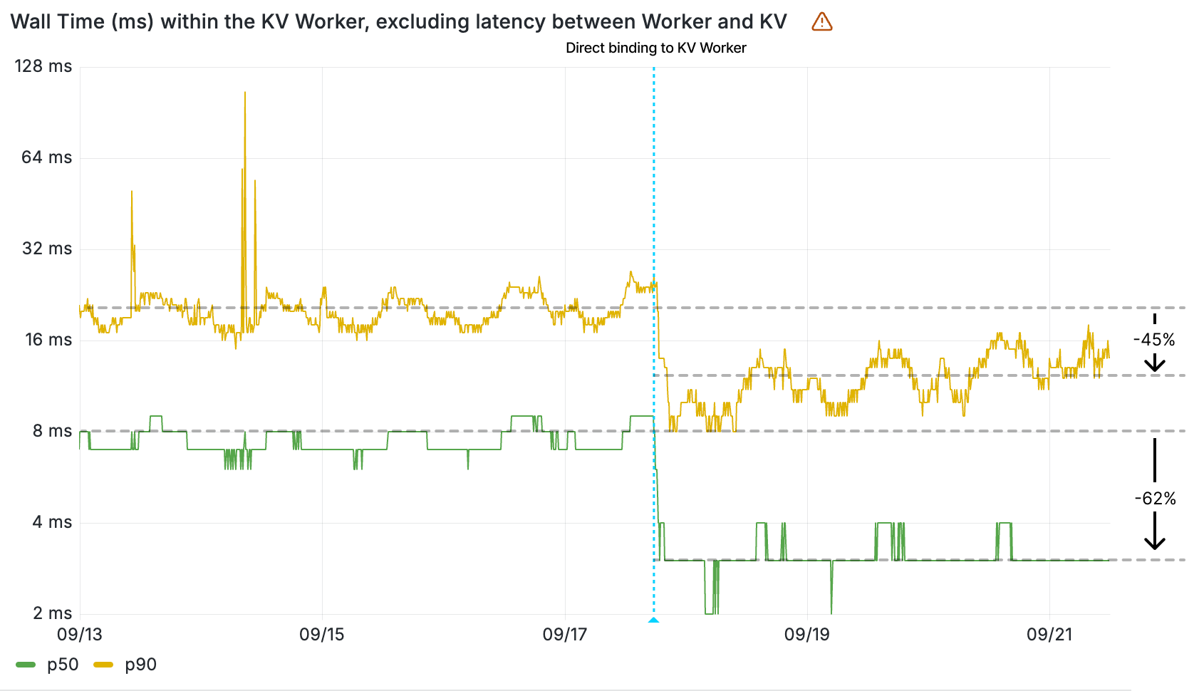
The impact of the direct binding to cache is clearly seen in the wall time of the KV Worker, given this value measures the duration of a retrieval of a key-value pair from cache. The 90th percentile of all KV Worker invocations now resolve in less than 12 ms — before the direct binding to cache, that was 22 ms. That’s a 10 ms decrease in latency.
Wall time (ms) within the KV Worker by percentile
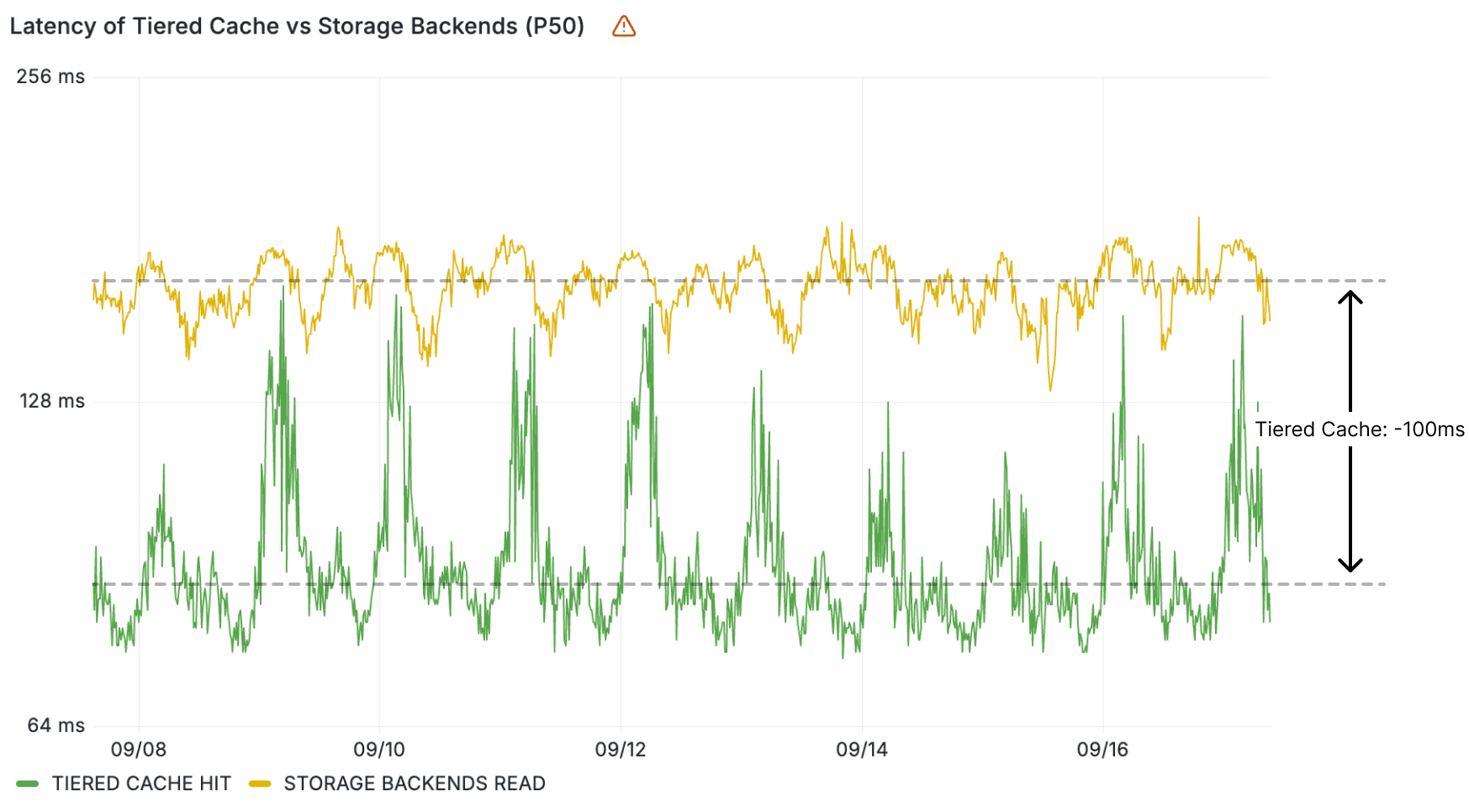
These KV read operations resolve quickly because the data is cached locally in the same Cloudflare location. But what about reads that aren’t resolved locally? ~30% of these resolve regionally within the tiered cache. Reads from tiered cache are up to 100 ms faster than when resolved at central storage backends, once again contributing to making KV reads faster in aggregate.
Wall time (ms) within the KV Worker for tiered cache vs. storage backends reads
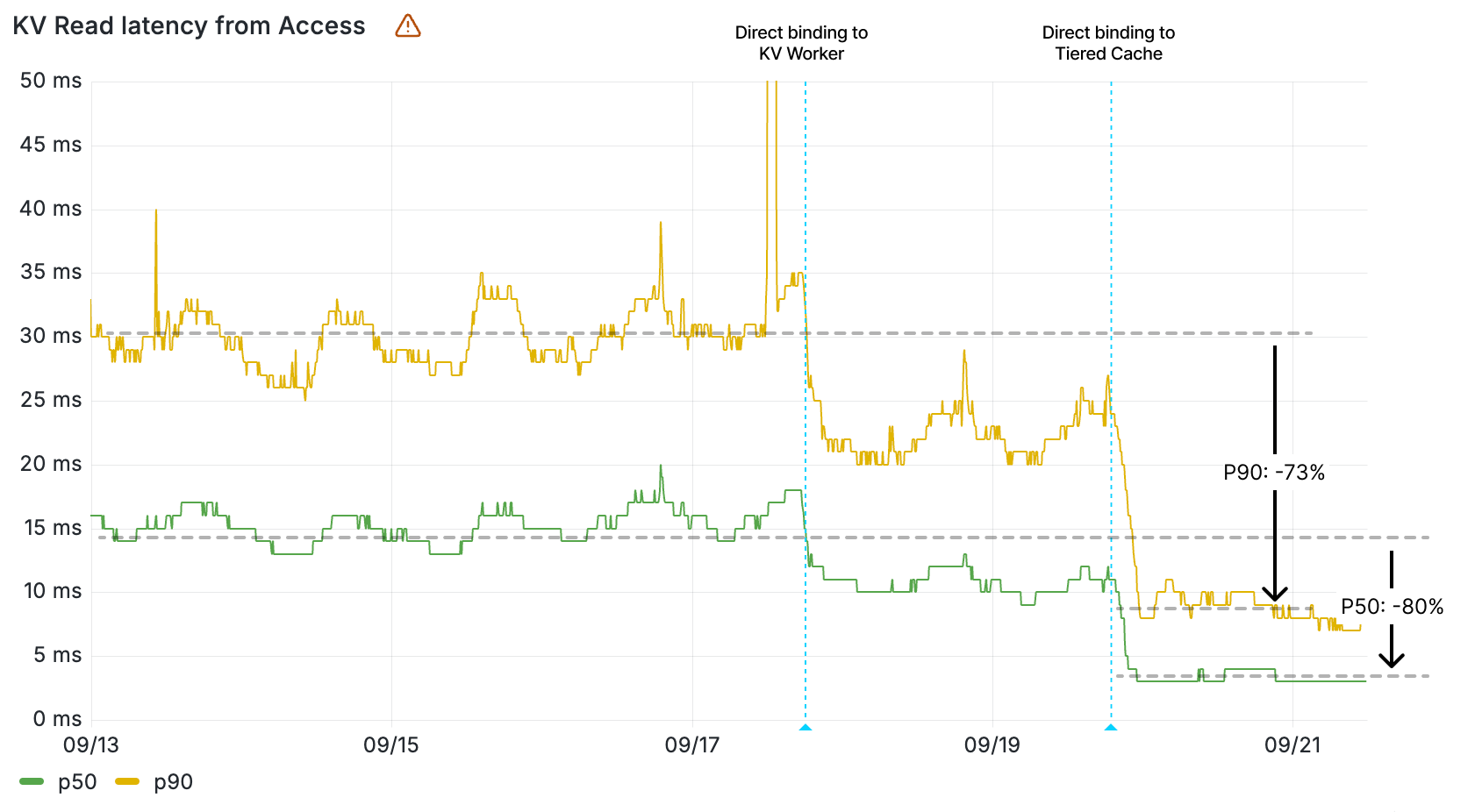
These graphs demonstrate the impact of direct binding from the KV binding to cache, and tiered cache. To see the impact of the direct binding from a Worker to the KV Worker, we need to look at the latencies reported by Cloudflare products that use KV.
Cloudflare Pages, which serves static assets like HTML, CSS, and scripts from KV, saw load times for fetching assets improve by up to 68%. Workers asset hosting, which we also announced as part of today’s Builder Day announcements, gets this improved performance from day 1.
Workers KV read operation latency measured within Cloudflare Pages by percentile
Queues and Access also saw their latencies for KV operations drop, with their KV read operations now 2-5x faster. These services rely on Workers KV data for configuration and routing data, so KV’s performance improvement directly contributes to making them faster on each request.
Workers KV read operation latency measured within Cloudflare Queues by percentile
Workers KV read operation latency measured within Cloudflare Access by percentile
These are just some of the direct effects that a faster KV has had on other services. Across the board, requests are resolving faster thanks to KV’s faster response times.
And we have one more thing to make KV lightning fast.
Optimizing KV’s hottest keys with an in-memory cache
Less than 0.03% of keys account for nearly half of requests to the Workers KV service across all namespaces. These keys are read thousands of times per second, so making these faster has a disproportionate impact. Could these keys be resolved within the KV Worker without needing additional network hops?
Almost all of these keys are under 100 KB. At this size, it becomes possible to use the in-memory cache of the KV Worker — a limited amount of memory within the main runtime process of a Worker sandbox. And that’s exactly what we did. For the highest throughput keys across Workers KV, reads resolve without even needing to leave the Worker runtime process.
Sequence diagram of KV operations with the hottest keys resolved within an in-memory cache
As a result of these changes, KV reads for these keys, which represent over 40% of Workers KV requests globally, resolve in under a millisecond. We’re actively testing these changes internally and expect to roll this out during October to speed up the hottest key-value pairs on Workers KV.
A faster KV for all
Most of these speed gains are already enabled with no additional action needed from customers. Your websites that are using KV are already responding to requests faster for your users, as are the other Cloudflare services using KV under the hood and the countless websites that depend upon them.
And we’re not done: we’ll continue to chase performance throughout our stack to make your websites faster. That’s how we’re going to move the needle towards a faster Internet.
To see Workers KV’s recent speed gains for your own KV namespaces, head over to your dashboard and check out the new KV analytics, with latency and cache status detailed per namespace.
Over the past 14 years, Cloudflare has evolved far beyond a Content Delivery Network (CDN), expanding its offerings to include a comprehensive Zero Trust security portfolio, network security & performance services, application security & performance optimizations, and a powerful developer platform. But customers also continue to rely on Cloudflare for caching and delivering static website content. CDNs are often judged on their ability to return content to visitors as quickly as possible. However, the speed at which content is removed from a CDN’s global cache is just as crucial.
When customers frequently update content such as news, scores, or other data, it is essential they avoid serving stale, out-of-date information from cache to visitors. This can lead to a subpar experience where users might see invalid prices, or incorrect news. The goal is to remove the stale content and cache the new version of the file on the CDN, as quickly as possible. And that starts by issuing a “purge.”
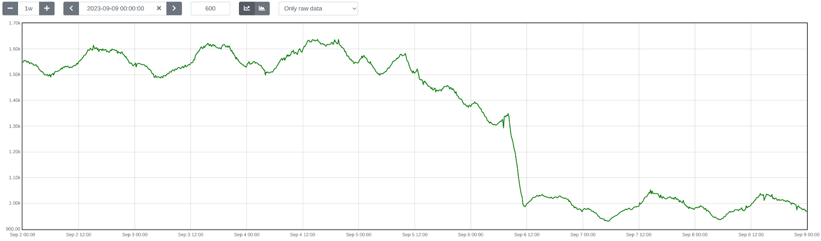
In May 2022, we released the first partof the series detailing our efforts to rebuild and publicly document the steps taken to improve the system our customers use, to purge their cached content. Our goal was to increase scalability, and importantly, the speed of our customer’s purges. In that initial post, we explained how our purge system worked and the design constraints we found when scaling. We outlined how after more than a decade, we had outgrown our purge system and started building an entirely new purge system, and provided purge performance benchmarking that users experienced at the time. We set ourselves a lofty goal: to be the fastest.
Today, we’re excited to share that we’ve built the fastest cache purge in the industry. We now offer a global purge latency for purge by tags, hostnames, and prefixes of less than 150ms on average (P50), representing a 90% improvement since May 2022. Users can now purge from anywhere, (almost) instantly. By the time you hit enter on a purge request and your eyes blink, the file is now removed from our global network — including data centers in 330 cities and 120+ countries.
But that’s not all. It wouldn’t be Birthday Week if we stopped at just being the fastest purge. We are alsoannouncing that we’re opening up more purge options to Free, Pro, and Business plans. Historically, only Enterprise customers had access to the full arsenal of cache purge methods supported by Cloudflare, such as purge by cache-tags, hostnames, and URL prefixes. As part of rebuilding our purge infrastructure, we’re not only fast but we are able to scale well beyond our current capacity. This enables more customers to use different types of purge. We are excited to offer these new capabilities to all plan types once we finish rolling out our new purge infrastructure, and expect to begin offering additional purge capabilities to all plan types in early 2025.
Why cache and purge?
Caching content is like pulling off a spectacular magic trick. It makes loading website content lightning-fast for visitors, slashes the load on origin servers and the cost to operate them, and enables global scalability with a single button press. But here’s the catch: for the magic to work, caching requires predicting the future. The right content needs to be cached in the right data center, at the right moment when requests arrive, and in the ideal format. This guarantees astonishing performance for visitors and game-changing scalability for web properties.
Cloudflare helps make this caching magic trick easy. But regular users of our cache know that getting content into cache is only part of what makes it useful. When content is updated on an origin, it must also be updated in the cache. The beauty of caching is that it holds content until it expires or is evicted. To update the content, it must be actively removed and updated across the globe quickly and completely. If data centers are not uniformly updated or are updated at drastically different times, visitors risk getting different data depending on where they are located. This is where cache “purging” (also known as “cache invalidation”) comes in.
One-to-many purges on Cloudflare
Back in part 2 of the blog series, we touched on how there are multiple ways of purging cache: by URL, cache-tag, hostname, URL prefix, and “purge everything”, and discussed a necessary distinction between purging by URL and the other four kinds of purge — referred to as flexible purges — based on the scope of their impact.
The reason flexible purge isn’t also fully coreless yet is because it’s a more complex task than “purge this object”; flexible purge requests can end up purging multiple objects – or even entire zones – from cache. They do this through an entirely different process that isn’t coreless compatible, so to make flexible purge fully coreless we would have needed to come up with an entirely new multi-purge mechanism on top of redesigning distribution. We chose instead to start with just purge by URL, so we could focus purely on the most impactful improvements, revamping distribution, without reworking the logic a data center uses to actually remove an object from cache.
We said our next steps included a redesign of flexible purges at Cloudflare, and today we’d like to walk you through the resulting system. But first, a brief history of flexible cache purges at Cloudflare and elaboration on why the old flexible purge system wasn’t “coreless compatible”.
Just in time
“Cache” within a given data center is made up of many machines, all contributing disk space to store customer content. When a request comes in for an asset, the URL and headers are used to calculate a cache key, which is the filename for that content on disk and also determines which machine in the datacenter that file lives on. The filename is the same for every data center, and every data center knows how to use it to find the right machine to cache the content. A purge request for a URL (plus headers) therefore contains everything needed to generate the cache key — the pointer to the response object on disk — and getting that key to every data center is the hardest part of carrying out the purge.
Purging content based on response properties has a different hardest part. If a customer wants to purge all content with the cache-tag “foo”, for example, there’s no way for us to generate all the cache keys that will point to the files with that cache-tag at request time. Cache-tags are response headers, and the decision of where to store a file is based on request attributes only. To find all files with matching cache-tags, we would need to look at every file in every cache disk on every machine in every data center. That’s thousands upon thousands of machines we would be scanning for each purge-by-tag request. There are ways to avoid actually continuously scanning all disks worldwide (foreshadowing!) but for our first implementation of our flexible purge system, we hoped to avoid the problem space altogether.
An alternative approach to going to every machine and looking for all files that match some criteria to actively delete from disk was something we affectionately referred to as “lazy purge”. Instead of deleting all matching files as soon as we process a purge request, we wait to do so when we get an end user request for one of those files. Whenever a request comes in, and we have the file in cache, we can compare the timestamp of any recent purge requests from the file owner to the insertion timestamp of the file we have on disk. If the purge timestamp is fresher than the insertion timestamp, we pretend we didn’t find the file on disk. For this to work, we needed to keep track of purge requests going back further than a data center’s maximum cache eviction age to be sure that any file a customer sends a matching flex purge to clear from cache will either be naturally evicted, or forced to cache MISS and get refreshed from the origin. With this approach, we just needed a distribution and storage system for keeping track of flexible purges.
Purge looks a lot like a nail
At Cloudflare there is a lot of configuration data that needs to go “everywhere”: cache configuration, load balancer settings, firewall rules, host metadata — countless products, features, and services that depend on configuration data that’s managed through Cloudflare’s control plane APIs. This data needs to be accessible by every machine in every datacenter in our network. The vast majority of that data is distributed via a system introduced several years ago called Quicksilver. The system works very, very well (sub-second p99 replication lag, globally). It’s extremely flexible and reliable, and reads are lightning fast. The team responsible for the system has done such a good job that Quicksilver has become a hammer that when wielded, makes everything look like a nail… like flexible purges.
Core-based purge request entering a data center and getting backhauled to a core data center where Quicksilver distributes the request to all network data centers (hub and spoke).
Our first version of the flexible purge system used Quicksilver’s spoke-hub distribution to send purges from a core data center to every other data center in our network. It took less than a second for flexible purges to propagate, and once in a given data center, the purge key lookups in the hot path to force cache misses were in the low hundreds of microseconds. We were quite happy with this system at the time, especially because of the simplicity. Using well-supported internal infrastructure meant we weren’t having to manage database clusters or worry about transport between data centers ourselves, since we got that “for free”. Flexible purge was a new feature set and the performance seemed pretty good, especially since we had no predecessor to compare against.
Victims of our own success
Our first version of flexible purge didn’t start showing cracks for years, but eventually both our network and our customer base grew large enough that our system was reaching the limits of what it could scale to. As mentioned above, we needed to store purge requests beyond our maximum eviction age. Purge requests are relatively small, and compress well, but thousands of customers using the API millions of times a day adds up to quite a bit of storage that Quicksilver needed on each machine to maintain purge history, and all of that storage cut into disk space we could otherwise be using to cache customer content. We also found the limits of Quicksilver in terms of how many writes per second it could handle without replication slowing down. We bought ourselves more runway by putting Kafka queues in front of Quicksilver to buffer and throttle ourselves to even out traffic spikes, and increased batching, but all of those protections introduced latency. We knew we needed to come up with a solution without such a strong correlation between usage and operational costs.
Another pain point exposed by our growing user base that we mentioned in Part 2 was the excessive round trip times experienced by customers furthest away from our core data centers. A purge request sent by a customer in Australia would have to cross the Pacific Ocean and back before local customers would see the new content.
To summarize, three issues were plaguing us:
Latency corresponding to how far a customer was from the centralized ingest point.
Latency due to the bottleneck for writes at the centralized ingest point.
Storage needs in all data centers correlating strongly with throughput demand.
Coreless purge proves useful
The first two issues affected all types of purge. The spoke-hub distribution model was problematic for purge-by-URL just as much as it was for flexible purges. So we embarked on the path to peer-to-peer distribution for purge-by-URL to address the latency and throughput issues, and the results of that project were good enough that we wanted to propagate flexible purges through the same system. But doing so meant we’d have to replace our use of Quicksilver; it was so good at what it does (fast/reliable replication network-wide, extremely fast/high read throughput) in large part because of the core assumption of spoke-hub distribution it could optimize for. That meant there was no way to write to Quicksilver from “spoke” data centers, and we would need to find another storage system for our purges.
Flipping purge on its head
We decided if we’re going to replace our storage system we should dig into exactly what our needs are and find the best fit. It was time to revisit some of our oldest conclusions to see if they still held true, and one of the earlier ones was that proactively purging content from disk would be difficult to do efficiently given our storage layout.
But was that true? Or could we make active cache purge fast and efficient (enough)? What would it take to quickly find files on disk based on their metadata? “Indexes!” you’re probably screaming, and for good reason. Indexing files’ hostnames, cache-tags, and URLs would undoubtedly make querying for relevant files trivial, but a few aspects of our network make it less straightforward.
Cloudflare has hundreds of data centers that see trillions of unique files, so any kind of global index — even ignoring the networking hurdles of aggregation — would suffer the same type of bottlenecking issues with our previous spoke-hub system. Scoping the indices to the data center level would be better, but they vary in size up to several hundred machines. Managing a database cluster in each data center scaled to the appropriate size for the aggregate traffic of all the machines was a daunting proposition; it could easily end up being enough work on its own for a separate team, not something we should take on as a side hustle.
The next step down in scope was an index per machine. Indexing on the same machine as the cache proxy had some compelling upsides:
The proxy could talk to the index over UDS (Unix domain sockets), avoiding networking complexities in the hottest paths.
As a sidecar service, the index just had to be running anytime the machine was accepting traffic. If a machine died, so would the index, but that didn’t matter, so there wasn’t any need to deal with the complexities of distributed databases.
While data centers were frequently adding and removing machines, machines weren’t frequently adding and removing disks. An index could reasonably count on its maximum size being predictable and constant based on overall disk size.
But we wanted to make sure it was feasible on our machines. We analyzed representative cache disks from across our fleet, gathering data like the number of cached assets per terabyte and the average number of cache-tags per asset. We looked at cache MISS, REVALIDATED, and EXPIRED rates to estimate the required write throughput.
After conducting a thorough analysis, we were convinced the design would work. With a clearer understanding of the anticipated read/write throughput, we started looking at databases that could meet our needs. After benchmarking several relational and non-relational databases, we ultimately chose RocksDB, a high-performance embedded key-value store. We found that with proper tuning, it could be extremely good at the types of queries we needed.
Putting it all together
And so CacheDB was born — a service written in Rust and built on RocksDB, which operates on each machine alongside the cache proxy to manage the indexing and purging of cached files. We integrated the cache proxy with CacheDB to ensure that indices are stored whenever a file is cached or updated, and they’re deleted when a file is removed due to eviction or purging. In addition to indexing data, CacheDB maintains a local queue for buffering incoming purge operations. A background process reads purge operations in the queue, looking up all matching files using the indices, and deleting the matched files from disk. Once all matched files for an operation have been deleted, the process clears the indices and removes the purge operation from the queue.
To further optimize the speed of purges taking effect, the cache proxy was updated to check with CacheDB — similar to the previous lazy purge approach — when a cache HIT occurs before returning the asset. CacheDB does a quick scan of its local queue to see if there are any pending purge operations that match the asset in question, dictating whether the cache proxy should respond with the cached file or fetch a new copy. This means purges will prevent the cache proxy from returning a matching cached file as soon as a purge reaches the machine, even if there are millions of files that correspond to a purge key, and it takes a while to actually delete them all from disk.
Coreless purge using CacheDB and Durable Objects to distribute purges without needing to first stop at a core data center.
The last piece to change was the distribution pipeline, updated to broadcast flexible purges not just to every data center, but to the CacheDB service running on every machine. We opted for CacheDB to handle the last-mile fan out of machine to machine within a data center, using consul to keep each machine informed of the health of its peers. The choice let us keep the Workers largely the same for purge-by-URL (more here) and flexible purge handling, despite the difference in termination points.
The payoff
Our new approach reduced the long tail of the lazy purge, saving 10x storage. Better yet, we can now delete purged content immediately instead of waiting for the lazy purge to happen or expire. This new-found storage will improve cache retention on disk for all users, leading to improved cache HIT ratios and reduced egress from your origin.
The shift from lazy content purging (left) to the new Coreless Purge architecture allows us to actively delete content (right). This helps reduce storage needs and increase cache retention times across our service.
With the new coreless cache purge, we can now get a purge request into any datacenter, distribute the keys to purge, and instantly purge the content from the cache database. This all occurs in less than 150 milliseconds on P50 for tags, hostnames, and prefix URL, covering all 330 cities in 120+ countries.
Benchmarks
To measure Instant Purge, we wanted to make sure that we were looking at real user metrics — that these were purges customers were actually issuing and performance that was representative of what we were seeing under real conditions, rather than marketing numbers.
The time we measure represents the period when a request enters the local datacenter, and ends with when the purge has been executed in every datacenter. When the local data center receives the request, one of the first things we do is to add a timestamp to the purge request. When all data centers have completed the purge action, another timestamp is added to “stop the clock.” Each purge request generates this performance data, and it is then sent to a database for us to measure the appropriate quantiles and to help us understand how we can improve further.
In August 2024, we took purge performance data and segmented our collected data by region based on where the local data center receiving the request was located.
Region
P50 Aug 2024 (Coreless)
P50 May 2022 (Core-based)
Improvement
Africa
303ms
1,420ms
78.66%
Asia Pacific Region (APAC)
199ms
1,300ms
84.69%
Eastern Europe (EEUR)
140ms
1,240ms
88.70%
Eastern North America (ENAM)
119ms
1,080ms
88.98%
Oceania
191ms
1,160ms
83.53%
South America (SA)
196ms
1,250ms
84.32%
Western Europe (WEUR)
131ms
1,190ms
88.99%
Western North America (WNAM)
115ms
1,000ms
88.5%
Global
149ms
1,570ms
90.5%
Note: Global latency numbers on the core-based measurements (May 2022) may be larger than the regional numbers because it represents all of our data centers instead of only a regional portion, so outliers and retries might have an outsized effect.
What’s next?
We are currently wrapping up the roll-out of the last throughput changes which allow us to efficiently scale purge requests. As that happens, we will revise our rate limits and open up purge by tag, hostname, and prefix to all plan types! We expect to begin rolling out the additional purge types to all plans and users beginning in early 2025.
In addition, in the process of implementing this new approach, we have identified improvements that will shave a few more milliseconds off our single-file purge. Currently, single-file purges have a P50 of 234ms. However, we want to, and can, bring that number down to below 200ms.
If you want to come work on the world’s fastest purge system, check out our open positions.
When it comes to the Internet, everyone wants to be the fastest. At Cloudflare, we’re no different. We want to be the fastest network in the world, and are constantly working towards that goal. Since June 2021, we’ve been measuring and ranking our network performance against the top global networks. We use this data to improve our performance, and to share the results of those initiatives.
In this post, we’re going to share with you how our network performance has changed since our last post in March 2024, and discuss the tools and processes we are using to assess network performance.
Digging into the data
Cloudflare has been measuring network performance across these top networks from the top 1,000 ISPs by estimated population (according to the Asia Pacific Network Information Centre (APNIC)), and optimizing our network for ISPs and countries where we see opportunities to improve. For performance benchmarking, we look at TCP connection time. This is the time it takes an end user to connect to the website or endpoint they are trying to reach. We chose this metric to show how our network helps make your websites faster by serving your traffic where your customers are. Back in June 2021, Cloudflare was ranked #1 in 33% of the networks.
As of September 2024, examining 95th percentile (p95) TCP connect times measured from September 4 to September 19, Cloudflare is the #1 provider in 44% of the top 1000 networks:
This graph shows that we are fastest in 410 networks, but that would only make us the fastest in 41% of the top 1,000. To make sure we’re looking at the networks that eyeballs connect from, we exclude networks like transit networks that aren’t last-mile ISPs. That brings the number of measured networks to 932, which makes us fastest in 44% of ISPs.
Now let’s take a look at the fastest provider by country. The map below shows the top network by 95th percentile TCP connection time, and Cloudflare is fastest in many countries. For those where we weren’t, we were within a few milliseconds of our closest competitor.
This color coding is generated by grouping all the measurements we generate by which country the measurement originates from, and then looking at the 95th percentile measurements for each provider to see who is the fastest. This is in contrast to how we measure who is fastest in individual networks, which involves grouping the measurements by ISP and measuring which provider is fastest. Cloudflare is still the fastest provider in 44% of the measured networks, which is consistent with our March report. Cloudflare is also the fastest in many countries, but the map is less orange than it was when we published our measurements from March 2024:
This can be explained by the fact that the fastest provider in a country is often determined by latency differences so small it is often less than 5% faster than the second-fastest provider. As an example, let’s take a look at India, a country where we are now the fastest:
India performance by provider
Rank
Entity
95th percentile TCP Connect (ms)
Difference from #1
1
Cloudflare
290 ms
–
2
Google
291 ms
+0.28% (+0.81 ms)
3
CloudFront
304 ms
+4.61% (+13 ms)
4
Fastly
325 ms
+12% (+35 ms)
5
Akamai
373 ms
+29% (+83 ms)
In India, we are the fastest network, but we are beating the runner-up by less than a millisecond, which shakes out to less than 1% difference between us and the number two! The competition for the number one spot in many countries is fierce and sometimes can be determined by what days you’re looking at the data, because variance in connectivity or last-mile outages can materially impact this data.
For example, on September 17, there was an outage on a major network in India, which impacted many users’ ability to access the Internet. People using this network were significantly impacted in their ability to connect to Cloudflare, and you can actually see that impact in the data. Here’s what the data looked like on the day of the outage, as we dropped from the number one spot that day:
India performance by provider
Rank
Entity
95th percentile TCP Connect (ms)
Difference from #1
1
Google
219 ms
–
2
CloudFront
230 ms
+5% (+11 ms)
3
Cloudflare
236 ms
+7.47% (+16 ms)
4
Fastly
261 ms
+19% (+41 ms)
5
Akamai
286 ms
+30% (+67 ms)
We were impacted more than other providers here because our automated traffic management systems detected the high packet loss as a result of the outage and aggressively moved all of our traffic away from the impacted provider. After review internally, we have identified opportunities to improve our traffic management to be more fine-grained in our approach to outages of this type, which would help us continue to be fast despite changes in the surrounding ecosystem. These unplanned occurrences can happen to any network, but these events also provide us opportunities to improve and mitigate the randomness we see on the Internet.
The phenomenon of providers having fluctuating latencies can also work against us. Consider Poland, a country where we were the fastest provider in March, but are no longer the fastest provider today. Digging into the data a bit more, we can see that even though we are no longer the fastest, we’re slower by less than a millisecond, giving us confidence that our architecture is optimized for performance in the region:
Poland performance by provider
Rank
Entity
95th percentile TCP Connect (ms)
Difference from #1
1
Google
246 ms
–
2
Cloudflare
246 ms
+0.15% (+0.36 ms)
3
CloudFront
250 ms
+1.7% (+4.17 ms)
4
Akamai
272 ms
+11% (+26 ms)
5
Fastly
295 ms
+20% (+50 ms)
These nuances in the data can make us look slower in more countries than we actually are. From a numbers’ perspective we’re neck-and-neck with our competitors and still fastest in the most networks around the world. Going forward, we’re going to take a longer look at how we’re visualizing our network performance to paint a clearer picture for you around performance. But let’s go into more about how we actually get the underlying data we use to measure ourselves.
How we measure performance
When you see a Cloudflare-branded error page, something interesting happens behind the scenes. Every time one of these error pages is displayed, Cloudflare gathers Real User Measurements (RUM) by fetching a tiny file from various networks, including Cloudflare, Akamai, Amazon CloudFront, Fastly, and Google Cloud CDN. Your browser sends back performance data from the end-user’s perspective, helping us get a clear view of how these different networks stack up in terms of speed. The main goal? Figure out where we’re fast, and more importantly, where we can make Cloudflare even faster. If you’re curious about the details, the original Speed Week blog post dives deeper into the methodology.
Using this RUM data, we track key performance metrics such as TCP Connection Time, Time to First Byte (TTFB), and Time to Last Byte (TTLB) for Cloudflare and the other networks.
Starting from March, we fixed the list of networks we look at to be the top 1000 networks by estimated population as determined by APNIC, and we removed networks that weren’t last-mile ISPs. This change makes our measurements and reporting more consistent because we look at the same set of networks for every reporting cycle.
How does Cloudflare use this data?
Cloudflare uses this data to improve our network performance in lagging regions. For example, in 2022 we recognized that performance on a network in Finland was not as fast as some comparable regions. Users were taking 300+ ms to connect to Cloudflare at the 95th percentile:
Performance for Finland network
Rank
Entity
95th percentile TCP Connect (ms)
Difference from #1
1
Fastly
15 ms
–
2
CloudFront
19 ms
+19% (+3 ms)
3
Akamai
20 ms
+28% (+4.3 ms)
4
Google
72 ms
+363% (+56 ms)
5
Cloudflare
368 ms
+2378% (+353 ms)
After investigating, we recognized that one major network in Finland was seeing high latency due to issues resulting from congestion. Simply put, we were using all the capacity we had. We immediately planned an expansion, and within two weeks of that expansion completion, our latency decreased, and we became the fastest provider in the region, as you can see in the map above.
We are constantly improving our network and infrastructure to better serve our customers. Data like this helps us identify where we can be most impactful, and improve service for our customers.
What’s next
We’re sharing our updates on our journey to become as fast as we can be everywhere so that you can see what goes into running the fastest network in the world. From here, our plan is the same as always: identify where we’re slower, fix it, and then tell you how we’ve gotten faster.
The Compute and Performance Engineering teams at Netflix regularly investigate performance issues in our multi-tenant environment. The first step is determining whether the problem originates from the application or the underlying infrastructure. One issue that often complicates this process is the "noisy neighbor" problem. On Titus, our multi-tenant compute platform, a "noisy neighbor" refers to a container or system service that heavily utilizes the server's resources, causing performance degradation in adjacent containers. We usually focus on CPU utilization because it is our workload's most frequent source of noisy neighbor issues.
Detecting the effects of noisy neighbors is complex. Traditional performance analysis tools such as perf can introduce significant overhead, risking further performance degradation. Additionally, these tools are typically deployed after the fact, which is too late for effective investigation.Another challenge is that debugging noisy neighbor issues requires significant low-level expertise and specialized tooling. In this blog post, we'll reveal how we leveraged eBPF to achieve continuous, low-overhead instrumentation of the Linux scheduler, enabling effective self-serve monitoring of noisy neighbor issues. Learn how Linux kernel instrumentation can improve your infrastructure observability with deeper insights and enhanced monitoring.
Continuous Instrumentation of the Linux Scheduler
To ensure the reliability of our workloads that depend on low latency responses, we instrumented the run queue latency for each container, which measures the time processes spend in the scheduling queue before being dispatched to the CPU. Extended waiting in this queue can be a telltale of performance issues, especially when containers are not utilizing their total CPU allocation. Continuous instrumentation is critical to catching such matters as they emerge, and eBPF, with its hooks into the Linux scheduler with minimal overhead, enabled us to monitor run queue latency efficiently.
To emit a run queue latency metric, we leveraged three eBPF hooks: sched_wakeup, sched_wakeup_new, and sched_switch.
The sched_wakeup and sched_wakeup_new hooks are invoked when a process changes state from 'sleeping' to 'runnable.' They let us identify when a process is ready to run and is waiting for CPU time. During this event, we generate a timestamp and store it in an eBPF hash map using the process ID as the key.
Conversely, the sched_switch hook is triggered when the CPU switches between processes. This hook provides pointers to the process currently utilizing the CPU and the process about to take over. We use the upcoming task's process ID (PID) to fetch the timestamp from the eBPF map. This timestamp represents when the process entered the queue, which we had previously stored. We then calculate the run queue latency by simply subtracting the timestamps.
// fetch timestamp of when the next task was enqueued u64 *tsp = bpf_map_lookup_elem(&runq_lat, &next_pid); if (tsp == NULL) { return 0; // missed enqueue }
// calculate runq latency before deleting the stored timestamp u64 now = bpf_ktime_get_ns(); u64 runq_lat = now - *tsp;
// delete pid from enqueued map bpf_map_delete_elem(&runq_lat, &next_pid); ....
One of the advantages of eBPF is its ability to provide pointers to the actual kernel data structures representing processes or threads, also known as tasks in kernel terminology. This feature enables access to a wealth of information stored about a process. We required the process's cgroup ID to associate it with a container for our specific use case. However, the cgroup information in the struct is safeguarded by an RCU (Read Copy Update) lock.
To safely access this RCU-protected information, we can leverage kfuncs in eBPF. kfuncs are kernel functions that can be called from eBPF programs. There are kfuncs available to lock and unlock RCU read-side critical sections. These functions ensure that our eBPF program remains safe and efficient while retrieving the cgroup ID from the task struct.
Having the data ready, we must package it and send it to userspace. For this purpose, we chose the eBPF ring buffer. It is efficient, high-performing, and user-friendly. It can handle variable-length data records and allows data reading without necessitating extra memory copying or syscalls. However, the sheer amount of data points was causing the userspace program to use too much CPU, so we implemented a rate limiter in eBPF to sample the data effectively.
// check the rate limit for the cgroup_id in consideration // before doing more work if (now - last_ts_val < RATE_LIMIT_NS) { // Rate limit exceeded, drop the event return 0; }
if (event) { event->prev_cgroup_id = prev_cgroup_id; event->cgroup_id = cgroup_id; event->runq_lat = runq_lat; event->ts = now; bpf_ringbuf_submit(event, 0); // Update the last event timestamp for the current cgroup_id bpf_map_update_elem(&cgroup_id_to_last_event_ts, &cgroup_id, &now, BPF_ANY);
}
return 0; }
Our userspace application, developed in Go, processes events from the ring buffer to emit metrics to our metrics backend, Atlas. Each event includes a run queue latency sample with a cgroup ID, which we associate with running containers on the host. We categorize it as a system service if no such association is found. When a cgroup ID correlates with a container, we emit a percentile timer Atlas metric (runq.latency) for that container. We also increment a counter metric (sched.switch.out) to monitor preemptions occurring for the container's processes. Access to the prev_cgroup_id of the preempted process allows us to tag the metric with the cause of the preemption, whether it's due to a process within the same container (or cgroup), a process in another container, or a system service.
It's important to highlight that both the runq.latency metric and the sched.switch.out metrics are needed to determine if a container is affected by noisy neighbors, which is the goal we aim to achieve — relying solely on the runq.latency metric can lead to misconceptions. For example, if a container is at or over its cgroup CPU limit, the scheduler will throttle it, resulting in an apparent spike in run queue latency due to delays in the queue. If we were only to consider this metric, we might incorrectly attribute the performance degradation to noisy neighbors when it's actually because the container is hitting its CPU request limits. However, simultaneous spikes in both metrics, mainly when the cause is a different container or system process, clearly indicate a noisy neighbor issue.
A Noisy Neighbor Story
Below is the runq.latency metric for a server running a single container with ample CPU overhead. The 99th percentile averages 83.4µs (microseconds), serving as our baseline. Although there are some spikes reaching 400µs, the latency remains within acceptable parameters.
container1’s 99th percentile runq.latency averages 83µs (microseconds), with spikes up to 400µs, without adjacent containers. This serves as our baseline for a container not contending for CPU on a host.
At 10:35, launching container2, which fully utilized all CPUs on the host, caused a significant 131-millisecond spike (131,000 microseconds) in container1's P99 run queue latency. This spike would be noticeable in the userspace application if it were serving HTTP traffic. If userspace app owners reported an unexplained latency spike, we could quickly identify the noisy neighbor issue through run queue latency metrics.
Launching container2 at 10:35, which maxes out all CPUs on the host, caused a 131-millisecond spike in container1’s P99 run queue latency due to increased preemptions by system processes. This indicates a noisy neighbor issue, where system services compete for CPU time with containers.
The sched.switch.out metric indicates that the spike was due to increased preemptions by system processes, highlighting a noisy neighbor issue where system services compete with containers for CPU time. Our metrics show that the noisy neighbors were actually system processes, likely triggered by container2 consuming all available CPU capacity.
Optimizing eBPF Code
We developed an open-source eBPF process monitor called bpftop to measure the overhead of eBPF code in this hot kernel path. Our estimates suggest that the instrumentation adds less than 600 nanoseconds to each sched_* hook. We conducted a performance analysis on a Java service running in a container, and the instrumentation did not introduce significant overhead. The performance variance with the run queue profiling code active versus inactive was not measurable in milliseconds.
During our research on how eBPF statistics are measured in the kernel, we identified an opportunity to improve its calculation. We submitted this patch, which was included in the Linux kernel 6.10 release.
Through trial and error and using bpftop, we identified several optimizations that helped maintain low overhead for this code:
We found that BPF_MAP_TYPE_HASH was the most performant for storing enqueued timestamps. Using BPF_MAP_TYPE_TASK_STORAGE resulted in nearly a twofold performance decline. BPF_MAP_TYPE_PERCPU_HASH was slightly less performant than BPF_MAP_TYPE_HASH, which was unexpected and requires further investigation.
The BPF_CORE_READ helper adds 20–30 nanoseconds per invocation. In the case of raw tracepoints, specifically those that are "BTF-enabled" (tp_btf/*), it is safe and more efficient to access the task struct members directly. Andrii Nakryiko recommends this approach in this blog post.
BPF_MAP_TYPE_LRU_HASH maps are 40–50 nanoseconds slower per operation than regular hash maps. Due to space concerns from PID churn, we initially used them for enqueued timestamps. We have since increased the map size, mitigating this risk.
The sched_switch, sched_wakeup, and sched_wakeup_new are all triggered for kernel tasks, which are identifiable by their PID of 0. We found monitoring these tasks unnecessary, so we implemented several early exit conditions and conditional logic to prevent executing costly operations, such as accessing BPF maps, when dealing with a kernel task. Notably, kernel tasks operate through the scheduler queue like any regular process.
Conclusion
Our findings highlight the value of low-overhead continuous instrumentation of the Linux kernel with eBPF. We have integrated these metrics into customer dashboards, enabling actionable insights and guiding multitenancy performance discussions. We can also now use these metrics to refine CPU isolation strategies to minimize the impact of noisy neighbors. Additionally, thanks to these metrics, we've gained deeper insights into the Linux scheduler.
This project has also deepened our understanding of eBPF technology and underscored the importance of tools like bpftop for optimizing eBPF code. As eBPF adoption increases, we foresee more infrastructure observability and business logic shifting to it. One promising project in this space is sched_ext, potentially revolutionizing how scheduling decisions are made and tailored to specific workload needs.
Netflix has an extensive history of using Java as our primary programming language across our vast fleet of microservices. As we pick up newer versions of Java, our JVM Ecosystem team seeks out new language features that can improve the ergonomics and performance of our systems. In a recent article, we detailed how our workloads benefited from switching to generational ZGC as our default garbage collector when we migrated to Java 21. Virtual threads is another feature we are excited to adopt as part of this migration.
For those new to virtual threads, they are described as “lightweight threads that dramatically reduce the effort of writing, maintaining, and observing high-throughput concurrent applications.” Their power comes from their ability to be suspended and resumed automatically via continuations when blocking operations occur, thus freeing the underlying operating system threads to be reused for other operations. Leveraging virtual threads can unlock higher performance when utilized in the appropriate context.
In this article we discuss one of the peculiar cases that we encountered along our path to deploying virtual threads on Java 21.
The problem
Netflix engineers raised several independent reports of intermittent timeouts and hung instances to the Performance Engineering and JVM Ecosystem teams. Upon closer examination, we noticed a set of common traits and symptoms. In all cases, the apps affected ran on Java 21 with SpringBoot 3 and embedded Tomcat serving traffic on REST endpoints. The instances that experienced the issue simply stopped serving traffic even though the JVM on those instances remained up and running. One clear symptom characterizing the onset of this issue is a persistent increase in the number of sockets in closeWait state as illustrated by the graph below:
Collected diagnostics
Sockets remaining in closeWait state indicate that the remote peer closed the socket, but it was never closed on the local instance, presumably because the application failed to do so. This can often indicate that the application is hanging in an abnormal state, in which case application thread dumps may reveal additional insight.
In order to troubleshoot this issue, we first leveraged our alerts system to catch an instance in this state. Since we periodically collect and persist thread dumps for all JVM workloads, we can often retroactively piece together the behavior by examining these thread dumps from an instance. However, we were surprised to find that all our thread dumps show a perfectly idle JVM with no clear activity. Reviewing recent changes revealed that these impacted services enabled virtual threads, and we knew that virtual thread call stacks do not show up in jstack-generated thread dumps. To obtain a more complete thread dump containing the state of the virtual threads, we used the “jcmd Thread.dump_to_file” command instead. As a last-ditch effort to introspect the state of JVM, we also collected a heap dump from the instance.
Analysis
Thread dumps revealed thousands of “blank” virtual threads:
#119821 "" virtual

#119820 "" virtual

#119823 "" virtual

#120847 "" virtual

#119822 "" virtual
...
These are the VTs (virtual threads) for which a thread object is created, but has not started running, and as such, has no stack trace. In fact, there were approximately the same number of blank VTs as the number of sockets in closeWait state. To make sense of what we were seeing, we need to first understand how VTs operate.
A virtual thread is not mapped 1:1 to a dedicated OS-level thread. Rather, we can think of it as a task that is scheduled to a fork-join thread pool. When a virtual thread enters a blocking call, like waiting for a Future, it relinquishes the OS thread it occupies and simply remains in memory until it is ready to resume. In the meantime, the OS thread can be reassigned to execute other VTs in the same fork-join pool. This allows us to multiplex a lot of VTs to just a handful of underlying OS threads. In JVM terminology, the underlying OS thread is referred to as the “carrier thread” to which a virtual thread can be “mounted” while it executes and “unmounted” while it waits. A great in-depth description of virtual thread is available in JEP 444.
In our environment, we utilize a blocking model for Tomcat, which in effect holds a worker thread for the lifespan of a request. By enabling virtual threads, Tomcat switches to virtual execution. Each incoming request creates a new virtual thread that is simply scheduled as a task on a Virtual Thread Executor. We can see Tomcat creates a VirtualThreadExecutor here.
Tying this information back to our problem, the symptoms correspond to a state when Tomcat keeps creating a new web worker VT for each incoming request, but there are no available OS threads to mount them onto.
Why is Tomcat stuck?
What happened to our OS threads and what are they busy with? As described here, a VT will be pinned to the underlying OS thread if it performs a blocking operation while inside a synchronized block or method. This is exactly what is happening here. Here is a relevant snippet from a thread dump obtained from the stuck instance:
In this stack trace, we enter the synchronization in brave.RealSpan.finish(RealSpan.java:134). This virtual thread is effectively pinned — it is mounted to an actual OS thread even while it waits to acquire a reentrant lock. There are 3 VTs in this exact state and another VT identified as “<redacted> @DefaultExecutor – 46542” that also follows the same code path. These 4 virtual threads are pinned while waiting to acquire a lock. Because the app is deployed on an instance with 4 vCPUs, the fork-join pool that underpins VT execution also contains 4 OS threads. Now that we have exhausted all of them, no other virtual thread can make any progress. This explains why Tomcat stopped processing the requests and why the number of sockets in closeWait state keeps climbing. Indeed, Tomcat accepts a connection on a socket, creates a request along with a virtual thread, and passes this request/thread to the executor for processing. However, the newly created VT cannot be scheduled because all of the OS threads in the fork-join pool are pinned and never released. So these newly created VTs are stuck in the queue, while still holding the socket.
Who has the lock?
Now that we know VTs are waiting to acquire a lock, the next question is: Who holds the lock? Answering this question is key to understanding what triggered this condition in the first place. Usually a thread dump indicates who holds the lock with either “- locked <0x…> (at …)” or “Locked ownable synchronizers,” but neither of these show up in our thread dumps. As a matter of fact, no locking/parking/waiting information is included in the jcmd-generated thread dumps. This is a limitation in Java 21 and will be addressed in the future releases. Carefully combing through the thread dump reveals that there are a total of 6 threads contending for the same ReentrantLock and associated Condition. Four of these six threads are detailed in the previous section. Here is another thread:
Note that while this thread seemingly goes through the same code path for finishing a span, it does not go through a synchronized block. Finally here is the 6th thread:
This is actually a normal platform thread, not a virtual thread. Paying particular attention to the line numbers in this stack trace, it is peculiar that the thread seems to be blocked within the internal acquire() method aftercompleting the wait. In other words, this calling thread owned the lock upon entering awaitNanos(). We know the lock was explicitly acquired here. However, by the time the wait completed, it could not reacquire the lock. Summarizing our thread dump analysis:
There are 5 virtual threads and 1 regular thread waiting for the lock. Out of those 5 VTs, 4 of them are pinned to the OS threads in the fork-join pool. There’s still no information on who owns the lock. As there’s nothing more we can glean from the thread dump, our next logical step is to peek into the heap dump and introspect the state of the lock.
Inspecting the lock
Finding the lock in the heap dump was relatively straightforward. Using the excellent Eclipse MAT tool, we examined the objects on the stack of the AsyncReporter non-virtual thread to identify the lock object. Reasoning about the current state of the lock was perhaps the trickiest part of our investigation. Most of the relevant code can be found in the AbstractQueuedSynchronizer.java. While we don’t claim to fully understand the inner workings of it, we reverse-engineered enough of it to match against what we see in the heap dump. This diagram illustrates our findings:
First off, the exclusiveOwnerThread field is null (2), signifying that no one owns the lock. We have an “empty” ExclusiveNode (3) at the head of the list (waiter is null and status is cleared) followed by another ExclusiveNode with waiter pointing to one of the virtual threads contending for the lock — #119516 (4). The only place we found that clears the exclusiveOwnerThread field is within the ReentrantLock.Sync.tryRelease() method (source link). There we also set state = 0 matching the state that we see in the heap dump (1).
With this in mind, we traced the code path to release() the lock. After successfully calling tryRelease(), the lock-holding thread attempts to signal the next waiter in the list. At this point, the lock-holding thread is still at the head of the list, even though ownership of the lock is effectively released. The next node in the list points to the thread that is about to acquire the lock.
To understand how this signaling works, let’s look at the lock acquire path in the AbstractQueuedSynchronizer.acquire() method. Grossly oversimplifying, it’s an infinite loop, where threads attempt to acquire the lock and then park if the attempt was unsuccessful:
When the lock-holding thread releases the lock and signals to unpark the next waiter thread, the unparked thread iterates through this loop again, giving it another opportunity to acquire the lock. Indeed, our thread dump indicates that all of our waiter threads are parked on line 754. Once unparked, the thread that managed to acquire the lock should end up in this code block, effectively resetting the head of the list and clearing the reference to the waiter.
To restate this more concisely, the lock-owning thread is referenced by the head node of the list. Releasing the lock notifies the next node in the list while acquiring the lock resets the head of the list to the current node. This means that what we see in the heap dump reflects the state when one thread has already released the lock but the next thread has yet to acquire it. It’s a weird in-between state that should be transient, but our JVM is stuck here. We know thread #119516 was notified and is about to acquire the lock because of the ExclusiveNode state we identified at the head of the list. However, thread dumps show that thread #119516 continues to wait, just like other threads contending for the same lock. How can we reconcile what we see between the thread and heap dumps?
The lock with no place to run
Knowing that thread #119516 was actually notified, we went back to the thread dump to re-examine the state of the threads. Recall that we have 6 total threads waiting for the lock with 4 of the virtual threads each pinned to an OS thread. These 4 will not yield their OS thread until they acquire the lock and proceed out of the synchronized block. #107 “AsyncReporter <redacted>” is a regular platform thread, so nothing should prevent it from proceeding if it acquires the lock. This leaves us with the last thread: #119516. It is a VT, but it is not pinned to an OS thread. Even if it’s notified to be unparked, it cannot proceed because there are no more OS threads left in the fork-join pool to schedule it onto. That’s exactly what happens here — although #119516 is signaled to unpark itself, it cannot leave the parked state because the fork-join pool is occupied by the 4 other VTs waiting to acquire the same lock. None of those pinned VTs can proceed until they acquire the lock. It’s a variation of the classic deadlock problem, but instead of 2 locks we have one lock and a semaphore with 4 permits as represented by the fork-join pool.
Now that we know exactly what happened, it was easy to come up with a reproducible test case.
Conclusion
Virtual threads are expected to improve performance by reducing overhead related to thread creation and context switching. Despite some sharp edges as of Java 21, virtual threads largely deliver on their promise. In our quest for more performant Java applications, we see further virtual thread adoption as a key towards unlocking that goal. We look forward to Java 23 and beyond, which brings a wealth of upgrades and hopefully addresses the integration between virtual threads and locking primitives.
This exploration highlights just one type of issue that performance engineers solve at Netflix. We hope this glimpse into our problem-solving approach proves valuable to others in their future investigations.
We made our WAF Machine Learning models 5.5x faster, reducing execution time by approximately 82%, from 1519 to 275 microseconds! Read on to find out how we achieved this remarkable improvement.
WAF Attack Score is Cloudflare’s machine learning (ML)-powered layer built on top of our Web Application Firewall (WAF). Its goal is to complement the WAF and detect attack bypasses that we haven’t encountered before. This has proven invaluable in catching zero-day vulnerabilities, like the one detected in Ivanti Connect Secure, before they are publicly disclosed and enhancing our customers’ protection against emerging and unknown threats.
Since its launch in 2022, WAF attack score adoption has grown exponentially, now protecting millions of Internet properties and running real-time inference on tens of millions of requests per second. The feature’s popularity has driven us to seek performance improvements, enabling even broader customer use and enhancing Internet security.
In this post, we will discuss the performance optimizations we’ve implemented for our WAF ML product. We’ll guide you through specific code examples and benchmark numbers, demonstrating how these enhancements have significantly improved our system’s efficiency. Additionally, we’ll share the impressive latency reduction numbers observed after the rollout.
Before diving into the optimizations, let’s take a moment to review the inner workings of the WAF Attack Score, which powers our WAF ML product.
WAF Attack Score system design
Cloudflare’s WAF attack score identifies various traffic types and attack vectors (SQLi, XSS, Command Injection, etc.) based on structural or statistical content properties. Here’s how it works during inference:
HTTP Request Content: Start with raw HTTP input.
Normalization & Transformation: Standardize and clean the data, applying normalization, content substitutions, and de-duplication.
Feature Extraction: Tokenize the transformed content to generate statistical and structural data.
Machine Learning Model Inference: Analyze the extracted features with pre-trained models, mapping content representations to classes (e.g., XSS, SQLi or RCE) or scores.
Classification Output in WAF: Assign a score to the input, ranging from 1 (likely malicious) to 99 (likely clean), guiding security actions.
Next, we will explore feature extraction and inference optimizations.
Feature extraction optimizations
In the context of the WAF Attack Score ML model, feature extraction or pre-processing is essentially a process of tokenizing the given input and producing a float tensor of 1 x m size:
In our initial pre-processing implementation, this is achieved via a sliding window of 3 bytes over the input with the help of Rust’s std::collections::HashMap to look up the tensor index for a given ngram.
Initial benchmarks
To establish performance baselines, we’ve set up four benchmark cases representing example inputs of various lengths, ranging from 44 to 9482 bytes. Each case exemplifies typical input sizes, including those for a request body, user agent, and URI. We run benchmarks using the Criterion.rs statistics-driven micro-benchmarking tool:
Here are initial numbers for these benchmarks executed on a Linux laptop with a 13th Gen Intel® Core™ i7-13800H processor:
Benchmark case
Pre-processing time, μs
Throughput, MiB/s
preprocessing/long-body-9482
248.46
36.40
preprocessing/avg-body-1000
28.19
33.83
preprocessing/avg-url-44
1.45
28.94
preprocessing/avg-ua-91
2.87
30.24
An important observation from these results is that pre-processing time correlates with the length of the input string, with throughput ranging from 28 MiB/s to 36 MiB/s. This suggests that considerable time is spent iterating over longer input strings. Optimizing this part of the process could significantly enhance performance. The dependency of processing time on input size highlights a key area for performance optimization. To validate this, we should examine where the processing time is spent by analyzing flamegraphs created from a 100-second profiling session visualized using pprof:
Looking at the pre-processing flamegraph above, it’s clear that most of the time was spent on the following two operations:
Function name
% Time spent
std::collections::hash::map::HashMap<K,V,S>::get
61.8%
regex::regex::bytes::Regex::replace_all
18.5%
Let’s tackle the HashMap lookups first. Lookups are happening inside the tensor_populate_ngrams function, where input is split into windows of 3 bytes representing ngram and then lookup inside two hash maps:
fn tensor_populate_ngrams(tensor: &mut [f32], input: &[u8]) {
   // Populate the NORM ngrams
   let mut unknown_norm_ngrams = 0;
   let norm_offset = 1;

   for s in input.windows(3) {
       match NORM_VOCAB.get(s) {
           Some(pos) => {
               tensor[*pos as usize + norm_offset] += 1.0f32;
           }
           None => {
               unknown_norm_ngrams += 1;
           }
       };
   }

   // Populate the SIG ngrams
   let mut unknown_sig_ngrams = 0;
   let sig_offset = norm_offset + NORM_VOCAB.len();

   let res = SIG_REGEX.replace_all(&input, b"#");

   for s in res.windows(3) {
       match SIG_VOCAB.get(s) {
           Some(pos) => {
               // adding +1 here as the first position will be the unknown_sig_ngrams
               tensor[*pos as usize + sig_offset + 1] += 1.0f32;
           }
           None => {
               unknown_sig_ngrams += 1;
           }
       }
   }
}
So essentially the pre-processing function performs a ton of hash map lookups, the volume of which depends on the size of the input string, e.g. 1469 lookups for the given benchmark case avg-body-1000.
Optimization attempt #1: HashMap → Aho-Corasick
Rust hash maps are generally quite fast. However, when that many lookups are being performed, it’s not very cache friendly.
So can we do better than hash maps, and what should we try first? The answer is the Aho-Corasick library.
This library provides multiple pattern search principally through an implementation of the Aho-Corasick algorithm, which builds a fast finite state machine for executing searches in linear time.
We can also tune Aho-Corasick settings based on this recommendation:
Then we use the constructed AhoCorasick dictionary to lookup ngrams using its find_overlapping_iter method:
for mat in NORM_VOCAB_AC.find_overlapping_iter(&input) {
    tensor_input_data[mat.pattern().as_usize() + 1] += 1.0;
}
We ran benchmarks and compared them against the baseline times shown above:
Benchmark case
Baseline time, μs
Aho-Corasick time, μs
Optimization
preprocessing/long-body-9482
248.46
129.59
-47.84% or 1.64x
preprocessing/avg-body-1000
28.19
16.47
-41.56% or 1.71x
preprocessing/avg-url-44
1.45
1.01
-30.38% or 1.44x
preprocessing/avg-ua-91
2.87
1.90
-33.60% or 1.51x
That’s substantially better – Aho-Corasick DFA does wonders.
Optimization attempt #2: Aho-Corasick → match
One would think optimization with Aho-Corasick DFA is enough and that it seems unlikely that anything else can beat it. Yet, we can throw Aho-Corasick away and simply use the Rust match statement and let the compiler do the optimization for us!
Here’s how it performs in practice, based on the assembly generated by the Godbolt compiler explorer. The corresponding assembly code efficiently implements this lookup by employing a jump table and byte-wise comparisons to determine the return value based on input sequences, optimizing for quick decisions and minimal branching. Although the example only includes ten ngrams, it’s important to note that in applications like our WAF Attack Score ML models, we deal with thousands of ngrams. This simple match-based approach outshines both HashMap lookups and the Aho-Corasick method.
Benchmark case
Baseline time, μs
Match time, μs
Optimization
preprocessing/long-body-9482
248.46
112.96
-54.54% or 2.20x
preprocessing/avg-body-1000
28.19
13.12
-53.45% or 2.15x
preprocessing/avg-url-44
1.45
0.75
-48.37% or 1.94x
preprocessing/avg-ua-91
2.87
1.4076
-50.91% or 2.04x
Switching to match gave us another 7-18% drop in latency, depending on the case.
Optimization attempt #3: Regex → WindowedReplacer
So, what exactly is the purpose of Regex::replace_all in pre-processing? Regex is defined and used like this:
pub static SIG_REGEX: Lazy<Regex> =
    Lazy::new(|| RegexBuilder::new("[a-z]+").unicode(false).build().unwrap());
    ...
    let res = SIG_REGEX.replace_all(&input, b"#");
    for s in res.windows(3) {
        tensor[sig_vocab_lookup(s.try_into().unwrap())] += 1.0;
    }
Essentially, all we need is to:
Replace every sequence of lowercase letters in the input with a single byte “#”.
Iterate over replaced bytes in a windowed fashion with a step of 3 bytes representing an ngram.
Look up the ngram index and increment it in the tensor.
This logic seems simple enough that we could implement it more efficiently with a single pass over the input and without any allocations:
type Window = [u8; 3];
type Iter<'a> = Peekable<std::slice::Iter<'a, u8>>;

pub struct WindowedReplacer<'a> {
    window: Window,
    input_iter: Iter<'a>,
}

#[inline]
fn is_replaceable(byte: u8) -> bool {
    matches!(byte, b'a'..=b'z')
}

#[inline]
fn next_byte(iter: &mut Iter) -> Option<u8> {
    let byte = iter.next().copied()?;
    if is_replaceable(byte) {
        while iter.next_if(|b| is_replaceable(**b)).is_some() {}
        Some(b'#')
    } else {
        Some(byte)
    }
}

impl<'a> WindowedReplacer<'a> {
    pub fn new(input: &'a [u8]) -> Option<Self> {
        let mut window: Window = Default::default();
        let mut iter = input.iter().peekable();
        for byte in window.iter_mut().skip(1) {
            *byte = next_byte(&mut iter)?;
        }
        Some(WindowedReplacer {
            window,
            input_iter: iter,
        })
    }
}

impl<'a> Iterator for WindowedReplacer<'a> {
    type Item = Window;

    #[inline]
    fn next(&mut self) -> Option<Self::Item> {
        for i in 0..2 {
            self.window[i] = self.window[i + 1];
        }
        let byte = next_byte(&mut self.input_iter)?;
        self.window[2] = byte;
        Some(self.window)
    }
}
By utilizing the WindowedReplacer, we simplify the replacement logic:
if let Some(replacer) = WindowedReplacer::new(&input) {
    for ngram in replacer.windows(3) {
        tensor[sig_vocab_lookup(ngram.try_into().unwrap())] += 1.0;
    }
}
This new approach not only eliminates the need for allocating additional buffers to store replaced content, but also leverages Rust’s iterator optimizations, which the compiler can more effectively optimize. You can view an example of the assembly output for this new iterator at the provided Godbolt link.
Now let’s benchmark this and compare against the original implementation:
Benchmark case
Baseline time, μs
Match time, μs
Optimization
preprocessing/long-body-9482
248.46
51.00
-79.47% or 4.87x
preprocessing/avg-body-1000
28.19
5.53
-80.36% or 5.09x
preprocessing/avg-url-44
1.45
0.40
-72.11% or 3.59x
preprocessing/avg-ua-91
2.87
0.69
-76.07% or 4.18x
The new letters replacement implementation has doubled the preprocessing speed compared to the previously optimized version using match statements, and it is four to five times faster than the original version!
Optimization attempt #4: Going nuclear with branchless ngram lookups
At this point, 4-5x improvement might seem like a lot and there is no point pursuing any further optimizations. After all, using an ngram lookup with a match statement has beaten the following methods, with benchmarks omitted for brevity:
A Rust crate that allows you to use static compile-time generated hash maps and hash sets using PTHash perfect hash functions.
However, if we look again at the assembly of the norm_vocab_lookup function, it is clear that the execution flow has to perform a bunch of comparisons using cmp instructions. This creates many branches for the CPU to handle, which can lead to branch mispredictions. Branch mispredictions occur when the CPU incorrectly guesses the path of execution, causing delays as it discards partially completed instructions and fetches the correct ones. By reducing or eliminating these branches, we can avoid these mispredictions and improve the efficiency of the lookup process. How can we get rid of those branches when there is a need to look up thousands of unique ngrams?
Since there are only 3 bytes in each ngram, we can build two lookup tables of 256 x 256 x 256 size, storing the ngram tensor index. With this naive approach, our memory requirements will be: 256 x 256 x 256 x 2 x 2 = 64 MB, which seems like a lot.
However, given that we only care about ASCII bytes 0..127, then memory requirements can be lower: 128 x 128 x 128 x 2 x 2 = 8 MB, which is better. However, we will need to check for bytes >= 128, which will introduce a branch again.
So can we do better? Considering that the actual number of distinct byte values used in the ngrams is significantly less than the total possible 256 values, we can reduce memory requirements further by employing the following technique:
1. To avoid the branching caused by comparisons, we use precomputed offset lookup tables. This means instead of comparing each byte of the ngram during each lookup, we precompute the positions of each possible byte in a lookup table. This way, we replace the comparison operations with direct memory accesses, which are much faster and do not involve branching. We build an ngram bytes offsets lookup const array, storing each unique ngram byte offset position multiplied by the number of unique ngram bytes:
const NGRAM_OFFSETS: [[u32; 256]; 3] = [
    [
        // offsets of first byte in ngram
    ],
    [
        // offsets of second byte in ngram
    ],
    [
        // offsets of third byte in ngram
    ],
];
2. Then to obtain the ngram index, we can use this simple const function:
#[inline]
const fn ngram_index(ngram: [u8; 3]) -> usize {
    (NGRAM_OFFSETS[0][ngram[0] as usize]
        + NGRAM_OFFSETS[1][ngram[1] as usize]
        + NGRAM_OFFSETS[2][ngram[2] as usize]) as usize
}
3. To look up the tensor index based on the ngram index, we construct another const array at compile time using a list of all ngrams, where N is the number of unique ngram bytes:
4. Finally, to update the tensor based on given ngram, we lookup the ngram index, then the tensor index, and then increment it with help of get_unchecked_mut, which avoids unnecessary (in this case) boundary checks and eliminates another source of branching:
This logic works effectively, passes correctness tests, and most importantly, it’s completely branchless! Moreover, the memory footprint of used lookup arrays is tiny – just ~500 KiB of memory – which easily fits into modern CPU L2/L3 caches, ensuring that expensive cache misses are rare and performance is optimal.
The last trick we will employ is loop unrolling for ngrams processing. By taking 6 ngrams (corresponding to 8 bytes of the input array) at a time, the compiler can unroll the second loop and auto-vectorize it, leveraging parallel execution to improve performance:
const CHUNK_SIZE: usize = 6;

let chunks_max_offset =
    ((input.len().saturating_sub(2)) / CHUNK_SIZE) * CHUNK_SIZE;
for i in (0..chunks_max_offset).step_by(CHUNK_SIZE) {
    for ngram in input[i..i + CHUNK_SIZE + 2].windows(3) {
        update_tensor_with_ngram(tensor, ngram.try_into().unwrap());
    }
}
Tying up everything together, our final pre-processing benchmarks show the following:
Benchmark case
Baseline time, μs
Branchless time, μs
Optimization
preprocessing/long-body-9482
248.46
21.53
-91.33% or 11.54x
preprocessing/avg-body-1000
28.19
2.33
-91.73% or 12.09x
preprocessing/avg-url-44
1.45
0.26
-82.34% or 5.66x
preprocessing/avg-ua-91
2.87
0.43
-84.92% or 6.63x
The longer input is, the higher the latency drop will be due to branchless ngram lookups and loop unrolling, ranging from six to twelve times faster than baseline implementation.
After trying various optimizations, the final version of pre-processing retains optimization attempts 3 and 4, using branchless ngram lookup with offset tables and a single-pass non-allocating replacement iterator.
There are potentially more CPU cycles left on the table, and techniques like memory pre-fetching and manual SIMD intrinsics could speed this up a bit further. However, let’s now switch gears into looking at inference latency a bit closer.
Model inference optimizations
Initial benchmarks
Let’s have a look at original performance numbers of the WAF Attack Score ML model, which uses TensorFlow Lite 2.6.0:
Benchmark case
Inference time, μs
inference/long-body-9482
247.31
inference/avg-body-1000
246.31
inference/avg-url-44
246.40
inference/avg-ua-91
246.88
Model inference is actually independent of the original input length, as inputs are transformed into tensors of predetermined size during the pre-processing phase, which we optimized above. From now on, we will refer to a singular inference time when benchmarking our optimizations.
Digging deeper with profiler, we observed that most of the time is spent on the following operations:
The most expensive operation is matrix multiplication, which boils down to iteration within three nested loops:
void PortableMatrixBatchVectorMultiplyAccumulate(const float* matrix,
                                                 int m_rows, int m_cols,
                                                 const float* vector,
                                                 int n_batch, float* result) {
  float* result_in_batch = result;
  for (int b = 0; b < n_batch; b++) {
    const float* matrix_ptr = matrix;
    for (int r = 0; r < m_rows; r++) {
      float dot_prod = 0.0f;
      const float* vector_in_batch = vector + b * m_cols;
      for (int c = 0; c < m_cols; c++) {
        dot_prod += *matrix_ptr++ * *vector_in_batch++;
      }
      *result_in_batch += dot_prod;
     ++result_in_batch;
    }
  }
}
This doesn’t look very efficient and many blogs and research papers have been written on how matrix multiplication can be optimized, which basically boils down to:
Blocking: Divide matrices into smaller blocks that fit into the cache, improving cache reuse and reducing memory access latency.
Vectorization: Use SIMD instructions to process multiple data points in parallel, enhancing efficiency with vector registers.
Loop Unrolling: Reduce loop control overhead and increase parallelism by executing multiple loop iterations simultaneously.
To gain a better understanding of how these techniques work, we recommend watching this video, which brilliantly depicts the process of matrix multiplication:
Tensorflow Lite with AVX2
TensorFlow Lite does, in fact, support SIMD matrix multiplication – we just need to enable it and re-compile the TensorFlow Lite library:
if [[ "$(uname -m)" == x86_64* ]]; then
    # On x86_64 target x86-64-v3 CPU to enable AVX2 and FMA.
    arguments+=("--copt=-march=x86-64-v3")
fi
After running profiler again using the SIMD-optimized TensorFlow Lite library:
Matrix multiplication now uses AVX2 instructions, which uses blocks of 8×8 to multiply and accumulate the multiplication result.
Proportionally, matrix multiplication and quantization operations take a similar time share when compared to non-SIMD version, however in absolute numbers, it’s almost twice as fast when SIMD optimizations are enabled:
Benchmark case
Baseline time, μs
SIMD time, μs
Optimization
inference/avg-body-1000
246.31
130.07
-47.19% or 1.89x
Quite a nice performance boost just from a few lines of build config change!
Tensorflow Lite with XNNPACK
Tensorflow Lite comes with a useful benchmarking tool called benchmark_model, which also has a built-in profiler.
Tensorflow Lite with XNNPACK enabled emerges as a leader, achieving ~50% latency reduction, when compared to the original Tensorflow Lite implementation.
More technical details about XNNPACK can be found in these blog posts:
Re-running benchmarks with XNNPack enabled, we get the following results:
Benchmark case
Baseline time, μs TFLite 2.6.0
SIMD time, μs TFLite 2.6.0
SIMD time, μs TFLite 2.16.1
SIMD + XNNPack time, μs TFLite 2.16.1
Optimization
inference/avg-body-1000
246.31
130.07
115.17
56.22
-77.17% or 4.38x
By upgrading TensorFlow Lite from 2.6.0 to 2.16.1 and enabling SIMD optimizations along with the XNNPack, we were able to decrease WAF ML model inference time more than four-fold, achieving a 77.17% reduction.
Caching inference result
While making code faster through pre-processing and inference optimizations is great, it’s even better when code doesn’t need to run at all. This is where caching comes in. Amdahl’s Law suggests that optimizing only parts of a program has diminishing returns. By avoiding redundant executions with caching, we can achieve significant performance gains beyond the limitations of traditional code optimization.
A simple key-value cache would quickly occupy all available memory on the server due to the high cardinality of URLs, HTTP headers, and HTTP bodies. However, because “everything on the Internet has an L-shape” or more specifically, follows a Zipf’s law distribution, we can optimize our caching strategy.
Zipf‘s law states that in many natural datasets, the frequency of any item is inversely proportional to its rank in the frequency table. In other words, a few items are extremely common, while the majority are rare. By analyzing our request data, we found that URLs, HTTP headers, and even HTTP bodies follow this distribution. For example, here is the user agent header frequency distribution against its rank:
By caching the top-N most frequently occurring inputs and their corresponding inference results, we can ensure that both pre-processing and inference are skipped for the majority of requests. This is where the Least Recently Used (LRU) cache comes in – frequently used items stay hot in the cache, while the least recently used ones are evicted.
We use lua-resty-mlcache as our caching solution, allowing us to share cached inference results between different Nginx workers via a shared memory dictionary. The LRU cache effectively exploits the space-time trade-off, where we trade a small amount of memory for significant CPU time savings.
This approach enables us to achieve a ~70% cache hit ratio, significantly reducing latency further, as we will analyze in the final section below.
Optimization results
The optimizations discussed in this post were rolled out in several phases to ensure system correctness and stability.
First, we enabled SIMD optimizations for TensorFlow Lite, which reduced WAF ML total execution time by approximately 41.80%, decreasing from 1519 ➔ 884 μs on average.
Next, we upgraded TensorFlow Lite from version 2.6.0 to 2.16.1, enabled XNNPack, and implemented pre-processing optimizations. This further reduced WAF ML total execution time by ~40.77%, bringing it down from 932 ➔ 552 μs on average. The initial average time of 932 μs was slightly higher than the previous 884 μs due to the increased number of customers using this feature and the months that passed between changes.
Lastly, we introduced LRU caching, which led to an additional reduction in WAF ML total execution time by ~50.18%, from 552 ➔ 275 μs on average.
Overall, we cut WAF ML execution time by ~81.90%, decreasing from 1519 ➔ 275 μs, or 5.5x faster!
To illustrate the significance of this: with Cloudflare’s average rate of 9.5 million requests per second passing through WAF ML, saving 1244 microseconds per request equates to saving ~32 years of processing time every single day! That’s in addition to the savings of 523 microseconds per request or 65 years of processing time per day demonstrated last year in our Every request, every microsecond: scalable machine learning at Cloudflare post about our Bot Management product.
Conclusion
We hope you enjoyed reading about how we made our WAF ML models go brrr, just as much as we enjoyed implementing these optimizations to bring scalable WAF ML to more customers on a truly global scale.
Looking ahead, we are developing even more sophisticated ML security models. These advancements aim to bring our WAF and Bot Management products to the next level, making them even more useful and effective for our customers.
Profile-guided optimisation (PGO) is a technique where CPU profile data for an application is collected and fed back into the next compiler build of Go application. The compiler then uses this CPU profile data to optimise the performance of that build by around 2-14% currently (future releases could likely improve this figure further).
High level view of how PGO works
PGO is a widely used technique that can be implemented with many programming languages. When it was released in May 2023, PGO was introduced as a preview in Go 1.20.
Enabling PGO on a service
Profile the service to get pprof file
First, make sure that your service is built using Golang version v1.20 or higher, as only these versions support PGO.
TalariaDB: TalariaDB is a distributed, highly available, and low latency time-series database for Presto open sourced by Grab.
It is a service that runs on an EKS cluster and is entirely managed by our team, we will use it as an example here.
Since the cluster deployment relies on a Docker image, we only need to update the Docker image’s go build command to include -PGO=./talaria.PGO. The talaria.PGO file is a pprof profile collected from production services over a span of 360 seconds.
If you’re utilising a go plugin, as we do in TalariaDB, it’s crucial to ensure that the PGO is also applied to the plugin.
Here’s our Dockerfile, with the additions to support PGO.
FROM arm64v8/golang:1.21 AS builder

ARG GO111MODULE="on"
ARG GOOS="linux"
ARG GOARCH="arm64"
ENV GO111MODULE=${GO111MODULE}
ENV GOOS=${GOOS}
ENV GOARCH=${GOARCH}

RUN mkdir -p /go/src/talaria
COPY . src/talaria
#RUN cd src/talaria && go mod download  && go build && test -x talaria
RUN cd src/talaria && go mod download  && go build -PGO=./talaria.PGO && test -x talaria

RUN mkdir -p /go/src/talaria-plugin
COPY ./talaria-plugin  src/talaria-plugin
RUN cd src/talaria-plugin && make plugin && test -f talaria-plugin.so
FROM arm64v8/debian:latest AS base

RUN apt-get update && apt-get install -y ca-certificates && rm -rf /var/cache/apk/*

WORKDIR /root/
ARG GO_BINARY=talaria
COPY  --from=builder /go/src/talaria/${GO_BINARY} .
COPY  --from=builder /go/src/talaria-plugin/talaria-plugin.so .

ADD entrypoint.sh .
RUN mkdir /etc/talaria/ && chmod +x /root/${GO_BINARY} /root/entrypoint.sh
ENV TALARIA_RC=/etc/talaria/talaria.rc
EXPOSE 8027
ENTRYPOINT ["/root/entrypoint.sh"]
Result on enabling PGO on one GrabX service
It’s important to mention that the pprof utilised for PGO was not captured during peak hours and was limited to a duration of 360 seconds.
Service TalariaDB has three clusters and the time we enabled PGO for these clusters are:
We enabled PGO on cluster 0, and deployed on 4 Sep 11.16 AM.
We enabled PGO on cluster 1, and deployed on 5 Sep 15:00 PM.
We enabled PGO on cluster 2, and deployed on 6 Sep 16:00 PM.
The size of the instances, their quantity, and all other dependencies remained unchanged.
CPU metrics on cluster
Cluster CPU usage before enabling PGO
Cluster CPU usage after enabling PGO
It’s evident that enabling PGO resulted in at least a 10% reduction in CPU usage.
Memory metrics on cluster
Memory usage of the cluster before enabling PGO
Percentage of free memory after enabling PGO
It’s clear that enabling PGO led to a reduction of at least 10GB (30%) in memory usage.
Volume metrics on cluster
Persistent volume usage on cluster before enabling PGO
Volume usage after enabling PGO
Enabling PGO resulted in a reduction of at least 7GB (38%) in volume usage. This volume is utilised for storing events that are queued for ingestion.
Ingested event count/CPU metrics on cluster
To gauge the enhancements, I employed the metric of ingested event count per CPU unit (event count / CPU). This approach was adopted to account for the variable influx of events, which complicates direct observation of performance gains.
Count of ingested events on cluster after enabling PGO
Upon activating PGO, there was a noticeable increase in the ingested event count per CPU, rising from 1.1 million to 1.7 million, as depicted by the blue line in the cluster screenshot.
How we enabled PGO on a Catwalk service
We also experimented with enabling PGO on certain orchestrators in a Catwalk service. This section covers our findings.
Enabling PGO on the test-golang-orch-tfs orchestrator
Attempt 1: Take pprof for 59 seconds
Just 1 pod running with a constant throughput of 420 QPS.
Load test started with a non-PGO image at 5:39 PM SGT.
Take pprof for 59 seconds.
Image with PGO enabled deployed at 5:49 PM SGT.
Observation: CPU usage increased after enabling PGO with pprof for 59 seconds.
We suspected that taking pprof for just 59 seconds may not be sufficient to collect accurate metrics. Hence, we extended the duration to 6 minutes in our second attempt.
Attempt 2 : Take pprof for 6 minutes
Just 1 pod running with a constant throughput of 420 QPS.
Deployed non PGO image with custom pprof server at 6:13 PM SGT.
pprof taken at 6:19 PM SGT for 6 minutes.
Image with PGO enabled deployed at 6:29 PM SGT.
Observation: CPU usage decreased after enabling PGO with pprof for 6 minutes.
CPU usage after enabling PGO on Catwalk
Container memory utilisation after enabling PGO on Catwalk
Based on this experiment, we found that the impact of PGO is around 5% but the effort involved to enable PGO outweighs the impact. To enable PGO on Catwalk, we would need to create Docker images for each application through CI pipelines.
Additionally, the Catwalk team would require a workaround to pass the pprof dump, which is not a straightforward task. Hence, we decided to put off the PGO application for Catwalk services.
Looking into PGO for monorepo services
From the information provided above, enabling PGO for a service requires the following support mechanisms:
A pprof service, which is currently facilitated through Jenkins.
A build process that supports PGO arguments and can attach or retrieve the pprof file.
For services that are hosted outside the monorepo and are self-managed, the effort required to experiment is minimal. However, for those within the monorepo, we will require support from the build process, which is currently unable to support this.
Conclusion/Learnings
Enabling PGO has proven to be highly beneficial for some of our services, particularly TalariaDB. By using PGO, we’ve observed a clear reduction in both CPU usage and memory usage to the tune of approximately 10% and 30% respectively. Furthermore, the volume used for storing queued ingestion events has been reduced by a significant 38%. These improvements definitely underline the benefits and potential of utilising PGO on services.
Interestingly, applying PGO resulted in an increased rate of ingested event count per CPU unit on TalariaDB, which demonstrates an improvement in the service’s efficiency.
Experiments with the Catwalk service have however shown that the effort involved to enable PGO might not always justify the improvements gained. In our case, a mere 5% improvement did not appear to be worth the work required to generate Docker images for each application via CI pipelines and create a solution to pass the pprof dump.
On the whole, it is evident that the applicability and benefits of enabling PGO can vary across different services. Factors such as application characteristics, current architecture, and available support mechanisms can influence when and where PGO optimisation is feasible and beneficial.
Moving forward, further improvements to go-build and the introduction of PGO support for monorepo services may drive greater adoption of PGO. In turn, this has the potential to deliver powerful system-wide gains that translate to faster response times, lower resource consumption, and improved user experiences. As always, the relevance and impact of adopting new technologies or techniques should be considered on a case-by-case basis against operational realities and strategic objectives.
Join us
Grab is the leading superapp platform in Southeast Asia, providing everyday services that matter to consumers. More than just a ride-hailing and food delivery app, Grab offers a wide range of on-demand services in the region, including mobility, food, package and grocery delivery services, mobile payments, and financial services across 428 cities in eight countries.
Powered by technology and driven by heart, our mission is to drive Southeast Asia forward by creating economic empowerment for everyone. If this mission speaks to you, join our team today!
Golang 1.20 introduced support for Profile Guided Optimization (PGO) to the go compiler. This allows guiding the compiler to introduce optimizations based on the real world behaviour of your system. In the Observability Team at Cloudflare, we maintain a few Go-based services that use thousands of cores worldwide, so even the 2-7% savings advertised would drastically reduce our CPU footprint, effectively for free. This would reduce the CPU usage for our internal services, freeing up those resources to serve customer requests, providing measurable improvements to our customer experience. In this post, I will cover the process we created for experimenting with PGO – collecting representative profiles across our production infrastructure and then deploying new PGO binaries and measuring the CPU savings.
How does PGO work?
PGO itself is not a Go-specific tool, although it is relatively new. PGO allows you to take CPU profiles from a program running in production and use that to optimise the generated assembly for that program. This includes a bunch of different optimisations such as inlining heavily used functions more aggressively, reworking branch prediction to favour the more common branches, and rearranging the generated code to lump hot paths together to save on CPU cache swapping.
The general flow for using PGO is to compile a non-PGO binary and deploy it to production, collect CPU profiles from the binary in production, and then compile a second binary using that CPU profile. CPU Profiles contain samples of what the CPU was spending the most time on when executing a program, which provides valuable context to the compiler when it’s making decisions about optimising a program. For example, the compiler may choose to inline a function that is called many times to reduce the function call overhead, or it might choose to unroll a particularly jump-heavy loop. Crucially, using a profile from production can guide the compiler much more efficiently than any upfront heuristics.
A practical example
In the Observability team, we operate a system we call “wshim”. Wshim is a service that runs on every one of our edge servers, providing a push gateway for telemetry sourced from our internal Cloudflare Workers. Because this service runs on every server, and is called every time an internal worker is called, wshim requires a lot of CPU time to run. In order to track exactly how much, we put wshim into its own cgroup, and use cadvisor to expose Prometheus metrics pertaining to the resources that it uses.
Before deploying PGO, wshim was using over 3000 cores globally:
container_cpu_time_seconds is our internal metric that tracks the amount of time a CPU has spent running wshim across the world. Even a 2% saving would return 60 cores to our customers, making the Cloudflare network even more efficient.
The first step in deploying PGO was to collect representative profiles from our servers worldwide. The first problem we run into is that we run thousands of servers, each with different usage patterns at given points in time – a datacenter serving lots of requests during daytime hours will have a different usage pattern than a different data center that locally is in the middle of the night. As such, selecting exactly which servers to profile is paramount to collecting good profiles for PGO to use.
In the end, we decided that the best samples would be from those datacenters experiencing heavy load – those are the ones where the slowest parts of wshim would be most obvious. Even further, we will only collect profiles from our Tier 1 data centers. These are data centers that serve our most heavily populated regions, are generally our largest, and are generally under very heavy loads during peak hours.
Concretely, we can get a list of high CPU servers by querying our Thanos infrastructure:
num_profiles="1000"

# Fetch the top n CPU users for wshim across the edge using Thanos.
cloudflared access curl "https://thanos/api/v1/query?query=topk%28${num_profiles}%2Cinstance%3Acontainer_cpu_time_seconds_total%3Arate2m%7Bapp_name%3D%22wshim.service%22%7D%29&dedup=true&partial_response=true" --compressed | jq '.data.result[].metric.instance' -r > "${instances_file}"
Go makes actually fetching CPU profiles trivial with pprof. In order for our engineers to debug their systems in production, we provide a method to easily retrieve production profiles that we can use here. Wshim provides a pprof interface that we can use to retrieve profiles, and we can collect these again with bash:
# For every instance, attempt to pull a CPU profile. Note that due to the transient nature of some data centers
# a certain percentage of these will fail, which is fine, as long as we get enough nodes to form a representative sample.
while read instance; do fetch-pprof $instance –port 8976 –seconds 30' > "${working_dir}/${instance}.pprof" & done < "${instances_file}"

wait $(jobs -p)
And then merge all the gathered profiles into one, with go tool:
# Merge the fetched profiles into one.
go tool pprof -proto "${working_dir}/"*.pprof > profile.pprof
It’s this merged profile that we will use to compile our pprof binary. As such, we commit it to our repo so that it lives alongside all the other deployment components of wshim:
And update our Makefile to pass in the -pgo flag to the go build command:
build:
       go build -pgo ./pgo/profile.pprof -o /tmp/wshim ./cmd/wshim
After that, we can build and deploy our new PGO optimized version of wshim, like any other version.
Results
Once our new version is deployed, we can review our CPU metrics to see if we have any meaningful savings. Resource usages are notoriously hard to compare. Because wshim’s CPU usage scales with the amount of traffic that any given server is receiving, it has a lot of potentially confounding variables, including the time of day, day of the year, and whether there are any active attacks affecting the datacenter. That being said, we can take a couple of numbers that might give us a good indication of any potential savings.
Firstly, we can look at the CPU usage of wshim immediately before and after the deployment. This may be confounded by the time difference between the sets, but it shows a decent improvement. Because our release takes just under two hours to roll to every tier 1 datacenter, we can use PromQLs `offset` operator to measure the difference:
This indicates that following the release, we’re using ~97 cores fewer than before the release, a ~3.5% reduction. This seems to be inline with the upstream documentation that gives numbers between 2% and 14%.
The second number we can look at is the usage at the same time of day on different days of the week. The average usage for the 7 days prior to the release was 3067.83 cores, whereas the 7 days after the release were 2996.78, a savings of 71 CPUs. Not quite as good as our 97 CPU savings, but still pretty substantial!
This seems to prove the benefits of PGO – without changing the code at all, we managed to save ourselves several servers worth of CPU time.
Future work
Looking at these initial results certainly seems to prove the case for PGO – saving multiple servers worth of CPU without any code changes is a big win for freeing up resources to better serve customer requests. However, there is definitely more work to be done here. In particular:
This is the first of the series of our work at Netflix on leveraging data insights and Machine Learning (ML) to improve the operational automation around the performance and cost efficiency of big data jobs. Operational automation–including but not limited to, auto diagnosis, auto remediation, auto configuration, auto tuning, auto scaling, auto debugging, and auto testing–is key to the success of modern data platforms. In this blog post, we present our project on Auto Remediation, which integrates the currently used rule-based classifier with an ML service and aims to automatically remediate failed jobs without human intervention. We have deployed Auto Remediation in production for handling memory configuration errors and unclassified errors of Spark jobs and observed its efficiency and effectiveness (e.g., automatically remediating 56% of memory configuration errors and saving 50% of the monetary costs caused by all errors) and great potential for further improvements.
Introduction
At Netflix, hundreds of thousands of workflows and millions of jobs are running per day across multiple layers of the big data platform. Given the extensive scope and intricate complexity inherent to such a distributed, large-scale system, even if the failed jobs account for a tiny portion of the total workload, diagnosing and remediating job failures can cause considerable operational burdens.
For efficient error handling, Netflix developed an error classification service, called Pensive, which leverages a rule-based classifier for error classification. The rule-based classifier classifies job errors based on a set of predefined rules and provides insights for schedulers to decide whether to retry the job and for engineers to diagnose and remediate the job failure.
However, as the system has increased in scale and complexity, the rule-based classifier has been facing challenges due to its limited support for operational automation, especially for handling memory configuration errors and unclassified errors. Therefore, the operational cost increases linearly with the number of failed jobs. In some cases–for example, diagnosing and remediating job failures caused by Out-Of-Memory (OOM) errors–joint effort across teams is required, involving not only the users themselves, but also the support engineers and domain experts.
To address these challenges, we have developed a new feature, called Auto Remediation, which integrates the rule-based classifier with an ML service. Based on the classification from the rule-based classifier, it uses an ML service to predict retry success probability and retry cost and selects the best candidate configuration as recommendations; and a configuration service to automatically apply the recommendations. Its major advantages are below:
Integrated intelligence. Instead of completely deprecating the current rule-based classifier, Auto Remediation integrates the classifier with an ML service so that it can leverage the merits of both: the rule-based classifier provides static, deterministic classification results per error class, which is based on the context of domain experts; the ML service provides performance- and cost-aware recommendations per job, which leverages the power of ML. With the integrated intelligence, we can properly meet the requirements of remediating different errors.
Fully automated. The pipeline of classifying errors, getting recommendations, and applying recommendations is fully automated. It provides the recommendations together with the retry decision to the scheduler, and particularly uses an online configuration service to store and apply recommended configurations. In this way, no human intervention is required in the remediation process.
Multi-objective optimizations. Auto Remediation generates recommendations by considering both performance (i.e., the retry success probability) and compute cost efficiency (i.e., the monetary costs of running the job) to avoid blindly recommending configurations with excessive resource consumption. For example, for memory configuration errors, it searches multiple parameters related to the memory usage of job execution and recommends the combination that minimizes a linear combination of failure probability and compute cost.
These advantages have been verified by the production deployment for remediating Spark jobs’ failures. Our observations indicate that Auto Remediationcan successfully remediate about 56% of all memory configuration errors by applying the recommended memory configurations online without human intervention; and meanwhile reduce the cost of about 50% due to its ability to recommend new configurations to make memory configurations successful and disable unnecessary retries for unclassified errors. We have also noted a great potential for further improvement by model tuning (see the section of Rollout in Production).
Rule-based Classifier: Basics and Challenges
Basics
Figure 1 illustrates the error classification service, i.e., Pensive, in the data platform. It leverages the rule-based classifier and is composed of three components:
Log Collector is responsible for pulling logs from different platform layers for error classification (e.g., the scheduler, job orchestrator, and compute clusters).
Rule Execution Engine is responsible for matching the collected logs against a set of predefined rules. A rule includes (1) the name, source, log, and summary, of the error and whether the error is restartable; and (2) the regex to identify the error from the log. For example, the rule with the name SparkDriverOOM includes the information indicating that if the stdout log of a Spark job can match the regex SparkOutOfMemoryError:, then this error is classified to be a user error, not restartable.
Result Finalizer is responsible for finalizing the error classification result based on the matched rules. If one or multiple rules are matched, then the classification of the first matched rule determines the final classification result (the rule priority is determined by the rule ordering, and the first rule has the highest priority). On the other hand, if no rules are matched, then this error will be considered unclassified.
Challenges
While the rule-based classifier is simple and has been effective, it is facing challenges due to its limited ability to handle the errors caused by misconfigurations and classify new errors:
Memory configuration errors. The rules-based classifier provides error classification results indicating whether to restart the job; however, for non-transient errors, it still relies on engineers to manually remediate the job. The most notable example is memory configuration errors. Such errors are generally caused by the misconfiguration of job memory. Setting an excessively small memory can result in Out-Of-Memory (OOM) errors while setting an excessively large memory can waste cluster memory resources. What’s more challenging is that some memory configuration errors require changing the configurations of multiple parameters. Thus, setting a proper memory configuration requires not only the manual operation but also the expertise of Spark job execution. In addition, even if a job’s memory configuration is initially well tuned, changes such as data size and job definition can cause performance to degrade. Given that about 600 memory configuration errors per month are observed in the data platform, timely remediation of memory configuration errors alone requires non-trivial engineering efforts.
Unclassified errors. The rule-based classifier relies on data platform engineers to manually add rules for recognizing errors based on the known context; otherwise, the errors will be unclassified. Due to the migrations of different layers of the data platform and the diversity of applications, existing rules can be invalid, and adding new rules requires engineering efforts and also depends on the deployment cycle. More than 300 rules have been added to the classifier, yet about 50% of all failures remain unclassified. For unclassified errors, the job may be retried multiple times with the default retry policy. If the error is non-transient, these failed retries incur unnecessary job running costs.
Evolving to Auto Remediation: Service Architecture
Methodology
To address the above-mentioned challenges, our basic methodology is to integrate the rule-based classifier with an ML service to generate recommendations, and use a configuration service to apply the recommendations automatically:
Generating recommendations. We use the rule-based classifier as the first pass to classify all errors based on predefined rules, and the ML service as the second pass to provide recommendations for memory configuration errors and unclassified errors.
Applying recommendations. We use an online configuration service to store and apply the recommended configurations. The pipeline is fully automated, and the services used to generate and apply recommendations are decoupled.
Service Integrations
Figure 2 illustrates the integration of the services generating and applying the recommendations in the data platform. The major services are as follows:
Nightingale is a service running the ML model trained using Metaflow and is responsible for generating a retry recommendation. The recommendation includes (1) whether the error is restartable; and (2) if so, the recommended configurations to restart the job.
ConfigService is an online configuration service. The recommended configurations are saved in ConfigService as a JSON patch with a scope defined to specify the jobs that can use the recommended configurations. When Scheduler calls ConfigService to get recommended configurations, Scheduler passes the original configurations to ConfigService and ConfigService returns the mutated configurations by applying the JSON patch to the original configurations. Scheduler can then restart the job with the mutated configurations (including the recommended configurations).
Pensive is an error classification service that leverages the rule-based classifier. It calls Nightingale to get recommendations and stores the recommendations to ConfigService so that it can be picked up by Scheduler to restart the job.
Scheduler is the service scheduling jobs (our current implementation is with Netflix Maestro). Each time when a job fails, it calls Pensive to get the error classification to decide whether to restart a job and calls ConfigServices to get the recommended configurations for restarting the job.
Figure 3 illustrates the sequence of service calls with Auto Remediation:
Upon a job failure, Scheduler calls Pensive to get the error classification.
Pensive classifies the error based on the rule-based classifier. If the error is identified to be a memory configuration error or an unclassified error, it calls Nightingale to get recommendations.
With the obtained recommendations, Pensive updates the error classification result and saves the recommended configurations to ConfigService; and then returns the error classification result to Scheduler.
Based on the error classification result received from Pensive, Scheduler determines whether to restart the job.
Before restarting the job, Scheduler calls ConfigService to get the recommended configuration and retries the job with the new configuration.
Evolving to Auto Remediation: ML Service
Overview
The ML service, i.e., Nightingale, aims to generate a retry policy for a failed job that trades off between retry success probability and job running costs. It consists of two major components:
A prediction model that jointly estimates a) probability of retry success, and b) retry cost in dollars, conditional on properties of the retry.
An optimizer which explores the Spark configuration parameter space to recommend a configuration which minimizes a linear combination of retry failure probability and cost.
The prediction model is retrained offline daily, and is called by the optimizer to evaluate each candidate set of configuration parameter values. The optimizer runs in a RESTful service which is called upon job failure. If there is a feasible configuration solution from the optimization, the response includes this recommendation, which ConfigService uses to mutate the configuration for the retry. If there is no feasible solution–in other words, it is unlikely the retry will succeed by changing Spark configuration parameters alone–the response includes a flag to disable retries and thus eliminate wasted compute cost.
Prediction Model
Given that we want to explore how retry success and retry cost might change under different configuration scenarios, we need some way to predict these two values using the information we have about the job. Data Platform logs both retry success outcome and execution cost, giving us reliable labels to work with. Since we use a shared feature set to predict both targets, have good labels, and need to run inference quickly online to meet SLOs, we decided to formulate the problem as a multi-output supervised learning task. In particular, we use a simple Feedforward Multilayer Perceptron (MLP) with two heads, one to predict each outcome.
Training: Each record in the training set represents a potential retry which previously failed due to memory configuration errors or unclassified errors. The labels are: a) did retry fail, b) retry cost. The raw feature inputs are largely unstructured metadata about the job such as the Spark execution plan, the user who ran it, and the Spark configuration parameters and other job properties. We split these features into those that can be parsed into numeric values (e.g., Spark executor memory parameter) and those that cannot (e.g., user name). We used feature hashing to process the non-numeric values because they come from a high cardinality and dynamic set of values. We then create a lower dimensionality embedding which is concatenated with the normalized numeric values and passed through several more layers.
Inference: Upon passing validation audits, each new model version is stored in Metaflow Hosting, a service provided by our internal ML Platform. The optimizer makes several calls to the model prediction function for each incoming configuration recommendation request, described in more detail below.
Optimizer
When a job attempt fails, it sends a request to Nightingale with a job identifier. From this identifier, the service constructs the feature vector to be used in inference calls. As described previously, some of these features are Spark configuration parameters which are candidates to be mutated (e.g., spark.executor.memory, spark.executor.cores). The set of Spark configuration parameters was based on distilled knowledge of domain experts who work on Spark performance tuning extensively. We use Bayesian Optimization (implemented via Meta’s Ax library) to explore the configuration space and generate a recommendation. At each iteration, the optimizer generates a candidate parameter value combination (e.g., spark.executor.memory=7192 mb, spark.executor.cores=8), then evaluates that candidate by calling the prediction model to estimate retry failure probability and cost using the candidate configuration (i.e., mutating their values in the feature vector). After a fixed number of iterations is exhausted, the optimizer returns the “best” configuration solution (i.e., that which minimized the combined retry failure and cost objective) for ConfigService to use if it is feasible. If no feasible solution is found, we disable retries.
One downside of the iterative design of the optimizer is that any bottleneck can block completion and cause a timeout, which we initially observed in a non-trivial number of cases. Upon further profiling, we found that most of the latency came from the candidate generated step (i.e., figuring out which directions to step in the configuration space after the previous iteration’s evaluation results). We found that this issue had been raised to Ax library owners, who added GPU acceleration options in their API. Leveraging this option decreased our timeout rate substantially.
Rollout in Production
We have deployed Auto Remediation in production to handle memory configuration errors and unclassified errors for Spark jobs. Besides the retry success probability and cost efficiency, the impact on user experience is the major concern:
For memory configuration errors: Auto remediation improves user experience because the job retry is rarely successful without a new configuration for memory configuration errors. This means that a successful retry with the recommended configurations can reduce the operational loads and save job running costs, while a failed retry does not make the user experience worse.
For unclassified errors: Auto remediation recommends whether to restart the job if the error cannot be classified by existing rules in the rule-based classifier. In particular, if the ML model predicts that the retry is very likely to fail, it will recommend disabling the retry, which can save the job running costs for unnecessary retries. For cases in which the job is business-critical and the user prefers always retrying the job even if the retry success probability is low, we can add a new rule to the rule-based classifier so that the same error will be classified by the rule-based classifier next time, skipping the recommendations of the ML service. This presents the advantages of the integrated intelligence of the rule-based classifier and the ML service.
The deployment in production has demonstrated that Auto Remediationcan provide effective configurations for memory configuration errors, successfully remediating about 56% of all memory configuration without human intervention. It also decreases compute cost of these jobs by about 50% because it can either recommend new configurations to make the retry successful or disable unnecessary retries. As tradeoffs between performance and cost efficiency are tunable, we can decide to achieve a higher success rate or more cost savings by tuning the ML service.
It is worth noting that the ML service is currently adopting a conservative policy to disable retries. As discussed above, this is to avoid the impact on the cases that users prefer always retrying the job upon job failures. Although these cases are expected and can be addressed by adding new rules to the rule-based classifier, we consider tuning the objective function in an incremental manner to gradually disable more retries is helpful to provide desirable user experience. Given the current policy to disable retries is conservative, Auto Remediation presents a great potential to eventually bring much more cost savings without affecting the user experience.
Beyond Error Handling: Towards Right Sizing
Auto Remediation is our first step in leveraging data insights and Machine Learning (ML) for improving user experience, reducing the operational burden, and improving cost efficiency of the data platform. It focuses on automating the remediation of failed jobs, but also paves the path to automate operations other than error handling.
One of the initiatives we are taking, called Right Sizing, is to reconfigure scheduled big data jobs to request the proper resources for job execution. For example, we have noted that the average requested executor memory of Spark jobs is about four times their max used memory, indicating a significant overprovision. In addition to the configurations of the job itself, the resource overprovision of the container that is requested to execute the job can also be reduced for cost savings. With heuristic- and ML-based methods, we can infer the proper configurations of job execution to minimize resource overprovisions and save millions of dollars per year without affecting the performance. Similar to Auto Remediation, these configurations can be automatically applied via ConfigService without human intervention. Right Sizing is in progress and will be covered with more details in a dedicated technical blog post later. Stay tuned.
Acknowledgements
Auto Remediation is a joint work of the engineers from different teams and organizations. This work would have not been possible without the solid, in-depth collaborations. We would like to appreciate all folks, including Spark experts, data scientists, ML engineers, the scheduler and job orchestrator engineers, data engineers, and support engineers, for sharing the context and providing constructive suggestions and valuable feedback (e.g., John Zhuge, Jun He, Holden Karau, Samarth Jain, Julian Jaffe, Batul Shajapurwala, Michael Sachs, Faisal Siddiqi).
Today, we are proud to open source Pingora, the Rust framework we have been using to build services that power a significant portion of the traffic on Cloudflare. Pingora is released under the Apache License version 2.0.
As mentioned in our previous blog post, Pingora is a Rust async multithreaded framework that assists us in constructing HTTP proxy services. Since our last blog post, Pingora has handled nearly a quadrillion Internet requests across our global network.
We are open sourcing Pingora to help build a better and more secure Internet beyond our own infrastructure. We want to provide tools, ideas, and inspiration to our customers, users, and others to build their own Internet infrastructure using a memory safe framework. Having such a framework is especially crucial given the increasing awareness of the importance of memory safety across the industry and the US government. Under this common goal, we are collaborating with the Internet Security Research Group (ISRG) Prossimo project to help advance the adoption of Pingora in the Internet’s most critical infrastructure.
In our previous blog post, we discussed why and how we built Pingora. In this one, we will talk about why and how you might use Pingora.
Pingora provides building blocks for not only proxies but also clients and servers. Along with these components, we also provide a few utility libraries that implement common logic such as event counting, error handling, and caching.
What’s in the box
Pingora provides libraries and APIs to build services on top of HTTP/1 and HTTP/2, TLS, or just TCP/UDP. As a proxy, it supports HTTP/1 and HTTP/2 end-to-end, gRPC, and websocket proxying. (HTTP/3 support is on the roadmap.) It also comes with customizable load balancing and failover strategies. For compliance and security, it supports both the commonly used OpenSSL and BoringSSL libraries, which come with FIPS compliance and post-quantum crypto.
Besides providing these features, Pingora provides filters and callbacks to allow its users to fully customize how the service should process, transform and forward the requests. These APIs will be especially familiar to OpenResty and NGINX users, as many map intuitively onto OpenResty’s “*_by_lua” callbacks.
Operationally, Pingora provides zero downtime graceful restarts to upgrade itself without dropping a single incoming request. Syslog, Prometheus, Sentry, OpenTelemetry and other must-have observability tools are also easily integrated with Pingora as well.
Who can benefit from Pingora
You should consider Pingora if:
Security is your top priority: Pingora is a more memory safe alternative for services that are written in C/C++. While some might argue about memory safety among programming languages, from our practical experience, we find ourselves way less likely to make coding mistakes that lead to memory safety issues. Besides, as we spend less time struggling with these issues, we are more productive implementing new features.
Your service is performance-sensitive: Pingora is fast and efficient. As explained in our previous blog post, we saved a lot of CPU and memory resources thanks to Pingora’s multi-threaded architecture. The saving in time and resources could be compelling for workloads that are sensitive to the cost and/or the speed of the system.
Your service requires extensive customization: The APIs that the Pingora proxy framework provides are highly programmable. For users who wish to build a customized and advanced gateway or load balancer, Pingora provides powerful yet simple ways to implement it. We provide examples in the next section.
Let’s build a load balancer
Let’s explore Pingora’s programmable API by building a simple load balancer. The load balancer will select between https://1.1.1.1/ and https://1.0.0.1/ to be the upstream in a round-robin fashion.
Any object that implements the ProxyHttp trait (similar to the concept of an interface in C++ or Java) is an HTTP proxy. The only required method there is upstream_peer(), which is called for every request. This function should return an HttpPeer which contains the origin IP to connect to and how to connect to it.
Next let’s implement the round-robin selection. The Pingora framework already provides the LoadBalancer with common selection algorithms such as round robin and hashing, so let’s just use it. If the use case requires more sophisticated or customized server selection logic, users can simply implement it themselves in this function.
pub struct LB(Arc<LoadBalancer<RoundRobin>>);

#[async_trait]
impl ProxyHttp for LB {
    async fn upstream_peer(...) -> Result<Box<HttpPeer>> {
        let upstream = self.0
            .select(b"", 256) // hash doesn't matter for round robin
            .unwrap();

        // Set SNI to one.one.one.one
        let peer = Box::new(HttpPeer::new(upstream, true, "one.one.one.one".to_string()));
        Ok(peer)
    }
}
Since we are connecting to an HTTPS server, the SNI also needs to be set. Certificates, timeouts, and other connection options can also be set here in the HttpPeer object if needed.
Finally, let’s put the service in action. In this example we hardcode the origin server IPs. In real life workloads, the origin server IPs can also be discovered dynamically when the upstream_peer() is called or in the background. After the service is created, we just tell the LB service to listen to 127.0.0.1:6188. In the end we created a Pingora server, and the server will be the process which runs the load balancing service.
fn main() {
    let mut upstreams = LoadBalancer::try_from_iter(["1.1.1.1:443", "1.0.0.1:443"]).unwrap();

    let mut lb = pingora_proxy::http_proxy_service(&my_server.configuration, LB(upstreams));
    lb.add_tcp("127.0.0.1:6188");

    let mut my_server = Server::new(None).unwrap();
    my_server.add_service(lb);
    my_server.run_forever();
}
We can see that the proxy is working, but the origin server rejects us with a 403. This is because our service simply proxies the Host header, 127.0.0.1:6188, set by curl, which upsets the origin server. How do we make the proxy correct that? This can simply be done by adding another filter called upstream_request_filter. This filter runs on every request after the origin server is connected and before any HTTP request is sent. We can add, remove or change http request headers in this filter.
curl 127.0.0.1:6188 -svo /dev/null
< HTTP/1.1 200 OK
This time it works! The complete example can be found here.
Below is a very simple diagram of how this request flows through the callback and filter we used in this example. The Pingora proxy framework currently provides more filters and callbacks at different stages of a request to allow users to modify, reject, route and/or log the request (and response).
Behind the scenes, the Pingora proxy framework takes care of connection pooling, TLS handshakes, reading, writing, parsing requests and any other common proxy tasks so that users can focus on logic that matters to them.
Open source, present and future
Pingora is a library and toolset, not an executable binary. In other words, Pingora is the engine that powers a car, not the car itself. Although Pingora is production-ready for industry use, we understand a lot of folks want a batteries-included, ready-to-go web service with low or no-code config options. Building that application on top of Pingora will be the focus of our collaboration with the ISRG to expand Pingora’s reach. Stay tuned for future announcements on that project.
Other caveats to keep in mind:
Today, API stability is not guaranteed. Although we will try to minimize how often we make breaking changes, we still reserve the right to add, remove, or change components such as request and response filters as the library evolves, especially during this pre-1.0 period.
Support for non-Unix based operating systems is not currently on the roadmap. We have no immediate plans to support these systems, though this could change in the future.
How to contribute
Feel free to raise bug reports, documentation issues, or feature requests in our GitHub issue tracker. Before opening a pull request, we strongly suggest you take a look at our contribution guide.
Conclusion
In this blog we announced the open source of our Pingora framework. We showed that Internet entities and infrastructure can benefit from Pingora’s security, performance and customizability. We also demonstrated how easy it is to use Pingora and how customizable it is.
Whether you’re building production web services or experimenting with network technologies we hope you find value in Pingora. It’s been a long journey, but sharing this project with the open source community has been a goal from the start. We’d like to thank the Rust community as Pingora is built with many great open-sourced Rust crates. Moving to a memory safe Internet may feel like an impossible journey, but it’s one we hope you join us on.
Today, we are thrilled to announce the release of bpftop, a command-line tool designed to streamline the performance optimization and monitoring of eBPF applications. As Netflix increasingly adopts eBPF [1, 2], applying the same rigor to these applications as we do to other managed services is imperative. Striking a balance between eBPF’s benefits and system load is crucial, ensuring it enhances rather than hinders our operational efficiency. This tool enables Netflix to embrace eBPF’s potential.
Introducing bpftop
bpftop provides a dynamic real-time view of running eBPF programs. It displays the average execution runtime, events per second, and estimated total CPU % for each program. This tool minimizes overhead by enabling performance statistics only while it is active.
bpftop simplifies the performance optimization process for eBPF programs by enabling an efficient cycle of benchmarking, code refinement, and immediate feedback. Without bpftop, optimization efforts would require manual calculations, adding unnecessary complexity to the process. With bpftop, users can quickly establish a baseline, implement improvements, and verify enhancements, streamlining the process.
A standout feature of this tool is its ability to display the statistics in time series graphs. This approach can uncover patterns and trends that could be missed otherwise.
How it works
bpftop uses the BPF_ENABLE_STATS syscall command to enable global eBPF runtime statistics gathering, which is disabled by default to reduce performance overhead. It collects these statistics every second, calculating the average runtime, events per second, and estimated CPU utilization for each eBPF program within that sample period. This information is displayed in a top-like tabular format or a time series graph over a 10s moving window. Once bpftop terminates, it turns off the statistics-gathering function. The tool is written in Rust, leveraging the libbpf-rs and ratatui crates.
Getting started
Visit the project’s GitHub page to learn more about using the tool. We’ve open-sourced bpftop under the Apache 2 license and look forward to contributions from the community.
It is no secret that Cloudflare is encouraging companies to deprecate their use of IPv4 addresses and move to IPv6 addresses. We have a couple articles on the subject from this year:
And many more in our catalog. To help with this, we spent time this last year investigating and implementing infrastructure to reduce our internal and egress use of IPv4 addresses. We prefer to re-allocate our addresses than to purchase more due to increasing costs. And in this effort we discovered that our cache service is one of our bigger consumers of IPv4 addresses. Before we remove IPv4 addresses for our cache services, we first need to understand how cache works at Cloudflare.
How does cache work at Cloudflare?
Describing the full scope of the architecture is out of scope of this article, however, we can provide a basic outline:
Internet User makes a request to pull an asset
Cloudflare infrastructure routes that request to a handler
Handler machine returns cached asset, or if miss
Handler machine reaches to origin server (owned by a customer) to pull the requested asset
The particularly interesting part is the cache miss case. When a very popular origin has an uncached asset that many Internet Users are trying to access at once, we may make upwards of: 50k TCP unicast connections to a single destination.
That is a lot of connections! We have strategies in place to limit the impact of this or avoid this problem altogether. But in these rare cases when it occurs, we will then balance these connections over two source IPv4 addresses.
Our goal is to remove the load balancing and prefer one IPv4 address. To do that, we need to understand the performance impact of two IPv4 addresses vs one.
TCP connect() performance of two source IPv4 addresses vs one IPv4 address
We leveraged a tool called wrk, and modified it to distribute connections over multiple source IP addresses. Then we ran a workload of 70k connections over 48 threads for a period of time.
During the test we measured the function tcp_v4_connect() with the BPF BCC libbpf-tool funclatency tool to gather latency metrics as time progresses.
Note that throughout the rest of this article, all the numbers are specific to a single machine with no production traffic. We are making the assumption that if we can improve a worse case scenario in an algorithm with a best case machine, that the results could be extrapolated to production. Lock contention was specifically taken out of the equation, but will have production implications.
Two IPv4 addresses
The y-axis are buckets of nanoseconds in powers of ten. The x-axis represents the number of connections made per bucket. Therefore, more connections in a lower power of ten buckets is better.
We can see that the majority of the connections occur in the fast case with roughly ~20k in the slow case. We should expect this bimodal to increase over time due to wrk continuously closing and establishing connections.
Now let us look at the performance of one IPv4 address under the same conditions.
One IPv4 address
In this case, the bimodal distribution is even more pronounced. Over half of the total connections are in the slow case than in the fast! We may conclude that simply switching to one IPv4 address for cache egress is going to introduce significant latency on our connect() syscalls.
The next logical step is to figure out where this bottleneck is happening.
Port selection is not what you think it is
To investigate this, we first took a flame graph of a production machine:
Flame graphs depict a run-time function call stack of a system. Y-axis depicts call-stack depth, and x-axis depicts a function name in a horizontal bar that represents the amount of times the function was sampled. Checkout this in-depth guide about flame graphs for more details.
Most of the samples are taken in the function __inet_hash_connect(). We can see that there are also many samples for __inet_check_established() with some lock contention sampled between. We have a better picture of a potential bottleneck, but we do not have a consistent test to compare against.
Wrk introduces a bit more variability than we would like to see. Still focusing on the function tcp_v4_connect(), we performed another synthetic test with a homegrown benchmark tool to test one IPv4 address. A tool such as stress-ng may also be used, but some modification is necessary to implement the socket option IP_LOCAL_PORT_RANGE. There is more about that socket option later.
We are now going to ensure a deterministic amount of connections, and remove lock contention from the problem. The result is something like this:
On the y-axis we measured the latency between the start and end of a connect() syscall. The x-axis denotes when a connect() was called. Green dots are even numbered ports, and red dots are odd numbered ports. The orange line is a linear-regression on the data.
The disparity between the average time for port allocation between even and odd ports provides us with a major clue. Connections with odd ports are found significantly slower than the even. Further, odd ports are not interleaved with earlier connections. This implies we exhaust our even ports before attempting the odd. The chart also confirms our bimodal distribution.
__inet_hash_connect()
At this point we wanted to understand this split a bit better. We know from the flame graph and the function __inet_hash_connect() that this holds the algorithm for port selection. For context, this function is responsible for associating the socket to a source port in a late bind. If a port was previously provided with bind(), the algorithm just tests for a unique TCP 4-tuple (src ip, src port, dest ip, dest port) and ignores port selection.
Before we dive in, there is a little bit of setup work that happens first. Linux first generates a time-based hash that is used as the basis for the starting port, then adds randomization, and then puts that information into an offset variable. This is always set to an even integer.
   offset &= ~1U;

other_parity_scan:
    port = low + offset;
    for (i = 0; i < remaining; i += 2, port += 2) {
        if (unlikely(port >= high))
            port -= remaining;

        inet_bind_bucket_for_each(tb, &head->chain) {
            if (inet_bind_bucket_match(tb, net, port, l3mdev)) {
                if (!check_established(death_row, sk, port, &tw))
                    goto ok;
                goto next_port;
            }
        }
    }

    offset++;
    if ((offset & 1) && remaining > 1)
        goto other_parity_scan;
Then in a nutshell: loop through one half of ports in our range (all even or all odd ports) before looping through the other half of ports (all odd or all even ports respectively) for each connection. Specifically, this is a variation of the Double-Hash Port Selection Algorithm. We will ignore the bind bucket functionality since that is not our main concern.
Depending on your port range, you either start with an even port or an odd port. In our case, our low port, 9024, is even. Then the port is picked by adding the offset to the low port:
If low was odd, we will have an odd starting port because odd + even = odd.
There is a bit too much going on in the loop to explain in text. I have an example instead:
This example is bound by 8 ports and 8 possible connections. All ports start unused. As a port is used up, the port is grayed out. Green boxes represent the next chosen port. All other colors represent open ports. Blue arrows are even port iterations of offset, and red are the odd port iterations of offset. Note that the offset is randomly picked, and once we cross over to the odd range, the offset is incremented by one.
For each selection of a port, the algorithm then makes a call to the function check_established() which dereferences __inet_check_established(). This function loops over sockets to verify that the TCP 4-tuple is unique. The takeaway is that the socket list in the function is usually smaller than not. This grows as more unique TCP 4-tuples are introduced to the system. Longer socket lists may slow down port selection eventually. We have a blog post that dives into the socket list and port uniqueness criteria.
At this point, we can summarize that the odd/even port split is what is causing our performance bottleneck. And during the investigation, it was not obvious to me (or even maybe you) why the offset was initially calculated the way it was, and why the odd/even port split was introduced. After some git-archaeology the decisions become more clear.
Security considerations
Port selection has been shown to be used in device fingerprinting in the past. This led the authors to introduce more randomization into the initial port selection. Prior, ports were predictably picked solely based on their initial hash and a salt value which does not change often. This helps with explaining the offset, but does not explain the split.
Why the even/odd split?
Prior to this patch and that patch, services may have conflicts between the connect() and bind() heavy workloads. Thus, to avoid those conflicts, the split was added. An even offset was chosen for the connect() workloads, and an odd offset for the bind() workloads. However, we can see that the split works great for connect() workloads that do not exceed one half of the allotted port range.
Now we have an explanation for the flame graph and charts. So what can we do about this?
User space solution (kernel < 6.8)
We have a couple of strategies that would work best for us. Infrastructure or architectural strategies are not considered due to significant development effort. Instead, we prefer to tackle the problem where it occurs.
Select, test, repeat
For the “select, test, repeat” approach, you may have code that ends up looking like this:
sys = get_ip_local_port_range()
estab = 0
i = sys.hi
while i >= 0:
    if estab >= sys.hi:
        break

    random_port = random.randint(sys.lo, sys.hi)
    connection = attempt_connect(random_port)
    if connection is None:
        i += 1
        continue

    i -= 1
    estab += 1
The algorithm simply loops through the system port range, and randomly picks a port each iteration. Then test that the connect() worked. If not, rinse and repeat until range exhaustion.
This approach is good for up to ~70-80% port range utilization. And this may take roughly eight to twelve attempts per connection as we approach exhaustion. The major downside to this approach is the extra syscall overhead on conflict. In order to reduce this overhead, we can consider another approach that allows the kernel to still select the port for us.
Select port by random shifting range
This approach leverages the IP_LOCAL_PORT_RANGE socket option. And we were able to achieve performance like this:
That is much better! The chart also introduces black dots that represent errored connections. However, they have a tendency to clump at the very end of our port range as we approach exhaustion. This is not dissimilar to what we may see in “select, test, repeat”.
We first fetch the system’s local port range, define a custom port range, and then randomly shift the custom range within the system range. Introducing this randomization helps the kernel to start port selection randomly at an odd or even port. Then reduces the loop search space down to the range of the custom window.
We tested with a few different window sizes, and determined that a five hundred or one thousand size works fairly well for our port range:
Window size
Errors
Total test time
Connections/second
500
868
~1.8 seconds
~30,139
1,000
1,129
~2 seconds
~27,260
5,000
4,037
~6.7 seconds
~8,405
10,000
6,695
~17.7 seconds
~3,183
As the window size increases, the error rate increases. That is because a larger window provides less random offset opportunity. A max window size of 56,512 is no different from using the kernels default behavior. Therefore, a smaller window size works better. But you do not want it to be too small either. A window size of one is no different from “select, test, repeat”.
In kernels >= 6.8, we can do even better.
Kernel solution (kernel >= 6.8)
A new patch was introduced that eliminates the need for the window shifting. This solution is going to be available in the 6.8 kernel.
Instead of picking a random window offset for setsockopt(IPPROTO_IP, IP_LOCAL_PORT_RANGE, …), like in the previous solution, we instead just pass the full system port range to activate the solution. The code may look something like this:
Setting IP_LOCAL_PORT_RANGE option is what tells the kernel to use a similar approach to “select port by random shifting range” such that the start offset is randomized to be even or odd, but then loops incrementally rather than skipping every other port. We end up with results like this:
The performance of this approach is quite comparable to our user space implementation. Albeit, a little faster. Due in part to general improvements, and that the algorithm can always find a port given the full search space of the range. Then there are no cycles wasted on a potentially filled sub-range.
These results are great for TCP, but what about other protocols?
Other protocols & connect()
It is worth mentioning at this point that the algorithms used for the protocols are mostly the same for IPv4 & IPv6. Typically, the key difference is how the sockets are compared to determine uniqueness and where the port search happens. We did not compare performance for all protocols. But it is worth mentioning some similarities and differences with TCP and a couple of others.
DCCP
The DCCP protocol leverages the same port selection algorithm as TCP. Therefore, this protocol benefits from the recent kernel changes. It is also possible the protocol could benefit from our user space solution, but that is untested. We will let the reader exercise DCCP use-cases.
UDP & UDP-Lite
UDP leverages a different algorithm found in the function udp_lib_get_port(). Similar to TCP, the algorithm will loop over the whole port range space incrementally. This is only the case if the port is not already supplied in the bind() call. The key difference between UDP and TCP is that a random number is generated as a step variable. Then, once a first port is identified, the algorithm loops on that port with the random number. This relies on an uint16_t overflow to eventually loop back to the chosen port. If all ports are used, increment the port by one and repeat. There is no port splitting between even and odd ports.
The best comparison to the TCP measurements is a UDP setup similar to:
sk = socket(AF_INET, SOCK_DGRAM)
sk.bind((src_ip, 0))
sk.connect((dest_ip, dest_port))
And the results should be unsurprising with one IPv4 source address:
UDP fundamentally behaves differently from TCP. And there is less work overall for port lookups. The outliers in the chart represent a worst-case scenario when we reach a fairly bad random number collision. In that case, we need to more-completely loop over the ephemeral range to find a port.
UDP has another problem. Given the socket option SO_REUSEADDR, the port you get back may conflict with another UDP socket. This is in part due to the function udp_lib_lport_inuse() ignoring the UDP 2-tuple (src ip, src port) check given the socket option. When this happens you may have a new socket that overwrites a previous. Extra care is needed in that case. We wrote more in depth about these cases in a previous blog post.
In summary
Cloudflare can make a lot of unicast egress connections to origin servers with popular uncached assets. To avoid port-resource exhaustion, we balance the load over a couple of IPv4 source addresses during those peak times. Then we asked: “what is the performance impact of one IPv4 source address for our connect()-heavy workloads?”. Port selection is not only difficult to get right, but is also a performance bottleneck. This is evidenced by measuring connect() latency with a flame graph and synthetic workloads. That then led us to discovering TCP’s quirky port selection process that loops over half your ephemeral ports before the other for each connect().
We then proposed three solutions to solve the problem outside of adding more IP addresses or other architectural changes: “select, test, repeat”, “select port by random shifting range”, and an IP_LOCAL_PORT_RANGE socket option solution in newer kernels. And finally closed out with other protocol honorable mentions and their quirks.
Do not take our numbers! Please explore and measure your own systems. With a better understanding of your workloads, you can make a good decision on which strategy works best for your needs. Even better if you come up with your own strategy!
If you’ve ever been part of a technical support team (or dealt with technical support as a customer, for that matter) you’re aware that there are as many different types of technical support teams as there are types of businesses.
However, there are a few best practices that all technical support teams share, no matter what industry they’re in. Read on to learn a bit more about them and see how our technical support team at Zabbix embodies each one.
Table of Contents
Offer omnichannel technical support
Omnichannel support is the practice of providing support across every touchpoint that a customer uses to interact with your business. It’s not to be confused with multi-channel support, where teams work in silos and have little or no interaction.
Omnichannel support provides a unified experience across different channels, including email, phone, live chat, in-app chat, etc. Customers can start a conversation on any channel, at any time, and pick it up from where they left off on any other channel, any other time. Businesses can keep all customer data in the form of contacts inside a single platform, so that their support representatives can address issues with the proper context.
The goal of our technical support service at Zabbix has always been to provide responsive, dependable, quality support to resolve any issues regarding the installation, operation, and use of Zabbix.
Our specialists also leverage their skills, experience, and proximity to the design and development teams pass along the kind of helpful hints, tips, and tricks that help customers get the most out of their Zabbix installation.
The backbone of our support delivery is the Zabbix Support System. Available to every Zabbix customer, it guarantees swift and easy communication between customers and our technical specialists.
Email and remote sessions can be used to communicate with Zabbix support at any time. Customers with our Global or Enterprise support tiers can access support services by phone or take advantage of on-site visits anywhere in the world by lead technical engineers.
No matter the channel, there’s no guesswork involved – all information is automatically entered into the support system to keep track of issues and resolutions.
Set realistic SLAs and stick to them
Service level agreements (SLAs) are critical to technical support performance. They help set clear expectations for both the service provider and the customer by outlining what services will be provided, how they will be delivered, and the expected level of performance. This gives everyone involved a clear understanding of what to expect, prevents any misunderstandings, and makes sure that the customer’s needs are being met.
SLAs also provide a way to measure the performance of the service provider. By defining metrics and targets, both parties can track the provider’s performance and make sure that they’re meeting the agreed-upon standards. This can help identify areas for improvement and provide a way to hold the service provider accountable if they don’t meet their obligations.
Here at Zabbix, we don’t just meet our SLAs – we exceed them by getting to the root cause of customer issues and providing extensive documentation with the aim of making sure they don’t happen again.
Our support goes far beyond the support of Zabbix as software – we do our best to support the whole monitoring infrastructure, which in some cases can even mean troubleshooting issues that are only tangentially connected to Zabbix as a monitoring system.
That might involve architecture questions, best practices in gathering data from one or another data source, or helping a customer understand and optimize some third-party scripts. No matter what the case may be, we do our best to help.
Listen to what customers need and communicate effectively
As anyone who’s ever contacted technical support knows, the best support isn’t necessarily provided by someone with genius level knowledge who understands every function of a product in minute detail.
For efficient technical support, communication skills are just as vital as technical knowledge. Specialists need to listen first, ask questions to confirm that they understand the problem, and restate what they’ve heard to give the customer the opportunity to provide more information. Above all, they need to speak to the customer’s level of understanding, avoiding jargon and needless details.
Our technical support team sees itself as a bridge between the customer’s needs and the solutions we provide. A key principle of technical support at Zabbix is the notion that the information our customers are sharing with us is precious. The way we see it, our customers give us valuable insights into what’s working in our product and what isn’t.
Listening carefully to the different support queries that we get allows us to form a complete feedback loop between our users and our solutions. For example, if our support team notices issues with collecting specific types of data or monitoring particular endpoints, they can prevent further queries by including a link to our FAQ section while our developers work to fix the issue.
Help customers help themselves
In technical support as in life, self-help is often the best help. It may seem illogical, but the best technical support is usually when the customer is either not asking for help or is able to help themselves.
Allowing customers to perform self-service saves them the time needed to call in or submit an online ticket, and it also improves turnaround time and serves them in the channel they prefer.
Giving customers the tools to be self-sufficient has been a part of our technical support philosophy at Zabbix from day one, and we’re fortunate to have a dedicated and devoted user community to help us do it.
Our users regularly post troubleshooting articles on our blog, and all official product documentation (including an extensive FAQ section) is available on our website. What’s more, our employees make a habit of sharing their knowledge on community Telegram channels, on-site and virtual meetups, and free webinars.
The official Zabbix forum is also a great place to go for support. Customers can interact with each other and get their problems solved easily. No matter what the issue, there’s a good chance that somebody somewhere has experienced it as well and may have a clever workaround or trick to share.
Self-help has limits, however. Your data and infrastructure are the core of your business, and some things are simply best left to experts. That’s why it’s a good idea to add to your knowledge via our official training sessions and have your most urgent issues taken care of by the skilled professionals on our support team.
Embrace automation where it makes sense to do so
Not all technical support tasks can or should be automated. Most require complex problem-solving, creativity, and emotional intelligence. Others are repetitive, simple, or predictable. It’s important to identify the best use cases for automation based on what the customer expects, the nature and value of the task, and what resources are available.
Our philosophy at Zabbix has always been that there’s no substitute for the human element when it comes to technical support. Our customers trust us to handle complicated, urgent, and sensitive issues, and there’s no substitute for the hands-on assistance that our support team can provide. It’s why we take great pains to make sure that all our team members display soft skills like interpersonal communication, personality traits, and social awareness.
However, we also harness the power of automation to assist with lower-level and more menial tasks, such as ticket assignment and processing counts. Thanks to automation, our specialists don’t need to manually grab tickets from a pool. Instead, everything is automated based on the calendar and who is working on a particular shift.
The ultimate goal is always the same – choosing the best automation path for the particular task at hand so that the customer’s issue gets resolved as quickly as possible with a minimum of disruption.
Conclusion
At Zabbix, we see our role as solving problems, not questions. 95.7% of our resolved support tickets receive positive reviews, and it’s because of the hard work, dedication, knowledge, and soft skills of our support team, as well as their goal of providing sustainable growth, long-term success, and measurable outcomes.
Our support team is a truly global entity that can provide round-the-clock support, and it’s made up of highly skilled Zabbix professionals, experts, and trainers who can boast years or even decades of Zabbix experience.
We offer multiple support tiers at a variety of price points, so you can be sure that no matter what the support needs of your organization happen to be, we have a plan that will fit perfectly. Contact us to learn more and find the support tier that’s right for you.
Launched in 2019, Segmentation Platform has been Grab’s one-stop platform for user segmentation and audience creation across all business verticals. User segmentation is the process of dividing passengers, driver-partners, or merchant-partners (users) into sub-groups (segments) based on certain attributes. Segmentation Platform empowers Grab’s teams to create segments using attributes available within our data ecosystem and provides APIs for downstream teams to retrieve them.
Checking whether a user belongs to a segment (Membership Check) influences many critical flows on the Grab app:
When a passenger launches the Grab app, our in-house experimentation platform will tailor the app experience based on the segments the passenger belongs to.
When a driver-partner goes online on the Grab app, the Drivers service calls Segmentation Platform to ensure that the driver-partner is not blacklisted.
When launching marketing campaigns, Grab’s communications platform relies on Segmentation Platform to determine which passengers, driver-partners, or merchant-partners to send communication to.
This article peeks into the current design of Segmentation Platform and how the team optimised the way segments are stored to reduce read latency thus unlocking new segmentation use cases.
Architecture
Segmentation Platform comprises two major subsystems:
Segment creation
Segment serving
Fig 1. Segmentation Platform architecture
Segment creation
Segment creation is powered by Spark jobs. When a Grab team creates a segment, a Spark job is started to retrieve data from our data lake. After the data is retrieved, cleaned, and validated, the Spark job calls the serving sub-system to populate the segment with users.
Segment serving
Segment serving is powered by a set of Go services. For persistence and serving, we use ScyllaDB as our primary storage layer. We chose to use ScyllaDB as our NoSQL store due to its ability to scale horizontally and meet our <80ms p99 SLA. Users in a segment are stored as rows indexed by the user ID. The table is partitioned by the user ID ensuring that segment data is evenly distributed across the ScyllaDB clusters.
User ID
Segment Name
Other metadata columns
1221
Segment_A
…
3421
Segment_A
…
5632
Segment_B
…
7889
Segment_B
…
With this design, Segmentation Platform handles up to 12K read and 36K write QPS, with a p99 latency of 40ms.
Problems
The existing system has supported Grab, empowering internal teams to create rich and personalised experiences. However, with the increased adoption and use, certain challenges began to emerge:
As more and larger segments are being created, the write QPS became a bottleneck leading to longer wait times for segment creation.
Grab services requested even lower latency for membership checks.
Long segment creation times
As more segments were created by different teams within Grab, the write QPS was no longer able to keep up with the teams’ demands. Teams would have to wait for hours for their segments to be created, reducing their operational velocity.
Read latency
Further, while the platform already offers sub-40ms p99 latency for reads, this was still too slow for certain services and their use cases. For example, Grab’s communications platform needed to check whether a user belongs to a set of segments before sending out communication and incurring increased latency for every communication request was not acceptable. Another use case was for Experimentation Platform, where checks must have low latency to not impact the user experience.
Thus, the team explored alternative ways of storing the segment data with the goals of:
Reducing segment creation time
Reducing segment read latency
Maintaining or reducing cost
Solution
Segments as bitmaps
One of the main engineering challenges was scaling the write throughput of the system to keep pace with the number of segments being created. As a segment is stored across multiple rows in ScyllaDB, creating a large segment incurs a huge number of writes to the database. What we needed was a better way to store a large set of user IDs. Since user IDs are represented as integers in our system, a natural solution to storing a set of integers was a bitmap.
For example, a segment containing the following user IDs: 1, 6, 25, 26, 89 could be represented with a bitmap as follows:
Fig 2. Bitmap representation of a segment
To perform a membership check, a bitwise operation can be used to check if the bit at the user ID’s index is 0 or 1. As a bitmap, the segment can also be stored as a single Blob in object storage instead of inside ScyllaDB.
However, as the number of user IDs in the system is large, a small and sparse segment would lead to prohibitively large bitmaps. For example, if a segment contains 2 user IDs 100 and 200,000,000, it will require a bitmap containing 200 million bits (25MB) where all but 2 of the bits are just 0. Thus, the team needed an encoding to handle sparse segments more efficiently.
Roaring Bitmaps
After some research, we landed on Roaring Bitmaps, which are compressed uint32 bitmaps. With roaring bitmaps, we are able to store a segment with 1 million members in a Blob smaller than 1 megabyte, compared to 4 megabytes required by a naive encoding.
Roaring Bitmaps achieve good compression ratios by splitting the set into fixed-size (216) integer chunks and using three different data structures (containers) based on the data distribution within the chunk. The most significant 16 bits of the integer are used as the index of the chunk, and the least significant 16 bits are stored in the containers.
Array containers
Array containers are used when data is sparse (<= 4096 values). An array container is a sorted array of 16-bit integers. It is memory-efficient for sparse data and provides logarithmic-time access.
Bitmap containers
Bitmap containers are used when data is dense. A bitmap container is a 216 bit container where each bit represents the presence or absence of a value. It is memory-efficient for dense data and provides constant-time access.
Run containers
Finally, run containers are used when a chunk has long consecutive values. Run containers use run-length encoding (RLE) to reduce the storage required for dense bitmaps. Run containers store a pair of values representing the start and the length of the run. It provides good memory efficiency and fast lookups.
The diagram below shows how a dense bitmap container that would have required 91 bits can be compressed into a run container by storing only the start (0) and the length (90). It should be noted that run containers are used only if it reduces the number of bytes required compared to a bitmap.
Fig 3. A dense bitmap container compressed into a run container
By using different containers, Roaring Bitmaps are able to achieve good compression across various data distributions, while maintaining excellent lookup performance. Additionally, as segments are represented as Roaring Bitmaps, service teams are able to perform set operations (union, interaction, and difference, etc) on the segments on the fly, which previously required re-materialising the combined segment into the database.
Caching with an SDK
Even though the segments are now compressed, retrieving a segment from the Blob store for each membership check would incur an unacceptable latency penalty. To mitigate the overhead of retrieving a segment, we developed an SDK that handles the retrieval and caching of segments.
Fig 4. How the SDK caches segments
The SDK takes care of the retrieval, decoding, caching, and watching of segments. Users of the SDK are only required to specify the maximum size of the cache to prevent exhausting the service’s memory. The SDK provides a cache with a least-recently-used eviction policy to ensure that hot segments are kept in the cache. They are also able to watch for updates on a segment and the SDK will automatically refresh the cached segment when it is updated.
Hero teams
Communications Platform
Communications Platform has adopted the SDK to implement a new feature to control the communication frequency based on which segments a user belongs to. Using the SDK, the team is able to perform membership checks on multiple multi-million member segments, achieving peak QPS 15K/s with a p99 latency of <1ms. With the new feature, they have been able to increase communication engagement and reduce the communication unsubscribe rate.
Experimentation Platform
Experimentation Platform powers experimentation across all Grab services. Segments are used heavily in experiments to determine a user’s experience. Prior to using the SDK, Experimentation Platform limited the maximum size of the segments that could be used to prevent exhausting a service’s memory.
After migrating to the new SDK, they were able to lift this restriction due to the compression efficiency of Roaring Bitmaps. Users are now able to use any segments as part of their experiment without worrying that it would require too much memory.
Closing
This blog post discussed the challenges that Segmentation Platform faced when scaling and how the team explored alternative storage and encoding techniques to improve segment creation time, while also achieving low latency reads. The SDK allows our teams to easily make use of segments without having to handle the details of caching, eviction, and updating of segments.
Moving forward, there are still existing use cases that are not able to use the Roaring Bitmap segments and thus continue to rely on segments from ScyllaDB. Therefore, the team is also taking steps to optimise and improve the scalability of our service and database.
Special thanks to Axel, the wider Segmentation Platform team, and Data Technology team for reviewing the post.
Join us
Grab is the leading superapp platform in Southeast Asia, providing everyday services that matter to consumers. More than just a ride-hailing and food delivery app, Grab offers a wide range of on-demand services in the region, including mobility, food, package and grocery delivery services, mobile payments, and financial services across 428 cities in eight countries.
Powered by technology and driven by heart, our mission is to drive Southeast Asia forward by creating economic empowerment for everyone. If this mission speaks to you, join our team today!
Coban, Grab’s real-time data streaming platform team, has been building an ecosystem around Kafka, serving all Grab verticals. Along with stability and performance, one of our priorities is also cost efficiency.
In this article, we explain how the Coban team has substantially reduced Grab’s annual cost for data streaming by enabling Kafka consumers to fetch from the closest replica.
Problem statement
The Grab platform is primarily hosted on AWS cloud, located in one region, spanning over three Availability Zones (AZs). When it comes to data streaming, both the Kafka brokers and Kafka clients run across these three AZs.
Figure 1 – Initial design, consumers fetching from the partition leader
Figure 1 shows the initial design of our data streaming platform. To ensure high availability and resilience, we configured each Kafka partition to have three replicas. We have also set up our Kafka clusters to be rack-aware (i.e. 1 “rack” = 1 AZ) so that all three replicas reside in three different AZs.
The problem with this design is that it generates staggering cross-AZ network traffic. This is because, by default, Kafka clients communicate only with the partition leader, which has a 67% probability of residing in a different AZ.
This is a concern as we are charged for cross-AZ traffic as per AWS’s network traffic pricing model. With this design, our cross-AZ traffic amounted to half of the total cost of our Kafka platform.
The Kafka cross-AZ traffic for this design can be broken down into three components as shown in Figure 1:
Producing (step 1): Typically, a single service produces data to a given Kafka topic. Cross-AZ traffic occurs when the producer does not reside in the same AZ as the partition leader it is producing data to. This cross-AZ traffic cost is minimal, because the data is transferred to a different AZ at most once (excluding retries).
Replicating (step 2): The ingested data is replicated from the partition leader to the two partition followers, which reside in two other AZs. The cost of this is also relatively small, because the data is only transferred to a different AZ twice.
Consuming (step 3): Most of the cross-AZ traffic occurs here because there are many consumers for a single Kafka topic. Similar to the producers, the consumers incur cross-AZ traffic when they do not reside in the same AZ as the partition leader. However, on the consuming side, cross-AZ traffic can occur as many times as there are consumers (on average, two-thirds of the number of consumers). The solution described in this article addresses this particular component of the cross-AZ traffic in the initial design.
Solution
Kafka 2.3 introduced the ability for consumers to fetch from partition replicas. This opens the door to a more cost-efficient design.
Figure 2 – Target design, consumers fetching from the closest replica
Step 3 of Figure 2 shows how consumers can now consume data from the replica that resides in their own AZ. Implementing this feature requires rack-awareness and extra configurations for both the Kafka brokers and consumers. We will describe this in the following sections.
The Coban journey
Kafka upgrade
Our journey started with the upgrade of our legacy Kafka clusters. We decided to upgrade them directly to version 3.1, in favour of capturing bug fixes and optimisations over version 2.3. This was a safe move as version 3.1 was deemed stable for almost a year and we projected no additional operational cost for this upgrade.
To perform an online upgrade with no disruptions for our users, we broke down the process into three stages.
Stage 1: Upgrading Zookeeper. All versions of Kafka are tested by the community with a specific version of Zookeeper. To ensure stability, we followed this same process. The upgraded Zookeeper would be backward compatible with the pre-upgrade version of Kafka which was still in use at this early stage of the operation.
Stage 2: Rolling out the upgrade of Kafka to version 3.1 with an explicit backward-compatible inter-broker protocol version (inter.broker.protocol.version). During this progressive rollout, the Kafka cluster is temporarily composed of brokers with heterogeneous Kafka versions, but they can communicate with one another because they are explicitly set up to use the same inter-broker protocol version. At this stage, we also upgraded Cruise Control to a compatible version, and we configured Kafka to import the updated cruise-control-metrics-reporter JAR file on startup.
Stage 3: Upgrading the inter-broker protocol version. This last stage makes all brokers use the most recent version of the inter-broker protocol. During the progressive rollout of this change, brokers with the new protocol version can still communicate with brokers on the old protocol version.
Configuration
Enabling Kafka consumers to fetch from the closest replica requires a configuration change on both Kafka brokers and Kafka consumers. They also need to be aware of their AZ, which is done by leveraging Kafka rack-awareness (1 “rack” = 1 AZ).
Brokers
In our Kafka brokers’ configuration, we already had broker.rack set up to distribute the replicas across different AZs for resiliency. Our Ansible role for Kafka automatically sets it with the AZ ID that is dynamically retrieved from the EC2 instance’s metadata at deployment time.
- name: Get availability zone ID
  uri:
    url: http://169.254.169.254/latest/meta-data/placement/availability-zone-id
    method: GET
    return_content: yes
  register: ec2_instance_az_id
Note that we use AWS AZ IDs (suffixed az1, az2, az3) instead of the typical AWS AZ names (suffixed 1a, 1b, 1c) because the latter’s mapping is not consistent across AWS accounts.
Also, we added the new replica.selector.class parameter, set with value org.apache.kafka.common.replica.RackAwareReplicaSelector, to enable the new feature on the server side.
Consumers
On the Kafka consumer side, we mostly rely on Coban’s internal Kafka SDK in Golang, which streamlines how service teams across all Grab verticals utilise Coban Kafka clusters. We have updated the SDK to support fetching from the closest replica.
Our users only have to export an environment variable to enable this new feature. The SDK then dynamically retrieves the underlying host’s AZ ID from the host’s metadata on startup, and sets a new client.rack parameter with that information. This is similar to what the Kafka brokers do at deployment time.
We have also implemented the same logic for our non-SDK consumers, namely Flink pipelines and Kafka Connect connectors.
Impact
We rolled out fetching from the closest replica at the turn of the year and the feature has been progressively rolled out on more and more Kafka consumers since then.
Figure 3 – Variation of our cross-AZ traffic before and after enabling fetching from the closest replica
Figure 3 shows the relative impact of this change on our cross-AZ traffic, as reported by AWS Cost Explorer. AWS charges cross-AZ traffic on both ends of the data transfer, thus the two data series. On the Kafka brokers’ side, less cross-AZ traffic is sent out, thereby causing the steep drop in the dark green line. On the Kafka consumers’ side, less cross-AZ traffic is received, causing the steep drop in the light green line. Hence, both ends benefit by fetching from the closest replica.
Throughout the observeration period, we maintained a relatively stable volume of data consumption. However, after three months, we observed a substantial 25% drop in our cross-AZ traffic compared to December’s average. This reduction had a direct impact on our cross-AZ costs as it directly correlates with the cross-AZ traffic volume in a linear manner.
Caveats
Increased end-to-end latency
After enabling fetching from the closest replica, we have observed an increase of up to 500ms in end-to-end latency, that comes from the producer to the consumers. Though this is expected by design, it makes this new feature unsuitable for Grab’s most latency-sensitive use cases. For these use cases, we retained the traditional design whereby consumers fetch directly from the partition leaders, even when they reside in different AZs.
Figure 4 – End-to-end latency (99th percentile) of one of our streams, before and after enabling fetching from the closest replica
Inability to gracefully isolate a broker
We have also verified the behaviour of Kafka clients during a broker rotation; a common maintenance operation for Kafka. One of the early steps of our corresponding runbook is to demote the broker that is to be rotated, so that all of its partition leaders are drained and moved to other brokers.
In the traditional architecture design, Kafka clients only communicate with the partition leaders, so demoting a broker gracefully isolates it from all of the Kafka clients. This ensures that the maintenance is seamless for them. However, by fetching from the closest replica, Kafka consumers still consume from the demoted broker, as it keeps serving partition followers. When the broker effectively goes down for maintenance, those consumers are suddenly disconnected. To work around this, they must handle connection errors properly and implement a retry mechanism.
Potentially skewed load
Another caveat we have observed is that the load on the brokers is directly determined by the location of the consumers. If they are not well balanced across all of the three AZs, then the load on the brokers is similarly skewed. At times, new brokers can be added to support an increasing load on an AZ. However, it is undesirable to remove any brokers from the less loaded AZs as more consumers can suddenly relocate there at any time. Having these additional brokers and underutilisation of existing brokers on other AZs can also impact cost efficiency.
Figure 5 – Average CPU utilisation by AZ of one of our critical Kafka clusters
Figure 5 shows the CPU utilisation by AZ for one of our critical Kafka clusters. The skewage is visible after 01/03/2023. To better manage this skewage in load across AZs, we have updated our SDK to expose the AZ as a new metric. This allows us to monitor the skewness of the consumers and take measures proactively, for example, moving some of them to different AZs.
What’s next?
We have implemented the feature to fetch from the closest replica on all our Kafka clusters and all Kafka consumers that we control. This includes internal Coban pipelines as well as the managed pipelines that our users can self-serve as part of our data streaming offering.
We are now evangelising and advocating for more of our users to adopt this feature.
Beyond Coban, other teams at Grab are also working to reduce their cross-AZ traffic, notably, Sentry, the team that is in charge of Grab’s service mesh.
Join us
Grab is the leading superapp platform in Southeast Asia, providing everyday services that matter to consumers. More than just a ride-hailing and food delivery app, Grab offers a wide range of on-demand services in the region, including mobility, food, package and grocery delivery services, mobile payments, and financial services across 428 cities in eight countries.
Powered by technology and driven by heart, our mission is to drive Southeast Asia forward by creating economic empowerment for everyone. If this mission speaks to you, join our team today!
The collective thoughts of the interwebz
Manage Consent
To provide the best experiences, we use technologies like cookies to store and/or access device information. Consenting to these technologies will allow us to process data such as browsing behavior or unique IDs on this site. Not consenting or withdrawing consent, may adversely affect certain features and functions.
Functional
Always active
The technical storage or access is strictly necessary for the legitimate purpose of enabling the use of a specific service explicitly requested by the subscriber or user, or for the sole purpose of carrying out the transmission of a communication over an electronic communications network.
Preferences
The technical storage or access is necessary for the legitimate purpose of storing preferences that are not requested by the subscriber or user.
Statistics
The technical storage or access that is used exclusively for statistical purposes.The technical storage or access that is used exclusively for anonymous statistical purposes. Without a subpoena, voluntary compliance on the part of your Internet Service Provider, or additional records from a third party, information stored or retrieved for this purpose alone cannot usually be used to identify you.
Marketing
The technical storage or access is required to create user profiles to send advertising, or to track the user on a website or across several websites for similar marketing purposes.

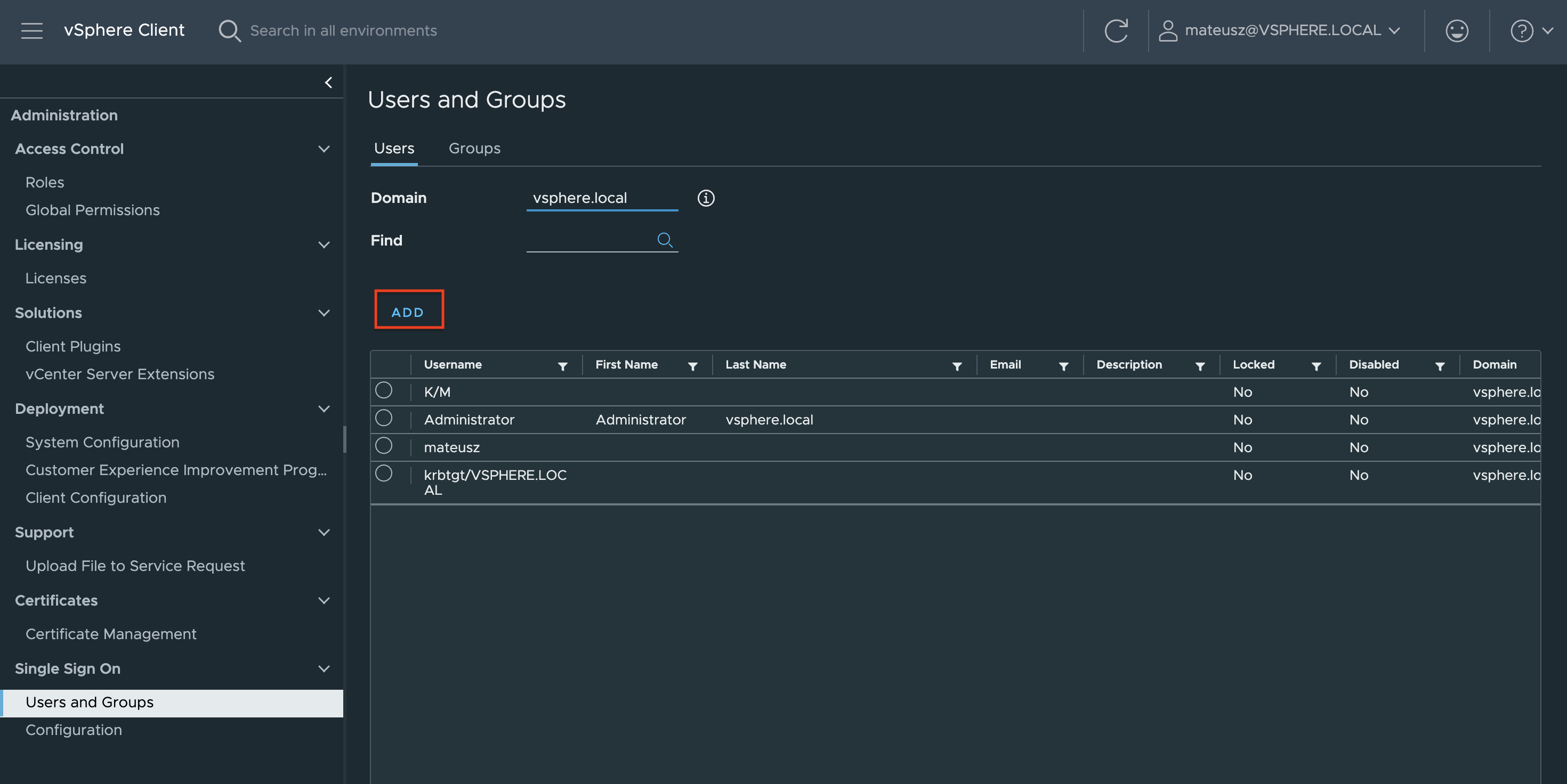
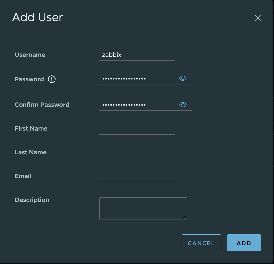
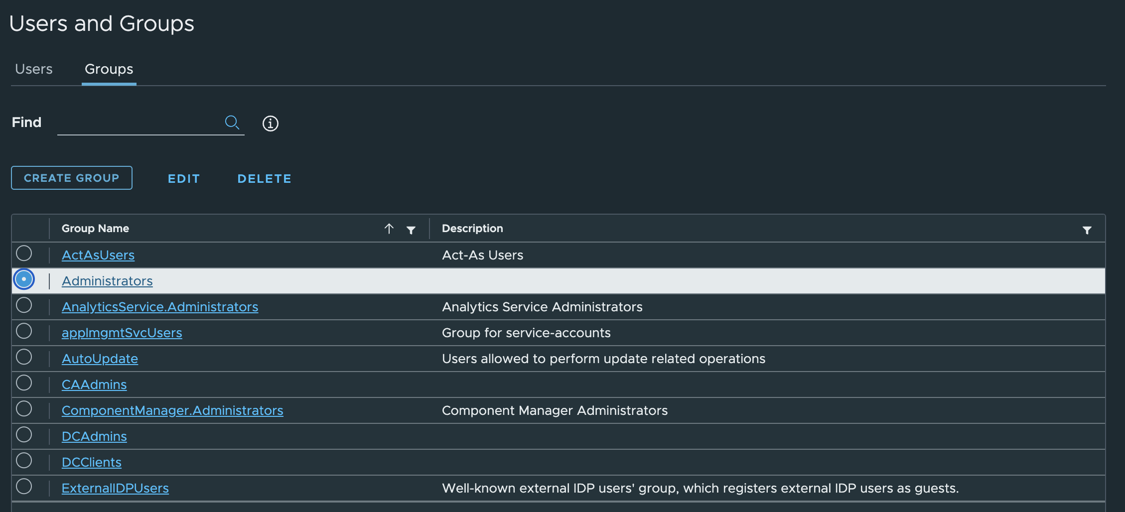
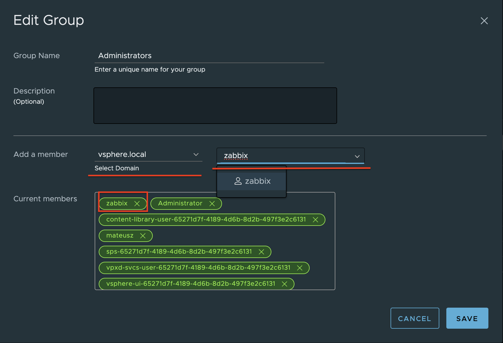

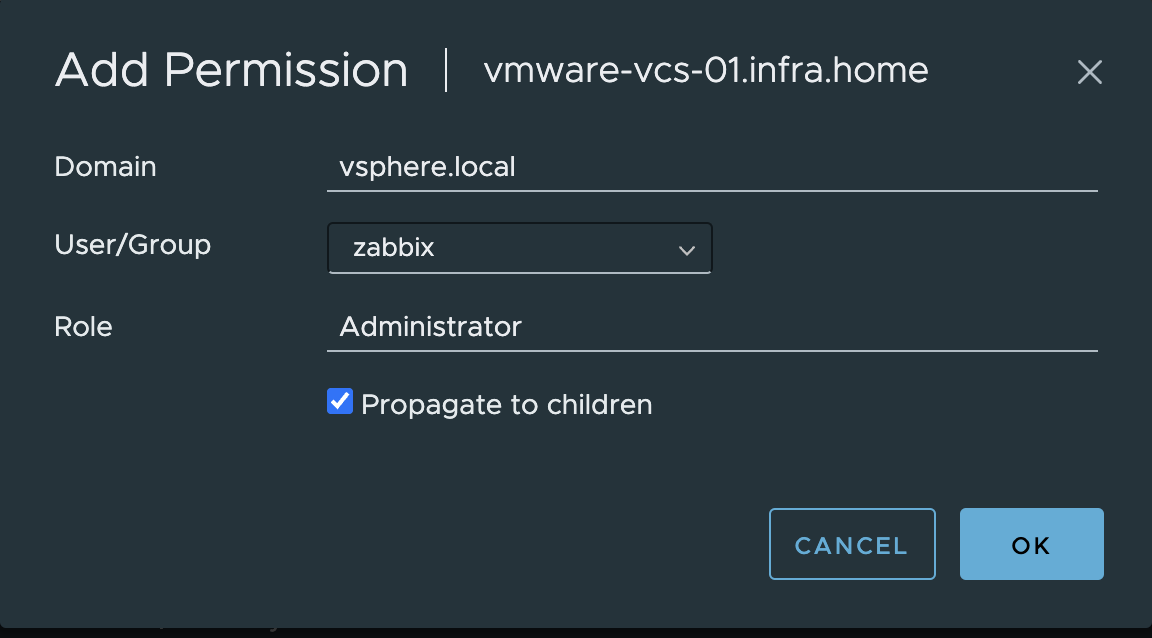
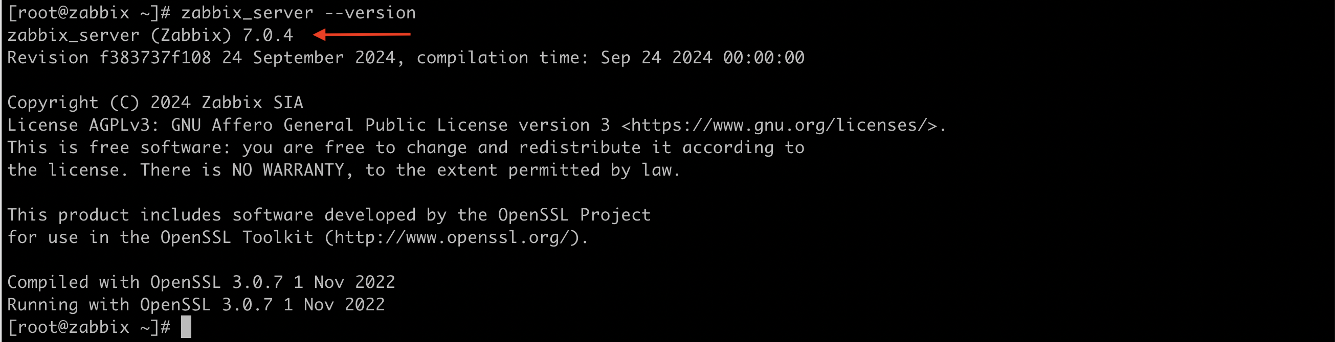

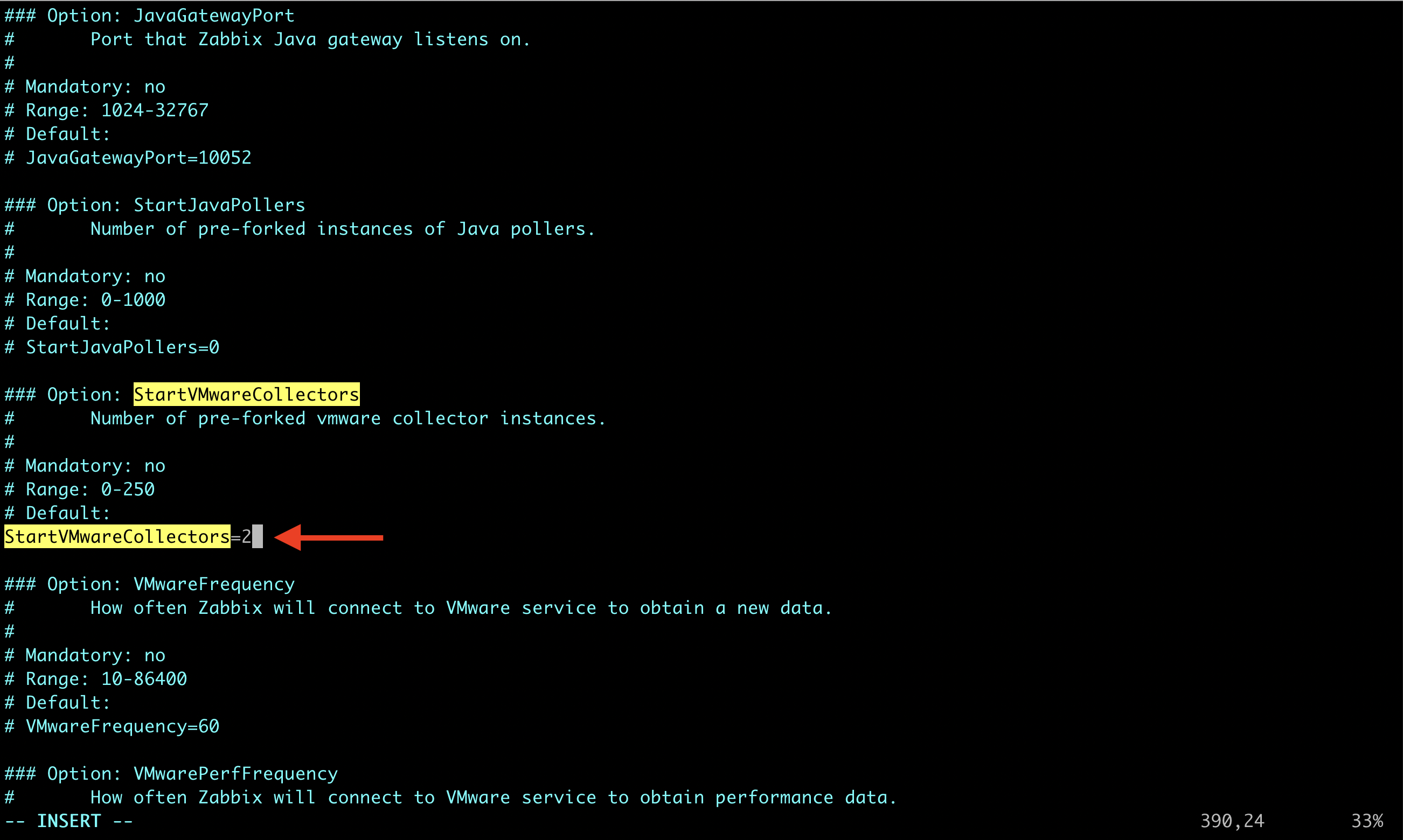

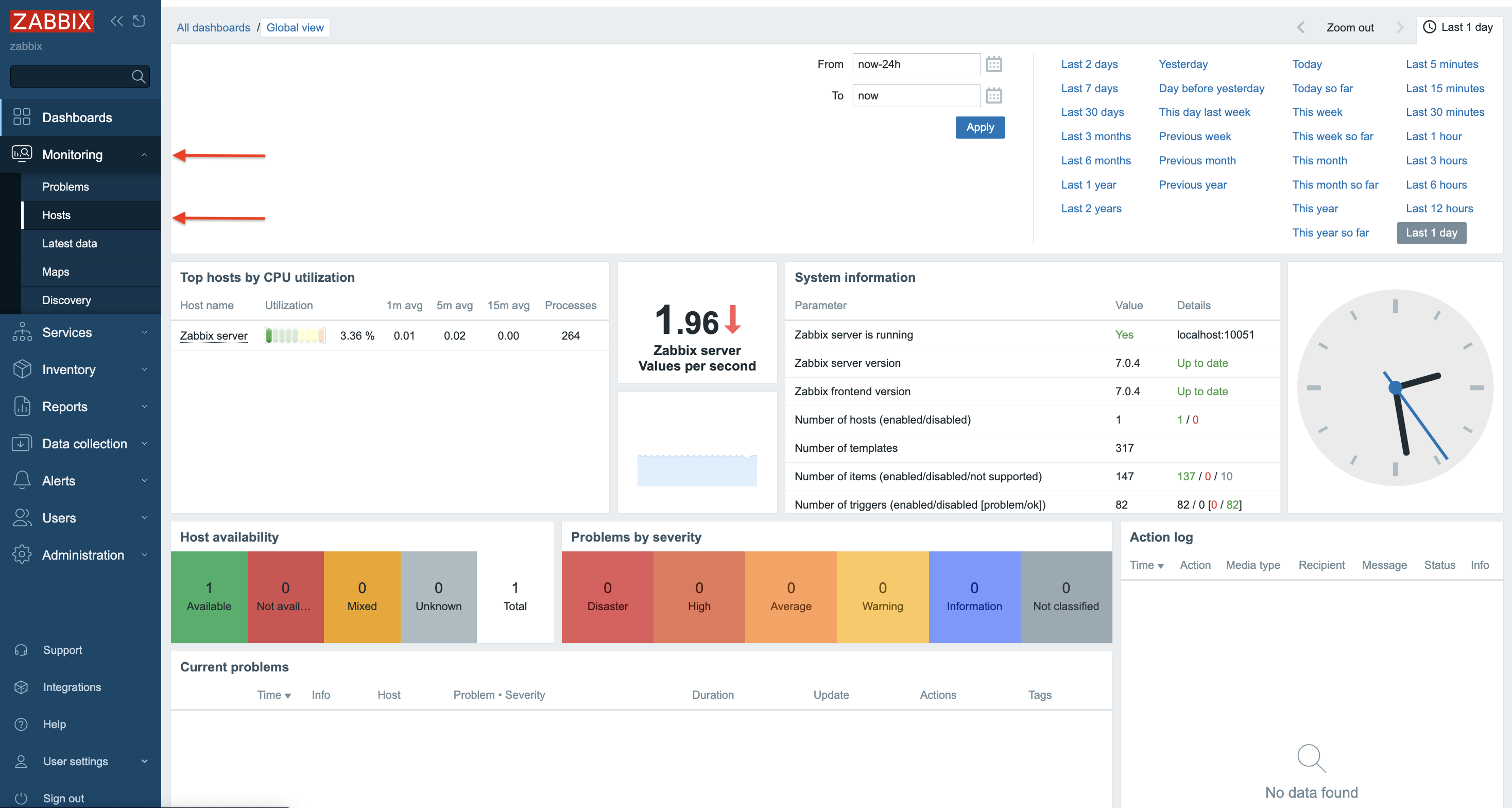
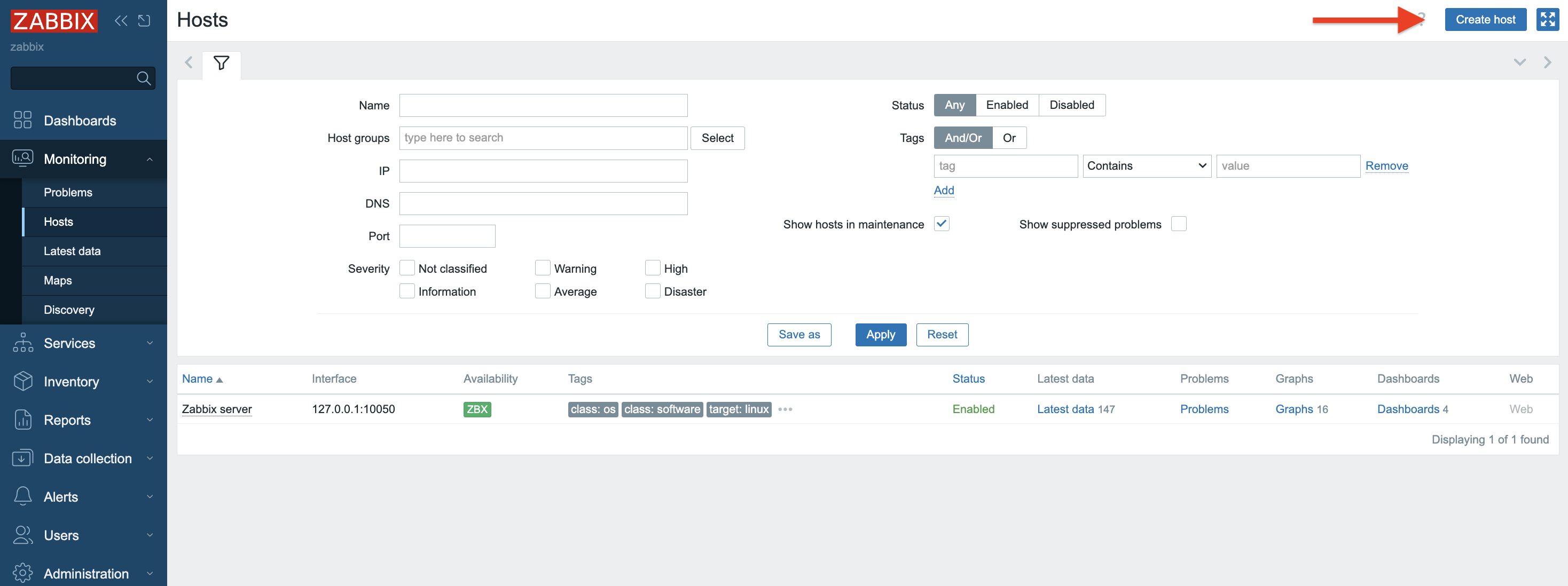
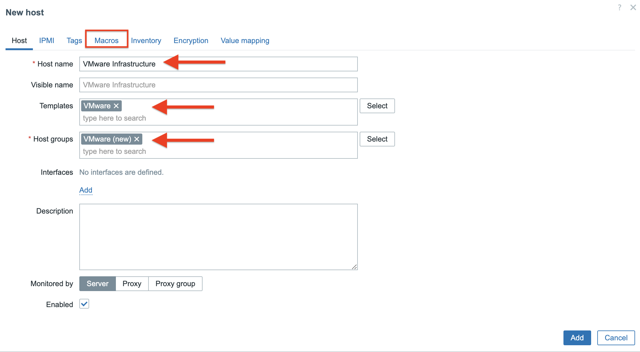
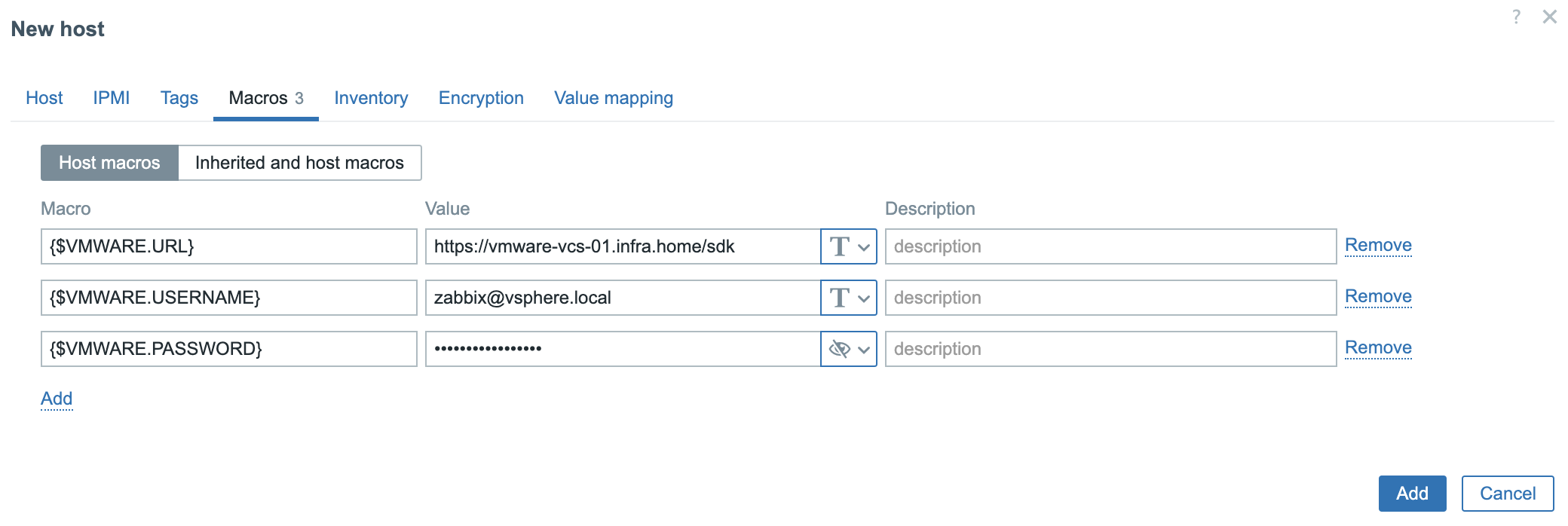
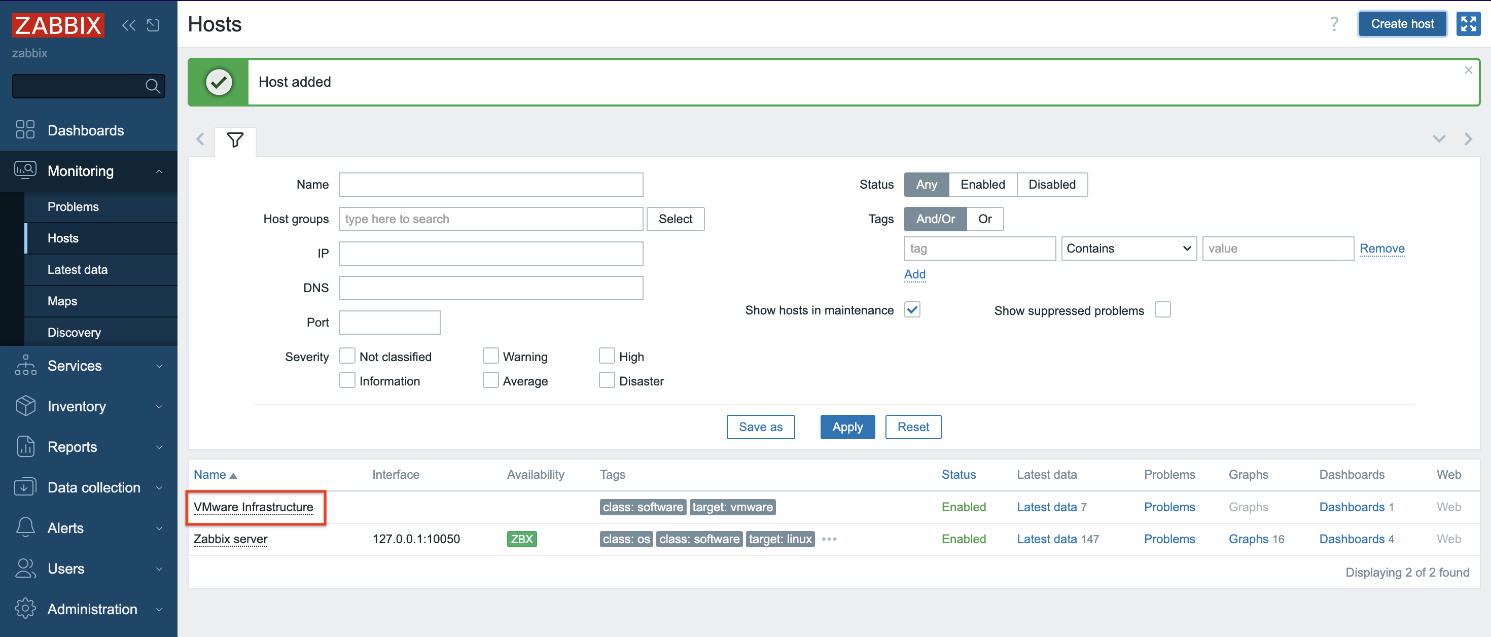
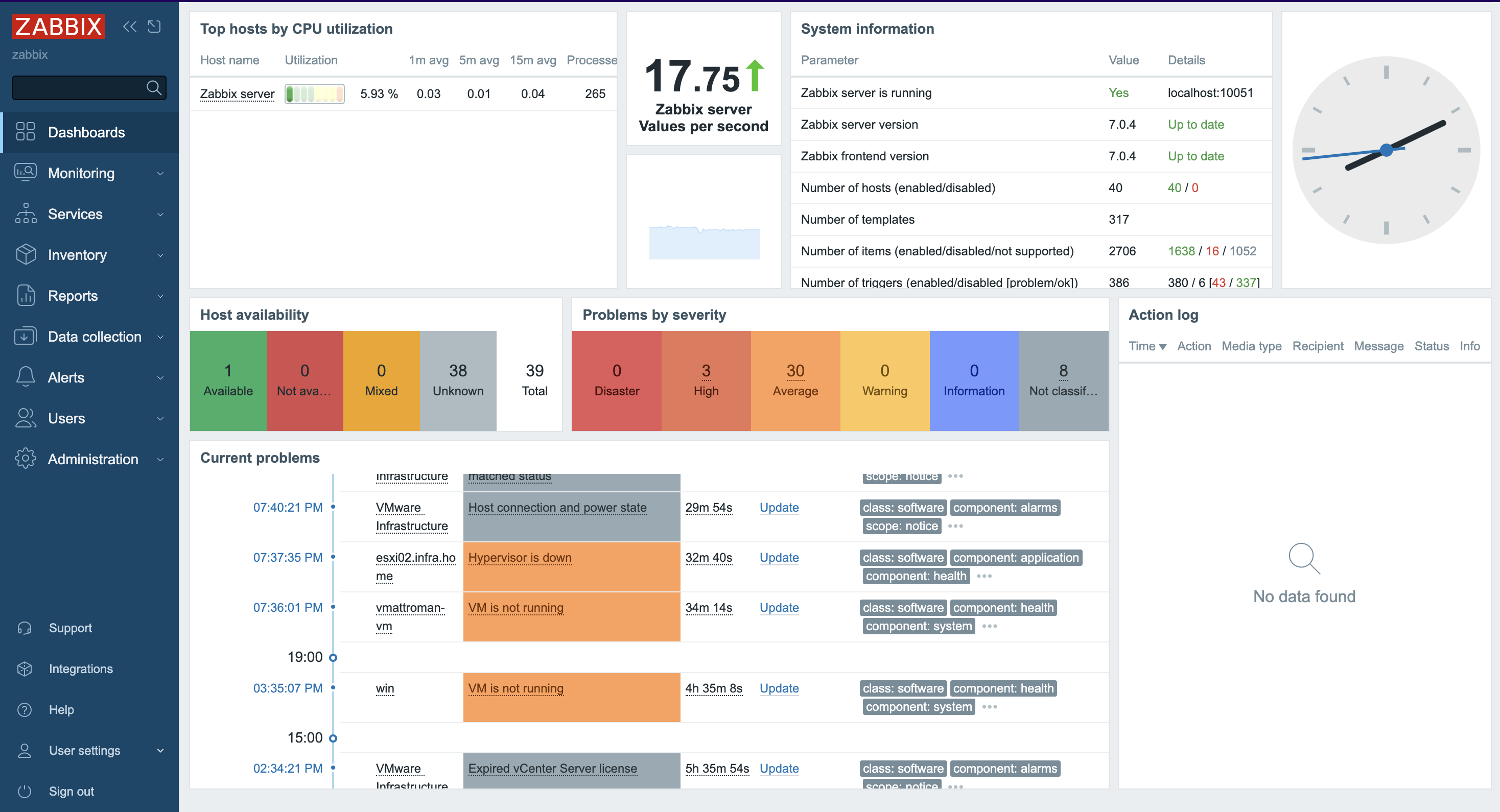
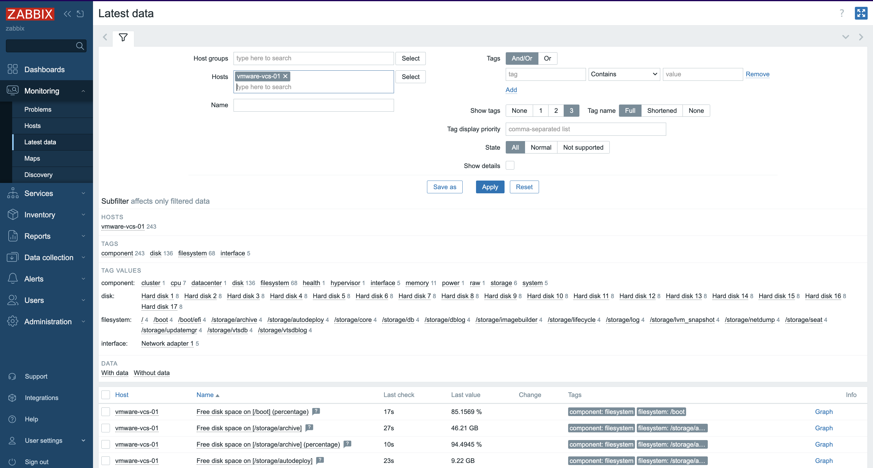
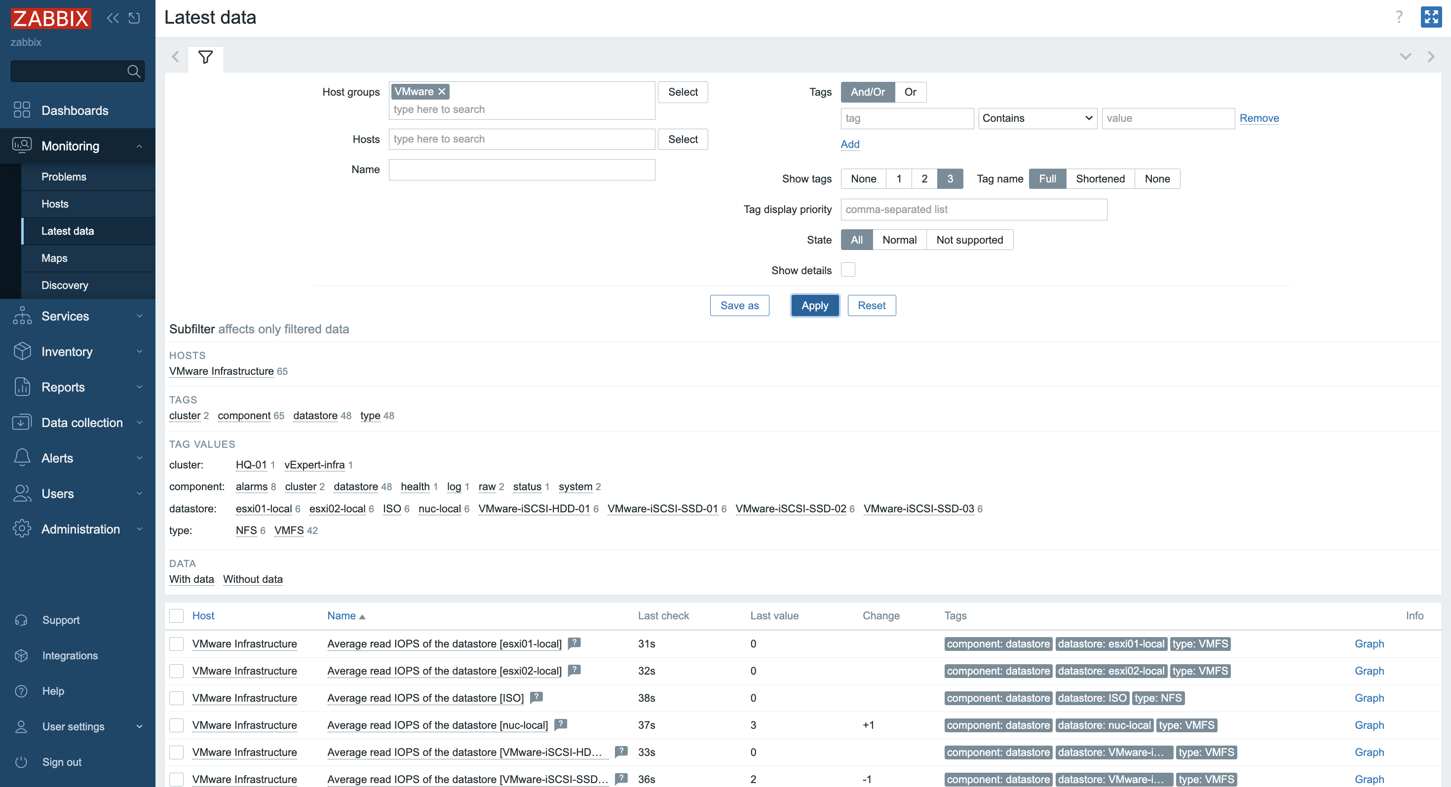
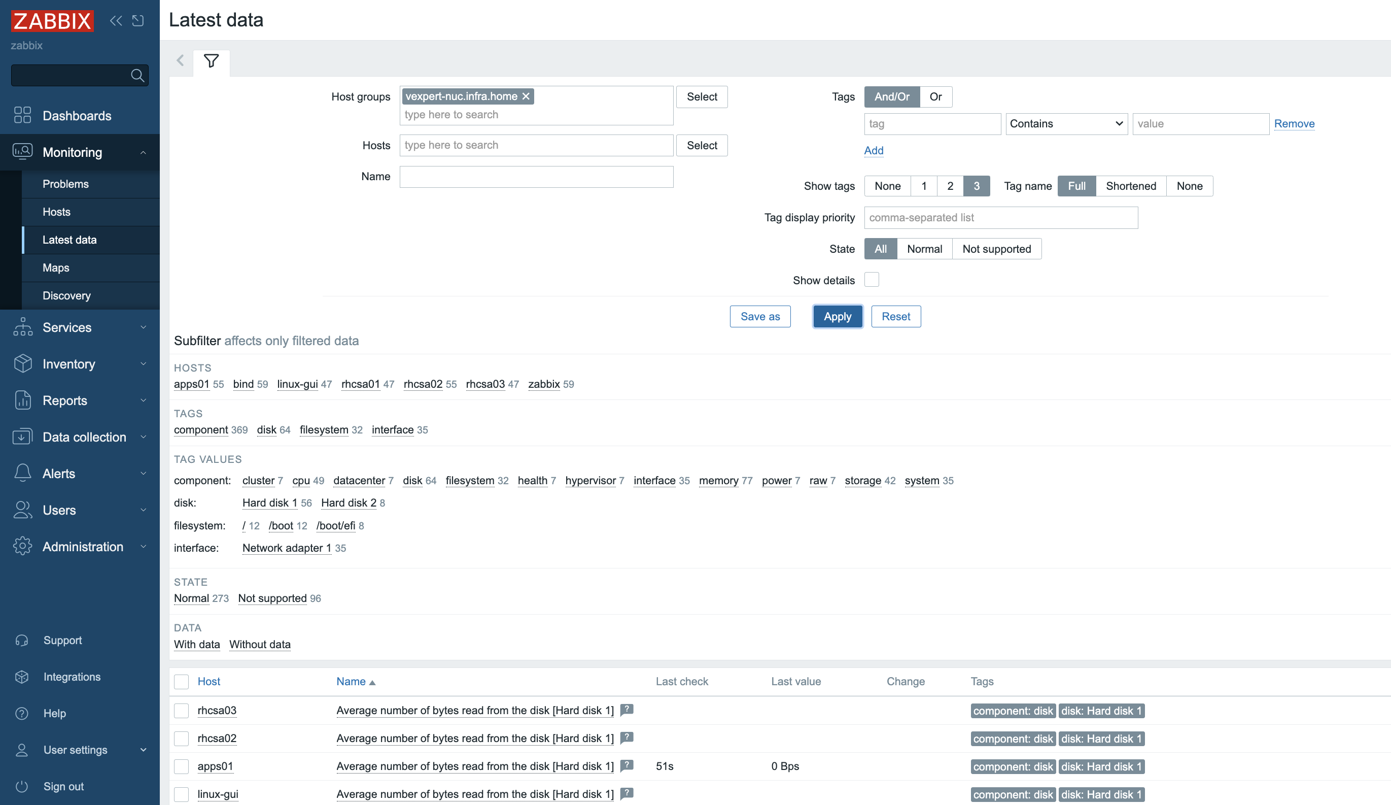


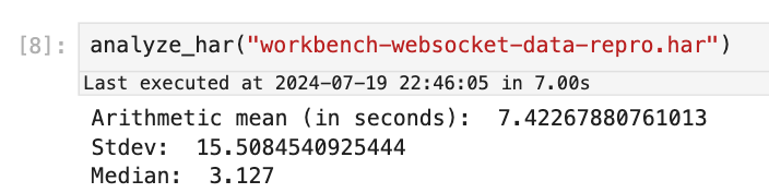
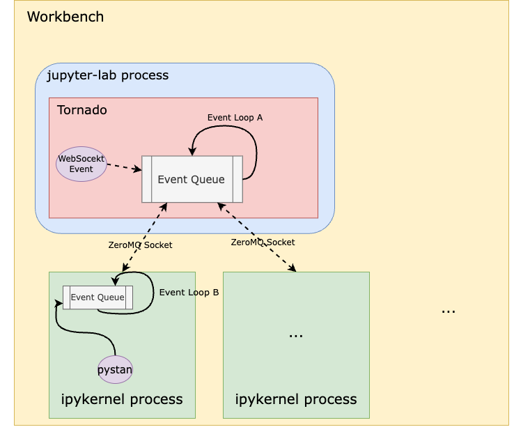
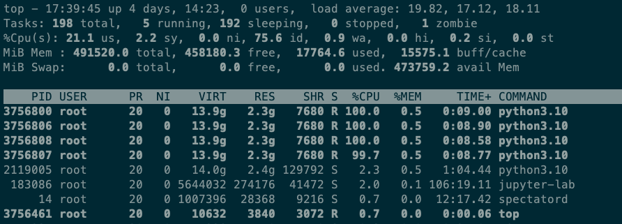
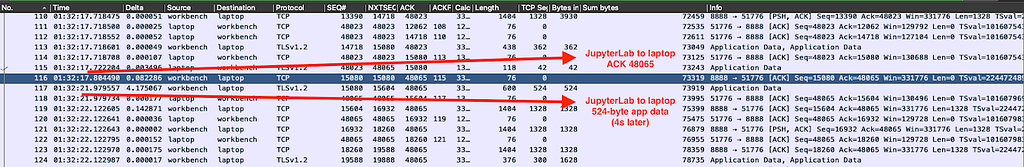
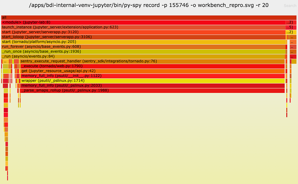
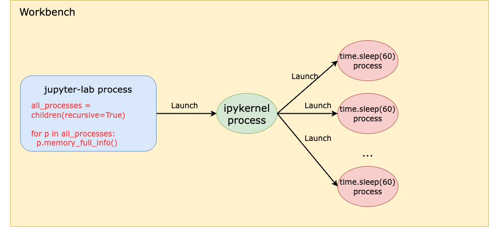
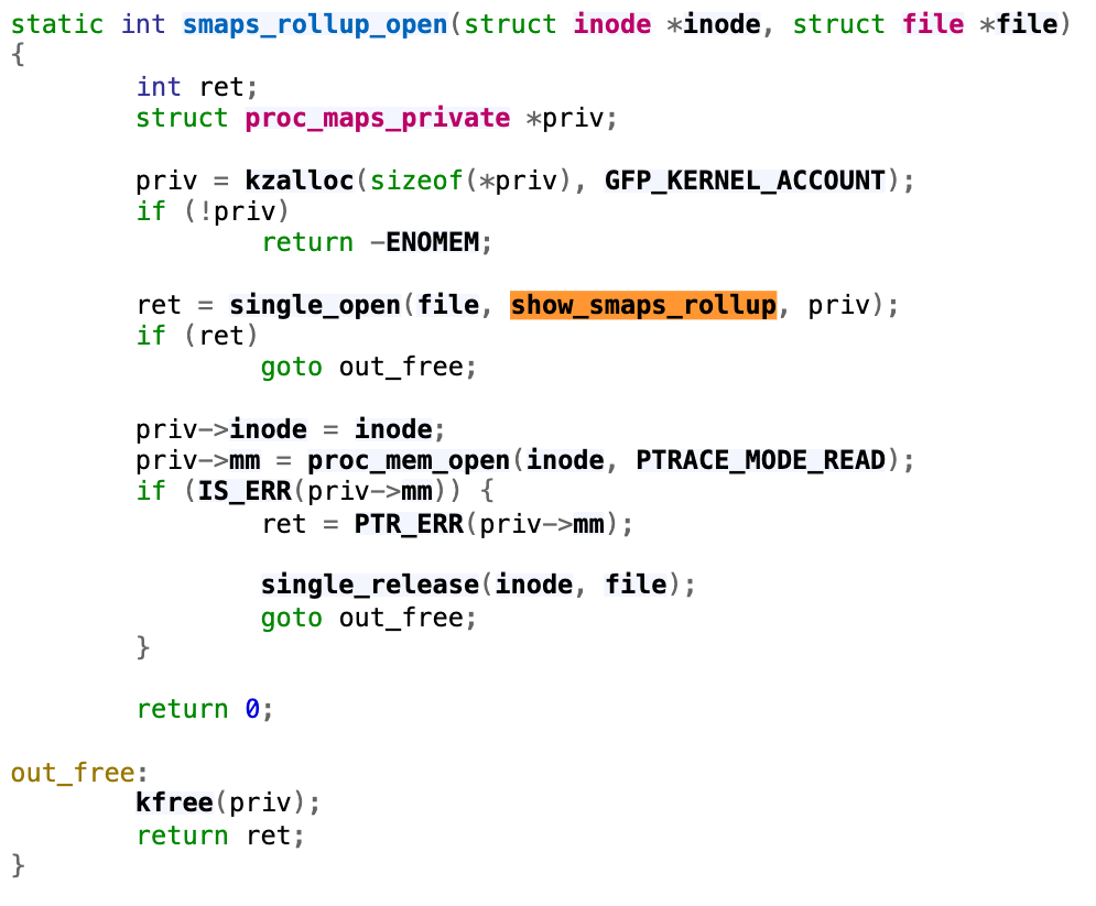


 Kalaiselvi Kamaraj is a Sr. Software Development Engineer with Amazon. She has worked on several projects within Redshift Query processing team and currently focusing on performance related projects for Redshift Data Lake.
 Mark Lyons is a Principal Product Manager on the Amazon Redshift team. He works on the intersection of data lakes and data warehouses. Prior to joining AWS, Mark held product leadership roles with Dremio and Vertica. He is passionate about data analytics and empowering customers to change the world with their data.
 Asser Moustafa is a Principal Worldwide Specialist Solutions Architect at AWS, based in Dallas, Texas, USA. He partners with customers worldwide, advising them on all aspects of their data architectures, migrations, and strategic data visions to help organizations adopt cloud-based solutions, maximize the value of their data assets, modernize legacy infrastructures, and implement cutting-edge capabilities like machine learning and advanced analytics. Prior to joining AWS, Asser held various data and analytics leadership roles, completing an MBA from New York University and an MS in Computer Science from Columbia University in New York. He is passionate about empowering organizations to become truly data-driven and unlock the transformative potential of their data.