Researchers at University of Guelph in Ontario, Canada, recovered logs from laptops after receiving overnight repairs from 12 commercial shops. The logs showed that technicians from six of the locations had accessed personal data and that two of those shops also copied data onto a personal device. Devices belonging to females were more likely to be snooped on, and that snooping tended to seek more sensitive data, including both sexually revealing and non-sexual pictures, documents, and financial information.
[…]
In three cases, Windows Quick Access or Recently Accessed Files had been deleted in what the researchers suspect was an attempt by the snooping technician to cover their tracks. As noted earlier, two of the visits resulted in the logs the researchers relied on being unrecoverable. In one, the researcher explained they had installed antivirus software and performed a disk cleanup to “remove multiple viruses on the device.” The researchers received no explanation in the other case.
[…]
The laptops were freshly imaged Windows 10 laptops. All were free of malware and other defects and in perfect working condition with one exception: the audio driver was disabled. The researchers chose that glitch because it required only a simple and inexpensive repair, was easy to create, and didn’t require access to users’ personal files.
Half of the laptops were configured to appear as if they belonged to a male and the other half to a female. All of the laptops were set up with email and gaming accounts and populated with browser history across several weeks. The researchers added documents, both sexually revealing and non-sexual pictures, and a cryptocurrency wallet with credentials.
A few notes. One: this is a very small study—only twelve laptop repairs. Two, some of the results were inconclusive, which indicated—but did not prove—log tampering by the technicians. Three, this study was done in Canada. There would probably be more snooping by American repair technicians.
The moral isn’t a good one: if you bring your laptop in to be repaired, you should expect the technician to snoop through your hard drive, taking what they want.
Security updates have been issued by Debian (chromium, commons-configuration2, graphicsmagick, heimdal, inetutils, ini4j, jackson-databind, and varnish), Fedora (drupal7-i18n, grub2, kubernetes, and python-slixmpp), Mageia (botan, golang, kernel, kernel-linus, radare2/rizin, and xterm), Red Hat (krb5, varnish, and varnish:6), SUSE (busybox, chromium, erlang, exiv2, firefox, freerdp, ganglia-web, java-1_8_0-openj9, nodejs12, nodejs14, opera, pixman, python3, sudo, tiff, and xen), and Ubuntu (libice and shadow).
We want our digital data to be safe. We want to visit websites, send bank details, type passwords, sign documents online, login into remote computers, encrypt data before storing it in databases and be sure that nobody can tamper with it. Cryptography can provide a high degree of data security, but we need to protect cryptographic keys.
At the same time, we can’t have our key written somewhere securely and just access it occasionally. Quite the opposite, it’s involved in every request where we do crypto-operations. If a site supports TLS, then the private key is used to establish each connection.
Unfortunately cryptographic keys sometimes leak and when it happens, it is a big problem. Many leaks happen because of software bugs and security vulnerabilities. In this post we will learn how the Linux kernel can help protect cryptographic keys from a whole class of potential security vulnerabilities: memory access violations.
Memory access violations
According to the NSA, around 70% of vulnerabilities in both Microsoft’s and Google’s code were related to memory safety issues. One of the consequences of incorrect memory accesses is leaking security data (including cryptographic keys). Cryptographic keys are just some (mostly random) data stored in memory, so they may be subject to memory leaks like any other in-memory data. The below example shows how a cryptographic key may accidentally leak via stack memory reuse:
broken.c
#include <stdio.h>
#include <stdint.h>

static void encrypt(void)
{
    uint8_t key[] = "hunter2";
    printf("encrypting with super secret key: %s\n", key);
}

static void log_completion(void)
{
    /* oh no, we forgot to init the msg */
    char msg[8];
    printf("not important, just fyi: %s\n", msg);
}

int main(void)
{
    encrypt();
    /* notify that we're done */
    log_completion();
    return 0;
}
Compile and run our program:
$ gcc -o broken broken.c
$ ./broken
encrypting with super secret key: hunter2
not important, just fyi: hunter2
Oops, we printed the secret key in the “fyi” logger instead of the intended log message! There are two problems with the code above:
we didn’t securely destroy the key in our pseudo-encryption function (by overwriting the key data with zeroes, for example), when we finished using it
our buggy logging function has access to any memory within our process
And while we can probably easily fix the first problem with some additional code, the second problem is the inherent result of how software runs inside the operating system.
Each process is given a block of contiguous virtual memory by the operating system. It allows the kernel to share limited computer resources among several simultaneously running processes. This approach is called virtual memory management. Inside the virtual memory a process has its own address space and doesn’t have access to the memory of other processes, but it can access any memory within its address space. In our example we are interested in a piece of process memory called the stack.
The stack consists of stack frames. A stack frame is dynamically allocated space for the currently running function. It contains the function’s local variables, arguments and return address. When compiling a function the compiler calculates how much memory needs to be allocated and requests a stack frame of this size. Once a function finishes execution the stack frame is marked as free and can be used again. A stack frame is a logical block, it doesn’t provide any boundary checks, it’s not erased, just marked as free. Additionally, the virtual memory is a contiguous block of addresses. Both of these statements give the possibility for malware/buggy code to access data from anywhere within virtual memory.
The stack of our program broken.c will look like:
At the beginning we have a stack frame of the main function. Further, the main() function calls encrypt() which will be placed on the stack immediately below the main() (the code stack grows downwards). Inside encrypt() the compiler requests 8 bytes for the key variable (7 bytes of data + C-null character). When encrypt() finishes execution, the same memory addresses are taken by log_completion(). Inside the log_completion() the compiler allocates eight bytes for the msg variable. Accidentally, it was put on the stack at the same place where our private key was stored before. The memory for msg was only allocated, but not initialized, the data from the previous function left as is.
Additionally, to the code bugs, programming languages provide unsafe functions known for the safe-memory vulnerabilities. For example, for C such functions are printf(), strcpy(), gets(). The function printf() doesn’t check how many arguments must be passed to replace all placeholders in the format string. The function arguments are placed on the stack above the function stack frame, printf() fetches arguments according to the numbers and type of placeholders, easily going off its arguments and accessing data from the stack frame of the previous function.
The NSA advises us to use safety-memory languages like Python, Go, Rust. But will it completely protect us?
The Python compiler will definitely check boundaries in many cases for you and notify with an error:
>>> print("x: {}, y: {}, {}".format(1, 2))
Traceback (most recent call last):
  File "<stdin>", line 1, in <module>
IndexError: Replacement index 2 out of range for positional args tuple
However, this is a quote from one of 36 (for now) vulnerabilities:
Python 2.7.14 is vulnerable to a Heap-Buffer-Overflow as well as a Heap-Use-After-Free.
Golang has its own list of overflow vulnerabilities, and has an unsafe package. The name of the package speaks for itself, usual rules and checks don’t work inside this package.
Heartbleed
In 2014, the Heartbleed bug was discovered. The (at the time) most used cryptography library OpenSSL leaked private keys. We experienced it too.
Mitigation
So memory bugs are a fact of life, and we can’t really fully protect ourselves from them. But, given the fact that cryptographic keys are much more valuable than the other data, can we do better protecting the keys at least?
As we already said, a memory address space is normally associated with a process. And two different processes don’t share memory by default, so are naturally isolated from each other. Therefore, a potential memory bug in one of the processes will not accidentally leak a cryptographic key from another process. The security of ssh-agent builds on this principle. There are always two processes involved: a client/requester and the agent.
The agent will never send a private key over its request channel. Instead, operations that require a private key will be performed by the agent, and the result will be returned to the requester. This way, private keys are not exposed to clients using the agent.
A requester is usually a network-facing process and/or processing untrusted input. Therefore, the requester is much more likely to be susceptible to memory-related vulnerabilities but in this scheme it would never have access to cryptographic keys (because keys reside in a separate process address space) and, thus, can never leak them.
At Cloudflare, we employ the same principle in Keyless SSL. Customer private keys are stored in an isolated environment and protected from Internet-facing connections.
Linux Kernel Key Retention Service
The client/requester and agent approach provides better protection for secrets or cryptographic keys, but it brings some drawbacks:
we need to develop and maintain two different programs instead of one
we also need to design a well-defined-interface for communication between the two processes
we need to implement the communication support between two processes (Unix sockets, shared memory, etc.)
we might need to authenticate and support ACLs between the processes, as we don’t want any requester on our system to be able to use our cryptographic keys stored inside the agent
we need to ensure the agent process is up and running, when working with the client/requester process
What if we replace the agent process with the Linux kernel itself?
it is already running on our system (otherwise our software would not work)
it has a well-defined interface for communication (system calls)
Initially it was designed for kernel services like dm-crypt/ecryptfs, but later was opened to use by userspace programs. It gives us some advantages:
the keys are stored outside the process address space
the well-defined-interface and the communication layer is implemented via syscalls
the keys are kernel objects and so have associated permissions and ACLs
the keys lifecycle can be implicitly bound to the process lifecycle
The Linux Kernel Key Retention Service operates with two types of entities: keys and keyrings, where a keyring is a key of a special type. If we put it into analogy with files and directories, we can say a key is a file and a keyring is a directory. Moreover, they represent a key hierarchy similar to a filesystem tree hierarchy: keyrings reference keys and other keyrings, but only keys can hold the actual cryptographic material similar to files holding the actual data.
Keys have types. The type of key determines which operations can be performed over the keys. For example, keys of user and logon types can hold arbitrary blobs of data, but logon keys can never be read back into userspace, they are exclusively used by the in-kernel services.
For the purposes of using the kernel instead of an agent process the most interesting type of keys is the asymmetric type. It can hold a private key inside the kernel and provides the ability for the allowed applications to either decrypt or sign some data with the key. Currently, only RSA keys are supported, but work is underway to add ECDSA key support.
While keys are responsible for safeguarding the cryptographic material inside the kernel, keyrings determine key lifetime and shared access. In its simplest form, when a particular keyring is destroyed, all the keys that are linked only to that keyring are securely destroyed as well. We can create custom keyrings manually, but probably one the most powerful features of the service are the “special keyrings”.
These keyrings are created implicitly by the kernel and their lifetime is bound to the lifetime of a different kernel object, like a process or a user. (Currently there are four categories of “implicit” keyrings), but for the purposes of this post we’re interested in two most widely used ones: process keyrings and user keyrings.
User keyring lifetime is bound to the existence of a particular user and this keyring is shared between all the processes of the same UID. Thus, one process, for example, can store a key in a user keyring and another process running as the same user can retrieve/use the key. When the UID is removed from the system, all the keys (and other keyrings) under the associated user keyring will be securely destroyed by the kernel.
Process keyrings are bound to some processes and may be of three types differing in semantics: process, thread and session. A process keyring is bound and private to a particular process. Thus, any code within the process can store/use keys in the keyring, but other processes (even with the same user id or child processes) cannot get access. And when the process dies, the keyring and the associated keys are securely destroyed. Besides the advantage of storing our secrets/keys in an isolated address space, the process keyring gives us the guarantee that the keys will be destroyed regardless of the reason for the process termination: even if our application crashed hard without being given an opportunity to execute any clean up code – our keys will still be securely destroyed by the kernel.
A thread keyring is similar to a process keyring, but it is private and bound to a particular thread. For example, we can build a multithreaded web server, which can serve TLS connections using multiple private keys, and we can be sure that connections/code in one thread can never use a private key, which is associated with another thread (for example, serving a different domain name).
A session keyring makes its keys available to the current process and all its children. It is destroyed when the topmost process terminates and child processes can store/access keys, while the topmost process exists. It is mostly useful in shell and interactive environments, when we employ the keyctl tool to access the Linux Kernel Key Retention Service, rather than using the kernel system call interface. In the shell, we generally can’t use the process keyring as every executed command creates a new process. Thus, if we add a key to the process keyring from the command line – that key will be immediately destroyed, because the “adding” process terminates, when the command finishes executing. Let’s actually confirm this with bpftrace.
In one terminal we will trace the user_destroy function, which is responsible for deleting a user key:
And in another terminal let’s try to add a key to the process keyring:
$ keyctl add user mykey hunter2 @p
742524855
Going back to the first terminal we can immediately see:
…
Attaching 1 probe...
destroying key 742524855
And we can confirm the key is not available by trying to access it:
$ keyctl print 742524855
keyctl_read_alloc: Required key not available
So in the above example, the key “mykey” was added to the process keyring of the subshell executing keyctl add user mykey hunter2 @p. But since the subshell process terminated the moment the command was executed, both its process keyring and the added key were destroyed.
Instead, the session keyring allows our interactive commands to add keys to our current shell environment and subsequent commands to consume them. The keys will still be securely destroyed, when our main shell process terminates (likely, when we log out from the system).
So by selecting the appropriate keyring type we can ensure the keys will be securely destroyed, when not needed. Even if the application crashes! This is a very brief introduction, but it will allow you to play with our examples, for the whole context, please, reach the official documentation.
Replacing the ssh-agent with the Linux Kernel Key Retention Service
We gave a long description of how we can replace two isolated processes with the Linux Kernel Retention Service. It’s time to put our words into code. We talked about ssh-agent as well, so it will be a good exercise to replace our private key stored in memory of the agent with an in-kernel one. We picked the most popular SSH implementation OpenSSH as our target.
Some minor changes need to be added to the code to add functionality to retrieve a key from the kernel:
$ autoreconf
$ ./configure --with-libs=-lkeyutils --disable-pkcs11
…
$ make
…
Note that we instruct the build system to additionally link with libkeyutils, which provides convenient wrappers to access the Linux Kernel Key Retention Service. Additionally, we had to disable PKCS11 support as the code has a function with the same name as in `libkeyutils`, so there is a naming conflict. There might be a better fix for this, but it is out of scope for this post.
Now that we have the patched OpenSSH – let’s test it. Firstly, we need to generate a new SSH RSA key that we will use to access the system. Because the Linux kernel only supports private keys in the PKCS8 format, we’ll use it from the start (instead of the default OpenSSH format):
Normally, we would be using `ssh-add` to add this key to our ssh agent. In our case we need to use a replacement script, which would add the key to our current session keyring:
ssh-add-keyring.sh
#/bin/bash -e

in=$1
key_desc=$2
keyring=$3

in_pub=$in.pub
key=$(mktemp)
out="${in}_keyring"

function finish {
    rm -rf $key
}
trap finish EXIT

# https://github.com/openssh/openssh-portable/blob/master/PROTOCOL.key
# null-terminanted openssh-key-v1
printf 'openssh-key-v1\0' > $key
# cipher: none
echo '00000004' | xxd -r -p >> $key
echo -n 'none' >> $key
# kdf: none
echo '00000004' | xxd -r -p >> $key
echo -n 'none' >> $key
# no kdf options
echo '00000000' | xxd -r -p >> $key
# one key in the blob
echo '00000001' | xxd -r -p >> $key

# grab the hex public key without the (00000007 || ssh-rsa) preamble
pub_key=$(awk '{ print $2 }' $in_pub | base64 -d | xxd -s 11 -p | tr -d '\n')
# size of the following public key with the (0000000f || ssh-rsa-keyring) preamble
printf '%08x' $(( ${#pub_key} / 2 + 19 )) | xxd -r -p >> $key
# preamble for the public key
# ssh-rsa-keyring in prepended with length of the string
echo '0000000f' | xxd -r -p >> $key
echo -n 'ssh-rsa-keyring' >> $key
# the public key itself
echo $pub_key | xxd -r -p >> $key

# the private key is just a key description in the Linux keyring
# ssh will use it to actually find the corresponding key serial
# grab the comment from the public key
comment=$(awk '{ print $3 }' $in_pub)
# so the total size of the private key is
# two times the same 4 byte int +
# (0000000f || ssh-rsa-keyring) preamble +
# a copy of the public key (without preamble) +
# (size || key_desc) +
# (size || comment )
priv_sz=$(( 8 + 19 + ${#pub_key} / 2 + 4 + ${#key_desc} + 4 + ${#comment} ))
# we need to pad the size to 8 bytes
pad=$(( 8 - $(( priv_sz % 8 )) ))
# so, total private key size
printf '%08x' $(( $priv_sz + $pad )) | xxd -r -p >> $key
# repeated 4-byte int
echo '0102030401020304' | xxd -r -p >> $key
# preamble for the private key
echo '0000000f' | xxd -r -p >> $key
echo -n 'ssh-rsa-keyring' >> $key
# public key
echo $pub_key | xxd -r -p >> $key
# private key description in the keyring
printf '%08x' ${#key_desc} | xxd -r -p >> $key
echo -n $key_desc >> $key
# comment
printf '%08x' ${#comment} | xxd -r -p >> $key
echo -n $comment >> $key
# padding
for (( i = 1; i <= $pad; i++ )); do
    echo 0$i | xxd -r -p >> $key
done

echo '-----BEGIN OPENSSH PRIVATE KEY-----' > $out
base64 $key >> $out
echo '-----END OPENSSH PRIVATE KEY-----' >> $out
chmod 600 $out

# load the PKCS8 private key into the designated keyring
openssl pkcs8 -in $in -topk8 -outform DER -nocrypt | keyctl padd asymmetric $key_desc $keyring
Depending on how our kernel was compiled, we might also need to load some kernel modules for asymmetric private key support:
$ sudo modprobe pkcs8_key_parser
$ ./ssh-add-keyring.sh ~/.ssh/id_rsa myssh @s
Enter pass phrase for ~/.ssh/id_rsa:
723263309
Finally, our private ssh key is added to the current session keyring with the name “myssh”. In addition, the ssh-add-keyring.sh will create a pseudo-private key file in ~/.ssh/id_rsa_keyring, which needs to be passed to the main ssh process. It is a pseudo-private key, because it doesn’t have any sensitive cryptographic material. Instead, it only has the “myssh” identifier in a native OpenSSH format. If we use multiple SSH keys, we have to tell the main ssh process somehow which in-kernel key name should be requested from the system.
Before we start testing it, let’s make sure our SSH server (running locally) will accept the newly generated key as a valid authentication:
$ cat ~/.ssh/id_rsa.pub >> ~/.ssh/authorized_keys
Now we can try to SSH into the system:
$ SSH_AUTH_SOCK="" ./ssh -i ~/.ssh/id_rsa_keyring localhost
The authenticity of host 'localhost (::1)' can't be established.
ED25519 key fingerprint is SHA256:3zk7Z3i9qZZrSdHvBp2aUYtxHACmZNeLLEqsXltynAY.
This key is not known by any other names.
Are you sure you want to continue connecting (yes/no/[fingerprint])? yes
Warning: Permanently added 'localhost' (ED25519) to the list of known hosts.
Linux dev 5.15.79-cloudflare-2022.11.6 #1 SMP Mon Sep 27 00:00:00 UTC 2010 x86_64
…
It worked! Notice that we’re resetting the `SSH_AUTH_SOCK` environment variable to make sure we don’t use any keys from an ssh-agent running on the system. Still the login flow does not request any password for our private key, the key itself is resident of the kernel address space, and we reference it using its serial for signature operations.
User or session keyring?
In the example above, we set up our SSH private key into the session keyring. We can check if it is there:
We might have used user keyring as well. What is the difference? Currently, the “myssh” key lifetime is limited to the current login session. That is, if we log out and login again, the key will be gone, and we would have to run the ssh-add-keyring.sh script again. Similarly, if we log in to a second terminal, we won’t see this key:
Notice that the serial number of the session keyring _ses in the second terminal is different. A new keyring was created and “myssh” key along with the previous session keyring doesn’t exist anymore:
$ SSH_AUTH_SOCK="" ./ssh -i ~/.ssh/id_rsa_keyring localhost
Load key "/home/ignat/.ssh/id_rsa_keyring": key not found
…
If instead we tell ssh-add-keyring.sh to load the private key into the user keyring (replace @s with @u in the command line parameters), it will be available and accessible from both login sessions. In this case, during logout and re-login, the same key will be presented. Although, this has a security downside – any process running as our user id will be able to access and use the key.
Summary
In this post we learned about one of the most common ways that data, including highly valuable cryptographic keys, can leak. We talked about some real examples, which impacted many users around the world, including Cloudflare. Finally, we learned how the Linux Kernel Retention Service can help us to protect our cryptographic keys and secrets.
We also introduced a working patch for OpenSSH to use this cool feature of the Linux kernel, so you can easily try it yourself. There are still many Linux Kernel Key Retention Service features left untold, which might be a topic for another blog post. Stay tuned!
AWS VP and Chief Evangelist Jeff Barr, plus a select group of AWS Developer Advocate colleagues, have personally chosen their picks for some of the most impactful and exciting product and service launches to debut at AWS re:Invent 2022. From now through Dec. 1, we’ll update this page daily with links to their AWS News Blog posts (plus a few noteworthy preview posts) so you can dive deeper once the launches have been announced.
As always, there’s simply too much for the team to cover and even if a launch doesn’t make this list, that doesn’t mean it’s not noteworthy. Make sure to check out What’s New for a complete rundown of all the AWS re:Invent 2022 announcements.
Here are a few more resources to help you keep up with all the re:Invent news:
The Official AWS Podcast will have keynote recaps each day and more deep dive episodes in the coming weeks.
AWS OnAir will be livestreaming from the show floor.
(This post was updated: 10:23 p.m. PST, Nov. 27, 2022.)
Classifying and Extracting Mortgage Loan Data with Amazon Textract The new API was created in response to requests from major lenders in the industry to help them process applications faster and reduce errors, which improves the end-customer experience and lowers operating costs.
Protect Sensitive Data with Amazon CloudWatch Logs This new set of capabilities for Amazon CloudWatch Logs leverages pattern matching and machine learning (ML) to detect and protect sensitive log data in transit.
AWS Backup allows you to define a central backup policy to manage data protection of your applications and can now also protect your Amazon Redshift clusters.
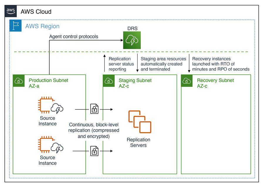
Announcing Automated in-AWS Failback for AWS Elastic Disaster Recovery The new automated support provides a simplified and expedited experience to fail back Amazon Elastic Compute Cloud (Amazon EC2) instances to the original Region, and both failover and failback processes (for on-premises or in-AWS recovery) can be conveniently started from the AWS Management Console.
RDS makes it easier for you to set up, operate, and scale a relational database in the cloud. You get direct database access without worrying about infrastructure provisioning, software maintenance, or common database management tasks.
Since that launch we have continued to do our best to help you to avoid all of those items, while also working to make RDS ever-more cost effective. For example, we recently launched Graviton2 DB Instances that deliver up to 52% better price/performance and a new Multi-AZ Deployment Option that delivers up to 33% better price/performance along with 2x faster transaction commit latency.
Today I would like to tell you about two new features that will accelerate your Amazon RDS for MySQL workloads:
Amazon RDS Optimized Reads achieve faster query processing by placing temporary tables generated by MySQL on NVMe-based SSD block storage that is physically connected to the host server. Queries that use temporary tables, such as those involving sorts, hash aggregations, high-load joins, and Common Table Expressions (CTEs) can execute up to 50% faster with Optimized Reads.
Amazon RDS Optimized Writes deliver an improvement of up to 2x in write transaction throughput at no extra charge, and with the same level of provisioned IOPS. Optimized Writes are a great fit for write-heavy workloads that generate lots of concurrent transactions. This includes digital payments, financial trading platforms, and online games.
Amazon RDS Optimized Reads Amazon RDS for MySQL without Optimized Reads places temporary tables on Amazon Elastic Block Store (Amazon EBS) volumes. Optimized Reads offload the operations on temporary objects from EBS to the instance store attached to r5d, m5d, r6gd and m6gd instances. As a result EBS volumes can be more efficiently utilized for reads and writes on persistent data, as well as background operations such as flushes, insert buffer merges, and so forth. This increased efficiency is (of course) always nice to have, but it is particularly beneficial for certain use cases:
Analytical Queries that include Complex Table Expressions, derived tables, and grouping operations.
Read Replicas that handle the unoptimized queries for an application.
On-Demand or Dynamic Reporting Queries with complex operations such as GROUP BY and ORDER BY that can’t always use appropriate indexes.
Other Workloads that use internal temporary tables.
You can monitor the MySQL status variable created_tmp_files to observe the rate of creation for temporary tables.
The amount of instance storage available on the instance varies by instance family and size. Here’s a guide:
Instance Family
Minimum Storage
Maximum Storage
m5d
75 GB
3.6 TB
m6gd
237 GB
3.8 TB
r5d
75 GB
3.6 TB
r6gd
59 GB
3.8 TB
Using Optimized Reads To take advantage of this new feature, choose MySQL engine version 8.0.28 or newer and launch Amazon RDS for MySQL on one of the instance types listed above:
You can monitor the use of instance storage by watching new CloudWatch metrics including FreeLocalStorage, ReadIOPSLocalStorage, WriteIOPSLocalStorage, and so forth (see the User Guide for a complete list of new and existing metrics).
Optimized Reads are available in all AWS Regions where the eligible database instance types are available.
Amazon RDS Optimized Writes By default, MySQL uses an on-disk doublewrite buffer that serves as an intermediate stop between memory and the final on-disk storage. Each page of the buffer is 16 KiB but is written to the final on-disk storage in 4 KiB chunks. This extra step maintains data integrity, but also consumes additional I/O bandwidth. When running those write-heavy workloads that I described earlier, this might require provisioning of additional IOPS to meet your performance and throughput requirements.
Optimized Writes uses uniform 16 KiB database pages, file system blocks, and operating system pages, and writes them to storage atomically (all or nothing), resulting in the performance improvement of up to 2x that I mentioned earlier.
Using Optimized Writes You must create a new DB Instance from scratch on a db.r5b or db.r6i instance with the latest version of MySQL 8.0 in order to make use of Optimized Writes:
This setting affects the format of DB snapshots, with two important consequences:
You cannot restore an existing non-optimized snapshot to a new, optimized one in order to enable Optimized Writes.
Restoring a snapshot that was made with optimization enabled will enable Optimized Writes in the new instance.
If you scale to an instance type that does not support Optimized Writes, Amazon RDS will enable MySQL’s doublewrite mode on the instance as a fallback. If you scale into an instance that supports Optimized Writes from one that does not, Amazon RDS will launch MySQL in doublewrite mode, wait for the recovery and log replay to complete, and then relaunch MySQL with doublewrite disabled.
Optimized Writes are now available in the US East (Ohio, N. Virginia), US West (Oregon), Asia Pacific (Singapore, Tokyo), and Europe (Frankfurt, Ireland, Paris) Regions and you can start to benefit from them today!
Mortgage loan applications, at least in the United States, comprise around 500 or more pages of diverse documents. In order for applications to be reviewed, all these documents need to be classified, and the data on each form extracted. This isn’t as easy as it might sound! Besides different data structures in each document, the same data element may have different names on different documents—for example, SSN, or Social Security Number, or Tax ID. These three all refer to the same data.
Today, a new Analyze Lending API, for analyzing and classifying the documents contained in mortgage loan application packages, and extracting the data they contain, is available for Amazon Textract. The new API was created in response to requests from major lenders in the industry to help them process applications faster and reduce errors, which improves the end-customer experience and lower operating costs.
Until now, classification and extraction of data from mortgage loan application packages have been human-intensive tasks, although some lenders have used a hybrid approach, using technology such as Amazon Textract. However, customers told us that they needed even greater workflow automation to speed up automation efforts and reduce human error so that their staff could focus on higher-value tasks.
The new API also provides additional value-add services. It’s able to perform signature detection in terms of which documents have signatures and which don’t. It also provides a summary output of the documents in a mortgage application package and identifies select important documents such as bank statements and 1003 forms that would normally be present. The new workflow is powered by a collection of machine learning (ML) models. When a mortgage application package is uploaded, the workflow classifies the documents in the package before routing them to the right ML model, based on their classification, for data extraction.
Test-Driving the New Analyze Lending API Although the new API is intended for lenders to incorporate into their business process workflows and applications, anyone can actually try it using the Amazon Textract console. This enables you to see how the API classifies documents and extracts the data elements they contain. If you’re interested in the application of machine learning and artificial intelligence, this may be of interest to you even if you’re not processing a mortgage application package.
I start by opening the Amazon Textract console, expanding Analyze Lending in the navigation panel, and then selecting Demo. The demo console immediately analyzes a set of synthetic test files, and outputs the results shown below (you can always restart the demo by clicking the Reset demo button). I get a summary of the analysis results and a document carousel for each of the documents in the package. The demo console also has a handy help panel containing (among other things) a summary of terminology related to the documents.
In the carousel I can see that one document has a signature badge, indicating a signature was detected, but, before taking a look, if I scroll the carousel, I can see that one document was labeled Unclassified:
Returning in the carousel to the document marked with a signature badge, I can see that it’s a check. Signature detection is usually a highly manual process so having the document analysis automatically mark when one is detected is a significant time saver.
Payslips are another document type that customers have told us can be difficult and time-consuming to handle. Selecting the detected payslip in the carousel shows the data extracted from it.
The synthetic data in the demo console provides an overview of how the API is able to analyze, classify, and extract data from the documents in a mortgage application package. However, I can also use my own documents. To do this in the demo console, I click the Upload package button and provide a single file, up to 5 MB, and 10 pages maximum for testing in the demo console, containing documents to analyze. Outside use in the demo console, the API supports documents with up to 3000 pages.
The results, for both the synthetic and your own data, can be downloaded by clicking the Download results button. This provides a .zip file containing four files—two are the raw JSON responses from the API. The other two are CSV-format files containing the summary (summary.csv) and the extracted data (extractions.csv). Both files are in key-value format.
The contents of the summary data file, for the synthetic test data, are below.
Below is an example of the data contained in the extractions file.
'key,'value
"'PAY PERIOD END DATE","'7/18/2008"
"'PAY DATE","'7/25/2008"
"'BORROWER NAME","'JOHN STILES"
"'BORROWER ADDRESS","'101 MAIN STREET ANYTOWN, USA 12345"
"'COMPANY NAME","'ANY COMPANY CORP."
"'COMPANY ADDRESS","'475 ANY AVENUE ANYTOWN, USA 10101"
"'FEDERAL FILING STATUS","'Married"
"'STATE FILING STATUS","'2"
"'CURRENT GROSS PAY","'$ 452.43"
"'YTD GROSS PAY","'23,526.80"
"'CURRENT NET PAY","'$ 291.90"
"'REGULAR HOURLY RATE","'10.00"
"'HOLIDAY HOURLY RATE","'10.00"
"'WARNINGS MESSAGES NOTES","'EFFECTIVE THIS PAY PERIOD YOUR REGULAR HOURLY RATE HAS BEEN CHANGED FROM $8.00 TO $10.00 PER HOUR."
"'CURRENT REGULAR PAY","'320"
...
Try the Analyze Lending API Yourself The new API is available in all Regions where Amazon Textract is offered but do be aware that the workflow and processing are focused on US-centric documents. Pricing for the new API is the same as for the existing table, form, and queries. You can find more details on the service pricing page. Finally, you can read more on the API in the Developer Guide.
While developers try to prevent logging sensitive information such as Social Security numbers, credit card details, email addresses, and passwords, sometimes it gets logged. Until today, customers relied on manual investigation or third-party solutions to detect and mitigate sensitive information from being logged. If sensitive data is not redacted during ingestion, it will be visible in plain text in the logs and in any downstream system that consumed those logs.
Enforcing prevention across the organization is challenging, which is why quick detection and prevention of access to sensitive data in the logs is important from a security and compliance perspective. Starting today, you can enable Amazon CloudWatch Logs data protection to detect and mask sensitive log data as it is ingested into CloudWatch Logs or as it is in transit.
Customers from all industries that want to take advantage of native data protection capabilities can benefit from this feature. But in particular, it is useful for industries under strict regulations that need to make sure that no personal information gets exposed. Also, customers building payment or authentication services where personal and sensitive information may be captured can use this new feature to detect and mask sensitive information as it’s logged.
When you create the policy, you can specify the data you want to protect. Choose from over 100 managed data identifiers, which are a repository of common sensitive data patterns spanning financial, health, and personal information. This feature provides you with complete flexibility in choosing from a wide variety of data identifiers that are specific to your use cases or geographical region.
If you want to monitor and get notified when sensitive data is detected, you can create an alarm around the metric LogEventsWithFindings. This metric shows how many findings there are in a particular log group. This allows you to quickly understand which application is logging sensitive data.
When sensitive information is logged, CloudWatch Logs data protection will automatically mask it per your configured policy. This is designed so that none of the downstream services that consume these logs can see the unmasked data. From the AWS Management Console, AWS CLI, or any third party, the sensitive information in the logs will appear masked.
Available Now Data protection is available in US East (Ohio), US East (N. Virginia), US West (N. California), US West (Oregon), Africa (Cape Town), Asia Pacific (Hong Kong), Asia Pacific (Jakarta), Asia Pacific (Mumbai), Asia Pacific (Osaka), Asia Pacific (Seoul), Asia Pacific (Singapore), Asia Pacific (Sydney), Asia Pacific (Tokyo), Canada (Central), Europe (Frankfurt), Europe (Ireland), Europe (London), Europe (Milan), Europe (Paris), Europe (Stockholm), Middle East (Bahrain), and South America (São Paulo) AWS Regions.
Amazon CloudWatch Logs data protection pricing is based on the amount of data that is scanned for masking. You can check the CloudWatch Logs pricing page to learn more about the pricing of this feature in your Region.
Deploying applications using multiple AWS accounts is a good practice to establish security and billing boundaries between teams and reduce the impact of operational events. When you adopt a multi-account strategy, you have to analyze telemetry data that is scattered across several accounts. To give you the flexibility to monitor all the components of your applications from a centralized view, we are introducing today Amazon CloudWatchcross-account observability, a new capability to search, analyze, and correlate cross-account telemetry data stored in CloudWatch such as metrics, logs, and traces.
You can now set up a central monitoring AWS account and connect your other accounts as sources. Then, you can search, audit, and analyze logs across your applications to drill down into operational issues in a matter of seconds. You can discover and visualize metrics from many accounts in a single place and create alarms that evaluate metrics belonging to other accounts. You can start with an aggregated cross-account view of your application to visually identify the resources exhibiting errors and dive deep into correlated traces, metrics, and logs to find the root cause. This seamless cross-account data access and navigation helps reduce the time and effort required to troubleshoot issues.
Let’s see how this works in practice.
Configuring CloudWatch Cross-Account Observability To enable cross-account observability, CloudWatch has introduced the concept of monitoring and source accounts:
A monitoring account is a central AWS account that can view and interact with observability data shared by other accounts.
A source account is an individual AWS account that shares observability data and resources with one or more monitoring accounts.
You can configure multiple monitoring accounts with the level of visibility you need. CloudWatch cross-account observability is also integrated with AWS Organizations. For example, I can have a monitoring account with wide access to all accounts in my organization for central security and operational teams and then configure other monitoring accounts with more restricted visibility across a business unit for individual service owners.
First, I configure the monitoring account. In the CloudWatch console, I choose Settings in the navigation pane. In the Monitoring account configuration section, I choose Configure.
Now I can choose which telemetry data can be shared with the monitoring account: Logs, Metrics, and Traces. I leave all three enabled.
To list the source accounts that will share data with this monitoring account, I can use account IDs, organization IDs, or organization paths. I can use an organization ID to include all the accounts in the organization or an organization path to include all the accounts in a department or business unit. In my case, I have only one source account to link, so I enter the account ID.
When using the CloudWatch console in the monitoring account to search and display telemetry data, I see the account ID that shared that data. Because account IDs are not easy to remember, I can display a more descriptive “account label.” When configuring the label via the console, I can choose between the account name or the email address used to identify the account. When using an email address, I can also choose whether to include the domain. For example, if all the emails used to identify my accounts are using the same domain, I can use as labels the email addresses without that domain.
There is a quick reminder that cross-account observability only works in the selected Region. If I have resources in multiple Regions, I can configure cross-account observability in each Region. To complete the configuration of the monitoring account, I choose Configure.
The monitoring account is now enabled, and I choose Resources to link accounts to determine how to link my source accounts.
To link source accounts in an AWS organization, I can download an AWS CloudFormation template to be deployed in a CloudFormation delegated administration account.
To link individual accounts, I can either download a CloudFormation template to be deployed in each account or copy a URL that helps me use the console to set up the accounts. I copy the URL and paste it into another browser where I am signed in as the source account. Then, I can configure which telemetry data to share (logs, metrics, or traces). The Amazon Resource Name (ARN) of the monitoring account configuration is pre-filled because I copy-pasted the URL in the previous step. If I don’t use the URL, I can copy the ARN from the monitoring account and paste it here. I confirm the label used to identify my source account and choose Link.
In the Confirm monitoring account permission dialog, I type Confirm to complete the configuration of the source account.
Using CloudWatch Cross-Account Observability To see how things work with cross-account observability, I deploy a simple cross-account application using two AWS Lambda functions, one in the source account (multi-account-function-a) and one in the monitoring account (multi-account-function-b). When triggered, the function in the source account publishes an event to an Amazon EventBridge event bus in the monitoring account. There, an EventBridge rule triggers the execution of the function in the monitoring account. This is a simplified setup using only two accounts. You’d probably have your workloads running in multiple source accounts.
I prepare a test event in the Lambda console of the source account. Then, I choose Test and run the function a few times.
Now, I want to understand what the components of my application, running in different accounts, are doing. I start with logs and then move to metrics and traces.
In the CloudWatch console of the monitoring account, I choose Log groups in the Logs section of the navigation pane. There, I search for and find the log groups created by the two Lambda functions running in different AWS accounts. As expected, each log group shows the account ID and label originating the data. I select both log groups and choose View in Logs Insights.
I can now search and analyze logs from different AWS accounts using the CloudWatch Logs Insights query syntax. For example, I run a simple query to see the last twenty messages in the two log groups. I include the @log field to see the account ID that the log belongs to.
I can now also create Contributor Insights rules on cross-account log groups. This enables me, for example, to have a holistic view of what security events are happening across accounts or identify the most expensive Lambda requests in a serverless application running in multiple accounts.
Then, I choose All metrics in the Metrics section of the navigation pane. To see the Lambda function runtime performance metrics collected by CloudWatch Lambda Insights, I choose LambdaInsights and then function_name. There, I search for multi-account and memory to see the memory metrics. Again, I see the account IDs and labels that tell me that these metrics are coming from two different accounts. From here, I can just select the metrics I am interested in and create cross-account dashboards and alarms. With the metrics selected, I choose Add to dashboard in the Actions dropdown.
I create a new dashboard and choose the Stacked area widget type. Then, I choose Add to dashboard.
I do the same for the CPU and memory metrics (but using different widget types) to quickly create a cross-account dashboard where I can keep under control my multi-account setup. Well, there isn’t a lot of traffic yet but I am hopeful.
Finally, I choose Service map from the X-Ray traces section of the navigation pane to see the flow of my multi-account application. In the service map, the client triggers the Lambda function in the source account. Then, an event is sent to the other account to run the other Lambda function.
In the service map, I select the gear icon for the function running in the source account (multi-account-function-a) and then View traces to look at the individual traces. The traces contain data from multiple AWS accounts. I can search for traces coming from a specific account using a syntax such as:
service(id(account.id: "123412341234"))
The service map now stitches together telemetry from multiple accounts in a single place, delivering a consolidated view to monitor their cross-account applications. This helps me to pinpoint issues quickly and reduces resolution time.
Having a central point of view to monitor all the AWS accounts that you use gives you a better understanding of your overall activities and helps solve issues for applications that span multiple accounts.
Specifically, the AWS Schema Conversion Tool (AWS SCT) makes heterogeneous database and data warehouse migrations predictable and can automatically convert the source schema and a majority of the database code objects, including views, stored procedures, and functions, to a format compatible with the target engine. For example, it supports the conversion of Oracle PL/SQL and SQL Server T-SQL code to equivalent code in the Amazon Aurora MySQL dialect of SQL or the equivalent PL/pgSQL code in PostgreSQL. You can download the AWS SCT for your platform, including Windows or Linux (Fedora and Ubuntu).
Today we announce fully managed AWS DMS Schema Conversion, which streamlines database migrations by making schema assessment and conversion available inside AWS DMS. With DMS Schema Conversion, you can now plan, assess, convert and migrate under one central DMS service. You can access features of DMS Schema Conversion in the AWS Management Console without downloading and executing AWS SCT.
AWS DMS Schema Conversion automatically converts your source database schemas, and a majority of the database code objects to a format compatible with the target database. This includes tables, views, stored procedures, functions, data types, synonyms, and so on, similar to AWS SCT. Any objects that cannot be automatically converted are clearly marked as action items with prescriptive instructions on how to migrate to AWS manually.
In this launch, DMS Schema Conversion supports the following databases as sources for migration projects:
Microsoft SQL Server version 2008 R2 and higher
Oracle version 10.2 and later, 11g and up to 12.2, 18c, and 19c
DMS Schema Conversion supports the following databases as targets for migration projects:
Amazon RDS for MySQL version 8.x
Amazon RDS for PostgreSQL version 14.x
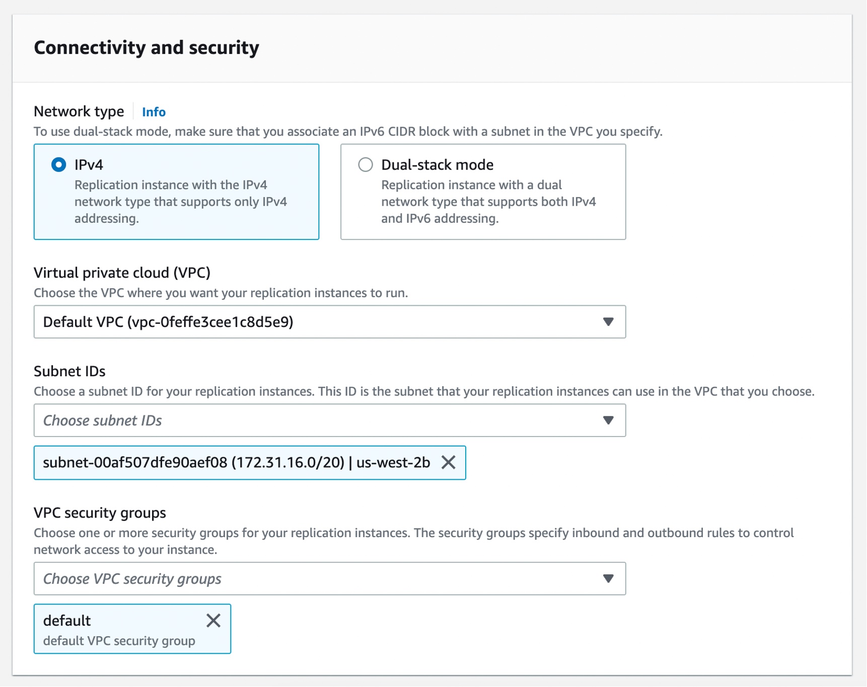
Setting Up AWS DMS Schema Conversion To get started with DMS Schema Conversion, and if it is your first time using AWS DMS, complete the setup tasks to create a virtual private cloud (VPC) using the Amazon VPC service, source, and target database. To learn more, see Prerequisites for AWS Database Migration Service in the AWS documentation.
In the AWS DMS console, you can see new menus to set up Instance profiles, add Data providers, and create Migration projects.
Before you create your migration project, set up an instance profile by choosing Instance profiles in the left pane. An instance profile specifies network and security settings for your DMS Schema Conversion instances. You can create multiple instance profiles and select an instance profile to use for each migration project.
Choose Create instance profile and specify your default VPC or a new VPC, Amazon Simple Storage Service (Amazon S3) bucket to store your schema conversion metadata, and additional settings such as AWS Key Management Service (AWS KMS) keys.
You can create the simplest network configuration with a single VPC configuration. If your source or target data providers are in different VPCs, you can create your instance profile in one of the VPCs, and then link these two VPCs by using VPC peering.
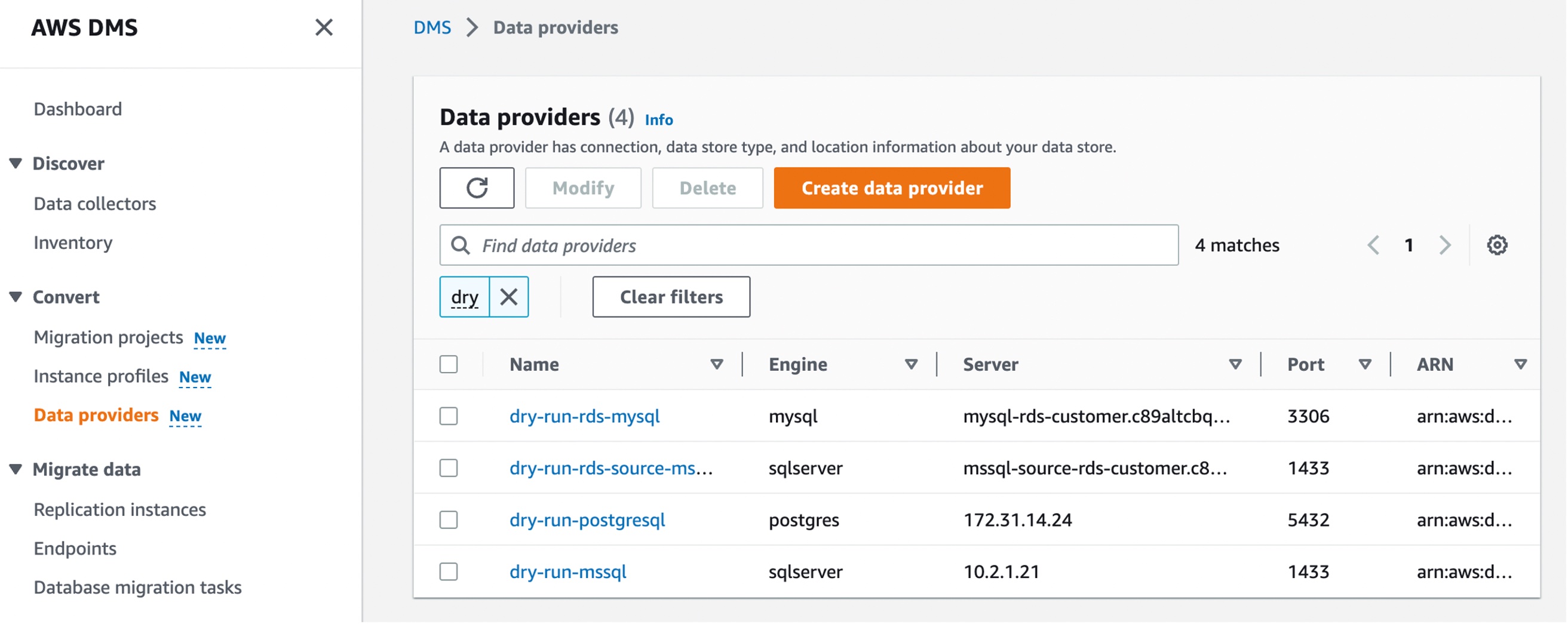
Next, you can add data providers that store the data store type and location information about your source and target databases by choosing Data providers in the left pane. For each database, you can create a single data provider and use it in multiple migration projects.
Your data provider can be a fully managed Amazon RDS instance or a self-managed engine running either on-premises or on an Amazon Elastic Compute Cloud (Amazon EC2) instance.
Choose Create data provider to create a new data provider. You can set the type of the database location manually, such as database engine, domain name or IP address, port number, database name, and so on, for your data provider. Here, I have selected an RDS database instance.
After you create a data provider, make sure that you add database connection credentials in AWS Secrets Manager. DMS Schema Conversion uses this information to connect to a database.
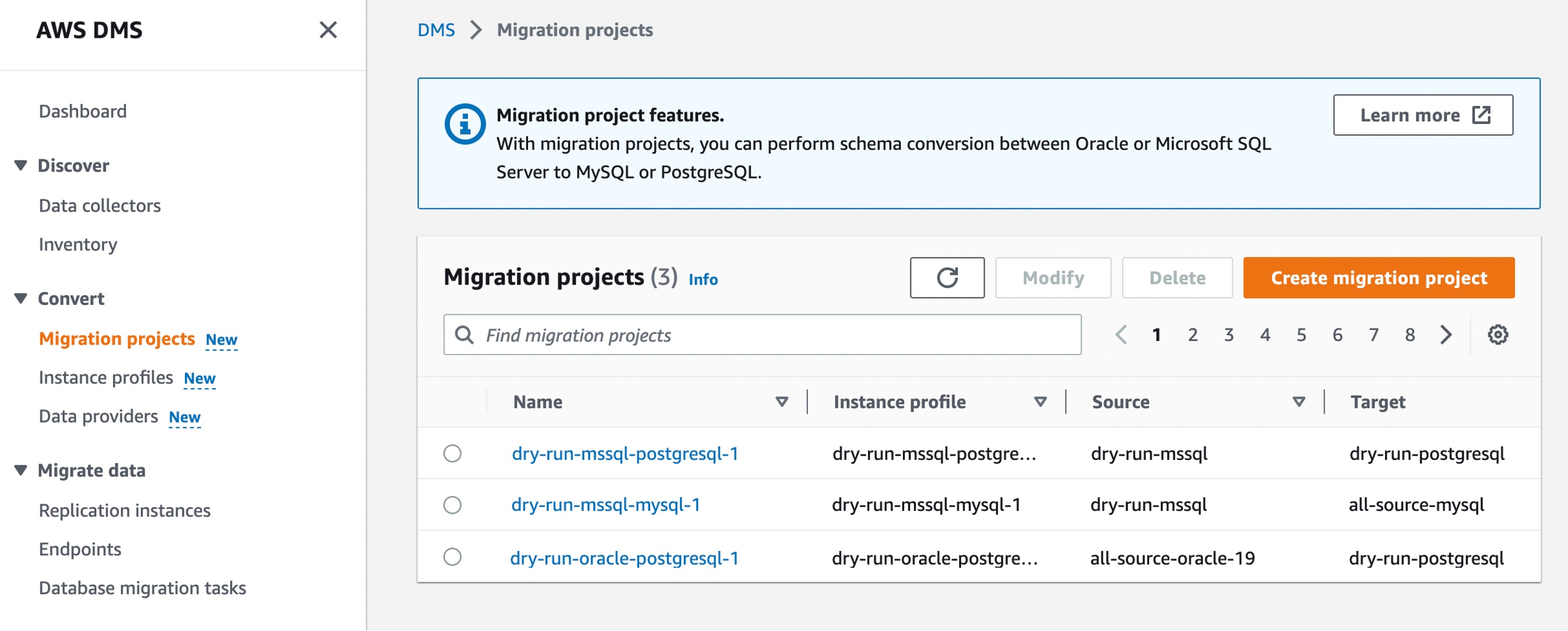
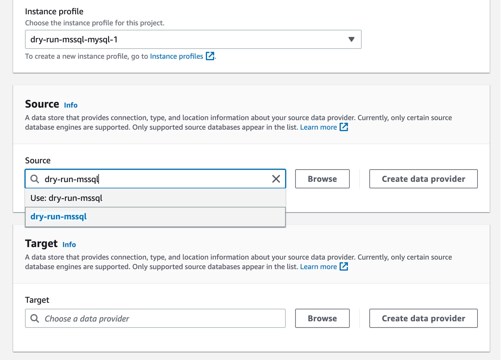
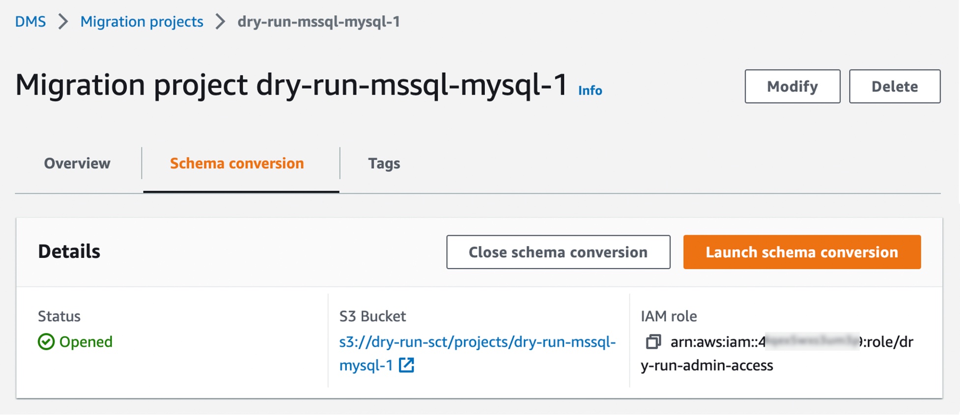
Converting your database schema with AWS DMS Schema Conversion Now, you can create a migration project for DMS Schema Conversion by choosing Migration projects in the left pane. A migration project describes your source and target data providers, your instance profile, and migration rules. You can also create multiple migration projects for different source and target data providers.
Choose Create migration project and select your instance profile and source and target data providers for DMS Schema Conversion.
After creating your migration project, you can use the project to create assessment reports and convert your database schema. Choose your migration project from the list, then choose the Schema conversion tab and click Launch schema conversion.
Migration projects in DMS Schema Conversion are always serverless. This means that AWS DMS automatically provisions the cloud resources for your migration projects, so you don’t need to manage schema conversion instances.
Of course, the first launch of DMS Schema Conversion requires starting a schema conversion instance, which can take up to 10–15 minutes. This process also reads the metadata from the source and target databases. After a successful first launch, you can access DMS Schema Conversion faster.
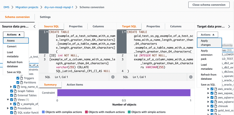
An important part of DMS Schema Conversion is that it generates a database migration assessment report that summarizes all of the schema conversion tasks. It also details the action items for schema that cannot be converted to the DB engine of your target database instance. You can view the report in the AWS DMS console or export it as a comma-separated value (.csv) file.
To create your assessment report, choose the source database schema or schema items that you want to assess. After you select the checkboxes, choose Assess in the Actions menu in the source database pane. This report will be archived with .csv files in your S3 bucket. To change the S3 bucket, edit the schema conversion settings in your instance profile.
Then, you can apply the converted code to your target database or save it as a SQL script. To apply converted code, choose Convert in the pane of Source data provider and then Apply changes in the pane of Target data provider.
Once the schema has been converted successfully, you can move on to the database migration phase using AWS DMS. To learn more, see Getting started with AWS Database Migration Service in the AWS documentation.
Now Available AWS DMS Schema Conversion is now available in the US East (Ohio), US East (N. Virginia), US West (Oregon), Asia Pacific (Singapore), Asia Pacific (Sydney), Asia Pacific (Tokyo), Europe (Frankfurt), Europe (Ireland), and Europe (Stockholm) Regions, and you can start using it today.
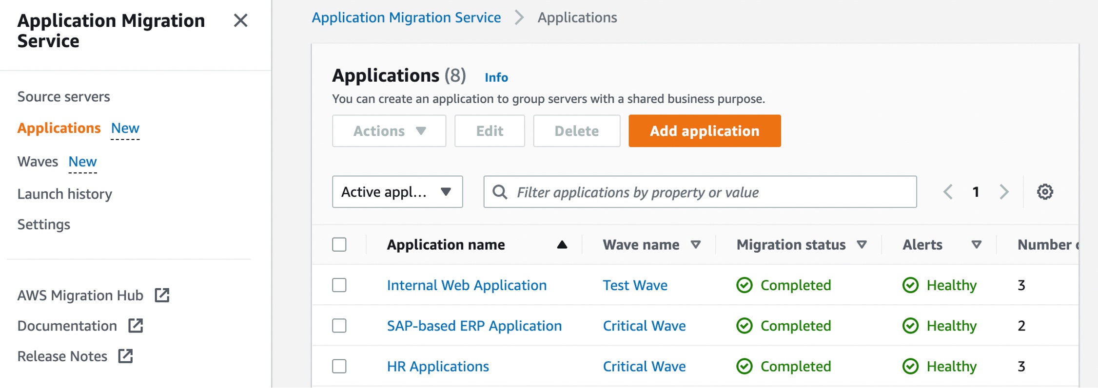
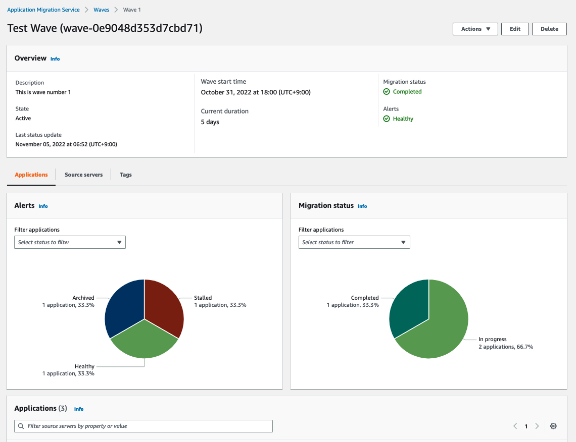
Today we announce three major updates of Application Migration Service to support your migration projects of any size:
New Migration Servers Grouping – You can group migration servers into “applications,” a group of servers that function together as a single application, and manage the migration stage in “waves,” a plan of migrations including grouping servers and applications.
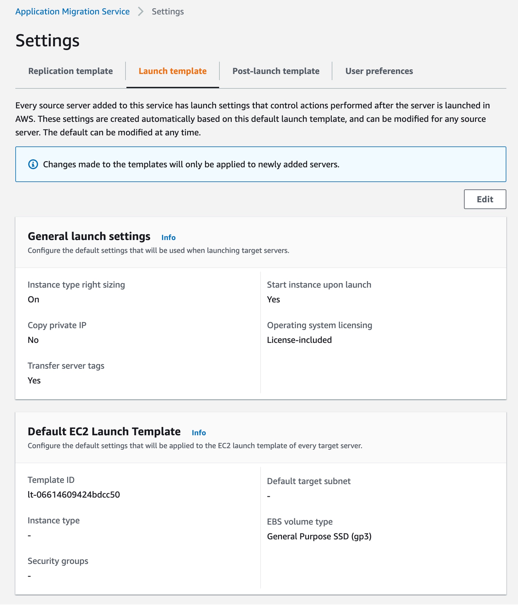
Updated Launch Template – You can modify the general settings and default launch template, and this template is then used to generate the Amazon Elastic Compute Cloud (Amazon EC2) instance launch template of subsequently installed source servers.
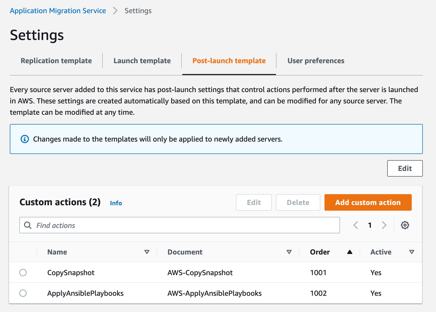
Updated Post-Launch Template – You can configure custom modernization actions for the post-launch template. You can associate any AWS Systems Manager documents and their parameters with a post-launch custom action.
Let’s dive deep into each launch!
New Migration Servers Grouping – Applications and Waves Customers have clusters of servers that comprise an application, with dependencies between them. The servers within an application share the same configurations, such as network, security policies, etc. Customers want to migrate complete applications and services, as well as set up and configure the application environment.
We introduce the new concept of “application,” representing a group of servers, and you can manage the migration of an application.
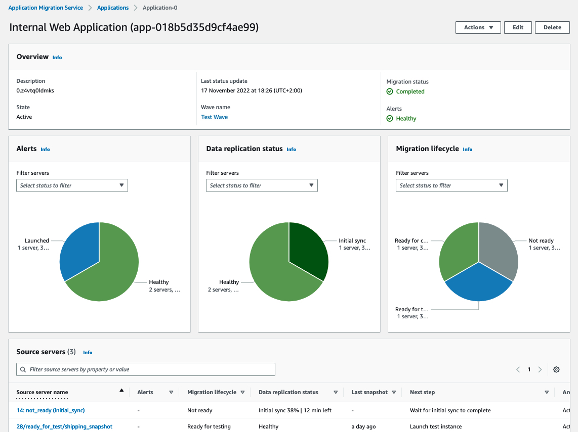
The new application feature groups source servers together with the same application for integrated migration jobs. It includes configuring the environment before migrating the application’s servers, creating the appropriate security groups, and performing bulk actions on all of the applications servers.
You can track and monitor the status of application migration and data replication within the migration lifecycle from source servers.
Also, customers with large migrations plan their migration, grouping servers and applications in waves. These are logical groups that describe the migration plan over time. Waves may include multiple servers and applications that do not necessarily have dependencies between them.
We introduce the new concept of “wave,” assisting customers in building their migration plan, as well as executing and monitoring it.
Application Migration Service supports actions on waves, such as launching all servers in a testing environment or performing cutover of a wave. Application Migration Service also provides reporting and monitoring information at the wave level so that customers will be able to manage their migration projects.
Updated Launch Template – Launch Settings and Default EC2 Launch Template The launch template allows you to control the way Application Migration Service launches instances in the AWS Cloud. You can change the settings for existing and newly added servers individually. Previously, we only supported the AWS Migration Acceleration Program (MAP) option to add tags to launched migration instances.
We added two new options to modify the global launch template, and this template is then used to generate the EC2 launch templates of subsequently installed source servers. Customers start with a global Application Migration Service launch template, which can be used for predefined launch templates. They would then potentially only have to perform modifications to a smaller subset of source servers, as opposed to all of them.
Here are default settings that will be used when launching target servers:
Activate instance type right-sizing – The service will determine the best match instance type. The default instance type defined in the EC2 template will be ignored.
Start instance upon launch – The service will launch instances automatically. If this option is not selected, the launched instance will need to be manually started after launch.
Copy private IP – This enables you to copy the private IP of your source server to the target.
Transfer server tags – Transfer the tags from the source server to the launched instances.
Operating system licensing – Specify whether to continue to use the Bring Your Own License model (BYOL) of the source server or use an AWS provided license.
Also, you can configure the default settings that will be applied to the EC2 launch template of every target server, such as default target subnet, additional security groups, default instance type, Amazon Elastic Block Store (Amazon EBS) volume type, IOPS, and throughput to associate with all instances launched by this service.
Updated Post-Launch Template – Custom Actions Post-launch settings allow you to control and automate actions performed after the server has been launched in AWS. It includes four built-in actions: installing the AWS Systems Manager agent, installing the AWS Elastic Disaster Recover agent and configuring replication, CentOS conversion, and SUSE subscription conversion.
We added a new option to configure custom actions in the post-launch template. You can associate any AWS Systems Manager and its action parameters. It also includes the order in which the actions will be executed and the source server’s operating systems for which the custom action can be configured.
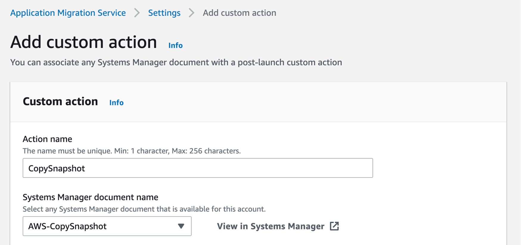
Choose Add custom action to make a new post-launch custom action. For example, the AWS-CopySnapshot, one of Systems Manager Automation’s runbooks, copies a point-in-time snapshot of an EBS volume. You can copy the snapshot within the same AWS Region or from one Region to another.
You can create your own Systems Manager document to define the actions that Systems Manager performs on your managed instances. Systems Manager offers more than 100 preconfigured documents that you can use by specifying parameters as the post-launch actions. To learn more, see AWS Systems Manager Automation runbook reference in the AWS documentation.
Now Available The new migration servers grouping, updates on the launch, and post-launch template are available now, and you can start using them today in all Regions where AWS Application Migration Service is supported.
Today, we are announcing the availability of Amazon EFS Elastic Throughput, a new throughput mode for Amazon EFS that is designed to provide your applications with as much throughput as they need with pay-as-you-use pricing. This new throughput mode enables you to further simplify running workloads and applications on AWS by providing shared file storage that doesn’t need provisioning or capacity management.
Elastic Throughput is ideal for spiky and unpredictable workloads with performance requirements that are difficult to forecast. When you enable Elastic Throughput on an Amazon EFS file system, you no longer need to think about actively managing your file system performance or over-paying for idle resources in order to ensure performance for your applications. When you enable Elastic Throughput, you don’t specify or provision throughput capacity, Amazon EFS automatically delivers the throughput performance your application needs while you the builder pays only for the amount of data read or written.
Amazon EFS is built to provide serverless, fully elastic file storage that lets you share file data for your cloud-based applications without having to think about provisioning or managing storage capacity and performance. With Elastic Throughput, Amazon EFS now extends its simplicity and elasticity to performance, enabling you to run an even broader range of file workloads on Amazon EFS. Amazon EFS is well suited to support a broad spectrum of use cases that include analytics and data science, machine learning, CI/CD tools, content management and web serving, and SaaS applications.
A Quick Review As you may already know, Amazon EFS already has the Bursting Throughput mode, which is available as a default and supports bursting to higher levels for up to 12 hours a day. If your application is throughput constrained on Bursting mode (for example, utilizes more than 80 percent of permitted throughput or exhausts burst credits), then you should consider using Provisioned (which we announced in 2018), or the new Elastic Throughput modes.
With this announcement of Elastic Throughput mode, and in addition to the already existing Provisioned Throughput mode, Amazon EFS now offers two options for workloads that require higher levels of throughput performance. You should use Provisioned Throughput if you know your workload’s performance requirements and you expect your workload to consume a higher share (more than 5 percent on average) of your application’s peak throughput capacity. You should use Elastic Throughput if you don’t know your application’s throughput or your application is very spiky.
To access Elastic Throughput mode (or any of the Throughput modes), select Customize (selecting Create instead will create your file system with the default Bursting mode).
Create File system
New – Elastic Throughput
You can also enable Elastic Throughput for new and existing General Purpose file systems using the Amazon EFS console or programmatically using the Amazon EFS CLI, Amazon EFS API, or AWS CloudFormation.
Elastic Throughput in Action Once you have enabled Elastic Throughput mode, you will be able to monitor your cost and throughput usage using Amazon CloudWatch and set alerts on unplanned throughput charges using AWS Budgets.
I have a test file system elasticblogthat I created previously using the Amazon EFS console, and now I cannot wait to see Elastic Throughput in action.
I have also created CloudWatch Alarms, which will monitor throughput usage and set alarm thresholds (ReadIOBytes, WriteIOBytes, TotalIOBytes, and MetadataIOBytes).
CloudWatch for Throughput Usage
The CloudWatch dashboard for my test file system elasticbloglooks like this.
CloudWatch Dashboard – TotalIOBytes for File System
Elastic Throughput allows you to drive throughput up to a limit of 3 GiB/s for read operations and 1 GiB/s for write operations per file system in all Regions.
Available Now Amazon EFS Elastic Throughput is available in all Regions supporting EFS except for the AWS China Regions.
With Amazon Redshift, you can analyze data in the cloud at any scale. Amazon Redshift offers native data protection capabilities to protect your data using automatic and manual snapshots. This works great by itself, but when you’re using other AWS services, you have to configure more than one tool to manage your data protection policies.
To make this easier, I am happy to share that we added support for Amazon Redshift in AWS Backup. AWS Backup allows you to define a central backup policy to manage data protection of your applications and can now also protect your Amazon Redshift clusters. In this way, you have a consistent experience when managing data protection across all supported services. If you have a multi-account setup, the centralized policies in AWS Backup let you define your data protection policies across all your accounts within your AWS Organizations. To help you meet your regulatory compliance needs, AWS Backup now includes Amazon Redshift in its auditor-ready reports. You also have the option to use AWS Backup Vault Lock to have immutable backups and prevent malicious or inadvertent changes.
Let’s see how this works in practice.
Using AWS Backup with Amazon Redshift The first step is to turn on the Redshift resource type for AWS Backup. In the AWS Backup console, I choose Settings in the navigation pane and then, in the Service opt-in section, Configure resources. There, I toggle the Redshift resource type on and choose Confirm.
Now, I can create or update a backup plan to include the backup of all, or some, of my Redshift clusters. In the backup plan, I can define how often these backups should be taken and for how long they should be kept. For example, I can have daily backups with one week of retention, weekly backups with one month of retention, and monthly backups with one year of retention.
I can also create on-demand backups. Let’s see this with more details. I choose Protected resources in the navigation pane and then Create on-demand backup.
I select Redshift in the Resource type dropdown. In the Cluster identifier, I select one of my clusters. For this workload, I need two weeks of retention. Then, I choose Create on-demand backup.
My data warehouse is not huge, so after a few minutes, the backup job has completed.
I now see my Redshift cluster in the list of the resources protected by AWS Backup.
In the Protected resources list, I choose the Redshift cluster to see the list of the available recovery points.
When I choose one of the recovery points, I have the option to restore the full data warehouse or just a table into a new Redshift cluster.
I now have the possibility to edit the cluster and database configuration, including security and networking settings. I just update the cluster identifier, otherwise the restore would fail because it must be unique. Then, I choose Restore backup to start the restore job.
After some time, the restore job has completed, and I see the old and the new clusters in the Amazon Redshift console. Using AWS Backup gives me a simple centralized way to manage data protection for Redshift clusters as well as many other resources in my AWS accounts.
There is no additional cost for using AWS Backup compared to the native snapshot capability of Amazon Redshift. Your overall costs depend on the amount of storage and retention you need. For more information, see AWS Backup pricing.
When updating databases, using a blue/green deployment technique is an appealing option for users to minimize risk and downtime. This method of making database updates requires two database environments—your current production environment, or blue environment, and a staging environment, or green environment. You must then keep these two environments in sync with each other so you may safely test and upgrade your changes to production.
Amazon Aurora and Amazon Relational Database Service (Amazon RDS) customers can use database cloning and promotable read replicas to help self-manage a blue/green deployment. However, self-managing a blue/green deployment can be costly and complex to build and manage. As a result, customers sometimes delay implementing database updates, choosing availability over the benefits that they would gain from updating their databases.
Today, we are announcing the general availability of Amazon RDS Blue/Green Deployments, a new feature for Amazon Aurora with MySQL compatibility, Amazon RDS for MySQL, and Amazon RDS for MariaDB that enables you to make database updates safer, simpler, and faster.
With just a few steps, you can use Blue/Green Deployments to create a separate, synchronized, fully managed staging environment that mirrors the production environment. The staging environment clones your production environment’s primary database and in-Region read replicas. Blue/Green Deployments keep these two environments in sync using logical replication.
In as fast as a minute, you can promote the staging environment to be the new production environment with no data loss. During switchover, Blue/Green Deployments blocks writes on blue and green environments so that the green catches up with the blue, ensuring no data loss. Then, Blue/Green Deployments redirects production traffic to the newly promoted staging environment, all without any code changes to your application.
With Blue/Green Deployments, you can make changes, such as major and minor version upgrades, schema modifications, and operating system or maintenance updates, to the staging environment without impacting the production workload.
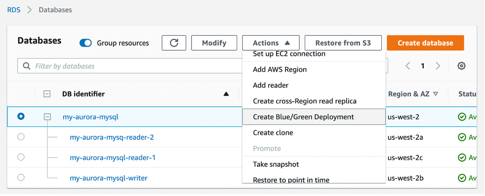
Getting Started with Blue/Green Deployments for MySQL Clusters You can start updating your databases with just a few clicks in the AWS Management Console. To get started, simply select the database that needs to be updated in the console and click Create Blue/Green Deployment under the Actions dropdown menu.
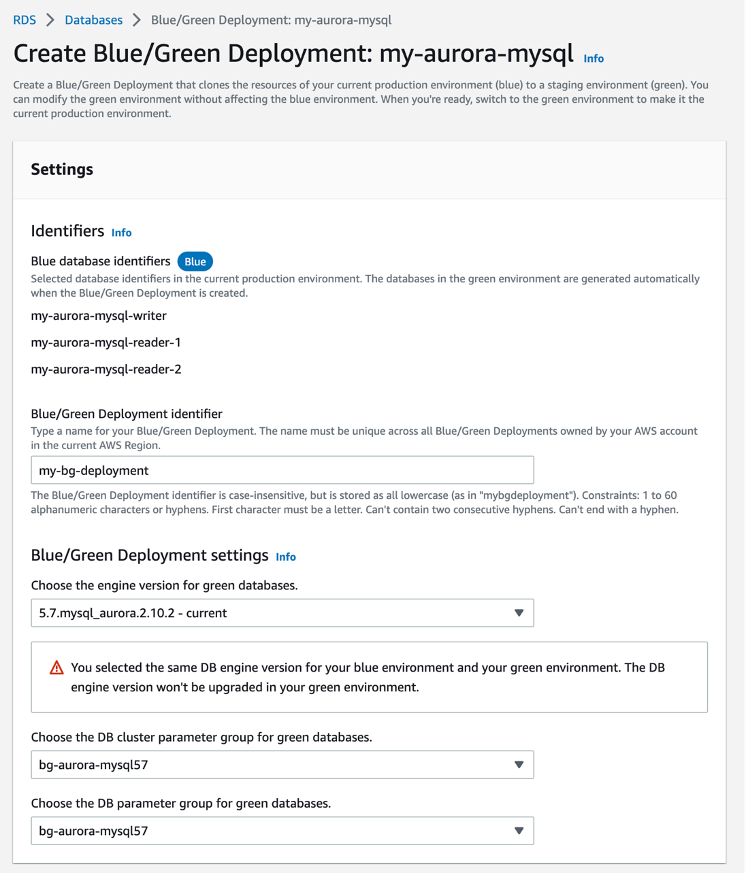
You can set a Blue/Green Deployment identifier and the attributes of your database to be modified, such as the engine version, DB cluster parameter group, and DB parameter group for green databases. To use a Blue/Green Deployment in your Aurora MySQL DB cluster, you should turn on binary logging, changing the value for the binlog_format parameter from OFF to MIXED in the DB cluster parameter group.
When you choose Create Blue/Green Deployment, it creates a new staging environment and runs automated tasks to prepare the database for production. Note, you will be charged the cost of the green database, including read replicas and DB instances in Multi-AZ deployments, and any other features such as Amazon RDS Performance Insights that you may have enabled on green.
You can also do the same job in the AWS Command Line Interface (AWS CLI). To perform an engine version upgrade, simply add a targetEngineVersion parameter and specify the engine version you’d like to upgrade to. This parameter works with both minor and major version upgrades, and it accepts short versions like 5.7 for Amazon Aurora MySQL-Compatible.
After creation is complete, you now have a staging environment that is ready for test and validation before promoting it to be the new production environment.
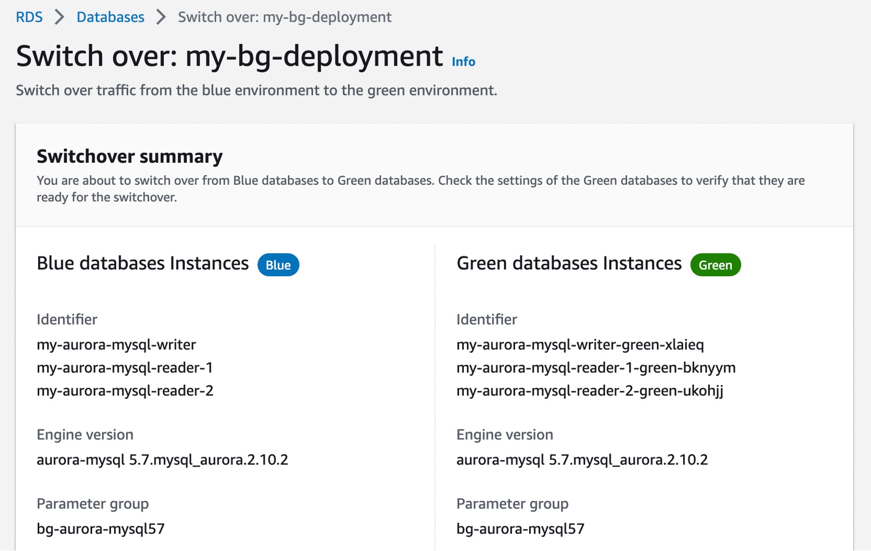
When testing and qualification of changes are complete, you can choose Switch over in the Actions dropdown menu to promote the staging environment marked as Green to be the new production system.
Now you are nearly ready to switch over your green databases to production. Check the settings of your green databases to verify that they are ready for the switchover. You may also set a timeout setting to determine the maximum time limit for your switchover. If Blue/Green Deployments’ switchover guardrails detect that it would take longer than the specified duration, then the switchover is canceled, and no changes are made to the environments. We recommend that you identify times of low or moderate production traffic to initiate a switchover.
After switchover, Blue/Green Deployments does not delete your old production environment. You may access it for additional validations and performance/regression testing, if needed. Please note that it is your responsibility to delete the old production environment when you no longer need it. Standard billing charges apply on old production instances until you delete them.
Now Available Amazon RDS Blue/Green Deployments is available today on Amazon Aurora with MySQL Compatibility 5.6 or higher, Amazon RDS for MySQL major version 5.6 or higher, and Amazon RDS for MariaDB 10.2 and higher in all AWS commercial Regions, excluding China, and AWS GovCloud Regions.
To define the data protection policy of an application, you have to look at its components and find which ones store data that needs to be protected. Those are the stateful components of your application, such as databases and file systems. Other components don’t store data but need to be restored as well in case of issues. These are stateless components, such as containers and their network configurations.
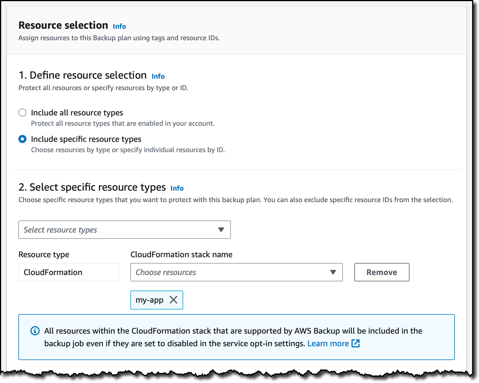
When you manage your application using infrastructure as code (IaC), you have a single repository where all these components are described. Can we use this information to help protect your applications? Yes! AWS Backup now supports attaching an AWS CloudFormation stack to your data protection policies.
When you use CloudFormation as a resource, all stateful components supported by AWS Backup are backed up around the same time. The backup also includes the stateless resources in the stack, such as AWS Identity and Access Management (IAM) roles and Amazon Virtual Private Cloud (Amazon VPC) security groups. This gives you a single recovery point that you can use to recover the application stack or the individual resources you need. In case of recovery, you don’t need to mix automated tools with custom scripts and manual activities to recover and put the whole application stack back together. As you modernize and update an application managed with CloudFormation, AWS Backup automatically keeps track of changes and updates the data protection policies for you.
CloudFormation support for AWS Backup also helps you prove compliance of your data protection policies. You can monitor your application resources in AWS Backup Audit Manager, a feature of AWS Backup that enables you to audit and report on the compliance of data protection policies. You can also use AWS Backup Vault Lock to manage the immutability of your backups as required by your compliance obligations.
Let’s see how this works in practice.
Using AWS Backup Support for CloudFormation Stacks First, I need to turn on the CloudFormation resource type for AWS Backup. In the AWS Backup console, I choose Settings in the navigation pane and then, in the Service opt-in section, Configure resources. There, I toggle the CloudFormation resource type on and choose Confirm.
Now that CloudFormation support is enabled, I choose Dashboard in the navigation pane and then Create backup plan. I select the Start with a template option and then the Daily-35day-Retention template. As the name suggests, this template creates daily backups that are kept for 35 days before being automatically deleted. I enter a name for the backup plan and choose Create plan.
Now I can assign resources to my backup plan. I enter a resource assignment name and use the default IAM role that is automatically created with the correct permissions.
In the Resource selection, I can select Include all resource types to automatically protect all resource types that are enabled in my account. Because I’d like to show how CloudFormation support works, I select Include specific resource types and then CloudFormation in the Select resource types dropdown menu. In the Choose resources menu, I can use the All supported CloudFormation stacks option to have all my stacks protected. For simplicity, I choose to protect only one stack, the my-app stack.
I leave the other options at their default values and choose Assign resources. That’s all! Now the CloudFormation stack that I selected will be backed up daily with 35 days of retention. What does that mean? Let’s have a look at what happens when I create an on-demand backup of a CloudFormation stack.
Creating On-Demand Backups for CloudFormation Stacks I choose Protected resources in the navigation pane and then Create on-demand backup. The next steps are similar to what I did before when assigning resources to a backup plan. I select the CloudFormation resource type and the my-app stack. I use the Create backup now option to start the backup within one hour. I choose 7 days of retention and the Default backup vault. Backup vaults are logical containers that store and organize your backups. I select the default IAM role and choose Create on-demand backup.
Within a few minutes, the backup job is running. I expand the Backup job ID in the Backup jobs list to see the resources being backed up. The stateful resources (such as Amazon DynamoDB tables and Amazon Relational Database Service (RDS) databases) are listed with the current state of the backup job. The stateless resources in my stack (such as IAM roles, AWS Lambda functions, and VPC configurations) are backed up by the job with the CloudFormation resource type.
When the backup job has completed, I go back to the Protected resources page to see the list of resources that I can now restore. In the list, I see the IDs of the stateful resources (in this case, two DynamoDB tables and an Aurora database) and of the CloudFormation stack. If I choose each of the stateful resources, I see the available recovery points corresponding to the different points in time when that resource has been backed up.
If I choose the CloudFormation stack, I get a list of composite recovery points. Each composite recovery point includes all stateless and stateful resources in the stack. More specifically, the stateless resources are included in the CloudFormation template recovery point (the last one in the following screenshot).
Restoring a CloudFormation Backup Inside the composite recovery point, I select the recovery point of the CloudFormation stack and choose Restore. Restoring a CloudFormation stack backup creates a new stack with a change set that represents the backup. I enter the new stack and change set names and choose Restore backup. After a few minutes, the restore job is completed.
In the CloudFormation console, the new stack is under review. I need to apply the change set.
I choose the new stack and select the change set created by the restore job to apply the change set.
After some time, the resources in my original stack have been recreated in the new stack. The stateful resources have been recreated empty. To recover the stateful resources, I can go back to the list of recovery points, select the recovery point I need, and initiate a restore.
Availability and Pricing AWS Backup support for CloudFormation stacks is available today using the console, AWS Command Line Interface (CLI), and AWS SDKs in all AWS Regions where AWS Backup is offered. There is no additional cost for the stateless resources backed up and restored by AWS Backup. You only pay for the stateful resources such as databases, storage volumes, or file systems. For more information, see AWS Backup pricing.
You now have an automated solution to create and restore your applications with a simplified experience, eliminating the need to manage custom scripts.
How many times have you had monitoring dashboards show you a normal situation, and at the same time, you have received customer tickets reporting your app is “slow” or unavailable to them? How much time did it take to diagnose these customer reports?
You told us one of your challenges when monitoring internet-facing applications is to gather data outside of AWS to build a realistic picture of how your application behaves for your customers connected to multiple and geographically distant internet providers. Capturing and monitoring data about internet traffic before it reaches your infrastructure is either difficult or very expensive.
I am happy to announce the public preview of Amazon CloudWatch Internet Monitor, a new capability of CloudWatch that gives visibility into how an internet issue might impact the performance and availability of your applications. It allows you to reduce the time it takes to diagnose internet issues from days to minutes.
Internet Monitor uses the connectivity data that we capture from our global networking footprint to calculate a baseline of performance and availability for internet traffic. This is the same data that we use at AWS to monitor our own internet uptime and availability. With Internet Monitor, you can gain awareness of problems that arise on the internet experienced by your end users in different geographic locations and networks.
There is no need to instrument your application code. You can enable the service in the CloudWatch section of the AWS Management Console and start to use it immediately.
Let’s See It in Action Getting started with Internet Monitor is easy. Let’s imagine I want to monitor the network paths between my customers and my AWS resources. I open the AWS Management Console and navigate to CloudWatch. I select Internet Monitor on the left-side navigation menu. Then, I select Create monitor.
On the Create monitor page, I enter a Monitor name, and I select Add resources to choose the resources to monitor. For this demo, I select the VPC and the CloudFront distribution hosting my customer-facing application.
I have the opportunity to review my choices. Then, I select Create monitor.
From that moment on, Internet Monitor starts to collect data based on my application’s resource logs behind the scene. There is no need for you to activate (or pay for) VPC Flow Logs, CloudFront logs, or other log types.
After a while, I receive customer complaints about our application being slow. I open Internet Monitor again, I select the monitor I created earlier (Monitor_example), and I immediately see that the application suffers from internet performance issues.
The Health scores graph shows you performance and availability information for your global traffic. AWS has substantial historical data about internet performance and availability for network traffic between geographic locations for different network providers and services. By applying statistical analysis to the data, we can detect when the performance and availability towards your application have dropped, compared to an estimated baseline that we’ve calculated. To make it easier to see those drops, we report that information to you in the form of an estimated performance score and an availability score.
I scroll a bit down the page. The Internet traffic overview map shows the overall event status across all monitored locations. I look at the details in the Health events table. It also highlights other events that are happening globally, sorted by total traffic impact. I notice that a performance issue in Las Vegas, Nevada, US, is affecting my application traffic the most.
Now that I have identified the issue, I am curious about the historical data. Has it happened before?
I select the Historical Explorer tab to understand trends and see earlier data related to this location and network provider. I can view aggregated metrics such as performance score, availability score, bytes transferred, and round-trip time at p50, p90, and p95 percentiles, for a customized timeframe, up to 18 months in the past.
I can see today’s incident is not the first one. This specific client location and network provider has had multiple issues in the past few months.
Now that I understand the context, I wonder what action I can take to mitigate the issue.
I switch to the Traffic insights tab. I see overall traffic data and top client locations that are being monitored based on total traffic (bytes). Apparently, Las Vegas, Nevada, US, is one of the top client locations.
I select the graph to see traffic details for Las Vegas, Nevada, US. In the Lowest Time To First Byte (TTFB) column, I see AWS service and AWS Region setup recommendations for all of the top client location and network combinations. The Predicted Time To First Byte in the table shows the potential impact if I make the suggested architectural change.
In this example, Internet Monitor suggests having CloudFront distribute the traffic currently distributed by EC2 and to allow for some additional traffic to be served by EC2 instances in us-east-1 in addition to us-east-2.
Available Today Internet Monitor is available in public preview today in 20 AWS Regions:
In the Americas: US East (Ohio), US East (N. Virginia), US West (N. California), US West (Oregon), Canada (Central), South America (São Paulo).
In Asia and Pacific: Asia Pacific (Hong Kong), Asia Pacific (Mumbai), Asia Pacific (Seoul), Asia Pacific (Singapore), Asia Pacific (Sydney), Asia Pacific (Tokyo).
In Europe, Middle East, and Africa: Africa (Cape Town), Europe (Frankfurt), Europe (Ireland), Europe (London), Europe (Milan), Europe (Paris), Europe (Stockholm), Middle East (Bahrain)
Note that AWS CloudFormation support is missing at the moment; it will be added soon.
There is no costs associated with the service during the preview period. Just keep in mind that Internet Monitor vends metrics and logs to CloudWatch; you will be charged for these additional CloudWatch logs and CloudWatch metrics.
Whether you work for a startup or a large enterprise, CloudWatch Internet Monitor helps you be proactive about your application performance and availability. Give it a try today!
The experience customers have when interacting with a contact center can have a profound impact on them. For this reason, we launched Amazon Transcribe Call Analytics last year to help you analyze customer call recordings and get insights into issues and trends related to customer satisfaction and agent performance.
To assist agents in resolving live calls faster, we are introducing today real-time call analytics in Amazon Transcribe Call Analytics. Real-time call analytics provides APIs for developers to accurately transcribe live calls and at the same time identify customer experience issues and sentiment in real time. Transcribe Call Analytics uses state-of-the-art machine learning capabilities to automatically assess thousands of in-progress calls and detect customer experience issues, such as repeated requests to speak to a manager or cancel a subscription.
With a few clicks, supervisors and analysts can create categories in the AWS console to identify customer experience issues using criteria such as specific terms such as “not happy,” “poor quality,” and “cancel my subscription.” Transcribe Call Analytics analyzes in-progress calls in real time to detect when a category is met. Developers can use those signals, along with sentiment trends from the API, to build a proactive system that alerts supervisors about emerging issues or assists agents with relevant information to solve customer issues.
Transcribe Call Analytics also provides a real-time transcript of the live conversation that supervisors can use to quickly get up to speed on the customer interaction and assess the appropriate action. The in-call transcript also eliminates the need for customers to repeat themselves if the call is transferred to another agent. Agents can focus all their attention on the customer during the call instead of taking notes for entry in a CRM system because Transcribe Call Analytics includes an automated call summarization capability, which identifies the issue, outcome, and action item associated with a call.
Exploring Real-Time Call Analytics in the Console To see how this works visually, I use the Amazon Transcribe console. First, I create a category to be notified if some terms are used in the call that would require an escalation. I choose Category Management from the navigation pane and then Create category.
I enter Escalation as the name for the category. I select REAL_TIME in the Category type dropdown. Then, I choose Create from scratch.
I only need one rule for this category. In the Rule type dropdown, I select Transcript content match. In the next three options, I choose to trigger the rule when any of the words are mentioned during the entire call, and the speaker is either the customer or the agent. Now, I can enter the words or phrases to look for in the transcript. In this case, I enter cancel, canceled, cancelled, manager, and supervisor. In your case, you might be more specific depending on your business. For example, if subscriptions are your business, you can look for the phrase cancel my subscription.
Now that the category has been created, I use one of the sample calls in the console to test it. I choose Real-Time Analytics in the navigation pane. By choosing Configure advanced settings, I can configure the personally identifiable information (PII) identification and redaction settings. For example, I can choose to identify personal data such as email addresses or redact financial data like bank account numbers.
With no additional charge, I can enable Post-call Analytics so that, at the end of the call, I receive the output of the transcription job in an Amazon Simple Storage Service (Amazon S3) bucket. This output is in a similar format to what I’d receive if I were analyzing a call recording with Transcribe Call Analytics. In this way, I can use the post-call analytics output derived from the audio stream in any process I already have in place for output of analytics generated from call recordings, for example, to update dashboards or generate periodic reports.
With Insurance complaints in Step 1: Specify input audio selected, I choose Start streaming. In the Transcription output section of the console, I receive in real-time the transcription of the call. The words of the customer and agent appear as they are pronounced. Each sentence is flagged with its recognized sentiment (positive, neutral, or negative). The Escalation category that I just configured is found in two sentences, first, when the customer mentions that their insurance has been canceled, and then when the agent mentions their manager. Also, part of a sentence is underlined because an issue has been detected.
Using the Download dropdown, I download the full JSON transcript. If I am only interested in the transcription, I can download the text transcript. The JSON transcript contains an array where each item is similar to what I’d get in real time when using the real-time call analytics API.
Using the Live Call Analytics With Agent Assist (LCA) Solution You can use the open-source real-time call analytics with agent assist solution for your contact center or as an inspiration of what Amazon Transcribe enables for developers. Let’s look at a couple of screenshots to understand how it works.
Here there is a list of on-going calls with the overall sentiment, the sentiment trend (is it improving or not?), and the categories found in real-time during the call that can be used for specific activities.
When selecting a call from the list, you have access to more in-depth information, including the call transcript and the issues found during the on-going call. This allows to take action quickly to help resolve the call.
Availability and Pricing Amazon Transcribe Call Analytics with real-time capabilities is available today in US (N. Virginia, Oregon), Canada (Central), Europe (Frankfurt, London), and Asia Pacific (Seoul, Sydney, Tokyo) and supports US English, British English, Australian English, US Spanish, Canadian French, French, German, Italian, and Brazilian Portuguese.
With Amazon Transcribe Call Analytics, you pay as you go and are billed monthly based on tiered pricing. For more information, see Amazon Transcribe pricing.
As part of the AWS Free Tier, you can get started with Amazon Transcribe Call Analytics for free, including the new real-time call analytics API. You can analyze up to 60 minutes of call audio monthly for free for the first 12 months. For more information, see the AWS Free Tier page.
I first covered AWS Elastic Disaster Recovery (DRS) in a 2021 blog post. In that post, I described how DRS “enables customers to use AWS as an elastic recovery site for their on-premises applications without needing to invest in on-premises DR infrastructure that lies idle until needed. Once enabled, DRS maintains a constant replication posture for your operating systems, applications, and databases.” I’m happy to announce that, today, DRS now also supports in-AWS failback, adding to the existing support for non-disruptive recovery drills and on-premises failback included in the original release.
I also wrote in my earlier post that drills are an important part of disaster recovery since, if you don’t test, you simply won’t know for sure that your disaster recovery solution will work properly when you need it to. However, customers rarely like to test because it’s a time-consuming activity and also disruptive. Automation and simplification encourage frequent drills, even at scale, enabling you to be better prepared for disaster, and now you can use them irrespective of whether your applications are on-premises or in AWS. Non-disruptive recovery drills provide confidence that you will meet your recovery time objectives (RTOs) and recovery point objectives (RPOs) should you ever need to initiate a recovery or failback. More information on RTOs and RPOs, and why they’re important to define, can be found in the recovery objectives documentation.
The new automated support provides a simplified and expedited experience to fail back Amazon Elastic Compute Cloud (Amazon EC2) instances to the original Region, and both failover and failback processes (for on-premises or in-AWS recovery) can be conveniently started from the AWS Management Console. Also, for customers that want to customize the granular steps that make up a recovery workflow, DRS provides three new APIs, linked at the bottom of this post.
Failover vs. Failback Failover is switching the running application to another Availability Zone, or even a different Region, should outages or issues occur that threaten the availability of the application. Failback is the process of returning the application to the original on-premises location or Region. For failovers to another Availability Zone, customers who are agnostic to the zone may continue running the application in its new zone indefinitely if so required. In this case, they will reverse the recovery replication, so the recovered instance is protected for future recovery. However, if the failover was to a different Region, its likely customers will want to eventually fail back and return to the original Region when the issues that caused failover have been resolved.
The below images illustrate architectures for in-AWS applications protected by DRS. The architecture in the image below is for cross-Availability Zone scenarios.
The architecture diagram below is for cross-Region scenarios.
Let’s assume an incident occurs with an in-AWS application, so we initiate a failover to another AWS Region. When the issue has been resolved, we want to fail back to the original Region. The following animation illustrates the failover and failback processes.
Learn more about in-AWS failback with Elastic Disaster Recovery As I mentioned earlier, three new APIs are also available for customers who want to customize the granular steps involved. The documentation for these can be found using the links below.
Microservices architectures are a well-known software development approach to make applications composed of small independent services that communicate over well-defined application programming interfaces (APIs). Customers faced challenges when they started breaking down their monolith applications into microservices, as it required specialized networking knowledge to communicate internally with other microservices.
Amazon Elastic Container Services (Amazon ECS) customers have several solutions for service-to-service, but each one comes with some challenges and complications: 1) Elastic Load Balancing (ELB) needs to carefully plan for configuring infrastructure for high availability and incur additional infrastructure cost. 2) Using Amazon ECS Service Discovery often requires developers to write custom application code for collecting traffic metrics and for making network calls resilient. 3) Service mesh solutions such as AWS App Mesh run outside of Amazon ECS despite having advanced traffic monitoring and routing features between services.
Today, we are announcing the general availability of Amazon ECS Service Connect, a new capability that simplifies building and operating resilient distributed applications. ECS Service Connect provides an easy network setup and seamless service communication deployed across multiple ECS clusters and virtual private clouds (VPCs). You can add a layer of resilience to your ECS service communication and get traffic insights with no changes to your application code.
With ECS Service Connect, you can refer and connect to your services by logical names using a namespace provided by AWS Cloud Map and automatically distribute traffic between ECS tasks without deploying and configuring load balancers. You can set some safe defaults for traffic resilience, such as health checking, automatic retries for 503 errors, and connection draining, for each of your ECS services. Additionally, the Amazon ECS console provides easy-to-use dashboards with real-time network traffic metrics for operational convenience and simplified debugging.
Getting Started with Amazon ECS Service Connect To get started with the ECS Service Connect, you can specify a namespace as part of creating an ECS cluster or create one in the Cloud Map. A namespace represents a way to structure your services and can span across multiple ECS clusters residing in different VPCs. All ECS services that belong to a specific namespace can communicate with existing services in the namespaces, provided existing network-level connectivity.
You can also see a list of Cloud Map namespaces in Namespaces in the left navigation pane of the Amazon ECS console. When you select a namespace, it shows a list of services with the same namespace from two different ECS clusters with database services (db-mysql, db-redis) and backend services (webui, appserver).
When you create an ECS cluster, you can select one of the namespaces in the Default namespaces of the Networking setting. ECS Service Connect is enabled for all new ECS services running in both AWS Fargate and Amazon EC2 instances. To enable all existing services, you would need to redeploy with either a new version of ECS-optimized Amazon Machine Image (AMI), or with a new Fargate Agent that supports ECS Service Connect.
Or, you can simply create a cluster via AWS Command Line Interface (AWS CLI) with serviceConnect parameter and a default Cloud Map namespace name for service discovery purposes.
This command will create an ECS cluster with the namespace on AWS’s behalf. If you would like to use an already existing Cloud Map namespace, you can simply pass the name of the existing namespace here.
Next, let’s create a service with a task definition and expose your web user-interface server using ECS Service Connect.
In this command, portName represents a reference to the container port, and clientAliases assigns the port number and DNS name, overriding the discovery name that is used in the endpoint. Each service has an endpoint URL that contains the protocol, a DNS name, and the port. You can select the protocol and port name in the task definition or the ECS service configuration. For example, an endpoint could be http://webui:80, grpc://appserver:8080, or http://db-redis:8888.
In the ECS console, you can see this configuration of ECS Service Connect for the webui service in the svc-cluster-2 cluster.
As you can see, you can run the same workloads across different clusters with the same clientAlias and namespace name for high availability. ECS Service Connect will intelligently load balance the traffic to the ECS tasks. To connect to services running in different ECS clusters, you need to specify the same namespace name for all your ECS services that need to talk to each other. ECS Service Connect will make your services discoverable to all other services in the same namespace.
Improving Service Resilience with Observability Data You can collect traffic metrics with ECS Service Connect observability capabilities. By default, for each ECS service, you can see the number of healthy and unhealthy endpoints, along with inbound and outbound traffic volume.
ECS Service Connect supports HTTP/1, HTTP/2, gRPC, and TCP protocols. So, you can collect the number of requests, number of HTTP errors, and average call latency. For gRPC and TCP, you can see the total number of active connections. All of these metrics are pushed to Amazon CloudWatch or other AWS analytics services via custom log routing
In the Advanced menu, you can publish ECS Service Connect Agent logs for help in debugging in case of issues.
These metrics are only visible in the original interface of the CloudWatch console. When you use the CloudWatch console, switch to the original interface to see the additional metric dimensions of “discovery name” and “target discovery name” under the ECS grouping.
The default settings provide you with a starting point for building resilient applications, and you can fine-tune parameters to limit the impact of failures, latency spikes, and network fluctuations on your application behavior using AWS Management Console or dedicated ECS APIs.
Now Available Amazon ECS Service Connect is available in all commercial Regions, except China, where Amazon ECS is available. ECS Service Connect is fully supported in AWS CloudFormation, AWS CDK, AWS Copilot, and AWS Proton for infrastructure provisioning, code deployments, and monitoring of your services. To learn more, see the Amazon ECS Service Connect Developer Guide.
My colleagues, Hemanth AVS, Senior Container Specialist SA, and Satya Vajrapu, Senior DevOps Consultant, prepared a hands-on workshop to demonstrate an example of the ECS Service Connect. Join CON303 Networking, service mesh, and service discovery with Amazon ECS when you attend AWS re:Invent 2022.
Give it a try, and please send feedback to AWS re:Post for Amazon ECS or through your usual AWS support contacts.
To provide the best experiences, we use technologies like cookies to store and/or access device information. Consenting to these technologies will allow us to process data such as browsing behavior or unique IDs on this site. Not consenting or withdrawing consent, may adversely affect certain features and functions.
Functional
Always active
The technical storage or access is strictly necessary for the legitimate purpose of enabling the use of a specific service explicitly requested by the subscriber or user, or for the sole purpose of carrying out the transmission of a communication over an electronic communications network.
Preferences
The technical storage or access is necessary for the legitimate purpose of storing preferences that are not requested by the subscriber or user.
Statistics
The technical storage or access that is used exclusively for statistical purposes.The technical storage or access that is used exclusively for anonymous statistical purposes. Without a subpoena, voluntary compliance on the part of your Internet Service Provider, or additional records from a third party, information stored or retrieved for this purpose alone cannot usually be used to identify you.
Marketing
The technical storage or access is required to create user profiles to send advertising, or to track the user on a website or across several websites for similar marketing purposes.


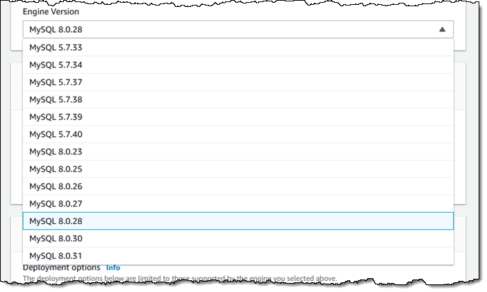
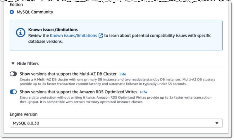
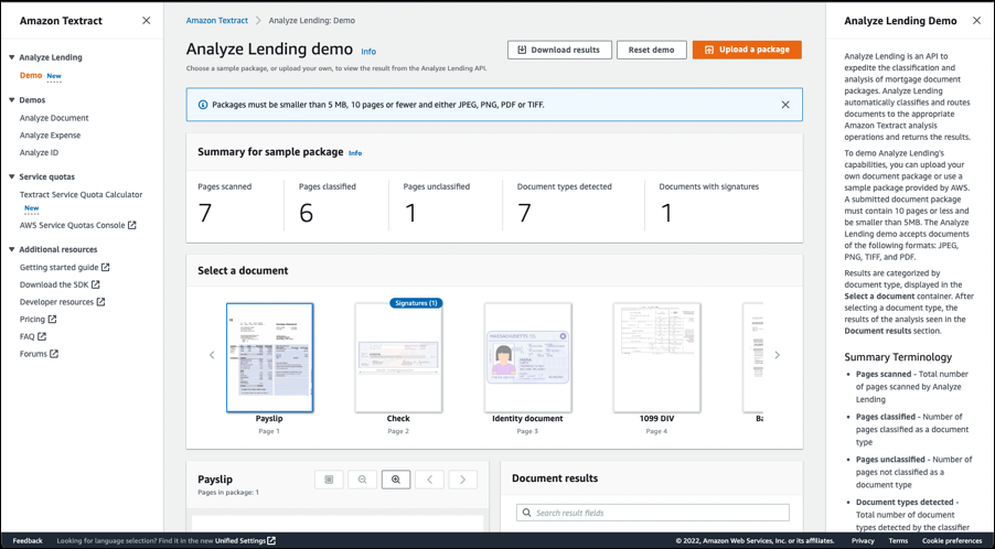
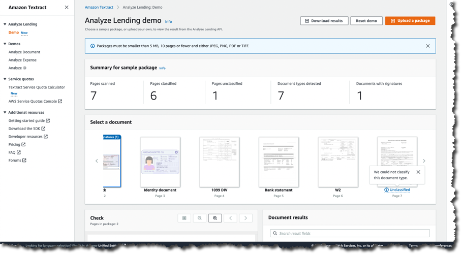


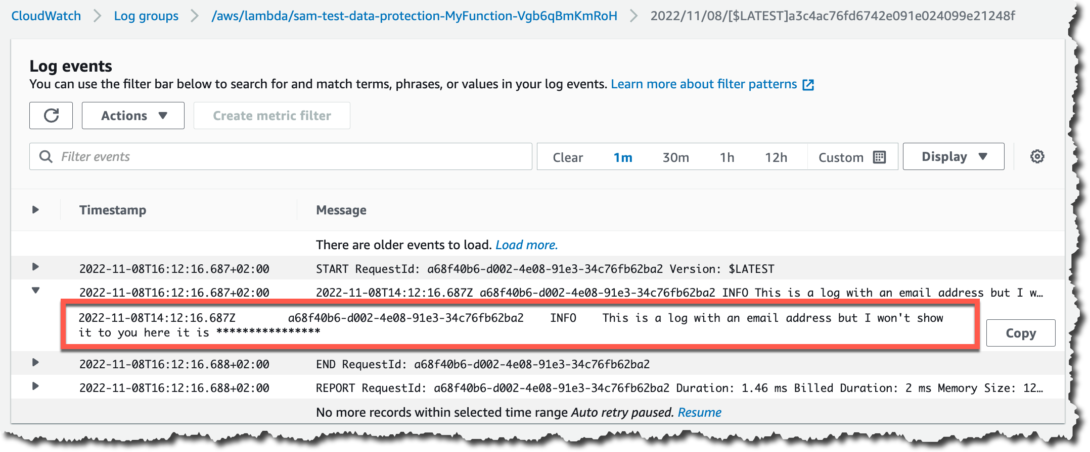

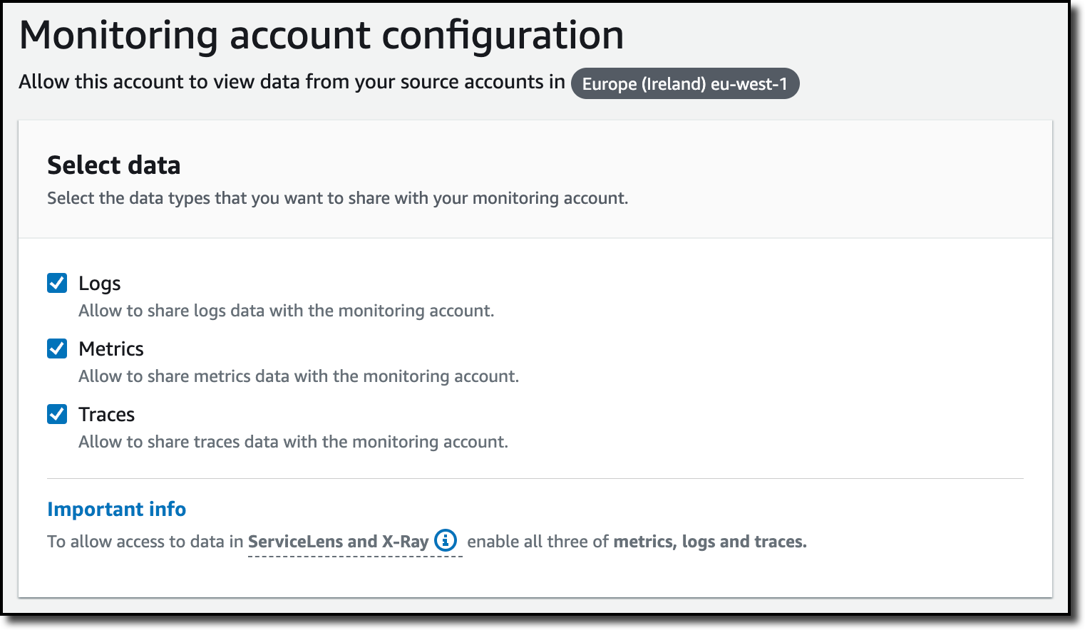

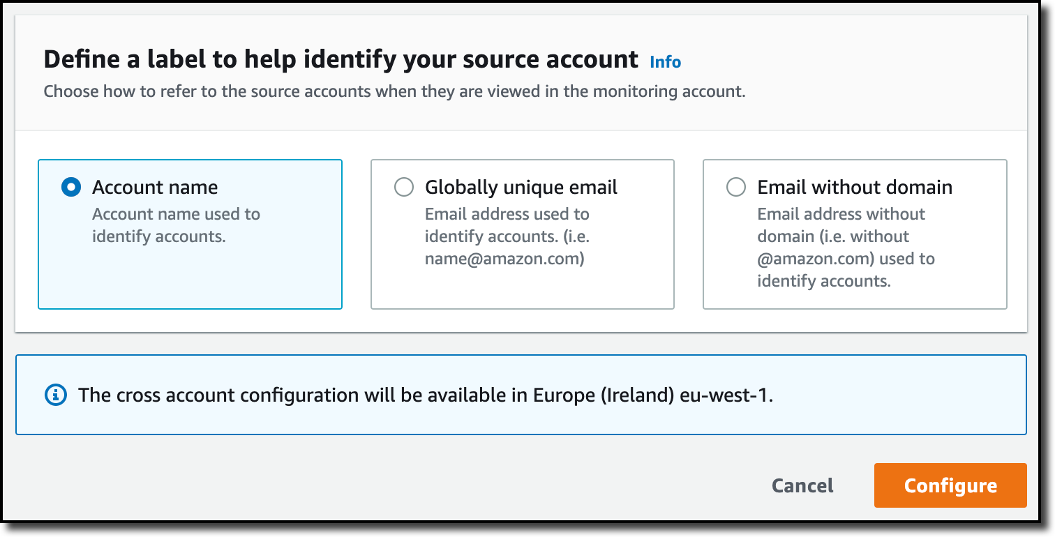


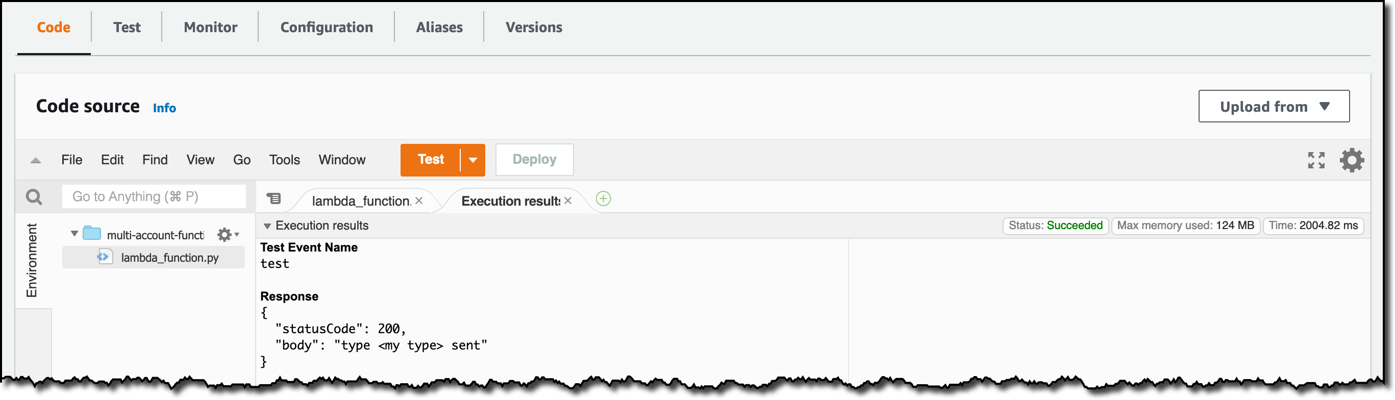


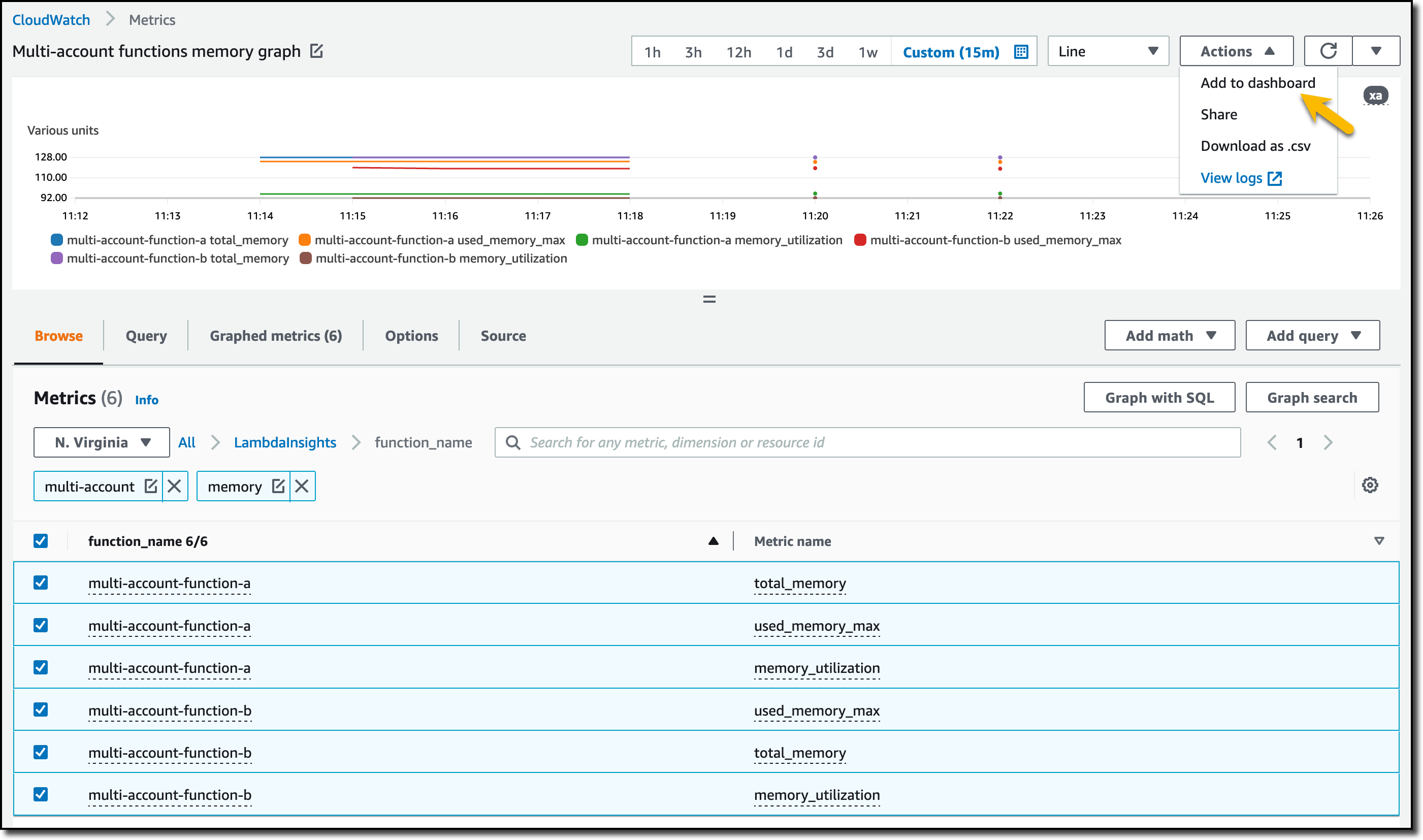
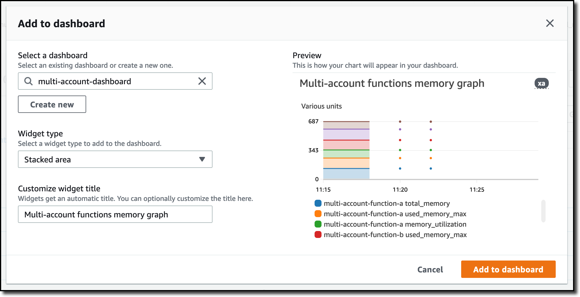


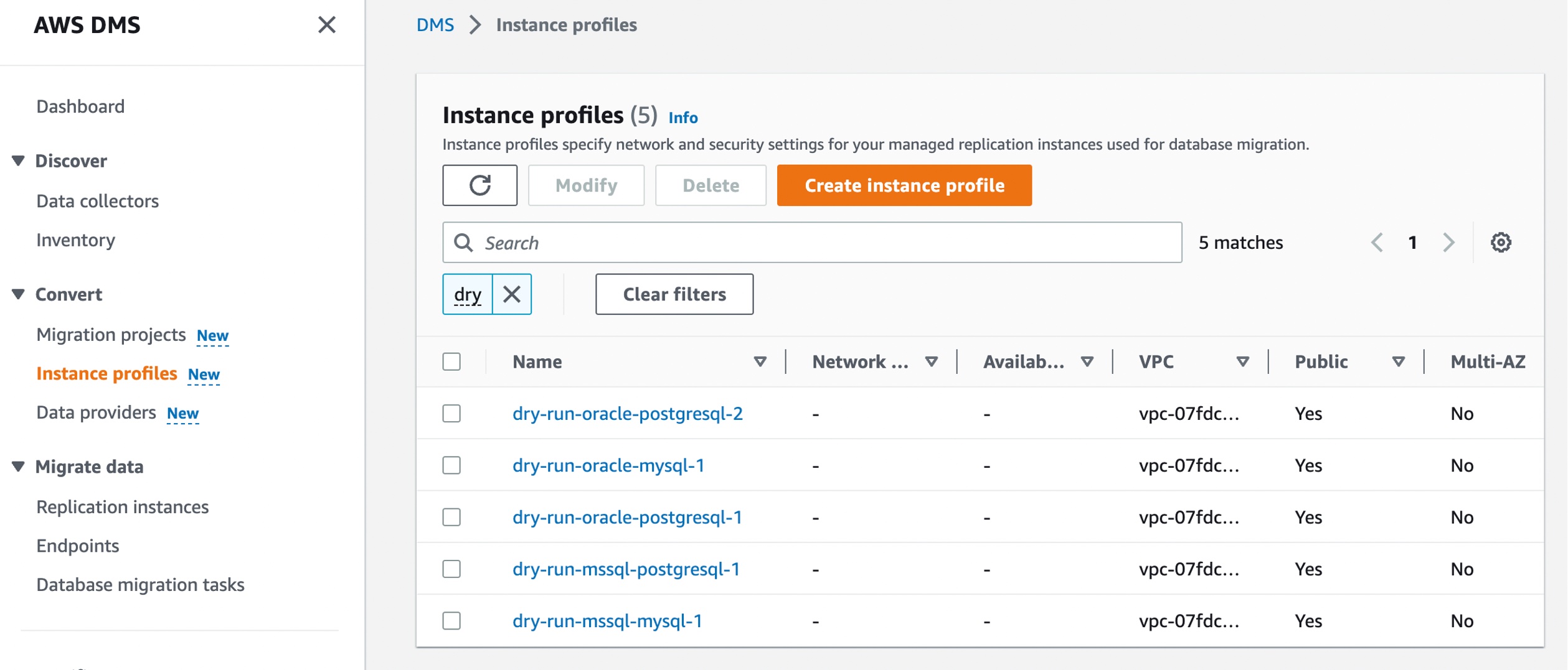 Choose Create instance profile and specify your default VPC or a new VPC,