Post Syndicated from Maria Guerra original https://aws.amazon.com/blogs/big-data/build-the-next-generation-cross-account-event-driven-data-pipeline-orchestration-product/
This is a guest post by Mehdi Bendriss, Mohamad Shaker, and Arvid Reiche from Scout24.
At Scout24 SE, we love data pipelines, with over 700 pipelines running daily in production, spread across over 100 AWS accounts. As we democratize data and our data platform tooling, each team can create, maintain, and run their own data pipelines in their own AWS account. This freedom and flexibility is required to build scalable organizations. However, it’s full of pitfalls. With no rules in place, chaos is inevitable.
We took a long road to get here. We’ve been developing our own custom data platform since 2015, developing most tools ourselves. Since 2016, we have our self-developed legacy data pipeline orchestration tool.
The motivation to invest a year of work into a new solution was driven by two factors:
- Lack of transparency on data lineage, especially dependency and availability of data
- Little room to implement governance
As a technical platform, our target user base for our tooling includes data engineers, data analysts, data scientists, and software engineers. We share the vision that anyone with relevant business context and minimal technical skills can create, deploy, and maintain a data pipeline.
In this context, in 2015 we created the predecessor of our new tool, which allows users to describe their pipeline in a YAML file as a list of steps. It worked well for a while, but we faced many problems along the way, notably:
- Our product didn’t support pipelines to be triggered by the status of other pipelines, but based on the presence of
_SUCCESS files in Amazon Simple Storage Service (Amazon S3). Here we relied on periodic pulls. In complex organizations, data jobs often have strong dependencies to other work streams.
- Given the previous point, most pipelines could only be scheduled based on a rough estimate of when their parent pipelines might finish. This led to cascaded failures when the parents failed or didn’t finish on time.
- When a pipeline fails and gets fixed, then manually redeployed, all its dependent pipelines must be rerun manually. This means that the data producer bears the responsibility of notifying every single team downstream.
Having data and tooling democratized without the ability to provide insights into which jobs, data, and dependencies exist diminishes synergies within the company, leading to silos and problems in resource allocation. It became clear that we needed a successor for this product that would give more flexibility to the end-user, less computing costs, and no infrastructure management overhead.
In this post, we describe, through a hypothetical case study, the constraints under which the new solution should perform, the end-user experience, and the detailed architecture of the solution.
Case study
Our case study looks at the following teams:
- The
core-data-availability team has a data pipeline named listings that runs every day at 3:00 AM on the AWS account Account A, and produces on Amazon S3 an aggregate of the listings events published on the platform on the previous day.
- The
search team has a data pipeline named searches that runs every day at 5:00 AM on the AWS account Account B, and exports to Amazon S3 the list of search events that happened on the previous day.
- The
rent-journey team wants to measure a metric referred to as X; they create a pipeline named pipeline-X that runs daily on the AWS account Account C, and relies on the data of both previous pipelines. pipeline-X should only run daily, and only after both the listings and searches pipelines succeed.
User experience
We provide users with a CLI tool that we call DataMario (relating to its predecessor DataWario), and which allows users to do the following:
- Set up their AWS account with the necessary infrastructure needed to run our solution
- Bootstrap and manage their data pipeline projects (creating, deploying, deleting, and so on)
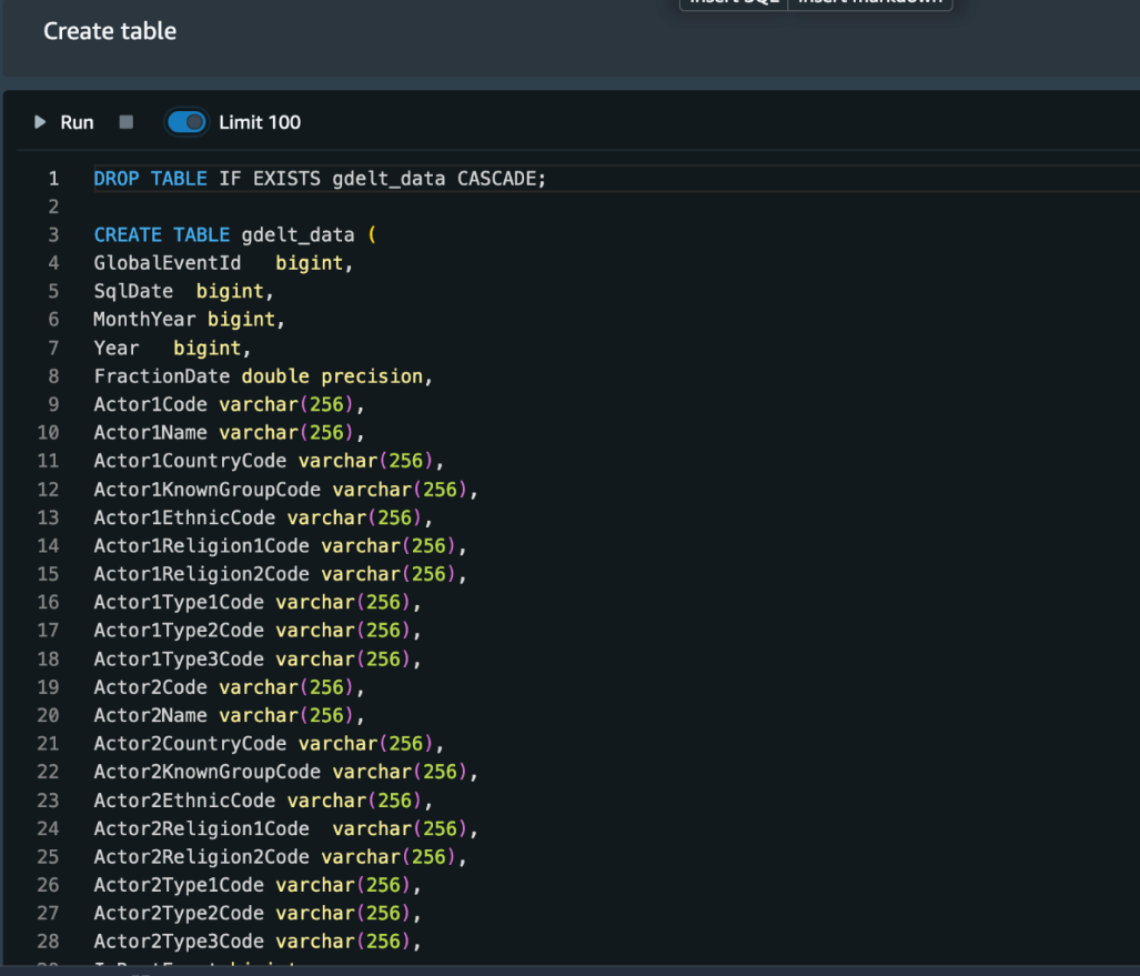
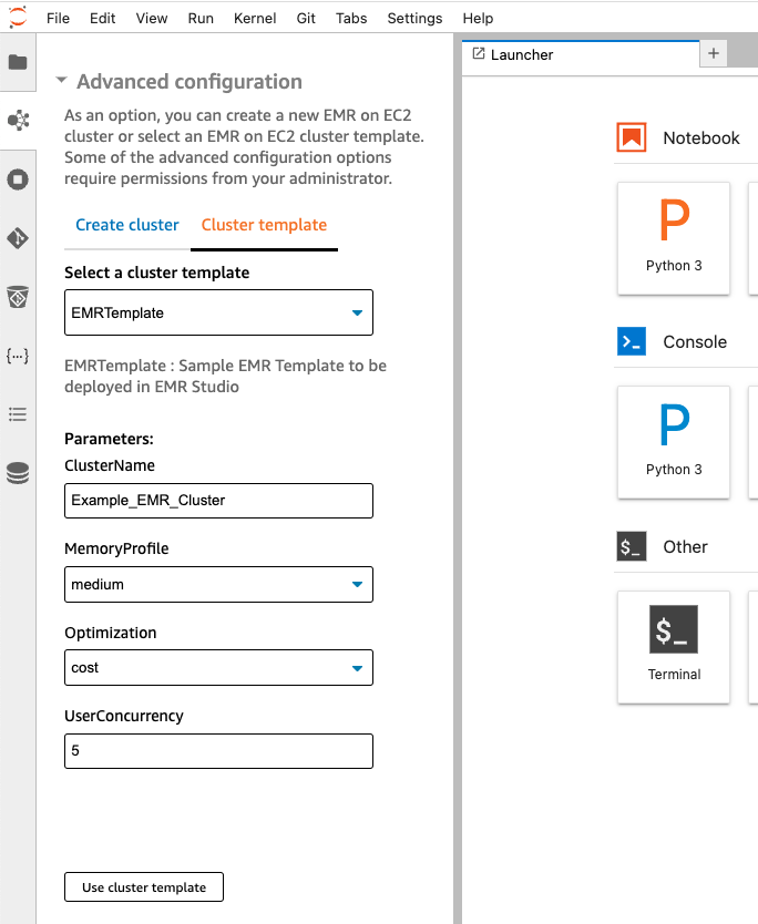
When creating a new project with the CLI, we generate (and require) every project to have a pipeline.yaml file. This file describes the pipeline steps and the way they should be triggered, alerting, type of instances and clusters in which the pipeline will be running, and more.
In addition to the pipeline.yaml file, we allow advanced users with very niche and custom needs to create their pipeline definition entirely using a TypeScript API we provide them, which allows them to use the whole collection of constructs in the AWS Cloud Development Kit (AWS CDK) library.
For the sake of simplicity, we focus on the triggering of pipelines and the alerting in this post, along with the definition of pipelines through pipeline.yaml.
The listings and searches pipelines are triggered as per a scheduling rule, which the team defines in the pipeline.yaml file as follows:
trigger:
    schedule:
        hour: 3
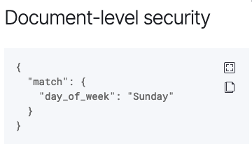
pipeline-x is triggered depending on the success of both the listings and searches pipelines. The team defines this dependency relationship in the project’s pipeline.yaml file as follows:
trigger:
    executions:
        allOf:
            - name: listings
              account: Account_A_ID
              status:
                  - SUCCESS
            - name: searches
              account: Account_B_ID
              status:
                  - SUCCESS
The executions block can define a complex set of relationships by combining the allOf and anyOf blocks, along with a logical operator operator: OR / AND, which allows mixing the allOf and anyOf blocks. We focus on the most basic use case in this post.
Accounts setup
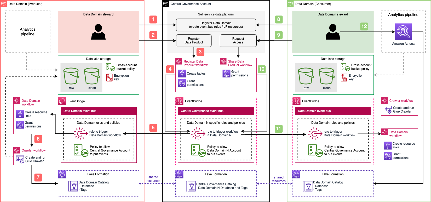
To support alerting, logging, and dependencies management, our solution has components that must be pre-deployed in two types of accounts:
- A central AWS account – This is managed by the Data Platform team and contains the following:
- A central data pipeline Amazon EventBridge bus receiving all the run status changes of AWS Step Functions workflows running in user accounts
- An AWS Lambda function logging the Step Functions workflow run changes in an Amazon DynamoDB table to verify if any downstream pipelines should be triggered based on the current event and previous run status changes log
- A Slack alerting service to send alerts to the Slack channels specified by users
- A trigger management service that broadcasts triggering events to the downstream buses in the user accounts
- All AWS user accounts using the service – These accounts contain the following:
- A data pipeline EventBridge bus that receives Step Functions workflow run status changes forwarded from the central EventBridge bus
- An S3 bucket to store data pipelines artifacts, along their logs
- Resources needed to run Amazon EMR clusters, like security groups, AWS Identity and Access Management (IAM) roles, and more
With the provided CLI, users can set up their account by running the following code:
Solution overview
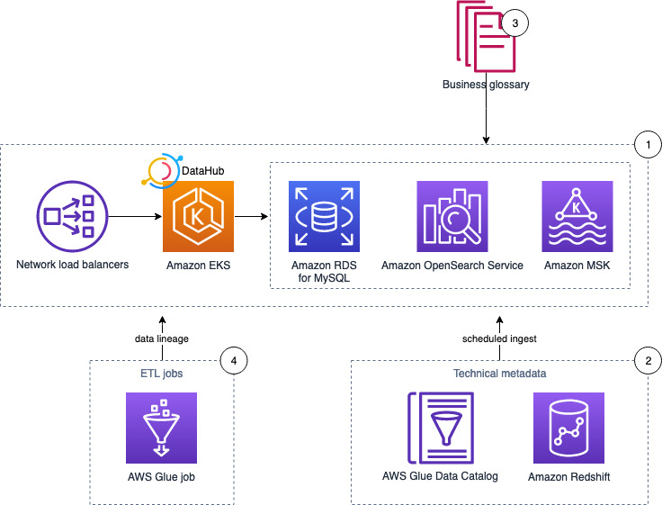
The following diagram illustrates the architecture of the cross-account, event-driven pipeline orchestration product.

In this post, we refer to the different colored and numbered squares to reference a component in the architecture diagram. For example, the green square with label 3 refers to the EventBridge bus default component.
Deployment flow
This section is illustrated with the orange squares in the architecture diagram.
A user can create a project consisting of a data pipeline or more using our CLI tool as follows:
$ dpc create-project -n 'project-name'
The created project contains several components that allow the user to create and deploy data pipelines, which are defined in .yaml files (as explained earlier in the User experience section).
The workflow of deploying a data pipeline such as listings in Account A is as follows:
- Deploy
listings by running the command dpc deploy in the root folder of the project. An AWS CDK stack with all required resources is automatically generated.
- The previous stack is deployed as an AWS CloudFormation template.
- The stack uses custom resources to perform some actions, such as storing information needed for alerting and pipeline dependency management.
- Two Lambda functions are triggered, one to store the mapping
pipeline-X/slack-channels used for alerting in a DynamoDB table, and another one to store the mapping between the deployed pipeline and its triggers (other pipelines that should result in triggering the current one).
- To decouple alerting and dependency management services from the other components of the solution, we use Amazon API Gateway for two components:
- The Slack API.
- The dependency management API.
- All calls for both APIs are traced in Amazon CloudWatch log groups and two Lambda functions:
- The Slack channel publisher Lambda function, used to store the mapping
pipeline_name/slack_channels in a DynamoDB table.
- The dependencies publisher Lambda function, used to store the pipelines dependencies (the
mapping pipeline_name/parents) in a DynamoDB table.
Pipeline trigger flow
This is an event-driven mechanism that ensures that data pipelines are triggered as requested by the user, either following a schedule or a list of fulfilled upstream conditions, such as a group of pipelines succeeding or failing.
This flow relies heavily on EventBridge buses and rules, specifically two types of rules:
- Scheduling rules.
- Step Functions event-based rules, with a payload matching the set of statuses of all the parents of a given pipeline. The rules indicate for which set of statuses all the parents of
pipeline-X should be triggered.
Scheduling
This section is illustrated with the black squares in the architecture diagram.
The listings pipeline running on Account A is set to run every day at 3:00 AM. The deployment of this pipeline creates an EventBridge rule and a Step Functions workflow for running the pipeline:
- The EventBridge rule is of type
schedule and is created on the default bus (this is the EventBridge bus responsible for listening to native AWS events—this distinction is important to avoid confusion when introducing the other buses). This rule has two main components:
- A cron-like notation to describe the frequency at which it runs:
0 3 * * ? *.
- The target, which is the Step Functions workflow describing the workflow of the
listings pipeline.
- The
listings Step Function workflow describes and runs immediately when the rule gets triggered. (The same happens to the searches pipeline.)
Each user account has a default EventBridge bus, which listens to the default AWS events (such as the run of any Lambda function) and scheduled rules.
Dependency management
This section is illustrated with the green squares in the architecture diagram. The current flow starts after the Step Functions workflow (black square 2) starts, as explained in the previous section.
As a reminder, pipeline-X is triggered when both the listings and searches pipelines are successful. We focus on the listings pipeline for this post, but the same applies to the searches pipeline.
The overall idea is to notify all downstream pipelines that depend on it, in every AWS account, passing by and going through the central orchestration account, of the change of status of the listings pipeline.
It’s then logical that the following flow gets triggered multiple times per pipeline (Step Functions workflow) run as its status changes from RUNNING to either SUCCEEDED, FAILED, TIMED_OUT, or ABORTED. The reason being that there could be pipelines downstream potentially listening on any of those status change events. The steps are as follows:
- The event of the Step Functions workflow starting is listened to by the
default bus of Account A.
- The rule
export-events-to-central-bus, which specifically listens to the Step Function workflow run status change events, is then triggered.
- The rule forwards the event to the central bus on the central account.
- The event is then caught by the rule
trigger-events-manager.
- This rule triggers a Lambda function.
- The function gets the list of all children pipelines that depend on the current run status of
listings.
- The current run is inserted in the run log Amazon Relational Database Service (Amazon RDS) table, following the
schema sfn-listings, time (timestamp), status (SUCCEEDED, FAILED, and so on). You can query the run log RDS table to evaluate the running preconditions of all children pipelines and get all those that qualify for triggering.
- A triggering event is broadcast in the central bus for each of those eligible children.
- Those events get broadcast to all accounts through the
export rules—including Account C, which is of interest in our case.
- The
default EventBridge bus on Account C receives the broadcasted event.
- The EventBridge rule gets triggered if the event content matches the expected payload of the rule (notably that both pipelines have a
SUCCEEDED status).
- If the payload is valid, the rule triggers the Step Functions workflow
pipeline-X and triggers the workflow to provision resources (which we discuss later in this post).
Alerting
This section is illustrated with the gray squares in the architecture diagram.
Many teams handle alerting differently across the organization, such as Slack alerting messages, email alerts, and OpsGenie alerts.
We decided to allow users to choose their preferred methods of alerting, giving them the flexibility to choose what kind of alerts to receive:
- At the step level – Tracking the entire run of the pipeline
- At the pipeline level – When it fails, or when it finishes with a
SUCCESS or FAILED status
During the deployment of the pipeline, a new Amazon Simple Notification Service (Amazon SNS) topic gets created with the subscriptions matching the targets specified by the user (URL for OpsGenie, Lambda for Slack or email).
The following code is an example of what it looks like in the user’s pipeline.yaml:
notifications:
    type: FULL_EXECUTION
    targets:
        - channel: SLACK
          addresses:
               - data-pipeline-alerts
        - channel: EMAIL
          addresses:
               - [email protected]
The alerting flow includes the following steps:
- As the pipeline (Step Functions workflow) starts (black square 2 in the diagram), the run gets logged into CloudWatch Logs in a log group corresponding to the name of the pipeline (for example,
listings).
- Depending on the user preference, all the run steps or events may get logged or not thanks to a subscription filter whose target is the
execution-tracker-lambda Lambda function. The function gets called anytime a new event gets published in CloudWatch.
- This Lambda function parses and formats the message, then publishes it to the SNS topic.
- For the email and OpsGenie flows, the flow stops here. For posting the alert message on Slack, the Slack API caller Lambda function gets called with the formatted event payload.
- The function then publishes the message to the
/messages endpoint of the Slack API Gateway.
- The Lambda function behind this endpoint runs, and posts the message in the corresponding Slack channel and under the right Slack thread (if applicable).
- The function retrieves the secret Slack REST API key from AWS Secrets Manager.
- It retrieves the Slack channels in which the alert should be posted.
- It retrieves the root message of the run, if any, so that subsequent messages get posted under the current run thread on Slack.
- It posts the message on Slack.
- If this is the first message for this run, it stores the mapping with the DB schema
execution/slack_message_id to initiate a thread for future messages related to the same run.
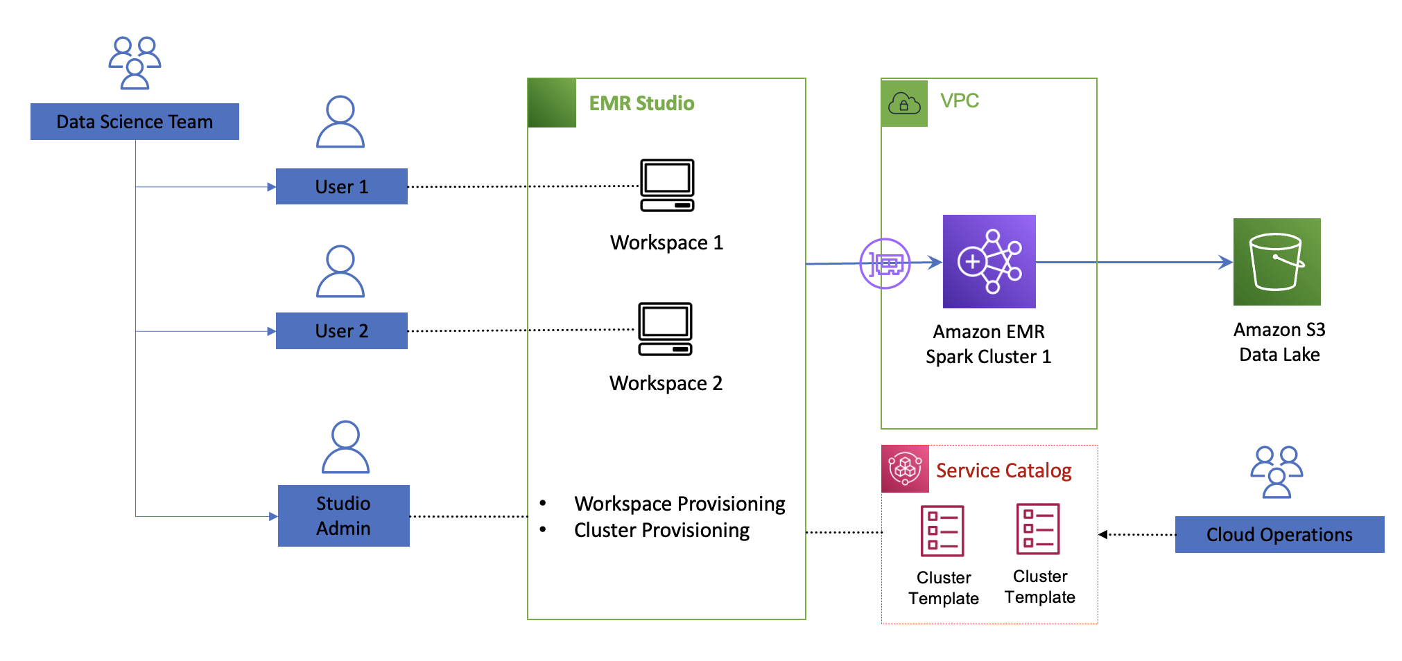
Resource provisioning
This section is illustrated with the light blue squares in the architecture diagram.
To run a data pipeline, we need to provision an EMR cluster, which in turn requires some information like Hive metastore credentials, as shown in the workflow. The workflow steps are as follows:
- Trigger the Step Functions workflow
listings on schedule.
- Run the
listings workflow.
- Provision an EMR cluster.
- Use a custom resource to decrypt the Hive metastore password to be used in Spark jobs relying on central Hive tables or views.
End-user experience
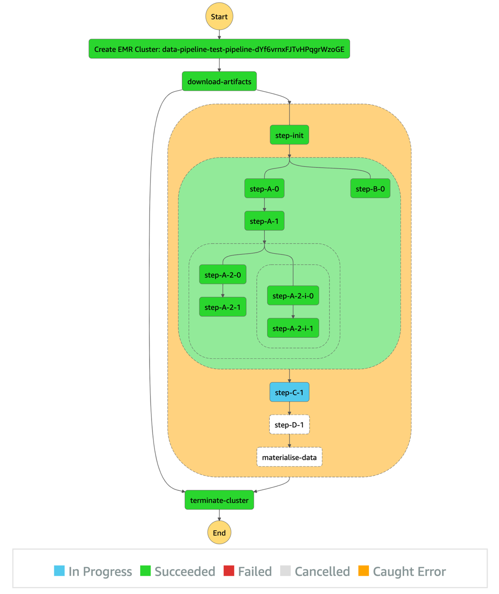
After all preconditions are fulfilled (both the listings and searches pipelines succeeded), the pipeline-X workflow runs as shown in the following diagram.

As shown in the diagram, the pipeline description (as a sequence of steps) defined by the user in the pipeline.yaml is represented by the orange block.
The steps before and after this orange section are automatically generated by our product, so users don’t have to take care of provisioning and freeing compute resources. In short, the CLI tool we provide our users synthesizes the user’s pipeline definition in the pipeline.yaml and generates the corresponding DAG.
Additional considerations and next steps
We tried to stay consistent and stick to one programming language for the creation of this product. We chose TypeScript, which played well with AWS CDK, the infrastructure as code (IaC) framework that we used to build the infrastructure of the product.
Similarly, we chose TypeScript for building the business logic of our Lambda functions, and of the CLI tool (using Oclif) we provide for our users.
As demonstrated in this post, EventBridge is a powerful service for event-driven architectures, and it plays a central and important role in our products. As for its limitations, we found that pairing Lambda and EventBridge could fulfill all our current needs and granted a high level of customization that allowed us to be creative in the features we wanted to serve our users.
Needless to say, we plan to keep developing the product, and have a multitude of ideas, notably:
- Extend the list of core resources on which workloads run (currently only Amazon EMR) by adding other compute services, such Amazon Elastic Compute Cloud (Amazon EC2)
- Use the Constructs Hub to allow users in the organization to develop custom steps to be used in all data pipelines (we currently only offer Spark and shell steps, which suffice in most cases)
- Use the stored metadata regarding pipeline dependencies for data lineage, to have an overview of the overall health of the data pipelines in the organization, and more
Conclusion
This architecture and product brought many benefits. It allows us to:
- Have a more robust and clear dependency management of data pipelines at Scout24.
- Save on compute costs by avoiding scheduling pipelines based approximately on when its predecessors are usually triggered. By shifting to an event-driven paradigm, no pipeline gets started unless all its prerequisites are fulfilled.
- Track our pipelines granularly and in real time on a step level.
- Provide more flexible and alternative business logic by exposing multiple event types that downstream pipelines can listen to. For example, a fallback downstream pipeline might be run in case of a parent pipeline failure.
- Reduce the cross-team communication overhead in case of failures or stopped runs by increasing the transparency of the whole pipelines’ dependency landscape.
- Avoid manually restarting pipelines after an upstream pipeline is fixed.
- Have an overview of all jobs that run.
- Support the creation of a performance culture characterized by accountability.
We have big plans for this product. We will use DataMario to implement granular data lineage, observability, and governance. It’s a key piece of infrastructure in our strategy to scale data engineering and analytics at Scout24.
We will make DataMario open source towards the end of 2022. This is in line with our strategy to promote our approach to a solution on a self-built, scalable data platform. And with our next steps, we hope to extend this list of benefits and ease the pain in other companies solving similar challenges.
Thank you for reading.
About the authors
 Mehdi Bendriss is a Senior Data / Data Platform Engineer, MSc in Computer Science and over 9 years of experience in software, ML, and data and data platform engineering, designing and building large-scale data and data platform products.
 Mohamad Shaker is a Senior Data / Data Platform Engineer, with over 9 years of experience in software and data engineering, designing and building large-scale data and data platform products that enable users to access, explore, and utilize their data to build great data products.
 Arvid Reiche is a Data Platform Leader, with over 9 years of experience in data, building a data platform that scales and serves the needs of the users.
 Marco Salazar is a Solutions Architect working with Digital Native customers in the DACH region with over 5 years of experience building and delivering end-to-end, high-impact, cloud native solutions on AWS for Enterprise and Sports customers across EMEA. He currently focuses on enabling customers to define technology strategies on AWS for the short- and long-term that allow them achieve their desired business objectives, specializing on Data and Analytics engagements. In his free time, Marco enjoys building side-projects involving mobile/web apps, microcontrollers & IoT, and most recently wearable technologies.


 Anna Montalat is a Senior Product Marketing Manager for AWS streaming data services which includes Amazon Managed Streaming for Apache Kafka (MSK), Kinesis Data Streams, Kinesis Video Streams, Kinesis Data Firehose, and Kinesis Data Analytics. She is passionate about bringing new and emerging technologies to market, working closely with service teams and enterprise customers. Outside of work, Anna skis through winter time and sails through summer.


 DoYeun Kim is the Head of Data Engineering at SOCAR. He is a passionate software engineering professional with 19+ years experience. He leads a team of 10+ engineers who are responsible for the data platform, data warehouse and MLOps engineering, as well as building in-house data products.
 SangSu Park is a Lead Data Architect in SOCAR’s cloud DB team. His passion is to keep learning, embrace challenges, and strive for mutual growth through communication. He loves to travel in search of new cities and places.
 YoungMin Park is a Lead Architect in SOCAR’s cloud infrastructure team. His philosophy in life is-whatever it may be-to challenge, fail, learn, and share such experiences to build a better tomorrow for the world. He enjoys building expertise in various fields and basketball.
 Younggu Yun is a Senior Data Lab Architect at AWS. He works with customers around the APAC region to help them achieve business goals and solve technical problems by providing prescriptive architectural guidance, sharing best practices, and building innovative solutions together. In his free time, his son and he are obsessed with Lego blocks to build creative models.
 Vicky Falconer leads the AWS Data Lab program across APAC, offering accelerated joint engineering engagements between teams of customer builders and AWS technical resources to create tangible deliverables that accelerate data analytics modernization and machine learning initiatives.
 Deepthi Mohan is a Principal Product Manager on the Kinesis Data Analytics team.


 , the leading open-source OLAP for big data. Kyligence offers an Intelligent OLAP Platform to simplify multi-dimensional analytics for cloud data lakes.


 Ying Wang is a Manager of Software Development Engineer. She has 12 years of expertise in data analytics and science. She assisted customers with enterprise data architecture solutions to scale their data analytics in the cloud during her time as a data architect. Currently, she helps customer to unlock the power of Data with QuickSight from engineering by delivering new features.
 Ian Liao is a Senior Data Visualization Architect at AWS Professional Services. Before AWS, Ian spent years building startups in data and analytics. Now he enjoys helping customer to scale their data application on the cloud.
 Maitri Brahmbhatt is a Business Intelligence Engineer at AWS. She helps customers and partners leverage their data to gain insights into their business and make data driven decisions by developing QuickSight dashboards.