Starting with version 7.10, Amazon EMR is transitioning from EMR File System (EMRFS) to EMR S3A as the default file system connector for Amazon Simple Storage Service (Amazon S3) access. This transition brings HBase on Amazon S3 to a new level, offering performance parity with EMRFS while delivering substantial improvements, including better standardization, improved portability, stronger community support, improved performance through non-blocking I/O, asynchronous clients, and better credential management with AWS SDK V2 integration.
In this post, we discuss this transition and its benefits.
Understanding file system usage in HBase with Amazon EMR
HBase on Amazon S3 uses Amazon S3 as the primary storage layer instead of HDFS. When the memstore gets flushed, HBase writes HFiles directly to Amazon S3 using the file system connector. The Write Ahead Logs (WALs) and other operational files are still maintained in HDFS on the local cluster for performance and durability reasons. Amazon EMR also provides durable off-cluster EMR WAL implementation to improve the durability of the data.
With the HBase on Amazon S3 architecture, you can take advantage of the virtually unlimited storage capacity and cost-effectiveness of Amazon S3 while maintaining acceptable read/write performance. When data is read, HBase retrieves the HFiles directly from Amazon S3, and the block cache in memory helps optimize frequent read operations. This design alleviates the need for a large HDFS cluster for data storage, reducing operational costs and management overhead. The Amazon S3 file system connector handles the communication between HBase and Amazon S3, managing aspects like authentication, retry logic, and consistency. However, this setup might have slightly higher latency compared to traditional HBase on HDFS due to the network calls to Amazon S3, but the trade-off is justified by the benefits of scalability, caching layer, and cost-effectiveness that Amazon S3 provides.
Performance comparison of EMR S3A with EMRFS and OSS S3A from 7.3 release
Amazon EMR is transitioning how it connects to Amazon S3 storage. Through Amazon EMR 7.9, Amazon EMR has used EMRFS as its primary connector to interact with Amazon S3 for HBase storage. HBase on Amazon S3 significantly improved its performance with EMR S3A starting from the 7.3 release comparing to OSS S3A and matching the performance levels of EMRFS. This enhancement was thoroughly tested using Yahoo! Cloud Serving Benchmark (YCSB) workloads with 100 million rows in Amazon EMR 7.3 (using Hadoop 3.3 with AWS SDK V1) and Amazon EMR 7.10 (using Hadoop 3.4 with AWS SDK V2).
YCSB includes various workloads with different read and write proportions and data distribution patterns, such as:
Workload A (50% reads, 50% writes) – Simulates a scenario with equal read and write operations (50% each). This is ideal for applications requiring frequent updates and reads, such as session stores.
Workload B (95% reads, 5% writes) – Models a read-heavy application with 95% reads and 5% writes. This is well-suited for scenarios where retrieval operations dominate, like content delivery networks.
Workload C (100% reads) – Simulates user profile cache patterns and serves as a content delivery system.
Workload D (read latest data) – Simulates user status updates where users want to read the latest status.
Workload E (scan heavy) – Simulates threaded conversations where users scan through message threads.
Workload F (read/modify/write operations) – Simulates user record update patterns such as online gaming platforms where player scores are frequently read and updated based on game outcomes.
The performance comparison between EMRFS, EMR S3A, and OSS S3A for Amazon EMR 7.3 (AWS SDK V1) and 7.10 (AWS SDK V2) are illustrated in the following graphs, showing substantial improvements across different workload types. The graphs demonstrate how Amazon EMR 7.3 and 7.10 with EMR S3A achieve performance metrics comparable with EMRFS and up to 65% faster than OSS S3A, especially in read-heavy and mixed read/write workloads.
EMR S3A as the default file system from Amazon EMR 7.10
These performance improvements demonstrate a significant evolution in the capabilities of Amazon EMR. Well before EMR S3A became the default file system in version 7.10, EMR HBase users were already experiencing enhanced Amazon S3 access performance through EMR S3A. The critical enhancements implemented in Amazon EMR 7.3 successfully minimized the performance differential between EMRFS and EMR S3A for HBase operations. This achievement delivered optimal performance to users while preserving EMR S3A’s distinct benefits within the analytics ecosystem, including improved standardization, better community integration, and enhanced portability.
Amazon EMR 7.10 marks a significant change for HBase on Amazon S3 users. EMR S3A becomes the default file system connector automatically, independent of how your root directory’s file system is configured. This seamless transition enables EMR HBase customers to use EMR S3A’s expanding feature set and improvements without manual intervention.
Conclusion
The evolution of file system connectors in EMR HBase demonstrates AWS’s commitment to delivering high-performance, scalable solutions for big data workloads. Starting with EMR S3A, which achieved performance parity with EMRFS in Amazon EMR 7.3 (as validated through extensive YCSB benchmark tests with 100 million rows) and improvement over OSS S3A, to the upcoming transition to S3A as the default connector in Amazon EMR 7.10, AWS continues to enhance its storage interface capabilities.
The transition represents more than just a technical upgrade; it delivers a trifecta of benefits: enhanced standardization across Hadoop ecosystems, improved workload portability, and robust community support. Most importantly, this advancement maintains the high-performance standards established by EMRFS while positioning EMR HBase for future innovations in storage interface capabilities. AWS’s strategic evolution of file system connectors demonstrates its commitment to providing enterprise-grade solutions that combine performance, scalability, and architectural excellence.
As big data workloads continue to grow and evolve, this foundation of reliable, high-performance storage access will become increasingly crucial for organizations using EMR HBase for their data processing needs. We recommend that you stay up to date with the latest Amazon EMR release to take advantage of the latest performance and feature benefits.
This post was written with Avinash Erupaka from Bayer (IT PH, Drug Innovation platform)
How can pharmaceutical companies unlock the full potential of their data to drive breakthrough innovations? Bayer, a global leader in health and nutrition, is dedicated to tackling the pressing challenges of our time, including a growing and aging population and the strain on our planet’s ecosystems. Its mission of “Health for All, Hunger for None” drives its commitment to addressing societal and environmental needs through groundbreaking research. Bayer is focused on developing innovative solutions that make a tangible difference in the world and value for its customers, employees, and stakeholders. Headquartered in Leverkusen, Germany, Bayer operates across 80 countries and is pioneering a data science ecosystem that transforms how research teams access, analyze, and derive insights from complex scientific data.
By harnessing the power of data, analytics, artificial intelligence and machine learning (AI/ML), and generative AI, Bayer is creating a cloud-based Pharma R&D Data Science Ecosystem (DSE) on AWS that powers cutting-edge technologies and concepts with robust data management. In doing so, R&D teams can fully realize the potential of unified data and analytics.
In this post, we discuss how Bayer used the next generation of SageMaker to build a solution that unified data ingestion, storage, analytics, and AI/ML workflows. Built on data mesh principles, Bayer’s DSE integrates advanced data ingestion, storage, analytics, and ML workflows to enable agile experimentation and scalable insight generation. It democratizes access to analytics, fosters cross-Region collaboration, and provides flexible integration of structured, semi-structured, and unstructured data.
Challenges in pharmaceutical research
In pharmaceutical research, data has become the most critical asset for driving innovation. However, managing this data effectively presents unprecedented challenges and traditional data management approaches are becoming increasingly inadequate for complex, global research initiatives. Many pharma R&D organization face a complex ecosystem of data and analytics related obstacles that hinder scientific discovery and operational efficiency:
Siloed datasets – Research datasets are siloed across domains, limiting reuse and slowing discovery.
Multiple data modalities – Clinical trial data (structured), real-world evidence (semi-structured), and genomic files (unstructured) existed in isolation, complicating integration and analysis.
Inflexible ingestion capabilities – Systems that support batch processing (such as trial data), real-time data streams (for example, from lab equipment), and event-driven ingestion (such as regulatory updates).
Rising R&D costs – Disparate technologies and disconnected systems create operational inefficiencies and increased licensing and maintenance costs.
Inconsistent landscape to fully use ML – The absence of a unified data architecture and standardized, domain-agnostic MLOps workflows mean that data and analytics innovation is often ad hoc and non-repeatable. Teams lack a streamlined way to scale successful patterns, resulting in redundant efforts, longer development cycles, and missed opportunities for cross-domain synergy.
Disconnected architectures – Software solutions are not integrated into the wider unified ecosystem, resulting in silos, redundancies, and inefficiencies.
Recognizing these systemic challenges, Bayer embarked on a transformative journey. DSE is not just a technological solution, but a strategic reimagining of how research data and analytics could be used across a global organization. By bringing together cutting-edge technologies, standardized frameworks, a collaborative data mesh, and lakehouse architecture, Bayer set out to help researchers and engineers accelerate pharmaceutical innovation.
Finding a solution with the next generation of SageMaker
Bayer envisioned a unified data science ecosystem that would provide the following:
A unified collaborative development experience for all data scientists regardless of their location or specialization
Seamless access to both structured and unstructured data through a consistent interface
Built-in governance and compliance controls appropriate for pharmaceutical research
Scalable compute resources to handle the most complex analytical workloads
Bayer conducted a comprehensive evaluation of various solutions before selecting the next generation of SageMaker as the cornerstone of their new data science ecosystem. Although other options had merits, Bayer prioritized the following capabilities:
Access to multimodal data – Essential for genomics, proteomics, and advanced biomarker research
Centralized asset marketplace – Central hub to discover and reuse data, features, models, and other enterprise assets
Integrated tooling ecosystem – Streamlined access to key tools like Git, ETL, MLflow, and generative AI application builders in one place
Multi-domain and cross-Region support – Critical for global research collaboration
Price-performance – Necessary for sustainable, long-term scaling
The capabilities of Amazon SageMaker Unified Studio and Amazon SageMaker Catalog aligned with Bayer’s vision of decentralized mesh execution combined with centralized discovery and governance. They enabled teams to work with their preferred tools, such as Jupyter Notebooks or workflow builders, while maintaining discoverability and reusability of assets.
Solution overview
This section describes the key features and architecture of Bayer’s DSE built on SageMaker. The DSE solution addresses the identified challenges through a multi-layered architecture:
Breaking down data silos – Multimodal data ingestion capabilities of the solution break down data silos by enabling unified storage, processing of structured, semi-structured, and unstructured data through batch, streaming, and event-driven pipelines.
Reducing costs through standardization – To address rising R&D costs and operational inefficiencies, pre-wired analytical workbenches offer standardized templates and integrated development environments (IDEs) that reduce redundancy and accelerate workflow development.
Unlocking AI/ML with Amazon SageMaker AI and Amazon Bedrock – Advanced AI/ML capabilities, powered by Amazon SageMaker AI and Amazon Bedrock, create a standardized, domain-agnostic MLOps environment that enables repeatable innovation and cross-domain synergy.
Managing tools ecosystem with end-to-end observability – Robust governance and observability features provide compliance and system reliability while integrating previously disconnected tools into a unified, well-monitored ecosystem that breaks down architectural silos and promotes efficient resource utilization.
The DSE architecture implements data mesh principles where data domains (omics, regulatory, clinical trials) are treated as products, with ownership and management responsibilities assigned to domain experts. These domains are decentralized for execution but remain discoverable and reusable through SageMaker Catalog. At the core of the architecture is a hybrid mesh lakehouse architecture that combines Amazon S3 and Iceberg, providing the flexibility to handle both structured and unstructured data efficiently. SageMaker Unified Studio provides an analytical layer where researchers can access the full suite of tools needed for their work. The following diagram illustrates this architecture.
Impact
The first phase of Bayer’s DSE confirmed the next generation of SageMaker as a powerful foundation for their R&D DSE—designed to balance decentralized innovation with centralized governance through a scalable data mesh architecture. With this solution, Bayer can catalog and manage multimodal data assets—including structured and unstructured data, ML features, models, and custom scientific assets—with context-rich metadata across diverse Pharma R&D domains. Bayer is now positioned to onboard over 300 TB of biomarker data and integrate siloed omics, clinical, and chemistry data repositories into a cohesive environment. With integrated tools like JupyterLab Spaces, MLflow, and SageMaker AI Studio, the DSE platform is laying the groundwork for a comprehensive, GxP-aware ML workbench—paving the way to operationalize over 25 high-value ML use cases and support more than 100 data scientists across the organization.
“The Data Science Ecosystem is vital for developing our medicines,” says Daniel Gusenleitner, Mission Lead for the R&D Data Science Ecosystem. “It enhances our business workflows with advanced analytics, helping us accelerate the search for new treatments. By integrating data from the entire research and development process, we improve the chances of technical success and ensure our efforts are efficient. Unlocking our data also facilitates target discovery, leading to groundbreaking advancements in patient care.”
Next steps
Bayer has successfully begun their Data Science Ecosystem on the next generation of Amazon SageMaker and is working to onboard the first use case of advanced biomarker research. Building on the strong foundation, Bayer is also accelerating the evolution of the DSE solution with the following key enhancements:
Federated catalogs and cross-domain integration – Enabling search and reuse of data assets across therapeutic areas and business units
Advanced ontology and semantic layer – Enriching metadata with domain knowledge to support AI-based search, discovery, and reasoning
Adoption of generative and agentic AI workflows – Driving novel drug discovery and accelerating hypothesis generation
Conclusion
By leveraging the next generation of Amazon SageMaker to build their cloud-based Data Science Ecosystem, Bayer is creating a foundation for faster, more efficient research and discovery. Amazon SageMaker is unifying diverse data types, enabling global collaboration, and standardizing ML workflows to help position Bayer at the forefront of data-driven innovation.
To learn more and get started with the next generation of SageMaker, refer to Amazon SageMaker or the AWS console.
Today, we’re announcing two new capabilities for Amazon S3 Tables: support for the new Intelligent-Tiering storage class that automatically optimizes costs based on access patterns, and replication support to automatically maintain consistent Apache Iceberg table replicas across AWS Regions and accounts without manual sync.
Organizations working with tabular data face two common challenges. First, they need to manually manage storage costs as their datasets grow and access patterns change over time. Second, when maintaining replicas of Iceberg tables across Regions or accounts, they must build and maintain complex architectures to track updates, manage object replication, and handle metadata transformations.
S3 Tables Intelligent-Tiering storage class With the S3 Tables Intelligent-Tiering storage class, data is automatically tiered to the most cost-effective access tier based on access patterns. Data is stored in three low-latency tiers: Frequent Access, Infrequent Access (40% lower cost than Frequent Access), and Archive Instant Access (68% lower cost compared to Infrequent Access). After 30 days without access, data moves to Infrequent Access, and after 90 days, it moves to Archive Instant Access. This happens without changes to your applications or impact on performance.
Table maintenance activities, including compaction, snapshot expiration, and unreferenced file removal, operate without affecting the data’s access tiers. Compaction automatically processes only data in the Frequent Access tier, optimizing performance for actively queried data while reducing maintenance costs by skipping colder files in lower-cost tiers.
By default, all existing tables use the Standard storage class. When creating new tables, you can specify Intelligent-Tiering as the storage class, or you can rely on the default storage class configured at the table bucket level. You can set Intelligent-Tiering as the default storage class for your table bucket to automatically store tables in Intelligent-Tiering when no storage class is specified during creation.
Let me show you how it works You can use the AWS Command Line Interface (AWS CLI) and the put-table-bucket-storage-class and get-table-bucket-storage-class commands to change or verify the storage tier of your S3 table bucket.
# Change the storage class
aws s3tables put-table-bucket-storage-class \
   --table-bucket-arn $TABLE_BUCKET_ARN  \
   --storage-class-configuration storageClass=INTELLIGENT_TIERING

# Verify the storage class
aws s3tables get-table-bucket-storage-class \
   --table-bucket-arn $TABLE_BUCKET_ARN  \

{ "storageClassConfiguration":
   {
      "storageClass": "INTELLIGENT_TIERING"
   }
}
S3 Tables replication support The new S3 Tables replication support helps you maintain consistent read replicas of your tables across AWS Regions and accounts. You specify the destination table bucket and the service creates read-only replica tables. It replicates all updates chronologically while preserving parent-child snapshot relationships. Table replication helps you build global datasets to minimize query latency for geographically distributed teams, meet compliance requirements, and provide data protection.
You can now easily create replica tables that deliver similar query performance as their source tables. Replica tables are updated within minutes of source table updates and support independent encryption and retention policies from their source tables. Replica tables can be queried using Amazon SageMaker Unified Studio or any Iceberg-compatible engine including DuckDB, PyIceberg, Apache Spark, and Trino.
You can create and maintain replicas of your tables through the AWS Management Console or APIs and AWS SDKs. You specify one or more destination table buckets to replicate your source tables. When you turn on replication, S3 Tables automatically creates read-only replica tables in your destination table buckets, backfills them with the latest state of the source table, and continually monitors for new updates to keep replicas in sync. This helps you meet time-travel and audit requirements while maintaining multiple replicas of your data.
Let me show you how it works To show you how it works, I proceed in three steps. First, I create an S3 table bucket, create an Iceberg table, and populate it with data. Second, I configure the replication. Third, I connect to the replicated table and query the data to show you that changes are replicated.
I take a note of the two S3 Tables bucket Amazon Resource Names (ARNs). In this demo, I refer to these as the environment variables SOURCE_TABLE_ARN and DEST_TABLE_ARN.
The replication starts automatically. Updates are typically replicated within minutes. The time it takes to complete depends on the volume of data in the source table.
Third step: Connect to the replicated table and query the data
Now, I connect to the EMR cluster again, and I start a second Spark session. This time, I use the destination table.
To verify the replication works, I insert a second row of data on the source table.
spark.sql("INSERT INTO s3tablesbucket.test.aws_news_blog VALUES ('cust2', 'val2')")
I wait a few minutes for the replication to trigger. I follow the status of the replication with the get-table-replication-status command.
When replication status shows ready, I connect to the EMR cluster and I query the destination table. Without surprise, I see the new row of data.
Additional things to know Here are a couple of additional points to pay attention to:
Replication for S3 Tables supports both Apache Iceberg V2 and V3 table formats, giving you flexibility in your table format choice.
You can configure replication at the table bucket level, making it straightforward to replicate all tables under that bucket without individual table configurations.
Your replica tables maintain the storage class you choose for your destination tables, which means you can optimize for your specific cost and performance needs.
Any Iceberg-compatible catalog can directly query your replica tables without additional coordination—they only need to point to the replica table location. This gives you flexibility in choosing query engines and tools.
Pricing and availability You can track your storage usage by access tier through AWS Cost and Usage Reports and Amazon CloudWatch metrics. For replication monitoring, AWS CloudTrail logs provide events for each replicated object.
There are no additional charges to configure Intelligent-Tiering. You only pay for storage costs in each tier. Your tables continue to work as before, with automatic cost optimization based on your access patterns.
For S3 Tables replication, you pay the S3 Tables charges for storage in the destination table, for replication PUT requests, for table updates (commits), and for object monitoring on the replicated data. For cross-Region table replication, you also pay for inter-Region data transfer out from Amazon S3 to the destination Region based on the Region pair.
To learn more about these new capabilities, visit the Amazon S3 Tables documentation or try them in the Amazon S3 console today. Share your feedback through AWS re:Post for Amazon S3 or through your AWS Support contacts.
Today, we’re announcing three new capabilities for Amazon S3 Storage Lens that give you deeper insights into your storage performance and usage patterns. With the addition of performance metrics, support for analyzing billions of prefixes, and direct export to Amazon S3 Tables, you have the tools you need to optimize application performance, reduce costs, and make data-driven decisions about your Amazon S3 storage strategy.
New performance metric categories S3 Storage Lens now includes eight new performance metric categories that help identify and resolve performance constraints across your organization. These are available at organization, account, bucket, and prefix levels. For example, the service helps you identify small objects in a bucket or prefix that can slow down application performance. This can be mitigated by batching small objects or using the Amazon S3 Express One Zone storage class for higher performance small object workloads.
To access the new performance metrics, you need to enable performance metrics in the S3 Storage Lens advanced tier when creating a new Storage Lens dashboard or editing an existing configuration.
Metric category
Details
Use case
Mitigation
Read request size
Distribution of read request sizes (GET) by day
Identify dataset with small read request patterns that slow down performance
Small request: Batch small objects or use Amazon S3 Express One Zone for high-performance small object workloads
Write request size
Distribution of write request sizes (PUT, POST, COPY, and UploadPart) by day
Identify dataset with small write request patterns that slow down performance
Large request: Parallelize requests, use MPU or use AWS CRT
Storage size
Distribution of object sizes
Identify dataset with small small objects that slow down performance
Small object sizes: Consider bundling small objects
Concurrent PUT 503 errors
Number of 503s due to concurrent PUT operation on same object
Identify prefixes with concurrent PUT throttling that slow down performance
For single writer, modify retry behavior or use Amazon S3 Express One Zone. For multiple writers, use consensus mechanism or use Amazon S3 Express One Zone
Cross-Region data transfer
Bytes transferred and requests sent across Region, in Region
Identify potential performance and cost degradation due to cross-Region data access
Co-locate compute with data in the same AWS Region
Unique objects accessed
Number or percentage of unique objects accessed per day
Identify datasets where small subset of objects are being frequently accessed. These can be moved to higher performance storage tier for better performance
Consider moving active data to Amazon S3 Express One Zone or other caching solutions
The daily average elapsed per request time from the first byte received to the last byte sent
How it works On the Amazon S3 console I choose Create Storage Lens dashboard to create a new dashboard. You can also edit an existing dashboard configuration. I then configure general settings such as providing a Dashboard name, Status, and the optional Tags. Then, I choose Next.
Next, I define the scope of the dashboard by selecting Include all Regions and Include all buckets and specifying the Regions and buckets to be included.
I opt in to the Advanced tier in the Storage Lens dashboard configuration, select Performance metrics, then choose Next.
Next, I select Prefix aggregation as an additional metrics aggregation, then leave the rest of the information as default before I choose Next.
I select the Default metrics report, then General purpose bucket as the bucket type, and then select the Amazon S3 bucket in my AWS account as the Destination bucket. I leave the rest of the information as default, then select Next.
I review all the information before I choose Submit to finalize the process.
After it’s enabled, I’ll receive daily performance metrics directly in the Storage Lens console dashboard. You can also choose to export report in CSV or Parquet format to any bucket in your account or publish to Amazon CloudWatch. The performance metrics are aggregated and published daily and will be available at multiple levels: organization, account, bucket, and prefix. In this dropdown menu, I choose the % concurrent PUT 503 error for the Metric, Last 30 days for the Date range, and 10 for the Top N buckets.
The Concurrent PUT 503 error count metric tracks the number of 503 errors generated by simultaneous PUT operations to the same object. Throttling errors can degrade application performance. For a single writer, modify retry behavior or use higher performance storage tier such as Amazon S3 Express One Zone to mitigate concurrent PUT 503 errors. For multiple writers scenario, use a consensus mechanism to avoid concurrent PUT 503 errors or use higher performance storage tier such as Amazon S3 Express One Zone.
Complete analytics for all prefixes in your S3 buckets S3 Storage Lens now supports analytics for all prefixes in your S3 buckets through a new Expanded prefixes metrics report. This capability removes previous limitations that restricted analysis to prefixes meeting a 1% size threshold and a maximum depth of 10 levels. You can now track up to billions of prefixes per bucket for analysis at the most granular prefix level, regardless of size or depth.
The Expanded prefixes metrics report includes all existing S3 Storage Lens metric categories: storage usage, activity metrics (requests and bytes transferred), data protection metrics, and detailed status code metrics.
How to get started I follow the same steps outlined in the How it works section to create or update the Storage Lens dashboard. In Step 4 on the console, where you select export options, you can select the new Expanded prefixes metrics report. Thereafter, I can export the expanded prefixes metrics report in CSV or Parquet format to any general purpose bucket in my account for efficient querying of my Storage Lens data.
Good to know This enhancement addresses scenarios where organizations need granular visibility across their entire prefix structure. For example, you can identify prefixes with incomplete multipart uploads to reduce costs, track compliance across your entire prefix structure for encryption and replication requirements, and detect performance issues at the most granular level.
Export S3 Storage Lens metrics to S3 Tables S3 Storage Lens metrics can now be automatically exported to S3 Tables, a fully managed feature on AWS with built-in Apache Iceberg support. This integration provides daily automatic delivery of metrics to AWS managed S3 Tables for immediate querying without requiring additional processing infrastructure.
How to get started I start by following the process outlined in Step 5 on the console, where I choose the export destination. This time, I choose Expanded prefixes metrics report. In addition to General purpose bucket, I choose Table bucket.
The new Storage Lens metrics are exported to new tables in an AWS managed bucketaws-s3.
I select the expanded_prefixes_activity_metrics table to view API usage metrics for expanded prefix reports.
I can preview the table on the Amazon S3 console or use Amazon Athena to query the table.
Good to know S3 Tables integration with S3 Storage Lens simplifies metric analysis using familiar SQL tools and AWS analytics services such as Amazon Athena, Amazon QuickSight, Amazon EMR, and Amazon Redshift, without requiring a data pipeline. The metrics are automatically organized for optimal querying, with custom retention and encryption options to suit your needs.
This integration enables cross-account and cross-Region analysis, custom dashboard creation, and data correlation with other AWS services. For example, you can combine Storage Lens metrics with S3 Metadata to analyze prefix-level activity patterns and identify objects in prefixes with cold data that are eligible for transition to lower-cost storage tiers.
For your agentic AI workflows, you can use natural language to query S3 Storage Lens metrics in S3 Tables with the S3 Tables MCP Server. Agents can ask questions such as ‘which buckets grew the most last month?’ or ‘show me storage costs by storage class’ and get instant insights from your observability data.
Now available All three enhancements are available in all AWS Regions where S3 Storage Lens is currently offered (except the China Regions and AWS GovCloud (US)).
These features are included in the Amazon S3 Storage Lens Advanced tier at no additional charge beyond standard advanced tier pricing. For the S3 Tables export, you pay only for S3 Tables storage, maintenance, and queries. There is no additional charge for the export functionality itself.
To learn more about Amazon S3 Storage Lens performance metrics, support for billions of prefixes, and export to S3 Tables, refer to the Amazon S3 user guide. For pricing details, visit the Amazon S3 pricing page.
Today we’re announcing serverless GPU acceleration and auto-optimization for vector index in Amazon OpenSearch Service that helps you build large-scale vector databases faster with lower costs and automatically optimize vector indexes for optimal trade-offs between search quality, speed, and cost.
Here are the new capabilities introduced today:
GPU acceleration – You can build vector databases up to 10 times faster at a quarter of the indexing cost when compared to non-GPU acceleration, and you can create billion-scale vector databases in under an hour. With significant gains in cost saving and speed, you get an advantage in time-to-market, innovation velocity, and adoption of vector search at scale.
Auto-optimization – You can find the best balance between search latency, quality, and memory requirements for your vector field without needing vector expertise. This optimization helps you achieve better cost-savings and recall rates when compared to default index configurations, while manual index tuning can take weeks to complete.
You can use these capabilities to build vector databases faster and more cost-effectively on OpenSearch Service. You can use them to power generative AI applications, search product catalogs and knowledge bases, and more. You can enable GPU acceleration and auto-optimization when you create a new OpenSearch domain or collection, as well as update an existing domain or collection.
Let’s go through how it works!
GPU acceleration for vector index When you enable GPU acceleration on your OpenSearch Service domain or Serverless collection, OpenSearch Service automatically detects opportunities to accelerate your vector indexing workloads. This acceleration helps build the vector data structures in your OpenSearch Service domain or Serverless collection.
You don’t need to provision the GPU instances, manage their usage or pay for idle time. OpenSearch Service securely isolates your accelerated workloads to your domain’s or collection’s Amazon Virtual Private Cloud (Amazon VPC) within your account. You pay only for useful processing through the OpenSearch Compute Units (OCU) – Vector Acceleration pricing.
To enable GPU acceleration, go to the OpenSearch Service console and choose Enable GPU Acceleration in the Advanced features section when you create or update your OpenSearch Service domain or Serverless collection.
You can create a vector index optimized for GPU processing. This example index stores 768-dimensional vectors for text embeddings by enabling index.knn.remote_index_build.enabled.
Now you can add vector data and optimize your index using standard OpenSearch Service operations using the bulk API. The GPU acceleration is automatically applied to indexing and force-merge operations.
We ran index build benchmarks and observed speed gains from GPU acceleration ranging between 6.4 to 13.8 times. Stay tuned for more benchmarks and further details in upcoming posts.
Auto-optimizing vector databases You can use the new vector ingestion feature to ingest documents from Amazon Simple Storage Service (Amazon S3), generate vector embeddings, optimize indexes automatically, and build large-scale vector indexes in minutes. During the ingestion, auto-optimization generates recommendations based on your vector fields and indexes of your OpenSearch Service domain or Serverless collection. You can choose one of these recommendations to quickly ingest and index your vector dataset instead of manually configuring these mappings.
To get started, choose Vector ingestion under the Ingestion menu in the left navigation pane of OpenSearch Service console.
You can create a new vector ingestion job with the following steps:
Prepare dataset – Prepare OpenSearch Service parquet documents in an S3 bucket and choose a domain or collection for your destination.
Configure index and automate optimizations – Auto-optimize your vector fields or manually configure them.
Ingest and accelerate indexing – Use OpenSearch ingestion pipelines to load data from Amazon S3 into OpenSearch Service. Build large vector indexes up to 10 times faster at a quarter of the cost.
In Step 2, configure your vector index with auto-optimize vector field. Auto-optimize is currently limited to one vector field. Further index mappings can be input after the auto-optimization job has completed.
Your vector field optimization settings depend on your use case. For example, if you need high search quality (recall rate) and don’t need faster responses, then choose Modest for the Latency requirements (p90) and more than or equal to 0.9 for the Acceptable search quality (recall). When you create a job, it starts to ingest vector data and auto-optimize vector index. The processing time depends on the vector dimensionality.
Now available GPU acceleration in Amazon OpenSearch Service is now available in the US East (N. Virginia), US West (Oregon), Asia Pacific (Sydney), Asia Pacific (Tokyo), and Europe (Ireland) Regions. Auto-optimization in OpenSearch Service is now available in the US East (Ohio), US East (N. Virginia), US West (Oregon), Asia Pacific (Mumbai), Asia Pacific (Singapore), Asia Pacific (Sydney), Asia Pacific (Tokyo), Europe (Frankfurt), and Europe (Ireland) Regions.
OpenSearch Service separately charges for used OCU – Vector Acceleration only to index your vector databases. For more information, visitOpenSearch Service pricing page.
Amazon FSx for NetApp ONTAP is the first and fully AWS managed NetApp ONTAP file system in the cloud to migrate on-premises applications that rely on NetApp ONTAP or other network-attached storage (NAS) appliances to AWS without having to change how you manage your data. FSx for NetApp ONTAP provides the popular capabilities, high performance, and data management APIs of ONTAP file systems with the added benefits of the AWS Cloud, such as simplified management, on-demand scaling, and seamless integration with other AWS services.
Over the years, AWS has developed a broad range of industry-leading AI, ML, and analytics services and applications that work with data in Amazon S3 that organizations use to innovate faster, discover new insights, and make even better data-driven decisions. However, some organizations want to use these services with their enterprise file data stored in NetApp ONTAP or other NAS appliances.
I have an existing FSx for ONTAP file system demo-create-s3access which I created by following the steps in the Creating file systems in the FSx for ONTAP documentation. Using the Amazon FSx console I now choose the file system ID fs-0c45b011a7f071d70 to access the full details of the file system.
I’ll attach the access point to the volume of the file system. I choose the volume vol1 and then select Create S3 Access Point from the Actions dropdown menu.
I enter details such as the access point name, the type of file system user identity and the network configuration, then choose Create s3 Access Point to finalize the process.
After it’s created, the access point my-s3-accesspoint is ready to allow access to the file data stored in my file system demo-create-s3access from Amazon S3. Amazon Access Points are S3 endpoints that can be attached to Amazon FSx volumes and used to perform Amazon S3 object operations.
I can now bring proprietary data stored in the file system demo-create-s3access to Amazon S3 for use in applications that work with Amazon S3 while my file data continues to reside in the FSx for NetApp ONTAP file system using the access point my-s3-accesspoint (this data remains accessible through the file protocols).
For the walkthrough in this post, I’ll integrate with Quick Suite.
Integrating decades of enterprise file data with the latest AI powered BI tools on AWS In the Quick Suite Console, in the left navigation pane, I choose Connections, then select Integrations. Before you begin, make sure that you have the correct permissions to the Amazon S3 AWS resource. You can control the AWS resources that Quick Suite can access by following the Amazon Quick Suite user guide.
After I’ve selected the Amazon S3 integration I enter my Amazon S3 Access Point alias as the S3 bucket URL, leave the rest of the information as default, then choose Create and continue.
I finalize the process by providing the Name of the knowledge base, the Description, then choose Create.
After the knowledge base has been created it’s automatically synchronized, it’s now available for interaction.
I want to learn more about the AWS European Sovereign Cloud so I’ve updated the file system (accessed through the S3 Access Point my-s3-accesspoin-iyytkgz83djdjj7abn3u711supfgkuse1b-ext-s3alias) with the AWS whitepaper on this topic. In the chat in Amazon Quick Suite. I start asking the first question “do we have any documentation on the europe sovereignty cloud?“. To answer my question, the chat agent accesses and analyzes various types of data sources I have permission to use, including uploaded files in my current conversation, spaces I have access to, knowledge bases from my integrations, and more.
When I verify the source, I see that the document I uploaded to my file system is listed as one of the sources.
Other use cases of Amazon S3 Access Points for Amazon FSx for NetApp ONTAP Earlier, we looked at use cases such as connecting an organization’s proprietary file data to Amazon Quick Suite for advanced business intelligence. Additionally, Amazon S3 Access Points for Amazon FSx for NetApp ONTAP can be used to seamlessly integrate enterprise file data with comprehensive analytics services, such as Amazon Athena for serverless SQL queries or AWS Glue for ETL processing, to name a few.
Amazon S3 Access Points for Amazon FSx for NetApp ONTAP are also suitable for data access from serverless compute workloads that are cloud-native with containerized microservices that require flexible access to shared enterprise datasets, such as configuration files, reference data, content libraries, model artifacts, and application assets.
Now available You can get started today using the Amazon FSx console, AWS CLI, or AWS SDK to attach Amazon S3 Access Points to your Amazon FSx for NetApp ONTAP file systems. The feature is available in the following AWS Regions: Africa (Cape Town), Asia Pacific (Hong Kong, Hyderabad, Jakarta, Melbourne, Mumbai, Osaka, Seoul, Singapore, Sydney, Tokyo), Canada (Central, Calgary), Europe (Frankfurt, Ireland, London, Milan, Paris, Spain, Stockholm, Zurich), Israel (Tel Aviv), Middle East (Bahrain, UAE), South America (Sao Paulo), US East (N. Virginia, Ohio), and US West (N. California Oregon). You’re billed by Amazon S3 for the requests and data transfer costs through your S3 Access Point, in addition to your standard Amazon FSx charges. Learn more on the Amazon FSx for NetApp ONTAP pricing page.
PS: Writing a blog post at AWS is always a team effort, even when you see only one name under the post title. In this case, I want to thank Luke Miller, for his expertise and generous help with technical guidance, which made this overview possible and comprehensive.
Today, we’re announcing privacy-enhancing synthetic dataset generation for AWS Clean Rooms, a new capability that organizations and their partners can use to generate privacy-enhancing synthetic datasets from their collective data to train regression and classification machine learning (ML) models. You can use this feature to generate synthetic training datasets that preserve the statistical patterns of the original data, without the model having access to original records, opening new opportunities for model training that were previously not possible due to privacy concerns.
When building ML models, data scientists and analysts typically face a fundamental tension between data utility and privacy protection. Access to high-quality, granular data is essential for training accurate models that can recognize trends, personalize experiences, and drive business outcomes. However, using granular data such as user-level event data from multiple parties raises significant privacy concerns and compliance challenges. Organizations want to answer questions like, “What characteristics indicate a high-probability customer conversion?”, but training on the individual-level signals often conflicts with privacy policies and regulatory requirements.
Privacy-enhancing synthetic dataset generation for custom ML To address this challenge, we’re introducing privacy-enhancing synthetic dataset generation in AWS Clean Rooms ML, which organizations can use to create synthetic versions of sensitive datasets that can be more securely used for ML model training. This capability uses advanced ML techniques to generate new datasets that maintain the statistical properties of the original data while de-identifying subjects from the original source data.
Traditional anonymization techniques such as masking still carry the risk of re-identifying individuals in a dataset—knowing attributes about a person such as zip code and date of birth can be sufficient to identify them with census data. Privacy-enhancing synthetic dataset generation addresses this risk through a fundamentally different approach. The system trains a model that learns the essential statistical patterns of the original dataset, then generates synthetic records by sampling values from the original dataset and using the model to predict the predicted value column. Rather than merely copying or perturbing the original data, the system uses a model capacity reduction technique to mitigate the risk that the model will memorize information about individuals in the training data. The resulting synthetic dataset has the same schema and statistical characteristics as the original data, making it suitable for training classification and regression models. This approach quantifiably reduces the risk of re-identification.
Organizations using this capability have control over the privacy parameters, including the amount of noise applied and the level of protection against membership inference attacks, where an adversary attempts to determine whether a specific individual’s data was included in the training set. After generating the synthetic dataset, AWS Clean Rooms provides detailed metrics to help customers and their compliance teams understand the quality of the synthetic dataset across two critical dimensions: fidelity to the original data and privacy preservation. The fidelity score uses KL-divergence to measure how similar the synthetic data is to the original dataset, and the privacy score quantifies how likely the dataset is protected from membership inference attacks.
Working with synthetic data in AWS Clean Rooms Getting started with privacy-enhancing synthetic dataset generation follows the established AWS Clean Rooms ML custom models workflow, with new steps to specify privacy requirements and review quality metrics. Organizations begin by creating configured tables with analysis rules using their preferred data sources, then join or create a collaboration with their partners and associate their tables with that collaboration.
The new capability introduces an enhanced analysis template where data owners define not only the SQL query that creates the dataset but also specify that the resulting dataset must be synthetic. Within this template, organizations classify columns to indicate which column the ML model will predict and which columns contain categorical versus numerical values. Critically, the template also includes privacy thresholds that the generated synthetic data must meet to be made available for training. These include an epsilon value that specifies how much noise must be present in the synthetic data to protect against re-identification, and a minimum protection score against membership inference attacks. Setting these thresholds appropriately requires understanding your organization’s specific privacy and compliance requirements, and we recommend engaging with your legal and compliance teams during this process.
After all data owners review and approve the analysis template, a collaboration member creates a machine learning input channel that references the template. AWS Clean Rooms then begins the synthetic dataset generation process, which typically completes within a few hours depending on the size and complexity of the dataset. If the generated synthetic dataset meets the required privacy thresholds defined in the analysis template, a synthetic machine learning input channel becomes available along with detailed quality metrics. Data scientists can review the actual protection score achieved against a simulated membership inference attack.
Once satisfied with the quality metrics, organizations can proceed to train their ML models using the synthetic dataset within the AWS Clean Rooms collaboration. Depending on the use case, they can export the trained model weights or continue to run inference jobs within the collaboration itself.
Let’s try it out When creating a new AWS Clean Rooms collaboration, I can now set who pays for synthetic dataset generation.
After my Collaboration is configured, I can choose Require analysis template output to be synthetic when creating a new analysis template.
After my synthetic analysis template is ready, I can use it when running protected queries and view all the relevant ML input channel details.
Now available You can start using privacy-enhancing synthetic dataset generation through AWS Clean Rooms today. The feature is available in all commercial AWS Regions where AWS Clean Rooms is available. Learn more about it in the AWS Clean Rooms documentation.
Privacy-enhancing synthetic dataset generation is billed separately based on usage. You pay only for the compute used to generate your synthetic dataset, charged as Synthetic Data Generation Units (SDGUs). The number of SDGUs varies based on the size and complexity of your original dataset. This fee can be configured as a payer setting, meaning any collaboration member can agree to pay the costs. For more information on pricing, refer to the AWS Clean Rooms pricing page.
The initial release supports training classification and regression models on tabular data. The synthetic datasets work with standard ML frameworks and can be integrated into existing model development pipelines without requiring changes to your workflows.
This capability represents a significant advancement in privacy-enhanced machine learning. Organizations can unlock the value of sensitive user-level data for model training while mitigating the risk that sensitive information about individual users could be leaked. Whether you’re optimizing advertising campaigns, personalizing insurance quotes, or enhancing fraud detection systems, privacy-enhancing synthetic dataset generation makes it possible to train more accurate models through data collaboration while respecting individual privacy.
In this post, we demonstrate the write performance benefits of using the Amazon EMR 7.12 runtime for Spark and Iceberg compares to open source Spark 3.5.6 with Iceberg 1.10.0 tables on a 3TB merge workload.
Write Benchmark Methodology
Our benchmarks demonstrate that Amazon EMR 7.12 can run 3TB merge workloads over 2 times faster than open source Spark 3.5.6 with Iceberg 1.10.0, delivering significant improvements for data ingestion and ETL pipelines while providing the advanced features of Iceberg including ACID transactions, time travel, and schema evolution.
Benchmark workload
To evaluate the write performance improvements in Amazon EMR 7.12, we chose a merge workload that reflects common data ingestion and ETL patterns. The benchmark consists of 37 basic merge operations on TPC-DS 3TB tables, testing the performance of INSERT, UPDATE, and DELETE operations. The workload is inspired by established benchmarking approaches from the open source community, including Delta Lake’s merge benchmark methodology and the LST-Bench framework. We combined and adapted these approaches to create a comprehensive test of Iceberg write performance on AWS. We also started with an initial focus on copy-on-write performance only.
Workload characteristics
The benchmark executes 37 basic sequential merge queries that modify TPC-DS fact tables. The 37 queries are organized into three categories:
Inserts (queries m1-m6): Adding new records to tables with varying data volumes. These queries use source tables with 5-100% new records and zero matches, testing pure insert performance at different scales.
Upserts (queries m8-m16): Modifying existing records while inserting new ones. These upsert operations combine different ratios of matched and non-matched records—for example, 1% matches with 10% inserts, or 99% matches with 1% inserts—representing typical scenarios where data is both updated and augmented.
Deletes (queries m7, m17-m37): Removing records with varying selectivity. These range from small, targeted deletes affecting 5% of files and rows to large-scale deletions, including partition-level deletes that can be optimized to metadata-only operations.
The queries operate on the table state created by previous operations, simulating real ETL pipelines where subsequent steps depend on earlier transformations. For example, the first six queries insert between 607,000 and 11.9 million records into the web_returns table. Later queries then update and delete from this modified table, testing read-after-write performance. Source tables were generated by sampling the TPC-DS web_returns table with controlled match/non-match ratios for consistent test conditions across the benchmark runs.
The merge operations vary in scale and complexity:
Small operations affecting 607,000 records
Large operations modifying over 12 million records
Selective deletes requiring file rewrites
Partition-level deletes optimized to metadata operations
Benchmark configuration
We ran the benchmark on identical hardware for both Amazon EMR 7.12 and open source Spark 3.5.6 with Iceberg 1.10.0:
We compared benchmark results for Amazon EMR 7.12 to open source Spark 3.5.6 and Iceberg 1.10.0. We ran the 37 merge queries in three sequential iterations, and the average runtime across these iterations was taken for comparison. The following table shows the results averaged across three iterations:
Amazon EMR 7.12 (seconds)
Open Source Spark 3.5.6 + Iceberg 1.10.0 (seconds)
Speedup
443.58
926.63
2.08x
The average runtime for the three iterations on Amazon EMR 7.12 with Iceberg enabled was 443.58 seconds, demonstrating a 2.08x speed increase compared to open source Spark 3.5.6 and Iceberg 1.10.0. The following figure presents the total runtimes in seconds.
The following table summarizes the metrics.
Metric
Amazon EMR 7.12 on EC2
Open source Spark 3.5.6 and Iceberg 1.10.0
Average runtime in seconds
443.58
926.63
Geometric mean over queries in seconds
6.40746
18.50945
Cost*
$1.58
$2.68
*Detailed cost estimates are discussed later in this post.
The following chart demonstrates the per-query performance improvement of Amazon EMR 7.12 relative to open source Spark 3.5.6 and Iceberg 1.10.0. The extent of the speedup varies from one query to another, with the fastest up to 13.3 times faster for query m31, with Amazon EMR outperforming open source Spark with Iceberg tables. The horizontal axis arranges the TPC-DS 3TB benchmark queries in descending order based on the performance improvement seen with Amazon EMR, and the vertical axis depicts the magnitude of this speedup as a ratio.
Performance optimizations in Amazon EMR
Amazon EMR 7.12 achieves over 2x faster write performance through systematic optimizations across the write execution pipeline. These improvements span multiple areas:
Metadata-only delete operations: When deleting entire partitions, EMR can now optimize these operations to metadata-only changes, eliminating the need to rewrite data files. This significantly reduces the time and cost for partition-level delete operations.
Bloom filter joins for merge operations: Enhanced join strategies using bloom filters reduce the amount of data that needs to be read and processed during merge operations, particularly benefiting queries with selective predicates.
Parallel file write out: Optimized parallelism during the write phase of merge operations improves throughput when writing filtered results back to Amazon S3, reducing overall merge operation time. We balanced the parallelism with read performance for overall optimized performance on the entire workload.
These optimizations work together to deliver consistent performance improvements across diverse write patterns. The result is significantly faster data ingestion and ETL pipeline execution while maintaining Iceberg’s ACID assurances and data consistency of Iceberg.
Cost comparison
Our benchmark provides the total runtime and geometric mean data to assess the performance of Spark and Iceberg in a complex, real-world decision support scenario. For additional insights, we also examine the cost aspect. We calculate cost estimates using formulas that account for EC2 On-Demand instances, Amazon Elastic Block Store (Amazon EBS), and Amazon EMR expenses.
Amazon EC2 cost (includes SSD cost) = number of instances * r5d.4xlarge hourly rate * job runtime in hours
4xlarge hourly rate = $1.152 per hour
Root Amazon EBS cost = number of instances * Amazon EBS per GB-hourly rate * root EBS volume size * job runtime in hours
Amazon EMR cost = number of instances * r5d.4xlarge Amazon EMR cost * job runtime in hours
The calculations reveal that the Amazon EMR 7.12 benchmark yields a 1.7x cost efficiency improvement over open source Spark 3.5.6 and Iceberg 1.10.0 in running the benchmark job.
Metric
Amazon EMR 7.12
Open source Spark 3.5.6 and Iceberg 1.10.0
Runtime in seconds
443.58
926.63
Number of EC2 instances(Includes primary node)
9
9
Amazon EBS Size
20gb
20gb
Amazon EC2(Total runtime cost)
$1.28
$2.67
Amazon EBS cost
$0.00
$0.01
Amazon EMR cost
$0.30
$0
Total cost
$1.58
$2.68
Cost savings
Amazon EMR 7.12 is 1.7 times better
Baseline
Run open source Spark benchmarks on Iceberg tables
We used separate EC2 clusters, each equipped with nine r5d.4xlarge instances, for testing both open source Spark 3.5.6 and Amazon EMR 7.12 for Iceberg workload. The primary node was equipped with 16 vCPU and 128 GB of memory, and the eight worker nodes together had 128 vCPU and 1024 GB of memory. We conducted tests using the Amazon EMR default settings to showcase the typical user experience and minimally adjusted the settings of Spark and Iceberg to maintain a balanced comparison.
The following table summarizes the Amazon EC2 configurations for the primary node and eight worker nodes of type r5d.4xlarge.
After the Spark job finishes, retrieve the test result file from the output S3 bucket at s3://<YOUR_S3_BUCKET>/benchmark_run/timestamp=xxxx/summary.csv/xxx.csv. This can be done either through the Amazon S3 console by navigating to the specified bucket location or by using the Amazon Command Line Interface (AWS CLI). The Spark benchmark application organizes the data by creating a timestamp folder and placing a summary file within a folder labeled summary.csv. The output CSV files contain four columns without headers:
Query name
Median time
Minimum time
Maximum time
With the data from three separate test runs with one iteration each time, we can calculate the average and geometric mean of the benchmark runtimes.
Amazon EMR is consistently enhancing the EMR runtime for Spark when used with Iceberg tables, achieving write performance that is over 2 times faster than open source Spark 3.5.6 and Iceberg 1.10.0 with EMR 7.12 on 3TB merge workloads. This represents a significant improvement for data ingestion and ETL pipelines, helping to deliver 1.7x cost reduction while maintaining the ACID assurances of Iceberg. We encourage you to keep up to date with the latest Amazon EMR releases to fully benefit from ongoing performance improvements.
To stay informed, subscribe to the RSS feed for the AWS Big Data Blog, where you can find updates on the EMR runtime for Spark and Iceberg, as well as tips on configuration best practices and tuning recommendations.
About the authors
Atul Felix Payapilly is a software development engineer for Amazon EMR at Amazon Web Services.
Akshaya KP is a software development engineer for Amazon EMR at Amazon Web Services.
Hari Kishore Chaparala is a software development engineer for Amazon EMR at Amazon Web Services.
Giovanni Matteo is the Senior Manager for the Amazon EMR Spark and Iceberg group.
This post was co-authored by Mike Araujo Principal Engineer at Medidata Solutions.
The life sciences industry is transitioning from fragmented, standalone tools towards integrated, platform-based solutions. Medidata, a Dassault Systèmes company, is building a next-generation data platform that addresses the complex challenges of modern clinical research. In this post, we show you how Medidata created a unified, scalable, real-time data platform that serves thousands of clinical trials worldwide with AWS services, Apache Iceberg, and a modern lakehouse architecture.
Challenges with legacy architecture
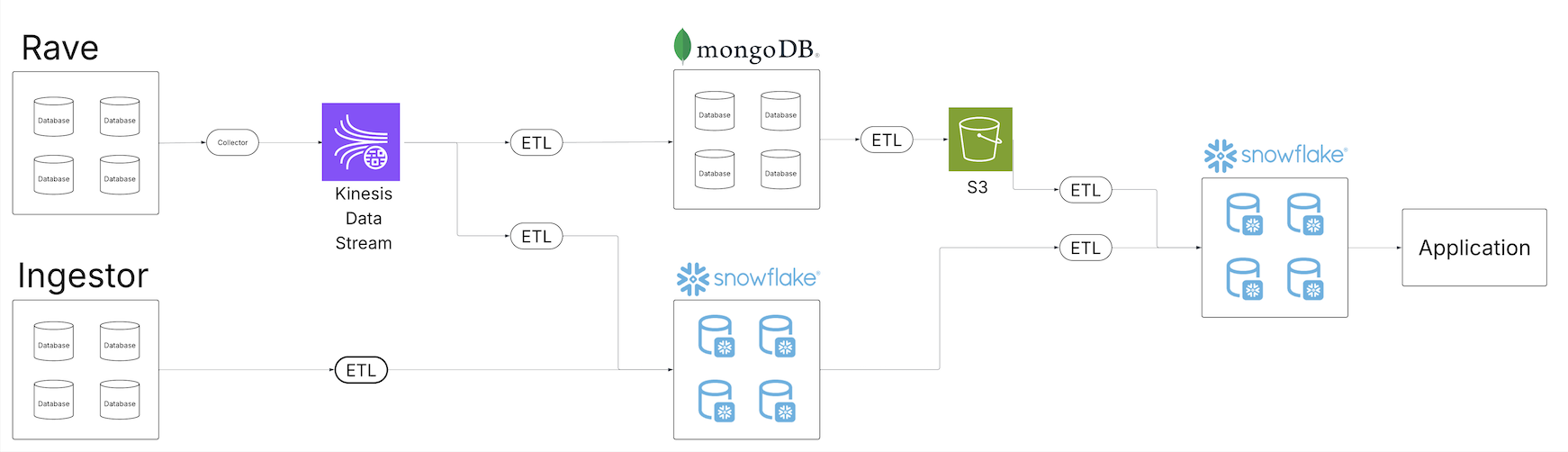
As the Medidata clinical data repository expanded, the team recognized the shortcomings of the legacy data solution to provide quality data products to their customers across their growing portfolio of data offerings. Several data tenants began to erode. The following diagram shows Medidata’s legacy extract, transform, and load (ETL) architecture.
Built upon a series of scheduled batch jobs, the legacy system proved ill-equipped to provide a unified view of the data across the entire ecosystem. Batch jobs ran at different intervals, often requiring a sufficient degree of scheduling buffer to make sure upstream jobs completed within the expected window. As the data volume expanded, the jobs and their schedules continued to inflate, introducing a latency window between ingestion and processing for dependent consumers. Different consumers operating from various underlying data services further magnified the problem as pipelines had to be continuously built across a variety of data delivery stacks.
The expanding portfolio of pipelines began to overwhelm existing maintenance operations. With more operations, the opportunity for failure expanded and recovery efforts further complicated. Existing observability systems were inundated with operational data, and identifying the root cause of data quality issues became a multi-day endeavor. Increases in the data volume required scaling considerations across the entire data estate.
Additionally, the proliferation of data pipelines and copies of the data in different technologies and storage systems necessitated expanding access controls with enhanced security features to make sure only the correct users had access to the subset of data to which they were permitted. Making sure access control changes were correctly propagated across all systems added a further layer of complexity to consumers and producers.
Solution overview
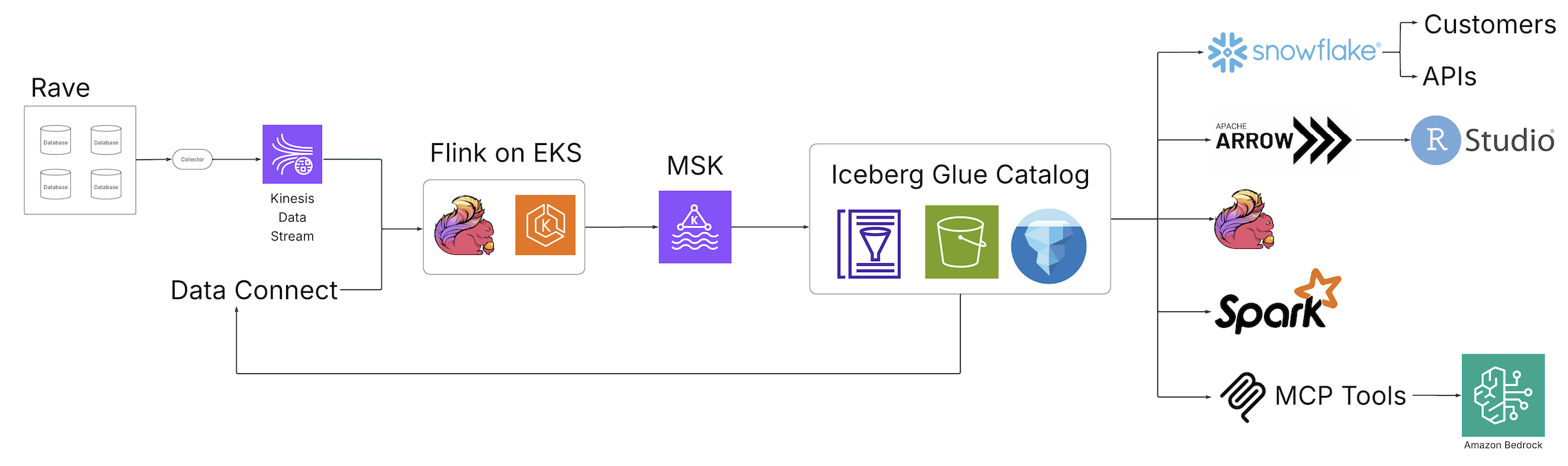
With the advent of Clinical Data Studio (Medidata’s unified data management and analytics solution for clinical trials) and Data Connect (Medidata’s data solution for acquiring, transforming, and exchanging electronic health record (EHR) data across healthcare organizations), Medidata introduced a new world of data discovery, analysis, and integration to the life sciences industry powered by open source technologies and hosted on AWS. The following diagram illustrates the solution architecture.
Fragmented batch ETL jobs were replaced by real-time Apache Flink streaming pipelines, an open source, distributed engine for stateful processing, and powered by Amazon Elastic Kubernetes Service (Amazon EKS), a fully managed Kubernetes service. The Flink jobs write to Apache Kafka running in Amazon Managed Apache Kafka (Amazon MSK), a streaming data service that manages Kafka infrastructure and operations, before landing in Iceberg tables backed by the AWS Glue Data Catalog, a centralized metadata repository for data assets. From this collection of Iceberg tables, a central, single source of data is now accessible from a variety of consumers without additional downstream processing, alleviating the need for custom pipelines to satisfy the requirements of downstream consumers. Through these fundamental architectural changes, the team at Medidata solved the issues presented by the legacy solution.
Data availability and consistency
With the introduction of the Flink jobs and Iceberg tables, the team was able to deliver a consistent view of their data across the Medidata data experience. Pipeline latency was reduced from days to minutes, helping Medidata customers realize a 99% performance gain from the data ingestion to the data analytics layers. Due to Iceberg’s interoperability, Medidata users saw the same view of the data regardless of where they viewed that data, minimizing the need for consumer-driven custom pipelines because Iceberg could plug into existing consumers.
Maintenance and durability
Iceberg’s interoperability provided a single copy of the data to satisfy their use cases, so the Medidata team could focus its observation and maintenance efforts on a five-times smaller subset of operations than previously required. Observability was enhanced by tapping into the various metadata components and metrics exposed by Iceberg and the Data Catalog. Quality management transformed from cross-system traces and queries to a single analysis of unified pipelines, with an added benefit of point in time data queries thanks to the Iceberg snapshot feature. Data volume increases are handled with out-of-box scaling supported by the entire infrastructure stack and AWS Glue Iceberg optimization features that include compaction, snapshot retention, and orphan file deletion, which provide a set-and-forget experience for solving a number of common Iceberg frustrations, such as the small file problem, orphan file retention, and query performance.
Security
With Iceberg at the center of its solution architecture, the Medidata team no longer had to spend the time building custom access control layers with enhanced security features at each data integration point. Iceberg on AWS centralizes the authorization layer using familiar systems such as AWS Identity and Access Management (IAM), providing a single and durable control for data access. The data also stays entirely within the Medidata virtual private cloud (VPC), further reducing the opportunity for unintended disclosures.
Conclusion
In this post, we demonstrated how legacy universe of consumer-driven custom ETL pipelines can be replaced with a scalable, high-performant streaming lakehouses. By putting Iceberg on AWS at the center of data operations, you can have a single source of data for your consumers.
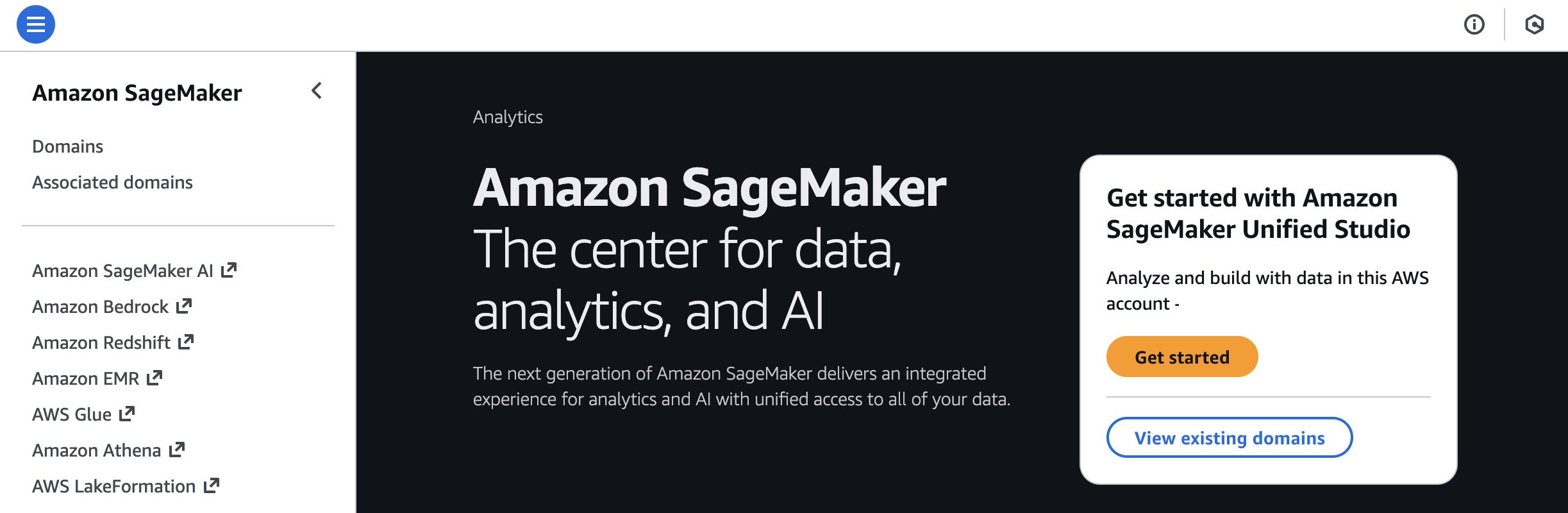
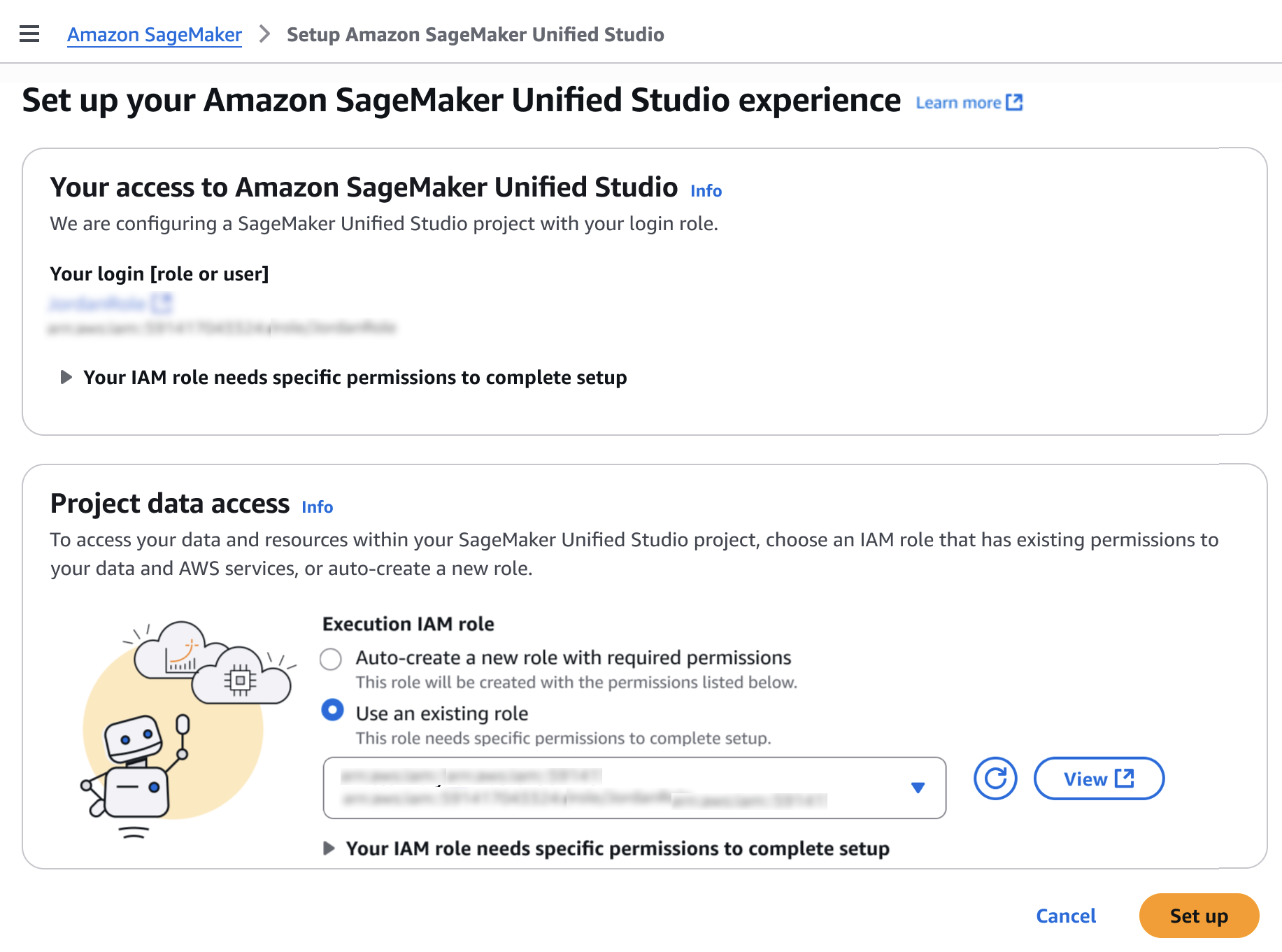
Today we’re announcing a faster way to get started with your existing AWS datasets in Amazon SageMaker Unified Studio. You can now start working with any data you have access to in a new serverless notebook with a built-in AI agent, using your existing AWS Identity and Access Management (IAM) roles and permissions.
Notebooks with a built-in AI agent – You can use a new serverless notebook with a built-in AI agent, which supports SQL, Python, Spark, or natural language and gives data engineers, analysts, and data scientists one place to develop and run both SQL queries and code.
Choose Set up. It takes a few minutes to complete your environment. After this role is granted access, you’ll be taken to the SageMaker Unified Studio landing page where you will see the datasets that you have access to in AWS Glue Data Catalog as well as a variety of analytics and AI tools to work with.
This environment automatically creates the following serverless compute: Amazon Athena Spark, Amazon Athena SQL, AWS Glue Spark, and Amazon Managed Workflows for Apache Airflow (MWAA) serverless. This means you completely skip provisioning and can start working immediately with just-in-time compute resources, and it automatically scales back down when you finish, helping to save on costs.
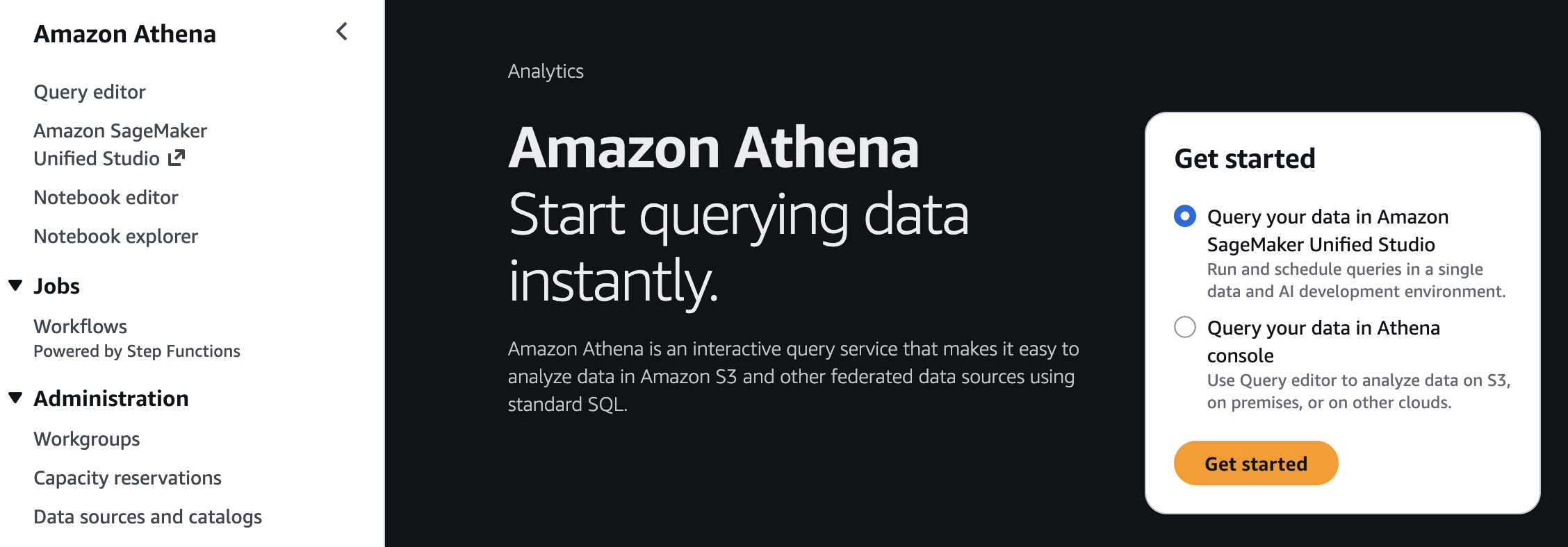
You can also get started working on specific tables in Amazon Athena, Amazon Redshift, and Amazon S3 Tables. For example, you can select Query your data in Amazon SageMaker Unified Studio and then choose Get started in Amazon Athena console.
If you start from these consoles, you’ll connect directly to the Query Editor with the data that you were looking at already accessible, and your previous query context preserved. By using this context-aware routing, you can run queries immediately once inside the SageMaker Unified Studio without unnecessary navigation.
Getting started with notebooks with a built-in AI agent Amazon SageMaker is introducing a new notebook experience that provides data and AI teams with a high-performance, serverless programming environment for analytics and ML jobs. The new notebook experience includes Amazon SageMaker Data Agent, a built-in AI agent that accelerates development by generating code and SQL statements from natural language prompts while guiding users through their tasks.
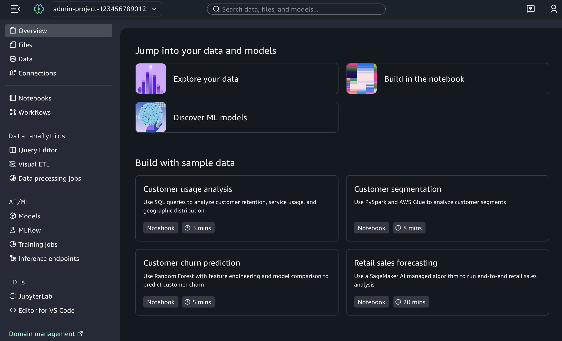
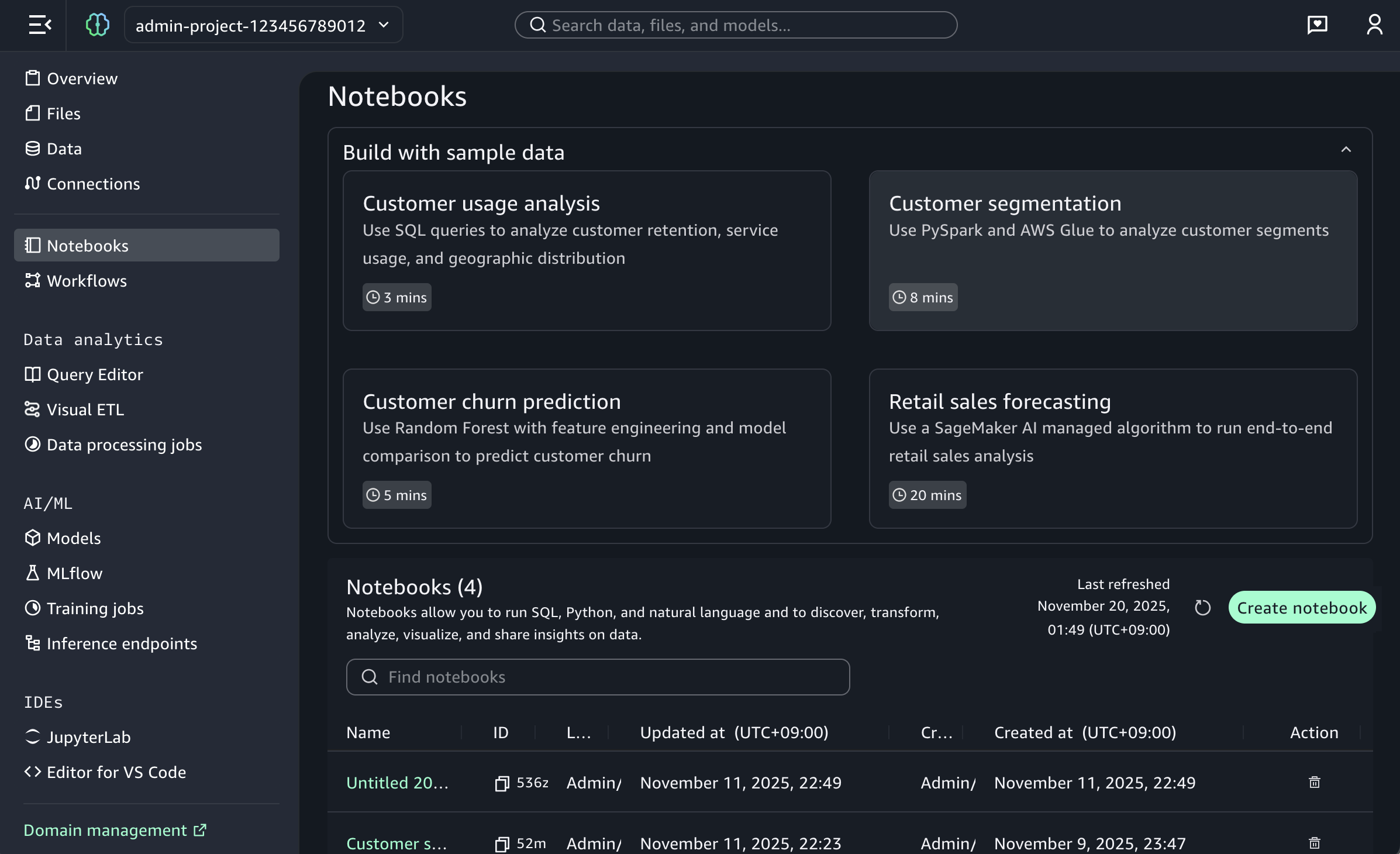
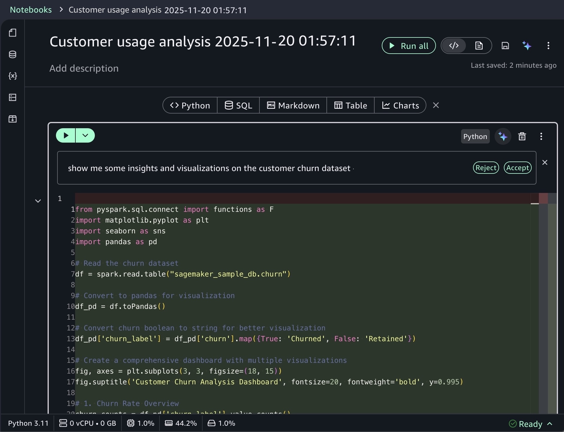
To start a new notebook, choose the Notebooks menu in the left navigation pane to run SQL queries, Python code, and natural language, and to discover, transform, analyze, visualize, and share insights on data. You can get started with sample data such as customer analytics and retail sales forecasting.
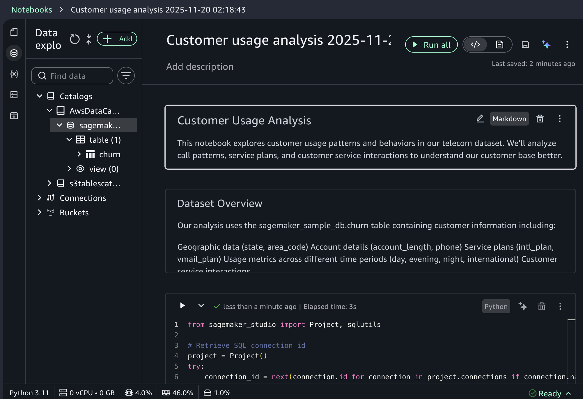
When you choose a sample project for customer usage analysis, you can open sample notebook to explore customer usage patterns and behaviors in a telecom dataset.
As I noted, the notebook includes a built-in AI agent that helps you interact with your data through natural language prompts. For example, you can start with data discovery using prompts like:
Show me some insights and visualizations on the customer churn dataset.
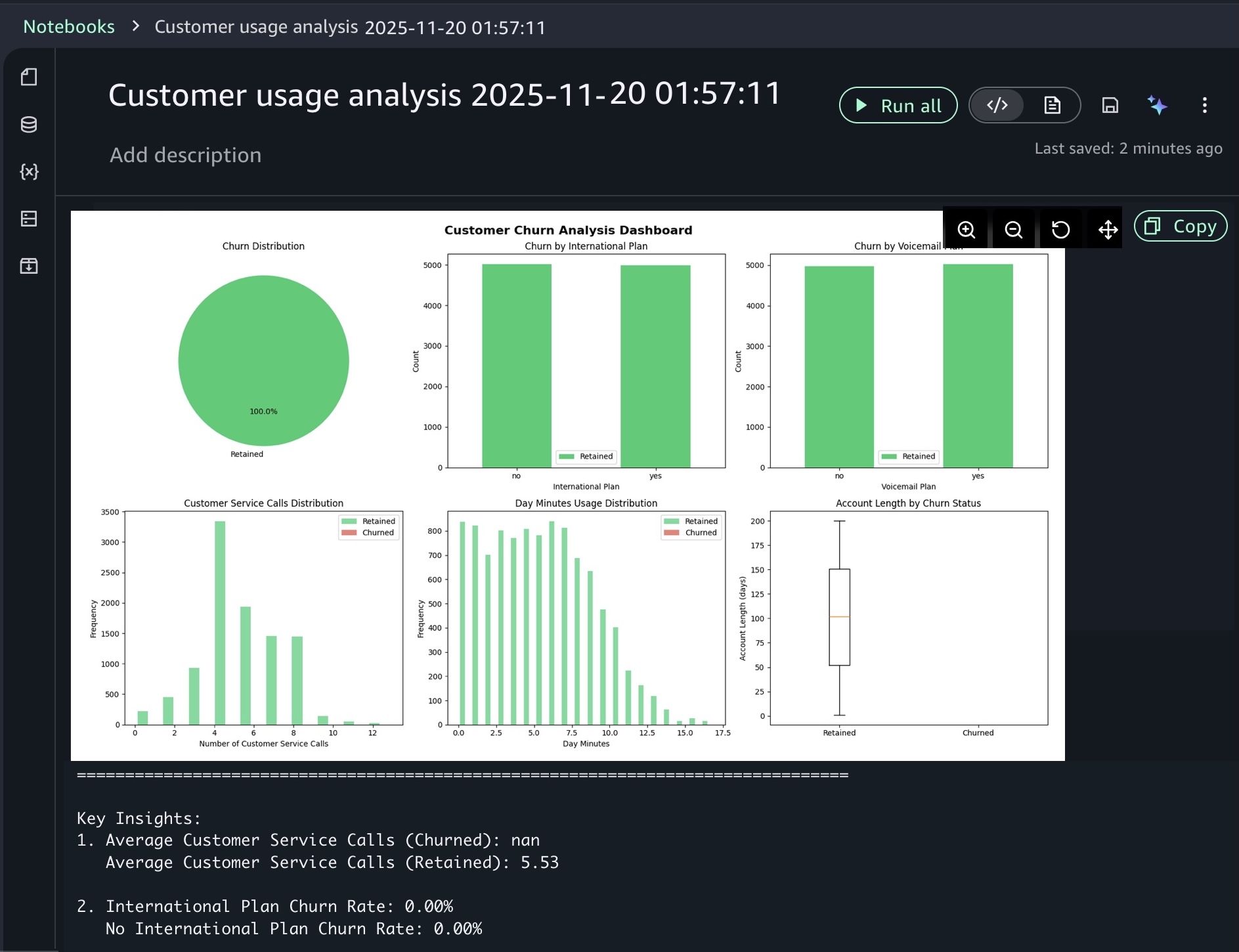
After you identify relevant tables, you can request specific analysis to generate Spark SQL. The AI agent creates step-by-step plans with initial code for data transformations and Python code for visualizations. If you see an error message while running the generated code, choose Fix with AI to get help resolving it. Here is a sample result:
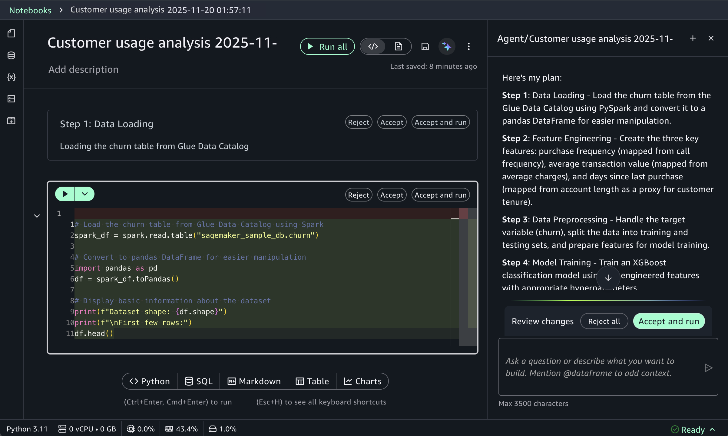
For ML workflows, use specific prompts like:
Build an XGBoost classification model for churn prediction using the churn table, with purchase frequency, average transaction value, and days since last purchase as features.
This prompt receives structured responses including a step-by-step plan, data loading, feature engineering, and model training code using the SageMaker AI capabilities, and evaluation metrics. SageMaker Data Agent works best with specific prompts and is optimized for AWS data processing services including Athena for Apache Spark and SageMaker AI.
Now available One-click onboarding and the new notebook experience in Amazon SageMaker Unified Studio are now available in US East (Ohio), US East (N. Virginia), US West (Oregon), Asia Pacific (Mumbai), Asia Pacific (Singapore), and Asia Pacific (Sydney), Asia Pacific (Tokyo), Europe (Frankfurt), Europe (Ireland) Regions. To learn more, visit the SageMaker Unified Studio product page.
With only a few clicks, you can curate data inventory assets with the required business metadata by adding or updating business names (asset and schema), descriptions (asset and schema), read me, glossary terms (asset and schema), and metadata forms. You can also create AI-generated suggestions, review and refine descriptions, and publish enriched asset metadata directly to the catalog. This helps reduce manual documentation effort, improves metadata consistency, and accelerates asset discoverability across organizations.
Starting today, you can use new capabilities in Amazon SageMaker Catalog metadata to improve business metadata and search:
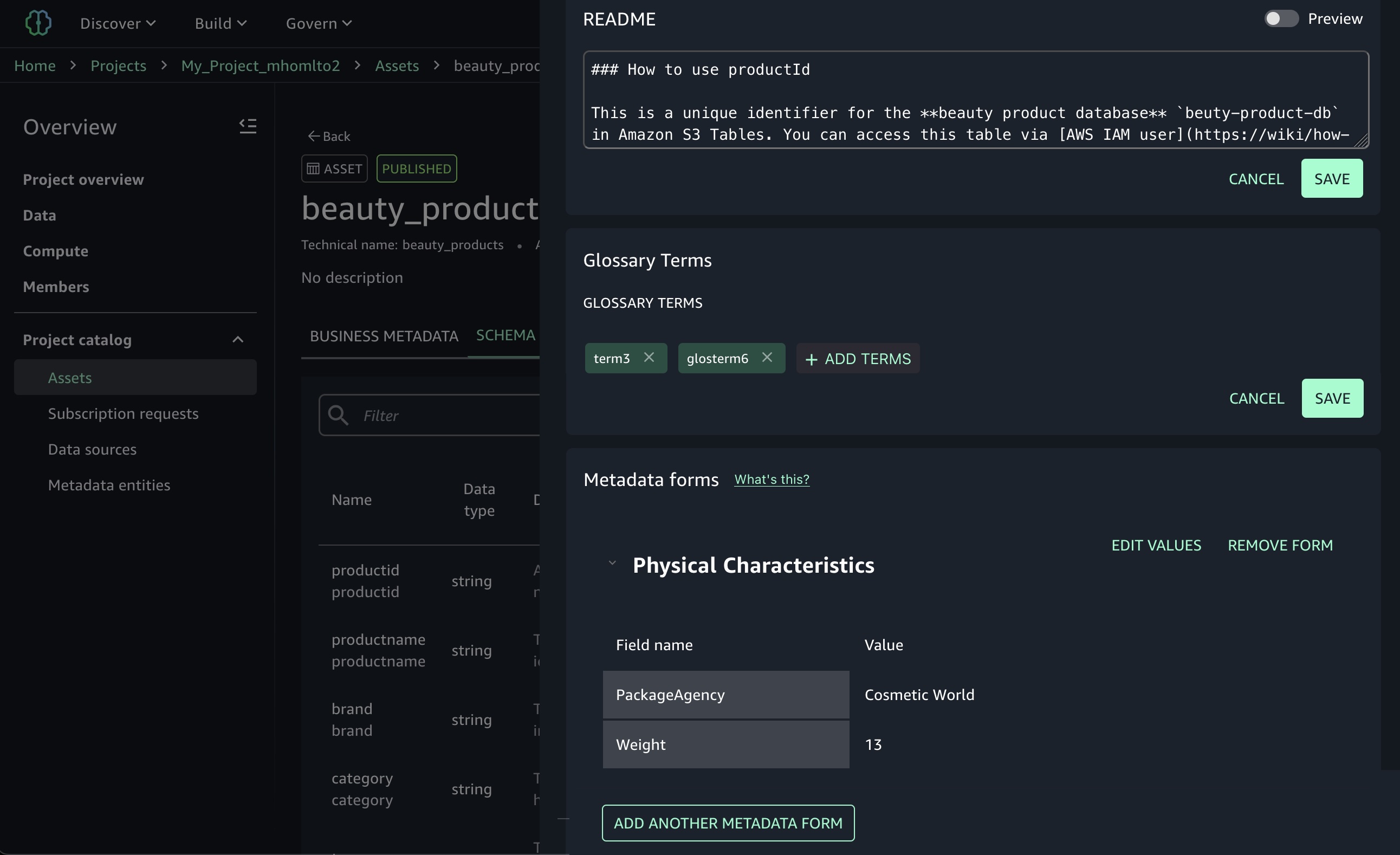
Column-level metadata forms and rich descriptions – You can create custom metadata forms to capture business-specific information directly in individual columns. Columns also support markdown-enabled rich text descriptions for comprehensive data documentation and business context.
Enforce metadata rules for glossary terms for asset publishing – You can use metadata enforcement rules for glossary terms, meaning data producers must use approved business vocabulary when publishing assets. By standardizing metadata practices, your organization can improve compliance, enhance audit readiness, and streamline access workflows for greater efficiency and control.
These new SageMaker Catalog metadata capabilities help address consistent data classification and improve discoverability across your organizational catalogs. Let’s take a closer look at each capability.
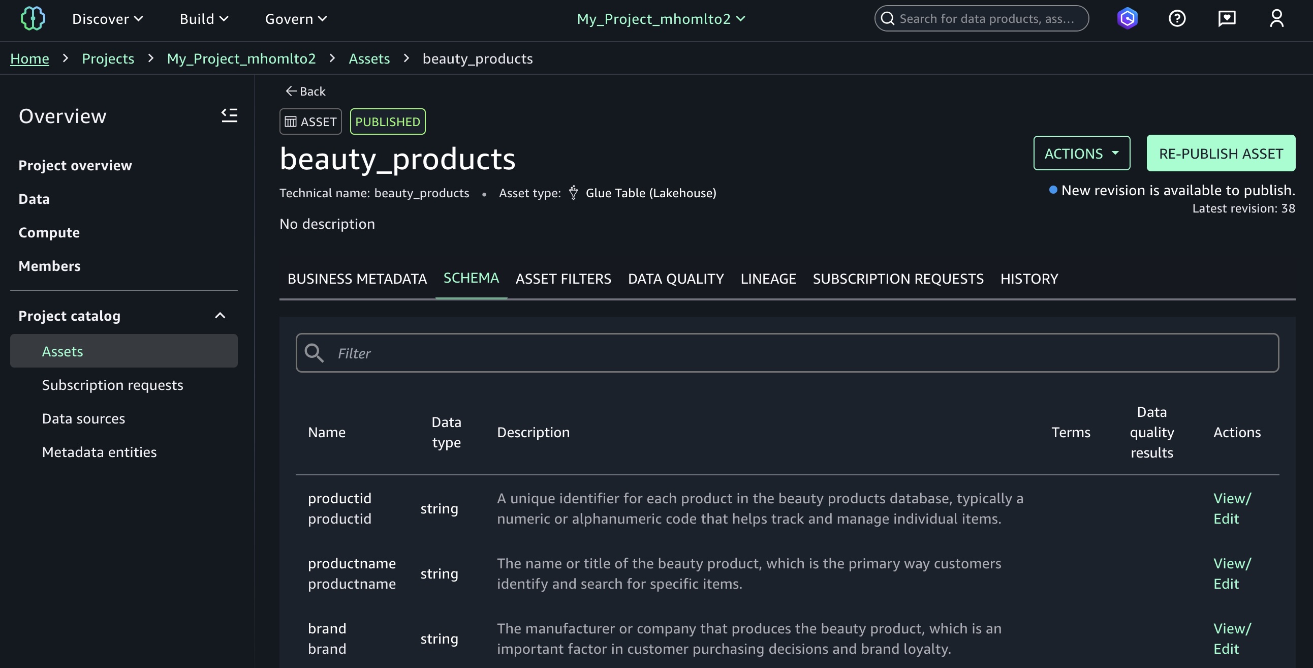
Column-level metadata forms and rich descriptions You can now use custom metadata forms and rich text descriptions at the column level, extending existing curation capabilities for business names, descriptions, and glossary term classifications. Custom metadata form field values and rich text content are indexed in real time and become immediately discoverable through search.
To edit column-level metadata, select the schema of your catalog asset used in your project and choose the View/Edit action for each column.
When you choose one of the columns as an asset owner, you can define custom key-value metadata forms and markdown descriptions to provide detailed column documentation.
Now data analysts in your organization can search using custom form field values and rich text content, alongside existing column names, descriptions, and glossary terms.
Enforce metadata rules for glossary terms for asset publishing You can define mandatory glossary term requirements for data assets during the publishing workflow. Your data producers must now classify their assets with approved business terms from organizational glossaries before publication, promoting consistent metadata standards and improving data discoverability. The enforcement rules validate that required glossary terms are applied, preventing assets from being published without proper business context.
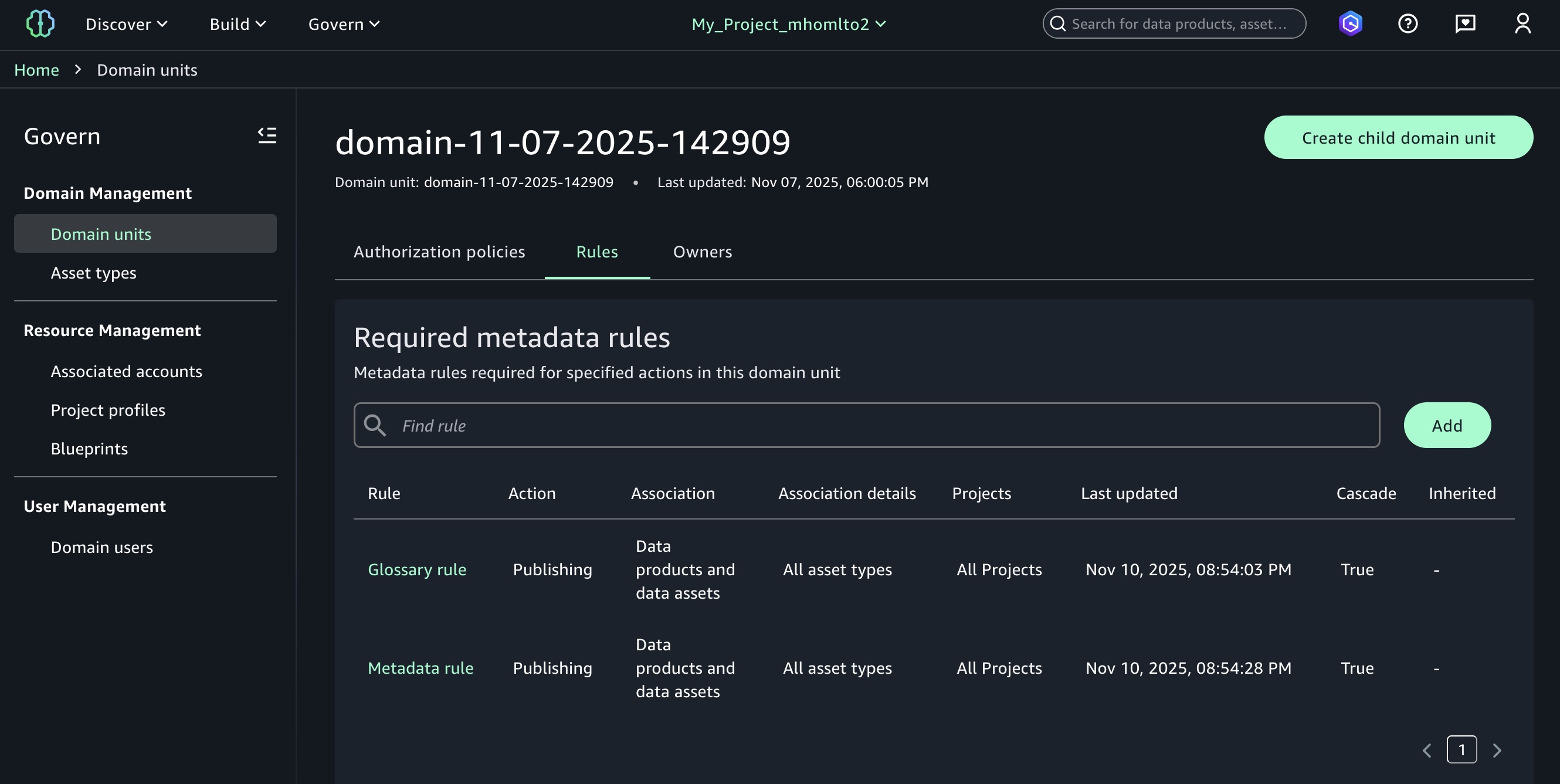
To enable a new metadata rule for glossary terms, choose Add in your domain units under the Domain Management section in the Govern menu.
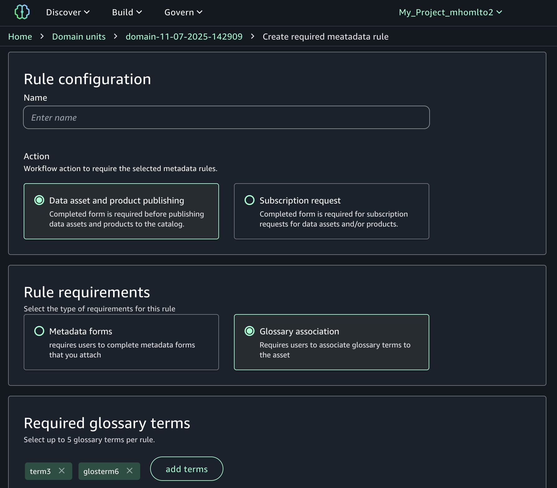
Now you can select either Metadata forms or Glossary association as a type of requirement for the rule. When you select Glossary association, you can choose up to 5 required glossary terms per rule.
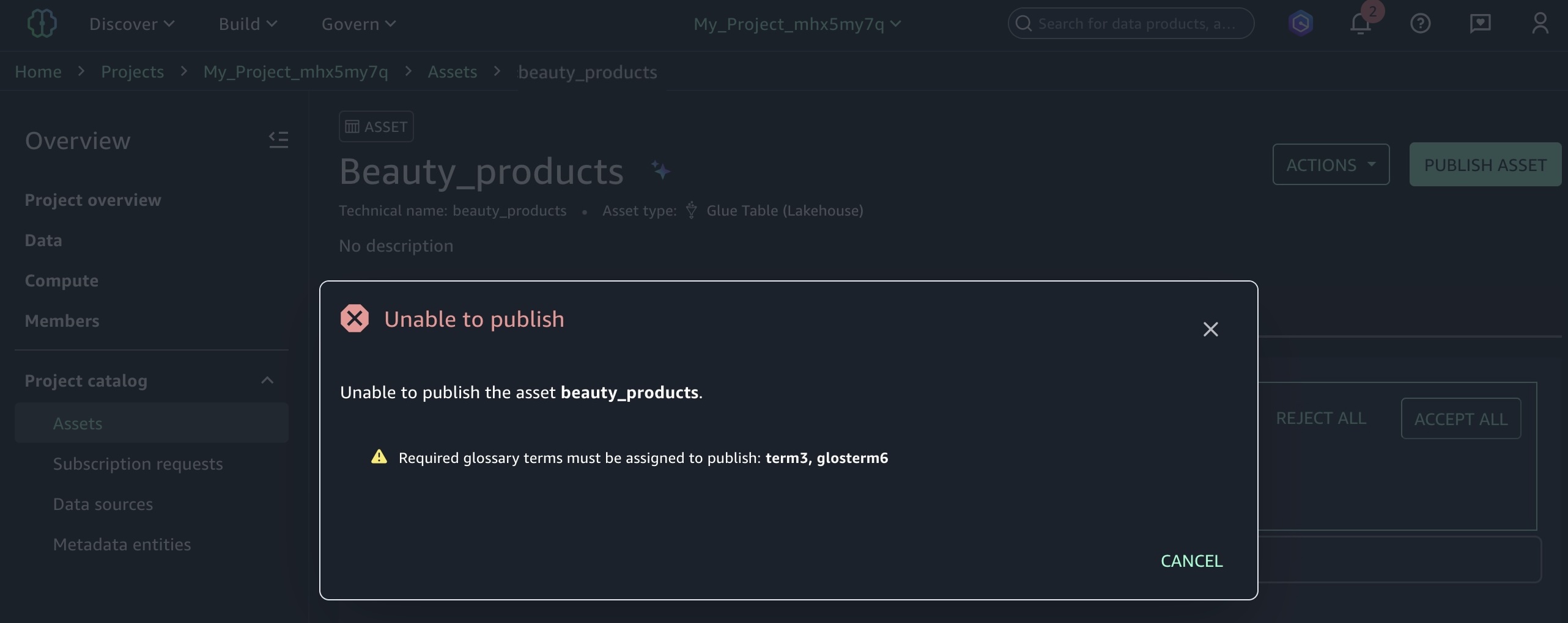
If you attempt to publish assets without adding the required glossary terms, the error message prompting you to enforce the glossary rule appears.
Standardizing metadata and aligning data schemas with business language enhances data governance and improves search relevance, helping your organization better understand and trust published data.
It’s that time of year again — AWS re:Invent is here! At re:Invent, bold ideas come to life. Get a front-row seat to hear inspiring stories from AWS experts, customers, and leaders as they explore today’s most impactful topics, from data analytics to AI.
For all the data enthusiasts and professionals, we’ve curated a comprehensive guide to every analytics session to help you plan your perfect agenda. Make sure to secure your seat early for must-attend sessions via the attendee portal.
Pro tip: Even if a session shows as fully reserved, we encourage you to join the walk-up line at the session location. Based on previous years’ experiences, additional seats often become available due to no-shows or last-minute schedule changes. The walk-up line operates on a first-come, first-served basis, and many attendees have successfully accessed their desired sessions this way. Just be sure to arrive at least 15 minutes before the session starts for the best chance of getting a seat.
Can’t make it in person? No problem — grab a free virtual pass to stream live sessions from anywhere.
And don’t forget to stop by the AWS Kiosk in the AWS Village Expo for AWS Analytics, Amazon SageMaker, Amazon OpenSearch Service and AWS Messaging and Streaming services! See live demos of analytics services, meet AWS experts, get your toughest data questions answered, explore the latest launches, join our data trivia, and even win exclusive AWS-authored books and many more swags.
Emerging trends, ranging from Open Table Formats (OTF) to agentic infrastructure, are rapidly changing how humans and applications interact with analytics to drive mission-critical business decisions. Join Mai-Lan Tomsen Bukovec, VP of AWS Technology, to explore emerging trends, the evolution of analytics engines and applications, and how to future-proof your data foundation for the rapidly changing landscape of analytics at scale. Learn how AWS is transforming data and analytics services to lead in optimized data storage, querying, streaming, processing, and governance – for both human users and agentic infrastructure.
Breakouts
Dive into cutting-edge topics with re:Invent breakout sessions. These immersive, hour-long lectures are led by AWS experts, customers, offering you unparalleled insights and knowledge in a concise format. Whether you’re exploring the latest in cloud technology, AWS Analytics advancements, or industry-specific solutions, these sessions are designed to expand your horizon and inspire your next big idea.
Monday, Dec 1
Tuesday, Dec 2
Wednesday, Dec 3
Thursday, Dec 4
8:30 AM – 9:30 AM PST | Venetian | Level 3 | Lido 3106
ANT203 | Enabling AI innovation with Amazon SageMaker Unified Studio
11:30 AM – 12:30 PM PST | Mandalay Bay | Level 2 South | Oceanside C | Content Hub | Turquoise Theater
BIZ207 | Democratize access to insights with Amazon Quick Suite
8:30 AM – 9:30 AM PST | MGM | Level 1 | Grand 123
ANT204 | Architecting the future: Amazon SageMaker as a data and AI platform
11:00 AM – 12:00 PM PST | Mandalay Bay | Level 2 South | Oceanside C | Content Hub | Pink Theater
ANT317 | Modernize your data warehouse by moving to Amazon Redshift
8:30 AM – 9:30 AM PST | MGM | Level 3 | Chairman’s 366
ANT318 | Scaling Amazon Redshift with a multi-warehouse architecture
11:30 AM – 12:30 PM PST | Mandalay Bay | Level 2 South | Oceanside C | Content Hub | Pink Theater
ANT216 | What’s new with Amazon SageMaker in the era of unified data and AI
10:00 AM – 11:00 AM PST | Mandalay Bay | Level 2 South | Oceanside C | Content Hub | Turquoise Theater
ANT335 | Agentic data engineering with AWS Analytics MCP Servers
BIZ228 | Reimagine business intelligence with Amazon Quick Sight
.
.
.
1:30 PM – 2:30 PM PST | Mandalay Bay | Level 3 South | South Seas E
OPN413 | Transforming Apache Kafka into a Scalable Message Queue
.
.
.
5:30 PM – 6:30 PM PST | Mandalay Bay | Level 3 South | South Seas F
ANT423 | Amazon Kinesis Data Streams under the hood
.
.
.
Chalk talks
These hour-long, highly engaging sessions offer a unique blend of expert insight and collaborative learning. An AWS specialist kicks off with a concise, informative lecture, setting the stage for an in-depth, interactive Q&A. With a limited audience size, you’ll have the opportunity to dive deep into topics, ask pressing questions, and engage in meaningful discussions with both the presenter and fellow attendees.
Monday, Dec 1
Tuesday, Dec 2
Wednesday, Dec 3
Thursday, Dec 4
Friday, Dec 5
8:30 AM – 9:30 AM PST | MGM | Level 1 | Boulevard 167
ANT301-R1 | Accelerating the shift from batch to real-time streaming
11:30 AM – 12:30 PM PST | Caesars Forum | Level 1 | Academy 411
ANT302-R1 | Accelerate GenAI-powered data discovery and sharing with SageMaker Catalog
9:00 AM – 10:00 AM PST | MGM | Level 3 | Room 353
ANT301-R | Accelerating the shift from batch to real-time streaming
ANT316 | Orchestrating with Apache Airflow, MWAA, and SageMaker Unified Studio
Builders’ sessions
Immerse yourself in our builders’ sessions – a hands-on learning experience designed to elevate your AWS skills. These focused, hour-long workshops bring together a small group of up to ten attendees with a dedicated AWS expert at each table.
Monday, Dec 1
Tuesday, Dec 2
Wednesday, Dec 3
Thursday, Dec 4
8:30 AM – 9:30 AM PST | Wynn | Convention Promenade | Latour 7
ANT407-R1 | Building event-driven applications with AWS Streaming and Messaging
OPN407-R | Performance tuning for streaming Ingestion into Apache Iceberg
.
.
.
4:00 PM – 5:00 PM PST | Mandalay Bay | Lower Level North | Islander H
ANT405-R | Build high performance Apache Iceberg data lakes with Amazon S3 Tables
.
.
.
Workshops
Roll your sleeves in our dynamic 2-hour workshops, where you’ll tackle real-world challenges using AWS services. These interactive sessions kick off with a brief, informative lecture to set the stage, then quickly transition into hands-on problem-solving. Bring your laptop and prepare to build alongside AWS experts, who will guide you through practical applications of cloud computing concepts. Whether you’re new to AWS or looking to sharpen your skills, these workshops offer a unique opportunity to learn by doing, enabling you to leave with confidence and applicable knowledge in AWS technologies.
Monday, Dec 1
Tuesday, Dec 2
Wednesday, Dec 3
Thursday, Dec 4
8:00 AM – 10:00 AM PST | Mandalay Bay | Lower Level North | Islander C
ANT402-R1 | Build a fraud detection system with Amazon SageMaker Unified Studio
BIZ204-R | Experience AI-powered BI with Amazon Quick Suite
3:30 PM – 5:30 PM PST | Mandalay Bay | Lower Level North | Islander C
ANT401 | Build an AI-powered enterprise search with Amazon OpenSearch service
.
3:00 PM – 5:00 PM PST | Mandalay Bay | Level 2 South | Mandalay Bay Ballroom K
ANT414 | Scale intelligent analytics with Amazon Redshift multi-cluster architectures
.
.
.
Lightning Talks
Located in the Expo Hall, each of these 20-minute theater presentations are dedicated to a specific customer story, service demo, or AWS Partner offering.
Monday, Dec 1
Tuesday, Dec 2
Wednesday, Dec 3
Thursday, Dec 4
5:00 PM – 5:20 PM PST | Venetian | Level 2 | Hall B | Expo | Theater 4
ANT334 | High-performance NLP & geospatial analysis with Redshift
.
3:00 PM – 3:20 PM PST | Mandalay Bay | Level 2 South | Oceanside C | Content Hub | Lightning Theater
ANT333 | Fast-track to insights: AWS-SAP data strategy
12:30 PM – 12:50 PM PST | Venetian | Level 2 | Hall B | Expo | Theater 3
ANT342 | ITTI’s Cross-Company Data Mesh Blueprint with Amazon SageMaker
6:00 PM – 6:20 PM PST | Venetian | Level 2 | Hall B | Expo | Theater 3
We hope this post acts as your go-to resource for navigating the AWS analytics track at re:Invent 2025. For staying in the know about the most recent trends and advancements in AWS Analytics, follow our LinkedIn page.
Covestro Deutschland AG, headquartered in Leverkusen, Germany, is a global leader in high-performance polymer materials and components. Since its spin-off from Bayer AG in 2015, Covestro has established itself as a key player in the chemical industry, with 48 production sites worldwide, €14.4 billion 2023 revenue, and 17,500 employees. Covestro’s core business focuses on developing innovative, sustainable solutions for products used in various aspects of daily life. The company offers materials for mobility, building and living, electrical and electronics sectors, in addition to sports and leisure, cosmetics, health, and the chemical industry. The company’s products, such as polycarbonates, polyurethanes, coatings, adhesives, and specialty elastomers, are important components in automotive, construction, electronics, and medical device industries.
To support this global operation and diverse product portfolio, Covestro adopted a robust data management solution. In this post, we show you how Covestro transformed its data architecture by implementing Amazon DataZone and AWS Serverless Data Lake Framework (SDLF), transitioning from a centralized data lake to a data mesh architecture. Through this strategic shift, teams can share and consume data while maintaining high quality standards through a consolidated data marketplace and business metadata glossary. The result: streamlined data access, better data quality, and stronger governance at scale that various producer and consumer teams can use to run data and analytics workloads at scale, enabling over 1,000 data pipelines and achieving a 70% reduction in time-to-market.
Business and data challenges
Prior to their transformation, Covestro operated with a centralized data lake managed by a single data platform team that handled the data engineering tasks. This centralized approach created several challenges: bottlenecks in project delivery because of limited engineering resources, complicated prioritization of use cases, and inefficient data sharing processes. The setup often resulted in unnecessary data duplication, which in turn slowed down time-to-market for new analytics initiatives, increased costs, and limited the ability of business units to act quickly on insights.The lack of visibility into data assets created significant operational challenges:
Teams could not find existing datasets, often recreating data already stored elsewhere
No clear understanding of data lineage or quality metrics
Difficulty in determining who owned specific data assets or who to contact for access
Absence of metadata and documentation about available datasets
Departments shared little knowledge about how they were using data
These visibility issues, combined with the lack of unified access controls, led to:
Siloed data initiatives across departments
Reduced trust in data quality
Inefficient use of resources
Delayed project timelines
Missed opportunities for cross-functional collaboration and insights
A strategic solution: Why Amazon DataZone and SDLF?
The challenges Covestro faced reflect deeper structural limitations of centralized data architectures. As Covestro scaled, central data teams often became bottlenecks, and lack of domain context led to fragmented quality, inconsistent standards, and poor collaboration. Instead of centralizing control, a data mesh gives ownership to the teams who generate and understand the data, while keeping the governance and interoperability consistent across the organization. This makes it well-suited for Covestro’s environment, which requires agility, scalability, and cross-team collaboration.
AWS Serverless Data Lake Framework (SDLF) is a solution to these challenges, providing a robust foundation for data mesh architectures. Traditional data lake implementations often centralize data ownership and governance, but with the flexible design of SDLF, organizations can build decentralized data domains that align with modern data mesh principles. The framework provides domain-oriented teams with the infrastructure, security controls, and operational patterns needed to own and manage their data products independently, while maintaining consistent governance across the organization. Through its modular architecture and infrastructure as code templates, SDLF accelerates the creation of domain-specific data products, so that Covestro’s teams can deploy standardized yet customizable data pipelines. This approach supports the key pillars of data mesh: domain-oriented decentralization, data as a product, self-serve infrastructure, and federated governance, providing Covestro with a practical path to overcome the limitations of traditional centralized architectures.
Amazon DataZone enhances the data mesh implementation through a unified experience for discovering and accessing data across decentralized domains. As a data management service, Amazon DataZone helps organizations catalog, discover, share, and govern data across organizational boundaries. It provides a central governance layer where organizations can establish data sharing agreements, manage access controls, and enable self-service data access while supporting security and compliance. While teams can use the SDLF framework to build and operate domain-specific data products, Amazon DataZone complements it with a searchable catalog enriched with metadata, business context, and usage policies, making data products easier to find, trust, and reuse.
Through the sharing capabilities of Amazon DataZone, domain teams can share their data products with other domains while maintaining granular access controls and governance policies, enabling cross-domain collaboration and data reuse. This integration means that domain teams can publish their SDLF-managed datasets to an Amazon DataZone catalog, so authorized consumers across the organization can discover and access them. Through the built-in governance capabilities built into Amazon DataZone, organizations can implement standardized data sharing workflows, check data quality, and enforce consistent access controls across their distributed data system, strengthening their data mesh architecture with robust data governance and democratization capabilities.Together, SDLF and Amazon DataZone provide Covestro with a comprehensive solution for implementing a modern data mesh architecture, enabling autonomous data domains to operate with consistent governance, seamless data sharing, and enterprise-wide data discovery.
Solution architecture and implementation
The following architecture illustrates the high-level design of the data mesh solution. The implementation used a comprehensive AWS solution built on AWS services to create a robust, scalable, and governed data mesh that serves multiple business domains across the Covestro organization.
Data domain foundation: Serverless Data Lake Framework
A key pillar of the implementation is the Serverless Data Lake Framework (SDLF), which provides the foundational infrastructure and security needed to support data mesh strategies. SDLF delivers the core building blocks for data domains such as Amazon S3 storage layers, built-in encryption with AWS KMS, IAM-based access control, and infrastructure as code (IaC) automation. By using these components, Covestro can deploy decentralized, domain-owned data products rapidly while maintaining consistent governance across the enterprise.
The framework uses Amazon Simple Storage Service (Amazon S3) as the primary data storage layer, delivering virtually unlimited scalability and eleven nines of durability for diverse data assets. The proposed S3 bucket architecture follows AWS Well-Architected principles, implementing a multi-tiered structure with distinct raw, staging, and analytics data zones. This layered approach helps different business domains to maintain data sovereignty (each domain owns and controls its data, while keeping accessibility patterns organization-wide).
Security is a fundamental aspect in Covestro’s data mesh implementation. SDLF automatically implements encryption at rest and in transit across data storage and processing components. AWS Key Management Service (AWS KMS) provides centralized key management, while carefully crafted AWS Identity and Access Management (IAM) roles enable resource isolation.
Data processing with AWS Glue
AWS Glue serves as the cornerstone of the data processing and transformation capabilities, offering serverless extract, transform, and load ETL services that automatically scale based on workload demands.
Covestro’s pre-existent centralized data lake was fed by more than 1,000 ingestion data pipelines interacting with a variety of source systems. To support the migration of existing ingestion and processing pipelines, Covestro developed reusable blueprints that included the development and security standards defined for the data mesh.Covestro released standardized patterns that teams can deploy across multiple domains while providing the flexibility needed for domain-specific requirements. These blueprints support diverse source systems, from traditional databases like Oracle, SQL Server, and MySQL to modern software as a service (SaaS) applications such as SAP C4C.
They also developed specialized blueprints for processing, standardizing, and cleaning ingested raw data. These blueprints store processed data in Apache Iceberg format, automatically saving metadata in the AWS Glue Data Catalog and providing built-in capabilities to handle schema evolution seamlessly.
Covestro relies on SDLF to quickly configure and deploy the blueprints as AWS Glue jobs inside the domain. With SDLF, teams deploy a data pipeline through a YAML configuration file, and the orchestration and management mechanisms of SDLF handle the rest. The solution includes comprehensive monitoring capabilities built on Amazon DynamoDB, providing real-time visibility into data pipeline health and performance metrics (when teams deploy a pipeline through SDLF, the system automatically integrates it with the monitoring setup).
Data quality with AWS Glue Data Quality
To achieve data reliability across domains, Covestro extended the capabilities of SDLF to incorporate AWS Glue Data Quality into data processing pipelines. This integration enables automated data quality checks as part of the standard data processing workflow. Thanks to the configuration-driven design of SDLF, data producers can implement quality controls either using recommended rules, which are automatically generated through data profiling, or applying their own domain-specific rules.
The integration provides data teams with the flexibility to define quality expectations while maintaining consistency in how quality checks are implemented at the pipeline level. The solution logs quality evaluation results, providing visibility into the data quality metrics for each data product. These elements are illustrated in the following figure.
Enterprise-ready access control with AWS Lake Formation
AWS Lake Formation integration with the Data Catalog supports the security and access control layer that makes the data mesh implementation enterprise-ready. Through Lake Formation, Covestro implemented fine-grained access controls that respect domain boundaries while enabling controlled cross-domain data sharing.
The service’s integration with IAM means that Covestro can implement role-based access patterns that align with their organizational structure, so users can access the data they need while keeping appropriate security boundaries.
Data democratization with Amazon DataZone
Amazon DataZone functions as the heart of the data mesh implementation. Deployed in a dedicated AWS account, it provides the data governance, discovery, and sharing capabilities that were missing in the previous centralized approach. DataZone offers a unified, searchable catalog enriched with business context, automated access controls, and standardized sharing workflows that enable true data democratization across the organization.
Through Amazon DataZone, Covestro established a comprehensive data catalog that helps business users across different domains to discover, understand, and request access to data assets without requiring deep technical expertise. The business glossary functionality supports consistent data definitions across domains, eliminating the confusion that often arises when different teams use different terminology for the same concepts.
Data product owners can use the integration of Amazon DataZone integration with AWS Lake Formation to grant or revoke cross-domain access to data, streamlining the data sharing process while supporting security and compliance requirements.
Managing cross-domain data pipeline dependencies
When implementing Covestro’s data mesh architecture on AWS, one of the most significant challenges was orchestrating data pipelines across multiple domains. The core question to address was “How can Data Domain A determine when a required dataset from Data Domain B has been refreshed and is ready for consumption?”.
In a data mesh architecture, domains maintain ownership of their data products while enabling consumption by other domains. This distributed model creates complex dependency chains where downstream pipelines must wait for upstream data products to complete processing before execution can begin.
To address this cross-domain dependency coordination, Covestro extended the SDLF with a custom dependency checker component that operates through both shared and domain-specific elements.
The shared components consist of two centralized Amazon DynamoDB tables located in a hub AWS account: one collecting successful pipeline execution logs from the domains, and another aggregating pipeline dependencies across the entire data mesh.
These domains deploy local components such as a dependency-tracking Amazon DynamoDB table and an AWS Step Functions state machine. The state machine checks prerequisites using centralized execution logs and integrates seamlessly as the first step in every SDLF-deployed pipeline, without additional configuration. The following diagram shows the process described.
To prevent circular dependencies that could create locks in the distributed orchestration system, Covestro implemented a sophisticated detection mechanism using Amazon Neptune. DynamoDB Streams automatically replicate dependency changes from domain tables to the central registry, triggering an AWS Lambda function that uses the Gremlin graph traversal language (using pygremlin) to construct, update, and analyze a directed acyclic graph (DAG) of the pipeline relationships, with native Gremlin functions detecting circular dependencies and sending automated notifications, as illustrated in the following diagram. This process continuously updates the graph to reflect any new pipeline dependencies or changes across the data mesh.
Operational excellence through infrastructure as code
Infrastructure as code (IaC) practices using AWS CloudFormation and the AWS Cloud Development Kit (AWS CDK) significantly improve the operational efficiency of the data mesh implementation. The infrastructure code is version-controlled in GitHub repositories, providing complete traceability and collaboration capabilities for data engineering teams. This approach uses a dedicated deployment account that uses AWS CodePipeline to orchestrate consistent deployments across multiple data mesh domains.
The centralized deployment model supports that infrastructure changes follow a standardized continuous integration and deployment (CI/CD) process, where code commits trigger automated pipelines that validate, test, and deploy infrastructure components to the appropriate domain accounts. Each data domain resides in its own separate set of AWS accounts (dev, qa, prod), and the centralized deployment pipeline respects these boundaries while enabling controlled infrastructure provisioning.
IaC enables the data mesh to scale horizontally when onboarding new domains, supporting the maintenance of consistent security, governance, and operational standards across the entire environment. Covestro provisions new domains quickly using proven templates, accelerating time-to-value for business teams.
Business impact and technical outcomes
The implementation of the data mesh architecture using Amazon DataZone and SDLF has delivered significant measurable benefits across Covestro’s organization:
Accelerated data pipeline development
70% reduction in time-to-market for new data products through standardized blueprints
Successful migration of more than 1,000 data pipelines to the new architecture
Automated pipeline creation without manual coding requirements
Standardized approach and sharing across domains
Enhanced data governance and quality
Comprehensive business glossary implementation that supports consistent terminology
Automated data quality checks integrated into pipelines
End-to-end data lineage visibility across domains
Standardized metadata management through Apache Iceberg integration
Improved data discovery and access
Self-service data discovery portal through Amazon DataZone
Streamlined cross-domain data sharing with appropriate security controls
Reduced data duplication through improved visibility of existing assets
Efficient management of cross-domain pipeline dependencies
Operational efficiency
Decreased central data team bottlenecks through domain-oriented ownership
Reduced operational overhead through automated deployment processes
Improved resource utilization through elimination of redundant data processing
Enhanced monitoring and troubleshooting capabilities
The new infrastructure has fundamentally transformed how Covestro’s teams interact with data, enabling business domains to operate autonomously while upholding enterprise-wide standards for quality and governance. This has created a more agile, efficient, and collaborative data ecosystem that supports both current needs and future growth.
What’s next
As Covestro’s data platform continues to evolve, the focus is now to support domain teams to effectively built data products for cross domain analytics. In parallel, Covestro is actively working to improve data transparency with data lineage in Amazon DataZone through OpenLineage to support more comprehensive data traceability across a diverse set of processing tools and formats.
Conclusion
In this post, we showed you how Covestro transformed its data architecture transitioning from a centralized data lake to a data mesh architecture, and how this foundation will prove invaluable in supporting their journey toward becoming a more data-driven organization. Their experience demonstrates how modern data architectures, when properly implemented with the right tools and frameworks, can transform business operations and unlock new opportunities for innovation.
This implementation serves as a blueprint for other enterprises looking to modernize their data infrastructure while maintaining security, governance, and scalability. It shows that with careful planning and the right technology choices, organizations can successfully transition from centralized to distributed data architectures without compromising on control or quality.
Efficient real-time synchronization of data within data lakes present challenges. Any data inaccuracies or latency issues can significantly compromise analytical insights and subsequent business strategies. Organizations increasingly require synchronized data in near real-time to extract actionable intelligence and respond promptly to evolving market dynamics. Additionally, scalability remains a concern for data lake implementations, which must accommodate expanding volumes of streaming data and maintain optimal performance without incurring high operational costs.
Schema evolution is the process of modifying the structure (schema) of a data table to accommodate changes in the data over time, such as adding or removing columns, without disrupting ongoing operations or requiring a complete data rewrite. Schema evolution is vital in streaming data environments for several reasons. Unlike batch processing, streaming pipelines operate continuously, ingesting data in real time from sources that are actively serving production applications. Source systems naturally evolve over time as businesses add new features, refine data models, or respond to changing requirements. Without proper schema evolution capabilities, even minor changes to source schemas can force streaming pipeline shutdowns, requiring developers to manually reconcile schema differences and rebuild tables.
Such disruptions reduce the core value proposition of streaming architectures—continuous, low-latency data processing. Organizations can maintain uninterrupted data flows and keep source systems evolving independently by using the seamless schema evolution provided by Apache Iceberg. This reduces operational friction and maintains the availability of real-time analytics and applications even as underlying data structures change.
Apache Iceberg is an open table format, delivering essential capabilities for streaming workloads, including robust schema evolution support. This critical feature enables table schemas to adapt dynamically as source database structures evolve, maintaining operational continuity. Consequently, when database columns undergo additions, removals, or modifications, the data lake accommodates these changes seamlessly without requiring manual intervention or risking data inconsistencies.
Our comprehensive solution showcases an end-to-end real-time CDC pipeline that enables immediate processing of data modifications from Amazon Relational Database Service (Amazon RDS) for MySQL, streaming altered records directly to AWS Glue streaming jobs using Amazon Managed Streaming for Apache Kafka (Amazon MSK) Serverless. These jobs continually process incoming changes and update Iceberg tables on Amazon Simple Storage Service (Amazon S3) so that the data lake reflects the current state of the operational database environment in real time. By using Apache Iceberg’s comprehensive schema evolution support, our ETL pipeline automatically adapts to database schema modifications, providing data lake consistency and currentness without manual intervention. This approach combines complete process control with instantaneous analytics on operational data, eliminating traditional latency, and future-proofs the solution to address evolving organizational data needs. The architecture’s inherent flexibility facilitates adaptation to diverse use cases requiring immediate data insights.
Solution overview
To effectively address streaming challenges, we propose an architecture using Amazon MSK Serverless, a comprehensive managed Apache Kafka service that autonomously provisions and scales computational and storage resources. This solution offers a frictionless mechanism for ingesting and processing streaming data without the complexity of capacity management. Our implementation uses Amazon MSK Connect with the Debezium MySQL connector to capture and stream database modifications in real time. Rather than employing traditional batch processing methodologies, we implement an AWS Glue streaming job that directly consumes data from Kafka topics, processes CDC events as they occur, and writes transformed data to Apache Iceberg tables on Amazon S3.
The workflow consists of the following:
Data flows from Amazon RDS through Amazon MSK Connect using the Debezium MySQL connector to Amazon MSK Serverless. This represents a CDC pipeline that captures database changes from the relational database and streams them to Kafka.
From Amazon MSK Serverless, the data then moves to AWS Glue job, which processes the data and stores it in Amazon S3 as Iceberg tables. The AWS Glue job interacts with the AWS Glue Data Catalog to maintain metadata about the datasets.
Analyze the data using the serverless interactive query service Amazon Athena, which can be used to query the iceberg table created in Data Catalog. This allows for interactive data analysis without managing infrastructure.
The following diagram illustrates the architecture that we implement through this post. Each number corresponds to the preceding list and shows major components that you implement.
Prerequisites
Before getting started, make sure you have the following:
An active AWS account with billing enabled
An AWS Identity and Access Management (IAM) user with specific permissions to create and manage resources, such as a virtual private cloud (VPC), subnet, security group, IAM roles, NAT gateway, internet gateway, Amazon Elastic Compute Cloud (Amazon EC2) client, MSK Serverless, MSK Connector and its plugin AWS Glue job, and S3 buckets.
Sufficient VPC capacity in your chosen AWS Region.
For this post, we create the solution resources in the US East (N. Virginia) – us-east-1 Region using AWS CloudFormation templates. In the following sections, we show you how to configure your resources and implement the solution.
Configuring CDC and processing using AWS CloudFormation
In this post, you use the CloudFormation template vpc-msk-mskconnect-rds-client-gluejob.yaml. This template sets up the streaming CDC pipeline resources such as a VPC, subnet, security group, IAM roles, NAT, internet gateway, EC2 client, MSK Serverless, MSK Connect, Amazon RDS, S3 buckets, and AWS Glue job.
To create the solution resources for the CDC pipeline, complete the following steps:
Launch the stack vpc-msk-mskconnect-rds-client-gluejob.yaml using the CloudFormation template:
Provide the parameter values as listed in the following table.
A
B
C
1
Parameters
Description
Sample value
2
EnvironmentName
An environment name that is prefixed to resource names.
msk-iceberg-cdc-pipeline
3
DatabasePassword
Database admin account password.
****
4
InstanceType
MSK client EC2 instance type.
t2.micro
5
LatestAmiId
Latest AMI ID of Amazon Linux 3 for ec2 instance. You can use the default value.
IP range (CIDR notation) for the public subnet in the first Availability Zone.
10.192.10.0/24
8
PublicSubnet2CIDR
IP range (CIDR notation) for the public subnet in the second Availability Zone.
10.192.11.0/24
9
PrivateSubnet1CIDR
IP range (CIDR notation) for the private subnet in the first Availability Zone.
10.192.20.0/24
10
PrivateSubnet2CIDR
IP range (CIDR notation) for the private subnet in the second Availability Zone.
10.192.21.0/24
11
NumberOfWorkers
Number of workers for AWS Glue streaming job.
3
12
GlueWorkerType
Worker type for AWS Glue streaming job. For example, G.1X.
G.1X
13
GlueDatabaseName
Name of the AWS Glue Data Catalog database.
glue_cdc_blogdb
14
GlueTableName
Name of the AWS Glue Data Catalog table.
iceberg_cdc_tbl
The stack creation process can take approximately 25 minutes to complete. You can check the Outputs tab for the stack after the stack is created, as shown in the following screenshot.
Following the successful deployment of the CloudFormation stack, you now have a fully operational Amazon RDS database environment. The database instance contains the salesdb database with the customer table populated with 30 data records.
These records have been streamed to the Kafka topic through the Debezium MySQL connector implementation, establishing a reliable CDC pipeline. With this foundation in place, proceed to the next phase of the data architecture: near real-time data processing using the AWS Glue streaming job.
Run the AWS Glue streaming job
To transfer the data load from the Kafka topic (created by the Debezium MySQL connector for database table customer) to the Iceberg table, run the AWS Glue streaming job configured by the CloudFormation setup. This process will migrate all existing customer data from the source database table to the Iceberg table. Complete the following steps:
On the CloudFormation console, choose the stack vpc-msk-mskconnect-rds-client-gluejob.yaml
On the Outputs tab, retrieve the name of the AWS Glue streaming job from the GlueJobName row. In the following screenshot, the name is IcebergCDC-msk-iceberg-cdc-pipeline.
On the AWS Glue console, choose ETL jobs in the navigation pane.
Search for the AWS Glue job named IcebergCDC-msk-iceberg-cdc-pipeline.
Choose the job name to open its details page.
Choose Run to start the job. On the Runs tab, confirm if the job ran without failure.
You need to wait approximately 2 minutes for the job to process before continuing. This pause allows the jobrun to fully process records from the Kafka topic (initial load) and create the Iceberg table.
Query the Iceberg table using Athena
After the AWS Glue streaming job has successfully started and the Iceberg table has been created in the Data Catalog, follow these steps to validate the data using Athena:
On the Athena console, navigate to the query editor.
Choose the Data Catalog as the data source.
Choose the database glue_cdc_blogdb.
To validate the data, enter the following query to preview the data and find the total count:
SELECT id, name, mktsegment FROM "glue_cdc_blogdb"."iceberg_cdc_tbl" order by id desc limit 40;

SELECT count(*) as total_rows FROM "glue_cdc_blogdb"."iceberg_cdc_tbl";
The following screenshot shows the output of the example query.
After performing the preceding steps, you’ve established a complete near real-time data processing pipeline by running an AWS Glue streaming job that transfers data from Kafka topics to an Apache Iceberg table, then verified the successful data migration by querying the results through Amazon Athena.
Upload incremental (CDC) data for further processing
Now that you’ve successfully completed the initial full data load, it’s time to focus on the dynamic aspects of the data pipeline. In this section, we explore how the system handles ongoing data modifications such as insertions, updates, and deletions in Amazon RDS for MySQL database. These changes won’t go unnoticed. Our Debezium MySQL connector stands ready to capture each modification event, transforming database changes into a continuous stream of data. Working in tandem with our AWS Glue streaming job, this architecture is designed to promptly process and propagate every change in our source database through our data pipeline.Let’s see this real-time data synchronization mechanism in action, demonstrating how our modern data infrastructure maintains consistency across systems with minimal latency. Follow these steps:
On the Amazon EC2 console, access the EC2 instance that you created using the CloudFormation template named as KafkaClientInstance.
Log in to the EC2 instance using AWS Systems Manager Agent (SSM Agent). Select the instance named as KafkaClientInstance and then choose Connect.
Enter the following commands to insert the data into the RDS table. Use the same database password you entered when you created the CloudFormation stack.
Now perform the insert, update, and delete in the CUSTOMER table.
use salesdb;

INSERT INTO customer VALUES(31, 'Customer Name 31', 'Market segment 31');
INSERT INTO customer VALUES(32, 'Customer Name 32', 'Market segment 32');

UPDATE customer SET name='Customer Name update 29', mktsegment='Market segment update 29' WHERE id = 29;
UPDATE customer SET name='Customer Name update 30', mktsegment='Market segment update 30' WHERE id = 30;

DELETE FROM customer WHERE id = 27;
DELETE FROM customer WHERE id = 28;
Validate the data to verify the insert, update, and delete records in the Iceberg table from Athena, as shown in the following screenshot.
After performing the preceding steps, you’ve learned how our CDC pipeline handles ongoing data modifications by performing insertions, updates, and deletions in the MySQL database and verifying how these changes are automatically captured by Debezium MySQL connector, streamed through Kafka, and reflected in the Iceberg table in near real time.
Schema evolution: Adding new columns to the Iceberg table
The schema evolution mechanism in this implementation provides an automated approach to detecting and adding new columns from incoming data to existing Iceberg tables. Although Iceberg inherently supports robust schema evolution capabilities (including adding, dropping, and renaming columns, updating types, and reordering), this code specifically automates the column addition process for streaming environments. This automation uses Iceberg’s underlying schema evolution capabilities, which guarantee correctness through unique column IDs that ensure new columns never read existing values from another column. By handling column additions programmatically, the system reduces operational overhead in streaming pipelines where manual schema management would create bottlenecks. However, dropping and renaming columns, updating types, and reordering still required manual intervention.
When new data arrives through Kafka streams, the handle_schema_evolution() function orchestrates a four-step process to ensure seamless table schema updates.
It analyzes the incoming batch DataFrame to infer its schema structure, cataloging all column names and their corresponding data types.
It retrieves the existing Iceberg table’s schema from the AWS Glue catalog to establish a baseline for comparison.
The system then performs a schema comparison using method compare_schemas() between batch schema with existing table schema.
If the incoming frame contains fewer columns than the catalog table, no action is taken.
It identifies any new columns present in the incoming data that don’t exist in the current table structure and returns a list of new columns that need to be added.
New columns will be added at the last.
Handle type evolution isn’t supported. If needed, you can handle the same at comment # Handle type evolution in the compare_schemas() method.
If the destination table has columns that are dropped in the source table, it doesn’t drop those columns. If that is required for your use case, you can use drop column manually usingALTER TABLE ... DROP COLUMN.
Renaming the column isn’t supported. To rename the column use case, manually evolve the schema using ALTER TABLE … RENAME COLUMN.
Finally, if new columns are discovered, the function executes ALTER TABLE … ADD COLUMN statements to evolve the Iceberg table schema, adding the new columns with their appropriate data types.
This approach eliminates the need for manual schema management and prevents data pipeline failures that would typically occur when encountering unexpected fields in streaming data. The implementation also includes proper error handling and logging to track schema evolution events, making it particularly valuable for environments where data structures frequently change.
def infer_schema_from_batch(batch_df):
    """
    Infer schema from the batch DataFrame
    Returns a dictionary with column names and their inferred types
    """
    schema_dict = {}
    for field in batch_df.schema.fields:
        schema_dict[field.name] = field.dataType
    return schema_dict

def get_existing_table_schema(spark, table_identifier):
    """
    Read the existing table schema from the Iceberg table
    Returns a dictionary with column names and their types
    """
    try:
        existing_df = spark.table(table_identifier)
        schema_dict = {}
        for field in existing_df.schema.fields:
            schema_dict[field.name] = field.dataType
        return schema_dict
    except Exception as e:
        print(f"Error reading existing table schema: {e}")
        return {}

def compare_schemas(batch_schema, existing_schema):
    """
    Compare batch schema with existing table schema
    Returns a list of new columns that need to be added
    """
    new_columns = []

    for col_name, col_type in batch_schema.items():
        if col_name not in existing_schema:
            new_columns.append((col_name, col_type))
        elif existing_schema[col_name] != col_type:
            # Handle type evolution if needed
            print(f"Warning: Column {col_name} type mismatch - existing: {existing_schema[col_name]}, new: {col_type}")

    return new_columns

def spark_type_to_sql_string(spark_type):
    """
    Convert Spark DataType to SQL string representation for ALTER TABLE
    """
    type_mapping = {
        'IntegerType': 'INT',
        'LongType': 'BIGINT',
        'StringType': 'STRING',
        'BooleanType': 'BOOLEAN',
        'DoubleType': 'DOUBLE',
        'FloatType': 'FLOAT',
        'TimestampType': 'TIMESTAMP',
        'DateType': 'DATE'
    }

    type_name = type(spark_type).__name__
    return type_mapping.get(type_name, 'STRING')

def evolve_table_schema(spark, table_identifier, new_columns):
    """
    Alter the Iceberg table to add new columns
    """
    if not new_columns:
        return

    try:
        for col_name, col_type in new_columns:
            sql_type = spark_type_to_sql_string(col_type)
            alter_sql = f"ALTER TABLE {table_identifier} ADD COLUMN {col_name} {sql_type}"
            print(f"Executing schema evolution: {alter_sql}")
            spark.sql(alter_sql)
            print(f"Successfully added column {col_name} with type {sql_type}")
    except Exception as e:
        print(f"Error during schema evolution: {e}")
        raise e

def handle_schema_evolution(spark, batch_df, table_identifier):
    """
    schema evolution steps
    1. Infer schema from batch DataFrame
    2. Read existing table schema
    3. Compare schemas and identify new columns
    4. Alter table if schema evolved
    """
    # Step 1: Infer schema from batch DataFrame
    batch_schema = infer_schema_from_batch(batch_df)
    print(f"Batch schema: {batch_schema}")

    # Step 2: Read existing table schema
    existing_schema = get_existing_table_schema(spark, table_identifier)
    print(f"Existing table schema: {existing_schema}")

    # Step 3: Compare schemas
    new_columns = compare_schemas(batch_schema, existing_schema)

    # Step 4: Evolve schema if needed
    if new_columns:
        print(f"Schema evolution detected. New columns: {new_columns}")
        evolve_table_schema(spark, table_identifier, new_columns)
        return True
    else:
        print("No schema evolution needed")
        return False
In this section, we demonstrate how our system handles structural changes to the underlying data model by adding a new status column to the customer table and populating it with default values. Our architecture is designed to seamlessly propagate these schema modifications throughout the pipeline so that downstream analytics and processing capabilities remain uninterrupted while accommodating the enhanced data model. This flexibility is essential for maintaining a responsive, business-aligned data infrastructure that can evolve alongside changing organizational needs.
Add a new status column to the customer table and populate it with default values as Green.
use salesdb;

ALTER TABLE customer ADD COLUMN status VARCHAR(20) NOT NULL;

UPDATE customer SET status = 'Green';
Use the Athena console to validate the data and schema evolution, as shown in the following screenshot.
When schema evolution occurs in an Iceberg table, the metadata.json file undergoes specific updates to track and manage these changes. In job when schema evolution detected, it ran the following query to evolve the schema for the Iceberg table.
ALTER TABLE glue_catalog.glue_cdc_blogdb.iceberg_cdc_tbl ADD COLUMN status string
We checked the metadata.json file in Amazon S3 for iceberg table location, and the following screenshot shows how the schema evolved.
We now explain how our implementation handles schema evolution by automatically detecting and adding new columns from incoming data streams to existing Iceberg tables. The system employs a four-step process that analyzes incoming data schemas, compares them with existing table structures, identifies new columns, and executes the necessary ALTER TABLE statements to evolve the schema without manual intervention, though certain schema changes still require manual handling.
Clean up
To clean up your resources, complete the following steps:
Stop the running AWS Glue streaming job:
On the AWS Glue console, choose ETL jobs in the navigation pane.
Search for the AWS Glue job named IcebergCDC-msk-iceberg-cdc-pipeline.
Choose the job name to open its details page.
On the Runs tab, select running jobrun and choose Stop job run. Confirm that the job stopped successfully.
Remove the AWS Glue database and table:
On the AWS Glue console, choose Tables in the navigation pane, select iceberg_cdc_tbl, and choose Delete.
Choose Databases in the navigation pane, select glue_cdc_blogdb, and choose Delete.
Delete the CloudFormation stack vpc-msk-mskconnect-rds-client-gluejob.yaml.
Conclusion
This post showcases a solution that businesses can use to access real-time data insights without the traditional delays between data creation and analysis. By combining Amazon MSK Serverless, Debezium MySQL connector, AWS Glue streaming, and Apache Iceberg tables, the architecture captures database changes instantly and makes them immediately available for analytics through Amazon Athena. A standout feature is the system’s ability to automatically adapt when database structures change—such as adding new columns—without disrupting operations or requiring manual intervention. This eliminates the technical complexity typically associated with real-time data pipelines and provides business users with the most current information for decision-making, effectively bridging the gap between operational databases and analytical systems in a cost-effective, scalable way.
This is a guest post by Hossein Johari, Lead and Senior Architect at Stifel Financial Corp, Srinivas Kandi and Ahmad Rawashdeh, Senior Architects at Stifel, in partnership with AWS.
Stifel Financial Corp, a diversified financial services holding company is expanding its data landscape that requires an orchestration solution capable of managing increasingly complex data pipeline operations across multiple business domains. Traditional time-based scheduling systems fall short in addressing the dynamic interdependencies between data products, requires event-driven orchestration. Key challenges include coordinating cross-domain dependencies, maintaining data consistency across business units, meeting stringent SLAs, and scaling effectively as data volumes grow. Without a flexible orchestration solution, these issues can lead to delayed business operations and insights, increased operational overhead, and heightened compliance risks due to manual interventions and rigid scheduling mechanisms that cannot adapt to evolving business needs.
In this post, we walk through how Stifel Financial Corp, in collaboration with AWS ProServe, has addressed these challenges by building a modular, event-driven orchestration solution using AWS native services that enables precise triggering of data pipelines based on dependency satisfaction, supporting near real-time responsiveness and cross-domain coordination.
Data platform orchestration
Stifel and AWS technology teams identified several key requirements that would guide their solution architecture to overcome the above listed challenges along with traditional data pipeline orchestration.
Coordinated pipeline execution across multiple data domains based on events
The orchestration solution must support triggering data pipelines across multiple business domains based on events such as data product publication or completion of upstream jobs.
Smart dependency management
The solution should intelligently manage pipeline dependencies across domains and accounts.
It must ensure that downstream pipelines wait for all necessary upstream data products, regardless of which team or AWS account owns them.
Dependency logic should be dynamic and adaptable to changes in data availability.
Business-aligned configuration
A no-code architecture should allow business users and data owners to define pipeline dependencies and triggers using metadata.
All changes to dependency configurations should be version-controlled, traceable, and auditable.
Scalable and flexible architecture
The orchestration solution should support hundreds of pipelines across multiple domains without performance degradation.
It should be easy to onboard new domains, define new dependencies, and integrate with existing data mesh components.
Visibility and monitoring
Business users and data owners should have access showing pipeline status, including success, failure, and progress.
Alerts and notifications should be sent when issues occur, with clear diagnostics to support rapid resolution.
Example Scenario
The following below illustrates a cross-domain data dependency scenario, where a data product in domain (D1 and D2) relies on the prompt refresh of data products from other domains, each operating on distinct schedules. Upon completion, these upstream data products emit refresh events that automatically trigger the execution of a dependent downstream pipeline.
Dataset DS1 for Domain D1 depends on RD1 and RD2 from raw data domain which gets refreshed at different times T1 and T2
Dataset DS2 for Domain D1 depends on RD3 from raw data domain which gets refreshed at different times T3
Dataset DS3 for Domain D1 depends on data refresh of datasets DS1 and DS2 from Domain D1
Dataset DS4 for Domain D1 depends on datasets DS3 from Domain D1 and dataset DS1 from Domain D2 which is refreshed at time T4.
Solution Overview
The orchestration solution involves two main components.
1. Cross account event sharing
The following diagram illustrates the architecture for distributing data refresh events across domains within the orchestration solution using Amazon EventBridge. Data producers emit refresh events to a centralized event bus upon completing their updates. These events are then propagated to all subscribing domains. Each domain evaluates incoming events against its pipeline dependency configurations, enabling precise and prompt triggering of downstream data pipelines.
The orchestration solution revolves around five core processors.
Data product pipeline scheduler
The scheduler is a daily scheduled Glue job that finds data products that are due for data refresh based on orchestration metadata and, for each identified data product, the scheduler retrieves both internal and external dependencies and stores them in the orchestration state management system database tables with a status of WAITING.
Data refresh events processor
Data refresh events are emitted from a central event bus and routed to domain-specific event buses. These domain buses send the events to a message queue for asynchronous processing. Any undeliverable events are redirected to a dead-letter queue for further inspection and recovery.
The event processor Lambda function consumes messages from the queue and evaluates whether the incoming event corresponds to any defined dependencies within the domain. If a match is found, the dependency status is updated from WAITING to ARRIVED. The processor also checks whether all dependencies for a given data product have been satisfied. If so, it starts the corresponding pipeline execution workflow by triggering an AWS Step Functions state machine.
Data product pipeline processor
Retrieves orchestration metadata to find the pipeline configuration and associated Glue job and parameters for the target data product. Triggers the Glue job using the retrieved configuration and parameters. This step ensures that the pipeline is launched with the correct context and input values. It also captures the Glue job run Id and updates the data product status to PROCESSING within the orchestration state management database, enabling downstream monitoring and status tracking.
Data product pipeline status processor
Each domain’s EventBridge is configured to listen for AWS Glue job state change events, which are routed to a message queue for asynchronous processing. A processing function evaluates incoming job state events:
For successful job completions, the corresponding pipeline status is updated from PROCESSING to COMPLETED in the orchestration state database. If the pipeline is configured to publish downstream events, a data refresh event is emitted to the central event bus.
For failed jobs, the pipeline status is updated from PROCESSING to ERROR, enabling downstream systems to manage exceptions or start retrying of a failed job.
Sample Glue Job state change events for successful completion. The glue job name from the event is used to update the status of the data product.
Data product pipeline monitor
The pipeline monitoring system operates through an EventBridge scheduled trigger that activates every 10 minutes to scan the orchestration state. During this scan, it identifies data products with satisfied dependencies but pending pipeline execution and initiates those pipelines automatically. When pipeline reruns are necessary, the system resets the orchestration state, allowing the monitor to reassess dependencies and trigger the appropriate pipelines. Any pipeline failures are promptly captured as exception notifications and directed to a dedicated notification queue for thorough analysis and team alerting.
Orchestration metadata data model
The following diagram describes the reference data model for storing the dependencies and state management of the data pipelines.
Table Name
Description
data_product
This table stores information on the data product and settings such publishing event for the data product.
data_product_dependencies
This table stores information on the data product dependencies for both internal and external data products.
data_product_schedule
This table stores information on the data product run schedule (Ex: daily / weekly)
data_pipeline_config
This table stores information about the Glue job used for the data pipeline (ex: Name of the glue job, connections)
data_pipeline_parameters
This table stores the Glue job parameters
data_product_status
This table tracks the execution status of the data product pipeline, transitioning states from ‘Waiting’ to either ‘Complete’ or ‘Error’ based on runtime outcomes
data_product_dependencies_events_status
This table stores the status of data dependencies refresh status. It is used to keep track of the dependencies and updates the status as the data refresh events arrive
data_product_status_history
This table stores the historical data of data product data pipeline executions for audit and reporting
data_product_dependencies_events_status_history
This table stores the historical data of data product data dependency status for audit and reporting
Outcome
With data pipeline orchestration and use of AWS serverless services, Stifel was able to speed up the data refresh process by cutting down the lag time associated with fixed scheduling of triggering data pipelines as well increase the parallelism of executing the data pipelines which was a constraint with on-premises data platform. This approach offers:
Scalability by supporting coordination across multiple data domains.
Reliability through automated tracking and resolution of pipeline dependencies.
Timeliness by ensuring pipelines are executed precisely when their prerequisites are met.
Cost optimization by leveraging AWS serverless technologies Lambda for compute, EventBridge for event routing, Aurora Serverless for database operations, and Step Functions for workflow orchestration and pay only for actual usage rather than provisioned capacity while providing automatic scaling to handle varying workloads.
Conclusion
In this post, we showed how a modular, event-driven orchestration solution can effectively manage cross-domain data pipelines. Organizations can refer to this blog post to build robust data pipeline orchestration avoiding rigid schedules and dependencies by leveraging event-based triggers.
Special thanks: This implementation success is a result of close collaboration between Stifel Financial leadership team (Kyle Broussard Managing Director, Martin Nieuwoudt Director of Data Strategy & Analytics) , AWS ProServe, and the AWS account team. We want to thank Stifel Financial Executives and the Leadership Team for the strong sponsorship and direction.
Twilio is a customer engagement platform that powers real-time, personalized customer experiences for leading brands through APIs that democratize communications channels like voice, text, chat, and video.
At Twilio, we manage a 20 petabyte-scale Amazon Simple Storage Service (Amazon S3) data lake that serves the analytics needs of over 1,500 users, processing 2.5 million queries monthly, and scanning an average of 85 PB of data. To meet our growing demands for scalability, emerging technology support, and data mesh architecture adoption, we built Odin, a multi-engine query platform that provides an abstraction layer built on top of Presto Gateway.
In this post, we discuss how we designed and built Odin, combining Amazon Athena with open-source Presto to create a flexible, scalable data querying solution.
A growing need for a multi-engine platform
Our data platform has been built on Presto since its inception, but over the years as we expanded to support multiple business lines and diverse use cases, we began to encounter challenges related to scalability, operational overhead, and cost management. Maintaining the platform through frequent version upgrades also became difficult. These upgrades required significant time to evaluate backwards compatibility, integrate with our existing data ecosystem, and determine optimal configurations across releases.
The administrative burden of upgrades and our commitment to minimizing user disruption caused our Presto version to fall behind. This prevented us from accessing the latest features and optimizations available in later releases. The adoption of Apache Hudi for our transaction-dependent critical workloads created a new requirement which our existing Presto deployment version couldn’t support. We needed an up-to-date Presto or Trino compatible service to accommodate these use cases while still reducing the operational overhead of maintaining our own query infrastructure.
Building a comprehensive data platform required us to balance multiple competing requirements and business constraints. We needed a solution that could support diverse workload types, from interactive analytics to ETL batch processing, while providing the flexibility to optimize compute resources based on specific use cases. We also wanted to improve upon cost management and attribution in our shared multi-tenanted query platform. Additionally, we needed to ensure that adopting any new technology did not cause any disruption to our users and maintained backward compatibility with existing systems during the transition period.
Selecting Amazon Athena as our modern analytics engine
Our users relied on SQL for interactive analysis, and we wanted to preserve this experience and make use of our existing jobs and application code. This meant we needed a Presto-compatible analytics service to modernize our data platform.
Amazon Athena is a serverless interactive query service built on Presto and Trino that allows you to run queries using a familiar ANSI SQL interface. Athena appealed to us due to its compatibility with open-source Trino and its seamless upgrade experience. Athena helps to ease the burden of managing a large-scale query infrastructure, and with provisioned capacity, offers predictable and scalable pricing for our largest query workloads. Athena’s workgroups provided the query and cost management capabilities we needed to efficiently support diverse teams and workload patterns with minimal overhead.
The ability to blend on-demand and dedicated serverless capacity models allows us to optimize workload distribution for our requirements, achieving the flexibility and scalability needed in a managed query environment. To address latency-sensitive and predictive query workloads, we adopted provisioned capacity for its serverless capacity guarantee and workload concurrency control features. For queries that may be ad-hoc and more flexible in scheduling, we opted to use the cost-efficient multi-tenant on-demand model, which optimizes resource utilization through shared infrastructure. In parallel to migrating workloads to Athena, we also needed a way to support legacy workloads that use custom implementations of Presto features. This requirement drove us to abstract the underlying implementation, allowing us to present users with a unified interface. This would give us the flexibility key to future proof our infrastructure and use the most appropriate compute for the workload and use case.
The birth of Odin
The following diagram shows Twilio’s multi-engine query platform that incorporates both Amazon Athena and open-source Presto.
High Level Architecture of Odin’s Query Engines
Odin is a Presto-based gateway built on Zuul, an open-source L7 application gateway developed by Netflix. Zuul had already demonstrated its scalability at Twilio, having been successfully adopted by other internal teams. Since end users primarily connect to the platform via a JDBC connector using the Presto Driver (which operates through HTTP calls), Zuul’s specialization in HTTP call management made it an ideal technical choice for our needs.
Odin functions as a central hub for query processing, employing a pluggable design that accommodates various query frameworks for maximum extensibility and flexibility. To interact with the Odin platform users are initially directed to an Amazon Application Load Balancer that sits in front of the Odin instances running on Amazon EC2. The Odin instances handle the authentication, routing, and entire query workflow throughout the query’s lifetime. Amazon ElastiCache for Redis handles the query tracking for Athena and Amazon DynamoDB is responsible for the maintaining the query history. Both query engines, Amazon Athena and the Presto clusters running on Amazon EC2,are supported by the AWS Glue Data Catalog as the metastore repository and query data from our Amazon S3-based data lake.
Routing queries to multiple engines
We had a variety of use cases that were being served by this query platform and therefore we opted to use Amazon Athena as our primary query engine while continuing to route certain legacy workloads to our Presto clusters. Prior to our architectural redesign, we encountered operational challenges due to our end users being tightly bound to specific Presto clusters which led to inevitable disruptions during maintenance windows. Additionally, users frequently overloaded individual clusters with diverse workloads ranging from lightweight ad-hoc analytics to complex data warehousing queries and resource-intensive ETL processes. This prompted us to implement a more sophisticated routing solution, one that was use case focused and not tightly bound to the specific underlying compute.
To enable routing across multiple query engines within the same platform, we developed a query hint mechanism that allows users to specify their intended use case. Users append this hint to the JDBC string via the X-Presto-Extra-Credential header, which Odin’s logical routing layer then evaluates alongside multiple factors including user identity, query origin, and fallback planning. The system also assesses whether the target resource has sufficient capacity, if not, it reroutes the query to an alternative resource with available capacity. While users provide initial context through their hints, Odin makes the final routing decisions intelligently on the server side. This approach balances user input with centralized orchestration, ensuring consistent performance and resource availability.
For example, say a user might specify the following connection string when connecting to the Odin platform from a Tableau client:
The connection string uses the extraCredentials header to signal execution on Athena, where Odin validates query submission details, including the submitting user and tool, before determining the appropriate Athena workgroup for initial routing. Since this Tableau data source and user qualify as “critical queries,” the system routes them to a workgroup backed by capacity reservations. However, if that workgroup has too many pending queries in the execution queue, Odin’s routing logic automatically redirects to alternative workgroups with greater available resources. When necessary, queries may ultimately route to workgroups running on on-demand capacity. Through this fallback logic, Odin provides built-in load balancing at the routing layer, ensuring optimal utilization across the underlying compute infrastructure.
Here is an example workflow of how our queries are routed to Athena workgroups:
Once a query has been submitted to a workgroup for execution, Odin will also log the routing decision in our tracking system based on Amazon ElastiCache for Redis so that Odin’s routing logic can maintain real-time awareness of queue depths across all Athena workgroups. Additionally, Odin uses Amazon EventBridge to integrate with Amazon Athena to keep track of a query state change and create event-based workflows. Our Redis-based query tracking system effectively handles edge cases, such as when a JDBC client terminates mid-query. Even during such unexpected interruptions, the platform consistently maintains and updates the accurate state of the query.
Query history
Following successful query routing to either an Athena workgroup or one of our open-source Presto clusters, Odin persists the query identifier and destination endpoint in a query history table in DynamoDB. This design utilizes a RESTful architecture where initial query submissions operate as POST requests, while subsequent status checks function as GET requests that utilize DynamoDB as the authoritative lookup mechanism to locate and poll the appropriate execution engine. By centralizing query execution records in DynamoDB rather than maintaining state on individual servers, we’ve created a truly stateless system where incoming requests can be handled by any Amazon EC2 instance hosting our Odin web service.
Lessons learned
The transition from open-source Presto to Athena required some adaptation time, due to subtle differences in how these query engines operate. Since our Odin framework was built on the Presto driver, we needed to modify our processing approach to ensure compatibility between both systems.
As we began to adopt Athena for more use cases, we noticed a difference in the record counts between Athena and the original Presto queries. We discovered this was due to open-source Presto returning results with every page containing a header column, whereas Athena results only contain the header column on the first page and subsequent pages containing records only. This difference meant that for a 60-page result set, Athena would return 59 fewer rows than open-source Presto. Once we identified this pagination behavior, we optimized Odin’s result handling logic to properly interpret and process Athena’s format, so that queries would return accurate results.
Due to the nature of using the Odin platform, most of our interactions with the Athena service are API driven so we make use of the ResultSet object with the GetQueryResults API to retrieve query execution data. Using this mechanism, the API returns the data as all VARCHAR data type, even for complex types such as row, map, or array. This created a challenge because Odin uses the Presto driver for query parsing, resulting in a type mismatch between the expected formats and actual returned data. To address this, we implemented a translation layer within the Odin framework that converts all data types to VARCHAR and handles any downstream implications of this conversion internally.
These technical adjustments, while initially challenging, highlighted the importance of carefully managing the subtle differences between different query execution engines when building a unified data platform.
Scale of Odin and looking ahead
The Odin platform serves over 1,500 users who execute approximately 80,000 queries daily, totaling 2.5 million queries per month. Odin also powers more than 5,000 Business Intelligence (BI) reports and dashboards for Tableau and Looker. The queries are executed across our multi-engine landscape of more than 30 workgroups in Athena based on both provisioned capacity and on-demand workgroups and 4 Presto clusters on running on EC2 instances with Auto Scaling enabled that run on average 180 instances each. As Twilio continues to experience rapid growth, our Odin platform has enabled us to mature our technology stacks by both upgrading existing compute resources and integrating new technologies. We can do all this without disrupting the experience for our end users. While Odin serves as our foundation, we’re excited to continue to expand this pluggable infrastructure. Our roadmap includes migrating our self-managed open-source Presto implementation to EMR Trino, introducing Apache Spark as a compute engine via Amazon EMR Serverless or AWS Glue jobs, and integrating generative AI capabilities to intelligently route queries across Odin’s various compute options.
Conclusion
In this post, we’ve shared how we built Odin, our unified multi-engine query platform. By combining AWS services like Amazon Athena, Amazon ElastiCache for Redis, and Amazon DynamoDB with our open-source technology stack, we created a transparent abstraction layer for users. This integration has resulted in a highly available and resilient platform environment that serves our query processing needs.
By embracing this multi-engine approach, not only did we solve our query infrastructure challenges but we also established a flexible foundation that will continue to evolve with our data needs, ensuring we can deliver powerful insights at scale regardless of how technology trends shift in the future.
To learn more and get started using Amazon Athena, please see the Athena User Guide.
Amazon Redshift is a fast, petabyte-scale cloud data warehouse that makes it simple and cost-effective to analyze your data using standard SQL and your existing business intelligence (BI) tools. Tens of thousands of customers rely on Amazon Redshift to analyze exabytes of data and run complex analytical queries, delivering the best price-performance.
With a fully managed, AI-powered, massively parallel processing (MPP) architecture, Amazon Redshift drives business decision-making quickly and cost-effectively. Previously, Amazon Redshift offered DC2 (Dense Compute) node types optimized for compute-intensive workloads. However, they lacked the flexibility to scale compute and storage independently and didn’t support many of the modern features now available. As analytical demands grow, many customers are upgrading from DC2 to RA3 or Amazon Redshift Serverless, which offer independent compute and storage scaling, along with advanced capabilities such as data sharing, zero-ETL integration, and built-in artificial intelligence and machine learning (AI/ML) support with Amazon Redshift ML.
This post provides a practical guide to plan your target architecture and migration strategy, covering upgrade options, key considerations, and best practices to facilitate a successful and seamless transition.
Upgrade process from DC2 nodes to RA3 and Redshift Serverless
The first step towards upgrade is to understand how the new architecture should be sized; for this, AWS provides a recommendation table for provisioned clusters. When determining the configuration for Redshift Serverless endpoints, you can assess compute capacity details by examining the relationship between RPUs and memory. Each RPU allocates 16 GiB of RAM. To estimate the base RPU requirement, divide your DC2 nodes cluster’s total RAM by 16. These recommendations provide guidance in sizing the initial target architecture but depend on the computing requirements of your workload. To better estimate your requirements, consider conducting a proof of concept that uses Redshift Test Drive to run potential configurations. To learn more, see Find the best Amazon Redshift configuration for your workload using Redshift Test Drive and Successfully conduct a proof of concept in Amazon Redshift. After you decide on the target configuration and architecture, you can build the strategy for upgrading.
Architecture patterns
The first step is to define the target architecture for your solution. You can choose the main architecture pattern that best aligns with your use case from the options presented in Architecture patterns to optimize Amazon Redshift performance at scale. There are two main scenarios, as illustrated in the following diagram.
At the time of writing, Redshift Serverless doesn’t have manual workload management; everything runs with automatic workload management. Consider isolating your workload into multiple endpoints based on use case to enable independent scaling and better performance. For more information, refer to Architecture patterns to optimize Amazon Redshift performance at scale.
Upgrade strategies
You can choose from two possible upgrade options when upgrading from DC2 nodes to RA3 nodes or Redshift Serverless:
Full re-architecture – The first step is to evaluate and assess the workloads to determine whether you could benefit from a modern data architecture, then re-architect the existing platform during the upgrade process from DC2 nodes.
Phased approach– This is a two-stage strategy. The first stage involves a straightforward migration to the target RA3 or Serverless configuration. In the second stage, you can modernize the target architecture by taking advantage of cutting-edge Redshift features.
We usually recommend a phased approach, which allows for a smoother transition while enabling future optimization. The first stage of a phased approach consists of the following steps:
Evaluate an equivalent RA3 nodes or Redshift Serverless configuration for your existing DC2 cluster, using the sizing guidelines for provisioned clusters or the compute capacity options for serverless endpoints.
Thoroughly validate the chosen target configuration in a non-production environment using Redshift Test Drive. This automated tool simplifies the process of simulating your production workloads on various potential target configurations, enabling a comprehensive what-if analysis. This step is strongly recommended.
Proceed to the upgrade process when you are satisfied with the price-performance ratio of a particular target configuration, using one of the methods detailed in the following section.
Redshift RA3 instances and Redshift Serverless provide access to powerful new capabilities, including zero-ETL, Amazon Redshift Streaming Ingestion, data sharing writes, and independent compute and storage scaling. To maximize these benefits, we recommend conducting a comprehensive review of your current architecture (the second stage of a phased approach) to identify opportunities for modernization using Amazon Redshift’s latest features. For example:
Implement zero-ETL to streamline operations and reduce maintenance overhead if you currently rely on AWS Database Migration Service (AWS DMS) for transferring data from transactional sources to Amazon Redshift
Upgrade options
You can choose from three ways to resize or upgrade a Redshift cluster from DC2 to RA3 or Redshift Serverless: snapshot restore, classic resize, and elastic resize.
Snapshot restore
The snapshot restore method follows a sequential process that begins with capturing a snapshot of your existing (source) cluster. This snapshot is then used to create a new target cluster with your desired specifications. After creation, it’s essential to verify data integrity by confirming that data has been correctly transferred to the target cluster. An important consideration is that any data written to the source cluster after the initial snapshot must be manually transferred to maintain synchronization.
This method offers the following advantages:
Allows for the validation of the new RA3 or Serverless setup without affecting the existing DC2 cluster
Provides the flexibility to restore to different AWS Regions or Availability Zones
Minimizes cluster downtime for write operations during the transition
Keep in mind the following considerations:
Setup and data restore might take longer than elastic resize.
You might encounter data synchronization challenges. Any new data written to the source cluster after snapshot creation requires manual copying to the target. This process might need multiple iterations to achieve full synchronization and require downtime before cutoff.
A new Redshift endpoint is generated, necessitating connection updates. Consider renaming both clusters in order to maintain the original endpoint (make sure the new target cluster adopts the original source cluster’s name)
Classic resize
Amazon Redshift creates a target cluster and migrates your data and metadata to it from the source cluster using a backup and restore operation. All your data, including database schemas and user configurations, is accurately transferred to the new cluster. The source cluster restarts initially and is unavailable for a few minutes, causing minimal downtime. It quickly resumes, allowing both read and write operations as the resize continues in the background.
Stage 1 (critical path) – During this stage, metadata migration occurs between the source and target configurations, temporarily placing the source cluster in read-only mode. This initial phase is typically brief. When this phase is complete, the cluster is made available for read and write queries. Although tables originally configured with KEY distribution style are temporarily stored using EVEN distribution, they will be redistributed to their original KEY distribution during Stage 2 of the process.
Stage 2 (background operations) – This stage focuses on restoring data to its original distribution patterns. This operation runs in the background with low priority without interfering with the primary migration process. The duration of this stage varies based on multiple factors, including the volume of data being redistributed, ongoing cluster workload, and the target configuration being used.
The overall resize duration is primarily determined by the data volume being processed. You can monitor progress on the Amazon Redshift console or by using the SYS_RESTORE_STATE system view, which displays the percentage completed for the table being converted (accessing this view requires superuser privileges).
The classic resize approach offers the following advantages:
All possible target node configurations are supported
A comprehensive reconfiguration of the source cluster rebalances the data slices to default per node, leading to even data distribution across the nodes
However, keep in mind the following:
Stage 2 redistributes the data for optimal performance. However, Stage 2 runs at a lower priority, and in busy clusters, it can take a long time to complete. To speed up the process, you can manually run the ALTER TABLE DISTSTYLE command on your tables having KEY DISTSTYLE. By executing this command, you can prioritize the data redistribution to happen faster, mitigating any potential performance degradation due to the ongoing Stage 2 process.
Due to the Stage 2 background redistribution process, queries can take longer to complete during the resize operation. Consider enabling concurrency scaling as a mitigation strategy.
Drop unnecessary and unused tables before initiating a resize to speed up data distribution.
The snapshot used for the resize operation becomes dedicated to this operation only. Therefore, it can’t be used for a table restore or other purpose.
The cluster must operate within a virtual private cloud (VPC).
This approach requires a new or a recent manual snapshot taken before initiating a classic resize.
We recommend scheduling the operation during off-peak hours or maintenance windows for minimal business impact.
Elastic resize
When using elastic resize to change the node type, Amazon Redshift follows a sequential process. It begins by creating a snapshot of your existing cluster, then provisions a new target cluster using the most recent data from that snapshot. While data transfers to the new cluster in the background, the system remains in read-only mode. As the resize operation approaches completion, Amazon Redshift automatically redirects the endpoint to the new cluster and stops all connections to the original one. If any issues arise during this process, the system typically performs an automatic rollback without requiring manual intervention, though such failures are rare.
Elastic resize offers several advantages:
It’s a quick process that takes 10–15 minutes on average
Users maintain read access to their data during the process, experiencing only minimal interruption
The cluster endpoint remains unchanged throughout and after the operation
When considering this approach, keep in mind the following:
Elastic resize operations can only be performed on clusters using the EC2-VPC platform. Therefore, it’s not available for Redshift Serverless.
The target node configuration must provide sufficient storage capacity for existing data.
After the process is started, elastic resize can’t be stopped.
Data slices remain unchanged; this can potentially cause some data or CPU skew.
Upgrade recommendations
The following flowchart visually guides the decision-making process for choosing the appropriate Amazon Redshift upgrade method.
When upgrading Amazon Redshift, the method depends on the target configuration and operational constraints. For Redshift Serverless, always use the snapshot restore method. If upgrading to an RA3 provisioned cluster, you can choose from two options: use snapshot restore if a full maintenance window with downtime is acceptable, or choose classic resize for minimal downtime, because it rebalances the data slices to default per node, leading to even data distribution across the nodes. Although you can use elastic resize for certain node type changes (for example, DC2 to RA3) within specific ranges, it’s not recommended because elastic resize doesn’t change the number of slices, potentially leading to data or CPU skew, which can later impact the performance of the Redshift cluster. However, elastic resize remains the primary recommendation when you need to add or reduce nodes in an existing cluster.
Best practices for migration
When planning your migration, consider the following best practices:
Choose the right target architecture based on your use cases and workloads. You can use Redshift Test Drive to determine the right target architecture.
Backup using manual snapshots, and enable automated rollback.
Communicate timelines, downtime, and changes to stakeholders.
Update runbooks with new architecture details and endpoints.
Validate workloads using benchmarks and data checksum.
Use maintenance windows for final syncs and cutovers.
By following these practices, you can achieve a controlled, low-risk migration that balances performance, cost, and operational continuity.
Conclusion
Migrating from Redshift DC2 nodes to RA3 nodes or Redshift Serverless requires a structured approach to support performance, cost-efficiency, and minimal disruption. By selecting the right architecture for your workload, and validating data and workloads post-migration, organizations can seamlessly modernize their data platforms. This upgrade facilitates long-term success, helping teams fully harness RA3’s scalable storage or Redshift Serverless auto scaling capabilities while optimizing costs and performance.
In hospital intensive care units (ICUs), continuous patient monitoring is critical. Medical devices generate vast amounts of real-time data on vital signs such as heart rate, blood pressure, and oxygen saturation. The key challenge lies in early detection of patient deterioration through vital sign trending. Healthcare teams must process thousands of data points daily per patient to identify concerning patterns, a task crucial for timely intervention and potentially life-saving care.
AWS Lambda event source mapping can help in this scenario by automatically polling data streams and triggering functions in real-time without additional infrastructure management. By using AWS Lambda for real-time processing of sensor data and storing aggregated results in secure data structures designed for large analytic datasets called Iceberg tables in Amazon Simple Storage Service (Amazon S3) buckets, medical teams can achieve both immediate alerting capabilities and gain long-term analytical insights, enhancing their ability to provide timely and effective care.
In this post, we demonstrate how to build a serverless architecture that processes real-time ICU patient monitoring data using Lambda event source mapping for immediate alert generation and data aggregation, followed by persistent storage in Amazon S3 with an Iceberg catalog for comprehensive healthcare analytics. The solution demonstrates how to handle high-frequency vital sign data, implement critical threshold monitoring, and create a scalable analytics platform that can grow with your healthcare organization’s needs and help monitor sensor alert fatigue in the ICU.
Architecture
The following architecture diagram illustrates a real-time ICU patient analytics system.
In this architecture, real-time patient monitoring data from hospital ICU sensors is ingested into AWS IoT Core, which then streams the data into Amazon Kinesis Data Streams. Two Lambda functions consume this streaming data concurrently for different purposes, both using Lambda event source mapping integration with Kinesis Data Streams. The first Lambda function uses the filtering feature of event source mapping to detect critical health events where SpO2(blood oxygen saturation) levels fall below 90%, immediately triggering notifications to caregivers through Amazon Simple Notification Service (Amazon SNS) for rapid response. The second Lambda function employs the tumbling window feature of event source mapping to aggregate sensor data over 10-minute time intervals. This aggregated data is then systematically stored in S3 buckets in Apache Iceberg format for historical analysis and reporting. The entire pipeline operates in a serverless manner, providing scalable, real-time processing of critical healthcare data while maintaining both immediate alerting capabilities and long-term data storage for analytics.
Amazon S3 data, with its support for Apache Iceberg table format, enables healthcare organizations to efficiently store and query large volumes of time-series patient data. This solution allows for complex analytical queries across historical patient data while maintaining high performance and cost efficiency.
Prerequisites
To implement the solution provided in this post, you should have the following:
An active AWS account
IAM permissions to deploy CloudFormation templates and provision AWS resources
Python installed on your machine to run the ICU patient sensor data simulator code
Deploy a real-time ICU patient analytics pipeline using CloudFormation
You use AWS CloudFormation templates to create the resources for a real-time data analytics pipeline.
To get started, Sign in to the console as Account user and select the appropriate Region.
Amazon CloudWatch log groups to record for Kinesis Firehose activity and Lambda functions.
Solution walkthrough
Now that you’ve deployed the solution, let’s review a functional walkthrough. First, simulate patient vital signs data and send it to AWS IoT Core using the following Python code on your local machine. To run this code successfully, ensure you have the necessary IAM permissions to publish messages to the IoT topic in the AWS account where the solution is deployed.
import boto3
import json
import random
import time
# AWS IoT Data client
iot_data_client = boto3.client(
    'iot-data',
    region_name='us-west-2'
)
# IOT Topic to publish
topic = 'icu/sensors'
# Fixed set of patient IDs
patient_ids = [1, 2, 3, 4, 5, 6, 7, 8, 9, 10]
print("Infinite sensor data simulation...")
try:
    while True:
        for patient_id in patient_ids:
            # Generate sensor data
            message = {
                "patient_id": patient_id,
                "timestamp": int(time.time()),
                "spo2": random.randint(91, 99),
                "heart_rate": random.randint(60, 100),
                "temperature_f": round(random.uniform(97.0, 100.0), 1)
            }
            # Publish to topic
            response = iot_data_client.publish(
                topic=topic,
                qos=1,
                payload=json.dumps(message)
            )
            print(f"Published: {message}")
        # Wait 30 seconds before next round
        print("Sleeping for 30 seconds...\n")
        time.sleep(30)
except KeyboardInterrupt:
    print("\nSimulation stopped by user.")
The following is the format of a sample ICU sensor message produced by the simulator.
Data is published to the icu/sensors IoT topic every 30 seconds for 10 different patients, creating a continuous stream of ICU patient monitoring data. Messages published to AWS IoT Core are passed to Kinesis Data Streams using the following message routing rule deployed by our solution.
Two Lambda functions consume data from Data Streams concurrently, both using the Lambda event source mapping integration with Kinesis Data Streams.
Event source mapping
Lambda event source mapping automatically triggers Lambda functions in response to data changes from supported event sources like Amazon DynamoDB Streams, Amazon Kinesis Data Streams, Amazon Simple Queue Service (Amazon SQS), Amazon MQ, and Amazon Managed Streaming for Apache Kafka. This serverless integration works by having Lambda poll these sources for new records, which are then processed in configurable batch sizes ranging from 1 to 10,000 records. When new data is detected, Lambda automatically invokes the function synchronously, handling the scaling automatically based on the workload. The service supports at-least-once delivery and provides robust error handling through retry policies and dead-letter queues for failed events. Event source mappings can be fine-tuned through various parameters such as batch windows, maximum record age, and retry attempts, making them highly adaptable to different use cases. This feature is particularly valuable in event-driven architectures, so that customers can focus on business logic while AWS manages the complexities of event processing, scaling, and reliability.
Event source mapping uses tumbling windows and filtering to process and analyze data.
Tumbling windows
Tumbling windows in Lambda event processing enable data aggregation in fixed, non-overlapping time intervals, where each event belongs to exactly one window. This is ideal for time-based analytics and periodic reporting. When combined with event source mapping, this approach allows efficient batch processing of events within defined time periods (for example, 10-minute windows), enabling calculations such as average vital signs or cumulative fluid intake and output while optimizing function invocations and resource usage.
When you configure an event source mapping between Kinesis Data Streams and a Lambda function, use the Tumbling Window Duration setting, which appears in the trigger configuration in the Lambda console. The solution you deployed using the CloudFormation template includes the AggregateSensorData Lambda function, which uses a 10-minute tumbling window configuration. Depending on the volume of messages flowing through the Amazon Kinesis stream, the AggregateSensorData function can be invoked multiple times for each 10-minute window, sequentially, with the following attributes in the event supplied to the function.
Window start and end: The beginning and ending timestamps for the current tumbling window.
State: An object containing the state returned from the previous window, which is initially empty. The state object can contain up to 1 MB of data.
isFinalInvokeForWindow: Indicates if this is the last invocation for the tumbling window. This only occurs once per window period.
isWindowTerminatedEarly: A window ends early only if the state exceeds the maximum allowed size of 1 MB.
In a tumbling window, there is a series of Lambda invocations in the following pattern:
AggregateSensorData Lambda code snippet:
def handler(event, context):

    state_across_window = event['state']
    # Iterate through each record and decode the base64 data
    for record in event['Records']:
        encoded_data = record['kinesis']['data']
        partition_key = record['kinesis']['partitionKey']
        decoded_bytes = base64.b64decode(encoded_data)
        decoded_str = decoded_bytes.decode('utf-8')
        decoded_json = json.loads(decoded_str)
        # create partition_key attribute if it do not exists in state
        if partition_key not in state_across_window:
            state_across_window[partition_key] = {"min_spo2": decoded_json['spo2'], "max_spo2": decoded_json['spo2'], "avg_spo2": decoded_json['spo2'], "sum_spo2": decoded_json['spo2'], "min_heart_rate": decoded_json['heart_rate'], "max_heart_rate": decoded_json['heart_rate'], "avg_heart_rate": decoded_json['heart_rate'], "sum_heart_rate": decoded_json['heart_rate'], "min_temperature_f": decoded_json['temperature_f'], "max_temperature_f": decoded_json['temperature_f'], "avg_temperature_f": decoded_json['temperature_f'], "sum_temperature_f": decoded_json['temperature_f'], "record_count": 1}
        else:
            min_spo2 = state_across_window[partition_key]['min_spo2'] if state_across_window[partition_key]['min_spo2'] < decoded_json['spo2'] else decoded_json['spo2']
            max_spo2 = state_across_window[partition_key]['max_spo2'] if state_across_window[partition_key]['max_spo2'] > decoded_json['spo2'] else decoded_json['spo2']
            sum_spo2 = state_across_window[partition_key]['sum_spo2'] + decoded_json['spo2']
            min_heart_rate = state_across_window[partition_key]['min_heart_rate'] if state_across_window[partition_key]['min_heart_rate'] < decoded_json['heart_rate'] else decoded_json['heart_rate']
            max_heart_rate = state_across_window[partition_key]['max_heart_rate'] if state_across_window[partition_key]['max_heart_rate'] > decoded_json['heart_rate'] else decoded_json['heart_rate']
            sum_heart_rate = state_across_window[partition_key]['sum_heart_rate'] + decoded_json['heart_rate']

            min_temperature_f = state_across_window[partition_key]['min_temperature_f'] if state_across_window[partition_key]['min_temperature_f'] < decoded_json['temperature_f'] else decoded_json['temperature_f']
            max_temperature_f = state_across_window[partition_key]['max_temperature_f'] if state_across_window[partition_key]['max_temperature_f'] > decoded_json['temperature_f'] else decoded_json['temperature_f']
            sum_temperature_f = state_across_window[partition_key]['sum_temperature_f'] + decoded_json['temperature_f']

            record_count = state_across_window[partition_key]['record_count'] + 1
            avg_spo2 = sum_spo2/record_count
            avg_heart_rate = sum_heart_rate/record_count
            avg_temperature_f = sum_temperature_f/record_count

            state_across_window[partition_key] = {"min_spo2": min_spo2, "max_spo2": max_spo2, "avg_spo2": avg_spo2, "sum_spo2": sum_spo2, "min_heart_rate": min_heart_rate, "max_heart_rate": max_heart_rate, "avg_heart_rate": avg_heart_rate, "sum_heart_rate": sum_heart_rate, "min_temperature_f": min_temperature_f, "max_temperature_f": max_temperature_f, "avg_temperature_f": avg_temperature_f, "sum_temperature_f": sum_temperature_f, "record_count": record_count}

    # Determine if the window is final (window end)
    is_final_window = event.get('isFinalInvokeForWindow', False)
    # Determine if the window is terminated (window ended early)
    is_terminated_window = event.get('isWindowTerminatedEarly', False)
    window_start = event['window']['start']
    window_end = event['window']['end']
    if is_final_window or is_terminated_window:
        firehose_client = boto3.client('firehose')
        firehose_stream = os.environ['FIREHOSE_STREAM_NAME']
        for key, value in state_across_window.items():
            value['patient_id'] = key
            value['window_start'] = window_start
            value['window_end'] = window_end

            firehose_client.put_record(
                DeliveryStreamName= firehose_stream,
                Record={'Data': json.dumps(value) }
            )

        return {
            "state": {},
            "batchItemFailures": []
        }
    else:
        print(f"interim call for window: ws: {window_start} we: {window_end}")
        return {
            "state": state_across_window,
            "batchItemFailures": []
        }
The first invocation contains an empty state object in the event. The function returns a state object containing custom attributes that are specific to the custom logic in the aggregation.
The second invocation contains the state object provided by the first Lambda invocation. This function returns an updated state object with new aggregated values. Subsequent invocations follow this same sequence. Following is a sample of the aggregated state, which can be supplied to subsequent Lambda invocations within the same 10-minute tumbling window.
The final invocation in the tumbling window has the isFinalInvokeForWindow flag set to the true. This contains the state returned by the most recent Lambda invocation. This invocation is responsible for passing aggregated state messages to the Data Firehose stream, which delivers data to the Amazon S3 bucket using Iceberg data format.
After the aggregated data is sent to Amazon S3, you can query the data using Athena.
Query: SELECT * FROM "cfdb_<<Database>>"."table_<<Table>>"
Sample result of the preceding Athena query:
Event source mapping with filtering
Lambda event source mapping with filtering optimizes data processing from sources like Amazon Kinesis by applying JSON pattern filtering before function invocation. This is demonstrated in the ICU patient monitoring solution, where the system filters for SpO2 readings from Kinesis Data Streams that are below 90%. Instead of processing all incoming data, the filtering capability is used to selectively processes only critical readings, significantly reducing costs and processing overhead. The solution uses DynamoDB for sophisticated state management, tracking low SpO2 events through a schema combining PatientID and timestamp-based keys within defined monitoring windows.
This state-aware implementation balances clinical urgency with operational efficiency by sending immediate Amazon SNS notifications when critical conditions are first detected while implementing a 15-minute alert suppression window to prevent alert fatigue among healthcare providers. By maintaining state across multiple Lambda invocations, the system helps ensure rapid response to potentially life-threatening situations while minimizing unnecessary notifications for the same patient condition. The integration of Lambda’event filtering, DynamoDB state management, and reliable alert delivery provided by Amazon SNS creates a robust, scalable healthcare monitoring solution that exemplifies how AWS services can be strategically combined to address complex requirements while balancing technical efficiency with clinical effectiveness.
Filter sensor data Lambda code snippet:
sns_client = boto3.client('sns')
dynamodb = boto3.resource('dynamodb')
table_name = os.environ['DYNAMODB_TABLE']
sns_topic_arn = os.environ['SNS_TOPIC_ARN']
table = dynamodb.Table(table_name)
FIFTEEN_MINUTES = 15 * 60  # 15 minutes in seconds
def handler(event, context):
    for record in event['Records']:
        print(f"Aggregated event: {record}")
        encoded_data = record['kinesis']['data']
        partition_key = record['kinesis']['partitionKey']
        decoded_bytes = base64.b64decode(encoded_data)
        decoded_str = decoded_bytes.decode('utf-8')
        # Check last notification timestamp from DynamoDB
        try:
            response = table.get_item(Key={'partition_key': partition_key})
            item = response.get('Item')
            now = int(time.time())
            if item:
                last_sent = item.get('timestamp', 0)
                if now - last_sent < FIFTEEN_MINUTES:
                    print(f"Notification for {partition_key} skipped (sent recently)")
                    continue
            # Send SNS Notification
            sns_response = sns_client.publish(
                TopicArn=sns_topic_arn,
                Message=f"Patient SpO2 below 90 percentage event information: {decoded_str}",
                Subject=f"Low SpO2 detected for patient ID {partition_key}"
            )
            print("Message sent to SNS! MessageId:", sns_response['MessageId'])
            # Update DynamoDB with current timestamp and TTL
            table.put_item(Item={
                'partition_key': partition_key,
                'timestamp': now,
                'ttl': now + FIFTEEN_MINUTES + 60  # Add extra buffer to TTL
            })
        except Exception as e:
            print("Error processing event:", e)
            return {
                'statusCode': 500,
                'body': json.dumps('Error processing event')
            }
    return {
        'statusCode': 200,
        'body': {}
    }
To generate an alert notification through the deployed solution, update the preceding simulator code by setting the SpO2 value to less than 90 and run it again. Within 1 minute, you should receive an alert notification at the email address you provided during stack creation. The following image is an example of an alert notification generated by the deployed solution.
Clean up
To avoid ongoing costs after completing this tutorial, delete the CloudFormation stack that you deployed earlier in this post. This will remove most of the AWS resources created for this solution. You might need to manually delete objects created in Amazon S3, because CloudFormation won’t remove non-empty buckets during stack deletion.
Conclusion
As demonstrated in this post, you can build a serverless real-time analytics pipeline for healthcare monitoring by using AWS IoT Core, Amazon S3 buckets with iceberg format, and Amazon Kinesis Data Streams integration with AWS Lambda event source mapping. This architectural approach eliminates the need for complex code while enabling rapid critical patient care alerts and data aggregation for analysis using Lambda. The solution is particularly valuable for healthcare organizations looking to modernize their patient monitoring systems with real-time capabilities. The architecture can be extended to handle various medical devices and sensor data streams, making it adaptable for different healthcare monitoring scenarios. This post presents one implementation approach, and organizations adopting this solution should ensure the architecture and code meets their specific application performance, security, privacy, and regulatory compliance needs.
If this post helps you or inspires you to solve a problem, we would love to hear about it!
Are you modernizing your legacy batch processing systems? At Vanguard, we faced significant challenges with our legacy mainframe system that limited our ability to deliver modern, personalized customer experiences. Our centralized database architecture created performance bottlenecks and made it difficult to scale services independently for our millions of personal and institutional investors.
In this post, we show you how we modernized our data architecture using Amazon Redshift as our Operational Read-only Data Store (ORDS). You’ll learn how we transitioned to a cloud-native, domain-driven architecture while preserving critical batch processing capabilities. We show you how this solution enabled us to create logically isolated data domains while maintaining cross-domain analytics capabilities—all while adhering to the principles of bounded contexts and distributed data ownership.
Background and challenges
As financial needs continue to evolve, Vanguard is committed to delivering adaptable, top-notch experiences that foster long-lasting customer relationships. This commitment spans from enhancing the personal investor journey to bringing personalized mobile dashboards and connecting institutional clients with advanced advice offerings.
To elevate customer experience and drive digital transformation, Vanguard has embraced domain-driven design principles. This approach focuses on creating autonomous teams, fostering faster innovation, and building data mesh architecture. Central to this transformation is the Personal Investor team’s mainframe modernization effort, transitioning from a legacy system to a cloud-based, distributed data architecture organized around bounded contexts – distinct business domains that manage their own data. As part of this shift, each microservice now manages its own local data store using Amazon Aurora PostgreSQL-Compatible Edition or Amazon DynamoDB. This approach enables domain-level data ownership and operational autonomy.
Vanguard’s existing mainframe system, built on a centralized Db2 database, enables cross-domain data access and integration but also introduces several architectural challenges. Though batch processes can join data across multiple bounded contexts using SQL joins and database operations to integrate information from various sources, this tight coupling creates significant risks and operational issues.
Challenges with the centralized database approach include:
Resource Contention: Processes from one domain can negatively impact other domains due to shared compute resources, leading to performance degradation across the system.
Lack of Domain Isolation: Changes in one bounded context can have unintended ripple effects across other domains, increasing the risk of system-wide failures.
Scalability Constraints: The centralized architecture creates bottlenecks as load increases, making it difficult to scale individual components independently.
High Coupling: Tight integration between domains makes it challenging to modify or upgrade individual components without affecting the entire system.
Limited Fault Tolerance: Issues in one domain can cascade across the entire system due to shared infrastructure and data dependencies.
To address these architectural challenges, we chose to use Amazon Redshift as our Operational Read-only Data Store (ORDS). The Amazon Redshift architecture has compute and storage separation, which enables us to create multi-cluster architectures with a separate endpoint for each domain with independent scaling of compute and storage resources. Our solution leverages the data sharing capabilities of Amazon Redshift to create logically isolated data domains while maintaining the ability to perform cross-domain analytics when needed.
Key benefits of the Amazon Redshift solution include:
Resource Isolation: Each domain can be assigned dedicated Amazon Redshift compute resources, making sure one domain’s workload doesn’t impact others.
Independent Scaling: Domains can scale their compute resources independently based on their specific needs.
Controlled Data Sharing: Amazon Redshift’s data sharing feature enables secure and controlled cross-domain data access without tight coupling, maintaining clear domain boundaries.
Let’s explore the different solutions we evaluated before selecting ORDS with Amazon Redshift as our optimal approach.
Solutions explored
We implemented ORDS as our optimal solution after conducting a comprehensive evaluation of available options. This section outlines our decision-making process and examines the alternatives we considered during our assessment.
Operational Read-only Data Store (ORDS):
In our evaluation, we found that using Amazon Redshift for ORDS provides a powerful solution for handling data across different business areas. It excels at managing large volumes of data from multiple sources, providing fast access to replicated data for batch processes that require cross-bounded context data, and combining information using familiar SQL queries. The solution particularly shines in handling high-volume reads from our data sources.
Advantages:
Works well in a relational database
Excels at real-time access to data from multiple business areas
Improves performance of batch jobs dealing with large data volumes
Stores data in familiar table format, accessible via SQL
Enforces clear data ownership, with each business area responsible for its data
Offers scalable architecture that reduces the risk of single point of failure
Disadvantages:
Requires additional data validation during loading processes to maintain data uniqueness
Needs careful management of primary key constraints since Amazon Redshift optimizes for analytical performance
May require additional monitoring and controls compared to traditional RDBMS systems
Here are the other solutions we evaluated:
Bulk APIs:
We found that Bulk APIs provides an approach for handling large volumes of data.
Advantages:
Near real time access to bulk data through a single request
Autonomous teams have control over access patterns
Efficient batch processing of large datasets with multi-record retrieval
Disadvantages:
Each product team needs to create their own bulk API
If you need data from different areas, you must combine it yourself
The team providing the API must make sure it can handle large amounts of requests
You might need to use multiple APIs to get all the data you want
If you’re getting data in chunks (pagination), you might miss some information if it changes between requests
While Bulk APIs offer powerful capabilities, we found they require substantial team coordination and careful implementation to be effective.
Data Lake:
Our evaluation showed that data lakes can effectively combine information from different parts of our business. They excel at processing large amounts of data at once, providing search capabilities through unified data formats, and managing large volumes of diverse and complex data.
Advantages:
Handles massive data volumes efficiently
Supports multiple data formats and structures
Enables complex analytics and data science workloads
Provides cost-effective storage solutions
Accommodates both structured and unstructured data
Disadvantages:
May not provide real-time, high-speed data access
Requires additional effort with complex data structures, especially those with many interconnected parts
Needs specific strategies to organize data in a simple, flat structure
Demands significant data governance and management
Requires specialized skills for effective implementation
While data lakes excel at big-picture analysis of large datasets, they weren’t optimal for our real-time data needs and complex data relationships.
S3 Export/Exchange:
In our analysis, we found that S3 Export/Exchange provides a method for sharing data between different business areas using file storage. This approach effectively handles large volumes of data and allows straightforward filtering of information using data frames.
Advantages:
Provides simple, cost-effective data storage
Supports high-volume data transfers
Enables straightforward data filtering capabilities
Offers flexible access control
Facilitates cross-region data sharing
Disadvantages:
Not suitable for real-time data needs
Requires extra processing to convert data into usable table format
Demands significant data preparation effort
Lacks immediate data consistency
Needs additional tools for data transformation
While S3 Export/Exchange works well for sharing large datasets between teams, it didn’t meet our requirements for quick, real-time access or immediately usable data formats.
The following table provides a high-level comparison of the different data integration solutions we considered for our modernization efforts. It outlines where each solution is most appropriate to use and when it might not be the best choice:
Solution
Bulk APIs
Data Lake
ORDS
S3 Export/Exchange
When to use
Real-time operational data is needed
Fetching specific data subsets
Processing large amounts of data at once
Many bounded context
Near real-time access across multiple bounded contexts
Large volume batch processing
Few bounded contextsHandling large volumes of data
Point-in-time export is sufficient
When not to use
Many bounded contexts involved
Real-time data access needed
Structured, transactional data processing
Within a single bounded context
Real-time data needs
Many bounded contexts
Table 1: Data Integration Solutions Comparison
Based on our comparison, we found ORDS to be the optimal solution for our needs, particularly when our batch processes require access to data from multiple bounded contexts in real-time. Our implementation efficiently handles large volumes of data, significantly improving the performance of our batch jobs. We chose ORDS because it stores data in a familiar table format, accessible via SQL, making it simple and efficient for our teams to use.
The architecture also aligns with our domain-driven design principles by enforcing clear data ownership, where each bounded context maintains responsibility for its own data management. This approach provides us with both scalability and reliability, reducing the risk of a single point of failure.
Amazon Redshift serves as the backbone of our ORDS implementation, offering several crucial features that support our modernization goals:
Data Sharing
Our solution leveraged the robust data sharing capabilities of Amazon Redshift, available on both Server-based Redshift RA3 instances and Redshift Serverless options. This functionality provided us with instant, secure, and live data access without copies, maintaining transactional consistency across our environment. The flexibility of same account, cross-account, and cross-Region data sharing has been particularly valuable for our distributed architecture.
High Performance
We’ve achieved significant performance improvements through Amazon Redshift’s efficient query processing and data retrieval capabilities. The system effectively handles our complex data needs while maintaining robust performance across various workloads and data volumes.
Multi-Availability Zone Support
Our implementation benefited from Amazon Redshift’s Multi-AZ support, which maintains high availability and reliability for our critical operations. This feature minimizes downtime without requiring extensive setup and significantly reduces our risk of data loss.
Familiar Interface
The relational environment of Amazon Redshift, similar traditional databases like Amazon RDS and IBM Db2, has enabled a smooth transition for our teams. This familiarity has accelerated adoption and improved productivity, as our teams can leverage their existing SQL expertise. By centralizing data from multiple business areas in ORDS using Amazon Redshift, we maintain consistent, efficient, and secure data access across our product teams. This setup is particularly valuable for our batch processing that requires data from various parts of the business, offering us a blend of performance, reliability, and ease of use.
Operational Read-only Data Store (ORDS) using Amazon Redshift
Here’s how our ORDS architecture implements Amazon Redshift data sharing to solve these challenges:
Figure 1: Vanguard’s ORDS Architecture using Amazon Redshift Data Sharing
Amazon Redshift Ingestion Pattern:
We utilized Amazon Redshift’s zero-ETL functionality to integrate data and enable real-time analytics directly on operational data, which helped reduce complexity and maintenance overhead. To complement this capability and to fulfill our comprehensive compliance requirements that necessitate complete transaction replication, we implemented additional data ingestion pipelines.
Our data ingestion strategy for Amazon Redshift employs different AWS services depending on the source. For Amazon Aurora PostgreSQL databases, we use AWS Database Migration Service (AWS DMS) to directly replicate data into Amazon Redshift. For data from Amazon DynamoDB, we leverage Amazon Kinesis to stream the data into Amazon Redshift, where it lands in materialized views. These views are then further processed to generate tables for end-users.
This approach allows us to efficiently ingest data from our operational data stores while meeting both analytical needs and compliance requirements.
Amazon Redshift Data Sharing:
We used the Amazon Redshift’s data sharing feature to effectively decouple our data producers from consumers, allowing each group to operate within their own boundaries while maintaining a unified and simplified governed mechanism for data sharing.
Our implementation followed a clear process: once data is ingested and available in Amazon Redshift table format, we created views for consumers to access the data. We then established data shares and granted access to these views to consumer Amazon Redshift data warehouses for batch processing. In our environment with multiple bounded contexts, we’ve established a collaborative model where consumers work with various producer teams to access data from different data shares, each created per bounded context.
This access remained strictly read-only—when consumers need to update or write new data that falls outside their bounded context, they must use APIs or other designated mechanisms for such operations. This approach has proven effective for our organization, promoting clear data ownership and governance while enabling flexible data access across organizational boundaries. It simplified our data management and made sure each team can operate independently while still sharing data effectively.
Example: VG couple of cross bounded context
Disclaimer: This is provided for reference purposes only and does not represent a real example.
Let’s look at a practical example: our brokerage account statement generation process. This cross-bounded context batch process requires integrating data from multiple sources, accessing hundreds of tables and processing large volumes of data monthly. The challenge was to create an efficient, cost-effective solution that minimizes data replication while maintaining data accessibility.ORDS proved ideal for this use case, as it provides data from multiple bounded contexts without replication, offers near real-time access, and enables straightforward data aggregation using SQL-like queries in Amazon Redshift.
The following diagram shows how we implemented this solution:
Figure 2: Cross-Bounded Context Example for Brokerage Account Statement Generation
We need the following bounded contexts to generate brokerage statements for millions of our clients.
Account:
Details: Includes information about the client’s brokerage accounts, such as account numbers, types, and statuses.
Holdings and Positions: Provides current holdings and positions within the account, detailing the securities owned, their quantities, and current market values.
Balance Information: Contains the balance information of the account, including cash balances, margin balances, and total account value.
Client Profile:
Personal Information: Information about the client, such as their name, date of birth, and social security number.
Contact Information: Includes the client’s email address, physical address, and phone numbers.
Transaction History:
Transaction Records: A comprehensive record of transactions associated with the account, including buys, sales, transfers, and dividends.
Transaction Details: Each transaction record includes details such as transaction date, type, quantity, price, and associated fees.
Historical Data: Historical data of transactions over time, providing a complete view of the account’s activity.
Through this architecture, we efficiently generate accurate and comprehensive brokerage account statements by consolidating data from these bounded contexts, meeting both our clients’ needs and regulatory requirements.
Business Outcome
Our journey with the Operational Read-only Data Store (ORDS) and Amazon Redshift has enhanced our client experience (CX) through improved data management and accessibility. By transitioning from our mainframe system to a cloud-based, domain-driven architecture, we have empowered our autonomous teams and established a resilient batch architecture.
This shift facilitates efficient cross-domain data access, maintains high-quality data consistency, and provides scalability. Our ORDS implementation, supported by Amazon Redshift, offers near-real-time access to large data volumes, guaranteeing high performance, reliability, and cost-effectiveness. This modernization effort aligns with our mission to deliver exceptional, personalized client experiences and sustain long-lasting client relationships.
Call to Action
If you are facing similar challenges with your batch processing systems, we encourage you to explore how an Operational Read-only Data Store (ORDS) can transform your data architecture. Start by assessing your current system’s limitations and identifying opportunities for improvement through domain-driven design and cloud-based solutions. Consider how this approach can help you manage large volumes of data from multiple sources, provide fast access to replicated data for batch processes, and support high-volume reads from various data sources.
Take the next step by conducting a proof of concept (POC) to evaluate ORDS effectiveness in achieving efficient cross-domain data access, improving the performance of batch jobs, and maintaining clear data ownership within your business domains. By implementing this solution, you can enhance your data management capabilities, reduce operational risks, and drive innovation within your organization. Embrace this opportunity to elevate your data architecture and deliver exceptional customer experiences.
Conclusion
Our transition to a cloud-native, domain-driven architecture with ORDS using Amazon Redshift has successfully transformed our batch processing capabilities in AWS cloud. This modernization effort has significantly enhanced the performance, reliability, and scalability of our batch operations while maintaining seamless data access and integration across different business domains.
The strategic adoption of ORDS has harnessed the potential of cross-domain data access in a distributed environment, providing us with a robust solution for real-time data access and efficient batch processing. This transformation has empowered us to better meet the demands of the digital age, delivering superior customer experiences and reinforcing our commitment to innovation in the financial services industry.
Laravel, one of the world’s most popular web frameworks, launched its first-party observability platform, Laravel Nightwatch, to provide developers with real-time insights into application performance. Built entirely on AWS managed services and ClickHouse Cloud, the service already processes over one billion events per day while maintaining sub-second query latency, giving developers instant visibility into the health of their applications.
The challenge: Delivering real-time monitoring for a global developer community
The Laravel framework powers millions of applications worldwide, serving billions of requests each month. Each request can generate potentially hundreds of observability events, such as database queries, queued jobs, cache lookups, emails, notifications, and exceptions. For Nightwatch’s launch, Laravel anticipated instant adoption from its global community, with tens of thousands of applications sending events around the clock from day one.
Laravel Nightwatch needed an architecture that could:
Ingest millions of JSON events per second from customer applications reliably.
Provide sub-second analytical queries for real-time dashboards.
Scale horizontally to handle unpredictable traffic spikes.
Deliver all of this in a cost-effective, low-maintenance manner.
The challenge was to process data on a global scale and provide deep insights into application health without compromising on a straightforward setup experience for developers.
The solution: A decoupled streaming and analytics pipeline
Laravel Nightwatch implemented a dual-database, streaming-first architecture, shown in the preceding figure, that separates transactional and analytical workloads.
Transactional workloads – user accounts, organization settings, billing, and similar workloads run on Amazon RDS for PostgreSQL.
Analytical workloads – telemetry events, metrics, query logs, and request traces are handled by ClickHouse Cloud.
Key components
The key components of the solution include the following:
Ingestion layer
Amazon API Gateway receives telemetry from Laravel agents embedded in customer applications
Lambda validates and enriches events. Validated and enriched events are published to Amazon MSK, partitioned for scalability
Streaming to analytics
ClickPipes in ClickHouse Cloud subscribe directly to MSK topics, reducing the need to build and manage extract, transform, and load (ETL) pipelines
Materialized views in ClickHouse pre-aggregate and transform raw JSON into query-ready formats
Cloudflare CDN provides low-latency delivery to global users
Why Amazon MSK and ClickHouse Cloud?
Nightwatch requires a durable, horizontally scalable, and low maintenance streaming backbone.
With Amazon MSK Express brokers, we have achieved over 1 million events per second during load testing, benefiting from low-latency, elastic scaling, and simplified operations. MSK Express brokers require no storage sizing or provisioning, scale up to 20 times faster, and recover 90% quicker than standard Apache Kafka brokers—all while enforcing best-practice defaults and client quotas for reliable performance. Its seamless integration with other AWS services—such as Lambda, Amazon Simple Storage Service (Amazon S3), and Amazon CloudWatch—made it straightforward to build a resilient, end-to-end streaming architecture.
To ingest and transform these events in real time, Nightwatch uses ClickHouse Cloud and its managed integration platform, ClickPipes. ClickHouse Cloud excels at analytical workloads by delivering up to 100 times faster query performance for analytics compared to traditional row-based databases. Its advanced compression algorithms provide up to 90% storage savings, significantly reducing infrastructure costs while maintaining high performance. With its columnar architecture and optimized execution engine, ClickHouse Cloud can query billions of rows in under 1 second, enabling Laravel Nightwatch to serve real-time dashboards and analytics at global scale.
By integrating Amazon MSK and ClickHouse using ClickPipes, Laravel also reduced the operational burden of building and managing ETL pipelines, reducing latency and complexity.
Overcoming challenges
Testing complexity
While synthetic benchmarking and test datasets yield useful results, a more realistic workload is required to rigorously test infrastructure and code before deployment to production. The team used Terraform to manage infrastructure alongside application code, creating multiple dev and test environments, and allowing them to test the platform internally with their own applications before each release.
Multi-region infrastructure
The need to cater to multiple data storage regions also brought challenges—with latency, complexity, and cost the foremost concerns. However, the AWS, ClickHouse Cloud, and Cloudflare stack made available a powerful set of networking tools and scaling options. While VPC peering, RDS replication, and global server load balancing did the heavy lifting on the networking side, the ability to scale and right-size each resource kept costs to a minimum.
Query performance at scale
Materialized views, intelligent time-series partitioning, and specialized ClickHouse codecs helped ensure that queries remained sub-second even as data volumes grew into the billions. Meanwhile, compute separation allowed distinct workloads to scale separately while accessing the same data, with clusters right-sized horizontally and vertically depending on the requirements of each load.
760,000 exceptions logged and analyzed in real time
By building on Amazon MSK and ClickHouse Cloud, we were able to scale from zero to billions of events without sacrificing performance or developer experience.
What’s next
Laravel plans to expand Nightwatch with:
More regions to cater to customers with data sovereignty requirements outside the US and EU
Broader data collection to provide even deeper insight into customers’ applications
SOC 2 certification to cater to customers with tighter compliance requirements
More advanced monitoring and analysis to identify issues before they affect users
The current architecture comfortably supports applications of all sizes, from hobby to enterprise (including a generous free tier), and is designed to handle over one trillion monthly events without performance degradation.
Conclusion
Laravel Nightwatch demonstrates how Amazon MSK, ClickHouse Cloud, and AWS serverless technologies can be combined to build a cost-effective, real-time monitoring platform at global scale. By designing for scale from day one, Laravel delivered sub-second analytics across billions of events, while maintaining the developer-friendly experience their community expects.
About the authors
The collective thoughts of the interwebz
Manage Consent
To provide the best experiences, we use technologies like cookies to store and/or access device information. Consenting to these technologies will allow us to process data such as browsing behavior or unique IDs on this site. Not consenting or withdrawing consent, may adversely affect certain features and functions.
Functional
Always active
The technical storage or access is strictly necessary for the legitimate purpose of enabling the use of a specific service explicitly requested by the subscriber or user, or for the sole purpose of carrying out the transmission of a communication over an electronic communications network.
Preferences
The technical storage or access is necessary for the legitimate purpose of storing preferences that are not requested by the subscriber or user.
Statistics
The technical storage or access that is used exclusively for statistical purposes.The technical storage or access that is used exclusively for anonymous statistical purposes. Without a subpoena, voluntary compliance on the part of your Internet Service Provider, or additional records from a third party, information stored or retrieved for this purpose alone cannot usually be used to identify you.
Marketing
The technical storage or access is required to create user profiles to send advertising, or to track the user on a website or across several websites for similar marketing purposes.
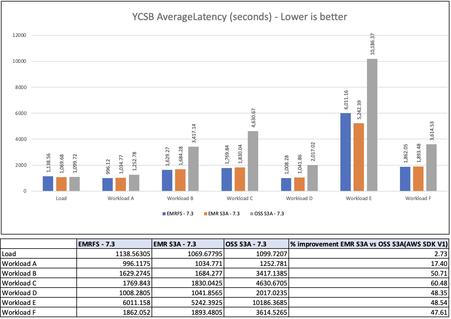
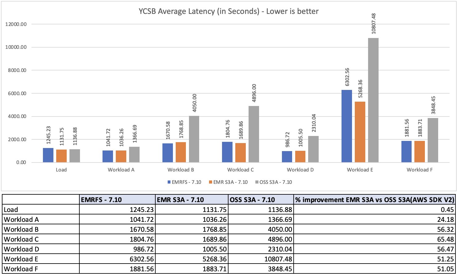
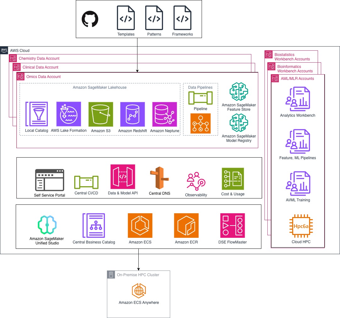
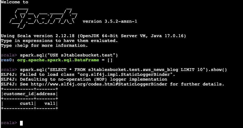

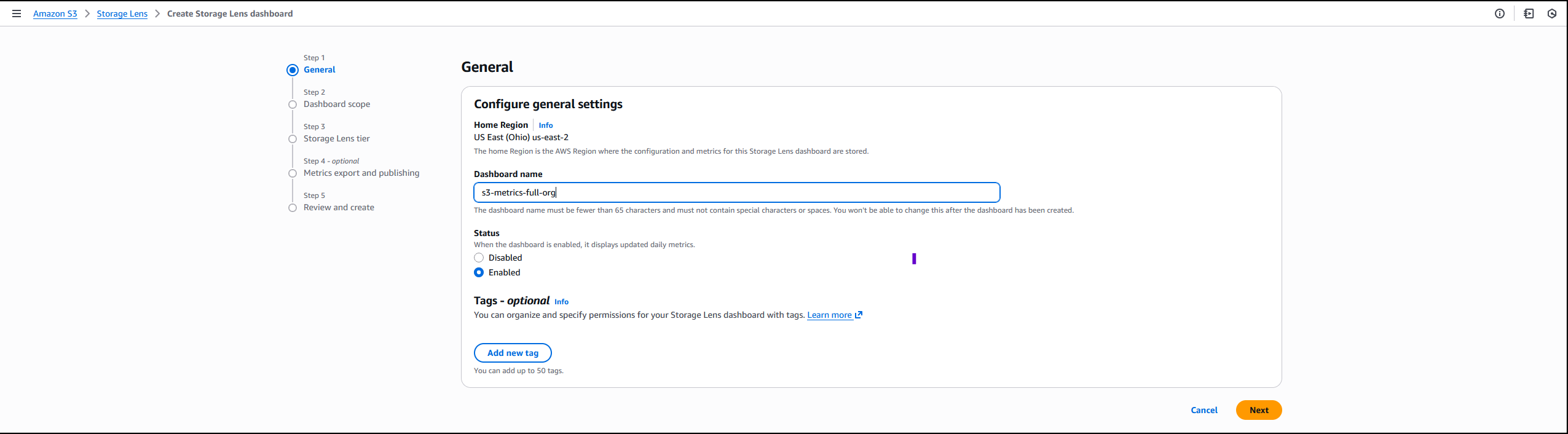
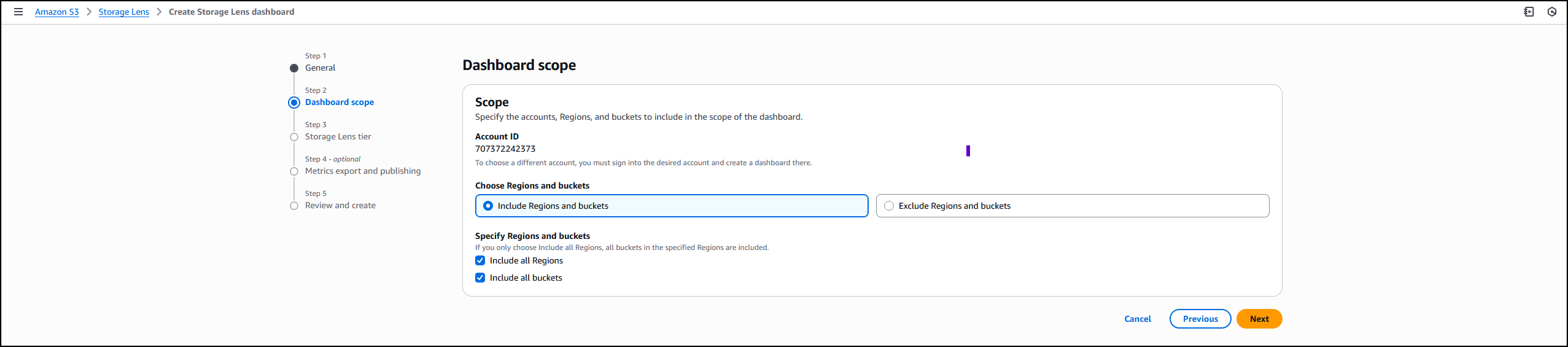
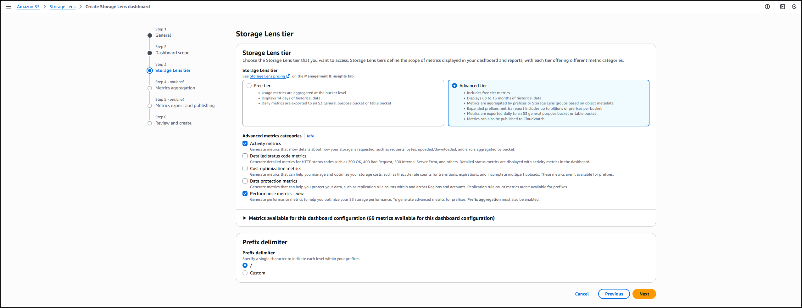

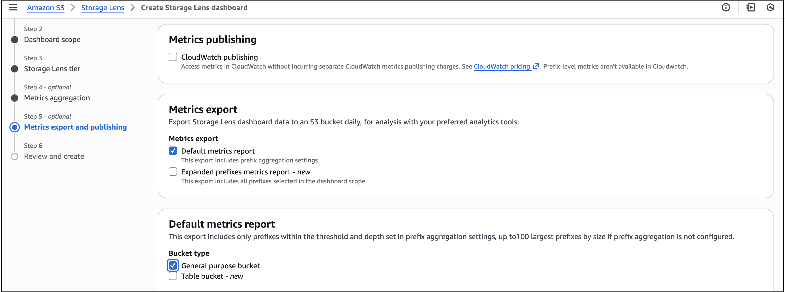
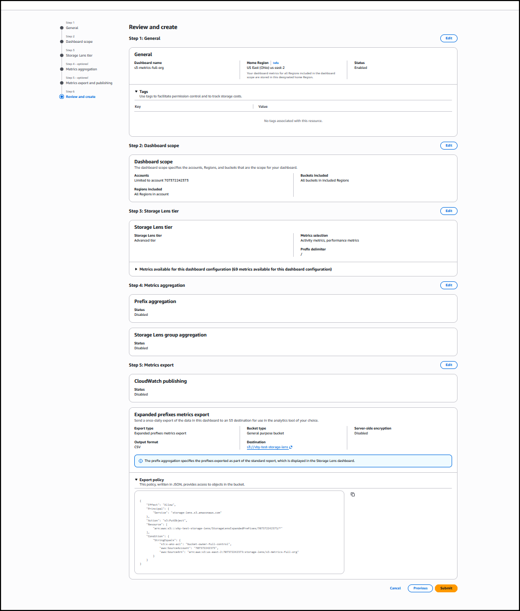

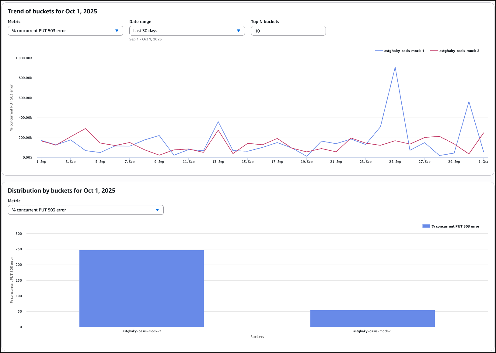
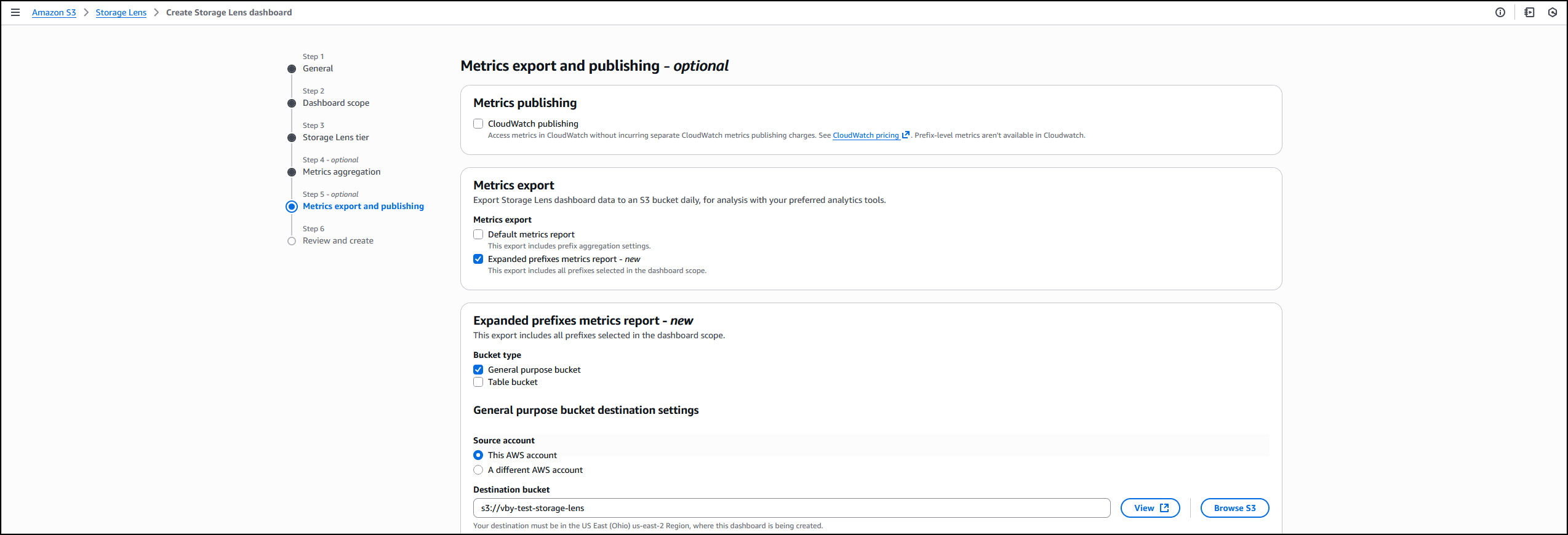
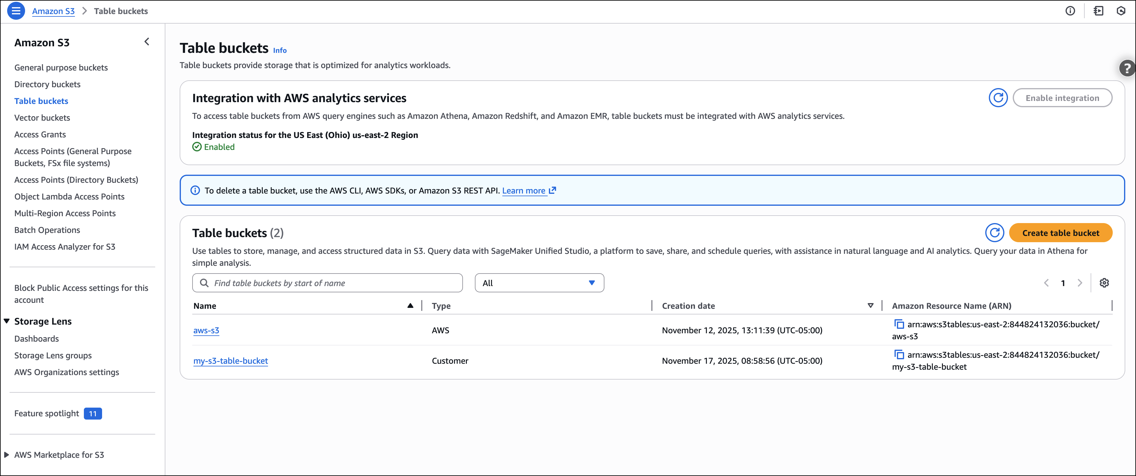
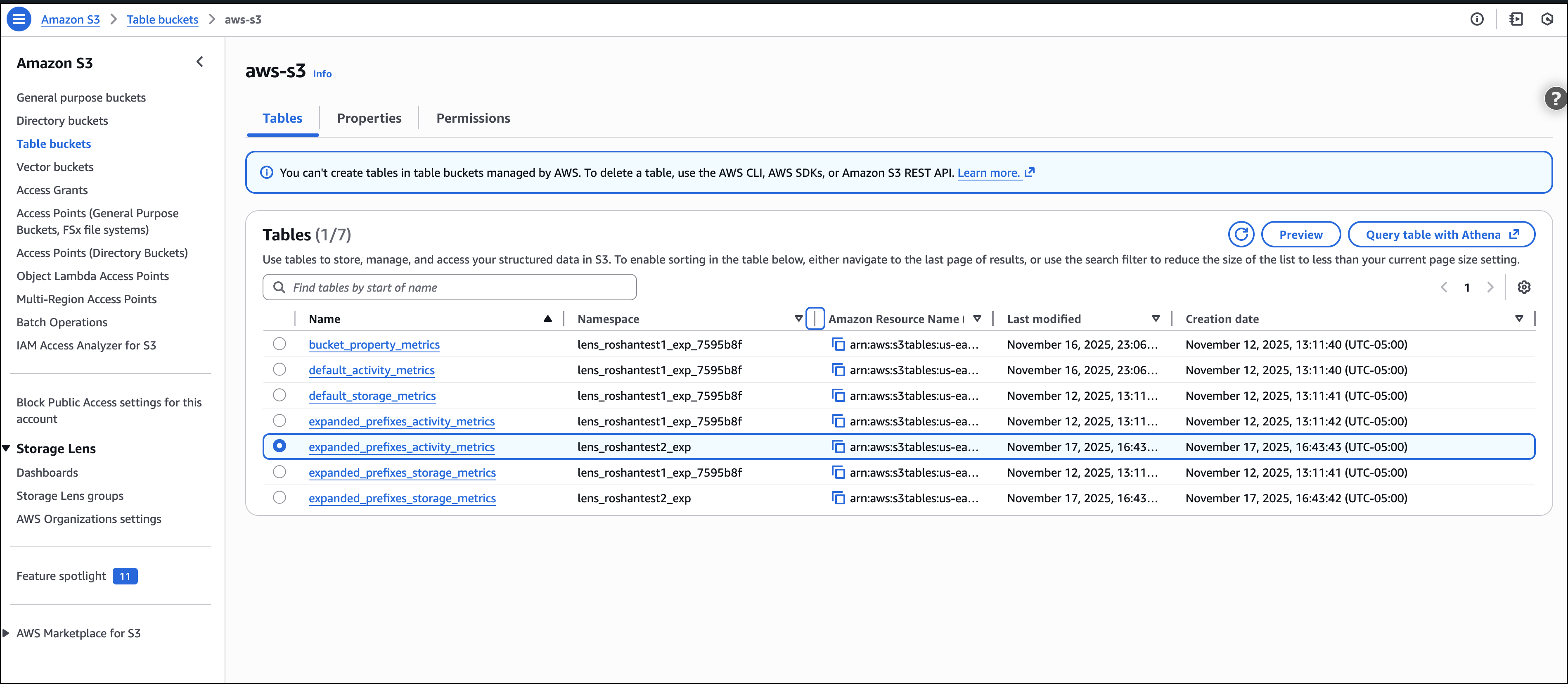
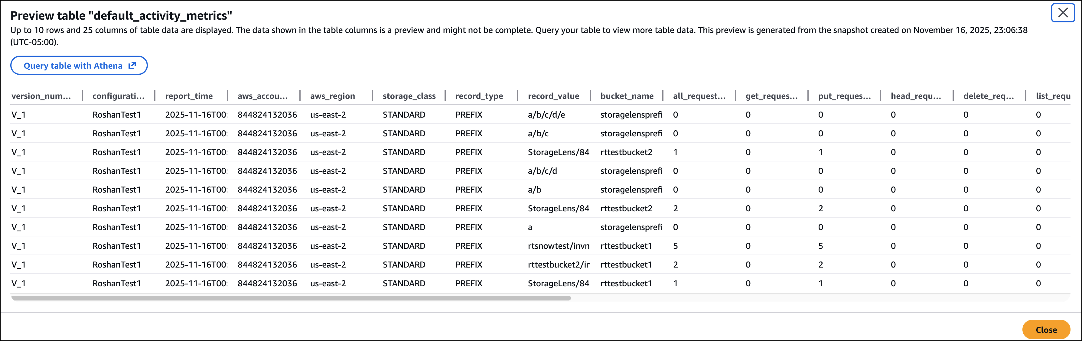
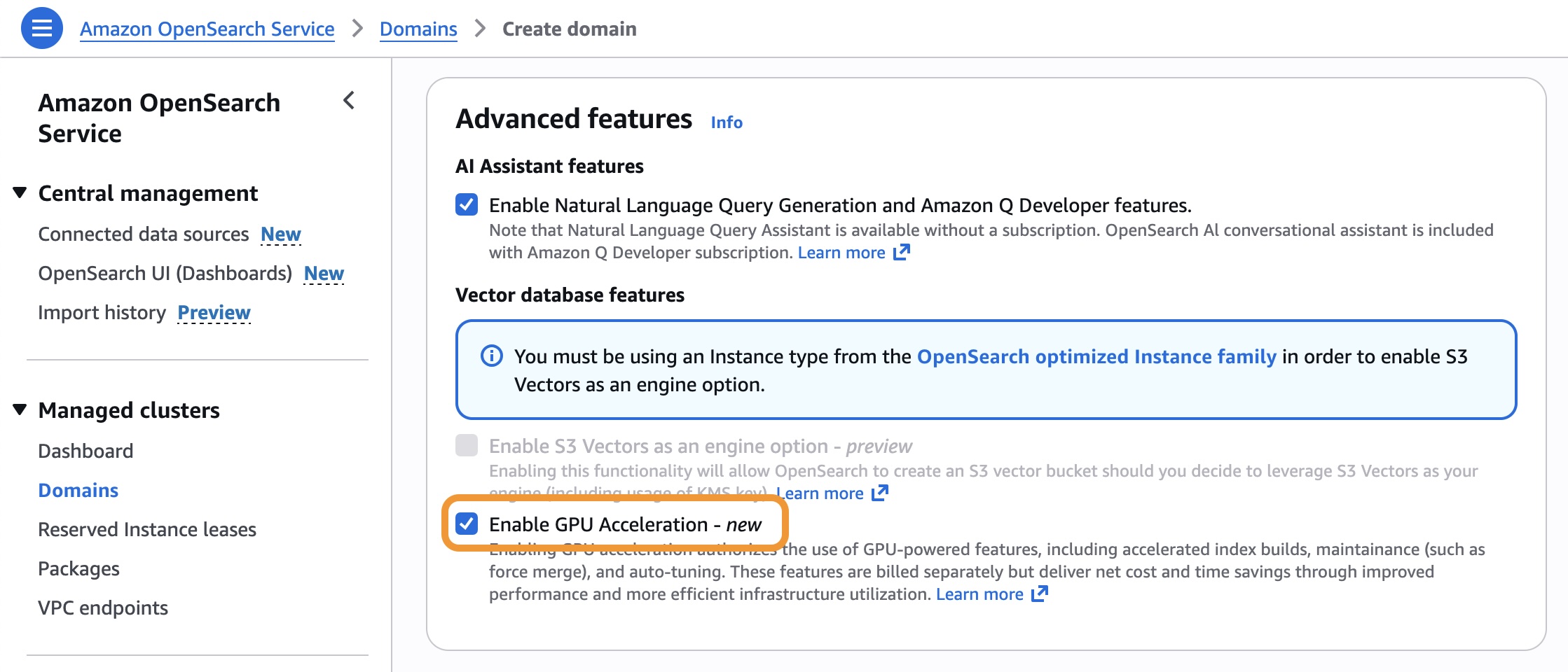
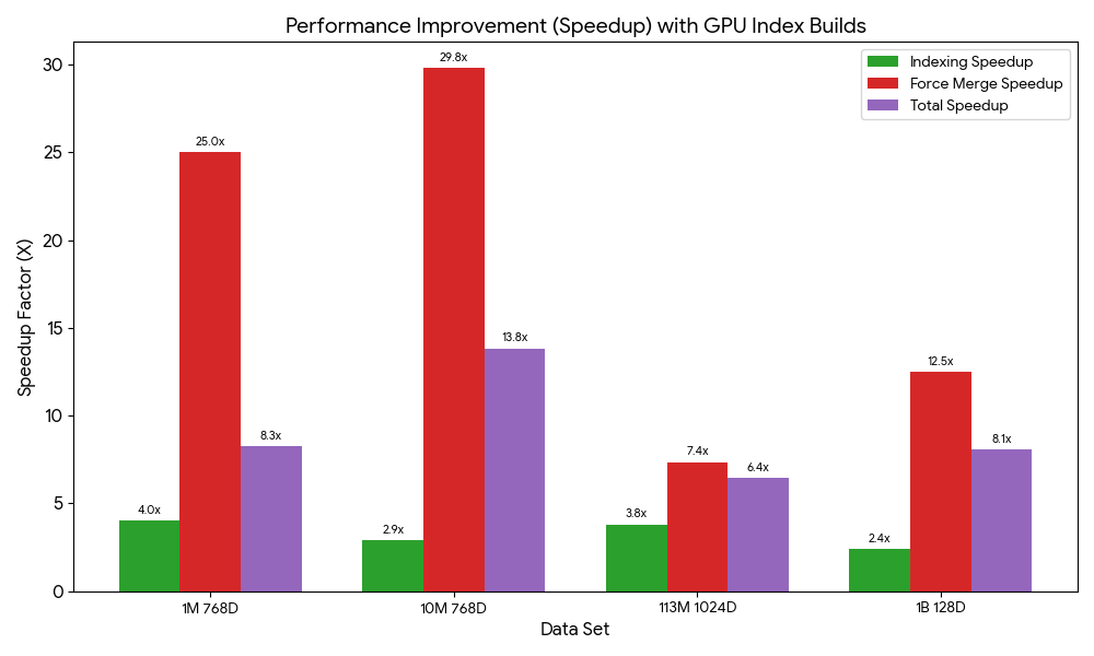
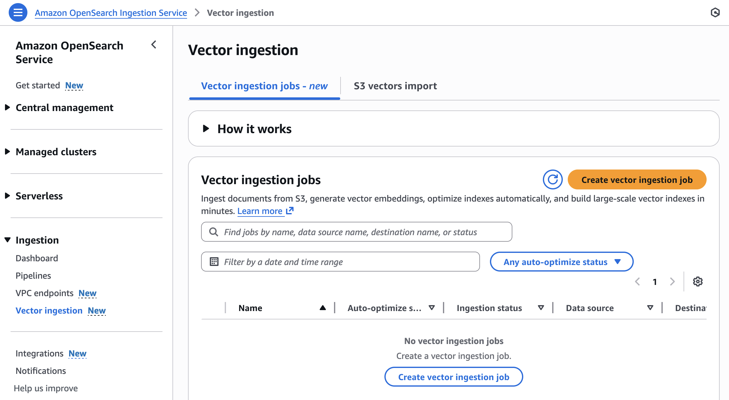
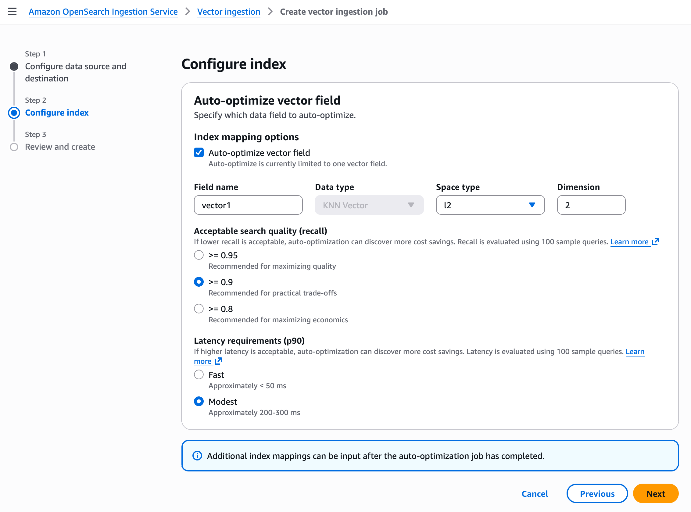

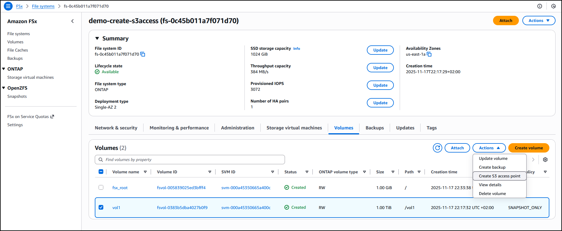

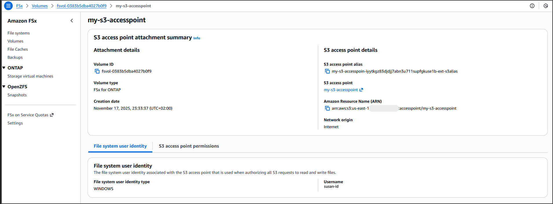
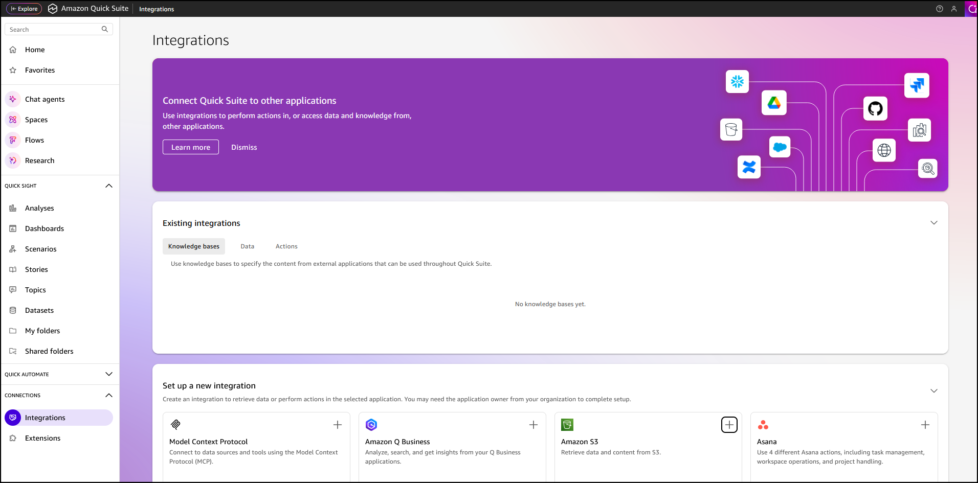
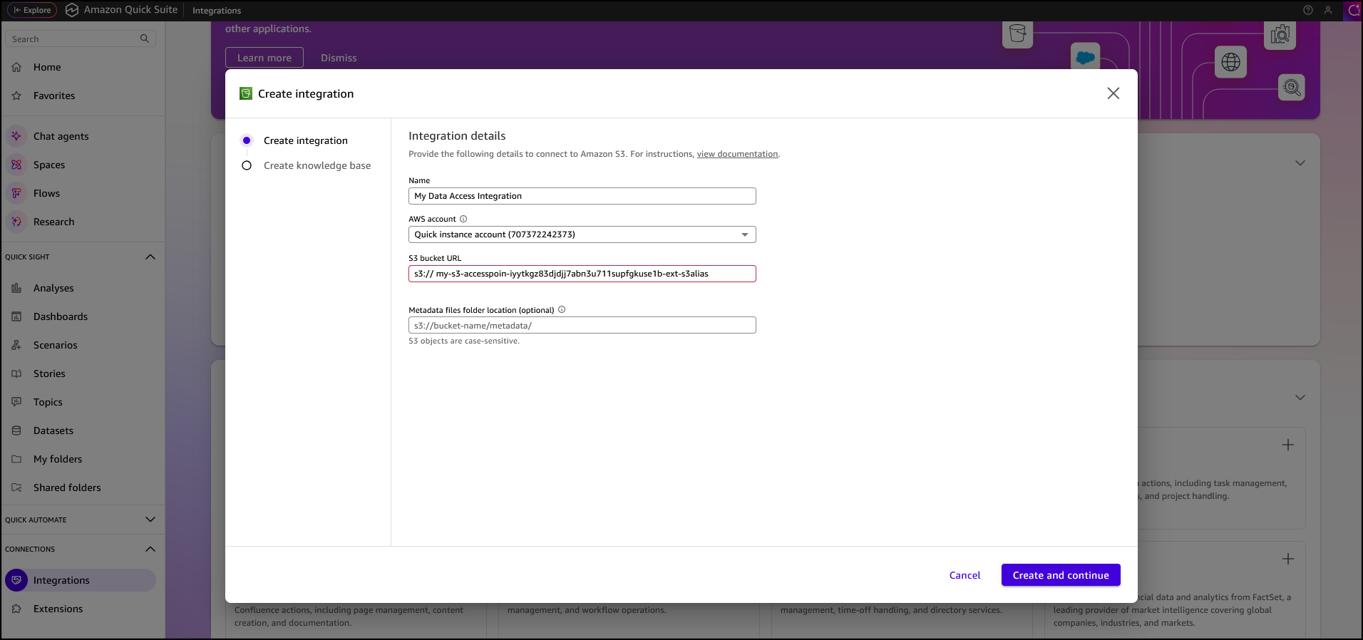


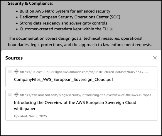
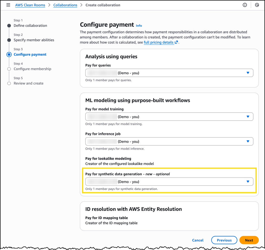
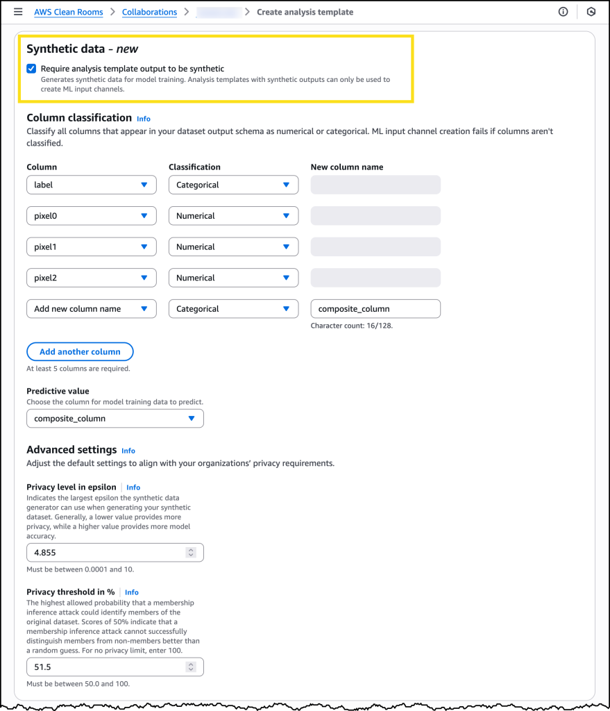
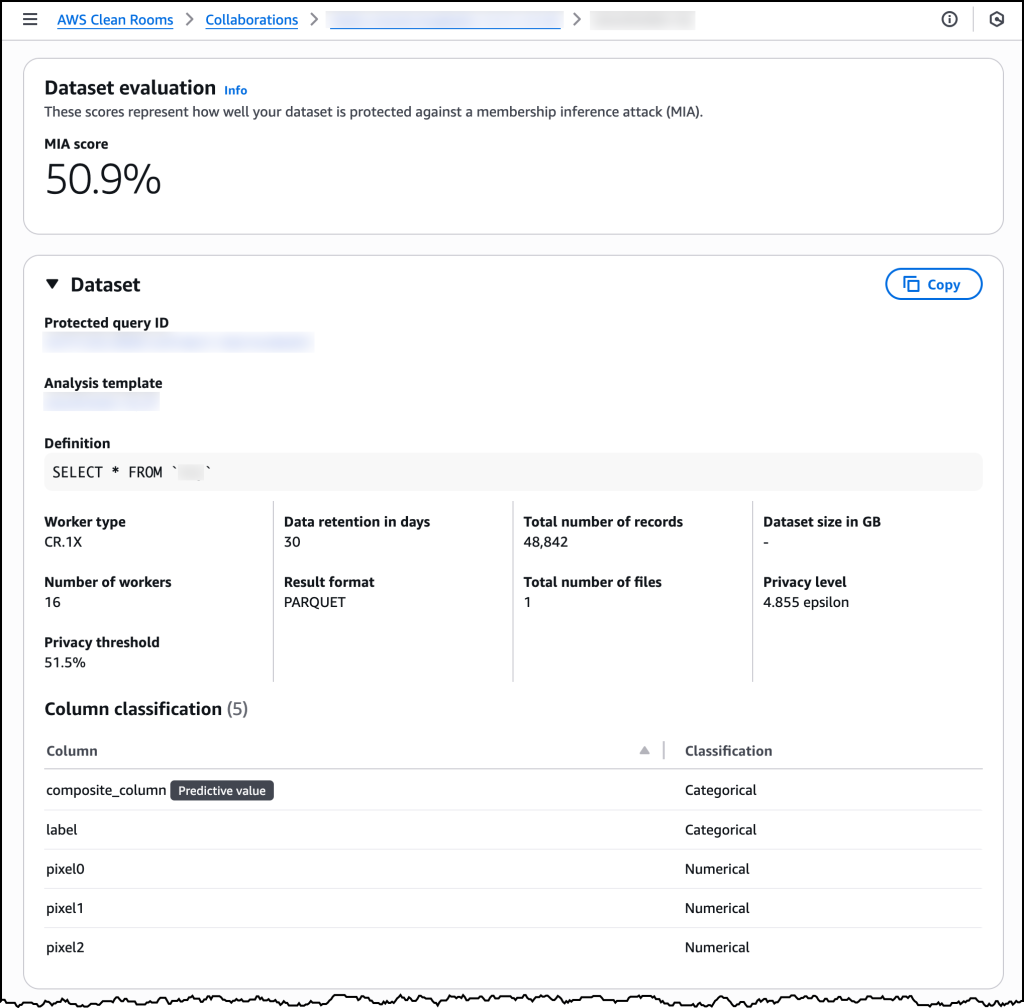
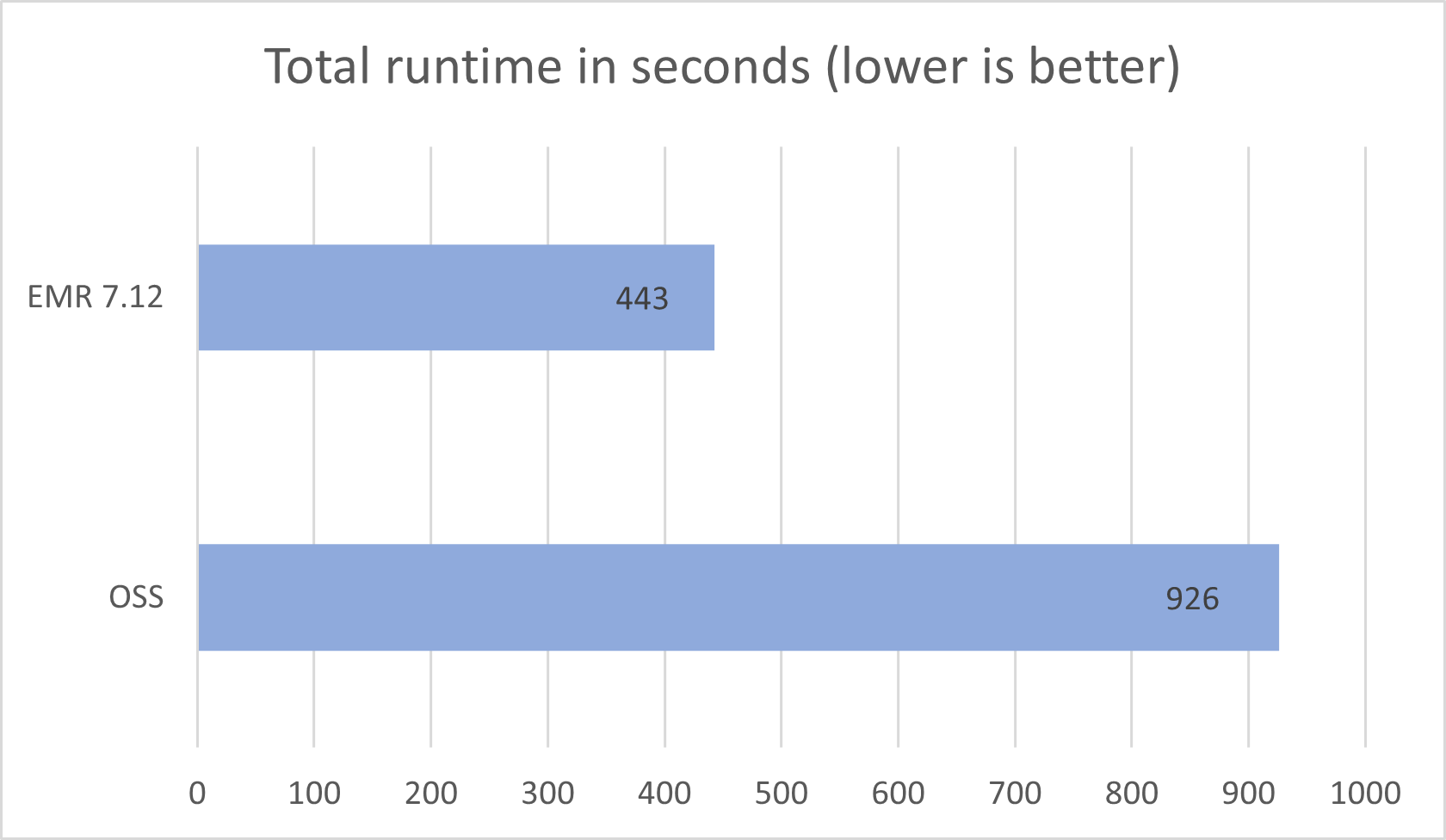
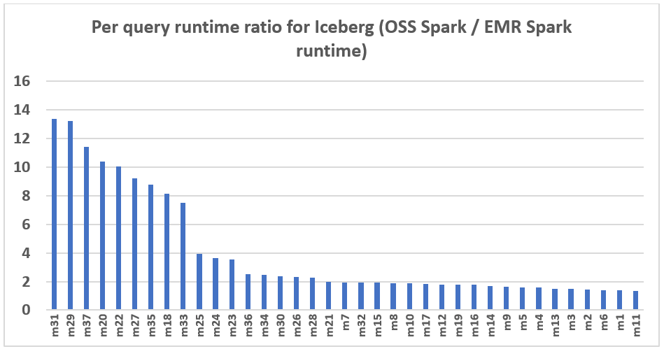
 Atul Felix Payapilly is a software development engineer for Amazon EMR at Amazon Web Services.
 Akshaya KP is a software development engineer for Amazon EMR at Amazon Web Services.
 Giovanni Matteo is the Senior Manager for the Amazon EMR Spark and Iceberg group.