We recently introduced Oxy, our Rust framework for building proxies. Through a YAML file, Oxy allows applications to easily configure listeners (e.g. IP, MASQUE, HTTP/1), telemetry, and much more. However, when it comes to application logic, a programming language is often a better tool for the job. That’s why in this post we’re introducing Oxy’s rich dependency injection capabilities for programmatically modifying all aspects of a proxy.
The idea of extending proxies with scripting is well established: we've had great past success with Lua in our OpenResty/NGINX deployments and there are numerous web frameworks (e.g. Express) with middleware patterns. While Oxy is geared towards the development of forward proxies, they all share the model of a pre-existing request pipeline with a mechanism for integrating custom application logic. However, the use of Rust greatly helps developer productivity when compared to embedded scripting languages. Having confidence in the types and mutability of objects being passed to and returned from callbacks is wonderful.
Oxy exports a series of hook traits that “hook” into the lifecycle of a connection, not just a request. Oxy applications need to control almost every layer of the OSI model: how packets are received and sent, what tunneling protocols they could be using, what HTTP version they are using (if any), and even how DNS resolution is performed. With these hooks you can extend Oxy in any way possible in a safe and performant way.
First, let's take a look from the perspective of an Oxy application developer, and then we can discuss the implementation of the framework and some of the interesting design decisions we made.
Adding functionality with hooks
Oxy’s dependency injection is a barebones version of what Java or C# developers might be accustomed to. Applications simply implement the start method and return a struct with their hook implementations:
We can define a simple callback, EgressHook::handle_connection, that will forward all connections to the upstream requested by the client. Oxy calls this function before attempting to make an upstream connection.
Oxy simply proxies the connection, but we might want to consider restricting which upstream IPs our clients are allowed to connect to. The implementation above allows everything, but maybe we have internal services that we wish to prevent proxy users from accessing.
#[async_trait]
impl<Ext> EgressHook<Ext> for MyEgressHook
where
    Ext: OxyExt,
{
    async fn handle_connection(
        &self,
        upstream_addr: SocketAddr,
        _egress_ctx: EgressConnectionContext<Ext>,
    ) -> ProxyResult<EgressDecision> {
        if self.private_cidrs.find(upstream_addr).is_some() {
            return Ok(EgressDecision::Block);
        }

        Ok(EgressDecision::ExternalDirect(upstream_addr))
    }
}
This blocking strategy is crude. Sometimes it’s useful to allow certain clients to connect to internal services – a Prometheus scraper is a good example. To authorize these connections, we’ll implement a simple Pre-Shared Key (PSK) authorization scheme – if the client sends the header Proxy-Authorization: Preshared oxy-is-a-proxy, then we’ll let them connect to private addresses via the proxy.
To do this, we need to attach some state to the connection as it passes through Oxy. Client headers only exist in the HTTP CONNECT phase, but we need access to the PSK during the egress phase. With Oxy, this can be done by leveraging its Opaque Extensions to attach arbitrary (yet fully typed) context data to a connection. Oxy initializes the data and passes it to each hook. We can mutate this data when we read headers from the client, and read it later during egress.
#[derive(Default)]
struct AuthorizationResult {
    can_access_private_cidrs: Arc<AtomicBool>,
}

#[async_trait]
impl<Ext> HttpRequestHook<Ext> for MyHttpHook
where
    Ext: OxyExt<IngressConnectionContext = AuthorizationResult>,
{
    async fn handle_proxy_connect_request(
        self: Arc<Self>,
        connect_req_head: &Parts,
        req_ctx: RequestContext<Ext>,
    ) -> ConnectDirective {
        const PSK_HEADER: &str = "Preshared oxy-is-a-proxy";

        // Grab the authorization header and update
        // the ingress_ctx if the preshared key matches.
        if let Some(authorization_header) =
          connect_req_head.headers.get("Proxy-Authorization") {
            if authorization_header.to_str().unwrap() == PSK_HEADER {
                req_ctx
                    .ingress_ctx()
                    .ext()
                    .can_access_private_cidrs
                    .store(true, Ordering::SeqCst);
            }
        }

        ConnectDirective::Allow
    }
}
From here, any hook in the pipeline can access this data. For our purposes, we can just update our existing handle_connection callback:
#[async_trait]
impl<Ext> EgressHook<Ext> for MyEgressHook
where
    Ext: OxyExt<IngressConnectionContext = AuthorizationResult>,
{
    async fn handle_connection(
        &self,
        upstream_addr: SocketAddr,
        egress_ctx: EgressConnectionContext<Ext>,
    ) -> ProxyResult<EgressDecision> {
        if self.private_cidrs.find(upstream_addr).is_some() {
            if !egress_ctx
                .ingress_ctx()
                .ext()
                .can_access_private_cidrs
                .load(Ordering::SeqCst)
            {
                return Ok(EgressDecision::Block);
            }
        }

        Ok(EgressDecision::ExternalDirect(upstream_addr))
    }
}
This is a somewhat contrived example, but in practice hooks and their extension types allow Oxy apps to fully customize all aspects of proxied traffic.
A real world example would be implementing the RFC 9209 next-hop Proxy-Status header. This involves setting a header containing the IP address we connected to on behalf of the client. We can do this with two pre-existing callbacks and a little bit of state: first we save the upstream passed to EgressHook::handle_connection_established and then read the value in the HttpRequestHook:handle_proxy_connect_response in order to set the header on the CONNECT response.
These examples only consider a few of the hooks along the HTTP CONNECT pipeline, but many real Oxy applications don’t even have L7 ingress! We will talk about the abundance of hooks later, but for now let’s look at their implementation.
Hook implementation
Oxy exists to be used by multiple teams, all with different needs and requirements. It needs a pragmatic solution to extensibility that allows one team to be productive without incurring too much of a cost on others. Hooks and their Opaque Extensions provide effectively limitless customization to applications via a clean, strongly typed interface.
The implementation of hooks within Oxy is relatively simple – throughout the code there are invocations of hook callbacks:
if let Some(ref hook) = self.hook {
    hook.handle_connection_established(upstream_addr, &egress_ctx)
        .await;
}
If a user-provided hook exists, we call it. Some hooks are more like events (e.g. handle_connection_established), and others have return values (e.g. handle_connection) which are matched on by Oxy for control flow. If a callback isn’t implemented, the default trait implementation is used. If a hook isn’t implemented at all, Oxy’s business logic just executes its default functionality. These levels of default behavior enable the minimal example we started with earlier.
While hooks solve the problem of integrating app logic into the framework, there is invariably a need to pass custom state around as we demonstrated in our PSK example. Oxy manages this custom state, passing it to hook invocations. As it is generic over the type defined by the application, this is where things get more interesting.
Generics and opaque types
Every team that works with Oxy has unique business needs, so it is important that one team’s changes don’t cause a cascade of refactoring for the others. Given that these context fields are of a user-defined type, you might expect heavy usage of generics. With Oxy we took a different approach: a generic interface is presented to application developers, but within the framework the type is erased. Keeping generics out of the internal code means adding new extension types to the framework is painless.
Our implementation relies on the Any trait. The framework treats the data as an opaque blob, but when it traverses the public API, the wrapped Any object is downcast into the concrete type defined by the user. The public API layer enforces that the user type must implement Default, which allows Oxy to be wholly responsible for creating and managing instances of the type. Mutations are then done by users of the framework through interior mutability, usually with atomics and locks.
As you might have gathered, Oxy cares a lot about the productivity of Oxy app developers. The plethora of injection points lets users quickly add features and functionality without worrying about “irrelevant” proxy logic. Sane defaults help balance customizability with complexity.
Only a subset of callbacks will be invoked for a given packet: applications operating purely at L3 will see different hook callbacks fired compared to one operating at L7. This again is customizable – if desired, Oxy’s design allows connections to be upgraded (or downgraded) which would cause a different set of callbacks to be invoked.
The ingress phase is where the hooks controlling the upgrading of L3 and decapsulation of specific L4 protocols reside. For our L3 IP Tunnel, Oxy has powerful callbacks like IpFlowHook::handle_flow which allow applications to drop, upgrade or redirect flows. IpFlowHook::handle_packet gives that same level of control at the packet level – even allowing us to modify the byte array as it passes through.
Let’s consider the H2 Proxy Protocol example in the above diagram. After Oxy has accepted the Proxy Protocol connection it fires ProxyProtocolConnectionHook::handle_connection with the parsed header, allowing applications to handle any TLVs of interest. Hook like these are common – Oxy handles the heavy lifting and then passes the application some useful information.
From here, L4 connections are funneled through the IngressHook which contains a callback we saw in our initial example: IngressHook::handle_connection. This works as you might expect, allowing applications to control whether to Allow or Block a connection as it ingresses. There is a counterpart: IngressHook::handle_connection_close, which when called gives applications insight into ingress connection statistics like loss, retransmissions, bytes transferred, etc.
Next up is the transformation phase, where we start to see some of our more powerful hooks. Oxy invokes TunnelHook::should_intercept_https, passing the SNI along with the usual connection context. This enables applications to easily configure HTTPS interception based on hostname and any custom context data (e.g. ACLs). By default, Oxy effectively splices the ingress and egress sockets, but if applications wish to have complete control over the tunneling, that is possible with TunnelHook::get_app_tunnel_pipeline, where applications are simply provided the two sockets and can implement whatever interception capabilities they wish.
Of particular interest to those wishing to implement L7 firewalls, the HttpRequestHookPipeline has two very powerful callbacks: handle_request and handle_response. Both of these offer a similar high level interface for streaming rewrites or scanning of HTTP bodies.
The EgressHook has the most callbacks, including some of the most powerful ones. For situations where hostnames are provided, DNS resolution must occur. At its simplest, Oxy allows applications to specify the nameservers used in resolution. If more control is required, Oxy provides a callback – EgressHook::handle_upstream_ips – which gives applications an opportunity to mutate the resolved IP addresses before Oxy connects. If applications want absolute control, they can turn to EgressHook::dns_resolve_override which is invoked with a hostname and expects a Vec<IpAddr> to be returned.
Much like the IngressHook, there is an EgressHook::handle_connection hook, but rather than just Allow or Block, applications can instruct Oxy to egress their connection externally, internally within Cloudflare, or even downgrade to IP packets. While it’s often best to defer to the framework for connection establishment, Oxy again offers complete control to those who want it with a few override callbacks, e.g. tcp_connect_override, udp_connect_override. This functionality is mainly leveraged by our egress service, but available to all Oxy applications if they need it.
Lastly, one of the newest additions, the AppLifecycleHook. Hopefully this sees orders of magnitude fewer invocations than the rest. The AppLifecycleHook::state_for_restart callback is invoked by Oxy during a graceful shutdown. Applications are then given the opportunity to serialize their state which will be passed to the child process. Graceful restarts are a little more nuanced, but this hook cleanly solves the problem of passing application state between releases of the application.
Right now we have around 64 public facing hooks and we keep adding more. The above diagram is (largely) accurate at time of writing but if a team needs a hook and there can be a sensible default for it, then it might as well be added. One of the primary drivers of the hook architecture for Oxy is that different teams can work on and implement the hooks that they need. Business logic is kept outside Oxy, so teams can readily leverage each other's work.
We would be remiss not to mention the issue of discoverability. For most cases, it isn’t an issue, however application developers may find when developing certain features that a more holistic understanding is necessary. This inevitably means looking into the Oxy source to fully understand when and where certain hook callbacks will be invoked. Reasoning about the order callbacks will be invoked is even thornier. Many of the hooks alter control flow significantly, so there’s always some risk that a change in Oxy could mean a change in the semantics of the applications built on top of it. To solve this, we’re experimenting with different ways to record hook execution orders when running integration tests, maybe through a proc-macro or compiler tooling.
Conclusion
In this post we’ve just scratched the surface of what’s possible with hooks in Oxy. In our example we saw a glimpse of their power: just two simple hooks and a few lines of code, and we have a forward proxy with built-in metrics, tracing, graceful restarts and much, much more.
Oxy’s extensibility with hooks is “only” dependency injection, but we’ve found this to be an extremely powerful way to build proxies. It’s dependency injection at all layers of the networking stack, from IP packets and tunnels all the way up to proxied UDP streams over QUIC. The shared core with hooks approach has been a terrific way to build a proxy framework. Teams add generic code to the framework, such as new Opaque Extensions in specific code paths, and then use those injection points to implement the logic for everything from iCloud Private Relay to Cloudflare Zero Trust. The generic capabilities are there for all teams to use, and there’s very little to no cost if you decide not to use them. We can’t wait to see what the future holds and for Oxy’s further adoption within Cloudflare.
At Cloudflare, we are constantly monitoring and optimizing the performance and resource utilization of our systems. Recently, we noticed that some of our TCP sessions were allocating more memory than expected.
The Linux kernel allows TCP sessions that match certain characteristics to ignore memory allocation limits set by autotuning and allocate excessive amounts of memory, all the way up to net.ipv4.tcp_rmem max (the per-session limit). On Cloudflare’s production network, there are often many such TCP sessions on a server, causing the total amount of allocated TCP memory to reach net.ipv4.tcp_mem thresholds (the server-wide limit). When that happens, the kernel imposes memory use constraints on all TCP sessions, not just the ones causing the problem. Those constraints have a negative impact on throughput and latency for the user. Internally within the kernel, the problematic sessions trigger TCP collapse processing, “OFO” pruning (dropping of packets already received and sitting in the out-of-order queue), and the dropping of newly arriving packets.
This blog post describes in detail the root cause of the problem and shows the test results of a solution.
TCP receive buffers are excessively big for some sessions
Our journey began when we started noticing a lot of TCP sessions on some servers with large amounts of memory allocated for receive buffers. Receive buffers are used by Linux to hold packets that have arrived from the network but have not yet been read by the local process.
Digging into the details, we observed that most of those TCP sessions had a latency (RTT) of roughly 20ms. RTT is the round trip time between the endpoints, measured in milliseconds. At that latency, standard BDP calculations tell us that a window size of 2.5 MB can accommodate up to 1 Gbps of throughput. We then counted the number of TCP sessions with an upper memory limit set by autotuning (skmem_rb) greater than 5 MB, which is double our calculated window size. The relationship between the window size and skmem_rb is described in more detail here. There were 558 such TCP sessions on one of our servers. Most of those sessions looked similar to this:
The key fields to focus on above are:
recvq – the user payload bytes in the receive queue (waiting to be read by the local userspace process)
skmem “r” field – the actual amount of kernel memory allocated for the receive buffer (this is the same as the kernel variable sk_rmem_alloc)
skmem “rb” field – the limit for “r” (this is the same as the kernel variable sk_rcvbuf)
l7read – the user payload bytes read by the local userspace process
Note the value of 256MiB for skmem_r and skmem_rb. That is the red flag that something is very wrong, because those values match the system-wide maximum value set by sysctl net.ipv4.tcp_rmem. Linux autotuning should not permit the buffers to grow that large for these sessions.
Memory limits are not being honored for some TCP sessions
Here is a graph of one of the problematic sessions, showing skmem_r (allocated memory) and skmem_rb (the limit for “r”) over time:
This graph is showing us that the limit being set by autotuning is being ignored, because every time skmem_r exceeds skmem_rb, skmem_rb is simply being raised to match it. So something is wrong with how skmem_rb is being handled. This explains the high memory usage. The question now is why.
The reproducer
At this point, we had only observed this problem in our production environment. Because we couldn’t predict which TCP sessions would fall into this dysfunctional state, and because we wanted to see the session information for these dysfunctional sessions from the beginning of those sessions, we needed to collect a lot of TCP session data for all TCP sessions. This is challenging in a production environment running at the scale of Cloudflare’s network. We needed to be able to reproduce this in a controlled lab environment. To that end, we gathered more details about what distinguishes these problematic TCP sessions from others, and ran a large number of experiments in our lab environment to reproduce the problem.
After a lot of attempts, we finally got it.
We were left with some pretty dirty lab machines by the time we got to this point, meaning that a lot of settings had been changed. We didn’t believe that all of them were related to the problem, but we didn’t know which ones were and which were not. So we went through a further series of tests to get us to a minimal set up to reproduce the problem. It turned out that a number of factors that we originally thought were important (such as latency) were not important.
The minimal set up turned out to be surprisingly simple:
At the sending host, run a TCP program with an infinite loop, sending 1500B packets, with a 1 ms delay between each send.
At the receiving host, run a TCP program with an infinite loop, reading 1B at a time, with a 1 ms delay between each read.
That’s it. Run these programs and watch your receive queue grow unbounded until it hits net.ipv4.tcp_rmem max.
tcp_server_sender.py
import time
import socket
import errno

daemon_port = 2425
payload = b'a' * 1448

listen_sock = socket.socket(socket.AF_INET, socket.SOCK_STREAM)
listen_sock.bind(('0.0.0.0', daemon_port))

# listen backlog
listen_sock.listen(32)
listen_sock.setblocking(True)

while True:
    mysock, _ = listen_sock.accept()
    mysock.setblocking(True)

    # do forever (until client disconnects)
    while True:
        try:
            mysock.send(payload)
            time.sleep(0.001)
        except Exception as e:
            print(e)
            mysock.close()
            break
tcp_client_receiver.py
import socket
import time

def do_read(bytes_to_read):
    total_bytes_read = 0
    while True:
        bytes_read = client_sock.recv(bytes_to_read)
        total_bytes_read += len(bytes_read)
        if total_bytes_read >= bytes_to_read:
            break

server_ip = “192.168.2.139”
server_port = 2425

client_sock = socket.socket(socket.AF_INET, socket.SOCK_STREAM)
client_sock.connect((server_ip, server_port))
client_sock.setblocking(True)

while True:
    do_read(1)
    time.sleep(0.001)
Reproducing the problem
First, we ran the above programs with these settings:
Kernel 6.1.14 vanilla
net.ipv4.tcp_rmem max = 256 MiB (window scale factor 13, or 8192 bytes)
net.ipv4.tcp_adv_win_scale = -2
Here is what this TCP session is doing:
At second 189 of the run, we see these packets being exchanged:
This is a significant failure because the memory limits are being ignored, and memory usage is unbounded until net.ipv4.tcp_rmem max is reached.
When net.ipv4.tcp_rmem max is reached:
The kernel drops incoming packets.
A ZeroWindow is never sent. A ZeroWindow is a packet sent by the receiver to the sender telling the sender to stop sending packets. This is normal and expected behavior when the receiver buffers are full.
The sender retransmits, with exponential backoff.
Eventually (~15 minutes, depending on system settings) the session times out and the connection is broken (“Errno 110 Connection timed out”).
Note that there is a range of packet sizes that can be sent, and a range of intervals which can be used for the delays, to cause this abnormal condition. This first reproduction is intentionally defined to grow the receive buffer quickly. These rates and delays do not reflect exactly what we see in production.
A closer look at real traffic in production
The prior section describes what is happening in our lab systems. Is that consistent with what we see in our production streams? Let’s take a look, now that we know more about what we are looking for.
We did find similar TCP sessions on our production network, which provided confirmation. But we also found this one, which, although it looks a little different, is actually the same root cause:
During this TCP session, the rate at which the userspace process is reading from the socket (the L7read rate line) after second 411 is zero. That is, L7 stops reading entirely at that point.
Notice that the bottom two graphs have a log scale on their y-axis to show that throughput and window size are never zero, even after L7 stops reading.
Here is the pattern of packet exchange that repeats itself during the erroneous “growth phase” after L7 stopped reading at the 411 second mark:
This variation of the problem is addressed below in the section called “Reader never reads”.
Getting to the root cause
sk_rcvbuf is being increased inappropriately. Somewhere. Let’s review the code to narrow down the possibilities.
sk_rcvbuf only gets updated in three places (that are relevant to this issue):
Actually, we are not calling tcp_set_rcvlowat, which eliminates that one. Next we used bpftrace scripts to figure out if it’s in tcp_clamp_window or tcp_rcv_space_adjust. After bpftracing, the answer is: It’s tcp_clamp_window.
Sometimes rmem_alloc > sk_rcvbuf. When that happens, prune is called, which calls tcp_clamp_window. tcp_clamp_window increases sk_rcvbuf to match rmem_alloc. That is unexpected.
The key question is: Why is rmem_alloc > sk_rcvbuf?
Why is rmem_alloc > sk_rcvbuf?
More kernel code review ensued, reviewing all the places where rmem_alloc is increased, and looking to see where rmem_alloc could be exceeding sk_rcvbuf. After more bpftracing, watching netstats, etc., the answer is: TCP coalescing.
TCP coalescing
Coalescing is where the kernel will combine packets as they are being received.
Note that this is not Generic Receive Offload (GRO). This is specific to TCP for packets on the INPUT path. Coalesce is a L4 feature that appends user payload from an incoming packet to an already existing packet, if possible. This saves memory (header space).
tcp_rcv_established calls tcp_queue_rcv, which calls tcp_try_coalesce. If the incoming packet can be coalesced, then it will be, and rmem_alloc is raised to reflect that. Here’s the important part: rmem_alloc can and does go above sk_rcvbuf because of the logic in that routine.
Summarizing what we know so far, part II
Data packets are being received
tcp_rcv_established will coalesce, raising rmem_alloc above sk_rcvbuf
tcp_try_rmem_schedule -> tcp_prune_queue -> tcp_clamp_window will raise sk_rcvbuf to match rmem_alloc
The kernel then increases the window size based upon the new sk_rcvbuf value
In step 2, in order for rmem_alloc to exceed sk_rcvbuf, it has to be near sk_rcvbuf in the first place. We use tcp_adv_win_scale of -2, which means the window size will be 25% of the available buffer size, so we would not expect rmem_alloc to even be close to sk_rcvbuf. In our tests, the truesize ratio is not close to 4, so something unexpected is happening.
Why is rmem_alloc even close to sk_rcvbuf?
Why is rmem_alloc close to sk_rcvbuf?
Sending a ZeroWindow (a packet advertising a window size of zero) is how a TCP receiver tells a TCP sender to stop sending when the receive window is full. This is the mechanism that should keep rmem_alloc well below sk_rcvbuf.
During our tests, we happened to notice that the SNMP metric TCPWantZeroWindowAdv was increasing. The receiver was not sending ZeroWindows when it should have been. So our attention fell on the window calculation logic, and we arrived at the root cause of all of our problems.
The root cause
The problem has to do with how the receive window size is calculated. This is the value in the TCP header that the receiver sends to the sender. Together with the ACK value, it communicates to the sender what the right edge of the window is.
The way TCP’s sliding window works is described in Stevens, “TCP/IP Illustrated, Volume 1”, section 20.3. Visually, the receive window looks like this:
In the early days of the Internet, wide-area communications links offered low bandwidths (relative to today), so the 16 bits in the TCP header was more than enough to express the size of the receive window needed to achieve optimal throughput. Then the future happened, and now those 16-bit window values are scaled based upon a multiplier set during the TCP 3-way handshake.
The window scaling factor allows us to reach high throughputs on modern networks, but it also introduced an issue that we must now discuss.
The granularity of the receive window size that can be set in the TCP header is larger than the granularity of the actual changes we sometimes want to make to the size of the receive window.
When window scaling is in effect, every time the receiver ACKs some data, the receiver has to move the right edge of the window either left or right. The only exception would be if the amount of ACKed data is exactly a multiple of the window scale factor, and the receive window size specified in the ACK packet was reduced by the same multiple. This is rare.
So the right edge has to move. Most of the time, the receive window size does not change and the right edge moves to the right in lockstep with the ACK (the left edge), which always moves to the right.
The receiver can decide to increase the size of the receive window, based on its normal criteria, and that’s fine. It just means the right edge moves farther to the right. No problems.
But what happens when we approach a window full condition? Keeping the right edge unchanged is not an option. We are forced to make a decision. Our choices are:
Move the right edge to the right
Move the right edge to the left
But if we have arrived at the upper limit, then moving the right edge to the right requires us to ignore the upper limit. This is equivalent to not having a limit. This is what Linux does today, and is the source of the problems described in this post.
This occurs for any window scaling factor greater than one. This means everyone.
A sidebar on terminology
The window size specified in the TCP header is the receive window size. It is sent from the receiver to the sender. The ACK number plus the window size defines the range of sequence numbers that the sender may send. It is also called the advertised window, or the offered window.
There are three terms related to TCP window management that are important to understand:
Closing the window. This is when the left edge of the window moves to the right. This occurs every time an ACK of a data packet arrives at the sender.
Opening the window. This is when the right edge of the window moves to the right.
Shrinking the window. This is when the right edge of the window moves to the left.
Opening and shrinking is not the same thing as the receive window size in the TCP header getting larger or smaller. The right edge is defined as the ACK number plus the receive window size. Shrinking only occurs when that right edge moves to the left (i.e. gets reduced).
Letting the window grow is the same as ignoring the memory limits set by autotuning. It results in allocating excessive amounts of memory for no reason. This is really just kicking the can down the road until allocated memory reaches net.ipv4.tcp_rmem max, when we are forced to choose from among one of the other two options.
Drop incoming packets
Dropping incoming packets will cause the sender to retransmit the dropped packets, with exponential backoff, until an eventual timeout (depending on the client read rate), which breaks the connection. ZeroWindows are never sent. This wastes bandwidth and processing resources by retransmitting packets we know will not be successfully delivered to L7 at the receiver. This is functionally incorrect for a window full situation.
Shrink the window
Shrinking the window involves moving the right edge of the window to the left when approaching a window full condition. A ZeroWindow is sent when the window is full. There is no wasted memory, no wasted bandwidth, and no broken connections.
The current situation is that we are letting the window grow (option #1), and when net.ipv4.tcp_rmem max is reached, we are dropping packets (option #2).
We need to stop doing option #1. We could either drop packets (option #2) when sk_rcvbuf is reached. This avoids excessive memory usage, but is still functionally incorrect for a window full situation. Or we could shrink the window (option #3).
Shrinking the window
It turns out that this issue has already been addressed in the RFC’s.
“there are instances when a retracted window can be offered”
“Implementations MUST ensure that they handle a shrinking window”
Appendix F of that RFC describes our situation, adding:
“This is a general problem and can happen any time the sender does a write, which is smaller than the window scale factor.”
Kernel patch
The Linux kernel patch we wrote to enable TCP window shrinking can be found here. This patch will also be submitted upstream.
Rerunning the test above with kernel patch
Here is the test we showed above, but this time using the kernel patch:
Here is the pattern of packet exchanges that repeat when using the kernel patch:
We see that the memory limit is being honored, ZeroWindows are being sent, there are no retransmissions, and no disconnects after 15 minutes. This is the desired result.
Test results using a TCP window scaling factor of 8
The window scaling factor of 8 and tcp_adv_win_scale of 1 is commonly seen on the public Internet, so let’s test that.
kernel 6.1.14 vanilla
tcp_rmem max = 8 MiB (window scale factor 8, or 256 bytes)
tcp_adv_win_scale = 1
Without the kernel patch
At the ~2100 second mark, we see the same problems we saw earlier when using wscale 13.
With the kernel patch
The kernel patch is working as expected.
Test results using an oscillating reader
This is a test run where the reader alternates every 240 seconds between reading slow and reading fast. Slow is 1B every 1 ms and fast is 3300B every 1 ms.
kernel 6.1.14 vanilla
net.ipv4.tcp_rmem max = 256 MiB (window scale factor 13, or 8192 bytes)
tcp_adv_win_scale = -2
Without the kernel patch
With the kernel patch
The kernel patch is working as expected.
NB. We do see the increase of skmem_rb at the 720 second mark, but it only goes to ~20MB and does not grow unbounded. Whether or not 20MB is the most ideal value for this TCP session is an interesting question, but that is a topic for a different blog post.
Reader never reads
Here’s a good one. Say a reader never reads from the socket. How much TCP receive buffer memory would we expect that reader to consume? One might assume the answer is that the reader would read a few packets, store the payload in the receive queue, then pause the flow of packets until the userspace program starts reading. The actual answer is that the reader will read packets until the receive queue grows to the size of net.ipv4.tcp_rmem max. This is incorrect behavior, to say the very least.
For this test, the sender sends 4 bytes every 1 ms. The reader, literally, never reads from the socket. Not once.
kernel 6.1.14 vanilla
net.ipv4.tcp_rmem max = 8 MiB (window scale factor 8, or 256 bytes)
net.ipv4.tcp_adv_win_scale = -2
Without the kernel patch:
With the kernel patch:
Using the kernel patch produces the expected behavior.
Results from the Cloudflare production network
We deployed this patch to the Cloudflare production network, and can see the effects in aggregate when running at scale.
Packet Drop Rates
This first graph shows RcvPruned, which shows how many incoming packets per second were dropped due to memory constraints.
The patch was enabled on most servers on 05/01 at 22:00, eliminating those drops.
TCPRcvCollapsed
Recall that TCPRcvCollapsed is the number of packets per second that are merged together in the queue in order to reduce memory usage (by eliminating header metadata). This occurs when memory limits are reached.
The patch was enabled on most servers on 05/01 at 22:00. These graphs show the results from one of our data centers. The upper graph shows that the patch has eliminated all collapse processing. The lower graph shows the amount of time spent in collapse processing (each line in the lower graph is a single server). This is important because it can impact Cloudflare’s responsiveness in processing HTTP requests. The result of the patch is that all latency due to TCP collapse processing has been eliminated.
Memory
Because the memory limits set by autotuning are now being enforced, the total amount of memory allocated is reduced.
In this graph, the green line shows the total amount of memory allocated for TCP buffers in one of our data centers. This is with the patch enabled. The purple line is the same total, but from exactly 7 days prior to the time indicated on the x axis, before the patch was enabled. Using this approach to visualization, it is clear to see the memory saved with the patch enabled.
ZeroWindows
TCPWantZeroWindowAdv is the number of times per second that the window calculation based on available buffer memory produced a result that should have resulted in a ZeroWindow being sent to the sender, but was not. In other words, this is how often the receive buffer was increased beyond the limit set by autotuning.
After a receiver has sent a Zero Window to the sender, the receiver is not expecting to get any additional data from the sender. Should additional data packets arrive at the receiver during the period when the window size is zero, those packets are dropped and the metric TCPZeroWindowDrop is incremented. These dropped packets are usually just due to the timing of these events, i.e. the Zero Window packet in one direction and some data packets flowing in the other direction passed by each other on the network.
The patch was enabled on most servers on 05/01 at 22:00, although it was enabled for a subset of servers on 04/26 and 04/28.
The upper graph tells us that ZeroWindows are indeed being sent when they need to be based on the available memory at the receiver. This is what the lack of “Wants” starting on 05/01 is telling us.
The lower graph reports the packets that are dropped because the session is in a ZeroWindow state. These are ok to drop, because the session is in a ZeroWindow state. These drops do not have a negative impact, for the same reason (it’s in a ZeroWindow state).
All of these results are as expected.
Importantly, we have also not found any peer TCP stacks that are non-RFC compliant (i.e. that are not able to accept a shrinking window).
Summary
In this blog post, we described when and why TCP memory limits are not being honored in the Linux kernel, and introduced a patch that fixes it. All in a day’s work at Cloudflare, where we are helping build a better Internet.
Cloudflare’s website, application security and performance products handle upwards of 46 million HTTP requests per second, every second. These products were originally built as a set of native Linux services, but we’re increasingly building parts of the system using our Cloudflare Workers developer platform to make these products faster, more robust, and easier to develop. This blog post digs into how and why we’re doing this.
System architecture
Our architecture can best be thought of as a chain of proxies, each communicating over HTTP. At first, these proxies were all implemented based on NGINX and Lua, but in recent years many of them have been replaced – often by new services built in Rust, such as Pingora.
The proxies each have distinct purposes – some obvious, some less so. One which we’ll be discussing in more detail is the FL service, which performs “Front Line” processing of requests, applying customer configuration to decide how to handle and route the request.
This architecture has worked well for more than a decade. It allows parts of the system to be developed and deployed independently, parts of the system to be scaled independently, and traffic to be routed to different nodes in our systems according to load, or to ensure efficient cache utilization.
So, why change it?
At the level of latency we care about, service boundaries aren’t cheap, particularly when communicating over HTTP. Each step in the chain adds latency due to communication overheads, so we can’t add more services as we develop new products. And we have a lot of products, with many more on the way.
To avoid this overhead, we put most of the logic for many different products into FL. We’ve developed a simple modular architecture in this service, allowing teams to make and deploy changes with some level of isolation. This has become a very complex service which takes a constant effort by a team of skilled engineers to maintain and operate.
Even with this effort, the developer experience for Cloudflare engineers has often been much harder than we would like. We need to be able to start working on implementing any change quickly, but even getting a version of the system running in a local development environment is hard, requiring installation of custom tooling and Linux kernels.
The structure of the code limits the ease of making changes. While some changes are easy to make, other things run into surprising limits due to the underlying platform. For example, it is not possible to perform I/O in many parts of the code which handle HTTP response processing, leading to complex workarounds to preload resources in case they are needed.
Deploying updates to the software is high risk, so is done slowly and with care. Massive improvements have been made in the past years to our processes here, but it’s not uncommon to have to wait a week to see changes reach production, and changes tend to be deployed in large batches, making it hard to isolate the effect of each change in a release.
Finally, the code has a modular structure, but once in production there is limited isolation and sandboxing, so tracing potential side effects is hard, and debugging often requires knowledge of the whole system, which takes years of experience to obtain.
Developer platform to the rescue
As soon as Cloudflare workers became part of our stack in 2017, we started looking at ways to use them to improve our ability to build new products. Now, in 2023, many of our products are built in part using workers and the wider developer platform; for example, read this post from the Waiting Room team about how they use Workers and Durable Objects, or this post about our cache purge system doing the same. Products like Cloudflare Zero Trust, R2, KV, Turnstile, Queues, and Exposed credentials check are built using Workers at large scale, handling every request processed by the products. We also use Workers for many of our pieces of internal tooling, from dashboards to building chatbots.
While we can and do spend time improving the tooling and architecture of all our systems, the developer platform is focussed all the time on making developers productive, and being as easy to use as possible. Many of the other posts this week on this blog talk about our work here. On the developer platform, any customer can get something running in minutes, and build and deploy full complex systems within days.
We have been working to give developers working on internal Cloudflare products the same benefits.
Customer workers vs internal workers
At this point, we need to talk about two different types of worker.
The first type is created when a customer writes a Cloudflare Worker. The code is deployed to our network, and will run whenever a request to the customer’s site matches the worker’s route. Many Cloudflare engineering teams use workers just like this to build parts of our product – for example, we wrote about our Coreless Purge system for Cache recently. In these cases, our engineering teams are using exactly the same process and tooling as any Cloudflare customer would use.
However, we also have another type of worker, which can only be deployed by Cloudflare. These are not associated with a single customer. Instead, they are run for all customers for which a particular product or other piece of logic needs to be performed.
For the rest of this post, we’re only going to be talking about these internal workers. The underlying tech is the same – the difference to remember is that these workers run in response to requests from many Cloudflare customers rather than one.
Initial integration of internal workers
We first integrated internal workers into our architecture in 2019, in a very simple way. An ordered chain of internal workers was created, which run before any customer scripts.
I previously said that adding more steps in our chain would cause excessive latency. So why isn’t this a problem for internal workers?
The answer is that these internal workers run within the same service as each other, and as customer workers which are operating on the request. So, there’s no need to marshal the request into HTTP to pass it on to the next step in the chain; the runtime just needs to pass a memory reference around, and perform a lightweight shift of control. There is still a cost of adding more steps – but the cost per step is much lower.
The integration gave us several benefits immediately. We were able to take advantage of the strong sandbox model for workers, removing any risk of unexpected side effects between customers or requests. It also allowed isolated deployments – teams could deploy their updates on their own schedule, without waiting for or disrupting other teams.
However, it also had a number of limitations. Internal workers could only run in one place in the lifetime of a request. This meant they couldn’t affect services running before them, such as the Cloudflare WAF.
Also, for security reasons, internal workers were published with an internal API using special credentials, rather than the public workers API. In 2019, this was no big deal, but since then there has been a ton of work to improve tooling such as wrangler, and build the developer platform. All of this tooling was unavailable for internal workers.
We had very limited observability of internal workers, lacking metrics and detailed logs, making them hard to debug.
We realized that we could do a lot more with the platform to improve our development processes. We also wondered how far it would be possible to go with the platform. Would it be possible to migrate all the logic implemented in the NGINX-based FL service to the developer platform? And if not, why not?
So we started, in late 2021, with a prototype. This routed traffic directly from our TLS ingress service to our workers runtime, skipping the FL service. We named this prototype Flame.
It worked. Just about. Most importantly for a prototype, we could see that we were missing some fundamental capabilities. We couldn’t access other Cloudflare internal services, such as our DNS infrastructure or our customer configuration database, and we couldn’t emit request logs to our data pipeline, for analytics and billing purposes.
We rely heavily on caching for performance, and there was no way to cache state between requests. We also couldn’t emit HTTP requests directly to customer origins, or to our cache, without using our full existing chain-of-proxies pipeline.
Also, the developer experience for this prototype was very poor. We couldn’t take advantage of all the developer experience work being put into wrangler, due to the need to use special APIs to deploy internal workers. We couldn’t record metrics and traces to our standard observability tooling systems, so we were blind to the behavior of the system in production. And we had no way to perform a controlled and gradual deployment of updated code.
Improving the developer platform for internal services
We set out to address these problems one by one. Wherever possible, we wanted to use the same tooling for internal purposes as we provide to customers. This not only reduces the amount of tooling we need to support, but also means that we understand the problems our customers face better, and can improve their experience as well as ours.
Tooling and routing
We started with the basics – how can we deploy code for internal services to the developer platform.
I mentioned earlier that we used special internal APIs for deploying our internal workers, for “security reasons”. We reviewed this with our security team, and found that we had good protections on our API to identify who was publishing a worker. The main thing we needed to add was a secure registry of accounts which were allowed to use privileged resources. Initially we did this by hard-coding a set of permissions into our API service – later this was replaced by a more flexible permissions control plane.
Even more importantly, there is a strong distinction between publishing a worker and deploying a worker.
Publishing is the process of pushing the worker to our configuration store, so that the code to be run can be loaded when it is needed. Internally, each worker version which is published creates a new artifact in our store.
The Workers runtime uses a capability-based security model. When it is published, each script is bundled together with a list of bindings, representing the capabilities that the script has to access other resources. This mechanism is a key part of providing safety – in order to be able to access resources, the script must have been published by an account with the permissions to provide the capabilities. The secure management of bindings to internal resources is a key part of our ability to use the developer platform for internal systems.
Deploying is the process of hooking up the worker to be triggered when a request comes in. For a customer worker, deployment means attaching the worker to a route. For our internal workers, deployment means updating a global configuration store with the details of the specific artifact to run.
After some work, we were finally able to use wrangler to build and publish internal services. But there was a problem! In order to deploy an internal worker, we needed to know the identifier for the artifact which was published. Fortunately, this was a simple change: we updated wrangler to output debug information which contained this information.
A big benefit of using wrangler is that we could make tools like “wrangler test” and “wrangler dev” work. An engineer can check out the code, and get going developing their feature with well-supported tooling, and within a realistic environment.
Event logging
We run a comprehensive data pipeline, providing streams of data for our customers to allow them to see what is happening on their sites, for our operations teams to understand how our system is behaving in production, and for us to provide services like DoS protection and accurate billing.
This pipeline starts from our network as messages in Cap’n Proto format. So we needed to build a new way to push pieces of log data to our internal pipeline, from inside a worker. The pipeline starts with a service called “logfwdr”, so we added a new binding which allowed us to push an arbitrary log message to the logfwdr service. This work was later a foundation of the Workers Analytics Engine bindings, which allow customers to use the same structured logging capabilities.
Observability
Observability is the ability to see how code is behaving. If you don’t have good observability tooling, you spend most of your time guessing. It’s inefficient and frankly unsafe to operate such a system.
At Cloudflare, we have very many systems for observability, but three of the most important are:
Unstructured logs (“syslogs”). These are ingested to systems such as Kibana, which allow searching and visualizing the logs.
Metrics. Also emitted from all our systems, these are a set of numbers representing things like “CPU usage” or “requests handled”, and are ingested to a massive Prometheus system. These are used for understanding the overall behavior of our systems, and for alerting us when unexpected or undesirable changes happen.
Traces. We use systems based around Open Telemetry to record detailed traces of the interactions of the components of our system. This lets us understand which information is being passed between each service, and the time being spent in each service.
Initial support for syslogs, metrics and traces for internal workers was built by our observability team, who provided a set of endpoints to which workers could push information. We wrapped this in a simple library, called “flame-common”, so that emitting observability events could be done without needing to think about the mechanics behind it.
Our initial wrapper looked something like this:
import { ObservabilityContext } from "flame-common";

export default {
    async fetch(
        request: Request,
        env: Env,
        ctx: ExecutionContext
    ): Promise<Response> {

        const obs = new ObservabilityContext(request, env, ctx);

        // Logging to syslog and kibana
        obs.logInfo("some information")
        obs.logError("an error occurred")

        // Metrics to Prometheus
        obs.counter("rps", "how many requests per second my service is doing")?.inc();

        // Tracing
        obs.startSpan("my code");
        obs.addAttribute("key", 42);
    },
};
An awkward part of this API was the need to pass the “ObservabilityContext” around to be able to emit events. Resolving this was one of the reasons that we recently added support for AsyncLocalStorage to the Workers runtime.
While our current observability system works, the internal implementation isn’t as efficient as we would like. So, we’re also working on adding native support for emitting events, metrics and traces from the Workers runtime. As we did with the Workers Analytics Engine, we want to find a way to do this which can be hooked up to our internal systems, but which can also be used by customers to add better observability to their workers.
Accessing internal resources
One of our most important internal services is our configuration store, Quicksilver. To be able to move more logic into the developer platform, we need to be able to access this configuration store from inside internal workers. We also need to be able to access a number of other internal services – such as our DNS system, and our DoS protection systems.
Our systems use Cap’n Proto in many places as a serialization and communication mechanism, so it was natural to add support for Cap’n Proto RPC to our Workers runtime. The systems which we need to talk to are mostly implemented in Go or Rust, which have good client support for this protocol.
We therefore added support for making connections to internal services over Cap’n Proto RPC to our Workers runtime. Each service will listen for connections from the runtime, and publish a schema to be used to communicate with it. The Workers runtime manages the conversion of data from JavaScript to Cap’n Proto, according to a schema which is bundled together with the worker at publication time. This makes the code for talking to an internal service, in this case our DNS service being used to identify the account owning a particular hostname, as simple as:
let ownershipInterface = env.RRDNS.getCapability();

let query = {
  request: {
    queryName: url.hostname,
    connectViaAddr: control_header.connect_via_addr,
  },
};

let response = await ownershipInterface.lookupOwnership(query);
Caching
Computers run on cache, and our services are no exception. Looking at the previous example, if we have 10,000 requests coming in quick succession for the same hostname, we don’t want to look up the hostname in our DNS system for each one. We want to cache the lookups.
At first sight, this is incompatible with the design of workers, where we give no guarantees of state being preserved between requests. However, we have added a new internal binding to provide a “volatile in-memory cache”. Wherever it is possible to efficiently share this cache between workers, we will do so.
The following flowchart describes the semantics of this cache.
To use the cache, we simply need to wrap a block of code in a call to the cache:
const owner = await env.OWNERSHIPCACHE.read<OwnershipData>(
  key,
  async (key) => {
    let ownershipInterface = env.RRDNS.getCapability();

    let query = {
      request: {
        queryName: url.hostname,
        connectViaAddr: control_header.connect_via_addr,
      },
    };

    let response = await ownershipInterface.lookupOwnership(query);
    const value = response.response;
    const expiration = new Date(Date.now() + 30_000);
    return { value, expiration };
  }
);
This cache drastically reduces the number of calls needed to fetch external resources. We are likely to improve it further, by adding support for refreshing in the background to reduce P99 latency, and improving observability of its usage and hit rates.
Direct egress from workers
If you looked at the architecture diagrams above closely, you might have noticed that the next step after the Workers runtime is always FL. Historically, the runtime only communicated with the FL service – allowing some product logic which was implemented in FL to be performed after workers had processed the requests.
However, in many cases this added unnecessary overhead; no logic actually needs to be performed in this step. So, we’ve added the ability for our internal workers to control how egress of requests works. In some cases, egress will go directly to our cache systems. In others, it will go directly to the Internet.
Gradual deployment
As mentioned before, one of the critical requirements is that we can deploy changes to our code in a gradual and controlled manner. In the rare event that something goes wrong, we need to make sure that it is detected as soon as possible, rather than triggering an issue across our entire network.
Teams using internal workers have built a number of different systems to address this issue, but they are all somewhat hard to use, with manual steps involving copying identifiers around, and triggering advancement at the right times. Manual effort like this is inefficient – we want developers to be thinking at a higher level of abstraction, not worrying about copying and pasting version numbers between systems.
We’ve therefore built a new deployment system for internal workers, based around a few principles:
Control deployments through git. A deployment to an internal-only environment would be triggered by a merge to a staging branch (with appropriate reviews). A deployment to production would be triggered by a merge to a production branch.
Progressive deployment. A deployment starts with the lowest impact system (ideally, a pre-production system which mirrors production, but has no customer impact if it breaks). It then progresses through multiple stages, each one with a greater level of impact, until the release is completed.
Health-mediated advancement. Between each stage, a set of end-to-end tests is performed, metrics are reviewed, and a minimum time must elapse. If any of these fail, the deployment is paused, or reverted; and this happens automatically, without waiting for a human to respond.
This system allows developers to focus on the behavior of their system, rather than the mechanics of a deployment.
There are still plenty of plans for further improvement to many of these systems – but they’re running now in production for many of our internal workers.
Moving from prototype to production
Our initial prototype has done its job: it’s shown us what capabilities we needed to add to our developer platform to be able to build more of our internal systems on it. We’ve added a large set of capabilities for internal service development to the developer platform, and are using them in production today for relatively small components of the system. We also know that if we were about to build our application security and performance products from scratch today, we could build them on the platform.
But there’s a world of difference between having a platform that is capable of running our internal systems, and migrating existing systems over to it. We’re at a very early stage of migration; we have real traffic running on the new platform, and expect to migrate more pieces of logic, and some full production sites, to run without depending on the FL service within the next few months.
We’re also still working out what the right module structure for our system is. As discussed, the platform allows us to split our logic into many separate workers, which communicate efficiently, internally. We need to work out what the right level of subdivision is to match our development processes, to keep our code understandable and maintainable, while maintaining efficiency and throughput.
What’s next?
We have a lot more exploration and work to do. Anyone who has worked on a large legacy system knows that it is easy to believe that rewriting the system from scratch would allow you to fix all its problems. And anyone who has actually done this knows that such a project is doomed to be many times harder than you expect – and risks recreating all the problems that the old architecture fixed long ago.
Any rewrite or migration we perform will need to give us a strong benefit, in terms of improved developer experience, reliability and performance.
And it has to be possible to migrate without slowing down the pace at which we develop new products, even for a moment.
In fact, this isn’t even the first time we’ve rewritten our entire technical architecture for this very system. The first version of our performance and security proxy was implemented in PHP. This was retired in 2013 after an effort to rebuild the system from scratch. One interesting aspect of that rewrite is that it was done without stopping. The new system was so much easier to build that the developers working on it were able to catch up with the changes being made in the old system. Once the new system was mostly ready, it started handling requests; and if it found it wasn’t able to handle a request, it fell back to the old system. Eventually, enough logic was implemented that the old system could be turned off, leading to:
Our systems are a lot more complicated than they were in 2013. The approach we’re taking is one of gradual change. We will not rebuild our systems as a new, standalone reimplementation. Instead, we will identify separable parts of our systems, where we can have a concrete benefit in the immediate future, and migrate these to new architectures. We’ll then learn from these experiences, feed them back into improving our platform and tooling, and identify further areas to work on.
Modularity of our code is of key importance; we are designing a system that we expect to be modified by many teams. To control this complexity, we need to introduce strong boundaries between code modules, allowing reasoning about the system to be done at a local level, rather than needing global knowledge.
Part of the answer may lie in producing multiple different systems for different use cases. Part of the strength of the developer platform is that we don’t have to publish a single version of our software – we can have as many as we need, running concurrently on the platform.
The Internet is a wild place, and we see every odd technical behavior you can imagine. There are standards and RFCs which we do our best to follow – but what happens in practice is often undocumented. Whenever we change any edge case behavior of our system, which is sometimes unavoidable with a migration to a new architecture, we risk breaking an assumption that someone has made. This doesn’t mean we can never make such changes – but we do need to be deliberate about it and understand the impact, so that we can minimize disruption.
To help with this, another essential piece of the puzzle is our testing infrastructure. We have many tests that run on our software and network, but we’re building new capabilities to test every edge-case behavior of our system, in production, before and after each change. This will let us experiment with a great deal more confidence, and decide when we migrate pieces of our system to new architectures whether to be “bug-for-bug” compatible, and if not, whether we need to warn anyone about the change. Again – this isn’t the first time we’ve done such a migration: for example, when we rebuilt our DNS pipeline to make it three times faster, we built similar tooling to allow us to see if the new system behaved in any way differently from the earlier system.
The one thing I’m sure of is that some of the things we learn will surprise us and make us change direction. We’ll use this to improve the capabilities and ease of use of the developer platform. In addition, the scale at which we’re running these systems will help to find any previously hidden bottlenecks and scaling issues in the platform. I look forward to talking about our progress, all the improvements we’ve made, and all the surprise lessons we’ve learnt, in future blog posts.
I want to know more
We’ve covered a lot here. But maybe you want to know more, or you want to know how to get access to some of the features we’ve talked about here for your own projects.
If you’re interested in hearing more about this project, or in letting us know about capabilities you want to add to the developer platform, get in touch on Discord.
When shopping for DDR4 memory modules, we typically look at the memory density and memory speed. For example a 32GB DDR4-2666 memory module has 32GB of memory density, and the data rate transfer speed is 2666 mega transfers per second (MT/s).
If we take a closer look at the selection of DDR4 memories, we will then notice that there are several other parameters to choose from. One of them is rank x organization, for example 1Rx8, 2Rx4, 2Rx8 and so on. What are these and does memory module rank and organization have an effect on DDR4 module performance?
In this blog, we will study the concepts of memory rank and organization, and how memory rank and organization affect the memory bandwidth performance by reviewing some benchmarking test results.
Memory rank
Memory rank is a term that is used to describe how many sets of DRAM chips, or devices, exist on a memory module. A set of DDR4 DRAM chips is always 64-bit wide, or 72-bit wide if ECC is supported. Within a memory rank, all chips share the address, command and control signals.
The concept of memory rank is very similar to memory bank. Memory rank is a term used to describe memory modules, which are small printed circuit boards with memory chips and other electronic components on them; and memory bank is a term used to describe memory integrated circuit chips, which are the building blocks of the memory modules.
A single-rank (1R) memory module contains one set of DRAM chips. Each set of DRAM chips is 64-bits wide, or 72-bits wide if Error Correction Code (ECC) is supported.
A dual-rank (2R) memory module is similar to having two single-rank memory modules. It contains two sets of DRAM chips, therefore doubling the capacity of a single-rank module. The two ranks are selected one at a time through a chip select signal, therefore only one rank is accessible at a time.
Likewise, a quad-rank (4R) memory module contains four sets of DRAM chips. It is similar to having two dual-rank memories on one module, and it provides the greatest capacity. There are two chip select signals needed to access one of the four ranks. Again, only one rank is accessible at a time.
Figure 1 is a simplified view of the DQ signal flow on a dual-rank memory module. There are two identical sets of memory chips: set 1 and set 2. The 64-bit data I/O signals of each memory set are connected to a data I/O module. A single bit chip select (CS_n) signal controls which set of memory chips is accessed and the data I/O signals of the selected set will be connected to the DQ pins of the memory module.
Figure 1: DQ signal path on a dual rank memory module
Dual-rank and quad-rank memory modules double or quadruple the memory capacity on a module, within the existing memory technology. Even though only one rank can be accessed at a time, the other ranks are not sitting idle. Multi-rank memory modules use a process called rank interleaving, where the ranks that are not accessed go through their refresh cycles in parallel. This pipelined process reduces memory response time, as soon as the previous rank completes data transmission, the next rank can start its transmission.
On the other hand, there is some I/O latency penalty with multi-rank memory modules, since memory controllers need additional clock cycles to move from one rank to another. The overall latency performance difference between single rank and multi-rank memories depend heavily on the type of application.
In addition, because there are less memory chips on each module, single-rank modules produce less heat and are less likely to fail.
Memory depth and width
The capacity of each memory chip, or device, is defined as memory depth x memory width. Memory width refers to the width of the data bus, i.e. the number of DQ lines of each memory chip.
The width of memory chips are standard, they are either x4, x8 or x16. From here, we can calculate how many memory chips are in a 64-bit wide single rank memory. For example, with x4 memory chips, we will need 16 pieces (64 ÷ 4 = 16); and with x8 memory chips, we will only need 8 of them.
Let’s look at the following two high-level block diagrams of 1Gbx8 and 2Gbx4 memory chips. The total memory capacity for both of them is 8Gb. Figure 2 describes the 1Gb x8 configuration, and Figure 3 describes the 2Gbx4 configuration. With DDR4, both x4 and x8 devices have 4 groups of 4 banks. x16 devices have 2 groups of 4 banks.
We can think of each memory chip as a library. Within that library, there are four bank groups, which are the four floors of the library. On each floor, there are four shelves, each shelf is similar to one of the banks. And we can locate each one of the memory cells by its row and column addresses, just like the library book call numbers. Within each bank, the row address MUX activates a line in the memory array through the Row address latch and decoder, based on the given row address. This line is also called the word line. When a word line is activated, the data on the word line is loaded on to the sense amplifiers. Subsequently, the column decoder accesses the data on the sense amplifier based on the given column address.
Figure 2: 1Gbx8 block diagram
The capacity, or density of a memory chip is calculated as:
Memory Depth = Number of Rows * Number of Columns * Number of Banks
Total Memory Capacity = Memory Depth * Memory Width
In the example of a 1Gbx8 device as shown in Figure 2 above:
Figure 3 describes the function block diagram of a 2 Gb x 4 device.
Figure 3: 2Gbx4 Block Diagram
Number of Row Address Bits = 17
Total Number of Rows = 2 ^ 17 = 131072
Number of Column Address Bits = 10
Total Number of Columns = 2 ^ 10 = 1024
And the calculation goes:
Memory Depth = 131072 * 1024 * 16 = 2Gb
Total Memory Capacity = 2Gb* 4 = 8Gb
Memory module capacity
Memory rank and memory width determine how many memory devices are needed on each memory module.
A 64-bit DDR4 module with ECC support has a total of 72 bits for the data bus. Of the 72 bits, 8 bits are used for ECC. It would require a total of 18 x4 memory devices for a single rank module. Each memory device would supply 4 bits, and the total number of bits with 18 devices is 72 bits. For a dual rank module, we would need to double the amount of memory devices to 36.
If each x4 memory device has a memory capacity of 8Gb, a single rank module with 16 + 2 (ECC) devices would have 16GB module capacity.
8Gb * 16 = 128Gb = 16GB
And a dual rank ECC module with 36 8Gb (2Gb x 4) devices would have 32GB module capacity.
8Gb * 32 = 256Gb = 32GB
If the memory devices are x8, a 64-bit DDR4 module with ECC support would require a total of 9 x8 memory devices for a single rank module, and 18 x8 memory devices for a dual rank memory module. If each of these x8 memory devices has a memory capacity of 8Gb, a single rank module would have 8GB module capacity.
8Gb * 8 = 64Gb = 8GB
A dual rank ECC module with 18 8Gb (1Gb x 8) devices would have 16GB module capacity.
8Gb * 16 = 128Gb = 16GB
Notice that within the same memory device technology, for example 8Gb in our example, higher memory module capacity is achieved through using x4 device width, or dual-rank, or even quad-rank.
ACTIVATE timing and DRAM page sizes
Memory device width, whether it is x4, x8 or x16, also has an effect on memory timing parameters such as tFAW.
tFAW refers to Four Active Window time. It specifies a timing window within which four ACTIVATE commands can be issued. An ACTIVATE command is issued to open a row within a bank. In the block diagrams above we can see that each bank has its own set of sense amplifiers, thus one row can remain active per bank. A memory controller can issue four back-to-back ACTIVATE commands, but once the fourth ACTIVATE is done, the fifth ACTIVATE cannot be issued until the tFAW window expires.
The table below lists out the tFAW window lengths assigned to various DDR4 speeds and page sizes. Notice that under the same DDR4 speed, the bigger the page size, the longer the tFAW window is. For example, DDR4-1600 has a tFAW window of 20ns with 1/2KB page size. This means that within a bank, once a command to open a first row is issued, the controller must wait for 20ns, or 16 clock cycles (CK) before a command to open a fifth row can be issued.
The JEDEC memory standard specification for DDR4 tFAW timing varies by page sizes: 1/2KB, 1KB and 2KB.
Symbol
DDR4-1600
DDR4-1866
DDR4-2133
DDR4-2400
Four ACTIVATE windows for 1/2KB page size (minimum)
tFAW (1/2KB)
greater of 16CK or 20ns
greater of 16CK or 17ns
greater of 16CK or 15ns
greater of 16CK or 13ns
Four ACTIVATE windows for 1KB page size (minimum)
tFAW (1KB)
greater of 20CK or 25ns
greater of 20CK or 23ns
greater of 20CK or 21ns
greater of 20CK or 21ns
Four ACTIVATE windows for 2KB page size (minimum)
tFAW (2KB)
greater of 28CK or 35ns
greater of 28CK or 30ns
greater of 28CK or 30ns
greater of 28CK or 30ns
What is the relationship between page sizes and memory device width? Since we briefly compared two 8Gb memory devices earlier, it makes sense to take another look at those two in terms of page sizes.
Page size is the number of bits loaded into the sense amplifiers when a row is activated. Therefore page size is directly related to the number of bits per row, or number of columns per row.
Page Size = Number of Columns * Memory Device Width = 1024 * Memory Device Width
The table below shows the page sizes for each device width:
Device Width
Page Size (Kb)
Page Size (KB)
x4
4 Kb
1/2 KB
x8
8 Kb
1 KB
x16
16 Kb
2 KB
Among the three device widths, x4 devices have the shortest tFAW timing limit, and x16 devices have the longest tFAW timing limit. The difference in tFAW specification has a negative timing performance impact on devices with higher device width.
An experiment with 2Rx4 and 2Rx8 DDR4 modules
To quantify the impact on memory performance from different memory device widths, an experiment has been conducted on our Gen11 servers with AMD EPYC 7713 Rome CPU. The Rome CPU has 64 cores, supports 8 memory channels.
Our production Gen11 servers are configured with 1 DIMM populated in each memory channel. In order to achieve 6GB/core memory per core ratio, the total memory for the Gen11 system is 64 core * 6 GB/core = 384 GB. This is achieved by installing four pieces of 32GB 2Rx8 and four pieces of 64GB 2Rx4 memory modules.
Figure 5: Gen11 server memory configuration
To compare the bandwidth performance difference between 2Rx4 and 2Rx8 DDR4 modules, two test cases are needed. One with all 2Rx4 DDR4 modules, and another one with 2Rx8 DDR4 modules. Each test case populates eight pieces of 32GB 32Mbps DDR4 RDIMM memories in each memory channel (1DPC). As shown in the table below, the difference between the set up of the two test cases is: case A tests 2Rx4 memory modules, and case B tests 2Rx8 memory modules.
Test case
Number of DIMMs
Memory vendor
Part number
Memory size
Memory speed
Memory organization
A
8
Samsung
M393A4G43BB4-CWE
32GB
3200 MT/s
2Rx8
B
8
Samsung
M393A4K40EB3-CWECQ
32GB
3200 MT/s
2Rx4
Memory Latency Checker results
Memory Latency Checker is an Intel developed synthetic benchmarking tool. It measures memory latency and bandwidth, and how they vary with workloads of different read/write ratios, as well as stream triad. Stream triad is a memory benchmark workload that contains three operations: it first multiples a large 1D array with a scalar, then adds it to a second array, and assigns it to a third array.
2Rx8 32GB bandwidth (MB/s)
2Rx4 32GB bandwidth (MB/s)
Percentage difference
All reads
173,287
173,650
0.21%
3:1 reads-writes
154,593
156,343
1.13%
2:1 reads-writes
151,660
155,289
2.39%
1:1 reads-writes
146,895
151,199
2.93%
Stream-triad like
156,273
158,710
1.56%
The bandwidth performance difference in the All reads test case is not very significant, only 0.21%.
As the amount of writes increase, from 25% (3:1 reads-writes) to 50% (1:1 reads-writes), the bandwidth performance differences between test case A and test case B increase from 1.13% to 2.93%.
LMBench Results
LMBench is another synthetic benchmarking tool often used to study bandwidth performances of memory. Our LMBench bw_mem tests results are comparable to the results obtained from the MLC benchmark test.
2Rx8 32GB bandwidth (MB/s)
2Rx4 32GB bandwidth (MB/s)
Percentage difference
Read
170,285
173,897
2.12%
Write
73,179
76,019
3.88%
Read then write
72,804
74,926
2.91%
Copy
50,332
51,776
2.87%
The biggest bandwidth performance difference is with Write workload. The 2Rx4 test case has 3.88% higher write bandwidth than the 2Rx8 test case.
Summary
Memory organization and memory width has a slight effect on memory bandwidth performance. The difference is most obvious in write-heavy workloads than read-heavy workloads. But even in write-heavy workloads, the difference is less than 4% according to our benchmark tests.
Memory modules with x4 width require twice the number of memory devices on the memory module, as compared to memory modules with x8 width of the same capacity. More memory devices would consume more power. According to Micron’s measurement data, 2Rx8 32GB memory modules using 16Gb devices consume 31% less power than 2Rx4 32GB memory modules using 8Gb devices. The substantial power saving of using x8 memory modules may outweigh the slight bandwidth performance impact.
Our Gen11 servers are configured with a mix of 2Rx4 and 2Rx8 DDR4 modules. For our future generations, we may consider using 2Rx8 memory where possible, in order to reduce overall system power consumption, with minimal impact to bandwidth performance.
Have you noticed how simple questions sometimes lead to complex answers? Today we will tackle one such question. Category: our favorite – Linux networking.
When can two TCP sockets share a local address?
If I navigate to https://blog.cloudflare.com/, my browser will connect to a remote TCP address, might be 104.16.132.229:443 in this case, from the local IP address assigned to my Linux machine, and a randomly chosen local TCP port, say 192.0.2.42:54321. What happens if I then decide to head to a different site? Is it possible to establish another TCP connection from the same local IP address and port?
To find the answer let’s do a bit of learning by discovering. We have prepared eight quiz questions. Each will let you discover one aspect of the rules that govern local address sharing between TCP sockets under Linux. Fair warning, it might get a bit mind-boggling.
Questions are split into two groups by test scenario:
In the first test scenario, two sockets connect from the same local port to the same remote IP and port. However, the local IP is different for each socket.
While, in the second scenario, the local IP and port is the same for all sockets, but the remote address, or actually just the IP address, differs.
In our quiz questions, we will either:
let the OS automatically select the the local IP and/or port for the socket, or
Because we will be examining corner cases in the bind() logic, we need a way to exhaust available local addresses, that is (IP, port) pairs. We could just create lots of sockets, but it will be easier to tweak the system configuration and pretend that there is just one ephemeral local port, which the OS can assign to sockets:
Each quiz question is a short Python snippet. Your task is to predict the outcome of running the code. Does it succeed? Does it fail? If so, what fails? Asking ChatGPT is not allowed 😉
There is always a common setup procedure to keep in mind. We will omit it from the quiz snippets to keep them short:
from os import system
from socket import *

# Missing constants
IP_BIND_ADDRESS_NO_PORT = 24

# Our network namespace has just *one* ephemeral port
system("sysctl -w net.ipv4.ip_local_port_range='60000 60000'")

# Open a listening socket at *:1234. We will connect to it.
ln = socket(AF_INET, SOCK_STREAM)
ln.bind(("", 1234))
ln.listen(SOMAXCONN)
With the formalities out of the way, let us begin. Ready. Set. Go!
Scenario #1: When the local IP is unique, but the local port is the same
In Scenario #1 we connect two sockets to the same remote address – 127.9.9.9:1234. The sockets will use different local IP addresses, but is it enough to share the local port?
local IP
local port
remote IP
remote port
unique
same
same
same
127.0.0.1 127.1.1.1 127.2.2.2
60_000
127.9.9.9
1234
Quiz #1
On the local side, we bind two sockets to distinct, explicitly specified IP addresses. We will allow the OS to select the local port. Remember: our local ephemeral port range contains just one port (60,000).
Here, the setup is almost identical as before. However, we ask the OS to select the local IP address and port for the first socket. Do you think the result will differ from the previous question?
This quiz question is just like the one above. We just changed the ordering. First, we connect a socket from an explicitly specified local address. Then we ask the system to select a local address for us. Obviously, such an ordering change should not make any difference, right?
Scenario #2: When the local IP and port are the same, but the remote IP differs
In Scenario #2 we reverse our setup. Instead of multiple local IP’s and one remote address, we now have one local address 127.0.0.1:60000 and two distinct remote addresses. The question remains the same – can two sockets share the local port? Reminder: ephemeral port range is still of size one.
local IP
local port
remote IP
remote port
same
same
unique
same
127.0.0.1
60_000
127.8.8.8 127.9.9.9
1234
Quiz #4
Let’s start from the basics. We connect() to two distinct remote addresses. This is a warm up 🙂
Just when you thought it couldn’t get any weirder, we add SO_REUSEADDR into the mix.
First, we ask the OS to allocate a local address for us. Then we explicitly bind to the same local address, which we know the OS must have assigned to the first socket. We enable local address reuse for both sockets. Is this allowed?
Is it all clear now? Well, probably no. It feels like reverse engineering a black box. So what is happening behind the scenes? Let’s take a look.
Linux tracks all TCP ports in use in a hash table named bhash. Not to be confused with with ehash table, which tracks sockets with both local and remote address already assigned.
Each hash table entry points to a chain of so-called bind buckets, which group together sockets which share a local port. To be precise, sockets are grouped into buckets by:
But in the simplest possible setup – single network namespace, no VRFs – we can say that sockets in a bind bucket are grouped by their local port number.
The set of sockets in each bind bucket, that is sharing a local port, is backed by a linked list named owners.
When we ask the kernel to assign a local address to a socket, its task is to check for a conflict with any existing socket. That is because a local port number can be shared only under some conditions:
/* There are a few simple rules, which allow for local port reuse by
 * an application.  In essence:
 *
 *   1) Sockets bound to different interfaces may share a local port.
 *      Failing that, goto test 2.
 *   2) If all sockets have sk->sk_reuse set, and none of them are in
 *      TCP_LISTEN state, the port may be shared.
 *      Failing that, goto test 3.
 *   3) If all sockets are bound to a specific inet_sk(sk)->rcv_saddr local
 *      address, and none of them are the same, the port may be
 *      shared.
 *      Failing this, the port cannot be shared.
 *
 * The interesting point, is test #2.  This is what an FTP server does
 * all day.  To optimize this case we use a specific flag bit defined
 * below.  As we add sockets to a bind bucket list, we perform a
 * check of: (newsk->sk_reuse && (newsk->sk_state != TCP_LISTEN))
 * As long as all sockets added to a bind bucket pass this test,
 * the flag bit will be set.
 * ...
 */
The comment above hints that the kernel tries to optimize for the happy case of no conflict. To this end the bind bucket holds additional state which aggregates the properties of the sockets it holds:
Let’s focus our attention just on the first aggregate property – fastreuse. It has existed since, now prehistoric, Linux 2.1.90pre1. Initially in the form of a bit flag, as the comment says, only to evolve to a byte-sized field over time.
The other six fields came on much later with the introduction of SO_REUSEPORT in Linux 3.9. Because they play a role only when there are sockets with the SO_REUSEPORT flag set. We are going to ignore them today.
Whenever the Linux kernel needs to bind a socket to a local port, it first has to look for the bind bucket for that port. What makes life a bit more complicated is the fact that the search for a TCP bind bucket exists in two places in the kernel. The bind bucket lookup can happen early – at bind() time – or late – at connect() – time. Which one gets called depends on how the connected socket has been set up:
However, whether we land in inet_csk_get_port or __inet_hash_connect, we always end up walking the bucket chain in the bhash looking for the bucket with a matching port number. The bucket might already exist or we might have to create it first. But once it exists, its fastreuse field is in one of three possible states: -1, 0, or +1. As if Linux developers were inspired by quantum mechanics.
That state reflects two aspects of the bind bucket:
What sockets are in the bucket?
When can the local port be shared?
So let us try to decipher the three possible fastreuse states then, and what they mean in each case.
First, what does the fastreuse property say about the owners of the bucket, that is the sockets using that local port?
fastreuse is
owners list contains
-1
sockets connect()’ed from an ephemeral port
0
sockets bound without SO_REUSEADDR
+1
sockets bound with SO_REUSEADDR
While this is not the whole truth, it is close enough for now. We will soon get to the bottom of it.
When it comes port sharing, the situation is far less straightforward:
yes IFF local IP is unique OR conflicting socket uses SO_REUSEADDR ①
← idem
yes ②
connect() from the same ephemeral port to the same remote (IP, port)
yes IFF local IP unique ③
no ③
no ③
connect() from the same ephemeral port to a unique remote (IP, port)
yes ③
no ③
no ③
① Determined by inet_csk_bind_conflict() called from inet_csk_get_port() (specific port bind) or inet_csk_get_port() → inet_csk_find_open_port() (ephemeral port bind).
③ Because inet_hash_connect() → __inet_hash_connect()skips buckets with fastreuse != -1.
While it all looks rather complicated at first sight, we can distill the table above into a few statements that hold true, and are a bit easier to digest:
bind(), or early local address allocation, always succeeds if there is no local IP address conflict with any existing socket,
connect(), or late local address allocation, always fails when TCP bind bucket for a local port is in any state other than fastreuse = -1,
connect() only succeeds if there is no local and remote address conflict,
SO_REUSEADDR socket option allows local address sharing, if all conflicting sockets also use it (and none of them is in the listening state).
This is crazy. I don’t believe you.
Fortunately, you don’t have to. With drgn, the programmable debugger, we can examine the bind bucket state on a live kernel:
#!/usr/bin/env drgn

"""
dump_bhash.py - List all TCP bind buckets in the current netns.

Script is not aware of VRF.
"""

import os

from drgn.helpers.linux.list import hlist_for_each, hlist_for_each_entry
from drgn.helpers.linux.net import get_net_ns_by_fd
from drgn.helpers.linux.pid import find_task


def dump_bind_bucket(head, net):
    for tb in hlist_for_each_entry("struct inet_bind_bucket", head, "node"):
        # Skip buckets not from this netns
        if tb.ib_net.net != net:
            continue

        port = tb.port.value_()
        fastreuse = tb.fastreuse.value_()
        owners_len = len(list(hlist_for_each(tb.owners)))

        print(
            "{:8d}  {:{sign}9d}  {:7d}".format(
                port,
                fastreuse,
                owners_len,
                sign="+" if fastreuse != 0 else " ",
            )
        )


def get_netns():
    pid = os.getpid()
    task = find_task(prog, pid)
    with open(f"/proc/{pid}/ns/net") as f:
        return get_net_ns_by_fd(task, f.fileno())


def main():
    print("{:8}  {:9}  {:7}".format("TCP-PORT", "FASTREUSE", "#OWNERS"))

    tcp_hashinfo = prog.object("tcp_hashinfo")
    net = get_netns()

    # Iterate over all bhash slots
    for i in range(0, tcp_hashinfo.bhash_size):
        head = tcp_hashinfo.bhash[i].chain
        # Iterate over bind buckets in the slot
        dump_bind_bucket(head, net)


main()
Let’s take this script for a spin and try to confirm what Table 1 claims to be true. Keep in mind that to produce the ipython --classic session snippets below I’ve used the same setup as for the quiz questions.
Two connected sockets sharing ephemeral port 60,000:
With such tooling, proving that Table 2 holds true is just a matter of writing a bunch of exploratory tests.
But what has happened in that last snippet? The bind bucket has clearly transitioned from one fastreuse state to another. This is what Table 1 fails to capture. And it means that we still don’t have the full picture.
We have yet to find out when the bucket’s fastreuse state can change. This calls for a state machine.
Das State Machine
As we have just seen, a bind bucket does not need to stay in the initial fastreuse state throughout its lifetime. Adding sockets to the bucket can trigger a state change. As it turns out, it can only transition into fastreuse = 0, if we happen to bind() a socket that:
Now that we have the full picture, this begs the question…
Why are you telling me all this?
Firstly, so that the next time bind() syscall rejects your request with EADDRINUSE, or connect() refuses to cooperate by throwing the EADDRNOTAVAIL error, you will know what is happening, or at least have the tools to find out.
Secondly, because we have previously advertised a technique for opening connections from a specific range of ports which involves bind()’ing sockets with the SO_REUSEADDR option. What we did not realize back then, is that there exists a corner case when the same port can’t be shared with the regular, connect()‘ed sockets. While that is not a deal-breaker, it is good to understand the consequences.
To make things better, we have worked with the Linux community to extend the kernel API with a new socket option that lets the user specify the local port range. The new option will be available in the upcoming Linux 6.3. With it we no longer have to resort to bind()-tricks. This makes it possible to yet again share a local port with regular connect()‘ed sockets.
Closing thoughts
Today we posed a relatively straightforward question – when can two TCP sockets share a local address? – and worked our way towards an answer. An answer that is too complex to compress it into a single sentence. What is more, it’s not even the full answer. After all, we have decided to ignore the existence of the SO_REUSEPORT feature, and did not consider conflicts with TCP listening sockets.
If there is a simple takeaway, though, it is that bind()’ing a socket can have tricky consequences. When using bind() to select an egress IP address, it is best to combine it with IP_BIND_ADDRESS_NO_PORT socket option, and leave the port assignment to the kernel. Otherwise we might unintentionally block local TCP ports from being reused.
It is too bad that the same advice does not apply to UDP, where IP_BIND_ADDRESS_NO_PORT does not really work today. But that is another story.
Until next time 🖖.
If you enjoy scratching your head while reading the Linux kernel source code, we are hiring.
We use Prometheus to gain insight into all the different pieces of hardware and software that make up our global network. Prometheus allows us to measure health & performance over time and, if there’s anything wrong with any service, let our team know before it becomes a problem.
At the moment of writing this post we run 916 Prometheus instances with a total of around 4.9 billion time series. Here’s a screenshot that shows exact numbers:
That’s an average of around 5 million time series per instance, but in reality we have a mixture of very tiny and very large instances, with the biggest instances storing around 30 million time series each.
Operating such a large Prometheus deployment doesn’t come without challenges. In this blog post we’ll cover some of the issues one might encounter when trying to collect many millions of time series per Prometheus instance.
Metrics cardinality
One of the first problems you’re likely to hear about when you start running your own Prometheus instances is cardinality, with the most dramatic cases of this problem being referred to as “cardinality explosion”.
So let’s start by looking at what cardinality means from Prometheus’ perspective, when it can be a problem and some of the ways to deal with it.
Let’s say we have an application which we want to instrument, which means add some observable properties in the form of metrics that Prometheus can read from our application. A metric can be anything that you can express as a number, for example:
The speed at which a vehicle is traveling.
Current temperature.
The number of times some specific event occurred.
To create metrics inside our application we can use one of many Prometheus client libraries. Let’s pick client_python for simplicity, but the same concepts will apply regardless of the language you use.
from prometheus_client import Counter

# Declare our first metric.
# First argument is the name of the metric.
# Second argument is the description of it.
c = Counter(mugs_of_beverage_total, 'The total number of mugs drank.')

# Call inc() to increment our metric every time a mug was drank.
c.inc()
c.inc()
With this simple code Prometheus client library will create a single metric. For Prometheus to collect this metric we need our application to run an HTTP server and expose our metrics there. The simplest way of doing this is by using functionality provided with client_python itself – see documentation here.
When Prometheus sends an HTTP request to our application it will receive this response:
# HELP mugs_of_beverage_total The total number of mugs drank.
# TYPE mugs_of_beverage_total counter
mugs_of_beverage_total 2
This format and underlying data model are both covered extensively in Prometheus’ own documentation.
We can add more metrics if we like and they will all appear in the HTTP response to the metrics endpoint.
Prometheus metrics can have extra dimensions in form of labels. We can use these to add more information to our metrics so that we can better understand what’s going on.
With our example metric we know how many mugs were consumed, but what if we also want to know what kind of beverage it was? Or maybe we want to know if it was a cold drink or a hot one? Adding labels is very easy and all we need to do is specify their names. Once we do that we need to pass label values (in the same order as label names were specified) when incrementing our counter to pass this extra information.
Let’s adjust the example code to do this.
from prometheus_client import Counter

c = Counter(mugs_of_beverage_total, 'The total number of mugs drank.', ['content', 'temperature'])

c.labels('coffee', 'hot').inc()
c.labels('coffee', 'hot').inc()
c.labels('coffee', 'cold').inc()
c.labels('tea', 'hot').inc()
Our HTTP response will now show more entries:
# HELP mugs_of_beverage_total The total number of mugs drank.
# TYPE mugs_of_beverage_total counter
mugs_of_beverage_total{content="coffee", temperature="hot"} 2
mugs_of_beverage_total{content="coffee", temperature="cold"} 1
mugs_of_beverage_total{content="tea", temperature="hot"} 1
As we can see we have an entry for each unique combination of labels.
And this brings us to the definition of cardinality in the context of metrics. Cardinality is the number of unique combinations of all labels. The more labels you have and the more values each label can take, the more unique combinations you can create and the higher the cardinality.
Metrics vs samples vs time series
Now we should pause to make an important distinction between metrics and time series.
A metric is an observable property with some defined dimensions (labels). In our example case it’s a Counter class object.
A time series is an instance of that metric, with a unique combination of all the dimensions (labels), plus a series of timestamp & value pairs – hence the name “time series”. Names and labels tell us what is being observed, while timestamp & value pairs tell us how that observable property changed over time, allowing us to plot graphs using this data.
What this means is that a single metric will create one or more time series. The number of time series depends purely on the number of labels and the number of all possible values these labels can take.
Every time we add a new label to our metric we risk multiplying the number of time series that will be exported to Prometheus as the result.
In our example we have two labels, “content” and “temperature”, and both of them can have two different values. So the maximum number of time series we can end up creating is four (2*2). If we add another label that can also have two values then we can now export up to eight time series (2*2*2). The more labels we have or the more distinct values they can have the more time series as a result.
If all the label values are controlled by your application you will be able to count the number of all possible label combinations. But the real risk is when you create metrics with label values coming from the outside world.
If instead of beverages we tracked the number of HTTP requests to a web server, and we used the request path as one of the label values, then anyone making a huge number of random requests could force our application to create a huge number of time series. To avoid this it’s in general best to never accept label values from untrusted sources.
To make things more complicated you may also hear about “samples” when reading Prometheus documentation. A sample is something in between metric and time series – it’s a time series value for a specific timestamp. Timestamps here can be explicit or implicit. If a sample lacks any explicit timestamp then it means that the sample represents the most recent value – it’s the current value of a given time series, and the timestamp is simply the time you make your observation at.
If you look at the HTTP response of our example metric you’ll see that none of the returned entries have timestamps. There’s no timestamp anywhere actually. This is because the Prometheus server itself is responsible for timestamps. When Prometheus collects metrics it records the time it started each collection and then it will use it to write timestamp & value pairs for each time series.
That’s why what our application exports isn’t really metrics or time series – it’s samples.
Confusing? Let’s recap:
We start with a metric – that’s simply a definition of something that we can observe, like the number of mugs drunk.
Our metrics are exposed as a HTTP response. That response will have a list of samples – these are individual instances of our metric (represented by name & labels), plus the current value.
When Prometheus collects all the samples from our HTTP response it adds the timestamp of that collection and with all this information together we have a time series.
Cardinality related problems
Each time series will cost us resources since it needs to be kept in memory, so the more time series we have, the more resources metrics will consume. This is true both for client libraries and Prometheus server, but it’s more of an issue for Prometheus itself, since a single Prometheus server usually collects metrics from many applications, while an application only keeps its own metrics.
Since we know that the more labels we have the more time series we end up with, you can see when this can become a problem. Simply adding a label with two distinct values to all our metrics might double the number of time series we have to deal with. Which in turn will double the memory usage of our Prometheus server. If we let Prometheus consume more memory than it can physically use then it will crash.
This scenario is often described as “cardinality explosion” – some metric suddenly adds a huge number of distinct label values, creates a huge number of time series, causes Prometheus to run out of memory and you lose all observability as a result.
How is Prometheus using memory?
To better handle problems with cardinality it’s best if we first get a better understanding of how Prometheus works and how time series consume memory.
For that let’s follow all the steps in the life of a time series inside Prometheus.
Step one – HTTP scrape
The process of sending HTTP requests from Prometheus to our application is called “scraping”. Inside the Prometheus configuration file we define a “scrape config” that tells Prometheus where to send the HTTP request, how often and, optionally, to apply extra processing to both requests and responses.
It will record the time it sends HTTP requests and use that later as the timestamp for all collected time series.
After sending a request it will parse the response looking for all the samples exposed there.
Step two – new time series or an update?
Once Prometheus has a list of samples collected from our application it will save it into TSDB – Time Series DataBase – the database in which Prometheus keeps all the time series.
But before doing that it needs to first check which of the samples belong to the time series that are already present inside TSDB and which are for completely new time series.
As we mentioned before a time series is generated from metrics. There is a single time series for each unique combination of metrics labels.
This means that Prometheus must check if there’s already a time series with identical name and exact same set of labels present. Internally time series names are just another label called __name__, so there is no practical distinction between name and labels. Both of the representations below are different ways of exporting the same time series:
Since everything is a label Prometheus can simply hash all labels using sha256 or any other algorithm to come up with a single ID that is unique for each time series.
Knowing that it can quickly check if there are any time series already stored inside TSDB that have the same hashed value. Basically our labels hash is used as a primary key inside TSDB.
Step three – appending to TSDB
Once TSDB knows if it has to insert new time series or update existing ones it can start the real work.
Internally all time series are stored inside a map on a structure called Head. That map uses labels hashes as keys and a structure called memSeries as values. Those memSeries objects are storing all the time series information. The struct definition for memSeries is fairly big, but all we really need to know is that it has a copy of all the time series labels and chunks that hold all the samples (timestamp & value pairs).
Labels are stored once per each memSeries instance.
Samples are stored inside chunks using “varbit” encoding which is a lossless compression scheme optimized for time series data. Each chunk represents a series of samples for a specific time range. This helps Prometheus query data faster since all it needs to do is first locate the memSeries instance with labels matching our query and then find the chunks responsible for time range of the query.
By default Prometheus will create a chunk per each two hours of wall clock. So there would be a chunk for: 00:00 – 01:59, 02:00 – 03:59, 04:00 – 05:59, …, 22:00 – 23:59.
There’s only one chunk that we can append to, it’s called the “Head Chunk”. It’s the chunk responsible for the most recent time range, including the time of our scrape. Any other chunk holds historical samples and therefore is read-only.
There is a maximum of 120 samples each chunk can hold. This is because once we have more than 120 samples on a chunk efficiency of “varbit” encoding drops. TSDB will try to estimate when a given chunk will reach 120 samples and it will set the maximum allowed time for current Head Chunk accordingly.
If we try to append a sample with a timestamp higher than the maximum allowed time for current Head Chunk, then TSDB will create a new Head Chunk and calculate a new maximum time for it based on the rate of appends.
All chunks must be aligned to those two hour slots of wall clock time, so if TSDB was building a chunk for 10:00-11:59 and it was already “full” at 11:30 then it would create an extra chunk for the 11:30-11:59 time range.
Since the default Prometheus scrape interval is one minute it would take two hours to reach 120 samples.
What this means is that using Prometheus defaults each memSeries should have a single chunk with 120 samples on it for every two hours of data.
Going back to our time series – at this point Prometheus either creates a new memSeries instance or uses already existing memSeries. Once it has a memSeries instance to work with it will append our sample to the Head Chunk. This might require Prometheus to create a new chunk if needed.
Step four – memory-mapping old chunks
After a few hours of Prometheus running and scraping metrics we will likely have more than one chunk on our time series:
One “Head Chunk” – containing up to two hours of the last two hour wall clock slot.
One or more for historical ranges – these chunks are only for reading, Prometheus won’t try to append anything here.
Since all these chunks are stored in memory Prometheus will try to reduce memory usage by writing them to disk and memory-mapping. The advantage of doing this is that memory-mapped chunks don’t use memory unless TSDB needs to read them.
The Head Chunk is never memory-mapped, it’s always stored in memory.
Step five – writing blocks to disk
Up until now all time series are stored entirely in memory and the more time series you have, the higher Prometheus memory usage you’ll see. The only exception are memory-mapped chunks which are offloaded to disk, but will be read into memory if needed by queries.
This allows Prometheus to scrape and store thousands of samples per second, our biggest instances are appending 550k samples per second, while also allowing us to query all the metrics simultaneously.
But you can’t keep everything in memory forever, even with memory-mapping parts of data.
Every two hours Prometheus will persist chunks from memory onto the disk. This process is also aligned with the wall clock but shifted by one hour.
When using Prometheus defaults and assuming we have a single chunk for each two hours of wall clock we would see this:
02:00 – create a new chunk for 02:00 – 03:59 time range
03:00 – write a block for 00:00 – 01:59
04:00 – create a new chunk for 04:00 – 05:59 time range
05:00 – write a block for 02:00 – 03:59
…
22:00 – create a new chunk for 22:00 – 23:59 time range
23:00 – write a block for 20:00 – 21:59
Once a chunk is written into a block it is removed from memSeries and thus from memory. Prometheus will keep each block on disk for the configured retention period.
Blocks will eventually be “compacted”, which means that Prometheus will take multiple blocks and merge them together to form a single block that covers a bigger time range. This process helps to reduce disk usage since each block has an index taking a good chunk of disk space. By merging multiple blocks together, big portions of that index can be reused, allowing Prometheus to store more data using the same amount of storage space.
Step six – garbage collection
After a chunk was written into a block and removed from memSeries we might end up with an instance of memSeries that has no chunks. This would happen if any time series was no longer being exposed by any application and therefore there was no scrape that would try to append more samples to it.
A common pattern is to export software versions as a build_info metric, Prometheus itself does this too:
prometheus_build_info{version="2.42.0"} 1
When Prometheus 2.43.0 is released this metric would be exported as:
prometheus_build_info{version="2.43.0"} 1
Which means that a time series with version=”2.42.0” label would no longer receive any new samples.
Once the last chunk for this time series is written into a block and removed from the memSeries instance we have no chunks left. This means that our memSeries still consumes some memory (mostly labels) but doesn’t really do anything.
To get rid of such time series Prometheus will run “head garbage collection” (remember that Head is the structure holding all memSeries) right after writing a block. This garbage collection, among other things, will look for any time series without a single chunk and remove it from memory.
Since this happens after writing a block, and writing a block happens in the middle of the chunk window (two hour slices aligned to the wall clock) the only memSeries this would find are the ones that are “orphaned” – they received samples before, but not anymore.
What does this all mean?
TSDB used in Prometheus is a special kind of database that was highly optimized for a very specific workload:
Time series scraped from applications are kept in memory.
Samples are compressed using encoding that works best if there are continuous updates.
Chunks that are a few hours old are written to disk and removed from memory.
When time series disappear from applications and are no longer scraped they still stay in memory until all chunks are written to disk and garbage collection removes them.
This means that Prometheus is most efficient when continuously scraping the same time series over and over again. It’s least efficient when it scrapes a time series just once and never again – doing so comes with a significant memory usage overhead when compared to the amount of information stored using that memory.
If we try to visualize how the perfect type of data Prometheus was designed for looks like we’ll end up with this:
A few continuous lines describing some observed properties.
If, on the other hand, we want to visualize the type of data that Prometheus is the least efficient when dealing with, we’ll end up with this instead:
Here we have single data points, each for a different property that we measure.
Although you can tweak some of Prometheus’ behavior and tweak it more for use with short lived time series, by passing one of the hidden flags, it’s generally discouraged to do so. These flags are only exposed for testing and might have a negative impact on other parts of Prometheus server.
To get a better understanding of the impact of a short lived time series on memory usage let’s take a look at another example.
Let’s see what happens if we start our application at 00:25, allow Prometheus to scrape it once while it exports:
prometheus_build_info{version="2.42.0"} 1
And then immediately after the first scrape we upgrade our application to a new version:
prometheus_build_info{version="2.43.0"} 1
At 00:25 Prometheus will create our memSeries, but we will have to wait until Prometheus writes a block that contains data for 00:00-01:59 and runs garbage collection before that memSeries is removed from memory, which will happen at 03:00.
This single sample (data point) will create a time series instance that will stay in memory for over two and a half hours using resources, just so that we have a single timestamp & value pair.
If we were to continuously scrape a lot of time series that only exist for a very brief period then we would be slowly accumulating a lot of memSeries in memory until the next garbage collection.
Looking at memory usage of such Prometheus server we would see this pattern repeating over time:
The important information here is that short lived time series are expensive. A time series that was only scraped once is guaranteed to live in Prometheus for one to three hours, depending on the exact time of that scrape.
The cost of cardinality
At this point we should know a few things about Prometheus:
We know what a metric, a sample and a time series is.
We know that the more labels on a metric, the more time series it can create.
We know that each time series will be kept in memory.
We know that time series will stay in memory for a while, even if they were scraped only once.
With all of that in mind we can now see the problem – a metric with high cardinality, especially one with label values that come from the outside world, can easily create a huge number of time series in a very short time, causing cardinality explosion. This would inflate Prometheus memory usage, which can cause Prometheus server to crash, if it uses all available physical memory.
To get a better idea of this problem let’s adjust our example metric to track HTTP requests.
Our metric will have a single label that stores the request path.
from prometheus_client import Counter

c = Counter(http_requests_total, 'The total number of HTTP requests.', ['path'])

# HTTP request handler our web server will call
def handle_request(path):
  c.labels(path).inc()
  ...
If we make a single request using the curl command:
> curl https://app.example.com/index.html
We should see these time series in our application:
# HELP http_requests_total The total number of HTTP requests.
# TYPE http_requests_total counter
http_requests_total{path="/index.html"} 1
But what happens if an evil hacker decides to send a bunch of random requests to our application?
# HELP http_requests_total The total number of HTTP requests.
# TYPE http_requests_total counter
http_requests_total{path="/index.html"} 1
http_requests_total{path="/jdfhd5343"} 1
http_requests_total{path="/3434jf833"} 1
http_requests_total{path="/1333ds5"} 1
http_requests_total{path="/aaaa43321"} 1
With 1,000 random requests we would end up with 1,000 time series in Prometheus. If our metric had more labels and all of them were set based on the request payload (HTTP method name, IPs, headers, etc) we could easily end up with millions of time series.
Often it doesn’t require any malicious actor to cause cardinality related problems. A common class of mistakes is to have an error label on your metrics and pass raw error objects as values.
from prometheus_client import Counter

c = Counter(errors_total, 'The total number of errors.', [error])

def my_func:
  try:
    ...
  except Exception as err:
    c.labels(err).inc()
This works well if errors that need to be handled are generic, for example “Permission Denied”:
errors_total{error="Permission Denied"} 1
But if the error string contains some task specific information, for example the name of the file that our application didn’t have access to, or a TCP connection error, then we might easily end up with high cardinality metrics this way:
Once scraped all those time series will stay in memory for a minimum of one hour. It’s very easy to keep accumulating time series in Prometheus until you run out of memory.
Each time series stored inside Prometheus (as a memSeries instance) consists of:
Copy of all labels.
Chunks containing samples.
Extra fields needed by Prometheus internals.
The amount of memory needed for labels will depend on the number and length of these. The more labels you have, or the longer the names and values are, the more memory it will use.
The way labels are stored internally by Prometheus also matters, but that’s something the user has no control over. There is an open pull request which improves memory usage of labels by storing all labels as a single string.
Chunks will consume more memory as they slowly fill with more samples, after each scrape, and so the memory usage here will follow a cycle – we start with low memory usage when the first sample is appended, then memory usage slowly goes up until a new chunk is created and we start again.
You can calculate how much memory is needed for your time series by running this query on your Prometheus server:
Note that your Prometheus server must be configured to scrape itself for this to work.
Secondly this calculation is based on all memory used by Prometheus, not only time series data, so it’s just an approximation. Use it to get a rough idea of how much memory is used per time series and don’t assume it’s that exact number.
Thirdly Prometheus is written in Golang which is a language with garbage collection. The actual amount of physical memory needed by Prometheus will usually be higher as a result, since it will include unused (garbage) memory that needs to be freed by Go runtime.
Protecting Prometheus from cardinality explosions
Prometheus does offer some options for dealing with high cardinality problems. There are a number of options you can set in your scrape configuration block. Here is the extract of the relevant options from Prometheus documentation:
# An uncompressed response body larger than this many bytes will cause the
# scrape to fail. 0 means no limit. Example: 100MB.
# This is an experimental feature, this behaviour could
# change or be removed in the future.
[ body_size_limit: <size> | default = 0 ]
# Per-scrape limit on number of scraped samples that will be accepted.
# If more than this number of samples are present after metric relabeling
# the entire scrape will be treated as failed. 0 means no limit.
[ sample_limit: <int> | default = 0 ]

# Per-scrape limit on number of labels that will be accepted for a sample. If
# more than this number of labels are present post metric-relabeling, the
# entire scrape will be treated as failed. 0 means no limit.
[ label_limit: <int> | default = 0 ]

# Per-scrape limit on length of labels name that will be accepted for a sample.
# If a label name is longer than this number post metric-relabeling, the entire
# scrape will be treated as failed. 0 means no limit.
[ label_name_length_limit: <int> | default = 0 ]

# Per-scrape limit on length of labels value that will be accepted for a sample.
# If a label value is longer than this number post metric-relabeling, the
# entire scrape will be treated as failed. 0 means no limit.
[ label_value_length_limit: <int> | default = 0 ]

# Per-scrape config limit on number of unique targets that will be
# accepted. If more than this number of targets are present after target
# relabeling, Prometheus will mark the targets as failed without scraping them.
# 0 means no limit. This is an experimental feature, this behaviour could
# change in the future.
[ target_limit: <int> | default = 0 ]
Setting all the label length related limits allows you to avoid a situation where extremely long label names or values end up taking too much memory.
Going back to our metric with error labels we could imagine a scenario where some operation returns a huge error message, or even stack trace with hundreds of lines. If such a stack trace ended up as a label value it would take a lot more memory than other time series, potentially even megabytes. Since labels are copied around when Prometheus is handling queries this could cause significant memory usage increase.
Setting label_limit provides some cardinality protection, but even with just one label name and huge number of values we can see high cardinality. Passing sample_limit is the ultimate protection from high cardinality. It enables us to enforce a hard limit on the number of time series we can scrape from each application instance.
The downside of all these limits is that breaching any of them will cause an error for the entire scrape.
If we configure a sample_limit of 100 and our metrics response contains 101 samples, then Prometheus won’t scrape anything at all. This is a deliberate design decision made by Prometheus developers.
The main motivation seems to be that dealing with partially scraped metrics is difficult and you’re better off treating failed scrapes as incidents.
How does Cloudflare deal with high cardinality?
We have hundreds of data centers spread across the world, each with dedicated Prometheus servers responsible for scraping all metrics.
Each Prometheus is scraping a few hundred different applications, each running on a few hundred servers.
Combined that’s a lot of different metrics. It’s not difficult to accidentally cause cardinality problems and in the past we’ve dealt with a fair number of issues relating to it.
Basic limits
The most basic layer of protection that we deploy are scrape limits, which we enforce on all configured scrapes. These are the sane defaults that 99% of application exporting metrics would never exceed.
By default we allow up to 64 labels on each time series, which is way more than most metrics would use.
We also limit the length of label names and values to 128 and 512 characters, which again is more than enough for the vast majority of scrapes.
Finally we do, by default, set sample_limit to 200 – so each application can export up to 200 time series without any action.
What happens when somebody wants to export more time series or use longer labels? All they have to do is set it explicitly in their scrape configuration.
Those limits are there to catch accidents and also to make sure that if any application is exporting a high number of time series (more than 200) the team responsible for it knows about it. This helps us avoid a situation where applications are exporting thousands of times series that aren’t really needed. Once you cross the 200 time series mark, you should start thinking about your metrics more.
CI validation
The next layer of protection is checks that run in CI (Continuous Integration) when someone makes a pull request to add new or modify existing scrape configuration for their application.
These checks are designed to ensure that we have enough capacity on all Prometheus servers to accommodate extra time series, if that change would result in extra time series being collected.
For example, if someone wants to modify sample_limit, let’s say by changing existing limit of 500 to 2,000, for a scrape with 10 targets, that’s an increase of 1,500 per target, with 10 targets that’s 10*1,500=15,000 extra time series that might be scraped. Our CI would check that all Prometheus servers have spare capacity for at least 15,000 time series before the pull request is allowed to be merged.
This gives us confidence that we won’t overload any Prometheus server after applying changes.
Our custom patches
One of the most important layers of protection is a set of patches we maintain on top of Prometheus. There is an open pull request on the Prometheus repository. This patchset consists of two main elements.
First is the patch that allows us to enforce a limit on the total number of time series TSDB can store at any time. There is no equivalent functionality in a standard build of Prometheus, if any scrape produces some samples they will be appended to time series inside TSDB, creating new time series if needed.
This is the standard flow with a scrape that doesn’t set any sample_limit:
With our patch we tell TSDB that it’s allowed to store up to N time series in total, from all scrapes, at any time. So when TSDB is asked to append a new sample by any scrape, it will first check how many time series are already present.
If the total number of stored time series is below the configured limit then we append the sample as usual.
The difference with standard Prometheus starts when a new sample is about to be appended, but TSDB already stores the maximum number of time series it’s allowed to have. Our patched logic will then check if the sample we’re about to append belongs to a time series that’s already stored inside TSDB or is it a new time series that needs to be created.
If the time series already exists inside TSDB then we allow the append to continue. If the time series doesn’t exist yet and our append would create it (a new memSeries instance would be created) then we skip this sample. We will also signal back to the scrape logic that some samples were skipped.
This is the modified flow with our patch:
By running “go_memstats_alloc_bytes / prometheus_tsdb_head_series” query we know how much memory we need per single time series (on average), we also know how much physical memory we have available for Prometheus on each server, which means that we can easily calculate the rough number of time series we can store inside Prometheus, taking into account the fact the there’s garbage collection overhead since Prometheus is written in Go:
memory available to Prometheus / bytes per time series = our capacity
This doesn’t capture all complexities of Prometheus but gives us a rough estimate of how many time series we can expect to have capacity for.
By setting this limit on all our Prometheus servers we know that it will never scrape more time series than we have memory for. This is the last line of defense for us that avoids the risk of the Prometheus server crashing due to lack of memory.
The second patch modifies how Prometheus handles sample_limit – with our patch instead of failing the entire scrape it simply ignores excess time series. If we have a scrape with sample_limit set to 200 and the application exposes 201 time series, then all except one final time series will be accepted.
This is the standard Prometheus flow for a scrape that has the sample_limit option set:
The entire scrape either succeeds or fails. Prometheus simply counts how many samples are there in a scrape and if that’s more than sample_limit allows it will fail the scrape.
With our custom patch we don’t care how many samples are in a scrape. Instead we count time series as we append them to TSDB. Once we appended sample_limit number of samples we start to be selective.
Any excess samples (after reaching sample_limit) will only be appended if they belong to time series that are already stored inside TSDB.
The reason why we still allow appends for some samples even after we’re above sample_limit is that appending samples to existing time series is cheap, it’s just adding an extra timestamp & value pair.
Creating new time series on the other hand is a lot more expensive – we need to allocate new memSeries instances with a copy of all labels and keep it in memory for at least an hour.
This is how our modified flow looks:
Both patches give us two levels of protection.
The TSDB limit patch protects the entire Prometheus from being overloaded by too many time series.
This is because the only way to stop time series from eating memory is to prevent them from being appended to TSDB. Once they’re in TSDB it’s already too late.
While the sample_limit patch stops individual scrapes from using too much Prometheus capacity, which could lead to creating too many time series in total and exhausting total Prometheus capacity (enforced by the first patch), which would in turn affect all other scrapes since some new time series would have to be ignored. At the same time our patch gives us graceful degradation by capping time series from each scrape to a certain level, rather than failing hard and dropping all time series from affected scrape, which would mean losing all observability of affected applications.
It’s also worth mentioning that without our TSDB total limit patch we could keep adding new scrapes to Prometheus and that alone could lead to exhausting all available capacity, even if each scrape had sample_limit set and scraped fewer time series than this limit allows.
Extra metrics exported by Prometheus itself tell us if any scrape is exceeding the limit and if that happens we alert the team responsible for it.
This also has the benefit of allowing us to self-serve capacity management – there’s no need for a team that signs off on your allocations, if CI checks are passing then we have the capacity you need for your applications.
The main reason why we prefer graceful degradation is that we want our engineers to be able to deploy applications and their metrics with confidence without being subject matter experts in Prometheus. That way even the most inexperienced engineers can start exporting metrics without constantly wondering “Will this cause an incident?”.
Another reason is that trying to stay on top of your usage can be a challenging task. It might seem simple on the surface, after all you just need to stop yourself from creating too many metrics, adding too many labels or setting label values from untrusted sources.
In reality though this is as simple as trying to ensure your application doesn’t use too many resources, like CPU or memory – you can achieve this by simply allocating less memory and doing fewer computations. It doesn’t get easier than that, until you actually try to do it. The more any application does for you, the more useful it is, the more resources it might need. Your needs or your customers’ needs will evolve over time and so you can’t just draw a line on how many bytes or cpu cycles it can consume. If you do that, the line will eventually be redrawn, many times over.
In general, having more labels on your metrics allows you to gain more insight, and so the more complicated the application you’re trying to monitor, the more need for extra labels.
In addition to that in most cases we don’t see all possible label values at the same time, it’s usually a small subset of all possible combinations. For example our errors_total metric, which we used in example before, might not be present at all until we start seeing some errors, and even then it might be just one or two errors that will be recorded. This holds true for a lot of labels that we see are being used by engineers.
This means that looking at how many time series an application could potentially export, and how many it actually exports, gives us two completely different numbers, which makes capacity planning a lot harder.
Especially when dealing with big applications maintained in part by multiple different teams, each exporting some metrics from their part of the stack.
For that reason we do tolerate some percentage of short lived time series even if they are not a perfect fit for Prometheus and cost us more memory.
Documentation
Finally we maintain a set of internal documentation pages that try to guide engineers through the process of scraping and working with metrics, with a lot of information that’s specific to our environment.
Prometheus and PromQL (Prometheus Query Language) are conceptually very simple, but this means that all the complexity is hidden in the interactions between different elements of the whole metrics pipeline.
Managing the entire lifecycle of a metric from an engineering perspective is a complex process.
You must define your metrics in your application, with names and labels that will allow you to work with resulting time series easily. Then you must configure Prometheus scrapes in the correct way and deploy that to the right Prometheus server. Next you will likely need to create recording and/or alerting rules to make use of your time series. Finally you will want to create a dashboard to visualize all your metrics and be able to spot trends.
There will be traps and room for mistakes at all stages of this process. We covered some of the most basic pitfalls in our previous blog post on Prometheus – Monitoring our monitoring. In the same blog post we also mention one of the tools we use to help our engineers write valid Prometheus alerting rules.
Having good internal documentation that covers all of the basics specific for our environment and most common tasks is very important. Being able to answer “How do I X?” yourself without having to wait for a subject matter expert allows everyone to be more productive and move faster, while also avoiding Prometheus experts from answering the same questions over and over again.
Closing thoughts
Prometheus is a great and reliable tool, but dealing with high cardinality issues, especially in an environment where a lot of different applications are scraped by the same Prometheus server, can be challenging.
We had a fair share of problems with overloaded Prometheus instances in the past and developed a number of tools that help us deal with them, including custom patches.
But the key to tackling high cardinality was better understanding how Prometheus works and what kind of usage patterns will be problematic.
Having better insight into Prometheus internals allows us to maintain a fast and reliable observability platform without too much red tape, and the tooling we’ve developed around it, some of which is open sourced, helps our engineers avoid most common pitfalls and deploy with confidence.
A few months ago we started getting a handful of crash reports for flowtrackd, our Advanced TCP Protection system that runs on our global network. The provided stack traces indicated that the panics occurred while parsing a TCP packet that was truncated.
What was most interesting wasn’t that we failed to parse the packet. It isn’t rare that we receive malformed packets from the Internet that are (deliberately or not) truncated. Those packets will be caught the first time we parse them and won’t make it to the latter processing stages. However, in our case, the panic occurred the second time we parsed the packet, indicating it had been truncated after we received it and successfully parsed it the first time. Both parse calls were made from a single green thread and referenced the same packet buffer in memory, and we made no attempts to mutate the packet in between.
It can be easy to dread discovering a bug like this. Is there a race condition? Is there memory corruption? Is this a kernel bug? A compiler bug? Our plan to get to the root cause of this potentially complex issue was to identify symptom(s) related to the bug, create theories on what may be occurring and create a way to test our theories or gather more information.
Before we get into the details we first need some background information about AF_XDP and our setup.
AF_XDP overview
AF_XDP is the high performance asynchronous user-space networking API in the Linux kernel. For network devices that support it, AF_XDP provides a way to perform extremely fast, zero-copy packet forwarding using a memory buffer that’s shared between the kernel and a user-space application.
A number of components need to be set up by the user-space application to start interacting with the packets entering a network device using AF_XDP.
First, a shared packet buffer (UMEM) is created. This UMEM is divided into equal-sized “frames” that are referenced by a “descriptor address,” which is just the offset from the start of the UMEM.
Next, multiple AF_XDP sockets (XSKs) are created – one for each hardware queue on the network device – and bound to the UMEM. Each of these sockets provides four ring buffers (or “queues”) which are used to send descriptors back and forth between the kernel and user-space.
User-space sends packets by taking an unused descriptor and copying the packet into that descriptor (or rather, into the UMEM frame that the descriptor points to). It gives the descriptor to the kernel by enqueueing it on the TX queue. Some time later, the kernel dequeues the descriptor from the TX queue and transmits the packet that it points to out of the network device. Finally, the kernel gives the descriptor back to user-space by enqueueing it on the COMPLETION queue, so that user-space can reuse it later to send another packet.
To receive packets, user-space provides the kernel with unused descriptors by enqueueing them on the FILL queue. The kernel copies packets it receives into these unused descriptors, and then gives them to user-space by enqueueing them on the RX queue. Once user-space processes the packets it dequeues from the RX queue, it either transmits them back out of the network device by enqueueing them on the TX queue, or it gives them back to the kernel for later reuse by enqueueing them on the FILL queue.
Queue
User space
Kernel space
Content description
COMPLETION
Consumes
Produces
Descriptors containing a packet that was successfully transmitted by the kernel
FILL
Produces
Consumes
Descriptors that are empty and ready to be used by the kernel to receive packets
RX
Consumes
Produces
Descriptors containing a packet that was recently received by the kernel
TX
Produces
Consumes
Descriptors containing a packet that is ready to be transmitted by the kernel
Finally, a BPF program is attached to the network device. Its job is to direct incoming packets to whichever XSK is associated with the specific hardware queue that the packet was received on.
Here is an overview of the interactions between the kernel and user-space:
Our setup
Our application uses AF_XDP on a pair of multi-queue veth interfaces (“outer” and “inner”) that are each in different network namespaces. We follow the process outlined above to bind an XSK to each of the interfaces’ queues, forward packets from one interface to the other, send packets back out of the interface they were received on, or drop them. This functionality enables us to implement bidirectional traffic inspection to perform DDoS mitigation logic.
This setup is depicted in the following diagram:
Information gathering
All we knew to start with was that our program was occasionally seeing corruption that seemed to be impossible. We didn’t know what these corrupt packets actually looked like. It was possible that their contents would reveal more details about the bug and how to reproduce it, so our first step was to log the packet bytes and discard the packet instead of panicking. We could then take the logs with packet bytes in them and create a PCAP file to analyze with Wireshark. This showed us that the packets looked mostly normal, except for Wireshark’s TCP analyzer complaining that their “IPv4 total length exceeds packet length”. In other words, the “total length” IPv4 header field said the packet should be (for example) 60 bytes long, but the packet itself was only 56 bytes long.
Lengths mismatch
Could it be possible that the number of bytes we read from the RX ring was incorrect? Let’s check.
This context structure contains two pointers (as __u32) referring to start and the end of the packet. Getting the packet length can be done by subtracting data from data_end.
If we compare that value with the one we get from the descriptors, we would surely find they are the same right?
We can use the BPF helper function bpf_xdp_adjust_meta() (since the veth driver supports it) to declare a metadata space that will hold the packet buffer length that we computed. We use it the same way this kernel sample code does.
After deploying the new code in production, we saw the following lines in our logs:
Here you can see three interesting things:
As we theorized, the length of the packet when first seen in XDP doesn’t match the length present in the descriptor.
We had already observed from our truncated packet panics that sometimes the descriptor length is shorter than the actual packet length, however the prints show that sometimes the descriptor length might be larger than the real packet bytes.
These often appeared to happen in “pairs” where the XDP length and descriptor length would swap between packets.
Two packets and one buffer?
Seeing the XDP and descriptor lengths swap in “pairs” was perhaps the first lightbulb moment. Are these two different packets being written to the same buffer? This also revealed a key piece of information that we failed to add to our debug prints, the descriptor address! We took this opportunity to print additional information like the packet bytes, and to print at multiple locations in the path to see if anything changed over time.
The real key piece of information that these debug prints revealed was that not only were each swapped “pair” sharing a descriptor address, but nearly every corrupt packet on a single server was always using the same descriptor address. Here you can see 49750 corrupt packets that all used descriptor address 69837056:
This was the second lightbulb moment. Not only are we trying to copy two packets to the same buffer, but it is always the same buffer. Perhaps the problem is that this descriptor has been inserted into the AF_XDP rings twice? We tested this theory by updating our consumer code to test if a batch of descriptors read from the RX ring ever contained the same descriptor twice. This wouldn’t guarantee that the descriptor isn’t in the ring twice since there is no guarantee that the two descriptors will be in the same read batch, but we were lucky enough that it did catch the same descriptor twice in a single read proving this was our issue. In hindsight the linux kernel AF_XDP documentation points out this very issue:
Q: My packets are sometimes corrupted. What is wrong?
A: Care has to be taken not to feed the same buffer in the UMEM into more than one ring at the same time. If you for example feed the same buffer into the FILL ring and the TX ring at the same time, the NIC might receive data into the buffer at the same time it is sending it. This will cause some packets to become corrupted. Same thing goes for feeding the same buffer into the FILL rings belonging to different queue ids or netdevs bound with the XDP_SHARED_UMEM flag.
We now understand why we have corrupt packets, but we still don’t understand how a descriptor ever ends up in the AF_XDP rings twice. I would love to blame this on a kernel bug, but as the documentation points out this is more likely that we’ve placed the descriptor in the ring twice in our application. Additionally, since this is listed as a FAQ for AF_XDP we will need sufficient evidence proving that this is caused by a kernel bug and not user error before reporting to the kernel mailing list(s).
Tracking descriptor transitions
Auditing our application code did not show any obvious location where we might be inserting the same descriptor address into either the FILL or TX ring twice. We do however know that descriptors transition through a set of known states, and we could track those transitions with a state machine. The below diagram shows all the possible valid transitions:
For example, a descriptor going from the RX ring to either the FILL or the TX ring is a perfectly valid transition. On the other hand, a descriptor going from the FILL ring to the COMP ring is an invalid transition.
To test the validity of the descriptor transitions, we added code to track their membership across the rings. This produced some of the following log messages:
Nov 16 23:49:01 fuzzer4 flowtrackd[45807]: thread 'flowtrackd-ZrBh' panicked at 'descriptor 26476800 transitioned from Fill to Tx'
Nov 17 02:09:01 fuzzer4 flowtrackd[45926]: thread 'flowtrackd-Ay0i' panicked at 'descriptor 18422016 transitioned from Comp to Rx'
Nov 29 10:52:08 fuzzer4 flowtrackd[83849]: thread 'flowtrackd-5UYF' panicked at 'descriptor 3154176 transitioned from Tx to Rx'
The first print shows a descriptor was put on the FILL ring and transitioned directly to the TX ring without being read from the RX ring first. This appears to hint at a bug in our application, perhaps indicating that our application duplicates the descriptor putting one copy in the FILL ring and the other copy in the TX ring.
The second invalid transition happened for a descriptor moving from the COMP ring to the RX ring without being put first on the FILL ring. This appears to hint at a kernel bug, perhaps indicating that the kernel duplicated a descriptor and put it both in the COMP ring and the RX ring.
The third invalid transition was from the TX to the RX ring without going through the FILL or COMP ring first. This seems like an extended case of the previous COMP to RX transition and again hints at a possible kernel bug.
Confused by the results we double-checked our tracking code and attempted to find any possible way our application could duplicate a descriptor putting it both in the FILL and TX rings. With no bugs found we felt we needed to gather more information.
Using ftrace as a “flight recorder”
While using a state machine to catch invalid descriptor transitions was able to catch these cases, it still lacked a number of important details which might help track down the ultimate cause of the bug. We still didn’t know if the bug was a kernel issue or an application issue. Confusingly the transition states seemed to indicate it was both.
To gather some more information we ideally wanted to be able to track the history of a descriptor. Since we were using a shared UMEM a descriptor could in theory transition between interfaces, and receive queues. Additionally, our application uses a single green thread to handle each XSK, so it might be interesting to track those descriptor transitions by XSK, CPU, and thread. A simple but unscalable way to achieve this would be to simply print this information at every transition point. This of course is not really an option for a production environment that needs to be able to process millions of packets per second. Both the amount of data produced and the overhead of printing that information will not work.
Up to this point we had been carefully debugging this issue in production systems. The issue was rare enough that even with our large production deployment it might take a day for some production machines to start to display the issue. If we did want to explore more resource intensive debugging techniques we needed to see if we could reproduce this in a test environment. For this we created 10 virtual machines that were continuously load testing our application with iperf. Fortunately with this setup we were able to reproduce the issue about once a day, giving us some more freedom to try some more resource intensive debugging techniques.
Even using a virtual machine it still doesn’t scale to print logs at every descriptor transition, but do you really need to see every transition? In theory the most interesting events are the events right before the bug occurs. We could build something that internally keeps a log of the last N events and only dump that log when the bug occurs. Something like a black box flight recorder used in airplanes to track the events leading up to a crash. Fortunately for us, we don’t really need to build this, and instead can use the Linux kernel’s ftrace feature, which has some additional features that might help us ultimately track down the cause of this bug.
ftrace is a kernel feature that operates by internally keeping a set of per-CPU ring buffers of trace events. Each event stored in the ring buffer is time-stamped and contains some additional information about the context where the event occurred, the CPU, and what process or thread was running at the time of the event. Since these events are stored in per-CPU ring buffers, once the ring is full, new events will overwrite the oldest events leaving a log of the most recent events on that CPU. Effectively we have our flight recorder that we desired, all we need to do is add our events to the ftrace ring buffers and disable tracing when the bug occurs.
ftrace is controlled using virtual files in the debugfs filesystem. Tracing can be enabled and disabled by writing either a 1 or a 0 to:
/sys/kernel/debug/tracing/tracing_on
We can update our application to insert our own events into the tracing ring buffer by writing our messages into the trace_marker file:
/sys/kernel/debug/tracing/trace_marker
And finally after we’ve reproduced the bug and our application has disabled tracing we can extract the contents of all the ring buffers into a single trace file by reading the trace file:
/sys/kernel/debug/tracing/trace
It is worth noting that writing messages to the trace_marker virtual file still involves making a system call and copying your message into the ring buffers. This can still add overhead and in our case where we are logging several prints per packet that overhead might be significant. Additionally, ftrace is a systemwide kernel tracing feature, so you may need to either adjust the permissions of virtual files, or run your application with the appropriate permissions.
There is of course one more big advantage of using ftrace to assist in debugging this issue. As shown above we can log or own application messages to ftrace using the trace_marker file, but at its core ftrace is a kernel tracing feature. This means that we can additionally use ftrace to log events from the kernel side of the AF_XDP packet processing. There are several ways to do this, but for our purposes we used kprobes so that we could target very specific lines of code and print some variables. kprobes can be created directly in ftrace, but I find it easier to create them using the “perf probe” command of perf tool in Linux. Using the “-L” and “-V” arguments you can find which lines of a function can be probed and which variables can be viewed at those probe points. Finally, you can add the probe with the “-a” argument. For example after examining the kernel code we insert the following probe in the receive path of a XSK:
perf probe -a '__xsk_rcv_zc:7 addr len xs xs->pool->fq xs->dev'
This will probe line 7 of __xsk_rcv_zc() and print the descriptor address, the packet length, the XSK address, the fill queue address and the net device address. For context here is what __xsk_rcv_zc() looks like from the perf probe command:
In our case line 7 is the call to xskq_prod_reserve_desc(). At this point in the code the kernel has already removed a descriptor from the FILL queue and copied a packet into that descriptor. The call to xsk_prod_reserve_desc() will ensure that there is space in the RX queue, and if there is space will add that descriptor to the RX queue. It is important to note that while xskq_prod_reserve_desc() will put the descriptor in the RX queue it does not update the producer pointer of the RX ring or notify the XSK that packets are ready to be read because the kernel tries to batch these operations.
Similarly, we wanted to place a probe in the transmit path on the kernel side and ultimately placed the following probe:
perf probe -a 'xp_raw_get_data:0 addr'
There isn’t much interesting to show here in the code, but this probe is placed at a location where descriptors have been removed from the TX queue but have not yet been put in the COMPLETION queue.
In both of these probes it would have been nice to put the probes at the earliest location where descriptors were added or removed from the XSK queues, and to print as much information as possible at these locations. However, in practice the locations where kprobes can be placed and the variables available at those locations limits what can be seen.
With the probes created we still need to enable them to be seen in ftrace. This can be done with:
With our application updated to trace the transition of every descriptor and stop tracing when an invalid transition occurred we were ready to test again.
Tracking descriptor state is not enough
Unfortunately our initial test of our “flight recorder” didn’t immediately tell us anything new. Instead, it mostly confirmed what we already knew, which was that somehow we would end up in a state with the same descriptor twice. It also highlighted the fact that catching an invalid descriptor transition doesn’t mean you have caught the earliest point where the duplicate descriptor appeared. For example assume we have our descriptor A and our duplicate A’. If these are already both present in the FILL queue it is perfectly valid to:
RX A -> FILL A RX A’ -> FILL A’
This can occur for many cycles, before an invalid transition eventually occurs when both descriptors are seen either in the same batch or between queues.
Instead, we needed to rethink our approach. We knew that the kernel removes descriptors from the FILL queue, fills them, and places them in the RX queue. This means that for any given XSK the order that descriptors are inserted into the FILL queue should match the order that they come out of the RX queue. If a descriptor was ever duplicated in this kernel RX path we should see the duplicate descriptor appear out-of-order. With this in mind we updated our application to independently track the order of the FILL queue using a double ended queue. As our application puts descriptors into the FILL queue we also push the descriptor address into the tail of our tracking queue and when we receive packets we pop the descriptor address from the head of our tracking queue and ensure the address matches. If it ever doesn’t match we again can log to trace_marker and stop ftrace.
Below is the end of the first trace we captured with the updated code tracking the order of the FILL to RX queues. The color has been added to improve readability:
Here you can see the power of our ftrace flight recorder. For example, we can follow the full cycle of descriptor 0x16ce900 as it is first received in the kernel, received by our application which forwards the packet by adding to the TX queue, the kernel transmitting, and finally our application receiving the completion and placing the descriptor back in the FILL queue.
The trace starts to get interesting on the next two packets received by the kernel. We can see 0x160a100 received first in the kernel and then by our application. However things go wrong when the kernel receives 0x13d3900 but our application receives 0x1229100. The last print of the trace shows the result of our descriptor order tracking. We can see that the kernel side appears to match our next expected descriptor and the next two descriptors, yet unexpectedly we see 0x1229100 arrive out of nowhere. We do think that the descriptor is present in the FILL queue, but it is much further down the line in the queue. Another potentially interesting detail is that between 0x160a100 and 0x13d3900 the kernel’s softirq switches from CPU 1 to CPU 2.
If you recall, our __xsk_rcv_zc_L7 kprobe was placed on the call to xskq_prod_reserve_desc() which adds the descriptor to the RX queue. Below we can examine that function to see if there are any clues on how the descriptor address received by our application could be different from what we think should have been inserted by the kernel.
Here you can see that the queue’s cached_prod pointer is incremented first before we update the descriptor address and length. As the name implies the cached_prod pointer isn’t the actual producer pointer which means that at some point xsk_flush() must be called to sync the cached_prod pointer and the prod pointer to actually expose the newly received descriptors to user-mode. Perhaps there is a race where xsk_flush() is called after updating the cached_prod pointer, but before the actual descriptor address has been updated in the ring? If this were to occur our application would see the old descriptor address from that slot in the RX queue and would cause us to “duplicate” that descriptor.
We can test our theory by making two more changes. First we can update our application to write back a known “poisoned” descriptor address to each RX queue slot after we have received a packet. In this case we chose 0xdeadbeefdeadbeef as our known invalid address and if we ever receive this value back out of the RX queue we know a race has occurred and exposed an uninitialized descriptor. The second change we can make is to add a kprobe on xsk_flush() to see if we can actually capture the race in the trace.
Here we appear to have our smoking gun. As we predicted we can see that xsk_flush() is called on CPU 0 while a softirq is currently in progress on CPU 2. After the flush our application sees the expected 0xff0900 filled in from the softirq on CPU 0, and then 0xdeadbeefdeadbeef which is our poisoned uninitialized descriptor address.
We now have evidence that the following order of operations is happening:
CPU 2                                                   CPU 0
-----------------------------------                     --------------------------------
__xsk_rcv_zc(struct xdp_sock *xs):                      xsk_flush(struct xdp_sock *xs):

idx = xs->rx->cached_prod++ & xs->rx->ring_mask;
                                                        // Flush the cached pointer as the new head pointer of
                                                        // the RX ring.
                                                        smp_store_release(&xs->rx->ring->producer, xs->rx->cached_prod);

                                                        // Notify user-side that new descriptors have been produced to
                                                        // the RX ring.
                                                        sock_def_readable(&xs->sk);

                                                        // flowtrackd reads a descriptor "too soon" where the addr
                                                        // and/or len fields have not yet been updated.
xs->rx->ring->desc[idx].addr = addr;
xs->rx->ring->desc[idx].len = len;
The AF_XDP documentation states that: “All rings are single-producer/single-consumer, so the user-space application needs explicit synchronization of multiple processes/threads are reading/writing to them.” The explicit synchronization requirement must also apply on the kernel side. How can two operations on the RX ring of a socket run at the same time?
On Linux, a mechanism called NAPI prevents CPU interrupts from occurring every time a packet is received by the network interface. It instructs the network driver to process a certain amount of packets at a frequent interval. For the veth driver that polling function is called veth_poll, and it is registered as the function handler for each queue of the XDP enabled network device. A NAPI-compliant network driver provides the guarantee that the processing of the packets tied to a NAPI context (struct napi_struct *napi) will not be happening at the same time on multiple processors. In our case, a NAPI context exists for each queue of the device which means per AF_XDP socket and their associated set of ring buffers (RX, TX, FILL, COMPLETION).
static int veth_poll(struct napi_struct *napi, int budget)
{
	struct veth_rq *rq =
		container_of(napi, struct veth_rq, xdp_napi);
	struct veth_stats stats = {};
	struct veth_xdp_tx_bq bq;
	int done;

	bq.count = 0;

	xdp_set_return_frame_no_direct();
	done = veth_xdp_rcv(rq, budget, &bq, &stats);

	if (done < budget && napi_complete_done(napi, done)) {
		/* Write rx_notify_masked before reading ptr_ring */
		smp_store_mb(rq->rx_notify_masked, false);
		if (unlikely(!__ptr_ring_empty(&rq->xdp_ring))) {
			if (napi_schedule_prep(&rq->xdp_napi)) {
				WRITE_ONCE(rq->rx_notify_masked, true);
				__napi_schedule(&rq->xdp_napi);
			}
		}
	}

	if (stats.xdp_tx > 0)
		veth_xdp_flush(rq, &bq);
	if (stats.xdp_redirect > 0)
		xdp_do_flush();
	xdp_clear_return_frame_no_direct();

	return done;
}
veth_xdp_rcv() processes as many packets as the budget variable is set to, marks the NAPI processing as complete, potentially reschedules a NAPI polling, and then, calls xdp_do_flush(), breaking the NAPI guarantee cited above. After the call to napi_complete_done(), any CPU is free to execute the veth_poll() function before all the flush operations of the previous call are complete, allowing the race on the RX ring.
The race condition can be fixed by completing all the packet processing before signaling the NAPI poll as complete. The patch as well as the discussion on the kernel mailing list that lead to the fix are available here: [PATCH] veth: Fix race with AF_XDP exposing old or uninitialized descriptors. The patch was recently merged upstream.
Conclusion
We’ve found and fixed a race condition in the Linux virtual ethernet (veth) driver that was corrupting packets for AF_XDP enabled devices!
This issue was a tough one to find (and to reproduce) but logical iterations lead us all the way down to the internals of the Linux kernel where we saw that a few lines of code were not executed in the correct order.
A rigorous methodology and the knowledge of the right debugging tools are essential to go about tracking down the root cause of potentially complex bugs.
This was important for us to fix because while TCP was designed to recover from occasional packet drops, randomly dropping legitimate packets slightly increased the latency of connection establishments and data transfers across our network.
Interested about other deep dive kernel debugging journeys? Read more of them on our blog!
We want our digital data to be safe. We want to visit websites, send bank details, type passwords, sign documents online, login into remote computers, encrypt data before storing it in databases and be sure that nobody can tamper with it. Cryptography can provide a high degree of data security, but we need to protect cryptographic keys.
At the same time, we can’t have our key written somewhere securely and just access it occasionally. Quite the opposite, it’s involved in every request where we do crypto-operations. If a site supports TLS, then the private key is used to establish each connection.
Unfortunately cryptographic keys sometimes leak and when it happens, it is a big problem. Many leaks happen because of software bugs and security vulnerabilities. In this post we will learn how the Linux kernel can help protect cryptographic keys from a whole class of potential security vulnerabilities: memory access violations.
Memory access violations
According to the NSA, around 70% of vulnerabilities in both Microsoft’s and Google’s code were related to memory safety issues. One of the consequences of incorrect memory accesses is leaking security data (including cryptographic keys). Cryptographic keys are just some (mostly random) data stored in memory, so they may be subject to memory leaks like any other in-memory data. The below example shows how a cryptographic key may accidentally leak via stack memory reuse:
broken.c
#include <stdio.h>
#include <stdint.h>

static void encrypt(void)
{
    uint8_t key[] = "hunter2";
    printf("encrypting with super secret key: %s\n", key);
}

static void log_completion(void)
{
    /* oh no, we forgot to init the msg */
    char msg[8];
    printf("not important, just fyi: %s\n", msg);
}

int main(void)
{
    encrypt();
    /* notify that we're done */
    log_completion();
    return 0;
}
Compile and run our program:
$ gcc -o broken broken.c
$ ./broken
encrypting with super secret key: hunter2
not important, just fyi: hunter2
Oops, we printed the secret key in the “fyi” logger instead of the intended log message! There are two problems with the code above:
we didn’t securely destroy the key in our pseudo-encryption function (by overwriting the key data with zeroes, for example), when we finished using it
our buggy logging function has access to any memory within our process
And while we can probably easily fix the first problem with some additional code, the second problem is the inherent result of how software runs inside the operating system.
Each process is given a block of contiguous virtual memory by the operating system. It allows the kernel to share limited computer resources among several simultaneously running processes. This approach is called virtual memory management. Inside the virtual memory a process has its own address space and doesn’t have access to the memory of other processes, but it can access any memory within its address space. In our example we are interested in a piece of process memory called the stack.
The stack consists of stack frames. A stack frame is dynamically allocated space for the currently running function. It contains the function’s local variables, arguments and return address. When compiling a function the compiler calculates how much memory needs to be allocated and requests a stack frame of this size. Once a function finishes execution the stack frame is marked as free and can be used again. A stack frame is a logical block, it doesn’t provide any boundary checks, it’s not erased, just marked as free. Additionally, the virtual memory is a contiguous block of addresses. Both of these statements give the possibility for malware/buggy code to access data from anywhere within virtual memory.
The stack of our program broken.c will look like:
At the beginning we have a stack frame of the main function. Further, the main() function calls encrypt() which will be placed on the stack immediately below the main() (the code stack grows downwards). Inside encrypt() the compiler requests 8 bytes for the key variable (7 bytes of data + C-null character). When encrypt() finishes execution, the same memory addresses are taken by log_completion(). Inside the log_completion() the compiler allocates eight bytes for the msg variable. Accidentally, it was put on the stack at the same place where our private key was stored before. The memory for msg was only allocated, but not initialized, the data from the previous function left as is.
Additionally, to the code bugs, programming languages provide unsafe functions known for the safe-memory vulnerabilities. For example, for C such functions are printf(), strcpy(), gets(). The function printf() doesn’t check how many arguments must be passed to replace all placeholders in the format string. The function arguments are placed on the stack above the function stack frame, printf() fetches arguments according to the numbers and type of placeholders, easily going off its arguments and accessing data from the stack frame of the previous function.
The NSA advises us to use safety-memory languages like Python, Go, Rust. But will it completely protect us?
The Python compiler will definitely check boundaries in many cases for you and notify with an error:
>>> print("x: {}, y: {}, {}".format(1, 2))
Traceback (most recent call last):
  File "<stdin>", line 1, in <module>
IndexError: Replacement index 2 out of range for positional args tuple
However, this is a quote from one of 36 (for now) vulnerabilities:
Python 2.7.14 is vulnerable to a Heap-Buffer-Overflow as well as a Heap-Use-After-Free.
Golang has its own list of overflow vulnerabilities, and has an unsafe package. The name of the package speaks for itself, usual rules and checks don’t work inside this package.
Heartbleed
In 2014, the Heartbleed bug was discovered. The (at the time) most used cryptography library OpenSSL leaked private keys. We experienced it too.
Mitigation
So memory bugs are a fact of life, and we can’t really fully protect ourselves from them. But, given the fact that cryptographic keys are much more valuable than the other data, can we do better protecting the keys at least?
As we already said, a memory address space is normally associated with a process. And two different processes don’t share memory by default, so are naturally isolated from each other. Therefore, a potential memory bug in one of the processes will not accidentally leak a cryptographic key from another process. The security of ssh-agent builds on this principle. There are always two processes involved: a client/requester and the agent.
The agent will never send a private key over its request channel. Instead, operations that require a private key will be performed by the agent, and the result will be returned to the requester. This way, private keys are not exposed to clients using the agent.
A requester is usually a network-facing process and/or processing untrusted input. Therefore, the requester is much more likely to be susceptible to memory-related vulnerabilities but in this scheme it would never have access to cryptographic keys (because keys reside in a separate process address space) and, thus, can never leak them.
At Cloudflare, we employ the same principle in Keyless SSL. Customer private keys are stored in an isolated environment and protected from Internet-facing connections.
Linux Kernel Key Retention Service
The client/requester and agent approach provides better protection for secrets or cryptographic keys, but it brings some drawbacks:
we need to develop and maintain two different programs instead of one
we also need to design a well-defined-interface for communication between the two processes
we need to implement the communication support between two processes (Unix sockets, shared memory, etc.)
we might need to authenticate and support ACLs between the processes, as we don’t want any requester on our system to be able to use our cryptographic keys stored inside the agent
we need to ensure the agent process is up and running, when working with the client/requester process
What if we replace the agent process with the Linux kernel itself?
it is already running on our system (otherwise our software would not work)
it has a well-defined interface for communication (system calls)
Initially it was designed for kernel services like dm-crypt/ecryptfs, but later was opened to use by userspace programs. It gives us some advantages:
the keys are stored outside the process address space
the well-defined-interface and the communication layer is implemented via syscalls
the keys are kernel objects and so have associated permissions and ACLs
the keys lifecycle can be implicitly bound to the process lifecycle
The Linux Kernel Key Retention Service operates with two types of entities: keys and keyrings, where a keyring is a key of a special type. If we put it into analogy with files and directories, we can say a key is a file and a keyring is a directory. Moreover, they represent a key hierarchy similar to a filesystem tree hierarchy: keyrings reference keys and other keyrings, but only keys can hold the actual cryptographic material similar to files holding the actual data.
Keys have types. The type of key determines which operations can be performed over the keys. For example, keys of user and logon types can hold arbitrary blobs of data, but logon keys can never be read back into userspace, they are exclusively used by the in-kernel services.
For the purposes of using the kernel instead of an agent process the most interesting type of keys is the asymmetric type. It can hold a private key inside the kernel and provides the ability for the allowed applications to either decrypt or sign some data with the key. Currently, only RSA keys are supported, but work is underway to add ECDSA key support.
While keys are responsible for safeguarding the cryptographic material inside the kernel, keyrings determine key lifetime and shared access. In its simplest form, when a particular keyring is destroyed, all the keys that are linked only to that keyring are securely destroyed as well. We can create custom keyrings manually, but probably one the most powerful features of the service are the “special keyrings”.
These keyrings are created implicitly by the kernel and their lifetime is bound to the lifetime of a different kernel object, like a process or a user. (Currently there are four categories of “implicit” keyrings), but for the purposes of this post we’re interested in two most widely used ones: process keyrings and user keyrings.
User keyring lifetime is bound to the existence of a particular user and this keyring is shared between all the processes of the same UID. Thus, one process, for example, can store a key in a user keyring and another process running as the same user can retrieve/use the key. When the UID is removed from the system, all the keys (and other keyrings) under the associated user keyring will be securely destroyed by the kernel.
Process keyrings are bound to some processes and may be of three types differing in semantics: process, thread and session. A process keyring is bound and private to a particular process. Thus, any code within the process can store/use keys in the keyring, but other processes (even with the same user id or child processes) cannot get access. And when the process dies, the keyring and the associated keys are securely destroyed. Besides the advantage of storing our secrets/keys in an isolated address space, the process keyring gives us the guarantee that the keys will be destroyed regardless of the reason for the process termination: even if our application crashed hard without being given an opportunity to execute any clean up code – our keys will still be securely destroyed by the kernel.
A thread keyring is similar to a process keyring, but it is private and bound to a particular thread. For example, we can build a multithreaded web server, which can serve TLS connections using multiple private keys, and we can be sure that connections/code in one thread can never use a private key, which is associated with another thread (for example, serving a different domain name).
A session keyring makes its keys available to the current process and all its children. It is destroyed when the topmost process terminates and child processes can store/access keys, while the topmost process exists. It is mostly useful in shell and interactive environments, when we employ the keyctl tool to access the Linux Kernel Key Retention Service, rather than using the kernel system call interface. In the shell, we generally can’t use the process keyring as every executed command creates a new process. Thus, if we add a key to the process keyring from the command line – that key will be immediately destroyed, because the “adding” process terminates, when the command finishes executing. Let’s actually confirm this with bpftrace.
In one terminal we will trace the user_destroy function, which is responsible for deleting a user key:
And in another terminal let’s try to add a key to the process keyring:
$ keyctl add user mykey hunter2 @p
742524855
Going back to the first terminal we can immediately see:
…
Attaching 1 probe...
destroying key 742524855
And we can confirm the key is not available by trying to access it:
$ keyctl print 742524855
keyctl_read_alloc: Required key not available
So in the above example, the key “mykey” was added to the process keyring of the subshell executing keyctl add user mykey hunter2 @p. But since the subshell process terminated the moment the command was executed, both its process keyring and the added key were destroyed.
Instead, the session keyring allows our interactive commands to add keys to our current shell environment and subsequent commands to consume them. The keys will still be securely destroyed, when our main shell process terminates (likely, when we log out from the system).
So by selecting the appropriate keyring type we can ensure the keys will be securely destroyed, when not needed. Even if the application crashes! This is a very brief introduction, but it will allow you to play with our examples, for the whole context, please, reach the official documentation.
Replacing the ssh-agent with the Linux Kernel Key Retention Service
We gave a long description of how we can replace two isolated processes with the Linux Kernel Retention Service. It’s time to put our words into code. We talked about ssh-agent as well, so it will be a good exercise to replace our private key stored in memory of the agent with an in-kernel one. We picked the most popular SSH implementation OpenSSH as our target.
Some minor changes need to be added to the code to add functionality to retrieve a key from the kernel:
$ autoreconf
$ ./configure --with-libs=-lkeyutils --disable-pkcs11
…
$ make
…
Note that we instruct the build system to additionally link with libkeyutils, which provides convenient wrappers to access the Linux Kernel Key Retention Service. Additionally, we had to disable PKCS11 support as the code has a function with the same name as in `libkeyutils`, so there is a naming conflict. There might be a better fix for this, but it is out of scope for this post.
Now that we have the patched OpenSSH – let’s test it. Firstly, we need to generate a new SSH RSA key that we will use to access the system. Because the Linux kernel only supports private keys in the PKCS8 format, we’ll use it from the start (instead of the default OpenSSH format):
Normally, we would be using `ssh-add` to add this key to our ssh agent. In our case we need to use a replacement script, which would add the key to our current session keyring:
ssh-add-keyring.sh
#/bin/bash -e

in=$1
key_desc=$2
keyring=$3

in_pub=$in.pub
key=$(mktemp)
out="${in}_keyring"

function finish {
    rm -rf $key
}
trap finish EXIT

# https://github.com/openssh/openssh-portable/blob/master/PROTOCOL.key
# null-terminanted openssh-key-v1
printf 'openssh-key-v1\0' > $key
# cipher: none
echo '00000004' | xxd -r -p >> $key
echo -n 'none' >> $key
# kdf: none
echo '00000004' | xxd -r -p >> $key
echo -n 'none' >> $key
# no kdf options
echo '00000000' | xxd -r -p >> $key
# one key in the blob
echo '00000001' | xxd -r -p >> $key

# grab the hex public key without the (00000007 || ssh-rsa) preamble
pub_key=$(awk '{ print $2 }' $in_pub | base64 -d | xxd -s 11 -p | tr -d '\n')
# size of the following public key with the (0000000f || ssh-rsa-keyring) preamble
printf '%08x' $(( ${#pub_key} / 2 + 19 )) | xxd -r -p >> $key
# preamble for the public key
# ssh-rsa-keyring in prepended with length of the string
echo '0000000f' | xxd -r -p >> $key
echo -n 'ssh-rsa-keyring' >> $key
# the public key itself
echo $pub_key | xxd -r -p >> $key

# the private key is just a key description in the Linux keyring
# ssh will use it to actually find the corresponding key serial
# grab the comment from the public key
comment=$(awk '{ print $3 }' $in_pub)
# so the total size of the private key is
# two times the same 4 byte int +
# (0000000f || ssh-rsa-keyring) preamble +
# a copy of the public key (without preamble) +
# (size || key_desc) +
# (size || comment )
priv_sz=$(( 8 + 19 + ${#pub_key} / 2 + 4 + ${#key_desc} + 4 + ${#comment} ))
# we need to pad the size to 8 bytes
pad=$(( 8 - $(( priv_sz % 8 )) ))
# so, total private key size
printf '%08x' $(( $priv_sz + $pad )) | xxd -r -p >> $key
# repeated 4-byte int
echo '0102030401020304' | xxd -r -p >> $key
# preamble for the private key
echo '0000000f' | xxd -r -p >> $key
echo -n 'ssh-rsa-keyring' >> $key
# public key
echo $pub_key | xxd -r -p >> $key
# private key description in the keyring
printf '%08x' ${#key_desc} | xxd -r -p >> $key
echo -n $key_desc >> $key
# comment
printf '%08x' ${#comment} | xxd -r -p >> $key
echo -n $comment >> $key
# padding
for (( i = 1; i <= $pad; i++ )); do
    echo 0$i | xxd -r -p >> $key
done

echo '-----BEGIN OPENSSH PRIVATE KEY-----' > $out
base64 $key >> $out
echo '-----END OPENSSH PRIVATE KEY-----' >> $out
chmod 600 $out

# load the PKCS8 private key into the designated keyring
openssl pkcs8 -in $in -topk8 -outform DER -nocrypt | keyctl padd asymmetric $key_desc $keyring
Depending on how our kernel was compiled, we might also need to load some kernel modules for asymmetric private key support:
$ sudo modprobe pkcs8_key_parser
$ ./ssh-add-keyring.sh ~/.ssh/id_rsa myssh @s
Enter pass phrase for ~/.ssh/id_rsa:
723263309
Finally, our private ssh key is added to the current session keyring with the name “myssh”. In addition, the ssh-add-keyring.sh will create a pseudo-private key file in ~/.ssh/id_rsa_keyring, which needs to be passed to the main ssh process. It is a pseudo-private key, because it doesn’t have any sensitive cryptographic material. Instead, it only has the “myssh” identifier in a native OpenSSH format. If we use multiple SSH keys, we have to tell the main ssh process somehow which in-kernel key name should be requested from the system.
Before we start testing it, let’s make sure our SSH server (running locally) will accept the newly generated key as a valid authentication:
$ cat ~/.ssh/id_rsa.pub >> ~/.ssh/authorized_keys
Now we can try to SSH into the system:
$ SSH_AUTH_SOCK="" ./ssh -i ~/.ssh/id_rsa_keyring localhost
The authenticity of host 'localhost (::1)' can't be established.
ED25519 key fingerprint is SHA256:3zk7Z3i9qZZrSdHvBp2aUYtxHACmZNeLLEqsXltynAY.
This key is not known by any other names.
Are you sure you want to continue connecting (yes/no/[fingerprint])? yes
Warning: Permanently added 'localhost' (ED25519) to the list of known hosts.
Linux dev 5.15.79-cloudflare-2022.11.6 #1 SMP Mon Sep 27 00:00:00 UTC 2010 x86_64
…
It worked! Notice that we’re resetting the `SSH_AUTH_SOCK` environment variable to make sure we don’t use any keys from an ssh-agent running on the system. Still the login flow does not request any password for our private key, the key itself is resident of the kernel address space, and we reference it using its serial for signature operations.
User or session keyring?
In the example above, we set up our SSH private key into the session keyring. We can check if it is there:
We might have used user keyring as well. What is the difference? Currently, the “myssh” key lifetime is limited to the current login session. That is, if we log out and login again, the key will be gone, and we would have to run the ssh-add-keyring.sh script again. Similarly, if we log in to a second terminal, we won’t see this key:
Notice that the serial number of the session keyring _ses in the second terminal is different. A new keyring was created and “myssh” key along with the previous session keyring doesn’t exist anymore:
$ SSH_AUTH_SOCK="" ./ssh -i ~/.ssh/id_rsa_keyring localhost
Load key "/home/ignat/.ssh/id_rsa_keyring": key not found
…
If instead we tell ssh-add-keyring.sh to load the private key into the user keyring (replace @s with @u in the command line parameters), it will be available and accessible from both login sessions. In this case, during logout and re-login, the same key will be presented. Although, this has a security downside – any process running as our user id will be able to access and use the key.
Summary
In this post we learned about one of the most common ways that data, including highly valuable cryptographic keys, can leak. We talked about some real examples, which impacted many users around the world, including Cloudflare. Finally, we learned how the Linux Kernel Retention Service can help us to protect our cryptographic keys and secrets.
We also introduced a working patch for OpenSSH to use this cool feature of the Linux kernel, so you can easily try it yourself. There are still many Linux Kernel Key Retention Service features left untold, which might be a topic for another blog post. Stay tuned!
Today, we are announcing the general availability of OpenAPI Schemas for the Cloudflare API. These are published via GitHub and will be updated regularly as Cloudflare adds and updates APIs. OpenAPI is the widely adopted standard for defining APIs in a machine-readable format. OpenAPI Schemas allow for the ability to plug our API into a wide breadth of tooling to accelerate development for ourselves and customers. Internally, it will make it easier for us to maintain and update our APIs. Before getting into those benefits, let’s start with the basics.
What is OpenAPI?
Much of the Internet is built upon APIs (Application Programming Interfaces) or provides them as services to clients all around the world. This allows computers to talk to each other in a standardized fashion. OpenAPI is a widely adopted standard for how to define APIs. This allows other machines to reliably parse those definitions and use them in interesting ways. Cloudflare’s own API Shield product uses OpenAPI schemas to provide schema validation to ensure only well-formed API requests are sent to your origin.
Cloudflare itself has an API that customers can use to interface with our security and performance products from other places on the Internet. How do we define our own APIs? In the past we used a standard called JSON Hyper-Schema. That had served us well, but as time went on we wanted to adopt more tooling that could both benefit ourselves internally and make our customer’s lives easier. The OpenAPI community has flourished over the past few years providing many capabilities as we will discuss that were unavailable while we used JSON Hyper-Schema. As of today we now use OpenAPI.
You can learn more about OpenAPI itself here. Having an open, well-understood standard for defining our APIs allows for shared tooling and infrastructure to be used that can read these standard definitions. Let’s take a look at a few examples.
Uses of Cloudflare’s OpenAPI schemas
Most customers won’t need to use the schemas themselves to see value. The first system leveraging OpenAPI schemas is our new API Docs that were announced today. Because we now have OpenAPI schemas, we leverage the open source tool Stoplight Elements to aid in generating this new doc site. This allowed us to retire our previously custom-built site that was hard to maintain. Additionally, many engineers at Cloudflare are familiar with OpenAPI, so we gain teams can write new schemas more quickly and are less likely to make mistakes by using a standard that teams understand when defining new APIs.
There are ways to leverage the schemas directly, however. The OpenAPI community has a huge number of tools that only require a set of schemas to be able to use. Two such examples are mocking APIs and library generation.
Mocking Cloudflare’s API
Say you have code that calls Cloudflare’s API and you want to be able to easily run unit tests locally or integration tests in your CI/CD pipeline. While you could just call Cloudflare’s API in each run, you may not want to for a few reasons. First, you may want to run tests frequently enough that managing the creation and tear down of resources becomes a pain. Also, in many of these tests you aren’t trying to validate logic in Cloudflare necessarily, but your own system’s behavior. In this case, mocking Cloudflare’s API would be ideal since you can gain confidence that you aren’t violating Cloudflare’s API contract, but without needing to worry about specifics of managing real resources. Additionally, mocking allows you to simulate different scenarios, like being rate limited or receiving 500 errors. This allows you to test your code for typically rare circumstances that can end up having a serious impact.
As an example, Spotlight Prism could be used to mock Cloudflare’s API for testing purposes. With a local copy of Cloudflare’s API Schemas you can run the following command to spin up a local mock server:
This means faster development and shorter test runs while still catching API contract issues early before they get merged or deployed.
Library generation
Cloudflare has libraries in many programming languages like Terraform and Go, but we don’t support every possible programming language. Fortunately, using a tool like openapi generator, you can feed in Cloudflare’s API schemas and generate a library in a wide range of languages to then use in your code to talk to Cloudflare’s API. For example, you could generate a Java library using the following commands:
And then start using that client in your Java code to talk to Cloudflare’s API.
How Cloudflare transitioned to OpenAPI
As mentioned earlier, we previously used JSON Hyper-Schema to define our APIs. We have roughly 600 endpoints that were already defined in the schemas. Here is a snippet of what one endpoint looks like in JSON Hyper-Schema:
/zones:
    get:
      description: List, search, sort, and filter your zones.
      operationId: zone-list-zones
      responses:
        4xx:
          content:
            application/json:
              schema:
                allOf:
                - $ref: '#/components/schemas/components-schemas-response_collection'
                - $ref: '#/components/schemas/api-response-common-failure'
          description: List Zones response failure
        "200":
          content:
            application/json:
              schema:
                $ref: '#/components/schemas/components-schemas-response_collection'
          description: List Zones response
      security:
      - api_email: []
        api_key: []
      summary: List Zones
      tags:
      - Zone
      x-cfPermissionsRequired:
        enum:
        - '#zone:read'
      x-cfPlanAvailability:
        business: true
        enterprise: true
        free: true
        pro: true
You can see that the two look fairly similar and for the most part the same information is contained in each including method type, a description, and request and response definitions (although those are linked in $refs). The value of migrating from one to the other isn’t the change in how we define the schemas themselves, but in what we can do with these schemas. Numerous tools can parse the latter, the OpenAPI, while much fewer can parse the former, the JSON Hyper-Schema.
If this one API was all that made up the Cloudflare API, it would be easy to just convert the JSON Hyper-Schema into the OpenAPI Schema by hand and call it a day. Doing this 600 times, however, was going to be a huge undertaking. When considering that teams are constantly adding new endpoints, it would be impossible to keep up. It was also the case that our existing API docs used the existing JSON Hyper-Schema, so that meant that we would need to keep both schemas up to date during any transition period. There had to be a better way.
Auto conversion
Given both JSON Hyper-Schema and OpenAPI are standards, it reasons that it should be possible to take a file in one format and convert to the other, right? Luckily the answer is yes! We built a tool that took all existing JSON Hyper-Schema and output fully compliant OpenAPI schemas. This of course didn’t happen overnight, but because of existing OpenAPI tooling, we could iteratively improve the auto convertor and run OpenAPI validation tooling over the output schemas to see what issues the conversion tool still had.
After many iterations and improvements to the conversion tool, we finally had fully compliant OpenAPI Spec schemas being auto-generated from our existing JSON Hyper-Schema. While we were building this tool, teams kept adding and updating the existing schemas and our Product Content team was also updating text in the schemas to make our API docs easier to use. The benefit of this process is we didn’t have to slow any of that work down since anything that changed in the old schemas was automatically reflected in the new schemas!
Once the tool was ready, the remaining step was to decide when and how we would stop making updates to the JSON Hyper-Schemas and move all teams to the OpenAPI Schemas. The (now old) API docs were the biggest concern, given they only understood JSON Hyper-Schema. Thanks to the help of our Developer Experience and Product Content teams, we were able to launch the new API docs today and can officially cut over to OpenAPI today as well!
What’s next?
Now that we have fully moved over to OpenAPI, more opportunities become available. Internally, we will be investigating what tooling we can adopt in order to help reduce the effort of individual teams and speed up API development. One idea we are exploring is automatically creating openAPI schemas from code notations. Externally, we now have the foundational tools necessary to begin exploring how to auto generate and support more programming language libraries for customers to use. We are also excited to see what you may do with the schemas yourself, so if you do something cool or have ideas, don’t hesitate to share them with us!
Early on when we learn to program, we get introduced to the concept of recursion. And that it is handy for computing, among other things, sequences defined in terms of recurrences. Such as the famous Fibonnaci numbers – Fn = Fn-1 + Fn-2.
Later on, perhaps when diving into multithreaded programming, we come to terms with the fact that the stack space for call frames is finite. And that there is an “okay” way and a “cool” way to calculate the Fibonacci numbers using recursion:
This has an important consequence – as fib recursively calls itself, the stacks keep growing. We can observe it with a bit of help from the debugger.
$ gdb --quiet --batch --command=trace_rsp.gdb --args ./fib_okay 6
Breakpoint 1 at 0x401188: file fib_okay.c, line 3.
[Thread debugging using libthread_db enabled]
Using host libthread_db library "/lib64/libthread_db.so.1".
n = 6, %rsp = 0xffffd920
n = 5, %rsp = 0xffffd900
n = 4, %rsp = 0xffffd8e0
n = 3, %rsp = 0xffffd8c0
n = 2, %rsp = 0xffffd8a0
n = 1, %rsp = 0xffffd880
n = 1, %rsp = 0xffffd8c0
n = 2, %rsp = 0xffffd8e0
n = 1, %rsp = 0xffffd8c0
n = 3, %rsp = 0xffffd900
n = 2, %rsp = 0xffffd8e0
n = 1, %rsp = 0xffffd8c0
n = 1, %rsp = 0xffffd900
13
[Inferior 1 (process 50904) exited normally]
$
While the “cool” variant makes no use of the stack.
$ gdb --quiet --batch --command=trace_rsp.gdb --args ./fib_cool 6
Breakpoint 1 at 0x40118a: file fib_cool.c, line 13.
[Thread debugging using libthread_db enabled]
Using host libthread_db library "/lib64/libthread_db.so.1".
n = 6, %rsp = 0xffffd938
13
[Inferior 1 (process 50949) exited normally]
$
Where did the calls go?
The smart compiler turned the last function call in the body into a regular jump. Why was it allowed to do that?
It is the last instruction in the function body we are talking about. The caller stack frame is going to be destroyed right after we return anyway. So why keep it around when we can reuse it for the callee’s stack frame?
This optimization, known as tail call elimination, leaves us with no function calls in the “cool” variant of our fib implementation. There was only one call to eliminate – right at the end.
Once applied, the call becomes a jump (loop). If assembly is not your second language, decompiling the fib_cool.o object file with Ghidra helps see the transformation:
long fib(ulong param_1)

{
  long lVar1;
  long lVar2;
  long lVar3;

  if (param_1 < 2) {
    lVar3 = 1;
  }
  else {
    lVar3 = 1;
    lVar2 = 1;
    do {
      lVar1 = lVar3;
      param_1 = param_1 - 1;
      lVar3 = lVar2 + lVar1;
      lVar2 = lVar1;
    } while (param_1 != 1);
  }
  return lVar3;
}
Listing 4. fib_cool.o decompiled by Ghidra
This is very much desired. Not only is the generated machine code much shorter. It is also way faster due to lack of calls, which pop up on the profile for fib_okay.
But I am no performance ninja and this blog post is not about compiler optimizations. So why am I telling you about it?
The concept of tail call elimination made its way into the BPF world. Although not in the way you might expect. Yes, the LLVM compiler does get rid of the trailing function calls when building for -target bpf. The transformation happens at the intermediate representation level, so it is backend agnostic. This can save you some BPF-to-BPF function calls, which you can spot by looking for call -N instructions in the BPF assembly.
However, when we talk about tail calls in the BPF context, we usually have something else in mind. And that is a mechanism, built into the BPF JIT compiler, for chaining BPF programs.
We first adopted BPF tail calls when building our XDP-based packet processing pipeline. Thanks to it, we were able to divide the processing logic into several XDP programs. Each responsible for doing one thing.
BPF tail calls have served us well since then. But they do have their caveats. Until recently it was impossible to have both BPF tails calls and BPF-to-BPF function calls in the same XDP program on arm64, which is one of the supported architectures for us.
Why? Before we get to that, we have to clarify what a BPF tail call actually does.
A tail call is a tail call is a tail call
BPF exposes the tail call mechanism through the bpf_tail_call helper, which we can invoke from our BPF code. We don’t directly point out which BPF program we would like to call. Instead, we pass it a BPF map (a container) capable of holding references to BPF programs (BPF_MAP_TYPE_PROG_ARRAY), and an index into the map.
long bpf_tail_call(void *ctx, struct bpf_map *prog_array_map, u32 index)

       Description
              This  special  helper is used to trigger a "tail call", or
              in other words, to jump into  another  eBPF  program.  The
              same  stack frame is used (but values on stack and in reg‐
              isters for the caller are not accessible to  the  callee).
              This  mechanism  allows  for  program chaining, either for
              raising the maximum number of available eBPF instructions,
              or  to  execute  given programs in conditional blocks. For
              security reasons, there is an upper limit to the number of
              successive tail calls that can be performed.
At first glance, this looks somewhat similar to the execve(2) syscall. It is easy to mistake it for a way to execute a new program from the current program context. To quote the excellent BPF and XDP Reference Guide from the Cilium project documentation:
Tail calls can be seen as a mechanism that allows one BPF program to call another, without returning to the old program. Such a call has minimal overhead as unlike function calls, it is implemented as a long jump, reusing the same stack frame.
But once we add BPF function calls into the mix, it becomes clear that the BPF tail call mechanism is indeed an implementation of tail call elimination, rather than a way to replace one program with another:
Tail calls, before the actual jump to the target program, will unwind only its current stack frame. As we can see in the example above, if a tail call occurs from within the sub-function, the function’s (func1) stack frame will be present on the stack when a program execution is at func2. Once the final function (func3) function terminates, all the previous stack frames will be unwinded and control will get back to the caller of BPF program caller.
Alas, one with sometimes slightly surprising semantics. Consider the code like below, where a BPF function calls the bpf_tail_call() helper:
We have two seemingly not so different BPF programs – server1() and server2(). They both call the same BPF function bring_order(). The function tail calls into the serve_drink() program, if the bar[0] map entry points to it (let’s assume that).
Do both server1 and server2 return the same value? Turns out that – no, they don’t. We get a hex 🍔 from server1, and a ☕ from server2. How so?
First thing to notice is that a BPF tail call unwinds just the current function stack frame. Code past the bpf_tail_call() invocation in the function body never executes, providing the tail call is successful (the map entry was set, and the tail call limit has not been reached).
When the tail call finishes, control returns to the caller of the function which made the tail call. Applying this to our example, the control flow is serverX() --> bring_order() --> bpf_tail_call() --> serve_drink() -return-> serverX() for both programs.
The second thing to keep in mind is that the compiler does not know that the bpf_tail_call() helper changes the control flow. Hence, the unsuspecting compiler optimizes the code as if the execution would continue past the BPF tail call.
The call graph for server1() and server2() is the same, but the return value differs due to build time optimizations.
In our case, the compiler thinks it is okay to propagate the constant which bring_order() returns to server1(). Possibly catching us by surprise, if we didn’t check the generated BPF assembly.
We can prevent it by forcing the compiler to make a tail call to bring_order(). This way we ensure that whatever bring_order() returns will be used as the server2() program result.
🛈 General rule – for least surprising results, use musttail attribute when calling a function that contain a BPF tail call.
How does the bpf_tail_call() work underneath then? And why the BPF verifier wouldn’t let us mix the function calls with tail calls on arm64? Time to dig deeper.
What does a bpf_tail_call() helper call translate to after BPF JIT for x86-64 has compiled it? How does the implementation guarantee that we don’t end up in a tail call loop forever?
To find out we will need to piece together a few things.
First, there is the BPF JIT compiler source code, which lives in arch/x86/net/bpf_jit_comp.c. Its code is annotated with helpful comments. We will focus our attention on the following call chain within the JIT:
It is sometimes hard to visualize the generated instruction stream just from reading the compiler code. Hence, we will also want to inspect the input – BPF instructions – and the output – x86-64 instructions – of the JIT compiler.
To inspect BPF and x86-64 instructions of a loaded BPF program, we can use bpftool prog dump. However, first we must populate the BPF map used as the tail call jump table. Otherwise, we might not be able to see the tail call jump!
This is due to optimizations that use instruction patching when the index into the program array is known at load time.
There is a caveat. The target addresses for tail call jumps in bpftool prog dump jited output will not make any sense. To discover the real jump targets, we have to peek into the kernel memory. That can be done with gdb after we find the address of our JIT’ed BPF programs in /proc/kallsyms:
Lastly, it will be handy to have a cheat sheet of mapping between BPF registers (r0, r1, …) to hardware registers (rax, rdi, …) that the JIT compiler uses.
BPF
x86-64
r0
rax
r1
rdi
r2
rsi
r3
rdx
r4
rcx
r5
r8
r6
rbx
r7
r13
r8
r14
r9
r15
r10
rbp
internal
r9-r12
Now we are prepared to work out what happens when we use a BPF tail call.
In essence, bpf_tail_call() emits a jump into another function, reusing the current stack frame. It is just like a regular optimized tail call, but with a twist.
Because of the BPF security guarantees – execution terminates, no stack overflows – there is a limit on the number of tail calls we can have (MAX_TAIL_CALL_CNT = 33).
Counting the tail calls across BPF programs is not something we can do at load-time. The jump table (BPF program array) contents can change after the program has been verified. Our only option is to keep track of tail calls at run-time. That is why the JIT’ed code for the bpf_tail_call() helper checks and updates the tail_call_cnt counter.
The updated count is then passed from one BPF program to another, and from one BPF function to another, as we will see, through the rax register (r0 in BPF).
Luckily for us, the x86-64 calling convention dictates that the rax register does not partake in passing function arguments, but rather holds the function return value. The JIT can repurpose it to pass an additional – hidden – argument.
The function body is, however, free to make use of the r0/rax register in any way it pleases. This explains why we want to save the tail_call_cnt passed via rax onto stack right after we jump to another program. bpf_tail_call() can later load the value from a known location on the stack.
This way, the code emitted for each bpf_tail_call() invocation, and the BPF function prologue work in tandem, keeping track of tail call count across BPF program boundaries.
But what if our BPF program is split up into several BPF functions, each with its own stack frame? What if these functions perform BPF tail calls? How is the tail call count tracked then?
Mixing BPF function calls with BPF tail calls
BPF has its own terminology when it comes to functions and calling them, which is influenced by the internal implementation. Function calls are referred to as BPF to BPF calls. Also, the main/entry function in your BPF code is called “the program”, while all other functions are known as “subprograms”.
Each call to subprogram allocates a stack frame for local state, which persists until the function returns. Naturally, BPF subprogram calls can be nested creating a call chain. Just like nested function calls in user-space.
BPF subprograms are also allowed to make BPF tail calls. This, effectively, is a mechanism for extending the call chain to another BPF program and its subprograms.
static int check_max_stack_depth(struct bpf_verifier_env *env)
{
        …
        /* protect against potential stack overflow that might happen when
         * bpf2bpf calls get combined with tailcalls. Limit the caller's stack
         * depth for such case down to 256 so that the worst case scenario
         * would result in 8k stack size (32 which is tailcall limit * 256 =
         * 8k).
         *
         * To get the idea what might happen, see an example:
         * func1 -> sub rsp, 128
         *  subfunc1 -> sub rsp, 256
         *  tailcall1 -> add rsp, 256
         *   func2 -> sub rsp, 192 (total stack size = 128 + 192 = 320)
         *   subfunc2 -> sub rsp, 64
         *   subfunc22 -> sub rsp, 128
         *   tailcall2 -> add rsp, 128
         *    func3 -> sub rsp, 32 (total stack size 128 + 192 + 64 + 32 = 416)
         *
         * tailcall will unwind the current stack frame but it will not get rid
         * of caller's stack as shown on the example above.
         */
        if (idx && subprog[idx].has_tail_call && depth >= 256) {
                verbose(env,
                        "tail_calls are not allowed when call stack of previous frames is %d bytes. Too large\n",
                        depth);
                return -EACCES;
        }
        …
}
While the stack depth can be calculated by the BPF verifier at load-time, we still need to keep count of tail call jumps at run-time. Even when subprograms are involved.
This means that we have to pass the tail call count from one BPF subprogram to another, just like we did when making a BPF tail call, so we yet again turn to value passing through the rax register.
Control flow in a BPF program with a function call followed by a tail call.
🛈 To keep things simple, BPF code in our examples does not allocate anything on stack. I encourage you to check how the JIT’ed code changes when you add some local variables. Just make sure the compiler does not optimize them out.
To make it work, we need to:
① load the tail call count saved on stack into rax before call’ing the subprogram, ② adjust the subprogram prologue, so that it does not reset the rax like the main program does, ③ save the passed tail call count on subprogram’s stack for the bpf_tail_call() helper to consume it.
A bpf_tail_call() within our suprogram will then:
④ load the tail call count from stack, ⑤ unwind the BPF stack, but keep the current subprogram’s stack frame in tact, and ⑥ jump to the target BPF program.
Now we have seen how all the pieces of the puzzle fit together to make BPF tail work on x86-64 safely. The only open question is does it work the same way on other platforms like arm64? Time to shift gears and dive into a completely different BPF JIT implementation.
If you try loading a BPF program that uses both BPF function calls (aka BPF to BPF calls) and BPF tail calls on an arm64 machine running the latest 5.15 LTS kernel, or even the latest 5.19 stable kernel, the BPF verifier will kindly ask you to reconsider your choice:
That is a pity! We have been looking forward to reaping the benefits of code sharing with BPF to BPF calls in our lengthy machine generated BPF programs. So we asked – how hard could it be to make it work?
After all, BPF JIT for arm64 already can handle BPF tail calls and BPF to BPF calls, when used in isolation.
It is “just” a matter of understanding the existing JIT implementation, which lives in arch/arm64/net/bpf_jit_comp.c, and identifying the missing pieces.
To understand how BPF JIT for arm64 works, we will use the same method as before – look at its code together with sample input (BPF instructions) and output (arm64 instructions).
We don’t have to read the whole source code. It is enough to zero in on a few particular code paths:
One thing that the arm64 architecture, and RISC architectures in general, are known for is that it has a plethora of general purpose registers (x0-x30). This is a good thing. We have more registers to allocate to JIT internal state, like the tail call count. A cheat sheet of what roles the hardware registers play in the BPF JIT will be helpful:
BPF
arm64
r0
x7
r1
x0
r2
x1
r3
x2
r4
x3
r5
x4
r6
x19
r7
x20
r8
x21
r9
x22
r10
x25
internal
x9-x12, x26 (tail_call_cnt), x27
Now let’s try to understand the state of things by looking at the JIT’s input and output for two particular scenarios: (1) a BPF tail call, and (2) a BPF to BPF call.
It is hard to read assembly code selectively. We will have to go through all instructions one by one, and understand what each one is doing.
⚠ Brace yourself. Time to decipher a bit of ARM64 assembly. If this will be your first time reading ARM64 assembly, you might want to at least skim through this Guide to ARM64 / AArch64 Assembly on Linux before diving in.
① BPF program prologue starts with Pointer Authentication Code (PAC), which protects against Return Oriented Programming attacks. PAC instructions are emitted by JIT only if CONFIG_ARM64_PTR_AUTH_KERNEL is enabled.
③ Registers X19 to X28, and X29 (FP) plus X30 (LR), are callee saved. ARM64 BPF JIT does not use registers X23 and X24 currently, so they are not saved.
④ We track the tail call depth in X26. No need to save it onto stack since we use a register dedicated just for this purpose.
⑥ Reserve space for the BPF program stack. The stack layout is now as shown in a diagram in build_prologue() source code.
⑦ The BPF function body starts here.
⑧ bpf_tail_call() instructions start here.
⑨ The epilogue starts here.
Whew! That was a handful 😅.
Notice that the BPF tail call implementation on arm64 is not as optimized as on x86-64. There is no code patching to make direct jumps when the target program index is known at the JIT-compilation time. Instead, the target address is always loaded from the BPF program array.
Ready for the second scenario? I promise it will be shorter. Function prologue and epilogue instructions will look familiar, so we are going to keep annotations down to a minimum.
We have now seen what a BPF tail call and a BPF function/subprogram call compiles down to. Can you already spot what would go wrong if mixing the two was allowed?
That’s right! Every time we enter a BPF subprogram, we reset the X26 register, which holds the tail call count, to zero (mov x26, #0x0). This is bad. It would let users create program chains longer than the MAX_TAIL_CALL_CNT limit.
How about we just skip this step when emitting the prologue for BPF subprograms?
Believe it or not. This is everything that was missing to get BPF tail calls working with function calls on arm64. The feature will be enabled in the upcoming Linux 6.0 release.
Outro
From recursion to tweaking the BPF JIT. How did we get here? Not important. It’s all about the journey.
Along the way we have unveiled a few secrets behind BPF tails calls, and hopefully quenched your thirst for low-level programming. At least for today.
All that is left is to sit back and watch the fruits of our work. With GDB hooked up to a VM, we can observe how a BPF program calls into a BPF function, and from there tail calls to another BPF program:
This is an adapted transcript of a talk we gave at Monitorama 2022. You can find the slides with presenter’s notes here and video here.
When a request at Cloudflare throws an error, information gets logged in our requests_error pipeline. The error logs are used to help troubleshoot customer-specific or network-wide issues.
We, Site Reliability Engineers (SREs), manage the logging platform. We have been running Elasticsearch clusters for many years and during these years, the log volume has increased drastically. With the log volume increase, we started facing a few issues. Slow query performance and high resource consumption to list a few. We aimed to improve the log consumer’s experience by improving query performance and providing cost-effective solutions for storing logs. This blog post discusses challenges with logging pipelines and how we designed the new architecture to make it faster and cost-efficient.
Before we dive into challenges in maintaining the logging pipelines, let us look at the characteristics of logs.
Characteristics of logs
Unpredictable – In today’s world, where there are tons of microservices, the amount of logs a centralized logging system will receive is very unpredictable. There are various reasons why capacity estimation of log volume is so difficult. Primarily because new applications get deployed to production continuously, existing applications are automatically scaled up or down to handle business demands or sometimes application owners enable debug log levels and forget to turn it off.
Semi-structured – Every application adopts a different logging format. Some are represented in plain-text and others use JSON. The timestamp field within these log lines also varies. Multi-line exceptions and stack traces make them even more unstructured. Such logs add extra resource overhead, requiring additional data parsing and mangling.
Contextual – For debugging issues, often contextual information is required, that is, logs before and after an event happened. A single logline hardly helps, generally, it’s the group of loglines that helps in building the context. Also, we often need to correlate the logs from multiple applications to draw the full picture. Hence it’s essential to preserve the order in which logs get populated at the source.
Write-heavy – Any centralized logging system is write-intensive. More than 99% of logs that are written, are never read. They occupy space for some time and eventually get purged by the retention policies. The remaining less than 1% of the logs that are read are very important and we can’t afford to miss them.
Logging pipeline
Like most other companies, our logging pipeline consists of a producer, shipper, a queue, a consumer and a datastore.
Applications (Producers) running on the Cloudflare global network generate the logs. These logs are written locally in Cap’n Proto serialized format. The Shipper (in-house solution) pushes the Cap’n Proto serialized logs through streams for processing to Kafka (queue). We run Logstash (consumer), which consumes from Kafka and writes the logs into ElasticSearch (datastore).The data is then visualized by using Kibana or Grafana. We have multiple dashboards built in both Kibana and Grafana to visualize the data.
Elasticsearch bottlenecks at Cloudflare
At Cloudflare, we have been running Elasticsearch clusters for many years. Over the years, log volume increased dramatically and while optimizing our Elasticsearch clusters to handle such volume, we found a few limitations.
Mapping Explosion
Mapping Explosion is one of the very well-known limitations of Elasticsearch. Elasticsearch maintains a mapping that decides how a new document and its fields are stored and indexed. When there are too many keys in this mapping, it can take a significant amount of memory resulting in frequent garbage collection. One way to prevent this is to make the schema strict, which means any log line not following this strict schema will end up getting dropped. Another way is to make it semi-strict, which means any field not part of this mapping will not be searchable.
Multi-tenancy support
Elasticsearch doesn’t have very good multi-tenancy support. One bad user can easily impact cluster performance. There is no way to limit the maximum number of documents or indexes a query can read or the amount of memory an Elasticsearch query can take. A bad query can easily degrade cluster performance and even after the query finishes, it can still leave its impact.
Cluster operational tasks
It is not easy to manage Elasticsearch clusters, especially multi-tenant ones. Once a cluster degrades, it takes significant time to get the cluster back to a fully healthy state. In Elasticsearch, updating the index template means reindexing the data, which is quite an overhead. We use hot and cold tiered storage, i.e., recent data in SSD and older data in magnetic drives. While Elasticsearch moves the data from hot to cold storage every day, it affects the read and write performance of the cluster.
Garbage collection
Elasticsearch is developed in Java and runs on a Java Virtual Machine (JVM). It performs garbage collection to reclaim memory that was allocated by the program but is no longer referenced. Elasticsearch requires garbage collection tuning. The default garbage collection in the latest JVM is G1GC. We tried other GC like ZGC, which helped in lowering the GC pause but didn’t give us much performance benefit in terms of read and write throughput.
Elasticsearch is a good tool for full-text search and these limitations are not significant with small clusters, but in Cloudflare, we handle over 35 to 45 million HTTP requests per second, out of which over 500K-800K requests fail per second. These failures can be due to an improper request, origin server errors, misconfigurations by users, network issues and various other reasons.
Our customer support team uses these error logs as the starting point to triage customer issues. The error logs have a number of fields metadata about various Cloudflare products that HTTP requests have been through. We were storing these error logs in Elasticsearch. We were heavily sampling them since storing everything was taking a few hundreds of terabytes crossing our resource allocation budget. Also, dashboards built over it were quite slow since they required heavy aggregation over various fields. We need to retain these logs for a few weeks per the debugging requirements.
Proposed solution
We wanted to remove sampling completely, that is, store every log line for the retention period, to provide fast query support over this huge amount of data and to achieve all this without increasing the cost.
To solve all these problems, we decided to do a proof of concept and see if we could accomplish our requirements using ClickHouse.
Cloudflare was an early adopter of ClickHouse and we have been managing ClickHouse clusters for years. We already had a lot of in-house tooling and libraries for inserting data into ClickHouse, which made it easy for us to do the proof of concept. Let us look at some of the ClickHouse features that make it the perfect fit for storing logs and which enabled us to build our new logging pipeline.
ClickHouse is a column-oriented database which means all data related to a particular column is physically stored next to each other. Such data layout helps in fast sequential scan even on commodity hardware. This enabled us to extract maximum performance out of older generation hardware.
ClickHouse is designed for analytical workloads where the data has a large number of fields that get represented as ClickHouse columns. We were able to design our new ClickHouse tables with a large number of columns without sacrificing performance.
ClickHouse indexes work differently than those in relational databases. In relational databases, the primary indexes are dense and contain one entry per table row. So if you have 1 million rows in the table, the primary index will also have 1 million entries. While In ClickHouse, indexes are sparse, which means there will be only one index entry per a few thousand table rows. ClickHouse indexes enabled us to add new indexes on the fly.
ClickHouse compresses everything with LZ4 by default. An efficient compression not only helps in minimizing the storage needs but also lets ClickHouse use page cache efficiently.
One of the cool features of ClickHouse is that the compression codecs can be configured on a per-column basis. We decided to keep default LZ4 compression for all columns. We used special encodings like Double-Delta for the DateTime columns, Gorilla for Float columns and LowCardinality for fixed-size String columns.
ClickHouse is linearly scalable; that is, the writes can be scaled by adding new shards and the reads can be scaled by adding new replicas. Every node in a ClickHouse cluster is identical. Not having any special nodes helps in scaling the cluster easily.
Let’s look at some optimizations we leveraged to provide faster read/write throughput and better compression on log data.
Inserter
Having an efficient inserter is as important as having an efficient data store. At Cloudflare, we have been operating quite a few analytics pipelines from where we borrowed most of the concepts while writing our new inserter. We use Cap’n Proto messages as the transport data format since it provides fast data encoding and decoding. Scaling inserters is easy and can be done by adding more Kafka partitions and spawning new inserter pods.
Batch Size
One of the key performance factors while inserting data into ClickHouse is the batch size. When batches are small, ClickHouse creates many small partitions, which it then merges into bigger ones. Thus smaller batch size creates extra work for ClickHouse to do in the background, thereby reducing ClickHouse’s performance. Hence it is crucial to set it big enough that ClickHouse can accept the data batch happily without hitting memory limits.
Data modeling in ClickHouse.
ClickHouse provides in-built sharding and replication without any external dependency. Earlier versions of ClickHouse depended on ZooKeeper for storing replication information, but the recent version removed the ZooKeeper dependency by adding clickhouse-keeper.
To read data across multiple shards, we use distributed tables, a special kind of table. These tables don’t store any data themselves but act as a proxy over multiple underlying tables storing the actual data.
Like any other database, choosing the right table schema is very important since it will directly impact the performance and storage utilization. We would like to discuss three ways you can store log data into ClickHouse.
The first is the simplest and the most strict table schema where you specify every column name and data type. Any logline having a field outside this predefined schema will get dropped. From our experience, this schema will give you the fastest query capabilities. If you already know the list of all possible fields ahead, we would recommend using it. You can always add or remove columns by running ALTER TABLE queries.
The second schema uses a very new feature of ClickHouse, where it does most of the heavy lifting. You can insert logs as JSON objects and behind the scenes, ClickHouse will understand your log schema and dynamically add new columns with appropriate data type and compression. This schema should only be used if you have good control over the log schema and the number of total fields is less than 1,000. On the one hand it provides flexibility to add new columns as new log fields automatically, but at the same time, one lousy application can easily bring down the ClickHouse cluster.
The third schema stores all fields of the same data type in one array and then uses ClickHouse inbuilt array functions to query those fields. This schema scales pretty well even when there are more than 1,000 fields, as the number of columns depends on the data types used in the logs. If an array element is accessed frequently, it can be taken out as a dedicated column using the materialized column feature of ClickHouse. We recommend adopting this schema since it provides safeguards against applications logging too many fields.
Data partitioning
A partition is a unit of ClickHouse data. One common mistake ClickHouse users make is overly granular partitioning keys, resulting in too many partitions. Since our logging pipeline generates TBs of data daily, we created the table partitioned with `toStartOfHour(dateTime).` With this partitioning logic, when a query comes with the timestamp in the WHERE clause, ClickHouse knows the partition and retrieves it quickly. It also helps design efficient data purging rules according to the data retention policies.
Primary key selection
ClickHouse stores the data on disk sorted by primary key. Thus, selecting the primary key impacts the query performance and helps in better data compression. Unlike relational databases, ClickHouse doesn’t require a unique primary key per row and we can insert multiple rows with identical primary keys. Having multiple primary keys will negatively impact the insertion performance. One of the significant ClickHouse limitations is that once a table is created the primary key can not be updated.
Data skipping indexes
ClickHouse query performance is directly proportional to whether it can use the primary key when evaluating the WHERE clause. We have many columns and all these columns can not be part of the primary key. Thus queries on these columns will have to do a full scan resulting in slower queries. In traditional databases, secondary indexes can be added to handle such situations. In ClickHouse, we can add another class of indexes called data skipping indexes, which uses bloom filters and skip reading significant chunks of data that are guaranteed to have no match.
ABR
We have multiple dashboards built over the requests_error logs. Loading these dashboards were often hitting the memory limits set for the individual query/user in ClickHouse.
The dashboards built over these logs were mainly used to identify anomalies. To visually identify an anomaly in a metric, the exact numbers are not required, but an approximate number would do. For instance, to understand that errors have increased in a data center, we don’t need the exact number of errors. So we decided to use an in-house library and tool built around a concept called ABR.
ABR stands for “Adaptive Bit Rate” – the term ABR is mainly used in video streaming services where servers select the best resolution for a video stream to match the client and network connection. It is described in great detail in the blog post – Explaining Cloudflare’s ABR Analytics
In other words, the data is stored at multiple resolutions or sample intervals and the best solution is picked for each query.
The way ABR works is at the time of writing requests to ClickHouse, it writes the data in a number of tables with different sample intervals. For instance table_1 stores 100% of data, table_10 stores 10% of data, table_100 stores 1% of data and table_1000 stores 0.1% data so on and so forth. The data is duplicated between the tables. Table_10 would be a subset of table_1.
Demo
In Cloudflare, we use in-house libraries and tools to insert data into ClickHouse, but this can be achieved by using an open source tool – vector.dev
If you would like to test how log ingestion into ClickHouse works, you can refer or use the demo here.
Make sure you have docker installed and run `docker compose up` to get started.
This would bring up three containers, Vector.dev for generating vector demo logs, writing it into ClickHouse, ClickHouse container to store the logs and Grafana instance to visualize the logs.
Logs are supposed to be immutable by nature and ClickHouse works best with immutable data. We were able to migrate one of the critical and significant log-producing applications from Elasticsearch to a much smaller ClickHouse cluster.
CPU and memory consumption on the inserter side were reduced by eight times. Each Elasticsearch document which used 600 bytes, came down to 60 bytes per row in ClickHouse. This storage gain allowed us to store 100% of the events in a newer setup. On the query side, the 99th percentile of the query latency also improved drastically.
Elasticsearch is great for full-text search and ClickHouse is great for analytics.
When August comes, for many, at least in the Northern Hemisphere, it’s time to enjoy summer and/or vacations. Here are some deep dive reading suggestions from our Cloudflare Blog for any time, weather or time of the year. There’s also some reading material on how the Internet works, and a glimpse into our history.
To create the list (that goes beyond 2022), initially we asked inside the company for favorite blog posts. Many explained how a particular blog post made them want to work at Cloudflare (including some of those who have been at the company for many years). And then, we also heard from readers by asking the question on our Twitter account: “What’s your favorite blog post from the Cloudflare Blog and why?”
2022, deep dive & trends odyssey
In early July (thinking of the July 4 US holiday) we did a sum up where some of the more recent blog posts were referenced. We’ve added a few to that list:
Eliminating CAPTCHAs on iPhones and Macs (✍️) How it works using open standards. On this topic, you can also read the detailed blog post from our research team, from 2021: Humanity wastes about 500 years per day on CAPTCHAs. It’s time to end this madness.
Optimizing TCP for high WAN throughput while preserving low latency(✍️) If you like networks, this is an in depth look of how we tune TCP parameters for low latency and high throughput.
Live-patching the Linux kernel (✍️) A detail focused blog focused on using eBPF. Code, Makefiles and more within.
Early Hints in the real world (✍️) In depth dataabout it where we show how much faster the web is with it (in a Cloudflare, Google, and Shopify partnership).
Internet Explorer, we hardly knew ye (✍️) A look at the demise of Internet Explorer and the rise of the Edge browser (after Microsoft announced the end-of-life for IE).
When the window is not fully open, your TCP stack is doing more than you think (✍️) A recent deep dive shows how Linux manages TCP receive buffers and windows, and how to tune the TCP connection for the best speed. Similar blogs are: How to stop running out of ephemeral ports and start to love long-lived connections; Everything you ever wanted to know about UDP sockets but were afraid to ask.
How Ramadan shows up in Internet trends (✍️) What happens to the Internet traffic in countries where many observe Ramadan? Depending on the country, there are clear shifts and changing patterns in Internet use, particularly before dawn and after sunset. This is all coming from our Radar platform. We can see many human trends, from a relevant outage in a country (here’s the list of Q2 2022 disruptions), to events like elections, the Eurovision, the ‘Jubilee’ celebration or the James Webb Telescope pictures revelation.
2022, research focused
Hertzbleed attack (✍️) A deep explainerwhere we compare a runner in a long distance race with how CPU frequency scaling leads to a nasty side channel affecting cryptographic algorithms. Don’t be confused with the older and impactful Heartbleed.
Unlocking QUIC’s proxying potential with MASQUE (✍️) A deep dive into QUIC transport protocol and a good up to date way to know more about it (related: HTTP usage trends).
HPKE: Standardizing public-key encryption (finally!)(✍️) Two research groups have finally published the next reusable, and future-proof generation of (hybrid) public-key encryption (PKE) for Internet protocols and applications: Hybrid Public Key Encryption (HPKE).
Sizing Up Post-Quantum Signatures (✍️) This blog (followed by this deep dive one that includes quotes from Ancient Greece) was highlighted by a reader as “life changing”. It shows the peculiar relationship between PQC (post-quantum cryptography) signatures and TLS (Transport Layer Security) size and connection quality. It’s research about how quantum computers could unlock the next age of innovation, and will break the majority of the cryptography used to protect our web browsing (more on that below). But it is also about how to make a website really fast.
If you like Twitter threads, here is a recent one from our Head of Cloudflare Research, Nick Sullivan, that explains in simple terms the way privacy on the Internet works and challenges in protecting it now and for the future.
This month we also did a full reading list/guide with our blog posts about all sorts of attacks (from DDoS to phishing, malware or ransomware) and how to stay protected in 2022.
How does it (the Internet) work
Cloudflare’s view of the Rogers Communications outage in Canada (✍️ 2022) One of the largest ISPs in Canada, Rogers Communications, had a huge outage on July 8, 2022, that lasted for more than 17 hours. From our view of the Internet, we show why we concluded it seemed caused by an internal error and how the Internet, being a network of networks, all bound together by BGP, was related to the disruption.
Understanding how Facebook disappeared from the Internet (✍️ 2021). “Facebook can’t be down, can it?”, we thought, for a second, on October 4, 2021. It was, and we had a deep dive about it, where BGP was also ‘king’.
Albert Einstein’s special theory of relativity famously dictates that no known object can travel faster than the speed of light in vacuum, which is 299,792 km/s.
Welcome to Speed Week and a Waitless Internet(✍️ 2021). There’s no object, as far as we, humans, know, that is faster than the speed of light. In this blog post you’ll get a sense of the physical limits of Internet speeds (“the speed of light is really slow”). How it all works through electrons through wires, lasers blasting data down fiber optic cables, and how building a waitless Internet is hard. We go on to explain the factors that go into building our fast global network: bandwidth, latency, reliability, caching, cryptography, DNS, preloading, cold starts, and more; and how Cloudflare zeroes in on the most powerful number there is: zero. And here’s a challenge, there are a few movies, books, board game references hidden in the post for you to find.
“People ask me to predict the future, when all I want to do is prevent it. Better yet, build it. Predicting the future is much too easy, anyway. You look at the people around you, the street you stand on, the visible air you breathe, and predict more of the same. To hell with more. I want better.” — Ray Bradbury, from Beyond 1984: The People Machines
Securing the post-quantum world (✍️ 2020). This one is more about the future of the Internet. We have many post-quantum related posts, including the recent standardization one (‘NIST’s pleasant post-quantum surprise’), but here you have an easy-to-understand explanation of a complex but crucial for the future of the Internet topic. More on those challenges and opportunities in 2022 here. The sum up is: “Quantum computers are coming that will have the ability to break the cryptographic mechanisms we rely on to secure modern communications, but there is hope”. For a quantum computing starting point, check: The Quantum Menace.
SAD DNS Explained (✍️ 2020). A 2020 attack against the Domain Name System (DNS) called SAD DNS (Side channel AttackeD DNS) leveraged features of the networking stack in modern operating systems. It’s a good excuse to explain how the DNS protocol and spoofing work, and how the industry can prevent it — another post expands on improving DNS privacy with Oblivious DoH in 1.1.1.1.
Privacy needs to be built into the Internet (✍️ 2020) A bit of history is always interesting and of value (at least for me). To launch one of our Privacy Weeks, in 2020, here’s a general view to the three different phases of the Internet. Until the 1990s the race was for connectivity. With the introduction of SSL in 1994, the Internet moved to a second phase where security became paramount (it helped create the dotcom rush and the secure, online world we live in today). Now, it’s all about the Phase 3 of the Internet we’re helping to build: always on, always secure, always private.
50 Years of The Internet. Work in Progress to a Better Internet (✍️2019) In 2019, we were celebrating 50 years from when the very first network packet took flight from the Los Angeles campus at UCLA to the Stanford Research Institute (SRI) building in Palo Alto. Those two California sites had kicked-off the world of packet networking, on the ARPANET, and of the modern Internet as we use and know it today. Here we go through some Internet history. This reminds me of this December 2021 conversation about how the Web began, 30 years earlier. Cloudflare CTO John Graham-Cumming meets Dr. Ben Segal, early Internet pioneer and CERN’s first official TCP/IP Coordinator, and Francois Fluckiger, director of the CERN School of Computing. Here, we learn how the World Wide Web became an open source project.
Welcome to Crypto Week (✍️2018). If you want to know why cryptography is so important for the Internet, here’s a good place to start. The Internet, with all of its marvels in connecting people and ideas, needs an upgrade, and one of the tools that can make things better is cryptography. There’s also a more mathematical privacy pass protocol related perspective (that is the basis of the work to eliminate CAPTCHAs).
Why TLS 1.3 isn’t in browsers yet (✍️ 2017). It’s all about: “Upgrading a security protocol in an ecosystem as complex as the Internet is difficult. You need to update clients and servers and make sure everything in between continues to work correctly. The Internet is in the middle of such an upgrade right now.” More on that from 2021 here: Handshake Encryption: Endgame (an ECH update).
How to build your own public key infrastructure (✍️2015). A way of getting to know how a major part of securing a network as geographically diverse as Cloudflare’s is protecting data as it travels between datacenters. “Great security architecture requires a defense system with multiple layers of protection”. From the same year, here’s something about digital signatures being the bedrock of trust.
A (Relatively Easy To Understand) Primer on Elliptic Curve Cryptography (✍️ 2013). Also thinking of how the Internet will continue to work for years to come, here’s a very complex topic made simple about one of the most powerful but least understood types of cryptography in wide use.
Why Google Went Offline Today and a Bit about How the Internet Works (✍️ 2012). We had several similar blog posts over the years, but this 10-year old one from Tom Paseka set the tone on how we could give a good technical explanation for something that was impacting so many. Here Internet routing, route leakages are discussed and it all ends on a relevant note: “Just another day in our ongoing efforts to #savetheweb.” Quoting from someone in the company for nine years: “This blog was the one that first got me interested in Cloudflare”.
Again, if you like Twitter threads, this recent Nick Sullivan one starts with an announcement (Cloudflare now allows experiments with post-quantum cryptography) and goes on explaining what some of the more relevant Internet acronyms mean. Example: TLS, or Transport Layer Security, it’s the ubiquitous encryption and authentication protocol that protects web requests online.
Blast from the past (some history)
A few also recently referenced blog posts from the past, some more technical than others.
Introducing DNS Resolver, 1.1.1.1 (not a joke) (✍️ 2018). The first consumer-focused service Cloudflare has ever released, our DNS resolver, 1.1.1.1 — a recursive DNS service — was launched on April 1, 2018, and this is the technical explanation. With this offering, we started fixing the foundation of the Internet by building a faster, more secure and privacy-centric public DNS resolver. And, just this month, we’ve added privacy proofed features (a geolocation accuracy “pizza test” included).
Cloudflare goes InterPlanetary – Introducing Cloudflare’s IPFS Gateway (✍️ 2018). We introduced Cloudflare’s IPFS Gateway, an easy way to access content from the InterPlanetary File System (IPFS). This served as the platform for many new, at the time, highly-reliable and security-enhanced web applications. It was the first product to be released as part of our Distributed Web Gateway project and is a different perspective from the traditional web. IPFS is a peer-to-peer file system composed of thousands of computers around the world, each of which stores files on behalf of the network. And, yes, it can be used as a method for a possible Mars (Moon, etc.) Internet in the future. About that, the same goes for code that will need to be running on Mars, something we mention about Workers here.
LavaRand in Production: The Nitty-Gritty Technical Details (✍️ 2017). Our lava lamps wall in the San Francisco office is much more than a wall of lava lamps (the YouTuber Tom Scott did a 2017 video about it) and in this blog we explain the in-depth look at the technical details (there’s a less technical one on how randomness in cryptography works).
Introducing Cloudflare Workers (✍️ 2017). There are several announcements each year, but this blog (associated with the explanation, Code Everywhere: Why We Built Cloudflare Workers) was referenced this week by some as one of those with a clear impact. It was when we started making Cloudflare’s network programmable. In 2018, Workers was available to everyone and, in 2019, we registered the trademark for The Network is the Computer®, to encompass how Cloudflare is using its network to pave the way for the future of the Internet.
What’s the story behind the names of CloudFlare’s name servers? (✍️ 2013) Another one referenced this week is the answer to the question we got often back in 2013: what the names of our nameservers mean. Here’s the story — there’s even an Apple co-founder Steve Wozniak tribute.
This blogpost describes the debugging journey to find the bug, as well as a fix.
flowtrackd is a volumetric denial of service defense mechanism that sits in the Magic Transit customer’s data path and protects the network from complex randomized TCP floods. It does so by challenging TCP connection establishments and by verifying that TCP packets make sense in an ongoing flow.
It uses the Linux kernel AF_XDP feature to transfer packets from a network device in kernel space to a memory buffer in user space without going through the network stack. We use most of the helper functions of the C libbpf with the Rust bindings to interact with AF_XDP.
In our setup, both the ingress and the egress network interfaces are in different network namespaces. When a packet is determined to be valid (after a challenge or under some thresholds), it is forwarded to the second network interface.
For the rest of this post the network setup will be the following:
e.g. eyeball packets arrive at the outer device in the root network namespace, they are picked up by flowtrackd and then forwarded to the inner device in the inner-ns namespace.
AF_XDP
The kernel and the userspace share a memory buffer called the UMEM. This is where packet bytes are written to and read from.
The UMEM is split in contiguous equal-sized “frames” that are referenced by “descriptors” which are just offsets from the start address of the UMEM.
The interactions and synchronization between the kernel and userspace happen via a set of queues (circular buffers) as well as a socket from the AF_XDP family.
Most of the work is about managing the ownership of the descriptors. Which descriptors the kernel owns and which descriptors the userspace owns.
The interface provided for the ownership management are a set of queues:
Queue
User space
Kernel space
Content description
COMPLETION
Consumes
Produces
Frame descriptors that have successfully been transmitted
FILL
Produces
Consumes
Frame descriptors ready to get new packet bytes written to
RX
Consumes
Produces
Frame descriptors of a newly received packet
TX
Produces
Consumes
Frame descriptors to be transmitted
When the UMEM is created, a FILL and a COMPLETION queue are associated with it.
An RX and a TX queue are associated with the AF_XDP socket (abbreviated Xsk) at its creation. This particular socket is bound to a network device queue id. The userspace can then poll() on the socket to know when new descriptors are ready to be consumed from the RX queue and to let the kernel deal with the descriptors that were set on the TX queue by the application.
The last plumbing operation to be done to use AF_XDP is to load a BPF program attached with XDP on the network device we want to interact with and insert the Xsk file descriptor into a BPF map (of type XSKMAP). Doing so will enable the BPF program to redirect incoming packets (with the bpf_redirect_map()function) to a specific socket that we created in userspace:
Once everything has been allocated and strapped together, what I call “the descriptors dance” can start. While this has nothing to do with courtship behaviors it still requires a flawless execution:
When the kernel receives a packet (more specifically the device driver), it will write the packet bytes to a UMEM frame (from a descriptor that the userspace put in the FILL queue) and then insert the frame descriptor in the RX queue for the userspace to consume. The userspace can then read the packet bytes from the received descriptor, take a decision, and potentially send it back to the kernel for transmission by inserting the descriptor in the TX queue. The kernel can then transmit the content of the frame and put the descriptor from the TX to the COMPLETION queue. The userspace can then “recycle” this descriptor in the FILL or TX queue.
The overview of the queue interactions from the application perspective is represented on the following diagram (note that the queues contain descriptors that point to UMEM frames):
flowtrackd I/O rewrite project
To increase flowtrackd performance and to be able to scale with the growth of the Magic Transit product we decided to rewrite the I/O subsystem.
There will be a public blogpost about the technical aspects of the rewrite.
Prior to the rewrite, each customer had a dedicated flowtrackd instance (Unix process) that attached itself to dedicated network devices. A dedicated UMEM was created per network device (see schema on the left side below). The packets were copied from one UMEM to the other.
In this blogpost, we will only focus on the new usage of the AF_XDP shared UMEM feature which enables us to handle all customer accounts with a single flowtrackd instance per server and with a single shared UMEM (see schema on the right side below).
The Linux kernel documentation describes the additional plumbing steps to share a UMEM across multiple AF_XDP sockets:
Followed by the instructions for our use case:
Hopefully for us a helper function in libbpf does it all for us: xsk_socket__create_shared()
The final setup is the following: Xsks are created for each queue of the devices in their respective network namespaces. flowtrackd then handles the descriptors like a puppeteer while applying our DoS mitigation logic on the packets that they reference with one exception… (notice the red crosses on the diagram):
What “Invalid argument” ??!
We were happily near the end of the rewrite when, suddenly, after porting our integration tests in the CI, flowtrackd crashed!
The following errors was displayed:
[...]
Thread 'main' panicked at 'failed to create Xsk: Libbpf("Invalid argument")', flowtrack-io/src/packet_driver.rs:144:22
note: run with `RUST_BACKTRACE=1` environment variable to display a backtrace
According to the line number, the first socket was created with success and flowtrackd crashed when the second Xsk was created:
Here is what we do: we enter the network namespace where the interface sits, load and attach the BPF program and for each queue of the interface, we create a socket. The UMEM and the config parameters are the same with the ingress Xsk creation. Only the ingress_veth and egress_veth are different.
This is what the code to create an Xsk looks like:
Which argument is “invalid”? And why is this error not showing up when we run flowtrackd locally but only in the CI?
We can try to reproduce locally with a similar network setup script used in the CI:
#!/bin/bash

set -e -u -x -o pipefail

OUTER_VETH=${OUTER_VETH:=outer}
TEST_NAMESPACE=${TEST_NAMESPACE:=inner-ns}
INNER_VETH=${INNER_VETH:=inner}
QUEUES=${QUEUES:=$(grep -c ^processor /proc/cpuinfo)}

ip link delete $OUTER_VETH &>/dev/null || true
ip netns delete $TEST_NAMESPACE &>/dev/null || true
ip netns add $TEST_NAMESPACE
ip link \
  add name $OUTER_VETH numrxqueues $QUEUES numtxqueues $QUEUES type veth \
  peer name $INNER_VETH netns $TEST_NAMESPACE numrxqueues $QUEUES numtxqueues $QUEUES
ethtool -K $OUTER_VETH tx off rxvlan off txvlan off
ip link set dev $OUTER_VETH up
ip addr add 169.254.0.1/30 dev $OUTER_VETH
ip netns exec $TEST_NAMESPACE ip link set dev lo up
ip netns exec $TEST_NAMESPACE ethtool -K $INNER_VETH tx off rxvlan off txvlan off
ip netns exec $TEST_NAMESPACE ip link set dev $INNER_VETH up
ip netns exec $TEST_NAMESPACE ip addr add 169.254.0.2/30 dev $INNER_VETH
For the rest of the blogpost, we set the number of queues per interface to 1. If you have questions about the set command in the script, check this out.
Not much success triggering the error.
What differs between my laptop setup and the CI setup?
I managed to find out that when the outer and inner interface index numbers are the same then it crashes. Even though the interfaces don’t have the same name, and they are not in the same network namespace. When the tests are run by the CI, both interfaces got index number 5 which was not the case on my laptop since I have more interfaces:
We can edit the script to set a fixed interface index number:
ip link \
  add name $OUTER_VETH numrxqueues $QUEUES numtxqueues $QUEUES index 4242 type veth \
  peer name $INNER_VETH netns $TEST_NAMESPACE numrxqueues $QUEUES numtxqueues $QUEUES index 4242
And we can now reproduce the issue locally!
Interesting observation: I was not able to reproduce this issue with the previous flowtrackd version. Is this somehow related to the shared UMEM feature that we are now using?
Back to the “invalid” argument. strace to the rescue:
The bind function of the protocol specific socket operations gets called. Searching for “AF_XDP” in the code, we quickly found the bind function call related to the AF_XDP socket address family.
So, where in the syscall could this value be returned?
First, let’s examine the syscall parameters to see if the libbpf xsk_socket__create_shared() function sets weird values for us.
We use the pahole tool to print the structure definitions:
File descriptor of the first AF_XDP socket associated to the UMEM
expected
The arguments look good…
We could statically try to infer where the EINVAL was returned looking at the source code. But this analysis has its limits and can be error-prone.
Overall, it seems that the network namespaces are not taken into account somewhere because it seems that there is some confusion with the interface indexes.
Is the issue on the kernel-side?
Digging deeper
It would be nice if we had step-by-step runtime inspection of code paths and variables.
Let’s:
Compile a Linux kernel version closer to the one used on our servers (5.15) with debug symbols.
Generate a root filesystem for the kernel to boot.
Attach gdb to it and set a breakpoint on the syscall.
Check where the EINVAL value is returned.
We could have used buildroot with a minimal reproduction code, but it wasn’t funny enough. Instead, we install a minimal Ubuntu and load our custom kernel. This has the benefit of having a package manager if we need to install other debugging tools.
Let’s install a minimal Ubuntu server 21.10 (with ext4, no LVM and a ssh server selected in the installation wizard):
After executing the network setup script and running flowtrackd, we hit the xsk_bind breakpoint:
We continue to hit the second xsk_bind breakpoint (the one that returns EINVAL) and after a few next and step commands, we find which function returned the EINVAL value:
In our Rust code, we allocate a new FILL and a COMPLETION queue for each queue id of the device prior to calling xsk_socket__create_shared(). Why are those set to NULL? Looking at the code, pool->fq comes from a struct field named fq_tmp that is accessed from the sock pointer (print ((struct xdp_sock *)sock->sk)->fq_tmp). The field is set in the first call to xsk_bind() but isn’t in the second call. We note that at the end of the xsk_bind() function, fq_tmp and cq_tmp are set to NULL as per this comment: “FQ and CQ are now owned by the buffer pool and cleaned up with it.”.
Something is definitely going wrong in libbpf because the FILL queue and COMPLETION queue pointers are missing.
Back to the libbpf xsk_socket__create_shared() function to check where the queues are set for the socket and we quickly notice two functions that interact with the FILL and COMPLETION queues:
Remembering our setup, can you spot what the issue is?
The bug / missing feature
The issue is in the comparison performed in the xsk_get_ctx() to find the right socket context structure associated with the (ifindex, queue_id) pair in the linked-list. The UMEM being shared across Xsks, the same umem->ctx_list linked list head is used to find the sockets that use this UMEM. Remember that in our setup, flowtrackd attaches itself to two network devices that live in different network namespaces. Using the interface index and the queue_id to find the right context (FILL and COMPLETION queues) associated to a socket is not sufficient because another network interface with the same interface index can exist at the same time in another network namespace.
What can we do about it?
We need to tell apart two network devices “system-wide”. That means across the network namespace boundaries.
Could we fetch and store the network namespace inode number of the current process (stat -c%i -L /proc/self/ns/net) at the context creation and then use it in the comparison? According to man 7 inode: “Each file in a filesystem has a unique inode number. Inode numbers are guaranteed to be unique only within a filesystem”. However, inode numbers can be reused:
# ip netns add a
# stat -c%i /run/netns/a
4026532570
# ip netns delete a
# ip netns add b
# stat -c%i /run/netns/b
4026532570
Here are our options:
Do a quick hack to ensure that the interface indexes are not the same (as done in the integration tests).
Explain our use case to the libbpf maintainers and see how the API for the xsk_socket__create_shared() function should change. It could be possible to pass an opaque “cookie” as a parameter at the socket creation and pass it to the functions that access the socket contexts.
Take our chances and look for Linux patches that contain the words “netns” and “cookie”
This is almost what we need! This patch adds a kernel function named bpf_get_netns_cookie() that would get us the network namespace cookie linked to a socket:
A second patch enables us to get this cookie from userspace:
I know this Lorenz from somewhere 😀
Note that this patch was shipped with the Linux v5.14 release.
We have more guaranties now:
The cookie is generated for us by the kernel.
There is a strong bound to the socket from its creation (the netns cookie value is present in the socket structure).
The network namespace cookie remains stable for its lifetime.
It provides a global identifier that can be assumed unique and not reused.
A patch
At the socket creation, we retrieve the netns_cookie from the Xsk file descriptor with getsockopt(), insert it in the xsk_ctx struct and add it in the comparison performed in xsk_get_ctx().
Our initial patch was tested on Linux v5.15 with libbpf v0.8.0.
Testing the patch
We keep the same network setup script, but we set the number of queues per interface to two (QUEUES=2). This will help us check that two sockets created in the same network namespace have the same netns_cookie.
After recompiling flowtrackd to use our patched libbpf, we can run it inside our guest with gdb and set breakpoints on xsk_get_ctx as well as xsk_create_ctx. We now have two instances of gdb running at the same time, one debugging the system and the other debugging the application running in that system. Here is the gdb guest view:
Here is the gdb system view:
We can see that the netns_cookie value for the first two Xsks is 1 (root namespace) and the net_cookie value for the two other Xsks is 8193 (inner-ns namespace).
flowtrackd didn’t crash and is behaving as expected. It works!
Conclusion
Situation
Creating AF_XDP sockets with the XDP_SHARED_UMEM flag set fails when the two devices’ ifindex (and the queue_id) are the same. This can happen with devices in different network namespaces.
In the shared UMEM mode, each Xsk is expected to have a dedicated fill and completion queue. Context data about those queues are set by libbpf in a linked-list stored by the UMEM object. The comparison performed to pick the right context in the linked-list only takes into account the device ifindex and the queue_id which can be the same when devices are in different network namespaces.
Resolution
We retrieve the netns_cookie associated with the socket at its creation and add it in the comparison operation.
The fix has been submitted and merged in libxdp which is where the AF_XDP parts of libbpf now live.
Here at Cloudflare we’re constantly working on improving our service. Our engineers are looking at hundreds of parameters of our traffic, making sure that we get better all the time.
One of the core numbers we keep a close eye on is HTTP request latency, which is important for many of our products. We regard latency spikes as bugs to be fixed. One example is the 2017 story of “Why does one NGINX worker take all the load?”, where we optimized our TCP Accept queues to improve overall latency of TCP sockets waiting for accept().
Performance tuning is a holistic endeavor, and we monitor and continuously improve a range of other performance metrics as well, including throughput. Sometimes, tradeoffs have to be made. Such a case occurred in 2015, when a latency spike was discovered in our processing of HTTP requests. The solution at the time was to set tcp_rmem to 4 MiB, which minimizes the amount of time the kernel spends on TCP collapse processing. It was this collapse processing that was causing the latency spikes. Later in this post we discuss TCP collapse processing in more detail.
The tradeoff is that using a low value for tcp_rmem limits TCP throughput over high latency links. The following graph shows the maximum throughput as a function of network latency for a window size of 2 MiB. Note that the 2 MiB corresponds to a tcp_rmem value of 4 MiB due to the tcp_adv_win_scale setting in effect at the time.
For the Cloudflare products then in existence, this was not a major problem, as connections terminate and content is served from nearby servers due to our BGP anycast routing.
Since then, we have added new products, such as Magic WAN, WARP, Spectrum, Gateway, and others. These represent new types of use cases and traffic flows.
For example, imagine you’re a typical Magic WAN customer. You have connected all of your worldwide offices together using the Cloudflare global network. While Time to First Byte still matters, Magic WAN office-to-office traffic also needs good throughput. For example, a lot of traffic over these corporate connections will be file sharing using protocols such as SMB. These are elephant flows over long fat networks. Throughput is the metric every eyeball watches as they are downloading files.
We need to continue to provide world-class low latency while simultaneously providing high throughput over high-latency connections.
Before we begin, let’s introduce the players in our game.
TCP receive window is the maximum number of unacknowledged user payload bytes the sender should transmit (bytes-in-flight) at any point in time. The size of the receive window can and does go up and down during the course of a TCP session. It is a mechanism whereby the receiver can tell the sender to stop sending if the sent packets cannot be successfully received because the receive buffers are full. It is this receive window that often limits throughput over high-latency networks.
net.ipv4.tcp_adv_win_scale is a (non-intuitive) number used to account for the overhead needed by Linux to process packets. The receive window is specified in terms of user payload bytes. Linux needs additional memory beyond that to track other data associated with packets it is processing.
The value of the receive window changes during the lifetime of a TCP session, depending on a number of factors. The maximum value that the receive window can be is limited by the amount of free memory available in the receive buffer, according to this table:
tcp_adv_win_scale
TCP window size
4
15/16 * available memory in receive buffer
3
⅞ * available memory in receive buffer
2
¾ * available memory in receive buffer
1
½ * available memory in receive buffer
0
available memory in receive buffer
-1
½ * available memory in receive buffer
-2
¼ * available memory in receive buffer
-3
⅛ * available memory in receive buffer
We can intuitively (and correctly) understand that the amount of available memory in the receive buffer is the difference between the used memory and the maximum limit. But what is the maximum size a receive buffer can be? The answer is sk_rcvbuf.
sk_rcvbuf is a per-socket field that specifies the maximum amount of memory that a receive buffer can allocate. This can be set programmatically with the socket option SO_RCVBUF. This can sometimes be useful to do, for localhost TCP sessions, for example, but in general the use of SO_RCVBUF is not recommended.
So how is sk_rcvbuf set? The most appropriate value for that depends on the latency of the TCP session and other factors. This makes it difficult for L7 applications to know how to set these values correctly, as they will be different for every TCP session. The solution to this problem is Linux autotuning.
Linux autotuning
Linux autotuning is logic in the Linux kernel that adjusts the buffer size limits and the receive window based on actual packet processing. It takes into consideration a number of things including TCP session RTT, L7 read rates, and the amount of available host memory.
Autotuning can sometimes seem mysterious, but it is actually fairly straightforward.
The central idea is that Linux can track the rate at which the local application is reading data off of the receive queue. It also knows the session RTT. Because Linux knows these things, it can automatically increase the buffers and receive window until it reaches the point at which the application layer or network bottleneck links are the constraint on throughput (and not host buffer settings). At the same time, autotuning prevents slow local readers from having excessively large receive queues. The way autotuning does that is by limiting the receive window and its corresponding receive buffer to an appropriate size for each socket.
The values set by autotuning can be seen via the Linux “ss” command from the iproute package (e.g. “ss -tmi”). The relevant output fields from that command are:
Recv-Q is the number of user payload bytes not yet read by the local application.
rcv_ssthresh is the window clamp, a.k.a. the maximum receive window size. This value is not known to the sender. The sender receives only the current window size, via the TCP header field. A closely-related field in the kernel, tp->window_clamp, is the maximum window size allowable based on the amount of available memory. rcv_sshthresh is the receiver-side slow-start threshold value.
skmem_r is the actual amount of memory that is allocated, which includes not only user payload (Recv-Q) but also additional memory needed by Linux to process the packet (packet metadata). This is known within the kernel as sk_rmem_alloc.
Note that there are other buffers associated with a socket, so skmem_r does not represent the total memory that a socket might have allocated. Those other buffers are not involved in the issues presented in this post.
skmem_rb is the maximum amount of memory that could be allocated by the socket for the receive buffer. This is higher than rcv_ssthresh to account for memory needed for packet processing that is not packet data. Autotuning can increase this value (up to tcp_rmem max) based on how fast the L7 application is able to read data from the socket and the RTT of the session. This is known within the kernel as sk_rcvbuf.
rcv_space is the high water mark of the rate of the local application reading from the receive buffer during any RTT. This is used internally within the kernel to adjust sk_rcvbuf.
Earlier we mentioned a setting called tcp_rmem. net.ipv4.tcp_rmem consists of three values, but in this document we are always referring to the third value (except where noted). It is a global setting that specifies the maximum amount of memory that any TCP receive buffer can allocate, i.e. the maximum permissible value that autotuning can use for sk_rcvbuf. This is essentially just a failsafe for autotuning, and under normal circumstances should play only a minor role in TCP memory management.
It’s worth mentioning that receive buffer memory is not preallocated. Memory is allocated based on actual packets arriving and sitting in the receive queue. It’s also important to realize that filling up a receive queue is not one of the criteria that autotuning uses to increase sk_rcvbuf. Indeed, preventing this type of excessive buffering (bufferbloat) is one of the benefits of autotuning.
What’s the problem?
The problem is that we must have a large TCP receive window for high BDP sessions. This is directly at odds with the latency spike problem mentioned above.
Something has to give. The laws of physics (speed of light in glass, etc.) dictate that we must use large window sizes. There is no way to get around that. So we are forced to solve the latency spikes differently.
A brief recap of the latency spike problem
Sometimes a TCP session will fill up its receive buffers. When that happens, the Linux kernel will attempt to reduce the amount of memory the receive queue is using by performing what amounts to a “defragmentation” of memory. This is called collapsing the queue. Collapsing the queue takes time, which is what drives up HTTP request latency.
We do not want to spend time collapsing TCP queues.
Why do receive queues fill up to the point where they hit the maximum memory limit? The usual situation is when the local application starts out reading data from the receive queue at one rate (triggering autotuning to raise the max receive window), followed by the local application slowing down its reading from the receive queue. This is valid behavior, and we need to handle it correctly.
Selecting sysctl values
Before exploring solutions, let’s first decide what we need as the maximum TCP window size.
As we have seen above in the discussion about BDP, the window size is determined based upon the RTT and desired throughput of the connection.
Because Linux autotuning will adjust correctly for sessions with lower RTTs and bottleneck links with lower throughput, all we need to be concerned about are the maximums.
For latency, we have chosen 300 ms as the maximum expected latency, as that is the measured latency between our Zurich and Sydney facilities. It seems reasonable enough as a worst-case latency under normal circumstances.
For throughput, although we have very fast and modern hardware on the Cloudflare global network, we don’t expect a single TCP session to saturate the hardware. We have arbitrarily chosen 3500 mbps as the highest supported throughput for our highest latency TCP sessions.
The calculation for those numbers results in a BDP of 131MB, which we round to the more aesthetic value of 128 MiB.
Recall that allocation of TCP memory includes metadata overhead in addition to packet data. The ratio of actual amount of memory allocated to user payload size varies, depending on NIC driver settings, packet size, and other factors. For full-sized packets on some of our hardware, we have measured average allocations up to 3 times the packet data size. In order to reduce the frequency of TCP collapse on our servers, we set tcp_adv_win_scale to -2. From the table above, we know that the max window size will be ¼ of the max buffer space.
A tcp_rmem of 512MiB and tcp_adv_win_scale of -2 results in a maximum window size that autotuning can set of 128 MiB, our desired value.
Disabling TCP collapse
Patient: Doctor, it hurts when we collapse the TCP receive queue.
Doctor: Then don’t do that!
Generally speaking, when a packet arrives at a buffer when the buffer is full, the packet gets dropped. In the case of these receive buffers, Linux tries to “save the packet” when the buffer is full by collapsing the receive queue. Frequently this is successful, but it is not guaranteed to be, and it takes time.
There are no problems created by immediately just dropping the packet instead of trying to save it. The receive queue is full anyway, so the local receiver application still has data to read. The sender’s congestion control will notice the drop and/or ZeroWindow and will respond appropriately. Everything will continue working as designed.
At present, there is no setting provided by Linux to disable the TCP collapse. We developed an in-house patch to the kernel to disable the TCP collapse logic.
Kernel patch – Attempt #1
The kernel patch for our first attempt was straightforward. At the top of tcp_try_rmem_schedule(), if the memory allocation fails, we simply return (after pred_flag = 0 and tcp_sack_reset()), thus completely skipping the tcp_collapse and related logic.
It didn’t work.
Although we eliminated the latency spikes while using large buffer limits, we did not observe the throughput we expected.
One of the realizations we made as we investigated the situation was that standard network benchmarking tools such as iperf3 and similar do not expose the problem we are trying to solve. iperf3 does not fill the receive queue. Linux autotuning does not open the TCP window large enough. Autotuning is working perfectly for our well-behaved benchmarking program.
We need application-layer software that is slightly less well-behaved, one that exercises the autotuning logic under test. So we wrote one.
A new benchmarking tool
Anomalies were seen during our “Attempt #1” that negatively impacted throughput. The anomalies were seen only under certain specific conditions, and we realized we needed a better benchmarking tool to detect and measure the performance impact of those anomalies.
This tool has turned into an invaluable resource during the development of this patch and raised confidence in our solution.
It consists of two Python programs. The reader opens a TCP session to the daemon, at which point the daemon starts sending user payload as fast as it can, and never stops sending.
The reader, on the other hand, starts and stops reading in a way to open up the TCP receive window wide open and then repeatedly causes the buffers to fill up completely. More specifically, the reader implemented this logic:
reads as fast as it can, for five seconds
this is called fast mode
opens up the window
calculates 5% of the high watermark of the bytes reader during any previous one second
for each second of the next 15 seconds:
this is called slow mode
reads that 5% number of bytes, then stops reading
sleeps for the remainder of that particular second
most of the second consists of no reading at all
steps 1-3 are repeated in a loop three times, so the entire run is 60 seconds
This has the effect of highlighting any issues in the handling of packets when the buffers repeatedly hit the limit.
Revisiting default Linux behavior
Taking a step back, let’s look at the default Linux behavior. The following is kernel v5.15.16.
The Linux kernel is effective at freeing up space in order to make room for incoming packets when the receive buffer memory limit is hit. As documented previously, the cost for saving these packets (i.e. not dropping them) is latency.
However, the latency spikes, in milliseconds, for tcp_try_rmem_schedule(), are:
These are the latency spikes we cannot have on the Cloudflare global network.
Kernel patch – Attempt #2
So the “something” that was not working in Attempt #1 was that the receive queue memory limit was hit early on as the flow was just ramping up (when the values for sk_rmem_alloc and sk_rcvbuf were small, ~800KB). This occurred at about the two second mark for 137p4 test (about 2.25 seconds for 170p2).
In hindsight, we should have noticed that tcp_prune_queue() actually raises sk_rcvbuf when it can. So we modified the patch in response to that, added a guard to allow the collapse to execute when sk_rmem_alloc is less than the threshold value.
net.ipv4.tcp_collapse_max_bytes = 6291456
The next section discusses how we arrived at this value for tcp_collapse_max_bytes.
The tcp_notsent_lowat setting is discussed in the last section of this post.
The middle value of tcp_rmem was changed as a result of separate work that found that Linux autotuning was setting receive buffers too high for localhost sessions. This updated setting reduces TCP memory usage for those sessions, but does not change anything about the type of TCP sessions that is the focus of this post.
For the following benchmarks, we used non-Cloudflare host machines in Iowa, US, and Melbourne, Australia performing data transfers to the Cloudflare data center in Marseille, France. In Marseille, we have some hosts configured with the existing production settings, and others with the system settings described in this post. Software used is perf3 version 3.9, kernel 5.15.32.
Throughput results
RTT (ms)
Throughput with Current Settings (mbps)
Throughput with New Settings (mbps)
Increase Factor
Iowa to Marseille
121
276
6600
24x
Melbourne to Marseille
282
120
3800
32x
Iowa-Marseille throughput
Iowa-Marseille receive window and bytes-in-flight
Melbourne-Marseille throughput
Melbourne-Marseille receive window and bytes-in-flight
Even with the new settings in place, the Melbourne to Marseille performance is limited by the receive window on the Cloudflare host. This means that further adjustments to these settings yield even higher throughput.
Latency results
The Y-axis on these charts are the 99th percentile time for TCP collapse in seconds.
Cloudflare hosts in Marseille running the current production settings
Cloudflare hosts in Marseille running the new settings
The takeaway in looking at these graphs is that maximum TCP collapse time for the new settings is no worse than with the current production settings. This is the desired result.
Send Buffers
What we have shown so far is that the receiver side seems to be working well, but what about the sender side?
As part of this work, we are setting tcp_wmem max to 512 MiB. For oscillating reader flows, this can cause the send buffer to become quite large. This represents bufferbloat and wasted kernel memory, both things that nobody likes or wants.
Fortunately, there is already a solution: tcp_notsent_lowat. This setting limits the size of unsent bytes in the write queue. More details can be found at https://lwn.net/Articles/560082.
The results are significant:
The RTT for these tests was 466ms. Throughput is not negatively affected. Throughput is at full wire speed in all cases (1 Gbps). Memory usage is as reported by /proc/net/sockstat, TCP mem.
Our web servers already set tcp_notsent_lowat to 131072 for its sockets. All other senders are using 4 GiB, the default value. We are changing the sysctl so that 131072 is in effect for all senders running on the server.
Conclusion
The goal of this work is to open the throughput floodgates for high BDP connections while simultaneously ensuring very low HTTP request latency.
Linux Security Modules (LSM) is a hook-based framework for implementing security policies and Mandatory Access Control in the Linux kernel. Until recently users looking to implement a security policy had just two options. Configure an existing LSM module such as AppArmor or SELinux, or write a custom kernel module.
Linux 5.7 introduced a third way: LSM extended Berkeley Packet Filters (eBPF) (LSM BPF for short). LSM BPF allows developers to write granular policies without configuration or loading a kernel module. LSM BPF programs are verified on load, and then executed when an LSM hook is reached in a call path.
Let’s solve a real-world problem
Modern operating systems provide facilities allowing “partitioning” of kernel resources. For example FreeBSD has “jails”, Solaris has “zones”. Linux is different – it provides a set of seemingly independent facilities each allowing isolation of a specific resource. These are called “namespaces” and have been growing in the kernel for years. They are the base of popular tools like Docker, lxc or firejail. Many of the namespaces are uncontroversial, like the UTS namespace which allows the host system to hide its hostname and time. Others are complex but straightforward – NET and NS (mount) namespaces are known to be hard to wrap your head around. Finally, there is this very special very curious USER namespace.
USER namespace is special, since it allows the owner to operate as “root” inside it. How it works is beyond the scope of this blog post, however, suffice to say it’s a foundation to having tools like Docker to not operate as true root, and things like rootless containers.
Due to its nature, allowing unpriviledged users access to USER namespace always carried a great security risk. One such risk is privilege escalation.
Privilege escalation is a common attack surface for operating systems. One way users may gain privilege is by mapping their namespace to the root namespace via the unshare syscall and specifying the CLONE_NEWUSER flag. This tells unshare to create a new user namespace with full permissions, and maps the new user and group ID to the previous namespace. You can use the unshare(1) program to map root to our original namespace:
$ id
uid=1000(fred) gid=1000(fred) groups=1000(fred) …
$ unshare -rU
# id
uid=0(root) gid=0(root) groups=0(root),65534(nogroup)
# cat /proc/self/uid_map
         0       1000          1
In most cases using unshare is harmless, and is intended to run with lower privileges. However, this syscall has been known to be used to escalate privileges.
Syscalls clone and clone3 are worth looking into as they also have the ability to CLONE_NEWUSER. However, for this post we’re going to focus on unshare.
Since upstreaming code that restricts USER namespace seem to not be an option, we decided to use LSM BPF to circumvent these issues. This requires no modifications to the kernel and allows us to express complex rules guarding the access.
Track down an appropriate hook candidate
First, let us track down the syscall we’re targeting. We can find the prototype in the include/linux/syscalls.h file. From there, it’s not as obvious to track down, but the line:
/* kernel/fork.c */
Gives us a clue of where to look next in kernel/fork.c. There a call to ksys_unshare() is made. Digging through that function, we find a call to unshare_userns(). This looks promising.
Up to this point, we’ve identified the syscall implementation, but the next question to ask is what hooks are available for us to use? Because we know from the man-pages that unshare is used to mutate tasks, we look at the task-based hooks in include/linux/lsm_hooks.h. Back in the function unshare_userns()we saw a call to prepare_creds(). This looks very familiar to the cred_prepare hook. To verify we have our match via prepare_creds(), we see a call to the security hook security_prepare_creds()which ultimately calls the hook:
Without going much further down this rabbithole, we know this is a good hook to use because prepare_creds() is called right before create_user_ns() in unshare_userns() which is the operation we’re trying to block.
LSM BPF solution
We’re going to compile with the eBPF compile once-run everywhere (CO-RE) approach. This allows us to compile on one architecture and load on another. But we’re going to target x86_64 specifically. LSM BPF for ARM64 is still in development, and the following code will not run on that architecture. Watch the BPF mailing list to follow the progress.
This solution was tested on kernel versions >= 5.15 configured with the following:
Next we set up our necessary structures for CO-RE relocation in the following way:
deny_unshare.bpf.c:
…

typedef unsigned int gfp_t;

struct pt_regs {
	long unsigned int di;
	long unsigned int orig_ax;
} __attribute__((preserve_access_index));

typedef struct kernel_cap_struct {
	__u32 cap[_LINUX_CAPABILITY_U32S_3];
} __attribute__((preserve_access_index)) kernel_cap_t;

struct cred {
	kernel_cap_t cap_effective;
} __attribute__((preserve_access_index));

struct task_struct {
    unsigned int flags;
    const struct cred *cred;
} __attribute__((preserve_access_index));

char LICENSE[] SEC("license") = "GPL";

…
We don’t need to fully-flesh out the structs; we just need the absolute minimum information a program needs to function. CO-RE will do whatever is necessary to perform the relocations for your kernel. This makes writing the LSM BPF programs easy!
deny_unshare.bpf.c:
SEC("lsm/cred_prepare")
int BPF_PROG(handle_cred_prepare, struct cred *new, const struct cred *old,
             gfp_t gfp, int ret)
{
    struct pt_regs *regs;
    struct task_struct *task;
    kernel_cap_t caps;
    int syscall;
    unsigned long flags;

    // If previous hooks already denied, go ahead and deny this one
    if (ret) {
        return ret;
    }

    task = bpf_get_current_task_btf();
    regs = (struct pt_regs *) bpf_task_pt_regs(task);
    // In x86_64 orig_ax has the syscall interrupt stored here
    syscall = regs->orig_ax;
    caps = task->cred->cap_effective;

    // Only process UNSHARE syscall, ignore all others
    if (syscall != UNSHARE_SYSCALL) {
        return 0;
    }

    // PT_REGS_PARM1_CORE pulls the first parameter passed into the unshare syscall
    flags = PT_REGS_PARM1_CORE(regs);

    // Ignore any unshare that does not have CLONE_NEWUSER
    if (!(flags & CLONE_NEWUSER)) {
        return 0;
    }

    // Allow tasks with CAP_SYS_ADMIN to unshare (already root)
    if (caps.cap[CAP_TO_INDEX(CAP_SYS_ADMIN)] & CAP_TO_MASK(CAP_SYS_ADMIN)) {
        return 0;
    }

    return -EPERM;
}
Creating the program is the first step, the second is loading and attaching the program to our desired hook. There are several ways to do this: Cilium ebpf project, Rust bindings, and several others on the ebpf.io project landscape page. We’re going to use native libbpf.
deny_unshare.c:
#include <bpf/libbpf.h>
#include <unistd.h>
#include "deny_unshare.skel.h"

static int libbpf_print_fn(enum libbpf_print_level level, const char *format, va_list args)
{
    return vfprintf(stderr, format, args);
}

int main(int argc, char *argv[])
{
    struct deny_unshare_bpf *skel;
    int err;

    libbpf_set_strict_mode(LIBBPF_STRICT_ALL);
    libbpf_set_print(libbpf_print_fn);

    // Loads and verifies the BPF program
    skel = deny_unshare_bpf__open_and_load();
    if (!skel) {
        fprintf(stderr, "failed to load and verify BPF skeleton\n");
        goto cleanup;
    }

    // Attaches the loaded BPF program to the LSM hook
    err = deny_unshare_bpf__attach(skel);
    if (err) {
        fprintf(stderr, "failed to attach BPF skeleton\n");
        goto cleanup;
    }

    printf("LSM loaded! ctrl+c to exit.\n");

    // The BPF link is not pinned, therefore exiting will remove program
    for (;;) {
        fprintf(stderr, ".");
        sleep(1);
    }

cleanup:
    deny_unshare_bpf__destroy(skel);
    return err;
}
Lastly, to compile, we use the following Makefile:
Makefile:
CLANG ?= clang-13
LLVM_STRIP ?= llvm-strip-13
ARCH := x86
INCLUDES := -I/usr/include -I/usr/include/x86_64-linux-gnu
LIBS_DIR := -L/usr/lib/lib64 -L/usr/lib/x86_64-linux-gnu
LIBS := -lbpf -lelf

.PHONY: all clean run

all: deny_unshare.skel.h deny_unshare.bpf.o deny_unshare

run: all
	sudo ./deny_unshare

clean:
	rm -f *.o
	rm -f deny_unshare.skel.h

#
# BPF is kernel code. We need to pass -D__KERNEL__ to refer to fields present
# in the kernel version of pt_regs struct. uAPI version of pt_regs (from ptrace)
# has different field naming.
# See: https://git.kernel.org/pub/scm/linux/kernel/git/torvalds/linux.git/commit/?id=fd56e0058412fb542db0e9556f425747cf3f8366
#
deny_unshare.bpf.o: deny_unshare.bpf.c
	$(CLANG) -g -O2 -Wall -target bpf -D__KERNEL__ -D__TARGET_ARCH_$(ARCH) $(INCLUDES) -c $< -o $@
	$(LLVM_STRIP) -g $@ # Removes debug information

deny_unshare.skel.h: deny_unshare.bpf.o
	sudo bpftool gen skeleton $< > $@

deny_unshare: deny_unshare.c deny_unshare.skel.h
	$(CC) -g -Wall -c $< -o [email protected]
	$(CC) -g -o $@ $(LIBS_DIR) [email protected] $(LIBS)

.DELETE_ON_ERROR:
Result
In a new terminal window run:
$ make run
…
LSM loaded! ctrl+c to exit.
In another terminal window, we’re successfully blocked!
$ sudo su
# cd /sys/kernel/debug/tracing
# echo 1 > events/syscalls/sys_enter_unshare/enable ; echo 1 > events/syscalls/sys_exit_unshare/enable
At this point, we’re enabling tracing for the syscall enter and exit for unshare specifically. Now we set the time-resolution of our enter/exit calls to count CPU cycles:
unshare-92014 used 63294 cycles. unshare-92019 used 70138 cycles.
We have a 6,844 (~10%) cycle penalty between the two measurements. Not bad!
These numbers are for a single syscall, and add up the more frequently the code is called. Unshare is typically called at task creation, and not repeatedly during normal execution of a program. Careful consideration and measurement is needed for your use case.
Outro
We learned a bit about what LSM BPF is, how unshare is used to map a user to root, and how to solve a real-world problem by implementing a solution in eBPF. Tracking down the appropriate hook is not an easy task, and requires a bit of playing and a lot of kernel code. Fortunately, that’s the hard part. Because a policy is written in C, we can granularly tweak the policy to our problem. This means one may extend this policy with an allow-list to allow certain programs or users to continue to use an unprivileged unshare. Finally, we looked at the performance impact of this program, and saw the overhead is worth blocking the attack vector.
“Cannot allocate memory” is not a clear error message for denying permissions. We proposed a patch to propagate error codes from the cred_prepare hook up the call stack. Ultimately we came to the conclusion that a new hook is better suited to this problem. Stay tuned!
You may have heard a bit about the Hertzbleed attack that was recently disclosed. Fortunately, one of the student researchers who was part of the team that discovered this vulnerability and developed the attack is spending this summer with Cloudflare Research and can help us understand it better.
The first thing to note is that Hertzbleed is a new type of side-channel attack that relies on changes in CPU frequency. Hertzbleed is a real, and practical, threat to the security of cryptographic software.
“If you are an ordinary user and not a cryptography engineer, probably not: you don’t need to apply a patch or change any configurations right now. If you are a cryptography engineer, read on. Also, if you are running a SIKE decapsulation server, make sure to deploy the mitigation described below.”
Notice: As of today, there is no known attack that uses Hertzbleed to target conventional and standardized cryptography, such as the encryption used in Cloudflare products and services. Having said that, let’s get into the details of processor frequency scaling to understand the core of this vulnerability.
In short, the Hertzbleed attack shows that, under certain circumstances, dynamic voltage and frequency scaling (DVFS), a power management scheme of modern x86 processors, depends on the data being processed. This means that on modern processors, the same program can run at different CPU frequencies (and therefore take different wall-clock times). For example, we expect that a CPU takes the same amount of time to perform the following two operations because it uses the same algorithm for both. However, there is an observable time difference between them:
Trivia: Could you guess which operation runs faster?
Before giving the answer we will explain some details about how Hertzbleed works and its impact on SIKE, a new cryptographic algorithm designed to be computationally infeasible for an adversary to break, even for an attacker with a quantum computer.
Frequency Scaling
Suppose a runner is in a long distance race. To optimize the performance, the heart monitors the body all the time. Depending on the input (such as distance or oxygen absorption), it releases the appropriate hormones that will accelerate or slow down the heart rate, and as a result tells the runner to speed up or slow down a little. Just like the heart of a runner, DVFS (dynamic voltage and frequency scaling) is a monitor system for the CPU. It helps the CPU to run at its best under present conditions without being overloaded.
Just as a runner’s heart causes a runner’s pace to fluctuate throughout a race depending on the level of exertion, when a CPU is running a sustained workload, DVFS modifies the CPU’s frequency from the so-called steady-state frequency. DVFS causes it to switch among multiple performance levels (called P-states) and oscillate among them. Modern DVFS gives the hardware almost full control to adjust the P-states it wants to execute in and the duration it stays at any P-state. These modifications are totally opaque to the user, since they are controlled by hardware and the operating system provides limited visibility and control to the end-user.
The ACPI specification defines P0 state as the state the CPU runs at its maximum performance capability. Moving to higher P-states makes the CPU less performant in favor of consuming less energy and power.
Suppose a CPU’s steady-state frequency is 4.0 GHz. Under DVFS, frequency can oscillate between 3.9-4.1 GHz.
How long does the CPU stay at each P-state? Most importantly, how can this even lead to a vulnerability? Excellent questions!
Modern DVFS is designed this way because CPUs have a Thermal Design Point (TDP), indicating the expected power consumption at steady state under a sustained workload. For a typical computer desktop processor, such as a Core i7-8700, the TDP is 65 W.
To continue our human running analogy: a typical person can sprint only short distances, and must run longer distances at a slower pace. When the workload is of short duration, DVFS allows the CPU to enter a high-performance state, called Turbo Boost on Intel processors. In this mode, the CPU can temporarily execute very quickly while consuming much more power than TDP allows. But when running a sustained workload, the CPU average power consumption should stay below TDP to prevent overheating. For example, as illustrated below, suppose the CPU has been free of any task for a while, the CPU runs extra hard (Turbo Boost on) when it just starts running the workload. After a while, it realizes that this workload is not a short one, so it slows down and enters steady-state. How much does it slow down? That depends on the TDP. When entering steady-state, the CPU runs at a certain speed such that its current power consumption is not above TDP.
CPU entering steady state after running at a higher frequency.
Beyond protecting CPUs from overheating, DVFS also wants to maximize the performance. When a runner is in a marathon, she doesn’t run at a fixed pace but rather her pace floats up and down a little. Remember the P-state we mentioned above? CPUs oscillate between P-states just like runners adjust their pace slightly over time. P-states are CPU frequency levels with discrete increments of 100 MHz.
CPU frequency levels with discrete increments
The CPU can safely run at a high P-state (low frequency) all the time to stay below TDP, but there might be room between its power consumption and the TDP. To maximize CPU performance, DVFS utilizes this gap by allowing the CPU to oscillate between multiple P-states. The CPU stays at each P-state for only dozens of milliseconds, so that its temporary power consumption might exceed or fall below TDP a little, but its average power consumption is equal to TDP.
To understand this, check out this figure again.
If the CPU only wants to protect itself from overheating, it can run at P-state 3.9 GHz safely. However, DVFS wants to maximize the CPU performance by utilizing all available power allowed by TDP. As a result, the CPU oscillates around the P-state 4.0 GHz. It is never far above or below. When at 4.1 GHz, it overloads itself a little, it then drops to a higher P-state. When at 3.9 GHz, it recovers itself, it quickly climbs to a lower P-state. It may not stay long in any P-state, which avoids overheating when at 4.1 GHz and keeps the average power consumption near the TDP.
This is exactly how modern DVFS monitors your CPU to help it optimize power consumption while working hard.
Again, how can DVFS and TDP lead to a vulnerability? We are almost there!
Frequency Scaling vulnerability
The design of DVFS and TDP can be problematic because CPU power consumption is data-dependent! The Hertzbleed paper gives an explicit leakage model of certain operations identifying two cases.
First, the larger the number of bits set (also known as the Hamming weight) in the operands, the more power an operation takes. The Hamming weight effect is widely observed with no known explanation of its root cause. For example,
The addition on the left will consume more power compared to the one on the right.
Similarly, when registers change their value there are power variations due to transistor switching. For example, a register switching its value from A to B (as shown in the left) requires flipping only one bit because the Hamming distance of A and B is 1. Meanwhile, switching from C to D will consume more energy to perform six bit transitions since the Hamming distance between C and D is 6.
Hamming distance
Now we see where the vulnerability is! When running sustained workloads, CPU overall performance is capped by TDP. Under modern DVFS, it maximizes its performance by oscillating between multiple P-states. At the same time, the CPU power consumption is data-dependent. Inevitably, workloads with different power consumption will lead to different CPU P-state distribution. For example, if workload w1 consumes less power than workload w2, the CPU will stay longer in lower P-state (higher frequency) when running w1.
Different power consumption leads to different P-state distribution
As a result, since the power consumption is data-dependent, it follows that CPU frequency adjustments (the distribution of P-states) and execution time (as 1 Hertz = 1 cycle per second) are data-dependent too.
Consider a program that takes five cycles to finish as depicted in the following figure.
CPU frequency directly translate to running time
As illustrated in the table below, f the program with input 1 runs at 4.0 GHz (red) then it takes 1.25 nanoseconds to finish. If the program consumes more power with input 2, under DVFS, it will run at a lower frequency, 3.5 GHz (blue). It takes more time, 1.43 nanoseconds, to finish. If the program consumes even more power with input 3, under DVFS, it will run at an even lower frequency of 3.0 GHz (purple). Now it takes 1.67 nanoseconds to finish. This program always takes five cycles to finish, but the amount of power it consumes depends on the input. The power influences the CPU frequency, and CPU frequency directly translates to execution time. In the end, the program’s execution time becomes data-dependent.
Execution time of a five cycles program
Frequency
4.0 GHz
3.5 GHz
3.0 GHz
Execution Time
1.25 ns
1.43 ns
1.67 ns
To give you another concrete example: Suppose we have a sustained workload Foo. We know that Foo consumes more power with input data 1, and less power with input data 2. As shown on the left in the figure below, if the power consumption of Foo is below the TDP, CPU frequency as well as running time stays the same regardless of the choice of input data. However, as shown in the middle, if we add a background stressor to the CPU, the combined power consumption will exceed TDP. Now we are in trouble. CPU overall performance is monitored by DVFS and capped by TDP. To prevent itself from overheating, it dynamically adjusts its P-state distribution when running workload with various power consumption. P-state distribution of Foo(data 1) will have a slight right shift compared to that of Foo(data 2). As shown on the right, CPU running Foo(data 1) results in a lower overall frequency and longer running time. The observation here is that, if datais a binary secret, an attacker can infer databy simply measuring the running time of Foo!
Complete recap of Hertzbleed. Figure taken from Intel’s documentation.
This observation is astonishing because it conflicts with our expectation of a CPU. We expect a CPU to take the same amount of time computing these two additions.
However, Hertzbleed tells us that just like a person doing math on paper, a CPU not only takes more power to compute more complicated numbers but also spends more time as well! This is not what a CPU should do while performing a secure computation! Because anyone that measures the CPU execution time should not be able to infer the data being computed on.
This takeaway of Hertzbleed creates a significant problem for cryptography implementations because an attacker shouldn’t be able to infer a secret from program’s running time. When developers implement a cryptographic protocol out of mathematical construction, a goal in common is to ensure constant-time execution. That is, code execution does not leak secret information via a timing channel. We have witnessed that timing attacks are practical: notable examples are those shown by Kocher, Brumley-Boneh, Lucky13, and many others. How to properly implement constant-time code is subject of extensive study.
Historically, our understanding of which operations contribute to time variation did not take DVFS into account. The Hertzbleed vulnerability derives from this oversight: any workload which differs by significant power consumption will also differ in timing. Hertzbleed proposes a new perspective on the development of secure programs: any program vulnerable to power analysis becomes potentially vulnerable to timing analysis!
Which cryptographic algorithms are vulnerable to Hertzbleed is unclear. According to the authors, a systematic study of Hertzbleed is left as future work. However, Hertzbleed was exemplified as a vector for attacking SIKE.
Brief description of SIKE
The Supersingular Isogeny Key Encapsulation (SIKE) protocol is a Key Encapsulation Mechanism (KEM) finalist of the NIST Post-Quantum Cryptography competition (currently at Round 3). The building block operation of SIKE is the calculation of isogenies (transformations) between elliptic curves. You can find helpful information about the calculation of isogenies in our previous blog post. In essence, calculating isogenies amounts to evaluating mathematical formulas that take as inputs points on an elliptic curve and produce other different points lying on a different elliptic curve.
SIKE bases its security on the difficulty of computing a relationship between two elliptic curves. On the one hand, it’s easy computing this relation (called an isogeny) if the points that generate such isogeny (called the kernel of the isogeny) are known in advance. On the other hand, it’s difficult to know the isogeny given only two elliptic curves, but without knowledge of the kernel points. An attacker has no advantage if the number of possible kernel points to try is large enough to make the search infeasible (computationally intractable) even with the help of a quantum computer.
Similarly to other algorithms based on elliptic curves, such as ECDSA or ECDH, the core of SIKE is calculating operations over points on elliptic curves. As usual, points are represented by a pair of coordinates (x,y) which fulfill the elliptic curve equation
$ y^2= x^3 + Ax^2 +x $
where A is a parameter identifying different elliptic curves.
For performance reasons, SIKE uses one of the fastest elliptic curve models: the Montgomery curves. The special property that makes these curves fast is that it allows working only with the x-coordinate of points. Hence, one can express the x-coordinate as a fraction x = X / Z, without using the y-coordinate at all. This representation simplifies the calculation of point additions, scalar multiplications, and isogenies between curves. Nonetheless, such simplicity does not come for free, and there is a price to be paid.
The formulas for point operations using Montgomery curves have some edge cases. More technically, a formula is said to be complete if for any valid input a valid output point is produced. Otherwise, a formula is not complete, meaning that there are some exceptional inputs for which it cannot produce a valid output point.
In practice, algorithms working with incomplete formulas must be designed in such a way that edge cases never occur. Otherwise, algorithms could trigger some undesired effects. Let’s take a closer look at what happens in this situation.
A subtle yet relevant property of some incomplete formulas is the nature of the output they produce when operating on points in the exceptional set. Operating with anomalous inputs, the output has both coordinates equal to zero, so X=0 and Z=0. If we recall our basics on fractions, we can figure out that there is something odd in a fraction X/Z = 0/0; furthermore it was always regarded as something not well-defined. This intuition is not wrong, something bad just happened. This fraction does not represent a valid point on the curve. In fact, it is not even a (projective) point.
The domino effect
Exploiting this subtlety of mathematical formulas makes a case for the Hertzbleed side-channel attack. In SIKE, whenever an edge case occurs at some point in the middle of its execution, it produces a domino effect that propagates the zero coordinates to subsequent computations, which means the whole algorithm is stuck on 0. As a result, the computation gets corrupted obtaining a zero at the end, but what is worse is that an attacker can use this domino effect to make guesses on the bits of secret keys.
Trying to guess one bit of the key requires the attacker to be able to trigger an exceptional case exactly at the point in which the bit is used. It looks like the attacker needs to be super lucky to trigger edge cases when it only has control of the input points. Fortunately for the attacker, the internal algorithm used in SIKE has some invariants that can help to hand-craft points in such a way that triggers an exceptional case exactly at the right point. A systematic study of all exceptional points and edge cases was, independently, shown by De Feo et al. as well as in the Hertzbleed article.
With these tools at hand, and using the DVFS side channel, the attacker can now guess bit-by-bit the secret key by passing hand-crafted invalid input points. There are two cases an attacker can observe when the SIKE algorithm uses the secret key:
If the bit of interest is equal to the one before it, no edge cases are present and computation proceeds normally, and the program will take the expected amount of wall-time since all the calculations are performed over random-looking data.
On the other hand, if the bit of interest is different from the one before it, the algorithm will enter the exceptional case, triggering the domino effect for the rest of the computation, and the DVFS will make the program run faster as it automatically changes the CPU’s frequency.
Using this oracle, the attacker can query it, learning bit by bit the secret key used in SIKE.
Ok, let’s recap.
SIKE uses special formulas to speed up operations, but if these formulas are forced to hit certain edge cases then they will fail. Failing due to these edge cases not only corrupts the computation, but also makes the formulas output coordinates with zeros, which in machine representation amount to several registers all loaded with zeros. If the computation continues without noticing the presence of these edge cases, then the processor registers will be stuck on 0 for the rest of the computation. Finally, at the hardware level, some instructions can consume fewer resources if operands are zeroed. Because of that, the DVFS behind CPU power consumption can modify the CPU frequency, which alters the steady-state frequency. The ultimate result is a program that runs faster or slower depending on whether it operates with all zeros versus with random-looking data.
Hertzbleed’s authors contacted Cloudflare Research because they showed a successful attack on CIRCL, our optimized Go cryptographic library that includes SIKE. We worked closely with the authors to find potential mitigations in the early stages of their research. While the embargo of the disclosure was in effect, another research group including De Feo et al. independently described a systematic study of the possible failures of SIKE formulas, including the same attack found by the Hertzbleed team, and pointed to a proper countermeasure. Hertzbleed borrows such a countermeasure.
What countermeasures are available for SIKE?
The immediate action specific for SIKE is to prevent edge cases from occurring in the first place. Most SIKE implementations provide a certain amount of leeway, assuming that inputs will not trigger exceptional cases. This is not a safe assumption. Instead, implementations should be hardened and should validate that inputs and keys are well-formed.
Enforcing a strict validation of untrusted inputs is always the recommended action. For example, a common check on elliptic curve-based algorithms is to validate that inputs correspond to points on the curve and that their coordinates are in the proper range from 0 to p-1 (as described in Section 3.2.2.1 of SEC 1). These checks also apply to SIKE, but they are not sufficient.
What malformed inputs have in common in the case of SIKE is that input points could have arbitrary order—that is, in addition to checking that points must lie on the curve, they must also have a prescribed order, so they are valid. This is akin to small subgroup attacks for the Diffie-Hellman case using finite fields. In SIKE, there are several overlapping groups in the same curve, and input points having incorrect order should be detected.
The countermeasure, originally proposed by Costello, et al., consists of verifying whether the input points are of the right full-order. To do so, we check whether an input point vanishes only when multiplied by its expected order, and not before when multiplied by smaller scalars. By doing so, the hand-crafted invalid points will not pass this validation routine, which prevents edge cases from appearing during the algorithm execution. In practice, we observed around a 5-10% performance overhead on SIKE decapsulation. The ciphertext validation is already available in CIRCL as of version v1.2.0. We strongly recommend updating your projects that depend on CIRCL to this version, so you can make sure that strict validation on SIKE is in place.
Closing comments
Hertzbleed shows that certain workloads can induce changes on the frequency scaling of the processor, making programs run faster or slower. In this setting, small differences on the bit pattern of data result in observable differences on execution time. This puts a spotlight on the state-of-the-art techniques we know so far used to protect against timing attacks, and makes us rethink the measures needed to produce constant-time code and secure implementations. Defending against features like DVFS seems to be something that programmers should start to consider too.
Although SIKE was the victim this time, it is possible that other cryptographic algorithms may expose similar symptoms that can be leveraged by Hertzbleed. An investigation of other targets with this brand-new tool in the attacker’s portfolio remains an open problem.
Hertzbleed allowed us to learn more about how the machines we have in front of us work and how the processor constantly monitors itself, optimizing the performance of the system. Hardware manufacturers have focused on performance of processors by providing many optimizations, however, further study of the security of computations is also needed.
If you are excited about this project, at Cloudflare we are working on raising the bar on the production of code for cryptography. Reach out to us if you are interested in high-assurance tools for developers, and don’t forget our outreach programs whether you are a student, a faculty member, or an independent researcher.
This blog offers Cloudflare’s perspective on how remote browser isolation can help organizations offload internal web application use cases currently secured by virtual desktop infrastructure (VDI). VDI has historically been useful to secure remote work, particularly when users relied on desktop applications. However, as web-based apps have become more popular than desktop apps, the drawbacks of VDI – high costs, unresponsive user experience, and complexity – have become harder to ignore. In response, we offer practical recommendations and a phased approach to transition away from VDI, so that organizations can lower cost and unlock productivity by improving employee experiences and simplifying administrative overhead.
Modern Virtual Desktop usage
Background on Virtual Desktop Infrastructure (VDI)
Virtual Desktop Infrastructure describes running desktop environments on virtual computers hosted in a data center. When users access resources within VDI, video streams from those virtual desktops are delivered securely to endpoint devices over a network. Today, VDI is predominantly hosted on-premise in data centers and either managed directly by organizations themselves or by third-party Desktop-as-a-Service (DaaS) providers. In spite of web application usage growing in favor of desktop applications, DaaS is growing, with Gartner® recently projecting DaaS spending to double by 2024.
Both flavors of VDI promise benefits to support remote work. For security, VDI offers a way to centralize configuration for many dispersed users and to keep sensitive data far away from devices. Business executives are often attracted to VDI because of potential cost savings over purchasing and distributing devices to every user. The theory is that when processing is shifted to centralized servers, IT teams can save money shipping out fewer managed laptops and instead support bring-your-own-device (BYOD). When hardware is needed, they can purchase less expensive devices and even extend the lifespan of older devices.
Challenges with VDI
High costs
The reality of VDI is often quite different. In particular, it ends up being much more costly than organizations anticipate for both capital and operational expenditures. Gartner® projects that “by 2024, more than 90% of desktop virtualization projects deployed primarily to save cost will fail to meet their objectives.”
The reasons are multiple. On-premise VDI comes with significant upfront capital expenditures (CapEx) in servers. DaaS deployments require organizations to make opaque decisions about virtual machines (e.g. number, region, service levels, etc.) and their specifications (e.g. persistent vs. pooled, always-on vs. on-demand, etc.). In either scenario, the operational expenditures (OpEx) from maintenance and failing to rightsize capacity can lead to surprises and overruns. For both flavors, the more organizations commit to virtualization, the more they are locked into high ongoing compute expenses, particularly as workforces grow remotely.
Poor user experience
VDI also delivers a subpar user experience. Expectations for frictionless IT experiences have only increased during remote work, and users can still tell the difference between accessing apps directly versus from within a virtual desktop. VDI environments that are not rightsized can lead to clunky, latent, and unresponsive performance. Poor experiences can negatively impact productivity, security (as users seek workarounds outside of VDI), and employee retention (as users grow disaffected).
Complexity
Overall, VDI is notoriously complex. Initial setup is multi-faceted and labor-intensive, with steps including investing in servers and end user licenses, planning VM requirements and capacity, virtualizing apps, setting up network connectivity, and rolling out VDI thin clients. Establishing security policies is often the last step, and for this reason, can sometimes be overlooked, leading to security gaps.
Moving VDI into full production not only requires cross-functional coordination across typical teams like IT, security, and infrastructure & operations, but also typically requires highly specialized talent, often known as virtual desktop administrators. These skills are hard to find and retain, which can be risky to rely on during this current high-turnover labor market.
Even still, administrators often need to build their own logging, auditing, inspection, and identity-based access policies on top of these virtualized environments. This means additional overhead of configuring separate services like secure web gateways.
Some organizations deploy VDI primarily to avoid the shipping costs, logistical hassles, and regulatory headaches of sending out managed laptops to their global workforce. But with VDI, what seemed like a fix for one problem can quickly create more overhead and frustration. Wrestling with VDI’s complexity is likely not worthwhile, particularly if users only need to access a select few internal web services.
Offloading Virtual Desktop use cases with Remote Browser Isolation
To avoid these frictions, organizations are exploring ways to shift use cases away from VDI, particularly when on-prem. Most applications that workforces rely on today are accessible via the browser and are hosted in public or hybrid cloud or SaaS environments, and even occasionally in legacy data centers. As a result, modern services like remote browser isolation (RBI) increasingly make sense as alternatives to begin offloading VDI workloads and shift security to the cloud.
Like VDI, Cloudflare Browser Isolation minimizes attack surface by running all app and web code away from endpoints — in this case, on Cloudflare’s global network. In the process, Cloudflare can secure data-in-use within a browser from untrusted users and devices, plus insulate those endpoints from threats like ransomware, phishing and even zero-day attacks. Within an isolated browser, administrators can set policies to protect sensitive data on any web-based or SaaS app, just as they would with VDI. Sample controls include restrictions on file uploads / downloads, copy and paste, keyboard inputs, and printing functionality.
This comparable security comes with more achievable business benefits, starting with helping employees be more productive:
End users benefit from a faster and more transparent experience than with VDI. Our browser isolation is designed to run across our 270+ locations, so that isolated sessions are served as close to end users as possible. Unlike with VDI, there is no backhauling user traffic to centralized data centers. Plus, Cloudflare’s Network Vector Rendering (NVR) approach ensures that the in-app experience feels like a native, local browser – without bandwidth intensive pixel pushing techniques.
Administrators benefit because they can skip all the up-front planning, ongoing overhead, and scaling pains associated with VDI. Instead, administrators turn on isolation policies from a single dashboard and let Cloudflare handle scaling to users and devices. Plus, native integrations with ZTNA, SWG, CASB, and other security services make it easy to begin modernizing VDI-adjacent use cases.
On the cost side, expenses associated with browser isolation are overall lower, smoother, and more predictable than with VDI. In fact, Gartner® recently highlighted that “RBI is cheaper than using VDI for isolation if the only application being isolated is the browser.”
Unlike on-prem VDI, there are no capital expenditures on VM capacity, and unlike DaaS subscriptions, Cloudflare offers simple, seat-based pricing with no add-on fees for configurations. Organizations also can skip purchasing standalone point solutions because Cloudflare’s RBI comes natively integrated with other services in the Cloudflare Zero Trust platform. Most notably, we do not charge for cloud consumption, which is a common source of VDI surprise.
Transitioning to Cloudflare Browser Isolation
Note: Above diagram includes this table below
Customer story: PensionBee
PensionBee, a leading online pension provider in the UK, recognized this opportunity to offload virtual desktop use cases and switch to RBI. As a reaction to the pandemic, PensionBee initially onboarded a DaaS solution (Amazon WorkSpaces) to help employees access internal resources remotely. Specifically, CTO Jonathan Lister Parsons was most concerned about securing Salesforce, where PensionBee held its customers’ sensitive pension data.
The DaaS supported access controls similar to PensionBee configured for employees when they previously were in the office (e.g. allowlisting the IPs of the virtual desktops). But shortly after rollout, Lister Parsons began developing concerns about the unresponsive user experience. In this recent webinar, he in fact guesstimated that “users are generally about 10% less productive when they’re using the DaaS to do their work.” This negative experience increased the support burden on PensionBee’s IT staff to the point where they had to build an automated tool to reboot an employee’s DaaS service whenever it was acting up.
“From a usability perspective, it’s clearly better if employees can have a native browsing experience that people are used to compared to a remote desktop. That’s sort of a no-brainer,” Lister Parsons said. “But typically, it’s been hard to deliver that while keeping security in place, costs low, and setup complexity down.”
When Lister Parsons encountered Cloudflare Browser Isolation, he was impressed with the service’s performance and lightweight user experience. Because PensionBee employees accessed the vast majority of their apps (including Salesforce) via a browser, RBI was a strong fit. Cloudflare’s controls over copy/paste and file downloads reduced the risk of customer pension details in Salesforce reaching local devices.
“We started using Cloudflare Zero Trust with Browser Isolation to help provide the best security for our customers’ data and protect employees from malware,” he said. “It worked so well I forgot it was on.”
PensionBee is just one of many organizations developing a roadmap for this transition from VDI. In the next section, we provide Cloudflare’s recommendations for planning and executing that journey.
Practical recommendations
Pre-implementation planning
Understanding where to start this transition some forethought. Specifically, cross-functional teams – across groups like IT, security, and infrastructure & operations (IO) – should develop a collective understanding of how VDI is used today, what use cases should be offloaded first, and what impact any changes will have across both end users and administrators.
In our own consultations, we start by asking about the needs and expectations of end users because their consistent adoption will dictate an initiative’s success. Based on that foundation, we then typically help organizations map out and prioritize the applications and data they need to secure. Last but not least, we strategize around the ‘how:’ what administrators and expertise will be needed not only for the initial configuration of new services, but also for the ongoing improvement. Below are select questions we ask customers to consider across those key dimensions to help them navigate their VDI transition.
Questions to consider
Migration from VDI to RBI
Organizations can leverage Cloudflare Browser Isolation and other Zero Trust services to begin offloading VDI use cases and realize cost savings and productivity gains within days of rollout. Our recommended three-phase approach focuses on securing the most critical services with the least disruption to user experience, while also prioritizing quick time-to-value.
Phase 1: Configure clientless web isolation for web-based applications
Using our clientless web isolation approach, administrators can send users to their private web application served in an isolated browser environment with just a hyperlink – without any software needed on endpoints. Then, administrators can build data protection rules preventing risky user actions within these isolated browser-based apps. Plus, because administrators avoid rolling out endpoint clients, scaling access to employees, contractors, or third parties even on unmanaged devices is as easy as sending a link.
These isolated links can exist in parallel with your existing VDI, enabling a graceful migration to this new approach longer term. Comparing the different experiences side by side can help your internal stakeholders evangelize the RBI-based approach over time. Cross-functional communication is critical throughout this phased rollout: for example, in prioritizing what web apps to isolate before configuration, and after configuration, articulating how those changes will affect end users.
Phase 2: Shift SSH- and VNC-based apps from VDI to Cloudflare
Clientless isolation is a great fit to secure web apps. This next phase helps secure non-web apps within VDI environments, which are commonly accessed via an SSH or VNC connection. For example, privileged administrators often use SSH to control remote desktops and fulfill service requests. Other less technical employees may need the VNC’s graphical user interface to work in legacy apps inaccessible via a modern operating system.
Cloudflare enables access to these SSH and VNC environments through a browser – again without requiring any software installed on endpoints. Both the SSH and VNC setups are similar in that administrators create a secure outbound-only connection between a machine and Cloudflare’s network before a terminal is rendered in a browser. By sending traffic to our network, Cloudflare can authenticate access to apps based on identity check and other granular policies and can provide detailed audits of each user session. (You can read more about the SSH and VNC experience in prior blog posts.)
We recommend first securing SSH apps to support privileged administrators, who can provide valuable feedback. Then, move to support the broader range of users who rely on VNC. Administrators will set up connections and policies using our ZTNA service from the same management panel used for RBI. Altogether, this browser-based experience should reduce latency and have users feeling more at home and productive than in their virtualized desktops.
Phase 3: Progress towards Zero Trust security posture
Step 3A: Set up identity verification policies per application With phases 1 and 2, you have been using Cloudflare to progressively secure access to web and non-app apps for select VDI use cases. In phase 3, build on that foundation by adopting ZTNA for all your applications, not just ones accessed through VDI.
Administrators use the same Cloudflare policy builder to add more granular conditional access rules in line with Zero Trust security best practices, including checking for an identity provider (IdP). Cloudflare integrates with multiple IdPs simultaneously and can federate multiple instances of the same IdP, enabling flexibility to support any variety of users. After setting up IdP verification, we see administrators often enhance security by requiring MFA. These types of identity checks can also be set up within VDI environments, which can build confidence in adopting Zero Trust before deprecating VDI entirely.
Step 3B: Rebuild confidence in user devices by layering in device posture checks So far, the practical steps we’ve recommended do not require any Cloudflare software on endpoints – which optimizes for deployment speed in offloading VDI use cases. But longer term, there are security, visibility, and productivity benefits to deploying Cloudflare’s device client where it makes sense.
Cloudflare’s device client (aka WARP) works across all major operating systems and is optimized for flexible deployment. For managed devices, use any script-based method with popular mobile device management (MDM) software, and self-enrollment is a useful option for third-party users. With WARP deployed, administrators can enhance application access policies by first checking for the presence of specific programs or files, disk encryption status, the right OS version, and other additional attributes. Plus, if your organization uses endpoint protection (EPP) providers like Crowdstrike, SentinelOne, and more, verify access by first checking for the presence of that software or examining device health.
Altogether, adding device posture signals both levels up security and enables more granular visibility for both managed and BYOD devices. As with identity verification, administrators can start by enabling device posture checks for users still using virtual desktops. Over time, as administrators build more confidence in user devices, they should begin routing users on managed devices to apps directly, as opposed to through the slower VDI experience.
Step 3C: Progressively shift security services away from virtualized environments to Zero Trust Rethinking application access use cases in prior phases has reduced reliance on complex VDI. By now, Administrators should already be building comfort with Zero Trust policies, as enabled by Cloudflare. Our final recommendation in this article is to continue that journey away from virtualization and towards Zero Trust Network Access.
Instead of sending any users into virtualized apps in virtualized desktops, organizations can reduce their overhead entirely and embrace cloud-delivered ZTNA to protect one-to-one connections between all users and all apps in any cloud environment. The more apps secured with Cloudflare vs. VDI, the greater consistency of controls, visibility, and end user experience.
Virtualization has provided a powerful technology to bridge the gap between our hardware-centric legacy investments and IT’s cloud-first future. At this point, however, reliance on virtualization puts undue pressure on your administrators and risks diminishing end user productivity. As apps, users, and data accelerate their migration to the cloud, it only makes sense to shift security controls there too with cloud-native, not virtualized services.
As longer term steps, organizations can explore taking advantage of Cloudflare’s other natively-integrated services, such as our Secure Web Gateway (SWG), Cloud Access Security Broker (CASB), and email security. Other blogs this week outline how to transition to these Cloudflare services from other legacy technologies.
Summary table
Best practices and progress metrics
Below are sample best practices we recommend achieving as smooth a transition as possible, followed by sample metrics to track progress on your initiative:
Be attuned to end user experiences: Whatever replaces VDI needs to perform better than what came before. When trying to change user habits and drive adoption, administrators must closely track what users like and dislike about the new services.
Prioritize cross-functional collaboration: Sunsetting VDI will inevitably involve coordination across diverse teams across IT, security, infrastructure, and virtual desktop administrators. It is critical to establish shared ways of working and trust to overcome any road bumps.
Roll out incrementally and learn: Test out each step with a subset of users and apps before rolling out more widely to figure out what works (and does not). Start by testing out clientless web isolation for select apps to gain buy-in from users and executives.
Sample progress metrics
Explore your VDI transition
Cloudflare Zero Trust makes it easy to begin sunsetting your VDI, beginning with leveraging our clientless browser isolation to secure web apps.
To learn more about how to move towards Zero Trust and away from virtualized desktops, request a consultation today.Replacing your VDI is a great project to fit into your overall Zero Trust roadmap. For a full summary of Cloudflare One Week and what’s new, tune in to our recap webinar.
Earlier this month, Cloudflare’s systems automatically detected and mitigated a 15.3 million request-per-second (rps) DDoS attack — one of the largest HTTPS DDoS attacks on record.
While this isn’t the largest application-layer attack we’ve seen, it is the largest we’ve seen over HTTPS. HTTPS DDoS attacks are more expensive in terms of required computational resources because of the higher cost of establishing a secure TLS encrypted connection. Therefore it costs the attacker more to launch the attack, and for the victim to mitigate it. We’ve seen very large attacks in the past over (unencrypted) HTTP, but this attack stands out because of the resources it required at its scale.
The attack, lasting less than 15 seconds, targeted a Cloudflare customer on the Professional (Pro) plan operating a crypto launchpad. Crypto launchpads are used to surface Decentralized Finance projects to potential investors. The attack was launched by a botnet that we’ve been observing — we’ve already seen large attacks as high as 10M rps matching the same attack fingerprint.
Cloudflare customers are protected against this botnet and do not need to take any action.
The attack
What’s interesting is that the attack mostly came from data centers. We’re seeing a big move from residential network Internet Service Providers (ISPs) to cloud compute ISPs.
This attack was launched from a botnet of approximately 6,000 unique bots. It originated from 112 countries around the world. Almost 15% of the attack traffic originated from Indonesia, followed by Russia, Brazil, India, Colombia, and the United States.
Within those countries, the attack originated from over 1,300 different networks. The top networks included the German provider Hetzner Online GmbH (Autonomous System Number 24940), Azteca Comunicaciones Colombia (ASN 262186), OVH in France (ASN 16276), as well as other cloud providers.
How this attack was automatically detected and mitigated
To defend organizations against DDoS attacks, we built and operate software-defined systems that run autonomously. They automatically detect and mitigate DDoS attacks across our entire network — and just as in this case, the attack was automatically detected and mitigated without any human intervention.
Our system starts by sampling traffic asynchronously; it then analyzes the samples and applies mitigations when needed.
Sampling
Initially, traffic is routed through the Internet via BGP Anycast to the nearest Cloudflare data centers that are located in over 250 cities around the world. Once the traffic reaches our data center, our DDoS systems sample it asynchronously allowing for out-of-path analysis of traffic without introducing latency penalties.
Analysis and mitigation
The analysis is done using data streaming algorithms. HTTP request samples are compared to conditional fingerprints, and multiple real-time signatures are created based on dynamic masking of various request fields and metadata. Each time another request matches one of the signatures, a counter is increased. When the activation threshold is reached for a given signature, a mitigation rule is compiled and pushed inline. The mitigation rule includes the real-time signature and the mitigation action, e.g. block.
Cloudflare customers can also customize the settings of the DDoS protection systems by tweaking the HTTP DDoS Managed Rules.
You can read more about our autonomous DDoS protection systems and how they work in our deep-dive technical blog post.
Helping build a better Internet
At Cloudflare, everything we do is guided by our mission to help build a better Internet. The DDoS team’s vision is derived from this mission: our goal is to make the impact of DDoS attacks a thing of the past. The level of protection that we offer is unmetered and unlimited — It is not bounded by the size of the attack, the number of the attacks, or the duration of the attacks. This is especially important these days because as we’ve recently seen, attacks are getting larger and more frequent.
Not using Cloudflare yet? Start now with our Free and Pro plans to protect your websites, or contact us for comprehensive DDoS protection for your entire network using Magic Transit.
At Cloudflare, we’re used to being the fastest in the world. However, for approximately 30 minutes last December, Cloudflare was slow. Between 20:10 and 20:40 UTC on December 16, 2021, web requests served by Cloudflare were artificially delayed by up to five seconds before being processed. This post tells the story of how a missing shell option called “pipefail” slowed Cloudflare down.
Background
Before we can tell this story, we need to introduce you to some of its characters.
Cloudflare’s Front Line protects millions of users from some of the largest attacks ever recorded. This protection is orchestrated by a sidecar service called dosd, which analyzes traffic and looks for attacks. When dosd detects an attack, it provides Front Line with a list of attack fingerprints that describe how Front Line can match and block the attack traffic.
Instances of dosd run on every Cloudflare server, and they communicate with each other using a peer-to-peer mesh to identify malicious traffic patterns. This decentralized design allows dosd to perform analysis with much higher fidelity than is possible with a centralized system, but its scale also imposes some strict performance requirements. To meet these requirements, we need to provide dosd with very fast access to large amounts of configuration data, which naturally means that dosd depends on Quicksilver. Cloudflare developed Quicksilver to manage configuration data and replicate it around the world in milliseconds, allowing it to be accessed by services like dosd in microseconds.
One piece of configuration data that dosd needs comes from the Addressing API, which is our authoritative IP address management service. The addressing data it provides is important because dosd uses it to understand what kind of traffic is expected on particular IPs. Since addressing data doesn’t change very frequently, we use a simple Kubernetes cron job to query it at 10 minutes past each hour and write it into Quicksilver, allowing it to be efficiently accessed by dosd.
With this context, let’s walk through the change we made on December 16 that ultimately led to the slowdown.
The Change
Approximately once a week, all of our Bug Fixes and Performance Improvements to the Front Line codebase are released to the network. On December 16, the Front Line team released a fix for a subtle bug in how the code handled compression in the presence of a Cache-Control: no-transform header. Unfortunately, the team realized pretty quickly that this fix actually broke some customers who had started depending on that buggy behavior, so the team decided to roll back the release and work with those customers to correct the issue.
Here’s a graph showing the progression of the rollback. While most releases and rollbacks are fully automated, this particular rollback needed to be performed manually due to its urgency. Since this was a manual rollback, SREs decided to perform it in two batches as a safety measure. The first batch went to our smaller tier 2 and 3 data centers, and the second batch went to our larger tier 1 data centers.
SREs started the first batch at 19:25 UTC, and it completed in about 30 minutes. Then, after verifying that there were no issues, they started the second batch at 20:10. That’s when the slowdown started.
The Slowdown
Within minutes of starting the second batch of rollbacks, alerts started firing. “Traffic levels are dropping.” “CPU utilization is dropping.” “A P0 incident has been automatically declared.” The timing could not be a coincidence. Somehow, a deployment of known-good code, which had been limited to a subset of the network and which had just been successfully performed 40 minutes earlier, appeared to be causing a global problem.
A P0 incident is an “all hands on deck” emergency, so dozens of Cloudflare engineers quickly began to assess impact to their services and test their theories about the root cause. The rollback was paused, but that did not fix the problem. Then, approximately 10 minutes after the start of the incident, my team – the DOS team – received a concerning alert: “dosd is not running on numerous servers.” Before that alert fired we had been investigating whether the slowdown was caused by an unmitigated attack, but this required our immediate attention.
Based on service logs, we were able to see that dosd was panicking because the customer addressing data in Quicksilver was corrupted in some way. Remember: the data in this Quicksilver key is important. Without it, dosd could not make correct choices anymore, so it refused to continue.
Once we realized that the addressing data was corrupted, we had to figure out how it was corrupted so that we could fix it. The answer turned out to be pretty obvious: the Quicksilver key was completely empty.
Following the old adage – “did you try restarting it?” – we decided to manually re-run the Kubernetes cron job that populates this key and see what happened. At 20:40 UTC, the cron job was manually triggered. Seconds after it completed, dosd started running again, and traffic levels began returning to normal. We confirmed that the Quicksilver key was no longer empty, and the incident was over.
The Aftermath
Despite fixing the problem, we still didn’t really understand what had just happened.
Why was the Quicksilver key empty?
It was urgent that we quickly figure out how an empty value was written into that Quicksilver key, because for all we knew, it could happen again at any moment.
We started by looking at the Kubernetes cron job, which turned out to have a bug:
This cron job is implemented using a small Bash script. If you’re unfamiliar with Bash (particularly shell pipelining), here’s what it does:
First, the dos-make-addr-conf executable runs. Its job is to query the Addressing API for various bits of JSON data and serialize it into a Toml document. Afterward, that Toml is “piped” as input into the dosctl executable, whose job is to simply write it into a Quicksilver key called template_vars.
Can you spot the bug? Here’s a hint: what happens if dos-make-addr-conf fails for some reason and exits with a non-zero error code? It turns out that, by default, the shell pipeline ignores the error code and continues executing the next command! This means that the output of dos-make-addr-conf (which could be empty) gets unconditionally piped into dosctl and used as the value of the template_vars key, regardless of whether dos-make-addr-conf succeeded or failed.
30 years ago, when the first users of Bourne shell were burned by this problem, a shell option called “pipefail” was introduced. Enabling this option changes the shell’s behavior so that, when any command in a pipeline series fails, the entire pipeline stops processing. However, this option is not enabled by default, so it’s widely recommended as best practice that all scripts should start by enabling this (and a few other) options.
Here’s the fixed version of that cron job:
This bug was particularly insidious because dosd actually did attempt to gracefully handle the case where this Quicksilver key contained invalid Toml. However, an empty string is a perfectly valid Toml document. If an error message had been accidentally written into this Quicksilver key instead of an empty string, then dosd would have rejected the update and continued to use the previous value.
Why did that cause the Front Line to slow down?
We had figured out how an empty key could be written into Quicksilver, and we were confident that it wouldn’t happen again. However, we still needed to untangle how that empty key caused such a severe incident.
As I mentioned earlier, the Front Line relies on dosd to tell it how to mitigate attacks, but it doesn’t depend on dosd directly to serve requests. Instead, once every few seconds, the Front Line asynchronously asks dosd for new attack fingerprints and stores them in an in-memory cache. This cache is consulted while serving each request, and if dosd ever fails to provide fresh attack fingerprints, then the stale fingerprints will continue to be used instead. So how could this have caused the impact that we saw?
As part of the rollback process, the Front Line’s code needed to be reloaded. Reloading this code implicitly flushed the in-memory caches, including the attack fingerprint data from dosd. The next time that a request tried to consult with the cache, the caching layer realized that it had no attack fingerprints to return and a “cache miss” happened.
To handle a cache miss, the caching layer tried to reach out to dosd, and this is when the slowdown happened. While the caching layer was waiting for dosd to reply, it blocked all pending requests from progressing. Since dosd wasn’t running, the attempt eventually timed out after five seconds when the caching layer gave up. But in the meantime, each pending request was stuck waiting for the timeout to happen. Once it did, all the pending requests that were queued up over the five-second timeout period became unblocked and were finally allowed to progress. This cycle repeated over and over again every five seconds on every server until the dosd failure was resolved.
To trigger this slowdown, not only did dosd have to fail, but the Front Line’s in-memory cache had to also be flushed at the same time. If dosd had failed, but the Front Line’s cache had not been flushed, then the stale attack fingerprints would have remained in the cache and request processing would not have been impacted.
Why didn’t the first rollback cause this problem?
These two batches of rollbacks were performed by forcing servers to run a Salt highstate. When each batch was executed, thousands of servers began running highstates at the same time. The highstate process involves, among other things, contacting the Addressing API in order to retrieve various bits of customer addressing information.
The first rollback started at 19:25 UTC, and the second rollback started 45 minutes later at 20:10. Remember how I mentioned that our Kubernetes cron job only runs on the 10th minute of every hour? At 21:10 – exactly the time that our cron job started executing – thousands of servers also began to highstate, flooding the Addressing API with requests. All of these requests were queued up and eventually served, but it took the Addressing API a few minutes to work through the backlog. This delay was long enough to cause our cron job to time out, and, due to the “pipefail” bug, inadvertently clobber the Quicksilver key that it was responsible for updating.
To trigger the “pipefail” bug, not only did we have to flood the Addressing API with requests, we also had to do it at exactly 10 minutes after the hour. If SREs had started the second batch of rollbacks a few minutes earlier or later, this bug would have continued to lay dormant.
Lessons Learned
This was a unique incident where a chain of small or unlikely failures cascaded into a severe and painful outage that we deeply regret. In response, we have hardened each link in the chain:
A manual rollback inadvertently triggered the thundering herd problem, which overwhelmed the Addressing API. We have since significantly scaled out the Addressing API, so that it can handle high request rates if it ever again has to.
An error in a Kubernetes cron job caused invalid data to be written to Quicksilver. We have since made sure that, when this cron job fails, it is no longer possible for that failure to clobber the Quicksilver key.
dosd did not correctly handle all possible error conditions when loading configuration data from Quicksilver, causing it to fail. We have since taken these additional conditions into account where necessary, so that dosd will gracefully degrade in the face of corrupt Quicksilver data.
The Front Line had an unexpected dependency on dosd, which caused it to fail when dosd failed. We have since removed all such dependencies, and the Front Line will now gracefully survive dosd failures.
More broadly, this incident has served as an example to us of why code and systems must always be resilient to failure, no matter how unlikely that failure may seem.
In the last post, we discussed how HTTP CONNECT can be used to proxy TCP-based applications, including DNS-over-HTTPS and generic HTTPS traffic, between a client and target server. This provides significant benefits for those applications, but it doesn’t lend itself to non-TCP applications. And if you’re wondering whether or not we care about these, the answer is an affirmative yes!
For instance, HTTP/3 is based on QUIC, which runs on top of UDP. What if we wanted to speak HTTP/3 to a target server? That requires two things: (1) the means to encapsulate a UDP payload between client and proxy (which the proxy decapsulates and forward to the target in an actual UDP datagram), and (2) a way to instruct the proxy to open a UDP association to a target so that it knows where to forward the decapsulated payload. In this post, we’ll discuss answers to these two questions, starting with encapsulation.
Encapsulating datagrams
While TCP provides a reliable and ordered byte stream for applications to use, UDP instead provides unreliable messages called datagrams. Datagrams sent or received on a connection are loosely associated, each one is independent from a transport perspective. Applications that are built on top of UDP can leverage the unreliability for good. For example, low-latency media streaming often does so to avoid lost packets getting retransmitted. This makes sense, on a live teleconference it is better to receive the most recent audio or video rather than starting to lag behind while you’re waiting for stale data
QUIC is designed to run on top of an unreliable protocol such as UDP. QUIC provides its own layer of security, packet loss detection, methods of data recovery, and congestion control. If the layer underneath QUIC duplicates those features, they can cause wasted work or worse create destructive interference. For instance, QUIC congestion control defines a number of signals that provide input to sender-side algorithms. If layers underneath QUIC affect its packet flows (loss, timing, pacing, etc), they also affect the algorithm output. Input and output run in a feedback loop, so perturbation of signals can get amplified. All of this can cause congestion control algorithms to be more conservative in the data rates they use.
If we could speak HTTP/3 to a proxy, and leverage a reliable QUIC stream to carry encapsulated datagrams payload, then everything can work. However, the reliable stream interferes with expectations. The most likely outcome being slower end-to-end UDP throughput than we could achieve without tunneling. Stream reliability runs counter to our goals.
Fortunately, QUIC’s unreliable datagram extension adds a new DATAGRAM frame that, as its name plainly says, is unreliable. It has several uses; the one we care about is that it provides a building block for performant UDP tunneling. In particular, this extension has the following properties:
DATAGRAM frames are individual messages, unlike a long QUIC stream.
DATAGRAM frames do not contain a multiplexing identifier, unlike QUIC’s stream IDs.
Like all QUIC frames, DATAGRAM frames must fit completely inside a QUIC packet.
DATAGRAM frames are subject to congestion control, helping senders to avoid overloading the network.
DATAGRAM frames are acknowledged by the receiver but, importantly, if the sender detects a loss, QUIC does not retransmit the lost data.
The Datagram “Unreliable Datagram Extension to QUIC” specification will be published as an RFC soon. Cloudflare’s quiche library has supported it since October 2020.
Now that QUIC has primitives that support sending unreliable messages, we have a standard way to effectively tunnel UDP inside it. QUIC provides the STREAM and DATAGRAM transport primitives that support our proxying goals. Now it is the application layer responsibility to describe how to use them for proxying. Enter MASQUE.
MASQUE: Unlocking QUIC’s potential for proxying
Now that we’ve described how encapsulation works, let’s now turn our attention to the second question listed at the start of this post: How does an application initialize an end-to-end tunnel, informing a proxy server where to send UDP datagrams to, and where to receive them from? This is the focus of the MASQUE Working Group, which was formed in June 2020 and has been designing answers since. Many people across the Internet ecosystem have been contributing to the standardization activity. At Cloudflare, that includes Chris (as co-chair), Lucas (as co-editor of one WG document) and several other colleagues.
MASQUE started solving the UDP tunneling problem with a pair of specifications: a definition for how QUIC datagrams are used with HTTP/3, and a new kind of HTTP request that initiates a UDP socket to a target server. These have built on the concept of extended CONNECT, which was first introduced for HTTP/2 in RFC 8441 and has now been ported to HTTP/3. Extended CONNECT defines the :protocol pseudo-header that can be used by clients to indicate the intention of the request. The initial use case was WebSockets, but we can repurpose it for UDP and it looks like this:
A client sends an extended CONNECT request to a proxy server, which identifies a target server in the :path. If the proxy succeeds in opening a UDP socket, it responds with a 2xx (Successful) status code. After this, an end-to-end flow of unreliable messages between the client and target is possible; the client and proxy exchange QUIC DATAGRAM frames with an encapsulated payload, and the proxy and target exchange UDP datagrams bearing that payload.
Anatomy of Encapsulation
UDP tunneling has a constraint that TCP tunneling does not – namely, the size of messages and how that relates to path MTU (Maximum Transmission Unit; for more background see our Learning Center article). The path MTU is the maximum size that is allowed on the path between client and server. The actual maximum is the smallest maximum across all elements at every hop and at every layer, from the network up to application. All it takes is for one component with a small MTU to reduce the path MTU entirely. On the Internet, 1,500 bytes is a common practical MTU. When considering tunneling using QUIC, we need to appreciate the anatomy of QUIC packets and frames in order to understand how they add bytes of overheard. This consumes bytes and subtracts from our theoretical maximum.
We’ve been talking in terms of HTTP/3 which normally has its own frames (HEADERS, DATA, etc) that have a common type and length overhead. However, there is no HTTP/3 framing when it comes to DATAGRAM, instead the bytes are placed directly into the QUIC frame. This frame is composed of two fields. The first field is a variable number of bytes, called the Quarter Stream ID field, which is an encoded identifier that supports independent multiplexed DATAGRAM flows. It does so by binding each DATAGRAM to the HTTP request stream ID. In QUIC, stream IDs use two bits to encode four types of stream. Since request streams are always of one type (client-initiated bidirectional, to be exact), we can divide their ID by four to save space on the wire. Hence the name Quarter Stream ID. The second field is payload, which contains the end-to-end message payload. Here’s how it might look on the wire.
If you recall our lesson from the last post, DATAGRAM frames (like all frames) must fit completely inside a QUIC packet. Moreover, since QUIC requires that fragmentation is disabled, QUIC packets must fit completely inside a UDP datagram. This all combines to limit the maximum size of things that we can actually send: the path MTU determines the size of the UDP datagram, then we need to subtract the overheads of the UDP datagram header, QUIC packet header, and QUIC DATAGRAM frame header. For a better understanding of QUIC’s wire image and overheads, see Section 5 of RFC 8999 and Section 12.4 of RFC 9000.
If a sender has a message that is too big to fit inside the tunnel, there are only two options: discard the message or fragment it. Neither of these are good options. Clients create the UDP tunnel and are more likely to accurately calculate the real size of encapsulated UDP datagram payload, thus avoiding the problem. However, a target server is most likely unaware that a client is behind a proxy, so it cannot accommodate the tunneling overhead. It might send a UDP datagram payload that is too big for the proxy to encapsulate. This conundrum is common to all proxy protocols! There’s an art in picking the right MTU size for UDP-based traffic in the face of tunneling overheads. While approaches like path MTU discovery can help, they are not a silver bullet. Choosing conservative maximum sizes can reduce the chances of tunnel-related problems. However, this needs to be weighed against being too restrictive. Given a theoretical path MTU of 1,500, once we consider QUIC encapsulation overheads, tunneled messages with a limit between 1,200 and 1,300 bytes can be effective.This is especially important when we think about tunneling QUIC itself. RFC 9000 Section 8.1 details how clients that initiate new QUIC connections must send UDP datagrams of at least 1,200 bytes. If a proxy can’t support that, then QUIC will not work in a tunnel.
Nested tunneling for Improved Privacy Proxying
MASQUE gives us the application layer building blocks to support efficient tunneling of TCP or UDP traffic. What’s cool about this is that we can combine these blocks into different deployment architectures for different scenarios or different needs.
One example of this case is nested tunneling via multiple proxies, which can minimize the connection metadata available to each individual proxy or server (one example of this type of deployment is described in our recent post on iCloud Private Relay). In this kind of setup, a client might manage at least three logical connections. First, a QUIC connection between Client and Proxy 1. Second, a QUIC connection between Client and Proxy 2, which runs via a CONNECT tunnel in the first connection. Third, an end-to-end byte stream between Client and Server, which runs via a CONNECT tunnel in the second connection. A real TCP connection only exists between Proxy 2 and Server. If additional Client to Server logical connections are needed, they can be created inside the existing pair of QUIC connections.
Towards a full tunnel with IP tunneling
Proxy support for UDP and TCP already unblocks a huge assortment of use cases, including TLS, QUIC, HTTP, DNS, and so on. But it doesn’t help protocols that use different IP protocols, like ICMP or IPsec Encapsulating Security Payload (ESP). Fortunately, the MASQUE Working Group has also been working on IP tunneling. This is a lot more complex than UDP tunneling, so they first spent some time defining a common set of requirements. The group has recently adopted a new specification to support IP proxying over HTTP. This behaves similarly to the other CONNECT designs we’ve discussed but with a few differences. Indeed, IP proxying support using HTTP as a substrate would unlock many applications that existing protocols like IPsec and WireGuard enable.
At this point, it would be reasonable to ask: “A complete HTTP/3 stack is a bit excessive when all I need is a simple end-to-end tunnel, right?” Our answer is, it depends! CONNECT-based IP proxies use TLS and rely on well established PKIs for creating secure channels between endpoints, whereas protocols like WireGuard use a simpler cryptographic protocol for key establishment and defer authentication to the application. WireGuard does not support proxying over TCP but can be adapted to work over TCP transports, if necessary. In contrast, CONNECT-based proxies do support TCP and UDP transports, depending on what version of HTTP is used. Despite these differences, these protocols do share similarities. In particular, the actual framing used by both protocols – be it the TLS record layer or QUIC packet protection for CONNECT-based proxies, or WireGuard encapsulation – are not interoperable but only slightly differ in wire format. Thus, from a performance perspective, there’s not really much difference.
In general, comparing these protocols is like comparing apples and oranges – they’re fit for different purposes, have different implementation requirements, and assume different ecosystem participants and threat models. At the end of the day, CONNECT-based proxies are better suited to an ecosystem and environment that is already heavily invested in TLS and the existing WebPKI, so we expect CONNECT-based solutions for IP tunnels to become the norm in the future. Nevertheless, it’s early days, so be sure to watch this space if you’re interested in learning more!
Looking ahead
The IETF has chartered the MASQUE Working Group to help design an HTTP-based solution for UDP and IP that complements the existing CONNECT method for TCP tunneling. Using HTTP semantics allows us to use features like request methods, response statuses, and header fields to enhance tunnel initialization. For example, allowing for reuse of existing authentication mechanisms or the Proxy-Status field. By using HTTP/3, UDP and IP tunneling can benefit from QUIC’s secure transport native unreliable datagram support, and other features. Through a flexible design, older versions of HTTP can also be supported, which helps widen the potential deployment scenarios. Collectively, this work brings proxy protocols to the masses.
While the design details of MASQUE specifications continue to be iterated upon, so far several implementations have been developed, some of which have been interoperability tested during IETF hackathons. This running code helps inform the continued development of the specifications. Details are likely to continue changing before the end of the process, but we should expect the overarching approach to remain similar. Join us during the MASQUE WG meeting in IETF 113 to learn more!
The collective thoughts of the interwebz
Manage Consent
To provide the best experiences, we use technologies like cookies to store and/or access device information. Consenting to these technologies will allow us to process data such as browsing behavior or unique IDs on this site. Not consenting or withdrawing consent, may adversely affect certain features and functions.
Functional
Always active
The technical storage or access is strictly necessary for the legitimate purpose of enabling the use of a specific service explicitly requested by the subscriber or user, or for the sole purpose of carrying out the transmission of a communication over an electronic communications network.
Preferences
The technical storage or access is necessary for the legitimate purpose of storing preferences that are not requested by the subscriber or user.
Statistics
The technical storage or access that is used exclusively for statistical purposes.The technical storage or access that is used exclusively for anonymous statistical purposes. Without a subpoena, voluntary compliance on the part of your Internet Service Provider, or additional records from a third party, information stored or retrieved for this purpose alone cannot usually be used to identify you.
Marketing
The technical storage or access is required to create user profiles to send advertising, or to track the user on a website or across several websites for similar marketing purposes.


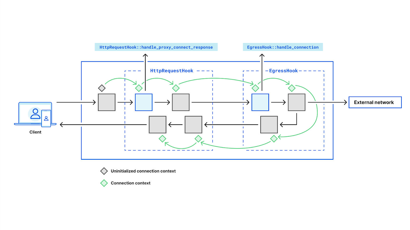
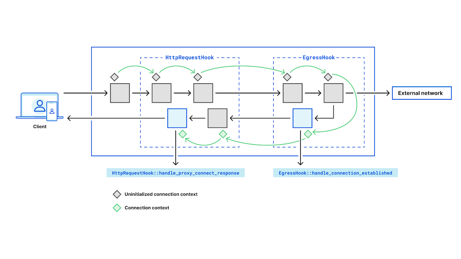
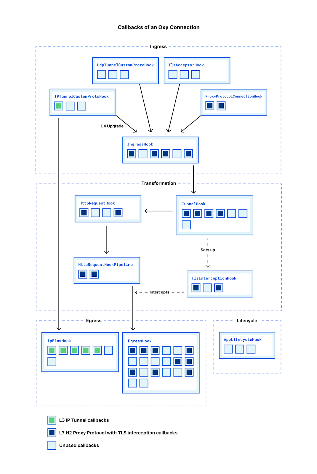

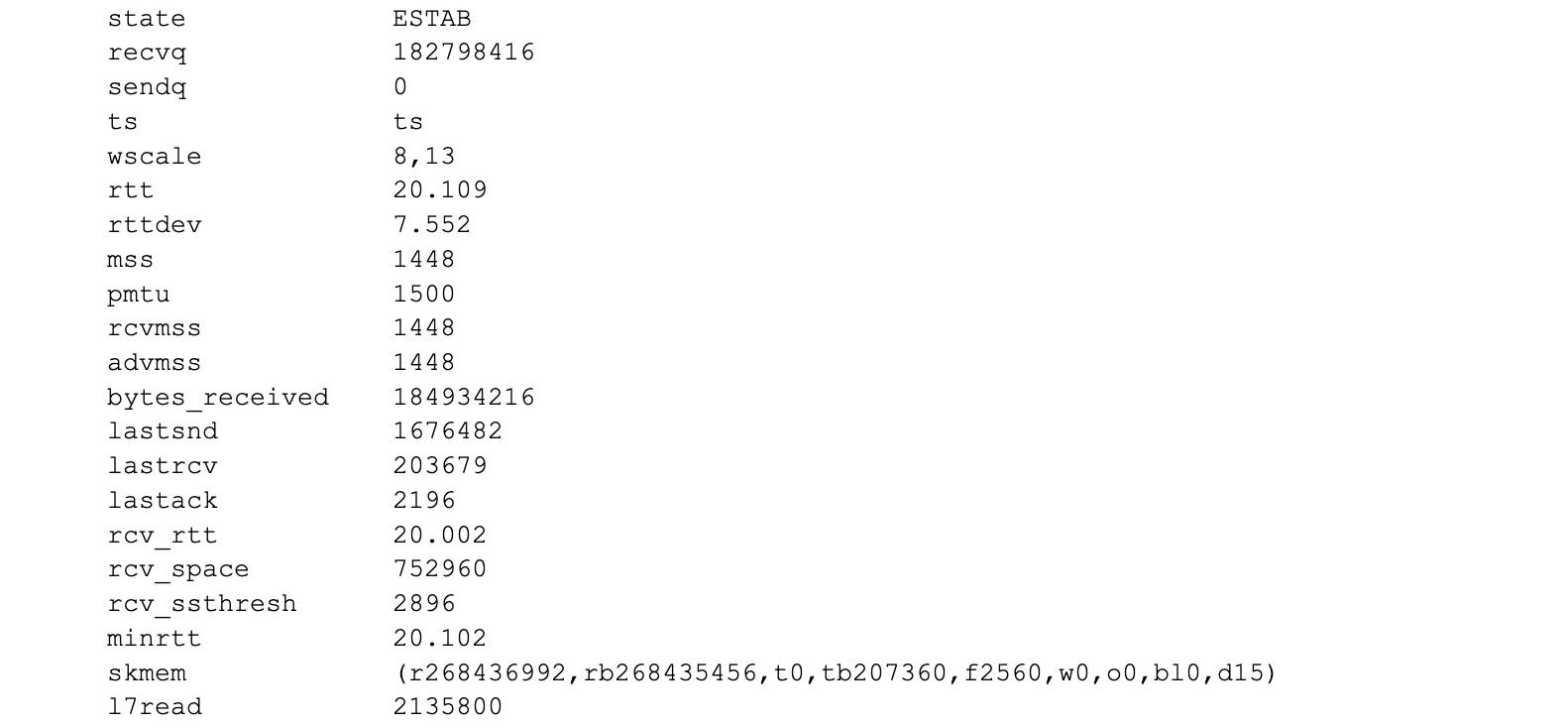
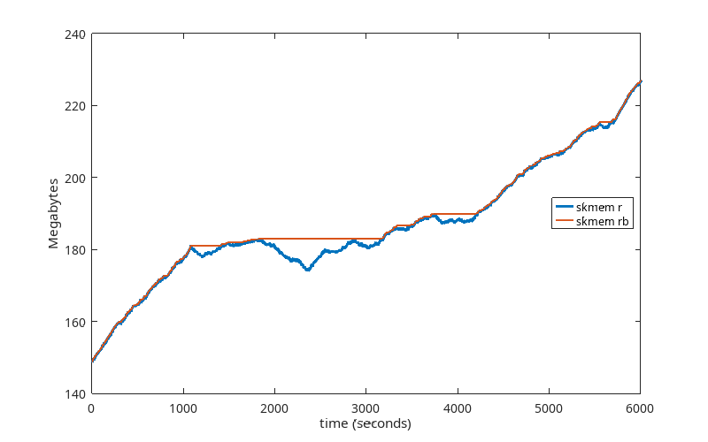
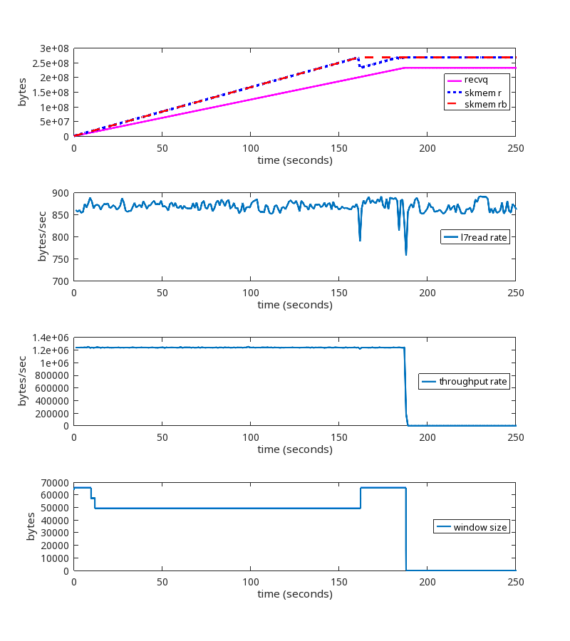
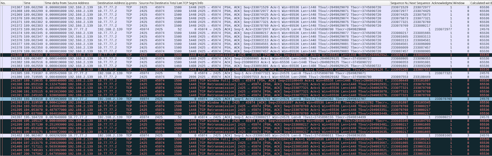
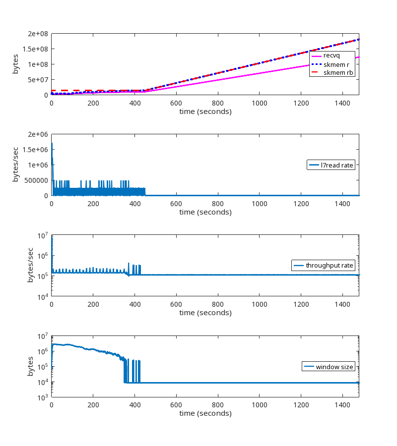
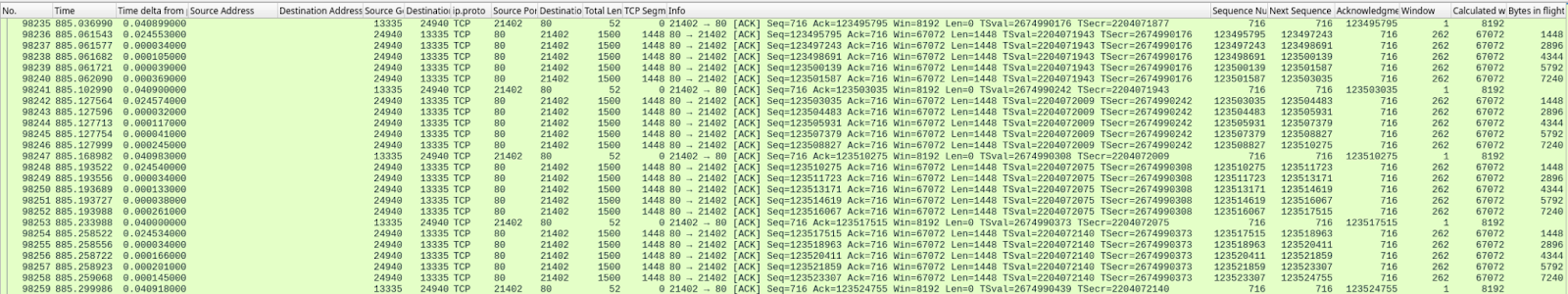
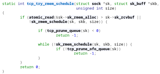
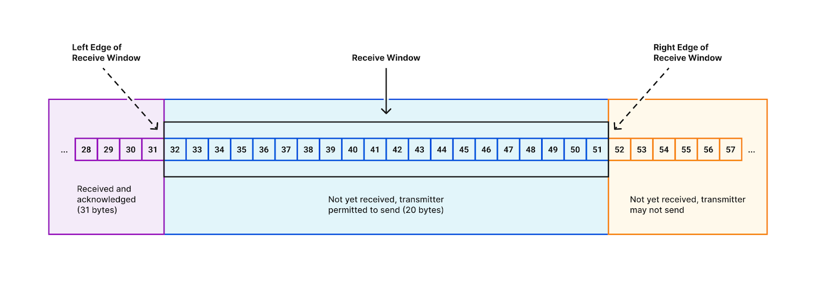
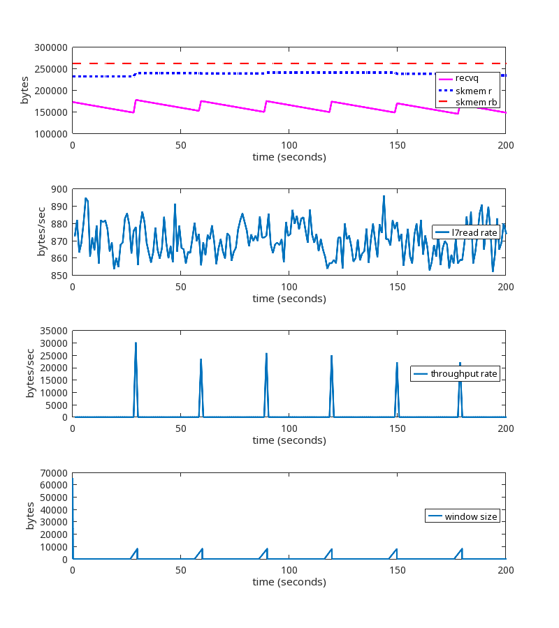
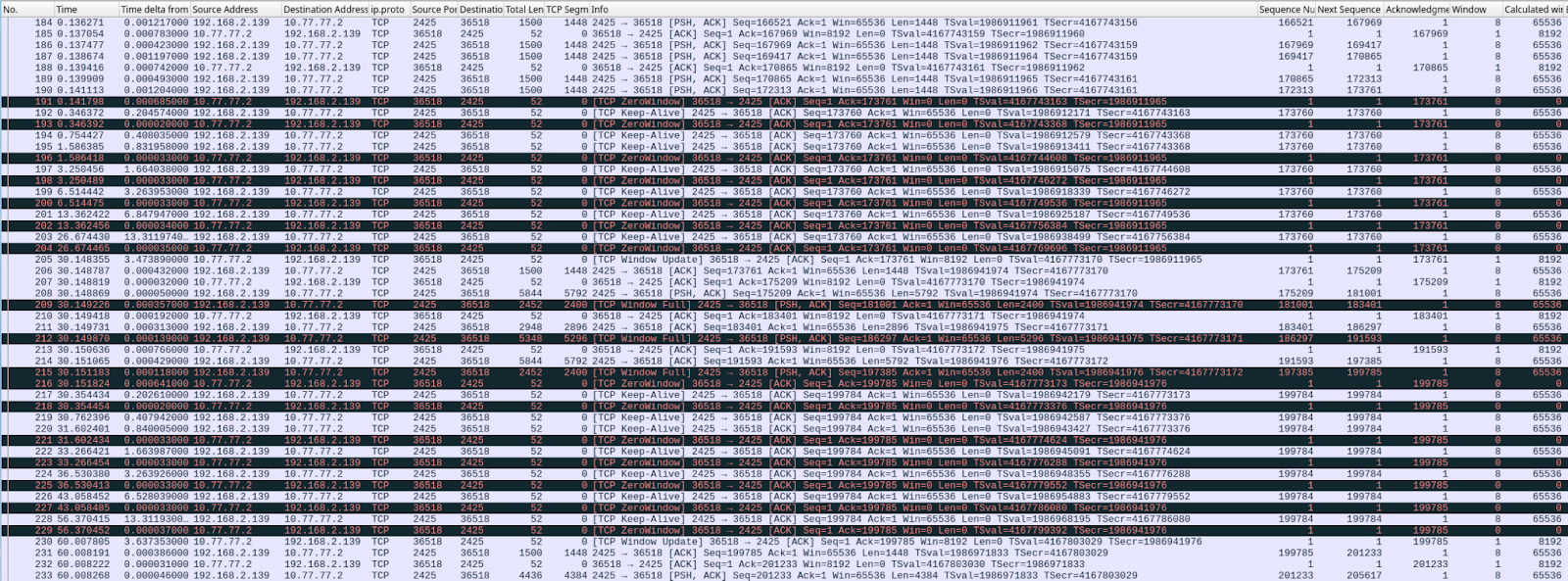
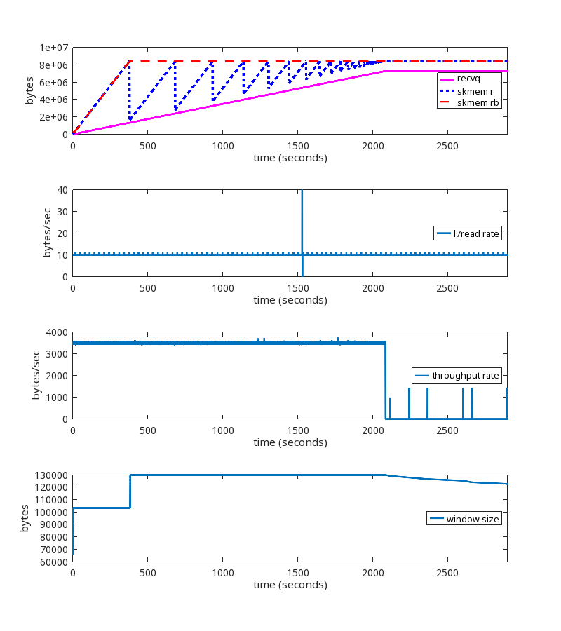
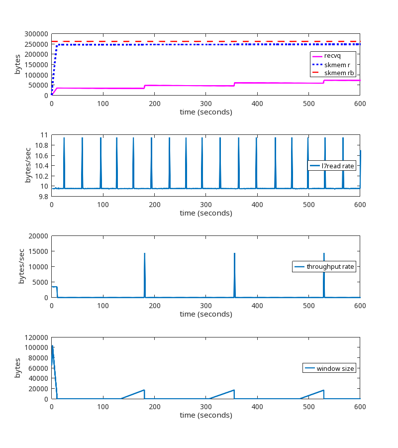
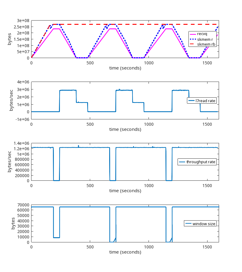
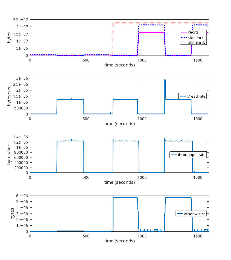
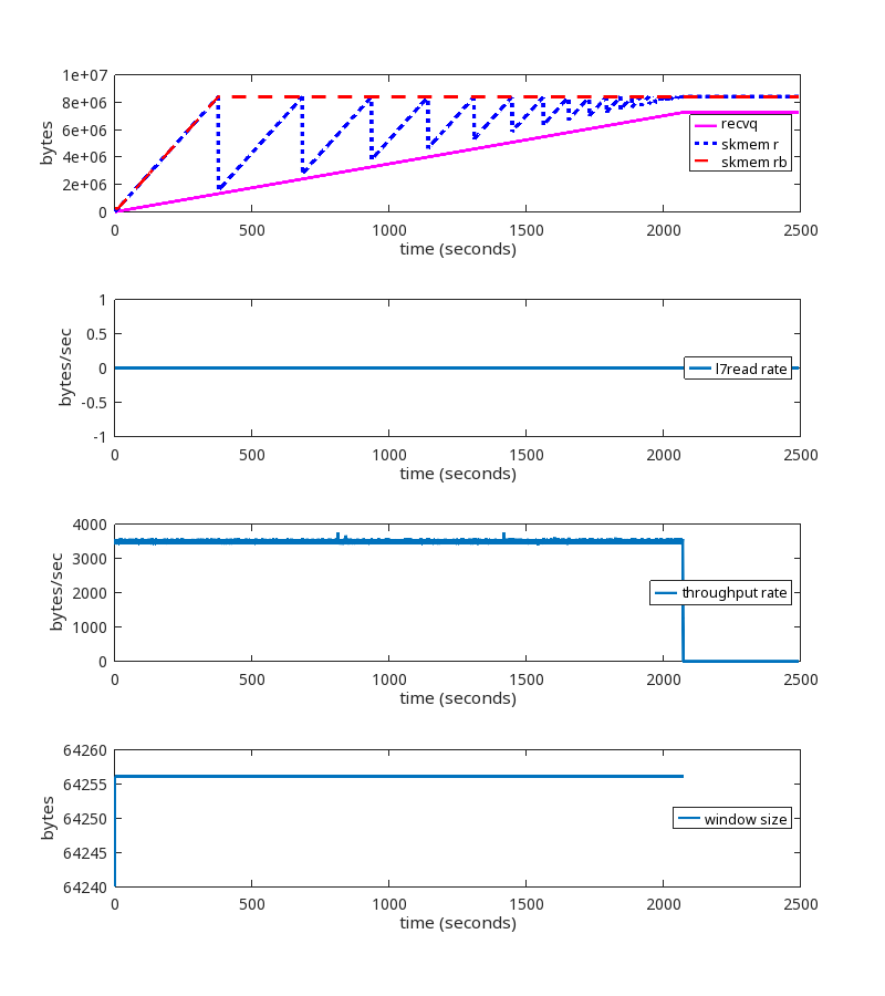
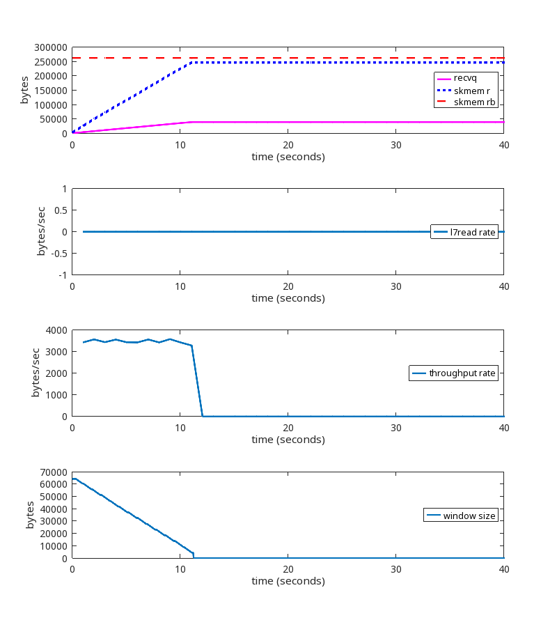
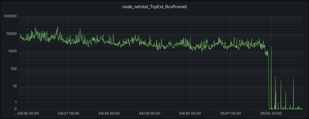
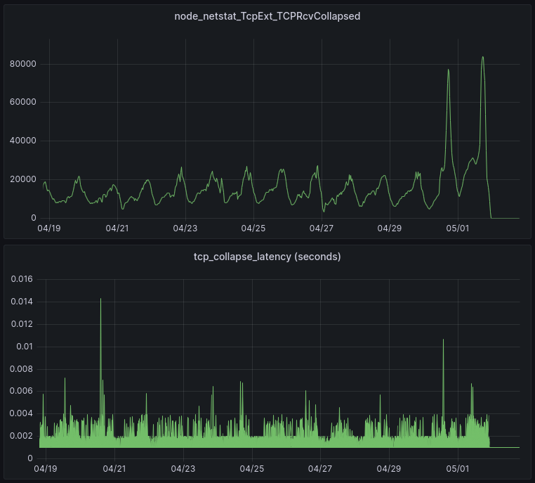
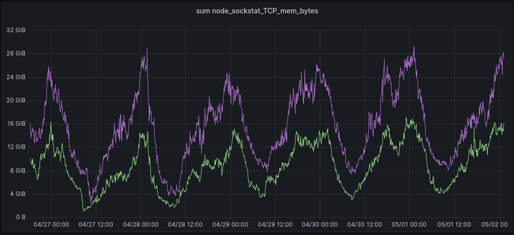
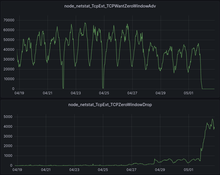

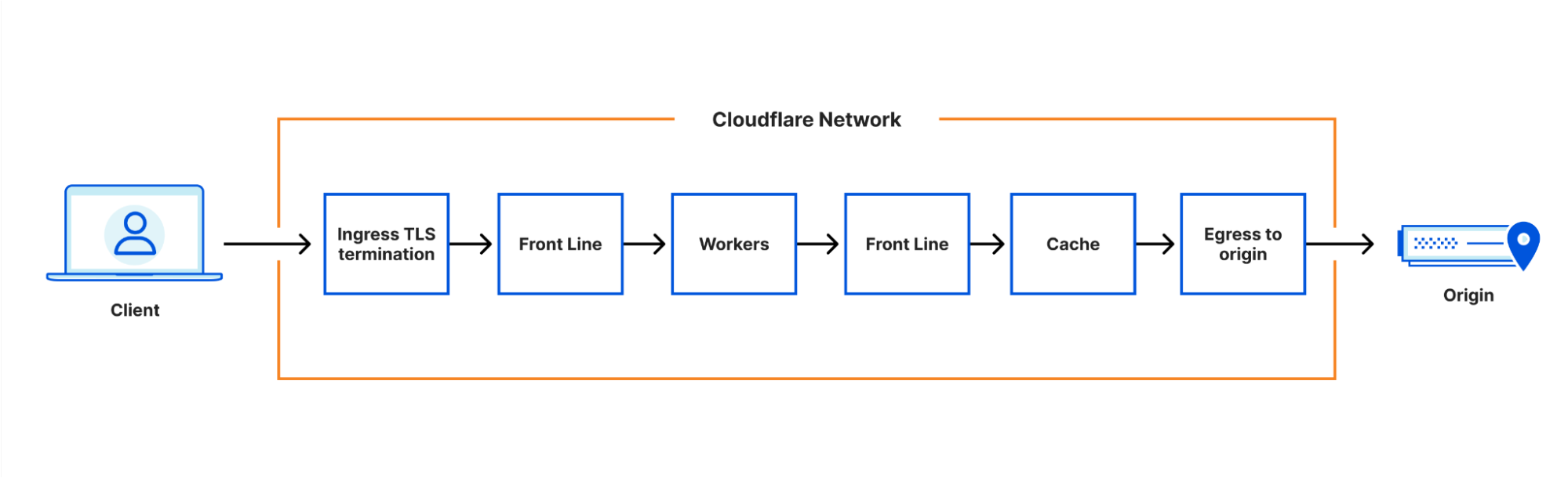
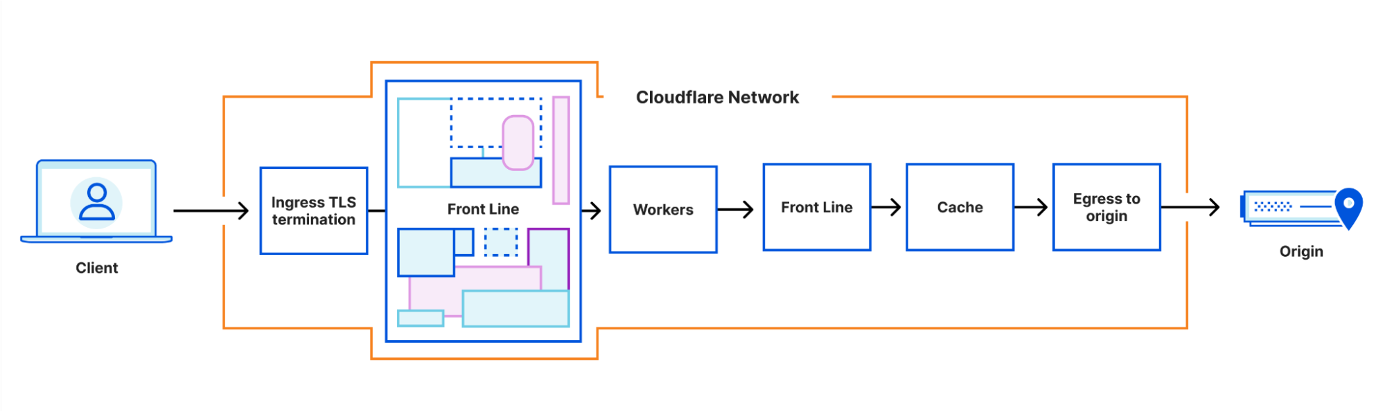
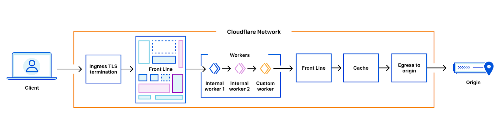
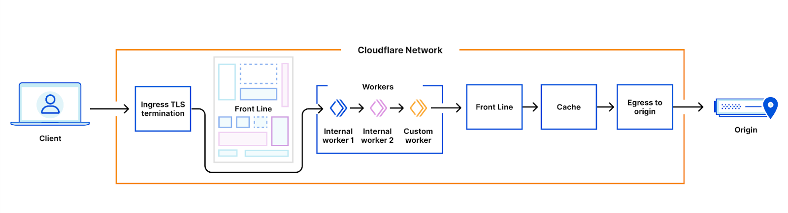
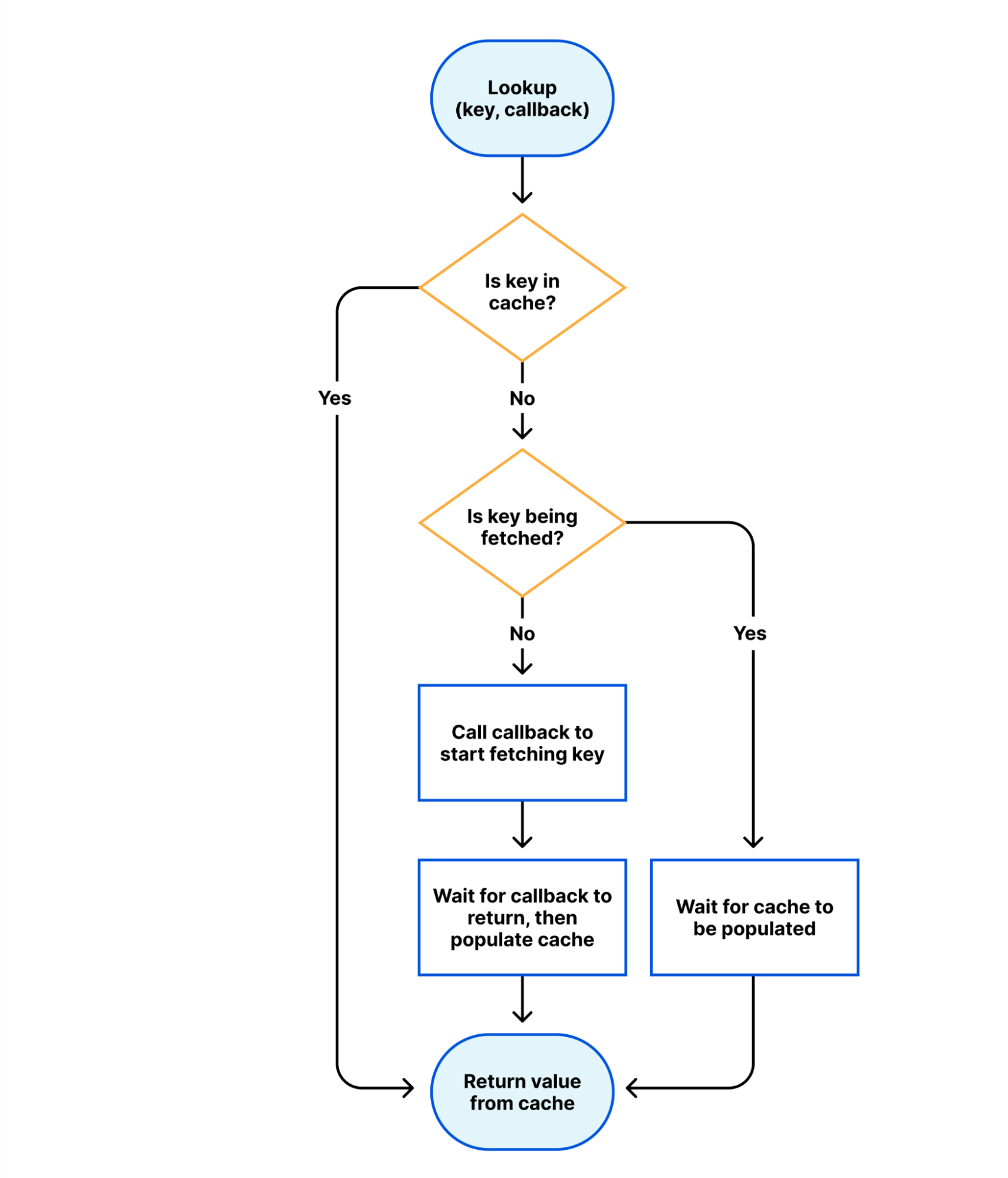
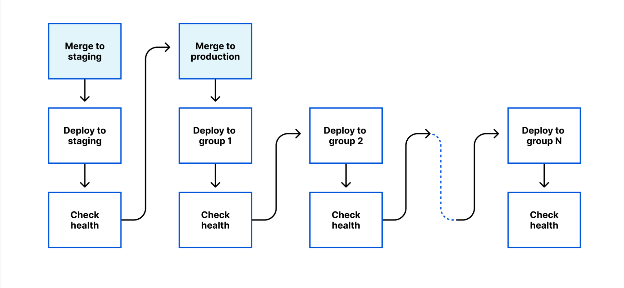


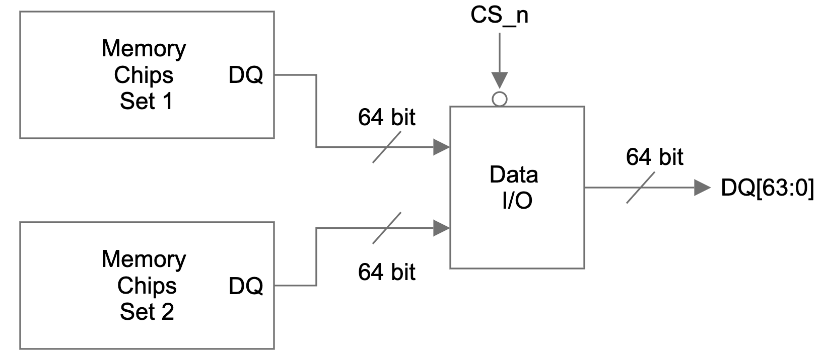
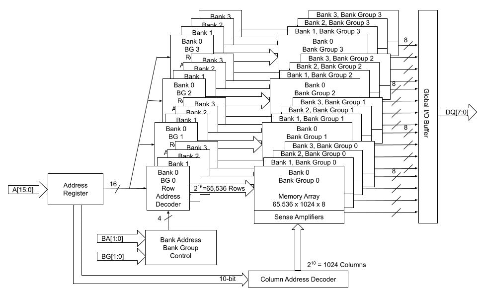
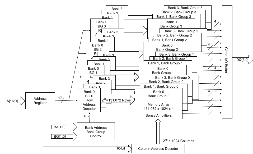
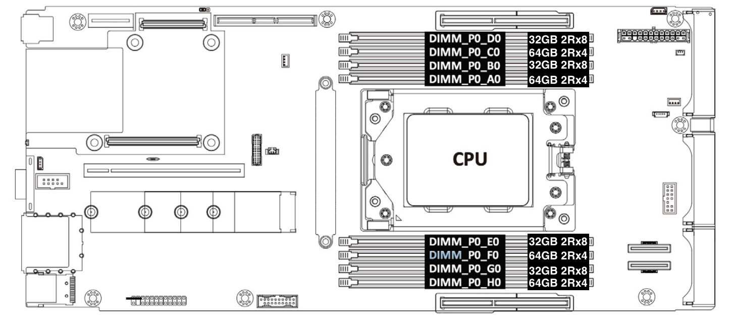
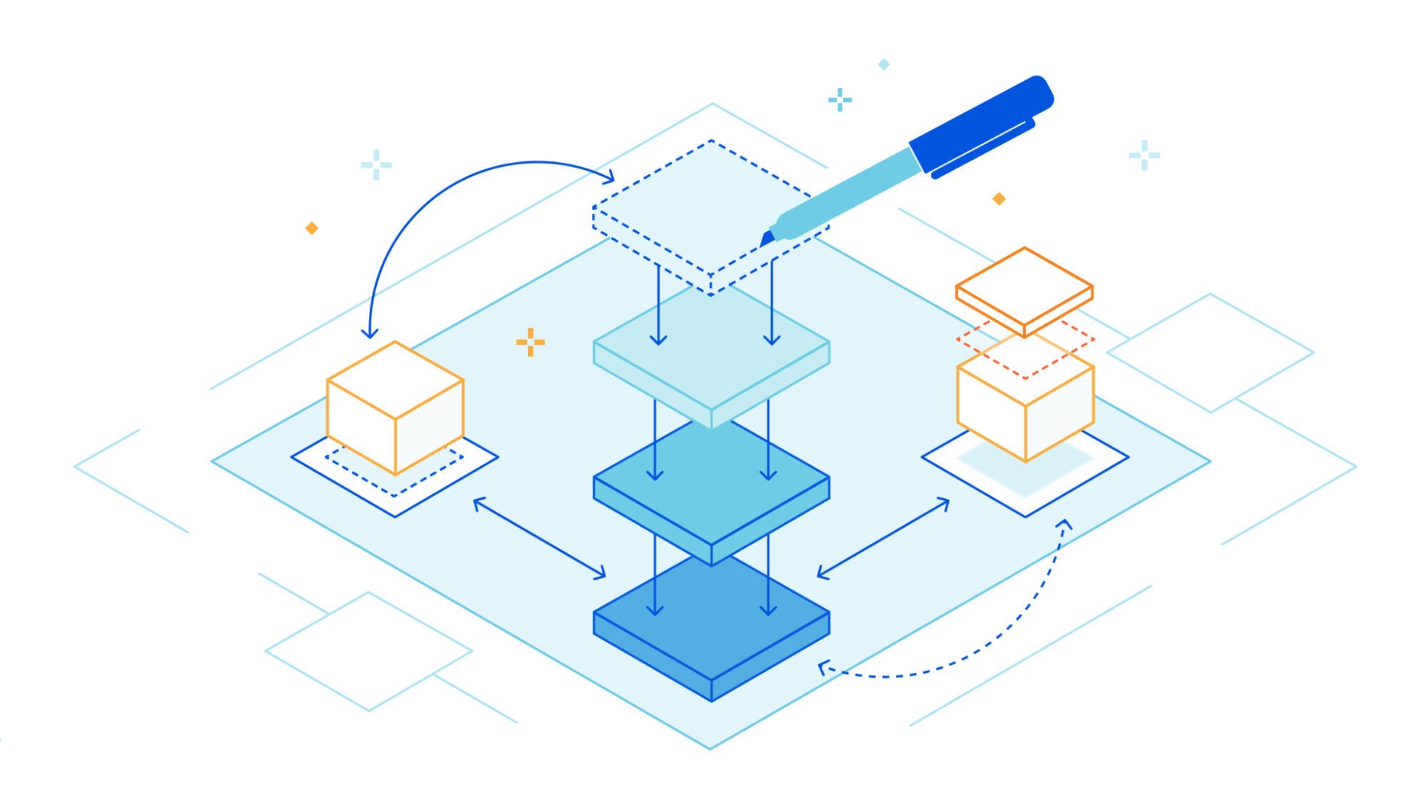

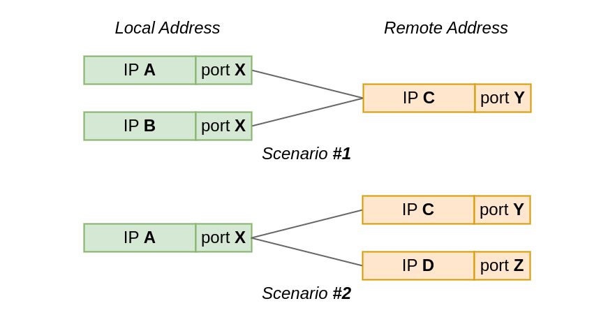
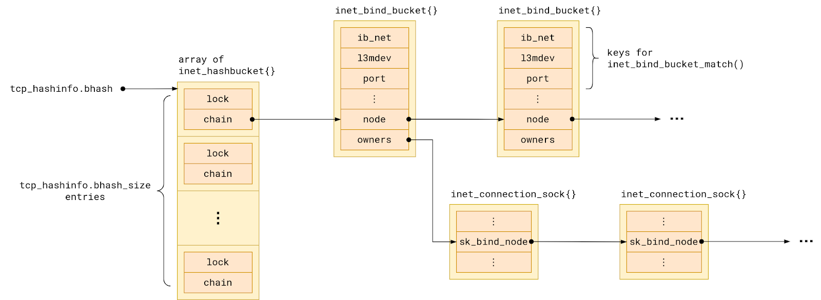
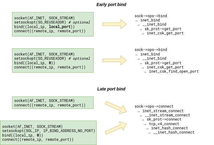
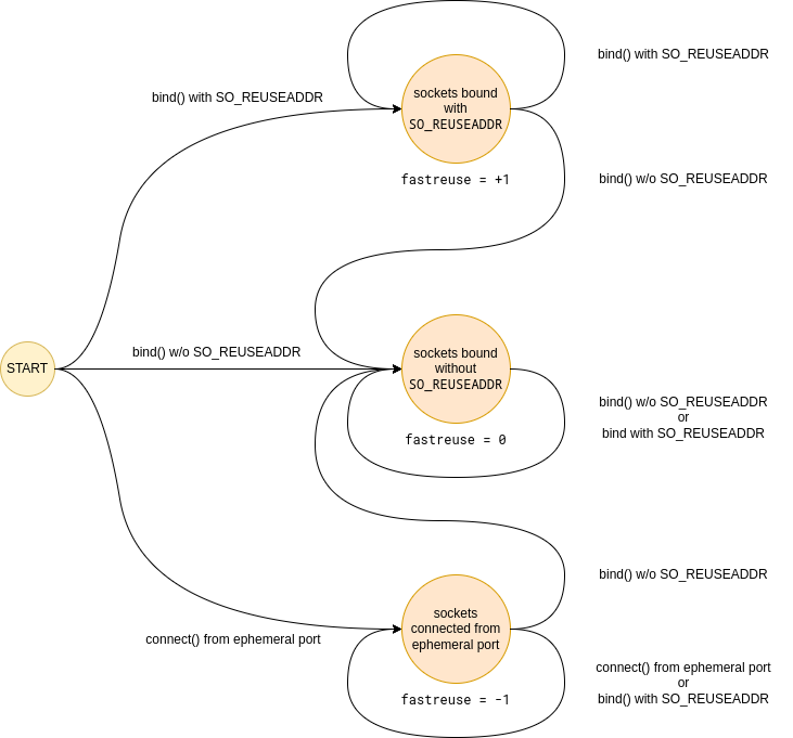


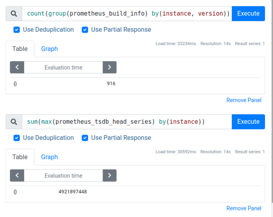
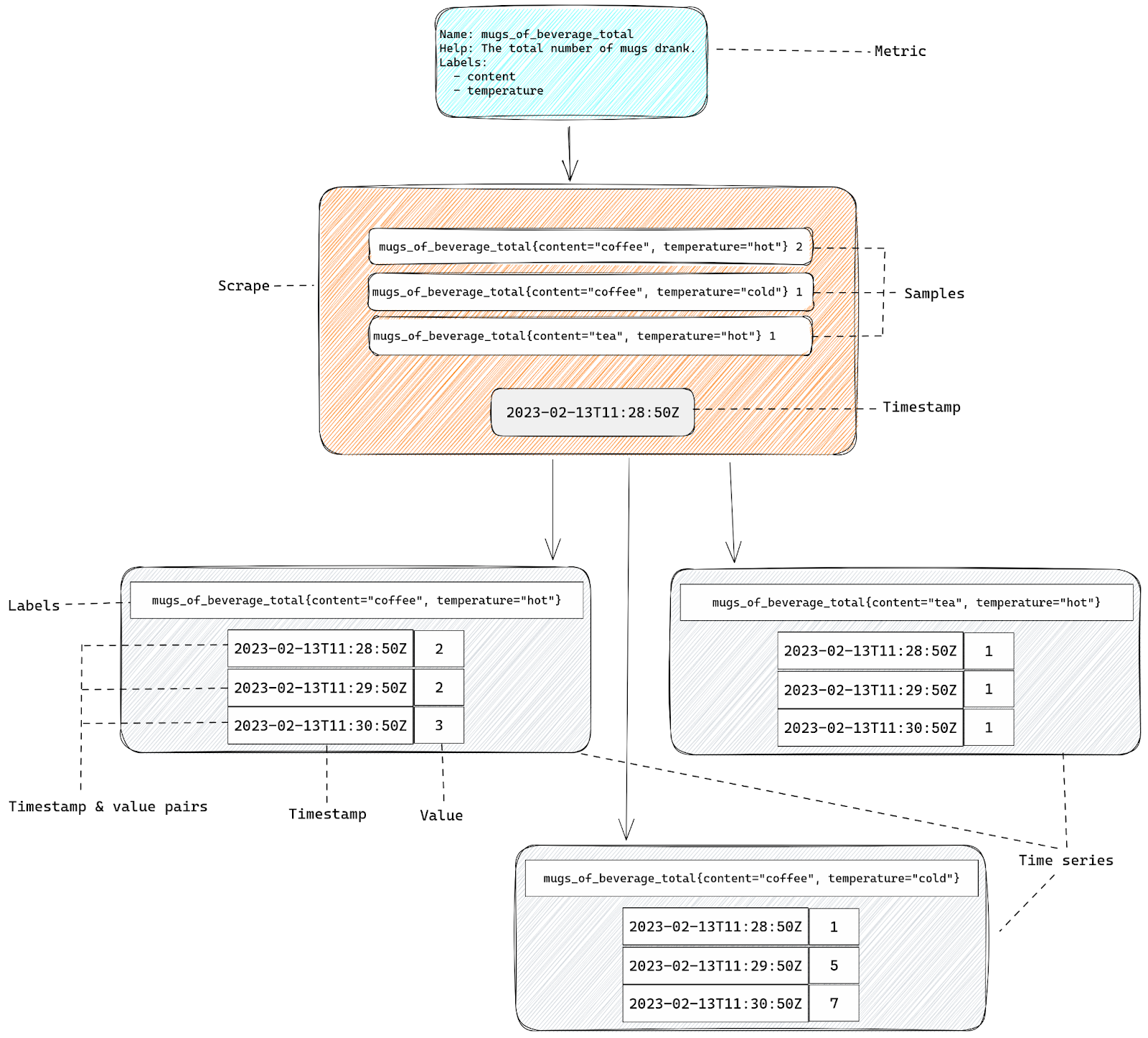
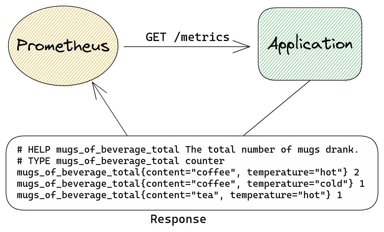
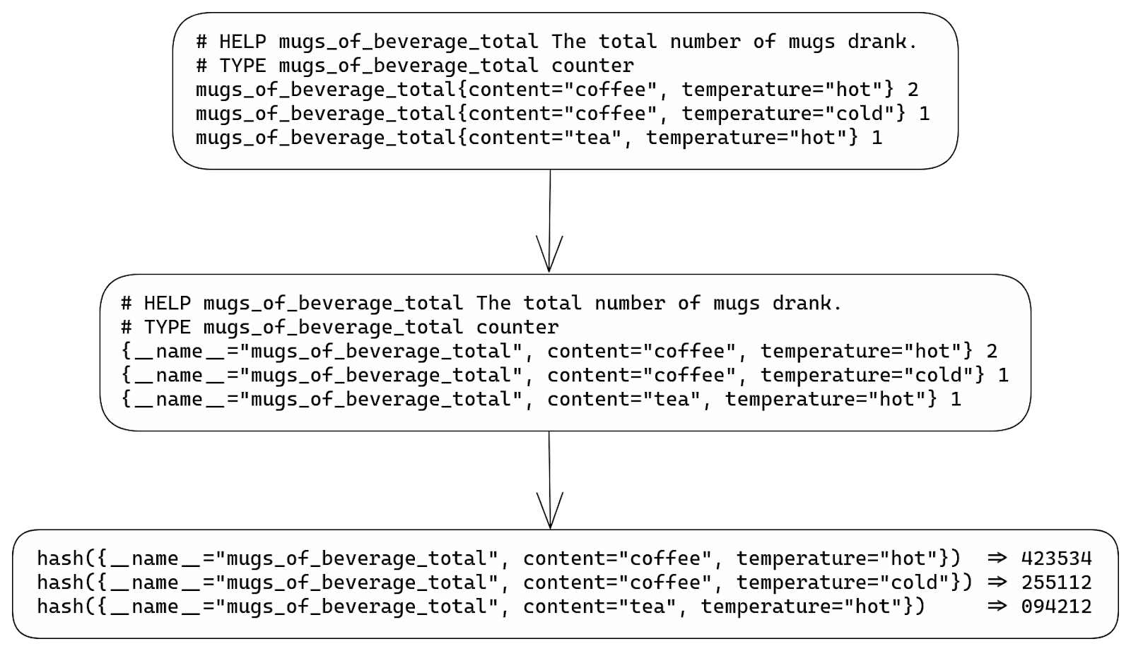
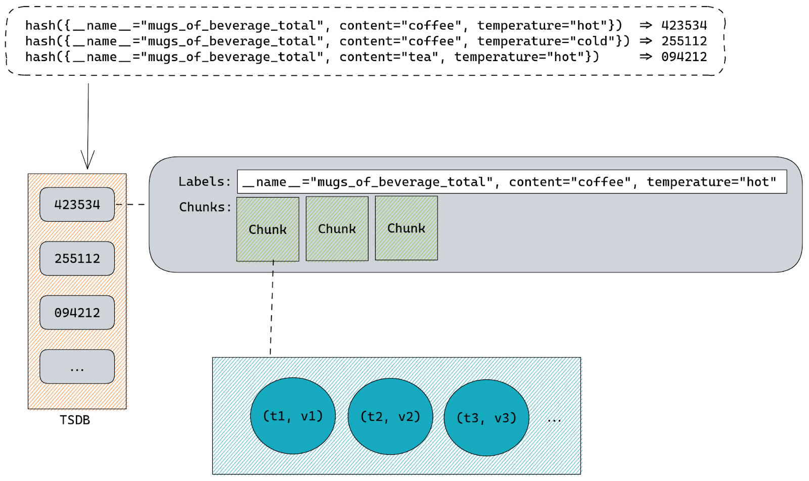
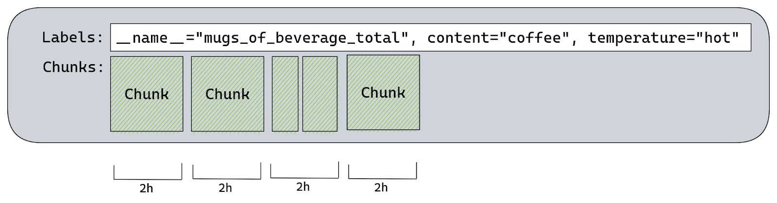
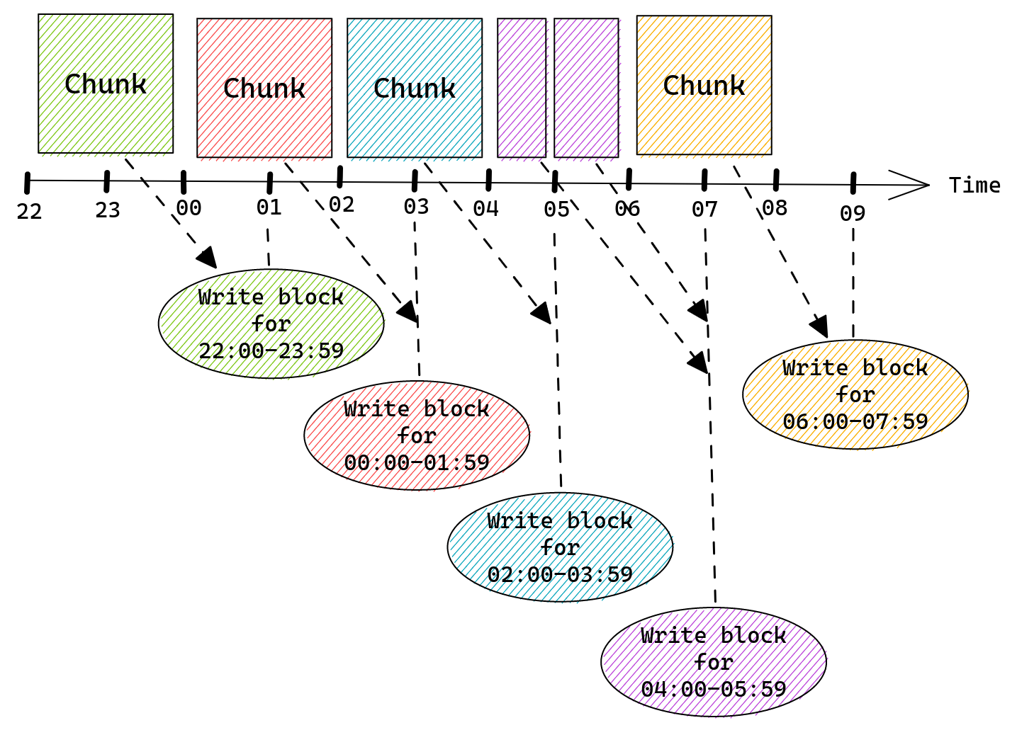
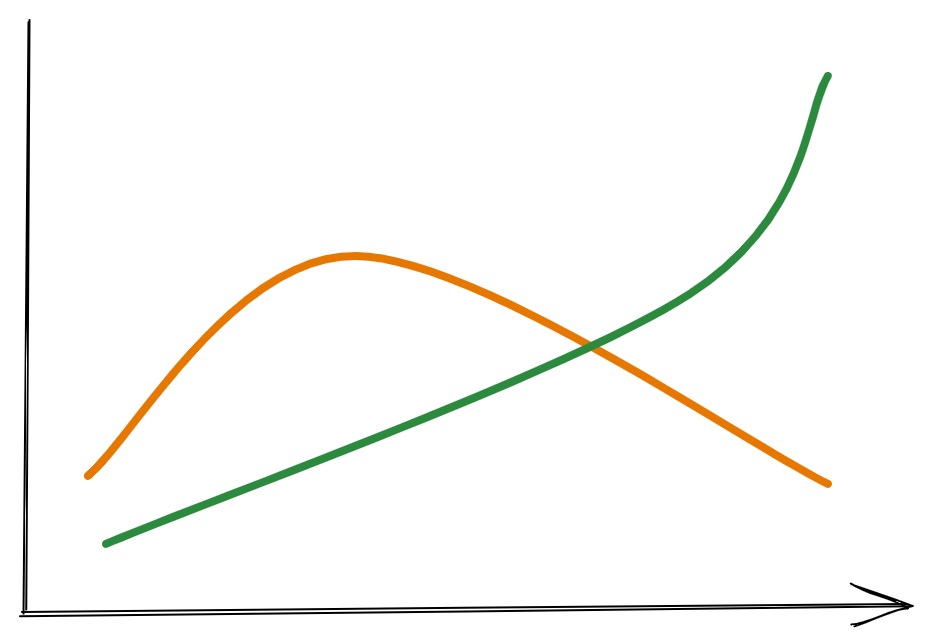
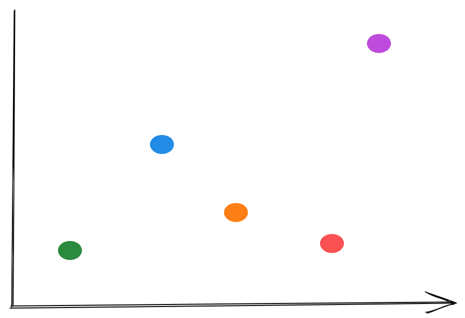
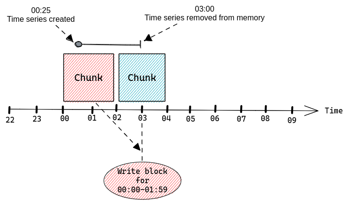
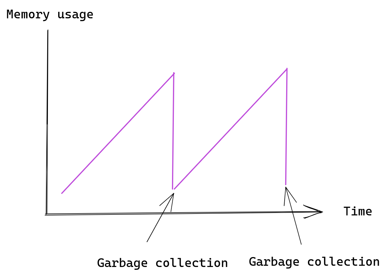
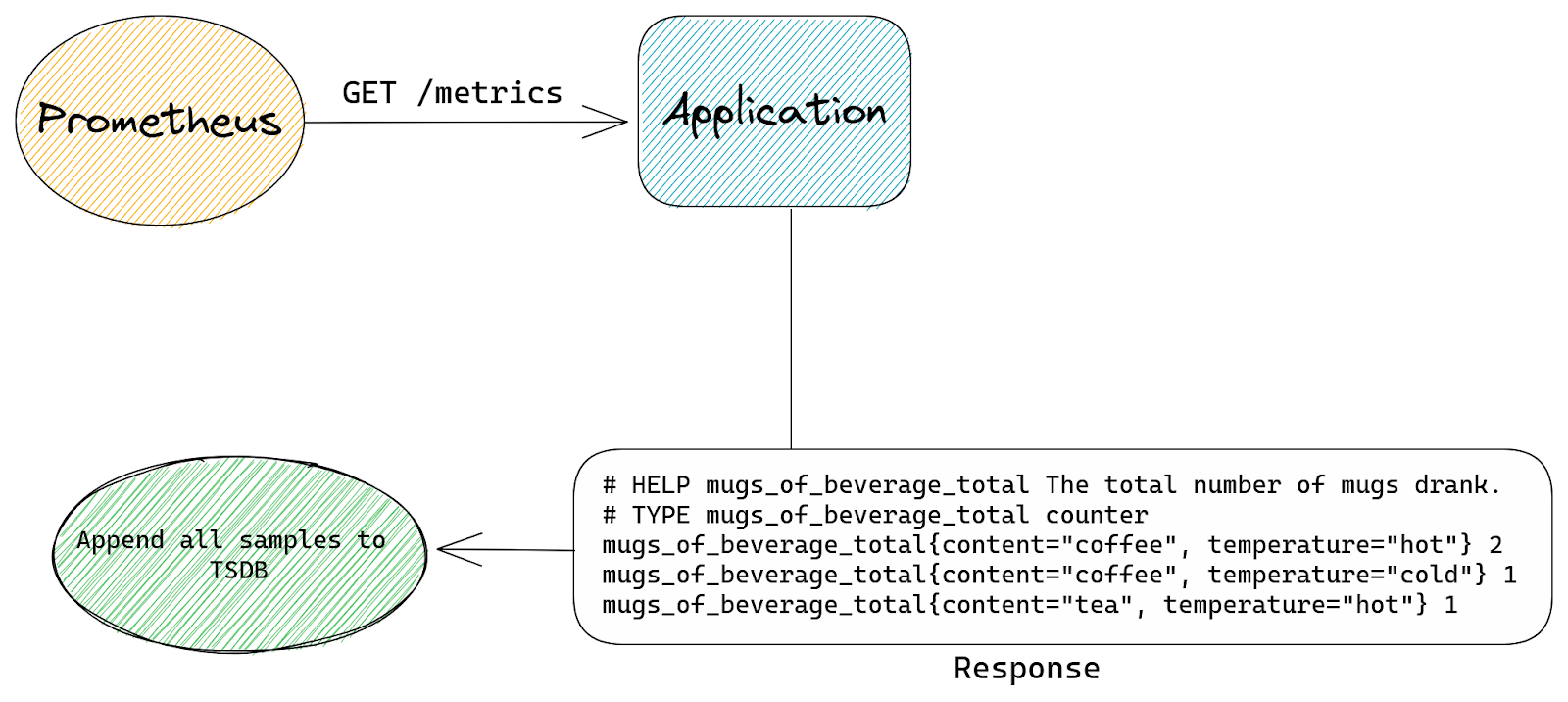
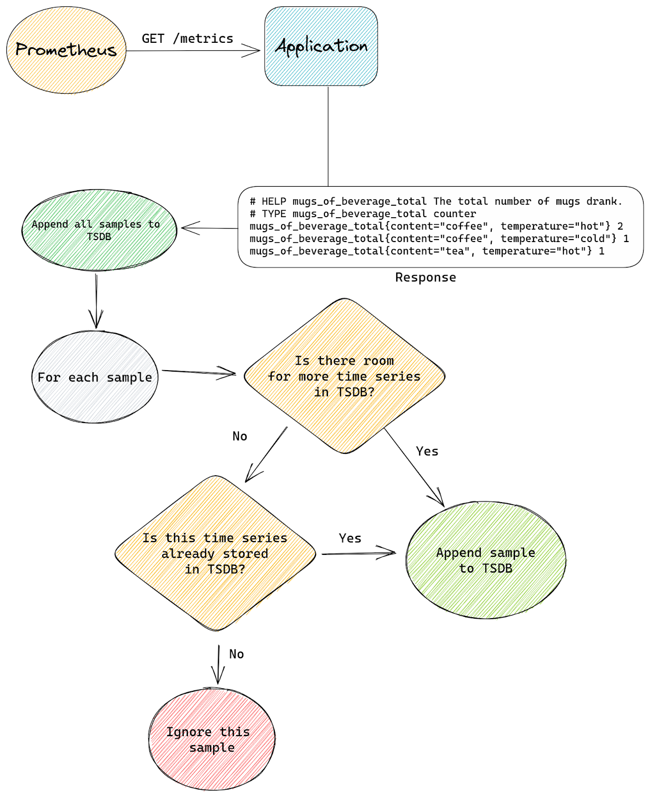
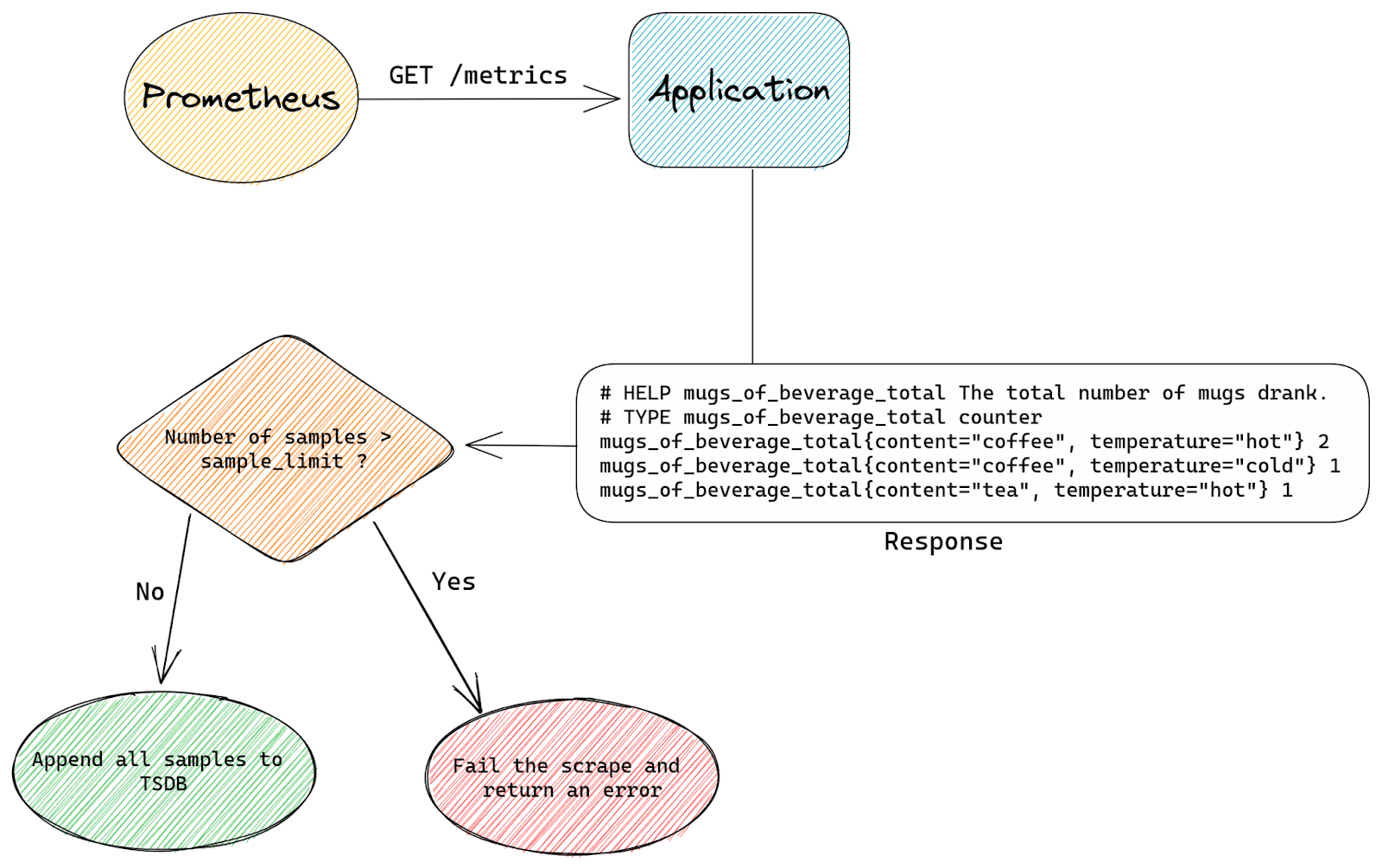
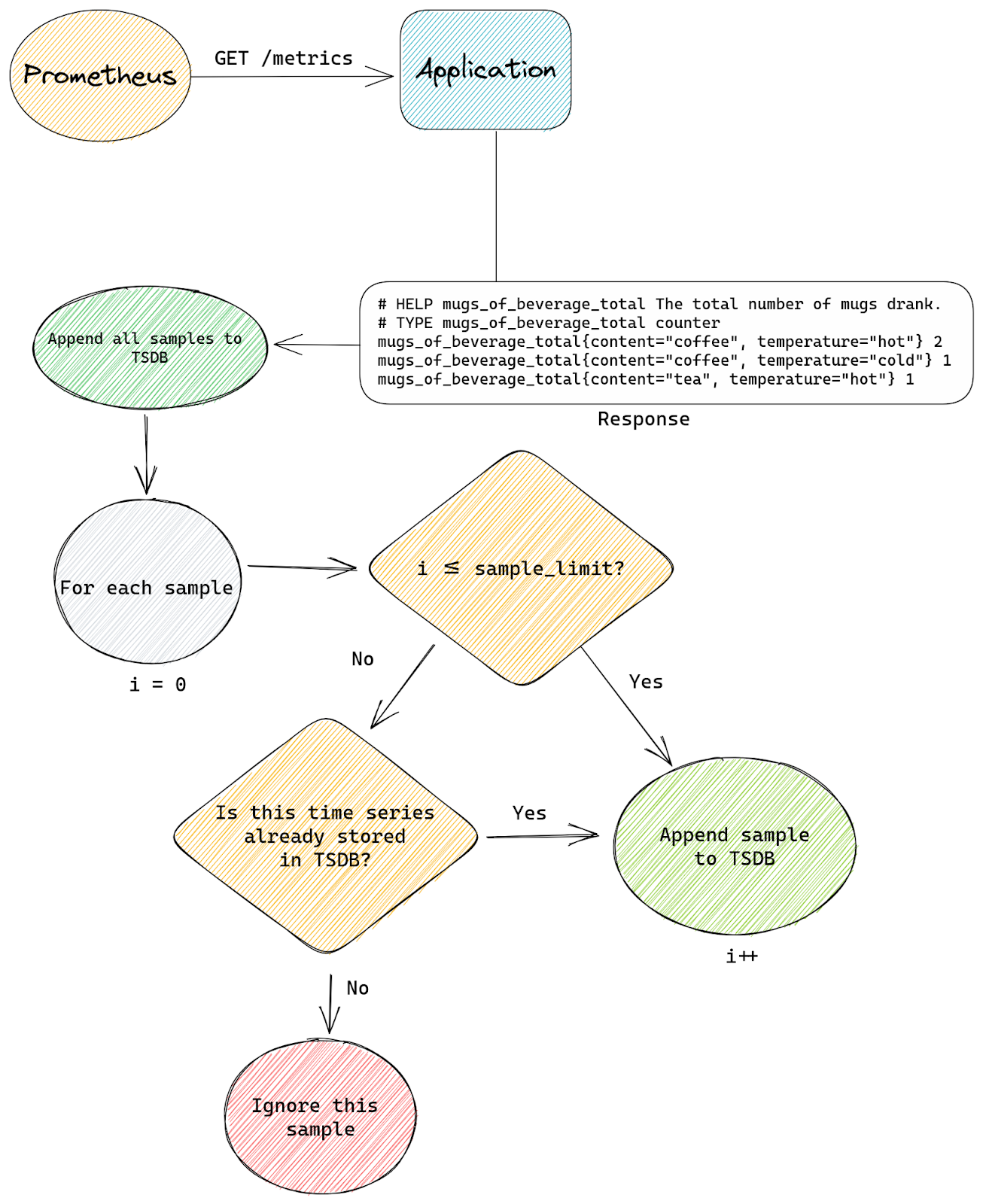


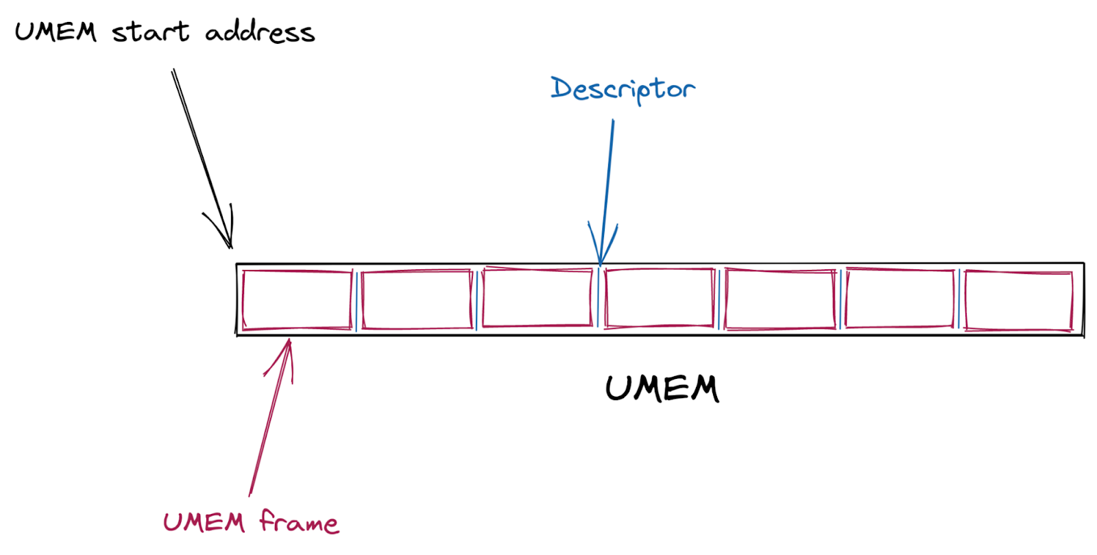
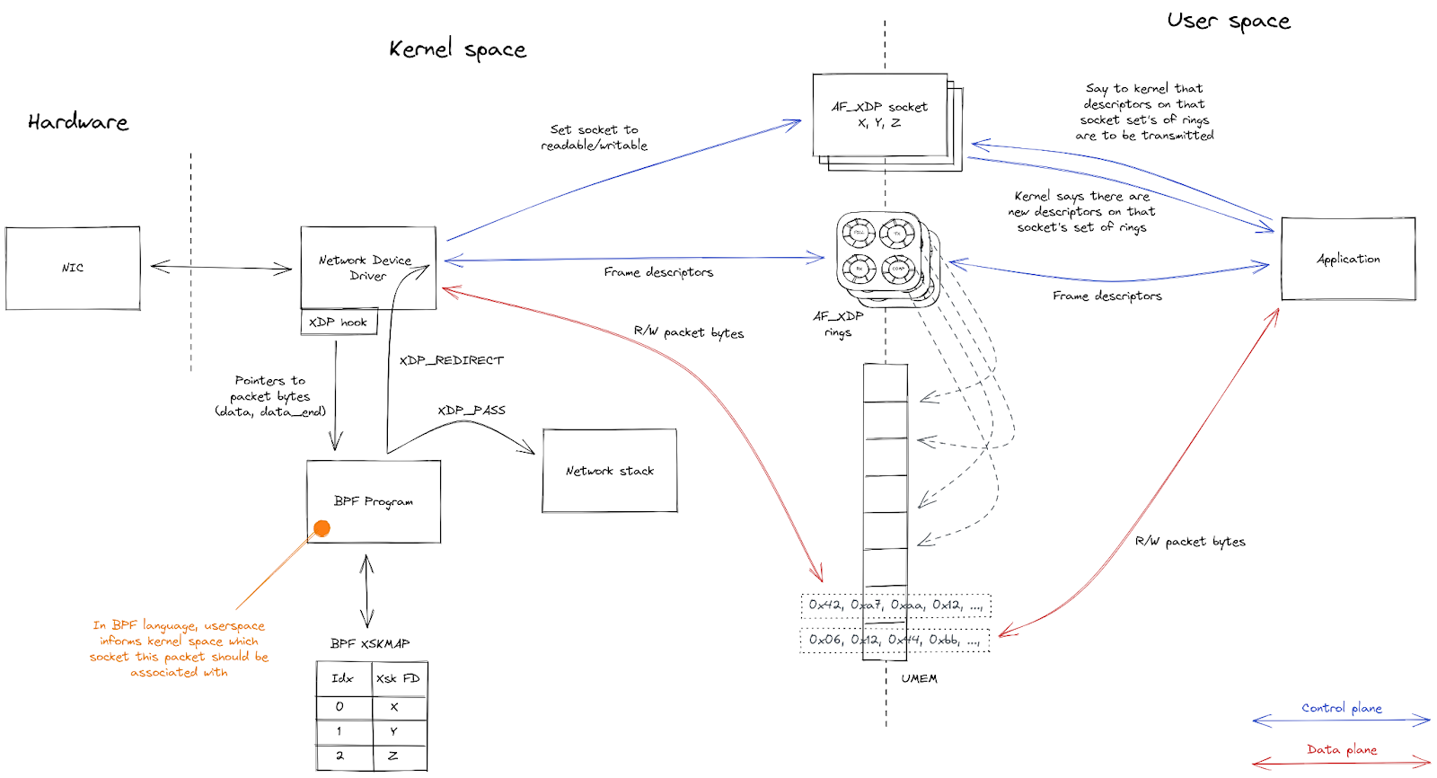
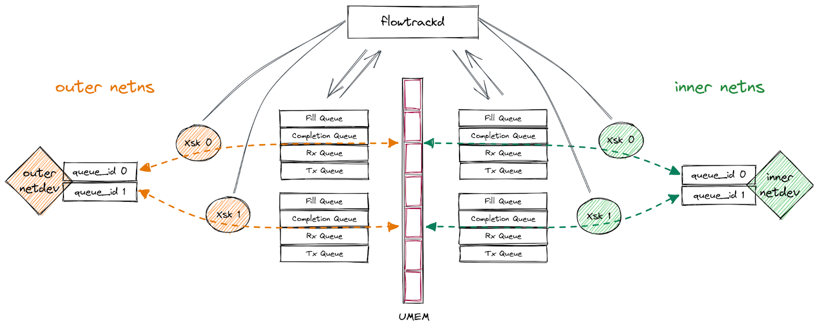
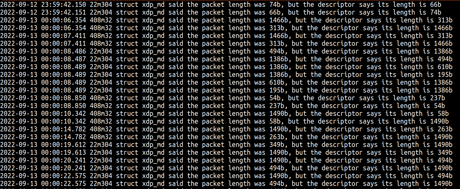
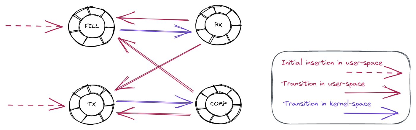


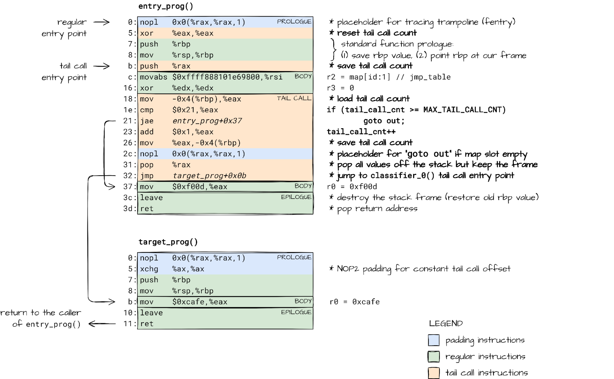
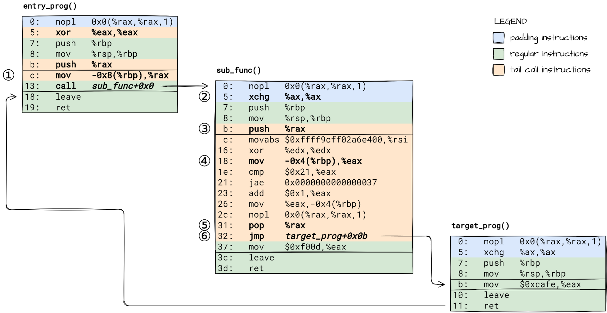


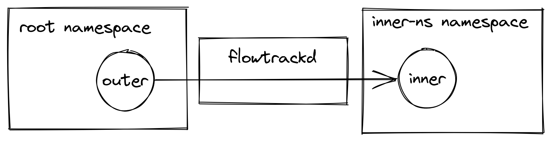
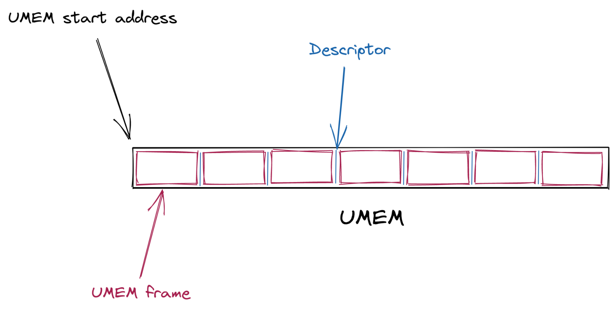
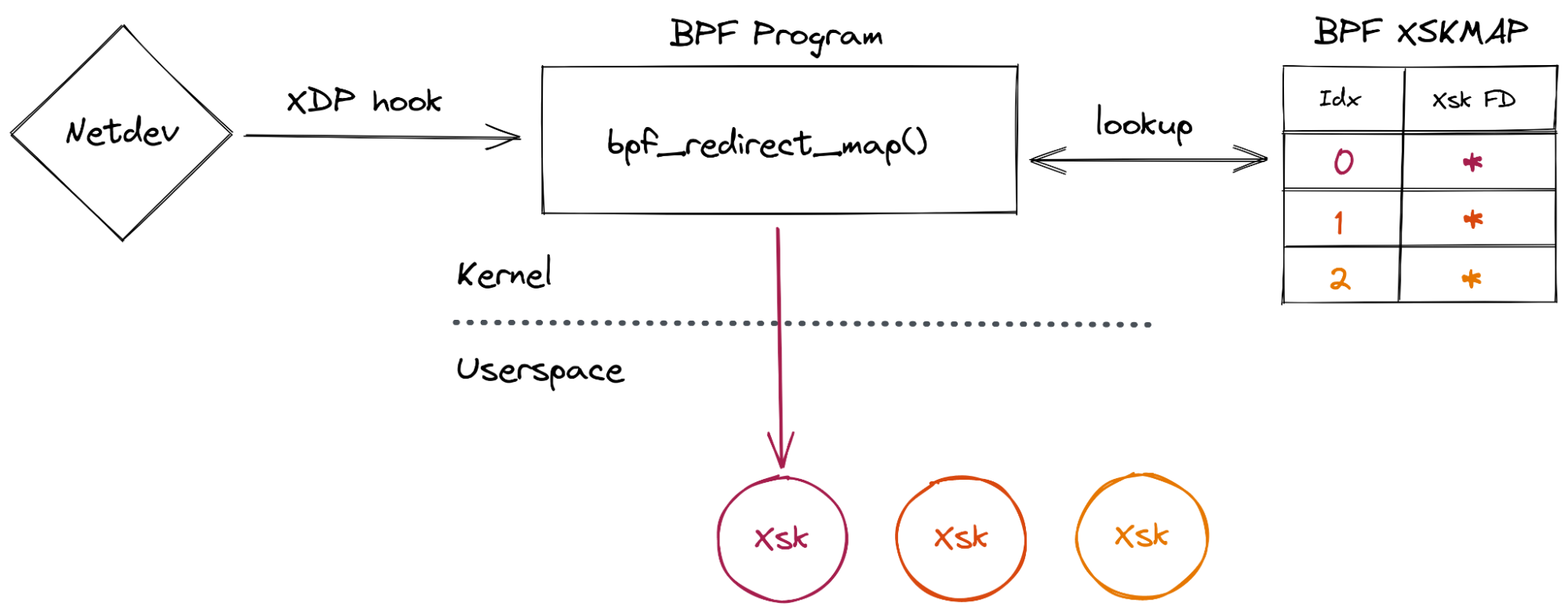
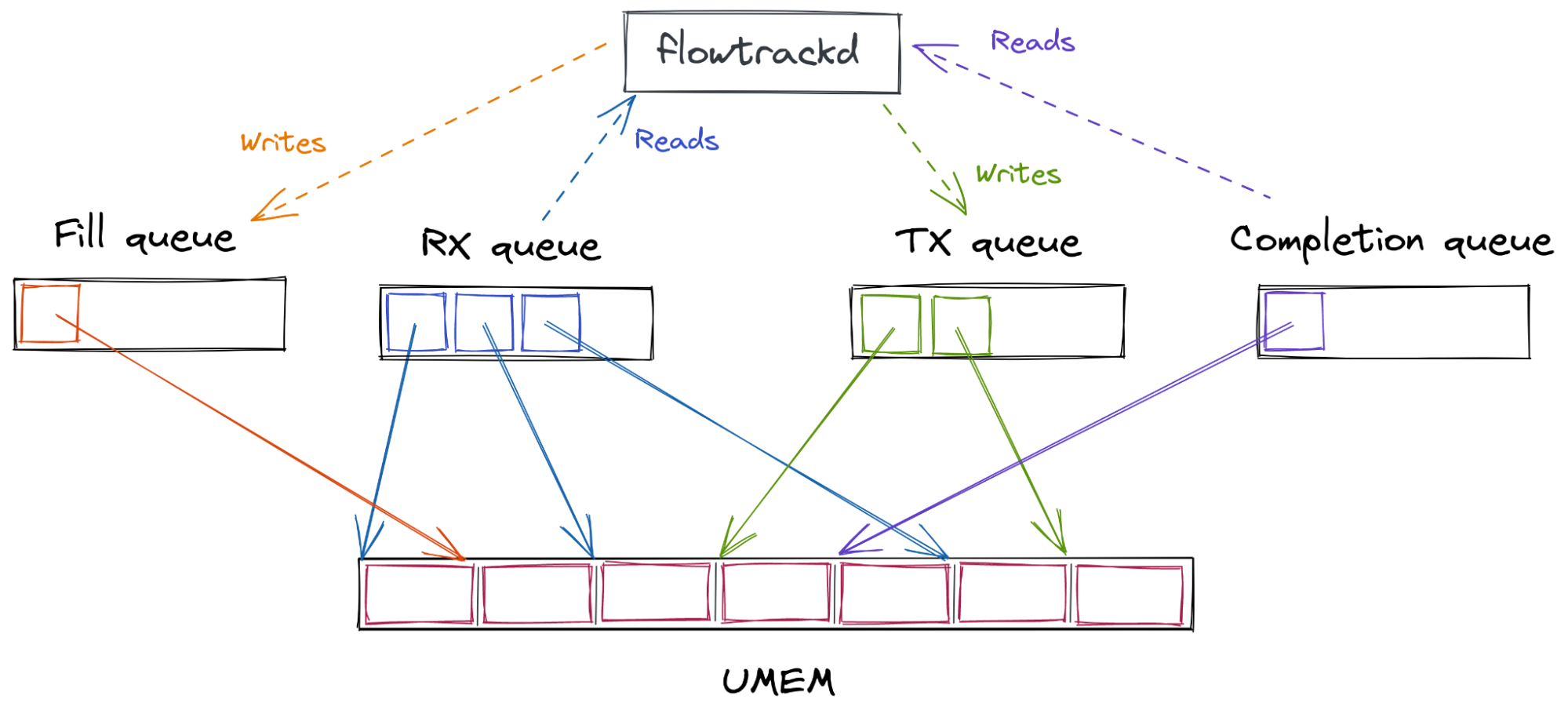
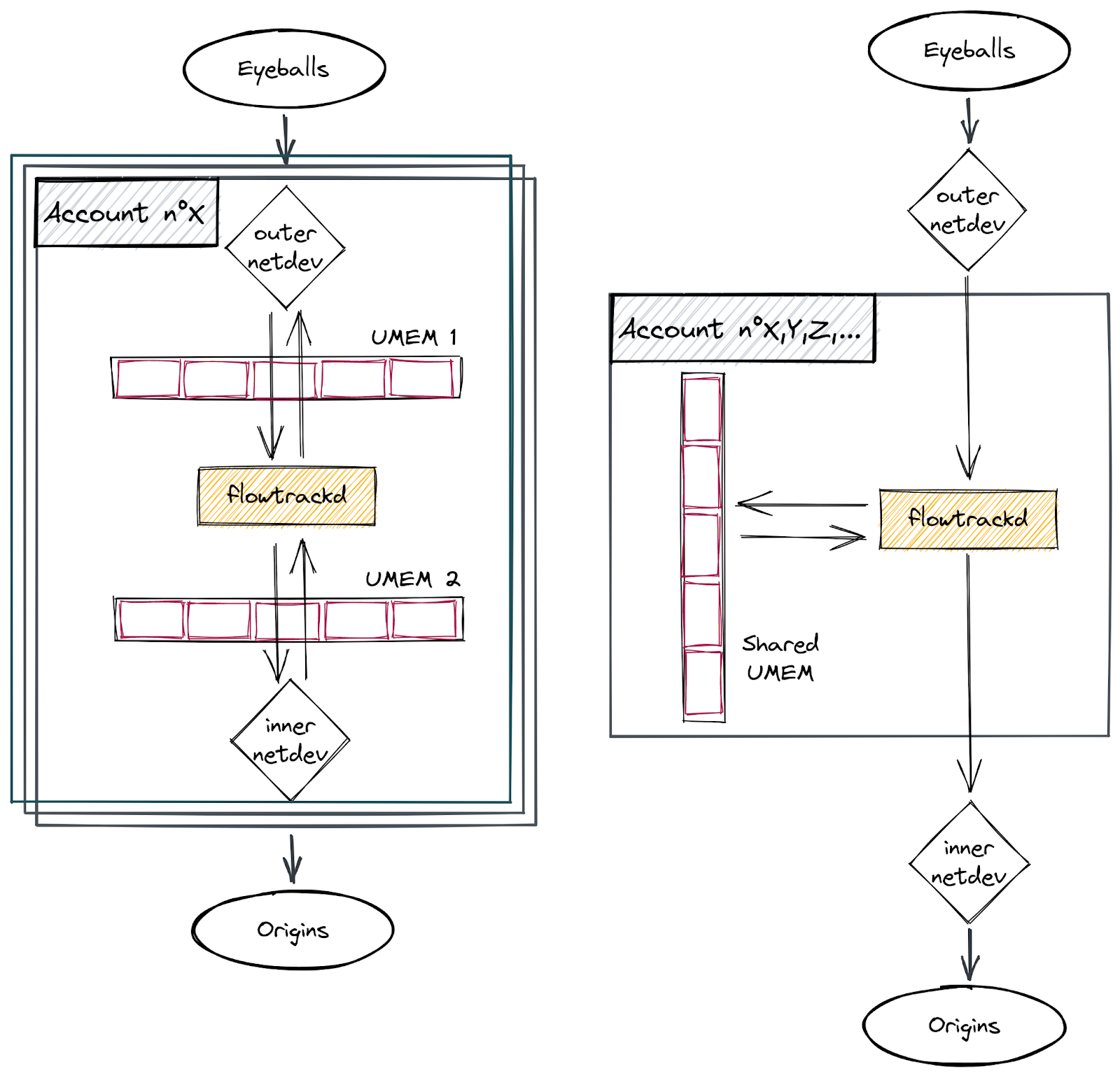
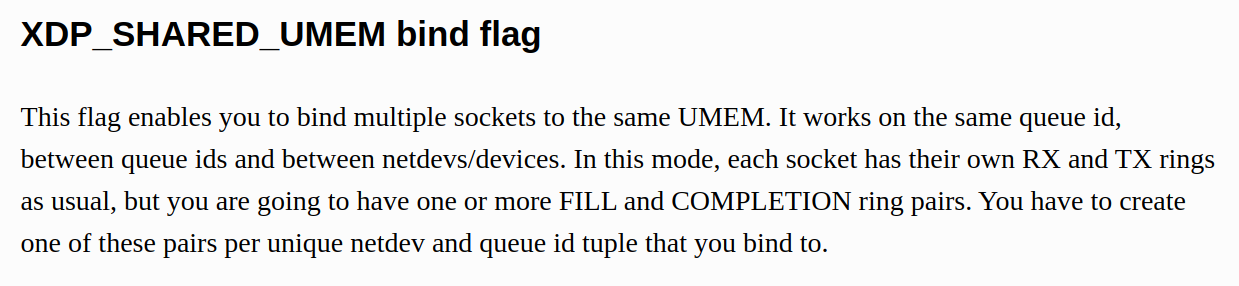
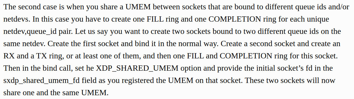
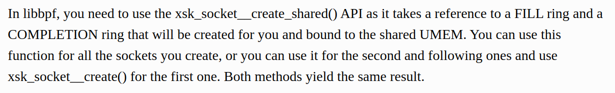
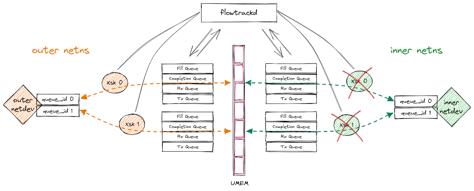
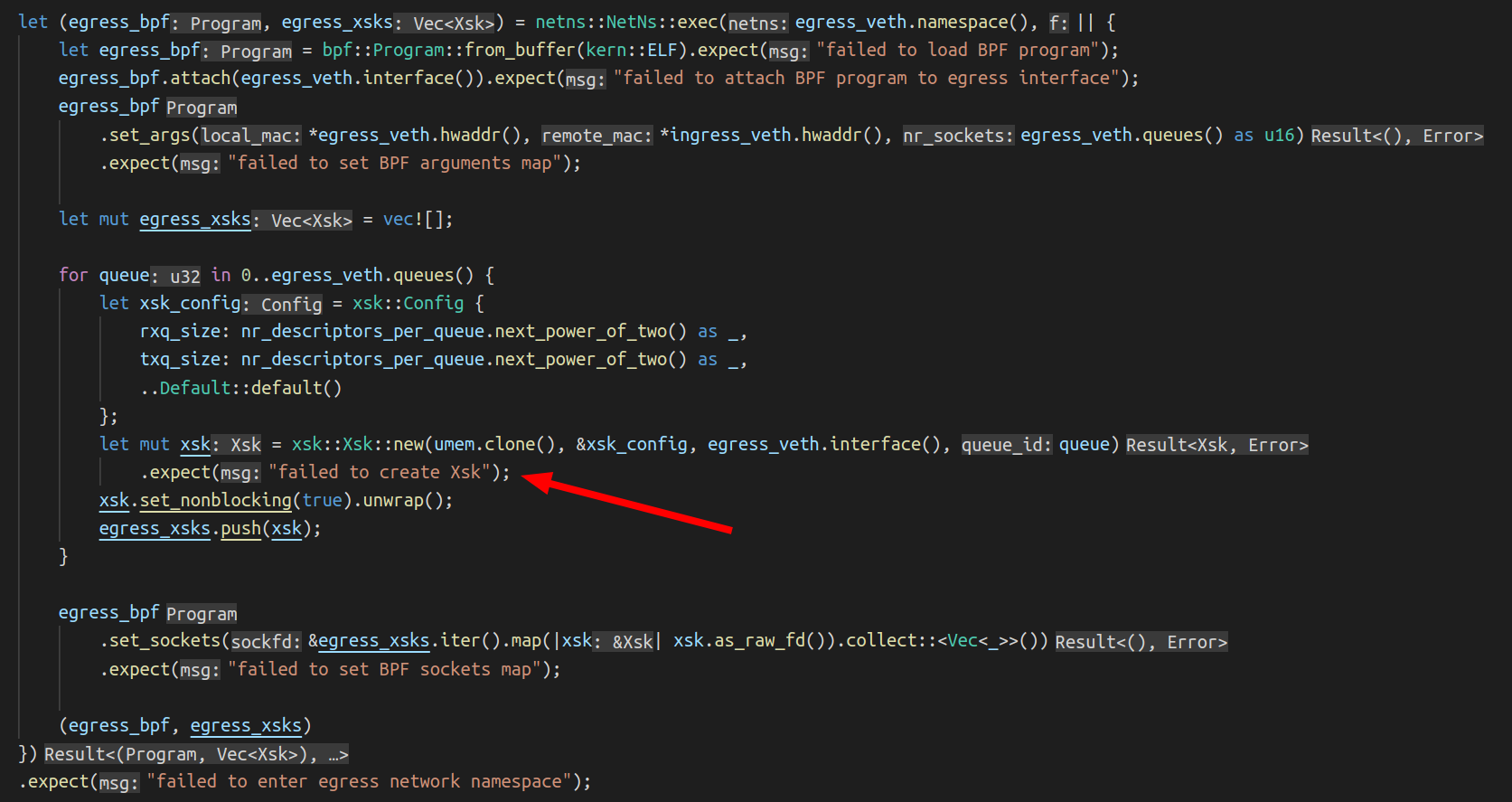
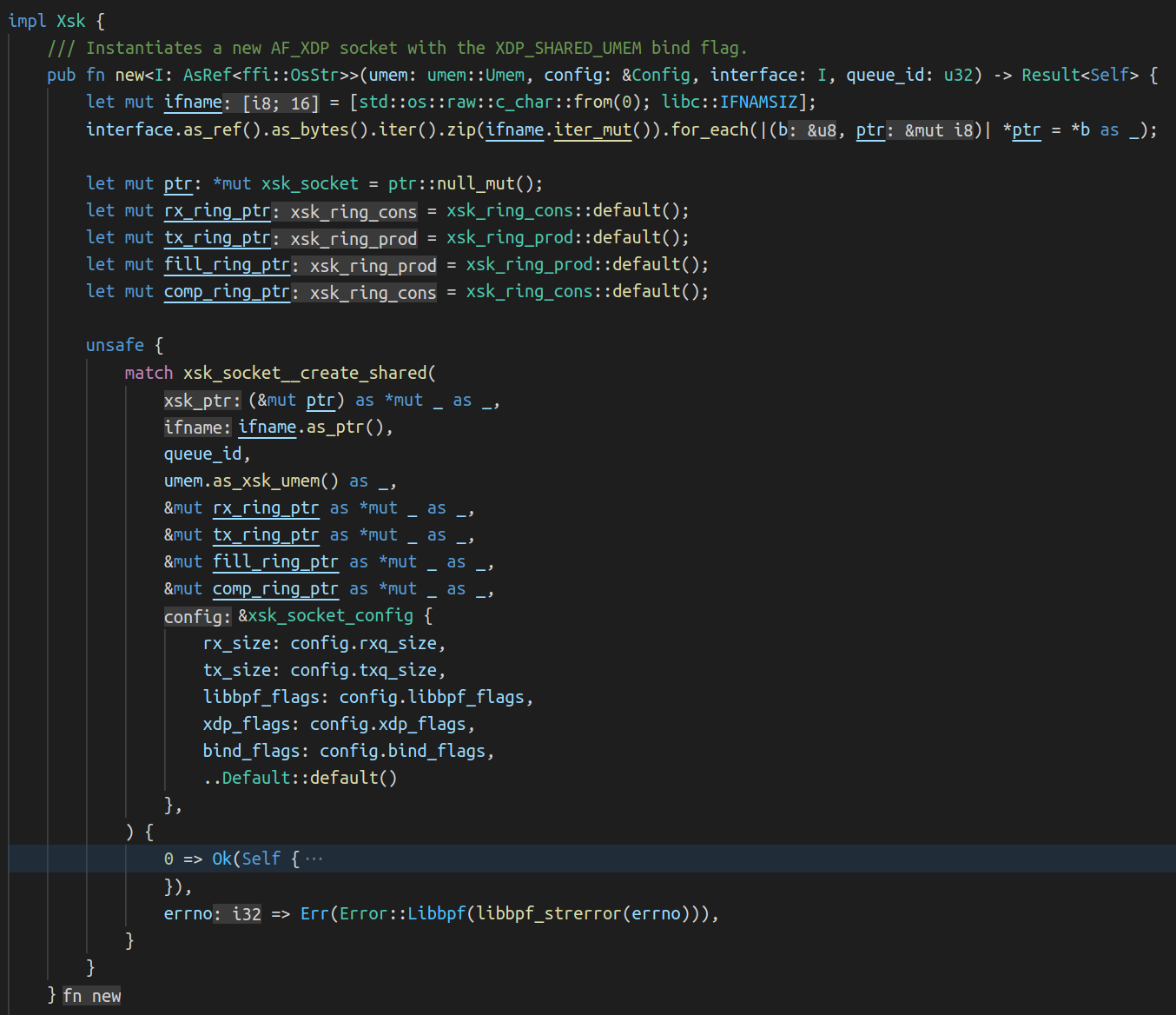
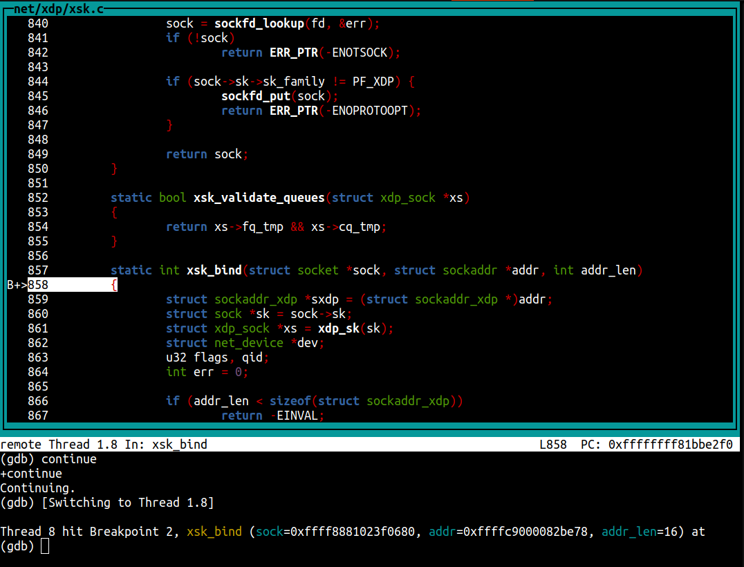
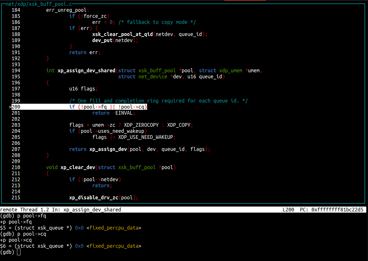
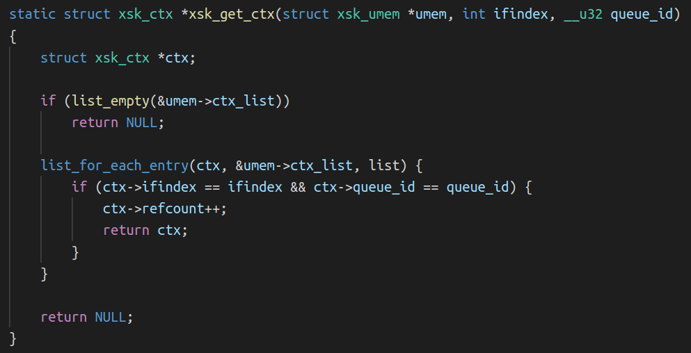
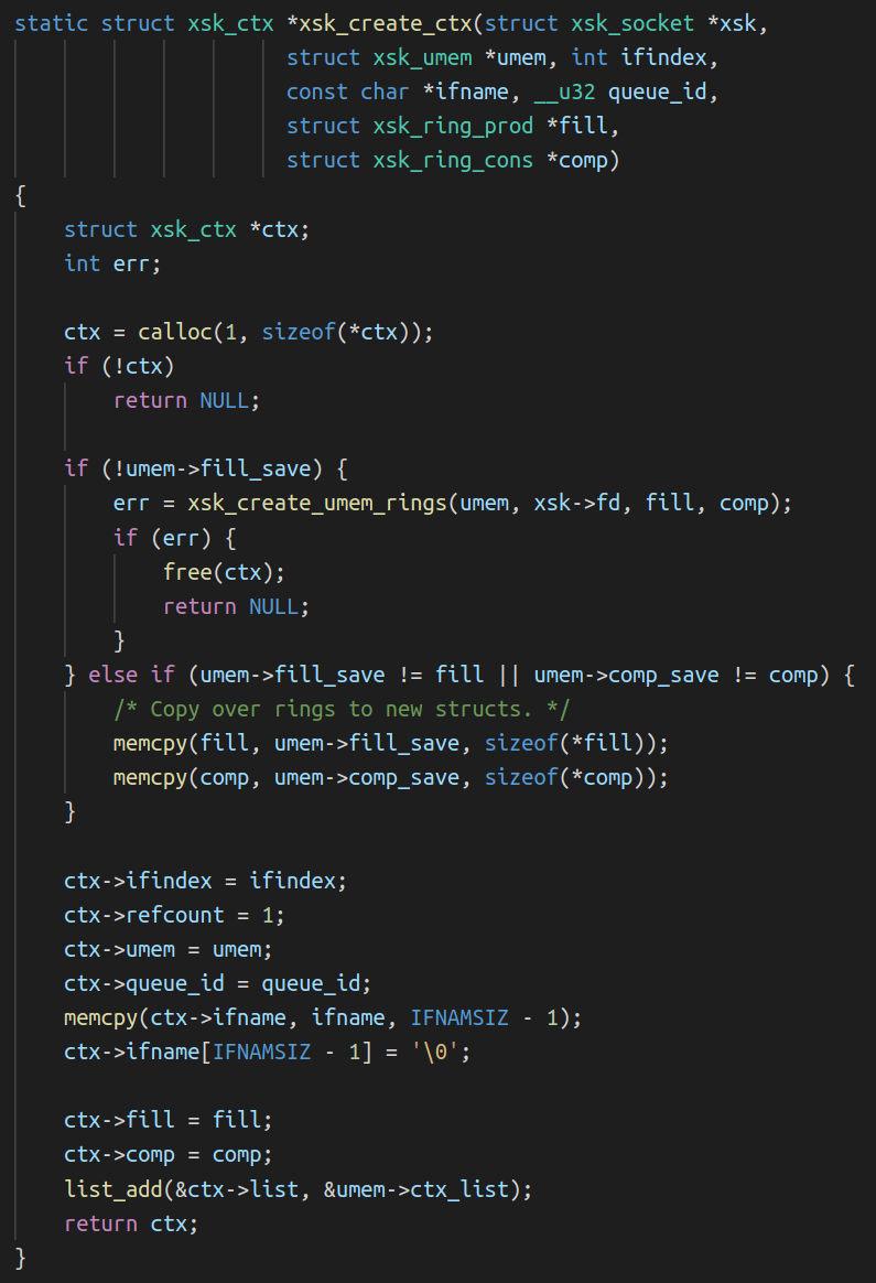
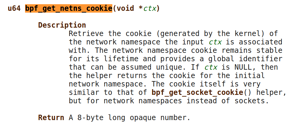
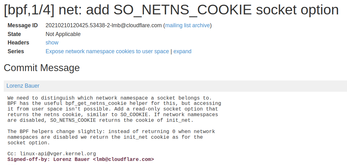
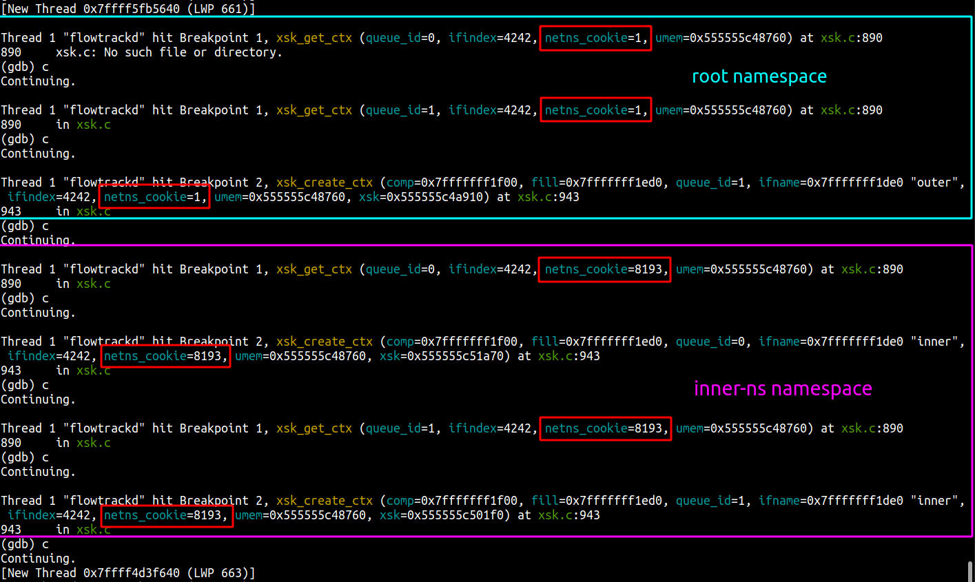
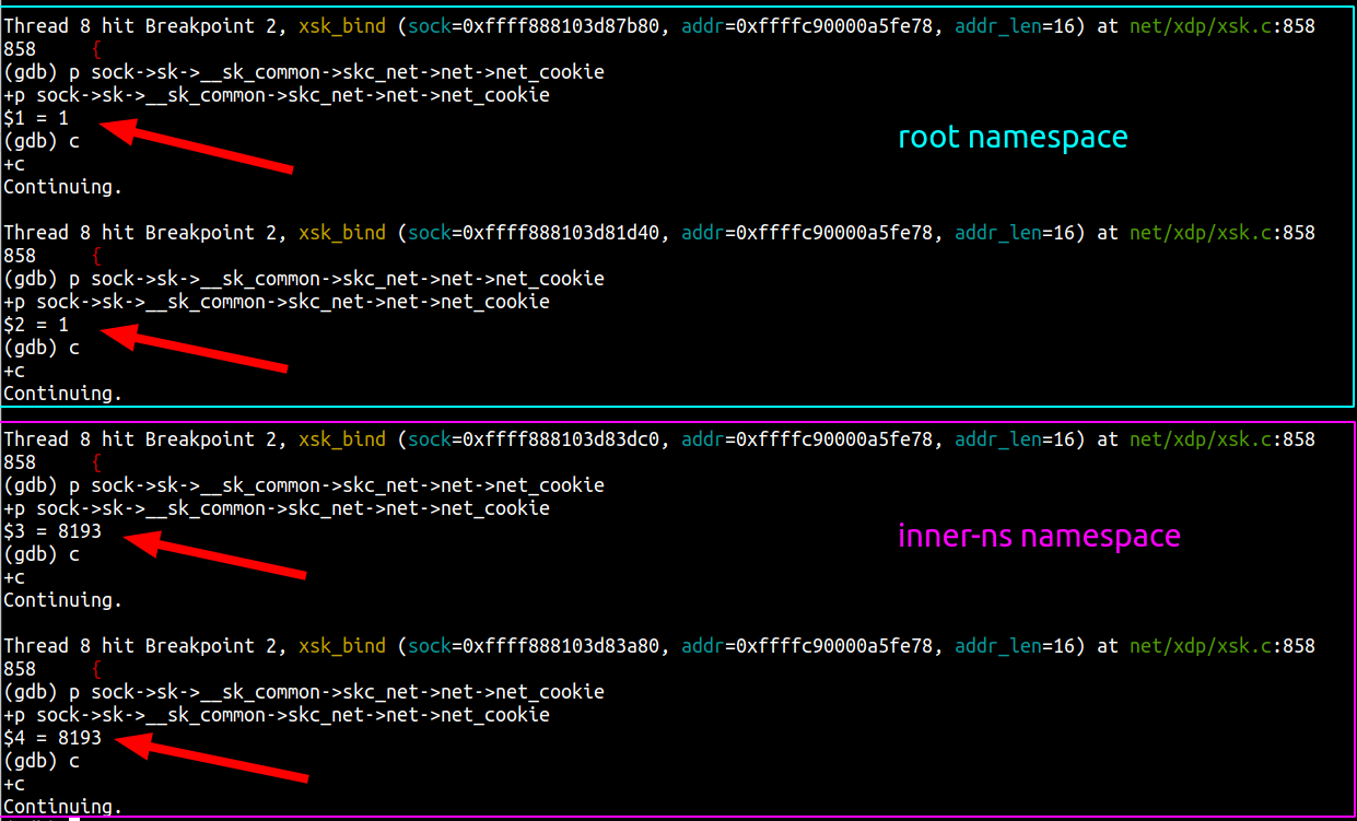

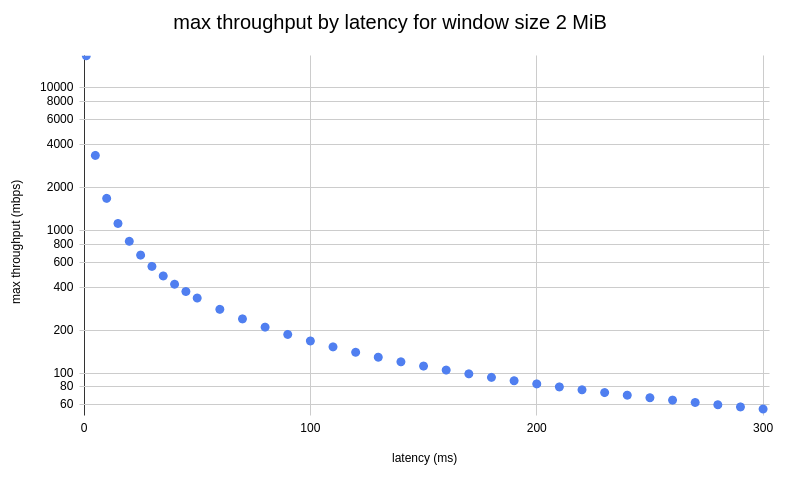
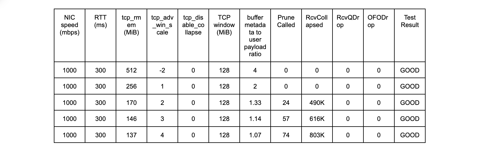
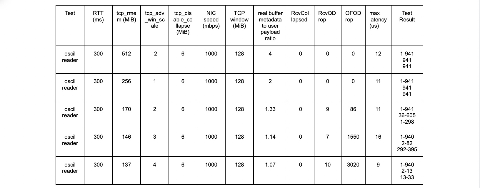
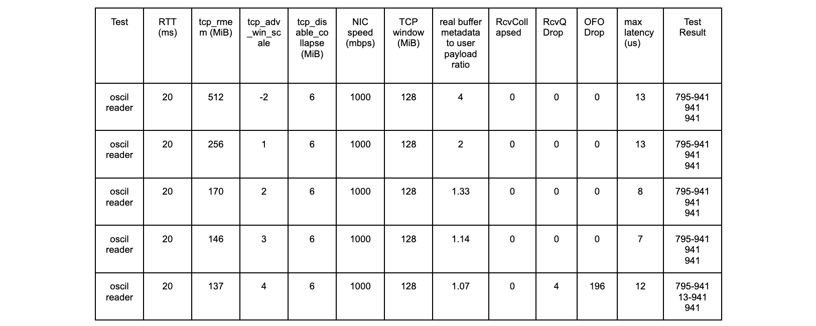
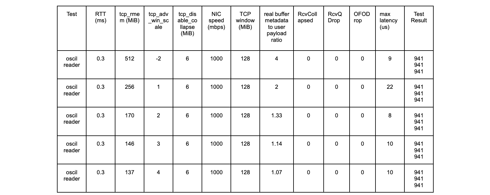
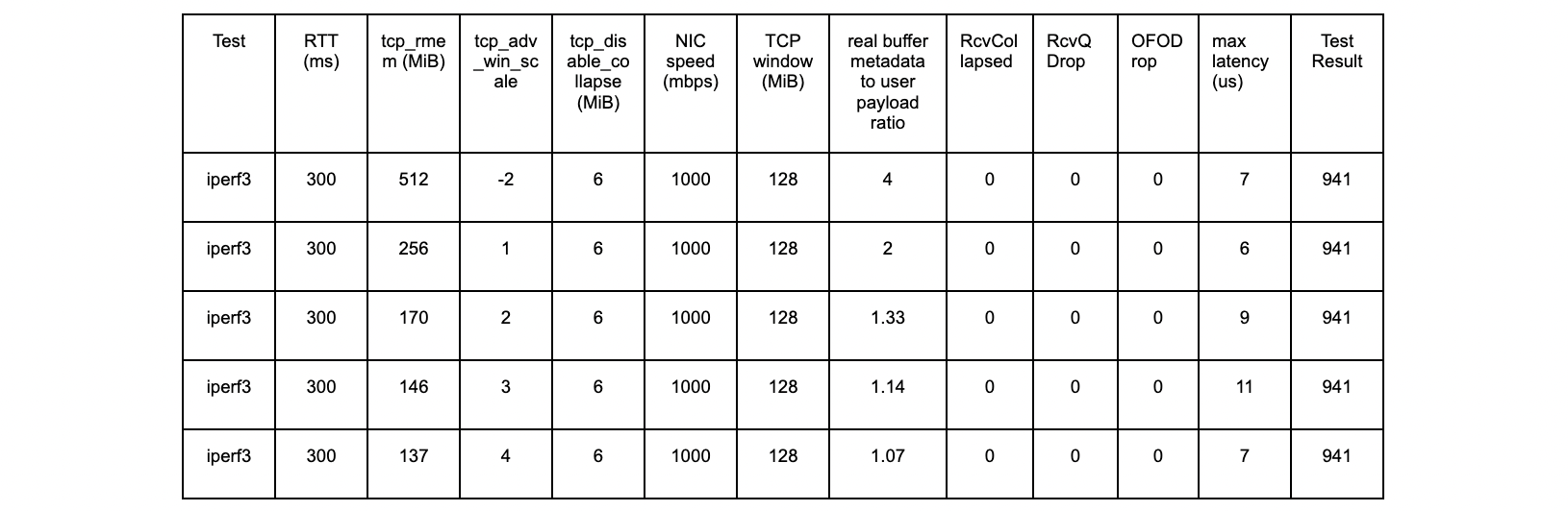
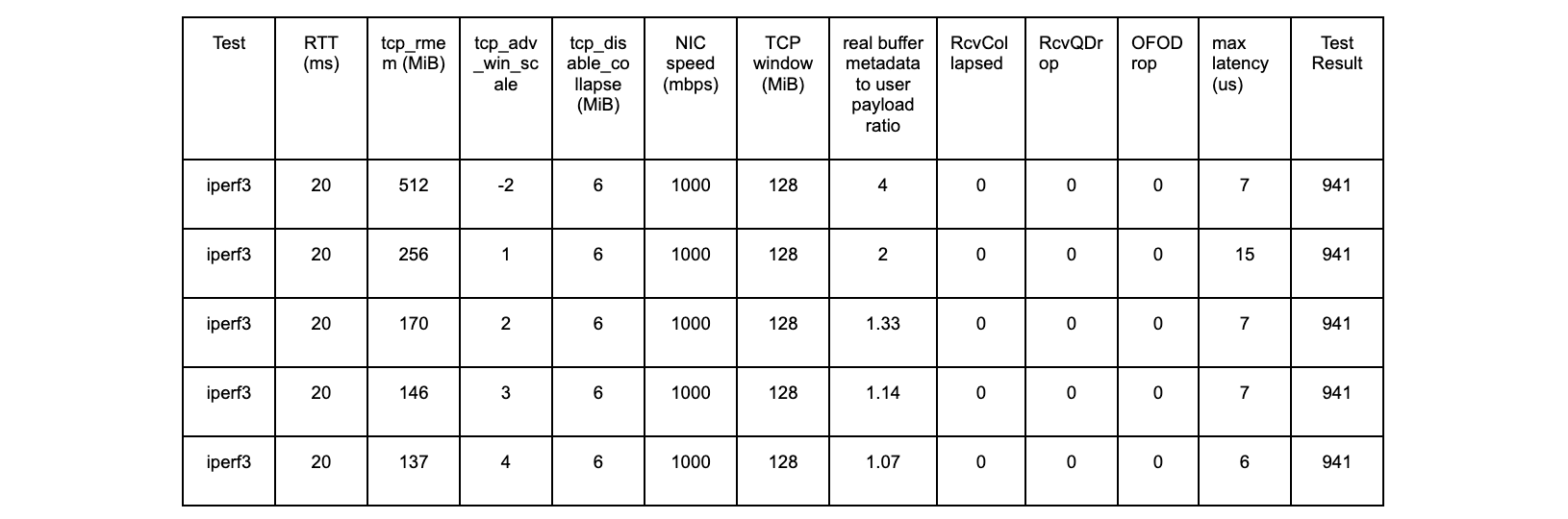
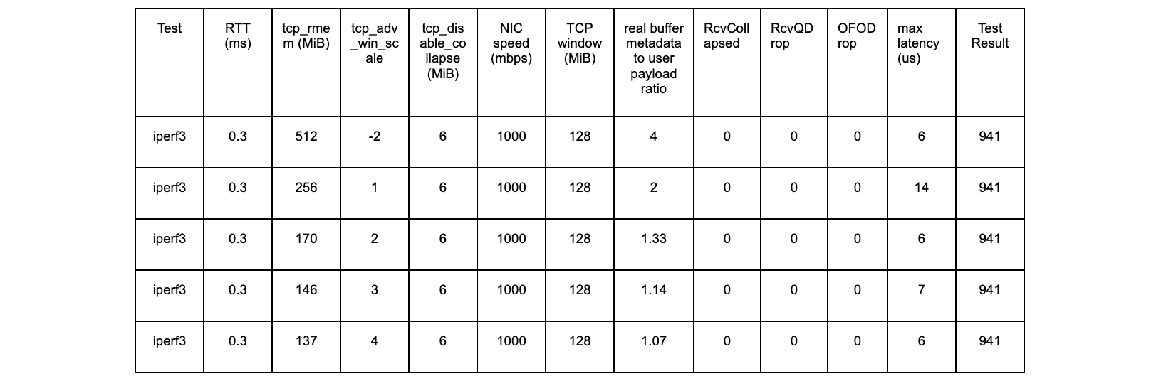
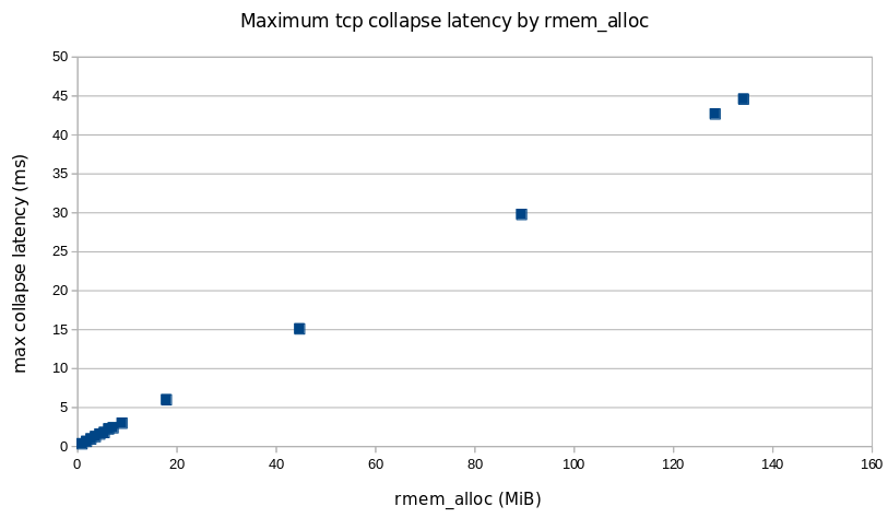
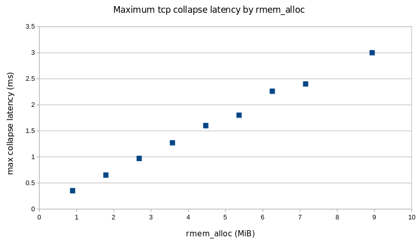
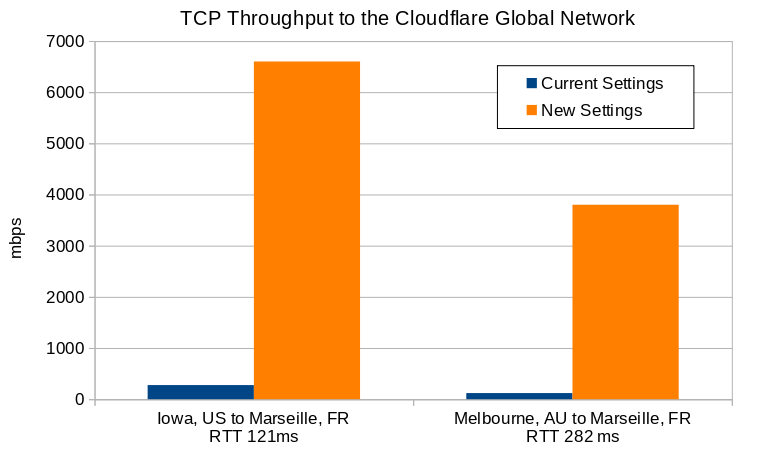
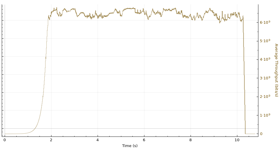
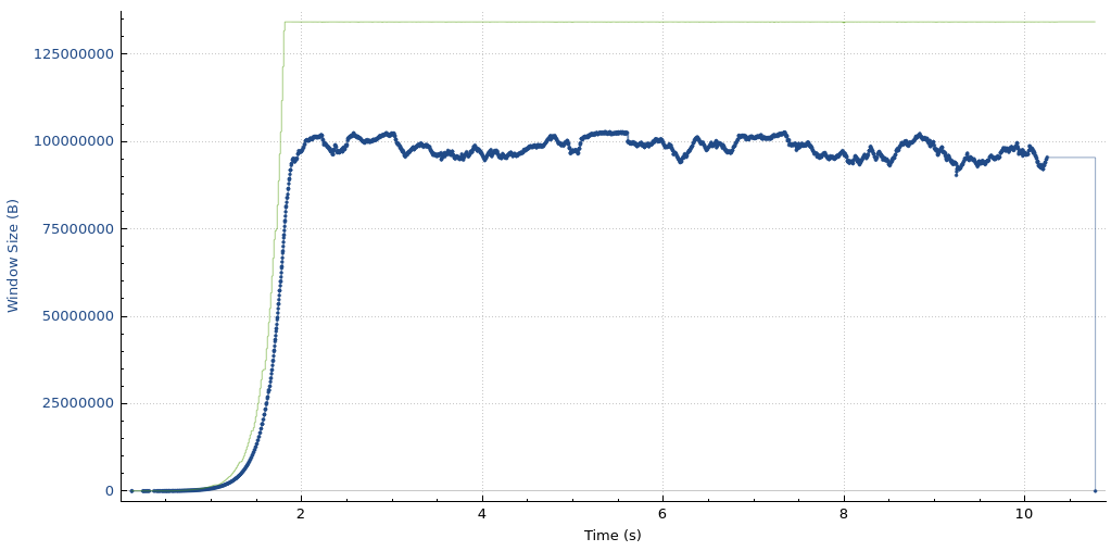
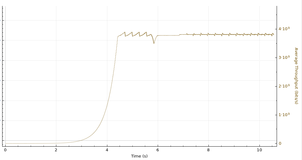
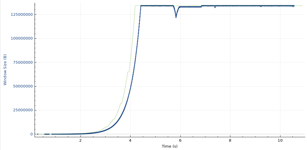
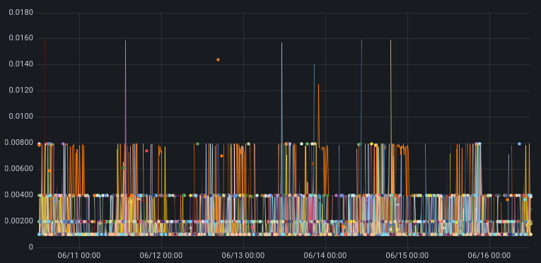
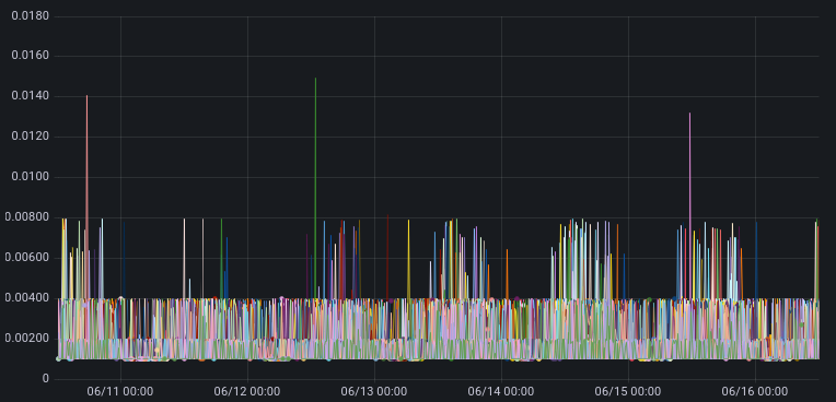
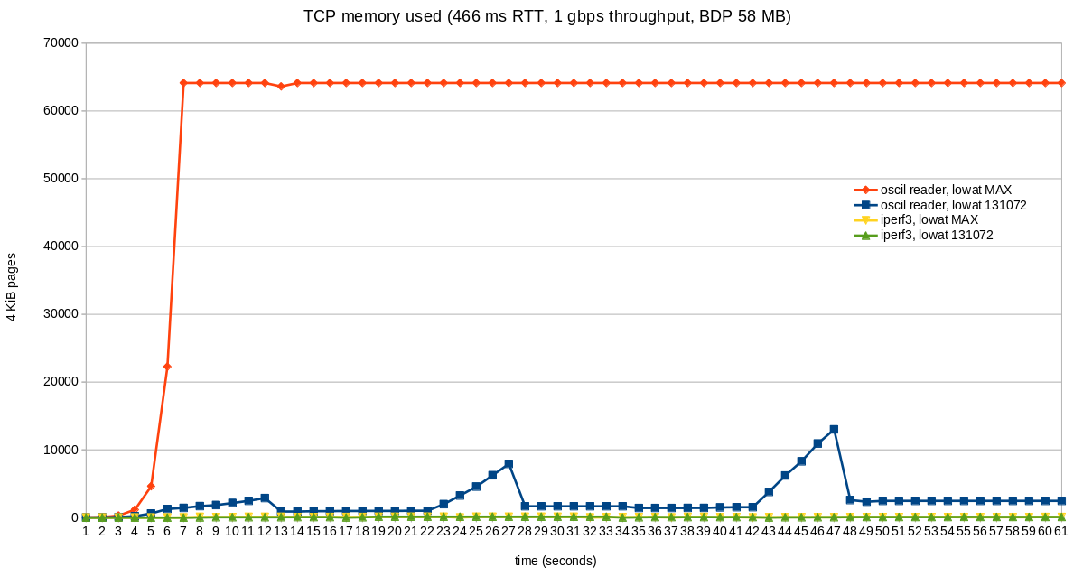


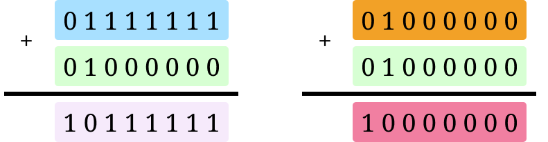


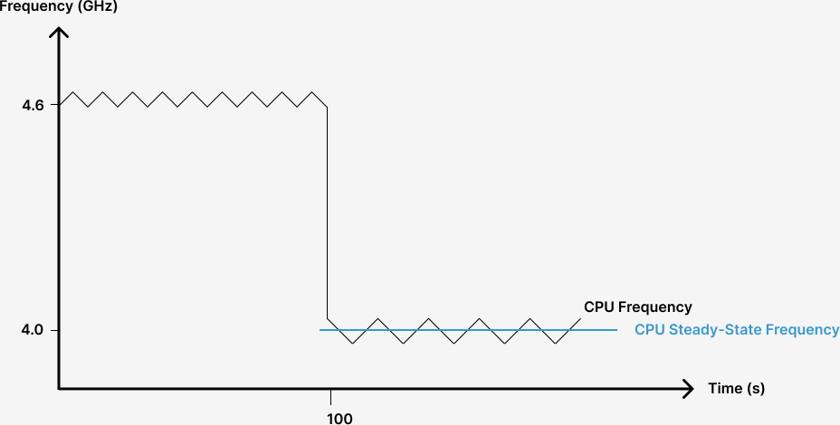
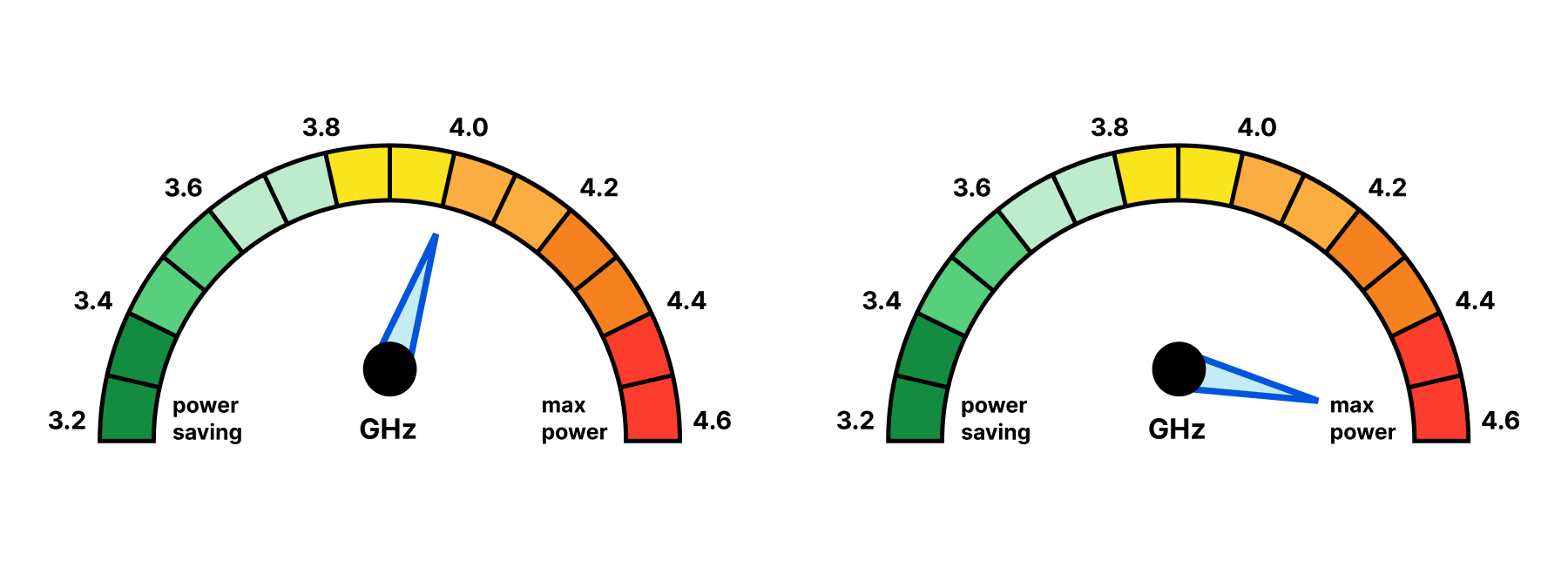
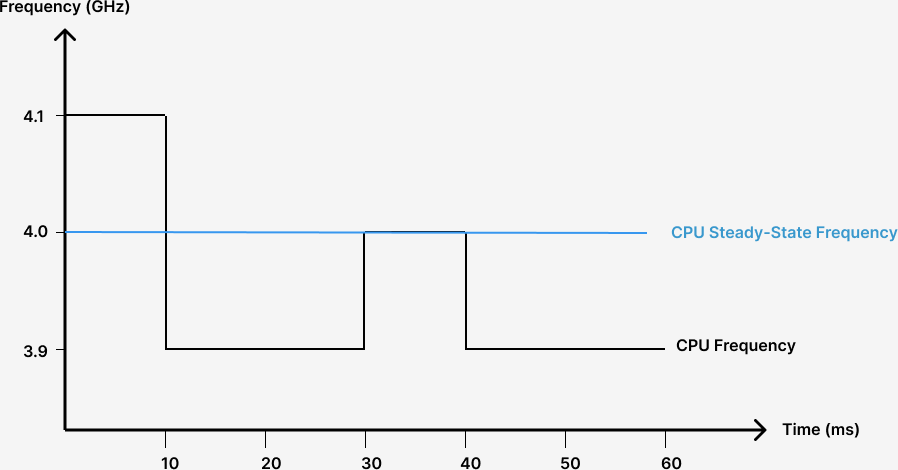

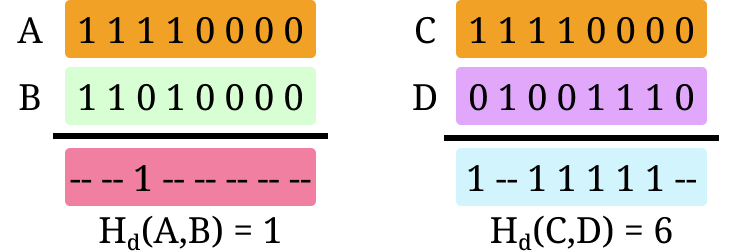
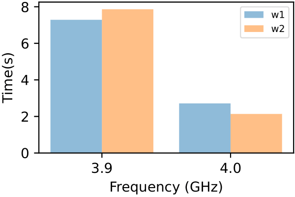
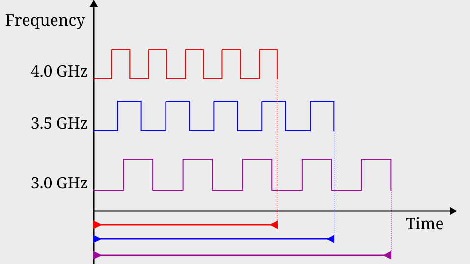
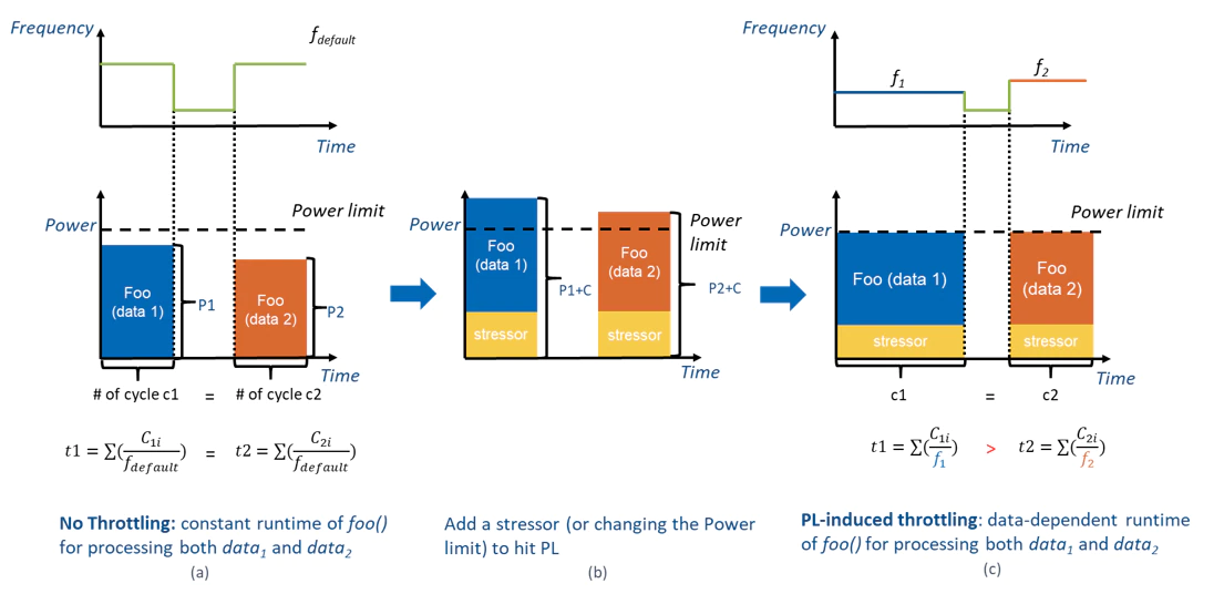
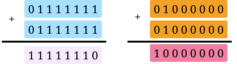
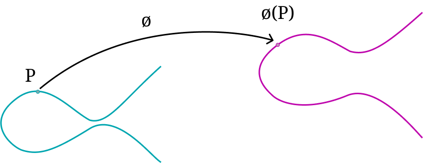
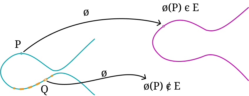


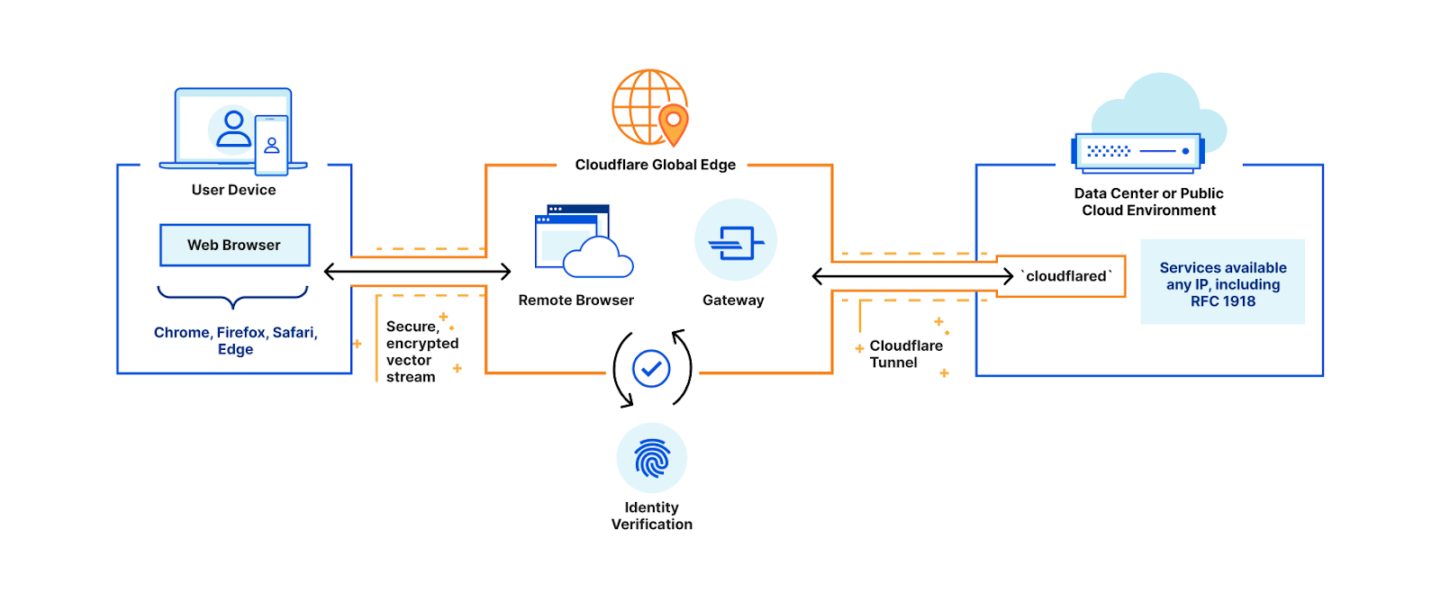
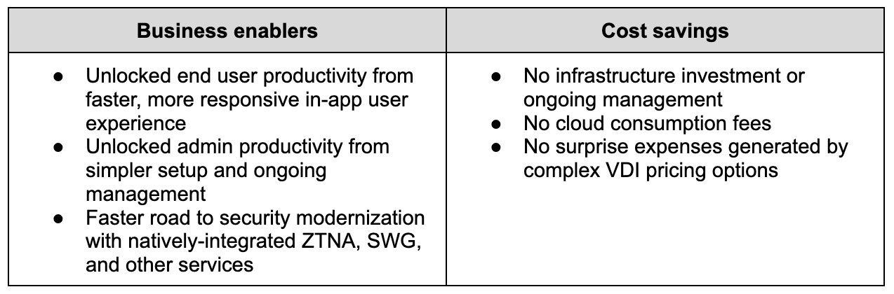
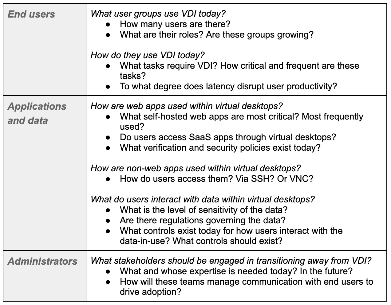
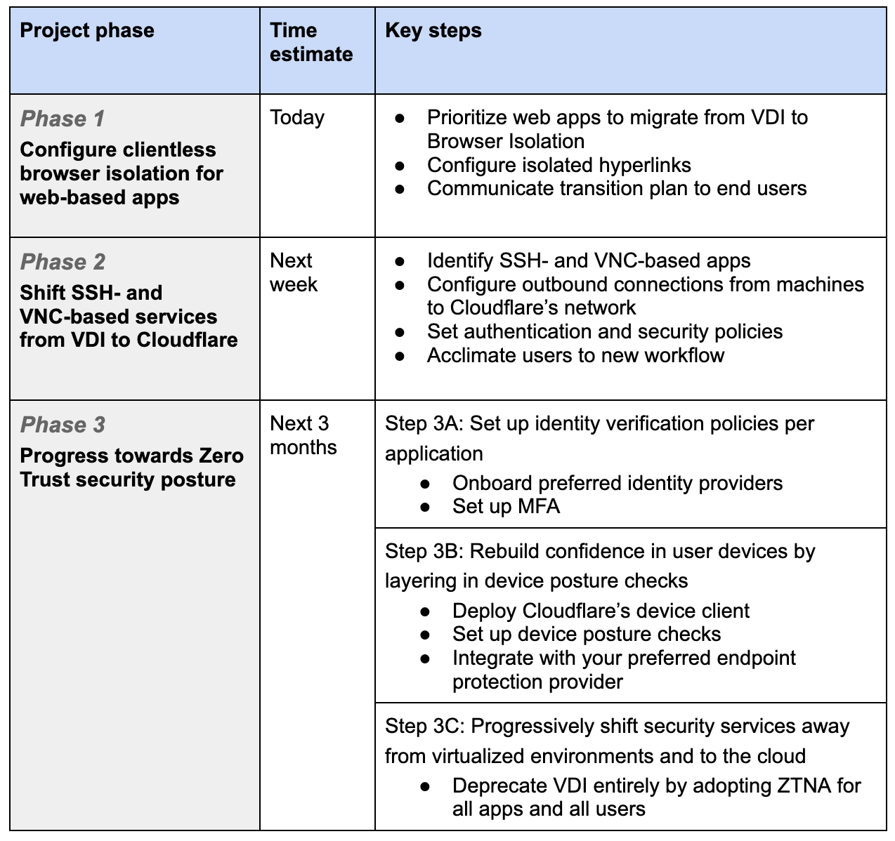
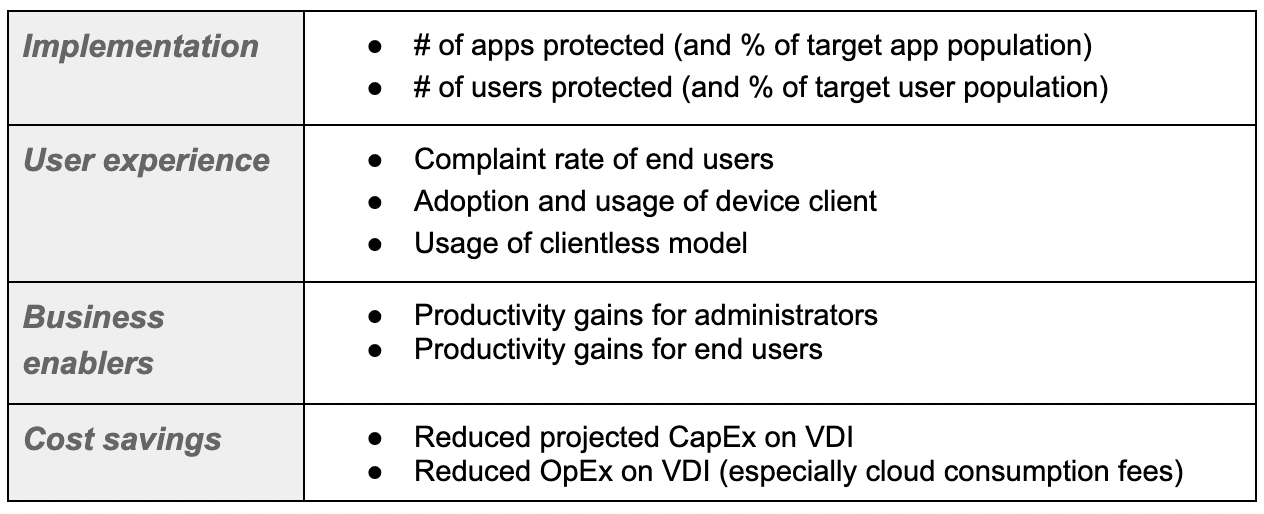


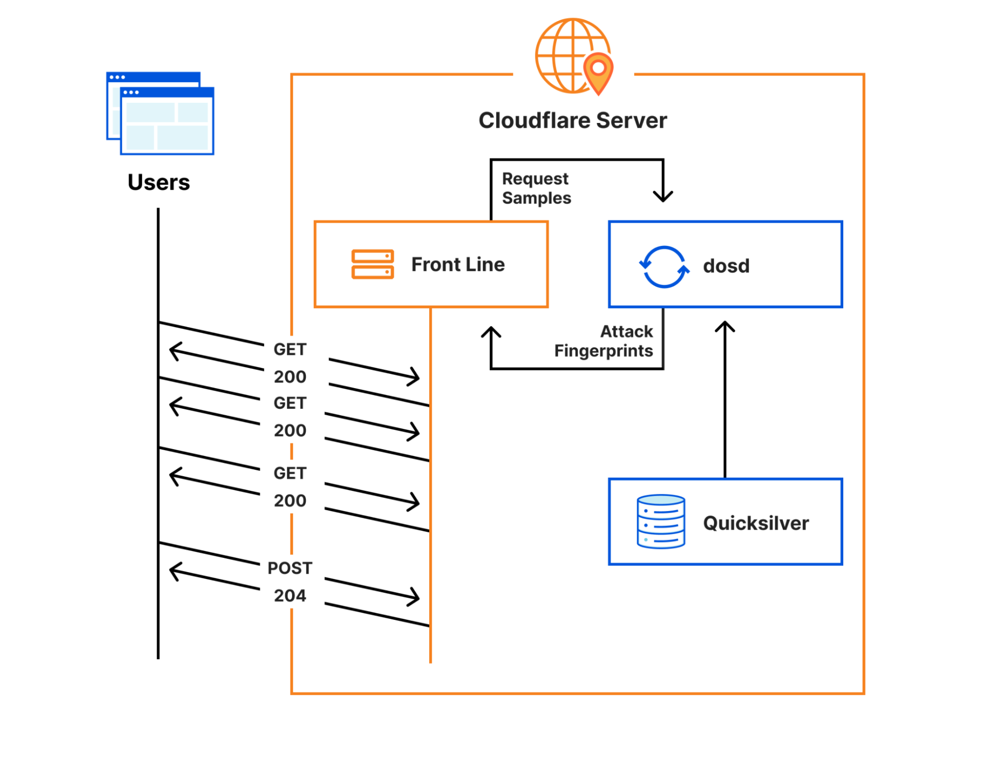
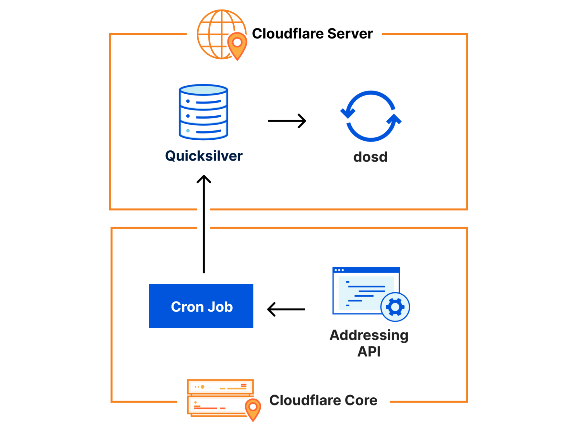
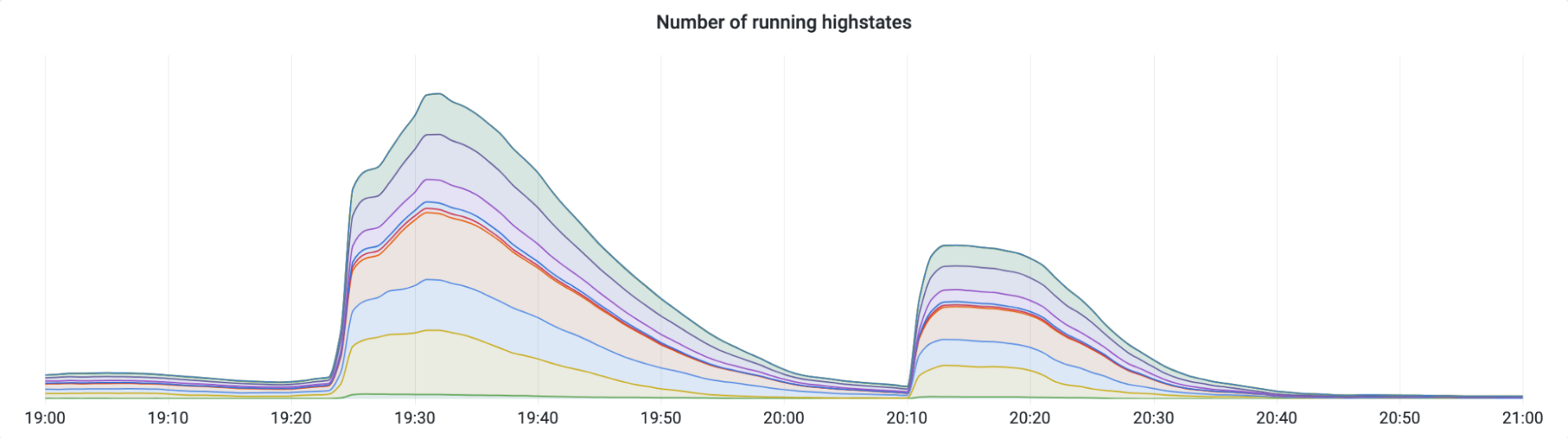

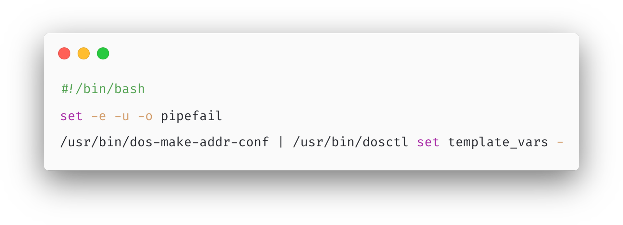
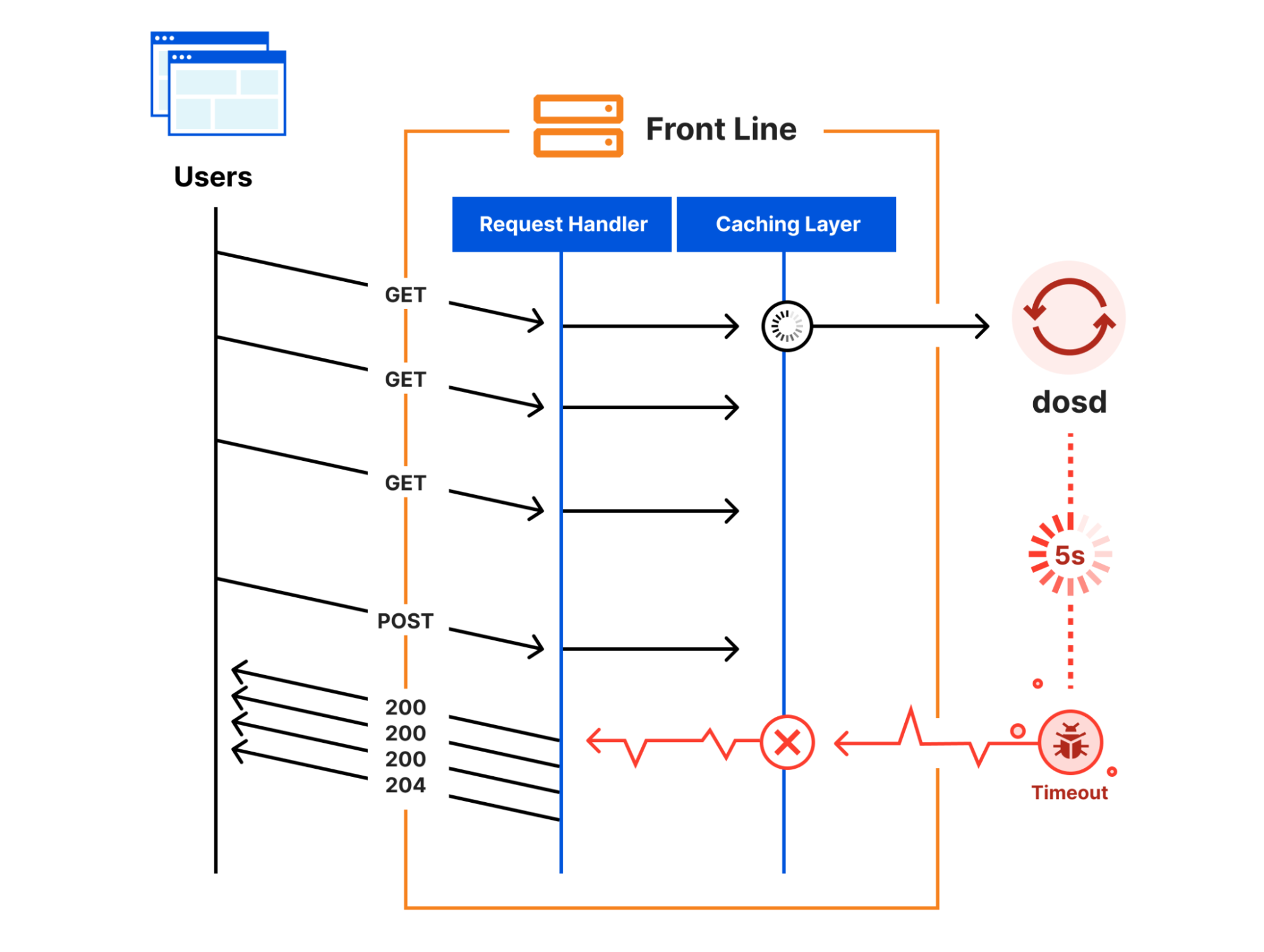

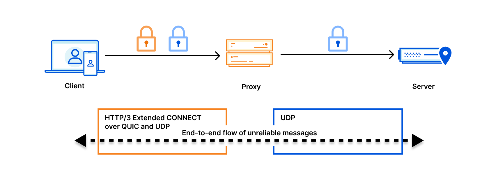

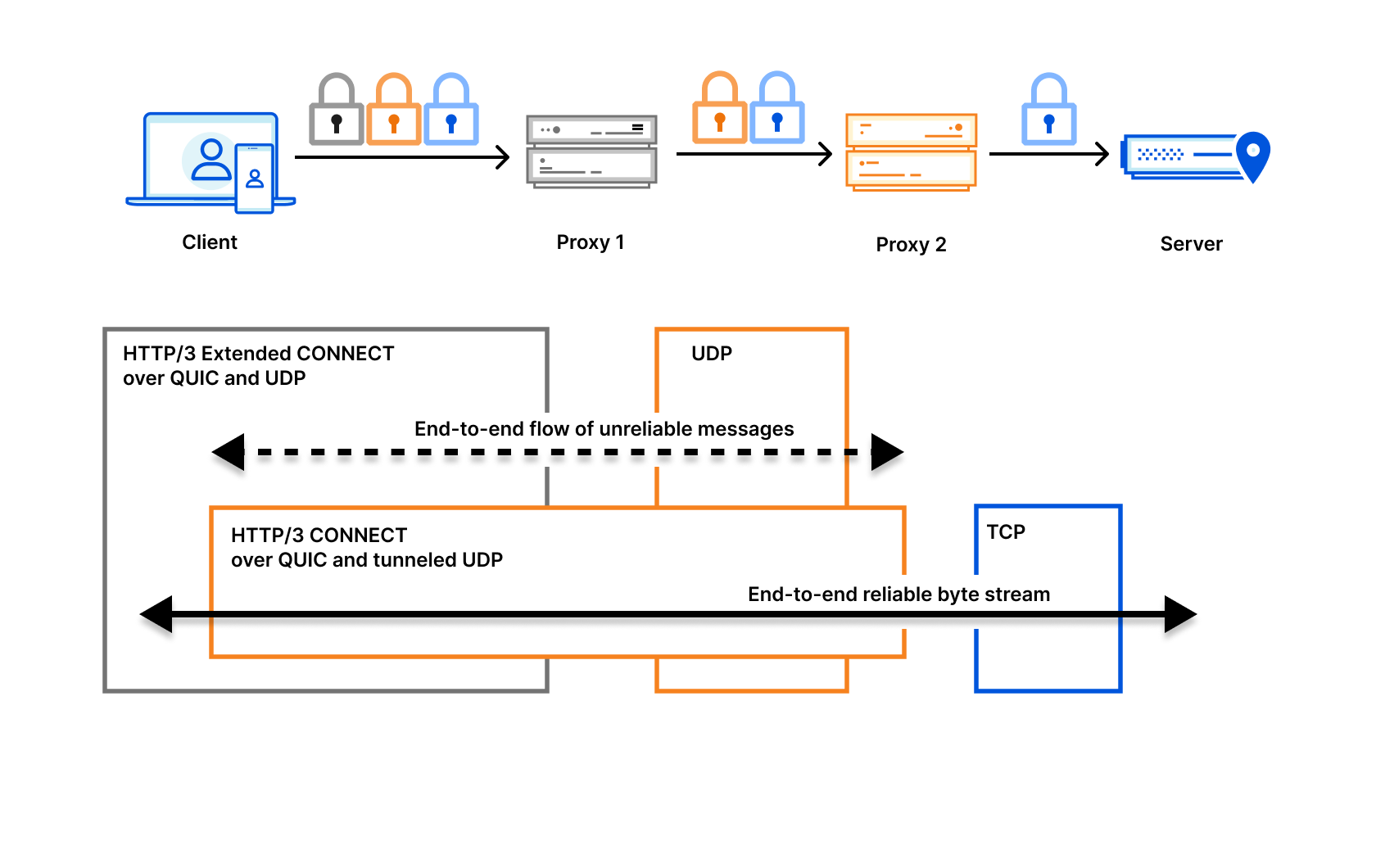