This blog post highlights notable Java language features, Java Lambda runtime updates, and how you can use the new Java 25 runtime in your serverless applications.
Java 25 language features
Java 25 introduces several language features to enhance developer productivity. There is a new feature that allows statements to appear before an explicit constructor invocation. You can now write code in the constructors without having to invoke super(…) or this(…) as the first statement. In the following example, the Employee class has a constructor which validates the input first and then invokes super(...):
class Person {
    int age;

    Person(int age) {
        if (age < 0)
            throw new IllegalArgumentException("Age cannot be negative");

        this.age = age;
    }
}

class Employee extends Person {
    String name;

    Employee(String name, int age) {
        // This is now allowed - code before super()
        if (age < 18 || age > 67)
            throw new IllegalArgumentException(...);

        super(age);
        this.name = name;
    }
}
Java 25 supports pattern matching that can handle primitive types in switch and instanceof statements. Previously, pattern matching was limited to reference types (Objects). For example, you can now perform pattern matching with int values, not just Integer objects:
void primitivePatternMatching(Object obj) {
    if (obj instanceof int i) {
        System.out.println("This is an int: " + i);
    }
}
Module import declarations simplifies working with. Instead of writing multiple individual package imports from the same module, you can use the import module syntax to bring publicly exported types into scope. This reduces boilerplate code and makes it easier to work with modular applications. Previously if you used the java.net.http module, you had to import multiple classes with individual import statements:
import java.net.URI;
import java.net.http.HttpClient;
import java.net.http.HttpRequest;

public class HttpClientExample {
    public void makeRequest() {
        HttpClient client = HttpClient.newHttpClient();
        HttpRequest request = HttpRequest.newBuilder()
            .uri(URI.create("https://api.example.com"))
            .build();
        // ... rest of implementation
    }
}
Now you can import the whole java.net.http module:
import module java.net.http;

public class HttpClientExample {
    public void makeRequest() {
        HttpClient client = HttpClient.newHttpClient();
        HttpRequest request = HttpRequest.newBuilder()
            .uri(URI.create("https://api.example.com"))
            .build();
        // Exported types from java.net.http module are now available
    }
}
Garbage collection
The generational mode of the Shenandoah garbage collector changes from an experimental feature in Java 24 to an optional product feature. Shenandoah is the low pause time garbage collector that reduces pause times by performing more garbage collection work concurrently with the running Java program. Shenandoah does the bulk of GC work concurrently, including the concurrent compaction, which means its pause times are no longer directly proportional to the size of the heap. The generational mode of Shenandoah improves sustainable throughput, load-spike resilience, and memory utilization.
To use the generational model of Shenandoah in Lambda, set JAVA_TOOL_OPTIONS to -XX:+UseShenandoahGC -XX:ShenandoahGCMode=generational.
Lambda runtime updates
The Java 25 runtime includes several performance optimizations, tuned to optimize cold and warm start performance for a broad range of customer workloads. Cold start refers to the initialization delay that occurs when Lambda prepares a new execution environment for a function that hasn’t been invoked recently, or to process an incoming invoke when all existing execution environments are in use. Warm start refers to invokes that are allocated to a previously initialized execution environment.
Ahead-of-Time (AOT) caches
Starting with Java 25, AWS Lambda replaces the traditional Class Data Sharing (CDS) with ahead-of-time (AOT) caches. This is an advanced optimization feature from Project Leyden that is designed to improve application startup times and reduce memory footprint. Lambda’s benchmarking results show that AOT caches deliver faster cold start performance compared to CDS.
AOT caches are enabled by default to provide performance benefits. Since you cannot use both AOT caches and CDS, if you enable CDS in your Lambda function, then Lambda disables AOT caches. If you use your own custom AOT caches in the Java 25 managed runtime, then the caches may be invalidated when Lambda updates the Java runtime during routine patching. AWS strongly suggests that you don’t use custom AOT caches with managed runtimes.
If you deploy Java 25 functions using container images, you can either implement your own AOT caches or continue using CDS. Since container images are immutable, the issue of AOT caches being invalidated following automatic runtime patching does not arise. To enable AOT caches, pass the flag -XX:AOTCache=/path/to/aot/cache/file via the JAVA_TOOL_OPTIONS environment variable. To enable CDS, pass the flag -Xshare:on -XX:SharedArchiveFile=/var/lang/lib/server/runtime.jsa.
Tiered compilation
Java’s tiered compilation is a just-in-time (JIT) optimization strategy that employs multiple compiler tiers to enhance the performance of frequently executed code progressively using runtime profiling data. Since Java 17, AWS Lambda has modified the default JVM behavior by stopping compilation at the C1 tier (client compiler). This minimizes cold start times for function invocations for most functions, although for compute-intensive functions with a long duration, customers can benefit from tuning tiered compilation to their workload. Starting with Java 25, Lambda no longer stops tiered compilation at C1 for SnapStart and Provisioned Concurrency. This improves performance in these cases without incurring a cold start penalty since tiered compilation occurs outside of the invoke path in these cases.
Priming
Priming is another technique to optimize performance for functions using either SnapStart or Provisioned Concurrency. This involves preloading dependencies, initializing resources, and executing code paths during function initialization. This front-loads work and triggers JIT compilation before taking the SnapStart snapshot, or when Provisioned Concurrency execution environments are pre-provisioned. The result is faster code execution when these execution environments are used for a function warm invoke. For detailed guidance on implementing priming strategies, see the Optimizing cold start performance of AWS Lambda using advanced priming strategies with SnapStart blog post.
Log4j patch for Log4Shell
Log4j is a widely used open source logging library maintained by the Apache Software Foundation. In November 2021, Log4j reported Log4Shell, a zero-day vulnerability involving arbitrary code execution. The Lambda team responded by deploying an emergency patch across all Java runtimes to protect customers from potential exploitation. However, this emergency patch introduced a performance overhead during cold starts. The vulnerability was permanently resolved in Log4j version 2.17.0 in December 2021. Consequently, AWS has removed this patch from the Java 25 runtime to restore optimal performance. You must verify you are using Log4j version 2.17.0 or later.
Lambda runtimes for Java 8, 11, 17, and 21 continue to enable the emergency patch by default. Customers who are using Log4j version 2.17.0 or higher with these runtimes can disable this patch, improving cold start performance. To disable the patch, set the AWS_LAMBDA_DISABLE_CVE_2021_44228_PROTECTION environment variable to true.
Additional performance considerations
At launch, new Lambda runtimes receive less usage than existing, established runtimes. This can result in longer cold start times due to reduced cache residency within internal Lambda sub-systems. Cold start times typically improve in the weeks following launch as usage increases. As a result, AWS recommends not drawing conclusions from side-by-side performance comparisons with other Lambda runtimes until the performance has stabilized.
Since performance is highly dependent on workload, customers with performance-sensitive workloads should conduct their own testing instead of relying on generic test benchmarks. To maximize performance, your workload may benefit from additional workload-specific performance tuning.
Using Java 25 in AWS Lambda
You can use Java 25 for your Lambda functions in the AWS Management Console, an AWS Lambda container image, AWS SAM, or the AWS CDK.
AWS Management Console
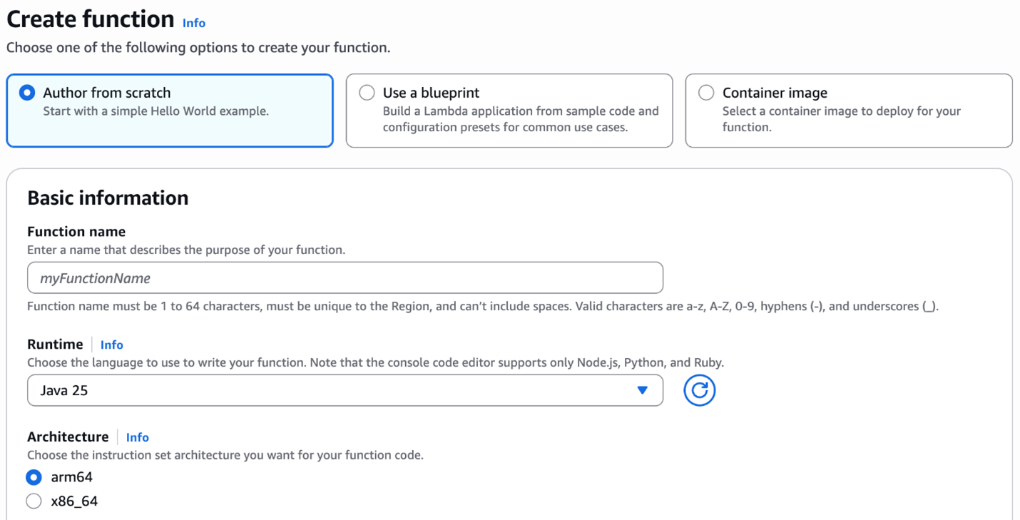
To use the Java 25 runtime to develop your Lambda functions, specify a runtime parameter value Java 25 when creating or updating a function. The Java 25 runtime version is now available in the Runtime dropdown menu on the Create function page in the AWS Lambda console:
Creating Java 25 function in AWS Management Console
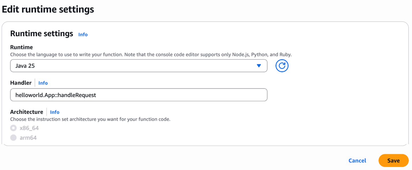
To update an existing Lambda function to Java 25, navigate to the function in the Lambda console, then choose Java 25 in the Runtime settings section. The new version is available in the Runtime dropdown menu:
Changing a function to Java 25
AWS Lambda container image
Use the Java base image version with the java:25 tag by modifying the FROM statement in your Dockerfile.
Example Dockerfile:
FROM public.ecr.aws/lambda/java:25
# Copy function code and runtime dependencies from Maven layout
COPY target/classes ${LAMBDA_TASK_ROOT}
COPY target/dependency/* ${LAMBDA_TASK_ROOT}/lib/
# Set the CMD to your handler (could also be done as a parameter override outside of the Dockerfile)
CMD [ "com.example.myapp.App::handleRequest" ]
AWS SAM supports generating this template with Java 25 for new serverless applications using the sam init command. Refer to the AWS SAM documentation.
AWS Cloud Development Kit (AWS CDK)
In the AWS CDK, set the runtime attribute to Runtime.JAVA_25 to use this version.
import software.amazon.awscdk.core.Construct;
import software.amazon.awscdk.core.Stack;
import software.amazon.awscdk.core.StackProps;
import software.amazon.awscdk.services.lambda.Code;
import software.amazon.awscdk.services.lambda.Function;
import software.amazon.awscdk.services.lambda.Runtime;

public class InfrastructureStack extends Stack {

    public InfrastructureStack(final Construct parent, final String id, final StackProps props) {

        super(parent, id, props);

        Function.Builder.create(this, "HelloWorldFunction")
                .runtime(Runtime.JAVA_25)
                .code(Code.fromAsset("target/hello-world.jar"))
                .handler("helloworld.App::handleRequest")
                .memorySize(1024)
                .build();

        // rest of your CDK code
    }
}
Conclusion
Lambda now supports Java 25 as a managed language runtime or with your own custom runtime. This release includes the latest Java 25 language features as well as performance enhancements optimized for Lambda workloads.
You can build and deploy functions using Java 25 using the AWS Management Console, AWS CLI, AWS SDK, AWS SAM, AWS CDK, or your choice of infrastructure as code tool. You can also use the Java container base image with the 25 tag if you prefer to build and deploy your functions using container images.
The Java 25 runtime helps developers build more efficient, powerful, and scalable serverless applications. Read about the Java programming model in the Lambda documentation to learn more about writing functions in Java 25.
This is a guest post by Umesh Dangat, Senior Principal Engineer for Distributed Services and Systems at Yelp, and Toby Cole, Principle Engineer for Data Processing at Yelp, in partnership with AWS.
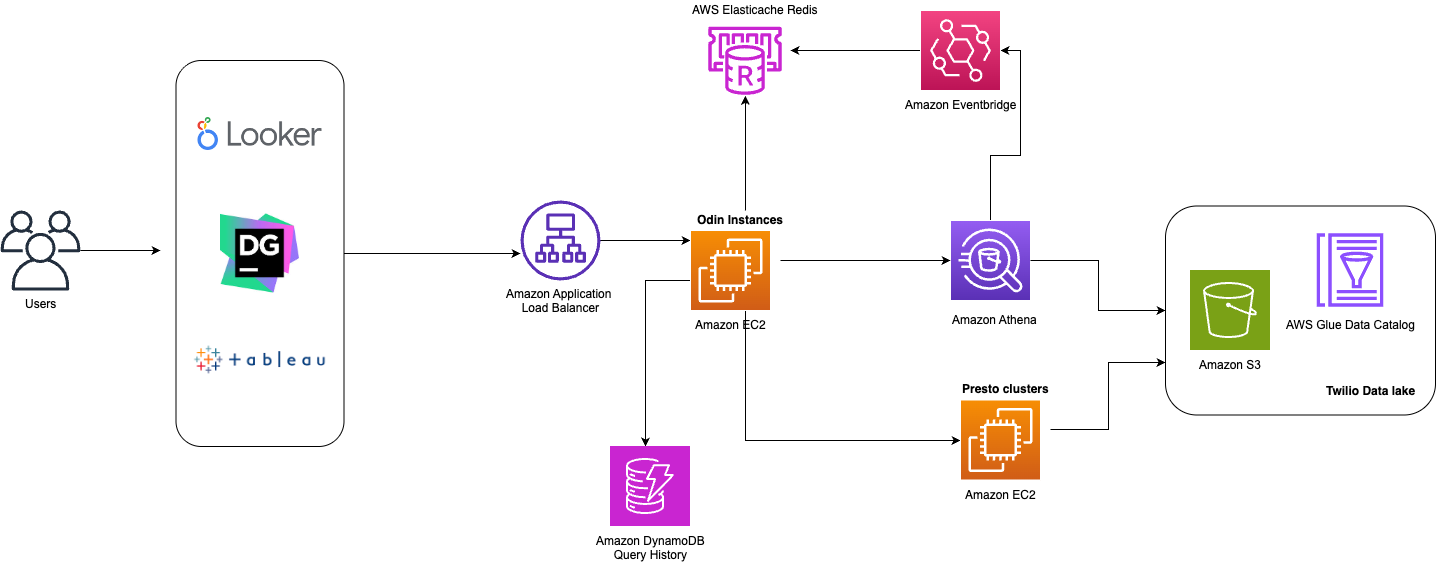
Yelp processes massive amounts of user data daily—over 300 million business reviews, 100,000 photo uploads, and countless check-ins. Maintaining sub-minute data freshness with this volume presented a significant challenge for our Data Processing team. Our homegrown data pipeline, built in 2015 using then-modern streaming technologies, scaled effectively for many years. As our business and data needs evolved, we began to encounter new challenges in managing observability and governance across an increasingly complex data ecosystem, prompting the need for a more modern approach. This affected our outage incidents, making it harder to both assess impact and restore service. At the same time, our streaming framework struggled with Kafka for data streaming and permanent data storage. In addition, our connectors to analytical data stores experienced latencies exceeding 18 hours.
This came to a head when our efforts to comply with General Data Protection Regulation (GDPR) requirements revealed gaps in our infrastructure that would require us to clean up our data, while simultaneously maintaining operational reliability and reducing data processing times. Something had to change.
In this post, we share how we modernized our data infrastructure by embracing a streaming lakehouse architecture, achieving real-time processing capabilities at a fraction of the cost while reducing operational complexity. With this modernization effort, we reduced analytics data latencies from 18 hours to mere minutes, while also removing the need for using Kafka as a permanent storage for our change log streams.
The problem: Why we needed change
We started this transformation by initiating a migration from self-managed Apache Kafka to Amazon Managed Streaming for Apache Kafka (Amazon MSK), which significantly reduced our operational overhead and enhanced security. Amazon MSK’s express brokers also provided better elasticity for our Apache Kafka clusters. While these improvements were a promising start, we recognized the need for a more fundamental architectural change
Legacy architecture pain points
Let’s examine the specific challenges and limitations of our previous architecture that prompted us to seek a modern solution.
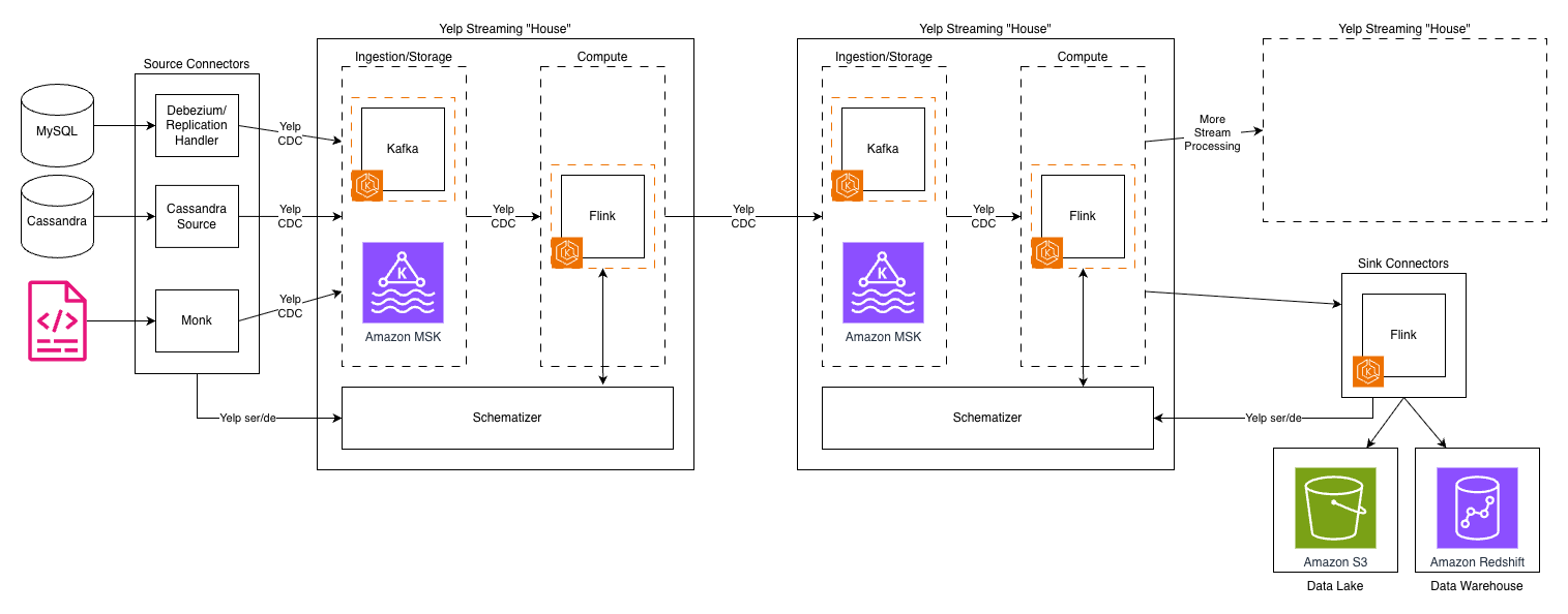
The following diagram depicts Yelp’s original data architecture.
Kafka topics proliferated across our infrastructure, creating long processing chains. As a result, each hop added latency, operational overhead, and storage costs. The system’s reliance on Kafka for both ingestion and storage created a fundamental bottleneck—Kafka’s architecture, optimized for high-throughput messaging, wasn’t designed for long-term storage and to handle complex querying patterns.
Another challenge was our custom “Yelp CDC” format—a proprietary change data capture language—was powerful and tailored to our needs. However, as our team grew and our use cases expanded, it introduced complexity and a steeper learning curve for new engineers. It also made integrations with off-the-shelf systems more complex and maintenance intensive.
The cost and latency trade-off
The traditional trade-off between real-time processing and cost efficiency had us caught in an expensive bind. Real-time streaming systems demand significant resources to maintain state within compute engines like Apache Flink, keep multiple copies of data across Kafka clusters, and run always-on processing jobs. Our infrastructure costs were growing, and it was largely driven by:
Long Kafka chains: Data often traversed 4-5 Kafka topics before reaching its destination and each topic was replicated for reliability
Duplicate data storage: The same data existed in multiple formats across different systems—raw in Kafka, processed in intermediate topics, and final forms in data warehouses and Flink RocksDB for join-like use cases
Complex custom tooling maintenance: The proprietary nature of our tools meant engineering resources were focused on maintenance rather than building new capabilities
Meanwhile, our business requirements became more demanding. Teams at Yelp needed faster insights, near-real-time results, and the ability to quickly run complex historical analyses without delay. This pushed us to shape our new architecture to improve streaming discovery and metadata visibility, provide more flexible transformation tooling, and simplify operational workflows with faster recovery times.
Understanding the streamhouse concept
To understand how we solved our data infrastructure challenges, it’s important to first grasp the concept of a streamhouse and how it differs from traditional architectures.
Evolution of data architecture
To understand why a streaming lakehouse or streamhouse was the answer to our challenges, it’s helpful to trace the evolution of data architectures. The journey from data warehouses to modern streaming systems reveals why each generation solved certain problems while creating new ones.
Data warehouses like Amazon Redshift and Snowflake brought structure and reliability to analytics, but their batch-oriented nature meant accepting hours or days of latency. Data lakes emerged to handle the volume and variety of big data, using low-cost object storage like Amazon S3, but often became “data swamps” without proper governance. The lakehouse architecture, pioneered by technologies like Apache Iceberg and Delta Lake, promised to combine the best of both, the structure of warehouses with the flexibility and economics of lakes.
But even lakehouses were designed with batch processing in mind. While they added streaming capabilities, these were often bolted on rather than fundamental to the architecture. What we needed was something different: a reimagining that treated streaming as a first-class citizen while maintaining lakehouse economics.
What makes a streamhouse different
A streamhouse, as we define it, is “a stream processing framework with a storage layer that leverages a table format, making intermediate streaming data directly queryable.” This seemingly simple definition represents a fundamental shift in how we think about data processing.
Traditional streaming systems maintain dynamic tables like materialized views in databases, but these aren’t directly queryable. You can only consume them as streams, limiting their utility for ad-hoc analysis or debugging. Lakehouses, conversely, excel at queries but struggle with low-latency updates and complex streaming operations like out-of-order event handling or partial updates.
The streamhouse bridges this gap by:
Treating batch as a special case of streaming, rather than a separate paradigm
Making data, including intermediate processing results, queryable via SQL
Providing streaming-native features like database change-data capture (CDC) and temporal joins
Leveraging cost-effective object storage while maintaining minute-level latencies
Core capabilities we needed
Our requirements for a streaming lakehouse were shaped by years of operating at scale:
Real-time processing with minute-level latency: While sub-second latency wasn’t necessary for most use cases, our previous hours-long delays weren’t acceptable. The sweet spot was processing latencies measured in minutes fast enough for real-time decision-making but relaxed enough to leverage cost-effective storage.
Efficient CDC handling: With numerous MySQL databases powering our applications, the ability to efficiently capture and process database changes was crucial. The solution needed to handle both initial snapshots and ongoing changes seamlessly, without manual intervention or downtime.
Cost-effective scaling: The architecture had to break the linear relationship between data volume and cost. This meant leveraging tiered storage, with hot data on fast storage and cold data on low-cost object storage, all while maintaining query performance.
Built-in data management: Schema evolution, data lineage, time travel queries, and data quality controls needed to be first-class features, not afterthoughts. Our experience maintaining our custom Schematizer taught us that these capabilities were essential for operating at scale.
The solution architecture
Our modernized data infrastructure combines several key technologies into a cohesive streamhouse architecture that addresses our core requirements while maintaining operational efficiency.
Our technology stack selection
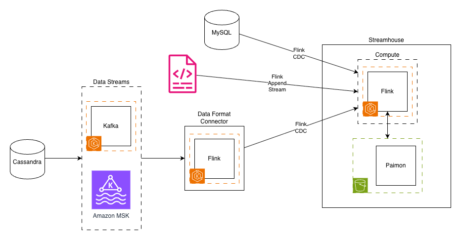
We carefully selected and integrated several proven technologies to build our streamhouse solution.The following diagram depicts Yelp’s new data architecture.
After extensive evaluation, we assembled a modern streaming lakehouse stack, streamhouse, built on proven open source technologies:
Amazon MSK continues to deliver existing streams as they did before from source applications and services.
Apache Flink on Amazon EKS served as our compute engine, a natural choice given our existing expertise and investment in Flink-based processing. Its powerful stream processing capabilities, exactly-once semantics, and mature framework made it ideal for the computational layer.
Apache Paimon emerged as the key innovation, providing the streaming lakehouse storage layer. Born from the Flink community’s FLIP-188 proposal for built-in dynamic table storage, Paimon was designed from the ground up for streaming workloads. Its LSM-tree-based architecture provided the high-speed ingestion capabilities we needed.
Amazon S3 serves as our streamhouse storage layer, offering highly scalable capacity at a fraction of the cost. The shift from compute-coupled storage (Kafka brokers) to object storage represented a fundamental architectural change that unlocked massive cost savings.
Flink CDC connectors replaced our custom CDC implementations, providing battle-tested integrations with databases like MySQL. These connectors handled the complexity of initial snapshots, incremental updates, and schema changes automatically.
Architectural transformation
The transformation from our legacy architecture to the streamhouse model involved three key architectural shifts:
1. Decoupling ingestion from storage
In our old world, Kafka handled both data ingestion and storage, creating an expensive coupling. Every byte ingested had to be stored on Kafka brokers with replication for reliability. Our new architecture separated these concerns: Flink CDC handled ingestion by immediately writing to Paimon tables backed by S3. This separation reduced our storage costs by over 80% and improved reliability through the 11 nines of durability of S3.
2. Unified data format
The migration from our proprietary CDC format to the industry-standard Debezium format was more than a technical change. It reflected a broader move toward community-supported standards. We built a Data Format Converter that bridged the gap, allowing legacy streams to continue functioning while new streams leveraged standard formats. This approach facilitated backward compatibility while paving the way for future simplification.
3. Streamhouse tables
Perhaps the most radical change was replacing some of our Kafka topics with Paimon tables. These weren’t just storage locations—they were dynamic, versioned, queryable entities that supported:
Time travel queries in the table’s snapshot retention period
Automatic schema evolution without downtime
SQL-based access for both streaming and batch workloads
Built-in compaction and optimization
Key design decisions
Several key design decisions shaped our implementation:
SQL as the primary interface: Rather than requiring developers to write Java or Scala code for every transformation, SQL became our lingua franca. This democratized access to streaming data, allowing analysts and data scientists to work with real-time data using familiar tools.
Separation of compute and storage: By decoupling these layers, we could scale them independently. A spike in processing needs no longer meant provisioning more storage, and historical data could be kept indefinitely without impacting compute costs.
Embracing open source standards: The shift from home-grown formats and tools to community-supported projects reduced our maintenance burden and accelerated feature development. When issues arose, our engineers could leverage community knowledge rather than debugging in isolation.
Implementation journey
Our transition to the new streamhouse architecture followed a carefully planned path, encompassing prototype development, phased migration, and systematic validation of each component.
Migration strategy
Our migration to the streamhouse architecture required careful planning and execution. The strategy had to balance the need for transformation with the reality of maintaining critical production systems.
1. Prototype development
Our journey began with building foundational components:
Pure Java client library: Removing Scala dependencies were crucial for broader adoption. Our new library removed reliance on Yelp-specific configurations, allowing it to run in many environments.
Data Format Converter: This bridge component translated between our proprietary CDC format and the standard Debezium format, making sure existing consumers could continue operating during the migration.
Paimon ingestor: A Flink job that could ingest data from Kafka sources into Paimon tables, handling schema evolution automatically.
2. Phased rollout approach
Rather than attempting a “big bang” migration, we adopted a per-use case approach—moving a vertical slice of data rather than the entire system at once. Our phased rollout followed these steps:
Select a representative, real-world use case that provides broad coverage of the existing feature set.
In our use case, this included data sourced from both databases and event streams, with writes going to Cassandra and Nrtsearch
Re-implement the use case on the new stack in a development environment using sample data to test the logic
Shadow-launch the new stack in production to test it at scale
This was a critical step for us, as we had to iterate through various configuration tweaks before the system could reliably sustain our production traffic.
Verify the new production deployment against the legacy system’s output
Switch live traffic to the new system only after both the Yelp Platform team and data owners are confident in its performance and reliability
Decommission the legacy system for that use case once the migration is complete
This phased approach allowed our team to build confidence, identify issues early, and refine our processes before touching business-critical systems in production.
Technical challenges we overcame
The migration surfaced several technical challenges that required innovative solutions:
System integration: We developed comprehensive monitoring to track end-to-end latencies and built automated alerting to detect any degradation in performance.
Performance tuning: Initial write performance to Paimon tables was suboptimal for our higher-throughput streams. After careful analysis, we identified that Paimon was re-reading manifest files from S3 on every commit. To alleviate this, we enabled Paimon’s sink writer coordinator cache setting, which is disabled by default. This massively reduced the number of S3 calls during commits. We also found that writing parallelism in Paimon is limited by the number of “buckets” within a partition. Selecting the right number of buckets to allow you to scale horizontally, but also not spread your data too thinly is important for balancing write performance against query performance.
Data validation: Validating data consistency between our legacy Yelp CDC streams and the new Debezium-based format presented notable challenges. During the parallel run phase, we implemented comprehensive validation frameworks to make sure the Data Format Convertor accurately transformed messages, while maintaining data integrity, ordering guarantees, and schema compatibility across both systems.
Data migration complexity: For consistency, we developed custom tooling to verify ordering guarantees and implemented parallel running of old and new systems. We chose Spark as the framework to implement our validations as every data source and sink in our framework has mature connectors, and Spark is a well-supported system at Yelp.
Simplified streaming stack: By replacing multiple custom components with standardized tools, we avoided years of technical debt in one migration. We reduced our complexity and thereby simplified our entire streaming architecture, leading to higher reliability and less maintenance overhead. Our Schematizer, encryption layer, and custom CDC format were all replaced by built-in features from Paimon and standard Kafka, along with IAM controls across S3 and MSK.
Fine-grained access management: Moving our analytical use cases read via Iceberg unlocked a huge win for us: the ability to enable AWS Lake Formation on our data lake. Previously, our access management relied on large, complex S3 bucket policy documents that were approaching their size limits. By moving to Lake Formation we could build an access request lifecycle into our in-house Access Hub to automate access granting and revocation.
Built-in data management features: Capabilities that would have required months of custom development came out-of-the-box, such as automatic schema evolution, time travel queries, and incremental snapshots for efficient processing.
Potential for reduced operational costs: We anticipate that transitioning from Kafka storage to S3 in a streamhouse architecture will significantly reduce storage costs. Avoiding long Kafka chains will also simplify data pipelines and reduce compute costs.
Enhanced troubleshooting capabilities: The streamhouse architecture promises built-in observability features that will make debugging easier. Rather than having to manually look through event streams for problematic data, which can be time-consuming and complex for multi-stream pipelines, engineers can now query live data directly from tables using standard SQL.
Lessons learned and best practices
Throughout this transformation, we gained valuable insights about both technical implementation and organizational change management that can benefit others undertaking similar modernization efforts.
Technical insights
Our journey revealed several crucial technical lessons:
Battle-tested open source wins: Choosing Apache Paimon and Flink CDC over custom solutions proved wise. The community support, continuous improvements, and shared knowledge base accelerated our development and reduced risk.
SQL interfaces democratize access: Making streaming data accessible via SQL transformed who could work with real-time data. Engineers and analysts familiar with SQL can now understand how streaming pipelines work. The barrier to entry has been significantly lowered as engineers no longer need to understand Flink-specific APIs to create a streaming application.
Separation of storage and compute is fundamental: This architectural principle unlocked cost savings and operational flexibility that wouldn’t have been possible otherwise. Our teams can now optimize storage and compute independently based on their specific needs.
Organizational learnings
The human side of the transformation was equally important:
Phased migration reduces risk: Our gradual approach allowed teams to build confidence and expertise, while maintaining business continuity. Each successful phase created momentum for the next. Building trust with newer systems helps gain velocity in later stages of migrations.
Backward compatibility enables progress: By maintaining compatibility layers, our teams could migrate at their own pace without forcing synchronized changes across the organization.
Investment in learning pays dividends: Giving our teams space to learn new technologies like Paimon and streaming SQL had some opportunity cost, but they paid off through increased productivity and reduced operational burden.
Conclusion
Our transformation to a streaming lakehouse architecture (streamhouse) has revolutionized Yelp’s data infrastructure, delivering impressive results across multiple dimensions. By implementing Apache Paimon with AWS services like Amazon S3 and Amazon MSK, we reduced our analytics data latencies from 18 hours to just minutes while cutting storage costs by 80%. The migration also simplified our architecture by replacing multiple custom components with standardized tools, significantly reducing maintenance overhead and improving reliability.
Key achievements include the successful implementation of real-time processing capabilities, streamlined CDC handling, and enhanced data management features like automatic schema evolution and time travel queries. The shift to SQL-based interfaces has democratized access to streaming data, while the separation of compute and storage has given us unprecedented flexibility in resource optimization. These improvements have transformed not just our technology stack, but also how our teams work with data.
For organizations facing similar challenges with data processing latency, operational costs, and infrastructure complexity, we encourage you to explore the streamhouse approach. Start by evaluating your current architecture against modern streaming solutions, particularly those leveraging cloud services and open-source technologies like Apache Paimon. Make sure to leverage security best practices when implementing your solution. You can find AWS security best practices here. Visit the Apache Paimon website or AWS documentation to learn more about implementing these solutions in your environment.
Effective today, all new Amazon Managed Streaming for Apache Kafka (Amazon MSK) Provisioned clusters with Express brokers will support Intelligent Rebalancing at no additional cost. With this new capability you can perform automatic partition balancing operations when scaling Apache Kafka clusters up or down. Intelligent Rebalancing maximizes the capacity utilization of Amazon MSK clusters with Express brokers by optimally rebalancing Kafka resources on them for better performance, eliminating the need to manage partitions independently or by using third-party tools. Intelligent Rebalancing on Amazon MSK Express brokers performs these operations up to 180 times faster compared to Standard brokers.
We launched Amazon MSK Express brokers in November 2024 to reimagine Apache Kafka for ease of use, best-in-class price performance, and predictable availability. Amazon MSK Express brokers are designed to deliver up to three times more throughput per-broker, scale up to 20 times faster, and reduce recovery time by 90 percent as compared to Standard brokers running Apache Kafka. Since launch, we have expanded Amazon MSK Express brokers to additional AWS Regions, instance types, and most recently increased support to 5x more partitions per Express broker, improving price-performance by up to 50% for partition-bound workloads.
With Intelligent Rebalancing, Amazon MSK Express broker clusters are continuously monitored for resource imbalance or overload based on intelligent Amazon MSK defaults to maximize cluster performance. When required, brokers are efficiently scaled, without affecting cluster availability for clients to produce and consume data. Customers can now take full advantage of the scaling and performance benefits of Amazon MSK Provisioned clusters for Express brokers while simplifying cluster management operations.
In this post we’ll introduce the Intelligent Rebalancing feature and show an example of how it works to improve operation performance.
When to use Intelligent Rebalancing
With Intelligent Rebalancing, Amazon MSK Express brokers now offer a fully automated solution for managing and scaling Kafka clusters, requiring no additional tools or configuration. Intelligent Rebalancing is enabled by default on all new Amazon MSK Express brokers clusters, so we recommend always keeping it on. Intelligent Rebalancing uses Amazon MSK best practices to trigger automatic rebalancing during the following situations:
Scaling in and out clusters: When customers add or remove brokers from their Amazon MSK Express brokers clusters, Intelligent Rebalancing automatically redistributes partitions to balance resource utilization across the brokers. This ensures that the cluster continues to operate at peak performance, making scaling in and out possible with a single update operation.
Steady-state rebalancing: Even during normal operations, Intelligent Rebalancing continuously monitors the Amazon MSK Express brokers cluster and triggers rebalancing when it detects resource imbalances or hotspots. For example, if certain brokers become overloaded due to uneven distribution of partitions or skewed traffic patterns, Intelligent Rebalancing will automatically move partitions to less utilized brokers to restore balance.
How to use Intelligent Rebalancing
To demonstrate the power of Intelligent Rebalancing, let’s run a few tests on an Amazon MSK Express brokers cluster:
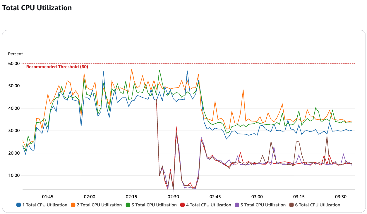
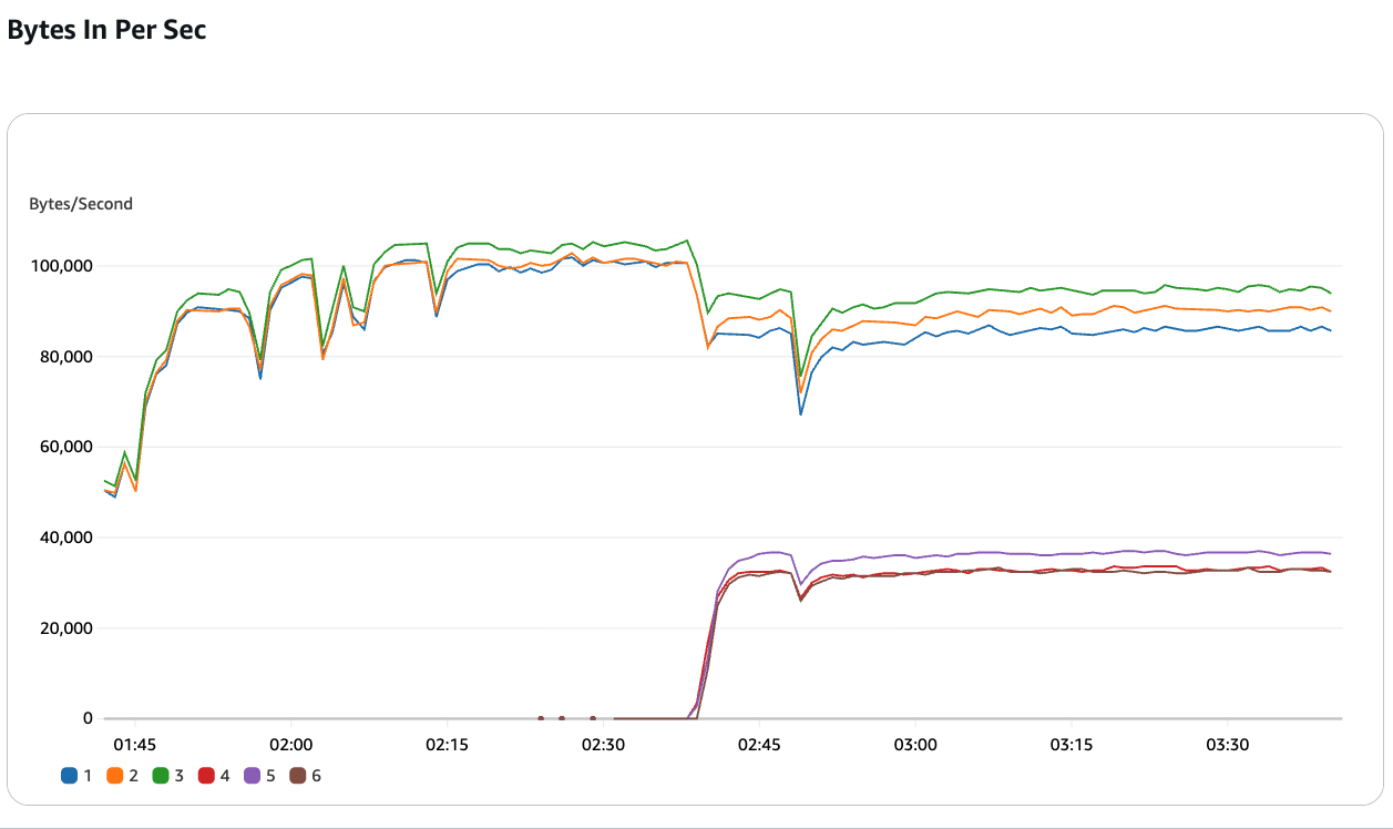
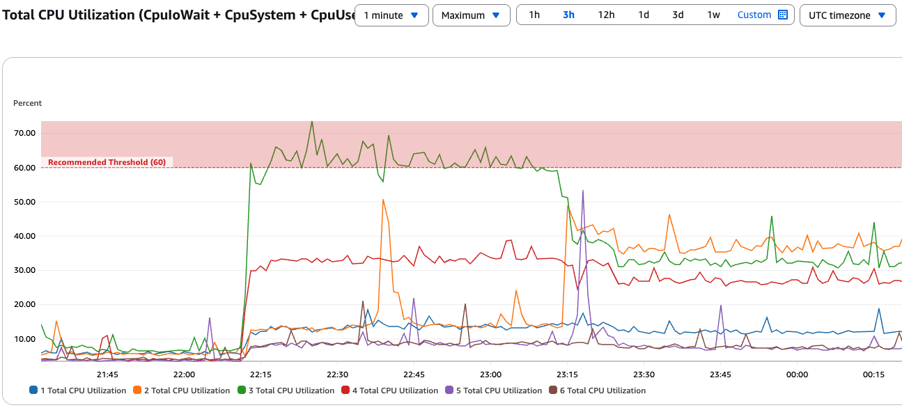
Scaling test: We’ll start by creating an Amazon MSK Express brokers cluster with 3 brokers. We’ll then rapidly scale the cluster up to 6 brokers and back down to 3 brokers, simulating a sudden spike in workload. With Intelligent Rebalancing enabled, you’ll see that the rebalancing of partitions is completed within 5-10 minutes, so that the cluster can sustain the increased throughput without any drop in performance.
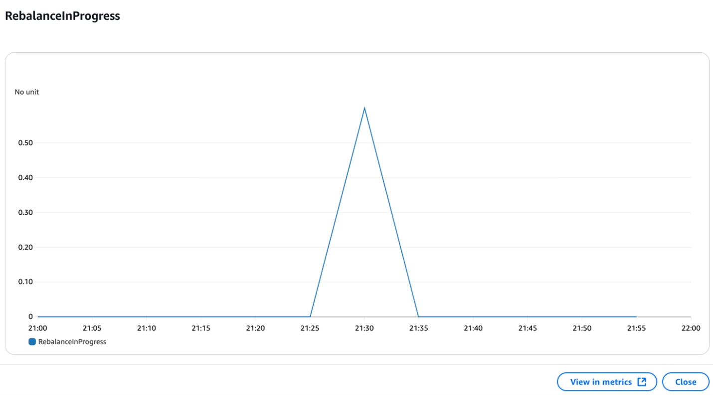
You can track the current and historical rebalancing operations using the metric RebalanceInProgress. In the picture below, you can also see that the clients on the producer side are not impacted during this rebalancing.
Next, we’ll create an imbalance in the cluster by directing a large portion of the traffic to a single broker. You’ll see that Intelligent Rebalancing detects this imbalance within minutes and automatically redistributes the partitions, restoring the cluster to an optimal state.
The intelligent rebalancing feature detects hotspots and automatically redistributes affected partitions across other brokers to optimize resource utilization. Without Intelligent Rebalancing, the resource imbalance would persist, potentially leading to performance issues or the need for manual intervention by the customer.
These tests showcase how Intelligent Rebalancing with Amazon MSK Express brokers enables scaling Kafka clusters seamlessly while maintaining consistently high performance, even under varying workload conditions.
Conclusion
Intelligent Rebalancing for Amazon MSK Provisioned clusters with Express brokers are currently being rolled out over the next few weeks in all AWS Regions where Amazon MSK Express brokers are supported. This feature is automatically enabled for all new Amazon MSK Provisioned clusters with Express brokers at no additional cost.
The new IRAP report includes four additional AWS services that are now assessed at the PROTECTED level under IRAP. This brings the total number of services assessed at the PROTECTED level to 168.
We have developed an IRAP documentation pack to help our Australian customers and their partners plan, architect, and assess risk for their workloads when they use AWS Cloud services.
The IRAP pack on AWS Artifact also includes newly updated versions of the AWS Consumer Guide and the whitepaper Reference Architectures for ISM PROTECTED Workloads in the AWS Cloud.
Reach out to your AWS representatives to let us know which additional services you would like to see in scope for upcoming IRAP assessments. We strive to bring more services into scope at the PROTECTED level under IRAP to support your requirements.
If you have feedback about this post, submit comments in the Comments section below.
Today, AWS announced the new Amazon Kinesis Data Streams On-demand Advantage mode, which includes warm throughput capability and an updated pricing structure. With this feature you can enable instant scaling for traffic surges while optimizing costs for consistent streaming workloads. On-demand Advantage mode is a cost-effective way to stream with Kinesis Data Streams for use cases that ingest at least 10 MiB/s in aggregate or have hundreds of data streams in an AWS Region.
In this post, we explore this new feature, including key use cases, configuration options, pricing considerations, and best practices for optimal performance.
Real-world use cases
As streaming data volumes grow and use cases evolve, you can face two common challenges with your streaming workloads:
Challenge 1: Preparing for traffic spikes
Many businesses experience predictable but significant traffic surges during events like product launches, content releases, or holiday sales. Using an on-demand capacity mode, you have to complete several steps when preparing for traffic spikes:
Transition to provisioned mode
Manually estimate and increase shards based on anticipated peak demand
Wait for scaling operations to finish
Subsequently return to on-demand mode
This mode-switching process was time consuming, required careful planning, and introduced operational complexity, forcing customers to either accept this operational burden, overprovision capacity well in advance, or risk throttling during critical business periods when data ingestion reliability matters most.
Challenge 2: Cost optimization for consistent workloads
Organizations with large, consistent streaming workloads want to optimize costs without sacrificing the simplicity and scalability available with on-demand streams. On-demand capacity mode serves well for fluctuating data traffic, yet customers desired a more economical approach to handle high-volume streaming workloads.
On-demand Advantage directly address both challenges by providing the capability to warm on-demand streams and a new pricing structure. With the new On-demand Advantage mode, there is no longer a fixed, per-stream charge, and the throughput usage is priced at a lower rate. The only requirement is that the account commits to streaming with at least 25 MiB/s of data ingest and 25 MiB/s of data retrieval usage.
This launch improves data streaming across multiple industries:
Online gaming companies can now prepare their streams for game launches without the cumbersome process of switching between modes and manually calculating shard requirements
Media and entertainment providers can support smooth data ingestion during major content releases and live events
E-commerce services can handle holiday sales traffic while optimizing costs for their baseline workloads.
By combining instant scaling with cost efficiency, you can confidently manage both predictable traffic surges and consistent streaming volumes without compromising on performance or budget.
How it works
The key features of On-demand Advantage mode are warm throughput and committed-usage pricing.
Warm throughput
With the warm throughput feature, available once you’ve enabled On-demand Advantage mode, you can configure your Kinesis Data Streams on-demand streams to have instantly available throughput capacity up to 10 GiB/s. This means you can proactively prepare on-demand streams for expected peak traffic events without the cumbersome process of switching between provisioned modes and manually calculating shard requirements. Key benefits include:
The ability to prepare for peak events so you can handle traffic surges smoothly
Alleviation of the need to build custom scaling solutions
The capability to continue scaling automatically beyond warm throughput if needed, up to 10 GiB/s or 10 million events per second
No additional fee for maintaining warm capacity
Committed-usage pricing
When you’ve enabled On-demand Advantage mode, the billing for the on-demand streams switches to a new structure that removes the stream hour charge and offers a discount of at least 60% for the throughput usage. Based on US East (N. Virginia) pricing, data ingested is priced 60% lower, data retrieval is priced 60% lower, Enhanced fan-out data retrieval is 68% lower, and extended retention is priced 77% lower. In return, you commit to stream 25 MiB/s for at least 24 hours. Even when actual usage is lower, if you enable this setting, you’re charged for the minimum 25 MiB/s throughput at the discounted price. Overall, the signficant discounts offered means that On-demand Advantage is more cost-effective for use cases that ingest at least 10 MiB/s in aggregate, fan out to more than two consumer applications, or have hundreds of data streams in an AWS Region.
Getting started
Follow these steps to start using On-demand Advantage mode.
Enabling On-demand Advantage mode
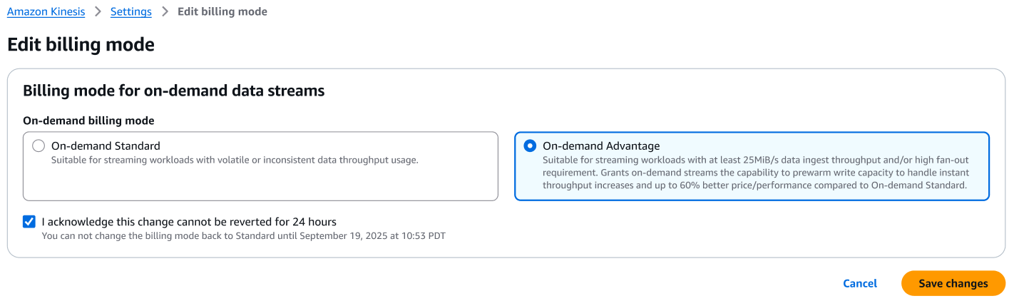
To start using the On-demand Advantage mode:
In the AWS Management Console
Navigate to the Kinesis Data Streams console
Navigate to the Account Settings tab
Choose Edit billing mode
Select the On-demand Advantage option
Select the checkbox, I acknowledge this change cannot be reverted for 24 hours
Choose Save changes
Using the AWS CLI
You can run the following CLI command to enable the minimum throughput billing commitment:
You can also create a new on-demand stream with warm throughput using the existing CreateStream API, or set warm throughput when converting a data stream from provisioned to On-demand Advantage mode.
Throttling and best practices for optimal performance
When working with warm throughput, it’s important to understand how capacity is managed. Each stream can instantly handle traffic up to the configured warm throughput level and will automatically scale beyond that as needed.
For optimal performance with warm throughput:
Use a uniformly distributed partition key strategy to evenly distribute records across shards and avoid hotspots and consider your partition key strategy carefully as you can ingest a maximum of 1 MiB/s of data per partition key, regardless of the warm throughput configured.
For cost optimization with committed usage pricing:
Analyze your daily throughput to verify it is at least 10 MiB/s.
Consider consolidating streams across your organization to maximize the benefit of the discount for on-demand streams.
Use cost effective data retrievals with – Use Enhanced Fan-Out – Use Enhanced Fan-Out consumers for applications that need dedicated throughput with 68% lower data retrievals cost in advantage mode.
Warm throughput in action
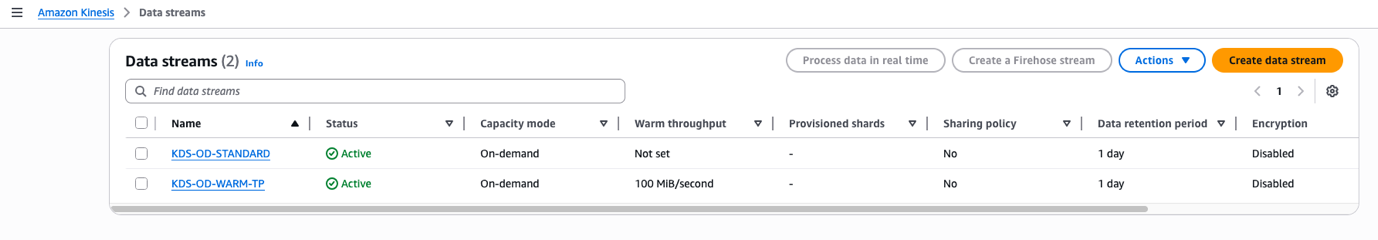
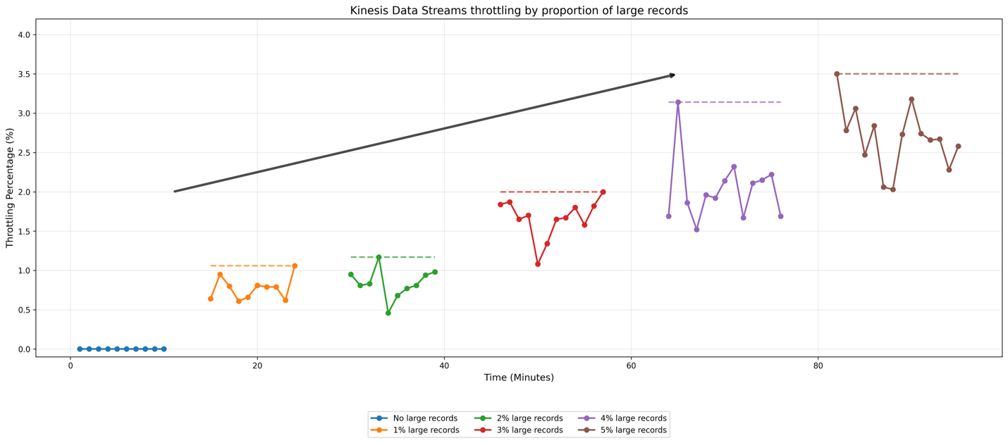
To demonstrate how warm throughput behaves, we enabled committed pricing in an AWS account and created two on-demand streams: “KDS-OD-STANDARD” and “KDS-OD-WARM-TP”. The “KDS-OD-WARM-TP” stream was configured with 100 MiB/second warm throughput, while “KDS-OD-STANDARD” remained as a regular on-demand stream without warm throughput, as demonstrated in the following screenshot.
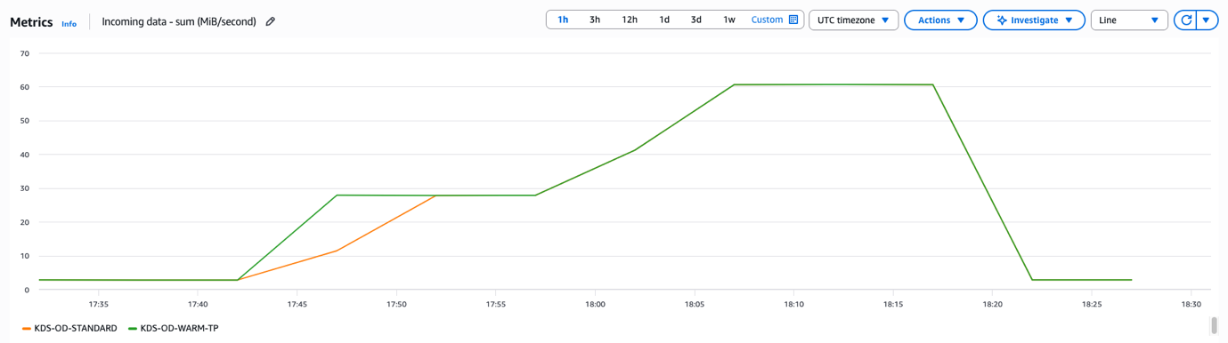
In our experiment, we initially simulated approximately 2 MiB/second traffic ingest for both “KDS-OD-STANDARD” and “KDS-OD-WARM-TP” streams. We used a UUID as a partition key so that traffic was evenly distributed across the shards of the Kinesis data streams, helping prevent potential hotspots that might skew our results. After establishing this baseline, we increased the ingest traffic to around 28 MiB/second within 10 minutes. We then further escalated the traffic to exceed 60 MiB/second within 15 minutes of the initial increase, as illustrated in the following screenshot.
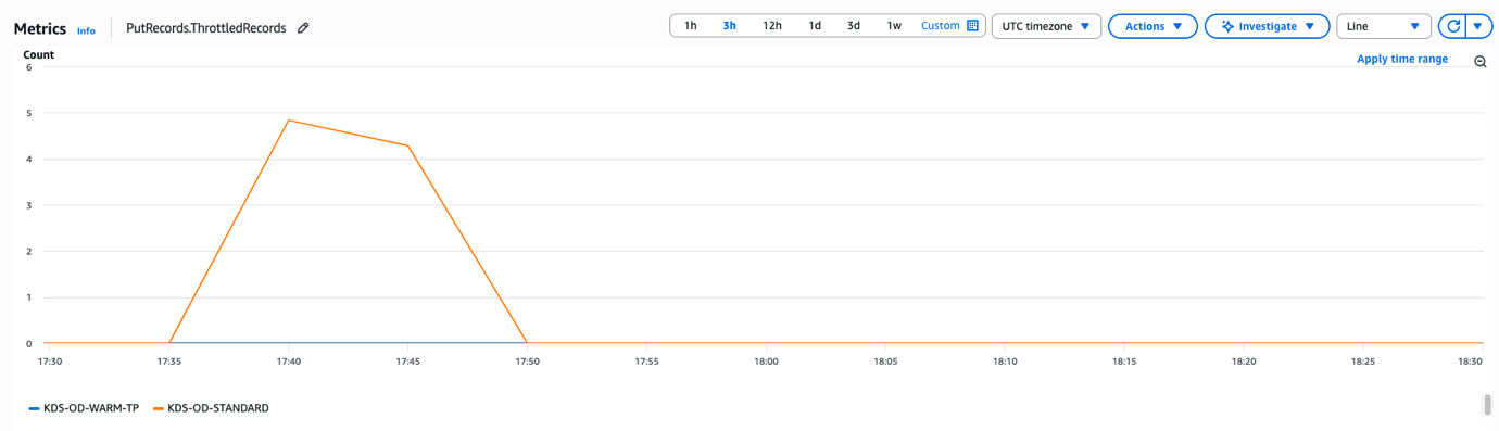
The following graph shows the ThrottledRecords CloudWatch metric for both “KDS-OD-STANDARD” and “KDS-OD-WARM-TP” that the warm throughput-enabled stream (“KDS-OD-WARM-TP”) did not encounter throttles during both traffic spikes, as it had 100 MiB/second warm throughput configured. In contrast, the standard on-demand stream (“KDS-OD-STANDARD”) experienced throttling when we increased traffic by 14x initially and by 2x later, before eventually scaling to bring throttles back to zero. This experiment demonstrates that you can use warm throughput to instantly prepare for peak usage times and avoid throttling during sudden traffic increases.
Conclusion
As we outlined in this post, the new Amazon Kinesis Data Streams On-demand Advantage mode provides significant benefits for organizations of different sizes:
Instant scaling for predictable traffic surges without overprovisioning.
Cost optimization for consistent streaming workloads with at least 60% discount.
Simplified operations with no need to switch between different capacity modes.
Enhanced flexibility to handle both expected and unexpected traffic patterns.
With these enhancements you can build and operate real-time streaming applications at many scales. Kinesis Data Streams now provides the ideal combination of scalability, performance, and cost-efficiency.
Covestro Deutschland AG, headquartered in Leverkusen, Germany, is a global leader in high-performance polymer materials and components. Since its spin-off from Bayer AG in 2015, Covestro has established itself as a key player in the chemical industry, with 48 production sites worldwide, €14.4 billion 2023 revenue, and 17,500 employees. Covestro’s core business focuses on developing innovative, sustainable solutions for products used in various aspects of daily life. The company offers materials for mobility, building and living, electrical and electronics sectors, in addition to sports and leisure, cosmetics, health, and the chemical industry. The company’s products, such as polycarbonates, polyurethanes, coatings, adhesives, and specialty elastomers, are important components in automotive, construction, electronics, and medical device industries.
To support this global operation and diverse product portfolio, Covestro adopted a robust data management solution. In this post, we show you how Covestro transformed its data architecture by implementing Amazon DataZone and AWS Serverless Data Lake Framework (SDLF), transitioning from a centralized data lake to a data mesh architecture. Through this strategic shift, teams can share and consume data while maintaining high quality standards through a consolidated data marketplace and business metadata glossary. The result: streamlined data access, better data quality, and stronger governance at scale that various producer and consumer teams can use to run data and analytics workloads at scale, enabling over 1,000 data pipelines and achieving a 70% reduction in time-to-market.
Business and data challenges
Prior to their transformation, Covestro operated with a centralized data lake managed by a single data platform team that handled the data engineering tasks. This centralized approach created several challenges: bottlenecks in project delivery because of limited engineering resources, complicated prioritization of use cases, and inefficient data sharing processes. The setup often resulted in unnecessary data duplication, which in turn slowed down time-to-market for new analytics initiatives, increased costs, and limited the ability of business units to act quickly on insights.The lack of visibility into data assets created significant operational challenges:
Teams could not find existing datasets, often recreating data already stored elsewhere
No clear understanding of data lineage or quality metrics
Difficulty in determining who owned specific data assets or who to contact for access
Absence of metadata and documentation about available datasets
Departments shared little knowledge about how they were using data
These visibility issues, combined with the lack of unified access controls, led to:
Siloed data initiatives across departments
Reduced trust in data quality
Inefficient use of resources
Delayed project timelines
Missed opportunities for cross-functional collaboration and insights
A strategic solution: Why Amazon DataZone and SDLF?
The challenges Covestro faced reflect deeper structural limitations of centralized data architectures. As Covestro scaled, central data teams often became bottlenecks, and lack of domain context led to fragmented quality, inconsistent standards, and poor collaboration. Instead of centralizing control, a data mesh gives ownership to the teams who generate and understand the data, while keeping the governance and interoperability consistent across the organization. This makes it well-suited for Covestro’s environment, which requires agility, scalability, and cross-team collaboration.
AWS Serverless Data Lake Framework (SDLF) is a solution to these challenges, providing a robust foundation for data mesh architectures. Traditional data lake implementations often centralize data ownership and governance, but with the flexible design of SDLF, organizations can build decentralized data domains that align with modern data mesh principles. The framework provides domain-oriented teams with the infrastructure, security controls, and operational patterns needed to own and manage their data products independently, while maintaining consistent governance across the organization. Through its modular architecture and infrastructure as code templates, SDLF accelerates the creation of domain-specific data products, so that Covestro’s teams can deploy standardized yet customizable data pipelines. This approach supports the key pillars of data mesh: domain-oriented decentralization, data as a product, self-serve infrastructure, and federated governance, providing Covestro with a practical path to overcome the limitations of traditional centralized architectures.
Amazon DataZone enhances the data mesh implementation through a unified experience for discovering and accessing data across decentralized domains. As a data management service, Amazon DataZone helps organizations catalog, discover, share, and govern data across organizational boundaries. It provides a central governance layer where organizations can establish data sharing agreements, manage access controls, and enable self-service data access while supporting security and compliance. While teams can use the SDLF framework to build and operate domain-specific data products, Amazon DataZone complements it with a searchable catalog enriched with metadata, business context, and usage policies, making data products easier to find, trust, and reuse.
Through the sharing capabilities of Amazon DataZone, domain teams can share their data products with other domains while maintaining granular access controls and governance policies, enabling cross-domain collaboration and data reuse. This integration means that domain teams can publish their SDLF-managed datasets to an Amazon DataZone catalog, so authorized consumers across the organization can discover and access them. Through the built-in governance capabilities built into Amazon DataZone, organizations can implement standardized data sharing workflows, check data quality, and enforce consistent access controls across their distributed data system, strengthening their data mesh architecture with robust data governance and democratization capabilities.Together, SDLF and Amazon DataZone provide Covestro with a comprehensive solution for implementing a modern data mesh architecture, enabling autonomous data domains to operate with consistent governance, seamless data sharing, and enterprise-wide data discovery.
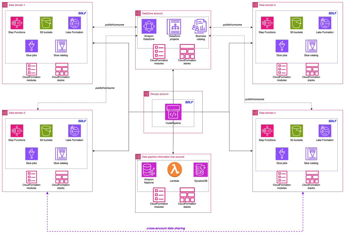
Solution architecture and implementation
The following architecture illustrates the high-level design of the data mesh solution. The implementation used a comprehensive AWS solution built on AWS services to create a robust, scalable, and governed data mesh that serves multiple business domains across the Covestro organization.
Data domain foundation: Serverless Data Lake Framework
A key pillar of the implementation is the Serverless Data Lake Framework (SDLF), which provides the foundational infrastructure and security needed to support data mesh strategies. SDLF delivers the core building blocks for data domains such as Amazon S3 storage layers, built-in encryption with AWS KMS, IAM-based access control, and infrastructure as code (IaC) automation. By using these components, Covestro can deploy decentralized, domain-owned data products rapidly while maintaining consistent governance across the enterprise.
The framework uses Amazon Simple Storage Service (Amazon S3) as the primary data storage layer, delivering virtually unlimited scalability and eleven nines of durability for diverse data assets. The proposed S3 bucket architecture follows AWS Well-Architected principles, implementing a multi-tiered structure with distinct raw, staging, and analytics data zones. This layered approach helps different business domains to maintain data sovereignty (each domain owns and controls its data, while keeping accessibility patterns organization-wide).
Security is a fundamental aspect in Covestro’s data mesh implementation. SDLF automatically implements encryption at rest and in transit across data storage and processing components. AWS Key Management Service (AWS KMS) provides centralized key management, while carefully crafted AWS Identity and Access Management (IAM) roles enable resource isolation.
Data processing with AWS Glue
AWS Glue serves as the cornerstone of the data processing and transformation capabilities, offering serverless extract, transform, and load ETL services that automatically scale based on workload demands.
Covestro’s pre-existent centralized data lake was fed by more than 1,000 ingestion data pipelines interacting with a variety of source systems. To support the migration of existing ingestion and processing pipelines, Covestro developed reusable blueprints that included the development and security standards defined for the data mesh.Covestro released standardized patterns that teams can deploy across multiple domains while providing the flexibility needed for domain-specific requirements. These blueprints support diverse source systems, from traditional databases like Oracle, SQL Server, and MySQL to modern software as a service (SaaS) applications such as SAP C4C.
They also developed specialized blueprints for processing, standardizing, and cleaning ingested raw data. These blueprints store processed data in Apache Iceberg format, automatically saving metadata in the AWS Glue Data Catalog and providing built-in capabilities to handle schema evolution seamlessly.
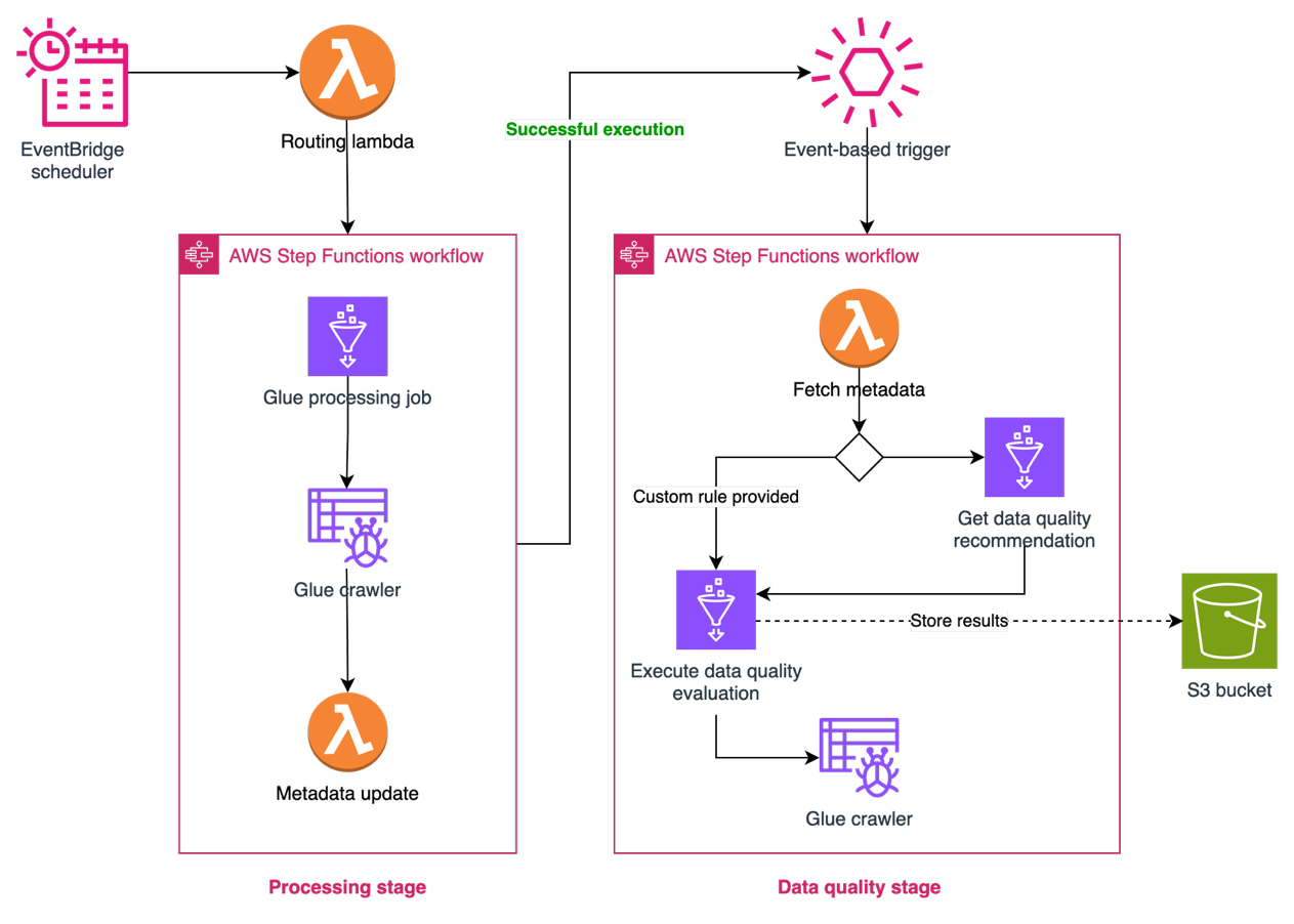
Covestro relies on SDLF to quickly configure and deploy the blueprints as AWS Glue jobs inside the domain. With SDLF, teams deploy a data pipeline through a YAML configuration file, and the orchestration and management mechanisms of SDLF handle the rest. The solution includes comprehensive monitoring capabilities built on Amazon DynamoDB, providing real-time visibility into data pipeline health and performance metrics (when teams deploy a pipeline through SDLF, the system automatically integrates it with the monitoring setup).
Data quality with AWS Glue Data Quality
To achieve data reliability across domains, Covestro extended the capabilities of SDLF to incorporate AWS Glue Data Quality into data processing pipelines. This integration enables automated data quality checks as part of the standard data processing workflow. Thanks to the configuration-driven design of SDLF, data producers can implement quality controls either using recommended rules, which are automatically generated through data profiling, or applying their own domain-specific rules.
The integration provides data teams with the flexibility to define quality expectations while maintaining consistency in how quality checks are implemented at the pipeline level. The solution logs quality evaluation results, providing visibility into the data quality metrics for each data product. These elements are illustrated in the following figure.
Enterprise-ready access control with AWS Lake Formation
AWS Lake Formation integration with the Data Catalog supports the security and access control layer that makes the data mesh implementation enterprise-ready. Through Lake Formation, Covestro implemented fine-grained access controls that respect domain boundaries while enabling controlled cross-domain data sharing.
The service’s integration with IAM means that Covestro can implement role-based access patterns that align with their organizational structure, so users can access the data they need while keeping appropriate security boundaries.
Data democratization with Amazon DataZone
Amazon DataZone functions as the heart of the data mesh implementation. Deployed in a dedicated AWS account, it provides the data governance, discovery, and sharing capabilities that were missing in the previous centralized approach. DataZone offers a unified, searchable catalog enriched with business context, automated access controls, and standardized sharing workflows that enable true data democratization across the organization.
Through Amazon DataZone, Covestro established a comprehensive data catalog that helps business users across different domains to discover, understand, and request access to data assets without requiring deep technical expertise. The business glossary functionality supports consistent data definitions across domains, eliminating the confusion that often arises when different teams use different terminology for the same concepts.
Data product owners can use the integration of Amazon DataZone integration with AWS Lake Formation to grant or revoke cross-domain access to data, streamlining the data sharing process while supporting security and compliance requirements.
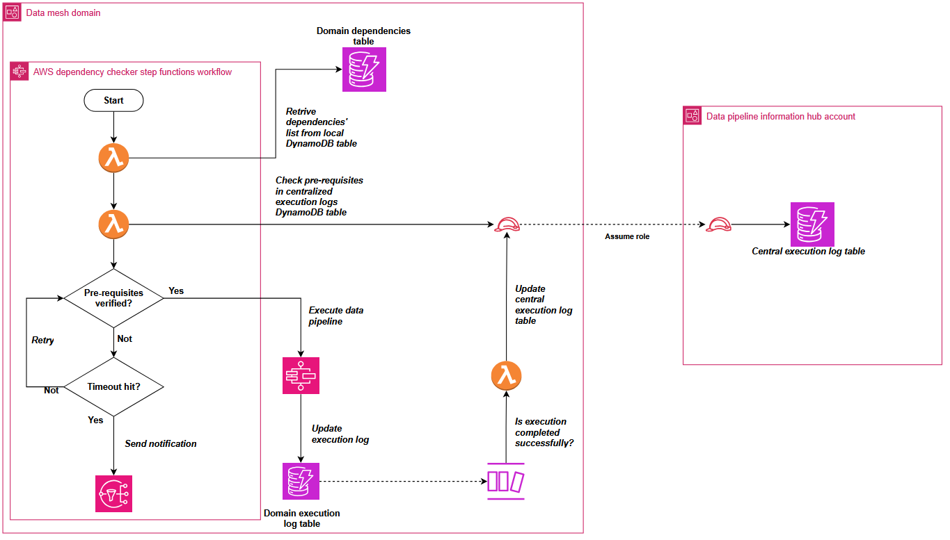
Managing cross-domain data pipeline dependencies
When implementing Covestro’s data mesh architecture on AWS, one of the most significant challenges was orchestrating data pipelines across multiple domains. The core question to address was “How can Data Domain A determine when a required dataset from Data Domain B has been refreshed and is ready for consumption?”.
In a data mesh architecture, domains maintain ownership of their data products while enabling consumption by other domains. This distributed model creates complex dependency chains where downstream pipelines must wait for upstream data products to complete processing before execution can begin.
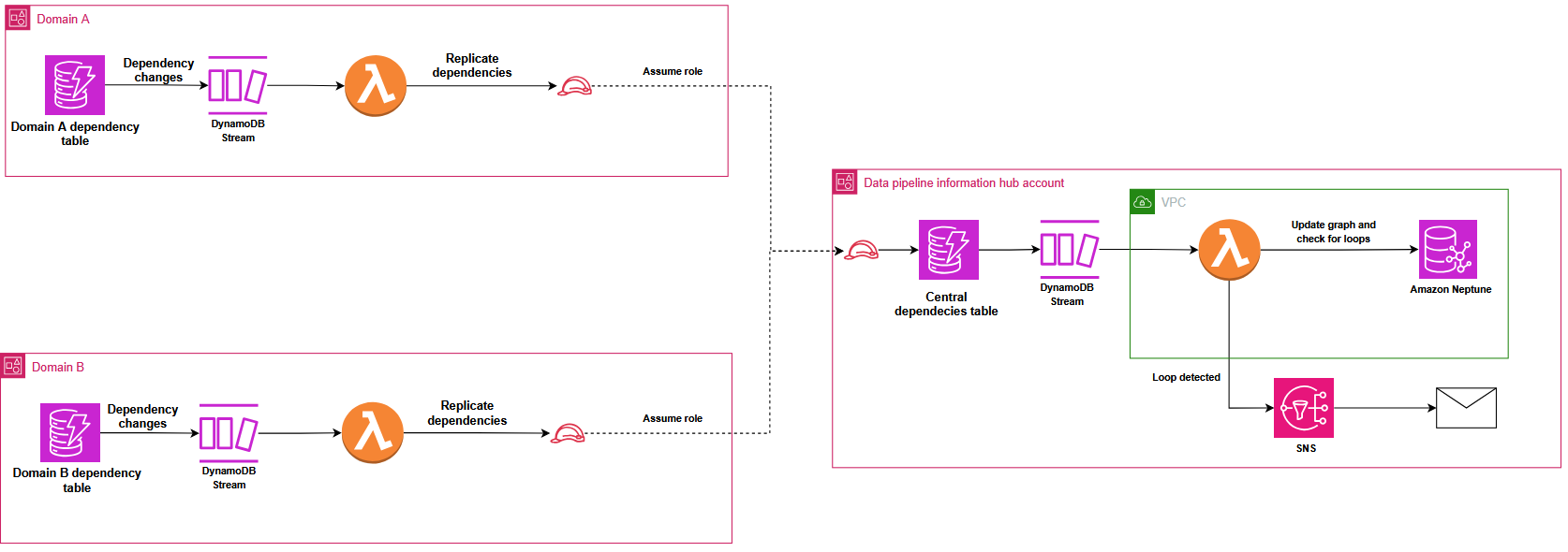
To address this cross-domain dependency coordination, Covestro extended the SDLF with a custom dependency checker component that operates through both shared and domain-specific elements.
The shared components consist of two centralized Amazon DynamoDB tables located in a hub AWS account: one collecting successful pipeline execution logs from the domains, and another aggregating pipeline dependencies across the entire data mesh.
These domains deploy local components such as a dependency-tracking Amazon DynamoDB table and an AWS Step Functions state machine. The state machine checks prerequisites using centralized execution logs and integrates seamlessly as the first step in every SDLF-deployed pipeline, without additional configuration. The following diagram shows the process described.
To prevent circular dependencies that could create locks in the distributed orchestration system, Covestro implemented a sophisticated detection mechanism using Amazon Neptune. DynamoDB Streams automatically replicate dependency changes from domain tables to the central registry, triggering an AWS Lambda function that uses the Gremlin graph traversal language (using pygremlin) to construct, update, and analyze a directed acyclic graph (DAG) of the pipeline relationships, with native Gremlin functions detecting circular dependencies and sending automated notifications, as illustrated in the following diagram. This process continuously updates the graph to reflect any new pipeline dependencies or changes across the data mesh.
Operational excellence through infrastructure as code
Infrastructure as code (IaC) practices using AWS CloudFormation and the AWS Cloud Development Kit (AWS CDK) significantly improve the operational efficiency of the data mesh implementation. The infrastructure code is version-controlled in GitHub repositories, providing complete traceability and collaboration capabilities for data engineering teams. This approach uses a dedicated deployment account that uses AWS CodePipeline to orchestrate consistent deployments across multiple data mesh domains.
The centralized deployment model supports that infrastructure changes follow a standardized continuous integration and deployment (CI/CD) process, where code commits trigger automated pipelines that validate, test, and deploy infrastructure components to the appropriate domain accounts. Each data domain resides in its own separate set of AWS accounts (dev, qa, prod), and the centralized deployment pipeline respects these boundaries while enabling controlled infrastructure provisioning.
IaC enables the data mesh to scale horizontally when onboarding new domains, supporting the maintenance of consistent security, governance, and operational standards across the entire environment. Covestro provisions new domains quickly using proven templates, accelerating time-to-value for business teams.
Business impact and technical outcomes
The implementation of the data mesh architecture using Amazon DataZone and SDLF has delivered significant measurable benefits across Covestro’s organization:
Accelerated data pipeline development
70% reduction in time-to-market for new data products through standardized blueprints
Successful migration of more than 1,000 data pipelines to the new architecture
Automated pipeline creation without manual coding requirements
Standardized approach and sharing across domains
Enhanced data governance and quality
Comprehensive business glossary implementation that supports consistent terminology
Automated data quality checks integrated into pipelines
End-to-end data lineage visibility across domains
Standardized metadata management through Apache Iceberg integration
Improved data discovery and access
Self-service data discovery portal through Amazon DataZone
Streamlined cross-domain data sharing with appropriate security controls
Reduced data duplication through improved visibility of existing assets
Efficient management of cross-domain pipeline dependencies
Operational efficiency
Decreased central data team bottlenecks through domain-oriented ownership
Reduced operational overhead through automated deployment processes
Improved resource utilization through elimination of redundant data processing
Enhanced monitoring and troubleshooting capabilities
The new infrastructure has fundamentally transformed how Covestro’s teams interact with data, enabling business domains to operate autonomously while upholding enterprise-wide standards for quality and governance. This has created a more agile, efficient, and collaborative data ecosystem that supports both current needs and future growth.
What’s next
As Covestro’s data platform continues to evolve, the focus is now to support domain teams to effectively built data products for cross domain analytics. In parallel, Covestro is actively working to improve data transparency with data lineage in Amazon DataZone through OpenLineage to support more comprehensive data traceability across a diverse set of processing tools and formats.
Conclusion
In this post, we showed you how Covestro transformed its data architecture transitioning from a centralized data lake to a data mesh architecture, and how this foundation will prove invaluable in supporting their journey toward becoming a more data-driven organization. Their experience demonstrates how modern data architectures, when properly implemented with the right tools and frameworks, can transform business operations and unlock new opportunities for innovation.
This implementation serves as a blueprint for other enterprises looking to modernize their data infrastructure while maintaining security, governance, and scalability. It shows that with careful planning and the right technology choices, organizations can successfully transition from centralized to distributed data architectures without compromising on control or quality.
WhatsApp is one of the most widely used messaging platforms globally, making it an ideal
channel for customer engagement. Whether you’re building a virtual assistant, a customer AI assistant, or an internal communication tool, developing a WhatsApp AI assistant presents unique design and operational challenges.
In this post, we explore best practices for building a WhatsApp AI assistant using AWS services—with a focus on how the AWS Summit Assistant used AWS End User Messaging and Amazon Bedrock to power a responsive, secure, and scalable generative AI assistant.
Why build a WhatsApp AI assistant with AWS End User Messaging
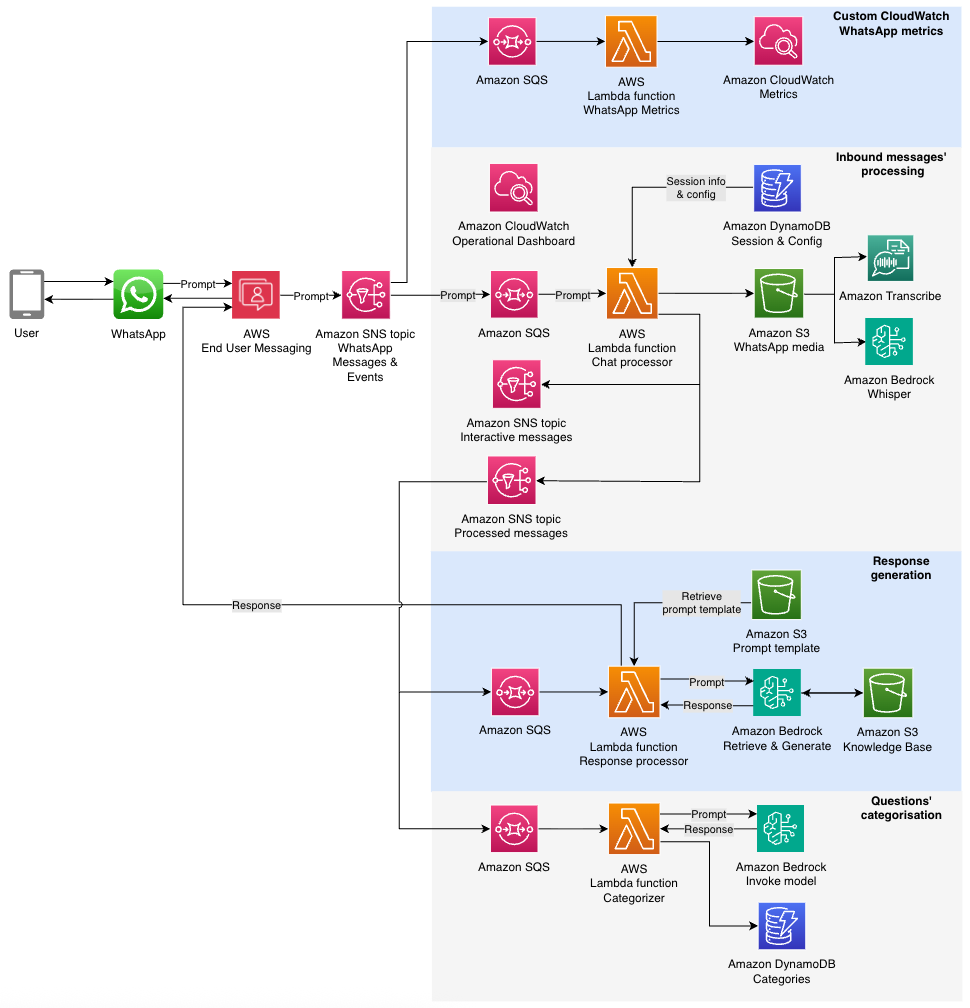
AWS offers a comprehensive set of services that can seamlessly handle the full lifecycle of a WhatsApp interaction—from ingesting and validating inbound messages, storing session context, generating AI responses, to monitoring key performance indicators in real time.
AWS End User Messaging provides native integration with WhatsApp, so you can send and receive messages directly using a REST API or SDK. It also supports AWS Identity and Access Management (IAM), enabling fine-grained control over access, authentication, and user roles.
The following sections outline best practices for designing, building, and operating WhatsApp AI assistants on AWS. Although not every recommendation will apply to every use case, they are based on real-world lessons learned from production deployments like the AWS Summit Assistant.
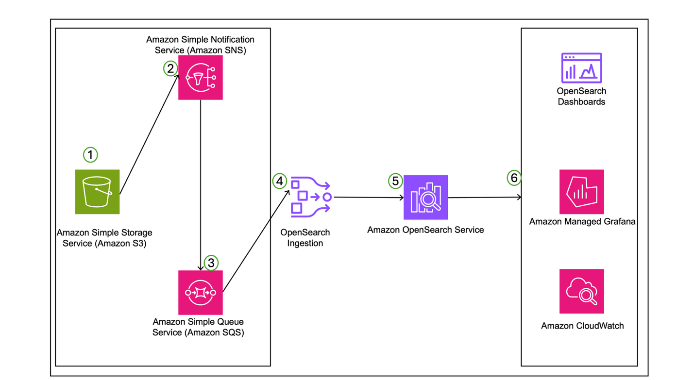
Use a modular, event-driven architecture
Rather than relying on tightly coupled services or monolithic workflows, design your WhatsApp AI assistant as a set of loosely coupled, modular components. AWS services such as Amazon Simple Notification Service (Amazon SNS), Amazon Simple Queue Service (Amazon SQS), and AWS Lambda are ideal for building scalable, event-driven systems.
By default, AWS End User Messaging publishes inbound WhatsApp messages and engagement events to an SNS topic. To manage throughput and avoid overwhelming downstream components, subscribe an SQS queue to this topic. With this setup, you can process messages at a controlled pace and buffer traffic during bursts.
Depending on your use case, you might choose to skip dead-letter queues (DLQs) in favor of logging failures to Amazon CloudWatch Logs, especially given the real-time nature of chatbots where retrying a failed message hours later might no longer be relevant. Instead, the AI assistant should respond to the user immediately, explaining the issue and suggesting corrective actions such as rephrasing their question or trying again later.
A typical modular structure might have the following components:
SQS queue – An SQS queue subscribed to the WhatsApp Messages & Events SNS topic to control throughput and isolate retries.
A messages processor function for inbound processing and audio processing (optional) – This AWS Lambda function handles initial validation and message-type filtering and transcribes the voice message. The output is published to the Processed messages SNS topic.
Fan-out to downstream consumers – Other Lambda functions through Amazon SQS subscribe to the Processed messages SNS topic to handle specialized tasks like response generation using Amazon Bedrock or categorization and analytics’ purposes.
The following diagram illustrates the solution architecture.
This fan-out architecture promotes clean separation of concerns, avoids redundant processing, and makes it straightforward to introduce new capabilities such as sentiment analysis or content moderation by simply adding new subscribers. By decoupling components and using Amazon SNS and Amazon SQS patterns, each part of the system can scale independently and recover gracefully from localized failures.
Design for controlled processing throughput
When integrating with other AWS services such as Amazon Bedrock, with soft service quotas, it’s critical to manage throughput carefully. Use Amazon SQS to decouple the SNS topic from Lambda invocations. This makes sure spikes in message volume don’t result in throttling or failed invocations. It also lets you scale consumer Lambda functions based on queue depth, allowing for burst handling without dropping messages. In cases where message failure is unrecoverable (such as invalid content or unsupported message types), log the error and notify the user with a helpful message rather than retrying. This keeps the user informed and prevents queues from growing unnecessarily due to retry cycles. This design pattern of Amazon SNS to Amazon SQS to Lambda is foundational for building resilient, scalable AI assistants that meet user expectations for speed and reliability.
Handle voice messages with Amazon Transcribe or Whisper
WhatsApp voice messages are received in OGG format. To process these messages, you can use the AWS End User Messaging GetWhatsAppMessageMedia API to retrieve media files, including audio, images, and video. The audio needs to be converted to a compatible format for transcription: PCM for Amazon Transcribe or WAV for Hugging Face Whisper (available through Amazon Bedrock Marketplace). This conversion can be achieved using a library like FFmpeg, implemented as a Lambda layer.
The processing flow involves fetching audio from WhatsApp, which is then automatically stored in Amazon Simple Storage Service (Amazon S3) in a bucket you create and own (this is the default behavior of the GetWhatsAppMessageMedia API). Next, the audio is converted to the required format and stored locally in Lambda for faster processing before being transcribed.
As a best practice, consider deleting audio files after processing to simplify data management and reduce storage requirements for personally identifiable information (PII). This approach facilitates efficient handling and transcription of WhatsApp voice messages while maintaining data privacy standards.
Enforce strict message validation
To promote quality and security, implement layered validation within your message processing Lambda function. This might differ depending your use case and requirements:
Message status indicators – Mark inbound messages as read and indicate you are responding to maintain the recipients’ interest while generating a response. WhatsApp’s API allows marking messages as read by message ID and setting the typing indicator to true. The typing indicator automatically dismisses after 25 seconds without a reply.
Message type validation – Filter by message type using the inbound WhatsApp message payload’s type field. Implement checks based on your AI assistant’s supported message types and provide static responses for unsupported formats. For example, a text only AI assistant shouldn’t process message types such as Media, Reaction, Template, Location, Contacts or Interactive.
Size limit protection – Add message size validation based on character count. This prevents resource drainage from potential bad actors who might attempt to send extremely large text chunks that could generate excessive large language model (LLM) input tokens.
Conversation management – Track message counts and total character length per conversation, resetting the context when necessary to manage costs and prevent resource drainage. Implement this using Amazon DynamoDB with the recipient’s hashed phone number as the primary key.
Processing lock mechanism – Prevent duplicate processing by implementing a flag system in DynamoDB. When processing a message, set the recipient’s flag to true. While active, new messages receive a static response indicating that a previous message is being processed, avoiding out-of-sync responses and resource waste.
Access control – Consider implementing an allow list for beta functionality or controlled access. This provides selective AI assistant activation for testing while restricting general audience access when needed.
Error handling – Manage response generation failures with clear, static replies to the customer. Include troubleshooting steps or alternative contact channels based on the issue’s severity to maintain a positive user experience.
Security
Consider the following security best practices for message processing systems:
Encryption standards – Encrypt SNS topics, SQS queues, and DynamoDB tables using AWS Key Management Service (AWS KMS) service managed keys or customer managed keys (CMKs) to facilitate data protection at rest and in transit.
PII data protection – For analytics and troubleshooting purposes, avoid logging raw phone numbers when the full number isn’t required. Instead, implement hashing of phone numbers before logging to maintain user privacy while preserving tracking capabilities.
Data retention management – Enable Time-To-Live (TTL) attributes on DynamoDB tables to automatically purge old session data, maintaining data hygiene and avoiding storing PII data when not needed.
Content safety controls – Implement Amazon Bedrock Guardrails to prevent processing or generating unwanted content and messages. When required, use the data loss protection features of Amazon Bedrock Guardrails to safeguard sensitive information.
Use Amazon Bedrock for generative responses and categorization
The AWS Summit Assistant used two key Amazon Bedrock capabilities:
Amazon Bedrock Knowledge Bases – Powered by Amazon Bedrock Knowledge Bases using OpenSearch vector embeddings and Anthropic on Amazon Bedrock, the AI assistant could answer user questions using publicly available event data.
Categorization – Using the InvokeModel API, inbound messages were tagged with categories for analytics. A DynamoDB table stored category counts, enabling trend detection across users.
Sessions persisted using the Amazon Bedrock native session ID feature for consistent conversation flow.
Monitoring
Consider the following monitoring and data analysis options:
Message status tracking – WhatsApp provides six distinct events per message. Though valuable, these should be complemented with AWS service operational metrics for comprehensive monitoring. These events are published on the WhatsApp SNS topic in your AWS account.
Real-time monitoring with CloudWatch – Set up CloudWatch alarms to track SNS message publication rates, providing real-time visibility into WhatsApp activity for both inbound and outbound messages. Extend monitoring to include Lambda function and Amazon Bedrock metrics. For tracking WhatsApp’s six message states, implement a dedicated Lambda function that subscribes to the WhatsApp SNS topic and records each event as a custom CloudWatch metric.
Detailed analysis with CloudWatch Logs Insights – Use CloudWatch Logs Insights for granular monitoring with minimal development overhead. This approach enables advanced queries for metrics not available through standard CloudWatch metrics, such as unique conversation counts and user engagement statistics. The logs’ content depends on your requirements.
Advanced analytics integration – For sophisticated use cases, implement a data pipeline using Amazon Data Firehose to store events in Amazon S3, then visualize using business intelligence tools like Amazon Quick Sight for custom dashboards. For a reference implementation, refer to the following GitHub repo.
Example use case: AWS Summit Assistant
Deployed at AWS Summit Dubai 2025, AWS Summit Johannesburg 2025, AWS Cloud Day Türkiye, AWS Cloud Day Riyadh and re:Inforce re:Cap London 2025, this WhatsApp AI assistant performed the following functions:
Used Amazon Bedrock Knowledge Bases to answer attendee questions
Transcribed voice messages using Whisper
Categorized questions for trend reporting
Operated with near real-time responsiveness using Amazon SNS, Amazon SQS, and Lambda
The AI assistant processed over 2,000 questions with no service interruptions, showing the viability of serverless architecture for WhatsApp-based assistants.
Conclusion
Building a scalable and secure WhatsApp AI assistant with AWS offers numerous advantages for businesses looking to enhance customer engagement. By using AWS services like AWS End User Messaging, Amazon Bedrock, Lambda, and DynamoDB, builders can create robust, AI-powered assistants that handle high message volumes while maintaining security and performance. Key takeaways include:
Adopting a modular, event-driven architecture for flexibility and scalability
Implementing thorough message validation and security measures
Using Amazon Bedrock for advanced Gen AI capabilities
Establishing comprehensive monitoring and analytics
Although these practices provide a strong foundation, they represent just a subset of possible best practices. As WhatsApp and AWS services grow and industry standards change, best practices continue to evolve. Stay current by regularly reviewing AWS documentation and keeping up with new feature releases.
Today, AWS announced that Amazon Kinesis Data Streams now supports record sizes up to 10MiB – a tenfold increase from the previous limit. With this launch, you can now publish intermittent larger data payloads on your data streams while continuing to use existing Kinesis Data Streams APIs in your applications without additional effort. This launch is accompanied by a 2x increase in the maximum PutRecords request size from 5MiB to 10MiB, simplifying data pipelines and reducing operational overhead for IoT analytics, change data capture, and generative AI workloads.
In this post, we explore Amazon Kinesis Data Streams large record support, including key use cases, configuration of maximum record sizes, throttling considerations, and best practices for optimal performance.
Real world use cases
As data volumes grow and use cases evolve, we’ve seen increasing demand for supporting larger record sizes in streaming workloads. Previously, when you needed to process records larger than 1MiB, you had two options:
Split large records into multiple smaller records in producer applications and reassemble them in consumer applications
Both these approaches are useful, but they add complexity to data pipelines, requiring additional code, increasing operational overhead, and complicating error handling and debugging, particularly when customers need to stream large records intermittently.
This enhancement improves the ease of use and reduces operational overhead for customers handling intermittent data payloads across various industries and use cases. In the IoT analytics domain, connected vehicles and industrial equipment are generating increasing volumes of sensor telemetry data, with the size of individual telemetry records occasionally exceeding the previous 1MiB limit in Kinesis. This required customers to implement complex workarounds, such as splitting large records into multiple smaller ones or storing the large records separately and only sending metadata through Kinesis. Similarly, in database change data capture (CDC) pipelines, large transaction records can be produced, especially during bulk operations or schema changes. In the machine learning and generative AI space, workflows are increasingly requiring the ingestion of larger payloads to support richer feature sets and multi-modal data types like audio and images. The increased Kinesis record size limit from 1MiB to 10MiB limits the need for these types of complex workarounds, simplifying data pipelines and reducing operational overhead for customers in IoT, CDC, and advanced analytics use cases. Customers can now more easily ingest and process these intermittent large data records using the same familiar Kinesis APIs.
How it works
To start processing larger records:
Update your stream’s maximum record size limit (maxRecordSize) through the AWS Console, AWS CLI, or AWS SDKs.
Continue using the same PutRecord and PutRecords APIs for producers.
Continue using the same GetRecords or SubscribeToShard APIs for consumers.
Your stream will be in Updating status for a few seconds before being ready to ingest larger records.
Getting started
To start processing larger records with Kinesis Data Streams, you can update the maximum record size by using the AWS Management Console, CLI or SDK.
On the AWS Management Console,
Navigate to the Kinesis Data Streams console.
Choose your stream and select the Configuration tab.
Choose Edit (next to Maximum record size).
Set your desired maximum record size (up to 10MiB).
Save your changes.
Note: This setting only adjusts the maximum record size for this Kinesis data stream. Before increasing this limit, verify that all downstream applications can handle larger records.
Throttling and best practices for optimal performance
Individual shard throughput limits of 1MiB/s for writes and 2MiB/s for reads remain unchanged with support for larger record sizes. To work with large records, let’s understand how throttling works. In a stream, each shard has a throughput capacity of 1 MiB per second. To accommodate large records, each shard temporarily bursts up to 10MiB/s, eventually averaging out to 1MiB per second. To help visualize this behavior, think of each shard having a capacity tank that refills at 1MiB per second. After sending a large record (for example, a 10MiB record), the tank begins refilling immediately, allowing you to send smaller records as capacity becomes available. This capacity to support large records is continuously refilled into the stream. The rate of refilling depends on the size of the large records, the size of the baseline record, the overall traffic pattern, and your chosen partition key strategy. When you process large records, each shard continues to process baseline traffic while leveraging its burst capacity to handle these larger payloads.
To illustrate how Kinesis Data Streams handles different proportions of large records, let’s examine the results a simple test. For our test configuration, we set up a producer that sends data to an on-demand stream (defaults to 4 shards) at a rate of 50 records per second. The baseline records are 10KiB in size, while large records are 2MiB each. We conducted multiple test cases by progressively increasing the proportion of large records from 1% to 5% of the total stream traffic, along with a baseline case containing no large records. To ensure consistent testing conditions, we distributed the large records uniformly over time for example, in the 1% scenario, we sent one large record for every 100 baseline records. The following graph shows the results:
In the graph, horizontal annotations indicate throttling occurrence peaks. The baseline scenario, represented by the blue line, shows minimal throttling events. As the proportion of large records increases from 1% to 5%, we observe an increase in the rate at which your stream throttles your data, with a notable acceleration in throttling events between the 2% and 5% scenarios. This test demonstrates how Kinesis Data Streams manages increasing proportion of large records.
We recommend maintaining large records at 1-2% of your total record count for optimal performance. In production environments, actual stream behavior varies based on three key factors: the size of baseline records, the size of large records, and the frequency at which large records appear in the stream. We recommend that you test with your demand pattern to determine the specific behavior.
With on-demand streams, when the incoming traffic exceeds 500 KB/s per shard, it splits the shard within 15 minutes. The parent shard’s hash key values are redistributed evenly across child shards. Kinesis automatically scales the stream to increase the number of shards, enabling distribution of large records across a larger number of shards depending on the partition key strategy employed.
For optimal performance with large records:
Use a random partition key strategy to distribute large records evenly across shards.
Implement backoff and retry logic in producer applications.
Monitor shard-level metrics to identify potential bottlenecks.
If you still need to continuously stream of large records, consider using Amazon S3 to store payloads and send only metadata references to the stream. Refer to Processing large records with Amazon Kinesis Data Streams for more information.
Conclusion
Amazon Kinesis Data Streams now supports record sizes up to 10MiB, a tenfold increase from the previous 1MiB limit. This enhancement simplifies data pipelines for IoT analytics, change data capture, and AI/ML workloads by eliminating the need for complex workarounds. You can continue using existing Kinesis Data Streams APIs without additional code changes and benefit from increased flexibility in handling intermittent large payloads.
For optimal performance, we recommend maintaining large records at 1-2% of total record count.
For best results with large records, implement a uniformly distributed partition key strategy to evenly distribute records across shards, include backoff and retry logic in producer applications, and monitor shard-level metrics to identify potential bottlenecks.
Before increasing the maximum record size, verify that all downstream applications and consumers can handle larger records.
We’re excited to see how you’ll leverage this capability to build more powerful and efficient streaming applications. To learn more, visit the Amazon Kinesis Data Streams documentation.
You can use AWS Step Functions to orchestrate complex business problems. However, as workflows grow and evolve, you can find yourself grappling with monolithic state machines that become increasingly difficult to maintain and update. In this post, we show you strategies for decomposing large Step Functions workflows into modular, maintainable components. We dive deep into architectural patterns like parent-child workflows, domain-based separation, and shared utilities that can help you break down complexity while maintaining business functionality. By implementing these decoupling techniques, you can achieve faster deployments, better error isolation, and reduced operational overhead – all while keeping your workflows scalable and efficient. Whether you’re dealing with payment processing, data transformation, or complex business logic, these patterns will help you build more resilient and manageable Step Functions applications.
The Complexity of Single-State Machine Architectures
While monolithic workflows can be suitable for simple, linear processes with limited states and clear dependencies, they become problematic when handling complex business logic across multiple domains. If your workflow involves more than 15-20 states, crosses multiple business domains, or requires frequent updates from different teams, it’s a strong indicator that you should consider a decomposed approach instead of a monolithic one. However, monolithic workflows remain a valid choice for scenarios with straightforward business logic, single-team ownership, infrequent changes, and workflows with less than 15 states – especially when rapid development and simplified debugging are priorities.
Let’s examine a real-world example of such a monolithic workflow and understand the challenges it presents for development teams, operational efficiency, and business agility. Below is an example of a state machine that is a mix of payment processes, inventory management, and notification mechanisms for an e-commerce implementation:
Figure 1: A state machine that is a mix of payment processes, inventory management, and notification mechanisms for an e-commerce implementation
State Explosion
Modifying a single state in a monolithic workflow triggers a cascade of changes across multiple interconnected states due to their tight coupling and dependencies. For example, adding a new payment method would require modifications across various states including validation, processing, and error handling, creating a ripple effect throughout the workflow. This inter dependency makes even simple changes complex and risky, as altering one component can have unintended consequences on other parts of the workflow.
Looking at the provided architecture, we can see a clear example of state explosion where a single workflow handles multiple business processes including order validation, payment processing, inventory management, shipping calculations, and customer notifications. This creates a complex web of dependent states that becomes increasingly difficult to manage. The result is a “spider web” of states that becomes progressively harder to understand, debug, and maintain.
Version Management
Version management in monolithic workflows requires deploying the entire workflow even for minor changes to individual components, making it difficult to isolate and update specific business logic. The provided architecture demonstrates the version management challenge clearly. For instance, if the shipping calculation logic needs an urgent fix, the entire workflow must be redeployed, requiring comprehensive testing of all components, including unmodified ones, to ensure nothing breaks in the process.
Resource Limitations
While not immediately visible in the architecture diagram, Monolithic workflows face operational constraints as they grow in complexity, particularly with state transitions, maximum event payload size, and execution history size. Refer to the Service quotas documentation to understand such limits. These constraints become critical bottlenecks as workflows grow in complexity and handle increased transaction volumes. In the monolithic state machine, long-running operations like payment processing and shipping calculations, combined with multiple state transitions, could approach these limits, especially for high-volume scenarios.
Additionally, we also come across generic design challenges such as error handling. In monolithic approach, workflows leads to redundant try-catch blocks and retry configurations across different operations. This creates challenges in implementing distinct error strategies for different business scenarios and makes it difficult to maintain proper rollback mechanisms when failures occur in middle states.
These challenges collectively highlight the need for a more modular approach to Step Functions workflow design.
Transforming Complex Workflows Through Decomposition
When transforming complex monolithic workflows into more manageable components, you can employ several decomposition strategies to achieve better modularity and maintainability. These strategies include the parent-child pattern, which creates a hierarchical structure of workflows, domain separation that breaks down workflows based on business capabilities, shared utilities that serve as reusable components for common operations, and specialized error workflows for centralized error handling. Each of these strategies can be implemented either individually or in combination, depending on the specific requirements and complexity of the application, allowing organizations to create more efficient, scalable, and maintainable Step Functions workflows while ensuring proper separation of concerns and reduced operational overhead.
Parent-Child Pattern
The parent-child pattern represents a hierarchical approach to workflow organization where a main (parent) workflow orchestrates multiple sub-workflows (children). Parent workflows manage the overall business process and coordination, while child workflows handles specific, short-lived operations. This pattern is particularly effective when you need to balance between orchestration complexity and execution speed.
Figure 2 : Decoupled parent state machine
The current monolithic workflow can be restructured by creating a parent workflow focused on order orchestration while delegating specific operations to Express child workflows. The parent workflow would maintain the high-level flow from order validation through completion, while time-sensitive operations like ValidateOrder, ProcessPayment, and ProcessShipping could become Express child workflows.
Kindly note that during an architecture re-vamp, Express workflows are different when compared to Standard Workflows. For example, you cannot have an Express parent workflow invoke a Standard child workflow. Also, an Express workflow does not support Job-run (.sync) or Callback (.waitForTaskToken) service integration patterns. You can refer to the differences between Standard and Express workflows documentation to choose the right architecture pattern.
For instance, the payment processing section could be transformed into a child Express workflow that handles all payment-related states (ProcessPayment, ProcessStandardPayment, ValidatePaymentPart) as a single unit. An express workflow is more suitable for sections like payment processing as their executions complete within 5 minutes. Hence this would also reduce the over-all cost of the workflow. Similarly, the shipping calculation logic involving CalculateExpressShipping and CalculateStandardShipping could be consolidated into another Express child workflow, leading to reduced costs and easier updates to shipping logic.
Domain Separation
Domain separation involves breaking down workflows based on distinct business capabilities or functional areas. Each domain-specific workflow becomes responsible for a complete business function, operating independently while communicating through well-defined interfaces. This approach aligns closely with micro-service architecture principles and domain-driven design. The architecture shows clear boundaries between different business domains that can be separated into independent workflows. Three primary domains emerge:
Payment Domain: Encompassing ValidateOrder, ProcessPayment, ValidatePaymentPart, and related error handlers
Inventory Domain: Including CheckInventory, UpdateInventory, and associated states
Shipping Domain: Containing ProcessShipping, shipping calculations, and shipping status updates
Each domain would become its own workflow, with clear input/output contracts. This separation would allow specialized teams to maintain and deploy updates to their domain workflows independently ensuring implementation of domain-specific retry policies, error handling, and business rules without affecting other domains. For example, the payment team could enhance payment processing logic without impacting shipping or inventory operations.
Figure 3 : Child state machine that handles payment workflow
Figure 4 : Child state machine that handles shipping workflow
Shared Utilities
Shared utility workflows serve as reusable components for common operations that appear across multiple business processes. These workflows encapsulate standard functionality like notification handling, data validation, logging, or audit trail creation. By centralizing these common operations, organizations can ensure consistency and reduce duplication across their Step Functions applications.
The current architecture repeats several common patterns that could be extracted into shared utility workflows. Most notably, the notification handling logic (SendEmail, SendSMSNotification, SendPushNotification) appears as a cluster of states at the end of the workflow. This could be consolidated into a single “NotificationManager” utility workflow that handles all types of notifications. These utility workflows could then be called from any other workflow in the system, ensuring consistent behavior and reducing code duplication.
Figure 5 : Re-usable notification workflow
Error Workflows
Error workflows represent a specialized form of decomposition focused on centralizing error handling and recovery logic. Instead of embedding complex error handling in each business workflow, organizations can create dedicated workflows that manage different types of failures, retries, and compensation actions. This approach provides a consistent and maintainable way to handle errors across the application.
Each of these decomposition strategies can be used individually or in combination, depending on the specific needs of your application. For instance, utilization of Domain Separation pattern has resulted in streamlined error workflows. The key is to choose the appropriate combination that provides the right balance of maintainability, scalability, and operational efficiency for your use case. However, implementing all four strategies in a phased approach would provide the most comprehensive solution for long-term maintainability and scalability.
Results:
The comparison between monolithic and decoupled approaches reveals notable differences in performance and operational metrics. In order to emulate similar test environments across monolithic and decomposed state machines, we tested them in us-east-1 AWS region. We made use of the aforementioned workflows, both monolithic and decomposed to achieve a similar end goal. Pricing comparison is based on a monolithic workflow processing 11 state transitions per workflow across 30,000 monthly requests. For the decomposed approach, calculations assume Express child workflows configured with 64MB memory and 100ms execution duration, while the parent workflow handles 8 state transitions per workflow for the same volume of 30,000 monthly requests. AWS Lambda task states in both approaches complete within 2 seconds of execution time.
When decoupled, the workflows can be re-designed to use either Express or Standard mechanisms depending on their execution time and integration pattern requirements. In this use-case, we identified multiple workflows like PaymentProcessing, CalculateExpressShipping that are revamped to use Express workflows as per their requirement. While the monolithic approach shows a slightly faster execution duration of 11.5 seconds compared to 13 seconds in the decomposed approach, the monthly pricing significantly favors the decoupled architecture at $6.37 USD versus $11.90 USD for the monolithic approach. The decoupled approach demonstrates superior debugging capabilities with better error isolation and domain-specific debugging, contrasting with the monolithic approach’s complex debugging challenges due to heavy payloads and middle-state failure tracking. Additionally, the decoupled architecture benefits from smaller payload sizes through distributed data handling, whereas the monolithic workflow carries larger payloads across its 18 state transitions.
Monolithic Approach
Decoupled Approach
Execution Duration
11.5 seconds for complete workflow execution
13 seconds with distributed processing across parent-child workflows
Monthly Pricing
$11.90 USD (476,000 billable state transitions)
$6.37 USD (Combined cost of Standard parent workflow and Express child workflows)
Debug Effort
High – Complex debugging due to heavy payloads and difficulty in tracking failures in middle states. Cannot effectively use ResultSelector when final notification state needs all details.
Lower – Easier to debug with isolated domains and smaller payloads. Better error isolation and domain-specific debugging.
Payload Size
Larger payload size throughout workflow execution as all data needs to be carried across 18 state transitions
Smaller payload size due to domain separation and distributed data handling across parent-child workflows
Conclusion
The need for decomposing Step Functions workflows becomes evident when you face challenges with monolithic workflows such as state explosion, version management complexities, and resource limitations. These challenges result in reduced operational efficiency, increased debugging complexity, and higher maintenance overhead as demonstrated by the comparison results showing differences in execution duration, pricing, debugging effort, and payload management. Organizations should evaluate workflow decomposition when they observe workflows exceeding 15-20 states, multiple team involvement in workflow maintenance, frequent independent updates across different business domains, complex error handling requirements, and the need for reusable components across workflows. The implementation of decomposition strategies through parent-child pattern for hierarchical workflow organization, domain separation for business capability isolation, shared utilities for common operations, and dedicated error workflows for centralized error handling has shown tangible benefits in terms of reduced costs, better error isolation, and more efficient payload management.
While implementing decomposition strategies, organizations must be cautious to avoid over-decomposition of workflows, maintaining tight coupling between workflows, and ignoring core design principles of loose coupling and single responsibility. This strategic approach to workflow decomposition ultimately leads to more maintainable, scalable, and cost-effective Step Functions applications that better serve business needs while reducing operational overhead. The transformation from monolithic to decomposed workflows represents a significant architectural improvement that enables organizations to better manage complex business processes while maintaining operational efficiency and system reliability.
Twilio is a customer engagement platform that powers real-time, personalized customer experiences for leading brands through APIs that democratize communications channels like voice, text, chat, and video.
At Twilio, we manage a 20 petabyte-scale Amazon Simple Storage Service (Amazon S3) data lake that serves the analytics needs of over 1,500 users, processing 2.5 million queries monthly, and scanning an average of 85 PB of data. To meet our growing demands for scalability, emerging technology support, and data mesh architecture adoption, we built Odin, a multi-engine query platform that provides an abstraction layer built on top of Presto Gateway.
In this post, we discuss how we designed and built Odin, combining Amazon Athena with open-source Presto to create a flexible, scalable data querying solution.
A growing need for a multi-engine platform
Our data platform has been built on Presto since its inception, but over the years as we expanded to support multiple business lines and diverse use cases, we began to encounter challenges related to scalability, operational overhead, and cost management. Maintaining the platform through frequent version upgrades also became difficult. These upgrades required significant time to evaluate backwards compatibility, integrate with our existing data ecosystem, and determine optimal configurations across releases.
The administrative burden of upgrades and our commitment to minimizing user disruption caused our Presto version to fall behind. This prevented us from accessing the latest features and optimizations available in later releases. The adoption of Apache Hudi for our transaction-dependent critical workloads created a new requirement which our existing Presto deployment version couldn’t support. We needed an up-to-date Presto or Trino compatible service to accommodate these use cases while still reducing the operational overhead of maintaining our own query infrastructure.
Building a comprehensive data platform required us to balance multiple competing requirements and business constraints. We needed a solution that could support diverse workload types, from interactive analytics to ETL batch processing, while providing the flexibility to optimize compute resources based on specific use cases. We also wanted to improve upon cost management and attribution in our shared multi-tenanted query platform. Additionally, we needed to ensure that adopting any new technology did not cause any disruption to our users and maintained backward compatibility with existing systems during the transition period.
Selecting Amazon Athena as our modern analytics engine
Our users relied on SQL for interactive analysis, and we wanted to preserve this experience and make use of our existing jobs and application code. This meant we needed a Presto-compatible analytics service to modernize our data platform.
Amazon Athena is a serverless interactive query service built on Presto and Trino that allows you to run queries using a familiar ANSI SQL interface. Athena appealed to us due to its compatibility with open-source Trino and its seamless upgrade experience. Athena helps to ease the burden of managing a large-scale query infrastructure, and with provisioned capacity, offers predictable and scalable pricing for our largest query workloads. Athena’s workgroups provided the query and cost management capabilities we needed to efficiently support diverse teams and workload patterns with minimal overhead.
The ability to blend on-demand and dedicated serverless capacity models allows us to optimize workload distribution for our requirements, achieving the flexibility and scalability needed in a managed query environment. To address latency-sensitive and predictive query workloads, we adopted provisioned capacity for its serverless capacity guarantee and workload concurrency control features. For queries that may be ad-hoc and more flexible in scheduling, we opted to use the cost-efficient multi-tenant on-demand model, which optimizes resource utilization through shared infrastructure. In parallel to migrating workloads to Athena, we also needed a way to support legacy workloads that use custom implementations of Presto features. This requirement drove us to abstract the underlying implementation, allowing us to present users with a unified interface. This would give us the flexibility key to future proof our infrastructure and use the most appropriate compute for the workload and use case.
The birth of Odin
The following diagram shows Twilio’s multi-engine query platform that incorporates both Amazon Athena and open-source Presto.
High Level Architecture of Odin’s Query Engines
Odin is a Presto-based gateway built on Zuul, an open-source L7 application gateway developed by Netflix. Zuul had already demonstrated its scalability at Twilio, having been successfully adopted by other internal teams. Since end users primarily connect to the platform via a JDBC connector using the Presto Driver (which operates through HTTP calls), Zuul’s specialization in HTTP call management made it an ideal technical choice for our needs.
Odin functions as a central hub for query processing, employing a pluggable design that accommodates various query frameworks for maximum extensibility and flexibility. To interact with the Odin platform users are initially directed to an Amazon Application Load Balancer that sits in front of the Odin instances running on Amazon EC2. The Odin instances handle the authentication, routing, and entire query workflow throughout the query’s lifetime. Amazon ElastiCache for Redis handles the query tracking for Athena and Amazon DynamoDB is responsible for the maintaining the query history. Both query engines, Amazon Athena and the Presto clusters running on Amazon EC2,are supported by the AWS Glue Data Catalog as the metastore repository and query data from our Amazon S3-based data lake.
Routing queries to multiple engines
We had a variety of use cases that were being served by this query platform and therefore we opted to use Amazon Athena as our primary query engine while continuing to route certain legacy workloads to our Presto clusters. Prior to our architectural redesign, we encountered operational challenges due to our end users being tightly bound to specific Presto clusters which led to inevitable disruptions during maintenance windows. Additionally, users frequently overloaded individual clusters with diverse workloads ranging from lightweight ad-hoc analytics to complex data warehousing queries and resource-intensive ETL processes. This prompted us to implement a more sophisticated routing solution, one that was use case focused and not tightly bound to the specific underlying compute.
To enable routing across multiple query engines within the same platform, we developed a query hint mechanism that allows users to specify their intended use case. Users append this hint to the JDBC string via the X-Presto-Extra-Credential header, which Odin’s logical routing layer then evaluates alongside multiple factors including user identity, query origin, and fallback planning. The system also assesses whether the target resource has sufficient capacity, if not, it reroutes the query to an alternative resource with available capacity. While users provide initial context through their hints, Odin makes the final routing decisions intelligently on the server side. This approach balances user input with centralized orchestration, ensuring consistent performance and resource availability.
For example, say a user might specify the following connection string when connecting to the Odin platform from a Tableau client:
The connection string uses the extraCredentials header to signal execution on Athena, where Odin validates query submission details, including the submitting user and tool, before determining the appropriate Athena workgroup for initial routing. Since this Tableau data source and user qualify as “critical queries,” the system routes them to a workgroup backed by capacity reservations. However, if that workgroup has too many pending queries in the execution queue, Odin’s routing logic automatically redirects to alternative workgroups with greater available resources. When necessary, queries may ultimately route to workgroups running on on-demand capacity. Through this fallback logic, Odin provides built-in load balancing at the routing layer, ensuring optimal utilization across the underlying compute infrastructure.
Here is an example workflow of how our queries are routed to Athena workgroups:
Once a query has been submitted to a workgroup for execution, Odin will also log the routing decision in our tracking system based on Amazon ElastiCache for Redis so that Odin’s routing logic can maintain real-time awareness of queue depths across all Athena workgroups. Additionally, Odin uses Amazon EventBridge to integrate with Amazon Athena to keep track of a query state change and create event-based workflows. Our Redis-based query tracking system effectively handles edge cases, such as when a JDBC client terminates mid-query. Even during such unexpected interruptions, the platform consistently maintains and updates the accurate state of the query.
Query history
Following successful query routing to either an Athena workgroup or one of our open-source Presto clusters, Odin persists the query identifier and destination endpoint in a query history table in DynamoDB. This design utilizes a RESTful architecture where initial query submissions operate as POST requests, while subsequent status checks function as GET requests that utilize DynamoDB as the authoritative lookup mechanism to locate and poll the appropriate execution engine. By centralizing query execution records in DynamoDB rather than maintaining state on individual servers, we’ve created a truly stateless system where incoming requests can be handled by any Amazon EC2 instance hosting our Odin web service.
Lessons learned
The transition from open-source Presto to Athena required some adaptation time, due to subtle differences in how these query engines operate. Since our Odin framework was built on the Presto driver, we needed to modify our processing approach to ensure compatibility between both systems.
As we began to adopt Athena for more use cases, we noticed a difference in the record counts between Athena and the original Presto queries. We discovered this was due to open-source Presto returning results with every page containing a header column, whereas Athena results only contain the header column on the first page and subsequent pages containing records only. This difference meant that for a 60-page result set, Athena would return 59 fewer rows than open-source Presto. Once we identified this pagination behavior, we optimized Odin’s result handling logic to properly interpret and process Athena’s format, so that queries would return accurate results.
Due to the nature of using the Odin platform, most of our interactions with the Athena service are API driven so we make use of the ResultSet object with the GetQueryResults API to retrieve query execution data. Using this mechanism, the API returns the data as all VARCHAR data type, even for complex types such as row, map, or array. This created a challenge because Odin uses the Presto driver for query parsing, resulting in a type mismatch between the expected formats and actual returned data. To address this, we implemented a translation layer within the Odin framework that converts all data types to VARCHAR and handles any downstream implications of this conversion internally.
These technical adjustments, while initially challenging, highlighted the importance of carefully managing the subtle differences between different query execution engines when building a unified data platform.
Scale of Odin and looking ahead
The Odin platform serves over 1,500 users who execute approximately 80,000 queries daily, totaling 2.5 million queries per month. Odin also powers more than 5,000 Business Intelligence (BI) reports and dashboards for Tableau and Looker. The queries are executed across our multi-engine landscape of more than 30 workgroups in Athena based on both provisioned capacity and on-demand workgroups and 4 Presto clusters on running on EC2 instances with Auto Scaling enabled that run on average 180 instances each. As Twilio continues to experience rapid growth, our Odin platform has enabled us to mature our technology stacks by both upgrading existing compute resources and integrating new technologies. We can do all this without disrupting the experience for our end users. While Odin serves as our foundation, we’re excited to continue to expand this pluggable infrastructure. Our roadmap includes migrating our self-managed open-source Presto implementation to EMR Trino, introducing Apache Spark as a compute engine via Amazon EMR Serverless or AWS Glue jobs, and integrating generative AI capabilities to intelligently route queries across Odin’s various compute options.
Conclusion
In this post, we’ve shared how we built Odin, our unified multi-engine query platform. By combining AWS services like Amazon Athena, Amazon ElastiCache for Redis, and Amazon DynamoDB with our open-source technology stack, we created a transparent abstraction layer for users. This integration has resulted in a highly available and resilient platform environment that serves our query processing needs.
By embracing this multi-engine approach, not only did we solve our query infrastructure challenges but we also established a flexible foundation that will continue to evolve with our data needs, ensuring we can deliver powerful insights at scale regardless of how technology trends shift in the future.
To learn more and get started using Amazon Athena, please see the Athena User Guide.
By using Amazon Bedrock AgentCore, developers can build agentic workloads using a comprehensive set of enterprise-grade services that help quickly and securely deploy and operate AI agents at scale using any framework and model, hosted on Amazon Bedrock or elsewhere. AgentCore services are modular and composable, allowing them to be used together or independently. To get a high level overview of Amazon Bedrock AgentCore and all of the modular services, be sure to read the Introducing Amazon Bedrock AgentCore blog post.
In this post, I take a deeper look at AgentCore Identity, powered by Amazon Cognito, to introduce the identity and credential management features designed specifically for AI agents and automated workloads. AgentCore Identity provides secure, scalable agent identity and access management capabilities that are compatible with existing identity providers, avoiding the need for user migration or rebuilding authentication flows. Additionally, AgentCore Identity provides a token vault to help secure user access tokens and a native integration with AWS Secrets Manager to secure API keys and OAuth client credentials for external resources and tools, helps orchestrate standard OAuth flows, and centralizes AI agent identities to a secure central directory.
More specifically, here are some key features provided by AgentCore Identity:
Centralized agent identity management – A unified directory feature that serves as the single source of truth for managing agent identities across your organization, providing each agent a unique identity and associated metadata. This provides each agent identity a distinct identifier using Amazon Resource Names (ARNs) and providing a central view of your agents whether they’re hosted in AWS, self-hosted, or using a hybrid deployment.
Token vault – Securely store OAuth 2.0 Access and Refresh tokens, API keys, and OAuth 2.0 client secrets. Credentials are encrypted using AWS Key Management Service (AWS KMS) keys with support for customer-managed keys. The system implements strict access controls for credential retrieval, limiting access to individual agents only. For user-specific credentials such as OAuth 2.0 tokens, agents are restricted to accessing them solely on behalf of the associated user, maintaining least privilege and proper delegation mechanisms. When an expired access token is retrieved from the token vault and fails authorization with the resource server, the AI agent can use a secured refresh token to obtain and store a new access token. This allows a high security bar to be met, while improving the user experience by requiring less authentication requests to obtain new access tokens.
OAuth 2.0 flow support – Provides native support for OAuth 2.0 client credentials grant, also known as two-legged OAuth (2LO), and authorization code grant, also known as three-legged OAuth (3LO). This includes built-in credential providers for popular services and support for custom integrations. The service handles OAuth 2.0 implementations while offering simple APIs for agents to access AWS resources and third-party services.
Agent identity and access controls – Supports delegated authentication flow allowing agents to access resources using provided credentials while maintaining audit trails and access controls. Authorization decisions are based on the provided credentials during the delegation process.
AgentCore SDK integration – Offers integration through declarative annotations that automatically handle credential retrieval and injection, reducing boilerplate code, and providing a seamless developer experience. The Bedrock AgentCore SDK provides automatic error handling for common scenarios such as token expiration and user consent requirements.
Identity-aware authorization – Passes user context to agent code that allows the full access token to be forwarded to the agent code. AgentCore Identity first validates the token, then passes it to the agent where it can be decoded to obtain user context. In the case of passing an access token that does not have the full user context, the agent code can use it to call an OpenID Connect (OIDC) user info endpoint and retrieve user information. This can make sure agents get only the right access through dynamic decisions based on the user’s identity context, delivering enhanced security controls.
To start diving deeper into AgentCore Identity and how it can be used as a modular service, I’ll walk through an example use case involving a web application that uses AI agents. Using one of the features of the example application, the user can interact with an AI agent to help schedule meetings in their Google calendar. The AI agent will eventually be able to act on behalf of the authenticated human user. Let’s take a deeper look into this use case and better understand the end-to-end flow.
End-to-end flow example
The following sequence diagram (Figure 1) provides the details of an example end-to-end interaction between a human user signing in to a web application and interacting with an AI agent to perform actions on behalf of the human user. This shows how AgentCore Identity provides AI agent builders the identity primitives to create and secure AI agent identities, orchestrate a 3LO flow (following an authorization code grant flow), and securing temporary access tokens in the token vault for third-party OAuth resources, such as Google.
To help understand the end-to-end flow, I’ve broken this down into three different sub-flows. The first sub-flow is user authentication—in the example, the human user needs to first sign in to the web application. Amazon Cognito is used here, but you can use the identity provider of your choice. The second sub-flow is AI agent interaction—this is how the human user is interacting with the AI agent by way of the web application. This sub-flow also handles the orchestration between the human user and the AI agent, including consent, acquiring access tokens on behalf of the user, and securing them in the token vault. The third and last sub-flow is AI agent acting on behalf of user—as the name implies, these are the actions the AI agent is taking on behalf of the human user. This could include performing actions entirely within the application itself or by accessing external resource servers, such as Google Calendar in Figure 1.
Two prerequisites for the flow require setting up an OAuth 2.0 credential provider (Google is used for this flow) using the CreateOauth2CredentialProvider API, and creating your AI agent identity using the CreateWorkloadIdentity API.
Figure 1: End-to-end flow showing an example of a human user securely interacting with an AI agent.
User authentication
The user navigates to the web application.
There are no existing sessions or tokens. The client will redirect the user to the Amazon Cognito managed login and the user signs in with their username and password, or uses a passwordless OTP or passkey.
Amazon Cognito happens to be used in this flow with a local Cognito user account. This can also support federated login flows with third-party identity providers, including social, SAML, or OIDC providers.
After successful authentication an authorization code is returned to the application, and this is used to call the /oauth2/token endpoint to get Cognito tokens.
Amazon Cognito ID, access, and refresh tokens are returned to the client. I’ll refer to this access token as the human access token going forward.
AI agent interaction
With the user signed in, they begin interacting with the AI agent through the web application and ask the AI agent to help with scheduling a meeting in their Google calendar.
The prompt is sent to the backend where the AI agent is running along with the human access token.
The AI agent will first obtain its own access token from AgentCore Identity. It will also provide the human access token as a request parameter. This is using the AgentCore Identity GetWorkloadAccessTokenForJWT API.
When using the GetWorkloadAccessTokenForJWT API, AgentCore Identity will verify the human access token signature and verify the token is not expired.
AgentCore Identity returns an access token for the AI agent, going forward I’ll call this the AI agent access token. Because the human access token was provided during the initial request to get the AI agent access token, the specific returned AI agent access token is bound to the human user’s identity.
AgentCore Identity will derive the human user’s identity by combing the ISS and SUB claims within the human access token. You can learn more about obtaining credentials in the AgentCore Identity developer guide.
The AI agent, using its own access token, will begin the process of obtaining a third, new access token from a third-party OAuth resource, which is Google in this flow. The AI agent will call the AgentCore Identity GetResourceOauth2Token API. Because this is the initial login flow and a human user is involved, an OAuth 2.0 authorization code grant flow will begin for the OAuth resource (that is, Google). This can be referred to as a 3LO flow.
The goal of this process is to obtain a temporary access token to be used with Google calendar that will be secured in the token vault. It’s important to note that as long as this access token for Google remains active after the human user has given consent, it can continue to securely be retrieved and used by the AI agent from the token vault.
The Google authorization URL will be generated by AgentCore identity service based on the pre-configured Google OAuth client.
The Google authorization URL is sent to the client from the AI agent.
The client will immediately redirect to Google’s authorization endpoint and begin the auth flow for the human user to sign in to Google.
After a successful authentication with Google, an authorization code is returned to AgentCore Identity, and an access token is obtained following the OAuth 2.0 authorization code grant flow.
The access token from Google for the user is secured in the token vault. I’ll call this third access token going forward the Google access token.
Tokens are secured in the token vault under the agent identity ID and the user ID, this way the token is bound between the agent identity, the human identity, and the Google access token.
As the authorization code grant completes its process to obtain a Google access token in the backend, the user will be redirected back to the frontend of the application. This is configured as the callback URL.
AI agent acting on behalf of the user
The AI agent will call the GetResourceOauth2Token API again (same as step 9) and include the AI agent access token as the workloadIdentityToken request parameter.
However, this time the Google access token is returned from the token vault. This provides an enhanced user experience by reducing consent fatigue and minimizing the number of authorization prompts.
With the original context and intent of having the AI agent help schedule a meeting in Google calendar, the AI agent will call the Google Calendar APIs with the Google access token.
The Google access token used by the AI agent will have the https://www.googleapis.com/auth/calendar.events scope, authorizing certain calendar actions.
After actions are complete between the AI agent and Google calendar, success responses (or failures) will be returned to the AI agent.
This could be an opportunity for the AI agent to perform other automated actions, such as updating a user record in the web application’s backend.
After all actions of the AI agent are complete, a success response is returned to the frontend application.
The previous flow describes the entire end-to-end process starting from a human user needing to sign in to the web application and ending with an AI agent performing an automated action on behalf of the user. Three different access tokens were involved in this process, and the following is a summary of these access tokens.
Human access token – This is issued by an Amazon Cognito user pool (or another identity provider). This access token is used to access the web application and is used to obtain the AI agent access token using the GetWorkloadAccessTokenForJWT API.
AI agent access token –This is issued by AgentCore Identity. This access token is used by the AI agent to securely access the token vault.
Google access token – This is issued by Google representing the human user. This access token is what’s secured in the token vault and can be securely retrieved by the AI agent access token.
Conclusion
Organizations are rapidly seeking opportunities to use AI agents to automate workflows and enhance user experiences, but this adoption can introduce security and compliance challenges that can’t be ignored. Organizations must make sure that AI agents can securely access resources on behalf of users while protecting sensitive credentials and maintaining compliance at scale. AgentCore Identity addresses these fundamental challenges by providing enterprise-grade security that protects user credentials and maintains strict access controls. This helps make sure that AI agents can only access what they need when they need it. The service integrates with existing identity systems, avoiding the need for complex migrations or rebuilding authentication flows. Its centralized management of AI agent identities reduces operational overhead and strengthens security posture. For organizations scaling their AI initiatives, these capabilities translate into faster time-to-market and reduced risk of unauthorized access. By implementing AgentCore Identity, organizations can confidently deploy AI agents with built-in OAuth support and secure token management, while lowering development and maintenance costs through streamlined security controls that scale with their business needs.
To learn more about building with AgentCore Identity in your organization, review some example use cases and visit the Getting started with AgentCore Identity section of the developer guide to explore prerequisites, SDK usage, best practices, and start building your first authenticated agent.
The whitepaper covers the core security principles of Amazon EKS Auto Mode, highlighting its unique approach to managing Kubernetes clusters. This includes how AWS has reimagined node management by building on top of Amazon Elastic Compute Cloud (Amazon EC2) managed instances, which introduces a new way for customers to delegate operational control of EC2 instances to an AWS service.
Designed for cloud architects, security professionals, and Kubernetes practitioners, the whitepaper serves as a comprehensive guide to understanding the security architecture of Amazon EKS Auto Mode. It represents the AWS commitment to providing secure, manageable, and innovative Kubernetes infrastructure solutions that minimize undifferentiated heavy lifting, so that customers can focus more on application development and less on infrastructure management.
If you have feedback about this post, submit comments in the Comments section below. If you have questions about this post, contact AWS Support.
Are you modernizing your legacy batch processing systems? At Vanguard, we faced significant challenges with our legacy mainframe system that limited our ability to deliver modern, personalized customer experiences. Our centralized database architecture created performance bottlenecks and made it difficult to scale services independently for our millions of personal and institutional investors.
In this post, we show you how we modernized our data architecture using Amazon Redshift as our Operational Read-only Data Store (ORDS). You’ll learn how we transitioned to a cloud-native, domain-driven architecture while preserving critical batch processing capabilities. We show you how this solution enabled us to create logically isolated data domains while maintaining cross-domain analytics capabilities—all while adhering to the principles of bounded contexts and distributed data ownership.
Background and challenges
As financial needs continue to evolve, Vanguard is committed to delivering adaptable, top-notch experiences that foster long-lasting customer relationships. This commitment spans from enhancing the personal investor journey to bringing personalized mobile dashboards and connecting institutional clients with advanced advice offerings.
To elevate customer experience and drive digital transformation, Vanguard has embraced domain-driven design principles. This approach focuses on creating autonomous teams, fostering faster innovation, and building data mesh architecture. Central to this transformation is the Personal Investor team’s mainframe modernization effort, transitioning from a legacy system to a cloud-based, distributed data architecture organized around bounded contexts – distinct business domains that manage their own data. As part of this shift, each microservice now manages its own local data store using Amazon Aurora PostgreSQL-Compatible Edition or Amazon DynamoDB. This approach enables domain-level data ownership and operational autonomy.
Vanguard’s existing mainframe system, built on a centralized Db2 database, enables cross-domain data access and integration but also introduces several architectural challenges. Though batch processes can join data across multiple bounded contexts using SQL joins and database operations to integrate information from various sources, this tight coupling creates significant risks and operational issues.
Challenges with the centralized database approach include:
Resource Contention: Processes from one domain can negatively impact other domains due to shared compute resources, leading to performance degradation across the system.
Lack of Domain Isolation: Changes in one bounded context can have unintended ripple effects across other domains, increasing the risk of system-wide failures.
Scalability Constraints: The centralized architecture creates bottlenecks as load increases, making it difficult to scale individual components independently.
High Coupling: Tight integration between domains makes it challenging to modify or upgrade individual components without affecting the entire system.
Limited Fault Tolerance: Issues in one domain can cascade across the entire system due to shared infrastructure and data dependencies.
To address these architectural challenges, we chose to use Amazon Redshift as our Operational Read-only Data Store (ORDS). The Amazon Redshift architecture has compute and storage separation, which enables us to create multi-cluster architectures with a separate endpoint for each domain with independent scaling of compute and storage resources. Our solution leverages the data sharing capabilities of Amazon Redshift to create logically isolated data domains while maintaining the ability to perform cross-domain analytics when needed.
Key benefits of the Amazon Redshift solution include:
Resource Isolation: Each domain can be assigned dedicated Amazon Redshift compute resources, making sure one domain’s workload doesn’t impact others.
Independent Scaling: Domains can scale their compute resources independently based on their specific needs.
Controlled Data Sharing: Amazon Redshift’s data sharing feature enables secure and controlled cross-domain data access without tight coupling, maintaining clear domain boundaries.
Let’s explore the different solutions we evaluated before selecting ORDS with Amazon Redshift as our optimal approach.
Solutions explored
We implemented ORDS as our optimal solution after conducting a comprehensive evaluation of available options. This section outlines our decision-making process and examines the alternatives we considered during our assessment.
Operational Read-only Data Store (ORDS):
In our evaluation, we found that using Amazon Redshift for ORDS provides a powerful solution for handling data across different business areas. It excels at managing large volumes of data from multiple sources, providing fast access to replicated data for batch processes that require cross-bounded context data, and combining information using familiar SQL queries. The solution particularly shines in handling high-volume reads from our data sources.
Advantages:
Works well in a relational database
Excels at real-time access to data from multiple business areas
Improves performance of batch jobs dealing with large data volumes
Stores data in familiar table format, accessible via SQL
Enforces clear data ownership, with each business area responsible for its data
Offers scalable architecture that reduces the risk of single point of failure
Disadvantages:
Requires additional data validation during loading processes to maintain data uniqueness
Needs careful management of primary key constraints since Amazon Redshift optimizes for analytical performance
May require additional monitoring and controls compared to traditional RDBMS systems
Here are the other solutions we evaluated:
Bulk APIs:
We found that Bulk APIs provides an approach for handling large volumes of data.
Advantages:
Near real time access to bulk data through a single request
Autonomous teams have control over access patterns
Efficient batch processing of large datasets with multi-record retrieval
Disadvantages:
Each product team needs to create their own bulk API
If you need data from different areas, you must combine it yourself
The team providing the API must make sure it can handle large amounts of requests
You might need to use multiple APIs to get all the data you want
If you’re getting data in chunks (pagination), you might miss some information if it changes between requests
While Bulk APIs offer powerful capabilities, we found they require substantial team coordination and careful implementation to be effective.
Data Lake:
Our evaluation showed that data lakes can effectively combine information from different parts of our business. They excel at processing large amounts of data at once, providing search capabilities through unified data formats, and managing large volumes of diverse and complex data.
Advantages:
Handles massive data volumes efficiently
Supports multiple data formats and structures
Enables complex analytics and data science workloads
Provides cost-effective storage solutions
Accommodates both structured and unstructured data
Disadvantages:
May not provide real-time, high-speed data access
Requires additional effort with complex data structures, especially those with many interconnected parts
Needs specific strategies to organize data in a simple, flat structure
Demands significant data governance and management
Requires specialized skills for effective implementation
While data lakes excel at big-picture analysis of large datasets, they weren’t optimal for our real-time data needs and complex data relationships.
S3 Export/Exchange:
In our analysis, we found that S3 Export/Exchange provides a method for sharing data between different business areas using file storage. This approach effectively handles large volumes of data and allows straightforward filtering of information using data frames.
Advantages:
Provides simple, cost-effective data storage
Supports high-volume data transfers
Enables straightforward data filtering capabilities
Offers flexible access control
Facilitates cross-region data sharing
Disadvantages:
Not suitable for real-time data needs
Requires extra processing to convert data into usable table format
Demands significant data preparation effort
Lacks immediate data consistency
Needs additional tools for data transformation
While S3 Export/Exchange works well for sharing large datasets between teams, it didn’t meet our requirements for quick, real-time access or immediately usable data formats.
The following table provides a high-level comparison of the different data integration solutions we considered for our modernization efforts. It outlines where each solution is most appropriate to use and when it might not be the best choice:
Solution
Bulk APIs
Data Lake
ORDS
S3 Export/Exchange
When to use
Real-time operational data is needed
Fetching specific data subsets
Processing large amounts of data at once
Many bounded context
Near real-time access across multiple bounded contexts
Large volume batch processing
Few bounded contextsHandling large volumes of data
Point-in-time export is sufficient
When not to use
Many bounded contexts involved
Real-time data access needed
Structured, transactional data processing
Within a single bounded context
Real-time data needs
Many bounded contexts
Table 1: Data Integration Solutions Comparison
Based on our comparison, we found ORDS to be the optimal solution for our needs, particularly when our batch processes require access to data from multiple bounded contexts in real-time. Our implementation efficiently handles large volumes of data, significantly improving the performance of our batch jobs. We chose ORDS because it stores data in a familiar table format, accessible via SQL, making it simple and efficient for our teams to use.
The architecture also aligns with our domain-driven design principles by enforcing clear data ownership, where each bounded context maintains responsibility for its own data management. This approach provides us with both scalability and reliability, reducing the risk of a single point of failure.
Amazon Redshift serves as the backbone of our ORDS implementation, offering several crucial features that support our modernization goals:
Data Sharing
Our solution leveraged the robust data sharing capabilities of Amazon Redshift, available on both Server-based Redshift RA3 instances and Redshift Serverless options. This functionality provided us with instant, secure, and live data access without copies, maintaining transactional consistency across our environment. The flexibility of same account, cross-account, and cross-Region data sharing has been particularly valuable for our distributed architecture.
High Performance
We’ve achieved significant performance improvements through Amazon Redshift’s efficient query processing and data retrieval capabilities. The system effectively handles our complex data needs while maintaining robust performance across various workloads and data volumes.
Multi-Availability Zone Support
Our implementation benefited from Amazon Redshift’s Multi-AZ support, which maintains high availability and reliability for our critical operations. This feature minimizes downtime without requiring extensive setup and significantly reduces our risk of data loss.
Familiar Interface
The relational environment of Amazon Redshift, similar traditional databases like Amazon RDS and IBM Db2, has enabled a smooth transition for our teams. This familiarity has accelerated adoption and improved productivity, as our teams can leverage their existing SQL expertise. By centralizing data from multiple business areas in ORDS using Amazon Redshift, we maintain consistent, efficient, and secure data access across our product teams. This setup is particularly valuable for our batch processing that requires data from various parts of the business, offering us a blend of performance, reliability, and ease of use.
Operational Read-only Data Store (ORDS) using Amazon Redshift
Here’s how our ORDS architecture implements Amazon Redshift data sharing to solve these challenges:
Figure 1: Vanguard’s ORDS Architecture using Amazon Redshift Data Sharing
Amazon Redshift Ingestion Pattern:
We utilized Amazon Redshift’s zero-ETL functionality to integrate data and enable real-time analytics directly on operational data, which helped reduce complexity and maintenance overhead. To complement this capability and to fulfill our comprehensive compliance requirements that necessitate complete transaction replication, we implemented additional data ingestion pipelines.
Our data ingestion strategy for Amazon Redshift employs different AWS services depending on the source. For Amazon Aurora PostgreSQL databases, we use AWS Database Migration Service (AWS DMS) to directly replicate data into Amazon Redshift. For data from Amazon DynamoDB, we leverage Amazon Kinesis to stream the data into Amazon Redshift, where it lands in materialized views. These views are then further processed to generate tables for end-users.
This approach allows us to efficiently ingest data from our operational data stores while meeting both analytical needs and compliance requirements.
Amazon Redshift Data Sharing:
We used the Amazon Redshift’s data sharing feature to effectively decouple our data producers from consumers, allowing each group to operate within their own boundaries while maintaining a unified and simplified governed mechanism for data sharing.
Our implementation followed a clear process: once data is ingested and available in Amazon Redshift table format, we created views for consumers to access the data. We then established data shares and granted access to these views to consumer Amazon Redshift data warehouses for batch processing. In our environment with multiple bounded contexts, we’ve established a collaborative model where consumers work with various producer teams to access data from different data shares, each created per bounded context.
This access remained strictly read-only—when consumers need to update or write new data that falls outside their bounded context, they must use APIs or other designated mechanisms for such operations. This approach has proven effective for our organization, promoting clear data ownership and governance while enabling flexible data access across organizational boundaries. It simplified our data management and made sure each team can operate independently while still sharing data effectively.
Example: VG couple of cross bounded context
Disclaimer: This is provided for reference purposes only and does not represent a real example.
Let’s look at a practical example: our brokerage account statement generation process. This cross-bounded context batch process requires integrating data from multiple sources, accessing hundreds of tables and processing large volumes of data monthly. The challenge was to create an efficient, cost-effective solution that minimizes data replication while maintaining data accessibility.ORDS proved ideal for this use case, as it provides data from multiple bounded contexts without replication, offers near real-time access, and enables straightforward data aggregation using SQL-like queries in Amazon Redshift.
The following diagram shows how we implemented this solution:
Figure 2: Cross-Bounded Context Example for Brokerage Account Statement Generation
We need the following bounded contexts to generate brokerage statements for millions of our clients.
Account:
Details: Includes information about the client’s brokerage accounts, such as account numbers, types, and statuses.
Holdings and Positions: Provides current holdings and positions within the account, detailing the securities owned, their quantities, and current market values.
Balance Information: Contains the balance information of the account, including cash balances, margin balances, and total account value.
Client Profile:
Personal Information: Information about the client, such as their name, date of birth, and social security number.
Contact Information: Includes the client’s email address, physical address, and phone numbers.
Transaction History:
Transaction Records: A comprehensive record of transactions associated with the account, including buys, sales, transfers, and dividends.
Transaction Details: Each transaction record includes details such as transaction date, type, quantity, price, and associated fees.
Historical Data: Historical data of transactions over time, providing a complete view of the account’s activity.
Through this architecture, we efficiently generate accurate and comprehensive brokerage account statements by consolidating data from these bounded contexts, meeting both our clients’ needs and regulatory requirements.
Business Outcome
Our journey with the Operational Read-only Data Store (ORDS) and Amazon Redshift has enhanced our client experience (CX) through improved data management and accessibility. By transitioning from our mainframe system to a cloud-based, domain-driven architecture, we have empowered our autonomous teams and established a resilient batch architecture.
This shift facilitates efficient cross-domain data access, maintains high-quality data consistency, and provides scalability. Our ORDS implementation, supported by Amazon Redshift, offers near-real-time access to large data volumes, guaranteeing high performance, reliability, and cost-effectiveness. This modernization effort aligns with our mission to deliver exceptional, personalized client experiences and sustain long-lasting client relationships.
Call to Action
If you are facing similar challenges with your batch processing systems, we encourage you to explore how an Operational Read-only Data Store (ORDS) can transform your data architecture. Start by assessing your current system’s limitations and identifying opportunities for improvement through domain-driven design and cloud-based solutions. Consider how this approach can help you manage large volumes of data from multiple sources, provide fast access to replicated data for batch processes, and support high-volume reads from various data sources.
Take the next step by conducting a proof of concept (POC) to evaluate ORDS effectiveness in achieving efficient cross-domain data access, improving the performance of batch jobs, and maintaining clear data ownership within your business domains. By implementing this solution, you can enhance your data management capabilities, reduce operational risks, and drive innovation within your organization. Embrace this opportunity to elevate your data architecture and deliver exceptional customer experiences.
Conclusion
Our transition to a cloud-native, domain-driven architecture with ORDS using Amazon Redshift has successfully transformed our batch processing capabilities in AWS cloud. This modernization effort has significantly enhanced the performance, reliability, and scalability of our batch operations while maintaining seamless data access and integration across different business domains.
The strategic adoption of ORDS has harnessed the potential of cross-domain data access in a distributed environment, providing us with a robust solution for real-time data access and efficient batch processing. This transformation has empowered us to better meet the demands of the digital age, delivering superior customer experiences and reinforcing our commitment to innovation in the financial services industry.
Search technology, specifically web search technology, has been around for more than 30 years. You entered a few words in a text box, clicked “Search,” and received a series of links. However, the results were often a mix of related, non-related, and general links. If the results didn’t contain the information you needed, you reformulated your query and submitted it to the search engine again. Some of the breakdowns occurred around language—the text you matched was missing some context that disambiguated your search terms. Other breakdowns were conceptual in nature—you made inferences yourself that led you to new, successful search terms. In all cases, you were the agent that adjusted your search until you received the right information in response. Search engines fail to understand context, so you had to act as translators between your information needs and the rigid keyword system.
With the advent of natural language models like large language models (LLMs) and foundation models (FMs), AI-powered search systems are able to incorporate more of the searcher’s intelligence into the application, relieving you of some of the burden of iterating over search results. On the search side, application designers can choose to employ semantic, hybrid, multimodal, and sparse search. These methods use LLMs and other models to generate a vector representation of a piece of text and a query to provide nearest-neighbor matching. On the application side, application designers are employing AI agents embedded in workflows that can make multiple passes over the search system, rewrite user queries, and rescore results. With these advances, searchers expect intelligent, context-aware results.
As user interactions become more nuanced, many organizations are enhancing their existing search capabilities with intent-based understanding. The emergence of language models that create vector embeddings brings opportunities to further enhance search systems by combining traditional relevancy algorithms with semantic understanding. This hybrid approach allows applications to better interpret user intent, handle natural language variations, and deliver more contextually relevant results. By integrating these complementary capabilities, organizations can build upon their robust search infrastructure to create more intuitive and responsive search experiences that understand the keywords and also the reason behind the query.
This post describes how organizations can enhance their existing search capabilities with vector embeddings using Amazon OpenSearch Service. We discuss why traditional keyword search falls short of modern user expectations, how vector search enables more intelligent and contextual results, and the measurable business impact achieved by organizations like Amazon Prime Video, Juicebox, and Amazon Music. We examine the practical steps for modernizing search infrastructure while maintaining the precision of traditional search systems. This post is the first in a series designed to guide you through implementing modernized search applications, using technologies such as vector search, generative AI, and agentic AI to create more powerful and intuitive search experiences.
Going beyond keyword search
Keyword-based search engines remain essential in today’s digital landscape, providing precise results for product matching and structured queries. Although these traditional systems excel at exact matches and metadata filtering, many organizations are enhancing them with semantic capabilities to better understand user intent and natural language variations. This complementary approach allows search systems to maintain their foundational strengths while adapting to more diverse search patterns and user expectations. In practice, this leads to several business-critical challenges:
Missed opportunities and inefficient discovery – Traditional search approaches tend to oversimplify user intent, grouping diverse search behaviors into broad categories. When Amazon Prime Video users searched for “live soccer,” the search results included documentaries like “This is Football: Season 1”; users were seeing irrelevant results that were keyword matches, but missed the context encoded in “live” as a keyword.
Inability to adapt to changing search behavior – Search behavior is evolving rapidly. Users now employ conversational language, ask full questions, and expect systems to understand context and nuance. Juicebox encountered this challenge with recruiting search engines that relied on simple Boolean or keyword-based searches, and couldn’t capture the nuance and intent behind complex recruiting queries, leading to large volumes of irrelevant results.
Limited personalization and contextual understanding – Search engines can be enhanced with personalization capabilities through additional investment in technology and infrastructure. For example, Amazon Music improved its recommendation system by augmenting traditional search capabilities with personalization features, allowing the service to consider user preferences, listening history, and behavioral patterns when delivering results. This demonstrates how organizations can build upon fundamental search functionality to create more tailored experiences when specific use cases warrant the investment.
Hidden business impact of poor search – Inefficient search also has measurable business impacts. For instance, Juicebox recruiters were spending unnecessary time filtering through irrelevant results, making the process time-consuming and inefficient. Amazon Prime Video discovered that their original search experience, designed for movies and TV shows, wasn’t meeting the needs of sports fans, creating a disconnect between search queries and relevant results.
Importance of building modern search applications
Organizations are at a pivotal moment in enterprise search evolution. User interactions with information are fundamentally changing and analysts predict that the shift from traditional search interactions to AI-powered interfaces will continue to accelerate through 2026, as users increasingly expect more conversational and context-aware experiences. This transformation reflects evolving user expectations for more intuitive, intent-driven search experiences that understand not just what users type, but what they mean.
Real-world implementations demonstrate the tangible value of enhancing existing search. Examples like Amazon Prime Video and Juicebox demonstrate how semantic understanding and augmenting traditional search with vector capabilities can improve performance and increase end-customer satisfaction. The ability to deliver personalized, context-aware search experiences is becoming a key differentiator in today’s digital landscape.
Although organizations recognize these opportunities, many seek guidance on practical implementation. Successful organizations are taking a complementary approach by enhancing their proven search infrastructure with vector capabilities rather than replacing existing systems. Organizations can deliver more sophisticated search experiences that meet both current and future user needs, combining traditional search precision with semantic understand. The path forward isn’t about replacing existing search systems but enhancing them to create more powerful, intuitive search experiences that drive measurable business value.
Transforming business value and user experiences with vector search
Building upon the strong foundation of traditional search systems, businesses are expanding their search functionality to support more conversational interactions and diverse content types. Vector search complements existing search capabilities, helping organizations extend their search experiences into new domains while maintaining the precision and reliability that traditional search provides. This combination of proven search technology with emerging capabilities creates opportunities for more dynamic and interactive user experiences.
If you’re using OpenSearch Service to power your keyword search, you’re already using a scalable, reliable solution. Juicebox’s migration to vector search reduced query latency from 700 milliseconds to 250 milliseconds while surfacing 35% more relevant candidates for complex queries. Despite handling a massive database of 800 million profiles, the system maintained high recall accuracy and delivered aggregation queries across 100 million profiles. Amazon Music’s success story further reinforces the scalability of vector search solutions. Their recommendation system now efficiently manages 1.05 billion vectors, handling peak loads of 7,100 vector queries per second across multiple geographies to power real-time music recommendations for their vast catalog of 100 million songs.
How vector embeddings transform user experience
Consumers increasingly rely on digital platforms and apps to quickly discover healthy and delicious meal options, especially as busy schedules leave little time for meal planning and preparation. For organizations building these applications, the traditional keyword-based search approach often falls short in delivering the most relevant results to their users. This is where vector search, powered by embeddings and semantic understanding, can make a significant difference.
Imagine you’re a developer at an ecommerce company building a food delivery app for your customers. When a user enters a search query like “Quick, healthy dinner with tofu, no dairy,” a traditional keyword-based search would only return recipes that explicitly contain those exact words in the metadata. This approach has several shortcomings:
Missed synonyms – Recipes labeled as “30-minute meals” instead of “quick” would be missed, even though they match the user’s intent.
Lack of semantic understanding – Dishes that are healthy and nutrient-dense, but don’t use the word “healthy” in the metadata, would not be surfaced. The search engine lacks the ability to understand the semantic relationship between “healthy” and nutritional value.
Inability to detect absence of ingredients – Recipes that don’t contain dairy but don’t explicitly state “dairy-free” would also be missed. The search engine can’t infer the absence of an ingredient.
This limitation means organizations miss valuable opportunities to delight their users and keep them engaged. Imagine if your app’s search function could truly understand the user’s intent, by correlating that “quick” refers to meals under 30 minutes, “healthy” relates to nutrient density, and “no dairy” means excluding ingredients like milk, butter, or cheese. This is precisely where vector search powered by embeddings and semantic understanding can transform the user experience.
Conclusion
This post covered key concepts and business benefits of incorporating vector search into your existing applications and infrastructure. We discussed the limitations of traditional keyword-based search and how vector search can significantly improve user experience. Vector search, powered by generative AI, can detect relevant attributes, better infer the presence or absence of specific criteria, and surface results that better align with user intent, whether your users are searching for products, recipes, research, or knowledge.
Modernizing your search capabilities with vector embeddings is a strategic move that can drive engagement, improve satisfaction, and deliver measurable business outcomes. By taking incremental steps to integrate vector search, your organization can future-proof its applications and stay ahead in an ever-evolving digital landscape.
Our next post will dive into Automatic Semantic Enrichment. We discuss how to generate semantic embeddings using Amazon Bedrock, set up vector-based indexes in OpenSearch Service, and combine vector and keyword search for even more relevant results. We provide step-by-step guidance and sample code to help you enhance your OpenSearch Service infrastructure with vector search, so your users can discover and engage with your data in more meaningful ways.
To learn more, refer to Amazon OpenSearch Service as a Vector Database, and visit our Migration Hub if you’re looking for migration and system modernization guidance and resources. For more blog posts about vector databases, refer to the AWS Big Data Blog. The following posts can help you learn more about vector database best practices and OpenSearch Service capabilities:
The enhanced AWS Security Hub (currently in public preview) prioritizes your critical security issues and helps you respond at scale to protect your environment. It detects critical issues by correlating and enriching signals into actionable insights, enabling streamlined response. You can use these capabilities to gain visibility across your cloud environment through centralized management in a unified cloud security solution. During the preview period, these enhanced Security Hub capabilities are available at no additional cost. While the integrated services—Amazon GuardDuty, Amazon Inspector, Amazon Macie, and AWS Security Hub Cloud Security Posture Management (CSPM)—will continue to incur standard charges, new customers can use the trial periods available at no additional cost for each of these underlying security services. By combining these trials with the Security Hub preview, organizations can conduct comprehensive proof of concept (POC) evaluations without significant upfront investment.
In this blog post, we guide you through how to plan and implement a proof of concept (POC) for Security Hub to assess the implementation, functionality, and value of Security Hub in your environment. We walk you through the following steps:
Understand the value of Security Hub
Determine success criteria for the POC
Define Security Hub configuration
Prepare for deployment
Enable Security Hub
Validate deployment
Understand the value of Security Hub
Figure1: AWS Security Hub overview
Figure 1 provides a visualization of how Security Hub unifies signals from multiple AWS security services and capabilities. The signals, which are ingested by Security Hub from multiple AWS security services and capabilities, include:
At its core, Security Hub provides four key capabilities in one unified solution:
Unified security operations: Security Hub delivers a unified security operations experience, bringing your security signals into a single consolidated view and avoiding the need to switch between multiple security tools. This provides comprehensive visibility across your AWS environment, empowering your security teams to efficiently detect, prioritize, and respond to potential security risks.
Intelligent prioritization helps focus on what matters most: AWS Security Hub helps you identify and prioritize critical security risks that might be missed when viewing findings in isolation. Security findings are correlated by analyzing resource relationships and signals from AWS security services and capabilities.
Actionable insights guide security teams on next steps:Gain actionable insights through advanced analytics to transform correlated findings into clear, prioritized insights that highlight the most critical security risks in your environment. You can quickly understand potential impacts, visualize relationships, and identify which security issues pose the greatest risk to critical resources
Streamlined security response and automation capabilities: Security Hub enhances your security operations by enabling streamlined response capabilities. It seamlessly integrates with your existing ticketing systems to help facilitate efficient incident management.
With this integrated approach your security team can:
Investigate critical risks that need immediate attention
Monitor security trends across cloud environment
Automate responses to streamline remediation
Understand the Open Cybersecurity Schema Framework
Security Hub uses the Open Cybersecurity Schema Framework (OCSF) to help standardize security data and analysis and enable better integration between security tools. This standardization helps simplify how security findings are structured and analyzed across your environment. This standardized data model enables seamless integration and data exchange across your security tooling, providing normalized and consistent data formats. When implementing your Security Hub POC, make sure that you’re familiar with the OCSF specifications. The OCSF schema has eight categories to organize event classes, and each of them are aligned with a specific domain or area of focus. Security Hub uses the Findings category and the classes in the following list.
Compliance: describes results of evaluations performed against resources, to check compliance with various industry frameworks or security standards.
Data Security: describes detections or alerts generated by various data security processes such as data loss prevention (DLP), data classification, secrets management, digit rights management (DRM), and data security posture management (DSPM).
Detection: describes detections or alerts generated by security products using correlation engines, detection engines or other methodologies.
Vulnerability: notifications about weakness in an information system, system security procedures, internal controls, or implementation that could be exploited or triggered by a threat source.
Additionally, confirm that any analytics or security information and event management (SIEM) tools you plan to integrate with support the OCSF data format to maximize the value of the consolidated security insights provided by Security Hub.
Determine success criteria
Establishing clear, measurable objectives is fundamental to a successful POC. Begin by defining success metrics that will demonstrate the effectiveness of Security Hub, and whether Security Hub has helped address challenges that you’re facing. Some examples of success criteria include:
Alert consolidation metrics: I use multiple security services and need a solution that I can use to correlate signals from each service to help me prioritize risks in my environment.
o Reduced time spent correlating alerts across different services.
o Fewer duplicate alerts across services.
Response time improvements: I need to visualize potential attack paths that adversaries could use to exploit resources and assess the potential blast radius.
Reduced mean time to detect (MTTD) security incidents.
Reduced mean time to response (MTTR) for critical findings.
Reduced time to identify potentially affected resources in blast radius.
Increased accuracy of attack path analysis.
Number of controls implemented based on attack path insights.
Automation capabilities: I want to automate and reduce the time my team takes to implement response and remediation actions and want to integrate more automated workflows, including a ticketing system.
Increased percentage of security findings automatically routed to correct teams using Jira Cloud or ServiceNow.
Reduced average time from detection to ticket creation.
Risk visibility improvements: I want to collect an inventory of my assets within my environment, understand which resources have security coverage by AWS security services, and identify which are the most critical and have the most risk.
Reduced time to identify critical resources affected by new vulnerabilities, threats, and misconfigurations.
Faster identification and remediation of security coverage gaps across my AWS Organizations.
After establishing your success criteria, it’s essential to evaluate organizational readiness and potential constraints that might impact your POC implementation. Begin by conducting a comprehensive assessment of your current environment: Are the foundational security services (GuardDuty, Amazon Inspector, Security Hub CSPM, and Macie) enabled across your accounts?
Review your administrative capabilities within AWS Organizations to verify that you have the necessary permissions and control over service deployment. Consider your team’s capacity—do you have dedicated people who can focus on implementation and testing? Additionally, verify that the timing aligns with stakeholder availability for proper evaluation and feedback.
Maximize your POC value through service activation
To get the most comprehensive evaluation of the capabilities of Security Hub, carefully plan your service activation timeline to optimize the trial periods available at no additional cost. Here’s how to strategically enable services:
Coordinate the activation of foundational security services to maximize their overlapping trial periods available at no additional cost:
Consider enabling these services simultaneously so that you have at least two weeks of overlapping coverage to evaluate the full correlation and risk prioritization capabilities of Security Hub across each service. Optionally, if you want to conduct a POC with minimal configuration because of limitations, you can enable Security Hub CSPM and Amazon Inspector during the initial POC phase to properly assess the results and data.
Note: Document your activation dates and trial expiration dates carefully. Create calendar reminders for trial end dates and schedule your key POC evaluation milestones to occur while services are active. This will help make sure that you can thoroughly assess the unified security operations capabilities of Security Hub when services are running at full capacity.
If you already have one or more of these underlying services enabled, you can proceed to enable the new Security Hub. To fully use the new Security Hub capabilities, particularly the exposure findings feature, specific service dependencies must be met, both Security Hub CSPM and Amazon Inspector are essential because they provide the foundational data needed for the Security Hub correlation engine and exposure findings features. The combination enables Security Hub to deliver comprehensive risk analysis and prioritization by correlating configuration risks with runtime vulnerabilities. If you have other security services already enabled (such as GuardDuty or Macie), you can maintain these existing services while enabling Security Hub, and it will automatically begin incorporating their findings into its consolidated view, enhancing your overall security posture visualization.
Resources
To maximize the value of your Security Hub POC you can use this GuardDuty findings tester repository hosted in the AWS Labs GitHub account and discussed in the Testing and evaluating GuardDuty detections. This repository contains scripts and guidance that you can use as a POC to generate GuardDuty findings related to real AWS resources. There are multiple tests that can be run independently or together depending on the findings you want to generate.
These findings are correlated with Security Hub CSPM control checks to detect misconfigurations and Inspector for vulnerabilities as shown in Figure 2. The example shows the finding page for a Potential Remote Execution finding: Lambda function has network-exploitable software vulnerabilities with a high likelihood of exploitation. The Potential attack path shows that the Lambda function can be exploited remotely over the network with no user interaction or special privileges.
Note: It’s recommended that you deploy these tests in a non-production account to help make sure that findings generated by these tests can be clearly identified.
Define your Security Hub configuration
After your success criteria have been established, you’re ready to plan your configuration. Some important decisions include:
Determine AWS service integrations: In addition to the core security capabilities of posture management through Security Hub CSPM and vulnerability management through Amazon Inspector, Security Hub integrates signals from other AWS security services such as GuardDuty and Macie.
Define third-party integrations:
For ticketing, Security Hub has native integrations with popular service management systems such as Atlassian’s Jira Service Management Cloud and ServiceNow.
Partners who already support or intend to support the OCSF schema to receive findings from Security Hub include companies such as Arctic Wolf, CrowdStrike, DataBee, Datadog, DTEX Systems, Dynatrace, Fortinet, IBM, Netskope, Orca Security, Palo Alto Neworks, Rapid7, Securonix, SentinelOne, Sophos, Splunk, Sumo Logic, Tines, Trellix, Wiz, and Zscaler.
Service partners such as Accenture, Caylent, Deloitte, IBM, and Optiv can help you adopt Security Hub and the OCSF schema.
Select a delegated administrator: From the AWS Organizations management account, you can set a delegated administrator for your organization. As a best practice, we recommend using the same delegated administrator across security services for consistent governance.
Select accounts in scope: Define accounts you want to have Security Hub enabled for.
Define regions: Determine regional restrictions or considerations.
Prepare for deployment
After you determine your success criteria and your Security Hub configuration, you should have an idea of your stakeholders, desired state, and timeframe. Now, you need to prepare for deployment. In this step, you should complete as much as possible before you deploy Security Hub. The following are some steps to take:
Create a project plan and timeline so that everyone involved understands what success look like and what the scope and timeline is.
Define the relevant stakeholders and consumers of the Security Hub data. Some common stakeholders include security operations center (SOC) analysts, incident responders, security engineers, cloud engineers, and finance.
Define who is responsible, accountable, consulted, and informed during the deployment. Make sure that team members understand their roles.
Make sure that you have access through your AWS Organizations management account to enable Security Hub for your organization and delegate an administrator.
Determine which accounts and AWS Regions you want to enable Security Hub in.
Enable Security Hub
AWS security services integrate with AWS Organizations to help you centrally manage Security Hub.
If you haven’t already done so, enable at least Security Hub CSPM and Amazon Inspector. Also enable any other AWS security services that you want to integrate with Security Hub.
Note: As a best practice, we recommend using the same delegated administrator across security services for consistent governance.
Sign into the delegated administrator with an IAM policy that gives you permission to enable and disable member accounts. With this policy, you will have granular control to decide what Regions you want enabled.
Note: After you enable Security Hub, exposure findings in your environment are created and analyzed immediately. However, it can take up to 6 hours to receive an exposure finding for a resource.
Validate deployment
The final step is to confirm that Security Hub is configured correctly and evaluate the solution against your success criteria.
Validate policy: Verify that you have the correct permissions to manage member accounts and regional restrictions are configured correctly.
Validate integrations: Verify that tickets with ServiceNow or Jira Cloud are working correctly by signing in to the AWS Management Console for Security hub and choosing Inventory in the navigation pane. Select Findings and verify there is a ticket ID in your finding.
Assess success criteria: Determine if you achieved the success criteria that you defined at the beginning of the project.
Clean up
You might want to remove Security Hub if you do not plan to move forward with deploying into production or need to gain approvals before continuing to use Security Hub. To properly clean up your test environment make sure you address each item below:
Before completing the cleanup, document your evaluation results, findings, and recommendations for production implementation.
If you used the GuardDuty findings tester or other testing tools, remove these resources first to stop generating test findings.
If you enabled services specifically for the POC and don’t plan to continue using them, disable them:
Disable third-party integrations (such as Jira Cloud or ServiceNow connections)
Disable Security Hub
Disable Amazon Inspector, GuardDuty, and Macie if they were enabled only for testing
Remove any test resources that were created specifically for the POC such as IAM roles, and policies.
Conclusion
In this post, we showed you how to plan and implement a Security Hub POC. You learned how to do so through phases, including defining success criteria, configuring Security Hub, and validating that Security Hub meets your business needs. Remember to use the trial periods to maximize your testing window without incurring significant costs. Throughout the POC, maintain focus on your predefined success criteria while remaining open to unexpected benefits or challenges that may arise. Maintain open communication with your AWS account team to address any questions or concerns to help you get the most out of your Security Hub POC experience.
With the Amazon EMR 7.10 runtime, Amazon EMR has introduced EMR S3A, an improved implementation of the open source S3A file system connector. This enhanced connector is now automatically set as the default S3 file system connector for Amazon EMR deployment options, including Amazon EMR on EC2, Amazon EMR Serverless, Amazon EMR on Amazon EKS, and Amazon EMR on AWS Outposts, maintaining complete API compatibility with open source Apache Spark.
In the Amazon EMR 7.10 runtime for Apache Spark, the EMR S3A connector exhibits performance comparable to EMRFS for read workloads, as demonstrated by TPC-DS query benchmark. The connector’s most significant performance gains are evident in write operations, with a 7% improvement in static partition overwrites and a 215% improvement for dynamic partition overwrites when compared to EMRFS. In this post, we showcase the enhanced read and write performance advantages of using Amazon EMR 7.10.0 runtime for Apache Spark with EMR S3A as compared to EMRFS and the open source S3A file system connector.
Read workload performance comparison
To evaluate the read performance, we used a test environment based on Amazon EMR runtime version 7.10.0 running Spark 3.5.5 and Hadoop 3.4.1. Our testing infrastructure featured an Amazon Elastic Compute Cloud (Amazon EC2) cluster comprised of nine r5d.4xlarge instances. The primary node has 16 vCPU and 128 GB memory, and the eight core nodes have a total of 128 vCPU and 1024 GB memory.
The performance evaluation was conducted using a comprehensive testing methodology designed to provide accurate and meaningful results. For the source data, we chose the 3 TB scale factor, which contains 17.7 billion records, approximately 924 GB of compressed data partitioned in Parquet file format. The setup instructions and technical details can be found in the GitHub repository. We used Spark’s in-memory data catalog to store metadata for TPC-DS databases and tables.
To produce a fair and accurate comparison between EMR S3A vs. EMRFS and open source S3A implementations, we implemented a three-phase testing approach:
Phase 1: Baseline performance:
Established a baseline using default Amazon EMR configuration with EMR’s S3A connector
Created a reference point for subsequent comparisons
Phase 2: EMRFS analysis:
Maintained the default file system as EMRFS
Preserved other configuration settings
Phase 3: Open source S3A testing:
Modified only the hadoop-aws.jar file by replacing it with the open source Hadoop S3A 3.4.1 version
Maintained identical configurations across other components
This controlled testing environment was crucial for our evaluation for the following reasons:
We could isolate the performance impact specifically to the S3A connector implementation
It removed potential variables that could skew the results
It provided accurate measurements of performance improvements between Amazon’s S3A implementation and the open source alternative
Test execution and results
Throughout the testing process, we maintained consistency in test conditions and configurations, making sure any observed performance differences could be directly attributed to the S3A connector implementation variations. A total of 104 SparkSQL queries were run in 10 iterations sequentially, and an average of each query’s runtime in these 10 iterations was used for comparison. The average of the 10 iterations’ runtime on the Amazon EMR 7.10 runtime for Apache Spark with EMR S3A was 1116.87 seconds, which is 1.08 times faster than open source S3A and comparable with EMRFS. The following figure illustrates the total runtime in seconds.
The following table summarizes the metrics.
Metric
OSS S3A
EMRFS
EMR S3A
Average runtime in seconds
1208.26
1129.64
1116.87
Geometric mean over queries in seconds
7.63
7.09
6.99
Total cost *
$6.53
$6.40
$6.15
*Detailed cost estimates are discussed later in this post.
The following chart demonstrates the per-query performance improvement of EMR S3A relative to open source S3A on the Amazon EMR 7.10 runtime for Apache Spark. The extent of the speedup varies from one query to another, with the fastest up to 1.51 times faster for q3, with Amazon EMR S3A outperforming open source S3A. The horizontal axis arranges the TPC-DS 3TB benchmark queries in descending order based on the performance improvement seen with Amazon EMR, and the vertical axis depicts the magnitude of this speedup as a ratio.
Read cost comparison
Our benchmark outputs the total runtime and geometric mean figures to measure the Spark runtime performance. The cost metric can provide us with additional insights. Cost estimates are computed using the following formulas. They factor in Amazon EC2, Amazon Elastic Block Store (Amazon EBS), and Amazon EMR costs, but don’t include Amazon Simple Storage Service (Amazon S3) GET and PUT costs.
Amazon EC2 cost (include SSD cost) = number of instances * r5d.4xlarge hourly rate * job runtime in hours
r5d.4xlarge hourly rate = $1.152 per hour
Root Amazon EBS cost = number of instances * Amazon EBS per GB-hourly rate * root EBS volume size * job runtime in hours
Amazon EMR cost = number of instances * r5d.4xlarge Amazon EMR cost * job runtime in hours
We conducted benchmark tests to assess the write performance of the Amazon EMR 7.10 runtime for Apache Spark.
Static table/partition overwrite
We evaluated the static table/partition overwrite write performance of the different file system by executing the following INSERT OVERWRITE Spark SQL query. The SELECT * FROM range(...) clause generated data at execution time. This produced approximately 15 GB of data across exactly 100 Parquet files in Amazon S3.
SET rows=4e9; -- 4 Billion
SET partitions=100;
INSERT OVERWRITE DIRECTORY 's3://${bucket}/perf-test/${trial_id}'
USING PARQUET SELECT * FROM range(0, ${rows}, 1, ${partitions});
The test environment was configured as follows:
EMR cluster with emr-7.10.0 release label
Single m5d.2xlarge instance (primary group)
Eight m5d.2xlarge instances (core group)
S3 bucket in the same AWS Region as the EMR cluster
The trial_id property used a UUID generator to avoid conflict between test runs
Results
After running 10 trials for each file system, we captured and summarized query runtimes in the following chart. Whereas EMR S3A averaged only 26.4 seconds, the EMRFS and open source S3A averaged 28.4 seconds and 31.4 seconds—a 1.07 times and 1.19 times improvement, respectively.
Dynamic partition overwrite
We also evaluated the write performance by executing the following INSERT OVERWRITE dynamic partition Spark SQL query, which joins TPC-DS 3TB partitioned Parquet data of the table web_sales and date_dim tables, which inserts approximately 2,100 partitions, where each partition contains one Parquet file with a combined size of approximately 31.2 GB in Amazon S3.
SET spark.sql.sources.partitionOverwriteMode=DYNAMIC;
INSERT OVERWRITE TABLE <TABLE_NAME> PARTITION(wsdt_year,wsdt_month, wsdt_day)
SELECT ws_order_number,ws_quantity,ws_list_price,ws_sales_price,
ws_net_paid_inc_ship_tax,ws_net_profit,dt.d_year as wsdt_year,dt.d_moy
as wsdt_month,dt.d_dom as wsdt_day FROM web_sales, date_dim dt
WHERE ws_sold_date_sk = d_date_sk;
The test environment was configured as follows:
EMR cluster with emr-7.10.0 release label
Single r5d.4xlarge instance (master group)
Five r5d.4xlarge instances (core group)
Approximately 2,100 partitions with one Parquet file each
Combined size of approximately 31.2 GB in Amazon S3
Results
After running 10 trials for each file system, we captured and summarized query runtimes in the following chart. Whereas EMR S3A averaged only 90.9 seconds, the EMRFS and open source S3A averaged 286.4 seconds and 1,438.5 seconds—a 3.15 times and 15.82 times improvement, respectively.
Summary
Amazon EMR consistently enhances its Apache Spark runtime and S3A connector, delivering continuous performance improvements that help big data customers execute analytics workloads more cost-effectively. Beyond performance gains, the strategic shift to S3A introduces critical advantages, including enhanced standardization, improved cross-platform portability, and robust community-driven support—all while maintaining or surpassing the performance benchmarks established by the previous EMRFS implementation.
We recommend that you stay up-to-date with the latest Amazon EMR release to take advantage of the latest performance and feature benefits. Subscribe to the AWS Big Data Blog’s RSS feed to learn more about the Amazon EMR runtime for Apache Spark, configuration best practices, and tuning advice.
Security and governance teams across all environments face a common challenge: translating abstract security and governance requirements into a concrete, integrated control framework. AWS services provide capabilities that organizations can use to implement controls across multiple layers of their architecture—from infrastructure provisioning to runtime monitoring. Many organizations deploy multi-account environments with AWS Control Tower, or Landing Zone Accelerator to implement a foundational baseline of controls and security architecture. Once their environment is provisioned, organizations typically look to add additional detective controls from services such as AWS Security Hub and AWS Config based on security, compliance, and operational requirements. While this sequence is a great start, there are more opportunities during this time to implement layered defense-in-depth coverage to enhance your security posture.
Highly regulated industries such as fintech and financial services are often viewed as the gold standard for governance and security controls. While these sectors have established robust frameworks, there’s consistently room for improvement and valuable lessons for other industries looking to enhance their control environments. However, many organizations struggle to move beyond a basic compliance-focused approach. In our experience working with customers across various sectors, this limited perspective often stems from multiple factors, including:
Immediate compliance pressures
Resource constraints
Limited understanding of control maturity pathways
Focus on detection rather than prevention
A tendency to prioritize technology-agnostic controls over bult-in AWS capabilities, leading to unnecessarily complex implementations
The good news? A more comprehensive approach that uses AWS preventative, proactive, detective, and responsive controls can significantly reduce risk while decreasing operational overhead through automation.
In this post, we outline a practical framework that you can adopt to evolve your security and governance controls strategy. We explore how your organization can mature from a detection-focused security posture to a multi-layered control framework, using real-world examples across the resource lifecycle, including infrastructure-as-code testing and preventative controls such as service control policies (SCPs), resource control policies (RCPs), and declarative policies (DPs).
Drawing from best practices in highly regulated industries while incorporating modern cloud capabilities through services such as AWS Organizations and AWS Control Tower, we provide a structured framework that you can use to elevate your organization’s control environment beyond basic compliance requirements.
Customer challenges in implementing controls
Organizations face several significant challenges when attempting to implement a comprehensive control framework in AWS. Let’s explore the main obstacles:
Resource constraints and expertise gaps
Security teams often find themselves caught between limited resources and expanding responsibilities in the cloud. With constrained budgets and personnel, teams typically gravitate toward quick wins through detective controls, which appear straightforward to implement initially. While this provides immediate visibility, it can leave critical gaps in security posture. Many teams lack comprehensive expertise across all control types, particularly in implementing preventative, proactive, and responsive controls effectively. The pressure to demonstrate immediate security improvements, combined with day-to-day operational demands, frequently results in tactical solutions rather than strategic, layered security approaches.
Analysis paralysis
Deciding which tools to prioritize can be a challenge; the breadth of options and extensive capabilities available across AWS security services and third-party tools can feel overwhelming at times. Security teams struggle to determine the optimal mix of controls for their environment and where to begin implementation. This challenge is compounded by the complexity of mapping technical compliance requirements to cloud-focused capabilities and maintaining visibility into emerging threats as the security landscape evolves. The layers of abstraction created by proliferating security controls can further obscure clear decision-making, leading teams to delay critical security improvements while seeking perfect solutions.
Misunderstanding of defense in depth
Defense in depth as a concept is good, but it can be misunderstood and difficult to achieve, leading to vulnerabilities in the security architecture. A common misconception is that a single strong control, separation of duties in AWS Identity and Access Management (IAM) roles, least permission in IAM policies, and so on, provide sufficient protection. This overlooks the crucial value of implementing controls at multiple points and how different control types can be combined to create a robust security posture. Teams often miss how organizational controls like SCPs can work in harmony with workload-specific controls to achieve greater protection. The role of preventative controls in guiding technical implementations is frequently under appreciated.
Maturity journey challenges
The path to security maturity presents numerous obstacles. Many organizations remain stuck in the early stages, implementing detective controls but never progressing to preventative measures. Security controls are often implemented in isolation, without consideration for the broader security landscape. Organizations struggle to create and follow a clear roadmap for evolving their security posture, and measuring improvement over time proves challenging.
Scale and consistency issues
As AWS environments grow, maintaining consistent governance and security becomes increasingly complex. Organizations face mounting challenges in managing exceptions and special cases across their expanding infrastructure. These interrelated challenges often result in controls implementations that fail to achieve their intended risk reduction goals. You need a structured approach to overcome these obstacles and implement comprehensive security controls, which we explore in the following sections.
Strategic investment in security
While implementing comprehensive controls requires an initial investment in time and resources, the long-term benefits fundamentally transform how organizations operate.
The foundation for this transformation begins with establishing baseline controls through proven starting points such as AWS Control Tower and its customization options. AWS Control Tower provides building blocks for secure multi-account architectures with hundreds of security capabilities and proactive controls already built in. Rather than trying to create baselines from scratch by wrangling vast amounts of account-level or resource-specific controls, you can use these accelerators to rapidly establish a strong security foundation. With these baseline controls in place, this transformation extends beyond security teams to enable the entire organization to operate more efficiently. Development and operations teams can deploy faster with confidence when security guardrails are in place. Security becomes an enabler rather than a bottleneck, so that teams across the organization can innovate while maintaining a strong security posture.
As you mature your organization’s control framework through automation and layered defenses, a security transformation occurs. Security teams shift from constant firefighting to proactive risk management. Automated policy enforcement replaces manual reviews, and the time previously spent on routine tasks can be redirected to strategic initiatives.
Preventative controls establish the foundation of a secure environment by defining the policies, standards, and requirements that guide security implementations. At their core, these controls encompass corporate security policies that outline acceptable resource configurations across the organization. They work in conjunction with compliance requirements and frameworks to help maintain regulatory alignment, while architectural standards and guidelines provide technical direction for implementations. Data classification policies play a crucial role by determining specific security requirements based on data sensitivity.
To illustrate how preventative controls work in practice, consider a common S3 bucket security requirement. A typical preventative control might establish a corporate policy stating All S3 buckets must be private by default, with public access granted only through an approved exception process. This simple but effective policy sets clear expectations and requirements before a technical implementation begins.
Organization level: SCPs blocking public S3 bucket creation.
Resource level:
RCPs enforcing network access controls, such as requiring authenticated access or limiting requests to your organization’s network range.
SCPs to stop malicious overwrites of S3 objects using SSE-C encryption by blocking s3:PutObject requests with customer-provided keys unless explicitly allowed, paired with AWS IAM Roles Anywhere for short-term credential enforcement.
Proactive controls act as an early warning system, identifying and addressing potential security issues before they manifest in your environment. These controls work by validating configurations and changes against established security requirements during the development and deployment phases. Through automated validation and policy enforcement at build and deploy time, proactive controls help prevent misconfigurations from reaching production environments, reducing the operational overhead of fixing security issues after the fact. Think of proactive controls as your first line of defense in maintaining a secure cloud environment. In AWS, these can be implemented at multiple levels:
Amazon S3 Block Public Access settings at the account level.
Policy-as-code checks in continuous integration and delivery (CI/CD) pipelines (such as CFN-Nag, or AWS Config proactive rules).
AWS CloudFormation hooks for pre-deployment validation and policy enforcement.
AWS Config rules in proactive mode to evaluate resources before creation.
At the resource level, you can use:
IAM policies restricting bucket policy modifications
CloudFormation Guard rules
#####################################
##           Gherkin               ##
#####################################
# Rule Identifier:
#    S3_BUCKET_SERVER_SIDE_ENCRYPTION_ENABLED
# Description:
#   Checks if your Amazon S3 bucket either has the Amazon S3 default encryption enabled or that the Amazon S3 bucket policy
#   explicitly denies put-object requests without server side encryption that uses AES-256 or AWS Key Management Service.
# Reports on:
#    AWS::S3::Bucket
# Evaluates:
#    AWS CloudFormation
# Rule Parameters:
#    NA
# Scenarios:
# a) SKIP: when there are no S3 resource present
# b) PASS: when all S3 resources Bucket Encryption ServerSideEncryptionByDefault is set to either "aws:kms" or "AES256"
# c) FAIL: when all S3 resources have Bucket Encryption ServerSideEncryptionByDefault is not set or does not have "aws:kms" or "AES256" configurations
# d) SKIP: when metadata includes the suppression for rule S3_BUCKET_SERVER_SIDE_ENCRYPTION_ENABLED
#
# Select all S3 resources from incoming template (payload)
#
let s3_buckets_server_side_encryption = Resources.*[ Type == 'AWS::S3::Bucket'
  Metadata.cfn_nag.rules_to_suppress not exists or
  Metadata.cfn_nag.rules_to_suppress.*.id != "W41"
  Metadata.guard.SuppressedRules not exists or
  Metadata.guard.SuppressedRules.* != "S3_BUCKET_SERVER_SIDE_ENCRYPTION_ENABLED"
]
rule S3_BUCKET_SERVER_SIDE_ENCRYPTION_ENABLED when %s3_buckets_server_side_encryption !empty {
  %s3_buckets_server_side_encryption.Properties.BucketEncryption exists
  %s3_buckets_server_side_encryption.Properties.BucketEncryption.ServerSideEncryptionConfiguration[*].ServerSideEncryptionByDefault.SSEAlgorithm in ["aws:kms","AES256"]
  <<
    Violation: S3 Bucket must enable server-side encryption.
    Fix: Set the S3 Bucket property BucketEncryption.ServerSideEncryptionConfiguration.ServerSideEncryptionByDefault.SSEAlgorithm to either "aws:kms" or "AES256"
  >>
}
Detective controls provide continuous visibility into your security posture by monitoring for and identifying potential security violations or unauthorized changes within your environment. While preventative controls aim to stop issues before they occur, detective controls help you maintain awareness of your security state and can identify when preventative controls have been bypassed or failed. These controls form a critical layer of defense by enabling rapid identification of security issues and providing the visibility needed for effective incident response and compliance reporting. While many organizations start and stop here, detective controls are only part of the solution:
AWS Config rules monitoring for public buckets
Security Hub findings to flag non-compliant resources
Responsive controls complete the security lifecycle by providing automated and manual mechanisms to address security issues after they’re detected. These controls define and implement the actions taken when security violations are identified, ranging from automated remediation of common misconfigurations to coordinated incident response procedures for complex security events. By establishing clear response patterns and using automation where appropriate, responsive controls help facilitate consistent and timely handling of security issues while reducing the mean time to remediation. Responsive controls address violations when they occur:
The power comes not from implementing these controls in isolation, but from using them together in a coordinated way. This layered approach begins with preventative controls to establish the requirements, followed by proactive controls to block most potential violations at the source. Issues that manage to slip through are caught by detective controls, while responsive controls automatically remediate identified problems. Throughout this process, comprehensive documentation tracks issues, remediation plans, and progress, such as through a plan of action and milestones (POAM), helping to make sure that compliance requirements are met and improvements can be measured over time.
Implementation lifecycles: Ideal compared to reality
You can follow one of two paths when implementing security controls: starting fresh with a comprehensive approach or evolving from an existing detective-focused implementation. Let’s examine both scenarios.
Starting fresh: The ideal approach
When starting from scratch, you have a unique opportunity to build your security and governance following an ideal approach. Your team can take advantage of this clean slate to architect controls and processes methodically, free from legacy constraints. The following steps offer guidance though establishing a strong foundation while maintaining the flexibility you need as your business grows.
Rationalize controls against requirements and risk profile:
Choose appropriate security frameworks (for example, CIS and NIST).
Map compliance, regulatory, legal, and contractual requirements to your base framework.
Define clear security objectives and success criteria for your security and compliance program.
Design a comprehensive control strategy:
Document control requirements across all four types (preventive, proactive, detective, and responsive controls). You can use the framework to decide which controls are best for each type of requirement.
Plan implementation phases and priorities.
Define metrics for measuring effectiveness.
Implement controls in layers:
Start with AWS Control Tower, which gives you foundational controls to mature from. You can add customizations if required.
Think about additional preventative controls that can help establish a stronger security and compliance posture.
Deploy proactive controls to stop violations.
Add detective controls as safeguards.
Implement responsive controls for automated or manual remediation.
Monitor and assess effectiveness
Evaluate control performance against defined metrics.
Identify gaps and areas for improvement.
Adjust controls based on emerging threats and changing requirements.
Implement continuous improvement feedback loop.
Evolution from detective controls: The common path
Most organizations find themselves starting with detective controls and face challenges in maturing from there:
Initial state:
Baseline detective controls through Security Hub and AWS Config
Manual remediation processes
Limited visibility into security posture
Maturation steps:
Analyze findings to identify patterns
Implement automated remediation for common issues
Add preventative and proactive controls based on recurring events
Periodically refine and update policies
Optimization:
Review control effectiveness
Identify gaps in coverage
Implement additional preventative, proactive, detective, and responsive measures
Automate processes where possible
The goal: Comprehensive and layered security controls
The goal of implementing security controls across multiple layers isn’t just about compliance or following best practices—it’s about creating a robust, resilient security posture that can effectively help prevent, detect, and respond to security issues. Let’s explore why this approach is crucial:
Why multiple control layers matter
Security controls shouldn’t exist in isolation. When implementing a security requirement, you should consider:
How can we prevent this issue from occurring?
How will we detect if our preventative controls fail?
What should happen when we detect a violation?
What policies and standards guide these decisions?
Moving beyond detection
While detective controls are important, they signal that a security violation has already occurred. A mature security posture requires:
Strong preventative controls to stop violations before they happen
Detective controls as a safety net if there is drift or a violation
Automated remediation where possible, to reduce exposure time
Clear policies to guide implementation and decisions
Measuring success
You should measure the effectiveness of your control framework through several key performance indicators. Success can be seen in the steady reduction of security findings over time, coupled with decreasing time-to-remediation metrics. The maturity of the framework becomes evident through an increasing percentage of automated remediation activities and a declining number of recurring issues. These improvements manifest in better audit outcomes, providing tangible evidence that the control framework is delivering its intended results.
Practical implementation: From theory to practice
Let’s examine how to implement a comprehensive control framework using a common security requirement: preventing exposure of sensitive data through public S3 buckets. This example demonstrates how different control types work together to create defense in depth. While not every control might be necessary for every situation, each should be carefully considered and evaluated based on various factors including system criticality, data sensitivity, operational overhead, and organizational risk tolerance. The decision to implement or omit specific controls should be deliberate and documented, rather than occurring by default.
The architecture will have layers and components like the following.
Preventative layer:
Service control policies (SCPs) or resource control policies (RCPs)
An effective security and compliance strategy includes all four types of security controls. While preventative controls are a first line of defense to help prevent unauthorized access or unwanted changes to your network, it’s important to make sure that you establish detective and responsive controls so that you know when an event occurs and can take immediate and appropriate action to remediate it. Using proactive controls adds another layer of security because it complements preventative controls, which are generally stricter in nature.
Begin by defining your security objectives, then establish clear policies to meet those objectives:
Define organizational and business objectives:
Identify data protection goals
Determine acceptable risk levels
Align with compliance requirements
Establish clear policies:
For example, document business requirements for external data sharing and access controls in security policies. These requirements will drive technical decisions around AWS storage configurations such as S3 bucket policies and public access settings.
Define permitted use cases for public access.
Establish exception processes.
Set clear ownership and responsibilities.
Deploy preventative guardrails:
Organization level:
SCPs to block public bucket creation at the organization level
Account-level S3 Block Public Access settings to enforce account-level restrictions
Resource level:
IAM policies restricting bucket policy modifications
S3 bucket policy templates with controlled deployment
RCPs to enforce rules on specific resource types across your organization
Deploy proactive guardrails:
Infrastructure as code:
Implement policy-as-code checks in CI/CD pipelines using:
Enable relevant optional AWS Control Tower guardrails
Add detective controls by creating a monitoring framework:
AWS CloudTrail for comprehensive API activity logging and auditing to enable investigation of unauthorized access attempts and configuration changes.
AWS Config rules for bucket configuration. AWS Config rules or AWS Config conformance packs deployed for the entire organization can monitor S3 bucket configurations for compliance.
Security Hub findings for continuous assessment by aggregating findings and flagging non-compliant resources.
Amazon EventBridge rules for policy changes to detect and route S3 bucket policy modifications.
IAM Access Analyzer for external access review.
Regular compliance reporting, which can be automated through AWS Audit Manager.
Implement responsive controls by automating remediation where possible:
Security Hub and Systems Manager integration to automate incident response workflows.
Custom Lambda functions for specific use cases.
Integration with ITSM for human review when needed.
The following table describes control types, what a basic implementation includes, and the services and methods used for advanced implementation.
Control type
Basic implementation
Advanced implementation
Preventative
Documentation, peer reviews
SCPs, RCPs, DPs, IAM policies, and S3 Block Public Access
Detective
Security Hub, AWS Config rules
Security Hub, AWS Config, and CloudWatch alerts
Responsive
Manual remediation
Auto-remediation through AWS Config, Systems Manager, EventBridge, and Lambda
Compliance
One-time checks
CIS/NIST mapping with Security Hub and automation of evidence collection and reporting using AWS Audit Manager
Automation
Limited
Full CI/CD Integration (for example, using CloudFormation or Terraform)
Cost optimization effort
High (manual effort)
Low (automation reduces overhead)
Scaling and management considerations
As your security and governance program matures, scaling these controls across a growing organization requires thoughtful management and automation. This section explores key considerations for effectively managing your security posture at scale, optimizing costs, and maintaining consistency across your AWS environment. Whether you’re expanding across multiple accounts, business units, or AWS Regions, these practices help you balance security requirements with operational efficiency and cost management.
Use AWS services effectively:
Consider deploying AWS Control Tower for consistent account setup and centrally deploying and managing controls at scale across multiple use cases and organizational units.
AWS Organizations can aid hierarchical policy management and the implementation of:
IAM policies for identity-based guardrails and permissions
SCPs for access guardrails
RCPs define permissions based on resource attributes
DPs to help facilitate consistent resource configurations across your organization
Tag policies for consistent resource categorization
Backup policies for data protection standards
AI service opt-out policies for data privacy requirements
Cost allocation tag policies to standardize cost attribution
Data residency policies to enforce regional restrictions
Implement resource governance through policy integration
For example, use Organizations tag policies to enforce a Confidential tag on S3 buckets storing personally identifiable information (PII). Combine this with SCPs that mandate AES-256 encryption for tagged buckets, overriding developer attempts to disable it.
Using backup policies to enforce retention rules (for example, Retention=7 years).
Use DPs to help maintain consistent security configurations across resources, such as enforcing encryption settings on Amazon Elastic Block Store (Amazon EBS) volumes or requiring specific security group rules.
Centralize logging and monitoring
Manage compliance exceptions:
Implement clear exception processes
Document and track approved exceptions
Establish regular periodic reviews of exceptions
Use time-bound approvals with automated expiration
Optimize costs:
Use periodic instead of continuous checking where appropriate
Implement targeted monitoring based on resource criticality
Implementing a comprehensive control framework is a journey, not a destination. Start from your organization’s current position, whether that’s with basic detective controls or a fresh implementation, and focus on progressive improvement rather than attempting to implement everything at once. Success comes from carefully documenting decisions about control implementation, regularly reviewing them, and using automation to reduce operational overhead while improving consistency. Progress can be measured through concrete metrics: reduced findings, faster remediation times, and increased automation.
Remember that the goal extends beyond better security—it’s about transforming security and governance from a reactive operation to a strategic enabler that provides real business value. This transformation manifests through reduced risk from systematic controls, improved operational efficiency through automation, and enhanced visibility and governance. Perhaps most importantly, it frees security teams to focus on strategic initiatives rather than routine operational tasks.
By following this approach, you can build a robust security and governance posture that not only protects your organization’s AWS environment but also supports business innovation and growth. The result is a security program that evolves alongside the business, enabling rather than hindering progress, while maintaining a strong approach that can scale with your organization’s needs.
If you have feedback about this post, submit comments in the Comments section below. If you have questions about this post, contact AWS Support.
This is a guest post by Leeneksh Dubey, Cloud Engineer at Trellix, in partnership with AWS.
Trellix, a global leader in cybersecurity solutions, emerged in 2022 from the merger of McAfee Enterprise and FireEye. Serving over 40,000 enterprise customers worldwide, Trellix delivers the industry’s most comprehensive, open, and native AI-powered security platform. Their solution helps organizations build operational resilience against advanced threats through automated detection, investigation, and response capabilities.
Today security teams face an increasingly complex landscape of cybersecurity threats, while the volume of security and application logs grows exponentially. With limited resources and personnel, teams struggle to investigate all security events, potentially missing emerging threats. Trellix addresses these challenges by unifying security tools across endpoints, networks, cloud, and email into a single, AI-powered platform. By automating threat detection, investigation, and response, it enables security teams to identify and neutralize threats faster while reducing operational complexity.
To address exponential log growth across their multi-tenant, multi-Region infrastructure, Trellix used Amazon OpenSearch Service, Amazon OpenSearch Ingestion, and Amazon Simple Storage Service (Amazon S3) to modernize their log infrastructure. Facing challenges with self-managed Elasticsearch clusters on Amazon Elastic Compute Cloud (Amazon EC2), Trellix’s migration to managed OpenSearch Service significantly optimized their operations. This strategic implementation enabled them to process terabytes of daily security data across multiple AWS Regions while achieving a 35% reduction in storage costs as of Q3 2024. The shift to managed services saved up to 10 hours of infrastructure maintenance time weekly, helping developers focus more on value-added tasks.
In this post, we share how, by adopting these AWS solutions, Trellix enhanced their system’s performance, availability, and scalability while reducing operational overhead.
Solution overview
Trellix’s innovative log management solution, built on AWS services, addresses the challenges of processing large volumes of security data across multiple Regions. This enterprise-grade architecture demonstrates how organizations can effectively manage security logs at scale while optimizing costs. The solution addresses three critical business challenges: efficient management of long-term log storage, scalable distribution of analytics and alerting functions, and optimization of storage costs across their multi-regional infrastructure. The architecture is illustrated in the following diagram, demonstrating how Trellix managed the security logs at scale while optimizing costs.
The Trellix security log management solution on AWS implements a comprehensive data pipeline that seamlessly handles log ingestion, processing, storage, and analysis. In the following sections, we explore the six steps of the workflow in more detail.
Step 1: Load data to Amazon S3
The solution begins with a data ingestion process using the Amazon S3 globally distributed and highly scalable infrastructure. Raw security and application logs are captured from multiple Regional deployments, helping Trellix maintain both data sovereignty and low latency access across various jurisdictions. These logs are then processed by the Trellix internal engine, which enriches them using proprietary security logic. This enriched dataset is subsequently stored back in Amazon S3, establishing a secure, scalable foundation for further security analytics and downstream processing.
Step 2: Amazon SNS notification triggered by S3 Events
After the enriched data is successfully stored in Amazon S3, the system initiates an event-driven automation sequence. Amazon S3 is configured to emit event notifications to an Amazon Simple Notification Service (Amazon SNS) topic whenever new data is uploaded. Amazon SNS acts as a notification hub, efficiently broadcasting these events to subscribed services or endpoints. This approach helps the architecture remain responsive and decoupled, because it allows various consumers to be alerted in real time as new data becomes available in the system.
Step 3: Message queuing in Amazon SQS
As the next step in the workflow, the SNS notifications are routed to Amazon Simple Queue Service (Amazon SQS), which serves as a durable and scalable queuing layer between producers and consumers. This queue acts as a buffer, facilitating reliable and asynchronous delivery of event metadata to downstream processing components. The use of Amazon SQS provides message persistence and fault tolerance, particularly under high-throughput or failure scenarios, allowing OpenSearch Ingestion to process incoming data in a controlled and resilient manner.
Step 4: Automated data processing with OpenSearch Ingestion
OpenSearch Ingestion continuously polls the SQS queue for new messages indicating the availability of data in Amazon S3. Upon receiving these messages, it uses its built-in integration capabilities to fetch the corresponding data directly from Amazon S3. After the data is retrieved, the ingestion pipeline performs the necessary transformations before forwarding it to the OpenSearch Service domain. To facilitate optimal cost-efficiency and performance, Trellix selected OR1 instances types for their OpenSearch deployment. These instances offer a high memory-to-vCPU ratio and are specifically optimized for intensive indexing and search workloads, making them ideal for handling large-scale log analytics operations.
Step 5: Log lifecycle setup using Index State Management
To optimize storage usage and manage data retention, Trellix has implemented Index State Management (ISM) policies within the OpenSearch Service. These policies automate the lifecycle of ingested log data by transitioning it through defined stages based on age and access patterns. Initially, logs reside in the hot tier for up to 24 hours, enabling immediate access for real-time security analysis. As logs age beyond this threshold, they are automatically transitioned to the UltraWarm storage, which offers a more cost-effective storage option while keeping the data queryable. Finally, after the predefined retention period expires, the ISM policy deletes the data from the system. This fully automated lifecycle management approach balances performance, compliance, and cost-efficiency.
Step 6: Comprehensive monitoring and visualization
Using the extensive monitoring capabilities of Amazon CloudWatch, complemented by Trellix’s in-house automations using OpenSearch public APIs for custom monitoring, the solution provides end-to-end visibility through integrated visualization tools. OpenSearch Dashboards provides security teams with powerful log analysis and search capabilities, so they can dive deep into security events and identify potential threats. Additionally, the solution uses Amazon Managed Grafana to create customized dashboards that monitor both the data pipeline health and OpenSearch cluster performance.
This dual visualization approach delivers multiple benefits: real-time security event monitoring and analysis, comprehensive performance metrics across the infrastructure, automated alerting for rapid threat response, custom dashboard views for different security operations needs, and unified visibility across the multiple Regional deployments. The combined power of these tools creates a robust monitoring framework that helps Trellix maintain a strong security posture while facilitating optimal performance across their global infrastructure.This six-step implementation demonstrates how AWS services can be combined to create a scalable, cost-efficient security log management solution that processes terabytes of daily security data while maintaining high performance and operational efficiency.
Key benefits
Trellix’s implementation of OpenSearch Service as their logging solution delivered three significant advantages that transformed their security operations.
Simplified log management architecture
Trellix streamlined their security operations by implementing a cohesive log management architecture that avoids the complexity of managing multiple disparate tools. By using OpenSearch Ingestion, a fully managed serverless data pipeline, Trellix simplified their data pipeline for processing real-time security data. The integration with Managed Grafana provides a unified visualization layer, enabling security teams to focus on threat detection rather than infrastructure management.
Scalability and resilience
The implementation of OpenSearch Service enables Trellix to achieve unprecedented scalability and resilience in their security operations. Trellix’s architecture uses an OpenSearch Ingestion pipeline to provide effortless handling of sudden log volume spikes across multiple Regional deployments. OpenSearch Ingestion enables dynamic scaling with automated resource optimization, facilitating seamless capacity management as data volumes grow. This capability helps Trellix maintain consistent performance even during periods of increased security event logging. The solution also implements a robust Multi-AZ deployment strategy to maintain maximum resilience and continuous service availability. During self-healing testing, the architecture demonstrated impressive recovery times under 9 minutes when a node was rebooted, showcasing its ability to maintain business continuity even in case of node failure. The automated failover capabilities facilitate minimal disruption to security operations, so Trellix can maintain constant vigilance over their customers’ security posture. Lastly, the solution uses automated Amazon S3 backups combined with hourly snapshots for comprehensive point-in-time recovery capabilities. Each Region maintains additional customer data replicas, creating a multi-layered data protection strategy that maintains the integrity and availability of critical security information.
Effortless scalability with optimized cost
Trellix’s exponential growth in security data processing demanded a solution that could scale dynamically while maintaining cost-efficiency. The strategic implementation of Amazon S3 and OpenSearch Service with UltraWarm storage provided the foundation for this scalable architecture. UltraWarm, a fully managed warm storage tier for OpenSearch Service, revolutionized how Trellix manages their extensive security data across multiple Regions. The solution uses UltraWarm’s innovative architecture, which uses Amazon S3 for durable storage while maintaining fast query performance for security analysis. A key advantage of UltraWarm’s Amazon S3 backed architecture is the removal of index replicas, significantly reducing cluster size and associated costs while maintaining data durability.The intelligent log prioritization framework forms the backbone of Trellix’s data management strategy, categorizing incoming data based on security significance. This systematic approach enables efficient routing of P2 and P3 log sources, optimized processing paths for different security priorities, reduced load on primary SIEM infrastructure, and customized handling based on customer requirements. The implementation has proven particularly valuable for security log analytics, where historical data analysis is crucial for threat detection and compliance requirements.The implementation delivered substantial operational and financial benefits for Trellix. By combining priority-based routing and tiered storage management, the organization achieved a 35% reduction in storage and compute costs while maintaining high-performance security operations. The solution enables efficient storage and analysis of extensive historical data, supporting Trellix’s commitment to comprehensive security monitoring while optimizing operational costs. This implementation demonstrates how AWS services can help organizations optimize costs without compromising security capabilities or operational efficiency.
What’s next
The successful implementation of this solution has positioned Trellix to explore additional AWS capabilities and emerging technologies to enhance their security operations:
Integration of AWS ML/AI services to analyze petabytes of security log data
Implementation of ML-based anomaly detection within OpenSearch Service
Using security analytics plugins for advanced threat detection
Custom configurations and pre-built security rules implementation
Summary
Trellix successfully modernized its log management infrastructure through collaboration with AWS, implementing a sophisticated architecture that addresses the challenges of processing terabytes of daily security data across multiple Regions. By using OpenSearch Service with UltraWarm nodes and integrating Amazon S3, the solution delivered significant performance enhancements, including faster log ingestion and streamlined operational management. The architecture’s innovative tiered storage approach, combined with optimized retention policies, resulted in a 35% reduction in storage costs while maintaining compliance requirements.This transformation has positioned Trellix to efficiently handle growing data volumes and evolving security challenges, demonstrating how strategic use of cloud services can simultaneously improve performance, reduce costs, and enhance operational efficiency.
Amazon OpenSearch Ingestion is a powerful data ingestion pipeline that AWS customers use for many different purposes, such as observability, analytics, and zero-ETL search. Many customers today push logs, traces, and metrics from their applications to OpenSearch Ingestion to store and analyze this data.
Today, we are happy to announce that OpenSearch Ingestion pipelines now support cross-account ingestion for push-based sources such as HTTP and OpenTelemetry (OTel). Organizations can now use this feature to effortlessly share data across teams. For example, many organizations have central observability teams—now these teams can create OpenSearch Ingestion pipelines and share them with other teams in their organization. You can also use this feature to ingest data into Amazon OpenSearch Service domains or Amazon OpenSearch Serverless collections in other accounts.
Previously, sharing OpenSearch Ingestion pipelines across accounts required teams to use virtual private cloud (VPC) features to share access. For example, teams could use VPC peering, which is not always feasible, or AWS Transit Gateway. The new cross-account ingestion features in OpenSearch Ingestion can simplify your deployment and reduce cost for sharing pipelines.
Solution overview
Let’s look at how to share a pipeline from a central logging account with two other development accounts (A and B). The central logging account can create an OpenSearch Ingestion pipeline using a push-based source, for example, HTTP. After creating the pipeline, a member of the central logging team can grant access to the other teams. They can use a resource policy that gives permissions to the two other team accounts to create pipeline endpoints. After making this change, the OpenSearch Ingestion pipeline is available for use by the other teams.
The following diagram illustrates this configuration.
In the following sections, we demonstrate how to implement this solution.
Prerequisites
First, the central logging account must have a VPC with two options enabled.
The development accounts that are going to connect to the pipeline also must have VPCs in the same region with the same DNS options enabled.
enableDnsSupport must be set to true
enableDnsHostnames must be set to true
Create resource policy
As the owner of the pipeline, you can create a resource policy that allows the two development accounts to create pipeline endpoints against your pipeline.
The following is an example resource policy for this scenario:
The OpenSearch Ingestion console makes it straightforward to create these policies, as shown in the following screenshot.
Create pipeline endpoint
Now that the central logging account has shared permissions on their pipeline, the development accounts can create pipeline endpoints. A pipeline endpoint is a connection from one VPC to an OpenSearch Ingestion pipeline.
The development accounts are responsible for creating the pipeline endpoints in the VPCs they want to connect from. They create this in the subnets they need and provide a security group. The security group should have an inbound rule allowing access port HTTPS over port 443 from any source that the development accounts need to ingest logs.
Development team A can create a pipeline endpoint using a command similar to the following:
Development team A can also use the OpenSearch Ingestion console to create the pipeline endpoint.
After performing this change, the VPC for development team A will have a pipeline endpoint. This pipeline endpoint now allows for ingesting data into the central logging pipeline. Now, Amazon Elastic Compute Cloud (Amazon EC2) instances, Amazon Elastic Container Service (Amazon ECS) tasks, Kubernetes pods, and other compute running in the VPC can ingest their log data into the pipeline using tools such as FluentBit.
At the same time or at a later time, development team B can create a pipeline endpoint as well. This team will create it for their own VPC.
After this, the pipeline will now have two pipeline endpoints, so both teams can ingest their log data into the central logging VPC.
Clean up
After a pipeline endpoint is created, either account can remove it. The development teams in our scenario can use the DeletePipelineEndpoint API to delete it from their accounts. Additionally, if the central logging account needs to remove a pipeline endpoint from a pipeline, it can use the RevokePipelineEndpointConnections API. Both options are available on the OpenSearch Ingestion console as well.
After the pipeline endpoints are removed, the central logging team can also remove the pipeline if they no longer need it.
Conclusion
The new pipeline endpoint feature for OpenSearch Ingestion simplifies how you can share pipelines for cross-account ingestion. This can help teams use the powerful features of OpenSearch Ingestion and open up new possibilities for teams or organizations using multiple accounts and VPCs. The new pipeline endpoint feature is available today in AWS Regions where OpenSearch Ingestion is available.
To get started with cross-account ingestion in OpenSearch Ingestion, refer to OpenSearch Ingestion documentation or try creating your first cross-account pipeline on the OpenSearch Ingestion console.
Amazon SageMaker Unified Studio is a single data and AI development environment that brings together data preparation, analytics, machine learning (ML), and generative AI development in one place. By unifying these workflows, it saves teams from managing multiple tools and makes it straightforward for data scientists, analysts, and developers to build, train, and deploy ML models and AI applications while collaborating seamlessly.
In SageMaker Unified Studio, a project is a boundary where you can collaborate with other users to work on a business use case. A blueprint defines what AWS tools and services members of a project can use as they work with their data. Blueprints are defined by an administrator and are powered by AWS CloudFormation. Instead of manually piecing together project structures or workflow configurations, teams can rapidly spin up secure, compliant, and consistent analytics and AI environments. This streamlined approach significantly reduces setup time and provides standardized workspaces across the organization. Out of the box, SageMaker Unified Studio comes with several default blueprints.
We recently launched the custom blueprints feature in SageMaker Unified Studio. Organizations can now incorporate their specific dependencies, security controls using their own managed AWS Identity and Access Management (IAM) policies, and best practices, making it straightforward for them to align with internal standards. Because they’re defined through infrastructure as code (IaC), blueprints are straightforward to version control, share across teams, and evolve over time. This speeds up onboarding and keeps projects consistent and governed, no matter how big or distributed your data organization becomes.
For enterprises, this means more time focusing on insights, models, and innovation. The custom blueprints feature is designed to help teams move faster and stay consistent while maintaining their organization’s security controls and best practices. In this post, we show how to get started with custom blueprints in SageMaker Unified Studio.
Solution overview
We provide a CloudFormation template to implement a custom blueprint in SageMaker Unified Studio. The template deploys the following resources in the project environment:
The CloudFormation template uses parameters that are reserved to your SageMaker environment, such as datazoneEnvironmentEnvironmentId, datazoneEnvironmentProjectId, s3BucketArn, and privateSubnets. These parameters are automatically populated by SageMaker when creating the project. The parameters also help in retrieving other environment variables, such as SecurityGroupIds, as shown in the following snippets.
The following code illustrates defining reserved environment parameters:
"Parameters": {
        "datazoneEnvironmentEnvironmentId": {
            "Type": "String",
            "Description": "EnvironmentId for which the resource will be created for."
        },
        "datazoneEnvironmentProjectId": {
            "Type": "String",
            "Description": "DZ projectId for which project the resource will be created for."
        },
        "s3BucketArn": {
            "Type": "String",
            "Description": "Project S3 Bucket ARN"
        },
        "privateSubnets": {
            "Type": "String",
            "Description": "Project Private Subnets"
        }
}
The following code illustrates using reserved environment parameters to import other necessary values:
By default, SageMaker Unified Studio creates a project role and attaches several managed policies to the role. These managed policies are defined in the tooling blueprint. With custom blueprints, you can configure and attach your own IAM policies, in addition to the default policies, to the project role. To do this, include the IAM policies in your CloudFormation template and use the Export feature in the Outputs section, as shown in the following code. SageMaker Unified Studio gathers the policy information and adds it to the project role.
"GlueAccessManagedPolicy": {
            "Description": "ARN of the created managed policy",
            "Value": {
                "Ref": "GlueAccessManagedPolicy"
            },
            "Export": {
                "Name": {
                    "Fn::Sub": "datazone-managed-policy-glue-${glueDbName}-${datazoneEnvironmentEnvironmentId}"
                }
            }
        },
"RedshiftAccessManagedPolicy": {
            "Description": "ARN of the created Redshift managed policy",
            "Value": {
                "Ref": "RedshiftAccessManagedPolicy"
            },
            "Export": {
                "Name": {
                    "Fn::Sub": "datazone-managed-policy-redshift-${redshiftWorkgroupName}-${datazoneEnvironmentEnvironmentId}"
                }
            }
        }
Create custom blueprint
Complete the following steps to create a custom blueprint using the CloudFormation template:
On the Amazon SageMaker console, open the domain where you want to create a custom blueprint.
On the Blueprints tab, choose Create.
Under Name and description, enter a name and optional description.
Under Upload CloudFormation template, select Upload a template file and upload the provided template.
Choose Next. SageMaker will automatically detect the reserved parameters defined in the template, as shown in the following screenshot.
For Editable parameters, edit the Value column if necessary, and specify whether the values can be editable at the time of project creation.
Choose Next. As shown in the following screenshot, the reserved parameters described earlier are not shown on this page.
Select Enable blueprint.
Choose the provisioning role to be used by SageMaker to provision the environment resources.
Choose the domain units authorized to use the blueprint.
Choose Next.
Review the blueprint information and choose Create blueprint.
Create project profile
Complete the following steps to create a custom project profile that includes the custom blueprint created in the previous section:
On the SageMaker console, open your domain.
On the Project profiles tab, choose Create.
Enter the project profile name and optional description.
Select Custom create.
Choose the blueprints to be included in the project profile, including the custom blueprint you created in the previous section.
Choose the account and AWS Region to be used.
Choose the authorized users.
Select Enable project profile on creation.
Choose Create project profile.
Create project
Complete the following steps to create a new project that is based on the custom project profile and custom blueprint created in the previous sections:
In the SageMaker Unified Studio environment, choose Create project.
Enter a project name and optional description.
For Project profile, choose the profile created in the previous section.
Choose Continue.
On the Customize blueprint parameters page, review the parameters, modify as necessary, and choose Continue.
Review your selections and choose Create project.
SageMaker Unified Studio will create the project environments with the resources defined in your custom blueprint.
It will also attach the custom IAM policies defined and add them to the project role, as shown in the following screenshot.
Clean up
To avoid incurring additional costs, complete the following steps:
In this post, we discussed custom blueprints, a new option during administrator setup in SageMaker Unified Studio. We showed how to create new custom blueprints and create custom project profiles that include the newly created custom blueprints. We also demonstrated how to create projects that implement custom blueprints.
Custom blueprints in SageMaker Unified Studio are intended to streamline and standardize data, analytics and AI workflows. By helping organizations create templated environments with preconfigured resources, security controls, and best practices, custom blueprints can reduce setup time while providing consistency and compliance across projects.
Organizations can now enforce their specific security standards and access controls at the project level using the ability to incorporate custom IAM policies directly into these blueprints. This granular control over permissions helps organizations create projects that adhere to corporate security policies right from inception. Custom blueprints can help you scale analytics and AI/ML operations securely, by including tooling designed to version control these templates, share them across teams, and automatically apply custom IAM policies.
To learn more about custom blueprints in SageMaker Unified Studio, refer to Custom blueprints.
About the Authors
The collective thoughts of the interwebz
Manage Consent
To provide the best experiences, we use technologies like cookies to store and/or access device information. Consenting to these technologies will allow us to process data such as browsing behavior or unique IDs on this site. Not consenting or withdrawing consent, may adversely affect certain features and functions.
Functional
Always active
The technical storage or access is strictly necessary for the legitimate purpose of enabling the use of a specific service explicitly requested by the subscriber or user, or for the sole purpose of carrying out the transmission of a communication over an electronic communications network.
Preferences
The technical storage or access is necessary for the legitimate purpose of storing preferences that are not requested by the subscriber or user.
Statistics
The technical storage or access that is used exclusively for statistical purposes.The technical storage or access that is used exclusively for anonymous statistical purposes. Without a subpoena, voluntary compliance on the part of your Internet Service Provider, or additional records from a third party, information stored or retrieved for this purpose alone cannot usually be used to identify you.
Marketing
The technical storage or access is required to create user profiles to send advertising, or to track the user on a website or across several websites for similar marketing purposes.