Post Syndicated from Rushabh Lokhande original https://aws.amazon.com/blogs/big-data/simplify-aws-glue-job-orchestration-and-monitoring-with-amazon-mwaa/
Organizations across all industries have complex data processing requirements for their analytical use cases across different analytics systems, such as data lakes on AWS, data warehouses (Amazon Redshift), search (Amazon OpenSearch Service), NoSQL (Amazon DynamoDB), machine learning (Amazon SageMaker), and more. Analytics professionals are tasked with deriving value from data stored in these distributed systems to create better, secure, and cost-optimized experiences for their customers. For example, digital media companies seek to combine and process datasets in internal and external databases to build unified views of their customer profiles, spur ideas for innovative features, and increase platform engagement.
In these scenarios, customers looking for a serverless data integration offering use AWS Glue as a core component for processing and cataloging data. AWS Glue is well integrated with AWS services and partner products, and provides low-code/no-code extract, transform, and load (ETL) options to enable analytics, machine learning (ML), or application development workflows. AWS Glue ETL jobs may be one component in a more complex pipeline. Orchestrating the run of and managing dependencies between these components is a key capability in a data strategy. Amazon Managed Workflows for Apache Airflows (Amazon MWAA) orchestrates data pipelines using distributed technologies including on-premises resources, AWS services, and third-party components.
In this post, we show how to simplify monitoring an AWS Glue job orchestrated by Airflow using the latest features of Amazon MWAA.
Overview of solution
This post discusses the following:
- How to upgrade an Amazon MWAA environment to version 2.4.3.
- How to orchestrate an AWS Glue job from an Airflow Directed Acyclic Graph (DAG).
- The Airflow Amazon provider package’s observability enhancements in Amazon MWAA. You can now consolidate run logs of AWS Glue jobs on the Airflow console to simplify troubleshooting data pipelines. The Amazon MWAA console becomes a single reference to monitor and analyze AWS Glue job runs. Previously, support teams needed to access the AWS Management Console and take manual steps for this visibility. This feature is available by default from Amazon MWAA version 2.4.3.
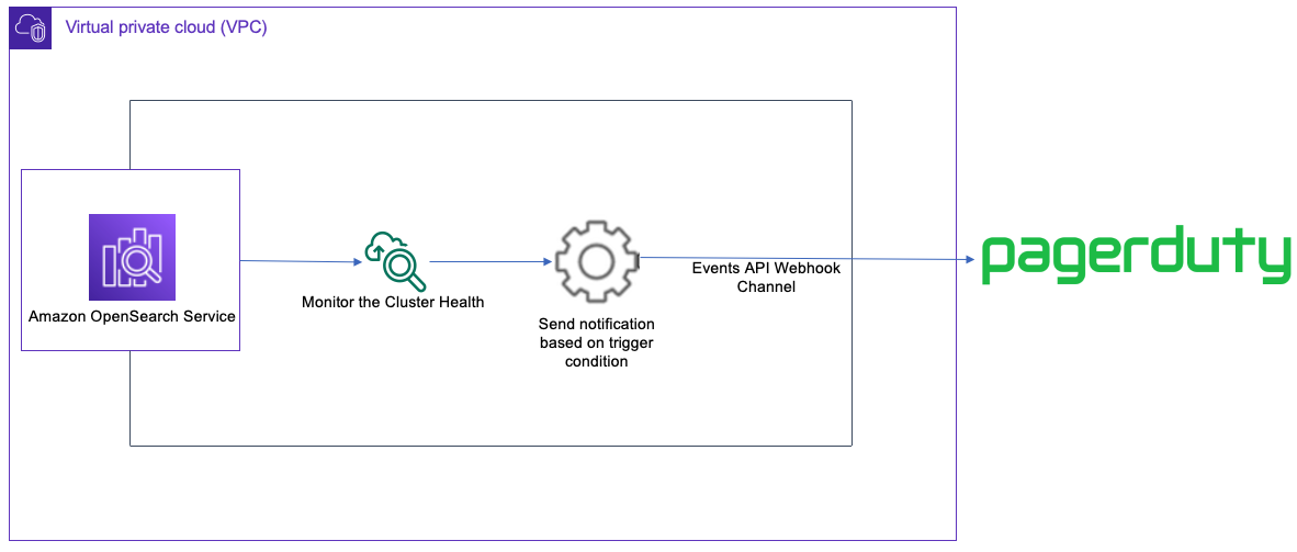
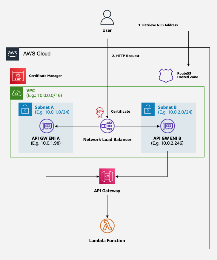
The following diagram illustrates our solution architecture.

Prerequisites
You need the following prerequisites:
Set up the Amazon MWAA environment
For instructions on creating your environment, refer to Create an Amazon MWAA environment. For existing users, we recommend upgrading to version 2.4.3 to take advantage of the observability enhancements featured in this post.
The steps to upgrade Amazon MWAA to version 2.4.3 differ depending on whether the current version is 1.10.12 or 2.2.2. We discuss both options in this post.
Prerequisites for setting up an Amazon MWAA environment
You must meet the following prerequisites:
Upgrade from version 1.10.12 to 2.4.3
If you’re using Amazon MWAA version 1.10.12, refer to Migrating to a new Amazon MWAA environment to upgrade to 2.4.3.
Upgrade from version 2.0.2 or 2.2.2 to 2.4.3
If you’re using Amazon MWAA environment version 2.2.2 or lower, complete the following steps:
- Create a requirements.txt for any custom dependencies with specific versions required for your DAGs.
- Upload the file to Amazon S3 in the appropriate location where the Amazon MWAA environment points to the requirements.txt for installing dependencies.
- Follow the steps in Migrating to a new Amazon MWAA environment and select version 2.4.3.
Update your DAGs
Customers who upgraded from an older Amazon MWAA environment may need to make updates to existing DAGs. In Airflow version 2.4.3, the Airflow environment will use the Amazon provider package version 6.0.0 by default. This package may include some potentially breaking changes, such as changes to operator names. For example, the AWSGlueJobOperator has been deprecated and replaced with the GlueJobOperator. To maintain compatibility, update your Airflow DAGs by replacing any deprecated or unsupported operators from previous versions with the new ones. Complete the following steps:
- Navigate to Amazon AWS Operators.
- Select the appropriate version installed in your Amazon MWAA instance (6.0.0. by default) to find a list of supported Airflow operators.
- Make the necessary changes in the existing DAG code and upload the modified files to the DAG location in Amazon S3.
Orchestrate the AWS Glue job from Airflow
This section covers the details of orchestrating an AWS Glue job within Airflow DAGs. Airflow eases the development of data pipelines with dependencies between heterogeneous systems such as on-premises processes, external dependencies, other AWS services, and more.
Orchestrate CloudTrail log aggregation with AWS Glue and Amazon MWAA
In this example, we go through a use case of using Amazon MWAA to orchestrate an AWS Glue Python Shell job that persists aggregated metrics based on CloudTrail logs.
CloudTrail enables visibility into AWS API calls that are being made in your AWS account. A common use case with this data would be to gather usage metrics on principals acting on your account’s resources for auditing and regulatory needs.
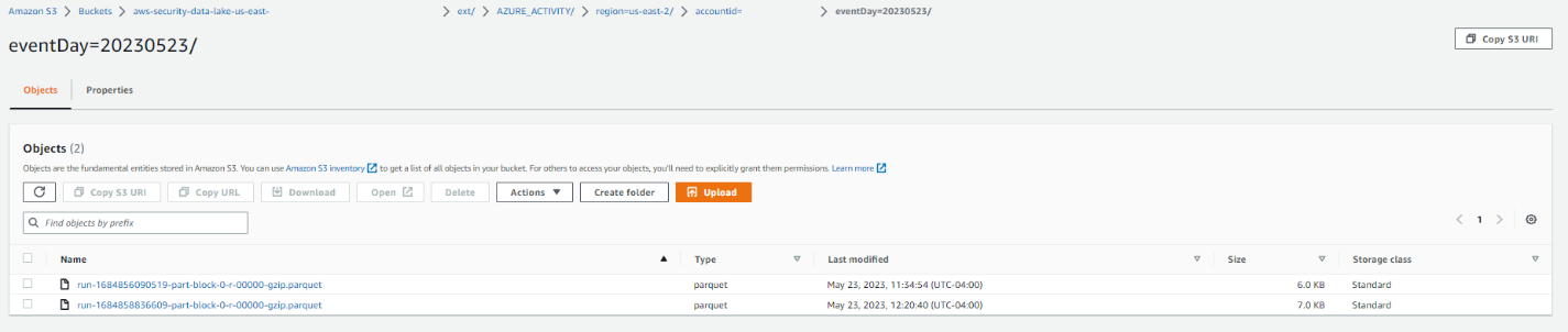
As CloudTrail events are being logged, they are delivered as JSON files in Amazon S3, which aren’t ideal for analytical queries. We want to aggregate this data and persist it as Parquet files to allow for optimal query performance. As an initial step, we can use Athena to do the initial querying of the data before doing additional aggregations in our AWS Glue job. For more information about creating an AWS Glue Data Catalog table, refer to Creating the table for CloudTrail logs in Athena using partition projection data. After we’ve explored the data via Athena and decided what metrics we want to retain in aggregate tables, we can create an AWS Glue job.
Create an CloudTrail table in Athena
First, we need to create a table in our Data Catalog that allows CloudTrail data to be queried via Athena. The following sample query creates a table with two partitions on the Region and date (called snapshot_date). Be sure to replace the placeholders for your CloudTrail bucket, AWS account ID, and CloudTrail table name:
create external table if not exists `<<<CLOUDTRAIL_TABLE_NAME>>>`(
  `eventversion` string comment 'from deserializer',
  `useridentity` struct<type:string,principalid:string,arn:string,accountid:string,invokedby:string,accesskeyid:string,username:string,sessioncontext:struct<attributes:struct<mfaauthenticated:string,creationdate:string>,sessionissuer:struct<type:string,principalid:string,arn:string,accountid:string,username:string>>> comment 'from deserializer',
  `eventtime` string comment 'from deserializer',
  `eventsource` string comment 'from deserializer',
  `eventname` string comment 'from deserializer',
  `awsregion` string comment 'from deserializer',
  `sourceipaddress` string comment 'from deserializer',
  `useragent` string comment 'from deserializer',
  `errorcode` string comment 'from deserializer',
  `errormessage` string comment 'from deserializer',
  `requestparameters` string comment 'from deserializer',
  `responseelements` string comment 'from deserializer',
  `additionaleventdata` string comment 'from deserializer',
  `requestid` string comment 'from deserializer',
  `eventid` string comment 'from deserializer',
  `resources` array<struct<arn:string,accountid:string,type:string>> comment 'from deserializer',
  `eventtype` string comment 'from deserializer',
  `apiversion` string comment 'from deserializer',
  `readonly` string comment 'from deserializer',
  `recipientaccountid` string comment 'from deserializer',
  `serviceeventdetails` string comment 'from deserializer',
  `sharedeventid` string comment 'from deserializer',
  `vpcendpointid` string comment 'from deserializer')
PARTITIONED BY (
  `region` string,
  `snapshot_date` string)
ROW FORMAT SERDE
  'com.amazon.emr.hive.serde.CloudTrailSerde'
STORED AS INPUTFORMAT
  'com.amazon.emr.cloudtrail.CloudTrailInputFormat'
OUTPUTFORMAT
  'org.apache.hadoop.hive.ql.io.HiveIgnoreKeyTextOutputFormat'
LOCATION
  's3://<<<CLOUDTRAIL_BUCKET>>>/AWSLogs/<<<ACCOUNT_ID>>>/CloudTrail/'
TBLPROPERTIES (
  'projection.enabled'='true',
  'projection.region.type'='enum',
  'projection.region.values'='us-east-2,us-east-1,us-west-1,us-west-2,af-south-1,ap-east-1,ap-south-1,ap-northeast-3,ap-northeast-2,ap-southeast-1,ap-southeast-2,ap-northeast-1,ca-central-1,eu-central-1,eu-west-1,eu-west-2,eu-south-1,eu-west-3,eu-north-1,me-south-1,sa-east-1',
  'projection.snapshot_date.format'='yyyy/mm/dd',
  'projection.snapshot_date.interval'='1',
  'projection.snapshot_date.interval.unit'='days',
  'projection.snapshot_date.range'='2020/10/01,now',
  'projection.snapshot_date.type'='date',
  'storage.location.template'='s3://<<<CLOUDTRAIL_BUCKET>>>/AWSLogs/<<<ACCOUNT_ID>>>/CloudTrail/${region}/${snapshot_date}')
Run the preceding query on the Athena console, and note the table name and AWS Glue Data Catalog database where it was created. We use these values later in the Airflow DAG code.
Sample AWS Glue job code
The following code is a sample AWS Glue Python Shell job that does the following:
- Takes arguments (which we pass from our Amazon MWAA DAG) on what day’s data to process
- Uses the AWS SDK for Pandas to run an Athena query to do the initial filtering of the CloudTrail JSON data outside AWS Glue
- Uses Pandas to do simple aggregations on the filtered data
- Outputs the aggregated data to the AWS Glue Data Catalog in a table
- Uses logging during processing, which will be visible in Amazon MWAA
import awswrangler as wr
import pandas as pd
import sys
import logging
from awsglue.utils import getResolvedOptions
from datetime import datetime, timedelta

# Logging setup, redirects all logs to stdout
LOGGER = logging.getLogger()
formatter = logging.Formatter('%(asctime)s.%(msecs)03d %(levelname)s %(module)s - %(funcName)s: %(message)s')
streamHandler = logging.StreamHandler(sys.stdout)
streamHandler.setFormatter(formatter)
LOGGER.addHandler(streamHandler)
LOGGER.setLevel(logging.INFO)

LOGGER.info(f"Passed Args :: {sys.argv}")

sql_query_template = """
select
region,
useridentity.arn,
eventsource,
eventname,
useragent

from "{cloudtrail_glue_db}"."{cloudtrail_table}"
where snapshot_date='{process_date}'
and region in ('us-east-1','us-east-2')
"""

required_args = ['CLOUDTRAIL_GLUE_DB',
                'CLOUDTRAIL_TABLE',
                'TARGET_BUCKET',
                'TARGET_DB',
                'TARGET_TABLE',
                'ACCOUNT_ID']
arg_keys = [*required_args, 'PROCESS_DATE'] if '--PROCESS_DATE' in sys.argv else required_args
JOB_ARGS = getResolvedOptions ( sys.argv, arg_keys)

LOGGER.info(f"Parsed Args :: {JOB_ARGS}")

# if process date was not passed as an argument, process yesterday's data
process_date = (
    JOB_ARGS['PROCESS_DATE']
    if JOB_ARGS.get('PROCESS_DATE','NONE') != "NONE"
    else (datetime.today() - timedelta(days=1)).strftime("%Y-%m-%d")
)

LOGGER.info(f"Taking snapshot for :: {process_date}")

RAW_CLOUDTRAIL_DB = JOB_ARGS['CLOUDTRAIL_GLUE_DB']
RAW_CLOUDTRAIL_TABLE = JOB_ARGS['CLOUDTRAIL_TABLE']
TARGET_BUCKET = JOB_ARGS['TARGET_BUCKET']
TARGET_DB = JOB_ARGS['TARGET_DB']
TARGET_TABLE = JOB_ARGS['TARGET_TABLE']
ACCOUNT_ID = JOB_ARGS['ACCOUNT_ID']

final_query = sql_query_template.format(
    process_date=process_date.replace("-","/"),
    cloudtrail_glue_db=RAW_CLOUDTRAIL_DB,
    cloudtrail_table=RAW_CLOUDTRAIL_TABLE
)

LOGGER.info(f"Running Query :: {final_query}")

raw_cloudtrail_df = wr.athena.read_sql_query(
    sql=final_query,
    database=RAW_CLOUDTRAIL_DB,
    ctas_approach=False,
    s3_output=f"s3://{TARGET_BUCKET}/athena-results",
)

raw_cloudtrail_df['ct']=1

agg_df = raw_cloudtrail_df.groupby(['arn','region','eventsource','eventname','useragent'],as_index=False).agg({'ct':'sum'})
agg_df['snapshot_date']=process_date

LOGGER.info(agg_df.info(verbose=True))

upload_path = f"s3://{TARGET_BUCKET}/{TARGET_DB}/{TARGET_TABLE}"

if not agg_df.empty:
    LOGGER.info(f"Upload to {upload_path}")
    try:
        response = wr.s3.to_parquet(
            df=agg_df,
            path=upload_path,
            dataset=True,
            database=TARGET_DB,
            table=TARGET_TABLE,
            mode="overwrite_partitions",
            schema_evolution=True,
            partition_cols=["snapshot_date"],
            compression="snappy",
            index=False
        )
        LOGGER.info(response)
    except Exception as exc:
        LOGGER.error("Uploading to S3 failed")
        LOGGER.exception(exc)
        raise exc
else:
    LOGGER.info(f"Dataframe was empty, nothing to upload to {upload_path}")
The following are some key advantages in this AWS Glue job:
- We use an Athena query to ensure initial filtering is done outside of our AWS Glue job. As such, a Python Shell job with minimal compute is still sufficient for aggregating a large CloudTrail dataset.
- We ensure the analytics library-set option is turned on when creating our AWS Glue job to use the AWS SDK for Pandas library.
Create an AWS Glue job
Complete the following steps to create your AWS Glue job:
- Copy the script in the preceding section and save it in a local file. For this post, the file is called
script.py.
- On the AWS Glue console, choose ETL jobs in the navigation pane.
- Create a new job and select Python Shell script editor.
- Select Upload and edit an existing script and upload the file you saved locally.
- Choose Create.

- On the Job details tab, enter a name for your AWS Glue job.
- For IAM role, choose an existing role or create a new role that has the required permissions for Amazon S3, AWS Glue, and Athena. The role needs to query the CloudTrail table you created earlier and write to an output location.
You can use the following sample policy code. Replace the placeholders with your CloudTrail logs bucket, output table name, output AWS Glue database, output S3 bucket, CloudTrail table name, AWS Glue database containing the CloudTrail table, and your AWS account ID.
{
    "Version": "2012-10-17",
    "Statement": [
        {
            "Action": [
                "s3:List*",
                "s3:Get*"
            ],
            "Resource": [
                "arn:aws:s3:::<<<CLOUDTRAIL_LOGS_BUCKET>>>/*",
                "arn:aws:s3:::<<<CLOUDTRAIL_LOGS_BUCKET>>>*"
            ],
            "Effect": "Allow",
            "Sid": "GetS3CloudtrailData"
        },
        {
            "Action": [
                "glue:Get*",
                "glue:BatchGet*"
            ],
            "Resource": [
                "arn:aws:glue:us-east-1:<<<YOUR_AWS_ACCT_ID>>>:catalog",
                "arn:aws:glue:us-east-1:<<<YOUR_AWS_ACCT_ID>>>:database/<<<GLUE_DB_WITH_CLOUDTRAIL_TABLE>>>",
                "arn:aws:glue:us-east-1:<<<YOUR_AWS_ACCT_ID>>>:table/<<<GLUE_DB_WITH_CLOUDTRAIL_TABLE>>>/<<<CLOUDTRAIL_TABLE>>>*"
            ],
            "Effect": "Allow",
            "Sid": "GetGlueCatalogCloudtrailData"
        },
        {
            "Action": [
                "s3:PutObject*",
                "s3:Abort*",
                "s3:DeleteObject*",
                "s3:GetObject*",
                "s3:GetBucket*",
                "s3:List*",
                "s3:Head*"
            ],
            "Resource": [
                "arn:aws:s3:::<<<OUTPUT_S3_BUCKET>>>",
                "arn:aws:s3:::<<<OUTPUT_S3_BUCKET>>>/<<<OUTPUT_GLUE_DB>>>/<<<OUTPUT_TABLE_NAME>>>/*"
            ],
            "Effect": "Allow",
            "Sid": "WriteOutputToS3"
        },
        {
            "Action": [
                "glue:CreateTable",
                "glue:CreatePartition",
                "glue:UpdatePartition",
                "glue:UpdateTable",
                "glue:DeleteTable",
                "glue:DeletePartition",
                "glue:BatchCreatePartition",
                "glue:BatchDeletePartition",
                "glue:Get*",
                "glue:BatchGet*"
            ],
            "Resource": [
                "arn:aws:glue:us-east-1:<<<YOUR_AWS_ACCT_ID>>>:catalog",
                "arn:aws:glue:us-east-1:<<<YOUR_AWS_ACCT_ID>>>:database/<<<OUTPUT_GLUE_DB>>>",
                "arn:aws:glue:us-east-1:<<<YOUR_AWS_ACCT_ID>>>:table/<<<OUTPUT_GLUE_DB>>>/<<<OUTPUT_TABLE_NAME>>>*"
            ],
            "Effect": "Allow",
            "Sid": "AllowOutputToGlue"
        },
        {
            "Action": [
                "logs:CreateLogGroup",
                "logs:CreateLogStream",
                "logs:PutLogEvents"
            ],
            "Resource": "arn:aws:logs:*:*:/aws-glue/*",
            "Effect": "Allow",
            "Sid": "LogsAccess"
        },
        {
            "Action": [
                "s3:GetObject*",
                "s3:GetBucket*",
                "s3:List*",
                "s3:DeleteObject*",
                "s3:PutObject",
                "s3:PutObjectLegalHold",
                "s3:PutObjectRetention",
                "s3:PutObjectTagging",
                "s3:PutObjectVersionTagging",
                "s3:Abort*"
            ],
            "Resource": [
                "arn:aws:s3:::<<<ATHENA_RESULTS_BUCKET>>>",
                "arn:aws:s3:::<<<ATHENA_RESULTS_BUCKET>>>/*"
            ],
            "Effect": "Allow",
            "Sid": "AccessToAthenaResults"
        },
        {
            "Action": [
                "athena:StartQueryExecution",
                "athena:StopQueryExecution",
                "athena:GetDataCatalog",
                "athena:GetQueryResults",
                "athena:GetQueryExecution"
            ],
            "Resource": [
                "arn:aws:glue:us-east-1:<<<YOUR_AWS_ACCT_ID>>>:catalog",
                "arn:aws:athena:us-east-1:<<<YOUR_AWS_ACCT_ID>>>:datacatalog/AwsDataCatalog",
                "arn:aws:athena:us-east-1:<<<YOUR_AWS_ACCT_ID>>>:workgroup/primary"
            ],
            "Effect": "Allow",
            "Sid": "AllowAthenaQuerying"
        }
    ]
}
For Python version, choose Python 3.9.
- Select Load common analytics libraries.
- For Data processing units, choose 1 DPU.
- Leave the other options as default or adjust as needed.

- Choose Save to save your job configuration.
Configure an Amazon MWAA DAG to orchestrate the AWS Glue job
The following code is for a DAG that can orchestrate the AWS Glue job that we created. We take advantage of the following key features in this DAG:
"""Sample DAG"""
import airflow.utils
from airflow.providers.amazon.aws.operators.glue import GlueJobOperator
from airflow import DAG
from datetime import timedelta
import airflow.utils

# allow backfills via DAG run parameters
process_date = '{{ dag_run.conf.get("process_date") if dag_run.conf.get("process_date") else "NONE" }}'

dag = DAG(
    dag_id = "CLOUDTRAIL_LOGS_PROCESSING",
    default_args = {
        'depends_on_past':False,
        'start_date':airflow.utils.dates.days_ago(0),
        'retries':1,
        'retry_delay':timedelta(minutes=5),
        'catchup': False
    },
    schedule_interval = None, # None for unscheduled or a cron expression - E.G. "00 12 * * 2" - at 12noon Tuesday
    dagrun_timeout = timedelta(minutes=30),
    max_active_runs = 1,
    max_active_tasks = 1 # since there is only one task in our DAG
)

## Log ingest. Assumes Glue Job is already created
glue_ingestion_job = GlueJobOperator(
    task_id="<<<some-task-id>>>",
    job_name="<<<GLUE_JOB_NAME>>>",
    script_args={
        "--ACCOUNT_ID":"<<<YOUR_AWS_ACCT_ID>>>",
        "--CLOUDTRAIL_GLUE_DB":"<<<GLUE_DB_WITH_CLOUDTRAIL_TABLE>>>",
        "--CLOUDTRAIL_TABLE":"<<<CLOUDTRAIL_TABLE>>>",
        "--TARGET_BUCKET": "<<<OUTPUT_S3_BUCKET>>>",
        "--TARGET_DB": "<<<OUTPUT_GLUE_DB>>>", # should already exist
        "--TARGET_TABLE": "<<<OUTPUT_TABLE_NAME>>>",
        "--PROCESS_DATE": process_date
    },
    region_name="us-east-1",
    dag=dag,
    verbose=True
)

glue_ingestion_job
Increase observability of AWS Glue jobs in Amazon MWAA
The AWS Glue jobs write logs to Amazon CloudWatch. With the recent observability enhancements to Airflow’s Amazon provider package, these logs are now integrated with Airflow task logs. This consolidation provides Airflow users with end-to-end visibility directly in the Airflow UI, eliminating the need to search in CloudWatch or the AWS Glue console.
To use this feature, ensure the IAM role attached to the Amazon MWAA environment has the following permissions to retrieve and write the necessary logs:
{
  "Version": "2012-10-17",
  "Statement": [
    {
      "Effect": "Allow",
      "Action": [
        "logs:CreateLogGroup",
        "logs:CreateLogStream",
        "logs:PutLogEvents",
        "logs:GetLogEvents",
        "logs:GetLogRecord",
        "logs:DescribeLogStreams",
        "logs:FilterLogEvents",
        "logs:GetLogGroupFields",
        "logs:GetQueryResults",

      ],
      "Resource": [
        "arn:aws:logs:*:*:log-group:airflow-243-<<<Your environment name>>>-*"--Your Amazon MWAA Log Stream Name
      ]
    }
  ]
}
If verbose=true, the AWS Glue job run logs show in the Airflow task logs. The default is false. For more information, refer to Parameters.
When enabled, the DAGs read from the AWS Glue job’s CloudWatch log stream and relay them to the Airflow DAG AWS Glue job step logs. This provides detailed insights into an AWS Glue job’s run in real time via the DAG logs. Note that AWS Glue jobs generate an output and error CloudWatch log group based on the job’s STDOUT and STDERR, respectively. All logs in the output log group and exception or error logs from the error log group are relayed into Amazon MWAA.
AWS admins can now limit a support team’s access to only Airflow, making Amazon MWAA the single pane of glass on job orchestration and job health management. Previously, users needed to check AWS Glue job run status in the Airflow DAG steps and retrieve the job run identifier. They then needed to access the AWS Glue console to find the job run history, search for the job of interest using the identifier, and finally navigate to the job’s CloudWatch logs to troubleshoot.
Create the DAG
To create the DAG, complete the following steps:
- Save the preceding DAG code to a local .py file, replacing the indicated placeholders.
The values for your AWS account ID, AWS Glue job name, AWS Glue database with CloudTrail table, and CloudTrail table name should already be known. You can adjust the output S3 bucket, output AWS Glue database, and output table name as needed, but make sure the AWS Glue job’s IAM role that you used earlier is configured accordingly.
- On the Amazon MWAA console, navigate to your environment to see where the DAG code is stored.
The DAGs folder is the prefix within the S3 bucket where your DAG file should be placed.
- Upload your edited file there.

- Open the Amazon MWAA console to confirm that the DAG appears in the table.

Run the DAG
To run the DAG, complete the following steps:
- Choose from the following options:
- Trigger DAG – This causes yesterday’s data to be used as the data to process
- Trigger DAG w/ config – With this option, you can pass in a different date, potentially for backfills, which is retrieved using
dag_run.conf in the DAG code and then passed into the AWS Glue job as a parameter

The following screenshot shows the additional configuration options if you choose Trigger DAG w/ config.

- Monitor the DAG as it runs.
- When the DAG is complete, open the run’s details.
On the right pane, you can view the logs, or choose Task Instance Details for a full view.

- View the AWS Glue job output logs in Amazon MWAA without using the AWS Glue console thanks to the
GlueJobOperator verbose flag.

The AWS Glue job will have written results to the output table you specified.
- Query this table via Athena to confirm it was successful.

Summary
Amazon MWAA now provides a single place to track AWS Glue job status and enables you to use the Airflow console as the single pane of glass for job orchestration and health management. In this post, we walked through the steps to orchestrate AWS Glue jobs via Airflow using GlueJobOperator. With the new observability enhancements, you can seamlessly troubleshoot AWS Glue jobs in a unified experience. We also demonstrated how to upgrade your Amazon MWAA environment to a compatible version, update dependencies, and change the IAM role policy accordingly.
For more information about common troubleshooting steps, refer to Troubleshooting: Creating and updating an Amazon MWAA environment. For in-depth details of migrating to an Amazon MWAA environment, refer to Upgrading from 1.10 to 2. To learn about the open-source code changes for increased observability of AWS Glue jobs in the Airflow Amazon provider package, refer to the relay logs from AWS Glue jobs.
Finally, we recommend visiting the AWS Big Data Blog for other material on analytics, ML, and data governance on AWS.
About the Authors
 Rushabh Lokhande is a Data & ML Engineer with the AWS Professional Services Analytics Practice. He helps customers implement big data, machine learning, and analytics solutions. Outside of work, he enjoys spending time with family, reading, running, and golf.
Ryan Gomes is a Data & ML Engineer with the AWS Professional Services Analytics Practice. He is passionate about helping customers achieve better outcomes through analytics and machine learning solutions in the cloud. Outside of work, he enjoys fitness, cooking, and spending quality time with friends and family.
 Vishwa Gupta is a Senior Data Architect with the AWS Professional Services Analytics Practice. He helps customers implement big data and analytics solutions. Outside of work, he enjoys spending time with family, traveling, and trying new food.


 Ayah Chamseddin is a Sr. Engagement Manager at AWS. She has a deep understanding of cloud technologies and has successfully overseen and lead strategic projects, partnering with clients to define business objectives, develop implementation strategies, and drive the successful delivery of solutions.
 Vamsi Bhadriraju is a Data Architect at AWS. He works closely with enterprise customers to build data lakes and analytical applications on the AWS Cloud.
 Srikanth Baheti is a Specialized World Wide Principal Solutions Architect for Amazon QuickSight. He started his career as a consultant and worked for multiple private and government organizations. Later he worked for PerkinElmer Health and Sciences & eResearch Technology Inc, where he was responsible for designing and developing high traffic web applications, highly scalable and maintainable data pipelines for reporting platforms using AWS services and Serverless computing.
 Raji Sivasubramaniam is a Sr. Solutions Architect at AWS, focusing on Analytics. Raji is specialized in architecting end-to-end Enterprise Data Management, Business Intelligence and Analytics solutions for Fortune 500 and Fortune 100 companies across the globe. She has in-depth experience in integrated healthcare data and analytics with wide variety of healthcare datasets including managed market, physician targeting and patient analytics.


 Shana Schipers is an Analytics Specialist Solutions Architect at AWS, focusing on big data. She supports customers worldwide in building transactional data lakes using open table formats like Apache Hudi, Apache Iceberg and Delta Lake on AWS.
 Ian Meyers is a Director of Product Management for AWS Analytics Services. He works with many of AWS largest customers on emerging technology needs, and leads several data and analytics initiatives within AWS including support for Data Mesh.


 Manikanta Gona is a Data and ML Engineer at AWS Professional Services. He joined AWS in 2021 with 6+ years of experience in IT. At AWS, he is focused on Data Lake implementations, and Search, Analytical workloads using Amazon OpenSearch Service. In his spare time, he love to garden, and go on hikes and biking with his husband.
 Vivek Shrivastava is a Principal Data Architect, Data Lake in AWS Professional Services. He is a Bigdata enthusiast and holds 14 AWS Certifications. He is passionate about helping customers build scalable and high-performance data analytics solutions in the cloud. In his spare time, he loves reading and finds areas for home automation
 Ravikiran Rao is a Data Architect at AWS and is passionate about solving complex data challenges for various customers. Outside of work, he is a theatre enthusiast and an amateur tennis player.
 Hari Krishna KC is a Data Architect with the AWS Professional Services Team. He specializes in AWS Data Lakes & AWS OpenSearch Service and have helped numerous client migrate their workload to Data Lakes and Search data stores
 Parnab Basak is a Solutions Architect and a Serverless Specialist at AWS. He specializes in creating new solutions that are cloud native using modern software development practices like serverless, DevOps, and analytics. Parnab works closely in the analytics and integration services space helping customers adopt AWS services for their workflow orchestration needs.
 Fernando Gamero is a Senior Solutions Architect engineer at AWS, having more than 25 years of experience in the technology industry, from telecommunications, banking to startups. He is now helping customers with building Event Driven Architectures, adopting IoT solutions at the Edge, and transforming their data and machine learning pipelines at scale.
 Shubham Mehta is an experienced product manager with over eight years of experience and a proven track record of delivering successful products. In his current role as a Senior Product Manager at AWS, he oversees Amazon Managed Workflows for Apache Airflow (Amazon MWAA) and spearheads the Apache Airflow open-source contributions to further enhance the product’s functionality.


 Abdel Jaidi is a Senior Cloud Engineer for AWS Professional Services. He works on open-source projects focused on AWS Data & Analytics services. In his spare time, he enjoys playing tennis and hiking.
 Anton Kukushkin is a Data Engineer for AWS Professional Services based in London, UK. In his spare time, he enjoys playing musical instruments.
 Leon Luttenberger is a Data Engineer for AWS Professional Services based in Austin, Texas. He works on AWS open-source solutions that help our customers analyze their data at scale. In his spare time, he enjoys reading and traveling.
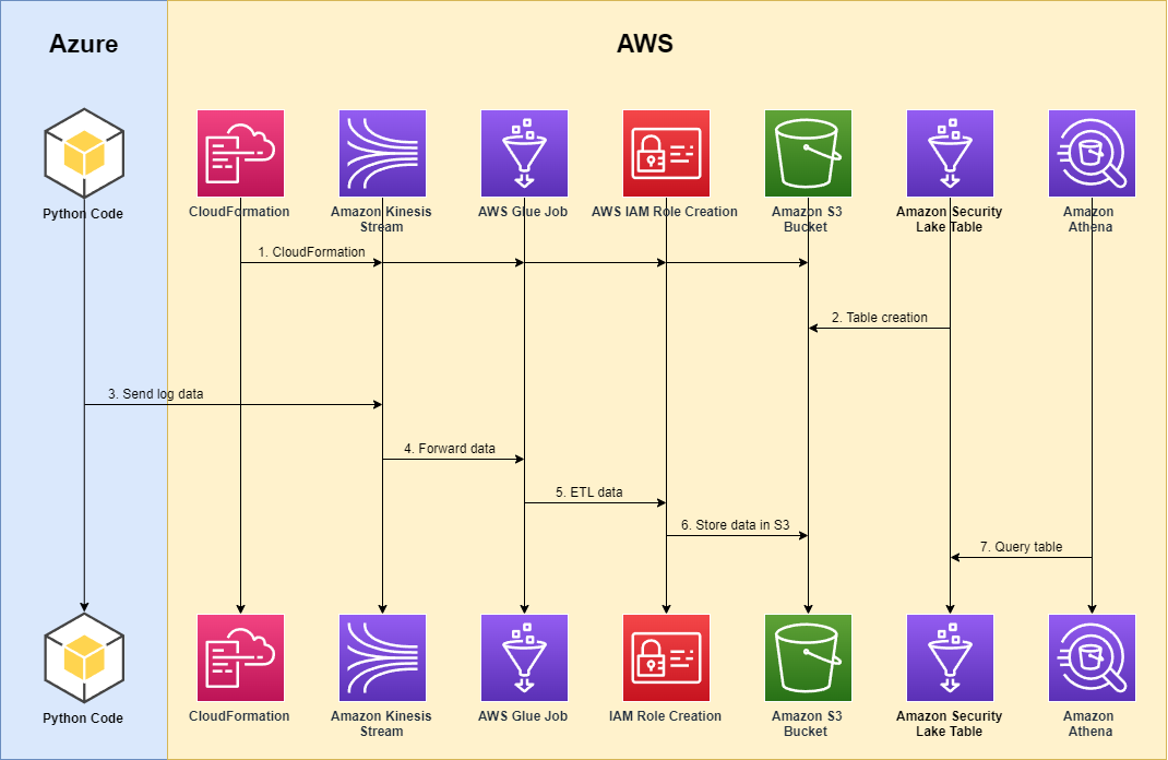


 Manish Kola is a Data Lab Solutions Architect at AWS, where he works closely with customers across various industries to architect cloud-native solutions for their data analytics and AI needs. He partners with customers on their AWS journey to solve their business problems and build scalable prototypes. Before joining AWS, Manish’s experience includes helping customers implement data warehouse, BI, data integration, and data lake projects.
 Santosh Kotagiri is a Solutions Architect at AWS with experience in data analytics and cloud solutions leading to tangible business results. His expertise lies in designing and implementing scalable data analytics solutions for clients across industries, with a focus on cloud-native and open-source services. He is passionate about leveraging technology to drive business growth and solve complex problems.
 Chiho Sugimoto is a Cloud Support Engineer on the AWS Big Data Support team. She is passionate about helping customers build data lakes using ETL workloads. She loves planetary science and enjoys studying the asteroid Ryugu on weekends.
 Noritaka Sekiyama is a Principal Big Data Architect on the AWS Glue team. He is responsible for building software artifacts to help customers. In his spare time, he enjoys cycling with his new road bike.
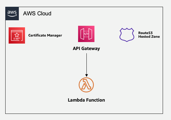

 Antonio Vespoli is a Software Development Engineer in AWS. He works on Amazon Kinesis Data Analytics, the managed offering for running Apache Flink applications on AWS.
 Samuel Siebenmann is a Software Development Engineer in AWS. He works on Amazon Kinesis Data Analytics, the managed offering for running Apache Flink applications on AWS.
 Nuno Afonso is a Software Development Engineer in AWS. He works on Amazon Kinesis Data Analytics, the managed offering for running Apache Flink applications on AWS.
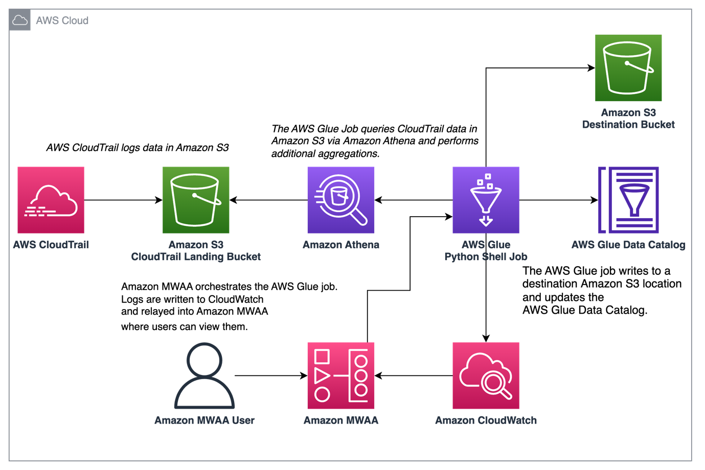


 Rushabh Lokhande is a Data & ML Engineer with the AWS Professional Services Analytics Practice. He helps customers implement big data, machine learning, and analytics solutions. Outside of work, he enjoys spending time with family, reading, running, and golf.
 Ryan Gomes is a Data & ML Engineer with the AWS Professional Services Analytics Practice. He is passionate about helping customers achieve better outcomes through analytics and machine learning solutions in the cloud. Outside of work, he enjoys fitness, cooking, and spending quality time with friends and family.
 Vishwa Gupta is a Senior Data Architect with the AWS Professional Services Analytics Practice. He helps customers implement big data and analytics solutions. Outside of work, he enjoys spending time with family, traveling, and trying new food.
 Vishal Vijayvargiya is a Software Engineer working on Amazon MWAA at Amazon Web Services. He is passionate about building distributed and scalable software systems. Vishal also enjoys playing badminton and cricket.


 Manish Virwani is a Sr. Solutions Architect at AWS. He has more than a decade of experience designing and implementing large-scale big data and analytics solutions. He provides technical guidance, design advice, and thought leadership to some of the key AWS customers and partners.
 Indira Balakrishnan is a Principal Solutions Architect in the AWS Analytics Specialist SA Team. She is passionate about helping customers build cloud-based analytics solutions to solve their business problems using data-driven decisions. Outside of work, she volunteers at her kids’ activities and spends time with her family.


 Bin Qiu is a Global Partner Solutions Architect focusing on ER&I at AWS. He has more than 20 years’ experience in the energy and power industries, designing, leading, and building different smart grid projects, such as distributed energy resources, microgrid, AI/ML implementation for resource optimization, IoT smart sensor application for equipment predictive maintenance, EV car and grid integration, and more. Bin is passionate about helping utilities achieve digital and sustainability transformations.
 Steve Alexander is a Senior Manager, IT Products at PG&E. He leads product teams building wildfire prevention and risk mitigation data products. Recent work has been focused on integrating data from various sources including weather, asset data, sensors, and dynamic protective devices to improve situational awareness and decision-making. Steve has over 20 years of experience with data systems and cutting-edge IT research and development, and is passionate about applying creative thinking in technical domains.
 Karthik Tharmarajan is a Senior Specialist Solutions Architect for Amazon QuickSight. Karthik has over 15 years of experience implementing enterprise business intelligence (BI) solutions and specializes in integration of BI solutions with business applications and enabling data-driven decisions.
 Ranjan Banerji is a Principal Partner Solutions Architect at AWS focused on the power and utilities vertical. Ranjan has been at AWS for 5 years, first on the department of defense (DoD) team helping the branches of the DoD migrate and/or build new systems on AWS ensuring security and compliance requirements and now supporting the power and utilities team. Ranjan’s expertise ranges from server less architecture to security and compliance for regulated industries. Ranjan has over 25 years of experience building and designing systems for the DoD, federal agencies, energy, and financial industry.


 Gonzalo Herreros is a Senior Big Data Architect on the AWS Glue team.