Tag Archives: Intermediate (200)

Introducing the AWS Network Firewall CloudWatch Dashboard

Post Syndicated from Ajinkya Patil original https://aws.amazon.com/blogs/security/introducing-the-aws-network-firewall-cloudwatch-dashboard/

Amazon CloudWatch dashboards are customizable pages in the CloudWatch console that you can use to monitor your resources in a single view. This post focuses on deploying a CloudWatch dashboard that you can use to create a customizable monitoring solution for your AWS Network Firewall firewall. It’s designed to provide deeper insights into your firewall’s performance and security events simplifying security monitoring.

Network Firewall is a managed service that you can use to deploy essential network protections to Amazon Virtual Private Clouds (Amazon VPCs). Network Firewall provides comprehensive logs and metrics through CloudWatch, and we’re expanding its capabilities with this CloudWatch dashboard. This enhancement makes it easier to visualize, analyze, and act on the wealth of data generated by your firewall.

This open source solution streamlines network security monitoring with a user-friendly AWS CloudFormation template that quickly deploys a dedicated monitoring dashboard. This solution incorporates a suite of CloudWatch features—basic monitoring metrics, vended logs, Logs Insights queries, Contributor Insights rules, and the dashboard itself—into a centralized view. Preconfigured widgets provide instant insights into critical areas such as top talkers, protocol distributions, and alert log trends, in addition to HTTP and TLS flow analysis. A consolidated view of key metrics and logs enables faster identification of potential security threats or performance issues. With all of this relevant network firewall data in one place, your team can respond more quickly to emerging security events.

In this blog post, we provide an overview of the dashboard and a step-by-step guide to deploy it in your environment.

Solution overview

The CloudWatch dashboard can be deployed in all AWS Regions where Network Firewall is available today, including the AWS GovCloud (US) Regions and China Regions. While the dashboard comes pre-configured, you can quickly adjust queries, time ranges, and refresh intervals to help meet your specific needs. By default, the dashboard queries firewall flow and alert log events over a 3-hour period, impacting the number of log events scanned. Logs Insights and Contributor Insights widgets showcase the top 10 data points by default, but you can enhance results by modifying queries or adjusting the Top Contributors value, though this might lead to increased costs. You can configure the auto-refresh interval of the widgets to get real-time visibility and optimize costs. See the Amazon CloudWatch Pricing guide for up-to-date free and paid tier pricing considerations.

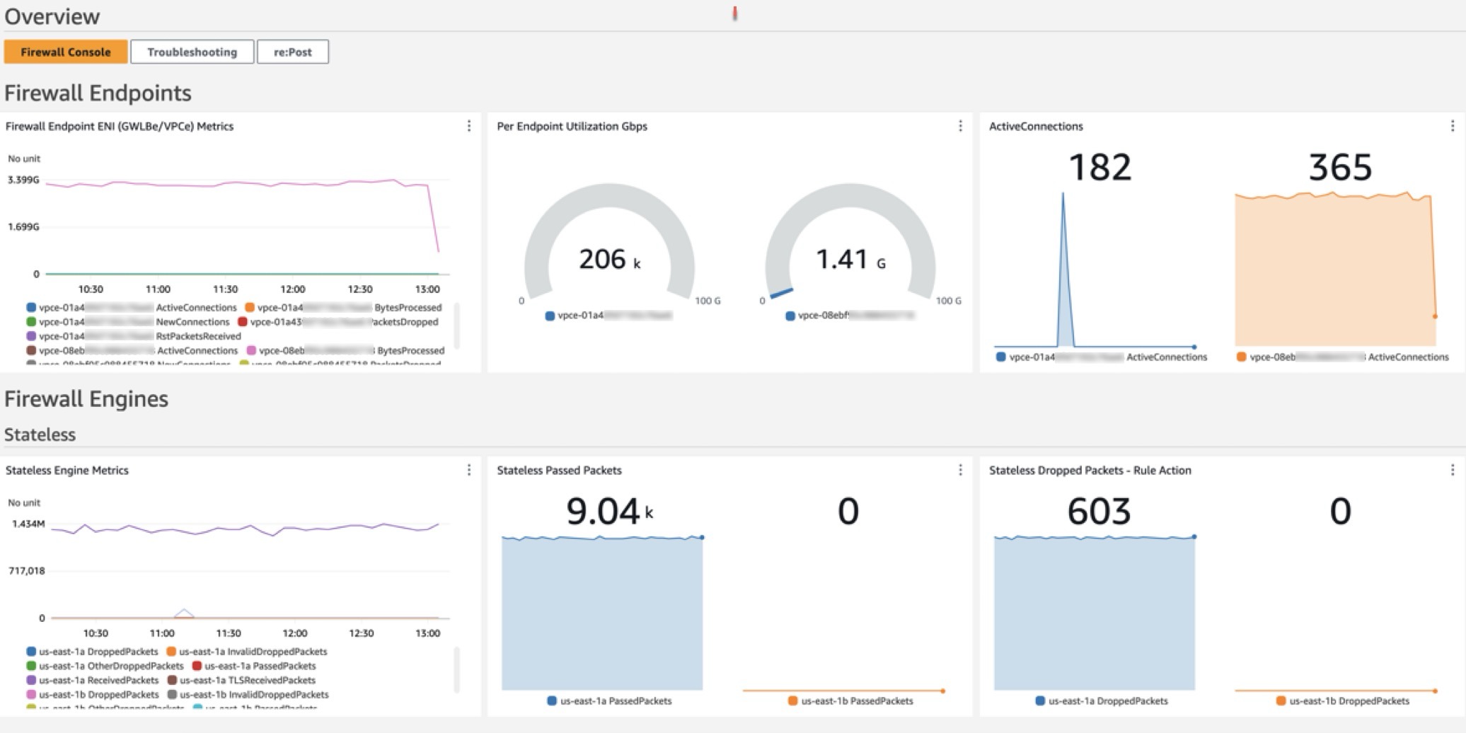
The dashboard, shown in Figure 1, can be deployed using CloudFormation and includes data and analytics from the following sources:

  1. Native CloudWatch metrics from the AWS/NetworkFirewall and AWS/PrivateLinkEndpoints namespaces
  2. CloudWatch Logs Insights queries that analyze Network Firewall flow and alert logs
  3. CloudWatch Contributor Insights rules that aggregate data from Network Firewall flow and alert logs.

Figure 1: CloudWatch dashboard

Figure 1: CloudWatch dashboard

Walkthrough

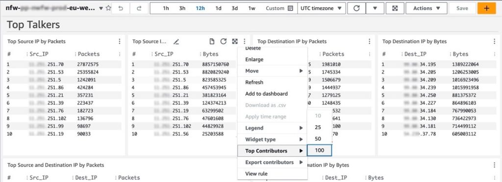
In the dashboard, the Logs Insights and Contributor Insights widgets display the top 10 data points by default. You can edit the Insights queries or change the Top Contributors to a larger value to display more results, as shown in Figure 2.

Figure 2: Top Talkers dashboard showing a change to the Top Contributors value

Figure 2: Top Talkers dashboard showing a change to the Top Contributors value

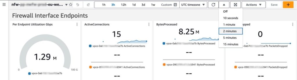
You can also manually refresh the data within a single or multiple widgets, or you can configure the entire dashboard to automatically refresh at a configured time interval as shown in Figure 3. The dashboard won’t automatically refresh the widget data by default.

Figure 3: Configuring the dashboard to automatically refresh

Figure 3: Configuring the dashboard to automatically refresh

Prerequisites

Deploying the Network Firewall CloudWatch Dashboard is straightforward. You will need the following:

  1. A Network Firewall in your VPC.
  2. Your Network Firewall must be configured to publish firewall flow and alert logs to two different CloudWatch log groups. For example, firewall flow logs are published to /my-firewall-flow-logs and alert logs are published to /my-firewall-alert-logs.

If you haven’t deployed Network Firewall in your VPC, you can use one of the available AWS Network Firewall Deployment Architecture templates to create a firewall. After creating a firewall, configure CloudWatch log groups for the firewall flow and alert logs and configure stateful logging as described previously. Fine-tune your firewall policy and rule configuration and make sure that you’re routing traffic symmetrically through the firewall. With the firewall now in the routed path and publishing metrics and log events, you can proceed with this Network Firewall CloudWatch dashboard template.

Deployment

The Network Firewall dashboard CloudFormation template creates a monitoring dashboard for a single Network Firewall firewall. Make sure that you launch this CloudFormation stack in the same AWS Region and account as the firewall, regardless of whether the firewall is set up centrally or in a distributed manner.

To deploy the dashboard:

  1. Choose Launch Stack for the relevant AWS Region. Make sure that you’re signed in to the appropriate AWS account and Region.
    • Region: China

      Launch Stack

    • Region: Gov Cloud

      Launch Stack

    • Region: All other regions supported by AWS Network Firewall

      Launch Stack

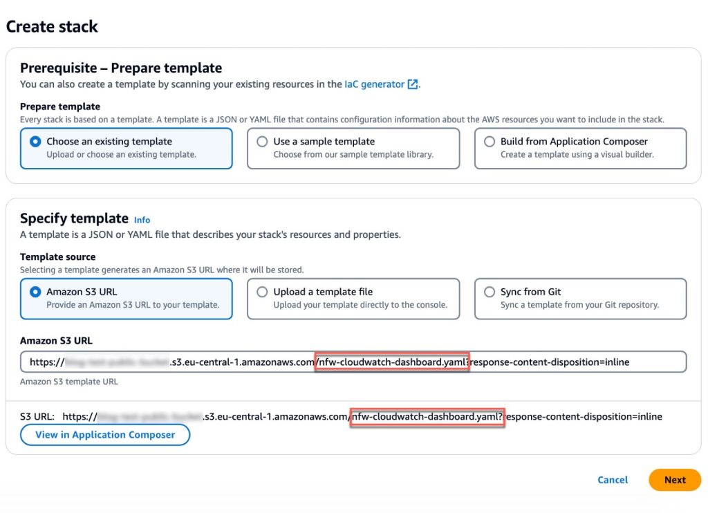
  2. You will be redirected to the Create stack page in the AWS Management Console for CloudFormation. Make sure that you’re in the correct Region and using the correct template. Choose Next. The following are the Regions and their template names:
    1. China Region: nfw-cloudwatch-dashboard-china.yaml
    2. Gov Cloud Region: nfw-cloudwatch-dashboard-govcloud.yaml
    3. All other Regions: nfw-cloudwatch-dashboard.yaml
Figure 4: Make sure that you’re using the correct template

Figure 4: Make sure that you’re using the correct template

When launching the stack, you will need to enter the following parameters:

  1. Stack name: A descriptive name for this CloudFormation stack. For example, my-firewall-dashboard.
  2. Firewall name: The firewall name as seen in the Amazon VPC console. In the Amazon VPC console, choose Network Firewall in the navigation pane, then choose Firewalls.
  3. Firewall subnets: The firewall subnet IDs to which your firewall endpoints are attached. The firewall subnets can be found on the Firewall details tab of your firewall in the Amazon VPC
  4. Flow log group name: The name of the CloudWatch log group where your firewall flow logs are stored.
  5. Alert log group name: The name of the CloudWatch log group where your firewall alert logs are stored.
  6. Contributor Insights rule state: Enable or disable the Contributor Insights rules (the template defaults to enabled). Disabling will stop the rules from scanning log data and displaying results in the Contributor Insights widgets. After the rules are created, you can change the state of one or more Contributor Insights rules from CloudWatch console by choosing Insights from the navigation pane, and then choosing Contributor Insights.

After the stack reaches CREATE_COMPLETE status, go to the Outputs tab and choose the FirewallDashboardURI link to open the new dashboard in the CloudWatch Dashboards console. It might take a few minutes for the Logs Insights and Contributor Insights widgets to start displaying data. For more details about each widget, see the README. If you don’t have log events matching the query parameters in the widgets, some widgets might not show data points.

Troubleshooting

If you encounter issues during or after deployment, review the following:

  • Firewall logging is enabled and configured to use CloudWatch instead of Amazon Simple Storage Service (Amazon S3) or Amazon Kinesis.
  • Both firewall flow and alert logging are enabled, not just one.
  • Log group names are entered correctly; incorrect names will cause widgets to point to invalid data.
  • Correct subnets are selected. Incorrect choices can impact the PrivateLink metrics widgets.
  • Firewall name is entered correctly. An incorrect name can disrupt metrics widgets, dashboard, and Contributor Insights widget names and break the firewall link.

Cleaning up

You can delete the Network Firewall CloudWatch dashboard and all of the associated resources with a few clicks. Deleting the dashboard will not impact the routing and network traffic inspection performed by the firewall.

  1. Sign in to the CloudFormation console in the Region where you launched the stack and choose Stacks from the navigation pane.
  2. Select the Stack name you chose when launching the stack. For example, my-firewall-dashboard.
  3. Choose Delete.

Conclusion

We encourage you to see for yourself how this new dashboard can enhance your network security management. To get started with the AWS Network Firewall CloudWatch Dashboard, visit our GitHub repository for detailed instructions and the CloudFormation template. For a visual overview of the dashboard and its capabilities, check out our YouTube video.

If you have feedback about this post, submit comments in the Comments section below. If you have questions about this post, contact AWS Support.
 

Ajinkya Patil
Ajinkya Patil

Ajinkya is a Security Consultant at Amazon Professional Services, specializing in security consulting for AWS customers within the automotive industry since 2019. He has presented at AWS re:Inforce and contributed articles to the AWS Security blog and AWS Prescriptive Guidance. Beyond his professional commitments, he indulges in travel and photography.
Todd Pula
Todd Pula

Todd is a Sr. Cloud Support Engineer at AWS and a service experience owner for AWS Network Firewall. He is an accomplished problem solver helping customers build and troubleshoot complex cloud networking and security solutions. He has a Master’s degree in Information Technology and is a Cisco Certified Internetwork Expert (CCIE).
Amish Shah
Amish Shah

Amish is a seasoned product leader with over 15 years of experience in developing innovative and scalable solutions for networking, security, and cloud use cases. He currently leads the AWS Network Firewall service, where he helps to develop security solutions that protect AWS workloads. Outside of work, Amish enjoys playing cricket and soccer, loves to travel, and has recently picked up a hobby of collecting niche fragrances.

Introducing an enhanced version of the AWS Secrets Manager transform: AWS::SecretsManager-2024-09-16

Post Syndicated from Sanjay Varma Datla original https://aws.amazon.com/blogs/security/introducing-an-enhanced-version-of-the-aws-secrets-manager-transform-awssecretsmanager-2024-09-16/

We’re pleased to announce an enhanced version of the AWS Secrets Manager transform: AWS::SecretsManager-2024-09-16. This update is designed to simplify infrastructure management by reducing the need for manual security updates, bug fixes, and runtime upgrades.

AWS Secrets Manager helps you manage, retrieve, and rotate database credentials, API keys, and other secrets throughout their lifecycles. Some AWS services offer managed rotation of secrets, but for other secrets, you perform rotation by using an AWS Lambda function that updates your secret and the database or service.

Transforms are macros hosted by AWS CloudFormation that enable you to create or manage complex infrastructure setups. For general information on transforms, see the AWS CloudFormation documentation.

The AWS::SecretsManager transforms are used in conjunction with the AWS::SecretsManager::RotationSchedule resource type and HostedRotationLambda property to automatically extend your CloudFormation template to include a nested stack that creates the appropriate rotation Lambda function for your database or service. The transforms provide a convenient way to deploy an AWS vended rotation Lambda function into your own account as part of your CloudFormation templates, without having to rely on creating rotation Lambda functions through the AWS Serverless Application Repository or the AWS Management Console.

In this post, we’ll explore the new features of the transform, compare them to the previous version, and guide you through updating an existing Lambda function that was created using the old transform version to use the new transform version.

New features in AWS::SecretsManager-2024-09-16

The new transform version introduces several enhancements over the previous version (AWS::SecretsManager-2020-07-23):

  • Automatic Lambda upgrades: Your rotation Lambda functions’ runtime configuration and internal dependencies now update automatically when you update your CloudFormation stacks. This helps you verify that you’re using the most secure and stable versions of Secrets Manager vended rotation Lambda function code and runtimes. Currently, AWS Lambda supports Python runtimes 3.9 and above. With Python 3.8 being deprecated, this feature allows for a seamless transition to newer supported runtimes. For more information on runtime deprecations, see the AWS Lambda runtimes documentation and the Python version guide.
  • Additional resource attributes: The new transform now supports additional resource attributes for the AWS::SecretsManager::RotationSchedule resource type when used with the HostedRotationLambda property. The following attributes are applied to the nested stack (of type AWS::CloudFormation::Stack) that creates the rotation Lambda function:
    • CreationPolicy
    • DependsOn
    • Metadata
    • UpdatePolicy
    • Condition

For more information on these resource attributes, see the AWS CloudFormation resource attribute reference.

Resource attributes comparison

The following table shows which resource attributes are supported by the two versions of the Secrets Manager transform.

Attribute AWS::SecretsManager-2020-07-23 AWS::SecretsManager-2024-09-16
DeletionPolicy Supported Supported
UpdateReplacePolicy Supported Supported
CreationPolicy Not Supported Supported
DependsOn Not Supported Supported
Metadata Not Supported Supported
UpdatePolicy Not Supported Supported
Condition Not Supported Supported

Important considerations

Before you use the AWS::SecretsManager-2024-09-16 transform, it’s essential to be aware of the following considerations so that you can make sure your CloudFormation stacks are properly created or updated:

  • Non-backward compatibility: The new transform version isn’t backward compatible with the previous version. If you downgrade from AWS::SecretsManager-2024-09-16 to AWS::SecretsManager-2020-07-23, the additional resource attributes won’t be supported, which might change the behavior of existing stacks.
  • Rollback behavior during upgrade: When you upgrade to the AWS::SecretsManager-2024-09-16 transform from the previous version and a stack rollback occurs for any reason, the rotation Lambda function might not revert to its previous state. This is because the older transform’s nested stack might not use the same Lambda deployment package that was used before the upgrade.
  • Direct Lambda changes: If you make direct changes to the Lambda function created by the new transform outside of a CloudFormation stack update, those modifications might be overwritten during subsequent CloudFormation stack updates or rollbacks.
  • Lambda runtime management: When you use the new transform version, the rotation Lambda function’s runtime aligns with the compiled binaries that are vended in Secrets Manager rotation Lambda templates, without you needing to specify a Runtime value in the HostedRotationLambda property. If you specify a Runtime value, make sure it’s the same version that is supported by Secrets Manager vended rotation Lambda templates. Otherwise, the Lambda runtime will be incompatible with the binaries that are published in the rotation Lambda function. For more information on the supported runtime, see the rotation function templates documentation.
  • End of support plans: AWS Secrets Manager will end support for the previous transform version (AWS::SecretsManager-2020-07-23) in the future. We recommend that you migrate your stacks to the new transform to benefit from improvements and security enhancements going forward.

How to upgrade

To upgrade to the new transform version, follow these steps:

  1. Review your existing CloudFormation stacks that use the AWS::SecretsManager-2020-07-23 transform.
  2. Update your CloudFormation stack templates to use AWS::SecretsManager-2024-09-16 in the Transform key at the top of your template: Transform: AWS::SecretsManager-2024-09-16
  3. If you have previously defined a Runtime value in the HostedRotationLambda property, remove it from your template so that your rotation Lambda function’s runtime is updated properly in future stack updates.
  4. Incorporate the new resource attributes as needed. We recommend that you minimize all other template changes while upgrading to reduce the likelihood of rollbacks.
  5. Deploy the changes by updating your CloudFormation stack with the revised template.

By following these steps, your Secrets Manager vended rotation Lambda functions will benefit from the latest improvements and security enhancements. Remember to test the changes in a non-production environment before you apply them to your production stacks. If you encounter any issues during the upgrade process, refer to our documentation or contact AWS Support for assistance.

 
If you have feedback about this post, submit comments in the Comments section below. If you have questions about this post, contact AWS Support.
 

Sanjay Varma Datla
Sanjay Varma Datla

Sanjay is a Software Development Engineer at AWS Secrets Manager. With a strong background in software engineering and a passion for secure application design, he focuses on empowering developers to manage sensitive information safely. Outside of work, Sanjay enjoys hiking and exploring new cuisines.
Rob Stevens
Rob Stevens

Rob is a System Development Engineer for AWS Secrets Manager and is committed to building secure and scalable distributed systems for AWS and its customers. Outside of work, Rob is a fitness enthusiast and also enjoys traveling.

AWS Network Firewall Geographic IP Filtering launch

Post Syndicated from Prasanjit Tiwari original https://aws.amazon.com/blogs/security/aws-network-firewall-geographic-ip-filtering-launch/

AWS Network Firewall is a managed service that provides a convenient way to deploy essential network protections for your virtual private clouds (VPCs). In this blog post, we discuss Geographic IP Filtering, a new feature of Network Firewall that you can use to filter traffic based on geographic location and meet compliance requirements.

Customers with internet-facing applications are constantly in need of advanced security features to protect their applications from threat actors. This includes restricting traffic to and from their workloads in Amazon Web Services (AWS) to certain geographies because of security risk. Customers operating in highly regulated industries—such as banking, public sector, or insurance—might have specific security requirements that can be addressed by Geographic IP Filtering.

Previously, customers had to rely on third-party tools for retrieving an IP address list of specific countries and updating their firewall rules on a regular basis to meet applicable requirements. Now, with Geographic IP Filtering on Network Firewall, you can protect your application workloads based on the geolocation of the IP address. As new IP addresses are assigned by the Internet Assigned Numbers Authority (IANA), the Geographic IP database underneath Network Firewall is automatically updated so that the service can consistently filter inbound and outbound traffic from specific countries based on country codes. It supports IPv4 and IPv6 traffic.

Geographic IP Filtering is supported in all AWS Regions where Network Firewall is available today, including the AWS GovCloud (US) Regions.

Set up Geographic IP Filtering in Network Firewall

You can use Network Firewall to inspect network traffic and protect your VPCs using layer 3–7 rules (network layer to application layer of the OSI model). When traffic reaches Network Firewall, it will identify the location of the source and destination IP address from the Geographic IP database and block traffic if you have a firewall rule to block that location. You can choose to pass, drop, reject, or create an alert for traffic coming from or going to specific countries.

Before setting up Geographic IP Filtering rules, you need to deploy Network Firewall and attach a firewall policy. You can learn more about these steps in the Network Firewall Getting Started guide. You can configure Network Firewall Geographic IP Filtering in minutes using the AWS Management Console, AWS Command Line Interface (AWS CLI), AWS SDK, or the Network Firewall API.

To configure Geographic IP Filtering rules using the console:

  1. Sign in to the AWS Management Console and open the Amazon VPC console.
  2. In the navigation pane, under Network Firewall, choose Network Firewall rule groups.
  3. Choose Create rule group.
  4. In the Create rule group page, for the Rule group type, select Stateful rule group.
  5. For the Rule group format, select Standard stateful rule.
  6. For Rule evaluation order, select either Strict order (recommended) or Action order.
  7. Enter a name for the stateful rule group.
  8. For Capacity, enter the maximum capacity you want to allow for the stateful rule group.
  9. Under Standard stateful rules, for Geographic IP Filtering, select whether you want to Disable Geographic IP filtering, Match only selected countries, or Match all but selected countries.
  10. If you opt for Geographic IP Filtering, then select the Geographic IP traffic direction and Country codes that you want to filter the traffic for.
  11. Enter the appropriate values for Protocol, Source, Source port, Destination, and Destination port.
  12. For Action, select the action that you want Network Firewall to take when a packet matches the rule settings.

    Figure 1: Standard stateful rule

    Figure 1: Standard stateful rule

  13. Click Add rule and then review the rule to create the rule group.

    Figure 2: Geographic IP Filtering rules

    Figure 2: Geographic IP Filtering rules

Suricata compatibility

You can also use Geographic IP filtering with Suricata-compatible rule strings using the geoip keyword.

To create a Suricata compatible rule string:

  1. Follow steps 1 through 4 of the previous procedure.
  2. For the Rule group format, select Suricata compatible rule string.
  3. For Rule evaluation order, select either Strict order (recommended) or Action order.
  4. Enter a name for the stateful rule group.
  5. For Capacity, enter the maximum capacity you want to allow for the stateful rule group.
  6. Under Suricata compatible rule string, enter an appropriate string based on your source and destination along with the country code to filter traffic for. To use a Geographic IP filter, provide the geoip keyword, the filter type, and the country codes for the countries that you want to filter for.
  7. Suricata supports filtering for source and destination IPs. You can filter on either of these types by itself, by specifying dst or src. You can filter on the two types together with AND or OR logic, by specifying both or any.

For example, the following sample Suricata rule string drops traffic originating from Japan:

drop ip any any -> any any (msg:"Geographic IP from JP,Japan"; geoip:src,JP; sid:55555555; rev:1;)

Note that Suricata determines the location of requests using MaxMind GeoIP databases. MaxMind reports very high accuracy of their data at the country level, although accuracy varies according to factors such as country and type of IP. For more information about MaxMind, see MaxMind IP Geolocation.

If you think any of the Geographic IP data is incorrect, you can submit a correction request to MaxMind at MaxMind Correct GeoIP Data.

Logging Geographic IP Filtering

You can configure Network Firewall logging for your firewall’s stateful engine to get detailed information about the packet and any stateful rule action taken against the packet. There are no changes to the logging and monitoring mechanism with the introduction of the Geographic IP Filtering feature. However, by explicitly specifying the msg and metadata keywords, you can see additional geographic information in the alert logs that can help with troubleshooting. If these keywords aren’t specified in the Suricata rule string, the log event will not show any geographic information.

Suricata rule examples

In this section, you will find examples of Suricata rule strings to pass, block, reject, and alert on traffic to or from a specific country.

Example 1: To pass ingress traffic from a specific country

The following example passes ingress traffic from India.

Note: The rule evaluation order should be set to Strict for alert logs to be generated in this example. If the rule evaluation order is set to Action, then although the traffic will pass, alert logs will not be generated.

alert ip $EXTERNAL_NET any -> $HOME_NET any (msg:"Ingress traffic from IN allowed"; flow:to_server; geoip:src,IN; metadata:geo IN; sid:202409301;)
pass ip $EXTERNAL_NET any -> $HOME_NET any (msg:"Ingress traffic from IN allowed"; flow:to_server; geoip:src,IN; metadata:geo IN; sid:202409302;)

The following are the alert and flow logs for Example 1.

Alert logs:

{
    "firewall_name": "Test-NFW",
    "availability_zone": "eu-north-1a",
    "event_timestamp": "1731102856",
    "event": {
        "src_ip": "13.127.20.X",
        "src_port": 56630,
        "event_type": "alert",
        "alert": {
            "severity": 3,
            "signature_id": 202409301,
            "rev": 0,
            "metadata": {
                "geo": ["IN"]
            },
            "signature": "Ingress traffic from IN allowed",
            "action": "allowed",
            "category": ""
        },
        "flow_id": 234143298308779,
        "dest_ip": "172.31.2.4",
        "proto": "TCP",
        "verdict": {
            "action": "pass"
        },
        "dest_port": 80,
        "pkt_src": "geneve encapsulation",
        "timestamp": "2024-11-08T21:54:16.972019+0000",
        "direction": "to_server"
    }
}

Flow logs from source to destination:

{
    "firewall_name": "Test-NFW",
    "availability_zone": "eu-north-1a",
    "event_timestamp": "1731102918",
    "event": {
        "tcp": {
            "tcp_flags": "13",
            "syn": true,
            "fin": true,
            "ack": true
        },
        "app_proto": "unknown",
        "src_ip": "13.127.20.X",
        "src_port": 56630,
        "netflow": {
            "pkts": 4,
            "bytes": 216,
            "start": "2024-11-08T21:54:16.972019+0000",
            "end": "2024-11-08T21:54:17.263030+0000",
            "age": 1,
            "min_ttl": 112,
            "max_ttl": 112
        },
        "event_type": "netflow",
        "flow_id": 234143298308779,
        "dest_ip": "172.31.2.4",
        "proto": "TCP",
        "dest_port": 80,
        "timestamp": "2024-11-08T21:55:18.257416+0000"
    }
}

Flow logs from destination to source:

{
    "firewall_name": "Test-NFW",
    "availability_zone": "eu-north-1a",
    "event_timestamp": "1731102918",
    "event": {
        "tcp": {
            "tcp_flags": "13",
            "syn": true,
            "fin": true,
            "ack": true
        },
        "app_proto": "unknown",
        "src_ip": "172.31.2.4",
        "src_port": 80,
        "netflow": {
            "pkts": 2,
            "bytes": 112,
            "start": "2024-11-08T21:54:16.972019+0000",
            "end": "2024-11-08T21:54:17.263030+0000",
            "age": 1,
            "min_ttl": 126,
            "max_ttl": 126
        },
        "event_type": "netflow",
        "flow_id": 234143298308779,
        "dest_ip": "13.127.20.X",
        "proto": "TCP",
        "dest_port": 56630,
        "timestamp": "2024-11-08T21:55:18.257449+0000"
    }
}

Example 2: To block ingress traffic from a specific country

The following example blocks ingress traffic from Japan.

drop ip $EXTERNAL_NET any -> $HOME_NET any (msg:"Ingress traffic from JP blocked"; flow:to_server; geoip:any,JP; metadata:geo JP; sid:202409303;)

Example 3: To block ingress SSH traffic from a specific country

The following example blocks ingress SSH traffic from Russia.

drop ssh $EXTERNAL_NET any -> $HOME_NET any (msg:"Ingress SSH traffic from RU blocked"; flow:to_server; geoip:src,RU; metadata:geo RU; sid:202409304;)

Example 4: To reject egress TCP traffic to a specific country:

The following example rejects egress TCP traffic to Iran.

reject tcp $HOME_NET any -> $EXTERNAL_NET any (msg:"Egress traffic to IR rejected"; flow:to_server; geoip:dst,IR; metadata:geo IR; sid:202409305;)

Example 5: To alert on traffic originating from or destined to specific country

The following example alerts on traffic that originates from Venezuela.

alert ip any any -> any any (msg:"Geographic IP is from VE, Venezuela"; geoip:any,VE; sid: 202409306;)

Conclusion

You can use the new Geographic IP Filtering feature in AWS Network Firewall to enhance your security posture by controlling traffic based on geographic locations. In this post, you learned about the key concepts, configuration steps, and examples for implementing the Geographic IP Filtering feature in Network Firewall. By using this feature, businesses can protect their networks from potentially harmful traffic and control which geographic locations can interact with their infrastructure. As cyber threats continue to evolve, the Geographic IP Filtering feature serves as a vital tool for strengthening network security.

If you have feedback about this post, submit comments in the Comments section below. If you have questions about this post, contact AWS Support.
 

Prasanjit Tiwari
Prasanjit Tiwari

Prasanjit is a Cloud Support Engineer II based out of Virginia, USA. He has a Master of Science in Telecommunications Engineering from the University of Maryland. He is a WAF and Route 53 subject matter expert and enjoys working on networking and perimeter security services. He is enthusiastic about using innovative solutions to address customer challenges.
Dhiren Patel
Dhiren Patel

Dhiren is a Cloud Support Engineer-II based out of Virginia, USA. He has a Master of Science in Electrical and Computer Engineering from New York University. As a WAF and Route 53 subject matter expert, he specializes in AWS networking and security services. He’s passionate about helping customers solve their AWS issues and get the best cloud experience possible through AWS.

Run Apache XTable in AWS Lambda for background conversion of open table formats

Post Syndicated from Matthias Rudolph original https://aws.amazon.com/blogs/big-data/run-apache-xtable-in-aws-lambda-for-background-conversion-of-open-table-formats/

This post was co-written with Dipankar Mazumdar, Staff Data Engineering Advocate with AWS Partner OneHouse.

Data architecture has evolved significantly to handle growing data volumes and diverse workloads. Initially, data warehouses were the go-to solution for structured data and analytical workloads but were limited by proprietary storage formats and their inability to handle unstructured data. This led to the rise of data lakes based on columnar formats like Apache Parquet, which came with different challenges like the lack of ACID capabilities.

Eventually, transactional data lakes emerged to add transactional consistency and performance of a data warehouse to the data lake. Central to a transactional data lake are open table formats (OTFs) such as Apache Hudi, Apache Iceberg, and Delta Lake, which act as a metadata layer over columnar formats. These formats provide essential features like schema evolution, partitioning, ACID transactions, and time-travel capabilities, that address traditional problems in data lakes.

In practice, OTFs are used in a broad range of analytical workloads, from business intelligence to machine learning. Moreover, they can be combined to benefit from individual strengths. For instance, a streaming data pipeline can write tables using Hudi because of its strength in low-latency, write-heavy workloads. In later pipeline stages, data is converted to Iceberg, to benefit from its read performance. Traditionally, this conversion required time-consuming rewrites of data files, resulting in data duplication, higher storage, and increased compute costs. In response, the industry is shifting toward interoperability between OTFs, with tools that allow conversions without data duplication. Apache XTable (incubating), an emerging open source project, facilitates seamless conversions between OTFs, eliminating many of the challenges associated with table format conversion.

In this post, we explore how Apache XTable, combined with the AWS Glue Data Catalog, enables background conversions between OTFs residing on Amazon Simple Storage Service (Amazon S3) based data lakes, with minimal to no changes to existing pipelines in a scalable and cost-effective way, as shown in the following diagram.

This post is one of multiple posts about XTable on AWS. For more examples and references to other posts, refer to the following GitHub repository.

Apache XTable

Apache XTable (incubating) is an open source project designed to enable interoperability among various data lake table formats, allowing omnidirectional conversions between formats without the need to copy or rewrite data. Originally open sourced in November 2023 under the name OneTable, with contributions from amongst others OneHouse, it was licensed under Apache 2.0. In March 2024, the project was donated to the Apache Software Foundation (ASF) and rebranded as Apache XTable, where it is now incubating. XTable isn’t a new table format but provides abstractions and tools to translate the metadata associated with existing formats. The primary objective of XTable is to allow users to start with any table format and have the flexibility to switch to another as needed.

Inner workings and features

At a fundamental level, Hudi, Iceberg, and Delta Lake share similarities in their structure. When data is written to a distributed file system, these formats consist of a data layer, typically Parquet files, and a metadata layer that provides the necessary abstraction (see the following diagram). XTable uses these commonalities to enable interoperability between formats.

The synchronization process in XTable works by translating table metadata using the existing APIs of these table formats. It reads the current metadata from the source table and generates the corresponding metadata for one or more target formats. This metadata is then stored in a designated directory within the base path of your table, such as _delta_log for Delta Lake, metadata for Iceberg, and .hoodie for Hudi. This allows the existing data to be interpreted as if it were originally written in any of these formats.

XTable provides two metadata translation methods: Full Sync, which translates all commits, and Incremental Sync, which only translates new, unsynced commits for greater efficiency with large tables. If issues arise with Incremental Sync, XTable automatically falls back to Full Sync to provide uninterrupted translation.

Community and future

In terms of future plans, XTable is focused on achieving feature parity with OTFs’ built-in features, including adding critical capabilities like support for Merge-on-Read (MoR) tables. The project also plans to facilitate synchronization of table formats across multiple catalogs, such as AWS Glue, Hive, and Unity catalog.

Run XTable as a continuous background conversion mechanism

In this post, we describe a background conversion mechanism for OTFs that doesn’t require changes to data pipelines. The mechanism periodically scans a data catalog like the AWS Glue Data Catalog for tables to convert with XTable.

On a data platform, a data catalog stores table metadata and typically contains the data model and physical storage location of the datasets. It serves as the central integration with analytical services. To maximize ease of use, compatibility, and scalability on AWS, the conversion mechanism described in this post is built around the AWS Glue Data Catalog.

The following diagram illustrates the solution at a glance. We design this conversion mechanism based on Lambda, AWS Glue, and XTable.

In order for the Lambda function to be able to detect the tables inside the Data Catalog, the following information needs to be associated with a table: source format and target formats. For each detected table, the Lambda function invokes the XTable application, which is packaged into the functions environment. Then XTable translates between source and target formats and writes the new metadata on the same data store.

Solution overview

We implement the solution with the AWS Cloud Development Kit (AWS CDK), an open source software development framework for defining cloud infrastructure in code, and provide it on GitHub. The AWS CDK solution deploys the following components:

  • A converter Lambda function that contains the XTable application and starts the conversion job for the detected tables
  • A detector Lambda function that scans the Data Catalog for tables that are to be converted and invokes the converter Lambda function
  • An Amazon EventBridge schedule that invokes the detector Lambda function on an hourly basis

Currently, the XTable application needs to be built from source. We therefore provide a Dockerfile that implements the required build steps and use the resulting Docker image as the Lambda function runtime environment.

In case you don’t have sample data available for testing, we provide scripts for generating sample datasets on GitHub. Data and metadata are shown in blue in the following detail diagram.

Converter Lambda function: Run XTable

The converter Lambda function invokes the XTable JAR, wrapped with the third-party library jpype, and converts the metadata layer of the respective data lake tables.

The function is defined in the AWS CDK through the DockerImageFunction, which uses a Dockerfile and builds a Docker container as part of the deploy step. With this mechanism, we can bundle the XTable application inside our Lambda function.

First, we download the XTtable GitHub repository and build the jar with the maven CLI. This is done as a part of the Docker container build process:

# Dockerfile # clone sources
RUN git clone --depth 1 --branch <xtable_branch> https://github.com/apache/incubator-xtable.git

# build xtable jar
WORKDIR /incubator-xtable
RUN /apache-maven-<maven_version>/bin/mvn package -DskipTests=true
WORKDIR /

To automatically build and upload the Docker image, we create a DockerImageFunction in the AWS CDK and reference the Dockerfile in its definition. To successfully run Spark and therefore XTable in a Lambda function, we need to set the LOCAL_IP variable of Spark to localhost and therefore to 127.0.0.1:

# cdk_stack.py
detector = _lambda.DockerImageFunction(
    scope=self,
    id="Converter",
    # Dockerfile in ./src directory
    code=_lambda.DockerImageCode.from_image_asset(
        directory="src", cmd=["detector.handler"]
    )
    environment={"SPARK_LOCAL_IP": "127.0.0.1"}
    ...
)

To call the XTtable JAR, we use a third-party Python library called jpype, which handles the communication with the Java virtual machine. In our Python code, the XTtable call is as follows:

# call java class with configuration files
run_sync = jpype.JPackage("org").apache.xtable.utilities.RunSync.main
run_sync(
    [
        "--datasetConfig",
        "<path_to_dataset_config>",
        "--icebergCatalogConfig",
        "<path_to_catalog_config>",
    ]
)

For more information on XTable application parameters, see Creating your first interoperable table.

Detector Lambda function: Identify tables to convert in the Data Catalog

The detector Lambda function scans the tables in the Data Catalog. For a table that will be converted, it invokes the converter Lambda function through an event. This decouples the scanning and conversion parts and makes our solution more resilient to potential failures.

The detection mechanism searches in the table parameters for the parameters xtable_table_type and xtable_target_formats. If they exist, the conversion is invoked. See the following code:

# detector.py
# create paginator to loop through AWS Glue tables
tables = glue_client.get_paginator("get_tables").paginate(
    DatabaseName=database["Name"]
)
for table_list in tables:
    table_list = table_list["TableList"]
…
# loop through all tables and check for required custom glue parameters
for table in table_list:
    required_parameters={"xtable_table_type", "xtable_target_formats"}
    # if required table parameters exist pass on table for conversion
    if required_parameters <= table["Parameters"].keys():
        yield table

EventBridge Scheduler rule

In the AWS CDK, you define an EventBridge Scheduler rule as follows. Based on the rule, EventBridge will then call the Lambda detector function every hour:

# cdk_stack.py
event = events.Rule(
    scope=self,
    id="DetectorSchedule",
    schedule=events.Schedule.rate(Duration.hours(1)),
)
event.add_target(targets.LambdaFunction(detector))

Prerequisites

Let’s dive deeper into how to deploy the provided AWS CDK stack. You need one of the following container runtimes:

  • Finch (an open source client for container development)
  • Docker

You also need the AWS CDK configured. For more details, see Getting started with the AWS CDK.

Build and deploy the solution

Complete the following steps:

  1. To deploy the stack, clone the GitHub repo, change into the folder for this post (xtable_lambda), and deploy the AWS CDK stack:
    git clone https://github.com/aws-samples/apache-xtable-on-aws-samples.git
    cd xtable_lambda
    cdk deploy

This deploys the described Lambda functions and the EventBridge Scheduler rule.

  1. When using Finch, you need to set the CDK_DOCKER environment variable before deployment:
    export CDK_DOCKER=finch

After successful deployment, the conversion mechanism starts to run every hour.

  1. The following parameters need to exist on the AWS Glue table that will be converted:
    1. "xtable_table_type": "<source_format>"
    2. "xtable_target_formats": "<target_format>, <target_format>"

On the AWS Glue console, the parameters look like the following screenshot and can be set under Table properties when editing an AWS Glue table.

  1. Optionally, if you don’t have sample data, the following scripts can help you set up a test environment either with your local machine or in an AWS Glue for Spark job:
    # local: create hudi dataset on S3
    cd scripts
    pip install -r requirements.txt
    python ./create_hudi_s3.py

Convert a streaming table (Hudi to Iceberg)

Let’s assume we have a Hudi table on Amazon S3, which is registered in the Data Catalog, and want to periodically translate it to Iceberg format. Data is streaming in continuously. We have deployed the provided AWS CDK stack and set the required AWS Glue table properties to translate the dataset to the Iceberg format. In the following steps, we run the background job, see the results in AWS Glue and Amazon S3, and query it with Amazon Athena, a serverless and interactive analytics service that provides a simplified and flexible way to analyze petabytes of data.

In Amazon S3 and AWS Glue, we can see our Hudi dataset and table along with the metadata folder .hoodie. On the AWS Glue console, we set the following table properties:

  • "xtable_target_type": "HUDI"
  • "xtable_table_formats": "ICEBERG"

Our Lambda function is invoked periodically every hour. After the run, we can find the Iceberg-specific metadata folder in our S3 bucket, which was generated by XTable.

If we look at the Data Catalog, we can see the new table <table_name>_converted was registered as an Iceberg table.

img-registered-table-after-conversion

With the Iceberg format, we can now take advantage of the time travel feature by querying the dataset with a downstream analytical service like Athena. In the following screenshot, you can see at Name: that the table is in Iceberg format.

Querying all snapshots, we can see that we created three snapshots with overwrites after the initial one.

We then take the current time and query the dataset representation of 180 minutes ago, resulting in the data from the first snapshot committed.

Summary

In this post, we demonstrated how to build a background conversion job for OTFs, using XTable and the Data Catalog, which is independent from data pipelines and transformation jobs. Through Xtable, it allows for efficient translation between OTFs, because data files are reused and only the metadata layer is processed. The integration with the Data Catalog provides wide compatability with AWS analytical services.

You can reuse the Lambda based XTable deployment in other solutions. For instance, you could use it in a reactive mechanism for near real-time conversion of OTFs, which is invoked by Amazon S3 object events resulting from changes to OTF metadata.

For further information about XTable, see the project’s official website. For more examples and references to other posts on using XTable on AWS, refer to the following GitHub repository.


About the authors

Matthias Rudolph is a Solutions Architect at AWS, digitalizing the German manufacturing industry, focusing on analytics and big data. Before that he was a lead developer at the German manufacturer KraussMaffei Technologies, responsible for the development of data platforms.

Dipankar Mazumdar is a Staff Data Engineer Advocate at Onehouse.ai, focusing on open-source projects like Apache Hudi and XTable to help engineering teams build and scale robust analytics platforms, with prior contributions to critical projects such as Apache Iceberg and Apache Arrow.

Stephen Said is a Senior Solutions Architect and works with Retail/CPG customers. His areas of interest are data platforms and cloud-native software engineering.

How SmugMug Increased Data Modeling Productivity with Amazon Q Developer

Post Syndicated from Will Matos original https://aws.amazon.com/blogs/devops/how-smugmug-increased-data-modeling-productivity-with-amazon-q-developer/

This post is co-written with Dr. Geoff Ryder, Manager, at SmugMug.

Introduction

SmugMug operates two very large online photo platforms: SmugMug and Flickr. These platforms enable more than 100 million customers to safely store, search, share, and sell tens of billions of photos every day. However, the data science and engineering team at SmugMug and Flickr often faces complex data modeling challenges that require significant time to resolve.

These challenges arise due to several factors. First, the team has to contend with diverse datasets from different sources. Additionally, the database schema and tables are highly complex, and the team needs to quickly understand application (PHP) code and database table structures in order to generate the necessary complex database queries. Specifically, SmugMug uses Amazon Redshift as its cloud data warehouse to analyze patterns in petabyte-scale data stored in Amazon S3, as well as transactional data in Amazon Aurora and Amazon DynamoDB. This allows them to generate dozens of business reports daily.

However, the complexity increases further as many database tables also need to be imported from third-party organizations into Amazon Redshift, where they are joined with SmugMug and Flickr’s internal tables. In extreme cases, properly modeling all these database tables and handling issues like granularity, cardinality, timestamps and missing data could take years – an impractical timeline for the business. We are excited to walk through SmugMug’s data modeling use cases and how SmugMug uses Amazon Q Developer to improve the data science and engineering team’s productivity.

Discovering Amazon Q Developer

SmugMug was one of the first customers to pilot Amazon Q Developer (previously Amazon CodeWhisperer), the most capable AI-powered assistant for software development that re-imagines the experience across the entire software development lifecycle, making it easier and faster to build, secure, manage, optimize, operate, and transform applications on AWS. There are multiple Amazon Q Developer use cases at SmugMug and Flickr, such as using Amazon Q Developer agent (/dev) for software development (i.e. generating implementation plans and the accompanying code), generating inline code suggestions, asking Amazon Q Developer in chat about AWS services and best practices, and analyzing AWS usage and costs for Cloud Financial Management (CFM) needs. For the data science and engineering team specifically, the key feature is chatting with Amazon Q Developer in integrated development environments (IDEs) like Intellij DataGrip. The data analysts and data scientists at SmugMug and Flickr ask questions in Amazon Q Developer chat to analyze database schemas, generate data model diagrams from DDL (Data Definition Language) statements, convert queries between languages, automatically generate complex database queries for data analysis, generate code to validate table contents, and predict trends using ML (Machine Learning).

Implementing Amazon Q Developer

To solve the data modeling challenges SmugMug faced, the team collaborated closely with their AWS Account Team, AWS Professional Services, and the Amazon Q Developer service team to create and test a data modeling assistant solution using Amazon Q Developer.

As a first step, the data modeler needs to bring the right metadata to bear. For simpler cases, the commands “show view myschema.v” or “show table myschema.t“ retrieve DDL schema information about the specified view or table from Amazon Redshift into the IDE console.

Here’s an example using simulated data for a hypothetical company. For this typical company that handles orders for products, the result of typing “show table sample.orderinfo” and “show table sample.skuinfo”might be:

Image of SQL statement generated by the show table statement. "CREATE TABLE sample.skuinfo ( sku_id bigint ENCODE raw, sku_vendor bigint ENCODE az64, sku_category character varying(18) ENCODE lzo, sku_description character varying(255) ENCODE lzo, date_sku_created timestamp without time zone ENCODE az64, date_sku_updated timestamp without time zone ENCODE az64, pipeline_inserted_at timestamp without time zone ENCODE az64 ) DISTSTYLE KEY SORTKEY ( sku_id );"

Image of SQL statement generated by the show table statement. "CREATE TABLE sample.orderinfo ( order_id bigint ENCODE raw, shipper_id bigint ENCODE az64 distkey, product_id bigint ENCODE az64, quantity_ordered integer ENCODE az64, date_order_placed timestamp without time zone ENCODE az64 ) DISTSTYLE KEY SORTKEY ( order_id );"

This DDL text is now in the open tab. By selecting the text to highlight it, that DDL text becomes part of the context that Amazon Q Developer sees. The modeler can start asking questions about them in the Amazon Q Developer chat window in the IDE.

Diagram showing what is considered part of the context included in a request including the RAG query result, related documents when using the at-workspace key word, the highlighted text in the IDE open tab,the chat history, and the prompt.

In complex scenarios, establishing the correct modeling context requires a combination of schema information, legacy SQL, application source code in various programming languages, sample values, and natural language documentation. Amazon Q Developer addresses this by creating a local index of relevant files and content. When a question is asked using @workspace, this index is consulted to identify and include pertinent sections of code and information in the request. (See this article for additional details on workspace). The prompt plays a crucial role in measuring similarity, so providing comprehensive context within it is essential. To optimize this process, the IDE settings feature a tunable workspace index function, allowing for enhanced performance in identifying and incorporating relevant context.

Image showing the Amazon Q Settings window where you enable the Workspace feature by checking the "Workspace index" box. You can also change the number of worker threads used, and the maximum workspace index size in MB.

Workspace Index Settings

By adopting Amazon Q Developer as a team, we are able to jointly develop and share proprietary prompt text to address the four steps in our modeling process, as follows.

Step 1. Define the goal for the data modeling project

From prior knowledge, sketch a high-level goal for a data model. Gather the data for it manually, or by e.g. querying a vector database and adding its documents to the project.

For this example, we choose as the goal to compute aggregated metrics from a new table or view composed of two existing tables, sample.orderinfo and sample.skuinfo. These contain simulated data about product sales that are common to many companies. The order table is in the style of a fact table that logs customer orders, and the stock keeping unit (SKU) table is a dimension table that provides additional data points of interest about each order. The order and SKU information need to be combined by a join operation before we can compute the metrics. We would like Amazon Q Developer to tell us how to write that SQL join statement.

Step 2. Conduct an exploratory analysis and generate candidates

Next, prompt Amazon Q Developer for candidate foreign keys to join the tables, and for SQL code to execute those joins. Generate an entity-relationship diagram (ERD) as a visual aid. Prompts do not have to be complicated. For example:

@workspace What columns of database tables sample.orderinfo and sample.skuinfo 
would be best to join the two tables? Provide SQL code for the join. Draw an 
entity relationship diagram that shows the joins between the two tables, and 
includes only the fields involved in the join. Add a crow's foot cardinality 
marker to indicate a 1:many relationship, and add it next to the high 
cardinality table.

Image with the first part of the response to the prompt with the following text: "Based on the table schemas, sku_id is the appropriate column to join these tables. The relationship is likely one-to-many (1:M) where one SKU can appear in multiple orders. Here's the SQL join: SELECT o.order_id, o.sku_id, s.sku_description FROM sample.orderinfo o JOIN sample.skuinfo s ON o.sku_id = s.sku_id;

Image with the second part of the response to the prompt with the ASCII relationship diagram showing the join relationship.

Each time tables are joined together, new aggregated metrics become available to drive business insights. Now, for instance, we can find the top selling SKUs in October thanks to our results:

Image shows the top 5 results from the prior query showing the top skus in October.

Sometimes we need to look at code written in languages other than SQL to complete the data model. For example, the names of some vendors this company works with happen to appear in application PHP code as human readable strings, but are saved in the application database as numbers. The analytics data staged in Redshift only contain the numbers. So, we pull a copy of the PHP text file into @workspace, and ask Amazon Q Developer to translate the relevant string-integer mappings into a SQL case statement.

Image shows the selected PHP code with a switch statement mapping Vendor Ids to Vendor Names.

PHP Switch statement showing the mapping of Vendor Ids to String Names.

I am a Redshift database administrator and I am working on a data modeling 
problem. I would like to write SQL statements to join tables sample.orderinfo 
and sample.skuinfo. Please write that SQL to join the two tables. Also, I 
would like to write a SQL case statement to recover all string values defined 
in PHP that are represented as integer values in the database table.

The output of that prompt is shown below.

Image showing the updated SQL query that maps the Vendor Id to the Vendor Name.

Amazon Q Developer automatically detected the PHP switch case statement, converted to SQL, and added it to the final query. Many other programming languages are supported, and modelers should try this technique with other kinds of source code. Note that data scientists and analysts may not know where to look in complex application code for these details, so this discovery-plus-code translation step is a net new benefit to our company that is only possible thanks to Amazon Q Developer.

Step 3. Create code to test the analysis

Now we request SQL source code for a battery of small test queries. These can return cardinality, grain, arithmetic, and null count results.

Please write a short SQL test to compute counts of the key fields that are used 
in the joins, which will verify the cardinality assignments indicated in the 
entity relationship diagram above. The SQL test should compare distinct counts 
to total counts and null counts when it verifies the cardinality.

Image of resulting SQL queries to check cardinality.

Step 4. Validate the results of the analysis

Run the test queries to see if the candidate solution from step 2 meets our goals. The “Insert at cursor” button at the bottom of the response is handy for this. The data modeler can easily spot an error in the join logic and ERD from inspecting the output of the test query. (Or, if it’s hard to interpret the results, keep making the test queries simpler.) If errors arise from the AI misinterpreting or miscalculating a result, or from a vaguely worded prompt, simply adjust the prompt in step 2 to fix the known errors, and repeat steps 2 – 4.

Image showing the query results from the cardinality query.

After a few iterations, taking from seconds to at most tens of minutes each, the modeling errors have been worked out and we arrive at a valid production query.

Key Benefits and Results

With this Amazon Q Developer powered solution and iterative approach, SmugMug has achieved highly accurate data modeling results across numerous database tables. Once the correct modeling configuration is established, various useful outputs may become available.

We already described production SQL, unit tests, and ERDs for documentation. By the end of the process, because Amazon Q Developer has a good understanding of the data it just modeled in its chat history, it will also generate useful Python machine learning programs to predict business trends. Here is a prompt for that, and a partial screenshot of the Python output:

Please write Python code to implement a linear regression that predicts the 
quantity_ordered value based on other fields in the data set. Choose predictor 
variables that are less likely to cause multi-collinearity problems.

Image showing the python code generated to predict quantity_ordered value.

This only shows the model training step, but the full response included all library imports, a Redshift query, feature engineering steps, ML performance metrics, and code for plotting the metrics. And the AI can produce other types of predictive models. For example, you can try:

Please write Python code to implement an XGBoost model that predicts the 
quantity_ordered value based on other fields in the data set.

Ultimately, the solution has improved team productivity for both existing and new team members, while maintaining legacy knowledge needed to onboard new team members more efficiently. Key benefits include:

  1. Reducing SmugMug data analyst and scientist’s time spent on data modeling tasks from days to hours, allowing them to reallocate this time to other high-priority projects.
  2. Automating the generation of BI documentation and predictive ML, also saving crucial time.
  3. Providing net new value by translating application code constant definitions into SQL. Due to organizational boundaries, we would not have achieved this without an assist from the AI.

Future Plans and Expansion

SmugMug conducted the initial data modeling use case testing with over a dozen data science team members and analysts. We are moving on to analyze more complex tables and data schemas, and generating Python code in Amazon SageMaker for ML tasks like data preparation, training, inference, and MLOps. From our experience, Amazon Q Developer has become a preferred internal tool for development that has a data modeling component, and its use continues to expand to different groups around the company.

For SmugMug’s data modeling projects, we continue to enhance the four-step process described above. In order to gather the most relevant context to solve a problem, we build vector database collections to pull from schemas, older SQL code, application source code, BI tool content, and curated documentation. The vector search operation surfaces the right content, and spares data modelers from manually searching in different code archives. We use ChromaDB to do the searches, and bring the results from ChromaDB into the workspace as additional files.

Conclusion

Using Amazon Q Developer for data modeling use cases, SmugMug has managed to increase data science and engineering team productivity by up to 100% when compared to prior workflows. To explore how Amazon Q Developer can benefit your organization, get started here. If you have questions or suggestions, please leave a comment below.

About the Authors

Image of Dr. Geoffrey Ryder

Dr. Geoffrey Ryder

Dr. Geoff Ryder serves as the Manager of Data Science and Engineering at SmugMug, where he leads Team Prophecy in managing the company’s cloud-based data warehouse and analytics platforms. With a focus on leveraging the best AI tools, his team empowers photography clients to enhance their sales of both physical and digital photographic products. Geoff brings over two decades of experience in technical and business roles across Silicon Valley companies, and holds a PhD in Computer Engineering from UC-Santa Cruz.

Will Matos

Will Matos is a Principal Specialist Solutions Architect at AWS, revolutionizing developer productivity through Generative AI, AI-powered chat interfaces, and code generation. With 25 years of tech experience, and over 9 years with AWS, he collaborates with product teams to create intelligent solutions that streamline workflows and accelerate software development cycles. A thought leader engaging early adopters, Will bridges innovation and real-world needs.

Sreenivas Adiki

Sreenivas Adiki is a Sr. Customer Delivery Architect in ProServe, with a focus on data and analytics. He ensures success in designing, building, optimizing, and transforming in the area of Big Data/Analytics. Ensuring solutions are well-designed for successful deployment, Sreenivas participates in deep architectural discussions and design exercises. He has also published several AWS assets, such as whitepapers and proof-of-concept papers.

Kevin Bell

Kevin Bell is a Sr. Solutions Architect at AWS based in Seattle. He has been building things in the cloud for about 10 years. You can find him online as @bellkev on GitHub.

Corey Keane

Corey Keane is a Media and Entertainment (M&E) Sr. Account Manager at AWS. Corey has held a number of positions at Amazon and AWS throughout his 8 years with the company across M&E—including technical business development for strategic partnerships with international game developers, in addition to his current role managing AWS customers in the Media vertical. He leans on his pan-Amazon experience from working on other teams to identify new partnerships between our customers and other Amazon businesses to bring disruptive products to market.

Secure root user access for member accounts in AWS Organizations

Post Syndicated from Jonathan VanKim original https://aws.amazon.com/blogs/security/secure-root-user-access-for-member-accounts-in-aws-organizations/

AWS Identity and Access Management (IAM) now supports centralized management of root access for member accounts in AWS Organizations. With this capability, you can remove unnecessary root user credentials for your member accounts and automate some routine tasks that previously required root user credentials, such as restoring access to Amazon Simple Storage Service (Amazon S3) buckets and Amazon Simple Queue Service (Amazon SQS) queues that have policies that deny all access.

In this blog post, we show how you can centrally manage root credentials and perform tasks that previously required root credentials across member accounts in your organization.

Centralized root access

This new IAM capability has two features: root credentials management and privileged root actions in member accounts.

Root credentials management enables you to centrally monitor, remove, and disallow recovery of long-term root credentials across your member accounts in AWS Organizations. This helps to prevent unintended root access and improves account security at scale throughout your organization. It helps reduce the number of privileged credentials and multi-factor authentication (MFA) devices that you need to manage.

Note: After you enable root credentials management in your organization, new AWS accounts you create from AWS Organizations will not have a root user password, and will not be eligible for the root user password recovery procedure until you re-enable account recovery.

Privileged root actions in member accounts provide you with a way to centrally perform the most common privileged tasks that previously required root user credentials in your organization member accounts. Your security teams can support your member account users by performing privileged tasks such as unlocking a misconfigured S3 bucket or SQS queue centrally, through short-term (maximum 15 minutes) task-scoped root sessions. You can authorize the root session to perform only the actions that the session was intended for. For example, a root session that you initiate to unlock an S3 bucket policy can only unlock an S3 bucket policy, and cannot be used for other root tasks. The root sessions can only be initiated from your management account or from a delegated administrator account. An IAM principal requires permissions to the new IAM action sts:AssumeRoot in the management account or the delegated administrator account to create a root session.

Service control policies, VPC endpoint policies, and other relevant policies remain effective during the root sessions. For example, you can restrict root sessions to only expected networks.

You can scope temporary root sessions with one of the following AWS managed policies:

  • policy/root-task/IAMDeleteRootUserCredentials – The root session is scoped to allow the deletion of member root credentials (console passwords, access keys, signing certificates, and MFA devices).
  • policy/root-task/IAMCreateRootUserPassword – The root session is scoped to allow the creation of a member root login profile.
  • policy/root-task/IAMAuditRootUserCredentials – The root session is scoped to review root credentials.
  • policy/root-task/S3UnlockBucketPolicy – The root session is scoped to allow deletion of an S3 bucket policy
  • policy/root-task/SQSUnlockQueuePolicy – The root session is scoped to allow deletion of an SQS queue resource policy.

Enable centralized root access

In this section, we show you how to enable centralized management of root access. You must be signed in to your organization management account with Organizations admin permissions.

To enable centralized root access (console)

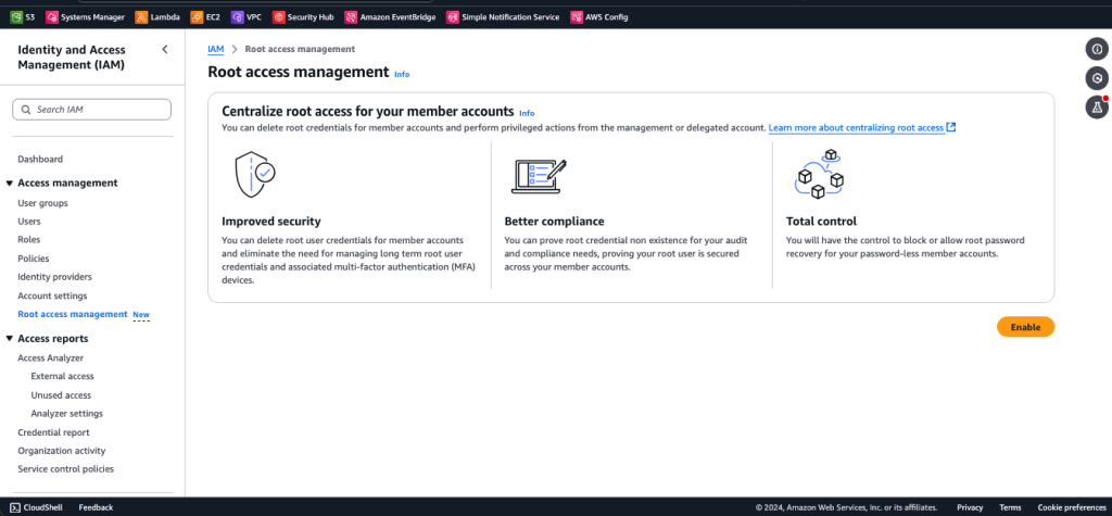
  1. In the IAM console, in the left navigation menu, choose Root access management.
  2. Choose the Enable When you enable centralized root access by using the console, you also enable trusted access for IAM in AWS Organizations.

    Figure 1: Centralized root access capability in the IAM console

    Figure 1: Centralized root access capability in the IAM console

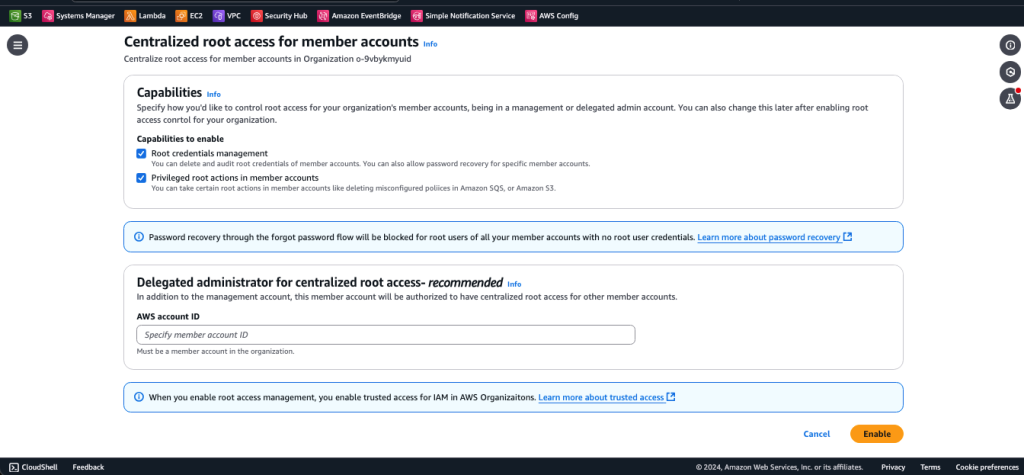
    On the Centralized root access for member accounts page, both the Root credentials management and Privileged root actions in member accounts capabilities are selected by default, as shown in Figure 2. As a security best practice, AWS strongly recommends that you delegate the administration of this service to a dedicated member account used by your security team that is separate from AWS accounts that are used to host your workloads or applications. You can also use a delegated administrator account to avoid unnecessary access to your management account.

Figure 2: Enable root access management

Figure 2: Enable root access management

Enable centralized root access (CLI)

From the Organizations management account, you can also enable centralized root access from the command line.

To enable centralized root access (CLI)

  1. First, make sure that you’ve updated to the latest AWS CLI so that the new APIs are available.
  2. After you’ve verified your CLI version, turn on the feature by running the following command:
      aws organizations enable-aws-service-access \
    --service-principal iam.amazonaws.com

  3. To reduce unnecessary access to the management account, delegate the administration of this service to a dedicated Security member account by using the following command. Make sure to replace <MEMBER_ACCOUNT_ID> with the member account ID where the delegated administrator will register.
    aws organizations register-delegated-administrator --service-principal iam.amazonaws.com --account-id <MEMBER_ACCOUNT_ID>

  4. Next, enable root actions:
    aws iam enable-organizations-root-sessions 
    aws iam enable-organizations-root-credentials-management

Centralized root access is now enabled and delegated to a dedicated Security member account. From that account, you can manage root credentials for member accounts or gain short-term task-scoped root access into member accounts in order to perform specific root actions. Sign in to the Security member account to follow the rest of the steps in this post.

Root credentials management

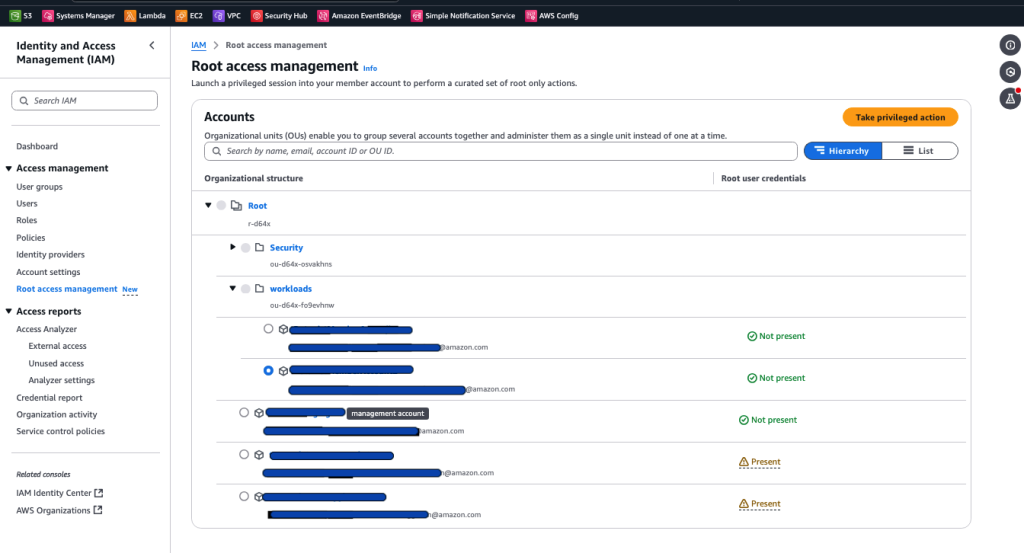
The first feature that we will discuss is root credentials management. Navigate to the new centralized root access management console page as described earlier, and you will see the organizational structure. As shown in Figure 3, there is a Root user credentials field for each AWS account, which tells you if the root user credential is present.

Figure 3: Preview of member accounts with root credential status

Figure 3: Preview of member accounts with root credential status

From this console page, you can delete or create the root user console password (login profile) for each member account.

To delete or create the root user console password

  1. Under Accounts, select one account and choose the Take privileged action button.
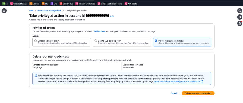
  2. Select either Delete root user credentials or Allow password recovery (for AWS accounts where root credentials do not exist). Note that creating a root user login profile does not restore the previous root user configurations, such as the previously set password and associated MFA device.

Figure 4: The Delete root user credentials feature in the IAM console

Figure 4: The Delete root user credentials feature in the IAM console

Privileged root tasks

After you enable the privileged root actions feature, you (as a security admin) will be able to use the console or CLI to perform privileged tasks such as unlocking S3 bucket or SQS queue policies in member accounts.

To perform privileged root actions (console)

  1. From your delegated administrator account, navigate to the IAM console. In the left navigation menu, choose Root access management.
  2. Select the account where your S3 bucket or SQS queue exists. Then choose the Take privileged action button.
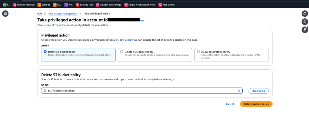
  3. Select the privileged task you want to perform on the member account and provide the details of the S3 bucket or SQS queue from which you would like remove the resource policy. In the example in Figure 5, we’ve selected the Delete S3 bucket policy action and entered the URI of the S3 bucket in the member account.

    Figure 5: Privileged root actions in the IAM console

    Figure 5: Privileged root actions in the IAM console

  4. Confirm your intent to delete the resource policy and then choose Delete bucket policy.

To perform privileged root actions (CLI)

  1. From a terminal, update to the latest AWS CLI to make sure that the new APIs are available.
  2. From the delegated admin account, get a root session in a member account by using the STS/AssumeRoot API action, as shown following. The default and maximum duration for the root session is 15 minutes. Make sure to replace <MEMBER_ACCOUNT_ID> with your member account ID.
     aws sts assume-root \
    --target-principal <MEMBER_ACCOUNT_ID> \
    --task-policy-arn arn=arn:aws:iam::aws:policy/root-task/S3UnlockBucketPolicy 

  3. Use the following command to load the new credentials in the CLI:
    export AWS_ACCESS_KEY_ID=[from sts assume root response]
    export AWS_SECRET_ACCESS_KEY=[from sts assume root response] 
    export AWS_SESSION_TOKEN=[from sts assume root response]

  4. Delete the locked S3 bucket policy, making sure to replace <value> with the name of the bucket:
    aws s3api delete-bucket-policy --bucket <value>

Now the bucket policy is available, and the bucket owner can write a new policy.

Best practices for centralized root access

This section outlines security considerations for centralized root access and usage of temporary root sessions.

Restrict who can use root sessions

Only grant access to use the new root sessions with AssumeRoot to admins and automations that need access. Within your organization’s management and delegated admin account for root management, only grant sts:AssumeRoot permissions to the persons and automations who need it.

You can further limit the root actions that an admin or automation principal can perform by using the AWS Security Token Service (AWS STS) condition key sts:TaskPolicyArn, as shown in the following policy statement.

{
   "Sid": "AllowLaunchingRootSessionsforS3Action",
   "Effect": "Allow",
   "Action": "sts:AssumeRoot",
   "Resource": "*",
   "Condition": {
      "StringEquals": {
         "sts:TaskPolicyARN": "arn:aws:iam::aws:policy/root-task/S3UnlockBucketPolicy"
      }
   }
}

Provide break glass access for root access

Break glass access refers to an alternative method of gaining access for use in exceptional circumstances, such as tasks that can only be performed with root access. When you follow the recommendations for break glass access, root user access is not needed. Review and update your existing procedures that rely on the root user to reduce the dependency of break glass access on root credentials.

Automate routine root actions

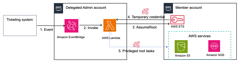
Because the centralized root access feature launched with AWS API, CLI, and SDK support, you can build automations to save time and reduce the need for security teams to take manual actions. For example, you can build an Amazon EventBridge integration with your ticketing system, where an EventBridge rule triggers an AWS Lambda function when the queue or bucket owner submits a ticket with approval. The Lambda function then uses a task-scoped root session to delete the policy on an SQS queue or S3 bucket. The diagram in Figure 6 shows an example of this type of automation.

Figure 6: An automation to delete policies on SQS queues or S3 buckets upon ticket approval

Figure 6: An automation to delete policies on SQS queues or S3 buckets upon ticket approval

The flow of the automation is as follows:

  1. When a ticket to delete a policy on an S3 bucket or SQS queue is approved in your ticketing system, an event is put on the EventBridge event bus and an EventBridge rule is triggered on your delegated admin account.
  2. The EventBridge rule triggers and invokes a Lambda function, passing a copy of the event.
  3. The Lambda function uses the assumeRoot action, with the scope as one of the centralized root access task policies.
  4. AWS STS returns temporary credentials with the scope that was determined in the task policy in the preceding step.
  5. Using the temporary credentials, the Lambda function performs the privileged root action of deletion of S3 bucket or SQS queue policies on your member account.

Review and update your root usage and root credentials management procedures

Now that the tasks that most commonly required root user access (S3 bucket recovery and SQS queue recovery) no longer require long-lived root user credentials, you should revisit your procedures for those use cases and migrate to using root sessions instead of long-lived root users.

Because it is now possible to delete the root user’s login profile, you should revisit the credential management procedures for the root users of your organization’s member accounts. Rather than performing password rotation or MFA device management, you might be able to improve your overall security posture by deleting the root login profile so no credential can be used to access the root user, and no way to initiate the password recovery procedure.

Continue to follow root user best practices for the root user in your organization’s management account

The new capability allows you to more simply manage root credentials from your organization’s member accounts. However, the organization’s management account root user must still exist with a known credential. See the IAM User Guide to learn more about the best practices for managing the organization’s management account root user.

If you don’t have an MFA device for your organization’s management account root user, AWS will provide a free MFA device to eligible customers.

How to remove root credentials in a scalable manner

This section outlines an approach to securely remove your root user credentials at scale. First, get a summary of root credentials for your member accounts. Review the usage of root credentials and identify accounts where root credentials can be safely removed. Then build automation to remove unused root credentials at scale across your member accounts.

Get a summary of root credentials for your member accounts

First, verify whether the root account for your member accounts has credentials before you remove them. If you already have a security admin role in your member accounts, use the getAccountSummary action to audit root credentials. If you don’t have such a role and can’t create an audit role across your member accounts, you can build automation that uses an assume-root session scoped for the IAMAuditRootUserCredentials task to determine whether root credentials exist, and the last time the persistent root credentials were used. The persistent root account can have two types of credentials, password and access keys. You need to check both.

Below is a sample bash script that you can run from your delegated admin account to get a summary of the root credentials on your member accounts.

To use the bash script to get a summary of root credentials

  1. Make sure that you have the AWS CLI installed and are signed in to your delegated admin account using admin role credentials with permissions to the organizations:ListAccounts and sts:AssumeRoot actions.
  2. Save the code that follows to GetRootCredentialsSummary.sh.
  3. The profile used in the scripts is root-access-management. You can modify the scripts to use another profile.
  4. Run GetRootCredentialsSummary.sh on your terminal.
  5. The output will have a .csv file for the root accounts that lists their last login, for both password and access key. Use this information to determine which root accounts are safe to remove. If there is no last-used information, then the credentials are unused, and you can proceed to remove them. If they were used, trace the actions for which they were used in AWS CloudTrail. If the credentials were used for root actions, replace them with an alternative method for member accounts. Identify accounts for which root credentials cannot be removed at this time and need to be excluded from the deletion process.
#!/bin/bash

# Specify the AWS profile to use
AWS_PROFILE="root-access-management"

# Specify the account IDs to exclude (comma-separated)
EXCLUDED_ACCOUNTS="111122223333,444455556666"

# Get the list of accounts in the organization
ACCOUNTS=$(aws organizations list-accounts  --profile $AWS_PROFILE --query 'Accounts[*].[Id]' --output text 2>&1) || handle_error $? $LINENO
# Open a CSV file for writing
: > root_user_last_login.csv  # Create an empty file
echo "AccountId,MFADevices,AccountAccessKeysPresent,AccountMFAEnabled,AccountPasswordPresent,PasswordLastUsedTime" >> root_user_last_login.csv
# Set the assume-root parameters\
REGION="us-east-1"
TASK_POLICY_ARN="arn=arn:aws:iam::aws:policy/root-task/IAMAuditRootUserCredentials"
# Iterate over each account
while IFS=',' read -r account_id account_name; do
    # Check if the account is excluded
    if [[ ",$EXCLUDED_ACCOUNTS," == *,"$account_id",* ]]; then
        echo "Skipping account $account_id ($account_name) as it is excluded."
        continue
    fi
    # Set the role ARN and session name for the current account
    SESSION_NAME="session_${account_id}"
    TARGET_PRINCIPAL="${account_id}"
    # Assume the role and capture the JSON response
    # Assume the role
    ASSUME_ROLE_OUTPUT=$(aws  sts assume-root \
        --profile "$AWS_PROFILE" \
        --region $REGION \
        --task-policy-arn "$TASK_POLICY_ARN" \
        --target-principal "$TARGET_PRINCIPAL" \
        --output json )
        
    # Extract the temporary credentials from the JSON response
    ACCESS_KEY_ID=$(echo "$ASSUME_ROLE_OUTPUT" | jq -r '.Credentials.AccessKeyId')
    SECRET_ACCESS_KEY=$(echo "$ASSUME_ROLE_OUTPUT" | jq -r '.Credentials.SecretAccessKey')
    SESSION_TOKEN=$(echo "$ASSUME_ROLE_OUTPUT" | jq -r '.Credentials.SessionToken')
    # Export the temporary credentials as environment variables
    export AWS_ACCESS_KEY_ID="$ACCESS_KEY_ID"
    export AWS_SECRET_ACCESS_KEY="$SECRET_ACCESS_KEY"
    export AWS_SESSION_TOKEN="$SESSION_TOKEN"
    
    # Fetch IAM account summary using get-account-summary
    iam_summary=$(aws iam get-account-summary --query 'SummaryMap')
    
    # Extract relevant information
    mfa_devices=$(echo "$iam_summary" | jq -r '.MFADevices // "No"')
    account_accesskeys_present=$(echo "$iam_summary" | jq -r '.AccountAccessKeysPresent // "No"')
                       
    # Extract MFA and password status for the root user
    mfa_enabled=$(echo "$iam_summary" | jq -r '.AccountMFAEnabled // "No"')
    password_present=$(echo "$iam_summary" | jq -r '.AccountPasswordPresent // "No"')

    # Get the root user's password last used information
    ROOT_PASSWORD_LAST_USED=$(aws iam get-user  --query User.PasswordLastUsed --output text 2>&1)  
    # Unset temporary credentials for security
    unset AWS_ACCESS_KEY_ID
    unset AWS_SECRET_ACCESS_KEY
    unset AWS_SESSION_TOKEN

    # Write the account information to the CSV file
    echo "$account_id,$mfa_devices,$account_accesskeys_present,$mfa_enabled,$password_present,$ROOT_PASSWORD_LAST_USED" >> root_user_last_login.csv
    sleep .1 # Waits 0.1 second.
done <<< "$ACCOUNTS"
echo "Root user last login information has been written to root_user_last_login.csv"

Remove root credentials at scale

After you determine which AWS accounts have persistent root credentials that you want to remove, use the new action, assumeRoot, to access these accounts and remove the root credentials.

Below is a script that will remove root login profiles across your entire organization. You can exclude certain accounts by updating the variable EXCLUDED_ACCOUNTS.

To use the script to remove root credentials

  1. Make sure that you have the AWS CLI installed and are signed in to your delegated admin account using admin role credentials with permissions to the organizations:ListAccounts and sts:AssumeRoot actions.
  2. Save the code that follows to DeleteRootCredentials.sh.
  3. The profile used in the script is root-access-management. You can modify the script to use another profile.
  4. Run ./DeleteRootCredentials.sh on your terminal.
  5. The output will have a .csv file for the root accounts (except the ones in EXCLUDED_ACCOUNTS) with the status for root login profile deletion.
#/bin/bash

# Specify the account IDs to exclude (comma-separated)
EXCLUDED_ACCOUNTS="111122223333,444455556666"

# Specify the AWS profile to use
AWS_PROFILE="root-access-management"

# Set the role name and additional parameters
REGION="us-east-1"
TASK_POLICY_ARN="arn=arn:aws:iam::aws:policy/root-task/IAMDeleteRootUserCredentials"

# Function to handle errors
handle_error() {
    echo "Error on line $2: Command exited with status $1" >&2
    exit $1
}

# Get the list of accounts in the organization
ACCOUNTS=$(aws organizations list-accounts  --profile $AWS_PROFILE  --query 'Accounts[*].[Id]' --output text 2>&1) || handle_error $? $LINENO

# Open a CSV file for writing
: > root_user_deletion.csv  # Create an empty file
echo "AccountId,AccountName,RootUserDeleted" >> root_user_deletion.csv

# Iterate over each account
while IFS=$'\t' read -r account_id ; do
    # Check if the account is excluded
    if [[ ",$EXCLUDED_ACCOUNTS," == *,"$account_id",* ]]; then
        echo "Skipping account $account_id ($account_name) as it is excluded."
        continue
    fi

    SESSION_NAME="session_${account_id}"
    TARGET_PRINCIPAL="${account_id}"
    
    # Assume the role
    assume_role=$(aws  sts assume-root \
        --profile "$AWS_PROFILE" \
        --region $REGION \
        --task-policy-arn "$TASK_POLICY_ARN" \
        --target-principal "$TARGET_PRINCIPAL" \
        --output json)


    # Extract temporary credentials from the assume role response
    export AWS_ACCESS_KEY_ID=$(echo $assume_role | jq -r '.Credentials.AccessKeyId')
    export AWS_SECRET_ACCESS_KEY=$(echo $assume_role | jq -r '.Credentials.SecretAccessKey')
    export AWS_SESSION_TOKEN=$(echo $assume_role | jq -r '.Credentials.SessionToken')

    # Attempt to delete the root user
    ROOT_USER_DELETED="false"
    if aws iam delete-login-profile  ; then
        ROOT_USER_DELETED="true"
    fi

     # Unset temporary credentials for security
    unset AWS_ACCESS_KEY_ID
    unset AWS_SECRET_ACCESS_KEY
    unset AWS_SESSION_TOKEN
    
    # Write the account information to the CSV file
    echo "$account_id,$account_name,$ROOT_USER_DELETED" >> root_user_deletion.csv

done <<< "$ACCOUNTS"

echo "Root user deletion results have been written to root_user_deletion.csv"

You can extend this script to delete root access keys by using the delete-access-key command. To do so, you retrieve the list of access keys by using the list-access-keys command, iterate through the list of access keys to determine which keys to delete, and pass the resulting access key IDs to delete-access-key to delete the access keys.

Similarly, you can extend the script to delete MFA devices by doing the following. Retrieve the list of MFA devices by using list-mfa-devices, iterate through the list to determine which MFA devices to delete, and pass the resulting device serial numbers to deactivate-mfa-device and delete-virtual-mfa-device to deactivate the MFA devices and further delete the virtual MFA devices.

Conclusion

In this post, we showed you how to enable and use the various features of centralized root access. Additionally, we covered best practices for using this new capability and discussed considerations for adoption.

To learn more about centralized root access and root user best practices, review our documentation. If you have questions, reach out to AWS Support or post a question at re:Post.

Jonathan VanKim
Jonathan VanKim

Jonathan is a Principal Solutions Architect who specializes in security and identity for AWS. In 2014, he started working at AWS Professional Services and transitioned to solutions architecture four years later. His AWS career has been focused on helping customers of all sizes build secure AWS architectures. He enjoys snowboarding, wakesurfing, travelling, and experimental cooking.
Sowjanya Rajavaram
Sowjanya Rajavaram

Sowjanya is a Senior Solutions Architect who specializes in security and identity for AWS. Her career has been focused on helping customers of all sizes solve their identity and access management problems. She enjoys traveling and experiencing new cultures and food.

Run high-availability long-running clusters with Amazon EMR instance fleets

Post Syndicated from Garima Arora original https://aws.amazon.com/blogs/big-data/run-high-availability-long-running-clusters-with-amazon-emr-instance-fleets/

AWS now supports high availability Amazon EMR on EC2 clusters with instance fleet configuration. With high availability instance fleet clusters, you now get the enhanced resiliency and fault tolerance of high availability architecture, along with the improved flexibility and intelligence in Amazon Elastic Compute Cloud (Amazon EC2) instance selection of instance fleets. Amazon EMR is a cloud big data platform for petabyte-scale data processing, interactive analysis, streaming, and machine learning (ML) using open source frameworks such as Apache Spark, Presto and Trino, and Apache Flink. Customers love the scalability and flexibility that Amazon EMR on EC2 offers. However, like most distributed systems running mission-critical workloads, high availability is a core requirement, especially for those with long-running workloads.

In this post, we demonstrate how to launch a high availability instance fleet cluster using the newly redesigned Amazon EMR console, as well as using an AWS CloudFormation template. We also go over the basic concepts of Hadoop high availability, EMR instance fleets, the benefits and trade-offs of high availability, and best practices for running resilient EMR clusters.

High availability in Hadoop

High availability (HA) provides continuous uptime and fault tolerance for a Hadoop cluster. The core components of Hadoop, like Hadoop Distributed File System (HDFS) NameNode and YARN ResourceManager, are single points of failure in clusters with a single primary node. In the event that any of them crash, the entire cluster goes down. High Availability removes this single point of failure by introducing redundant standby nodes that can quickly take over if the primary node fails.

In a high availability EMR cluster, one node serves as the active NameNode that handles client operations, and others act as standby NameNodes. The standby NameNodes constantly synchronize their state with the active one, enabling seamless failover to maintain service availability. To learn more, see Supported applications in an Amazon EMR Cluster with multiple primary nodes.

Key instance fleet differentiations

Amazon EMR recommends using the instance fleet configuration option for provisioning EC2 instances in EMR clusters because it offers a flexible and robust approach to cluster provisioning. Some key advantages include:

  • Flexible instance provisioning – Instance fleets provide a powerful and simple way to specify up to five EC2 instance types on the Amazon EMR console, or up to 30 when using the AWS Command Line Interface (AWS CLI) or API with an allocation strategy. This enhanced diversity helps optimize for cost and performance while increasing the likelihood of fulfilling capacity requirements.
  • Target capacity management – You can specify target capacities for On-Demand and Spot Instances for each fleet. Amazon EMR automatically manages the mix of instances to meet these targets, reducing operational overhead.
  • Improved availability – By spanning multiple instance types and purchasing options such as On-Demand and Spot, instance fleets are more resilient to capacity fluctuations in specific EC2 instance pools.
  • Enhanced Spot Instance handling – Instance fleets offer superior management of Spot Instances, including the ability to set timeouts and specify actions if Spot capacity can’t be provisioned.
  • Reliable cluster launches – You can configure your instance fleet to select multiple subnets for different Availability Zones, allowing Amazon EMR to find the best combination of instances and purchasing options across these zones to launch your cluster in. Amazon EMR will identify the best Availability Zone based on your configuration and available EC2 capacity and launch the cluster.

Prerequisites

Before you launch the high availability EMR instance fleet clusters, make sure you have the following:

  • Latest Amazon EMR release – We recommend that you use the latest Amazon EMR release to benefit from the highest level of resiliency and stability for your high availability clusters. High availability for instance fleets is supported with Amazon EMR releases 5.36.1, 6.8.1, 6.9.1, 6.10.1, 6.11.1, 6.12.0, and later.
  • Supported applications – High availability for instance fleets is supported for applications such as Apache Spark, Presto, Trino, and Apache Flink. Refer to Supported applications in an Amazon EMR Cluster with multiple primary nodes for the complete list of supported applications and their failover processes.

Launch a high availability instance fleet cluster using the Amazon EMR console

Complete the following steps on the Amazon EMR console to configure and launch a high availability EMR cluster with instance fleets:

  1. On the Amazon EMR console, create a new cluster.
  2. For Name, enter a name.
  3. For Amazon EMR release, choose the Amazon EMR release that supports high availability clusters with instance fleets. The setting will default to the latest available Amazon EMR release.

CreateHACluster-EMRRelease

  1. Under Cluster configuration, choose the desired instance types for the primary fleet. (You can select up to five when using the Amazon EMR console.)
  2. Select Use high availability to launch the cluster with three primary nodes.

CreateHACluster

  1. Choose the instance types and target On-Demand and Spot size for the core and task fleet according to your requirements.

InstanceFleet-CreateFleets

  1. Under Allocation strategy, select Apply allocation strategy.
    1. 1 We recommend that you select Price-capacity optimized for your allocation strategy for your cluster for faster cluster provisioning, more accurate Spot Instance allocation, and fewer Spot Instance interruptions.
  2. Under Networking, you can choose multiple subnets for different Availability Zones. This allows Amazon EMR to look across those subnets and launch the cluster in an Availability Zone that best suits your instance and purchasing option requirements.

allocationStrategy

  1. Review your cluster configuration and choose Create cluster.

Amazon EMR will launch your cluster in a few minutes. You can view the cluster details on the Amazon EMR console.
ClusterDetailPage

Launch a high availability cluster with AWS CloudFormation

To launch a high availability cluster using AWS CloudFormation, complete the following steps:

  1. Create a CloudFormation template with EMR resource type AWS::EMR::Cluster and JobFlowInstancesConfig property types MasterInstanceFleet, CoreInstanceFleet and (optional) TaskInstanceFleets. To launch a high availability cluster, configure TargetOnDemandCapacity=3, TargetSpotCapacity=0 for the primary instance fleet and weightedCapacity=1 for each instance type configured for the fleet. See the following code:
{
  "AWSTemplateFormatVersion": "2010-09-09",
  "Resources": {
    "cluster": {
      "Type": "AWS::EMR::Cluster",
      "Properties": {
        "Instances": {
          "Ec2SubnetIds": [
            "subnet-003c889b8379f42d1",
            "subnet-0382aadd4de4f5da9",
            "subnet-078fbbb77c92ab099"
          ],
          "MasterInstanceFleet": {
            "Name": "HAPrimaryFleet",
            "TargetOnDemandCapacity": 3,
            "TargetSpotCapacity": 0,
            "InstanceTypeConfigs": [
              {
                "InstanceType": "m5.xlarge",
                "WeightedCapacity": 1
              },
              {
                "InstanceType": "m5.2xlarge",
                "WeightedCapacity": 1
              },
              {
                "InstanceType": "m5.4xlarge",
                "WeightedCapacity": 1
              }
            ]
          },
          "CoreInstanceFleet": {
            "Name": "cfnCore",
            "InstanceTypeConfigs": [
              {
                "InstanceType": "m5.xlarge",
                "WeightedCapacity": 1
              },
              {
                "InstanceType": "m5.2xlarge",
                "WeightedCapacity": 2
              },
              {
                "InstanceType": "m5.4xlarge",
                "WeightedCapacity": 4
              }
            ],
            "LaunchSpecifications": {
              "SpotSpecification": {
                "TimeoutAction": "SWITCH_TO_ON_DEMAND",
                "TimeoutDurationMinutes": 20,
                "AllocationStrategy": "PRICE_CAPACITY_OPTIMIZED"
              }
            },
            "TargetOnDemandCapacity": "4",
            "TargetSpotCapacity": 0
          },
          "TaskInstanceFleets": [
            {
              "Name": "cfnTask",
              "InstanceTypeConfigs": [
                {
                  "InstanceType": "m5.xlarge",
                  "WeightedCapacity": 1
                },
                {
                  "InstanceType": "m5.2xlarge",
                  "WeightedCapacity": 2
                },
                {
                  "InstanceType": "m5.4xlarge",
                  "WeightedCapacity": 4
                }
              ],
              "LaunchSpecifications": {
                "SpotSpecification": {
                  "TimeoutAction": "SWITCH_TO_ON_DEMAND",
                  "TimeoutDurationMinutes": 20,
                  "AllocationStrategy": "PRICE_CAPACITY_OPTIMIZED"
                }
              },
              "TargetOnDemandCapacity": "0",
              "TargetSpotCapacity": 4
            }
          ]
        },
        "Name": "TestHACluster",
        "ServiceRole": "EMR_DefaultRole",
        "JobFlowRole": "EMR_EC2_DefaultRole",
        "ReleaseLabel": "emr-6.15.0",
        "PlacementGroupConfigs": [
          {
            "InstanceRole": "MASTER",
            "PlacementStrategy": "SPREAD"
          }
        ]
      }
    }
  }
}

Make sure to use an Amazon EMR release that supports high availability clusters with instance fleets.

  1. Create a CloudFormation stack with the preceding template:
aws cloudformation create-stack --stack-name HAInstanceFleetCluster --template-body file://cfn-template.json --region us-east-1
  1. Retrieve the cluster ID from the list-clusters response to use in the following steps. You can further filter this list based on filters like cluster status, creation date, and time.
aws emr list-clusters --query "Clusters[?Name=='<YourClusterName>']"
  1. Run the following describe-cluster command:
aws emr describe-cluster --cluster-id j-XXXXXXXXXXX --region us-east-1

If the high availability cluster was launched successfully, the describe-cluster response will return the state of the primary fleet as RUNNING and provisionedOnDemandCapacity as 3. By this point, all three primary nodes have been started successfully.

DescribeClusterResponse

Primary node failover with High Availability clusters

To fetch information on all EC2 instances for an instance fleet, use the list-instances command:

aws emr list-instances --cluster-id j-XXXXXXXXXXX --instance-fleet-type MASTER --region us-east-1

For high availability clusters, it will return three instances in RUNNING state for the primary fleet and other attributes like public and private DNS names.

PrimaryInstance-DescribeCluster

The following screenshot shows the instance fleet status on the Amazon EMR console.

Instancefleet status

Let’s examine two cases for primary node failover.

Case 1: One of the three primary instances is accidentally stopped

When an EC2 instance is accidentally stopped by a user, Amazon EMR detects this and performs a failover for the stopped primary node. Amazon EMR also attempts to launch a new primary node with the same private IP and DNS name to recover back the quorum. During this failover, the cluster remains fully operational, providing true resiliency to single primary node failures.

The following screenshots illustrate the instance fleet details.

InstanceFleetDetail-PrimaryInstanceTerminated

instanceFleerRecovery

This automatic recovery for primary nodes is also reflected in the MultiMasterInstanceGroupNodesRunning or MultiMasterInstanceGroupNodesRunningPercentage Amazon CloudWatch metric emitted by Amazon EMR for your cluster. The following screenshot shows an example of these metrics.

CloudwatchMetrics

Case 2: One of the three primary instances becomes unhealthy

If Amazon EMR continuously receives failures when trying to connect to a primary instance, it is deemed as unhealthy and Amazon EMR will attempt to replace it. Similar to case 1, Amazon EMR will perform a failover for the stopped primary node and also attempt to launch a new primary node with the same private IP and DNS name to recover the quorum.

UnhealthyPrimaryInstance
PrimaryInstanceFailover-2

If you list the instances for the primary fleet, the response will include information for the EC2 instance that was stopped by the user and the new primary instance that replaced it with the same private IP and DNS name.
DescribeClusterResponse-instanceFailover

The following screenshot shows an example of the CloudWatch metrics.

An instance can have connection failures for multiple reasons, including but not limited to disk space unavailable on the instance, critical cluster daemons like instance controller shut down with errors, high CPU utilization, and more. Amazon EMR is continuously improving its health monitoring criteria to better identify unhealthy nodes on an EMR cluster.

Considerations and best practices

The following are some of the key considerations and best practices for using EMR instance fleets to launch a high availability cluster with multiple primary nodes:

  • Use the latest EMR release – With the latest EMR releases, you get the highest level of resiliency and stability for your high availability EMR clusters with multiple primary nodes.
  • Configure subnets for high availability – Amazon EMR can’t replace a failed primary node if the subnet is oversubscribed (there aren’t any available private IP addresses in the subnet). This results in a cluster failure as soon as the second primary node fails. Limited availability of IP addresses in a subnet can also result in cluster launch or scaling failures. To avoid such scenarios, we recommend that you dedicate an entire subnet to an EMR cluster.
  • Configure core nodes for enhanced data availability – To minimize the risk of local HDFS data loss on your production clusters, we recommend that you set the dfs.replication parameter to 3 and launch at least four core nodes. Setting dfs.replication to 1 on clusters with fewer than four core nodes can lead to data loss if a single core node goes down. For clusters with three or fewer core nodes, set dfs.replication parameter to at least 2 to achieve sufficient HDFS data replication. For more information, see HDFS configuration.
  • Use an allocation strategy – We recommend enabling an allocation strategy option for your instance fleet cluster to provide faster cluster provisioning, more accurate Spot Instance allocation, and fewer Spot Instance interruptions.
  • Set alarms for monitoring primary nodes – You should monitor the health and status of primary nodes of your long-running clusters to maintain smooth operations. Configure alarms using CloudWatch metrics such as MultiMasterInstanceGroupNodesRunning, MultiMasterInstanceGroupNodesRunningPercentage, or MultiMasterInstanceGroupNodesRequested.
  • Integrate with EC2 placement groups – You can also choose to protect primary instances against hardware failures by using a placement group strategy for your primary fleet. This will spread the three primary instances across separate underlying hardware to avoid loss of multiple primary nodes at the same time in the event of a hardware failure. See Amazon EMR integration with EC2 placement groups for more details.

When setting up a high availability instance fleet cluster with Amazon EMR on EC2, it’s important to understand that all EMR nodes, including the three primary nodes, are launched within a single Availability Zone. Although this configuration maintains high availability within that Availability Zone, it also means that the entire cluster can’t tolerate an Availability Zone outage. To mitigate the risk of cluster failures due to Spot Instance reclamation, Amazon EMR launches the primary nodes using On-Demand instances, providing an additional layer of reliability for these critical components of the cluster.

Conclusion

This post demonstrated how you can use high availability with EMR on EC2 instance fleets to enhance the resiliency and reliability of your big data workloads. By using instance fleets with multiple primary nodes, EMR clusters can withstand failures and maintain uninterrupted operations, while providing enhanced instance diversity and better Spot capacity management within a single Availability Zone. You can quickly set up these high availability clusters using the Amazon EMR console or AWS CloudFormation, and monitor their health using CloudWatch metrics.

To learn more about the supported applications and their failover process, see Supported applications in an Amazon EMR Cluster with multiple primary nodes. To get started with this feature and launch a high availability EMR on EC2 cluster, refer to Plan and configure primary nodes.


About the Authors

Garima Arora is a Software Development Engineer for Amazon EMR at Amazon Web Services. She specializes in capacity optimization and helps build services that allow customers to run big data applications and petabyte-scale data analytics faster. When not hard at work, she enjoys reading fiction novels and watching anime.

Ravi Kumar is a Senior Product Manager Technical-ES (PMT) at Amazon Web Services, specialized in building exabyte-scale data infrastructure and analytics platforms. With a passion for building innovative tools, he helps customers unlock valuable insights from their structured and unstructured data. Ravi’s expertise lies in creating robust data foundations using open-source technologies and advanced cloud computing, that powers advanced artificial intelligence and machine learning use cases. A recognized thought leader in the field, he advances the data and AI ecosystem through pioneering solutions and collaborative industry initiatives. As a strong advocate for customer-centric solutions, Ravi constantly seeks ways to simplify complex data challenges and enhance user experiences. Outside of work, Ravi is an avid technology enthusiast who enjoys exploring emerging trends in data science, cloud computing, and machine learning.

Tarun Chanana is a Software Development Manager for Amazon EMR at Amazon Web Services.

Proactively validate your AWS CloudFormation templates with AWS Lambda

Post Syndicated from Kirankumar Chandrashekar original https://aws.amazon.com/blogs/devops/proactively-validate-your-aws-cloudformation-templates-with-aws-lambda/

AWS CloudFormation is a service that allows you to define, manage, and provision your AWS cloud infrastructure using code. To enhance this process and ensure your infrastructure meets your organization’s standards, AWS offers CloudFormation Hooks. These Hooks are extension points that allow you to invoke custom logic at specific points during CloudFormation stack operations, enabling you to perform validations, make modifications, or trigger additional processes. Among these, the Lambda hook is a powerful option provided by AWS. This managed hook allows you to use Lambda functions to validate your CloudFormation templates before deployment. By using a Lambda hook, you can invoke custom logic to check infrastructure configurations on create or update or delete CloudFormation resources or stacks or change sets, as well as create or update operations for AWS Cloud Control API (CCAPI) resources. This enables you to enforce defined policies for your infrastructure-as-code (IaC), preventing the deployment of non-compliant resources or emitting warnings for potential issues. In this blog post, you will explore how to use a Lambda hook to validate your CloudFormation templates before deployment, ensuring your infrastructure is compliant and secure from the start.

Introducing Lambda Hook

The Lambda hook is an AWS-provided managed hook with the type AWS::Hooks::LambdaHook. It simplifies the integration of custom logic into CloudFormation stacks. This powerful feature allows you to focus on building and testing your custom logic as a Lambda function, without the complexity of creating a hook from scratch.

By using the Lambda hook, you can activate a pre-built hook and deploy your custom logic into a Lambda function using familiar tools like AWS CLI or AWS Serverless Application Model (SAM) or AWS Cloud Development Kit (CDK). This approach reduces the number of components you need to manage in your workflow, allowing for more streamlined operations. The Lambda hook also offers flexible evaluation capabilities, enabling you to respond to specific template properties or configurations as needed.

One of the key advantages of the Lambda hook is the enhanced control it provides. You can benefit from features such as VPC integration, local logging, and granular resource management, all while leveraging the power of AWS Lambda functions. To get started with the Lambda hook, you’ll need to activate it in your AWS account. This activation process eliminates the need for authoring, testing, packaging, and deploying a custom hook using the AWS CloudFormation Command Line Interface (CFN-CLI), significantly simplifying your workflow.

Example Use Case: S3 Bucket Versioning Validation

This blog post demonstrates using the Lambda hook to validate S3 Bucket versioning before deployment. While focused on S3 buckets, this approach can be applied to other resource types, properties, stack, and change set operations.

By leveraging the Lambda hook, you’ll streamline custom logic integration into your CloudFormation stacks. The process involves:

  1. Activating Lambda hook of type AWS::Hooks::LambdaHook in your account
  2. Writing a Lambda function for validation
  3. Providing the Lambda ARN as input to the hook

This example showcases how to enhance your infrastructure-as-code practices, ensuring compliant and secure deployments from the start.

Architecture

This section shows you how the Lambda hook and Lambda function work together to enhance your CloudFormation deployments.

Lambda hook and Lambda function

First, you need to create a Lambda function with the business logic to respond to the hook. Then, you need to create an IAM execution role with the necessary permissions to invoke the Lambda Function. Once you have the Lambda function and the IAM execution role, you can activate the AWS provided Lambda hook. Follow the steps in the documentation to activate a Lambda hook from the AWS console. Alternatively, you can activate it using the AWS Command Line Interface (AWS CLI) by using the activate-type and set-type-configuration commands. Lastly, you can also use AWS::CloudFormation::LambdaHook as a CloudFormation resource to activate and configure Lambda hook from a CloudFormation template. You can share this resource across your other accounts and regions using AWS CloudFormation StackSets by following this blog.

Lambda hook in action

The following diagram and explanation illustrate the step-by-step workflow of how Lambda hook integrates with your CloudFormation operations, providing a visual representation of the process from template creation to resource deployment or modification.

Lambda Hooks Architecture and its working in action

Diagram 1: Lambda hooks in action

The architecture diagram illustrates the step-by-step flow of how the Lambda hook is used during a CloudFormation stack operation.

  1. Author a template: Author a CloudFormation template, including the necessary resources to configure.
  2. Create the stack: The CloudFormation stack creation process has started, but the process of creating the defined resources in the template has not yet begun.
  3. Request is received by CloudFormation service: When a resource creation, update, or deletion is requested, the CloudFormation service receives the request.
  4. Invoke the Hook: The CloudFormation service then invokes the Lambda hook.
  5. The hook invokes your the Lambda Function: The Lambda hook, in turn, triggers the execution of the Lambda function that was defined in the hook activation.
  6. The Lambda function processes the request and responds back to the Hook: The Lambda function processes the request, performing validation, or additional tasks as required. The Lambda function then responds back to the Lambda hook.
  7. The stack workflow progresses further in either continuing the resource creation/update/deletion with/without a warning or fails: Based on the Lambda function’s output, the Lambda hook either allows the stack operation to proceed with the resource operation (for example, creation of the resource), or deny the resource operation causing a rollback of the stack.

This workflow demonstrates how Lambda hook seamlessly integrates into the CloudFormation stack deployment process, allowing you to implement custom validations, enforce policies, and extend the capabilities of your infrastructure-as-code deployments through the power of Lambda functions. By leveraging the Lambda hook and the custom Lambda function, customers can extend the capabilities of their CloudFormation deployments, enabling advanced use cases such as resource validation, or additional task execution.

Sample Deployment

This section shows you how to enable the Lambda hook, which is of type AWS::Hooks::LambdaHook, and add the business logic in the Lambda function to validate the versioning configuration of an S3 bucket. The sample solution shown in this blog post demonstrates the hook triggering for the resource type AWS::S3::Bucket, and if you want to trigger this for every resource type, then you can use the Resource filter within Hook filters configuration that can take wildcard "AWS::*::*" as a value or multiple targets of resource types for example "AWS::S3::Bucket", "AWS::DynamoDB::Table", and you’ll also want to make sure that the Lambda Function has the logic to handle the additional resource type. You can also add additional Hook targets , for example to validate your STACK or CHANGE_SET.

In the example used in this blog post, you will configure the hook and activate on create and update operations operations. For more information about TargetFilters, see Hook configuration schema and for more information about Lambda hook see here. With these modifications, you need to consider two important points: First, you will need to handle the business logic to deal with different resource types in your Lambda function code. Second, additional pricing may apply based on your resource usage, for more details see the Lambda pricing page.

Creating the Lambda Function

You can create a Lambda function in several ways – on the AWS Console, using CloudFormation, using AWS CLI, or by directly invoking the API via SDK. In this section, we will cover creating a Lambda function with a few clicks on the AWS console. See Using Lambda with infrastructure as code (IaC) for deploying Lambda Function using SAM CLI, CDK or CloudFormation.

Create the Lambda function on the AWS console by following create a Lambda function with the console instructions and use the following sample Python code.

"""Example Lambda function called by AWS::Hooks::LambdaHook."""


import logging


HOOK_INVOCATION_POINTS = [
    "CREATE_PRE_PROVISION",
    "UPDATE_PRE_PROVISION",
    "DELETE_PRE_PROVISION",
]

TARGET_NAMES = [
    "AWS::S3::Bucket",
]

LOGGER = logging.getLogger()

LOGGER.setLevel("INFO")


def lambda_handler(event, context):
  """Define the entry point of the function."""
  try:
    request = event
    
    LOGGER.info(f"Request: {request}")

    invocation_point = request["actionInvocationPoint"]
    LOGGER.info(f"Invocation point: {invocation_point}")

    target_name = request["requestData"]["targetName"]
    LOGGER.info(f"Target name: {target_name}")
    
    clientRequestToken = request["clientRequestToken"]

    if (
      invocation_point not in HOOK_INVOCATION_POINTS
      or target_name not in TARGET_NAMES
    ):
      message = (
        f"Skipping {target_name} evaluation for {invocation_point}."
      )
      LOGGER.info(message)
      payload = {
        "clientRequestToken": clientRequestToken,
        "hookStatus": "SUCCESS",
        "errorCode": None,
        "message": message,
        "callbackContext": None,
        "callbackDelaySeconds": 0,
      }
      LOGGER.debug(payload)
      return payload

    target_model = request["requestData"]["targetModel"]

    resource_properties = (
      target_model.get("resourceProperties")
      if target_model and target_model.get("resourceProperties")
      else None
    )
    LOGGER.debug(f"Resource properties: {resource_properties}")

    versioning_configuration = (
      resource_properties.get("VersioningConfiguration")
      if resource_properties
      and resource_properties.get("VersioningConfiguration")
      else None
    )
    versioning_configuration_status = (
      versioning_configuration.get("Status")
      if versioning_configuration
      and versioning_configuration.get("Status")
      else None
    )
    if (
      not resource_properties
      or not versioning_configuration
      or not versioning_configuration_status
      or not versioning_configuration_status == "Enabled"
    ):
      message = "Versioning not set or not enabled for the S3 bucket."
      LOGGER.error(message)
      payload = {
        "clientRequestToken": clientRequestToken,
        "hookStatus": "FAILED",
        "errorCode": "NonCompliant",
        "message": message,
      }
    else:
      message = "Versioning is enabled for the S3 bucket."
      LOGGER.info(message)
      payload = {
        "clientRequestToken": clientRequestToken,
        "hookStatus": "SUCCESS",
        "errorCode": None,
        "message": message,
      }

    LOGGER.debug(payload)
    return payload
  except Exception as exception:
    message = str(exception)
    payload = {
      "clientRequestToken":  event["clientRequestToken"],
      "hookStatus": "FAILED",
      "errorCode": "InternalFailure",
      "message": message,
      "callbackContext": None,
      "callbackDelaySeconds": 0,
    }
    LOGGER.error(message)
    return payload

Example event sent to Lambda by the hook

{
  "clientRequestToken": "XXXXXXXXXXXX-XXXX-XXXX-XXXX-XXXXXXXXXXXX",
  "awsAccountId": "111111111111",
  "stackId": "arn:aws:cloudformation:<AWS-Region>:111111111111:stack/example-stack/xxxxxxxx-xxxx-xxxx-xxxx-xxxxxxxxxxxx",
  "changeSetId": "None",
  "hookTypeName": "AWS::Hooks::LambdaHook",
  "hookTypeVersion": "00000001",
  "hookModel":
    {
      "LambdaFunction": "example-hook-function-name",
    },
  "actionInvocationPoint": "CREATE_PRE_PROVISION",
  "requestData":
    {
      "targetName": "AWS::S3::Bucket",
      "targetType": "AWS::S3::Bucket",
      "targetLogicalId": "Bucket",
      "callerCredentials": "None",
      "providerCredentials": "None",
      "providerLogGroupName": "None",
      "hookEncryptionKeyArn": "None",
      "hookEncryptionKeyRole": "None",
      "targetModel":
        {
          "resourceProperties":
            {
              "PublicAccessBlockConfiguration":
                { "RestrictPublicBuckets": true, "IgnorePublicAcls": true },
              "BucketName": "XXXXXXXXXXXXXXXXXXXXXXXXXXX",
              "VersioningConfiguration": { "Status": "Enabled" },
            },
          "previousResourceProperties": "None",
        },
    },
  "requestContext": { "invocation": 1, "callbackContext": "None" },
}

Explanation of the Lambda Function code

The Lambda Function code is designed to process the event received from the Lambda hook and validate the versioning configuration of the target S3 bucket resource. Here’s a detailed explanation of the code:

  1. The function first extracts the relevant information from the event, including the invocation point and the target resource type.
  2. It then checks if the current invocation point is in the configured HOOK_INVOCATION_POINTS list and if the target resource type is AWS::S3::Bucket. If not, the function returns a success response, skipping the validation for this particular invocation.

Note: this code that skips the validation is put here as a fallback logic in the event the user has not chosen to use TargetFilters. As this is a wildcard hook, without TargetFilters the hook will always be invoked for any AWS resource type described in the template, and since the hook targets preCreate, preUpdate, and preDelete by default, the hook will be invoked for these invocation points by default. To narrow the scope and reduce costs by avoiding to invoke the hook for all AWS resource type targets and invocation points, use TargetFilters.

  1. Next, the function retrieves the resource properties from the event, specifically looking for the VersioningConfiguration property and its Status.
  2. If the VersioningConfiguration property is not present or its Status is not set to Enabled, the function returns a failure response, indicating that the versioning is not enabled for the S3 bucket.
  3. If the versioning is enabled, the function returns a success response.
  4. The function also includes a fallback mechanism to return a failure response in case of any other exceptions. By evaluating this sample code, you can validate the versioning configuration of the S3 bucket during the CloudFormation stack creation and update processes, with your infrastructure-as-code policies.

Enabling Lambda Hook in your AWS Account/Region

  1. Navigate to the AWS CloudFormation service on the AWS Console, then choose “Create Hook” → “with Lambda” from the main Hooks page:

Lambda Hooks Creation

Diagram 2: Create a Hook with Lambda console page

You will see the page explaining how the Lambda function work as a hook.

Lambda hooks provide lambda

Diagram 3: Provide a Lambda function to Hook Console page

  1. Provide the Hooks details: the name, the Lambda function it should take, the type, and the mode. You can also create your execution role directly from the console by choosing “New execution role”.
Lambdas Hooks Details Config

Diagram 3: Provide a Lambda function to Hook Console page

You can review the Lambda hook and activate it from the next page.

Lambda Hooks details and configuration

Diagram 4: Review Lambda hook Console page

Test a sample

In this section, you will test the hook and the Lambda Function that you activated for a S3 bucket resource.

Create an S3 Bucket without versioning

AWSTemplateFormatVersion: "2010-09-09"

Description: This CloudFormation template provisions an S3 Bucket without versioning enabled

Resources:
  S3Bucket:
    DeletionPolicy: Delete
    Type: AWS::S3::Bucket
    Properties:
      BucketName: !Sub test-bucket-versioning-1-${AWS::Region}-${AWS::AccountId}

You will see the hook invoking Lambda function and the Lambda Function responding back with a failure message since the Versioning is not enabled.

When you create or update a stack with the template above, the Lambda hook will be invoked, and the Lambda Function will respond with a failure message since bucket versioning is not enabled. The Lambda Function code will extract the resourceProperties from the event, check the VersioningConfiguration property, and find that the Status is not set to Enabled. As a result, if you use the example template above where you describe the S3 bucket without versioning enabled, the Lambda Function will send a failure response back to the hook, causing the CloudFormation stack operation to fail as shown in the following screenshot.

Lambda Hooks Failure stack

Diagram 5: Lambda Hook failure Stack

Create an S3 Bucket with versioning enabled You can try creating an S3 Bucket with versioning enabled to see how Hooks assessment succeeded.

AWSTemplateFormatVersion: "2010-09-09"

Description: This CloudFormation template provisions an S3 Bucket with Versioning enabled

Resources:
  S3Bucket:
    DeletionPolicy: Delete
    Type: AWS::S3::Bucket
    Properties:
      BucketName: !Sub test-bucket-versioning-2-${AWS::Region}-${AWS::AccountId}
      VersioningConfiguration:
        Status: Enabled

In this case, you will see the hook invoking the Lambda function and getting a success message since the Versioning is enabled

When you create a stack with this CloudFormation template, the Lambda hook will be invoked, and the Lambda Function will respond with a success message since the versioning is enabled. The Lambda Function code will extract the resourceProperties from the event, check the VersioningConfiguration property, and find that the Status is set to Enabled. As a result, the Lambda Function will send a success response back to the hook, allowing the CloudFormation stack operation to proceed as shown in the following screenshot.

Lambda Hooks Success stack

Diagram 6: Lambda Hook success Stack

By testing these two scenarios, you can verify that the Lambda hook and the associated Lambda Function are working as expected, enforcing the S3 bucket versioning policy during CloudFormation stack operations.

Clean up

To clean up, refer to the following documentation to delete CloudFormation Stacks: Deleting a stack on the AWS CloudFormation console or Deleting a stack using AWS CLI. Refer to documentation to deactivate the hook.

Conclusion

In this blog post, you explored the capabilities of CloudFormation Hooks and how they can be leveraged to extend the functionality of your infrastructure-as-code deployments. Specifically, you learned about the Lambda hook, a pre-built hook that simplifies the process of integrating custom logic into your CloudFormation stacks.

By activating the Lambda hook, and deploying a custom Lambda Function, you were able to validate the versioning configuration of an S3 bucket during the CloudFormation stack creation and update processes. This approach allows you to enforce infrastructure-as-code policies and ensure compliance at the point of deployment, rather than relying on post-deployment checks or indirect governance mechanisms. The ability to leverage familiar tools and workflows, such as the AWS CLI, AWS SAM, CI/CD pipelines, or the AWS CDK, makes it easier to incorporate custom logic into your CloudFormation deployments. This reduces the overhead and complexity associated with traditional hook orchestration and packaging, empowering you to streamline your infrastructure-as-code practices.

As you continue to build and deploy your cloud infrastructure, consider exploring the various CloudFormation Hooks available, for example, see aws-cloudformation/aws-cloudformation-samples and aws-cloudformation/community-registry-extensions GitHub repositories. The approach demonstrated in this blog post can be applied to other resource types supported by CloudFormation, allowing you to validate and enforce policies for a wide range of infrastructure components, from EC2 instances and VPCs to databases and application services.

About the Author

kirankumar.jpeg

Kirankumar Chandrashekar is a Sr. Solutions Architect for Strategic Accounts at AWS. He focuses on leading customers in architecting DevOps, modernization using serverless, containers and container orchestration technologies like Docker, ECS, EKS to name a few. Kirankumar is passionate about DevOps, Infrastructure as Code, modernization and solving complex customer issues. He enjoys music, as well as cooking and traveling.

stella.jpegStella Hie is a Sr. Product Manager Technical for AWS Infrastructure as Code. She focuses on proactive control and governance space, working on delivering the best experience for customers to use AWS solutions safely. Outside of work, she enjoys hiking, playing piano, and watching live shows.

Threat modeling your generative AI workload to evaluate security risk

Post Syndicated from Danny Cortegaca original https://aws.amazon.com/blogs/security/threat-modeling-your-generative-ai-workload-to-evaluate-security-risk/

As generative AI models become increasingly integrated into business applications, it’s crucial to evaluate the potential security risks they introduce. At AWS re:Invent 2023, we presented on this topic, helping hundreds of customers maintain high-velocity decision-making for adopting new technologies securely. Customers who attended this session were able to better understand our recommended approach for qualifying security risk and maintaining a high security bar for the applications they build. In this blog post, we’ll revisit the key steps for conducting effective threat modeling on generative AI workloads, along with additional best practices and examples, including some typical deliverables and outcomes you should look for across each stage. Throughout this post we will link to specific examples that we created with the AWS Threat Composer tool. Threat Composer is an open source AWS tool you can use to document your threat model, available at no additional cost.

This post covers a practical approach for threat modeling a generative AI workload and assumes you know the basics of threat modeling. If you want to get an overview on threat modeling, we recommend that you check out this blog post. In addition, this post is part of a larger series on the security and compliance considerations of generative AI.

Why use threat modeling for generative AI?

Each new technology comes with its own learning curve when it comes to identifying and mitigating the unique security risks it presents. The adoption of generative AI into workloads is no different. These workloads, specifically the use of large language models (LLMs), introduce new security challenges because they can generate highly customized and non-deterministic outputs based on user prompts, which introduces the possibility for potential misuse or abuse. In addition, relies on access to large and customized data sets, often internal data sources which might contain sensitive information.

Although working with LLMs is a relatively new practice and has some unique and nuanced security risks and impacts, it’s crucial to remember that LLMs are only one portion of a larger workload. It’s important to apply the threat modeling approach to parts of the system, taking into account well-known threats such as injections or the compromise of credentials. Part 1 of the Securing generative AI AWS blog series, An introduction to the Generative AI Security Scoping Matrix, provides a great overview of what those nuances are, and how the risks differ depending on how you make use of LLMs in your organization.

The four stages of threat modeling for generative AI

As a quick refresher, threat modeling is a structured approach to identifying, understanding, addressing, and communicating the security risks in a given system or application. It is a fundamental element of the design phase that allows you to identify and implement appropriate mitigations and make fundamental security decisions as early as possible.

At AWS, threat modeling is a required input to initiating our Application Security (AppSec) process for the builder teams at AWS, and our builder teams get support from a Security Guardian to build threat models for their features or services.

A useful way of structuring the approach to threat modeling, created by expert Adam Shostack, involves answering four key questions. We’ll look into each one and how to apply them to your generative AI workload.

  1. What are we working on?
  2. What can go wrong?
  3. What are we going to do about it?
  4. Did we do a good enough job?

What are we working on?

This question aims to get a detailed understanding of your business context and application architecture. The detail that you’re looking for should already be captured as part of the comprehensive system documentation created by the builders of your generative AI solution. By starting from this documentation, you can streamline the threat modeling process and focus on identifying potential threats and vulnerabilities, rather than on re-creating foundational system knowledge.

Example outcomes or deliverables

At a minimum, builders should capture the key components of the solution, including data flows, assumptions, and design decisions. This lays the groundwork for identifying potential threats. Key elements to document are the following:

  • Data flow diagrams (DFDs) that clearly illustrate the critical data flows of the application, from request to response, detailing what happens at each component or “hop”
  • Well-articulated assumptions about how users are expected to interact with and ask questions of the system, or how the model will interact with other parts of the system. For example, in a RAG scenario where the model needs to retrieve data that is stored in other systems, how it will authenticate and translate that data into an appropriate response for the user
  • Documentation of key design decisions made by the business, including the rationale behind these decisions
  • Detailed business context about the application, such as whether it is considered a critical system, what types of data it handles (for example, confidential, high-integrity, high-availability), and the primary business concerns for the application (for example, data confidentiality, data integrity, system availability)

Figure 1 shows how Threat Composer allows you to input information about the application in the Application Information, Architecture, Dataflow, and Assumptions sections.

Figure 1: Threat composer dataflow diagram view for a generative AI chatbot example

Figure 1: Threat composer dataflow diagram view for a generative AI chatbot example

What can go wrong?

For this question, you identify possible threats to your application using the context and information you gathered for the previous question. To help you identify possible threats, make use of existing repositories of knowledge, especially those related to the new technologies you are adopting. These often have tangible examples that you can apply to your application. Useful resources are the OWASP top 10 for LLMs, MITRE ATLAS framework, and the AI Risk Repository. You can also use a structured framework such as STRIDE to aid you in your thinking. Use the information you received from the “What are we building?” question and apply the most relevant STRIDE categories to your thinking. For example, if your application hosts critical data that the business has no risk appetite for losing, then you might think about the various Information Disclosure threats first.

You can write and document these possible threats to your application in the form of threat statements. Threat statements are a way to maintain consistency and conciseness when you document your threat. At AWS, we adhere to a threat grammar which follows the syntax:

A [threat source] with [prerequisites] can [threat action] which leads to [threat impact], negatively impacting [impacted assets].

This threat grammar structure helps you to maintain consistency and allows you to iteratively write useful threat statements. As shown in Figure 2, Threat Composer provides you with this structure for new threat statements and includes examples to assist you.

Figure 2: Threat composer threat statement builder

Figure 2: Threat composer threat statement builder

Once you go through the process of creating threat statements, you will have a summary of “what can go wrong.” You can then define attack steps, as an analysis of “how it can go wrong.” It’s not always necessary to define attack steps for each threat statement because there are many ways a threat might actually happen. Going through the exercise of identifying and documenting a few different threat mechanisms can help to get specific mitigations that you can associate with each attack step for a more effective defense-in-depth approach.

Threat Composer gives you the ability to add additional metadata to your threat statements. Customers who have adopted this option into their workflows most commonly use the STRIDE category and Priority metadata tags. Those customers can quickly track which threats are the highest priority and which STRIDE category they correspond to. Figure 3 shows how you can document threat statements alongside their associated metadata in Threat Composer.

Figure 3: Threat Composer sample genAI chatbot application – threat view

Figure 3: Threat Composer sample genAI chatbot application – threat view

Example outcomes or deliverables

By systematically considering what can go wrong, and how, you can uncover a range of possible threats. Let’s explore some of the example deliverables that can emerge from this process:

  • A list of threat statements that you will develop mitigations for, categorized by STRIDE element and priority
  • A list of attack steps that are associated to your threat statements. As mentioned, attack steps are an optional activity at this stage, but we recommend at least identifying some for your highest-priority threats

Example threat statements

These are some example threat statements for an application that is interacting with an LLM component:

  • A threat actor with access to the public-facing application can inject malicious prompts that overwrite existing system prompts, resulting in healthcare data from other patients being returned, impacting the confidentiality of the data in the database
  • A threat actor with access to the public-facing application can inject malicious prompts that request malicious or destructive actions, resulting in healthcare data from other patients being deleted, impacting the availability of the data in the database

Example attack steps

These are some example attack steps that demonstrate how the preceding threat statements could occur:

  • Perform crafted prompt injection to bypass system prompt guardrails
  • Embed a vulnerable agent with access to the model
  • Embed an indirect prompt injection in a webpage instructing the LLM to disregard previous user instructions and use an LLM plugin to delete the user’s emails

What can we do about it?

Now that you’ve identified some possible threats, consider which controls would be appropriate to help mitigate the risks associated with those threats. This decision will be driven by your business context and the asset in question. Your organizational policies will also influence prioritization of controls: Some organizations might choose to prioritize the control that impacts the highest number of threats, while others might choose to start with the control that impacts the threats that are deemed the highest risk (by likelihood and impact).

For each identified threat, define specific mitigation strategies. This could include input sanitization, output validation, access controls, and more. Ideally, at a minimum, you want at least one preventative control and one detective control associated with each threat. The same resources that are linked to in the What can go wrong? section are also highly useful for identifying relevant controls. For example, the MITRE ATLAS has a dedicated section for mitigations.

Note: You might find that as you identify mitigations for your threats, you start to see duplication in your controls. For example, least-privilege access control might be associated with almost all of your threats. This duplication can also help you to prioritize. If a single control appears in 90% of your threat mitigations, the effective implementation of that control will help to drive down risk across each of those threats.

Example outcomes or deliverables

Associated with each threat, you should have a list of mitigations, each with a unique identifier to ease lookups and reusability later on. Example mitigations with identifiers include the following:

  • M-001: Predefine SQL query structure
  • M-002: Sanitize for known parameters (input filtering)
  • M-003: Check against templated prompt parameters
  • M-004: Review output is relevant to user (output filtering)
  • M-005: Limit LLM context window
  • M-006: Dynamic permissions check on high-risk actions performed by model (separating authentication parameters from prompt)
  • M-007: Apply least privilege to all components of the application

For more information on relevant security controls for your workload, we recommend that you read Part 3 of our Securing generative AI series: Applying relevant security controls.

Figure 4 shows some completed example threat statements in Threat Composer, with mitigations linked to each.

Figure 4: Completed threat statements with metadata and linked mitigations

Figure 4: Completed threat statements with metadata and linked mitigations

After answering the first three questions, you have your completed threat model. The documentation should contain your DFDs, threat statements, [optional] attack steps, and mitigations.

For a more detailed example, including a visual dashboard that shows a breakdown of a threat summary, see the full GenAI chatbot example in Threat Composer.

Did we do a good enough job?

A threat model is a living document. This post has discussed how creating a threat model helps you to identify technical controls for threats, but it’s also important to consider the non-technical benefits that the process of threat modeling provides.

For your final activity, you should validate both elements of the threat modeling activity.

Validate the effectiveness of the identified mitigation: Some of the mitigations you identify might be new, and some you might already have had in place. Regardless, it’s important to continuously test and verify that your security measures are working as intended. This could involve penetration testing or automated security scans. At AWS, threat models serve as inputs to automated test cases to be embedded in the pipeline. The threats defined are also used to define the scope of the penetration testing, to confirm whether those threats have been mitigated sufficiently.

Validate the effectiveness of the process: Threat modeling is fundamentally a human activity. It requires interaction across your business, builder teams, and security functions. Those closest to the creation and operations of the application should own the threat model document and revisit it often, with support from their security team (or Security Guardian equivalent). How often this is done will depend on your organizational policies and the criticality of the workload, though it is important to define triggers that will initiate a review of the threat model. Example triggers can include threat intelligence updates, new features that significantly change data flows, or new features that impact security-related aspects of the system (such as authentication or authorization, or logging). Validating your process periodically is especially important when you adopt new technologies because the threat landscape for these evolves faster than usual.

Performing a retrospective on the threat modeling process is also a good way to work through and discuss what worked well, what didn’t work well, and what changes you will commit to the next time the threat model is revisited.

Example outputs

These are some example outputs for this step of the process:

  • Automated test case definitions based on mitigations
  • A defined scope for penetration testing, and test cases based on threats
  • A living document for the threat model that is stored alongside application documentation (including a data flow diagram)
  • A retrospective overview, including lessons learned and feedback from the threat modeling participants, and what will be done next time to improve

Conclusion

In this blog post, we explored a practical and proactive approach to threat modeling for generative AI workloads. The key steps we covered provide a structured framework for conducting effective threat modeling, from understanding the business context and application architecture to identifying potential threats, defining mitigation strategies, and validating the overall effectiveness of the process.

By following this approach, organizations can better equip themselves to maintain a high security bar as they adopt generative AI technologies. The threat modeling process not only helps to mitigate known risks, but also fosters a culture of security-mindedness that is crucial for organizations to adopt. This can help your organization to unlock the full potential of these powerful technologies while maintaining the security and privacy of your systems and data.

Want to look deeper into additional areas of generative AI security? Check out the other posts in the Securing Generative AI series:


Danny Cortegaca

Danny Cortegaca

Danny is a Security Specialist Solutions Architect and is the Telco lead for AWS Industries. He joined AWS in 2021 and partners with some of the largest organizations in the world to help them navigate complex security and regulatory environments. He loves talking about application security with customers and has helped many adopt threat modeling into their practices.

Ana Malhotra

Ana Malhotra

Ana previously worked as a Security Specialist Solutions Architect at AWS and was the Healthcare and Life Sciences (HCLS) Security Lead for AWS Industry. She is no longer with AWS. As a former AWS Application Security Engineer, Ana loved talking all things AppSec, including people, process, and technology. In her free time, she enjoys tapping into her creative side with music and dance.

Kareem Abdol-Hamid

Kareem Abdol-Hamid

Kareem is a Senior Accelerated Compute Specialist for Startups. As an Accelerated Compute specialist, Kareem experiences novel challenges every day involving generative AI, High Performance Compute, and massively scaled workloads. In his free time, he plays piano and competes in the video game Street Fighter.

Enrich your AWS Glue Data Catalog with generative AI metadata using Amazon Bedrock

Post Syndicated from Manos Samatas original https://aws.amazon.com/blogs/big-data/enrich-your-aws-glue-data-catalog-with-generative-ai-metadata-using-amazon-bedrock/

Metadata can play a very important role in using data assets to make data driven decisions. Generating metadata for your data assets is often a time-consuming and manual task. By harnessing the capabilities of generative AI, you can automate the generation of comprehensive metadata descriptions for your data assets based on their documentation, enhancing discoverability, understanding, and the overall data governance within your AWS Cloud environment. This post shows you how to enrich your AWS Glue Data Catalog with dynamic metadata using foundation models (FMs) on Amazon Bedrock and your data documentation.

AWS Glue is a serverless data integration service that makes it straightforward for analytics users to discover, prepare, move, and integrate data from multiple sources. Amazon Bedrock is a fully managed service that offers a choice of high-performing FMs from leading AI companies like AI21 Labs, Anthropic, Cohere, Meta, Mistral AI, Stability AI, and Amazon through a single API.

Solution overview

In this solution, we automatically generate metadata for table definitions in the Data Catalog by using large language models (LLMs) through Amazon Bedrock. First, we explore the option of in-context learning, where the LLM generates the requested metadata without documentation. Then we improve the metadata generation by adding the data documentation to the LLM prompt using Retrieval Augmented Generation (RAG).

AWS Glue Data Catalog

This post uses the Data Catalog, a centralized metadata repository for your data assets across various data sources. The Data Catalog provides a unified interface to store and query information about data formats, schemas, and sources. It acts as an index to the location, schema, and runtime metrics of your data sources.

The most common method to populate the Data Catalog is to use an AWS Glue crawler, which automatically discovers and catalogs data sources. When you run the crawler, it creates metadata tables that are added to a database you specify or the default database. Each table represents a single data store.

Generative AI models

LLMs are trained on vast volumes of data and use billions of parameters to generate outputs for common tasks like answering questions, translating languages, and completing sentences. To use an LLM for a specific task like metadata generation, you need an approach to guide the model to produce the outputs you expect.

This post shows you how to generate descriptive metadata for your data with two different approaches:

  • In-context learning
  • Retrieval Augmented Generation (RAG)

The solutions uses two generative AI models available in Amazon Bedrock: for text generation and Amazon Titan Embeddings V2 for text retrieval tasks.

The following sections describe the implementation details of each approach using the Python programming language. You can find the accompanying code in the GitHub repository. You can implement it step by step in Amazon SageMaker Studio and JupyterLab or your own environment. If you’re new to SageMaker Studio, check out the Quick setup experience, which allows you to launch it with default settings in minutes. You can also use the code in an AWS Lambda function or your own application.

Approach 1: In-context learning

In this approach, you use an LLM to generate the metadata descriptions. You employ prompt engineering techniques to guide the LLM on the outputs you want it to generate. This approach is ideal for AWS Glue databases with a small number of tables. You can send the table information from the Data Catalog as context in your prompt without exceeding the context window (the number of input tokens that most Amazon Bedrock models accept). The following diagram illustrates this architecture.

Approach 2: RAG architecture

If you have hundreds of tables, adding all of the Data Catalog information as context to the prompt may lead to a prompt that exceeds the LLM’s context window. In some cases, you may also have additional content such as business requirements documents or technical documentation you want the FM to reference before generating the output. Such documents can be several pages that typically exceed the maximum number of input tokens most LLMs will accept. As a result, they can’t be included in the prompt as they are.

The solution is to use a RAG approach. With RAG, you can optimize the output of an LLM so it references an authoritative knowledge base outside of its training data sources before generating a response. RAG extends the already powerful capabilities of LLMs to specific domains or an organization’s internal knowledge base, without the need to fine-tune the model. It is a cost-effective approach to improving LLM output, so it remains relevant, accurate, and useful in various contexts.

With RAG, the LLM can reference technical documents and other information about your data before generating the metadata. As a result, the generated descriptions are expected to be richer and more accurate.

The example in this post ingests data from a public Amazon Simple Storage Service (Amazon S3): s3://awsglue-datasets/examples/us-legislators/all. The dataset contains data in JSON format about US legislators and the seats that they have held in the U.S. House of Representatives and U.S. Senate. The data documentation was retrieved from and the Popolo specification http://www.popoloproject.com/.

The following architecture diagram illustrates the RAG approach.


The steps are as follows:

  1. Ingest the information from the data documentation. The documentation can be in a variety of formats. For this post, the documentation is a website.
  2. Chunk the contents of the HTML page of the data documentation. Generate and store vector embeddings for the data documentation.
  3. Fetch information for the database tables from the Data Catalog.
  4. Perform a similarity search in the vector store and retrieve the most relevant information from the vector store.
  5. Build the prompt. Provide instructions on how to create metadata and add the retrieved information and the Data Catalog table information as context. Because this is a rather small database, containing six tables, all of the information about the database is included.
  6. Send the prompt to the LLM, get the response, and update the Data Catalog.

Prerequisites

To follow the steps in this post and deploy the solution in your own AWS account, refer to the GitHub repository.

You need the following prerequisite resources:

 {
   "Version": "2012-10-17",
    "Statement": [
        {
          "Effect": "Allow",
          "Action": [
              "s3:GetObject",
              "s3:PutObject"
          ],
          "Resource": [
              "arn:aws:s3:::aws-gen-ai-glue-metadata-*/*"
          ]
        }
    ]
}
  • An IAM role for your notebook environment. The IAM role should have the appropriate permissions for AWS Glue, Amazon Bedrock, and Amazon S3. The following is an example policy. You can apply additional conditions to restrict it further for your own environment.
{
      "Version": "2012-10-17",
      "Statement": [
           {
                 "Sid": "GluePermissions",
                 "Effect": "Allow",
                 "Action": [
                      "glue:GetCrawler",
                      "glue:DeleteDatabase",
                      "glue:GetTables",
                      "glue:DeleteCrawler",
                      "glue:StartCrawler",
                      "glue:CreateDatabase",
                      "glue:UpdateTable",
                      "glue:DeleteTable",
                      "glue:UpdateCrawler",
                      "glue:GetTable",
                      "glue:CreateCrawler"
                 ],
                 "Resource": "*"
           },
           {
                 "Sid": "S3Permissions",
                 "Effect": "Allow",
                 "Action": [
                      "s3:PutObject",
                      "s3:GetObject",
                      "s3:CreateBucket",
                      "s3:ListBucket",
                      "s3:DeleteObject",
                      "s3:DeleteBucket"
                 ],
                 "Resource": "arn:aws:s3:::<bucket_name>"
           },
           {
                 "Sid": "IAMPermissions",
                 "Effect": "Allow",
                 "Action": "iam:PassRole",
                 "Resource": "arn:aws:iam::<account_ID>:role/GlueCrawlerRoleBlog"

           },
           {
                 "Sid": "BedrockPermissions",
                 "Effect": "Allow",
                 "Action": "bedrock:InvokeModel",
                 "Resource": [
                      "arn:aws:bedrock:*::foundation-model/anthropic.claude-3-sonnet-20240229-v1:0",
                      "arn:aws:bedrock:*::foundation-model/amazon.titan-embed-text-v2:0"
                 ]
           }
      ]
}
  • Model access for Anthropic’s Claude 3 and Amazon Titan Text Embeddings V2 on Amazon Bedrock.
  • The notebook glue-catalog-genai_claude.ipynb.

Set up the resources and environment

Now that you have completed the prerequisites, you can switch to the notebook environment to run the next steps. First, the notebook will create the required resources:

  • S3 bucket
  • AWS Glue database
  • AWS Glue crawler, which will run and automatically generate the database tables

After you finish the setup steps, you will have an AWS Glue database called legislators.

The crawler creates the following metadata tables:

  • persons
  • memberships
  • organizations
  • events
  • areas
  • countries

This is a semi-normalized collection of tables containing legislators and their histories.

Follow the rest of the steps in the notebook to complete the environment setup. It should only take a few minutes.

Inspect the Data Catalog

Now that you have completed the setup, you can inspect the Data Catalog to familiarize yourself with it and the metadata it captured. On the AWS Glue console, choose Databases in the navigation pane, then open the newly created legislators database. It should contain six tables, as shown in the following screenshot:

You can open any table to inspect the details. The table description and comment for each column is empty because they aren’t completed automatically by the AWS Glue crawlers.

You can use the AWS Glue API to programmatically access the technical metadata for each table. The following code snippet uses the AWS Glue API through the AWS SDK for Python (Boto3) to retrieve tables for a chosen database and then prints them on the screen for validation. The following code, found in the notebook of this post, is used to get the data catalog information programmatically.

def get_alltables(database):
    tables = []
    get_tables_paginator = glue_client.get_paginator('get_tables')
    for page in get_tables_paginator.paginate(DatabaseName=database):
        tables.extend(page['TableList'])
    return tables

def json_serial(obj):
    if isinstance(obj, (datetime, date)):
        return obj.isoformat()
    raise TypeError ("Type %s not serializable" % type(obj))

database_tables =  get_alltables(database)

for table in database_tables:
    print(f"Table: {table['Name']}")
    print(f"Columns: {[col['Name'] for col in table['StorageDescriptor']['Columns']]}")

Now that you’re familiar with the AWS Glue database and tables, you can move to the next step to generate table metadata descriptions with generative AI.

Generate table metadata descriptions with Anthropic’s Claude 3 using Amazon Bedrock and LangChain

In this step, we generate technical metadata for a selected table that belongs to an AWS Glue database. This post uses the persons table. First, we get all the tables from the Data Catalog and include it as part of the prompt. Even though our code aims to generate metadata for a single table, giving the LLM wider information is useful because you want the LLM to detect foreign keys. In our notebook environment we install LangChain v0.2.1. See the following code:

from langchain_core.output_parsers import StrOutputParser
from langchain_core.prompts import ChatPromptTemplate
from botocore.config import Config
from langchain_aws import ChatBedrock

glue_data_catalog = json.dumps(get_alltables(database),default=json_serial)


model_kwargs ={
    "temperature": 0.5, # You can increase or decrease this value depending on the amount of randomness you want injected into the response. A value closer to 1 increases the amount of randomness.
    "top_p": 0.999
}

model = ChatBedrock(
    client = bedrock_client,
    model_id=model_id,
    model_kwargs=model_kwargs
)

table = "persons"
response_get_table = glue_client.get_table( DatabaseName = database, Name = table )
pprint.pp(response_get_table)

user_msg_template_table="""
I'd like you to create metadata descriptions for the table called {table} in your AWS Glue data catalog. Please follow these steps:
1. Review the data catalog carefully
2. Use all the data catalog information to generate the table description
3. If a column is a primary key or foreign key to another table mention it in the description.
4. In your response, reply with the entire JSON object for the table {table}
5. Remove the DatabaseName, CreatedBy, IsRegisteredWithLakeFormation, CatalogId,VersionId,IsMultiDialectView,CreateTime, UpdateTime.
6. Write the table description in the Description attribute
7. List all the table columns under the attribute "StorageDescriptor" and then the attribute Columns. Add Location, InputFormat, and SerdeInfo
8. For each column in the StorageDescriptor, add the attribute "Comment". If a table uses a composite primary key, then the order of a given column in a table’s primary key is listed in parentheses following the column name.
9. Your response must be a valid JSON object.
10. Ensure that the data is accurately represented and properly formatted within the JSON structure. The resulting JSON table should provide a clear, structured overview of the information presented in the original text.
11. If you cannot think of an accurate description of a column, say 'not available'
Here is the data catalog json in <glue_data_catalog></glue_data_catalog> tags.
<glue_data_catalog>
{data_catalog}
</glue_data_catalog>
Here is some additional information about the database in <notes></notes> tags.
<notes>
Typically foreign key columns consist of the name of the table plus the id suffix
<notes>
"""
messages = [
    ("system", "You are a helpful assistant"),
    ("user", user_msg_template_table),
]

prompt = ChatPromptTemplate.from_messages(messages)

chain = prompt | model | StrOutputParser()

# Chain Invoke

TableInputFromLLM = chain.invoke({"data_catalog": {glue_data_catalog}, "table":table})
print(TableInputFromLLM)

In the preceding code, you instructed the LLM to provide a JSON response that fits the TableInput object expected by the Data Catalog update API action. The following is an example response:

{
  "Name": "persons",
  "Description": "This table contains information about individual persons, including their names, identifiers, contact details, and other relevant personal data.",
  "StorageDescriptor": {
    "Columns": [
      {
        "Name": "family_name",
        "Type": "string",
        "Comment": "The family name or surname of the person."
      },
      {
        "Name": "name",
        "Type": "string",
        "Comment": "The full name of the person."
      },
      {
        "Name": "links",
        "Type": "array<struct<note:string,url:string>>",
        "Comment": "An array of links related to the person, containing a note and URL."
      },
      {
        "Name": "gender",
        "Type": "string",
        "Comment": "The gender of the person."
      },
      {
        "Name": "image",
        "Type": "string",
        "Comment": "A URL or path to an image of the person."
      },
      {
        "Name": "identifiers",
        "Type": "array<struct<scheme:string,identifier:string>>",
        "Comment": "An array of identifiers for the person, each with a scheme and identifier value."
      },
      {
        "Name": "other_names",
        "Type": "array<struct<lang:string,note:string,name:string>>",
        "Comment": "An array of other names the person may be known by, including the language, a note, and the name itself."
      },

      {
        "Name": "sort_name",
        "Type": "string",
        "Comment": "The name to be used for sorting or alphabetical ordering."
      },
      {
        "Name": "images",
        "Type": "array<struct<url:string>>",
        "Comment": "An array of URLs or paths to additional images of the person."
      },
      {
        "Name": "given_name",
        "Type": "string",
        "Comment": "The given name or first name of the person."
      },
      {
        "Name": "birth_date",
        "Type": "string",
        "Comment": "The date of birth of the person."
      },
      {
        "Name": "id",
        "Type": "string",
        "Comment": "The unique identifier for the person (likely a primary key)."
      },
      {
        "Name": "contact_details",
        "Type": "array<struct<type:string,value:string>>",
        "Comment": "An array of contact details for the person, including the type (e.g., email, phone) and the value."
      },
      {
        "Name": "death_date",
        "Type": "string",
        "Comment": "The date of death of the person, if applicable."
      }
    ],
    "Location": "s3://<your-s3-bucket>/persons/",
    "InputFormat": "org.apache.hadoop.mapred.TextInputFormat",
    "SerdeInfo": {
      "SerializationLibrary": "org.openx.data.jsonserde.JsonSerDe",
      "Parameters": {
        "paths": "birth_date,contact_details,death_date,family_name,gender,given_name,id,identifiers,image,images,links,name,other_names,sort_name"
      }
    }
  },
  "PartitionKeys": [],
  "TableType": "EXTERNAL_TABLE"
}

You can also validate the JSON generated to make sure it conforms to the format expected by the AWS Glue API:

from jsonschema import validate

schema_table_input = {
    "type": "object",
    "properties" : {
            "Name" : {"type" : "string"},
            "Description" : {"type" : "string"},
            "StorageDescriptor" : {
            "Columns" : {"type" : "array"},
            "Location" : {"type" : "string"} ,
            "InputFormat": {"type" : "string"} ,
            "SerdeInfo": {"type" : "object"}
        }
    }
}
validate(instance=json.loads(TableInputFromLLM), schema=schema_table_input)

Now that you have generated table and column descriptions, you can update the Data Catalog.

Update the Data Catalog with metadata

In this step, use the AWS Glue API to update the Data Catalog:

response = glue_client.update_table(DatabaseName=database, TableInput= json.loads(TableInputFromLLM) )
print(f"Table {table} metadata updated!")

The following screenshot shows the persons table metadata with a description.

The following screenshot shows the table metadata with column descriptions.

Now that you have enriched the technical metadata stored in Data Catalog, you can improve the descriptions by adding external documentation.

Improve metadata descriptions by adding external documentation with RAG

In this step, we add external documentation to generate more accurate metadata. The documentation for our dataset can be found online as an HTML. We use the LangChain HTML community loader to load the HTML content:

from langchain_community.document_loaders import AsyncHtmlLoader

# We will use an HTML Community loader to load the external documentation stored on HTLM
urls = ["http://www.popoloproject.com/specs/person.html", "http://docs.everypolitician.org/data_structure.html",'http://www.popoloproject.com/specs/organization.html','http://www.popoloproject.com/specs/membership.html','http://www.popoloproject.com/specs/area.html']
loader = AsyncHtmlLoader(urls)
docs = loader.load()

After you download the documents, split the documents into chunks:

text_splitter = CharacterTextSplitter(
    separator='\n',
    chunk_size=1000,
    chunk_overlap=200,

)
split_docs = text_splitter.split_documents(docs)

embedding_model = BedrockEmbeddings(
    client=bedrock_client,
    model_id=embeddings_model_id
)

Next, vectorize and store the documents locally and perform a similarity search. For production workloads, you can use a managed service for your vector store such as Amazon OpenSearch Service or a fully managed solution for implementing the RAG architecture such as Amazon Bedrock Knowledge Bases.

vs = FAISS.from_documents(split_docs, embedding_model)
search_results = vs.similarity_search(
    'What standards are used in the dataset?', k=2
)
print(search_results[0].page_content)

Next, include the catalog information along with the documentation to generate more accurate metadata:

from operator import itemgetter
from langchain_core.callbacks import BaseCallbackHandler
from typing import Dict, List, Any


class PromptHandler(BaseCallbackHandler):
    def on_llm_start( self, serialized: Dict[str, Any], prompts: List[str], **kwargs: Any) -> Any:
        output = "\n".join(prompts)
        print(output)

system = "You are a helpful assistant. You do not generate any harmful content."
# specify a user message
user_msg_rag = """
Here is the guidance document you should reference when answering the user:

<documentation>{context}</documentation>
I'd like to you create metadata descriptions for the table called {table} in your AWS Glue data catalog. Please follow these steps:

1. Review the data catalog carefully.
2. Use all the data catalog information and the documentation to generate the table description.
3. If a column is a primary key or foreign key to another table mention it in the description.
4. In your response, reply with the entire JSON object for the table {table}
5. Remove the DatabaseName, CreatedBy, IsRegisteredWithLakeFormation, CatalogId,VersionId,IsMultiDialectView,CreateTime, UpdateTime.
6. Write the table description in the Description attribute. Ensure you use any relevant information from the <documentation>
7. List all the table columns under the attribute "StorageDescriptor" and then the attribute Columns. Add Location, InputFormat, and SerdeInfo
8. For each column in the StorageDescriptor, add the attribute "Comment". If a table uses a composite primary key, then the order of a given column in a table’s primary key is listed in parentheses following the column name.
9. Your response must be a valid JSON object.
10. Ensure that the data is accurately represented and properly formatted within the JSON structure. The resulting JSON table should provide a clear, structured overview of the information presented in the original text.
11. If you cannot think of an accurate description of a column, say 'not available'
<glue_data_catalog>
{data_catalog}
</glue_data_catalog>
Here is some additional information about the database in <notes></notes> tags.
<notes>
Typically foreign key columns consist of the name of the table plus the id suffix
<notes>
"""
messages = [
    ("system", system),
    ("user", user_msg_rag),
]
prompt = ChatPromptTemplate.from_messages(messages)

# Retrieve and Generate
retriever = vs.as_retriever(
    search_type="similarity",
    search_kwargs={"k": 3},
)

chain = (  
    {"context": itemgetter("table")| retriever, "data_catalog": itemgetter("data_catalog"), "table": itemgetter("table")}
    | prompt
    | model
    | StrOutputParser()
)

TableInputFromLLM = chain.invoke({"data_catalog":glue_data_catalog, "table":table})
print(TableInputFromLLM)

The following is the response from the LLM:

{
  "Name": "persons",
  "Description": "This table contains information about individual persons, including their names, identifiers, contact details, and other personal information. It follows the Popolo data specification for representing persons involved in government and organizations. The 'person_id' column relates a person to an organization through the 'memberships' table.",
  "StorageDescriptor": {
    "Columns": [
      {
        "Name": "family_name",
        "Type": "string",
        "Comment": "The family or last name of the person."
      },
      {
        "Name": "name",
        "Type": "string",
        "Comment": "The full name of the person."
      },
      {
        "Name": "links",
        "Type": "array<struct<note:string,url:string>>",
        "Comment": "An array of links related to the person, with a note and URL for each link."
      },
      {
        "Name": "gender",
        "Type": "string",
        "Comment": "The gender of the person."
      },
      {
        "Name": "image",
        "Type": "string",
        "Comment": "A URL or path to an image representing the person."
      },
      {
        "Name": "identifiers",
        "Type": "array<struct<scheme:string,identifier:string>>",
        "Comment": "An array of identifiers for the person, with a scheme and identifier value for each."
      },
      {
        "Name": "other_names",
        "Type": "array<struct<lang:string,note:string,name:string>>",
        "Comment": "An array of other names the person may be known by, with language, note, and name for each."
      },
      {
        "Name": "sort_name",
        "Type": "string",
        "Comment": "The name to be used for sorting or alphabetical ordering of the person."
      },
      {
        "Name": "images",
        "Type": "array<struct<url:string>>",
        "Comment": "An array of URLs or paths to additional images representing the person."
      },
      {
        "Name": "given_name",
        "Type": "string",
        "Comment": "The given or first name of the person."
      },
      {
        "Name": "birth_date",
        "Type": "string",
        "Comment": "The date of birth of the person."
      },
      {
        "Name": "id",
        "Type": "string",
        "Comment": "The unique identifier for the person. This is likely a primary key."
      },
      {
        "Name": "contact_details",
        "Type": "array<struct<type:string,value:string>>",
        "Comment": "An array of contact details for the person, with a type and value for each."
      },
      {
        "Name": "death_date",
        "Type": "string",
        "Comment": "The date of death of the person, if applicable."
      }
    ],
    "Location": "s3:<your-s3-bucket>/persons/",
    "InputFormat": "org.apache.hadoop.mapred.TextInputFormat",
    "SerdeInfo": {
      "SerializationLibrary": "org.openx.data.jsonserde.JsonSerDe"
    }
  }
}

Similar to the first approach, you can validate the output to make sure it conforms to the AWS Glue API.

Update the Data Catalog with new metadata

Now that you have generated the metadata, you can update the Data Catalog:

response = glue_client.update_table(DatabaseName=database, TableInput= json.loads(TableInputFromLLM) )
print(f"Table {table} metadata updated!")

Let’s inspect the technical metadata generated. You should now see a newer version in the Data Catalog for the persons table. You can access schema versions on the AWS Glue console.

Note the persons table description this time. It should differ slightly from the descriptions provided earlier:

  • In-context learning table description – “This table contains information about persons, including their names, identifiers, contact details, birth and death dates, and associated images and links. The ‘id’ column is the primary key for this table.”
  • RAG table description – “This table contains information about individual persons, including their names, identifiers, contact details, and other personal information. It follows the Popolo data specification for representing persons involved in government and organizations. The ‘person_id’ column relates a person to an organization through the ‘memberships’ table.”

The LLM demonstrated knowledge around the Popolo specification, which was part of the documentation provided to the LLM.

Clean up

Now that you have completed the steps described in the post, don’t forget to clean up the resources with the code provided in the notebook so you don’t incur unnecessary costs.

Conclusion

In this post, we explored how you can use generative AI, specifically Amazon Bedrock FMs, to enrich the Data Catalog with dynamic metadata to improve the discoverability and understanding of existing data assets. The two approaches we demonstrated, in-context learning and RAG, showcase the flexibility and versatility of this solution. In-context learning works well for AWS Glue databases with a small number of tables, whereas the RAG approach uses external documentation to generate more accurate and detailed metadata, making it suitable for larger and more complex data landscapes. By implementing this solution, you can unlock new levels of data intelligence, empowering your organization to make more informed decisions, drive data-driven innovation, and unlock the full value of your data. We encourage you to explore the resources and recommendations provided in this post to further enhance your data management practices.


About the Authors

Manos Samatas is a Principal Solutions Architect in Data and AI with Amazon Web Services. He works with government, non-profit, education and healthcare customers in the UK on data and AI projects, helping build solutions using AWS. Manos lives and works in London. In his spare time, he enjoys reading, watching sports, playing video games and socialising with friends.

Anastasia Tzeveleka is a Senior GenAI/ML Specialist Solutions Architect at AWS. As part of her work, she helps customers across EMEA build foundation models and create scalable generative AI and machine learning solutions using AWS services.

Updated whitepaper: Architecting for PCI DSS Segmentation and Scoping on AWS

Post Syndicated from Abdul Javid original https://aws.amazon.com/blogs/security/updated-whitepaper-architecting-for-pci-dss-segmentation-and-scoping-on-aws/

Our mission at AWS Security Assurance Services is to assist with Payment Card Industry Data Security Standard (PCI DSS) compliance for Amazon Web Services (AWS) customers. We work closely with AWS customers to answer their questions about compliance on the AWS Cloud, finding and implementing solutions, and optimizing their controls and assessments. We’ve compiled the most frequent and foundational questions in the updated Architecting for PCI DSS Scoping and Segmentation on AWS whitepaper, which aligns with the PCI Council’s Information Supplement: Guidance for PCI DSS Scoping and Network Segmentation.

This whitepaper provides guidance on how you can properly define the scope of your PCI DSS 4.0 workloads that are running in the AWS Cloud. The whitepaper describes how to define segmentation boundaries between your in-scope and out-of-scope resources by using AWS Cloud–based services, provides recommendations for segmentation best practices for various workloads, and offers insights into network traffic flows for segmentation at both east-west (internal) and north-south (external) network communication paths.

This update brings significant enhancements by offering practical and actionable design patterns at the network layer, tailored to support PCI DSS. For readers who have consulted the previous version of the whitepaper, this update brings the following important enhancements:

  • Reference architectures for account structure: AWS Organizations organizational units (OUs) and AWS account structure form the foundation of network layer design and segmentation. We provide recommendations for these structures that are designed to help you with PCI DSS compliance.
  • Actionable network design patterns: Network layer architectural patterns help customers to structure their workload traffic flows.
  • Firewall rule examples: Rule configurations in this update make it easier to enforce traffic controls that are aligned with PCI DSS requirements.
  • Enhanced segmentation guidance: Moving beyond high-level segmentation advice, this version provides hands-on implementation information that applies to practical application scenarios.

The whitepaper is not only intended for engineers and solution builders, but also serves as a guide for Qualified Security Assessors (QSAs) and internal security assessors (ISAs) to better understand the various segmentation controls that are available within AWS products and services, along with associated scoping considerations.

Compared to on-premises environments, software-defined networking on AWS transforms the scoping process for applications by providing additional segmentation controls beyond network segmentation. Thoughtful design of your applications and selection of security-impacting services for implementing your required controls can reduce the number of systems and services in your cardholder data environment (CDE).

Compliance at cloud scale

New security and governance tools available from AWS and the AWS Partner Network (APN) enable you to build business-as-usual compliance and automated security tasks so you can shift your focus to scaling and innovating your business.

If you have questions or want to learn more, contact your account executive, or leave a comment below.

Abdul Javid

Abdul Javid

Abdul is a Senior Security Assurance Consultant and PCI DSS Qualified Security Assessor with AWS Security Assurance Services, and has more than 25 years of IT governance, operations, security, risk, and compliance experience. He uses his experience and knowledge to advise AWS customers on their compliance journey. Abdul holds various industry-recognized certifications in security, program, and risk management.

Padmakar Bhosale

Padmakar Bhosale

Padmakar is a Senior Technical Account Manager with over 25 years of experience in the financial, banking, and cloud services sectors. He provides AWS customers with guidance and advice on payment services, core banking ecosystem, credit union banking technologies, resiliency on the AWS Cloud, AWS accounts and network levels PCI segmentations, and optimization of the customer’s cloud journey experience on AWS Cloud.

Ted Tanner

Ted Tanner

Ted is a Principal Assurance Consultant and PCI DSS QSA with AWS Security Assurance Services. He has more than 25 years of IT, security, and compliance experience, which he uses to advise customers on building and optimizing their cloud compliance programs. He is co-author of several PCI DSS–related publications at AWS.

How Volkswagen Autoeuropa built a data solution with a robust governance framework, simplifying access to quality data using Amazon DataZone

Post Syndicated from Dhrubajyoti Mukherjee original https://aws.amazon.com/blogs/big-data/how-volkswagen-autoeuropa-built-a-data-solution-with-a-robust-governance-framework-simplifying-access-to-quality-data-using-amazon-datazone/

This is a joint post co-authored with Martin Mikoleizig from Volkswagen Autoeuropa.

This second post of a two-part series that details how Volkswagen Autoeuropa, a Volkswagen Group plant, together with AWS, built a data solution with a robust governance framework using Amazon DataZone to become a data-driven factory. Part 1 of this series focused on the customer challenges, overall solution architecture and solution features, and how they helped Volkswagen Autoeuropa overcome their challenges. This post dives into the technical details, highlighting the robust data governance framework that enables ease of access to quality data using Amazon DataZone.

At Amazon, we work backward, a systematic way to vet ideas and create new products. The key tenet of this approach is to start by defining the customer experience, then iteratively work backward from that point until the team achieves clarity of thought around what to build. The first section of this post discusses how we aligned the technical design of the data solution with the data strategy of Volkswagen Autoeuropa. Next, we detail the governance guardrails of the Volkswagen Autoeuropa data solution. Finally, we highlight the key business outcomes.

Aligning the solution with the data strategy

At an early stage of the project, the Volkswagen Autoeuropa and AWS team identified that a data mesh architecture for the data solution aligns with the Volkswagen Autoeuropa’s vision of becoming a data-driven factory. With this in mind, the team implemented the following steps:

  • Define data domains – In a workshop, the team identified the data landscape and its distribution in Volkswagen Autoeuropa. Next, the team grouped the data assets of the organization along the lines of business and defined the data domains. Because Volkswagen Autoeuropa is at an early stage of their data mesh journey, defining data domains along the lines of business is the recommended approach. As the data solution evolves, Volkswagen Autoeuropa might consider other criteria such as business subdomains to define data domains. The team defined more than five data domains, such as production, quality, logistics, planning, and finance.
  • Identify pioneer cases – The team identified the pioneer use cases that onboard the data solution first, to validate its business value. The team identified two use cases. The first use case helps predict test results during the car assembly process. The second use case enables the creation of reports containing shop floor key metrics for different management levels. The following criteria were considered to identify these use cases:
    • Use cases that deliver measurable business value for Volkswagen Autoeuropa.
    • Use cases with high AWS maturity.
    • Use cases whose requirements can be met with the first release version of the data solution.
  • Onboard key data products – The team identified the key data products that enabled these two use cases and aligned to onboard them into the data solution. These data products belonged to data domains such as production, finance, and logistics. In addition, the team aligned on business metadata attributes that would help with data discovery. The data products are classified as either source-based data or consumer-based data. Source-based data is the unaltered, raw data that is generated from source systems (for example, quality data, safety data) and is useful for other business use cases. Consumer-based data is the aggregated and transformed data from source systems. Reuse of consumer-based data saves cost in extract, transform, and load (ETL) implementation and system maintenance.

In addition to the preceding steps, the team established a data quality framework to improve the quality of the data product registered in the data solution. The following table shows the mapping of the data mesh-based solution components to Amazon DataZone and AWS Glue features. The table also provides generic examples of the components in the automotive industry.

Data Solution Components AWS Service Features Generic Examples
Data domains Amazon DataZone projects and Amazon DataZone domain units Production, logistics
Use cases Amazon DataZone projects Smart manufacturing, predictive maintenance
Data products Amazon DataZone assets Sales data, sensor data
Business metadata Amazon DataZone glossaries and metadata forms Data product owner information, data refresh frequency
Data quality framework AWS Glue Data Quality  A quality score of 92%

Empowering teams with a governance framework

This section discusses the governance framework that was put in place to empower the teams at Volkswagen Autoeuropa by enhancing their analytics journey. It highlights the guardrails that enable ease of access to quality data.

Business metadata

Business metadata helps users understand the context of the data, which can lead to increased trust in the data. Moreover, establishing a common set of attributes of the data products promotes a consistent experience for the users. In addition to the business context, at Volkswagen Autoeuropa, the metadata includes information related to data classification and if the data contains personally identifiable information (PII). The data solution uses Amazon DataZone glossaries and metadata forms to provide business context to their data. Apart from the previous benefits, using the appropriate keywords in Amazon DataZone glossary terms and metadata forms can help with the search and filtering capability of data products in the Amazon DataZone data portal.

Data quality framework

The data quality framework is a comprehensive solution designed to streamline the process of data quality checks and publishing a quality score. It uses AWS Glue Data Quality to generate recommendation rulesets, run orchestrated jobs, store results, and send notifications. This framework can be seamlessly integrated into an AWS Glue job, providing a quality score for data pipeline jobs. The quality score of a data product is published in the Amazon DataZone data portal for consumers to evaluate. The key components of the solution are as follows:

  • Recommendation ruleset generation – The framework generates tailored rulesets based on metadata from the AWS Glue Data Catalog table, providing relevant and comprehensive quality checks.
  • Orchestrated job execution – Jobs are run in AWS Step Functions to perform data quality checks using the generated rulesets against data sources, evaluating data quality based on defined rules and criteria.
  • Result storage and notification – Results, including quality scores, quality status, and rulesets checked, are stored in an Amazon Simple Storage Service (Amazon S3) bucket, maintaining a historical record. End-users receive notifications with relevant details.
  • Data quality score publishing – The quality scores are published in the Amazon DataZone data portal, enabling consumers to access and evaluate data quality.
  • Subscription and quality score requirements – Consumers can subscribe to data sources or targets based on their desired quality score thresholds, making sure they receive data that meets their specific needs and standards.
  • Integration and extensibility – The framework is designed for seamless integration into existing AWS Glue jobs or data pipelines and provides a flexible and extensible architecture for customization and enhancement.

Federated governance

Federated governance empowers producer and consumer teams to operate independently while adhering to a central governance model. For the data solution at Volkswagen Autoeuropa, this meant a centralized team defined the governance guardrails and decentralized data teams employed those guardrails. The following are a few examples of how the team established federated governance in Volkswagen Autoeuropa:

  • Management of Amazon DataZone glossaries and metadata forms – In this mechanism, the Volkswagen Autoeuropa IT team defined the Amazon DataZone glossaries and metadata forms in a central manner. The data teams used them to publish the data assets in the Amazon DataZone. This provides consistency of business metadata across the organization. The following figure explains the process.
    The workflow in the Amazon DataZone data portal consists of the following steps:
    1. The data solution administrator belonging to the Volkswagen Autoeuropa IT team aligns with stakeholders such as data producers, data consumers, and source system owners, and maintains the business metadata using the Amazon DataZone glossaries and metadata forms.
    2. The producer project teams use the Amazon DataZone glossary terms and fill the Amazon DataZone metadata forms to enrich the inventory assets.
    3. After the business metadata is populated, the team publishes the assets in the Amazon DataZone data portal.
  • Management of Amazon DataZone project membership – In this scenario, the management of Amazon DataZone project membership is delegated to a designated administrator of the project. The following figure explains the process.
    The workflow consists of the following steps:
    1. The data solution administrator belonging to the Volkswagen Autoeuropa IT team provisions the Amazon DataZone project and environment using automation. The data solution administrator is the owner of the project.
    2. The data solution administrator delegates the management of the Amazon DataZone project membership to a designated administrator by assigning the owner role.
    3. The Amazon DataZone project administrator assigns the contributor role to eligible users.
    4. The users access the Amazon DataZone project and its assets from the Amazon DataZone data portal.

Authentication and authorization

The Amazon DataZone portal supports two types of authorizations: AWS Identity and Access Management (IAM) roles and AWS IAM Identity Center users. The data solution supports both of these authorization methods. The choice of authentication mechanism is a function of the type of authorization used for Amazon DataZone.

For IAM role authorization, an IAM role is created for each user, incorporating a prefix. Each data solution user role has a permission to list the Amazon DataZone domains (datazone:ListDomains) and to get the data portal login URL (datazone:GetIamPortalLoginUrl) in the Amazon DataZone AWS account. For reasons that are out of scope for this post, there could only be three SAML federated roles in an AWS account in the customer environment. As such, the team didn’t have a dedicated SAML federated role for each Amazon DataZone user. The data solution user role implemented a trust policy allowing the user’s AWS Security Token Service (AWS STS) federated user session principal Amazon Resource Name (ARN). If you don’t have limitations on the number of SAML federated roles per AWS account, you can make all data solution user roles SAML federated roles and update the trust policy accordingly.

For IAM Identity Center authorization, the configuration is done either at the AWS Organizations level or AWS account level in IAM Identity Center. Because there are currently no APIs available for identity source configuration in IAM Identity Center, the team followed the appropriate instructions to configure the identity source on the AWS Management Console.

After the chosen authorization option is activated, Amazon DataZone administrators grant the IAM principals (IAM role or IAM Identity Center user) access to the Amazon DataZone portal. For more details, refer to Manage users in the Amazon DataZone console.

Business outcomes

Volkswagen Autoeuropa and AWS established an iterative mechanism to enable the continuous growth of the data solution. This iterative improvement is expressed as a flywheel as shown in the following figure.

The outcome of each component of the flywheel powers the next component, creating a virtuous cycle. The data solution flywheel consists of five components:

  1. Data solution growth – The primary focus of the flywheel is to accelerate the growth of the data solution. This growth is measured by metrics such as number of data products, number of use cases onboarded into the solution, and number of users.
  2. Enhancing user experience – This component focuses on enhancing the user experience of the data solution. One way to measure the user experience is through user feedback surveys.
  3. Data solution use cases – Improved, positive user experience with the data solution contributes to the increased number of use cases that want to onboard the data solution.
  4. Data producers and consumers – As the number of use cases increases, so does the number of data producers and consumers. Data producers make data available to power the use cases. Data consumers use the data to drive the use cases.
  5. Selection of data products – After data producers onboard the data solution, they publish the assets in the Amazon DataZone data portal. This leads to a larger selection of data products. This, in turn, creates a positive experience for the data solution users.

In addition to the previous components, the positive user experience is reinforced by improving governance guardrails, increasing number of reusable assets, and maximizing operational excellence.

As of writing this post, Volkswagen Autoeuropa reduced the time to discover data from days to minutes using the data solution. This led to approximately 384 times improvement in data discovery time. Data access took several weeks before the Volkswagen Autoeuropa and AWS collaboration. With the help of the data solution powered by Amazon DataZone, the data access time was reduced to minutes. Overall, the data solution resulted in regaining between 48 hours and weeks of customer productivity over the course of a month.

The data solution powered by Amazon DataZone is driving measurable business impact for Volkswagen Autoeuropa. It enables Volkswagen Autoeuropa to deliver digital use cases faster, with less effort, and a higher overall quality. Volkswagen Autoeuropa believes that Amazon DataZone will be key in their journey to become a data-driven factory and to leverage AI.

Conclusion

This post explored how Volkswagen Autoeuropa built a robust and scalable data solution using Amazon DataZone. The first step was to align the solution with Volkswagen Autoeuropa’s overarching data strategy to drive business value.

The establishment of a comprehensive governance framework was central to this effort. This framework encompasses key components, such as business metadata, data quality, federated governance, access controls, and security, which maintain the trustworthiness and reliability of Volkswagen Autoeuropa’s data assets. The post highlighted the Volkswagen Autoeuropa data solution flywheel, showcasing how the solution enabled improved decision-making, increased operational efficiency, and accelerated digital transformation initiatives across the organization.

The data solution built at Volkswagen Autoeuropa is one of the first implementations within the Volkswagen Group and is a blueprint for other Volkswagen production plants.

“This project is a blueprint for other Volkswagen production plants. By involving the AWS team and using Amazon DataZone, we are able to govern our data centrally and make it accessible in an automated and secure way.”

– Daniel Madrid, Head of IT, Volkswagen Autoeuropa.

If you’re looking to harness the power of data mesh to drive innovation and business value within your organization, we’ve got you covered. In Strategies for building a data mesh-based enterprise solution on AWS, we dive deep into the key considerations and current recommendations to establish a robust, scalable, and well-governed data mesh on AWS. This documentation covers everything from aligning your data mesh with overall business strategy to implementing the data mesh strategy framework.

To get hands-on experience with real-world code examples, see our GitHub repository. This open source project provides a step-by-step blueprint for constructing a data mesh architecture using the powerful capabilities of Amazon DataZone, AWS Cloud Development Kit (AWS CDK), and AWS CloudFormation.


About the Authors

BDB-4558-DhrubaDhrubajyoti Mukherjee is a Cloud Infrastructure Architect with a strong focus on data strategy, data analytics, and data governance at AWS. He uses his deep expertise to provide guidance to global enterprise customers across industries, helping them build scalable and secure AWS solutions that drive meaningful business outcomes. Dhrubajyoti is passionate about creating innovative, customer-centric solutions that enable digital transformation, business agility, and performance improvement. An active contributor to the AWS community, Dhrubajyoti authors AWS Prescriptive Guidance publications, blog posts, and open source artifacts, sharing his insights and best practices with the broader community. Outside of work, Dhrubajyoti enjoys spending quality time with his family and exploring nature through his love of hiking mountains.

BDB-4558-RaviRavi Kumar is a Data Architect and Analytics expert at AWS, where he finds immense fulfilment in working with data. His days are dedicated to designing and analyzing complex data systems, uncovering valuable insights that drive business decisions. Outside of work, he unwinds by listening to music and watching movies, activities that allow him to recharge after a long day of data wrangling.

Martin Mikoleizig studied mechanical engineering and production technology at the RWTH Aachen University before starting to work in Dr. h.c. Ing. F. Porsche AG 2015 as a production planner for the engine assembly. Over several years as a Project Manager on Testing Technology for new engine models, he also introduced several innovations like human-machine collaborations and intelligent assistance systems. Starting in 2017, he was responsible for the shop floor IT team of the module lines in Zuffenhausen before he became responsible for the planning of the E-Drive assembly at Porsche. Additionally, he was responsible for the Digitalisation Strategy of the Production Ressort at Porsche. In October 2022, he was assigned to Volkswagen Autoeuropa in Portugal in the role of a Digital Transformation Manager for the plant, driving the digital transformation towards a data-driven factory.

BDB-4558-WeiWeizhou Sun is a Lead Architect at AWS, specializing in digital manufacturing solutions and IoT. With extensive experience in Europe, she has enhanced operational efficiencies, reducing latency and increasing throughput. Weizhou’s expertise includes industrial computer vision, predictive maintenance, and predictive quality, consistently delivering top performance and client satisfaction. A recognized thought leader in IoT and remote driving, she has contributed to business growth through innovations and open source work. Committed to knowledge sharing, Weizhou mentors colleagues and contributes to practice development. Known for her problem-solving skills and customer focus, she delivers solutions that exceed expectations. In her free time, Weizhou explores new technologies and fosters a collaborative culture.

BDB-4558-AjinkyaAjinkya Patil is a Senior Security Architect with AWS Professional Services, specializing in security consulting for customers in the automotive industry. Since joining AWS in 2019, he has played a key role in helping automotive companies design and implement robust security solutions on AWS. Ajinkya is an active contributor to the AWS community, having presented at AWS re:Inforce and authored articles for the AWS Security Blog and AWS Prescriptive Guidance. Outside of his professional pursuits, Ajinkya is passionate about travel and photography, often capturing the diverse landscapes he encounters on his journeys.

BDB-4558-AdjoaAdjoa Taylor has over 20 years of experience in industrial manufacturing, providing industry and technology consulting services, digital transformation, and solution delivery. Currently, Adjoa leads Product Centric Digital Transformation, enabling customers in solving complex manufacturing problems using smart factory and industry-leading transformation mechanisms. Most recently, she drives value with AI/ML and generative AI use cases for the plant floor. Adjoa is an experienced leader, having spent over 20 years of her career delivering projects in countries throughout North America, Latin America, Europe, and Asia. Adjoa brings deep experience across multiple business segments with a focus on business outcome-driven solutions. Adjoa is passionate about helping customers solve problems while realizing the art of the possible through implementing value-based solutions.

Use Amazon Kinesis Data Streams to deliver real-time data to Amazon OpenSearch Service domains with Amazon OpenSearch Ingestion

Post Syndicated from M Mehrtens original https://aws.amazon.com/blogs/big-data/use-amazon-kinesis-data-streams-to-deliver-real-time-data-to-amazon-opensearch-service-domains-with-amazon-opensearch-ingestion/

In this post, we show how to use Amazon Kinesis Data Streams to buffer and aggregate real-time streaming data for delivery into Amazon OpenSearch Service domains and collections using Amazon OpenSearch Ingestion. You can use this approach for a variety of use cases, from real-time log analytics to integrating application messaging data for real-time search. In this post, we focus on the use case for centralizing log aggregation for an organization that has a compliance need to archive and retain its log data.

Kinesis Data Streams is a fully managed, serverless data streaming service that stores and ingests various streaming data in real time at any scale. For log analytics use cases, Kinesis Data Streams enhances log aggregation by decoupling producer and consumer applications, and providing a resilient, scalable buffer to capture and serve log data. This decoupling provides advantages over traditional architectures. As log producers scale up and down, Kinesis Data Streams can be scaled dynamically to persistently buffer log data. This prevents load changes from impacting an OpenSearch Service domain, and provides a resilient store of log data for consumption. It also allows for multiple consumers to process log data in real time, providing a persistent store of real-time data for applications to consume. This allows the log analytics pipeline to meet Well-Architected best practices for resilience (REL04-BP02) and cost (COST09-BP02).

OpenSearch Ingestion is a serverless pipeline that provides powerful tools for extracting, transforming, and loading data into an OpenSearch Service domain. OpenSearch Ingestion integrates with many AWS services, and provides ready-made blueprints to accelerate ingesting data for a variety of analytics use cases into OpenSearch Service domains. When paired with Kinesis Data Streams, OpenSearch Ingestion allows for sophisticated real-time analytics of data, and helps reduce the undifferentiated heavy lifting of creating a real-time search and analytics architecture.

Solution overview

In this solution, we consider a common use case for centralized log aggregation for an organization. Organizations might consider a centralized log aggregation approach for a variety of reasons. Many organizations have compliance and governance requirements that have stipulations for what data needs to be logged, and how long log data must be retained and remain searchable for investigations. Other organizations seek to consolidate application and security operations, and provide common observability toolsets and capabilities across their teams.

To meet such requirements, you need to collect data from log sources (producers) in a scalable, resilient, and cost-effective manner. Log sources may vary between application and infrastructure use cases and configurations, as illustrated in the following table.

Log Producer Example Example Producer Log Configuration
Application Logs AWS Lambda Amazon CloudWatch Logs
Application Agents FluentBit Amazon OpenSearch Ingestion
AWS Service Logs Amazon Web Application Firewall Amazon S3

The following diagram illustrates an example architecture.

You can use Kinesis Data Streams for a variety of these use cases. You can configure Amazon CloudWatch logs to send data to Kinesis Data Streams using a subscription filter (see Real-time processing of log data with subscriptions). If you send data with Kinesis Data Streams for analytics use cases, you can use OpenSearch Ingestion to create a scalable, extensible pipeline to consume your streaming data and write it to OpenSearch Service indexes. Kinesis Data Streams provides a buffer that can support multiple consumers, configurable retention, and built-in integration with a variety of AWS services. For other use cases where data is stored in Amazon Simple Storage Service (Amazon S3), or where an agent writes data such as FluentBit, an agent can write data directly to OpenSearch Ingestion without an intermediate buffer thanks to OpenSearch Ingestion’s built-in persistent buffers and automatic scaling.

Standardizing logging approaches reduces development and operational overhead for organizations. For example, you might standardize on all applications logging to CloudWatch logs when feasible, and also handle Amazon S3 logs where CloudWatch logs are unsupported. This reduces the number of use cases that a centralized team needs to handle in their log aggregation approach, and reduces the complexity of the log aggregation solution. For more sophisticated development teams, you might standardize on using FluentBit agents to write data directly to OpenSearch Ingestion to lower cost when log data doesn’t need to be stored in CloudWatch.

This solution focuses on using CloudWatch logs as a data source for log aggregation. For the Amazon S3 log use case, see Using an OpenSearch Ingestion pipeline with Amazon S3. For agent-based solutions, see the agent-specific documentation for integration with OpenSearch Ingestion, such as Using an OpenSearch Ingestion pipeline with Fluent Bit.

Prerequisites

Several key pieces of infrastructure used in this solution are required to ingest data into OpenSearch Service with OpenSearch Ingestion:

  • A Kinesis data stream to aggregate the log data from CloudWatch
  • An OpenSearch domain to store the log data

When creating the Kinesis data stream, we recommend starting with On-Demand mode. This will allow Kinesis Data Streams to automatically scale the number of shards needed for your log throughput. After you identify the steady state workload for your log aggregation use case, we recommend moving to Provisioned mode, using the number of shards identified in On-Demand mode. This can help you optimize long-term cost for high-throughput use cases.

In general, we recommend using one Kinesis data stream for your log aggregation workload. OpenSearch Ingestion supports up to 96 OCUs per pipeline, and 24,000 characters per pipeline definition file (see OpenSearch Ingestion quotas). This means that each pipeline can support a Kinesis data stream with up to 96 shards, because each OCU processes one shard. Using one Kinesis data stream simplifies the overall process to aggregate log data into OpenSearch Service, and simplifies the process for creating and managing subscription filters for log groups.

Depending on the scale of your log workloads, and the complexity of your OpenSearch Ingestion pipeline logic, you may consider more Kinesis data streams for your use case. For example, you may consider one stream for each major log type in your production workload. Having log data for different use cases separated into different streams can help reduce the operational complexity of managing OpenSearch Ingestion pipelines, and allows you to scale and deploy changes to each log use case separately when required.

To create a Kinesis Data Stream, see Create a data stream.

To create an OpenSearch domain, see Creating and managing Amazon OpenSearch domains.

Configure log subscription filters

You can implement CloudWatch log group subscription filters at the account level or log group level. In both cases, we recommend creating a subscription filter with a random distribution method to make sure log data is evenly distributed across Kinesis data stream shards.

Account-level subscription filters are applied to all log groups in an account, and can be used to subscribe all log data to a single destination. This works well if you want to store all your log data in OpenSearch Service using Kinesis Data Streams. There is a limit of one account-level subscription filter per account. Using Kinesis Data Streams as the destination also allows you to have multiple log consumers to process the account log data when relevant. To create an account-level subscription filter, see Account-level subscription filters.

Log group-level subscription filters are applied on each log group. This approach works well if you want to store a subset of your log data in OpenSearch Service using Kinesis Data Streams, and if you want to use multiple different data streams to store and process multiple log types. There is a limit of two log group-level subscription filters per log group. To create a log group-level subscription filter, see Log group-level subscription filters.

After you create your subscription filter, verify that log data is being sent to your Kinesis data stream. On the Kinesis Data Streams console, choose the link for your stream name.

Choose a shard with Starting position set as Trim horizon, and choose Get records.

You should see records with a unique Partition key column value and binary Data column. This is because CloudWatch sends data in .gzip format to compress log data.

Configure an OpenSearch Ingestion pipeline

Now that you have a Kinesis data stream and CloudWatch subscription filters to send data to the data stream, you can configure your OpenSearch Ingestion pipeline to process your log data. To begin, you create an AWS Identity and Access Management (IAM) role that allows read access to the Kinesis data stream and read/write access to the OpenSearch domain. To create your pipeline, your manager role that is used to create the pipeline will require iam:PassRole permissions to the pipeline role created in this step.

  1. Create an IAM role with the following permissions to read from your Kinesis data stream and access your OpenSearch domain:
    {
        "Version": "2012-10-17",
        "Statement": [
            {
                "Sid": "allowReadFromStream",
                "Effect": "Allow",
                "Action": [
                    "kinesis:DescribeStream",
                    "kinesis:DescribeStreamConsumer",
                    "kinesis:DescribeStreamSummary",
                    "kinesis:GetRecords",
                    "kinesis:GetShardIterator",
                    "kinesis:ListShards",
                    "kinesis:ListStreams",
                    "kinesis:ListStreamConsumers",
                    "kinesis:RegisterStreamConsumer",
                    "kinesis:SubscribeToShard"
                ],
                "Resource": [
                    "arn:aws:kinesis:{{region}}:{{account-id}}:stream/{{stream-name}}"
                ]
            },
            {
                "Sid": "allowAccessToOS",
                "Effect": "Allow",
                "Action": [
                    "es:DescribeDomain",
                    "es:ESHttp*"
                ],
                "Resource": [
                    "arn:aws:es:{region}:{account-id}:domain/{domain-name}",
                    "arn:aws:es:{region}:{account-id}:domain/{domain-name}/*"
                ]
            }
        ]
    }

  2. Give your role a trust policy that allows access from osis-pipelines.amazonaws.com:
    {
        "Version": "2012-10-17",
        "Statement": [
            {
                "Sid": "",
                "Effect": "Allow",
                "Principal": {
                    "Service": [
                        "osis-pipelines.amazonaws.com"
                    ]
                },
                "Action": "sts:AssumeRole",
                "Condition": {
                    "StringEquals": {
                        "aws:SourceAccount": "{account-id}"
                    },
                    "ArnLike": {
                        "aws:SourceArn": "arn:aws:osis:{region}:{account-id}:pipeline/*"
                    }
                }
            }
        ]
    }

For a pipeline to write data to a domain, the domain must have a domain-level access policy that allows the pipeline role to access it, and if your domain uses fine-grained access control, then the IAM role needs to be mapped to a backend role in the OpenSearch Service security plugin that allows access to create and write to indexes.

  1. After you create your pipeline role, on the OpenSearch Service console, choose Pipelines under Ingestion in the navigation pane.
  2. Choose Create pipeline.
  3. Search for Kinesis in the blueprints, select the Kinesis Data Streams blueprint, and choose Select blueprint.
  4. Under Pipeline settings, enter a name for your pipeline, and set Max capacity for the pipeline to be equal to the number of shards in your Kinesis data stream.

If you’re using On-Demand mode for the data stream, choose a capacity equal to the current number of shards in the stream. This use case doesn’t require a persistent buffer, because Kinesis Data Streams provides a persistent buffer for the log data, and OpenSearch Ingestion tracks its position in the Kinesis data stream over time, preventing data loss on restarts.

  1. Under Pipeline configuration, update the pipeline source settings to use your Kinesis data stream name and pipeline IAM role Amazon Resource Name (ARN).

For full configuration information, see . For most configurations, you can use the default values. By default, the pipeline will write batches of 100 documents every 1 second, and will subscribe to the Kinesis data stream from the latest position in the stream using enhanced fan-out, checkpointing its position in the stream every 2 minutes. You can adjust this behavior as desired to tune how frequently the consumer checkpoints, where it begins in the stream, and use polling to reduce costs from enhanced fan-out.

  source:
    kinesis-data-streams:
      acknowledgments: true
      codec:
        # JSON codec supports parsing nested CloudWatch events into
        # individual log entries that will be written as documents to
        # OpenSearch
        json:
          key_name: "logEvents"
          # These keys contain the metadata sent by CloudWatch Subscription Filters
          # in addition to the individual log events:
          # https://docs.aws.amazon.com/AmazonCloudWatch/latest/logs/SubscriptionFilters.html#DestinationKinesisExample
          include_keys: ['owner', 'logGroup', 'logStream' ]
      streams:
        # Update to use your Kinesis Stream name used in your Subscription Filters:
        - stream_name: "KINESIS_STREAM_NAME"
          # Can customize initial position if you don't want OSI to consume the entire stream:
          initial_position: "EARLIEST"
          # Compression will always be gzip for CloudWatch, but will vary for other sources:
          compression: "gzip"
      aws:
        # Provide the Role ARN with access to KDS. This role should have a trust relationship with osis-pipelines.amazonaws.com
        # This must be the same role used below in the Sink configuration.
        sts_role_arn: "PIPELINE_ROLE_ARN"
        # Provide the region of the Data Stream.
        region: "REGION"
  1. Update the pipeline sink settings to include your OpenSearch domain endpoint URL and pipeline IAM role ARN.

The IAM role ARN must be the same for both the OpenSearch Servicer sink definition and the Kinesis Data Streams source definition. You can control what data gets indexed in different indexes using the index definition in the sink. For example, you can use metadata about the Kinesis data stream name to index by data stream (${getMetadata("kinesis_stream_name")), or you can use document fields to index data depending on the CloudWatch log group or other document data (${path/to/field/in/document}). In this example, we use three document-level fields (data_stream.type, data_stream.dataset, and data_stream.namespace) to index our documents, and create these fields in our pipeline processor logic in the next section:

  sink:
    - opensearch:
        # Provide an AWS OpenSearch Service domain endpoint
        hosts: [ "OPENSEARCH_ENDPOINT" ]
        # Route log data to different target indexes depending on the log context:
        index: "ss4o_${data_stream/type}-${data_stream/dataset}-${data_stream/namespace}"
        aws:
          # Provide a Role ARN with access to the domain. This role should have a trust relationship with osis-pipelines.amazonaws.com
          # This role must be the same as the role used above for Kinesis.
          sts_role_arn: "PIPELINE_ROLE_ARN"
          # Provide the region of the domain.
          region: "REGION"
          # Enable the 'serverless' flag if the sink is an Amazon OpenSearch Serverless collection
          serverless: false

Finally, you can update the pipeline configuration to include processor definitions to transform your log data before writing documents to the OpenSearch domain. For example, this use case adopts Simple Schema for Observability (SS4O) and uses the OpenSearch Ingestion pipeline to create the desired schema for SS4O. This includes adding common fields to associate metadata with the indexed documents, as well as parsing the log data to make data more searchable. This use case also uses the log group name to identify different log types as datasets, and uses this information to write documents to different indexes depending on their use cases.

  1. Rename the CloudWatch event timestamp to mark the observed timestamp when the log was generated using the rename_keys processor, and add the current timestamp as the processed timestamp when OpenSearch Ingestion handled the record using the date processor:
      #  Processor logic is used to change how log data is parsed for OpenSearch.
      processor:
        - rename_keys:
            entries:
            # Include CloudWatch timestamp as the observation timestamp - the time the log
            # was generated and sent to CloudWatch:
            - from_key: "timestamp"
              to_key: "observed_timestamp"
        - date:
            # Include the current timestamp that OSI processed the log event:
            from_time_received: true
            destination: "processed_timestamp"

  2. Use the add_entries processor to include metadata about the processed document, including the log group, log stream, account ID, AWS Region, Kinesis data stream information, and dataset metadata:
        - add_entries:
            entries:
            # Support SS4O common log fields (https://opensearch.org/docs/latest/observing-your-data/ss4o/)
            - key: "cloud/provider"
              value: "aws"
            - key: "cloud/account/id"
              format: "${owner}"
            - key: "cloud/region"
              value: "us-west-2"
            - key: "aws/cloudwatch/log_group"
              format: "${logGroup}"
            - key: "aws/cloudwatch/log_stream"
              format: "${logStream}"
            # Include default values for the data_stream:
            - key: "data_stream/namespace"
              value: "default"
            - key: "data_stream/type"
              value: "logs"
            - key: "data_stream/dataset"
              value: "general"
            # Include metadata about the source Kinesis message that contained this log event:
            - key: "aws/kinesis/stream_name"
              value_expression: "getMetadata(\"stream_name\")"
            - key: "aws/kinesis/partition_key"
              value_expression: "getMetadata(\"partition_key\")"
            - key: "aws/kinesis/sequence_number"
              value_expression: "getMetadata(\"sequence_number\")"
            - key: "aws/kinesis/sub_sequence_number"
              value_expression: "getMetadata(\"sub_sequence_number\")"

  3. Use conditional expression syntax to update the data_stream.dataset fields depending on the log source, to control what index the document is written to, and use the delete_entries processor to delete the original CloudWatch document fields that were renamed:
        - add_entries:
            entries:
            # Update the data_stream fields based on the log event context - in this case
            # classifying the log events by their source (CloudTrail or Lambda).
            # Additional logic could be added to classify the logs by business or application context:
            - key: "data_stream/dataset"
              value: "cloudtrail"
              add_when: "contains(/logGroup, \"cloudtrail\") or contains(/logGroup, \"CloudTrail\")"
              overwrite_if_key_exists: true
            - key: "data_stream/dataset"
              value: "lambda"
              add_when: "contains(/logGroup, \"/aws/lambda/\")"
              overwrite_if_key_exists: true
            - key: "data_stream/dataset"
              value: "apache"
              add_when: "contains(/logGroup, \"/apache/\")"
              overwrite_if_key_exists: true
        # Remove the default CloudWatch fields, as we re-mapped them to SS4O fields:
        - delete_entries:
            with_keys:
              - "logGroup"
              - "logStream"
              - "owner"

  4. Parse the log message fields to allow structured and JSON data to be more searchable in the OpenSearch indexes using the grok and parse_json

Grok processors use pattern matching to parse data from structured text fields. For examples of built-in Grok patterns, see java-grok patterns and dataprepper grok patterns.

    # Use Grok parser to parse non-JSON apache logs
    - grok:
        grok_when: "/data_stream/dataset == \"apache\""
        match:
          message: ['%{COMMONAPACHELOG_DATATYPED}']
        target_key: "http"
    # Attempt to parse the log data as JSON to support field-level searches in the OpenSearch index:
    - parse_json:
        # Parse root message object into aws.cloudtrail to match SS4O standard for SS4O logs
        source: "message"
        destination: "aws/cloudtrail"
        parse_when: "/data_stream/dataset == \"cloudtrail\""
        tags_on_failure: ["json_parse_fail"]
    - parse_json:
        # Parse root message object as JSON when possible for Lambda function logs - can also set up Grok support
        # for Lambda function logs to capture non-JSON logging function data as searchable fields
        source: "message"
        destination: "aws/lambda"
        parse_when: "/data_stream/dataset == \"lambda\""
        tags_on_failure: ["json_parse_fail"]
    - parse_json:
        # Parse root message object as JSON when possible for general logs
        source: "message"
        destination: "body"
        parse_when: "/data_stream/dataset == \"general\""
        tags_on_failure: ["json_parse_fail"]

When it’s all put together, your pipeline configuration will look like the following code:

version: "2"
kinesis-pipeline:
  source:
    kinesis-data-streams:
      acknowledgments: true
      codec:
        # JSON codec supports parsing nested CloudWatch events into
        # individual log entries that will be written as documents to
        # OpenSearch
        json:
          key_name: "logEvents"
          # These keys contain the metadata sent by CloudWatch Subscription Filters
          # in addition to the individual log events:
          # https://docs.aws.amazon.com/AmazonCloudWatch/latest/logs/SubscriptionFilters.html#DestinationKinesisExample
          include_keys: ['owner', 'logGroup', 'logStream' ]
      streams:
        # Update to use your Kinesis Stream name used in your Subscription Filters:
        - stream_name: "KINESIS_STREAM_NAME"
          # Can customize initial position if you don't want OSI to consume the entire stream:
          initial_position: "EARLIEST"
          # Compression will always be gzip for CloudWatch, but will vary for other sources:
          compression: "gzip"
      aws:
        # Provide the Role ARN with access to KDS. This role should have a trust relationship with osis-pipelines.amazonaws.com
        # This must be the same role used below in the Sink configuration.
        sts_role_arn: "PIPELINE_ROLE_ARN"
        # Provide the region of the Data Stream.
        region: "REGION"
        
  #  Processor logic is used to change how log data is parsed for OpenSearch.
  processor:
    - rename_keys:
        entries:
        # Include CloudWatch timestamp as the observation timestamp - the time the log
        # was generated and sent to CloudWatch:
        - from_key: "timestamp"
          to_key: "observed_timestamp"
    - date:
        # Include the current timestamp that OSI processed the log event:
        from_time_received: true
        destination: "processed_timestamp"
    - add_entries:
        entries:
        # Support SS4O common log fields (https://opensearch.org/docs/latest/observing-your-data/ss4o/)
        - key: "cloud/provider"
          value: "aws"
        - key: "cloud/account/id"
          format: "${owner}"
        - key: "cloud/region"
          value: "us-west-2"
        - key: "aws/cloudwatch/log_group"
          format: "${logGroup}"
        - key: "aws/cloudwatch/log_stream"
          format: "${logStream}"
        # Include default values for the data_stream:
        - key: "data_stream/namespace"
          value: "default"
        - key: "data_stream/type"
          value: "logs"
        - key: "data_stream/dataset"
          value: "general"
        # Include metadata about the source Kinesis message that contained this log event:
        - key: "aws/kinesis/stream_name"
          value_expression: "getMetadata(\"stream_name\")"
        - key: "aws/kinesis/partition_key"
          value_expression: "getMetadata(\"partition_key\")"
        - key: "aws/kinesis/sequence_number"
          value_expression: "getMetadata(\"sequence_number\")"
        - key: "aws/kinesis/sub_sequence_number"
          value_expression: "getMetadata(\"sub_sequence_number\")"
    - add_entries:
        entries:
        # Update the data_stream fields based on the log event context - in this case
        # classifying the log events by their source (CloudTrail or Lambda).
        # Additional logic could be added to classify the logs by business or application context:
        - key: "data_stream/dataset"
          value: "cloudtrail"
          add_when: "contains(/logGroup, \"cloudtrail\") or contains(/logGroup, \"CloudTrail\")"
          overwrite_if_key_exists: true
        - key: "data_stream/dataset"
          value: "lambda"
          add_when: "contains(/logGroup, \"/aws/lambda/\")"
          overwrite_if_key_exists: true
        - key: "data_stream/dataset"
          value: "apache"
          add_when: "contains(/logGroup, \"/apache/\")"
          overwrite_if_key_exists: true
    # Remove the default CloudWatch fields, as we re-mapped them to SS4O fields:
    - delete_entries:
        with_keys:
          - "logGroup"
          - "logStream"
          - "owner"
    # Use Grok parser to parse non-JSON apache logs
    - grok:
        grok_when: "/data_stream/dataset == \"apache\""
        match:
          message: ['%{COMMONAPACHELOG_DATATYPED}']
        target_key: "http"
    # Attempt to parse the log data as JSON to support field-level searches in the OpenSearch index:
    - parse_json:
        # Parse root message object into aws.cloudtrail to match SS4O standard for SS4O logs
        source: "message"
        destination: "aws/cloudtrail"
        parse_when: "/data_stream/dataset == \"cloudtrail\""
        tags_on_failure: ["json_parse_fail"]
    - parse_json:
        # Parse root message object as JSON when possible for Lambda function logs - can also set up Grok support
        # for Lambda function logs to capture non-JSON logging function data as searchable fields
        source: "message"
        destination: "aws/lambda"
        parse_when: "/data_stream/dataset == \"lambda\""
        tags_on_failure: ["json_parse_fail"]
    - parse_json:
        # Parse root message object as JSON when possible for general logs
        source: "message"
        destination: "body"
        parse_when: "/data_stream/dataset == \"general\""
        tags_on_failure: ["json_parse_fail"]

  sink:
    - opensearch:
        # Provide an AWS OpenSearch Service domain endpoint
        hosts: [ "OPENSEARCH_ENDPOINT" ]
        # Route log data to different target indexes depending on the log context:
        index: "ss4o_${data_stream/type}-${data_stream/dataset}-${data_stream/namespace}"
        aws:
          # Provide a Role ARN with access to the domain. This role should have a trust relationship with osis-pipelines.amazonaws.com
          # This role must be the same as the role used above for Kinesis.
          sts_role_arn: "PIPELINE_ROLE_ARN"
          # Provide the region of the domain.
          region: "REGION"
          # Enable the 'serverless' flag if the sink is an Amazon OpenSearch Serverless collection
          serverless: false
  1. When your configuration is complete, choose Validate pipeline to check your pipeline syntax for errors.
  2. In the Pipeline role section, optionally enter a suffix to create a unique service role that will be used to start your pipeline run.
  3. In the Network section, select VPC access.

For a Kinesis Data Streams source, you don’t need to select a virtual private cloud (VPC), subnets, or security groups. OpenSearch Ingestion only requires these attributes for HTTP data sources that are located within a VPC. For Kinesis Data Streams, OpenSearch Ingestion uses AWS PrivateLink to read from Kinesis Data Streams and write to OpenSearch domains or serverless collections.

  1. Optionally, enable CloudWatch logging for your pipeline.
  2. Choose Next to review and create your pipeline.

If you’re using account-level subscription filters for CloudWatch logs in the account where OpenSearch Ingestion is running, this log group should be excluded from the account-level subscription. This is because OpenSearch Ingestion pipeline logs could cause a recursive loop with the subscription filter that could lead to high volumes of log data ingestion and cost.

  1. In the Review and create section, choose Create pipeline.

When your pipeline enters the Active state, you’ll see logs begin to populate in your OpenSearch domain or serverless collection.

Monitor the solution

To maintain the health of the log ingestion pipeline, there are several key areas to monitor:

  • Kinesis Data Streams metrics – You should monitor the following metrics:
    • FailedRecords – Indicates an issue in CloudWatch subscription filters writing to the Kinesis data stream. Reach out to AWS Support if this metric stays at a non-zero level for a sustained period.
    • ThrottledRecords – Indicates your Kinesis data stream needs more shards to accommodate the log volume from CloudWatch.
    • ReadProvisionedThroughputExceeded – Indicates your Kinesis data stream has more consumers consuming read throughput than supplied by the shard limits, and you may need to move to an enhanced fan-out consumer strategy.
    • WriteProvisionedThroughputExceeded – Indicates your Kinesis data stream needs more shards to accommodate the log volume from CloudWatch, or that your log volume is being unevenly distributed to your shards. Make sure the subscription filter distribution strategy is set to random, and consider enabling enhanced shard-level monitoring on the data stream to identify hot shards.
    • RateExceeded – Indicates that a consumer is incorrectly configured for the stream, and there may be an issue in your OpenSearch Ingestion pipeline causing it to subscribe too often. Investigate your consumer strategy for the Kinesis data stream.
    • MillisBehindLatest – Indicates the enhanced fan-out consumer isn’t keeping up with the load in the data stream. Investigate the OpenSearch Ingestion pipeline OCU configuration and make sure there are sufficient OCUs to accommodate the Kinesis data stream shards.
    • IteratorAgeMilliseconds – Indicates the polling consumer isn’t keeping up with the load in the data stream. Investigate the OpenSearch Ingestion pipeline OCU configuration and make sure there are sufficient OCUs to accommodate the Kinesis data stream shards, and investigate the polling strategy for the consumer.
  • CloudWatch subscription filter metrics – You should monitor the following metrics:
    • DeliveryErrors – Indicates an issue in CloudWatch subscription filter delivering data to the Kinesis data stream. Investigate data stream metrics.
    • DeliveryThrottling – Indicates insufficient capacity in the Kinesis data stream. Investigate data stream metrics.
  • OpenSearch Ingestion metrics – For recommended monitoring for OpenSearch Ingestion, see Recommended CloudWatch alarms.
  • OpenSearch Service metrics – For recommended monitoring for OpenSearch Service, see Recommended CloudWatch alarms for Amazon OpenSearch Service.

Clean up

Make sure you clean up unwanted AWS resources created while following this post in order to prevent additional billing for these resources. Follow these steps to clean up your AWS account:

  1. Delete your Kinesis data stream.
  2. Delete your OpenSearch Service domain.
  3. Use the DeleteAccountPolicy API to remove your account-level CloudWatch subscription filter.
  4. Delete your log group-level CloudWatch subscription filter:
    1. On the CloudWatch console, select the desired log group.
    2. On the Actions menu, choose Subscription Filters and Delete all subscription filter(s).
  5. Delete the OpenSearch Ingestion pipeline.

Conclusion

In this post, you learned how to create a serverless ingestion pipeline to deliver CloudWatch logs in real time to an OpenSearch domain or serverless collection using OpenSearch Ingestion. You can use this approach for a variety of real-time data ingestion use cases, and add it to existing workloads that use Kinesis Data Streams for real-time data analytics.

For other use cases for OpenSearch Ingestion and Kinesis Data Streams, consider the following:

To continue improving your log analytics use cases in OpenSearch, consider using some of the pre-built dashboards available in Integrations in OpenSearch Dashboards.


About the authors

M Mehrtens has been working in distributed systems engineering throughout their career, working as a Software Engineer, Architect, and Data Engineer. In the past, M has supported and built systems to process terrabytes of streaming data at low latency, run enterprise Machine Learning pipelines, and created systems to share data across teams seamlessly with varying data toolsets and software stacks. At AWS, they are a Sr. Solutions Architect supporting US Federal Financial customers.

Arjun Nambiar is a Product Manager with Amazon OpenSearch Service. He focuses on ingestion technologies that enable ingesting data from a wide variety of sources into Amazon OpenSearch Service at scale. Arjun is interested in large-scale distributed systems and cloud-centered technologies, and is based out of Seattle, Washington.

Muthu Pitchaimani is a Search Specialist with Amazon OpenSearch Service. He builds large-scale search applications and solutions. Muthu is interested in the topics of networking and security, and is based out of Austin, Texas.

Achieve data resilience using Amazon OpenSearch Service disaster recovery with snapshot and restore

Post Syndicated from Samir Patel original https://aws.amazon.com/blogs/big-data/achieve-data-resilience-using-amazon-opensearch-service-disaster-recovery-with-snapshot-and-restore/

Amazon OpenSearch Service is a fully managed service offered by AWS that enables you to deploy, operate, and scale OpenSearch domains effortlessly. OpenSearch is a distributed search and analytics engine, which is an open-source project. OpenSearch Service seamlessly integrates with other AWS offerings, providing a robust solution for building scalable and resilient search and analytics applications in the cloud.

Disaster recovery is vital for organizations, offering a proactive strategy to mitigate the impact of unforeseen events like system failures, natural disasters, or cyberattacks.

In Disaster Recovery (DR) Architecture on AWS, Part I: Strategies for Recovery in the Cloud, we introduced four major strategies for disaster recovery (DR) on AWS. These strategies enable you to prepare for and recover from a disaster. By using the best practices provided in the AWS Well-Architected Reliability Pillar to design your DR strategy, your workloads can remain available despite disaster events such as natural disasters, technical failures, or human actions. OpenSearch Service provides various DR solutions, including active-passive and active-active approaches. This post focuses on introducing an active-passive approach using a snapshot and restore strategy.

Snapshot and restore in OpenSearch Service

The snapshot and restore strategy in OpenSearch Service involves creating point-in-time backups, known as snapshots, of your OpenSearch domain. These snapshots capture the entire state of the domain, including indexes, mappings, and settings. In the event of data loss or system failure, these snapshots will be used to restore the domain to a specific point in time. Implementing a snapshot and restore strategy helps organizations meet Recovery Point Objectives (RPOs) and Recovery Time Objectives (RTOs), providing minimal data loss and rapid system recovery in case of disasters.

Snapshot and restore results in longer downtimes and greater loss of data between when the disaster event occurs and recovery. However, backup and restore can still be the right strategy for your workload because it is the most straightforward and least expensive strategy to implement. Additionally, not all workloads require RTO and RPO in minutes or less.

Solution overview

The following architecture diagram illustrates how manual snapshots are taken from the OpenSearch Service domain in the primary AWS Region and stored in an Amazon Simple Storage Service (Amazon S3) bucket in the secondary Region.

We walk through each step and discuss scenarios for failing over to the OpenSearch Service domain in the secondary Region in the event of a disaster in the primary Region, as well as how to fail back to the OpenSearch Service domain to resume operations in the primary Region.

bdb-4227-Arch1.1

The workflow consists of the following initial steps:

  1. OpenSearch Service is hosted in the primary Region, and all the active traffic is routed to the OpenSearch Service domain in the primary Region.
  2. The manual snapshots from the OpenSearch Service domain in the primary Region are transferred to the S3 bucket in the secondary Region on a predefined schedule.

This process can be programmatically scheduled using an AWS Lambda function, as described in Unleash the power of Snapshot Management to take automated snapshots using Amazon OpenSearch Service. This gives you the most effective protection from disasters of any scope of impact. In the event of a disaster in the primary Region, in addition to OpenSearch data recovery from backup, you must also be able to restore your infrastructure in the secondary Region. Infrastructure as code (IaC) methods such as using AWS CloudFormation or the AWS Cloud Development Kit (AWS CDK) enable you to deploy consistent infrastructure across Regions.

The following diagram illustrates the architecture in the event of a disaster.

bdb-4227-Arch1.2

The workflow consists of the following steps:

  1. In the event of a disaster making the OpenSearch Service domain in the primary Region unavailable, all active traffic routed to the primary Region’s OpenSearch Service domain will cease.
  2. When the OpenSearch Service domain becomes unavailable, the manual snapshots to Amazon S3 will no longer be taken at the predefined intervals.
  3. To fail over, launch the OpenSearch Service domain in the secondary Region using IaC. Restore manual snapshots from the S3 bucket in the secondary Region to the OpenSearch Service domain in the secondary domain. For log workloads, restore only recent or relevant logs to save time and use this opportunity to purge unnecessary documents or indexes.
  4. Update the DNS controller (Amazon Route 53) to redirect traffic to the OpenSearch Service domain in the secondary Region.
  5. When the primary Region becomes available, set up manual snapshots from the OpenSearch Service domain in the secondary Region to the S3 bucket in the primary Region.

The following diagram illustrates the architecture after the primary Region becomes available.

bdb-4227-Arch1.3

The workflow consists of the following steps:

  1. When the primary Region becomes available again, destroy the existing OpenSearch domain in the primary Region. Launch a new OpenSearch Service domain in the primary Region.
  2. Restore manual snapshots from the S3 bucket in the primary Region to the new OpenSearch Service domain created in the previous step.
  3. Update Route 53 to redirect traffic to the new OpenSearch Service domain in the primary Region.
  4. Set up manual snapshots from the new OpenSearch Service domain in the primary Region to a new prefix in the S3 bucket in the secondary Region.
  5. After successfully failing back to the OpenSearch Service domain in the primary Region, destroy the OpenSearch Service domain in the secondary Region.

In this post, we demonstrate how to launch an OpenSearch Service domain in the primary Region and set up manual snapshots to an S3 bucket in the secondary Region. Then we simulate a failover to resume operations using the OpenSearch Service domain in the secondary Region in the event of a disaster. Finally, we illustrate the failback mechanism by reverting to the OpenSearch Service domain in the primary Region.

Regular operations

In this section, we discuss the regular operations to set up the solution architecture.

Launch an OpenSearch Service domain in the primary Region

Create an OpenSearch Service domain in the primary Region by following the instructions in Creating and managing Amazon OpenSearch Service domains with fine-grained access control enabled. Do not enable standby mode. Create indexes and populate them with documents.

Create an S3 bucket in the secondary Region

To store OpenSearch snapshots in the secondary Region, you need to create S3 buckets in that Region. For instructions, see Creating a bucket.

Create the snapshot IAM role

The snapshot AWS Identity and Access Management (IAM) role is necessary to grant permissions specifically for managing snapshots within the OpenSearch Service domain. For instructions, see Creating an IAM role (console). We refer to this role as TheSnapshotRole in this post.

  1. Attach the following IAM policy to TheSnapshotRole:
    {
      "Version": "2012-10-17",
      "Statement": [{
          "Action": [
            "s3:ListBucket"
          ],
          "Effect": "Allow",
          "Resource": [
            "arn:aws:s3:::s3-bucket-name"
          ]
        },
        {
          "Action": [
            "s3:GetObject",
            "s3:PutObject",
            "s3:DeleteObject"
          ],
          "Effect": "Allow",
          "Resource": [
            "arn:aws:s3:::s3-bucket-name/*"
          ]
        }
      ]
    }

  2. Edit the trust relationship of TheSnapshotRole to specify OpenSearch Service in the Principal statement, as shown in the following example:
{
  "Version": "2012-10-17",
  "Statement": [{
    "Sid": "",
    "Effect": "Allow",
    "Principal": {
      "Service": "es.amazonaws.com"
    },
    "Action": "sts:AssumeRole"
  }]
}

To register the snapshot repository, you need to be able to pass TheSnapshotRole to OpenSearch Service. You also need access to the es:ESHttpPut action.

  1. To grant both of these permissions, attach the following policy to the IAM role whose credentials are being used to sign the request:
{
  "Version": "2012-10-17",
  "Statement": [
    {
      "Effect": "Allow",
      "Action": "iam:PassRole",
      "Resource": "arn:aws:iam::123456789012:role/TheSnapshotRole"
    },
    {
      "Effect": "Allow",
      "Action": "es:ESHttpPut",
      "Resource": "arn:aws:es:region:123456789012:domain/domain-name/*"
    }
  ]
}

Associate the IAM role or user to the OpenSearch security role for manual snapshots

Fine-grained access control introduces an additional step when registering a repository. Even if you use HTTP basic authentication for all other purposes, you need to map the manage_snapshots role to your IAM role that has iam:PassRole permissions to pass TheSnapshotRole. Snapshots can only be taken by a process or user associated with an IAM identity. This makes sure only authorized entities can create, manage, or restore snapshots.

One such method is to use Amazon Cognito. With Amazon Cognito, users can sign in with IAM credentials indirectly, either using proxy mapping with SAML or through user pool credentials. This setup provides a secure way to manage access while using the capabilities of IAM. The preferred method is to use a process that signs requests with AWS SigV4. This approach involves programmatically signing each request to OpenSearch with the appropriate IAM credentials, making sure only authorized processes can manage snapshots. This method is recommended because it provides a higher level of security and can be automated using Lambda functions as part of your backup and DR workflows.

  1. On OpenSearch Dashboards, navigate to the main menu and choose Security.
  2. Choose Roles and search for the manage_snapshots
  3. Choose Mapped users and choose Manage mappings.
  4. Add the Amazon Resource Name (ARN) of TheSnapshotRole to the backend roles.

bdb-4227-AssociateRole

Register a snapshot repository on the OpenSearch Service domain

To register a snapshot repository, send a signed PUT request to the OpenSearch Service domain endpoint using Curl; integrated development environments (IDEs) like PyCharm or VS Code, Postman; or another method. Using a PUT request in OpenSearch Dashboards for repository registration is not supported. For more details, see Using OpenSearch Dashboards with Amazon OpenSearch Service.

The curl command is as follows:

curl —aws-sigv4 "aws:amz:us-east-1:es" —user "ACCESS_KEY:SECRET_KEY" -XPUT "https://DOMAIN_ENDPOINT/_snapshot/REPOSITORY_NAME" -H 'Content-Type: application/json' -d '{ "type": "s3", "settings": { "bucket": "BUCKET_NAME", "endpoint": "s3.amazonaws.com", "role_arn": "ROLE_ARN" }}'

Use the curl command to register a snapshot repository in the OpenSearch Service domain in the primary Region pointing to the S3 bucket in the secondary Region.

To verify the snapshot repository creation, run the following query:

GET /_snapshot/os-snapshot-repo

bdb-4227-GetSnapshot

Take manual snapshots

To take a manual snapshot, perform the following steps from OpenSearch Dashboards. To include or exclude certain indexes and specify other settings, add a request body. For the request structure, see Take snapshots in the OpenSearch documentation.

  1. To create a manual snapshot, use the following query. In this query, the repository name is os-snapshot-repo and the snapshot name is 2023-11-18.

PUT /_snapshot/os-snapshot-repo/2023-11-18

bdb-4227-PutSnapshot

  1. Verify the snapshot has been created and indexes for which snapshot was taken:

GET /_snapshot/os-snapshot-repo/_all

bdb-4227-GetAllSnapshots

  1. Schedule your manual snapshot at a defined interval (for example, every 1 hour) based on your RPO requirements.

You can schedule this by creating an Amazon EventBridge rule to invoke a Lambda function every hour. For instructions, see Tutorial: Create an EventBridge scheduled rule for AWS Lambda functions. The Lambda function will transfer incremental manual snapshots into Amazon S3. For more information, see Unleash the power of Snapshot Management to take automated snapshots using Amazon OpenSearch Service.

Failover scenario

In a disaster, if your OpenSearch Service domain in the primary Region goes down, you can fail over to a domain in the secondary Region. This provides business continuity and minimizes downtime during unexpected Region failures.

To maintain business continuity during a disaster, you can use message queues like Amazon Simple Queue Service (Amazon SQS) and streaming solutions like Apache Kafka or Amazon Kinesis. These tools buffer incoming data in the primary Region, allowing you to replay traffic on a predefined period in the secondary Region when you fail over, to keep the OpenSearch Service domain up to date with all recent changes.

Launch an OpenSearch Service domain in the Secondary Region

Create an OpenSearch Service domain in the secondary Region by following the instructions in Creating and managing Amazon OpenSearch Service domains with fine-grained access control enabled. Do not enable standby mode.

Depending on your RTO requirements, you can keep the OpenSearch Service domain in the secondary Region up and running if you have an RTO of less than 1 hour. However, it will incur additional costs. If you have an RTO of more than 1 hour, you can launch a new OpenSearch Service domain in the secondary Region during the failover activity to reduce operational costs.

Associate the IAM role or user to the OpenSearch security role for manual snapshots

Follow the instructions in the previous section to associate the IAM role with the OpenSearch security role.

Register a snapshot repository on the OpenSearch Service domain

To make sure your data is available for failover, you need to register a snapshot repository on the OpenSearch Service domain in the secondary Region. The snapshots taken from your OpenSearch Service domain in the primary Region can be restored. Use the following command:

curl —aws-sigv4 "aws:amz:us-west-2:es" —user "ACCESS_KEY:SECRET_KEY" -XPUT "https://DOMAIN_ENDPOINT/_snapshot/REPOSITORY_NAME" -H 'Content-Type: application/json' -d '{ "type": "s3", "settings": { "bucket": "BUCKET_NAME", "endpoint": "s3.amazonaws.com", "role_arn": "ROLE_ARN" }}'

The S3 bucket should be the bucket created in the secondary Region where the snapshots from your OpenSearch Service domain in the primary Region are stored.

Restore snapshots

Before you restore a snapshot, make sure that the destination domain doesn’t use Multi-AZ with standby.

After you register the snapshot repository on your OpenSearch Service domain in the secondary Region, the next step is to restore the desired indexes from the snapshot repository. This step makes sure your data is available in the OpenSearch Service domain in the secondary Region. This step allows you to selectively restore specific index from your snapshot, providing flexibility to recover only the necessary data. Use the following command:

POST /_snapshot/<REPOSITORY_NAME>/<SNAPSHOT_NAME>/_restore
{
"indices": "movie-index"
}

bdb-4227-Restore

Verify the snapshots for all the necessary indexes are stored in the OpenSearch Service domain in the secondary Region.

Update Route 53 to redirect traffic to the OpenSearch Service domain in the secondary Region

After you restore the snapshots to the OpenSearch Service domain in the secondary Region, update the DNS settings (Route 53) with the new OpenSearch Service domain endpoint to redirect indexing traffic to the OpenSearch Service domain in the secondary Region. Route 53, a scalable DNS service, can seamlessly redirect traffic to the new OpenSearch endpoint by updating its DNS records.

A Route 53 resource record set directs internet traffic to specific resources, such as an OpenSearch Service domain. It includes a domain name, a record type (for example, CNAME), and the DNS name or IP address of the endpoint. To redirect traffic to a new endpoint, update or create a new record set.

Set up manual snapshots from the OpenSearch Service domain in the secondary Region to the Amazon S3 bucket in the primary Region

Complete the following steps to set up manual snapshots from the OpenSearch Service domain in the secondary Region to the S3 bucket in the primary Region:

  1. Create S3 bucket in the primary Region, following the steps from earlier in this post.
  2. Associate the IAM role or user to the OpenSearch security role for taking manual snapshots in your OpenSearch Service domain in the secondary Region. For instructions, refer to the earlier section in this post.
  3. Register a snapshot repository on the OpenSearch Service domain in the secondary Region pointing to the S3 bucket in the primary Region. For instructions, refer to the earlier section in this post.
  4. Take manual snapshots of the OpenSearch Service domain in the secondary Region to the S3 bucket in the primary Region, following the instructions from earlier in this post.
  5. Schedule your manual snapshot from the OpenSearch Service domain in the secondary Region to the S3 bucket in the primary Region at a defined interval (for example, every 1 hour) based on your RPO requirements.

Failback scenario

When the primary Region becomes available again, you can seamlessly revert to the OpenSearch Service domain in the primary Region. This failback process involves the following steps.

Destroy an existing OpenSearch Service domain in the primary Region

When the primary Region becomes available again, destroy the existing OpenSearch Service domain in the primary Region from the OpenSearch Service console. In the following screenshot, the primary Region is US East (N. Virginia).

bdb-4227-DestroyDomain

Launch a new OpenSearch Service domain in the primary Region

Create an OpenSearch Service domain in the primary Region by following the instructions in Creating and managing Amazon OpenSearch Service domains with fine-grained access control. Do not enable standby mode.

Associate the IAM role or user to the OpenSearch security role for restoring manual snapshots

Follow the instructions from earlier in this post to associate the IAM role or user to the OpenSearch security role.

Register a snapshot repository on the OpenSearch Service domain

To make sure your data is available for failover, you need to register a snapshot repository on the new OpenSearch Service domain in the primary Region. The snapshots taken from your OpenSearch Service domain in the secondary Region can be restored. Use the following command:

curl —aws-sigv4 "aws:amz:us-west-2:es" —user "ACCESS_KEY:SECRET_KEY" -XPUT "https://DOMAIN_ENDPOINT/_snapshot/REPOSITORY_NAME" -H 'Content-Type: application/json' -d '{ "type": "s3", "settings": { "bucket": "BUCKET_NAME", "endpoint": "s3.amazonaws.com", "role_arn": "ROLE_ARN" }}'

The S3 bucket should be the bucket created in the primary Region where the snapshots from your OpenSearch Service domain in the secondary Region are stored.

Restore manual snapshots from the S3 bucket in the primary Region to the new OpenSearch Service domain in the primary Region

To restore the manual snapshots, complete the following steps:

  1. Use the following code to restore the manual snapshots from the S3 bucket in the primary Region to the new OpenSearch Service domain in the primary Region:

POST /_snapshot/os-snapshot-repo/2023-11-18/_restore
{
"indices": "movie-index"
}

bdb-4227-Restore

  1. Verify data integrity and make sure the primary domain is up to date by checking the document count of the index:

GET movie-index/_count

bdb-4227-IndexCount

  1. Update Route 53 to redirect traffic to the new OpenSearch Service domain in the primary Region.
  2. Set up manual snapshots from the new OpenSearch Service domain in the primary Region to a new prefix in the S3 bucket in the secondary Region.

Destroy the OpenSearch Service domain in the secondary Region

After you have successfully failed back to the OpenSearch Service domain in the primary Region, destroy the OpenSearch Service domain in the secondary Region. In the following screenshot, the secondary Region is US West (Oregon).

bdb-4227-DestroyDomain2

Conclusion

In this post, we explained how you can implement a DR pattern on OpenSearch Service using a snapshot and restore strategy. It’s highly recommended to define your RPO and RTO for your workload and choose an appropriate DR strategy. Then, using AWS services, you can design an architecture that achieves the RTO and RPO for your business needs.


About the Authors

Samir Patel is a Senior Data Architect at Amazon Web Services, where he specializes in OpenSearch, data analytics, and cutting-edge generative AI technologies. Samir works directly with enterprise customers to design and build customized solutions catered to their data analytics and cybersecurity needs. When not immersed in technical work, Samir pursues his passion for outdoor activities, including hiking, pickleball, and grilling with family and friends.

Sesha Sanjana Mylavarapu is an Associate Data Lake Consultant at AWS Professional Services. She specializes in cloud-based data management and collaborates with enterprise clients to design and implement scalable data lakes. She has a strong interest in data analytics and enjoys assisting customers solve their business and technical challenges. Beyond her professional pursuits, Sanjana enjoys hiking, playing guitar, and is passionate about teaching yoga.

Vivek Gautam is a Senior Data Architect with specialization in data analytics at AWS Professional Services. He works with enterprise customers building data products, analytics platforms, streaming, and search solutions on AWS. When not building and designing data products, Vivek is a food enthusiast who also likes to explore new travel destinations and go on hikes.

Incremental refresh for Amazon Redshift materialized views on data lake tables

Post Syndicated from Raks Khare original https://aws.amazon.com/blogs/big-data/incremental-refresh-for-amazon-redshift-materialized-views-on-data-lake-tables/

Amazon Redshift is a fast, fully managed cloud data warehouse that makes it cost-effective to analyze your data using standard SQL and business intelligence tools. You can use Amazon Redshift to analyze structured and semi-structured data and seamlessly query data lakes and operational databases, using AWS designed hardware and automated machine learning (ML)-based tuning to deliver top-tier price performance at scale.

Amazon Redshift delivers price performance right out of the box. However, it also offers additional optimizations that you can use to further improve this performance and achieve even faster query response times from your data warehouse.

One such optimization for reducing query runtime is to precompute query results in the form of a materialized view. Materialized views in Redshift speed up running queries on large tables. This is useful for queries that involve aggregations and multi-table joins. Materialized views store a precomputed result set of these queries and also support incremental refresh capability for local tables.

Customers use data lake tables to achieve cost effective storage and interoperability with other tools. With open table formats (OTFs) such as Apache Iceberg, data is continuously being added and updated.

Amazon Redshift now provides the ability to incrementally refresh your materialized views on data lake tables including open file and table formats such as Apache Iceberg.

In this post, we will show you step-by-step what operations are supported on both open file formats and transactional data lake tables to enable incremental refresh of the materialized view.

Prerequisites

To walk through the examples in this post, you need the following prerequisites:

  1. You can test the incremental refresh of materialized views on standard data lake tables in your account using an existing Redshift data warehouse and data lake. However, if you want to test the examples using sample data, download the sample data. The sample files are ‘|’ delimited text files.
  2. An AWS Identity and Access Management (IAM) role attached to Amazon Redshift to grant the minimum permissions required to use Redshift Spectrum with Amazon Simple Storage Service (Amazon S3) and AWS Glue.
  3. Set the IAM Role as the default role in Amazon Redshift.

Incremental materialized view refresh on standard data lake tables

In this section, you learn how to can build and incrementally refresh materialized views in Amazon Redshift on standard text files in Amazon S3, maintaining data freshness with a cost-effective approach.

  1. Upload the first file, customer.tbl.1, downloaded from the Prerequisites section in your desired S3 bucket with the prefix customer.
  2. Connect to your Amazon Redshift Serverless workgroup or Redshift provisioned cluster using Query editor v2.
  3. Create an external schema.
    create external schema datalake_mv_demo
    from data catalog   
    database 'datalake-mv-demo'
    iam_role default;

  4. Create an external table named customer in the external schema datalake_mv_demo created in the preceding step.
    create external table datalake_mv_demo.customer(
            c_custkey int8,
            c_name varchar(25),
            c_address varchar(40),
            c_nationkey int4,
            c_phone char(15),
            c_acctbal numeric(12, 2),
            c_mktsegment char(10),
            c_comment varchar(117)
        ) row format delimited fields terminated by '|' stored as textfile location 's3://<your-s3-bucket-name>/customer/';

  5. Validate the sample data in the external customer.
    select * from datalake_mv_demo.customer;

  6. Create a materialized view on the external table.
    CREATE MATERIALIZED VIEW customer_mv 
    AS
    select * from datalake_mv_demo.customer;

  7. Validate the data in the materialized view.
    select * from customer_mv limit 5;

  8. Upload a new file customer.tbl.2 in the same S3 bucket and customer prefix location. This file contains one additional record.
  9. Using Query editor v2 , refresh the materialized view customer_mv.
    REFRESH MATERIALIZED VIEW customer_mv;

  10. Validate the incremental refresh of the materialized view when the new file is added.
    select mv_name, status, start_time, end_time
    from SYS_MV_REFRESH_HISTORY
    where mv_name='customer_mv'
    order by start_time DESC;

  11. Retrieve the current number of rows present in the materialized view customer_mv.
    select count(*) from customer_mv;

  12. Delete the existing file customer.tbl.1 from the same S3 bucket and prefix customer. You should only have customer.tbl.2 in the customer prefix of your S3 bucket.
  13. Using Query editor v2, refresh the materialized view customer_mv again.
    REFRESH MATERIALIZED VIEW customer_mv;

  14. Verify that the materialized view is refreshed incrementally when the existing file is deleted.
    select mv_name, status, start_time, end_time
    from SYS_MV_REFRESH_HISTORY
    where mv_name='customer_mv'
    order by start_time DESC;

  15. Retrieve the current row count in the materialized view customer_mv. It should now have one record as present in the customer.tbl.2 file.
    select count(*) from customer_mv;

  16. Modify the contents of the previously downloaded customer.tbl.2 file by altering the customer key from 999999999 to 111111111.
  17. Save the modified file and upload it again to the same S3 bucket, overwriting the existing file within the customer prefix.
  18. Using Query editor v2, refresh the materialized view customer_mv
    REFRESH MATERIALIZED VIEW customer_mv;

  19. Validate that the materialized view was incrementally refreshed after the data was modified in the file.
    select mv_name, status, start_time, end_time
    from SYS_MV_REFRESH_HISTORY
    where mv_name='customer_mv'
    order by start_time DESC;

  20. Validate that the data in the materialized view reflects your prior data changes from 999999999 to 111111111.
    select * from customer_mv;

Incremental materialized view refresh on Apache Iceberg data lake tables

Apache Iceberg is a data lake open table format that’s rapidly becoming an industry standard for managing data in data lakes. Iceberg introduces new capabilities that enable multiple applications to work together on the same data in a transactionally consistent manner.

In this section, we will explore how Amazon Redshift can seamlessly integrate with Apache Iceberg. You can use this integration to build materialized views and incrementally refresh them using a cost-effective approach, maintaining the freshness of the stored data.

  1. Sign in to the AWS Management Console, go to Amazon Athena, and execute the following SQL to create a database in an AWS Glue catalog.
    create database iceberg_mv_demo;

  2. Create a new Iceberg table
    create table iceberg_mv_demo.category (
      catid int ,
      catgroup string ,
      catname string ,
      catdesc string)
      PARTITIONED BY (catid, bucket(16,catid))
      LOCATION 's3://<your-s3-bucket-name>/iceberg/'
      TBLPROPERTIES (
      'table_type'='iceberg',
      'write_compression'='snappy',
      'format'='parquet');

  3. Add some sample data to iceberg_mv_demo.category.
    insert into iceberg_mv_demo.category values
    (1, 'Sports', 'MLB', 'Major League Basebal'),
    (2, 'Sports', 'NHL', 'National Hockey League'),
    (3, 'Sports', 'NFL', 'National Football League'),
    (4, 'Sports', 'NBA', 'National Basketball Association'),
    (5, 'Sports', 'MLS', 'Major League Soccer');

  4. Validate the sample data in iceberg_mv_demo.category.
    select * from iceberg_mv_demo.category;

  5. Connect to your Amazon Redshift Serverless workgroup or Redshift provisioned cluster using Query editor v2.
  6. Create an external schema
    CREATE external schema iceberg_schema
    from data catalog
    database 'iceberg_mv_demo'
    region 'us-east-1'
    iam_role default;

  7. Query the Iceberg table data from Amazon Redshift.
    SELECT *  FROM "dev"."iceberg_schema"."category";

  8. Create a materialized view using the external schema.
    create MATERIALIZED view mv_category as
    select  * from
    "dev"."iceberg_schema"."category";

  9. Validate the data in the materialized view.
    select  * from
    "dev"."iceberg_schema"."category";

  10. Using Amazon Athena, modify the Iceberg table iceberg_mv_demo.category and insert sample data.
    insert into category values
    (12, 'Concerts', 'Comedy', 'All stand-up comedy performances'),
    (13, 'Concerts', 'Other', 'General');

  11. Using Query editor v2, refresh the materialized view mv_category.
    Refresh  MATERIALIZED view mv_category;

  12. Validate the incremental refresh of the materialized view after the additional data was populated in the Iceberg table.
    select mv_name, status, start_time, end_time
    from SYS_MV_REFRESH_HISTORY
    where mv_name='mv_category'
    order by start_time DESC;

  13. Using Amazon Athena, modify the Iceberg table iceberg_mv_demo.category by deleting and updating records.
    delete from iceberg_mv_demo.category
    where catid = 3;
     
    update iceberg_mv_demo.category
    set catdesc= 'American National Basketball Association'
    where catid=4;

  14. Validate the sample data in iceberg_mv_demo.category to confirm that catid=4 has been updated and catid=3 has been deleted from the table.
    select * from iceberg_mv_demo.category;

  15. Using Query editor v2, Refresh the materialized view mv_category.
    Refresh  MATERIALIZED view mv_category;

  16. Validate the incremental refresh of the materialized view after one row was updated and another was deleted.
    select mv_name, status, start_time, end_time
    from SYS_MV_REFRESH_HISTORY
    where mv_name='mv_category'
    order by start_time DESC;

Performance Improvements

To understand the performance improvements of incremental refresh over full recompute, we used the industry-standard TPC-DS benchmark using 3 TB data sets for Iceberg tables configured in copy-on-write. In our benchmark, fact tables are stored on Amazon S3, while dimension tables are in Redshift. We created 34 materialized views representing different customer use cases on a Redshift provisioned cluster of size ra3.4xl with 4 nodes. We applied 1% inserts and deletes on fact tables, i.e., tables store_sales, catalog_sales and web_sales. We ran the inserts and deletes with Spark SQL on EMR serverless. We refreshed all 34 materialized views using incremental refresh and measured refresh latencies. We repeated the experiment using full recompute.

Our experiments show that incremental refresh provides substantial performance gains over full recompute. After insertions, incremental refresh was 13.5X faster on average than full recompute (maximum 43.8X, minimum 1.8X). After deletions, incremental refresh was 15X faster on average (maximum 47X, minimum 1.2X). The following graphs illustrate the latency of refresh.

Inserts

Deletes

Clean up

When you’re done, remove any resources that you no longer need to avoid ongoing charges.

  1. Run the following script to clean up the Amazon Redshift objects.
    DROP  MATERIALIZED view mv_category;
    
    DROP  MATERIALIZED view customer_mv;

  2. Run the following script to clean up the Apache Iceberg tables using Amazon Athena.
    DROP  TABLE iceberg_mv_demo.category;

Conclusion

Materialized views on Amazon Redshift can be a powerful optimization tool. With incremental refresh of materialized views on data lake tables, you can store pre-computed results of your queries over one or more base tables, providing a cost-effective approach to maintaining fresh data. We encourage you to update your data lake workloads and use the incremental materialized view feature. If you’re new to Amazon Redshift, try the Getting Started tutorial and use the free trial to create and provision your first cluster and experiment with the feature.

See Materialized views on external data lake tables in Amazon Redshift Spectrum for considerations and best practices.


About the authors

Raks KhareRaks Khare is a Senior Analytics Specialist Solutions Architect at AWS based out of Pennsylvania. He helps customers across varying industries and regions architect data analytics solutions at scale on the AWS platform. Outside of work, he likes exploring new travel and food destinations and spending quality time with his family.

Tahir Aziz is an Analytics Solution Architect at AWS. He has worked with building data warehouses and big data solutions for over 15+ years. He loves to help customers design end-to-end analytics solutions on AWS. Outside of work, he enjoys traveling and cooking.

Raza Hafeez is a Senior Product Manager at Amazon Redshift. He has over 13 years of professional experience building and optimizing enterprise data warehouses and is passionate about enabling customers to realize the power of their data. He specializes in migrating enterprise data warehouses to AWS Modern Data Architecture.

Enrico Siragusa is a Senior Software Development Engineer at Amazon Redshift. He contributed to query processing and materialized views. Enrico holds a M.Sc. in Computer Science from the University of Paris-Est and a Ph.D. in Bioinformatics from the International Max Planck Research School in Computational Biology and Scientific Computing in Berlin.

Fine-grained access control in Amazon EMR Serverless with AWS Lake Formation

Post Syndicated from Anubhav Awasthi original https://aws.amazon.com/blogs/big-data/fine-grained-access-control-in-amazon-emr-serverless-with-aws-lake-formation/

In today’s data-driven world , enterprises are increasingly reliant on vast amounts of data to drive decision-making and innovation. With this reliance comes the critical need for robust data security and access control mechanisms. Fine-grained access control restricts access to specific data subsets, protecting sensitive information and maintaining regulatory compliance. It allows organizations to set detailed permissions at various levels, including database, table, column, and row. This precise control mitigates risks of unauthorized access, data leaks, and misuse. In the unfortunate event of a security incident, fine-grained access control helps limit the scope of the breach, minimizing potential damage.
AWS is introducing general availability of fine-grained access control based on AWS Lake Formation for Amazon EMR Serverless on Amazon EMR 7.2. Enterprises can now significantly enhance their data governance and security frameworks. This new integration supports the implementation of modern data lake architectures, such as data mesh, by providing a seamless way to manage and analyze data. You can use EMR Serverless to enforce data access controls using Lake Formation when reading data from Amazon Simple Storage Service (Amazon S3), enabling robust data processing workflows and real-time analytics without the overhead of cluster management.

In this post, we discuss how to implement fine-grained access control in EMR Serverless using Lake Formation. With this integration, organizations can achieve better scalability, flexibility, and cost-efficiency in their data operations, ultimately driving more value from their data assets.

Key use cases for fine-grained access control in analytics

The following are key use cases for fine-grained access control in analytics:

  • Customer 360 – You can enable different departments to securely access specific customer data relevant to their functions. For example, the sales team can be granted access only to data such as customer purchase history, preferences, and transaction patterns. Meanwhile, the marketing team is limited to viewing campaign interactions, customer demographics, and engagement metrics.
  • Financial reporting – You can enable financial analysts to access the necessary data for reporting and analysis while restricting sensitive financial details to authorized executives.
  • Healthcare analytics – You can enable healthcare researchers and data scientists to analyze de-identified patient data for medical advancements and research, while making sure Protected Health Information (PHI) remains confidential and accessible only to authorized healthcare professionals and personnel.
  • Supply chain optimization – You can grant logistics teams visibility into inventory and shipment data while limiting access to pricing or supplier information to relevant stakeholders.

Solution overview

In this post, we explore how to implement fine-grained access control on Iceberg tables within an EMR Serverless application, using the capabilities of Lake Formation. If you’re interested in learning how to implement fine-grained access control on open table formats in Amazon EMR running on Amazon Elastic Compute Cloud (Amazon EC2) instances using Lake Formation, refer to Enforce fine-grained access control on Open Table Formats via Amazon EMR integrated with AWS Lake Formation.
With the data access control features available in Lake Formation, you can enforce granular permissions and govern access to specific columns, rows, or cells within your Iceberg tables. This approach makes sure sensitive data remains secure and accessible only to authorized users or applications, aligning with your organization’s data governance policies and regulatory compliance requirements.

A cross-account modern data platform on AWS involves setting up a centralized data lake in a primary AWS account, while allowing controlled access to this data from secondary AWS accounts. This setup helps organizations maintain a single source of truth for their data, provides consistent data governance, and uses the robust security features of AWS across multiple business units or project teams.

To demonstrate how you can use Lake Formation to implement cross account fine-grained access control within an EMR Serverless environment, we use the TPC-DS dataset to create tables in the AWS Glue Data Catalog in the AWS producer account and provision different user personas to reflect various roles and access levels in the AWS consumer account, forming a secure and governed data lake.

The following diagram illustrates the solution architecture.

The producer account contains the following persona:

  • Data engineer – Tasks include data preparation, bulk updates, and incremental updates. The data engineer has the following access:
    • Table-level access – Full read/write access to all TPC-DS tables.

The consumer account contains the following personas:

  • Finance analyst – We run a sample query that performs a sales data analysis to guide marketing, inventory, and promotion strategies based on demographic and geographic performance. The finance analyst has the following access:
    • Table-level access – Full access to tables store_sales, catalog_sales, web_sales, item, and promotion for comprehensive financial analysis.
    • Column-level access – Limited access to cost-related columns in the sales tables to avoid exposure to sensitive pricing strategies. Limited access to sensitive columns like credit_rating in the customer_demographics table.
    • Row-level access – Access only to sales data from the current fiscal year or specific promotional periods.
  • Product analyst – We run a sample query that does a customer behavior analysis to tailor marketing, promotions, and loyalty programs based on purchase patterns and regional insights. The product analyst has the following access:
    • Table-level access – Full access to tables item, store_sales, and customer tables to evaluate product and market trends.
    • Column-level access – Restricted access to personal identifiers in the customer table, such as customer_address , email_address, and date of birth.

Prerequisites

You should have the following prerequisites:

Set up infrastructure in the producer account

We provide a CloudFormation template to deploy the data lake stack with the following resources:

  • Two S3 buckets: one for scripts and query results, and one for the data lake storage
  • An Amazon Athena workgroup
  • An EMR Serverless application
  • An AWS Glue database and tables on external public S3 buckets of TPC-DS data
  • An AWS Glue database for the data lake
  • An IAM role and polices

Set up Lake Formation for the data engineer in the producer account

Set up Lake Formation cross-account data sharing version settings:

  1. Open the Lake Formation console with the Lake Formation data lake administrator in the producer account.
  2. Under Data Catalog settings, pick Version 4 under Cross-account version settings.

To learn more about the differences between data sharing versions, refer to Updating cross-account data sharing version settings. Make sure Default permissions for newly created databases and tables is unchecked.

Register the Amazon S3 location as the data lake location

When you register an Amazon S3 location with Lake Formation, you specify an IAM role with read/write permissions on that location. After registering, when EMR Serverless requests access to this Amazon S3 location, Lake Formation will supply temporary credentials of the provided role to access the data. We already created the role LakeFormationServiceRole using the CloudFormation template. To register the Amazon S3 location as the data lake location, complete the following steps:

  1. Open the Lake Formation console with the Lake Formation data lake administrator in the producer account.
  2. In the navigation pane, choose Data lake locations under Administration.
  3. Choose Register location.
  4. For Amazon S3 path, enter s3://<DatalakeBucketName>. (Copy the bucket name from the CloudFormation stack’s Outputs tab.)
  5. For IAM role, enter LakeFormationServiceRoleDatalake.
  6. For Permission mode, select Lake Formation.
  7. Choose Register location.

Generate TPC-DS tables in the producer account

In this section, we generate TPC-DS tables in Iceberg format in the producer account.
Grant database permissions to the data engineer
First, let’s grant database permissions to the data engineer IAM role Amazon-EMR-ExecutionRole_DE that we will use with EMR Serverless. Complete the following steps:

  1. Open the Lake Formation console with the Lake Formation data lake administrator in the producer account.
  2. Choose Databases and Create database.
  3. Enter iceberg_db for Name and s3://<DatalakeBucketName> for Location.
  4. Choose Create database.
  5. In the navigation pane, choose Data lake permissions and choose Grant.
  6. In the Principles section, select IAM users and roles and choose Amazon-EMR-ExecutionRole_DE.
  7. In the LF-Tags or catalog resources section, select Named Data Catalog resources and choose tpc-source and iceberg_db for Databases.
  8. Select Super for both Database permissions and Grantable permissions and choose Grant.

Create an EMR Serverless application

Now, let’s log in to EMR Serverless using Amazon EMR Studio and complete the following steps:

  1. On the Amazon EMR console, choose EMR Serverless.
  2. Under Manage applications, choose my-emr-studio. You will be directed to the Create application page on EMR Studio. Let’s create a Lake Formation enabled EMR Serverless application
  3.  Under Application settings, provide the following information:
    1. For Name, enter a name emr-fgac-application.
    2. For Type, choose Spark.
    3. For Release version, choose emr-7.2.0.
    4. For Architecture, choose x86_64.
  4. Under Application setup options, select Use custom settings.
  5. Under Interactive endpoint, select Enable endpoint for EMR studio
  6. Under Additional configurations, for Metastore configuration, select Use AWS Glue Data Catalog as metastore, then select Use Lake Formation for fine-grained access control.
  7. Under Network connections, choose emrs-vpc for the VPC, enter any two private subnets, and enter emr-serverless-sg for Security groups.
  8. Choose Create and start application.

Create a Workspace

Complete the following steps to create an EMR Workspace:

  1. On the Amazon EMR console, choose Workspaces in the navigation pane and choose Create Workspace.
  2. Enter the Workspace name emr-fgac-workspace.
  3. Leave all other settings as default and choose Create Workspace.
  4. Choose Launch Workspace. Your browser might request to allow pop-up permissions for the first time launching the Workspace.
  5. After the Workspace is launched, in the navigation pane, choose Compute.
  6. For Compute type¸ select EMR Serverless application and enter emr-fgac-application for the application and Amazon-EMR-ExecutionRole_DE as the runtime role.
  7. Make sure the kernel attached to the Workspace is PySpark.
  8. Navigate to the File browser section and choose Upload files.
  9. Upload the file Iceberg-ingest-final_v2.ipynb.
  10. Update the data lake bucket name, AWS account ID, and AWS Region accordingly.
  11. Choose the double arrow icon to restart the kernel and rerun the notebook.


To verify that the data is generated, you can go to the AWS Glue console. Under Data Catalog, Databases, you should see TPC-DS tables ending with _iceberg for the database iceberg_db.

Share the database and TPC-DS tables to the consumer account

We now grant permissions to the consumer account, including grantable permissions. This allows the Lake Formation data lake administrator in the consumer account to control access to the data within the account.

Grant database permissions to the consumer account

Complete the following steps:

  1. Open the Lake Formation console with the Lake Formation data lake administrator in the producer account.
  2. In the navigation pane, choose Databases.
  3. Select the database iceberg_db, and on the Actions menu, under Permissions, choose Grant.
  4. In the Principles section, select External accounts and enter the consumer account.
  5. In the LF-Tags or catalog resources section, select Named Data Catalog resources and choose iceberg_db for Databases.
  6. In the Database permissions section, select Describe for both Database permissions and Grantable permissions.

This allows the data lake administrator in the consumer account to describe the database and grant describe permissions to other principals in the consumer account.

Grant table permissions to the consumer account

Repeat the preceding steps to grant table permissions to the consumer account.

Choose All tables under Tables and provide select and describe permissions for Table permissions and Grantable permissions.

Set up Lake Formation in the consumer account

For the remaining section of the post, we focus on the consumer account. Deploy the following CloudFormation stack to set up resources:

The template will create the Amazon EMR runtime role for both analyst user personas.
Log in to the AWS consumer account and accept the AWS RAM invitation first:

  1. Open the AWS RAM console with the IAM identity that has AWS RAM access.
  2. In the navigation pane, choose Resource shares under Shared with me.
  3. You should see two pending resource shares from the producer account.
  4. Accept both invitations.

You should be able to see the iceberg_db database on the Lake Formation console.

Create a resource link for the shared database

To access the database and table resources that were shared by the producer AWS account, you need to create a resource link in the consumer AWS account. A resource link is a Data Catalog object that is a link to a local or shared database or table. After you create a resource link to a database or table, you can use the resource link name wherever you would use the database or table name. In this step, you grant permission on the resource links to the job runtime roles for EMR Serverless. The runtime roles will then access the data in shared databases and underlying tables through the resource link.
To create a resource link, complete the following steps:

  1. Open the Lake Formation console with the Lake Formation data lake administrator in the consumer account.
  2. In the navigation pane, choose Databases.
  3. Select the iceberg_db database, verify that the owner account ID is the producer account, and on the Actions menu, choose Create resource links.
  4. For Resource link name, enter the name of the resource link (iceberg_db_shared).
  5. For Shared database’s region, choose the Region of the iceberg_db database.
  6. For Shared database, choose the iceberg_db database.
  7. For Shared database’s owner ID, enter the account ID of the producer account.
  8. Choose Create.

Grant permissions on the resource link to the EMR job runtime roles

Grant permissions on the resource link to Amazon-EMR-ExecutionRole_Finance and Amazon-EMR-ExecutionRole_Product using the following steps:

  1. Open the Lake Formation console with the Lake Formation data lake administrator in the consumer account.
  2. In the navigation pane, choose Databases.
  3. Select the resource link (iceberg_db_shared) and on the Actions menu, choose Grant.
  4. In the Principles section, select IAM users and roles, and choose Amazon-EMR-ExecutionRole_Finance and Amazon-EMR-ExecutionRole_Product.
  5. In the LF-Tags or catalog resources section, select Named Data Catalog resources and for Databases, choose iceberg_db_shared.
  6. In the Resource link permissions section, select Describe for Resource link permissions.

This allows the EMR Serverless job runtime roles to describe the resource link. We don’t make any selections for grantable permissions because runtime roles shouldn’t be able to grant permissions to other principles.
Choose Grant.

Grant table permissions for the finance analyst

Complete the following steps:

  1. Open the Lake Formation console with the Lake Formation data lake administrator in the consumer account.
  2. In the navigation pane, choose Databases.
  3. Select the resource link (iceberg_db_shared) and on the Actions menu, choose Grant on target.
  4. In the Principles section, select IAM users and roles, then choose Amazon-EMR-ExecutionRole_Finance.
  5. In the LF-Tags or catalog resources section, select Named Data Catalog resources and specify the following:
    1. For Databases, choose iceberg_db.
    2. For Tables¸ choose store_sales_iceberg.
  6. In the Table permissions section, for Table permissions, select Select.
  7. In the Data permissions section, select Column-based access.
  8. Select Exclude columns and choose all cost-related columns (ss_wholesale_cost and ss_ext_wholesale_cost).
  9. Choose Grant.
  10. Similarly, grant access to table customer_demographics_iceberg and exclude the column cd_credit_rating.
  11. Following the same steps, grant All data access for tables store_iceberg and item_iceberg.
  12. For the table date_dim_iceberg, we provide selective row-level access.
  13. Similar to the preceding table permissions, select date_dim_iceberg under Tables and in the Data filters section, choose Create new.
  14. For Data filter name, enter FA_Filter_year.
  15. Select Access to all columns under Column-level access.
  16. Select Filter rows and for Row filter expression, enter d_year=2002 to only provide access to the 2002 year.
  17. Choose Save changes.
  18. Choose Create filter.
  19. Make sure FA_Filter_year is selected under Data filters and grant select permissions on the filter.

Grant table permissions for the product analyst

You can provide permissions for the next set of tables required for the product analyst role using the Lake Formation console. Alternatively, you can use the AWS Command Line Interface (AWS CLI) to grant permissions. We provide grant on target permissions for the resource link iceberg_db_shared to IAM role Amazon-EMR-ExecutionRole_Product.

  1. Similar to steps followed in previous sections, for table store_sales_iceberg, date_dim_iceberg, store_iceberg, and house_hold_demographics_iceberg, provide select permissions for All data access. Make sure the role selected is Amazon-EMR-ExecutionRole_Product.

For table customer_iceberg, we limit access to personally identifiable information (PII) columns.

  1. Under Data permissions, select Column-based access and Exclude columns.
  2. Choose columns c_birth_day, c_birth_month, c_birth_year, c_current_addr_sk, c_customer_id, c_email_address, and c_birth_country.

Verify access using interactive notebooks from EMR Studio

Complete the following steps to test role access:

  1. Log in to the AWS consumer account and open the Amazon EMR console.
  2. Choose EMR Serverless in the navigation pane and choose an existing EMR Studio.
  3. If you don’t have EMR Studio configured, choose Get Started and select Create and launch EMR Studio.
  4. Create a Lake Formation enabled EMR Serverless application as described in previous sections.
  5. Create an EMR Studio Workspace as described in previous sections.
  6. Use emr-studio-service-role for Service role and datalake-resources-<account_id>-<region> for Workspace storage, then launch your Workspace.

Now, let’s verify access for the finance analyst.

  1. Make sure the compute type inside your Workspace is pointing to the EMR Serverless application created in the prior step and Amazon-EMR-ExecutionRole_Finance as the interactive runtime role.
  2. Go to File browser in the navigation pane, choose Upload files, and add Notebook_FA.ipynb to your Workspace.
  3. Run all the cells to verify fine-grained access.

Now let’s test access for the product analyst.

  1. In the same Workspace, detach and attach the same EMR Serverless application with Amazon-EMR-ExecutionRole_Product as the interactive runtime role.
  2. Upload Notebook_PA.ipynb under the File browser section.
  3. Run all the cells to verify fine-grained access for the product analyst.

In a real-world scenario, both analysts will likely have their own Workspace with restricted rights to assume only the authorized interactive runtime role.

Considerations and limitations

EMR Serverless with Lake Formation uses Spark resource profiles to create two profiles and two Spark drivers for access control. Read this white paper to learn about the feature details. The user profile runs the supplied code, and the system profile enforces Lake Formation policies. Therefore, it’s recommended that you have a minimum of two Spark drivers when pre-initialized capacity is used with Lake Formation enabled jobs. No change in executor count is required. Refer to Using EMR Serverless with AWS Lake Formation for fine-grained access control to learn more about the technical implementation of the Lake Formation integration with EMR Serverless.

You can expect a performance overhead after enabling Lake Formation. The level of access (table, column, or row) and the amount of data filtered will have significant impact on query performance.

Clean up

To avoid incurring ongoing costs, complete the following steps to clean up your resources:

  1. In your secondary (consumer)  account, log in to the Lake Formation console.
  2. Drop the resource share table.
  3. In your primary (producer) account, log in to the Lake Formation console.
  4. Revoke the access you configured.
  5. Drop the AWS Glue tables and database.
  6. Delete the AWS Glue job.
  7. Delete the S3 buckets and any other resources that you created as part of the prerequisites for this post.

Conclusion

In this post, we showed how to integrate Lake Formation with EMR Serverless to manage access to Iceberg tables. This solution showcases a modern way to enforce fine-grained access control in a multi-account open data lake setup. The approach simplifies data management in the main account while carefully controlling how users access data in other secondary accounts.

Try out the solution for your own use case, and let us know your feedback and questions in the comments section.


About the Authors

Anubhav Awasthi is a Sr. Big Data Specialist Solutions Architect at AWS. He works with customers to provide architectural guidance for running analytics solutions on Amazon EMR, Amazon Athena, AWS Glue, and AWS Lake Formation.

Nishchai JM is an Analytics Specialist Solutions Architect at Amazon Web services. He specializes in building Big-data applications and help customer to modernize their applications on Cloud. He thinks Data is new oil and spends most of his time in deriving insights out of the Data.

How Volkswagen Autoeuropa built a data mesh to accelerate digital transformation using Amazon DataZone

Post Syndicated from Dhrubajyoti Mukherjee original https://aws.amazon.com/blogs/big-data/how-volkswagen-autoeuropa-built-a-data-mesh-to-accelerate-digital-transformation-using-amazon-datazone/

This is a joint blog post co-authored with Martin Mikoleizig from Volkswagen Autoeuropa.

Volkswagen Autoeuropa is a Volkswagen Group plant that produces the T-Roc. The plant is located near Lisbon, Portugal and produces about 934 cars per day. In 2023, Volkswagen Autoeuropa represented 1.3% of the national GDP of Portugal and 4% in national export of goods impact with a sales volume of 3.3511 billion Euros. Volkswagen Autoeuropa aims to become a data-driven factory and has been using cutting-edge technologies to enhance digitalization efforts.

In this post, we discuss how Volkswagen Autoeuropa used Amazon DataZone to build a data marketplace based on data mesh architecture to accelerate their digital transformation. The data mesh, built on Amazon DataZone, simplified data access, improved data quality, and established governance at scale to power analytics, reporting, AI, and machine learning (ML) use cases. As a result, the data solution offers benefits such as faster access to data, expeditious decision making, accelerated time to value for use cases, and enhanced data governance.

Understanding Volkswagen Autoeuropa’s challenges

At the time of writing this post, Volkswagen Autoeuropa has already implemented more than 15 successful digital use cases in the context of real-time visualization, business intelligence, industrial computer vision, and AI.

Before the AWS partnership, Volkswagen Autoeuropa faced the following challenges.

  • Long lead time to access data – The digital use cases launched by Volkswagen Autoeuropa spent most of their project time getting access to the data that was relevant to their use cases. After the right data for the use case was found, the IT team provided access to the data through manual configuration. The lead time to access data was often from several days to weeks.
  • Insufficient data governance and auditing – Data was shared directly to use cases by copying it. Therefore, the IT team connected the data manually from their sources to the desired destinations multiple times. This process wasn’t centrally tracked to discover any information on the data sharing process. For example, if the data was copied in the past, how many use cases have access to the data, when access was granted, and who granted the access.
  • Redundant effort to process the same information – Because the IT team copied the data sources based on the exact use case requirements, they shared specific columns of the tables from the data. As additional use cases requested access to the same data with different column requirements, even more copies of the data were created.
  • Repeated process to establish security and governance guardrails – Each time the IT and the security team provided a connection to a new data source, they had to set up the security and governance guardrails. This required repeated manual effort.
  • Data quality issues – Because the data was processed redundantly and shared multiple times, there was no guarantee of or control over the quality of the data. This led to reduced trust in the data.
  • Absence of data catalog and metadata management – Data didn’t have any metadata associated with it, and so use cases couldn’t consume the data without further explanation from the data source owners and specialists. Furthermore, no process to discover new data existed. Similar to the consumption process, use cases would consult specialists to understand the context of the data and if it could provide value.

Envisioning a data solution for Volkswagen Autoeuropa

To address these challenges, Volkswagen Autoeuropa embarked on a bold vision. They envisioned a seamless data consumption process, similar to an online shopping experience. They envisioned a data marketplace where data users could browse and access high-quality, secure data with clear specifications, business context, and relevant attributes. This vision materialized into a project aimed at transforming data accessibility and governance as the foundation for the digital ecosystem. The vision to be realized: Data as seamless as online shopping.

In collaboration with Amazon Web Services (AWS), Volkswagen Autoeuropa joined the Enhanced Plant Onboarding Program of the Global Volkswagen Group’s Digital Production Platform (DPP EPO) strategy. Through this partnership, AWS and Volkswagen Autoeuropa created a data marketplace that significantly improved data availability.

In the discovery phase of the project, Volkswagen Autoeuropa and AWS evaluated several options to build the data solution. In the end, Volkswagen Autoeuropa chose a solution based on data mesh architecture using Amazon DataZone. Being a managed service, Amazon DataZone provided the necessary speed and agility to build the solution. At the same time, it led to higher operational efficiencies and lower operational overhead. The team adopted a data mesh architecture because the principles of the data mesh aligned with Volkswagen Autoeuropa’s vision of being a data driven factory.

Solution overview

This section describes the key features and architecture of the Volkswagen Autoeuropa data solution. The solution is based on a data mesh architecture.

Data solution features

The following figure shows the key capabilities of the Volkswagen Autoeuropa data solution.

The key capabilities of the solution are:

  • Data quality – In the solution, we’ve built a data quality framework to streamline the process of data quality checks and publishing quality scores. It uses AWS Glue Data Quality to generate recommendation rulesets, run orchestrated jobs, store results, and send notifications to users. This framework can be seamlessly integrated into AWS Glue jobs, providing a quality score for data pipeline jobs. In addition, the quality score is published in the Amazon DataZone data portal, allowing consumers to subscribe to the data based on its quality score.Assigning a quality score to the data helps build trust in the data, and shifts the responsibility of maintaining data quality to the data owner. As a result, the quality of the results delivered by these use cases improves.
  • Data registration – The producers sign in to the Amazon DataZone data portal using their AWS Identity and Access Management (IAM) credentials or single sign-on with integration through AWS IAM Identity Center. They register their data assets, which are stored in Amazon Simple Storage Service (Amazon S3), in the Amazon DataZone data catalog. The metadata of the data assets is stored in an AWS Glue catalog and made available in the business data catalog of Amazon DataZone and in the Amazon DataZone data source. The producers add business context such as business unit name, data owner contact information, and data refresh frequency using Amazon DataZone glossaries and metadata forms. In addition, they use generative AI capabilities to generate business metadata. After the business metadata is generated, they review the changes and modify the metadata if needed.Because all data products in Volkswagen Autoeuropa are now registered in the same location, the likelihood of data duplication is significantly reduced. Moreover, the data producers are improving the quality of the data by adding business context to it.
  • Data discovery – The consumers sign in to the Amazon DataZone data portal using their IAM credentials or single sign-on with integration through IAM Identity Center and search the data using keywords in the search bar. After the results are returned, they can further filter the results using glossary terms and project names. Finally, they review the business metadata of the data assets to evaluate if the data is relevant to their business use cases. They can check the quality score of the data assets and the refresh schedule for their use cases.With a data discovery capability in place, consumers can gain information about the data without the need to consult the source system owners or specialists.
  • Data access management – When the consumers find a data asset that’s relevant to their use case, they request access to it using the subscription feature of Amazon DataZone. Data is classified as public, internal, and confidential. For public and internal data assets, the access request is automatically approved. For confidential data assets, the data producer team reviews the access request and either accepts or rejects the subscription request.With a central place to manage data access, data owners can view which use cases have access to their data and when the access request was granted. The fine-grained access control feature of Amazon DataZone gives data owners granular control of their data at the row and column levels.
  • Data consumption – Upon approval of the subscription request, Amazon DataZone provisions the backend infrastructure to make the data accessible to the corresponding consumers. After this process is complete, the consumers can access the data through Amazon Athena using the deep link feature of Amazon DataZone. The data consumption pattern in Volkswagen Autoeuropa supports two use cases:
    • Cloud-to-cloud consumption – Both data assets and consumer teams or applications are hosted in the cloud.
    • Cloud-to-on-premises consumption – Data assets are hosted in the cloud and consumer use cases or applications are hosted on-premises.

Requirements specific to a use case requires access to the relevant data assets; sharing data to use cases using Amazon DataZone doesn’t require creating multiple copies. As a result, duplication and processing of data. Furthermore, by reducing the number of copies of the data, the overall quality of the data products improves. In addition, the backend automation of Amazon DataZone to make data available to use cases reduces the manual effort and improves the lead time to access data.

  • Single collaborative environment – The Amazon DataZone data portal provides a single collaborative environment to the users in Volkswagen Autoeuropa. Data consumers such as use case owners, data engineers, data scientists, and ML engineers can browse and request access to data assets. At the same time, data producers, such as use case owners and source system owners, can publish and curate their data in the Amazon DataZone data portal. This collaborative experience promotes teamwork and accelerates the realization of business value. Furthermore, the security and governance guardrails scales across the organization as the number of use cases increases.

Data solution architecture

The following figure displays the reference architecture of the data solution at Volkswagen Autoeuropa. In the next part of the post, we discuss how we arrived at the solution.

The architecture includes:

  1. The data from SAP applications, manufacturing execution systems (MES), and supervisory control and data acquisition (SCADA) systems is ingested into the producer accounts of Volkswagen Autoeuropa.
  2. In the producer account, raw data is transformed using AWS Glue. The technical metadata of the data is stored in AWS Glue catalog. The data quality is measured using the data quality framework. The data stored in Amazon Simple Storage Service (Amazon S3) is registered as an asset in the Amazon DataZone data catalog hosted in the central governance account.
  3. The central governance account hosts the Amazon DataZone domain and the related Amazon DataZone data portal. The AWS accounts of the data producers and consumers are associated with the Amazon DataZone domain. Amazon DataZone projects belonging to the data producers and consumers are created under the related Amazon DataZone domain units.
  4. Consumers of the data products sign in to the Amazon DataZone data portal hosted in the central governance account using their IAM credentials or single sign-on with integration through IAM Identity Center. They search, filter, and view asset information (for example, data quality, business, and technical metadata).
  5. After the consumer finds the asset they need, they request access to the asset using the subscription feature of Amazon DataZone. Based on the validity of the request, the asset owner approves or rejects the request.
  6. After the subscription request is granted and fulfilled, the asset is accessed in the consumer account for a one-time query using Athena and Microsoft Power BI applications hosted on premises. This consumption pattern can be extended for AI and machine learning (AI/ML) model development using Amazon SageMaker and reporting purposes using Amazon QuickSight.

User journey

After discussing the desired system with the use case teams and stakeholders and analyzing the current workflow, Volkswagen Autoeuropa grouped the user personas of the data solution into three main categories: data producer, data consumer, and data solution administrator. This sets the foundation for the desired user experience and what’s needed to achieve the solution goals.

Data producer

Data producers create the data products in the data solution. There are two types of data producers.

  • Data source owners – Data source owners publish the raw data in the Amazon DataZone data portal. These data products are attributed as source-based data.
  • Use case owners – Use case owners publish data that’s fit for consumption by other use cases. These data products are called consumer-based data.

The following figure shows the user journey of a data producer:


A data producer’s journey includes:

  1. Identify data of interest –
    1. Identify data (Volkswagen Autoeuropa network).
    2. Perform data quality checks (Volkswagen Autoeuropa network).
  2. Connect data to the data solution –
    1. Ingest data into the data solution (Amazon DataZone portal).
    2. Start process to connect data using AWS Glue.
  3. Locate the data source in the data solution –
    1. Register data (Amazon DataZone portal).
    2. Add data to the inventory in Amazon DataZone.
  4. Add or edit metadata –
    1. Add or edit metadata (Amazon DataZone portal).
    2. Publish data assets (Amazon DataZone portal).
  5. Approve or reject subscription request –
    1. Review subscription requests.
  6. Maintain data assets –
    1. Manage data assets (Amazon DataZone portal).

Data consumer

Data consumers use data for business analytics, machine learning, AI, and business reporting. Data consumers are data engineers, data scientists, ML engineers, and business users. The following diagram shows the journey of a data consumer.

A data consumer’s journey includes:

  1. Access Amazon DataZone portal –
    1. Amazon DataZone portal – Access is granted based on the user’s assigned domain and projects.
  2. Search for data assets –
    1. Data assets in Amazon DataZone portal – Search for data and brows the results by glossary terms or the project name. Use additional filters to refine the results.
  3. View business metadata –
    1. Select a data asset to see additional information – Review the description, data quality score and metadata.
  4. Request access to data (subscribe) –
    1. Subscribe to request access.
    2. After the subscription request is approved, review the data products that you have access to.
    3. Query the data to view and consume the data.
  5. Retrieve additional data –
    1. Repeat the steps as needed to access and retrieve additional data.

Data solution administrator

Data solution administrators are responsible for performing administrative tasks on the data solution. The following figure shows the common tasks performed by the data solution administrator.

A data administrator’s journey includes:

  1. Manage projects –
    1. Manage Amazon DataZone domain.
    2. Manage Amazon DataZone projects within the domain.
  2. Manage environment –
    1. Set up the environment to manage the infrastructure.
  3. Manage business metadata glossary –
    1. Manage and enable Amazon DataZone glossaries and metadata forms.
  4. Manage data assets –
    1. Manage assets.
    2. Query the data to view and consume the data.
  5. Manage access to data solution –
    1. Monitor and revoke access when appropriate.

Conclusion

In this post, you learned how Volkswagen Autoeuropa embarked on a bold vision to become a data driven factory. It shows how this vision was put into action by building a data solution based on data mesh architecture using Amazon DataZone. It highlights the key features and architecture of the data solutions and presents the user journey. As of writing this post, Volkswagen Autoeuropa reduced the data discovery time from days to minutes using the data solution. The time to access data took several weeks before the Volkswagen Autoeuropa and AWS collaboration. Now, with the help of the data solution, the data access time has been reduced to several minutes.

In May 2024, the team achieved a major milestone by successfully offering data on the data solution and transporting it instantly to Power BI, a process that previously took several weeks.

“After one year of work, we did the full roundtrip from offering data on our new data marketplace built using Amazon DataZone to transporting it instantly to third-party tools, a process that previously took several weeks. This was a big achievement for our team.”

– Jorge Paulino, Product owner of the data solution. Volkswagen Autoeuropa.

The next post of the two-part series details discusses how we built the solution, its technical details, and the business value created.

If you want to harness the agility and scalability of a data mesh architecture and Amazon DataZone to accelerate innovation and drive business value for your organization, we have the resources to get you started. Be sure to check out the AWS Prescriptive Guidance: Strategies for building a data mesh-based enterprise solution on AWS. This comprehensive guide covers the key considerations and best practices for establishing a robust, well-governed data mesh on AWS. From aligning your data mesh with overall business strategy to scaling the data mesh across your organization, this Prescriptive Guidance provides a clear roadmap to help you succeed.

If you’re curious to get hands-on, see the GitHub repository: Building an enterprise Data Mesh with Amazon DataZone, Amazon DataZone, AWS CDK, and AWS CloudFormation. This open source project delivers a step-by-step guide to build a data mesh architecture using Amazon DataZone, AWS Cloud Development Kit (AWS CDK), and AWS CloudFormation.


About the Authors

Dhrubajyoti Mukherjee is a Cloud Infrastructure Architect with a strong focus on data strategy, data analytics, and data governance at Amazon Web Services (AWS). He uses his deep expertise to provide guidance to global enterprise customers across industries, helping them build scalable and secure AWS solutions that drive meaningful business outcomes. Dhrubajyoti is passionate about creating innovative, customer-centric solutions that enable digital transformation, business agility, and performance improvement. An active contributor to the AWS community, Dhrubajyoti authors AWS Prescriptive Guidance publications, blog posts, and open-source artifacts, sharing his insights and best practices with the broader community. Outside of work, Dhrubajyoti enjoys spending quality time with his family and exploring nature through his love of hiking mountains.

Ravi Kumar is a Data Architect and Analytics expert at Amazon Web Services; he finds immense fulfillment in working with data. His days are dedicated to designing and analyzing complex data systems, uncovering valuable insights that drive business decisions. Outside of work, he unwinds by listening to music and watching movies, activities that allow him to recharge after a long day of data wrangling.

Martin Mikoleizig studied mechanical engineering and production technology at the RWTH Aachen University before starting to work in Dr. h.c. Ing. F. Porsche AG 2015 as a production planner for the engine assembly. In several years as a Project Manager on Testing Technology for new engine models he also introduced several innovations like human-machine-collaborations and intelligent assistance systems. From 2017, he was responsible for the Shopfloor IT team of the module lines in Zuffenhausen before he became responsible for the Planning of the E-Drive assembly at Porsche. Beside this he was responsible for the Digitalisation Strategy of the Production Ressort at Porsche. Since October 2022, he has been assigned to Volkswagen Autoeuropa in Portugal in the role of a Digital Transformation Manager for the plant driving the Digital Transformation towards a Data Driven Factory.

Weizhou Sun is a Lead Architect at Amazon Web Services, specializing in digital manufacturing solutions and IoT. With extensive experience in Europe, she has enhanced operational efficiencies, reducing latency and increasing throughput. Weizhou’s expertise includes Industrial Computer Vision, predictive maintenance, and predictive quality, consistently delivering top performance and client satisfaction. A recognized thought leader in IoT and remote driving, she has contributed to business growth through innovations and open-source work. Committed to knowledge sharing, Weizhou mentors colleagues and contributes to practice development. Known for her problem-solving skills and customer focus, she delivers solutions that exceed expectations. In her free time, Weizhou explores new technologies and fosters a collaborative culture.

Shameka Almond is an Advisory Consultant at Amazon Web Services. She works closely with enterprise customers to help them better understand the business impact and value of implementing data solutions, including data governance best practices. Shameka has over a decade of wide-ranging IT experience in the manufacturing and aerospace industries, and the nonprofit sector. She has supported several data governance initiatives, helping both public and private organizations identify opportunities for improvement and increased efficiency. Outside of the office she enjoys hosting large family gatherings, and supporting community outreach events dedicated to introducing students in K-12 to STEM.

Adjoa Taylor has over 20 years of experience in industrial manufacturing, providing industry and technology consulting services, digital transformation, and solution delivery. Currently Adjoa leads Product Centric Digital Transformation, enabling customers to solve complex manufacturing problems by leveraging Smart Factory and Industry leading transformation mechanisms. Most recently driving value with AI/ML and generative AI use-cases for the plant floor. Adjoa is an experienced leader spending over 20 years of her career delivering projects in countries throughout North America, Latin America, Europe, and Asia. Through prior roles, Adjoa brings deep experience across multiple business segments with a focus on business outcome driven solutions. Adjoa is passionate about helping customers solve problems while realizing the art of the possible via the right impacting value-based solution.

Expanding data analysis and visualization options: Amazon DataZone now integrates with Tableau, Power BI, and more

Post Syndicated from Ramesh H Singh original https://aws.amazon.com/blogs/big-data/expanding-data-analysis-and-visualization-options-amazon-datazone-now-integrates-with-tableau-power-bi-and-more/

Amazon DataZone  now launched authentication supports through the  Amazon Athena JDBC driver, allowing data users to seamlessly query their subscribed data lake assets via popular business intelligence (BI) and analytics tools like Tableau, Power BI, Excel, SQL Workbench, DBeaver, and more. This integration empowers data users to access and analyze governed data within Amazon DataZone using familiar tools, boosting both productivity and flexibility.

Customers use Amazon DataZone to streamline data access and governance by enabling data users to locate and subscribe to data from multiple sources within a single project. Amazon DataZone natively integrates with Amazon-specific options like Amazon Athena, Amazon Redshift, and Amazon SageMaker, allowing users to analyze their project governed data. With this launch of JDBC connectivity, Amazon DataZone expands its support for data users, including analysts and scientists, allowing them to work in their preferred environments—whether it’s SQL Workbench, Domino, or Amazon-native solutions—while ensuring secure, governed access within Amazon DataZone.

Collaborating closely with our partners, we have tested and validated Amazon DataZone authentication via the Athena JDBC connection, providing an intuitive and secure connection experience for users. With this integration, you can now seamlessly query your governed data lake assets in Amazon DataZone using popular business intelligence (BI) and analytics tools, including partner solutions like Tableau.

Ali Tore, Senior Vice President of Advanced Analytics at Salesforce, highlighting the value of this integration, says

“We’re excited to partner with Amazon to bring Tableau’s powerful data exploration and AI-driven analytics capabilities to customers managing data across organizational boundaries with Amazon DataZone. This integration enables our customers to seamlessly explore data with AI in Tableau, build visualizations, and uncover insights hidden in their governed data, all while leveraging Amazon DataZone to catalog, discover, share, and govern data across AWS, on premises, and from third-party sources—enhancing both governance and decision-making.”

With this launch, Amazon DataZone strengthens its commitment to empowering enterprise customers with secure, governed access to data across the tools and platforms they rely on. For example, Guardant Health uses Amazon DataZone to democratize data access across its organization, enabling diverse teams to efficiently access, query, and analyze data tailored to their specific needs.

Rajesh Kucharlapati, Senior Director of Data, CRM, and Analytics at Guardant Health, says

“By harmonizing data across multiple business domains, we foster a culture of data sharing. Using Amazon DataZone lets us avoid building and maintaining an in-house platform, allowing our developers to focus on tailored solutions. Leveraging AWS’s managed service was crucial for us to access business insights faster, apply standardized data definitions, and tap into generative AI potential. We also needed an easy connection process for widely-used analytics tools like Tableau, DBeaver, and Domino, directly within Amazon DataZone projects. This new JDBC connectivity feature enables our governed data to flow seamlessly into these tools, supporting productivity across our teams.”

Getting started

To get started, download and install the latest Athena JDBC driver for your tool of choice. After installation, copy the JDBC connection string from the Amazon DataZone portal into the JDBC connection configuration to establish a connection from your tool. This will direct you to authenticate using single sign-on (SSO) with your corporate credentials. After connecting, you can query, visualize, and share data—governed by Amazon DataZone—within the tools you already know and trust.

In this post, we’ll guide you through connecting various analytics tools to Amazon DataZone using the Athena JDBC driver, enabling seamless access to your subscribed data within your Amazon DataZone projects.

Solution overview

To demonstrate these capabilities, consider a use case where your marketing team wants to drive a campaign that’s focused on product adoption. To achieve this, you need access to sales orders, shipment details, and customer data owned by the retail team. The retail team, acting as the data producer, publishes the necessary data assets to Amazon DataZone, allowing you, as a consumer, to discover and subscribe to these assets.

After the subscription is approved, the data assets become available within your marketing team’s project environment in Amazon DataZone. You can then use your preferred tool (for example, DBeaver, as shown in the following diagram) to perform data exploration.

Prerequisites

To follow along with this post, you need to have the following prerequisites in place:

  1. AWS account – You must have an active AWS account. If you don’t have one, see How do I create and activate a new AWS account?.
  2. Amazon DataZone resources – You need a domain for Amazon DataZone, an Amazon DataZone project, and a new Amazon DataZone project environment (DefaultDataLake environment with a DataLakeProfile).
  3. Publish data assets – As the data producer from the retail team, you must ingest individual data assets into Amazon DataZone. For this use case, create a data source and import the technical metadata of four data assets—customers, order_items, orders, products, reviews, and shipments—from AWS Glue Data Catalog. Ensure the data assets are enriched with business descriptions and published to the catalog.
  4. Subscribe data assets – As a data analyst from the marketing team, you must discover and subscribe to the data assets. The data producer from the retail team will review and approve your subscription. Upon successful fulfillment, the data assets will be added to your data lake environment. For detailed subscription instructions, see the Amazon DataZone User Guide.

The following figure shows the subscribed assets added to the data lake environment in your marketing project.

In the following sections, we will walk you through the steps to configure DBeaver to consume the subscribed assets from Amazon DataZone.

Configuring DBeaver to access subscribed data assets

In this section, you configure DBeaver to access the subscribed assets from the Marketing project

To configure DBeaver:

  1. Connect with JDBC: In the Amazon DataZone portal, navigate to the Marketing project, select the Environments tab and select Connect with JDBC.
    1. Select Marketing from the list in the top navigation are.
    2. Choose Environments
    3. Select Connect with JDBC.

  1. A new screen will display the JDBC connection parameters. Make sure to capture these details for configuring the database connection in DBeaver, including the JDBC URL, Domain ID, Environment ID, Region, and IDC Issuer URL.
  2. Download and install the latest Athena driver:
    • If DBeaver has the Athena driver pre-installed, it might be the older (v2) version. To ensure compatibility with Amazon DataZone, you need the latest driver (v3), which includes the necessary authentication features.
    • Download the latest JDBC driver—version 3.x.
    • To install the latest driver:
      • Go to Database and then to Driver Manager in DBeaver.
      • Select the Athena driver and choose Edit.
      • Choose Download to fetch the latest driver version.
      • If prompted, select the appropriate version and confirm the download.
  1. In the DBeaver SQL client, create a new database connection and select the Athena driver.
  2. In the Driver Properties section, enter the parameters that you captured from Amazon DataZone:
    • CredentialsProvider: The credentials provider to authenticate requests to AWS
    • DataZoneDomainId: The ID of your Amazon DataZone domain
    • DataZoneDomainRegion: The AWS Region where your domain is hosted.
    • DataZoneEnvironmentId: The ID of your DefaultDataLake environment.
    • IdentityCenterIssuerUrl: The issuer URL used by AWS IAM Identity Center for token issuance.
    • OutputLocation: Amazon S3 path for storing query results.
    • Region: The Region where the environment is created.
    • Workgroup: Amazon Athena workgroup of the environment.

  1. Choose Test connection.
  2. You will be redirected to the IAM Identity Center sign-in portal. Sign in with your credentials. If you’re already signed in through single sign-on (SSO), this step will be skipped.
  3. After you sign in, you will be prompted to authorize the DataZoneAuthPlugin. Choose Allow access to authorize access to Amazon DataZone from DBeaver.
  4. After the connection is established, a success message will appear as shown in the screenshot
  5. You can now view and query all subscribed assets directly within DBeaver.

These steps might also apply to other analytics tools and clients that support JDBC connections. If you’re using a different tool, you might need to adapt these instructions accordingly to ensure proper configuration and access to Amazon DataZone data assets.

Integration with other applications

You can use similar steps for other BI and analytics tools that support standard database connections.

Connect to Tableau Desktop

Use the Athena JDBC driver to connect Tableau to Amazon DataZone and visualize your subscribed data.

To connect to Tableau Desktop:

  1. Make sure that you’re using the latest Athena JDBC 3.x driver.
  2. Copy the JDBC driver file and place it in the appropriate folders for your operating system
    • For Mac OS: ~/Library/Tableau/Drivers
    • For Windows: C:\Program Files\Tableau\Drivers 
  3. Open Tableau Desktop. From the To a Server connection menu, select Other Databases (JDBC) to connect to Amazon DataZone.
  4. Paste the JDBC connection string you copied from the DataZone portal into the URL Leave other fields such as Dialect, Username, and Password blank and choose Sign in.
  5. This will redirect you to authenticate with IAM Identity Center. Enter the credentials of the Identity Center user that you used to sign in to the DataZone portal. Authorize the DataZoneAuthPlugin to access Amazon DataZone from Tableau. Once the connection is established with the success message, you now view your project’s subscribed data directly within Tableau and build dashboards.

See the Amazon DataZone and Tableau blog post for step-by-step instructions.

Connect to Microsoft Power BI

Now, let’s look at connecting Amazon DataZone with Microsoft Power BI on Windows.

While Amazon Athena provides a native ODBC driver for connecting to ODBC-compatible tools like Microsoft Power BI, it currently doesn’t support Amazon DataZone authentication. Therefore, in this post, we will use an ODBC-JDBC bridge to connect Amazon DataZone with Microsoft Power BI using the Athena JDBC driver, which supports DataZone authentication.

In this post, we’re using the ZappySys driver as the ODBC-JDBC bridge. This is a third-party solution that requires a separate licensing fee, which isn’t included in the AWS solution. You can choose to use any other solution for ODBC-JDBC bridge.

To connect to Power BI:

  1. Make sure that you have administrator privileges to run the ODBC Data Source Administrator.
  2. From the Windows Start menu, run the ODBC Data Source Administrator (the 64-bit version) using run as Administrator.
  3. Create a New Data Source with the ZappySys JDBC Bridge Driver. You will be prompted to enter your connection details.
  4. Paste the JDBC URL you copied from the DataZone portal in the Connection String, along with the driver class and JDBC driver file. Make sure that you’re using the latest Athena JDBC 3.x driver.
  5. Choose Test Connection. A new dialog window will pop up after the connection is successful.
  6. After configuring the data source, launch Power BI. Create a blank report or use an existing report to integrate the new visuals. Choose Get Data and select the name of the data source you created. This will open a new browser window to authenticate your credentials. Allow access to authorize the DataZone plugin. After authorization is complete, you can build your reports in Microsoft Power BI with the subscribed data assets.

Connect to SQL Workbench

Discover how SQL Workbench can connect to Amazon DataZone for users who prefer a SQL interface to query data lake tables and views subscribed through projects in Amazon DataZone.

To connect to SQL Workbench

  1. Make sure that you’re using the latest Athena JDBC 3.x driver.
  2. Open SQL Workbench/J and choose Manage Drivers.
  3. Select the option to add a new driver. Enter a name for it, such as DatazoneAthenaJDBC, and import the driver you downloaded in the previous steps.
  4. Create a new connection and enter a name it, such as datazone-profile. In the Driver option, select the driver you configured.
  5. For the URL, enter the string jdbc:athena://region=us-east-1; (In the example, the Virginia Region is being used). Choose Extended Properties.
  6. Under Extended Properties, add the following parameters that you copied from the DataZone portal and choose OK. You can also include these parameters in the JDBC (URL) connection string.

    1. The parameters to add are:
      • Workgroup
      • DataZoneEndpointOverride
      • OutputLocation
      • DataZoneDomainId
      • IdentityCenterIssuerURL
      • CredentialsProvider
      • DatazoneEnvironmentId
      • DataZoneDomainRegain

  1. You will be prompted to sign in and authenticate. Allow access and authorization to Amazon DataZone.
  2. After successful connection, in SQL Workbench/J, under Database Explorer, select the desired database. For example, select the database that has access to the subscribed data asset orders. Select the data asset and execute the query.

Cleanup

To ensure no additional charges are incurred after testing, be sure to delete the Amazon DataZone domain. See Delete Amazon DataZone domains for instructions.

Conclusion

Amazon DataZone continues to expand its offerings, providing you with more flexibility to access, analyze, and visualize your subscribed data. With support for the Athena JDBC driver, you can now use a wide range of popular BI and analytics tools, making data accessed through Amazon DataZone more accessible than ever before. Whether you’re using Tableau, Power BI, or other familiar tools, the integration with Amazon DataZone ensures that your data remains secure and accessible to authorized users.

The feature is supported in all AWS commercial Regions where Amazon DataZone is currently available. Watch the video below to learn how to connect Amazon DataZone to external analytics tools via JDBC. Get started with our technical documentation.


About the Authors

Ramesh H Singh is a Senior Product Manager Technical (External Services) at AWS in Seattle, Washington, currently with the Amazon DataZone team. He is passionate about building high-performance ML/AI and analytics products that enable enterprise customers to achieve their critical goals using cutting-edge technology. Connect with him on LinkedIn.

Eric Fleishman is a software engineer at AWS in Seattle. He loves diving into cloud technology and solving complex problems to build impactful solutions. Outside of work, he is all about staying active—whether its snowboarding down the slopes or working out. He enjoys pushing his limits and embracing new challenges.

Theo Tolv is a Senior Analytics Architect based in Stockholm, Sweden. He’s worked with small and big data for most of his career, and has built applications running on AWS since 2008. In his spare time he likes to tinker with electronics and read space opera.

Joel Farvault is Principal Specialist SA Analytics for AWS with 25 years’ experience working on enterprise architecture, data governance and analytics, mainly in the financial services industry. Joel has led data transformation projects on fraud analytics, claims automation, and Master Data Management. He leverages his experience to advise customers on their data strategy and technology foundations.

Lakshmi Nair is a Senior Analytics Specialist Solutions Architect at AWS. She specializes in designing advanced analytics systems across industries. She focuses on crafting cloud-based data platforms, enabling real-time streaming, big data processing, and robust data governance.

Fabricio Hamada is a Senior Data Strategy Solutions Architect at AWS.

Lionel Pulickal is Sr. Solutions Architect at AWS

Leverage Amazon Q Developer and AWS Chatbot within Slack

Post Syndicated from Jonathan Wong original https://aws.amazon.com/blogs/devops/leverage-amazon-q-developer-and-aws-chatbot-within-slack/

The release of Amazon Q Developer and its ability to be integrated into AWS Chatbot allows users who use Microsoft Teams or Slack to stay within their communication platform and interact with a conversational generative artificial intelligence (AI) AWS expert.

Amazon Q Developer is a conversational generative AI chatbot that provides AWS assistance in the form of best practices, documentation, and answers your AWS related questions. AWS Chatbot is a service that lets you interact with AWS services directly from your communications platform such as Microsoft Teams, Amazon Chime, or Slack. Users can ask Q about best practices, building solutions, troubleshooting issues, and more, creating a productive and collaborative environment. Users can also interface with Chatbot to run AWS CLI commands or open support cases all within Slack.

In this post, we show you how you can leverage Q Developer and Chatbot in your Slack workspace by highlighting a number of use cases along with solution screenshots that can enhance a company’s AWS productivity. We will also showcase an architecture diagram, detailing the flow of actions and the use of different services. To learn more about how to implement Q Developer and Chatbot in Slack, refer to this documentation.

Disclaimer: The information and solutions provided by Q Developer are based on patterns from AWS-related data and best practices. While we strive to offer accurate and helpful guidance, please note that the suggestions may not always be fully accurate or applicable to every situation. It is essential to conduct additional research and verify the information with official AWS documentation or consult with AWS support before implementing any recommendations. Always use your judgment and consider the specific requirements of your environment when making decisions based on AI-generated advice.

Leveraging Q Developer and Chatbot

Q Developer and Chatbot serve a wide range of personas across an organization, catering to both AWS-savvy users and those with limited cloud expertise. Software engineers, for instance, can leverage Q Developer to quickly locate documentation, troubleshoot issues, or find best practices, streamlining their workflow. Security engineers can interact with Chatbot to monitor incidents and receive real-time alerts. Even non-technical users, like project managers or operations staff, can benefit from these tools without needing deep cloud knowledge. Together, these tools enhance productivity and collaboration across the company, regardless of technical expertise.

Use Cases

The use cases section is split into two categories, one for Q Developer, and the other for Chatbot. Both services provide unique abilities to interact with AWS to get the response you are looking for and can be accessed by sending a message to @aws on Slack. Q Developer allows users to ask questions in natural language and responds back with a response and a list of sources. Chatbot allows users to open support cases and to run a number of AWS CLI commands for services such as S3, Lambda, and CloudWatch.

Q Developer Use Cases

Q Developer is a versatile tool designed to assist teams for a number of AWS related use cases. In this post, we will focus on training and onboarding, troubleshooting issues, and implementing AWS best practices.

Training and Onboarding

Benefit: Q Developer can act as a virtual learning assistant, providing personalized training and learning paths for users based on their role, skill level, and current projects. It helps team members stay updated with the latest AWS features and best practices, enhances their skills, and ensures that they can leverage AWS services effectively and efficiently. By offering targeted resources, Q Developer supports continuous learning and helps users prepare for AWS certifications or new roles.

Use Case: AWS Beginner Recommendations. When a new employee joins the team, Q Developer can help them get up to speed by suggesting beginner-level tutorials and essential AWS concepts based on the team’s current tech stack and projects.

The conversation covers recommendations for resources to learn more about AWS, including AWS Documentation, AWS Training and Certification, AWS Blogs and Community, and AWS re:Invent and other events.

Figure 1 – AWS Beginner Recommendations

Use Case: Certification Guidance. An employee aims to get another AWS certification. They can ask Q Developer to provide a structured learning path with recommended courses, study guides, whitepapers, and practice exams to prepare effectively.

The conversation discusses a structured learning path to prepare for the AWS Machine Learning Specialty Certification, covering topics like the AWS Certified Cloud Practitioner certification, the AWS Certified Machine Learning - Specialty certification, and recommended study materials and practices.

Figure 2 – Certification Guidance

Troubleshooting Issues

Benefit: Q Developer provides targeted troubleshooting guidance, helping users to diagnose and resolve issues efficiently. By leveraging AWS service documentation, best practices, and community discussions, Q Developer reduces the time spent on searching for solutions and allows users to focus on resolving issues faster. This improves operational efficiency and minimizes downtime or disruptions.

Use Case: Optimization Recommendations. A developer is facing an issue with running their application on EC2 during peak hours and is looking for recommendations to diagnose the issue.

The conversation provides recommendations to address performance issues with an EC2 instance, including EBS volume configuration, network optimization, system optimization, and cost-effective solutions.

Figure 3 – Optimizations Recommendations

Use Case: Service Troubleshooting. An engineer is working on configuring API Gateway with their application but receives a 504 Gateway Timeout error. Q Developer can look up HTTP response codes for specific services and recommend a plan to tackle the issue.

The conversation discusses troubleshooting a 504 Gateway Timeout error with an API Gateway, providing steps to check CloudWatch logs, review the Lambda function, optimize the Lambda function's performance, and implement client-side retry logic.

Figure 4 – Service Troubleshooting

Best Practices

Benefit: Q Developer provides access to AWS best practices, ensuring that users can build, manage, and maintain their cloud infrastructure effectively. By adhering to best practices, users can optimize their applications for performance, security, scalability, and cost-efficiency. Q Developer helps users stay informed about evolving best practices for using AWS services, ensuring their deployments are up-to-date and compliant with industry standards.

Use Case: Designing Resilient Architectures. A solutions architect is designing a new application on AWS and wants to ensure it’s highly available and fault-tolerant. By asking Q Developer for best practices, they can receive guidance on a number topics including region selection, software, architecture, and deployment strategies to maximize uptime and reliability.

The conversation covers best practices for designing a highly available and fault-tolerant application on AWS, including region selection, alignment to demand, software and architecture, data management, hardware and services, process and culture, deployment strategies, and monitoring and logging.

Figure 5 – Designing Resilient Architectures

Use Case: Deploying Applications for Operational Excellence. An engineer is looking for best practices to deploy an application onto AWS Elastic Beanstalk. Q Developer can assist with providing specific tips for the job that conforms with AWS’ operational excellence pillar found in the AWS Well-Architected Framework.

Recommends several best practices such as choosing the right deployment policy, using rolling updates, implementing auto scaling, and optimizing for content delivery.

Figure 6 – Operational Excellence

Chatbot Use Cases

Chatbot can be used to run AWS CLI commands, open support cases, and more within Slack. To learn more about how to get started with these commands, please visit Chatbot’s documentation and refer to this AWS Blog for additional information.

Using Chatbot and Q Developer Together

We can use Chatbot and Q Developer together to provide clarity in situations where an organization receives alerts on their Slack channel. For example, you can configure Chatbot to receive notifications using Amazon Simple Notification Service based off of rules set up within Amazon EventBridge and it will be delivered directly into your Slack channel. Given that an organization can have many types of notifications enabled for their AWS services, there may be times where the message that is being sent to Slack can be confusing and not well understood. You can take the message provided to you from the notification and provide that as context to Q Developer to help you dive deep into the situation and help figure out next steps. To learn more about setting up notifications and having them be sent to your Slack, please refer to this documentation.

Notification from Chatbot on Slack indicating to the user that there is an issue.

Figure 7 – Chatbot Error Notification

Q to address the issue, such as verifying the instance's health, ensuring the Auto Scaling group's configuration is correct, and reviewing the instance's configuration.

Figure 8 – Q Developer Deep Dive into Chatbot Notification

Architecture Diagram

Diagram illustrating the flow of information between a user, Slack Workspace, AWS Chatbot, and an Amazon Q Developer.

Figure 9 – Solution Overview 

  1. A user logs into Slack and can either ask a question, run AWS command(s), or open a support case.
  2. Slack sends the request to Chatbot which then validates that it can be processed from the channel role and associated guardrail policies, both of which are setup through AWS Identity and Access Management. If the request follows the Chatbot use case(s), we can disregard step 3 and move to step 4.
  3. The request is forwarded to Q Developer where it is processed and formulates a response which is then sent back to Chatbot. Chatbot will then relay the response back to Slack which is displayed to the user.
  4. Logs are captured from the original message and the response and can be located within Amazon CloudWatch


Next Steps

Refer to these AWS documentation links that cover how to get started with setting up Q Developer and Chatbot in Slack. It is important to follow the order of the listed documents and to adhere to each of the steps listed to be able to get started with using the solution.

Integration Steps

  • Setting up AWS Chatbot
    1. AWS Chatbot Getting Started documentation outlines the steps to set up AWS Chatbot for interacting with AWS infrastructure. It covers steps such as setting up an AWS account, configuring IAM permissions, and setting up Amazon SNS topics for notifications.
  • Configuring Slack with Chatbot
    1. This documentation shows how to integrate AWS Chatbot with Slack, enabling AWS notifications and interactions in Slack channels. It covers Slack client and channel configuration and testing notifications from AWS services to Slack. Once completed with setting up Slack with Chatbot, refer back to the main Chatbot documentation where you can additional links on monitoring AWS services, customizing Chatbot and performing CLI commands on the lefthand side.
  • Setting up Q Developer with Chatbot
    1. After following the previous documentation steps,you can now integrate Amazon Q Developer with AWS Chatbot in Slack, allowing users to ask questions about AWS services directly in chat. It includes IAM role setup with managed policies and necessary configuration steps. Once completed, this will allow you to use Q Developer through Chatbot’s interface on Slack.

Conclusion

This post highlights how using Q Developer and Chatbot within Slack can boost productivity for a number of use cases. Individuals, teams, and organizations can use these two services’ capabilities to navigate the intricacies of AWS, troubleshoot ongoing issues, and provide real-time guidance all without leaving the familiarity of Slack.

Jonathan Wong

Jonathan Wong is a Solutions Architect at AWS assisting with initiatives within Strategic Accounts. He is passionate about solving customer challenges and has been exploring emerging technologies to accelerate innovation.

Control your AWS Glue Studio development interface with AWS Glue job mode API property

Post Syndicated from Shovan Kanjilal original https://aws.amazon.com/blogs/big-data/control-your-aws-glue-studio-development-interface-with-aws-glue-job-mode-api-property/

In recent years, as the importance of big data has grown, efficient data processing and analysis have become crucial factors in determining a company’s competitiveness. AWS Glue, a serverless data integration service for integrating data across multiple data sources at scale, addresses these data processing needs. Among its features, the AWS Glue Jobs API stands out as a particularly noteworthy tool.

The AWS Glue Jobs API is a robust interface that allows data engineers and developers to programmatically manage and run ETL jobs. By using this API, it becomes possible to automate, schedule, and monitor data pipelines, enabling efficient operation of large-scale data processing tasks.

To improve customer experience with the AWS Glue Jobs API, we added a new property describing the job mode corresponding to script, visual, or notebook. In this post, we explore how the updated AWS Glue Jobs API works in depth and demonstrate the new experience with the updated API.

JobMode property

A new property JobMode describes the mode of AWS Glue jobs (script, visual, or notebook) to improve your UI experience. AWS Glue users can use the mode that best fits your preference. Some extract, transform, and load (ETL) developers prefer to use visual mode and create visual jobs using AWS Glue Studio visual editor. Some data scientists prefer to use notebooks jobs and use AWS Glue Studio notebooks. Some data engineers and developers prefer to implement script through the AWS Glue Studio script editor or preferred integrated development environment (IDE). After the job is created with the preferred mode, you can search for it by filtering on the job mode within your saved AWS Glue jobs page and find it easily. Additionally, if you are migrating existing iPython notebook files to AWS Glue Studio notebook jobs, you can now choose and set the job mode and do so for multiple jobs using this new API property, as demonstrated in this post.

How CreateJob API works with the new JobMode property

You can use CreateJob API to create AWS Glue script or a visual or notebook job. The following is an example of how it works for a visual job using AWS SDK for Python (Boto3): (replace <your-bucket-name> with your S3 bucket)

CODE_GEN_JSON_STR = '''
{
  "node-1": {
    "S3ParquetSource": {
      "Name": "Amazon S3",
      "Paths": [
        "s3://aws-bigdata-blog/generated_synthetic_reviews/data/product_category=Books/"
      ],
      "Exclusions": [],
      "Recurse": true,
      "AdditionalOptions": {
        "EnableSamplePath": false,
        "SamplePath": "s3://aws-bigdata-blog/generated_synthetic_reviews/data/product_category=Books/73612da260b94159b705cf4df12364cb_0.snappy.parquet"
      },
      "OutputSchemas": [
        {
          "Columns": [
            {
              "Name": "marketplace",
              "Type": "string"
            },
            {
              "Name": "customer_id",
              "Type": "string"
            },
            {
              "Name": "review_id",
              "Type": "string"
            },
            {
              "Name": "product_id",
              "Type": "string"
            },
            {
              "Name": "product_title",
              "Type": "string"
            },
            {
              "Name": "star_rating",
              "Type": "bigint"
            },
            {
              "Name": "helpful_votes",
              "Type": "bigint"
            },
            {
              "Name": "total_votes",
              "Type": "bigint"
            },
            {
              "Name": "insight",
              "Type": "string"
            },
            {
              "Name": "review_headline",
              "Type": "string"
            },
            {
              "Name": "review_body",
              "Type": "string"
            },
            {
              "Name": "review_date",
              "Type": "timestamp"
            },
            {
              "Name": "review_year",
              "Type": "bigint"
            }
          ]
        }
      ]
    }
  },
  "node-2": {
    "DropFields": {
      "Name": "Drop Fields",
      "Inputs": [
        "node-1"
      ],
      "Paths": [
        [
          "review_headline"
        ],
        [
          "review_body"
        ],
        [
          "review_date"
        ]
      ]
    }
  },
  "node-3": {
    "S3DirectTarget": {
      "Name": "Amazon S3",
      "Inputs": [
        "node-2"
      ],
      "PartitionKeys": [],
      "Path": "s3://<your-bucket-name>/data/jobmode-blog/output/parquet/",
      "Compression": "snappy",
      "Format": "parquet",
      "SchemaChangePolicy": {
        "EnableUpdateCatalog": false
      }
    }
  }
}
'''

glue_client = boto3.client('glue')
codeGenJson = json.loads(constants.CODE_GEN_JSON_STR, strict=False)

# Call the create_job method
try:
    glue_client.create_job(
        Name="glue-visual-job",
        Description="Glue Visual ETL job",
        Command={'Name': 'glueetl', 'ScriptLocation': "s3://aws-glue-assets-<account-id>-<region>/scripts/glue-visual-job", 'PythonVersion': "3"},
        WorkerType=constants.WORKERTYPE,
        NumberOfWorkers="G.1X",
        Role=<role-arn>,  
        GlueVersion="4.0",        
        CodeGenConfigurationNodes=codeGenJson,
        JobMode="VISUAL"
    )
    print("Successfully created Glue job")
except Exception as e:
    print(f"Error creating Glue job: {str(e)}")

CODE_GEN_JSON_STR represents the visual nodes for the AWS Glue Job. There are three nodes: node-1 uses S3 source, node-2 does transformation, and node-3 uses S3 target. The script instantiates the AWS Glue Boto3 client, loads the JSON, and calls the create_job. JobMode is set to VISUAL.

After you run the Python script, a new job is created. The following screenshot shows how the created job looks in AWS Glue visual editor.

There are three nodes in the visual directed acyclic graph (DAG): node 1 sources product review data for the product_category book from the public S3 bucket, node-2 drops some of the fields that aren’t needed for downstream systems, and node-3 persists the transformed data in a local S3 bucket.

How CloudFormation works with the new JobMode property

You can use AWS CloudFormation to create different types of AWS Glue jobs by specifying the JobMode parameter with the AWS::Glue::Job resource. The supported job modes include:

  • SCRIPT
  • VISUAL
  • NOTEBOOK

In this example, you create a AWS Glue notebook job using AWS CloudFormation, which requires setting the JobMode parameter to NOTEBOOK.

  1. Create a Jupyter Notebook file containing your logic and code, and save the notebook file with a descriptive name, such as my-glue-notebook.ipynb. Alternatively you can download the notebook file, and rename it to my-glue-notebook.ipynb.
  2. Upload the Notebook file to the notebooks/ folder within the aws-glue-assets-<account-id>-<region> S3 bucket.
  3. Create a new CloudFormation template to create a new AWS Glue job, specifying the NotebookJobName parameter as the same name as the Notebook file. Here’s the sample snippet of CloudFormation template:
    AWSTemplateFormatVersion: '2010-09-09'
    Description: CloudFormation template for creating an AWS Glue ETL job using a Jupyter Notebook
    
    Parameters:
      NotebookJobName:
        Type: String
        Description: Name of the AWS Glue ETL Notebook job
    
    Resources:
      GlueJobRole:
        Type: AWS::IAM::Role
        Properties:
          RoleName: !Sub ${AWS::StackName}-GlueJobRole
          AssumeRolePolicyDocument:
            Version: '2012-10-17'
            Statement:
              - Effect: Allow
                Principal:
                  Service:
                    - glue.amazonaws.com
                Action:
                  - sts:AssumeRole
          ManagedPolicyArns:
            - arn:aws:iam::aws:policy/service-role/AWSGlueServiceRole
          Policies:
            - PolicyName: GlueJobS3Access
              PolicyDocument:
                Version: '2012-10-17'
                Statement:
                  - Effect: Allow
                    Action:
                      - iam:PassRole
                    Resource:
                      - !Sub arn:aws:iam::${AWS::AccountId}:role/${AWS::StackName}-GlueJobRole
    
      ETLNotebookJob:
        Type: AWS::Glue::Job
        Properties:
          Name: !Ref NotebookJobName
          Description: ETL job using a Jupyter Notebook
          Role: !GetAtt GlueJobRole.Arn
          Command:
            Name: glueetl
            PythonVersion: '3'
            ScriptLocation: !Sub s3://aws-glue-assets-${AWS::AccountId}-${AWS::Region}/scripts/${NotebookJobName}.py
          DefaultArguments:
            '--job-bookmark-option': job-bookmark-enable
          JobMode: NOTEBOOK
    
    Outputs:
      ETLNotebookJobName:
        Value: !Ref ETLNotebookJob
        Description: Name of the ETL Notebook job

  4. Deploy the CloudFormation template. For NotebookJobName, enter same name as the notebook file.
  5. Verify that the AWS Glue job you created is listed and that it has the name you specified in the CloudFormation template.

AWS Glue notebook shows the Notebook job that contains the existing cells that you had in the ipynb file. You can review the job details to confirm it’s configured correctly.

Console experience

On the AWS Glue console, in the navigation pane, choose ETL Jobs to observe all your ETL jobs listed. Here you have different columns Job name, Type, Created by, Last modified, and AWS Glue version. You can sort and filter by these columns. The following screenshot shows how it looks.

We also enhanced the console experience with the JobMode introduction. The Created by column on the console gives you information about JobMode of the job. You can filter access jobs created by VISUAL, NOTEBOOK, or SCRIPT, as shown in the following screenshot.

This new console experience helps you search and discover your jobs based on JobMode.

Conclusion

This post demonstrated how AWS Glue Job API works with the newly introduced job mode property. With the new property, you can explicitly choose the mode of each job. The steps instructed detailed usage in API, AWS SDK, and CloudFormation. Additionally, the property makes it straightforward to search and discover your jobs quickly on the AWS Glue console.


About the Authors

Shovan Kanjilal is a Senior Analytics and Machine Learning Architect with Amazon Web Services. He is passionate about helping customers build scalable, secure, and high-performance data solutions in the cloud.

Manoj Shunmugam is a DevOps Consultant in Professional Services at Amazon Web Services. He works with customers to establish infrastructures using cloud-centered and/or container-based platforms in the AWS Cloud.

Noritaka Sekiyama is a Principal Big Data Architect on the AWS Glue team. He is responsible for building software artifacts to help customers. In his spare time, he enjoys cycling on his road bike.

Gal HeyneGal Heyne is a Product Manager for AWS Glue with a strong focus on AI/ML, data engineering, and BI. She is passionate about developing a deep understanding of customers’ business needs and collaborating with engineers to design easy-to-use data products.