Post Syndicated from Prashob Krishnan original https://aws.amazon.com/blogs/security/how-to-use-oauth-2-0-in-amazon-cognito-learn-about-the-different-oauth-2-0-grants/
Implementing authentication and authorization mechanisms in modern applications can be challenging, especially when dealing with various client types and use cases. As developers, we often struggle to choose the right authentication flow to balance security, user experience, and application requirements. This is where understanding the OAuth 2.0 grant types comes into play. Whether you’re building a traditional web application, a mobile app, or a machine-to-machine communication system, understanding the OAuth 2.0 grant types can help you implement robust and secure authentication and authorization mechanism.
In this blog post, we show you the different OAuth 2.0 grants and how to implement them in Amazon Cognito. We review the purpose of each grant, their relevance in modern application development, and which grant is best suited for different application requirements.
OAuth 2.0 is an authorization framework that enables secure and seamless access to resources on behalf of users without the need to share sensitive credentials. The primary objective of OAuth 2.0 is to establish a secure, delegated, and scoped access mechanism that allows third-party applications to interact with user data while maintaining robust privacy and security measures.
OpenID Connect, often referred to as OIDC, is a protocol based on OAuth 2.0. It extends OAuth 2.0 to provide user authentication, identity verification, and user information retrieval. OIDC is a crucial component for building secure and user-friendly authentication experiences in applications. Amazon Cognito supports OIDC, meaning it supports user authentication and identity verification according to OIDC standards.
Amazon Cognito is an identity environment for web and mobile applications. Its two main components are user pools and identity pools. A Cognito user pool is a user directory, an authentication server, and an authorization service for OAuth 2.0 tokens. With it, you can authenticate and authorize users natively or from a federated identity such as your enterprise directory, or from consumer identity providers such as Google or Facebook. Cognito Identity Pool can exchange OAuth 2.0 tokens (among other options) for AWS credentials.
Implementing OAuth 2.0 grants using Amazon Cognito
The OAuth 2.0 standard defines four main roles; these are important to know as we discuss the grants:
- A resource owner owns the data in the resource server and can grant access to the resource (such as a database admin).
- A resource server hosts the protected resources that the application wants to access (such as a SQL server).
- A client is an application making requests for the protected resources on behalf of the resource owner and with its authorization (such as an analytics application).
- An authorization server is a server that issues scoped tokens after the user is authenticated and has consented to the issuance of the token under the desired scope (such as Amazon Cognito).
A few other useful concepts before we dive into the OAuth 2.0 grants:
- Access tokens are at the core of OAuth 2.0’s operation. These tokens are short-lived credentials that the client application uses to prove its authorized status when requesting resources from the resource server. Additionally, OAuth 2.0 might involve the use of refresh tokens, which provide a mechanism for clients to obtain new access tokens without requiring the resource owner’s intervention.
- An ID token is a JSON Web Token (JWT) introduced by OpenID Connect that contains information about the authentication event of the user. They allow applications to verify the identity of the user, make informed decisions about the user’s authentication status, and personalize the user’s experience.
- A scope is a level of access that an application can request to a resource. Scopes define the specific permissions that a client application can request when obtaining an access token. You can use scopes to fine-tune the level of access granted to the client. For example, an OAuth 2.0 request might include the scope read:profile, indicating that the client application is requesting read-only access to the user’s profile information. Another request might include the scope write:photos, indicating the client’s need to write to the user’s photo collection. In Amazon Cognito, you can define custom scopes along with standard OAuth 2.0 scopes such as openid, profile, email, or phone to align with your application’s requirements. You can use this flexibility to manage access permissions efficiently and securely.
A typical high-level OAuth 2.0 flow looks like the Figure 1:
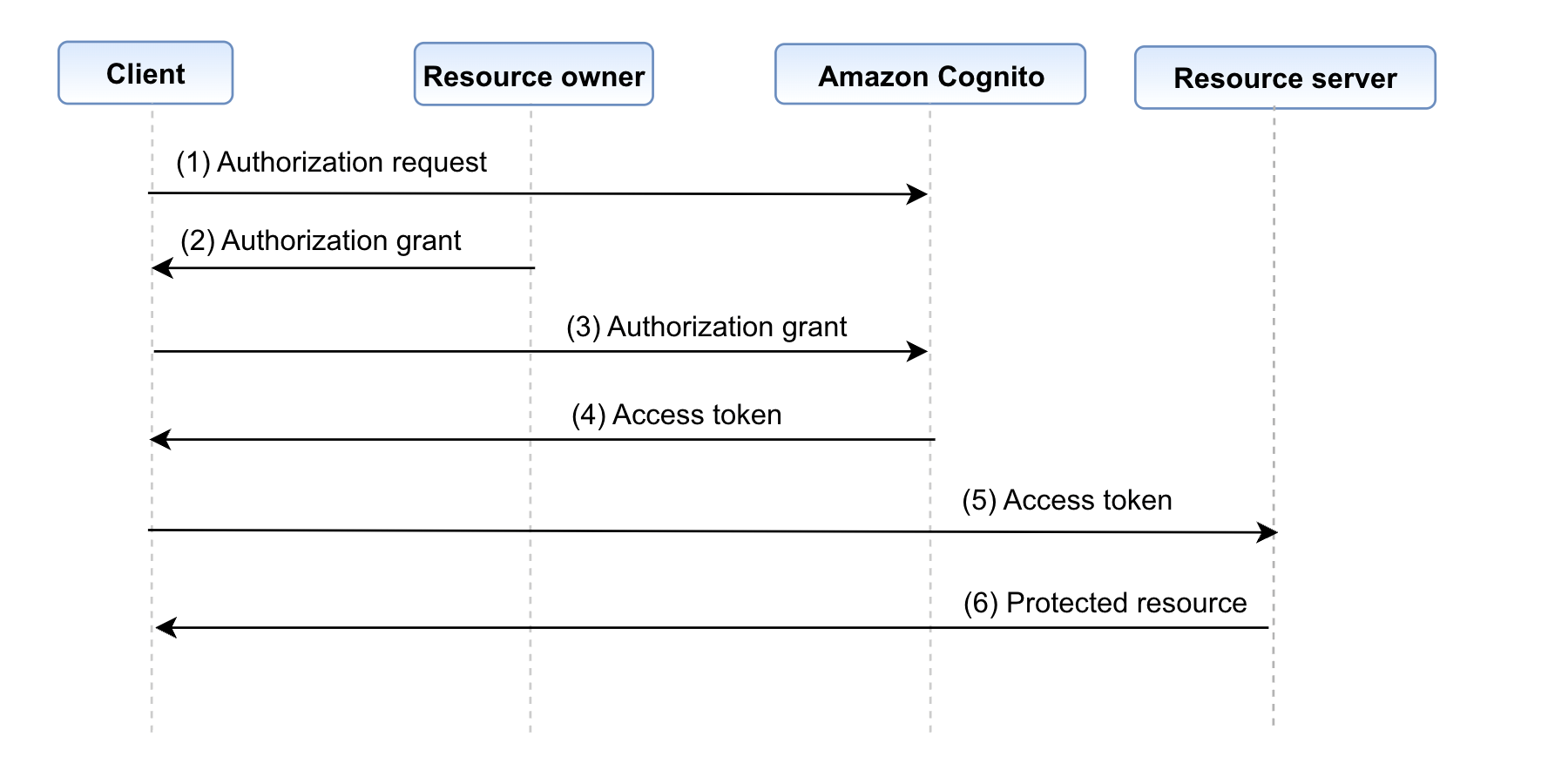
Figure 1: OAuth 2.0 flow
Below are the steps involved in the OAuth 2.0 flow
- The client requests authorization from the resource owner. This is done through the authorization server (Amazon Cognito) as an intermediary.
- The resource owner provides the authorization grant to the client. This can be one of the many grant types, which are discussed in detail in the next paragraph. The type of grant used depends on the method used by the client to request authorization from the resource owner.
- The client requests an access token by authenticating with Cognito.
- Cognito authenticates the client (the authentication method based on the grant type) and issues an access token if the authorization is valid.
- The access token is presented to the resource server as the client requests the protected resource.
- The resource server checks the access token’s signature and attributes and serves the request if it is valid.
There are several different grant types, four of which are described in the following sections.
Authorization code grant
The authorization code grant type is used by clients to securely exchange an authorization code for an access token. It’s used by both web applications and native applications to get an access token after a user authenticates to an application. After the user returns to the client through the redirect URI (the URL where the authentication server redirects the browser after it authorizes the user), the application gets the authorization code from the URL and uses it to request an access token.
This grant type is suitable for general cases as only one authentication flow is used, regardless of what operation is performed or who is performing it. This grant is considered secure as it requests an access token with a single-use code instead of exposing the actual access tokens. This helps prevent the application from potentially accessing user credentials.
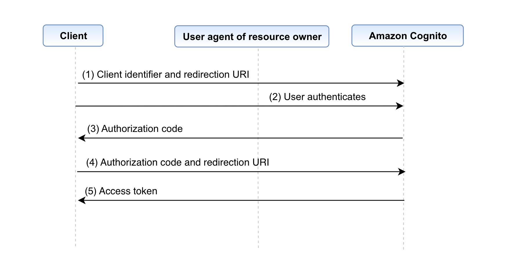
Figure 2: Authorization code grant flow
Below are the steps involved in the authorization code grant flow
- The process begins with the client initiating the sequence, directing the user-agent (that is, the browser) of the resource owner to the authorization endpoint. In this action, the client provides its client identifier, the scope it’s requesting, a local state, and a redirection URI to which the authorization server (Amazon Cognito) will return the user agent after either granting or denying access.
- Cognito authenticates the resource owner (through the user agent) and establishes whether the resource owner grants or denies the client’s access request using user pool authentication.
- Cognito redirects the user agent back to the client using the redirection URI that was provided in step (1) with an authorization code in the query string (such as http://www.example.com/webpage?code=<authcode>).
- The client requests an access token from the Cognito’s token endpoint by including the authorization code received in step (3). When making the request, the client authenticates with the Cognito typically with a client ID and a secret. The client includes the redirection URI used to obtain the authorization code for verification.
- Cognito authenticates the client, validates the authorization code, and makes sure that the redirection URI received matches the URI used to redirect the client in step (3). If valid, Cognito responds with an access token.
An implementation of the authorization code grant using Amazon Cognito looks like the following:
- An application makes an HTTP
GETrequest to_DOMAIN/oauth2/authorize, whereAUTH_DOMAINrepresents the user pool’s configured domain. This request includes the following query parameters:response_type– Set tocodefor this grant type.client_id– The ID for the desired user pool app client.redirect_uri– The URL that a user is directed to after successful authentication.state(optional but recommended) – A random value that’s used to prevent cross-site request forgery (CSRF) attacks.scope(optional) – A space-separated list of scopes to request for the generated tokens. Note that:- An ID token is only generated if the
openidscope is requested. - The
phone,email, andprofilescopes can only be requested ifopenidis also requested. - A vended access token can only be used to make user pool API calls if
aws.cognito.signin.user.admin(user pool’s reserved API scope) is requested.
- An ID token is only generated if the
identity_provider(optional) – Indicates the provider that the end user should authenticate with.idp_identifier(optional) – Same asidentity_providerbut doesn’t expose the provider’s real name.nonce(optional) – A random value that you can add to the request. Thenoncevalue that you provide is included in the ID token that Amazon Cognito issues. To guard against replay attacks, your app can inspect the nonce claim in the ID token and compare it to the one you generated. For more information about the nonce claim, see ID token validation in the OpenID Connect standard.
- A CSRF token is returned in a cookie. If an identity provider was specified in the request from step 1, the rest of this step is skipped. The user is automatically redirected to the appropriate identity provider’s authentication page. Otherwise, the user is redirected to https://AUTH_DOMAIN/login (which hosts the auto-generated UI) with the same query parameters set from step 1. They can then either authenticate with the user pool or select one of the third-party providers that’s configured for the designated app client.
- The user authenticates with their identity provider through one of the following means:
- If the user uses the native user pool to authenticate, the hosted UI submits the user’s credentials through a
POSTrequest to https://AUTH_DOMAIN/login (including the original query parameters) along with some additional metadata. - If the user selects a different identity provider to authenticate with, the user is redirected to that identity provider’s authentication page. After successful authentication the provider redirects the user to https://AUTH_DOMAIN/saml2/idpresponse with either an authorization token in the
codequery parameter or a SAML assertion in aPOSTrequest.
- If the user uses the native user pool to authenticate, the hosted UI submits the user’s credentials through a
- After Amazon Cognito verifies the user pool credentials or provider tokens it receives, the user is redirected to the URL that was specified in the original
redirect_uriquery parameter. The redirect also sets acodequery parameter that specifies the authorization code that was vended to the user by Cognito. - The custom application that’s hosted at the redirect URL can then extract the authorization code from the query parameters and exchange it for user pool tokens. The exchange occurs by submitting a
POSTrequest to https://AUTH_DOMAIN/oauth2/token with the followingapplication/x-www-form-urlencodedparameters:grant_type– Set toauthorization_codefor this grant.code– The authorization code that’s vended to the user.client_id– Same as from the request in step 1.redirect_uri– Same as from the request in step 1.
If the client application that was configured with a secret, the Authorization header for this request is set as Basic BASE64(CLIENT_ID:CLIENT_SECRET), where BASE64(CLIENT_ID:CLIENT_SECRET) is the base64 representation of the application client ID and application client secret, concatenated with a colon.
The JSON returned in the resulting response has the following keys:
access_token– A valid user pool access token.refresh_token– A valid user pool refresh token. This can be used to retrieve new tokens by sending it through aPOSTrequest tohttps://AUTH_DOMAIN/oauth2/token, specifying therefresh_tokenandclient_idparameters, and setting thegrant_typeparameter torefresh_token.id_token– A valid user pool ID token. Note that an ID token is only provided if theopenidscope was requested.expires_in– The length of time (in seconds) that the provided ID or access tokens are valid.token_type– Set toBearer.
Here are some of the best practices to be followed when using the authorization code grant:
- Use the Proof Key for Code Exchange (PKCE) extension with the authorization code grant, especially for public clients such as a single page web application. This is discussed in more detail in the following section.
- Regularly rotate client secrets and credentials to minimize the risk of unauthorized access.
- Implement session management to handle user sessions securely. This involves managing access token lifetimes, storing tokens, rotating refresh tokens, implementing token revocations and providing easy logout mechanisms that invalidate access and refresh tokens on user’s devices.
Authorization code grant with PKCE
To enhance security when using the authorization code grant, especially in public clients such as native applications, the PKCE extension was introduced. PKCE adds an extra layer of protection by making sure that only the client that initiated the authorization process can exchange the received authorization code for an access token. This combination is sometimes referred to as a PKCE grant.
It introduces a secret called the code verifier, which is a random value created by the client for each authorization request. This value is then hashed using a transformation method such as SHA256—this is now called the code challenge. The same steps are followed as the flow from Figure 2, however the code challenge is now added to the query string for the request to the authorization server (Amazon Cognito). The authorization server stores this code challenge for verification after the authentication process and redirects back with an authorization code. This authorization code along with the code verifier is sent to the authorization server, which then compares the previously stored code challenge with the code verifier. Access tokens are issued after the verification is successfully completed. Figure 3 outlines this process.
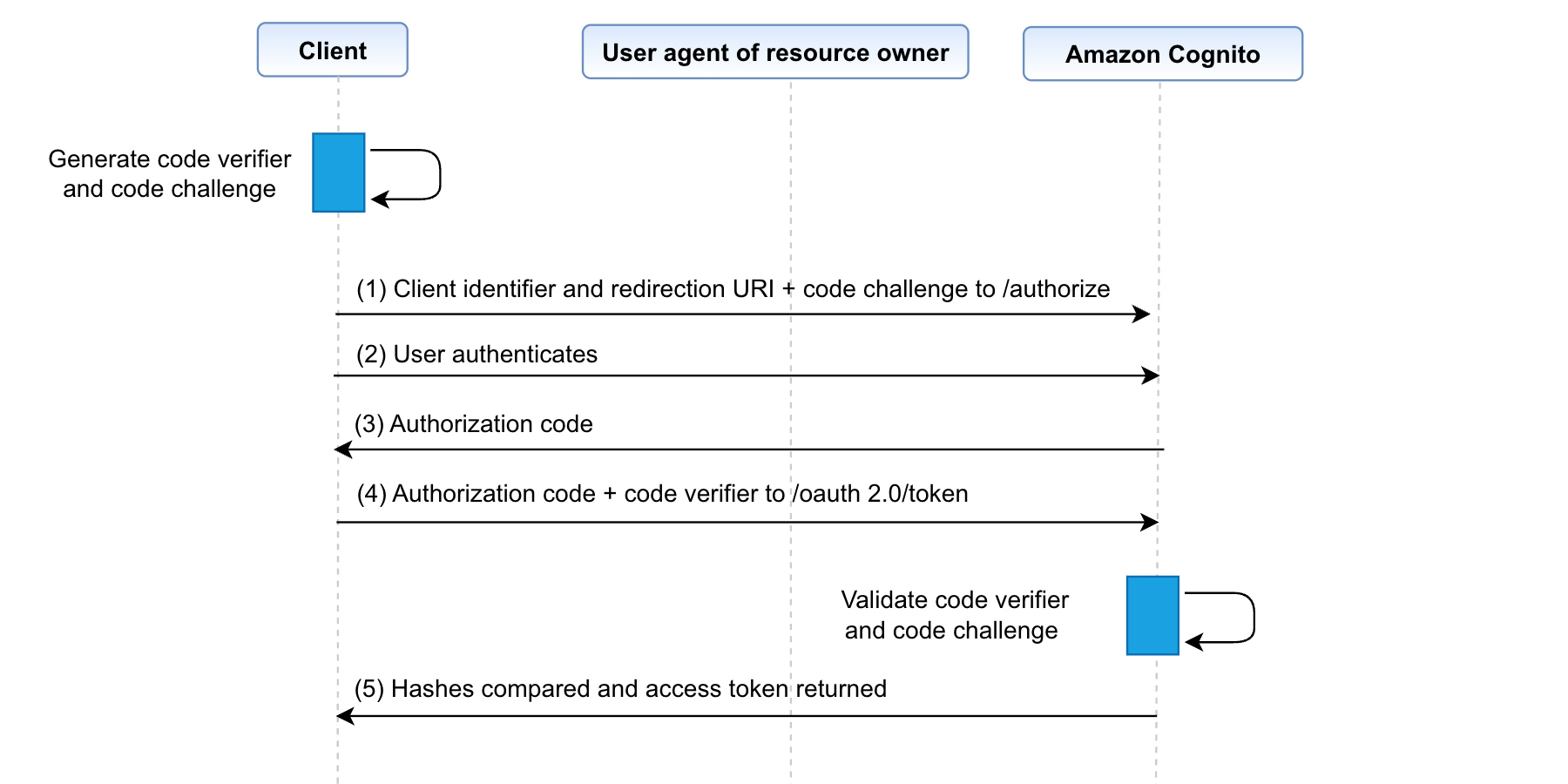
Figure 3: Authorization code grant flow with PKCE
Authorization code grant with PKCE implementation is identical to authorization code grant except that Step 1 requires two additional query parameters:
code_challenge– The hashed, base64 URL-encoded representation of a random code that’s generated client side (code verifier). It serves as a PKCE, which mitigates bad actors from being able to use intercepted authorization codes.code_challenge_method– The hash algorithm that’s used to generate thecode_challenge. Amazon Cognito currently only supports setting this parameter to S256. This indicates that thecode_challengeparameter was generated using SHA-256.
In step 5, when exchanging the authorization code with the user pool token, include an additional parameter:
code_verifier– The base64 URL-encoded representation of the unhashed, random string that was used to generate the PKCEcode_challengein the original request.
Implicit grant (not recommended)
Implicit grant was an OAuth 2.0 authentication grant type that allowed clients such as single-page applications and mobile apps to obtain user access tokens directly from the authorization endpoint. The grant type was implicit because no intermediate credentials (such as an authorization code) were issued and later used to obtain an access token. The implicit grant has been deprecated and it’s recommended that you use authorization code grant with PKCE instead. An effect of using the implicit grant was that it exposed access tokens directly in the URL fragment, which could potentially be saved in the browser history, intercepted, or exposed to other applications residing on the same device.
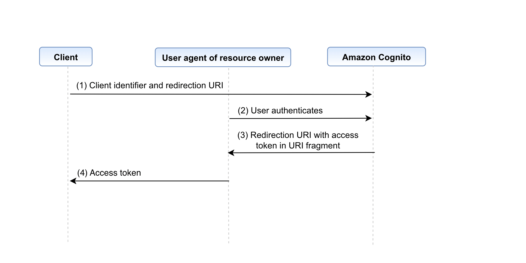
Figure 4: Implicit grant flow
The implicit grant flow was designed to enable public client-side applications—such as single-page applications or mobile apps without a backend server component—to exchange authorization codes for tokens.
Steps 1, 2, and 3 of the implicit grant are identical to the authorization code grant steps, except that the response_type query parameter is set to token. Additionally, while a PKCE challenge can technically be passed, it isn’t used because the /oauth2/token endpoint is never accessed. The subsequent steps—starting with step 4—are as follows:
- After Amazon Cognito verifies the user pool credentials or provider tokens it receives, the user is redirected to the URL that was specified in the original
redirect_uriquery parameter. The redirect also sets the following query parameters:access_token– A valid user pool access token.expires_in– The length of time (in seconds) that the provided ID or access tokens are valid for.token_type– Set toBearer.id_token– A valid user pool ID token. Note that an ID token is only provided if theopenidscope was requested.
Note that no refresh token is returned during an implicit grant, as specified in the RFC standard.
- The custom application that’s hosted at the redirect URL can then extract the access token and ID token (if they’re present) from the query parameters.
Here are some best practices for implicit grant:
- Make access token lifetimes short. Implicit grant tokens can’t be revoked, so expiry is the only way to end their validity.
- Implicit grant type is deprecated and should be used only for scenarios where a backend server component can’t be implemented, such as browser-based applications.
Client credentials grant
The client credentials grant is for machine-to-machine authentication. For example, a third-party application must verify its identity before it can access your system. The client can request an access token using only its client credentials (or other supported means of authentication) when the client is requesting access to the protected resources under its control or those of another resource owner that have been previously arranged with the authorization server.
The client credentials grant type must be used only by confidential clients. This means the client must have the ability to protect a secret string from users. Note that to use the client credentials grant, the corresponding user pool app client must have an associated app client secret.
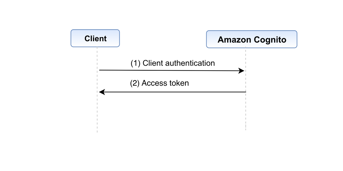
Figure 5: Client credentials grant
The flow illustrated in Figure 5 includes the following steps:
- The client authenticates with the authorization server using a client ID and secret and requests an access token from the token endpoint.
- The authorization server authenticates the client, and if valid, issues an access token.
The detailed steps for the process are as follows:
- The application makes a
POSTrequest tohttps://AUTH_DOMAIN/oauth2/token, and specifies the following parameters:grant_type– Set toclient_credentialsfor this grant type.client_id– The ID for the desired user pool app client.scope– A space-separated list of scopes to request for the generated access token. Note that you can only use a custom scope with the client credentials grant.
In order to indicate that the application is authorized to make the request, the Authorization header for this request is set as Basic BASE64(CLIENT_ID:CLIENT_SECRET), where BASE64(CLIENT_ID:CLIENT_SECRET) is the base64 representation of the client ID and client secret, concatenated with a colon.
The Amazon Cognito authorization server returns a JSON object with the following keys:
access_token– A valid user pool access token.expires_in– The length of time (in seconds) that the provided access token is valid.token_type– Set toBearer.
Note that, for this grant type, an ID token and a refresh token aren’t returned.
- The application uses the access token to make requests to an associated resource server.
- The resource server validates the received token and, if everything checks out, processes the request from the app.
Following are a few recommended practices while using the client credentials grant:
- Store client credentials securely and avoid hardcoding them in your application. Use appropriate credential management practices, such as environment variables or secret management services.
- Limit use cases. The client credentials grant is suitable for machine-to-machine authentication in highly trusted scenarios. Limit its use to cases where other grant types are not applicable.
Extension grant
Extension grants are a way to add support for non-standard token issuance scenarios such as token translation, delegation, or custom credentials. It lets you exchange access tokens from a third-party OAuth 2.0 authorization service with access tokens from Amazon Cognito. By defining the grant type using an absolute URI (determined by the authorization server) as the value of the grant_type argument of the token endpoint, and by adding other parameters required, the client can use an extension grant type.
An example of an extension grant is OAuth 2.0 device authorization grant (RFC 8628). This authorization grant makes it possible for internet-connected devices with limited input capabilities or that lack a user-friendly browser (such as wearables, smart assistants, video-streaming devices, smart-home automation, and health or medical devices) to review the authorization request on a secondary device, such as a smartphone, that has more advanced input and browser capabilities.
Some of the best practices to be followed when deciding to use extension grants are:
- Extension grants are for non-standard token issuance scenarios. Use them only when necessary, and thoroughly document their use and purpose.
- Conduct security audits and code reviews when implementing Extension grants to identify potential vulnerabilities and mitigate risks.
While Amazon Cognito doesn’t natively support extension grants currently, here is an example implementation of OAuth 2.0 device grant flow using AWS Lambda and Amazon DynamoDB.
Conclusion
In this blog post, we’ve reviewed various OAuth 2.0 grants, each catering to specific application needs, The authorization code grant ensures secure access for web applications (and offers additional security with the PKCE extension), and the client credentials grant is ideal for machine-to-machine authentication. Amazon Cognito acts as an encompassing identity platform, streamlining user authentication, authorization, and integration. By using these grants and the features provided by Cognito, developers can enhance security and the user experience in their applications. For more information and examples, see OAuth 2.0 grants in the Cognito Developer Guide.
Now that you understand implementing OAuth 2.0 grants in Amazon Cognito, see How to customize access tokens in Amazon Cognito user pools to learn about customizing access tokens to make fine-grained authorization decisions and provide a differentiated end-user experience.
If you have feedback about this post, submit comments in the Comments section below. If you have questions about this post, contact AWS Support.


 Ziad WALI is an Acceleration Lab Solutions Architect at Amazon Web Services. He has over 10 years of experience in databases and data warehousing, where he enjoys building reliable, scalable, and efficient solutions. Outside of work, he enjoys sports and spending time in nature.
 Omama Khurshid is an Acceleration Lab Solutions Architect at Amazon Web Services. She focuses on helping customers across various industries build reliable, scalable, and efficient solutions. Outside of work, she enjoys spending time with her family, watching movies, listening to music, and learning new technologies.
 Srikant Das is an Acceleration Lab Solutions Architect at Amazon Web Services. His expertise lies in constructing robust, scalable, and efficient solutions. Beyond the professional sphere, he finds joy in travel and shares his experiences through insightful blogging on social media platforms.


 Lorenzo Nicora works as Senior Streaming Solution Architect at AWS, helping customers across EMEA. He has been building cloud-native, data-intensive systems for over 25 years, working in the finance industry both through consultancies and for FinTech product companies. He has leveraged open-source technologies extensively and contributed to several projects, including Apache Flink.
 Francisco Morillo is a Streaming Solutions Architect at AWS. Francisco works with AWS customers, helping them design real-time analytics architectures using AWS services, supporting Amazon MSK and Amazon Managed Service for Apache Flink.


 Edvin Hallvaxhiu is a Senior Global Security Architect with AWS Professional Services and is passionate about cybersecurity and automation. He helps customers build secure and compliant solutions in the cloud. Outside work, he likes traveling and sports.
 Rahul Shaurya is a Principal Big Data Architect with AWS Professional Services. He helps and works closely with customers building data platforms and analytical applications on AWS. Outside of work, Rahul loves taking long walks with his dog Barney.
 Andrea Montanari is a Senior Big Data Architect with AWS Professional Services. He actively supports customers and partners in building analytics solutions at scale on AWS.
 María Guerra is a Big Data Architect with AWS Professional Services. Maria has a background in data analytics and mechanical engineering. She helps customers architecting and developing data related workloads in the cloud.
 Pushpraj Singh is a Senior Data Architect with AWS Professional Services. He is passionate about Data and DevOps engineering. He helps customers build data driven applications at scale.
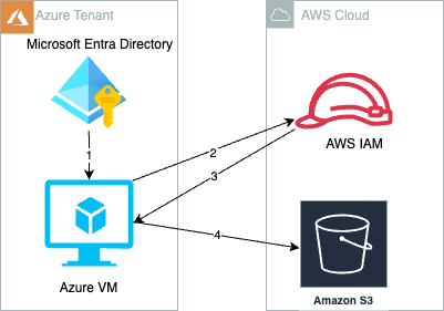


 Muthu Pitchaimani is a Search Specialist with Amazon OpenSearch Service. He builds large-scale search applications and solutions. Muthu is interested in the topics of networking and security, and is based out of Austin, Texas.
 Prashant Agrawal is a Sr. Search Specialist Solutions Architect with Amazon OpenSearch Service. He works closely with customers to help them migrate their workloads to the cloud and helps existing customers fine-tune their clusters to achieve better performance and save on cost. Before joining AWS, he helped various customers use OpenSearch and Elasticsearch for their search and log analytics use cases. When not working, you can find him traveling and exploring new places. In short, he likes doing Eat → Travel → Repeat.
 Rahul Sharma is a Technical Account Manager at Amazon Web Services. He is passionate about the data technologies that help leverage data as a strategic asset and is based out of New York city, New York.


 Noritaka Sekiyama is a Principal Big Data Architect on the AWS Glue team. He is responsible for building software artifacts to help customers. In his spare time, he enjoys cycling with his new road bike.
 Xiaoxi Liu is a Software Development Engineer on the AWS Glue team. Her passion is building scalable distributed systems for efficiently managing big data on the cloud, and her concentrations are distributed system, big data, and cloud computing.
 Akira Ajisaka is a Senior Software Development Engineer on the AWS Glue team. He likes open source software and distributed systems. In his spare time, he enjoys playing arcade games.
 Shenoda Guirguis is a Senior Software Development Engineer on the AWS Glue team. His passion is in building scalable and distributed data infrastructure and processing systems. When he gets a chance, Shenoda enjoys reading and playing soccer.
 Sean Ma is a Principal Product Manager on the AWS Glue team. He has an 18-year track record of innovating and delivering enterprise products that unlock the power of data for users. Outside of work, Sean enjoys scuba diving and college football.
 Mohit Saxena is a Senior Software Development Manager on the AWS Glue team. His team focuses on building distributed systems to enable customers with interactive and simple to use interfaces to efficiently manage and transform petabytes of data seamlessly across data lakes on Amazon S3, databases and data-warehouses on cloud.


 Venkata Kampana is a Senior Solutions Architect in the AWS Health and Human Services team and is based in Sacramento, CA. In that role, he helps public sector customers achieve their mission objectives with well-architected solutions on AWS.
 Jim Daniel is the Public Health lead at Amazon Web Services. Previously, he held positions with the United States Department of Health and Human Services for nearly a decade, including Director of Public Health Innovation and Public Health Coordinator. Before his government service, Jim served as the Chief Information Officer for the Massachusetts Department of Public Health.