Post Syndicated from Explosm.net original https://explosm.net/comics/shoot-me
New Cyanide and Happiness Comic
Post Syndicated from Explosm.net original https://explosm.net/comics/shoot-me
New Cyanide and Happiness Comic
Post Syndicated from Grab Tech original https://engineering.grab.com/road-localisation-grabmaps
In 2022, Grab achieved self-sufficiency in its Geo services. As part of this transition, one crucial step was moving towards using an internally-developed map tailored specifically to the market in which Grab operates. Now that we have full control over the map layer, we can add more data to it or improve it according to the needs of the services running on top. One key aspect that this transition unlocked for us was the possibility of creating hyperlocal data at map level.
For instance, by determining the country to which a road belongs, we can now automatically infer the official language of that country and display the street name in that language. In another example, knowing the country for a specific road, we can automatically infer the driving side (left-handed or right-handed) leading to an improved navigation experience. Furthermore, this capability also enables us to efficiently handle various scenarios. For example, if we know that a road is part of a gated community, an area where our driver partners face restricted access, we can prevent the transit through that area.
These are just some examples of the possibilities from having full control over the map layer. By having an internal map, we can align our maps with specific markets and provide better experiences for our driver-partners and customers.
For all these to be possible, we first needed to localise the roads inside the map. Our goal was to include hyperlocal data into the map, which refers to data that is specific to a certain area, such as a country, city, or even a smaller part of the city like a gated community. At the same time, we aimed to deliver our map with a high cadence, thus, we needed to find the right way to process this large amount of data while continuing to create maps in a cost-effective manner.
In the following sections of this article, we will use an extract from the Southeast Asia map to provide visual representations of the concepts discussed.
In Figure 1, Image 1 shows a visualisation of the road network, the roads belonging to this area. The coloured lines in Image 2 represent the borders identifying the countries in the same area. Overlapping the information from Image 1 and Image 2, we can extrapolate and say that the entire surface included in a certain border could have the same set of common properties as shown in Image 3. In Image 4, we then proceed with adding localised roads for each area.
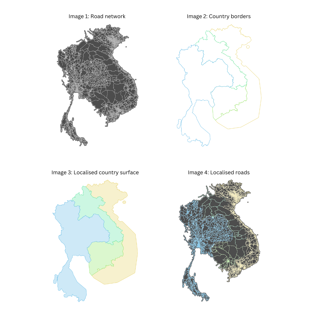
For this to be possible, we have to find a way to localise each road and identify its associated country. Once this localisation process is complete, we can replicate all this information specific to a given border onto each individual road. This information includes details such as the country name, driving side, and official language. We can go even further and infer more information, and add hyperlocal data. For example, in Vietnam, we can automatically prevent motorcycle access on the motorways.
Assigning each road on the map to a specific area, such as a country, service area, or subdivision, presents a complex task. So, how can we efficiently accomplish this?
The most straightforward approach would be to test the inclusion of each road into each area boundary, but that is easier said than done. With close to 30 million road segments in the Southeast Asia map and over 10 thousand areas, the computational cost of determining inclusion or intersection between a polyline and a polygon is expensive.
Our solution to this challenge involves replacing the expensive yet precise operation with a decent approximation. We introduce a proxy entity, the geohash, and we use it to approximate the areas and also to localise the roads.
We replace the geometrical inclusion with a series of simpler and less expensive operations. First, we conduct an inexpensive precomputation where we identify all the geohases that belong to a certain area or within a defined border. We then identify the geohashes to which the roads belong to. Finally, we use these precomputed values to assign roads to their respective areas. This process is also computationally inexpensive.
Given the large area we process, we leverage big data techniques to distribute the execution across multiple nodes and thus speed up the operation. We want to deliver the map daily and this is one of the many operations that are part of the map-making process.
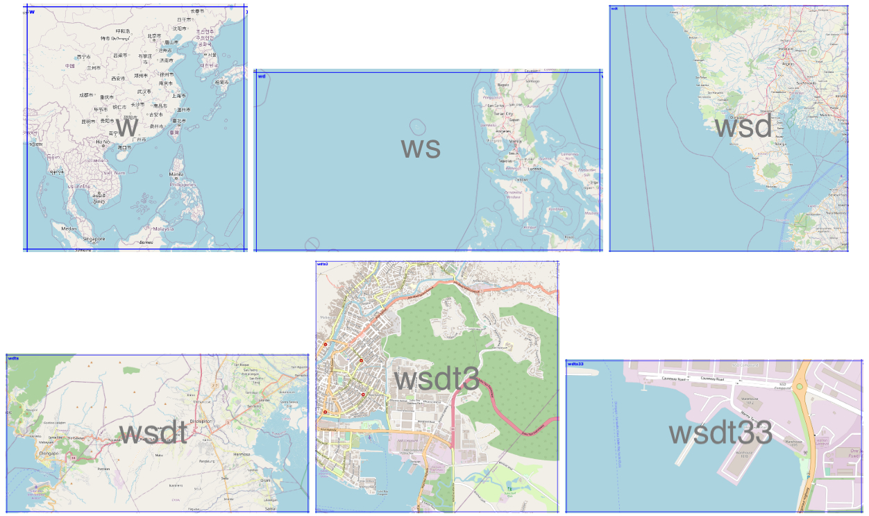
To further understand our implementation we will first explain the geohash concept. A geohash is a unique identifier of a specific region on the Earth. The basic idea is that the Earth is divided into regions of user-defined size and each region is assigned a unique id, which is known as its geohash. For a given location on earth, the geohash algorithm converts its latitude and longitude into a string.
Geohashes uses a Base-32 alphabet encoding system comprising characters ranging from 0 to 9 and A to Z, excluding “A”, “I”, “L” and “O”. Imagine dividing the world into a grid with 32 cells. The first character in a geohash identifies the initial location of one of these 32 cells. Each of these cells are then further subdivided into 32 smaller cells.This subdivision process continues and refines to specific areas in the world. Adding characters to the geohash sub-divides a cell, effectively zooming in to a more detailed area.
The precision factor of the geohash determines the size of the cell. For instance, a precision factor of one creates a cell 5,000 km high and 5,000 km wide. A precision factor of six creates a cell 0.61km high and 1.22 km wide. Furthermore, a precision factor of nine creates a cell 4.77 m high and 4.77 m wide. It is important to note that cells are not always square and can have varying dimensions.
In Figure 2, we have exemplified a geohash 6 grid and its code is wsdt33.
Calculating the inclusion of the roads inside a certain border is an expensive operation. However, quantifying the exact expense is challenging as it depends on several factors. One factor is the complexity of the border. Borders are usually irregular and very detailed, as they need to correctly reflect the actual border. The complexity of the road geometry is another factor that plays an important role as roads are not always straight lines.
Since this operation is expensive both in terms of cloud cost and time to run, we need to identify a cheaper and faster way that would yield similar results. Knowing that the complexity of the border lines is the cause of the problem, we tried using a different alternative, a rectangle. Calculating the inclusion of a polyline inside a rectangle is a cheaper operation.
So we transformed this large, one step operation, where we test each road segment for inclusion in a border, into a series of smaller operations where we perform the following steps:
In Figure 5, we identify that the road belongs to two geohashes and that the two geohashes are part of the border we use.
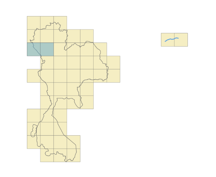
Now, all we need to do is join the two data sets together. This kind of operation is a great candidate for a big data approach, as it allows us to run it in parallel and speed up the processing time.
We mentioned earlier that, for the sake of argument, we replace precision with a decent approximation. Let’s now delve into the real tradeoff by adopting this approach.
The first thing that stands out with this approach is that we traded precision for cost. We are able to reduce the cost as this approach uses less hardware resources and computation time. However, this reduction in precision suffers, particularly for roads located near the borders as they might be wrongly classified.
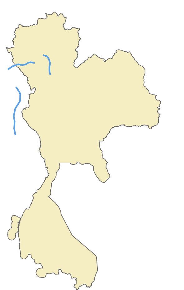
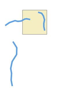
Going back to the initial example, let’s take the case of the external road, on the left side of the area. As you can see in Figure 6, it is clear that the road does not belong to our border. But when we apply the geohash approach it gets included into the middle geohash.
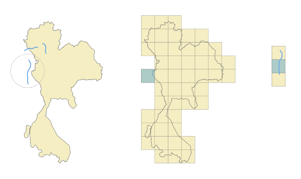
Given that just a small part of the geohash falls inside the border, the entire geohash will be classified as belonging to that area, and, as a consequence, the road that belongs to that geohash will be wrongly localised and we’ll end up adding the wrong localisation information to that road. This is clearly a consequence of the precision tradeoff. So, how can we solve this?
One option is to increase the geohash precision. By using smaller and smaller geohashes, we can better reflect the actual area. As we go deeper and we further split the geohash, we can accurately follow the border. However, a high geohash precision also equates to a computationally intensive operation bringing us back to our initial situation. Therefore, it is crucial to find the right balance between the geohash size and the complexity of operations.
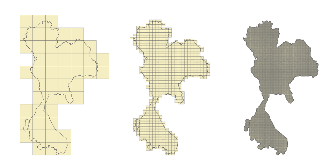
To find a balance between precision and data loss, we looked into calculating the geohash coverage percentage. For example, in Figure 8, the blue geohash is entirely within the border. Here we can say that it has a 100% geohash coverage.
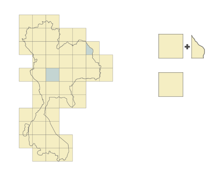
However, take for example the geohash in Figure 9. It touches the border and has only around 80% of its surface inside the area. Given that most of its surface is within the border, we still can say that it belongs to the area.
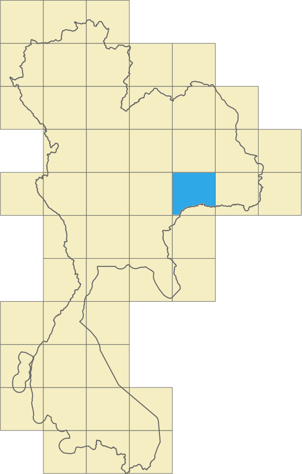
Let’s look at another example. In Figure 10, only a small part of the geohash is within the border. We can say that the geohash coverage percentage here is around 5%. For these cases, it becomes difficult for us to determine whether the geohash does belong to the area. What would be a good tradeoff in this case?
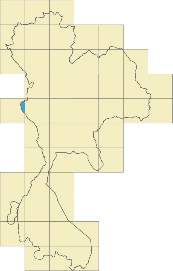
To go one step further, we can consider a mixed solution, where we use the border shape but only for the geohashes touching the border. This would still be an intensive computational operation but the number of roads located in these geohashes will be much smaller, so it is still a gain.
For the geohashes with full coverage inside the area, we’ll use the geohash for the localisation, the simpler operation. For the geohashes that are near the border, we’ll use a different approach. To increase the precision around the borders, we can cut the geohash following the border’s shape. Instead of having a rectangle, we’ll use a more complex shape which is still simpler than the initial border shape.
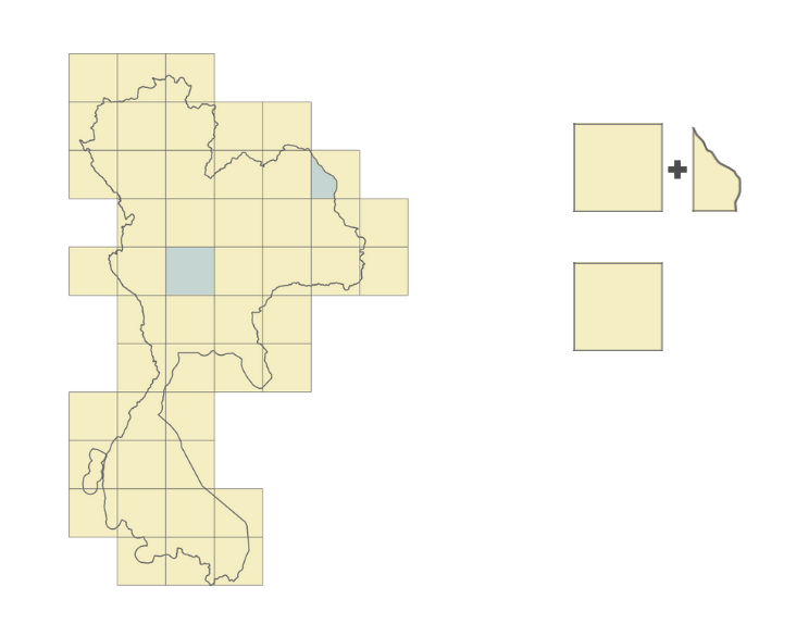
We began with a simple approach and we enhanced it to improve precision. This also increased the complexity of the operation. We then asked, what are the actual gains? Was it worthwhile to go through all this process? In this section, we put this to the test.
We first created a benchmark by taking a small sample of the data and ran the localisation process on a laptop. The sample comprised approximately 2% of the borders and 0.0014% of the roads. We ran the localisation process using two approaches.
However, it is important to note that this is not an apples-to-apples comparison. The operation that we measured was the localisation of the roads but we did not include the border filling operation where we fill the borders with geohashes. This is because this operation does not need to be run every time. It can be run once and reused multiple times.
Though not often required, it is still crucial to understand and consider the operation of precomputing areas and filling borders with geohashes. The precomputation process depends on several factors:
Going back to our hypothesis, although this precomputation might be expensive, it is rarely run as the borders don’t change often and can be triggered only when needed. However, regular computation, where we find the area to which each road belongs to, is often run as the roads change constantly. In our system, we run this localisation for each map processing.
We can also further optimise this process by applying the opposite approach. Geohashes that have full coverage inside a border can be merged together into larger geohashes thus simplifying the computation inside the border. In the end, we can have a solution that is fully optimised for our needs with the best cost-to-performance ratio.
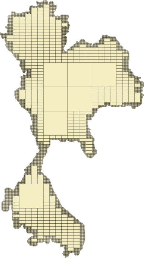
Although geohashes seem to be the right solution for this kind of problem, we also need to monitor their content. One consideration is the road density inside a geohash. For example, a geohash inside a city centre usually has a lot of roads while one in the countryside may have much less. We need to consider this aspect to have a balanced computation operation and take full advantage of the big data approach. In our case, we achieve this balance by considering the number of road kilometres within a geohash.
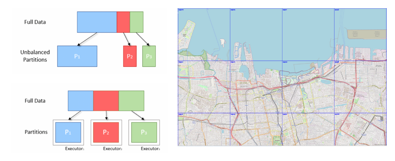
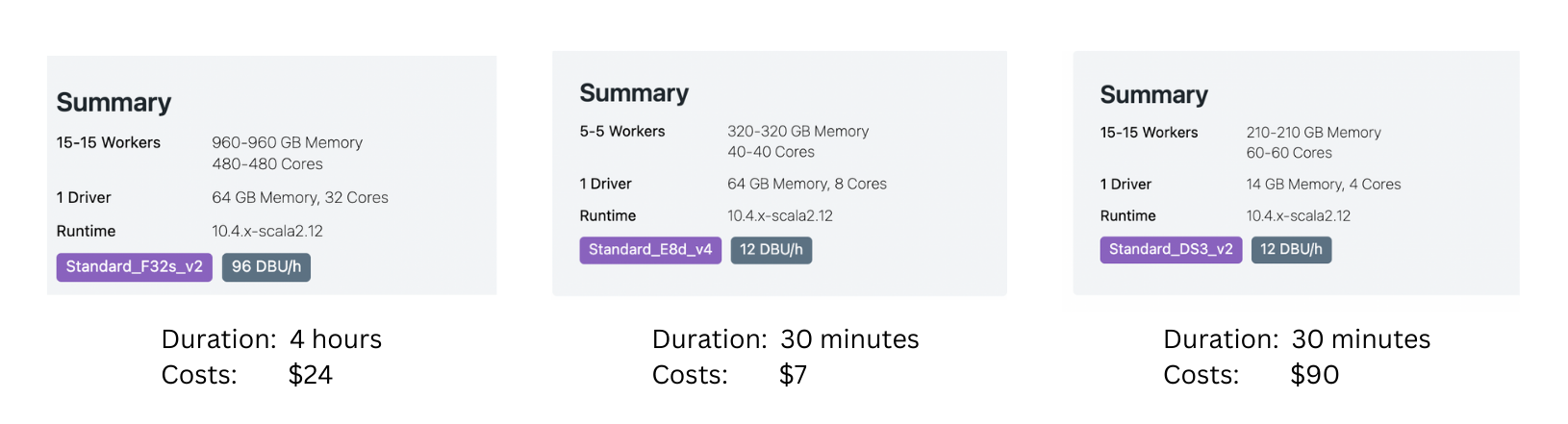
Additionally, the resources that we choose also matter. To optimise time and cost, we need to find the right balance between the running time and resource cost. As shown in Figure 14, based on a sample data we ran, sometimes, we get the best result when using smaller machines.
The achievements and insights showcased in this article are indebted to the contributions made by Mihai Chintoanu. His expertise and collaborative efforts have profoundly enriched the content and findings presented herein.
Grab is the leading superapp platform in Southeast Asia, providing everyday services that matter to consumers. More than just a ride-hailing and food delivery app, Grab offers a wide range of on-demand services in the region, including mobility, food, package and grocery delivery services, mobile payments, and financial services across 428 cities in eight countries.
Powered by technology and driven by heart, our mission is to drive Southeast Asia forward by creating economic empowerment for everyone. If this mission speaks to you, join our team today!
Post Syndicated from xkcd.com original https://xkcd.com/2856/

Post Syndicated from Talks at Google original https://www.youtube.com/watch?v=nCVGIIvBaJY
Post Syndicated from Danilo Poccia original https://aws.amazon.com/blogs/aws/happy-anniversary-amazon-cloudfront-15-years-of-evolution-and-internet-advancements/
I can’t believe it’s been 15 years since Amazon CloudFront was launched! When Amazon S3 became available in 2006, developers loved the flexibility and started to build a new kind of globally distributed applications where storage was not a bottleneck. These applications needed to be performant, reliable, and cost-efficient for every user on the planet. So in 2008 a small team (a “two-pizza team“) launched CloudFront in just 200 days. Jeff Barr hinted at the new and yet unnamed service in September and introduced CloudFront two months later.
Since the beginning, CloudFront has provided an easy way to distribute content to end users with low latency, high data transfer speeds, and no long-term commitments. What started as a simple cache for Amazon S3 quickly evolved into a fully featured content delivery network. Now CloudFront delivers applications at blazing speeds across the globe, supporting live sporting events such as NFL, Cricket World Cup, and FIFA World Cup.
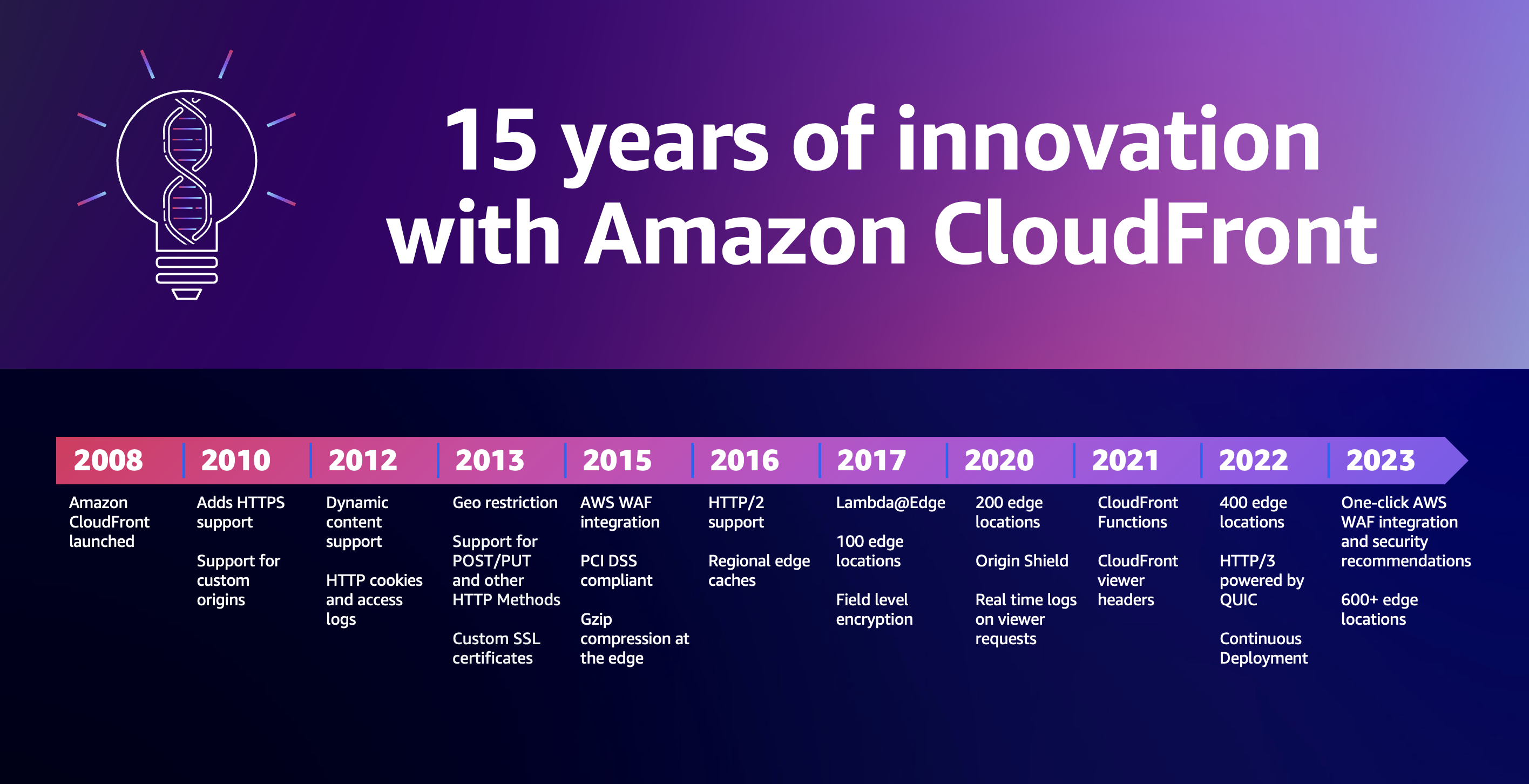
At the same time, we also want to provide you with the best tools to secure applications. In 2015, we announced AWS WAF integration with CloudFront to provide fast and secure access control at the edge. Then, we focused on developing robust threat intelligence by combining signals across services. This threat intelligence integrates with CloudFront, adding AWS Shield to protect applications from common exploits and distributed denial of service (DDoS) attacks. For example, we recently detected an unusual spike in HTTP/2 requests to Amazon CloudFront. We quickly realized that CloudFront had automatically mitigated a new type of HTTP request flood DDoS event.
A lot also happens at lower levels than HTTP. For example, when you serve your application with CloudFront, all of the packets received by the application are inspected by a fully inline DDoS mitigation system which doesn’t introduce any observable latency. In this way, L3/L4 DDoS attacks against CloudFront distributions are mitigated in real time.
We also made under-the-hood improvements like s2n-tls (short for “signal to noise”), an open-source implementation of the TLS protocol that has been designed to be small and fast with simplicity as a priority. Another similar improvement is s2n-quic, an open-source QUIC protocol implementation written in Rust.
With CloudFront, you can also control access to content through a number of capabilities. You can restrict access to only authenticated viewers or, through geo-restriction capability, configure the specific geographic locations that can access content.
Security is always important, but not every organization has dedicated security experts on staff. To make robust security more accessible, CloudFront now includes built-in protections such as one-click web application firewall setup, security recommendations, and an intuitive security dashboard. With these integrated security features, teams can put critical safeguards in place without deep security expertise. Our goal is to empower all customers to easily implement security best practices.
Web applications delivery
During the past 15 years, web applications have become much more advanced and essential to end users. When CloudFront launched, our focus was helping deliver content stored in S3 buckets. Dynamic content was introduced to optimize web applications where portions of a website change for each user. Dynamic content also improves access to APIs that need to be delivered globally.
As applications become more distributed, we looked at ways to help developers make efficient use of its global footprint and resources at the edge. To allow customization and personalization of content close to end users and minimize latency, Lambda@Edge was introduced.
When fewer compute resources are needed, CloudFront Functions can run lightweight JavaScript functions across edge locations for low-latency HTTP manipulations and personalized content delivery. Recently, CloudFront Functions expanded to further customize responses, including modifying HTTP status codes and response bodies.
Today, CloudFront handles over 3 trillion HTTP requests daily and uses a global network of more than 600 points of presence and 13 Regional edge caches in more than 100 cities across 50 countries. This scale helps power the most demanding online events. For example, during the 2023 Amazon Prime Day, CloudFront handled peak loads of over 500 million HTTP requests per minute, totaling over 1 trillion HTTP requests.
Amazon CloudFront has more than 600,000 active developers building and delivering applications to end users. To help teams work at their full speed, CloudFront introduced continuous deployment so developers can test and validate configuration changes on a portion of traffic before full deployment.
Media and entertainment
It’s now common to stream music, movies, and TV series to our homes, but 15 years ago, renting DVDs was still the norm. Running streaming servers was technically complex, requiring long-term contracts to access the global infrastructure needed for high performance.
First, we added support for audio and video streaming capabilities using custom protocols since technical standards were still evolving. To handle large audiences and simplify cost-effective delivery of live events, CloudFront launched live HTTP streaming and, shortly after, improved support for both Flash-based (popular at the time) and Apple iOS devices.
As the media industry continued moving to internet-based delivery, AWS acquired Elemental, a pioneer in software-defined video solutions. Integrating Elemental offerings helped provide services, software, and appliances that efficiently and economically scale video infrastructures for use cases such as broadcast and content production.
The evolution of technologies and infrastructure allows for new ways of communication to become possible, such as when NASA did the first-ever live 4K stream from space using CloudFront.
Today, the world’s largest events and leading video platforms rely on CloudFront to deliver massive video catalogs and live stream content to millions. For example, CloudFront delivered streams for the FIFA World Cup 2022 on behalf of more than 19 major broadcasters globally. More recently, CloudFront handled over 120 Tbps of peak data transfer during one of the Thursday Night Football games of the NFL season on Prime Video and helped deliver the Cricket World Cup to millions of viewers across the globe.
What’s next?
Many things have changed during these 15 years but the focus on security, performance, and scalability stays the same. At AWS, it’s always Day 1, and the CloudFront team is constantly looking for ways to improve based on your feedback.
The rise of botnets is driving an ever-evolving, highly dynamic, and shifting threat landscape. Layer 7 DDoS attacks are becoming increasingly prevalent. The pervasiveness of bot traffic is increasing exponentially. As this occurs, we are evolving how we mitigate threats at the network border, at the edge, and in the Region, making it simpler for customers to configure the right security options.
Web applications are becoming more complex and interactive, and viewer expectations on latency and resiliency are even more stringent. This will drive new innovation. As new applications use generative artificial intelligence (AI), needs will evolve. These trends are will continue growing, so our investments will be focused on improving security and edge compute capabilities to support these new use cases.
With the current macroeconomic environment, many customers, especially small and medium-sized businesses and startups, look at how they can reduce their costs. Providing optimal price-performance has always been a priority for CloudFront. Cacheable data transferred to CloudFront edge locations from AWS resources does not incur additional fees. Also, 1 TB of data transfer from CloudFront to the internet per month is included in the free tier. CloudFront operates on a pay-as-you-go model with no upfront costs or minimum usage requirements. For more info, see CloudFront pricing.
As we approach AWS re:Invent, take note of these sessions that can help you learn about the latest innovations and connect with experts:
To learn more on how to speed up your websites and APIs and keep them protected, see the Application Security and Performance section of the AWS Developer Center.
Reduce latency and improve the security for your applications with Amazon CloudFront.
— Danilo
Post Syndicated from Asser Moustafa original https://aws.amazon.com/blogs/big-data/power-enterprise-grade-data-vaults-with-amazon-redshift-part-1/
Amazon Redshift is a popular cloud data warehouse, offering a fully managed cloud-based service that seamlessly integrates with an organization’s Amazon Simple Storage Service (Amazon S3) data lake, real-time streams, machine learning (ML) workflows, transactional workflows, and much more—all while providing up to 7.9x better price-performance than other cloud data warehouses.
As with all AWS services, Amazon Redshift is a customer-obsessed service that recognizes there isn’t a one-size-fits-all for customers when it comes to data models, which is why Amazon Redshift supports multiple data models such as Star Schemas, Snowflake Schemas and Data Vault. This post discusses best practices for designing enterprise-grade Data Vaults of varying scale using Amazon Redshift; the second post in this two-part series discusses the most pressing needs when designing an enterprise-grade Data Vault and how those needs are addressed by Amazon Redshift.
Whether it’s a desire to easily retain data lineage directly within the data warehouse, establish a source-system agnostic data model within the data warehouse, or more easily comply with GDPR regulations, customers that implement a Data Vault model will benefit from this post’s discussion of considerations, best practices, and Amazon Redshift features relevant to the building of enterprise-grade Data Vaults. Building a starter version of anything can often be straightforward, but building something with enterprise-grade scale, security, resiliency, and performance typically requires knowledge of and adherence to battle-tested best practices, and using the right tools and features in the right scenario.
Let’s first briefly review the core Data Vault premise and concepts. Data models provide a framework for how the data in a data warehouse should be organized into database tables. Amazon Redshift supports a number of data models, and some of the most popular data models include STAR schemas and Data Vault.
Data Vault is not only a modeling methodology, it’s also an opinionated framework that tells you how to solve certain problems in your data ecosystem. An opinionated framework provides a set of guidelines and conventions that developers are expected to follow, rather than leaving all decisions up to the developer. You can compare this with what big enterprise frameworks like Spring or Micronauts do when developing applications at enterprise scale. This is incredibly helpful especially on large data warehouse projects, because it structures your extract, load, and transform (ELT) pipeline and clearly tells you how to solve certain problems within the data and pipeline contexts. This also allows for a high degree of automation.
Data Vault 2.0 allows for the following:
However, Data Vault 2.0 also comes with costs, and there are use cases where it’s not a good fit, such as the following:
Data Vault typically organizes an organization’s data into a pipeline of four layers: staging, raw, business, and presentation. The staging layer represents data intake and light data transformations and enhancements that occur before the data comes to its more permanent resting place, the raw Data Vault (RDV).
The RDV holds the historized copy of all of the data from multiple source systems. It is referred to as raw because no filters or business transformations have occurred at this point except for storing the data in source system independent targets. The RDV organizes data into three key types of tables:
product_info and customer_infoThe RDV is used to feed data into the business Data Vault (BDV), which is responsible for reorganizing, denormalizing, and aggregating data for optimized consumption by the presentation mart. The presentation marts, also known as the data mart layer, further reorganizes the data for optimized consumption by downstream clients such as business dashboards. The presentation marts may, for example, reorganize data into a STAR schema.
For a more detailed overview of Data Vault along with a discussion of its applicability in the context of very interesting use cases, refer to the following:
Currently, the lake house paradigm is becoming a major pattern in data warehouse design, even as part of a data mesh architecture. This follows the pattern of data lakes getting closer to what a data warehouse can do and vice versa. To compete with the flexibility of a data lake, Data Vault is a good choice. This way, the data warehouse doesn’t become a bottleneck and you can achieve similar agility, flexibility, scalability, and adaptability when ingestion and onboarding new data.
In this section, we discuss some recommended Redshift configurations for Data Vaults of varying scale. As mentioned earlier, the layers within a Data Vault platform are well known. We typically see a flow from the staging layer to the RDV, BDV, and finally presentation mart.
The Amazon Redshift is highly flexible in supporting both modest and large-scale Data Vaults, offering features like the following:
Amazon Redshift is flexible in how you decide to structure these layers. For modest data vaults, a single Redshift warehouse with one database with multiple schemas will work just fine.
For large data vaults with more complex transformations, we would look at multiple warehouses, each with their own schema of mastered data representing one or more layer. The reason for using multiple warehouses is to take advantage of the Amazon Redshift architecture’s flexibility for implementing large-scale data vault implementations, such as using Redshift RA3 nodes and Redshift Serverless for separating the compute from the data storage layer and using Redshift data sharing to share the data between different Redshift warehouses. This enables you to scale the compute capacity independently at each layer depending on the processing complexity. The staging layer, for example, can be a layer within your data lake (Amazon S3 storage) or a schema within a Redshift database.
Using Amazon Aurora zero-ETL integrations with Amazon Redshift, you can create a data vault implementation with a staging layer in an Amazon Aurora database that will take care of real-time transaction processing and move the data to Amazon Redshift automatically for further processing in the Data Vault implementation without creating any complex ETL pipelines. This way, you can use Amazon Aurora for transactions and Amazon Redshift for analytics. Compute resources are isolated for the same data, and you’re using the most efficient tools to process it.
For larger Data Vaults platforms, concurrency and compute power become important to process both the loading of data and any business transformations. Amazon Redshift offers flexibility to increase compute capacity both horizontally via concurrency scaling and vertically via cluster resize and also via different architectures for each Data Vault layer.
You can create a data warehouse for the staging layer and perform hard business rules processing here, including calculation of hash keys, hash diffs, and addition of technical metadata columns. If data is not loaded 24/7, consider either pause/resume or a Redshift Serverless workgroup.
For raw Data Vault (RDV), it’s recommended to either create one Redshift warehouse for the whole RDV or one Redshift warehouse for one or more subject areas within the RDV. For example, if the volume of data and number of normalized tables within the RDV for a particular subject area is large (either the raw data layer has so many tables that it runs out of maximum table limit on Amazon Redshift or the advantage of workload isolation within a single Redshift warehouse outweighs the overhead of performance and management), this subject area within the RDV can be run and mastered on its own Redshift warehouse.
The RDV is typically loaded 24/7 so a provisioned Redshift data warehouse may be most suitable here to take advantage of reserved instance pricing.
For creating a data warehouse for the business Data Vault (BDV) layer, this could be larger in size than the previous data warehouses due to the nature of the BDV processing, typically denormalization of data from a large number of source RDV tables.
Some customers run their BDV processing once a day, so a pause/resume window for Redshift provisioned cluster may be cost beneficial here. You can also run BDV processing on an Amazon Redshift Serverless warehouse which will automatically pause when workloads complete and resume when workloads start processing again.
For creating Redshift (provisioned or serverless) warehouses for one or more data marts, the schemas within these marts typically contain views or materialized views, so a Redshift data share will be set up between the data marts and the previous layers.
We need to ensure there is enough concurrency to cope with the increased read traffic at this level. This is achieved via multiple read only warehouses with a data share or the use of concurrency scaling to auto scale.
The following diagram illustrates an example platform for a modest Data Vault model.

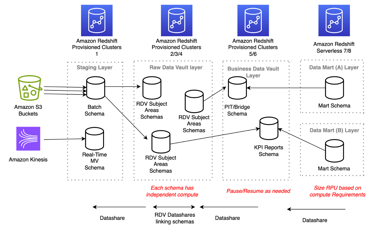
The following diagram illustrates the architecture for a large-scale Data Vault model.
In this section, we discuss some recommended design principles for joining and filtering table access within a Data Vault implementation. These guiding principles address different combinations of entity type access, but should be tested for suitability with each client’s particular use case.
Let’s begin with a brief refresher of table distribution styles in Amazon Redshift. There are four ways that a table’s data can be distributed among the different compute nodes in a Redshift cluster: ALL, KEY, EVEN, and AUTO.
The ALL distribution style ensures that a full copy of the table is maintained on each compute node to eliminate the need for inter-node network communication during workload runs. This distribution style is ideal for tables that are relatively small in size (such as fewer than 5 million rows) and don’t exhibit frequent changes.
The KEY distribution style uses a hash-based approach to persisting a table’s rows in the cluster. A distribution key column is defined to be one of the columns in the row, and the value of that column is hashed to determine on which compute node the row will be persisted. The current generation RA3 node type is built on the AWS Nitro System with managed storage that uses high performance SSDs for your hot data and Amazon S3 for your cold data, providing ease of use, cost-effective storage, and fast query performance. Managed storage means this mapping of row to compute node is more in terms of metadata and compute node ownership rather than the actual persistence. This distribution style is ideal for large tables that have well-known and frequent join patterns on the distribution key column.
The EVEN distribution style uses a round-robin approach to locating a table’s row. Simply put, table rows are cycled through the different compute nodes and when the last compute node in the cluster is reached, the cycle begins again with the next row being persisted to the first compute node in the cluster. This distribution style is ideal for large tables that exhibit frequent table scans.
Finally, the default table distribution style in Amazon Redshift is AUTO, which empowers Amazon Redshift to monitor how a table is used and change the table’s distribution style at any point in the table’s lifecycle for greater performance with workloads. However, you are also empowered to explicitly state a particular distribution style at any point in time if you have a good understanding of how the table will be used by workloads.
Hub and hub satellites are often joined together, so it’s best to co-locate these datasets based on the primary key of the hub, which will also be part of the compound key of each satellite. As mentioned earlier, for smaller volumes (typically fewer than 5–7 million rows) use the ALL distribution style and for larger volumes, use the KEY distribution style (with the _PK column as the distribution KEY column).
Link and link satellites are often joined together, so it’s best to co-locate these datasets based on the primary key of the link, which will also be part of the compound key of each link satellite. These typically involve larger data volumes, so look at a KEY distribution style (with the _PK column as the distribution KEY column).
You may decide to denormalize key satellite attributes by adding them to point in time (PIT) tables with the goal of reducing or eliminating runtime joins. Because denormalization of data helps reduce or eliminate the need for runtime joins, denormalized PIT tables can be defined with an EVEN distribution style to optimize table scans.
However, if you decide not to denormalize, then smaller volumes should use the ALL distribution style and larger volumes should use the KEY distribution style (with the _PK column as the distribution KEY column). Also, be sure to define the business key column as a sort key on the PIT table for optimized filtering.
Similar to PIT tables, you may decide to denormalize key satellite attributes by adding them to bridge tables with the goal of reducing or eliminating runtime joins. Although denormalization of data helps reduce or eliminate the need for runtime joins, denormalized bridge tables are still typically larger in data volume and involved frequent joins, so the KEY distribution style (with the _PK column as the distribution KEY column) would be the recommended distribution style. Also, be sure to define the bridge of the dominant business key columns as sort keys for optimized filtering.
KPI and reporting tables are designed to meet the specific needs of each customer, so flexibility on their structure is key here. These are often standalone tables that exhibit multiple types of interactions, so the EVEN distribution style may be the best table distribution style to evenly spread the scan workloads.
Be sure to choose a sort key that is based on common WHERE clauses such as a date[time] element or a common business key. In addition, a time series table can be created for very large datasets that are always sliced on a time attribute to optimize workloads that typically interact with one slice of time. We discuss this subject in greater detail later in the post.
In this section, we discuss potential additional data dimensions that are often created and married with business data to satisfy non-functional requirements. In the physical data model, these additional data dimensions take the form of technical columns added to each row to enable tracking of non-functional requirements. Many of these technical columns will be populated by the Data Vault framework. The following table lists some of the common technical columns, but you can extend the list as needed.
| Column Name | Applies to Table | Description |
| LOAD_DTS | All | A timestamp recording of when this row was inserted. This is a primary key column for historized targets (links, satellites, reference), and a non-primary key column for transactional links and hubs. |
| BATCH_ID | All | A unique process ID identifying the run of the ETL code that populated the row. |
| JOB_NAME | All | The process name from the ETL framework. This may be a sub-process within a larger process. |
| SOURCE_SYSTEM_CD | All | The system from which this data was discovered. |
| HASH_DIFF | Satellite | A method in Data Vault of performing change data capture (CDC) changes. |
| RECORD_ID | Satellite Link Reference |
A unique identifier captured by the code framework for each row. |
| EFFECTIVE_DTS | Link | Business effective dates to record the business validity of the row. It’s set to the LOAD_DTS if no business date is present or needed. |
| DQ_AUDIT | Satellite Link Reference |
Warnings and errors found during staging for this row, tied to the RECORD_ID. |
In this section, we discuss potential optimizations that can be deployed at the start or later on in the lifecycle of the Data Vault implementation.
Let’s begin with a brief refresher on time series tables as a pattern. Time series tables involve taking a large table and segmenting it into multiple identical tables that hold a time-bound portion of the rows in the original table. One common scenario is to divide a monolithic sales table into monthly or annual versions of the sales table (such as sales_jan,sales_feb, and so on). For example, let’s assume we want to maintain data for a rolling time period using a series of tables, as the following diagram illustrates.

With each new calendar quarter, we create a new table to hold the data for the new quarter and drop the oldest table in the series. Furthermore, if the table rows arrive in a naturally sorted order (such as sales date), then no work is needed to sort the table data, resulting in skipping the expensive VACUUM SORT operation on table.
Time series tables can help significantly optimize workloads that often need to scan these large tables but within a certain time range. Furthermore, by segmenting the data across tables that represent calendar quarters, we are able to drop aged data with a single DROP command. Had we tried to perform the same DELETE operation on a monolithic table design using the DELETE command, for example, it would have been a more expensive deletion operation that would have left the table in a suboptimal state requiring defragmentation and also saves to run a subsequent VACUUM process to reclaim space.
Should a workload ever need to query against the entire time range, you can use standard or materialized views using a UNION ALL operation within Amazon Redshift to easily stitch all the component tables back into the unified dataset. Materialized views can also be used to abstract the table segmentation from downstream users.
In the context of Data Vault, time series tables can be useful for archiving rows within satellites, PIT, and bridge tables that aren’t used often. Time series tables can then be used to distribute the remaining hot rows (rows that are either recently added or referenced often) with more aggressive table properties.
In this post, we discussed a number of areas ripe for optimization and automation to successfully implement a Data Vault 2.0 system at scale and the Amazon Redshift capabilities that you can use to satisfy the related requirements. There are many more Amazon Redshift capabilities and features that will surely come in handy, and we strongly encourage current and prospective customers to reach out to us or other AWS colleagues to delve deeper into Data Vault with Amazon Redshift.
 Asser Moustafa is a Principal Analytics Specialist Solutions Architect at AWS based out of Dallas, Texas. He advises customers globally on their Amazon Redshift and data lake architectures, migrations, and visions—at all stages of the data ecosystem lifecycle—starting from the POC stage to actual production deployment and post-production growth.
 Philipp Klose is a Global Solutions Architect at AWS based in Munich. He works with enterprise FSI customers and helps them solve business problems by architecting serverless platforms. In this free time, Philipp spends time with his family and enjoys every geek hobby possible.
 Saman Irfan is a Specialist Solutions Architect at Amazon Web Services. She focuses on helping customers across various industries build scalable and high-performant analytics solutions. Outside of work, she enjoys spending time with her family, watching TV series, and learning new technologies.
Post Syndicated from Asser Moustafa original https://aws.amazon.com/blogs/big-data/power-enterprise-grade-data-vaults-with-amazon-redshift-part-2/
Amazon Redshift is a popular cloud data warehouse, offering a fully managed cloud-based service that seamlessly integrates with an organization’s Amazon Simple Storage Service (Amazon S3) data lake, real-time streams, machine learning (ML) workflows, transactional workflows, and much more—all while providing up to 7.9x better price-performance than any other cloud data warehouses.
As with all AWS services, Amazon Redshift is a customer-obsessed service that recognizes there isn’t a one-size-fits-all for customers when it comes to data models, which is why Amazon Redshift supports multiple data models such as Star Schemas, Snowflake Schemas and Data Vault. This post discusses the most pressing needs when designing an enterprise-grade Data Vault and how those needs are addressed by Amazon Redshift in particular and AWS cloud in general. The first post in this two-part series discusses best practices for designing enterprise-grade data vaults of varying scale using Amazon Redshift.
Whether it’s a desire to easily retain data lineage directly within the data warehouse, establish a source-system agnostic data model within the data warehouse, or more easily comply with GDPR regulations, customers that implement a data vault model will benefit from this post’s discussion of considerations, best practices, and Amazon Redshift features as well as the AWS cloud capabilities relevant to the building of enterprise-grade data vaults. Building a starter version of anything can often be straightforward, but building something with enterprise-grade scale, security, resiliency, and performance typically requires knowledge and adherence to battle-tested best practices, and using the right tools and features in the right scenario.
For a brief review of the core Data Vault premise and concepts, refer to the first post in this series.
In the following sections, we discuss the most common areas of consideration that are critical for Data Vault implementations at scale: data protection, performance and elasticity, analytical functionality, cost and resource management, availability, and scalability. Although these areas can also be critical areas of consideration for any data warehouse data model, in our experience, these areas present their own flavor and special needs to achieve data vault implementations at scale.
Security is always priority-one at AWS, and we see the same attention to security every day with our customers. Data security has many layers and facets, ranging from encryption at rest and in transit to fine-grained access controls and more. In this section, we explore the most common data security needs within the raw and business data vaults and the Amazon Redshift features that help achieve those needs.
Amazon Redshift encrypts data in transit by default. With the click of a button, you can configure Amazon Redshift to encrypt data at rest at any point in a data warehouse’s lifecycle, as shown in the following screenshot.

You can use either AWS Key Management Service (AWS KMS) or Hardware Security Module (HSM) to perform encryption of data at rest. If you use AWS KMS, you can either use an AWS managed key or customer managed key. For more information, refer to Amazon Redshift database encryption.
You can also modify cluster encryption after cluster creation, as shown in the following screenshot.


Moreover, Amazon Redshift Serverless is encrypted by default.
When it comes to achieving fine-grained access controls at scale, Data Vaults typically need to use both static and dynamic access controls. You can use static access controls to restrict access to databases, tables, rows, and columns to explicit users, groups, or roles. With dynamic access controls, you can mask part or all portions of a data item, such as a column based on a user’s role or some other functional analysis of a user’s privileges.
Amazon Redshift has long supported static access controls through the GRANT and REVOKE commands for databases, schemas, and tables, at row level and column level. Amazon Redshift also supports row-level security, where you can further restrict access to particular rows of the visible columns, as well as role-based access control, which helps simplify the management of security privileges in Amazon Redshift.
In the following example, we demonstrate how you can use GRANT and REVOKE statements to implement static access control in Amazon Redshift.
user1 and check permissions for user1 on the credit_cards table. We use SET SESSION AUTHORIZATION to switch to user1 in the current session:
credit_cards table to user1:
credit_cards for user1:
Static access controls are often useful to establish hard boundaries (guardrails) of the user communities that should be able to access certain datasets (for example, only those users that are part of the marketing user group should be allowed access to marketing data). However, what if access controls need to restrict only partial aspects of a field, not the entire field? Amazon Redshift supports partial, full, or custom data masking of a field through dynamic data masking. Dynamic data masking enables you to protect sensitive data in your data warehouse. You can manipulate how Amazon Redshift shows sensitive data to the user at query time without transforming it in the database by using masking policies.
In the following example, we achieve a full redaction of credit card numbers at runtime using a masking policy on the previously used credit_cards table.
mask_credit_card_full to the credit_cards table as the default policy. Note that all users will see this masking policy unless a higher priority masking policy is attached to them or their role.
You can achieve a great deal of scale by combining static and dynamic access controls to span a broad swath of user communities, datasets, and access scenarios. However, what about datasets that are shared across multiple Redshift warehouses, as might be done between raw data vaults and business data vaults? How can scale be achieved with access controls for a dataset that resides on one Redshift warehouse but is authorized for use across multiple Redshift warehouses using Amazon Redshift data sharing?
The integration of Amazon Redshift with AWS Lake Formation enables centrally managed access and permissions for data sharing. Amazon Redshift data sharing policies are established in Lake Formation and will be honored by all of your Redshift warehouses.
It is not uncommon for sub-second SLAs to be associated with data vault queries, particularly when interacting with the business vault and the data marts sitting atop the business vault. Amazon Redshift delivers on that needed performance through a number of mechanisms such as caching, automated data model optimization, and automated query rewrites.
The following are common performance requirements for Data Vault implementations at scale:
In this section, we discuss Amazon Redshift features and capabilities that address those performance requirements.
Amazon Redshift uses multiple layers of caching to deliver subsecond response times for repeat queries. Through Amazon Redshift in-memory result set caching and compilation caching, workloads ranging from dashboarding to visualization to business intelligence (BI) that run repeat queries experience a significant performance boost.
With in-memory result set caching, queries that have a cached result set and no changes to the underlying data return immediately and typically within milliseconds.
The current generation RA3 node type is built on the AWS Nitro System with managed storage that uses high performance SSDs for your hot data and Amazon S3 for your cold data, providing ease of use, cost-effective storage, and fast query performance. In short, managed storage means fast retrieval for your most frequently accessed data and automated/managed identification of hot data by Amazon Redshift.
The large majority of queries in a typical production data warehouse are repeat queries, and data warehouses with data vault implementations observe the same pattern. The most optimal run profile for a repeat query is one that avoids costly query runtime interpretation, which is why queries in Amazon Redshift are compiled during the first run and the compiled code is cached in a global cache, providing repeat queries a significant performance boost.
Pre-computing the result set for repeat queries is a powerful mechanism for boosting performance. The fact that it automatically refreshes to reflect the latest changes in the underlying data is yet another powerful pattern for boosting performance. For example, consider the denormalization queries that might be run on the raw data vault to populate the business vault. It’s quite possible that some less-active source systems will have exhibited little to no changes in the raw data vault since the last run. Avoiding the hit of rerunning the business data vault population queries from scratch in those cases could be a tremendous boost to performance. Redshift materialized views provide that exact functionality by storing the precomputed result set of their backing query.
Queries that are similar to the materialized view’s backing query don’t have to rerun the same logic each time, because they can pull records from the existing result set. Developers and analysts can choose to create materialized views after analyzing their workloads to determine which queries would benefit. Materialized views also support automatic query rewriting to have Amazon Redshift rewrite queries to use materialized views, as well as auto refreshing materialized views, where Amazon Redshift can automatically refresh materialized views with up-to-date data from its base tables.
Alternatively, the automated materialized views (AutoMV) feature provides the same performance benefits of user-created materialized views without the maintenance overhead because Amazon Redshift automatically creates the materialized views based on observed query patterns. Amazon Redshift continually monitors the workload using machine learning and then creates new materialized views when they are beneficial. AutoMV balances the costs of creating and keeping materialized views up to date against expected benefits to query latency. The system also monitors previously created AutoMVs and drops them when they are no longer beneficial. AutoMV behavior and capabilities are the same as user-created materialized views. They are refreshed automatically and incrementally, using the same criteria and restrictions.
Also, whether the materialized views are user-created or auto-generated, Amazon Redshift automatically rewrites queries, without users to change queries, to use materialized views when there is enough of a similarity between the query and the materialized view’s backing query.
Amazon Redshift automatically and elastically scales query processing power to provide consistently fast performance for hundreds of concurrent queries. Concurrency scaling resources are added to your Redshift warehouse transparently in seconds, as concurrency increases, to process read/write queries without wait time. When workload demand subsides, Amazon Redshift automatically shuts down concurrency scaling resources to save you cost. You can continue to use your existing applications and BI tools without any changes.
Because Data Vault allows for highly concurrent data processing and is primarily run within Amazon Redshift, concurrency scaling is the recommended way to handle concurrent transformation operations. You should avoid operations that aren’t supported by concurrency scaling.
One of the key attractions of Data Vault 2.0 is its ability to support high-volume concurrent ingestion from multiple source systems into the data warehouse. Amazon Redshift provides a number of options for concurrent ingestion, including batch and streaming.
For batch- and microbatch-based ingestion, we suggest using the COPY command in conjunction with CSV format. CSV is well supported by concurrency scaling. In case your data is already on Amazon S3 but in Bigdata formats like ORC or Parquet, always consider the trade-off of converting the data to CSV vs. non-concurrent ingestion. You can also use workload management to prioritize non-concurrent ingestion jobs to keep the throughput high.
For low-latency workloads, we suggest using the native Amazon Redshift streaming capability or the Amazon Redshift Zero ETL capability in conjunction with Amazon Aurora. By using Aurora as a staging layer for the raw data, you can handle small increments of data efficiently and with high concurrency, and then use this data inside your Redshift data warehouse without any extract, transform, and load (ETL) processes. For stream ingestion, we suggest using the native streaming feature (Amazon Redshift streaming ingestion) and have a dedicated stream for ingesting each table. This might require a stream processing solution upfront, which splits the input stream into the respective elements like the hub and the satellite record.
The Data Vault 2.0 methodology often involves time-sensitive lookup queries against potentially very large satellite tables (in terms of row count) that have low-cardinality hash/string indexes. Low-cardinality indexes and very large tables tend to work against time-sensitive queries. Amazon Redshift, however, provides a specialized compression method for low-cardinality string-based indexes called BYTEDICT. Using BYTEDICT creates a dictionary of the low-cardinality string indexes that allow Amazon Redshift to reads the rows even in a compressed state, thereby significantly improving performance. You can manually select the BYTEDICT compression method for a column, or alternatively rely on Amazon Redshift automated table optimization facilities to select it for you.
Data Vault 2.0 is an insert-only framework. Therefore, reorganizing data to save money is a challenge you may face. Amazon Redshift integrates seamlessly with S3 data lakes allowing you to perform data lake queries in your S3 using standard SQL as you would with native tables. This way, you can outsource less frequently used satellites to your S3 data lake, which is cheaper than keeping it as a native table.
Modern transactional lake formats like Apache Iceberg are also an excellent option to store this data. They ensure transactional safety and therefore ensure that your audit trail, which is a fundamental feature of Data Vault, doesn’t break.
We also see customers using these frameworks as a mechanism to implement incremental loads. Apache Iceberg lets you query for the last state for a given point in time. You can use this mechanism to optimize merge operations while still making the data accessible from within Amazon Redshift.
For large-scale Data Vault implementation, one of the preferred design principals is to have a separate Redshift data warehouse for each layer (staging, raw Data Vault, business Data Vault, and presentation data mart). These layers have separate Redshift provisioned or serverless warehouses according to their storage and compute requirements and use Amazon Redshift data sharing to share the data between these layers without physically moving the data.
Amazon Redshift data sharing enables you to seamlessly share live data across multiple Redshift warehouses without any data movement. Because the data sharing feature serves as the backbone in implementing large-scale Data Vaults, it’s important to understand the performance of Amazon Redshift in this scenario.
In a data sharing architecture, we have producer and consumer Redshift warehouses. The producer warehouse shares the data objects to one or more consumer warehouse for read purposes only without having to copy the data.
From a performance perspective, the producer (provisioned or serverless) warehouse is not responsible for query performance running on the consumer (provisioned or serverless) warehouse and has zero impact in terms of performance or activity on the producer Redshift warehouse. It depends on the consumer Redshift warehouse compute capacity. The producer warehouse is only responsible for the shared data.
Amazon Redshift uses result set caching to speed up the retrieval of data when it knows that the data in the underlying table has not changed. In a data sharing architecture, Amazon Redshift also uses result set caching on the consumer Redshift warehouse. This is quite helpful for repeatable queries that commonly occur in a data warehousing environment.
In Data Vault implementation, the presentation data mart layer typically contains views or materialized views. There are two possible routes to create materialized views for the presentation data mart layer. First, create the materialized views on the producer Redshift warehouse (business data vault layer) and share materialized views with the consumer Redshift warehouse (dedicated data marts). Alternatively, share the table objects directly from the business data vault layer to the presentation data mart layer and build the materialized view on the shared objects directly on the consumer Redshift warehouse.
The second option is recommended in this case, because it gives us the flexibility of creating customized materialized views of data on each consumer according to the specific use case and simplifies the management because each data mart user can create and manage materialized views on their own Redshift warehouse rather than be dependent on the producer warehouse.
Table distribution style and how data is distributed across Amazon Redshift plays a significant role in query performance. In Amazon Redshift data sharing, the data is distributed on the producer Redshift warehouse according to the distribution style defined for table. When we associate the data via a data share to the consumer Redshift warehouse, it maps to the same disk block layout. Also, a bigger consumer Redshift warehouse will result in better query performance for queries running on it.
Concurrency scaling is also supported on both producer and consumer Redshift warehouses for read and write operations.
Given that multiple source systems and users will interact heavily with the data vault data warehouse, it’s a prudent best practice to enable usage and query limits to serve as guardrails against runaway queries and unapproved usage patterns. Furthermore, it often helps to have a systematic way for allocating service costs based on usage of the data vault to different source systems and user groups within your organization.
The following are common cost and resource management requirements for Data Vault implementations at scale:
In this section, we discuss Amazon Redshift features and capabilities that address those cost and resource management requirements.
Runaway queries and excessive auto scaling are likely to be the two most common runaway patterns observed with data vault implementations at scale.
A Redshift provisioned cluster supports usage limits for features such as Redshift Spectrum, concurrency scaling, and cross-Region data sharing. A concurrency scaling limit specifies the threshold of the total amount of time used by concurrency scaling in 1-minute increments. A limit can be specified for a daily, weekly, or monthly period (using UTC to determine the start and end of the period).
You can also define multiple usage limits for each feature. Each limit can have a different action, such as logging to system tables, alerting via Amazon CloudWatch alarms and optionally Amazon Simple Notification Service (Amazon SNS) subscriptions to that alarm (such as email or text), or disabling the feature outright until the next time period begins (such as the start of the month). When a usage limit threshold is reached, events are also logged to a system table.
Redshift provisioned clusters also support query monitoring rules to define metrics-based performance boundaries for workload management queues and the action that should be taken when a query goes beyond those boundaries. For example, for a queue dedicated to short-running queries, you might create a rule that cancels queries that run for more than 60 seconds. To track poorly designed queries, you might have another rule that logs queries that contain nested loops.
Each query monitoring rule includes up to three conditions, or predicates, and one query action (such as stop, hop, or log). A predicate consists of a metric, a comparison condition (=, <, or >), and a value. If all of the predicates for any rule are met, that rule’s action is triggered. Amazon Redshift evaluates metrics every 10 seconds and if more than one rule is triggered during the same period, Amazon Redshift initiates the most severe action (stop, then hop, then log).
Redshift Serverless also supports usage limits where you can specify the base capacity according to your price-performance requirements. You can also set the maximum RPU (Redshift Processing Units) hours used per day, per week, or per month to keep the cost predictable and specify different actions, such as write to system table, receive an alert, or turn off user queries when the limit is reached. A cross-Region data sharing usage limit is also supported, which limits how much data transferred from the producer Region to the consumer Region that consumers can query.
You can also specify query limits in Redshift Serverless to stop poorly performing queries that exceed the threshold value.
Not all queries have the same performance profile or priority, and data vault queries are no different. Amazon Redshift workload management (WLM) adapts in real time to the priority, resource allocation, and concurrency settings required to optimally run different data vault queries. These queries could consist of a high number of joins between the hubs, links, and satellites tables; large-scale scans of the satellite tables; or massive aggregations. Amazon Redshift WLM enables you to flexibly manage priorities within workloads so that, for example, short or fast-running queries won’t get stuck in queues behind long-running queries.
You can use automatic WLM to maximize system throughput and use resources effectively. You can enable Amazon Redshift to manage how resources are divided to run concurrent queries with automatic WLM. Automatic WLM manages the resources required to run queries. Amazon Redshift determines how many queries run concurrently and how much memory is allocated to each dispatched query.
Amazon Redshift provides different pricing models to cater to different customer needs. On-demand pricing offers the greatest flexibility, whereas Reserved Instances provide significant discounts for predictable and steady usage scenarios. Redshift Serverless provides a pay-as-you-go model that is ideal for sporadic workloads.
However, with any of these pricing models, Amazon Redshift customers can attribute cost to different users. To start, Amazon Redshift provides itemized billing like many other AWS services in AWS Cost Explorer to attain the overall cost of using Amazon Redshift. Moreover, the cross-group collaboration (data sharing) capability of Amazon Redshift enables a more explicit and structured chargeback model to different teams.
In the modern data organization, data warehouses are no longer used purely to perform historical analysis in batches overnight with relatively forgiving SLAs, Recovery Time Objectives (RTOs), and Recovery Point Objectives (RPOs). They have become mission-critical systems in their own right that are used for both historical analysis and near-real-time data analysis. Data Vault systems at scale very much fit that mission-critical profile, which makes availability key.
The following are common availability requirements for Data Vault implementations at scale:
In this section, we discuss the features and capabilities in Amazon Redshift that address those availability requirements.
AWS and Amazon Redshift are inherently resilient. With Amazon Redshift, there’s no additional cost for active-passive disaster recovery. Amazon Redshift replicates all of your data within your data warehouse when it is loaded and also continuously backs up your data to Amazon S3. Amazon Redshift always attempts to maintain at least three copies of your data (the original and replica on the compute nodes, and a backup in Amazon S3).
With separation of storage and compute and Amazon S3 as the persistence layer, you can achieve an RPO of near-zero, if not zero itself.
Amazon Redshift provisioned RA3 clusters support cluster relocation to another Availability Zone in events where cluster operation in the current Availability Zone is not optimal, without any data loss or changes to your application. Cluster relocation is available free of charge; however, relocation might not always be possible if there is a resource constraint in the target Availability Zone.
For many customers, the cluster relocation feature is sufficient; however, enterprise data warehouse customers require a low RTO and higher availability to support their business continuity with minimal impact to applications.
Amazon Redshift supports Multi-AZ deployment for provisioned RA3 clusters.
A Redshift Multi-AZ deployment uses compute resources in multiple Availability Zones to scale data warehouse workload processing as well as provide an active-active failover posture. In situations where there is a high level of concurrency, Amazon Redshift will automatically use the resources in both Availability Zones to scale the workload for both read and write requests using active-active processing. In cases where there is a disruption to an entire Availability Zone, Amazon Redshift will continue to process user requests using the compute resources in the sister Availability Zone.
With features such as multi-AZ deployment, you can achieve a low RTO, should there ever be a disruption to the primary Redshift cluster or an entire Availability Zone.
Amazon Redshift automatically takes incremental snapshots that track changes to the data warehouse since the previous automated snapshot. Automated snapshots retain all of the data required to restore a data warehouse from a snapshot. You can create a snapshot schedule to control when automated snapshots are taken, or you can take a manual snapshot any time.
Automated snapshots can be taken as often as once every hour and retained for up to 35 days at no additional charge to the customer. Manual snapshots can be kept indefinitely at standard Amazon S3 rates. Furthermore, automated snapshots can be automatically replicated to another Region and stored there as a disaster recovery site also at no additional charge (with the exception of data transfer charges across Regions) and manual snapshots can also be replicated with standard Amazon S3 rates applying (and data transfer costs).
As a managed service, Amazon Redshift frees you from being the first and only line of defense against disruptions. AWS will use commercially reasonable efforts to make Amazon Redshift available with a monthly uptime percentage for each Multi-AZ Redshift cluster during any monthly billing cycle, of at least 99.99% and for multi-node cluster, at least 99.9%. In the event that Amazon Redshift doesn’t meet the Service Commitment, you will be eligible to receive a Service Credit.
One of the major motivations of organizations migrating to the cloud is improved and increased scalability. With Amazon Redshift, Data Vault systems will always have a number of scaling options available to them.
The following are common scalability requirements for Data Vault implementations at scale:
In this section, we discuss the features and capabilities in Amazon Redshift that address those scalability requirements.
Amazon Redshift uses concurrency scaling automatically to support virtually unlimited horizontal scaling of concurrent users and concurrent queries, with consistently fast query performance. Furthermore, concurrency scaling requires no downtime, supports read/write operations, and is typically the most impactful and used scaling option for customers during normal business operations to maintain consistent performance.
With Amazon Redshift provisioned warehouse, as your data warehousing capacity and performance needs to change or grow, you can vertically scale your cluster to make the best use of the computing and storage options that Amazon Redshift provides. Resizing your cluster by changing the node type or number of nodes can typically be achieved in 10–15 minutes. Vertical scaling typically occurs much less frequently in response to persistent and organic growth and is typically performed during a planned maintenance window when the short downtime doesn’t impact business operations.
Explicit horizontal or vertical resize and pause operations can be automated per a schedule (for example, development clusters can be automatically scaled down or paused for the weekends). Note that the storage of paused clusters remains accessible to clusters with which their data was shared.
For resource-intensive workloads that might benefit from a vertical scaling operation vs. concurrency scaling, there are also other best-practice options that avoid downtime, such as deploying the workload onto its own Redshift Serverless warehouse while using data sharing.
Redshift Serverless measures data warehouse capacity in RPUs, which are resources used to handle workloads. You can specify the base data warehouse capacity Amazon Redshift uses to serve queries (ranging from as little as 8 RPUs to as high as 512 RPUs) and change the base capacity at any time.
Amazon Redshift data sharing is a secure and straightforward way to share live data for read purposes across Redshift warehouses within the same or different accounts and Regions. This enables high-performance data access while preserving workload isolation. You can have separate Redshift warehouses, either provisioned or serverless, for different use cases according to your compute requirement and seamlessly share data between them.
Common use cases for data sharing include setting up a central ETL warehouse to share data with many BI warehouses to provide read workload isolation and chargeback, offering data as a service and sharing data with external consumers, multiple business groups within an organization, sharing and collaborating on data to gain differentiated insights, and sharing data between development, test, and production environments.
The diagram in this section shows one possible reference architecture of a Data Vault 2.0 system implemented with Amazon Redshift.
We suggest using three different Redshift warehouses to run a Data Vault 2.0 model in Amazon Redshift. The data between these data warehouses is shared via Amazon Redshifts data sharing and allows you to consume data from a consumer data warehouse even if the provider data warehouse is inactive.
If the workload pattern is unknown, we suggest starting with a Redshift Serverless warehouse and learning the workload pattern. You can easily migrate between a serverless and provisioned Redshift cluster at a later stage based on your processing requirements, as discussed in Part 1 of this series.
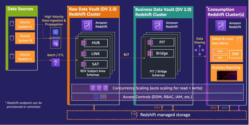
In this section, we cover how the AWS Cloud as a whole plays its role in building an enterprise-grade Data Vault warehouse on Amazon Redshift.
Education is a fundamental success factor. Data Vault is more complex than traditional data modeling methodologies. Before you start the project, make sure everyone understands the principles of Data Vault. Amazon Redshift is designed to be very easy to use, but to ensure the most optimal Data Vault implementation on Amazon Redshift, gaining a good understanding of how Amazon Redshift works is recommended. Start with free resources like reaching out to your AWS account representative to schedule a free Amazon Redshift Immersion Day or train for the AWS Analytics specialty certification.
Automation is a major benefit of Data Vault. This will increase efficiency and consistency across your data landscape. Most customers focus on the following aspects when automating Data Vault:
Depending on your needs and skills, we typically see three different approaches:
Whichever approach of the above-mentioned approaches you choose, all three approaches offer multiple benefits. For example, you can take away repetitive tasks from your development team and enforce modeling standards like data types, data quality rules, and naming conventions. To generate the code and deploy it, you can use AWS DevOps services. As part of this process, you save the generated metadata to the AWS Glue Data Catalog, which serves as a central technical metadata catalog. You then deploy the generated code to Amazon Redshift (SQL scripts) and to AWS Glue.
We designed AWS CloudFormation for automation; it’s the AWS-native way of automating infrastructure creation and management. A major use case for infrastructure as code (IaC) is to create new ingestion pipelines for new data sources or add new entities to existing one.
You can also use our new AI coding tool Amazon CodeWhisperer, which helps you quickly write secure code by generating whole line and full function code suggestions in your IDE in real time, based on your natural language comments and surrounding code. For example, CodeWhisperer can automatically take a prompt such as “get new files uploaded in the last 24 hours from the S3 bucket” and suggest appropriate code and unit tests. This can greatly reduce development effort in writing code, for example for ETL pipelines or generating SQL queries, and allow more time for implementing new ideas and writing differentiated code.
As previously mentioned, one of the benefits of Data Vault is the high level of automation which, in conjunction with serverless technologies, can lower the operating efforts. On the other hand, some industry products come with built-in schedulers or orchestration tools, which might increase operational complexity. By using AWS-native services, you’ll benefit from integrated monitoring options of all AWS services.
In this series, we discussed a number of crucial areas required for implementing a Data Vault 2.0 system at scale, and the Amazon Redshift capabilities and AWS ecosystem that you can use to satisfy those requirements. There are many more Amazon Redshift capabilities and features that will surely come in handy, and we strongly encourage current and prospective customers to reach out to us or other AWS colleagues to delve deeper into Data Vault with Amazon Redshift.
Asser Moustafa is a Principal Analytics Specialist Solutions Architect at AWS based out of Dallas, Texas. He advises customers globally on their Amazon Redshift and data lake architectures, migrations, and visions—at all stages of the data ecosystem lifecycle—starting from the POC stage to actual production deployment and post-production growth.
Philipp Klose is a Global Solutions Architect at AWS based in Munich. He works with enterprise FSI customers and helps them solve business problems by architecting serverless platforms. In this free time, Philipp spends time with his family and enjoys every geek hobby possible.
Saman Irfan is a Specialist Solutions Architect at Amazon Web Services. She focuses on helping customers across various industries build scalable and high-performant analytics solutions. Outside of work, she enjoys spending time with her family, watching TV series, and learning new technologies.
Post Syndicated from corbet original https://lwn.net/Articles/951750/
Version
1.74.0 of the Rust language has been released. New features include
better configuration for linters, authenticated cargo repositories, and
support for projections in opaque return types.
Post Syndicated from David Boyne original https://aws.amazon.com/blogs/compute/introducing-advanced-logging-controls-for-aws-lambda-functions/
This post is written by Nati Goldberg, Senior Solutions Architect and Shridhar Pandey, Senior Product Manager, AWS Lambda
Today, AWS is launching advanced logging controls for AWS Lambda, giving developers and operators greater control over how function logs are captured, processed, and consumed.
This launch introduces three new capabilities to provide a simplified and enhanced default logging experience on Lambda.
First, you can capture Lambda function logs in JSON structured format without having to use your own logging libraries. JSON structured logs make it easier to search, filter, and analyze large volumes of log entries.
Second, you can control the log level granularity of Lambda function logs without making any code changes, enabling more effective debugging and troubleshooting.
Third, you can also set which Amazon CloudWatch log group Lambda sends logs to, making it easier to aggregate and manage logs at scale.
Being able to identify and filter relevant log messages is essential to troubleshoot and fix critical issues. To help developers and operators monitor and troubleshoot failures, the Lambda service automatically captures and sends logs to CloudWatch Logs.
Previously, Lambda emitted logs in plaintext format, also known as unstructured log format. This unstructured format could make the logs challenging to query or filter. For example, you had to search and correlate logs manually using well-known string identifiers such as “START”, “END”, “REPORT” or the request id of the function invocation. Without a native way to enrich application logs, you needed custom work to extract data from logs for automated analysis or to build analytics dashboards.

Previously, operators could not control the level of log detail generated by functions. They relied on application development teams to make code changes to emit logs with the required granularity level, such as INFO, DEBUG, or ERROR.
Lambda-based applications often comprise microservices, where a single microservice is composed of multiple single-purpose Lambda functions. Before this launch, Lambda sent logs to a default CloudWatch log group created with the Lambda function with no option to select a log group. Now you can aggregate logs from multiple functions in one place so you can uniformly apply security, governance, and retention policies to your logs.
Lambda now natively supports capturing structured logs in JSON format as a series of key-value pairs, making it easier to search and filter logs more easily.
JSON also enables you to add custom tags and contextual information to logs, enabling automated analysis of large volumes of logs to help understand the function performance. The format adheres to the OpenTelemetry (OTel) Logs Data Model, a popular open-source logging standard, enabling you to use open-source tools to monitor functions.

To set the log format in the Lambda console, select the Configuration tab, choose Monitoring and operations tools on the left pane, then change the log format property:

Currently, Lambda natively supports capturing application logs (logs generated by the function code) and system logs (logs generated by the Lambda service) in JSON structured format.
This is for functions that use non-deprecated versions of Python, Node.js, and Java Lambda managed runtimes, when using Lambda recommended logging methods such as using logging library for Python, console object for Node.js, and LambdaLogger or Log4j for Java.
For other managed runtimes, Lambda currently only supports capturing system logs in JSON structured format. However, you can still capture application logs in JSON structured format for these runtimes by manually configuring logging libraries. See configuring advanced logging controls section in the Lambda Developer Guide to learn more. You can also use Powertools for AWS Lambda to capture logs in JSON structured format.
Changing log format from text to JSON can be a breaking change if you parse logs in a telemetry pipeline. AWS recommends testing any existing telemetry pipelines after switching log format to JSON.
You can use JSON structured format with CloudWatch Embedded Metric Format (EMF) to embed custom metrics alongside JSON structured log messages, and CloudWatch automatically extracts the custom metrics for visualization and alarming. However, to use JSON log format along with EMF libraries for Node.js Lambda functions, you must use the latest version of the EMF client library for Node.js or the latest version of Powertools for AWS Lambda (TypeScript) library.
You can now filter Lambda logs by log level, such as ERROR, DEBUG, or INFO, without code changes. Simplified log level filtering enables you to choose the required logging granularity level for Lambda functions, without sifting through large volumes of logs to debug errors.
You can specify separate log level filters for application logs (which are logs generated by the function code) and system logs (which are logs generated by the Lambda service, such as START and REPORT log messages). Note that log level controls are only available if the log format of the function is set to JSON.
The Lambda console allows setting both the Application log level and System log level properties:

You can define the granularity level of each log event in your function code. The following statement prints out the event input of the function, emitted as a DEBUG log message:
console.debug(event);Once configured, log events emitted with a lower log level than the one selected are not published to the function’s CloudWatch log stream. For example, setting the function’s log level to INFO results in DEBUG log events being ignored.
This capability allows you to choose the appropriate amount of logs emitted by functions. For example, you can set a higher log level to improve the signal-to-noise ratio in production logs, or set a lower log level to capture detailed log events for testing or troubleshooting purposes.
Previously, you could not specify a custom CloudWatch log group for functions, so you could not stream logs from multiple functions into a shared log group. Also, to set custom retention policy for multiple log groups, you had to create each log group separately using a pre-defined name (for example, /aws/lambda/<function name>).
Now you can select a custom CloudWatch log group to aggregate logs from multiple functions automatically within an application in one place. You can apply security, governance, and retention policies at the application level instead of individually to every function.
To distinguish between logs from different functions in a shared log group, each log stream contains the Lambda function name and version.

You can share the same log group between multiple functions to aggregate logs together. The function’s IAM policy must include the logs:CreateLogStream and logs:PutLogEvents permissions for Lambda to create logs in the specified log group. The Lambda service can optionally create these permissions, when you configure functions in the Lambda console.
You can set the custom log group in the Lambda console by entering the destination log group name. If the entered log group does not exist, Lambda creates it automatically.

Advanced logging controls for Lambda can be configured using Lambda API, AWS Management Console, AWS Command Line Interface (CLI), and infrastructure as code (IaC) tools such as AWS Serverless Application Model (AWS SAM) and AWS CloudFormation.
This section demonstrates how to use the new advanced logging controls for Lambda using AWS SAM to build and deploy the resources in your AWS account.
The following diagram shows Lambda functions processing newly created objects inside an Amazon S3 bucket, where both functions emit logs into the same CloudWatch log group:

The architecture includes the following steps:
This uses AWS SAM to define the Lambda functions and configure the required logging controls. The IAM policy allows the function to create a log stream and emit logs to the selected log group:
DetectLabelsFunction:
    Type: AWS::Serverless::Function
    Properties:
      CodeUri: detect-labels/
      Handler: app.lambdaHandler
      Runtime: nodejs18.x
      Policies:
        ...
        - Version: 2012-10-17
          Statement:
            - Sid: CloudWatchLogGroup
              Action:
                - logs:CreateLogStream
                - logs:PutLogEvents
              Resource: !GetAtt CloudWatchLogGroup.Arn
              Effect: Allow
      LoggingConfig:
        LogFormat: JSON
        ApplicationLogLevel: DEBUG
        SystemLogLevel: INFO
        LogGroup: !Ref CloudWatchLogGroup
To deploy the example:
git clone https://github.com/aws-samples/advanced-logging-controls-lambda/

cd advanced-logging-controls-lambdasam buildsam deploy --guidedadvanced-logging-controls-lambdaus-east-1)aws s3 cp samples/skateboard.jpg s3://example-s3-images-bucketExplore CloudWatch Logs to view the logs emitted into the log group created, AggregatedLabelsLogGroup:

The DetectLabels Lambda function emits DEBUG log events in JSON format to the log stream. Log events with the same log level from the ExtractText Lambda function are omitted. This is a result of the different application log level settings for each function (DEBUG and INFO).
You can also use CloudWatch Logs Insights to search, filter, and analyze the logs in JSON format using this sample query:

You can see the results:

Advanced logging controls for Lambda give you greater control over logging. Use advanced logging controls to control your Lambda function’s log level and format, allowing you to search, query, and filter logs to troubleshoot issues more effectively.
You can also choose the CloudWatch log group where Lambda sends your logs. This enables you to aggregate logs from multiple functions into a single log group, apply retention, security, governance policies, and easily manage logs at scale.
To get started, specify the required settings in the Logging Configuration for any new or existing Lambda functions.
Advanced logging controls for Lambda are available in all AWS Regions where Lambda is available at no additional cost. Learn more about AWS Lambda Advanced Logging Controls.
For more serverless learning resources, visit Serverless Land.
Post Syndicated from James Greenwood original https://aws.amazon.com/blogs/security/use-scalable-controls-for-aws-services-accessing-your-resources/
Sometimes you want to configure an AWS service to access your resource in another service. For example, you can configure AWS CloudTrail, a service that monitors account activity across your AWS infrastructure, to write log data to your bucket in Amazon Simple Storage Service (Amazon S3). When you do this, you want assurance that the service will only access your resource on your behalf—you don’t want an untrusted entity to be able to use the service to access your resource. Before today, you could achieve this by using the two AWS Identity and Access Management (IAM) condition keys, aws:SourceAccount and aws:SourceArn. You can use these condition keys to help make sure that a service accesses your resource only on behalf of specific accounts or resources that you trust. However, because these condition keys require you to specify individual accounts and resources, they can be difficult to manage at scale, especially in larger organizations.
Recently, IAM launched two new condition keys that can help you achieve this in a more scalable way that is simpler to manage within your organization:
aws:SourceOrgID — use this condition key to make sure that an AWS service can access your resources only when the request originates from a particular organization ID in AWS Organizations.aws:SourceOrgPaths — use this condition key to make sure that an AWS service can access your resources only when the request originates from one or more organizational units (OUs) in your organization.In this blog post, we describe how you can use the four available condition keys, including the two new ones, to help you control how AWS services access your resources.
Imagine a scenario where you configure an AWS service to access your resource in another service. Let’s say you’re using Amazon CloudWatch to observe resources in your AWS environment, and you create an alarm that activates when certain conditions occur. When the alarm activates, you want it to publish messages to a topic that you create in Amazon Simple Notification Service (Amazon SNS) to generate notifications.
Figure 1 depicts this process.

Figure 1: Amazon CloudWatch publishing messages to an SNS topic
In this scenario, there’s a resource-based policy controlling access to your SNS topic. For CloudWatch to publish messages to it, you must configure the policy to allow access by CloudWatch. When you do this, you identify CloudWatch using an AWS service principal, in this case cloudwatch.amazonaws.com.
This is an example of a common pattern known as cross-service access. With cross-service access, a calling service accesses your resource in a called service, and a resource-based policy attached to your resource grants access to the calling service. The calling service is identified using an AWS service principal in the form <SERVICE-NAME>.amazonaws.com, and it accesses your resource on behalf of an originating resource, such as a CloudWatch alarm.
Figure 2 shows cross-service access.

Figure 2: Cross-service access
When you configure cross-service access, you want to make sure that the calling service will access your resource only on your behalf. That means you want the originating resource to be controlled by someone whom you trust. If an untrusted entity creates their own CloudWatch alarm in their AWS environment, for example, then their alarm should not be able to publish messages to your SNS topic.
If an untrusted entity could use a calling service to access your resource on their behalf, it would be an example of what’s known as the confused deputy problem. The confused deputy problem is a security issue in which an entity that doesn’t have permission to perform an action coerces a more privileged entity (in this case, a calling service) to perform the action instead.
AWS provides global condition keys to help you prevent cross-service confused deputy issues. You can use these condition keys to control how AWS services access your resources.
Before today, you could use the aws:SourceAccount or aws:SourceArn condition keys to make sure that a calling service accesses your resource only when the request originates from a specific account (with aws:SourceAccount) or a specific originating resource (with aws:SourceArn). However, there are situations where you might want to allow multiple resources or accounts to use a calling service to access your resource. For example, you might want to create many VPC flow logs in an organization that publish to a central S3 bucket. To achieve this using the aws:SourceAccount or aws:SourceArn condition keys, you must enumerate all the originating accounts or resources individually in your resource-based policies. This can be difficult to manage, especially in large organizations, and can potentially cause your resource-based policy documents to reach size limits.
Now, you can use the new aws:SourceOrgID or aws:SourceOrgPaths condition keys to make sure that a calling service accesses your resource only when the request originates from a specific organization (with aws:SourceOrgID) or a specific organizational unit (with aws:SourceOrgPaths). This helps avoid the need to update policies when accounts are added or removed, reduces the size of policy documents, and makes it simpler to create and review policy statements.
The following table summarizes the four condition keys that you can use to help prevent cross-service confused deputy issues. These keys work in a similar way, but with different levels of granularity.
| Use case | Condition key | Value | Allowed operators | Single/multi valued | Example value |
| Allow a calling service to access your resource only on behalf of an organization that you trust. | aws:SourceOrgID |
AWS organization ID of the resource making a cross-service access request | String operators | Single-valued key | o-a1b2c3d4e5 |
| Allow a calling service to access your resource only on behalf of an organizational unit (OU) that you trust. | aws:SourceOrgPaths |
Organization entity paths of the resource making a cross-service access request | Set operators and string operators | Multivalued key | o-a1b2c3d4e5/r-ab12/ou-ab12-11111111/ou-ab12-22222222/ |
| Allow a calling service to access your resource only on behalf of an account that you trust. | aws:SourceAccount |
AWS account ID of the resource making a cross-service access request | String operators | Single-valued key | 111122223333 |
| Allow a calling service to access your resource only on behalf of a resource that you trust. | aws:SourceArn |
Amazon Resource Name (ARN) of the resource making a cross- service access request | ARN operators (recommended) or string operators | Single-valued key | arn:aws:cloudwatch:eu-west-1:111122223333:alarm:myalarm |
AWS recommends that you use these condition keys in any resource-based policy statements that allow access by an AWS service, except where the relevant condition key is not yet supported by the service. To find out whether a condition key is supported by a particular service, see AWS global condition context keys in the AWS Identity and Access Management User Guide.
Note: Only use these condition keys in resource-based policies that allow access by an AWS service. Don’t use them in other use cases, including identity-based policies and service control policies (SCPs), where these condition keys won’t be populated.
AWS services use a variety of mechanisms to help prevent cross-service confused deputy issues, and the details vary by service. For example, where a calling service accesses an S3 bucket, some services use S3 prefixes to help prevent confused deputy issues. For more information, see the relevant service documentation.
Where supported by the service, AWS recommends that you use the condition keys we describe in this post regardless of whether the service has another mechanism in place to help prevent cross-service confused deputy issues. This helps to make your intentions explicit, provide defense in depth, and guard against misconfigurations.
Let’s walk through some example use cases to learn how to use these condition keys in practice.
First, imagine you’re using Amazon Virtual Private Cloud (Amazon VPC) to manage logically isolated virtual networks. In Amazon VPC, you can configure flow logs, which capture information about your network traffic. Let’s say you want a flow log to write data into an S3 bucket for later analysis. This process is depicted in Figure 3.

Figure 3: Amazon VPC writing flow logs to an S3 bucket
This constitutes another cross-service access scenario. In this case, Amazon VPC is the calling service, Amazon S3 is the called service, the VPC flow log is the originating resource, and the S3 bucket is your resource in the called service.
To allow access, the resource-based policy for your S3 bucket (known as a bucket policy) must allow Amazon VPC to put objects there. The Principal element in this policy specifies the AWS service principal of the service that will access the resource, which for VPC flow logs is delivery.logs.amazonaws.com.
The following is an initial version of the bucket policy that allows Amazon VPC to put objects in the bucket but doesn’t yet provide confused deputy prevention. We’re showing this policy for illustration purposes; don’t use it in its current form.
Note: For simplicity, we only show one of the policy statements that you need to allow VPC flow logs to write to a bucket. In a real-life bucket policy for flow logs, you need two policy statements: one allowing actions on the bucket, and one allowing actions on the bucket contents. These are described in Publish flow logs to Amazon S3. Both policy statements work in the same way with respect to confused deputy prevention.
This policy statement allows Amazon VPC to put objects in the bucket. However, it allows Amazon VPC to do that on behalf of any flow log in any account. There’s nothing in the policy to tell Amazon VPC that it should access this bucket only if the flow log belongs to a specific organization, OU, account, or resource that you trust.
Let’s now update the policy to help prevent cross-service confused deputy issues. For the rest of this post, the remaining policy samples provide confused deputy protection, but at different levels of granularity.
Continuing with the previous example, imagine that you now have an organization in AWS Organizations, and you want to create VPC flow logs in various accounts within your organization that publish to a central S3 bucket. You want Amazon VPC to put objects in the bucket only if the request originates from a flow log that resides in your organization.
You can achieve this by using the new aws:SourceOrgID condition key. In a cross-service access scenario, this condition key evaluates to the ID of the organization that the request came from. You can use this condition key in the Condition element of a resource-based policy to allow actions only if aws:SourceOrgID matches the ID of a specific organization, as shown in the following example. In your own policy, make sure to replace <DOC-EXAMPLE-BUCKET> and <MY-ORGANIZATION-ID> with your own information.
The revised policy states that Amazon VPC can put objects in the bucket only if the request originates from a flow log in your organization. Now, if someone creates a flow log outside your organization and configures it to access your bucket, they will get an access denied error.
You can use aws:SourceOrgID in this way to allow a calling service to access your resource only if the request originates from a specific organization, as shown in Figure 4.

Figure 4: Specify a trusted organization using aws:SourceOrgID
What if you don’t want to trust your entire organization, but only part of it? Let’s consider a different scenario. Imagine that you want to send messages from Amazon SNS into a queue in Amazon Simple Queue Service (Amazon SQS) so they can be processed by consumers. This is depicted in Figure 5.

Figure 5: Amazon SNS sending messages to an SQS queue
Now imagine that you want your SQS queue to receive messages only if they originate from an SNS topic that resides in a specific organizational unit (OU) in your organization. For example, you might want to allow messages only if they originate from a production OU that is subject to change control.
You can achieve this by using the new aws:SourceOrgPaths condition key. As before, you use this condition key in a resource-based policy attached to your resource. In a cross-service access scenario, this condition key evaluates to the AWS Organizations entity path that the request came from. An entity path is a text representation of an entity within an organization.
You build an entity path for an OU by using the IDs of the organization, root, and all OUs in the path down to and including the OU. For example, consider the organizational structure shown in Figure 6.

Figure 6: Example organization structure
In this example, you can specify the Prod OU by using the following entity path:
For more information about how to construct an entity path, see Understand the AWS Organizations entity path.
Let’s now match the aws:SourceOrgPaths condition key against a specific entity path in the Condition element of a resource-based policy for an SQS queue. In your own policy, make sure to replace <MY-QUEUE-ARN> and <MY-ENTITY-PATH> with your own information.
Note:
aws:SourceOrgPathsis a multivalued condition key, which means it’s capable of having multiple values in the request context. At the time of writing, it contains a single entity path if the request originates from an account in an organization, and a null value if the request originates from an account that’s not in an organization. Because this key is multivalued, you need to use both a set operator and a string operator to compare values.
In this policy, there are two conditions in the Condition block. The first uses the Null condition operator and compares with a false value to confirm that the condition key’s value is not null. The second uses set operator ForAllValues, which returns true if every condition key value in the request matches at least one value in your policy condition, and string operator StringEquals, which requires an exact match with a value specified in your policy condition.
Note: The reason for the null check is that set operator
ForAllValuesreturns true when a condition key resolves to null. With anAlloweffect and the null check in place, access is denied if the request originates from an account that’s not in an organization.
With this policy applied to your SQS queue, Amazon SNS can send messages to your queue only if the message came from an SNS topic in a specific OU.
You can use aws:SourceOrgPaths in this way to allow a calling service to access your resource only if the request originates from a specific organizational unit, as shown in Figure 7.

Figure 7: Specify a trusted OU using aws:SourceOrgPaths
In the previous example, we specified a trusted OU, but that didn’t include its child OUs. What if you want to include its children as well?
You can achieve this by replacing the string operator StringEquals with StringLike. This allows you to use wildcards in the entity path. Using the organization structure from the previous example, the following Condition evaluates to true only if the condition key value is not null and the request originates from the Prod OU or any of its child OUs.
If you want to be more granular, you can allow a service to access your resource only if the request originates from a specific account. You can achieve this by using the aws:SourceAccount condition key. In a cross-service access scenario, this condition key evaluates to the ID of the account that the request came from.
The following Condition evaluates to true only if the request originates from the account that you specify in the policy. In your own policy, make sure to replace <MY-ACCOUNT-ID> with your own information.
You can use this condition element within a resource-based policy to allow a calling service to access your resource only if the request originates from a specific account, as shown in Figure 8.

Figure 8: Specify a trusted account using aws:SourceAccount
If you want to be even more granular, you can allow a service to access your resource only if the request originates from a specific resource. For example, you can allow Amazon SNS to send messages to your SQS queue only if the request originates from a specific topic within Amazon SNS.
You can achieve this by using the aws:SourceArn condition key. In a cross-service access scenario, this condition key evaluates to the Amazon Resource Name (ARN) of the originating resource. This provides the most granular form of cross-service confused deputy prevention.
The following Condition evaluates to true only if the request originates from the resource that you specify in the policy. In your own policy, make sure to replace <MY-RESOURCE-ARN> with your own information.
Note: AWS recommends that you use an ARN operator rather than a string operator when comparing ARNs. This example uses
ArnEqualsto match the condition key value against the ARN specified in the policy.
You can use this condition element within a resource-based policy to allow a calling service to access your resource only if the request comes from a specific originating resource, as shown in Figure 9.

Figure 9: Specify a trusted resource using aws:SourceArn
The four condition keys allow you to specify multiple trusted entities by matching against an array of values. This allows you to specify multiple trusted resources, accounts, OUs, or organizations in your policies.
In this post, you learned about cross-service access, in which an AWS service communicates with another AWS service to access your resource. You saw that it’s important to make sure that such services access your resources only on your behalf in order to help avoid cross-service confused deputy issues.
We showed you how to help prevent cross-service confused deputy issues by using two new condition keys aws:SourceOrgID and aws:SourceOrgPaths, as well as the other available condition keys aws:SourceAccount and aws:SourceArn. You learned that you should use these condition keys in any resource-based policy statements that allow access by an AWS service, if the condition key is supported by the service. This helps make sure that a calling service can access your resource only when the request originates from a specific organization, OU, account, or resource that you trust.
If you have feedback about this post, submit comments in the Comments section below. If you have questions about this post, start a new thread on AWS IAM re:Post or contact AWS Support.
Want more AWS Security news? Follow us on Twitter.
Post Syndicated from Jeff Barr original https://aws.amazon.com/blogs/aws/new-long-form-voices-for-amazon-polly/
We are launching three new voices for Polly. Powered by a new long-form engine, the voices are natural and expressive, with appropriate pauses, emphasis, and tone.
New Voices
The new long-form voices are perfect for blog posts, news articles, training videos, and marketing content. The underlying Machine Learning model extracts meaning from the text, learning about speech segments, prosody (the pattern of rhythm and pauses), intonation, and other aspects of expressive speech, allowing the synthesized audio to express emotions, especially in dialogs. The new long-form engine uses a deep learning text-to-speech (TTS) model trained to acquire a contextual understanding of the text that allows it to express prosody in an appropriate way. This allows the intention of the story to drive the vocal performance and create the correct emphasis, pauses, and tones of a realistic human voice.
Here are the new voices:
| Name | Locale | Gender | Language | Sample |
| Danielle | en_US | Female | English (US) | |
| Gregory | en_US | Male | English (US) | |
| Ruth | en_US | Female | English (US) |
Using the New Voices
You can access the new voices using the AWS Management Console, AWS Command Line Interface (AWS CLI), or the AWS SDKs. Using the CLI, I start by listing the voices that use the new long-form engine:
I can pick one, or I can try all of them:
My shell script had a small quoting bug, but the resulting audio was too funny not to include!
Programmatically, you can reproduce my example by writing code that calls the DescribeVoices and SynthesizeSpeech functions.
Things to Know
Here are some interesting things that you should know about the new voices:
Pricing – Long-form voices are priced at $100 per million characters or Speech Marks requests. Check out the Amazon Polly Pricing page to learn more.
Engines & Voices – Some of the voices that I listed above can be used with more than one engine. For example, the Danielle voice can be used with the new long-form engine and the existing neural engine.
Regions – The new engine and voices are available in the US East (N. Virginia) Region.
Check out the new voices, build something awesome, and let me know what you think!
— Jeff;
Post Syndicated from Chris Munns original https://aws.amazon.com/blogs/compute/its-about-time-microsecond-accurate-clocks-on-amazon-ec2-instances/
This post is written by Josh Levinson, AWS Principal Product Manager and Julien Ridoux, AWS Principal Software Engineer
Today, we announced that we improved the Amazon Time Sync Service to microsecond-level clock accuracy on supported Amazon EC2 instances. This new capability adds a local reference clock to your EC2 instance and is designed to deliver clock accuracy in the low double-digit microsecond range within your instance’s guest OS software. This post shows you how to connect to the improved clocks on your EC2 instances. This post also demonstrates how you can measure your clock accuracy and easily generate and compare timestamps from your EC2 instances with ClockBound, an open source daemon and library.
In general, it’s hard to achieve high-fidelity clock synchronization due to hardware limitations and network variability. While customers have depended on the Amazon Time Sync Service to provide one millisecond clock accuracy, workloads that need microsecond-range accuracy, such as financial trading and broadcasting, required customers to maintain their own time infrastructure, which is a significant operational burden, and expensive. Other clock-sensitive applications that run on the cloud, including distributed databases and storage, have to incorporate message exchange delays with wait periods, data locks, or transaction journaling to maintain consistency at scale.
With global and reliable microsecond-range clock accuracy, you can now migrate and modernize your most time-sensitive applications in the cloud and retire your burdensome on-premises time infrastructure. You can also simplify your applications and increase their throughput by leveraging the high-accuracy timestamps to determine the ordering of events and transactions on workloads across instances, Availability Zones, and Regions. Additionally, you can audit the improved Amazon Time Sync Service to measure and monitor the expected microsecond-range accuracy.
The new local clock source can be accessed over the existing Amazon Time Sync Service’s Network Time Protocol (NTP) IPv4 and IPv6 endpoints, or by configuring a new Precision Time Protocol (PTP) reference clock device, to get the best accuracy possible. It’s important to note that both NTP and the new PTP Hardware Clock (PHC) device share the same highly accurate source of time. The new PHC device is part of the AWS Nitro System, so it is directly accessible on supported bare metal and virtualized Amazon EC2 instances without using any customer resources.
Leap seconds, introduced in 1972, are occasional one-second adjustments to UTC time to factor in irregularities in Earth’s rotation to UTC time in order to accommodate differences between International Atomic Time (TAI) and solar time (Ut1). To manage leap seconds on behalf of customers, we designed leap second smearing within the Amazon Time Sync Service (details on smearing time in “Look Before You Leap”).
Leap seconds are going away, and we are in full support of the decision made at the 27th General Conference on Weights and Measures to abandon leap seconds by or before 2035.
To support this transition, we still plan on smearing time when accessing the Amazon Time Sync Service over the local NTP connection or our Public NTP pools (time.aws.com). The new PHC device, however, will not provide a smeared time option. In the event of a leap seconds, PHC would add the leap seconds following UTC standards. Leap smeared and leap second time sources are the same in most cases. But, since they differ during a leap second event, we do not recommend mixing smeared and non-smeared time sources in your time client configuration during a leap second event.
You can connect to the new, microsecond-accurate clocks over NTP the same way you use the Amazon Time Sync Service today at the 169.254.169.123 IPv4 address or the fd00:ec2::123 IPv6 address. This is already the default configuration on all Amazon AMIs and many partner AMIs, including RHEL, Ubuntu, and SUSE. You can verify this connection in your NTP daemon. The below example, using the chrony daemon, verifies that chrony is using the 169.254.169.123 IPv4 address of the Amazon Time Sync Service to synchronize the time:
[ec2-user@ ~]$ chronyc sources
MS Name/IP address         Stratum Poll Reach LastRx Last sample
===============================================================================
^- pacific.latt.net              3  10   377    69  +5630us[+5632us] +/-   90ms
^- edge-lax.txryan.com           2   8   377   224   -691us[ -689us] +/-   33ms
^* 169.254.169.123               1   4   377     2  -4487ns[-5914ns] +/-   85us
^- blotch.image1tech.net         2   9   377   327  -1710us[-1720us] +/-   64ms
^- 44.190.40.123                 2   9   377   161  +3057us[+3060us] +/-   84ms
The 169.254.169.123 IPv4 address of the Amazon Time Sync Service is designated with a *, showing it is the source of synchronization on this instance. See the EC2 User Guide for more details on configuring the Amazon Time Sync Service if it is not already configured by default.
First, you need to install the latest Elastic Network Adapter (ENA) driver. This driver will allow you to connect directly to the PHC. Connect to your instance and install the Linux kernel driver for Elastic Network Adapter (ENA) version 2.10.0 or later. For the installation instructions, see Linux kernel driver for Elastic Network Adapter (ENA) family on GitHub. To enable PTP support in the driver follow the instructions in the section “PTP Hardware Clock (PHC)“.
Once the driver is installed, you need to configure your NTP daemon to connect to the PHC. Below is an example on how to change the configuration in chrony by adding the PHC to your chrony configuration file. Then restart chrony for the change to take place:
[ec2-user ~]$ sudo sh -c 'echo "refclock PHC /dev/ptp0 poll 0 delay 0.000010 prefer" >> /etc/chrony.conf'
[ec2-user ~]$ sudo systemctl restart chronyd
This example uses a +/-5 microsecond range in receiving the reference signal from the PHC. These 10 microseconds are needed to account for operating system latency.
After changing your configuration, you can validate your daemon is correctly syncing to the PHC. Below is an example of output from the chronyc command. An asterisk will appear next to the PHC0 source indicating that you are now syncing to the PHC:
[ec2-user@ ~]$ chronyc sources
MS Name/IP address         Stratum Poll Reach LastRx Last sample
=============================================================================
#* PHC0                           0   0   377     1   +18ns[  +20ns] +/- 5032ns
The PHC0 device of the Amazon Time Sync Service is designated with a *, showing it is the source of synchronization on this instance
Your chrony tracking information will also show that you are syncing to the PHC:
[ec2-user@ ~]$ chronyc tracking
Reference ID    : 50484330 (PHC0)
Stratum         : 1
Ref time (UTC)  : Mon Nov 13 18:43:09 2023
System time     : 0.000000004 seconds fast of NTP time
Last offset     : -0.000000010 seconds
RMS offset      : 0.000000012 seconds
Frequency       : 7.094 ppm fast
Residual freq   : -0.000 ppm
Skew            : 0.004 ppm
Root delay      : 0.000010000 seconds
Root dispersion : 0.000001912 seconds
Update interval : 1.0 seconds
Leap status     : Normal
See the EC2 User Guide for more details on configuring the PHC.
Clock accuracy is a measure of clock error, typically defined as the offset to UTC. This clock error is the difference between the observed time on the computer and the reference time (also known as true time). If your instance is configured to use the Amazon Time Sync Service where the microsecond-accurate enhancement is available, you will typically see a clock error bound of under 100us using the NTP connection. When configured and synchronized correctly with the new PHC connection, you will typically see a clock error bound of under 40us.
We previously published a blog on measuring and monitoring clock accuracy over NTP, which still applies to the improved NTP connection.
If you are connected to the PHC, your time daemon, such as chronyd, will underestimate the clock error bound. This is because inherently, a PTP hardware clock device in Linux does not pass any “error bound” information to chrony, the way the NTP would. As a result, your clock synchronization daemon assumes the clock itself is accurate to UTC and thus has an “error bound” of 0. To get around this issue, the Nitro System calculates the error bound of the PTP Hardware Clock itself, and exposes it to your EC2 instance over the ENA driver sysfs filesystem. You can read this directly as a value in nanoseconds with the command cat /sys/devices/pci0000:00/0000:00:05.0/phc_error_bound. To get your clock error bound at some instant, you would need to add the clock error bound from chrony or ClockBound at the time that chronyd polls the PTP Hardware Clock and add it to this phc_error_bound value.
Below is how you would calculate the clock error incorporating the PHC clock error to get your true clock error bound:
CLOCK ERROR BOUND = SYSTEM TIME + (.5 * ROOT DELAY) + ROOTDISPERSION + PHC Error Bound
For the values in the example:
PHC Error Bound = cat /sys/devices/pci0000:00/0000:00:05.0/phc_error_bound
The System Time, Root Delay, and Root Dispersion are values taken from the chrony tracking information.
However accurate, a clock is never perfect. Instead of providing an estimate of the clock error, ClockBound provides a reliable confidence interval by automatically calculating the clock accuracy, using the calculations in which the reference time (true time) does exist. The open source ClockBound daemon provides a convenient way to retrieve this confidence interval, and work is continuing to make it easier to integrate into high performance workloads.
The Amazon Time Sync Service’s new microsecond-accurate clocks can be leveraged to migrate and modernize your most clock-sensitive applications in the cloud. In this post, we showed you how to can connect to the improved clocks on supported Amazon EC2 instances, how to measure your clock accuracy, and how to easily generate and compare timestamps from your Amazon EC2 instances with ClockBound. Launch a supported instance and get started today to build using this new capability.
To learn more about the Amazon Time Sync Service, see the EC2 UserGuide for Linux and Windows.
If you have questions about this post, start a new thread on the AWS Compute re:Post or contact AWS Support.
We will speak in more detail about the Amazon Time Sync Service during re:invent 2023. Look for Session ID CMP220 in the AWS re:Invent session catalog to register.
Post Syndicated from Kenny Johnson original http://blog.cloudflare.com/introducing-advanced-session-audit-capabilities-in-cloudflare-one/

The basis of Zero Trust is defining granular controls and authorization policies per application, user, and device. Having a system with a sufficient level of granularity to do this is crucial to meet both regulatory and security requirements. But there is a potential downside to so many controls: in order to troubleshoot user issues, an administrator has to consider a complex combination of variables across applications, user identity, and device information, which may require painstakingly sifting through logs.
We think there’s a better way — which is why, starting today, administrators can easily audit all active user sessions and associated data used by their Cloudflare One policies. This enables the best of both worlds: extremely granular controls, while maintaining an improved ability to troubleshoot and diagnose Zero Trust deployments in a single, simple control panel. Information that previously lived in a user’s browser or changed dynamically is now available to administrators without the need to bother an end user or dig into logs.

Authentication and Authorization are the two components that a Zero Trust policy evaluates before allowing a user access to a resource.
Authentication is the process of verifying the identity of a user, device, or system. Common methods of authentication include entering usernames and passwords, presenting a digital certificate, or even biometrics like a fingerprint or face scan. Multi-factor authentication (MFA) requires two or more separate methods of authentication for enhanced security, like a hardware key in combination with a password.
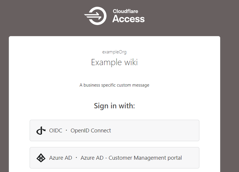
Authorization is the process of granting or denying access to specific resources or permissions once an entity has been successfully authenticated. It defines what the authenticated entity can and cannot do within the system.
Web applications, which we’ll focus on, generally use HTTP cookies to handle both authentication and authorization.
Authentication:
Authorization:
This way, the user stays authenticated (and their authorization can be checked) for all subsequent requests after logging in, until the session expires, or they log out.
In modern web applications, this session state is most commonly stored in the form of a JSON Web Token (JWT).
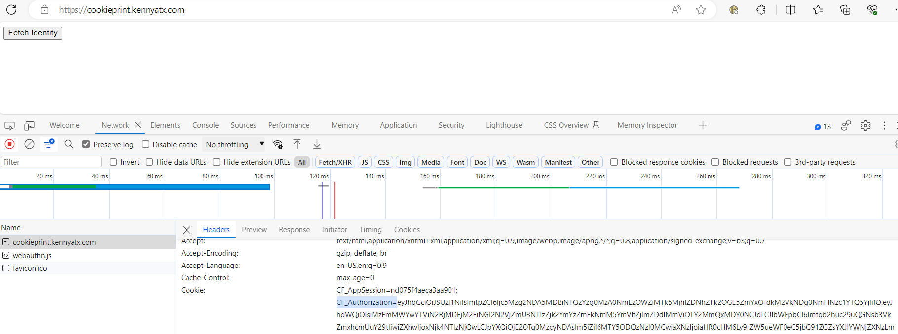
JWTs are used in many modern web applications, and Zero Trust Network Access (ZTNA) solutions like Cloudflare Access, for authentication and authorization. A JWT includes a payload that encodes information about the user and possibly other data, and it’s signed by the server to prevent tampering. JWTs are often used in a stateless manner, meaning the server doesn’t keep a copy of each JWT—it simply verifies and decodes them as they come in with requests. The stateless nature of JWTs means that you do not have to rely on a central system to handle user session management which avoids creating scalability issues as the number of users accessing a system increases.
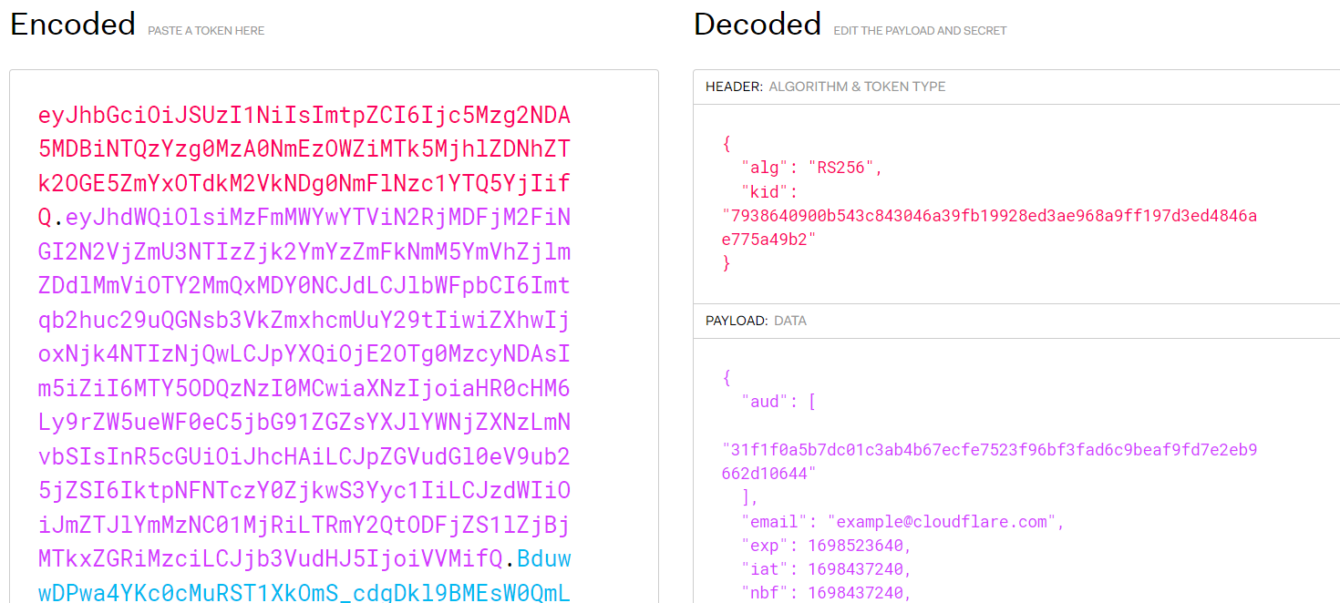
However, this stateless nature of JWTs makes debugging JWT-based authentication tricky without getting the specific JWT from a user. Here’s why:
1. Token Specificity: Each JWT is specific to a user and a session. It contains information (claims) about the user, the issuing authority, the token’s issuing time, expiration time, and possibly other data. Therefore, to debug a problem, you often need the exact JWT that’s causing the issue.
2. No Server-side Records: Since JWTs are stateless, the server does not store sessions by default. It can’t look up past tokens or their associated state, unless it’s been specifically designed to log them, which is usually not the case due to privacy and data minimization considerations.
3. Transient Issues: Problems with JWTs can be transient—they might relate to the specific moment the token was used. For instance, if a token was expired when a user tried to use it, you’d need that specific token to debug the issue.
4. Privacy and Security: JWTs can contain sensitive information, so they should be handled with care. Getting a JWT from a user might expose their personal information or security credentials to whoever is debugging the issue. In addition, if a user sends their JWT through an insecure channel to a developer or an IT help desk, it could be intercepted (Cloudflare recently released a free HAR Sanitizer to help mitigate this concern).
These factors make it difficult to troubleshoot issues with JWT based authentication without having the specific token in question.
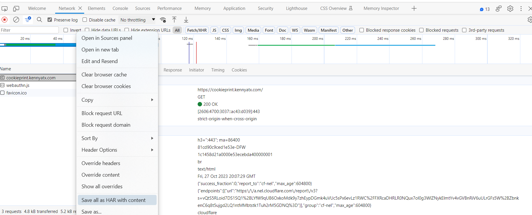
We set out to build a better way to debug issues related to a user’s identity in Cloudflare Zero Trust without sharing JWTs or HAR files back and forth. Administrators can now view a user’s Registry Identity (used for Gateway policies) and all active Access sessions.
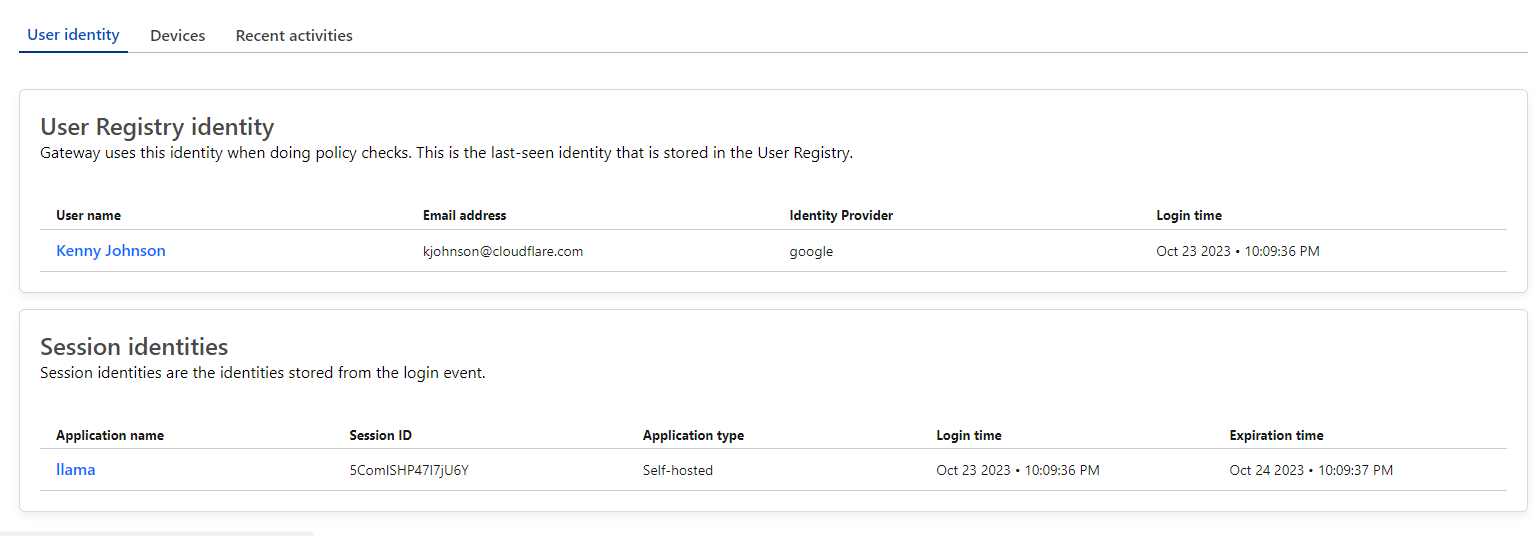
This session information includes the full identity evaluated by Zero Trust including IdP claims, device posture information, network context and more. We were able to build this feature without any additional load on Access’ authentication logic by leveraging Cloudflare Workers KV. At the time a user authenticates with Access, their associated identity is immediately saved into a Key/Value pair in Workers KV. This all occurs within the context of the user’s authentication event which means there is minimal latency impact or reliance on an external service.
This feature is available to all customers across all Zero Trust plans. If you would like to get started with Cloudflare Zero Trust, sign up for a free account for up to 50 users, today! Or, collaborate with Cloudflare experts to discuss SSE or SASE for your organization and tackle your Zero Trust use cases one step at a time.
Post Syndicated from Bruce Schneier original https://www.schneier.com/blog/archives/2023/11/ftcs-voice-cloning-challenge.html
The Federal Trade Commission is running a competition “to foster breakthrough ideas on preventing, monitoring, and evaluating malicious voice cloning.”
Post Syndicated from James Beswick original https://aws.amazon.com/blogs/compute/aws-integrated-application-test-kit/
This post is written by Dan Fox, Principal Specialist Solutions Architect, and Brian Krygsman, Senior Solutions Architect.
Today, AWS announced the public preview launch of the AWS Integrated Application Test Kit (IATK). AWS IATK is a software library that helps you write automated tests for cloud-based applications. This blog post presents several initial features of AWS IATK, and then shows working examples using an example video processing application. If you are getting started with serverless testing, learn more at serverlessland.com/testing.
When you create applications composed of serverless services like AWS Lambda, Amazon EventBridge, or AWS Step Functions, many of your architecture components cannot be deployed to your desktop, but instead only exist in the AWS Cloud. In contrast to working with applications deployed locally, these types of applications benefit from cloud-based strategies for performing automated tests. For its public preview launch, AWS IATK helps you implement some of these strategies for Python applications. AWS IATK will support other languages in future launches.
When you write automated tests for cloud resources, you need the physical IDs of your resources. The physical ID is the name AWS assigns to a resource after creation. For example, to send requests to Amazon API Gateway you need the physical ID, which forms the API endpoint.
If you deploy cloud resources in separate infrastructure as code stacks, you might have difficulty locating physical IDs. In CloudFormation, you create the logical IDs of the resources in your template, as well as the stack name. With IATK, you can get the physical ID of a resource if you provide the logical ID and stack name. You can also get stack outputs by providing the stack name. These convenient methods simplify locating resources for the tests that you write.
To write integration tests for event driven architectures, establish logical boundaries by breaking your application into subsystems. Your subsystems should be simple enough to reason about, and contain understandable inputs and outputs. One useful technique for testing subsystems is to create test harnesses. Test harnesses are resources that you create specifically for testing subsystems.
For example, an integration test can begin a subsystem process by passing an input test event to it. IATK can create a test harness for you that listens to Amazon EventBridge for output events. (Under the hood, the harness is composed of an EventBridge Rule that forwards the output event to Amazon Simple Queue Service.) Your integration test then queries the test harness to examine the output and determine if the test passes or fails. These harnesses help you create integration tests in the cloud for event driven architectures.
If you write a synchronous service, your automated tests make requests and expect immediate responses. When your architecture is asynchronous, your service accepts a request and then performs a set of actions at a later time. How can you test for the success of an activity if it does not have a specified duration?
Consider creating reasonable timeouts for your asynchronous systems. Document timeouts as service level agreements (SLAs). You may decide to publish your SLAs externally or to document them as internal standards. IATK contains a polling feature that allows you to establish timeouts. This feature helps you to test that your asynchronous systems complete tasks in a timely manner.
If you want to gain more visibility into the interior details of your application, instrument with AWS X-Ray. With AWS X-Ray, you trace the path of an event through multiple services. IATK provides conveniences that help you set the AWS X-Ray sampling rate, get trace trees, and assert for trace durations. These features help you observe and test your distributed systems in greater detail.
Learn more about testing asynchronous architectures at aws-samples/serverless-test-samples.
To demonstrate the features of IATK, this post uses a portion of a serverless video application designed with a plugin architecture. A core development team creates the primary application. Distributed development teams throughout the organization create the plugins. One AWS CloudFormation stack deploys the primary application. Separate stacks deploy each plugin.
Communications between the primary application and the plugins are managed by an EventBridge bus. Plugins pull application lifecycle events off the bus and must put completion notification events back on the bus within 20 seconds. For testing, the core team has created an AWS Step Functions workflow that mimics the production process by emitting properly formatted example lifecycle events. Developers run this test workflow in development and test environments to verify that their plugins are communicating properly with the event bus.
The following demonstration shows an integration test for the example application that validates plugin behavior. In the integration test, IATK locates the Step Functions workflow. It creates a test harness to listen for the event completion notification to be sent by the plugin. The test then runs the workflow to begin the lifecycle process and start plugin actions. Then IATK uses a polling mechanism with a timeout to verify that the plugin complies with the 20 second service level agreement. This is the sequence of processing:

Follow these steps to review this application, build it locally, deploy it in your AWS account, and test it.
git clone https://github.com/aws-samples/serverless-test-samplespython-test-samples/integrated-application-test-kit. Change to this directory:
cd serverless-test-samples/python-test-samples/integrated-application-test-kitBefore deploying the application, review how the integration test uses the IATK by opening plugins/2-postvalidate-plugins/python-minimal-plugin/tests/integration/test_by_polling.py in your text editor. The test class instantiates the IATK at the top of the file.
iatk_client = aws_iatk.AwsIatk(region=aws_region)In the setUp() method, the test class uses IATK to fetch CloudFormation stack outputs. These outputs are references to deployed cloud components like the plugin tester AWS Step Functions workflow:
stack_outputs = self.iatk_client.get_stack_outputs(
    stack_name=self.plugin_tester_stack_name,
    output_names=[
        "PluginLifecycleWorkflow",
        "PluginSuccessEventRuleName"
    ],
)
The test class attaches a listener to the default event bus using an Event Rule provided in the stack outputs. The test uses this listener later to poll for events.
add_listener_output = self.iatk_client.add_listener(
    event_bus_name="default",
    rule_name=self.existing_rule_name
)
The test class cleans up the listener in the tearDown() method.
self.iatk_client.remove_listeners(
    ids=[self.listener_id]
)
Once the configurations are complete, the method test_minimal_plugin_event_published_polling() implements the actual test.
The test first initializes the trigger event.
trigger_event = {
    "eventHook": "postValidate",
    "pluginTitle": "PythonMinimalPlugin"
}
Next, the test starts an execution of the plugin tester Step Functions workflow. It uses the plugin_tester_arn that was fetched during setUp.
self.step_functions_client.start_execution(
    stateMachineArn=self.plugin_tester_arn,
    input=json.dumps(trigger_event)
)
The test polls the listener, waiting for the plugin to emit events. It stops polling once it hits the SLA timeout or receives the maximum number of messages.
poll_output = self.iatk_client.poll_events(
    listener_id=self.listener_id,
    wait_time_seconds=self.SLA_TIMEOUT_SECONDS,
    max_number_of_messages=1,
)
Finally, the test asserts that it receives the right number of events, and that they are well-formed.
self.assertEqual(len(poll_output.events), 1)
self.assertEqual(received_event["source"], "video.plugin.PythonMinimalPlugin")
self.assertEqual(received_event["detail-type"], "plugin-complete")
You need the following prerequisites to build this example:
--use-container flag to the build command to instruct AWS SAM to create the application in a provided container. You can accept or override the default values during the deploy process. You will use “Stack Name” and “AWS Region” later to run the integration test.
cd plugins/plugin_tester # Move to the plugin tester directory

sam build --use-container # Build the plugin tester

sam deploy --guided # Deploy the plugin tester
cd ../2-postvalidate-plugins/python-minimal-plugin # Move to the plugin directory

sam build --use-container # Build the plugin
sam deploy --guided # Deploy the pluginYou can run tests written with IATK using standard Python test runners like unittest and pytest. The example application test uses unittest.
python3 -m venv .venv # Create the virtual environment
source .venv/bin/activate # Activate the virtual environment
cd tests
pip3 install -r requirements.txt
samconfig.toml file of the plugin_tester directory.
cd integration

PLUGIN_TESTER_STACK_NAME=video-plugin-tester \
AWS_REGION=us-west-2 \
python3 -m unittest ./test_by_polling.py
You should see output as unittest runs the test.
Open the Step Functions console in your AWS account, then choose the PluginLifecycleWorkflow-<random value> workflow to validate that the plugin tester successfully ran. A recent execution shows a Succeeded status:

The example application includes examples of other IATK features like generating mock events and retrieving AWS X-Ray traces.
Use AWS SAM to clean up both the plugin and the plugin tester resources from your AWS account.
cd ../.. # Move to the plugin directory
sam delete # Delete the plugin
cd ../../plugin_tester # Move to the plugin tester directory
sam delete # Delete the plugin tester
The temporary test harness resources that IATK created during the test are cleaned up when the tearDown method runs. If there are problems during teardown, some resources may not be deleted. IATK adds tags to all resources that it creates. You can use these tags to locate the resources then manually remove them. You can also add your own tags.
The AWS Integrated Application Test Kit is a software library that provides conveniences to help you write automated tests for your cloud applications. This blog post shows some of the features of the initial Python version of the IATK.
To learn more about automated testing for serverless applications, visit serverlessland.com/testing. You can also view code examples at serverlessland.com/testing/patterns or at the AWS serverless-test-samples repository on GitHub.
For more serverless learning resources, visit Serverless Land.
Post Syndicated from KC Higgins original https://blog.rapid7.com/2023/11/16/manage-enterprise-risk-at-scale-with-a-unified-holistic-approach/

The rapid pace of technological change and the attendant rise of cyber threats in both speed and number leave most organizations at a disadvantage.
Historically, many firms faced this challenge simply by purchasing more technology in the hopes that the latest threat protection software would keep their data safe. But those days have come to an end. Not only have budgets come under increased scrutiny, but the sheer number of tools in most environments has become a handicap as well: Tools don’t always work well together and the expertise required to manage them remains in short supply. According to some analysts, the current complexity and diversity of tech environments also hampers visibility into vulnerability risks, at least in part because data must be obtained from disparate systems or laboriously exported into spreadsheets and data analytics platforms to fine tune and understand relevant risks.
For organizations looking for a unified perspective of risk across their cloud and on-prem environments, prioritizing risk, eliminating repetitive manual work, maintaining complete risk visibility, and consolidating point solutions will enable them to meet cyber threats with speed and success.
You’ll hear companies claim to stop all threats everywhere all the time, but such claims are neither true nor practical – anyone who follows the news even casually knows that the threats keep coming. The key is to understand which threats pose the largest risks and mitigate those first. Tools like Rapid7’s InsightVM analyze enterprise-wide asset and vulnerability data to identify the actions that will have the largest impact on risk reduction in a given organization. Instead of thousand-page lists of individual patches to apply, organizations can make informed, up-to-the-minute decisions on how to allocate resources for maximum risk reduction.
InsightVM also offers live dashboards that update whenever new data is discovered, allowing teams to track the attack surface and risk as they change. Dashboard views can even be customized for different technical teams or stakeholders as organizational perimeters expand into the cloud and beyond. Other approaches, such as cloud risk management, allow organizations to manage, prioritize, and act on risks within the large scale of modern multi-cloud environments and on-prem footprints by helping them understand the potential impact of a particular risk and its likelihood of exploitation.
In addition to trying to tackle every imaginable risk, maintaining maximum visibility into attack-surface risk is the only way organizations can hope to minimize security gaps while managing the many containers, cloud services, and virtual devices that are often spun up and down without direct involvement from the security team.
While InsightVM integrates directly with dynamic infrastructure to give full visibility into the risks posed by these assets, solutions like Executive Risk View provide complete visibility into hybrid-environment risk by ingesting data with purpose-built collection mechanisms – regardless of whether work is running on-premises or in the cloud.
Executive Risk View also aggregates and normalizes disparate risk assessments from on-premises and cloud environments for a unified, interactive dashboard that brings clarity to discovered vulnerabilities and the risks each represents so that security teams can prioritize remediation actions and share insights cross functionally. Insight into how vulnerabilities translate into business risk – and which of them are most likely to be targeted by attackers – means teams can quickly and effectively address the risks that pose the most significant danger.
Prioritization, automation, and visibility are all foundational elements of unified risk protection, but if organizations rely on multiple vendors to manage them, they will continue to lose efficiencies and battle tool proliferation. Cloud Risk Complete offers all of these solutions from one comprehensive platform and single subscription model. This means organizations can secure hybrid environments from development to production; detect and address risk across endpoints, cloud workloads, and traditional infrastructure; and perform dynamic application security testing to remediate application risk – all with a single subscription.
Learn more about the ways Rapid7 can help increase your security posture.
Post Syndicated from Marcia Villalba original https://aws.amazon.com/blogs/compute/triggering-aws-lambda-function-from-a-cross-account-amazon-managed-streaming-for-apache-kafka/
This post is written by Subham Rakshit, Senior Specialist Solutions Architect, and Ismail Makhlouf, Senior Specialist Solutions Architect.
Many organizations use a multi-account strategy for stream processing applications. This involves decomposing the overall architecture into a single producer account and many consumer accounts. Within AWS, in the producer account, you can use Amazon Managed Streaming for Apache Kafka (Amazon MSK), and in their consumer accounts have AWS Lambda functions for event consumption. This blog post explains how you can trigger Lambda functions from a cross-account Amazon MSK cluster.
The Lambda event sourcing mapping (ESM) for Amazon MSK continuously polls for new events from the Amazon MSK cluster, aggregates them into batches, and then triggers the target Lambda function. The ESM for Amazon MSK functions as a serverless set of Kafka consumers that ensures that each event is processed at least once. Additionally, events are processed in the same order they are received within each Kafka partition. In addition, the ESM batches the stream of data and filters the events based on configured logic.
Amazon MSK supports two different deployment types: provisioned and serverless. Triggering a Lambda function from a cross-account Amazon MSK cluster is only supported with a provisioned cluster deployed within the same Region. To facilitate this functionality, Amazon MSK uses multi-VPC private connectivity, powered by AWS PrivateLink, which simplifies connecting Kafka consumers hosted in different AWS accounts to an Amazon MSK cluster.
The following diagram illustrates the architecture of this example:

The architecture is divided in two parts: the producer and the consumer.
In the producer account, you have the Amazon MSK cluster with multi-VPC connectivity enabled. Multi-VPC connectivity is only available for authenticated Amazon MSK clusters. Cluster policies are required to grant permissions to other AWS accounts, allowing them to establish private connectivity to the Amazon MSK cluster. You can delegate permissions to relevant roles or users. When combined with AWS Identity and Access Management (IAM) client authentication, cluster policies offer fine-grained control over Kafka data plane permissions for connecting applications.
In the consumer account, you have the Lambda ESM for Amazon MSK and the managed VPC connection deployed within the same VPC. The managed VPC connection allows private connectivity from the consumer application VPC to the Amazon MSK cluster. The Lambda ESM for Amazon MSK connects to the cross-account Amazon MSK cluster via IAM authentication. It also supports SASL/SCRAM, and mutual TLS (mTLS) authenticated clusters. The ESM receives the event from the Kafka topic and invokes the Lambda function to process it.
To set up the Lambda function trigger from a cross-account Amazon MSK cluster as the event source, follow these steps. The AWS CloudFormation templates for deploying the example are accessible in the GitHub repository.
As a part of this example, some sample data is published using the Kafka console producer and Lambda processes these events and writes to Amazon S3.
For this example, you need two AWS accounts. This post uses the following naming conventions:
To get started:
git clone https://github.com/aws-samples/lambda-cross-account-msk.gitproducer-account.yaml from the AWS console and take note of the MSKClusterARN from the CloudFormation outputs tab.consumer-account.yaml from the AWS console with the input parameter MSKAccountId, that is the producer AWS account ID (for example, account Id: 1111 1111 1111). Note the LambdaRoleArn from the CloudFormation outputs tab.Once the accounts are created, you must enable connectivity between them. By enabling multi-VPC private connectivity in the Amazon MSK cluster, you set up the network connection to allow the cross-account consumers to connect to the cluster.

producer-msk-cluster-policy.yaml from the AWS console with the following input parameters:producer-account.yaml.consumer-account.yaml.In the producer account, navigate to the Amazon MSK console. Choose the Amazon MSK cluster named producer-cluster. Choose View client information to show the bootstrap server.

The CloudFormation template also deploys a Kafka client instance to create topics and publish events.
To access the client, go to the Amazon EC2 console and choose the instance producer-KafkaClientInstance1. Connect to EC2 instance with Session Manager:
You must use the single-VPC Private endpoint for the Amazon MSK cluster and not the multi-VPC private endpoint, as you are going to publish events from a Kafka console producer from the producer account.
Run these scripts to create the customer topic and publish sample events in the topic:
To establish a connection to the Amazon MSK cluster in the producer account, you must create a managed VPC connection in the consumer account. Lambda communicates with cross-account Amazon MSK through this managed VPC connection.
For detailed setup steps, read the Amazon MSK managed VPC connection documentation.
The final step is to set up the Lambda ESM for Amazon MSK. Setting up the ESM enables you to connect to the Amazon MSK cluster in the producer account via the managed VPC endpoint. This allows you to trigger the Lambda function to process the data produced from the Kafka topic:

To configure this trigger:


Scroll to the bottom and choose Add. This starts creating the Amazon MSK trigger, which takes several minutes. After creation, the state of the trigger shows as Enabled.
The Lambda function receives the events and writes them in an S3 bucket.
To validate that the function is working, go to the consumer account and navigate to the S3 console. Search for the cross-account-lambda-consumer-data-<<REGION>>-<<AWS Account Id>> bucket. In the bucket, you see the customer-data-<<datetime>>.csv files.

You must empty and delete the S3 bucket, managed VPC connection, and the Lambda ESM for Amazon MSK manually from the consumer account. Next, delete the CloudFormation stacks from the AWS console from both the producer and consumer accounts to remove all other resources created as a part of the example.
With Lambda and Amazon MSK, you can now build a decentralized application distributed across multiple AWS accounts. This post shows how you can set up Amazon MSK as an event source for cross-account Lambda functions and also walks you through the configuration required in both producer and consumer accounts.
For further reading on AWS Lambda with Amazon MSK as an event source, visit the documentation.
For more serverless learning resources, visit Serverless Land.
Post Syndicated from Jeff Barr original https://aws.amazon.com/blogs/aws/build-ai-apps-with-partyrock-and-amazon-bedrock/
If you are ready to learn more about Generative AI while having fun and building cool stuff, check out PartyRock.aws . You can experiment, learn all about prompt engineering, build mini-apps, and share them with your friends — all without writing any code or creating an AWS account. You can also start with an app that has been shared with you and remix it to further enhance and customize it.
Using PartyRock
To get started, I visit https://partyrock.aws/ , click Sign in, and log in using my Apple, Amazon, or Google account:
After authenticating, I am on the front page of PartyRock. I can review some sample apps, or I can click Build your own app to get started:
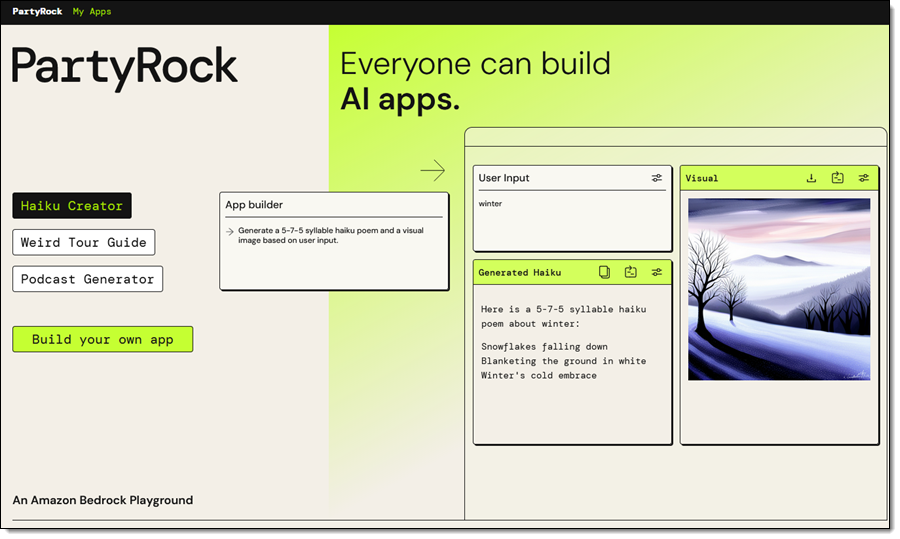
I can enter a description of the app that I want to build and use PartyRock’s Generative AI to get a running start, or I can built it myself on a widget-by-widget basis:
I am knee-deep in blog posts for AWS re:Invent right now. While most of my colleagues patiently wait for their draft to be ready, a few of them are impatient and keep asking me (this is the adult version of “Are we there yet?”). While I try to maintain a sense of humor about this, I sometimes get just a bit snarky with them. Let’s see if PartyRock can help. I enter my prompt and click Generate App:
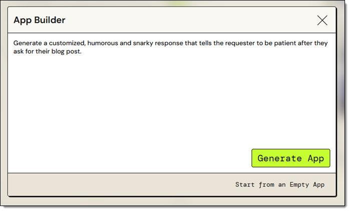
My app (Snarky Patient Blogger) is ready within a few seconds, and I enter some input to see if the output has sufficient snark for my needs:
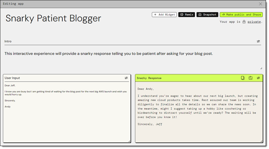
That looks great, so let’s take it apart and see how it works!
The application (Snarky Patient Blogger) has two widgets: User Input and Snarky Response. I click the Edit icon on the first widget, and see that it has a title, loading text, and a default value. The title allows widgets to reference each other by name:

This simple widget encapsulates a call to the Amazon Bedrock InvokeModel function. The widget specifies the use of the Claude v2 model, and a simple prompt, which references the User Input widget. I can experiment by changing either one, saving the change, and waiting a second or two for the result. For example, changing the model to Claude Instant gives me a slightly different response:
Now I want a visual representation of the reply. I’ll use a Text Generation widget to find the most important nouns in the response, and an Image Generation widget to visualize the results. I add the first widget and use a simple prompt:
I test it by clicking the Retry icon and the output looks perfect:
I add the Image Generation widget, and fiddle with the prompt a bit. After a minute or two I have what I want:
The finished app looks like this:
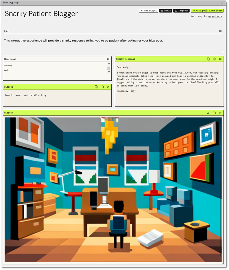
Once I am happy with the app, I can Make public and Share:
The finished app is at https://partyrock.aws/u/jeffbarr/E-FXPUkO7/Snarky-Patient-Blogger and you are welcome to play with it. You can also log in and click Remix to use it as the starting point for an even better app of your own.
But Wait, There’s More
As is usually the case with my blog posts, I did not have room to show you every last feature in detail. Here are a few that I skipped:
Empty App – I used the App Builder in my example, but I can also choose Start from an Empty App, select my widgets, and set them up as desired:
Remix – I can start with an existing app (mine or another public one) and Remix it to customize or enhance it:
Chatbot Widget – I can interact with my app using a prompt as a starting point:
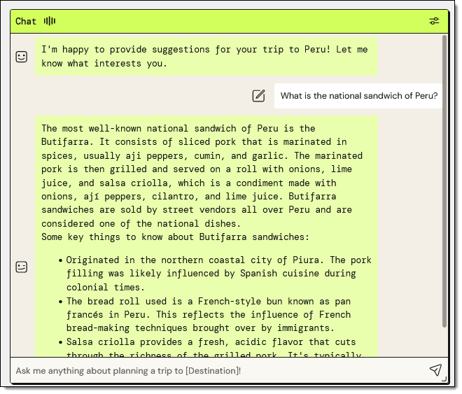
@ Referencing – I can use the “@” to reference other widgets by name while I am building my app:
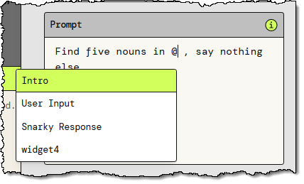
Advanced Settings – Some of the widgets offer advanced settings. For example, the Text Generation widget gives me the option to control the Temperature and Top P parameters to the model:
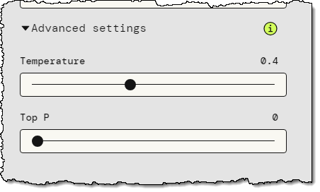
Backstage – The PartyRock Backstage lets me see my apps and my cumulative consumption of PartyRock credits:

Things to Know
Here are a couple of things that you should know about PartyRock:
Pricing – For a limited time, AWS offers new PartyRock users a free trial without the need to provide a credit card or sign up for an AWS account, so that you can begin learning fundamental skills without the worry of incurring costs. You can track your credit consumption in the Backstage, as shown above. Credit usage is calculated based on your input tokens, output tokens, and generated images; for full details read the Billing and Support section of the PartyRock FAQ.
Model Access – We plan to give you access to additional models over time.
In the Works – We are working on even more widgets and features, so stay tuned for more information.
Learning Resources – To learn more, check out these resources:
Party Time
The next step is up to you. Log in to PartyRock, create something cool, and share it with everyone you know. Let me know what you come up with!
— Jeff;
Post Syndicated from Yev original https://www.backblaze.com/blog/holiday-gift-guide-2023/

The holidays are fast approaching and with them the many cyber sales that provide both inspiration and opportunity for gift giving on any budget. To help narrow the field, every year I ask my fellow Backblazers to submit the gifts that they are looking forward to both gifting and receiving. (Hopefully some of their loved ones read the blog?) And of course, I’ve sprinkled in a few of my favorites as well. Without further ado, here’s what we suggest looking into for your 2023 gift giving!

This little thing is pretty neat. It helps you keep track of your health, tracking everything from sleep to stress levels. It lasts for a week on a single charge, and is super easy on the eyes, so you’ll want to wear it all over the place.

We have a lot of hikers, joggers, and runners at Backblaze and, as firm believers in thinking about your backup options before a disaster, the Garmin is an awesome-to-have trail buddy.

While a cocktail shaker is a pretty common household item, this one is sure to impress. Ask questions like, “Could my drink possibly get any colder and stay that way?” and “Can I customize my shaker with a sticker of my cat’s face?” And the Yeti’s answer is yes. Also, you know we love when a product comes in red.

Wine anyone? If you or someone in your life is a big wino, older wines are a delicious treat, with a potentially fatal stumbling block: old, crumbly corks. The Durand corkscrew helps take them out with no breakage.

Another one for winos, the Coravin is an incredible wine system that uses tiny needles and argon gas to pour wine into your glass without having to actually open it. I can personally vouch for this one as a single human who has nice wine bottles and often wants a single glass once or twice a week.

Tea time is a dreamy time and this matcha set allows you to make yourself a traditional cup. And if you need some matcha powder for it, this one comes high comes highly recommended: Organic Ceremonial Grade Matcha Powder.

Tea and coffee at a campsite are a must-have, and if you’ve never tried a Jet Boil, this model is easy to use. Also helpful for those times where you lose power and need to make some hot water in a hurry.

Foodies know and love the sous vide method, a.k.a. low temperature, long time (LTLT). If you’re into cooking your food in a hot tub, you’ll be happy to know that this accessory has come down in price dramatically over time. We like this version of a kitchen appliance, but there is certainly a wide world of sous vide gadgets out there if you’re interested.

Pizza night gets fancier with this pizza oven that can make you a Neapolitan style pizza in less than five minutes. You gotta love that efficiency.

Love fancy foods but can’t travel to get them? Goldbelly has become the go-to for nationwide delivery of local favorites, and they now do meal kits as well. We’re not going to say you should give up on your standard, probably nutritionally balanced Hello Freshes of the world, but we will say that these are a whole lot more, well, iconic.

Have your own mini-garden whether you’re in a house or an apartment. With just a little bit of counter space, a semi-green thumb, some patience, and water, you’ll never have herbs go bad in your fridge again.

Not since the times of the Game Boy Advance or maybe the Nintendo 3DS have handheld gaming systems seen such a rise in popularity. Along with the Nintendo Switch, these three handhelds bring the power of a computer to your fingertips on the go. While it’s not quite a gaming rig, it’s good enough for most airline flights, and hey…they’ll all play Baldur’s Gate 3.
It’s a great time to be a nerd. Critical Role, Dimension 20, The Adventure Zone, and many more role playing games (RPGs) are super popular nowadays, and it’s high time you take part. Get the D&D starter kit, some dice, and your soon-to-be best friends, create your character and get rolling.

Backblaze is based in California, but that doesn’t mean that we don’t know about weather. (What’s this wet stuff falling from the sky again?) That said, as a Midwesterner by heritage (dontcha know), I know something about staying warm. Heated clothes take the benefits of your favorite heated blanket and give them to you on the go.

Camping? Walking? Freezing? How about a sleeping bag that you can walk in, eh?

We’re all about being good community members, and this local (to us) company makes hats, fanny packs, and bomber jackets using environmentally friendly materials. They’re good products, in more ways than one.

Studies have shown that meditation has measurable benefits for your mind and body. There are a plethora of tools out there to help you build good habits (see below), but this one is stinkin’ cute. Let this little guy help visually take you through a guided meditation. Bonus: it’s a great gift for kids, too.
The Calm app helps people stay mindful with everything from guided meditation to celebrity-read stories. We’re big fans of their social posts that just encourage you to take a 15 second break—it’s a positive interruption to the doomscroll effect, and a great way to preview some of the app’s content.

A twist on photo frames: you can send pictures to it and have all of your favorite memories staring back at you when you look over. Or, send photos to anyone, anywhere. Definitely some potential prank opportunities to be had; but it’s also a great way to keep in touch with far-flung family members.

Sonos surround systems are a great addition to homes. Multiple speakers can sync up to make sure that you’re never far away from rocking out to Weird Al, no matter where you are in the house.

Music’s always better with light shows and this lightbox from Ikea matches beats and keeps things groovy. Yet another reason to love Ikea!

For the audiophiles in your life, the AirPods Max are the over-the-ear variant of the traditional AirPod. They’re much harder to lose, giving you that impressive combo of sound and noise cancellation you’ve come to expect.

To balance the scales for our Android lovers, here are Google’s in-ear buds. They have a lot of bells and whistles including noise cancellation and built-in Android Assistant. Now when you talk to yourself, someone will answer. (That’s a good thing right?).

LEGO is having a bit of a moment (at least in my family) and we have spent a lot of time building complicated models. For the adults in your life that love to tinker, we recommend some of these cool sets!
LEGO Sanderson Sisters’ Cottage
And, of course, we’d be remiss if we didn’t remind you that Backblaze Computer Backup makes a great gift. Help your family and friends experience the sweet, sweet peace of mind that comes from a good backup strategy and make sure they never lose a file again. Bonus: you don’t even have to go to the store to get it.

We hope this guide sparked some ideas and simplified some choices. We’ll also be publishing our second-annual book guide in December if you’re struggling with something for the literary folks in your life. (There’s some good stuff in the first one too.) We love hearing about what folks are excited about, so feel free to give us some more good options in the comments below.
The post Holiday Gift Guide 2023 appeared first on Backblaze Blog | Cloud Storage & Cloud Backup.
Post Syndicated from BeardedTinker original https://www.youtube.com/watch?v=iFkobVE6s7o