Manage your Amazon QuickSight datasets more efficiently with the new user interface

Post Syndicated from Arturo Duarte original https://aws.amazon.com/blogs/big-data/manage-your-amazon-quicksight-datasets-more-efficiently-with-the-new-user-interface/

Amazon QuickSight has launched a new user interface for dataset management. Previously, the dataset management experience was a popup dialog modal with limited space, and all functionality was displayed in this one small modal. The new dataset management experience replaces the existing popup dialog with a full-page experience, providing a clearer breakdown of a dataset’s properties.

In this post, we walk through the end-to-end dataset management user experience.

Access the new UI

To get started, choose Datasets in the navigation pane on the QuickSight console, and choose any dataset that you want to manage.
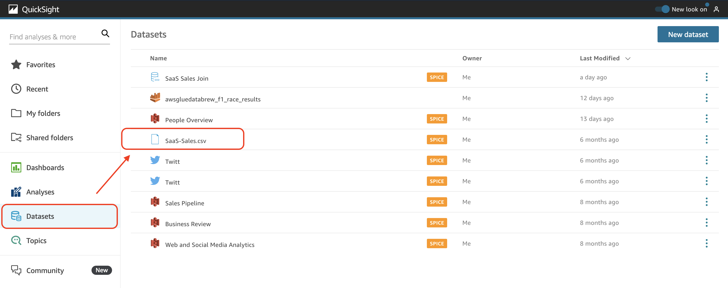
When you choose a dataset, you see the full-page dataset management UI. This new UI is divided into four main tabs: Summary, Refresh, Permissions, and Usage.
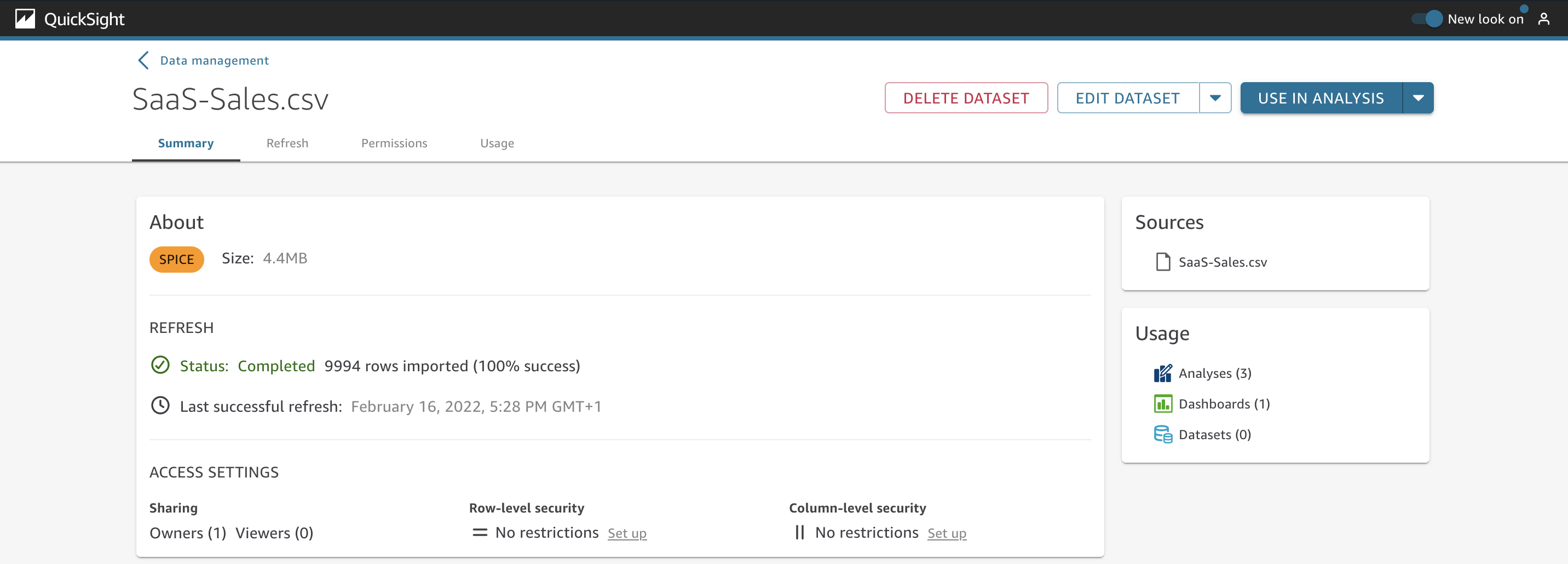
Use case overview

Let’s consider a fictional company, AnyCompany. They have used QuickSight for a long time and now have a large number of datasets that have to be managed. Among the datasets they use, they have a combination of Direct Query and SPICE modes. They need a unified view of each dataset, with details related to permissions, refreshes, and usage. Additionally, they need to be able to schedule when they want to refresh the data and have a history of all the successful and failed attempts of these updates.

The Summary tab

As a data analyst at AnyCompany, you need to review details about your datasets. You can find several options by navigating to the Summary tab.

The About section shows if the dataset is stored in SPICE or if it’s using Direct Query. If the dataset is stored in SPICE, you can also get the size of the dataset. If the dataset is using Direct Query, you can choose Set alert schedule to setup a schedule for when alerts on dashboards should be evaluated.
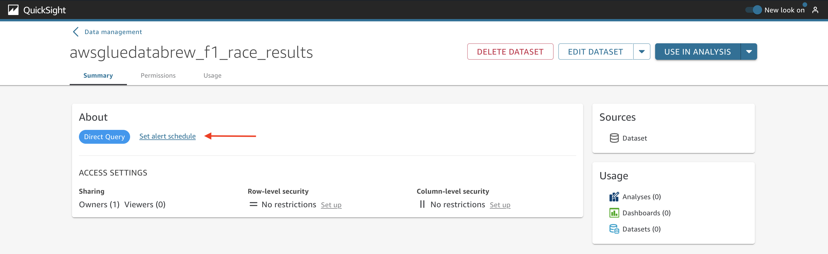
Specify the time zone, if you want to repeat it daily or hourly, and the start time.

To continue exploring the dataset, choose a new dataset that is stored in SPICE. In the Refresh section, you can verify the status of the SPICE dataset and the last successful refresh date.

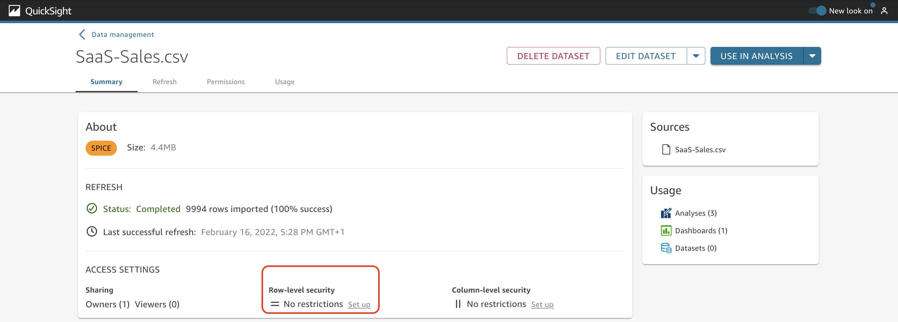
Under Access Settings, you can see details about how many owners and viewers this dataset has and also the options to enable row-level and column-level security.

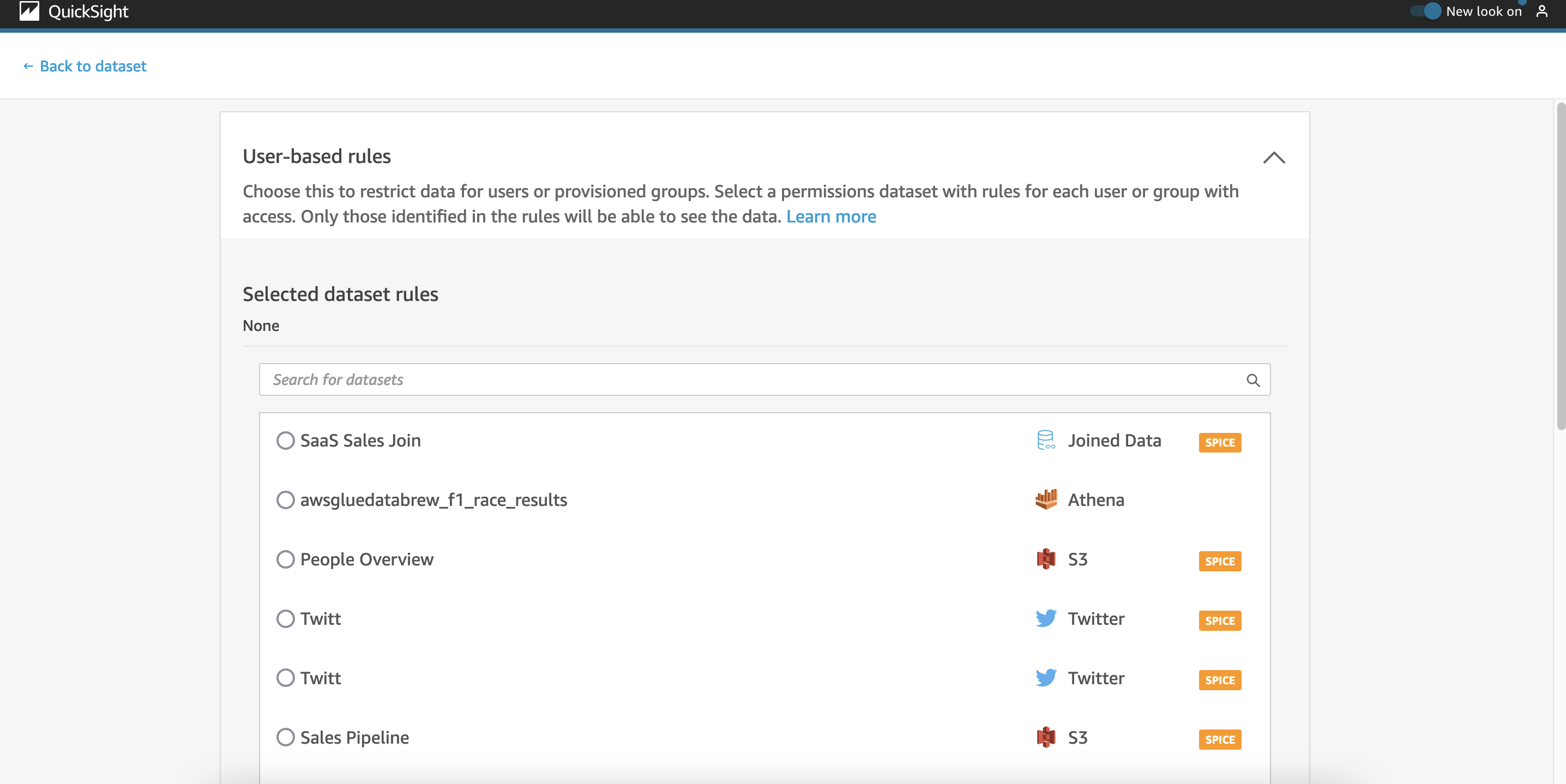
To add row-level security to this dataset, choose Set up under Row-level security.
Under User-based rules, select the permissions dataset with rules to restrict access for each user or group.
To apply column-level security, choose Set up under Column-level security.
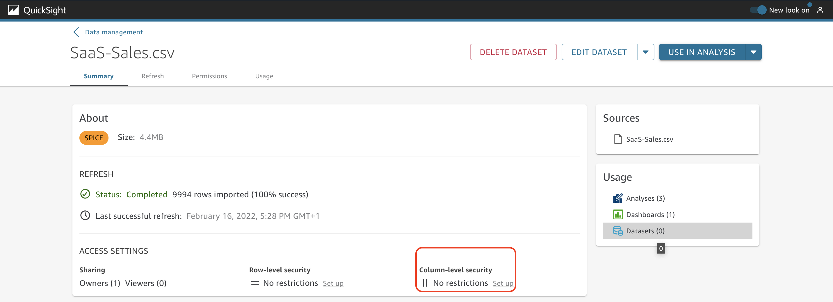
Select the columns to be restricted and choose Next.
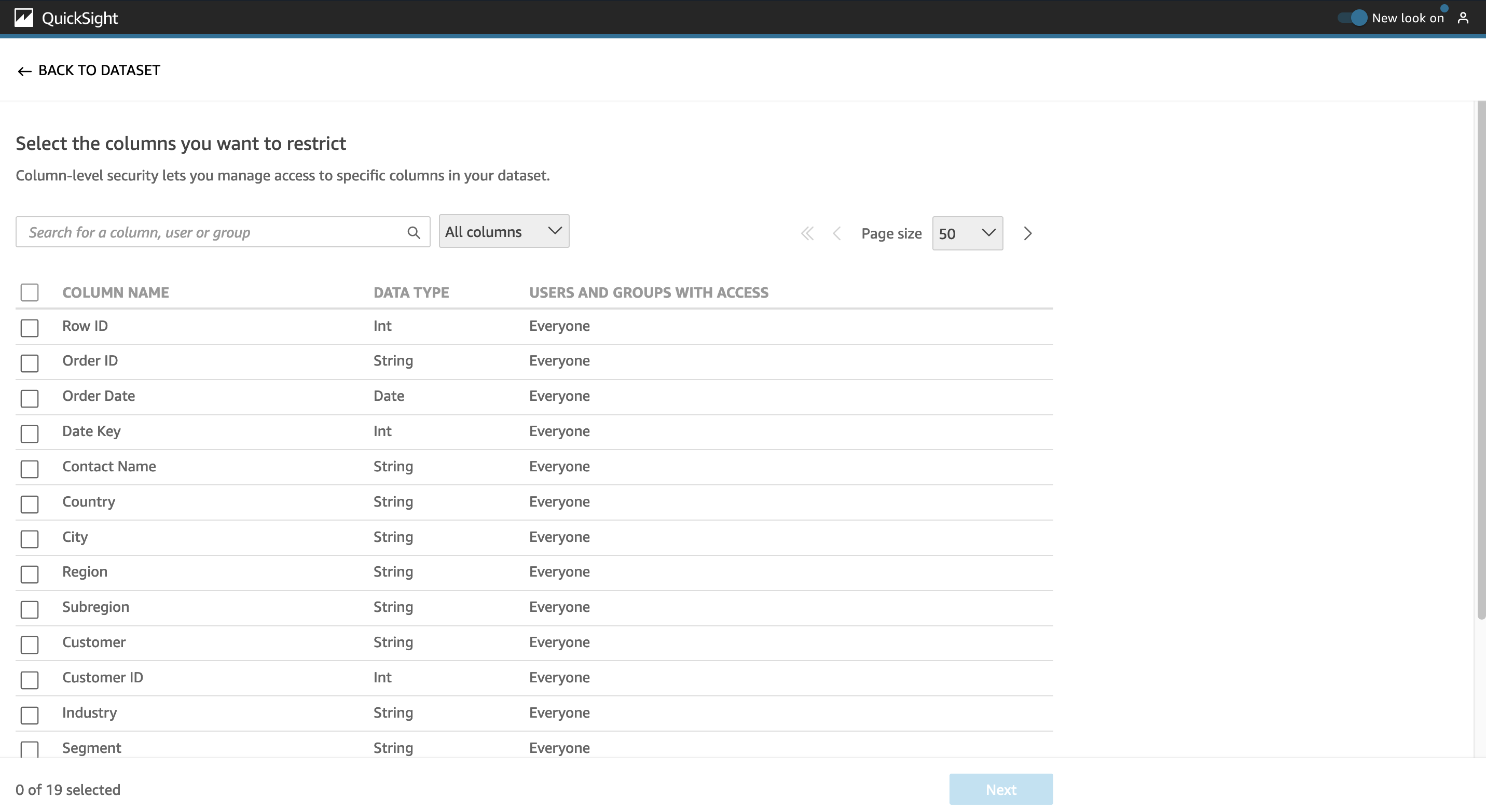
Choose who can access the restricted columns and choose Apply.
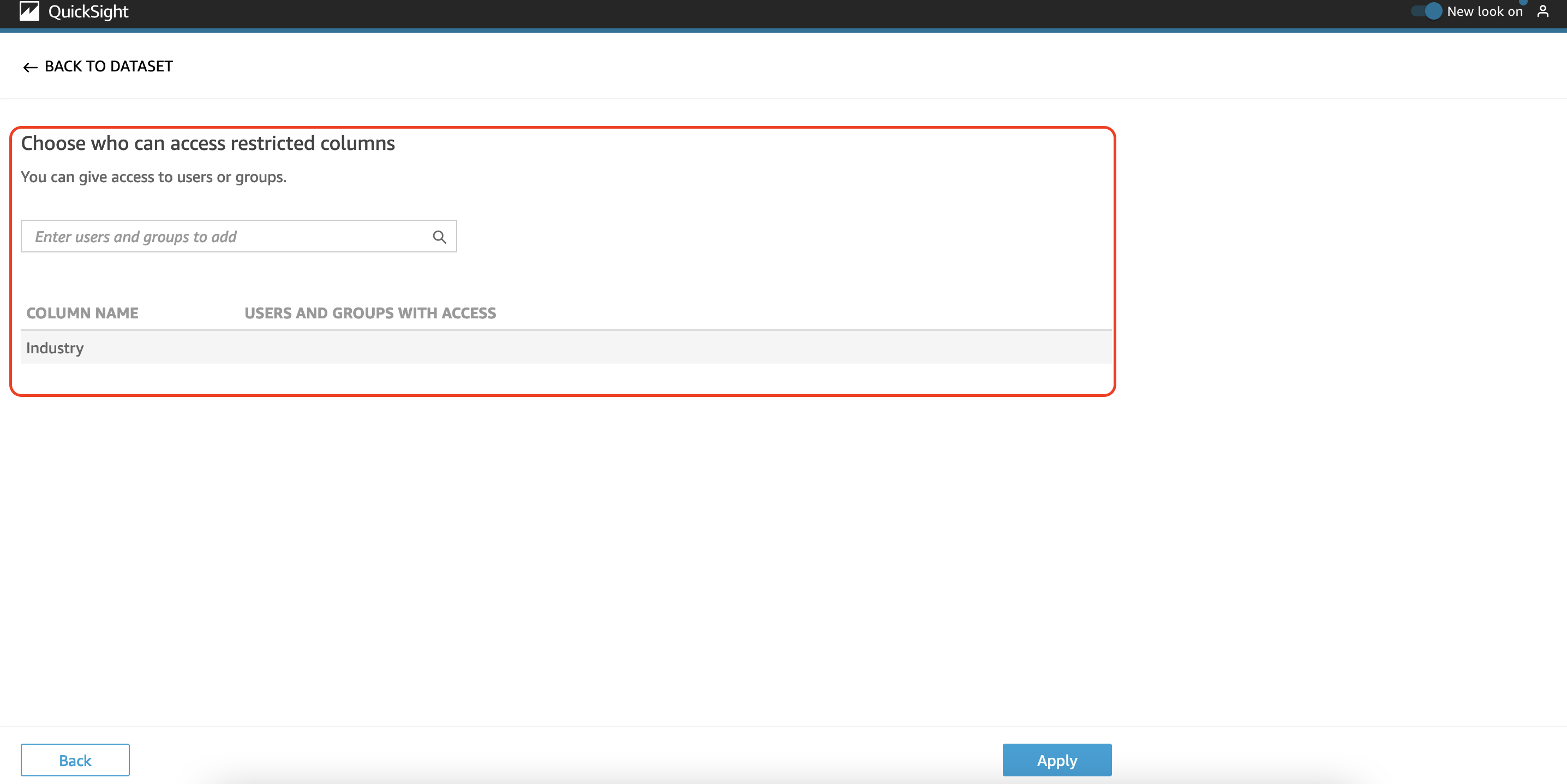
In the Sources section on the Summary tab, a list of data sources is displayed to show the ones used in this dataset. In the following example, we can see the sources SaaS Sales 2022.csv and SaaS-Sales-MonthlySummary.
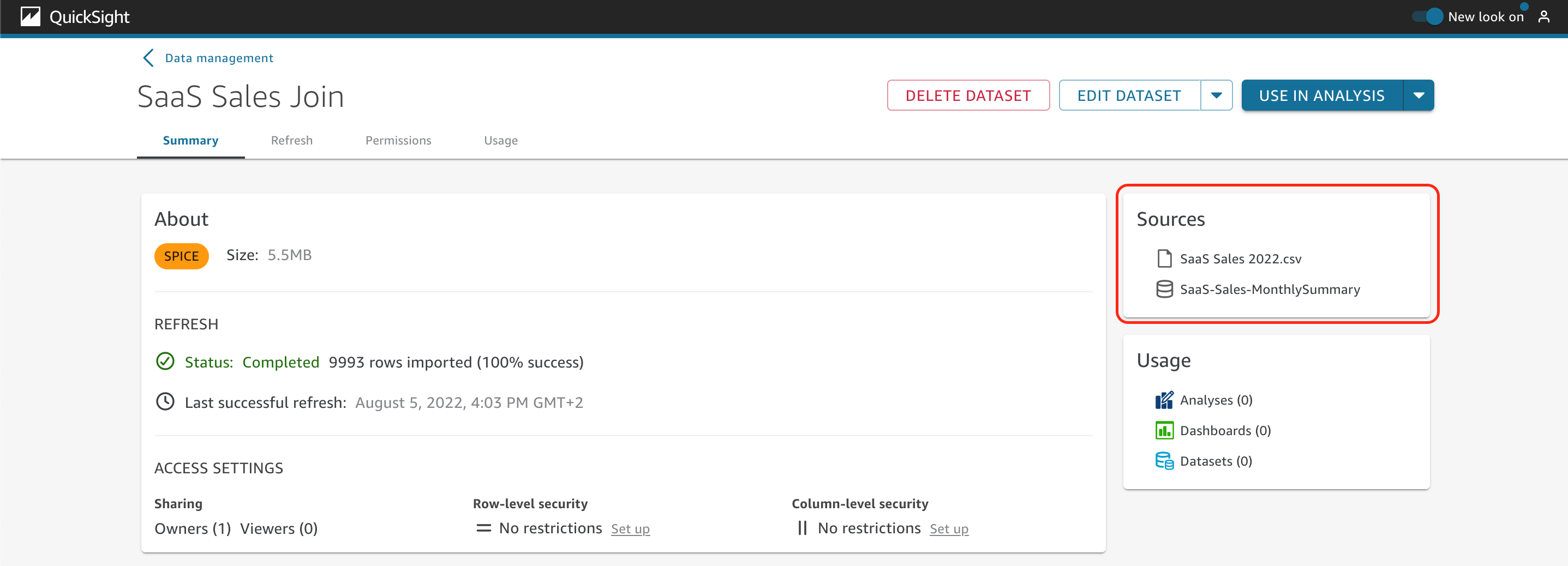
You also need to identify where (analysis, dashboards, or other datasets) the different datasets are being used, to determine if you can eliminate some unused ones.

To verify this, you just have to look at the Usage section (more details are on the Usage tab).
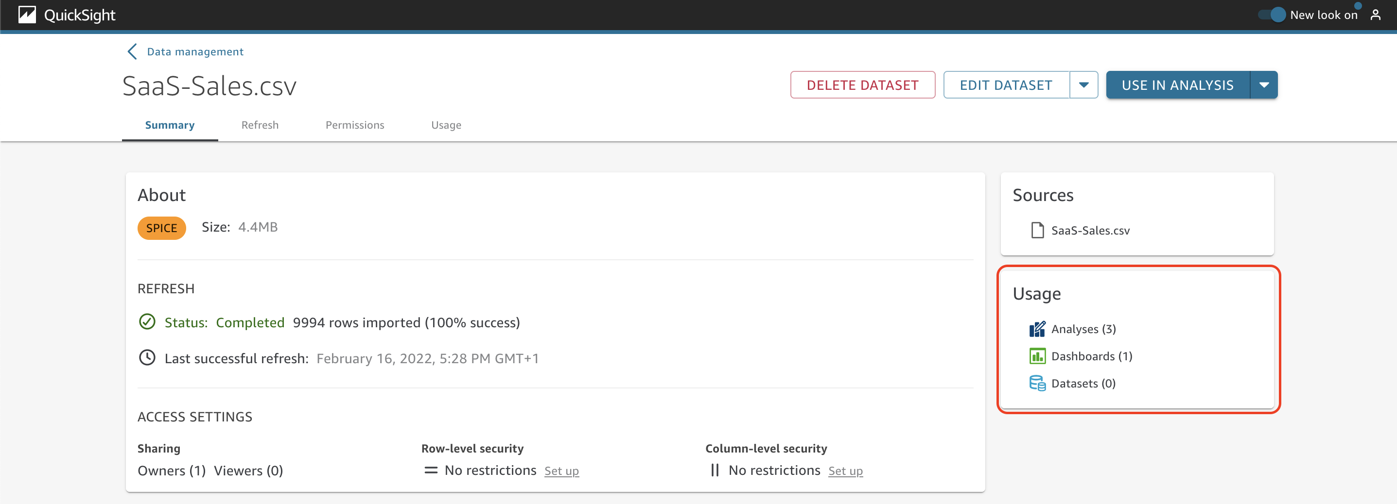
It’s also possible to go to the data prep interface by choosing Edit dataset or duplicate it by opening the drop-down menu.

You can also directly create a new analysis with this dataset or choose Use in dataset to take advantage of dataset as a source capability. When you use this option, any data preparation that the parent dataset contains, such as any joins or calculated fields, is kept. You can add additional preparation to the data in the new, child datasets, such as joining new data and filtering data. You can also set up your own data refresh schedule for the child dataset and track the dashboards and analyses that use it. Some of the advantages are: Central management of datasets, reduction of dataset management, predefined key metrics and flexibility to customize data.

The Refresh tab

At AnyCompany, you also need to refresh the latest data for your datasets. To achieve this, you have two different options.

You can choose Refresh now to manually get the latest records in the dataset.
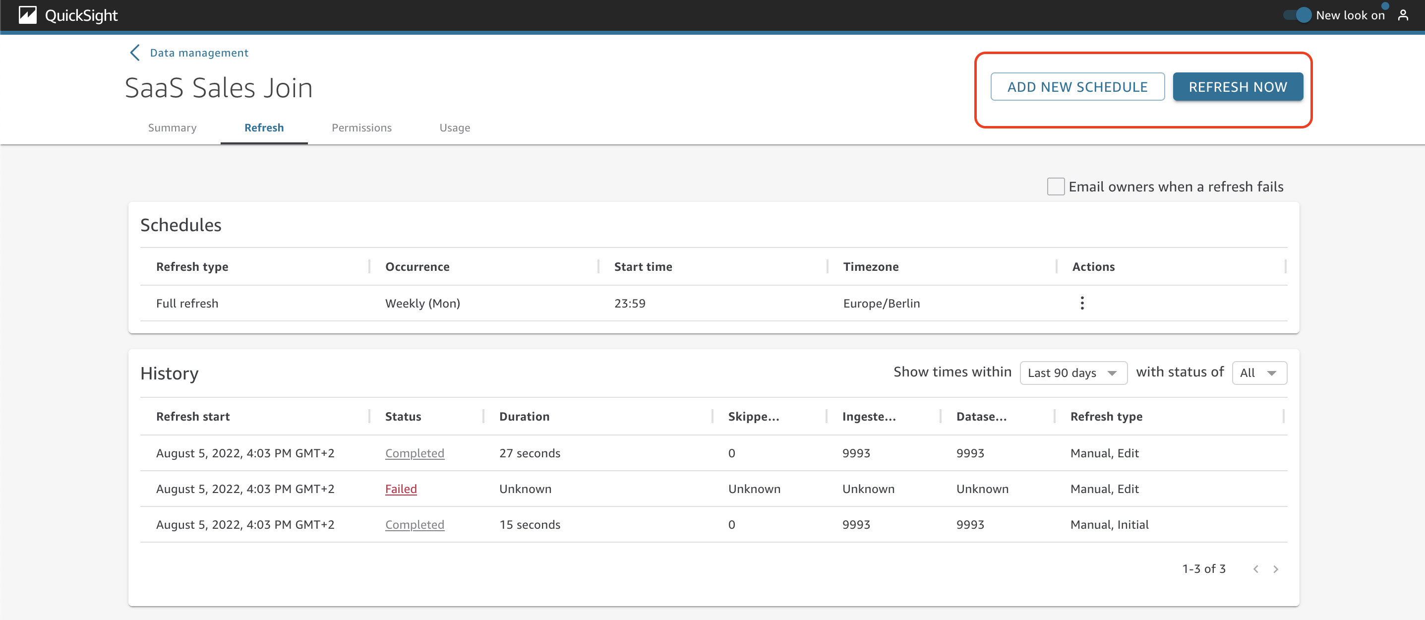
You can also choose Add new schedule to create a refresh schedule and not worry about running it manually in the future. You can set the time zone, start time, and frequency.
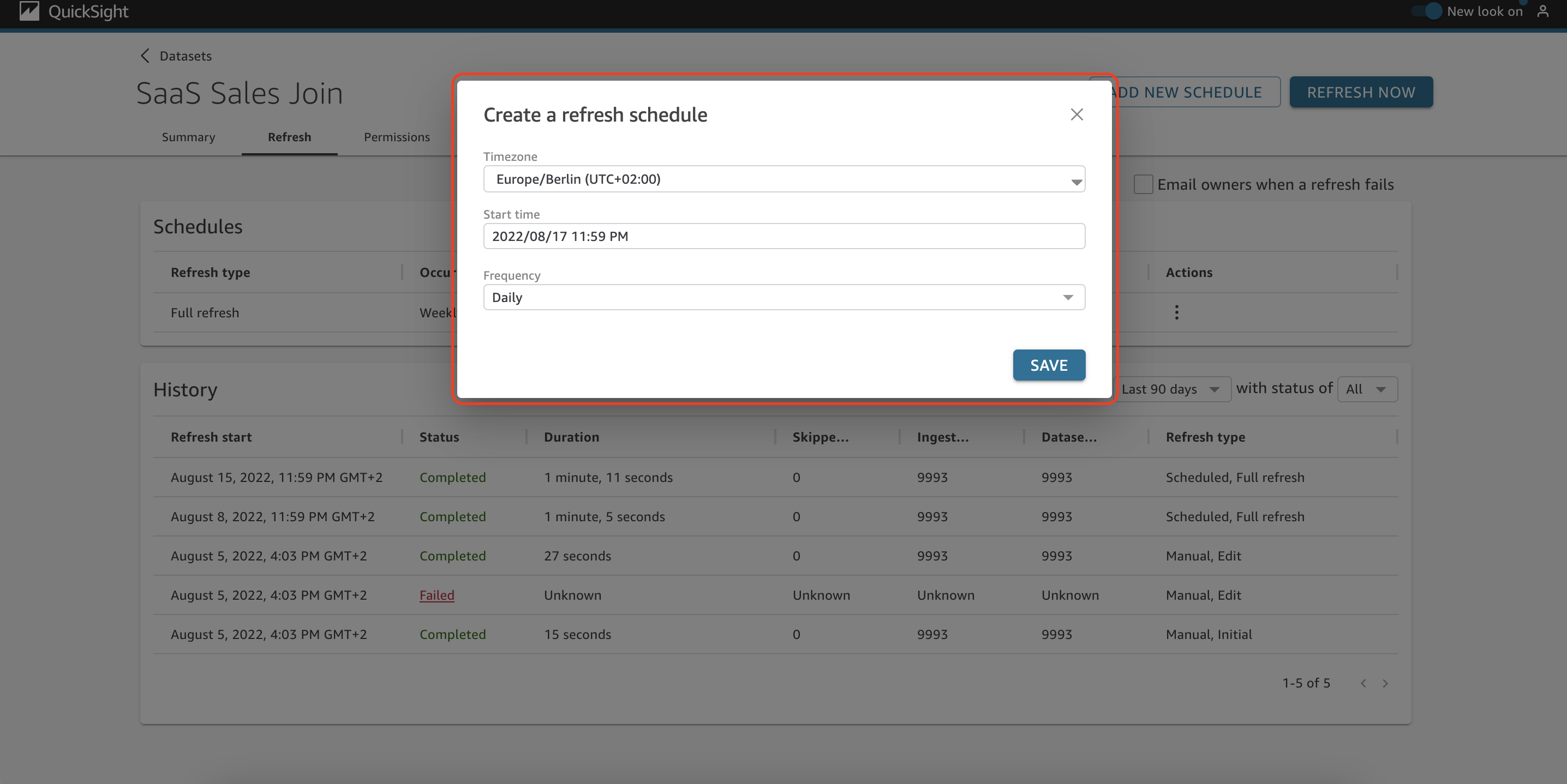
There are two types of scheduled refresh: full refresh and incremental refresh. Full refresh will completely reload the whole dataset, while incremental refresh only updates a specified small portion of your dataset. Using incremental refresh enables you to access the most recent insights much sooner.

In order to setup the incremental refresh, you need to perform the following actions:

  1. Choose Refresh Now.
  2. For Refresh type, choose Incremental refresh.
  3. If this is your first incremental refresh on the dataset, choose Configure.
  4. On the Configure incremental refresh page, do the following:
    1. For Date column, choose a date column that you want to base the look-back window on.
    2. For Window size, enter a number for size, and then choose an amount of time that you want to look back for changes.You can choose to refresh changes to the data that occurred within a specified number of hours, days, or weeks from now. For example, you can choose to refresh changes to the data that occurred within two weeks of the current date.
  5. Choose Submit.

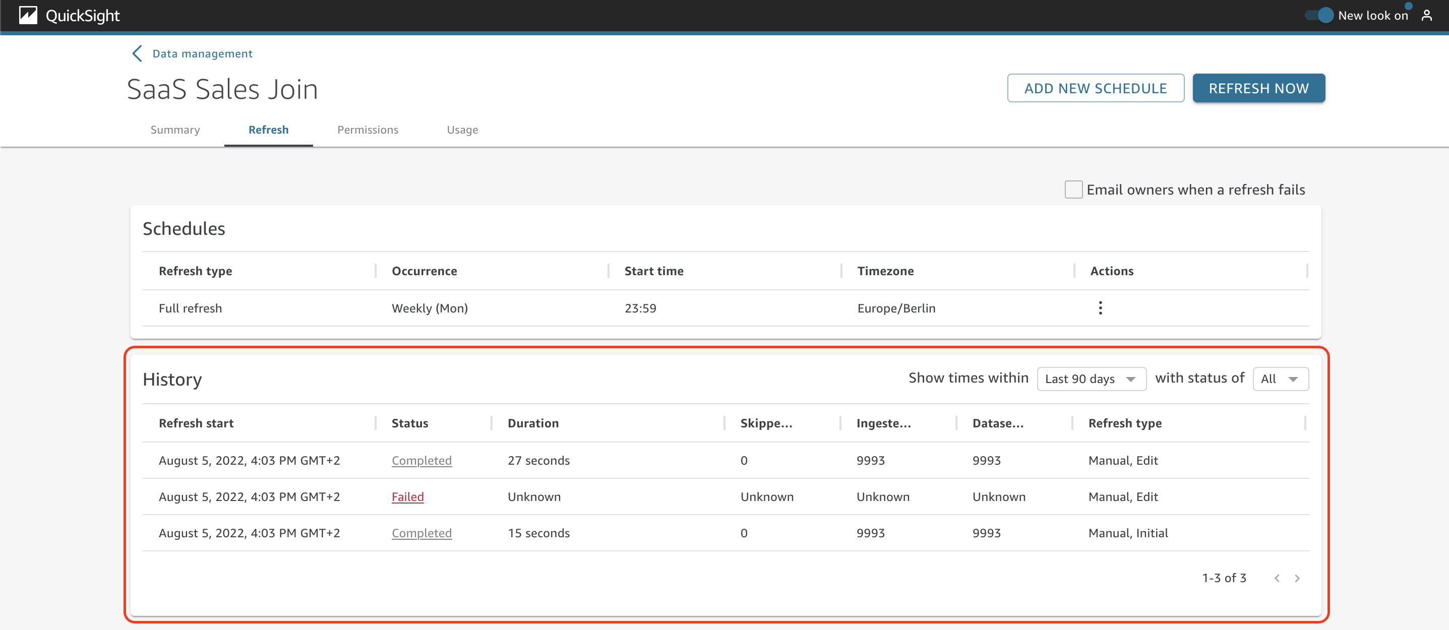
There are two main sections on the Refresh tab: Schedules and History. Under Schedules, you can see details about the scheduled refreshes of the dataset. There is also the option to edit and delete the schedule.
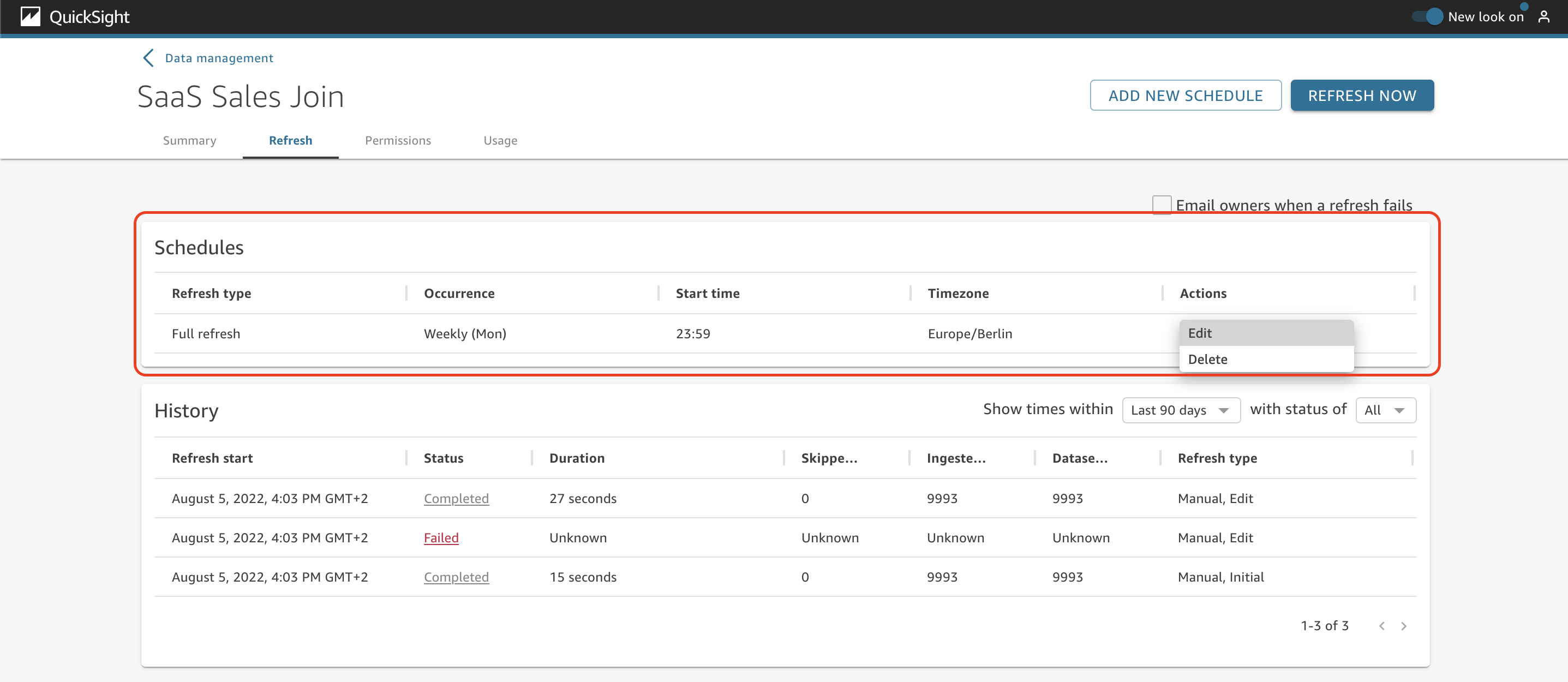
In the History section, you can see details about the past refreshes, such as status, duration, skipped rows, ingested rows, dataset rows, and refresh type.
The Permissions tab

On the Permissions tab, you can manage the settings and permissions for users and groups that access the dataset.

As the dataset owner at AnyCompany, you need to manage access to the datasets and add users and groups. To do so, simply choose Add users & groups.
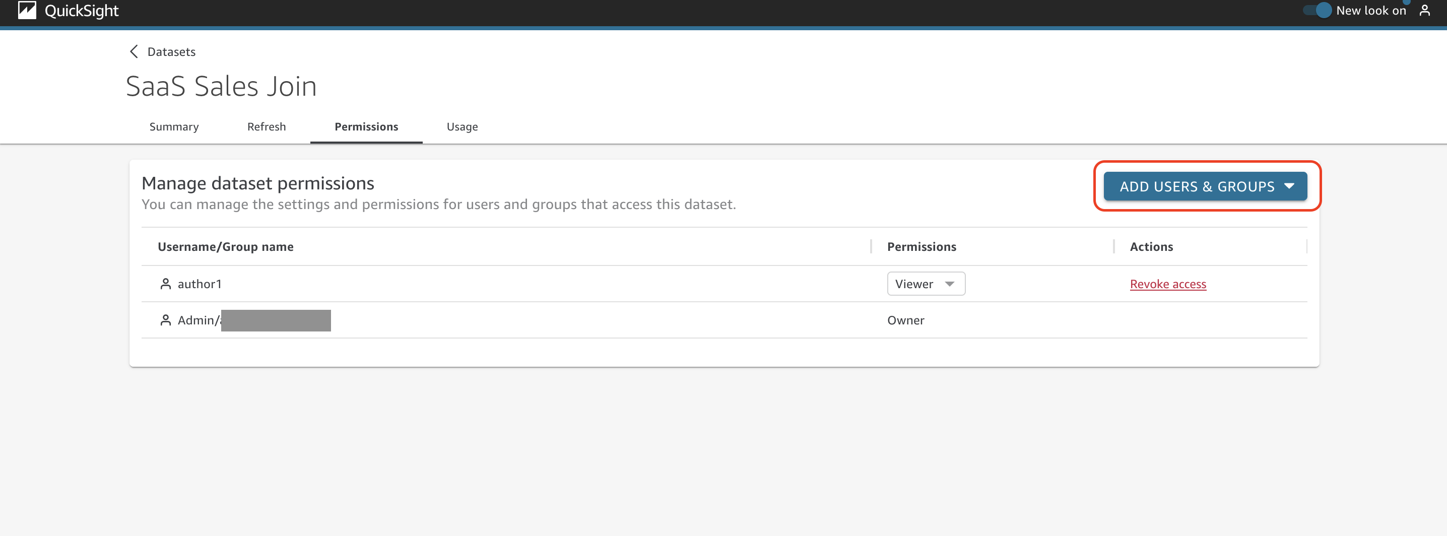
Choose the specific user or group to provide access to this dataset.

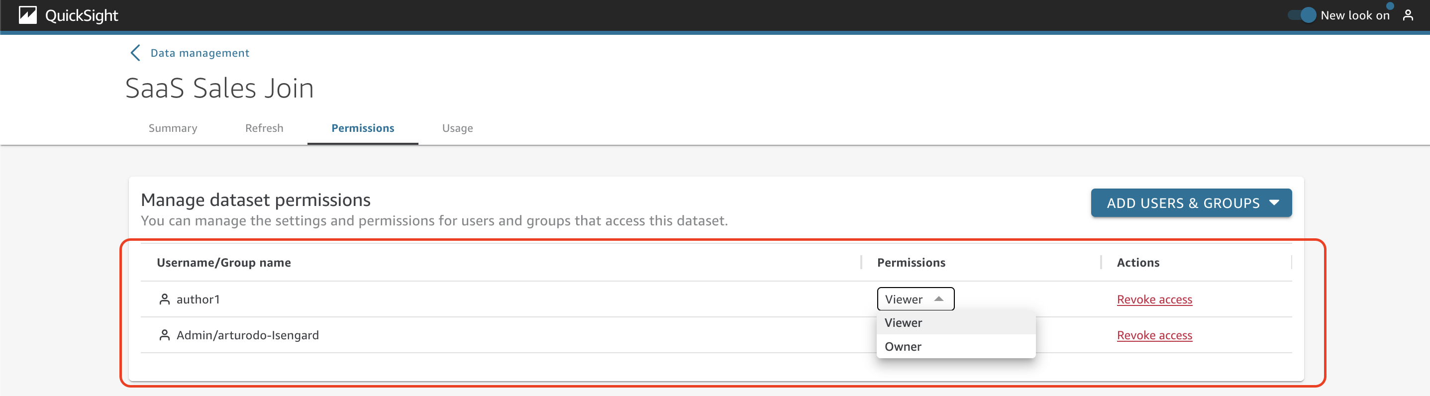
Review the list of users and groups that have access to the dataset as well as the level of permission (viewer or owner). You can also revoke access to the users or groups.
The Usage tab

It’s not always easy for AnyCompany to determine whether or not a dataset is being used by users or in other assets such as analyses or dashboards.

To answer this kind of question, you can easily review the information on the Usage tab. Here you can review the list of analyses and dashboards where the dataset is being used (choose the name of an analysis or dashboard to view the actual asset).
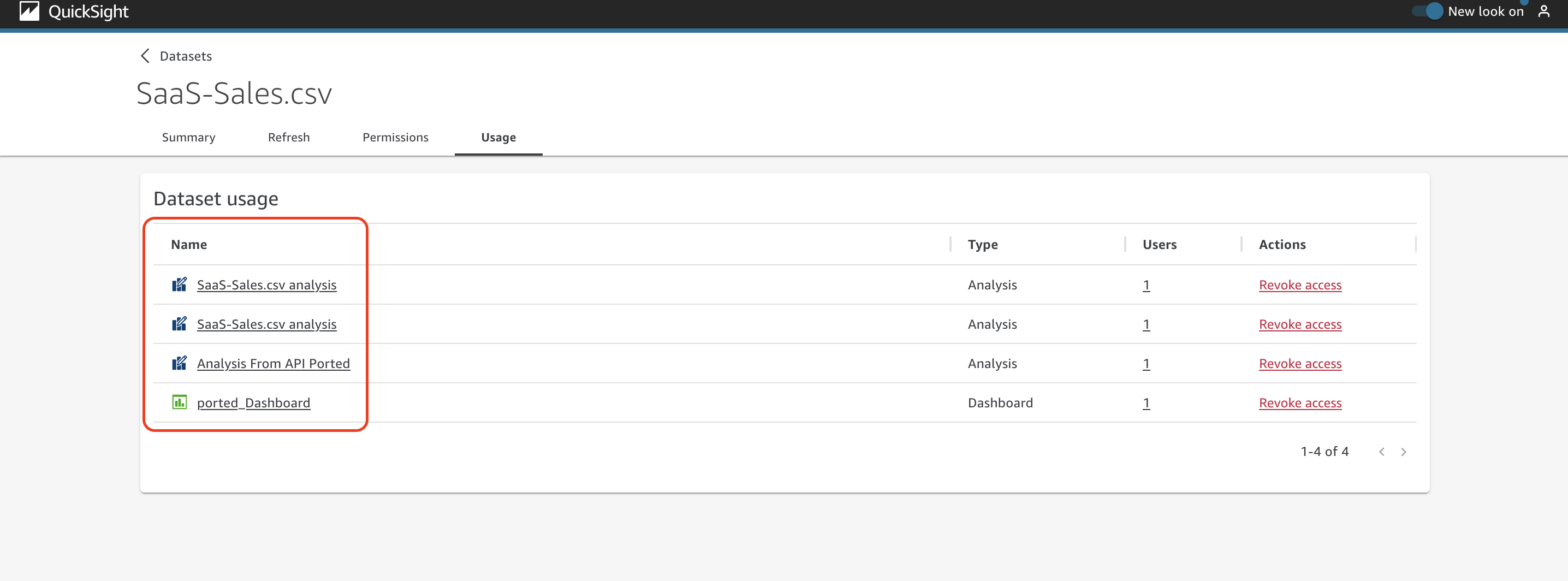
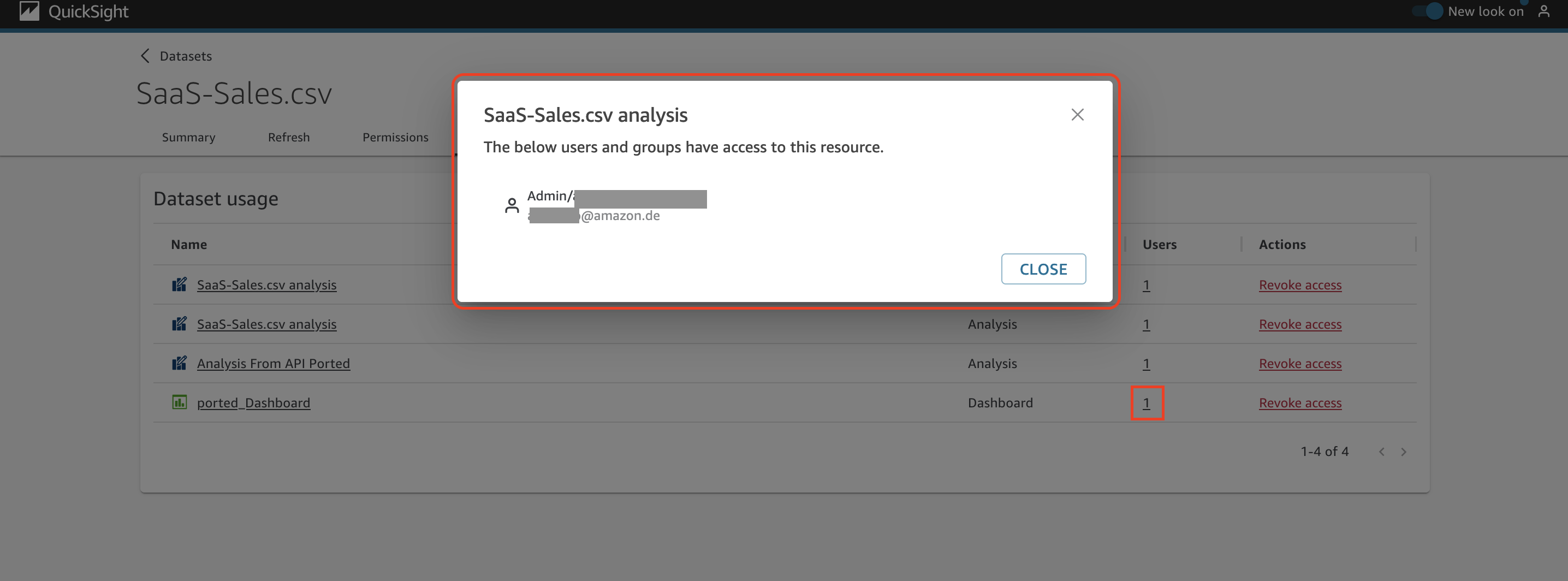
Under the Users column, you can get the details about who is using this analysis or dashboard.
Conclusion

In this post, we introduced the new user interface of the dataset management page on the QuickSight console. This new user interface simplifies the administration and use of datasets by having everything organized and centralized. This will primarily help authors and administrators quickly manage their datasets, while also contributing to a better QuickSight navigation experience. The new user interface is now generally available in all supported QuickSight Regions.

We look forward to your feedback and stories on how you use the new dataset management interface for your business needs.


About the Authors

Arturo Duarte is a Partner Solutions Architect focused on Amazon QuickSight at Amazon Web Services. He works with EMEA APN Partners to help develop their data and analytics practices with enterprise and mission-critical solutions for their end customers.

Emily Zhu is a Senior Product Manager at Amazon QuickSight, AWS’s cloud-native, fully managed SaaS BI service. She leads the development of the QuickSight analytics and query capability. Before joining AWS, she worked in the Amazon Prime Air drone delivery program and the Boeing company as senior strategist for several years. Emily is passionate about the potential of cloud-based BI solutions and looks forward to helping customers advance in their data-driven strategy making.

Automate data archival for Amazon Redshift time series tables

Post Syndicated from Nita Shah original https://aws.amazon.com/blogs/big-data/automate-data-archival-for-amazon-redshift-time-series-tables/

Amazon Redshift is a fast, scalable, secure, and fully managed cloud data warehouse that makes it simple and cost-effective to analyze all of your data using standard SQL. Tens of thousands of customers today rely on Amazon Redshift to analyze exabytes of data and run complex analytical queries, making it the most widely used cloud data warehouse. You can run and scale analytics in seconds on all your data without having to manage your data warehouse infrastructure.

A data retention policy is part of an organization’s overall data management. In a big data world, the size of data is consistently increasing, which directly affects the cost of storing the data in data stores. It’s necessary to keep optimizing your data in data warehouses for consistent performance, reliability, and cost control. It’s crucial to define how long an organization needs to hold on to specific data, and if data that is no longer needed should be archived or deleted. The frequency of data archival depends on the relevance of the data with respect to your business or legal needs.

Data archiving is the process of moving data that is no longer actively used in a data warehouse to a separate storage device for long-term retention. Archive data consists of older data that is still important to the organization and may be needed for future reference, as well as data that must be retained for regulatory compliance.

Data purging is the process of freeing up space in the database or deleting obsolete data that isn’t required by the business. The purging process can be based on the data retention policy, which is defined by the data owner or business need.

This post walks you through the process of how to automate data archival and purging of Amazon Redshift time series tables. Time series tables retain data for a certain period of time (days, months, quarters, or years) and need data to be purged regularly to maintain the rolling data to be analyzed by end-users.

Solution overview

The following diagram illustrates our solution architecture.

We use two database tables as part of this solution.

The arch_table_metadata database table stores the metadata for all the tables that need to be archived and purged. You need to add rows into this table that you want to archive and purge. The arch_table_metadata table contains the following columns.

ColumnName Description
id Database-generated, automatically assigns a unique value to each record.
schema_name Name of the database schema of the table.
table_name Name of the table to be archived and purged.
column_name Name of the date column that is used to identify records to be archived and purged.
s3_uri Amazon S3 location where the data will be archived.
retention_days Number of days the data will be retained for the table. Default is 90 days.

The arch_job_log database table stores the run history of stored procedures. Records are added to this table by the stored procedure. It contains the following columns.

ColumnName Description
job_run_id Assigns unique numeric value per stored procedure run.
arch_table_metadata_id Id column value from table arch_table_metadata.
no_of_rows_bfr_delete Number of rows in the table before purging.
no_of_rows_deleted Number of rows deleted by the purge operation.
job_start_time Time in UTC when the stored procedure started.
job_end_time Time in UTC when the stored procedure ended.
job_status Status of the stored procedure run: IN-PROGRESS, COMPLETED, or FAILED.

Prerequisites

For this solution, complete the following prerequisites:

  1. Create an Amazon Redshift provisioned cluster or Amazon Redshift serverless workgroup.
  2. In Amazon Redshift query editor v2 or a compatible SQL editor of your choice, create the tables arch_table_metadata and arch_job_log. Use the following code for the table DDLs:
    create table arch_table_metadata
    (
    id integer identity(0,1) not null, 
    schema_name varchar(100) not null, 
    table_name varchar(100) not null, 
    column_name varchar(100) not null,
    s3_uri varchar(1000) not null,
    retention_days integer default 90
    );
    
    create table arch_job_log
    (
    job_run_id bigint not null, 
    arch_table_metadata_id  integer not null,
    no_of_rows_bfr_delete bigint,
    no_of_rows_deleted bigint,
    table_arch_start_time timestamp default current_timestamp,
    table_arch_end_time timestamp default current_timestamp,
    job_start_time timestamp default current_timestamp,
    job_end_time timestamp default current_timestamp,
    job_status varchar(20)
    );
    

  3. Create the stored procedure sp_archive_data with the following code snippet. The stored procedure takes the AWS Identity and Access Management (IAM) role ARN as an input argument if you’re not using the default IAM role. If you’re using the default IAM role for your Amazon Redshift cluster, you can pass the input parameter as default. For more information, refer to Creating an IAM role as default in Amazon Redshift.
    CREATE OR REPLACE PROCEDURE archive_data_sp(p_iam_role IN varchar(256))
    AS $$
    DECLARE
    
    v_command           varchar(500);
    v_sql               varchar(500);
    v_count_sql         text;
    
    v_table_id          int;
    v_schema_name       text;
    v_table_name        text;
    v_column_name       text;
    v_s3_bucket_url     text;
    v_s3_folder_name_prefix     text;
    v_retention_days            int = 0;
    v_no_of_rows_before_delete  int = 0;
    v_no_of_deleted_rows        int =0;
    v_job_start_time            timestamp;
    v_job_status                int = 1;
    v_job_id                    int =0;
    
    
    table_meta_data_cur CURSOR FOR
    SELECT id, schema_name, table_name, column_name,s3_uri,retention_days
    FROM arch_table_metadata;
    
    BEGIN
    
        SELECT NVL(MAX(job_run_id),0) + 1 INTO v_job_id FROM arch_job_log;
        RAISE NOTICE '%', v_job_id;
    
        OPEN table_meta_data_cur;
        FETCH table_meta_data_cur INTO v_table_id,v_schema_name, v_table_name, v_column_name, v_s3_bucket_url, v_retention_days;
        WHILE v_table_id IS NOT NULL LOOP
    
            v_count_sql = 'SELECT COUNT(*) AS v_no_of_rows_before_delete FROM ' || v_schema_name || '.' || v_table_name;
            RAISE NOTICE '%', v_count_sql;
            EXECUTE v_count_sql INTO v_no_of_rows_before_delete;
            RAISE NOTICE 'v_no_of_rows_before_delete %', v_no_of_rows_before_delete;
    
            v_job_start_time = GETDATE();
            v_s3_folder_name_prefix = v_schema_name || '.' || v_table_name || '/';
            v_sql = 'SELECT * FROM ' || v_schema_name || '.' || v_table_name || ' WHERE ' || v_column_name || ' <= DATEADD(DAY,-' || v_retention_days || ',CURRENT_DATE)';
    
            IF p_iam_role = 'default' THEN
                v_command = 'UNLOAD (''' || v_sql ||  ''') to ''' || v_s3_bucket_url || v_s3_folder_name_prefix || ''' IAM_ROLE default  PARQUET PARTITION BY (' || v_column_name || ') INCLUDE ALLOWOVERWRITE';
            ELSE
                v_command = 'UNLOAD (''' || v_sql ||  ''') to ''' || v_s3_bucket_url || v_s3_folder_name_prefix || ''' IAM_ROLE ''' || p_iam_role || ''' PARQUET PARTITION BY (' || v_column_name || ') INCLUDE ALLOWOVERWRITE';
            END IF;
            RAISE NOTICE '%', v_command;
            EXECUTE v_command;
    
            v_sql := 'DELETE FROM ' || v_schema_name || '.' || v_table_name || ' WHERE ' || v_column_name || ' <= DATEADD(DAY,-' || v_retention_days || ',CURRENT_DATE)';
            RAISE NOTICE '%', v_sql;
            EXECUTE v_sql;
    
            GET DIAGNOSTICS v_no_of_deleted_rows := ROW_COUNT;
            RAISE INFO '# of rows deleted = %', v_no_of_deleted_rows;
    
            v_sql = 'INSERT INTO arch_job_log (job_run_id, arch_table_metadata_id ,no_of_rows_bfr_delete,no_of_rows_deleted,job_start_time,job_end_time,job_status) VALUES ('
                        || v_job_id || ',' || v_table_id || ',' || v_no_of_rows_before_delete || ',' || v_no_of_deleted_rows || ',''' || v_job_start_time || ''',''' || GETDATE() || ''',' || v_job_status || ')';
            RAISE NOTICE '%', v_sql;
            EXECUTE v_sql;
    
            FETCH table_meta_data_cur INTO v_table_id,v_schema_name, v_table_name, v_column_name, v_s3_bucket_url, v_retention_days;
        END LOOP;
        CLOSE table_meta_data_cur;
    
        EXCEPTION
        WHEN OTHERS THEN
            RAISE NOTICE 'Error - % ', SQLERRM;
    END;
    $$ LANGUAGE plpgsql;
    

Archival and purging

For this use case, we use a table called orders, for which we want to archive and purge any records older than the last 30 days.

Use the following DDL to create the table in the Amazon Redshift cluster:

create table orders (
  O_ORDERKEY bigint NOT NULL,
  O_CUSTKEY bigint,
  O_ORDERSTATUS varchar(1),
  O_TOTALPRICE decimal(18,4),
  O_ORDERDATE Date,
  O_ORDERPRIORITY varchar(15),
  O_CLERK varchar(15),
  O_SHIPPRIORITY Integer,
  O_COMMENT varchar(79))
distkey (O_ORDERKEY)
sortkey (O_ORDERDATE);

The O_ORDERDATE column makes it a time series table, which you can use to retain the rolling data for a certain period.

In order to load the data into the orders table using the below COPY command , you would need to have default IAM role attached to your Redshift cluster or replace the default keyword in the COPY command with the arn of the IAM role attached to the Redshift cluster

copy orders from 's3://redshift-immersionday-labs/data/orders/orders.tbl.'
iam_role default
region 'us-west-2' lzop delimiter '|' COMPUPDATE PRESET;

When you query the table, you can see that this data is for 1998. To test this solution, you need to manually update some of the data to the current date by running the following SQL statement:

update orders set O_ORDERDATE = current_date where O_ORDERDATE < '1998-08-02';

The table looks like the following screenshot after running the update statement.

Now let’s run the following SQL to get the count of number of records to be archived and purged:

select count (*) from orders where O_ORDERDATE <= DATEADD(DAY,-30,CURRENT_DATE)

Before running the stored procedure, we need to insert a row into the arch_file_metadata table for the stored procedure to archive and purge records in the orders table. In the following code, provide the Amazon Simple Storage Service (Amazon S3) bucket name where you want to store the archived data:

INSERT INTO arch_table_metadata (schema_name, table_name, column_name, s3_uri, retention_days) VALUES ('public', 'orders', 'O_ORDERDATE', 's3://<your-bucketname>/redshift_data_archival/', 30);

The stored procedure performs the following high-level steps:

  1. Open a cursor to read and loop through the rows in the arch_table_metadata table.
  2. Retrieve the total number of records in the table before purging.
  3. Export and archive the records to be deleted into the Amazon S3 location as specified in the s3_uri column value. Data is partitioned in Amazon S3 based on the column_name field in arch_table_metadata. The stored procedure uses the IAM role passed as input for the UNLOAD operation.
  4. Run the DELETE command to purge the identified records based on the retention_days column value.
  5. Add a record in arch_job_log with the run details.

Now, let’s run the stored procedure via the call statement passing a role ARN as input parameter to verify the data was archived and purged correctly:

call archive_data_sp('arn:aws:iam:<your-account-id>:role/RedshiftRole-7OR1UWVPFI5J');

As shown in the following screenshot, the stored procedure ran successfully.

Now let’s validate the table was purged successfully by running the following SQL:

select count (*) from orders where O_ORDERDATE <= DATEADD(DAY,-30,CURRENT_DATE)

We can navigate to the Amazon S3 location to validate the archival process. The following screenshot shows the data has been archived into the Amazon S3 location specified in the arch_table_metadata table.

Now let’s run the following SQL statement to look at the stored procedure run log entry:

select a.* from arch_job_log a, arch_table_metadata b
where a.arch_table_metadata_id = b.id
and b.table_name = 'orders'

The following screenshot shows the query results.

In this example, we demonstrated how you can set up and validate your Amazon Redshift table archival and purging process.

Schedule the stored procedure

Now that you have learned how to set up and validate your Amazon Redshift tables for archival and purging, you can schedule this process. For instructions on how to schedule a SQL statement using either the AWS Management Console or the AWS Command Line Interface (AWS CLI), refer to Scheduling SQL queries on your Amazon Redshift data warehouse.

Archive data in Amazon S3

As part of this solution, data is archived in an S3 bucket before it’s deleted from the Amazon Redshift table. This helps reduce the storage on the Amazon Redshift cluster and enables you to analyze the data for any ad hoc requests without needing to load back into the cluster. In the stored procedure, the UNLOAD command exports the data to be purged to Amazon S3, partitioned by the date column, which is used to identify the records to purge. To save costs on Amazon S3 storage, you can manage the storage lifecycle with Amazon S3 lifecycle configuration.

Analyze the archived data in Amazon S3 using Amazon Redshift Spectrum

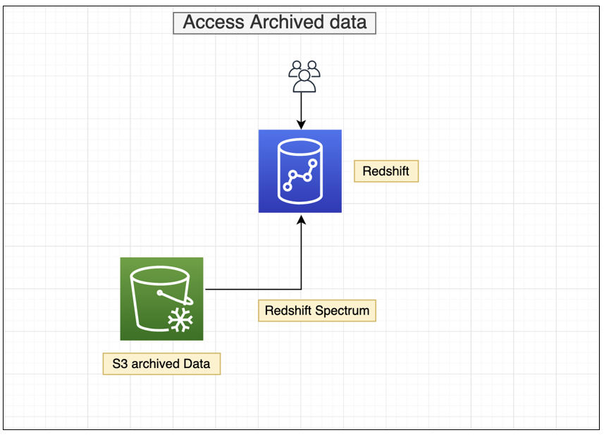
With Amazon Redshift Spectrum, you can efficiently query and retrieve structured and semistructured data from files in Amazon S3, and easily analyze the archived data in Amazon S3 without having to load it back in Amazon Redshift tables. For further analysis of your archived data (cold data) and frequently accessed data (hot data) in the cluster’s local disk, you can run queries joining Amazon S3 archived data with tables that reside on the Amazon Redshift cluster’s local disk. The following diagram illustrates this process.

Let’s take an example where you want to view the number of orders for the last 2 weeks of December 1998, which is archived in Amazon S3. You need to complete the following steps using Redshift Spectrum:

  1. Create an external schema in Amazon Redshift.
  2. Create a late-binding view to refer to the underlying Amazon S3 files with the following query:
    create view vw_orders_hist as select count(*),o_orderdate
    from <external_schema>. orders 
    where o_orderdate between '1998-12-15' and '1998-12-31' group by 2
    with no schema binding;
    

  3. To see a unified view of the orders historical data archived in Amazon S3 and the current data stored in the Amazon Redshift local table, you can use a UNION ALL clause to join the Amazon Redshift orders table and the Redshift Spectrum orders table:
    create view vw_orders_unified as 
    select * from <external_schema>.orders
    union all
    select * from public.orders
    with no schema binding;

To learn more about the best practices for Redshift Spectrum, refer to Best Practices for Amazon Redshift Spectrum.

Best practices

The following are some best practices to reduce your storage footprint and optimize performance of your workloads:

Conclusion

In this post, we demonstrated the automatic archival and purging of data in Amazon Redshift tables to meet your compliance and business requirements, thereby optimizing your application performance and reducing storage costs. As an administrator, you can start working with application data owners to identify retention policies for Amazon Redshift tables to achieve optimal performance, prevent any storage issues specifically for DS2 and DC2 nodes, and reduce overall storage costs.


About the authors

Nita Shah is an Analytics Specialist Solutions Architect at AWS based out of New York. She has been building data warehouse solutions for over 20 years and specializes in Amazon Redshift. She is focused on helping customers design and build enterprise-scale well-architected analytics and decision support platforms.

Ranjan Burman is an Analytics Specialist Solutions Architect at AWS. He specializes in Amazon Redshift and helps customers build scalable analytical solutions. He has more than 15 years of experience in different database and data warehousing technologies. He is passionate about automating and solving customer problems with the use of cloud solutions.


Prathap Thoguru is an Enterprise Solutions Architect at Amazon Web Services. He has over 15 years of experience in the IT industry and is a 9x AWS certified professional. He helps customers migrate their on-premises workloads to the AWS Cloud.

Ekstrand: Introducing NVK

Post Syndicated from original https://lwn.net/Articles/910319/

Jason Ekstrand announces
a new Vulkan driver for NVIDIA hardware
on the Collabora blog. It
seems to be off to a good start, but there is some work yet to do:

Normally, I would have submitted the merge request long ago. There
are far more alpha-quality drivers already in Mesa. The problem is
that we really need a new kernel uAPI to support Vulkan properly
and I don’t want to be stuck supporting the current nouveau uAPI
for the next five years.

“An Ideal Solution”: Daltix’s Automated Data Lake Archive Saves $100K

Post Syndicated from Amrit Singh original https://www.backblaze.com/blog/an-ideal-solution-daltixs-automated-data-lake-archive-saves-100k/

In the fast-moving consumer goods space, Daltix is a pioneer in providing complete, transparent, and high-quality retail data. With global industry leaders like GFK and Unilever depending on their pricing, product, promotion, and location data to build go-to market strategies and make critical decisions, maintaining a reliable data ecosystem is an imperative for Daltix.

As the company has grown since its founding in 2016, the amount of data Daltix is processing has increased exponentially. They’re currently managing around 250TB, but that amount is spread across billions of files, which soon created a massive drag on time and resources. With an infrastructure built almost entirely around AWS and billions of miniscule files to manage, Daltix started to outgrow AWS’ storage options in both scalability and cost efficiency.

The Daltix team in Belgium.

We got to chat with Charlie Orford, Principal Software Engineer for Daltix, about how Datix switched to Backblaze B2 Cloud Storage and their takeaways from that process. Here are some highlights:

  • They used a custom engine to migrate billions of files from AWS S3 to Backblaze B2.
  • Monthly costs reduced by $2,500 while increasing data portability and reliability.
  • Daltix established the infrastructure to automatically back up 8.4 million data objects every day.

Read on to learn how they did it.

A Complex Data Pipeline Built Around AWS

Most of the S3-based infrastructure Daltix built in the company’s early days is still intact. Historically, the data pipeline started with web-scraped resources written directly to Amazon S3, which were then standardized by Lamba-based extractors before being sent back to S3. Then AWS Batch picked up the resources to be augmented and enriched using other data sources.

All those steps took place before the data was ready for Daltix’s team of analysts. In order to optimize the pipeline and increase efficiency, Orford started absorbing pieces of that process into Kubernetes. But there was still a data storage problem; Daltix generates about 300GB of compressed data per day, and that figure was growing rapidly. “As we’d scaled up our data collection, we’d had to sharpen our focus on cost control, data portability, and reliability,” said Orford. “They’re obvious, but at scale, they’re extremely important.”

Cost Concerns Inspire The Search For Warm Archival Storage

By 2020, Daltix had started to realize the limitations of building so much of their infrastructure in AWS. For example, heavy customization around S3 metadata made the ability to move objects entirely dependent on the target system’s compatibility with S3. Orford was also concerned about the costs of permanently storing such a huge data lake in S3. As he puts it, “It was clear that there was no need to have everything in S3 forever. If we didn’t do anything about it, our S3 costs were going to continue to rise and eventually dwarf virtually all of our other AWS costs.”

Side-by-side comparison of server costs.

Because Daltix works with billions of tiny files, using Glacier was out of the question as its pricing model is based around retrieval fees. Even using Glacier Instant Retrieval, the sheer number of files Daltix works with would have forced them to rack up an additional $200,000 in fees per year. So Daltix’s data collection team—which produces more than 85% of the company’s overall data—pushed for an alternative solution that could address a number of competing concerns:

  • The sheer size of the data lake.
  • The need to store raw resources as discrete files (which means that batching is not an option).
  • Limitations on the team’s ability to invest time and effort.
  • A desire for simplicity to guarantee the solution’s reliability.

Daltix settled on using Amazon S3 for hot storage and moving warm storage into a new archival solution, which would reduce costs while keeping priority data accessible—even if the intention is to keep files stored away. “It was important to find something that would be very easy to integrate, have a low development risk, and start meaningfully eating into our costs,” said Orford. “For us, Backblaze really ticked all the boxes.”

Initial Migration Unlocks Immediate Savings of $2,000 Per Month

Before launching into a full migration, Orford and his team tested a proof of concept (POC) to make sure the solution addressed his key priorities:

  • Making sure the huge volume of data was migrated successfully.
  • Avoiding data corruption and checking for errors with audit logs.
  • Preserving custom metadata on each individual object.

“Early on, Backblaze worked with us hand-in-hand to come up with a custom migration tool that fit all our requirements,” said Orford. “That’s what gave us the confidence to proceed.” In partnership with Flexify, Backblaze delivered a tailor-made engine to ensure that the migration process would transfer the entire data lake reliably and with object-level metadata intact. After the initial POC bucket was migrated successfully, Daltix had everything they needed to start modeling and forecasting future costs. “As soon as we started interacting with Backblaze, we stopped looking at other options,” Orford said.

In August 2021, Daltix moved a 120TB bucket of 2.2 billion objects from standard storage in S3 to Backblaze B2 cloud storage. That initial migration alone unlocked an immediate cost savings of $2,000 per month, or $24,000 per year.

A peaceful data lake.

Quadruple the Data, Direct S3 Compatibility, and $100,000 Cumulative Savings

Today, Daltix is migrating about 3.2 million data objects (approximately 70GB of data) from Amazon S3 into Backblaze B2 every day. They keep 18 months of hot data in S3, and as soon as an object reaches 18 months and one day, it becomes eligible for archiving in B2. On the rare occasions that Daltix receives requests for data outside that 18-month window, they can pull data directly from Backblaze B2 into Amazon S3 thanks to Backblaze’s S3-compatible API and ever-available data.

Daily audit logs summarize how much data has been transferred, and the entire migration process happens automatically every day. “It runs in the background, there’s nothing to manage, we have full visibility, and it’s cost effective,” Orford said. “Backblaze B2 is an ideal solution for us.”

As daily data collection increases and more data ages out of the hot storage window, Orford expects more cost reductions. Orford expects it will take about a year and a half for daily migrations to nearly triple their current levels: that means Daltix will be backing up 9 million objects (about 450GB of data) to Backblaze B2 every day. Taking that long-term view, we see incredible cost savings for Daltix by switching from Amazon S3 to Backblaze B2. “By 2023, we forecast we will have realized a cumulative saving in the region of $75,000-$100,000 on our storage spend thanks to leveraging Backblaze B2, with expected ongoing savings of at least $30,000 per year,” said Orford.

“It runs in the background, there’s nothing to manage, we have full visibility, and it’s cost effective. B2 is an ideal solution for us.” —Charlie Orford, Principal Software Engineer, Daltix

Crunch the Numbers and See for Yourself

Want to find out what your business could do with an extra $30,000 a year? Check out our Cloud Storage Pricing Calculator to see what you could save switching to Backblaze B2.

The post “An Ideal Solution”: Daltix’s Automated Data Lake Archive Saves $100K appeared first on Backblaze Blog | Cloud Storage & Cloud Backup.

Velociraptor Version 0.6.6: Multi-Tenant Mode and More Let You Dig Deeper at Scale Like Never Before

Post Syndicated from Carlos Canto original https://blog.rapid7.com/2022/10/04/velociraptor-version-0-6-6-multi-tenant-mode-and-more-let-you-dig-deeper-at-scale-like-never-before/

Velociraptor Version 0.6.6: Multi-Tenant Mode and More Let You Dig Deeper at Scale Like Never Before

Rapid7 is excited to announce the release of version 0.6.6 of Velociraptor –  an advanced, open-source digital forensics and incident response (DFIR) tool that enhances visibility into your organization’s endpoints. After several months of development and testing, we are excited to share its powerful new features and improvements.

Multi-tenant mode

The largest improvement in the 0.6.6 release by far is the introduction of organizational division within Velociraptor. Velociraptor is now a fully multi-tenanted application. Each organization is like a completely different Velociraptor installation, with unique hunts, notebooks, and clients. That means:

  1. Organizations can be created and deleted easily with no overheads.
  2. Users can seamlessly switch between organizations using the graphic user interface (GUI).
  3. Operations like hunting and post processing can occur across organizations.

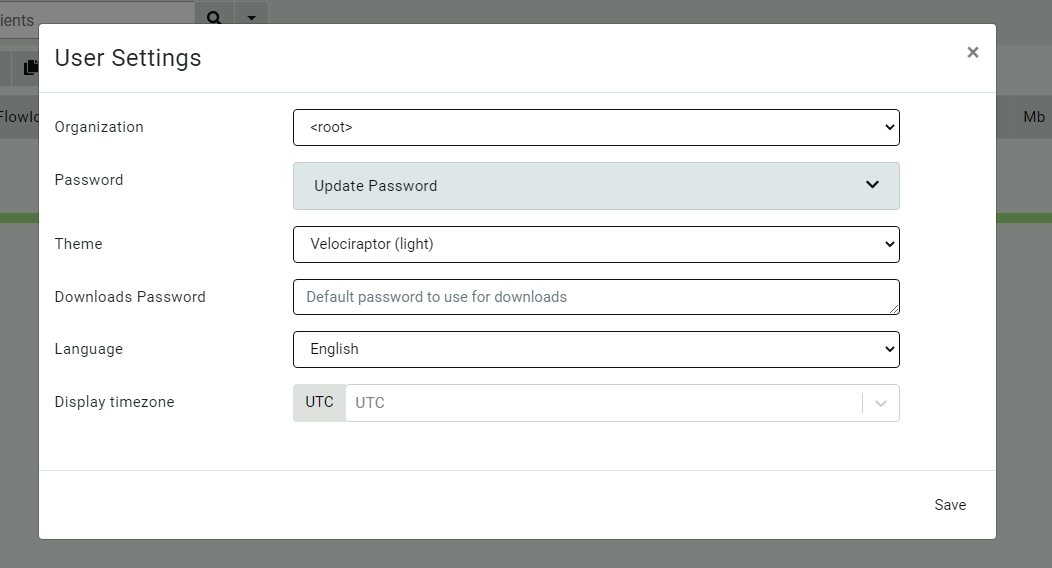
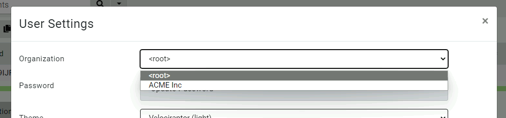
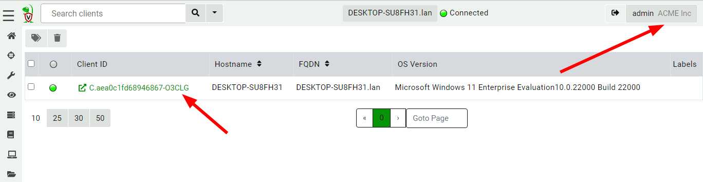
When looking at the latest Velociraptor GUI you might notice the organizations selector in the User Setting page.

Velociraptor Version 0.6.6: Multi-Tenant Mode and More Let You Dig Deeper at Scale Like Never Before
The latest User Settings page

This allows the user to switch between the different organizations they belong in.

Multi-tenanted example

Let’s go through a quick example of how to create a new organization and use this feature in practice.

Multi-tenancy is simply a layer of abstraction in the GUI separating Velociraptor objects (such as clients, hunts, notebooks, etc.) into different organizational units.

You do not need to do anything specific to prepare for a multi-tenant deployment. Every Velociraptor deployment can create a new organization at any time without affecting the current install base at all.

By default all Velociraptor installs (including upgraded ones) have a root organization which contains their current clients, hunts, notebooks, etc. (You can see this in the screenshot above.) If you choose to not use the multi-tenant feature, your Velociraptor install will continue working with the root organization without change.

Suppose a new customer is onboarded, but they do not have a large enough install base to warrant a new cloud deployment (with the associated infrastructure costs). We want to create a new organization for this customer in the current Velociraptor deployment.

Creating a new organization

To create a new organization, we simply run the Server.Orgs.NewOrg server artifact from the Server Artifacts screen.

Velociraptor Version 0.6.6: Multi-Tenant Mode and More Let You Dig Deeper at Scale Like Never Before
Creating a new organization

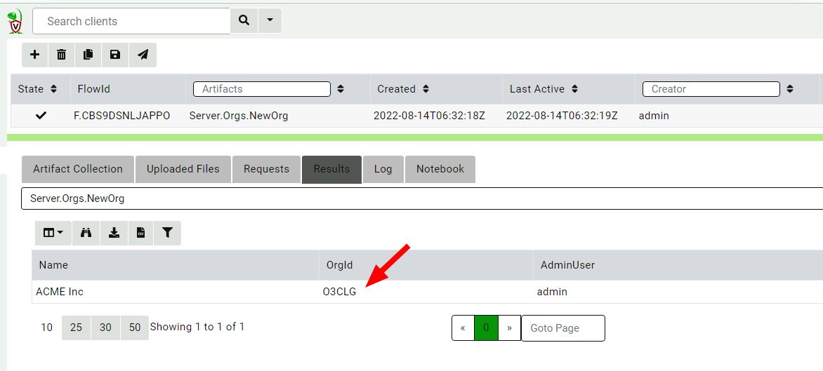
All we need to do is give the organization a name.

Velociraptor Version 0.6.6: Multi-Tenant Mode and More Let You Dig Deeper at Scale Like Never Before
New organization is created with a new OrgId and an Admin User

Velociraptor uses the OrgId internally to refer to the organization, but the organization name is used in the GUI to select the different organizations. The new organization is created with the current user being the new administrator of this org.

Deploying clients to the new organization

Since all Velociraptor agents connect to the same server, there has to be a way for the server to identify which organization each client belongs in. This is determined by the unique nonce inside the client’s configuration file. Therefore, each organization has a unique client configuration that should be deployed to that organization.

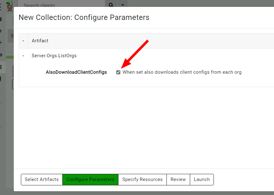
We will list all the organizations on the server using the Server.Orgs.ListOrgs artifact. Note that we are checking the AlsoDownloadConfigFiles parameter to receive the relevant configuration files.

Velociraptor Version 0.6.6: Multi-Tenant Mode and More Let You Dig Deeper at Scale Like Never Before
Listing all the organizations on the server

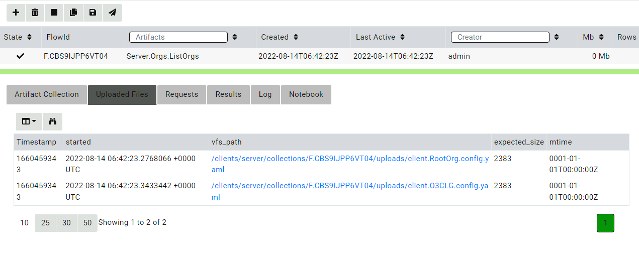
The artifact also uploads the configuration files.

Velociraptor Version 0.6.6: Multi-Tenant Mode and More Let You Dig Deeper at Scale Like Never Before
Viewing the organization’s configuration files

Now, we go through the usual deployment process with these configuration files and prepare MSI, RPM, or Deb packages as normal.

Switching between organizations

We can now switch between organizations using the organization selector.

Velociraptor Version 0.6.6: Multi-Tenant Mode and More Let You Dig Deeper at Scale Like Never Before
Switching between orgs

Now the interface is inside the new organization.

Velociraptor Version 0.6.6: Multi-Tenant Mode and More Let You Dig Deeper at Scale Like Never Before
Viewing an organization

Note the organization name is shown in the user tile, and client IDs have the org ID appended to them to remind us that the client exists within the org.

The new organization is functionally equivalent to a brand-new deployed server! It has a clean data store with new hunts, clients, notebooks, etc. Any server artifacts will run on this organization only, and server monitoring queries will also only apply to this organization.

Adding other users to the new organization

By default, the user which created the organization is given the administrator role within that organization. Users can be assigned arbitrary roles within the organization – so, for example, a user may be an administrator in one organization but a reader in another organization.

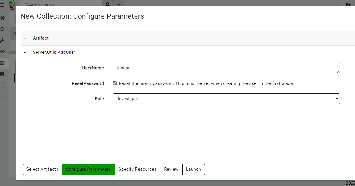
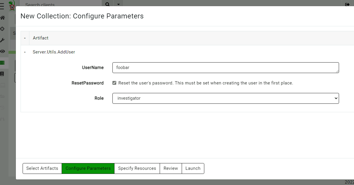
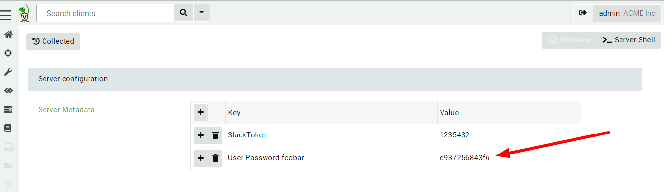
You can add new users or change the user’s roles using the Server.Utils.AddUser artifact. When using basic authentication, this artifact will create a user with a random password. The password will then be stored in the server’s metadata, where it can be shared with the user. We normally recommend Velociraptor to be used with single sign-on (SSO), such as OAuth2 or SAML, and not to use passwords to manage access.

Velociraptor Version 0.6.6: Multi-Tenant Mode and More Let You Dig Deeper at Scale Like Never Before
Adding a new user into the org

View the user’s password in the server metadata screen. (You can remove this entry when done with it or ask the user to change their password.)

Velociraptor Version 0.6.6: Multi-Tenant Mode and More Let You Dig Deeper at Scale Like Never Before
View the new user password in the server metadata screen

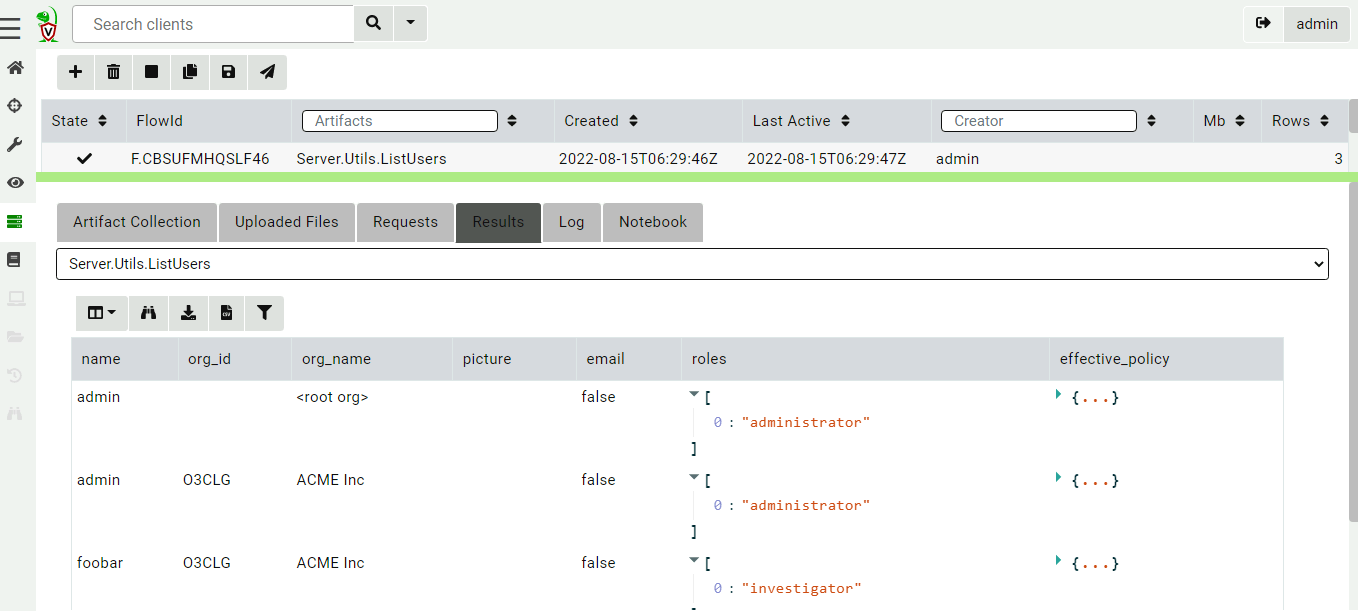
You can view all users in all orgs by collecting the Server.Utils.ListUsers artifact within the root org context.

Velociraptor Version 0.6.6: Multi-Tenant Mode and More Let You Dig Deeper at Scale Like Never Before
Viewing all the users on the system

Although Velociraptor respects the assigned roles of users within an organization, at this stage this should not be considered an adequate security control. This is because there are obvious escalation paths between roles on the same server. For example, currently an administrator role by design has the ability to write arbitrary files on the server and run arbitrary commands (primarily this functionality allows for post processing flows with external tools).

This is currently also the case in different organizations, so an organization administrator can easily add themselves to another organization (or indeed to the root organization) or change their own role.

Velociraptor is not designed to contain untrusted users to their own organization unit at this stage – instead, it gives administrators flexibility and power.

GUI improvements

The 0.6.6 release introduces a number of other GUI improvements.

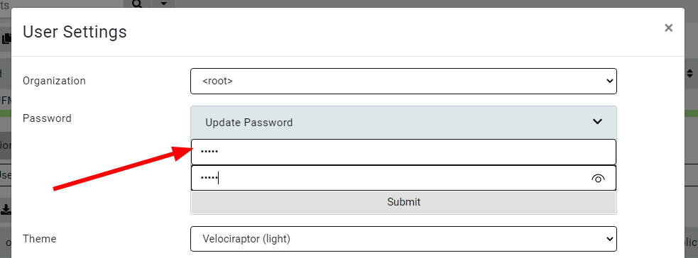
Updating user’s passwords

Usually Velociraptor is deployed in production using SSO such as Google’s OAuth2, and in this case, users manage their passwords using the provider’s own infrastructure.

However, it is sometimes convenient to deploy Velociraptor in Basic authentication mode (for example, for on-premises or air-gapped deployment). Velociraptor now lets users change their own passwords within the GUI.

Velociraptor Version 0.6.6: Multi-Tenant Mode and More Let You Dig Deeper at Scale Like Never Before
Users may update their passwords in the GUI

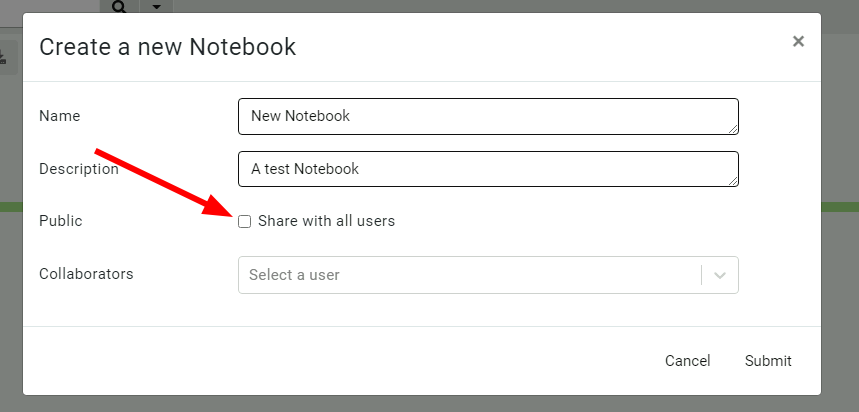
Allow notebook GUI to set notebooks to public

Previously, notebooks could be shared with specific other users, but this proved unwieldy for larger installs with many users. In this release, Velociraptor offers a notebook to be public – this means the notebook will be shared with all users within the org.

Velociraptor Version 0.6.6: Multi-Tenant Mode and More Let You Dig Deeper at Scale Like Never Before
Sharing a notebook with all users

More improvements to the process tracker

The experimental process tracker is described in more details here, but you can already begin using it by enabling the Windows.Events.TrackProcessesBasic client event artifact and using artifacts just as Generic.System.Pstree, Windows.System.Pslist, and many others.

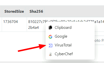
Context menu

A new context menu is now available to allow sending any table cell data to an external service.

Velociraptor Version 0.6.6: Multi-Tenant Mode and More Let You Dig Deeper at Scale Like Never Before
Sending a cell content to an external service

This allows for quick lookups using VirusTotal or a quick CyberChef analysis. You can also add your own send to items in the configuration files.

Conclusion

If you’re interested in the new features, take Velociraptor for a spin by downloading it from our release page. It’s available for free on GitHub under an open-source license.

As always, please file bugs on the GitHub issue tracker or submit questions to our mailing list by emailing [email protected]. You can also chat with us directly on our Discord server.

Learn more about Velociraptor by visiting any of our web and social media channels below:

NEVER MISS A BLOG

Get the latest stories, expertise, and news about security today.

Additional reading:

OpenSSH 9.1 released

Post Syndicated from original https://lwn.net/Articles/910301/

OpenSSH 9.1 has been released. It is advertised as a bug-fix release (and
it addresses a few low-priority memory-safety bugs), but
there’s also a new option to set the minimum RSA key size for
authentication, a few sftp extensions, and more.

Security updates for Tuesday

Post Syndicated from original https://lwn.net/Articles/910300/

Security updates have been issued by Debian (barbican), Fedora (libdxfrw, librecad, and python-oauthlib), Oracle (bind), Red Hat (bind and rh-python38-python), SUSE (bind, chromium, colord, libcroco, libgit2, lighttpd, nodejs12, python, python3, slurm, slurm_20_02, and webkit2gtk3), and Ubuntu (linux-azure, python-django, strongswan, and wayland).

NSA Employee Charged with Espionage

Post Syndicated from Bruce Schneier original https://www.schneier.com/blog/archives/2022/10/nsa-employee-charged-with-espionage.html

An ex-NSA employee has been charged with trying to sell classified data to the Russians (but instead actually talking to an undercover FBI agent).

It’s a weird story, and the FBI affidavit raises more questions than it answers. The employee only worked for the NSA for three weeks—which is weird in itself. I can’t figure out how he linked up with the undercover FBI agent. It’s not clear how much of this was the employee’s idea, and whether he was goaded by the FBI agent. Still, hooray for not leaking NSA secrets to the Russians. (And, almost ten years after Snowden, do we still have this much trouble vetting people before giving them security clearances?)

Mr. Dalke, who had already left the N.S.A. but told the agent that he still worked there on a temporary assignment, then revealed that had taken “highly sensitive information” related to foreign targeting of U.S. systems and information on cyber operations, the prosecutors said. He offered the information in exchange for cryptocurrency and said he was in “financial need.” Court records show he had nearly $84,000 in debt between student loans and credit cards.

EDITED TO ADD (10/5): Marcy Wheeler notes that the FBI seems to be sitting on some common recruitment point, and collecting potential Russian spies.

Защо нямаме „Закон за Фалит на Физическите лица” и как би ни помогнал?

Post Syndicated from VassilKendov original http://kendov.com/personal_bankruptcy/

Защо нямаме „Закон за Фалита на Физическите лица” и как би ни помогнал?
Ще започна с това, че години наред аз и други икономисти, и юристи сме се опитвали многократно да „убедим” политическите партии в нуждата от Закон за Фалита на Физическите лица.
Личният ми опит от последното народно събрание също претърпя неуспех, след доста арогантно отношение и изказване от трибуната на Асен Василев, но няма да ви занимавам с това. Важното е да знаете, че сегашните пратии в парламента освен, че нямат желание, нямат и капацитет да го направят. Естествено по някое време някоя партия ще бъде „мотивирана” да въвеже такъв закон, само и само да не го въведе някой друг „по-мотивиран”, по начин по който „мотивиращия” не харесва.

КАКАВО ТРЯБВА ДА РЕГУЛИРА ЕДИН ТАКЪВ ЗАКОН

В медицинската статистика се приема, че ако едно заболяване причинява 1% смътност, то всеки от нас ще има познат, който е починал от него. Така е и с лошите гредити. Сигурен съм, че всчки от вас познава човек, който има лош кредит. Тези хора рядко споделят този факт, защото ситуацията е нова и надали очакват „помощ от приятел”, което ги оставя на милостта на банките и банковото законодателство. А то не е съвсем равноправно. На практика човек става нещо като „роб” за следващите 10 години от живота си. А ако има неблагоразумието да почине в този период, децата му ще наследят задълженията му. Nice, a?

В моята практика „упътвам” доста клиенти какво да правят в този случай. Много от тях избират ЧУЖБИНА, за да не бъдат оставени на мислостта на банките и банковото законодателство в тази сфера. Друга част са принудени да излязат в сивата икономика, за да могат да живеят следващите 10 години, защото в противен случай дори да взимат 5000 лева на месец, банките ще им оставят минимална работна заплата. Как очакваме един човек да живее, да се развива и да гледа семейство с минимална работна заплата аз не знам, но законът е такъв към момента. ЕТО ТОВА ТРЯБВА ДА СЕ РЕГУЛИРА СЪС ЗАКОН ЗА ФАЛИТА НА ФИЗИЧЕСКИТЕ ЛИЦА. Трябва да се създадат условия за оставане в България на длъжниците и участието им в икономическия живот на България, а не на друга държава или сива икономика!

МАНТРАТА „ЗАЩО КРЕДИТОИСКАТЕЛЯ НЕ СИ Е НАПРАВИЛ СМЕТКАТА”

Много странен въпрос, макар и задаван от хора с претенции за добро образование.
Когато кандидатстваш за кредит, банката прави оценка на твоя личен риск и ти прави предложение. ЗАБЕЛЕЖЕТЕ – Не вие казвате на банката какъв кредит да отпусне, а банката решава какви параметри и за какъв период. И това е след оценка на риска.
Нали не си представяте как една шивачка или един компютърен специалист ще има повече икономическа информация от Отдел Риск на която и да е банка? Ако те не могат да оценят Вашия риск, след цялата предоставена информация и справки, как очаквате Вие да го оцените?

В никакъв случай не казвам, че проблемът с лошия кредит е само на банката, но определно не трябва да бъде и изцяло за сметка на получателя. Това също се регламентира със закон за фалита на физическите лица. Той ще определи докъде е отговорен кредитоискатели и докъде е отговорна банката.

За срещи и консултации по банкови кредити и неволи, моля използвайте посочената форма.

[contact-form-7]

КАК Е РЕШЕН ТОЗИ ПРОБЛЕМ В ЦИВИЛИЗОВАНИЯ СВЯТ

Има два подхода и модела на един такъв закон. Първият е АНГЛОСАКСОНСКИЯ. При него процедурите са максимално бързи и опростени с цел кредитоискателя да влезе максимално бързо отново в икономическия живот на общството и съответно да плаща данъци. Няма да влизам в подробности как функционира там един такъв закон, но 2 месеца са приемлив срок за приклюване на една такава процедура по фалит. Разбира се има и последствия свързани с невъзможност на взимане на нови кредити за определен период или купуване на стоки на изплащане, но ако работиш няма да ти взимат всички заработени пари.

Вторият е ЕВРОПЕЙСКИЯ (КОНТИНЕНТАЛНИЯ). Аз му казвам Германския. Той се характеризира с 10 годишен период, в който кредиторите си търсят парите, но за сметка на това кредитоискателят се ползва от всички придобивки на социалната система – карта за градски траспорт, помощи за безработица, здравни, социално жилище…

У НАС няма модел, защото няма такъв закон. Ние сме взели най-непрактичното от двата модела. От една страна дължиш за срок от 10 години, от друга не можеш да разчиташ на социални придобивки. Едиствените избори са свързани със сиват аикономика или чужбина.

МОЕТО ВИЖДАНЕ ПО ВЪПРОСА КАКЪВ ДА БЪДЕ МОДЕЛА У НАС

Най-важно е да създадем модел, в който хората не напускат България и не влизат в сивата икономика. Повярвайте ми веднъж влезли там, няма излизане. От една страна забравяш за държавата (и тя за теб), от друга се услажда. Губим обаче всички останали.

Предвид слабата социална политика, които имаме, не виждам начин един работещ човек да издържи на социални помощи 10 години и да се развие в някаква насока. ЗАТОВА АНГЛОСАКСОНСКИЯ МОДЕЛ Е ЗА ПРЕДПОЧИТАНЕ! Ние просто нямаме финансовата възможност да приложим германския.

Относно загубите на банките. Ако се заровите в отчетите на БНБ, ще видите, че печалбата на банковата ни система върви само нагоре. Без значение дали е криза или подем, банковата печалба расте. И какво се прави с тази печалба? Дали се харчи за „подобряване на финансовите услуги”? Кога последно си казахте – „Ей тая моята банка е страшна работа. Много съм доволен”? Аз ще Ви кажа – печалбите се изнасят!

От друга страна все още нямаме Финансов Омбудсман или бюро за кредитен рейтинг, но това е тема на друг анализ. Въпросът си остава – ПРАВИЛНО ЛИ ПРЕРАЗПРЕДЕЛЯМЕ ПЕЧАЛБАТА ОТ БАНКОВИЯ СЕКТОР? Дали няма да е по-разумно да жертваме част от нея в полза на кредитоискателите с лоши кредити, за да не отиват те в чужбина и да не излизат в сивата икономика?

Оставям всеки да реши за себе си. Аз аз продължавам да напомням за този закон и да помагам  кредитоискатели с лоши кредити.
Нямам голяма надежда и за този праламент, но нищо не пречи отново да пробвам.

Ако текста Ви е харесал, моля абонирайте се за каналите в Youtube, Telegram или споделете във ФБ

https://www.youtube.com/channel/Kendov
https://t.me/KendovCom

Васил Кендов
www.Draftis.com – Кредитни Консултанти

За срещи и консултации по банкови неволи, моля използвайте посочената форма.

[contact-form-7]

The post Защо нямаме „Закон за Фалит на Физическите лица” и как би ни помогнал? appeared first on Kendov.com.

What’s Up, Home? – Staring at the Video Stream

Post Syndicated from Janne Pikkarainen original https://blog.zabbix.com/whats-up-home-staring-at-the-video-stream/23882/

Can you make sure your video streams are up with Zabbix? Of course, you can! By day, I am a monitoring technical lead in a global cyber security company. By night, I monitor my home with Zabbix & Grafana Labs and do some weird experiments with them. Welcome to my weekly blog about the project.

You might have a surveillance camera at home to record suspicious activities in your yard while you are away or so. Most of the time the cameras do work just fine but might require a hard reboot from time to time, for example, due to harsh weather, or not coming back after a network outage. A networked camera responding to ping does not 100% mean the camera is actually functional. I have seen our camera going black and refusing to connect to its stream even though it thinks it’s working just fine.

Zabbix to the rescue!

Connecting to your camera

My post for this week is mostly to maybe give you a new approach for monitoring your cameras, not so much a functional solution as I’m still figuring out how to do this properly.

For example, I can connect to our camera via RTSP protocol and pass some credentials with it, so rtsp://myusername:[email protected]:443/myAddress

To figure out a connection address for your camera model, iSpyConnect has a nice camera database.

Playing the stream

To test if the video stream works, VLC and mplayer are good options; for visually verifying the stream works, try something like

mplayer ‘rtsp://myusername:[email protected]:443/myAddress’

or for those who like to use a GUI, in VLC, File –> Open Network –> enter your camera address.

For obvious reasons, I am not posting here an image from our camera. Anyway, trust me, this method should work if you have a compatible camera.

Let’s go next for the neat tricks part, which I’m still figuring out myself, too.

Making sure the stream works

To make sure the video stream is up and running, make your Zabbix server, Zabbix proxy, or a dedicated media server to continuously stream your video feed. For example:

mplayer -vo null ‘rtsp://myusername:[email protected]:443/myAddress’

The combination above would make mplayer play the stream with a null video driver; thus, the stream will be continuously played, but just with no visual video output generated. In other words, under perfect conditions, the mplayer process should be running on the server all the time. If anything goes wrong with the stream, mplayer quits itself, and the process goes away from the process list, too.

Using Zabbix to check the player status

Now that you have some server continuously playing the stream, it’s time to check the status with Zabbix.

From here, checking the stream status with Zabbix is simple, just

  • create a new item to check if for example mplayer process is around with Zabbix Agent item type and proc.num[,mplayer] key and
  • make your Zabbix alert about it if the number of mplayer processes is <1
Camera screenshots to your Zabbix user interface

Both mplayer and VLC can be controlled remotely, so here’s an idea I have not yet implemented but testing out.

If a motion sensor, either an external unit or a built-in, detects movement, make Zabbix send a command to the camera to record a screenshot of the camera stream, or possibly a short video. Then just make the script to save the photo or video in a directory that Zabbix can access and then show with its URL widget type.

mplayer has a slave mode for receiving commands from external programs, which might work together with a FIFO pipe.

Real-time video stream in your Zabbix user interface

At least VLC can transcode RTSP to HTTP stream in real-time, so in theory, then embedding the resulting stream to your Zabbix user interface should very much be doable with a short HTML file and Zabbix URL widget type. This one I did not yet even start to try out, though.

So, that’s all for this week’s blog post. I’m still building this thing out, but if you have successfully done something similar, please let me know!

I have been working at Forcepoint since 2014 and am a true fan of functional testing. — Janne Pikkarainen

This post was originally published on the author’s LinkedIn account.

The post What’s Up, Home? – Staring at the Video Stream appeared first on Zabbix Blog.

IAM Access Analyzer makes it simpler to author and validate role trust policies

Post Syndicated from Mathangi Ramesh original https://aws.amazon.com/blogs/security/iam-access-analyzer-makes-it-simpler-to-author-and-validate-role-trust-policies/

AWS Identity and Access Management (IAM) Access Analyzer provides many tools to help you set, verify, and refine permissions. One part of IAM Access Analyzer—policy validation—helps you author secure and functional policies that grant the intended permissions. Now, I’m excited to announce that AWS has updated the IAM console experience for role trust policies to make it simpler for you to author and validate the policy that controls who can assume a role. In this post, I’ll describe the new capabilities and show you how to use them as you author a role trust policy in the IAM console.

Overview of changes

A role trust policy is a JSON policy document in which you define the principals that you trust to assume the role. The principals that you can specify in the trust policy include users, roles, accounts, and services. The new IAM console experience provides the following features to help you set the right permissions in the trust policy:

  • An interactive policy editor prompts you to add the right policy elements, such as the principal and the allowed actions, and offers context-specific documentation.
  • As you author the policy, IAM Access Analyzer runs over 100 checks against your policy and highlights issues to fix. This includes new policy checks specific to role trust policies, such as a check to make sure that you’ve formatted your identity provider correctly. These new checks are also available through the IAM Access Analyzer policy validation API.
  • Before saving the policy, you can preview findings for the external access granted by your trust policy. This helps you review external access, such as access granted to a federated identity provider, and confirm that you grant only the intended access when you create the policy. This functionality was previously available through the APIs, but now it’s also available in the IAM console.

In the following sections, I’ll walk you through how to use these new features.

Example scenario

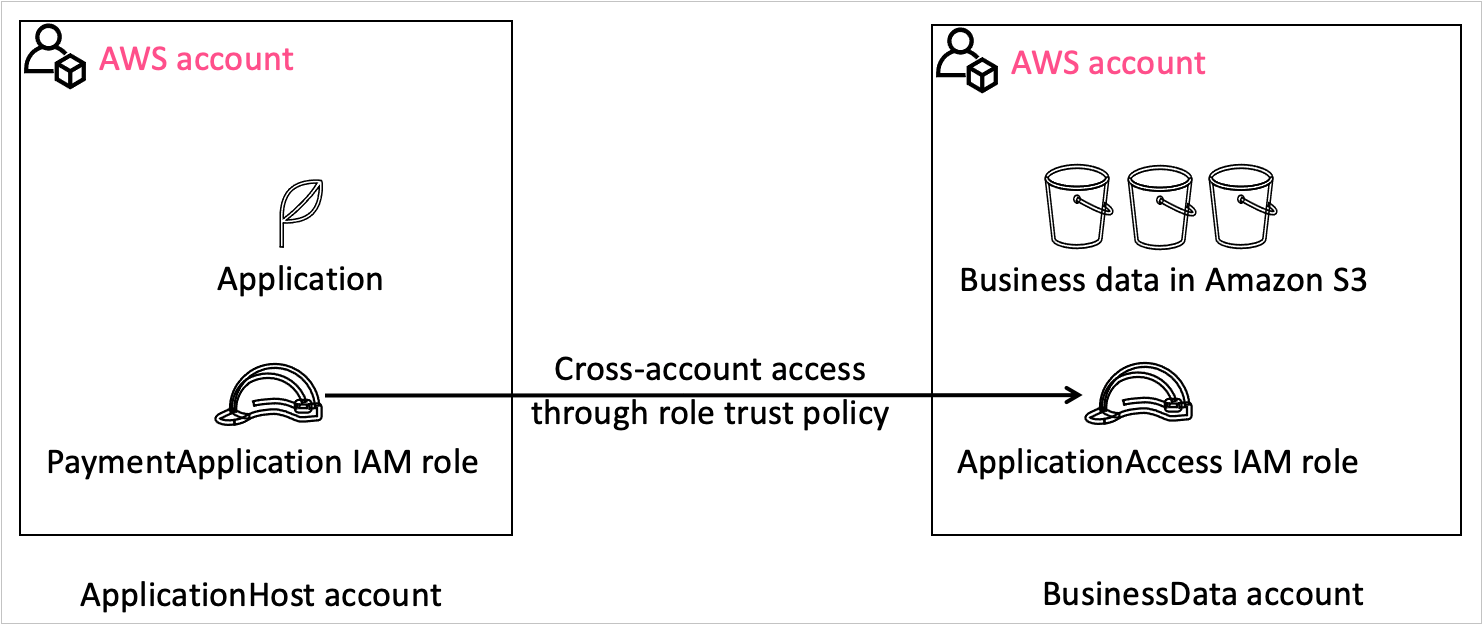
For the walkthrough, consider the following example, which is illustrated in Figure 1. You are a developer for Example Corp., and you are working on a web application. You want to grant the application hosted in one account—the ApplicationHost account—access to data in another account—the BusinessData account. To do this, you can use an IAM role in the BusinessData account to grant temporary access to the application through a role trust policy. You will grant a role in the ApplicationHost account—the PaymentApplication role—to access the BusinessData account through a role—the ApplicationAccess role. In this example, you create the ApplicationAccess role and grant cross-account permissions through the trust policy by using the new IAM console experience that helps you set the right permissions.

Figure 1: Visual explanation of the scenario

Figure 1: Visual explanation of the scenario

Create the role and grant permissions through a role trust policy with the policy editor

In this section, I will show you how to create a role trust policy for the ApplicationAccess role to grant the application access to the data in your account through the policy editor in the IAM console.

To create a role and grant access

  1. In the BusinessData account, open the IAM console, and in the left navigation pane, choose Roles.
  2. Choose Create role, and then select Custom trust policy, as shown in Figure 2.
    Figure 2: Select "Custom trust policy" when creating a role

    Figure 2: Select “Custom trust policy” when creating a role

  3. In the Custom trust policy section, for 1. Add actions for STS, select the actions that you need for your policy. For example, to add the action sts:AssumeRole, choose AssumeRole.
    Figure 3: JSON role trust policy

    Figure 3: JSON role trust policy

  4. For 2. Add a principal, choose Add to add a principal.
  5. In the Add principal box, for Principal type, select IAM roles. This populates the ARN field with the format of the role ARN that you need to add to the policy, as shown in Figure 4.
    Figure 4: Add a principal to your role trust policy

    Figure 4: Add a principal to your role trust policy

  6. Update the role ARN template with the actual account and role information, and then choose Add principal. In our example, the account is ApplicationHost with an AWS account number of 111122223333, and the role is PaymentApplication role. Therefore, the role ARN is arn:aws:iam:: 111122223333: role/PaymentApplication. Figure 5 shows the role trust policy with the action and principal added.
    Figure 5: Sample role trust policy

    Figure 5: Sample role trust policy

  7. (Optional) To add a condition, for 3. Add a condition, choose Add, and then complete the Add condition box according to your needs.

Author secure policies by reviewing policy validation findings

As you author the policy, you can see errors or warnings related to your policy in the policy validation window, which is located below the policy editor in the console. With this launch, policy validation in IAM Access Analyzer includes 13 new checks focused on the trust relationship for the role. The following are a few examples of these checks and how to address them:

  • Role trust policy unsupported wildcard in principal – you can’t use a * in your role trust policy.
  • Invalid federated principal syntax in role trust policy – you need to fix the format of the identity provider.
  • Missing action for condition key – you need to add the right action for a given condition, such as the sts:TagSession when there are session tag conditions.

For a complete list of checks, see Access Analyzer policy check reference.

To review and fix policy validation findings

  1. In the policy validation window, do the following:
    • Choose the Security tab to check if your policy is overly permissive.
    • Choose the Errors tab to review any errors associated with the policy.
    • Choose the Warnings tab to review if aspects of the policy don’t align with AWS best practices.
    • Choose the Suggestions tab to get recommendations on how to improve the quality of your policy.
    Figure 6: Policy validation window in IAM Access Analyzer with a finding for your policy

    Figure 6: Policy validation window in IAM Access Analyzer with a finding for your policy

  2. For each finding, choose Learn more to review the documentation associated with the finding and take steps to fix it. For example, Figure 6 shows the error Mismatched Action For Principal. To fix the error, remove the action sts:AssumeRoleWithWebIdentity.

Preview external access by reviewing cross-account access findings

IAM Access Analyzer also generates findings to help you assess if a policy grants access to external entities. You can review the findings before you create the policy to make sure that the policy grants only intended access. To preview the findings, you create an analyzer and then review the findings.

To preview findings for external access

  1. Below the policy editor, in the Preview external access section, choose Go to Access Analyzer, as shown in Figure 7.

    Note: IAM Access Analyzer is a regional service, and you can create a new analyzer in each AWS Region where you operate. In this situation, IAM Access Analyzer looks for an analyzer in the Region where you landed on the IAM console. If IAM Access Analyzer doesn’t find an analyzer there, it asks you to create an analyzer.

    Figure 7: Preview external access widget without an analyzer

    Figure 7: Preview external access widget without an analyzer

  2. On the Create analyzer page, do the following to create an analyzer:
    • For Name, enter a name for your analyzer.
    • For Zone of trust, select the correct account.
    • Choose Create analyzer.
    Figure 8: Create an analyzer to preview findings

    Figure 8: Create an analyzer to preview findings

  3. After you create the analyzer, navigate back to the role trust policy for your role to review the external access granted by this policy. The following figure shows that external access is granted to PaymentApplication.
    Figure 9: Preview finding

    Figure 9: Preview finding

  4. If the access is intended, you don’t need to take any action. In this example, I want the PaymentApplication role in the ApplicationHost account to assume the role that I’m creating.
  5. If the access is unintended, resolve the finding by updating the role ARN information.
  6. Select Next and grant the required IAM permissions for the role.
  7. Name the role ApplicationAccess, and then choose Save to save the role.

Now the application can use this role to access the BusinessData account.

Conclusion

By using the new IAM console experience for role trust policies, you can confidently author policies that grant the intended access. IAM Access Analyzer helps you in your least-privilege journey by evaluating the policy for potential issues to make it simpler for you to author secure policies. IAM Access Analyzer also helps you preview external access granted through the trust policy to help ensure that the granted access is intended. To learn more about how to preview IAM Access Analyzer cross-account findings, see Preview access in the documentation. To learn more about IAM Access Analyzer policy validation checks, see Access Analyzer policy validation. These features are also available through APIs.

If you have feedback about this post, submit comments in the Comments section below. If you have questions about this post, start a new thread at AWS IAM re:Post or contact AWS Support.

Mathangi Ramesh

Mathangi Ramesh

Mathangi is the product manager for AWS Identity and Access Management. She enjoys talking to customers and working with data to solve problems. Outside of work, Mathangi is a fitness enthusiast and a Bharatanatyam dancer. She holds an MBA degree from Carnegie Mellon University.

Announcing General Availability of Amazon Connect Cases

Post Syndicated from Veliswa Boya original https://aws.amazon.com/blogs/aws/announcing-general-availability-of-amazon-connect-cases/

In June 2022 AWS announced a preview of Amazon Connect Cases, a feature of Amazon Connect that simplifies these customer interactions and reduces the average handle times of issues.

Today I am excited to announce the general availability of Amazon Connect Cases. Cases, a feature of Amazon Connect, makes it easy for your contact center agents to create, collaborate on, and quickly resolve customer issues that require several customer conversations and follow-up tasks, and they can focus on solving the customer issue, no matter how simple or how complex. Agents have relevant case details (such as date and time opened, issue summary, or customer information) in a single unified view, and they can focus on solving the customer issue.

Getting started with Cases takes only a few clicks because it is built into Amazon Connect. With Cases, you automatically create cases or find existing cases, saving agents time searching and entering data manually. Cases accelerates resolution times, improves efficiency, and reduces errors to help increase customer satisfaction.

Best of all, Cases is part of the unified agent application that also includes the Amazon Connect Contact Control Panel to handle contacts, Amazon Connect Customer Profiles to identify the customer and personalize the experience, Amazon Connect Wisdom to surface relevant knowledge articles, and Amazon Connect Tasks to automate, track, and monitor follow up items.

An Overview of Amazon Connect Cases

Litigation Practice Group is a provider of legal support for debt relief. Litigation’s Director of Business Intelligence, Alex Miles, spoke about how they have experienced Cases. He said:

“Amazon Connect not only addresses many of the technological limitations we were facing but brings with it a suite of modern solutions for all our business needs. One of those needs is case management to handle operating activities, including payments, document control, and legal cases. Amazon Connect Cases seamlessly integrates with our existing contact center workflows. Our agents and legal teams now have full performance visibility and spend less time on manual tasks, creating more time to find solutions to enhance the customer journey.”

Cases provides built-in case management capabilities, eliminating the need for contact centers to build custom solutions or integrate with third-party products to handle complex customer
issues. For every issue, Cases enables agents to view case history and activity all in one place, automatically capture case data from interactive voice response (IVR) or chats (via Amazon Lex), and track follow-up work with Tasks.

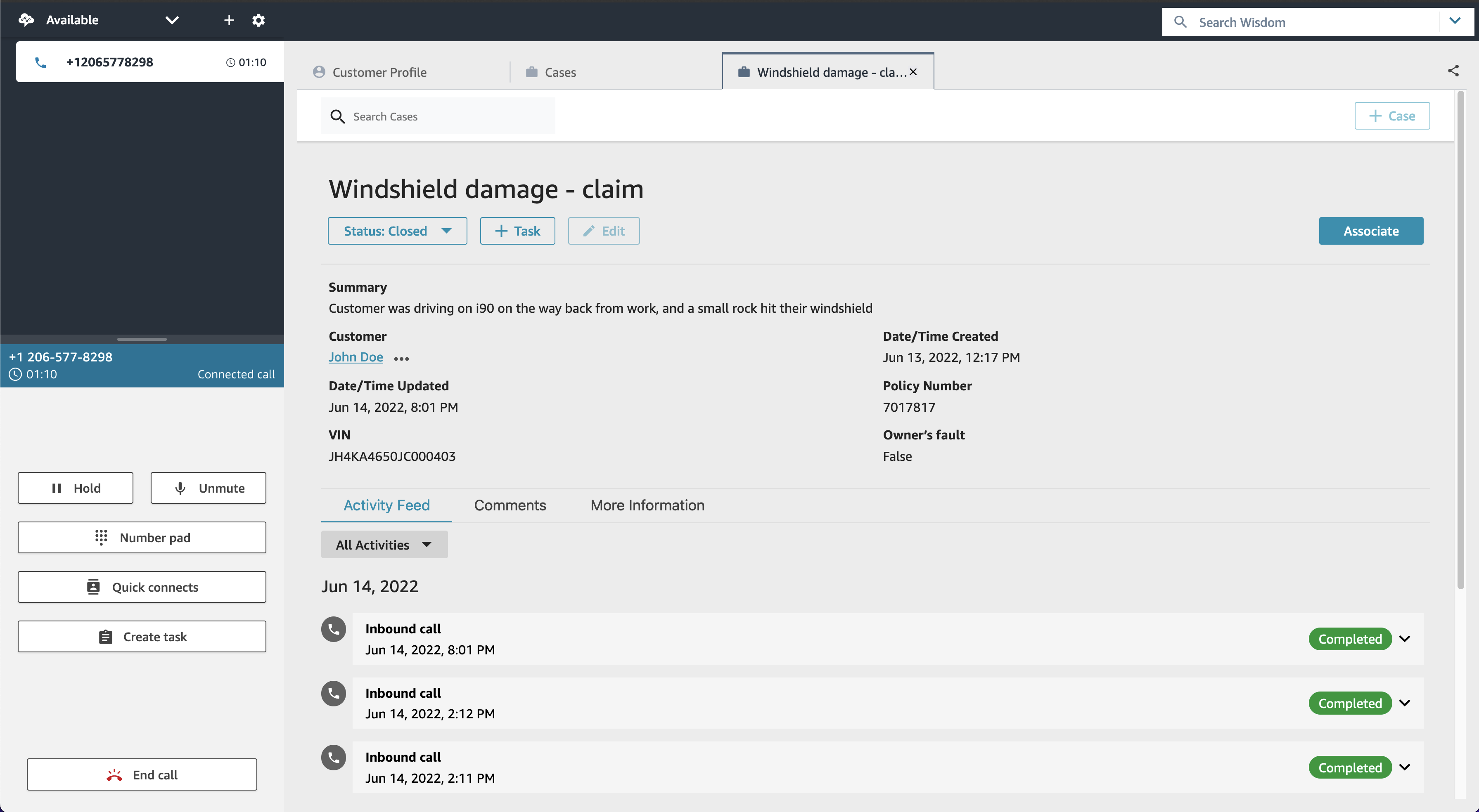
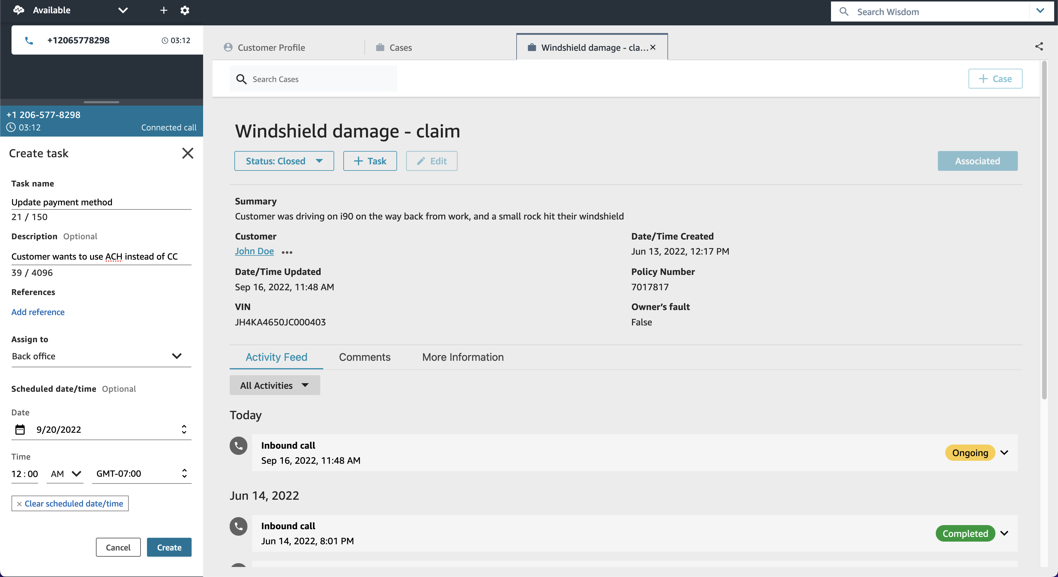
  1. View case history and activity all in one place – Agents view the details of the customer issue (including calls, tasks, and chats associated with the case) all in one place within the unified Amazon Connect agent application. The timeline view shows agents a case at a glance, removing the need for agents to go back and forth between applications.

    View case history and activity in one place

    View case history and activity in one place

  2. Automatically capture case data from interactive voice response (IVR) or chats – With this feature you can automatically create and update cases by using information gathered in a customer’s self-service IVR or chatbot interaction. When agent assistance is required, the contact will then be routed to an available agent with the relevant case attached, resulting in improved average handle time and first-contact resolution.

    Automatically capture case data from your IVR and chatbots

    Automatically capture case data from your IVR and chatbots

  3. Take action with task management – This feature is Cases working together with Amazon Connect Tasks to help you reduce resolution time and improve efficiency. Tasks, which tracks the work that must be done to resolve the customer’s issue, ensures that a case is captured and includes prior and pending actions needed to resolve the issue. This makes it easier for agents to create, prioritize, and monitor work assigned to other agents or teams. Here I’d also like to highlight how all this results in great collaboration between agents and ultimately, teams.

    Take action with task management

    Take action with task management

  4. Get started in a few clicks! Turn on Cases and configure permissions, fields, and templates, all within Amazon Connect. No third-party tools or integrations are required.
    Get Started

    Get Started

General Availability
Amazon Connect Cases is generally available in US East (N. Virginia), and US West (Oregon).

– Veliswa x

Git 2.38 released

Post Syndicated from original https://lwn.net/Articles/910213/

Version 2.38.0 of the Git distributed version-control system has been released. It comes with lots of new features and bug fixes, some of the former are described in a GitHub blog post by Taylor Blau. Highlights include the promotion of the scalar addition for large repositories into Git core, improvements to multi-branch rebase operations with --update-refs, performance improvements, a bash prompt indication for unmerged indexes, and lots more.

Netdev 0x16 accepted sessions announced

Post Syndicated from original https://lwn.net/Articles/910210/

The accepted sessions for the upcoming Netdev 0x16 have been posted. The conference will be held virtually and in-person in Lisbon, Portugal October 24-28. In addition, early-bird registration rates have been extended to October 4.

Netdev 0x16, like all the previous netdev conferences, is a conference of the netdev community, by the netdev community, for the netdev community. Linux kernel networking and user space utilization of the interfaces to the Linux kernel networking subsystem are the focus. If you are using Linux as a boot system for proprietary networking, then this conference _may not be for you_.

AWS Week in Review – October 3, 2022

Post Syndicated from Danilo Poccia original https://aws.amazon.com/blogs/aws/aws-week-in-review-october-3-2022/

This post is part of our Week in Review series. Check back each week for a quick roundup of interesting news and announcements from AWS!

A new week and a new month just started. Curious which were the most significant AWS news from the previous seven days? I got you covered with this post.

Last Week’s Launches
Here are the launches that got my attention last week:

Amazon File Cache – A high performance cache on AWS that accelerates and simplifies demanding cloud bursting and hybrid workflows by giving access to files using a fast and familiar POSIX interface, no matter if the original files live on premises on any file system that can be accessed through NFS v3 or on S3.

Amazon Data Lifecycle Manager – You can now automatically archive Amazon EBS snapshots to save up to 75 percent on storage costs for those EBS snapshots that you intend to retain for more than 90 days and rarely access.

AWS App Runner – You can now build and run web applications and APIs from source code using the new Node.js 16 managed runtime.

AWS Copilot – The CLI for containerized apps adds IAM permission boundaries, support for FIFO SNS/SQS for the Copilot worker-service pattern, and using Amazon CloudFront for low-latency content delivery and fast TLS-termination for public load-balanced web services.

Bottlerocket – The Linux-based operating system purpose-built to run container workloads is now supported by Amazon Inspector. Amazon Inspector can now recommend an update of Bottlerocket if it finds a vulnerability.

Amazon SageMaker Canvas – Now supports mathematical functions and operators for richer data exploration and to understand the relationships between variables in your data.

AWS Compute Optimizer – Now provides cost and performance optimization recommendations for 37 new EC2 instance types, including bare metal instances (m6g.metal) and compute optimized instances (c7g.2xlarge, hpc6a.48xlarge), and new memory metrics for Windows instances.

AWS Budgets – Use a simplified 1-click workflow for common budgeting scenarios with step-by-step tutorials on how to use each template.

Amazon Connect – Now provides an updated flow designer UI that makes it easier and faster to build personalized and automated end-customer experiences, as well as a queue dashboard to view and compare real-time queue performance through time series graphs.

Amazon WorkSpaces – You can now provision Ubuntu desktops and use virtual desktops for new categories of workloads, such as for your developers, engineers, and data scientists.

Amazon WorkSpaces Core – A fully managed infrastructure-only solution for third-party Virtual Desktop Infrastructure (VDI) management software that simplifies VDI migration and combines your current VDI software with the security and reliability of AWS. Read more about it in this Desktop and Application Streaming blog post.

For a full list of AWS announcements, be sure to keep an eye on the What’s New at AWS page.

Other AWS News
A few more blog posts you might have missed:

Introducing new language extensions in AWS CloudFormation – In this Cloud Operations & Migrations blog post, we introduce the new language transform that enhances CloudFormation core language with intrinsic functions that simplify handling JSON strings (Fn::ToJsonString), array lengths (Fn::Length), and update and deletion policies.

Building a GraphQL API with Java and AWS Lambda – This blog shows different options for resolving GraphQL queries using serverless technologies on AWS.

For AWS open-source news and updates, here’s the latest newsletter curated by Ricardo to bring you the most recent updates on open-source projects, posts, events, and more.

Upcoming AWS Events
As usual, there are many opportunities to meet:

AWS Summits– Connect, collaborate, and learn about AWS at these free in-person events: Bogotá (October 4), and Singapore (October 6).

AWS Community Days – AWS Community Day events are community-led conferences to share and learn together. Join us in Amersfoort, Netherlands (on October 3, today), Warsaw, Poland (October 14), and Dresden, Germany (October 19).

That’s all from me for this week. Come back next Monday for another Week in Review!

— Danilo

Highlights from Git 2.38

Post Syndicated from Taylor Blau original https://github.blog/2022-10-03-highlights-from-git-2-38/

The open source Git project just released Git 2.38, with features and bug fixes from over 92 contributors, 24 of them new. We last caught up with you on the latest in Git back when 2.37 was released.

To celebrate this most recent release, here’s GitHub’s look at some of the most interesting features and changes introduced since last time.

A repository management tool for large repositories

We talk a lot about performance in Git, especially in the context of large repositories. Returning readers of these blog posts will no doubt be familiar with the dozens of performance optimizations that have landed in Git over the years.

But with so many features to keep track of, it can be easy to miss out some every now and then (along with their corresponding performance gains).

Git’s new built-in repository management tool, Scalar, attempts to solve that problem by curating and configuring a uniform set of features with the biggest impact on large repositories. To start using it, you can either clone a new repository with scalar clone:

$ scalar clone /path/to/repo

Or, you can use the --full-clone option if you don’t want to start out with a sparse checkout. To apply Scalar’s recommended configuration to a clone you already have, you can instead run:

$ cd /path/to/repo
$ scalar register

At the time of writing, Scalar’s default configured features include:

Scalar’s configuration is updated as new (even experimental!) features are introduced to Git. To make sure you’re always using the latest and greatest, be sure to run scalar reconfigure /path/to/repo after a new release to update your repository’s config (or scalar reconfigure -a to update all of your Scalar-registered repositories at once).

Git 2.38 is the first time Scalar has been included in the release, but it has actually existed for much longer. Check back soon for a blog post on how Scalar came to be—from its early days as a standalone .NET application to its journey into core Git!

[source]

Rebase dependent branches with –update-refs

When working on a large feature, it’s often helpful to break up the work across multiple branches that build on each other.

But these branches can become cumbersome to manage when you need to rewrite history in an earlier branch. Since each branch depends on the previous ones, rewriting commits in one branch will leave the subsequent branches disconnected from history after rewriting.

In case that didn’t quite make sense, let’s walk through an example.

Suppose that you are working on a feature (my-feature), but want to break it down into a few distinct parts (maybe for ease of review, or to ensure you’re deploying it safely, etc.). Before you share your work with your colleagues, you build the entire feature up front to make sure that the end-result is feasible, like so.

$ git log --oneline origin/main..HEAD
741a3174683 (HEAD -> my-feature/part-three) Part 3: all done!
1ff073007eb Part 3: step two
880c07e326f Part 3: step one
40529bd11dc (my-feature/part-two) Part 2: step two
0a92cc3acd8 Part 2: step one
eed018043ba (my-feature/part-one) Part 1: step three
646c870d69e Part 1: step two
9147f6d2eb4 Part 1: step one

In the example below, the my-feature/part-three branch resembles what you imagine the final state will look like. But the intermediate check-points (my-feature/part-one, and so on) represent the chunks you intend to submit for code review.

After you submit everything, what happens if you want to make a change to one of the patches in part one?

You might create a fixup! commit on top, but squashing that patch into the one you wanted to change from part one will cause parts two and three to become disconnected:

Creating a fixup commit that causes parts two and three to become disconnected

Notice that after we squashed our fix into “Part 1: step one,” the subsequent branches vanished from history. That’s because they didn’t get updated to depend on the updated tip of my-feature/part-one after rebasing.

You could go through and manually checkout each branch, resetting each to the right commit. But this can get cumbersome quickly if you have a lot of branches, are making frequent changes, or both.

Git 2.38 ships with a new option to git rebase called --update-refs that knows how to perform these updates for you. Let’s try that same example again with the new version of Git.

Rebasing with the new viersion of Git, which updates each branch for you.

Because we used --update-refs, git rebase knew to update our dependent branches, so our history remains intact without having to manually update each individual branch.

If you want to use this option every time you rebase, you can run git config --global rebase.updateRefs true to have Git act as if the --update-refs option is always given.

[source]

Tidbits

This release coincides with the Git project’s participation in the annual Google Summer of Code program. This year, the Git project mentored two students, Shaoxuan Yuan, and Abhradeep Chakraborty, working on sparse index integration and various improvements to reachability bitmaps, respectively.

  • Shaoxuan’s first contribution was integrating the git rm command with the sparse index. The sparse index is a relatively new Git feature that enables Git to shrink the size of its index data structure to only track the contents of your sparse checkout, instead of the entire repository. Long-time readers will remember that Git commands have been converted to be compatible with the sparse-index one-by-one. Commands that aren’t compatible with the sparse index need to temporarily expand the index to cover the entire repository, leading to slow-downs when working in a large repository.

    Shaoxuan’s work made the git rm command compatible with the sparse index, causing it to only expand the index when necessary, bringing Git closer to having all commands be compatible with the sparse index by default.

    [source]

  • Shaoxuan also worked on improving git mv‘s behavior when moving a path from within the sparse checkout definition (sometimes called a “cone”) to outside of the sparse checkout. There were a number of corner cases that required careful reasoning, and curious readers can learn more about exactly how this was implemented in the patches linked below.

    [source]

  • Abhradeep worked on adding a new “lookup table” extension to Git’s reachability bitmap index. For those unfamiliar, this index (stored in a .bitmap file) associates a set of commits to a set of bitmaps, where each bit position corresponds to an object. A 1 bit indicates that a commit can reach the object specified by that bit position, and a 0 indicates that it cannot.

    But .bitmap files do not list their selected commits in a single location. Instead, they prefix each bitmap with the object ID of the commit it corresponds to. That means that in order to know what set of commits are covered by a .bitmap, Git must read the entire contents of the file to discover the set of bitmapped commits.

    Abhradeep addressed this shortcoming by adding an optional “lookup table” at the end of the .bitmap format, which provides a concise list of selected commits, as well as the offset of their corresponding bitmaps within the file. This provided some speed-ups across a handful of benchmarks, making bitmaps faster to load and use, especially for large repositories.

    [source]

  • Abhradeep also worked on sprucing up the technical documentation for the .bitmap format. So if you have ever been curious about or want to hack on Git’s bitmap internals, now is the time!

    [source]

For more about these projects, you can check out each contributor’s final blog posts here and here. Thank you, Shaoxuan, and Abhradeep!

Now that we’ve covered a handful of changes contributed by Google Summer of Code students, let’s take a look at some changes in this release of Git from other Git contributors.

  • You may not be familiar with Git’s merge-tree command, which historically was used to compute trivial three-way merges using Git’s recursive merge strategy. In Git 2.38, this command now knows how to integrate with the new ort merge strategy, allowing it to compute non-trivial merges without touching the index or working copy.

    The existing mode is still available behind a (deprecated) --trivial-merge option. When the new --write-tree mode is used, merge-tree takes two branches to merge, and computes the result using the ort strategy, all without touching the working copy or index. It outputs the resulting tree’s object ID, along with some information about any conflicts it encountered.

    As an aside, we at GitHub recently started using merge-ort to compute merges on GitHub.com more than an order of magnitude faster than before. We had previously used the implementation in libgit2 in order to compute merges without requiring a worktree, since GitHub stores repositories as bare, meaning we do not have a worktree to rely on. These changes will make their way to GitHub Enterprise beginning with verion 3.7.

    [source]

  • Bare Git repositories can be stored in and distributed with other Git repositories. This is often convenient, for example, as an easy mechanism to distribute Git repositories for use as test fixtures.

    When using repositories from less-than-trustworthy sources, this can also present a security risk. Git repositories often execute user-defined programs specified via the $GIT_DIR/config file. For example, core.pager defines which pager program Git uses, and core.editor defines which editor Git opens when you want to write a commit message (among other things).

    There are other examples, but an often-discussed one is the core.fsmonitor configuration, which can be used to specify a path to a filesystem monitoring hook. Because Git often needs to query the state of the filesystem, this hook (when configured) is invoked many times, including from git status, which people commonly script around in their shell prompt.

    This means that it’s possible to convince a victim to run arbitrary code by convincing them to clone a repository with a malicious bare repository embedded inside of it. If they change their working directory into the malicious repository within (since you cannot embed a bare repository at the top-level directory of a repository) and run some Git command, then they are likely to execute the script specified by core.fsmonitor (or any other configuration that specifies a command to execute).

    For this reason, the new safe.bareRepository configuration was introduced. When set to “explicit,” Git will only work with bare repositories specified by the top-level --git-dir argument. Otherwise, when set to “all” (which is the default), Git will continue to work with all bare repositories, embedded or not.

    It is worth noting that setting safe.bareRepository to “explicit” is only required if you worry that you may be cloning malicious repositories and executing Git commands in them.

    [source]

  • git grep learned a new -m option (short for --max-count), which behaves like GNU grep‘s options of the same name. This new option limits the number of matches shown per file. This can be especially useful when combined with other options, like -C or -p (which show code context, or the name of the function which contains each match).

    You could, for example, combine all three of these options to show a summary of how some function is called by many different files in your project. Git has a handful of objects that contain the substring oid_object_info. If you want to look at how callers across different files are structured without seeing more than one example from the same file, you can now run:

    $ git grep -C3 -p -m1 oid_object_info

    [source]

  • If you’ve ever scripted around the directory contents of your Git repository, there’s no doubt that you’ve encountered the git ls-files command. Unlike ls-tree (which lists the contents of a tree object), ls-files lists the contents of the index, the working directory, or both.

    There are already lots of options which can further specify what does or doesn’t get printed in ls-files‘s output. But its output was not easily customizable without additional scripting.

    In Git 2.38, that is no longer the case, with ls-files‘s new --format option. You can now customize how each entry is printed, with fields to print an object’s name and mode, as well as more esoteric options, like its stage in the index, or end-of-line (EOL) behavior.

    [source]

  • git cat-file also learned a new option to respect the mailmap when printing the contents of objects with identifiers in them. This feature was contributed by another Google Summer of Code student, this time working on behalf of GitLab!

    For the uninitiated, the mailmap is a feature which allows mapping name and email pairs to their canonical values, which can be useful if you change your name or email and want to retain authorship over historical commits without rewriting history.

    git show, and many other tools already understand how to remap identities under the mailmap (for example, git show‘s %aN and %aE format placeholders print the mailmapped author name and email, respectively, as opposed to %an and %ae, which don’t respect the mailmap). But git cat-file, which is a low-level command which prints the contents of objects, did not know how to perform this conversion.

    That meant that if you wanted to print a stream of objects, but transform any author, committer, or tagger identities according to the mailmap, you would have to pipe their contents through git show or similar. This is no longer the case, since git cat-file now understands the --[no]-use-mailmap option, meaning this transformation can be done before printing out object contents.

    [source]

  • Finally, Git’s developer documentation got an improvement in this most recent release, by adding a codified version of the Git community’s guidelines for code review. This document is a helpful resource for new and existing contributors to learn about the cultural norms around reviewing patches on the Git mailing list.

    If you’ve ever had the itch to contribute to the Git project, I highly encourage you to read the new reviewing guidelines (as well as the coding guidelines, and the “My First Contribution” document) and get started!

    [source]

The rest of the iceberg

That’s just a sample of changes from the latest release. For more, check out the release notes for 2.38, or any previous version in the Git repository.

The collective thoughts of the interwebz