What Are Microservices?

Post Syndicated from Molly Clancy original https://www.backblaze.com/blog/what-are-microservices/

Back in 2008, Netflix was facing scaling challenges: service outages, database corruption, a three-day lapse in DVD shipments. (Remember when Netflix still shipped DVDs?) Netflix solved these problems by refactoring their monolithic application to avoid the single points of failure that caused these issues. They implemented a microservices architecture before the term “microservices” even existed, making them pioneers in the field.

Today, almost all of the most popular applications—Uber, Amazon, Etsy—run in a microservices environment. If you’ve ever wondered what that means, you’re not alone. In this post, we’re digging into this popular method for developing web applications: the benefits, drawbacks, and considerations for choosing a cloud provider to support your microservices approach.

First, Some History: Monolithic Software Development

How would you develop a large, complex software system before the age of microservices? For developers who learned their craft in the dot com boom, it meant a large and complex development process, with tightly interlocking subsystems, a waterfall development model, and an extensive QA phase. Most of the code was built from scratch. There was a lot of focus on developing extremely reliable code, since it was very difficult and expensive to update products in the field. This is how software was developed for many years. The approach works, but it has some major issues. It’s slower, and it tends to produce complex software monoliths that are tough to maintain and upgrade.

What Are Microservices?

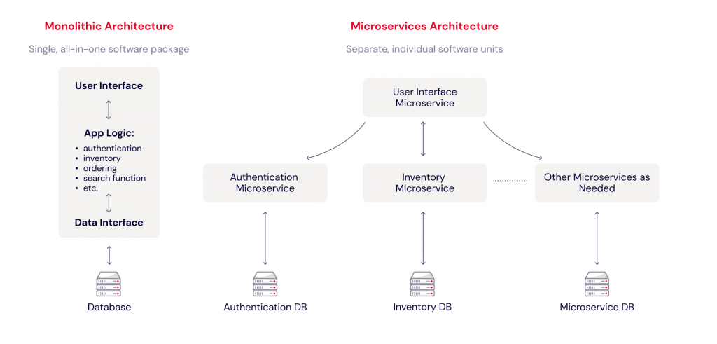
Current software engineering practices encourage a DevOps model using small, reusable units of functionality, or microservices. Microservices run essentially as a standalone process, carrying whatever information or intelligence they need to do their job. Their interfaces are limited and standardized to encourage reuse. This restricted access to internal logic very effectively implements the information-hiding practices that prevent other code from “peeking inside” your modules and making internal tweaks that destabilize your code. The result is (hopefully) an assortment of tools (databases, web servers, etc.) that can be snapped together like Legos™ to greatly reduce the development effort.
Microservices: Pros and Cons

This newer approach has many advantages:

  • It encourages and supports code reuse. Developers usually have access to an extensive library of microservices that can easily be plugged into their application.
  • It enforces logical module isolation to simplify the architecture and improve reliability. This makes initial design, implementation, product updates, enhancements, and bug fixes much easier and less error-prone.
  • It enables much more nimble development and delivery techniques, like DevOps and Agile. It’s much easier to add new functionality when you can just tweak a small piece of code (not worrying about potential invisible linkages to other modules), and then instantly push out an update to your users. You can improve your time to market by getting a “good enough” solution out there, and improve it to “ultimate” through ongoing updates.
  • It’s inherently scalable. By implementing microservices with containers, you can use an orchestration tool like Kubernetes or Cycle.io to handle scaling, failover, and load balancing. Each microservice component is independently scalable—if one part of your application experiences high load, it can respond to that demand without impacting other components.

However, like anything else, there are drawbacks. For one, moving from a monolithic architecture to a microservices architecture requires not just a change to the way your software is built but also the way your software team functions. And while a microservices architecture is more nimble, it also introduces complexity where none may have existed before in a monolithic deployment.

Microservices Use Cases

Microservices, and especially the containers and orchestration used to structure them, enable a number of different use cases that could benefit your organization, including:

  • Making a legacy application cloud-ready. If you want to modernize a legacy application and move it to the cloud, taking a microservices approach to your architecture is helpful. Refactoring a monolithic application and moving it to the cloud allows you to achieve the cost savings associated with the cloud’s pay-as-you-go model.
  • Cloud-native development. Similarly, if you want to take a cloud-first approach, it can help to start with a microservices architecture as it will serve you well later as your application scales.
  • Moving to DevOps. Microservices as an architectural model lend themselves to, and in many cases require, a change to a DevOps or Agile operational model. If you’re interested in moving from Waterfall to Agile development, microservices go hand in hand.
  • Running big data applications. Applications that ingest and process large amounts of data benefit from being broken down into microservices where each step in the data processing pipeline is handled independently.

When NOT to Use Microservices

The microservices model can introduce unnecessary complexity into an otherwise simple solution. If you have a simple or monolithic implementation and it’s meeting your needs just fine, then there is no need to throw it away and microservice-ize it. But if (when) it becomes difficult to update or maintain it, or when you’re planning new development, consider a more modular architecture for the new implementation.

Microservices + Cloud Storage: Considerations for Choosing a Cloud Provider

One impact of moving to a containerized, microservices model is the need for persistent storage. The state of a container can be lost at any time due to situations like hardware/software crashes or spinning down excess containers when load drops. The application running in the container should store its state in external (usually cloud) storage, and read the current state when it starts up.

Thus, administrators should carefully consider different providers before selecting one to trust with their data. Consider the following factors in an evaluation of any cloud provider:

  • Integrations/partner network: One of the risks of moving to the cloud is vendor lock-in. Avoid getting stuck in one cloud ecosystem by researching the providers’ partner network and integrations. Does the provider already work with software you have in place? Will it be easy to change vendors should you need to? Consider the provider’s egress fees both in general and between partners, especially if you have a high-bandwidth use case.
  • Interoperability and API compatibility: Similarly, make sure the cloud provider you’re considering favors an open ecosystem and offers APIs that are compatible with your architecture.
  • Security: What protections does the provider have against ransomware and other data corruption? Does the provider include features like Object Lock to make data immutable? Protection like this is recommended considering the rising threat of ransomware attacks.
  • Infrastructure as Code capability: Does the provider enable you to use infrastructure as code (IaC) to provision storage automatically? Using IaC to provision storage enables you to scale your storage without manually managing the process.
  • Pricing transparency: With varying data retention requirements, transparent pricing tiers will help you budget more easily. Understand how the provider prices their service including fees for things like egress, retention minimums, and other fine print. Look for backup providers that offer pricing compatible with your organization’s needs.

Are You Using Microservices?

Are you using microservices to build your applications? According to a TechRepublic survey, 73% of organizations have integrated microservices into their application architectures. If you’re one of them, we’d love to know how it’s going. Let us know in the comments.

The post What Are Microservices? appeared first on Backblaze Blog | Cloud Storage & Cloud Backup.
Use New Amazon EC2 M1 Mac Instances to Build & Test Apps for iPhone, iPad, Mac, Apple Watch, and Apple TV

Post Syndicated from Sébastien Stormacq original https://aws.amazon.com/blogs/aws/use-amazon-ec2-m1-mac-instances-to-build-test-macos-ios-ipados-tvos-and-watchos-apps/

Last year at AWS re:Invent, Jeff Barr wrote about the exciting availability of Amazon Elastic Compute Cloud (Amazon EC2) Mac instances. Today, we’re announcing the preview of a new EC2 M1 Mac instance.

The introduction of EC2 Mac instances brought the flexibility, scalability, and cost benefits of AWS to all Apple developers. EC2 Mac instances are dedicated Mac mini computers attached through Thunderbolt to the AWS Nitro System, which lets the Mac mini appear and behave like another EC2 instance. It connects to your Amazon Virtual Private Cloud (VPC), boot from Amazon Elastic Block Store (EBS) volumes, and leverage EBS snapshots, security groups and other AWS services. EC2 Mac instances let you scale your build and test fleets of Macs, paying as you go. There is no hypervisor involved, and you get full bare metal performance of the underlying Mac mini. An EC2 dedicated host reserves a Mac mini for your usage.

The availability (in preview) of EC2 M1 Mac instances lets you access machines built around the Apple-designed M1 System on Chip (SoC). If you are a Mac developer and re-architecting your apps to natively support Macs with Apple silicon, you may now build and test your apps and take advantage of all the benefits of AWS. Developers building for iPhone, iPad, Apple Watch, and Apple TV will also benefit from faster builds. EC2 M1 Mac instances deliver up to 60% better price performance over the x86-based EC2 Mac instances for iPhone and Mac app build workloads.

EC2 M1 Mac instances are powered by a combination of two hardware components:

  • The Mac mini, featuring M1 SoC with 8 CPU cores, 8 GPU cores, 16 GiB of memory, and a 16 core Apple Neural Engine.
  • The AWS Nitro System, providing up to 10 Gbps of VPC network bandwidth and 8 Gbps of EBS storage bandwidth through a high-speed Thunderbolt connection.

How to Get Started
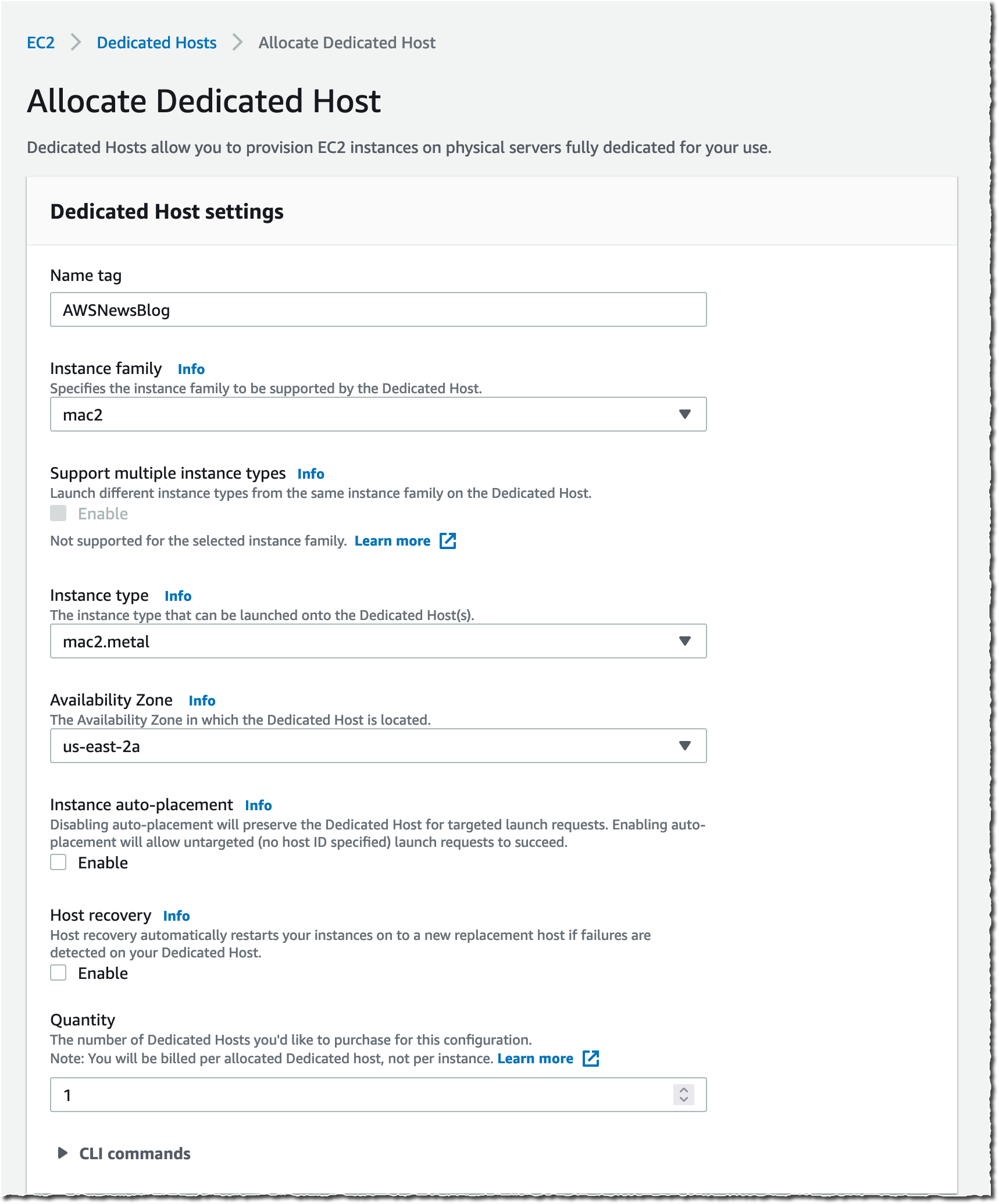
As I explained previously, when using EC2 Mac instances, there is no virtual machine involved. These are running on bare metal servers, each hosting a Mac mini. The first step, therefore, involves grabbing a dedicated server. I open the AWS Management Console, navigate to the Amazon EC2 section, then I select Dedicated Hosts. I select Allocate Dedicated Host to allocate a server to my AWS account.

EC2 Mac2 Instances - Dedicated Hosts

Alternatively, I may use the AWS Command Line Interface (CLI).

➜  ~ aws ec2 allocate-hosts                  \
         --instance-type mac2.metal          \
         --availability-zone us-east-2b      \
         --quantity 1 
{
    "HostIds": [
        "h-0fxxxxxxx90"
    ]
}

Once the host is allocated, I start an EC2 instance on it. The procedure is no different from starting any EC2 instance type. I just have to ensure I select a macOS AMI version that suits my requirements. I select the mac2.metal instance type and select host Tenancy and the dedicated Host I just created.

EC2 Dedicated TenancyAlternatively, I may use the CLI.

➜ ~ aws ec2 run-instances                                     \
	    --instance-type mac2.metal                             \
        --key-name my_key                                      \
        --placement HostId=h-0fxxxxxxx90                       \
        --security-group-ids sg-01000000000000032              \
        --image-id AWS_OR_YOUR_AMI_ID
{
    "Groups": [],
    "Instances": [
        {
            "AmiLaunchIndex": 0,
            "ImageId": "ami-01xxxxbd",
            "InstanceId": "i-08xxxxx5c",
            "InstanceType": "mac2.metal",
            "KeyName": "my_key",
            "LaunchTime": "2021-11-08T16:47:39+00:00",
            "Monitoring": {
                "State": "disabled"
            },
... redacted for brevity ....

When you use EC2 Mac instances for the first time, you’re likely to ask questions such as, “How do I connect through Apple Remote Desktop?” or “How do I increase the size of the APFS file system on the EBS volume?” The EC2 Mac documentation covers the answers for you and provides examples of commands to run on macOS to perform these common tasks.

I use SSH to connect to the newly launched instance as usual.

EC2 Mac M1 Instance uname -a

I may enable Apple Remote Desktop and start a VNC session to the EC2 instance. The EC2 Mac instance documentation page has the details.

mac2 GUI VNC

Availability and Pricing
EC2 M1 Mac instances are now available in preview in US East (N. Virginia) and US West (Oregon), with other AWS Regions coming at launch.

Pricing metrics are similar to the previous generation of EC2 Mac instances. You are charged per hour of reservation of the dedicated host, not for the time the instance is running, and there is a minimum charge of 24 hours for reserving a dedicated host.

In the two preview Regions, the on-demand price is $0.6498 per hour. You can save up to 42 percent over the on-demand price with Savings Plans. Check our Dedicated Host on-demand pricing page, as well as the Savings Plans page to learn the details.

You can sign up for the preview of EC2 Mac M1 instances today!

— seb

Handy Tips #14: Gain new insights into your metrics with the Graph widget

Post Syndicated from Arturs Lontons original https://blog.zabbix.com/handy-tips-13-gain-new-insights-into-your-metrics-with-the-graph-widget/17416/

Group, aggregate, and visualize your collected metrics with the Graph widget to obtain additional insights.

Sometimes simple graphs may not be sufficient – we may need to visualize data trends, display all metrics matching a pattern, or define custom draw styles for specific metrics.

The Graph widget allows you to visualize your metrics in an advanced fashion:

  • Customize your graph draw styles
  • Select between displaying History or Trend values
  • Calculate and display aggregated metric values on the fly

  • Define custom aggregation intervals
  • Define flexible problem display logic
  • Visually group metrics by defining item and host data sets

Check out the video to learn how to visualize your metrics by using the Graph widget.

How to visualize data with the Graph widget:

  1. Navigate to Monitoring → Dashboards – All Dashboards
  2. Click Create Dashboard to create a new Dashboard
  3. Left-click on an empty space and select Add Widget
  4. Select Widget type – Graph
  5. Type in the data set host and item patterns
  6. Use wildcard symbol ‘*‘ to match multiple hosts/items
  7. Click Add new data set to add a second data set
  8. Fill in the host pattern and item pattern to match a different set of metrics
  9. For both data sets, select an Aggregation function, Aggregation interval, and Aggregate – Data set
  10. Observe how metrics get aggregated in the graph on the fly

Tips and best practices:
  • Wildcards can be used in host and item pattern matching
  • The Overrides section can be used to further customize a particular set of items
  • Items within a single data set will use the same base color
  • Up to 50 items may be displayed in the graph

Hacky Holidays From Rapid7! Announcing Our New Festive Blog Series

Post Syndicated from Jesse Mack original https://blog.rapid7.com/2021/12/02/hacky-holidays-from-rapid7-announcing-our-new-festive-blog-series/

Hacky Holidays From Rapid7! Announcing Our New Festive Blog Series

The holiday season often inspires reflection on the year coming to a close — but with the new year approaching, this season can also signal the opportunity for a fresh start.

In that spirit, we’re announcing a refreshed theme and approach to our annual holiday blog series: Hacky Holidays!

While we’ll always treasure the years of HaXmas, we wanted to do something more inclusive this year, so infosec practitioners from all walks of life can take part, regardless of what year-end observances you might keep. The change also gives us an opportunity to expand our publishing dates outside the traditional 12 Days of Christmas, so we can supply you with festively themed security content all season long — we’ll be running Hacky Holidays here on the Rapid7 blog throughout the whole month of December.

Our greatest holiday hits

Before we tell you more about the exciting content we have planned for the inaugural edition of Hacky Holidays, let’s pay a little homage to HaXmas and take a look at some of our holiday highlights from years past.

  • We gave you some tips for how to fill the role of sysadmin for your non-security-minded family (without going totally crazy).
  • We told the tale of Kevin the Elf, admin for Santa’s master list, who receives a suspicious email claiming to come from the Claus himself.


Hacky Holidays From Rapid7! Announcing Our New Festive Blog Series

What’s waiting under the tree this year

Now that we’ve got you in the spirit of cybersecurity cheer, here’s a look ahead at what we have planned for the inaugural Hacky Holidays.

  • Our team’s predictions for what 2022 might hold for security pros
  • A look back at the latest season of Security Nation — where some behind-the-mic personalities turn the tables to interview Jen and Tod
  • A deep dive into some of the inspiring ways security pros are giving back to the community
  • An brief tutorial on membership inference for neural networks from our resident AI expert, Erick Galinkin
  • A wrap-up of all things Metasploit from 2021
  • And much more!

Check back with us throughout the month so you don’t miss out on the Hacky Holiday cheer!

NEVER MISS A BLOG

Get the latest stories, expertise, and news about security today.

This shouldn’t have happened: A vulnerability postmortem (Project Zero blog)

Post Syndicated from original https://lwn.net/Articles/877420/rss

Over on the Project Zero blog, Tavis Ormandy has a lengthy postmortem on a vulnerability that he found in the Network Security Services (NSS) cryptography library. The vulnerability is a bog-standard buffer overflow that has existed in the library since 2012 despite various kinds of static analysis, testing, and fuzzing that Mozilla and others have applied to it over the years. He found it with a new fuzzing technique:

To solve this problem, I’ve been experimenting with monitoring the call stack during execution.

The naive implementation is too slow to be practical, but after a lot of optimization I had come up with a library that was fast enough to be integrated into coverage-guided fuzzing, and was testing how it performed with NSS and other libraries.

[…] The fuzzer I was using is able to isolate and extract interesting new ASN.1 OIDs, SEQUENCEs, INTEGERs, and so on. Once extracted, it can then randomly combine or insert them into template data. This isn’t really a new idea, but is a new implementation. I’m planning to open source this code in the future.

Deploying Zabbix in Amazon Web Services cloud platform

Post Syndicated from Arturs Lontons original https://blog.zabbix.com/deploying-zabbix-in-amazon-web-services-cloud-platform/17283/

With the rapid evolution and proliferation of different cloud services, many organizations have decided to move parts of their infrastructures from on-prem to cloud. As an essential part of your infrastructure, Zabbix is no exception – you always have the option to either deploy Zabbix on-prem or select from one of the many supported cloud service providers to deploy your Zabbix Server or Zabbix Proxy on.

In this blog post, let’s look at how we can quickly deploy Zabbix Server and Zabbix Proxy nodes in Amazon Web Services cloud platform.

Deploying the Zabbix Server in AWS

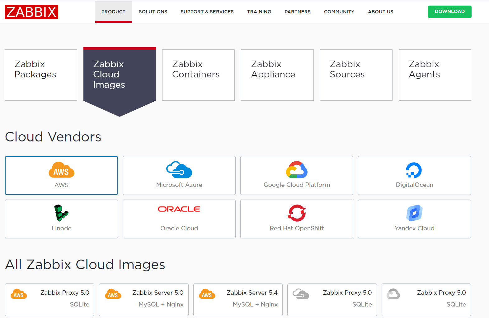
Let’s begin with the Zabbix download page. Under the Zabbix Cloud Images section, select the AWS cloud vendor and then the Cloud Image you wish to deploy. Let’s start with Zabbix Server 5.0 with MySQL DB backend and Nginx Web server backend for our frontend.

Next, we will be redirected to the AWS marketplace, where we will have to subscribe to the Zabbix Server 5.0 image.

Once we have subscribed to the Zabbix Server image, we can continue with the deployment configuration.

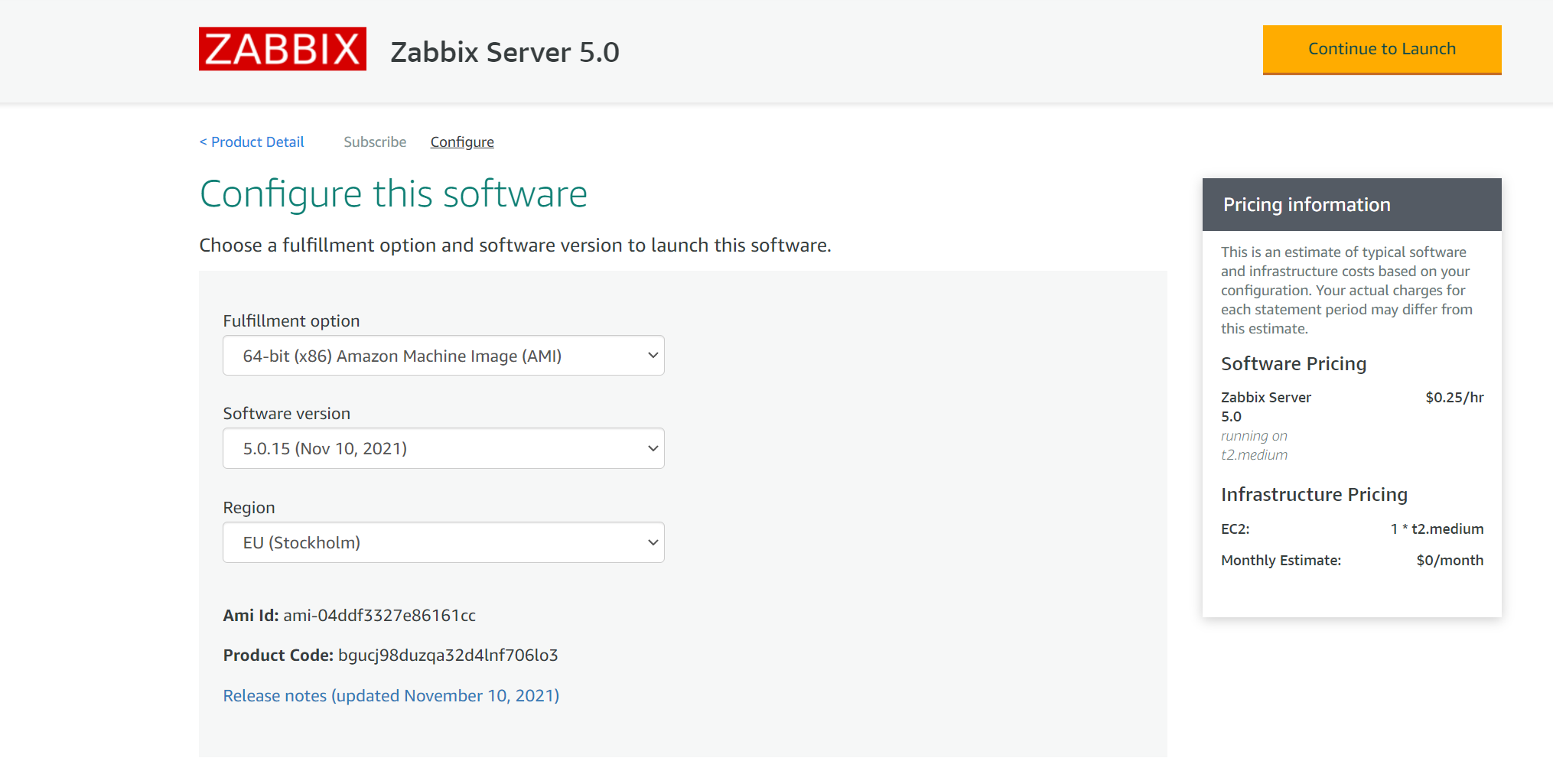
Next, we must select our Region, Zabbix minor version (usually the latest available), and the Fulfillment option. Once that is done, we can finalize the launch configuration.

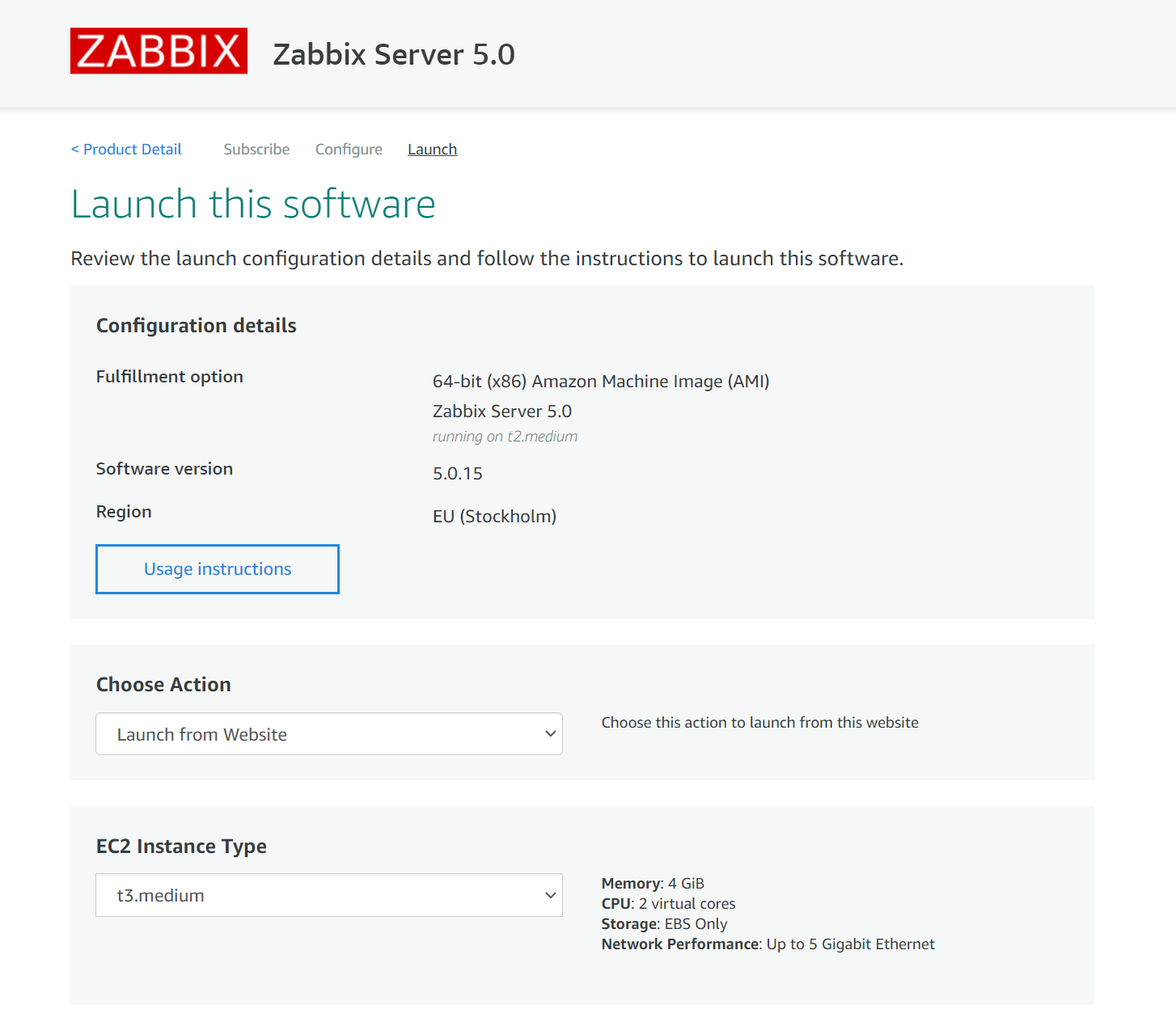
Select the preferred Launch option, EC2 Instance Type, VPC, and Subent settings on the Launch page.

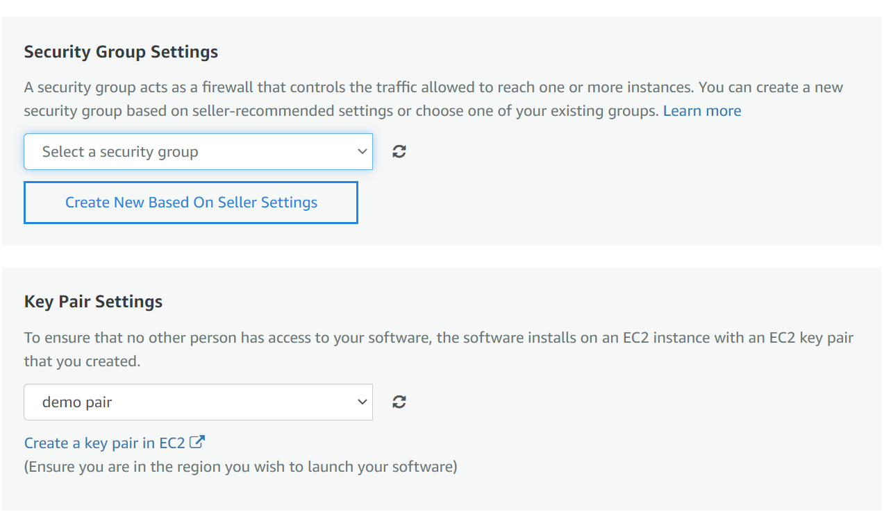
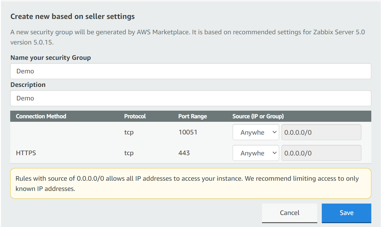
Next – We have to select or create a security group.

We also have to select or generate EC 2 Key pair – make sure to save your private key in a safe location!

Note that creating a security group based on seller settings does not guarantee that the group will have an inbound SSH access rule! Make sure to double-check the security group and manually add the SSH inbound rule if it hasn’t yet been added. We will need to access this instance via SSH to obtain the initial frontend login credentials!

Once you click on the Launch button, the deployment process for your Zabbix application will be initiated.

Accessing the application

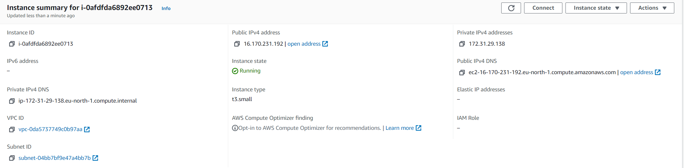
Let’s open up the Instances section and open our newly deployed Zabbix instance

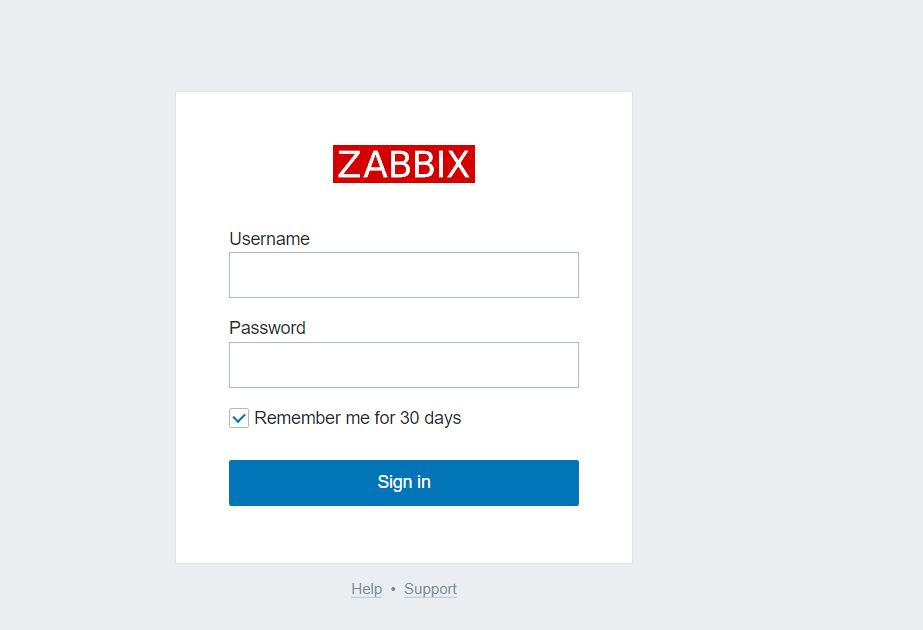
We can access the Zabbix Frontend by opening the Public IPv4 address or Public IPv4 DNS of the Zabbix instance

Note that the Zabbix frontend password is still unknown to us. Recall how I mention that we will need to access the instance via SSH to obtain the frontend password. Let’s do so now.

Write down the login credentials and use them to log in to the Zabbix instance.

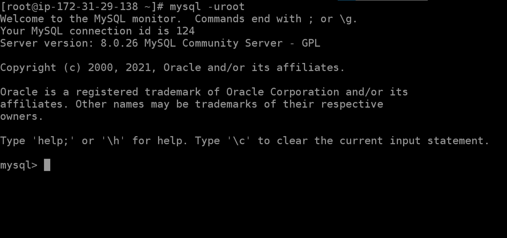
Accessing the database

In case we wish to access the Zabbix database backend, we can do so from the command line. Zabbix database can be accessed by using the root user. By default, it can be used without a password.

The MySQL root password is stored in /root/.my.cnf configuration file.

Modifying the Zabbix Frontend timezone

By default, the Zabbix frontend uses the “UTC” timezone. If you need to change it, edit php_value[date.timezone] PHP variable in /etc/php-fpm.d/zabbix.conf and restart php-fpm process:

systemctl restart php-fpm

Zabbix proxy

If you wish to deploy a Zabbix proxy instance in your AWS cloud, the deployment steps are very much the same. Most likely, you will still require SSH access if you wish to perform some configuration changes in the Zabbix proxy configuration file.

Note, that by default, the SQLite proxy database is stored in /tmp/zabbix_proxy.sqlite3

As always, don’t forget the point the proxy at your Zabbix server instance by modifying the Server parameter in the Zabbix proxy configuration file, located in /etc/zabbix/zabbix_proxy.conf

And that’s all! With just a few clicks, we are able to deploy a fully functional Zabbix instance or a small Zabbix proxy to distribute or scale our monitoring. Don’t forget that AWS is just one of the many cloud service providers you can use with Official Zabbix images. If you have any questions about the AWS deployment – you are very much encouraged to leave a comment under this blog post.

If you wish to learn more about the Zabbix Monitoring solution, check out the official documentation https://www.zabbix.com/documentation/current/manual/quickstart.

Smart Contract Bug Results in $31 Million Loss

Post Syndicated from Bruce Schneier original https://www.schneier.com/blog/archives/2021/12/smart-contract-bug-results-in-31-million-loss.html

A hacker stole $31 million from the blockchain company MonoX Finance , by exploiting a bug in software the service uses to draft smart contracts.

Specifically, the hack used the same token as both the tokenIn and tokenOut, which are methods for exchanging the value of one token for another. MonoX updates prices after each swap by calculating new prices for both tokens. When the swap is completed, the price of tokenIn­that is, the token sent by the user­decreases and the price of tokenOut­or the token received by the user­increases.

By using the same token for both tokenIn and tokenOut, the hacker greatly inflated the price of the MONO token because the updating of the tokenOut overwrote the price update of the tokenIn. The hacker then exchanged the token for $31 million worth of tokens on the Ethereum and Polygon blockchains.

The article goes on to talk about how common these sorts of attacks are. The basic problem is that the code is the ultimate authority — there is no adjudication protocol — so if there’s a vulnerability in the code, there is no recourse. And, of course, there are lots of vulnerabilities in code.

To me, this is reason enough never to use smart contracts for anything important. Human-based adjudication systems are not useless pre-Internet human baggage, they’re vital.

Security updates for Thursday

Post Syndicated from original https://lwn.net/Articles/877410/rss

Security updates have been issued by CentOS (kernel, openssh, and rpm), Debian (nss), Fedora (seamonkey), Mageia (glibc), openSUSE (go1.16, go1.17, kernel, mariadb, netcdf, openexr, poppler, python-Pygments, python-sqlparse, ruby2.5, speex, and webkit2gtk3), Oracle (nss), Red Hat (nss), SUSE (clamav, glibc, gmp, go1.16, go1.17, kernel, mariadb, netcdf, OpenEXR, openexr, openssh, poppler, python-Pygments, python-sqlparse, ruby2.1, ruby2.5, speex, webkit2gtk3, and xen), and Ubuntu (nss and thunderbird).

Record numbers of young people have sent us ideas for Astro Pi Mission Space Lab 2021/22

Post Syndicated from Claire Given original https://www.raspberrypi.org/blog/young-people-space-experiment-ideas-astro-pi-mission-space-lab-2021-22/

We and our partners ESA Education are delighted to announce that for this year’s Mission Space Lab of the European Astro Pi Challenge, a record number of 800 teams from 23 countries sent us their ideas for experiments to run on board the International Space Station (ISS).

This is an incredible 83% increase from last year and means that more than 3100 young people from across Europe and other eligible countries have taken part in Phase 1 of Mission Space Lab.

Young people’s scientific experiments in space with Mission Space Lab

Every year since 2015, thanks to our yearly Astro Pi Challenge, Mission Space Lab teams of young people have created code for their own scientific experiments to run on the ISS’s two Astro Pi units. These Astro Pi units are Raspberry Pi computers in space-proof cases, with cameras and an array of sensors. In Phase 1 of Mission Space Lab, teams submit their idea for an experiment that uses the Astro Pi hardware to investigate either the environmental conditions inside the Columbus module on the ISS, or life on the Earth’s surface.

A photo of the Maledives taken from the International Space Station by an Astro Pi unit programmed by a Mission Space Lab team.
The Maldives as photographed by a Mission Space Lab team from a previous round

This year, we are sending two upgraded Astro Pi units up into space to the ISS. These consist of the newest model of the Raspberry Pi computer, the newest Raspberry Pi camera, an augmented sensor board and a Coral machine learning accelerator. Young people can vote for the new Astro Pi units’ names by doing the Astro Pi beginners’ coding activity, Mission Zero.

Astro Pi MK II hardware.
The new Astro Pi units

For Mission Space Lab participants, the new hardware opens up a range of options for experiments that were not possible before. Among these are experiments using elements of artificial intelligence such as advanced machine learning, and higher-resolution photography than ever before.

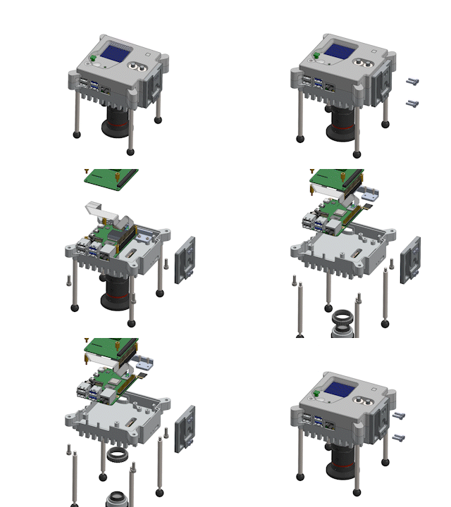
Animation of how the components of the Mark 2 Astro Pi hardware unit fit together.
Inside the new Astro Pi unit

It’s clear that young people are really excited about the new hardware. Not only did we see an overall increase in participating teams, but 49% of the Mission Space Lab experiment ideas that teams sent us involved machine learning.

Mission Space Lab teams are getting ready to write and test their code

We’ve now selected 502 teams for Phase 2 of Mission Space Lab based on the quality of their experiment ideas. Despite the fierce competition, this is 26% more teams than we were able to progress to Phase 2 last year.

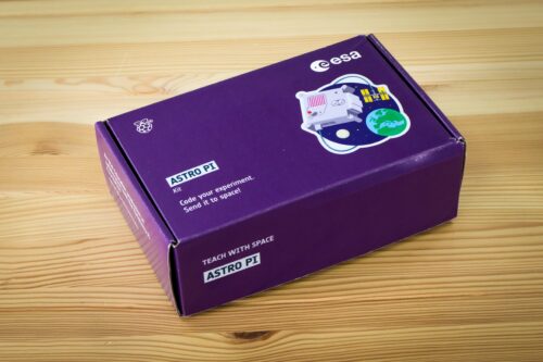
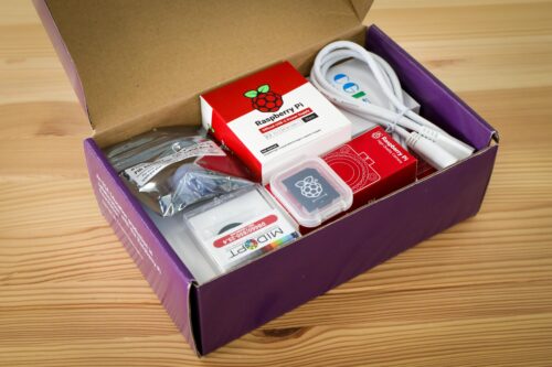
All the teams we’ve selected are about to be sent a special Astro Pi hardware kit to help them write the programs for their experiments. These kits include all the components to replicate the new Astro Pi units that will travel to space in December: a Raspberry Pi 4 computer, a Raspberry Pi High Quality Camera, and the same sensors that are on the Astro Pi computers on the ISS. In addition, teams conducting experiments involving machine learning will receive a Coral machine learning accelerator, and teams conducting experiments involving Infrared photography will receive a red optical filter.

Once the teams of young people have received their hardware kits, they’ll be able to familiarise themselves with the Astro Pi sensors and cameras, and then create and test (and re-test!) their code.

Young people’s code will run in space next year

The teams’ deadline for submitting the code for their experiments to us is Thursday 24 February 2022. Once their code has gone through our checks and tests, it will be ready to run on the shiny new Astro Pi units on board the ISS in April or May.

Congratulations to the successful teams, and thank you to everyone who sent us their ideas for Mission Space Lab this year. And a special thank you to all the teachers, educators, club volunteers, and other wonderful people who are acting as Mission Space Lab team mentors this year. You are helping your young people do something remarkable that they will remember for the rest of their lives.

If your team was unsuccessful this time, we’re sorry for the disappointment — please try again next year.

Logo of Mission Zero, part of the European Astro Pi Challenge.

Young people up to age 19 can also take part in Mission Zero, the beginners’ coding activity of the European Astro Pi Challenge, to vote for which European scientist they think we should name the units after. All Mission Zero entries are guaranteed to run on the ISS for 30 seconds!

The post Record numbers of young people have sent us ideas for Astro Pi Mission Space Lab 2021/22 appeared first on Raspberry Pi.

Run queries 3x faster with up to 70% cost savings on the latest Amazon Athena engine

Post Syndicated from Pathik Shah original https://aws.amazon.com/blogs/big-data/run-queries-3x-faster-with-up-to-70-cost-savings-on-the-latest-amazon-athena-engine/

Amazon Athena is an interactive query service that makes it easy to analyze data in Amazon Simple Storage Service (Amazon S3) using standard SQL. Athena is serverless, so there is no infrastructure to manage, and you pay only for the queries that you run.

In November 2020, Athena announced the General Availability of the V2 version of its core engine in addition to performance enhancements and new feature capabilities. Today, V2 is the default engine version for every Athena workgroup and it includes additional enhancements made since its first release. Engine enhancements are released frequently and are automatically available to you without the need for manual intervention.

In this post, we discuss the performance benchmarks and performance enhancements of Athena’s latest engine.

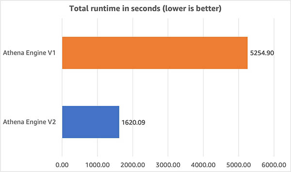
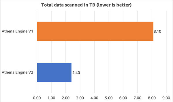
We performed benchmark testing on our latest engine using TPC-DS benchmark queries at 3 TB scale and observed that query performance improved by 3x and cost decreased by 70% as a result of reduced scanned data size when compared to our earlier engine.

Performance and cost comparison on TPC-DS benchmarks

We used the industry-standard TPC-DS 3 TB to represent different customer use cases. These benchmark tests have a range of accuracy within +/- 10% and are representative of workloads with 10 times the stated benchmark size. This means a 3 TB benchmark dataset accurately represents customer workloads on 30–50 TB datasets.

In our testing, the dataset was stored in Amazon S3 in non-compressed Parquet format with no additional optimizations and the AWS Glue Data Catalog was used to store metadata for databases and tables. Fact tables were partitioned on the date column used for join operations and each fact table consisted of 2,000 partitions. We selected 71 of the 99 queries from the TPC-DS benchmark that best illustrated the differences between engines V1 and V2. We ran the queries with a concurrency of 3. This means up to 3 queries were in a running state at any given time and the next query was submitted as soon as one of the 3 running queries completed.

The following graph illustrates the total runtime of queries on engines V1 and V2 and shows runtime was 3x faster on engine V2.

We also compared the amount of data scanned by queries in this benchmark. As shown in the following graph, we found that the data scanned – and the resulting per-query costs – were 70% lower with engine V2.

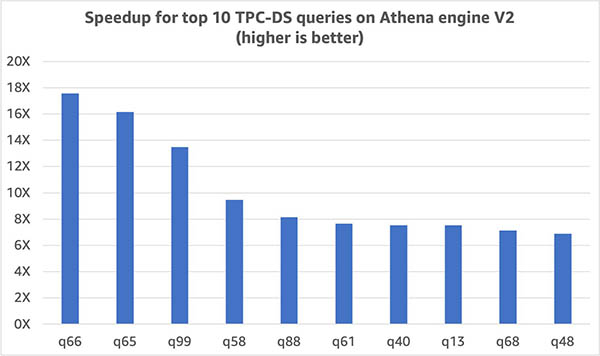
Queries in our benchmark were consistently more performant with engine V2. The following graph shows the 10 TPC-DS queries with the largest improvement in runtime. For this set of queries, runtime improved by 6.9 times.

Now, let’s look at some of the enhancements in engine V2 that contributed towards these astounding results.

Performance enhancements in engine V2

The Athena engine is built upon Presto, an open-source distributed SQL query engine optimized for low latency. We’re continuously improving Athena’s engine with enhancements developed by Athena and AWS engineering teams as well as incorporating contributions from the PrestoDB and Trino community. The result is an engine with continuously increasing performance and cost-effectiveness benefits that are automatically available to you. A few such enhancements are highlighted in the following sections.

More efficient joins via dynamic filtering and dynamic partition pruning

Dynamic filtering and dynamic partition pruning improves the query runtime and reduces data scanned for queries with joins and a very selective filter clause for the table on the right side of join, as shown in the following example.

In the following query, Table_B is a small table with a very selective filter. (column_A = “value”). After the selective filter is applied to Table_B, a value list for a joined column Table_B.date is extracted first, and it’s pushed down to a joined table Table_A as a filter. It’s used to filter out unnecessary rows and partitions of Table_A. This results in reading fewer rows and partitions from the source for Table_A and helping reduce query runtime and data scan size, which in turn helps reduce the costs of running the query in Athena.

SELECT count(*)
FROM Table_A
    JOIN Table_B ON Table_A.date = Table_B.date
WHERE Table_B.column_A = "value"

More intelligent join ordering and distribution selections

Choosing a better join order and join algorithm is critical to better query performance. They can easily affect how much data is read from a particular table, how much data is transferred to the intermediate stages through networks, and how much memory is needed to build up a hash table to facilitate a join. Join order and join algorithm decisions are part of the cost-based optimizer that uses statistics to improve query plans by deciding how tables and subqueries are joined.

For cases where statistics aren’t available, we introduced a similar concept but through enumerating and analyzing the metadata of the S3 files to optimize query plans. The logic for those rules takes into account both small tables and small subqueries while making these decisions. For example, consider the following query:

SELECT *
FROM A, B, C
WHERE A.key = B.key AND C.key = B.key

The syntactical join order is A join B join C. With those optimization rules, if A is considered a small table after retrieving the approximate size through fast file enumeration on Amazon S3, the rules place table A on the build side (the side that is built into a hash table for a join) and makes the join as a broadcast join to speed up the query and reduce memory consumption. Additionally, the rules reorder the joins to minimize the intermediate result size, which helps further speed up the overall query runtime.

Nested field pruning for complex data types

In this improvement for Parquet and ORC datasets, when a nested field is queried in a complex data type like struct, array of structs, or map, only the specific subfield or nested field is read from the source instead of reading the entire row. If there is a filter on the nested field, Athena can now push down the predicate to the Parquet or ORC file to prune the content at source level. This has led to significant savings in data scanned and a reduction in query runtime. With this feature, you don’t need to flatten your nested data to improve query performance.

Optimized top N rank() functions

Previously, all input data for rank() window functions was sent to the window operator for processing and the LIMIT and filter clauses were applied at a later stage.

With this optimization, the engine can replace the window operator with a top N rank operator, push down the filters, and only keep top N (where N is the LIMIT number) entries for each window group to save memory and I/O throughput.

A good example of a query that benefited from this optimization is query 67 (shown in the following code) of the TPC-DS benchmark. It contains a subquery with a memory- and CPU-heavy window function rank() that is applied to the output of another subquery, which generates a huge amount of intermediate data after scanning the large fact table store_sales. The output of this subquery is further filtered with LIMIT and comparison operators before returning the final results. Because of the LIMIT and comparison operator, only records with the lowest 100 total sales are meaningful in each item category window group; the rest are discarded. Processing these records (which are discarded later through window functions) is memory and network intensive.

With this enhancement, only a small amount of data is kept in memory and sent across the network because the filters and limits are pushed down. This makes the entire workflow more efficient and enables the engine to process a larger amount of data with the same resources.

Query 67 was unsuccessful on engine V1 despite the considerable effort and time needed to scan (approximately 75 GB of data) and process data that was eventually thrown away due to resource exhaustion. On engine V2, this query completes in approximately 165 seconds and scans only 17 GB of data.

In the following query, filter clause rk <=100 and limit 100 are pushed to the rank() function as described earlier:

select * from
(select i_category, i_class, i_brand, i_product_name, d_year, d_qoy, d_moy, s_store_id,
            sumsales, 
            rank() over (partition by i_category order by sumsales desc) rk
     from
     (select i_category, i_class, i_brand, i_product_name, d_year, d_qoy, d_moy,
                s_store_id, sum(coalesce(ss_sales_price*ss_quantity,0)) sumsales
         from store_sales, date_dim, store, item
         where  ss_sold_date_sk=d_date_sk
         and ss_item_sk=i_item_sk
         and ss_store_sk = s_store_sk
         and d_month_seq between 1200 and 1200+11
         group by rollup(i_category, i_class, i_brand, i_product_name, d_year, d_qoy,
                       d_moy,s_store_id))dw1) dw2
where rk <= 100 
order by  i_category, i_class, i_brand, i_product_name, d_year, 
d_qoy, d_moy, s_store_id, sumsales, rk
limit 100  

Other optimizations

In addition to these optimizations, the following contributed towards faster queries and reduced data scan for the queries in our benchmark:

  • Further pushdown of LIMIT and filter operators to reduce the intermediate results size and data scanned from the sources
  • Enhancement of aggregation and window functions to consume much less memory and provide better performance
  • Addition of a distributed sort for the ORDER BY operator to utilize resources effectively which helps sort more data reliably
  • Improvement in task-scheduling mechanisms for more efficient processing across resources

Conclusion

With the performance optimizations in the latest engine V2 of Athena, you can run queries faster and at lower cost than before. The TPC-DS benchmark queries on engine V2 showed a 3x improvement in query runtime and cost reduction of 70%.

In our mission to innovate on behalf of customers, Athena routinely releases performance and reliability enhancements on its latest engine version. To stay up to date with the latest engine release, ensure your Athena workgroups have selected Automatic query engine upgrade in your workgroup settings.

For more information, see the performance enhancements for engine V2 and check our release notes to learn about new features and enhancements.


About the Authors

Pathik Shah is a Sr. Big Data Architect on Amazon Athena. He joined AWS in 2015 and has been focusing in the big data analytics space since then, helping customers build scalable and robust solutions using AWS analytics services.

Xuanyu Zhan is a Software Development Engineer on Amazon Athena. He joined Athena in 2019 and has been working on different areas of Athena engine V2, including engine upgrade, engine reliability, and engine performance.

Sungheun Wi is a Sr. Software Development Engineer on Amazon Athena. He joined AWS in 2019 and has been working on multiple database engines such as Athena and Aurora, focusing on analytic query processing enhancements.

Introducing Amazon Simple Queue Service dead-letter queue redrive to source queues

Post Syndicated from Julian Wood original https://aws.amazon.com/blogs/compute/introducing-amazon-simple-queue-service-dead-letter-queue-redrive-to-source-queues/

This blog post is written by Mark Richman, a Senior Solutions Architect for SMB.

Today AWS is launching a new capability to enhance the dead-letter queue (DLQ) management experience for Amazon Simple Queue Service (SQS). DLQ redrive to source queues allows SQS to manage the lifecycle of unconsumed messages stored in DLQs.

SQS is a fully managed message queuing service that enables you to decouple and scale microservices, distributed systems, and serverless applications. Using Amazon SQS, you can send, store, and receive messages between software components at any volume without losing messages or requiring other services to be available.

To use SQS, a producer sends messages to an SQS queue, and a consumer pulls the messages from the queue. Sometimes, messages can’t be processed due to a number of possible issues. These can include logic errors in consumers that cause message processing to fail, network connectivity issues, or downstream service failures. This can result in unconsumed messages remaining in the queue.

Understanding SQS dead-letter queues (DLQs)

SQS allows you to manage the life cycle of the unconsumed messages using dead-letter queues (DLQs).

A DLQ is a separate SQS queue that one or many source queues can send messages that can’t be processed or consumed. DLQs allow you to debug your application by letting you isolate messages that can’t be processed correctly to determine why their processing didn’t succeed. Use a DLQ to handle message consumption failures gracefully.

When you create a source queue, you can specify a DLQ and the condition under which SQS moves messages from the source queue to the DLQ. This is called the redrive policy. The redrive policy condition specifies the maxReceiveCount. When a producer places messages on an SQS queue, the ReceiveCount tracks the number of times a consumer tries to process the message. When the ReceiveCount for a message exceeds the maxReceiveCount for a queue, SQS moves the message to the DLQ. The original message ID is retained.

For example, a source queue has a redrive policy with maxReceiveCount set to 5. If the consumer of the source queue receives a message 6, without successfully consuming it, SQS moves the message to the dead-letter queue.

You can configure an alarm to alert you when any messages are delivered to a DLQ. You can then examine logs for exceptions that might have caused them to be delivered to the DLQ. You can analyze the message contents to diagnose consumer application issues. Once the issue has been resolved and the consumer application recovers, these messages can be redriven from the DLQ back to the source queue to process them successfully.

Previously, this required dedicated operational cycles to review and redrive these messages back to their source queue.

DLQ redrive to source queues

DLQ redrive to source queues enables SQS to manage the second part of the lifecycle of unconsumed messages that are stored in DLQs. Once the consumer application is available to consume the failed messages, you can now redrive the messages from the DLQ back to the source queue. You can optionally review a sample of the available messages in the DLQ. You redrive the messages using the Amazon SQS console. This allows you to more easily recover from application failures.

Using redrive to source queues

To show how to use the new functionality there is an existing standard source SQS queue called MySourceQueue.

SQS does not create DLQs automatically. You must first create an SQS queue and then use it as a DLQ. The DLQ must be in the same region as the source queue.

Create DLQ

  1. Navigate to the SQS Management Console and create a standard SQS queue for the DLQ called MyDLQ. Use the default configuration. Refer to the SQS documentation for instructions on creating a queue.
  2. Navigate to MySourceQueue and choose Edit.
  3. Navigate to the Dead-letter queue section and choose Enabled.
  4. Select the Amazon Resource Name (ARN) of the MyDLQ queue you created previously.
  5. You can configure the number of times that a message can be received before being sent to a DLQ by setting Set Maximum receives to a value between 1 and 1,000. For this demo enter a value of 1 to immediately drive messages to the DLQ.
  6. Choose Save.
Configure source queue with DLQ

Configure source queue with DLQ

The console displays the Details page for the queue. Within the Dead-letter queue tab, you can see the Maximum receives value and DLQ ARN.

DLQ configuration

DLQ configuration

Send and receive test messages

You can send messages to test the functionality in the SQS console.

  1. Navigate to MySourceQueue and choose Send and receive messages
  2. Send a number of test messages by entering the message content in Message body and choosing Send message.
  3. Send and receive messages

    Send and receive messages

  4. Navigate to the Receive messages section where you can see the number of messages available.
  5. Choose Poll for messages. The Maximum message count is set to 10 by default If you sent more than 10 test messages, poll multiple times to receive all the messages.
Poll for messages

Poll for messages

All the received messages are sent to the DLQ because the maxReceiveCount is set to 1. At this stage you would normally review the messages. You would determine why their processing didn’t succeed and resolve the issue.

Redrive messages to source queue

Navigate to the list of all queues and filter if required to view the DLQ. The queue displays the approximate number of messages available in the DLQ. For standard queues, the result is approximate because of the distributed architecture of SQS. In most cases, the count should be close to the actual number of messages in the queue.

Messages available in DLQ

Messages available in DLQ

  1. Select the DLQ and choose Start DLQ redrive.
  2. DLQ redrive

    DLQ redrive

    SQS allows you to redrive messages either to their source queue(s) or to a custom destination queue.

  3. Choose to Redrive to source queue(s), which is the default.
  4. Redrive has two velocity control settings.

  • System optimized sends messages back to the source queue as fast as possible
  • Custom max velocity allows SQS to redrive messages with a custom maximum rate of messages per second. This feature is useful for minimizing the impact to normal processing of messages in the source queue.

You can optionally inspect messages prior to redrive.

  • To redrive the messages back to the source queue, choose DLQ redrive.
  • DLQ redrive

    DLQ redrive

    The Dead-letter queue redrive status panel shows the status of the redrive and percentage processed. You can refresh the display or cancel the redrive.

    Dead-letter queue redrive status

    Dead-letter queue redrive status

    Once the redrive is complete, which takes a few seconds in this example, the status reads Successfully completed.

    Redrive status completed

    Redrive status completed

  • Navigate back to the source queue and you can see all the messages are redriven back from the DLQ to the source queue.
  • Messages redriven from DLQ to source queue

    Messages redriven from DLQ to source queue

    Conclusion

    Dead-letter queue redrive to source queues allows you to effectively manage the life cycle of unconsumed messages stored in dead-letter queues. You can build applications with the confidence that you can easily examine unconsumed messages, recover from errors, and reprocess failed messages.

    You can redrive messages from their DLQs to their source queues using the Amazon SQS console.

    Dead-letter queue redrive to source queues is available in all commercial regions, and coming soon to GovCloud.

    To get started, visit https://aws.amazon.com/sqs/

    For more serverless learning resources, visit Serverless Land.

    Lucerna Health uses Amazon QuickSight embedded analytics to help healthcare customers uncover new insights

    Post Syndicated from David Atkins original https://aws.amazon.com/blogs/big-data/lucerna-health-uses-amazon-quicksight-embedded-analytics-to-help-healthcare-customers-uncover-new-insights/

    This is a guest post by Lucerna Health. Founded in 2018, Lucerna Health is a data technology company that connects people and data to deliver value-based care (VBC) results and operational transformation.

    At Lucerna Health, data is at the heart of our business. Every day, we use clinical, sales, and operational data to help healthcare providers and payers grow and succeed in the value-based care (VBC) environment. Through our HITRUST CSF® certified Healthcare Data Platform, we support payer-provider integration, health engagement, database marketing, and VBC operations.

    As our business grew, we found that faster real-time analysis and reporting capabilities through our platform were critical to success. However, that was a challenge for our data analytics team, which was busier than ever developing our proprietary data engine and data model. No matter how many dashboards we built, we knew we could never keep up with user demand with our previous BI solutions. We needed a more scalable technology that could grow as our customer base continued to expand.

    In this post, we will outline how Amazon QuickSight helped us overcome these challenges.

    Embedding analytics with QuickSight

    We had a rising demand for business intelligence (BI) from our customers, and we needed a better tool to help us keep pace that met our security requirements and was part of a comprehensive business associate contract (BAA) and met HIPAA and other privacy standards. We were using several other BI solutions internally for impromptu analysis and reporting, but we realized we needed a fully embedded solution to provide more automation and an integrated experience within our Healthcare Data Platform. After trying out a different solution, we discovered it wasn’t cost-effective for us. That’s when we turned our attention to AWS.

    Three years ago, we decided to go all-in on AWS, implementing a range of AWS services for compute, storage, and networking. Today, each of the building blocks we have in our IT infrastructure run on AWS. For example, we use Amazon Redshift, AWS Glue, and Amazon EMR for our Spark data pipelines, data lake, and data analytics. Because of our all-in approach, we were pleased to find that AWS had a BI platform called QuickSight. QuickSight is a powerful and cost-effective BI service that offers a strong feature set including self-service BI capabilities and interactive dashboards, and we liked the idea of continuing to be all-in on AWS by implementing this service.

    One of the QuickSight’s features we were most excited about was its ability to embed analytics deep within our Healthcare Data Platform. With this solution’s embedded analytics software, we were able to integrate QuickSight dashboards directly into our own platform. For example, we offer our customers a portal where they can register a new analytical dashboard through our user interface. That interface connects to the QuickSight application programming interface (API) to enable embedding in a highly configurable and secure way.

    With this functionality, our customers can ingest and visualize complex healthcare data, such as clinical data from electronic medical record (EMR) systems, eligibility and claims, CRM and digital interactions data. Our Insights data model is projected into Quicksight’s high performance in memory calculation engine enabling high performance analysis on massive datasets.

    Creating a developer experience for customers

    We have also embedded the QuickSight console into our platform. Through this approach, our healthcare data customers can build their own datasets and quickly share that data with a wider group of users through our platform. This gives our customers a developer experience that enables them to customize and share analytical reports with their colleagues. With only a few clicks, users can aggregate and compare data from their sales and EMR solutions.

    QuickSight has also improved collaboration for our own teams when it comes to custom reports. In the past, teams could only do monthly or specialized reports, spending a lot of time building them, downloading them as PDFs, and sending them out to clients as slides. It was a time-consuming and inefficient way to share data. Now, our users can get easy access to data from previously siloed sources, and then simply publish reports and share access to that data immediately.

    Helping healthcare providers uncover new insights

    Because healthcare providers now have centralized data at their fingertips, they can make faster and more strategic decisions. For instance, management teams can look at dashboards on our platform to see updated demand data to plan more accurate staffing models. We’ve also created patient and provider data models that provide a 360-degree view of patient and payer data, increasing visibility. Additionally, care coordinators can reprioritize tasks and take action if necessary because they can view gaps in care through the dashboards. Armed with this data, care coordinators can work to improve the patient experience at the point of care.

    Building and publishing reports twice as fast

    QuickSight is a faster BI solution than anything we’ve used before. We can now craft a new dataset, apply permissions to it, build out an analysis, and publish and share it in a report twice as fast as we could before. The solution also gives our developers a better overall experience. For rapid development and deployment at scale, QuickSight performs extremely well at a very competitive price.

    Because QuickSight is a serverless solution, we no longer need to worry about our BI overhead. With our previous solution, we had a lot of infrastructure, maintenance, and licensing costs. We have eliminated those challenges by implementing QuickSight. This is a key benefit because we’re an early stage company and our lean product development team can now focus on innovation instead of spinning up servers.

    As our platform has become more sophisticated over the past few years, QuickSight has introduced vast number of great features for data catalog management, security, ML integrations, and look/feel that has really improved on our original solution’s BI capabilities. We look forward to continuing to use this powerful tool to help our customers get more out of their data.


    About the Authors

    David Atkins is the Co-Founder & Chief Operating Officer at Lucerna Health. Before co-founding Lucnera Health in 2018, David held multiple leadership roles in healthcare organizations, including spending six years at Centen Corporation as the Corporate Vice President of Enterprise Data and Analytic Solutions. Additionally, he served as the Provider Network Management Director at Anthem. When he isn’t spending time with his family, he can be found on the ski slopes or admiring his motorcycle, which he never rides.

    Adriana Murillo is the Co-Founder & Chief Marketing Officer at Lucerna Health. Adriana has been involved in the healthcare industry for nearly 20 years. Before co-founding Lucerna Health, she founded Andes Unite, a marketing firm primarily serving healthcare provider organizations and health insurance plans. In addition, Adriana held leadership roles across market segment leadership, product development, and multicultural marketing at not-for-profit health solutions company Florida Blue. Adriana is a passionate cook who loves creating recipes and cooking for her family.

    How to automate AWS Managed Microsoft AD scaling based on utilization metrics

    Post Syndicated from Dennis Rothmel original https://aws.amazon.com/blogs/security/how-to-automate-aws-managed-microsoft-ad-scaling-based-on-utilization-metrics/

    AWS Directory Service for Microsoft Active Directory (AWS Managed Microsoft AD), provides a fully managed service for Microsoft Active Directory (AD) in the AWS cloud. When you create your directory, AWS deploys two domain controllers in separate Availability Zones that are exclusively yours for high availability. For use cases requiring even higher resilience and performance, in a specific Region or during specific hours, AWS Managed Microsoft AD allows you to scale by deploying additional domain controllers to meet your needs. These domain controllers can help load-balance, increase overall performance, or simply provide additional nodes to protect against temporary availability issues. AWS Managed Microsoft AD allows you to define the correct number of domain controllers for your directory based on your individual use case.

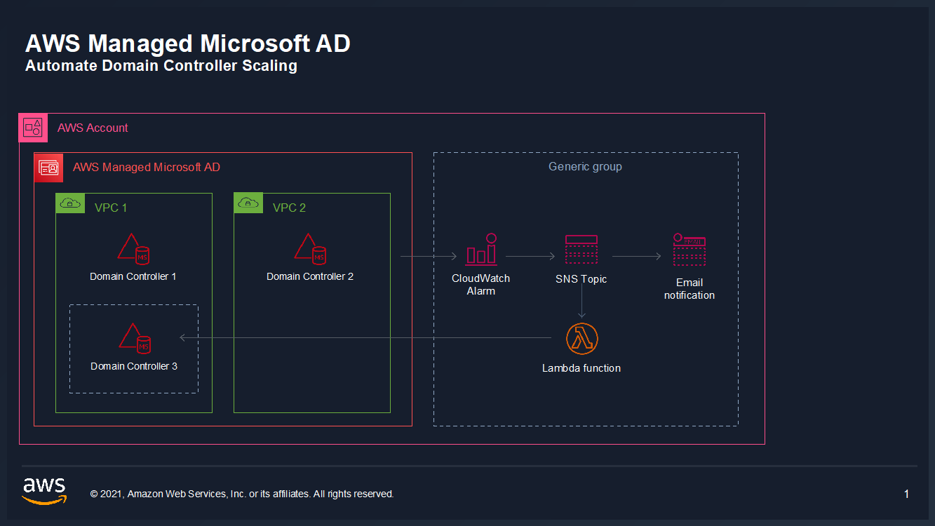
    This post will walk you through how to automate scaling in AWS Managed Microsoft AD using utilization metrics from your directory. You’ll do this using Amazon CloudWatch Alarms, SNS notifications, and a Lambda function to increase the number of domain controllers in your directory based on utilization peaks.

    Simplified directory scaling

    AWS Managed Microsoft AD has now simplified this directory scaling process by integrating with Amazon CloudWatch metrics. This new integration enables you to:

    1. Analyze your directory to identify expected average and peak directory utilization
    2. Scale your directory based on utilization data to adequately address the expected load
    3. Automate the addition of domain controllers to handle unexpected load.

    Integration is available for both domain controller utilization metrics such as CPU, Memory, Disk and Network, and for AD-specific metrics, such as LDAP searches, binds, DNS queries, and Directory reads/writes. Analyzing this data over time to identify expected average and peak utilization on your directory can help you deploy additional domain controllers in Regions that need them. Once you’ve established this utilization baseline, you can deploy additional domain controllers to service this load, and configure alarms for anything exceeding this baseline.

    Solution overview

    In this example, our AWS Managed Microsoft AD has the default two domain controllers; once your utilization threshold is reached, you’ll add one additional domain controller (domain controller 3 in the diagram) to cover this additional load. 

    Figure 1: Solution overview

    Figure 1: Solution overview

    To create a CloudWatch Alarm with SNS topic notifications

    1. In the AWS Console, navigate to CloudWatch
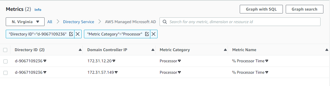
    2. Choose Metrics to see the Browse Metrics panel
    3. Choose the Directory Service namespace, then choose AWS Managed Microsoft AD.
    4. In the Directory ID column, select your directory and check search for this only.
    5. From the Metric Category column, select Processor from Metric Category and check add to search. This view will show the processor utilization for your directory.
    6.  

      Figure 2. Processor utilization metrics

      Figure 2. Processor utilization metrics

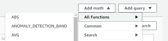
    7. To see the average utilization across all domain controllers, choose Add Math, then All Functions, then AVG to create a metric math expression for average CPU utilization across all domain controllers.
    8.  

      Figure 3. Adding a math function to compute average

      Figure 3. Adding a math function to compute average

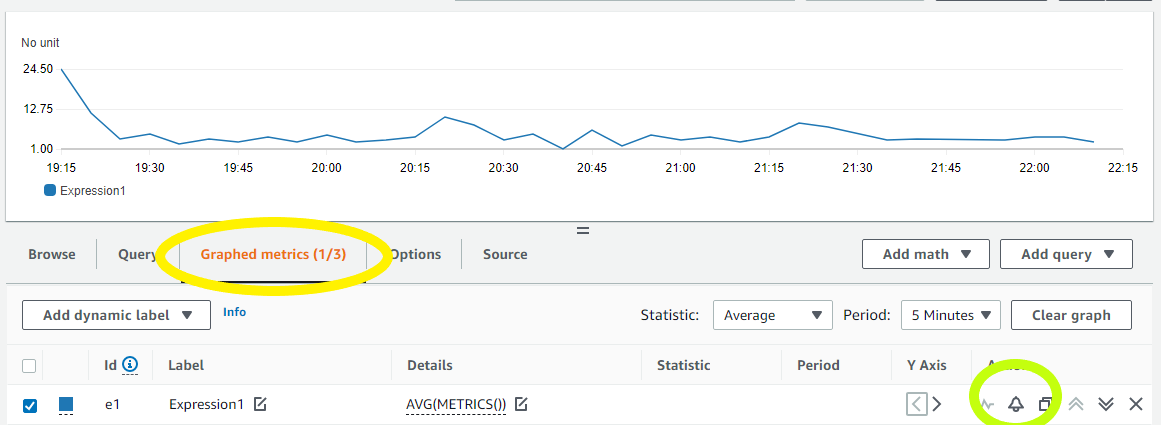
    9. Next, choose the Graphed Metrics tab in the CloudWatch metrics console, select the newly created expression, then select the bell icon from the Actions column to create a CloudWatch alarm based on this metric.
    10. Figure 4. Create a CloudWatch Alarm using Metric Math Expression

      Figure 4. Create a CloudWatch Alarm using Metric Math Expression

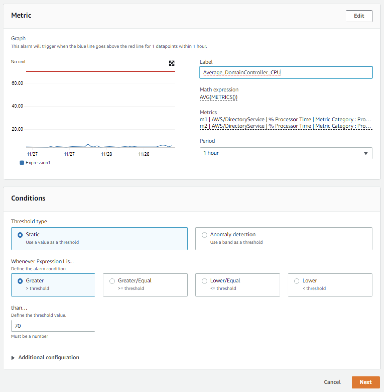
    11. Configure the threshold alarm to trigger when CPU utilization exceeds 70%.
    12.  In the Metrics section, under Period, choose 1 Hour.
       In the Conditions section, under Threshold Type, choose Static. Under Define the alarm condition, choose Greater than threshold. Under Define the threshold value, enter 70. See Figure 5 for an image of how alarm parameters should look on your screen. Choose Next to Configure actions. 

      Figure 5. Configure the alarm parameters

      Figure 5. Configure the alarm parameters

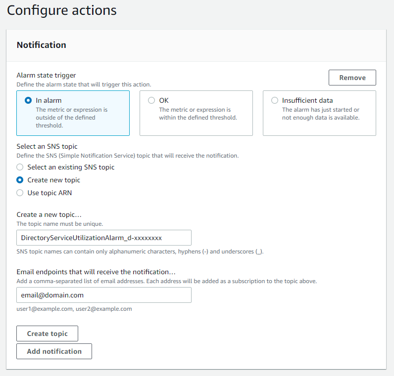
    13. On the Configure actions screen, configure the actions using the parameters listed below to send an email notification when the alarm state is triggered. See Figure 6 for an image of how email notifications are configured.
    14.   In the Notification section, set Alarm state trigger to In alarm.   Set Select an SNS topic to Create topic.  Fill in the name of the alarm in the Create a new topic field, and add the email where notifications should be sent to the Email endpoints that will receive notification field. An email address is required to create the SNS topic and you should use an email address that’s accessible by your operations team. This SNS topic will be used to trigger the Lambda automation described in a later section. Note: make a note of the SNS topic name you chose; you will use it later when creating the Lambda function in the To create an AWS Lambda function to automate scale out procedure below. 

      Figure 6. Create SNS topic and email notification

      Figure 6. Create SNS topic and email notification

    15. In the Alarm name field, provide a name for the alarm. You can optionally also add an Alarm description. Choose Next.
    16. Review your configuration, and choose Create alarm to create the alarm.

    Once you’ve completed these steps, you will now have an alarm implemented for when domain controller CPU utilization exceeds an average of 70% across both domain controllers. This will trigger an SNS topic when your directory is experiencing a heavy load, which will be used to start the Lambda automation and will send an informational email notification. In the next section, we’ll configure an AWS Lambda function to automate the addition of a domain controller based on this SNS topic.

    For additional details on CloudWatch Alarms, please see the Amazon CloudWatch documentation.

    To create an AWS Lambda function to automate scale out

    The sample Lambda function shown below checks the number of domain controllers in this Region, and increases that by adding one additional domain controller. This procedure describes how to configure the IAM role required for this Lambda function, then how to deploy the Lambda function to execute when the alarm is triggered to automatically add a domain controller when your load exceeds your typical usage baseline.

    Note: For additional details on Lambda creation, please see the AWS Lambda documentation.

    To automate scale-out using AWS Lambda

    1. In the AWS Console, navigate to IAM and choose Policies, then choose Create Policy.
    2. Choose the JSON tab, and create a new IAM role using the policy provided in JSON below.
    3. For more details on this configuration, see the AWS Directory Service documentation.

      Sample policy


      {
      	"Version":"2012-10-17",
      	"Statement":[
      	{
      		"Effect":"Allow",
      		"Action":[
      			"ds:DescribeDomainControllers",
      			"ds:UpdateNumberOfDomainControllers",
      			"ec2:DescribeSubnets",
      			"ec2:DescribeVpcs",
      			"ec2:CreateNetworkInterface",
      			"ec2:DescribeNetworkInterfaces",
      			"ec2:DeleteNetworkInterface"
      		],
      		"Resource":"*"
      	}
      	]
      }
      

    4. Choose Next:Tags to add tags (optional) before choosing Next:Review.
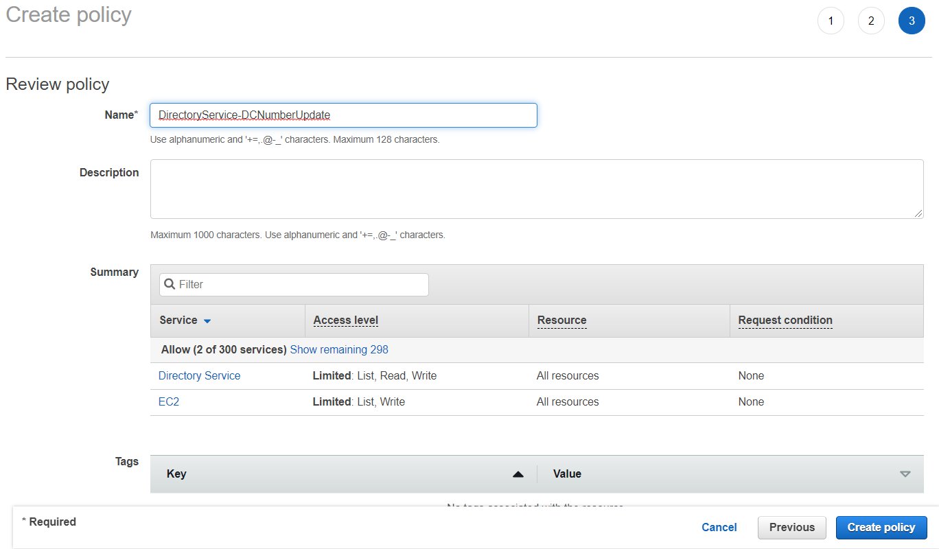
    5. On the Create Policy screen, provide a name in the Name field. You can optionally also add a description. Choose Create policy to complete creating the new policy.
    6.  
      Note: make a note of the policy name you chose; you will use it later when updating the execution role for the Lambda function.  

      Figure 7. Provide a name to create the IAM policy

      Figure 7. Provide a name to create the IAM policy

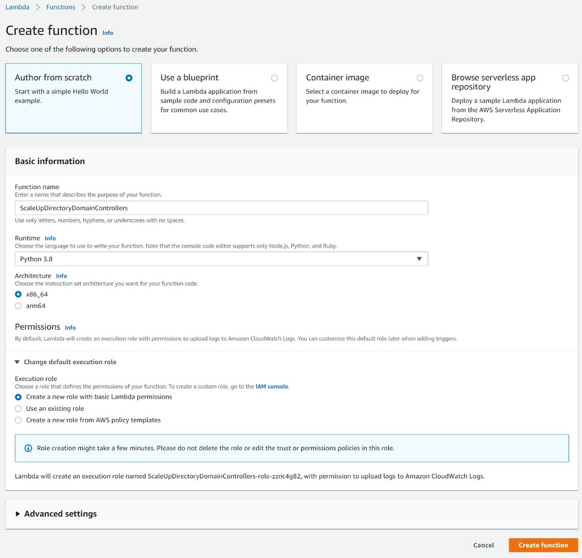
    7. In the AWS Console, navigate to Lambda and choose Create Function
    8. On the Create Function screen, select Author from Scratch and provide a Name, then choose Create Function.
    9. Figure 8. Create a Lambda function

      Figure 8. Create a Lambda function

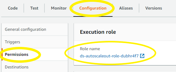
    10. Once created, on the Lambda function’s page, choose the Configuration tab, then choose Permissions from the sidebar and choose the execution role name linked under Role name. This will open the IAM console in another tab, preloaded to your Lambda execution role.
    11.  

      Figure 9: Select the Execution Role

      Figure 9: Select the Execution Role

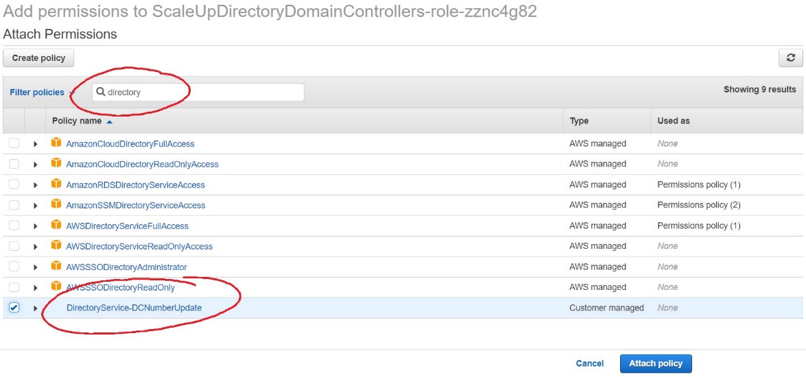
    12. On the execution role screen, choose Attach policies and select the IAM policy you’ve just created (e.g. DirectoryService-DCNumber Update). On the Attach Permissions screen, choose Attach policy to complete updating the execution role. Once completed this step, you may close this tab and return the previous browser tab.
    13.  

      Figure 10. Select and attach the IAM policy

      Figure 10. Select and attach the IAM policy

    14. On the Lambda function screen, choose the Configuration tab, then choose Triggers from the sidebar.
    15. On the Add Trigger screen, choose the pulldown under Trigger configuration and select SNS. On the SNS topic box, select the SNS topic you created in Step 9 of the To create a CloudWatch Alarm with SNS topic notifications procedure above. Then choose Add to complete the trigger configuration.
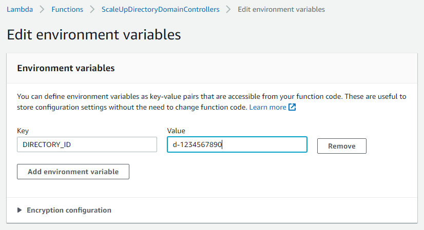
    16. On the Lambda function screen, choose the Configuration tab, then choose Environment variables from the sidebar.
    17. On the Environment variables card, click Edit.
    18. On the Edit environment variables screen, choose Add environment variables and use the Key “DIRECTORY_ID” and the Value will be the directory ID for you AWS Managed Microsoft AD.
    19.  

      Figure 11. The "Edit environment variables" screen

      Figure 11. The “Edit environment variables” screen

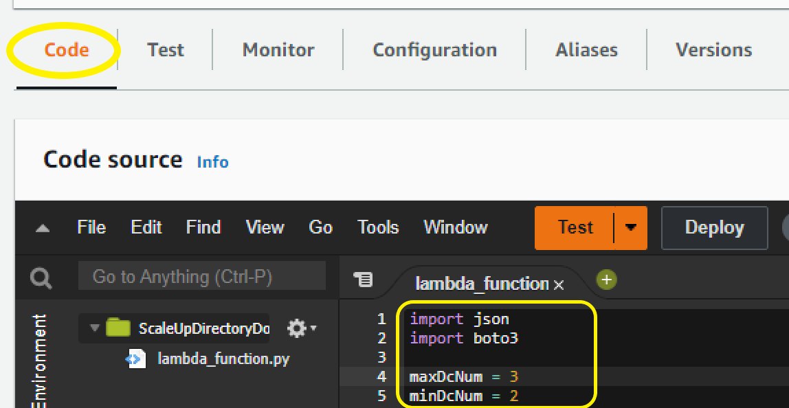
    20. On the Lambda function screen, choose the Code tab to open the in-browser code editor experience inside the Code source card. Paste in the sample Lambda function code given below to complete the implementation.
    21.  

      Figure 12. Paste sample code to complete the Lambda function setup

      Figure 12. Paste sample code to complete the Lambda function setup

    Sample Lambda function code

    The sample Lambda function given below automates adding another domain controller to your directory. When your CloudWatch alarm triggers, you will receive a notification email, and an additional domain controller will be deployed to provide the added capacity to support the increase in directory usage.

    Note: The example code contains a variable for the maximum number of domain controllers (maxDcNum), to prevent you from over provisioning in the event of a missed configuration. This value is set to 3 for this blog post’s example and can be increased to suit your use case. 

    import json
    import boto3
    
    maxDcNum = 10
    minDcNum = 2
    region   = "us-east-1"
    dsId = "d-906752246f"
    
    ds = boto3.client('ds', region_name=region)
    
    def lambda_handler(event, context):
        
        ## get the current number of domain controllers
        dcs = ds.describe_domain_controllers(DirectoryId = dsId)
    
        DomainControllers = dcs["DomainControllers"]
        
        DCcount = len(DomainControllers)
        print(">>> Current number of DCs:" + str(DCcount))
    
        #increase the number of DCs
        if DCcount < maxDcNum:
            NewDCnumber = DCcount + 1 
            response = ds.update_number_of_domain_controllers(DirectoryId = dsId, DesiredNumber =  NewDCnumber);    
    
            return {
                'statusCode': 200,
                'body': json.dumps("New DC number will be " + str(NewDCnumber))
            }
        else:
            return {
                'statusCode': 200,
                'body': json.dumps("Max number of DCs reached. The number of DCs is" + str(DCcount))
            }
    

    Note: When testing this Lambda function, remember that this will increase the number of domain controllers for your directory in that Region. If the additional domain controller is not needed, please reduce the count after the test to avoid costs for an additional domain controller. The same principles used in this article to automate the addition of domain controllers can be applied to automate the reduction of domain controllers and you should consider automating the reduction to optimize for resilience, performance and cost.

    Conclusion

    In this post, you’ve implemented alarms based on thresholds in Domain Controller utilization using AWS CloudWatch and automation to increase the number of domain controllers using AWS Lambda functions. This solution helps to cost-effectively improve resilience and performance of your directory, by scaling your directory based on historical load patterns.

    To learn more about using AWS Managed Microsoft AD, visit the AWS Directory Service documentation. For general information and pricing, see the AWS Directory Service home page. If you have comments about this blog post, submit a comment in the Comments section below. If you have implementation or troubleshooting questions, start a new thread on the Directory Service forum or contact AWS Support.

    Want more AWS Security news? Follow us on Twitter.

    Author

    Dennis Rothmel

    Dennis is a Sr. Product Manager from AWS Identity with a passion for modernization and automation. He has worked globally across Asia Pacific, Europe, and America, and enjoys the travel, languages, cultures and foods that come with global working.

    Author

    Vladimir Provorov

    Vladimir is a Product Solutions Architect from AWS Identity focused on Workforce Identity and Directory Service. He works on developing new features to make Enterprise Identity simpler and more scalable. He is excited to travel and explore the world with his family.

    New – Site-to-Site Connectivity with AWS Direct Connect SiteLink

    Post Syndicated from Sébastien Stormacq original https://aws.amazon.com/blogs/aws/new-site-to-site-connectivity-with-aws-direct-connect-sitelink/

    We are launching AWS Direct Connect SiteLink, a new capability of AWS Direct Connect that lets you create connections between your on-premises networks through the AWS global network backbone.

    Until today, when you needed direct connectivity between your data centers or branch offices, you had to rely on public internet or expensive and hard-to-deploy fixed networks. These are geographically constrained and can be tied to long-term contracts. This rigidity becomes a pain point as you expand your businesses globally. In turn, you’re required to create custom workarounds to interconnect networks from different providers, which increases your operating costs.

    Starting today, you may connect your sites through Direct Connect locations, without sending your traffic through an AWS Region. We have 108 Direct Connect locations available in 32 countries as I am writing this post, located across Africa, Americas, Asia-Pacific, Europe, and the Middle East. Traffic flows from one Direct Connect location to another following the shortest possible path. You no longer need to connect through the closest AWS Region and manage and configure an AWS Transit Gateway for site-to-site network connectivity.

    You can take advantage of Direct Connect’s reliability and global footprint to build a network that grows with your business, with no long-term contracts, flexible pay-as-you-go pricing, and a wide range of port-speeds, from 50 Mbps to 100 Gbps. SiteLink also integrates with other AWS services, letting you reach your VPCs, other AWS services, and your on-premises networks from your Direct Connect connections.

    When talking about network topology, a small diagram is always more descriptive than long phrases.

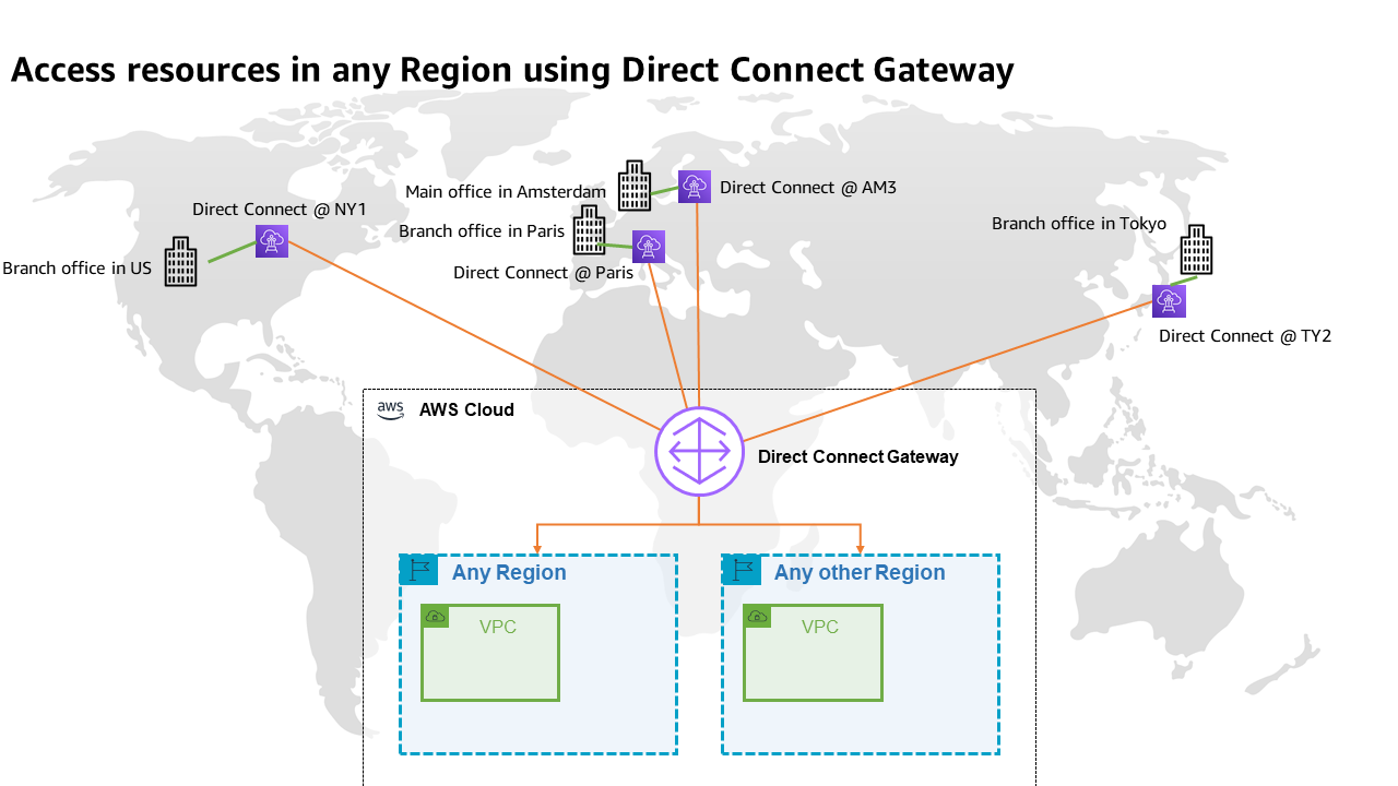
    The following diagram shows the way that you use Direct Connect today. Direct Connect is currently optimized to let you reach your AWS Resources running in any Region as quickly as possible. Sending data from one Direct Connect location to another is not possible.

    Once you connect your locations (NY1, AM3, Paris, and TY2 in the diagram) to a Direct Connect gateway, those connections can reach any AWS Region (except the two AWS China Regions). No peering between Regions is necessary, because Direct Connect gateways are global resources.

    Site-to-site connectivity without SiteLink

    The following diagram shows how you connect multiple sites using SiteLink. The data flows between Direct Connect locations without going through an AWS Region.

    Site-to-site connectivity with SiteLink

    How to Get Started?
    Configuring these connections is very similar to what you do today. The first step is to connect my network to Direct Connect locations. After that, SiteLink can be enabled or disabled in minutes.

    Using the AWS Management Console, I navigate to the Direct Connect section, and I select Create virtual interface to create a virtual interface. Under the Additional Settings section, I make sure the SiteLink switch is turned on. Obviously, I repeat this on another virtual interface, once per site, to connect.

    SiteLink - enable sitelink for VIF

    I have access to similar monitoring dashboards and metrics published to CloudWatch. I select my virtual interface, and then navigate to the Monitoring tab (hopefully your ViF will have more data available than mine that was created just for this post).

    SiteLink VIF Monitoring

    Availability and Pricing
    You can connect your on-premises networks or branch offices to any of our Direct Connect locations available today, except in China.

    Pricing is pay-as-you-go, with no commitment or recurring fees. In addition to existing Direct Connect charges, your monthly bill will include a price-per-hour for SiteLink virtual interfaces, as well as the cost of SiteLink data transfer. Check the pricing page to get the details.

    Go ahead an start connecting your on-premises locations together with Direct Connect SiteLink!

    — seb

    New – Enhanced Dead-letter Queue Management Experience for Amazon SQS Standard Queues

    Post Syndicated from Alex Casalboni original https://aws.amazon.com/blogs/aws/enhanced-dlq-management-sqs/

    Hundreds of thousands of customers use Amazon Simple Queue Service (SQS) to build message-based applications to decouple and scale microservices, distributed systems, and serverless apps. When a message cannot be successfully processed by the queue consumer, you can configure SQS to store it in a dead-letter queue (DLQ).

    As a software developer or architect, you’d like to examine and review unconsumed messages in your DLQs to figure out why they couldn’t be processed, identify patterns, resolve code errors, and ultimately reprocess these messages in the original queue. The life cycle of these unconsumed messages is part of your error-handling workflow, which is often manual and time consuming.

    Today, I’m happy to announce the general availability of a new enhanced DLQ management experience for SQS standard queues that lets you easily redrive unconsumed messages from your DLQ to the source queue.

    This new functionality is available in the SQS console and helps you focus on the important phase of your error handling workflow, which consists of identifying and resolving processing errors. With this new development experience, you can easily inspect a sample of the unconsumed messages and move them back to the original queue with a click, and without writing, maintaining, and securing any custom code. This new experience also takes care of redriving messages in batches, reducing overall costs.

    DLQ and Lambda Processor Setup
    If you’re already comfortable with the DLQ setup, then skip the setup and jump into the new DLQ redrive experience.

    First, I create two queues: the source queue and the dead-letter queue.

    I edit the source queue and configure the Dead-letter queue section. Here, I pick the DLQ and configure the Maximum receives, which is the number of times after which a message is reprocessed before being sent to the DLQ. For this demonstration, I’ve set it to one. This means that every failed message goes to the DLQ immediately. In a real-world environment, you might want to set a higher number depending on your requirements and based on what a failure means with respect to your application.

    I also edit the DLQ to make sure that only my source queue is allowed to use this DLQ. This configuration is optional: when this Redrive allow policy is disabled, any SQS queue can use this DLQ. There are cases where you want to reuse a single DLQ for multiple queues. But usually it’s considered best practices to setup independent DLQs per source queue to simplify the redrive phase without affecting cost. Keep in mind that you’re charged based on the number of API calls, not the number of queues.

    Once the DLQ is correctly set up, I need a processor. Let’s implement a simple message consumer using AWS Lambda.

    The Lambda function written in Python will iterate over the batch of incoming messages, fetch two values from the message body, and print the sum of these two values.

    import json
    
    def lambda_handler(event, context):
        for record in event['Records']:
            payload = json.loads(record['body'])
    
            value1 = payload['value1']
            value2 = payload['value2']
    
            value_sum = value1 + value2
            print("the sum is %s" % value_sum)
            
        return "OK"
    

    The code above assumes that each message’s body contains two integer values that can be summed, without dealing with any validation or error handling. As you can imagine, this will lead to trouble later on.

    Before processing any messages, you must grant this Lambda function enough permissions to read messages from SQS and configure its trigger. For the IAM permissions, I use the managed policy named AWSLambdaSQSQueueExecutionRole, which grants permissions to invoke sqs:ReceiveMessage, sqs:DeleteMessage, and sqs:GetQueueAttributes.

    I use the Lambda console to set up the SQS trigger. I could achieve the same from the SQS console too.

    Now I’m ready to process new messages using Send and receive messages for my source queue in the SQS console. I write {"value1": 10, "value2": 5} in the message body, and select Send message.

    When I look at the CloudWatch logs of my Lambda function, I see a successful invocation.

    START RequestId: 637888a3-c98b-5c20-8113-d2a74fd9edd1 Version: $LATEST
    the sum is 15
    END RequestId: 637888a3-c98b-5c20-8113-d2a74fd9edd1
    REPORT RequestId: 637888a3-c98b-5c20-8113-d2a74fd9edd1	Duration: 1.31 ms	Billed Duration: 2 ms	Memory Size: 128 MB	Max Memory Used: 39 MB	Init Duration: 116.90 ms	

    Troubleshooting powered by DLQ Redrive
    Now what if a different producer starts publishing messages with the wrong format? For example, {"value1": "10", "value2": 5}. The first number is a string and this is quite likely to become a problem in my processor.

    In fact, this is what I find in the CloudWatch logs:

    START RequestId: 542ac2ca-1db3-5575-a1fb-98ce9b30f4b3 Version: $LATEST
    [ERROR] TypeError: can only concatenate str (not "int") to str
    Traceback (most recent call last):
      File "/var/task/lambda_function.py", line 8, in lambda_handler
        value_sum = value1 + value2
    END RequestId: 542ac2ca-1db3-5575-a1fb-98ce9b30f4b3
    REPORT RequestId: 542ac2ca-1db3-5575-a1fb-98ce9b30f4b3	Duration: 1.69 ms	Billed Duration: 2 ms	Memory Size: 128 MB	Max Memory Used: 39 MB	

    To figure out what’s wrong in the offending message, I use the new SQS redrive functionality, selecting DLQ redrive in my dead-letter queue.

    I use Poll for messages and fetch all unconsumed messages from the DLQ.

    And then I inspect the unconsumed message by selecting it.

    The problem is clear, and I decide to update my processing code to handle this case properly. In the ideal world, this is an upstream issue that should be fixed in the message producer. But let’s assume that I can’t control that system and it’s critically important for the business that I process this new type of messages.

    Therefore, I update the processing logic as follows:

    import json
    
    def lambda_handler(event, context):
        for record in event['Records']:
            payload = json.loads(record['body'])
            value1 = int(payload['value1'])
            value2 = int(payload['value2'])
            value_sum = value1 + value2
            print("the sum is %s" % value_sum)
            # do some more stuff
            
        return "OK"
    

    Now that my code is ready to process the unconsumed message, I start a new redrive task from the DLQ to the source queue.

    By default, SQS will redrive unconsumed messages to the source queue. But you could also specify a different destination and provide a custom velocity to set the maximum number of messages per second.

    I wait for the redrive task to complete by monitoring the redrive status in the console. This new section always shows the status of most recent redrive task.

    The message has been moved back to the source queue and successfully processed by my Lambda function. Everything looks fine in my CloudWatch logs.

    START RequestId: 637888a3-c98b-5c20-8113-d2a74fd9edd1 Version: $LATEST
    the sum is 15
    END RequestId: 637888a3-c98b-5c20-8113-d2a74fd9edd1
    REPORT RequestId: 637888a3-c98b-5c20-8113-d2a74fd9edd1	Duration: 1.31 ms	Billed Duration: 2 ms	Memory Size: 128 MB	Max Memory Used: 39 MB	Init Duration: 116.90 ms	

    Available Today at No Additional Cost
    Today you can start leveraging the new DLQ redrive experience to simplify your development and troubleshooting workflows, without any additional cost. This new console experience is available in all AWS Regions where SQS is available, and we’re looking forward to hearing your feedback.

    — Alex

    Network Address Management and Auditing at Scale with Amazon VPC IP Address Manager

    Post Syndicated from Steve Roberts original https://aws.amazon.com/blogs/aws/network-address-management-and-auditing-at-scale-with-amazon-vpc-ip-address-manager/

    Managing, monitoring, and auditing IP address allocation for at-scale networks, as the growth in cloud workloads and connected devices continues at a rapid pace, is a complex, time-consuming, and potentially error-prone task. Traditionally, network administrators have resorted to using combinations of spreadsheets, home-grown tools, and scripts to track address assignments across multiple accounts, virtual private clouds (VPCs), and Regions. Manually updating spreadsheets when application development teams request IP address assignments takes time, and care, to avoid errors. Errors which, should they go unnoticed, can lead to address conflicts and subsequent downtime, causing serious operational and business issues. In turn, the time taken to make these updates, sometimes several days, causes delays in onboarding new applications or expanding existing applications, impacting the velocity of development teams. The need to keep those home-grown tools and scripts up-to-date and error-free also results in taking staff hours away from more strategic and business-impacting projects.

    Today, I’m happy to announce Amazon VPC IP Address Manager, a new feature that provides network administrators with an automated IP management workflow. IPAM makes it easier for network administrators to organize, assign, monitor, and audit IP addresses in at-scale networks, lowering the management and monitoring burden and eliminating the manual processes that can lead to delays and unintended errors.

    Amazon VPC IP Address Manager dashboard homepage

    Introducing Amazon VPC IP Address Manager
    IPAM enables management and auditing of IP address assignments across an organization’s accounts, Amazon Virtual Private Cloud (VPC)‘s, and AWS Regions, using a single operational dashboard. From this centralized view, you can manage your IP addresses across AWS.

    In each Region in which you have resources needing IP addresses, you create a regional pool. Pools are collections of CIDRs and help you to organize your IP space. Unused address space from your top-level pools can be used to fill your regional pools. Further, if you have applications or environments with different security needs, you can create additional pools. For example, you could create different pools for ‘dev’ and ‘prod’ environments if they are subject to different connectivity requirements. The screenshots below illustrate the process of creating a global pool and, from it, three regional pools. Although my example stops after configuring regional pools, in production, you would continue subdividing the regional pools further as needed.

    Creating the global IPAM pool

    Next, I configure a set of regional pools. Below, I’m creating a regional pool for my US East (N. Virginia) Region resources, scoped within my global pool.

    Creating a regional pool, step 1

    As part of configuring a regional pool, I must specify the CIDRs to provision from the global pool and can optionally enable automatic discovery of resources and rules for allocation.

    Configuring a regional pool

    After repeating the process of creating and configuring regional pools for my two remaining Regions, US East (Ohio) and Europe (Ireland) in this example, this is my final pool hierarchy. As I noted above, this hierarchy ends at a regional set of pools but could be subdivided further.

    IPAM pool hierarchy

    Once the IPAM pools have been configured, development teams and resources needing new IP address assignments are able to make use of an automated, self-service process, unblocking the developers, and eliminating errors from using manual processes that can lead to connectivity issues. To govern IP address assignments, you can make use of automated and simple business rules. With IPAM‘s self-service model, developers can now directly create resources and receive IP addresses based on business rules in seconds, removing the delays in onboarding applications and improving the velocity of the development team. In the screenshot below, I’m referencing my pools to set the address ranges to be used when creating a new VPC.

    Assigning address ranges for a new VPC from IPAM pools

    You can also share your IPAM with your organization, created using AWS Organizations, and AWS Resource Access Manager (RAM). When you share your IPAM, you gain fully automated CIDR allocation to your Amazon VPCs across member accounts in your organization and Regions.

    For network administrators, IPAM provides observability and auditing capabilities, helping to speed up troubleshooting, and providing oversight and monitoring of the used and unused addresses across an organization’s global network address pool using a single dashboard. For each assigned address, IPAM tracks critical information, for example, the AWS account, the VPC, routing, and the security domain, eliminating the bookkeeping work that burdens administrators. Having used IPAM to eliminate IP assignment errors, customers can use IPAM to monitor assigned addresses and receive alerts when potential issues are detected – for example, depleting IP addresses that can stall their network’s growth or overlapping IP addresses that can result in erroneous routing. You can proactively act on those alerts and fix issues before they can become major outages.

    The screenshot below illustrates monitoring pool utilization across a set of VPCs.

    Monitoring an IPAM pool

    Utilization of address space within a pool can also be monitored. You can add Amazon CloudWatch Alarms that you can configure to trigger at your chosen utilization percentage value so that you can take proactive action before the address space is exhausted.

    Monitoring pool utilization with alarms

    Overlapping address spaces are another headache that network administrators need to manage, usually discovered after the fact during an outage. IPAM can help lower the burden here, too, providing a view of resources that warns of overlapping address ranges.

    Detecting overlapping address spaces

    To further help troubleshoot network issues and audits of network security and routing policies, network administrators can also take advantage of the current and historical data that IPAM makes available to gain usage insights.

    IPAM historical insights

    IPAM works with any VPC resource where an IP address needs to be assigned, including public and private addresses and Elastic IP Addresses (EIP), and also supports bring your own IP (BYOIP) for both IPv4 and IPv6 addresses.

    Start managing and auditing your IP addresses at scale today
    Amazon VPC IP Address Manager is available today in all commercial AWS Regions. Get started today, first creating your IPAM for all Regions and accounts, then creating your pools, and finally setting application policy. Then, you can take advantage of IPAM to automate IP address assignment, monitor, troubleshoot, and audit your network addresses assignments.

    For those of you with existing VPCs, after you create IPAM it will start monitoring, without any action on your part, to create an inventory of all your VPCs and EIPs. Once you create pools, IPAM will then backfill your VPCs into the pool. This means you can create VPCs today, using your existing workflow, and use IPAM for monitoring and audit only. Later on, you can switch your workflow to IPAM-based automated VPC assignment.

    — Steve

    New – Amazon VPC Network Access Analyzer

    Post Syndicated from Jeff Barr original https://aws.amazon.com/blogs/aws/new-amazon-vpc-network-access-analyzer/

    If you are a member of your organization’s networking, cloud operations, or security teams, you are going to love this new feature. The new Amazon VPC Network Access Analyzer helps you identify network configurations that lead to unintended network access. As you will see in a moment, it will point out ways that you can improve your security posture while still letting you and your organization be agile and flexible. In contrast to manual checking of network configurations, which is error prone and hard to scale, this tool lets you analyze your AWS networks of any size and complexity.

    Introducing Network Access Analyzer
    Network Access Analyzer takes advantage of our automated reasoning technology that already powers AWS IAM Access Analyzer, Amazon VPC Reachability Analyzer, Amazon Inspector Network Reachability, and other provable security tools.

    This new tool uses Network Access Scopes to specify the desired connectivity between your AWS resources. You can get started with a set of Amazon-created scopes, and then either copy & customize them, or create your own from scratch. The scopes are high-level and independent of any particular network architecture or configuration, and can be thought of as a language for specifying the proper level of access & connectivity for your network. You can, for example, create a scope to verify that all web apps use a firewall to access Internet resources, or to indicate that AWS resources used by your Finance team are separate, distinct, and unreachable from the resources used by your Development team.

    To evaluate your network against a particular scope, you select it and initiate an analysis. It runs for a few minutes and then generates a set of findings, each of which indicates an unexpected network path between the AWS resources defined in the scope. You can analyze the findings, adjust your configuration or modify the scope in response to the findings, and re-run the analysis, all in just a few minutes.

    The analysis process examines a very wide range of AWS resources including Security Groups, CIDR blocks, prefix lists, Elastic Network Interfaces, EC2 instances, Load Balancers, VPC, VPC subnets, VPC endpoints, VPC endpoint services, Transit Gateways, NAT Gateways, Internet Gateways, VPN Gateways, Peering Connections, and Network Firewalls. Your scopes can use Resource Groups to reference all resources that are tagged in a particular way.

    Using Network Access Analyzer
    To get started, I open the VPC Console, find the Network Analysis section on the left-side navigation, and click Network Access Analyzer:

    I can see all of my scopes. Initially, I have four, all created by Amazon and ready to use:

    To conduct an analysis, I select a scope (AWS-VPC-Ingress (Amazon created)) and click Analyze. The scope’s description reads:

    “Identify ingress paths into your VPCs from Internet Gateways, Peering Connections, VPC Service Endpoints, VPN and Transit Gateways.”

    The analysis runs for a couple of minutes and displays the findings as soon as it is done:

    There’s a lot of very useful information here! The spectrum chart provides an overview of the resources that are in the findings. I can hover my mouse over any of the segments to learn more, or click on one in order to filter the findings and show only those that reference a particular resource or resource type:

    For example, I click VPC Peering Connections and I can see all of the findings that reference the VPC peering connection:

    As you can see, the Path details highlight the VPC peering connection in the path! The next step is to examine the findings, decide which ones are expected, and to add them to the scope so that they are excluded from future findings (more on that in a bit).

    Inside a Network Access Scope
    Let’s take a quick look inside of the Network Access Scope that I used above, and then build another scope from scratch using the visual builder. Each scope is represented in JSON format, and indicates what is considered in-scope (acceptable) traffic between sources and destinations:

    {
              "networkInsightsAccessScopeId": "nis-070dc1d37ca315e86",
              "matchPaths": [
                        {
                                  "source": {
                                            "resourceStatement": {
                                                      "resources": [],
                                                      "resourceTypes": [
                                                                "AWS::EC2::InternetGateway",
                                                                "AWS::EC2::VPCPeeringConnection",
                                                                "AWS::EC2::VPCEndpointService",
                                                                "AWS::EC2::TransitGatewayAttachment",
                                                                "AWS::EC2::VPNGateway"
                                                      ]
                                            }
                                  },
                                  "destination": {
                                            "resourceStatement": {
                                                      "resources": [],
                                                      "resourceTypes": [
                                                                "AWS::EC2::NetworkInterface"
                                                      ]
                                            }
                                  }
                        }
              ],
              "excludePaths": []
    }

    The matchPaths element contains source and destination elements. Each of these elements, in turn, identifies AWS resource types and specific resources. While not shown here, scopes can also contain source and destination IP addresses, ports, prefix lists, and traffic types (TCP or UDP). The excludePaths can contain resource types, specific resources, and so forth. I could, for example, define sources and destinations that match all Internet Gateway ingress traffic, but exclude traffic that flows through a Load Balancer, or I could exclude SSH traffic destined for my bastion instances.

    Building a Network Access Scope
    I can build a new scope in three ways. I can Duplicate and modify an existing one, I can start from scratch and use the visual builder, or I can write my own JSON and use either the CLI or the API to create a scope. I click Create Network Access Scope to use the builder:

    I can start with one of five predefined templates, or I can build my own:

    I enter a name and a description:

    Then I define the source and destinations by resource type, id, traffic type, and so forth:

    I have many options for matching the traffic type. This allows me to create scopes for very specific purposes:

    I can use a similar interface to add any optional exclusions.

    Things to Know
    This is a very powerful tool and one that I think you are going to love. Here are a couple of things to know about it:

    Pricing – You pay $0.002 for each Elastic Network Interface (ENI) analyzed as part of an assessment.

    Regions – Network Access Analyzer is available in the US East (N. Virginia), US East (Ohio), US West (N. California), US West (Oregon), Africa (Cape Town), Asia Pacific (Hong Kong), Asia Pacific (Mumbai), Asia Pacific (Seoul), Asia Pacific (Singapore), Asia Pacific (Sydney), Asia Pacific (Tokyo), Canada (Central), Europe (Frankfurt), Europe (Ireland), Europe (London), Europe (Milan), Europe (Paris), Europe (Stockholm), South America (São Paulo), and Middle East (Bahrain) Regions.

    In the Works – We have lots of additional features on the product roadmap including support for AWS Organizations, the ability to run your analyses on a regular schedule, and support for IPv6 address ranges and resources.

    — Jeff;

    The collective thoughts of the interwebz