Today we’re excited to announce that we’ve added the Mistral-7B-v0.1-instruct to Workers AI. Mistral 7B is a 7.3 billion parameter language model with a number of unique advantages. With some help from the founders of Mistral AI, we’ll look at some of the highlights of the Mistral 7B model, and use the opportunity to dive deeper into “attention” and its variations such as multi-query attention and grouped-query attention.
Approaches CodeLlama 7B performance on code, while remaining good at English tasks, and
The chat fine-tuned version we’ve deployed outperforms Llama 2 13B chat in the benchmarks provided by Mistral.
Here’s an example of using streaming with the REST API:
curl -X POST \
“https://api.cloudflare.com/client/v4/accounts/{account-id}/ai/run/@cf/mistral/mistral-7b-instruct-v0.1” \
-H “Authorization: Bearer {api-token}” \
-H “Content-Type:application/json” \
-d '{ “prompt”: “What is grouped query attention”, “stream”: true }'

API Response: { response: “Grouped query attention is a technique used in natural language processing  (NLP) and machine learning to improve the performance of models…” }
And here’s an example using a Worker script:
import { Ai } from ‘@cloudflare/ai’;
export default {
    async fetch(request, env) {
        const ai = new Ai(env.AI);
        const stream = await ai.run(‘@cf/mistral/mistral-7b-instruct-v0.1’, {
            prompt: ‘What is grouped query attention’,
            stream: true
        });
        return Response.json(stream, { headers: { “content-type”: “text/event-stream” } });
    }
}
Mistral takes advantage of grouped-query attention for faster inference. This recently-developed technique improves the speed of inference without compromising output quality. For 7 billion parameter models, we can generate close to 4x as many tokens per second with Mistral as we can with Llama, thanks to Grouped-Query attention.
You don’t need any information beyond this to start using Mistral-7B, you can test it out today ai.cloudflare.com. To learn more about attention and Grouped-Query attention, read on!
So what is “attention” anyway?
The basic mechanism of attention, specifically “Scaled Dot-Product Attention” as introduced in the landmark paper Attention Is All You Need, is fairly simple:
We call our particular attention “Scale Dot-Product Attention”. The input consists of query and keys of dimension d_k, and values of dimension d_v. We compute the dot products of the query with all the keys, divide each by sqrt(d_k) and apply a softmax function to obtain the weights on the values.
In simpler terms, this allows models to focus on important parts of the input. Imagine you are reading a sentence and trying to understand it. Scaled dot product attention enables you to pay more attention to certain words based on their relevance. It works by calculating the similarity between each word (K) in the sentence and a query (Q). Then, it scales the similarity scores by dividing them by the square root of the dimension of the query. This scaling helps to avoid very small or very large values. Finally, using these scaled similarity scores, we can determine how much attention or importance each word should receive. This attention mechanism helps models identify crucial information (V) and improve their understanding and translation capabilities.
Easy, right? To get from this simple mechanism to an AI that can write a “Seinfeld episode in which Jerry learns the bubble sort algorithm,” we’ll need to make it more complex. In fact, everything we’ve just covered doesn’t even have any learned parameters — constant values learned during model training that customize the output of the attention block! Attention blocks in the style of Attention is All You Need add mainly three types of complexity:
Learned parameters
Learned parameters refer to values or weights that are adjusted during the training process of a model to improve its performance. These parameters are used to control the flow of information or attention within the model, allowing it to focus on the most relevant parts of the input data. In simpler terms, learned parameters are like adjustable knobs on a machine that can be turned to optimize its operation.
Vertical stacking – layered attention blocks
Vertical layered stacking is a way to stack multiple attention mechanisms on top of each other, with each layer building on the output of the previous layer. This allows the model to focus on different parts of the input data at different levels of abstraction, which can lead to better performance on certain tasks.
Horizontal stacking – aka Multi-Head Attention
The figure from the paper displays the full multi-head attention module. Multiple attention operations are carried out in parallel, with the Q-K-V input for each generated by a unique linear projection of the same input data (defined by a unique set of learned parameters). These parallel attention blocks are referred to as “attention heads”. The weighted-sum outputs of all attention heads are concatenated into a single vector and passed through another parameterized linear transformation to get the final output.
This mechanism allows a model to focus on different parts of the input data concurrently. Imagine you are trying to understand a complex piece of information, like a sentence or a paragraph. In order to understand it, you need to pay attention to different parts of it at the same time. For example, you might need to pay attention to the subject of the sentence, the verb, and the object, all simultaneously, in order to understand the meaning of the sentence. Multi-headed attention works similarly. It allows a model to pay attention to different parts of the input data at the same time, by using multiple “heads” of attention. Each head of attention focuses on a different aspect of the input data, and the outputs of all the heads are combined to produce the final output of the model.
Styles of attention
There are three common arrangements of attention blocks used by large language models developed in recent years: multi-head attention, grouped-query attention and multi-query attention. They differ in the number of K and V vectors relative to the number of query vectors. Multi-head attention uses the same number of K and V vectors as Q vectors, denoted by “N” in the table below. Multi-query attention uses only a single K and V vector. Grouped-query attention, the type used in the Mistral 7B model, divides the Q vectors evenly into groups containing “G” vectors each, then uses a single K and V vector for each group for a total of N divided by G sets of K and V vectors. This summarizes the differences, and we’ll dive into the implications of these below.
Number of Key/Value Blocks
Quality
Memory Usage
Multi-head attention (MHA)
N
Best
Most
Grouped-query attention (GQA)
N / G
Better
Less
Multi-query attention (MQA)
1
Good
Least
Summary of attention styles
And this diagram helps illustrate the difference between the three styles:
Multi-query attention was described in 2019 in the paper from Google: Fast Transformer Decoding: One Write-Head is All You Need. The idea is that instead of creating separate K and V entries for every Q vector in the attention mechanism, as in multi-head attention above, only a single K and V vector is used for the entire set of Q vectors. Thus the name, multiple queries combined into a single attention mechanism. In the paper, this was benchmarked on a translation task and showed performance equal to multi-head attention on the benchmark task.
Originally the idea was to reduce the total size of memory that is accessed when performing inference for the model. Since then, as generalized models have emerged and grown in number of parameters, the GPU memory needed is often the bottleneck which is the strength of multi-query attention, as it requires the least accelerator memory of the three types of attention. However, as models grew in size and generality, performance of multi-query attention fell relative to multi-head attention.
Grouped-Query Attention
The newest of the bunch — and the one used by Mistral — is grouped-query attention, as described in the paper GQA: Training Generalized Multi-Query Transformer Models from Multi-Head Checkpoints that was published on arxiv.org in May 2023. Grouped-query attention combines the best of both worlds: the quality of multi-headed attention with the speed and low memory usage of multi-query attention. Instead of either a single set of K and V vectors or one set for every Q vector, a fixed ratio of 1 set of K and V vectors for every Q vector is used, reducing memory usage but retaining high performance on many tasks.
Often choosing a model for a production task is not just about picking the best model available because we must consider tradeoffs between performance, memory usage, batch size, and available hardware (or cloud costs). Understanding these three styles of attention can help guide those decisions and understand when we might choose a particular model given our circumstances.
Enter Mistral — try it today
Being one of the first large language models to leverage grouped-query attention and combining it with sliding window attention, Mistral seems to have hit the goldilocks zone — it’s low latency, high-throughput, and it performs really well on benchmarks even when compared to bigger models (13B). All this to say is that it packs a punch for its size, and we couldn’t be more excited to make it available to all developers today, via Workers AI.
Head over to our developer docs to get started, and if you need help, want to give feedback, or want to share what you’re building just pop into our Developer Discord!
The Workers AI team is also expanding and hiring; check our jobs page for open roles if you’re passionate about AI engineering and want to help us build and evolve our global, serverless GPU-powered inference platform.
Google’s Threat Analysis Group announced a zero-day against the Zimbra Collaboration email server that has been used against governments around the world.
TAG has observed four different groups exploiting the same bug to steal email data, user credentials, and authentication tokens. Most of this activity occurred after the initial fix became public on Github. To ensure protection against these types of exploits, TAG urges users and organizations to keep software fully up-to-date and apply security updates as soon as they become available.
The vulnerability was discovered in June. It has been patched.
Since launching our free online courses about computing on the edX platform back in August, we’ve been training course facilitators and analysing the needs of educators around the world. We want every course participant to have a great experience learning with us — read on to find out what we’re doing right now and into 2024 to ensure this.
Online courses for all adults who support young people
Educators of all kinds are key for supporting children and young people to engage with computing technology and develop digital skills. You might be a professional teacher, or a parent, volunteer, youth worker, librarian… there are so many roles in which people share knowledge with young learners.
That’s why our online courses are designed to support any kind of educator to:
Understand the full breadth of topics within computing
Discover how to introduce computing to young people in clear and exciting ways that are grounded in the latest research
We are constantly improving our online courses based on your feedback, the latest education research, and the insights our team members gain through supporting you on your course learning journeys. Three principles guide these improvements: accessibility, scalability, and sustainability.
Making our courses more relevant and accessible
Our online courses are used by people who live around the world and bring various knowledge and experiences. Some participants are classroom teachers, others have computing experience from their job and want to volunteer at a kids’ coding club, and some may be parents who want to support their children. It’s important to us that our courses are relevant and accessible to all kinds of adult learners.
We’re currently working to:
Simplify the English in the courses for participants who speak it as a second language
Adapt the course activities for specific settings where participants help young people learn so that e.g. teachers see how the activities work in the classroom, and volunteers who run coding clubs see how they work in club sessions
Ensure our course facilitators have experience in a range of different settings including coding clubs, and in a variety of different contexts around the world
Making our courses useful for more groups of people
When we think about the scalability of our courses, we think about how to best support as many educators around the world as possible. If we can make the jobs of all educators easier, whatever their setting is like, then we are making the right choices.
We’re currently working to:
Talk with the global network of educators we’re a part of to better understand what works for them so we can reflect that in the courses
Include a wider range of examples for settings beyond the classroom in the courses
Adapt our courses so they are relevant to participants with various needs while sustaining the high quality of the overall learning experience
Making the learning from our courses sustainable
The educators who take our courses work to achieve amazing things, and this means they are often busy. That they take the time to complete one of our courses to learn new things is a commitment we want to make sure is rewarded. The learning you get from participating in our online courses should continue to benefit you far beyond the time you spend completing it. This is what we mean by sustainability.
We’re currently working to:
Lay out clear learning pathways so you can build on the knowledge you gain in one course in the next course
Offer course resources that are easy to access after you’ve completed the course
Explore ways to build communities around our courses where you can share successes and learning outcomes with your fellow participants
Learn with us, and help us design better courses for you
Our work to improve the accessibility, scalability, and sustainability of our courses will continue into 2024, and these three principles will likely be part of our online training strategy for the following year too.
If you’d like to support young people in your life to learn about computing and digital technologies, take one of our free courses now and learn something new. We have twenty courses available right now and they are totally free.
We are also looking for adult testers for new course content. So if you’re any kind of educator and would like to test upcoming online course content and share your feedback and experiences, please send us a message with the subject ‘Educator training’.
Incremental processing is an approach to process new or changed data in workflows. The key advantage is that it only incrementally processes data that are newly added or updated to a dataset, instead of re-processing the complete dataset. This not only reduces the cost of compute resources but also reduces the execution time in a significant manner. When workflow execution has a shorter duration, chances of failure and manual intervention reduce. It also improves the engineering productivity by simplifying the existing pipelines and unlocking the new patterns.
In this blog post, we talk about the landscape and the challenges in workflows at Netflix. We will show how we are building a clean and efficient incremental processing solution (IPS) by using Netflix Maestro and Apache Iceberg. IPS provides the incremental processing support with data accuracy, data freshness, and backfill for users and addresses many of the challenges in workflows. IPS enables users to continue to use the data processing patterns with minimal changes.
Introduction
Netflix relies on data to power its business in all phases. Whether in analyzing A/B tests, optimizing studio production, training algorithms, investing in content acquisition, detecting security breaches, or optimizing payments, well structured and accurate data is foundational. As our business scales globally, the demand for data is growing and the needs for scalable low latency incremental processing begin to emerge. There are three common issues that the dataset owners usually face.
Data Freshness: Large datasets from Iceberg tables needed to be processed quickly and accurately to generate insights to enable faster product decisions. The hourly processing semantics along with valid–through-timestamp watermark or data signals provided by the Data Platform toolset today satisfies many use cases, but is not the best for low-latency batch processing. Before IPS, the Data Platform did not have a solution for tracking the state and progression of data sets as a single easy to use offering. This has led to a few internal solutions such as Psyberg. These internal libraries process data by capturing the changed partitions, which works only on specific use cases. Additionally, the libraries have tight coupling to the user business logic, which often incurs higher migration costs, maintenance costs, and requires heavy coordination with the Data Platform team.
Data Accuracy: Late arriving data causes datasets processed in the past to become incomplete and as a result inaccurate. To compensate for that, ETL workflows often use a lookback window, based on which they reprocess the data in that certain time window. For example, a job would reprocess aggregates for the past 3 days because it assumes that there would be late arriving data, but data prior to 3 days isn’t worth the cost of reprocessing.
Backfill: Backfilling datasets is a common operation in big data processing. This requires repopulating data for a historical time period which is before the scheduled processing. The need for backfilling could be due to a variety of factors, e.g. (1) upstream data sets got repopulated due to changes in business logic of its data pipeline, (2) business logic was changed in a data pipeline, (3) anew metric was created that needs to be populated for historical time ranges, (4) historical data was found missing, etc.
These challenges are currently addressed in suboptimal and less cost efficient ways by individual local teams to fulfill the needs, such as
Lookback: This is a generic and simple approach that data engineers use to solve the data accuracy problem. Users configure the workflow to read the data in a window (e.g. past 3 hours or 10 days). The window is set based on users’ domain knowledge so that users have a high confidence that the late arriving data will be included or will not matter (i.e. data arrives too late to be useful). It ensures the correctness with a high cost in terms of time and compute resources.
Foreach pattern: Users build backfill workflows using Maestro foreach support. It works well to backfill data produced by a single workflow. If the pipeline has multiple stages or many downstream workflows, users have to manually create backfill workflows for each of them and that requires significant manual work.
The incremental processing solution (IPS) described here has been designed to address the above problems. The design goal is to provide a clean and easy to adopt solution for the Incremental processing to ensure data freshness, data accuracy, and to provide easy backfill support.
Data Freshness: provide the support for scheduling workflows in a micro batch fashion (e.g. 15 min interval) with state tracking functionality
Data Accuracy: provide the support to process all late arriving data to achieve data accuracy needed by the business with significantly improved performance in terms of multifold time and cost efficiency
Backfill: provide managed backfill support to build, monitor, and validate the backfill, including automatically propagating changes from upstream to downstream workflows, to greatly improve engineering productivity (i.e. a few days or weeks of engineering work to build backfill workflows vs one click for managed backfill)
Approach Overview
General Concept
Incremental processing is an approach to process data in batch — but only on new or changed data. To support incremental processing, we need an approach for not only capturing incremental data changes but also tracking their states (i.e. whether a change is processed by a workflow or not). It must be aware of the change and can capture the changes from the source table(s) and then keep tracking those changes. Here, changes mean more than just new data itself. For example, a row in an aggregation target table needs all the rows from the source table associated with the aggregation row. Also, if there are multiple source tables, usually the union of the changed data ranges from all input tables gives the full change data set. Thus, change information captured must include all related data including those unchanged rows in the source table as well. Due to previously mentioned complexities, change tracking cannot be simply achieved by using a single watermark. IPS has to track those captured changes in finer granularity.
The changes from the source tables might affect the transformed result in the target table in various ways.
If one row in the target table is derived from one row in the source table, newly captured data change will be the complete input dataset for the workflow pipeline.
If one row in the target table is derived from multiple rows in the source table, capturing new data will only tell us the rows have to be re-processed. But the dataset needed for ETL is beyond the change data itself. For example, an aggregation based on account id requires all rows from the source table about an account id. The change dataset will tell us which account ids are changed and then the user business logic needs to load all data associated with those account ids found in the change data.
If one row in the target table is derived based on the data beyond the changed data set, e.g. joining source table with other tables, newly captured data is still useful and can indicate a range of data to be affected. Then the workflow will re-process the data based on the range. For example, assuming we have a table that keeps the accumulated view time for a given account partitioned by the day. If the view time 3-days ago is updated right now due to late arriving data, then the view time for the following two days has to be re-calculated for this account. In this case, the captured late arriving data will tell us the start of the re-calculation, which is much more accurate than recomputing everything for the past X days by guesstimate, where X is a cutoff lookback window decided by business domain knowledge.
Once the change information (data or range) is captured, a workflow has to write the data to the target table in a slightly more complicated way because the simple INSERT OVERWRITE mechanism won’t work well. There are two alternatives:
Merge pattern: In some compute frameworks, e.g. Spark 3, it supports MERGE INTO to allow new data to be merged into the existing data set. That solves the write problem for incremental processing. Note that the workflow/step can be safely restarted without worrying about duplicate data being inserted when using MERGE INTO.
Append pattern: Users can also use append only write (e.g. INSERT INTO) to add the new data to the existing data set. Once the processing is completed, the append data is committed to the table. If users want to re-run or re-build the data set, they will run a backfill workflow to completely overwrite the target data set (e.g. INSERT OVERWRITE).
Additionally, the IPS will naturally support the backfill in many cases. Downstream workflows (if there is no business logic change) will be triggered by the data change due to backfill. This enables auto propagation of backfill data in multi-stage pipelines. Note that the backfill support is skipped in this blog. We will talk about IPS backfill support in another following blog post.
Netflix Maestro
Maestro is the Netflix data workflow orchestration platform built to meet the current and future needs of Netflix. It is a general-purpose workflow orchestrator that provides a fully managed workflow-as-a-service (WAAS) to the data platform users at Netflix. It serves thousands of users, including data scientists, data engineers, machine learning engineers, software engineers, content producers, and business analysts, in various use cases. Maestro is highly scalable and extensible to support existing and new use cases and offers enhanced usability to end users.
Since the last blog on Maestro, we have migrated all the workflows to it on behalf of users with minimal interruption. Maestro has been fully deployed in production with 100% workload running on it.
IPS is built upon Maestro as an extension by adding two building blocks, i.e. a new trigger mechanism and step job type, to enable incremental processing for all workflows. It is seamlessly integrated into the whole Maestro ecosystem with minimal onboarding cost.
Apache Iceberg
Iceberg is a high-performance format for huge analytic tables. Iceberg brings the reliability and simplicity of SQL tables to big data, while making it possible for engines like Spark, Trino, Flink, Presto, Hive and Impala to safely work with the same tables, at the same time. It supports expressive SQL, full schema evolution, hidden partitioning, data compaction, and time travel & rollback. In the IPS, we leverage the rich features provided by Apache Iceberg to develop a lightweight approach to capture the table changes.
Incremental Change Capture Design
Using Netflix Maestro and Apache Iceberg, we created a novel solution for incremental processing, which provides the incremental change (data and range) capture in a super lightweight way without copying any data. During our exploration, we see a huge opportunity to improve cost efficiency and engineering productivity using incremental processing.
Here is our solution to achieve incremental change capture built upon Apache Iceberg features. As we know, an iceberg table contains a list of snapshots with a set of metadata data. Snapshots include references to the actual immutable data files. A snapshot can contain data files from different partitions.
The graph above shows that s0 contains data for Partition P0 and P1 at T1. Then at T2, a new snapshot s1 is committed to the table with a list of new data files, which includes late arriving data for partition P0 and P1 and data for P2.
We implemented a lightweight approach to create an iceberg table (called ICDC table), which has its own snapshot but only includes the new data file references from the original table without copying the data files. It is highly efficient with a low cost. Then workflow pipelines can just load the ICDC table to process only the change data from partition P0, P1, P2 without reprocessing the unchanged data in P0 and P1. Meanwhile, the change range is also captured for the specified data field as the Iceberg table metadata contains the upper and lower bound information of each data field for each data file. Moreover, IPS will track the changes in data file granularity for each workflow.
This lightweight approach is seamlessly integrated with Maestro to allow all (thousands) scheduler users to use this new building block (i.e. incremental processing) in their tens of thousands of workflows. Each workflow using IPS will be injected with a table parameter, which is the table name of the lightweight ICDC table. The ICDC table contains only the change data. Additionally, if the workflow needs the change range, a list of parameters will be injected to the user workflow to include the change range information. The incremental processing can be enabled by a new step job type (ICDC) and/or a new incremental trigger mechanism. Users can use them together with all existing Maestro features, e.g. foreach patterns, step dependencies based on valid–through-timestamp watermark, write-audit-publish templatized pattern, etc.
Main Advantages
With this design, user workflows can adopt incremental processing with very low efforts. The user business logic is also decoupled from the IPS implementation. Multi-stage pipelines can also mix the incremental processing workflows with existing normal workflows. We also found that user workflows can be simplified after using IPS by removing additional steps to handle the complexity of the lookback window or calling some internal libraries.
Adding incremental processing features into Netflix Maestro as new features/building blocks for users will enable users to build their workflows in a much more efficient way and bridge the gaps to solve many challenging problems (e.g. dealing with late arriving data) in a much simpler way.
Emerging Incremental Processing Patterns
While onboarding user pipelines to IPS, we have discovered a few incremental processing patterns:
Incrementally process the captured incremental change data and directly append them to the target table
This is the straightforward incremental processing use case, where the change data carries all the information needed for the data processing. Upstream changes (usually from a single source table) are propagated to the downstream (usually another target table) and the workflow pipeline only needs to process the change data (might join with other dimension tables) and then merge into (usually append) to the target table. This pattern will replace lookback window patterns to take care of late arriving data. Instead of overwriting past X days of data completely by using a lookback window pattern, user workflows just need to MERGE the change data (including late arriving data) into the target table by processing the ICDC table.
Use captured incremental change data as the row level filter list to remove unnecessary transformation
ETL jobs usually need to aggregate data based on certain group-by keys. Change data will disclose all the group-by keys that require a re-aggregation due to the new landing data from the source table(s). Then ETL jobs can join the original source table with the ICDC table on those group-by keys by using ICDC as a filter to speed up the processing to enable calculations of a much smaller set of data. There is no change to business transform logic and no re-design of ETL workflow. ETL pipelines keep all the benefits of batch workflows.
Use the captured range parameters in the business logic
This pattern is usually used in complicated use cases, such as joining multiple tables and doing complex processings. In this case, the change data do not give the full picture of the input needed by the ETL workflow. Instead, the change data indicates a range of changed data sets for a specific set of fields (might be partition keys) in a given input table or usually multiple input tables. Then, the union of the change ranges from all input tables gives the full change data set needed by the workflow. Additionally, the whole range of data usually has to be overwritten because the transformation is not stateless and depends on the outcome result from the previous ranges. Another example is that the aggregated record in the target table or window function in the query has to be updated based on the whole data set in the partition (e.g. calculating a medium across the whole partition). Basically, the range derived from the change data indicates the dataset to be re-processed.
Use cases
Data workflows at Netflix usually have to deal with late arriving data which is commonly solved by using lookback window pattern due to its simplicity and ease of implementation. In the lookback pattern, the ETL pipeline will always consume the past X number of partition data from the source table and then overwrite the target table in every run. Here, X is a number decided by the pipeline owners based on their domain expertise. The drawback is the cost of computation and execution time. It usually costs almost X times more than the pipeline without considering late arriving data. Given the fact that the late arriving data is sparse, the majority of the processing is done on the data that have been already processed, which is unnecessary. Also, note that this approach is based on domain knowledge and sometimes is subject to changes of the business environment or the domain expertise of data engineers. In certain cases, it is challenging to come up with a good constant number.
Below, we will use a two-stage data pipeline to illustrate how to rebuild it using IPS to improve the cost efficiency. We will observe a significant cost reduction (> 80%) with little changes in the business logic. In this use case, we will set the lookback window size X to be 14 days, which varies in different real pipelines.
Original Data Pipeline with Lookback Window
playback_table: an iceberg table holding playback events from user devices ingested by streaming pipelines with late arriving data, which is sparse, only about few percents of the data is late arriving.
playback_daily_workflow: a daily scheduled workflow to process the past X days playback_table data and write the transformed data to the target table for the past X days
playback_daily_table: the target table of the playback_daily_workflow and get overwritten every day for the past X days
playback_daily_agg_workflow: a daily scheduled workflow to process the past X days’ playback_daily_table data and write the aggregated data to the target table for the past X days
playback_daily_agg_table: the target table of the playback_daily_agg_workflow and get overwritten every day for the past 14 days.
We ran this pipeline in a sample dataset using the real business logic and here is the average execution result of sample runs
The first stage workflow takes about 7 hours to process playback_table data
The second stage workflow takes about 3.5 hours to process playback_daily_table data
New Data Pipeline with Incremental Processing
Using IPS, we rewrite the pipeline to avoid re-processing data as much as possible. The new pipeline is shown below.
Stage 1:
ips_playback_daily_workflow: it is the updated version of playback_daily_workflow.
The workflow spark sql job then reads an incremental change data capture (ICDC) iceberg table (i.e. playback_icdc_table), which only includes the new data added into the playback_table. It includes the late arriving data but does not include any unchanged data from playback_table.
The business logic will replace INSERT OVERWRITE by MERGE INTO SQL query and then the new data will be merged into the playback_daily_table.
Stage 2:
IPS captures the changed data of playback_daily_table and also keeps the change data in an ICDC source table (playback_daily_icdc_table). So we don’t need to hard code the lookback window in the business logic. If there are only Y days having changed data in playback_daily_table, then it only needs to load data for Y days.
In ips_playback_daily_agg_workflow, the business logic will be the same for the current day’s partition. We then need to update business logic to take care of late arriving data by
JOIN the playback_daily table with playback_daily_icdc_table on the aggregation group-by keys for the past 2 to X days, excluding the current day (i.e. day 1)
Because late arriving data is sparse, JOIN will narrow down the playback_daily_table data set so as to only process a very small portion of it.
The business logic will use MERGE INTO SQL query then the change will be propagated to the downstream target table
For the current day, the business logic will be the same and consume the data from playback_daily_table and then write the outcome to the target table playback_daily_agg_table using INSERT OVERWRITE because there is no need to join with the ICDC table.
With these small changes, the data pipeline efficiency is greatly improved. In our sample run,
The first stage workflow takes just about 30 minutes to process X day change data from playback_table.
The second stage workflow takes about 15 minutes to process change data between day 2 to day X from playback_daily_table by joining with playback_daily_cdc_table data and takes another 15 minutes to process the current day (i.e. day 1) playback_daily_table change data.
Here the spark job settings are the same in original and new pipelines. So in total, the new IPS based pipeline overall needs around 10% of resources (measured by the execution time) to finish.
Looking Forward
We will improve IPS to support more complicated cases beyond append-only cases. IPS will be able to keep track of the progress of the table changes and support multiple Iceberg table change types (e.g. append, overwrite, etc.). We will also add managed backfill support into IPS to help users to build, monitor, and validate the backfill.
We are taking Big Data Orchestration to the next level and constantly solving new problems and challenges, please stay tuned. If you are motivated to solve large scale orchestration problems, please join us.
Acknowledgements
Thanks to our Product Manager Ashim Pokharel for driving the strategy and requirements. We’d also like to thank Andy Chu, Kyoko Shimada, Abhinaya Shetty, Bharath Mummadisetty, John Zhuge, Rakesh Veeramacheneni, and other stunning colleagues at Netflix for their suggestions and feedback while developing IPS. We’d also like to thank Prashanth Ramdas, Eva Tse, Charles Smith, and other leaders of Netflix engineering organizations for their constructive feedback and suggestions on the IPS architecture and design.
For any modern data-driven company, having smooth data integration pipelines is crucial. These pipelines pull data from various sources, transform it, and load it into destination systems for analytics and reporting. When running properly, it provides timely and trustworthy information. However, without vigilance, the varying data volumes, characteristics, and application behavior can cause data pipelines to become inefficient and problematic. Performance can slow down or pipelines can become unreliable. Undetected errors result in bad data and impact downstream analysis. That’s why robust monitoring and troubleshooting for data pipelines is essential across the following four areas:
Reliability
Performance
Throughput
Resource utilization
Together, these four aspects of monitoring provide end-to-end visibility and control over a data pipeline and its operations.
Today we are pleased to announce a new class of Amazon CloudWatch metrics reported with your pipelines built on top of AWS Glue for Apache Spark jobs. The new metrics provide aggregate and fine-grained insights into the health and operations of your job runs and the data being processed. In addition to providing insightful dashboards, the metrics provide classification of errors, which helps with root cause analysis of performance bottlenecks and error diagnosis. With this analysis, you can evaluate and apply the recommended fixes and best practices for architecting your jobs and pipelines. As a result, you gain the benefit of higher availability, better performance, and lower cost for your AWS Glue for Apache Spark workload.
This post demonstrates how the new enhanced metrics help you monitor and debug AWS Glue jobs.
Enable the new metrics
The new metrics can be configured through the job parameter enable-observability-metrics.
The new metrics are enabled by default on the AWS Glue Studio console. To configure the metrics on the AWS Glue Studio console, complete the following steps:
On the AWS Glue console, choose ETL jobs in the navigation pane.
Under Your jobs, choose your job.
On the Job details tab, expand Advanced properties.
Under Job observability metrics, select Enable the creation of additional observability CloudWatch metrics when this job runs.
To enable the new metrics in the AWS Glue CreateJob and StartJobRun APIs, set the following parameters in the DefaultArguments property:
Key – --enable-observability-metrics
Value – true
To enable the new metrics in the AWS Command Line Interface (AWS CLI), set the same job parameters in the --default-arguments argument.
Use case
A typical workload for AWS Glue for Apache Spark jobs is to load data from a relational database to a data lake with SQL-based transformations. The following is a visual representation of an example job where the number of workers is 10.
When the example job ran, the workerUtilization metrics showed the following trend.
Note that workerUtilization showed values between 0.20 (20%) and 0.40 (40%) for the entire duration. This typically happens when the job capacity is over-provisioned and many Spark executors were idle, resulting in unnecessary cost. To improve resource utilization efficiency, it’s a good idea to enable AWS Glue Auto Scaling. The following screenshot shows the same workerUtilization metrics graph when AWS Glue Auto Scaling is enabled for the same job.
workerUtilization showed 1.0 in the beginning because of AWS Glue Auto Scaling and it trended between 0.75 (75%) and 1.0 (100%) based on the workload requirements.
Query and visualize metrics in CloudWatch
Complete the following steps to query and visualize metrics on the CloudWatch console:
On the CloudWatch console, choose All metrics in the navigation pane.
Under Custom namespaces, choose Glue.
Choose Observability Metrics (or Observability Metrics Per Source, or Observability Metrics Per Sink).
Search for and select the specific metric name, job name, job run ID, and observability group.
On the Graphed metrics tab, configure your preferred statistic, period, and so on.
Query metrics using the AWS CLI
Complete the following steps for querying using the AWS CLI (for this example, we query the worker utilization metric):
Create a metric definition JSON file (provide your AWS Glue job name and job run ID):
For example, for skewness, you can set an alarm for skewness.stage with a threshold of 1.0, and skewness.job with a threshold of 0.5. This threshold is just a recommendation; you can adjust the threshold based on your specific use case (for example, some jobs are expected to be skewed and it’s not an issue to be alarmed for). Our recommendation is to evaluate the metric values of your job runs for some time before qualifying the anomalous values and configuring the thresholds to alarm.
Other enhanced metrics
For a full list of other enhanced metrics available with AWS Glue jobs, refer to Monitoring with AWS Glue Observability metrics. These metrics allow you to capture the operational insights of your jobs, such as resource utilization (memory and disk), normalized error classes such as compilation and syntax, user or service errors, and throughput for each source or sink (records, files, partitions, and bytes read or written).
Job observability dashboards
You can further simplify observability for your AWS Glue jobs using dashboards for the insight metrics that enable real-time monitoring using Amazon Managed Grafana, and enable visualization and analysis of trends with Amazon QuickSight.
Conclusion
This post demonstrated how the new enhanced CloudWatch metrics help you monitor and debug AWS Glue jobs. With these enhanced metrics, you can more easily identify and troubleshoot issues in real time. This results in AWS Glue jobs that experience higher uptime, faster processing, and reduced expenditures. The end benefit for you is more effective and optimized AWS Glue for Apache Spark workloads. The metrics are available in all AWS Glue supported Regions. Check it out!
About the Authors
Noritaka Sekiyama is a Principal Big Data Architect on the AWS Glue team. He is responsible for building software artifacts to help customers. In his spare time, he enjoys cycling with his new road bike.
Shenoda Guirguis is a Senior Software Development Engineer on the AWS Glue team. His passion is in building scalable and distributed Data Infrastructure/Processing Systems. When he gets a chance, Shenoda enjoys reading and playing soccer.
Sean Ma is a Principal Product Manager on the AWS Glue team. He has an 18+ year track record of innovating and delivering enterprise products that unlock the power of data for users. Outside of work, Sean enjoys scuba diving and college football.
Mohit Saxena is a Senior Software Development Manager on the AWS Glue team. His team focuses on building distributed systems to enable customers with interactive and simple to use interfaces to efficiently manage and transform petabytes of data seamlessly across data lakes on Amazon S3, databases and data-warehouses on cloud.
In AWS, hundreds of thousands of customers use AWS Glue, a serverless data integration service, to discover, combine, and prepare data for analytics and machine learning. When you have complex datasets and demanding Apache Spark workloads, you may experience performance bottlenecks or errors during Spark job runs. Troubleshooting these issues can be difficult and delay getting jobs working in production. Customers often use Apache Spark Web UI, a popular debugging tool that is part of open source Apache Spark, to help fix problems and optimize job performance. AWS Glue supports Spark UI in two different ways, but you need to set it up yourself. This requires time and effort spent managing networking and EC2 instances, or through trial-and error with Docker containers.
Today, we are pleased to announce serverless Spark UI built into the AWS Glue console. You can now use Spark UI easily as it’s a built-in component of the AWS Glue console, enabling you to access it with a single click when examining the details of any given job run. There’s no infrastructure setup or teardown required. AWS Glue serverless Spark UI is a fully-managed serverless offering and generally starts up in a matter of seconds. Serverless Spark UI makes it significantly faster and easier to get jobs working in production because you have ready access to low level details for your job runs.
This post describes how the AWS Glue serverless Spark UI helps you to monitor and troubleshoot your AWS Glue job runs.
Getting started with serverless Spark UI
You can access the serverless Spark UI for a given AWS Glue job run by navigating from your Job’s page in AWS Glue console.
On the AWS Glue console, choose ETL jobs.
Choose your job.
Choose the Runs tab.
Select the job run you want to investigate, then choose Spark UI.
The Spark UI will display in the lower pane, as shown in the following screen capture:
Alternatively, you can get to the serverless Spark UI for a specific job run by navigating from Job run monitoring in AWS Glue.
On the AWS Glue console, choose job run monitoring under ETL jobs.
Select your job run, and choose View run details.
Scroll down to the bottom to view the Spark UI for the job run.
Prerequisites
Complete the following prerequisite steps:
Enable Spark UI event logs for your job runs. It is enabled by default on Glue console and once enabled, Spark event log files will be created during the job run, and stored in your S3 bucket. The serverless Spark UI parses a Spark event log file generated in your S3 bucket to visualize detailed information for both running and completed job runs. A progress bar shows the percentage to completion, with a typical parsing time of less than a minute. Once logs are parsed, you can
When logs are parsed, you can use the built-in Spark UI to debug, troubleshoot, and optimize your jobs.
A typical workload for AWS Glue for Apache Spark jobs is loading data from relational databases to S3-based data lakes. This section demonstrates how to monitor and troubleshoot an example job run for the above workload with serverless Spark UI. The sample job reads data from MySQL database and writes to S3 in Parquet format. The source table has approximately 70 million records.
The following screen capture shows a sample visual job authored in AWS Glue Studio visual editor. In this example, the source MySQL table has already been registered in the AWS Glue Data Catalog in advance. It can be registered through AWS Glue crawler or AWS Glue catalog API. For more information, refer to Data Catalog and crawlers in AWS Glue.
Now it’s time to run the job! The first job run finished in 30 minutes and 10 seconds as shown:
Let’s use Spark UI to optimize the performance of this job run. Open Spark UI tab in the Job runs page. When you drill down to Stages and view the Duration column, you will notice that Stage Id=0 spent 27.41 minutes to run the job, and the stage had only one Spark task in the Tasks:Succeeded/Total column. That means there was no parallelism to load data from the source MySQL database.
To optimize the data load, introduce parameters called hashfield and hashpartitions to the source table definition. For more information, refer to Reading from JDBC tables in parallel. Continuing to the Glue Catalog table, add two properties: hashfield=emp_no, and hashpartitions=18 in Table properties.
This means the new job runs reading parallelize data load from the source MySQL table.
Let’s try running the same job again! This time, the job run finished in 9 minutes and 9 seconds. It saved 21 minutes from the previous job run.
As a best practice, view the Spark UI and compare them before and after the optimization. Drilling down to Completed stages, you will notice that there was one stage and 18 tasks instead of one task.
In the first job run, AWS Glue automatically shuffled data across multiple executors before writing to destination because there were too few tasks. On the other hand, in the second job run, there was only one stage because there was no need to do extra shuffling, and there were 18 tasks for loading data in parallel from source MySQL database.
Considerations
Keep in mind the following considerations:
Serverless Spark UI is supported in AWS Glue 3.0 and later
Serverless Spark UI will be available for jobs that ran after November 20, 2023, due to a change in how AWS Glue emits and stores Spark logs
Serverless Spark UI can visualize Spark event logs which is up to 1 GB in size
There is no limit in retention because serverless Spark UI scans the Spark event log files on your S3 bucket
Serverless Spark UI is not available for Spark event logs stored in S3 bucket that can only be accessed by your VPC
Conclusion
This post described how the AWS Glue serverless Spark UI helps you monitor and troubleshoot your AWS Glue jobs. By providing instant access to the Spark UI directly within the AWS Management Console, you can now inspect the low-level details of job runs to identify and resolve issues. With the serverless Spark UI, there is no infrastructure to manage—the UI spins up automatically for each job run and tears down when no longer needed. This streamlined experience saves you time and effort compared to manually launching Spark UIs yourself.
Give the serverless Spark UI a try today. We think you’ll find it invaluable for optimizing performance and quickly troubleshooting errors. We look forward to hearing your feedback as we continue improving the AWS Glue console experience.
About the authors
Noritaka Sekiyama is a Principal Big Data Architect on the AWS Glue team. He works based in Tokyo, Japan. He is responsible for building software artifacts to help customers. In his spare time, he enjoys cycling on his road bike.
Alexandra Tello is a Senior Front End Engineer with the AWS Glue team in New York City. She is a passionate advocate for usability and accessibility. In her free time, she’s an espresso enthusiast and enjoys building mechanical keyboards.
Matt Sampson is a Software Development Manager on the AWS Glue team. He loves working with his other Glue team members to make services that our customers benefit from. Outside of work, he can be found fishing and maybe singing karaoke.
Matt Su is a Senior Product Manager on the AWS Glue team. He enjoys helping customers uncover insights and make better decisions using their data with AWS Analytic services. In his spare time, he enjoys skiing and gardening.
Recently, AWS launched a new feature that allows deployment of account instances of AWS IAM Identity Center . With this launch, you can now have two types of IAM Identity Center instances: organization instances and account instances. An organization instance is the IAM Identity Center instance that’s enabled in the management account of your organization created with AWS Organizations. This instance is used to manage access to AWS accounts and applications across your entire organization. Organization instances are the best practice when deploying IAM Identity Center. Many customers have requested a way to enable AWS applications using test or sandbox identities. The new account instances are intended to support sand-boxed deployments of AWS managed applications such as Amazon CodeCatalyst and are only usable from within the account and AWS Region in which they were created. They can exist in a standalone account or in a member account within AWS Organizations.
In this blog post, we show you when to use each instance type, how to control the deployment of account instances, and how you can monitor, manage, and audit these instances at scale using the enhanced IAM Identity Center APIs.
IAM Identity Center instance types
IAM Identity Center now offers two deployment types, the traditional organization instance and an account instance, shown in Figure 1. In this section, we show you the differences between the two.
Figure 1: IAM Identity Center instance types
Organization instance of IAM Identity Center
An organization instance of IAM Identity Center is the fully featured version that’s available with AWS Organizations. This type of instance helps you securely create or connect your workforce identities and manage their access centrally across AWS accounts and applications in your organization. The recommended use of an organization instance of Identity Center is for workforce authentication and authorization on AWS for organizations of any size and type.
Using the organization instance of IAM Identity Center, your identity center administrator can create and manage user identities in the Identity Center directory, or connect your existing identity source, including Microsoft Active Directory, Okta, Ping Identity, JumpCloud, Google Workspace, and Azure Active Directory (Entra ID). There is only one organization instance of IAM Identity Center at the organization level. If you have enabled IAM Identity Center before November 15, 2023, you have an organization instance.
Account instances of IAM Identity Center
Account instances of IAM Identity Center provide a subset of the features of the organization instance. Specifically, account instances support user and group assignments initially only to Amazon CodeCatalyst. They are bound to a single AWS account, and you can deploy them in either member accounts of an organization or in standalone AWS accounts. You can only deploy one account instance per AWS account regardless of Region.
You can use account instances of IAM Identity Center to provide access to supported Identity Center enabled application if the application is in the same account and Region.
When should I use account instances of IAM Identity Center?
Account instances are intended for use in specific situations where organization instances are unavailable or impractical, including:
You want to run a temporary trial of a supported AWS managed application to determine if it suits your business needs. See Additional Considerations.
You are unable to deploy IAM Identity Center across your organization, but still want to experiment with one or more AWS managed applications. See Additional Considerations.
You have an organization instance of IAM Identity Center, but you want to deploy a supported AWS managed application to an isolated set of users that are distinct from those in your organization instance.
Additional considerations
When working with multiple instances of IAM Identity Center, you want to keep a number of things in mind:
Each instance of IAM Identity Center is separate and distinct from other Identity Center instances. That is, users and assignments are managed separately in each instance without a means to keep them in sync.
Migration between instances isn’t possible. This means that migrating an application between instances requires setting up that application from scratch in the new instance.
Account instances have the same considerations when changing your identity source as an organization instance. In general, you want to set up with the right identity source before adding assignments.
Automating assigning users to applications through the IAM Identity Center public APIs also requires using the applications APIs to ensure that those users and groups have the right permissions within the application. For example, if you assign groups to CodeCatalyst using Identity Center, you still have to assign the groups to the CodeCatalyst space from the Amazon CodeCatalyst page in the AWS Management Console. See the Setting up a space that supports identity federation documentation.
By default, account instances require newly added users to register a multi-factor authentication (MFA) device when they first sign in. This can be altered in the AWS Management Console for Identity Center for a specific instance.
Controlling IAM Identity Center instance deployments
If you’ve enabled IAM Identity Center prior to November 15, 2023 then account instance creation is off by default. If you want to allow account instance creation, you must enable this feature from the Identity Center console in your organization’s management account. This includes scenarios where you’re using IAM Identity Center centrally and want to allow deployment and management of account instances. See Enable account instances in the AWS Management Console documentation.
If you enable IAM Identity Center after November 15, 2023 or if you haven’t enabled Identity Center at all, you can control the creation of account instances of Identity Center through a service control policy (SCP). We recommend applying the following sample policy to restrict the use of account instances to all but a select set of AWS accounts. The sample SCP that follows will help you deny creation of account instances of Identity Center to accounts in the organization unless the account ID matches the one you specified in the policy. Replace <ALLOWED-ACCOUNT_ID> with the ID of the account that is allowed to create account instances of Identity Center:
If your organization has an existing log ingestion pipeline solution to collect logs and generate reports through AWS CloudTrail, then IAM Identity Center supported CloudTrail operations will automatically be present in your pipeline, including additional account instances of IAM Identity Center actions such as sso:CreateInstance.
To create a monitoring solution for IAM Identity Center events in your organization, you should set up monitoring through AWS CloudTrail. CloudTrail is a service that records events from AWS services to facilitate monitoring activity from those services in your accounts. You can create a CloudTrail trail that captures events across all accounts and all Regions in your organization and persists them to Amazon Simple Storage Service (Amazon S3).
After creating a trail for your organization, you can use it in several ways. You can send events to Amazon CloudWatch Logs and set up monitoring and alarms for Identity Center events, which enables immediate notification of supported IAM Identity Center CloudTrail operations. With multiple instances of Identity Center deployed within your organization, you can also enable notification of instance activity, including new instance creation, deletion, application registration, user authentication, or other supported actions.
The following is an example of a simple query that shows you a list of the Identity Center instances created and deleted, the account where they were created, and the user that created them. Replace <Event_data_store_ID> with your store ID.
SELECT
    userIdentity.arn AS userARN, eventName, userIdentity.accountId
FROM
    <Event_data_store_ID>
WHERE
    userIdentity.arn IS NOT NULL
    AND eventName = 'DeleteInstance'
    OR eventName = 'CreateInstance'
You can save your query result to an S3 bucket and download a copy of the results in CSV format. To learn more, follow the steps in Download your CloudTrail Lake saved query results. Figure 2 shows the CloudTrail Lake query results.
Figure 2: AWS CloudTrail Lake query results
If you want to automate the sourcing, aggregation, normalization, and data management of security data across your organization using the Open Cyber Security Framework (OCSF) standard, you will benefit from using Amazon Security Lake. This service helps make your organization’s security data broadly accessible to your preferred security analytics solutions to power use cases such like threat detection, investigation, and incident response. Learn more in What is Amazon Security Lake?
Instance management and discovery within an organization
You can create account instances of IAM Identity Center in a standalone account or in an account that belongs to your organization. Creation can happen from an API call (CreateInstance) from the Identity Center console in a member account or from the setup experience of a supported AWS managed application. Learn more about Supported AWS managed applications.
If you decide to apply the DenyCreateAccountInstances SCP shown earlier to accounts in your organization, you will no longer be able to create account instances of IAM Identity Center in those accounts. However, you should also consider that when you invite a standalone AWS account to join your organization, the account might have an existing account instance of Identity Center.
To identify existing instances, who’s using them, and what they’re using them for, you can audit your organization to search for new instances. The following script shows how to discover all IAM Identity Center instances in your organization and export a .csv summary to an S3 bucket. This script is designed to run on the account where Identity Center was enabled. Click here to see instructions on how to use this script.
. . .
. . .
accounts_and_instances_dict={}
duplicated_users ={}

main_session = boto3.session.Session()
sso_admin_client = main_session.client('sso-admin')
identity_store_client = main_session.client('identitystore')
organizations_client = main_session.client('organizations')
s3_client = boto3.client('s3')
logger = logging.getLogger()
logger.setLevel(logging.INFO)

#create function to list all Identity Center instances in your organization
def lambda_handler(event, context):
    application_assignment = []
    user_dict={}

    current_account = os.environ['CurrentAccountId']

    logger.info("Current account %s", current_account)

    paginator = organizations_client.get_paginator('list_accounts')
    page_iterator = paginator.paginate()
    for page in page_iterator:
        for account in page['Accounts']:
            get_credentials(account['Id'],current_account)
            #get all instances per account - returns dictionary of instance id and instances ARN per account
            accounts_and_instances_dict = get_accounts_and_instances(account['Id'], current_account)

def get_accounts_and_instances(account_id, current_account):
    global accounts_and_instances_dict

    instance_paginator = sso_admin_client.get_paginator('list_instances')
    instance_page_iterator = instance_paginator.paginate()
    for page in instance_page_iterator:
        for instance in page['Instances']:
            #send back all instances and identity centers
            if account_id == current_account:
                accounts_and_instances_dict = {current_account:[instance['IdentityStoreId'],instance['InstanceArn']]}
            elif instance['OwnerAccountId'] != current_account:
                accounts_and_instances_dict[account_id]= ([instance['IdentityStoreId'],instance['InstanceArn']])
    return accounts_and_instances_dict
  . . .
  . . .
  . . .
The following table shows the resulting IAM Identity Center instance summary report with all of the accounts in your organization and their corresponding Identity Center instances.
AccountId
IdentityCenterInstance
111122223333
d-111122223333
111122224444
d-111122223333
111122221111
d-111111111111
Duplicate user detection across multiple instances
A consideration of having multiple IAM Identity Center instances is the possibility of having the same person existing in two or more instances. In this situation, each instance creates a unique identifier for the same person and the identifier associates application-related data to the user. Create a user management process for incoming and outgoing users that is similar to the process you use at the organization level. For example, if a user leaves your organization, you need to revoke access in all Identity Center instances where that user exists.
The code that follows can be added to the previous script to help detect where duplicates might exist so you can take appropriate action. If you find a lot of duplication across account instances, you should consider adopting an organization instance to reduce your management overhead.
...
#determine if the member in IdentityStore have duplicate
def get_users(identityStoreId, user_dict):
    global duplicated_users
    paginator = identity_store_client.get_paginator('list_users')
    page_iterator = paginator.paginate(IdentityStoreId=identityStoreId)
    for page in page_iterator:
        for user in page['Users']:
            if ( 'Emails' not in user ):
                print("user has no email")
            else:
                for email in user['Emails']:
                    if email['Value'] not in user_dict:
                        user_dict[email['Value']] = identityStoreId
                    else:
                        print("Duplicate user found " + user['UserName'])
                        user_dict[email['Value']] = user_dict[email['Value']] + "," + identityStoreId
                        duplicated_users[email['Value']] = user_dict[email['Value']]
    return user_dict
...
The following table shows the resulting report with duplicated users in your organization and their corresponding IAM identity Center instances.
The full script for all of the above use cases is available in the multiple-instance-management-iam-identity-center GitHub repository. The repository includes instructions to deploy the script using AWS Lambda within the management account. After deployment, you can invoke the Lambda function to get .csv files of every IAM Identity center instance in your organization, the applications assigned to each instance, and the users that have access to those applications. With this function, you also get a report of users that exist in more than one local instance.
Conclusion
In this post, you learned the differences between an IAM Identity Center organization instance and an account instance, considerations for when to use an account instance, and how to use Identity Center APIs to automate discovery of Identity Center account instances in your organization.
If you have feedback about this post, submit comments in the Comments section below. If you have questions about this post, start a new thread on AWS IAM Identity Center re:Post or contact AWS Support.
Want more AWS Security news? Follow us on Twitter.
SonarCloud, a software-as-a-service (SaaS) product developed by Sonar, seamlessly integrates into developers’ CI/CD workflows to increase code quality and identify vulnerabilities. Over the last few months, Sonar’s cloud engineers have worked on modernizing SonarCloud to increase the lead time to production.
Following Domain Driven Design principles, Sonar split the application into multiple business domains, each owned by independent teams. They also built a unified API to expose these domains publicly.
This solution isn’t exclusive to Sonar; it’s a blueprint for organizations modernizing their applications towards domain-driven design or microservices with public service exposure.
Introduction
SonarCloud’s core was initially built as a monolithic application on AWS, managed by a single team. Over time, it gained widespread adoption among thousands of organizations, leading to the introduction of new features and contributions from multiple teams.
In response to this growth, Sonar recognized the need to modernize its architecture. The decision was made to transition to domain-driven design, aligning with the team’s structure. New functionalities are now developed within independent domains, managed by dedicated teams, while existing components are gradually refactored using the strangler pattern.
This transformation resulted in SonarCloud being composed of multiple domains, and securely exposing them to customers became a key challenge. To address this, Sonar’s engineers built a unified API, a solution we’ll explore in the following section.
Solution overview
Figure 1 illustrates the architecture of the unified API, the gateway through which end-users access SonarCloud services. It is built on an Application Load Balancer and Amazon API Gateway private APIs.
Figure 1. Unified API architecture
The VPC endpoint for API Gateway spans three Availability Zones (AZs), providing an Elastic Network Interface (ENI) in each private subnet. Meanwhile, the ALB is configured with an HTTPS listener, linked to a target group containing the IP addresses of the ENIs.
To streamline access, we’ve established an API Gateway custom domain at api.example.com. Within this domain, we’ve created API mappings for each domain. This setup allows for seamless routing, with paths like /domain1 leading directly to the corresponding domain1 private API of the API Gateway service.
Here is how it works:
The user makes a request to api.example.com/domain1, which is routed to the ALB using Amazon Route53 for DNS resolution.
The ALB terminates the connection, decrypts the request and sends it to one of the VPC endpoint ENIs. At this point, the domain name and the path of the request respectively match our custom domain name, api.example.com, and our API mapping for /domain1.
Based on the custom domain name and API mapping, the API Gateway service routes the request to the domain1 private API.
In this solution, we leverage the two following functionalities of the Amazon API Gateway:
Private REST APIs in Amazon API Gateway can only be accessed from your virtual private cloud by using an interface VPC endpoint. This is an ENI that you create in your VPC.
API Gateway custom domains allow you to set up your API’s hostname. The default base URL for an API is: https://api-id.execute-api.region.amazonaws.com/stage
With custom domains you can define a more intuitive URL, such as: https://api.example.com/domain1This is not supported for private REST APIs by default so we are using a workaround documented in https://github.com/aws-samples/.
Conclusion
In this post, we described the architecture of a unified API built by Sonar to securely expose multiple domains through a single API endpoint. To conclude, let’s review how this solution is aligned with the best practices of the AWS Well-Architected Framework.
Security
The unified API approach improves the security of the application by reducing the attack surface as opposed to having a public API per domain. AWS Web Application Firewall (WAF) used on the ALB protects the application from common web exploits. AWS Shield, enabled by default on Amazon CloudFront, provides Network/Transport layer protection against DDoS attacks.
Operational Excellence
The design allows each team to independently deploy application and infrastructure changes behind a dedicated private API Gateway. This leads to a minimal operational overhead for the platform team and was a requirement. In addition, the architecture is based on managed services, which scale automatically as SonarCloud usage evolves.
Reliability
The solution is built using AWS services providing high-availability by default across Availability Zones (AZs) in the AWS Region. Requests throttling can be configured on each private API Gateway to protect the underlying resources from being overwhelmed.
Performance
Amazon CloudFront increases the performance of the API, especially for users located far from the deployment AWS Region. The traffic flows through the AWS network backbone which offers superior performance for accessing the ALB.
Cost
The ALB is used as the single entry-point and brings an extra cost as opposed to exposing multiple public API Gateways. This is a trade-off for enhanced security and customer experience.
Sustainability
By using serverless managed services, Sonar is able to match the provisioned infrastructure with the customer demand. This avoids overprovisioning resources and reduces the environmental impact of the solution.
The command line is used by over thirty million engineers to write, build, run, debug, and deploy software. However, despite how critical it is to the software development process, the command line is notoriously hard to use. Its output is terse, its interface is from the 1970s, and it offers no hints about the ‘right way’ to use it. With tens of thousands of command line applications (called command-line interfaces or CLIs), it’s almost impossible to remember the correct input syntax. The command line’s lack of input validation also means typos can cause unnecessary errors, security risks, and even production outages. It’s no wonder that most software engineers find the command line an error-prone and often frustrating experience.
Announcing Amazon CodeWhisperer for command line Amazon CodeWhisperer for command line is a new set of capabilities and integrations for AI-powered productivity tool, Amazon CodeWhisperer, that makes software developers more productive in the command line. CodeWhisperer for command line modernizes the command line with features such personalized code completions, inline documentation, and AI natural-language-to-code translation. You don’t need to change the tools you use to start benefiting from CodeWhisperer for command line: it integrates directly with your existing tools, such as iTerm2 or the VS Code embedded terminal.
IDE-style completions for 500+ CLIs CodeWhisperer for command line adds IDE-style completions for hundreds of popular CLIs like as Git, npm, Docker, MongoDB Atlas, and the AWS CLI. These typeahead completions increase your productivity by reducing the time spent typing repetitive or boilerplate commands. Inline documentation helps you understand CLI functionality without context-switching to the browser and interrupting your workflow.
Previously, typing a CLI command like git and hitting tab either wouldn’t show you any completions or would show an incomplete list of completions in a clunky interface without descriptions. Now, you can type git and see all the git subcommands, options, and arguments with descriptions, ordered by usage recency. You can also type cd to see a list of all your directories, npm install to see a list of all the node packages available to install, or aws to see a list of all the AWS CLI subcommands.
Natural language-to-bash translation CLI completions are great for tasks where you already know how to do something and just want to move faster. But what do you do when you’re trying to solve a problem and you’re not 100% sure how? Enter: cw ai!
The cw ai command lets you write a natural language instruction and CodeWhisperer will translate it to an instantly executable shell code snippet. For instance, imagine you want to copy a file from your local machine to Amazon Simple Storage Service (Amazon S3). You would write “copy all files in my current directory to s3” and CodeWhisperer will output aws s3 cp . s3://$BUCKET_NAME --recursive — now all you need to do is choose an S3 bucket. Natural language to bash translation is perfect for those workflows you occasionally have to do, but always forget the correct bash syntax like reversing a git commit, finding strings inside files with grep, or compressing files with tar. And just like with CLI completions, cw ai translator works great with the AWS CLI.
Get started CodeWhisperer for command line is available on macOS for all major shells (bash, zsh, and fish) and major terminal emulators such as Terminal, iTerm2, Hyper, and the built-in terminals in Visual Studio Code and JetBrains.
Amazon Web Services (AWS) is proud to announce the successful completion of its first Standar Nasional Indonesia (SNI) certification for the AWS Asia Pacific (Jakarta) Region in Indonesia. SNI is the Indonesian National Standard, and it comprises a set of standards that are nationally applicable in Indonesia. AWS is now certified according to the SNI 27001 requirements. An independent third-party auditor that is accredited by the Komite Akreditasi Nasional (KAN/National Accreditation Committee) assessed AWS, per regulations in Indonesia.
SNI 27001 is based on the ISO/IEC 27001 standard, which provides a framework for the development and implementation of an effective information security management system (ISMS). An ISMS that is implemented according to this standard is a tool for risk management, cyber-resilience, and operational excellence.
AWS achieved the certification for compliance with SNI 27001 on October 28, 2023. The SNI 27001 certification covers the Asia Pacific (Jakarta) Region in Indonesia. For a full list of AWS services that are certified under the SNI 27001, see the SNI 27001 compliance page. Customers can also download the latest SNI 27001 certificate on AWS Artifact, a self-service portal for on-demand access to AWS compliance reports. Sign in to AWS Artifact in the AWS Management Console, or learn more at Getting Started with AWS Artifact.
AWS is committed to bringing new services into the scope of its compliance programs to help you meet your architectural, business, and regulatory needs. If you have questions about the SNI 27001 certification, contact your AWS account team.
If you have feedback about this post, submit comments in the Comments section below.
Want more AWS Security how-to content, news, and feature announcements? Follow us on Twitter.
Last week I saw an astonishing 160+ new service launches. There were so many updates that we decided to publish a weekly roundup again. This continues the same innovative pace of the previous week as we are getting closer to AWS re:Invent 2023.
Our News Blog team is also finalizing new blog posts for re:Invent to introduce awesome launches with service teams for your reading pleasure. Jeff Barr shared The Road to AWS re:Invent 2023 to explain our blogging journey and process. Please stay tuned in the next week!
Last week’s launches Here are some of the launches that caught my attention last week:
Amazon EC2 DL2q instances – New DL2q instances are powered by Qualcomm AI 100 Standard accelerators and are the first to feature Qualcomm’s AI technology in the public cloud. With eight Qualcomm AI 100 Standard accelerators and 128 GiB of total accelerator memory, you can run popular generative artificial intelligence (AI) applications and extend to edge devices across smartphones, autonomous driving, personal compute, and extended reality headsets to develop and validate these AI workloads before deploying.
PartyRock for Amazon Bedrock – We introduced PartyRock, a fun and intuitive hands-on, generative AI app-building playground powered by Amazon Bedrock. You can experiment, learn all about prompt engineering, build mini-apps, and share them with your friends—all without writing any code or creating an AWS account.
AWS Amplify celebrates its sixth birthday – We announced six new launches; a new documentation site, support for Next.js 14 with our hosting and JavaScript library, added custom token providers and an automatic React Native social sign-in update to Amplify Auth, new ChangePassword and DeleteUser account settings components, and updated all Amplify UI packages to use new Amplify JavaScript v6. You can also use wildcard subdomains when using a custom domain with your Amplify application deployed to AWS Amplify Hosting.
Also check out other News Blog posts about major launches published in the past week:
Amazon CloudWatch – You can use a new CloudWatch metric called EBS Stalled I/O Check to monitor the health of your Amazon EBS volumes, the regular expression for Amazon CloudWatch Logs Live Tail filter pattern syntax to search and match relevant log events, observability of SAP Sybase ASE database in CloudWatch Application Insights, and up to two stats commands in a Log Insights query to perform aggregations on the results.
AWS Local Zones in Dallas – You can enable the new Local Zone in Dallas, Texas, us-east-1-dfw-2a, with Amazon EC2 C6i, M6i, R6i, C6gn, and M6g instances and Amazon EBS volume types gp2, gp3, io1, sc1, and st1. You can also access Amazon ECS, Amazon EKS, Application Load Balancer, and AWS Direct Connect in this new Local Zone to support a broad set of workloads at the edge.
Additionally, Amazon RDS Multi-AZ deployments with two readable standbys now supports minor version upgrades and system maintenance updates with typically less than one second of downtime when using Amazon RDS Proxy.
Amazon QuickSight – You can programmatically manage user access and custom permissions support for roles to restrict QuickSight functionality to the QuickSight account for IAM Identity Center and Active Directory using APIs. You can also use shared restricted folders, a Contributor role and support for data source asset types in folders and the Custom Week Start feature, an addition designed to enhance the data analysis experience for customers across diverse industries and social contexts.
AWS Trusted Advisor – You can use new APIs to programmatically access Trusted Advisor best practices checks, recommendations, and prioritized recommendations and 37 new Amazon RDS checks that provide best practices guidance by analyzing DB instance configuration, usage, and performance data.
There’s a lot more launch news that I haven’t covered. See AWS What’s New for more details.
See you virtually in AWS re:Invent Next week we’ll hear the latest from AWS, learn from experts, and connect with the global cloud community in Las Vegas. If you come, check out the agenda, session catalog, and attendee guides before your departure.
Welcome to the fifth post in the Establishing a data perimeter on AWS series. Throughout this series, we’ve discussed how a set of preventative guardrails can create an always-on boundary to help ensure that your trusted identities are accessing your trusted resources over expected networks. In a previous post, we emphasized the importance of preventing access from unexpected locations, even for authorized users. For example, you wouldn’t expect non-public corporate data to be accessed from outside the corporate network. In this post, we demonstrate how to use preventative controls to help ensure that your resources are deployed within your Amazon Virtual Private Cloud (Amazon VPC), so that you can effectively enforce the network perimeter controls. We also explore detective controls you can use to detect the lack of adherence to this requirement.
Let’s begin with a quick refresher on the fundamental concept of data perimeters using Figure 1 as a reference. Customers generally prefer establishing a high-level perimeter to help prevent untrusted entities from coming in and data from going out. The perimeter defines what access customers expect within their AWS environment. It refers to the access patterns among your identities, resources, and networks that should always be blocked. Using those three elements, an assertion can be made to define your perimeter’s goal: access can only be allowed if the identity is trusted, the resource is trusted, and the network is expected. If any of these conditions are false, then the access inside the perimeter is unintended and should be denied. The perimeter is composed of controls implemented on your identities, resources, and networks to maintain that the necessary conditions are true.
Figure 1: A high-level depiction of defining a perimeter around your AWS resources to prevent interaction with unintended IAM principals, unintended resources, and unexpected networks
Now, let’s consider a scenario to understand the problem statement this post is trying to solve. Assume a setup like the one in Figure 2, where an application needs to access an Amazon Simple Storage Service (Amazon S3) bucket using its temporary AWS Identity and Access Management (IAM) credentials over an Amazon S3 VPC endpoint.
Figure 2: Scenario of a simple app using its temporary credential to access an S3 bucket
From our previous posts in this series, we’ve learned that we can use the following set of capabilities to build a network perimeter to achieve our control objectives for this sample scenario.
Control objective
Implemented using
Applicable IAM capability
My identities can access resources only from expected networks. For example, in Figure 2, my application’s temporary credential can only access my S3 bucket when my application is within my expected network space.
Service control policies (SCP)
aws:SourceIp aws:SourceVpc aws:SourceVpce
My resources can only be accessed from expected networks. For example, in Figure 2, my S3 bucket can only be accessed from my expected network space.
Resource-based policies
aws:SourceIp aws:SourceVpc aws:SourceVpce
But there are certain AWS services that allow for different network deployment models, such as providing the choice of associating the service resources with either an AWS managed VPC or a customer managed VPC. For example, an AWS Lambda function always runs inside a VPC owned by the Lambda service (AWS managed VPC) and by default isn’t connected to VPCs in your account (customer managed VPC). For more information, see Connecting Lambda functions to your VPC.
This means that if your application code was deployed as a Lambda function that isn’t connected to your VPC, then the function cannot access your resources with standard network perimeter controls enforced. Let’s understand this situation better using Figure 3, where a Lambda function isn’t configured to connect to the customer VPC. This function cannot access your S3 bucket over the internet because of how the recommended data perimeter in the preceding table has been defined, that is, to only allow your bucket to be accessible from a known network segment (the customer VPC and IP CIDR range) and only allow the IAM role associated with the Lambda function to allow accessing the bucket from known networks. The function also cannot access your S3 bucket through your S3 VPC endpoint because the function isn’t associated with the customer VPC. Lastly, unless other compensating controls are in place, this function might be able to access untrusted resources as your standard data perimeter controls enforced with the VPC endpoint policies won’t be in effect, which might not meet your company’s security requirements.
Figure 3: Lambda function configured to be associated with AWS managed VPC
This means that for the Lambda function to conform to your data perimeter, it must be associated with your network segment (customer VPC) as shown in Figure 4.
Figure 4: Lambda function configured to be associated with the customer managed VPC
To make sure that your Lambda functions are deployed into your networks so that they can access your resources under the purview of data perimeter controls, it’s preferable to have a way to automatically prevent deployment or configuration errors. Additionally, if you have a large deployment of Lambda functions across hundreds or even thousands of accounts, you want an efficient way to enforce conformance of these functions to your data perimeter.
To solve for this problem and make sure that an application team or a developer cannot create a function that’s not associated with your VPC, you can use the lambda:VpcIds or lambda:SubnetIds IAM condition keys (for more information, see Using IAM condition keys for VPC settings). These keys allow you to create and update functions only when VPC settings are satisfied.
In the following SCP example, an IAM principal that is subject to the following SCP policy will only be able to create or update a Lambda function if the function is associated with a VPC (customer VPC). When the customer VPC isn’t specified, the lambda:VpcIds condition key has no value—it is null—and thus this policy will deny creating or updating the function. For more information about how the Null condition operator functions, see Condition operator to check existence of condition keys.
AWS services such as AWS Glue and Amazon SageMaker have similar feature behavior and provide similar condition keys. For example, the glue:VpcIds condition key allows you to govern the creation of AWS Glue jobs only in your VPC. For further details and an example policy, see Control policies that control settings using condition keys.
The AWS Well-Architected Framework recommends applying a defense in-depth approach with multiple security controls (see Security Pillar). This is why in addition to the preventative controls discussed in the form of condition keys in this post, you should also consider using AWS native fully managed governance tools to help you manage your environment’s deployed resources and their conformance to your data perimeter (see Management and Governance on AWS).
In this post, we discussed how you can enforce that specific AWS services resources can only be created such that they adhere to your data perimeter. We used a sample scenario to dive into AWS Lambda and its network deployment options. We then used IAM condition keys as preventative controls to enforce predictable creation of Lambda functions conforming with our security standard. We also discussed additional AWS services that have similar behavior when the same concepts apply. Finally, we briefly discussed some AWS provided managed rules and security checks that you can use as supplementary detective controls to ensure that your preventative controls are in effect as expected.
Additional resources
The following are some additional resources that you can use to further explore data perimeters.
2024 is a year of elections, with more than 70 elections scheduled in 40 countries around the world. One of the key pillars of democracy is trust. To that end, ensuring that the Internet is trusted, secure, reliable, and accessible for the public and those working in the election space is critical to any free and fair election.
Cloudflare has considerable experience in gearing up for elections and identifying how our cyber security tools can be used to help vulnerable groups in the election space. In December 2022, we expanded our product set to include Zero Trust products to assist these groups against new and emerging threats. Over the last few years, we’ve reported on our work in protecting a range of election entities and as we prepare for the 2024 elections, we want to provide insight into attack trends we’ve seen against these groups to understand what to expect in the next year.
For this blog post, we identified cyber attack trends for a variety of groups in the elections space based in the United States, as many of our Cloudflare Impact projects provide services to these groups. These include U.S. state and local government websites protected under the Athenian Project, as well as U.S. nonprofit organizations that work in voting rights and promoting democracy under Project Galileo, and political campaigns and parties under Cloudflare for Campaigns.
Our main findings:
From November 1, 2022, to August 31, 2023, Cloudflare mitigated 234,740,000 threats to U.S elections groups surveyed.
Internet traffic to these websites has steadily increased, up nearly 25% between January 2023 and August 2023.
We observed an increase in traffic to political campaign websites during elections, then steadily decreasing traffic until elections in the following year, as shown with the traffic spikes we see during the analyzed time period.
HTTP Anomaly remained the top layer 7 attack vector mitigated by the Web Application Firewall, followed by SQL Injection.
Supporting state and local governments that run elections with the Athenian Project
Under the Athenian Project, Cloudflare provides our highest level of protection to state and local governments in the United States that run elections. As of November 2023, 390 state and local governments in 31 states are protected under the project. Across this cohort, Cloudflare mitigated 213.78 million threats to government election sites between November 1, 2022, and August 31, 2023, an average of 703,223 threats per day.
On Election Day, November 7, 2022, we saw traffic to state and local government sites increase by more than 500%. Analysis shows that 80% of this traffic was classified as coming from human users, which is expected, as we tend to see an increase in traffic during election time as constituents view their local county board of election sites to identify polling locations and election results.
We’ve also seen an increase in state and local governments onboarding .gov domains to Cloudflare. In September 2022, The U.S Department of Homeland Security’s Cybersecurity and Infrastructure Security Agency (CISA) announced the agency would launch a new .gov registrar with the intent of making it easier for government organizations to set up a .gov website, while also making the domain more secure. We observed that 65% of traffic to Athenian domains is to .gov domains.
When we look at traffic that was mitigated by Cloudflare’s Web Application Firewall (WAF), specifically Cloudflare managed rulesets, we see an oscillating traffic pattern identified as HTTP anomalies until a sudden (and seemingly permanent) drop after mid-April 2023. Managed rulesets are pre-configured firewall rules that provide immediate protection against common vulnerabilities. These managed rulesets are created by the Cloudflare security team, provide fast and effective protection for customer applications, and are updated frequently to cover new vulnerabilities and reduce false positives.
The managed rules are a great feature, especially for organizations with limited security resources, as they are easy to enable and protect against common vulnerabilities that Cloudflare has identified that have hit thousands of websites. Within the WAF Managed Rules, the top category that we see for mitigations is HTTP Anomaly. HTTP anomalies include such things as malformed method names, null byte characters in headers, non-standard ports, or content length of zero with a POST request.
We found 76% of traffic that was mitigated by the WAF was HTTP anomalies, followed by SQL Injection (SQLi) at only 8%. There is another pattern seen in XSS (Cross-Site-Scripting) attempts that are observed every 23rd day of the month. Given this very “strict” pattern, this could be due to an automated attack of some sort.
Supporting political campaigns and state parties with Cloudflare for Campaigns
Cloudflare launched Cloudflare for Campaigns in January 2020, in partnership with the nonprofit, nonpartisan organization Defending Digital Campaigns. Under the partnership, we protect 70 political campaigns and 20 political parties in the United States. Between November 1, 2022, and August 31, 2023,Cloudflare mitigated 1.83 million threats to political campaign sites, which is an average of 6,019 threats per day.
When we look at traffic trends for these domains, we see a spike in November 2022 during the midterm elections in the United States, but significantly lower traffic after this time. Overall, interest in these campaign websites appears to be limited only to election times and some months prior.
When we identify traffic that was blocked by Cloudflare, a majority (79%) was blocked by WAF rules. However, this wasn’t all from malicious sources, as some of the rules have been configured by the campaigns themselves to block other types of unwanted traffic. For example, some campaigns block traffic from outside of the United States from accessing the website, which would be classified as a blocked request. As we’ve worked with many campaigns in the past on how to get the most out of Cloudflare security tools, we think it is a sign of progress that campaigns are setting specific rules that help them mitigate or challenge traffic that they may not want to access the site.
In addition to the customer-configured rules, these campaign sites are also protected by WAF managed rules (run by Cloudflare), with 47% of mitigated traffic identified as HTTP Anomaly and 30% SQLi.
Supporting organizations that promote free and fair elections with Project Galileo
As part of our analysis we also identified 69 organizations in the United States that are protected under Project Galileo that work on a range of topics related to voting rights and promoting free and fair elections. For those organizations, Cloudflare mitigated 19.13 million threats between November 1, 2022, and August 31, 2023, an average of 62,927 threats per day.
We saw a spike in traffic during election time in November 2022 and another slight increase in April 2023. During this time, the largest number of blocked requests was mitigated by Cloudflare’s Security Level. Cloudflare’s Security Level is a security tool that ranks requests based on IP reputation to decide whether to present a Managed Challenge page. A managed challenge helps determine whether the request is considered malicious or legitimate. If the visitor passes the challenge, their request is allowed. If they fail, the request will be blocked. Many of these challenges are issued as a result of domains enabling Under Attack Mode, which enforces an elevated Security Level to help mitigate layer 7 DDoS attacks.
For traffic that was mitigated by the WAF, we found the top mitigation categories to be HTTP Anomalies at 48% and SQLi at 25%. Overall, we saw more requests mitigated by Cloudflare’s WAF than traffic that was considered DDoS.
Taking our elections expertise global
In 2021, we announced our partnership with the International Foundation for Electoral Systems (IFES) to provide our highest level of protection for free to election management bodies (EMBs) around the world. An EMB is an institution responsible for organizing and overseeing elections in a particular jurisdiction with a primary role of ensuring that the electoral process is conducted fairly and transparently. Since beginning our partnership, we’ve provided protection or expertise to 7 election management bodies to support their work in promoting free and fair elections. As part of this, we’ve worked with election commissions in Kosovo and North Macedonia to protect their election infrastructure.
“Security is the cornerstone of any democratic process, and free and fair elections are no exception. Security products like those from Cloudflare become even more critical in an increasingly digital world. With Cloudflare, we have effectively mitigated numerous cyber threats, ensuring citizens uninterrupted access to electoral information in Kosovo. This has significantly fostered trust and transparency in our electoral processes.” – Kreshnik Spahiu Director of the Information Technology Department, Central Election Commission of Kosovo
As we approach 2024 with many elections in newly emerging democracies, we are excited to continue our work with IFES to provide our services and share our expertise to help election groups stay secure online.
Looking toward 2024…
If 2024 is anything like 2023, we should continue to expect irregularities regarding Internet access during elections. We’ve seen this in areas such as Cambodia, where ahead of the 2023 elections, Cambodian officials ordered internet service providers to block website access to three news outlets reporting on the election as a way to control the independent media. In Zimbabwe, a new law known as the Patriotic Bill was passed before the general election, encompassing a wide range of provisions that make it illegal to engage in speech deemed to pose a threat to the nation’s sovereignty or vital national interests.
The last few years contain many examples of how governments have undermined and controlled the flow of information through Internet shutdowns, restricted social media sites during elections, and imposed blocking of websites that report on results. If current trends continue, 2024 will be a pivotal year for online freedoms.
In light of this, we want to ensure that all groups working to promote democracy around the world have the tools they need to stay secure online. If you work in the election space and need our help, please apply at https://www.cloudflare.com/election-security.
Greg Kroah-Hartman has announced the release of the 6.6.2, 6.5.12, 6.1.63, 5.15.139, 5.10.201, 5.4.261, 4.19.299, and 4.14.330 stable kernels. They contain a
rather large number of important fixes throughout the kernel tree.
It’s that time of year again! AWS Re:Invent, Amazon Web Services’ annual mega-conference will soon kick off in Las Vegas and there are sure to be a ton of new cloud security innovations unveiled throughout the week. From a Rapid7 perspective, we’re launching an exciting new capability – Cloud Anomaly Detection.
Now available in early access for Rapid7 customers, Cloud Anomaly Detection helps security teams detect unknown threats in their cloud environments that traditional rule-based detections miss, and with more precision to avoid excess noise and false positives.
Leveraging AI to Find a Needle in the Haystack
Detecting malicious activity in cloud environments poses a formidable challenge in cybersecurity due to the inherent speed and complexity of the cloud. Cloud infrastructure is dynamic, with constantly changing virtual assets, which makes it hard to pinpoint and respond to threats effectively. The complexity of cloud configurations, the transient nature of assets, and the vast data generated can obscure malicious activities, necessitating advanced monitoring and analysis tools.
Additionally, the unique cloud threat landscape, the different dynamics of detection and response compared to traditional IT environments, and the multiplicity of stakeholders involved further complicate the security landscape. Cloud incident investigations are often hindered by inefficient data access and a lack of context for affected cloud assets. This complexity, combined with a skills gap and the ongoing transition to cloud technologies, makes cloud security particularly challenging.
For some time now Rapid7 customers have benefited from the ability to ingest native threat detections from cloud providers and consolidate them into a single place. Cloud Anomaly Detection represents a significant leap forward adding native threat detections fueled by Rapid7’s proprietary AI detection engine to analyze control plane API activity and surface anomalous behavior across customers’ cloud environments. When combined with deep, real-time understanding of the environment, the platform allows security teams to respond to threats quickly and with the context needed to determine root cause and potential impact.
Taming the Noise Associated With Anomaly Detection
One of the persistent challenges that comes with attempting to detect anomalous user and entity behavior is that it can often present a significant amount of excess noise, often associated with a flood of false positives. This is due in large part to the complexity and rate of change that we outlined earlier. Not only is the overall composition of the environment constantly changing, but the way users and services in turn interact with each other are constantly-changing in kind. Often security teams are faced with a tradeoff between casting a wide net and dealing with the inevitable situation of chasing down benign activity or honing in further and risking actually malicious activity going undetected.
Rapid7’s Cloud Anomaly Detection connects to your cloud environment – without the need for an agent – to monitor API activity by analyzing audit logs, creating an activity profile for each cloud principal, such as users, machines, storage buckets, and more. What sets this engine apart is its ability to automatically search for behavioral anomalies and prioritize potential risks in less than 10 minutes based on historical data. Importantly, the engine is calibrated to reduce false positive alerts by focusing on detecting malicious activity without relying on specific pre-configured attack indicators. It also considers the context of suspicious activity, taking into account recent actions by the same principal and adapting to changes in overall activity profiles and the cloud environment automatically.
Integrating Cloud Threat Detections Into Your SOC Workflows
When talking with SOC analysts, one of the things that became crystal clear to the team here at Rapid7 early on in the development process was the desire to consolidate threat detection and response activities into the existing workflows teams had in place today, including the SIEM/XDR tools that the SOC teams relied on (and had made significant investment in already). Integrating cloud threat detections, including both native and third-party solutions, into your current SOC workflows involves making the cloud threat findings themselves as well as the context needed to enrich those findings with all relevant environment details accessible through an API for easy ingestion into SIEM/XDR tools.
To that end, we’ve ensured teams can easily send detections from Cloud Anomaly Detection via API into whatever tools they’re using today. The Cloud Context Enrichment API, which was released earlier this year, provides a wide range of data related to cloud attributes, insights, misconfigurations, vulnerabilities, risks, and more, to expedite the investigative process, enhancing the efficiency of security operations. The combination of Cloud Anomaly Detection and Cloud Context Enrichment ensures SOC teams have the tools needed to incorporate cloud into their existing detection and response workflows.
Interested in learning more? Come see us at AWS Re:Invent!
We’ll be showcasing Cloud Anomaly Detection at AWS Re:Invent, so if you’re there be sure to stop by booth #1270 and check it out!
To provide the best experiences, we use technologies like cookies to store and/or access device information. Consenting to these technologies will allow us to process data such as browsing behavior or unique IDs on this site. Not consenting or withdrawing consent, may adversely affect certain features and functions.
Functional
Always active
The technical storage or access is strictly necessary for the legitimate purpose of enabling the use of a specific service explicitly requested by the subscriber or user, or for the sole purpose of carrying out the transmission of a communication over an electronic communications network.
Preferences
The technical storage or access is necessary for the legitimate purpose of storing preferences that are not requested by the subscriber or user.
Statistics
The technical storage or access that is used exclusively for statistical purposes.The technical storage or access that is used exclusively for anonymous statistical purposes. Without a subpoena, voluntary compliance on the part of your Internet Service Provider, or additional records from a third party, information stored or retrieved for this purpose alone cannot usually be used to identify you.
Marketing
The technical storage or access is required to create user profiles to send advertising, or to track the user on a website or across several websites for similar marketing purposes.


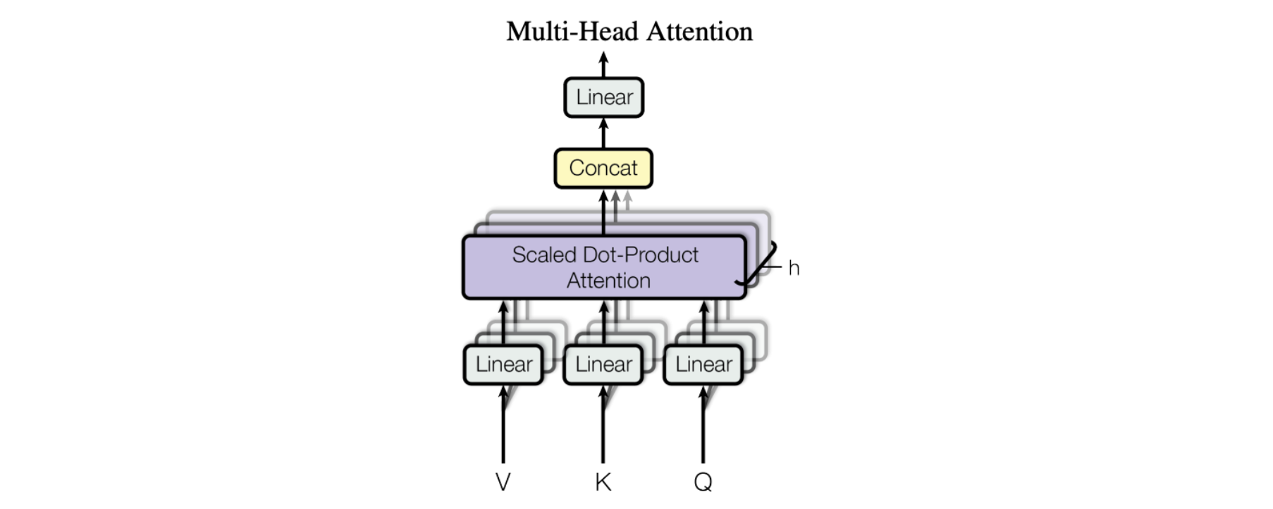
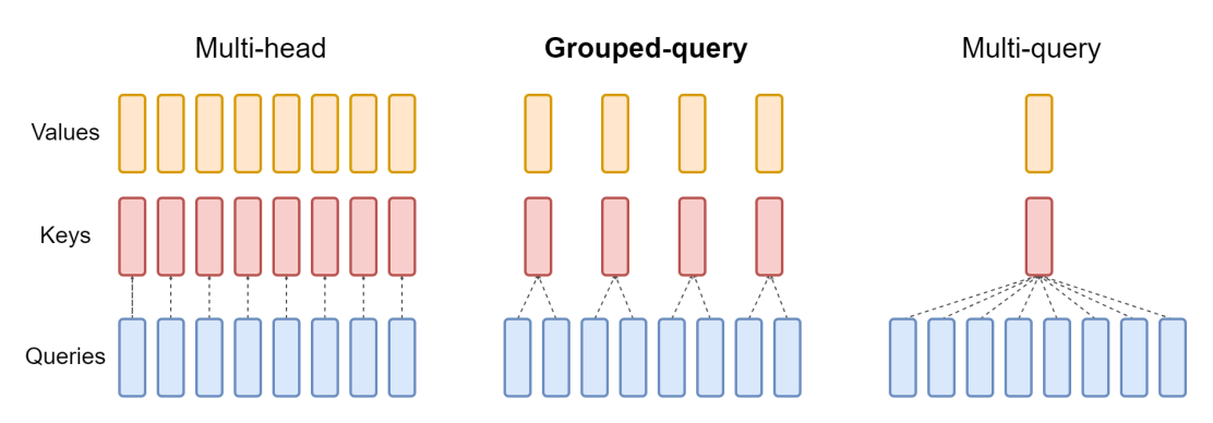


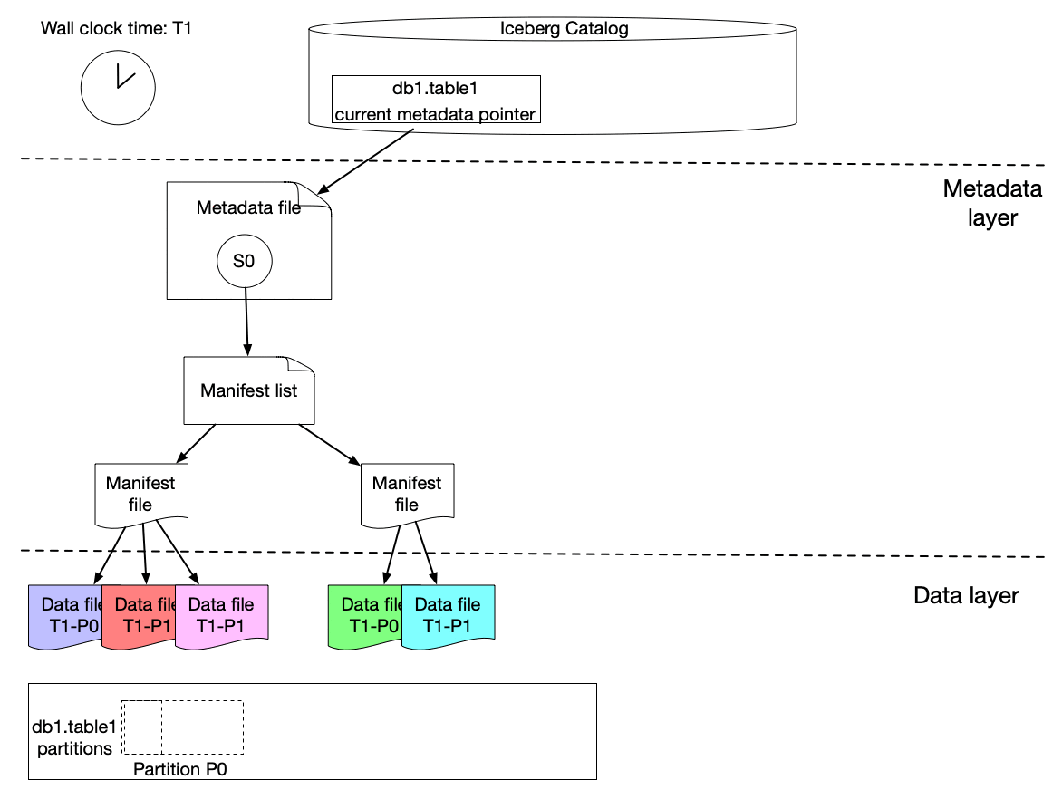


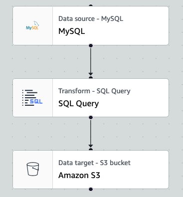
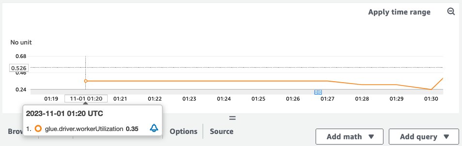
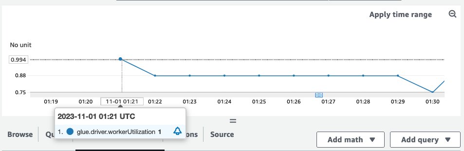
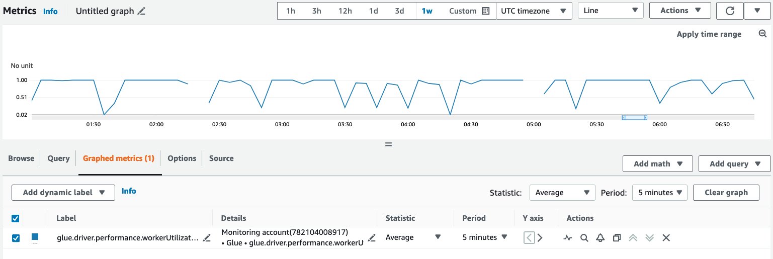
 Noritaka Sekiyama is a Principal Big Data Architect on the AWS Glue team. He is responsible for building software artifacts to help customers. In his spare time, he enjoys cycling with his new road bike.
 Shenoda Guirguis is a Senior Software Development Engineer on the AWS Glue team. His passion is in building scalable and distributed Data Infrastructure/Processing Systems. When he gets a chance, Shenoda enjoys reading and playing soccer.
 Sean Ma is a Principal Product Manager on the AWS Glue team. He has an 18+ year track record of innovating and delivering enterprise products that unlock the power of data for users. Outside of work, Sean enjoys scuba diving and college football.
 Mohit Saxena is a Senior Software Development Manager on the AWS Glue team. His team focuses on building distributed systems to enable customers with interactive and simple to use interfaces to efficiently manage and transform petabytes of data seamlessly across data lakes on Amazon S3, databases and data-warehouses on cloud.
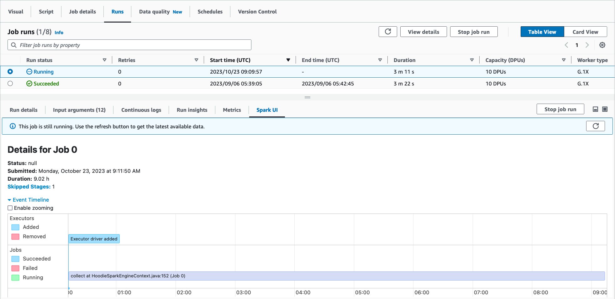
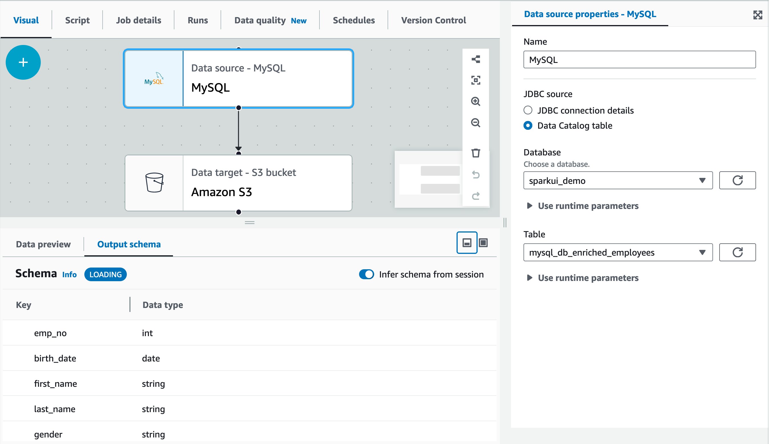
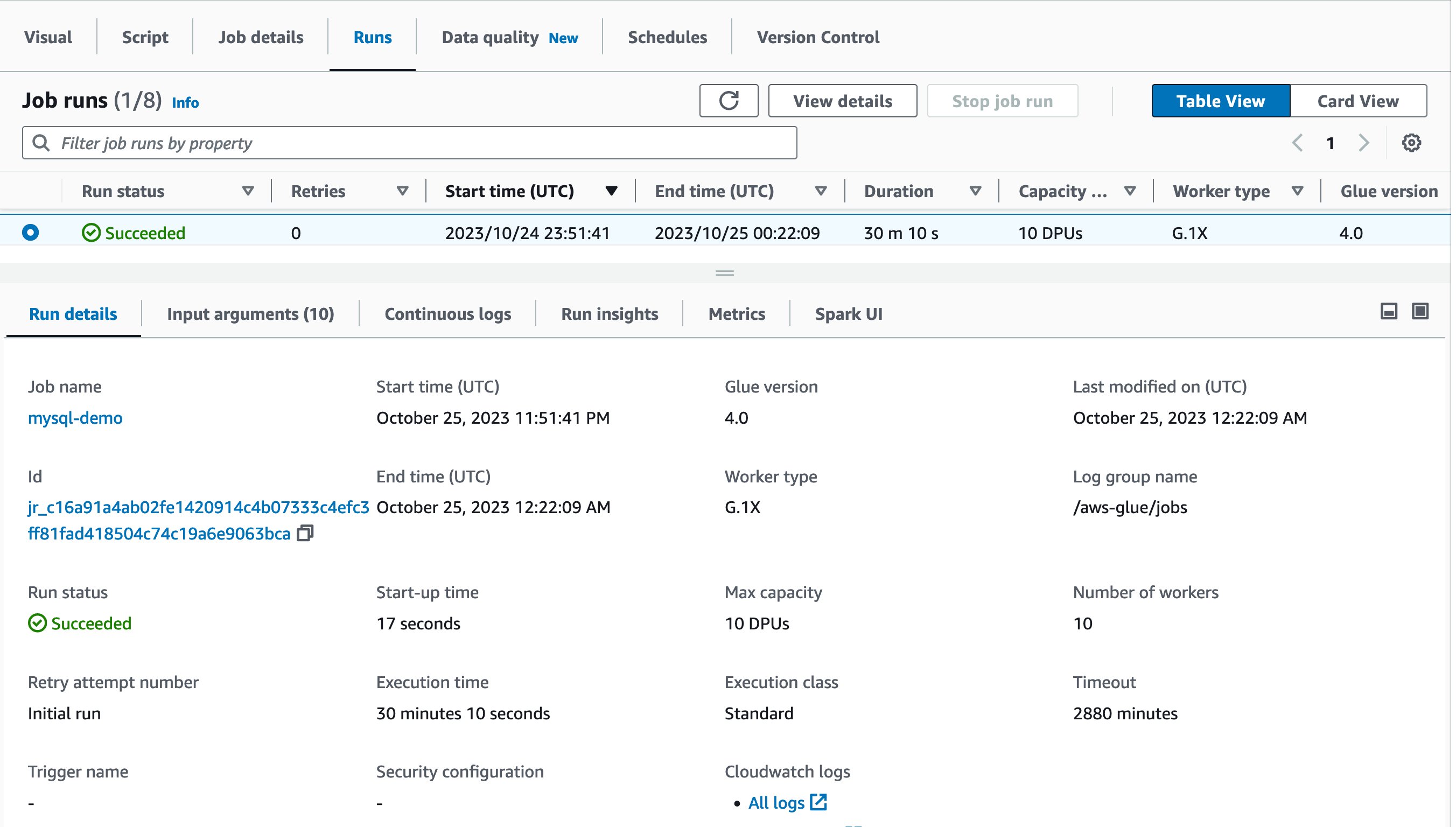

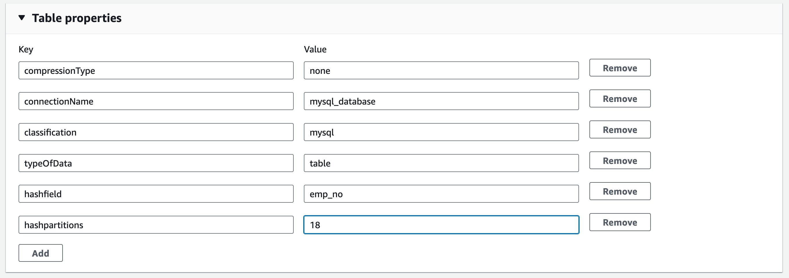
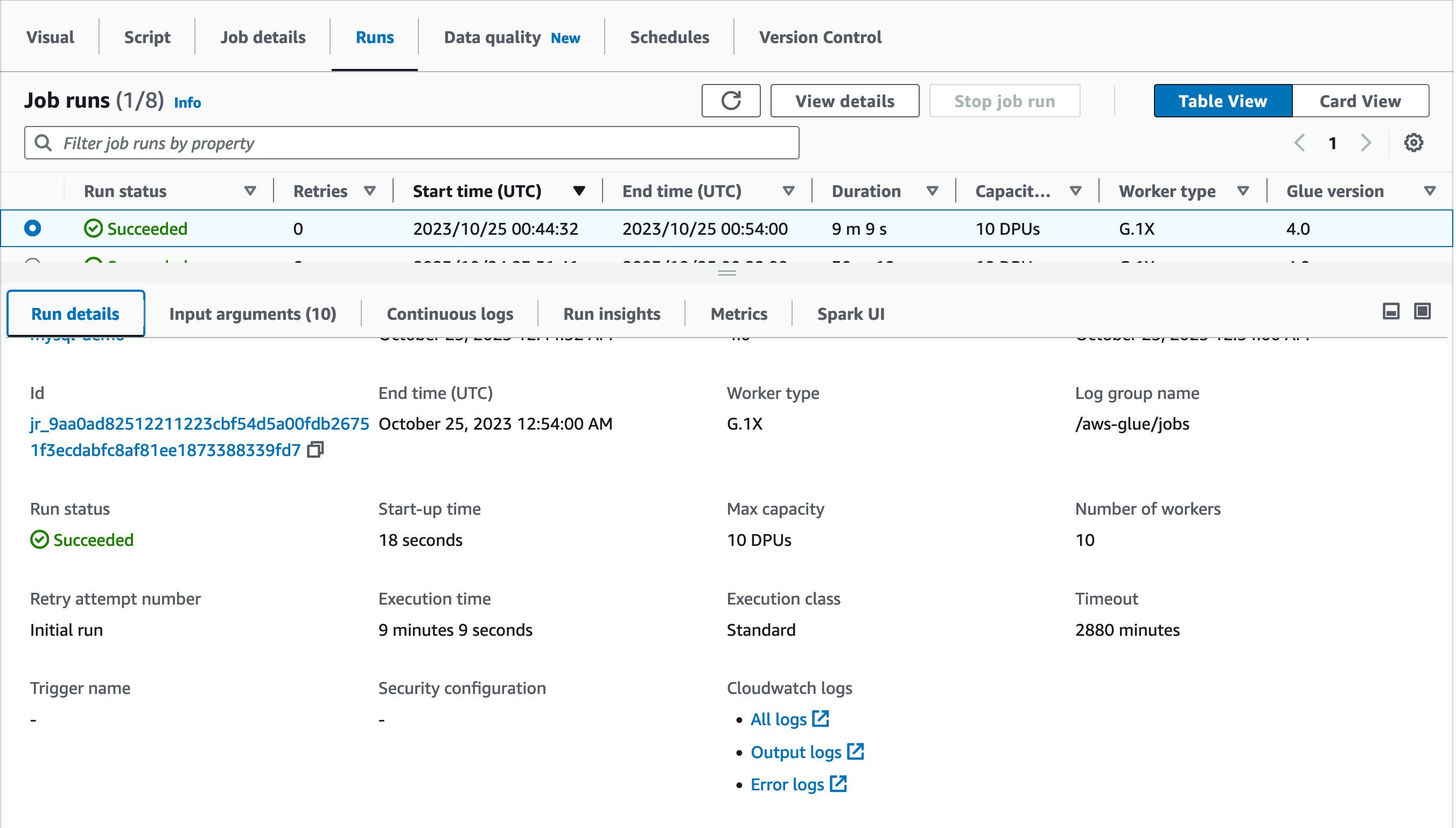
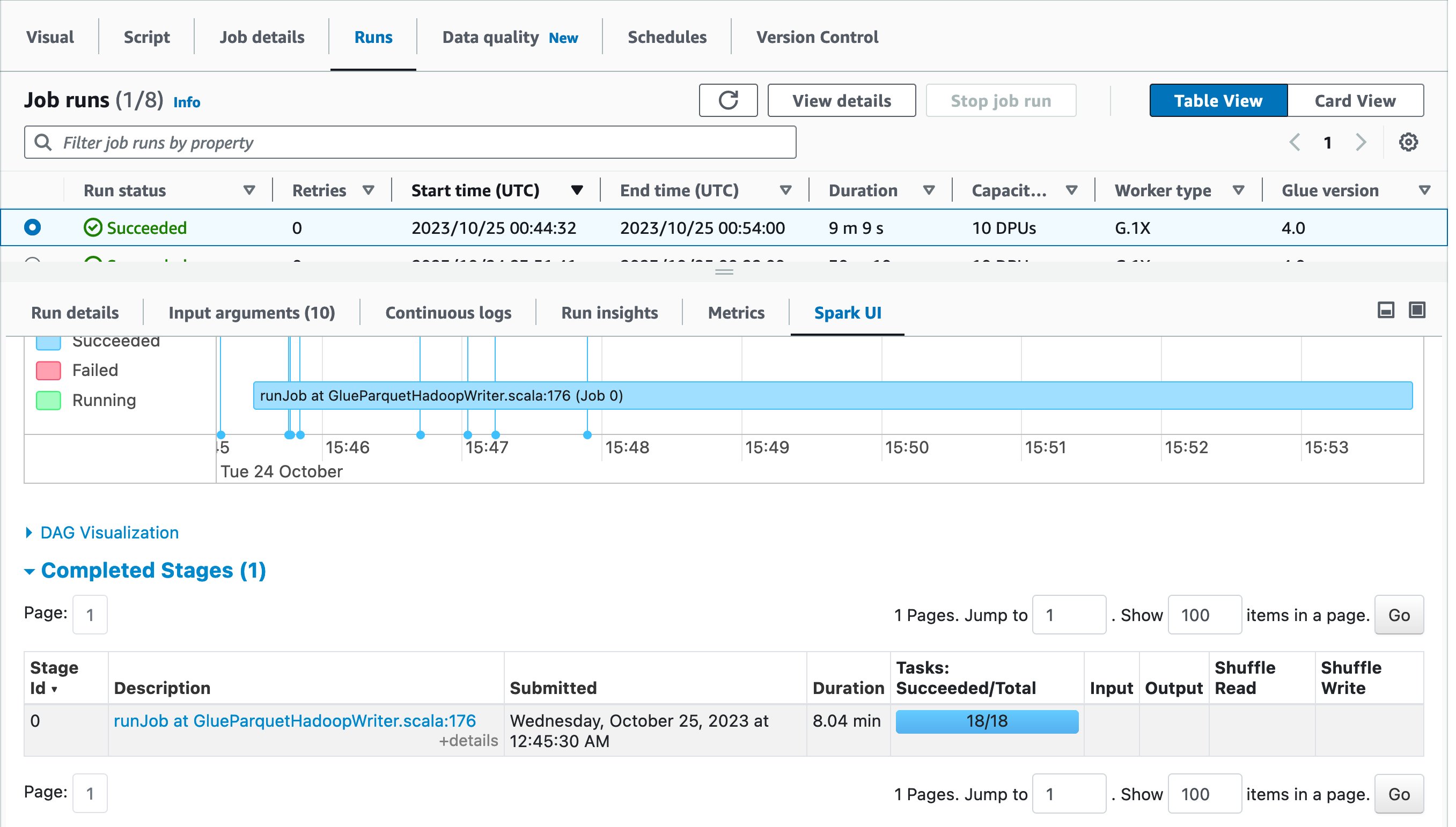
 Alexandra Tello is a Senior Front End Engineer with the AWS Glue team in New York City. She is a passionate advocate for usability and accessibility. In her free time, she’s an espresso enthusiast and enjoys building mechanical keyboards.
 Matt Sampson is a Software Development Manager on the AWS Glue team. He loves working with his other Glue team members to make services that our customers benefit from. Outside of work, he can be found fishing and maybe singing karaoke.
 Matt Su is a Senior Product Manager on the AWS Glue team. He enjoys helping customers uncover insights and make better decisions using their data with AWS Analytic services. In his spare time, he enjoys skiing and gardening.