Tag Archives: Amazon EMR

Use Apache Iceberg in a data lake to support incremental data processing

Post Syndicated from Flora Wu original https://aws.amazon.com/blogs/big-data/use-apache-iceberg-in-a-data-lake-to-support-incremental-data-processing/

Apache Iceberg is an open table format for very large analytic datasets, which captures metadata information on the state of datasets as they evolve and change over time. It adds tables to compute engines including Spark, Trino, PrestoDB, Flink, and Hive using a high-performance table format that works just like a SQL table. Iceberg has become very popular for its support for ACID transactions in data lakes and features like schema and partition evolution, time travel, and rollback.

Apache Iceberg integration is supported by AWS analytics services including Amazon EMR, Amazon Athena, and AWS Glue. Amazon EMR can provision clusters with Spark, Hive, Trino, and Flink that can run Iceberg. Starting with Amazon EMR version 6.5.0, you can use Iceberg with your EMR cluster without requiring a bootstrap action. In early 2022, AWS announced general availability of Athena ACID transactions, powered by Apache Iceberg. The recently released Athena query engine version 3 provides better integration with the Iceberg table format. AWS Glue 3.0 and later supports the Apache Iceberg framework for data lakes.

In this post, we discuss what customers want in modern data lakes and how Apache Iceberg helps address customer needs. Then we walk through a solution to build a high-performance and evolving Iceberg data lake on Amazon Simple Storage Service (Amazon S3) and process incremental data by running insert, update, and delete SQL statements. Finally, we show you how to performance tune the process to improve read and write performance.

How Apache Iceberg addresses what customers want in modern data lakes

More and more customers are building data lakes, with structured and unstructured data, to support many users, applications, and analytics tools. There is an increased need for data lakes to support database like features such as ACID transactions, record-level updates and deletes, time travel, and rollback. Apache Iceberg is designed to support these features on cost-effective petabyte-scale data lakes on Amazon S3.

Apache Iceberg addresses customer needs by capturing rich metadata information about the dataset at the time the individual data files are created. There are three layers in the architecture of an Iceberg table: the Iceberg catalog, the metadata layer, and the data layer, as depicted in the following figure (source).

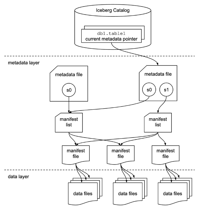
The Iceberg catalog stores the metadata pointer to the current table metadata file. When a select query is reading an Iceberg table, the query engine first goes to the Iceberg catalog, then retrieves the location of the current metadata file. Whenever there is an update to the Iceberg table, a new snapshot of the table is created, and the metadata pointer points to the current table metadata file.

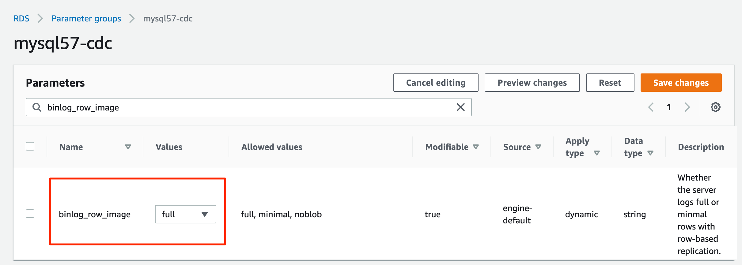
The following is an example Iceberg catalog with AWS Glue implementation. You can see the database name, the location (S3 path) of the Iceberg table, and the metadata location.

The metadata layer has three types of files: the metadata file, manifest list, and manifest file in a hierarchy. At the top of the hierarchy is the metadata file, which stores information about the table’s schema, partition information, and snapshots. The snapshot points to the manifest list. The manifest list has the information about each manifest file that makes up the snapshot, such as location of the manifest file, the partitions it belongs to, and the lower and upper bounds for partition columns for the data files it tracks. The manifest file tracks data files as well as additional details about each file, such as the file format. All three files work in a hierarchy to track the snapshots, schema, partitioning, properties, and data files in an Iceberg table.

The data layer has the individual data files of the Iceberg table. Iceberg supports a wide range of file formats including Parquet, ORC, and Avro. Because the Iceberg table tracks the individual data files instead of only pointing to the partition location with data files, it isolates the writing operations from reading operations. You can write the data files at any time, but only commit the change explicitly, which creates a new version of the snapshot and metadata files.

Solution overview

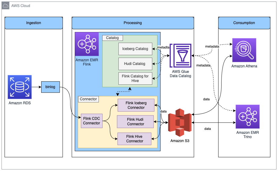
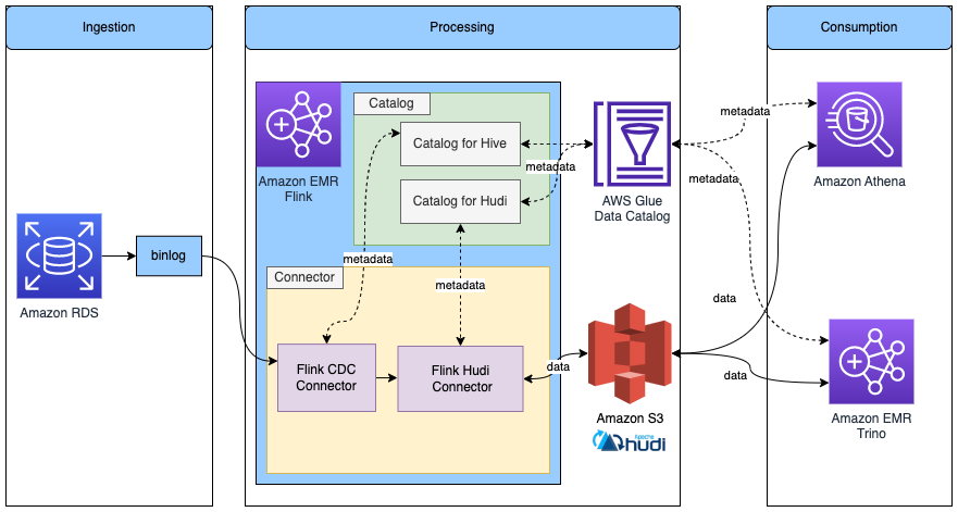
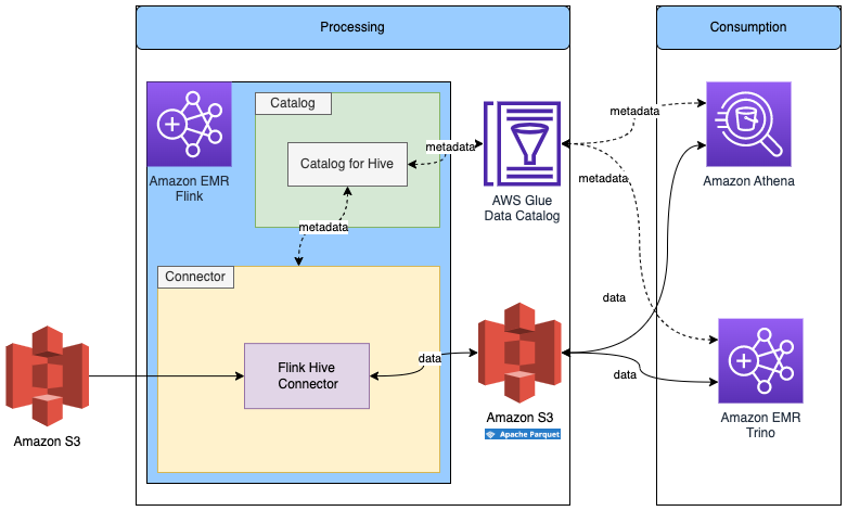
In this post, we walk you through a solution to build a high-performing Apache Iceberg data lake on Amazon S3; process incremental data with insert, update, and delete SQL statements; and tune the Iceberg table to improve read and write performance. The following diagram illustrates the solution architecture.

To demonstrate this solution, we use the Amazon Customer Reviews dataset in an S3 bucket (s3://amazon-reviews-pds/parquet/). In real use case, it would be raw data stored in your S3 bucket. We can check the data size with the following code in the AWS Command Line Interface (AWS CLI):

//Run this AWS CLI command to check the data size
aws s3 ls --summarize --human-readable --recursive s3://amazon-reviews-pds/parquet

The total object count is 430, and total size is 47.4 GiB.

To set up and test this solution, we complete the following high-level steps:

  1. Set up an S3 bucket in the curated zone to store converted data in Iceberg table format.
  2. Launch an EMR cluster with appropriate configurations for Apache Iceberg.
  3. Create a notebook in EMR Studio.
  4. Configure the Spark session for Apache Iceberg.
  5. Convert data to Iceberg table format and move data to the curated zone.
  6. Run insert, update, and delete queries in Athena to process incremental data.
  7. Carry out performance tuning.

Prerequisites

To follow along with this walkthrough, you must have an AWS account with an AWS Identity and Access Management (IAM) role that has sufficient access to provision the required resources.

Set up the S3 bucket for Iceberg data in the curated zone in your data lake

Choose the Region in which you want to create the S3 bucket and provide a unique name:

s3://iceberg-curated-blog-data

Launch an EMR cluster to run Iceberg jobs using Spark

You can create an EMR cluster from the AWS Management Console, Amazon EMR CLI, or AWS Cloud Development Kit (AWS CDK). For this post, we walk you through how to create an EMR cluster from the console.

  1. On the Amazon EMR console, choose Create cluster.
  2. Choose Advanced options.
  3. For Software Configuration, choose the latest Amazon EMR release. As of January 2023, the latest release is 6.9.0. Iceberg requires release 6.5.0 and above.
  4. Select JupyterEnterpriseGateway and Spark as the software to install.
  5. For Edit software settings, select Enter configuration and enter [{"classification":"iceberg-defaults","properties":{"iceberg.enabled":true}}].
  6. Leave other settings at their default and choose Next.
  7. For Hardware, use the default setting.
  8. Choose Next.
  9. For Cluster name, enter a name. We use iceberg-blog-cluster.
  10. Leave the remaining settings unchanged and choose Next.
  11. Choose Create cluster.

Create a notebook in EMR Studio

We now walk you through how to create a notebook in EMR Studio from the console.

  1. On the IAM console, create an EMR Studio service role.
  2. On the Amazon EMR console, choose EMR Studio.
  3. Choose Get started.

The Get started page appears in a new tab.

  1. Choose Create Studio in the new tab.
  2. Enter a name. We use iceberg-studio.
  3. Choose the same VPC and subnet as those for the EMR cluster, and the default security group.
  4. Choose AWS Identity and Access Management (IAM) for authentication, and choose the EMR Studio service role you just created.
  5. Choose an S3 path for Workspaces backup.
  6. Choose Create Studio.
  7. After the Studio is created, choose the Studio access URL.
  8. On the EMR Studio dashboard, choose Create workspace.
  9. Enter a name for your Workspace. We use iceberg-workspace.
  10. Expand Advanced configuration and choose Attach Workspace to an EMR cluster.
  11. Choose the EMR cluster you created earlier.
  12. Choose Create Workspace.
  13. Choose the Workspace name to open a new tab.

In the navigation pane, there is a notebook that has the same name as the Workspace. In our case, it is iceberg-workspace.

  1. Open the notebook.
  2. When prompted to choose a kernel, choose Spark.

Configure a Spark session for Apache Iceberg

Use the following code, providing your own S3 bucket name:

%%configure -f
{
"conf": {
"spark.sql.catalog.demo": "org.apache.iceberg.spark.SparkCatalog",
"spark.sql.catalog.demo.catalog-impl": "org.apache.iceberg.aws.glue.GlueCatalog",
"spark.sql.catalog.demo.warehouse": "s3://iceberg-curated-blog-data",
"spark.sql.extensions":"org.apache.iceberg.spark.extensions.IcebergSparkSessionExtensions",
"spark.sql.catalog.demo.io-impl":"org.apache.iceberg.aws.s3.S3FileIO"
}
}

This sets the following Spark session configurations:

  • spark.sql.catalog.demo – Registers a Spark catalog named demo, which uses the Iceberg Spark catalog plugin.
  • spark.sql.catalog.demo.catalog-impl – The demo Spark catalog uses AWS Glue as the physical catalog to store Iceberg database and table information.
  • spark.sql.catalog.demo.warehouse – The demo Spark catalog stores all Iceberg metadata and data files under the root path defined by this property: s3://iceberg-curated-blog-data.
  • spark.sql.extensions – Adds support to Iceberg Spark SQL extensions, which allows you to run Iceberg Spark procedures and some Iceberg-only SQL commands (you use this in a later step).
  • spark.sql.catalog.demo.io-impl – Iceberg allows users to write data to Amazon S3 through S3FileIO. The AWS Glue Data Catalog by default uses this FileIO, and other catalogs can load this FileIO using the io-impl catalog property.

Convert data to Iceberg table format

You can use either Spark on Amazon EMR or Athena to load the Iceberg table. In the EMR Studio Workspace notebook Spark session, run the following commands to load the data:

// create a database in AWS Glue named reviews if not exist
spark.sql("CREATE DATABASE IF NOT EXISTS demo.reviews")

// load reviews - this load all the parquet files
val reviews_all_location = "s3://amazon-reviews-pds/parquet/"
val reviews_all = spark.read.parquet(reviews_all_location)

// write reviews data to an Iceberg v2 table
reviews_all.writeTo("demo.reviews.all_reviews").tableProperty("format-version", "2").createOrReplace()

After you run the code, you should find two prefixes created in your data warehouse S3 path (s3://iceberg-curated-blog-data/reviews.db/all_reviews): data and metadata.

Process incremental data using insert, update, and delete SQL statements in Athena

Athena is a serverless query engine that you can use to perform read, write, update, and optimization tasks against Iceberg tables. To demonstrate how the Apache Iceberg data lake format supports incremental data ingestion, we run insert, update, and delete SQL statements on the data lake.

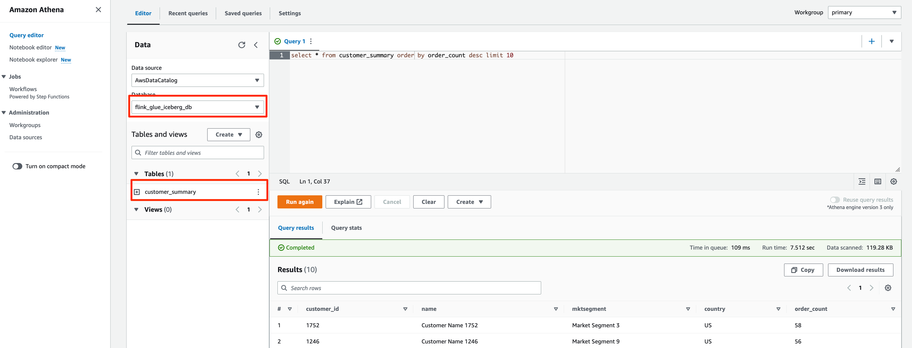
Navigate to the Athena console and choose Query editor. If this is your first time using the Athena query editor, you need to configure the query result location to be the S3 bucket you created earlier. You should be able to see that the table reviews.all_reviews is available for querying. Run the following query to verify that you have loaded the Iceberg table successfully:

select * from reviews.all_reviews limit 5;

Process incremental data by running insert, update, and delete SQL statements:

//Example update statement
update reviews.all_reviews set star_rating=5 where product_category = 'Watches' and star_rating=4

//Example delete statement
delete from reviews.all_reviews where product_category = 'Watches' and star_rating=1

Performance tuning

In this section, we walk through different ways to improve Apache Iceberg read and write performance.

Configure Apache Iceberg table properties

Apache Iceberg is a table format, and it supports table properties to configure table behavior such as read, write, and catalog. You can improve the read and write performance on Iceberg tables by adjusting the table properties.

For example, if you notice that you write too many small files for an Iceberg table, you can config the write file size to write fewer but bigger size files, to help improve query performance.

Property Default Description
write.target-file-size-bytes 536870912 (512 MB) Controls the size of files generated to target about this many bytes

Use the following code to alter the table format:

//Example code to alter table format in EMR Studio Workspace notebook
spark.sql("ALTER TABLE demo.reviews.all_reviews 
SET TBLPROPERTIES ('write_target_data_file_size_bytes'='536870912')")

Partitioning and sorting

To make a query run fast, the less data read the better. Iceberg takes advantage of the rich metadata it captures at write time and facilitates techniques such as scan planning, partitioning, pruning, and column-level stats such as min/max values to skip data files that don’t have match records. We walk you through how query scan planning and partitioning work in Iceberg and how we use them to improve query performance.

Query scan planning

For a given query, the first step in a query engine is scan planning, which is the process to find the files in a table needed for a query. Planning in an Iceberg table is very efficient, because Iceberg’s rich metadata can be used to prune metadata files that aren’t needed, in addition to filtering data files that don’t contain matching data. In our tests, we observed Athena scanned 50% or less data for a given query on an Iceberg table compared to original data before conversion to Iceberg format.

There are two types of filtering:

  • Metadata filtering – Iceberg uses two levels of metadata to track the files in a snapshot: the manifest list and manifest files. It first uses the manifest list, which acts as an index of the manifest files. During planning, Iceberg filters manifests using the partition value range in the manifest list without reading all the manifest files. Then it uses selected manifest files to get data files.
  • Data filtering – After selecting the list of manifest files, Iceberg uses the partition data and column-level stats for each data file stored in manifest files to filter data files. During planning, query predicates are converted to predicates on the partition data and applied first to filter data files. Then, the column stats like column-level value counts, null counts, lower bounds, and upper bounds are used to filter out data files that can’t match the query predicate. By using upper and lower bounds to filter data files at planning time, Iceberg greatly improves query performance.

Partitioning and sorting

Partitioning is a way to group records with the same key column values together in writing. The benefit of partitioning is faster queries that access only part of the data, as explained earlier in query scan planning: data filtering. Iceberg makes partitioning simple by supporting hidden partitioning, in the way that Iceberg produces partition values by taking a column value and optionally transforming it.

In our use case, we first run the following query on the Iceberg table not partitioned. Then we partition the Iceberg table by the category of the reviews, which will be used in the query WHERE condition to filter out records. With partitioning, the query could scan much less data. See the following code:

//Example code in EMR Studio Workspace notebook to create an Iceberg table all_reviews_partitioned partitioned by product_category
reviews_all.writeTo("demo.reviews.all_reviews_partitioned").tableProperty("format-version", "2").partitionedBy($"product_category").createOrReplace()

Run the following select statement on the non-partitioned all_reviews table vs. the partitioned table to see the performance difference:

//Run this query on all_reviews table and the partitioned table for performance testing
select marketplace,customer_id, review_id,product_id,product_title,star_rating from reviews.all_reviews where product_category = 'Watches' and review_date between date('2005-01-01') and date('2005-03-31')

//Run the same select query on partitioned dataset
select marketplace,customer_id, review_id,product_id,product_title,star_rating from reviews.all_reviews_partitioned where product_category = 'Watches' and review_date between date('2005-01-01') and date('2005-03-31')

The following table shows the performance improvement of data partitioning, with about 50% performance improvement and 70% less data scanned.

Dataset Name Non-Partitioned Dataset Partitioned Dataset
Runtime (seconds) 8.20 4.25
Data Scanned (MB) 131.55 33.79

Note that the runtime is the average runtime with multiple runs in our test.

We saw good performance improvement after partitioning. However, this can be further improved by using column-level stats from Iceberg manifest files. In order to use the column-level stats effectively, you want to further sort your records based on the query patterns. Sorting the whole dataset using the columns that are often used in queries will reorder the data in such a way that each data file ends up with a unique range of values for the specific columns. If these columns are used in the query condition, it allows query engines to further skip data files, thereby enabling even faster queries.

Copy-on-write vs. read-on-merge

When implementing update and delete on Iceberg tables in the data lake, there are two approaches defined by the Iceberg table properties:

  • Copy-on-write – With this approach, when there are changes to the Iceberg table, either updates or deletes, the data files associated with the impacted records will be duplicated and updated. The records will be either updated or deleted from the duplicated data files. A new snapshot of the Iceberg table will be created and pointing to the newer version of data files. This makes the overall writes slower. There might be situations that concurrent writes are needed with conflicts so retry has to happen, which increases the write time even more. On the other hand, when reading the data, there is no extra process needed. The query will retrieve data from the latest version of data files.
  • Merge-on-read – With this approach, when there are updates or deletes on the Iceberg table, the existing data files will not be rewritten; instead new delete files will be created to track the changes. For deletes, a new delete file will be created with the deleted records. When reading the Iceberg table, the delete file will be applied to the retrieved data to filter out the delete records. For updates, a new delete file will be created to mark the updated records as deleted. Then a new file will be created for those records but with updated values. When reading the Iceberg table, both the delete and new files will be applied to the retrieved data to reflect the latest changes and produce the correct results. So, for any subsequent queries, an extra step to merge the data files with the delete and new files will happen, which will usually increase the query time. On the other hand, the writes might be faster because there is no need to rewrite the existing data files.

To test the impact of the two approaches, you can run the following code to set the Iceberg table properties:

//Run code to alter Iceberg table property to set copy-on-write and merge-on-read in EMR Studio Workspace notebook
spark.sql(“ALTER TABLE demo.reviews.all_reviews 
SET TBLPROPERTIES (‘write.delete.mode’=’copy-on-write’,’write.update.mode’=’copy-on-write’)”)

Run the update, delete, and select SQL statements in Athena to show the runtime difference for copy-on-write vs. merge-on-read:

//Example update statement
update reviews.all_reviews set star_rating=5 where product_category = ‘Watches’ and star_rating=4

//Example delete statement
delete from reviews.all_reviews where product_category = ‘Watches’ and star_rating=1

//Example select statement
select marketplace,customer_id, review_id,product_id,product_title,star_rating from reviews.all_reviews where product_category = ‘Watches’ and review_date between date(‘2005-01-01’) and date(‘2005-03-31’)

The following table summarizes the query runtimes.

Query Copy-on-Write Merge-on-Read
UPDATE DELETE SELECT UPDATE DELETE SELECT
Runtime (seconds) 66.251 116.174 97.75 10.788 54.941 113.44
Data scanned (MB) 494.06 3.07 137.16 494.06 3.07 137.16

Note that the runtime is the average runtime with multiple runs in our test.

As our test results show, there are always trade-offs in the two approaches. Which approach to use depends on your use cases. In summary, the considerations come down to latency on the read vs. write. You can reference the following table and make the right choice.

. Copy-on-Write Merge-on-Read
Pros Faster reads Faster writes
Cons Expensive writes Higher latency on reads
When to use Good for frequent reads, infrequent updates and deletes or large batch updates Good for tables with frequent updates and deletes

Data compaction

If your data file size is small, you might end up with thousands or millions of files in an Iceberg table. This dramatically increases the I/O operation and slows down the queries. Furthermore, Iceberg tracks each data file in a dataset. More data files lead to more metadata. This in turn increases the overhead and I/O operation on reading metadata files. In order to improve the query performance, it’s recommended to compact small data files to larger data files.

When updating and deleting records in Iceberg table, if the read-on-merge approach is used, you might end up with many small deletes or new data files. Running compaction will combine all these files and create a newer version of the data file. This eliminates the need to reconcile them during reads. It’s recommended to have regular compaction jobs to impact reads as little as possible while still maintaining faster write speed.

Run the following data compaction command, then run the select query from Athena:

//Data compaction 
optimize reviews.all_reviews REWRITE DATA USING BIN_PACK

//Run this query before and after data compaction
select marketplace,customer_id, review_id,product_id,product_title,star_rating from reviews.all_reviews where product_category = 'Watches' and review_date between date('2005-01-01') and date('2005-03-31')

The following table compares the runtime before vs. after data compaction. You can see about 40% performance improvement.

Query Before Data Compaction After Data Compaction
Runtime (seconds) 97.75 32.676 seconds
Data scanned (MB) 137.16 M 189.19 M

Note that the select queries ran on the all_reviews table after update and delete operations, before and after data compaction. The runtime is the average runtime with multiple runs in our test.

Clean up

After you follow the solution walkthrough to perform the use cases, complete the following steps to clean up your resources and avoid further costs:

  1. Drop the AWS Glue tables and database from Athena or run the following code in your notebook:
// DROP the table 
spark.sql("DROP TABLE demo.reviews.all_reviews") 
spark.sql("DROP TABLE demo.reviews.all_reviews_partitioned") 

// DROP the database 
spark.sql("DROP DATABASE demo.reviews")
  1. On the EMR Studio console, choose Workspaces in the navigation pane.
  2. Select the Workspace you created and choose Delete.
  3. On the EMR console, navigate to the Studios page.
  4. Select the Studio you created and choose Delete.
  5. On the EMR console, choose Clusters in the navigation pane.
  6. Select the cluster and choose Terminate.
  7. Delete the S3 bucket and any other resources that you created as part of the prerequisites for this post.

Conclusion

In this post, we introduced the Apache Iceberg framework and how it helps resolve some of the challenges we have in a modern data lake. Then we walked you though a solution to process incremental data in a data lake using Apache Iceberg. Finally, we had a deep dive into performance tuning to improve read and write performance for our use cases.

We hope this post provides some useful information for you to decide whether you want to adopt Apache Iceberg in your data lake solution.


About the Authors

Flora Wu is a Sr. Resident Architect at AWS Data Lab. She helps enterprise customers create data analytics strategies and build solutions to accelerate their businesses outcomes. In her spare time, she enjoys playing tennis, dancing salsa, and traveling.

Daniel Li is a Sr. Solutions Architect at Amazon Web Services. He focuses on helping customers develop, adopt, and implement cloud services and strategy. When not working, he likes spending time outdoors with his family.

Reduce Amazon EMR cluster costs by up to 19% with new enhancements in Amazon EMR Managed Scaling

Post Syndicated from Sushant Majithia original https://aws.amazon.com/blogs/big-data/reduce-amazon-emr-cluster-costs-by-up-to-19-with-new-enhancements-in-amazon-emr-managed-scaling/

In June 2020, AWS announced the general availability of Amazon EMR Managed Scaling. With EMR Managed Scaling, you specify the minimum and maximum compute limits for your clusters, and Amazon EMR automatically resizes your cluster for optimal performance and resource utilization. EMR Managed Scaling constantly monitors key workload-related metrics and uses an algorithm that optimizes the cluster size for best resource utilization. Given that the feature is completely managed, improvements to the algorithm are immediately realized without needing a version upgrade. Amazon EMR can scale the cluster up during peaks and scale it down gracefully during idle periods, reducing your costs and optimizing cluster capacity for the best performance.

Throughout 2022, we made multiple enhancements to the EMR Managed Scaling algorithm. With these improvements, we observed that for clusters enabled with EMR Managed Scaling, utilization improved by up to 15 percent, and total costs were reduced further by up to 19 percent. Starting mid-December 2022, EMR Managed Scaling enhancements were enabled by default for clusters using Amazon EMR versions 5.34.0 and later and Amazon EMR versions 6.4.0 and later for both new and existing clusters. Further, given that the feature is completely managed, you will get the new optimized Managed Scaling algorithm by default, and no action is needed on your end.

Listed below are some of the key enhancements we enabled for EMR Managed Scaling:

  • Improved cluster utilization with targeted scale-down of your EMR cluster
  • Reduced costs by preventing scale-down of instances that store intermediate shuffle data using Spark Shuffle data awareness
  • Improved cluster utilization and reduce costs with gradual scale-up of your EMR cluster

Customer success stories

How the enhanced EMR Managed Scaling algorithm helped a technology enterprise reduce costs:

To illustrate the cost savings by examples, we looked at an EMR clusters for a technology enterprise, which heavily uses Amazon EMR to process real time billing data between Kafka and S3 using Spark. They run a persistent EMR cluster with EMR version 5.35 and have EMR Managed Scaling turned-on. The following Amazon CloudWatch dashboard shows how starting December 21, the enhanced Managed Scaling algorithm provisioned (total nodes requested) only 70 nodes vs. the previous Managed Scaling algorithm which provisioned 179 nodes for a similar job profile. The lower the number of resources provisioned to run your jobs, the lower the total cost of your EMR cluster.

How the enhanced EMR Managed Scaling algorithm helped an advertising enterprise reduce costs:

We also looked at an EMR cluster for an advertising enterprise, which leverages Amazon EMR for their data analytics strategy and executes their batch ETL jobs using Spark. They run their clusters on EMR version 6.5 and have EMR Managed Scaling turned-on. The following Amazon CloudWatch dashboard shows how starting December 15, the enhanced Managed Scaling algorithm provisioned (total units requested) only 41 nodes vs. the previous Managed Scaling algorithm which provisioned 86 nodes for a similar job profile.

Estimating the cost savings and utilization improvements for your EMR clusters:

Cluster cost savings:

To view estimated cost savings for your EMR cluster with the EMR Managed Scaling enhancements, please follow the steps below:

  • Open the CloudWatch metrics console and, under EMR, search by your ClusterId.
  • From the list of metrics available for EMR, select the following two metrics:
    • Running capacity – Based on the unit type you specified in your Managed Scaling policy, this will be available as either “TotalUnitsRunning” or “TotalNodesRunning” or “TotalVCPURunning
    • Capacity requested by Managed Scaling – Based on the unit type you specified in your Managed Scaling policy, this will be available as either “TotalUnitsRequested” or “TotalNodesRequested” or “TotalVCPURequested
  •  Plot both of the metrics to your CloudWatch dashboard.
  • Select the time frame as the 3 months between November 2022 and January 2023 to view the improvements with the enhanced Managed Scaling algorithm when compared to the previous Managed Scaling algorithm.

Cluster utilization improvements:

To estimate the improvements in your EMR cluster utilization with the EMR Managed Scaling enhancements, please follow the steps below:

  • Open the CloudWatch metrics console and, under EMR, search by your ClusterId.
  • From the list of metrics available for EMR, select the “YARNMemoryAvailablePercentage” metric.
  • To derive memory utilized by YARN, add a math expression such as “Add Math → Start with empty expression”
    • For the new math expression, set Label=Yarn Utilization and set Details=100-YARNMemoryAvailablePercentage.
  • Plot the cluster utilization metric to your CloudWatch dashboard.
  • Select the time frame as the 3 months between November 2022 and January 2023 to view the improvements with the enhanced Managed Scaling algorithm when compared to the previous Managed Scaling algorithm.

What’s next

We will continue to tune the Managed Scaling algorithm with every new EMR release and thereby improve the customer experience when scaling clusters with EMR Managed Scaling.

Conclusion

In this post, we provided an overview of the key enhancement we launched in EMR Managed Scaling. With these enhancements, we observed that the cluster utilization improved by up to 15 percent, and cluster cost was reduced by up to 19 percent. Starting mid-December 2022, these enhancements were enabled by default for EMR clusters using Amazon EMR versions 5.34.0 and later, and Amazon EMR versions 6.4.0 and later. Given that EMR Managed Scaling is a completely managed feature, you will get the new, optimized EMR Managed Scaling algorithm by default, and no action is needed from your end.

To learn more and get started with EMR Managed Scaling, visit the EMR Managed Scaling documentation page.


About the Authors

Sushant Majithia is a Principal Product Manager for EMR at Amazon Web Services.

 Vishal Vyas is a Senior Software Engineer for EMR at Amazon Web Services.

Matthew Liem is a Senior Solution Architecture Manager at AWS.

Achieve up to 27% better price-performance for Spark workloads with AWS Graviton2 on Amazon EMR Serverless

Post Syndicated from Karthik Prabhakar original https://aws.amazon.com/blogs/big-data/achieve-up-to-27-better-price-performance-for-spark-workloads-with-aws-graviton2-on-amazon-emr-serverless/

Amazon EMR Serverless is a serverless option in Amazon EMR that makes it simple to run applications using open-source analytics frameworks such as Apache Spark and Hive without configuring, managing, or scaling clusters.

At AWS re:Invent 2022, we announced support for running serverless Spark and Hive workloads with AWS Graviton2 (Arm64) on Amazon EMR Serverless. AWS Graviton2 processors are custom-built by AWS using 64-bit Arm Neoverse cores, delivering a significant leap in price-performance for your cloud workloads.

This post discusses the performance improvements observed while running Apache Spark jobs using AWS Graviton2 on EMR Serverless. We found that Graviton2 on EMR Serverless achieved 10% performance improvement for Spark workloads based on runtime. AWS Graviton2 is offered at a 20% lower cost than the x86 architecture option (see the Amazon EMR pricing page for details), resulting in a 27% overall better price-performance for workloads.

Spark performance test results

The following charts compare the benchmark runtime with and without Graviton2 for a EMR Serverless Spark application (note that the charts are not drawn to scale). We observed up to 10% improvement in total runtime and 8% improvement in geometric mean for the queries compared to x86.

The following table summarizes our results.

Metric Graviton2 x86 %Gain
Total Execution Time (in seconds) 2,670 2,959 10%
Geometric Mean (in seconds) 22.06 24.07 8%

Testing configuration

To evaluate the performance improvements, we use benchmark tests derived from TPC-DS 3 TB scale performance benchmarks. The benchmark consists of 104 queries, and each query is submitted sequentially to an EMR Serverless application. EMR Serverless has automatic and fine-grained scaling enabled by default. Spark provides Dynamic Resource Allocation (DRA) to dynamically adjust the application resources based on the workload, and EMR Serverless uses the signals from DRA to elastically scale workers as needed. For our tests, we chose a predefined pre-initialized capacity that allows the application to scale to default limits. Each application has 1 driver and 100 workers configured as pre-initialized capacity, allowing it to scale to a maximum of 8000 vCPU/60000 GB capacity. When launching the applications, as default we use x86_64 to get baseline numbers and Arm64 for AWS Graviton2, and the application had VPC networking enabled.

The following table summarizes the Spark application configuration.

Number of Drivers Driver Size Number of Executors Executor Size Ephemeral Storage Amazon EMR release label
1 4 vCPUs, 16 GB Memory 100 4 vCPUs, 16 GB Memory 200 G 6.9

Performance test results and cost comparison

Let’s do a cost comparison of the benchmark tests. Because we used 1 driver [4 vCPUs, 16 GB memory] and 100 executors [4 vCPUs, 16 GB memory] for each run, the total capacity used is 4*101=192 vCPUs, 16*101=1616 GB memory, 200*100=20000 GB storage. The following table summarizes the cost.

Test Total time (Seconds) vCPUs Memory (GB) Ephemeral (Storage GB) Cost
x86_64 2,958.82 404 1616 18000 $26.73
Graviton2 2,670.38 404 1616 18000 $19.59

The calculations are as follows:

  • Total vCPU cost = (number of vCPU * per vCPU rate * job runtime in hour)
  • Total GB = (Total GB of memory configured * per GB-hours rate * job runtime in hour)
  • Storage = 20 GB of ephemeral storage is available for all workers by default—you pay only for any additional storage that you configure per worker

Cost breakdown

Let’s look at the cost breakdown for x86:

  • Job runtime – 49.3 minutes = 0.82 hours
  • Total vCPU cost – 404 vCPUs x 0.82 hours job runtime x 0.052624 USD per vCPU = 17.4333 USD
  • Total GB cost – 1,616 memory-GBs x 0.82 hours job runtime x 0.0057785 USD per memory GB = 7.6572 USD
  • Storage cost – 18,000 storage-GBs x 0.82 hours job runtime x 0.000111 USD per storage GB = 1.6386 USD
  • Additional storage – 20,000 GB – 20 GB free tier * 100 workers = 18,000 additional storage GB
  • EMR Serverless total cost (x86): 17.4333 USD + 7.6572 USD + 1.6386 USD = 26.7291 USD

Let’s compare to the cost breakdown for Graviton 2:

  • Job runtime – 44.5 minutes = 0.74 hours
  • Total vCPU cost – 404 vCPUs x 0.74 hours job runtime x 0.042094 USD per vCPU = 12.5844 USD
  • Total GB cost – 1,616 memory-GBs x 0.74 hours job runtime x 0.004628 USD per memory GB = 5.5343 USD
  • Storage cost – 18,000 storage-GBs x 0.74 hours job runtime x 0.000111 USD per storage GB = 1.4785 USD
  • Additional storage – 20,000 GB – 20 GB free tier * 100 workers = 18,000 additional storage GB
  • EMR Serverless total cost (Graviton2): 12.5844 USD + 5.5343 USD + 1.4785 USD = 19.5972 USD

The tests indicate that for the benchmark run, AWS Graviton2 lead to an overall cost savings of 27%.

Individual query improvements and observations

The following chart shows the relative speedup of individual queries with Graviton2 compared to x86.

We see some regression in a few shorter queries, which had little impact on the overall benchmark runtime. We observed better performance gains for long running queries, for example:

  • q67 average 86 seconds for x86, 74 seconds for Graviton2 with 24% runtime performance gain
  • q23a and q23b gained 14% and 16%, respectively
  • q32 regressed by 7%; the difference between average runtime is <500 milliseconds (11.09 seconds for Graviton2 vs. 10.39 seconds for x86)

To quantify performance, we use benchmark SQL derived from TPC-DS 3 TB scale performance benchmarks.

If you’re evaluating migrating your workloads to Graviton2 architecture on EMR Serverless, we recommend testing the Spark workloads based on your real-world use cases. The outcome might vary based on the pre-initialized capacity and number of workers chosen. If you want to run workloads across multiple processor architectures, (for example, test the performance on x86 and Arm vCPUs) follow the walkthrough in the GitHub repo to get started with some concrete ideas.

Conclusion

As demonstrated in this post, Graviton2 on EMR Serverless applications consistently yielded better performance for Spark workloads. Graviton2 is available in all Regions where EMR Serverless is available. To see a list of Regions where EMR Serverless is available, see the EMR Serverless FAQs. To learn more, visit the Amazon EMR Serverless User Guide and sample codes with Apache Spark and Apache Hive.

If you’re wondering how much performance gain you can achieve with your use case, try out the steps outlined in this post and replace with your queries.

To launch your first Spark or Hive application using a Graviton2-based architecture on EMR Serverless, see Getting started with Amazon EMR Serverless.


About the authors

Karthik Prabhakar is a Senior Big Data Solutions Architect for Amazon EMR at AWS. He is an experienced analytics engineer working with AWS customers to provide best practices and technical advice in order to assist their success in their data journey.

Nithish Kumar Murcherla is a Senior Systems Development Engineer on the Amazon EMR Serverless team. He is passionate about distributed computing, containers, and everything and anything about the data.

Amazon EMR Serverless supports larger worker sizes to run more compute and memory-intensive workloads

Post Syndicated from Veena Vasudevan original https://aws.amazon.com/blogs/big-data/amazon-emr-serverless-supports-larger-worker-sizes-to-run-more-compute-and-memory-intensive-workloads/

Amazon EMR Serverless allows you to run open-source big data frameworks such as Apache Spark and Apache Hive without managing clusters and servers. With EMR Serverless, you can run analytics workloads at any scale with automatic scaling that resizes resources in seconds to meet changing data volumes and processing requirements. EMR Serverless automatically scales resources up and down to provide just the right amount of capacity for your application.

We are excited to announce that EMR Serverless now offers worker configurations of 8 vCPUs with up to 60 GB memory and 16 vCPUs with up to 120 GB memory, allowing you to run more compute and memory-intensive workloads on EMR Serverless. An EMR Serverless application internally uses workers to execute workloads. and you can configure different worker configurations based on your workload requirements. Previously, the largest worker configuration available on EMR Serverless was 4 vCPUs with up to 30 GB memory. This capability is especially beneficial for the following common scenarios:

  • Shuffle-heavy workloads
  • Memory-intensive workloads

Let’s look at each of these use cases and the benefits of having larger worker sizes.

Benefits of using large workers for shuffle-intensive workloads

In Spark and Hive, shuffle occurs when data needs to be redistributed across the cluster during a computation. When your application performs wide transformations or reduce operations such as join, groupBy, sortBy, or repartition, Spark and Hive triggers a shuffle. Also, every Spark stage and Tez vertex is bounded by a shuffle operation. Taking Spark as an example, by default, there are 200 partitions for every Spark job defined by spark.sql.shuffle.partitions. However, Spark will compute the number of tasks on the fly based on the data size and the operation being performed. When a wide transformation is performed on top of a large dataset, there could be GBs or even TBs of data that need to be fetched by all the tasks.

Shuffles are typically expensive in terms of both time and resources, and can lead to performance bottlenecks. Therefore, optimizing shuffles can have a significant impact on the performance and cost of a Spark job. With large workers, more data can be allocated to each executor’s memory, which minimizes the data shuffled across executors. This in turn leads to increased shuffle read performance because more data will be fetched locally from the same worker and less data will be fetched remotely from other workers.

Experiments

To demonstrate the benefits of using large workers for shuffle-intensive queries, let’s use q78 from TPC-DS, which is a shuffle-heavy Spark query that shuffles 167 GB of data over 12 Spark stages. Let’s perform two iterations of the same query with different configurations.

The configurations for Test 1 are as follows:

  • Size of executor requested while creating EMR Serverless application = 4 vCPUs, 8 GB memory, 200 GB disk
  • Spark job config:
    • spark.executor.cores = 4
    • spark.executor.memory = 8
    • spark.executor.instances = 48
    • Parallelism = 192 (spark.executor.instances * spark.executor.cores)

The configurations for Test 2 are as follows:

  • Size of executor requested while creating EMR Serverless application = 8 vCPUs, 16 GB memory, 200 GB disk
  • Spark job config:
    • spark.executor.cores = 8
    • spark.executor.memory = 16
    • spark.executor.instances = 24
    • Parallelism = 192 (spark.executor.instances * spark.executor.cores)

Let’s also disable dynamic allocation by setting spark.dynamicAllocation.enabled to false for both tests to avoid any potential noise due to variable executor launch times and keep the resource utilization consistent for both tests. We use Spark Measure, which is an open-source tool that simplifies the collection and analysis of Spark performance metrics. Because we’re using a fixed number of executors, the total number of vCPUs and memory requested are the same for both the tests. The following table summarizes the observations from the metrics collected with Spark Measure.

. Total Time Taken for Query in milliseconds shuffleLocalBlocksFetched shuffleRemoteBlocksFetched shuffleLocalBytesRead shuffleRemoteBytesRead shuffleFetchWaitTime shuffleWriteTime
Test 1 153244 114175 5291825 3.5 GB 163.1 GB 1.9 hr 4.7 min
Test 2 108136 225448 5185552 6.9 GB 159.7 GB 3.2 min 5.2 min

As seen from the table, there is a significant difference in performance due to shuffle improvements. Test 2, with half the number of executors that are twice as large as Test 1, ran 29.44% faster, with 1.97 times more shuffle data fetched locally compared to Test 1 for the same query, same parallelism, and same aggregate vCPU and memory resources. Therefore, you can benefit from improved performance without compromising on cost or job parallelism with the help of large executors. We have observed similar performance benefits for other shuffle-intensive TPC-DS queries such as q23a and q23b.

Recommendations

To determine if the large workers will benefit your shuffle-intensive Spark applications, consider the following:

  • Check the Stages tab from the Spark History Server UI of your EMR Serverless application. For example, from the following screenshot of Spark History Server, we can determine that this Spark job wrote and read 167 GB of shuffle data aggregated across 12 stages, looking at the Shuffle Read and Shuffle Write columns. If your jobs shuffle over 50 GB of data, you may potentially benefit from using larger workers with 8 or 16 vCPUs or spark.executor.cores.

  • Check the SQL / DataFrame tab from the Spark History Server UI of your EMR Serverless application (only for Dataframe and Dataset APIs). When you choose the Spark action performed, such as collect, take, showString, or save, you will see an aggregated DAG for all stages separated by the exchanges. Every exchange in the DAG corresponds to a shuffle operation, and it will contain the local and remote bytes and blocks shuffled, as seen in the following screenshot. If the local shuffle blocks or bytes fetched is much less compared to the remote blocks or bytes fetched, you can rerun your application with larger workers (with 8 or 16 vCPUs or spark.executor.cores) and review these exchange metrics in a DAG to see if there is any improvement.

  • Use the Spark Measure tool with your Spark query to obtain the shuffle metrics in the Spark driver’s stdout logs, as shown in the following log for a Spark job. Review the time taken for shuffle reads (shuffleFetchWaitTime) and shuffle writes (shuffleWriteTime), and the ratio of the local bytes fetched to the remote bytes fetched. If the shuffle operation takes more than 2 minutes, rerun your application with larger workers (with 8 or 16 vCPUs or spark.executor.cores) with Spark Measure to track the improvement in shuffle performance and the overall job runtime.
Time taken: 177647 ms

Scheduling mode = FIFO
Spark Context default degree of parallelism = 192

Aggregated Spark stage metrics:
numStages => 22
numTasks => 10156
elapsedTime => 159894 (2.7 min)
stageDuration => 456893 (7.6 min)
executorRunTime => 28418517 (7.9 h)
executorCpuTime => 20276736 (5.6 h)
executorDeserializeTime => 326486 (5.4 min)
executorDeserializeCpuTime => 124323 (2.1 min)
resultSerializationTime => 534 (0.5 s)
jvmGCTime => 648809 (11 min)
shuffleFetchWaitTime => 340880 (5.7 min)
shuffleWriteTime => 245918 (4.1 min)
resultSize => 23199434 (22.1 MB)
diskBytesSpilled => 0 (0 Bytes)
memoryBytesSpilled => 0 (0 Bytes)
peakExecutionMemory => 1794288453176
recordsRead => 18696929278
bytesRead => 77354154397 (72.0 GB)
recordsWritten => 0
bytesWritten => 0 (0 Bytes)
shuffleRecordsRead => 14124240761
shuffleTotalBlocksFetched => 5571316
shuffleLocalBlocksFetched => 117321
shuffleRemoteBlocksFetched => 5453995
shuffleTotalBytesRead => 158582120627 (147.7 GB)
shuffleLocalBytesRead => 3337930126 (3.1 GB)
shuffleRemoteBytesRead => 155244190501 (144.6 GB)
shuffleRemoteBytesReadToDisk => 0 (0 Bytes)
shuffleBytesWritten => 156913371886 (146.1 GB)
shuffleRecordsWritten => 13867102620

Benefits of using large workers for memory-intensive workloads

Certain types of workloads are memory-intensive and may benefit from more memory configured per worker. In this section, we discuss common scenarios where large workers could be beneficial for running memory-intensive workloads.

Data skew

Data skews commonly occur in several types of datasets. Some common examples are fraud detection, population analysis, and income distribution. For example, when you want to detect anomalies in your data, it’s expected that only less than 1% of the data is abnormal. If you want to perform some aggregation on top of normal vs. abnormal records, 99% of the data will be processed by a single worker, which may lead to that worker running out of memory. Data skews may be observed for memory-intensive transformations like groupBy, orderBy, join, window functions, collect_list, collect_set, and so on. Join types such as BroadcastNestedLoopJoin and Cartesan product are also inherently memory-intensive and susceptible to data skews. Similarly, if your input data is Gzip compressed, a single Gzip file can’t be read by more than one task because the Gzip compression type is unsplittable. When there are a few very large Gzip files in the input, your job may run out of memory because a single task may have to read a huge Gzip file that doesn’t fit in the executor memory.

Failures due to data skew can be mitigated by applying strategies such as salting. However, this often requires extensive changes to the code, which may not be feasible for a production workload that failed due to an unprecedented data skew caused by a sudden surge in incoming data volume. For a simpler workaround, you may just want to increase the worker memory. Using larger workers with more spark.executor.memory allows you to handle data skew without making any changes to your application code.

Caching

In order to improve performance, Spark allows you to cache the data frames, datasets, and RDDs in memory. This enables you to reuse a data frame multiple times in your application without having to recompute it. By default, up to 50% of your executor’s JVM is used to cache the data frames based on the property spark.memory.storageFraction. For example, if your spark.executor.memory is set to 30 GB, then 15 GB is used for cache storage that is immune to eviction.

The default storage level of cache operation is DISK_AND_MEMORY. If the size of the data frame you are trying to cache doesn’t fit in the executor’s memory, a portion of the cache spills to disk. If there isn’t enough space to write the cached data in disk, the blocks are evicted and you don’t get the benefits of caching. Using larger workers allows you to cache more data in memory, boosting job performance by retrieving cached blocks from memory rather than the underlying storage.

Experiments

For example, the following PySpark job leads to a skew, with one executor processing 99.95% of the data with memory-intensive aggregates like collect_list. The job also caches a very large data frame (2.2 TB). Let’s run two iterations of the same job on EMR Serverless with the following vCPU and memory configurations.

Let’s run Test 3 with the previously largest possible worker configurations:

  • Size of executor set while creating EMR Serverless application = 4 vCPUs, 30 GB memory, 200 GB disk
  • Spark job config:
    • spark.executor.cores = 4
    • spark.executor.memory = 27 G

Let’s run Test 4 with the newly released large worker configurations:

  • Size of executor set in while creating EMR Serverless application = 8 vCPUs, 60 GB memory, 200 GB disk
  • Spark job config:
    • spark.executor.cores = 8
    • spark.executor.memory = 54 G

Test 3 failed with FetchFailedException, which resulted due to the executor memory not being sufficient for the job.

Also, from the Spark UI of Test 3, we see that the reserved storage memory of the executors was fully utilized for caching the data frames.

The remaining blocks to cache were spilled to disk, as seen in the executor’s stderr logs:

23/02/06 16:06:58 INFO MemoryStore: Will not store rdd_4_1810
23/02/06 16:06:58 WARN MemoryStore: Not enough space to cache rdd_4_1810 in memory! (computed 134.1 MiB so far)
23/02/06 16:06:58 INFO MemoryStore: Memory use = 14.8 GiB (blocks) + 507.5 MiB (scratch space shared across 4 tasks(s)) = 15.3 GiB. Storage limit = 15.3 GiB.
23/02/06 16:06:58 WARN BlockManager: Persisting block rdd_4_1810 to disk instead.

Around 33% of the persisted data frame was cached on disk, as seen on the Storage tab of the Spark UI.

Test 4 with larger executors and vCores ran successfully without throwing any memory-related errors. Also, only about 2.2% of the data frame was cached to disk. Therefore, cached blocks of a data frame will be retrieved from memory rather than from disk, offering better performance.

Recommendations

To determine if the large workers will benefit your memory-intensive Spark applications, consider the following:

  • Determine if your Spark application has any data skews by looking at the Spark UI. The following screenshot of the Spark UI shows an example data skew scenario where one task processes most of the data (145.2 GB), looking at the Shuffle Read size. If one or fewer tasks process significantly more data than other tasks, rerun your application with larger workers with 60–120 G of memory (spark.executor.memory set anywhere from 54–109 GB factoring in 10% of spark.executor.memoryOverhead).

  • Check the Storage tab of the Spark History Server to review the ratio of data cached in memory to disk from the Size in memory and Size in disk columns. If more than 10% of your data is cached to disk, rerun your application with larger workers to increase the amount of data cached in memory.
  • Another way to preemptively determine if your job needs more memory is by monitoring Peak JVM Memory on the Spark UI Executors tab. If the peak JVM memory used is close to the executor or driver memory, you can create an application with a larger worker and configure a higher value for spark.executor.memory or spark.driver.memory. For example, in the following screenshot, the maximum value of peak JVM memory usage is 26 GB and spark.executor.memory is set to 27 G. In this case, it may be beneficial to use larger workers with 60 GB memory and spark.executor.memory set to 54 G.

Considerations

Although large vCPUs help increase the locality of the shuffle blocks, there are other factors involved such as disk throughput, disk IOPS (input/output operations per second), and network bandwidth. In some cases, more small workers with more disks could offer higher disk IOPS, throughput, and network bandwidth overall compared to fewer large workers. We encourage you to benchmark your workloads against suitable vCPU configurations to choose the best configuration for your workload.

For shuffle-heavy jobs, it’s recommended to use large disks. You can attach up to 200 GB disk to each worker when you create your application. Using large vCPUs (spark.executor.cores) per executor may increase the disk utilization on each worker. If your application fails with “No space left on device” due to the inability to fit shuffle data in the disk, use more smaller workers with 200 GB disk.

Conclusion

In this post, you learned about the benefits of using large executors for your EMR Serverless jobs. For more information about different worker configurations, refer to Worker configurations. Large worker configurations are available in all Regions where EMR Serverless is available.


About the Author

Veena Vasudevan is a Senior Partner Solutions Architect and an Amazon EMR specialist at AWS focusing on big data and analytics. She helps customers and partners build highly optimized, scalable, and secure solutions; modernize their architectures; and migrate their big data workloads to AWS.

Monitor Apache HBase on Amazon EMR using Amazon Managed Service for Prometheus and Amazon Managed Grafana

Post Syndicated from Anubhav Awasthi original https://aws.amazon.com/blogs/big-data/monitor-apache-hbase-on-amazon-emr-using-amazon-managed-service-for-prometheus-and-amazon-managed-grafana/

Amazon EMR provides a managed Apache Hadoop framework that makes it straightforward, fast, and cost-effective to run Apache HBase. Apache HBase is a massively scalable, distributed big data store in the Apache Hadoop ecosystem. It is an open-source, non-relational, versioned database that runs on top of the Apache Hadoop Distributed File System (HDFS). It’s built for random, strictly consistent, real-time access for tables with billions of rows and millions of columns. Monitoring HBase clusters is critical in order to identify stability and performance bottlenecks and proactively preempt them. In this post, we discuss how you can use Amazon Managed Service for Prometheus and Amazon Managed Grafana to monitor, alert, and visualize HBase metrics.

HBase has built-in support for exporting metrics via the Hadoop metrics subsystem to files or Ganglia or via JMX. You can either use AWS Distro for OpenTelemetry or Prometheus JMX exporters to collect metrics exposed by HBase. In this post, we show how to use Prometheus exporters. These exporters behave like small webservers that convert internal application metrics to Prometheus format and serve it at /metrics path. A Prometheus server running on an Amazon Elastic Compute Cloud (Amazon EC2) instance collects these metrics and remote writes to an Amazon Managed Service for Prometheus workspace. We then use Amazon Managed Grafana to create dashboards and view these metrics using an Amazon Managed Service for Prometheus workspace as its data source.

This solution can be extended to other big data platforms such as Apache Spark and Apache Presto that also use JMX to expose their metrics.

Solution overview

The following diagram illustrates our solution architecture.

Solution Architecture

This post uses an AWS CloudFormation template to perform below actions:

  1. Install an open-source Prometheus server on an EC2 instance.
  2. Create appropriate AWS Identity and Access Management (IAM) roles and security group for the EC2 instance running the Prometheus server.
  3. Create an EMR cluster with an HBase on Amazon S3 configuration.
  4. Install JMX exporters on all EMR nodes.
  5. Create additional security groups for the EMR master and worker nodes to connect with the Prometheus server running on the EC2 instance.
  6. Create a workspace in Amazon Managed Service for Prometheus.

Prerequisites

To implement this solution, make sure you have the following prerequisites:

aws emr create-default-roles

Deploy the CloudFormation template

Deploy the CloudFormation template in the us-east-1 Region:

Launch Stack

It will take 15–20 minutes for the template to complete. The template requires the following fields:

  • Stack Name – Enter a name for the stack
  • VPC – Choose an existing VPC
  • Subnet – Choose an existing subnet
  • EMRClusterName – Use EMRHBase
  • HBaseRootDir – Provide a new HBase root directory (for example, s3://hbase-root-dir/).
  • MasterInstanceType – Use m5x.large
  • CoreInstanceType – Use m5x.large
  • CoreInstanceCount – Enter 2
  • SSHIPRange – Use <your ip address>/32 (you can go to https://checkip.amazonaws.com/ to check your IP address)
  • EMRKeyName – Choose a key pair for the EMR cluster
  • EMRRleaseLabel – Use emr-6.9.0
  • InstanceType – Use the EC2 instance type for installing the Prometheus server

cloud formation parameters

Enable remote writes on the Prometheus server

The Prometheus server is running on an EC2 instance. You can find the instance hostname in the CloudFormation stack’s Outputs tab for key PrometheusServerPublicDNSName.

  1. SSH into the EC2 instance using the key pair:
    ssh -i <sshKey.pem> ec2-user@<Public IPv4 DNS of EC2 instance running Prometheus server>

  2. Copy the value for Endpoint – remote write URL from the Amazon Managed Service for Prometheus workspace console.

  1. Edit remote_write url in /etc/prometheus/conf/prometheus.yml:
sudo vi /etc/prometheus/conf/prometheus.yml

It should look like the following code:

  1. Now we need to restart the Prometheus server to pick up the changes:
sudo systemctl restart prometheus

Enable Amazon Managed Grafana to read from an Amazon Managed Service for Prometheus workspace

We need to add the Amazon Managed Prometheus workspace as a data source in Amazon Managed Grafana. You can skip directly to step 3 if you already have an existing Amazon Managed Grafana workspace and want to use it for HBase metrics.

  1. First, let’s create a workspace on Amazon Managed Grafana. You can follow the appendix to create a workspace using the Amazon Managed Grafana console or run the following API from your terminal (provide your role ARN):
aws grafana create-workspace \
--account-access-type CURRENT_ACCOUNT \
--authentication-providers AWS_SSO \
--permission-type CUSTOMER_MANAGED \
--workspace-data-sources PROMETHEUS \
--workspace-name emr-metrics \
--workspace-role-arn <role-ARN> \
--workspace-notification-destinations SNS
  1. On the Amazon Managed Grafana console, choose Configure users and select a user you want to allow to log in to Grafana dashboards.

Make sure your IAM Identity Center user type is admin. We need this to create dashboards. You can assign the viewer role to all the other users.

  1. Log in to the Amazon Managed Grafana workspace URL using your admin credentials.
  2. Choose AWS Data Sources in the navigation pane.

  1. For Service, choose Amazon Managed Service for Prometheus.

  1. For Regions, choose US East (N. Virginia).

Create an HBase dashboard

Grafana labs has an open-source dashboard that you can use. For example, you can follow the guidance from the following HBase dashboard. Start creating your dashboard and chose the import option. Provide the URL of the dashboard or enter 12722 and choose Load. Make sure your Prometheus workspace is selected on the next page. You should see HBase metrics showing up on the dashboard.

Key HBase metrics to monitor

HBase has a wide range of metrics for HMaster and RegionServer. The following are a few important metrics to keep in mind.

HMASTER Metric Name Metric Description
. hadoop_HBase_numregionservers Number of live region servers
. hadoop_HBase_numdeadregionservers Number of dead region servers
. hadoop_HBase_ritcount Number of regions in transition
. hadoop_HBase_ritcountoverthreshold Number of regions that have been in transition longer than a threshold time (default: 60 seconds)
. hadoop_HBase_ritduration_99th_percentile Maximum time taken by 99% of the regions to remain in transition state
REGIONSERVER Metric Name Metric Description
. hadoop_HBase_regioncount Number of regions hosted by the region server
. hadoop_HBase_storefilecount Number of store files currently managed by the region server
. hadoop_HBase_storefilesize Aggregate size of the store files
. hadoop_HBase_hlogfilecount Number of write-ahead logs not yet archived
. hadoop_HBase_hlogfilesize Size of all write-ahead log files
. hadoop_HBase_totalrequestcount Total number of requests received
. hadoop_HBase_readrequestcount Number of read requests received
. hadoop_HBase_writerequestcount Number of write requests received
. hadoop_HBase_numopenconnections Number of open connections at the RPC layer
. hadoop_HBase_numactivehandler Number of RPC handlers actively servicing requests
Memstore . .
. hadoop_HBase_memstoresize Total memstore memory size of the region server
. hadoop_HBase_flushqueuelength Current depth of the memstore flush queue (if increasing, we are falling behind with clearing memstores out to Amazon S3)
. hadoop_HBase_flushtime_99th_percentile 99th percentile latency for flush operation
. hadoop_HBase_updatesblockedtime Number of milliseconds updates have been blocked so the memstore can be flushed
Block Cache . .
. hadoop_HBase_blockcachesize Block cache size
. hadoop_HBase_blockcachefreesize Block cache free size
. hadoop_HBase_blockcachehitcount Number of block cache hits
. hadoop_HBase_blockcachemisscount Number of block cache misses
. hadoop_HBase_blockcacheexpresshitpercent Percentage of the time that requests with the cache turned on hit the cache
. hadoop_HBase_blockcachecounthitpercent Percentage of block cache hits
. hadoop_HBase_blockcacheevictioncount Number of block cache evictions in the region server
. hadoop_HBase_l2cachehitratio Local disk-based bucket cache hit ratio
. hadoop_HBase_l2cachemissratio Bucket cache miss ratio
Compaction . .
. hadoop_HBase_majorcompactiontime_99th_percentile Time in milliseconds taken for major compaction
. hadoop_HBase_compactiontime_99th_percentile Time in milliseconds taken for minor compaction
. hadoop_HBase_compactionqueuelength Current depth of the compaction request queue (if increasing, we are falling behind with storefile compaction)
. flush queue length Number of flush operations waiting to be processed in the region server (a higher number indicates flush operations are slow)
IPC Queues . .
. hadoop_HBase_queuesize Total data size of all RPC calls in the RPC queues in the region server
. hadoop_HBase_numcallsingeneralqueue Number of RPC calls in the general processing queue in the region server
. hadoop_HBase_processcalltime_99th_percentile 99th percentile latency for RPC calls to be processed in the region server
. hadoop_HBase_queuecalltime_99th_percentile 99th percentile latency for RPC calls to stay in the RPC queue in the region server
JVM and GC . .
. hadoop_HBase_memheapusedm Heap used
. hadoop_HBase_memheapmaxm Total heap
. hadoop_HBase_pausetimewithgc_99th_percentile Pause time in milliseconds
. hadoop_HBase_gccount Garbage collection count
. hadoop_HBase_gctimemillis Time spent in garbage collection, in milliseconds
Latencies . .
. HBase.regionserver.<op>_<measure> Operation latencies, where <op> is Append, Delete, Mutate, Get, Replay, or Increment, and <measure> is min, max, mean, median, 75th_percentile, 95th_percentile, or 99th_percentile
. HBase.regionserver.slow<op>Count Number of operations we thought were slow, where <op> is one of the preceding list
Bulk Load . .
. Bulkload_99th_percentile hadoop_HBase_bulkload_99th_percentile
I/O . .
. FsWriteTime_99th_percentile hadoop_HBase_fswritetime_99th_percentile
. FsReadTime_99th_percentile hadoop_HBase_fsreadtime_99th_percentile
Exceptions . .
. exceptions.RegionTooBusyException .
. exceptions.callQueueTooBig .
. exceptions.NotServingRegionException .

Considerations and limitations

Note the following when using this solution:

  • You can set up alerts on Amazon Managed Service for Prometheus and visualize them in Amazon Managed Grafana.
  • This architecture can be easily extended to include other open-source frameworks such as Apache Spark, Apache Presto, and Apache Hive.
  • Refer to the pricing details for Amazon Managed Service for Prometheus and Amazon Managed Grafana.
  • These scripts are for guidance purposes only and aren’t ready for production deployments. Make sure to perform thorough testing.

Clean up

To avoid ongoing charges, delete the CloudFormation stack and workspaces created in Amazon Managed Grafana and Amazon Managed Service for Prometheus.

Conclusion

In this post, you learned how to monitor EMR HBase clusters and set up dashboards to visualize key metrics. This solution can serve as a unified monitoring platform for multiple EMR clusters and other applications. For more information on EMR HBase, see Release Guide and HBase Migration whitepaper.


Appendix

Complete the following steps to create a workspace on Amazon Managed Grafana:

  1. Log in to the Amazon Managed Grafana console and choose Create workspace.

  1. For Authentication access, select AWS IAM Identity Center.

If you don’t have IAM Identity Center enabled, refer to Enable IAM Identity Center.

  1. Optionally, to view Prometheus alerts in your Grafana workspace, select Turn Grafana alerting on.

  1. On the next page, select Amazon Managed Service for Prometheus as the data source.

  1. After the workspace is created, assign users to access Amazon Managed Grafana.

  1. For a first-time setup, assign admin privileges to the user.

You can add other users with only viewer access.

Make sure you are able to log in to the Grafana workspace URL using your IAM Identity Center user credentials.


About the Author

Anubhav Awasthi is a Sr. Big Data Specialist Solutions Architect at AWS. He works with customers to provide architectural guidance for running analytics solutions on Amazon EMR, Amazon Athena, AWS Glue, and AWS Lake Formation.

Deep dive into the AWS ProServe Hadoop Migration Delivery Kit TCO tool

Post Syndicated from Jiseong Kim original https://aws.amazon.com/blogs/big-data/deep-dive-into-the-aws-proserve-hadoop-migration-delivery-kit-tco-tool/

In the post Introducing the AWS ProServe Hadoop Migration Delivery Kit TCO tool, we introduced the AWS ProServe Hadoop Migration Delivery Kit (HMDK) TCO tool and the benefits of migrating on-premises Hadoop workloads to Amazon EMR. In this post, we dive deep into the tool, walking through all steps from log ingestion, transformation, visualization, and architecture design to calculate TCO.

Solution overview

Let’s briefly visit the HMDK TCO tool’s key features. The tool provides a YARN log collector to connect Hadoop Resource Manager to collect YARN logs. A Python-based Hadoop workload analyzer, called the YARN log analyzer, scrutinizes Hadoop applications. Amazon QuickSight dashboards showcase the results from the analyzer. The same results also accelerate the design of future EMR instances. Additionally, a TCO calculator generates the TCO estimation of an optimized EMR cluster for facilitating the migration.

Now let’s look at how the tool works. The following diagram illustrates the end-to-end workflow.

In the next sections, we walk through the five main steps of the tool:

  1. Collect YARN job history logs.
  2. Transform the job history logs from JSON to CSV.
  3. Analyze the job history logs.
  4. Design an EMR cluster for migration.
  5. Calculate the TCO.

Prerequisites

Before getting started, make sure to complete the following prerequisites:

  1. Clone the hadoop-migration-assessment-tco repository.
  2. Install Python 3 on your local machine.
  3. Have an AWS account with permission on AWS Lambda, QuickSight (Enterprise edition), and AWS CloudFormation.

Collect YARN job history logs

First, you run a YARN log collector, start-collector.sh, on your local machine. This step collects Hadoop YARN logs and places the logs on your local machine. The script connects your local machine with the Hadoop primary node and communicates with Resource Manager. Then it retrieves the job history information (YARN logs from application managers) by calling the YARN ResourceManager application API.

Prior to running the YARN log collector, you need to configure and establish the connection (HTTP: 8088 or HTTPS: 8090; the latter is recommended) to verify the accessibility of YARN ResourceManager and enabled YARN Timeline Server (Timeline Server v1 or later are supported). You may need to define the YARN logs’ collection interval and retention policy. To ensure that you collect consecutive YARN logs, you can use a cron job to schedule the log collector in a proper time interval. For example, for a Hadoop cluster with 2,000 daily applications and the setting yarn.resourcemanager.max-completed-applications set to 1,000, theoretically, you have to run the log collector at least twice to get all the YARN logs. In addition, we recommend collecting at least 7 days of YARN logs for analyzing holistic workloads.

For more details on how to configure and schedule the log collector, refer to the yarn-log-collector GitHub repo.

Transform the YARN job history logs from JSON to CSV

After obtaining YARN logs, you run a YARN log organizer, yarn-log-organizer.py, which is a parser to transform JSON-based logs to CSV files. These output CSV files are the inputs for the YARN log analyzer. The parser also has other capabilities, including sorting events by time, removing dedicates, and merging multiple logs.

For more information on how to use the YARN log organizer, refer to the yarn-log-organizer GitHub repo.

Analyze the YARN job history logs

Next, you launch the YARN log analyzer to analyze the YARN logs in CSV format.

With QuickSight, you can visualize YARN log data and conduct analysis against the datasets generated by pre-built dashboard templates and a widget. The widget automatically creates QuickSight dashboards in the target AWS account, which configured in a CloudFormation template.

The following diagram illustrates the HMDK TCO architecture.

The YARN log analyzer provides four key functionalities:

  1. Upload transformed YARN job history logs in CSV format (for example, cluster_yarn_logs_*.csv) to Amazon Simple Storage Service (Amazon S3) buckets. These CSV files are the outputs from the YARN log organizer.
  2. Create a manifest JSON file (for example, yarn-log-manifest.json) for QuickSight and upload it to the S3 bucket:
    {
        "fileLocations": [ { 
            "URIPrefixes": [
                "s3://emr-tco-date-bucket/yarn-log/demo/logs/"] 
        } ], 
        "globalUploadSettings": { 
            "format": "CSV", 
            "delimiter": ",", 
            "textqualifier": "'", 
            "containsHeader": "true" 
        }
     }

  3. Deploy QuickSight dashboards using a CloudFormation template, which is in YAML format. After deploying, choose the refresh icon until you see the stack’s status as CREATE_COMPLETE. This step creates datasets on QuickSight dashboards in your AWS target account.
  4. On the QuickSight dashboard, you can find insights of the analyzed Hadoop workloads from various charts. These insights help you design future EMR instances for migration acceleration, as demonstrated in the next step.

Design an EMR cluster for migration

The results of the YARN log analyzer help you understand the actual Hadoop workloads on the existing system. This step accelerates designing future EMR instances for migration by using an Excel template. The template contains a checklist for conducting workload analysis and capacity planning:

  • Are the applications running on the cluster being used appropriately with their current capacity?
  • Is the cluster under load at a certain time or not? If so, when is the time?
  • What types of applications and engines (such as MR, TEZ, or Spark) are running on the cluster, and what is the resource usage for each type?
  • Are different jobs’ run cycles (real-time, batch, ad hoc) running in one cluster?
  • Are any jobs running in regular batches, and if so, what are these schedule intervals? (For example, every 10 minutes, 1 hour, 1 day.) Do you have jobs that use a lot of resources during a long time period?
  • Do any jobs need performance improvement?
  • Are any specific organizations or individuals monopolizing the cluster?
  • Are any mixed development and operation jobs operating in one cluster?

After you complete the checklist, you’ll have a better understanding of how to design the future architecture. For optimizing EMR cluster cost effectiveness, the following table provides general guidelines of choosing the proper type of EMR cluster and Amazon Elastic Compute Cloud (Amazon EC2) family.

To choose the proper cluster type and instance family, you need to perform several rounds of analysis against YARN logs based on various criteria. Let’s look at some key metrics.

Timeline

You can find workload patterns based on the number of Hadoop applications run in a time window. For example, the daily or hourly charts “Count of Records by Startedtime” provide the following insights:

  • In daily time series charts, you compare the number of application runs between working days and holidays, and among calendar days. If the numbers are similar, it means the daily utilizations of the cluster are comparable. On the other hand, if the deviation is large, the proportion of ad hoc jobs is significant. You also can figure out the possible weekly or monthly jobs on particular days. In the situation, you can easily see specific days in a week or a month with high workload concentration.
  • In hourly time series charts, you further understand how applications are run in hourly windows. You can find peak and off-peak hours in a day.

Users

The YARN logs contain the user ID of each application. This information helps you understand who submits an application to a queue. Based on the statistics of individual and aggregated application runs per queue and per user, you can determine the existing workload distribution by user. Usually, users at the same team have shared queues. Sometime, multiple teams have shared queues. When designing queues for users, you now have insights to help you design and distribute application workloads that are more balanced across queues than they previously were.

Application types

You can segment workloads based on various application types (such as Hive, Spark, Presto, or HBase) and run engines (such as MR, Spark, or Tez). For the compute-heavy workloads such as MapReduce or Hive-on-MR jobs, use CPU-optimized instances. For memory-intensive workloads such as Hive-on-TEZ, Presto, and Spark jobs, use memory-optimized instances.

ElapsedTime

You can categorize applications by runtime. The embedded CloudFormation template automatically creates an elapsedGroup field in a QuickSight dashboard. This enables a key feature to allow you to observe long-running jobs in one of four charts on QuickSight dashboards. Therefore, you can design tailored future architectures for these large jobs.

The corresponding QuickSight dashboards include four charts. You can drill down each chart, which is associated to one group.

Group
Number
Runtime/Elapsed Time of a Job
1 Less than 10 minutes
2 Between 10 minutes and 30 minutes
3 between 30 minutes and 1 hour
4 Greater than 1 hour

In the chart of Group 4, you can concentrate on scrutinizing large jobs based on various metrics, including user, queue, application type, timeline, resource usage, and so on. Based on this consideration, you may have dedicated queues on a cluster or a dedicated EMR cluster for large jobs. Meanwhile, you may submit small jobs to shared queues.

Resources

Based on resource (CPU, memory) consumption patterns, you choose the right size and family of EC2 instances for performance and cost effectiveness. For compute-intensive applications, we recommend instances of CPU-optimized families. For memory-intensive applications, the memory-optimized instance families are recommended.

In addition, based on the nature of the application workloads and resource utilization over the time, you may choose a persistent or transient EMR cluster, Amazon EMR on EKS, or Amazon EMR Serverless.

After analyzing YARN logs by various metrics, you’re ready to design future EMR architectures. The following table lists examples of proposed EMR clusters. You can find more details in the optimized-tco-calculator GitHub repo.

Calculate TCO

Finally, on your local machine, run tco-input-generator.py to aggregate YARN job history logs on an hourly basis prior to using an Excel template to calculate the optimized TCO. This step is crucial because the results simulate the Hadoop workloads in future EMR instances.

The prerequisite of TCO simulation is to run tco-input-generator.py, which generates hourly aggregated logs. Next, you open an Excel template file to enable macros and provide your inputs in green cells for calculating the TCO. Regarding the input data, you enter the actual data size without replication, and the hardware specifications (vCore, mem) of the Hadoop primary node and data nodes. You also need to select and upload previously generated hourly aggregated logs. After you set the TCO simulation variables, such as Region, EC2 type, Amazon EMR high availability, engine effect, Amazon EC2 and Amazon EBS discount (EDP), Amazon S3 volume discount, local currency rate, and EMR EC2 task/core pricing ratio and price/hour, the TCO simulator automatically calculates the optimum cost of future EMR instances on Amazon EC2. The following screenshots show an example of HMDK TCO results.

For additional information and instructions of HMDK TCO calculations, refer to the optimized-tco-calculator GitHub repo.

Clean up

After you complete all the steps and finish testing, complete the following steps to delete resources to avoid incurring costs:

  1. On the AWS CloudFormation console, choose the stack you created.
  2. Choose Delete.
  3. Choose Delete stack.
  4. Refresh the page until you see the status DELETE_COMPLETE.
  5. On the Amazon S3 console, delete S3 bucket you created.

Conclusion

The AWS ProServe HMDK TCO tool significantly reduces migration planning efforts, which are the time-consuming and challenging tasks of assessing your Hadoop workloads. With the HMDK TCO tool, the assessment usually takes 2–3 weeks. You can also determine the calculated TCO of future EMR architectures. With the HMDK TCO tool, you are able to quickly understand your workloads and resource usage patterns. With the insights generated by the tool, you are equipped to design optimal future EMR architectures. In many use cases, a 1-year TCO of the optimized refactored architecture provides significant cost savings (64–80% reduction) on compute and storage, compared to lift-and-shift Hadoop migrations.

To learn more about accelerating your Hadoop migrations to Amazon EMR and the HMDK CTO tool, refer to the Hadoop Migration Delivery Kit TCO GitHub repo, or reach out to [email protected].


About the authors

Sungyoul Park is a Senior Practice Manager at AWS ProServe. He helps customers innovate their business with AWS Analytics, IoT, and AI/ML services. He has a specialty in big data services and technologies and an interest in building customer business outcomes together.

Jiseong Kim is a Senior Data Architect at AWS ProServe. He mainly works with enterprise customers to help data lake migration and modernization, and provides guidance and technical assistance on big data projects such as Hadoop, Spark, data warehousing, real-time data processing, and large-scale machine learning. He also understands how to apply technologies to solve big data problems and build a well-designed data architecture.

George Zhao is a Senior Data Architect at AWS ProServe. He is an experienced analytics leader working with AWS customers to deliver modern data solutions. He is also a ProServe Amazon EMR domain specialist who enables ProServe consultants on best practices and delivery kits for Hadoop to Amazon EMR migrations. His area of interests are data lakes and cloud modern data architecture delivery.

Kalen Zhang was the Global Segment Tech Lead of Partner Data and Analytics at AWS. As a trusted advisor of data and analytics, she curated strategic initiatives for data transformation, led data and analytics workload migration and modernization programs, and accelerated customer migration journeys with partners at scale. She specializes in distributed systems, enterprise data management, advanced analytics, and large-scale strategic initiatives.

Introducing the AWS ProServe Hadoop Migration Delivery Kit TCO tool

Post Syndicated from George Zhao original https://aws.amazon.com/blogs/big-data/introducing-the-aws-proserve-hadoop-migration-delivery-kit-tco-tool/

When migrating Hadoop workloads to Amazon EMR, it’s often difficult to identify the optimal cluster configuration without analyzing existing workloads by hand. To solve this, we’re introducing the Hadoop migration assessment Total Cost of Ownership (TCO) tool. You now have a Hadoop migration assessment TCO tool within the AWS ProServe Hadoop Migration Delivery Kit (HMDK). The self-serve HMDK TCO tool accelerates the design of new cost-effective Amazon EMR clusters by analyzing the existing Hadoop workload and calculating the total cost of the ownership (TCO) running on the future Amazon EMR system. The Amazon EMR TCO report with the new Amazon EMR design can demonstrate the Amazon EMR migration with detailed cost saving and business benefits.

In this post, we introduce a use case and the functions and components of the tool. We also share case studies to show you the benefits of using the tool. Finally, we show you the technical information to use the tool.

Use case overview

Migrating Hadoop workloads to Amazon EMR accelerates big data analytics modernization, increases productivity, and reduces operational cost. Refactoring coupled compute and storage to a decoupling architecture is a modern data solution. It enables compute such as EMR instances and storage such as Amazon Simple Storage Service (Amazon S3) data lakes to scale. For various Hadoop jobs, customers have bespoke deployment options of fully managed Amazon EMR, Amazon EMR on Amazon EKS, and EMR Serverless. The optimized future EMR cluster yields the same results and values with much lower TCO compared to the source Hadoop cluster. But we need a TCO report to showcase the cost saving details, as shown in the following figure.

Typically, the commencement of a Hadoop migration needs Hadoop experts to spend weeks or even months to assess current Hadoop cluster workloads towards a plan for subsequent migration. This could delay the project from being accepted without a good TCO report.

To accelerate Hadoop migrations and mitigate the workload assessment efforts by SMEs, AWS ProServe created the Hadoop migration assessment TCO tool within the AWS ProServe Hadoop Migration Delivery Kit.

Introduction to the HMDK TCO tool

As a Hadoop migration accelerator, the HMDK TCO tool has three components:

  • YARN log collector – Retrieves the existing workload logs from YARN Resource Manager
  • YARN log analyzer – Provides a deep time-based insight on different aspects of the jobs
  • TCO calculator – Generates a 3-year or 1-year TCO calculated automatically

The self-serve HMDK TCO tool is available for download on GitHub.

Using the tool consists of three steps:

  1. First, the YARN Log collector communicates with the current Hadoop system to retrieve YARN logs.
  2. With the collected YARN logs, the next step is to use the YARN log analyzer and set up the log analyzer stack using AWS CloudFormation. The results of the log analyzer reveal Hadoop workload insights with various views and metrics of the Hadoop applications shown in Amazon QuickSight dashboards, which leads to the design of a future EMR cluster.
  3. Lastly, the TCO calculator generates the TCO report by simulating hourly resource usage of a future EMR cluster. To accelerate Hadoop migration assessment, the TCO report provides crucial information and values for your business stakeholders to make a buy-in decision.

The following diagram illustrates this architecture.

The Hadoop workload insights enable you to design a well-architected EMR cluster to achieve performance and cost-effectiveness in an agile way. For conducting well-architected designs, you need to deliberate between various system specifications of an EMR cluster and multiple cost considerations.

The system specifications are as follows:

  • Number of EMR clusters – Amazon EMR enables you to run multiple elastic clusters in the AWS Cloud to serve the same purpose of a shared static Hadoop cluster on premises
  • Types of EMR cluster (persistent or transient) – Design your system to keep minimum persistent clusters to save cost
  • Instance types and configuration (memory, vCore, and so on) – Choose the right instance for your job
  • Resource allocation for applications and cluster utilization – Based on the on-premises workload analysis, design effective resource allocation and efficient resource utilization in future EMR clusters

The cost considerations are as follows:

  • Latest price list (from thousands of available EC2 instances available) – The HMDK TCO tool makes the price calculation with Amazon Elastic Compute Cloud (Amazon EC2) instance types, configurations, and their prices.
  • Amazon S3 storage cost (standard, Glacier, and so on) – Data replication is no longer required for reliability. You can use tired storage in Amazon S3 for cost savings.

YARN log collector

The HMDK TCO tool enables a simple way to capture Hadoop YARN logs, which include the Hadoop job runs statistics and the corresponding resource usages. The following screenshot is an example of a YARN log.

The tool supports HTTPS protocol to communicate with YARN Resource Manager. The tool transports the JSON YARN logs as the inputs to a Python parser, which converts the YARN logs from JSON to CSV format. The new CSV formatted logs are the standard input files for the YARN log analyzer.

For more information, see the GitHub repo.

YARN log analyzer and optimized design use cases

With the log, we can follow up the steps in the TCO yarn-log-analysis README file to use AWS CloudFormation to set up QuickSight resources.

The HMDK TCO log analyzer generates a QuickSight dashboard on various metrics:

  • Job timeline – How many jobs are running at one time
  • Job user – Breakdown of users and queues
  • Application type and engine type – Breakdown by application types (Spark, Hive, Presto) and run engine type (MapReduce, Spark, Tez)
  • Elapsed time – The time span of completing an application
  • Resources – Memory and CPU

The following screenshot shows an example dashboard.

The QuickSight dashboards exhibit insights based on consecutive YARN logs collected in a long-enough period of time (for example, a 2-week window). The insights from the logs reveal the application types, users, queues, running cadence, time spans, and resource usages. The data also helps you discover daily batch jobs or ad hoc jobs, long-running jobs, and resource consumption. These insights help you design the right clusters, such as transient clusters or baseline permanent clusters, and choose the right EC2 instance for memory- or compute-intensive jobs. With the log analyzer results, the TCO tool automatically calculates the TCO of a future EMR cluster.

Let’s see some real customer use cases in the following sections.

Case 1: Use transient and persistent clusters wisely

For this use case, a customer in the financial sector has an 11-node Hadoop cluster.

The QuickSight timeline dashboard shows the peak time job runs because of the daily batch job. This guides us to design two clusters for fulfilling the existing workloads. When we keep a persistent cluster at a minimal size, we can have the transient EMR cluster to handle the batch style job around the peak time.

Therefore, we designed the clusters to have a persistent cluster with 2 data nodes, while transient nodes can scale from 0–10 between the hours of 1:00 AM and 4:00 AM.

The following figure illustrates this design.

This balanced design using transient and persistent clusters resulted in a cost savings of about 80% compared to a lift-and-shift design.

Case 2: Identify Hadoop queue usage and long-running jobs to design multiple clusters and optimized runs

For our next use case, a company runs 196 nodes using Hadoop 3.1 with jobs like Hive, Spark, and Kafka. The Hadoop default queue and four other queues were used to group various workloads. As illustrated in the following figure, some very long-running jobs are seen in the shared cluster, resulting in queued jobs that have resource competition and unbalanced resource allocation.

The QuickSight user dashboard guides us through the queue usage, the elapsed time dashboard guides us through the long-running jobs, and the resource dashboard guides us through the memory and vCore usage for the jobs.

Therefore, we design a solution to transfer queue jobs to run in separated clusters, and the default queue jobs are split to run in different clusters. By identifying the long-running jobs and understanding the resource needs, we could design a cluster to run such jobs more efficiently.

This design allows the job to run faster and the clusters to be used more efficiently with a cost savings benefit.

Cluster design

The HMDK TCO tool provides a cluster design template like the following example.

Here we have two clusters, one transient and one persistent, to handle the Spark and Tez jobs accordingly. The starting and ending hour for each cluster can be determined from the log analysis. With this cluster design, we can get the hourly workload resource usage forecast. Then the TCO calculator gets all the information needed to generate costs based on the TCO simulation variables you choose.

TCO calculator

The HMDK TCO calculator is a component guiding the EMR cluster design by using the EMR design template. Then it generates the hourly aggregated resource usage forecast using a Python program. The component provides guidelines and an Excel template to input system and cost specification parameters. The component has the logic with a built-in Amazon EMR price list. The 1-year and 3-year TCO cost can be automatically generated by the macro-enabled Excel TCO template.

The following figure shows the details of our HMDK TCO simulation.

The following figures show the TCO report.

TCO tool engagement outcomes

In this section, we share some of the engagement outcomes from customers after using the TCO tool for 1–2 weeks. Additionally, with the TCO tool, we can refactor on-premises Hadoop clusters to EMR clusters utilizing Amazon S3 as a data lake. The modern data solution of migrating to Amazon EMR provides unlimited scalability with operational efficiency and cost savings.

The following table illustrates four case studies of some engagements using the tool.

Case# Case Description Engagement Outcome
1 Pressured by the Hadoop License, they migrated to AWS using Amazon EMR and used Spark for replacing Hive. They designed the new EMR clusters using a balanced design of transient and persistent clusters. They can get job insights through the tool and design the new EMR clusters to fulfill the existing workloads, and expect to achieve 80% cost savings and six times performance enhancement.
2 Their goal was to migrate a Hadoop cluster with over 1,000 nodes from HDFS to Amazon S3 and Hive to Spark, and redesign the cluster using a balanced design of transient and persistent clusters. They can get job insights and redesign the cluster with a 1-year TCO of the optimized redesign architecture expected to have 64% cost savings.
3 Their goal was to migrate to Hadoop 3.1. They transferred the Hadoop queue-based job, which shared the same cluster, to two transient clusters and five persistent clusters with optimized resource usage for each job run, and handled long-running jobs faster. They can get Amazon EMR TCO results quickly in 2 weeks. Customers get insights on their workloads and long-running jobs and get the job done faster and cheaper.
4 Their goal was to migrate from Hive 1 to Spark and design an auto scaling EMR cluster. They can get Amazon EMR TCO results in 1 week. They’re expecting to see 75% cost savings on the redesigned EMR clusters and 10 times on performance improvement.

Conclusion

This post introduced use cases, functions, and components of the HMDK TCO tool. Through the case studies discussed in this post, you learned about real examples of the tool usage and its benefits. The HMDK TCO tool is designed for automating source Hadoop cluster workload assessment with calculated TCO calculation, and it can be done in 2–3 weeks instead of months.

More and more customers are adopting the HMDK TCO tool to accelerate their migration to Amazon EMR.

To dive deep into the HMDK TCO tool, refer to the next post in this series, How AWS ProServe Hadoop TCO tool accelerate Hadoop workload migrations to Amazon EMR.


About the authors

Sungyoul Park is a Senior Practice Manager at AWS ProServe. He helps customers innovate their business with AWS Analytics, IoT, and AI/ML services. He has a specialty in big data services and technologies and an interest in building customer business outcomes together.

Jiseong Kim is a Senior Data Architect at AWS ProServe. He mainly works with enterprise customers to help data lake migration and modernization, and provides guidance and technical assistance on big data projects such as Hadoop, Spark, data warehousing, real-time data processing, and large-scale machine learning. He also understands how to apply technologies to solve big data problems and build a well-designed data architecture.

George Zhao is a Senior Data Architect at AWS ProServe. He is an experienced analytics leader working with AWS customers to deliver modern data solutions. He is also a ProServe Amazon EMR domain specialist who enables ProServe consultants on best practices and delivery kits for Hadoop to Amazon EMR migrations. His area of interests are data lakes and cloud modern data architecture delivery.

Kalen Zhang was the Global Segment Tech Lead of Partner Data and Analytics at AWS. As a trusted advisor of data and analytics, she curated strategic initiatives for data transformation, led data and analytics workload migration and modernization programs, and accelerated customer migration journeys with partners at scale. She specializes in distributed systems, enterprise data management, advanced analytics, and large-scale strategic initiatives.

Improve observability across Amazon MWAA tasks

Post Syndicated from Payal Singh original https://aws.amazon.com/blogs/big-data/improve-observability-across-amazon-mwaa-tasks/

Amazon Managed Workflows for Apache Airflow (Amazon MWAA) is a managed orchestration service for Apache Airflow that makes it simple to set up and operate end-to-end data pipelines in the cloud at scale. A data pipeline is a set of tasks and processes used to automate the movement and transformation of data between different systems.­ The Apache Airflow open-source community provides over 1,000 pre-built operators (plugins that simplify connections to services) for Apache Airflow to build data pipelines. The Amazon provider package for Apache Airflow comes with integrations for over 31 AWS services, such as Amazon Simple Storage Service (Amazon S3), Amazon Redshift, Amazon EMR, AWS Glue, Amazon SageMaker, and more.

The most common use case for Airflow is ETL (extract, transform, and load). Nearly all Airflow users implement ETL pipelines ranging from simple to complex. Operationalizing machine learning (ML) is another growing use case, where data has to be transformed and normalized before it can be loaded into an ML model. In both use cases, the data pipeline is preparing the data for consumption by ingesting data from different sources and transforming it through a series of steps.

Observability across the different processes within the data pipeline is a key component to monitor the success or failure of the pipeline. Although scheduling the runs of tasks within the data pipeline is controlled by Airflow, the run of the task itself (transforming, normalizing, and aggregating data) is done by different services based on the use case. Having an end-to-end view of the data flow is a challenge due to multiple touch points in the data pipeline.

In this post, we provide an overview of logging enhancements when working with Amazon MWAA, which is one of the pillars of observability. We then discuss a solution to further enhance end-to-end observability by modifying the task definitions that make up the data pipeline. For this post, we focus on task definitions for two services: AWS Glue and Amazon EMR­, however the same method can be applied across different services.

Challenge

Many customers’ data pipelines start simple, orchestrating a few tasks, and over time grow to be more complex, consisting of a large number of tasks and dependencies between them. As the complexity increases, it becomes increasingly hard to operate and debug in case of failure, which creates a need for a single pane of glass to provide end-to-end data pipeline orchestration and health management. For data pipeline orchestration, the Apache Airflow UI is a user-friendly tool that provides detailed views into your data pipeline. When it comes to pipeline health management, each service that your tasks are interacting with could be storing or publishing logs to different locations, such as an S3 bucket or Amazon CloudWatch logs. As the number of integration touch points increases, stitching the distributed logs generated by different services in various locations can be challenging.

One solution provided by Amazon MWAA to consolidate the Airflow and task logs within the directed acyclic graph (DAG) is to forward the logs to CloudWatch log groups. A separate log group is created for each enabled Airflow logging option (For example, DAGProcessing, Scheduler, Task, WebServer, and Worker). These logs can be queried across log groups using CloudWatch Logs Insights.

A common approach in distributed tracing is to use a correlation ID to stitch and query distributed logs. A correlation ID is a unique identifier that is passed through a request flow for tracking a sequence of activities throughout the lifetime of the workflow. When each service in the workflow needs to log information, it can include this correlation ID, thereby ensuring you can track a full request from start to finish.

The Airflow engine passes a few variables by default that are accessible to all templates. run_id is one such variable, which is a unique identifier for a DAG run. The run_id can be used as the correlation ID to query against different log groups within CloudWatch to capture all the logs for a particular DAG run.

However, be aware that services that your tasks are interacting with will use a separate log group and won’t log the run_id as part of their output. This will prevent you from getting an end-to-end view across the DAG run.

For example, if your data pipeline consists of an AWS Glue task running a Spark job as part of the pipeline, then the Airflow task logs will be available in one CloudWatch log group and the AWS Glue job logs will be in a different CloudWatch log group. However, the Spark job that is run as part of the AWS Glue job doesn’t have access to the correlation ID and can’t be tied back to a particular DAG run. So even if you use the correlation ID to query the different CloudWatch log groups, you won’t get any information about the run of the Spark job.

Solution overview

As you now know, run_id is a variable that is a unique identifier for a DAG run. The run_id is present as part of the Airflow task logs. To use the run_id effectively and increase the observability across the DAG run, we use run_id as the correlation ID and pass it to different tasks with the DAG. The correlation ID is then be consumed by the scripts used within the tasks.

The following diagram illustrates the solution architecture.

Architecture Diagram

The data pipeline that we focus on consists of the following components:

  • An S3 bucket that contains the source data
  • An AWS Glue crawler that creates the table metadata in the Data Catalog from the source data
  • An AWS Glue job that transforms the raw data into a processed data format while performing file format conversions
  • An EMR job that generates reporting datasets

For details on the architecture and complete steps on how to run the DAG refer, to Amazon MWAA for Analytics Workshop.

In the next sections, we explore the following topics:

  • The DAG file, in order to understand how to define and then pass the correlation ID in the AWS Glue and EMR tasks
  • The code needed in the Python scripts to output information based on the correlation ID

Refer to the GitHub repo for the detailed DAG definition and Spark scripts. To run the scripts, refer to the Amazon MWAA analytics workshop.

DAG definitions

In this section, we look at snippets of the additions needed to the DAG file. We also discuss how to pass the correlation ID to the AWS Glue and EMR jobs. Refer to the GitHub repo for the complete DAG code.

The DAG file begins by defining the variables:

# Variables

correlation_id = “{{ run_id }}” 
dag_name = “data_pipeline” 
S3_BUCKET_NAME = “airflow_data_pipeline_bucket”

Next, let’s look at how to pass the correlation ID to the AWS Glue job using the AWS Glue operator. Operators are the building blocks of Airflow DAGs. They contain the logic of how data is processed in the data pipeline. Each task in a DAG is defined by instantiating an operator.

Airflow provides operators for different tasks. For this post, we use the AWS Glue operator.

The AWS Glue task definition contains the following:

  • The Python Spark job script (raw_to_tranform.py) to run the job
  • The DAG name, task ID, and correlation ID, which are passed as arguments
  • The AWS Glue service role assigned, which has permissions to run the crawler and the jobs

See the following code:

# Glue Task definition

glue_task = AwsGlueJobOperator(
    task_id=’glue_task’,
    job_name=’raw_to_transform’,
    iam_role_name=’AWSGlueServiceRoleDefault’,
    script_args={‘--dag_name’: dag_name,
                 ‘--task_id’: ‘glue_task’,
                 ‘--correlation_id’: correlation_id},
)

Next, we pass the correlation ID to the EMR job using the EMR operator. This includes the following steps:

  1. Define the configuration of an EMR cluster.
  2. Create the EMR cluster.
  3. Define the steps to be run by the EMR job.
  4. Run the EMR job:
    1. We use the Python Spark job script aggregations.py.
    2. We pass the DAG name, task ID, and correlation ID as arguments to the steps for the EMR task.

Let’s start with defining the configuration for the EMR cluster. The correlation_id is passed in the name of the cluster to easily identify the cluster corresponding to a DAG run. The logs generated by EMR jobs are published to a S3 bucket; the correlation_id is part of the LogUri as well. See the following code:

# Define the EMR cluster configuration

emr_task_id=’create_emr_cluster’
JOB_FLOW_OVERRIDES = {
    "Name": dag_name + "." + emr_task_id + "-" + correlation_id,
    "ReleaseLabel": "emr-5.29.0",
    "LogUri": "s3://{}/logs/emr/{}/{}/{}".format(S3_BUCKET_NAME, dag_name, emr_task_id, correlation_id),
    "Instances": {
      "InstanceGroups": [{
         "Name": "Master nodes",
         "Market": "ON_DEMAND",
         "InstanceRole": "MASTER",
         "InstanceType": "m5.xlarge",
         "InstanceCount": 1
       },{
         "Name": "Slave nodes",
         "Market": "ON_DEMAND",
         "InstanceRole": "CORE",
         "InstanceType": "m5.xlarge",
         "InstanceCount": 2
       }],
       "TerminationProtected": False,
       "KeepJobFlowAliveWhenNoSteps": True
}}

Now let’s define the task to create the EMR cluster based on the configuration:

# Create the EMR cluster

cluster_creator = EmrCreateJobFlowOperator(
    task_id= emr_task_id,
    job_flow_overrides=JOB_FLOW_OVERRIDES,
    aws_conn_id=’aws_default’,
    emr_conn_id=’emr_default’,
    dag=dag
)

Next, let’s define the steps needed to run as part of the EMR job. The input and output data processed by the EMR job is stored in an S3 bucket passed as arguments. Dag_name, task_id, and correlation_id are also passed in as arguments. The task_id used can be the name of your choice; here we use add_steps:

# EMR steps to be executed by EMR cluster

SPARK_TEST_STEPS = [{
    'Name': 'Run Spark',
    'ActionOnFailure': 'CANCEL_AND_WAIT',
    'HadoopJarStep': {
        'Jar': 'command-runner.jar',
        'Args': ['spark-submit',
        '/home/hadoop/aggregations.py',
            's3://{}/data/transformed/green'.format(S3_BUCKET_NAME),
            's3://{}/data/aggregated/green'.format(S3_BUCKET_NAME),
             dag_name,
             'add_steps',
             correlation_id]
}]

Next, let’s add a task to run the steps on the EMR cluster. The job_flow_id is the ID of the JobFlow, which is passed down from the EMR create task described earlier using Airflow XComs. See the following code:

#Run the EMR job

step_adder = EmrAddStepsOperator(
    task_id='add_steps',
    job_flow_id="{{ task_instance.xcom_pull('create_emr_cluster', key='return_value') }}",      
    aws_conn_id='aws_default',
    steps=SPARK_TEST_STEPS,
)

This completes the steps needed to pass the correlation ID within the DAG task definition.

In the next section, we use this ID within the script run to log details.

Job script definitions

In this section, we review the changes required to log information based on the correlation_id. Let’s start with the AWS Glue job script (for the complete code, refer to the following file in GitHub):

# Script changes to file ‘raw_to_transform’

## @params: [JOB_NAME]
args = getResolvedOptions(sys.argv, ['JOB_NAME','dag_name','task_id','correlation_id'])

sc = SparkContext()
glueContext = GlueContext(sc)
spark = glueContext.spark_session
job = Job(glueContext)
job.init(args['JOB_NAME'], args)
logger = glueContext.get_logger()
correlation_id = args['dag_name'] + "." + args['task_id'] + " " + args['correlation_id']
logger.info("Correlation ID from GLUE job: " + correlation_id)

Next, we focus on the EMR job script (for the complete code, refer to the file in GitHub):

# Script changes to file ‘nyc_aggregations’

from __future__ import print_function
import sys
from pyspark.sql import SparkSession
from pyspark.sql.functions import sum

if __name__ == "__main__":
    if len(sys.argv) != 6:
        print("""
        Usage: nyc_aggregations.py <s3_input_path> <s3_output_path> <dag_name> <task_id> <correlation_id>
        """, file=sys.stderr)
        sys.exit(-1)
    input_path = sys.argv[1]
    output_path = sys.argv[2]
    dag_task_name = sys.argv[3] + "." + sys.argv[4]
    correlation_id = dag_task_name + " " + sys.argv[5]
    spark = SparkSession\
        .builder\
        .appName(correlation_id)\
        .getOrCreate()
    sc = spark.sparkContext
    log4jLogger = sc._jvm.org.apache.log4j
    logger = log4jLogger.LogManager.getLogger(dag_task_name)
    logger.info("Spark session started: " + correlation_id)

This completes the steps for passing the correlation ID to the script run.

After we complete the DAG definitions and script additions, we can run the DAG. Logs for a particular DAG run can be queried using the correlation ID. The correlation ID for a DAG run can be found via the Airflow UI. An example of a correlation ID is manual__2022-07-12T00:22:36.111190+00:00. With this unique string, we can run queries on the relevant CloudWatch log groups using CloudWatch Logs Insights. The result of the query includes the logging provided by the AWS Glue and EMR scripts, along with other logs associated with the correlation ID.

Example query for DAG level logs : manual__2022-07-12T00:22:36.111190+00:00

We can also obtain task-level logs by using the format <dag_name.task_id correlation_id>:

Example query : data_pipeline.glue_task manual__2022-07-12T00:22:36.111190+00:00

Clean up

If you created the setup to run and test the scripts using the Amazon MWAA analytics workshop, perform the cleanup steps to avoid incurring charges.

Conclusion

In this post, we showed how to send Amazon MWAA logs to CloudWatch log groups. We then discussed how to tie in logs from different tasks within a DAG using the unique correlation ID. The correlation ID can be outputted with as much or as little information needed by your job to provide more details across your entire DAG run. You can then use CloudWatch Logs Insights to query the logs.

With this solution, you can use Amazon MWAA as a single pane of glass for data pipeline orchestration and CloudWatch logs for data pipeline health management. The unique identifier improves the end-to-end observability for a DAG run and helps reduce the time needed for troubleshooting.

To learn more and get hands-on experience, start with the Amazon MWAA analytics workshop and then use the scripts in the GitHub repo to gain more observability of your DAG run.


About the Author

Payal Singh is a Partner Solutions Architect at Amazon Web Services, focused on the Serverless platform. She is responsible for helping partner and customers modernize and migrate their applications to AWS.

Amazon EMR launches support for Amazon EC2 C7g (Graviton3) instances to improve cost performance for Spark workloads by 7–13%

Post Syndicated from Al MS original https://aws.amazon.com/blogs/big-data/amazon-emr-launches-support-for-amazon-ec2-c7g-graviton3-instances-to-improve-cost-performance-for-spark-workloads-by-7-13/

Amazon EMR provides a managed service to easily run analytics applications using open-source frameworks such as Apache Spark, Hive, Presto, Trino, HBase, and Flink. The Amazon EMR runtime for Spark and Presto includes optimizations that provide over twice the performance improvements compared to open-source Apache Spark and Presto.

With Amazon EMR release 6.7, you can now use Amazon Elastic Compute Cloud (Amazon EC2) C7g instances, which use the AWS Graviton3 processors. These instances improve price-performance of running Spark workloads on Amazon EMR by 7.93–13.35% over previous generation instances, depending on the instance size. In this post, we describe how we estimated the price-performance benefit.

Amazon EMR runtime performance with EC2 C7g instances

We ran TPC-DS 3 TB benchmark queries on Amazon EMR 6.9 using the Amazon EMR runtime for Apache Spark (compatible with Apache Spark 3.3) with C7g instances. Data was stored in Amazon Simple Storage Service (Amazon S3), and results were compared to equivalent C6g clusters from the previous generation instance family. We measured performance improvements using the total query runtime and geometric mean of the query runtime across TPC-DS 3 TB benchmark queries.

Our results showed 13.65–18.73% improvement in total query runtime performance and 16.98–20.28% improvement in geometric mean on EMR clusters with C7g compared to equivalent EMR clusters with C6g instances, depending on the instance size. In comparing costs, we observed 7.93–13.35% reduction in cost on the EMR cluster with C7g compared to the equivalent with C6g, depending on the instance size. We did not benchmark the C6g xlarge instance because it didn’t have sufficient memory to run the queries.

The following table shows the results from running the TPC-DS 3 TB benchmark queries using Amazon EMR 6.9 compared to equivalent C7g and C6g instance EMR clusters.

Instance Size 16 XL 12 XL 8 XL 4 XL 2 XL
Total size of the cluster (1 leader + 5 core nodes) 6 6 6 6 6
Total query runtime on C6g (seconds) 2774.86205 2752.84429 3173.08086 5108.45489 8697.08117
Total query runtime on C7g (seconds) 2396.22799 2336.28224 2698.72928 4151.85869 7249.58148
Total query runtime improvement with C7g 13.65% 15.13% 14.95% 18.73% 16.64%
Geometric mean query runtime C6g (seconds) 22.2113 21.75459 23.38081 31.97192 45.41656
Geometric mean query runtime C7g (seconds) 18.43905 17.65898 19.01684 25.48695 37.43737
Geometric mean query runtime improvement with C7g 16.98% 18.83% 18.66% 20.28% 17.57%
EC2 C6g instance price ($ per hour) $2.1760 $1.6320 $1.0880 $0.5440 $0.2720
EMR C6g instance price ($ per hour) $0.5440 $0.4080 $0.2720 $0.1360 $0.0680
(EC2 + EMR) instance price ($ per hour) $2.7200 $2.0400 $1.3600 $0.6800 $0.3400
Cost of running on C6g ($ per instance) $2.09656 $1.55995 $1.19872 $0.96493 $0.82139
EC2 C7g instance price ($ per hour) $2.3200 $1.7400 $1.1600 $0.5800 $0.2900
EMR C7g price ($ per hour per instance) $0.5800 $0.4350 $0.2900 $0.1450 $0.0725
(EC2 + EMR) C7g instance price ($ per hour) $2.9000 $2.1750 $1.4500 $0.7250 $0.3625
Cost of running on C7g ($ per instance) $1.930290 $1.411500 $1.086990 $0.836140 $0.729990
Total cost reduction with C7g including performance improvement -7.93% -9.52% -9.32% -13.35% -11.13%

The following graph shows per-query improvements observed on C7g 2xlarge instances compared to equivalent C6g generations.

Benchmarking methodology

The benchmark used in this post is derived from the industry-standard TPC-DS benchmark, and uses queries from the Spark SQL Performance Tests GitHub repo with the following fixes applied.

We calculated TCO by multiplying cost per hour by number of instances in the cluster and time taken to run the queries on the cluster. We used on-demand pricing in the US East (N. Virginia) Region for all instances.

Conclusion

In this post, we described how we estimated the cost-performance benefit from using Amazon EMR with C7g instances compared to using equivalent previous generation instances. Using these new instances with Amazon EMR improves cost-performance by an additional 7–13%.


About the authors

AI MSAl MS is a product manager for Amazon EMR at Amazon Web Services.

Kyeonghyun Ryoo is a Software Development Engineer for EMR at Amazon Web Services. He primarily works on designing and building automation tools for internal teams and customers to maximize their productivity. Outside of work, he is a retired world champion in professional gaming who still enjoy playing video games.

Yuzhou Sun is a software development engineer for EMR at Amazon Web Services.

Steve Koonce is an Engineering Manager for EMR at Amazon Web Services.

Run Apache Spark workloads 3.5 times faster with Amazon EMR 6.9

Post Syndicated from Sekar Srinivasan original https://aws.amazon.com/blogs/big-data/run-apache-spark-workloads-3-5-times-faster-with-amazon-emr-6-9/

The Amazon EMR runtime for Apache Spark is a performance-optimized runtime for Apache Spark that is 100% API compatible with open-source Apache Spark. With Amazon EMR release 6.9.0, the EMR runtime for Apache Spark supports equivalent Spark version 3.3.0.

With Amazon EMR 6.9.0, you can now run your Apache Spark 3.x applications faster and at lower cost without requiring any changes to your applications. In our performance benchmark tests, derived from TPC-DS performance tests at 3 TB scale, we found the EMR runtime for Apache Spark 3.3.0 provides a 3.5 times (using total runtime) performance improvement on average over open-source Apache Spark 3.3.0.

In this post, we analyze the results from our benchmark tests running a TPC-DS application on open-source Apache Spark and then on Amazon EMR 6.9, which comes with an optimized Spark runtime that is compatible with open-source Spark. We walk through a detailed cost analysis and finally provide step-by-step instructions to run the benchmark.

Results observed

To evaluate the performance improvements, we used an open-source Spark performance test utility that is derived from the TPC-DS performance test toolkit. We ran the tests on a seven-node (six core nodes and one primary node) c5d.9xlarge EMR cluster with the EMR runtime for Apache Spark, and a second seven-node self-managed cluster on Amazon Elastic Compute Cloud (Amazon EC2) with the equivalent open-source version of Spark. We ran both the tests with data in Amazon Simple Storage Service (Amazon S3).

Dynamic Resource Allocation (DRA) is a great feature to use for varying workloads. However, for a benchmarking exercise where we compare two platforms purely on performance, and test data volumes don’t change (3 TB in our case), we believe it’s best to avoid variability in order to run an apples-to-apples comparison. In our tests in both open-source Spark and Amazon EMR, we disabled DRA while running the benchmarking application.

The following table shows the total job runtime for all queries (in seconds) in the 3 TB query dataset between Amazon EMR version 6.9.0 and open-source Spark version 3.3.0. We observed that our TPC-DS tests had a total job runtime on Amazon EMR on Amazon EC2 that was 3.5 times faster than that using an open-source Spark cluster of the same configuration.

The per-query speedup on Amazon EMR 6.9 with and without the EMR runtime for Apache Spark is illustrated in the following chart. The horizontal axis shows each query in the 3 TB benchmark. The vertical axis shows the speedup of each query due to the EMR runtime. Notable performance gains are over 10 times faster for TPC-DS queries 24b, 72, 95, and 96.

Cost analysis

The performance improvements of the EMR runtime for Apache Spark directly translate to lower costs. We were able to realize a 67% cost savings running the benchmark application on Amazon EMR in comparison with the cost incurred to run the same application on open-source Spark on Amazon EC2 with the same cluster sizing due to reduced hours of Amazon EMR and Amazon EC2 usage. Amazon EMR pricing is for EMR applications running on EMR clusters with EC2 instances. The Amazon EMR price is added to the underlying compute and storage prices such as EC2 instance price and Amazon Elastic Block Store (Amazon EBS) cost (if attaching EBS volumes). Overall, the estimated benchmark cost in the US East (N. Virginia) Region is $27.01 per run for the open-source Spark on Amazon EC2 and $8.82 per run for Amazon EMR.

Benchmark Job Runtime (Hour) Estimated Cost Total EC2 Instance Total vCPU Total Memory (GiB) Root Device (Amazon EBS)

Open-source Spark on Amazon EC2

(1 primary and 6 core nodes)

2.23 $27.01 7 252 504 20 GiB gp2

Amazon EMR on Amazon EC2

(1 primary and 6 core nodes)

0.63 $8.82 7 252 504 20 GiB gp2

Cost breakdown

The following is the cost breakdown for the open-source Spark on Amazon EC2 job ($27.01):

  • Total Amazon EC2 cost – (7 * $1.728 * 2.23) = (number of instances * c5d.9xlarge hourly rate * job runtime in hour) = $26.97
  • Amazon EBS cost – ($0.1/730 * 20 * 7 * 2.23) = (Amazon EBS per GB-hourly rate * root EBS size * number of instances * job runtime in hour) = $0.042

The following is the cost breakdown for the Amazon EMR on Amazon EC2 job ($8.82):

  • Total Amazon EMR cost – (7 * $0.27 * 0.63) = ((number of core nodes + number of primary nodes)* c5d.9xlarge Amazon EMR price * job runtime in hour) = $1.19
  • Total Amazon EC2 cost – (7 * $1.728 * 0.63) = ((number of core nodes + number of primary nodes)* c5d.9xlarge instance price * job runtime in hour) = $7.62
  • Amazon EBS cost – ($0.1/730 * 20 GiB * 7 * 0.63) = (Amazon EBS per GB-hourly rate * EBS size * number of instances * job runtime in hour) = $0.012

Set up OSS Spark benchmarking

In the following sections, we provide a brief outline of the steps involved in setting up the benchmarking. For detailed instructions with examples, refer to the GitHub repo.

For our OSS Spark benchmarking, we use the open-source tool Flintrock to launch our Amazon EC2-based Apache Spark cluster. Flintrock provides a quick way to launch an Apache Spark cluster on Amazon EC2 using the command line.

Prerequisites

Complete the following prerequisite steps:

  1. Have Python 3.7.x or above.
  2. Have Pip3 22.2.2 or above.
  3. Add the Python bin directory to your environment path. The Flintrock binary will be installed in this path.
  4. Run aws configure to configure your AWS Command Line Interface (AWS CLI) shell to point to the benchmarking account. Refer to Quick configuration with aws configure for instructions.
  5. Have a key pair with restrictive file permissions to access the OSS Spark primary node.
  6. Create a new S3 bucket in your test account if needed.
  7. Copy the TPC-DS source data as input to your S3 bucket.
  8. Build the benchmark application following the steps provided in Steps to build spark-benchmark-assembly application. Alternatively, you can download a pre-built spark-benchmark-assembly-3.3.0.jar if you want a Spark 3.3.0-based application.

Deploy the Spark cluster and run the benchmark job

Complete the following steps:

  1. Install the Flintrock tool via pip as shown in Steps to setup OSS Spark Benchmarking.
  2. Run the command flintrock configure, which pops up a default configuration file.
  3. Modify the default config.yaml file based on your needs. Alternatively, copy and paste the config.yaml file content to the default configure file. Then save the file to where it was.
  4. Finally, launch the 7-node Spark cluster on Amazon EC2 via Flintrock.

This should create a Spark cluster with one primary node and six worker nodes. If you see any error messages, double-check the config file values, especially the Spark and Hadoop versions and the attributes of download-source and the AMI.

The OSS Spark cluster doesn’t come with YARN resource manager. To enable it, we need to configure the cluster.

  1. Download the yarn-site.xml and enable-yarn.sh files from the GitHub repo.
  2. Replace <private ip of primary node> with the IP address of the primary node in your Flintrock cluster.

You can retrieve the IP address from the Amazon EC2 console.

  1. Upload the files to all the nodes of the Spark cluster.
  2. Run the enable-yarn script.
  3. Enable Snappy support in Hadoop (the benchmark job reads Snappy compressed data).
  4. Download the benchmark utility application JAR file spark-benchmark-assembly-3.3.0.jar to your local machine.
  5. Copy this file to the cluster.
  6. Log in to the primary node and start YARN.
  7. Submit the benchmark job on the open-source Spark cluster as shown in Submit the benchmark job.

Summarize the results

Download the test result file from the output S3 bucket s3://$YOUR_S3_BUCKET/EC2_TPCDS-TEST-3T-RESULT/timestamp=xxxx/summary.csv/xxx.csv. (Replace $YOUR_S3_BUCKET with your S3 bucket name.) You can use the Amazon S3 console and navigate to the output S3 location or use the AWS CLI.

The Spark benchmark application creates a timestamp folder and writes a summary file inside a summary.csv prefix. Your timestamp and file name will be different from the one shown in the preceding example.

The output CSV files have four columns without header names. They are:

  • Query name
  • Median time
  • Minimum time
  • Maximum time

The following screenshot shows a sample output. We have manually added column names. The way we calculate the geomean and the total job runtime is based on arithmetic means. We first take the mean of the med, min, and max values using the formula AVERAGE(B2:D2). Then we take a geometric mean of the Avg column using the formula GEOMEAN(E2:E105).

Set up Amazon EMR benchmarking

For detailed instructions, see Steps to setup EMR Benchmarking.

Prerequisites

Complete the following prerequisite steps:

  1. Run aws configure to configure your AWS CLI shell to point to the benchmarking account. Refer to Quick configuration with aws configure for instructions.
  2. Upload the benchmark application to Amazon S3.

Deploy the EMR cluster and run the benchmark job

Complete the following steps:

  1. Spin up Amazon EMR in your AWS CLI shell using command line as shown in Deploy EMR Cluster and run benchmark job.
  2. Configure Amazon EMR with one primary (c5d.9xlarge) and six core (c5d.9xlarge) nodes. Refer to create-cluster for a detailed description of AWS CLI options.
  3. Store the cluster ID from the response. You need this in the next step.
  4. Submit the benchmark job in Amazon EMR using add-steps in the AWS CLI.

Summarize the results

Summarize the results from the output bucket s3://$YOUR_S3_BUCKET/blog/EMRONEC2_TPCDS-TEST-3T-RESULT in the same manner as we did for the OSS results and compare.

Clean up

To avoid incurring future charges, delete the resources you created using the instructions in the Cleanup section of the GitHub repo.

  1. Stop the EMR and OSS Spark clusters. You may also delete them if you don’t want to retain the content. You can delete these resources by running the script cleanup-benchmark-env.sh from a terminal in your benchmark environment.
  2. If you used AWS Cloud9 as your IDE for building the benchmark application JAR file using Steps to build spark-benchmark-assembly application, you may want to delete the environment as well.

Conclusion

You can run your Apache Spark workloads 3.5 times (based on total runtime) faster and at lower cost without making any changes to your applications by using Amazon EMR 6.9.0.

To keep up to date, subscribe to the Big Data Blog’s RSS feed to learn more about the EMR runtime for Apache Spark, configuration best practices, and tuning advice.

For past benchmark tests, see Run Apache Spark 3.0 workloads 1.7 times faster with Amazon EMR runtime for Apache Spark. Note that the past benchmark result of 1.7 times performance was based on geometric mean. Based on geometric mean, the performance in Amazon EMR 6.9 was two times faster.


About the authors

Sekar Srinivasan is a Sr. Specialist Solutions Architect at AWS focused on Big Data and Analytics. Sekar has over 20 years of experience working with data. He is passionate about helping customers build scalable solutions modernizing their architecture and generating insights from their data. In his spare time he likes to work on non-profit projects, especially those focused on underprivileged Children’s education.

Prabu Ravichandran is a Senior Data Architect with Amazon Web Services, focussed on Analytics, data Lake architecture and implementation. He helps customers architect and build scalable and robust solutions using AWS services. In his free time, Prabu enjoys traveling and spending time with family.

Build a data lake with Apache Flink on Amazon EMR

Post Syndicated from Jianwei Li original https://aws.amazon.com/blogs/big-data/build-a-unified-data-lake-with-apache-flink-on-amazon-emr/

To build a data-driven business, it is important to democratize enterprise data assets in a data catalog. With a unified data catalog, you can quickly search datasets and figure out data schema, data format, and location. The AWS Glue Data Catalog provides a uniform repository where disparate systems can store and find metadata to keep track of data in data silos.

Apache Flink is a widely used data processing engine for scalable streaming ETL, analytics, and event-driven applications. It provides precise time and state management with fault tolerance. Flink can process bounded stream (batch) and unbounded stream (stream) with a unified API or application. After data is processed with Apache Flink, downstream applications can access the curated data with a unified data catalog. With unified metadata, both data processing and data consuming applications can access the tables using the same metadata.

This post shows you how to integrate Apache Flink in Amazon EMR with the AWS Glue Data Catalog so that you can ingest streaming data in real time and access the data in near-real time for business analysis.

Apache Flink connector and catalog architecture

Apache Flink uses a connector and catalog to interact with data and metadata. The following diagram shows the architecture of the Apache Flink connector for data read/write, and catalog for metadata read/write.

Flink Glue Architecture

For data read/write, Flink has the interface DynamicTableSourceFactory for read and DynamicTableSinkFactory for write. A different Flink connector implements two interfaces to access data in different storage. For example, the Flink FileSystem connector has FileSystemTableFactory to read/write data in Hadoop Distributed File System (HDFS) or Amazon Simple Storage Service (Amazon S3), the Flink HBase connector has HBase2DynamicTableFactory to read/write data in HBase, and the Flink Kafka connector has KafkaDynamicTableFactory to read/write data in Kafka. You can refer to Table & SQL Connectors for more information.

For metadata read/write, Flink has the catalog interface. Flink has three built-in implementations for the catalog. GenericInMemoryCatalog stores the catalog data in memory. JdbcCatalog stores the catalog data in a JDBC-supported relational database. As of this writing, MySQL and PostgreSQL databases are supported in the JDBC catalog. HiveCatalog stores the catalog data in Hive Metastore. HiveCatalog uses HiveShim to provide different Hive version compatibility. We can configure different metastore clients to use Hive Metastore or the AWS Glue Data Catalog. In this post, we configure the Amazon EMR property hive.metastore.client.factory.class to com.amazonaws.glue.catalog.metastore.AWSGlueDataCatalogHiveClientFactory (see Using the AWS Glue Data Catalog as the metastore for Hive) so that we can use the AWS Glue Data Catalog to store Flink catalog data. Refer to Catalogs for more information.

Most Flink built-in connectors, such as for Kafka, Amazon Kinesis, Amazon DynamoDB, Elasticsearch, or FileSystem, can use Flink HiveCatalog to store metadata in the AWS Glue Data Catalog. However, some connector implementations such as Apache Iceberg have their own catalog management mechanism. FlinkCatalog in Iceberg implements the catalog interface in Flink. FlinkCatalog in Iceberg has a wrapper to its own catalog implementation. The following diagram shows the relationship between Apache Flink, the Iceberg connector, and the catalog. For more information, refer to Creating catalogs and using catalogs and Catalogs.

Flink Iceberg Glue Architecture

Apache Hudi also has its own catalog management. Both HoodieCatalog and HoodieHiveCatalog implements a catalog interface in Flink. HoodieCatalog stores metadata in a file system such as HDFS. HoodieHiveCatalog stores metadata in Hive Metastore or the AWS Glue Data Catalog, depending on whether you configure hive.metastore.client.factory.class to use com.amazonaws.glue.catalog.metastore.AWSGlueDataCatalogHiveClientFactory. The following diagram shows relationship between Apache Flink, the Hudi connector, and the catalog. For more information, refer to Create Catalog.

Flink Hudi Glue Architecture

Because Iceberg and Hudi have different catalog management mechanisms, we show three scenarios of Flink integration with the AWS Glue Data Catalog in this post:

  • Read/Write to Iceberg tables in Flink with metadata in Glue Data Catalog
  • Read/Write to Hudi tables in Flink with metadata in Glue Data Catalog
  • Read/Write to other storage format in Flink with metadata in Glue Data Catalog

Solution overview

The following diagram shows the overall architecture of the solution described in this post.

Flink Glue Integration

In this solution, we enable an Amazon RDS for MySQL binlog to extract transaction changes in real time. The Amazon EMR Flink CDC connector reads the binlog data and processes the data. Transformed data can be stored in Amazon S3. We use the AWS Glue Data Catalog to store the metadata such as table schema and table location. Downstream data consumer applications such as Amazon Athena or Amazon EMR Trino access the data for business analysis.

The following are the high-level steps to set up this solution:

  1. Enable binlog for Amazon RDS for MySQL and initialize the database.
  2. Create an EMR cluster with the AWS Glue Data Catalog.
  3. Ingest change data capture (CDC) data with Apache Flink CDC in Amazon EMR.
  4. Store the processed data in Amazon S3 with metadata in the AWS Glue Data Catalog.
  5. Verify all table metadata is stored in the AWS Glue Data Catalog.
  6. Consume data with Athena or Amazon EMR Trino for business analysis.
  7. Update and delete source records in Amazon RDS for MySQL and validate the reflection of the data lake tables.

Prerequisites

This post uses an AWS Identity and Access Management (IAM) role with permissions for the following services:

  • Amazon RDS for MySQL (5.7.40)
  • Amazon EMR (6.9.0)
  • Amazon Athena
  • AWS Glue Data Catalog
  • Amazon S3

Enable binlog for Amazon RDS for MySQL and initialize the database

To enable CDC in Amazon RDS for MySQL, we need to configure binary logging for Amazon RDS for MySQL. Refer to Configuring MySQL binary logging for more information. We also create the database salesdb in MySQL and create the tables customer, order, and others to set up the data source.

  1. On the Amazon RDS console, choose Parameter groups in the navigation pane.
  2. Create a new parameter group for MySQL.
  3. Edit the parameter group you just created to set binlog_format=ROW.

RDS-Binlog-Format

  1. Edit the parameter group you just created to set binlog_row_image=full.

RDS-Binlog-Row-Image

  1. Create an RDS for MySQL DB instance with the parameter group.
  2. Note down the values for hostname, username, and password, which we use later.
  3. Download the MySQL database initialization script from Amazon S3 by running the following command:
aws s3 cp s3://emr-workshops-us-west-2/glue_immersion_day/scripts/salesdb.sql ./salesdb.sql
  1. Connect to the RDS for MySQL database and run the salesdb.sql command to initialize the database, providing the host name and user name according to your RDS for MySQL database configuration:
mysql -h <hostname> -u <username> -p
mysql> source salesdb.sql

Create an EMR cluster with the AWS Glue Data Catalog

From Amazon EMR 6.9.0, the Flink table API/SQL can integrate with the AWS Glue Data Catalog. To use the Flink and AWS Glue integration, you must create an Amazon EMR 6.9.0 or later version.

  1. Create the file iceberg.properties for the Amazon EMR Trino integration with the Data Catalog. When the table format is Iceberg, your file should have following content:
iceberg.catalog.type=glue
connector.name=iceberg
  1. Upload iceberg.properties to an S3 bucket, for example DOC-EXAMPLE-BUCKET.

For more information on how to integrate Amazon EMR Trino with Iceberg, refer to Use an Iceberg cluster with Trino.

  1. Create the file trino-glue-catalog-setup.sh to configure the Trino integration with the Data Catalog. Use trino-glue-catalog-setup.sh as the bootstrap script. Your file should have the following content (replace DOC-EXAMPLE-BUCKET with your S3 bucket name):
set -ex 
sudo aws s3 cp s3://DOC-EXAMPLE-BUCKET/iceberg.properties /etc/trino/conf/catalog/iceberg.properties

  1. Upload trino-glue-catalog-setup.sh to your S3 bucket (DOC-EXAMPLE-BUCKET).

Refer to Create bootstrap actions to install additional software to run a bootstrap script.

  1. Create the file flink-glue-catalog-setup.sh to configure the Flink integration with the Data Catalog.
  2. Use a script runner and run the flink-glue-catalog-setup.sh script as a step function.

Your file should have the following content (the JAR file name here is using Amazon EMR 6.9.0; a later version JAR name may change, so make sure to update according to your Amazon EMR version).

Note that here we use an Amazon EMR step, not a bootstrap, to run this script. An Amazon EMR step script is run after Amazon EMR Flink is provisioned.

set -ex

sudo cp /usr/lib/hive/auxlib/aws-glue-datacatalog-hive3-client.jar /usr/lib/flink/lib
sudo cp /usr/lib/hive/lib/antlr-runtime-3.5.2.jar /usr/lib/flink/lib
sudo cp /usr/lib/hive/lib/hive-exec.jar /lib/flink/lib
sudo cp /usr/lib/hive/lib/libfb303-0.9.3.jar /lib/flink/lib
sudo cp /usr/lib/flink/opt/flink-connector-hive_2.12-1.15.2.jar /lib/flink/lib
sudo chmod 755 /usr/lib/flink/lib/aws-glue-datacatalog-hive3-client.jar
sudo chmod 755 /usr/lib/flink/lib/antlr-runtime-3.5.2.jar
sudo chmod 755 /usr/lib/flink/lib/hive-exec.jar
sudo chmod 755 /usr/lib/flink/lib/libfb303-0.9.3.jar
sudo chmod 755 /usr/lib/flink/lib/flink-connector-hive_2.12-1.15.2.jar

sudo wget https://repo1.maven.org/maven2/com/ververica/flink-sql-connector-mysql-cdc/2.2.1/flink-sql-connector-mysql-cdc-2.2.1.jar -O /lib/flink/lib/flink-sql-connector-mysql-cdc-2.2.1.jar
sudo chmod 755 /lib/flink/lib/flink-sql-connector-mysql-cdc-2.2.1.jar

sudo ln -s /usr/share/aws/iceberg/lib/iceberg-flink-runtime.jar /usr/lib/flink/lib/
sudo ln -s /usr/lib/hudi/hudi-flink-bundle.jar /usr/lib/flink/lib/

sudo mv /usr/lib/flink/opt/flink-table-planner_2.12-1.15.2.jar /usr/lib/flink/lib/
sudo mv /usr/lib/flink/lib/flink-table-planner-loader-1.15.2.jar /usr/lib/flink/opt/
  1. Upload flink-glue-catalog-setup.sh to your S3 bucket (DOC-EXAMPLE-BUCKET).

Refer to Configuring Flink to Hive Metastore in Amazon EMR for more information on how to configure Flink and Hive Metastore. Refer to Run commands and scripts on an Amazon EMR cluster for more details on running the Amazon EMR step script.

  1. Create an EMR 6.9.0 cluster with the applications Hive, Flink, and Trino.

You can create an EMR cluster with the AWS Command Line Interface (AWS CLI) or the AWS Management Console. Refer to the appropriate subsection for instructions.

Create an EMR cluster with the AWS CLI

To use the AWS CLI, complete the following steps:

  1. Create the file emr-flink-trino-glue.json to configure Amazon EMR to use the Data Catalog. Your file should have the following content:
[
{
"Classification": "hive-site",
"Properties": {
"hive.metastore.client.factory.class": "com.amazonaws.glue.catalog.metastore.AWSGlueDataCatalogHiveClientFactory"
}
},
{
"Classification": "trino-connector-hive",
"Properties": {
"hive.metastore": "glue"
}
}
]
  1. Run the following command to create the EMR cluster. Provide your local emr-flink-trino-glue.json parent folder path, S3 bucket, EMR cluster Region, EC2 key name, and S3 bucket for EMR logs.
aws emr create-cluster --release-label emr-6.9.0 \
--applications Name=Hive Name=Flink Name=Spark Name=Trino \
--region us-west-2 \
--name flink-trino-glue-emr69 \
--configurations "file:///<your configuration path>/emr-flink-trino-glue.json" \
--bootstrap-actions '[{"Path":"s3://DOC-EXAMPLE-BUCKET/trino-glue-catalog-setup.sh","Name":"Add iceberg.properties for Trino"}]' \
--steps '[{"Args":["s3://DOC-EXAMPLE-BUCKET/flink-glue-catalog-setup.sh"],"Type":"CUSTOM_JAR","ActionOnFailure":"CONTINUE","Jar":"s3://<region>.elasticmapreduce/libs/script-runner/script-runner.jar","Properties":"","Name":"Flink-glue-integration"}]' \
--instance-groups \
InstanceGroupType=MASTER,InstanceType=m6g.2xlarge,InstanceCount=1 \
InstanceGroupType=CORE,InstanceType=m6g.2xlarge,InstanceCount=2 \
--use-default-roles \
--ebs-root-volume-size 30 \
--ec2-attributes KeyName=<keyname> \
--log-uri s3://<s3-bucket-for-emr>/elasticmapreduce/

Create an EMR cluster on the console

To use the console, complete the following steps:

  1. On the Amazon EMR console, create an EMR cluster and select Use for Hive table metadata for AWS Glue Data Catalog settings.
  2. Add configuration settings with the following code:
[
{
"Classification": "trino-connector-hive",
"Properties": {
"hive.metastore": "glue"
}
}
]

EMR-6.9-Flink-Hive-Glue-1

  1. In the Steps section, add a step called Custom JAR.
  2. Set JAR location to s3://<region>.elasticmapreduce/libs/script-runner/script-runner.jar, where <region> is the region in which your EMR cluster resides.
  3. Set Arguments to the S3 path you uploaded earlier.

EMR-6.9-Flink-Hive-Glue-2

  1. In the Bootstrap Actions section, choose Custom Action.
  2. Set Script location to the S3 path you uploaded.

EMR-6.9-Flink-Hive-Glue-3

  1. Continue the subsequent steps to complete your EMR cluster creation.

Ingest CDC data with Apache Flink CDC in Amazon EMR

The Flink CDC connector supports reading database snapshots and captures updates in the configured tables. We have deployed the Flink CDC connector for MySQL by downloading flink-sql-connector-mysql-cdc-2.2.1.jar and putting it into the Flink library when we create our EMR cluster. The Flink CDC connector can use the Flink Hive catalog to store Flink CDC table schema into Hive Metastore or the AWS Glue Data Catalog. In this post, we use the Data Catalog to store our Flink CDC table.

Complete the following steps to ingest RDS for MySQL databases and tables with Flink CDC and store metadata in the Data Catalog:

  1. SSH to the EMR primary node.
  2. Start Flink on a YARN session by running the following command, providing your S3 bucket name:
flink-yarn-session -d -jm 2048 -tm 4096 -s 2 \
-D state.backend=rocksdb \
-D state.backend.incremental=true \
-D state.checkpoint-storage=filesystem \
-D state.checkpoints.dir=s3://<flink-glue-integration-bucket>/flink-checkponts/ \
-D state.checkpoints.num-retained=10 \
-D execution.checkpointing.interval=10s \
-D execution.checkpointing.mode=EXACTLY_ONCE \
-D execution.checkpointing.externalized-checkpoint-retention=RETAIN_ON_CANCELLATION \
-D execution.checkpointing.max-concurrent-checkpoints=1
  1. Start the Flink SQL client CLI by running the following command:
/usr/lib/flink/bin/sql-client.sh embedded
  1. Create the Flink Hive catalog by specifying the catalog type as hive and providing your S3 bucket name:
CREATE CATALOG glue_catalog WITH (
'type' = 'hive',
'default-database' = 'default',
'hive-conf-dir' = '/etc/hive/conf.dist'
);
USE CATALOG glue_catalog;
CREATE DATABASE IF NOT EXISTS flink_cdc_db WITH ('hive.database.location-uri'= 's3://<flink-glue-integration-bucket>/flink-glue-for-hive/warehouse/')
use flink_cdc_db;

Because we’re configuring the EMR Hive catalog use the AWS Glue Data Catalog, all the databases and tables created in the Flink Hive catalog are stored in the Data Catalog.

  1. Create the Flink CDC table, providing the host name, user name, and password for the RDS for MySQL instance you created earlier.

Note that because the RDS for MySQL user name and password will be stored in the Data Catalog as table properties, you should be enable AWS Glue database/table authorization with AWS Lake Formation to protect your sensitive data.

CREATE TABLE `glue_catalog`.`flink_cdc_db`.`customer_cdc` (
`CUST_ID` double NOT NULL,
`NAME` STRING NOT NULL,
`MKTSEGMENT` STRING NOT NULL,
PRIMARY KEY (`CUST_ID`) NOT ENFORCED
) WITH (
'connector' = 'mysql-cdc',
'hostname' = '<hostname>',
'port' = '3306',
'username' = '<username>',
'password' = '<password>',
'database-name' = 'salesdb',
'table-name' = 'CUSTOMER'
);

CREATE TABLE `glue_catalog`.`flink_cdc_db`.`customer_site_cdc` (
`SITE_ID` double NOT NULL,
`CUST_ID` double NOT NULL,
`ADDRESS` STRING NOT NULL,
`CITY` STRING NOT NULL,
`STATE` STRING NOT NULL,
`COUNTRY` STRING NOT NULL,
`PHONE` STRING NOT NULL,
PRIMARY KEY (`SITE_ID`) NOT ENFORCED
) WITH (
'connector' = 'mysql-cdc',
'hostname' = '<hostname>',
'port' = '3306',
'username' = '<username>',
'password' = '<password>',
'database-name' = 'salesdb',
'table-name' = 'CUSTOMER_SITE'
);

CREATE TABLE `glue_catalog`.`flink_cdc_db`.`sales_order_all_cdc` (
`ORDER_ID` int NOT NULL,
`SITE_ID` double NOT NULL,
`ORDER_DATE` TIMESTAMP NOT NULL,
`SHIP_MODE` STRING NOT NULL
) WITH (
'connector' = 'mysql-cdc',
'hostname' = '<hostname>',
'port' = '3306',
'username' = '<username>',
'password' = '<password>',
'database-name' = 'salesdb',
'table-name' = 'SALES_ORDER_ALL',
'scan.incremental.snapshot.enabled' = 'FALSE'
);
  1. Query the table you just created:
SELECT count(O.ORDER_ID) AS ORDER_COUNT,
C.CUST_ID,
C.NAME,
C.MKTSEGMENT
FROM   customer_cdc C
JOIN customer_site_cdc CS
ON C.CUST_ID = CS.CUST_ID
JOIN sales_order_all_cdc O
ON O.SITE_ID = CS.SITE_ID
GROUP  BY C.CUST_ID,
C.NAME,
C.MKTSEGMENT;

You will get a query result like following screenshot.

Flink-SQL-CDC-Test

Store processed data in Amazon S3 with metadata in the Data Catalog

As we’re ingesting the relational database data in Amazon RDS for MySQL, raw data may be updated or deleted. To support data update and delete, we can choose data lake technologies such as Apache Iceberg or Apache Hudi to store the processed data. As we mentioned earlier, Iceberg and Hudi have different catalog management. We show both scenarios to use Flink to read/write the Iceberg and Hudi tables with metadata in the AWS Glue Data Catalog.

For non-Iceberg and non-Hudi, we use a FileSystem Parquet file to show how the Flink built-in connector uses the Data Catalog.

Read/Write to Iceberg tables in Flink with metadata in Glue Data Catalog

The following diagram shows the architecture for this configuration.

Flink Glue Integration for Iceberg

  1. Create a Flink Iceberg catalog using the Data Catalog by specifying catalog-impl as org.apache.iceberg.aws.glue.GlueCatalog.

For more information about Flink and Data Catalog integration for Iceberg, refer to Glue Catalog.

  1. In the Flink SQL client CLI, run the following command, providing your S3 bucket name:
CREATE CATALOG glue_catalog_for_iceberg WITH (
'type'='iceberg',
'warehouse'='s3://<flink-glue-integration-bucket>/flink-glue-for-iceberg/warehouse/',
'catalog-impl'='org.apache.iceberg.aws.glue.GlueCatalog',
'io-impl'='org.apache.iceberg.aws.s3.S3FileIO',
'lock-impl'='org.apache.iceberg.aws.glue.DynamoLockManager',
'lock.table'='FlinkGlue4IcebergLockTable' );
  1. Create an Iceberg table to store processed data:
USE CATALOG glue_catalog_for_iceberg;
CREATE DATABASE IF NOT EXISTS flink_glue_iceberg_db;
USE flink_glue_iceberg_db;
CREATE TABLE `glue_catalog_for_iceberg`.`flink_glue_iceberg_db`.`customer_summary` (
`CUSTOMER_ID` bigint,
`NAME` STRING,
`MKTSEGMENT` STRING,
`COUNTRY` STRING,
`ORDER_COUNT` BIGINT,
PRIMARY KEY (`CUSTOMER_ID`) NOT Enforced
)
WITH (
'format-version'='2',
'write.upsert.enabled'='true');
  1. Insert the processed data into Iceberg:
INSERT INTO `glue_catalog_for_iceberg`.`flink_glue_iceberg_db`.`customer_summary`
SELECT CAST(C.CUST_ID AS BIGINT) CUST_ID,
C.NAME,
C.MKTSEGMENT,
CS.COUNTRY,
count(O.ORDER_ID) AS ORDER_COUNT
FROM   `glue_catalog`.`flink_cdc_db`.`customer_cdc` C
JOIN `glue_catalog`.`flink_cdc_db`.`customer_site_cdc` CS
ON C.CUST_ID = CS.CUST_ID
JOIN `glue_catalog`.`flink_cdc_db`.`sales_order_all_cdc` O
ON O.SITE_ID = CS.SITE_ID
GROUP  BY C.CUST_ID,
C.NAME,
C.MKTSEGMENT,
CS.COUNTRY;

Read/Write to Hudi tables in Flink with metadata in Glue Data Catalog

The following diagram shows the architecture for this configuration.

Flink Glue Integration for Hudi

Complete the following steps:

  1. Create a catalog for Hudi to use the Hive catalog by specifying mode as hms.

Because we already configured Amazon EMR to use the Data Catalog when we created the EMR cluster, this Hudi Hive catalog uses the Data Catalog under the hood. For more information about Flink and Data Catalog integration for Hudi, refer to Create Catalog.

  1. In the Flink SQL client CLI, run the following command, providing your S3 bucket name:
CREATE CATALOG glue_catalog_for_hudi WITH (
'type' = 'hudi',
'mode' = 'hms',
'table.external' = 'true',
'default-database' = 'default',
'hive.conf.dir' = '/etc/hive/conf.dist',
'catalog.path' = 's3://<flink-glue-integration-bucket>/flink-glue-for-hudi/warehouse/'
);
  1. Create a Hudi table using the Data Catalog, and provide your S3 bucket name:
USE CATALOG glue_catalog_for_hudi;
CREATE DATABASE IF NOT EXISTS flink_glue_hudi_db;
use flink_glue_hudi_db;
CREATE TABLE `glue_catalog_for_hudi`.`flink_glue_hudi_db`.`customer_summary` (
`CUSTOMER_ID` bigint,
`NAME` STRING,
`MKTSEGMENT` STRING,
`COUNTRY` STRING,
`ORDER_COUNT` BIGINT,
PRIMARY KEY (`CUSTOMER_ID`) NOT Enforced
)
WITH (
'connector' = 'hudi',
'write.tasks' = '4',
'path' = 's3://<flink-glue-integration-bucket>/flink-glue-for-hudi/warehouse/customer_summary',
'table.type' = 'COPY_ON_WRITE',
'read.streaming.enabled' = 'true',
'read.streaming.check-interval' = '1'
);
  1. Insert the processed data into Hudi:
INSERT INTO `glue_catalog_for_hudi`.`flink_glue_hudi_db`.`customer_summary`
SELECT CAST(C.CUST_ID AS BIGINT) CUST_ID,
C.NAME,
C.MKTSEGMENT,
CS.COUNTRY,
count(O.ORDER_ID) AS ORDER_COUNT
FROM   `glue_catalog`.`flink_cdc_db`.`customer_cdc` C
JOIN `glue_catalog`.`flink_cdc_db`.`customer_site_cdc` CS
ON C.CUST_ID = CS.CUST_ID
JOIN `glue_catalog`.`flink_cdc_db`.`sales_order_all_cdc` O
ON O.SITE_ID = CS.SITE_ID
GROUP  BY C.CUST_ID,
C.NAME,
C.MKTSEGMENT,
CS.COUNTRY;

Read/Write to other storage format in Flink with metadata in Glue Data Catalog

The following diagram shows the architecture for this configuration.

Flink Glue Integration for Parquet

We already created the Flink Hive catalog in the previous step, so we’ll reuse that catalog.

  1. In the Flink SQL client CLI, run the following command:
USE CATALOG glue_catalog;
CREATE DATABASE IF NOT EXISTS flink_hive_parquet_db;
use flink_hive_parquet_db;

We change the SQL dialect to Hive to create a table with Hive syntax.

  1. Create a table with the following SQL, and provide your S3 bucket name:
SET table.sql-dialect=hive;

CREATE TABLE `customer_summary` (
`CUSTOMER_ID` bigint,
`NAME` STRING,
`MKTSEGMENT` STRING,
`COUNTRY` STRING,
`ORDER_COUNT` BIGINT
)
STORED AS parquet
LOCATION 's3://<flink-glue-integration-bucket>/flink-glue-for-hive-parquet/warehouse/customer_summary';

Because Parquet files don’t support updated rows, we can’t consume data from CDC data. However, we can consume data from Iceberg or Hudi.

  1. Use the following code to query the Iceberg table and insert data into the Parquet table:
SET table.sql-dialect=default;
SET execution.runtime-mode = batch;
INSERT INTO `glue_catalog`.`flink_hive_parquet_db`.`customer_summary`
SELECT * from `glue_catalog_for_iceberg`.`flink_glue_iceberg_db`.`customer_summary`;

Verify all table metadata is stored in the Data Catalog

You can navigate to the AWS Glue console to verify all the tables are stored in the Data Catalog.

  1. On the AWS Glue console, choose Databases in the navigation pane to list all the databases we created.

Glue-Databases

  1. Open a database and verify that all the tables are in that database.

Glue-Tables

Consume data with Athena or Amazon EMR Trino for business analysis

You can use Athena or Amazon EMR Trino to access the result data.

Query the data with Athena

To access the data with Athena, complete the following steps:

  1. Open the Athena query editor.
  2. Choose flink_glue_iceberg_db for Database.

You should see the customer_summary table listed.

  1. Run the following SQL script to query the Iceberg result table:
select * from customer_summary order by order_count desc limit 10

The query result will look like the following screenshot.

Athena-Iceberg-Query

  1. For the Hudi table, change Database to flink_glue_hudi_db and run the same SQL query.

Athena-Hudi-Query

  1. For the Parquet table, change Database to flink_hive_parquet_db and run the same SQL query.

Athena-Parquet-Query

Query the data with Amazon EMR Trino

To access Iceberg with Amazon EMR Trino, SSH to the EMR primary node.

  1. Run the following command to start the Trino CLI:
trino-cli --catalog iceberg

Amazon EMR Trino can now query the tables in the AWS Glue Data Catalog.

  1. Run the following command to query the result table:
show schemas;
use flink_glue_iceberg_db;
show tables;
select * from customer_summary order by order_count desc limit 10;

The query result looks like the following screenshot.

EMR-Trino-Iceberg-Query

  1. Exit the Trino CLI.
  2. Start the Trino CLI with the hive catalog to query the Hudi table:
trino-cli --catalog hive
  1. Run the following command to query the Hudi table:
show schemas;
use flink_glue_hudi_db;
show tables;
select * from customer_summary order by order_count desc limit 10;

Update and delete source records in Amazon RDS for MySQL and validate the reflection of the data lake tables

We can update and delete some records in the RDS for MySQL database and then validate that the changes are reflected in the Iceberg and Hudi tables.

  1. Connect to the RDS for MySQL database and run the following SQL:
update CUSTOMER set NAME = 'updated_name' where CUST_ID=7;

delete from CUSTOMER where CUST_ID=11;
  1. Query the customer_summary table with Athena or Amazon EMR Trino.

The updated and deleted records are reflected in the Iceberg and Hudi tables.

Athena-Iceberg-Query-Updated

Clean up

When you’re done with this exercise, complete the following steps to delete your resources and stop incurring costs:

  1. Delete the RDS for MySQL database.
  2. Delete the EMR cluster.
  3. Drop the databases and tables created in the Data Catalog.
  4. Remove files in Amazon S3.

Conclusion

This post showed you how to integrate Apache Flink in Amazon EMR with the AWS Glue Data Catalog. You can use a Flink SQL connector to read/write data in a different store, such as Kafka, CDC, HBase, Amazon S3, Iceberg, or Hudi. You can also store the metadata in the Data Catalog. The Flink table API has the same connector and catalog implementation mechanism. In a single session, we can use multiple catalog instances pointing to different types, like IcebergCatalog and HiveCatalog, and use then interchangeably in your query. You can also write code with the Flink table API to develop the same solution to integrate Flink and the Data Catalog.

In our solution, we consumed the RDS for MySQL binary log directly with Flink CDC. You can also use Amazon MSK Connect to consume the binary log with MySQL Debezim and store the data in Amazon Managed Streaming for Apache Kafka (Amazon MSK). Refer to Create a low-latency source-to-data lake pipeline using Amazon MSK Connect, Apache Flink, and Apache Hudi for more information.

With the Amazon EMR Flink unified batch and streaming data processing function, you can ingest and process data with one computing engine. With Apache Iceberg and Hudi integrated in Amazon EMR, you can build an evolvable and scalable data lake. With the AWS Glue Data Catalog, you can manage all enterprise data catalogs in a unified manner and consume data easily.

Follow the steps in this post to build your unified batch and streaming solution with Amazon EMR Flink and the AWS Glue Data Catalog. Please leave a comment if you have any questions.


About the Authors

Jianwei Li is Senior Analytics Specialist TAM. He provides consultant service for AWS enterprise support customers to design and build modern data platform.


Samrat Deb is Software Development Engineer at Amazon EMR. In his spare time, he love exploring new places, different culture and food.


Prabhu Josephraj is a Senior Software Development Engineer working for Amazon EMR. He is focused on leading the team that builds solutions in Apache Hadoop and Apache Flink. In his spare time, Prabhu enjoys spending time with his family.

Improve the performance of Apache Iceberg’s metadata file operations using Amazon FSx for Lustre on Amazon EMR

Post Syndicated from Rajarshi Sarkar original https://aws.amazon.com/blogs/big-data/improve-the-performance-of-apache-icebergs-metadata-file-operations-using-amazon-fsx-for-lustre-on-amazon-emr/

Apache Iceberg is an open table format for large datasets in Amazon Simple Storage Service (Amazon S3), and provides fast query performance over large tables, atomic commits, concurrent writes, and SQL-compatible table evolution. With Amazon EMR 6.5+, you can use Apache Spark on EMR clusters with the Iceberg table format.

Iceberg helps data engineers manage complex challenges such as continuously evolving datasets while maintaining query performance. Iceberg allows you to do the following:

  • Maintain transactional consistency on tables between multiple applications where files can be added, removed, or modified atomically with full read isolation and multiple concurrent writes
  • Implement full schema evolution to track changes to a table over time
  • Issue time travel queries to query historical data and verify changes between updates
  • Organize tables into flexible partition layouts with partition evolution, enabling updates to partition schemes as queries and data volume changes without relying on physical directories
  • Roll back tables to prior versions to quickly correct issues and return tables to a known good state
  • Perform advanced planning and filtering in high-performance queries on large datasets

In this post, we show you how to improve the performance of Iceberg’s metadata file operations using Amazon FSx for Lustre and Amazon EMR.

Performance of metadata file operations in Iceberg

The catalog, metadata layer, and data layer of Iceberg are outlined in the following diagram.

Iceberg maintains metadata across multiple small files (metadata file, manifest list, and manifest files) to effectively prune data, filter data, read the correct snapshot, merge delta files, and more. Although Iceberg has implemented fast scan planning to make sure that metadata file operations don’t take a large amount of time, the time taken is slightly high for object storage like Amazon S3 because it has a higher read/write latency.

In use cases like a high-throughput streaming application writing data into an S3 data lake in near-real time, snapshots are produced in microbatches at a very fast rate, resulting in a high number of snapshot files and causing degradation in performance of metadata file operations.

As shown in the following architecture diagram, the EMR cluster consumes from Kafka and writes to an Iceberg table, which uses Amazon S3 as storage and AWS Glue as the catalog.

In this post, we dive deep into how to improve query performance by caching metadata files in a low-latency file system like FSx for Lustre.

Overview of solution

FSx for Lustre makes it easy and cost-effective to launch and run the high-performance Lustre file system. You use it for workloads where speed matters, such as high throughput streaming writes, machine learning, high performance computing (HPC), video processing, and financial modelling. You can also link the FSx for Lustre file system to an S3 bucket, if required. FSx for Lustre offers multiple deployment options, including the following:

  • Scratch file systems, which are designed for temporary storage and short-term processing of data. Data isn’t replicated and doesn’t persist if a file server fails. Use scratch file systems when you need cost-optimized storage for short-term, processing-heavy workloads.
  • Persistent file systems, which are designed for long-term storage and workloads. The file servers are highly available, and data is automatically replicated within the same Availability Zone in which the file system is located. The data volumes attached to the file servers are replicated independently from the file servers to which they are attached.

The use case with Iceberg’s metadata files is related to caching, and the workloads are short-running (a few hours), so the scratch file system can be considered as a viable deployment option. A Scratch-2 file system with 200 MB/s/TiB of throughput is sufficient for our needs because Iceberg’s metadata files are small in size and we don’t expect a very high number of parallel connections.

You can use FSx for Lustre as a cache for the metadata files (on top of an S3 location) to offer better performance in terms of metadata file operations. To read/write files, Iceberg provides a capability to load a custom FileIO dynamically during runtime. You can pass the FSxForLustreS3FileIO reference using a Spark configuration, which takes care of reading/writing to appropriate file systems (FSx for Lustre for reads and Amazon S3 for writes). By enabling the catalog properties lustre.mount.path, lustre.file.system.path, and data.repository.path, Iceberg resolves the S3 path to FSx for Lustre path at runtime.

As shown in the following architecture diagram, the EMR cluster consumes from Kafka and writes to an Iceberg table that uses Amazon S3 as storage and AWS Glue as the catalog. Metadata reads are redirected to FSx for Lustre, which updates asynchronously.

Pricing and performance

We took a sample dataset across 100, 1,000, and 10,000 snapshots, and could observe up to 8.78 times speedup in metadata file operations and up to 1.26 times speedup in query time. Note that the benefit was observed for tables with a higher number of snapshots. The environment components used in this benchmark are listed in the following table.

Iceberg Version Spark Version Cluster Version Master Workers
0.14.1-amzn-0 3.3.0-amzn-1 Amazon EMR 6.9.0 m5.8xlarge 15 x m5.8xlarge

The following graph compares the speedup for each amount of snapshots.

You can calculate the price using the AWS Pricing Calculator. The estimated monthly cost of an FSx for Lustre file system (scratch deployment type) in the US East (N. Virginia) Region with 1.2 TB storage capacity and 200 MBps/TiB per unit storage throughput is $336.38.

The overall benefit is significant considering the low cost incurred. The performance gain in terms of metadata file operations can help you achieve low-latency read for high-throughput streaming workloads.

Prerequisites

For this walkthrough, you need the following prerequisites:

Create an FSx for Lustre file system

In this section, we walk through the steps to create your FSx for Lustre file system via the FSx for Lustre console. To use the AWS Command Line Interface (AWS CLI), refer to create-file-system.

  1. On the Amazon FSx console, create a new file system.
  2. For File system options, select Amazon FSx for Lustre.
  3. Choose Next.
  4. For File system name¸ enter an optional name.
  5. For Deployment and storage type, select Scratch, SSD, because it’s designed for short-term storage and workloads.
  6. For Throughput per unit of storage, select 200 MB/s/TiB.You can choose the storage capacity according to your use case. A Scratch-2 file system with 200 MB/s/TiB of throughput is sufficient for our needs because Iceberg’s metadata files are small in size and we don’t expect a very high number of parallel connections.
  7. Enter an appropriate VPC, security group, and subnet.Make sure that the security group has the appropriate inbound and outbound rules enabled to access the FSx for Lustre file system from Amazon EMR.
  8. In the Data Repository Import/Export section, select Import data from and export data to S3.
  9. Select Update my file and directory listing as objects are added to, changed in, or deleted from my S3 bucket to keep the file system listing updated.
  10. For Import bucket, enter the S3 bucket to store the Iceberg metadata.
  11. Choose Next and verify the summary of the file system, then choose Create File System.

When the file system is created, you can view the DNS name and mount name.

Create an EMR cluster with FSx for Lustre mounted

This section shows how to create an Iceberg table using Spark, though we can use other engines as well. To create your EMR cluster with FSx for Lustre mounted, complete the following steps:

  1. On the Amazon EMR console, create an EMR cluster (6.9.0 or above) with Iceberg installed. For instructions, refer to Use a cluster with Iceberg installed.

To use the AWS CLI, refer to create-cluster.

  1. Keep the network (VPC) and EC2 subnet the same as the ones you used when creating the FSx for Lustre file system.
  2. Create a bootstrap script and upload it to an S3 bucket that is accessible to EMR.Refer to the following bootstrap script to mount FSx for Lustre in an EMR cluster (the file system gets mounted in the /mnt/fsx path of the cluster). The file system DNS name and the mount name can be found in the file system summary details.
    sudo amazon-linux-extras install -y lustre2.10
    sudo mkdir -p /mnt/fsx
    sudo mount -t lustre -o noatime <Lustre-File-System-DNS-Name>@tcp:/<mount-Name> /mnt/fsx
    sudo ln -s /mnt/fsx /lustre
    sudo chmod -R 755 /mnt/fsx
    sudo chmod -R 755 /lustre

  3. Add the bootstrap action script to the EMR cluster.
  4. Specify your EC2 key pair.
  5. Choose Create cluster.
  6. When the EMR cluster is running, SSH into the cluster and launch the spark-sql using the following code:
    spark-sql --conf spark.sql.catalog.my_catalog=org.apache.iceberg.spark.SparkCatalog \
        --conf spark.sql.catalog.my_catalog.warehouse=s3://<bucket>/warehouse/sample_table \
        --conf spark.sql.catalog.my_catalog.catalog-impl=org.apache.iceberg.aws.glue.GlueCatalog \
        --conf spark.sql.catalog.my_catalog.io-impl=org.apache.iceberg.aws.s3.FSxForLustreS3FileIO \
        --conf spark.sql.catalog.my_catalog.lustre.mount.path=file:///mnt/fsx \
        --conf spark.sql.catalog.my_catalog.lustre.file.system.path=/warehouse/sample_table/metadata \
        --conf spark.sql.catalog.my_catalog.data.repository.path=s3://<bucket>/warehouse/sample_table/metadata

Note the following:

    • At a Spark session level, the catalog properties io-impl, lustre.mount.path, lustre.file.system.path, and data.repository.path have been set.
    • io-impl sets a custom FileIO implementation that resolves the FSx for Lustre location (from the S3 location) during reads. lustre.mount.path is the local mount path in the EMR cluster, lustre.file.system.path is the FSx for Lustre file system path, and data.repository.path is the S3 data repository path, which is linked to the FSx for Lustre file system path. After all these properties are provided, the data.repository.path is resolved to the concatenation of lustre.mount.path and lustre.file.system.path during reads. Note that FSx for Lustre is eventually consistent after an update in Amazon S3. So, in case FSx for Lustre is catching up with the S3 updates, the FileIO will fall back to appropriate S3 paths.
    • If write.metadata.path is configured, make sure that the path doesn’t contain any trailing slashes and data.repository.path is equivalent to write.metadata.path.
  1. Create the Iceberg database and table using the following queries:
    spark-sql> CREATE DATABASE IF NOT EXISTS my_catalog.db_iceberg;
    
    spark-sql> CREATE TABLE IF NOT EXISTS my_catalog.db_iceberg.sample_table (id int, data string)
    USING iceberg
    LOCATION 's3://<bucket>/warehouse/sample_table';

    Note that to migrate an existing table to use FSx for Lustre, you must create the FSx for Lustre file system, mount the same while starting the EMR cluster, and start the Spark session as highlighted in the previous step. The Amazon S3 listing of the existing table is updated in the FSx for Lustre file system eventually.

  2. Insert the data into the table using an INSERT INTO query and then query the same:
    spark-sql> INSERT INTO my_catalog.db_iceberg.sample_table VALUES (1, 'a'), (2, 'b'), (3, 'c');
    
    spark-sql> SELECT * FROM my_catalog.db_iceberg.sample_table;

  3. You can now view the metadata files in the local FSx mount, which is also linked to the S3 bucket s3://<bucket>/warehouse/sample_table/metadata/:
    $ ls -ltr /mnt/fsx/warehouse/sample_table/metadata/
    total 3
    -rw-r--r-- 1 hadoop hadoop 1289 Mar 22 12:01 00000-40c0ef36-5a4c-4b3e-ba88-68398581c1a8.metadata.json
    -rw-r--r-- 1 hadoop hadoop 1289 Mar 22 12:01 00000-0b2b7ee5-4167-4fab-9527-d79d05c0a864.metadata.json
    -rw-r--r-- 1 hadoop hadoop 3727 Mar 22 12:03 snap-8127395396703547805-1-9a1cf328-db72-4cac-ad61-018048c3c470.avro
    -rw-r--r-- 1 hadoop hadoop 5853 Mar 22 12:03 9a1cf328-db72-4cac-ad61-018048c3c470-m0.avro
    -rw-r--r-- 1 hadoop hadoop 2188 Mar 22 12:03 00001-100c61d1-51c4-4337-8641-a6ed5ed9802e.metadata.json

  4. You can view the metadata files in Amazon S3:
    [hadoop@ip-172-31-17-161 ~]$ aws s3 ls s3://<bucket>/warehouse/sample_table/metadata/
    2022-03-24 05:29:46         20 .00000-0b2b7ee5-4167-4fab-9527-d79d05c0a864.metadata.json.crc
    2022-03-24 05:29:45         20 .00000-40c0ef36-5a4c-4b3e-ba88-68398581c1a8.metadata.json.crc
    2022-03-24 05:29:45         28 .00001-100c61d1-51c4-4337-8641-a6ed5ed9802e.metadata.json.crc
    2022-03-24 05:29:46         56 .9a1cf328-db72-4cac-ad61-018048c3c470-m0.avro.crc
    2022-03-24 05:29:45         40 .snap-8127395396703547805-1-9a1cf328-db72-4cac-ad61-018048c3c470.avro.crc
    2022-03-24 05:29:45       1289 00000-0b2b7ee5-4167-4fab-9527-d79d05c0a864.metadata.json
    2022-03-24 05:29:46       1289 00000-40c0ef36-5a4c-4b3e-ba88-68398581c1a8.metadata.json
    2022-03-24 05:29:45       2188 00001-100c61d1-51c4-4337-8641-a6ed5ed9802e.metadata.json
    2022-03-24 05:29:45       5853 9a1cf328-db72-4cac-ad61-018048c3c470-m0.avro
    2022-03-24 05:29:46       3727 snap-8127395396703547805-1-9a1cf328-db72-4cac-ad61-018048c3c470.avro

  5. You can also view the data files in Amazon S3:
    $ aws s3 ls s3://<bucket>/warehouse/sample_table/data/
    2022-03-22 12:03:04        619 00000-0-2a0e3499-189e-42c3-8c86-df47c91b1a11-00001.parquet
    2022-03-22 12:03:04        619 00001-1-b3e34418-30cf-4a81-80c7-04d2fc089435-00001.parquet

Clean up

When you’re done exploring the solution, complete the following steps to clean up the resources:

  1. Drop the Iceberg table.
  2. Delete the EMR cluster.
  3. Delete the FSx for Lustre file system.
  4. If any orphan files are present, empty the S3 bucket.
  5. Delete the EC2 key pair.
  6. Delete the VPC.

Conclusion

In this post, we demonstrated how to create an FSx for Lustre file system and an EMR cluster with the file system mounted. We observed the performance gain in terms of Iceberg metadata file operations and then cleaned up so as not to incur any additional charges.

Using FSx for Lustre with Iceberg on Amazon EMR allows you to gain significant performance in terms of metadata file operations. We observed 6.33–8.78 times speedup in metadata file operations and 1.06–1.26 times speedup in query time for Iceberg tables with 100, 1,000, and 10,000 snapshots. Note that this approach reduces the time for metadata file operations and not for the data operations. The overall performance gain would be dependent on the number of metadata files, size of each metadata files, amount of data that is being processed, and so on.


About the Author

Rajarshi Sarkar is a Software Development Engineer at Amazon EMR. He works on cutting-edge features of Amazon EMR and is also involved in open-source projects such as Apache Iceberg and Trino. In his spare time, he likes to travel, watch movies and hang out with friends.

How BookMyShow saved 80% in costs by migrating to an AWS modern data architecture

Post Syndicated from Mahesh Vandi Chalil original https://aws.amazon.com/blogs/big-data/how-bookmyshow-saved-80-in-costs-by-migrating-to-an-aws-modern-data-architecture/

This is a guest post co-authored by Mahesh Vandi Chalil, Chief Technology Officer of BookMyShow.

BookMyShow (BMS), a leading entertainment company in India, provides an online ticketing platform for movies, plays, concerts, and sporting events. Selling up to 200 million tickets on an annual run rate basis (pre-COVID) to customers in India, Sri Lanka, Singapore, Indonesia, and the Middle East, BookMyShow also offers an online media streaming service and end-to-end management for virtual and on-ground entertainment experiences across all genres.

The pandemic gave BMS the opportunity to migrate and modernize our 15-year-old analytics solution to a modern data architecture on AWS. This architecture is modern, secure, governed, and cost-optimized architecture, with the ability to scale to petabytes. BMS migrated and modernized from on-premises and other cloud platforms to AWS in just four months. This project was run in parallel with our application migration project and achieved 90% cost savings in storage and 80% cost savings in analytics spend.

The BMS analytics platform caters to business needs for sales and marketing, finance, and business partners (e.g., cinemas and event owners), and provides application functionality for audience, personalization, pricing, and data science teams. The prior analytics solution had multiple copies of data, for a total of over 40 TB, with approximately 80 TB of data in other cloud storage. Data was stored on‑premises and in the cloud in various data stores. Growing organically, the teams had the freedom to choose their technology stack for individual projects, which led to the proliferation of various tools, technology, and practices. Individual teams for personalization, audience, data engineering, data science, and analytics used a variety of products for ingestion, data processing, and visualization.

This post discusses BMS’s migration and modernization journey, and how BMS, AWS, and AWS Partner Minfy Technologies team worked together to successfully complete the migration in four months and saving costs. The migration tenets using the AWS modern data architecture made the project a huge success.

Challenges in the prior analytics platform

  • Varied Technology: Multiple teams used various products, languages, and versions of software.
  • Larger Migration Project: Because the analytics modernization was a parallel project with application migration, planning was crucial in order to consider the changes in core applications and project timelines.
  • Resources: Experienced resource churn from the application migration project, and had very little documentation of current systems.
  • Data : Had multiple copies of data and no single source of truth; each data store provided a view for the business unit.
  • Ingestion Pipelines: Complex data pipelines moved data across various data stores at varied frequencies. We had multiple approaches in place to ingest data to Cloudera, via over 100 Kafka consumers from transaction systems and MQTT(Message Queue Telemetry Transport messaging protocol) for clickstreams, stored procedures, and Spark jobs. We had approximately 100 jobs for data ingestion across Spark, Alteryx, Beam, NiFi, and more.
  • Hadoop Clusters: Large dedicated hardware on which the Hadoop clusters were configured incurring fixed costs. On-premises Cloudera setup catered to most of the data engineering, audience, and personalization batch processing workloads. Teams had their implementation of HBase and Hive for our audience and personalization applications.
  • Data warehouse: The data engineering team used TiDB as their on-premises data warehouse. However, each consumer team had their own perspective of data needed for analysis. As this siloed architecture evolved, it resulted in expensive storage and operational costs to maintain these separate environments.
  • Analytics Database: The analytics team used data sourced from other transactional systems and denormalized data. The team had their own extract, transform, and load (ETL) pipeline, using Alteryx with a visualization tool.

Migration tenets followed which led to project success:

  • Prioritize by business functionality.
  • Apply best practices when building a modern data architecture from Day 1.
  • Move only required data, canonicalize the data, and store it in the most optimal format in the target. Remove data redundancy as much possible. Mark scope for optimization for the future when changes are intrusive.
  • Build the data architecture while keeping data formats, volumes, governance, and security in mind.
  • Simplify ELT and processing jobs by categorizing the jobs as rehosted, rewritten, and retired. Finalize canonical data format, transformation, enrichment, compression, and storage format as Parquet.
  • Rehost machine learning (ML) jobs that were critical for business.
  • Work backward to achieve our goals, and clear roadblocks and alter decisions to move forward.
  • Use serverless options as a first option and pay per use. Assess the cost and effort for rearchitecting to select the right approach. Execute a proof of concept to validate this for each component and service.

Strategies applied to succeed in this migration:

  • Team – We created a unified team with people from data engineering, analytics, and data science as part of the analytics migration project. Site reliability engineering (SRE) and application teams were involved when critical decisions were needed regarding data or timeline for alignment. The analytics, data engineering, and data science teams spent considerable time planning, understanding the code, and iteratively looking at the existing data sources, data pipelines, and processing jobs. AWS team with partner team from Minfy Technologies helped BMS arrive at a migration plan after a proof of concept for each of the components in data ingestion, data processing, data warehouse, ML, and analytics dashboards.
  • Workshops – The AWS team conducted a series of workshops and immersion days, and coached the BMS team on the technology and best practices to deploy the analytics services. The AWS team helped BMS explore the configuration and benefits of the migration approach for each scenario (data migration, data pipeline, data processing, visualization, and machine learning) via proof-of-concepts (POCs). The team captured the changes required in the existing code for migration. BMS team also got acquainted with the following AWS services:
  • Proof of concept – The BMS team, with help from the partner and AWS team, implemented multiple proofs of concept to validate the migration approach:
    • Performed batch processing of Spark jobs in Amazon EMR, in which we checked the runtime, required code changes, and cost.
    • Ran clickstream analysis jobs in Amazon EMR, testing the end-to-end pipeline. Team conducted proofs of concept on AWS IoT Core for MQTT protocol and streaming to Amazon S3.
    • Migrated ML models to Amazon SageMaker and orchestrated with Amazon MWAA.
    • Created sample QuickSight reports and dashboards, in which features and time to build were assessed.
    • Configured for key scenarios for Amazon Redshift, in which time for loading data, query performance, and cost were assessed.
  • Effort vs. cost analysis – Team performed the following assessments:
    • Compared the ingestion pipelines, the difference in data structure in each store, the basis of the current business need for the data source, the activity for preprocessing the data before migration, data migration to Amazon S3, and change data capture (CDC) from the migrated applications in AWS.
    • Assessed the effort to migrate approximately 200 jobs, determined which jobs were redundant or need improvement from a functional perspective, and completed a migration list for the target state. The modernization of the MQTT workflow code to serverless was time-consuming, decided to rehost on Amazon Elastic Compute Cloud (Amazon EC2) and modernization to Amazon Kinesis in to the next phase.
    • Reviewed over 400 reports and dashboards, prioritized development in phases, and reassessed business user needs.

AWS cloud services chosen for proposed architecture:

  • Data lake – We used Amazon S3 as the data lake to store the single truth of information for all raw and processed data, thereby reducing the copies of data storage and storage costs.
  • Ingestion – Because we had multiple sources of truth in the current architecture, we arrived at a common structure before migration to Amazon S3, and existing pipelines were modified to do preprocessing. These one-time preprocessing jobs were run in Cloudera, because the source data was on-premises, and on Amazon EMR for data in the cloud. We designed new data pipelines for ingestion from transactional systems on the AWS cloud using AWS Glue ETL.
  • Processing – Processing jobs were segregated based on runtime into two categories: batch and near-real time. Batch processes were further divided into transient Amazon EMR clusters with varying runtimes and Hadoop application requirements like HBase. Near-real-time jobs were provisioned in an Amazon EMR permanent cluster for clickstream analytics, and a data pipeline from transactional systems. We adopted a serverless approach using AWS Glue ETL for new data pipelines from transactional systems on the AWS cloud.
  • Data warehouse – We chose Amazon Redshift as our data warehouse, and planned on how the data would be distributed based on query patterns.
  • Visualization – We built the reports in Amazon QuickSight in phases and prioritized them based on business demand. We discussed with business users their current needs and identified the immediate reports required. We defined the phases of report and dashboard creation and built the reports in Amazon QuickSight. We plan to use embedded reports for external users in the future.
  • Machine learning – Custom ML models were deployed on Amazon SageMaker. Existing Airflow DAGs were migrated to Amazon MWAA.
  • Governance, security, and compliance – Governance with Amazon Lake Formation was adopted from Day 1. We configured the AWS Glue Data Catalog to reference data used as sources and targets. We had to comply to Payment Card Industry (PCI) guidelines because payment information was in the data lake, so we ensured the necessary security policies.

Solution overview

BMS modern data architecture

The following diagram illustrates our modern data architecture.

The architecture includes the following components:

  1. Source systems – These include the following:
    • Data from transactional systems stored in MariaDB (booking and transactions).
    • User interaction clickstream data via Kafka consumers to DataOps MariaDB.
    • Members and seat allocation information from MongoDB.
    • SQL Server for specific offers and payment information.
  2. Data pipeline – Spark jobs on an Amazon EMR permanent cluster process the clickstream data from Kafka clusters.
  3. Data lake – Data from source systems was stored in their respective Amazon S3 buckets, with prefixes for optimized data querying. For Amazon S3, we followed a hierarchy to store raw, summarized, and team or service-related data in different parent folders as per the source and type of data. Lifecycle polices were added to logs and temp folders of different services as per teams’ requirements.
  4. Data processing – Transient Amazon EMR clusters are used for processing data into a curated format for the audience, personalization, and analytics teams. Small file merger jobs merge the clickstream data to a larger file size, which saved costs for one-time queries.
  5. Governance – AWS Lake Formation enables the usage of AWS Glue crawlers to capture the schema of data stored in the data lake and version changes in the schema. The Data Catalog and security policy in AWS Lake Formation enable access to data for roles and users in Amazon Redshift, Amazon Athena, Amazon QuickSight, and data science jobs. AWS Glue ETL jobs load the processed data to Amazon Redshift at scheduled intervals.
  6. Queries – The analytics team used Amazon Athena to perform one-time queries raised from business teams on the data lake. Because report development is in phases, Amazon Athena was used for exporting data.
  7. Data warehouse – Amazon Redshift was used as the data warehouse, where the reports for the sales teams, management, and third parties (i.e., theaters and events) are processed and stored for quick retrieval. Views to analyze the total sales, movie sale trends, member behavior, and payment modes are configured here. We use materialized views for denormalized tables, different schemas for metadata, and transactional and behavior data.
  8. Reports – We used Amazon QuickSight reports for various business, marketing, and product use cases.
  9. Machine learning – Some of the models deployed on Amazon SageMaker are as follows:
    • Content popularity – Decides the recommended content for users.
    • Live event popularity – Calculates the popularity of live entertainment events in different regions.
    • Trending searches – Identifies trending searches across regions.

Walkthrough

Migration execution steps

We standardized tools, services, and processes for data engineering, analytics, and data science:

  • Data lake
    • Identified the source data to be migrated from Archival DB, BigQuery, TiDB, and the analytics database.
    • Built a canonical data model that catered to multiple business teams and reduced the copies of data, and therefore storage and operational costs. Modified existing jobs to facilitate migration to a canonical format.
    • Identified the source systems, capacity required, anticipated growth, owners, and access requirements.
    • Ran the bulk data migration to Amazon S3 from various sources.
  • Ingestion
    • Transaction systems – Retained the existing Kafka queues and consumers.
    • Clickstream data – Successfully conducted a proof of concept to use AWS IoT Core for MQTT protocol. But because we needed to make changes in the application to publish to AWS IoT Core, we decided to implement it as part of mobile application modernization at a later time. We decided to rehost the MQTT server on Amazon EC2.
  • Processing
  • Listed the data pipelines relevant to business and migrated them with minimal modification.
  • Categorized workloads into critical jobs, redundant jobs, or jobs that can be optimized:
    • Spark jobs were migrated to Amazon EMR.
    • HBase jobs were migrated to Amazon EMR with HBase.
    • Metadata stored in Hive-based jobs were modified to use the AWS Glue Data Catalog.
    • NiFi jobs were simplified and rewritten in Spark run in Amazon EMR.
  • Amazon EMR clusters were configured one persistent cluster for streaming the clickstream and personalization workloads. We used multiple transient clusters for running all other Spark ETL or processing jobs. We used Spot Instances for task nodes to save costs. We optimized data storage with specific jobs to merge small files and compressed file format conversions.
  • AWS Glue crawlers identified new data in Amazon S3. AWS Glue ETL jobs transformed and uploaded processed data to the Amazon Redshift data warehouse.
  • Datawarehouse
    • Defined the data warehouse schema by categorizing the critical reports required by the business, keeping in mind the workload and reports required in future.
    • Defined the staging area for incremental data loaded into Amazon Redshift, materialized views, and tuning the queries based on usage. The transaction and primary metadata are stored in Amazon Redshift to cater to all data analysis and reporting requirements. We created materialized views and denormalized tables in Amazon Redshift to use as data sources for Amazon QuickSight dashboards and segmentation jobs, respectively.
    • Optimally used the Amazon Redshift cluster by loading last two years data in Amazon Redshift, and used Amazon Redshift Spectrum to query historical data through external tables. This helped balance the usage and cost of the Amazon Redshift cluster.
  • Visualization
    • Amazon QuickSight dashboards were created for the sales and marketing team in Phase 1:
      • Sales summary report – An executive summary dashboard to get an overview of sales across the country by region, city, movie, theatre, genre, and more.
      • Live entertainment – A dedicated report for live entertainment vertical events.
      • Coupons – A report for coupons purchased and redeemed.
      • BookASmile – A dashboard to analyze the data for BookASmile, a charity initiative.
  • Machine learning
    • Listed the ML workloads to be migrated based on current business needs.
    • Priority ML processing jobs were deployed on Amazon EMR. Models were modified to use Amazon S3 as source and target, and new APIs were exposed to use the functionality. ML models were deployed on Amazon SageMaker for movies, live event clickstream analysis, and personalization.
    • Existing artifacts in Airflow orchestration were migrated to Amazon MWAA.
  • Security
    • AWS Lake Formation was the foundation of the data lake, with the AWS Glue Data Catalog as the foundation for the central catalog for the data stored in Amazon S3. This provided access to the data by various functionalities, including the audience, personalization, analytics, and data science teams.
    • Personally identifiable information (PII) and payment data was stored in the data lake and data warehouse, so we had to comply to PCI guidelines. Encryption of data at rest and in transit was considered and configured in each service level (Amazon S3, AWS Glue Data Catalog, Amazon EMR, AWS Glue, Amazon Redshift, and QuickSight). Clear roles, responsibilities, and access permissions for different user groups and privileges were listed and configured in AWS Identity and Access Management (IAM) and individual services.
    • Existing single sign-on (SSO) integration with Microsoft Active Directory was used for Amazon QuickSight user access.
  • Automation
    • We used AWS CloudFormation for the creation and modification of all the core and analytics services.
    • AWS Step Functions was used to orchestrate Spark jobs on Amazon EMR.
    • Scheduled jobs were configured in AWS Glue for uploading data in Amazon Redshift based on business needs.
    • Monitoring of the analytics services was done using Amazon CloudWatch metrics, and right-sizing of instances and configuration was achieved. Spark job performance on Amazon EMR was analyzed using the native Spark logs and Spark user interface (UI).
    • Lifecycle policies were applied to the data lake to optimize the data storage costs over time.

Benefits of a modern data architecture

A modern data architecture offered us the following benefits:

  • Scalability – We moved from a fixed infrastructure to the minimal infrastructure required, with configuration to scale on demand. Services like Amazon EMR and Amazon Redshift enable us to do this with just a few clicks.
  • Agility – We use purpose-built managed services instead of reinventing the wheel. Automation and monitoring were key considerations, which enable us to make changes quickly.
  • Serverless – Adoption of serverless services like Amazon S3, AWS Glue, Amazon Athena, AWS Step Functions, and AWS Lambda support us when our business has sudden spikes with new movies or events launched.
  • Cost savings – Our storage size was reduced by 90%. Our overall spend on analytics and ML was reduced by 80%.

Conclusion

In this post, we showed you how a modern data architecture on AWS helped BMS to easily share data across organizational boundaries. This allowed BMS to make decisions with speed and agility at scale; ensure compliance via unified data access, security, and governance; and to scale systems at a low cost without compromising performance. Working with the AWS and Minfy Technologies teams helped BMS choose the correct technology services and complete the migration in four months. BMS achieved the scalability and cost-optimization goals with this updated architecture, which has set the stage for innovation using graph databases and enhanced our ML projects to improve customer experience.


About the Authors

Mahesh Vandi Chalil is Chief Technology Officer at BookMyShow, India’s leading entertainment destination. Mahesh has over two decades of global experience, passionate about building scalable products that delight customers while keeping innovation as the top goal motivating his team to constantly aspire for these. Mahesh invests his energies in creating and nurturing the next generation of technology leaders and entrepreneurs, both within the organization and outside of it. A proud husband and father of two daughters and plays cricket during his leisure time.

Priya Jathar is a Solutions Architect working in Digital Native Business segment at AWS. She has more two decades of IT experience, with expertise in Application Development, Database, and Analytics. She is a builder who enjoys innovating with new technologies to achieve business goals. Currently helping customers Migrate, Modernise, and Innovate in Cloud. In her free time she likes to paint, and hone her gardening and cooking skills.

Vatsal Shah is a Senior Solutions Architect at AWS based out of Mumbai, India. He has more than nine years of industry experience, including leadership roles in product engineering, SRE, and cloud architecture. He currently focuses on enabling large startups to streamline their cloud operations and help them scale on the cloud. He also specializes in AI and Machine Learning use cases.

Add your own libraries and application dependencies to Spark and Hive on Amazon EMR Serverless with custom images

Post Syndicated from Veena Vasudevan original https://aws.amazon.com/blogs/big-data/add-your-own-libraries-and-application-dependencies-to-spark-and-hive-on-amazon-emr-serverless-with-custom-images/

Amazon EMR Serverless allows you to run open-source big data frameworks such as Apache Spark and Apache Hive without managing clusters and servers. Many customers who run Spark and Hive applications want to add their own libraries and dependencies to the application runtime. For example, you may want to add popular open-source extensions to Spark, or add a customized encryption-decryption module that is used by your application.

We are excited to announce a new capability that allows you to customize the runtime image used in EMR Serverless by adding custom libraries that your applications need to use. This feature enables you to do the following:

  • Maintain a set of version-controlled libraries that are reused and available for use in all your EMR Serverless jobs as part of the EMR Serverless runtime
  • Add popular extensions to open-source Spark and Hive frameworks such as pandas, NumPy, matplotlib, and more that you want your EMR serverless application to use
  • Use established CI/CD processes to build, test, and deploy your customized extension libraries to the EMR Serverless runtime
  • Apply established security processes, such as image scanning, to meet the compliance and governance requirements within your organization
  • Use a different version of a runtime component (for example the JDK runtime or the Python SDK runtime) than the version that is available by default with EMR Serverless

In this post, we demonstrate how to use this new feature.

Solution Overview

To use this capability, customize the EMR Serverless base image using Amazon Elastic Container Registry (Amazon ECR), which is a fully managed container registry that makes it easy for your developers to share and deploy container images. Amazon ECR eliminates the need to operate your own container repositories or worry about scaling the underlying infrastructure. After the custom image is pushed to the container registry, specify the custom image while creating your EMR Serverless applications.

The following diagram illustrates the steps involved in using custom images for your EMR Serverless applications.

In the following sections, we demonstrate using custom images with Amazon EMR Serverless to address three common use cases:

  • Add popular open-source Python libraries into the EMR Serverless runtime image
  • Use a different or newer version of the Java runtime for the EMR Serverless application
  • Install a Prometheus agent and customize the Spark runtime to push Spark JMX metrics to Amazon Managed Service for Prometheus, and visualize the metrics in a Grafana dashboard

General prerequisites

The following are the prerequisites to use custom images with EMR Serverless. Complete the following steps before proceeding with the subsequent steps:

  1. Create an AWS Identity and Access Management (IAM) role with IAM permissions for Amazon EMR Serverless applications, Amazon ECR permissions, and Amazon S3 permissions for the Amazon Simple Storage Service (Amazon S3) bucket aws-bigdata-blog and any S3 bucket in your account where you will store the application artifacts.
  2. Install or upgrade to the latest AWS Command Line Interface (AWS CLI) version and install the Docker service in an Amazon Linux 2 based Amazon Elastic Compute Cloud (Amazon EC2) instance. Attach the IAM role from the previous step for this EC2 instance.
  3. Select a base EMR Serverless image from the following public Amazon ECR repository. Run the following commands on the EC2 instance with Docker installed to verify that you are able to pull the base image from the public repository:
    # If docker is not started already, start the process
    $ sudo service docker start 
    
    # Check if you are able to pull the latest EMR 6.9.0 runtime base image 
    $ sudo docker pull public.ecr.aws/emr-serverless/spark/emr-6.9.0:latest

  4. Log in to Amazon ECR with the following commands and create a repository called emr-serverless-ci-examples, providing your AWS account ID and Region:
    $ sudo aws ecr get-login-password --region <region> | sudo docker login --username AWS --password-stdin <your AWS account ID>.dkr.ecr.<region>.amazonaws.com
    
    $ aws ecr create-repository --repository-name emr-serverless-ci-examples --region <region>

  5. Provide IAM permissions to the EMR Serverless service principal for the Amazon ECR repository:
    1. On the Amazon ECR console, choose Permissions under Repositories in the navigation pane.
    2. Choose Edit policy JSON.
    3. Enter the following JSON and save:
      {
        "Version": "2012-10-17",
        "Statement": [
          {
            "Sid": "Emr Serverless Custom Image Support",
            "Effect": "Allow",
            "Principal": {
              "Service": "emr-serverless.amazonaws.com"
            },
            "Action": [
              "ecr:BatchGetImage",
              "ecr:DescribeImages",
              "ecr:GetDownloadUrlForLayer"
            ]
          }
        ]
      }

Make sure that the policy is updated on the Amazon ECR console.

For production workloads, we recommend adding a condition in the Amazon ECR policy to ensure only allowed EMR Serverless applications can get, describe, and download images from this repository. For more information, refer to Allow EMR Serverless to access the custom image repository.

In the next steps, we create and use custom images in our EMR Serverless applications for the three different use cases.

Use case 1: Run data science applications

One of the common applications of Spark on Amazon EMR is the ability to run data science and machine learning (ML) applications at scale. For large datasets, Spark includes SparkML, which offers common ML algorithms that can be used to train models in a distributed fashion. However, you often need to run many iterations of simple classifiers to fit for hyperparameter tuning, ensembles, and multi-class solutions over small-to-medium-sized data (100,000 to 1 million records). Spark is a great engine to run multiple iterations of such classifiers in parallel. In this example, we demonstrate this use case, where we use Spark to run multiple iterations of an XGBoost model to select the best parameters. The ability to include Python dependencies in the EMR Serverless image should make it easy to make the various dependencies (xgboost, sk-dist, pandas, numpy, and so on) available for the application.

Prerequisites

The EMR Serverless job runtime IAM role should be given permissions to your S3 bucket where you will be storing your PySpark file and application logs:

{
    "Version": "2012-10-17",
    "Statement": [
        {
            "Sid": "AccessToS3Buckets",
            "Effect": "Allow",
            "Action": [
                "s3:PutObject",
                "s3:GetObject",
                "s3:ListBucket"
            ],
            "Resource": [
                "arn:aws:s3:::<YOUR-BUCKET>",
                "arn:aws:s3:::<YOUR-BUCKET>/*"
            ]
        }
    ]
}

Create an image to install ML dependencies

We create a custom image from the base EMR Serverless image to install dependencies required by the SparkML application. Create the following Dockerfile in your EC2 instance that runs the docker process inside a new directory named datascience:

FROM public.ecr.aws/emr-serverless/spark/emr-6.9.0:latest

USER root

# python packages
RUN pip3 install boto3 pandas numpy
RUN pip3 install -U scikit-learn==0.23.2 scipy 
RUN pip3 install sk-dist
RUN pip3 install xgboost
RUN sed -i 's|import Parallel, delayed|import Parallel, delayed, logger|g' /usr/local/lib/python3.7/site-packages/skdist/distribute/search.py

# EMRS will run the image as hadoop
USER hadoop:hadoop

Build and push the image to the Amazon ECR repository emr-serverless-ci-examples, providing your AWS account ID and Region:

# Build the image locally. This command will take a minute or so to complete
sudo docker build -t local/emr-serverless-ci-ml /home/ec2-user/datascience/ --no-cache --pull
# Create tag for the local image
sudo docker tag local/emr-serverless-ci-ml:latest <your AWS account ID>.dkr.ecr.<region>.amazonaws.com/emr-serverless-ci-examples:emr-serverless-ci-ml
# Push the image to Amazon ECR. This command will take a few seconds to complete
sudo docker push <your AWS account ID>.dkr.ecr.<region>.amazonaws.com/emr-serverless-ci-examples:emr-serverless-ci-ml

Submit your Spark application

Create an EMR Serverless application with the custom image created in the previous step:

aws --region <region>  emr-serverless create-application \
    --release-label emr-6.9.0 \
    --type "SPARK" \
    --name data-science-with-ci \
    --image-configuration '{ "imageUri": "<your AWS account ID>.dkr.ecr.<region>.amazonaws.com/emr-serverless-ci-examples:emr-serverless-ci-ml" }'

Make a note of the value of applicationId returned by the command.

After the application is created, we’re ready to submit our job. Copy the application file to your S3 bucket:

aws s3 cp s3://aws-bigdata-blog/artifacts/BDB-2771/code/emrserverless-xgboost-spark-example.py s3://<YOUR BUCKET>/<PREFIX>/emrserverless-xgboost-spark-example.py

Submit the Spark data science job. In the following command, provide the name of the S3 bucket and prefix where you stored your application file. Additionally, provide the applicationId value obtained from the create-application command and your EMR Serverless job runtime IAM role ARN.

aws emr-serverless start-job-run \
        --region <region> \
        --application-id <applicationId> \
        --execution-role-arn <jobRuntimeRole> \
        --job-driver '{
            "sparkSubmit": {
                "entryPoint": "s3://<YOUR BUCKET>/<PREFIX>/emrserverless-xgboost-spark-example.py"
            }
        }' \
        --configuration-overrides '{
              "monitoringConfiguration": {
                "s3MonitoringConfiguration": {
                  "logUri": "s3://<YOUR BUCKET>/emrserverless/logs"
                }
              }
            }'

After the Spark job succeeds, you can view the best model estimates from our application by viewing the Spark driver’s stdout logs. Navigate to Spark History Server, Executors, Driver, Logs, stdout.

Use case 2: Use a custom Java runtime environment

Another use case for custom images is the ability to use a custom Java version for your EMR Serverless applications. For example, if you’re using Java11 to compile and package your Java or Scala applications, and try to run them directly on EMR Serverless, it may lead to runtime errors because EMR Serverless uses Java 8 JRE by default. To make the runtime environments of your EMR Serverless applications compatible with your compile environment, you can use the custom images feature to install the Java version you are using to package your applications.

Prerequisites

An EMR Serverless job runtime IAM role should be given permissions to your S3 bucket where you will be storing your application JAR and logs:

{
    "Version": "2012-10-17",
    "Statement": [
        {
            "Sid": "AccessToS3Buckets",
            "Effect": "Allow",
            "Action": [
                "s3:PutObject",
                "s3:GetObject",
                "s3:ListBucket"
            ],
            "Resource": [
                "arn:aws:s3:::<YOUR-BUCKET>",
                "arn:aws:s3:::<YOUR-BUCKET>/*"
            ]
        }
    ]
}

Create an image to install a custom Java version

We first create an image that will install a Java 11 runtime environment. Create the following Dockerfile in your EC2 instance inside a new directory named customjre:

FROM public.ecr.aws/emr-serverless/spark/emr-6.9.0:latest

USER root

# Install JDK 11
RUN amazon-linux-extras install java-openjdk11

# EMRS will run the image as hadoop
USER hadoop:hadoop

Build and push the image to the Amazon ECR repository emr-serverless-ci-examples, providing your AWS account ID and Region:

sudo docker build -t local/emr-serverless-ci-java11 /home/ec2-user/customjre/ --no-cache --pull
sudo docker tag local/emr-serverless-ci-java11:latest <your AWS account ID>.dkr.ecr.<region>.amazonaws.com/emr-serverless-ci-examples:emr-serverless-ci-java11
sudo docker push <your AWS account ID>.dkr.ecr.<region>.amazonaws.com/emr-serverless-ci-examples:emr-serverless-ci-java11

Submit your Spark application

Create an EMR Serverless application with the custom image created in the previous step:

aws --region <region>  emr-serverless create-application \
    --release-label emr-6.9.0 \
    --type "SPARK" \
    --name custom-jre-with-ci \
    --image-configuration '{ "imageUri": "<your AWS account ID>.dkr.ecr.<region>.amazonaws.com/emr-serverless-ci-examples:emr-serverless-ci-java11" }'

Copy the application JAR to your S3 bucket:

aws s3 cp s3://aws-bigdata-blog/artifacts/BDB-2771/code/emrserverless-custom-images_2.12-1.0.jar s3://<YOUR BUCKET>/<PREFIX>/emrserverless-custom-images_2.12-1.0.jar

Submit a Spark Scala job that was compiled with Java11 JRE. This job also uses Java APIs that may produce different results for different versions of Java (for example: java.time.ZoneId). In the following command, provide the name of the S3 bucket and prefix where you stored your application JAR. Additionally, provide the applicationId value obtained from the create-application command and your EMR Serverless job runtime role ARN with IAM permissions mentioned in the prerequisites. Note that in the sparkSubmitParameters, we pass a custom Java version for our Spark driver and executor environments to instruct our job to use the Java11 runtime.

aws emr-serverless start-job-run \
        --region <region> \
        --application-id <applicationId> \
        --execution-role-arn <jobRuntimeRole> \
        --job-driver '{
            "sparkSubmit": {
                "entryPoint": "s3://<YOUR BUCKET>/<PREFIX>/emrserverless-custom-images_2.12-1.0.jar",
                "entryPointArguments": ["40000000"],
                "sparkSubmitParameters": "--conf spark.executorEnv.JAVA_HOME=/usr/lib/jvm/java-11-openjdk-11.0.16.0.8-1.amzn2.0.1.x86_64 --conf spark.emr-serverless.driverEnv.JAVA_HOME=/usr/lib/jvm/java-11-openjdk-11.0.16.0.8-1.amzn2.0.1.x86_64 --class emrserverless.customjre.SyntheticAnalysis"
            }
        }' \
        --configuration-overrides '{
              "monitoringConfiguration": {
                "s3MonitoringConfiguration": {
                  "logUri": "s3://<YOUR BUCKET>/emrserverless/logs"
                }
              }
            }'

You can also extend this use case to install and use a custom Python version for your PySpark applications.

Use case 3: Monitor Spark metrics in a single Grafana dashboard

Spark JMX telemetry provides a lot of fine-grained details about every stage of the Spark application, even at the JVM level. These insights can be used to tune and optimize the Spark applications to reduce job runtime and cost. Prometheus is a popular tool used for collecting, querying, and visualizing application and host metrics of several different processes. After the metrics are collected in Prometheus, we can query these metrics or use Grafana to build dashboards and visualize them. In this use case, we use Amazon Managed Prometheus to gather Spark driver and executor metrics from our EMR Serverless Spark application, and we use Grafana to visualize the collected metrics. The following screenshot is an example Grafana dashboard for an EMR Serverless Spark application.

Prerequisites

Complete the following prerequisite steps:

  1. Create a VPC, private subnet, and security group. The private subnet should have a NAT gateway or VPC S3 endpoint attached. The security group should allow outbound access to the HTTPS port 443 and should have a self-referencing inbound rule for all traffic.


    Both the private subnet and security group should be associated with the two Amazon Managed Prometheus VPC endpoint interfaces.
  2. On the Amazon Virtual Private Cloud (Amazon VPC) console, create two endpoints for Amazon Managed Prometheus and the Amazon Managed Prometheus workspace. Associate the endpoints to the VPC, private subnet, and security group to both endpoints. Optionally, provide a name tag for your endpoints and leave everything else as default.

  3. Create a new workspace on the Amazon Managed Prometheus console.
  4. Note the ARN and the values for Endpoint – remote write URL and Endpoint – query URL.
  5. Attach the following policy to your Amazon EMR Serverless job runtime IAM role to provide remote write access to your Prometheus workspace. Replace the ARN copied from the previous step in the Resource section of "Sid": "AccessToPrometheus". This role should also have permissions to your S3 bucket where you will be storing your application JAR and logs.
    {
        "Version": "2012-10-17",
        "Statement": [
            {
                "Sid": "AccessToPrometheus",
                "Effect": "Allow",
                "Action": [
                    "aps:RemoteWrite"
                ],
                "Resource": "arn:aws:aps:<region>:<your AWS account>:workspace/<Workspace_ID>"
            }, {
                "Sid": "AccessToS3Buckets",
                "Effect": "Allow",
                "Action": [
                    "s3:PutObject",
                    "s3:GetObject",
                    "s3:ListBucket"
                ],
                "Resource": [
                    "arn:aws:s3:::<YOUR-BUCKET>",
                    "arn:aws:s3:::<YOUR-BUCKET>/*"
                ]
            }
        ]
    }

  6. Create an IAM user or role with permissions to create and query the Amazon Managed Prometheus workspace.

We use the same IAM user or role to authenticate in Grafana or query the Prometheus workspace.

Create an image to install the Prometheus agent

We create a custom image from the base EMR Serverless image to do the following:

  • Update the Spark metrics configuration to use PrometheusServlet to publish driver and executor JMX metrics in Prometheus format
  • Download and install the Prometheus agent
  • Upload the configuration YAML file to instruct the Prometheus agent to send the metrics to the Amazon Managed Prometheus workspace

Create the Prometheus config YAML file to scrape the driver, executor, and application metrics. You can run the following example commands on the EC2 instance.

  1. Copy the prometheus.yaml file from our S3 path:
    aws s3 cp s3://aws-bigdata-blog/artifacts/BDB-2771/prometheus-config/prometheus.yaml .

  2. Modify prometheus.yaml to replace the Region and value of the remote_write URL with the remote write URL obtained from the prerequisites:
    ## Replace your AMP workspace remote write URL 
    endpoint_url="https://aps-workspaces.<region>.amazonaws.com/workspaces/<ws-xxxxxxx-xxxx-xxxx-xxxx-xxxxxx>/api/v1/remote_write"
    
    ## Replace the remote write URL and region. Following is example for us-west-2 region. Modify the command for your region. 
    sed -i "s|region:.*|region: us-west-2|g" prometheus.yaml
    sed -i "s|url:.*|url: ${endpoint_url}|g" prometheus.yaml

  3. Upload the file to your own S3 bucket:
    aws s3 cp prometheus.yaml s3://<YOUR BUCKET>/<PREFIX>/

  4. Create the following Dockerfile inside a new directory named prometheus on the same EC2 instance that runs the Docker service. Provide the S3 path where you uploaded the prometheus.yaml file.
    # Pull base image
    FROM public.ecr.aws/emr-serverless/spark/emr-6.9.0:latest
    
    USER root
    
    # Install Prometheus agent
    RUN yum install -y wget && \
        wget https://github.com/prometheus/prometheus/releases/download/v2.26.0/prometheus-2.26.0.linux-amd64.tar.gz && \
        tar -xvf prometheus-2.26.0.linux-amd64.tar.gz && \
        rm -rf prometheus-2.26.0.linux-amd64.tar.gz && \
        cp prometheus-2.26.0.linux-amd64/prometheus /usr/local/bin/
    
    # Change Spark metrics configuration file to use PrometheusServlet
    RUN cp /etc/spark/conf.dist/metrics.properties.template /etc/spark/conf/metrics.properties && \
        echo -e '\
     *.sink.prometheusServlet.class=org.apache.spark.metrics.sink.PrometheusServlet\n\
     *.sink.prometheusServlet.path=/metrics/prometheus\n\
     master.sink.prometheusServlet.path=/metrics/master/prometheus\n\
     applications.sink.prometheusServlet.path=/metrics/applications/prometheus\n\
     ' >> /etc/spark/conf/metrics.properties
    
     # Copy the prometheus.yaml file locally. Change the value of bucket and prefix to where you stored your prometheus.yaml file
    RUN aws s3 cp s3://<YOUR BUCKET>/<PREFIX>/prometheus.yaml .
    
     # Create a script to start the prometheus agent in the background
    RUN echo -e '#!/bin/bash\n\
     nohup /usr/local/bin/prometheus --config.file=/home/hadoop/prometheus.yaml </dev/null >/dev/null 2>&1 &\n\
     echo "Started Prometheus agent"\n\
     ' >> /home/hadoop/start-prometheus-agent.sh && \ 
        chmod +x /home/hadoop/start-prometheus-agent.sh
    
     # EMRS will run the image as hadoop
    USER hadoop:hadoop

  5. Build the Dockerfile and push to Amazon ECR, providing your AWS account ID and Region:
    sudo docker build -t local/emr-serverless-ci-prometheus /home/ec2-user/prometheus/ --no-cache --pull
    sudo docker tag local/emr-serverless-ci-prometheus <your AWS account ID>.dkr.ecr.<region>.amazonaws.com/emr-serverless-ci-examples:emr-serverless-ci-prometheus
    sudo docker push <your AWS account ID>.dkr.ecr.<region>.amazonaws.com/emr-serverless-ci-examples:emr-serverless-ci-prometheus
    

Submit the Spark application

After the Docker image has been pushed successfully, you can create the serverless Spark application with the custom image you created. We use the AWS CLI to submit Spark jobs with the custom image on EMR Serverless. Your AWS CLI has to be upgraded to the latest version to run the following commands.

  1. In the following AWS CLI command, provide your AWS account ID and Region. Additionally, provide the subnet and security group from the prerequisites in the network configuration. In order to successfully push metrics from EMR Serverless to Amazon Managed Prometheus, make sure that you are using the same VPC, subnet, and security group you created based on the prerequisites.
    aws emr-serverless create-application \
    --name monitor-spark-with-ci \
    --region <region> \
    --release-label emr-6.9.0 \
    --type SPARK \
    --network-configuration subnetIds=<subnet-xxxxxxx>,securityGroupIds=<sg-xxxxxxx> \
    --image-configuration '{ "imageUri": "<your AWS account ID>.dkr.ecr.<region>.amazonaws.com/emr-serverless-ci-examples:emr-serverless-ci-prometheus" }'

  2. Copy the application JAR to your S3 bucket:
    aws s3 cp s3://aws-bigdata-blog/artifacts/BDB-2771/code/emrserverless-custom-images_2.12-1.0.jar s3://<YOUR BUCKET>/<PREFIX>/emrserverless-custom-images_2.12-1.0.jar

  3. In the following command, provide the name of the S3 bucket and prefix where you stored your application JAR. Additionally, provide the applicationId value obtained from the create-application command and your EMR Serverless job runtime IAM role ARN from the prerequisites, with permissions to write to the Amazon Managed Prometheus workspace.
    aws emr-serverless start-job-run \
        --region <region> \
        --application-id <applicationId> \
        --execution-role-arn <jobRuntimeRole> \
        --job-driver '{
            "sparkSubmit": {
                "entryPoint": "s3://<YOUR BUCKET>/<PREFIX>/emrserverless-custom-images_2.12-1.0.jar",
                "entryPointArguments": ["40000000"],
                "sparkSubmitParameters": "--conf spark.ui.prometheus.enabled=true --conf spark.executor.processTreeMetrics.enabled=true --class emrserverless.prometheus.SyntheticAnalysis"
            }
        }' \
        --configuration-overrides '{
              "monitoringConfiguration": {
                "s3MonitoringConfiguration": {
                  "logUri": "s3://<YOUR BUCKET>/emrserverless/logs"
                }
              }
            }'
    

Inside this Spark application, we run the bash script in the image to start the Prometheus process. You will need to add the following lines to your Spark code after initiating the Spark session if you’re planning to use this image to monitor your own Spark application:

import scala.sys.process._
Seq("/home/hadoop/start-prometheus-agent.sh").!!

For PySpark applications, you can use the following code:

import os
os.system("/home/hadoop/start-prometheus-agent.sh")

Query Prometheus metrics and visualize in Grafana

About a minute after the job changes to Running status, you can query Prometheus metrics using awscurl.

  1. Replace the value of AMP_QUERY_ENDPOINT with the query URL you noted earlier, and provide the job run ID obtained after submitting the Spark job. Make sure that you’re using the credentials of an IAM user or role that has permissions to query the Prometheus workspace before running the commands.
    $ export AMP_QUERY_ENDPOINT="https://aps-workspaces.<region>.amazonaws.com/workspaces/<Workspace_ID>/api/v1/query"
    $ awscurl -X POST --region <region> \
                              --service aps "$AMP_QUERY_ENDPOINT?query=metrics_<jobRunId>_driver_ExecutorMetrics_TotalGCTime_Value{}"
    

    The following is example output from the query:

    {
        "status": "success",
        "data": {
            "resultType": "vector",
            "result": [{
                "metric": {
                    "__name__": "metrics_00f6bueadgb0lp09_driver_ExecutorMetrics_TotalGCTime_Value",
                    "instance": "localhost:4040",
                    "instance_type": "driver",
                    "job": "spark-driver",
                    "spark_cluster": "emrserverless",
                    "type": "gauges"
                },
                "value": [1671166922, "271"]
            }]
        }
    }

  2. Install Grafana on your local desktop and configure our AMP workspace as a data source.Grafana is a commonly used platform for visualizing Prometheus metrics.
  3. Before we start the Grafana server, enable AWS SIGv4 authentication in order to sign queries to AMP with IAM permissions.
    ## Enable SIGv4 auth 
    export AWS_SDK_LOAD_CONFIG=true 
    export GF_AUTH_SIGV4_AUTH_ENABLED=true

  4. In the same session, start the Grafana server. Note that the Grafana installation path may vary based on your OS configurations. Modify the command to start the Grafana server in case your installation path is different from /usr/local/. Also, make sure that you’re using the credentials of an IAM user or role that has permissions to query the Prometheus workspace before running the following commands
    ## Start Grafana server
    grafana-server --config=/usr/local/etc/grafana/grafana.ini \
      --homepath /usr/local/share/grafana \
      cfg:default.paths.logs=/usr/local/var/log/grafana \
      cfg:default.paths.data=/usr/local/var/lib/grafana \
      cfg:default.paths.plugins=/usr/local/var/lib/grafana/plugin

  5. Log in to Grafana and go on the data sources configuration page /datasources to add your AMP workspace as a data source.The URL should be without the /api/v1/query at the end. Enable SigV4 auth, then choose the appropriate Region and save.

When you explore the saved data source, you can see the metrics from the application we just submitted.

You can now visualize these metrics and create elaborate dashboards in Grafana.

Clean up

When you’re done running the examples, clean up the resources. You can use the following script to delete resources created in EMR Serverless, Amazon Managed Prometheus, and Amazon ECR. Pass the Region and optionally the Amazon Managed Prometheus workspace ID as arguments to the script. Note that this script will not remove EMR Serverless applications in Running status.

aws s3 cp s3://aws-bigdata-blog/artifacts/BDB-2771/cleanup/cleanup_resources.sh .
chmod +x cleanup_resources.sh
sh cleanup_resources.sh <region> <AMP Workspace ID> 

Conclusion

In this post, you learned how to use custom images with Amazon EMR Serverless to address some common use cases. For more information on how to build custom images or view sample Dockerfiles, see Customizing the EMR Serverless image and Custom Image Samples.


About the Author

Veena Vasudevan is a Senior Partner Solutions Architect and an Amazon EMR specialist at AWS focusing on Big Data and Analytics. She helps customers and partners build highly optimized, scalable, and secure solutions; modernize their architectures; and migrate their Big Data workloads to AWS.

Happy New Year! AWS Week in Review – January 9, 2023

Post Syndicated from Channy Yun original https://aws.amazon.com/blogs/aws/happy-new-year-aws-week-in-review-january-9-2023/

Happy New Year! As we kick off 2023, I wanted to take a moment to remind you of some 2023 predictions by AWS leaders for you to help prepare for the new year.

You can also read the nine best things Amazon announced and AWS for Automotive at the Consumer Electronics Show (CES) 2023 in the last week to see the latest offerings from Amazon and AWS that are helping innovate at speed and create new customer experiences at the forefront of technology.

Last Year-End Launches
We skipped two weeks since the last week in review on December 19, 2022. I want to pick some important launches from them.

Last Week’s Launches
As usual, let’s take a look at some launches from the last week that I want to remind you of:

  • Amazon S3 Encrypts New Objects by Default – Amazon S3 encrypts all new objects by default. Now, S3 automatically applies server-side encryption (SSE-S3) for each new object, unless you specify a different encryption option. There is no additional cost for default object-level encryption.
  • Amazon Aurora MySQL Version 3 Backtrack Support – Backtrack allows you to move your MySQL 8.0 compatible Aurora database to a prior point in time without needing to restore from a backup, and it completes within seconds, even for large databases.
  • Amazon EMR Serverless Custom Images – Amazon EMR Serverless now allows you to customize images for Apache Spark and Hive. This means that you can package application dependencies or custom code in the image, simplifying running Spark and Hive workloads.
  • The Graph Explorer, Open-Source Low-Code Visual Exploration Tool – Amazon Neptune announced the graph-explorer, a React-based web application that enables users to visualize both property graph and Resource Description Framework (RDF) data and explore connections between data without having to write graph queries. To learn more about open source updates at AWS, see Ricardo’s OSS newsletter.

For a full list of AWS announcements, be sure to keep an eye on the What’s New at AWS page.

Other AWS News
Here are some other news items that you may find interesting in the new year:

  • AWS Collective on Stack Overflow – Please join the AWS Collective on Stack Overflow, which provides builders a curated space to engage and learn from this large developer’s community.
  • AWS Fundamentals Book – This upcoming AWS online book is intended to focus on AWS usage in the real world, and goes deeper with amazing per-service infographics.
  • AWS Security Events Workshops – AWS Customer Incident Response Team (CIRT) release five real-world workshops that simulate security events, such as server-side request forgery, ransomware, and cryptominer-based security events, to help you learn the tools and procedures that AWS CIRT uses.

Upcoming AWS Events
Check your calendars and sign up for these AWS events in the new year:

  • AWS Builders Online Series on January 18 – This online conference is designed for you to learn core AWS concepts, and step-by-step architectural best practices, including demonstrations to help you get started and accelerate your success on AWS.
  • AWS Community Day Singapore on January 28 – Come and join AWS User Group Singapore’s first AWS Community Day, a community-led conference for AWS users. See Events for Developers to learn about developer events hosted by AWS and the AWS Community.
  • AWS Cloud Practitioner Essentials Day in January and February – This online workshop provides a detailed overview of cloud concepts, AWS services, security, architecture, pricing, and support. This course also helps you prepare for the AWS Certified Cloud Practitioner examination.

You can browse all upcoming in-person, and virtual events.

That’s all for this week. Check back next Monday for another Week in Review!

— Channy

This post is part of our Week in Review series. Check back each week for a quick roundup of interesting news and announcements from AWS!

Accelerate your data exploration and experimentation with the AWS Analytics Reference Architecture library

Post Syndicated from Lotfi Mouhib original https://aws.amazon.com/blogs/big-data/accelerate-your-data-exploration-and-experimentation-with-the-aws-analytics-reference-architecture-library/

Organizations use their data to solve complex problems by starting small, running iterative experiments, and refining the solution. Although the power of experiments can’t be ignored, organizations have to be cautious about the cost-effectiveness of such experiments. If time is spent creating the underlying infrastructure for enabling experiments, it further adds to the cost.

Developers need an integrated development environment (IDE) for data exploration and debugging of workflows, and different compute profiles for running these workflows. If you choose Amazon EMR for such use cases, you can use an IDE called Amazon EMR Studio for data exploration, transformation, version control, and debugging, and run Spark jobs to process large volume of data. Deploying Amazon EMR on Amazon EKS simplifies management, reduces costs, and improves performance. However, a data engineer or IT administrator needs to spend time creating the underlying infrastructure, configuring security, and creating a managed endpoint for users to connect to. This means such projects have to wait until these experts create the infrastructure.

In this post, we show how a data engineer or IT administrator can use the AWS Analytics Reference Architecture (ARA) to accelerate infrastructure deployment, saving your organization both time and money spent on these data analytics experiments. We use the library to deploy an Amazon Elastic Kubernetes (Amazon EKS) cluster, configure it to use Amazon EMR on EKS, and deploy a virtual cluster and managed endpoints and EMR Studio. You can then either run jobs on the virtual cluster or run exploratory data analysis with Jupyter notebooks on Amazon EMR Studio and Amazon EMR on EKS. The architecture below represent the infrastructure you will deploy with the AWS Analytics Reference Architecture.

cdk-emr-eks-studio-architecture

Prerequisites

To follow along, you need to have an AWS account that is bootstrapped with the AWS Cloud Development Kit (AWS CDK). For instructions, refer to Bootstrapping. The following tutorial uses TypeScript, and requires version 2 or later of the AWS CDK. If you don’t have the AWS CDK installed, refer to Install the AWS CDK.

Set up an AWS CDK project

To deploy resources using the ARA, you first need to set up an AWS CDK project and install the ARA library. Complete the following steps:

  1. Create a folder named emr-eks-app:
    mkdir emr-eks-app && cd emr-eks-app

  2. Initialize an AWS CDK project in an empty directory and run the following command:
    cdk init app --language typescript

  3. Install the ARA library:
    npm install aws-analytics-reference-architecture --save

  4. In lib/emr-eks-app.ts, import the ARA library as follows. The first line calls the ARA library, the second one defines AWS Identity and Access Management (IAM) policies:
    import * as ara from 'aws-analytics-reference-architecture'; 
    import * as iam from 'aws-cdk-lib/aws-iam';

Create and define an EKS cluster and compute capacity

To create an EMR on EKS virtual cluster, you first need to deploy an EKS cluster. The ARA library defines a construct called EmrEksCluster. The construct provisions an EKS cluster, enables IAM roles for service accounts, and deploys a set of supporting controllers like certificate manager controller (needed by the managed endpoint that is used by Amazon EMR Studio) as well as a cluster auto scaler to have an elastic cluster and save on cost when no job is submitted to the cluster.

In lib/emr-eks-app.ts, add the following line:

const emrEks = ara.EmrEksCluster.getOrCreate(this,{ 
   eksAdminRoleArn:ROLE_ARN;, 
   eksClusterName:CLUSTER_NAME;
   autoscaling: Autoscaler.KARPENTER, 
});

To learn more about the properties you can customize, refer to EmrEksClusterProps. There are two mandatory parameters in EmrEksCluster construct: The first is eksAdminRoleArn role is mandatory and is the role you use to interact with the Kubernetes control plane. This role must have administrative permissions to create or update the cluster. The second parameter is autoscaling, this parameter allows you to select the autoscaling mechanism, either Karpenter or native Kubernetes Cluster Autoscaler. In this blog we will use Karpenter and we recommend its use due to faster autoscaling, simplified node management and provisioning. Now you’re ready to define the compute capacity.

One way to define worker nodes in Amazon EKS is to use managed node groups. We use one node group called tooling, which hosts the coredns, ingress controller, certificate manager, Karpenter and any other pod that is necessary for the running EMR on EKS jobs or ManagedEndpoint. We also define default Karpenter Provisioners that define capacity to be used for jobs submitted by EMR on EKS. These Provisioners are optimized for different Spark use cases (critical jobs, non-critical job, experimentation and interactive sessions). The construct also allows you to submit your own provisioner defined by a Kubernetes manifest through a method called addKarpenterProvisioner. Let’s discuss the predefined Provisioners.

Default Provisioners configurations

The default provisioners are set for rapid experimentation and are always created by default. However, if you don’t want to use them, you can set the defaultNodeGroups parameter to false in the EmrEksCluster properties at creation time. The Provisioners are defined as follows and are created in each of the subnets that are used by Amazon EKS:

  • Critical provisioner – It is dedicated to supporting jobs with aggressive SLAs and are time sensitive. The provisioner uses On-Demand Instances, which aren’t stopped, unlike Spot Instances, and their lifecycle follows through one of the jobs. The nodes use instance stores, which are NVMe disks physically attached to the host, which offer a high I/O throughput that allow better Spark performance, because it’s used as temporary storage for disk spill and shuffle. The instance types used in the node are of the m6gd family. The instances use the AWS Graviton processor, which offers better price/performance than x86 processors. To use this provisioner in your jobs, you can use the following sample configuration, which is referenced in the configuration override of the EMR on EKS job submission.
  • Non-critical provisioner – This Provisioner leverage Spot Instances to save costs for jobs that aren’t time sensitive or jobs that are used for experiments. This node use Spot Instances because the jobs aren’t critical and can be interrupted. These instances can be stopped if the instance is reclaimed. The instance types used in the node are of the m6gd family, the driver is On-Demand and executors are on spot instances.
  • Notebook provisioner – The Provisioner is for running managed endpoints that are used by Amazon EMR Studio for data exploration using Amazon EMR on EKS. The instances are of t3 family and are On-Demand for driver and Spot Instances for executors to keep the cost low. If the executor instances are stopped, new ones are started by Karpenter. If the executor instances are stopped too often, you can define your own that use On-Demand instances.

The following link provides more details about how each of the provisioner are defined. One import property that is defined in the default Provisioners is there is one for each AZ. This is important because it allows you to reduce inter-AZ network transfer cost when Spark runs a shuffle.

For this post, we use the default Provisioners, so you don’t need to add any lines of code for this section. If you want yo add your own Provisioners you can leverage the method addKarpenterProvisioner to apply your own manifests. You can use helper methods in Utils class like readYamlDocument to read YAML document and loadYaml load YAML files and pass them as arguments to addKarpenterProvisioner method.

Deploy the virtual cluster and an execution role

A virtual cluster is a Kubernetes namespace that Amazon EMR is registered with; when you submit a job, the driver and executor pods are running in the associated namespace. The EmrEksCluster construct offers a method called addEmrVirtualCluster, which creates the virtual cluster for you. The method takes EmrVirtualClusterOptions as a parameter, which has the following attributes:

  • name – The name of your virtual cluster.
  • createNamespace – An optional field that creates the EKS namespace. This is of type Boolean and by default it doesn’t create a separate EKS namespace, so your virtual cluster is created in the default namespace.
  • eksNamespace – The name of the EKS namespace to be linked with the virtual EMR cluster. If no namespace is supplied, the construct uses the default namespace.
  1. In lib/emr-eks-app.ts, add the following line to create your virtual cluster:
    const virtualCluster = emrEks.addEmrVirtualCluster(this,{ 
       name:'my-emr-eks-cluster', 
       eksNamespace: ‘batchjob’, 
       createNamespace: true 
    });

    Now we create the execution role, which is an IAM role that is used by the driver and executor to interact with AWS services. Before we can create the execution role for Amazon EMR, we need to first create the ManagedPolicy. Note that in the following code, we create a policy to allow access to the Amazon Simple Storage Service (Amazon S3) bucket and Amazon CloudWatch logs.

  2. In lib/emr-eks-app.ts, add the following line to create the policy:
    const emrEksPolicy = new iam.ManagedPolicy(this,'managed-policy',
    { statements: [ 
       new iam.PolicyStatement({ 
           effect: iam.Effect.ALLOW, 
           actions:['s3:PutObject','s3:GetObject','s3:ListBucket'], 
           resources:['YOUR-DATA-S3-BUCKET']
        }), 
       new iam.PolicyStatement({ 
           effect: iam.Effect.ALLOW, 
           actions:['logs:PutLogEvents','logs:CreateLogStream','logs:DescribeLogGroups','logs:DescribeLogStreams'], 
           resources:['arn:aws:logs:*:*:*'] 
        })
       ] 
    });

    If you want to use the AWS Glue Data Catalog, add its permission in the preceding policy.

    Now we create the execution role for Amazon EMR on EKS using the policy defined in the previous step using the createExecutionRole instance method. The driver and executor pods can then assume this role to access and process data. The role is scoped in such a way that only pods in the virtual cluster namespace can assume it. To learn more about the condition implemented by this method to restrict access to the role to only pods that are created by Amazon EMR on EKS in the namespace of the virtual cluster, refer to Using job execution roles with Amazon EMR on EKS.

  3. In lib/emr-eks-app.ts, add the following line to create the execution role:
    const role = emrEks.createExecutionRole(this,'emr-eks-execution-role', emrEksPolicy, ‘batchjob’,’ execRoleJob’);

    The preceding code produces an IAM role called execRoleJob with the IAM policy defined in emrekspolicy and scoped to the namespace dataanalysis.

  4. Lastly, we output parameters that are important for the job run:
// Virtual cluster Id to reference in jobs
new cdk.CfnOutput(this, 'VirtualClusterId', { value: virtualCluster.attrId });

// Job config for each nodegroup
new cdk.CfnOutput(this, 'CriticalConfig', { value: emrEks.criticalDefaultConfig });

// Execution role arn
new cdk.CfnOutput(this, 'ExecRoleArn', { value: role.roleArn });

Deploy Amazon EMR Studio and provision users

To deploy an EMR Studio for data exploration and job authoring, the ARA library has a construct called NotebookPlatform. This construct allows you to deploy as many EMR Studios as you need (within the account limit) and set them up with the authentication mode that is suitable for you and assign users to them. To learn more about the authentication modes available in Amazon EMR Studio, refer to Choose an authentication mode for Amazon EMR Studio.

The construct creates all the necessary IAM roles and policies needed by Amazon EMR Studio. It also creates an S3 bucket where all the notebooks are stored by Amazon EMR Studio. The bucket is encrypted with a customer managed key (CMK) generated by the AWS CDK stack. The following steps show you how to create your own EMR Studio with the construct.

The notebook platform construct takes NotebookPlatformProps as a property, which allows you to define your EMR Studio, a namespace, the name of the EMR Studio, and its authentication mode.

  1. In lib/emr-eks-app.ts, add the following line:
    const notebookPlatform = new ara.NotebookPlatform(this, 'platform-notebook', {
    emrEks: emrEks,
    eksNamespace: 'dataanalysis',
    studioName: 'platform',
    studioAuthMode: ara.StudioAuthMode.IAM,
    });

    For this post, we use IAM users so that you can easily reproduce it in your own account. However, if you have IAM federation or single sign-on (SSO) already in place, you can use them instead of IAM users.To learn more about the parameters of NotebookPlatformProps, refer to NotebookPlatformProps.

    Next, we need to create and assign users to the Amazon EMR Studio. For this, the construct has a method called addUser that takes a list of users and either assigns them to Amazon EMR Studio in case of SSO or updates the IAM policy to allows access to Amazon EMR Studio for the provided IAM users. The user can also have multiple managed endpoints, and each user can have their Amazon EMR version defined. They can use a different set of Amazon Elastic Compute Cloud (Amazon EC2) instances and different permissions using job execution roles.

  2. In lib/emr-eks-app.ts, add the following line:
    notebookPlatform.addUser([{
    identityName:<NAME-OF-EXISTING-IAM-USER>,
    notebookManagedEndpoints: [{
    emrOnEksVersion: 'emr-6.8.0-latest',
    executionPolicy: emrEksPolicy,
    managedEndpointName: ‘myendpoint’
    }],
    }]);

    In the preceding code, for the sake of brevity, we reuse the same IAM policy that we created in the execution role.

    Note that the construct optimizes the number of managed endpoints that are created. If two endpoints have the same name, then only one is created.

  3. Now that we have defined our deployment, we can deploy it:
   npm run build && cdk deploy

You can find a sample project that contains all the steps of the walk through in the following GitHub repository.

When the deployment is complete, the output contains the S3 bucket containing the assets for podTemplate, the link for the EMR Studio, and the EMR Studio virtual cluster ID. The following screenshot shows the output of the AWS CDK after the deployment is complete.

CDK output
Submit jobs

Because we’re using the default Provisioners, we will use the podTemplate that is defined by the construct available on the ARA GitHub repository. These are uploaded for you by the construct to an S3 bucket called <clustername>-emr-eks-assets; you only need to refer to them in your Spark job. In this job, you also use the job parameters in the output at the end of the AWS CDK deployment. These parameters allow you to use the AWS Glue Data Catalog and implement Spark on Kubernetes best practices like dynamicAllocation and pod collocation. At the end of cdk deploy ARA will output job sample configurations with the best practices listed before that you can use to submit a job. You can submit a job as follows.

A job run is a unit of work such as a Spark JAR file that is submitted to the EMR on EKS cluster. We start a job using the start-job-run command. Note you can use SparkSubmitParameters to specify the Amazon S3 path to the pod template, as shown in the following command:

aws emr-containers start-job-run \

--virtual-cluster-id <CLUSTER-ID>\

--name <SPARK-JOB-NAME>\

--execution-role-arn <ROLE-ARN> \

--release-label emr-6.8.0-latest \

--job-driver '{
"sparkSubmitJobDriver": {
"entryPoint": ""<S3URI-SPARK-JOB>"
}
}' --configuration-overrides '{
"applicationConfiguration": [
{
"classification": "spark-defaults",
"properties": {
"spark.hadoop.hive.metastore.client.factory.class": "com.amazonaws.glue.catalog.metastore.AWSGlueDataCatalogHiveClientFactory",

"spark.sql.catalogImplementation": "hive",

"spark.dynamicAllocation.enabled":"true",

"spark.dynamicAllocation.minExecutors": "8",

"spark.dynamicAllocation.maxExecutors": "40",

"spark.kubernetes.allocation.batch.size": "8",

"spark.executor.cores": "8",

"spark.kubernetes.executor.request.cores": "7",

"spark.executor.memory": "28G",

"spark.driver.cores": "2",

"spark.kubernetes.driver.request.cores": "2",

"spark.driver.memory": "6G",

"spark.dynamicAllocation.executorAllocationRatio": "1",

"spark.dynamicAllocation.shuffleTracking.enabled": "true",

"spark.dynamicAllocation.shuffleTracking.timeout": "300s",

"spark.kubernetes.driver.podTemplateFile": s3://<EKS-CLUSTER-NAME>-emr-eks-assets-<ACCOUNT-ID>-<REGION> /<EKS-CLUSTER-NAME>/pod-template/critical-driver.yaml ",

"spark.kubernetes.executor.podTemplateFile": s3://<EKS-CLUSTER-NAME>-emr-eks-assets-<ACCOUNT-ID>-<REGION> /<EKS-CLUSTER-NAME>/pod-template/critical-executor.yaml "
}
}
],
"monitoringConfiguration": {
"cloudWatchMonitoringConfiguration": {
"logGroupName": ""<Log_Group_Name>",
"logStreamNamePrefix": "<Log_Stream_Prefix>"
}
}'

The code takes the following values:

  • <CLUSTER-ID> – The EMR virtual cluster ID
  • <SPARK-JOB-NAME> – The name of your Spark job
  • <ROLE-ARN> – The execution role you created
  • <S3URI-SPARK-JOB> – The Amazon S3 URI of your Spark job
  • <S3URI-CRITICAL-DRIVER> – The Amazon S3 URI of the driver pod template, which you get from the AWS CDK output
  • <S3URI-CRITICAL-EXECUTOR> – The Amazon S3 URI of the executor pod template
  • <Log_Group_Name> – Your CloudWatch log group name
  • <Log_Stream_Prefix> – Your CloudWatch log stream prefix

You can go to the Amazon EMR console to check the status of your job and to view logs. You can also check the status by running the describe-job-run command:

aws emr-containers describe-job-run --<CLUSTER-ID> cluster-id --id <JOB-RUN-ID>

Explore data using Amazon EMR Studio

In this section, we show how you can create a workspace in Amazon EMR Studio and connect to the Amazon EKS managed endpoint from the workspace. From the output, use the link to Amazon EMR Studio to navigate to the EMR Studio deployment. You must sign in with the IAM username you provided in the addUser method.

Create a Workspace

To create a Workspace, complete the following steps:

  1. Log in to the EMR Studio created by the AWS CDK.
  2. Choose Create Workspace.
  3. Enter a workspace name and an optional description.
  4. Select Allow Workspace Collaboration if you want to work with other Studio users in this Workspace in real time.
  5. Choose Create Workspace.

create-emr-studio-workspace

After you create the Workspace, choose it from the list of Workspaces to open the JupyterLab environment.
emr studio workspace running

The following screenshot shows what the terminal looks like. For more information about the user interface, refer to Understand the Workspace user interface.

EMR Studio workspace view

Connect to an EMR on EKS managed endpoint

You can easily connect to the EMR on EKS managed endpoint from the Workspace.

  1. In the navigation pane, on the Clusters menu, select EMR Cluster on EKS for Cluster type.
    The virtual clusters appear on the EMR Cluster on EKS drop-down menu, and the endpoint appears on the Endpoint drop-down menu. If there are multiple endpoints, they appear here, and you can easily switch between endpoints from the Workspace.
  2. Select the appropriate endpoint and choose Attach.
    attach to managedendpoint

Work with a notebook

You can now open a notebook and connect to a preferred kernel to do your tasks. For instance, you can select a PySpark kernel, as shown in the following screenshot.
select-kernel

Explore your data

The first step of our data exploration exercise is to create a Spark session and then load the New York taxi dataset from the S3 bucket into a data frame. Use the following code block to load the data into a data frame. Copy the Amazon S3 URI for the location where the dataset resides in Amazon S3.

	from pyspark.sql import SparkSession
	from pyspark.sql.functions import *
	from datetime import datetime
	spark = SparkSession.builder.appName("SparkEDAA").getOrCreate()

After we load the data into a data frame, we replace the data of the current_date column with the actual current date, count the number of rows, and save the data into a Parquet file:

print("Total number of records: " + str(updatedNYTaxi.count()))
updatedNYTaxi.write.parquet("<YOUR-S3-PATH>")

The following screenshot shows the result of our notebook running on Amazon EMR Studio and with PySpark running on Amazon EMR on EKS.
notebook execution

Clean up

To clean up after this post, run cdk destroy.

Conclusion

In this post, we showed how you can use the ARA to quickly deploy a data analytics infrastructure and start experimenting with your data. You can find the full example referenced in this post in the GitHub repository. The AWS Analytics Reference Architecture implements common Analytics pattern and AWS best practices to offer you ready to use constructs to for your experiments. One of the patterns is the data mesh, which you can consult how to use in this blog post.

You can also explore other constructs offered in this library to experiment with AWS Analytics services before transitioning your workload for production.


About the Authors

co-author-1Lotfi Mouhib is a Senior Solutions Architect working for the Public Sector team with Amazon Web Services. He helps public sector customers across EMEA realize their ideas, build new services, and innovate for citizens. In his spare time, Lotfi enjoys cycling and running.

Sandipan Bhaumik is a Senior Analytics Specialist Solutions Architect based in London. He has worked with customers in different industries like Banking & Financial Services, Healthcare, Power & Utilities, Manufacturing and Retail helping them solve complex challenges with large-scale data platforms. At AWS he focuses on strategic accounts in the UK and Ireland and helps customers to accelerate their journey to the cloud and innovate using AWS analytics and machine learning services. He loves playing badminton, and reading books.

Run fault tolerant and cost-optimized Spark clusters using Amazon EMR on EKS and Amazon EC2 Spot Instances

Post Syndicated from Kinnar Kumar Sen original https://aws.amazon.com/blogs/big-data/run-fault-tolerant-and-cost-optimized-spark-clusters-using-amazon-emr-on-eks-and-amazon-ec2-spot-instances/

Amazon EMR on EKS is a deployment option in Amazon EMR that allows you to run Spark jobs on Amazon Elastic Kubernetes Service (Amazon EKS). Amazon Elastic Compute Cloud (Amazon EC2) Spot Instances save you up to 90% over On-Demand Instances, and is a great way to cost optimize the Spark workloads running on Amazon EMR on EKS. Because Spot is an interruptible service, if we can move or reuse the intermediate shuffle files, it improves the overall stability and SLA of the job. The latest versions of Amazon EMR on EKS have integrated Spark features to enable this capability.

In this post, we discuss these features—Node Decommissioning and Persistent Volume Claim (PVC) reuse—and their impact on increasing the fault tolerance of Spark jobs on Amazon EMR on EKS when cost optimizing using EC2 Spot Instances.

Amazon EMR on EKS and Spot

EC2 Spot Instances are spare EC2 capacity provided at a steep discount of up to 90% over On-Demand prices. Spot Instances are a great choice for stateless and flexible workloads. The caveat with this discount and spare capacity is that Amazon EC2 can interrupt an instance with a proactive or reactive (2-minute) warning when it needs the capacity back. You can provision compute capacity in an EKS cluster using Spot Instances using a managed or self-managed node group and provide cost optimization for your workloads.

Amazon EMR on EKS uses Amazon EKS to run jobs with the EMR runtime for Apache Spark, which can be cost optimized by running the Spark executors on Spot. It provides up to 61% lower costs and up to 68% performance improvement for Spark workloads on Amazon EKS. The Spark application launches a driver and executors to run the computation. Spark is a semi-fault tolerant framework that is resilient to executor loss due to an interruption and therefore can run on EC2 Spot. On the other hand, when the driver is interrupted, the job fails. Hence, we recommend running drivers on on-demand instances. Some of the best practices for running Spark on Amazon EKS are applicable with Amazon EMR on EKS.

EC2 Spot instances also helps in cost optimization by improving the overall throughput of the job. This can be achieved by auto-scaling the cluster using Cluster Autoscaler (for managed nodegroups) or Karpenter.

Though Spark executors are resilient to Spot interruptions, the shuffle files and RDD data is lost when the executor gets killed. The lost shuffle files need to be recomputed, which increases the overall runtime of the job. Apache Spark has released two features (in versions 3.1 and 3.2) that addresses this issue. Amazon EMR on EKS released features such as node decommissioning (version 6.3) and PVC reuse (version 6.8) to simplify recovery and reuse shuffle files, which increases the overall resiliency of your application.

Node decommissioning

The node decommissioning feature works by preventing scheduling of new jobs on the nodes that are to be decommissioned. It also moves any shuffle files or cache present in those nodes to other executors (peers). If there are no other available executors, the shuffle files and cache are moved to a remote fallback storage.

Node Decommissioning

Fig 1 : Node Decommissioning

Let’s look at the decommission steps in more detail.

If one of the nodes that is running executors is interrupted, the executor starts the process of decommissioning and sends the message to the driver:

21/05/05 17:41:41 WARN KubernetesClusterSchedulerBackend$KubernetesDriverEndpoint: Received executor 7 decommissioned message
21/05/05 17:41:41 DEBUG TaskSetManager: Valid locality levels for TaskSet 2.0: NO_PREF, ANY
21/05/05 17:41:41 INFO KubernetesClusterSchedulerBackend: Decommission executors: 7
21/05/05 17:41:41 DEBUG TaskSchedulerImpl: parentName: , name: TaskSet_2.0, runningTasks: 10
21/05/05 17:41:41 INFO BlockManagerMasterEndpoint: Mark BlockManagers (BlockManagerId(7, 192.168.82.107, 39007, None)) as being decommissioning.
21/05/05 20:22:17 INFO CoarseGrainedExecutorBackend: Decommission executor 1.
21/05/05 20:22:17 INFO CoarseGrainedExecutorBackend: Will exit when finished decommissioning
21/05/05 20:22:17 INFO BlockManager: Starting block manager decommissioning process...
21/05/05 20:22:17 DEBUG FileSystem: Looking for FS supporting s3a

The executor looks for RDD or shuffle files and tries to replicate or migrate those files. It first tries to find a peer executor. If successful, it will move the files to the peer executor:

22/06/07 20:41:38 INFO ShuffleStatus: Updating map output for 46 to BlockManagerId(4, 192.168.13.235, 34737, None)
22/06/07 20:41:38 DEBUG BlockManagerMasterEndpoint: Received shuffle data block update for 0 46, ignore.
22/06/07 20:41:38 DEBUG BlockManagerMasterEndpoint: Received shuffle index block update for 0 46, updating.

However, if It is not able to find a peer executor, it will try to move the files to a fallback storage if available.

Fallback Storage

Fig 2: Fallback Storage

The executor is then decommissioned. When a new executor comes up, the shuffle files are reused:

22/06/07 20:42:50 INFO BasicExecutorFeatureStep: Adding decommission script to lifecycle
22/06/07 20:42:50 DEBUG ExecutorPodsAllocator: Requested executor with id 19 from Kubernetes.
22/06/07 20:42:50 DEBUG ExecutorPodsWatchSnapshotSource: Received executor pod update for pod named amazon-reviews-word-count-bfd0a5813fd1b80f-exec-19, action ADDED
22/06/07 20:42:50 DEBUG BlockManagerMasterEndpoint: Received shuffle index block update for 0 52, updating.
22/06/07 20:42:50 INFO ShuffleStatus: Recover 52 BlockManagerId(fallback, remote, 7337, None)

The key advantage of this process is that it enables migrates blocks and shuffle data, thereby reducing recomputation, which adds to the overall resiliency of the system and reduces runtime. This process can be triggered by a Spot interruption signal (Sigterm) and node draining. Node draining  may happen due to high-priority task scheduling or independently.

When you use Amazon EMR on EKS with managed node groups/Karpenter, the Spot interruption handling is automated, wherein Amazon EKS gracefully drains and rebalances the Spot nodes to minimize application disruption when a Spot node is at elevated risk of interruption. If you’re using managed node groups/Karpenter, the decommission gets triggered when the nodes are getting drained and because it’s proactive, it gives you more time (at least 2 minutes) to move the files. In the case of self-managed node groups, we recommend installing the AWS Node Termination Handler to handle the interruption, and the decommission is triggered when the reactive (2-minute) notification is received. We recommend to use Karpenter with Spot Instances as it has faster node scheduling with early pod binding and binpacking to optimize the resource utilization.

The following code enables this configuration; more details are available on GitHub:

"spark.decommission.enabled": "true"
"spark.storage.decommission.rddBlocks.enabled": "true"
"spark.storage.decommission.shuffleBlocks.enabled" : "true"
"spark.storage.decommission.enabled": "true"
"spark.storage.decommission.fallbackStorage.path": "s3://<<bucket>>"

PVC reuse

Apache Spark enabled dynamic PVC in version 3.1, which is useful with dynamic allocation because we don’t have to pre-create the claims or volumes for the executors and delete them after completion. PVC enables true decoupling of data and processing when we’re running Spark jobs on Kubernetes, because we can use it as a local storage to spill in-process files too. The latest version of Amazon EMR 6.8 has integrated the PVC reuse feature of Spark, wherein if an executor is terminated due to EC2 Spot interruption or any other reason (JVM), then the PVC is not deleted but persisted and reattached to another executor. If there are shuffle files in that volume, then they are reused.

As with node decommission, this reduces the overall runtime because we don’t have to recompute the shuffle files. We also save the time required to request a new volume for an executor, and shuffle files can be reused without moving the files round.

The following diagram illustrates this workflow.

PVC Reuse

Fig 3: PVC Reuse

Let’s look at the steps in more detail.

If one or more of the nodes that are running executors is interrupted, the underlying pods get terminated and the driver gets the update. Note that the driver is the owner of the PVC of the executors, and they are not terminated. See the following code:

22/06/15 23:25:07 DEBUG ExecutorPodsWatchSnapshotSource: Received executor pod update for pod named amazon-reviews-word-count-9ee82b8169a75183-exec-3, action DELETED
22/06/15 23:25:07 DEBUG ExecutorPodsWatchSnapshotSource: Received executor pod update for pod named amazon-reviews-word-count-9ee82b8169a75183-exec-6, action MODIFIED
22/06/15 23:25:07 DEBUG ExecutorPodsWatchSnapshotSource: Received executor pod update for pod named amazon-reviews-word-count-9ee82b8169a75183-exec-6, action DELETED
22/06/15 23:25:07 DEBUG ExecutorPodsWatchSnapshotSource: Received executor pod update for pod named amazon-reviews-word-count-9ee82b8169a75183-exec-3, action MODIFIED

The ExecutorPodsAllocator tries to allocate new executor pods to replace the ones terminated due to interruption. During the allocation, it figures out how many of the existing PVCs have files and can be reused:

22/06/15 23:25:23 INFO ExecutorPodsAllocator: Found 2 reusable PVCs from 10 PVCs

The ExecutorPodsAllocator requests for a pod and when it launches it, the PVC is reused. In the following example, the PVC from executor 6 is reused for new executor pod 11:

22/06/15 23:25:23 DEBUG ExecutorPodsAllocator: Requested executor with id 11 from Kubernetes.
22/06/15 23:25:24 DEBUG ExecutorPodsWatchSnapshotSource: Received executor pod update for pod named amazon-reviews-word-count-9ee82b8169a75183-exec-11, action ADDED
22/06/15 23:25:24 INFO KubernetesClientUtils: Spark configuration files loaded from Some(/usr/lib/spark/conf) : log4j.properties,spark-env.sh,hive-site.xml,metrics.properties
22/06/15 23:25:24 INFO BasicExecutorFeatureStep: Decommissioning not enabled, skipping shutdown script
22/06/15 23:25:24 DEBUG ExecutorPodsWatchSnapshotSource: Received executor pod update for pod named amazon-reviews-word-count-9ee82b8169a75183-exec-11, action MODIFIED
22/06/15 23:25:24 INFO ExecutorPodsAllocator: Reuse PersistentVolumeClaim amazon-reviews-word-count-9ee82b8169a75183-exec-6-pvc-0

The shuffle files, if present in the PVC are reused.

The key advantage of this technique is that it allows us to reuse pre-computed shuffle files in their original location, thereby reducing the time of the overall job run.

This works for both static and dynamic PVCs. Amazon EKS offers three different storage offerings, which can be encrypted too: Amazon Elastic Block Store (Amazon EBS), Amazon Elastic File System (Amazon EFS), and Amazon FSx for Lustre. We recommend using dynamic PVCs with Amazon EBS because with static PVCs, you would need to create multiple PVCs.

The following code enables this configuration; more details are available on GitHub:

"spark.kubernetes.driver.ownPersistentVolumeClaim": "true"
"spark.kubernetes.driver.reusePersistentVolumeClaim": "true"

For this to work, we need to enable PVC with Amazon EKS and mention the details in the Spark runtime configuration. For instructions, refer to How do I use persistent storage in Amazon EKS? The following code contains the Spark configuration details for using PVC as local storage; other details are available on GitHub:

"spark.kubernetes.executor.volumes.persistentVolumeClaim.spark-local-dir-1.mount.readOnly": "false"
"spark.kubernetes.executor.volumes.persistentVolumeClaim.spark-local-dir-1.options.claimName": "OnDemand"
"spark.kubernetes.executor.volumes.persistentVolumeClaim.spark-local-dir-1.options.storageClass": "spark-sc"
"spark.kubernetes.executor.volumes.persistentVolumeClaim.spark-local-dir-1.options.sizeLimit": "10Gi"
"spark.kubernetes.executor.volumes.persistentVolumeClaim.spark-local-dir-1.mount.path": "/var/data/spill"

Conclusion

With Amazon EMR on EKS (6.9) and the features discussed in this post, you can further reduce the overall runtime for Spark jobs when running with Spot Instances. This also improves the overall resiliency and flexibility of the job while cost optimizing the workload on EC2 Spot.

Try out the EMR on EKS workshop for improved performance when running Spark workloads on Kubernetes and cost optimize using EC2 Spot Instances.


About the Author

Kinnar Kumar Sen is a Sr. Solutions Architect at Amazon Web Services (AWS) focusing on Flexible Compute. As a part of the EC2 Flexible Compute team, he works with customers to guide them to the most elastic and efficient compute options that are suitable for their workload running on AWS. Kinnar has more than 15 years of industry experience working in research, consultancy, engineering, and architecture.

Amazon EMR Serverless cost estimator

Post Syndicated from Radhika Ravirala original https://aws.amazon.com/blogs/big-data/amazon-emr-serverless-cost-estimator/

Amazon EMR Serverless is a serverless option in Amazon EMR that makes it easy for data analysts and engineers to run applications using open-source big data analytics frameworks such as Apache Spark and Hive without configuring, managing, and scaling clusters or servers. You get all the features of the latest open-source frameworks with the performance-optimized runtime of Amazon EMR, and without having to plan and operate instances and clusters.

With Amazon EMR, you can run your analytics applications on dedicated EMR clusters, on existing Amazon Elastic Kubernetes Service (Amazon EKS) clusters, or using the new EMR Serverless deployment option where you don’t have to manage clusters or instances. When you build a Spark or Hive application using an Amazon EMR release, say Amazon EMR 6.8, you can run the application on EMR clusters, on EKS clusters using Amazon EMR on EKS, or using EMR Serverless without having to change the application.

To learn about the benefits of each deployment option in EMR Serverless, refer to What are some of the feature differences between EMR Serverless and Amazon EMR on EC2? in the Amazon EMR FAQ. You can also learn about the pricing for these options from the Amazon EMR pricing page. Many customers already run data analytics applications on EMR clusters, and find that the new serverless option is simpler and less expensive.

In this post, we discuss how you can estimate what it may cost to run an application that currently runs on EMR clusters using the new serverless option, and perform this analysis simply by using your current application metrics. This approach helps you evaluate and adopt the deployment option that is most cost effective for the application. However, the Amazon EMR pricing page doesn’t tell you how you can easily estimate the cost of running your existing EMR cluster applications on EMR Serverless. In the following sections, we describe an approach that enables you to do that.

Although the example in this post discusses how you can get a cost estimate for applications running on EMR clusters, you can also use the approach if you’re running a Spark or Hive application elsewhere, and want to estimate the cost of running it on EMR Serverless. For example, if you run self-managed Spark or Hive applications on Amazon Elastic Compute Cloud (Amazon EC2) clusters, or if you run Spark jobs on AWS Glue, we show you how you can use this approach to estimate the cost of running the application on EMR Serverless.

Estimating the cost of running applications on your EMR cluster

When you run applications on Amazon EMR clusters, you’re separately charged for the following:

  1. The Amazon EC2 price of running cluster instances (the price for the underlying servers)
  2. The price for Amazon Elastic Block Store (Amazon EBS) volumes, if you choose to attach EBS volumes
  3. The Amazon EMR price for the cluster instances

The total cost of running the cluster includes all three. There are a variety of Amazon EC2 pricing options you can choose from, including On Demand, 1-year and 3-year Reserved Instances, Capacity Savings Plans, and Spot Instances. The Amazon EC2 pricing option that you choose determines (a), the Amazon EC2 price. The cost of running the application on EMR clusters is the sum of (a), (b), and (c). You can compute this cost for the lifetime of running the cluster (from the time a cluster is started to the time the cluster is terminated), or for a specific period of time while the cluster is running. We recommend running the former, that is to compute (a), (b), and (c) from the time the cluster is started to the time the cluster is terminated. If you have set up tags for your Amazon EMR cluster, you can easily get the detailed cost report for your EMR cluster using AWS Cost Explorer.

Estimating the cost of running the same applications using EMR Serverless

When you run the same applications using EMR Serverless, you pay for the amount of vCPU, memory, and storage resources consumed by your applications. There is no separate charge for EC2 instances or EBS volumes. And, you only pay for the resources that are actually used by the application and not for EC2 instances provisioned. For example, when running applications on EMR clusters, when an EC2 instance in the cluster is partially utilized (say, 16 GB memory is used out of 64 GB available on the instance, or 4 VCPUs are utilized out of 16 VCPUs available on the instance), or when the EC2 instance is idle (for example, when the instance is initializing or waiting for an application to start), you still incur Amazon EC2, Amazon EMR, and Amazon EBS charges for the full EC2 instance and for the duration that the instance is active in the EMR cluster. With EMR Serverless, you only pay for the vCPU, memory, and storage resources used from the time workers start to run your Spark or Hive job until the time they stop.

To estimate the cost of running your EMR Spark or Hive application on EMR Serverless, you need to first aggregate the total compute vCore-seconds, memory MB-seconds, and storage GB-seconds consumed by each YARN application that ran on your EMR cluster, from the time the YARN container is started to the time the YARN container is terminated. You can obtain these metrics from YARN resource manager logs accessible from YARN timeline server or YARN CLI tools. You can retrieve the running time, vCore-seconds, and memory MB-seconds used by each of the YARN applications.

If your cluster only runs Spark applications, there is a simpler approach to estimate. Instead of obtaining the vCore-seconds, memory MB-seconds, and storage GB-seconds from YARN resource manager logs, you can obtain these metrics from Spark event logs. We have provided the tool EMR Servless Estimator, which can parse the Spark event logs for your applications and provide the aggregated metrics for your cost estimate.

After you get the usage metrics for your application, you can compute the estimated EMR Serverless cost using EMR Serverless pricing. Simply multiple your aggregated vCore-seconds with EMR Serverless vCPU pricing per second, multiply aggregated memory MB-seconds with the EMR Serverless memory pricing per second, and multiply storage GB-seconds with the EMR Serverless storage pricing per second (only if the storage requirements exceed 20 GB per worker). By adding up these costs for vCPU, memory, and storage, you can compare the cost of running the same applications on EMR Serverless.

In this approach, we assume that the performance of the application is equivalent. In other words, the size (vCPU, memory) and runtime duration for each YARN container on the EMR cluster is the same as the number, size, and runtime duration of workers needed to run the application on EMR Serverless. We make this assumption because the EMR runtime for an EMR release is the same regardless of whether the application is run on an EMR cluster or on EMR Serverless.

Example

Let’s do a sample cost comparison of Amazon EMR on EC2 and EMR Serverless using a single cluster.

We ran a Spark application on an EMR cluster with five nodes (one primary, two core, and two task and gathered YARN metrics using the YARN CLI. The following code shows our aggregate resource allocation.

aggregate resource allocation

We computed the Amazon EMR on EC2 costs as follows:

  • Cluster instances
    • Primary: m5.2xlarge:1
    • Core: r5.2xlarge:2
    • Task: r5.2xlarge:2
  • Cluster runtime = 18 min
  • Instance on-demand cost
    • m5.2xlarge (8 vCPU, 32 GiB memory)
      • Amazon EC2: $0.384/hr
      • Amazon EMR incremental: $0.096/hr
    • r5.2xlarge (8 vCPU, 64 GiB memory)
      • Amazon EC2: $0.504/hr
      • Amazon EMR incremental: $0.126/hr

The following is the EMR on EC2 cost calculation:

  • Amazon EMR cost = ((1 primary node x $0.096/hr) + (2 core nodes x $ 0.126/hr) + (2 task nodes x $0.126/hr)) = $0.60
  • Amazon EC2 cost = ((1 primary x $0.384 /hr ) + (2 core nodes x $0.504/hr) + (2 task nodes x $0.504/hr)) = $2.40
  • Amazon EMR on EC2 cluster cost/hr = $0.6 + $2.40 = $3/hr * 8/60 hr (runtime in hrs)

The total Amazon EMR on Amazon EC2 cost is $0.40/hr.

To calculate EMR Serverless cost, aggregate the vCore-seconds and memory MB-seconds for the same application you ran previously on the EMR cluster. Then multiply those numbers with the EMR Serverless vCPU and memory price. Our calculation results are as follows:

  • Total_vcore_seconds = 5737
  • Total_Memory_mb_seconds = 120156631
  • Convert to vCPU/hr and memory-GB/hr:
    • Aggregated vCPU/hr: 5737/(60*60)=1.59
    • Aggregated memory/hr: 120156631/(60*60*1024)=32.5
  • Total vCPU-hours cost = 33 vCPU * 0.052624 VCPU/hr * 8/60 = $0.23
  • Total memory GB cost = 1.59 MB * 0.0057785 memory/hr * 8/60 = $0.00122

In this example, the total EMR Serverless cost is $0.231, a 42% reduction.

Conclusion

Amazon EMR Serverless is a recently launched serverless option in Amazon EMR that makes it easy to run open-source frameworks such as Spark and Hive without configuring, managing, and scaling clusters. Customers that already use EMR clusters want to understand how they can estimate the cost of running their EMR applications using EMR Serverless. We have presented an approach that you can use to conduct a cost analysis based on analyzing application metrics from your EMR clusters.

We hope you give this a try, and share your feedback with us!


About the authors

Radhika Ravirala is the Principal Product Manager at AWS.

Matthew Liem is the Senior Solution Architecture Manager at AWS.

Amazon EMR launches support for Amazon EC2 M6A, R6A instances to improve cost performance for Spark workloads by 15–50% 

Post Syndicated from Al MS original https://aws.amazon.com/blogs/big-data/amazon-emr-launches-support-for-amazon-ec2-m6a-r6a-instances-to-improve-cost-performance-for-spark-workloads-by-15-50/

Amazon EMR provides a managed service to easily run analytics applications using open-source frameworks such as Apache Spark, Hive, Presto, Trino, HBase, and Flink. The Amazon EMR runtime for Spark and Presto includes optimizations that provide over 2x performance improvements over open-source Apache Spark and Presto.

With Amazon EMR release 6.8, you can now use Amazon Elastic Compute Cloud (Amazon EC2) instances such as M6A and C6A, which use the third generation AMD EPYC processors. These instances improve the price performance of running Spark workloads on Amazon EMR by 15–50 percent over previous generation instances. In this blog post, we describe how we estimated this price performance benefit.

Amazon EMR runtime performance with EC2 M6A instances

We ran TPC-DS 3 TB benchmark queries on Amazon EMR 6.8 using Amazon EMR runtime for Apache Spark (compatible with Apache Spark 3.3) with M6a instances. Data was stored in Amazon Simple Storage Service (Amazon S3), and results were compared to equivalent clusters with M5a, which is the previous generation instance family. We measured performance improvements using the total query runtime and the geometric mean of query runtime across TPC-DS 3 TB benchmark queries.

Our results showed a 23.6–50.3 percent improvement in total query runtime performance and 22.8–52.4 percent in geometric mean on an EMR cluster with M6a compared to an equivalent EMR cluster with M5a instances. In comparing costs, we observed a 23.2–41.4 percent reduction in cost on the EMR cluster with M6a compared to the equivalent with M5a. M6A 48 XL and 32 XL instances were not benchmarked because the M5A generation does not offer equivalent sizes.

The following table shows the results from running TPC-DS 3 TB benchmark queries using Amazon EMR 6.8 over equivalent M6a and M5a instance EMR clusters.

Instance Size 24 XL 16 XL 12 XL 8 XL 4 XL 2 XL XL
Total size of the cluster (1 Leader + 5 core nodes) 6 6 6 6 6 6 6
Total query runtime on M5A (seconds) 6624.1713838714 5466.7251180433 5269.0578151495 5366.1486275129 7753.6218015794 12118.0922180235 21070.6905510002
Total query runtime on M6A (seconds) 3295.2894058371 3063.7807673078 3399.1509249577 3482.8401591909 4906.2216891762 9184.4366036450 16107.9707619002
Total query runtime improvement with M6A 50.25% 43.96% 35.49% 35.10% 36.72% 24.21% 23.55%
Geometric mean query runtime M5A (sec) 51.1422829354 40.9550798753 38.4890223194 35.3863834186 44.8454957416 61.0454658020 92.6414502105
Geometric mean query runtime M6A (sec) 24.3406154481 22.3484713891 22.9913163520 23.0351017440 28.2855683398 46.4363267349 71.5498816854
Geometric mean query runtime improvement with M6A 52.41% 45.43% 40.27% 34.90% 36.93% 23.93% 22.77%
EC2 M5A instance price ($ per hour) $4.12800 $2.75200 $2.06400 $1.37600 $0.68800 $0.34400 $0.17200
EMR M5A instance price ($ per hour) $0.27000 $0.27000 $0.27000 $0.27000 $0.17200 $0.08600 $0.04300
(EC2 + EMR) M5A instance price ($ per hour) $4.39800 $3.02200 $2.33400 $1.64600 $0.86000 $0.43000 $0.21500
Cost of running on M5A ($ per instance) $8.09253 $4.58901 $3.41611 $2.45352 $1.85225 $1.44744 $1.25839
EC2 M6A instance price ($ per hour) $4.14720 $2.76480 $2.07360 $1.38240 $0.69120 $0.34560 $0.17280
EMR M6A price ($ per hour per instance) $1.03680 $0.69120 $0.51840 $0.34560 $0.17280 $0.08640 $0.04320
(EC2 + EMR) M6A instance price ($ per hour) $5.18400 $3.45600 $2.59200 $1.72800 $0.86400 $0.43200 $0.21600
Cost of running on M6A ($ per instance) $4.74522 $2.94123 $2.44739 $1.67176 $1.17749 $1.10213 $0.96648
Total cost reduction with M6A including performance improvement -41.36% -35.91% -28.36% -31.86% -36.43% -23.86% -23.20%

The following graph shows per query improvements observed on M6a 2XL instances compared to equivalent M5a generation. We observed that two queries take longer to execute on M6a instance clusters compared to M5a instance clusters. Q91 regressed up to 6.64 percent and Q55 regressed up to 1.86 percent on 4 XL instance clusters.

Amazon EMR runtime performance with EC2 R6A instances

R6A instances showed a similar performance improvement while running Apache Spark workloads compared to equivalent R5A instances. R6A 32XL and 48XL instances were not benchmarked since R5A instances do not have 32XL and 48XL sizes available. Our results showed 16–58.22 percent improvement in total query runtime for seven different instance sizes within the instance family and 20.04–59.59 percent improvement in geometric mean. In comparing costs, we observed 15.85–-50.07 percent reduction in cost on R6A instance EMR clusters compared to R5A EMR instance clusters.

The following table shows the results from running TPC-DS 3 TB benchmark queries using Amazon EMR 6.8 over equivalent R6A and R5A instance EMR clusters.

Instance Size 24 XL 16 XL 12 XL 8 XL 4 XL 2 XL XL
Total size of the cluster (1 Leader + 5 core nodes) 6 6 6 6 6 6 6
Total query runtime on R5A (seconds) 6934.22936 5530.74672 5834.32344 5718.72582 7615.58392 11431.37368 20688.58642
Total query runtime on R6A (seconds) 2897.44817 2906.49952 3017.85315 3488.83875 4661.32856 7717.33575 17378.49043
Total query runtime improvement with R6A 58.22% 47.45% 48.27% 38.99% 38.79% 32.49% 16.00%
Geometric mean query runtime R5A (sec) 53.27574 41.76973 42.50324 37.62155 44.58173 58.88182 91.72095
Geometric mean query runtime R6A (sec) 21.52803 21.36831 19.94607 21.59493 26.90097 36.57557 73.3405
Geometric mean query runtime improvement with R6A 59.59% 48.84% 53.07% 42.60% 39.66% 37.88% 20.04%
EC2 R5A instance price ($ per hour) $5.42400 $3.61600 $2.71200 $1.80800 $0.90400 $0.45200 $0.22600
EMR R5A instance price ($ per hour) $0.27000 $0.27000 $0.27000 $0.27000 $0.22600 $0.11300 $0.05700
(EC2 + EMR) R5A instance price ($ per hour) $5.69400 $3.88600 $2.98200 $2.07800 $1.13000 $0.56500 $0.28300
Cost of running on R5A ($ per instance) $10.96764 $5.97013 $4.83276 $3.30098 $2.39045 $1.79409 $1.62635
EC2 R6A instance price ($ per hour) $5.44320 $3.62880 $2.72160 $1.81440 $0.90720 $0.45360 $0.22680
EMR R6A price ($ per hour per instance) $1.36080 $0.90720 $0.68040 $0.45360 $0.22680 $0.11340 $0.05670
(EC2 + EMR) R6A instance price ($ per hour) $6.80400 $4.53600 $3.40200 $2.26800 $1.13400 $0.56700 $0.28350
Cost of running on R6A ($ per instance) $5.47618 $3.66219 $2.85187 $2.19797 $1.46832 $1.21548 $1.36856
Total cost reduction with R6A including performance improvement -50.07% -38.66% -40.99% -33.41% -38.58% -32.25% -15.85%

Benchmarking methodology

The benchmark used in this post is derived from the industry-standard TPC-DS benchmark and uses queries from the Spark SQL Performance Tests GitHub repo with the following fixes applied.

We calculated TCO by multiplying cost per hour by number of instances in the cluster and time taken to run the queries on the cluster. We used the on-demand pricing in the US East (N. Virginia) Region for all instances.

Conclusion

In this post, we described how we estimated the cost-performance benefit from using Amazon EMR with M6A and R6A instances compared to using equivalent previous-generation instances. Using these new instances with Amazon EMR improves price performance by 15–50%.


About the authors

AI MSAl MS is a product manager for Amazon EMR at Amazon Web Services.

Kyeonghyun Ryoo is a Software Development Engineer for EMR at Amazon Web Services. He primarily works on designing and building automation tools for internal teams and customers to maximize their productivity. Outside of work, he is a retired world champion in professional gaming who still enjoy playing video games.

Amazon EMR launches support for Amazon EC2 C6i, M6i, I4i, R6i and R6id instances to improve cost performance for Spark workloads by 6–33%

Post Syndicated from Al MS original https://aws.amazon.com/blogs/big-data/amazon-emr-launches-support-for-amazon-ec2-c6i-m6i-i4i-r6i-and-r6id-instances-to-improve-cost-performance-for-spark-workloads-by-6-33/

Amazon EMR provides a managed service to easily run analytics applications using open-source frameworks such as Apache Spark, Hive, Presto, Trino, HBase, and Flink. The Amazon EMR runtime for Spark and Presto includes optimizations that provide over two times performance improvements over open-source Apache Spark and Presto, so that your applications run faster and at lower cost.

With Amazon EMR release 6.8, you can now use Amazon Elastic Compute Cloud (Amazon EC2) instances such as C6i, M6i, I4i, R6i, and R6id, which use the third-generation Intel Xeon scalable processors. Using these new instances with Amazon EMR improves cost-performance by an additional 5–33% over previous generation instances.

In this post, we describe how we estimated the cost-performance benefit from using Amazon EMR with these new instances compared to using equivalent previous generation instances.

Amazon EMR runtime performance improvements with EC2 I4i instances

We ran TPC-DS 3 TB benchmark queries on Amazon EMR 6.8 using the Amazon EMR runtime for Apache Spark (compatible with Apache Spark 3.3) with five node clusters of I4i instances with data in Amazon Simple Storage Service (Amazon S3), and compared it to equivalent sized I3 instances. We measured performance improvements using the total query runtime and geometric mean of query runtime across the TPC-DS 3 TB benchmark queries.

Our results showed between 36.41–44.39% improvement in total query runtime performance on I4i instance EMR clusters compared to equivalent I3 instance EMR clusters, and between 36–45.2% improvement in geometric mean. To measure cost improvement, we added up the Amazon EMR and Amazon EC2 cost per instance per hour (on-demand) and multiplied it by the total query runtime. Note that I4i 32XL instances were not benchmarked because I3 instances don’t have the 32 XL size available. We observed between 22.56–33.1% reduced instance hour cost on I4i instance EMR clusters compared to equivalent I3 instance EMR clusters to run the TPC-DS benchmark queries. All TPC-DS queries ran faster on I4i instance clusters compared to I3 instance clusters.

The following table shows the results from running TPC-DS 3 TB benchmark queries using Amazon EMR 6.8 over equivalent I3 and I4i instance EMR clusters.

Instance Size 16 XL 8 XL 4 XL 2 XL XL
Number of core instances in EMR cluster 5 5 5 5 5
Total query runtime on I3 (seconds) 4752.15457 4506.43694 7110.03042 11853.40336 21333.05743
Total query runtime on I4I (seconds) 2642.77407 2812.05517 4415.0023 7537.52779 12981.20251
Total query runtime improvement with I4I 44.39% 37.60% 37.90% 36.41% 39.15%
Geometric mean query runtime on I3 (sec) 34.99551 29.14821 41.53093 60.8069 95.46128
Geometric mean query runtime on I4I (sec) 19.17906 18.65311 25.66263 38.13503 56.95073
Geometric mean query runtime improvement with I4I 45.20% 36.01% 38.21% 37.29% 40.34%
EC2 I3 instance price ($ per hour) $4.990 $2.496 $1.248 $0.624 $0.312
EMR I3 instance price ($ per hour) $0.270 $0.270 $0.270 $0.156 $0.078
(EC2 + EMR) I3 instance price ($ per hour) $5.260 $2.766 $1.518 $0.780 $0.390
Cost of running on I3 ($ per instance) $6.943 $3.462 $2.998 $2.568 $2.311
EC2 I4I instance price ($ per hour) $5.491 $2.746 $1.373 $0.686 $0.343
EMR I4I price ($ per hour per instance) $1.373 $0.687 $0.343 $0.172 $0.086
(EC2 + EMR) I4I instance price ($ per hour) $6.864 $3.433 $1.716 $0.858 $0.429
Cost of running on I4I ($ per instance) $5.039 $2.681 $2.105 $1.795 $1.546
Total cost reduction with I4I including performance improvement -27.43% -22.56% -29.79% -30.09% -33.10%

The following graph shows per query improvements we observed on I4i 2XL instances with EMR Runtime for Spark on Amazon EMR version 6.8 compared to equivalent I3 2XL instances for the TPC-DS 3 TB benchmark.

Amazon EMR runtime performance improvements with EC2 M6i instances

M6i instances showed a similar performance improvement while running Apache Spark workloads compared to equivalent M5 instances. Our test results showed between 13.45–29.52% improvement in total query runtime for seven different instance sizes within the instance family, and between 7.98–25.37% improvement in geometric mean. On cost comparison, we observed 7.98–25.37% reduced instance hour cost on M6i instance EMR clusters compared to M5 EMR instance clusters to run the TPC-DS benchmark queries.

The following table shows the results from running TPC-DS 3 TB benchmark queries using Amazon EMR 6.8 over equivalent M6i and M5 instance EMR clusters.

Instance Size 24 XL 16 XL 12 XL 8 XL 4 XL 2 XL XL
Number of core instances in EMR cluster 5 5 5 5 5 5 5
Total query runtime on M5 (seconds) 4027.58043 3782.10766 3348.05362 3516.4308 5621.22532 10075.45109 17278.15146
Total query runtime on M6I (seconds) 3106.43834 2665.70607 2714.69862 3043.5975 4195.02715 8226.88301 14515.50394
Total query runtime improvement with M6I 22.87% 29.52% 18.92% 13.45% 25.37% 18.35% 15.99%
Geometric mean query runtime M5 (sec) 30.45437 28.5207 23.95314 23.55958 32.95975 49.43178 75.95984
Geometric mean query runtime M6I (sec) 23.76853 19.21783 19.16869 19.9574 24.23012 39.09965 60.79494
Geometric mean query runtime improvement with M6I 21.95% 32.62% 19.97% 15.29% 26.49% 20.90% 19.96%
EC2 M5 instance price ($ per hour) $4.61 $3.07 $2.30 $1.54 $0.77 $0.38 $0.19
EMR M5 instance price ($ per hour) $0.27 $0.27 $0.27 $0.27 $0.19 $0.10 $0.05
(EC2 + EMR) M5 instance price ($ per hour) $4.88 $3.34 $2.57 $1.81 $0.96 $0.48 $0.24
Cost of running on M5 ($ per instance) $5.46 $3.51 $2.39 $1.76 $1.50 $1.34 $1.15
EC2 M6I instance price ($ per hour) $4.61 $3.07 $2.30 $1.54 $0.77 $0.38 $0.19
EMR M6I price ($ per hour per instance) $1.15 $0.77 $0.58 $0.38 $0.19 $0.10 $0.05
(EC2 + EMR) M6I instance price ($ per hour) $5.76 $3.84 $2.88 $1.92 $0.96 $0.48 $0.24
Cost of running on M6I ($ per instance) $4.97 $2.84 $2.17 $1.62 $1.12 $1.10 $0.97
Total cost reduction with M6I including performance improvement -8.92% -19.02% -9.28% -7.98% -25.37% -18.35% -15.99%

Amazon EMR runtime performance improvements with EC2 R6i instances

R6i instances showed a similar performance improvement while running Apache Spark workloads compared to equivalent R5 instances. Our test results showed between 14.25–32.23% improvement in total query runtime for six different instance sizes within the instance family, and between 16.12–36.5% improvement in geometric mean. R5.xlarge instances didn’t have sufficient memory to run TPC-DS benchmark queries, and weren’t included in this comparison. On cost comparison, we observed 5.48–23.5% reduced instance hour cost on R6i instance EMR clusters compared to R5 EMR instance clusters to run the TPC-DS benchmark queries.

The following table shows the results from running TPC-DS 3 TB benchmark queries using Amazon EMR 6.8 over equivalent R6i and R5 instance EMR clusters.

Instance Size 24 XL 16 XL 12 XL 8 XL 4 XL 2XL
Number of core instances in EMR cluster 5 5 5 5 5 5
Total query runtime on R5 (seconds) 4024.4737 3715.74432 3552.97298 3535.69879 5379.73168 9121.41532
Total query runtime on R6I (seconds) 2865.83169 2518.24192 2513.4849 3031.71973 4544.44854 6977.9508
Total query runtime improvement with R6I 28.79% 32.23% 29.26% 14.25% 15.53% 23.50%
Geometric mean query runtime R5 (sec) 30.59066 28.30849 25.30903 23.85511 32.33391 47.28424
Geometric mean query runtime R6I (sec) 21.87897 17.97587 17.54117 20.00918 26.6277 34.52817
Geometric mean query runtime improvement with R6I 28.48% 36.50% 30.69% 16.12% 17.65% 26.98%
EC2 R5 instance price ($ per hour) $6.0480 $4.0320 $3.0240 $2.0160 $1.0080 $0.5040
EMR R5 instance price ($ per hour) $0.2700 $0.2700 $0.2700 $0.2700 $0.2520 $0.1260
(EC2 + EMR) R5 instance price ($ per hour) $6.3180 $4.3020 $3.2940 $2.2860 $1.2600 $0.6300
Cost of running on R5 ($ per instance) $7.0630 $4.4403 $3.2510 $2.2452 $1.8829 $1.5962
EC2 R6I instance price ($ per hour) $6.0480 $4.0320 $3.0240 $2.0160 $1.0080 $0.5040
EMR R6I price ($ per hour per instance) $1.5120 $1.0080 $0.7560 $0.5040 $0.2520 $0.1260
(EC2 + EMR) R6I instance price ($ per hour) $7.5600 $5.0400 $3.7800 $2.5200 $1.2600 $0.6300
Cost of running on R6I ($ per instance) $6.0182 $3.5255 $2.6392 $2.1222 $1.5906 $1.2211
Total cost reduction with R6I including performance improvement -14.79% -20.60% -18.82% -5.48% -15.53% -23.50%

Amazon EMR runtime performance improvements with EC2 C6i instances

C6i instances showed a similar performance improvement while running Apache Spark workloads compared to equivalent C5 instances. Our test results showed between 16.9–58.22% improvement in total query runtime for four different instance sizes within the instance family, and between 20.25–59.59% improvement in geometric mean. Only C6i 24, 12, 4, and 2xlarge sizes were benchmarked because C5 doesn’t have 32, 16 and 8 xlarge sizes. C5.xlarge instances didn’t have sufficient memory to run TPC-DS benchmark queries, and weren’t included in this comparison. On cost comparison, we observed 16.75–50.07% reduced instance hour cost on C6i instance EMR clusters compared to C5 EMR instance clusters to run the TPC-DS benchmark queries.

The following table shows the results from running TPC-DS 3 TB benchmark queries using Amazon EMR 6.8 over equivalent C6i and C5 instance EMR clusters.

Instance Size * 24 XL 12 XL 4 XL 2 XL
Number of core instances in EMR cluster 5 5 5 5
Total query runtime on C5 (seconds) 3435.59808 2900.84981 5945.12879 10173.00757
Total query runtime on C6I (seconds) 2711.16147 2471.86778 5195.30093 8787.43422
Total query runtime improvement with C6I 21.09% 14.79% 12.61% 13.62%
Geometric mean query runtime C5 (sec) 25.67058 20.06539 31.76582 46.78632
Geometric mean query runtime C6I (sec) 20.4458 17.14133 26.92196 39.32622
Geometric mean query runtime improvement with C6I 20.35% 14.57% 15.25% 15.95%
EC2 C5 instance price ($ per hour) $4.080 $2.040 $0.680 $0.340
EMR C5 instance price ($ per hour) $0.270 $0.270 $0.170 $0.085
(EC2 + EMR) C5 instance price ($ per hour) $4.35000 $2.31000 $0.85000 $0.42500
Cost of running on C5 ($ per instance) $4.15135 $1.86138 $1.40371 $1.20098
EC2 C6I instance price ($ per hour) $4.0800 $2.0400 $0.6800 $0.3400
EMR C6I price ($ per hour per instance) $1.02000 $0.51000 $0.17000 $0.08500
(EC2 + EMR) C6I instance price ($ per hour) $5.10000 $2.55000 $0.85000 $0.42500
Cost of running on C6I ($ per instance) $3.84081 $1.75091 $1.22667 $1.03741
Total cost reduction with C6I including performance improvement -7.48% -5.93% -12.61% -13.62%

Amazon EMR runtime performance improvements with EC2 R6id instances

R6id instances showed a similar performance improvement while running Apache Spark workloads compared to equivalent R5D instances. Our test results showed between 11.8–28.7% improvement in total query runtime for five different instance sizes within the instance family, and between 15.1–32.0% improvement in geometric mean. R6ID 32 XL instances were not benchmarked because R5D instances don’t have these sizes available. On cost comparison, we observed 6.8–11.5% reduced instance hour cost on R6ID instance EMR clusters compared to R5D EMR instance clusters to run the TPC-DS benchmark queries.

The following table shows the results from running TPC-DS 3 TB benchmark queries using Amazon EMR 6.8 over equivalent R6id and R5d instance EMR clusters.

Instance Size 24 XL 16 XL 12 XL 8 XL 4 XL 2 XL XL
Number of core instances in EMR cluster 5 5 5 5 5 5 5
Total query runtime on R5D (seconds) 4054.4492975042 3691.7569385583 3598.6869168064 3532.7398928104 5397.5330161574 9281.2627059927 16862.8766838096
Total query runtime on R6ID (seconds) 2992.1198446983 2633.7131630720 2632.3186613402 2729.8860537867 4583.1040980373 7921.9960917943 14867.5391541445
Total query runtime improvement with R6ID 26.20% 28.66% 26.85% 22.73% 15.09% 14.65% 11.83%
Geometric mean query runtime R5D (sec) 31.0238156851 28.1432927726 25.7532157307 24.0596427675 32.5800246829 48.2306670294 76.6771994376
Geometric mean query runtime R6ID (sec) 22.8681174894 19.1282742957 18.6161830746 18.0498249257 25.9500918360 39.6580341258 65.0947323858
Geometric mean query runtime improvement with R6ID 26.29% 32.03% 27.71% 24.98% 20.35% 17.77% 15.11%
EC2 R5D instance price ($ per hour) $6.912000 $4.608000 $3.456000 $2.304000 $1.152000 $0.576000 $0.288000
EMR R5D instance price ($ per hour) $0.270000 $0.270000 $0.270000 $0.270000 $0.270000 $0.144000 $0.072000
(EC2 + EMR) R5D instance price ($ per hour) $7.182000 $4.878000 $3.726000 $2.574000 $1.422000 $0.720000 $0.360000
Cost of running on R5D ($ per instance) $8.088626 $5.002331 $3.724641 $2.525909 $2.132026 $1.856253 $1.686288
EC2 R6ID instance price ($ per hour) $7.257600 $4.838400 $3.628800 $2.419200 $1.209600 $0.604800 $0.302400
EMR R6ID price ($ per hour per instance) $1.814400 $1.209600 $0.907200 $0.604800 $0.302400 $0.151200 $0.075600
(EC2 + EMR) R6ID instance price ($ per hour) $9.072000 $6.048000 $4.536000 $3.024000 $1.512000 $0.756000 $0.378000
Cost of running on R6ID ($ per instance) $7.540142 $4.424638 $3.316722 $2.293104 $1.924904 $1.663619 $1.561092
Total cost reduction with R6ID including performance improvement -6.78% -11.55% -10.95% -9.22% -9.71% -10.38% -7.42%

Benchmarking methodology

The benchmark used in this post is derived from the industry-standard TPC-DS benchmark, and uses queries from the Spark SQL Performance Tests GitHub repo with the following fixes applied.

We calculated TCO by multiplying cost per hour by number of instances in the cluster and time taken to run the queries on the cluster. We used the on-demand pricing in the US East (N. Virginia) Region for all instances.

Conclusion

In this post, we described how we estimated the cost-performance benefit from using Amazon EMR with C6i, M6i, I4i, R6i, and R6id, instances compared to using equivalent previous generation instances. Using these new instances with Amazon EMR improves cost-performance by an additional 5–33%.


About the authors

AI MSAl MS is a product manager for Amazon EMR at Amazon Web Services.

Kyeonghyun Ryoo is a Software Development Engineer for EMR at Amazon Web Services. He primarily works on designing and building automation tools for internal teams and customers to maximize their productivity. Outside of work, he is a retired world champion in professional gaming who still enjoy playing video games.