Post Syndicated from Songzhi Liu original https://aws.amazon.com/blogs/big-data/build-a-secure-data-visualization-application-using-the-amazon-redshift-data-api-with-aws-iam-identity-center/
In today’s data-driven world, securely accessing, visualizing, and analyzing data is essential for making informed business decisions. Tens of thousands of customers use Amazon Redshift for modern data analytics at scale, delivering up to three times better price-performance and seven times better throughput than other cloud data warehouses.
The Amazon Redshift Data API simplifies access to your Amazon Redshift data warehouse by removing the need to manage database drivers, connections, network configurations, data buffering, and more.
With the newly released feature of Amazon Redshift Data API support for single sign-on and trusted identity propagation, you can build data visualization applications that integrate single sign-on (SSO) and role-based access control (RBAC), simplifying user management while enforcing appropriate access to sensitive information.
For instance, a global sports gear company selling products across multiple regions needs to visualize its sales data, which includes country-level details. To maintain the right level of access, the company wants to restrict data visibility based on the user’s role and region. Regional sales managers should only see sales data for their specific region, such as North America or Europe. Conversely, the global sales executives require full access to the entire dataset, covering all countries.
In this post, we dive into the newly released feature of Amazon Redshift Data API support for SSO, Amazon Redshift RBAC for row-level security (RLS) and column-level security (CLS), and trusted identity propagation with AWS IAM Identity Center to let corporate identities connect to AWS services securely. We demonstrate how to integrate these services to create a data visualization application using Streamlit, providing secure, role-based access that simplifies user management while making sure that your organization can make data-driven decisions with enhanced security and ease.
Solution overview
We use multiple AWS services and open source tools to build a simple data visualization application with SSO to access data in Amazon Redshift with RBAC. The key components that power the solution are as follows:
- IAM Identity Center and trusted identity propagation – IAM Identity Center can simplify user management by enabling SSO across AWS services. This allows users to authenticate with their corporate credentials managed in their corporate identity provider (IdP) like Okta, providing seamless access to the application. We explore how trusted identity propagation enables managing application-level access control at scale and activity logging across AWS services, like Amazon Redshift, by propagating and maintaining identity context throughout the workflow.
- External IdP – We use Okta as an external IdP to manage user authentication. Okta connects to IAM Identity Center, allowing users to authenticate from external systems while maintaining centralized identity management within AWS. This makes sure that user access and roles are consistently maintained across both AWS services and external tools.
- Amazon Redshift Serverless workgroup, Amazon Redshift Data API, and Amazon Redshift RBAC – Amazon Redshift is a fully managed data warehouse service that allows for fast querying and analysis of large datasets. In this solution, we use the Redshift Data API, which offers a simple and secure HTTP-based connection to Amazon Redshift, eliminating the need for JDBC or ODBC driver-based connections. The Redshift Data API is the recommended method to connect with Amazon Redshift for web applications. We also use RBAC in Amazon Redshift to demonstrate access restrictions on sales data based on the region column, making sure that regional sales managers only see data for their assigned regions, while global sales managers have full access.
- Streamlit application – Streamlit is a widely used open source tool that enables the creation of interactive data applications with minimal code. In this solution, we use Streamlit to build a user-friendly interface where sales managers can view and analyze sales data in a visual, accessible format. The application will integrate with Amazon Redshift, providing users with access to the data based on their roles and permissions.
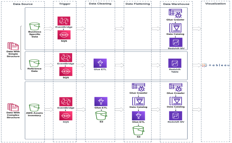
The following diagram illustrates the solution architecture for SSO with the Redshift Data API using IAM Identity Center.

The user workflow for the data visualization application consists of the following steps:
- The user (whether a regional sales manager or global sales manager) accesses the Streamlit application, which is integrated with SSO to provide a seamless authentication experience.
- The application redirects the user to authenticate through Okta, the external IdP. Okta verifies the user’s credentials and returns an ID token to the application.
- The application uses the token issued by Okta to assume a role and temporary AWS Identity and Access Management (IAM) session credentials to call the IAM Identity Center
AssumeRoleWithWebIdentityAPI and IAMAssumeRoleAPI in later steps. - The application exchanges the Okta ID token for a token issued by IAM Identity Center by calling the IAM Identity Center
CreateTokenWithIAMAPI using the temporary IAM credentials from the previous step. This token makes sure that the user is authenticated with AWS services and is tied to the IAM Identity Center user profile. - The application requests an identity-enhanced IAM role session using the IAM Identity Center token by calling the
AssumeRole - The application uses the identity-enhanced IAM role session credentials to securely query Amazon Redshift for sales data. The credentials make sure that only authorized users can interact with the Redshift data.
- As the query is processed, Amazon Redshift checks the identity context provided by IAM Identity Center. It verifies the user’s role and group membership, such as being a part of the North American region or the global sales manager group.
- Based on the user’s identity and group membership, and using Amazon Redshift RBAC and row-level security, Amazon Redshift makes an authorization decision. The groups for the illustration can be broadly classified into the following categories:
- Regional sales managers will be granted access to view sales data only for the specific country or region they manage. For instance, the AMER North American Sales Manager will only see sales data related to North America. Similarly, the access control based on EMEA and APAC regions will provide row-level security for the respective regions.
- The global sales managers will be granted full access to all regions, enabling them to view the entire global dataset.
The setup consists of two main steps:
- Provision the resources for IAM Identity Center, Amazon Redshift and Okta:
- Enable IAM Identity Center and configure Okta as the IdP to manage user authentication and group provisioning.
- Create an Okta application to authenticate users accessing the Streamlit application.
- Set up an Amazon Redshift IAM Identity Center connection application to enable trusted identity propagation for secure authentication.
- Provision an Amazon Redshift Serverless
- Create the tables and configure RBAC within the Redshift workgroup to enforce row-level security for different IAM Identity Center federated roles, mapped to IAM Identity Center groups.
- Download, configure, and run the Streamlit application:
- Create a customer managed application in IAM Identity Center for the Redshift Data API client (Streamlit application) to enable secure API-based queries and create the required IAM roles
- Configure the Streamlit application.
- Run the Streamlit application.
Prerequisites
You should have the following prerequisites:
- An AWS account. If you don’t have one, you can sign up for one.
- IAM Identity Center enabled. For more information, see Enabling AWS IAM Identity Center.
- A connection to IAM Identity Center with your preferred IdP and users and groups synchronized. Refer to IAM Identity Center identity source tutorials for the IdP setup.
- A Python virtual environment. We use Visual Studio Code integrated development environment (IDE) for this post.
Provision the resources for IAM Identity Center, Amazon Redshift, and Okta
In this section, we walk through the steps to provision the resources for IAM Identity Center, Amazon Redshift, and Okta.
Enable IAM Identity Center and configure Okta as the IdP
Complete the following steps to enable IAM Identity Center and configure Okta as the IdP to manage user authentication and group provisioning:
- Create the following users and groups in Okta:
- Ethan Global with email
[email protected], in groupexec-global - Frank Amer with email
[email protected], in groupamer-sales - Alex Emea with email
[email protected], in groupemea-sales - Ming Apac with email
[email protected], in groupapac-sales
- Ethan Global with email

- Create an IAM Identity Center instance in the AWS Region where Amazon Redshift is going to be deployed. An organization instance type is recommended.
- Configure Okta as the identity source and enable automatic user and group provisioning. The users and groups will be pushed to IAM Identity Center using SCIM protocol.
The following screenshot shows the users synced in IAM Identity Center using SCIM protocol.

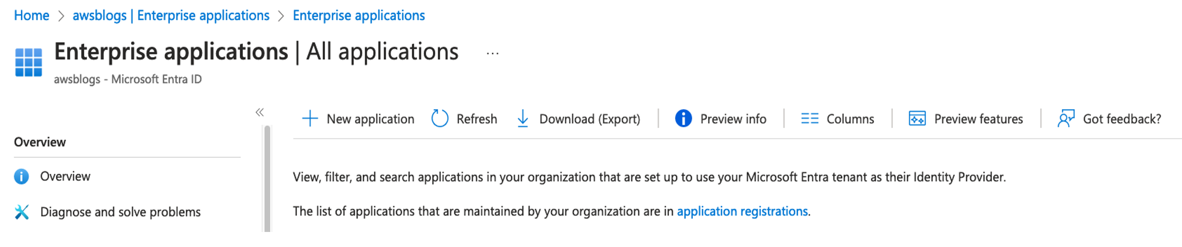
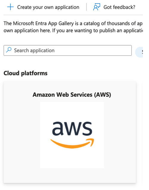
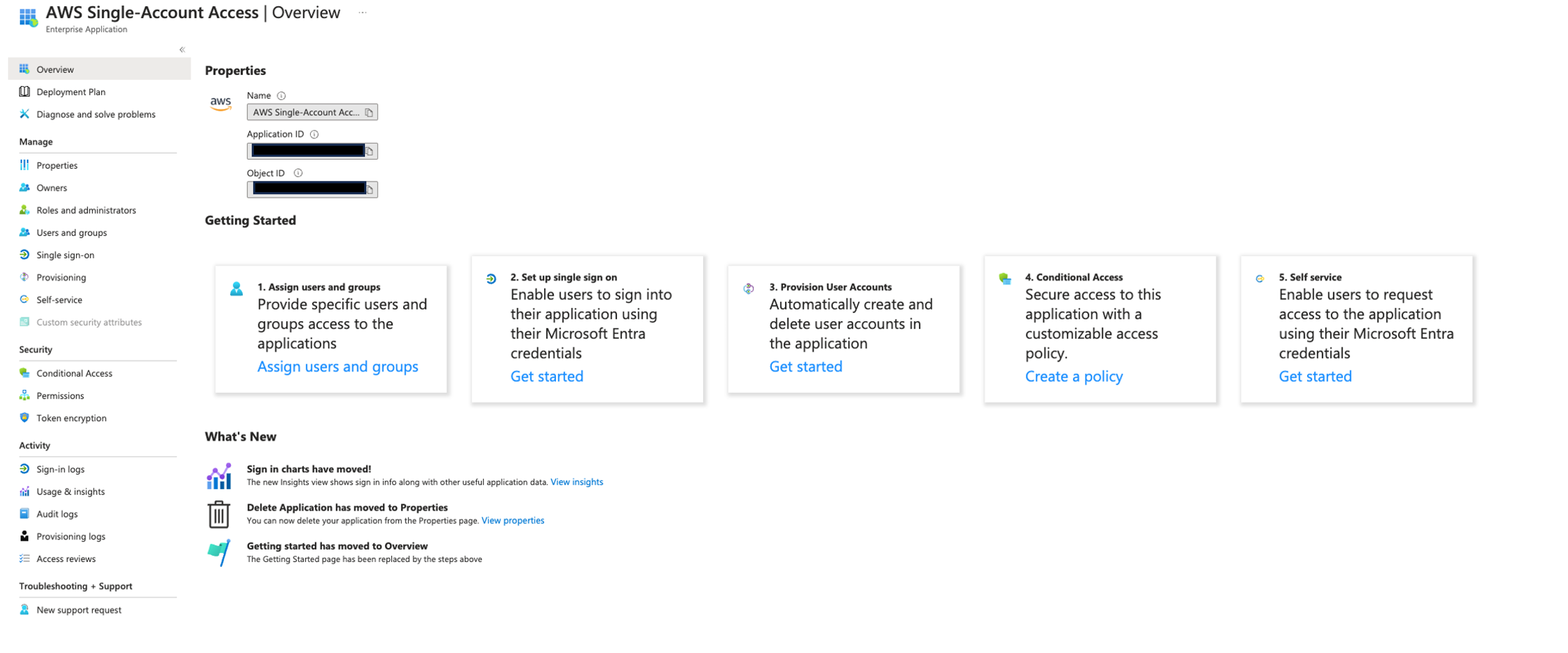
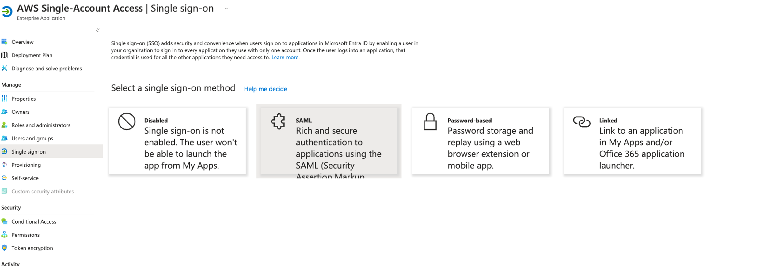
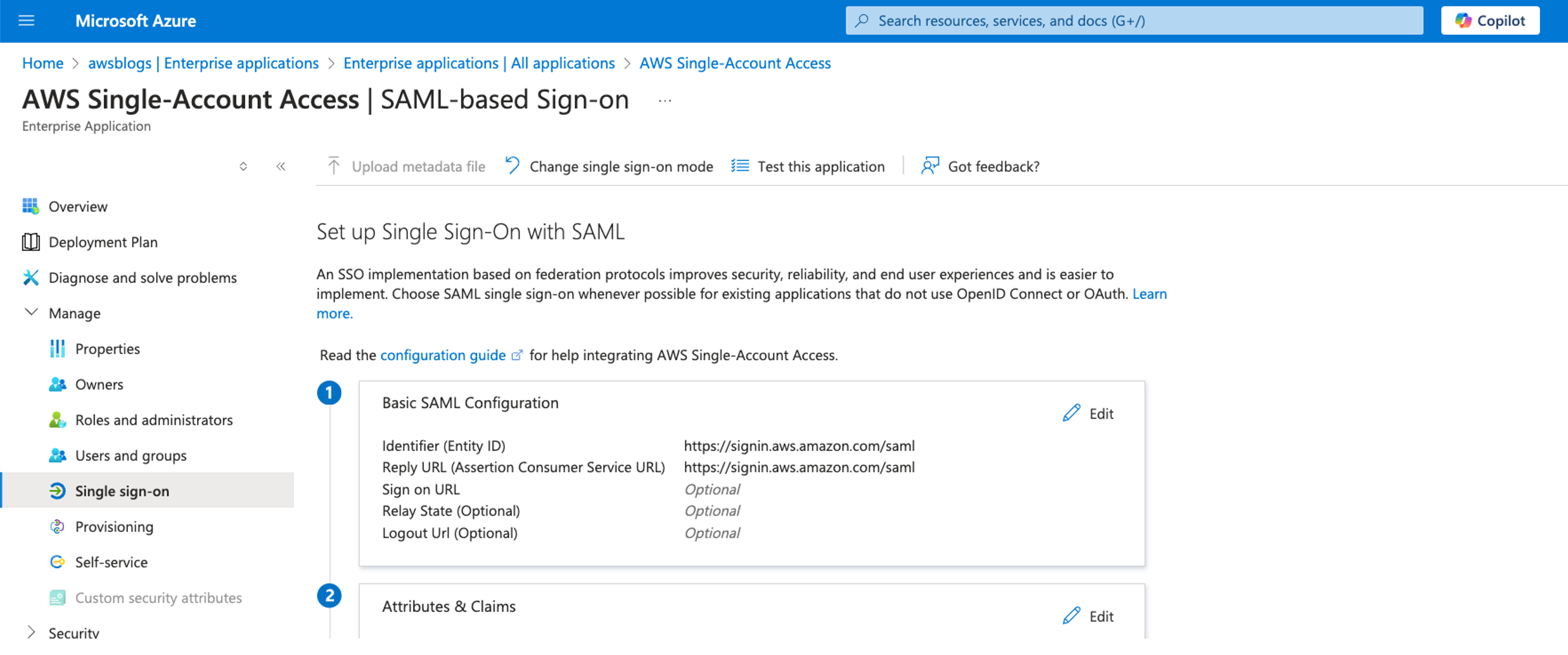
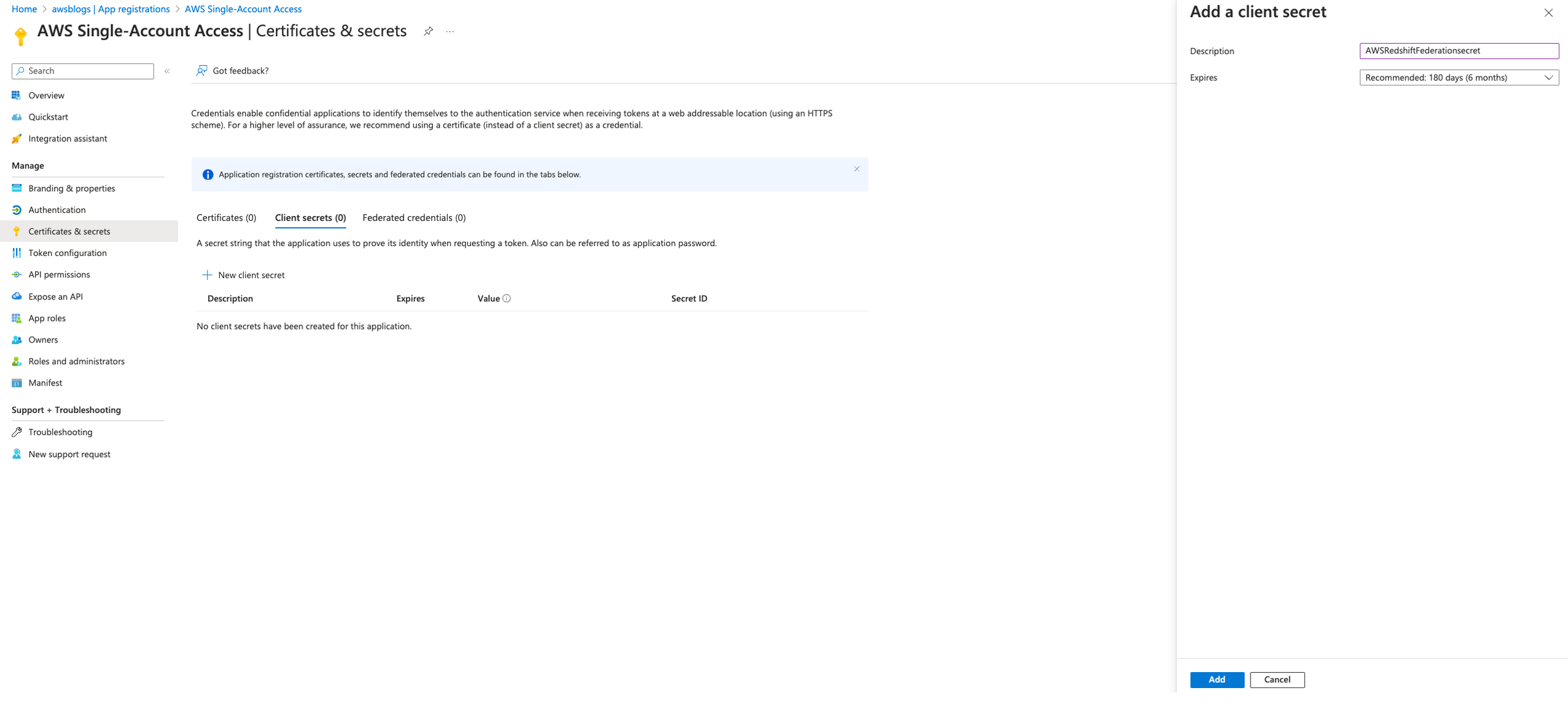
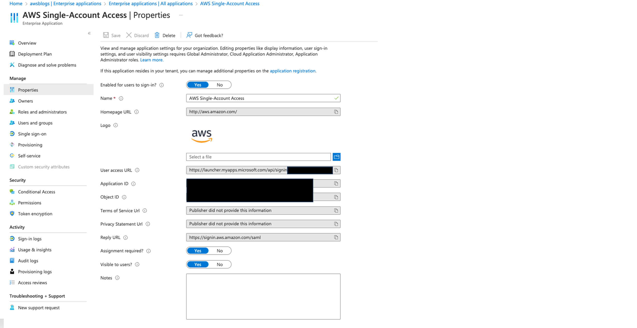
Create an Okta application
Complete the following steps to create an Okta application to authenticate users accessing the Streamlit application:
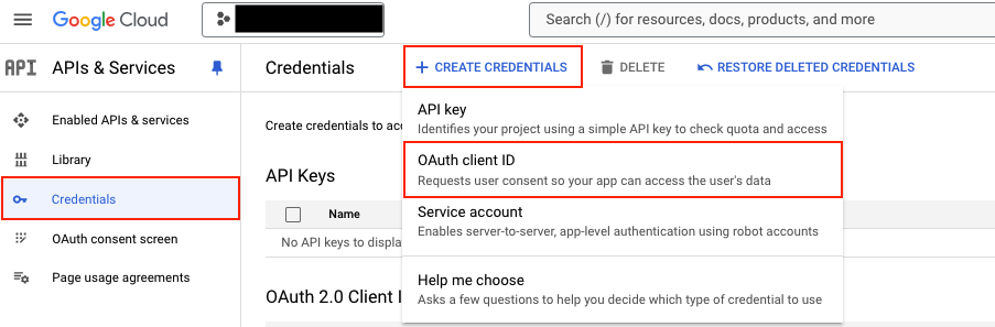
- Create an OIDC application in Okta.
- Copy and save the client ID and client secret needed later for the Streamlit application and the IAM Identity Center application to connect using the Redshift Data API.
- Generate the client secret and set sign-in redirect URL and sign-out URL to
http://localhost:8501(we will host the Streamlit application locally on port 8501). - Under Assignments, Controlled access, grant access to everyone.
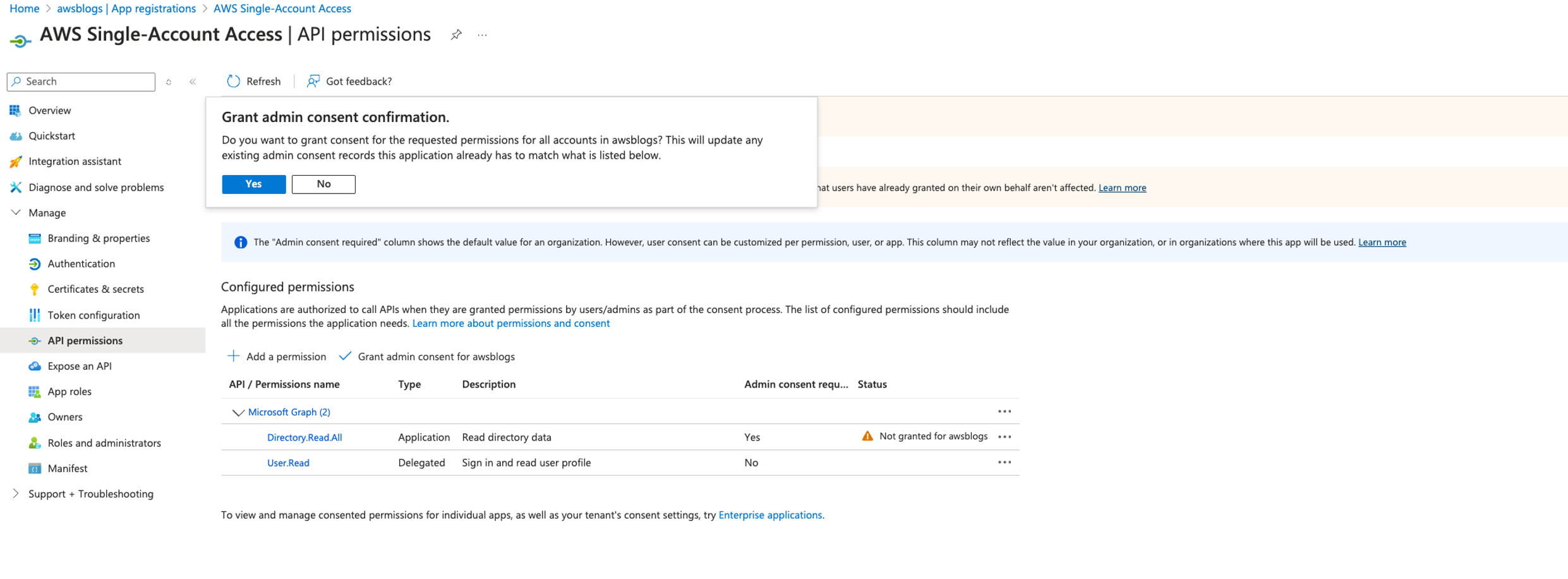
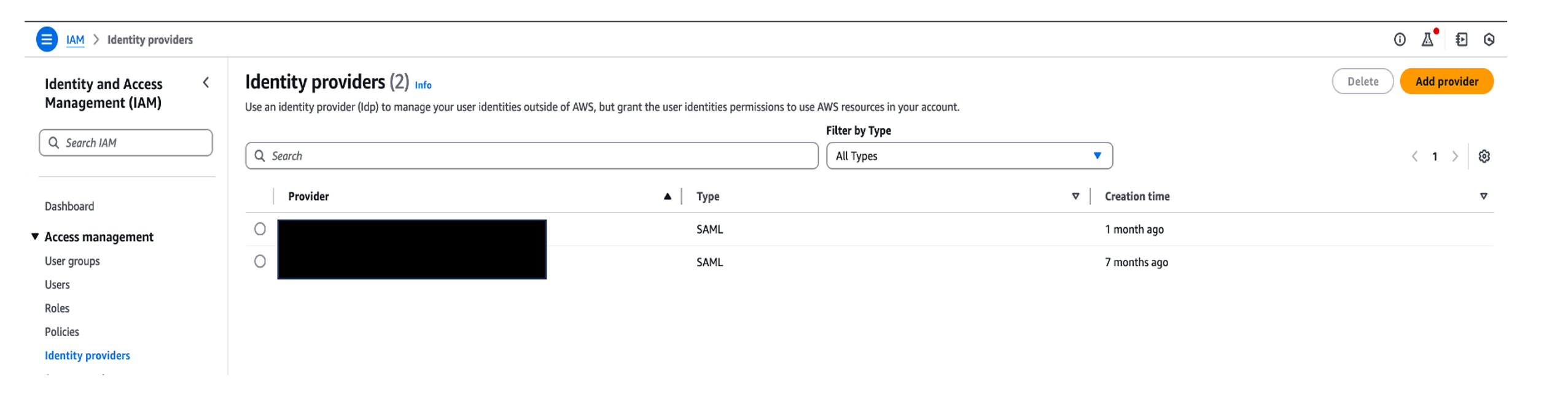
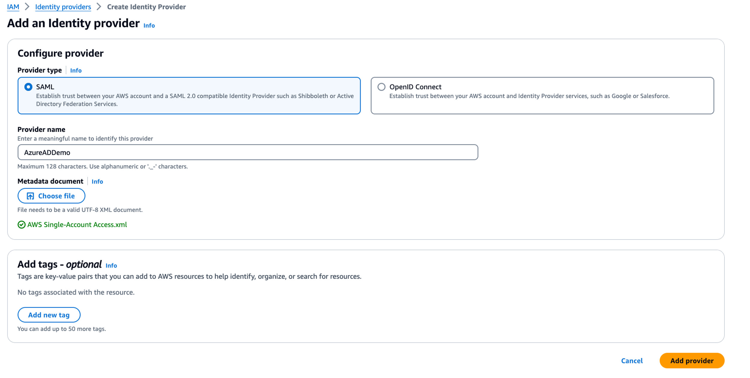
- Create an OIDC IdP on IAM the console. The following screenshot shows an IdP created on the IAM console.

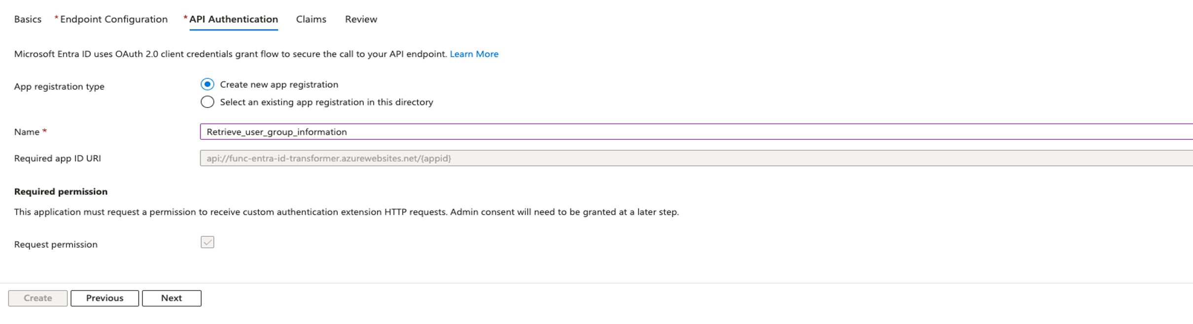
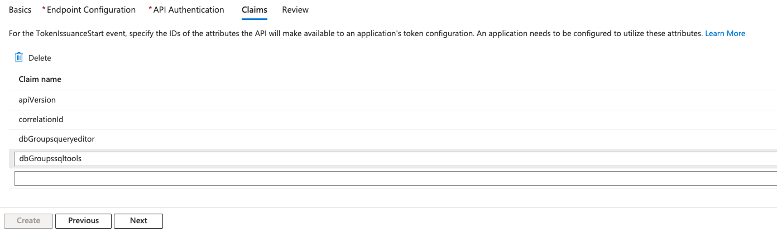
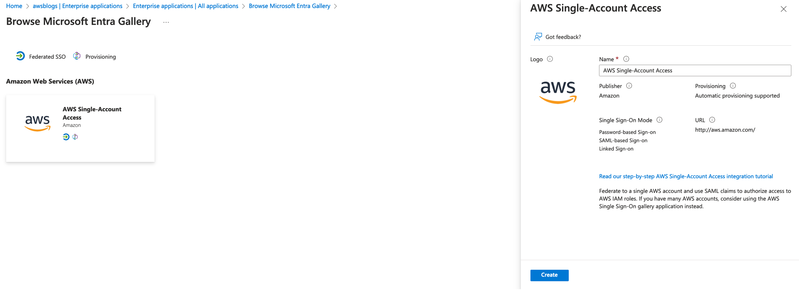
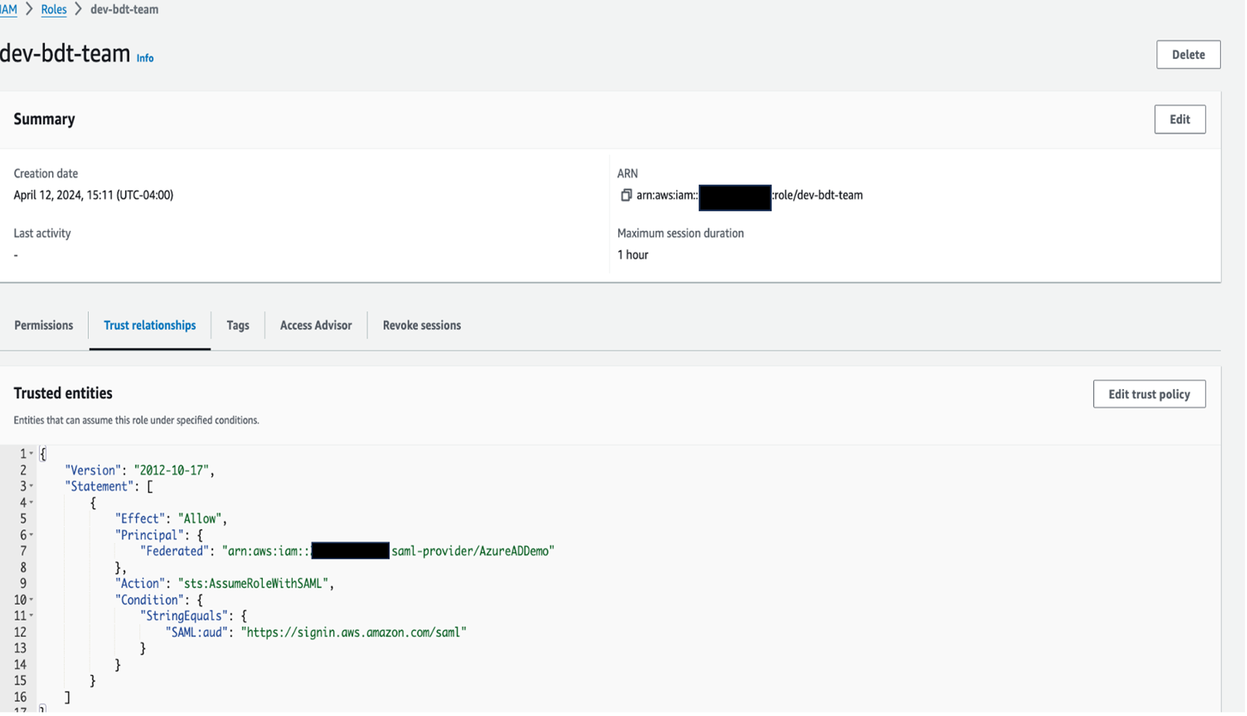
Set up an Amazon Redshift IAM Identity Center connection application
Complete the following steps to create an Amazon Redshift IAM Identity Center connection application to enable trusted identity propagation for secure authentication:
- On the Amazon Redshift console, choose IAM Identity Center connection in the navigation pane.
- Choose Create application.
- Name the application
redshift-data-api-okta-app. - Note down the IdP namespace. The default value
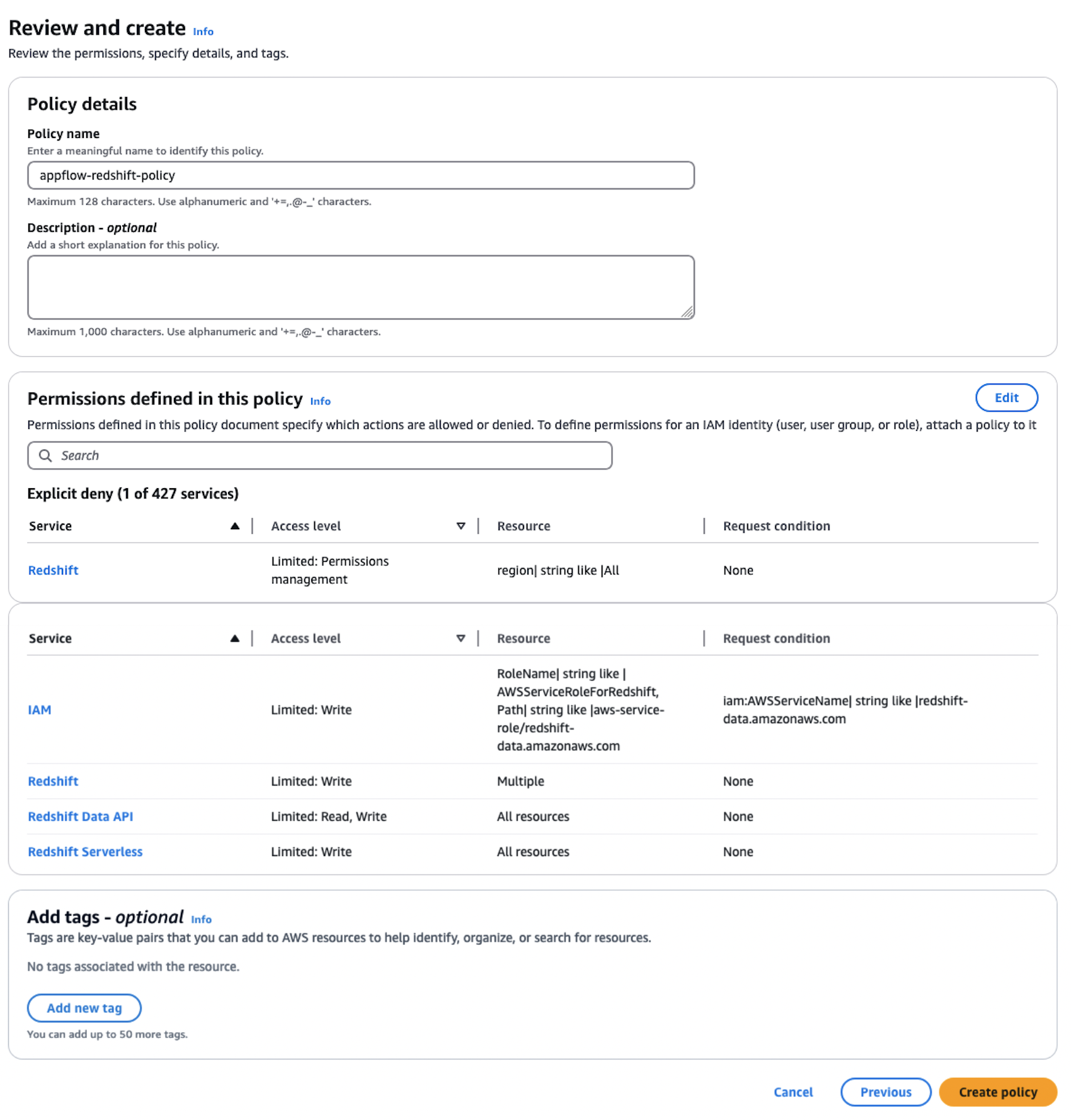
AWSIDCis used for this post. - In the IAM role for IAM Identity Center access section, you need to provide an IAM role. You can go to the IAM console and create an IAM role called
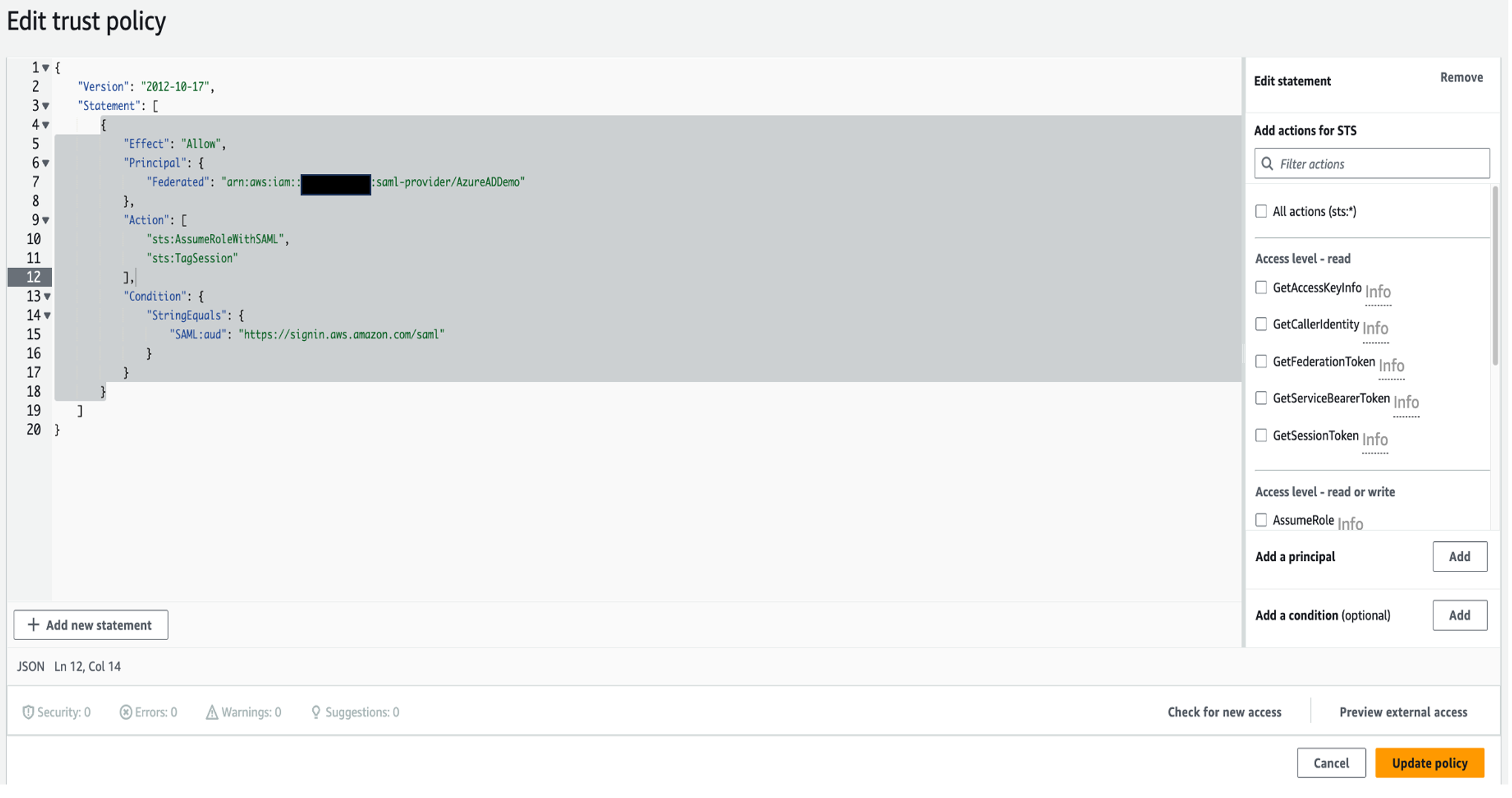
RedshiftOktaRolewith the following policy and trust relationship.RedshiftOktaRoleis used by the Amazon Redshift IAM Identity Center connection application to manage and interact with IAM Identity Center.- The policy attached to the role needs the following permissions:
- The role uses the following trust relationship:
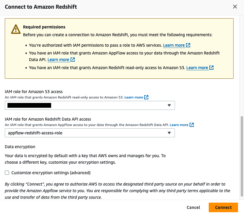
- Leave Trusted Identity propagation section unchanged, then choose Next. You have the option to choose AWS Lake Formation or Amazon S3 Access Grants for use cases like using Amazon Redshift Spectrum to query external tables in Lake Formation. In our use case, we only use Amazon Redshift native tables so we don’t choose either.
- In the Configure client connections that use third-party IdPs section, choose No.
- Review and choose Create application.
- When the application is created, navigate to your IAM Identity Center connection
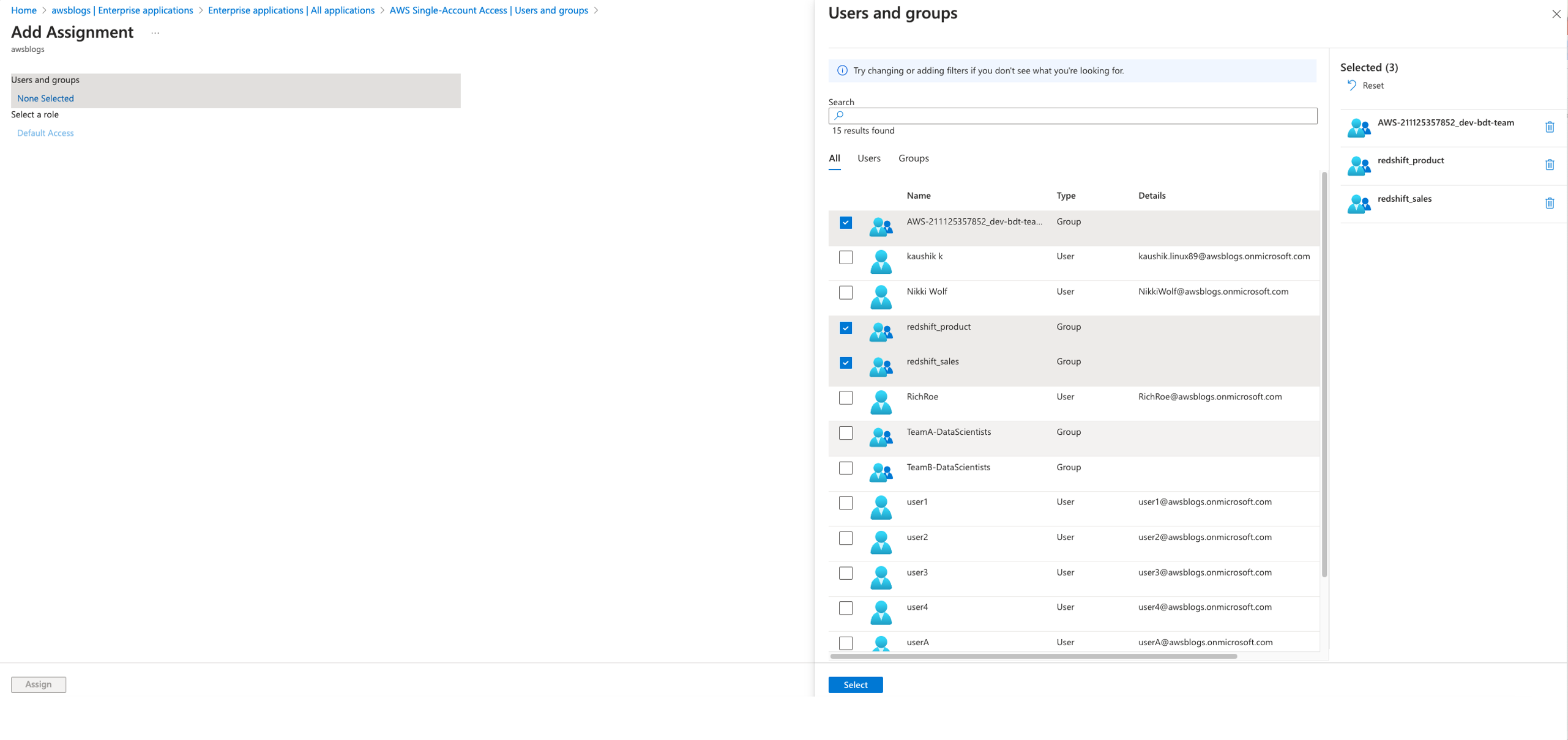
redshift-data-api-okta-appand choose Assign to add the groups that were synced in IAM Identity Center using SCIM protocol from Okta.
We will enable trusted identity propagation and third-party IdP (Okta) on the customer managed application for the Redshift Data API in a later step instead of configuring it in the Amazon Redshift connection application.
The following screenshot shows the IAM Identity Center connection application created on the Amazon Redshift console.

The following screenshot shows groups assigned to the Amazon Redshift IAM Identity Center connection for the managed application.

Provision a Redshift Serverless workgroup
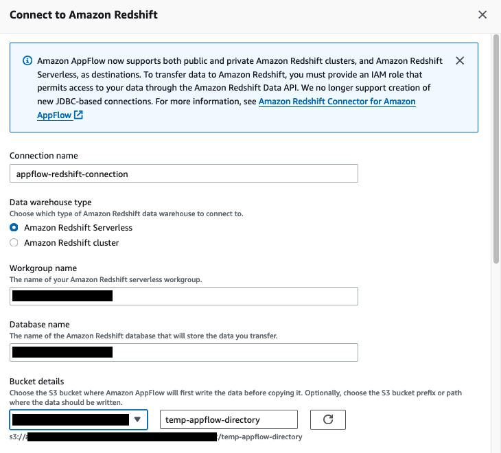
Complete the following steps to create a Redshift Serverless workgroup. For more details, refer to Creating a workgroup with a namespace.
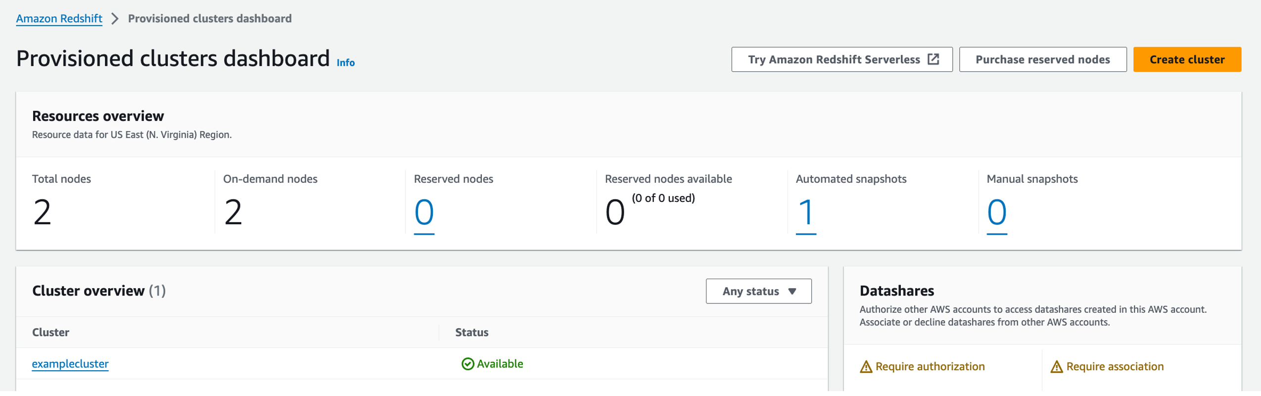
- On the Amazon Redshift console, navigate to the Redshift Serverless dashboard.
- Choose Create workgroup.
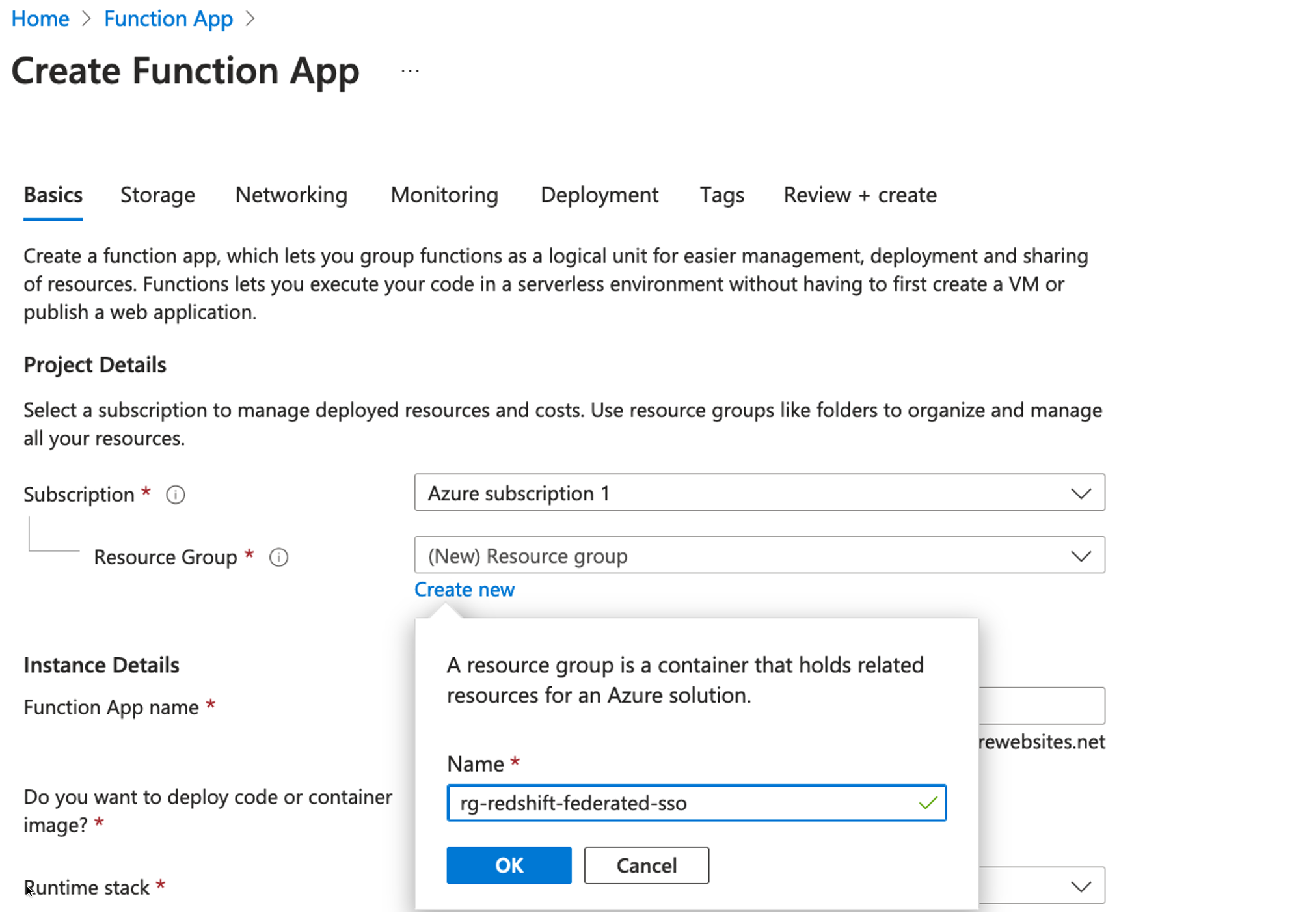
- Enter a name for your workgroup (for example,
redshift-tip-enabled). - Change the Base capacity to 8 RPU in the Performance and cost control
- You can configure network and security based on your virtual private cloud (VPC) and subnet you want to create the workgroup.
- In the Namespace section, create a new namespace for your workgroup. (For example,
redshift-tip-enabled-namespace). - In the Database name and password section, select Customize admin user credentials and set the admin user name and create a password. Note them down to use in a later step to configure RBAC in Amazon Redshift.
- In the Identity Center connections section, choose Enable for the cluster option and select the Amazon Redshift IAM Identity Center application created in the previous step (
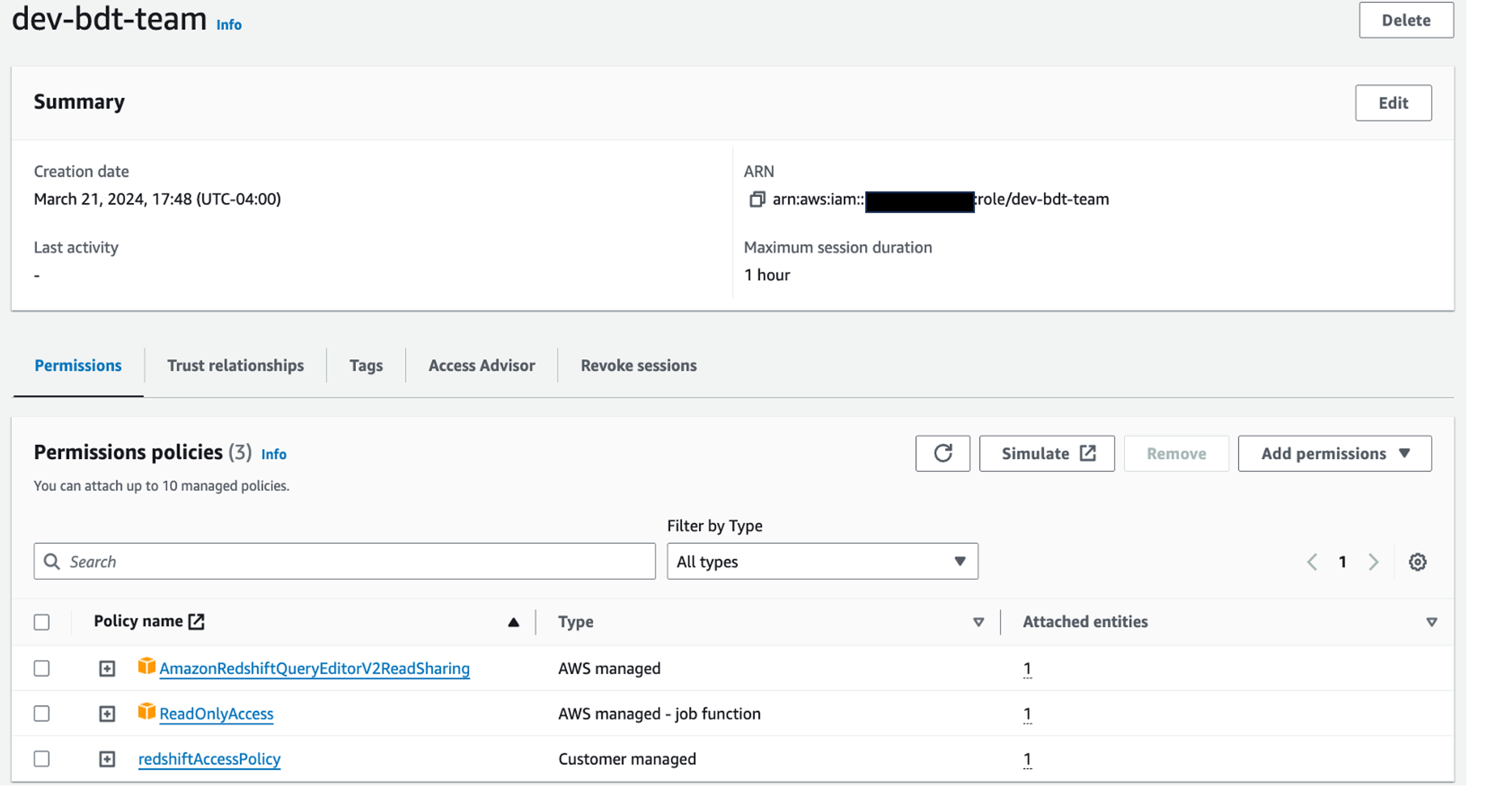
redshift-data-api-okta-app). - Associate an IAM role with the workgroup that has the following policies attached. Make it the default role to use.
- Leave other settings as default and choose Next.
- Review the settings and create the workgroup.
Wait until the workgroup is available before continuing to the next steps.

Create the tables and configure RBAC within the Redshift Serverless workgroup
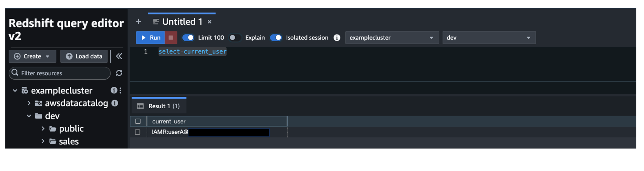
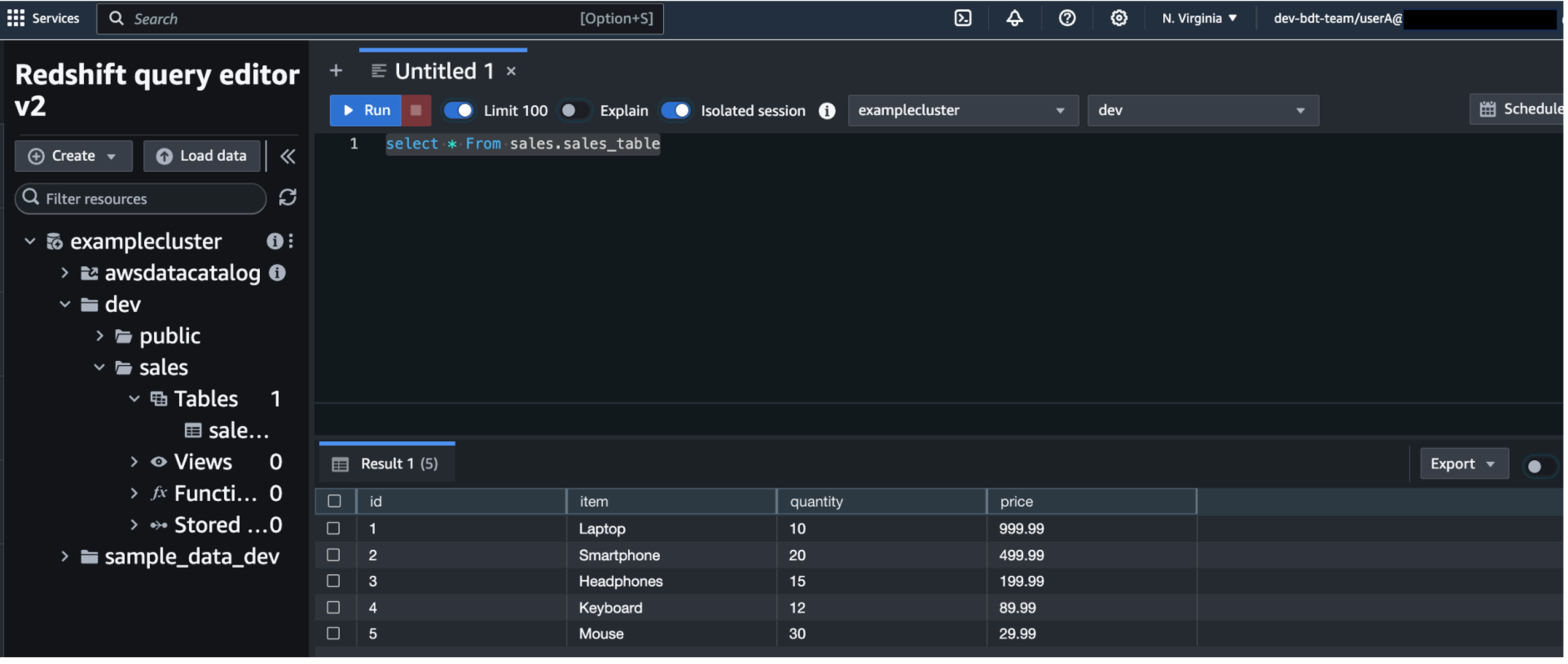
Next, you use the Amazon Redshift Query Editor V2 on the Amazon Redshift console to connect to the workgroup you just created. You create the tables and configure the Amazon Redshift roles corresponding to Okta groups for the groups in IAM Identity Center and use the RBAC policy to grant users privileges to view data only for their regions. Complete the following steps:
- On the Amazon Redshift console, open the Query Editor V2.
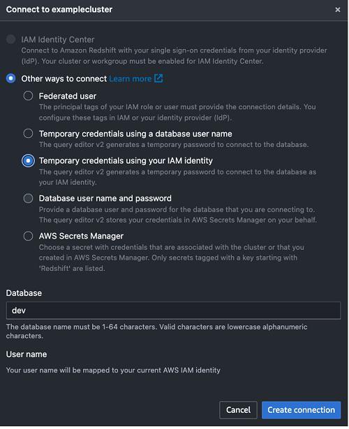
- Choose the options menu (three dots) next to the Redshift workgroup name and choose Edit connection.

- Select Other ways to connect and use the database user name and password to connect.
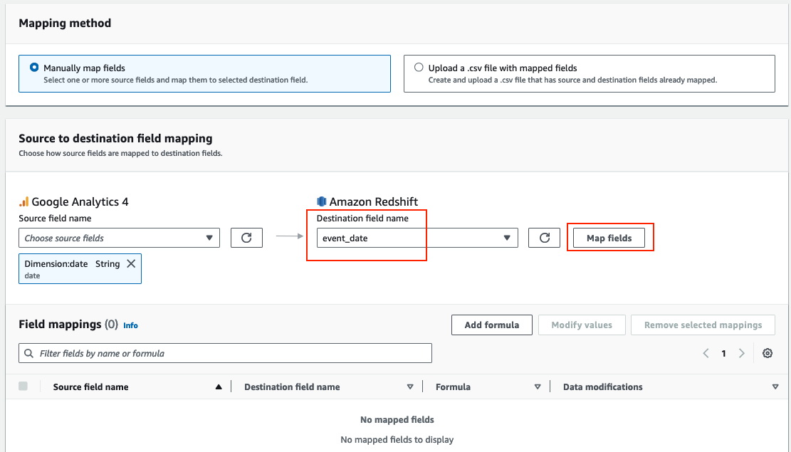
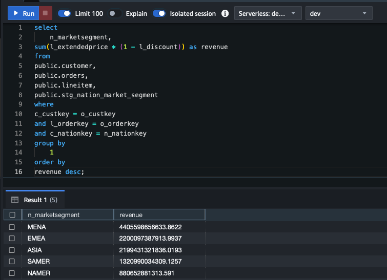
- In the query editor, run the following code to create the sales table and load the data from Amazon Simple Storage Service (Amazon S3):

IAM Identity Center will map the groups into the Redshift roles in the format of Namespace:IDCGroupName. Therefore, create the role name as AWSIDC:emea-sales and so on to match them with Okta group names synced in IAM Identity Center. The users will be created automatically within the groups as they log in using SSO into Amazon Redshift.
Download, configure, and run the Streamlit application
In this section, we walk through the steps to download, configure, and run the Streamlit application.
Create a customer managed application in IAM Identity Center for the Redshift Data API client
In order to start a trusted identity propagation workflow and allow Amazon Redshift to make authorization decisions based on the users and groups from IAM Identity Center (provisioned from the external IdP), you need an identity-enhanced IAM role session.
This requires a couple of IAM roles and a customer managed application in IAM Identity Center to handle the trust relationship between the external IdP and IAM Identity Center and control access for the Redshift Data API client, in this case, the Streamlit application.
First, you create two IAM roles, then you create a customer managed application for the Streamlit application. Complete the following steps:
- Create a temporary IAM role (we named it
IDCBridgeRole) to exchange the token with IAM Identity Center (assuming you don’t have an existing IAM identity to use). This role will be assumed by the Streamlit application withAssumeRoleWithWebIdentityto get a temporary set of role credentials to call theCreateTokenWithIAMandAssumeRoleAPIs to get the identity-enhanced role session.- Attach the following policy the role:
- In the trust relationship, provide your AWS account ID and IdP’s URL. The trusted principal to use is the Amazon Resource Name (ARN) of
oidc-provideryou created earlier.
- Create an IAM role with permissions to access the Redshift Data API (we named it
RedshiftDataAPIClientRole). This role will be assumed by the Streamlit application with the enhanced identities from IAM Identity Center and then used to authenticate requests to the Redshift Data API.- Attach the AmazonRedshiftDataFullAccess AWS managed policy. AWS recommends using the principle of least privilege in your IAM policy.
- Restrict the trust relationship to the
IDCBridgeRoleARN created in the previous step), and provide your AWS account ID:
Now you can create the customer managed application.
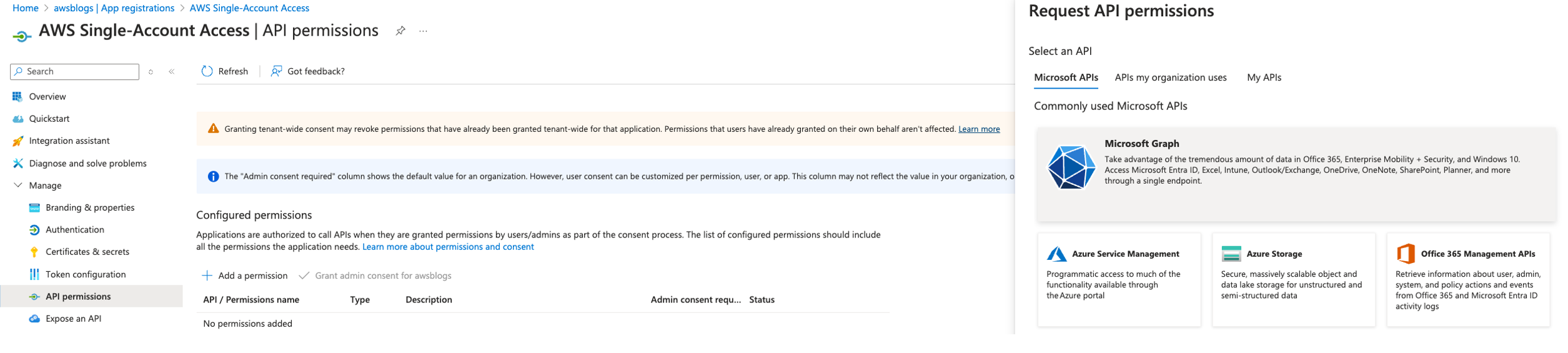
- On the IAM Identity Center console, choose Applications in the navigation pane.
- Choose Add application.
- Choose I have an application I want to setup, select the OAuth 2.0 application type, and choose Next.
- Enter a name for the application, for example,
RedshiftStreamlitDemo. - In User and group assignment method, choose Do not require assignment. This means all the users provisioned in IAM Identity Center from Okta can use their Okta credentials to sign in to the Streamlit application. You can alternatively select the Require assignments option and pick the users and groups you want to allow access to the application.
- In the AWS access portal section, choose Not visible, then choose Next.
- In the Authentication with trusted token issuer section, select Create trusted token issuer, then enter the Okta issuer URL and enter a name for the trusted token issuer.
- In the map attribute, use the default email to email mapping between the external IdP attribute and IAM Identity Center attribute, then create the trusted token issuer.
- Select the trusted token issuer you just created.
- In the Aud claim section, use the client ID of the Okta application you noted earlier, then choose Next.
- In the Specify application credentials section, choose Edit the application policy and use the following policy:
- Choose Submit.


After the application is created, you can view it in on the IAM Identity Center.
- Choose Applications in the navigation pane, and locate the Customer managed applications tab.


- Choose the application to navigate to the application details page.
- In the Trusted applications for identity propagation section, choose Specify trusted applications and select the setup type as Individual applications and specify access, then choose Next.
- Choose Amazon Redshift as the service, then choose Next.
- In the Application that can receive requests section, choose the Amazon Redshift IAM Identity Center application you created, then choose Next.
- In the Access Scopes to apply section, check the redshift:connect
- Review and then choose Trust application.


Configure and run the Streamlit application
Now that you have the roles and the customer managed application in IAM Identity Center, you can create an identity-enhanced IAM role session, which is the most critical step to enable trusted identity propagation. Following steps provide an overview of Streamlit application code to create the identity-enhanced IAM role session.
- Authenticate with and retrieve the
id_tokenfrom the external IdP (Okta). - Call
CreateTokenWithIAMusing the external IdP issuedid_tokento obtain an IAM Identity Center issuedid_token. - Use
AssumeRoleWithWebIdentityto obtain temporary IAM credentials (by assumingIDCBridgeRole, explained later). - Extract the
sts:identity_contextfrom the IAM Identity Center issuedid_token. - Assume the role
RedshiftDataAPIClientRolewith theAssumeRoleAPI and insert thests:identity_contextto obtain the identity-enhanced IAM role session credentials.
Now you can use these credentials to make requests to the Redshift Data API, and Amazon Redshift will be able to use the identity context for authorization decisions.
At this point, you should have all the required resources for creating the Streamlit application. Complete the following steps to test the Streamlit application:
- Download the Streamlit application code and modify the configuration section of the code based on the resources provisioned earlier:
We recommend hosting this application on an Amazon Elastic Compute Cloud (Amazon EC2) instance for production use cases, and using AWS Secrets Manager for sensitive information like the CLIENT_ID and CLIENT_SECRET provided as configuration parameters in the code for simplicity.
For this example, we use the Okta organization URL (/oauth2/v1/). You can use the customer authorization servers as well, for example, the default authorization server, but make sure all URLs are using the same authorization server. Refer to Authorization servers for more information about authorization servers in Okta.

After you modify the script for the Streamlit application, you can run it using a Python virtual environment.
- Create a Python virtual environment. The application has been tested successfully with versions v3.12.8 and v3.12.2.
You need to install the following packages, which are required libraries for the Streamlit application code you downloaded in your virtual environment:
streamlitstreamlit_oauthboto3pyjwtpydeckpandas
- You can install these libraries directly using the following command with the requirements file:
- Test the Streamlit application in the Python virtual environment with the following command:
- Log in with the user [email protected] from the
apac-salesgroup.


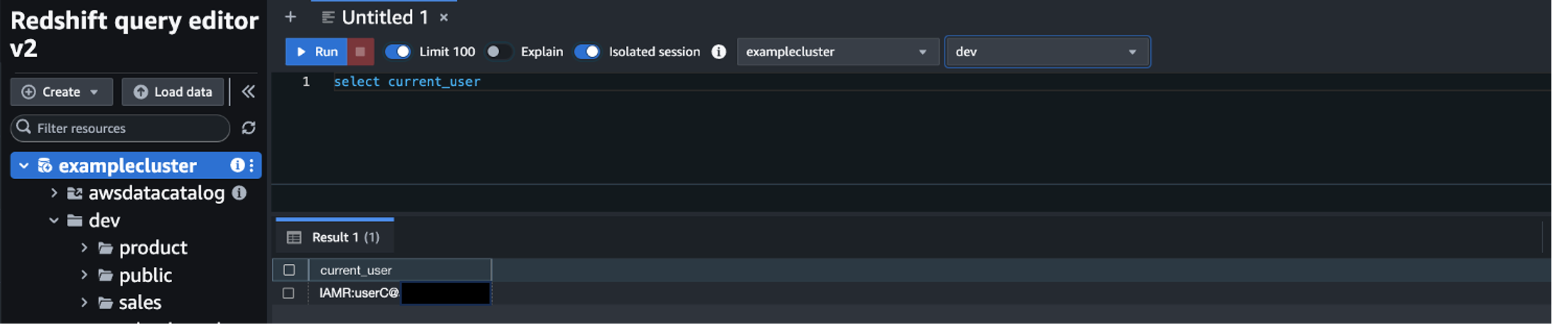
The identity-enhanced role session credentials will display on the top of the page after successful authentication with Okta.
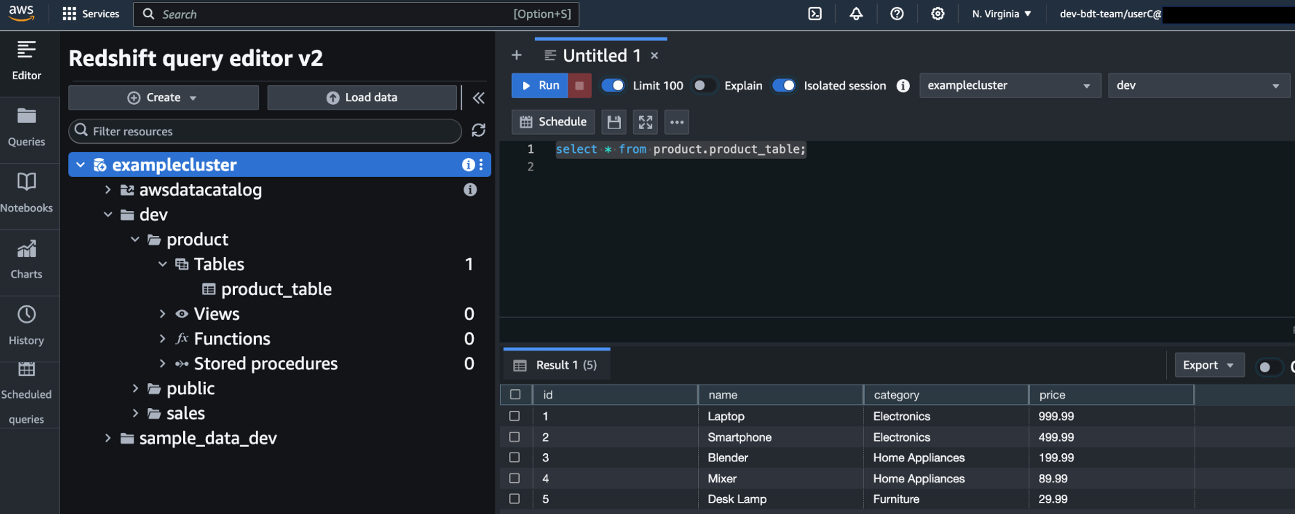
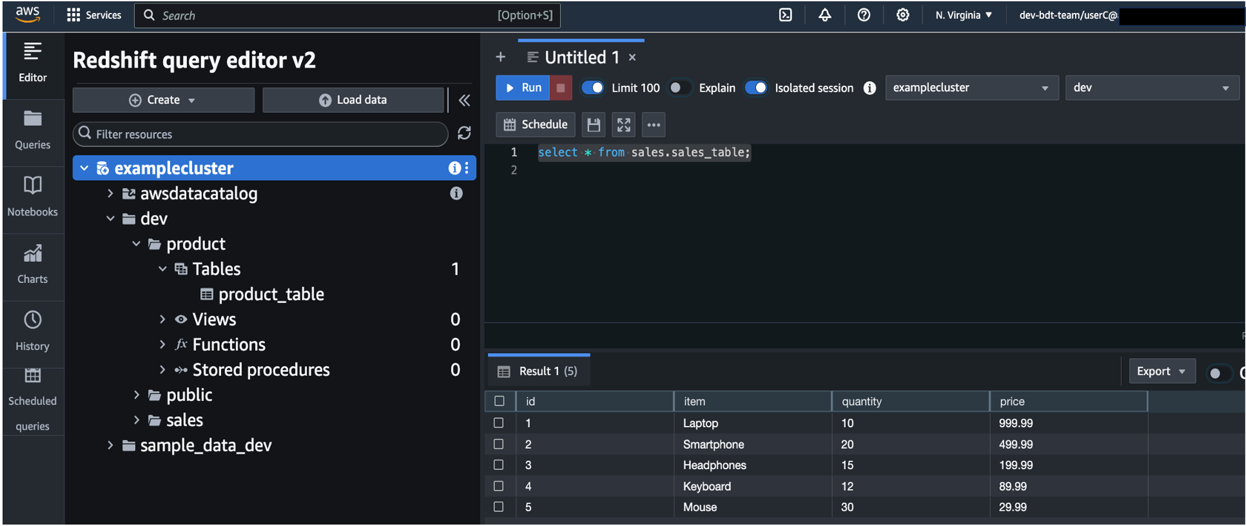
For the APAC region manager, you should only see the data from the countries in the Asia-Pacific region based on the row-level security filter you configured earlier.

- Log out and log back in with the global executive user, [email protected] from the
exec-global
You should see the data in all regions.

You can try other regional users’ logins and you should see only the data in the region they belong to.
Trusted identity propagation deep dive
In this section, you walk through the Python code of the Streamlit application and explain how trusted identity propagation works. The following is an explanation of key parts of the application code.
main()
The main() function of the Streamlit application implements the preceding steps to get the identity-enhanced IAM role session using the get_id_enhanded_session() function, which wraps the login to get the identity-enhanced role session credentials:
We use the Streamlit st.session_state provided by Streamlit to store important session states, including the authentication status as well as additional information like user information and the AWS identity-enhanced role session credentials.
get_id_enhanced_session()
The get_id_enhanced_session() function code has three steps:
- We use the
id_token(variable name:jwt_token) from Okta in JWT format to call theAssumeRoleWithWebIdentityAPI to assume the roleIDCBridgeRole. This is because the user doesn’t have any AWS credentials to interact with the IAM Identity Center API. If you plan to host this application in an AWS environment with an IAM role available, for example, on an EC2 instance, you can use the role associated with Amazon EC2 to make the call to the IAM Identity Center APIs without creatingIDCBridgeRole, but make sure the EC2 role has the required permissions we specified forIDCBridgeRole. - After we have the credentials of the temporary role, we use them to make a call to the
CreateTokenWithIAMAPI of IAM Identity Center. This API handles the exchange of tokens by taking in theid_tokenfrom Okta and returning an IAM Identity Center issued token, which will be used later to get the identity-enhanced role session. For more information, refer to the CreateTokenWithIAM API reference. - Lastly, we extract the
sts:identity_contextfrom the IAM Identity Center issuedid_tokenand pass it to the AWS Security Token Service (AWS STS)AssumeRoleThis is done by including thests:identity_contextin theContextAssertionparameter withinProvidedContexts, along withProviderArnset toarn:aws:iam::aws:contextProvider/IdentityCenter.
assume_role_with_web_identity()
The assume_role_with_web_identity() function code is as follows. We initialize the STS client, decode the JWT token, and then assume the role with the web identity.
create_token_with_iam()
The create_token_with_iam() function code is called to get the id_token from IAM Identity Center. The jwt_token is the id_token in JWT format issued by Okta; the id_token is the IAM Identity Center issued id_token.
In the CreateTokenWithIAM call, we pass the following parameters:
- clientId – The ARN of the IAM Identity Center application for the Redshift Data API client
- grantType –
urn:ietf:params:oauth:grant-type:jwt-bearer - assertion – The
id_token(jwt_token) issued by Okta
The idToken issued by IAM Identity Center is returned.
assume_enhanced_role_session()
The assume_enhanced_role_session() function uses the ID token to assume an identity-enhanced role session:
extract_identity_context_from_id_token()
The extract_identity_context_from_id_token() function extracts the sts:identity_context:
Now you have the identity-enhanced role session credentials to call the Amazon Redshift Data API.
execute_statement() and fetch_results()
The execute_statement() and fetch_results() functions demonstrate how to run Redshift queries and retrieve query results with trusted identity propagation for visualization:
Conclusion
In this post, we showed how to create a third-party application backed by analytics insights arriving from Amazon Redshift securely using OIDC. With Redshift Data API support of IAM Identity Center integration, you can connect to Amazon Redshift using SSO from the IdP of your choice. You can extend this method to authenticate other AWS services that support trusted identity propagation, such as Amazon Athena and Amazon QuickSight, enabling fine-grained access control for IAM Identity Center users and groups across your AWS ecosystem. We encourage you to set up your application using IAM Identity Center integration and unify your access control directly from your IdP across all IAM Identity Center supported AWS services.
For more information on AWS services and applications that support trusted identity propagation, refer to Trusted identity propagation overview.
About the Authors
 Songzhi Liu is a Principal Big Data Architect with the AWS Identity Solutions team. In this role, he collaborates closely with AWS customers and cross-functional teams to design and implement scalable data architectures, focusing on integrating big data and machine learning solutions to enhance identity awareness within the AWS ecosystem.
 Rohit Vashishtha is a Senior Analytics Specialist Solutions Architect at AWS based in Dallas, Texas. He has over 19 years of experience architecting, building, leading, and maintaining big data platforms. Rohit helps customers modernize their analytic workloads using the breadth of AWS services and ensures that customers get the best price/performance with utmost security and data governance.
 Fei Peng is a Senior Software Development Engineer working in the Amazon Redshift team, where he leads the development of Redshift Data API, enabling seamless and scalable access to cloud data warehouses.
 Yanzhu Ji is a Product Manager in the Amazon Redshift team. She has experience in product vision and strategy in industry-leading data products and platforms. She has outstanding skill in building substantial software products using web development, system design, database, and distributed programming techniques. In her personal life, Yanzhu likes painting, photography, and playing tennis.


 Raks Khare is a Senior Analytics Specialist Solutions Architect at AWS based out of Pennsylvania. He helps customers across varying industries and regions architect data analytics solutions at scale on the AWS platform. Outside of work, he likes exploring new travel and food destinations and spending quality time with his family.
 Jyoti Aggarwal is a Product Management Lead for AWS zero-ETL. She leads the product and business strategy, including driving initiatives around performance, customer experience, and security. She brings along an expertise in cloud compute, data pipelines, analytics, artificial intelligence (AI), and data services including databases, data warehouses and data lakes.
 Gopal Paliwal is a Principal Engineer for Amazon Redshift, leading the software development of ZeroETL initiatives for Amazon Redshift.
 Harman Nagra is a Principal Solutions Architect at AWS, based in San Francisco. He works with global financial services organizations to design, develop, and optimize their workloads on AWS.
 Sumanth Punyamurthula is a Senior Data and Analytics Architect at Amazon Web Services with more than 20 years of experience in leading large analytical initiatives, including analytics, data warehouse, data lakes, data governance, security, and cloud infrastructure across travel, hospitality, financial, and healthcare industries.


 Ricardo Serafim is a Senior Analytics Specialist Solutions Architect at AWS.
 Harshida Patel is a Analytics Specialist Principal Solutions Architect, with AWS.
 Milind Oke is a Data Warehouse Specialist Solutions Architect based out of New York. He has been building data warehouse solutions for over 15 years and specializes in Amazon Redshift.


 Michael Davies is a Data Engineer at OUA. He has extensive experience within the education industry, with a particular focus on building robust and efficient data architecture and pipelines.
 Emma Arrigo is a Solutions Architect at AWS, focusing on education customers across Australia. She specializes in leveraging cloud technology and machine learning to address complex business challenges in the education sector. Emma’s passion for data extends beyond her professional life, as evidenced by her dog named Data.


 Sean Zou is a Cloud Operations leader with MuleSoft at Salesforce. Sean has been involved in many aspects of MuleSoft’s Cloud Operations, and helped drive MuleSoft’s cloud infrastructure to scale more than tenfold in 7 years. He built the Oversight Engineering function at MuleSoft from scratch.
 Terry Quan focuses on FinOps issues. He works on MuleSoft Engineering on cloud computing budgets and forecasting, cost reduction efforts, costs-to-serve, and coordinates with Salesforce Finance. Terry is a FinOps Practitioner and Professional Certified.
 Audrey Yuan is a Software Engineer with MuleSoft at Salesforce. Audrey works on data lakehouse solutions to help drive cloud maturity across the six pillars of the Well-Architected Framework.
 Rueben Jimenez is a Senior Solutions Architect at AWS, designing and implementing complex data analytics, AI/ML, and cloud infrastructure solutions.
 Avijit Goswami is a Principal Solutions Architect at AWS specialized in data and analytics. He supports AWS strategic customers in building high-performing, secure, and scalable data lake solutions on AWS using AWS managed services and open source solutions. Outside of his work, Avijit likes to travel, hike, watch sports, and listen to music.


 Ritesh Kumar Sinha is an Analytics Specialist Solutions Architect based out of San Francisco. He has helped customers build scalable data warehousing and big data solutions for over 16 years. He loves to design and build efficient end-to-end solutions on AWS. In his spare time, he loves reading, walking, and doing yoga.
 Tahir Aziz is an Analytics Solution Architect at AWS. He has worked with building data warehouses and big data solutions for over 13 years. He loves to help customers design end-to-end analytics solutions on AWS. Outside of work, he enjoys traveling and cooking.
 Raza Hafeez is a Senior Product Manager at Amazon Redshift. He has over 13 years of professional experience building and optimizing enterprise data warehouses and is passionate about enabling customers to realize the power of their data. He specializes in migrating enterprise data warehouses to AWS Modern Data Architecture.
 Amit Ghodke is an Analytics Specialist Solutions Architect based out of Austin. He has worked with databases, data warehouses and analytical applications for the past 16 years. He loves to help customers implement analytical solutions at scale to derive maximum business value.
 Neeraja Rentachintala is Director, Product Management with AWS Analytics, leading Amazon Redshift and Amazon SageMaker Lakehouse. Neeraja is a seasoned technology leader, bringing over 25 years of experience in product vision, strategy, and leadership roles in data products and platforms. She has delivered products in analytics, databases, data integration, application integration, AI/ML, and large-scale distributed systems across on-premises and the cloud, serving Fortune 500 companies as part of ventures including MapR (acquired by HPE), Microsoft SQL Server, Oracle, Informatica, and Expedia.com

 Momota Sasaki is an Engineering Manager at DeSC Healthcare, a subsidiary of DeNA. He joined DeNA in 2021 and was seconded to DeSC Healthcare. Since then, he has been consistently involved in the healthcare business, leading and promoting the development and operation of the data platform.
 Kaito Tawara is a Data Engineer at DeSC Healthcare, a subsidiary of DeNA, focusing on improving healthcare data platforms. After gaining experience in backend development for web systems and data science, he transitioned to data engineering. He joined DeNA in 2023 and was seconded to DeSC Healthcare. Currently, he works remotely from Nagoya-city, contributing to the enhancement of healthcare data platforms.
 Shota Sato is an Analytics Specialist Solution Architect at AWS Japan, focusing on data analytics solutions powered by AWS for digital native business customers.


 Xu Feng is a Senior Industry Solution Architect at AWS, responsible for designing, building, and promoting industry solutions for the Media & Entertainment and Advertising sectors, such as intelligent customer service and business intelligence. With 20 years of software industry experience, currently focused on researching and implementing generative AI and AI-powered data solutions.
 Xu Da is a Amazon Web Services (AWS) Partner Solutions Architect based out of Shanghai, China. He has more than 25 years of experience in IT industry, software development and solution architecture. He is passionate about collaborative learning, knowledge sharing, and guiding community in their cloud technologies journey.


 Jagadish Kumar (Jag) is a Senior Specialist Solutions Architect at AWS focused on Amazon OpenSearch Service. He is deeply passionate about Data Architecture and helps customers build analytics solutions at scale on AWS.
 Adam Gaulding is a Solution Architect at Satori. At Satori, Adam is helping customers implement data security controls on databases, data lakes and data warehouses. Adam has been in and around the data space throughout his 20+ year career. He’s worked with companies large and small and prides himself in building creative solutions for technical problems.


 Koushik Konjeti is a Senior Solutions Architect at Amazon Web Services. He has a passion for aligning architectural guidance with customer goals, ensuring solutions are tailored to their unique requirements. Outside of work, he enjoys playing cricket and tennis.


 Leo Ramsamy is a Platform Architect specializing in data and analytics for ANZ’s Institutional division. He focuses on modern data practices, including Data Mesh architecture, data governance, quality management, and observability. His work aligns data strategies with business goals, improving accessibility and enabling better decision-making across ANZ.
 Srinivasan Kuppusamy is a Senior Cloud Architect – Data at AWS ProServe, where he helps customers solve their business problems using the power of AWS Cloud technology. His areas of interests are data and analytics, data governance, and AI/ML.
 Rada Stanic is a Chief Technologist at Amazon Web Services, where she helps ANZ customers across different segments solve their business problems using AWS Cloud technologies. Her special areas of interest are data analytics, machine learning/AI, and application modernization.


 Sotaro Hikita is an Analytics Solutions Architect. He supports customers across a wide range of industries in building and operating analytics platforms more effectively. He is particularly passionate about big data technologies and open source software.
 Noritaka Sekiyama is a Principal Big Data Architect on the AWS Glue team. He works based in Tokyo, Japan. He is responsible for building software artifacts to help customers. In his spare time, he enjoys cycling with his road bike.
 Kyle Duong is a Senior Software Development Engineer on the AWS Glue and AWS Lake Formation team. He is passionate about building big data technologies and distributed systems.
 Sandeep Adwankar is a Senior Product Manager at AWS. Based in the California Bay Area, he works with customers around the globe to translate business and technical requirements into products that enable customers to improve how they manage, secure, and access data.


 Poulomi Dasgupta is a Senior Analytics Solutions Architect with AWS. She is passionate about helping customers build cloud-based analytics solutions to solve their business problems. Outside of work, she likes travelling and spending time with her family.
 Saurav Das is part of the Amazon Redshift Product Management team. He has more than 16 years of experience in working with relational databases technologies and data protection. He has a deep interest in solving customer challenges centered around high availability and disaster recovery.