Post Syndicated from Jeremy Spell original https://aws.amazon.com/blogs/big-data/geospatial-data-lakes-with-amazon-redshift/
Data lake architectures help organizations offload data from premium storage systems without losing the ability to query and analyze the data. This architecture can be useful for geospatial data, where builders might have terabytes of infrequently accessed data in their databases that they want to cost-effectively maintain. However, this requires for their data lake query engine to support geographic information systems (GIS) data types and functions.
Amazon Redshift supports querying spatial data, including the GEOMETRY and GEOGRAPHY data types and functions that are used in querying GIS systems. Additionally, Amazon Redshift lets you query geospatial data both in your data lakes on Amazon S3 and your Redshift data warehouse, giving you the choice of how you can access your data. Additionally, AWS Lake Formation and support for AWS Identity and Access Management (IAM) in Esri’s ArcGIS Pro gives you a way to securely bridge data between your geospatial data lakes and map visualization tools. You can set up, manage, and secure geospatial data lakes in the cloud with a few clicks.
In this post, we walk through how to set up a geospatial data lake using Lake Formation and query the data with ArcGIS Pro using Amazon Redshift Serverless.
Solution overview
In our example, a county public health department has used Lake Formation to secure their data lake that contains public health information (PHI) data. Epidemiologists within the county want to create a map for the clinics providing vaccination for their communities. The county’s GIS analysts need access to the data lake to create the required maps without being able to access the PHI data.
This solution uses Lake Formation tags to allow column-level access in the database to the public information that includes the clinic names, addresses, zip codes, and longitude/latitude coordinates without allowing access to the PHI data within the same tables. We use Redshift Serverless and Amazon Redshift Spectrum to access this data from ArcGIS Pro, a GIS mapping software from Esri, an AWS Partner.
The following diagram shows the architecture for this solution.

The following is a sample schema for this post.
Description |
Column Name |
Geoproperty Tag |
Patient ID |
patient_id |
No |
Clinic ID |
clinic_id |
Yes |
Address of Clinic |
clinic_address |
Yes |
Clinic Zip Code |
clinic_zip |
Yes |
Clinic City |
clinic_city |
Yes |
First Name Patient |
first_name |
No |
Last Name Patient |
last_name |
No |
Patient Address |
patient_address |
No |
Patient Zip Code |
patient_zip |
No |
Vaccination Type |
vaccination_type |
No |
Latitude of Clinic |
clinic_lat |
Yes |
Longitude of Clinic |
clinic_long |
Yes |
In the following sections, we walk through the steps to set up the solution:
- Deploy the solution infrastructure using AWS CloudFormation.
- Upload a CSV with sample data to an Amazon Simple Storage Service (Amazon S3) bucket and run an AWS Glue crawler to crawl the data.
- Set up Lake Formation permissions.
- Configure the Amazon Redshift Query Editor v2.
- Set up the schemas in Amazon Redshift.
- Create a view in Amazon Redshift.
- Create a local database user in ArcGIS Pro.
- Connect ArcGIS Pro to the Redshift database.
Prerequisites
You should have the following prerequisites:
- An AWS account
- Lake Formation enabled in your target AWS Region
- Familiarity with Lake Formation and setting permissions on tables
- ArcGIS Pro
- Network connectivity from the ArcGIS Pro client to the virtual private cloud (VPC) where Amazon Redshift resources will be deployed using either VPN or AWS Direct Connect
Set up the infrastructure with AWS CloudFormation
To create the environment for the demo, complete the following steps:
- Log in to the AWS Management Console as an AWS account administrator and a Lake Formation data lake administrator—this account needs to be both an account admin and a data lake admin for the template to complete.
- Open the AWS CloudFormation console
- Choose Launch Stack.
The CloudFormation template creates the following components:
- S3 bucket –
samp-clinic-db-{ACCOUNT_ID} - AWS Glue database –
samp-clinical-glue-db - AWS Glue crawler –
samp-glue-crawler - Redshift Serverless workgroup –
samp-clinical-rs-wg - Redshift Serverless namespace –
samp-clinical-rs-ns - IAM role for Amazon Redshift –
demo-RedshiftIAMRole-{UNIQUE_ID} - IAM role for AWS Glue –
samp-clinical-glue-role - Lake Formation tag –
geoproperty
Upload a CSV to the S3 bucket and run the AWS Glue crawler
The next step is to create a data lake in our demo environment and then use an AWS Glue crawler to populate the AWS Glue database and update the schema and metadata in the AWS Glue Data Catalog.
The CloudFormation stack created the S3 bucket we will use as well as the AWS Glue database and crawler. We have provided a fictious test dataset that will represent the patient and clinical information. Download the file and complete the following steps:
- On the AWS CloudFormation console, open the stack you just launched.
- On the Resources tab, choose the link to the S3 bucket.
- Choose Upload and add the CSV file (data-with-geocode.csv), then choose Upload.
- On the AWS Glue console, choose Crawlers in the navigation pane.
- Select the crawler you created with the CloudFormation stack and choose Run.
The crawler run should only take a minute to complete, and will populate a table named clinic-sample-s3_ACCOUNT_ID with a fictious dataset.
- Choose Tables in the navigation pane and open the table the crawler populated.
You will see that the dataset contains fields that contain PHI and personally identifiable information (PII).

We now have a database set up and the Data Catalog populated with the schema and metadata we will use for the rest of the demo.
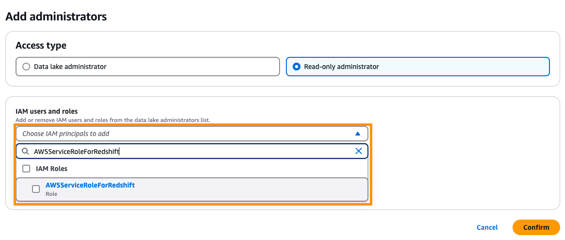
Set up Lake Formation permissions
In this next set of steps, we demonstrate how to secure PHI data to maintain compliance and empower GIS analysts to work effectively. To secure the data lake, we use AWS Lake Formation. In order to properly set up Lake Formation permissions, we need to gather details on how access to the data lake is established.
The Data Catalog provides metadata and schema information that enables services to access data within the data lake. To access the data lake from ArcGIS Pro, we use the ArcGIS Pro Redshift connector, which allows a connection from ArcGIS Pro to Amazon Redshift. Amazon Redshift can access the Data Catalog and provide connectivity to the data lake. The CloudFormation template created a Redshift Serverless instance and namespace and an IAM role that we will use to configure this connection. We still need to set up Lake Formation permissions so that GIS analysts can only access publicly available fields and not those containing PHI or PII. We will assign a Lake Formation tag on the columns containing the publicly available information and assign permissions to the GIS analysts to allow access to columns with this tag.
By default, the Lake Formation configuration allows Super access to IAMAllowedPrinciples; this is to maintain backward compatibility as detailed in Changing the default settings for your data lake. To demonstrate a more secure configuration, we will remove this default configuration.
- On the Lake Formation console, choose Administration in the navigation pane.
- In the Data Catalog settings section, make sure Use only IAM access control for new databases and Use only IAM access control for new tables in new databases are unchecked.

- In the navigation pane, under Permissions, choose Data permissions.
- Select
IAMAllowedPrincipalsand choose Revoke. - Choose Tables in the navigation pane.
- Open the table
clinic-sample-s3_ACCOUNT_IDand choose Edit schema. - Select the fields beginning with clinic_ and choose Edit LF-Tags.
- The CloudFormation stack created a Lake Formation tag named
geoproperty. Assigngeopropertyas the key and true for the value on all theclinic_fields, then choose Save.
Next, we need to grant the Amazon Redshift IAM role permission to access fields tagged with geoproperty = true.
- Choose Data lake permissions, then choose Grant.
- For the IAM role, choose
demo-RedshiftIAMRole-UNIQUE_ID. - Select
geopropertyfor the key and true for the value. - Under Database permissions, select Describe, and under Table permissions, select Select and Describe.
Configure the Amazon Redshift Query Editor v2
Next, we need to perform the initial configuration of Amazon Redshift required for database operations. We use an AWS Secrets Manager secret created by the template to make sure password access is managed securely in accordance with AWS best practices.
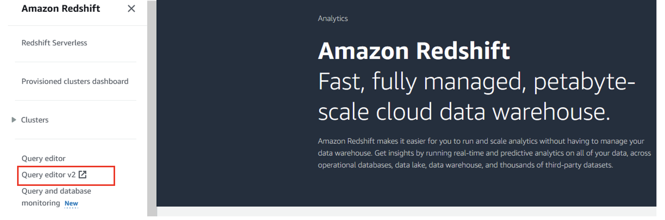
- On the Amazon Redshift console, choose Query editor v2.
- When you first start Amazon Redshift, a one-time configuration for the account appears. For this post, leave the options default and choose Configure account.
For more information about these options, refer to Configuring your AWS account.

The query editor will require credentials to connect to the serverless instance; these have been created by the template and stored in Secrets Manager.
- Select Other ways to connect, then select AWS Secrets Manager.
- For Secret, select (
Redshift-admin-credentials). - Choose Save.

Set up schemas in Amazon Redshift
An external schema in Amazon Redshift is a feature used to reference schemas that exist in external data sources. For information on creating external schemas, see External schemas in Amazon Redshift Spectrum. We use an external schema to provide access to the data lake in Amazon Redshift. From ArcGIS Pro, we will connect to Amazon Redshift to access the geospatial data.
The IAM role used in the creation of the external schema needs to be associated with the Redshift namespace. This has already been set up by the CloudFormation template, but it’s a good practice to verify that the role is set up correctly before proceeding.
- On the Redshift Serverless console, choose Namespace configuration in the navigation pane.
- Choose the namespace (
sample-rs-namespace).

On the Security and encryption tab, you should see the IAM role created by CloudFormation. If this role or the namespace isn’t present, verify the stack in AWS CloudFormation before proceeding.
- Copy the ARN of the role for use in a later step.

- Choose Query data to return to the query editor.

- In the query editor, enter the following SQL command; be sure to replace the example role ARN with your own. This SQL command will create an external schema that uses the same Redshift role associated with our namespace to attach to the AWS Glue database.
- In the query editor, perform a select query on
sample-glue-database:
Because the associated role has been granted access to columns tagged with geoproperty = true, only those fields will be returned, as shown in the following screenshot (the data in this example is fictionalized).

- Use the following command to create a local schema in Amazon Redshift. The external schema can’t be updated; we will use this local schema to add a geometry field with a Redshift function.
Create a view in Amazon Redshift
For the data to be viewable from ArcGIS Pro, we will need to create a view. Now that the schemas have been established, we can create the view that can be accessed from ArcGIS Pro.
Amazon Redshift provides many geospatial functions that can be used to create views with fields used by ArcGIS Pro to add points onto a map. We will use one of these functions because the dataset contains latitude and longitude.
Use the following SQL code in the Amazon Redshift Query Editor to create a new view named clinic_location_view. Replace {ACCOUNT_ID} with your own account ID.
The new view that is created under your local schema will have a column named geom containing map-based points that can be used by ArcGIS Pro to add points during map creation. The points in this example are for the clinics providing vaccines. In a real-world scenario, as new clinics are built and their data is added to the data lake, their locations would be added to the map created using this data.
Create a local database user for ArcGIS Pro
For this demo, we use a database user and group to provide access for ArcGIS Pro clients. Enter the following SQL code into the Amazon Redshift Query Editor to create a database user and group:
After the commands are complete, use the following code to grant permissions to the group:
Connect ArcGIS Pro to the Redshift database
In order to add the database connection to ArcGIS Pro, you need the endpoint for the Redshift Serverless workgroup. You can access the endpoint information on the sample-rs-wg workgroup details page on the Redshift Serverless console. The Redshift namespaces and workgroups are listed by default, as shown in the following screenshot.

You can copy the endpoint in the General information section. This endpoint will need to modified; the :5439/dev will need to be removed when configuring the connector in ArcGIS Pro.

- Open ArcGIS Pro with the project file you want to add the Redshift connection to.
| Make sure the Amazon Redshift ODBC connector has already been installed; this is required in order to make the connection. |
- On the menu, choose Insert and then Connections, Database, and New Database Connection.
- For Database Platform, choose Amazon Redshift.
- For Server, insert the endpoint you copied (remove everything following
.comfrom the endpoint). - For Database, choose your database.

If your ArcGIS Pro client doesn’t have access to the endpoint, you will receive an error during this step. A network path must exist between the ArcGIS Pro client and the Redshift Serverless endpoint. You can set up the network path with Direct Connect, AWS Site-to-Site VPN, or AWS Client VPN. Although it’s not recommended for security reasons, you can also configure Amazon Redshift with a publicly available endpoint. Be sure you consult your security and network teams for best practices and policy guidance before allowing public access to your Redshift Serverless instance.
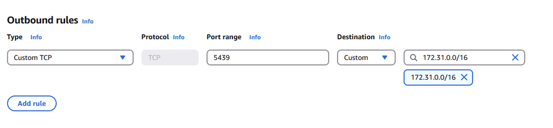
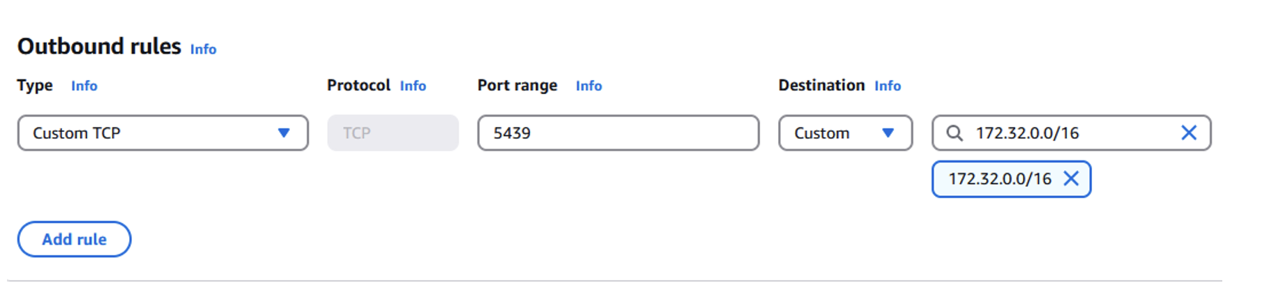
If a network path exists and you’re having issues connecting, verify the security group rules allow communication inbound from your ArcGIS Pro subnet over the port your Redshift Serverless instance is running on. The default port is 5439, but you can configure a range of ports depending on your environment; see Connecting to Amazon Redshift Serverless for more information.
If connectivity is successful, ArcGIS Pro will add the Amazon Redshift connection under Connection File Name.
- Choose OK.
- Choose the connection to display the view that was created to include geometry (
clinic_location_view). - Choose (right-click) the view and choose Add To Current Map.
ArcGIS Pro will add the points from the view onto the map. The final map displayed has the symbology edited to use red crosses to represent the clinics instead of dots.

Clean up
After you have finished the demo, complete the following steps to clean up your resources:
- On the Amazon S3 console, open the bucket created by the CloudFormation stack and delete the
data-with-geocode.csvfile. - On the AWS CloudFormation console, delete the demo stack to remove the resources it created.
Conclusion
In this post, we reviewed how to set up Redshift Serverless to use geospatial data contained within a data lake to enhance maps in ArcGIS Pro. This technique helps builders and GIS analysts use available datasets in data lakes and transform it in Amazon Redshift to further enrich the data before presenting it on a map. We also showed how to secure a data lake using Lake Formation, crawl a geospatial dataset with AWS Glue, and visualize the data in ArcGIS Pro.
For additional best practices for storing geospatial data in Amazon S3 and querying it with Amazon Redshift, see How to partition your geospatial data lake for analysis with Amazon Redshift. We invite you to leave feedback in the comments section.
About the authors
 Jeremy Spell is a Cloud Infrastructure Architect working with Amazon Web Services (AWS) Professional Services. He enjoys architecting and building solutions for customers. In his free time Jeremy makes Texas style BBQ, and spends time with his family and church community.
 Jeff Demuth is a solutions architect who joined Amazon Web Services (AWS) in 2016. He focuses on the geospatial community and is passionate about geographic information systems (GIS) and technology. Outside of work, Jeff enjoys traveling, building Internet of Things (IoT) applications, and tinkering with the latest gadgets.


 Raks Khare is a Senior Analytics Specialist Solutions Architect at AWS based out of Pennsylvania. He helps customers across varying industries and regions architect data analytics solutions at scale on the AWS platform. Outside of work, he likes exploring new travel and food destinations and spending quality time with his family.
 Ritesh Kumar Sinha is an Analytics Specialist Solutions Architect based out of San Francisco. He has helped customers build scalable data warehousing and big data solutions for over 16 years. He loves to design and build efficient end-to-end solutions on AWS. In his spare time, he loves reading, walking, and doing yoga.
 Yanzhu Ji is a Product Manager in the Amazon Redshift team. She has experience in product vision and strategy in industry-leading data products and platforms. She has outstanding skill in building substantial software products using web development, system design, database, and distributed programming techniques. In her personal life, Yanzhu likes painting, photography, and playing tennis.
 Harshida Patel is a Analytics Specialist Principal Solutions Architect, with AWS.


 Raghu Kuppala is an Analytics Specialist Solutions Architect experienced working in the databases, data warehousing, and analytics space. Outside of work, he enjoys trying different cuisines and spending time with his family and friends.
 Sumant Nemmani is a Senior Technical Product Manager at AWS. He is focused on helping customers of Amazon Redshift benefit from features that use machine learning and intelligent mechanisms to enable the service to self-tune and optimize itself, ensuring Redshift remains price-performant as they scale their usage.
 Gagan Goel is a Software Development Manager at AWS. He ensures that Amazon Redshift features meet customer needs by prioritising and guiding the team in delivering customer-centric solutions, monitor and enhance query performance for customer workloads.
 Kshitij Batra is a Software Development Engineer at Amazon, specializing in building resilient, scalable, and high-performing software solutions.
 Sanuj Basu is a Principal Engineer at AWS, driving the evolution of Amazon Redshift into a next-generation, exabyte-scale cloud data warehouse. He leads engineering for Redshift’s core data platform — including managed storage, transactions, and data sharing — enabling customers to power seamless multi-cluster analytics and modern data mesh architectures. Sanuj’s work helps Redshift customers break through th


 Konstantina Mavrodimitraki is a Senior Solutions Architect at Amazon Web Services, where she assists customers in designing scalable, robust, and secure systems in global markets. With deep expertise in data strategy, data warehousing, and big data systems, she helps organizations transform their data landscapes. A passionate technologist and people person, Konstantina loves exploring emerging technologies and supports the local tech communities. Additionally, she enjoys reading books and playing with her dog.
 Kostas Diamantis is the Head of the Data Warehouse at Skroutz company. With a background in software engineering, he transitioned into data engineering, using his technical expertise to build scalable data solutions. Passionate about data-driven decision-making, he focuses on optimizing data pipelines, enhancing analytics capabilities, and driving business insights.
 Donatas Kuchalskis is a Cloud Operations Architect at AWS, based in London, focusing on Financial Services customers in the UK. He helps customers optimize their AWS environments for cost, security, and resiliency while providing strategic cloud guidance. Prior to this role, he served as a Prototyping Architect specializing in Big Data and as a Specialist Solutions Architect for Retail. Before joining AWS, Donatas spent 6 years as a technical consultant in the retail sector.
 Jumana Nagaria is a Prototyping Architect at AWS. She builds innovative prototypes with customers to solve their business challenges. She is passionate about cloud computing and data analytics. Outside of work, Jumana enjoys travelling, reading, painting, and spending quality time with friends and family.


 If you select Redshift, you will be transferred to the Query editor where you can execute the SQL and see the results as shown in the following figure.
 Avijit Goswami is a Principal Data Solutions Architect at AWS specialized in data and analytics. He supports AWS strategic customers in building high-performing, secure, and scalable data lake solutions on AWS using AWS managed services and open-source solutions. Outside of his work, Avijit likes to travel, hike in the San Francisco Bay Area trails, watch sports, and listen to music.
 Saman Irfan is a Senior Specialist Solutions Architect focusing on Data Analytics at Amazon Web Services. She focuses on helping customers across various industries build scalable and high-performant analytics solutions. Outside of work, she enjoys spending time with her family, watching TV series, and learning new technologies.
 Sudarshan Narasimhan is a Principal Solutions Architect at AWS specialized in data, analytics and databases. With over 19 years of experience in Data roles, he is currently helping AWS Partners & customers build modern data architectures. As a specialist & trusted advisor he helps partners build & GTM with scalable, secure and high performing data solutions on AWS. In his spare time, he enjoys spending time with his family, travelling, avidly consuming podcasts and being heartbroken about Man United’s current state.


 Julia Beck is an Analytics Specialist Solutions Architect at AWS. She supports customers in validating analytics solutions by architecting proof of concept workloads designed to meet their specific needs.
 Scott St. Martin is a Solutions Architect at AWS who is passionate about helping customers build modern applications. Scott uses his decade of experience in the cloud to guide organizations in adopting best practices around operational excellence and reliability, with a focus the manufacturing and financial services spaces. Outside of work, Scott enjoys traveling, spending time with family, and playing piano.


 Satesh Sonti is a Sr. Analytics Specialist Solutions Architect based out of Atlanta, specializing in building enterprise data platforms, data warehousing, and analytics solutions. He has over 19 years of experience in building data assets and leading complex data platform programs for banking and insurance clients across the globe.
 Jonathan Katz is a Principal Product Manager – Technical on the Amazon Redshift team and is based in New York. He is a Core Team member of the open source PostgreSQL project and an active open source contributor, including PostgreSQL and the pgvector project.


 Nita Shah is an Analytics Specialist Solutions Architect at AWS based out of New York. She has been building data warehouse solutions for over 20 years and specializes in Amazon Redshift. She is focused on helping customers design and build enterprise-scale well-architected analytics and decision support platforms.
 Sushmita Barthakur is a Senior Data Solutions Architect at Amazon Web Services (AWS), supporting Strategic customers architect their data workloads on AWS. With a background in data analytics, she has extensive experience helping customers architect and build enterprise data lakes, ETL workloads, data warehouses and data analytics solutions, both on-premises and the cloud. Sushmita is based in Florida and enjoys traveling, reading and playing tennis.
 Jonathan Katz is a Principal Product Manager – Technical on the Amazon Redshift team and is based in New York. He is a Core Team member of the open source PostgreSQL project and an active open source contributor, including PostgreSQL and the pgvector project.


 Laura is an Identity Solutions Architect at AWS, where she thrives on helping customers overcome security and identity challenges. In her free time, she enjoys wreck diving and traveling around the world.


 Noritaka Sekiyama is a Principal Big Data Architect with Amazon Web Services (AWS) Analytics services. He’s responsible for building software artifacts to help customers. In his spare time, he enjoys cycling on his road bike.
 Stefano Sandonà is a Senior Big Data Specialist Solution Architect at Amazon Web Services (AWS). Passionate about data, distributed systems, and security, he helps customers worldwide architect high-performance, efficient, and secure data solutions.
 Derek Liu is a Senior Solutions Architect based out of Vancouver, BC. He enjoys helping customers solve big data challenges through Amazon Web Services (AWS) analytic services.
 Raj Ramasubbu is a Senior Analytics Specialist Solutions Architect focused on big data and analytics and AI/ML with Amazon Web Services (AWS). He helps customers architect and build highly scalable, performant, and secure cloud-based solutions on AWS. Raj provided technical expertise and leadership in building data engineering, big data analytics, business intelligence, and data science solutions for over 18 years prior to joining AWS. He helped customers in various industry verticals like healthcare, medical devices, life science, retail, asset management, car insurance, residential REIT, agriculture, title insurance, supply chain, document management, and real estate.
 Angel Conde Manjon is a Sr. EMEA Data & AI PSA, based in Madrid. He has previously worked on research related to data analytics and AI in diverse European research projects. In his current role, Angel helps partners develop businesses centered on data and AI.


 Sandeep Adwankar is a Senior Product Manager at AWS. Based in the California Bay Area, he works with customers around the globe to translate business and technical requirements into products that enable customers to improve how they manage, secure, and access data.
 Srividya Parthasarathy is a Senior Big Data Architect on the AWS Lake Formation team. She enjoys building data mesh solutions and sharing them with the community.
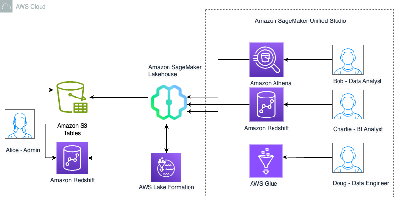


 Charlie can now further update the SQL query and use it to power QuickSight dashboards that can be shared with Sales team members.
 Sandeep Adwankar is a Senior Technical Product Manager at AWS. Based in the California Bay Area, he works with customers around the globe to translate business and technical requirements into products that enable customers to improve how they manage, secure, and access data.
 Srividya Parthasarathy is a Senior Big Data Architect on the AWS Lake Formation team. She works with the product team and customers to build robust features and solutions for their analytical data platform. She enjoys building data mesh solutions and sharing them with the community.


 BP Yau is a Sr Partner Solutions Architect at AWS. His role is to help customers architect big data solutions to process data at scale. Before AWS, he helped Amazon.com Supply Chain Optimization Technologies migrate its Oracle data warehouse to Amazon Redshift and build its next generation big data analytics platform using AWS technologies.
 Ali Alladin is the Senior Director of Product Management and Partner Solutions at ThoughtSpot. In this role, Ali oversees Cloud Engineering and Operations, ensuring seamless integration and optimal performance of ThoughtSpot’s cloud-based services. Additionally, Ali spearheads the development of AI-powered solutions in augmented and embedded analytics, collaborating closely with technology partners to drive innovation and deliver cutting-edge analytics capabilities. With a robust background in product management and a keen understanding of AI technologies, Ali is dedicated to pushing the boundaries of what’s possible in the analytics space, helping organizations harness the full potential of their data.


 Yogesh Dhimate is a Sr. Partner Solutions Architect at AWS, leading technology partnership with Salesforce. Prior to joining AWS, Yogesh worked with leading companies including Salesforce driving their industry solution initiatives. With over 20 years of experience in product management and solutions architecture Yogesh brings unique perspective in cloud computing and artificial intelligence.
 Ife Stewart is a Principal Solutions Architect in the Strategic ISV segment at AWS. She has been engaged with Salesforce Data Cloud over the last 2 years to help build integrated customer experiences across Salesforce and AWS. Ife has over 10 years of experience in technology. She is an advocate for diversity and inclusion in the technology field.
 Mike Patterson is a Senior Customer Solutions Manager in the Strategic ISV segment at AWS. He has partnered with Salesforce Data Cloud to align business objectives with innovative AWS solutions to achieve impactful customer experiences. In his spare time, he enjoys spending time with his family, sports, and outdoor activities.
 Drew Loika is a Director of Product Management at Salesforce and has spent over 15 years delivering customer value via data platforms and services. When not diving deep with customers on what would help them be more successful, he enjoys the acts of making, growing, and exploring the great outdoors.


 Satesh Sonti is a Sr. Analytics Specialist Solutions Architect based out of Atlanta, specialized in building enterprise data platforms, data warehousing, and analytics solutions. He has over 19 years of experience in building data assets and leading complex data platform programs for banking and insurance clients across the globe.


