This is a guest post co-written with Mike Mosher, Sr. Principal Cloud Platform Network Architect at a multi-national financial credit reporting company.
I work for a multi-national financial credit reporting company that offers credit risk, fraud, targeted marketing, and automated decisioning solutions. We are an AWS early adopter and have embraced the cloud to drive digital transformation efforts. Our Cloud Center of Excellence (CCoE) team operates a global AWS Landing Zone, which includes a centralized AWS network infrastructure. We are also an AWS PrivateLink Ready Partner and offer our E-Connect solution to allow our B2B customers to connect to a range of products through private, secure, and performant connectivity.
Our E-Connect solution is a platform comprised of multiple AWS services like Application Load Balancer (ALB), Network Load Balancer (NLB), Gateway Load Balancer (GWLB), AWS Transit Gateway, AWS PrivateLink, AWS WAF, and third-party security appliances. All of these services and resources, as well as the large amount of network traffic across the platform, create a large number of logs, and we needed a solution to aggregate and organize these logs for quick analysis by our operations teams when troubleshooting the platform.
Our original design consisted of Amazon OpenSearch Service, selected for its ability to return specific log entries from extensive datasets in seconds. We also complemented this with Logstash, allowing us to use multiple filters to enrich and augment the data before sending to the OpenSearch cluster, facilitating a more comprehensive and insightful monitoring experience.
In this post, we share our journey, including the hurdles we faced, the solutions we thought about, and why we went with Amazon OpenSearch Ingestion pipelines to make our log management smoother.
Overview of the initial solution
We originally wanted to store and analyze the logs in an OpenSearch cluster, and decided to use the AWS-managed service for OpenSearch called Amazon OpenSearch Service. We also wanted to enrich these logs with Logstash, but there was no AWS-managed service for this, so we needed to deploy the application on an Amazon Elastic Compute Cloud (Amazon EC2) server. This setup meant that we had to implement a lot of maintenance of the server, including using AWS CodePipeline and AWS CodeDeploy to push new Logstash configurations to the server and restart the service. We also needed to perform server maintenance tasks such as patching and updating the operating system (OS) and the Logstash application, and monitor server resources such as Java heap, CPU, memory, and storage.
The complexity extended to validating the network path from the Logstash server to the OpenSearch cluster, incorporating checks on Access Control Lists (ACLs) and security groups, as well as routes in the VPC subnets. Scaling beyond a single EC2 server introduced considerations for managing an auto scaling group, Amazon Simple Queue Service (Amazon SQS) queues, and more. Maintaining the continuous functionality of our solution became a significant effort, diverting focus from the core tasks of operating and monitoring the platform.
The following diagram illustrates our initial architecture.
Possible solutions for us:
Our team looked at multiple options to manage the logs from this platform. We possess a Splunk solution for storing and analyzing logs, and we did assess it as a potential competitor to OpenSearch Service. However, we opted against it for several reasons:
Our team is more familiar with OpenSearch Service and Logstash than Splunk.
Amazon OpenSearch Service, being a managed service in AWS, facilitates a smoother log transfer process compared to our on-premises Splunk solution. Also, transporting logs to the on-premises Splunk cluster would incur high costs, consume bandwidth on our AWS Direct Connect connections, and introduce unnecessary complexity.
Splunk’s pricing structure, based on storage in GBs, proved cost-prohibitive for the volume of logs we intended to store and analyze.
Initial designs for an OpenSearch Ingestion pipeline solution
The Amazon team approached me about a new feature they were launching: Amazon OpenSearch Ingestion. This feature offered a great solution to the problems we were facing with managing EC2 instances for Logstash. First, the new feature removed all the heavy lifting from our team of managing multiple EC2 instances, scaling the servers up and down based on traffic, and monitoring the ingestion of logs and the resources of the underlying servers. Second, Amazon OpenSearch Ingestion pipelines supported most if not all of the Logstash filters we were using in our current solution, which allowed us to use the same functionality of our current solution for enriching the logs.
We were thrilled to be accepted into the AWS beta program, emerging as one of its earliest and largest adopters. Our journey began with ingesting VPC flow logs for our internet ingress platform, alongside Transit Gateway flow logs connecting all VPCs in the AWS Region. Handling such a substantial volume of logs proved to be a significant task, with Transit Gateway flow logs alone reaching upwards of 14 TB per day. As we expanded our scope to include other logs like ALB and NLB access logs and AWS WAF logs, the scale of the solution translated to higher costs.
However, our enthusiasm was somewhat dampened by the challenges we faced initially. Despite our best efforts, we encountered performance issues with the domain. Through collaborative efforts with the AWS team, we uncovered misconfigurations within our setup. We had been using instances that were inadequately sized for the volume of data we were handling. Consequently, these instances were constantly operating at maximum CPU capacity, resulting in a backlog of incoming logs. This bottleneck cascaded into our OpenSearch Ingestion pipelines, forcing them to scale up unnecessarily, even as the OpenSearch cluster struggled to keep pace.
These challenges led to a suboptimal performance from our cluster. We found ourselves unable to analyze flow logs or access logs promptly, sometimes waiting days after their creation. Additionally, the costs associated with these inefficiencies far exceeded our initial expectations.
However, with the assistance of the AWS team, we successfully addressed these issues, optimizing our setup for improved performance and cost-efficiency. This experience underscored the importance of proper configuration and collaboration in maximizing the potential of AWS services, ultimately leading to a more positive outcome for our data ingestion processes.
Optimized design for our OpenSearch Ingestion pipelines solution
We collaborated with AWS to enhance our overall solution, building a solution that is both high performing, cost-effective, and aligned with our monitoring requirements. The solution involves selectively ingesting specific log fields into the OpenSearch Service domain using an Amazon S3 Select pipeline in the pipeline source; alternative selective ingestion can also be done by filtering within pipelines. You can use include_keys and exclude_keys in your sink to filter data that’s routed to destination. We also used the built-in Index State Management feature to remove logs older than a predefined period to reduce the overall cost of the cluster.
The ingested logs in OpenSearch Service empower us to derive aggregate data, providing insights into trends and issues across the entire platform. For additional detailed analysis of these logs including all original log fields, we use Amazon Athena tables with partitioning to quickly and cost-effectively query Amazon Simple Storage Service (Amazon S3) for logs stored in Parquet format.
This comprehensive solution significantly enhances our platform visibility, reduces overall monitoring costs for handling a large log volume, and expedites our time to identify root causes when troubleshooting platform incidents.
The following diagram illustrates our optimized architecture.
Performance comparison
The following table compares the performance of the initial design with Logstash on Amazon EC2, the original OpenSearch Ingestion pipeline solution, and the optimized OpenSearch Ingestion pipeline solution.
Initial Design with Logstash on Amazon EC2
Original Ingestion Pipeline Solution
Optimized Ingestion Pipeline Solution
Maintenance Effort
High: Solution required the team to manage multiple services and instances, taking effort away from managing and monitoring our platform.
Low: OpenSearch Ingestion managed most of the undifferentiated heavy lifting, leaving the team to only maintain the ingestion pipeline configuration file.
Low: OpenSearch Ingestion managed most of the undifferentiated heavy lifting, leaving the team to only maintain the ingestion pipeline configuration file.
Performance
High: EC2 instances with Logstash could scale up and down as needed in the auto scaling group.
Low: Due to insufficient resources on the OpenSearch cluster, the ingestion pipelines were constantly at max OpenSearch Compute Units (OCUs), causing log delivery to be delayed by multiple days.
High: Ingestion pipelines can scale up and down in OCUs as needed.
Real-time Log Availability
Medium: In order to pull, process, and deliver the large number of logs in Amazon S3, we needed a large number of EC2 instances. To save on cost, we ran fewer instances, which led to slower log delivery to OpenSearch.
Low: Due to insufficient resources on the OpenSearch cluster, the ingestion pipelines were constantly at max OCUs, causing log delivery to be delayed by multiple days.
High: The optimized solution was able to deliver a large number of logs to OpenSearch to be analyzed in near real time.
Cost Saving
Medium: Running multiple services and instances to send logs to OpenSearch increased the cost of the overall solution.
Low: Due to insufficient resources on the OpenSearch cluster, the ingestion pipelines were constantly at max OCUs, increasing the cost of the service.
High: The optimized solution was able to scale the ingestion pipeline OCUs up and down as needed, which kept the overall cost low.
Overall Benefit
Medium
Low
High
Conclusion
In this post, we highlighted my journey to build a solution using OpenSearch Service and OpenSearch Ingestion pipelines. This solution allows us to focus on analyzing logs and supporting our platform, without needing to support the infrastructure to deliver logs to OpenSearch. We also highlighted the need to optimize the service in order to increase performance and reduce cost.
As our next steps, we aim to explore the recently announced Amazon OpenSearch Service zero-ETL integration with Amazon S3 (in preview) feature within OpenSearch Service. This step is intended to further reduce the solution’s costs and provide flexibility in the timing and number of logs that are ingested.
About the Authors
Navnit Shukla serves as an AWS Specialist Solutions Architect with a focus on analytics. He possesses a strong enthusiasm for assisting clients in discovering valuable insights from their data. Through his expertise, he constructs innovative solutions that empower businesses to arrive at informed, data-driven choices. Notably, Navnit Shukla is the accomplished author of the book titled “Data Wrangling on AWS.” He can be reached via LinkedIn.
Mike Mosher is s Senior Principal Cloud Platform Network Architect at a multi-national financial credit reporting company. He has more than 16 years of experience in on-premises and cloud networking and is passionate about building new architectures on the cloud that serve customers and solve problems. Outside of work, he enjoys time with his family and traveling back home to the mountains of Colorado.
A standard use case for customers is to integrate existing identity providers (IdPs) with Amazon OpenSearch Service. OpenSearch Service offers built-in support for single sign-on (SSO) authentication for OpenSearch Dashboards, and uses SAML protocol. The SAML authentication for OpenSearch Service lets you integrate your existing third-party IdPs, such as Okta, Ping Identity, OneLogin, Auth0, ADFS, Azure Active Directory, and Keycloak, with OpenSearch Service dashboards.
In this post, we walk you through how to configure service provider-initiated authentication for OpenSearch Dashboards by using OpenSearch Service and Keycloak. We also discuss how to set up users, groups, and roles in Keycloak and configure their access to OpenSearch Dashboards.
Solution overview
The following diagram illustrates the SAML authentication flow for this solution.
The service provider (OpenSearch Service) uses the information about the IdP (Keycloak) to generate a SAML authentication request. The service provider redirects SAML authentication requests back to the browser.
The browser relays the SAML authentication request to Keycloak. Keycloak parses the SAML authentication request and asks for the user to insert their login and password to authenticate.
After a successful authentication, Keycloak generates a SAML authentication response that includes authenticated user details from Keycloak and sends the encoded SAML response to the browser.
The browser relays the SAML response to OpenSearch Service Assertion Consumer Service (ACS) URL.
OpenSearch Service validates the SAML response. If the validation checks are passed, the user is redirected to the front page of OpenSearch Dashboards. The authorization is performed according to the roles mapped to the user.
Prerequisites
To complete this walkthrough, you should have the following set up:
An OpenSearch Service domain running OpenSearch or Elasticsearch version 6.7 or later with fine-grained access control enabled within a VPC.
Keycloak installed and configured. In this post, we created the IdP in the same VPC of the OpenSearch domain. There is no need for a direct connection between the IdP and the service provider, so you can have the IdP in a different network as well.
A properly configured security group for OpenSearch Service and Keycloak IdP server to receive inbound traffic from users.
A browser with network connectivity to both Keycloak and OpenSearch Dashboards.
Enable SAML authentication for OpenSearch Service
The first step is to enable SAML authentication for OpenSearch Service. Complete the following steps:
On the OpenSearch Service console, open the details page for your OpenSearch Service domain.
On the Security configuration tab, choose Edit.
Select Enable SAML authentication.
Enabling this option automatically populates different IdP URLs, which is required to configure SAML support in the Keycloak IdP. Note down the values under Service provider entity ID and SP-initiated SSO URL. The OpenSearch Dashboards login flow can be configured either as service provider-initiated or IdP-initiated. The service provider-initiated login flow is initiated by OpenSearch Service, and the IdP-initiated login flow is initiated by the IdP (for example, Keycloak). In this post, we use a service provider-initiated login flow.
Configure Keycloak as IdP
During the SAML authentication process, when the user is authenticated, the browser receives a SAML assertion token from Keycloak and forwards it to OpenSearch Service. The OpenSearch Service domain authorizes the user with backend roles according to the attributes presented in the token.
To configure Keycloak as IdP, complete the following steps:
Log in to the Keycloak IdP admin console with admin user privileges (for example, https://<Keycloak server>:8081/admin/).
Choose Create Realm.
For Realm name, enter a name (for example, Amazon_OpenSearch) and choose Create.
For managing OpenSearch Service specific roles, users, and groups, you first create a separate client realm that provides a logical space to manage objects.
In the navigation pane, choose your realm, then choose Clients.
Choose Create client.
In the General Settings window, for Client type, choose SAML
For Client ID, use the service provider entity ID you copied earlier, then choose Next
Under Login settings, enter the service provider-initiated SSO URL copied from earlier (for example, https://vpc-abc123.us-east-1.es.amazonaws.com/_dashboards/_opendistro/_security/saml/acs) and choose Save.
On the client settings tab, under Signature and Encryption, turn on Sign Assertions and keep all other options as default, then choose Save.
On the Keys tab, under Signing keys config, turn Client signature required off.
Configure Keycloak users, roles, and groups
After you have configured the Keycloak IdP client for OpenSearch Service, you can create roles, groups, and users on the IdP side. For this post, we create two roles, two groups, and two users, as listed in the following table.
Users
Groups
Roles
super_user_1
super_user_group
super_user_role
readonly_user_1
readonly_user_group
readonly_user_role
Complete the following steps:
In the navigation pane for your realm, choose Realm roles.
Choose Create role.
For Rolename, enter a name (for this post, super_user_role) and choose Save.
Repeat these steps to create a second role, readonly_user_role.
Now let’s create groups, assign the roles to the groups, and map the users to the groups.
Under your realm, choose Groups in the navigation pane.
Choose Create group.
For Name, enter a group name (for example, super_user_group) and choose Save.
Repeat these steps to create a second group, readonly_user_group.
When the new groups are created, they will be listed on the Groups page.
On the details page for each group, on the Role mapping tab, choose Assign role.
For the group super_user_group, select the role super_user_role and choose Assign.
Repeat these steps to assign the role readonly_user_role to the group readonly_user_group.
The last step is to create users and assign them to groups so they automatically inherit group privileges. For this post, we create two users, super_user_1 and readonly_user_1, with dashboard admin and dashboard read-only privileges, respectively.
Under your realm, choose Users in the navigation pane.
Choose Create new user.
Under General, configure the user details, including user name, first name, last name, and email, then choose Create.
Set a temporary password on the Credentials tab after you create the user.
Choose Add user and repeat these steps to add your second user, readonly_user_1.
To join a user to a specific group, choose Join Group on the Groups tab of the respective user.
Select the group the user is joining and choose Join. For example, the user super_user_1 is joining the group super_user_group.
Repeat these steps for the user readonly_user_1 to join the group readonly_user_group.
Next, you can remove the default role mapping for the users because you already assigned the roles to their respective groups.
On the Role Mapping tab, select the default role.
Unassign the default role for the user by choosing Unassign and then Remove.
Repeat these steps for the other user.
Choose Client scopes in the navigation pane.
In the Name column, choose role_list.
On the Mappers tab, choose role list.
Turn on Single Role Attribute and choose Save.
Download SAML metadata from Keycloak
The configuration of Keycloak is now complete, so you can download the SAML metadata file from Keycloak. The SAML metadata is in XML format and is needed to configure SAML in the OpenSearch Service domain.
Under your realm, choose Realm settings in the navigation pane.
On the General tab, choose SAML 2.0 Identify Provider Metadata under Endpoints.
This will generate an IdP metadata file in another window. This XML file contains information on the provider, such as a TLS certificate, SSO endpoints, and the IdP entity ID.
Download this XML file locally so you can upload this file on the OpenSearch Service console in later steps.
Integrate OpenSearch Service SAML with Keycloak
To integrate OpenSearch Service with the Keycloak IDP, you need to upload the IdP metadata XML file on the OpenSearch Service console.
On the OpenSearch Service console, navigate to your domain.
Choose Security configuration, then choose Edit.
Under Metadata from IdP, choose Import from XML file to import the file and auto-populate the IdP entity ID.
Alternatively, you can copy and paste the contents of the entity ID property from the metadata file.
For SAML master backend role, enter super_user_role.
This means that a user with this role is provided manager user privileges to the cluster, but can only use permissions within OpenSearch Dashboards.
Expand the Additional settings section
For Roles key, enter an attribute from the assertion (in our case, Role) and choose Save Changes.
Test the OpenSearch Dashboards SAML authentication with Keycloak
You’re now ready to test the SAML integration with Keycloak as an IdP.
Choose the OpenSearch Dashboards URL provided on OpenSearch Service console.
It will automatically redirect you to the Keycloak sign-in page for authentication.
Enter the admin user name (super_user_1) and password and choose Sign In.
Upon successful authentication, it will redirect you to the home page of OpenSearch Dashboards. If you encounter issues at this step, refer to SAML troubleshooting for common issues.
Internally, the security plugin maps the backend role super_user_role to the reserved security roles all_access and security_manager. Therefore, Keycloak users with the backend role super_user_role are authorized with the privileges of the manager user in the domain. To grant read-only dashboard access to user readonly_user_1, log in to OpenSearch Dashboards as the user super_user_1. Then map the role readonly_user_role as a backend role for the reserved security role opensearch_dashboards_read_only.
When establishing access control for the cluster, it’s crucial to carefully manage the permissions granted to users, adhering to the principle of least privilege. By having both super_user_role with administrative capabilities and read-only readonly_user_role, you can strike a balance. This approach allows a small number of trusted users to have full administrative access within OpenSearch Dashboards, while also enabling read-only access for other stakeholders who require visibility but don’t need more access.
At the time of writing, if you specify the <SingleLogoutService /> details in the Keycloak metadata XML, when you sign out from OpenSearch Dashboards, it will call Keycloak directly and try to sign the user out. This doesn’t work currently with some of the versions of OpenSearch Service, because Keycloak expects the sign-out request to be signed with a certificate that OpenSearch Service doesn’t currently support. If you remove <SingleLogoutService /> from the metadata XML file, OpenSearch Service will use its own internal sign-out mechanism and sign the user out on the OpenSearch Service side. No calls will be made to Keycloak for signing out.
Clean up
If you don’t want to continue using the solution, delete the resources you created:
OpenSearch Service domain
VPN and Keycloak instance
Conclusion
In this post, you learned how to configure Keycloak as an IdP to access OpenSearch Dashboards using SAML. To learn more about OpenSearch Service and SAML integration, refer to SAML authentication for OpenSearch Dashboards. Stay tuned for a series of posts focusing on SAML integrations with OpenSearch Service and Amazon OpenSearch Serverless.
About the Author
Sajeev is a Senior Cloud Engineer (Big Data & Analytics) and a Subject Matter Expert for Amazon OpenSearch Service. He works closely with AWS customers to provide them architectural and engineering assistance and guidance. He dives deep into big data technologies and streaming solutions and leads onsite and online sessions for customers to design the best solutions for their use cases.
We’re excited to announce the general availability (GA) of Amazon DynamoDB zero-ETL integration with Amazon Redshift, which enables you to run high-performance analytics on your DynamoDB data in Amazon Redshift with little to no impact on production workloads running on DynamoDB. As data is written into a DynamoDB table, it’s seamlessly made available in Amazon Redshift, eliminating the need to build and maintain complex data pipelines.
Zero-ETL integrations facilitate point-to-point data movement without the need to create and manage data pipelines. You can create zero-ETL integration on an Amazon Redshift Serverless workgroup or Amazon Redshift provisioned cluster using RA3 instance types. You can then run enhanced analysis on this DynamoDB data with the rich capabilities of Amazon Redshift, such as high-performance SQL, built-in machine learning (ML) and Spark integrations, materialized views (MV) with automatic and incremental refresh, data sharing, and the ability to join data across multiple data stores and data lakes.
The DynamoDB zero-ETL integration with Amazon Redshift has helped our customers simplify their extract, transform, and load (ETL) pipelines. The following is a testimony from Keith McDuffee, Director of DevOps at Verisk Analytics, a customer who used zero-ETL integration with DynamoDB in place of their homegrown solution and benefitted from the seamless replication that it provided:
“We have dashboards built on top of our transactional data in Amazon Redshift. Earlier, we used our homegrown solution to move data from DynamoDB to Amazon Redshift, but those jobs would often time out and lead to a lot of operational burden and missed insights on Amazon Redshift. Using the DynamoDB zero-ETL integration with Amazon Redshift, we no longer run into such issues and the integration seamlessly and continuously replicates data to Amazon Redshift.”
In this post, we showcase how an ecommerce application can use this zero-ETL integration to analyze the distribution of customers by attributes such as location and customer signup date. You can also use the integration for retention and churn analysis by calculating retention rates by comparing the number of active profiles over different time periods.
Solution overview
The zero-ETL integration provides end-to-end fully managed process that allows data to be seamlessly moved from DynamoDB tables to Amazon Redshift without the need for manual ETL processes, ensuring efficient and incremental updates in Amazon Redshift environment. It leverages DynamoDB exports to incrementally replicate data changes from DynamoDB to Amazon Redshift every 15-30 minutes. The initial data load is a full load, which may take longer depending on the data volume. This integration also enables replicating data from multiple DynamoDB tables into a single Amazon Redshift provisioned cluster or serverless workgroup, providing a holistic view of data across various applications.
This replication is done with little to no performance or availability impact to your DynamoDB tables and without consuming DynamoDB read capacity units (RCUs). Your applications will continue to use DynamoDB while data from those tables will be seamlessly replicated to Amazon Redshift for analytics workloads such as reporting and dashboards.
The following diagram illustrates this architecture.
In the following sections, we show how to get started with DynamoDB zero-ETL integration with Amazon Redshift. This general availability release supports creating and managing the zero-ETL integrations using the AWS Command Line Interface (AWS CLI), AWS SDKs, API, and AWS Management Console. In this post, we demonstrate using the console.
Attach the resource-based policies to both DynamoDB and Amazon Redshift as mentioned in here.
Make sure the AWS Identity and Access Management (IAM) user or role creating the integration has an identity-based policy that authorizes actions listed in here.
Create the DynamoDB zero-ETL integration
You can create the integration either on the DynamoDB console or Amazon Redshift console. The following steps use the Amazon Redshift console.
On the Amazon Redshift console, choose Zero-ETL integrations in the navigation pane.
Choose Create DynamoDB integration.
If you choose to create the integration on the DynamoDB console, choose Integrations in the navigation pane and then choose Create integration and Amazon Redshift.
For Integration name, enter a name (for example, ddb-rs-customerprofiles-zetl-integration).
Choose Next.
Choose Browse DynamoDB tables and choose the table that will be the source for this integration.
Choose Next.
You can only choose one table. If you need data from multiple tables in a single Redshift cluster, you need to create a separate integration for each table.
If you don’t have PITR enabled on the source DynamoDB table, an error will pop up while choosing the source. In this case, you can select Fix it for me for DynamoDB to enable the PITR on your source table. Review the changes and choose Continue.
Choose Next.
Choose your target Redshift data warehouse. If it’s in the same account, you can browse and choose the target. If the target resides in a different account, you can provide the Amazon Resource Name (ARN) of the target Redshift cluster.
If you get an error about the resource policy, select Fix it for me for Amazon Redshift to fix policies as part of this creation process. Alternatively, you can add resource policies for Amazon Redshift manually prior to creating zero-ETL integration. Review the changes and choose Reboot and continue.
Choose Next and complete your integration.
The zero-ETL integration creation should show the status Creating. Wait for the status to change to Active.
Create a Redshift database from the integration
Complete the following steps to create a Redshift database:
On the Amazon Redshift console, navigate to the recently created zero-ETL integration.
Choose Create database from integration.
For Destination database name, enter a name (for example, ddb_rs_customerprofiles_zetl_db).
Choose Create database.
After you create the database, the database state should change from Creating to Active. This will start the replication of data in the source DynamoDB tables to the target Redshift tables, which will be created under the public schema of the destination database (ddb_rs_customerprofiles_zetl_db).
Now you can query your data in Amazon Redshift using the integration with DynamoDB.
Understanding your data
Data exported from DynamoDB to Amazon Redshift is stored in the Redshift database that you created from your zero-ETL integration (ddb_rs_customerprofiles_zetl_db). A single table of the same name as the DynamoDB source table is created and is under the default (public) Redshift schema. DynamoDB only enforces schemas for the primary key attributes (partition key and optionally sort key). Because of this, your DynamoDB table structure is replicated to Amazon Redshift in three columns: partition key, sort key, and a SUPER data type column named value that contains all the attributes. The data in this value column is in DynamoDB JSON format. For information about the data format, see DynamoDB table export output format.
The DynamoDB partition key is used as the Redshift table distribution key, and the combination of the DynamoDB partition and sort keys are used as the Redshift table sort keys. Amazon Redshift also allows changing the sort keys on the zero-ETL integration replicated tables using the ALTER SORT KEY command.
The DynamoDB data in Amazon Redshift is read-only data. After the data is available in the Amazon Redshift table, you can query the value column as a SUPER data type using PartiQL SQL or create and query materialized views on the table, which are incrementally refreshed automatically.
To validate the ingested records, you can use the Amazon Redshift Query Editor to query the target table in Amazon Redshift using PartiQL SQL. For example, you can use the following query to select email and unnest the data in the value column to the retrieve the customer name and address:
select email,
       value.custname."S"::text custname,
       value.address."S"::text custaddress,
       value
from "ddb_rs_customerprofiles_zetl_db".public."customerprofiles"
To demonstrate the replication of incremental changes in action, we make the following updates to the source DynamoDB table:
With these changes, the DynamoDB table customerprofiles has four items (three existing, two new, and one delete), as shown in the following screenshot.
Next, you can go to the query editor to validate these changes. At this point, you can expect incremental changes to reflect in the Redshift table (four records in table).
Create materialized views on zero-ETL replicated tables
Common analytics use cases generally involve aggregating data across multiple source tables using complex queries to generate reports and dashboards for downstream applications. Customers usually create late binding views to meet such use cases, which aren’t always optimized to meet the stringent query SLAs due to the long underlying query runtimes. Another option is to create a table that stores the data across multiple source tables, which brings the challenge of incrementally updating and refreshing data based on the changes in the source table.
To serve such use cases and get around the challenges associated with traditional options, you can create materialized views on top of zero-ETL replicated tables in Amazon Redshift, which can get automatically refreshed incrementally as the underlying data changes. Materialized views are also convenient for storing frequently accessed data by unnesting and shredding data stored in the SUPER column value by the zero-ETL integration.
For example, we can use the following query to create a materialized view on the customerprofiles table to analyze customer data:
CREATE MATERIALIZED VIEW dev.public.customer_mv
AUTO REFRESH YES
AS
SELECT value."custname"."S"::varchar(30) as cust_name, value."username"."S"::varchar(100) as user_name, value."email"."S"::varchar(60) as cust_email, value."address"."S"::varchar(100) as cust_addres, value."phone"."S"::varchar(100) as cust_phone_nbr, value."status"."S"::varchar(10) as cust_status,
value."custcreatedt"."S"::varchar(10) as cust_create_dt, value."custupddt"."S"::varchar(10) as cust_update_dt FROM "ddb_rs_customerprofiles_zetl_db"."public"."customerprofiles"
group by 1,2,3,4,5,6,7,8;
This view is set to AUTO REFRESH, which means it will be automatically and incrementally refreshed when the new data arrives in the underlying source table customerprofiles.
Now let’s say you want to understand the distribution of customers across different status categories. You can query the materialized view customer_mv created from the zero-ETL DynamoDB table as follows:
-- Customer count by status
select cust_status,count(distinct user_name) cust_status_count
from dev.public.customer_mv
group by 1;
Next, let’s say you want to compare the number of active customer profiles over different time periods. You can run the following query on customer_mv to get that data:
-- Customer active count by date
select cust_create_dt,count(distinct user_name) cust_count
from dev.public.customer_mv
where cust_status ='active'
group by 1;
Let’s try to make a few incremental changes, which involves two new items and one delete on the source DynamoDB table using following AWS CLI commands.
Validate the incremental refresh of the materialized view
To monitor the history of materialized view refreshes, you can use the SYS_MV_REFRESH_HISTORY system view. As you can see in the following output, the materialized view customer_mv was incrementally refreshed.
Now let’s query the materialized view created from the zero-ETL table. You can see two new records. The changes were propagated into the materialized view with an incremental refresh.
Monitor the zero-ETL integration
There are several options to obtain metrics on the performance and status of the DynamoDB zero-ETL integration with Amazon Redshift.
On the Amazon Redshift console, choose Zero-ETL integrations in the navigation pane. You can choose the zero-ETL integration you want and display Amazon CloudWatch metrics related to the integration. These metrics are also directly available in CloudWatch.
For each integration, there are two tabs with information available:
Integration metrics – Shows metrics such as the lag (in minutes) and data transferred (in KBps)
Table statistics – Shows details about tables replicated from DynamoDB to Amazon Redshift such as status, last updated time, table row count, and table size
After inserting, deleting, and updating rows in the source DynamoDB table, the Table statistics section displays the details, as shown in the following screenshot.
In addition to the CloudWatch metrics, you can query the following system views, which provide information about the integrations:
SVV_INTEGRATION – Provides configuration details for your integrations
AWS does not charge an additional fee for the zero-ETL integration. You pay for existing DynamoDB and Amazon Redshift resources used to create and process the change data created as part of a zero-ETL integration. These include DynamoDB PITR, DynamoDB exports for the initial and ongoing data changes to your DynamoDB data, additional Amazon Redshift storage for storing replicated data, and Amazon Redshift compute on the target. For pricing on DynamoDB PITR and DynamoDB exports, see Amazon DynamoDB pricing. For pricing on Redshift clusters, see Amazon Redshift pricing.
Clean up
When you delete a zero-ETL integration, your data isn’t deleted from the DynamoDB table or Redshift, but data changes happening after that point of time aren’t sent to Amazon Redshift.
To delete a zero-ETL integration, complete the following steps:
On the Amazon Redshift console, choose Zero-ETL integrations in the navigation pane.
Select the zero-ETL integration that you want to delete and on the Actions menu, choose Delete.
To confirm the deletion, enter confirm and choose Delete.
Conclusion
In this post, we explained how you can set up the zero-ETL integration from DynamoDB to Amazon Redshift to derive holistic insights across many applications, break data silos in your organization, and gain significant cost savings and operational efficiencies.
To learn more about zero-ETL integration, refer to documentation.
About the authors
Ekta Ahuja is an Amazon Redshift Specialist Solutions Architect at AWS. She is passionate about helping customers build scalable and robust data and analytics solutions. Before AWS, she worked in several different data engineering and analytics roles. Outside of work, she enjoys landscape photography, traveling, and board games.
Raghu Kuppala is an Analytics Specialist Solutions Architect experienced working in the databases, data warehousing, and analytics space. Outside of work, he enjoys trying different cuisines and spending time with his family and friends.
Veerendra Nayak is a Principal Database Solutions Architect based in the Bay Area, California. He works with customers to share best practices on database migrations, resiliency, and integrating operational data with analytics and AI services.
Attention all developers, architects, and IT professionals! We’re thrilled to announce the launch of the official Amazon OpenSearch Service YouTube channel—a comprehensive resource for anyone looking to master Amazon OpenSearch Service. Whether you’re just getting started with searches , vectors, analytics, or you’re looking to optimize large-scale implementations, our channel can be your go-to resource to help you unlock the full potential of OpenSearch Service.
OpenSearch is a distributed search and analytics suite that is open source, community-driven, Apache License v2 licensed, and governed by the OpenSearch Software Foundation, under the Linux Foundation.
Amazon OpenSearch Service is a managed service that makes it straightforward to deploy, operate, and scale OpenSearch domains in AWS. OpenSearch Service offers a robust set of features that can transform the way you handle log analytics, real-time monitoring, vector search, and advanced search workloads. But to truly unlock its full potential, you need more than just the basics. That’s where our new YouTube channel comes in.
Dive into a world of practical expertise
We’ve carefully curated a collection of videos that are designed to provide you with the tools, techniques, and insights you need to navigate OpenSearch Service with confidence. The channel also offers a direct line of communication between you and the AWS team. By leaving comments on our videos, you can share your feedback, ideas, and pain points. We’ll be closely monitoring these comments and using them to shape the content we create and influence the future roadmap of OpenSearch Service.
Here’s what sets our channel apart:
Bite-sized learning – Our videos are short and concise—each one packed with practical information that you can consume in under 15 minutes. Whether you’re looking for a quick tutorial or a deep-dive into advanced features, we make it effortless for you to learn on the go.
Curated content – We hand-pick the most important topics around OpenSearch Service and break them down into simple-to-follow, informative videos. From configuring clusters to scaling for petabyte-scale analytics, we cover the most relevant use cases to help you build, manage, and optimize your OpenSearch environment.
Organized playlists – The channel is organized into playlists based on workloads and features of OpenSearch Service such as log analytics, observability, lexical search, vector search, generative AI, and more.
Influence the AWS team – You can leave comments on our videos, and your feedback will be reviewed by the AWS team. This input allows us to work backward from your feedback to influence the content we create and feed into the product roadmap.
What you’ll learn
On the OpenSearch Service YouTube channel, you can expect new content regularly, including:
Log Analytics and Observability
Learn how to ingest, search, and visualize logs at scale with OpenSearch, making log analytics efficient and powerful for enterprises of all sizes. Gain deep insights into using OpenSearch Service for observability, including infrastructure monitoring, application performance management (APM), and more.
Lexical and Semantic Search
Discover the key differences between lexical and semantic search, and learn how to implement both in OpenSearch Service. We’ll cover optimizing search relevancy, handling complex queries, using machine learning models for semantic understanding and much more.
Vector Database & GenAI
Explore OpenSearch Service’s vector database capabilities to power advanced semantic search and AI-driven applications. Learn how generative AI models can enhance your search solutions.
Operational Best Practices
Learn the best practices for running OpenSearch Service in production, covering everything from security and scaling to performance tuning and cost management.
And More
Expect a wide array of content, including deep dives into new features, architecture best practices, how to demo videos, use case showcases, and interviews with industry experts.
Subscribe to stay ahead
Whether you’re a beginner looking to get started or an experienced professional seeking to optimize your workflows, make sure to subscribe to the OpenSearch Service YouTube channel so you don’t miss out on the latest tutorials, insights, and updates. Get ready to elevate your search and analytics skills and be part of shaping the future of this channel and powerful service.
About the Authors
Jagadish Kumar (Jag) is a Senior Specialist Solutions Architect at AWS focused on Amazon OpenSearch Service. He is deeply passionate about Data Architecture and helps customers build analytics solutions at scale on AWS.
Sohaib Katariwala is a Senior Specialist Solutions Architect at AWS focused on Amazon OpenSearch Service. He has over 14 years of experience helping organizations derive insights from their data.
Wendy Neu is a Senior Manager at AWS focused on leading the NoSQL Specialist Solutions Architecture team worldwide. She is passionate about Data Services and leverages her extensive expertise to help customers optimize their data storage, management, and analytics strategies, enabling them to drive innovation and achieve their business goals.
Amazon Kinesis Data Analytics for SQL is a data stream processing engine that helps you run your own SQL code against streaming sources to perform time series analytics, feed real-time dashboards, and create real-time metrics. AWS has made the decision to discontinue Kinesis Data Analytics for SQL, effective January 27, 2026. In this post, we explain why we plan to end support for Kinesis Data Analytics for SQL, alternative AWS offerings, and how to migrate your SQL queries and workloads.
Overview of Kinesis Data Analytics for SQL
The following diagram illustrates the workflow for using Kinesis Data Analytics for SQL.
Kinesis Data Analytics for SQL has been denoted a legacy offering since 2021 on our marketing pages, the AWS Management Console, and public documentation. In this time, we haven’t added new functionality or expanded Kinesis Data Analytics for SQL to new AWS Regions. However, we continue to actively maintain and patch the offering and support customers using the service. We will continue to undertake these activities.
To help you plan and migrate away from Kinesis Data Analytics for SQL, we will discontinue the offering gradually:
On October 15, 2025, you won’t be able to create new Kinesis Data Analytics for SQL applications from this time, but will be able to run any existing applications as normal.
We will delete any remaining customer applications on January 27, 2026. You won’t be able to start or operate your Kinesis Data Analytics for SQL applications and support will no longer be available for Kinesis Data Analytics for SQL from this time.
Overview of Managed Service for Apache Flink and Apache Flink Studio
Amazon Managed Service for Apache Flink is a serverless, low-latency, highly scalable, and highly available real-time stream processing service. Apache Flink is a distributed open source engine for processing data streams. These managed Flink-based offerings provide functionality not available in Kinesis Data Analytics for SQL and can help you build end-to-end streaming pipelines and maintain the accuracy and timeliness of data. For example, Amazon Managed Service for Apache Flink supports built-in scaling, exactly-once processing semantics, multi-language support (including SQL), over 40 source and destination connectors, durable application state, and more
We see customers migrating their Kinesis Data Analytics for SQL workloads to take advantage of the advanced features available with managed Flink offerings. Customers running SQL queries typically select Amazon Managed Service for Apache Flink Studio. Amazon Managed Service for Apache Flink Studio allows you to create a notebook, which is a web-based development environment. With notebooks, you get a simple interactive development experience combined with the advanced capabilities provided by Flink. Amazon Managed Service for Apache Flink Studio uses Apache Zeppelin as the notebook, and uses Flink as the stream processing engine. Amazon Managed Service for Apache Flink Studio notebooks seamlessly combine these technologies to make advanced analytics on data streams accessible to developers of all skill sets. Notebooks are provisioned quickly and provide a way for you to instantly view and analyze your streaming data. Zeppelin provides your Amazon Managed Service for Apache Flink Studio notebooks with a complete suite of analytics tools, including the following capabilities:
Visualizing data
Exporting data to files
Controlling the output format for straightforward analysis
Turning the notebook into a scalable, production application
The following diagram illustrates a common workflow for Managed Service for Apache Flink.
Unlike Kinesis Data Analytics for SQL, Managed Service for Apache Flink adds the following SQL support:
Real-time visualization of transformed data in a data stream
Using Python scripts or Scala programs within the same application
Changing offsets of the streaming layer
Another benefit of Amazon Managed Service for Apache Flink is the improved scalability of the solution post-deployment, because you can scale the underlying resources to meet demand. In Kinesis Data Analytics for SQL, scaling is performed by adding more pumps to persuade the application into adding more resources.
Migrate to Managed Service for Apache Flink
For more information about migrating Kinesis Data Analytics for SQL to Amazon Managed Service for Apache Flink Studio, see Migrate from Amazon Kinesis Data Analytics for SQL Applications to Amazon Managed Service for Apache Flink Studio. Additionally, we have provided guidance in our public documentation, including sample code for how to recreate 17 common Kinesis Data Analytics for SQL queries in Amazon Managed Service for Apache Flink Studio, which we will continue to expand over time. We have created step by step migration guidance for customers using Amazon Data Firehose as a source, or who want to use user-defined functions in Amazon Managed Service for Apache Flink . We also provide documentation to help customers migrating machine learning workloads from Kinesis Data Analytics for SQL to Amazon Managed Service for Apache Flink.
Conclusion
In this post, we outlined how we plan to discontinue Kinesis Data Analytics for SQL and why we’re taking these steps. We recommend migrating your Kinesis Data Analytics for SQL workloads to Amazon Managed Service for Apache Flink or Apache Flink Studio, and we have provided resources to help you get started with your migration. If you need more help, you can ask questions in re:Post, making sure to tag Kinesis Data Analytics for SQL.
About the author
Julian Payne is a Principal Product Manager at AWS. He is passionate about building products and features to help customers innovate using real-time data processing applications in the cloud. Outside of work he writes and illustrates graphic novels.
In today’s data-driven world, processing large datasets efficiently is crucial for businesses to gain insights and maintain a competitive edge. Amazon EMR is a managed big data service designed to handle these large-scale data processing needs across the cloud. It allows running applications built using open source frameworks on Amazon Elastic Compute Cloud (Amazon EC2), Amazon Elastic Kubernetes Service (Amazon EKS), or AWS Outposts, or completely serverless. One of the key features of Amazon EMR on EC2 is managed scaling, which dynamically adjusts computing capacity in response to application demands, providing optimal performance and cost-efficiency.
Although managed scaling aims to optimize EMR clusters for best price-performance and elasticity, some use cases require more granular resource allocation. For example, when multiple applications are submitted to the same clusters, resource contention may occur, potentially impacting both performance and cost-efficiency. Additionally, allocating the Application Master (AM) container to non-reliable nodes like Spot can potentially result in loss of the container and immediate shutdown of the entire YARN application, resulting in wasted resources and additional costs for rescheduling the entire YARN application. These uses cases require more granular resource allocation and sophisticated scheduling policies to optimize resource utilization and maintain high performance.
Starting with the Amazon EMR 7.2 release, Amazon EMR on EC2 introduced a new feature called Application Master (AM) label awareness, which allows users to enable YARN node labels to allocate the AM containers within On-Demand nodes only. Because the AM container is responsible for orchestrating the overall job execution, it’s crucial to verify that it gets allocated to a reliable instance and not be subjected to shutdown due to Spot Instance interruption. Additionally, limiting AM containers to On-Demand helps maintain consistent application launch time, because the fulfillment of the On-Demand Instance isn’t prone to unavailable Spot capacity or bid price.
In this post, we explore the key features and use cases where this new functionality can provide significant benefits, enabling cluster administrators to achieve optimal resource utilization, improved application reliability, and cost-efficiency in your EMR on EC2 clusters.
Solution overview
The Application Master label awareness feature in Amazon EMR works in conjunction with YARN node labels, a functionality offered by Hadoop that empowers you to define labels to nodes within a Hadoop cluster. You can use these labels to determine which nodes of the cluster should host specific YARN containers (such as mappers vs. reducers in a MapReduce, or drivers vs. executors in Apache Spark).
This feature is enabled by default when a cluster is launched with Amazon EMR 7.2.0 and later using Amazon EMR managed scaling, and it has been configured to use YARN node labels. The following code is a basic configuration setup that enables this feature:
Within this configuration snippet, we activate the Hadoop node label feature and define a value for the yarn.node-labels.am.default-node-label-expression property. This property defines the YARN node label that will be used to schedule the AM container of each YARN application submitted to the cluster. This specific container plays a key role in maintaining the lifecycle of the workflow, so verifying its placement on reliable nodes in production workloads is crucial, because the unexpected shutdown of this container can result in the shutdown and failure of the entire application.
Currently, the Application Master label awareness feature only supports two predefined node labels that can be specified to allocate the AM container of a YARN job: ON_DEMAND and CORE. When one of these labels is defined using Amazon EMR configurations (see the preceding example code), Amazon EMR automatically creates the corresponding node labels in YARN and labels the instances in the cluster accordingly.
To demonstrate how this feature works, we launch a sample cluster and run some Spark jobs to see how Amazon EMR managed scaling integrates with YARN node labels.
Launch an EMR cluster with Application Manager placement awareness
To perform some tests, you can launch the following AWS CloudFormation stack, which provisions an EMR cluster with managed scaling and the Application Manager placement awareness feature enabled. If this is your first time launching an EMR cluster, make sure to create the Amazon EMR default roles using the following AWS Command Line Interface (AWS CLI) command:
aws emr create-default-roles
To create the cluster, choose Launch Stack:
Provide the following required parameters:
VPC – An existing virtual private cloud (VPC) in your account where the cluster will be provisioned
Subnet – The subnet in your VPC where you want to launch the cluster
SSH Key Name – An EC2 key pair that you use to connect to the EMR primary node
After the EMR cluster has been provisioned, establish a tunnel to the Hadoop Resource Manager web UI to review the cluster configurations. To access the Resource Manager web UI, complete the following steps:
Point your browser to the URL http://<primary-node-public-dns>:8088/, using the public DNS name of your cluster’s primary node.
This will open the Hadoop Resource Manager web UI, where you can see how the cluster has been configured.
YARN node labels
In the CloudFormation stack, you launched a cluster specifying to allocate the AM containers on nodes labeled as ON_DEMAND. If you explore the Resource Manager web UI, you can see that Amazon EMR created two labels in the cluster: ON_DEMAND and SPOT. To review the YARN node labels present in your cluster, you can inspect the Node Labels page, as shown in the following screenshot.
On this page, you can see how the YARN labels were created in Amazon EMR:
During initial cluster creation, default node labels such as ON_DEMAND and SPOT are automatically generated as non-exclusive partitions
The DEFAULT_PARTITION label stays vacant because every node gets labeled based on its market type—either being an On-Demand or Spot Instance
In our example, because we launched a single core node as On-Demand, you can observe a single node assigned to the ON_DEMAND partition, and the SPOT partition remains empty. Because the labels are created as non-exclusive, nodes with these labels can run both containers launched with a specific YARN label and also containers that don’t specify a YARN label. For additional details on YARN node labels, see YARN Node Labels in the Hadoop documentation.
Now that we have discussed how the cluster was configured, we can perform some tests to validate and review the behavior of this feature when using it in combination with managed scaling.
Concurrent application submission with Spot Instances
To test the managed scaling capabilities, we submit a simple SparkPi job configured to utilize all available memory on the single core node initially launched in our cluster:
In the preceding snippet, we tuned specific Spark configurations to utilize all the resources of the cluster nodes launched (you could also achieve this using the maximizeResourceAllocation configuration while launching an EMR cluster). Because the cluster has been launched using m5.xlarge instances, we can launch individual containers up to 12 GB in terms of memory requirements. With these assumptions, the snippet configures the following:
The Spark driver and executors were configured with 10 GB of memory to utilize most of the available memory on the node, in order to have a single container running on each node of our cluster and simplify this example.
The node-labels.am.default-node-label-expression parameter was set to ON_DEMAND, making sure the Spark driver is automatically allocated to the ON_DEMAND partition of our cluster. Because we specified this configuration while launching the cluster, the AM containers are automatically requested to be scheduled on ON_DEMAND labeled instances, so we don’t need to specify it at the job level.
The yarn.executor.nodeLabelExpression=SPOT configuration verifies that the executors operated exclusively on TASK nodes using Spot Instances. Removing this configuration allows the Spark executors to be scheduled both on SPOT and ON_DEMAND labeled nodes.
The dynamicAllocation.maxExecutors setting was set to 1 to delay the processing time of the application and observe the scaling behavior when multiple YARN applications were submitted concurrently in the same cluster.
As the application transitioned to a RUNNING state, we can verify from the YARN Resource Manager UI that its driver placement was automatically assigned to the ON_DEMAND partition of our cluster (see the following screenshot).
Additionally, upon inspecting the YARN scheduler page, we can see that our SPOT partition doesn’t have a resource associated with it because the cluster was launched with just one On-Demand Instance.
Because the cluster didn’t have Spot Instances initially, you can observe from the Amazon EMR console that managed scaling generates a new Spot task group to accommodate the Spark executor requested to run on Spot nodes only (see the following screenshot) . Before this integration, managed scaling didn’t take into account the YARN labels requested by an application, potentially leading to unpredictable scaling behaviors. With this release, managed scaling now considers the YARN labels specified by applications, enabling more predictable and accurate scaling decisions.
While waiting for the launch of the new Spot node, we submitted another SparkPi job with identical specifications. However, because the memory required to allocate the new Spark Driver was 10 GB and such resources were currently unavailable in the ON_DEMAND partition, the application remained in a pending state until resources became available to schedule its container.
Upon detecting the lack of resources to allocate the new Spark driver, Amazon EMR managed scaling commenced scaling the core instance group (On-Demand Instances in our cluster) by launching a new core node. After the new core node was launched, YARN promptly allocated the pending container on the new node, enabling the application to start its processing. Subsequently, the application requested additional Spot nodes to allocate its own executors (see the following screenshot).
This example demonstrates how managed scaling and YARN labels work together to improve the resiliency of YARN applications, while using cost-effective job executions over Spot Instances.
When to use Application Manager placement awareness and managed scaling
You can use this placement awareness feature to improve cost-efficiency by using Spot Instances while protecting the Application Manager from being incorrectly shut down due to Spot interruptions. It’s particularly useful when you want to take advantage of the cost savings offered by Spot Instances while preserving the stability and reliability of your jobs running on the cluster. When working with managed scaling and the placement awareness feature, consider the following best practices:
Maximum cost-efficiency for non-critical jobs – If you have jobs that don’t have strict service level agreement (SLA) requirements, you can force all Spark executors to run on Spot Instances for maximum cost savings. This can be achieved by setting the following Spark configuration:
spark.yarn.executor.nodeLabelExpression=SPOT
Resilient execution for production jobs – For production jobs where you require a more resilient execution, you might consider not setting the yarn.executor.nodeLabelExpression parameter. When no label is specified, executors are dynamically allocated between both On-Demand and Spot nodes, providing a more reliable execution.
Limit dynamic allocation for concurrent applications – When working with managed scaling and clusters with multiple applications running concurrently (for example, an interactive cluster with concurrent user utilization), you should consider setting a maximum limit for Spark dynamic allocation using the dynamicAllocation.maxExecutors setting. This can help manage resources over-provisioning and facilitate predictable scaling behavior across applications running on the same cluster. For more details, see Dynamic Allocation in the Spark documentation.
Managed scaling configurations – Make sure your managed scaling configurations are set up correctly to facilitate efficient scaling of Spot Instances based on your workload requirements. For example, set an appropriate value for Maximum On-Demand instances in managed scaling based on the number of concurrent applications you want to run on the cluster. Additionally, if you’re planning to use your On-Demand Instances for running solely AM containers, we recommend setting scheduler.capacity.maximum-am-resource-percent to 1 using the Amazon EMR capacity-scheduler classification.
Improve startup time of the nodes – If your cluster is subject to frequent scaling events (for example, you have a long-running cluster that can run multiple concurrent EMR steps), you might want to optimize the startup time of your cluster nodes. When trying to get an efficient node startup, consider only installing the minimum required set of application frameworks in the cluster and, whenever possible, avoid installing non-YARN frameworks such as HBase or Trino, which might delay the startup of processing nodes dynamically attached by Amazon EMR managed scaling. Finally, whenever possible, don’t use complex and time-consuming EMR bootstrap actions to avoid increasing the startup time of nodes launched with managed scaling.
By following these best practices, you can take advantage of the cost savings of Spot Instances while maintaining the stability and reliability of your applications, particularly in scenarios where multiple applications are running concurrently on the same cluster.
Conclusion
In this post, we explored the benefits of the new integration between Amazon EMR managed scaling and YARN node labels, reviewed its implementation and usage, and defined a few best practices that can help you get started. Whether you’re running batch processing jobs, stream processing applications, or other YARN workloads on Amazon EMR, this feature can help you achieve substantial cost savings without compromising on performance or reliability.
As you embark on your journey to use Spot Instances in your EMR clusters, remember to follow the best practices outlined in this post, such as setting appropriate configurations for dynamic allocation, node label expressions, and managed scaling policies. By doing so, you can make sure that your applications run efficiently, reliably, and at the lowest possible cost.
About the authors
Lorenzo Ripani is a Big Data Solution Architect at AWS. He is passionate about distributed systems, open source technologies and security. He spends most of his time working with customers around the world to design, evaluate and optimize scalable and secure data pipelines with Amazon EMR.
Miranda Diaz is a Software Development Engineer for EMR at AWS. Miranda works to design and develop technologies that make it easy for customers across the world to automatically scale their computing resources to their needs, helping them achieve the best performance at the optimal cost.
Sajjan Bhattarai is a Senior Cloud Support Engineer at AWS, and specializes in BigData and Machine Learning workloads. He enjoys helping customers around the world to troubleshoot and optimize their data platforms.
Bezuayehu Wate is an Associate Big Data Specialist Solutions Architect at AWS. She works with customers to provide strategic and architectural guidance on designing, building, and modernizing their cloud-based analytics solutions using AWS.
Amazon Redshift has established itself as a highly scalable, fully managed cloud data warehouse trusted by tens of thousands of customers for its superior price-performance and advanced data analytics capabilities. Driven primarily by customer feedback, the product roadmap for Amazon Redshift is designed to make sure the service continuously evolves to meet the ever-changing needs of its users.
Amazon Redshift now enables the secure sharing of data lake tables—also known as external tables or Amazon Redshift Spectrum tables—that are managed in the AWS Glue Data Catalog, as well as Redshift views referencing those data lake tables. This breakthrough empowers data analytics to span the full breadth of shareable data, allowing you to seamlessly share local tables and data lake tables across warehouses, accounts, and AWS Regions—without the overhead of physical data movement or recreating security policies for data lake tables and Redshift views on each warehouse.
By using granular access controls, data sharing in Amazon Redshift helps data owners maintain tight governance over who can access the shared information. In this post, we explore powerful use cases that demonstrate how you can enhance cross-team and cross-organizational collaboration, reduce overhead, and unlock new insights by using this innovative data sharing functionality.
Overview of Amazon Redshift data sharing
Amazon Redshift data sharing allows you to securely share your data with other Redshift warehouses, without having to copy or move the data.
Data shared between warehouses doesn’t require the data to be physically copied or moved—instead, data remains in the original Redshift warehouse, and access is granted to other authorized users as part of a one-time setup. Data sharing provides granular access control, allowing you to control which specific tables or views are shared, and which users or services can access the shared data.
Since consumers access the shared data in-place, they always access the latest state of the shared data. Data sharing even allows for the automatic sharing of new tables created after that datashare was established.
You can share data across different Redshift warehouses within or across AWS accounts, and you can also do cross-region data sharing. This allows you to share data with partners, subsidiaries, or other parts of your organization, and enables the powerful workload isolation use case, as shown in the following diagram. With the seamless integration of Amazon Redshift with AWS Data Exchange, data can also be monetized and shared publicly, and public datasets such as census data can be added to a Redshift warehouse with just a few steps.
Figure 1: Amazon Redshift data sharing between producer and consumer warehouses
The data sharing capabilities in Amazon Redshift also enable the implementation of a data mesh architecture, as shown in the following diagram. This helps democratize data within the organization by reducing barriers to accessing and using data across different business units and teams. For datasets with multiple authors, Amazon Redshift data sharing supports both read and write use cases (write in preview at the time of writing). This enables the creation of 360-degree datasets, such as a customer dataset that receives contributions from multiple Redshift warehouses across different business units in the organization.
Figure 2: Data mesh architecture using Amazon Redshift data sharing
Overview of Redshift Spectrum and data lake tables
In the modern data organization, the data lake has emerged as a centralized repository—a single source of truth where all data within the organization ultimately resides at some point in its lifecycle. Redshift Spectrum enables seamless integration between the Redshift data warehouse and customers’ data lakes, as shown in the following diagram. With Redshift Spectrum, you can run SQL queries directly against data stored in Amazon Simple Storage Service (Amazon S3), without the need to first load that data into a Redshift warehouse. This allows you to maintain a comprehensive view of your data while optimizing for cost-efficiency.
Figure 3: Amazon Redshift bridges the data warehouse and data lake by enabling querying of data lake tables in-place
Redshift Spectrum supports a variety of open file formats, including Parquet, ORC, JSON, and CSV, as well as open table formats such as Apache Iceberg, all stored in Amazon S3. It runs these queries using a dedicated fleet of high-performance servers with low-latency connections to the S3 data lake. Data lake tables can be added to a Redshift warehouse either automatically through the Data Catalog, in the Amazon Redshift Query Editor, or manually using SQL commands.
From a user experience standpoint, there is little difference between querying a local Redshift table vs. a data lake table. SQL queries can be reused verbatim to perform the same aggregations and transformations on data residing in the data lake, as shown in the following examples. Additionally, by using columnar file formats like Parquet and pushing down query predicates, you can achieve further performance enhancements.
The following SQL is for a sample query against local Redshift tables:
SELECT top 10 mylocal_schema.sales.eventid, sum(mylocal_schema.sales.pricepaid) FROM mylocal_schema.sales, event
WHERE mylocal_schema.sales.eventid = event.eventid
AND mylocal_schema.sales.pricepaid > 30
GROUP BY mylocal_schema.sales.eventid
ORDER BY 2 DESC;
The following SQL is for the same query, but against data lake tables:
SELECT top 10 myspectrum_schema.sales.eventid, sum(myspectrum_schema.sales.pricepaid) FROM myspectrum_schema.sales, event
WHERE myspectrum_schema.sales.eventid = event.eventid
AND myspectrum_schema.sales.pricepaid > 30
GROUP BY myspectrum_schema.sales.eventid
ORDER BY 2 desc;
To maintain robust data governance, Redshift Spectrum integrates with AWS Lake Formation, enabling the consistent application of security policies and access controls across both the Redshift data warehouse and S3 data lake. When Lake Formation is used, Redshift producer warehouses first share their data with Lake Formation rather than directly with other Redshift consumer warehouses, and the data lake administrator grants fine-grained permissions for Redshift consumer warehouses to access the shared data. For more information, see Centrally manage access and permissions for Amazon Redshift data sharing with AWS Lake Formation.
In the past, however, sharing data lake tables across Redshift warehouses presented challenges. It wasn’t possible to do so without having to mount the data lake tables on each individual Redshift warehouse and then recreate the related security policies.
This barrier has now been addressed with the introduction of data sharing support for data lake tables. You can now share data lake tables just like any other table, using the built-in data sharing capabilities of Amazon Redshift. By combining the power of Redshift Spectrum data lake integration with the flexibility of Amazon Redshift data sharing, organizations can unlock new levels of cross-team collaboration and insights, while maintaining robust data governance and security controls.
In this post, we describe how to add data lake tables or views to a Redshift datashare, covering two key use cases:
Adding a late-binding view or materialized view to a producer datashare that references a data lake table
Adding a data lake table directly to a producer datashare
The first use case provides greater flexibility and convenience. Consumers can query the shared view without having to configure fine-grained permissions. The configuration, such as defining permissions on data stored in Amazon S3 with Lake Formation, is already handled on the producer side. You only need to add the view to the producer datashare one time, making it a convenient option for both the producer and the consumer.
An additional benefit of this approach is that you can add views to a datashare that join data lake tables with local Redshift tables. When these views are shared, you can relegate the trusted business logic to just the producer side.
Alternatively, you can add data lake tables directly to a datashare. In this case, consumers can query the data lake tables directly or join them with their own local tables, allowing them to add their own conditional logic as needed.
Add a view that references a data lake table to a Redshift datashare
When you create data lake tables that you intend to add to a datashare, the recommended and most common way to do this is to add a view to the datashare that references a data lake table or tables. There are three high-level steps involved:
Add the Redshift view’s schema (the local schema) to the Redshift datashare.
Add the Redshift view (the local view) to the Redshift datashare.
Add the Redshift external schemas (for the tables referenced by the Redshift view) to the Redshift datashare.
The following diagram illustrates the full workflow.
Figure 4: Sharing data lake tables via Amazon Redshift views
The workflow consists of the following steps:
Create a data lake table on the datashare producer. For more information on creating Redshift Spectrum objects, see External schemas for Amazon Redshift Spectrum. Data lake tables to be shared can include Lake Formation registered tables and Data Catalog tables, and if using the Redshift Query Editor, these tables are automatically mounted.
Create a view on the producer that references the data lake table that you created.
Create a datashare, if one doesn’t already exist, and add objects to your datashare, including the view you created that references the data lake table. For more information, see Creating datashares and adding objects (preview).
Add the external schema of the base Redshift table to the datashare (this is true of both local base tables and data lake tables). You don’t have to add a data lake table itself to the datashare.
On the consumer, the administrator makes the view available to consumer database users.
Database consumer users can write queries to retrieve data from the shared view and join it with other tables and views on the consumer.
After these steps are complete, database consumer users with access to the datashare views can reference them in their SQL queries. The following SQL queries are examples for achieving the preceding steps.
Create a data lake table on the producer warehouse:
CREATE VIEW mylocal_db.mylocal_schema.myspectrumview AS SELECT c1 FROM myspectrum_db.myspectrum_schema.v_test
WITH no schema binding;
Add a view to the datashare on the producer warehouse:
ALTER datashare mydatashare ADD SCHEMA mylocal_db.mylocal_schema;
ALTER datashare mydatashare ADD VIEW myspectrumview;
ALTER datashare mydatashare ADD SCHEMA myspectrum_db.myspectrum_schema;
Create a consumer datashare and grant permissions for the view in the consumer warehouse:
CREATE database myspectrum_db FROM datashare myspectrumproducer OF account '123456789012' namespace 'p1234567-8765-4321-p10987654321';
GRANT usage ON database myspectrum_db TO usernames;
Add a data lake table directly to a Redshift datashare
Adding a data lake table to a datashare is similar to adding a view. This process works well for a case where the consumers want the raw data from the data lake table and they want to write queries and join it to tables in their own data warehouse. There are two high-level steps involved:
Add the Redshift external schemas (of the data lake tables to be shared) to the Redshift datashare.
Add the data lake table (the Redshift external table) to the Redshift datashare.
The following diagram illustrates the full workflow.
Figure 5: Sharing data lake tables directly in an Amazon Redshift datashare
The workflow consists of the following steps:
Create a data lake table on the datashare producer.
Add objects to your datashare, including the data lake table you created. In this case, you don’t have any abstraction over the table.
On the consumer, the administrator makes the table available.
Database consumer users can write queries to retrieve data from the shared table and join it with other tables and views on the consumer.
The following SQL queries are examples for achieving the preceding producer steps.
Create a data lake table on the producer warehouse:
Add a data lake schema and table directly to the datashare on the producer warehouse:
ALTER datashare mydatashare ADD SCHEMA myspectrum_db.myspectrum_schema;
ALTER datashare mydatashare ADD TABLE myspectrum_db.myspectrum_schema.test;
Create a consumer datashare and grant permissions for the view in the consumer warehouse:
CREATE database myspectrum_db FROM datashare myspectrumproducer OF account '123456789012' namespace 'p1234567-8765-4321-p10987654321';
GRANT usage ON database myspectrum_db TO usernames;
Security considerations for sharing data lake tables and views
Data lake tables are stored outside of Amazon Redshift, in the data lake, and may not be owned by the Redshift warehouse, but are still referenced within Amazon Redshift. This setup requires special security considerations. Data lake tables operate under the security and governance of both Amazon Redshift and the data lake. For Lake Formation registered tables specifically, the Amazon S3 resources are secured by Lake Formation and made available to consumers using the provided credentials.
The data owner of the data in the data lake tables may want to impose restrictions on which external objects can be added to a datashare. To give data owners more control over whether warehouse users can share data lake tables, you can use session tags in AWS Identity and Access Management (IAM). These tags provide additional context about the user running the queries. For more details on tagging resources, refer to Tags for AWS Identity and Access Management resources.
Audit considerations for sharing data lake tables and views
When sharing data lake objects through a datashare, there are special logging considerations to keep in mind:
Access controls – You can also use CloudTrail log data in conjunction with IAM policies to control access to shared tables, including both Redshift datashare producers and consumers. The CloudTrail logs record details about who accesses shared tables. The identifiers in the log data are available in the ExternalId field under the AssumeRole CloudTrail logs. The data owner can configure additional limitations on data access in an IAM policy by means of actions. For more information about defining data access through policies, see Access to AWS accounts owned by third parties.
Centralized access – Amazon S3 resources such as data lake tables can be registered and centrally managed with Lake Formation. After they’re registered with Lake Formation, Amazon S3 resources are secured and governed by the associated Lake Formation policies and made available using the credentials provided by Lake Formation.
Billing considerations for sharing data lake tables and views
The billing model for Redshift Spectrum differs for Amazon Redshift provisioned and serverless warehouses. For provisioned warehouses, Redshift Spectrum queries (queries involving data lake tables) are billed based on the amount of data scanned during query execution. For serverless warehouses, data lake queries are billed the same as non-data-lake queries. Storage for data lake tables is always billed to the AWS account associated with the Amazon S3 data.
In the case of datashares involving data lake tables, costs are attributed for storing and scanning data lake objects in a datashare as follows:
When a consumer queries shared objects from a data lake, the cost of scanning is billed to the consumer:
When the consumer is a provisioned warehouse, Amazon Redshift uses Redshift Spectrum to scan the Amazon S3 data. Therefore, the Redshift Spectrum cost is billed to the consumer account.
When the consumer is an Amazon Redshift Serverless workgroup, there is no separate charge for data lake queries.
Amazon S3 costs for storage and operations, such as listing buckets, is billed to the account that owns each S3 bucket.
In this post, we explored how Amazon Redshift enhanced data sharing capabilities, including support for sharing data lake tables and Redshift views that reference those data lake tables, empower organizations to unlock the full potential of their data by bringing the full breadth of data assets in scope for advanced analytics. Organizations are now able to seamlessly share local tables and data lake tables across warehouses, accounts, and Regions.
We outlined the steps to securely share data lake tables and views that reference those data lake tables across Redshift warehouses, even those in separate AWS accounts or Regions. Additionally, we covered some considerations and best practices to keep in mind when using this innovative feature.
Sharing data lake tables and views through Amazon Redshift data sharing champions the modern, data-driven organization’s goal to democratize data access in a secure, scalable, and efficient manner. By eliminating the need for physical data movement or duplication, this capability reduces overhead and enables seamless cross-team and cross-organizational collaboration. Unleashing the full potential of your data analytics to span the full breadth of your local tables and data lake tables is just a few steps away.
For more information on Amazon Redshift data sharing and how it can benefit your organization, refer to the following resources:
Please also reach out to your AWS technical account manager or AWS account Solutions Architect. They will be happy to provide additional guidance and support.
About the Authors
Mohammed Alkateb is an Engineering Manager at Amazon Redshift. Prior to joining Amazon, Mohammed had 12 years of industry experience in query optimization and database internals as an individual contributor and engineering manager. Mohammed has 18 US patents, and he has publications in research and industrial tracks of premier database conferences including EDBT, ICDE, SIGMOD and VLDB. Mohammed holds a PhD in Computer Science from The University of Vermont, and MSc and BSc degrees in Information Systems from Cairo University.
Ramchandra Anil Kulkarni is a software development engineer who has been with Amazon Redshift for over 4 years. He is driven to develop database innovations that serve AWS customers globally. Kulkarni’s long-standing tenure and dedication to the Amazon Redshift service demonstrate his deep expertise and commitment to delivering cutting-edge database solutions that empower AWS customers worldwide.
Mark Lyons is a Principal Product Manager on the Amazon Redshift team. He works on the intersection of data lakes and data warehouses. Prior to joining AWS, Mark held product leadership roles with Dremio and Vertica. He is passionate about data analytics and empowering customers to change the world with their data.
Asser Moustafa is a Principal Worldwide Specialist Solutions Architect at AWS, based in Dallas, Texas. He partners with customers worldwide, advising them on all aspects of their data architectures, migrations, and strategic data visions to help organizations adopt cloud-based solutions, maximize the value of their data assets, modernize legacy infrastructures, and implement cutting-edge capabilities like machine learning and advanced analytics. Prior to joining AWS, Asser held various data and analytics leadership roles, completing an MBA from New York University and an MS in Computer Science from Columbia University in New York. He is passionate about empowering organizations to become truly data-driven and unlock the transformative potential of their data.
In this post, we highlight key lessons learned while helping a global financial services provider migrate their Apache Hadoop clusters to AWS and best practices that helped reduce their Amazon EMR, Amazon Elastic Compute Cloud (Amazon EC2), and Amazon Simple Storage Service (Amazon S3) costs by over 30% per month.
We outline cost-optimization strategies and operational best practices achieved through a strong collaboration with their DevOps teams. We also discuss a data-driven approach using a hackathon focused on cost optimization along with Apache Spark and Apache HBase configuration optimization.
Background
In early 2022, a business unit of a global financial services provider began their journey to migrate their customer solutions to AWS. This included web applications, Apache HBase data stores, Apache Solr search clusters, and Apache Hadoop clusters. The migration included over 150 server nodes and 1 PB of data. The on-premises clusters supported real-time data ingestion and batch processing.
Because of aggressive migration timelines driven by the closure of data centers, they implemented a lift-and-shift rehosting strategy of their Apache Hadoop clusters to Amazon EMR on EC2, as highlighted in the Amazon EMR migration guide.
Amazon EMR on EC2 provided the flexibility for the business unit to run their applications with minimal changes on managed Hadoop clusters with the required Spark, Hive, and HBase software and versions installed. Because the clusters are managed, they were able to decompose their large on-premises cluster and deploy purpose-built transient and persistent clusters for each use case on AWS without increasing operational overhead.
Challenge
Although the lift-and-shift strategy allowed the business unit to migrate with lower risk and allowed their engineering teams to focus on product development, this came with increased ongoing AWS costs.
The business unit deployed transient and persistent clusters for different use cases. Several application components relied on Spark Streaming for real-time analytics, which was deployed on persistent clusters. They also deployed the HBase environment on persistent clusters.
After the initial deployment, they discovered several configuration issues that led to suboptimal performance and increased cost. Despite using Amazon EMR managed scaling for persistent clusters, the configuration wasn’t efficient due to setting a minimum of 40 core nodes and task nodes, resulting in wasted resources. Core nodes were also misconfigured to auto scale. This led to scale-in events shutting down core nodes with shuffle data. The business unit also implemented Amazon EMR auto-termination policies. Because of shuffle data loss on the EMR on EC2 clusters running Spark applications, certain jobs ran five times longer than planned. Here, auto-termination policies didn’t mark a cluster as idle because a job was still running.
Lastly, there were separate environments for development (dev), user acceptance testing (UAT), production (prod), which were also over-provisioned with the minimum capacity units for the managed scaling policies configured too high, leading to higher costs as shown in the following figure.
Short-term cost-optimization strategy
The business unit completed the migration of applications, databases, and Hadoop clusters in 4 months. Their immediate goal was to get out of their data centers as quickly as possible, followed by cost optimization and modernization. Although they expected greater upfront costs because of the lift-and-shift approach, their costs were 40% higher than forecasted. This sped up their need to optimize.
They engaged with their shared services team and the AWS team to develop a cost-optimization strategy. The business unit began by focusing on cost-optimization best practices to implement immediately that didn’t require product development team engagement or impact their productivity. They performed a cost analysis to determine the largest contributors of cost were EMR on EC2 clusters running Spark, EMR on EC2 clusters running HBase, Amazon S3 storage, and EC2 instances running Solr.
The business unit started by enforcing auto-termination of EMR clusters in their dev environments by using automation. They considered using Amazon EMR isIdle Amazon CloudWatch metrics to build an event-driven solution with AWS Lambda, as described in Optimize Amazon EMR costs with idle checks and automatic resource termination using advanced Amazon CloudWatch metrics and AWS Lambda. They implemented a stricter policy to shut down clusters in their lower environments after 3 hours, regardless of usage. They also updated managed scaling policies in DEV and UAT and set the minimum cluster size to three instances to allow clusters to scale up as needed. This resulted in a 60% savings in monthly dev and UAT costs over 5 months, as shown in the following figure.
For the initial production deployment, they had a subset of Spark jobs running on a persistent cluster with an older Amazon EMR 5.(x) release. To optimize costs, they split smaller jobs and larger jobs to run on separate persistent clusters and configured the minimum number of core nodes required to support jobs in each cluster. Setting the core nodes to a constant size while using managed scaling for only task nodes is a recommended best practice and eliminated the issue of shuffle data loss. This also improved the time to scale in and out, because task nodes don’t store data in Hadoop Distributed File System (HDFS).
Solr clusters ran on EC2 instances. To optimize this environment, they ran performance tests to determine the best EC2 instances for their workload.
With over one petabyte of data, Amazon S3 contributed to over 15% of monthly costs. The business unit enabled the Amazon S3 Intelligent-Tiering storage class to optimize storage expenses for historical data and reduce their monthly Amazon S3 costs by over 40%, as shown in the following figure. They also migrated Amazon Elastic Block Store (Amazon EBS) volumes from gp2 to gp3 volume types.
Longer-term cost-optimization strategy
After the business unit realized initial cost savings, they engaged with the AWS team to organize a financial hackathon (FinHack) event. The goal of the hackathon was to reduce costs further by using a data-driven process to test cost-optimization strategies for Spark jobs. To prepare for the hackathon, they identified a set of jobs to test using different Amazon EMR deployment options (Amazon EC2, Amazon EMR Serverless) and configurations (Spot, AWS Graviton, Amazon EMR managed scaling, EC2 instance fleets) to arrive at the most cost-optimized solution for each job. A sample test plan for a job is shown in the following table. The AWS team also assisted with analyzing Spark configurations and job execution during the event.
Job
Test
Description
Configuration
Job 1
1
Run an EMR on EC2 job with default Spark configurations
Non Graviton, On-Demand Instances
2
Run an EMR on Serverless job with default Spark configurations
Default configuration
3
Run an EMR on EC2 job with default Spark configuration and Graviton instances
Graviton, On-Demand Instances
4
Run an EMR on EC2 job with default Spark configuration and Graviton instances. Hybrid Spot Instance allocation.
Graviton, On-Demand and Spot Instances
The business unit also performed extensive testing using Spot Instances before and during the FinHack. They initially used the Spot Instance advisor and Spot Blueprints to create optimal instance fleet configurations. They automated the process to select the most optimal Availability Zone to run jobs by querying for the Spot placement scores using the get_spot_placement_scores API before launching new jobs.
During the FinHack, they also developed an EMR job tracking script and report to granularly track cost per job and measure ongoing improvements. They used the AWS SDK for Python (Boto3) to list the status of all transient clusters in their account and report on cluster-level configurations and instance hours per job.
As they executed the test plan, they found several additional areas of enhancement:
One of the test jobs makes API calls to Solr clusters, which introduced a bottleneck in the design. To prevent Spark jobs from overwhelming the clusters, they fine-tuned executor.cores and spark.dynamicAllocation.maxExecutors properties.
Task nodes were over-provisioned with large EBS volumes. They reduced the size to 100 GB for additional cost savings.
They updated their instance fleet configuration by setting unit/weights proportional based on instance types selected.
During the initial migration, they set the spark.sql.shuffle.paritions configuration too high. The configuration was fine-tuned for their on-premises cluster but not updated to align with their EMR clusters. They optimized the configuration by setting the value to one or two times the number of vCores in the cluster .
The business unit reduced monthly costs by 30% over 3 months. This allowed them to continue migration efforts of remaining on-premises workloads. Most of their 2,000 jobs per month now run on EMR transient clusters. They have also increased AWS Graviton usage to 40% of total usage hours per month and Spot usage to 10% in non-production environments.
Conclusion
Through a data-driven approach involving cost analysis, adherence to AWS best practices, configuration optimization, and extensive testing during a financial hackathon, the global financial services provider successfully reduced their AWS costs by 30% over 3 months. Key strategies included enforcing auto-termination policies, optimizing managed scaling configurations, using Spot Instances, adopting AWS Graviton instances, fine-tuning Spark and HBase configurations, implementing cost allocation tagging, and developing cost tracking dashboards. Their partnership with AWS teams and a focus on implementing short-term and longer-term best practices allowed them to continue their cloud migration efforts while optimizing costs for their big data workloads on Amazon EMR.
For additional cost-optimization best practices, we recommend visiting AWS Open Data Analytics.
About the Authors
Omar Gonzalez is a Senior Solutions Architect at Amazon Web Services in Southern California with more than 20 years of experience in IT. He is passionate about helping customers drive business value through the use of technology. Outside of work, he enjoys hiking and spending quality time with his family.
Navnit Shukla, an AWS Specialist Solution Architect specializing in Analytics, is passionate about helping clients uncover valuable insights from their data. Leveraging his expertise, he develops inventive solutions that empower businesses to make informed, data-driven decisions. Notably, Navnit Shukla is the accomplished author of the book Data Wrangling on AWS, showcasing his expertise in the field. He also runs the YouTube channel Cloud and Coffee with Navnit, where he shares insights on cloud technologies and analytics. Connect with him on LinkedIn.
Today, customers are embarking on data modernization programs by migrating on-premises data warehouses and data lakes to the AWS Cloud to take advantage of the scale and advanced analytical capabilities of the cloud. Customers are migrating their on-premises data warehouse solutions built on databases like Netezza, PostgreSQL, Greenplum, and Teradata to AWS based modern data platforms using services like Amazon Simple Storage Service (Amazon S3) and Amazon Redshift. AWS based modern data platforms help you break down data silos and enable analytics and machine learning (ML) use cases at scale.
During migration, you might want to establish data parity checks between on-premises databases and AWS data platform services. Data parity is a process to validate that data was migrated successfully from source to target without any errors or failures. A successful data parity check means that data in the target platform has the equivalent content, values, and completeness as that of the source platform.
Data parity can help build confidence and trust with business users on the quality of migrated data. Additionally, it can help you identify errors in the new cloud-based extract, transform, and load (ETL) process.
Some customers build custom in-house data parity frameworks to validate data during migration. Others use open source data quality products for data parity use cases. These options involve a lot of custom code, configurations, and installation, and have scalability challenges. This takes away important person hours from the actual migration effort into building and maintaining a data parity framework.
In this post, we show you how to use AWS Glue Data Quality, a feature of AWS Glue, to establish data parity during data modernization and migration programs with minimal configuration and infrastructure setup. AWS Glue Data Quality enables you to automatically measure and monitor the quality of your data in data repositories and AWS Glue ETL pipelines.
Overview of solution
In large data modernization projects of migrating from an on-premises database to an Amazon S3 based data lake, it’s common to have the following requirements for data parity:
Compare one-time historical data from the source on-premises database to the target S3 data lake.
Compare ongoing data that is replicated from the source on-premises database to the target S3 data lake.
Compare the output of the cloud-based new ETL process with the existing on-premises ETL process. You can plan a period of parallel runs, where the legacy and new systems run in parallel, and the data is compared daily.
Use functional queries to compare high-level aggregated business metrics between the source on-premises database and the target data lake.
In this post, we use an example of PostgreSQL migration from an on-premises database to an S3 data lake using AWS Glue Data Quality.
The following diagram illustrates this use case’s historical data migration architecture.
The architecture shows a common pattern for on-premises databases (like PostgreSQL) to Amazon S3 based data lake migration. The workflow includes the following steps:
Schemas and tables are stored in an on-premises database (PostgreSQL), and you want to migrate to Amazon S3 for storage and AWS Glue for compute.
Use AWS Database Migration Service (AWS DMS) to migrate historical data from the source database to an S3 staging bucket.
Use AWS Glue ETL to curate data from the S3 staging bucket to an S3 curated bucket. In the curated bucket, AWS Glue tables are created using AWS Glue crawlers or an AWS Glue ETL job.
Use an AWS Glue connection to connect AWS Glue with the on-premises PostgreSQL database.
Use AWS Glue Data Quality to compare historical data from the source database to the target S3 bucket and write results to a separate S3 bucket.
The following diagram illustrates the incremental data migration architecture.
After historical data is migrated and validated, the workflow proceeds to the following steps:
Ingest incremental data from the source systems to the S3 staging bucket. This is done using an ETL ingestion tool like AWS Glue.
Curate incremental data from the S3 staging bucket to the S3 curated bucket using AWS Glue ETL.
Compare the incremental data using AWS Glue Data Quality.
In the next sections, we demonstrate how to use AWS Glue Data Quality to establish data parity between source (PostgreSQL) and target (Amazon S3). We cover the following scenarios:
Establish data parity for historical data migration – Historical data migration is defined as a one-time bulk data migration of historical data from legacy on-premises databases to the AWS Cloud. The data parity process maintains the validity of migrated historical data.
Establish data parity for incremental data – After the historical data migration, incremental data is loaded to Amazon S3 using the new cloud-based ETL process. The incremental data is compared between the legacy on-premises database and the AWS Cloud.
Establish data parity using functional queries – We perform business- and functional-level checks using SQL queries on migrated data.
Prerequisites
You need to set up the following prerequisite resources:
AWS DMS set up to ingest historical data from the PostgreSQL database to Amazon S3 and the AWS Glue Data Catalog
Establish data parity for historical data migration
For historical data migration and parity, we’re assuming that setting up a PostgreSQL database, migrating data to Amazon S3 using AWS DMS, and data curation have been completed as a prerequisite to perform data parity using AWS Glue Data Quality. For this use case, we use an on-premises PostgreSQL database with historical data loaded on Amazon S3 and AWS Glue. Our objective is to compare historical data between the on-premises database and the AWS Cloud.
We use the following tables in the on-premises PostgreSQL database. These have been migrated to the AWS Cloud using AWS DMS. As part of data curation, the following three additional columns have been added to the test_schema.sample_data table in the curated layer: id, etl_create_ts, and etl_user_id.
Create sample_data with the following code:
create table test_schema.sample_data
(
    job              text,
    company          text,
    ssn              text,
    residence        text,
    current_location text,
    website          text,
    username         text,
    name             text,
    gender_id        integer,
    blood_group_id   integer,
    address          text,
    mail             text,
    birthdate        date,
    insert_ts        timestamp with time zone,
    update_ts        timestamp with time zone
);
Create gender with the following code (contains gender details for lookup):
create table test_schema.gender
(
    gender_id integer,
    value     varchar(1)
);
Create blood_group with the following code (contains blood group information for lookup):
create table test_schema.blood_group
(
    blood_group_id integer,
    value          varchar(10)
);
We’re assuming that the preceding tables have been migrated to the S3 staging bucket using AWS DMS and curated using AWS Glue. For detailed instructions on how to set up AWS DMS to replicate data, refer to the appendix at the end of this post.
In the following sections, we showcase how to configure an AWS Glue Data Quality job for comparison.
Create an AWS Glue connection
AWS Glue Data Quality uses an AWS Glue connection to connect to the source PostgreSQL database. Complete the following steps to create the connection:
On AWS Glue console, under Data Catalog in the navigation pane, choose Connections.
Choose Create connection.
Set Connector type as JDBC.
Add connection details like the connection URL, credentials, and networking details.
AWS Glue 4.0 uses PostgreSQL JDBC driver 42.3.6. If your PostgreSQL database requires a different version JDBC driver, download the JDBC driver corresponding to your PostgreSQL version.
Create an AWS Glue data parity job for historical data comparison
As part of the preceding steps, you used AWS DMS to pull historical data from PostgreSQL to the S3 staging bucket. You then used an AWS Glue notebook to curate data from the staging bucket to the curated bucket and created AWS Glue tables. As part of this step, you use AWS Glue Data Quality to compare data between PostgreSQL and Amazon S3 to confirm the data is valid. Complete the following steps to create an AWS Glue job using the AWS Glue visual editor to compare data between PostgreSQL and Amazon S3:
Set the source as the PostgreSQL table sample_data.
Set the target as the AWS Glue table sample_data.
In the curated layer, we added a few additional columns: id, etl_create_ts, and etl_user_id. Because these columns are newly created, we use a transformation to drop these columns for comparison.
Additionally, the birth_date column is a timestamp in AWS Glue, so we change it to date format prior to comparison.
Choose Evaluate Data Quality in Transformations.
Specify the AWS Glue Data Quality rule as DatasetMatch, which checks if the data in the primary dataset matches the data in a reference dataset.
Provide the unique key (primary key) information for source and target. In this example, the primary key is a combination of columns job and username.
For Data quality transform output, specify your data to output:
Original data – This output includes all rows and columns in original data. In addition, you can select Add new columns to indicate data quality errors. This option adds metadata columns for each row that can be used to identify valid and invalid rows and the rules that failed validation. You can further customize row-level output to select only valid rows or convert the table format based on the use case.
Data quality results – This is a summary output grouped by a rule. For our data parity example, this output will have one row with a summary of the match percentage.
Configure the Amazon S3 targets for ruleOutcomes and rowLevelOutcomes to write AWS Glue Data Quality output in the Amazon S3 location in Parquet format.
Save and run the AWS Glue job.
When the AWS Glue job is complete, you can run AWS Glue crawler to automatically create rulesummary and row_level_output tables and view the output in Amazon Athena.
The following is an example of rule-level output. The screenshot shows the DatasetMatch value as 1.0, which implies all rows between the source PostgreSQL database and target data lake matched.
The following is an example of row-level output. The screenshot shows all source rows along with additional columns that confirm if a row has passed or failed validation.
Let’s update a few records in PostgreSQL to simulate a data issue during the data migration process:
update test_schema.sample_data set residence = null where blood_group_id = 8
Records updated 1,272
You can rerun the AWS Glue job and observe the output in Athena. In the following screenshot, the new match percentage is 87.27%. With this example, you were able to capture the simulated data issue with AWS Glue Data Quality successfully.
If you run the following query, the output will match the record count with the preceding screenshot:
SELECT count(*) FROM "gluedqblog"."rowleveloutput" where dataqualityevaluationresult='Failed'
Establish data parity for incremental data
After the initial historical migration, the next step is to implement a process to validate incremental data between the legacy on-premises database and the AWS Cloud. For incremental data validation, data output from the existing ETL process and the new cloud-based ETL process is compared daily. You can add a filter to the preceding AWS Glue data parity job to select data that has been modified for a given day using a timestamp column.
Establish data parity using functional queries
Functional queries are SQL statements that business analysts can run in the legacy system (for this post, an on-premises database) and the new AWS Cloud-based data lake to compare data metrics and output. To make sure the consumer applications work correctly with migrated data, it’s imperative to validate data functionally. The previous examples are primarily technical validation to make sure there is no data loss in the target data lake after data ingestion from both historical migration and change data capture (CDC) context. In a typical data warehouse migration use case, the historical migration pipeline often pulls data from a data warehouse, and the incremental or CDC pipeline integrates the actual source systems, which feed the data warehouse.
Functional data parity is the third step in the overall data validation framework, where you have the flexibility to continue similar business metrics validation driven by an aggregated SQL query. You can construct your own business metrics validation query, preferably working with subject matter experts (SMEs) from the business side. We have noticed that agility and perfection matter for a successful data warehouse migration, therefore reusing the time-tested and business SME-approved aggregated SQL query from the legacy data warehouse system with minimal changes can fast-track the implementation as well as maintain business confidence. In this section, we demonstrate how to implement a sample functional parity for a given dataset.
In this example, we use a set of source PostgreSQL tables and target S3 data lake tables for comparison. We use an AWS Glue crawler to create Data Catalog tables for the source tables, as described in the first example.
The sample functional validation compares the distribution count of gender and blood group for each company. This could be any functional query that joins facts and dimension tables and performs aggregations.
You can use a SQL transformation to generate an aggregated dataset for both the source and target query. In this example, the source query uses multiple tables. Apply SQL functions on the columns and required filter criteria.
The following screenshot illustrates the Source Functional Query transform.
The following screenshot illustrates the Target Functional Query transform.
The following screenshot illustrates the Evaluate Data Quality transform. You can apply the DatasetMatch rule to achieve a 100% match.
After the job runs, you can find the job run status on AWS Glue console.
The Data quality tab displays the data quality results.
AWS Glue Data Quality provides row- and rule-level outputs, as described in the previous examples.
Check the rule-level output in the Athena table. The outcome of the DatasetMatch rule shows a 100% match between the PostgreSQL source dataset and target data lake.
Check the row-level output in the Athena table. The following screenshot displays the row-level output with data quality evaluation results and rule status.
Let’s change the company value for Spencer LLC to Spencer LLC – New to simulate the impact on the data quality rule and overall results. This creates a gap in the count of records for the given company name while comparing source and target.
By rerunning the job and checking the AWS Glue Data Quality results, you will discover that the data quality rule has failed. This is due to the difference in company name between the source and target dataset because the data quality rule evaluation is tracking a 100% match. You can reduce the match percentage in the data quality expression based on the required threshold.
Next, revert the changes made for the data quality rule failure simulation.
If you rerun the job and validate the AWS Glue Data Quality results, you can find the data quality score is back to 100%.
Clean up
If you no longer want to keep the resources you created as part of this post in your AWS account, complete the following steps:
Delete the AWS Glue notebook and visual ETL jobs.
Remove all data and delete the staging and curated S3 buckets.
Delete the AWS Glue connection to the PostgreSQL database.
Delete the AWS DMS replication task and instance.
Delete the Data Catalog.
Conclusion
In this post, we discussed how you can use AWS Glue Data Quality to build a scalable data parity pipeline for data modernization programs. AWS Glue Data Quality enables you to maintain the quality of your data by automating many of the manual tasks involved in data quality monitoring and management. This helps prevent bad data from entering your data lakes and data warehouses. The examples in this post provided an overview on how to set up historical, incremental, and functional data parity jobs using AWS Glue Data Quality.
In this section, we demonstrate how to set up AWS DMS and replicate data. You can use AWS DMS to copy one-time historical data from the PostgreSQL database to the S3 staging bucket. Complete the following steps:
On the AWS DMS console, under Migrate data in the navigation pane, choose Replication instances.
Choose Create a replication instance.
Choose a VPC that has connectivity to the PostgreSQL instance.
After the instance is created, it should appear with the status as Available on the AWS DMS console.
4. Based on our solution architecture, you now create an S3 staging bucket for AWS DMS to write replicated output. For this post, the staging bucket name is gluedq-blog-dms-staging-bucket.
Under Migrate data in the navigation pane, choose Endpoints.
Create a source endpoint for the PostgreSQL connection.
After you create the source endpoint, choose Test endpoint to make sure it’s connecting successfully to the PostgreSQL Instance.
Similarly, create a target endpoint with the S3 staging bucket as a target and test the target endpoint.
We’ll be writing replicated output from PostgreSQL in CSV format. the addColumnName=true; property in the AWS DMS configuration to make sure the schema information is written as headers in CSV output.
Now you’re ready to create the migration task.
Under Migrate data in the navigation pane, choose Database migration tasks.
Create a new replication task.
Specify the source and target endpoints you created and choose the table that needs to be replicated.
After the replication task is created, it will start replicating data automatically.
When the status shows as Load complete, data should appear in the following S3 locations (the bucket name in this example is a placeholder):
Himanshu Sahni is a Senior Data Architect in AWS Professional Services. Himanshu specializes in building Data and Analytics solutions for enterprise customers using AWS tools and services. He is an expert in AI/ ML and Big Data tools like Spark, AWS Glue and Amazon EMR. Outside of work, Himanshu likes playing chess and tennis.
Arunabha Datta is a Senior Data Architect at AWS Professional Services. He collaborates with customers and partners to create and execute modern data architecture using AWS Analytics services. Arunabha’s passion lies in assisting customers with digital transformation, particularly in the areas of data lakes, databases, and AI/ML technologies. Besides work, his hobbies include photography and he likes to spend quality time with his family.
Charishma Ravoori is an Associate Data & ML Engineer at AWS Professional Services. She focuses on developing solutions for customers that include building out data pipelines, developing predictive models and generating ai chatbots using AWS/Amazon tools. Outside of work, Charishma likes to experiment with new recipes and play the guitar.
Retrieval-Augmented Generation (RAG) is a powerful process that is designed to integrate direct function calling to answer queries more efficiently by retrieving relevant information from a broad database. In the rapidly evolving business landscape, Data Analysts (DAs) are struggling with the growing number of data queries from stakeholders. The conventional method of manually writing and running similar queries repeatedly is time-consuming and inefficient. This is where RAG-powered Large Language Models (LLMs) step in, offering a transformative solution to streamline the analytics process and empower DAs to focus on higher value tasks.
In this article, we will share how the Integrity Analytics team has built out a data solution using LLMs to help automate tedious analytical tasks like generating regular metric reports and performing fraud investigations.
While LLMs are known for their proficiency in data interpretation and insight generation, they represent just a fragment of the entire solution. For a comprehensive solution, LLMs must be integrated with other essential tools. The following is required in assembling a solution:
Internally facing LLM tool – Spellvault is a platform within Grab that stores, shares, and refines LLM prompts. It features low/no-code RAG capabilities that lower the barrier of entry for people to create LLM applications.
Data – with real time or close to real-time latency to ensure accuracy. It has to be in a standardised format to ensure that all LLM data inputs are accurate.
Scheduler – runs LLM applications at regular intervals. Useful for automating routine tasks.
Messaging Tool – a user interface where users can interact with LLM by entering a command to receive reports and insights.
Introducing Data-Arks, the data middleware serving up relevant data to the LLM agents
For most data use cases, DAs are usually running the same set of SQL queries with minor changes to parameters like dates, age or other filter conditions. In most instances, we already have a clear understanding of the required data and format to accomplish a task. Therefore, we need a tool that can execute the exact SQL query and channel the data output to the LLM.
Figure 1. Data-Arks hosts various APIs which can be called to serve data to applications like SpellVault.
What is Data-Arks?
Data-Arks is an in-house Python-based API platform housing several frequently used SQL queries and python functions packaged into individual APIs. Data-Arks is also integrated with Slack, Wiki, and JIRA APIs, allowing users to parse and fetch information and data from these tools as well. The benefits of Data-Arks are summarised as follows:
Integration: Data-Arks service allows users to upload any SQL query or Python script on the platform. These queries are then surfaced as APIs, which can be called to serve data to the LLM agent.
Versatility: Data-Arks can be extended to everyone. Employees from various teams and functions at Grab can self-serve to upload any SQL query that they want onto the platform, allowing this tool to be used for different teams’ use cases.
Automating regular report generation and summarisation using Data-Arks and Spellvault
LLMs are just one piece of the puzzle, to build a comprehensive solution, they must be integrated with other tools. Figure 2 shows how different tools are used in executing report summaries in Slack.
Figure 2 shows how different tools are used in executing report summaries in Slack.
Figure 2. Report Summarizer uses various tools to summarise queries and deliver a summarised report through Slack.
Figure 3 is an example of a summarised report generated by the Report Summarizer using dummy data. Report Summarizer calls a Data-Arks API to generate the data in a tabular format and LLM helps summarise and generate a short paragraph of key insights. This automated report generation has helped save an estimated 3-4 hours per report.
Figure 3. Sample of a report generated using dummy data extracted from [https://data.gov.my/](https://data.gov.my/).
LLM bots for fraud investigations
LLMs also excel in helping to streamline fraud investigations, as LLMs are able to contextualise several different data points and information and derive useful insights from them.
Introducing A* bot, the team’s very own LLM fraud investigation helper.
A set of frequently used queries for fraud investigation is made available as Data-Arks APIs. Upon a user prompt or query, SpellVault selects the most relevant queries using RAG, executes them and provides a summary of the results to users through Slack.
Figure 4. A* bot uses Data-Arks and Spellvault to get information for fraud investigations.
Figure 5 shows a sample of fraud investigation responses from A* bot. Scaling to multiple queries for a fraud investigation process, what was once a time-consuming fraud investigation can now be reduced to a matter of minutes, as the A* bot is capable of providing all the necessary information simultaneously.
Figure 5. Sample of fraud investigation responses.
RAG vs fine-tuning
On deciding between RAG or fine-tuning to improve LLM accuracy, three key factors tipped the scales in favour of the RAG approach:
Effort and cost considerations
Fine-tuning requires significant computational cost as it involves taking a base model and further training it with smaller, domain specific data and context. RAG is computationally less expensive as it relies on retrieving only relevant data and context to augment a model’s response. As the same base model can be used for different use cases, RAG is the preferred choice due to its flexibility and cost efficiency.
Ability to respond with the latest information
Fine-tuning requires model re-training with each new information update, whereas RAG simply retrieves required context and data from a knowledge base to enhance its response. Thus, by using RAG, LLM is able to answer questions using the most current information from our production database, eliminating the need for model re-training.
Speed and scalability
Without the burden of model re-training, the team can rapidly scale and build out new LLM applications with a well managed knowledge base.
What’s next?
The potential of using RAG-powered LLM can be limitless as the ability of GPT is correlated with the tools it equips. Hence, the process does not stop here and we will try to onboard more tools or integration to GPT. In the near future, we plan to utilise Data-Arks to provide images to GPT as GPT-4o is a multimodal model that has vision capabilities. We are committed to pushing the boundaries of what’s possible with RAG-powered LLM, and we look forward to unveiling the exciting advancements that lie ahead.
Figure 6. What’s next?
We would like to express our sincere gratitude to the following individuals and teams whose invaluable support and contributions have made this project a reality: – Meichen Lu, a senior data scientist at Grab, for her guidance and assistance in building the MVP and testing the concept. – The data engineering team, particularly Jia Long Loh and Pu Li, for setting up the necessary services and infrastructure.
Join us
Grab is the leading superapp platform in Southeast Asia, providing everyday services that matter to consumers. More than just a ride-hailing and food delivery app, Grab offers a wide range of on-demand services in the region, including mobility, food, package and grocery delivery services, mobile payments, and financial services across 700 cities in eight countries.
Powered by technology and driven by heart, our mission is to drive Southeast Asia forward by creating economic empowerment for everyone. If this mission speaks to you, join our team today!
After December 31, 2024, customers will no longer be able to create Governed Tables transactions (lakeformation:StartTransaction), write to Governed Tables (lakeformation:UpdateTableObjects), or query your Governed Tables using Amazon Athena. Customers will still be able to access their table state information by calling the lakeformation:GetTableObjects and transaction information by calling lakeformation:ListTransactions until February 17, 2025. After February 17, 2025, all Governed Table APIs will start to fail. Governed Tables metadata will continue to exist within the AWS Glue Data Catalog, and the Governed Tables data will remain in your S3 buckets. No other table types will be affected by this change, including Hive (Apache Parquet, CSV, ORC, and so on), Iceberg, Hudi, and Delta Lake tables.
Migrating your Governed Tables
Customers can migrate their tables from Governed Tables to one of the open source formats by copying their governed table data directly to Apache Iceberg using Amazon Athena. To migrate data to Iceberg, you can use the Amazon Athena CREATE TABLE AS (CTAS) statement, as shown in the following code example.
CREATE TABLE my_iceberg_table WITH (
    table_type = 'ICEBERG',
    is_external = false,
    location = 's3://mybucket/myicebergdata/'
) AS
SELECT * FROM my_governed_table
Amazon Redshift enables you to efficiently query and retrieve structured and semi-structured data from open format files in Amazon S3 data lake without having to load the data into Amazon Redshift tables. Amazon Redshift extends SQL capabilities to your data lake, enabling you to run analytical queries. Amazon Redshift supports a wide variety of tabular data formats like CSV, JSON, Parquet, ORC and open tabular formats like Apache Hudi, Linux foundation Delta Lake and Apache Iceberg.
You create Redshift external tables by defining the structure for your files, S3 location of the files and registering them as tables in an external data catalog. The external data catalog can be AWS Glue Data Catalog, the data catalog that comes with Amazon Athena, or your own Apache Hive metastore.
Over the last year, Amazon Redshift added several performance optimizations for data lake queries across multiple areas of query engine such as rewrite, planning, scan execution and consuming AWS Glue Data Catalog column statistics. To get the best performance on data lake queries with Redshift, you can use AWS Glue Data Catalog’s column statistics feature to collect statistics on Data Lake tables. For Amazon Redshift Serverless instances, you will see improved scan performance through increased parallel processing of S3 files and this happens automatically based on RPUs used.
In this post, we highlight the performance improvements we observed using industry standard TPC-DS benchmarks. Overall execution time of TPC-DS 3 TB benchmark improved by 3x. Some of the queries in our benchmark experienced up to 12x speed up.
Performance Improvements
Several performance optimizations were done over the last year to improve performance of data lake queries including the following.
Consume AWS Glue Data Catalog column statistics and tuning of Redshift optimizer to improve quality of query plans
Utilize bloom filters for partition columns
Improved scan efficiency for Amazon Redshift Serverless instances through increased parallel processing of files
Novel query rewrite rules to merge similar scans
Faster retrieval of metadata from AWS Glue Data Catalog
To understand the performance gains, we tested the performance on the industry-standard TPC-DS benchmark using 3 TB data sets and queries which represents different customer use cases. Performance was tested on a Redshift serverless data warehouse with 128 RPU. In our testing, the dataset was stored in Amazon S3 in Parquet format and AWS Glue Data Catalog was used to manage external databases and tables. Fact tables were partitioned on the date column, and each fact table consisted of approximately 2,000 partitions. All of the tables had their row count table property, numRows, set as per the spectrum query performance guidelines.
We did a baseline run on Redshift patch version (patch 172) from last year. Later, we ran all TPC-DS queries on latest patch version (patch 180) that includes all performance optimizations added over last year. Then we used AWS Glue Data Catalog’s column statistics feature to compute statistics for all the tables and measured improvements with the presence of AWS Glue Data Catalog column statistics.
Our analysis revealed that the TPC-DS 3TB Parquet benchmark saw substantial performance gains with these optimizations. Specifically, partitioned Parquet with our latest optimizations achieved 2x faster runtimes compared to the previous implementation. Enabling AWS Glue Data Catalog column statistics further improved performance by 3x versus last year. The following graph illustrates these runtime improvements for the full benchmark (all TPC-DS queries) over the past year, including the additional boost from using AWS Glue Data Catalog column statistics.
Figure 1: Improvement in total runtime of TPC-DS 3T workload
The following graph presents the top queries from the TPC-DS benchmark with the greatest performance improvement over the last year with and without AWS Glue Data Catalog column statistics. You can see that performance improves a lot when statistics exist on AWS Glue Data Catalog (for details on how to get statistics for your Data Lake tables, please refer to optimizing query performance using AWS Glue Data Catalog column statistics). Specifically, multi-join queries will benefit the most from AWS Glue Data Catalog column statistics because the optimizer uses statistics to choose the right join order and distribution strategy.
Figure 2: Speed-up in TPC-DS queries
Let’s discuss some of the optimizations that contributed to improved query performance.
Optimizing with table-level statistics
Amazon Redshift’s design enables it to handle large-scale data challenges with superior speed and cost-efficiency. Its massively parallel processing (MPP) query engine, AI-powered query optimizer, auto-scaling capabilities, and other advanced features allow Redshift to excel at searching, aggregating, and transforming petabytes of data.
However, even the most powerful systems can experience performance degradation if they encounter anti-patterns like grossly inaccurate table statistics, such as the row count metadata.
Without this crucial metadata, Redshift’s query optimizer may be limited in the number of possible optimizations, especially those related to data distribution during query execution. This can have a significant impact on overall query performance.
To illustrate this, consider the following simple query involving an inner join between a large table with billions of rows and a small table with only a few hundred thousand rows.
select small_table.sellerid, sum(large_table.qtysold)
from large_table, small_table
where large_table.salesid = small_table.listid
 and small_table.listtime > '2023-12-01'
 and large_table.saletime > '2023-12-01'
group by 1 order by 1
If executed as-is, with the large table on the right-hand side of the join, the query will lead to sub-optimal performance. This is because the large table will need to be distributed (broadcast) to all Redshift compute nodes to perform the inner join with the small table, as shown in the following diagram.
Figure 3: Inaccurate table statistics lead to limited optimizations and large amounts of data broadcast among compute nodes for a simple inner join
Now, consider a scenario where the table statistics, such as the row count, are accurate. This allows the Amazon Redshift query optimizer to make more informed decisions, such as determining the optimal join order. In this case, the optimizer would immediately rewrite the query to have the large table on the left-hand side of the inner join, so that it is the small table that is broadcast across the Redshift compute nodes, as illustrated in the following diagram.
Figure 4: Accurate table statistics lead to high degree of optimizations and very little data broadcast among compute nodes for a simple inner join
Fortunately, Amazon Redshift automatically maintains accurate table statistics for local tables by running the ANALYZE command in the background. For external tables (data lake tables), however, AWS Glue Data Catalog column statistics are recommended for use with Amazon Redshift as we will discuss in the next section. For more general information on optimizing queries in Amazon Redshift, please refer to the documentation on factors affecting query performance, data redistribution, and Amazon Redshift best practices for designing queries.
Improvements with AWS Glue Data Catalog column statistics
AWS Glue Data Catalog has a feature to compute column level statistics for Amazon S3 backed external tables. AWS Glue Data Catalog can compute column level statistics such as NDV, Number of Nulls, Min/Max and Avg. column width for the columns without the need for additional data pipelines. Amazon Redshift cost-based optimizer utilizes these statistics to come up with better quality query plans. In addition to consuming statistics, we also made several improvements in cardinality estimations and cost tuning to get high quality query plans thereby improving query performance.
TPC-DS 3TB dataset showed 40% improvement in total query execution time when these AWS Glue Data Catalog column statistics were provided. Individual TPC-DS queries showed up to 5x improvements in query execution time. Some of the queries that had greater impact in execution time are Q85, Q64, Q75, Q78, Q94, Q16, Q04, Q24 and Q11.
We will go through an example where cost-based optimizer generated a better query plan with statistics and how it improved the execution time.
Let’s consider following simpler version of TPC-DS Q64 to showcase the query plan differences with statistics.
select i_product_name product_name
,i_item_sk item_sk
,ad1.ca_street_number b_street_number
,ad1.ca_street_name b_street_name
,ad1.ca_city b_city
,ad1.ca_zip b_zip
,d1.d_year as syear
,count(*) cnt
,sum(ss_wholesale_cost) s1
,sum(ss_list_price) s2
,sum(ss_coupon_amt) s3
FROM   tpcds_3t_alls3_pp_ext.store_sales
,tpcds_3t_alls3_pp_ext.store_returns
,tpcds_3t_alls3_pp_ext.date_dim d1
,tpcds_3t_alls3_pp_ext.customer
,tpcds_3t_alls3_pp_ext.customer_address ad1
,tpcds_3t_alls3_pp_ext.item
WHERE
ss_sold_date_sk = d1.d_date_sk AND
ss_customer_sk = c_customer_sk AND

ss_addr_sk = ad1.ca_address_sk and
ss_item_sk = i_item_sk and
ss_item_sk = sr_item_sk and
ss_ticket_number = sr_ticket_number and
i_color in ('firebrick','papaya','orange','cream','turquoise','deep') and
i_current_price between 42 and 42 + 10 and
i_current_price between 42 + 1 and 42 + 15
group by i_product_name
,i_item_sk
,ad1.ca_street_number
,ad1.ca_street_name
,ad1.ca_city
,ad1.ca_zip
,d1.d_year
Without Statistics
Following figure represents the logical query plan of Q64. You can observe that cardinality estimation of joins is not accurate. With inaccurate cardinalities, optimizer produces a sub-optimal query plan leading to higher execution time.
With Statistics
Following figure represents the logical query plan after consuming AWS Glue Data Catalog column statistics. Based on the highlighted changes, you can observe that the cardinality estimations of JOIN improved by many magnitudes helping the optimizer to choose a better join order and join strategy (broadcast DS_BCAST_INNER vs. distribute DS_DIST_BOTH). Switching the customer_address and customer table from inner to outer table and making join strategies as distribute has major impact because this reduces the data movement between the nodes and avoids spilling from hash table.
Figure 5: Logical query plan of Q64 without statistics
Figure 6: Logical query plan of Q64 after consuming AWS Glue Data Catalog column statistics
This change in query plan improved the query execution time of Q64 from 383s to 81s.
Given the greater benefits with AWS Glue Data Catalog column statistics for the optimizer, you should consider collecting stats for your data lake using AWS Glue. If your workload is a JOIN heavy workload, then collecting stats will show greater improvement on your workload. Refer to generating AWS Glue Data Catalog column statistics for instructions on how to collect statistics in AWS Glue Data Catalog.
Query rewrite optimization
We introduced a new query rewrite rule which combines scalar aggregates over the same common expression using slightly different predicates. This rewrite resulted in performance improvements on TPC-DS queries Q09, Q28, and Q88. Let’s focus on Q09 as a representative of these queries, given by the following fragment:
SELECT CASE
WHEN (SELECT COUNT(*)
FROM store_sales
WHERE ss_quantity BETWEEN 1 AND 20) > 48409437
THEN (SELECT AVG(ss_ext_discount_amt)
FROM store_sales
WHERE ss_quantity BETWEEN 1 AND 20)
ELSE (SELECT AVG(ss_net_profit)
FROM store_sales
WHERE ss_quantity BETWEEN 1 AND 20) END
AS bucket1,
<<4 more variations of the CASE expression above>>
FROM reason
WHERE r_reason_sk = 1
In total, there are 15 scans of the fact table store_sales, each one returning various aggregates over different subsets of data. The engine first performs subquery removal and transforms the various expressions in the CASE statements into relational subtrees connected via cross products, and then they are fused into one subquery handling all scalar aggregates. The resulting plan for Q09, described below using SQL for clarity, is given by:
SELECT CASE WHEN v1 > 48409437 THEN t1 ELSE e1 END,
<4 more variations>
FROM (SELECT COUNT(CASE WHEN b1 THEN 1 END) AS v1,
AVG(CASE WHEN b1 THEN ss_ext_discount_amt END) AS t1,
AVG(CASE WHEN b1 THEN ss_net_profit END) AS e1,
<4 more variations>
FROM reason,
(SELECT *,
ss_quantity BETWEEN 1 AND 20 AS b1,
<4 more variations>
FROM store_sales
WHERE ss_quantity BETWEEN 1 AND 20 OR
<4 more variations>))
WHERE r_reason_sk = 1)
In general, this rewrite rule results in the largest improvements both in latency (from 3x to 8x improvements) and bytes read from Amazon S3 (from 6x to 8x reduction in scanned bytes and, consequently, cost).
Bloom filter for partition columns
Amazon Redshift already uses Bloom filters on data columns of external tables in Amazon S3 to enable early and effective data filtering. Last year, we extended this support for partition columns as well. A Bloom filter is a probabilistic, memory-efficient data structure that accelerates join queries at scale by filtering rows that do not match the join relation, significantly reducing the amount of data transferred over the network. Amazon Redshift automatically determines what queries are suitable for leveraging Bloom filters at query runtime.
This optimization resulted in performance improvements on TPC-DS queries Q05, Q17 and Q54. This optimization resulted in large improvements in both latency (from 2x to 3x improvement) and bytes read from S3 (from 9x to 15x reduction in scanned bytes and, consequently cost).
Following is the subquery of Q05 which showcased improvements with runtime filter.
select s_store_id,
sum(sales_price) as sales,
sum(profit) as profit,
sum(return_amt) as returns,
sum(net_loss) as profit_loss
from
( select  ss_store_sk as store_sk,
ss_sold_date_sk  as date_sk,
ss_ext_sales_price as sales_price,
ss_net_profit as profit,
cast(0 as decimal(7,2)) as return_amt,
cast(0 as decimal(7,2)) as net_loss
from tpcds_3t_alls3_pp_ext.store_sales
union all
select sr_store_sk as store_sk,
sr_returned_date_sk as date_sk,
cast(0 as decimal(7,2)) as sales_price,
cast(0 as decimal(7,2)) as profit,
sr_return_amt as return_amt,
sr_net_loss as net_loss
from tpcds_3t_alls3_pp_ext.store_returns
) salesreturnss,
tpcds_3t_alls3_pp_ext.date_dim,
tpcds_3t_alls3_pp_ext.store
where date_sk = d_date_sk
and d_date between cast('1998-08-13' as date)
and (cast('1998-08-13' as date) +  14)
and store_sk = s_store_sk
group by s_store_id
Without bloom filter support on partition columns
Following figure is the logical query plan for sub-query of Q05. This appends two large fact tables store_sales (8B rows) and store_returns (863M rows) and then joins with very selective dimension tables date_dim and then with dimension table store. You can observe that join with date_dim table reduces the number of rows from 9B to 93M rows.
With bloom filter support on partition columns
With support of bloom filter on partition columns, we now create bloom filter for d_date_sk column of date_dim table and push down the bloom filters to store_sales and store_returns table. These bloom filters help to filter out the partitions in both store_sales and store_returns table because join happens on partition column (number of partitions processed reduces by 10x).
Figure 7: Logical query plan for sub-query of Q05 without bloom filter support on partition columns
Figure 8: Logical query plan for sub-query of Q05 with bloom filter support on partition columns
Overall, bloom filter on partition column will reduce the number of partitions processed resulting in reduced S3 listing calls and lesser number of data files to be read (reduction in scanned bytes). You can see that we only scan 89M rows from store_sales and 4M rows from store_returns because of the bloom filter. This reduced number of rows to process at JOIN level and helped in improving the overall query performance by 2x and scanned bytes by 9x.
Conclusion
In this post, we covered new performance optimizations in Amazon Redshift data lake query processing and how AWS Glue Data Catalog statistics helps to enhance quality of query plans for data lake queries in Amazon Redshift. These optimizations together improved TPC-DS 3 TB benchmark by 3x. Some of the queries in our benchmark benefited up to 12x speed up.
In summary, Amazon Redshift now offers enhanced query performance with optimizations such as AWS Glue Data Catalog column statistics, bloom filters on partition columns, new query rewrite rules and faster retrieval of metadata. These optimizations are enabled by default and Amazon Redshift users will benefit with better query response times for their workloads. For more information, please reach out to your AWS technical account manager or AWS account solutions architect. They will be happy to provide additional guidance and support.
About the authors
Kalaiselvi Kamaraj is a Sr. Software Development Engineer with Amazon. She has worked on several projects within Redshift Query processing team and currently focusing on performance related projects for Redshift Data Lake.
Mark Lyons is a Principal Product Manager on the Amazon Redshift team. He works on the intersection of data lakes and data warehouses. Prior to joining AWS, Mark held product leadership roles with Dremio and Vertica. He is passionate about data analytics and empowering customers to change the world with their data.
Asser Moustafa is a Principal Worldwide Specialist Solutions Architect at AWS, based in Dallas, Texas, USA. He partners with customers worldwide, advising them on all aspects of their data architectures, migrations, and strategic data visions to help organizations adopt cloud-based solutions, maximize the value of their data assets, modernize legacy infrastructures, and implement cutting-edge capabilities like machine learning and advanced analytics. Prior to joining AWS, Asser held various data and analytics leadership roles, completing an MBA from New York University and an MS in Computer Science from Columbia University in New York. He is passionate about empowering organizations to become truly data-driven and unlock the transformative potential of their data.
As organizations increasingly adopt Amazon Q Developer, understanding how developers use it is essential. Diving into specific telemetry events and user-level data clarifies how users interact with Amazon Q Developer, offering insights into feature usage and developer behaviors. This granular view, accessible through logs, is vital for identifying trends, optimizing performance, and enhancing the overall developer experience. This blog is intended to give visibility to key telemetry events logged by Amazon Q Developer and how to explore this data to gain insights.
To help you get started, the following sections will walk through several practical examples that showcase how to extract meaningful insights from AWS CloudTrail. By reviewing the logs, organizations can track usage patterns, identify top users, and empower them to train and mentor other developers, ultimately fostering broader adoption and engagement across teams.
Although the examples here focus on Amazon Athena for querying logs, the methods can be adapted to integrate with other tools like Splunk or Datadog for further analysis. Through this exploration, readers will learn how to query the log data to understand better how Amazon Q Developer is used within your organization.
Solution Overview
This solution leverages Amazon Q Developer’s logs from the Integrated Development Environment (IDE) and terminal, captured in AWS CloudTrail. The logs will be queried directly using Amazon Athena from Amazon Simple Storage Service (Amazon S3) to analyze feature usage, such as in-line code suggestions, chat interactions, and security scanning events.
Analyzing Telemetry Events in Amazon Q Developer
Amazon Athena is used to query the CloudTrail logs directly to analyze this data. By utilizing Athena, queries can be run on existing CloudTrail records, making it simple to extract insights from the data in its current format.
Ensuring CloudTrail is set up to log the data events.
Navigate to the AWS CloudTrail Console.
Edit an Existing Trail:
If you have a trail, verify it is configured to log data events for Amazon CodeWhisperer.
Note: As of 4/30/24, CodeWhisperer has been renamed to Amazon Q Developer. All the functionality previously provided by CodeWhisperer is now part of Amazon Q Developer. However, for consistency, the original API names have been retained.
Click on your existing trail in CloudTrail. Find the Data Events section and click edit.
For CodeWhisperer:
Data event type: CodeWhisperer
Log selector template: Log all events
Save your changes.
Note your “Trail log location.” This S3 bucket will be used in our Athena setup.
If you don’t have an existing trail, follow the instructions in the AWS CloudTrail User Guide to set up a new trail.
Below is a screenshot of the data events addition:
Steps to Create an Athena Table from CloudTrail Logs: This step aims to turn CloudTrail events into a queryable Athena table.
1. Navigate to the AWS Management Console > Athena > Editor.
2. Click on the plus to create a query tab.
3. Run the following query to create a database and table. Note to update the location to your S3 bucket.
-- Step 1: Create a new database (if it doesn't exist)
CREATE DATABASE IF NOT EXISTS amazon_q_metrics;

-- Step 2: Create the external table explicitly within the new database
CREATE EXTERNAL TABLE amazon_q_metrics.cloudtrail_logs (

    userIdentity STRUCT<
        accountId: STRING,
        onBehalfOf: STRUCT<
            userId: STRING,
            identityStoreArn: STRING
        >
    >,
    eventTime STRING,
    eventSource STRING,
    eventName STRING,
    requestParameters STRING,
    requestId STRING,
    eventId STRING,
    resources ARRAY<STRUCT<
        arn: STRING,
        accountId: STRING,
        type: STRING
    >>,
    recipientAccountId STRING

)
ROW FORMAT SERDE 'org.apache.hive.hcatalog.data.JsonSerDe'
STORED AS INPUTFORMAT 'com.amazon.emr.cloudtrail.CloudTrailInputFormat'
OUTPUTFORMAT 'org.apache.hadoop.hive.ql.io.HiveIgnoreKeyTextOutputFormat'
LOCATION 's3://{Insert Bucket Name from CloudTrail}/'
TBLPROPERTIES ('classification'='cloudtrail');
4. Click Run
5. Run a quick query to view the data.
SELECT
    eventTime,
    userIdentity.onBehalfOf.userId AS user_id,
    eventName,
    requestParameters
FROM
    amazon_q_metrics.cloudtrail_logs AS logs
WHERE
    eventName = 'SendTelemetryEvent'
LIMIT 10;
In this section, the significance of the telemetry events captured in the requestParameters field will be explained. The query begins by displaying key fields and their data, offering insights into how users interact with various features of Amazon Q Developer.
Query Breakdown:
eventTime: This field captures the time the event was recorded, providing insights into when specific user interactions took place.
userIdentity.onBehalfOf.userId: This extracts the userId of the user. This is critical for attributing interactions to the correct user, which will be covered in more detail later in the blog.
eventName: The query is filtered on SendTelemetryEvent. Telemetry events are triggered when the user interacts with particular features or when a developer uses the service.
requestParameters: The requestParameters field is crucial because it holds the details of the telemetry events. This field contains a rich set of information depending on the type of interaction and feature the developer uses, which programming languages are used, completion types, or code modifications.
In the context of the SendTelemetryEvent, various telemetry events are captured in the requestParameters field of CloudTrail logs. These events provide insights into user interactions, overall usage, and the effectiveness of Amazon Q Developer’s suggestions. Here are the key telemetry events along with their descriptions:
UserTriggerDecisionEvent
Description: This event is triggered when a user interacts with a suggestion made by Amazon Q Developer. It captures whether the suggestion was accepted or rejected, along with relevant metadata.
Key Fields:
completionType: Whether the completion was a block or a line.
suggestionState: Whether the user accepted, rejected, or discarded the suggestion.
programmingLanguage: The programming language associated with the suggestion.
generatedLine: The number of lines generated by the suggestion.
CodeScanEvent
Description: This event is logged when a code scan is performed. It helps track the scope and result of the scan, providing insights into security and code quality checks.
Key Fields:
codeAnalysisScope: Whether the scan was performed at the file level or the project level.
programmingLanguage: The language being scanned.
CodeScanRemediationsEvent
Description: This event captures user interactions with Amazon Q Developer’s remediation suggestions, such as applying fixes or viewing issue details.
Key Fields:
CodeScanRemediationsEventType: The type of remediation action taken (e.g., viewing details or applying a fix).
includesFix: A boolean indicating whether the user applied a fix.
ChatAddMessageEvent
Description: This event is triggered when a new message is added to an ongoing chat conversation. It captures the user’s intent which refers to the purpose or goal the user is trying to achieve with the chat message. The intent can include various actions, such as suggesting alternate implementations of the code, applying common best practices, improving the quality or performance of the code.
Key Fields:
conversationId: The unique identifier for the conversation.
messageId: The unique identifier for the chat message.
userIntent: The user’s intent, such as improving code or explaining code.
programmingLanguage: The language related to the chat message.
ChatInteractWithMessageEvent
Description: This event captures when users interact with chat messages, such as copying code snippets, clicking links, or hovering over references.
Key Fields:
interactionType: The type of interaction (e.g., copy, hover, click).
interactionTarget: The target of the interaction (e.g., a code snippet or a link).
acceptedCharacterCount: The number of characters from the message that were accepted.
acceptedSnippetHasReference: A boolean indicating if the accepted snippet included a reference.
TerminalUserInteractionEvent
Description: This event logs user interactions with terminal commands or completions in the terminal environment.
Key Fields:
terminalUserInteractionEventType: The type of interaction (e.g., terminal translation or code completion).
isCompletionAccepted: A boolean indicating whether the completion was accepted by the user.
terminal: The terminal environment in which the interaction occurred.
shell: The shell used for the interaction (e.g., Bash, Zsh).
Telemetry events are key to understanding how users engage with Amazon Q Developer. They track interactions such as code completion, security scans, and chat-based suggestions. Analyzing the data in the requestParameters field helps reveal usage patterns and behaviors that offer valuable insights.
By exploring events such as UserTriggerDecisionEvent, ChatAddMessageEvent, TerminalUserInteractionEvent, and others in the schema, organizations can assess the effectiveness of Amazon Q Developer and identify areas for improvement.
Example Queries for Analyzing Developer Engagement
To gain deeper insights into how developers interact with Amazon Q Developer, the following queries can help analyze key telemetry data from CloudTrail logs. These queries track in-line code suggestions, chat interactions, and code-scanning activities. By running these queries, you can uncover valuable metrics such as the frequency of accepted suggestions, the types of chat interactions, and the programming languages most frequently scanned. This analysis helps paint a clear picture of developer engagement and usage patterns, guiding efforts to enhance productivity.
These four examples only cover a sample set of the available telemetry events, but they serve as a starting point for further exploration of Amazon Q Developer’s capabilities.
SELECT
    eventTime,
    userIdentity.onBehalfOf.userId AS user_id,
    eventName,
    json_extract_scalar(requestParameters, '$.telemetryEvent.userTriggerDecisionEvent.suggestionState') AS suggestionState,
    json_extract_scalar(requestParameters, '$.telemetryEvent.userTriggerDecisionEvent.completionType') AS completionType
FROM
    amazon_q_metrics.cloudtrail_logs
WHERE
    eventName = 'SendTelemetryEvent'
    AND json_extract(requestParameters, '$.telemetryEvent.userTriggerDecisionEvent') IS NOT NULL
    AND json_extract_scalar(requestParameters, '$.telemetryEvent.userTriggerDecisionEvent.suggestionState') = 'ACCEPT';
Use Case:This use case focuses on how developers interact with in-line code suggestions by analyzing accepted snippets. It helps identify which users are accepting suggestions, the type of snippets being accepted (blocks or lines), and the programming languages involved. Understanding these patterns can reveal how well Amazon Q Developer aligns with the developers’ expectations.
Query Explanation: The query retrieves the event time, user ID, event name, suggestion state (filtered to show only ACCEPT), and completion type. TotalGeneratedLinesBlockAccept and totalGeneratedLinesLineAccept or discarded suggestions are not included, but this gives an idea of the developers using the service for in-line code suggestions and the lines or blocks they have accepted. Additionally, the programming language field can be extracted to see which languages are used during these interactions.
Query 2: Analyzing Chat Interactions
SELECT
    userIdentity.onBehalfOf.userId AS userId,
    json_extract_scalar(requestParameters, '$.telemetryEvent.chatInteractWithMessageEvent.interactionType') AS interactionType,
    COUNT(*) AS eventCount
FROM
    amazon_q_metrics.cloudtrail_logs
WHERE
    eventName = 'SendTelemetryEvent'
    AND json_extract(requestParameters, '$.telemetryEvent.chatInteractWithMessageEvent') IS NOT NULL
GROUP BY
    userIdentity.onBehalfOf.userId,
    json_extract_scalar(requestParameters, '$.telemetryEvent.chatInteractWithMessageEvent.interactionType')
ORDER BY
    eventCount DESC;
Use Case: This use case looks at how developers use chat options like upvoting, downvoting, and copying code snippets. Understanding the chat usage patterns shows which interactions are most used and how developers engage with Amazon Q Developer chat. As an organization, this insight can help support other developers in successfully leveraging this feature.
Query Explanation: The query provides insights into chat interactions within Amazon Q Developer by retrieving user IDs, interaction types, and event counts. This query aggregates data based on the interactionType field within chatInteractWithMessageEvent, showcasing various user actions such as UPVOTE, DOWNVOTE, INSERT_AT_CURSOR, COPY_SNIPPET, COPY, CLICK_LINK, CLICK_BODY_LINK, CLICK_FOLLOW_UP, and HOVER_REFERENCE.
This analysis highlights how users engage with the chat feature and the interactions, offering a view of interaction patterns. By focusing on the interactionType field, you can better understand how developers interact with the chat feature of Amazon Q Developer.
Query 3: Analyzing Code Scanning Jobs Across Programming Languages
SELECT
    userIdentity.onBehalfOf.userId AS userId,
    json_extract_scalar(requestParameters, '$.telemetryEvent.codeScanEvent.programmingLanguage.languageName') AS programmingLanguage,
    COUNT(json_extract_scalar(requestParameters, '$.telemetryEvent.codeScanEvent.codeScanJobId')) AS jobCount
FROM
    amazon_q_metrics.cloudtrail_logs
WHERE
    eventName = 'SendTelemetryEvent'
    AND json_extract(requestParameters, '$.telemetryEvent.codeScanEvent') IS NOT NULL
GROUP BY
    userIdentity.onBehalfOf.userId,
    json_extract_scalar(requestParameters, '$.telemetryEvent.codeScanEvent.programmingLanguage.languageName')
ORDER BY
    jobCount DESC;
Use Case: Amazon Q Developer includes security scanning, and this section helps determine how the security scanning feature is being used across different users and programming languages within the organization. Understanding these trends provides valuable insights into which users actively perform security scans and the specific languages targeted for these scans.
Query Explanation: The query provides insights into the distribution of code scanning jobs across different programming languages in Amazon Q Developer. It retrieves user IDs and the count of code-scanning jobs by programming language. This analysis focuses on the CodeScanEvent, aggregating data to show the total number of jobs executed per language.
By summing up the number of code scanning jobs per programming language, this query helps to understand which languages are most frequently analyzed. It provides a view of how users are leveraging the code-scanning feature. This can be useful for identifying trends in language usage and optimizing code-scanning practices.
Query 4: Analyzing User Activity across features.
SELECT
    userIdentity.onBehalfOf.userId AS user_id,
    COUNT(DISTINCT CASE
        WHEN json_extract(requestParameters, '$.telemetryEvent.userTriggerDecisionEvent') IS NOT NULL
        THEN eventId END) AS inline_suggestions_count,
    COUNT(DISTINCT CASE
        WHEN json_extract(requestParameters, '$.telemetryEvent.chatInteractWithMessageEvent') IS NOT NULL
        THEN eventId END) AS chat_interactions_count,
    COUNT(DISTINCT CASE
        WHEN json_extract(requestParameters, '$.telemetryEvent.codeScanEvent') IS NOT NULL
        THEN eventId END) AS security_scans_count,
    COUNT(DISTINCT CASE
        WHEN json_extract(requestParameters, '$.telemetryEvent.terminalUserInteractionEvent') IS NOT NULL
        THEN eventId END) AS terminal_interactions_count
FROM
    amazon_q_metrics.cloudtrail_logs
WHERE
    eventName = 'SendTelemetryEvent'
GROUP BY
    userIdentity.onBehalfOf.userId
Use Case:This use case looks at how developers use Amazon Q Developer across different features: in-line code suggestions, chat interactions, security scans, and terminal interactions. By tracking usage, organizations can see overall engagement and identify areas where developers may need more support or training. This helps optimize the use of Amazon Q Developer and helps teams get the most out of the tool.
Query Explanation: Let’s take the other events from the prior queries and additional events to get more detail overall and tie it all together. This expanded query provides a comprehensive view of user activity within Amazon Q Developer by tracking the number of in-line code suggestions, chat interactions, security scans, and terminal interactions performed by each user. By analyzing these events, organizations can gain a better understanding of how developers are using these key features.
By summing up the interactions for each feature, this query helps identify which users are most active in each category, offering insights into usage patterns and areas where additional training or support may be needed.
Enhancing Metrics with Display Names and Usernames
The previous queries had userid as a field; however, many customers would prefer to see a user alias (such as username or display name). The following section illustrates enhancing these metrics by augmenting user IDs with display names and usernames from the AWS IAM Identity Center. This will provide more human-readable user names.
In this example, the export is run locally to enhance user metrics with IAM Identity Center for simplicity. This method works well for demonstrating how to access and work with the data, but it provides a static snapshot of the users at the time of export. In a production environment, an automated solution would be preferable to capture newly added users continuously. For the purposes of this blog, this straightforward approach is used to focus on data access.
To proceed, install Python 3.8+ and Boto3, and configure AWS credentials via the CLI. Then, run the following Python script locally to export the data:
import boto3, csv
# replace this with the region of your IDC instance
RegionName='us-east-1'
# client creation
idstoreclient = boto3.client('identitystore', RegionName)
ssoadminclient = boto3.client('sso-admin', RegionName)

Instances= (ssoadminclient.list_instances()).get('Instances')
InstanceARN=Instances[0].get('InstanceArn')
IdentityStoreId=Instances[0].get('IdentityStoreId')

# query
UserDigestList = []
ListUserResponse = idstoreclient.list_users(IdentityStoreId=IdentityStoreId)
UserDigestList.extend([[user['DisplayName'], user['UserName'], user['UserId']] for user in ListUserResponse['Users']])
NextToken = None
if 'NextToken' in ListUserResponse.keys(): NextToken = ListUserResponse['NextToken']
while NextToken is not None:
    ListUserResponse = idstoreclient.list_users(IdentityStoreId=IdentityStoreId, NextToken=NextToken)
    UserDigestList.extend([[user['DisplayName'], user['UserName'], user['UserId']] for user in ListUserResponse['Users']])
    if 'NextToken' in ListUserResponse.keys(): NextToken = ListUserResponse['NextToken']
    else: NextToken = None

# write the query results to IDCUserInfo.csv
with open('IDCUserInfo.csv', 'w') as CSVFile:
    CSVWriter = csv.writer(CSVFile, quoting=csv.QUOTE_ALL)
    HeaderRow = ['DisplayName', 'UserName', 'UserId']
    CSVWriter.writerow(HeaderRow)
    for UserRow in UserDigestList:
        CSVWriter.writerow(UserRow)
This script will query the IAM Identity Center for all users and write the results to a CSV file, including DisplayName, UserName, and UserId. After generating the CSV file, upload it to an S3 bucket. Please make note of this S3 location.
Steps to Create an Athena Table from the above CSV output: Create a table in Athena to join the existing table with the user details.
1. Navigate to the AWS Management Console > Athena > Editor.
2. Click on the plus to create a query tab.
3. Run the following query to create our table. Note to update the location to your S3 bucket.
CREATE EXTERNAL TABLE amazon_q_metrics.user_data (
    DisplayName STRING,
    UserName STRING,
    UserId STRING
)
ROW FORMAT SERDE 'org.apache.hadoop.hive.serde2.OpenCSVSerde'
WITH SERDEPROPERTIES (
   'separatorChar' = ',',
   'quoteChar'     = '"'
)
STORED AS TEXTFILE
LOCATION 's3://{Update to your S3 object location}/'  -- Path containing CSV file
TBLPROPERTIES ('skip.header.line.count'='1');
4. Click Run
5. Now, let’s run a quick query to verify the data in the new table.
SELECT * FROM amazon_q_metrics.user_data limit 10;
The first query creates an external table in Athena from user data stored in a CSV file in S3. The user_data table has three fields: DisplayName, UserName, and UserId. To specify the correct parsing of the CSV, separatorChar is specified as a comma and quoteChar as a double quote. Additionally, the TBLPROPERTIES (‘skip.header.line.count’=’1’) flag skips the header row in the CSV file, ensuring that column names aren’t treated as data.
The user_data table holds key details: DisplayName (full name), UserName (username), and UserId (unique identifier). This table will be joined with the cloudtrail_q_metrics table using the userId field from the onBehalfOf struct, enriching the interaction logs with human-readable user names and display names instead of user IDs.
In the previous analysis of in-line code suggestions, the focus was on retrieving key metrics related to user interactions with Amazon Q Developer. The query below follows a similar structure but now includes a join with the user_data table to enrich insights with additional user details such as DisplayName and Username.
To include a join with the user_data table in the query, it is necessary to define a shared key between the cloudtrail_logs_amazon_q and user_data tables. For this example, user_id will be used.
SELECT
    logs.eventTime,
    user_data.displayname,  -- Additional field from user_data table
    user_data.username,     -- Additional field from user_data table
    json_extract_scalar(logs.requestParameters, '$.telemetryEvent.userTriggerDecisionEvent.suggestionState') AS suggestionState,
    json_extract_scalar(logs.requestParameters, '$.telemetryEvent.userTriggerDecisionEvent.completionType') AS completionType
FROM
    amazon_q_metrics.cloudtrail_logs AS logs  -- Specified database for cloudtrail_logs
JOIN
    amazon_q_metrics.user_data  -- Specified database for user_data
ON
    logs.userIdentity.onBehalfOf.userId = user_data.userid
WHERE
    logs.eventName = 'SendTelemetryEvent'
    AND json_extract_scalar(logs.requestParameters, '$.telemetryEvent.userTriggerDecisionEvent.suggestionState') = 'ACCEPT';
This approach allows for a deeper analysis by integrating user-specific information with the telemetry data, helping you better understand how different user roles interact with the in-line suggestions and other features of Amazon Q Developer.
Cleanup
If you have been following along with this workflow, it is important to clean up the resources to avoid unnecessary charges. You can perform the cleanup by running the following query in the Amazon Athena console:
-- Step 1: Drop the tables
DROP TABLE IF EXISTS amazon_q_metrics.cloudtrail_logs;
DROP TABLE IF EXISTS amazon_q_metrics.user_data;

-- Step 2: Drop the database after the tables are removed
DROP DATABASE IF EXISTS amazon_q_metrics CASCADE;
This query removes both the cloudtrail_logs and user_data tables, followed by the amazon_q_metrics database.
Remove the S3 objects used to store the CloudTrail logs and user data by navigating to the S3 console, selecting the relevant buckets or objects, and choosing “Delete.”
If a new CloudTrail trail was created, consider deleting it to stop further logging. For instructions, see Deleting a Trail. If an existing trail was used, remove the CodeWhisperer data events to prevent continued logging of those events.
Conclusion
By tapping into Amazon Q Developer’s logging capabilities, organizations can unlock detailed insights that drive better decision-making and boost developer productivity. The ability to analyze user-level interactions provides a deeper understanding of how the service is used.
Now that you have these insights, the next step is leveraging them to drive improvements. For example, organizations can use this data to identify opportunities for Proof of Concepts (PoCs) and pilot programs that further demonstrate the value of Amazon Q Developer. By focusing on areas where engagement is high, you can support the most engaged developers as champions to advocate for the tool across the organization, driving broader adoption.
The true potential of these insights lies in the “art of the possible.” With the data provided, it is up to you to explore how to query or visualize it further. Whether you’re examining metrics for in-line code suggestions, interactions, or security scanning, this foundational analysis is just the beginning.
As Amazon Q Developer continues to evolve, staying updated with emerging telemetry events is crucial for maintaining visibility into the available metrics. You can do this by regularly visiting the official Amazon Q Developer documentation and the Amazon Q Developer’s Changelog to stay up-to-date latest information and insights.
Amazon EMR Serverless allows you to run open source big data frameworks such as Apache Spark and Apache Hive without managing clusters and servers. With EMR Serverless, you can run analytics workloads at any scale with automatic scaling that resizes resources in seconds to meet changing data volumes and processing requirements.
We have launched job worker metrics in Amazon CloudWatch for EMR Serverless. This feature allows you to monitor vCPUs, memory, ephemeral storage, and disk I/O allocation and usage metrics at an aggregate worker level for your Spark and Hive jobs.
This post is part of a series about EMR Serverless observability. In this post, we discuss how to use these CloudWatch metrics to monitor EMR Serverless workers in near real time.
CloudWatch metrics for EMR Serverless
At the per-Spark job level, EMR Serverless emits the following new metrics to CloudWatch for both driver and executors. These metrics provide granular insights into job performance, bottlenecks, and resource utilization.
WorkerCpuAllocated
The total numbers of vCPU cores allocated for workers in a job run
WorkerCpuUsed
The total numbers of vCPU cores utilized by workers in a job run
WorkerMemoryAllocated
The total memory in GB allocated for workers in a job run
WorkerMemoryUsed
The total memory in GB utilized by workers in a job run
WorkerEphemeralStorageAllocated
The number of bytes of ephemeral storage allocated for workers in a job run
WorkerEphemeralStorageUsed
The number of bytes of ephemeral storage used by workers in a job run
WorkerStorageReadBytes
The number of bytes read from storage by workers in a job run
WorkerStorageWriteBytes
The number of bytes written to storage from workers in a job run
The following are the benefits of monitoring your EMR Serverless jobs with CloudWatch:
Optimize resource utilization – You can gain insights into resource utilization patterns and optimize your EMR Serverless configurations for better efficiency and cost savings. For example, underutilization of vCPUs or memory can reveal resource wastage, allowing you to optimize worker sizes to achieve potential cost savings.
Diagnose common errors – You can identify root causes and mitigation for common errors without log diving. For example, you can monitor the usage of ephemeral storage and mitigate disk bottlenecks by preemptively allocating more storage per worker.
Gain near real-time insights – CloudWatch offers near real-time monitoring capabilities, allowing you to track the performance of your EMR Serverless jobs as and when they are running, for quick detection of any anomalies or performance issues.
Configure alerts and notifications – CloudWatch enables you to set up alarms using Amazon Simple Notification Service (Amazon SNS) based on predefined thresholds, allowing you to receive notifications through email or text message when specific metrics reach critical levels.
Conduct historical analysis – CloudWatch stores historical data, allowing you to analyze trends over time, identify patterns, and make informed decisions for capacity planning and workload optimization.
Solution overview
To further enhance this observability experience, we have created a solution that gathers all these metrics on a single CloudWatch dashboard for an EMR Serverless application. You need to launch one AWS CloudFormation template per EMR Serverless application. You can monitor all the jobs submitted to a single EMR Serverless application using the same CloudWatch dashboard. To learn more about this dashboard and deploy this solution into your own account, refer to the EMR Serverless CloudWatch Dashboard GitHub repository.
In the following sections, we walk you through how you can use this dashboard to perform the following actions:
Optimize your resource utilization to save costs without impacting job performance
Diagnose failures due to common errors without the need for log diving and resolve those errors optimally
You need to submit all the jobs in this post to the same EMR Serverless application. If you want to monitor a different application, you can deploy this template for your own EMR Serverless application ID.
Optimize resource utilization
When running Spark jobs, you often start with the default configurations. It can be challenging to optimize your workload without any visibility into actual resource utilization. Some of the most common configurations that we’ve seen customers adjust are spark.driver.cores, spark.driver.memory, spark.executor.cores, and spark.executors.memory.
To illustrate how the newly added CloudWatch dashboard worker-level metrics can help you fine-tune your job configurations for better price-performance and enhanced resource utilization, let’s run the following Spark job, which uses the NOAA Integrated Surface Database (ISD) dataset to run some transformations and aggregations.
Use the following command to run this job on EMR Serverless. Provide your Amazon Simple Storage Service (Amazon S3) bucket and EMR Serverless application ID for which you launched the CloudFormation template. Make sure to use the same application ID to submit all the sample jobs in this post. Additionally, provide an AWS Identity and Access Management (IAM) runtime role.
Now let’s check the executor vCPUs and memory from the CloudWatch dashboard.
This job was submitted with default EMR Serverless Spark configurations. From the Executor CPU Allocated metric in the preceding screenshot, the job was allocated 396 vCPUs in total (99 executors * 4 vCPUs per executor). However, the job only used a maximum of 110 vCPUs based on Executor CPU Used. This indicates oversubscription of vCPU resources. Similarly, the job was allocated 1,584 GB memory in total based on Executor Memory Allocated. However, from the Executor Memory Used metric, we see that the job only used 176 GB of memory during the job, indicating memory oversubscription.
Now let’s rerun this job with the following adjusted configurations.
Let’s check the executor metrics from the CloudWatch dashboard again for this job run.
In the second job, we see lower allocation of both vCPUs (396 vs. 60) and memory (1,584 GB vs. 120 GB) as expected, resulting in better utilization of resources. The original job ran for 4 minutes, 41 seconds. The second job took 4 minutes, 54 seconds. This reconfiguration has resulted in 79% lower cost savings without affecting the job performance.
You can use these metrics to further optimize your job by increasing or decreasing the number of workers or the allocated resources.
Diagnose and resolve job failures
Using the CloudWatch dashboard, you can diagnose job failures due to issues related to CPU, memory, and storage such as out of memory or no space left on the device. This enables you to identify and resolve common errors quickly without having to check the logs or navigate through Spark History Server. Additionally, because you can check the resource utilization from the dashboard, you can fine-tune the configurations by increasing the required resources only as much as needed instead of oversubscribing to the resources, which further saves costs.
Driver errors
To illustrate this use case, let’s run the following Spark job, which creates a large Spark data frame with a few million rows. Typically, this operation is done by the Spark driver. While submitting the job, we also configure spark.rpc.message.maxSize, because it’s required for task serialization of data frames with a large number of columns.
After a few minutes, the job failed with the error message “Encountered errors when releasing containers,” as seen in the Job details section.
When encountering non-descriptive error messages, it becomes crucial to investigate further by examining the driver and executor logs to troubleshoot further. But before further log diving, let’s first check the CloudWatch dashboard, specifically the driver metrics, because releasing containers is generally performed by the driver.
We can see that the Driver CPU Used and Driver Storage Used are well within their respective allocated values. However, upon checking Driver Memory Allocated and Driver Memory Used, we can see that the driver was using all of the 16 GB memory allocated to it. By default, EMR Serverless drivers are assigned 16 GB memory.
Let’s rerun the job with more driver memory allocated. Let’s set driver memory to 27 GB as the starting point, because spark.driver.memory + spark.driver.memoryOverhead should be less than 30 GB for the default worker type. park.rpc.messsage.maxSize will be unchanged.
The job succeeded this time around. Let’s check the CloudWatch dashboard to observe driver memory utilization.
As we can see, the allocated memory is now 30 GB, but the actual driver memory utilization didn’t exceed 21 GB during the job run. Therefore, we can further optimize costs here by reducing the value of spark.driver.memory. We reran the same job with spark.driver.memory set to 22 GB, and the job still succeeded with better driver memory utilization.
Executor errors
Using CloudWatch for observability is ideal for diagnosing driver-related issues because there is only one driver per job and driver resources used is the actual resource usage of the single driver. On the other hand, executor metrics are aggregated across all the workers. However, you can use this dashboard to provide only an adequate amount of resources to make your job succeed, thereby avoiding oversubscription of resources.
To illustrate, let’s run the following Spark job, which simulates uniform disk over-utilization across all workers by processing very large NOAA datasets from several years. This job also transiently caches a very large data frame on disk.
After a few minutes, we can see that the job failed with “No space left on device” error in the Job details section, which indicates that some of the workers have run out of disk space.
Checking the Running Executors metric from the dashboard, we can identify that there were 99 executor workers running. Each worker comes with 20 GB storage by default.
Because this is a Spark task failure, let’s check the Executor Storage Allocated and Executor Storage Used metrics from the dashboard (because the driver won’t run any tasks).
As we can see, the 99 executors have used up a total of 1,940 GB from the total allocated executor storage of 2,126 GB. This includes both the data shuffled by the executors and the storage used for caching the data frame. We don’t see the full 2,126 GB being utilized from this graph because there might be a few executors out of the 99 executors that weren’t holding much data when the job failed (before these executors could start processing tasks and store the data frame chunks).
Let’s rerun the same job but with increased executor disk size using the parameter spark.emr-serverless.executor.disk. Let’s try with 40 GB disk per executor as a starting point.
This time, the job ran successfully. Let’s check the Executor Storage Allocated and Executor Storage Used metrics.
Executor Storage Allocated is now 4,251 GB because we’ve doubled the value of spark.emr-serverless.executor.disk. Although there is now twice as much aggregated executors’ storage, the job still used only a maximum of 1,940 GB out of 4,251 GB. This indicates that our executors were likely running out of disk space only by a few GBs. Therefore, we can try to set spark.emr-serverless.executor.disk to an even lower value like 25 GB or 30 GB instead of 40 GB to save storage costs as we did in the previous scenario. In addition, you can monitor Executor Storage Read Bytes and Executor Storage Write Bytes to see if your job is I/O intensive. In this case, you can use the Shuffle-optimized disks feature of EMR Serverless to further enhance your job’s I/O performance.
The dashboard is also useful to capture information about transient storage used while caching or persisting the data frames, including spill-to-disk scenarios. The Storage tab of Spark History Server records any caching activities, as seen in the following screenshot. However, this data will be lost from Spark History Server after the cache is evicted or when the job finishes. Therefore, Executor Storage Used can be used to do an analysis of a failed job run due to transient storage issues.
In this particular example, the data was evenly distributed among the executors. However, if you have a data skew (for, example only 1–2 executors out of 99 process the most amount of data, and as a result, your job runs out of disk space), the CloudWatch dashboard won’t accurately capture this scenario because the storage data is aggregated across all the executors for a job. For diagnosing issues at the individual executor level, we need to track per-executor-level metrics. We explore more advanced examples of how per-worker-level metrics can help you identify, mitigate, and resolve hard-to-find issues through EMR Serverless integration with Amazon Managed Service for Prometheus.
Conclusion
In this post, you learned how to effectively manage and optimize your EMR Serverless application using a single CloudWatch dashboard with enhanced EMR Serverless metrics. These metrics are available in all AWS Regions where EMR Serverless is available. For more details about this feature, refer to Job-level monitoring.
About the Authors
Kashif Khan is a Sr. Analytics Specialist Solutions Architect at AWS, specializing in big data services like Amazon EMR, AWS Lake Formation, AWS Glue, Amazon Athena, and Amazon DataZone. With over a decade of experience in the big data domain, he possesses extensive expertise in architecting scalable and robust solutions. His role involves providing architectural guidance and collaborating closely with customers to design tailored solutions using AWS analytics services to unlock the full potential of their data.
Veena Vasudevan is a Principal Partner Solutions Architect and Data & AI specialist at AWS. She helps customers and partners build highly optimized, scalable, and secure solutions; modernize their architectures; and migrate their big data, analytics, and AI/ML workloads to AWS.
In today’s rapidly evolving digital landscape, enterprises across regulated industries face a critical challenge as they navigate their digital transformation journeys: effectively managing and governing data from legacy systems that are being phased out or replaced. This historical data, often containing valuable insights and subject to stringent regulatory requirements, must be preserved and made accessible to authorized users throughout the organization.
Failure to address this issue can lead to significant consequences, including data loss, operational inefficiencies, and potential compliance violations. Moreover, organizations are seeking solutions that not only safeguard this legacy data but also provide seamless access based on existing user entitlements, while maintaining robust audit trails and governance controls. As regulatory scrutiny intensifies and data volumes continue to grow exponentially, enterprises must develop comprehensive strategies to tackle these complex data management and governance challenges, making sure they can use their historical information assets while remaining compliant and agile in an increasingly data-driven business environment.
In this post, we explore a solution using AWS Lake Formation and AWS IAM Identity Center to address the complex challenges of managing and governing legacy data during digital transformation. We demonstrate how enterprises can effectively preserve historical data while enforcing compliance and maintaining user entitlements. This solution enables your organization to maintain robust audit trails, enforce governance controls, and provide secure, role-based access to data.
Solution overview
This is a comprehensive AWS based solution designed to address the complex challenges of managing and governing legacy data during digital transformation.
In this blog post, there are three personas:
Data Lake Administrator (with admin level access)
User Silver from the Data Engineering group
User Lead Auditor from the Auditor group.
You will see how different personas in an organization can access the data without the need to modify their existing enterprise entitlements.
Note: Most of the steps here are performed by Data Lake Administrator, unless specifically mentioned for other federated/user logins. If the text specifies “You” to perform this step, then it assumes that you are a Data Lake administrator with admin level access.
In this solution you move your historical data into Amazon Simple Storage Service (Amazon S3) and apply data governance using Lake Formation. The following diagram illustrates the end-to-end solution.
The workflow steps are as follows:
You will use IAM Identity Center to apply fine-grained access control through permission sets. You can integrate IAM Identity Center with an external corporate identity provider (IdP). In this post, we have used Microsoft Entra ID as an IdP, but you can use another external IdP like Okta.
The data ingestion process is streamlined through a robust pipeline that combines AWS Database Migration service (AWS DMS) for efficient data transfer and AWS Glue for data cleansing and cataloging.
You will use AWS LakeFormation to preserve existing entitlements during the transition. This makes sure the workforce users retain the appropriate access levels in the new data store.
User personas Silver and Lead Auditor can use their existing IdP credentials to securely access the data using Federated access.
For analytics, Amazon Athena provides a serverless query engine, allowing users to effortlessly explore and analyze the ingested data. Athena workgroups further enhance security and governance by isolating users, teams, applications, or workloads into logical groups.
The following sections walk through how to configure access management for two different groups and demonstrate how the groups access data using the permissions granted in Lake Formation.
Prerequisites
To follow along with this post, you should have the following:
Set up IAM Identity Center with Entra ID as an external IdP.
In this post, we use users and groups in Entra ID. We have created two groups: Data Engineering and Auditor. The user Silver belongs to the Data Engineering and Lead Auditor belongs to the Auditor.
Configure identity and access management with IAM Identity Center
Entra ID automatically provisions (synchronizes) the users and groups created in Entra ID into IAM Identity Center. You can validate this by examining the groups listed on the Groups page on the IAM Identity Center console. The following screenshot shows the group Data Engineering, which was created in Entra ID.
If you navigate to the group Data Engineering in IAM Identity Center, you should see the user Silver. Similarly, the group Auditor has the user Lead Auditor.
You now create a permission set, which will align to your workforce job role in IAM Identity Center. This makes sure that your workforce operates within the boundary of the permissions that you have defined for the user.
On the IAM Identity Center console, choose Permission sets in the navigation pane.
Click Create Permission set. Select Custom permission set and then click Next. In the next screen you will need to specify permission set details.
Provide a permission set a name (for this post, Data-Engineer) while keeping rest of the option values to its default selection.
To enhance security controls, attach the inline policy text described here to Data-Engineer permission set, to restrict the users’ access to certain Athena workgroups. This additional layer of access management makes sure that users can only operate within the designated workgroups, preventing unauthorized access to sensitive data or resources.
For this post, we are using separate Athena workgroups for Data Engineering and Auditors. Pick a meaningful workgroup name (for example, Data-Engineer, used in this post) which you will use during the Athena setup. Provide the AWS Region and account number in the following code with the values relevant to your AWS account.
Edit the inline policy for Data-Engineer permission set. Copy and paste the following JSON policy text, replace parameters for the arn as suggested earlier and save the policy.
The preceding inline policy restricts anyone mapped to Data-Engineer permission sets to only the Data-Engineer workgroup in Athena. The users with this permission set will not be able to access any other Athena workgroup.
Next, you assign the Data-Engineer permission set to the Data Engineering group in IAM Identity Center.
Select AWS accounts in the navigation pane and then select the AWS account (for this post, workshopsandbox).
Select Assign users and groups to choose your groups and permission sets. Choose the group Data Engineering from the list of Groups, then select Next. Choose the permission set Data-Engineer from the list of permission sets, then select Next. Finally review and submit.
Follow the previous steps to create another permission set with the name Auditor.
Use an inline policy similar to the preceding one to restrict access to a specific Athena workgroup for Auditor.
Assign the permission set Auditor to the group Auditor.
This completes the first section of the solution. In the next section, we create the data ingestion and processing pipeline.
Create the data ingestion and processing pipeline
In this step, you create a source database and move the data to Amazon S3. Although the enterprise data often resides on premises, for this post, we create an Amazon Relational Database Service (Amazon RDS) for Oracle instance in a separate virtual private cloud (VPC) to mimic the enterprise setup.
Create an RDS for Oracle DB instance and populate it with sample data. For this post, we use the HR schema, which you can find in Oracle Database Sample Schemas.
Create source and target endpoints in AWS DMS:
The source endpoint demo-sourcedb points to the Oracle instance.
The target endpoint demo-targetdb is an Amazon S3 location where the relational database will be stored in Apache Parquet format.
The source database endpoint will have the configurations required to connect to the RDS for Oracle DB instance, as shown in the following screenshot. The target endpoint for the Amazon S3 location will have an S3 bucket name and folder where the relational database will be stored. Additional connection attributes, like DataFormat, can be provided on the Endpoint settings tab. The following screenshot shows the configurations for demo-targetdb. Set the DataFormat to Parquet for the stored data in the S3 bucket. Enterprise users can use Athena to query the data held in Parquet format. Next, you use AWS DMS to transfer the data from the RDS for Oracle instance to Amazon S3. In large organizations, the source database could be located anywhere, including on premises.
On the AWS DMS console, create a replication instance that will connect to the source database and move the data.
You need to carefully select the class of the instance. It should be proportionate to the volume of the data. The following screenshot shows the replication instance used in this post.
Provide the database migration task with the source and target endpoints, which you created in the previous steps.
The following screenshot shows the configuration for the task datamigrationtask.
After you create the migration task, select your task and start the job.
The full data load process will take a few minutes to complete.
You have data available in Parquet format, stored in an S3 bucket. To make this data accessible for analysis by your users, you need to create an AWS Glue crawler. The crawler will automatically crawl and catalog the data stored in your Amazon S3 location, making it available in Lake Formation.
When creating the crawler, specify the S3 location where the data is stored as the data source.
Provide the database name myappdb for the crawler to catalog the data into.
Run the crawler you created.
After the crawler has completed its job, your users will be able to access and analyze the data in the AWS Glue Data Catalog with Lake Formation securing access.
On the Lake Formation console, choose Databases in the navigation pane.
You will find mayappdb in the list of databases.
Configure data lake and entitlement access
With Lake Formation, you can lay the foundation for a robust, secure, and compliant data lake environment. Lake Formation plays a crucial role in our solution by centralizing data access control and preserving existing entitlements during the transition from legacy systems. This powerful service enables you to implement fine-grained permissions, so your workforce users retain appropriate access levels in the new data environment.
On the Lake Formation console, choose Data lake locations in the navigation pane.
Choose Register location to register the Amazon S3 location with Lake Formation so it can access Amazon S3 on your behalf.
For Amazon S3 path, enter your target Amazon S3 location.
For IAM role¸ keep the IAM role as AWSServiceRoleForLakeFormationDataAccess.
For the Permission mode, select Lake Formation option to manage access.
Create an LF-Tag data classification with the following values:
General – To imply that the data is not sensitive in nature.
Restricted – To imply generally sensitive data.
HighlyRestricted – To imply that the data is highly restricted in nature and only accessible to certain job functions.
Navigate to the database myappdb and on the Actions menu, choose Edit LF-Tags to assign an LF-Tag to the database. Choose Save to apply the change.
As shown in the following screenshot, we have assigned the value General to the myappdb database.
The database myappdb has 7 tables. For simplicity, we work with the table jobs in this post. We apply restrictions to the columns of this table so that its data is visible to only the users who are authorized to view the data.
Navigate to the jobs table and choose Edit schema to add LF-Tags at the column level.
Tag the value HighlyRestricted to the two columns min_salary and max_salary.
Choose Save as new version to apply these changes.
The goal is to restrict access to these columns for all users except Auditor.
Choose Databases in the navigation pane.
Select your database and on the Actions menu, choose Grant to provide permissions to your enterprise users.
For IAM users and roles, choose the role created by IAM Identity Center for the group Data Engineer. Choose the IAM role with prefix AWSResrevedSSO_DataEngineer from the list. This role is created as a result of creating permission sets in IAM identity Center.
In the LF-Tags section, select option Resources matched by LF-Tags. The choose Add LF-Tag key-value pair. Provide the LF-Tag key data classification and the values as General and Restricted. This grants the group of users (Data Engineer) to the database myappdb as long as the group is tagged with the values General and Restricted.
In the Database permissions and Table permissions sections, select the specific permissions you want to give to the users in the group Data Engineering. Choose Grant to apply these changes.
Repeat these steps to grant permissions to the role for the group Auditor. In this example, choose IAM role with prefix AWSResrevedSSO_Auditor and give the data classification LF-tag to all possible values.
This grant implies that the personas logging in with the Auditor permission set will have access to the data that is tagged with the values General, Restricted, and Highly Restricted.
You have now completed the third section of the solution. In the next sections, we demonstrate how the users from two different groups—Data Engineer and Auditor—access data using the permissions granted in Lake Formation.
Log in with federated access using Entra ID
Complete the following steps to log in using federated access:
On the IAM Identity Center console, choose Settings in the navigation pane.
Choose your job function Data-Engineer (this is the permission set from IAM Identity Center).
Perform data analytics and run queries in Athena
Athena serves as the final piece in our solution, working with Lake Formation to make sure individual users can only query the datasets they’re entitled to access. By using Athena workgroups, we create dedicated spaces for different user groups or departments, further reinforcing our access controls and maintaining clear boundaries between different data domains.
You can create Athena workgroup by navigating to Amazon Athena in AWS console.
Select Workgroups from left navigation and choose Create Workgroup.
On the next screen, provide workgroup name Data-Engineer and leave other fields as default values.
For the query result configuration, select the S3 location for the Data-Engineer workgroup.
Chose Create workgroup.
Similarly, create a workgroup for Auditors. Choose a separate S3 bucket for Athena Query results for each workgroup. Ensure that the workgroup name matches with the name used in arn string of the inline policy of the permission sets.
In this setup, users can only view and query tables that align with their Lake Formation granted entitlements. This seamless integration of Athena with our broader data governance strategy means that as users explore and analyze data, they’re doing so within the strict confines of their authorized data scope.
This approach not only enhances our security posture but also streamlines the user experience, eliminating the risk of inadvertent access to sensitive information while empowering users to derive insights efficiently from their relevant data subsets.
Let’s explore how Athena provides this powerful, yet tightly controlled, analytical capability to our organization.
When user Silver accesses Athena, they’re redirected to the Athena console. According to the inline policy in the permission set, they have access to the Data-Engineer workgroup only.
After they select the correct workgroup Data-Engineer from the Workgroup drop-down menu and the myapp database, it displays all columns except two columns. The min_sal and max_sal columns that were tagged as HighlyRestricted are not displayed.
This outcome aligns with the permissions granted to the Data-Engineer group in Lake Formation, making sure that sensitive information remains protected.
If you repeat the same steps for federated access and log in as Lead Auditor, you’re similarly redirected to the Athena console. In accordance with the inline policy in the permission set, they have access to the Auditor workgroup only.
When they select the correct workgroup Auditor from the Workgroup dropdown menu and the myappdb database, the job table will display all columns.
This behavior aligns with the permissions granted to the Auditor workgroup in Lake Formation, making sure all information is accessible to the group Auditor.
Enabling users to access only the data they are entitled to based on their existing permissions is a powerful capability. Large organizations often want to store data without having to modify queries or adjust access controls.
This solution enables seamless data access while maintaining data governance standards by allowing users to use their current permissions. The selective accessibility helps balance organizational needs for storage and data compliance. Companies can store data without compromising different environments or sensitive information.
This granular level of access within data stores is a game changer for regulated industries or businesses seeking to manage data responsibly.
Clean up
To clean up the resources that you created for this post and avoid ongoing charges, delete the following:
IAM Identity Center application in Entra ID
IAM Identity Center configurations
RDS for Oracle and DMS replication instances.
Athena workgroups and the query results in Amazon S3
S3 buckets
Conclusion
This AWS powered solution tackles the critical challenges of preserving, safeguarding, and scrutinizing historical data in a scalable and cost-efficient way. The centralized data lake, reinforced by robust access controls and self-service analytics capabilities, empowers organizations to maintain their invaluable data assets while enabling authorized users to extract valuable insights from them.
By harnessing the combined strength of AWS services, this approach addresses key difficulties related to legacy data retention, security, and analysis. The centralized repository, coupled with stringent access management and user-friendly analytics tools, enables enterprises to safeguard their critical information resources while simultaneously empowering sanctioned personnel to derive meaningful intelligence from these data sources.
If your organization grapples with similar obstacles surrounding the preservation and management of data, we encourage you to explore this solution and evaluate how it could potentially benefit your operations.
For more information on Lake Formation and its data governance features, refer to AWS Lake Formation Features.
About the authors
Manjit Chakraborty is a Senior Solutions Architect at AWS. He is a Seasoned & Result driven professional with extensive experience in Financial domain having worked with customers on advising, designing, leading, and implementing core-business enterprise solutions across the globe. In his spare time, Manjit enjoys fishing, practicing martial arts and playing with his daughter.
Neeraj Roy is a Principal Solutions Architect at AWS based out of London. He works with Global Financial Services customers to accelerate their AWS journey. In his spare time, he enjoys reading and spending time with his family.
Evren Sen is a Principal Solutions Architect at AWS, focusing on strategic financial services customers. He helps his customers create Cloud Center of Excellence and design, and deploy solutions on the AWS Cloud. Outside of AWS, Evren enjoys spending time with family and friends, traveling, and cycling.
Cross-Region deployments provide increased resilience to maintain business continuity during outages, natural disasters, or other operational interruptions. Many large enterprises, design and deploy special plans for readiness during such situations. They rely on solutions built with AWS services and features to improve their confidence and response times. Amazon OpenSearch Service is a managed service for OpenSearch, a search and analytics engine at scale. OpenSearch Service provides high availability within an AWS Region through its Multi-AZ deployment model and provides Regional resiliency with cross-cluster replication. Amazon OpenSearch Serverless is a deployment option that provides on-demand auto scaling, to which we continue to bring in many features.
With the existing cross-cluster replication feature in OpenSearch Service, you designate a domain as a leader and another as a follower, using an active-passive replication model. Although this model offers a way to continue operations during Regional impairment, it requires you to manually configure the follower. Additionally, after recovery, you need to reconfigure the leader-follower relationship between the domains.
In this post, we outline two solutions that provide cross-Region resiliency without needing to reestablish relationships during a failback, using an active-active replication model with Amazon OpenSearch Ingestion (OSI) and Amazon Simple Storage Service (Amazon S3). These solutions apply to both OpenSearch Service managed clusters and OpenSearch Serverless collections. We use OpenSearch Serverless as an example for the configurations in this post.
Solution overview
We outline two solutions in this post. In both options, data sources local to a region write to an OpenSearch ingestion (OSI) pipeline configured within the same region. The solutions are extensible to multiple Regions, but we show two Regions as an example as Regional resiliency across two Regions is a popular deployment pattern for many large-scale enterprises.
You can use these solutions to address cross-Region resiliency needs for OpenSearch Serverless deployments and active-active replication needs for both serverless and provisioned options of OpenSearch Service, especially when the data sources produce disparate data in different Regions.
After you complete these steps, you can create two OSI pipelines one in each Region with the configurations detailed in the following sections.
Use OpenSearch Ingestion (OSI) for cross-Region writes
In this solution, OSI takes the data that is local to the Region it’s in and writes it to the other Region. To facilitate cross-Region writes and increase data durability, we use an S3 bucket in each Region. The OSI pipeline in the other Region reads this data and writes to the collection in its local Region. The OSI pipeline in the other Region follows a similar data flow.
While reading data, you have choices: Amazon SQS or Amazon S3 scans. For this post, we use Amazon SQS because it helps provide near real-time data delivery. This solution also facilitates writing directly to these local buckets in the case of pull-based OSI data sources. Refer to Source under Key concepts to understand the different types of sources that OSI uses.
The following diagram shows the flow of data.
The data flow consists of the following steps:
Data sources local to a Region write their data to the OSI pipeline in their Region. (This solution also supports sources directly writing to Amazon S3.)
OSI writes this data into collections followed by S3 buckets in the other Region.
OSI reads the other Region data from the local S3 bucket and writes it to the local collection.
Collections in both Regions now contain the same data.
The following snippets shows the configuration for the two pipelines.
#pipeline config for cross region writes
version: "2"
write-pipeline:
  source:
    http:
      path: "/logs"
  processor:
    - parse_json:
  sink:
    # First sink to same region collection
    - opensearch:
        hosts: [ "https://abcdefghijklmn.us-east-1.aoss.amazonaws.com" ]
        aws:
          sts_role_arn: "arn:aws:iam::1234567890:role/pipeline-role"
          region: "us-east-1"
          serverless: true
        index: "cross-region-index"
    - s3:
        # Second sink to cross region S3 bucket
        aws:
          sts_role_arn: "arn:aws:iam::1234567890:role/pipeline-role"
          region: "us-east-2"
        bucket: "osi-cross-region-bucket"
        object_key:
          path_prefix: "osi-crw/%{yyyy}/%{MM}/%{dd}/%{HH}"
        threshold:
          event_collect_timeout: 60s
        codec:
          ndjson:
The code for the write pipeline is as follows:
#pipeline config to read data from local S3 bucket
version: "2"
read-write-pipeline:
  source:
    s3:
      # S3 source with SQS
      acknowledgments: true
      notification_type: "sqs"
      compression: "none"
      codec:
        newline:
      sqs:
        queue_url: "https://sqs.us-east-1.amazonaws.com/1234567890/my-osi-cross-region-write-q"
        maximum_messages: 10
        visibility_timeout: "60s"
        visibility_duplication_protection: true
      aws:
        region: "us-east-1"
        sts_role_arn: "arn:aws:iam::123567890:role/pipe-line-role"
  processor:
    - parse_json:
  route:
  # Routing uses the s3 keys to ensure OSI writes data only once to local region
    - local-region-write: "contains(/s3/key, \"osi-local-region-write\")"
    - cross-region-write: "contains(/s3/key, \"osi-cross-region-write\")"
  sink:
    - pipeline:
        name: "local-region-write-cross-region-write-pipeline"
    - pipeline:
        name: "local-region-write-pipeline"
        routes:
        - local-region-write
local-region-write-cross-region-write-pipeline:
  # Read S3 bucket with cross-region-write
  source:
    pipeline:
      name: "read-write-pipeline"
  sink:
   # Sink to local-region managed OpenSearch service
    - opensearch:
        hosts: [ "https://abcdefghijklmn.us-east-1.aoss.amazonaws.com" ]
        aws:
          sts_role_arn: "arn:aws:iam::12345678890:role/pipeline-role"
          region: "us-east-1"
          serverless: true
        index: "cross-region-index"
local-region-write-pipeline:
  # Read local-region write
  source:
    pipeline:
      name: "read-write-pipeline"
  processor:
    - delete_entries:
        with_keys: ["s3"]
  sink:
     # Sink to cross-region S3 bucket
    - s3:
        aws:
          sts_role_arn: "arn:aws:iam::1234567890:role/pipeline-role"
          region: "us-east-2"
        bucket: "osi-cross-region-write-bucket"
        object_key:
          path_prefix: "osi-cross-region-write/%{yyyy}/%{MM}/%{dd}/%{HH}"
        threshold:
          event_collect_timeout: "60s"
        codec:
          ndjson:
To separate management and operations, we use two prefixes, osi-local-region-write and osi-cross-region-write, for buckets in both Regions. OSI uses these prefixes to copy only local Region data to the other Region. OSI also creates the keys s3.bucket and s3.key to decorate documents written to a collection. We remove this decoration while writing across Regions; it will be added back by the pipeline in the other Region.
This solution provides near real-time data delivery across Regions, and the same data is available across both Regions. However, although OpenSearch Service contains the same data, the buckets in each Region contain only partial data. The following solution addresses this.
Use Amazon S3 for cross-Region writes
In this solution, we use the Amazon S3 Region replication feature. This solution supports all the data sources available with OSI. OSI again uses two pipelines, but the key difference is that OSI writes the data to Amazon S3 first. After you complete the steps that are common to both solutions, refer to Examples for configuring live replication for instructions to configure Amazon S3 cross-Region replication. The following diagram shows the flow of data.
The data flow consists of the following steps:
Data sources local to a Region write their data to OSI. (This solution also supports sources directly writing to Amazon S3.)
This data is first written to the S3 bucket.
OSI reads this data and writes to the collection local to the Region.
Amazon S3 replicates cross-Region data and OSI reads and writes this data to the collection.
The following snippets show the configuration for both pipelines.
version: "2"
s3-read-pipeline:
  source:
    s3:
      acknowledgments: true
      notification_type: "sqs"
      compression: "none"
      codec:
        newline:
      # Configure SQS to notify OSI pipeline
      sqs:
        queue_url: "https://sqs.us-east-2.amazonaws.com/1234567890/my-s3-crr-q"
        maximum_messages: 10
        visibility_timeout: "15s"
        visibility_duplication_protection: true
      aws:
        region: "us-east-2"
        sts_role_arn: "arn:aws:iam::1234567890:role/pipeline-role"
  processor:
    - parse_json:
  # Configure OSI sink to move the files from S3 to OpenSearch Serverless
  sink:
    - opensearch:
        hosts: [ "https://abcdefghijklmn.us-east-1.aoss.amazonaws.com" ]
        aws:
          # Role must have access to S3 OpenSearch Pipeline and OpenSearch Serverless
          sts_role_arn: "arn:aws:iam::1234567890:role/pipeline-role"
          region: "us-east-1"
          serverless: true
        index: "cross-region-index"
The configuration for this solution is relatively simpler and relies on Amazon S3 cross-Region replication. This solution makes sure that the data in the S3 bucket and OpenSearch Serverless collection are the same in both Regions.
Impairment scenarios and additional considerations
Let’s consider a Regional impairment scenario. For this use case, we assume that your application is powered by an OpenSearch Serverless collection as a backend. When a region is impaired, these applications can simply failover to the OpenSearch Serverless collection in the other Region and continue operations without interruption, because the entirety of the data present before the impairment is available in both collections.
When the Region impairment is resolved, you can failback to the OpenSearch Serverless collection in that Region either immediately or after you allow some time for the missing data to be backfilled in that Region. The operations can then continue without interruption.
You can automate these failover and failback operations to provide a seamless user experience. This automation is not in scope of this post, but will be covered in a future post.
The existing cross-cluster replication solution, requires you to manually reestablish a leader-follower relationship, and restart replication from the beginning once recovered from an impairment. But the solutions discussed here automatically resume replication from the point where it last left off. If for some reason only Amazon OpenSearch service that is collections or domain were to fail, the data is still available in a local buckets and it will be back filled as soon the collection or domain becomes available.
You can effectively use these solutions in an active-passive replication model as well. In those scenarios, it’s sufficient to have minimum set of resources in the replication Region like a single S3 bucket. You can modify this solution to solve different scenarios using additional services like Amazon Managed Streaming for Apache Kafka (Amazon MSK), which has a built-in replication feature.
In this post, we outlined two solutions that achieve Regional resiliency for OpenSearch Serverless and OpenSearch Service managed clusters. If you need explicit control over writing data cross Region, use solution one. In our experiments with few KBs of data majority of writes completed within a second between two chosen regions. Choose solution two if you need simplicity the solution offers. In our experiments replication completed completely in a few seconds. 99.99% of objects will be replicated within 15 minutes. These solutions also serve as an architecture for an active-active replication model in OpenSearch Service using OpenSearch Ingestion.
Muthu Pitchaimani is a Search Specialist with Amazon OpenSearch Service. He builds large-scale search applications and solutions. Muthu is interested in the topics of networking and security, and is based out of Austin, Texas.
Aruna Govindaraju is an Amazon OpenSearch Specialist Solutions Architect and has worked with many commercial and open source search engines. She is passionate about search, relevancy, and user experience. Her expertise with correlating end-user signals with search engine behavior has helped many customers improve their search experience.
AWS Community Days have been in full swing around the world. I am going to put the spotlight on AWS Community Day Argentina where Jeff Barr delivered the keynote, talks and shared his nuggets of wisdom with the community, including a fun story of how he once followed Bill Gates to a McDonald’s!
Last week’s launches Here are the launches that got my attention, starting off with the GA releases.
Amazon EC2 X8g Instances are now generally available – X8g instances are powered by AWS Graviton4 processors and deliver up to 60% better performance than AWS Graviton2-based Amazon EC2 X2gd instances. These instances offer larger sizes with up to 3x more vCPU (up to 48xlarge) and memory (up to 3TiB) than Graviton2-based X2gd instances.
Amazon Q generative SQL for Amazon Redshift is now generally available – Amazon Q generative SQL in Amazon Redshift Query Editor is an out-of-the-box web-based SQL editor for Amazon Redshift. It uses generative AI to analyze user intent, query patterns, and schema metadata to identify common SQL query patterns directly within Amazon Redshift, accelerating the query authoring process for users and reducing the time required to derive actionable data insights.
AWS Amplify now supports long-running tasks with asynchronous server-side function calls – Developers can use AWS Amplify to invoke Lambda function asynchronously for operations like generative AI model inferences, batch processing jobs, or message queuing without blocking the GraphQL API response. This improves responsiveness and scalability, especially for scenarios where immediate responses are not required or where long-running tasks need to be offloaded.
Amazon Corretto 23 is now generally available – Amazon Corretto is a no-cost, multi-platform, production-ready distribution of OpenJDK. Corretto 23 is an OpenJDK 23 Feature Release that includes an updated Vector API, expanded pattern matching and switch expression, and more. It will be supported through April, 2025.
Use OR1 instances for existing Amazon OpenSearch Service domains – With OpenSearch 2.15, you can leverage OR1 instances for your existing Amazon OpenSearch Service domains by simply updating your existing domain configuration, and choosing OR1 instances for data nodes. This will seamlessly move domains running OpenSearch 2.15 to OR1 instances using a blue/green deployment.
Amazon S3 Express One Zone now supports AWS KMS with customer managed keys – By default, S3 Express One Zone encrypts all objects with server-side encryption using S3 managed keys (SSE-S3). With S3 Express One Zone support for customer managed keys, you have more options to encrypt and manage the security of your data. S3 Bucket Keys are always enabled when you use SSE-KMS with S3 Express One Zone, at no additional cost.
AWS CodeBuild support for managed GitLab runners – Customers can configure their AWS CodeBuild projects to receive GitLab CI/CD job events and run them on ephemeral hosts. This feature allows GitLab jobs to integrate natively with AWS, providing security and convenience through features such as IAM, AWS Secrets Manager, AWS CloudTrail, and Amazon VPC.
We launched existing services in additional Regions:
Other AWS news Here are some additional projects, blog posts, and news items that you might find interesting:
Secure Cross-Cluster Communication in EKS – It demonstrates how you can use Amazon VPC Lattice and Pod Identity to secure cross-EKS-cluster application communication, along with an example that you can use as a reference to adapt to your own microservices applications.
AWS open source news and updates – My colleague Ricardo Sueiras writes about open source projects, tools, and events from the AWS Community; check out Ricardo’s page for the latest updates.
Upcoming AWS events Check your calendars and sign up for upcoming AWS events:
AWS Community Days – Join community-led conferences that feature technical discussions, workshops, and hands-on labs led by expert AWS users and industry leaders from around the world. Upcoming AWS Community Days are in Italy (Sep. 27), Taiwan (Sep. 28), Saudi Arabia (Sep. 28)), Netherlands (Oct. 3), and Romania (Oct. 5).
Generative artificial intelligence (AI) is now a household topic and popular across various public applications. Users enter prompts to get answers to questions, write code, create images, improve their writing, and synthesize information. As people become familiar with generative AI, businesses are looking for ways to apply these concepts to their enterprise use cases in a simple, scalable, and cost-effective way. These same needs are shared by a variety of security stakeholders. For example, if security directors want to summarize their security posture in natural language, a security architect will need to triage alerts or findings and investigate AWS CloudTrail logs to identify high priority remediation actions or detect potential threat actors by identifying potentially malicious activity. There are many ways to deploy solutions for these use cases.
In this blog post, we review a fully serverless solution for querying data stored in Amazon Security Lake using natural language (human language) with Amazon Q in QuickSight. This solution has multiple use cases, such as generating visualizations and querying vulnerability information for vulnerability management using tools such as Amazon Inspector that feed into AWS Security Hub. The solution helps reduce the time from detection to investigation by using natural language to query CloudTrail logs and Amazon Virtual Private Cloud (VPC) Flow Logs, resulting in quicker response to threats in your environment.
Amazon Security Lake is a fully managed security data lake service that automatically centralizes security data from AWS environments, software as a service (SaaS) providers, and on-premises and cloud sources into a purpose-built data lake that’s stored in your AWS account. The data lake is backed by Amazon Simple Storage Service (Amazon S3) buckets, and you retain ownership over your data. Security Lake converts ingested data into Apache Parquet format and a standard open source schema called the Open Cybersecurity Schema Framework (OCSF). With OCSF support, Security Lake normalizes and combines security data from AWS and a broad range of enterprise security data sources.
Amazon QuickSight is a cloud-scale business intelligence (BI) service that delivers insights to stakeholders, wherever they are. QuickSight connects to your data in the cloud and combines data from a variety of different sources. With QuickSight, users can meet varying analytic needs from the same source of truth through interactive dashboards, reports, natural language queries, and embedded analytics. With Amazon Q in QuickSight, business analysts and users can use natural language to build, discover, and share meaningful insights.
The recent announcements for Amazon Q in QuickSight, Security Lake, and the OCSF present a unique opportunity to apply generative AI to fully managed hybrid multi-cloud security related logs and findings from over 100 independent software vendors and partners.
Solution overview
The solution uses Security Lake as the data lake which has native ingestion for CloudTrail, VPC Flow Logs, and Security Hub findings as shown in Figure 1. Logs from these sources are sent to S3 buckets in your AWS account and are maintained by Security Lake. We then create Amazon Athena views from tables created by Security Lake for Security Hub findings, CloudTrail logs, and VPC Flow Logs to define the interesting fields from each of the log sources. Each of these views are ingested into a QuickSight dataset. From these datasets, we generate analyses and dashboards. We use Amazon Q topics to label columns in the dataset that are human-readable and create a named entity to present contextual and multi-visual answers in response to questions. After the topics are created, users can perform their analysis using Q topics, QuickSight analyses, or QuickSight dashboards.
Figure 1: Solution architecture
You can use the rollup AWS Region feature in Security Lake to aggregate logs from multiple Regions into a single Region. Specifying a rollup Region can help you adhere to regional compliance requirements. If you use rollup Regions, you must set up the solution described in this post for datasets only in rollup Regions. If you don’t use a rollup Region, you must deploy this solution for each Region you that want to collect data from.
Prerequisites
To implement the solution described in this post, you must meet the following requirements:
Basic understanding of Security Lake, Athena, and QuickSight.
Security Lake is already deployed and accepting CloudTrail management events, VPC Flow Logs, and Security Hub findings as sources. If you haven’t deployed Security Lake yet, we recommend following the best practices established in the security reference architecture.
This solution uses Security Lake data source version 2 to create the dashboards and visualizations. If you aren’t already using data source version 2, you will see a banner in your Security Lake console with instructions to update.
An existing QuickSight deployment that will be used to visualize Security Lake data or an account that is able to sign up for QuickSight to create visualizations.
QuickSight Author Pro and Reader Pro licenses are needed for using Amazon Q features in QuickSight. Non-pro Authors and Readers can still access Q topics if an Author Pro or Admin Pro user shares the topic with them. Non-pro Authors and Readers can also access data stories if a Reader Pro, Author Pro, or Admin Pro shares one with them. Review Generative AI features supported by each QuickSight licensing tiers.
In the following section, we walk through the steps to ingest Security Lake data into QuickSight using Athena views and then using Amazon Q in QuickSight to create visualizations and query data using natural language.
Provide cross-account query access
In alignment with our security reference architecture, it’s a best practice to isolate the Security Lake account from the accounts that are running the visualization and querying workloads. It’s recommended that QuickSight for security use cases be deployed in the security tooling account. See How to visualize Amazon Security Lake findings with Amazon QuickSight for information on how to set up cross-account query access. Follow the steps in the Configure a Security Lake subscriber section and configure Athena to visualize your data section.
When you get to the create resource link steps, create a resource link for data source version 2 for Security Hub, CloudTrail, and VPC flow log tables for a total of three resource links. The way to identify data source version 2 tables is by their name; it ends in _2_0. For example:
For the remainder of this post, we will be referencing the database name security_lake_visualization and the resource link names for Security Hub findings, CloudTrail logs, and VPC Flow Logs respectively, as shown in Figure 2:
We will call the QuickSight account the visualization account. If you plan to use same account as the Security Lake delegated administrator and QuickSight, then skip this step and go to the next section where you will create views in Athena.
Create views in Athena
A view in Athena is a logical table that helps simplify your queries by working with only a subset of the relevant data. Follow these steps to create three views in Athena, one each for Security Hub findings, CloudTrail logs, and the VPC Flow Logs in the visualization account.
These queries default to the previous week’s data starting from the previous day, but you can change the time frame by modifying the last line in the query from 8 to the number of days you prefer. Keep in mind that there is a limitation on the size of each SPICE table of 1 TB. If you want to limit the volume of data, you can delete the rows that you find unnecessary. We included the fields customers have identified as relevant to reduce the burden of writing the parsing details yourself.
To create views:
Sign in to the AWS Management Console in the visualization account and navigate to the Athena console.
If a Security Lake rollup Region is used, select the rollup Region.
Choose Launch Query Editor.
If this is the first time you’re using Athena, you will need to choose a bucket to store your query results.
Choose Edit Settings.
Choose Browse S3.
Search for your bucket name.
Select the radio button next to the name of your bucket.
Select Choose.
For Data Source, select AWSDataCatalog.
Select Database as security_lake_visualization. If you used a different name for the database for cross account query access, then select that database.
Figure 3: Athena database selection
Copy the query for the security_hub_view from the GitHub repo for this post. If you’re using a different name for the database and table resource link than the one specified in this post, edit the FROM statement at the bottom of the query to reflect the correct names.
Paste the query in the query editor and then choose Run. The name of the view is set in the first line of the query which is security_insights_security_hub_vw2.
To confirm this view was created correctly, choose the three dots next to the view that was created and select Preview View.
Figure 4: Previewing the view
Repeat steps 5–9 to create the CloudTrail and VPC Flow Logs views. The queries for each can be found in the GitHub repo.
Figure 5: Athena views
Create QuickSight dataset
Now that you’ve created the views, use Athena as the data source to create a dataset in QuickSight. Repeat these steps for the Security Hub findings, CloudTrail logs, and VPC Flow Logs. Start by creating a dataset for the Security Hub findings.
To configure permissions on tables:
Sign in to the QuickSight console in the visualization account. If a Security Lake rollup Region is used, select the rollup Region.
Although there are multiple ways to sign in to QuickSight, we used IAM based access to build the dashboards. To use QuickSight with Athena and Lake Formation, you first need to authorize connections through Lake Formation.
When using a cross-account configuration with AWS Glue Data Catalog, you need to configure permissions on tables that are shared through Lake Formation. For the use case in this post, use the following steps to grant access on the cross-account tables in the Glue Catalog. You must perform these steps for each of the Security Hub, CloudTrail, and VPC Flow Logs tables that you created in the preceding cross-account query access section. Because granting permissions on a resource link doesn’t grant permissions on the target (linked) database or table, you will grant permission twice, once to the target (linked table) and then to the resource link.
In the Lake Formation console, navigate to the Tables section and select the resource link for the Security Hub table. For example:
Select Actions. Under Permissions, select Grant on target.
For the next step, you need the Amazon Resource Name (ARN) of the QuickSight users or groups that need access to the table. To obtain the ARN through the AWS Command Line Interface (AWS CLI), run following commands (replacing account ID and Region with that of the visualization account.) You can use AWS CloudShell for this purpose.
After you have the ARN of the user or group, copy it and go back to the LakeFormation console Grant on Target page. For Principals, select SAML users and groups, and then add the QuickSight user’s ARN.
Figure 6: Selecting principals
For LF-Tags or catalog resources, keep the default settings.
Figure 7: Table grant on target permissions
For Table permissions, select Select for both Table Permissions and Grantable Permissions, and then choose Grant.
Figure 8: Selecting table permissions
Navigate back to the Tables section and select the resource link for the Security Hub table. For example:
Select Actions. This time under Permissions, and then choose Grant.
For Principals, select SAML users and groups, and then add the QuickSight user’s ARN captured earlier.
For the LF-Tags or catalog resources section, use the default settings.
For Resource link permissions choose Describe for both Table Permissions and Grantable Permissions.
Repeat steps a–k for the CloudTrail and VPC Flow Logs resource links.
To create datasets from views:
After permissions are in place, you create three datasets from the views created earlier. Because both Quicksight and Lake Formation are Regional services, verify that you’re using QuickSight in the same Region where Lake Formation is sharing the data. The simplest way to determine your Region is to check the QuickSight URL in your web browser. The Region will be at the beginning of the URL, such as us-east-1. To change the Region, select the settings icon in the top right of the QuickSight screen and select the correct Region from the list of available Regions in the drop-down menu.
Navigate back to the QuickSight console.
Select Datasets, and then choose New dataset.
Select Athena from the list of available data sources.
Enter a Data source name, for example security_lake_securityhub_dataset and leave the Athena workgroup as [primary]. Choose Create data source.
At the Choose your table prompt, for Catalog, select AwsDataCatalog. For Database, select security_lake_visualization. If you used a different name for the database for cross-account query access, then select that database. For Tables, select the view name security_insights_security_hub_vw2 to build your dashboards for Security Hub findings. Then choose Select.
Figure 9: Choose a table during QuickSight dataset creation
At the Finish dataset creation prompt, select Import to SPICE for quicker analytics. Choose Visualize. This will create a new dataset in QuickSight using the name of the Athena view, which is security_insights_security_hub_vw2. You will be taken to the Analysis page, exit out of it.
Go back to the QuickSight console and repeat steps 3–8 for the CloudTrail and VPC Flow Log datasets.
Create a topic
Now that you have created a dataset, you can create a topic. Q topics are collections of one or more datasets that represent a subject area for your business users to ask questions. Topics allow users to ask questions in natural language and to build visualizations using natural language.
To create a Q topic:
Navigate to the QuickSight console.
Choose Topics in the left navigation pane.
Figure 10: QuickSight navigation pane
Choose New topic. Create one topic each for the Security Hub findings, CloudTrail logs, and VPC Flow Logs
Figure 11: QuickSight topic creation
On the New topic page, do the following:
For Topic name, enter a descriptive name for the topic. Name the first one SecurityHubTopic. Your business users will identify the topic by this name and use it to ask questions.
For Description, enter a description for the topic. Your users can use this description to get more details about the topic.
Choose Continue.
On the Add data to topic page, choose the dataset you created in the Create a QuickSight dataset section. Start with the Security Hub dataset security_insights_security_hub_vw2.
Choose Continue. It will take a few minutes to create the topic.
Now that your topic has been created, navigate to the Data tab of the topic.
Your Data Fields sub-tab should be selected already. If not, choose Data Fields.
Figure 12: Topics data fields
For each of the fields in the list, turn on Include to make sure that all fields are included. For this example, we selected all fields, but you can adjust the included columns as needed for your use case. Note, you might see a banner at the top of the page indicating that the indexing is in progress. Depending on the size of your data, it might take some time for Q to make those fields available for querying. Most of the time, indexing is complete in less than 15 minutes.
Review the Synonyms column. These alternate representations of your column name are automatically generated by Amazon Q. You can add and remove synonyms as needed for your use case.
At this point, you’re ready to ask questions about your data using Amazon Q in QuickSight. Choose Ask a question about SecurityHubTopic at the top of the page.
Figure 13: Ask questions using Q
You can now ask questions about Security Hub findings in the prompt. Enter Show me findings with compliance status failed along with control id.
Figure 14: Q answers
Under the question, you will see how it was interpreted by QuickSight.
Repeat steps 1–13 to create CloudTrail and VPC Flow Log QuickSight topics.
Create named entities for your topics
Now that you’ve created your topics, you will now add named entities. Named entities are optional, but we’re using them in the solution to help make queries more effective. The information contained in named entities, the ordering of fields, and their ranking make it possible to present contextual, multi-visual answers in response to even vague questions.
To create a named entity:
In the QuickSight console, navigate to Topics.
Select the Security Hub topic that you created in the previous section.
Under the Data tab, select the Named Entity subtab, and choose Add Named Entity.
Figure 15: Named entity subtab
Enter Security Findings as the entity name.
Select the following datafields: Status, Metadata Product Name, Finding Info Title, Region, Severity, Cloud Account Uid, Time Dt, Compliance Status, and AccountId. The order of the fields helps Q to prioritize the data, so rearrange your data fields as needed.
Choose Save in the top right corner to save your results.
Repeat steps 1–6 with the CloudTrail dataset using the following datafields: API operation, Time Dt, Region, Status, AccountId, API Response Error, Actor User Credential Uid, Actor User Name, Actor User Type, Api Service Name, Actor Idp Name, Cloud Provider, Session Issuer, and Unmapped.
Figure 17: CloudTrail named entity creation
Repeat steps 1–6 with the VPC Flow Log dataset using the following datafields: Src Endpoint IP, Src Endpoint Port, Dst Endpoint IP, Dst Endpoint Port, Connection Info Direction, Traffic Bytes, Action, Accountid, Time Dt, and Region.
Figure 18: VPC Flow log named entity creation
Create visualizations using natural language
After your topic is done indexing, you can start creating visualizations using natural language. In QuickSight, an analysis is the same thing as a dashboard, but is only accessible by the authors. You can keep it private and make it as robust and detailed as you want. When you decide to publish it, the shared version is called a dashboard.
To create visualizations:
Open the QuickSight console and navigate to the Analysis tab.
In the top right, select New analysis.
Select the dataset you created previously, it will have the same naming convention as the Athena view. For reference, the Athena view query created a Security Hub dataset called security_insights_security_hub_vw2.
Validate the information about the data set you’re going to use in the analysis and choose USE IN ANALYSIS.
On the pop up, select the interactive sheet option and choose Create.
For datasets that have a corresponding Q topic, which you created in a previous step, choose Build visual at the top of the screen.
Figure 19: Build visual using natural language
Enter your prompt and choose BUILD. For example, enter findings with product security hub group by control id include count. Q automatically generates a visualization.
Figure 20: Q response
To add to your dashboard, choose ADD TO ANALYSIS to see your new visualization module in your current analysis.
The supplied questions are targeted towards a Security Hub findings topic, where you can ask questions about your security hub findings data. For example, show all Security Hub findings for critical severity for a specific resource or ARN.
If you use Amazon Inspector for software vulnerability management and you want to monitor top common vulnerabilities and exposures (CVEs) affecting your organization, choose Build visual and enter show all ACTIVE findings with product inspector group by Title add count in the prompt. We used the keyword ACTIVE because ACTIVE is a finding state in Security Hub that indicates the finding is still active as per the finding source and Amazon Inspector has not closed the finding yet. If Amazon Inspector has closed the finding, the finding will have a state of ARCHIVED.
Figure 21: Q Response for an Amazon Inspector findings question
To add the remaining datasets, which allows you to visualize data from multiple datasets in a single view, select the dropdown in the left navigation under Dataset.
Select Add a new dataset.
Search the name of the remaining datasets you created previously.
Select anywhere on the name of the dataset to make the radial button blue for the single dataset you want to add. Choose Select.
Repeat steps 7–12 in this section to add all the corresponding datasets you created previously.
Note: When you add additional datasets to the same Analysis and use Build visual to generate visualizations using natural language, the corresponding datasets with Q Topics are populated in the drop down under the prompt. Be sure to choose the correct dataset when asking questions.
Figure 22: Choosing a QuickSight dataset
To create dashboards:
After you’ve created the visual and are ready to publish the analysis as a dashboard, select PUBLISH in the top right corner.
Enter a name for your dashboard.
Choose Publish Dashboard.
After your dashboard is published, your users can ask questions about the data through the dashboard as well. This dashboard can be shared with other users. Users with QuickSight Reader Pro licenses can ask questions using Amazon Q.
To ask questions using the dashboard:
Navigate to the Dashboards section on the left navigation.
Select the dashboard you previously published.
Select Ask a question about [Topic Name] at the top of the screen. A module will open from the side of your screen. Questions can only be addressed to a single topic. To change the topic, select the name of the topic and a drop-down will appear. Select the name of the current topic to see other options and select the topic you want to ask a question about. For this example, select CloudTrailTopic.
Figure 23: Selecting a topic
Enter a question in the prompt. For this example, enter show top API operations in the last 24 hours with accessdenied.
Figure 24: CloudTrail question 1
Enter show all activity by user johndoe in the last 3 days.
Figure 25: CloudTrail question 2
Q will automatically build a small dashboard based on the questions provided.
Now change the topic to VPCFlowTopic as described in step 3.
Enter show me the top 5 dst ip by bytes for outbound traffic with dst port 443.
Figure 26: VPC Flow Log question
You can build executive summaries using QuickSight data stories, which also use generative AI. Data stories use Amazon Q prompts and visuals to produce a draft that incorporates the details that you provide. For example, you can create a data story about how a specific CVE affects your organization by asking Q questions, then add visuals from analyses you already created.
Conclusion
In this blog post, you learned how to use generative AI for your security use cases. We showed you how to use cross-account query access to allow a QuickSight visualization account to subscribe to Security Lake data for Security Hub findings, CloudTrail logs, and VPC Flow Logs. We then provided instructions for creating, Athena views, QuickSight datasets, Q topics, named entities, and for using natural language to build dashboards and query your data. You can customize the Athena views to create, update, or delete columns and column names as needed for your use case. You can also customize the Q topics and named entities to use naming conventions and structure responses based on your organization’s needs.
If you have feedback about this post, submit comments in the Comments section below. If you have questions about this post, contact AWS Support.
I’ve always loved the problem of search. At its core, search is about receiving a question, understanding that question, and then retrieving the best answer for it. A long time ago, I did an AI robotics project for my PhD that married a library of plan fragments to a real-world situation, through search. I’ve worked on and built a commercial search engine from the ground up in a prior job. And in my career at AWS, I’ve worked as a solutions architect, helping our customers adopt our search services in all their incarnations.
Like many developers, I share a passion for open source. This stems partly from my academic background, where scholars work for the greater good, building upon and benefiting from previous achievements in their fields. I’ve used and contributed to numerous open source technologies, ranging from small projects with a single purpose to large-scale initiatives with passionate, engaged communities. The search community has its own, special and academic flavor, because search itself is related to long-standing academic endeavors like information retrieval, psychology, and (symbolic) AI. Open source software has played a prominent role in this community. Search technology has been democratized, especially over the past 10–15 years, through open source projects like Apache Lucene, Apache Solr, Apache License, 2.0 version of Elasticsearch, and OpenSearch.
It’s that context that makes me so excited that today the Linux Foundation announced the OpenSearch Software Foundation. As part of the creation of the OpenSearch Foundation, AWS has transferred ownership of OpenSearch to the Linux Foundation. At the launch of the project in April of 2021, in introducing OpenSearch, we spoke of our desire to “ensure users continue to have a secure, high-quality, fully open source search and analytics suite with a rich roadmap of new and innovative functionality.” We’ve maintained that desire and commitment, and with this transfer, are deepening that commitment, and bringing in the broader community with open governance to help with that goal.
There are two key points regarding this announcement: first, nothing is changing if you’re a customer of Amazon OpenSearch Service; second a lot is changing on the open source side, and that’s a net benefit for the service. We’re moving into a future that includes an acceleration in innovation for the OpenSearch Project, driven by deeper collaboration and participation with the community. Ultimately, that’s going to come to the service and benefit our AWS customers.
Amazon OpenSearch Service: How we’ve worked
Amazon’s focus from the beginning was to work on OpenSearch in the open. Our first task was to release a working code base with code import and renaming capabilities. We launched OpenSearch1.0 in July 2021, followed by renaming our managed service to Amazon OpenSearch Service in September 2021. With the launch of Amazon OpenSearch Service, we announced support for OpenSearch 1.0 as an engine choice.
As our team at Amazon and the community grew and innovated in the OpenSearch Project, we brought those changes to Amazon OpenSearch Service along with support for the corresponding versions. At AWS, we embraced open source by jointly publishing and discussing ideas, RFCs,and feature requests with the community. As time passed and the project progressed, we onboarded community maintainers and accepted contributions from various sources within and outside AWS.
As an Amazon OpenSearch Service customer, you’ll continue to see updates and new versions flowing from open source to our managed service. You’ll also experience ongoing innovation driven by our investment in growing the project, its community, and code base.
Today the OpenSearch project has significant momentum, with more than 700 million software downloads and participation from thousands of contributors and more than 200 project maintainers. The OpenSearch Software Foundation launches with support from premier members AWS, SAP, and Uber and general members Aiven, Aryn, Atlassian, Canonical, Digital Ocean, Eliatra, Graylog, NetApp® Instaclustr, and Portal26.
Amazon OpenSearch Service: Going forward
This announcement doesn’t change anything for Amazon OpenSearch Service. Amazon remains committed to innovating for and contributing to the OpenSearch Project, with a growing number of committers and maintainers. If anything, this innovation will accelerate with broader and deeper participation bringing more diverse ideas from the global community. At the core of this commitment is our founding and continuing desire to “ensure users continue to have a secure, high-quality, fully open source search and analytics suite with a rich roadmap of new and innovative functionality.” We plan to continue closely working with the project, contributing code improvements and bringing those improvements to our managed service.
This announcement doesn’t change how you connect with or use Amazon OpenSearch Service. OpenSearch Service will continue to be a fully managed service, providing OpenSearch and OpenSearch Dashboards at service-provided endpoints, and with the full suite of existing managed-service features. If you’re using Amazon OpenSearch Service, you won’t need to change anything. There won’t be any licensing changes or cost changes driven by the move to a foundation.
Amazon will continue bringing its expertise to the project, funding new innovations where our customers need them the most, such as cloud-native large scale distributed systems, search, analytics, machine learning and AI. The Linux Foundation will also facilitate collaboration with other open source organizations such as Cloud Native Computing Foundation (CNCF), which is instrumental for cloud-native, open source projects. Our goal will remain to solve some of the most challenging customer problems, open source first. Finally, given the open source nature of the product we think there’s a big opportunity and are excited to partner with our customers to solve their problems together, in code.
We’ve always encouraged our customers to participate in the OpenSearch Project. Now, the project has a well-defined structure and management with the governing board, and technical steering committee, each staffed with members from diverse backgrounds, both in and out of Amazon. The governing board will look after the project’s funding and management, the technical steering committee will take care of the technical direction of the project. This opens the door wider for you to directly participate in shaping the technology you’re using in our managed service. If you’re an Amazon OpenSearch Service customer, the project welcomes your contributions, big or small, from filing issues and feature requests to commenting on RFCs and contributing code.
Conclusion
This is an exciting time, for the project, for the community, and for Amazon OpenSearch Service. As an AWS customer, you don’t need to make any changes in use, and there aren’t any changes in the Apache License, 2.0 or the pricing. But, moving to the Linux Foundation will help bring the spirit of cooperation from the open source world to the technology and from there to Amazon OpenSearch Service. As search continues to mature, together we’ll continue to get better at understanding questions, and providing relevant results.
Jon Handler is the Director of Solutions Architecture for Search Services at Amazon Web Services, based in Palo Alto, CA. Jon works closely with OpenSearch and Amazon OpenSearch Service, providing help and guidance to a broad range of customers who have search and log analytics workloads for OpenSearch. Prior to joining AWS, Jon’s career as a software developer included four years of coding a large-scale, eCommerce search engine. Jon holds a Bachelor of the Arts from the University of Pennsylvania, and a Master of Science and a Ph. D. in Computer Science and Artificial Intelligence from Northwestern University.
In the era of digital transformation and data-driven decision making, organizations must rapidly harness insights from their data to deliver exceptional customer experiences and gain competitive advantage. Salesforce and Amazon have collaborated to help customers unlock value from unified data and accelerate time to insights with bidirectional Zero Copy data sharing between Salesforce Data Cloud and Amazon Redshift.
In the Part 1 of this series, we discussed how to configure data sharing between Salesforce Data Cloud and customers’ AWS accounts in the same AWS Region. In this post, we discuss the architecture and implementation details of cross-Region data sharing between Salesforce Data Cloud and customers’ AWS accounts.
Solution overview
Salesforce Data Cloud provides a point-and-click experience to share data with a customer’s AWS account. On the AWS Lake Formation console, you can accept the datashare, create the resource link, mount Salesforce Data Cloud objects as data catalog views, and grant permissions to query the live and unified data in Amazon Redshift. Cross-Region data sharing between Salesforce Data Cloud and a customer’s AWS accounts is supported for two deployment scenarios: Amazon Redshift Serverless and Redshift provisioned clusters (RA3).
Cross-Region data sharing with Redshift Serverless
The following architecture diagram depicts the steps for setting up a cross-Region datashare between a Data Cloud instance in US-WEST-2 with Redshift Serverless in US-EAST-1.
Cross-Region data sharing set up consists of the following steps:
The Data Cloud admin identifies the objects to be shared and creates a Data Share in the data cloud provisioned in the US-WEST-2
The Data Cloud admin links the Data Share with the Amazon Redshift Data Share target. This creates an AWS Glue Data Catalog view and a cross-account Lake Formation resource share using the AWS Resource Access Manager (RAM) with the customer’s AWS account in US-WEST-2.
The customer’s Lake Formation admin accepts the datashare invitation in US-WEST-2 from the Lake Formation console and grants default (select and describe) permissions to an AWS Identity and Access Management (IAM) principal.
The Lake Formation admin switches to US-EAST-1 and creates a resource link pointing to the shared database in the US-WEST-2 Region.
The IAM principal can log in to the Amazon Redshift query editor in US-EAST-1 and creates an external schema referencing the datashare resource link. The data can be queried through these external tables.
Cross-Region data sharing with a Redshift provisioned cluster
Cross-Region data sharing across Salesforce Data Cloud and a Redshift provisioned cluster requires additional steps on top of the Serverless set up. Based on the Amazon Redshift Spectrum considerations, the provisioned cluster and the Amazon Simple Storage Service (Amazon S3) bucket must be in the same Region for Redshift external tables. The following architecture depicts a design pattern and steps to share data with Redshift provisioned clusters.
Steps 1–5 in the set up remain the same across Redshift Serverless and provisioned cluster cross-Region sharing. Encryption must be enabled on both Redshift Serverless and the provisioned cluster. Listed below are the additional steps:
Create a table from datashare data with the CREATE TABLE AS SELECT Create a datashare in Redshift serverless and grant access to the Redshift provisioned cluster.
Create a database in the Redshift provisioned cluster and grant access to the target IAM principals. The datashare is ready for query.
The new table needs to be refreshed periodically to get the latest data from the shared Data Cloud objects with this solution.
Considerations when using data sharing in Amazon Redshift
Data sharing is supported for all provisioned RA3 instance types (ra3.16xlarge, ra3.4xlarge, and ra3.xlplus) and Redshift Serverless. It isn’t supported for clusters with DC and DS node types.
For cross-account and cross-Region data sharing, both the producer and consumer clusters and serverless namespaces must be encrypted. However, they don’t need to share the same encryption key.
Data Catalog multi-engine views are generally available in commercial Regions where Lake Formation, the Data Catalog, Amazon Redshift, and Amazon Athena are available.
Cross-Region sharing is available in all LakeFormation supported regions.
Prerequisites
The prerequisites remain the same across same-Region and cross-Region data sharing, which are required before proceeding with the setup.
Configure cross-Region data sharing
The steps to create a datashare, create a datashare target, link the datashare target to the datashare, and accept the datashare in Lake Formation remain the same across same-Region and cross-Region data sharing. Refer to Part 1 of this series to complete the setup.
Cross-Region data sharing with Redshift Serverless
If you’re using Redshift Serverless, complete the following steps:
On the Lake Formation console, choose Databases in the navigation pane.
Choose Create database.
Under Database details¸ select Resource link.
For Resource link name, enter a name for the resource link.
For Shared database’s region, choose the Data Catalog view source Region.
The Shared database and Shared database’s owner ID fields are populated manually from the database metadata.
Choose Create to complete the setup.
The resource link appears on the Databases page on the Lake Formation console, as shown in the following screenshot.
Launch Redshift Query Editor v2 for the Redshift Serverless workspace The cross-region data share tables are auto-mounted and appear under awsdatacatalog. To query, run the following command and create an external schema. Specify the resource link as the Data Catalog database, the Redshift Serverless Region, and the AWS account ID.
CREATE external SCHEMA cross_region_data_share --<<SCHEMA_NAME>>
FROM DATA CATALOG DATABASE 'cross-region-data-share' --<<RESOURCE_LINK_NAME>>
REGION 'us-east-1' --<TARGET_REGION>
IAM_ROLE 'SESSION' CATALOG_ID '<<aws_account_id>>'; --<<REDSHIFT AWS ACCOUNT ID>>
Refresh the schemas to view the external schema created in the dev database
Run the show tables command to check the shared objects under the external database:
SHOW TABLES FROM SCHEMA dev.cross_region_data_share --<<schema name>>
Query the datashare as shown in the following screenshot.
SELECT * FROM dev.cross_region_data_share.churn_modellingcsv_tableaus3_dlm; --<<change schema name & table name>>
Cross-Region data sharing with Redshift provisioned cluster
This section is a continuation of the previous section with additional steps needed for data sharing to work when the consumer is a provisioned Redshift cluster. Refer to Sharing data in Amazon Redshift and Sharing datashares for a deeper understanding of concepts and the implementation steps.
Create a new schema and table in the Redshift Serverless in the consumer Region:
CREATE SCHEMA customer360_data_share;
CREATE TABLE customer360_data_share. customer_churn as
SELECT * from dev.cross_region_data_share.churn_modellingcsv_tableaus3__dlm;
Get the namespace for the Redshift Serverless (producer) and Redshift provisioned cluster (consumer) by running the following query in each cluster:
select current_namespace
Create a datashare in the Redshift Serverless (producer) and grant usage to the Redshift provisioned cluster (consumer). Set the datashare, schema, and table names to the appropriate values, and set the namespace to the consumer namespace.
CREATE DATASHARE customer360_redshift_data_share;
ALTER DATASHARE customer360_redshift_data_share ADD SCHEMA customer360_data_share;
ALTER DATASHARE customer360_redshift_data_share ADD TABLE customer360_data_share.customer_churn;
GRANT USAGE ON DATASHARE customer360_redshift_data_share
TO NAMESPACE '5709a006-6ac3-4a0c-a609-d740640d3080'; --<<Data Share Consumer Namespace>>
Log in as a superuser in the Redshift provisioned cluster, create a database from the datashare, and grant permissions. Refer to managing permissions for Amazon Redshift datashare for detailed guidance.
The datashare is now ready for query.
You can periodically refresh the table you created to get the latest data from the data cloud based on your business requirement.
Conclusion
Zero Copy data sharing between Salesforce Data Cloud and Amazon Redshift represents a significant advancement in how organizations can use their customer 360 data. By eliminating the need for data movement, this approach offers real-time insights, reduced costs, and enhanced security. As businesses continue to prioritize data-driven decision-making, Zero Copy data sharing will play a crucial role in unlocking the full potential of customer data across platforms.
This integration empowers organizations to break down data silos, accelerate analytics, and drive more agile customer-centric strategies. To learn more, refer to the following resources:
Rajkumar Irudayaraj is a Senior Product Director at Salesforce with over 20 years of experience in data platforms and services, with a passion for delivering data-powered experiences to customers.
Sriram Sethuraman is a Senior Manager in Salesforce Data Cloud product management. He has been building products for over 9 years using big data technologies. In his current role at Salesforce, Sriram works on Zero Copy integration with major data lake partners and helps customers deliver value with their data strategies.
Jason Berkowitz is a Senior Product Manager with AWS Lake Formation. He comes from a background in machine learning and data lake architectures. He helps customers become data-driven.
Ravi Bhattiprolu is a Senior Partner Solutions Architect at AWS. Ravi works with strategic ISV partners, Salesforce and Tableau, to deliver innovative and well-architected products and solutions that help joint customers achieve their business and technical objectives.
Avijit Goswami is a Principal Solutions Architect at AWS specialized in data and analytics. He supports AWS strategic customers in building high-performing, secure, and scalable data lake solutions on AWS using AWS managed services and open source solutions. Outside of his work, Avijit likes to travel, hike, watch sports, and listen to music.
Ife Stewart is a Principal Solutions Architect in the Strategic ISV segment at AWS. She has been engaged with Salesforce Data Cloud over the last 2 years to help build integrated customer experiences across Salesforce and AWS. Ife has over 10 years of experience in technology. She is an advocate for diversity and inclusion in the technology field.
Michael Chess is a Technical Product Manager at AWS Lake Formation. He focuses on improving data permissions across the data lake. He is passionate about enabling customers to build and optimize their data lakes to meet stringent security requirements.
Mike Patterson is a Senior Customer Solutions Manager in the Strategic ISV segment at AWS. He has partnered with Salesforce Data Cloud to align business objectives with innovative AWS solutions to achieve impactful customer experiences. In his spare time, he enjoys spending time with his family, sports, and outdoor activities.
The collective thoughts of the interwebz
Manage Consent
To provide the best experiences, we use technologies like cookies to store and/or access device information. Consenting to these technologies will allow us to process data such as browsing behavior or unique IDs on this site. Not consenting or withdrawing consent, may adversely affect certain features and functions.
Functional
Always active
The technical storage or access is strictly necessary for the legitimate purpose of enabling the use of a specific service explicitly requested by the subscriber or user, or for the sole purpose of carrying out the transmission of a communication over an electronic communications network.
Preferences
The technical storage or access is necessary for the legitimate purpose of storing preferences that are not requested by the subscriber or user.
Statistics
The technical storage or access that is used exclusively for statistical purposes.The technical storage or access that is used exclusively for anonymous statistical purposes. Without a subpoena, voluntary compliance on the part of your Internet Service Provider, or additional records from a third party, information stored or retrieved for this purpose alone cannot usually be used to identify you.
Marketing
The technical storage or access is required to create user profiles to send advertising, or to track the user on a website or across several websites for similar marketing purposes.


 Navnit Shukla serves as an AWS Specialist Solutions Architect with a focus on analytics. He possesses a strong enthusiasm for assisting clients in discovering valuable insights from their data. Through his expertise, he constructs innovative solutions that empower businesses to arrive at informed, data-driven choices. Notably, Navnit Shukla is the accomplished author of the book titled “Data Wrangling on AWS.” He can be reached via LinkedIn.
 Mike Mosher is s Senior Principal Cloud Platform Network Architect at a multi-national financial credit reporting company. He has more than 16 years of experience in on-premises and cloud networking and is passionate about building new architectures on the cloud that serve customers and solve problems. Outside of work, he enjoys time with his family and traveling back home to the mountains of Colorado.


 Raghu Kuppala is an Analytics Specialist Solutions Architect experienced working in the databases, data warehousing, and analytics space. Outside of work, he enjoys trying different cuisines and spending time with his family and friends.
 Jagadish Kumar (Jag) is a Senior Specialist Solutions Architect at AWS focused on Amazon OpenSearch Service. He is deeply passionate about Data Architecture and helps customers build analytics solutions at scale on AWS.
 Sohaib Katariwala is a Senior Specialist Solutions Architect at AWS focused on Amazon OpenSearch Service. He has over 14 years of experience helping organizations derive insights from their data.
 Wendy Neu is a Senior Manager at AWS focused on leading the NoSQL Specialist Solutions Architecture team worldwide. She is passionate about Data Services and leverages her extensive expertise to help customers optimize their data storage, management, and analytics strategies, enabling them to drive innovation and achieve their business goals.

 Julian Payne is a Principal Product Manager at AWS. He is passionate about building products and features to help customers innovate using real-time data processing applications in the cloud. Outside of work he writes and illustrates graphic novels.


 Miranda Diaz is a Software Development Engineer for EMR at AWS. Miranda works to design and develop technologies that make it easy for customers across the world to automatically scale their computing resources to their needs, helping them achieve the best performance at the optimal cost.
 Sajjan Bhattarai is a Senior Cloud Support Engineer at AWS, and specializes in BigData and Machine Learning workloads. He enjoys helping customers around the world to troubleshoot and optimize their data platforms.
 Bezuayehu Wate is an Associate Big Data Specialist Solutions Architect at AWS. She works with customers to provide strategic and architectural guidance on designing, building, and modernizing their cloud-based analytics solutions using AWS.


 Mohammed Alkateb is an Engineering Manager at Amazon Redshift. Prior to joining Amazon, Mohammed had 12 years of industry experience in query optimization and database internals as an individual contributor and engineering manager. Mohammed has 18 US patents, and he has publications in research and industrial tracks of premier database conferences including EDBT, ICDE, SIGMOD and VLDB. Mohammed holds a PhD in Computer Science from The University of Vermont, and MSc and BSc degrees in Information Systems from Cairo University.
 Ramchandra Anil Kulkarni is a software development engineer who has been with Amazon Redshift for over 4 years. He is driven to develop database innovations that serve AWS customers globally. Kulkarni’s long-standing tenure and dedication to the Amazon Redshift service demonstrate his deep expertise and commitment to delivering cutting-edge database solutions that empower AWS customers worldwide.
 Mark Lyons is a Principal Product Manager on the Amazon Redshift team. He works on the intersection of data lakes and data warehouses. Prior to joining AWS, Mark held product leadership roles with Dremio and Vertica. He is passionate about data analytics and empowering customers to change the world with their data.
 Asser Moustafa is a Principal Worldwide Specialist Solutions Architect at AWS, based in Dallas, Texas. He partners with customers worldwide, advising them on all aspects of their data architectures, migrations, and strategic data visions to help organizations adopt cloud-based solutions, maximize the value of their data assets, modernize legacy infrastructures, and implement cutting-edge capabilities like machine learning and advanced analytics. Prior to joining AWS, Asser held various data and analytics leadership roles, completing an MBA from New York University and an MS in Computer Science from Columbia University in New York. He is passionate about empowering organizations to become truly data-driven and unlock the transformative potential of their data.


 Himanshu Sahni is a Senior Data Architect in AWS Professional Services. Himanshu specializes in building Data and Analytics solutions for enterprise customers using AWS tools and services. He is an expert in AI/ ML and Big Data tools like Spark, AWS Glue and Amazon EMR. Outside of work, Himanshu likes playing chess and tennis.
 Arunabha Datta is a Senior Data Architect at AWS Professional Services. He collaborates with customers and partners to create and execute modern data architecture using AWS Analytics services. Arunabha’s passion lies in assisting customers with digital transformation, particularly in the areas of data lakes, databases, and AI/ML technologies. Besides work, his hobbies include photography and he likes to spend quality time with his family.
 Charishma Ravoori is an Associate Data & ML Engineer at AWS Professional Services. She focuses on developing solutions for customers that include building out data pipelines, developing predictive models and generating ai chatbots using AWS/Amazon tools. Outside of work, Charishma likes to experiment with new recipes and play the guitar.
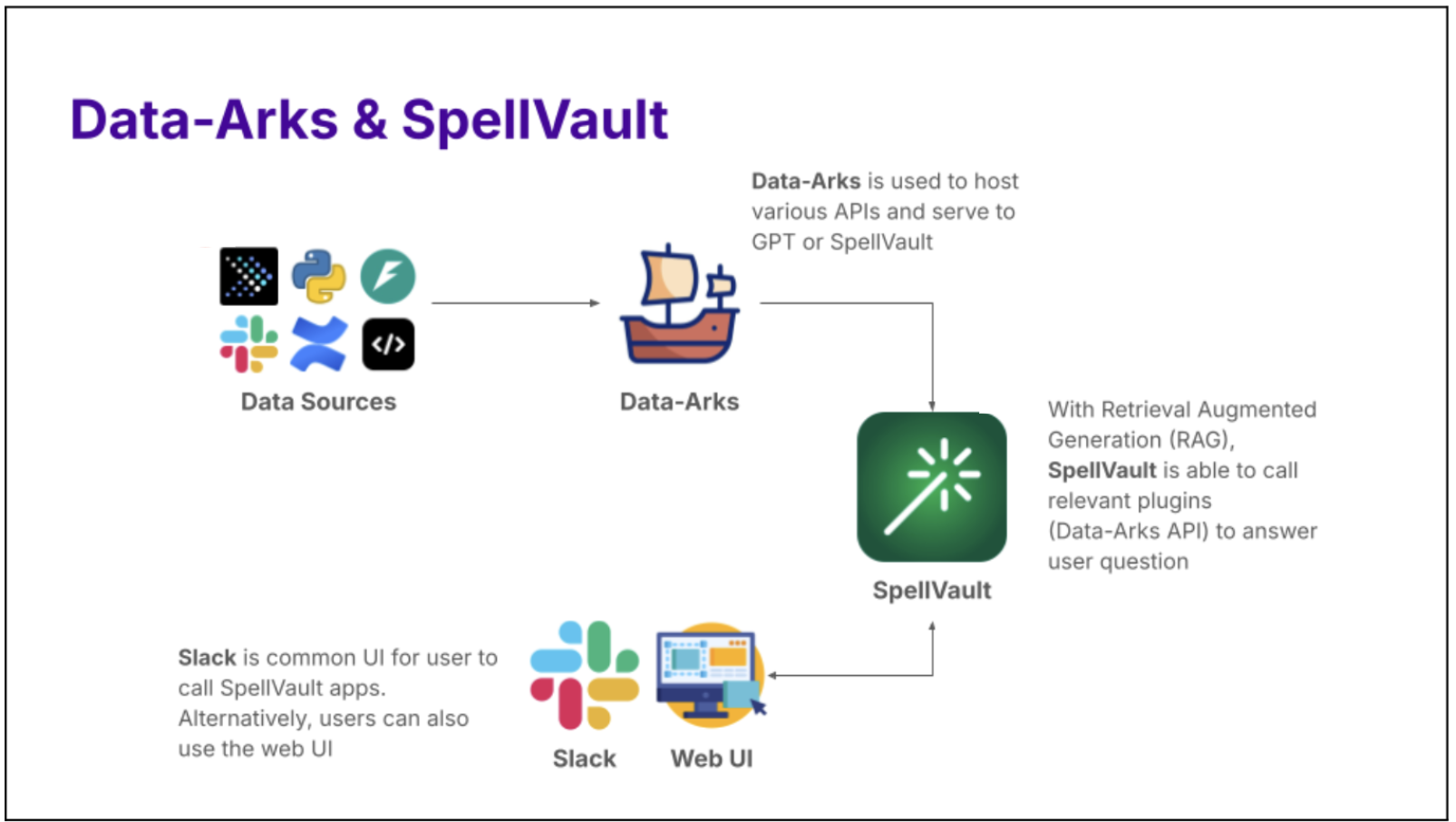
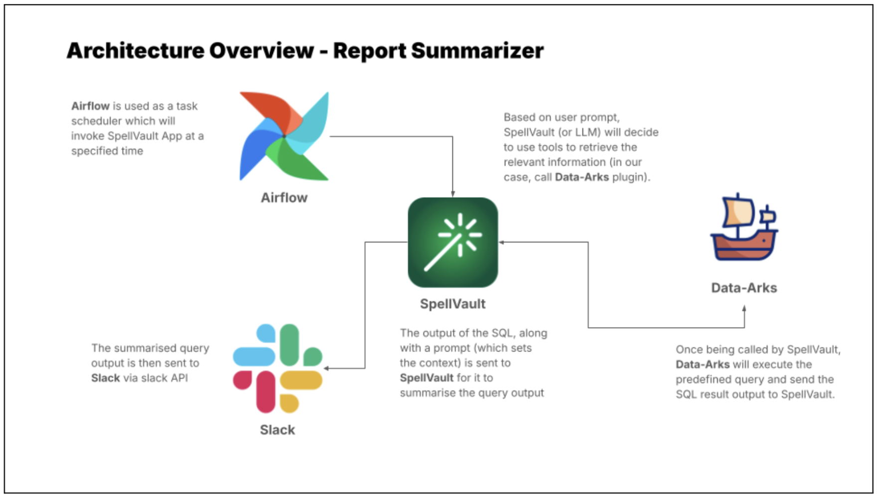
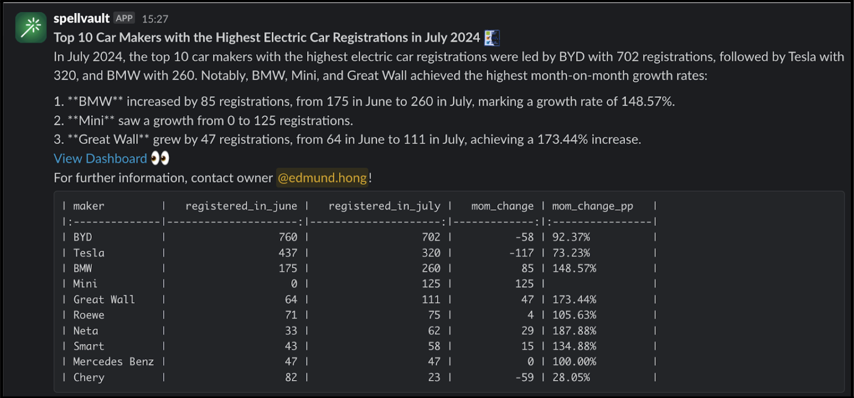
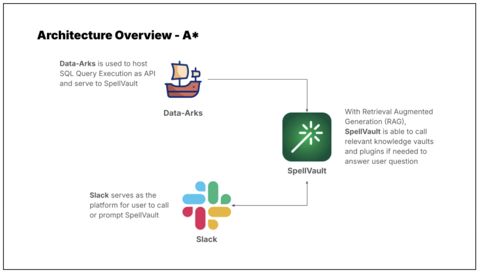
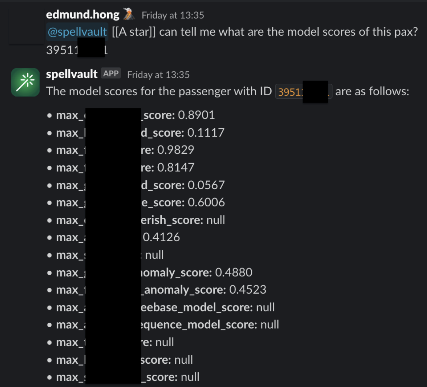
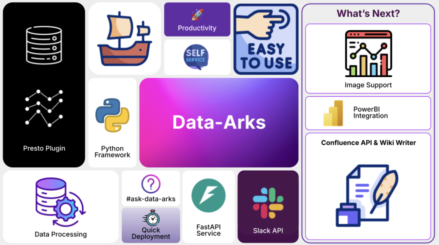
 Mert Hocanin is a Principal Big Data Architect with AWS Lake Formation.


 Kalaiselvi Kamaraj is a Sr. Software Development Engineer with Amazon. She has worked on several projects within Redshift Query processing team and currently focusing on performance related projects for Redshift Data Lake.
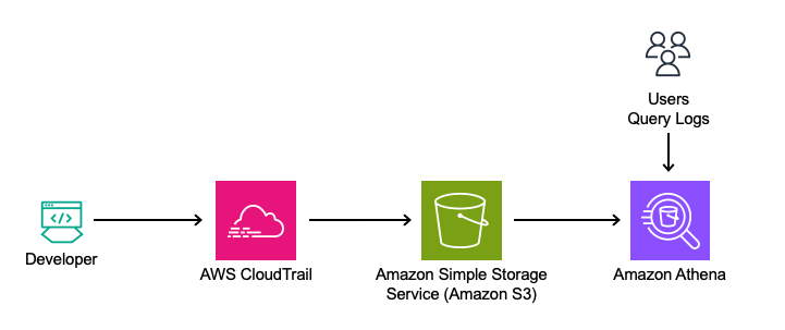
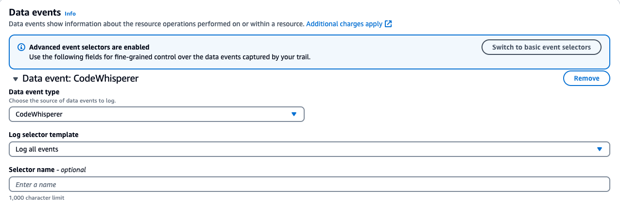


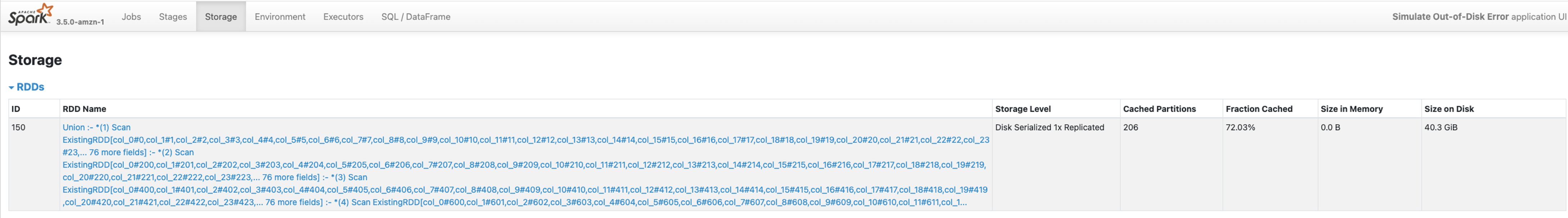
 Kashif Khan is a Sr. Analytics Specialist Solutions Architect at AWS, specializing in big data services like Amazon EMR, AWS Lake Formation, AWS Glue, Amazon Athena, and Amazon DataZone. With over a decade of experience in the big data domain, he possesses extensive expertise in architecting scalable and robust solutions. His role involves providing architectural guidance and collaborating closely with customers to design tailored solutions using AWS analytics services to unlock the full potential of their data.
 Veena Vasudevan is a Principal Partner Solutions Architect and Data & AI specialist at AWS. She helps customers and partners build highly optimized, scalable, and secure solutions; modernize their architectures; and migrate their big data, analytics, and AI/ML workloads to AWS.


 Manjit Chakraborty is a Senior Solutions Architect at AWS. He is a Seasoned & Result driven professional with extensive experience in Financial domain having worked with customers on advising, designing, leading, and implementing core-business enterprise solutions across the globe. In his spare time, Manjit enjoys fishing, practicing martial arts and playing with his daughter.
 Neeraj Roy is a Principal Solutions Architect at AWS based out of London. He works with Global Financial Services customers to accelerate their AWS journey. In his spare time, he enjoys reading and spending time with his family.


 Muthu Pitchaimani is a Search Specialist with Amazon OpenSearch Service. He builds large-scale search applications and solutions. Muthu is interested in the topics of networking and security, and is based out of Austin, Texas.
 Aruna Govindaraju is an Amazon OpenSearch Specialist Solutions Architect and has worked with many commercial and open source search engines. She is passionate about search, relevancy, and user experience. Her expertise with correlating end-user signals with search engine behavior has helped many customers improve their search experience.
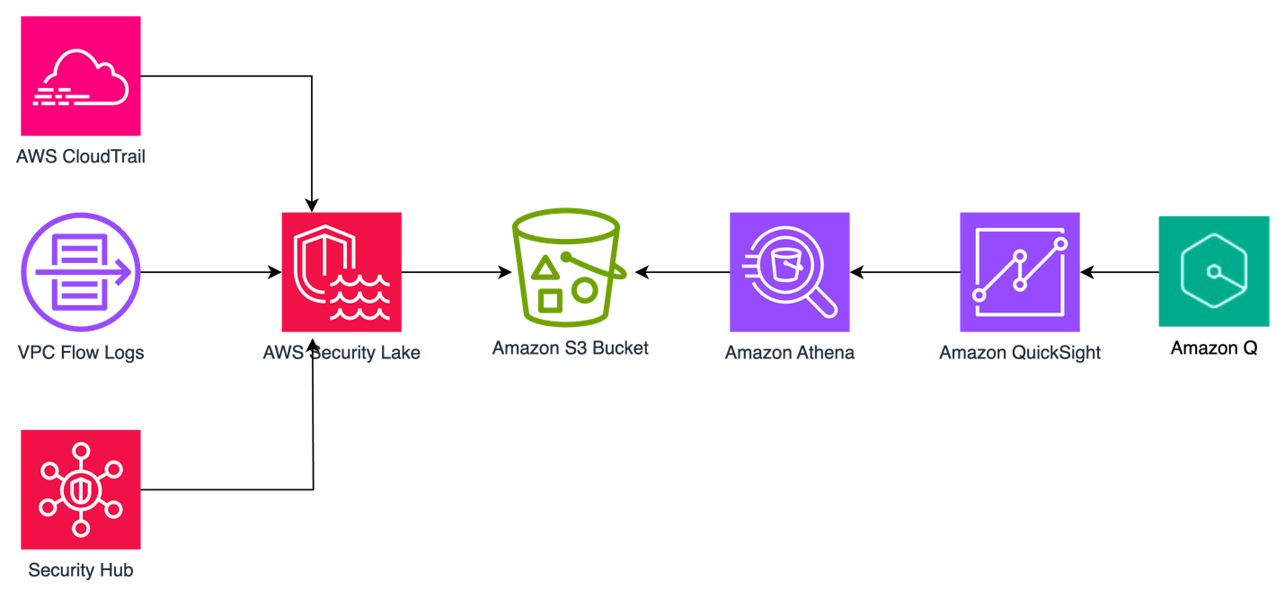
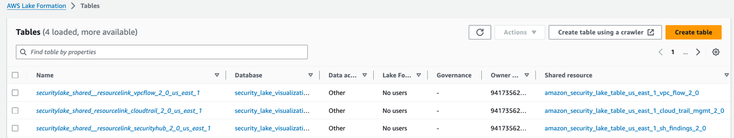


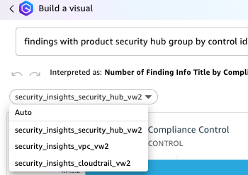


 Jon Handler is the Director of Solutions Architecture for Search Services at Amazon Web Services, based in Palo Alto, CA. Jon works closely with OpenSearch and Amazon OpenSearch Service, providing help and guidance to a broad range of customers who have search and log analytics workloads for OpenSearch. Prior to joining AWS, Jon’s career as a software developer included four years of coding a large-scale, eCommerce search engine. Jon holds a Bachelor of the Arts from the University of Pennsylvania, and a Master of Science and a Ph. D. in Computer Science and Artificial Intelligence from Northwestern University.


 Rajkumar Irudayaraj is a Senior Product Director at Salesforce with over 20 years of experience in data platforms and services, with a passion for delivering data-powered experiences to customers.
 Sriram Sethuraman is a Senior Manager in Salesforce Data Cloud product management. He has been building products for over 9 years using big data technologies. In his current role at Salesforce, Sriram works on Zero Copy integration with major data lake partners and helps customers deliver value with their data strategies.
 Jason Berkowitz is a Senior Product Manager with AWS Lake Formation. He comes from a background in machine learning and data lake architectures. He helps customers become data-driven.
 Ravi Bhattiprolu is a Senior Partner Solutions Architect at AWS. Ravi works with strategic ISV partners, Salesforce and Tableau, to deliver innovative and well-architected products and solutions that help joint customers achieve their business and technical objectives.
 Avijit Goswami is a Principal Solutions Architect at AWS specialized in data and analytics. He supports AWS strategic customers in building high-performing, secure, and scalable data lake solutions on AWS using AWS managed services and open source solutions. Outside of his work, Avijit likes to travel, hike, watch sports, and listen to music.
 Ife Stewart is a Principal Solutions Architect in the Strategic ISV segment at AWS. She has been engaged with Salesforce Data Cloud over the last 2 years to help build integrated customer experiences across Salesforce and AWS. Ife has over 10 years of experience in technology. She is an advocate for diversity and inclusion in the technology field.
 Michael Chess is a Technical Product Manager at AWS Lake Formation. He focuses on improving data permissions across the data lake. He is passionate about enabling customers to build and optimize their data lakes to meet stringent security requirements.
 Mike Patterson is a Senior Customer Solutions Manager in the Strategic ISV segment at AWS. He has partnered with Salesforce Data Cloud to align business objectives with innovative AWS solutions to achieve impactful customer experiences. In his spare time, he enjoys spending time with his family, sports, and outdoor activities.