Post Syndicated from Payal Singh original https://aws.amazon.com/blogs/big-data/use-snowflake-with-amazon-mwaa-to-orchestrate-data-pipelines/
This blog post is co-written with James Sun from Snowflake.
Customers rely on data from different sources such as mobile applications, clickstream events from websites, historical data, and more to deduce meaningful patterns to optimize their products, services, and processes. With a data pipeline, which is a set of tasks used to automate the movement and transformation of data between different systems, you can reduce the time and effort needed to gain insights from the data. Apache Airflow and Snowflake have emerged as powerful technologies for data management and analysis.
Amazon Managed Workflows for Apache Airflow (Amazon MWAA) is a managed workflow orchestration service for Apache Airflow that you can use to set up and operate end-to-end data pipelines in the cloud at scale. The Snowflake Data Cloud provides a single source of truth for all your data needs and allows your organizations to store, analyze, and share large amounts of data. The Apache Airflow open-source community provides over 1,000 pre-built operators (plugins that simplify connections to services) for Apache Airflow to build data pipelines.
In this post, we provide an overview of orchestrating your data pipeline using Snowflake operators in your Amazon MWAA environment. We define the steps needed to set up the integration between Amazon MWAA and Snowflake. The solution provides an end-to-end automated workflow that includes data ingestion, transformation, analytics, and consumption.
Overview of solution
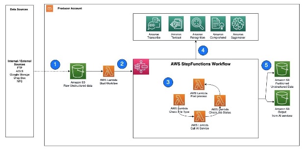
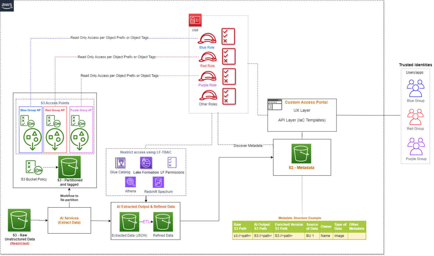
The following diagram illustrates our solution architecture.

The data used for transformation and analysis is based on the publicly available New York Citi Bike dataset. The data (zipped files), which includes rider demographics and trip data, is copied from the public Citi Bike Amazon Simple Storage Service (Amazon S3) bucket in your AWS account. Data is decompressed and stored in a different S3 bucket (transformed data can be stored in the same S3 bucket where data was ingested, but for simplicity, we’re using two separate S3 buckets). The transformed data is then made accessible to Snowflake for data analysis. The output of the queried data is published to Amazon Simple Notification Service (Amazon SNS) for consumption.
Amazon MWAA uses a directed acyclic graph (DAG) to run the workflows. In this post, we run three DAGs:
The following diagram illustrates this workflow.
See the GitHub repo for the DAGs and other files related to the post.
Note that in this post, we’re using a DAG to create a Snowflake connection, but you can also create the Snowflake connection using the Airflow UI or CLI.
Prerequisites
To deploy the solution, you should have a basic understanding of Snowflake and Amazon MWAA with the following prerequisites:
- An AWS account in an AWS Region where Amazon MWAA is supported.
- A Snowflake account with admin credentials. If you don’t have an account, sign up for a 30-day free trial. Select the Snowflake enterprise edition for the AWS Cloud platform.
- Access to Amazon MWAA, Secrets Manager, and Amazon SNS.
- In this post, we’re using two S3 buckets, called
airflow-blog-bucket-ACCOUNT_ID and citibike-tripdata-destination-ACCOUNT_ID. Amazon S3 supports global buckets, which means that each bucket name must be unique across all AWS accounts in all the Regions within a partition. If the S3 bucket name is already taken, choose a different S3 bucket name. Create the S3 buckets in your AWS account. We upload content to the S3 bucket later in the post. Replace ACCOUNT_ID with your own AWS account ID or any other unique identifier. The bucket details are as follows:
- airflow-blog-bucket-ACCOUNT_ID – The top-level bucket for Amazon MWAA-related files.
- airflow-blog-bucket-ACCOUNT_ID/requirements – The bucket used for storing the requirements.txt file needed to deploy Amazon MWAA.
- airflow-blog-bucket-ACCOUNT_ID/dags – The bucked used for storing the DAG files to run workflows in Amazon MWAA.
- airflow-blog-bucket-ACCOUNT_ID/dags/mwaa_snowflake_queries – The bucket used for storing the Snowflake SQL queries.
- citibike-tripdata-destination-ACCOUNT_ID – The bucket used for storing the transformed dataset.
When implementing the solution in this post, replace references to airflow-blog-bucket-ACCOUNT_ID and citibike-tripdata-destination-ACCOUNT_ID with the names of your own S3 buckets.
Set up the Amazon MWAA environment
First, you create an Amazon MWAA environment. Before deploying the environment, upload the requirements file to the airflow-blog-bucket-ACCOUNT_ID/requirements S3 bucket. The requirements file is based on Amazon MWAA version 2.6.3. If you’re testing on a different Amazon MWAA version, update the requirements file accordingly.
Complete the following steps to set up the environment:
- On the Amazon MWAA console, choose Create environment.
- Provide a name of your choice for the environment.
- Choose Airflow version 2.6.3.
- For the S3 bucket, enter the path of your bucket (
s3:// airflow-blog-bucket-ACCOUNT_ID).
- For the DAGs folder, enter the DAGs folder path (
s3:// airflow-blog-bucket-ACCOUNT_ID/dags).
- For the requirements file, enter the requirements file path (
s3:// airflow-blog-bucket-ACCOUNT_ID/ requirements/requirements.txt).
- Choose Next.
- Under Networking, choose your existing VPC or choose Create MWAA VPC.
- Under Web server access, choose Public network.
- Under Security groups, leave Create new security group selected.
- For the Environment class, Encryption, and Monitoring sections, leave all values as default.
- In the Airflow configuration options section, choose Add custom configuration value and configure two values:
- Set Configuration option to
secrets.backend and Custom value to airflow.providers.amazon.aws.secrets.secrets_manager.SecretsManagerBackend.
- Set Configuration option to
secrets.backend_kwargs and Custom value to {"connections_prefix" : "airflow/connections", "variables_prefix" : "airflow/variables"}. 
- In the Permissions section, leave the default settings and choose Create a new role.
- Choose Next.
- When the Amazon MWAA environment us available, assign S3 bucket permissions to the AWS Identity and Access Management (IAM) execution role (created during the Amazon MWAA install).

This will direct you to the created execution role on the IAM console.
For testing purposes, you can choose Add permissions and add the managed AmazonS3FullAccess policy to the user instead of providing restricted access. For this post, we provide only the required access to the S3 buckets.
- On the drop-down menu, choose Create inline policy.
- For Select Service, choose S3.
- Under Access level, specify the following:
- Expand List level and select
ListBucket.
- Expand Read level and select
GetObject.
- Expand Write level and select
PutObject.
- Under Resources, choose Add ARN.
- On the Text tab, provide the following ARNs for S3 bucket access:
arn:aws:s3:::airflow-blog-bucket-ACCOUNT_ID (use your own bucket).arn:aws:s3:::citibike-tripdata-destination-ACCOUNT_ID (use your own bucket).arn:aws:s3:::tripdata (this is the public S3 bucket where the Citi Bike dataset is stored; use the ARN as specified here).
- Under Resources, choose Add ARN.
- On the Text tab, provide the following ARNs for S3 bucket access:
arn:aws:s3:::airflow-blog-bucket-ACCOUNT_ID/* (make sure to include the asterisk).arn:aws:s3:::citibike-tripdata-destination-ACCOUNT_ID /*.arn:aws:s3:::tripdata/* (this is the public S3 bucket where the Citi Bike dataset is stored, use the ARN as specified here).
- Choose Next.
- For Policy name, enter
S3ReadWrite.
- Choose Create policy.
- Lastly, provide Amazon MWAA with permission to access Secrets Manager secret keys.
This step provides the Amazon MWAA execution role for your Amazon MWAA environment read access to the secret key in Secrets Manager.
The execution role should have the policies MWAA-Execution-Policy*, S3ReadWrite, and SecretsManagerReadWrite attached to it.

When the Amazon MWAA environment is available, you can sign in to the Airflow UI from the Amazon MWAA console using link for Open Airflow UI.

Set up an SNS topic and subscription
Next, you create an SNS topic and add a subscription to the topic. Complete the following steps:
- On the Amazon SNS console, choose Topics from the navigation pane.
- Choose Create topic.
- For Topic type, choose Standard.
- For Name, enter
mwaa_snowflake.
- Leave the rest as default.
- After you create the topic, navigate to the Subscriptions tab and choose Create subscription.

- For Topic ARN, choose
mwaa_snowflake.
- Set the protocol to Email.
- For Endpoint, enter your email ID (you will get a notification in your email to accept the subscription).
By default, only the topic owner can publish and subscribe to the topic, so you need to modify the Amazon MWAA execution role access policy to allow Amazon SNS access.
- On the IAM console, navigate to the execution role you created earlier.
- On the drop-down menu, choose Create inline policy.
- For Select service, choose SNS.
- Under Actions, expand Write access level and select Publish.
- Under Resources, choose Add ARN.
- On the Text tab, specify the ARN
arn:aws:sns:<<region>>:<<our_account_ID>>:mwaa_snowflake.
- Choose Next.
- For Policy name, enter
SNSPublishOnly.
- Choose Create policy.
Configure a Secrets Manager secret
Next, we set up Secrets Manager, which is a supported alternative database for storing Snowflake connection information and credentials.
To create the connection string, the Snowflake host and account name is required. Log in to your Snowflake account, and under the Worksheets menu, choose the plus sign and select SQL worksheet. Using the worksheet, run the following SQL commands to find the host and account name.
Run the following query for the host name:
WITH HOSTLIST AS
(SELECT * FROM TABLE(FLATTEN(INPUT => PARSE_JSON(SYSTEM$allowlist()))))
SELECT REPLACE(VALUE:host,'"','') AS HOST
FROM HOSTLIST
WHERE VALUE:type = 'SNOWFLAKE_DEPLOYMENT_REGIONLESS';
Run the following query for the account name:
WITH HOSTLIST AS
(SELECT * FROM TABLE(FLATTEN(INPUT => PARSE_JSON(SYSTEM$allowlist()))))
SELECT REPLACE(VALUE:host,'.snowflakecomputing.com','') AS ACCOUNT
FROM HOSTLIST
WHERE VALUE:type = 'SNOWFLAKE_DEPLOYMENT';
Next, we configure the secret in Secrets Manager.
- On the Secrets Manager console, choose Store a new secret.
- For Secret type, choose Other type of secret.
- Under Key/Value pairs, choose the Plaintext tab.
- In the text field, enter the following code and modify the string to reflect your Snowflake account information:
{"host": "<<snowflake_host_name>>", "account":"<<snowflake_account_name>>","user":"<<snowflake_username>>","password":"<<snowflake_password>>","schema":"mwaa_schema","database":"mwaa_db","role":"accountadmin","warehouse":"dev_wh"}
For example:
{"host": "xxxxxx.snowflakecomputing.com", "account":"xxxxxx" ,"user":"xxxxx","password":"*****","schema":"mwaa_schema","database":"mwaa_db", "role":"accountadmin","warehouse":"dev_wh"}
The values for the database name, schema name, and role should be as mentioned earlier. The account, host, user, password, and warehouse can differ based on your setup.

Choose Next.
- For Secret name, enter
airflow/connections/snowflake_accountadmin.
- Leave all other values as default and choose Next.
- Choose Store.
Take note of the Region in which the secret was created under Secret ARN. We later define it as a variable in the Airflow UI.
Configure Snowflake access permissions and IAM role
Next, log in to your Snowflake account. Ensure the account you are using has account administrator access. Create a SQL worksheet. Under the worksheet, create a warehouse named dev_wh.
The following is an example SQL command:
CREATE OR REPLACE WAREHOUSE dev_wh
 WITH WAREHOUSE_SIZE = 'xsmall'
 AUTO_SUSPEND = 60
 INITIALLY_SUSPENDED = true
 AUTO_RESUME = true
 MIN_CLUSTER_COUNT = 1
 MAX_CLUSTER_COUNT = 5;
For Snowflake to read data from and write data to an S3 bucket referenced in an external (S3 bucket) stage, a storage integration is required. Follow the steps defined in Option 1: Configuring a Snowflake Storage Integration to Access Amazon S3(only perform Steps 1 and 2, as described in this section).
Configure access permissions for the S3 bucket
While creating the IAM policy, a sample policy document code is needed (see the following code), which provides Snowflake with the required permissions to load or unload data using a single bucket and folder path. The bucket name used in this post is citibike-tripdata-destination-ACCOUNT_ID. You should modify it to reflect your bucket name.
{
  "Version": "2012-10-17",
  "Statement": [
    {
      "Effect": "Allow",
      "Action": [
        "s3:PutObject",
        "s3:GetObject",
        "s3:GetObjectVersion",
        "s3:DeleteObject",
        "s3:DeleteObjectVersion"
      ],
      "Resource": "arn:aws:s3::: citibike-tripdata-destination-ACCOUNT_ID/*"
    },
    {
      "Effect": "Allow",
      "Action": [
        "s3:ListBucket",
        "s3:GetBucketLocation"
      ],
      "Resource": "arn:aws:s3:::citibike-tripdata-destination-ACCOUNT_ID"
    }
  ]
}
Create the IAM role
Next, you create the IAM role to grant privileges on the S3 bucket containing your data files. After creation, record the Role ARN value located on the role summary page.

Configure variables
Lastly, configure the variables that will be accessed by the DAGs in Airflow. Log in to the Airflow UI and on the Admin menu, choose Variables and the plus sign.

Add four variables with the following key/value pairs:
- Key
aws_role_arn with value <<snowflake_aws_role_arn>> (the ARN for role mysnowflakerole noted earlier)
- Key
destination_bucket with value <<bucket_name>> (for this post, the bucket used in citibike-tripdata-destination-ACCOUNT_ID)
- Key
target_sns_arn with value <<sns_Arn>> (the SNS topic in your account)
- Key
sec_key_region with value <<region_of_secret_deployment>> (the Region where the secret in Secrets Manager was created)
The following screenshot illustrates where to find the SNS topic ARN.

The Airflow UI will now have the variables defined, which will be referred to by the DAGs.

Congratulations, you have completed all the configuration steps.
Run the DAG
Let’s look at how to run the DAGs. To recap:
- DAG1 (create_snowflake_connection_blog.py) – Creates the Snowflake connection in Apache Airflow. This connection will be used to authenticate with Snowflake. The Snowflake connection string is stored in Secrets Manager, which is referenced in the DAG file.
- DAG2 (create-snowflake_initial-setup_blog.py) – Creates the database, schema, storage integration, and stage in Snowflake.
- DAG3 (run_mwaa_datapipeline_blog.py) – Runs the data pipeline, which will unzip files from the source public S3 bucket and copy them to the destination S3 bucket. The next task will create a table in Snowflake to store the data. Then the data from the destination S3 bucket will be copied into the table using a Snowflake stage. After the data is successfully copied, a view will be created in Snowflake, on top of which the SQL queries will be run.
To run the DAGs, complete the following steps:
- Upload the DAGs to the S3 bucket
airflow-blog-bucket-ACCOUNT_ID/dags.
- Upload the SQL query files to the S3 bucket
airflow-blog-bucket-ACCOUNT_ID/dags/mwaa_snowflake_queries.
- Log in to the Apache Airflow UI.
- Locate DAG1 (
create_snowflake_connection_blog), un-pause it, and choose the play icon to run it.
You can view the run state of the DAG using the Grid or Graph view in the Airflow UI.

After DAG1 runs, the Snowflake connection snowflake_conn_accountadmin is created on the Admin, Connections menu.
- Locate and run DAG2 (
create-snowflake_initial-setup_blog).
After DAG2 runs, the following objects are created in Snowflake:
- The database
mwaa_db
- The schema
mwaa_schema
- The storage integration
mwaa_citibike_storage_int
- The stage
mwaa_citibike_stg
Before running the final DAG, the trust relationship for the IAM user needs to be updated.
- Log in to your Snowflake account using your admin account credentials.
- Open your SQL worksheet created earlier and run the following command:
DESC INTEGRATION mwaa_citibike_storage_int;
mwaa_citibike_storage_int is the name of the integration created by the DAG2 in the previous step.
From the output, record the property value of the following two properties:
- STORAGE_AWS_IAM_USER_ARN – The IAM user created for your Snowflake account.
- STORAGE_AWS_EXTERNAL_ID – The external ID that is needed to establish a trust relationship.
Now we grant the Snowflake IAM user permissions to access bucket objects.
- On the IAM console, choose Roles in the navigation pane.
- Choose the role
mysnowflakerole.
- On the Trust relationships tab, choose Edit trust relationship.
- Modify the policy document with the
DESC STORAGE INTEGRATION output values you recorded. For example:
{
  "Version": "2012-10-17",
  "Statement": [
    {
      "Effect": "Allow",
      "Principal": {
        "AWS": "arn:aws:iam::5xxxxxxxx:user/mgm4-s- ssca0079"
      },
      "Action": "sts:AssumeRole",
      "Condition": {
        "StringEquals": {
          "sts:ExternalId": "AWSPARTNER_SFCRole=4_vsarJrupIjjJh77J9Nxxxx/j98="
        }
      }
    }
  ]
}
The AWS role ARN and ExternalId will be different for your environment based on the output of the DESC STORAGE INTEGRATION query

- Locate and run the final DAG (
run_mwaa_datapipeline_blog).
At the end of the DAG run, the data is ready for querying. In this example, the query (finding the top start and destination stations) is run as part of the DAG and the output can be viewed from the Airflow XCOMs UI.

In the DAG run, the output is also published to Amazon SNS and based on the subscription, an email notification is sent out with the query output.

Another method to visualize the results is directly from the Snowflake console using the Snowflake worksheet. The following is an example query:
SELECT START_STATION_NAME,
COUNT(START_STATION_NAME) C FROM MWAA_DB.MWAA_SCHEMA.CITIBIKE_VW
GROUP BY
START_STATION_NAME ORDER BY C DESC LIMIT 10;

There are different ways to visualize the output based on your use case.
As we observed, DAG1 and DAG2 need to be run only one time to set up the Amazon MWAA connection and Snowflake objects. DAG3 can be scheduled to run every week or month. With this solution, the user examining the data doesn’t have to log in to either Amazon MWAA or Snowflake. You can have an automated workflow triggered on a schedule that will ingest the latest data from the Citi Bike dataset and provide the top start and destination stations for the given dataset.
Clean up
To avoid incurring future charges, delete the AWS resources (IAM users and roles, Secrets Manager secrets, Amazon MWAA environment, SNS topics and subscription, S3 buckets) and Snowflake resources (database, stage, storage integration, view, tables) created as part of this post.
Conclusion
In this post, we demonstrated how to set up an Amazon MWAA connection for authenticating to Snowflake as well as to AWS using AWS user credentials. We used a DAG to automate creating the Snowflake objects such as database, tables, and stage using SQL queries. We also orchestrated the data pipeline using Amazon MWAA, which ran tasks related to data transformation as well as Snowflake queries. We used Secrets Manager to store Snowflake connection information and credentials and Amazon SNS to publish the data output for end consumption.
With this solution, you have an automated end-to-end orchestration of your data pipeline encompassing ingesting, transformation, analysis, and data consumption.
To learn more, refer to the following resources:
About the authors
 Payal Singh is a Partner Solutions Architect at Amazon Web Services, focused on the Serverless platform. She is responsible for helping partner and customers modernize and migrate their applications to AWS.
 James Sun is a Senior Partner Solutions Architect at Snowflake. He actively collaborates with strategic cloud partners like AWS, supporting product and service integrations, as well as the development of joint solutions. He has held senior technical positions at tech companies such as EMC, AWS, and MapR Technologies. With over 20 years of experience in storage and data analytics, he also holds a PhD from Stanford University.
 Bosco Albuquerque is a Sr. Partner Solutions Architect at AWS and has over 20 years of experience working with database and analytics products from enterprise database vendors and cloud providers. He has helped technology companies design and implement data analytics solutions and products.
 Manuj Arora is a Sr. Solutions Architect for Strategic Accounts in AWS. He focuses on Migration and Modernization capabilities and offerings in AWS. Manuj has worked as a Partner Success Solutions Architect in AWS over the last 3 years and worked with partners like Snowflake to build solution blueprints that are leveraged by the customers. Outside of work, he enjoys traveling, playing tennis and exploring new places with family and friends.


 Roy (KDS) Wang is a Senior Product Manager with Amazon Kinesis Data Streams. He is passionate about learning from and collaborating with customers to help organizations run faster and smarter. Outside of work, Roy strives to be a good dad to his new son and builds plastic model kits.
 Ali Alemi is a Streaming Specialist Solutions Architect at AWS. Ali advises AWS customers with architectural best practices and helps them design real-time analytics data systems that are reliable, secure, efficient, and cost-effective. He works backward from customer’s use cases and designs data solutions to solve their business problems. Prior to joining AWS, Ali supported several public sector customers and AWS consulting partners in their application modernization journey and migration to the Cloud.
 Imtiaz (Taz) Sayed is the WW Tech Leader for Analytics at AWS. He enjoys engaging with the community on all things data and analytics. He can be reached via
  Navnit Shukla serves as an AWS Specialist Solution Architect with a focus on Analytics. He possesses a strong enthusiasm for assisting clients in discovering valuable insights from their data. Through his expertise, he constructs innovative solutions that empower businesses to arrive at informed, data-driven choices. Notably, Navnit Shukla is the accomplished author of the book titled “Data Wrangling on AWS.” He can be reached via
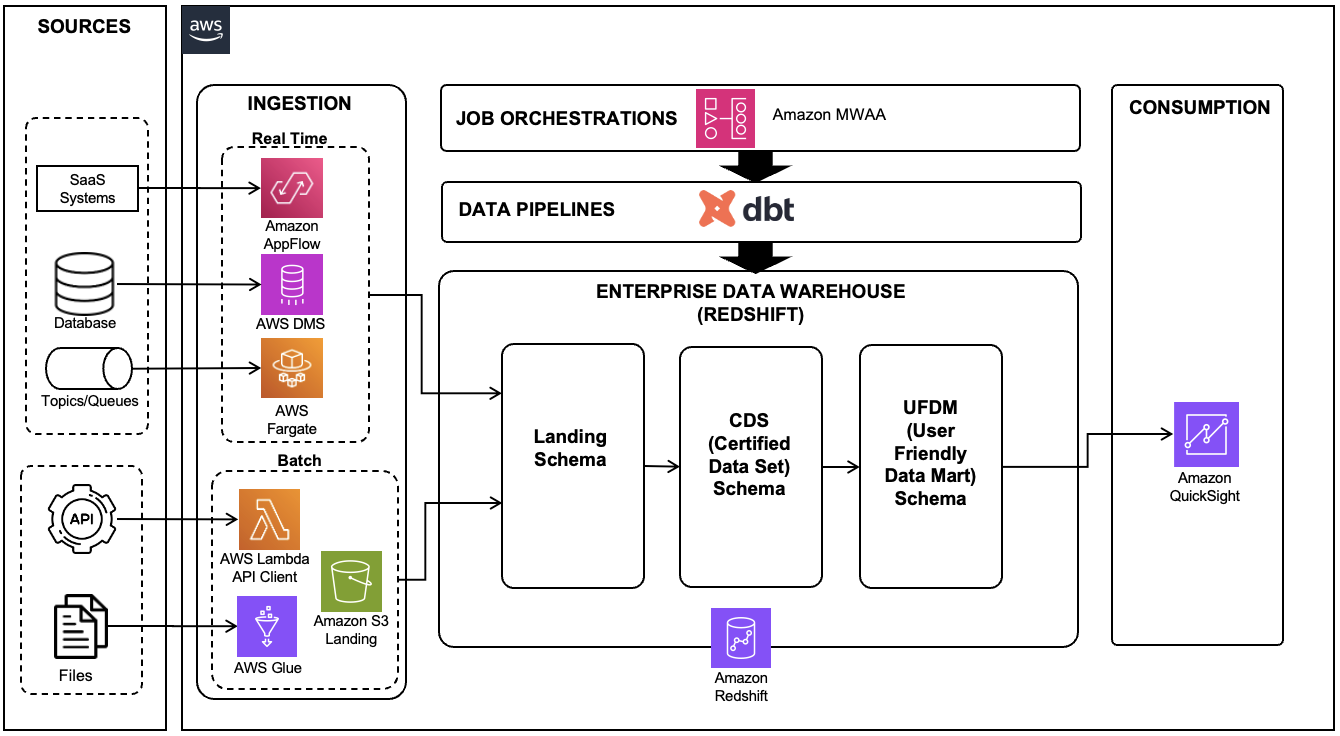


 Prantik Gachhayat is an Enterprise Architect at Infosys having experience in various technology fields and business domains. He has a proven track record helping large enterprises modernize digital platforms and delivering complex transformation programs. Prantik specializes in architecting modern data and analytics platforms in AWS. Prantik loves exploring new tech trends and enjoys cooking.
 Ashutosh Dubey is a Senior Partner Solutions Architect and Global Tech leader at Amazon Web Services based out of New Jersey, USA. He has extensive experience specializing in the Data and Analytics and AIML field including generative AI, contributed to the community by writing various tech contents, and has helped Fortune 500 companies in their cloud journey to AWS.


 Michael Hamilton is a Sr Analytics Solutions Architect focusing on helping enterprise customers in the south east modernize and simplify their analytics workloads on AWS. He enjoys mountain biking and spending time with his wife and three children when not working.
 Cody Penta is a Solutions Architect at Amazon Web Services and is based out of Charlotte, NC. He has a focus in security and CDK, and enjoys solving the really difficult problems in the technology world. Off the clock, he loves relaxing in the mountains, coding personal projects, and gaming.
 Angus Ferguson is a Solutions Architect at AWS who is passionate about meeting customers across the world, helping them solve their technical challenges. Angus specializes in Data & Analytics with a focus on customers in the financial services industry.
 Mukul Sharma is a Software Development Engineer on Data & Analytics (DnA) organization at GoDaddy. He is a polyglot programmer with experience in a wide array of technologies to rapidly deliver scalable solutions. He enjoys singing karaoke, playing various board games, and working on personal programming projects in his spare time.
 Ozcan Ilikhan is a Director of Engineering on Data & Analytics (DnA) organization at GoDaddy. He is passionate about solving customer problems and increasing efficiency using data and ML/AI. In his spare time, he loves reading, hiking, gardening, and working on DIY projects.
 Harsh Vardhan Singh Gaur is an AWS Solutions Architect, specializing in analytics. He has over 6 years of experience working in the field of big data and data science. He is passionate about helping customers adopt best practices and discover insights from their data.
 Ramesh Kumar Venkatraman is a Senior Solutions Architect at AWS who is passionate about containers and databases. He works with AWS customers to design, deploy, and manage their AWS workloads and architectures. In his spare time, he loves to play with his two kids and follows cricket.
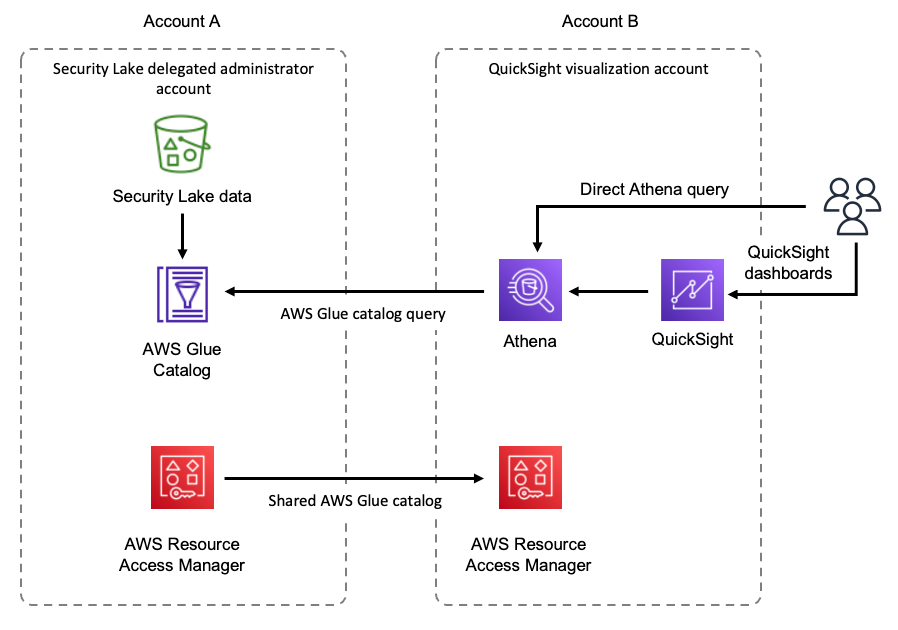


 Phil Bates is a Senior Analytics Specialist Solutions Architect at AWS. He has more than 25 years of experience implementing large-scale data warehouse solutions. He is passionate about helping customers through their cloud journey and using the power of ML within their data warehouse.
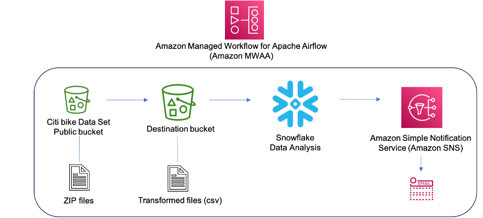


 John Cherian is Senior Solutions Architect(SA) at Amazon Web Services helps customers with strategy and architecture for building solutions on AWS.
 Emerson Antony is Senior Cloud Architect at Amazon Web Services helps customers with implementing AWS solutions.
 Kiran Anand is Principal AWS Data Lab Architect at Amazon Web Services helps customers with Big data & Analytics architecture.


 Kartikay Khator is a Solutions Architect in Global Life Sciences at Amazon Web Services (AWS). He is passionate about building innovative and scalable solutions to meet the needs of customers, focusing on AWS Analytics services. Beyond the tech world, he is an avid runner and enjoys hiking.
 Kamen Sharlandjiev is a Sr. Big Data and ETL Solutions Architect and Amazon AppFlow expert. He’s on a mission to make life easier for customers who are facing complex data integration challenges. His secret weapon? Fully managed, low-code AWS services that can get the job done with minimal effort and no coding.
 Anshul Sharma is a Software Development Engineer in AWS Glue Team. He is driving the connectivity charter which provide Glue customer native way of connecting any Data source (Data-warehouse, Data-lakes, NoSQL etc) to Glue ETL Jobs. Beyond the tech world, he is a cricket and soccer lover.


 Stefan Gromoll is a Senior Performance Engineer with Amazon Redshift team where he is responsible for measuring and improving Redshift performance. In his spare time, he enjoys cooking, playing with his three boys, and chopping firewood.
 Aamer Shah is a Senior Engineer in the Amazon Redshift Service team.
 Sanket Hase is a Software Development Manager in the Amazon Redshift Service team.
 Orestis Polychroniou is a Principal Engineer in the Amazon Redshift Service team.
 Prashant Agrawal is a Sr. Search Specialist Solutions Architect with Amazon OpenSearch Service. He works closely with customers to help them migrate their workloads to the cloud and helps existing customers fine-tune their clusters to achieve better performance and save on cost. Before joining AWS, he helped various customers use OpenSearch and Elasticsearch for their search and log analytics use cases. When not working, you can find him traveling and exploring new places. In short, he likes doing Eat → Travel → Repeat.


 Mikhail Vaynshteyn is a Solutions Architect with Amazon Web Services. Mikhail works with healthcare and life sciences customers to build solutions that help improve patients’ outcomes. Mikhail specializes in data analytics services.
 Muthu Pitchaimani is a Search Specialist with Amazon OpenSearch Service. He builds large-scale search applications and solutions. Muthu is interested in the topics of networking and security, and is based out of Austin, Texas.

 Sakti Mishra is a Principal Solutions Architect at AWS, where he helps customers modernize their data architecture and define their end-to-end data strategy, including data security, accessibility, governance, and more. He is also the author of the book
  Bhavana Chirumamilla is a Senior Resident Architect at AWS with a strong passion for data and machine learning operations. She brings a wealth of experience and enthusiasm to help enterprises build effective data and ML strategies. In her spare time, Bhavana enjoys spending time with her family and engaging in various activities such as traveling, hiking, gardening, and watching documentaries.
 Sheela Sonone is a Senior Resident Architect at AWS. She helps AWS customers make informed choices and trade-offs about accelerating their data, analytics, and AI/ML workloads and implementations. In her spare time, she enjoys spending time with her family—usually on tennis courts.
 Daniel Bruno is a Principal Resident Architect at AWS. He had been building analytics and machine learning solutions for over 20 years and splits his time helping customers build data science programs and designing impactful ML products.


 Aish Gunasekar is a Specialist Solutions Architect with a focus on Amazon OpenSearch Service. Her passion at AWS is to help customers design highly scalable architectures and help them in their cloud adoption journey. Outside of work, she enjoys hiking and baking.
 Satish Nandi is a Senior Technical Product Manager for Amazon OpenSearch Service.
 Jon Handler is a Senior Principal Solutions Architect at Amazon Web Services based in Palo Alto, CA. Jon works closely with OpenSearch and Amazon OpenSearch Service, providing help and guidance to a broad range of customers who have search and log analytics workloads that they want to move to the AWS Cloud. Prior to joining AWS, Jon’s career as a software developer included 4 years of coding a large-scale, ecommerce search engine. Jon holds a Bachelor of the Arts from the University of Pennsylvania, and a Master of Science and a PhD in Computer Science and Artificial Intelligence from Northwestern University.


 This will start a new session with the updated parameters.


 Pathik Shah is a Sr. Analytics Architect on Amazon Athena. He joined AWS in 2015 and has been focusing in the big data analytics space since then, helping customers build scalable and robust solutions using AWS analytics services.
 Raj Devnath is a Product Manager at AWS on Amazon Athena. He is passionate about building products customers love and helping customers extract value from their data. His background is in delivering solutions for multiple end markets, such as finance, retail, smart buildings, home automation, and data communication systems.