Post Syndicated from Amar Surjit original https://aws.amazon.com/blogs/big-data/resolve-private-dns-hostnames-for-amazon-msk-connect/
Amazon MSK Connect is a feature of Amazon Managed Streaming for Apache Kafka (Amazon MSK) that offers a fully managed Apache Kafka Connect environment on AWS. With MSK Connect, you can deploy fully managed connectors built for Kafka Connect that move data into or pull data from popular data stores like Amazon S3 and Amazon OpenSearch Service. With the introduction of the Private DNS support into MSK Connect, connectors are able to resolve private customer domain names, using their DNS servers configured in the customer VPC DHCP Options set. This post demonstrates a solution for resolving private DNS hostnames defined in a customer VPC for MSK Connect.
You may want to use private DNS hostname support for MSK Connect for multiple reasons. Before the private DNS resolution capability included with MSK Connect, it used the service VPC DNS resolver for DNS resolution. MSK Connect didn’t use the private DNS servers defined in the customer VPC DHCP option sets for DNS resolution. The connectors were only able to reference hostnames in the connector configuration or plugin that are publicly resolvable and couldn’t resolve private hostnames defined in either a private hosted zone or use DNS servers in another customer network.
Many customers ensure that their internal DNS applications are not publicly resolvable. For example, you might have a MySQL or PostgreSQL database and may not want the DNS name for your database to be publicly resolvable or accessible. Amazon Relational Database Service (Amazon RDS) or Amazon Aurora servers have DNS names that are publicly resolvable but not accessible. You can have multiple internal applications such as databases, data warehouses, or other systems where DNS names are not publicly resolvable.
With the recent launch of MSK Connect private DNS support, you can configure connectors to reference public or private domain names. Connectors use the DNS servers configured in your VPC’s DHCP option set to resolve domain names. You can now use MSK Connect to privately connect with databases, data warehouses, and other resources in your VPC to comply with your security needs.
If you have a MySQL or PostgreSQL database with private DNS, you can configure it on a custom DNS server and configure the VPC-specific DHCP option set to do the DNS resolution using the custom DNS server local to the VPC instead of using the service DNS resolution.
Solution overview
A customer can have different architecture options to set up their MSK Connect. For example, they can have Amazon MSK and MSK Connect are in the same VPC or source system in VPC1 and Amazon MSK and MSK Connect are in VPC2 or source system, Amazon MSK and MSK Connect are all in different VPCs.
The following setup uses two different VPCs, where the MySQL VPC hosts the MySQL database and the MSK VPC hosts Amazon MSK, MSK Connect, the DNS server, and various other components. You can extend this architecture to support other deployment topologies using appropriate AWS Identity and Access Management (IAM) permissions and connectivity options.
This post provides step-by-step instructions to set up MSK Connect where it will receive data from a source MySQL database with private DNS hostname in the MySQL VPC and send data to Amazon MSK using MSK Connect in another VPC. The following diagram illustrates the high-level architecture.

The setup instructions include the following key steps:
- Set up the VPCs, subnets, and other core infrastructure components.
- Install and configure the DNS server.
- Upload the data to the MySQL database.
- Deploy Amazon MSK and MSK Connect and consume the change data capture (CDC) records.
Prerequisites
To follow the tutorial in this post, you need the following:
- An AWS account.
- Permission to run an AWS CloudFormation script to create the services mentioned in the solution architecture.
- An Amazon Elastic Compute Cloud (Amazon EC2) key pair. For instructions, refer to create key-pair here.
- The following two parameters using Parameter Store, a capability of AWS Systems Manager, using the AWS Management Console or AWS Command Line Interface (AWS CLI). We use these parameters for the MySQL database root user and primary user password:
/Database/Credentials/root/Database/Credentials/master
Create the required infrastructure using AWS CloudFormation
Before configuring the MSK Connect, we need to set up the VPCs, subnets, and other core infrastructure components. To set up resources in your AWS account, complete the following steps:
- Choose Launch Stack to launch the stack in a Region that supports Amazon MSK and MSK Connect.

- Specify the private key that you use to connect to the EC2 instances.
- Update the SSH location with your local IP address and keep the other values as default.
- Choose Next.
- Review the details on the final page and select I acknowledge that AWS CloudFormation might create IAM resources.
- Choose Create stack and wait for the required resources to get created.
The CloudFormation template creates the following key resources in your account:
- VPCs:
- MSK VPC
- MySQL VPC
- Subnets in the MSK VPC:
- Three private subnets for Amazon MSK
- Private subnet for DNS server
- Private subnet for MSKClient
- Public subnet for bastion host
- Subnets in the MySQL VPC:
- Private subnet for MySQL database
- Public subnet for bastion host
- Internet gateway attached to the MySQL VPC and MSK VPC
- NAT gateways attached to MySQL public subnet and MSK public subnet
- Route tables to support the traffic flow between different subnets in a VPC and across VPCs
- Peering connection between the MySQL VPC and MSK VPC
- MySQL database and configurations
- DNS server
- MSK client with respective libraries
Please note, if you’re using VPC peering or AWS Transit Gateway with MSK Connect, don’t configure your connector for reaching the peered VPC resources with IPs in the CIDR ranges. For more information, refer to Connecting from connectors.
Configure the DNS server
Complete the following steps to configure the DNS server:
- Connect to the DNS server. There are three configuration files available on the DNS server under the
/home/ec2-userfolder:named.confmysql.internal.zonekafka.us-east-1.amazonaws.com.zone
- Run the following commands to install and configure your DNS server:
- Update
/etc/named.conf.
For the allow-transfer attribute, update the DNS server internal IP address to allow-transfer
{ localhost; <DNS Server internal IP address>; };.
You can find the DNS server IP address on the CloudFormation template Outputs tab.
Note that the MSK cluster is still not set up at this stage. We need to update the Kafka broker DNS names and their respective internal IP addresses in the /var/named/kafka.region.amazonaws.com configuration file after setting up the MSK cluster later in this post. For instructions, refer to here.
Also note that these settings configure the DNS server for this post. In your own environment, you can configure the DNS server as per your needs.
- Restart the DNS service:
You should see the following message:
Upload the data to the MySQL database
Typically, we can use an Amazon RDS for MySQL database, but for this post, we use custom MySQL database servers. The Amazon RDS DNS is publicly accessible and MSK Connect supports it, but it was not able to support databases or applications with private DNS in the past. With the latest private DNS hostnames feature launch, it can support applications’ private DNS as well, so we use a MySQL database on the EC2 instance.
This installation provides information about setting up the MySQL database on a single-node EC2 instance. This should not be used for your production setup. You should follow appropriate guidance for setting up and configuring MySQL in your account.
The MySQL database is already set up using the CloudFormation template and is ready to use now. To upload the data, complete the followings steps:
- SSH to the MySQL EC2 instance. For instructions, refer to Connect to your Linux instance. The data file
salesdb.sqlis already downloaded and available under the/home/ec2-userdirectory. - Log in to mysqldb with the user name master.
- To access the password, navigate to AWS Systems Manager and Parameter Store tab. Select /Database/Credentials/master and click on View Details and copy the value for the key.
- Log in to MySQL using the following command:
- Run the following commands to create the
salesdbdatabase and load the data to the table:
This will insert the records in various different tables in the salesdb database.
- Run show tables to see the following tables in the
salesdb:
Create a DHCP option set
DHCP option sets give you control over the following aspects of routing in your virtual network:
- You can control the DNS servers, domain names, or Network Time Protocol (NTP) servers used by the devices in your VPC.
- You can disable DNS resolution completely in your VPC.
To support private DNS, you can use an Amazon Route 53 private zone or your own custom DNS server. If you use a Route 53 private zone, the setup will work automatically and there is no need to make any changes to the default DHCP option set for the MSK VPC. For a custom DNS server, complete the following steps to set up a custom DHCP configuration using Amazon Virtual Private Cloud (Amazon VPC) and attach it to the MSK VPC.
There will be a default DHCP option set in your VPC attached to the Amazon provided DNS server. At this stage, the requests will go to Amazon’s provided DNS server for resolution. However, we create a new DHCP option set because we’re using a custom DNS server.
- On the Amazon VPC console, choose DHCP option set in the navigation pane.
- Choose Create DHCP option set.

- For DHCP option set name, enter
MSKConnect_Private_DHCP_OptionSet. - For Domain name, enter
mysql.internal. - For Domain name server, enter the DNS server IP address.
- Choose Create DHCP option set.
- Navigate to the MSK VPC and on the Actions menu, choose Edit VPC settings.
- Select the newly created DHCP option set and save it.
The following screenshot shows the example configurations.

- On the Amazon EC2 console, navigate to
privateDNS_bastion_host. - Choose Instance state and Reboot instance.
- Wait a few minutes and then run
nslookupfrom the bastion host; it should be able to resolve it using your local DNS server instead of Route 53:


Now our base infrastructure setup is ready to move to the next stage. As part of our base infrastructure, we have set up the following key components successfully:
- MSK and MySQL VPCs
- Subnets
- EC2 instances
- VPC peering
- Route tables
- NAT gateways and internet gateways
- DNS server and configuration
- Appropriate security groups and NACLs
- MySQL database with the required data
At this stage, the MySQL DB DNS name is resolvable using a custom DNS server instead of Route 53.
Set up the MSK cluster and MSK Connect
The next step is to deploy the MSK cluster and MSK Connect, which will fetch records from the salesdb and send it to an Amazon Simple Storage Service (Amazon S3) bucket. In this section, we provide a walkthrough of replicating the MySQL database (salesdb) to Amazon MSK using Debezium, an open-source connector. The connector will monitor for any changes to the database and capture any changes to the tables.
With MSK Connect, you can run fully managed Apache Kafka Connect workloads on AWS. MSK Connect provisions the required resources and sets up the cluster. It continuously monitors the health and delivery state of connectors, patches and manages the underlying hardware, and auto scales connectors to match changes in throughput. As a result, you can focus your resources on building applications rather than managing infrastructure.
MSK Connect will make use of the custom DNS server in the VPC and it won’t be dependent on Route 53.
Create an MSK cluster configuration
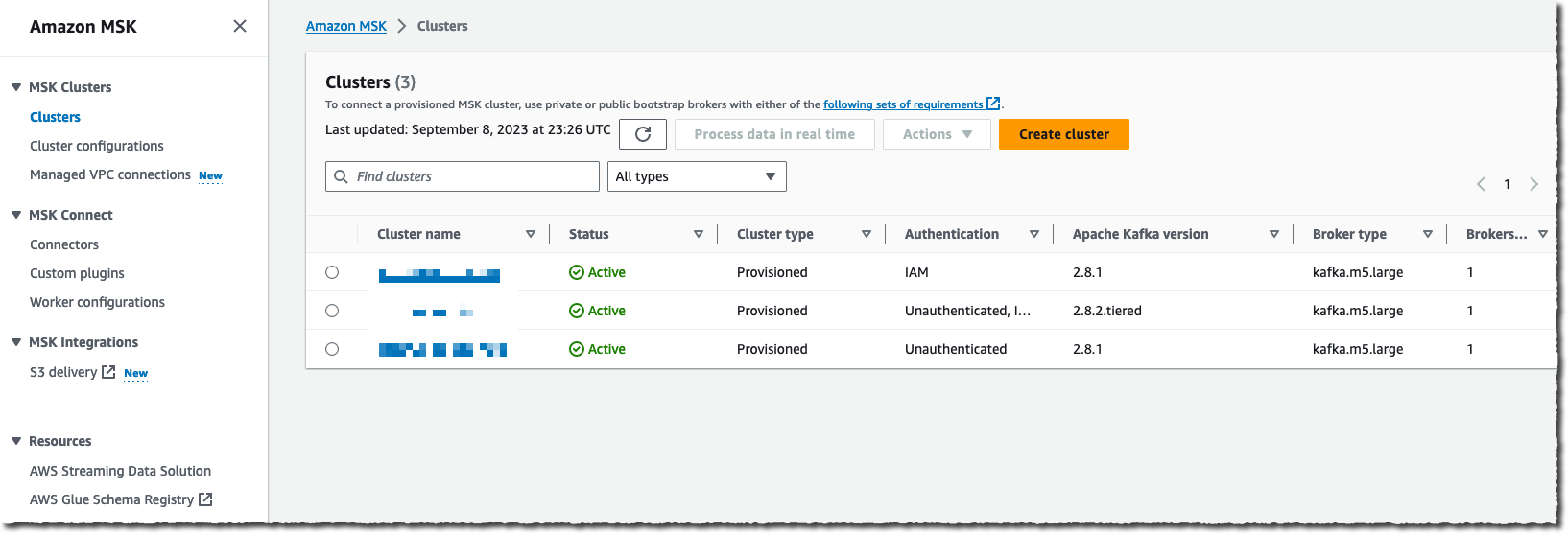
Complete the following steps to create an MSK cluster:
- On the Amazon MSK console, choose Cluster configurations under MSK clusters in the navigation pane.
- Choose Create configuration.
- Name the configuration
mskc-tutorial-cluster-configuration. - Under Configuration properties, remove everything and add the line
auto.create.topics.enable=true.

- Choose Create.

Create an MSK cluster and attach the configuration
In the next step, we attach this configuration to a cluster. Complete the following steps:
- On the Amazon MSK console, choose Clusters under MSK clusters in the navigation pane.
- Choose Create clusters and Custom create.
- For the cluster name, enter
mkc-tutorial-cluster. - Under General cluster properties, choose Provisioned for the cluster type and use the Apache Kafka default version 2.8.1.
- Use all the default options for the Brokers and Storage sections.
- Under Configurations, choose Custom configuration.
- Select
mskc-tutorial-cluster-configurationwith the appropriate revision and choose Next. - Under Networking, choose the MSK VPC.
- Select the Availability Zones depending upon your Region, such as
us-east1a,us-east1b, andus-east1c, and the respective private subnetsMSK-Private-1,MSK-Private-2, andMSK-Private-3if you are in theus-east-1Region. Public access to these brokers should be off. - Copy the security group ID from Chosen security groups.
- Choose Next.

- Under Access control methods, select IAM role-based authentication.
- In the Encryption section, under Between clients and brokers, TLS encryption will be selected by default.

- For Encrypt data at rest, select Use AWS managed key.
- Use the default options for Monitoring and select Basic monitoring.
- Select Deliver to Amazon CloudWatch Logs.

- Under Log group, choose visit Amazon CloudWatch Logs console.
- Choose Create log group.
- Enter a log group name and choose Create.

- Return to the Monitoring and tags page and under Log groups, choose Choose log group
- Choose Next.
- Review the configurations and choose Create cluster. You’re redirected to the details page of the cluster.
- Under Security groups applied, note the security group ID to use in a later step.


Cluster creation can typically take 25–30 minutes. Its status changes to Active when it’s created successfully.
Update the /var/named/kafka.region.amazonaws.com zone file
Before you create the MSK connector, update the DNS server configurations with the MSK cluster details.
- To get the list of bootstrap server DNS and respective IP addresses, navigate to the cluster and choose View client information.
- Copy the bootstrap server information with IAM authentication type.
- You can identify the broker IP addresses using
nslookupfrom your local machine and it will provide you the broker local IP address. Currently, your VPC points to the latest DHCP option set and your DNS server will not be able to resolve these DNS names from your VPC.
Now you can log in to the DNS server and update the records for different brokers and respective IP addresses in the /var/named/kafka.region.amazonaws.com file.
- Upload the
msk-access.pemfile toBastionHostInstancefrom your local machine: - Log in to the DNS server and open the
/var/named/kafka.region.amazonaws.comfile and update the following lines with the correct MSK broker DNS names and respective IP addresses:
Note that you need to provide the broker DNS as mentioned earlier. Remove .kafka.<region id>.amazonaws.com from the broker DNS name.
- Restart the DNS service:
You should see the following message:
Your custom DNS server is up and running now and you should be able to resolve using broker DNS names using the internal DNS server.
Update the security group for connectivity between the MySQL database and MSK Connect
It’s important to have the appropriate connectivity in place between MSK Connect and the MySQL database. Complete the following steps:
- On the Amazon MSK console, navigate to the MSK cluster and under Network settings, copy the security group.
- On the Amazon EC2 console, choose Security groups in the navigation pane.
- Edit the security group
MySQL_SGand choose Add rule. - Add a rule with MySQL/Aurora as the type and the MSK security group as the inbound resource for its source.
- Choose Save rules.
Create the MSK connector
To create your MSK connector, complete the following steps:
- On the Amazon MSK console, choose Connectors under MSK Connect in the navigation pane.
- Choose Create connector.
- Select Create custom plugin.
- Download the MySQL connector plugin for the latest stable release from the Debezium site or download Debezium.zip.
- Upload the MySQL connector zip file to the S3 bucket.
- Copy the URL for the file, such as
s3://<bucket name>/Debezium.zip. - Return to the Choose custom plugin page and enter the S3 file path for S3 URI.
- For Custom plugin name, enter
mysql-plugin.

- Choose Next.
- For Name, enter
mysql-connector. - For Description, enter a description of the connector.
- For Cluster type, choose MSK Cluster.
- Select the existing cluster from the list (for this post,
mkc-tutorial-cluster). - Specify the authentication type as IAM.
- Use the following values for Connector configuration:
- Update the following connector configuration:
- For Capacity type, choose Provisioned.
- For MCU count per worker, enter 1.
- For Number of workers, enter 1.
- Select Use the MSK default configuration.
- In the Access Permissions section, on the Choose service role menu, choose
MSK-Connect-PrivateDNS-MySQLConnector*, then choose Next. - In the Security section, keep the default settings.
- In the Logs section, select Deliver to Amazon CloudWatch logs.
- Choose visit Amazon CloudWatch Logs console.
- Under Logs in the navigation pane, choose Log group.
- Choose Create log group.

- Enter the log group name, retention settings, and tags, then choose Create.
- Return to the connector creation page and choose Browse log group.
- Choose the
AmazonMSKConnectlog group, then choose Next. - Review the configurations and choose Create connector.


Wait for the connector creation process to complete (about 10–15 minutes).

The MSK Connect connector is now up and running. You can log in to the MySQL database using your user ID and make a couple of record changes to the customer table record. MSK Connect will be able to receive CDC records and updates to the database will be available in the MSK <Customer> topic.
Consume messages from the MSK topic
To consume messages from the MSK topic, run the Kafka consumer on the MSK_Client EC2 instance available in the MSK VPC.
- SSH to the
MSK_ClientEC2 instance. TheMSK_Clientinstance has the required Kafka client libraries, Amazon MSK IAM JAR file,client.propertiesfile, and an instance profile attached to it, along with the appropriate IAM role using the CloudFormation template. - Add the
MSKClientSGsecurity group as the source for the MSK security group with the following properties:- For Type, choose All Traffic.
- For Source, choose Custom and MSK Security Group.
Now you’re ready to consume data.
- To list the topics, run the following command:
- To consume data from the
salesdb-server.salesdb.CUSTOMERtopic, use the following command:
Run the Kafka consumer on your EC2 machine and you will be able to log messages similar to the following:
While testing the application, records with CUST_ID 1998, 1999, and 2000 were updated, and these records are available in the logs.
Clean up
It’s always a good practice to clean up all the resources created as part of this post to avoid any additional cost. To clean up your resources, delete the MSK Cluster, MSK Connect connection, EC2 instances, DNS server, bastion host, S3 bucket, VPC, subnets and CloudWatch logs.
Additionally, clean up all other AWS resources that you created using AWS CloudFormation. You can delete these resources on the AWS CloudFormation console by deleting the stack.
Conclusion
In this post, we discussed the process of setting up MSK Connect using a private DNS. This feature allows you to configure connectors to reference public or private domain names.
We are able to receive the initial load and CDC records from a MySQL database hosted in a separate VPC and its DNS is not accessible or resolvable externally. MSK Connect was able to connect to the MySQL database and consume the records using the MSK Connect private DNS feature. The custom DHCP option set was attached to the VPC, which ensured DNS resolution was performed using the local DNS server instead of Route 53.
With the MSK Connect private DNS support feature, you can make your databases, data warehouses, and systems like secret managers that work with your own VPC inaccessible to the internet and be able to overcome this limitation and comply with your corporate security posture.
To learn more and get started, refer to private DNS for MSK connect.
About the author
 Amar is a Senior Solutions Architect at Amazon AWS in the UK. He works across power, utilities, manufacturing and automotive customers on strategic implementations, specializing in using AWS Streaming and advanced data analytics solutions, to drive optimal business outcomes.


 Satish Nandi is a Senior Technical Product Manager for Amazon OpenSearch Service.
 Rana Dutt is a Principal Solutions Architect at Amazon Web Services. He has a background in architecting scalable software platforms for financial services, healthcare, and telecom companies, and is passionate about helping customers build on AWS.
 Ranjith Rayaprolu is a Senior Solutions Architect at AWS working with customers in the Pacific Northwest. He helps customers design and operate Well-Architected solutions in AWS that address their business problems and accelerate the adoption of AWS services. He focuses on AWS security and networking technologies to develop solutions in the cloud across different industry verticals. Ranjith lives in the Seattle area and loves outdoor activities.
 Justin Leto is a Sr. Solutions Architect at Amazon Web Services with specialization in databases, big data analytics, and machine learning. His passion is helping customers achieve better cloud adoption. In his spare time, he enjoys offshore sailing and playing jazz piano. He lives in New York City with his wife and baby daughter.


 Kartikay Khator is a Solutions Architect on the Global Life Science at Amazon Web Services. He is passionate about helping customers on their cloud journey with focus on AWS analytics services. He is an avid runner and enjoys hiking.
 Kamen Sharlandjiev is a Sr. Big Data and ETL Solutions Architect and Amazon AppFlow expert. He’s on a mission to make life easier for customers who are facing complex data integration challenges. His secret weapon? Fully managed, low-code AWS services that can get the job done with minimal effort and no coding.


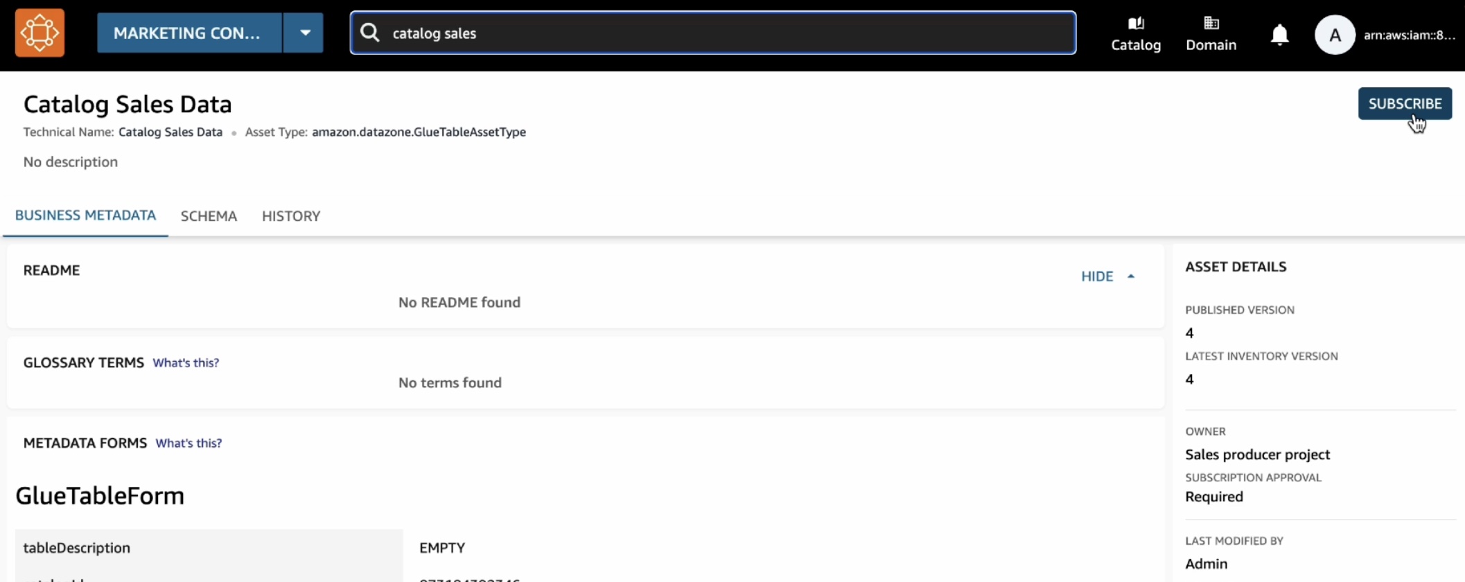
 Shikha Verma is Head of Product for Amazon DataZone at AWS.
 Steve McPherson is a General Manager with Amazon DataZone at AWS.
 Priya Tiruthani is a Senior Product Manager with Amazon DataZone at AWS.
 At AWS re:Invent 2022, we


 Rajdip Chaudhuri is a Senior Solutions Architect with Amazon Web Services specializing in data and analytics. He enjoys working with AWS customers and partners on data and analytics requirements. In his spare time, he enjoys soccer and movies.


 Avijit Goswami is a Principal Solutions Architect at AWS specialized in data and analytics. He supports AWS strategic customers in building high-performing, secure, and scalable data lake solutions on AWS using AWS managed services and open-source solutions. Outside of his work, Avijit likes to travel, hike, watch sports, and listen to music.
 Rajarshi Sarkar is a Software Development Engineer at Amazon EMR/Athena. He works on cutting-edge features of Amazon EMR/Athena and is also involved in open-source projects such as Apache Iceberg and Trino. In his spare time, he likes to travel, watch movies, and hang out with friends.


 available.


 Aarthi Srinivasan is a Senior Big Data Architect with AWS Lake Formation. She likes building data lake solutions for AWS customers and partners. When not on the keyboard, she explores the latest science and technology trends and spends time with her family.


 Annie Nelson is a Senior Solutions Architect at AWS. She is a data enthusiast who enjoys problem solving and tackling complex architectural challenges with customers.
 Keerthi Chadalavada is a Senior Software Development Engineer at AWS Glue. She is passionate about designing and building end-to-end solutions to address customer data integration and analytic needs.
 Zach Mitchell is a Sr. Big Data Architect. He works within the product team to enhance understanding between product engineers and their customers while guiding customers through their journey to develop their enterprise data architecture on AWS.
 Gal Heyne is a Product Manager for AWS Glue with a strong focus on AI/ML, data engineering and BI. She is passionate about developing a deep understanding of customer’s business needs and collaborating with engineers to design easy to use data products.