Tag Archives: announcements

AWS Weekly Roundup: Welcome DuckLabs to the team, Agentic Resource Discovery (ARD), and more (August 31, 2026)

Post Syndicated from Daniel Abib original https://aws.amazon.com/blogs/aws/aws-weekly-roundup-welcome-ducklabs-to-the-team-agentic-resource-discovery-ard-and-more-august-31-2026/

The news that interested me the most last week was the DuckLabs acquisition. AWS has signed a definitive agreement to acquire DuckLabs, the Amsterdam-based company behind DuckDB, the popular open source analytical database that runs in-process and executes SQL directly against files like Parquet, CSV, and JSON. DuckDB stays open source under its independent foundation and the MIT license, and over time AWS plans to combine its speed at everyday queries with the enterprise scale of services like Amazon S3, Amazon Redshift, and Amazon Athena.

Co-founded by Hannes Mühleisen and Mark Raasveldt, DuckDB runs locally or on Amazon S3, which makes it remarkably fast for the everyday queries (a terabyte or less) that make up the bulk of real-world analytics. It also happens to pair beautifully with AI agents, which “poke” and experiment their way through data much like humans do. The co-founders will continue leading its technical direction while AWS combines DuckDB’s speed with analytics services like Amazon EMR, AWS Glue, and Amazon SageMaker. For the bigger picture on why this matters, Andy Warfield, Vice President and Distinguished Engineer shared his thoughts on the post DuckDB and the changing physics of analytics on All Things Distributed.

Now, let’s get into this week’s AWS news…

Last week’s launches
Here are some launches and updates from this past week that caught my attention:

  • Amazon ECS now automatically detects and recovers container instances that lose agent connectivity – Amazon ECS now continuously monitors agent connectivity to the control plane and surfaces a new AGENT_CONNECTIVITY health event across AWS Fargate, Amazon ECS Managed Instances, and Amazon ECS on EC2. On Fargate and Managed Instances, ECS handles recovery automatically, draining tasks, launching replacements, and deregistering the impaired instance. On EC2, you can wire the event into your own workflow. Available at no additional cost in all AWS Commercial and AWS GovCloud (US) Regions.
  • AWS Lambda introduces public preview runtimes, starting with Node.js 26 and Python 3.15 – You can now test upcoming Lambda runtimes before they reach general availability. Preview runtimes use the same identifier as the eventual GA version, so your functions graduate automatically with no action required. Third-party tools and deployment frameworks can also validate compatibility ahead of GA. Not meant for production yet (breaking changes are possible), but a great way to get ahead of your next upgrade. Available in all AWS commercial, AWS GovCloud (US), and China Regions.
  • AWS IoT Core adds a native InfluxDB rule action – You can now route time-series data from your IoT devices straight into InfluxDB (Amazon Timestream-managed or self-hosted) without writing custom code or standing up an intermediate service. IoT Core formats data into InfluxDB’s line protocol and supports device-side and server-side batching. Available in all AWS Regions where Amazon Timestream for InfluxDB is offered.
  • Amazon GameLift Servers now includes enhanced DDoS protection – Your game servers now get automatic protection against network and transport layer (layers 3 and 4) DDoS attacks – UDP reflection, SYN floods, and similar vectors – with nothing to enable or opt into. Built on top of AWS Shield Standard with gaming-optimized traffic shaping, it turns on the moment your servers start running (Server SDK 5) at no extra cost. It’s available in all supported GameLift Servers Regions except China (Beijing) and China (Ningxia).
  • Amazon SageMaker HyperPod expands support for Ray – You can now run Ray workloads on SageMaker HyperPod with built-in observability, resilient training, and accelerated inference. Create and manage Ray clusters from Amazon SageMaker Studio, attach JupyterLab or your local IDE so a multi-node cluster behaves like a local dev environment, and get auto-provisioned Grafana dashboards. Node auto recovery, hung job detection, and tiered checkpointing keep large training runs healthy, while Ray Serve adds a tiered KV cache for inference. Your existing open source Ray code runs unchanged. Available for HyperPod clusters orchestrated by Amazon EKS.

For a full list of AWS announcements, be sure to keep an eye on the What’s New with AWS page.

Other AWS news
Here are some additional posts and resources that you might find interesting:

  • Happy 20th birthday, Amazon EC2! – Amazon EC2 turns 20. Channy Yun looks back at how EC2 grew from a single m1.small instance type in one Region to more than 1,200 instance types across 39 Regions, along with the custom silicon journey from the first Graviton to Graviton5 and Trainium3. A fun and worthwhile read on the service that still underpins so much of AWS – including Amazon ECS, Amazon EKS, AWS Lambda, Amazon SageMaker, and Amazon Bedrock.
  • Agentic Resource Discovery (ARD): an open specification for agent discovery – As organizations scale up agents, tools, and MCP servers, those resources end up scattered across clouds, on-premises infrastructure, and SaaS platforms – each with its own registry and metadata. ARD is a new open specification (Apache 2.0) that defines a common way to describe and discover agentic resources, so publishers “describe once” and consumers “discover everywhere” – think DNS, but for agents. AWS contributed feedback but doesn’t own the spec, and it complements the AWS Agent Registry by letting you federate across catalogs without migrating.
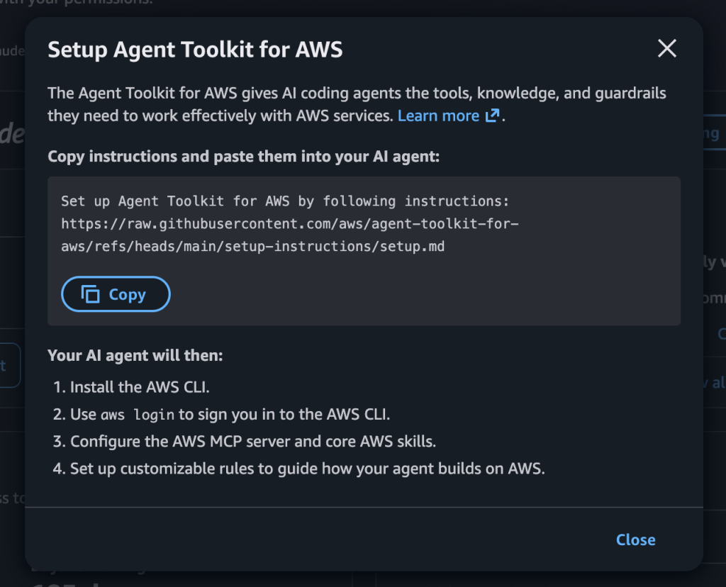
  • Get started with the Agent Toolkit for AWS in the AWS CLI – A single AWS CLI command (aws configure agent-toolkit) now equips AI coding agents like Kiro, Claude Code, Codex, and Cursor with curated, up-to-date AWS knowledge and a secure connection to thousands of AWS APIs through the AWS MCP Server. If you build with an AI coding assistant, this helps it choose the right services, use modern APIs, and follow security best practices – so it gets AWS code right more often the first time.

Upcoming AWS events
Check your calendar and sign up for upcoming AWS events:

  • AWS Summits – Free in-person events where builders come together to learn, connect, and explore the latest in cloud and AI. Upcoming stops include Zurich (September 2), São Paulo (September 3), Tel Aviv (September 10), and Dubai (September 30). Can’t attend in person? You can stream sessions through the Global Livestream and On-Demand Hub. I’ll be presenting two sessions on generative AI and Amazon Bedrock at the São Paulo Summit – if you’re there, come say hello.
  • AWS Community Days – Community-led conferences where content is planned, sourced, and delivered by community leaders. Upcoming events include JAWS SONIC 2026 in Tokyo (September 5) and Warsaw, Poland (September 8).

Join the AWS Builder Center to connect with builders, share solutions, and access content that supports your development. Browse here for upcoming AWS-led in-person and virtual events and developer-focused events.

That’s all for this week. Check back next Monday for another Weekly Roundup!

— Daniel Abib

This post is part of our Weekly Roundup series. Check back each week for a quick roundup of interesting news and announcements from AWS!

Build with geospatial and variant types in Iceberg v3 on AWS Glue 6.0

Post Syndicated from Shoukat Ghouse original https://aws.amazon.com/blogs/big-data/build-with-geospatial-and-variant-types-in-iceberg-v3-on-aws-glue-6-0/

As organizations build data lakes that combine geospatial data, high-frequency event streams, and heterogeneous payloads, the limitations of older table formats become acute. Without a native geospatial type, coordinates require separate float columns (latitude/longitude) with no spatial predicates. Without nanosecond-precision timestamps, sub-microsecond event ordering is lost. Without a variant type, semi-structured data forces a choice between rigid flattening and untyped JSON strings. Each workaround adds complexity, slows queries, and increases maintenance burden.

AWS Glue 6.0, powered by Apache Spark 4.1, removes these workarounds by adding support for Apache Iceberg v3, bringing new column-level capabilities to your data lake tables. These include new data types: native geospatial types (GEOMETRY with spatial predicates, and GEOGRAPHY), nanosecond-precision timestamps, and the VARIANT type for semi-structured data with automatic shredding. Iceberg v3 also adds support for DEFAULT column values. These are table format features. After they’re written, they’re readable by any Iceberg v3-compatible engine that supports these features.

In this post, we build a connected vehicle fleet monitoring pipeline that uses these capabilities in a single Iceberg v3 table. Vehicles emit telemetry events with GPS coordinates (geospatial), sub-microsecond event times (nanosecond), and sensor payloads that vary by vehicle type (variant). We ingest these events, run spatial queries to detect geofence violations, sequence events at nanosecond precision, and extract typed metrics from heterogeneous payloads, all without workarounds, flattening, or external libraries.

Solution overview

A logistics company operates a mixed fleet of delivery vehicles: vans, electric bikes, and delivery robots. Each vehicle type produces telemetry events with a different sensor payload schema. The operations team needs to:

  1. Detect geofence violations: flag vehicles that enter restricted zones (airports, pedestrian areas, private property).
  2. Sequence events precisely: at fleet scale, many events land in the same microsecond window. Nanosecond timestamps give a deterministic order and prevent ties when sequencing or deduplicating events during processing.
  3. Extract metrics from heterogeneous payloads: query battery level from delivery robots, fuel level from vans, and pedal cadence from bikes, all stored in the same column.

We address all three requirements with a single Iceberg v3 table on AWS Glue 6.0. The following data definition language (DDL) shows the table structure. The AWS Glue job we provision in subsequent steps executes this statement.

CREATE TABLE fleet_monitoring_db.vehicle_telemetry (
event_id STRING,
vehicle_id STRING,
vehicle_type STRING DEFAULT 'UNKNOWN',
event_time TIMESTAMP_NTZ(9),
location GEOMETRY(4326),
service_area GEOGRAPHY(4326),
sensor_payload VARIANT,
speed_kmh DOUBLE DEFAULT 0.0,
region STRING DEFAULT 'EMEA'
) USING ICEBERG
TBLPROPERTIES (
'format-version' = '3',
'write.delete.mode' = 'merge-on-read'
)
PARTITIONED BY (days(event_time), vehicle_type)

In the preceding statement, the database is shown as fleet_monitoring_db for readability. The deployed stack creates it as fleet_monitoring_<account-id>.

The following list describes the key columns:

  • event_time TIMESTAMP_NTZ(9): Stores the event timestamp at nanosecond precision.
  • location GEOMETRY(4326): Stores GPS coordinates as native spatial objects using (SRID 4326). You can use predicates like ST_Intersects directly in SQL, replacing hand-coded spatial math on raw latitude/longitude doubles (WGS 84).
  • service_area GEOGRAPHY(4326): Stores geographic coordinates using a spherical (geodesic) model, distinct from GEOMETRY’s planar model. AWS Glue 6.0 writes and reads GEOGRAPHY in Iceberg v3, and the type is portable to any Iceberg v3-compatible engine. Geodesic spatial predicates over GEOGRAPHY are engine-dependent today. In this post we run spatial queries on the GEOMETRY location column, which Glue 6.0 supports natively.
  • sensor_payload VARIANT: Each vehicle type produces a different JSON schema. Vans report fuel and engine metrics, robots report battery and camera status, bikes report cadence and heart rate. All land in this single column without schema unions or separate tables using variant data type.
  • vehicle_type STRING DEFAULT ‘UNKNOWN’ and speed_kmh DOUBLE DEFAULT 0.0: When an ingestion writer omits these fields, Iceberg applies the declared defaults automatically. Useful when multiple producers write to the same table and not all of them populate every column.

The table uses PARTITIONED BY (days(event_time), vehicle_type) so that analytical queries can prune by date range and vehicle type without scanning the full table. 'write.delete.mode' = 'merge-on-read' supports fast row-level corrections (for example, correcting a misreported GPS coordinate) through compact deletion vectors (Roaring Bitmaps) instead of accumulating positional delete files.

In this post, we insert sample data directly to focus on the new Iceberg data types and how to use them together. In production, these events would stream from Amazon Managed Streaming for Apache Kafka (Amazon MSK) into an AWS Glue 6.0 streaming job.

The following diagram illustrates the production architecture for reference:

Architecture diagram showing a vehicle fleet of vans, delivery robots, and electric bikes sending telemetry through Amazon MSK into an AWS account. Within a VPC, a hot path uses AWS Glue 6.0 Spark Real-Time Mode to detect geofence violations and send alerts to a Kafka topic, while a cold path uses a Glue 6.0 micro-batch job to write events into an Apache Iceberg v3 table with GEOMETRY, TIMESTAMP_NTZ(9), VARIANT, and DEFAULT columns. Amazon S3 stores the Iceberg data and the AWS Glue Data Catalog holds metadata. A batch analytics Glue job reads the Iceberg table for geofence detection, nanosecond event sequencing, and per-vehicle-type metric extraction using variant_get

Figure 1: Reference architecture for a fleet telemetry pipeline on AWS Glue 6.0

The architecture processes vehicle telemetry through two paths, with a downstream batch analytics layer:

Hot path (real-time, milliseconds): A Spark Real-Time Mode (RTM) job reads telemetry from Amazon MSK and evaluates geofence violations using spatial predicates like ST_Intersects, routing alerts to a downstream Kafka topic within milliseconds.

Cold path (near-real-time, seconds): A micro-batch job reads the same MSK topic and writes events into an Iceberg v3 table, converting payloads to GEOMETRY, TIMESTAMP_NTZ(9), and VARIANT columns with DEFAULT values applied.

Batch analytics: An AWS Glue job reads the Iceberg v3 table to run batch analytics on geofence detection, nanosecond event sequencing, and per-vehicle-type metric extraction.

Prerequisites

To follow along, you need:

  • An AWS account and an AWS Region where AWS Glue 6.0 is available.
  • An AWS Identity and Access Management (IAM) role with permissions to deploy AWS CloudFormation stacks and create resources including AWS Glue, Amazon Simple Storage Service (Amazon S3), and Amazon CloudWatch Logs.

Deploy the CloudFormation stack

We provide an AWS CloudFormation template that provisions all the resources needed for this walkthrough.

The stack provisions the following resources:

  • An Amazon S3 bucket for Iceberg table storage.
  • An IAM role with permissions for AWS Glue, Amazon S3, and Amazon CloudWatch Logs.
  • An AWS Glue database (fleet_monitoring_<account-id>).
  • An AWS Glue job fleet-telemetry-ingest-<account-id> (PySpark): creates the Iceberg v3 table vehicle_telemetry described earlier and inserts sample telemetry from three vehicle types.
  • An AWS Glue job fleet-telemetry-queries-<account-id> (PySpark): demonstrates geofence detection, nanosecond sequencing, variant extraction, and default values.

Deploy the CloudFormation stack:

  1. Download the CloudFormation template from the GitHub repository.
  2. Sign in to the AWS CloudFormation console.
  3. Choose Create stack, With new resources, Upload a template file, and upload the downloaded template.
  4. Acknowledge the IAM capabilities and choose Create stack.

Stack creation takes approximately 2–5 minutes. No parameters are required.

After the stack completes, navigate to the AWS Glue console and run the jobs in this order:

  1. Run fleet-telemetry-ingest-<account-id>. This job creates the Iceberg v3 table and inserts sample data (approximately 2 minutes).
  2. After it succeeds, run fleet-telemetry-queries-<account-id>. This job executes all demonstration queries (approximately 2 minutes).

The following sections describe each job in detail.

Job 1: Ingest sample telemetry data

The ingestion job creates the Iceberg v3 table described earlier and inserts four sample telemetry events: one for each of the three vehicle types (van, robot, bike), plus one with omitted fields to demonstrate DEFAULT values. You can view the complete script in the GitHub repository. Note that the geospatial types require one additional Spark configuration (spark.sql.geospatial.enabled=true), which is already set in the job’s --conf argument by the CloudFormation template. All other types work with no extra configuration.

The following are the key snippets from the script:

Van telemetry: GPS coordinates with engine metrics and route information:

spark.sql(f"""
INSERT INTO {TABLE} VALUES (
'EVT-001', 'VAN-042', 'VAN',
CAST('2026-07-28 09:15:30.123456789' AS TIMESTAMP_NTZ(9)),
ST_SetSrid(ST_GeomFromWKB(X'0101000000E17A14AE47E1C0BF1F85EB51B84E4940'), 4326),
ST_SetSrid(ST_GeogFromWKB(X'0101000000E17A14AE47E1C0BF1F85EB51B84E4940'), 4326),
PARSE_JSON('{{"fuel_pct": 0.72, "cargo_kg": 450, "door_open": false,
"engine": {{"rpm": 2100, "temp_c": 88.5}},
"route": {{"stops_remaining": 4, "eta_minutes": 35}}}}'),
35.2, 'EMEA'
)
""")

Delivery robot telemetry: Same table, completely different sensor schema (battery, cameras, navigation):

spark.sql(f"""
INSERT INTO {TABLE} VALUES (
'EVT-002', 'ROB-117', 'ROBOT',
CAST('2026-07-28 09:15:30.123456790' AS TIMESTAMP_NTZ(9)),
ST_SetSrid(ST_GeomFromWKB(X'01010000000000000000001040000000000000F03F'), 4326),
ST_SetSrid(ST_GeogFromWKB(X'01010000000000000000001040000000000000F03F'), 4326),
PARSE_JSON('{{"battery_pct": 0.62, "obstacle_distance_m": 2.8,
"navigation_mode": "autonomous",
"cameras": {{"front": "active", "rear": "recording"}}}}'),
48.0, 'EMEA'
)
""")

Note: EVT-001 and EVT-002 are exactly 1 nanosecond apart (.123456789 vs .123456790). Without TIMESTAMP_NTZ(9), both would round to the same microsecond and be indistinguishable.

Default values test: Event inserted with vehicle_type, speed_kmh, and region omitted:

spark.sql(f"""
INSERT INTO {TABLE}
(event_id, vehicle_id, event_time, location, service_area, sensor_payload)
VALUES (
'EVT-004', 'UNK-999',
CAST('2026-07-28 10:00:00.000000000' AS TIMESTAMP_NTZ(9)),
ST_SetSrid(ST_GeomFromWKB(X'0101000000000000000000F03F000000000000F03F'), 4326),
ST_SetSrid(ST_GeogFromWKB(X'0101000000000000000000F03F000000000000F03F'), 4326),
PARSE_JSON('{{"status": "initializing"}}')
)
""")

The omitted columns automatically receive their DEFAULT values: vehicle_type = 'UNKNOWN', speed_kmh = 0.0, region = 'EMEA'.

Job 2: Query the data

The query job demonstrates all four data types working together. After the job succeeds, select the run in the AWS Glue console and choose Output logs to see the results.

The following sections walk through the key queries from the job and the results of each.

Geofence detection with ST_Intersects

The job defines a polygon and finds all vehicles inside it:

POLY = "010300...."
SELECT event_id, vehicle_id, vehicle_type, speed_kmh
FROM fleet_monitoring_db.vehicle_telemetry
WHERE ST_Intersects(
location,ST_SetSrid(ST_GeomFromWKB(X'{POLY}'), 4326)
)
ORDER BY event_id

The polygon covers coordinates (0,0)-(5,0)-(5,2)-(0,2). Three vehicles are inside (ROBOT at (4,1), BIKE at (3,1), UNKNOWN at (1,1)). The VAN at (-0.1278, 51.5074) is outside.

Query results listing the ROBOT, BIKE, and UNKNOWN vehicles inside the geofence polygon, with the VAN excluded

Figure 2: Geofence query results showing the three vehicles inside the polygon

Nanosecond event sequencing

Order events by their sub-microsecond timestamps:

SELECT event_id, vehicle_id, CAST(event_time AS STRING) AS precise_time
FROM fleet_monitoring_db.vehicle_telemetry
WHERE event_id IN ('EVT-001', 'EVT-002', 'EVT-003')
ORDER BY event_time ASC

EVT-001 and EVT-002 are correctly distinguished and ordered despite being only 1 nanosecond apart. With standard TIMESTAMP_NTZ (microsecond precision), both would show .123456 and their relative order would be undefined.

Query results showing EVT-001 and EVT-002 ordered by nanosecond-precision timestamps one nanosecond apart

Figure 3: Nanosecond-precision ordering distinguishing two events one nanosecond apart

Variant extraction with variant_get

Different sensor schemas per vehicle type, all extracted with variant_get:

SELECT vehicle_id, vehicle_type,
CASE vehicle_type
WHEN 'VAN' THEN variant_get(sensor_payload, '$.fuel_pct', 'DOUBLE')
WHEN 'ROBOT' THEN variant_get(sensor_payload, '$.battery_pct', 'DOUBLE')
WHEN 'BIKE' THEN variant_get(sensor_payload, '$.battery_pct', 'DOUBLE')
ELSE NULL
END AS energy_level,
variant_get(sensor_payload, '$.engine.temp_c', 'DOUBLE') AS engine_temp,
variant_get(sensor_payload, '$.cameras.front', 'STRING') AS front_cam,
variant_get(sensor_payload, '$.deliveries.completed', 'INT') AS deliveries_done
FROM fleet_monitoring_db.vehicle_telemetry
WHERE vehicle_type != 'UNKNOWN'
ORDER BY vehicle_id
Query results showing variant_get extracting energy level, engine temperature, and camera status for each vehicle type

Figure 4: Variant extraction returning typed values from heterogeneous sensor payloads

variant_get takes three arguments: the column, a dot-path expression, and the expected return type. It supports arbitrary nesting depth. $.engine.temp_c reaches two levels deep, $.deliveries.completed reaches into a different structure entirely. When a path doesn’t exist in a particular row’s payload, it returns NULL.

Default values

Confirm that omitted columns received their defaults:

SELECT event_id, vehicle_type, speed_kmh, region
FROM fleet_monitoring_db.vehicle_telemetry
WHERE event_id = 'EVT-004'
Query results showing event EVT-004 with the default values UNKNOWN, 0.0, and EMEA applied

Figure 5: Default column values applied to the event inserted with omitted fields

EVT-004 was inserted without vehicle_type, speed_kmh, or region. The declared defaults were applied automatically.

Combined query: Combining spatial, temporal, and variant operations

The following query runs a geospatial predicate, nanosecond ordering, and variant extraction in a single SELECT statement:

SELECT vehicle_id, vehicle_type,
CAST(event_time AS STRING) AS precise_time,
CASE vehicle_type
WHEN 'VAN' THEN variant_get(sensor_payload, '$.fuel_pct', 'DOUBLE')
WHEN 'ROBOT' THEN variant_get(sensor_payload, '$.battery_pct', 'DOUBLE')
WHEN 'BIKE' THEN variant_get(sensor_payload, '$.battery_pct', 'DOUBLE')
ELSE NULL
END AS energy_level,
speed_kmh
FROM fleet_monitoring_db.vehicle_telemetry
WHERE ST_Intersects(location, ST_SetSrid(ST_GeomFromWKB(X'0103000000...'), 4326))
ORDER BY event_time ASC
Query results combining spatial filtering, nanosecond ordering, and variant extraction in a single query

Figure 6: Combined query results over a single Iceberg v3 table

This single query combines a spatial predicate, nanosecond ordering, and variant extraction over one table, with no external libraries, pre-processing, or joins to separate geometry or payload tables.

Clean up

To avoid ongoing charges from the AWS Glue jobs and Amazon S3 storage, delete the CloudFormation stack when you’re done:

  1. Open the AWS CloudFormation console.
  2. Select the stack you deployed earlier and choose Delete.

Conclusion

In this post, we stored and analyzed geospatial coordinates, nanosecond timestamps, and heterogeneous sensor payloads in a single Iceberg v3 table on AWS Glue 6.0, with sensible defaults applied automatically, no external libraries, and no schema flattening.

  • GEOMETRY columns replace latitude/longitude doubles and support native spatial predicates like ST_Intersects for geofence detection. GEOGRAPHY is stored natively.
  • TIMESTAMP_NTZ(9) preserves full nanosecond precision for event sequencing where microsecond resolution is insufficient.
  • VARIANT stores heterogeneous payloads (different schema per vehicle type) in one column with typed extraction through variant_get.
  • DEFAULT values keep field population consistent across multiple ingestion writers without duplicating logic.

All capabilities require Iceberg format-version 3. Geospatial requires one additional configuration (spark.sql.geospatial.enabled=true). Nanosecond timestamps, Variant, and DEFAULT values work with no extra configuration.

These capabilities apply wherever schemas vary by source (IoT fleets, multi-tenant software as a service (SaaS), event-driven architectures), timestamps need sub-microsecond precision (trading, sensor fusion, autonomous systems), or spatial operations replace coordinate workarounds (logistics, real estate, delivery networks).

For more information, see the AWS launch announcement (launch URL to be added before publishing), the AWS Glue documentation, and the Apache Iceberg v3 specification. AWS Glue 6.0 includes additional capabilities such as Spark Real-Time Mode and Spark Declarative Pipelines, which we cover in separate posts.


About the authors

Shoukat Ghouse

Shoukat Ghouse

Shoukat is a Senior Specialist Solutions Architect for Big Data, Analytics, and Data Governance at Amazon Web Services (AWS). He partners with enterprise and financial services customers across EMEA to design and scale production-grade data lakehouse platforms on Apache Spark, Apache Iceberg, AWS Glue, Amazon EMR, and Amazon SageMaker Unified Studio. His focus spans distributed data processing, fine-grained data governance, and helping organizations build AI-ready data foundations that power analytics and machine learning at scale.

Shrey Malpani

Shrey Malpani

Shrey is a Senior Product Manager Technical at Amazon Web Services (AWS), where he works at the intersection of distributed data processing and data integration. He is focused on building and scaling data integration and data management capabilities across services like AWS Glue, Amazon EMR, and Amazon Redshift that help customers build AI-ready data platforms for their analytics and machine learning workflows.

Kartik

Kartik

Kartik is a Software Development Manager on the AWS Glue team. His team builds generative AI features for the Data Integration and distributed system for data integration.

ICYMI: July 2026 @AWS Security

Post Syndicated from Rodolfo Brenes original https://aws.amazon.com/blogs/security/icymi-july-2026-aws-security/

If you found time for a bit of vacation this summer, you might be in catch-up mode. Here’s a list to help: all the expert blog posts, new service capabilities, code samples, and workshops, in case you missed it, from July 2026.

AWS Security Blog post

This month’s AWS Security Blog posts covered AI agent security, supply chain protection, network firewall automation, DDoS mitigation, and compliance readiness. Read on for guidance on securing AI coding agents, implementing dependency cooldowns, choosing the right key management solution, and preparing for HIPAA Technical Safeguard requirements.

AI Security

Enforce least-privilege authorization in multi-agent AI chains using Cedar
Authors: Dhananjay Karanjkar | Published: July 6, 2026
Learn to implement a three-layer Cedar policy model with OAuth 2.0 authentication to prevent authorization scope expansion across multi-agent delegation chains using Amazon Verified Permissions.

Enforce zero data retention on Amazon Bedrock with Bedrock Projects and service control policies
Author: Rob Higareda | Published: July 7, 2026
Learn to use Amazon Bedrock Projects and SCPs to centrally enforce zero data retention policies, preventing accounts from enabling data sharing with third-party model providers across your organization.

Designing for the inevitable: System prompt leakage and mitigations in generative AI applications
Author: Manideep Konakandla | Published: July 8, 2026
Learn to implement defense-in-depth mitigations for system prompt leakage using Amazon Bedrock Guardrails prompt attack filters, canary tokens, semantic similarity detection, and sandwich instruction patterns.

Balancing speed and safety: A control framework for AI coding agents
Authors: Daniel Begimher, Danny Cortegaca | Published: July 30, 2026
Learn to implement an application security control framework for AI coding agents, with author-time controls that shape what agents produce and build-time controls that verify what reaches production.

Data Protection

How to use the AWS Workload Credentials Provider for cross-account secret retrieval and prefetching secrets
Authors: Derik Wang, Paras Dhawan | Published: July 1, 2026
Learn to configure the AWS Workload Credentials Provider for cross-account secret retrieval using IAM role chaining and prefetching secrets at startup to reduce cold-start latency.

The CISO’s guide to post-quantum mandates and migrations
Author: Rushir Patel | Published: July 8, 2026
A strategic playbook for CISOs navigating post-quantum cryptography migration, covering regulatory timelines, dependency classification, cryptographic telemetry, and building crypto-agile organizations.

AWS KMS or AWS CloudHSM: Choose the right key management solution
Author: Derek Tumulak | Published: July 28, 2026
Learn how to choose between AWS KMS and AWS CloudHSM based on integration needs, cost, and whether you require traditional HSM interfaces or legacy algorithms.

Secure your npm and pip package updates in Amazon Linux
Author: Norbert Manthey | Published: July 29, 2026
Learn to implement a one-line dependency cooldown for npm and pip that skips packages published in the last 24 hours, protecting against supply chain events while still allowing urgent security patches.

Infrastructure security

Secure Amazon container workloads using container attribute-based rules in AWS Network Firewall
Authors: Amit Gaur, Amish Shah, Preetkumar Shah, Akash Kumar Sinha | Published: July 1, 2026
Learn to define AWS Network Firewall rules for Amazon EKS and Amazon ECS workloads using native container attributes like namespaces, pod names, and labels instead of ephemeral IP addresses.

Authenticate legitimate AI agent traffic with AWS WAF Bot Control
Authors: Harith Gaddamanugu, Kaustubh Phatak | Published: July 14, 2026
Learn to use Web Bot Authentication (WBA) in AWS WAF Bot Control to cryptographically verify legitimate AI agent traffic using HTTP message signatures and ed25519 keys.

Accelerating AWS Network Firewall troubleshooting with AWS DevOps Agent
Author: Salman Ahmed | Published: July 24, 2026
Learn to use AWS DevOps Agent to automate root cause analysis for AWS Network Firewall connectivity issues, including domain deny lists, stateless rule priority misconfigurations, and asymmetric cross-AZ routing drops.

AWS Shield Advanced is embracing the AWS WAF Anti-DDoS managed rule group: What changes and how to prepare
Authors: Eitav Arditti, Andrew Chen, Justin Kurpius | Published: July 27, 2026
AWS Shield Advanced is adopting the AWS WAF Anti-DDoS managed rule group as its default application-layer DDoS protection, with a phased migration from July 2026 through January 2027.

Threat detection and incident response

Introducing the Amazon GuardDuty investigation agent: on-demand AI-powered threat assessment
Author: Allan Holmes | Published: July 20, 2026
Learn to use the new Amazon GuardDuty investigation agent (public preview) to automate threat correlation and receive structured assessments with risk levels, confidence scores, MITRE ATT&CK mappings, and actionable recommendations.

Amazon identifies North Korean hacker group behind open-source supply chain attacks
Author: CJ Moses | Published: July 29, 2026
Learn how Amazon Threat Intelligence linked the compromises of axios, debug, chalk, and typo-crypto NPM packages to a single DPRK-linked threat actor, and how attacker tradecraft is evolving with generative AI.

Extend Amazon Inspector SBOM Generator with plugins
Authors: Michael Long, Anthony Verleysen, Charlie Bacon | Published: July 30, 2026
Learn to write custom Lua plugins for the Amazon Inspector SBOM Generator to inventory package ecosystems that aren’t supported out of the box, without modifying source code or waiting for an official release.

Security Hub adds AI workload protection and multicloud support for Microsoft Azure
Author: Michael Fuller | Published: July 14, 2026
AWS Security Hub now monitors Microsoft Azure resources for misconfigurations and vulnerabilities, adds GuardDuty AI Protection for Amazon Bedrock and Amazon SageMaker AI, and introduces an AI inventory for organization-wide visibility.

Governance and compliance

AWS designated as a critical third party to the UK financial sector
Author: Michael Jefferson | Published: July 10, 2026
AWS has been designated as a critical third party to the UK financial sector by HM Treasury, establishing direct regulatory oversight by the Bank of England, PRA, and FCA.

New compliance guidance available: HITRUST i1 on AWS
Authors: Abdul Javid, Shreya Singh | Published: July 13, 2026
AWS published new implementation guidance for HITRUST i1 certification, covering 11 technical control domains with AWS-specific controls for healthcare organizations seeking i1 assessment readiness.

HIPAA Security Rule on AWS – Technical Safeguards Implementation and Readiness Guidance
Authors: Abdul Javid, Hector Rodriguez, Kapil Temghare, Shreya Singh | Published: July 31, 2026
New guidance helping covered entities and business associates implement and evidence compliance with HIPAA Security Rule Technical Safeguards (§164.312) on AWS, including 2025 NPRM proposed changes.

Identity

Introducing OAuth support for AWS MCP Server
Authors: Vaibhav Chowla, Jaimin Bhatt, Ankur Joshi | Published: July 9, 2026
AWS MCP Server now supports OAuth 2.1 authorization through AWS Sign-In, enabling agents like Claude Code,Kiro, and Gemini CLI to connect using existing IAM credentials with browser-based authentication.

July Security Bulletins

In July 2026, AWS published 21 security bulletins (2026-049 through 2026-069) addressing vulnerabilities across open-source SDKs, MCP servers, and developer tools. Key themes include credential disclosure and SSRF, affecting HealthLake, HealthOmics, and API MCP servers, plus Strands Agents tools that could inadvertently expose secrets to unauthorized endpoints. Command and code injection impacted aws-cdk-lib, jsii-diff, Bedrock AgentCore SDK, and Amplify Codegen UI. The smithy-rs framework received three patches for denial-of-service via uncontrolled recursion and Slowloris issues.

Other notable issues include insecure file permissions in the AWS CLI, deserialization remote code execution in the Advanced JDBC Wrapper, SQL injection in mcp-gateway-registry, TLS 1.3 flaws in s2n-tls, and stored XSS in AWS Ops Wheel. A common thread: insufficient input validation in tools interacting with AI agents, reflecting the expanded surface area of LLM-integrated workflows. All patches are available, upgrade promptly. For more information, see AWS Security Bulletins.

AWS Samples

This month brings 14 new AWS samples spanning AI security, identity, data protection, governance, threat detection, and security posture management. From deploying governed AI agent platforms on Amazon Bedrock AgentCore to building data-residency-compliant chatbots and DevSecOps baselines for Kiro, these repositories help you implement security and governance best practices across your AWS environment.

AI Security

Lark MCP on AgentCore
Learn to deploy a hosted remote MCP service on Amazon Bedrock AgentCore that lets AI agents operate Feishu/Lark through 450+ tools, with per-user identity isolation and smart multi-step orchestration via 20+ domain Skills.

Lark CLI MCP Wrapper on AgentCore Runtime and Identity
Learn to securely wrap a CLI tool as an MCP server on AgentCore Runtime using a sidecar credential-isolation pattern, where the CLI process never holds real tokens and all secrets are resolved through AgentCore Identity’s Token Vault.

LiteLLM Bedrock Gateway on EKS
Learn to deploy a production-grade LiteLLM proxy on Amazon EKS as a unified OpenAI/Anthropic-compatible gateway to Amazon Bedrock, with four progressive layers covering network isolation, cross-region inference profiles, and cross-account delegation.

Enterprise Agentic AI Platform Accelerator on AgentCore
Learn to deploy a secure, governed foundation for production AI agents on Amazon Bedrock AgentCore with CDK stacks covering identity, gateway, memory, runtime, and observability; supporting multiple agent frameworks (Strands, LangGraph, Claude SDK) and opt-in security controls including VPC isolation, KMS encryption, Cedar policies, and Bedrock Guardrails.

FlowAMP: AI Agent Governance on AWS
Learn to deploy a single-pane-of-glass agent management platform on Amazon Bedrock AgentCore that discovers, monitors, scores, controls, and cost-accounts AI agents across an AWS Organization with agentic discovery, compliance scanning (NIST AI RMF, ISO 27001, SOC 2), Responsible-AI scoring, FinOps via Cost Explorer, and Cedar-based policy enforcement.

Kiro SecOps Baseline
Learn to deploy a DevSecOps security baseline for Kiro as a single Go CLI that installs global guardrails (permissions.yaml, steering, skills, a security-review agent) and per-project workspace hooks (fail-closed guard, PR/pipeline review gates, scanner configs for gitleaks, trivy, and checkov) with enterprise fleet distribution via MDM and Administration scope.

Identity

OAuth 2.0 Token Exchange with Amazon Cognito
Learn to implement RFC 8693 OAuth 2.0 Token Exchange using Amazon Cognitowith a true delegation pattern, enabling services to act on behalf of users while maintaining distinct service identities and least-privilege access in microservices architectures.

Lark Identity on AgentCore — Gateway Interceptor
Learn to implement enterprise identity pass-through on Amazon Bedrock AgentCore using a Gateway Request Interceptor that forwards the user’s identity and injects per-user credentials to downstream MCP tools, so the agent never holds a token and tools act only as the authenticated user against Lark.

Data Protection

Automated PII Detection Pipeline with Amazon Macie
Learn to build an event-driven pipeline that automatically detects PII in Amazon S3 objects using Amazon Macie, AWS Step Functions, and custom data identifiers, with CSV/JSON reporting and SNSalerting for high-severity findings.

Data-Residency Chatbot with Amazon Bedrock AgentCore
Learn to build a data-residency-compliant natural-language chatbot on Amazon Bedrock AgentCore that keeps all data and AI inference within a single AWS Region, using governed text-to-SQL with whitelist-validated queries, Aurora PostgreSQL in private subnets, and AgentCore Gateway for secure tool access.

Governance and compliance

Video Compliance Agent
Learn to build an end-to-end automated video compliance verification pipeline using Amazon Bedrock, ECS Fargate, and AWS Step Functions that processes videos shot-by-shot, extracting frames, audio transcripts, and OCR text, then flags potential broadcast guideline violations with structured per-shot reports.

Contract Compliance Search with Amazon OpenSearch
Learn to build a contract compliance search system that combines semantic search with semantic highlighting using Amazon OpenSearchService, Amazon Titan V2 embeddings, and a SageMaker-hosted highlighting model to surface relevant clauses across contract documents.

Threat detection and incident response

Multicloud Security Posture Assessment
Learn to deploy a centralized security assessment solution that scans AWS, Azure, Google Cloud Platform, and Oracle Cloud Infrastructure environments from a single AWS deployment using Prowler, with AWS CloudFormation templates for each provider and unified reporting in HTML, CSV, and JSON-OCSF formats.

Centralize AWS Security Agent Findings
Learn to deploy a AWS CloudFormation stack that automatically exports AWS Security Agentpenetration test findings to Amazon S3 and queries them centrally with Amazon Athena, using Amazon EventBridge, Step Functions, and a AWS Glue catalog for tracking findings over time.

Sentinel Harness — Production SecOps Agents as Configuration
Learn to build production security-operations agents as pure configuration on Amazon Bedrock AgentCore Harness, declaring model, prompt, tools, skills, memory, and limits in YAML while AWS runs the agent loop with human-in-the-loop gates, detection-engineering tools, adversary emulation, and a self-improvement closed loop.

AWS Labs

This month brings 1 new AWS Labs repository focused on data protection, helping organizations build automated PII detection and redaction pipelines with AI-powered processing across documents and audio files.

Data Protection

PII Anonymizer
Learn to build an automated PII detection and redaction pipeline using AWS Step Functions, Amazon Bedrock, Amazon Textract, and Amazon Transcribe; supporting PDFs, Word, Excel, images, and audio files with synthetic replacement or blackout modes, concurrency control, and customer-managed KMS encryption.

Conclusion

July 2026 provides guidance and examples for securing AI agent architectures at scale, from governed text-to-SQL with data residency controls and agent management platforms to DevSecOps baselines for AI coding tools. The posts and samples provide patterns for least-privilege authorization in multi-agent chains using Cedar, post-quantum migration planning, container-aware network firewall rules, and multicloud security posture management. Each resource includes deployment steps or runnable code so you can validate in your own environment before adopting. Subscribe to the AWS Security Blog RSS feed to receive updates as they publish, and revisit this digest monthly for a consolidated view of what changed and what to act on.

If you have feedback about this post, submit comments in the Comments section below.


Rodolfo Brenes

Rodolfo Brenes

Rodolfo is a Principal Solutions Architect focused on Cloud Governance and Compliance. With over 18 years of experience, he currently leads a technical field community in AWS helping customers scale and improve their security and governance frameworks. Besides work, Rodolfo enjoys video games, playing with his four cats, and won’t say no to a good outdoor adventure.

Anna Brinkmann

Anna has 18 years of experience in the technical content space and has spent the last 6 years managing the AWS Security Blog. Outside of work, she enjoys spending time with her family.

Migrate an OAuth 2.0 authenticated Apache Kafka cluster to Amazon MSK with MSK Replicator

Post Syndicated from Subham Rakshit original https://aws.amazon.com/blogs/big-data/migrate-an-oauth-2-0-authenticated-apache-kafka-cluster-to-amazon-msk-with-msk-replicator/

In an earlier post, we walked through how Amazon Managed Streaming for Apache Kafka (Amazon MSK) Replicator migrates external and self-managed Apache Kafka clusters to Amazon MSK. It replicates your topics and their configurations, keeps topic and consumer-group names intact, and synchronizes consumer-group offsets, so your producers and consumers can cut over on their own schedule instead of all at once. MSK Replicator now supports OAuth 2.0 (SASL/OAUTHBEARER) authentication to the external cluster, and that is what this post covers.

If your external Kafka cluster authenticates clients with OAuth, MSK Replicator can connect to it, but “OAuth” isn’t a single thing you switch on. It’s a family of grant types, and each one comes with its own trust model, its own set of inputs you need to supply, and its own configuration on both the Replicator side and your identity provider (IdP) side.

In this post, we walk you through the grant types one by one, show you how to configure Replicator for each, call out the network and TLS prerequisites that are commonly missed, and finish with how to handle IdPs that sit behind an additional identity layer. This mechanism works with any OAuth 2.0 (OIDC) identity provider, including Keycloak, Okta, Microsoft Entra ID, PingFederate, and Auth0. OAuth here governs only how Replicator authenticates to your external cluster, so the target can be either Amazon MSK Standard or Express brokers, which always use IAM.

How OAuth authentication works

Before you configure Replicator, it helps to be precise about how the OAuth Kafka handshake works.

The components

  • The Identity Provider (IdP) – Issues access tokens and publishes the public keys. Brokers use these keys to verify the tokens. Examples: Keycloak, Okta, Microsoft Entra ID, PingFederate, Auth0, or a custom OIDC server.
  • The client – In our case, MSK Replicator, acting as a Kafka consumer/producer against your external cluster.
  • The resource server – Your self-managed Kafka broker, which must decide whether to admit a connection.
  • The access token – A JWT (JSON Web Token): a base64url-encoded, three-part string header.payload.signature that the IdP cryptographically signs.

The SASL/OAUTHBEARER handshake, step by step

The following sequence diagram shows the full exchange, from Replicator requesting a token to the broker accepting the connection:

Sequence diagram of the SASL/OAUTHBEARER handshake: Replicator requests a token from the IdP, receives a signed JWT, presents it to the Kafka broker, and the broker verifies the JWT against cached JWKS keys before accepting the connection.

Figure 1: The SASL/OAUTHBEARER handshake. Replicator gets a signed JWT from the IdP and presents it to the broker, which verifies it against cached JWKS keys before accepting the connection.

Walking through it:

  1. Request a token – Replicator asks the IdP for an access token. The exact request depends on the grant type (covered in the next section).
  2. Receive a signed JWT – The IdP returns a signed JWT access token.
  3. Present the token – Replicator opens a SASL/OAUTHBEARER connection to the external Kafka brokers and presents the JWT.
  4. Verify locally – The broker verifies the JWT signature against the IdP’s cached JWKS public keys, without calling the IdP per message.
  5. Connection accepted – The broker admits the connection and derives the Kafka principal from the preferred_username claim.

Step 4 is worth dwelling on: the broker validates the token locally. It fetches the IdP’s JWKS (JSON Web Key Set, the public half of the IdP’s signing keys, RFC 7517) from an endpoint like https://idp.example.com/realms/kafka/protocol/openid-connect/certs and caches it, refreshing on a configurable interval (and re-fetching if it sees a key ID it doesn’t recognize). Incoming JWT signatures are then verified against those cached keys. The IdP is not in the hot path of message traffic. It is contacted only to (a) issue tokens to clients, and (b) serve its public keys for the periodic JWKS refresh.

What the Kafka broker checks

When Replicator presents a JWT, the broker validates:

  • Signature – Proves the IdP issued the token and no one tampered with it (verified against JWKS).
  • iss (issuer) – Must match the broker’s configured oauth.valid.issuer.uri, byte-for-byte, including scheme, host, port, and path. A mismatch is a common configuration error.
  • exp (expiry) – Expired tokens are rejected. Strimzi’s client callback handler proactively refreshes before expiry, so you shouldn’t see mid-stream failures.
  • The principal claim – Typically preferred_username. The broker uses this as the Kafka principal in ACLs (for example, User:service-account-msk-replicator). This matters: the identity Replicator authenticates as on the external cluster must have ACLs that you configure to grant it the read/describe permissions it needs.

Mapping your IdP to a Replicator grant type

A grant type is the protocol by which the client proves its identity to the IdP and obtains a token. This is the front half of the preceding handshake (steps 1 and 2). MSK Replicator supports three of them. You already know how your Kafka clients authenticate to your IdP today, so start from that.

Which grant to use?

Find the row that matches how your clients get tokens today:

How your Kafka clients get tokens from the IdP today Grant type Long-lived secret? What you trust/register on the IdP
A client_id / client_secret (confidential client) CLIENT_CREDENTIALS Yes (stored on AWS Secrets Manager) Nothing new: reuse the existing client, or create one for Replicator
You want secretless, and your IdP can trust an external token issuer IAM_JWT_BEARER No AWS STS as an external token (OIDC) issuer. Trust its JWKS
You want secretless, and your IdP models workloads as signed-JWT clients CLIENT_CREDENTIALS_ASSERTION No AWS STS as the client’s signing authority (private_key_jwt). Trust its JWKS

The simplest mapping is like-for-like: if your clients use a client_id/client_secret, point Replicator at the same client with CLIENT_CREDENTIALS. If you’d rather not give Replicator a long-lived secret, the two secretless grants let it authenticate with its AWS identity instead. Choose between them based on how your IdP prefers to trust an external party.

The rest of this section explains why the three grants differ, using an analogy. If your row is clear and you only want the configuration, skip ahead to Configuring and creating the replicator.

A scenario: checking in at a secure office building

A visitor needs to get into a secure office building. They can’t walk straight in. First they stop at the reception desk to prove who they are and collect a temporary access pass. Only then can they use that pass at the building’s turnstile to get inside. In OAuth terms: the building is your external Kafka cluster, the reception desk is the IdP, the temporary access pass is the access token (JWT), and the visitor is MSK Replicator. Presenting the pass at the turnstile is the SASL/OAUTHBEARER step, and it works the same way for every grant type. What differs is how the visitor proves who they are at the reception desk before it prints a pass.

Scenario 1: CLIENT_CREDENTIALS (the shared PIN)

CLIENT_CREDENTIALS scenario shown as a visitor entering a building: the visitor authenticates at reception with a PIN (the client secret), receives a temporary badge (the access token), and uses it to enter the building (the Kafka cluster).

Figure 2: CLIENT_CREDENTIALS. The visitor authenticates at reception with a PIN (the client_secret), gets a temporary badge (the access token), and uses it to enter the building (the Kafka cluster).

At the reception desk the visitor keys in a PIN the desk already have on file (the client_secret), collects a temporary access pass in return (the access token), and uses that pass to get into the building. Both sides hold the same secret. In practice (RFC 6749 §4.4), Replicator authenticates to the IdP with a client_id/client_secret stored on AWS Secrets Manager, receives the access token, and presents it to the external Kafka brokers over SASL/OAUTHBEARER. Use it when your IdP already issues client secrets for machine clients. This is usually a like-for-like move that reuses the client your existing producers and consumers use, or a new one created for Replicator.

Scenario 2: IAM_JWT_BEARER (the badge is the request)

IAM_JWT_BEARER scenario: the visitor presents an employer-signed badge (an STS JWT) to reception as the request itself and receives an access token, because reception trusts the employer’s stamp (the STS JWKS).

Figure 3: IAM_JWT_BEARER. The visitor shows an employer-signed badge (an STS JWT) to reception as the request itself and gets an access token. Reception accepts it because it trusts the employer’s stamp (the STS JWKS).

First, the visitor collects an employer-signed badge: Replicator calls STS GetWebIdentityToken to mint an STS JWT. At the reception desk the badge itself is the request. The visitor shows it to ask for a pass. Reception trusts the employer’s tamper-proof stamp (STS JWKS), so it accepts the badge and prints a temporary access pass. In practice (RFC 7523 §2.1), the STS JWT is sent as the authorization grant (assertion), and the IdP trusts AWS STS as an external token issuer. Use it when you want secretless authentication, and your IdP can trust an external issuer’s JWTs.

Scenario 3: CLIENT_CREDENTIALS_ASSERTION (the same badge, used as ID on the form)

CLIENT_CREDENTIALS_ASSERTION scenario: the visitor fills out reception’s standard request form and attaches the same STS JWT as identification to receive an access token, which reception grants by trusting the employer’s stamp (the STS JWKS).

Figure 4: CLIENT_CREDENTIALS_ASSERTION. The visitor fills out reception’s standard request form and attaches the same STS JWT as ID, getting an access token. Reception trusts the employer’s stamp (the STS JWKS).

The visitor again collects the same employer-signed badge (STS JWT). This time they fill out the reception desk’s standard access request form (the client_credentials grant) and attach the badge to it as identification, all in one submission. Reception trusts the same employer stamp (STS JWKS) and prints a temporary access pass. In practice (RFC 7521/RFC 7523 §2.2), the same STS JWT is sent as the client_assertion on the client_credentials grant, with the IdP trusting STS as the client’s signing authority (private_key_jwt). Use it when you want secretless authentication and your IdP models external workloads as signed-JWT clients.

Scenarios 2 and 3 in one sentence. Both mint the same STS JWT and share the same benefit: nothing shared can leak, because there is no secret. They differ only in where the STS JWT sits in the token request. IAM_JWT_BEARER sends it as the assertion (the badge is the request), while CLIENT_CREDENTIALS_ASSERTION sends it as the client_assertion on a standard client_credentials request (the badge is ID on the form). That single difference is what you register on the IdP: AWS STS as an external token issuer, or as the client’s signing authority.

Solution overview

Now that you can map your setup to a grant type, the next question is where these pieces actually run. MSK Replicator runs on AWS managed infrastructure but attaches elastic network interfaces (ENIs) into the subnets of the target Amazon MSK cluster’s virtual private cloud (VPC) and initiates every connection from there under a Service Execution Role (SER). Those ENIs sit in private subnets that typically have no NAT or internet gateway, so each external dependency needs an explicit network path. The following diagram shows the full topology for an OAuth migration, including the two pieces that are commonly missed: STS Outbound Web Identity Federation (for the secretless grants) and the interface VPC endpoints for STS and Secrets Manager.

Deployment architecture: the source environment holds the IdP and Kafka brokers; the AWS account holds STS, Secrets Manager, and the Amazon MSK VPC, whose private subnets contain the Replicator ENIs and target cluster, reached through interface VPC endpoints.

Figure 5: Deployment architecture. The source environment holds the IdP and Kafka brokers. The AWS account holds STS, Secrets Manager, and the Amazon MSK VPC, whose private subnets contain the Replicator ENIs and target cluster, reached through interface VPC endpoints.

The source environment (on the left, shown as on-premises here, but it can equally be another cloud or a self-managed cluster on AWS) holds two components: the IdP token endpoint and JWKS (Keycloak, Okta, Entra ID) and the external Kafka brokers on a SASL_SSL / OAUTHBEARER listener. Everything else runs in your AWS account.

The two dotted lines are trust relationships you configure ahead of time, not runtime calls:

  • External Kafka validates token by using IdP JWKS – The broker checks every presented access token against the IdP’s published public keys. This applies to all grants.
  • IdP trusts STS issuer through JWKS – For the secretless grants only, the IdP is configured to trust your account’s STS issuer and validate the STS-signed JWT against STS’s JWKS. When STS Outbound Web Identity Federation is enabled, AWS provisions a per-account issuer URL (https://<id>.tokens.sts.global.api.aws) whose JWKS the IdP trusts. This trust is not used by CLIENT_CREDENTIALS.

The numbered arrows are the runtime flow, all originating from the Replicator ENIs:

  • Step 1: Fetch client credentials and the CA certificate from AWS Secrets Manager, through its VPC endpoint. For CLIENT_CREDENTIALS this includes the client_id/client_secret. For the secretless grants it is only the CA certificate(s).
  • Step 1a (optional): Call GetWebIdentityToken on AWS STS, through the STS VPC endpoint, to mint a JWT of Replicator’s AWS identity. Required only for IAM_JWT_BEARER and CLIENT_CREDENTIALS_ASSERTION.
  • Step 2: Get a signed JWT access token from the IdP token endpoint, exchanging either the client secret or the STS JWT depending on the grant.
  • Step 3: Present the token to the external Kafka brokers over SASL/OAUTHBEARER.
  • Step 4: Replicate to the target Amazon MSK cluster using IAM authentication.

The two supporting pieces inside the VPC, the Secrets Manager and STS interface VPC endpoints, are commonly overlooked precisely because the private subnets have no NAT or internet gateway. We cover exactly why they’re needed, and when, in the following section, Cross-cutting requirements.

Configuring and creating the replicator

With the architecture in mind, you can now configure Replicator itself. MSK Replicator models OAuth through a saslOAuthBearer structure on the external cluster’s clientAuthentication. Exactly one of three mechanism members must be present: clientCredentials, iamJwtBearer, or clientCredentialsAssertion. The control plane enforces this mutual exclusivity. Fields shared across all three (tokenEndpointUrl, scope, tokenEndpointAuthenticationMethod, tokenEndpointTlsCertificateArn, and saslExtensions) live at the saslOAuthBearer level.

Before the per-grant details, here are the requirements that apply to every OAuth migration, whichever grant you choose. Most OAuth setup failures trace back to one of these, so review them first.

Cross-cutting requirements

Here are the five items that apply to every grant: TLS trust, secret format, network reachability, the Service Execution Role, and STS federation.

a) TLS everywhere, and two separate trust settings

Replicator connects to two TLS endpoints, and they are configured independently:

  • encryptionInTransit.rootCaCertificate: the CA that signed your Kafka brokers’ TLS certificates (the SASL_SSL listener – :9096).
  • tokenEndpointTlsCertificateArn: the CA that signed your IdP’s token endpoint TLS certificate (for example – Keycloak on :8443).

If your broker and IdP are signed by the same private CA, you still must supply the CA in both fields. Omitting tokenEndpointTlsCertificateArn when the IdP uses a private or self-signed cert produces a PKIX path building failed error during token acquisition. Because that fails before workers stabilize, you’ll see a generic failure with no worker logs. If your IdP uses a publicly-trusted certificate (for example, it sits behind a public endpoint), you can omit tokenEndpointTlsCertificateArn entirely.

b) Secret format: store key/value pairs, not raw values

Every secret Replicator reads (client credentials, CA certificate) is parsed by the config provider as a set of key/value pairs. Use the Secrets Manager console’s Key/value editor rather than pasting raw text, and it will serialize and escape the values for you.

The keys the provider expects:

Key Value Used for
certificate the CA in PEM (newlines escaped as \n) CA-certificate secrets (rootCaCertificate, tokenEndpointTlsCertificateArn)
client_id, client_secret your OAuth client credentials the CLIENT_CREDENTIALS token-request secret

Custom parameters, headers, and SASL extensions. Some IdPs require extra data on the token request, and some brokers require SASL/OAUTHBEARER extensions. The config provider supports both through reserved key prefixes in the same secret:

Prefix Effect Example key Example value
custom_param. adds a parameter to the token request sent to the IdP custom_param.tenant_token myTenantToken
custom_header. adds an HTTP header to the IdP token request custom_header.X-Tenant-Id acme
extension. adds a SASL/OAUTHBEARER extension presented to the broker (for example, Confluent Cloud’s logicalCluster) extension.logicalCluster myLogicalClusterId

For example, an IdP that expects a tenant token as a request parameter and a Confluent Cloud broker that requires a logical-cluster extension would add custom_param.tenant_token and extension.logicalCluster as extra key/value pairs alongside client_id/client_secret in the same secret.

c) Network reachability from Replicator’s ENIs

Replicator attaches ENIs into the subnets you specify (through the target amazonMskCluster cluster’s vpcConfig) and initiates all connections from there. Those ENIs must be able to reach:

  1. Your external brokers, over VPC peering, AWS Transit Gateway, AWS Direct Connect, or VPN, with security groups permitting the SASL_SSL port.
  2. Your IdP’s token endpoint, over the same networking. The endpoint hostname must resolve from those subnets.
  3. AWS Secrets Manager, to fetch credentials/CA. If the subnets have no NAT/internet gateway, add an interface VPC endpoint for com.amazonaws.<region>.secretsmanager with private DNS.
  4. AWS STS (only for IAM_JWT_BEARER and CLIENT_CREDENTIALS_ASSERTION), to call GetWebIdentityToken. In no-egress subnets this will time out (STS GetWebIdentityToken call failed: Connect timed out) unless you add an interface VPC endpoint for com.amazonaws.<region>.sts with private DNS. This is the most common oversight for the secretless grants.

Both endpoints use private DNS, so the standard secretsmanager.<region>.amazonaws.com and sts.<region>.amazonaws.com hostnames resolve to the endpoint inside the VPC, with no client change needed.

A note on vpcConfig placement. For an external Apache Kafka cluster, vpcConfig is specified on the target amazonMskCluster entry, not the external apacheKafkaCluster entry. The API rejects a vpcConfig on the external cluster. The ENIs it creates are what reach both clusters and all AWS endpoints.

d) The Service Execution Role (SER)

Replicator assumes an IAM role to do its work. Two parts matter:

  • Trust policy – Must allow the Replicator service to assume it. kafka.amazonaws.com needs to be trusted. A trust policy that is too narrow fails with AccessDenied.ServiceExecutionRoleUnassumable.
  • Permissions – The replication permissions are extensive and depend on which features you enable, so follow the service execution role permissions reference to build a least-privilege policy.

e) Enabling STS Outbound Web Identity Federation (secretless grants only)

For IAM_JWT_BEARER and CLIENT_CREDENTIALS_ASSERTION, sts:GetWebIdentityToken must be enabled for your account/role. When enabled, AWS provisions a dedicated issuer URL of the form https://<uuid>.tokens.sts.global.api.aws. Every JWT STS mints for your account carries this as its iss claim, and its public keys are published under this issuer’s JWKS. You configure your IdP to trust this issuer. Granting the sts:GetWebIdentityToken IAM action is necessary but not sufficient. The account-level federation feature must also be turned on.

Create the replicator

A repeatable way to create the replicator is with a request file and --cli-input-json, so you can keep the full configuration under version control. The following example is a complete CLIENT_CREDENTIALS request. The two secretless variants change only the saslOAuthBearer block (shown after).

aws kafka create-replicator \
  --region <region> \
  --cli-input-json file://create-replicator.json

create-replicator.json:

{
  "replicatorName": "oauth-migration-replicator",
  "serviceExecutionRoleArn": "arn:aws:iam::<acct>:role/msk-replicator-execution-role",
  "kafkaClusters": [
    {
      "apacheKafkaCluster": {
        "apacheKafkaClusterId": "<source-cluster-id>",
        "bootstrapBrokerString": "b-1.ext-kafka.example.com:9096,b-2.ext-kafka.example.com:9096"
      },
      "clientAuthentication": {
        "saslOAuthBearer": {
          "tokenEndpointUrl": "https://idp.example.com/realms/kafka/protocol/openid-connect/token",
          "clientCredentials": {
            "tokenRequestSecretArn": "arn:aws:secretsmanager:<region>:<acct>:secret:<oauth-creds>"
          },
          "tokenEndpointAuthenticationMethod": "POST",
          "tokenEndpointTlsCertificateArn": "arn:aws:secretsmanager:<region>:<acct>:secret:<idp-ca>"
        }
      },
      "encryptionInTransit": {
        "encryptionType": "TLS",
        "rootCaCertificate": "arn:aws:secretsmanager:<region>:<acct>:secret:<broker-ca>"
      }
    },
    {
      "amazonMskCluster": {
        "mskClusterArn": "arn:aws:kafka:<region>:<acct>:cluster/target-msk/<uuid>"
      },
      "vpcConfig": {
        "subnetIds": [
          "subnet-aaaa",
          "subnet-bbbb",
          "subnet-cccc"
        ],
        "securityGroupIds": [
          "sg-xxxxxxxx"
        ]
      }
    }
  ],
  "replicationInfoList": [
    {
      "sourceKafkaClusterId": "<source-cluster-id>",
      "targetKafkaClusterArn": "arn:aws:kafka:<region>:<acct>:cluster/target-msk/<uuid>",
      "targetCompressionType": "NONE",
      "topicReplication": {
        "topicsToReplicate": [
          ".*"
        ],
        "detectAndCopyNewTopics": true,
        "copyTopicConfigurations": true
      },
      "consumerGroupReplication": {
        "consumerGroupsToReplicate": [
          ".*"
        ],
        "detectAndCopyNewConsumerGroups": true,
        "synchroniseConsumerGroupOffsets": true
      }
    }
  ]
}

Field names and exact nesting follow the create-replicator API reference. Check it for the full schema and any Region-specific values.

The example above uses CLIENT_CREDENTIALS. For the full schema, any Region-specific values, and detailed examples for the other grant types, check the MSK documentation.

With the requirements and configuration in hand, here is the order to put them in:

  1. Pick your grant type using the preceding decision table. CLIENT_CREDENTIALS is the fastest path if you already manage a client secret. Otherwise choose a secretless grant based on how your IdP models external workloads. For a multi-hop internal chain, use IAM_JWT_BEARER against the proxy pattern described in the next section.
  2. Prepare the IdP: create the client (or the STS-trust configuration), and note the exact token endpoint URL and issuer.
  3. Stage secrets in Secrets Manager, as JSON (requirement b): client credentials (if any) and the CA certificate(s).
  4. Wire the network (requirement c): connectivity from Replicator’s subnets to your brokers and IdP, plus interface VPC endpoints for Secrets Manager and (secretless grants only) STS, both with private DNS.
  5. [Optional but recommended]: Smoke-test the path from inside the VPC – IdP setup is often the part that takes the most iterations, and Replicator provisioning is a slow way to discover a misconfigured token endpoint or a missing TLS trust. Spin up a small EC2 instance in Replicator’s subnets, install a Kafka client, and run an end-to-end produce/consume against the external brokers using SASL/OAUTHBEARER (a client_credentials flow is simplest). This validates the three things most likely to be wrong (network reachability to the IdP and brokers, both TLS trusts for the broker CA and IdP CA, and token vending) while you can still fix them in seconds. Tear the instance down once the round trip works.
  6. Enable STS Outbound Web Identity Federation (requirement e. Secretless grants only) and configure your IdP to trust the resulting issuer.
  7. Build the SER (requirement d) with a trust policy the Replicator service can assume and the required permissions.
  8. Create the replicator with the create-replicator request for your grant. Remember both TLS trust fields for a private-CA IdP (requirement a), and vpcConfig on the target entry only.
  9. Verify – Produce to a topic on the external cluster and confirm the records land on the target (consume with IAM auth on the Amazon MSK side). Then watch the health signals:
    • In the Amazon MSK console, the replicator should reach the RUNNING state.
    • In Amazon CloudWatch, under the AWS/Kafka namespace, watch the replicator’s ReplicationLatency and MessageLag metrics. Both should be low and stable, and MessageLag should trend toward zero as it catches up.
    • A healthy replicator commits offsets continuously. A steady “1 message per batch” with no producer activity is only the internal heartbeat topic, not a stall.

Handling an additional identity layer: the federation-proxy pattern

Who owns what – Before the details, the ownership line is simple and worth stating up front:

  • What Replicator guarantees: it calls the configured tokenEndpointUrl with the configured grant, includes the STS JWT, expects a standard {access_token, token_type, expires_in} response, and refreshes before expiry.
  • What you own: everything at and behind the proxy, including validating the STS JWT, the downstream token exchanges, claim mapping, and the availability and latency of the endpoint. The proxy runs in your VPC and is owned entirely by you.

So far we have assumed you can point Replicator at a single token endpoint. Some organizations can’t. Instead, they have an internal identity chain: several hops of token exchange and federation that a workload must traverse before it holds a token the Kafka brokers accept.

A representative example is a large financial institution whose chain has several hops: an AWS workload’s identity (a signed GetCallerIdentity request) is exchanged at an internal Token Exchange service for an intermediate JWT, which an internal IdP then consumes as a client_assertion to issue the final Bearer token the Kafka brokers accept.

Replicator connects to a single HTTPS token endpoint using one of the three grant types and expects a standard token response. When the identity flow spans multiple hops like this, you place a proxy in front of that chain so Replicator still sees a single endpoint.

The solution: a customer-owned proxy

You deploy a small proxy in your own VPC that collapses the chain behind a single endpoint. From Replicator’s perspective, this is an ordinary OAuth flow against one token endpoint. Everything behind that endpoint is opaque to Replicator and owned entirely by you.

The grant Replicator uses to reach the proxy is a separate choice from the exchanges happening behind it. We recommend a secretless grant (IAM_JWT_BEARER or CLIENT_CREDENTIALS_ASSERTION) so there is no long-lived secret between Replicator and the proxy. CLIENT_CREDENTIALS is also valid if you would rather the proxy authenticate Replicator with a client secret. The following walkthrough uses IAM_JWT_BEARER, where the proxy validates the STS JWT that Replicator presents.

How it works, end to end. The following sequence diagram traces the full token exchange, from Replicator’s request to the Bearer it finally presents to the external Kafka brokers.

Federation-proxy token flow: the proxy validates Replicator’s STS JWT, exchanges its own AWS identity at the Token Exchange service for an intermediate JWT, presents that to the internal IdP, and returns the resulting Bearer token to Replicator.

Figure 6: Federation-proxy token flow. The proxy validates Replicator’s STS JWT, exchanges its own AWS identity at the Token Exchange service for an intermediate JWT, presents that to the internal IdP, and returns the resulting Bearer to Replicator.

  1. Replicator to proxy – Replicator POSTs its STS JWT as assertion to the proxy’s token endpoint, a plain IAM_JWT_BEARER request (grant_type=jwt-bearer). Because the endpoint is private, Replicator reaches it through an execute-api interface VPC endpoint, the same private-connectivity approach used for Secrets Manager and STS. (Replicator first obtains the STS JWT by calling STS GetWebIdentityToken through the STS VPC endpoint.)
  2. Proxy validates the STS JWT (signature against STS’s JWKS, plus iss/aud/exp/sub checks. The sub is the caller’s AWS ARN).
  3. Proxy to Token Exchange service – The proxy exchanges its own AWS identity, presented as a signed GetCallerIdentity request, at the internal Token Exchange service.
  4. Token Exchange service → proxy – It returns a signed intermediate JWT.
  5. Proxy to internal IdP – The proxy makes a client_credentials request that carries the intermediate JWT as the client_assertion.
  6. Internal IdP to proxy – The IdP issues the final Bearer access token.
  7. Proxy to Replicator – The proxy returns the Bearer, and Replicator presents it to the external brokers over SASL/OAUTHBEARER. The brokers validate it against the final IdP’s JWKS, a completely ordinary OAuth handshake from their point of view.

Reference architecture

Here is the reference architecture for the end-to-end solution.

Federation-proxy reference architecture: Replicator ENIs in a private subnet call a customer-owned proxy (a Lambda function behind a private API Gateway) that runs the on-premises identity chain over Direct Connect before Replicator replicates into the target Amazon MSK cluster.

Figure 7: Federation-proxy reference architecture. Replicator ENIs in a private subnet call a customer-owned proxy (a Lambda behind a private API Gateway), which runs the on-premises identity chain over Direct Connect before Replicator replicates into the target Amazon MSK cluster.

Everything on the Replicator side runs in your VPC’s private subnets: the Replicator ENIs, the customer-owned proxy, and the target Amazon MSK cluster. The proxy here is an AWS Lambda function behind a private Amazon API Gateway, but it can run on any compute you prefer (EC2, ECS, or EKS) as long as it exposes a single private HTTPS token endpoint. Connectivity to the on-premises Token Exchange service, internal IdP, and Kafka brokers runs over AWS Direct Connect (a VPN or VPC peering works too).

The outer legs of this flow are exactly the base migration from Solution overview: step 1 (fetch the broker CA from Secrets Manager), step 1a (mint the STS JWT through STS), step 3 (present the Bearer to the brokers), and step 4 (replicate to the target with IAM). What’s new here is the proxy hop in the middle, which replaces the single “step 2” call to a token endpoint:

  • 2. POST /token – Replicator sends the STS JWT as the assertion to the proxy’s private token endpoint, reached through the execute-api interface VPC endpoint. The proxy validates it against STS’s JWKS.
  • 2a. Exchange AWS identity – The proxy presents its own AWS identity (a signed GetCallerIdentity request) to the internal Token Exchange service and gets back a signed intermediate JWT.
  • 2b. Present as client_assertion – The proxy sends a client_credentials request to the internal IdP with the intermediate JWT as the client_assertion, and receives the final Bearer.
  • 2c. Final Bearer token – The proxy returns the Bearer to Replicator, which then continues at step 3.

As in the base architecture, the dotted lines are prerequisite trust relationships, not runtime calls: the proxy trusts AWS STS as an issuer (validating the STS JWT against STS’s JWKS), and the Kafka brokers validate the final Bearer against the internal IdP’s JWKS.

One subtlety worth calling out is the split of TLS trust. Replicator connects directly only to the private API Gateway (which uses a publicly trusted certificate) and to the Kafka brokers, so the only certificate it fetches from Secrets Manager is the broker CA. The internal IdP’s CA is the proxy’s concern: the proxy terminates TLS to the Token Exchange service and internal IdP, so it carries their CA material, not Replicator.

The same single-endpoint pattern handles other “extra layer” scenarios without any Replicator change: claim enrichment (the proxy intercepts and augments), rate-limited IdPs (the proxy caches tokens), IdPs requiring mTLS (the proxy terminates Replicator’s HTTPS and initiates mTLS onward), and IdP migrations (swap the proxy’s target without touching Replicator config).

A working reference implementation of this customer-owned proxy is available at GitHub.

Conclusion

In this post, we walked through how to migrate a self-managed, OAuth-authenticated Apache Kafka cluster to Amazon MSK using MSK Replicator: how the SASL/OAUTHBEARER handshake works, how to map your identity provider to one of the three supported grant types, the deployment architecture and prerequisites that the connection depends on, and how to handle identity providers that sit behind an additional federation layer. To get started, see the Amazon MSK Developer Guide and the Amazon MSK Replicator documentation. For the federation-proxy example, see the sample implementation on GitHub.


About the author

Subham Rakshit

Subham Rakshit

Subham is a Streaming Solutions Architect for Analytics at AWS based in the UK. He works with customers to design and build search and streaming data platforms that help them achieve their business objective. Outside of work, he enjoys spending time solving jigsaw puzzles with his daughters.

Announcing in-place ZooKeeper-to-KRaft cluster upgrades for Amazon MSK

Post Syndicated from Austin Groeneveld original https://aws.amazon.com/blogs/big-data/announcing-in-place-zookeeper-to-kraft-cluster-upgrades-for-amazon-msk/

Apache Kafka 4.0 officially removes ZooKeeper. If your Amazon Managed Streaming for Apache Kafka (Amazon MSK) Provisioned clusters still run in ZooKeeper metadata mode, now is the time to plan your migration. Amazon MSK now supports in-place upgrades from ZooKeeper to KRaft metadata mode, so you can modernize your existing cluster’s metadata management through the familiar version upgrade workflow.

For more than a decade, Apache ZooKeeper provided dependable metadata management for Kafka, including controller election, partition state, broker registration, and topic configuration. With Apache Kafka 4.0, ZooKeeper is officially removed in favor of KRaft, an embedded Raft-based consensus protocol that handles metadata management internally. It brings those responsibilities into Apache Kafka itself, creating a more streamlined foundation for the continued evolution of Kafka. Amazon MSK has supported KRaft-mode clusters since May 2024, and all Kafka 4.x versions on Amazon MSK use KRaft.

With the in-place upgrade, you can retain your cluster data and metadata while Amazon MSK manages the control-plane transition. Your cluster remains available for produce and consume traffic throughout the process, with no expected downtime if you’re following best practices. By using the existing version upgrade workflow, the move to KRaft becomes a natural step in your cluster’s lifecycle. This prepares your cluster for Kafka 4.x and future Kafka releases.

Prerequisites

Before initiating the upgrade, review the following requirements to confirm your cluster is ready for the transition.

Supported source versions

Clusters must be running Kafka 3.9.x in ZooKeeper mode to use the in-place upgrade. If your cluster is running an earlier version, such as 3.6.0, 3.7.x, or 3.8.x, first complete a standard in-place version upgrade to 3.9.x. You can then initiate the upgrade to 3.9.x.kraft.

Kafka 3.9 is the bridge release for this transition because it supports both ZooKeeper and KRaft modes. To support customers through this migration process, Amazon MSK provides extended support for 3.9.x for a minimum of 2 years from its April 2025 release.

Client compatibility

Requirement Detail
Minimum client library Apache Kafka client v3.0+
Recommended client version v3.9 or above
Connection strings Must use bootstrap.servers only. Any ZooKeeper connection strings (the --zookeeper flag) must be removed before upgrade.

The --zookeeper admin flag was deprecated in Kafka 2.5 and removed in 3.0. Before upgrading, update any remaining applications or tools that connect directly to ZooKeeper.

Pre-upgrade checklist

Before beginning the upgrade, confirm the following:

  • For Standard brokers, the cluster must be deployed across three Availability Zones. Express brokers provide this by default.
  • The cluster is running Kafka 3.9.x in ZooKeeper mode.
  • Standard brokers expose direct ZooKeeper access on ports 2181 (plaintext) and 2182 (TLS). Before upgrading, validate that you’ve disabled ZooKeeper access on the cluster and none of your applications rely on these connections.
  • Solutions using dynamic Kafka configurations that relied on ZooKeeper have been removed before attempting the upgrade operation.
    • If you previously configured custom domain names on a ZooKeeper-based deployment using the dynamic override (kafka-configs.sh --alter on advertised.listeners), be aware that KRaft does not support this dynamic configuration. If you attempt to upgrade your MSK cluster to KRaft with altered advertised.listeners, the upgrade operation fails.
    • If you’re implementing your custom domain name solution on MSK moving forward with KRaft, we recommend our coinciding MSK release for custom domain name support by statically configuring the custom.advertised.listeners property through the UpdateClusterConfiguration API.
  • The cluster has no under-replicated partitions.
  • The cluster is running within per-broker partition limits for standard or express broker clusters.
  • For clusters running above the KRaft brokers-per-cluster limit, you might need an additional quota increase. If you previously raised a quota increase for your ZooKeeper brokers-per-cluster, submit another quota increase for the KRaft limit before attempting the upgrade.
  • The cluster has enough reserve capacity to support rolling broker restarts while serving client traffic.
  • As a best practice, verify that monitoring is ready for the transition from ZooKeeper-specific metrics to KRaft controller metrics.
    • After the migration, ZooKeeper-specific Amazon CloudWatch metrics such as ZookeeperRequestLatencyMsMean and ZookeeperSessionState are no longer available.
    • If you use Open Monitoring, Kafka also stops publishing ZooKeeper metrics. Plan to update or retire related alerts and dashboards as part of your migration preparation.

How the upgrade works

When you initiate the upgrade, Amazon MSK performs a managed, multi-phase migration:

  1. Controller quorum bootstrap: Amazon MSK provisions KRaft controller nodes alongside the existing ZooKeeper infrastructure. Both systems operate in parallel during this phase.
  2. Metadata migration: The KRaft controller reads the cluster state from ZooKeeper and writes it to the internal KRaft metadata log.
  3. Broker transition: Amazon MSK performs a rolling update and registers with the KRaft controller quorum. Data plane operations remain available during the transition.
  4. Validation and bake period: Amazon MSK verifies cluster health under KRaft, including partition leadership, replication state, and controller responsiveness.
  5. ZooKeeper decommissioning: After validation succeeds, Amazon MSK removes the ZooKeeper infrastructure and the cluster operates entirely in KRaft mode.

During the upgrade, the cluster enters UPDATING state. You can continue producing and consuming data, while Amazon MSK administrative API operations are temporarily unavailable until the cluster returns to ACTIVE.

Amazon MSK maintains a high bar for durability during the transition. It uses rigorous safety checks at each phase of the migration to protect customer metadata in both roll-forward and rollback scenarios.

Built-in recovery

Amazon MSK monitors cluster health throughout the upgrade. If it detects a condition that prevents the migration from completing, it automatically returns the cluster to its pre-migration state. No customer action is required during recovery.

The operation status changes to Reverting to pre-migration state while Amazon MSK restores the original Kafka version and reconnects ZooKeeper. After the cluster returns to ACTIVE, the describe-cluster-operation API provides error codes, failure reasons, and recommended remediation steps. You can use these to address the issue before starting the upgrade again.

How to perform the upgrade

The following steps walk you through the upgrade process using the Amazon MSK console. You can also perform these steps programmatically using the AWS Command Line Interface (AWS CLI) or SDK.

Step 1: Disable ZooKeeper access (standard brokers only)

Note: This step applies only to Standard broker clusters. Express broker clusters don’t expose direct ZooKeeper access and can skip directly to Step 2.

Standard brokers expose direct ZooKeeper access on ports 2181 (plaintext) and 2182 (TLS). Before upgrading, validate that none of your applications rely on these connections.

Navigate to your cluster’s Properties tab, choose Network settings, and then choose Edit ZooKeeper access.

Figure 1: Editing ZooKeeper access from the cluster network settings

Figure 1: Editing ZooKeeper access from the cluster network settings

In the pop-up window, verify that ZooKeeper access is set to Disabled, and then choose Save.

Edit ZooKeeper access dialog with access set to Disabled and the Save button

Figure 2: Confirming ZooKeeper access is disabled

Confirm that producers, consumers, and admin tooling continue operating normally without ZooKeeper connectivity. This step is fully reversible. Re-enable ZooKeeper access immediately if anything breaks.

Figure 3: Verifying client traffic continues without ZooKeeper access

Step 2: Initiate the version upgrade

In the Amazon MSK console, under Properties, choose Upgrade in the Apache Kafka version section.

Figure 4: Starting a version upgrade from the Apache Kafka version section

Select your cluster and start a version upgrade to 3.9.x with Target metadata mode set to KRaft. Choose Upgrade.

Figure 5: Selecting KRaft as the target metadata mode

You can monitor your upgrade progress on the cluster properties page.

Figure 6: Monitoring upgrade progress on the cluster properties page

Step 3: Monitor upgrade progress

Track progress on the Cluster operations tab in the Amazon MSK console or with the describe-cluster-operation API.

Figure 7: Tracking the upgrade on the Cluster operations tab

Step 4: Validate the KRaft cluster

After the cluster returns to ACTIVE state in KRaft mode:

  • Verify that topics, partitions, and consumer groups are present.
  • Confirm producer and consumer throughput aligns with pre-migration baselines.
  • Update or disable any ZooKeeper-specific monitoring alerts.
  • Update operational documentation and runbooks to reflect KRaft mode.

Figure 8: Cluster running in KRaft mode after the upgrade

After the upgrade completes, your cluster appears in an Active state with KRaft enabled as the metadata mode.

Get ready for the next generation of Kafka on Amazon MSK

The in-place ZooKeeper-to-KRaft mode upgrade makes it straightforward to prepare existing Amazon MSK clusters for the future of Apache Kafka. Beyond removing external metadata dependencies, KRaft delivers faster failover times and higher partition limits per cluster. Amazon MSK handles the entire metadata transition, rolling broker updates, validation, and recovery workflow for you. With the new in-place experience, you have a clear, streamlined path to upgrade on your schedule and unlock enhanced scalability and resilience.

For more details, see the Amazon MSK Developer Guide and the supported Kafka versions documentation.


About the authors

Austin Groeneveld

Austin Groeneveld

Austin is a Streaming Specialist Solutions Architect at Amazon Web Services (AWS), based in the San Francisco Bay Area. In this role, Austin is passionate about helping customers accelerate insights from their data using the AWS platform. He is particularly fascinated by the growing role that data streaming plays in driving innovation in the data analytics space. Outside of his work at AWS, Austin enjoys watching and playing soccer, traveling, and spending quality time with his family.

Ashley Millette

Ashley Millette

Ashley is a Specialist Solutions Architect for Streaming and Analytics at AWS. She partners with customers to design and implement real-time data streaming architectures using services like Amazon MSK, helping them build scalable, cost-effective pipelines that turn data in motion into actionable insights. She is passionate about simplifying complex streaming workloads and enabling customers to modernize their data infrastructure with confidence.

AWS and DuckLabs: Building the future of analytics together

Post Syndicated from Mai-Lan Tomsen Bukovec original https://aws.amazon.com/blogs/big-data/aws-and-ducklabs-building-the-future-of-analytics-together/

Today we are announcing that Amazon has signed a definitive agreement to acquire DuckLabs, the Amsterdam-based company behind the open-source analytical database DuckDB. We expect the transaction to close shortly, subject to customary closing conditions. Hannes Mühleisen and Mark Raasveldt, who created DuckDB and co-founded DuckLabs, will continue leading the team and the open-source project’s technical direction as part of AWS. The DuckDB open-source project will also continue to be driven by the DuckLabs team, remain open source under the independent Foundation (the non-profit that oversees DuckDB), and available under the MIT license as it does today (see DuckLabs blog).

Data has always been a core asset and differentiator for companies. That is true now more than ever, as organizations use their data to customize inference and build AI agents. For 20 years AWS has driven the frontier of data, starting with the launch of Amazon S3 to create data lakes for every business, the first cloud analytics service in Amazon EMR, the first cloud data warehouse with Amazon Redshift and the many capabilities that we have introduced with Athena, Glue ETL, etc. We continue innovating for AWS customers on the data frontier including providing Apache Iceberg capabilities directly in S3 Tables, vector storage in the data lake and our new optimized Graviton-based Redshift clusters.

DuckDB has also been at the forefront of changing how the world works with data. Hannes and Mark started DuckDB while at Centrum Wiskunde & Informatica (CWI), the national research institute in the Netherlands that also invented Python. The founders of DuckDB realized that older databases and analytics engines like Spark focused on performance for very large data processing but didn’t have an effective way to “scale down” to smaller size data queries that form the backbone of what most customers do with SQL analytics.

DuckDB set out to solve the problem of blazingly fast performance for the 90%+ of data queries in the world today, that often runs 1 terabyte of data or less as part of analysis and dashboarding. DuckDB’s architecture is based on that core premise of “make the everyday SQL query super fast” so DuckDB runs in-process to other applications which simplifies and speeds up data exchange with the application. DuckDB gets big performance gains from its vectorized execution because it does not require a heavy compiler to run simple statements like SELECT * FROM table. And what works for everyday queries also (unsurprisingly) works very well for agents because agents behave a lot like people when interacting with data. They poke. They experiment. They run exploratory analysis on small data sets before figuring out what they really want to do. DuckDB ends up being naturally optimized for AI agents to use. What started as an academic project is now widely adopted across data engineering, data science, analytics, and now AI agents, for its simplicity of use and raw performance. We plan to combine the superpower of DuckDB at everyday queries of a terabyte or less with the proven exabyte-plus enterprise scale of S3 and our AWS analytics services of Redshift, Athena, EMR, Glue-ETL, and SageMaker platform which power analytics across hundreds of terabytes to petabyte of data. Andy Warfield, Distinguished Engineer at AWS, talks about DuckDB and the Changing Physics of Analytics in Werner Vogel’s All Things Distributed blog.

Our customers use DuckDB today with AWS services and tell us how much they love it for its speed and simplicity. For example, DuckDB today executes SQL directly against external files, such as Parquet, CSV, and JSON, stored locally or on cloud storage like S3 for unparalleled performance and significantly lower cost. DuckDB can also run in-process to AWS Lambda functions.

David Feng, Executive Director, Scientific Computing at Allen Institute, said “The Allen Institute accelerates science for a healthier world by tackling the biggest questions in biology at a large scale, and that involves extensive analysis of large, multimodal data. We started using DuckDB to analyze terabytes of scientific data in 2025 and love it. We are storing data in S3 for realtime quality control and analysis of neurophysiology and behavior data, critical to driving the next data acquisition. Queries that took minutes now come back in less than a second, enabling completely new ways of interacting with data.”

We are excited to make DuckDB applications run best on AWS, and will continue to invest in deep integration between DuckDB and our building block services.

We are also using DuckDB in our own AWS infrastructure. When Amazon Quick wanted to augment the performance of their custom dashboarding engine, they picked DuckDB to query data in S3 Tables. The Quick team found that the DuckDB engine scales effortlessly with the number of CPUs, and its single library can easily plug into the internal Quick control plane subsystems. Since we launched Quick in October 2025, we have processed over 2.5B queries using our custom Quick query engine with the DuckDB integrations and optimizations. These DuckDB integrations and optimizations helped Amazon Quick reduce average query latency by 30%. We are going to look at how we can integrate DuckDB’s performance and simplicity in our other AWS services across data and analytics.

Stay tuned for more about how DuckLabs and AWS will reinvent the frontier of data together for applications, data engineers, and AI, meeting customers where they are today and giving them the benefits of DuckDB’s innovation within AWS.


About the author

Mai-Lan Tomsen Bukovec

Mai-Lan Tomsen Bukovec, Technology Vice President at AWS, leads the Amazon cloud data services that millions of AWS customers rely on for digital transformations, business analytics, machine learning, generative AI, and next generation customer experiences. With over 25 years of experience in the technology industry, Mai-Lan is a pioneer in helping customers take advantage of cloud-based technologies to transform their businesses.

Fast Track ISM-ready cloud environments and IRAP Assessments with Landing Zone Accelerator on AWS

Post Syndicated from Kevin Donohue original https://aws.amazon.com/blogs/security/fast-track-ism-ready-cloud-environments-and-irap-assessments-with-landing-zone-accelerator-on-aws/

This post announces the availability of a new independent assessment report available on AWS Artifact analyzing how Landing Zone Accelerator on AWS (LZA) can automatically deploy multi-account environments in Amazon Web Services (AWS) with Australian Government Information Security Manual (ISM) security controls coverage at scale. The report includes findings from an independent third-party analysis conducted by AWS Partner gwi.digital. In addition to the report, we talk about ISM compliance applicability to LZA and a new testing mechanism for measuring configuration drift, which together can provide Australian customers with a documented and validated foundation to accelerate IRAP assessment readiness.

Background

Australian organizations in public sector, defense, and critical infrastructure agencies must build cloud environments that meet (ISM requirements. The ISM defines 1,081 security control requirements across 22 guideline chapters. Demonstrating compliance is central to achieving an IRAP assessment outcome, but assessments typically require months of preparation, evidence gathering, and testing.

In October 2025, we introduced the LZA Universal Configuration and LZA Compliance Workbook. LZA provisions a multi-account security architecture that automates the deployment of nearly 200 security controls based on AWS Well-Architected pillars and AWS security best practices. The LZA Compliance Workbook, available on AWS Artifact, documents how the Universal Configuration (UC) maps to technical security requirements from 17 global compliance frameworks, with more being added. LZA is an ideal solution for customers with security and compliance obligations—both existing and anticipated—because the guardrails it deploys are applied automatically to new accounts as environments grow.

What’s in the report

To see how LZA can help customers in Australia we teamed up with AWS Partner gwi.digital to run LZA as a customer would. gwi.digital is a consultancy partner specializing in cybersecurity and governance, risk, and compliance (GRC) and has deep experience in IRAP assessments and the ISM framework. The team conducted an independent analysis and evaluation of LZA UC against 1,081 ISM controls. The assessment was conducted in a greenfield AWS environment hosted in the ap-southeast-2 (Sydney) AWS Region, positioned within Phase 2 of the ASD Cloud Security Assessment and Authorization Framework and focused on cloud consumers building on already-authorized AWS services. It builds on existing AWS IRAP foundations: Underlying AWS services were most recently independently assessed at the PROTECTED level by CyberCX last year. While this report does not constitute an official IRAP authorization, certification, or accreditation, it provides a professional evaluation of evidence based on what LZA delivers out of the box (and what it does not), so organizations can make informed decisions.

What the assessment found

Of the 1,081 ISM controls, 256 are within the addressable scope of LZA and include the technical infrastructure controls that a solution like LZA can meaningfully address. Of those 256, LZA achieves Full or Partial coverage for 234 (91%). The remaining 825 controls are outside the scope of LZA: physical security, personnel, organizational governance, and classification-level exclusions. A key contribution for the assessment was analysis of the shared responsibility model that goes beyond the traditional AWS/customer binary. It considers a three-tier view—AWS (provided), LZA (enabled), and Customer (responsibility)—and further categorizes the 825 out-of-scope controls into subcategories so customers can quickly determine which controls require their attention compared to which are already addressed at the infrastructure level. By combining automated deployment, ISM-specific compliance mappings, independent validation, and continuous evidence generation, Australian customers can reduce IRAP assessment timelines while achieving more reliable compliance outcomes.

Note: Results are based on the configuration as-provisioned based on the LZA version and during the time of this assessment. Results may vary depending on customer implementation and configuration choices.

Continuous validation with CATS

Confirming controls are implemented and operating effectively across your environment is complex and often lacks complete coverage. To simplify testing your LZA deployment, we developed the Controls Acceptance Testing Suite (CATS). CATS is an automated compliance validation engine that runs purpose-built tests against the security configuration baseline deployed by LZA UC. For the ISM assessment, CATS executed over 3,600 individual tests across six AWS accounts, evaluating account structure, identity and access, network configuration, logging, encryption, and backup. For Australian customers, CATS enables:

  • Automated evidence generation: Machine-readable results may replace weeks of manual evidence collection
  • ISM-enriched reporting: gwi-digital developed a conversion script that maps CATS output to ISM control references, enabling auditors to interpret results from an ISM perspective
  • OSCAL export: Results in Open Security Controls Assessment Language (OSCAL) format for interoperability with assessment tools
  • Continuous drift detection: Repeatable execution identifies when configurations deviate from the validated baseline between assessment cycles

Note: CATS availability is limited and currently accessible only through AWS Professional Services as a private beta solution and may be subject to change. Availability, features, and pricing are subject to change without notice. Contact your AWS account representative or reach out to a member of the LZA team for questions about CATS, or to provide feedback on the LZA ISM report.

ISM-optimized configuration

Through the assessment, gwi-digital identified configuration adjustments that elevate specific control ratings from Partial to Full, with minimal effort; for example, increasing the default password length from 14 to 15 characters or adjusting log retention to align with Australian Federal Disposal Authority standards. These recommendations have been communicated to the LZA UC team for inclusion in a future ISM-specific guidance section in LZA GitHub documentation.

Getting started

In addition to the LZA ISM report, you can also find the LZA Compliance Workbook available on AWS Artifact. It maps related ISM requirement identifiers to security implementation statements, giving you a starting point from which you can customize and enhance your compliance documentation for your unique use cases after deploying LZA.

  1. Sign in to your AWS account and then download the LZA Australia ISM Third-Party Analysis and Evaluation Report and LZA Compliance Workbook from AWS Artifact.
    Figure 1: LZA report and workbook in AWS Artifact

    Figure 1: LZA report and workbook in AWS Artifact

  2. Visit the LZA Universal Configuration GitHub repository to review and download the latest configuration baseline.
  3. Use the LZA Implementation Guide to see use cases, review pre-deployment considerations and then follow deployment steps.
  4. Set-up a security compliance chat agent. Consider creating a knowledge base with Amazon Bedrock using the LZA Compliance Workbook, LZA Implementation Guide, web crawlers to the LZA GitHub, and your custom resources to set up your own chat agent.

If you have questions, contact a gwi.digitalexpert, AWS LZA team member, or your AWS account representative.

Conclusion

The combination of ISM mappings in the LZA Compliance Workbook, the gwi-digital analysis report, and CATS evidence gives Australian customers a head start on IRAP assessments.

  • Weeks saved on scoping: Pre-determined control applicability significantly reduces upfront scoping effort
  • Documentation ready: Implementation statements and control requirement alignment reduce the documentation burden
  • Independent assurance: A third-party report that customers and their assessors can reference directly
  • Continuous evidence: CATS generates repeatable security evidence between assessment cycles, replacing periodic manual audits with ongoing assurance

Acknowledgements

The Landing Zone Accelerator team would like to thank Baden Hughes, Henrik Melkonyan, Iain Lindsay-German, and Ian Roderick from gwi.digital for their professionalism and expertise in performing an incredibly thorough assessment, helping us to make LZA better for customers, and for their contributions to this blog post.

If you have feedback about this post, submit comments in the Comments section below.


Kevin Donohue

Kevin Donohue

Kevin is a Senior Security Compliance Engineer at AWS, where he builds solutions and resources to help AWS customers achieve their security and compliance goals. Prior to joining the Landing Zone Accelerator team in AWS Professional Services in 2024, Kevin began his tenure with AWS Security in 2019 specializing in FedRAMP compliance and the shared responsibility model.

Dan Friebe

Dan Friebe

Dan is a Senior Solutions Architect at AWS, helping customers design and build secure cloud solutions. With over a decade of AWS experience and 16+ years supporting public sector missions, he has spent 8 years delivering solutions for customers and enabling partners to deliver at scale. He’s passionate about removing friction between compliance and innovation, helping customers move faster without compromising security.

Dave Connell

Dave Connell

Dave Connell is a Senior Systems Development Engineer within AWS Professional Services. He has spent the last 7 years building software to secure and scale AWS usage, enabling builders to delight customers and deliver business value through excellent software in the cloud. Dave is passionate about enabling delivery of predictable, safe and valuable customer outcomes by empowering the builder.

PythonOperator and BashOperator Now Available on Amazon Managed Workflows for Apache Airflow (Amazon MWAA) Serverless

Post Syndicated from Pradeep Kumar Nalluri original https://aws.amazon.com/blogs/big-data/pythonoperator-and-bashoperator-now-available-on-amazon-managed-workflows-for-apache-airflow-amazon-mwaa-serverless/

If you run Apache Airflow workflows on Amazon MWAA Serverless, you can now use PythonOperator and BashOperator to run custom code directly in the serverless runtime. Previously, Amazon Managed Workflows for Apache Airflow (Amazon MWAA) Serverless only supported orchestration of AWS services through operators for scheduling tasks, managing dependencies, and handling retries. It did not support running your own Python functions or shell scripts natively. If you needed custom Python logic or shell commands, you had to wrap code in AWS Lambda functions, start Amazon Elastic Container Service (Amazon ECS) tasks, or use other AWS compute services. These alternatives add complexity, cost, and latency to your orchestration pipelines.

With this launch, you can run custom Python functions and shell scripts directly within the serverless task runtime, without requiring additional infrastructure. This means you can now use PythonOperator and BashOperator many data engineering teams rely on for ETL pipelines and data quality checks – without provisioning additional compute.

In this post, we walk through how this feature works and demonstrate a practical example: building a serverless pipeline that converts CSV files to JSON format using a PythonOperator, and verifies the output using a BashOperator. By the end, you will know how to:

  • Package a Python module with dependencies and upload it to an Amazon Simple Storage Service (Amazon S3) bucket as a code bundle
  • Define a multi-task workflow using the dag-factory compatible YAML
  • Create and run a workflow with the AWS Command Line Interface (AWS CLI)
  • Verify that your pipeline produced the expected output

How it works

With MWAA Serverless, you can package your custom code, upload it to an Amazon S3 bucket, and reference it when creating a workflow. The service snapshots your code at workflow creation time and uses that snapshot for all subsequent runs of the same workflow version.

Code bundles

A code bundle is the package that contains your custom logic. You package your Python modules or shell scripts and upload them to an Amazon S3 bucket. A code bundle can be:

  • A single .py file or .sh bash script (uploaded to an Amazon S3 bucket)
  • A ZIP archive containing multiple shell scripts, Python modules and dependencies (up to 250 MB)

Execution model

When you create or update a workflow, MWAA Serverless snapshots your code bundle from an Amazon S3 bucket provided and stores it on the service side. At task execution time, the service uses this snapshot – not the object currently residing in your Amazon S3 bucket – to run your code in an isolated runtime environment.

Python and Bash tasks do not have internet access. They can reach only Amazon S3, Amazon Elastic Container Registry (Amazon ECR), and Amazon CloudWatch, which are the services the runtime requires to operate. To have internet access, configure the workflow with Amazon VPC so that it can go through the provided VPC.

Supported operators

The following table describes the two operators now available in MWAA Serverless.

Operator Description
PythonOperator Executes a Python callable (function) from your code bundle
BashOperator Runs shell commands or scripts

Security

AWS Key Management Service (AWS KMS) encrypts your code bundles at rest. IAM policies control who can create, update, and trigger the workflows. The execution role scopes what AWS resources your code can access at runtime.

Prerequisites

Before getting started, verify that you have the following resources and tools configured in your AWS account:

  • An AWS account with access to Amazon MWAA Serverless
  • AWS CLI v2 (latest version) installed and configured. To install or update, see Installing or updating to the latest version of the AWS CLI.
  • An Amazon S3 bucket for storing DAG definitions and code bundles
  • An IAM role that MWAA Serverless can assume (see the execution role setup below)

Walkthrough: Building a serverless CSV-to-JSON pipeline

In this walkthrough, we build a pipeline that converts CSV files to JSON format – a common data transformation for downstream APIs and analytics systems that consume JSON. The pipeline uses a PythonOperator for the conversion logic and a BashOperator to verify the output. Here is what the pipeline does:

  1. Reads a CSV file from an Amazon S3 bucket
  2. Converts it to JSON format with column type inference
  3. Writes the JSON file back to an Amazon S3 bucket
  4. Validates record counts match between source and output

Step 1: Create the execution role

Create an IAM role that your workflow assumes at runtime. The trust policy must allow the airflow-serverless.amazonaws.com service to assume the role:

cat > trust-policy.json << 'EOF'
{
  "Version": "2012-10-17",
  "Statement": [
    {
      "Effect": "Allow",
      "Principal": {
        "Service": "airflow-serverless.amazonaws.com"
      },
      "Action": "sts:AssumeRole"
    }
  ]
}
EOF

Create the role and attach an inline policy granting least-privilege access to your S3 bucket:

aws iam create-role \
  --role-name MWAAServerlessExecutionRole \
  --assume-role-policy-document file://trust-policy.json

aws iam put-role-policy \
  --role-name MWAAServerlessExecutionRole \
  --policy-name MWAAServerlessAccessPolicy \
  --policy-document '{
  "Version": "2012-10-17",
  "Statement": [
    {
      "Effect": "Allow",
      "Action": [
        "s3:GetObject",
        "s3:PutObject",
        "s3:ListBucket"
      ],
      "Resource": [
        "arn:aws:s3:::amzn-s3-demo-mwaa-data",
        "arn:aws:s3:::amzn-s3-demo-mwaa-data/*"
      ]
    },
    {
      "Effect": "Allow",
      "Action": [
        "logs:CreateLogGroup",
        "logs:CreateLogStream",
        "logs:PutLogEvents",
        "logs:DescribeLogStreams",
        "logs:GetLogEvents"
      ],
      "Resource": "arn:aws:logs:*:*:log-group:/aws/mwaa-serverless/*"
    }
  ]
}'

Step 2: Write the Python module

Create a file called csv_to_json.py with the conversion logic:

# csv_to_json.py
import csv
import json
import boto3
import io

def convert(**kwargs):
    """Read a CSV from S3 and write it back as JSON lines."""
    bucket = "amzn-s3-demo-mwaa-data"
    source_key = "raw/sales_data.csv"
    output_key = "processed/sales_data.json"

    s3 = boto3.client("s3")

    # Read source file
    response = s3.get_object(Bucket=bucket, Key=source_key)
    content = response["Body"].read().decode("utf-8")

    # Parse CSV
    reader = csv.DictReader(io.StringIO(content))
    rows = list(reader)

    # Type inference - convert numeric fields
    for row in rows:
        for key, value in row.items():
            try:
                row[key] = float(value)
            except (ValueError, TypeError):
                pass

    # Write as JSON lines
    output = "\n".join(json.dumps(row) for row in rows) + "\n"
    s3.put_object(Bucket=bucket, Key=output_key, Body=output.encode("utf-8"))

    print(f"Converted {len(rows)} rows to JSON lines")
    print(f"Output: s3://amzn-s3-demo-mwaa-data/{output_key}")
    return {"rows": len(rows), "output_key": output_key}

This function uses boto3 (which comes pre-installed with the MWAA Serverless execution environment) and Python’s built-in csv and json modules. The conversion reads the CSV, infers numeric types, and writes a JSON lines file back to the S3 bucket.

Step 3: Write the verification script

Create a file called verify_output.sh. This script validates the pipeline output by comparing the record count in the source CSV against the output JSON file. If the counts do not match, the task fails with a non-zero exit code, which causes the workflow run to fail.

#!/bin/bash
echo "=== Data Validation ==="

# Count source records (skip CSV header)
SOURCE_COUNT=$(python3 -m awscli s3 cp s3://amzn-s3-demo-mwaa-data/raw/sales_data.csv - | tail -n +2 | wc -l)
echo "Source CSV records: $SOURCE_COUNT"

# Count output records
OUTPUT_COUNT=$(python3 -m awscli s3 cp s3://amzn-s3-demo-mwaa-data/processed/sales_data.json - | wc -l)
echo "Output JSON records: $OUTPUT_COUNT"

# Validate counts match
if [ "$SOURCE_COUNT" -ne "$OUTPUT_COUNT" ]; then
    echo "FAILED: Record count mismatch (source=$SOURCE_COUNT, output=$OUTPUT_COUNT)"
    exit 1
fi

echo "PASSED: Record counts match ($OUTPUT_COUNT records)"
echo "Timestamp: $(date -u +%Y-%m-%dT%H:%M:%SZ)"

This script runs the AWS CLI, which is bundled as a dependency in the code package. The s3 cp streams the file content to stdout without writing to disk, allowing standard shell tools like wc -l and tail to process it. The execution role credentials are automatically available in the execution environment, so the CLI can access S3 without additional configuration.

Step 4: Package and upload the code to Amazon S3

Since the verification script uses the AWS CLI, bundle it as a dependency in the ZIP archive along with your Python module and shell script:

BUCKET="amzn-s3-demo-mwaa-data"
REGION="us-east-1"

# Install awscli into a package directory
pip install awscli \
  --target my_package/ \
  --platform manylinux2014_x86_64 \
  --python-version 3.12 \
  --only-binary=:all:

# Add your module
cp csv_to_json.py my_package/
cp verify_output.sh my_package/

# Create the ZIP archive
cd my_package && zip -r ../code_bundle.zip . && cd ..
# Upload to S3
aws s3 cp code_bundle.zip s3://$BUCKET/code/code_bundle.zip --region $REGION

Upload a sample CSV file for testing:

cat > sales_data.csv << 'EOF'
date,region,product,units,revenue
2026-07-01,us-east,widget-a,150,4500.00
2026-07-01,eu-west,widget-b,89,2670.00
2026-07-02,us-east,widget-a,203,6090.00
2026-07-02,ap-south,widget-c,67,1340.00
2026-07-03,us-east,widget-b,178,5340.00
EOF

aws s3 cp sales_data.csv s3://$BUCKET/raw/sales_data.csv --region $REGION

Step 5: Define the DAG (YAML)

MWAA Serverless uses a declarative YAML format for DAG definitions. Create a file called conversion_dag.yaml:

csv_to_json_pipeline:
  start_date: "2026-01-01"
  schedule: null
  tasks:
    convert_to_json:
      operator: airflow.operators.python.PythonOperator
      python_callable: csv_to_json.convert
    verify_output:
      operator: airflow.operators.bash.BashOperator
      bash_command: "verify_output.sh"
      dependencies:
        - convert_to_json

This DAG defines two tasks:

  • convert_to_json – Runs the convert function from the Python module to transform CSV to JSON lines.
  • verify_output – Runs a shell script that validates the pipeline output by comparing source and output record counts, failing the task if they do not match.

Upload the DAG definition to S3. Note: You can also run inline Bash commands directly without a shell script.

aws s3 cp conversion_dag.yaml s3://$BUCKET/dags/conversion_dag.yaml --region $REGION

Step 6: Create the workflow

Create the MWAA Serverless workflow, referencing the DAG definition and the code bundle:

ROLE_ARN="arn:aws:iam::<your-account-id>:role/MWAAServerlessExecutionRole"

aws mwaa-serverless create-workflow \
  --name csv-to-json-workflow \
  --definition-s3-location Bucket="$BUCKET",ObjectKey="dags/conversion_dag.yaml" \
  --code '{"S3Location": {"Bucket":"'"$BUCKET"'","ObjectKey":"code/code_bundle.zip"}}' \
  --role-arn $ROLE_ARN \
  --region $REGION

The response includes a WorkflowArn that you use to trigger runs:

{
  "WorkflowArn": "arn:aws:airflow-serverless:us-east-1:123456789012:workflow/csv-to-json-workflow-abc123",
  "CreatedAt": "2026-07-15T10:30:00.000000+00:00",
  "WorkflowVersion": "a1b2c3d4e5f6"
}

Step 7: Run the workflow

Trigger a workflow run:

WORKFLOW_ARN="arn:aws:airflow-serverless:us-east-1:123456789012:workflow/csv-to-json-workflow-abc123"

aws mwaa-serverless start-workflow-run \
  --workflow-arn $WORKFLOW_ARN \
  --region $REGION

The response confirms the run has started:

{
  "RunId": "6OZV9ABF9enHKXk",
  "Status": "STARTING"
}

Step 8: Monitor execution

Check the status of your run:

RUN_ID="6OZV9ABF9enHKXk"

aws mwaa-serverless get-workflow-run \
  --workflow-arn $WORKFLOW_ARN \
  --run-id $RUN_ID \
  --region $REGION

A successful run returns:

{
  "RunDetail": {
    "Duration": 45,
    "RunState": "SUCCESS",
    "TaskInstances": ["ex_abc123_convert_to_json_1", "ex_abc123_verify_output_1"]
  },
  "RunId": "6OZV9ABF9enHKXk",
  "RunType": "ON_DEMAND",
  "WorkflowArn": "arn:aws:airflow-serverless:us-east-1:123456789012:workflow/csv-to-json-workflow-abc123",
  "WorkflowVersion": "a1b2c3d4e5f6"
}

Step 9: Verify the output

Confirm the JSON file was written to the S3 bucket:

# List the output file
aws s3 ls s3://$BUCKET/processed/sales_data.json --region $REGION

You should see the JSON file:

2026-07-15 10:32:45 1847 sales_data.json

You can also verify task-level output in Amazon CloudWatch Logs. Open the log group for your workflow and find the convert_to_json task log stream:

Converted 5 rows to JSON lines
Output: s3://amzn-s3-demo-mwaa-data/processed/sales_data.json

Considerations and limits

When planning your workloads on MWAA Serverless with these operators, keep the following considerations in mind:

  • Code bundle size – ZIP archives must be under 250 MB per bundle.
  • Network access – Python and Bash tasks do not have internet access. They can reach a limited set of AWS services required for the runtime to function (Amazon S3, Amazon ECR, and Amazon CloudWatch) but cannot call other AWS services or external endpoints. If your workflow requires calls to external APIs, preprocess that data and store it in an Amazon S3 bucket before invoking the workflow.
  • Runtime dependencies – boto3 and the Python standard library are pre-installed. For additional packages (such as pandas or requests), bundle them in your ZIP archive following the Amazon MWAA Serverless packaging guidelines.
  • Execution timeout – Tasks are subject to the workflow’s configured timeout limits.
  • Python version – Check the Amazon MWAA Serverless documentation for the currently supported Python runtime version.
  • DAG format – MWAA Serverless uses YAML-based DAG definitions, not traditional Python DAG files. If you are migrating from MWAA Provisioned, you will need to convert your DAGs to the YAML format.
  • Operators not supported – Some Airflow community operators and custom plugins are not available in the Serverless runtime. Refer to the documentation for the full compatibility list.

Clean up

To avoid ongoing charges, delete the resources you created in this walkthrough. The following commands remove the workflow, S3 objects, and IAM role:

Note: $WORKFLOW_ARN is defined in Step 7.

# Delete the workflow
aws mwaa-serverless delete-workflow \
  --workflow-arn $WORKFLOW_ARN \
  --region $REGION

Note: $BUCKET is exported in Step 4. If appropriate, delete the bucket as well.

# Remove S3 objects
aws s3 rm s3://$BUCKET/code/code_bundle.zip
aws s3 rm s3://$BUCKET/dags/conversion_dag.yaml
aws s3 rm s3://$BUCKET/raw/sales_data.csv
aws s3 rm s3://$BUCKET/processed/sales_data.json
# Delete the IAM role
aws iam delete-role-policy \
  --role-name MWAAServerlessExecutionRole \
  --policy-name MWAAServerlessAccessPolicy

aws iam delete-role --role-name MWAAServerlessExecutionRole

Conclusion

With native support for PythonOperator and BashOperator, you can now run the custom code execution patterns that many data engineering teams rely on daily directly in MWAA Serverless. Run data transformations, format conversions, validations, and shell scripts in the serverless runtime – without provisioning additional compute or managing containers.

If you are running Airflow workloads on MWAA Provisioned or self-managed infrastructure, your existing PythonOperator and BashOperator logic requires minimal changes. Convert your Python DAG files to the YAML format, package your code as a bundle, and you are ready to run on MWAA Serverless.

To get started, visit the Amazon MWAA Serverless documentation and try the walkthrough earlier in this post with your own data. For pricing details, visit the Amazon MWAA pricing page. We look forward to your feedback.


About the authors

Pradeep Kumar Nalluri

Pradeep is a Software Development Engineer at AWS, specializing in architecting and developing scalable applications. In his free time, he enjoys watching TV shows and movies.

Karthik Seshadri

Karthik is a Sr. Software Development Engineer at AWS, where he specializes in orchestration of big data technologies. He is enthusiastic about serverless technologies, data engineering and building scalable services. Outside of work, he enjoys traveling and playing various sports.

Aritra Ghosh

Aritra is a Senior Product Manager at Amazon Web Services (AWS), where he leads product development for Amazon Managed Workflows for Apache Airflow (Amazon MWAA) and Amazon SageMaker Unified Studio. Outside of work, Aritra enjoys playing squash and hitting the gym.

Sriram Ramarathnam

Sriram is a Software Development Manager on the AWS Glue, AWS Data Pipeline and Managed Serverless Airflow team in AWS Analytics. His team works on solving challenging problems in orchestration space across serverless and provisioned compute offerings.

GPU-accelerated Apache Spark with Amazon EMR and NVIDIA RTX PRO 4500 on Amazon EC2 G7 instances runs up to 3.7x faster

Post Syndicated from McCall Peltier original https://aws.amazon.com/blogs/big-data/gpu-accelerated-apache-spark-with-amazon-emr-and-nvidia-rtx-pro-4500-on-amazon-ec2-g7-instances-runs-up-to-3-7x-faster/

For years, Apache Spark has been the backbone of large-scale data processing. However, as datasets grow and artificial intelligence and machine learning (AI/ML) pipelines become more complex, modern workloads demand more computational power. Feature engineering for machine learning models, large-scale extract, transform, and load (ETL) transformations, and real-time analytics workloads are computationally intensive by nature. GPU-accelerated instances improve performance and transform jobs that once took hours into minutes, so you can iterate on models faster and reduce operational costs. You can process larger datasets in single batches, make decisions in real time, and achieve strong performance without over-provisioning infrastructure.

We’re excited to share the benchmarking results on Amazon EMR with Amazon Elastic Compute Cloud (Amazon EC2) G7 instances, powered by NVIDIA RTX PRO 4500 Blackwell Server Edition GPUs. For data engineers and data scientists running Apache Spark workloads, this means faster pipelines, shorter iteration cycles, and more time spent on insights.

Amazon EMR on EKS natively supports the NVIDIA cuDF plugin for Apache Spark. This support is the result of joint engineering between AWS and NVIDIA to qualify the cuDF plugin for Amazon EMR, co-optimize Spark execution paths for RTX PRO 4500, and validate performance at scale through shared TPC-DS benchmarking on Amazon EC2 G7 instances. Now, Apache Spark workloads on Amazon EMR on EKS run up to 3.7x faster with Amazon EC2 G7 GPU instances than with comparable CPU instances, and require no changes to existing Spark code.

In the TPC-DS 3 TB benchmark, at the 64 GB memory tier, EC2 G7 instances with RTX PRO finished in 4.7 minutes. If you run large-scale data processing pipelines, you can cut job run times by more than two-thirds while maintaining full compatibility with the applications you already have in production.

The use cases that benefit most are those where speed directly unlocks business value. In AI/ML feature engineering, faster Spark jobs mean data science teams can iterate on features more quickly, reducing the time from raw data to trained model. In complex ETL pipelines, like financial transactions, clickstream aggregation, or supply chain data consolidation, GPU acceleration compresses multi-hour batch windows into near-real-time processing. For real-time analytics, teams running fraud detection, personalization engines, or operational dashboards can process larger volumes of data within tighter latency windows, without redesigning their architecture.

Beyond data analytics, the G7 instances will support a broad range of AI and graphics workloads, including conversational AI, content generation, recommender systems, and video streaming and rendering. Built on the AWS Nitro System, they deliver the security and resource efficiency that production AI, analytics, and graphics workloads demand.
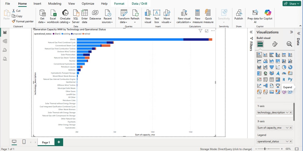
The following sections walk through the cluster configuration, benchmark methodology, and performance results.

Cluster configuration

We benchmarked four instance types to measure the real-world performance of G7 GPU instances against comparable CPU instances for Spark SQL performance. The g7.4xlarge also provides 80 Gbps network bandwidth (compared to 15–17 Gbps on the CPU baselines) and uses RapidsShuffleManager. However, CPU runs showed no evidence of being network- or shuffle-bound at this cluster scale. All tests used Amazon EMR on EKS 7.12.0 with Apache Spark 3.5.6 and cuDF plugin 26.04.2, running the full TPC-DS benchmark at 3 TB scale across 103 queries. Each experiment ran 5 iterations. We report the median. Data was stored as Parquet on Amazon Simple Storage Service (Amazon S3) (same-region gateway endpoint). All instances were launched in a single Availability Zone.

Instance specifications

All four instance types share the same compute footprint of 16 vCPUs and 64 GB system RAM. The g7.4xlarge additionally includes an NVIDIA RTX PRO 4500 Blackwell GPU with 32 GB of dedicated video memory (VRAM), which the cuDF plugin uses to accelerate Spark SQL operations. The baseline for all speedup and cost comparisons is m9gd.4xlarge (Graviton), the lowest-cost CPU instance in the group.

. g7.4xlarge m9gd.4xlarge m8id.4xlarge m8a.4xlarge
Architecture x86_64 arm64 (Graviton) x86_64 x86_64
vCPU 16 16 16 16
RAM 64 GB 64 GB 64 GB 64 GB
GPU 1× RTX PRO 4500 Blackwell (32 GB VRAM) – – –
NVMe 875 GB 950 GB 950 GB EBS only (GP3 16k IOPS and 2000 MB/s throughput to match NVMe
Network 80 Gbps Up to 17 Gbps Up to 15 Gbps Up to 15 Gbps

The g7.4xlarge uses the RTX PRO 4500 Blackwell Server Edition GPU. The CPU baselines cover all three major architectures: m8id.4xlarge (Intel x86), m8a.4xlarge (AMD x86), and m9gd.4xlarge (Graviton arm64).

Spark configuration

All instances used eight executor nodes with the following configuration:

Configuration GPU instances CPU instances
Amazon EMR release emr-7.12.0-spark-rapids-latest emr-7.12.0-latest
executor.cores 14 14
executor.instances 8 8
executor.memory 20G 20G
executor.memoryOverhead 30G 30G
spark.plugins com.nvidia.spark.SQLPlugin –
rapids.memory.pinnedPool.size 8G –
rapids.sql.concurrentGpuTasks 3 –
shuffle.manager RapidsShuffleManager default (sort)
sql.adaptive.enabled true true
io.compression.codec zstd zstd

CPU instances use the same 30 GB memoryOverhead as GPU to make sure that the memory comparison is apples-to-apples. This setting reserves off-heap memory for shuffle and caching on both sides.

For GPU instances, the cuDF plugin offloads Spark SQL operations to the GPU automatically. No code changes are required. The executor.memoryOverhead value is set higher on GPU instances to accommodate GPU memory management and the RAPIDS shuffle manager.

The cuDF plugin automatically falls back to CPU execution for unsupported operators and user-defined functions (UDFs). Your job still completes, but those stages run without GPU acceleration. To identify which operations run on GPU compared to CPU, set spark.rapids.sql.explain=NOT_ON_GPU in your Spark configuration. For a pre-migration assessment of your workloads, use the NVIDIA cuDF tool to estimate GPU acceleration potential before moving to G7 instances.

To tune settings like concurrentGpuTasks and pinnedPool.size, use the Spark History Server on Amazon EMR on EKS, which provides per-stage execution details to identify CPU fallback and shuffle bottlenecks.

Getting started

Reference the Using cuDF Accelerator for Apache Spark with Amazon EMR on EKS for detailed setup instructions.

Prerequisites

Before running GPU-accelerated Spark on Amazon EMR on EKS, make sure the following are in place:

  • Amazon EMR on EKS release version 6.9.0 or later (this post uses emr-7.12.0-spark-rapids-latest).

The -spark-rapids release variant ships the NVIDIA cuDF plugin pre-installed.

  • Amazon Elastic Kubernetes Service (Amazon EKS) cluster with a GPU-enabled node group using G7 instances.
  • Node AMI: AL2023_x86_64_NVIDIA (Amazon EKS optimized accelerated AMI).
  • NVIDIA device plugin installed in the cluster to expose GPUs to Kubernetes pods:
    kubectl apply -f https://raw.githubusercontent.com/NVIDIA/k8s-device-plugin/v0.9.0/nvidia-device-plugin.yml

  • Amazon EMR on EKS virtual cluster registered to the EKS namespace.

To validate GPU availability on your nodes:

kubectl get nodes "-o=custom-columns=NAME:.metadata.name,GPU:.status.allocatable.nvidia\.com/gpu"

Note: Getting started with GPU-accelerated Spark on Amazon EMR is straightforward. To use the latest cuDF plugin, overlay the latest version (for example, 26.04.2 as of May 2026) onto the Amazon EMR RAPIDS image using an initContainer technique. This replaces the bundled cuDF JAR  with a newer version while preserving all other Amazon EMR dependencies. We recommend using the latest Amazon EMR release to get the most up-to-date cuDF plugin for better performance. In our benchmarks, upgrading from cuDF plugin 25.08.0 to 26.04.2 reduced runtime by 36–38 percent. Download the latest cuDF plugin JAR from the NVIDIA repository. AWS Support covers Amazon EMR. For issues specific to a cuDF JAR, file a GitHub issue or contact NVIDIA at .

Performance benchmarks and cost efficiency

We ran the full TPC-DS benchmark suite (103 queries) at 3 TB scale on 8-node clusters in us-east-1. The following table summarizes the results:

. GPU instances CPU instances
Cost per run $2.06 $2.93–$3.18
Total time (103 queries) 281s (4.7 min) 1,010–1,043s (16.8–17.4 min)
Speedup compared to CPU instances 3.7× baseline

Cost per run is the total cluster cost for the benchmark’s duration: Cluster $/hr × (median runtime ÷ 3,600). The hourly rate combines the EC2 On-Demand cost for all 8 nodes and the Amazon EMR on EKS charge for the vCPU and memory the Spark pods consume. Both are billed per second (one-minute minimum), so you pay only for what a job uses while it runs. All runs used Amazon EMR on EKS 7.12.0 in us-east-1, with 8 × 4xlarge nodes (128 vCPU) on both the GPU and CPU sides. The g7.4xlarge cluster runs at $26.35/hr (8 × $3.042 EC2 = $24.34, plus $2.01 for Amazon EMR on EKS) and finishes in 281 seconds, at $2.06 per run. The CPU clusters run at a lower hourly rate ($10.43–$10.99) but take 1,010–1,043 seconds, landing at $2.93–$3.18 per run. All prices reflect On-Demand pricing in us-east-1 as of May 2026. G7 instances are also eligible for EC2 Spot and Compute Savings Plans, which can further reduce costs for recurring batch workloads.

Cost-per-run calculations include EC2 and Amazon EMR charges only. They exclude the EKS control-plane fee, EBS volumes, S3 request and storage costs, and the driver pod.

Bar chart of total TPC-DS runtime by instance type, showing g7.4xlarge finishing far faster than the CPU instances

Figure 1: Total runtime by instance type for all 103 TPC-DS queries at 3 TB scale. The g7.4xlarge with GPU acceleration completed the benchmark in 4.7 minutes, 3.7× faster than CPU instances (16.8-17.4 minutes)

Bar chart of total cost per benchmark run by instance type, showing the g7.4xlarge GPU instance costing less than the CPU instances

Figure 2: Total cost per benchmark run, including both Amazon EC2 instance and Amazon EMR on EKS cost across all 8 nodes. Despite a ~2.5× higher hourly rate, the g7.4xlarge GPU instance costs up to 31% less per run than Graviton because it finishes the workload 3.7× faster

Where GPU acceleration excels

GPU acceleration completed the 103-query power run in 281s compared to 1,032s on CPU, an overall 3.7× speedup that saves 750 seconds per run. GPU was faster on 102 of 103 query executions.

GPU acceleration delivers the largest gains on the long-running, compute- and shuffle-heavy queries where kernel throughput outweighs launch overhead. The biggest absolute time savings:

Query CPU time GPU time Speedup Time saved
q24 (part 1+2) 81.6s 15.9s ~5.1× 65.7s
q23 (part 1+2) 79.4s 16.4s ~4.9× 63.1s
q93 63.7s 5.6s 11.4× 58.1s
q76 30.4s 3.4s 9.0× 27.0s
q64 35.4s 8.5s 4.2× 26.9s
q50 27.6s 3.5s 7.9× 24.0s

Speedup distribution across all 103 executions:

Speedup band Queries
≥5× 15
4–5× 13
3–4× 21
2–3× 26
1–2× 27
<1× (CPU faster) 1

Median per-query speedup 2.94× (geomean 2.84×). The heaviest wins (q50, q76, q93) are aggregation- and shuffle-join-intensive queries that convert cleanly to GpuHashAggregate and GpuBroadcastHashJoin.

Where CPU wins

With RAPIDS 26.04.2, the following query showcases a workload pattern where CPU was faster:

Query CPU time GPU time Ratio Root cause
q16 0.96s 1.44s CPU 1.5x faster Trivial/near-empty scan. Sub-second runtime where GPU kernel-launch overhead is not amortized

Choosing the right instance

Instance Best for Summary
g7.4xlarge (RTX PRO GPU) Fastest and most cost-effective Up to 3.7× faster than comparable CPU instances and up to 31% cheaper per run. Completes in 4.7 min compared to 17.2 min. Best choice for both speed and cost efficiency.
CPU instances (m8a / m8id / m9gd) Flexibility, availability, and always-on workloads Multiple architecture options deliver similar Spark SQL performance. Choose CPU when GPUs are unavailable, when clusters need to remain running continuously (for example, overnight jobs ready for next-day analysis), or when workloads cannot use GPU acceleration. CPU instances offer broad availability and predictable capacity without startup delays.

G7 instances require a G-instance vCPU service quota in your account (default is often 0 for GPU types). Request a quota increase through the Service Quotas console, or use On-Demand Capacity Reservations (ODCRs) to guarantee availability for recurring batch jobs.

Based on these benchmark results, consider evaluating GPU acceleration for your own Apache Spark workloads. Start by identifying compute-intensive operations in your current pipelines, particularly those involving large-scale aggregations, joins, or machine learning feature engineering that could benefit from the performance improvements demonstrated here.

Conclusion

Amazon EMR on EKS with NVIDIA RTX PRO 4500 together provide a meaningful step forward for teams running data-intensive Spark workloads at scale. Whether you’re building ML pipelines that demand rapid feature iteration, running complex ETL transformations across massive datasets, or powering real-time analytics that can’t afford to wait on slow batch jobs, GPU-accelerated Spark on G7 delivers the performance and speed to do more. As data and AI workloads continue to evolve, GPU-accelerated analytics on Amazon EMR is becoming the foundation for data teams. Get started with GPU-accelerated Spark on Amazon EMR on EKS today by visiting Amazon EMR documentation to launch your first G7-powered cluster and see the performance gains for yourself.


About the authors

McCall Peltier

McCall Peltier

McCall is a Senior Product Marketing Manager at AWS focused on data processing services, including Amazon EMR. She leads messaging and launches that support customers building modern data platforms on AWS, collaborating across product and field teams to drive adoption and customer impact.

Karthik Prabhakar

Karthik Prabhakar

Karthik is a Data Processing Engines Architect for Amazon EMR at Amazon Web Services (AWS). He specializes in distributed systems architecture and query optimization, working with customers to solve complex performance challenges in large-scale data processing workloads. His focus spans engine internals, cost-optimization strategies, and architectural patterns that enable customers to run petabyte-scale analytics efficiently

Kshitija Dound

Kshitija Dound

Kshitija is a Specialist Solutions Architect at AWS based in New York City, focusing on data and AI. She collaborates with customers to transform their ideas into cloud solutions, using AWS Big Data and AI services. She also engages in public speaking opportunities, sharing her expertise on cloud technologies, industry trends, and career in the cloud. In her spare time, Kshitija enjoys exploring museums, indulging in art, and embracing NYC’s outdoor scene.

Kinshuk Paharae

Kinshuk Pahare

Kinshuk is head of product for data processing, leading product teams for AWS Glue, Amazon EMR, and Amazon Athena. He has been with AWS for over 6 years.

Introducing AWS Glue 6.0 for faster and more cost-effective data integration

Post Syndicated from Aarthi Srinivasan original https://aws.amazon.com/blogs/big-data/introducing-aws-glue-6-0-for-apache-spark/

Organizations running large data processing pipelines want lower costs, faster job runtimes, and dependable support for open table formats, without adding operational overhead. AWS Glue, a serverless, scalable data integration service that you can use to discover, prepare, move, and integrate data from multiple sources, has now launched AWS Glue 6.0, the new version of AWS Glue that addresses these needs. This version upgrade lowers AWS Glue pricing by 30% and improves performance with AWS optimized Apache Spark 4.1. It also augments developer experience with new features and adds support for Apache Iceberg V3 specifications that are suitable for enterprise adoption. The newly available AWS Glue 6.0 makes data processing workloads more manageable, faster to run, and easier to operate.

In this post, we cover the key capabilities of AWS Glue 6.0 and their performance benefits. We share code examples to help you take full advantage of the release, and we show you how to get started.

AWS Glue 6.0 highlights

AWS Glue 6.0 brings together four major improvements designed to transform how you build and run data integration workloads.

First, it upgrades the underlying runtime to Apache Spark 4.1.1, Python 3.13, Scala 2.13, and AWS SDK for Java 2.x, delivering performance improvements that can help with faster job completion times and lower costs.

Second, this release reduces current AWS Glue usage rate by 30%, and when combined with the performance improvements, you may realize an even lower effective cost.

Third, AWS Glue 6.0 introduces support for more capabilities of Apache Iceberg V3. This includes the VARIANT data type with automatic shredding, deletion vectors, row lineage tracking, nanosecond timestamps, and geo types. With these capabilities, you can build modern lakehouse architectures on the latest open table format standards.

Finally, new features like Spark Declarative Pipelines, Real-Time Mode for streaming and Python virtual environments with S3 caching are designed to further improve performance and developer experience. The following sections dive deeper into each of these areas.

Runtime upgrades

AWS Glue 6.0 upgrades the core runtime stack across the board, bringing newer versions of Apache Spark, Python, Scala, and the AWS SDK to your serverless data integration workloads.

  • Apache Spark 4.1.1 – AWS Glue 6.0 runs an AWS optimized build of Apache Spark 4.1.1, a major generational leap from Spark 3.5 on AWS Glue 5.1. This release introduces improvements focused on intent-driven data engineering, real-time streaming with sub-second latencies down to single-digit milliseconds for stateless tasks, faster PySpark performance, and expanded SQL features.
  • Python 3.13 – Supports Python 3.13, a stable release that brings interpreter changes, Python data model enhancements, standard library updates, and security updates.
  • Scala 2.13 – Upgrades to Scala 2.13 which includes a collections library overhaul, language and syntax feature changes, standard library additions, and compiler performance updates.

Reduced Pricing

AWS Glue 6.0 cuts current AWS Glue pricing by 30%. This means every job you run on AWS Glue 6.0 costs 30% less per DPU-hour compared to AWS Glue 5.1, with no changes required to your workload configuration. When you combine this pricing reduction with the performance improvements delivered by runtime upgrades, your effective cost savings can compound because jobs can complete faster and consume fewer DPU-hours on a lower price point. If you run large-scale Extract, Transform, and Load (ETL) pipelines or recurring batch workloads, this compounding effect can help reduce your monthly spend.
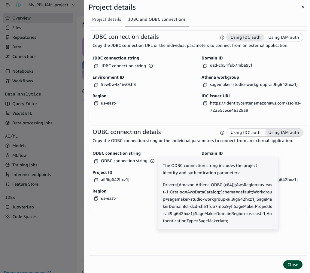
To quantify the comparison, we ran the industry-standard TPC-DS benchmark at 3 TB scale on Parquet data stored in Amazon Simple Storage Service (Amazon S3), using 30 G.2X workers on AWS Glue. The following table compares the results we obtained in our tests for AWS Glue 6.0 and AWS Glue 5.1. Thus, based on TPC-DS benchmark at 3 TB scale, AWS Glue 6.0 delivers up to 36% better price performance than AWS Glue 5.1.

. AWS Glue 6.0 AWS Glue 5.1
Estimated Cost ($) USD 5.61 USD 8.87

Table 1: 3TB TPC-DS benchmark comparison between AWS Glue 6.0 and AWS Glue 5.1

Updated Open Table Format (OTF) support

AWS Glue 6.0 ships with updated versions of all three major open table formats – Iceberg 1.11.0, Hudi 1.1.1, and Delta Lake 4.2.0 – providing better performance, improved merge-on-read capabilities, streamlined concurrency control, and expanded SQL compatibility.

Besides supporting the latest open table format versions, AWS Glue 6.0 delivers Apache Iceberg V3 specification that is suitable for enterprise use. The highlight is Variant shredding, which AWS Glue uses to automatically decompose semi-structured data into physically optimized, columnar sub-fields, which should result in faster query read performance. Combined with deletion vectors for efficient row-level updates, UNKNOWN column types, default column values, and richer data type support, AWS Glue 6.0 is designed to make your open data lakes faster, more flexible, and more cost-efficient. AWS Glue 6.0 also adds support for geospatial data types (Geometry and Geography) and nanosecond-precision timestamps from the Apache Iceberg V3 specification, neither of which are currently supported in open-source Apache Spark 4.1. Additional features like row lineage tracking round out the Apache Iceberg V3 capabilities available on AWS Glue 6.0.

In the following sections, we illustrate select capabilities from Apache Iceberg V3 specification on AWS Glue 6.0.

  1. VARIANT column type

Apache Iceberg V3 introduces the Variant type to store semi-structured data (think JSON, XML, logs, and deeply nested event data) in a compact binary format. Variant shredding is designed to automatically decompose VARIANT columns into physically optimized, columnar sub-fields, facilitating predicate pushdowns and reducing scan overhead. It aims to provide simpler management of semi-structured data, without the need for complex flattening logic. With Variant type, you get the flexibility of embedding a JSON data type in your table columns while shredding is designed to help accelerate read queries and reduce costs.
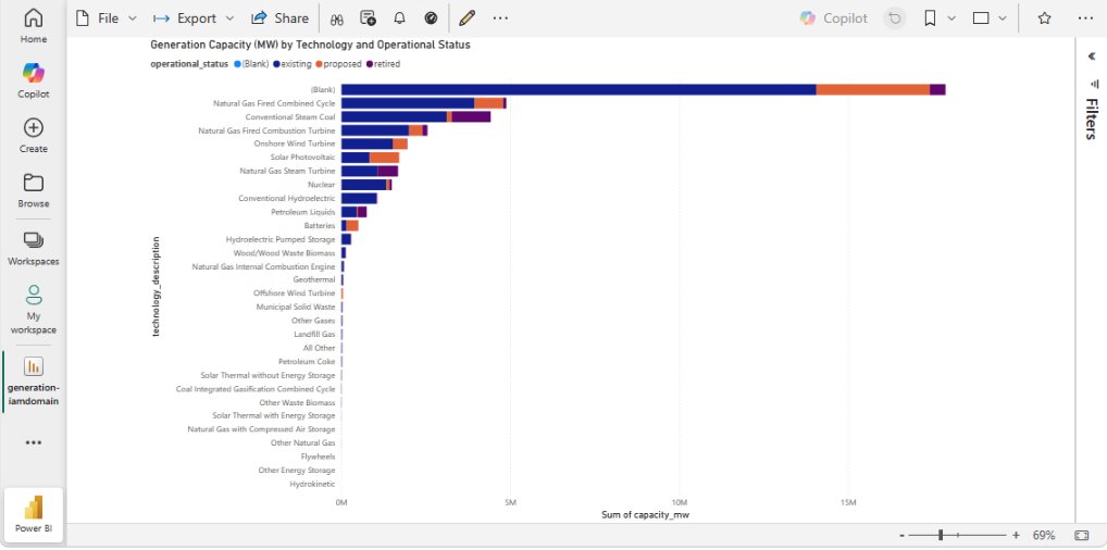
  1. UNKNOWN column type

The UNKNOWN type in Apache Iceberg V3 acts as a flexible placeholder for columns where the data type is not yet determined at the time of table creation or data ingestion. Tables can accept all-null data initially, and the column type can be upgraded later without breaking ingestion pipelines or consuming applications. This can simplify schema evolution for rapidly changing data sources. Apache Iceberg V3’s UNKNOWN column type maps to Spark 4.1’s VOID type.

  1. DEFAULT column values

Apache Iceberg V3’s DEFAULT column values allow specifying a default value for a column in the table metadata. When you add a new column, the query engine is designed to automatically apply this default to older rows, without rewriting data or running manual backfill operations.

The following code demonstrates creating an Apache Iceberg V3 table that uses VARIANT and UNKNOWN types, and DEFAULT values for a column.

Prerequisites

To get started with this code example, make sure you have the following prerequisites.

  1. An AWS account.
  2. An AWS Identity and Access Management (IAM) role with permissions for AWS Glue, the AWS Glue Data Catalog, and Amazon S3. For more information, see Setting up IAM permissions for AWS Glue. This will be the AWS Glue job execution role.
  3. An S3 bucket to store the Iceberg table data.

Steps

To create an AWS Glue 6.0 job, use the following steps.

  1. Log in to your AWS account and open the AWS Glue console.
  2. Create a new ETL job, with Script editor option.
    1. Choose engine as Spark in the drop-down menu.
    2. Start fresh, Create script and copy-paste the following code.
    3. Replace the demo S3 bucket name with your bucket name in the code.
# Example pySpark script for testing few Iceberg v3's new data types
from pyspark.sql import SparkSession

CATALOG = "glue_catalog"
DATABASE = "sample_glue6_iceberg_db"
TABLE_NAME = "sample_glue6_table"
TABLE = f"{CATALOG}.{DATABASE}.{TABLE_NAME}"
TABLE_LOCATION = "s3://amzn-s3-demo-table-bucket/glue6blog-newdatatypes/"

# Configure Spark to use Apache Iceberg with the AWS Glue Data Catalog.
spark = (
    SparkSession.builder
    .appName("Glue6NewDataTypes")
    .config("spark.sql.extensions", "org.apache.iceberg.spark.extensions.IcebergSparkSessionExtensions")
    .config(f"spark.sql.catalog.{CATALOG}", "org.apache.iceberg.spark.SparkCatalog")
    .config(f"spark.sql.catalog.{CATALOG}.catalog-impl", "org.apache.iceberg.aws.glue.GlueCatalog")
    .config(f"spark.sql.catalog.{CATALOG}.io-impl", "org.apache.iceberg.aws.s3.S3FileIO")
    .config(f"spark.sql.catalog.{CATALOG}.warehouse", "s3://amzn-s3-demo-table-bucket/glue6blog-newdatatypes")
    .config("spark.sql.defaultColumn.enabled", "true")
    .getOrCreate()
)

spark.sql(f"CREATE DATABASE IF NOT EXISTS {CATALOG}.{DATABASE}")

# Create an Iceberg v3 table with VARIANT, unknown, and a default value.
# Spark's VOID type is stored as the Iceberg v3 unknown type.
spark.sql(
    f"""
    CREATE TABLE {TABLE} (
        record_id BIGINT,
        payload VARIANT,
        reserved_field VOID,
        status STRING DEFAULT 'active'
    )
    USING ICEBERG
    LOCATION '{TABLE_LOCATION}'
    TBLPROPERTIES ('format-version' = '3')
    """
)

# Insert two rows. The omitted columns use null and the declared default.
spark.sql(
    f"""
    INSERT INTO {TABLE} (record_id, payload)
    VALUES
    (1, parse_json('{{"event_type":"created","score":98.5}}')),
    (2, parse_json('{{"event_type":"processed","score":87.2}}'))
    """
)

# Query the row and extract values from the VARIANT column.
spark.sql(
    f"""
    SELECT
        record_id,
        variant_get(payload, '$.event_type', 'string') AS event_type,
        variant_get(payload, '$.score', 'double') AS score,
        reserved_field,
        status
    FROM {TABLE}
    """
).show(truncate=False)

spark.stop()
  1. Provide the following details in the Job details tab.
    1. A Name for the job.
    2. The IAM role you have from Prerequisites (2) for the IAM role of the job.
    3. Choose Glue 6.0 for the Glue version.
    4. Leave the rest as defaults.The following screenshot shows the Job details tab with illustrated values in the AWS Glue console.

      AWS Glue Job details tab with the Glue version set to Glue 6.0 and other settings left as defaults

      Figure 1: Job details tab with the Glue version set to Glue 6.0

    5. Scroll down. Under Advanced properties, for Job parameters, add the following additional Job parameter key-value pair:--datalake-formats=icebergThe following screenshot shows the Job parameters with the illustrated key-value pair in the AWS Glue console.

      Advanced properties section showing the Job parameters key –datalake-formats set to the value iceberg

      Figure 2: Job parameters with the datalake-formats key set to iceberg

  2. Save the job and choose Run.
  3. After the job is completed successfully, from the Runs tab – Run details, you can inspect the Output logs that take you to the logs in the Amazon CloudWatch console. The following shows the sample output for the SELECT query in the script.
+---------+----------+-----+--------------+------+
|record_id|event_type|score|reserved_field|status|
+---------+----------+-----+--------------+------+
|1        |created   |98.5 |NULL          |active|
|2        |processed |87.2 |NULL          |active|
+---------+----------+-----+--------------+------+

Notice that we inserted two rows with values only in the record_id and the variant column. Variant column inserts were done using parse_json(). The reserved_field is of VOID type, hence returns NULL values. The status column is declared with a default active value and returns active, since the column was omitted during the insert operation.

  1. Deletion Vectors
    Apache Iceberg V3 replaces the traditional positional delete files used in Apache Iceberg V2 to deletion vectors. This change can help improve Merge-on-Read (MoR) performance. This shift replaces heavy, multi-file Parquet reads with highly compressed, direct binary bitmaps that can provide lower storage overhead and faster reads on delete-heavy tables. In scenarios with heavy table updates, such as streaming change data capture (CDC) from operational databases, Apache Iceberg V3 can offer read performance advantage over Apache Iceberg V2.

    To validate the performance of deletion vectors, we created two identical AWS Glue streaming jobs and ingested the events into two different Iceberg tables, one in Apache Iceberg V2 and another in Apache Iceberg V3 format. The streaming CDC events were approximately 150,000 events per second, merge-on-read, update-heavy. Every micro-batch writes row-level deletes. We froze both tables at the same delete-heavy state and disabled compaction, leaving the tables with roughly 1.7 million rows in valid state out of the 26.4 million physical rows. The following table summarizes the read performance latency of the two Iceberg tables. We observed in this testing that reading from the delete-heavy Apache Iceberg V3 is at least 1.5 times faster than the reading from a similar Apache Iceberg V2 table. For larger enterprise scale Apache Iceberg V3 tables, the read performance could improve further.

Read latency comparison showing Apache Iceberg V3 deletion vectors reading at least 1.5 times faster than Apache Iceberg V2 delete files

Table 2 – Read latency comparison between Apache Iceberg V2 delete files and Apache Iceberg V3 deletion vectors

New ETL features

AWS Glue 6.0 introduces several additional capabilities designed to simplify how you build and manage data pipelines, some of which are discussed in the following list.

  • Spark Declarative Pipelines (SDP) where you define the outcomes you want for your entire data pipelines in a declarative fashion with SQL statements or Python decorators while AWS Glue handles execution flow, dependency resolution, parallelism, checkpointing, CDC, and recovery automatically. This helps you focus on business logic rather than orchestration plumbing.
  • Real-Time Mode (RTM) for streaming delivers continuous execution for Structured Streaming with sub-second latencies, down to single-digit milliseconds for stateless tasks. This can help support real-time use cases like fraud detection, live dashboards, and event-driven architectures without managing dedicated streaming infrastructure.
  • Arrow-Native UDFs/UDTFs execute Python functions directly on PyArrow batches without Pandas conversion overhead, which can result in faster performance for custom transformation logic at scale.
  • Recursive Common Table Expressions (CTE) adds WITH RECURSIVE queries natively, allowing graph traversals and hierarchical queries without workarounds or external libraries.
  • Python data source filter pushdown evaluates filters at the data source designed to minimize data movement, reduce the volume of data scanned, and improve job performance.
  • With Python virtual environments and S3 caching, you can provide pre-built Python dependencies, which should result in reduced startup latency for AWS Glue jobs by eliminating runtime dependency resolution. For existing jobs that use --additional-python-modules, no action is required. AWS Glue automatically handles the conversion to virtual environments when your job runs on AWS Glue 6.0.

Dependent library upgrades

The following table summarizes the key runtime and library version upgrades on AWS Glue 6.0.

Feature Glue 6.0 Glue 5.1
Spark 4.1.1-amzn-0 3.5.6-amzn-1
Python 3.13.14 3.11.15
Scala 2.13.17 2.12.18
AWS SDK for Java 2.44.6
(Version 1.x removed)
2.35.5
Boto3 1.42.84 1.40.61
Java 17.0.20 17.0.19
Iceberg 1.11.0 1.10.0
Hudi 1.1.1 .0.2
Delta Lake 4.2.0 3.3.2
AWS Glue Data Catalog client 4.11.0 4.9.0
EMR DynamoDB connector 6.1.0 5.7.0
Arrow 18.3.0 2.0.1
Hive 2.3.10-amzn-1 2.3.9-amzn-4

Table 3: Runtime and library version comparison across AWS Glue 6.0 and AWS Glue 5.1

Getting started

To get started with AWS Glue 6.0, you can use one of the following methods.  

Clean up

To avoid incurring costs, clean up the resources you created for this post.

  1. Delete the Data Catalog database and the Iceberg table.
  2. Delete the data and metadata folders of the Iceberg table from your S3 bucket.
  3. Delete the AWS Glue job and the AWS Glue job execution IAM role.

Conclusion

AWS Glue 6.0 is designed to be faster, more cost-effective, and easier to use for building your open data lakehouse architectures and orchestrating your data pipelines. In this post, we discussed the key highlights of AWS Glue 6.0 and illustrated usage of Apache Iceberg V3 features with code samples. You can create new AWS Glue jobs on AWS Glue 6.0 or migrate your existing AWS Glue jobs to benefit from these improvements.

With Apache Spark 4.1.1, Apache Iceberg V3, Python 3.13, upgraded open table format libraries, and new streaming capabilities, AWS Glue 6.0 aims to help you build new data applications or to operate your existing data pipelines more efficiently and with less maintenance overhead.

We encourage you to test AWS Glue 6.0 in your development environment today. Check out this blog that talks about upgrading your AWS Glue jobs to AWS Glue 6.0. Also, in the coming days and weeks, look out for blogs on individual topics illustrating various features of Spark 4.1.1 and Apache Iceberg V3 on AWS Glue 6.0.

Acknowledgements: We thank the numerous engineers and leaders who helped build AWS Glue 6.0 to support customers with a highly performant Spark runtime and other value-added capabilities.


About the authors

Aarthi Srinivasan

Aarthi Srinivasan

Aarthi is a Senior Big Data Architect working on data, analytics and GenAI topics with the worldwide specialist org at AWS. She works with AWS customers and partners to architect open data lake solutions, enhance product features, and establish best practices for data governance and analytics services adoption.

Shrey Malpani

Shrey Malpani

Shrey is a Senior Product Manager Technical at Amazon Web Services (AWS), where he works at the intersection of distributed data processing and data integration. He is focused on building and scaling data integration and data management capabilities across services like AWS Glue, Amazon EMR, and Amazon Redshift that help customers build AI-ready data platforms for their analytics and machine learning workflows.

Angel Conde Manjon

Angel Conde Manjon

Angel is a Senior Solutions Architect at AWS where he helps partners develop businesses centered on Data and AI. He has previously worked on research related to Data Analytics and Artificial Intelligence in diverse European research projects. Angel is also an Apache Iceberg contributor.

Peter Tsai

Peter Tsai

Peter is a Software Development Engineer at AWS, where he enjoys solving challenges in the design and performance of the AWS Glue runtime. In his leisure time, he enjoys hiking and cycling.

Danylo Prozorov

Danylo Prozorov

Danylo is a Software Development Engineer at AWS Glue, where he works on building data integration and generative AI solutions for analytics customers. Outside of work, he enjoys sports, hiking, riding motorcycles, and building his overland rig.

Bo Li

Bo Li

Bo is a Senior Software Development Engineer on the AWS Glue team. He is devoted to designing and building end-to-end solutions to address customers’ data analytic and processing needs with cloud-based, data-intensive and GenAI technologies.

Kartik Panjabi

Kartik Panjabi

Kartik is a Software Development Manager on the AWS Glue team. His team builds generative AI features for the Data Integration and distributed system for data integration.

Mohit Saxena

Mohit Saxena

Mohit leads AWS Glue and AWS Data Analytics agentic AI initiatives that help customers build and operate big data applications on Apache Spark, Amazon S3, and cloud data lakes and warehouses, spanning across AWS Glue, Amazon EMR, and Amazon Athena.

Upgrade AWS Glue jobs to Glue 6.0 with AI-powered Spark upgrades

Post Syndicated from Prasad Nadig original https://aws.amazon.com/blogs/big-data/upgrade-aws-glue-jobs-to-glue-6-0-with-ai-powered-spark-upgrades/

Upgrading PySpark jobs to a new Apache Spark major version can introduce breaking changes. Removed configuration keys, stricter type casting, and Python library incompatibilities can cause runtime failures or silent behavior differences. With AWS Glue 6.0 now running Apache Spark 4.1 and Python 3.13, you need a reliable way to migrate your existing jobs while validating correctness.

In this post, we walk through upgrading a PySpark ETL job from AWS Glue 5.1 to AWS Glue 6.0. We use the generative AI upgrades for Apache Spark in the AWS Glue console. The upgrade analysis automatically identifies incompatibilities, iteratively resolves them, validates the result with data quality checks, and presents recommended changes for your review. AWS Glue 6.0 also delivers up to 36% better price performance* along with Iceberg v3, Spark Declarative Pipelines, Real-Time Mode, and Arrow-native Python UDFs.

What changes with AWS Glue 6.0

AWS Glue 6.0 runs Apache Spark 4.1, which introduces several behavioral changes from the Spark 3.5 runtime used in AWS Glue 5.1:

Behavior Spark 3.5 (AWS Glue 5.1) Spark 4.1 (AWS Glue 6.0)
ANSI SQL mode Disabled by default Enabled by default
Legacy Parquet datetime configs Supported Removed (renamed)
Python runtime 3.11 3.13

Beyond version compatibility, AWS Glue 6.0 also introduces:

  • Apache Iceberg v3 with VARIANT Shredding for efficient semi-structured data handling.
  • Spark Declarative Pipelines — agent-authorable ETL.
  • Real-Time Mode — single-digit millisecond streaming latency.
  • Arrow-native Python UDFs (PyArrow) for improved performance.
  • Built-in observability with structured metrics and enhanced Spark UI.
  • Up to 36% better price performance compared to AWS Glue 5.1*.

These runtime changes mean your existing AWS Glue jobs might encounter removed configuration keys, stricter type casting behavior, or Python package version incompatibilities when running on AWS Glue 6.0. Fixing these manually is time-consuming and error-prone. The following sections show how the generative upgrade analysis handles this automatically.

The sample job

Our example is a daily ecommerce order analytics pipeline running on AWS Glue 5.1:

What the job does:

  • Ingests 10,000 orders from Parquet files with INT96 timestamps (including pre-1900 historical dates from a legacy system migration).
  • Computes revenue metrics by casting string prices to numeric values and calculating line totals with discounts and tax.
  • Segments customers using recency, frequency, and monetary (RFM) scoring through mapInPandas with pandas and scikit-learn.
  • Writes enriched results back to Amazon Simple Storage Service (Amazon S3).

Job configuration (AWS Glue 5.1):

Glue version: 5.1
Worker type: G.1X
Workers: 10
Python modules: pandas==2.2.2, scikit-learn==1.5.0, numpy==1.26.4
Spark configs:
  spark.sql.legacy.parquet.datetimeRebaseModeInWrite=LEGACY
  spark.sql.legacy.parquet.int96RebaseModeInWrite=LEGACY
  spark.sql.parquet.datetimeRebaseModeInRead=LEGACY
  spark.sql.parquet.int96RebaseModeInRead=LEGACY

This job runs successfully on AWS Glue 5.1. The following sections walk through how the upgrade analysis identifies and resolves incompatibilities when upgrading this job to AWS Glue 6.0. Before starting, confirm you have the prerequisites in place.

Prerequisites

  • An AWS account with access to the AWS Glue console.
  • An existing AWS Glue job on version 5.1 or earlier with at least one successful run.
  • An Amazon S3 path for storing the upgrade analysis results.

Running the upgrade analysis from the console

The following steps walk through the upgrade analysis workflow using the AWS Glue console.

Step 1: Select your job

Navigate to your job in the AWS Glue Studio console. Confirm the job has a successful run history on AWS Glue 5.1 before starting the upgrade analysis.

AWS Glue Studio job run history showing a successful run on AWS Glue 5.1

Figure 1: Job run status for the job on AWS Glue 5.1

Step 2: Start the upgrade analysis

From the job’s Actions menu, select Upgrade with generative AI. Configure the following:

  • Target AWS Glue version: 6.0.
  • Results S3 path: An S3 location where the analysis stores its artifacts and recommendations.
Actions menu in AWS Glue Studio with the Upgrade with generative AI option

Figure 2: The Upgrade with generative AI option in the Actions menu

Configure the target AWS Glue version and the S3 results path, then choose Run.

Upgrade window with the target AWS Glue version set to 6.0 and an Amazon S3 results path

Figure 3: The Upgrade with generative AI window for setting the target AWS Glue version and results path

Choose Run. The analysis begins by running your job on AWS Glue 5.1 to establish a baseline. It then iteratively tests the job on AWS Glue 6.0, identifies failures, applies recommended fixes, and validates the job. If the upgrade analysis cannot resolve an incompatibility within its attempt budget, the analysis stops and reports the unresolved issue for manual review. Your original job remains unchanged.

Note: The upgrade analysis executes your job multiple times (one baseline run plus one or more validation attempts), and each run consumes Data Processing Units (DPUs). For large or long-running jobs, consider using the run configuration option to specify fewer workers or a smaller dataset to optimize analysis cost.

Step 3: Monitor progress

The console displays the analysis progressing through multiple validation attempts. Each attempt either succeeds or fails with a specific error, and the upgrade analysis uses that error signal to determine and apply the appropriate fix for the next attempt.

Upgrade analysis progress showing multiple validation attempts with success and failure states

Figure 4: Upgrade analysis progress across multiple validation attempts

What the upgrade analysis found and fixed

The analysis completed in four validation attempts, identifying and resolving three distinct incompatibilities. The upgrade uses deterministic migration rules for known config changes, and automated diagnosis for runtime or code errors.

Iteration 1: Removed Parquet legacy configuration

The analysis first sanitizes any Spark configurations that were removed in Spark 4.1. Our job used spark.sql.legacy.parquet.datetimeRebaseModeInWrite and spark.sql.legacy.parquet.int96RebaseModeInWrite, which no longer exist.

Migration rule applied: The SQL configs with the spark.sql.legacy prefix were removed in Spark 4.1. They have been renamed to their non-legacy equivalents, preserving the original values.

Recommended change:

Before:
spark.sql.legacy.parquet.datetimeRebaseModeInWrite=LEGACY
spark.sql.legacy.parquet.int96RebaseModeInWrite=LEGACY

After:
spark.sql.parquet.datetimeRebaseModeInWrite=LEGACY
spark.sql.parquet.int96RebaseModeInWrite=LEGACY

The read-side configs (datetimeRebaseModeInRead, int96RebaseModeInRead) already used the correct non-legacy names and required no changes.

However, with this fix applied, the validation run still failed because the Python module installation encountered an error on the AWS Glue 6.0 image.

Iteration 2: Python module version incompatibility

The pinned module versions (pandas==2.2.2, scikit-learn==1.5.0, numpy==1.26.4) could not be installed in the AWS Glue 6.0 Python 3.13 environment.

Error:

LAUNCH ERROR | Installation of Additional Python Modules failed

Recommended change: The upgrade analysis updated the version specifications from exact pins to minimum version constraints, allowing pip to resolve compatible versions for Python 3.13:

Before: pandas==2.2.2, scikit-learn==1.5.0, numpy==1.26.4
After:  pandas>=2.1.0, scikit-learn>=1.3.0, numpy>=1.24.0

With modules installing successfully, the job launched on AWS Glue 6.0 but encountered a runtime error.

Iteration 3: ANSI mode strict type casting

Spark 4.1 enables ANSI SQL mode by default (spark.sql.ansi.enabled=true). Our revenue calculation casts string prices to double, but approximately 1.8% of records contain non-numeric placeholder values such as “N/A”, “pending”, or “null” from the upstream system. From a business perspective, this meant 1.8% of revenue orders were silently excluded from revenue metrics. This data quality issue was invisible to the original pipeline.

On AWS Glue 5.1 (ANSI mode off), cast("N/A" as double) silently returns null. On AWS Glue 6.0 (ANSI mode on), this throws an exception:

Error:

NumberFormatException: [CAST_INVALID_INPUT] The value 'null' of the type
"STRING" cannot be cast to "DOUBLE" because it is malformed. Correct the
value as per the syntax, or change its target type. Use try_cast to
tolerate malformed input and return NULL instead. SQLSTATE: 22018

Migration rule applied: As of Spark 4.1, spark.sql.ansi.enabled is on by default. Casting a malformed value now raises CAST_INVALID_INPUT instead of returning NULL. The upgrade analysis resolved this by updating the script to use try_cast(), which safely returns NULL for malformed input while preserving ANSI mode protections for the rest of the job.

Recommended change:

Before (AWS Glue 5.1):

F.col("unit_price").cast("double")

After (AWS Glue 6.0, fixed by the upgrade analysis):

F.expr("try_cast(unit_price as double)")

This is a targeted fix that handles the known dirty data without disabling ANSI mode globally, keeping overflow detection and type safety active throughout the job.

Final validation and data quality check

After applying all three fixes, the analysis ran the job on AWS Glue 6.0 one final time and performed a data quality comparison between the AWS Glue 5.1 baseline output and the AWS Glue 6.0 output.

Result: The job completed successfully and all data validations passed with no mismatches detected between the source and target outputs.

Completed upgrade analysis status with links to the results output path in Amazon S3

Figure 5: Final analysis status with links to the results output path in Amazon S3

Reviewing the upgrade summary

The analysis produces a detailed summary stored in your S3 results path. This summary documents each validation attempt, the errors encountered, the migration rules applied, and the recommended configuration changes:

s3://amzn-s3-demo-bucket/scripts/auto-upgrade/ja-{analysis-id}/
    summary/
        summary.md                       # Full iteration-by-iteration report
        data_validation_summary.md       # Data quality comparison results
    artifact/
        attempt_N/
            script/main.py               # Recommended script (if modified)
            job_config_modifications.json  # Recommended parameter changes
            requirements.txt             # Updated dependency versions

The following is a snippet from the upgrade summary (summary.md) showing the recommended changes and validation attempt details:

The summary documents each validation attempt, the changes applied, and the data quality results.

Upgrade summary showing validation attempts, applied changes, and data quality comparison results

Figure 6: Upgrade summary snippet showing validation attempt details, data quality, and analysis results

After reviewing the recommendations, accept the changes to upgrade your job to AWS Glue 6.0. This updates your job definition with the recommended configuration, including the renamed Spark configs, updated module versions, and any script modifications. Because the analysis has already validated the job on AWS Glue 6.0 and confirmed data quality parity with the original, your job is ready for production.

After reviewing the recommendations, you can apply the upgraded script to your job.

AWS Glue Studio prompt to apply the upgraded script to the job

Figure 7: The option to apply the upgraded script to the job

Choose Apply to confirm the upgrade.

Confirmation dialog with the Apply button to upgrade the job to AWS Glue 6.0

Figure 8: The Apply button that confirms upgrading the job to AWS Glue 6.0

After applying, the job definition reflects the new AWS Glue version.

AWS Glue job details showing version 6.0 after applying the upgrade

Figure 9: The AWS Glue version for the job after applying the upgrade

Python virtual environments in AWS Glue 6.0

AWS Glue 6.0 introduces --python-virtual-env-storage-prefix, a service-managed virtual environment with S3 caching that simplifies Python dependency management.

For existing jobs that use --additional-python-modules, no action is required. AWS Glue automatically handles the conversion to virtual environments when your job runs on AWS Glue 6.0. Your jobs continue to work without any changes.

For new jobs on AWS Glue 6.0, we recommend using the virtual environment approach:

{
    "DefaultArguments": {
        "--python-virtual-env-storage-prefix": "s3://amzn-s3-demo-bucket/glue-venv-cache/",
        "--additional-python-modules": "pandas>=2.1.0,scikit-learn>=1.3.0,numpy>=1.24.0"
    }
}

How it works:

  • On the first run, AWS Glue installs your modules into a virtual environment, packages it, and caches the result to your specified S3 path (approximately 15–30 seconds of additional startup time).
  • On subsequent runs, AWS Glue downloads and extracts the cached virtual environment instead of running pip install.
  • The cache is automatically invalidated when your module list, versions, or AWS Glue version changes.

This approach provides faster cold starts after the first run, requires no Docker image management (unlike --python-virtual-env), and is entirely service-managed with no maintenance burden.

Conclusion

The generative upgrade analysis identified and resolved three distinct compatibility issues in our AWS Glue 5.1 job, so the job now runs successfully on AWS Glue 6.0 with Apache Spark 4.1:

  • The upgrade analysis renamed legacy Parquet datetime configuration keys (removed in Spark 4.1) to their current equivalents.
  • The upgrade analysis updated Python module version specifications that were incompatible with Python 3.13 to use flexible minimum version constraints.
  • The upgrade analysis addressed the new ANSI SQL mode default (which causes runtime failures on malformed data) with a targeted fix using try_cast() to safely handle non-numeric values while preserving ANSI mode protections.

The analysis validated that the upgraded job produces output consistent with the original, and presented all changes as recommendations for review before applying them to your job.

Next steps

After you have reviewed and accepted the upgrade changes, you can delete the analysis results stored in your S3 results path.

*Based on 3TB TPC-DS benchmark comparing AWS Glue 6.0 to AWS Glue 5.1.


About the authors

Prasad Nadig

Prasad Nadig

Prasad is a Senior Analytics Specialist Solutions Architect at Amazon Web Services (AWS), specializing in large-scale data analytics and AI. Prasad partners with customers to design, migrate, and modernize their analytics platforms on AWS into scalable, cost-effective solutions, with deep expertise in data lakes, data warehousing, distributed processing, and performance tuning at petabyte scale.

Shrey Malpani

Shrey Malpani

Shrey is a Senior Product Manager Technical at Amazon Web Services (AWS), where he works at the intersection of distributed data processing and data integration. He is focused on building and scaling data integration and data management capabilities across services like AWS Glue, Amazon EMR, and Amazon Redshift that help customers build AI-ready data platforms for their analytics and machine learning workflows.

Rishabh Nair

Rishabh Nair

Rishabh is a Software Development Engineer in the AWS analytics organization, where he combines generative AI with distributed systems to build agentic workflows that modernize large-scale data processing. He is passionate about the infrastructure that makes these workflows reliable and scalable for customers.

Keerthi Chadalavada

Keerthi Chadalavada

Keerthi is a Senior Software Development Engineer in the AWS analytics organization. She focuses on combining generative AI and data integration technologies to design and build comprehensive solutions for analytics and data engineering workloads.

AWS Weekly Roundup: Student Rewards on AWS Builder Center, Local Zone in Las Vegas, and more (August 24, 2026)

Post Syndicated from Esra Kayabali original https://aws.amazon.com/blogs/aws/aws-weekly-roundup-student-rewards-on-aws-builder-center-local-zone-in-las-vegas-and-more-august-24-2026/

During my time at AWS, I have always looked for opportunities to work with students. I have delivered over 50 talks at universities across the region, and watching the potential in the room is always a strong motivator. It reminds me of why I do this work, and that the students I meet today may well become our customers and collaborators tomorrow. That is why I am happy to open this week with Student Rewards on AWS Builder Center.

Rick Suttles published Introducing Student Rewards on AWS Builder Center, a new benefit for verified higher education students. When you verify your enrollment through SheerID and complete your Builder Center profile, you unlock 12 months of premium AWS Skill Builder access (900+ courses, hands-on labs, certification exam prep, and game-based learning). From there, you earn badges through actions on Builder Center: publishing articles, commenting, and maintaining engagement. At 7 badges, you unlock $10 in AWS Credits. At 14 badges, another $20 in credits. At 21 badges, you earn an AWS Foundational Certification exam voucher ($100 value).

This represents a commitment of over $500 million in resources during this back-to-school season, providing students with the training, tools, and certification needed to start building their careers in cloud and AI. Student Rewards is available to students 18 years or older and enrolled at accredited higher education institutions worldwide, subject to verification and applicable terms.

Verify your student status and start learning, earning badges, and unlocking rewards!

Last week’s launches
Here’s what else happened this week.

  • A new AWS Local Zone in Las Vegas, Nevada – This new Local Zone supports Amazon EC2 C7i, M7i, R7i, and C8gn instances, Amazon EBS, Amazon ECS, Amazon EKS, Application Load Balancer, and AWS Direct Connect. AWS Local Zones are now available in more than 30 metropolitan areas worldwide. In addition, AWS added a fourth Availability Zone to the Europe (London) Region, delivering next-generation AI and ML capacity with Trn3 and P6 accelerated instances alongside general-purpose compute.
  • Amazon EC2 Auto Scaling now supports batch instance termination – You can now pass up to 100 instance IDs to the TerminateInstanceInAutoScalingGroup API to terminate them as a batch, reducing the number of API calls needed to scale down your Auto Scaling groups. Batch termination is designed for workloads that need to rapidly scale down, such as AI/ML training jobs, container orchestrators, or event-driven architectures that spin up large fleets temporarily.
  • AWS CloudShell now includes a built-in visual file editor – CloudShell now includes a visual file editor that you can launch directly from your shell session using a single edit command. The editor supports syntax highlighting, find-and-replace, multi-line selection, copy-paste, and undo-redo in a single browser session. Whether you are updating a deployment script, modifying an agent steering file, editing a CloudFormation template, or fixing a Lambda function, the editor provides a seamless edit-and-run experience without leaving CloudShell.
  • Amazon Bedrock now supports SpaceXAI Grok 4.6 with cross-Region inference – Grok 4.6, a frontier model built for coding, agentic tasks, and knowledge work, is now available on Amazon Bedrock. The model runs on the bedrock-runtime endpoint with support for the Responses, Chat Completions, and Converse APIs, and works with existing account-level controls including model invocation logging, Amazon CloudWatch metrics, and cost itemization in AWS Cost Explorer.
  • Amazon Bedrock expands API support and introduces cross-Region inference for OpenAI models – Amazon Bedrock now supports OpenAI GPT-5.6 models (Sol, Terra, and Luna) with the Responses, Converse, and Chat Completions APIs, and adds cross-Region inference. Geo cross-Region inference routes requests within a predefined geography (including new US Geo support with this launch), while Global cross-Region inference serves requests from any commercial AWS Region at a lower per-token cost.
  • AgentCore payments is now generally available in Amazon Bedrock AgentCore – At general availability, AgentCore payments includes Quick Create for Coinbase credential provisioning directly within the AgentCore console, a curated Coinbase Bazar MCP server of pay-per-use x402 endpoints via AgentCore gateway, support for the Machine Payment Protocol (MPP), and the “upto” scheme in the x402 protocol for pay-per-inference and dynamic pricing use cases. To learn more, visit the AI Blog post.
  • AWS Glue 6.0 delivers 30% price reduction and Iceberg v3 support – AWS Glue 6.0 is built on a fully modernized runtime, Apache Spark 4.1, Python 3.13, and Scala 2.13, delivering 30% lower pricing than previous AWS Glue versions. With Iceberg v3, Glue 6.0 adds the VARIANT data type with automatic shredding for faster reads on semi-structured data, deletion vectors for high-performance row-level updates, geometry and geography data types for spatial processing, and flexible schema evolution.

For a full list of AWS announcements, be sure to keep an eye on the What’s New with AWS page.

Other AWS news
Here are some additional posts you may find useful:

  • Updates to your AWS Sign-In experience – AWS is gradually introducing updates to the sign-in and sign-up experience. The redesigned sign-in page introduces a unified email entry point for root users and customers using the new email-based sign-in method, while IAM users continue signing in with their account ID, username, and password. The page also includes sign-in options for customers whose AWS account was created using a supported identity provider (Google, GitHub, Apple, or Amazon.com). A redesigned session selection page simplifies viewing and managing multiple active account and role sessions. If your organization relies on browser automation or scripted workflows that interact with the sign-in page, review the post to understand how these changes might affect your configuration.
  • In the works: AWS Builder Lofts in Berlin, Hyderabad, and São Paulo – My colleague Channy announced plans to open new Builder Lofts in three cities. Since the first Builder Loft opened in San Francisco in July 2025, it has welcomed more than 22,500 developers through its doors. Each new location will be a permanent community space offering free workshops, networking events, pitch nights, content creation spaces, and co-working areas. Berlin will focus on digital sovereignty and security-readiness, Hyderabad on AI and cloud-native architecture, and São Paulo on supporting Latin America’s developer ecosystem.
  • AWS and Amazon WorkSpaces recognized as a Leader in the 2026 Gartner Magic Quadrant for Desktop as a Service – AWS has been named a Leader in the 2026 Gartner Magic Quadrant for Desktop as a Service (DaaS) for the third consecutive year, evaluated on Completeness of Vision and Ability to Execute. Gartner noted strengths in operations, geographic strategy, and overall viability. This is also the first year the evaluation includes Amazon WorkSpaces for AI agents, a capability that runs AI agents within the same desktop environment, security perimeter, and audit trail as human users.

For a full list of AWS blog posts, be sure to keep an eye on the AWS Blogs page.

Upcoming AWS events
Check your calendar and sign up for upcoming AWS events:

Visit the AWS Builder Center to meet other builders, contribute solutions, and find resources that help you keep building.

Summer is slowly coming to an end, and I am already planning a few days off in the coming months to keep me motivated through the rainy autumn ahead. I hope you are doing the same. Come back next week for more!

— Esra

Amazon Linux default SSM parameter will now track the latest kernel

Post Syndicated from Gokul Govindaraju original https://aws.amazon.com/blogs/compute/amazon-linux-default-ssm-parameter-will-now-track-the-latest-kernel/

Today we are announcing that the Amazon Linux kernel-default AWS Systems Manager (SSM) parameter will now update to point to the latest Amazon Linux kernel version as new kernel versions get released. On August 17, 2026, for Amazon Linux 2023 (AL2023), the SSM parameter was updated from kernel 6.1 to kernel 6.18. As new kernel versions get released (expected annually), the parameter will continue to update to the latest kernel version after a validation period.

This post explains the default kernel behavior, what it means for your workloads, and how to manage the transition.

What’s changing?

Amazon Linux ships multiple kernel versions and has tracked a default kernel for each OS version. For example,
the AL2023 parameter:

ssm:/aws/service/ami-amazon-linux-latest/al2023-ami-{minimal}-kernel-default-{x86_64 arm64}

has remained on kernel 6.1 since launch. Going forward, the kernel-default SSM parameter will update to the latest kernel as new versions are released. Each new kernel will go through a 3- to 6-month validation period after GA before we update the default. This window gives you time to test the new kernel before the change. We will announce the kernel-default upgrade date before it takes effect.

SSM Parameter Resolved to (Before) Resolves to (Now)
al2023-ami-{minimal}-kernel-default-{x86_64, arm64} Kernel 6.1 AMI Kernel 6.18 AMI (what’s changed)
al2023-ami-{minimal}-kernel-6.18-{x86_64, arm64} Kernel 6.18 AMI Kernel 6.18 AMI (unchanged)
al2023-ami-{minimal}-kernel-6.1-{x86_64, arm64} Kernel 6.1 AMI Kernel 6.1 AMI (unchanged)

Note: Already-running instances will keep the kernel they booted with and are not affected by this change. Only new instances launched from the kernel-default parameter will boot kernel 6.18. If you already use a version-specific SSM parameter, nothing changes for you.

Why are we making this change?

The Linux kernel is the foundation of workloads you run on Amazon Elastic Compute Cloud (Amazon EC2) and other services. Each new kernel brings meaningful improvements. For example, kernel 6.18 includes the Earliest Eligible Virtual Deadline First (EEVDF) CPU scheduler for fairer CPU time distribution and improved latency in mixed workloads. The kernel also increases Transmission Control Protocol (TCP) receive buffer for better network throughput on high-bandwidth instances.

Previously, customers who wanted to run the latest Amazon Linux kernel had to manually update their SSM parameter references and redeploy each time a new kernel became available. With this change, you can receive these improvements without needing to manually upgrade.

Evaluating the default kernel upgrade

Staying on the default kernel is the recommended approach as it allows your new instances to always run the latest validated kernel with no manual intervention. However, because the default will now advance annually, you should build processes to validate that the new kernel works for your workload before each upgrade takes effect. If your workload has specific requirements that mandate a fixed kernel version, evaluate whether the new default is compatible or revert to a kernel version that suits your use case.

If you haven’t validated kernel 6.18 yet, we recommend launching test instances on kernel 6.18 using the version-specific SSM parameter al2023-ami-{minimal}-kernel-6.18-{x86_64, arm64}. For instructions on referencing SSM parameters in your launch configuration, see the AL2023 User Guide.

Staying on or reverting to a specific kernel version

If you experience issues with the new default, or if your workload requires a specific kernel version for additional validation time or any other reason, revert to the version-specific SSM parameter. Change your references from al2023-ami-{minimal}-kernel-default-x86_64 to al2023-ami-{minimal}-kernel-{kernel_version}-x86_64 (for example, al2023-ami-kernel-6.1-x86_64). This applies anywhere you resolve an AL2023 AMI, including AWS CloudFormation templates, launch templates, Amazon EC2 Auto Scaling groups, CI/CD pipelines, or CLI scripts. For examples, refer to the AL2023 User Guide.

Each of the supported kernels (6.1, 6.12, and 6.18) continue to receive updates as defined in AL2023 kernel lifecycle. When staying on a specific version, we recommend tracking the kernel lifecycle and planning upgrades before the kernel reaches end of support.

Note: For Federal Information Processing Standards (FIPS) workloads, the default kernel may not always be the FIPS-validated kernel. If you require FIPS mode, see AL2023 FIPS FAQ.

Conclusion

In this post, we announced that the Amazon Linux default SSM parameter will now upgrade to the latest kernel as new kernel versions are released. The AL2023 kernel-default parameter was updated from kernel 6.1 to kernel 6.18 on August 17, 2026. We explained how the new cadence works, how already-running instances are unaffected, and how to stay on a specific kernel version if your workload requires it.

To learn more, see the AL2023 Kernel documentation and the AL2023 release notes. For questions or issues, contact AWS Support.

Long-term system tables retention in Amazon Redshift with Amazon S3 Tables

Post Syndicated from Nidhi Nayak original https://aws.amazon.com/blogs/big-data/long-term-system-tables-retention-in-amazon-redshift-with-amazon-s3-tables/

Amazon Redshift system tables capture a continuous stream of operational signals: every query that runs, every connection that is made. This data powers observability, performance analysis, and compliance auditing across your data warehouses. Until now, the system tables retained this critical data for only 7 days, making long-term compliance and auditing difficult without custom workarounds.

Amazon Redshift system table integration with Amazon S3 Tables, a capability of Amazon Simple Storage Service (Amazon S3), automatically delivers your system table logs data to Amazon S3 Tables and stores them in Apache Iceberg format. You can configure retention periods for Amazon Redshift system table beyond the current 7-day limit, giving you extended compliance, auditing, and cross-warehouse observability without custom ETL pipelines or cluster resource consumption. Your data is open, durable, and queryable from Amazon Redshift, Amazon Athena, AWS Glue, Amazon EMR, or other Apache Iceberg-compatible engines.

In this post, we walk through how the Amazon Redshift system table integration delivers log data to Amazon S3 Tables. This feature is supported on RA3 and RG provisioned clusters and Amazon Redshift Serverless workgroups.

The challenge

If you run Amazon Redshift, you often face operational challenges driven by the 7-day system table retention limit:

  1. Limited query trend visibility: You want to compare how the same query performed 30 days ago compared to today. When performance shifts gradually, extended baselines enable data-driven root cause analysis rather than reactive troubleshooting.
  2. Enable before-and-after comparisons: When you add a new workload, change instance type, or adjust Workload Management (WLM) queues, you want to measure the impact precisely. Extended retention preserves the baseline data you need.
  3. Unlock seasonal capacity planning: Month-end spikes, quarter-close surges, and annual peaks require months of historical data to identify and plan. Extended retention reveals seasonal patterns across months and years.
  4. Custom ETL pipeline overhead: To work around the retention limit, teams build custom pipelines that copy system table data hourly/daily into persistent tables within Amazon Redshift Managed Storage. These pipelines consume cluster resources, compete with production workloads, and require ongoing engineering maintenance. When Amazon Redshift updates system table schemas and data sharing configurations, these pipelines require manual intervention and create gaps in records.
  5. Compliance requirements: Regulated industries are required to maintain audit trails spanning months or years. The 7-day limit requires custom infrastructure to meet these requirements. Amazon S3 Tables integration for Amazon Redshift system tables now addresses this.

How it works

Amazon Redshift system tables integration with Amazon S3 Tables is a fully managed capability that automatically writes Amazon Redshift system table data to Amazon S3 tables in Apache Iceberg format. AWS handles partitioning, compression, and retention management automatically. The log writing process runs in an isolated background process that alleviates resource contention with production workloads. AWS manages the pipelines for you.

The feature supports over 25 system views at launch – see the supported system views documentation.

Setting up

Follow these steps to enable system table integration with Amazon S3 Tables from the Amazon Redshift console:

  1. Open the Amazon Redshift console and navigate to the System table integrations page. You can also access this from the detail page of your provisioned cluster or Serverless workgroup.
  2. Choose Create System table integration. This launches the configuration wizard.
  3. Select the Amazon Redshift Provisioned cluster or Amazon Redshift Serverless workgroup that you want to enable the feature on.

    Amazon Redshift console data warehouse selection step in the create System table integration wizard

    Figure 1: Selecting the Amazon Redshift data warehouse in the System table integration wizard

  4. Choose the system views to publish from the Available system tables list. Select individual SYS_* views, or choose Select all supported system tables to publish all current and future supported views. If you select all, new views added in the future are automatically included without requiring a configuration change.

    Available system tables list in the System table integration wizard with SYS views selected for publishing

    Figure 2: Choosing the system views to publish from the Available system tables list

  5. Select the deployment model. Choose how data is organized in Amazon S3 Tables:
  • Individual S3 table per system table per data warehouse to keep this warehouse’s data in its own set of tables.
  • Shared S3 table per system table across data warehouses to consolidate data from multiple warehouses in the account into a shared set of tables.
  1. Optionally configure encryption with an AWS Key Management Service (AWS KMS) customer managed key. By default, data is encrypted with Amazon S3-managed key (SSE-S3) encryption.
  2. Save your changes. Amazon Redshift begins publishing the selected views to Amazon S3 Tables and continues adding new records on a fixed frequency.

To verify the integration is active:

  • Navigate to your cluster or workgroup detail page.
  • Check the integration status and the last ingestion time for each view.
  • You can also view the published data from the Amazon S3 Tables console.

After it’s enabled, Amazon Redshift writes log data to Amazon S3 tables periodically through an isolated background process, separate from production workloads. To start querying the retained logs, you will need to perform a one-time setup that connects your Amazon Redshift environment to Amazon S3 Tables data through AWS Glue Catalog. Complete the following steps:

  1. Set up an AWS Identity and Access Management (IAM) role with the necessary permissions for AWS Glue Data Catalog and Amazon S3 Tables access, then associate it with your Amazon Redshift cluster or Amazon Redshift serverless namespace.
  2. In AWS Glue Data Catalog, create a resource link that points to the Amazon S3 Tables database where your logs reside.
  3. In Amazon Redshift, create an external schema that references the resource link:
    CREATE EXTERNAL SCHEMA <schema_name>
    FROM DATA CATALOG
    DATABASE '<resource_link_database>'
    IAM_ROLE '<iam_role_arn>';

  4. With this in place, you can query your historical system table data using familiar 2-part notation:
    SELECT * FROM <schema_name>.<table_name>;

Because access to Amazon S3 Tables is read-only, the integrity of your audit trails is inherently preserved.

For detailed setup instructions including IAM policy examples, see Registering the S3 Tables bucket with AWS Glue Data Catalog.

Your data is now in Apache Iceberg

Your system table data is stored in Apache Iceberg, an open table format, so you have the freedom to choose a compatible query engine. Your observability and auditing data works with the tool you already use.

You can analyze your operational data using:

  1. Amazon Redshift: After the S3 table bucket is integrated with AWS Glue Data Catalog, create an external schema in Amazon Redshift pointing at the resource link to query the retained tables.
  2. Amazon Athena: Run serverless SQL queries against historical logs with zero infrastructure provisioning.
  3. AWS Glue: Build automated data processing and transformation jobs on top of your operational data.
  4. Amazon EMR: Run Spark-based analytics at scale for complex cross-warehouse analysis.

Because the data is stored in open Apache Iceberg format in Amazon S3 Tables, you can query it with Amazon Redshift, Amazon Athena, AI agent skills for natural-language queries, Amazon SageMaker Unified Studio, an Iceberg-compatible engine, business intelligence (BI) tools, and observability systems.

Cost efficiency

Log delivery from Amazon Redshift to Amazon S3 Tables incurs no additional cost. You only pay for Amazon S3 Tables storage, maintenance, and querying the data with the engine of your choice.

Solution overview

The following scenarios illustrate how Amazon Redshift system tables integration with Amazon S3 Tables addresses common operational, compliance, and observability challenges across your Amazon Redshift environment. We also built a dedicated skill, querying-aws-redshift, for this feature and embedded it into the AWS MCP Server so you can query Amazon Redshift system tables from Amazon S3 Tables.

With months or years of SYS_QUERY_HISTORY data retained, you can trace how individual queries perform over extended periods. You can compare execution time, queue time, and resource consumption for a query across days, weeks, or months.

You can pinpoint exactly when performance started degrading and correlate it with what changed: a new schema, a spike in data volume, or an additional concurrent workload. Extended retention turns troubleshooting into proactive, data-driven root cause analysis.

Scenario 2: Assess workload impact before and after changes

Every workload change affects your system: a new ETL pipeline, an instance type change, a Workload Management (WLM) queue adjustment, or a new team of analysts running ad hoc queries. The question is always: how did this change affect performance?

With Amazon S3 Tables integration for Amazon Redshift system table, you can make data-driven decisions with confidence. Query SYS_QUERY_HISTORY to compare execution times, queue wait durations, and concurrency scaling events from the weeks before a change versus the weeks after. If you onboarded a new reporting workload two weeks ago and want to understand its effect on existing queries, the data to confirm that is already there, with zero custom pipeline required.

Scenario 3: Build observability dashboards

Your system table data is stored in Apache Iceberg and cataloged in AWS Glue, which means an observability or business intelligence (BI) tool that reads Apache Iceberg can connect directly to it. Visualize workload distribution trends in Amazon Quick Sight for executive reporting. Use Amazon SageMaker Unified Studio for deeper analytical exploration or to power AI-driven insights from your operational data. Beyond AWS services, connect your preferred third-party observability systems and BI tools to track query volumes, monitor connection patterns, set up alerts for anomalies, or correlate Amazon Redshift operational data alongside application-level logs.

Your observability and auditing data works with tools that you already use. Direct access to durable, structured operational data, with a tool you prefer.

Scenario 4: Plan capacity with seasonal context

Workload demand varies throughout the year. Month-end close, quarter-end reporting, annual planning cycles, and promotional events all create predictable usage spikes, but only if you have enough historical data to see the pattern.

With extended retention, you can analyze utilization trends across multiple business cycles. Identify when you consistently approach capacity limits, measure how demand shifts quarter over quarter, and validate whether your provisioned resources align with actual usage.

Scenario 5: Maintain compliance audit trails

For regulated industries, extended retention delivers a fully managed audit trail with built-in integrity.

SYS_CONNECTION_LOG records every authentication attempt. SYS_USERLOG captures user account changes. SYS_QUERY_HISTORY documents every query executed against your warehouse.

Configure retention to match your organization’s data retention policies: whether that is 90 days, one year, or multiple years. The read-only access policy helps prevent records from being altered after they are written, including by administrators.

Scenario 6: Centralize fleet observability across your warehouse

If you run multiple Amazon Redshift warehouses, you benefit from a unified view of operational data. The feature supports two deployment patterns to match your organizational structure:

  1. Individual tables per warehouse: Each warehouse writes to its own dedicated Amazon S3 tables, providing complete data isolation for compliance-sensitive environments. To query multiple warehouses, a UNION operation is required.
  2. Shared tables: Warehouses across the same account and same AWS Region write to a single shared set of Amazon S3 tables, with data distinguished by the warehouse_name column. Filter by warehouse for instant cross-cluster analysis.

Best practices

  1. Identify warehouses with logs requiring isolation for privacy reasons and select the individual table per warehouse option for those. For the remaining warehouses, use the Shared tables (consolidated) option for ease of management.
  2. Align retention duration with your compliance requirements. Configure the minimum retention period that satisfies your compliance requirements to reduce storage costs.
  3. When querying retained system tables, filter on metadata columns such as warehouse_account_id, warehouse_region_name, warehouse_namespace_arn, warehouse_name, and s3_tables_ingestion_time to reduce scan scope and improve performance. This is particularly important when querying large volumes of historical data across multiple warehouses.
  4. Rely on the built-in read-only access for audit trail integrity. Use the Amazon S3 Tables configuration APIs to manage retention and encryption settings.
  5. Plan your encryption strategy early. Choose your encryption key carefully at setup, as changes require recreating the integration. If you anticipate consolidating warehouses in the future, choose a shared AWS KMS key from the start.

Conclusion

Amazon Redshift system table integration with Amazon S3 Tables replaces custom ETL pipelines with a fully managed solution to preserve your Amazon Redshift operational data. With automatic Apache Iceberg-based storage, open format queryability, and built-in audit integrity, you get months or years of observability data, fully managed. You can enable it through the AWS Management Console, AWS Command Line Interface (AWS CLI), or AWS SDKs.

To learn more, visit the Amazon Redshift system tables documentation.


About the authors

Nidhi Nayak

Nidhi Nayak

Nidhi is a Senior Technical Account Manager with AWS, she helps enterprise customers build scalable, high-performance cloud applications and optimize cloud operations. With over a decade of experience in Data Analytics, Nidhi currently focuses on Redshift & Generative AI integration with Redshift.

Raza Hafeez

Raza Hafeez

Raza is a Senior Product Manager, Technical at Amazon Redshift. He has 15+ years of experience building and optimizing enterprise data warehouses and is passionate about making cloud analytics accessible and cost-effective for customers of all sizes.

Shubham Purwar

Shubham is an AWS Analytics Specialist Solution Architect. He helps organizations unlock the full potential of their data by designing and implementing scalable, secure, and high-performance analytics solutions on the AWS platform. With deep expertise in AWS analytics services, he collaborates with customers to uncover their distinct business requirements and create customized solutions that deliver actionable insights and drive business growth. In his free time, Shubham loves to spend time with his family and travel around the world.

Amrita Singh

Amrita Singh

Amrita is a Senior Technical Account Manager at AWS, based in Salt Lake City, USA. She specializes in Amazon Redshift, helping enterprise customers optimize their data warehouse environments for performance, scalability, and cost efficiency. Amrita works directly with AWS customers to provide guidance and technical assistance on their cloud journeys, helping them achieve higher flexibility, scale, and resiliency with AWS services.

AWS Network Firewall now supports rule hit count

Post Syndicated from Preetkumar Shah original https://aws.amazon.com/blogs/security/aws-network-firewall-now-supports-rule-hit-count/

As firewall rule sets grow in complexity, security teams face a common challenge: manual log analysis is used to determine which rules are actively matching traffic and which are consuming capacity without being triggered. This lack of visibility creates operational and compliance gaps. Organizations with governance policies that require removal of dormant rules after a defined period have no mechanism to identify them. Teams responsible for compliance frameworks such as Payment Card Industry (PCI) 4.0 and Digital Operational Resilience Act (DORA) can’t provide evidence that specific controls are actively functioning. Central teams managing firewalls on behalf of multiple business units have no way to determine which rules are unused or need updating.

In this post, you learn how a new AWS Network Firewall capability—rule hit count—addresses these challenges by providing traffic match data for stateful rules across both custom and managed rule groups. With this data, you can identify and remove unused rules, accelerate incident response, and validate security control effectiveness for compliance.

How it works

Rule hit counts track how often each stateful rule matches network traffic. The hit counter increments only when a rule match results in an alert log being created. This means any rule with an alert, drop, or reject action will increment the hit counter, because these actions generate alert logs. However, rules configured with a pass action don’t generate alert logs by default, meaning they won’t appear in the rule hit count metric.

To gain visibility into traffic matching pass rules, you can include the alert keyword within the pass rule. This generates an alert log while still permitting the traffic to its intended destination. The following Suricata rule demonstrates this approach:

pass tls $HOME_NET any -> $EXTERNAL_NET 443 (msg:"Pass and Log HTTPS traffic"; alert; sid:1000001; rev:1;)

This rule passes HTTPS traffic to its destination while also generating an alert log, making sure the rule appears in the hit count metric.

The rule hit count feature adds the following metadata to each alert log. Metadata is included by default and doesn’t require additional configuration:

“aws_metadata": { “resource_arn": “arn:aws:network-firewall:us-east-1:123456789012:stateful-rulegroup/StatefulRuleGroup” }

The following example shows a complete alert log with this metadata included:

{ 

    "firewall_name": "egress-and-east-west-firewall", 

    "availability_zone": "us-east-1a", 

    "event_timestamp": "1786112515", 

    "event": { 

        "tx_guessed": true, 

        "aws_category": "", 

        "tx_id": 0, 

        "app_proto": "http", 

        "ip_v": 4, 

        "src_ip": "10.2.1.205", 

        "src_port": 46240, 

        "event_type": "alert", 

        "alert": { 

            "severity": 3, 

            "signature_id": 10000003, 

            "rev": 0, 

            "signature": "Egress HTTP but not port TCP/80", 

            "action": "blocked", 

            "category": "" 

        }, 

        "ts_progress": "request_complete", 

        "flow_id": 927132830538451, 

        "dest_ip": "3.226.253.175", 

        "proto": "TCP", 

        "verdict": { 

            "action": "drop" 

        }, 

        "http": { 

            "hostname": "3.226.253.175", 

            "http_port": 4444, 

            "url": "/", 

            "http_user_agent": "curl/8.17.0", 

            "http_method": "GET", 

            "protocol": "HTTP/1.1", 

            "length": 0 

        }, 

        "tc_progress": "response_started", 

        "dest_port": 4444, 

        "pkt_src": "geneve encapsulation", 

        "aws_metadata": { 

            "resource_arn": "arn:aws:network-firewall:us-east-1:123456789012:stateful-rulegroup/StatefulRuleGroup" 

        }, 

        "timestamp": "2026-08-07T14:21:55.611810+0000", 

        "direction": "to_server" 

    } 

} 

The alert log data in the preceding example is the source for rule hit count metrics. Network Firewall pushes these alert logs to your Amazon CloudWatch Logs or Amazon Simple Storage Service (Amazon S3). To identify the specific rule that generated an alert, you can search using the combination of the sid (signature ID) and resource_arn fields. The firewall monitoring dashboard uses these fields to generate hit counts for each rule, so you can review rule activity directly on the dashboard without querying logs.

You can also access and analyze this data by querying those logs directly using CloudWatch Logs Insights for logs stored in CloudWatch, or Amazon Athena for logs stored in Amazon S3.

Getting started

Network Firewall rule hit count is enabled by default, so you don’t need to perform any additional configuration to start tracking rule hits on your firewall policies. This means that as soon as you deploy your firewall rules, you can begin to monitor which rules are being triggered, helping you gain visibility into your traffic patterns and identify potential security concerns.

Prerequisites

This walkthrough requires an existing network firewall configured to inspect traffic from your Amazon Virtual Private Cloud (Amazon VPC). If you don’t have one set up yet, follow the Getting started with AWS Network Firewall guide.

Additionally, ensure the following:

  1. Alert log delivery must be configured: The firewall must have alert logging enabled. Note that rule hit count metadata is captured regardless of log destination; however, the native dashboard feature requires logs to be sent to CloudWatch Logs or Amazon S3.
  2. Firewall monitoring must be enabled: To see the dashboard widget shown in figure 1, you must enable detailed monitoring through the firewall’s logging configuration or the Monitoring tab in the AWS Management Console for AWS Network Firewall. However, if you have a custom dashboard solution, the metadata required for rule hit count analysis is automatically included in the firewall logs regardless of whether detailed monitoring is enabled—so you can build your own visualizations using the log data directly.
  3. Pass rules must include the alert keyword to appear in hit count metrics: Rules configured with a pass action don’t generate alert logs by default. To track pass rule activity in the hit count metric, include the alert keyword in your pass rules, as demonstrated in the How it works section of this post.

The Top Rule Hits dashboard shows aggregated hit counts per firewall across all Availability Zones within the AWS Region where that firewall is deployed. To view rule hit count metrics, open the Network Firewall console and select your firewall. Navigate to the Monitoring and observability section. Under Top analysis, you will see the Top Rule Hits metric. Select a lookback period to view rule activity within that timeframe.

Figure 1: Rule hit count from the dashboard

Figure 1: Rule hit count from the dashboard

Figure 1 shows the Top Rule Hits panel from the AWS Network Firewall console, displaying the most frequently triggered stateful rules. It includes columns for Hit Count (with bar chart and fraction), percentage of total hits, Resource ARN, Signature ID, Description (the msg field from the Suricata rule), and Last Occurrence (UTC).

Signature IDs 2, 4, 6, and 8 are system-generated signatures corresponding to the firewall policy’s strict order default actions. Because these signatures originate from the policy rather than a rule group, the resource_arn field displays the firewall policy Amazon Resource Name (ARN) instead of a rule group ARN. They appear in the Top Rule Hits when the policy has default actions such as Drop established, Alert established, or their application-layer variants configured. These signatures fire on established connection packets that don’t match any explicit rule, enforcing the policy’s default deny posture.

The following examples demonstrate how rule hit counts help you address common operational challenges.

  • Identifying unused rules: Figure 1 shows all rule signature IDs and their descriptions (the msg field from the Suricata rule) that actively matched traffic during the selected lookback period. Any rule in your firewall policy whose signature ID doesn’t appear in this metric hasn’t matched any traffic during the specified timeframe. These rules are either stale or not ordered correctly within your rule group.
  • Accelerating incident response: Figure 1 shows signature ID 2525124575 (traffic_to_oast [oast[.]fun]) with six hits and a last occurrence of August 7, 2026, at 6:28:44 PM UTC. This rule is detecting traffic to an out-of-band application security testing (OAST) domain, which could indicate an attacker attempting to exfiltrate data or validate a vulnerability in your environment. By filtering the top rule hits metric to the timeframe of a suspected incident, your team can quickly identify this type of suspicious activity and scope the impact without manually parsing thousands of log entries.
  • Validating a newly added rule: Figure 1 shows signature ID 100000010 (Domain Category is AI/ML) with five hits and a last occurrence of August 7, 2026, at 6:28:21 PM UTC. After adding this rule to monitor or restrict traffic to AI/ML related domains, the hit count confirms the rule is actively matching traffic as intended. Similarly, signature ID 100000009 (Drop traffic to countries other than US) shows four hits, validating that the geofencing rule is functioning and blocking outbound connections to destinations outside the United States. These hit counts provide security teams with concrete evidence that newly deployed controls are working.

Pricing

Rule hit counts are included with Network Firewall at no additional cost. However, standard charges apply for storing and querying log data. If you configure log delivery to CloudWatch Logs, CloudWatch pricing applies. If you store logs in Amazon S3 and query them with Athena, standard Amazon S3 storage and Athena query charges apply. For complete pricing details, see AWS Network Firewall pricing.

Considerations

Keep the following in mind when you use rule hit counts:

  • To manage costs, review your log utilization and configure log filtering or retention policies.
  • Rule hit counts apply to stateful rules. Stateless rules don’t support hit count tracking at this time.
  • Rule hit counts are available in all AWS Regions where AWS Network Firewall is supported, except Middle East (UAE) and Middle East (Bahrain).

Conclusion

In this post, you learned how rule hit counts in AWS Network Firewall give you visibility into your firewall rule utilization and effectiveness. By tracking how frequently each rule matches traffic, you can identify unused or redundant rules, optimize rule ordering, validate security controls for compliance, and respond faster during security investigations. For more information, see AWS Network Firewall.

If you have feedback about this post, submit comments in the Comments section below.


Preetkumar Shah

Preetkumar Shah

Preetkumar is a Technical Account Manager at AWS, based in Atlanta, GA. He specializes in helping customers design and operate secure, scalable network architectures in the cloud. At AWS, he works with SMB customers and collaborates closely with service teams to proactively resolve complex challenges and ensure customers get the most from their AWS environment. Outside of work, his interests include spending time with family and going on trails.

Amit Gaur

Amit Gaur

Amit, a Cloud Infrastructure Architect at AWS, brings his passion for technology and knowledge-sharing to the networking community. Specializing in network architecture design, he helps customers build highly scalable and resilient environments on AWS. Through technical guidance and architectural expertise, Amit enables customers to accelerate their cloud adoption journey while making sure their systems are built for scale and reliability.

Santosh Shanbhag

Santosh is a seasoned product leader, specializing in security, data protection, and compliance. At AWS, he focuses on securing workloads through Network and Application Security services, including AWS Network Firewall and active threat defense.

Srivalsan Mannoor Sudhagar

Srivalsan is a Sr. Cloud Infrastructure Architect at Amazon Web Services Professional Services who brings expertise in Cloud Infrastructure and MLOps solutions. He is passionate about networking, container technologies and loves to innovate to help solve customer problems. He enjoys architecting solutions and providing technical guidance to help customers and partners achieve their technical and business objectives.

Cheriyan Mundapuzha

Cheriyan Mundapuzha

Cheriyan, a Cloud Infrastructure Architect at AWS, brings his infrastructure experience to some of the most complex migration challenges in the enterprise space. Through published architectural patterns, hands-on technical leadership, and mentorship of fellow professionals, he enables customers to accelerate their modernization journey while ensuring their systems are built for resilience and operational excellence.

Set up your AI coding agent to build with AWS Step Functions

Post Syndicated from D Surya Sai original https://aws.amazon.com/blogs/compute/set-up-your-ai-coding-agent-to-build-with-aws-step-functions/

You want to build an AWS Step Functions workflow, and you have an AI coding agent open in your terminal or IDE. But the agent doesn’t know about Amazon States Language (ASL), service integrations, or how to deploy state machines. Before you can start, you need to find the right Model Context Protocol (MCP) server package, figure out the configuration format for your specific agent, and set up credentials.

AWS Step Functions has added a “Copy agent prompt” button to the AWS Step Functions console that removes this setup entirely. You choose the button, paste the prompt into your agent, and the agent configures itself with Serverless skills and an MCP server. You can start building workflows with natural language immediately. The feature works with Claude Code, Kiro CLI, Cursor, GitHub Copilot, Codex, Devin Desktop, OpenCode, and any other MCP-compatible agent.

How it works

The button appears in three places in the Step Functions console:

  • The home page, under “How it works”.
  • The Create State Machine modal (at the top, before you begin building).
  • The Local Development section on the home page.

Here’s an example from the Create State Machine flow:

  1. Open the Step Functions console and choose Create state machine.
  2. At the top of the modal, you see the banner: “Set up your agent to build with Step Functions. Copy and paste this prompt into your AI agent to set up Step Functions skills and MCP server.”
Step Functions console modal showing the Copy agent prompt banner and button

Figure 1: Step Functions console modal showing the Copy agent prompt

  1. Choose Copy agent prompt. The console copies a fetch instruction to your clipboard.
  2. Paste the prompt into your AI agent’s chat or terminal.
  3. The agent reads the setup guide and self-configures.

The copied prompt is a fetch instruction that points to a setup guide hosted on AWS documentation. You paste it into your agent, and the agent installs two things:

AWS Serverless skill (from the Agent Toolkit for AWS) provides your agent with deep context on Step Functions. It includes how to write ASL, structure workflows with retries and error handling, choose between Standard and Express workflow types, implement patterns like saga orchestration and parallel fan-out, and deploy using AWS Serverless Application Model (AWS SAM) or AWS Cloud Development Kit (AWS CDK).

AWS Serverless MCP Server gives your agent direct access to AWS. Through the Model Context Protocol, your agent can create and update state machines, start and describe executions, inspect workflow history, and manage resources in your account.

Supported agents

The setup guide auto-detects your agent and provides the correct configuration format:

  • Claude Code: Installs through the plugin marketplace and registers the MCP server with claude mcp add.
  • Kiro CLI: Writes to ~/.kiro/settings/mcp.json.
  • Codex: Registers with codex mcp add.
  • Cursor: Writes to .cursor/mcp.json.
  • GitHub Copilot: Writes to .vscode/mcp.json.
  • Devin Desktop: Writes to .devin/mcp_config.json.
  • OpenCode: Writes to ~/.config/opencode/opencode.jsonc.

If you use a different MCP-compatible agent, the guide provides a generic JSON configuration block you can add to your agent’s config file.

What you can build

Once your agent is configured, you can describe workflows in natural language, and the agent produces valid, deployable state machines. Here are a few examples:

Order processing with compensation: “Build a workflow that validates a payment, reserves inventory and sends a confirmation email. If payment fails, release the inventory reservation.”

Parallel fan-out: “Create an Express workflow that calls three AWS Lambda functions in parallel, waits for all to complete, and merges the results into a single response.”

Human approval gate: “Add a step that pauses the workflow and waits for a manager to approve before proceeding with the deployment.”

Error handling: “Add retry with exponential backoff and a maximum of three attempts to the payment processing step. If all retries fail, route to a fallback notification step.”

Because the agent has the MCP server connected, it can also deploy the workflow directly to your account, start test executions, and inspect the results without leaving the agent interface.

Advantages

Always current: The Agent Toolkit for AWS content stays up to date as Step Functions adds new features, integrations, and patterns. When you run the prompt, your agent gets the latest skills and configurations automatically.

No context switching: You stay in your agent’s interface for the entire workflow: design, build, deploy, test, and iterate. No switching between the console, documentation, and your editor.

Works with your existing credentials: The MCP server uses your local AWS profile. No new AWS Identity and Access Management (IAM) roles or permissions are required beyond what you already use for Step Functions development.

Agent-agnostic: Whether you use Claude Code, Kiro, Cursor, Copilot, or another tool, the same button and prompt works. You don’t need to find agent-specific setup instructions.

Get started

  1. Open the AWS Step Functions console.
  2. Choose Copy agent prompt from the banner (on the home page under “How it works,” in the Local Development section, or in the Create State Machine modal).
  3. Paste the prompt into your AI coding agent.
  4. Start describing the workflow you want to build.

This feature is available in all commercial AWS Regions at no additional cost. To learn more about the setup process, see the agent setup guide. For more on the Agent Toolkit for AWS, see the GitHub repository. For AWS MCP Servers, see the documentation.

We’d like to hear how you use this feature. Tell us about it in the comments.

Security Hub Extended adds Supply Chain Security as its tenth category

Post Syndicated from Michael Fuller original https://aws.amazon.com/blogs/security/security-hub-extended-adds-supply-chain-security-as-its-tenth-category/

Since February, we’ve grown AWS Security Hub Extended from 14 curated partners across 9 categories to 23 partners across 10. At Black Hat this month, 14 of those partners were at the Amazon Web Services (AWS) booth demoing live. Four of those partners delivered theater talks and ten were featured on SecurityLive streaming. We hosted a partner reception that brought our leadership together with partner executives to plan what comes next. These are companies investing real engineering and real go-to-market (GTM) alongside us, and increasingly with each other, because the model resonates with the customers they’re talking to every day. The most common question we heard at the booth was when Supply Chain Security was coming.

It’s here. And that’s the thing I want to spend the most time on today, because it’s the category customers keep asking us about.

Supply Chain Security: The category customers have been asking for

Software supply chain risk has moved from a security-team concern to a board-level conversation. SolarWinds showed what happens when a build system is compromised. Log4j showed what a single transitive dependency vulnerability can do at global scale. The xz utils backdoor showed the patience of a maintainer-compromise attack executed over years. Each demonstrated a different dimension of the same problem, and the pace is accelerating. Attackers know that a fast way into an enterprise is through the open source packages that enterprise unknowingly trust.

Every customer I talked to at Black Hat had this on their risk register. Most still hadn’t operationalized a solution, because doing so meant a standalone deployment, a new contract, a new console, and integration work their security team couldn’t prioritize. That’s the friction we aim to remove.

Security Hub Extended now offers Supply Chain Security with Chainguard and Socket as the curated partners. Supply Chain Security uses the same model as everything else in Extended. Every offering has pay-as-you-go pricing, one bill, no required long-term commitment. For enterprises that prefer to continue using the procurement process they always have, Security Hub Extended Private Offers are also available. These are committed term agreements with deeper discounts, the ability to aggregate spend across partners on a single AWS bill, and both monthly and annual payment options throughout the term. You pick the path that fits how you buy.

What Chainguard does

Chainguard gives you open source dependencies rebuilt from source in a hardened, verified build process, so what enters your environment is malware-resistant and provenance-backed. Their research shows that rebuilding from source would have stopped 98% of known malicious packages from ever reaching production. If you can’t verify the source, it never appears in the Chainguard repository. That’s the filter between the public registry and your developers.

What Socket does

Socket analyzes the actual behavior of open source packages to block malicious dependencies at the time of install. Not after a Common Vulnerability and Exposures (CVE) is published days or weeks later. At the moment the package tries to land in your environment, Socket flags it based on what it does, not what a database says about it. Its reachability analysis then tells you which vulnerabilities are exploitable from your code instead of drowning your team in noise. You pay for the distinct packages you check, not for how often your builds run.

Why they work together

Together, Chainguard and Socket cover the two questions that matter:

  • Can I trust what I’m pulling in?
  • Can I stop malicious components before they get built into my applications?

Chainguard helps secure the foundation your code is built on. Socket secures the packages you pull into it. Both help protect your software supply chain regardless of where you deploy—across clouds or on-premises. Activate both through Security Hub Extended and their findings flow into Security Hub in OCSF (Open Cybersecurity Schema Framework) alongside everything else, so a supply chain risk is correlated and prioritized next to your endpoint, identity, and cloud signals. From there, it routes out to the downstream tools you’ve already integrated, so it fits the pipeline your builders run today.

23 partners, 10 categories. Built on what customers asked for

Every partner in Security Hub Extended is here because customers told us they needed that capability and that specific solution was already working for them. We add categories because the threat landscape evolves, and we add partners because customers point us to who’s solving those problems well. The goal is straightforward: Simplify adopting the security solutions your peers are already succeeding with, through the AWS relationship you already have.

The full set today spans endpoint, identity, email, network, data, browser, cloud, AI, security operations, and now supply chain. The 23 curated partners are 7AI, Britive, Chainguard, CrowdStrike, Cyera, Island, LayerX, Native Security, Noma, Okta, Oligo, Opti, Palo Alto Networks, Proofpoint, SailPoint, SentinelOne, Socket, Splunk, Sublime, Upwind, Varonis, Zenity, and Zscaler.

Our focus now is deepening integrations and reducing activation friction so these solutions work together, not in isolation. That’s where the real value compounds.

What we’re building next

Everything I’ve described so far is the commercial model working: Customers buying best-of-breed security through one AWS relationship with the flexibility they expect. But the bigger vision is the integration layer that makes these tools genuinely better together, not just easier to buy together.

The integration we’re most focused on is cross-partner correlation, turning signals from an endpoint solution, an identity solution, and a cloud solution into one exposure and one attack path instead of three disconnected alerts. Right alongside that, we’re dramatically reducing the activation, deployment, and integration friction so customers go from subscribing to seeing value in hours rather than weeks. Both efforts enable the curated solutions you already trust to deliver stronger outcomes together than they do apart.

That’s the build we’re accelerating with our partners now, and you’ll hear more leading into re:Invent.

Explore what’s available

If you’re running open source in production and don’t yet have supply chain visibility, start there. Activate Chainguard and Socket through the Security Hub console today. If you’re managing multiple security vendor relationships and want to understand what consolidation looks like with Security Hub Extended, talk to your AWS account team. Pricing for every partner is published on our pricing page, no sales call required. And if you’re already using Security Hub for posture management and threat detection, the Extended plan is available in the same console you already use.

We’re just getting started.

If you have feedback about this post, submit comments in the Comments section below.


Michael Fuller

Michael has been with AWS for 16 years and led product for AWS Security Services for 11 years. Michael has 29 years in the industry and held several roles in product management, business development, and software development for IBM, Cisco, and Amazon. Michael has a Bachelor’s of Science in Computer Engineering from the University of Arizona and an MBA from the University of Washington.

Amazon MSK simplifies configuring custom domain names

Post Syndicated from Ali Alemi original https://aws.amazon.com/blogs/big-data/amazon-msk-simplifies-configuring-custom-domain-names/

Previously, you had to manually override the advertised listener on each broker and repeat it every time a broker was added. This approach was operationally heavy and could not be implemented on a cluster in KRaft mode. With Amazon Managed Streaming for Apache Kafka (Amazon MSK), you can now configure custom domain names for your Provisioned clusters using a single property. This works for clusters in both ZooKeeper and KRaft mode. Now you define the domain once and Amazon MSK applies it across every broker, so custom domain names keep working through scaling of the MSK cluster.

Custom domain names on Amazon MSK

Amazon MSK is a fully managed service for building and running applications that use Apache Kafka to process streaming data. By default, Amazon MSK brokers advertise addresses that AWS generates (for example, b-1.cluster-name.kafka.us-east-1.amazonaws.com) to connecting clients. These addresses are unique to each cluster and change when a cluster is recreated.

Many organizations need a static, customer-controlled endpoint that stays the same regardless of the underlying cluster. They achieve this with a custom domain name, so that they can:

  • Route traffic through Network Load Balancers (NLBs) when IP exhaustion forces clusters into non-routable subnets.
  • Avoid client reconfiguration during cluster migrations, so clients keep the same endpoint even when the underlying cluster changes.
  • Simplify disaster recovery (DR) failover, where the same domain fronts both primary and standby clusters.
  • Align with organizational naming, security, and compliance conventions.

Until now, the only way to do this was to override the advertised.listeners on each broker using the kafka-configs.sh --alter tool. It required carefully preserving every internal listener and re-running that override every time a broker was added. This works, but it accepts any string with no validation. A single typo can cause an outage. It requires manual, per-broker steps with no cluster-wide mechanism. It cannot be managed through infrastructure as code, and it could not be implemented on Amazon MSK brokers in KRaft mode. This blocked customers who rely on custom domain names from using them on KRaft-based clusters. With this launch, a single configuration property replaces all of that.

What you set up, and what Amazon MSK manages

A working custom domain name has two parts, and understanding this split up front helps the rest of this post make sense. You own the client connectivity and trust layer. Amazon MSK owns the cluster-side advertised listener configuration. The following diagram shows the client connectivity and trust layer.

Diagram of the client connectivity and trust layer you manage and the advertised listener configuration Amazon MSK manages

Figure 1: The client connectivity and trust layer (left) is a prerequisite you own and manage. The advertised listener configuration on the cluster (right) is what Amazon MSK manages for you

Important: When you apply custom.advertised.listeners, your custom domain name replaces the default addresses that clients use to connect to broker nodes. If the networking and trust layer is not already in place, resolvable, reachable, and trusted from the client, the client cannot reconnect, even though it was connected moments earlier.

Part 1: The client connectivity and trust layer (you manage)

The Prerequisites section below shows the key requirements. You can find the detailed setup in an existing post, Configure a custom domain name for your Amazon MSK cluster, which includes a diagrammed walkthrough of the NLB, Amazon Route 53, and AWS Certificate Manager (ACM) topology.

Part 2: The advertised listener configuration (Amazon MSK managed)

After the connectivity layer exists, you tell the brokers which custom address to advertise to clients. This is the part that used to require a per-broker CLI override, and it is what this launch simplifies. This next section describes how it works.

Prerequisites

Before a client can reach your brokers through a custom domain, the connectivity and trust path must exist. You create and manage this layer. It covers three things:

  • Networking: A network gateway, like a Network Load Balancer (NLB), TLS certificate, DNS records, and security groups that route traffic from your custom domain to your broker IPs.
  • Certificate trust: The client’s truststore must include certificate authorities in the path (the load balancer’s custom-domain cert).
  • DNS resolution: Clients must resolve the custom domain to your NLB, typically through an Amazon Route 53 private hosted zone associated with the client virtual private cloud (VPC).

This layer must be in place for custom domain names to function. It is a prerequisite for this feature to work.

How it works

You add a property to your Amazon MSK configuration. The value takes the form:

custom.advertised.listeners=<LISTENER>://<hostname>:<port>

where <LISTENER> is one of your cluster’s client listeners and <hostname>:<port> is the custom address pattern. For example, on an IAM cluster:

custom.advertised.listeners=CLIENT_IAM://b-{broker_id}.example.com:9000+{broker_id}

The property specifies two things:

  1. Each listener corresponds to an authentication type on your cluster. Custom advertised endpoints can be set only for client listeners: CLIENT, CLIENT_SECURE, CLIENT_SECURE_PUBLIC, CLIENT_SASL_SCRAM, CLIENT_SASL_SCRAM_PUBLIC, CLIENT_IAM, and CLIENT_IAM_PUBLIC. Internal listeners (REPLICATION, CONTROLLER) are not supported and are rejected at validation. The listener you specify must also be bound (active) on your cluster. For example, if your cluster uses only IAM authentication, specifying CLIENT_SECURE is rejected, and the error message lists the valid client listeners for your cluster.
  2. A custom hostname:port pattern that includes the {broker_id} template variable. Each broker resolves to a unique address. In this pattern, the {broker_id} template variable is replaced with each broker’s numeric ID. The port number 9000+{broker_id} means the broker ID is added to the base port 9000, so broker 1 resolves to 9001, broker 2 to 9002, broker 10 to 9010, and so on. The base port 9000 is only an example. You can use any base port, as long as the resulting ports match the TLS listeners you provisioned on your NLB.

{broker_id} can appear in the hostname, the port, or both, as long as each broker’s resolved host:port is unique. Placing it in the port alone is valid, so a shared hostname with a per-broker port also works:

custom.advertised.listeners=CLIENT_IAM://example.com:9000+{broker_id}

Before you begin, you need an MSK configuration to hold this property. You create one with the CreateConfiguration API (or the AWS Management Console), passing your server properties as the configuration body. MSK returns a configuration ARN and a revision number, which together identify the exact configuration you apply to the cluster.

custom.advertised.listeners does not need its own standalone configuration. You can include it alongside any other broker-level properties MSK already supports, such as auto.create.topics.enable, num.partitions, or log-retention settings, within a single configuration revision. If you already manage an MSK configuration for your cluster, add custom.advertised.listeners to it and create a new revision using the UpdateConfiguration API. No separate configuration is needed.

You then apply the configuration to your cluster with the UpdateClusterConfiguration API. Amazon MSK then performs three actions:

  • Validates the configuration.
  • Resolves the pattern for each broker.
  • Applies it through a rolling restart across the cluster.

These safeguards prevent you from accidentally removing or modifying the internal listeners that Amazon MSK manages. Validation is synchronous. The listener must be a client-facing listener, the pattern must include {broker_id}, and each broker’s resolved host:port must be unique. If any check fails, the API returns a descriptive error and makes no change.

The override affects only the advertised address of the named listener. Replication, authentication, multi-VPC (CLIENT_IAM_VPCE), and AWS PrivateLink connectivity remain unaffected. The change is also fully reversible: remove the custom.advertised.listeners property and re-apply the configuration, and Amazon MSK reverts the listener to its original address.

You can track progress with the DescribeOperation API, which shows state transitions from UPDATE_IN_PROGRESS to UPDATE_COMPLETE or UPDATE_FAILED. If a broker fails to start, the rollout halts at that broker, the remaining brokers keep their previous configuration, and you can fix the property and re-apply to recover.

Setting up a custom domain name end to end

When you apply custom.advertised.listeners, your custom domain name replaces the default addresses that clients use to connect to broker nodes. If the networking and trust layer is not already in place, resolvable, reachable, and trusted from the client, the client cannot reconnect, even though it was connected moments earlier.

The networking layer, the Network Load Balancer (NLB), DNS, and TLS certificate that route traffic from your custom domain to your broker IPs, is a prerequisite you own. It is not specific to this launch. The existing post Configure a custom domain name for your Amazon MSK cluster covers it in detail, with a diagrammed walkthrough of the NLB, Route 53, and ACM topology. With the networking in place, the following steps cover the cluster-side setup this launch introduces.

Step 1: Add the custom domain to your Amazon MSK configuration

Create or update an Amazon MSK configuration that includes the custom.advertised.listeners property, matching the hostnames and ports you provisioned on the NLB. For a three-broker IAM cluster fronted by an NLB with ports 9001–9003, put the property in a file:

custom.advertised.listeners=CLIENT_IAM://b-{broker_id}.example.com:9000+{broker_id}

Then create the configuration, passing the file as the server properties:

aws kafka create-configuration \
    --name "custom-domain-iam" \
    --description "Custom advertised listeners for CLIENT_IAM" \
    --server-properties fileb://custom-domain-config.txt

Use fileb:// (not file://) so the CLI reads the file as bytes and base64-encodes it. Passing the value inline is fragile because of the {broker_id} braces. Leave {broker_id} literal in the file. Amazon MSK resolves it per broker at apply time. The response returns the configuration ARN and LatestRevision.Revision, which you use in the next step.

Step 2: Apply the configuration

Apply the configuration to your cluster with UpdateClusterConfiguration, using the console, AWS Command Line Interface (AWS CLI), AWS CloudFormation, CDK, or Terraform. This is the same workflow you already use for broker configuration changes.

aws kafka update-cluster-configuration \
    --cluster-arn <your-cluster-arn> \
    --configuration-info arn=<configuration-arn>,revision=<revision> \
    --current-version <current-cluster-version>

If the configuration fails to apply, review the errors. For details, see the troubleshooting section in the Amazon MSK Developer Guide.

Step 3: Track the rollout

aws kafka describe-cluster-operation-v2 \
    --cluster-operation-arn <operation-arn>

After the configuration is accepted, Amazon MSK applies it through a rolling restart. Wait until the operation reports SUCCESS. If it reports FAILED, a broker could not apply the change. The rollout halts at that broker, the remaining brokers keep their previous configuration, and you can fix the configuration and re-apply to recover.

Step 4: Verify

Confirm clients can connect through the custom domain:

kafka-topics.sh --list --bootstrap-server b-1.example.com:9001

If your topic list is returned, clients are successfully connecting through your custom domain. If the operation reported SUCCESS but clients cannot connect, the cluster-side configuration is correct, but your networking layer likely needs attention.

Client connectivity during rollout

This step is important. Clients can be disconnected if the networking is not ready. Kafka clients do not keep using the original address they bootstrapped with. On a periodic metadata refresh, each client learns the broker’s advertised listener. The client uses that address for all subsequent connections. When you apply a custom domain name, that advertised address changes from the default name that Amazon MSK generates to your custom domain, so at the next metadata refresh every client connects over the custom domain. For this reason, the connectivity and trust layer described in What you set up, and what Amazon MSK manages is a prerequisite, not a follow-up task.

The safe sequence, which is also how customers move from Amazon DNS to a custom domain today, is two phases:

  1. Build the networking path first: Stand up the NLB, DNS, and certificate, and point your clients at the custom bootstrap endpoint, but do not set the advertised listener yet. Clients bootstrap through the custom endpoint while still connecting to brokers over the addresses that Amazon MSK generates.
  2. Configure the advertised listener: With the path already in place, applying custom.advertised.listeners changes what the brokers advertise. At the next metadata refresh, clients pick up the custom domain and cut over to it automatically.

Because the path already exists, this cutover is transparent: as Amazon MSK applies the change broker by broker, clients reconnect on their own, with no restart or reconfiguration.

Scaling and replacement of brokers

When you scale the cluster or a broker is replaced during automated healing, Amazon MSK automatically applies the configuration to the new broker, resolving {broker_id} for its ID, with no manual steps required on the cluster side. Remember to add the corresponding NLB listener, target group, and DNS record for any new broker, because the networking layer does not auto-scale.

Conclusion

Custom domain name configuration turns a per-broker CLI workaround into a single, validated, cluster-wide Amazon MSK configuration property. It works identically on ZooKeeper and KRaft, persists through scaling and failover, and flows through your existing Terraform, CloudFormation, and CLI workflows. If you rely on custom domain names, we recommend adopting the static configuration now.

This capability is available on all Amazon MSK Provisioned clusters with Standard and Express brokers, in all AWS Regions where Amazon MSK Provisioned is available. To get started, see the Amazon MSK Developer Guide and the end-to-end networking walkthrough in Configure a custom domain name for your Amazon MSK cluster.


About the authors

Ali Alemi

Ali Alemi

Ali is a Streaming Specialist Solutions Architect at AWS. Ali advises AWS customers with architectural best practices and helps them design real-time analytics data systems. Prior to joining AWS, Ali supported several public sector customers and AWS consulting partners in their application modernization journey and migration to the cloud.

Subham Rakshit

Subham Rakshit

Subham is a Streaming Specialist Solutions Architect for Analytics at AWS based in the UK. He works with customers to design and build search and streaming data platforms that help them achieve their business objective. Outside of work, he enjoys spending time solving jigsaw puzzles with his daughter.

OAuth 2.0, LDAP, and HTTP auth for Amazon MQ for RabbitMQ

Post Syndicated from Vinodh Kannan Sadayamuthu original https://aws.amazon.com/blogs/big-data/oauth-2-0-ldap-and-http-auth-for-amazon-mq-for-rabbitmq/

This is Part 2 of a three-part series on authentication and authorization for Amazon MQ for RabbitMQ. For an overview of all available methods, see Authentication and Authorization Options for Amazon MQ for RabbitMQ. For certificate-based mTLS and SSL authentication, see Part 1. For AWS Identity and Access Management (IAM) authentication, see Part 3.

When you deploy Amazon MQ for RabbitMQ in an enterprise environment, authentication quickly becomes more complex than a single broker configuration. Your organization might already have an Active Directory managing thousands of users, or a cloud identity provider handling application access, or workloads that require short-lived, token-based credentials. Maintaining a separate set of static RabbitMQ credentials alongside these systems creates operational overhead and introduces security gaps. This is especially true when users change roles, leave the organization, or when credentials need to be rotated across multiple brokers.

Amazon MQ for RabbitMQ supports OAuth 2.0, LDAP, and HTTP-based authentication backends, so you can connect your broker directly to the identity infrastructure you already use. This post explains how each approach works, highlights the key configurations, and helps you decide which one fits your use case.

Overview

This post covers three authentication and authorization integrations for Amazon MQ for RabbitMQ:

  1. OAuth 2.0: Token-based authentication where clients obtain short-lived tokens from an identity provider and present them to the broker as bearer credentials. The broker validates tokens using JSON Web Key Sets (JWKS) and derives permissions from token scopes.
  2. LDAP: Directory-based authentication where the broker delegates credential verification to an LDAP directory such as Active Directory. Users authenticate with their directory credentials, and RabbitMQ permissions map to LDAP group memberships.
  3. HTTP authentication backend: A flexible approach where the broker delegates authentication and authorization decisions to an external HTTP service, so you can implement custom logic or integrate with identity systems that don’t support OAuth 2.0 or LDAP natively.

All three approaches eliminate the need to manage broker-local credentials. They provide centralized user management, fine-grained access control, and audit capabilities through your existing identity infrastructure.

How OAuth 2.0 authentication works

OAuth 2.0 authentication eliminates static broker credentials by using short-lived tokens issued by an external identity provider. Instead of storing usernames and passwords in the broker, clients obtain access tokens and present them as credentials when connecting.

When a client connects to a broker configured with OAuth 2.0 authentication:

  1. The client requests an access token from the OAuth 2.0 identity provider, specifying the required scopes.
  2. The identity provider validates the client credentials and issues a signed JWT (JSON Web Token) containing the granted scopes.
  3. The client connects to the Amazon MQ broker and presents the JWT as the password.
  4. The broker retrieves the identity provider’s public keys through the JWKS endpoint.
  5. The broker validates the token signature, expiration, and audience claim.
  6. The broker extracts RabbitMQ permissions from the token scopes and grants access accordingly.

The following diagram shows the OAuth 2.0 authentication flow.

OAuth 2.0 authentication flow between a client, an identity provider, and the Amazon MQ for RabbitMQ broker

Figure 1: OAuth 2.0 authentication flow for Amazon MQ for RabbitMQ

Scope-to-permission mapping

The broker maps OAuth 2.0 scopes to RabbitMQ permissions using a configurable prefix. For example, with the resource server ID rabbitmq, the following scopes grant specific access:

OAuth 2.0 scope RabbitMQ permission
rabbitmq.read:*/* Read access to all resources in all vhosts
rabbitmq.write:*/* Write access to all resources in all vhosts
rabbitmq.configure:*/* Configure access to all resources in all vhosts
rabbitmq.read:orders/* Read access to all resources in the orders vhost
rabbitmq.tag:management Management UI access
rabbitmq.tag:administrator Administrator access

Key configuration

The following rabbitmq.conf snippet shows the essential settings for OAuth 2.0 authentication:

# Enable OAuth 2.0 authentication (with internal fallback for the monitoring user)
auth_backends.1 = oauth2
auth_backends.2 = internal

# OAuth 2.0 resource server configuration
auth_oauth2.resource_server_id = rabbitmq
auth_oauth2.preferred_username_claims.1 = sub

# JWKS endpoint for token validation
auth_oauth2.jwks_uri = https://your-idp.example.com/.well-known/jwks.json

# Additional token validation
auth_oauth2.issuer = https://your-idp.example.com
auth_oauth2.scope_prefix = rabbitmq.

# Skip audience validation for IdPs that do not emit an aud claim matching resource_server_id
auth_oauth2.verify_aud = false

The following table describes each configuration setting.

Setting Purpose
auth_backends.1 = oauth2 Enables the OAuth 2.0 authentication backend (use auth_backends.2 = internal for the monitoring user fallback)
auth_oauth2.resource_server_id Identifies this broker as a resource server. Used as the scope prefix
auth_oauth2.preferred_username_claims.1 JWT claim used to extract the username for display and logging
auth_oauth2.jwks_uri URL of the identity provider’s JWKS endpoint for token signature validation (named jwks_url on RabbitMQ 3.x, jwks_uri on 4.x)
auth_oauth2.issuer Expected token issuer. Tokens from other issuers are rejected
auth_oauth2.verify_aud Whether the broker validates the token’s aud claim against resource_server_id. Set to false for IdPs that do not emit a matching aud
auth_oauth2.scope_prefix Prefix applied to scopes when mapping to RabbitMQ permissions

Important considerations

  1. By default the broker validates the token’s aud (audience) claim against the resource_server_id and rejects tokens without a match. Some identity providers (for example, Amazon Cognito) don’t emit an aud claim matching the resource server. For those, set auth_oauth2.verify_aud = false.
  2. If your identity provider cannot issue scopes in the native RabbitMQ form (for example, it disallows the * wildcard), use auth_oauth2.scope_aliases entries to translate the provider’s scope names to RabbitMQ scopes such as rabbitmq.read:*/*.
  3. Configure short-lived tokens (one hour or less) and implement token refresh logic in your client applications.
  4. The JWKS endpoint must be reachable from the broker’s network. For private identity providers, verify network connectivity and DNS resolution.
  5. On RabbitMQ 3.x the JWKS endpoint setting is auth_oauth2.jwks_url. On RabbitMQ 4.x it is auth_oauth2.jwks_uri. Use the setting name that matches your broker engine version.
  6. Amazon MQ automatically creates a system user named monitoring-AWS-OWNED-DO-NOT-DELETE with monitoring-only permissions. This user uses the internal RabbitMQ authentication system even on OAuth 2.0-enabled brokers.

How LDAP authentication works

LDAP authentication connects your RabbitMQ broker to an existing directory service such as Active Directory. Instead of managing users locally in the broker, the broker delegates authentication to the LDAP server and derives permissions from directory group memberships. This centralizes user management and lets you apply your existing password policies, account lockout rules, and audit trails to broker access.

When a client connects to a broker configured with LDAP authentication:

  1. The client connects to the Amazon MQ broker with a username and password.
  2. The broker constructs a Distinguished Name (DN) from the username using the configured user_dn_pattern.
  3. The broker performs an LDAP bind operation against the directory server using the constructed DN and the client’s password.
  4. If the bind succeeds, the broker queries the directory for the user’s group memberships.
  5. The broker maps group memberships to RabbitMQ permissions (vhost access, resource permissions, and management tags).
  6. The client is authenticated and authorized based on the LDAP query results.

The following diagram shows the LDAP authentication flow.

LDAP authentication flow showing the Amazon MQ broker binding to a directory server and mapping group memberships to permissions

Figure 2: LDAP authentication flow for Amazon MQ for RabbitMQ

LDAP directory structure

This implementation uses a group-centric LDAP model where RabbitMQ concepts (vhosts, exchanges, queues, and tags) are represented as sub-OUs under a single groups hierarchy:

OU=rabbitmq
├── OU=users
│   ├── CN=app-orders-producer
│   └── CN=app-orders-consumer
│
└── OU=groups
    ├── OU=vhosts
    │   ├── CN=vhost-orders
    │   └── CN=vhost-payments
    │
    ├── OU=exchanges
    │   ├── CN=orders-publisher
    │   └── CN=payments-publisher
    │
    ├── OU=queues
    │   ├── CN=orders-consumer
    │   └── CN=payments-consumer
    │
    └── OU=tags
        ├── CN=rmq-admin
        └── CN=rmq-monitor

Users are assigned to groups based on their required access. For example, app-orders-producer would be a member of vhost-orders and orders-publisher, granting it access to the orders vhost and write permissions on the orders exchange.

Key configuration

The following rabbitmq.conf snippet shows the essential settings for LDAP authentication:

# Enable LDAP as primary backend with internal as fallback
auth_backends.1 = ldap
auth_backends.2 = internal

# LDAP server connection (LDAPS on port 636)
auth_ldap.servers.1 = your-active-directory-server.example.com
auth_ldap.port = 636
auth_ldap.user_dn_pattern = CN=${username},OU=users,OU=rabbitmq,DC=example,DC=com
auth_ldap.use_ssl = true
auth_ldap.ssl_options.verify = verify_peer
auth_ldap.log = true

# AWS integration: assume an IAM role to retrieve the CA certificate for LDAPS
aws.arns.assume_role_arn = arn:aws:iam::111122223333:role/AmazonMqLdapRole
aws.arns.auth_ldap.ssl_options.cacertfile = arn:aws:s3:::your-ca-cert-bucket/ca-cert.pem

# Management console tags
auth_ldap.queries.tags = '''
[{administrator, {in_group, "CN=rmq-admin,OU=tags,OU=groups,OU=rabbitmq,DC=example,DC=com"}},
{management, {in_group, "CN=rmq-monitor,OU=tags,OU=groups,OU=rabbitmq,DC=example,DC=com"}}]
'''

# Vhost access control
auth_ldap.queries.vhost_access = '''
{in_group, "CN=vhost-${vhost},OU=vhosts,OU=groups,OU=rabbitmq,DC=example,DC=com"}
'''

# Resource access control
auth_ldap.queries.resource_access = '''
{for, [{permission, configure,
{in_group, "CN=rmq-admin,OU=tags,OU=groups,OU=rabbitmq,DC=example,DC=com"}},
{permission, write,
{for, [{resource, exchange,
{in_group, "CN=orders-publisher,OU=exchanges,OU=groups,OU=rabbitmq,DC=example,DC=com"}}]}},
{permission, read,
{for, [{resource, queue,
{in_group, "CN=orders-consumer,OU=queues,OU=groups,OU=rabbitmq,DC=example,DC=com"}}]}}]}
'''

The following table describes each configuration setting.

Setting Purpose
auth_backends.1 = ldap Sets LDAP as the primary authentication backend
auth_backends.2 = internal Falls back to internal authentication if LDAP is unavailable
auth_ldap.servers.1 LDAP server hostname or IP address
auth_ldap.user_dn_pattern Template for constructing the user DN from the provided username
auth_ldap.port LDAP server port; 636 for LDAPS
auth_ldap.use_ssl Enables an encrypted LDAPS connection to the directory server. Amazon MQ requires that you explicitly set either auth_ldap.use_ssl = true or auth_ldap.use_starttls = true. The broker fails configuration validation if neither is set.
auth_ldap.ssl_options.verify Certificate verification mode for the LDAPS connection. Verify_peer validates the server certificate
aws.arns.assume_role_arn ARN of the IAM role the broker assumes to retrieve the CA certificate
aws.arns.auth_ldap.ssl_options.cacertfile ARN of the CA certificate (in S3) used to validate the LDAP server’s TLS certificate
auth_ldap.queries.tags Maps directory group membership to the administrator and management console tags
auth_ldap.queries.vhost_access LDAP query that determines which vhosts a user can access based on group membership
auth_ldap.queries.resource_access LDAP query that determines resource-level permissions (configure, write, read) based on group membership

Important considerations

  1. Amazon MQ requires an encrypted LDAP connection: you must explicitly set either auth_ldap.use_ssl = true (LDAPS on port 636) or auth_ldap.use_starttls = true (StartTLS on port 389). The broker rejects the configuration if neither is set. Unencrypted LDAP transmits credentials in plaintext, so always use one of these options to protect credentials in transit between the broker and your directory server.
  2. The user_dn_pattern must match your directory’s organizational structure exactly. Verify the pattern with an LDAP browser before applying it to the broker.
  3. With Active Directory, user DNs are usually based on the display name rather than the sign-in name, so a fixed user_dn_pattern often will not match. In that case, configure DN lookup (auth_ldap.dn_lookup_bind, auth_ldap.dn_lookup_base, and auth_ldap.dn_lookup_attribute = sAMAccountName) so the broker resolves each username to its full DN before binding.
  4. LDAP configuration changes require a broker reboot to take effect. However, user permission changes in the directory (group membership additions or removals) take effect immediately for new connections.
  5. Configure the internal backend as a fallback to maintain access if the LDAP server becomes temporarily unavailable.

How HTTP authentication works

The HTTP authentication backend delegates all authentication and authorization decisions to an external HTTP service. When a client connects, the broker sends requests over HTTPS to your service, which responds with allow or deny decisions. Amazon MQ requires encrypted connections and rejects any configuration that uses a plain http endpoint. This approach provides maximum flexibility for integrating with identity systems that don’t support OAuth 2.0 or LDAP natively, or when you need custom authentication logic. The HTTP authentication backend is available on Amazon MQ for RabbitMQ version 4 and above.

When a client connects to a broker configured with HTTP authentication:

  1. The client connects to the Amazon MQ broker with a username and password.
  2. The broker sends an HTTPS POST request to the configured authentication endpoint with the username and password.
  3. The external authentication service validates the credentials against its identity store and responds with allow or deny.
  4. For each authorization check (vhost access, resource permissions, topic permissions), the broker sends additional HTTPS requests to the corresponding endpoints.
  5. The authentication service evaluates the authorization request and responds with allow, deny, or allow with tags.
  6. The client is authenticated and authorized based on the authentication service responses.

The following diagram shows the HTTP authentication flow.

HTTP authentication flow showing the Amazon MQ broker sending credential and authorization checks to an external HTTP service

Figure 3: HTTP authentication flow for Amazon MQ for RabbitMQ

The broker sends HTTPS POST requests to four endpoints. Each endpoint must return a plain-text response:

Endpoint Request parameters Expected response
/auth/user username, password allow [tag1, tag2] or deny
/auth/vhost username, vhost, ip allow or deny
/auth/resource username, vhost, resource, name, permission allow or deny
/auth/topic username, vhost, resource, name, permission, routing_key allow or deny

Key configuration

The following rabbitmq.conf snippet shows the essential settings for HTTP authentication:

# Enable the HTTP backend with caching to reduce load on the auth service
auth_backends.1 = cache
auth_backends.2 = http
auth_cache.cached_backend = http

# HTTP authentication endpoints (HTTPS required)
auth_http.http_method = post
auth_http.user_path = https://your-auth-service.example.com/auth/user
auth_http.vhost_path = https://your-auth-service.example.com/auth/vhost
auth_http.resource_path = https://your-auth-service.example.com/auth/resource
auth_http.topic_path = https://your-auth-service.example.com/auth/topic

# TLS configuration for the HTTPS connection to the auth service
auth_http.ssl_options.verify = verify_peer
auth_http.ssl_options.sni = your-auth-service.example.com

# AWS integration: IAM role and CA certificate for secure credential retrieval
aws.arns.assume_role_arn = <your-assume-role-arn>
aws.arns.auth_http.ssl_options.cacertfile = <your-ca-cert-arn>

The following table describes each configuration setting.

Setting Purpose
auth_backends.1 = cache auth_backends.2 = http Enables the HTTP authentication backend with a cache layer in front, which reduces the number of calls to your authentication service
auth_http.user_path URL the broker calls to authenticate users
auth_http.vhost_path URL the broker calls to check vhost access
auth_http.resource_path URL the broker calls to check resource permissions (queues, exchanges)
auth_http.topic_path URL the broker calls to check topic-level permissions
auth_http.http_method HTTP method the broker uses to call the endpoints. Set to post
auth_http.ssl_options.verify Certificate verification mode for the HTTPS connection to the auth service. Verify_peer validates the server certificate
auth_http.ssl_options.sni Server Name Indication hostname sent during the TLS handshake with the auth service
aws.arns.assume_role_arn ARN of the IAM role the broker assumes to securely retrieve the CA certificate
aws.arns.auth_http.ssl_options.cacertfile ARN of the CA certificate the broker uses to validate the auth service’s TLS certificate

Important considerations

  1. The HTTP authentication service must be highly available. If the service is unreachable, all authentication attempts fail. Consider deploying it behind a load balancer with health checks.
  2. HTTPS is mandatory for all authentication endpoints. The broker rejects any endpoint configured with a plain http URL, ensuring credentials are always protected in transit.
  3. Front the HTTP backend with the cache backend (auth_backends.1 = cache) to reduce the number of calls to your authentication service and improve connection latency. Also keep your service’s response times low to avoid connection timeouts and degraded broker performance.
  4. The authentication service receives plaintext passwords. Make sure the service handles credentials securely and doesn’t log them.
  5. The broker connects to your authentication service over TLS. Configure certificate validation with auth_http.ssl_options.verify = verify_peer, and provide the CA certificate and the IAM role for retrieving it through the aws.arns.auth_http.ssl_options.cacertfile and aws.arns.assume_role_arn settings.

Implementation guides

For step-by-step deployment and validation instructions, see the following resources:

  1. Amazon MQ for RabbitMQ OAuth 2.0 authentication – Configure OAuth 2.0 token-based authentication for Amazon MQ.
  2. Amazon MQ for RabbitMQ LDAP integration – Configure LDAP directory integration for Amazon MQ.
  3. Amazon MQ for RabbitMQ HTTP authentication backend – Configure the HTTP authentication backend for Amazon MQ.
  4. Amazon MQ samples repository – AWS Cloud Development Kit (AWS CDK) stacks and sample code for LDAP and OAuth 2.0 integrations.

Conclusion

This post explained how OAuth 2.0, LDAP, and HTTP authentication backends work for Amazon MQ for RabbitMQ, and when to use each one. OAuth 2.0 provides token-based, passwordless authentication with automatic credential expiration. LDAP connects your broker to existing directory infrastructure for centralized user and group management. The HTTP backend offers maximum flexibility for custom identity integrations. Used individually or in combination, these approaches eliminate broker-local credential management and provide centralized access control through your existing identity infrastructure.

In the next post in this series, we cover IAM authentication and OAuth 2.0 authorization for Amazon MQ for RabbitMQ.

For more information about Amazon MQ security, see the following resources:

  1. Amazon MQ Developer Guide: Security
  2. RabbitMQ OAuth 2.0 plugin documentation
  3. RabbitMQ LDAP plugin documentation
  4. Amazon MQ samples repository

If you have questions or feedback about this post, leave a comment in the Comments section. For troubleshooting help, visit the AWS re:Post community for Amazon MQ.


About the authors

Vinodh Kannan Sadayamuthu

Vinodh Kannan Sadayamuthu

Vinodh is a Senior Specialist Solutions Architect at Amazon Web Services (AWS). His expertise centers on AWS messaging and streaming services, where he provides architectural best practices consultation to AWS customers.

Sarath Kumar Kallayil Sreedharan

Sarath Kumar Kallayil Sreedharan

Sarath Kumar K.S. is a Senior Technical Account Manager/Enterprise Support lead at Amazon Web Services. Sarath works with enterprise customers to help them architect and build highly reliable and cost-effective solutions on AWS. He specializes in serverless, messaging technologies, and AI services, and has a background in application development and architecture. In his spare time, he enjoys reading, traveling, playing cricket, and spending time with his family

Mutual TLS and SSL certificate authentication for Amazon MQ for RabbitMQ

Post Syndicated from Harshith Mithamar original https://aws.amazon.com/blogs/big-data/mutual-tls-and-ssl-certificate-authentication-for-amazon-mq-for-rabbitmq/

This is Part 1 of a three-part series on authentication and authorization for Amazon MQ for RabbitMQ. For an overview of all available methods, see Authentication and Authorization Options for Amazon MQ for RabbitMQ. For OAuth 2.0, LDAP, and HTTP authentication, see Part 2. For IAM authentication, see Part 3.

When you use Amazon MQ for RabbitMQ to handle sensitive data, standard TLS encryption alone might not meet your compliance requirements. Compliance frameworks like SOX, HIPAA, and PCI DSS often require verification of the identity of both parties in a connection. Features like mutual TLS (mTLS) and SSL certificate authentication can help support those requirements by adding certificate-based identity verification to your messaging infrastructure.

Amazon MQ for RabbitMQ version 4 or later supports two certificate-based security features that address these needs: SSL certificate authentication for passwordless certificate-only login, and mTLS for certificate-based peer verification with username and password authentication. This post explains how each approach works, highlights the key configuration options, and helps you decide which one fits your use case.

Overview

This post covers two certificate-based security features for Amazon MQ for RabbitMQ:

  1. SSL certificate authentication: Passwordless authentication where clients authenticate solely using X.509 client certificates through the EXTERNAL SASL mechanism. The broker extracts the username directly from the certificate, eliminating the need for passwords.
  2. Mutual TLS (mTLS): Certificate-based peer verification where both the client and broker prove their identities using certificates, while clients still authenticate with a username and password. This secures AMQP connections and the RabbitMQ management interface.

Both features are available for Amazon MQ for RabbitMQ version 4 and above, and both use AWS ARNs for certificate and credential references, integrating with AWS Certificate Manager (ACM), and AWS Identity and Access Management (IAM).

How SSL certificate authentication works

SSL certificate authentication eliminates the need to transmit credentials during connection. The broker extracts the client’s identity from the certificate, though the corresponding user must exist in RabbitMQ’s internal store for authorization. Instead of using certificates only for transport-layer verification, the broker uses the EXTERNAL SASL mechanism to extract the client’s identity directly from the X.509 certificate.

When a client connects to a broker configured with SSL certificate authentication:

  1. The client initiates a TLS connection and presents its client certificate.
  2. The Amazon MQ broker assumes an IAM role to retrieve the CA certificate from ACM.
  3. The broker validates the client certificate against the configured CA certificate.
  4. The broker extracts the username from the client certificate using the configured field (Common Name, Distinguished Name, or Subject Alternative Name).
  5. The broker authenticates the client using the extracted username. No password required.

The following diagram shows the SSL certificate authentication flow. On the left, the client application holds only an X.509 client certificate with no credentials. In the center, the arrows show the TLS handshake carrying the client certificate to the broker, and the return path confirming authentication with no password needed. On the right, the Amazon MQ for RabbitMQ broker performs certificate validation, assuming an IAM role to retrieve the CA certificate from ACM. It then uses the EXTERNAL SASL mechanism to extract the username from the certificate’s CN, DN, or SAN field and establishes the authenticated session.

Client authenticates to the Amazon MQ for RabbitMQ broker using only an X.509 certificate through the EXTERNAL SASL mechanism, with no password

Figure 1: SSL certificate authentication flow

Username extraction options

The broker can extract the client identity from different fields of the X.509 certificate:

ssl_cert_login_from value Certificate field used Example
common_name Common Name (CN) CN=myapp → username myapp
distinguished_name Full Distinguished Name CN=myapp,O=MyOrg → username CN=myapp,O=MyOrg
subject_alternative_name Subject Alternative Name (SAN) entry SAN dns:myapp.example.com → username myapp.example.com

When you use subject_alternative_name, you also configure ssl_cert_login_san_type (dns, ip, email, uri, or other_name) and ssl_cert_login_san_index to specify which SAN entry to use.

Note: The username extraction options for ssl_cert_login_from apply only to SSL certificate authentication. mTLS doesn’t extract identity from the client certificate.

Key configuration

The following rabbitmq.conf snippet shows the essential settings for SSL certificate authentication:

# Enable certificate-only authentication
auth_mechanisms.1 = EXTERNAL
ssl_cert_login_from = common_name
auth_backends.1 = internal
# Require client certificates
ssl_options.verify = verify_peer
ssl_options.fail_if_no_peer_cert = true
# AWS integration for certificate retrieval
aws.arns.assume_role_arn = ${AmazonMqAssumeRoleArn}
aws.arns.ssl_options.cacertfile = ${CaCertArn}

The following table describes what each setting controls:

Setting Purpose
auth_mechanisms.1 = EXTERNAL Enables the EXTERNAL SASL mechanism, authenticating clients using their X.509 certificate instead of a username and password
ssl_cert_login_from = common_name Tells the broker which certificate field to extract the username from
ssl_options.verify = verify_peer Enables client certificate verification
ssl_options.fail_if_no_peer_cert = true Rejects connections from clients that do not present a certificate
aws.arns.assume_role_arn IAM role ARN the broker assumes to retrieve certificates from ACM
aws.arns.ssl_options.cacertfile ARN of the CA certificate in ACM used to validate client certificates

Note: EXTERNAL and internal serve different purposes. EXTERNAL is the authentication mechanism that verifies client identity using the X.509 certificate. internal is the authorization backend that resolves permissions for the authenticated user from RabbitMQ’s built-in user store.

Important considerations

  1. Client certificates must be signed by a trusted Certificate Authority (CA). The broker validates the certificate chain during authentication.
  2. Amazon MQ enforces the use of AWS ARNs for certificate-related settings. Use aws.arns.ssl_options.cacertfile instead of ssl_options.cacertfile.
  3. Amazon MQ automatically creates a system user named monitoring-AWS-OWNED-DO-NOT-DELETE with monitoring-only permissions. This user uses RabbitMQ’s internal authentication system even on SSL certificate-enabled brokers and is restricted to loopback interface access only.
  4. If any setting requires the use of an AWS ARN, you must also provide aws.arns.assume_role_arn.
  5. Amazon MQ doesn’t currently support CRL or OCSP for certificate revocation. To revoke a client certificate that’s no longer trusted, replace the CA certificate on AWS Private Certificate Authority (AWS Private CA), re-issue valid client certificates, and apply a configuration update to the broker.
  6. To rotate certificates, update the CA certificate on AWS Private CA and update the broker configuration. Configuration changes don’t take effect immediately. To apply your changes, wait for the next maintenance window or reboot the broker.

How mutual TLS (mTLS) works

Standard TLS works like visiting a secure website: only the server proves its identity to your browser using a certificate. With mTLS, both your client application and the message broker must prove their identities using certificates. This two-way authentication helps verify that only authorized clients can connect to your broker. Unlike SSL certificate authentication, mTLS still requires a username and password at the application layer.

When your client connects to an Amazon MQ broker with mTLS enabled, the following authentication process occurs:

  1. The client initiates a TLS connection and presents its client certificate.
  2. The Amazon MQ broker assumes an IAM role to retrieve the CA certificate from ACM.
  3. The broker validates the client certificate against the CA certificate.
  4. The client authenticates with a username and password in the application layer.
  5. Authentication succeeds, and the broker establishes a secure, encrypted connection with the client.

Note: Unlike SSL certificate authentication, mTLS doesn’t extract the username from the certificate. The client certificate proves transport-layer trust only. The broker validates it against the CA certificate but does not use any certificate fields for application-level authentication. The username provided at login doesn’t need to match the client certificate’s CN.

The following diagram illustrates this two-layer flow. On the left, the client application holds both a client certificate and a username and password. In the center, the arrows show the TLS handshake carrying the client certificate to the broker, followed by the credentials. On the right, the Amazon MQ for RabbitMQ broker performs certificate validation at the transport layer, assuming an IAM role to retrieve the CA certificate from ACM. It then authenticates the username and password at the application layer before establishing the secure connection to the client.

Mutual TLS flow in which the broker validates the client certificate, then authenticates the username and password at the application layer

Figure 2: Mutual TLS authentication flow

With mTLS, you can secure:

  • Client connections to the AMQP endpoint.
  • The RabbitMQ management interface.
  • Connections to OAuth 2.0 identity providers.
  • HTTPS authentication server connections.
  • Lightweight Directory Access Protocol (LDAP) server communications.

Key configuration

The following rabbitmq.conf snippet shows the essential settings for mTLS:

auth_backends.1 = internal
# Require client certificates for AMQP and management
ssl_options.verify = verify_peer
ssl_options.fail_if_no_peer_cert = true
management.ssl.verify = verify_peer
# AWS integration for certificate retrieval
aws.arns.assume_role_arn = ${AmazonMqAssumeRoleArn}
aws.arns.ssl_options.cacertfile = ${CaCertArn}
aws.arns.management.ssl.cacertfile = ${CaCertArn}

The following table describes the mTLS-specific settings and their purpose:

Setting Purpose
ssl_options.verify = verify_peer Enables client certificate verification for AMQP connections
ssl_options.fail_if_no_peer_cert = true Rejects connections from clients that do not present a certificate
management.ssl.verify = verify_peer Enables client certificate verification for the RabbitMQ management interface
aws.arns.ssl_options.cacertfile ARN of the CA certificate in ACM used to validate client certificates for AMQP
aws.arns.management.ssl.cacertfile ARN of the CA certificate in ACM used to validate client certificates for the management interface

Certificate requirements

Both SSL certificate authentication and mTLS require three types of certificates:

  • Server certificate: Authenticates the broker to clients. Obtain from AWS Private Certificate Authority (AWS Private CA) and reference using an AWS ARN.
  • Client certificates: Authenticate each client application to the broker. Issue from your organization’s CA or AWS Private CA.
  • CA certificate: Validates client certificates on the broker side. Store in ACM and reference in the broker’s SSL configuration.

Comparing SSL certificate authentication and mTLS

Use the following table to decide which method fits your security requirements:

Aspect SSL certificate authentication Mutual TLS (mTLS)
Authentication mechanism EXTERNAL SASL — certificate is the sole credential Transport-layer cert verification + username/password at application layer
Password required No Yes
Username source Extracted from certificate (CN, DN, or SAN) Provided by client at login
SASL mechanism EXTERNAL PLAIN (default)
Management interface cert verification Not included by default Supported through management.ssl.verify
Key config directive auth_mechanisms.1 = EXTERNAL ssl_options.verify = verify_peer
Use case Passwordless environments, PKI-managed identities Adding cert verification to existing credential-based auth
Compliance fit Environments requiring no passwords on the wire Frameworks requiring two-factor (something you have + something you know)

Choose SSL certificate authentication when eliminating passwords entirely from your messaging layer, or when your PKI infrastructure already manages client identities. Choose mTLS when adding transport-layer certificate verification to an existing deployment that relies on username/password authentication, or when compliance frameworks mandate two-factor authentication.

Additional SSL options

Both methods support the following additional configuration options:

Configuration Description
ssl_options.depth Maximum certificate chain depth for verification
ssl_options.hostname_verification Hostname verification mode: wildcard or none
ssl_cert_login_san_type SAN type when using Subject Alternative Name: dns, ip, email, uri, or other_name
ssl_cert_login_san_index Zero-based index of the SAN entry to use

Implementation guides

For step-by-step deployment and validation instructions, see the following resources:

Both tutorials use AWS CDK for infrastructure deployment and include validation scripts to test connectivity.

Conclusion

SSL certificate authentication and mTLS each address different security requirements for Amazon MQ for RabbitMQ. SSL certificate authentication uses the X.509 certificate as the sole credential through the EXTERNAL SASL mechanism, eliminating passwords entirely. mTLS adds transport-layer certificate verification on top of existing username/password authentication, giving you two-factor security. If you are building a regulated environment, SSL certificate authentication removes passwords from the wire entirely, which might help support security requirements in frameworks that address credential management. If you’re incrementally hardening an existing deployment, mTLS lets you add transport-layer verification without changing how clients authenticate. In the next post in this series, we cover OAuth 2.0, LDAP, and HTTP authentication for Amazon MQ for RabbitMQ.

To get started with Amazon MQ for RabbitMQ, see the Amazon MQ service page.

Additional resources

For more information about Amazon MQ security, see the following resources:


About the authors

Harshith Mithamar

Harshith Mithamar

Harshith is a Technical Account Manager at AWS. He works with enterprise customers to help them build secure, scalable messaging solutions on AWS.

Vinodh Kannan Sadayamuthu

Vinodh Kannan Sadayamuthu

Vinodh Kannan is a Senior Specialist Solutions Architect at Amazon Web Services (AWS). His expertise centers on AWS messaging and streaming services, where he provides architectural best practices consultation to AWS customers.