Tag Archives: AWS Glue

How to use Amazon Macie to preview sensitive data in S3 buckets

Post Syndicated from Koulick Ghosh original https://aws.amazon.com/blogs/security/how-to-use-amazon-macie-to-preview-sensitive-data-in-s3-buckets/

Security teams use Amazon Macie to discover and protect sensitive data, such as names, payment card data, and AWS credentials, in Amazon Simple Storage Service (Amazon S3). When Macie discovers sensitive data, these teams will want to see examples of the actual sensitive data found. Reviewing a sampling of the discovered data helps them quickly confirm that the object is truly sensitive according to their data protection and privacy policies.

In this post, we walk you through how your data security teams are able to use a new capability in Amazon Macie to retrieve up to 10 examples of sensitive data found in your S3 objects, so that you are able to confirm the nature of the data at a glance. Additionally, we will discuss how you are able to control who is able to use this capability, so that only authorized personnel have permissions to view these examples.

The challenge customers face

After a Macie sensitive data discovery job is run, security teams start their work. The security team will review the Macie findings to investigate the discovered sensitive data and decide what actions to take to protect such data. The findings provide details that include the severity of the finding, information on the affected S3 object, and a summary of the type, location, and amount of sensitive data found. However, Macie findings only contain pointers to data that Macie found in the object. In order to complete their investigation, customers in the past had to do additional work to extract the contents of a sensitive object, such as navigating to a different AWS account where the object is located, downloading and manually searching for keywords in a file editor, or writing and refining SQL queries by using Amazon S3 Select. The investigations are further slowed down when the object type is one that is not easily readable without additional tooling, such as big-data file types like Avro and Parquet. By using the Macie capability to retrieve sensitive data samples, you are able to review the discovered data and make decisions concerning the finding remediation.

Prerequisites

To implement the ability to retrieve and reveal samples of sensitive data, you’ll need the following prerequisites:

  • Enable Amazon Macie in your AWS account. For instructions, see Getting started with Amazon Macie.
  • Set your account as the delegated Macie administrator account and enable Macie in at least one member account by using AWS Organizations. In this post, we will refer to the delegated administrator account as Account A and the member account as Account B.
  • Configure Macie detailed classification results in Account A.

    Note: The detailed classification results contain a record for each Amazon S3 object that you configure the job to analyze, and include the location of up to 1,000 occurrences of each type of sensitive data that Macie found in an object. Macie uses the location information in the detailed classification results to retrieve the examples of sensitive data. The detailed classification results are stored in an S3 bucket of your choice. In this post, we will refer to this bucket as DOC-EXAMPLE-BUCKET1.

  • Create an S3 bucket that contains sensitive data in Account B. In this post, we will refer to this bucket as DOC-EXAMPLE-BUCKET2.

    Note: You should enable server-side encryption on this bucket by using customer managed AWS Key Management Service (AWS KMS) keys (a type of encryption known as SSE-KMS).

  • (Optional) Add sensitive data to DOC-EXAMPLE-BUCKET2. This post uses a sample dataset that contains fake sensitive data. You are able to download this sample dataset, unarchive the .zip folder, and follow these steps to upload the objects to S3. This is a synthetic dataset generated by AWS that we will use for the examples in this post. All data in this blog post has been artificially created by AWS for demonstration purposes and has not been collected from any individual person. Similarly, such data does not relate back to any individual person, nor is it intended to.
  • Create and run a sensitive data discovery job from Account A to analyze the contents of DOC-EXAMPLE-BUCKET2.
  • (Optional) Set up the AWS Command Line Interface (AWS CLI).

Configure Macie to retrieve and reveal examples of sensitive data

In this section, we’ll describe how to configure Macie so that you are able to retrieve and view examples of sensitive data from Macie findings.

To configure Macie (console)

  • In the AWS Management Console, in the Macie delegated administrator account (Account A), follow these steps from the Amazon Macie User Guide.

To configure Macie (AWS CLI)

  1. Confirm that you have Macie enabled.
    	$ aws macie2 get-macie-session --query 'status'
    	// The expected response is "ENABLED"

  2. Confirm that you have configured the detailed classification results bucket.
    	$ aws macie2 get-classification-export-configuration
    
    	// The expected response is:
    	{
       	 "configuration": {
       		 	    "s3Destination": {
            		    "bucketName": " DOC-EXAMPLE-BUCKET1 ",
               			"kmsKeyArn": "arn:aws:kms:<YOUR-REGION>:<YOUR-ACCOUNT-ID>:key/<KEY-USED-TO-ENCRYPT-DOC-EXAMPLE-BUCKET1>"
         		  	 }
    		}	
    	} 

  3. Create a new KMS key to encrypt the retrieved examples of sensitive data. Make sure that the key is created in the same AWS Region where you are operating Macie.
    $ aws kms create-key
    {
        "KeyMetadata": {
            "Origin": "AWS_KMS",
            "KeyId": "<YOUR-KEY-ID>",
            "Description": "",
            "KeyManager": "CUSTOMER",
            "Enabled": true,
            "KeySpec": "SYMMETRIC_DEFAULT",
            "CustomerMasterKeySpec": "SYMMETRIC_DEFAULT",
            "KeyUsage": "ENCRYPT_DECRYPT",
            "KeyState": "Enabled",
            "CreationDate": 1502910355.475,
            "Arn": "arn:aws:kms: <YOUR-AWS-REGION>:<AWS-ACCOUNT-A>:key/<YOUR-KEY-ID>",
            "AWSAccountId": "<AWS-ACCOUNT-A>",
            "MultiRegion": false
            "EncryptionAlgorithms": [
                "SYMMETRIC_DEFAULT"
            ],
        }
    }

  4. Give this key the alias REVEAL-KMS-KEY.
    $ aws kms CreateAlias
    {
       "AliasName": " <REVEAL-KMS-KEY> ",
       "TargetKeyId": "<YOUR-KEY-ID>"
    }

  5. Enable the feature in Macie and configure it to encrypt the data by using REVEAL-KMS-KEY. You do not specify a key policy for your new KMS key in this step. The key policy will be discussed later in the post.
    $ aws macie2 update-reveal-configuration --configuration '{"status":"ENABLED","kmsKeyId":"alias/ <REVEAL-KMS-KEY> "}'
    
    // The expected response is:
    {
        "configuration": {
            "kmsKeyId": "arn:aws:kms:<YOUR-REGION>: <YOUR ACCOUNT ID>:key/<REVEAL-KMS-KEY>.",
            "status": "ENABLED"
        }
    }

Control access to read sensitive data and protect data displayed in Macie

This new Macie capability uses the AWS Identity and Access Management (IAM) policies, S3 bucket policies, and AWS KMS key policies that you have defined in your accounts. This means that in order to see examples through the Macie console or by invoking the Macie API, the IAM principal needs to have read access to the S3 object and to decrypt the object if it is server-side encrypted. It’s important to note that Macie uses the IAM permissions of the AWS principal to locate, retrieve, and reveal the samples and does not use the Macie service-linked role to perform these tasks.

Using the setup discussed in the previous section, you will walk through how to control access to the ability to retrieve and reveal sensitive data examples. To recap, you created and ran a discovery job from the Amazon Macie delegated administrator account (Account A) to analyze the contents of DOC-EXAMPLE-BUCKET2 in a member account (Account B). You configured Macie to retrieve examples and to encrypt the examples of sensitive data with the REVEAL-KMS-KEY.

The next step is to create and use an IAM role that will be assumed by other users in Account A to retrieve and reveal examples of sensitive data discovered by Macie. In this post, we’ll refer to this role as MACIE-REVEAL-ROLE.

To apply the principle of least privilege and allow only authorized personnel to view the sensitive data samples, grant the following permissions so that Macie users who assume MACIE-REVEAL-ROLE will be able to successfully retrieve and reveal examples of sensitive data:

  • Step 1 – Update the IAM policy for MACIE-REVEAL-ROLE.
  • Step 2 – Update the KMS key policy for REVEAL-KMS-KEY.
  • Step 3 – Update the S3 bucket policy for DOC-EXAMPLE-BUCKET2 and the KMS key policy used for its server-side encryption in Account B.

After you grant these permissions, MACIE-REVEAL-ROLE is succcesfully able to retrieve and reveal examples of sensitive data in DOC-EXAMPLE-BUCKET2, as shown in Figure 1.

Figure 1: Macie runs the discovery job from the delegated administrator account in a member account, and MACIE-REVEAL-ROLE retrieves examples of sensitive data

Figure 1: Macie runs the discovery job from the delegated administrator account in a member account, and MACIE-REVEAL-ROLE retrieves examples of sensitive data

Step 1: Update the IAM policy

Provide the following required permissions to MACIE-REVEAL-ROLE:

  1. Allow GetObject from DOC-EXAMPLE-BUCKET2 in Account B.
  2. Allow decryption of DOC-EXAMPLE-BUCKET2 if it is server-side encrypted with a customer managed key (SSE-KMS).
  3. Allow GetObject from DOC-EXAMPLE-BUCKET1.
  4. Allow decryption of the Macie discovery results.
  5. Allow the necessary Macie actions to retrieve and reveal sensitive data examples.

To set up the required permissions

  • Use the following commands to provide the permissions. Make sure to replace the placeholders with your own data.
    {
        "Version": "2012-10-17",
        "Statement": [
    	{
                "Sid": "AllowGetFromCompanyDataBucket",
                "Effect": "Allow",
                "Action": "s3:GetObject",
                "Resource": "arn:aws:s3:::<DOC-EXAMPLE-BUCKET2>/*"
            },
            {
                "Sid": "AllowKMSDecryptForCompanyDataBucket",
                "Effect": "Allow",
                "Action": [
                    "kms:Decrypt"
                ],
                "Resource": "arn:aws:kms:<AWS-Region>:<AWS-Account-B>:key/<KEY-USED-TO-ENCRYPT-DOC-EXAMPLE-BUCKET2>"
            },
            {
                "Sid": "AllowGetObjectfromMacieResultsBucket",
                "Effect": "Allow",
                "Action": "s3:GetObject",
                "Resource": "arn:aws:s3:::<DOC-EXAMPLE-BUCKET1>/*"
            },
    	{
                "Sid": "AllowKMSDecryptForMacieRoleDiscoveryBucket",
                "Effect": "Allow",
                "Action": [
                    "kms:Decrypt"
                ],
                "Resource": "arn:aws:kms:<AWS-REGION>:<AWS-ACCOUNT-A>:key/<KEY-USED-TO-ENCRYPT-DOC-EXAMPLE-BUCKET1>"
            },
    	{
                "Sid": "AllowActionsRetrieveAndReveal",
                "Effect": "Allow",
                "Action": [
                    "macie2:GetMacieSession",
                    "macie2:GetFindings",
                    "macie2:GetSensitiveDataOccurrencesAvailability",
                    "macie2:GetSensitiveDataOccurrences",
                    "macie2:ListFindingsFilters",
                    "macie2:GetBucketStatistics",
                    "macie2:ListMembers",
                    "macie2:ListFindings",
                    "macie2:GetFindingStatistics",
                    "macie2:GetAdministratorAccount",
                    "macie2:GetClassificationExportConfiguration",
                    "macie2:GetRevealConfiguration",
                    "macie2:DescribeBuckets"
                ],
                "Resource": "*” 
            }
        ]
    }

Step 2: Update the KMS key policy

Next, update the KMS key policy that is used to encrypt sensitive data samples that you retrieve and reveal in your delegated administrator account.

To update the key policy

  • Allow the MACIE-REVEAL-ROLE access to the KMS key that you created for protecting the retrieved sensitive data, using the following commands. Make sure to replace the placeholders with your own data.
    	{
                "Sid": "AllowMacieRoleDecrypt",
                "Effect": "Allow",
                "Principal": {
                    "AWS": "arn:aws:iam:<AWS-REGION>:<AWS-ACCOUNT-A>:role/<MACIE-REVEAL-ROLE>"
                },
                "Action": [
                    "kms:Decrypt",
                    "kms:DescribeKey",
                    "kms:GenerateDataKey"
                ],
                "Resource": "arn:aws:kms:<AWS-REGION>:<AWS-ACCOUNT-A>:key/<REVEAL-KMS-KEY>"
            }

Step 3: Update the bucket policy of the S3 bucket

Finally, update the bucket policy of the S3 bucket in member accounts, and update the key policy of the key used for SSE-KMS.

To update the S3 bucket policy and KMS key policy

  1. Use the following commands to update key policy for the KMS key used for server-side encryption of the DOC-EXAMPLE-BUCKET2 bucket in Account B.
    	{
                "Sid": "AllowMacieRoleDecrypt”
                "Effect": "Allow",
                "Principal": {
                    "AWS": "arn:aws:iam:<AWS-REGION>:<AWS-ACCOUNT-A>:role/<MACIE-REVEAL-ROLE>"
                },
                "Action": "kms:Decrypt",
                "Resource": "arn:aws:kms:<AWS-REGION>:<AWS-ACCOUNT-B>:key/<KEY-USED-TO-ENCRYPT-DOC-EXAMPLE-BUCKET2>"
      }

  2. Use the following commands to update the bucket policy of DOC-EXAMPLE-BUCKET2 to allow cross-account access for MACIE-REVEAL-ROLE to get objects from this bucket.
    {
        "Version": "2012-10-17",
        "Statement": [
            {
                "Sid": "AllowMacieRoleGet",
                "Effect": "Allow",
                "Principal": {
                    "AWS": "arn:aws:iam::<AWS-ACCOUNT-A>:role/<MACIE-REVEAL-ROLE>"
                },
                "Action": "s3:GetObject",
                "Resource": "arn:aws:s3:::<DOC-EXAMPLE-BUCKET2>/*"
            }
        ]
    }

Retrieve and reveal sensitive data samples

Now that you’ve put in place the necessary permissions, users who assume MACIE-REVEAL-ROLE will be able to conveniently retrieve and reveal sensitive data samples.

To retrieve and reveal sensitive data samples

  1. In the Macie console, in the left navigation pane, choose Findings, and select a specific finding. Under Sensitive Data, choose Review.
    Figure 2: The finding details panel

    Figure 2: The finding details panel

  2. On the Reveal sensitive data page, choose Reveal samples.
    Figure 3: The Reveal sensitive data page

    Figure 3: The Reveal sensitive data page

  3. Under Sensitive data, you will be able to view up to 10 examples of the sensitive data found by Amazon Macie.
    Figure 4: Examples of sensitive data revealed in the Amazon Macie console

    Figure 4: Examples of sensitive data revealed in the Amazon Macie console

You are able to find additional information on setting up the Macie Reveal function in the Amazon Macie User Guide.

Conclusion

In this post, we showed how you are to retrieve and review examples of sensitive data that were found in Amazon S3 using Amazon Macie. This capability will make it easier for your data protection teams to review the sensitive contents found in S3 buckets across the accounts in your AWS environment. With this information, security teams are able to quickly take remediation actions, such as updating the configuration of sensitive buckets, quarantining files with sensitive information, or sending a notification to the owner of the account where the sensitive data resides. In certain cases, you are able to add the examples to an allow list in Macie if you don’t want Macie to report those as sensitive data (for example, corporate addresses or sample data that is used for testing).

The following are links to additional resources that you will be able to use to expand your knowledge of Amazon Macie capabilities and features:

If you have feedback about this post, submit comments in the Comments section below. If you have questions about this post, start a new thread on Amazon Macie re:Post.

Want more AWS Security news? Follow us on Twitter.

Koulick Ghosh

Koulick Ghosh

Koulick is a Senior Product Manager in AWS Security based in Seattle, WA. He loves speaking with customers on how AWS Security services can help make them more secure. In his free-time, he enjoys playing the guitar, reading, and exploring the Pacific Northwest.

Author

Michael Ingoldby

Michael is a Senior Security Solutions Architect at AWS based in Frisco, Texas. He provides guidance and helps customers to implement AWS native security services. Michael has been working in the security domain since 2006. When he is not working, he enjoys spending time outdoors.

Robert Wu

Robert Wu

Robert is the Software Development Engineer for AWS Macie, working on enabling customers with more sensitive data discovery capabilities. In his free time, he enjoys exploring and contributing to various open-source projects to widen his domain knowledge.

Introducing the Cloud Shuffle Storage Plugin for Apache Spark

Post Syndicated from Noritaka Sekiyama original https://aws.amazon.com/blogs/big-data/introducing-the-cloud-shuffle-storage-plugin-for-apache-spark/

AWS Glue is a serverless data integration service that makes it easy to discover, prepare, and combine data for analytics, machine learning (ML), and application development. In AWS Glue, you can use Apache Spark, an open-source, distributed processing system for your data integration tasks and big data workloads.

Apache Spark utilizes in-memory caching and optimized query execution for fast analytic queries against your datasets, which are split into multiple Spark partitions on different nodes so that you can process a large amount of data in parallel. In Apache Spark, shuffling happens when data needs to be redistributed across the cluster. During a shuffle, data is written to local disk and transferred across the network. The shuffle operation is often constrained by the available local disk capacity, or data skew, which can cause straggling executors. Spark often throws a No space left on device or MetadataFetchFailedException error when there isn’t enough disk space left on the executor and there is no recovery. Such Spark jobs can’t typically succeed without adding additional compute and attached storage, wherein compute is often idle, and results in additional cost.

In 2021, we launched Amazon S3 shuffle for AWS Glue 2.0 with Spark 2.4. This feature disaggregated Spark compute and shuffle storage by utilizing Amazon Simple Storage Service (Amazon S3) to store Spark shuffle files. Using Amazon S3 for Spark shuffle storage enabled you to run data-intensive workloads more reliably. After the launch, we continued investing in this area, and collected customer feedback.

Today, we’re pleased to release Cloud Shuffle Storage Plugin for Apache Spark. It supports the latest Apache Spark 3.x distribution so you can take advantage of the plugin in AWS Glue or any other Spark environments. It’s now also natively available to use in AWS Glue Spark jobs on AWS Glue 3.0 and the latest AWS Glue version 4.0 without requiring any extra setup or bringing external libraries. Like the Amazon S3 shuffle for AWS Glue 2.0, the Cloud Shuffle Storage Plugin helps you solve constrained disk space errors during shuffle in serverless Spark environments.

We’re also excited to announce the release of software binaries for the Cloud Shuffle Storage Plugin for Apache Spark under the Apache 2.0 license. You can download the binaries and run them on any Spark environment. The new plugin is open-cloud, comes with out-of-the box support for Amazon S3, and can be easily configured to use other forms of cloud storage such as Google Cloud Storage and Microsoft Azure Blob Storage.

Understanding a shuffle operation in Apache Spark

In Apache Spark, there are two types of transformations:

  • Narrow transformation – This includes map, filter, union, and mapPartition, where each input partition contributes to only one output partition.
  • Wide transformation – This includes join, groupBykey, reduceByKey, and repartition, where each input partition contributes to many output partitions. Spark SQL queries including JOIN, ORDER BY, GROUP BY require wide transformations.

A wide transformation triggers a shuffle, which occurs whenever data is reorganized into new partitions with each key assigned to one of them. During a shuffle phase, all Spark map tasks write shuffle data to a local disk that is then transferred across the network and fetched by Spark reduce tasks. The volume of data shuffled is visible in the Spark UI. When shuffle writes take up more space than the local available disk capacity, it causes a No space left on device error.

To illustrate one of the typical scenarios, let’s use the query q80.sql from the standard TPC-DS 3 TB dataset as an example. This query attempts to calculate the total sales, returns, and eventual profit realized during a specific time frame. It involves multiple wide transformations (shuffles) caused by left outer join and group by.

Let’s run the following query on AWS Glue 3.0 job with 10 G1.X workers where a total of 640GB of local disk space is available:

with ssr as
 (select  s_store_id as store_id,
          sum(ss_ext_sales_price) as sales,
          sum(coalesce(sr_return_amt, 0)) as returns,
          sum(ss_net_profit - coalesce(sr_net_loss, 0)) as profit
  from store_sales left outer join store_returns on
         (ss_item_sk = sr_item_sk and ss_ticket_number = sr_ticket_number),
     date_dim, store, item, promotion
 where ss_sold_date_sk = d_date_sk
       and d_date between cast('2000-08-23' as date)
                  and (cast('2000-08-23' as date) + interval '30' day)
       and ss_store_sk = s_store_sk
       and ss_item_sk = i_item_sk
       and i_current_price > 50
       and ss_promo_sk = p_promo_sk
       and p_channel_tv = 'N'
 group by s_store_id),
 csr as
 (select  cp_catalog_page_id as catalog_page_id,
          sum(cs_ext_sales_price) as sales,
          sum(coalesce(cr_return_amount, 0)) as returns,
          sum(cs_net_profit - coalesce(cr_net_loss, 0)) as profit
  from catalog_sales left outer join catalog_returns on
         (cs_item_sk = cr_item_sk and cs_order_number = cr_order_number),
     date_dim, catalog_page, item, promotion
 where cs_sold_date_sk = d_date_sk
       and d_date between cast('2000-08-23' as date)
                  and (cast('2000-08-23' as date) + interval '30' day)
        and cs_catalog_page_sk = cp_catalog_page_sk
       and cs_item_sk = i_item_sk
       and i_current_price > 50
       and cs_promo_sk = p_promo_sk
       and p_channel_tv = 'N'
 group by cp_catalog_page_id),
 wsr as
 (select  web_site_id,
          sum(ws_ext_sales_price) as sales,
          sum(coalesce(wr_return_amt, 0)) as returns,
          sum(ws_net_profit - coalesce(wr_net_loss, 0)) as profit
  from web_sales left outer join web_returns on
         (ws_item_sk = wr_item_sk and ws_order_number = wr_order_number),
     date_dim, web_site, item, promotion
 where ws_sold_date_sk = d_date_sk
       and d_date between cast('2000-08-23' as date)
                  and (cast('2000-08-23' as date) + interval '30' day)
        and ws_web_site_sk = web_site_sk
       and ws_item_sk = i_item_sk
       and i_current_price > 50
       and ws_promo_sk = p_promo_sk
       and p_channel_tv = 'N'
 group by web_site_id)
 select channel, id, sum(sales) as sales, sum(returns) as returns, sum(profit) as profit
 from (select
        'store channel' as channel, concat('store', store_id) as id, sales, returns, profit
      from ssr
      union all
      select
        'catalog channel' as channel, concat('catalog_page', catalog_page_id) as id,
        sales, returns, profit
      from csr
      union all
      select
        'web channel' as channel, concat('web_site', web_site_id) as id, sales, returns, profit
      from  wsr) x
 group by rollup (channel, id)
 order by channel, id

The following screenshot shows the Executor tab in the Spark UI.
Spark UI Executor Tab

The following screenshot shows the status of Spark jobs included in the AWS Glue job run.
Spark UI Jobs
In the failed Spark job (job ID=7), we can see the failed Spark stage in the Spark UI.
Spark UI Failed stage
There was 167.8GiB shuffle write during the stage, and 14 tasks failed due to the error java.io.IOException: No space left on device because the host 172.34.97.212 ran out of local disk.
Spark UI Tasks

Cloud Shuffle Storage for Apache Spark

Cloud Shuffle Storage for Apache Spark allows you to store Spark shuffle files on Amazon S3 or other cloud storage services. This gives complete elasticity to Spark jobs, thereby allowing you to run your most data intensive workloads reliably. The following figure illustrates how Spark map tasks write the shuffle files to the Cloud Shuffle Storage. Reducer tasks consider the shuffle blocks as remote blocks and read them from the same shuffle storage.

This architecture enables your serverless Spark jobs to use Amazon S3 without the overhead of running, operating, and maintaining additional storage or compute nodes.
Chopper diagram
The following Glue job parameters enable and tune Spark to use S3 buckets for storing shuffle data. You can also enable at-rest encryption when writing shuffle data to Amazon S3 by using security configuration settings.

Key Value Explanation
--write-shuffle-files-to-s3 TRUE This is the main flag, which tells Spark to use S3 buckets for writing and reading shuffle data.
--conf spark.shuffle.storage.path=s3://<shuffle-bucket> This is optional, and specifies the S3 bucket where the plugin writes the shuffle files. By default, we use –TempDir/shuffle-data.

The shuffle files are written to the location and create files such as following:

s3://<shuffle-storage-path>/<Spark application ID>/[0-9]/<Shuffle ID>/shuffle_<Shuffle ID>_<Mapper ID>_0.data

With the Cloud Shuffle Storage plugin enabled and using the same AWS Glue job setup, the TPC-DS query now succeeded without any job or stage failures.
Spark UI Jobs with Chopper plugin

Software binaries for the Cloud Shuffle Storage Plugin

You can now also download and use the plugin in your own Spark environments and with other cloud storage services. The plugin binaries are available for use under the Apache 2.0 license.

Bundle the plugin with your Spark applications

You can bundle the plugin with your Spark applications by adding it as a dependency in your Maven pom.xml as you develop your Spark applications, as shown in the follwoing code. For more details on the plugin and Spark versions, refer to Plugin versions.

<repositories>
   ...
    <repository>
        <id>aws-glue-etl-artifacts</id>
        <url>https://aws-glue-etl-artifacts.s3.amazonaws.com/release/</url>
    </repository>
</repositories>
...
<dependency>
    <groupId>com.amazonaws</groupId>
    <artifactId>chopper-plugin</artifactId>
    <version>3.1-amzn-LATEST</version>
</dependency>

You can alternatively download the binaries from AWS Glue Maven artifacts directly and include them in your Spark application as follows:

#!/bin/bash
sudo wget -v https://aws-glue-etl-artifacts.s3.amazonaws.com/release/com/amazonaws/chopper-plugin/3.1-amzn-LATEST/chopper-plugin-3.1-amzn-LATEST.jar -P /usr/lib/spark/jars

Submit the Spark application by including the JAR files on the classpath and specifying the two Spark configs for the plugin:

spark-submit --deploy-mode cluster \
--conf spark.shuffle.sort.io.plugin.class=com.amazonaws.spark.shuffle.io.cloud.ChopperPlugin \
--conf spark.shuffle.storage.path=s3://<s3 bucket>/<shuffle-dir> \
 --class <your class> <your application jar> 

The following Spark parameters enable and configure Spark to use an external storage URI such as Amazon S3 for storing shuffle files; the URI protocol determines which storage system to use.

Key Value Explanation
spark.shuffle.storage.path s3://<shuffle-storage-path> It specifies an URI where the shuffle files are stored, which much be a valid Hadoop FileSystem and be configured as needed
spark.shuffle.sort.io.plugin.class com.amazonaws.spark.shuffle.io.cloud.ChopperPlugin The entry class in the plugin

Other cloud storage integration

This plugin comes with out-of-the box support for Amazon S3 and can also be configured to use other forms of cloud storage such as Google Cloud Storage and Microsoft Azure Blob Storage. To enable other Hadoop FileSystem compatible cloud storage services, you can simply add a storage URI for the corresponding service scheme, such as gs:// for Google Cloud Storage instead of s3:// for Amazon S3, add the FileSystem JAR files for the service, and set the appropriate authentication configurations.

For more information about how to integrate the plugin with Google Cloud Storage and Microsoft Azure Blob Storage, refer to Using AWS Glue Cloud Shuffle Plugin for Apache Spark with Other Cloud Storage Services.

Best practices and considerations

Note the following considerations:

  • This feature replaces local shuffle storage with Amazon S3. You can use it to address common failures with price/performance benefits for your serverless analytics jobs and pipelines. We recommend enabling this feature when you want to ensure reliable runs of your data-intensive workloads that create a large amount of shuffle data or when you’re getting No space left on device error. You can also use this plugin if your job encounters fetch failures org.apache.spark.shuffle.MetadataFetchFailedException or if your data is skewed.
  • We recommend setting S3 bucket lifecycle policies on the shuffle bucket (spark.shuffle.storage.s3.path) in order to clean up old shuffle data automatically.
  • The shuffle data on Amazon S3 is encrypted by default. You can also encrypt the data with your own AWS Key Management Service (AWS KMS) keys.

Conclusion

This post introduced the new Cloud Shuffle Storage Plugin for Apache Spark and described its benefits to independently scale storage in your Spark jobs without adding additional workers. With this plugin, you can expect jobs processing terabytes of data to run much more reliably.

The plugin is available in AWS Glue 3.0 and 4.0 Spark jobs in all AWS Glue supported Regions. We’re also releasing the plugin’s software binaries under the Apache 2.0 license. You can use the plugin in AWS Glue or other Spark environments. We look forward to hearing your feedback.


About the Authors

Noritaka Sekiyama s a Principal Big Data Architect on the AWS Glue team. He is responsible for building software artifacts that help customers build data lakes on the cloud.

Rajendra Gujja is a Senior Software Development Engineer on the AWS Glue team. He is passionate about distributed computing and everything and anything about the data.

Chuhan Liu is a Software Development Engineer on the AWS Glue team.

Gonzalo Herreros is a Senior Big Data Architect on the AWS Glue team.

Mohit Saxena is a Senior Software Development Manager on the AWS Glue team. His team focuses on building distributed systems to enable customers with data integration and connectivity to a variety of sources, efficiently manage data lakes on Amazon S3, and optimizes Apache Spark for fault-tolerance with ETL workloads.

New — Amazon SageMaker Data Wrangler Supports SaaS Applications as Data Sources

Post Syndicated from Donnie Prakoso original https://aws.amazon.com/blogs/aws/new-amazon-sagemaker-data-wrangler-supports-saas-applications-as-data-sources/

Data fuels machine learning. In machine learning, data preparation is the process of transforming raw data into a format that is suitable for further processing and analysis. The common process for data preparation starts with collecting data, then cleaning it, labeling it, and finally validating and visualizing it. Getting the data right with high quality can often be a complex and time-consuming process.

This is why customers who build machine learning (ML) workloads on AWS appreciate the ability of Amazon SageMaker Data Wrangler. With SageMaker Data Wrangler, customers can simplify the process of data preparation and complete the required processes of the data preparation workflow on a single visual interface. Amazon SageMaker Data Wrangler helps to reduce the time it takes to aggregate and prepare data for ML.

However, due to the proliferation of data, customers generally have data spread out into multiple systems, including external software-as-a-service (SaaS) applications like SAP OData for manufacturing data, Salesforce for customer pipeline, and Google Analytics for web application data. To solve business problems using ML, customers have to bring all of these data sources together. They currently have to build their own solution or use third-party solutions to ingest data into Amazon S3 or Amazon Redshift. These solutions can be complex to set up and not cost-effective.

Introducing Amazon SageMaker Data Wrangler Supports SaaS Applications as Data Sources
I’m happy to share that starting today, you can aggregate external SaaS application data for ML in Amazon SageMaker Data Wrangler to prepare data for ML. With this feature, you can use more than 40 SaaS applications as data sources via Amazon AppFlow and have these data available on Amazon SageMaker Data Wrangler. Once the data sources are registered in AWS Glue Data Catalog by AppFlow, you can browse tables and schemas from these data sources using Data Wrangler SQL explorer. This feature provides seamless data integration between SaaS applications and SageMaker Data Wrangler using Amazon AppFlow.

Here is a quick preview of this new feature:

This new feature of Amazon SageMaker Data Wrangler works by using integration with Amazon AppFlow, a fully managed integration service that enables you to securely exchange data between SaaS applications and AWS services. With Amazon AppFlow, you can establish bidirectional data integration between SaaS applications, such as Salesforce, SAP, and Amplitude and all supported services, into your Amazon S3 or Amazon Redshift.

Then, with Amazon AppFlow, you can catalog the data in AWS Glue Data Catalog. This is a new feature where with Amazon AppFlow, you can create an integration with AWS Glue Data Catalog for Amazon S3 destination connector. With this new integration, customers can catalog SaaS data applications into AWS Glue Data Catalog with a few clicks, directly from the Amazon AppFlow Flow configuration, without the need to run any crawlers.

Once you’ve established a flow and inserted it into the AWS Glue Data Catalog, you can use this data inside the Amazon SageMaker Data Wrangler. Then, you can do the data preparation as you usually do. You can write Amazon Athena queries to preview data, join data from multiple sources, or import data to prepare for ML model training.

With this feature, you need to do a few simple steps to perform seamless data integration between SaaS applications into Amazon SageMaker Data Wrangler via Amazon AppFlow. This integration supports more than 40 SaaS applications, and for a complete list of supported applications, please check the Supported source and destination applications documentation.

Get Started with Amazon SageMaker Data Wrangler Support for Amazon AppFlow
Let’s see how this feature works in detail. In my scenario, I need to get data from Salesforce, and do the data preparation using Amazon SageMaker Data Wrangler.

To start using this feature, the first thing I need to do is to create a flow in Amazon AppFlow that registers the data source into the AWS Glue Data Catalog. I already have an existing connection with my Salesforce account, and all I need now is to create a flow.

One important thing to note is that to make SaaS application data available in Amazon SageMaker Data Wrangler, I need to create a flow with Amazon S3 as the destination. Then, I need to enable Create a Data Catalog table in the AWS Glue Data Catalog settings. This option will automatically catalog my Salesforce data into AWS Glue Data Catalog.

On this page, I need to select a user role with the required AWS Glue Data Catalog permissions and define the database name and the table name prefix. In addition, in this section, I can define the data format preference, be it in JSON, CSV, or Apache Parquet formats, and filename preference if I want to add a timestamp into the file name section.

To learn more about how to register SaaS data in Amazon AppFlow and AWS Glue Data Catalog, you can read Cataloging the data output from an Amazon AppFlow flow documentation page.

Once I’ve finished registering SaaS data, I need to make sure the IAM role can view the data sources in Data Wrangler from AppFlow. Here is an example of a policy in the IAM role:

{
    "Version": "2012-10-17",
    "Statement": [
        {
            "Effect": "Allow",
            "Action": "glue:SearchTables",
            "Resource": [
                "arn:aws:glue:*:*:table/*/*",
                "arn:aws:glue:*:*:database/*",
                "arn:aws:glue:*:*:catalog"
            ]
        }
    ]
} 

By enabling data cataloging with AWS Glue Data Catalog, from this point on, Amazon SageMaker Data Wrangler will be able to automatically discover this new data source and I can browse tables and schema using the Data Wrangler SQL Explorer.

Now it’s time to switch to the Amazon SageMaker Data Wrangler dashboard then select Connect to data sources.

On the following page, I need to Create connection and select the data source I want to import. In this section, I can see all the available connections for me to use. Here I see the Salesforce connection is already available for me to use.

If I would like to add additional data sources, I can see a list of external SaaS applications that I can integrate into the Set up new data sources section. To learn how to recognize external SaaS applications as data sources, I can learn more with the select How to enable access.

Now I will import datasets and select the Salesforce connection.

On the next page, I can define connection settings and import data from Salesforce. When I’m done with this configuration, I select Connect.

On the following page, I see my Salesforce data that I already configured with Amazon AppFlow and AWS Glue Data Catalog called appflowdatasourcedb. I can also see a table preview and schema for me to review if this is the data I need.

Then, I start building my dataset using this data by performing SQL queries inside the SageMaker Data Wrangler SQL Explorer. Then, I select Import query.

Then, I define a name for my dataset.

At this point, I can start doing the data preparation process. I can navigate to the Analysis tab to run the data insight report. The analysis will provide me with a report on the data quality issues and what transform I need to use next to fix the issues based on the ML problem I want to predict. To learn more about how to use the data analysis feature, see Accelerate data preparation with data quality and insights in the Amazon SageMaker Data Wrangler blog post.

In my case, there are several columns I don’t need, and I need to drop these columns. I select Add step.

One feature I like is that Amazon SageMaker Data Wrangler provides numerous ML data transforms. It helps me to streamline the process of cleaning, transforming and feature engineering my data in one dashboard. For more about what SageMaker Data Wrangler provides for transformation data, please read this Transform Data documentation page.

In this list, I select Manage columns.

Then, in the Transform section, I select the Drop column option. Then, I select a few columns that I don’t need.

Once I’m done, the columns I don’t need are removed and the Drop column data preparation step I just created is listed in the Add step section.

I can also see the visual of my data flow inside the Amazon SageMaker Data Wrangler. In this example, my data flow is quite basic. But when my data preparation process becomes complex, this visual view makes it easy for me to see all the data preparation steps.

From this point on, I can do what I require with my Salesforce data. For example, I can export data directly to Amazon S3 by selecting Export to and choosing Amazon S3 from the Add destination menu. In my case, I specify Data Wrangler to store the data in Amazon S3 after it has processed it by selecting Add destination and then Amazon S3.

Amazon SageMaker Data Wrangler provides me flexibility to automate the same data preparation flow using scheduled jobs. I can also automate feature engineering with SageMaker Pipelines (via Jupyter Notebook) and SageMaker Feature Store (via Jupyter Notebook), and deploy to Inference end point with SageMaker Inference Pipeline (via Jupyter Notebook).

Things to Know
Related news – This feature will make it easy for you to do data aggregation and preparation with Amazon SageMaker Data Wrangler. As this feature is an integration with Amazon AppFlow and also AWS Glue Data Catalog, you might want to learn more on Amazon AppFlow now supports AWS Glue Data Catalog integration and provides enhanced data preparation page.

Availability – Amazon SageMaker Data Wrangler supports SaaS applications as data sources available in all the Regions currently supported by Amazon AppFlow.

Pricing – There is no additional cost to use SaaS applications supports in Amazon SageMaker Data Wrangler, but there is a cost to running Amazon AppFlow to get the data in Amazon SageMaker Data Wrangler.

Visit Import Data From Software as a Service (SaaS) Platforms documentation page to learn more about this feature, and follow the getting started guide to start data aggregating and preparing SaaS applications data with Amazon SageMaker Data Wrangler.

Happy building!
Donnie

Join the Preview – AWS Glue Data Quality

Post Syndicated from Jeff Barr original https://aws.amazon.com/blogs/aws/join-the-preview-aws-glue-data-quality/

Back in 1980, at my second professional programming job, I was working on a project that analyzed driver’s license data from a bunch of US states. At that time data of that type was generally stored in fixed-length records, with values carefully (or not) encoded into each field. Although we were given schemas for the data, we would invariably find that the developers had to resort to tricks in order to represent values that were not anticipated up front. For example, coding for someone with heterochromia, eyes of different colors. We ended up doing a full scan of the data ahead of our actual time-consuming and expensive analytics run in order to make sure that we were dealing with known data. This was my introduction to data quality, or the lack thereof.

AWS makes it easier for you to build data lakes and data warehouses at any scale. We want to make it easier than ever before for you to measure and maintain the desired quality level of the data that you ingest, process, and share.

Introducing AWS Glue Data Quality
Today I would like to tell you about AWS Glue Data Quality, a new set of features for AWS Glue that we are launching in preview form. It can analyze your tables and recommend a set of rules automatically based on what it finds. You can fine-tune those rules if necessary and you can also write your own rules. In this blog post I will show you a few highlights, and will save the details for a full post when these features progress from preview to generally available.

Each data quality rule references a Glue table or selected columns in a Glue table and checks for specific types of properties: timeliness, accuracy, integrity, and so forth. For example, a rule can indicate that a table must have the expected number of columns, that the column names match a desired pattern, and that a specific column is usable as a primary key.

Getting Started
I can open the new Data quality tab on one of my Glue tables to get started. From there I can create a ruleset manually, or I can click Recommend ruleset to get started:

Then I enter a name for my Ruleset (RS1), choose an IAM Role that has permission to access it, and click Recommend ruleset:

My click initiates a Glue Recommendation task (a specialized type of Glue job) that scans the data and makes recommendations. Once the task has run to completion I can examine the recommendations:

I click Evaluate ruleset to check on the quality of my data.

The data quality task runs and I can examine the results:

In addition to creating Rulesets that are attached to tables, I can use them as part of a Glue job. I create my job as usual and then add an Evaluate Data Quality node:

Then I use the Data Quality Definition Language (DDQL) builder to create my rules. I can choose between 20 different rule types:

For this blog post, I made these rules more strict than necessary so that I could show you what happens when the data quality evaluation fails.

I can set the job options, and choose the original data or the data quality results as the output of the transform. I can also write the data quality results to an S3 bucket:

After I have created my Ruleset, I set any other desired options for the job, save it, and then run it. After the job completes I can find the results in the Data quality tab. Because I made some overly strict rules, the evaluation correctly flagged my data with a 0% score:

There’s a lot more, but I will save that for the next blog post!

Things to Know
Preview Regions – This is an open preview and you can access it today the US East (Ohio, N. Virginia), US West (Oregon), Asia Pacific (Tokyo), and Europe (Ireland) AWS Regions.

Pricing – Evaluating data quality consumes Glue Data Processing Units (DPU) in the same manner and at the same per-DPU pricing as any other Glue job.

Jeff;

New – Amazon Redshift Integration with Apache Spark

Post Syndicated from Channy Yun original https://aws.amazon.com/blogs/aws/new-amazon-redshift-integration-with-apache-spark/

Apache Spark is an open-source, distributed processing system commonly used for big data workloads. Spark application developers working in Amazon EMR, Amazon SageMaker, and AWS Glue often use third-party Apache Spark connectors that allow them to read and write the data with Amazon Redshift. These third-party connectors are not regularly maintained, supported, or tested with various versions of Spark for production.

Today we are announcing the general availability of Amazon Redshift integration for Apache Spark, which makes it easy to build and run Spark applications on Amazon Redshift and Redshift Serverless, enabling customers to open up the data warehouse for a broader set of AWS analytics and machine learning (ML) solutions.

With Amazon Redshift integration for Apache Spark, you can get started in seconds and effortlessly build Apache Spark applications in a variety of languages, such as Java, Scala, and Python.

Your applications can read from and write to your Amazon Redshift data warehouse without compromising on the performance of the applications or transactional consistency of the data, as well as performance improvements with pushdown optimizations.

Amazon Redshift integration for Apache Spark builds on an existing open source connector project and enhances it for performance and security, helping customers gain up to 10x faster application performance. We thank the original contributors on the project who collaborated with us to make this happen. As we make further enhancements we will continue to contribute back into the open source project.

Getting Started with Spark Connector for Amazon Redshift
To get started, you can go to AWS analytics and ML services, use data frame or Spark SQL code in a Spark job or Notebook to connect to the Amazon Redshift data warehouse, and start running queries in seconds.

In this launch, Amazon EMR 6.9, EMR Serverless, and AWS Glue 4.0 come with the pre-packaged connector and JDBC driver, and you can just start writing code. EMR 6.9 provides a sample notebook, and EMR Serverless provides a sample Spark Job too.

First, you should set AWS Identity and Access Management (AWS IAM) authentication between Redshift and Spark, between Amazon Simple Storage Service (Amazon S3) and Spark, and between Redshift and Amazon S3. The following diagram describes the authentication between Amazon S3, Redshift, the Spark driver, and Spark executors.

For more information, see Identity and access management in Amazon Redshift in the AWS documentation.

Amazon EMR
If you already have an Amazon Redshift data warehouse and the data available, you can create the database user and provide the right level of grants to the database user. To use this with Amazon EMR, you need to upgrade to the latest version of the Amazon EMR 6.9 that has the packaged spark-redshift connector. Select the emr-6.9.0 release when you create an EMR cluster on Amazon EC2.

You can use EMR Serverless to create your Spark application using the emr-6.9.0 release to run your workload.

EMR Studio also provides an example Jupyter Notebook configured to connect to an Amazon Redshift Serverless endpoint leveraging sample data that you can use to get started quickly.

Here is a Scalar example to build your applications both with Spark Dataframe and Spark SQL. Use IAM-based credentials for connecting to Redshift and use IAM role for unloading and loading data from S3.

// Create the JDBC connection URL and define the Redshift context
val jdbcURL = "jdbc:redshift:iam://<RedshiftEndpoint>:<Port>/<Database>?DbUser=<RsUser>"
val rsOptions = Map (
  "url" -> jdbcURL,
  "tempdir" -> tempS3Dir, 
  "aws_iam_role" -> roleARN,
  )
// Reference the sales table from Redshift 
val sales_df = spark
  .read 
  .format("io.github.spark_redshift_community.spark.redshift") 
  .options(rsOptions) 
  .option("dbtable", "sales") 
  .load() 
sales_df.createOrReplaceTempView("sales") 
// Reference the date table from Redshift using Data Frame 
sales_df.join(date_df, sales_df("dateid") === date_df("dateid"))
  .where(col("caldate") === "2008-01-05")
  .groupBy().sum("qtysold")
  .select(col("sum(qtysold)"))
  .show() 

If Amazon Redshift and Amazon EMR are in different VPCs, you have to configure VPC peering or enable cross-VPC access. Assuming both Amazon Redshift and Amazon EMR are in the same virtual private cloud (VPC), you can create a Spark job or Notebook and connect to the Amazon Redshift data warehouse and write Spark code to use the Amazon Redshift connector.

To learn more, see Use Spark on Amazon Redshift with a connector in the AWS documentation.

AWS Glue
When you use AWS Glue 4.0, the spark-redshift connector is available both as a source and target. In Glue Studio, you can use a visual ETL job to read or write to a Redshift data warehouse simply by selecting a Redshift connection to use within a built-in Redshift source or target node.

The Redshift connection contains Redshift connection details along with the credentials needed to access Redshift with the proper permissions.

To get started, choose Jobs in the left menu of the Glue Studio console. Using either of the Visual modes, you can easily add and edit a source or target node and define a range of transformations on the data without writing any code.

Choose Create and you can easily add and edit a source, target node, and the transform node in the job diagram. At this time, you will choose Amazon Redshift as Source and Target.

Once completed, the Glue job can be executed on Glue for the Apache Spark engine, which will automatically use the latest spark-redshift connector.

The following Python script shows an example job to read and write to Redshift with dynamicframe using the spark-redshift connector.

import sys
from awsglue.transforms import *
from awsglue.utils import getResolvedOptions
from pyspark.context import SparkContext
from awsglue.context import GlueContext
from awsglue.job import Job

## @params: [JOB_NAME]
args = getResolvedOptions(sys.argv, ['JOB_NAME'])
sc = SparkContext()
glueContext = GlueContext(sc)
spark = glueContext.spark_session
job = Job(glueContext)
job.init(args['JOB_NAME'], args)

print("================ DynamicFrame Read ===============")
url = "jdbc:redshift://<RedshiftEndpoint>:<Port>/dev"
read_options = {
    "url": url,
    "dbtable": dbtable,
    "redshiftTmpDir": redshiftTmpDir,
    "tempdir": redshiftTmpDir,
    "aws_iam_role": aws_iam_role,
    "autopushdown": "true",
    "include_column_list": "false"
}

redshift_read = glueContext.create_dynamic_frame.from_options(
    connection_type="redshift",
    connection_options=read_options
) 

print("================ DynamicFrame Write ===============")

write_options = {
    "url": url,
    "dbtable": dbtable,
    "user": "awsuser",
    "password": "Password1",
    "redshiftTmpDir": redshiftTmpDir,
    "tempdir": redshiftTmpDir,
    "aws_iam_role": aws_iam_role,
    "autopushdown": "true",
    "DbUser": "awsuser"
}

print("================ dyf write result: check redshift table ===============")
redshift_write = glueContext.write_dynamic_frame.from_options(
    frame=redshift_read,
    connection_type="redshift",
    connection_options=write_options
)

When you set up your job detail, you can only use the Glue 4.0 – Supports spark 3.3 Python 3 version for this integration.

To learn more, see Creating ETL jobs with AWS Glue Studio and Using connectors and connections with AWS Glue Studio in the AWS documentation.

Gaining the Best Performance
In the Amazon Redshift integration for Apache Spark, the Spark connector automatically applies predicate and query pushdown to optimize for performance. You can gain performance improvement by using the default Parquet format for the connector used for unloading with this integration.

As the following sample code shows, the Spark connector will turn the supported function into a SQL query and run the query in Amazon Redshift.

import sqlContext.implicits._val
sample= sqlContext.read
.format("io.github.spark_redshift_community.spark.redshift")
.option("url",jdbcURL )
.option("tempdir", tempS3Dir)
.option("unload_s3_format", "PARQUET")
.option("dbtable", "event")
.load()

// Create temporary views for data frames created earlier so they can be accessed via Spark SQL
sales_df.createOrReplaceTempView("sales")
date_df.createOrReplaceTempView("date")
// Show the total sales on a given date using Spark SQL API
spark.sql(
"""SELECT sum(qtysold)
| FROM sales, date
| WHERE sales.dateid = date.dateid
| AND caldate = '2008-01-05'""".stripMargin).show()

Amazon Redshift integration for Apache Spark adds pushdown capabilities for operations such as sort, aggregate, limit, join, and scalar functions so that only the relevant data is moved from the Redshift data warehouse to the consuming Spark application, thereby improving performance.

Available Now
The Amazon Redshift integration for Apache Spark is now available in all Regions that support Amazon EMR 6.9, AWS Glue 4.0, and Amazon Redshift. You can start using the feature directly from EMR 6.9 and Glue Studio 4.0 with the new Spark 3.3.0 version.

Give it a try, and please send us feedback either in the AWS re:Post for Amazon Redshift or through your usual AWS support contacts.

Channy

Scale AWS SDK for pandas workloads with AWS Glue for Ray

Post Syndicated from Abdel Jaidi original https://aws.amazon.com/blogs/big-data/scale-aws-sdk-for-pandas-workloads-with-aws-glue-for-ray/

AWS SDK for pandas is an open-source library that extends the popular Python pandas library, enabling you to connect to AWS data and analytics services using pandas data frames. We’ve seen customers use the library in combination with pandas for both data engineering and AI workloads. Although pandas data frames are simple to use, they have a limitation on the size of data that can be processed. Because pandas is single-threaded, jobs are bounded by the available resources. If the data you need to process is small, this won’t be a problem, and pandas makes analysis and manipulation simple, as well as interactions with many other tools that support machine learning (ML) and visualization. However, as your data size scales, you may run into problems. This can be especially frustrating if you’ve created a promising prototype that can’t be moved to production. In our work with customers, we’ve seen many projects, both in data science and data engineering, that are stuck while they wait for someone to rewrite using a big data framework such as Apache Spark.

We are excited to announce that AWS SDK for pandas now supports Ray and Modin, enabling you to scale your pandas workflows from a single machine to a multi-node environment, with no code changes. The simplest way to do this is to use AWS Glue with Ray, the new serverless option to run distributed Python code announced at AWS re:Invent 2022. AWS SDK for pandas also supports self-managed Ray on Amazon Elastic Compute Cloud (Amazon EC2).

In this post, we show you how you can use pandas to connect to AWS data and analytics services and manipulate data at scale by running on an AWS Glue with Ray job.

Overview of solution

Ray is a unified framework that enables you to scale AI and Python applications. The goal of the project is to take any Python code that’s written on a laptop and scale the workload on a cluster. This innovative framework opens the door to big data processing to a new audience. Previously, the only way to process large datasets on a cluster was to use tools such as Apache Hadoop, Apache Spark, or Apache Flink. These frameworks require additional skills because they provide their own programming model and often require languages such as Scala or Java to fully take advantage of the advanced capabilities. With Ray, you can just use Python to parallelize your code with few modifications.

Although Ray opens the door to big data processing, it’s not enough on its own to distribute pandas-specific methods. That task falls to Modin, a drop-in replacement of pandas, optimized to run in a distributed environment, such as Ray. Modin has the same API as pandas, so you can keep your code the same, but it parallelizes workloads to improve performance.

With today’s announcement, AWS SDK for pandas customers can use both Ray and Modin for their workloads. You have the option of loading data into Modin data frames, instead of regular pandas data frames. By configuring the library to use Ray and Modin, your existing data processing scripts can distribute operations end-to-end, with no code changes. AWS SDK for pandas takes care of parallelizing the read and write operations for your files across the compute cluster.

To use this feature, you can install the release candidate version of awswrangler with the ray and modin extras:

pip install "awswrangler[modin,ray]==3.0.0rc2"

Once installed, you can use the library in your code by importing it with the following statement:

import awswrangler as wr

When you run this code, the SDK for pandas looks for an environmental variable called WR_ADDRESS. If it finds it, it uses this value to send the commands to a remote cluster. If it doesn’t find it, it starts a local Ray runtime on your machine.

The following diagram shows what is happening when you run code that uses AWS SDK for pandas to read data from Amazon Simple Storage Service (Amazon S3) into a Modin data frame, perform a filtering operation, and write the data back to Amazon S3, using a multi-node cluster.

In the first phase, each node reads one or more input files and stores them in memory as blocks. During this phase, the head node builds a mapping reference that tracks the location of each block on the worker nodes. In the second phase, a filter operation is submitted to each node, creating a subset of the data. Finally, each worker node writes its blocks to Amazon S3.

It’s important to note that certain data frame operations (for example groupby or join) may result in the data being shuffled across nodes. Shuffling will also happen if you do partitioned or bucketed writes. This tends to slow down the job because data needs to move between nodes.

If you want to create your own Ray cluster on Amazon EC2, refer to the tutorial Distributing Calls on Ray Remote Cluster. The rest of this post shows you how to run AWS SDK for pandas and Modin on an AWS Glue with Ray job.

Use AWS Glue with Ray

Because AWS Glue with Ray is a fully managed environment, it’s a simple way to run jobs. Both AWS SDK for pandas and Modin are pre-loaded, you don’t need to worry about cluster management or installing the right set of dependencies, and the job auto scales with your workload. To get started, complete the following steps:

  1. Choose Launch Stack to provision an AWS CloudFormation stack in your AWS account:
    launch cloudformation stack
    Note that while in preview, AWS Glue with Ray is available in a limited set of AWS Regions.The stack takes about 3 minutes to complete. You can verify that everything was successfully deployed by checking that the CloudFormation stack shows the status CREATE_COMPLETE.
  2. Navigate to AWS Glue Studio to find an AWS Glue job named GlueRayJob with the following script.
  3. Choose Run to start the job and navigate to the Runs tab to monitor progress.

Here, we break down the script and show you what happens at each stage when we run this code on AWS Glue with Ray. First, we import the library:

import awswrangler as wr

At import, AWS SDK for pandas detects if the runtime supports Ray, and automatically initializes a Ray cluster with the default parameters. In this case, because we’re running on AWS Glue with Ray, AWS SDK for pandas automatically uses the Ray cluster with no extra configuration needed. Advanced users can override this process, however, by starting the Ray runtime before the import command.

Next, we read Amazon product data in Parquet format from Amazon S3 and load it into a distributed Modin data frame:

# Read Parquet data (1.2 Gb Parquet compressed)
df = wr.s3.read_parquet(
    path=f"s3://amazon-reviews-pds/parquet/product_category={category.title()}/",
)

Simple data transformations on the data frame are applied next. Modin data frames implement the same interface as pandas data frames, allowing you to perform familiar pandas operations at scale. First, we drop the customer_id column, then we filter for a subset of the reviews that received five-star ratings:

# Drop the customer_id column
df.drop("customer_id", axis=1, inplace=True)

# Filter reviews with 5-star rating
df5 = df[df["star_rating"] == 5]

The data is written back to Amazon S3 in Parquet format, partitioned by year and marketplace. The dataset=True argument ensures that an associated Hive table is also created in the AWS Glue metadata catalog:

# Write partitioned five-star reviews to S3 in Parquet format
wr.s3.to_parquet(
    df5,
    path=f"s3://{bucket_name}/{category}/",
    partition_cols=["year", "marketplace"],
    dataset=True, 
    database=glue_database,
    table=glue_table, 
)

Finally, a query is run in Amazon Athena, and the S3 objects resulting from this operation are read in parallel into a Modin data frame:

# Read the data back to a Modin df via Athena
df5_athena = wr.athena.read_sql_query(
    f"SELECT * FROM {glue_table}",
    database=glue_database,
    ctas_approach=False, 
    unload_approach=True, 
    workgroup=workgroup_name,
    s3_output=f"s3://{bucket_name}/unload/{category}/",
)

The Amazon CloudWatch logs of the job provide insights into the performance achieved from reading blocks in parallel in a multi-node Ray cluster.

For simplicity, this example showcased Amazon S3 and Athena APIs only, but AWS SDK for pandas supports other services, including Amazon Timestream and Amazon Redshift. For a full list of the APIs that support distribution, refer to Supported APIs.

Clean up AWS resources

To prevent unwanted charges to your AWS account, you can delete the AWS resources that you used for this example:

  1. On the Amazon S3 console, empty data from both buckets with prefix glue-ray-.
  2. On the AWS CloudFormation console, delete the SDKPandasOnGlueRay stack.

The resources created as part of the stack are automatically deleted with it.

Conclusion

In this post, we demonstrated how you can run your workloads at scale using AWS SDK for pandas. When used in combination with AWS Glue with Ray, this gives you access to a fully managed environment to distribute your Python scripts. We hope this solution can help with migrating your existing pandas jobs to achieve higher performance and speedups across multiple data stores on AWS.

For more examples, check out the tutorials in the AWS SDK for pandas documentation.


About the Authors

Abdel Jaidi is a Senior Cloud Engineer for AWS Professional Services. He works on open-source projects focused on AWS Data & Analytics services. In his spare time, he enjoys playing tennis and hiking.

Anton Kukushkin is a Data Engineer for AWS Professional Services based in London, United Kingdom. He works with AWS customers, helping them build and scale their data and analytics.

Leon Luttenberger is a Data Engineer for AWS Professional Services based in Austin, Texas. He works on AWS open-source solutions that help our customers analyze their data at scale.

Lucas Hanson is Senior Cloud Engineer for AWS Professional Services. He focuses on helping customers with infrastructure management and DevOps processes for data management solutions. Outside of work, he enjoys music production and practicing yoga.

New AWS Glue 4.0 – New and Updated Engines, More Data Formats, and More

Post Syndicated from Jeff Barr original https://aws.amazon.com/blogs/aws/new-aws-glue-4-0-new-and-updated-engines-more-data-formats-and-more/

AWS Glue is a scalable, serverless tool that helps you to accelerate the development and execution of your data integration and ETL workloads. Today we are launching Glue 4.0, with updated engines, support for additional data formats, Ray support, and a lot more.

Before I dive in, just a word about versioning. Unlike most AWS services, where the service team owns and has full control over the APIs, Glue includes a collection of libraries, engines, and tools developed by the open source community. Some of these components do not maintain strict backward compatibility, often in pursuit of efficiency. In order to make sure that changes to the components do not impact your Glue jobs, you must select a particular Glue version when you create the job.

Each version of Glue includes performance and reliability benefits in addition to the added features, and you should plan to upgrade your jobs over time to take advantage of all that Glue has to offer.

Dive in to Glue
Let’s take a look at what’s new in Glue 4.0:

Updated Engines – This version of Glue includes Python 3.10 and Apache Spark 3.3.0. Both engines include bug fixes and performance enhancements; Spark includes new features such as row-level runtime filtering, improved error messages, additional built-in functions, and much more. Glue and Amazon EMR make use of the same optimized Spark runtime, which has been optimized to run in the AWS cloud and can be 2-3 times faster than the basic open source version.

New Engine Plugins – Glue 4.0 adds native support for the Cloud Shuffle Service Plugin for Spark to help you scale your disk usage, and Adaptive Query Execution to dynamically optimize your queries as they run.

Pandas Support Pandas is an open source data analysis and manipulation tool that is built on top of Python. It is easy to learn and includes all kinds of interesting and useful data manipulation functions.

New Data Formats – Whether you are building a data lake or a data warehouse, Glue 4.0 now handles new open source data formats for sources and targets, with support for Apache Hudi, Apache Iceberg, and Delta Lake. To learn more about these new options and formats, read Get Started with Apache Hudi using AWS Glue by Implementing Key Design Concepts.

Everything Else – In addition to the above items, Glue 4.0 also includes the Parquet vectorized reader, with support for additional data types and encodings. It has been upgraded to use log4j 2 and is no longer dependent on log4j 1.

Available Now
Glue 4.0 is available today in the US East (Ohio, N. Virginia), US West (N. California, Oregon), Africa (Cape Town), Asia Pacific (Hong Kong, Jakarta, Mumbai, Osaka, Seoul, Singapore, Sydney, Tokyo), Canada (Central), Europe (Frankfurt, Ireland, London, Milan, Paris, Stockholm), Middle East (Bahrain), and South America (Sao Paulo) AWS Regions.

Jeff;

Introducing AWS Glue for Ray: Scaling your data integration workloads using Python

Post Syndicated from Zach Mitchell original https://aws.amazon.com/blogs/big-data/introducing-aws-glue-for-ray-scaling-your-data-integration-workloads-using-python/

AWS Glue is a serverless data integration service that makes it simple to discover, prepare, move, and integrate data from multiple sources for analytics, machine learning (ML), and application development. Today, AWS Glue processes customer jobs using either Apache Spark’s distributed processing engine for large workloads or Python’s single-node processing engine for smaller workloads. Customers like Python for its ease of use and rich collection of built-in data-processing libraries but might find it difficult for customers to scale Python beyond a single compute node. This limitation makes it difficult for customers to process large datasets. Customers want a solution that allows them to continue using familiar Python tools and AWS Glue jobs on data sets of all sizes, even those that can’t fit on a single instance.

We are happy to announce the release of a new AWS Glue job type: Ray. Ray is an open-source unified compute framework that makes it simple to scale AI and Python workloads. Ray started as an open-source project at RISELab in UC Berkeley. If your application is written in Python, you can scale it with Ray in a distributed cluster in a multi-node environment.  Ray is Python native and you can combine it with the AWS SDK for pandas to prepare, integrate and transform your data for running your data analytics and ML workloads in combination.

This post provides an introduction to AWS Glue for Ray and shows you how to start using Ray to distribute your Python workloads.

What is AWS Glue for Ray?

Customers like the serverless experience and fast start time offered by AWS Glue. With the introduction of Ray, we have ensured that you get the same experience. We have also ensured that you can use the AWS Glue job and AWS Glue interactive session primitives to access the Ray engine. AWS Glue jobs are fire-and-forget systems where customer submit their Ray code to the AWS Glue jobs API and AWS Glue automatically provisions the required compute resources and runs the job. AWS Glue interactive session APIs allow interactive exploration of the data for the purpose of job development. Regardless of the option used, you are only billed for the duration of the compute used. With AWS Glue for Ray, we are also introducing a new Graviton2 based worker (Z.2x) which offers 8 virtual CPUs and 64 GB of RAM.

AWS Glue for Ray consists of two major components:

  1. Ray Core – The distributed computing framework
  2. Ray Dataset – The distributed data framework based on Apache Arrow

When running a Ray job, AWS Glue provisions the Ray cluster for you and runs these distributed Python jobs on a serverless auto-scaling infrastructure.  The cluster in AWS Glue for Ray will consists of exactly one head node and one or more worker nodes.  

The head node is identical to the other worker nodes with the exception that it runs singleton processes for cluster management and the Ray driver process.  The driver is a special worker process in the head node that runs the top-level application in Python that starts the Ray job.  The worker node has processes that are responsible for submitting and running tasks.

The following figure provides a simple introduction to the Ray architecture.  The architecture illustrates how Ray is able to schedule jobs through processes called Raylets.  The Raylet manages the shared resources on each node and is shared between the concurrently running jobs.  For more information on how Ray works, see Ray.io.

The following figure shows the components of the worker node and the shared-memory object store:

There is a Global Control Store in the head node that can treat each separate machine as nodes, similar to how Apache Spark treats workers as nodes.  The following figure shows the components of the head node and the Global Control Store managing the cluster-level metadata.

AWS Glue for Ray comes included with Ray Core, Ray DatasetModin (distributed pandas) and the AWS SDK for pandas (on Modin) for seamless distributed integration into other AWS services.  Ray Core is the foundation of Ray and the basic framework for distributing Python functions and classes. Ray Dataset is a distributed data framework based on Apache Arrow and is most closely analogous to a dataframe in Apache Spark. Modin is a library designed to distribute pandas applications across a Ray cluster without any modification and is compatible with data in Ray Datasets. The included AWS SDK for pandas (formerly AWS Data Wrangler) is an abstraction layer on top of Modin to allow for the creation of pandas dataframes from (and writing to) many AWS sources such as Amazon Simple Storage Service (Amazon S3), Amazon Redshift, Amazon DynamoDB, Amazon OpenSearch Service, and others.

You can also install your own ARM compatible Python libraries via pip, either through Ray’s environmental configuration in @ray.remote or via --additional-python-modules.

To learn more about Ray, please visit the GitHub repo.

Why use AWS Glue for Ray?

Many of us start our data journey on AWS with Python, looking to prepare data for ML and data science, and move data at scale with AWS APIs and Boto3. Ray allows you to bring those familiar skills, paradigms, frameworks and libraries to AWS Glue and make them scale to handle massive datasets with minimal code changes. You can use the same data processing tools you currently have (such as Python libraries for data cleansing, computation, and ML) on datasets of all sizes. AWS Glue for Ray enables the distributed run of your Python scripts over multi-node clusters.

AWS Glue for Ray is designed for the following:

  • Task parallel applications (for example, when you want to apply multiple transforms in parallel)
  • Speeding up your Python workload as well as using Python native libraries.
  • Running the same workload across hundreds of data sources.
  • ML ingestion and parallel batch inference on data

Solution overview

For this post, you will use the Parquet Amazon Customer Reviews Dataset stored in the public S3 bucket. The objective is to perform transformations using the Ray dataset and then write it back to Amazon S3 in the Parquet file format.

Configure Amazon S3

The first step is to create an Amazon S3 bucket to store the transformed Parquet dataset as the end result.

  1. On the Amazon S3 console, choose Buckets in the navigation pane.
  2. Choose Create bucket.
  3. For Bucket name, enter a name for your Amazon S3 bucket.
  4. Choose Create.

Set up a Jupyter notebook with an AWS Glue interactive session

For our development environment, we use a Jupyter notebook to run the code.

You’re required to install the AWS Glue interactive sessions locally or run interactive sessions with an AWS Glue Studio notebook. Using AWS Glue Interactive sessions will help you follow and run the series of demonstration steps.

Refer to Getting started with AWS Glue interactive sessions for instructions to spin up a notebook on an AWS Glue interactive session.

Run your code using Ray in a Jupyter notebook

This section walks you through several notebook paragraphs on how to use AWS Glue for Ray. In this exercise, we look at the customer reviews from the Amazon Customer Review Parquet dataset, perform some Ray transformations, and write the results to Amazon S3 in a Parquet format.

  1. On Jupyter console, under New, choose Glue Python.
  2. Signify you want to use Ray as the engine by using the %glue_ray magic.
  3. Import the Ray library along with additional Python libraries:
    %glue_ray
    
    import ray
    import pandas
    import pyarrow
    from ray import data
    import time
    from ray.data import ActorPoolStrategy

  4. Initialize a Ray Cluster with AWS Glue.
    ray.init('auto')

  5. Next, we read a single partition from the dataset, which is Parquet file format:
    start = time.time()
    ds = ray.data.read_parquet("s3://amazon-reviews-pds/parquet/product_category=Wireless/")
    end = time.time()
    print(f"Reading the data to dataframe: {end - start} seconds")

  6. Parquet files store the number of rows per file in the metadata, so we can get the total number of records in ds without performing a full data read:
    ds.count()

  7. Next , we can check the schema of this dataset. We don’t have to read the actual data to get the schema; we can read it from the metadata:
    ds.schema()

  8. We can check the total size in bytes for the full Ray dataset:
    #calculate the size in bytes of the full dataset,  Note that for Parquet files, this size-in-bytes will be pulled from the Parquet
    #  metadata (not triggering a data read).
    ds.size_bytes()

  9. We can see a sample record from the Ray dataset:
    #Show sample records from the underlying Parquet dataset  
    start = time.time()
    ds.show(1)
    end = time.time()
    print(f"Time taken to show the data from dataframe : {end - start} seconds")

Applying dataset transformations with Ray

There are primarily two types of transformations that can be applied to Ray datasets:

  • One-to-One transformations – Each input block will contributes to only one output block, such as add_column(), map_batches() and drop_column() , and so on.
  • All-to-All transformations – Input blocks can contribute to multiple output blocks such as sort() and groupby(), and so on.

In the next series of steps we will apply some of these transformations on our resultant Ray datasets from the previous section.

  1. We can add a new column and check the schema to verify the newly added column, followed by retrieving a sample record. This transformation is only available for the datasets that can be converted to pandas format.
    # Add the given new column to the dataset and show the sample record after adding a new column
    
    start = time.time()
    ds = ds.add_column( "helpful_votes_ratio", lambda df: df["helpful_votes"] / df["total_votes"])
    end = time.time()
    print(f"Time taken to Add a new columns : {end - start} seconds")
    ds.show(1)

  2. Let’s drop a few columns we don’t need using a drop_columns transformation and then check the schema to verify if those columns are dropped from the Ray dataset:
    # Dropping few columns from the underlying Dataset 
    start = time.time()
    ds = ds.drop_columns(["review_body", "vine", "product_parent", "verified_purchase", "review_headline"])
    end = time.time()
    print(f"Time taken to drop a few columns : {end - start} seconds")
    ds.schema()


    Ray datasets have built-in transformations such as sorting the dataset by the specified key column or key function.

  3. Next, we apply the sort transformation using one of the columns present in the dataset (total_votes):
    #Sort the dataset by total votes
    start = time.time()
    ds =ds.sort("total_votes")
    end = time.time()
    print(f"Time taken for sort operation  : {end - start} seconds")
    ds.show(3)

  4. Next, we will create a Python UDF function that allows you to write customized business logic in transformations. In our UDF we have written a logic to find out the products that are rated low (i.e. total votes less than 100).We create a UDF as a function on pandas DataFrame batches. For the supported input batch formats, see the UDF Input Batch Format. We also demonstrate using map_batches() which applies the given function to the batches of records of this dataset. Map_batches() uses the default compute strategy (tasks), which helps distribute the data processing to multiple Ray workers, which are used to run tasks. For more information on a map_batches() transformation, please see the following documentation.
    # UDF as a function on pandas DataFrame - To Find products with total_votes < 100 
    def low_rated_products(df: pandas.DataFrame) -> pandas.DataFrame:
        return df[(df["total_votes"] < 100)]
        
    #Calculate the number of products which are rated low in terms of low votes i.e. less than 100
    # This technique is called Batch inference processing with Ray tasks (the default compute strategy).
    ds = ds.map_batches(low_rated_products)
    
    #See sample records for the products which are rated low in terms of low votes i.e. less than 100
    ds.show(1)

    #Count total number of products which are rated low 
    ds.count()

  5. If you have complex transformations that require more resources for data processing, we recommend utilizing Ray actors using additional configurations with applicable transformations. We have demonstrated with map_batches() below:
    # Batch inference processing with Ray actors. Autoscale the actors between 2 and 4.
    
    class LowRatedProducts:
        def __init__(self):
            self._model = low_rated_products
    
        def __call__(self, batch: pandas.DataFrame) -> pandas.DataFrame:
            return self._model(batch)
    
    start = time.time()
    predicted = ds.map_batches(
        LowRatedProducts, compute=ActorPoolStrategy(2, 4), batch_size=4)
    end = time.time()
    

  6. Next, before writing the final resultant Ray dataset we will apply map_batches() transformations to filter out the customer reviews data where the total votes for a given product is greater than 0 and the reviews belongs to the “US” marketplace only. Using map_batches() for the filter operation is better in terms of performance in comparison to filter() transformation.
    # Filter our records with total_votes == 0
    ds = ds.map_batches(lambda df: df[df["total_votes"] > 0])
    
    # Filter and select records with marketplace equals US only
    ds = ds.map_batches(lambda df: df[df["marketplace"] == 'US'])
    
    ds.count()

  7. Finally, we write the resultant data to the S3 bucket you created in a Parquet file format. You can use different dataset APIs available, such as write_csv() or write_json() for different file formats.  Additionally, you can convert the resultant dataset to another DataFrame type such as Mars, Modin or pandas.
    ds.write_parquet("s3://<your-own-s3-bucket>/manta/Output/Raydemo/")

Clean up

To avoid incurring future charges, delete the Amazon S3 bucket and Jupyter notebook.

  1. On the Amazon S3 console, choose Buckets.
  2. Choose the bucket you created.
  3. Choose Empty and enter your bucket name.
  4. Choose Confirm.
  5. Choose Delete and enter your bucket name.
  6. Choose Delete bucket.
  7. On the AWS Glue console, choose Interactive Sessions
  8. Choose the interactive session you created.
  9. Choose Delete to remove the interactive session.

Conclusion

In this post, we demonstrated how you can use AWS Glue for Ray to run your Python code in a distributed environment.  You can now run your data and ML applications in a multi-node environment.

Refer to the Ray documentation for additional information and use cases.


About the authors

Zach Mitchell is a Sr. Big Data Architect. He works within the product team to enhance understanding between product engineers and their customers while guiding customers through their journey to develop data lakes and other data solutions on AWS analytics services.

Ishan Gaur works as Sr. Big Data Cloud Engineer ( ETL ) specialized in AWS Glue. He’s passionate about helping customers build out scalable distributed ETL workloads and implement scalable data processing and analytics pipelines on AWS. When not at work, Ishan likes to cook, travel with his family, or listen to music.

Derek Liu is a Solutions Architect on the Enterprise team based out of Vancouver, BC.  He is part of the AWS Analytics field community and enjoys helping customers solve big data challenges through AWS analytic services.

Kinshuk Pahare is a Principal Product Manager on AWS Glue.

Optimize your modern data architecture for sustainability: Part 2 – unified data governance, data movement, and purpose-built analytics

Post Syndicated from Sam Mokhtari original https://aws.amazon.com/blogs/architecture/optimize-your-modern-data-architecture-for-sustainability-part-2-unified-data-governance-data-movement-and-purpose-built-analytics/

In the first part of this blog series, Optimize your modern data architecture for sustainability: Part 1 – data ingestion and data lake, we focused on the 1) data ingestion, and 2) data lake pillars of the modern data architecture. In this blog post, we will provide guidance and best practices to optimize the components within the 3) unified data governance, 4) data movement, and 5) purpose-built analytics pillars.
Figure 1 shows the different pillars of the modern data architecture. It includes data ingestion, data lake, unified data governance, data movement, and purpose-built analytics pillars.

Modern Data Analytics Reference Architecture on AWS

Figure 1. Modern Data Analytics Reference Architecture on AWS

3. Unified data governance

A centralized Data Catalog is responsible for storing business and technical metadata about datasets in the storage layer. Administrators apply permissions in this layer and track events for security audits.

Data discovery

To increase data sharing and reduce data movement and duplication, enable data discovery and well-defined access controls for different user personas. This reduces redundant data processing activities. Separate teams within an organization can rely on this central catalog. It provides first-party data (such as sales data) or third-party data (such as stock prices, climate change datasets). You’ll only need access data once, rather than having to pull from source repeatedly.

AWS Glue Data Catalog can simplify the process for adding and searching metadata. Use AWS Glue crawlers to update the existing schemas and discover new datasets. Carefully plan schedules to reduce unnecessary crawling.

Data sharing

Establish well-defined access control mechanisms for different data consumers using services such as AWS Lake Formation. This will enable datasets to be shared between organizational units with fine-grained access control, which reduces redundant copying and movement. Use Amazon Redshift data sharing to avoid copying the data across data warehouses.

Well-defined datasets

Create well-defined datasets and associated metadata to avoid unnecessary data wrangling and manipulation. This will reduce resource usage that might result from additional data manipulation.

4. Data movement

AWS Glue provides serverless, pay-per-use data movement capability, without having to stand up and manage servers or clusters. Set up ETL pipelines that can process tens of terabytes of data.

To minimize idle resources without sacrificing performance, use auto scaling for AWS Glue.

You can create and share AWS Glue workflows for similar use cases by using AWS Glue blueprints, rather than creating an AWS Glue workflow for each use case. AWS Glue job bookmark can track previously processed data.

Consider using Glue Flex Jobs for non-urgent or non-time sensitive data integration workloads such as pre-production jobs, testing, and one-time data loads. With Flex, AWS Glue jobs run on spare compute capacity instead of dedicated hardware.

Joins between several dataframes is a common operation in Spark jobs. To reduce shuffling of data between nodes, use broadcast joins when one of the merged dataframes is small enough to be duplicated on all the executing nodes.

The latest AWS Glue version provides more new and efficient features for your workload.

5. Purpose-built analytics

Data Processing modes

Real-time data processing options need continuous computing resources and require more energy consumption. For the most favorable sustainability impact, evaluate trade-offs and choose the optimal batch data processing option.

Identify the batch and interactive workload requirements and design transient clusters in Amazon EMR. Using Spot Instances and configuring instance fleets can maximize utilization.

To improve energy efficiency, Amazon EMR Serverless can help you avoid over- or under-provisioning resources for your data processing jobs. Amazon EMR Serverless automatically determines the resources that the application needs, gathers these resources to process your jobs, and releases the resources when the jobs finish.

Amazon Redshift RA3 nodes can improve compute efficiency. With RA3 nodes, you can scale compute up and down without having to scale storage. You can choose Amazon Redshift Serverless to intelligently scale data warehouse capacity. This will deliver faster performance for the most demanding and unpredictable workloads.

Energy efficient transformation and data model design

Data processing and data modeling best practices can reduce your organization’s environmental impact.

To avoid unnecessary data movement between nodes in an Amazon Redshift cluster, follow best practices for table design.

You can also use automatic table optimization (ATO) for Amazon Redshift to self-tune tables based on usage patterns.

Use the EXPLAIN feature in Amazon Athena or Amazon Redshift to tune and optimize the queries.

The Amazon Redshift Advisor provides specific, tailored recommendations to optimize the data warehouse based on performance statistics and operations data.

Consider migrating Amazon EMR or Amazon OpenSearch Service to a more power-efficient processor such as AWS Graviton. AWS Graviton 3 delivers 2.5–3 times better performance over other CPUs. Graviton 3-based instances use up to 60% less energy for the same performance than comparable EC2 instances.

Minimize idle resources

Use auto scaling features in EMR Clusters or employ Amazon Kinesis Data Streams On-Demand to minimize idle resources without sacrificing performance.

AWS Trusted Advisor can help you identify underutilized Amazon Redshift Clusters. Pause Amazon Redshift clusters when not in use and resume when needed.

Energy efficient consumption patterns

Consider querying the data in place with Amazon Athena or Amazon Redshift Spectrum for one-off analysis, rather than copying the data to Amazon Redshift.

Enable a caching layer for frequent queries as needed. This is in addition to the result caching that comes built-in with services such as Amazon Redshift. Also, use Amazon Athena Query Result Reuse for every query where the source data doesn’t change frequently.

Use materialized views capabilities available in Amazon Redshift or Amazon Aurora Postgres to avoid unnecessary computation.

Use federated queries across data stores powered by Amazon Athena federated query or Amazon Redshift federated query to reduce data movement. For querying across separate Amazon Redshift clusters, consider using Amazon Redshift data sharing feature that decreases data movement between these clusters.

Track and assess improvement for environmental sustainability

The optimal way to evaluate success in optimizing your workloads for sustainability is to use proxy measures and unit of work KPI. This can be GB per transaction for storage, or vCPU minutes per transaction for compute.

In Table 1, we list certain metrics you could collect on analytics services as proxies to measure improvement. These fall under each pillar of the modern data architecture covered in this post.

Pillar Metrics
Unified data governance
Data movement
Purpose-built Analytics

Table 1. Metrics for the Modern data architecture pillars

Conclusion

In this blog post, we provided best practices to optimize processes under the unified data governance, data movement, and purpose-built analytics pillars of modern architecture.

If you want to learn more, check out the Sustainability Pillar of the AWS Well-Architected Framework and other blog posts on architecting for sustainability.

If you are looking for more architecture content, refer to the AWS Architecture Center for reference architecture diagrams, vetted architecture solutions, Well-Architected best practices, patterns, icons, and more.

How GoDaddy built a data mesh to decentralize data ownership using AWS Lake Formation

Post Syndicated from Ankit Jhalaria original https://aws.amazon.com/blogs/big-data/how-godaddy-built-a-data-mesh-to-decentralize-data-ownership-using-aws-lake-formation/

This is a guest post co-written with Ankit Jhalaria from GoDaddy.

GoDaddy is empowering everyday entrepreneurs by providing all the help and tools to succeed online. With more than 20 million customers worldwide, GoDaddy is the place people come to name their idea, build a professional website, attract customers, and manage their work.

GoDaddy is a data-driven company, and getting meaningful insights from data helps them drive business decisions to delight their customers. In 2018, GoDaddy began a large infrastructure revamp and partnered with AWS to innovate faster than ever before to meet the needs of its customer growth around the world. As part of this revamp, the GoDaddy Data Platform team wanted to set the company up for long-term success by creating a well-defined data strategy and setting goals to decentralize the ownership and processing of data.

In this post, we discuss how GoDaddy uses AWS Lake Formation to simplify security management and data governance at scale, and enable data as a service (DaaS) supporting organization-wide data accessibility with cross-account data sharing using a data mesh architecture.

The challenge

In the vast ocean of data, deriving useful insights is an art. Prior to the AWS partnership, GoDaddy had a shared Hadoop cluster on premises that various teams used to create and share datasets with other analysts for collaboration. As the teams grew, copies of data started to grow in the Hadoop Distributed File System (HDFS). Several teams started to build tooling to manage this challenge independently, duplicating efforts. Managing permissions on these data assets became harder. Making data discoverable across a growing number of data catalogs and systems is something that had started to become a big challenge. Although the cost of storage these days is relatively inexpensive, when there are several copies of the same data asset available, it makes it harder for analysts to efficiently and reliably use the data available to them. Business analysts need robust pipelines on key datasets that they rely upon to make business decisions.

Solution overview

In GoDaddy’s data mesh hub and spoke model, a central data catalog contains information about all the data products that exist in the company. In AWS terminology, this is the AWS Glue Data Catalog. The data platform team provides APIs, SDKs, and Airflow Operators as components that different teams use to interact with the catalog. Activities such as updating the metastore to reflect a new partition for a given data product, and occasionally running MSCK repair operations, are all handled in the central governance account, and Lake Formation is used to secure access to the Data Catalog.

The data platform team introduced a layer of data governance that ensures best practices for building data products are followed throughout the company. We provide the tooling to support data engineers and business analysts while leaving the domain experts to run their data pipelines. With this approach, we have well-curated data products that are intuitive and easy to understand for our business analysts.

A data product refers to an entity that powers insights for analytical purposes. In simple terms, this could refer to an actual dataset pointing to a location in Amazon Simple Storage Service (Amazon S3). Data producers are responsible for the processing of data and creating new snapshots or partitions depending on the business needs. In some cases, data is refreshed every 24 hours, and other cases, every hour. Data consumers come to the data mesh to consume data, and permissions are managed in the central governance account through Lake Formation. Lake Formation uses AWS Resource Access Manager (AWS RAM) to send resource shares to different consumer accounts to be able to access the data from the central governance account. We go into details about this functionality later in the post.

The following diagram illustrates the solution architecture.

Solution architecture illustrated

Defining metadata with the central schema repository

Data is only useful if end-users can derive meaningful insights from it—otherwise, it’s just noise. As part of onboarding with the data platform, a data producer registers their schema with the data platform along with relevant metadata. This is reviewed by the data governance team that ensures best practices for creating datasets are followed. We have automated some of the most common data governance review items. This is also the place where producers define a contract about reliable data deliveries, often referred to as Service Level Objective (SLO). After a contract is in place, the data platform team’s background processes monitor and send out alerts when data producers fail to meet their contract or SLO.

When managing permissions with Lake Formation, you register the Amazon S3 location of different S3 buckets. Lake Formation uses AWS RAM to share the named resource.

When managing resources with AWS RAM, the central governance account creates AWS RAM shares. The data platform provides a custom AWS Service Catalog product to accept AWS RAM shares in consumer accounts.

Having consistent schemas with meaningful names and descriptions makes the discovery of datasets easy. Every data producer who is a domain expert is responsible for creating well-defined schemas that business users use to generate insights to make key business decisions. Data producers register their schemas along with additional metadata with the data lake repository. Metadata includes information about the team responsible for the dataset, such as their SLO contract, description, and contact information. This information gets checked into a Git repository where automation kicks in and validates the request to make sure it conforms to standards and best practices. We use AWS CloudFormation templates to provision resources. The following code is a sample of what the registration metadata looks like.

Sample code of what the registration metadata looks like

As part of the registration process, automation steps run in the background to take care of the following on behalf of the data producer:

  • Register the producer’s Amazon S3 location of the data with Lake Formation – This allows us to use Lake Formation for fine-grained access to control the table in the AWS Glue Data Catalog that refers to this location as well as to the underlying data.
  • Create the underlying AWS Glue database and table – Based on the schema specified by the data producer along with the metadata, we create the underlying AWS Glue database and table in the central governance account. As part of this, we also use table properties of AWS Glue to store additional metadata to use later for analysis.
  • Define the SLO contract – Any business-critical dataset needs to have a well-defined SLO contract. As part of dataset registration, the data producer defines a contract with a cron expression that gets used by the data platform to create an event rule in Amazon EventBridge. This rule triggers an AWS Lambda function to watch for deliveries of the data and triggers an alert to the data producer’s Slack channel if they breach the contract.

Consuming data from the data mesh catalog

When a data consumer belonging to a given line of business (LOB) identifies the data product that they’re interested in, they submit a request to the central governance team containing their AWS account ID that they use to query the data. The data platform provides a portal to discover datasets across the company. After the request is approved, automation runs to create an AWS RAM share with the consumer account covering the AWS Glue database and tables mapped to the data product registered in the AWS Glue Data Catalog of the central governance account.

The following screenshot shows an example of a resource share.

Example of a resource share

The consumer data lake admin needs to accept the AWS RAM share and create a resource link in Lake Formation to start querying the shared dataset within their account. We automated this process by building an AWS Service Catalog product that runs in the consumer’s account as a Lambda function that accepts shares on behalf of consumers.

When the resource linked datasets are available in the consumer account, the consumer data lake admin provides grants to IAM users and roles mapping to data consumers within the account. These consumers (application or user persona) can now query the datasets using AWS analytics services of their choice like Amazon Athena and Amazon EMR based on the access privileges granted by the consumer data lake admin.

Day-to-day operations and metrics

Managing permissions using Lake Formation is one part of the overall ecosystem. After permissions have been granted, data producers create new snapshots of the data at a certain cadence that can vary from every 15 minutes to a day. Data producers are integrated with the data platform APIs that informs the platform about any new refreshes of the data. The data platform automatically writes a 0-byte _SUCCESS file for every dataset that gets refreshed, and notifies the subscribed consumer account via an Amazon Simple Notification Service (Amazon SNS) topic in the central governance account. Consumers use this as a signal to trigger their data pipelines and processes to start processing newer version of the data utilizing an event-driven approach.

There are over 2,000 data products built on the GoDaddy data mesh on AWS. Every day, there are thousands of updates to the AWS Glue metastore in the central data governance account. There are hundreds of data producers generating data every hour in a wide array of S3 buckets, and thousands of data consumers consuming data across a wide array of tools, including Athena, Amazon EMR, and Tableau from different AWS accounts.

Business outcomes

With the move to AWS, GoDaddy’s Data Platform team laid the foundations to build a modern data platform that has increased our velocity of building data products and delighting our customers. The data platform has successfully transitioned from a monolithic platform to a model where ownership of data has been decentralized. We accelerated the data platform adoption to over 10 lines of business and over 300 teams globally, and are successfully managing multiple petabytes of data spread across hundreds of accounts to help our business derive insights faster.

Conclusion

GoDaddy’s hub and spoke data mesh architecture built using Lake Formation simplifies security management and data governance at scale, to deliver data as a service supporting company-wide data accessibility. Our data mesh manages multiple petabytes of data across hundreds of accounts, enabling decentralized ownership of well-defined datasets with automation in place, which helps the business discover data assets quicker and derive business insights faster.

This post illustrates the use of Lake Formation to build a data mesh architecture that enables a DaaS model for a modernized enterprise data platform. For more information, see Design a data mesh architecture using AWS Lake Formation and AWS Glue.


About the Authors

Ankit Jhalaria is the Director Of Engineering on the Data Platform at GoDaddy. He has over 10 years of experience working in big data technologies. Outside of work, Ankit loves hiking, playing board games, building IoT projects, and contributing to open-source projects.

Harsh Vardhan is an AWS Solutions Architect, specializing in Analytics. He has over 6 years of experience working in the field of big data and data science. He is passionate about helping customers adopt best practices and discover insights from their data.

Kyle Tedeschi is a Principal Solutions Architect at AWS. He enjoys helping customers innovate, transform, and become leaders in their respective domains. Outside of work, Kyle is an avid snowboarder, car enthusiast, and traveler.

Get started with data integration from Amazon S3 to Amazon Redshift using AWS Glue interactive sessions

Post Syndicated from Vikas Omer original https://aws.amazon.com/blogs/big-data/get-started-with-data-integration-from-amazon-s3-to-amazon-redshift-using-aws-glue-interactive-sessions/

Organizations are placing a high priority on data integration, especially to support analytics, machine learning (ML), business intelligence (BI), and application development initiatives. Data is growing exponentially and is generated by increasingly diverse data sources. Data integration becomes challenging when processing data at scale and the inherent heavy lifting associated with infrastructure required to manage it. This is one of the key reasons why organizations are constantly looking for easy-to-use and low maintenance data integration solutions to move data from one location to another or to consolidate their business data from several sources into a centralized location to make strategic business decisions.

Most organizations use Spark for their big data processing needs. If you’re looking to simplify data integration, and don’t want the hassle of spinning up servers, managing resources, or setting up Spark clusters, we have the solution for you.

AWS Glue is a serverless data integration service that makes it easy to discover, prepare, and combine data for analytics, ML, and application development. AWS Glue provides both visual and code-based interfaces to make data integration simple and accessible for everyone.

If you prefer a code-based experience and want to interactively author data integration jobs, we recommend interactive sessions. Interactive sessions is a recently launched AWS Glue feature that allows you to interactively develop AWS Glue processes, run and test each step, and view the results.

There are different options to use interactive sessions. You can create and work with interactive sessions through the AWS Command Line Interface (AWS CLI) and API. You can also use Jupyter-compatible notebooks to visually author and test your notebook scripts. Interactive sessions provide a Jupyter kernel that integrates almost anywhere that Jupyter does, including integrating with IDEs such as PyCharm, IntelliJ, and Visual Studio Code. This enables you to author code in your local environment and run it seamlessly on the interactive session backend. You can also start a notebook through AWS Glue Studio; all the configuration steps are done for you so that you can explore your data and start developing your job script after only a few seconds. When the code is ready, you can configure, schedule, and monitor job notebooks as AWS Glue jobs.

If you haven’t tried AWS Glue interactive sessions before, this post is highly recommended. We work through a simple scenario where you might need to incrementally load data from Amazon Simple Storage Service (Amazon S3) into Amazon Redshift or transform and enrich your data before loading into Amazon Redshift. In this post, we use interactive sessions within an AWS Glue Studio notebook to load the NYC Taxi dataset into an Amazon Redshift Serverless cluster, query the loaded dataset, save our Jupyter notebook as a job, and schedule it to run using a cron expression. Let’s get started.

Solution overview

We walk you through the following steps:

  1. Set up an AWS Glue Jupyter notebook with interactive sessions.
  2. Use notebook’s magics, including AWS Glue connection and bookmarks.
  3. Read data from Amazon S3, and transform and load it into Redshift Serverless.
  4. Save the notebook as an AWS Glue job and schedule it to run.

Prerequisites

For this walkthrough, we must complete the following prerequisites:

  1. Upload Yellow Taxi Trip Records data and the taxi zone lookup table datasets into Amazon S3. Steps to do that are listed in the next section.
  2. Prepare the necessary AWS Identity and Access Management (IAM) policies and roles to work with AWS Glue Studio Jupyter notebooks, interactive sessions, and AWS Glue.
  3. Create the AWS Glue connection for Redshift Serverless.

Upload datasets into Amazon S3

Download Yellow Taxi Trip Records data and taxi zone lookup table data to your local environment. For this post, we download the January 2022 data for yellow taxi trip records data in Parquet format. The taxi zone lookup data is in CSV format. You can also download the data dictionary for the trip record dataset.

  1. On the Amazon S3 console, create a bucket called my-first-aws-glue-is-project-<random number> in the us-east-1 Region to store the data.S3 bucket names must be unique across all AWS accounts in all the Regions.
  2. Create folders nyc_yellow_taxi and taxi_zone_lookup in the bucket you just created and upload the files you downloaded.
    Your folder structures should look like the following screenshots.s3 yellow taxi datas3 lookup data

Prepare IAM policies and role

Let’s prepare the necessary IAM policies and role to work with AWS Glue Studio Jupyter notebooks and interactive sessions. To get started with notebooks in AWS Glue Studio, refer to Getting started with notebooks in AWS Glue Studio.

Create IAM policies for the AWS Glue notebook role

Create the policy AWSGlueInteractiveSessionPassRolePolicy with the following permissions:

{
    "Version": "2012-10-17",
    "Statement": [
        {
        "Effect": "Allow",
        "Action": "iam:PassRole",
        "Resource":"arn:aws:iam::<AWS account ID>:role/AWSGlueServiceRole-GlueIS"
        }
    ]
}

This policy allows the AWS Glue notebook role to pass to interactive sessions so that the same role can be used in both places. Note that AWSGlueServiceRole-GlueIS is the role that we create for the AWS Glue Studio Jupyter notebook in a later step. Next, create the policy AmazonS3Access-MyFirstGlueISProject with the following permissions:

{
    "Version": "2012-10-17",
    "Statement": [
        {
            "Effect": "Allow",
            "Action": [
                "s3:GetObject",
                "s3:ListBucket"
            ],
            "Resource": [
                "arn:aws:s3:::<your s3 bucket name>",
                "arn:aws:s3:::<your s3 bucket name>/*"
            ]
        }
    ]
}

This policy allows the AWS Glue notebook role to access data in the S3 bucket.

Create an IAM role for the AWS Glue notebook

Create a new AWS Glue role called AWSGlueServiceRole-GlueIS with the following policies attached to it:

Create the AWS Glue connection for Redshift Serverless

Now we’re ready to configure a Redshift Serverless security group to connect with AWS Glue components.

  1. On the Redshift Serverless console, open the workgroup you’re using.
    You can find all the namespaces and workgroups on the Redshift Serverless dashboard.
  2. Under Data access, choose Network and security.
  3. Choose the link for the Redshift Serverless VPC security group.redshift serverless vpc security groupYou’re redirected to the Amazon Elastic Compute Cloud (Amazon EC2) console.
  4. In the Redshift Serverless security group details, under Inbound rules, choose Edit inbound rules.
  5. Add a self-referencing rule to allow AWS Glue components to communicate:
    1. For Type, choose All TCP.
    2. For Protocol, choose TCP.
    3. For Port range, include all ports.
    4. For Source, use the same security group as the group ID.
      redshift inbound security group
  6. Similarly, add the following outbound rules:
    1. A self-referencing rule with Type as All TCP, Protocol as TCP, Port range including all ports, and Destination as the same security group as the group ID.
    2. An HTTPS rule for Amazon S3 access. The s3-prefix-list-id value is required in the security group rule to allow traffic from the VPC to the Amazon S3 VPC endpoint.
      redshift outbound security group

If you don’t have an Amazon S3 VPC endpoint, you can create one on the Amazon Virtual Private Cloud (Amazon VPC) console.

s3 vpc endpoint

You can check the value for s3-prefix-list-id on the Managed prefix lists page on the Amazon VPC console.

s3 prefix list

Next, go to the Connectors page on AWS Glue Studio and create a new JDBC connection called redshiftServerless to your Redshift Serverless cluster (unless one already exists). You can find the Redshift Serverless endpoint details under your workgroup’s General Information section. The connection setting looks like the following screenshot.

redshift serverless connection page

Write interactive code on an AWS Glue Studio Jupyter notebook powered by interactive sessions

Now you can get started with writing interactive code using AWS Glue Studio Jupyter notebook powered by interactive sessions. Note that it’s a good practice to keep saving the notebook at regular intervals while you work through it.

  1. On the AWS Glue Studio console, create a new job.
  2. Select Jupyter Notebook and select Create a new notebook from scratch.
  3. Choose Create.
    glue interactive session create notebook
  4. For Job name, enter a name (for example, myFirstGlueISProject).
  5. For IAM Role, choose the role you created (AWSGlueServiceRole-GlueIS).
  6. Choose Start notebook job.
    glue interactive session notebook setupAfter the notebook is initialized, you can see some of the available magics and a cell with boilerplate code. To view all the magics of interactive sessions, run %help in a cell to print a full list. With the exception of %%sql, running a cell of only magics doesn’t start a session, but sets the configuration for the session that starts when you run your first cell of code.glue interactive session jupyter notebook initializationFor this post, we configure AWS Glue with version 3.0, three G.1X workers, idle timeout, and an Amazon Redshift connection with the help of available magics.
  7. Let’s enter the following magics into our first cell and run it:
    %glue_version 3.0
    %number_of_workers 3
    %worker_type G.1X
    %idle_timeout 60
    %connections redshiftServerless

    We get the following response:

    Welcome to the Glue Interactive Sessions Kernel
    For more information on available magic commands, please type %help in any new cell.
    
    Please view our Getting Started page to access the most up-to-date information on the Interactive Sessions kernel: https://docs.aws.amazon.com/glue/latest/dg/interactive-sessions.html
    Installed kernel version: 0.35 
    Setting Glue version to: 3.0
    Previous number of workers: 5
    Setting new number of workers to: 3
    Previous worker type: G.1X
    Setting new worker type to: G.1X
    Current idle_timeout is 2880 minutes.
    idle_timeout has been set to 60 minutes.
    Connections to be included:
    redshiftServerless

  8. Let’s run our first code cell (boilerplate code) to start an interactive notebook session within a few seconds:
    import sys
    from awsglue.transforms import *
    from awsglue.utils import getResolvedOptions
    from pyspark.context import SparkContext
    from awsglue.context import GlueContext
    from awsglue.job import Job
      
    sc = SparkContext.getOrCreate()
    glueContext = GlueContext(sc)
    spark = glueContext.spark_session
    job = Job(glueContext)

    We get the following response:

    Authenticating with environment variables and user-defined glue_role_arn:arn:aws:iam::xxxxxxxxxxxx:role/AWSGlueServiceRole-GlueIS
    Attempting to use existing AssumeRole session credentials.
    Trying to create a Glue session for the kernel.
    Worker Type: G.1X
    Number of Workers: 3
    Session ID: 7c9eadb1-9f9b-424f-9fba-d0abc57e610d
    Applying the following default arguments:
    --glue_kernel_version 0.35
    --enable-glue-datacatalog true
    --job-bookmark-option job-bookmark-enable
    Waiting for session 7c9eadb1-9f9b-424f-9fba-d0abc57e610d to get into ready status...
    Session 7c9eadb1-9f9b-424f-9fba-d0abc57e610d has been created

  9. Next, read the NYC yellow taxi data from the S3 bucket into an AWS Glue dynamic frame:
    nyc_taxi_trip_input_dyf = glueContext.create_dynamic_frame.from_options(
        connection_type = "s3", 
        connection_options = {
            "paths": ["s3://<your-s3-bucket-name>/nyc_yellow_taxi/"]
        }, 
        format = "parquet",
        transformation_ctx = "nyc_taxi_trip_input_dyf"
    )

    Let’s count the number of rows, look at the schema and a few rows of the dataset.

  10. Count the rows with the following code:
    nyc_taxi_trip_input_df = nyc_taxi_trip_input_dyf.toDF()
    nyc_taxi_trip_input_df.count()

    We get the following response:

    2463931

  11. View the schema with the following code:
    nyc_taxi_trip_input_df.printSchema()

    We get the following response:

    root
     |-- VendorID: long (nullable = true)
     |-- tpep_pickup_datetime: timestamp (nullable = true)
     |-- tpep_dropoff_datetime: timestamp (nullable = true)
     |-- passenger_count: double (nullable = true)
     |-- trip_distance: double (nullable = true)
     |-- RatecodeID: double (nullable = true)
     |-- store_and_fwd_flag: string (nullable = true)
     |-- PULocationID: long (nullable = true)
     |-- DOLocationID: long (nullable = true)
     |-- payment_type: long (nullable = true)
     |-- fare_amount: double (nullable = true)
     |-- extra: double (nullable = true)
     |-- mta_tax: double (nullable = true)
     |-- tip_amount: double (nullable = true)
     |-- tolls_amount: double (nullable = true)
     |-- improvement_surcharge: double (nullable = true)
     |-- total_amount: double (nullable = true)
     |-- congestion_surcharge: double (nullable = true)
     |-- airport_fee: double (nullable = true)

  12. View a few rows of the dataset with the following code:
    nyc_taxi_trip_input_df.show(5)

    We get the following response:

    +--------+--------------------+---------------------+---------------+-------------+----------+------------------+------------+------------+------------+-----------+-----+-------+----------+------------+---------------------+------------+--------------------+-----------+
    |VendorID|tpep_pickup_datetime|tpep_dropoff_datetime|passenger_count|trip_distance|RatecodeID|store_and_fwd_flag|PULocationID|DOLocationID|payment_type|fare_amount|extra|mta_tax|tip_amount|tolls_amount|improvement_surcharge|total_amount|congestion_surcharge|airport_fee|
    +--------+--------------------+---------------------+---------------+-------------+----------+------------------+------------+------------+------------+-----------+-----+-------+----------+------------+---------------------+------------+--------------------+-----------+
    |       2| 2022-01-18 15:04:43|  2022-01-18 15:12:51|            1.0|         1.13|       1.0|                 N|         141|         229|           2|        7.0|  0.0|    0.5|       0.0|         0.0|                  0.3|        10.3|                 2.5|        0.0|
    |       2| 2022-01-18 15:03:28|  2022-01-18 15:15:52|            2.0|         1.36|       1.0|                 N|         237|         142|           1|        9.5|  0.0|    0.5|      2.56|         0.0|                  0.3|       15.36|                 2.5|        0.0|
    |       1| 2022-01-06 17:49:22|  2022-01-06 17:57:03|            1.0|          1.1|       1.0|                 N|         161|         229|           2|        7.0|  3.5|    0.5|       0.0|         0.0|                  0.3|        11.3|                 2.5|        0.0|
    |       2| 2022-01-09 20:00:55|  2022-01-09 20:04:14|            1.0|         0.56|       1.0|                 N|         230|         230|           1|        4.5|  0.5|    0.5|      1.66|         0.0|                  0.3|        9.96|                 2.5|        0.0|
    |       2| 2022-01-24 16:16:53|  2022-01-24 16:31:36|            1.0|         2.02|       1.0|                 N|         163|         234|           1|       10.5|  1.0|    0.5|       3.7|         0.0|                  0.3|        18.5|                 2.5|        0.0|
    +--------+--------------------+---------------------+---------------+-------------+----------+------------------+------------+------------+------------+-----------+-----+-------+----------+------------+---------------------+------------+--------------------+-----------+
    only showing top 5 rows

  13. Now, read the taxi zone lookup data from the S3 bucket into an AWS Glue dynamic frame:
    nyc_taxi_zone_lookup_dyf = glueContext.create_dynamic_frame.from_options(
        connection_type = "s3", 
        connection_options = {
            "paths": ["s3://<your-s3-bucket-name>/taxi_zone_lookup/"]
        }, 
        format = "csv",
        format_options= {
            'withHeader': True
        },
        transformation_ctx = "nyc_taxi_zone_lookup_dyf"
    )

    Let’s count the number of rows, look at the schema and a few rows of the dataset.

  14. Count the rows with the following code:
    nyc_taxi_zone_lookup_df = nyc_taxi_zone_lookup_dyf.toDF()
    nyc_taxi_zone_lookup_df.count()

    We get the following response:

    265

  15. View the schema with the following code:
    nyc_taxi_zone_lookup_apply_mapping_dyf.toDF().printSchema()

    We get the following response:

    root
     |-- LocationID: string (nullable = true)
     |-- Borough: string (nullable = true)
     |-- Zone: string (nullable = true)
     |-- service_zone: string (nullable = true)

  16. View a few rows with the following code:
    nyc_taxi_zone_lookup_df.show(5)

    We get the following response:

    +----------+-------------+--------------------+------------+
    |LocationID|      Borough|                Zone|service_zone|
    +----------+-------------+--------------------+------------+
    |         1|          EWR|      Newark Airport|         EWR|
    |         2|       Queens|         Jamaica Bay|   Boro Zone|
    |         3|        Bronx|Allerton/Pelham G...|   Boro Zone|
    |         4|    Manhattan|       Alphabet City| Yellow Zone|
    |         5|Staten Island|       Arden Heights|   Boro Zone|
    +----------+-------------+--------------------+------------+
    only showing top 5 rows

  17. Based on the data dictionary, lets recalibrate the data types of attributes in dynamic frames corresponding to both dynamic frames:
    nyc_taxi_trip_apply_mapping_dyf = ApplyMapping.apply(
        frame = nyc_taxi_trip_input_dyf, 
        mappings = [
            ("VendorID","Long","VendorID","Integer"), 
            ("tpep_pickup_datetime","Timestamp","tpep_pickup_datetime","Timestamp"), 
            ("tpep_dropoff_datetime","Timestamp","tpep_dropoff_datetime","Timestamp"), 
            ("passenger_count","Double","passenger_count","Integer"), 
            ("trip_distance","Double","trip_distance","Double"),
            ("RatecodeID","Double","RatecodeID","Integer"), 
            ("store_and_fwd_flag","String","store_and_fwd_flag","String"), 
            ("PULocationID","Long","PULocationID","Integer"), 
            ("DOLocationID","Long","DOLocationID","Integer"),
            ("payment_type","Long","payment_type","Integer"), 
            ("fare_amount","Double","fare_amount","Double"),
            ("extra","Double","extra","Double"), 
            ("mta_tax","Double","mta_tax","Double"),
            ("tip_amount","Double","tip_amount","Double"), 
            ("tolls_amount","Double","tolls_amount","Double"), 
            ("improvement_surcharge","Double","improvement_surcharge","Double"), 
            ("total_amount","Double","total_amount","Double"), 
            ("congestion_surcharge","Double","congestion_surcharge","Double"), 
            ("airport_fee","Double","airport_fee","Double")
        ],
        transformation_ctx = "nyc_taxi_trip_apply_mapping_dyf"
    )

    nyc_taxi_zone_lookup_apply_mapping_dyf = ApplyMapping.apply(
        frame = nyc_taxi_zone_lookup_dyf, 
        mappings = [ 
            ("LocationID","String","LocationID","Integer"), 
            ("Borough","String","Borough","String"), 
            ("Zone","String","Zone","String"), 
            ("service_zone","String", "service_zone","String")
        ],
        transformation_ctx = "nyc_taxi_zone_lookup_apply_mapping_dyf"
    )

  18. Now let’s check their schema:
    nyc_taxi_trip_apply_mapping_dyf.toDF().printSchema()

    We get the following response:

    root
     |-- VendorID: integer (nullable = true)
     |-- tpep_pickup_datetime: timestamp (nullable = true)
     |-- tpep_dropoff_datetime: timestamp (nullable = true)
     |-- passenger_count: integer (nullable = true)
     |-- trip_distance: double (nullable = true)
     |-- RatecodeID: integer (nullable = true)
     |-- store_and_fwd_flag: string (nullable = true)
     |-- PULocationID: integer (nullable = true)
     |-- DOLocationID: integer (nullable = true)
     |-- payment_type: integer (nullable = true)
     |-- fare_amount: double (nullable = true)
     |-- extra: double (nullable = true)
     |-- mta_tax: double (nullable = true)
     |-- tip_amount: double (nullable = true)
     |-- tolls_amount: double (nullable = true)
     |-- improvement_surcharge: double (nullable = true)
     |-- total_amount: double (nullable = true)
     |-- congestion_surcharge: double (nullable = true)
     |-- airport_fee: double (nullable = true)

    nyc_taxi_zone_lookup_apply_mapping_dyf.toDF().printSchema()

    We get the following response:

    root
     |-- LocationID: integer (nullable = true)
     |-- Borough: string (nullable = true)
     |-- Zone: string (nullable = true)
     |-- service_zone: string (nullable = true)

  19. Let’s add the column trip_duration to calculate the duration of each trip in minutes to the taxi trip dynamic frame:
    # Function to calculate trip duration in minutes
    def trip_duration(start_timestamp,end_timestamp):
        minutes_diff = (end_timestamp - start_timestamp).total_seconds() / 60.0
        return(minutes_diff)

    # Transformation function for each record
    def transformRecord(rec):
        rec["trip_duration"] = trip_duration(rec["tpep_pickup_datetime"], rec["tpep_dropoff_datetime"])
        return rec
    nyc_taxi_trip_final_dyf = Map.apply(
        frame = nyc_taxi_trip_apply_mapping_dyf, 
        f = transformRecord, 
        transformation_ctx = "nyc_taxi_trip_final_dyf"
    )

    Let’s count the number of rows, look at the schema and a few rows of the dataset after applying the above transformation.

  20. Get a record count with the following code:
    nyc_taxi_trip_final_df = nyc_taxi_trip_final_dyf.toDF()
    nyc_taxi_trip_final_df.count()

    We get the following response:

    2463931

  21. View the schema with the following code:
    nyc_taxi_trip_final_df.printSchema()

    We get the following response:

    root
     |-- extra: double (nullable = true)
     |-- tpep_dropoff_datetime: timestamp (nullable = true)
     |-- trip_duration: double (nullable = true)
     |-- trip_distance: double (nullable = true)
     |-- mta_tax: double (nullable = true)
     |-- improvement_surcharge: double (nullable = true)
     |-- DOLocationID: integer (nullable = true)
     |-- congestion_surcharge: double (nullable = true)
     |-- total_amount: double (nullable = true)
     |-- airport_fee: double (nullable = true)
     |-- payment_type: integer (nullable = true)
     |-- fare_amount: double (nullable = true)
     |-- RatecodeID: integer (nullable = true)
     |-- tpep_pickup_datetime: timestamp (nullable = true)
     |-- VendorID: integer (nullable = true)
     |-- PULocationID: integer (nullable = true)
     |-- tip_amount: double (nullable = true)
     |-- tolls_amount: double (nullable = true)
     |-- store_and_fwd_flag: string (nullable = true)
     |-- passenger_count: integer (nullable = true)

  22. View a few rows with the following code:
    nyc_taxi_trip_final_df.show(5)

    We get the following response:

    +-----+---------------------+------------------+-------------+-------+---------------------+------------+--------------------+------------+-----------+------------+-----------+----------+--------------------+--------+------------+----------+------------+------------------+---------------+
    |extra|tpep_dropoff_datetime|     trip_duration|trip_distance|mta_tax|improvement_surcharge|DOLocationID|congestion_surcharge|total_amount|airport_fee|payment_type|fare_amount|RatecodeID|tpep_pickup_datetime|VendorID|PULocationID|tip_amount|tolls_amount|store_and_fwd_flag|passenger_count|
    +-----+---------------------+------------------+-------------+-------+---------------------+------------+--------------------+------------+-----------+------------+-----------+----------+--------------------+--------+------------+----------+------------+------------------+---------------+
    |  0.0|  2022-01-18 15:12:51| 8.133333333333333|         1.13|    0.5|                  0.3|         229|                 2.5|        10.3|        0.0|           2|        7.0|         1| 2022-01-18 15:04:43|       2|         141|       0.0|         0.0|                 N|              1|
    |  0.0|  2022-01-18 15:15:52|              12.4|         1.36|    0.5|                  0.3|         142|                 2.5|       15.36|        0.0|           1|        9.5|         1| 2022-01-18 15:03:28|       2|         237|      2.56|         0.0|                 N|              2|
    |  3.5|  2022-01-06 17:57:03| 7.683333333333334|          1.1|    0.5|                  0.3|         229|                 2.5|        11.3|        0.0|           2|        7.0|         1| 2022-01-06 17:49:22|       1|         161|       0.0|         0.0|                 N|              1|
    |  0.5|  2022-01-09 20:04:14| 3.316666666666667|         0.56|    0.5|                  0.3|         230|                 2.5|        9.96|        0.0|           1|        4.5|         1| 2022-01-09 20:00:55|       2|         230|      1.66|         0.0|                 N|              1|
    |  1.0|  2022-01-24 16:31:36|14.716666666666667|         2.02|    0.5|                  0.3|         234|                 2.5|        18.5|        0.0|           1|       10.5|         1| 2022-01-24 16:16:53|       2|         163|       3.7|         0.0|                 N|              1|
    +-----+---------------------+------------------+-------------+-------+---------------------+------------+--------------------+------------+-----------+------------+-----------+----------+--------------------+--------+------------+----------+------------+------------------+---------------+
    only showing top 5 rows

  23. Next, load both the dynamic frames into our Amazon Redshift Serverless cluster:
    nyc_taxi_trip_sink_dyf = glueContext.write_dynamic_frame.from_jdbc_conf(
        frame = nyc_taxi_trip_final_dyf, 
        catalog_connection = "redshiftServerless", 
        connection_options =  {"dbtable": "public.f_nyc_yellow_taxi_trip","database": "dev"}, 
        redshift_tmp_dir = "s3://aws-glue-assets-<AWS-account-ID>-us-east-1/temporary/", 
        transformation_ctx = "nyc_taxi_trip_sink_dyf"
    )

    nyc_taxi_zone_lookup_sink_dyf = glueContext.write_dynamic_frame.from_jdbc_conf(
        frame = nyc_taxi_zone_lookup_apply_mapping_dyf, 
        catalog_connection = "redshiftServerless", 
        connection_options = {"dbtable": "public.d_nyc_taxi_zone_lookup", "database": "dev"}, 
        redshift_tmp_dir = "s3://aws-glue-assets-<AWS-account-ID>-us-east-1/temporary/", 
        transformation_ctx = "nyc_taxi_zone_lookup_sink_dyf"
    )

    Now let’s validate the data loaded in Amazon Redshift Serverless cluster by running a few queries in Amazon Redshift query editor v2. You can also use your preferred query editor.

  24. First, we count the number of records and select a few rows in both the target tables (f_nyc_yellow_taxi_trip and d_nyc_taxi_zone_lookup):
    SELECT 'f_nyc_yellow_taxi_trip' AS table_name, COUNT(1) FROM "public"."f_nyc_yellow_taxi_trip"
    UNION ALL
    SELECT 'd_nyc_taxi_zone_lookup' AS table_name, COUNT(1) FROM "public"."d_nyc_taxi_zone_lookup";

    redshift table record count query output

    The number of records in f_nyc_yellow_taxi_trip (2,463,931) and d_nyc_taxi_zone_lookup (265) match the number of records in our input dynamic frame. This validates that all records from files in Amazon S3 have been successfully loaded into Amazon Redshift.

    You can view some of the records for each table with the following commands:

    SELECT * FROM public.f_nyc_yellow_taxi_trip LIMIT 10;

    redshift fact data select query

    SELECT * FROM public.d_nyc_taxi_zone_lookup LIMIT 10;

    redshift lookup data select query

  25. One of the insights that we want to generate from the datasets is to get the top five routes with their trip duration. Let’s run the SQL for that on Amazon Redshift:
    SELECT 
        CASE WHEN putzl.zone >= dotzl.zone 
            THEN putzl.zone || ' - ' || dotzl.zone 
            ELSE  dotzl.zone || ' - ' || putzl.zone 
        END AS "Route",
        COUNT(1) AS "Frequency",
        ROUND(SUM(trip_duration),1) AS "Total Trip Duration (mins)"
    FROM 
        public.f_nyc_yellow_taxi_trip ytt
    INNER JOIN 
        public.d_nyc_taxi_zone_lookup putzl ON ytt.pulocationid = putzl.locationid
    INNER JOIN 
        public.d_nyc_taxi_zone_lookup dotzl ON ytt.dolocationid = dotzl.locationid
    GROUP BY 
        "Route"
    ORDER BY 
        "Frequency" DESC, "Total Trip Duration (mins)" DESC
    LIMIT 5;

    redshift top 5 route query

Transform the notebook into an AWS Glue job and schedule it

Now that we have authored the code and tested its functionality, let’s save it as a job and schedule it.

Let’s first enable job bookmarks. Job bookmarks help AWS Glue maintain state information and prevent the reprocessing of old data. With job bookmarks, you can process new data when rerunning on a scheduled interval.

  1. Add the following magic command after the first cell that contains other magic commands initialized during authoring the code:
    %%configure
    {
        "--job-bookmark-option": "job-bookmark-enable"
    }

    To initialize job bookmarks, we run the following code with the name of the job as the default argument (myFirstGlueISProject for this post). Job bookmarks store the states for a job. You should always have job.init() in the beginning of the script and the job.commit() at the end of the script. These two functions are used to initialize the bookmark service and update the state change to the service. Bookmarks won’t work without calling them.

  2. Add the following piece of code after the boilerplate code:
    params = []
    if '--JOB_NAME' in sys.argv:
        params.append('JOB_NAME')
    args = getResolvedOptions(sys.argv, params)
    if 'JOB_NAME' in args:
        jobname = args['JOB_NAME']
    else:
        jobname = "myFirstGlueISProject"
    job.init(jobname, args)

  3. Then comment out all the lines of code that were authored to verify the desired outcome and aren’t necessary for the job to deliver its purpose:
    #nyc_taxi_trip_input_df = nyc_taxi_trip_input_dyf.toDF()
    #nyc_taxi_trip_input_df.count()
    #nyc_taxi_trip_input_df.printSchema()
    #nyc_taxi_trip_input_df.show(5)
    
    #nyc_taxi_zone_lookup_df = nyc_taxi_zone_lookup_dyf.toDF()
    #nyc_taxi_zone_lookup_df.count()
    #nyc_taxi_zone_lookup_df.printSchema()
    #nyc_taxi_zone_lookup_df.show(5)
    
    #nyc_taxi_trip_apply_mapping_dyf.toDF().printSchema()
    #nyc_taxi_zone_lookup_apply_mapping_dyf.toDF().printSchema()
    
    #nyc_taxi_trip_final_df = nyc_taxi_trip_final_dyf.toDF()
    #nyc_taxi_trip_final_df.count()
    #nyc_taxi_trip_final_df.printSchema()
    #nyc_taxi_trip_final_df.show(5)

  4. Save the notebook.
    glue interactive session save job
    You can check the corresponding script on the Script tab.glue interactive session script tabNote that job.commit() is automatically added at the end of the script.Let’s run the notebook as a job.
  5. First, truncate f_nyc_yellow_taxi_trip and d_nyc_taxi_zone_lookup tables in Amazon Redshift using the query editor v2 so that we don’t have duplicates in both the tables:
    truncate "public"."f_nyc_yellow_taxi_trip";
    truncate "public"."d_nyc_taxi_zone_lookup";

  6. Choose Run to run the job.
    glue interactive session run jobYou can check its status on the Runs tab.glue interactive session job run statusThe job completed in less than 5 minutes with G1.x 3 DPUs.
  7. Let’s check the count of records in f_nyc_yellow_taxi_trip and d_nyc_taxi_zone_lookup tables in Amazon Redshift:
    SELECT 'f_nyc_yellow_taxi_trip' AS table_name, COUNT(1) FROM "public"."f_nyc_yellow_taxi_trip"
    UNION ALL
    SELECT 'd_nyc_taxi_zone_lookup' AS table_name, COUNT(1) FROM "public"."d_nyc_taxi_zone_lookup";

    redshift count query output

    With job bookmarks enabled, even if you run the job again with no new files in corresponding folders in the S3 bucket, it doesn’t process the same files again. The following screenshot shows a subsequent job run in my environment, which completed in less than 2 minutes because there were no new files to process.

    glue interactive session job re-run

    Now let’s schedule the job.

  8. On the Schedules tab, choose Create schedule.
    glue interactive session create schedule
  9. For Name¸ enter a name (for example, myFirstGlueISProject-testSchedule).
  10. For Frequency, choose Custom.
  11. Enter a cron expression so the job runs every Monday at 6:00 AM.
  12. Add an optional description.
  13. Choose Create schedule.
    glue interactive session add schedule

The schedule has been saved and activated. You can edit, pause, resume, or delete the schedule from the Actions menu.

glue interactive session schedule action

Clean up

To avoid incurring future charges, delete the AWS resources you created.

  • Delete the AWS Glue job (myFirstGlueISProject for this post).
  • Delete the Amazon S3 objects and bucket (my-first-aws-glue-is-project-<random number> for this post).
  • Delete the AWS IAM policies and roles (AWSGlueInteractiveSessionPassRolePolicy, AmazonS3Access-MyFirstGlueISProject and AWSGlueServiceRole-GlueIS).
  • Delete the Amazon Redshift tables (f_nyc_yellow_taxi_trip and d_nyc_taxi_zone_lookup).
  • Delete the AWS Glue JDBC Connection (redshiftServerless).
  • Also delete the self-referencing Redshift Serverless security group, and Amazon S3 endpoint (if you created it while following the steps for this post).

Conclusion

In this post, we demonstrated how to do the following:

  • Set up an AWS Glue Jupyter notebook with interactive sessions
  • Use the notebook’s magics, including the AWS Glue connection onboarding and bookmarks
  • Read the data from Amazon S3, and transform and load it into Amazon Redshift Serverless
  • Configure magics to enable job bookmarks, save the notebook as an AWS Glue job, and schedule it using a cron expression

The goal of this post is to give you step-by-step fundamentals to get you going with AWS Glue Studio Jupyter notebooks and interactive sessions. You can set up an AWS Glue Jupyter notebook in minutes, start an interactive session in seconds, and greatly improve the development experience with AWS Glue jobs. Interactive sessions have a 1-minute billing minimum with cost control features that reduce the cost of developing data preparation applications. You can build and test applications from the environment of your choice, even on your local environment, using the interactive sessions backend.

Interactive sessions provide a faster, cheaper, and more flexible way to build and run data preparation and analytics applications. To learn more about interactive sessions, refer to Job development (interactive sessions), and start exploring a whole new development experience with AWS Glue. Additionally, check out the following posts to walk through more examples of using interactive sessions with different options:


About the Authors

Vikas blog picVikas Omer is a principal analytics specialist solutions architect at Amazon Web Services. Vikas has a strong background in analytics, customer experience management (CEM), and data monetization, with over 13 years of experience in the industry globally. With six AWS Certifications, including Analytics Specialty, he is a trusted analytics advocate to AWS customers and partners. He loves traveling, meeting customers, and helping them become successful in what they do.

Nori profile picNoritaka Sekiyama is a Principal Big Data Architect on the AWS Glue team. He enjoys collaborating with different teams to deliver results like this post. In his spare time, he enjoys playing video games with his family.

Gal blog picGal Heyne is a Product Manager for AWS Glue and has over 15 years of experience as a product manager, data engineer and data architect. She is passionate about developing a deep understanding of customers’ business needs and collaborating with engineers to design elegant, powerful and easy to use data products. Gal has a Master’s degree in Data Science from UC Berkeley and she enjoys traveling, playing board games and going to music concerts.

Announcing AWS Glue crawler support for Snowflake

Post Syndicated from Leonardo Gomez original https://aws.amazon.com/blogs/big-data/announcing-aws-glue-crawler-support-for-snowflake/

For data lake customers who need to discover petabytes of data, AWS Glue crawlers are a popular way to scan data in the background, so you can focus on using the data to make better intelligent decisions. You may also have data in data warehouses such as Snowflake and want the ability to discover the data in the warehouse and combine with data from data lakes to derive insights. AWS Glue crawlers now support Snowflake, making it easier for you to understand updates to Snowflake schema and extract meaningful insights.

To crawl a Snowflake database, you can create and schedule an AWS Glue crawler with an JDBC URL with credential information from AWS Secrets Manager. A configuration option allows you to specify if you want the crawler to crawl the entire database or limit the tables by including the schema or table path and exclude patterns to reduce crawl time. With each run of the crawler, the crawler inspects and catalogs information, such as updates or deletes to Snowflake tables, external tables, views, and materialized views in the AWS Glue Data Catalog. For Snowflake columns with non-Hive compatible types, such as geography or geometry, the crawler extracts that information as a raw data type and makes it available in the Data Catalog.

In this post, we set up an AWS Glue crawler to crawl the OpenStreetMap geospatial dataset, which is freely available through Snowflake Marketplace. This dataset includes all of the OpenStreetMap location data for New York. OpenStreetMap maintains data about businesses, roads, trails, cafes, railway stations, and much more, from all over the world.

Overview of solution

Snowflake is a cloud data platform that provides data solutions from data warehousing to data science. Snowflake Computing is an AWS Advanced Technology Partner with AWS Competencies in Data & Analytics, Machine Learning, and Retail, as well as an AWS service validation for AWS PrivateLink.

In this solution, we use a sample use case involving points of interest in New York City, based on the following Snowflake quick start. Follow sections 1 and 2 to get access to sample geospatial data from Snowflake Marketplace. We show how to interpret the geography data type and understand the different formats. We use the AWS Glue crawler to crawl this OpenStreetMap geospatial dataset and make it available in the Data Catalog with the geography data type maintained where appropriate.

Prerequisites

To follow along, you need the following:

  • An AWS account.
  • An AWS Identity and Access Management (IAM) user with access to the following services:
  • An IAM role with access to run AWS Glue crawlers.
  • If the AWS account you use to follow this post uses AWS Lake Formation to manage permissions on the AWS Glue Data Catalog, make sure that you log in as a user with access to create databases and tables. For more information, refer to Implicit Lake Formation permissions.
  • A Snowflake Enterprise Edition account with permission to create storage integrations, ideally in the AWS us-east-1 Region or closest available trial Region, like us-east-2. If necessary, you can subscribe to a Snowflake trial account on AWS Marketplace.
    • On the Marketplace listing page, choose Continue to Subscribe, and then choose Accept Terms. You’re redirected to the Snowflake website to begin using the software. To complete your registration, choose Set Up Your Account.
    • If you’re new to Snowflake, consider completing the Snowflake in 20 Minutes tutorial. By the end of the tutorial, you should know how to create required Snowflake objects, including warehouses, databases, and tables for storing and querying data.
  • A Snowflake worksheet (query editor) and associated access to a Snowflake virtual warehouse (compute) and database (storage).
  • Access to an existing Snowflake account with the ACCOUNTADMIN role or the IMPORT SHARE privilege.

Create an AWS Glue connection to Snowflake

For this post, an AWS Glue connection to your Snowflake cluster is necessary. For more details about how to create it, follow the steps in Performing data transformations using Snowflake and AWS Glue. The following screenshot shows the configuration used to create a connection to the Snowflake cluster for this post.
configuration used to create a connection to the Snowflake cluster for this post.

Create an AWS Glue crawler

To create your crawler, complete the following steps:

  1. On the AWS Glue console, choose Crawlers in the navigation pane.
    1. On the AWS Glue console, choose Crawlers in the navigation pane.
  2. Choose Create crawler.
    Choose Create crawler.
  3. For Name, enter a name (for example, glue-blog-snowflake-crawler).
  4. Choose Next.
    Choose Next
  5. For Is your data already mapped to Glue tables, select Not yet.
  6. In the Data sources section, choose Add a data source.
    6. In the Data sources section, choose Add a data source.

For this post, you use a JDBC dataset as a source.

  1. For Data source, choose JDBC.
  2. For Connection, select the connection that you created earlier (for this post, SA-snowflake-connection).
  3. For Include path, enter the path to the Snowflake database you created as a prerequisite (OSM_NEWYORK/NEW_YORK/%).
  4. For Additional metadata, choose COMMENTS and RAWTYPE.

This allows the crawler to harvest metadata related to comments and raw types like geospatial columns.

  1. Choose Add a JDBC data source.
  1. Choose Next.
    Choose Next
  2. For Existing IAM role¸ choose the role you created as a prerequisite (for this post, we use AWSGlueServiceRole-DefualtRole).
  3. Choose Next.
    Choose Next

Now let’s create an AWS Glue database.

  1. Under Target database, choose Add database.
    Under Target database, choose Add database.
  2. For Name, enter gluesnowdb.
  3. Choose Create database.
    Choose Create database.
  4. On the Set output and scheduling page, for Target database, choose the database you just created (gluesnowdb).
  5. For Table name prefix, enter blog_.
  6. For Frequency, choose On demand.
  7. Choose Next.
    Choose Next.
  8. Review the configuration and choose Create crawler.
    Review the configuration and choose Create crawler.

Run the AWS Glue crawler

To run the crawler, complete the following steps:

  1. On the AWS Glue console, choose Crawlers in the navigation pane.
  2. Choose the crawler you created.
    Choose the crawler you created.
  3. Choose Run crawler.
    Choose Run crawler

On the Crawler runs tab, you can see the current run of the crawler.

  1. Wait until the crawler run is complete.

As shown in the following screenshot, 27 tables were added.

Now let’s see how these tables look in the AWS Glue Data Catalog.

Explore the AWS Glue tables

Let’s explore the tables created by the crawler.

  1. On the AWS Glue console, chose Databases in the navigation pane.
    On the AWS Glue console, chose Databases in the navigation pane.
  2. Search for and choose the gluesnowdb database.
    Search for and choose the gluesnowdb database.

Now you can see the list of the tables created by the crawler.

  1. Choose the blog_osm_newyork_new_york_v_osm_ny_amenity table.
    3. Choose the blog_osm_newyork_new_york_v_osm_ny_amenity table.

In the Schema section, you can see that the raw type was also harvested from the source Snowflake database.

  1. Choose the Advanced properties tab.
  2. In the Table properties section, you can see that the classification is snowflake and the typeOfData is view.
    5. In the Table properties section, you can see that the classification is snowflake and the typeOfData is view.

Clean up

To avoid incurring future charges, and to clean up unused roles and policies, delete the resources you created: the CloudFormation stack, S3 bucket, AWS Glue crawler, AWS Glue database, and AWS Glue table.

Conclusion

AWS Glue crawlers now support Snowflake tables, views, and materialized views. Offering more options to integrate Snowflake databases to your AWS Glue Data Catalog. You can use AWS Glue crawlers to discover Snowflake datasets, extract schema information, and populate the Data Catalog.

In this post, we provided a procedure to set up AWS Glue crawlers to discover Snowflake tables, which reduces the time and cost needed to incrementally process Snowflake table data updates in the Data Catalog. To learn more about this feature, refer to the docs.

Special thanks to everyone who contributed to this crawler feature launch: Theo Xu, Hunny Vankawala, and Jessica Cheng.

Happy crawling!

Attribution

OpenStreetMap data by OpenStreetMap Foundation is licensed under Open Data Commons Open Database License (ODbL)


About the authors

Leonardo Gómez is a Senior Analytics Specialist Solutions Architect at AWS. Based in Toronto, Canada, he has over a decade of experience in data management, helping customers around the globe address their business and technical needs.

Bosco Albuquerque is a Sr. Partner Solutions Architect at AWS and has over 20 years of experience working with database and analytics products from enterprise database vendors and cloud providers. He has helped technology companies design and implement data analytics solutions and products.

Sandeep Adwankar is a Senior Technical Product Manager at AWS. Based in the California Bay Area, he works with customers around the globe to translate business and technical requirements into products that enable customers to improve how they manage, secure, and access data.

Use an event-driven architecture to build a data mesh on AWS

Post Syndicated from Jan Michael Go Tan original https://aws.amazon.com/blogs/big-data/use-an-event-driven-architecture-to-build-a-data-mesh-on-aws/

In this post, we take the data mesh design discussed in Design a data mesh architecture using AWS Lake Formation and AWS Glue, and demonstrate how to initialize data domain accounts to enable managed sharing; we also go through how we can use an event-driven approach to automate processes between the central governance account and data domain accounts (producers and consumers). We build a data mesh pattern from scratch as Infrastructure as Code (IaC) using AWS CDK and use an open-source self-service data platform UI to share and discover data between business units.

The key advantage of this approach is being able to add actions in response to data mesh events such as permission management, tag propagation, search index management, and to automate different processes.

Before we dive into it, let’s look at AWS Analytics Reference Architecture, an open-source library that we use to build our solution.

AWS Analytics Reference Architecture

AWS Analytics Reference Architecture (ARA) is a set of analytics solutions put together as end-to-end examples. It regroups AWS best practices for designing, implementing, and operating analytics platforms through different purpose-built patterns, handling common requirements, and solving customers’ challenges.

ARA exposes reusable core components in an AWS CDK library, currently available in Typescript and Python. This library contains AWS CDK constructs (L3) that can be used to quickly provision analytics solutions in demos, prototypes, proofs of concept, and end-to-end reference architectures.

The following table lists data mesh specific constructs in the AWS Analytics Reference Architecture library.

Construct Name Purpose
CentralGovernance Creates an Amazon EventBridge event bus for central governance account that is used to communicate with data domain accounts (producer/consumer). Creates workflows to automate data product registration and sharing.
DataDomain Creates an Amazon EventBridge event bus for data domain account (producer/consumer) to communicate with central governance account. It creates data lake storage (Amazon S3), and workflow to automate data product registration. It also creates a workflow to populate AWS Glue Catalog metadata for newly registered data product.

You can find AWS CDK constructs for the AWS Analytics Reference Architecture on Construct Hub.

In addition to ARA constructs, we also use an open-source Self-service data platform (User Interface). It is built using AWS Amplify, Amazon DynamoDB, AWS Step Functions, AWS Lambda, Amazon API Gateway, Amazon EventBridge, Amazon Cognito, and Amazon OpenSearch. The frontend is built with React. Through the self-service data platform you can: 1) manage data domains and data products, and 2) discover and request access to data products.

Central Governance and data sharing

For the governance of our data mesh, we will use AWS Lake Formation. AWS Lake Formation is a fully managed service that simplifies data lake setup, supports centralized security management, and provides transactional access on top of your data lake. Moreover, it enables data sharing across accounts and organizations. This centralized approach has a number of key benefits, such as: centralized audit; centralized permission management; and centralized data discovery. More importantly, this allows organizations to gain the benefits of centralized governance while taking advantage of the inherent scaling characteristics of decentralized data product management.

There are two ways to share data resources in Lake Formation: 1) Named Based Access Control (NRAC), and 2) Tag-Based Access Control (LF-TBAC). NRAC uses AWS Resource Access Manager (AWS RAM) to share data resources across accounts. Those are consumed via resource links that are based on created resource shares. Tag-Based Access Control (LF-TBAC) is another approach to share data resources in AWS Lake Formation, that defines permissions based on attributes. These attributes are called LF-tags. You can read this blog to learn about LF-TBAC in the context of data mesh.

The following diagram shows how NRAC and LF-TBAC data sharing works. In this example, data domain is registered as a node on mesh and therefore we create two databases in the central governance account. NRAC database is shared with data domain via AWS RAM. Access to data products that we register in this database will be handled through NRAC. LF-TBAC database is tagged with data domain N line of business (LOB) LF-tag: <LOB:N>. LOB tag is automatically shared with data domain N account and therefore database is available in that account. Access to Data Products in this database will be handled through LF-TBAC.

BDB-2279-ram-tag-share

In our solution we will demonstrate both NRAC and LF-TBAC approaches. With the NRAC approach, we will build up an event-based workflow that would automatically accept RAM share in the data domain accounts and automate the creation of the necessary metadata objects (eg. local database, resource links, etc). While with the LF-TBAC approach, we rely on permissions associated with the shared LF-Tags to allow producer data domains to manage their data products, and consumer data domains read access to the relevant data products associated with the LF-Tags that they requested access to.

We use CentralGovernance construct from ARA library to build a central governance account. It creates an EventBridge event bus to enable communication with data domain accounts that register as nodes on mesh. For each registered data domain, specific event bus rules are created that route events towards that account. Central governance account has a central metadata catalog that allows for data to be stored in different data domains, as opposed to a single central lake. For each registered data domain, we create two separate databases in central governance catalog to demonstrate both NRAC and LF-TBAC data sharing. CentralGovernance construct creates workflows for data product registration and data product sharing. We also deploy a self-service data platform UI  to enable good user experience to manage data domains, data products, and to simplify data discovery and sharing.

BDB-2279-central-gov

A data domain: producer and consumer

We use DataDomain construct from ARA library to build a data domain account that can be either producer, consumer, or both. Producers manage the lifecycle of their respective data products in their own AWS accounts. Typically, this data is stored in Amazon Simple Storage Service (Amazon S3). DataDomain construct creates a data lake storage with cross-account bucket policy that enables central governance account to access the data. Data is encrypted using AWS KMS, and central governance account has a permission to use the key. Config secret in AWS Secrets Manager contains all the necessary information to register data domain as a node on mesh in central governance. It includes: 1) data domain name, 2) S3 location that holds data products, and 3) encryption key ARN. DataDomain construct also creates data domain and crawler workflows to automate data product registration.

BDB-2279-data-domain

Creating an event-driven data mesh

Data mesh architectures typically require some level of communication and trust policy management to maintain least privileges of the relevant principals between the different accounts (for example, central governance to producer, central governance to consumer). We use event-driven approach via EventBridge to securely forward events from one event bus to event bus in another account while maintaining the least privilege access. When we register data domain to central governance account through the self-service data platform UI, we establish bi-directional communication between the accounts via EventBridge. Domain registration process also creates database in the central governance catalog to hold data products for that particular domain. Registered data domain is now a node on mesh and we can register new data products.

The following diagram shows data product registration process:

BDB-2279-register-dd-small

  1. Starts Register Data Product workflow that creates an empty table (the schema is managed by the producers in their respective producer account). This workflow also grants a cross-account permission to the producer account that allows producer to manage the schema of the table.
  2. When complete, this emits an event into the central event bus.
  3. The central event bus contains a rule that forwards the event to the producer’s event bus. This rule was created during the data domain registration process.
  4. When the producer’s event bus receives the event, it triggers the Data Domain workflow, which creates resource-links and grants permissions.
  5. Still in the producer account, Crawler workflow gets triggered when the Data Domain workflow state changes to Successful. This creates the crawler, runs it, waits and checks if the crawler is done, and deletes the crawler when it’s complete. This workflow is responsible for populating tables’ schemas.

Now other data domains can find newly registered data products using the self-service data platform UI and request access. The sharing process works in the same way as product registration by sending events from the central governance account to consumer data domain, and triggering specific workflows.

Solution Overview

The following high-level solution diagram shows how everything fits together and how event-driven architecture enables multiple accounts to form a data mesh. You can follow the workshop that we released to deploy the solution that we covered in this blog post. You can deploy multiple data domains and test both data registration and data sharing. You can also use self-service data platform UI to search through data products and request access using both LF-TBAC and NRAC approaches.

BDB-2279-arch-diagram

Conclusion

Implementing a data mesh on top of an event-driven architecture provides both flexibility and extensibility. A data mesh by itself has several moving parts to support various functionalities, such as onboarding, search, access management and sharing, and more. With an event-driven architecture, we can implement these functionalities in smaller components to make them easier to test, operate, and maintain. Future requirements and applications can use the event stream to provide their own functionality, making the entire mesh much more valuable to your organization.

To learn more how to design and build applications based on event-driven architecture, see the AWS Event-Driven Architecture page. To dive deeper into data mesh concepts, see the Design a Data Mesh Architecture using AWS Lake Formation and AWS Glue blog.

If you’d like our team to run data mesh workshop with you, please reach out to your AWS team.


About the authors


Jan Michael Go Tan is a Principal Solutions Architect for Amazon Web Services. He helps customers design scalable and innovative solutions with the AWS Cloud.

Dzenan Softic is a Senior Solutions Architect at AWS. He works with startups to help them define and execute their ideas. His main focus is in data engineering and infrastructure.

David Greenshtein is a Specialist Solutions Architect for Analytics at AWS with a passion for ETL and automation. He works with AWS customers to design and build analytics solutions enabling business to make data-driven decisions. In his free time, he likes jogging and riding bikes with his son.
Vincent Gromakowski is an Analytics Specialist Solutions Architect at AWS where he enjoys solving customers’ analytics, NoSQL, and streaming challenges. He has a strong expertise on distributed data processing engines and resource orchestration platform.

How Hudl built a cost-optimized AWS Glue pipeline with Apache Hudi datasets

Post Syndicated from Indira Balakrishnan original https://aws.amazon.com/blogs/big-data/how-hudl-built-a-cost-optimized-aws-glue-pipeline-with-apache-hudi-datasets/

This is a guest blog post co-written with Addison Higley and Ramzi Yassine from Hudl.

Hudl Agile Sports Technologies, Inc. is a Lincoln, Nebraska based company that provides tools for coaches and athletes to review game footage and improve individual and team play. Its initial product line served college and professional American football teams. Today, the company provides video services to youth, amateur, and professional teams in American football as well as other sports, including soccer, basketball, volleyball, and lacrosse. It now serves 170,000 teams in 50 different sports around the world. Hudl’s overall goal is to capture and bring value to every moment in sports.

Hudl’s mission is to make every moment in sports count. Hudl does this by expanding access to more moments through video and data and putting those moments in context. Our goal is to increase access by different people and increase context with more data points for every customer we serve. Using data to generate analytics, Hudl is able to turn data into actionable insights, telling powerful stories with video and data.

To best serve our customers and provide the most powerful insights possible, we need to be able to compare large sets of data between different sources. For example, enriching our MongoDB and Amazon DocumentDB (with MongoDB compatibility) data with our application logging data leads to new insights. This requires resilient data pipelines.

In this post, we discuss how Hudl has iterated on one such data pipeline using AWS Glue to improve performance and scalability. We talk about the initial architecture of this pipeline, and some of the limitations associated with this approach. We also discuss how we iterated on that design using Apache Hudi to dramatically improve performance.

Problem statement

A data pipeline that ensures high-quality MongoDB and Amazon DocumentDB statistics data is available in our central data lake, and is a requirement for Hudl to be able to deliver sports analytics. It’s important to maintain the integrity of the data between MongoDB and Amazon DocumentDB transactional data with the data lake capturing changes in near-real time along with upserts to records in the data lake. Because Hudl statistics are backed by MongoDB and Amazon DocumentDB databases, in addition to a broad range of other data sources, it’s important that relevant MongoDB and Amazon DocumentDB data is available in a central data lake where we can run analytics queries to compare statistics data between sources.

Initial design

The following diagram demonstrates the architecture of our initial design.

Intial Ingestion Pipeline Design

Let’s discuss the key AWS services of this architecture:

  • AWS Data Migration Service (AWS DMS) allowed our team to move quickly in delivering this pipeline. AWS DMS gives our team a full snapshot of the data, and also offers ongoing change data capture (CDC). By combining these two datasets, we can ensure our pipeline delivers the latest data.
  • Amazon Simple Storage Service (Amazon S3) is the backbone of Hudl’s data lake because of its durability, scalability, and industry-leading performance.
  • AWS Glue allows us to run our Spark workloads in a serverless fashion, with minimal setup. We chose AWS Glue for its ease of use and speed of development. Additionally, features such as AWS Glue bookmarking simplified our file management logic.
  • Amazon Redshift offers petabyte-scale data warehousing. Amazon Redshift provides consistently fast performance, and easy integrations with our S3 data lake.

The data processing flow includes the following steps:

  1. Amazon DocumentDB holds the Hudl statistics data.
  2. AWS DMS gives us a full export of statistics data from Amazon DocumentDB, and ongoing changes in the same data.
  3. In the S3 Raw Zone, the data is stored in JSON format.
  4. An AWS Glue job merges the initial load of statistics data with the changed statistics data to give a snapshot of statistics data in JSON format for reference, eliminating duplicates.
  5. In the S3 Cleansed Zone, the JSON data is normalized and converted to Parquet format.
  6. AWS Glue uses a COPY command to insert Parquet data into Amazon Redshift consumption base tables.
  7. Amazon Redshift stores the final table for consumption.

The following is a sample code snippet from the AWS Glue job in the initial data pipeline:

from awsglue.context import GlueContext 
from pyspark.sql.session import SparkSession

spark = SparkSession.builder.getOrCreate() 
spark_context = spark.sparkContext 
gc = GlueContext(spark_context)
   full_df = read_full_data()#Load entire dataset from S3 Cleansed Zone


cdc_df = read_cdc_data() # Read new CDC data which represents delta in the source MongoDB/DocumentDB


joined_df = full_df.join(cdc_df, '_id', 'full_outer') #Calculate final snapshot by joining the existing data with delta


result = joined_df.filter((joined_df.Op != 'D') | (joined_df.Op.isNull())) .select(coalesce(cdc_df._doc, full_df._doc).alias('_doc'))

gc.write_dynamic_frame.from_options(frame=DynamicFrame.fromDF(result, gc) , connection_type = "s3", connection_options = {"path": output_path}, format = "parquet", transformation_ctx = "ctx4")

Challenges

Although this initial solution met our need for data quality, we felt there was room for improvement:

  • The pipeline was slow – The pipeline ran slowly (over 2 hours) because for each batch, the whole dataset was compared. Every record had to be compared, flattened, and converted to Parquet, even when only a few records were changed from the previous daily run.
  • The pipeline was expensive – As the data size grew daily, the job duration also grew significantly (especially in step 4). To mitigate the impact, we needed to allocate more AWS Glue DPUs (Data Processing Units) to scale the job, which led to higher cost.
  • The pipeline limited our ability to scale – Hudl’s data has a long history of rapid growth with increasing customers and sporting events. Given this trend, our pipeline needed to run as efficiently as possible to handle only changing datasets to have predictable performance.

New design

The following diagram illustrates our updated pipeline architecture.

Although the overall architecture looks roughly the same, the internal logic in AWS Glue was significantly changed, along with addition of Apache Hudi datasets.

In step 4, AWS Glue now interacts with Apache HUDI datasets in the S3 Cleansed Zone to upsert or delete changed records as identified by AWS DMS CDC. The AWS Glue to Apache Hudi connector helps convert JSON data to Parquet format and upserts into the Apache HUDI dataset. Retaining the full documents in our Apache HUDI dataset allows us to easily make schema changes to our final Amazon Redshift tables without needing to re-export data from our source systems.

The following is a sample code snippet from the new AWS Glue pipeline:

from awsglue.context import GlueContext 
from pyspark.sql.session import SparkSession

spark = SparkSession.builder.getOrCreate() 
spark_context = spark.sparkContext 
gc = GlueContext(spark_context)

upsert_conf = {'className': 'org.apache.hudi', '
hoodie.datasource.hive_sync.use_jdbc': 'false', 
'hoodie.datasource.write.precombine.field': 'write_ts', 
'hoodie.datasource.write.recordkey.field': '_id', 
'hoodie.table.name': 'glue_table', 
'hoodie.consistency.check.enabled': 'true', 
'hoodie.datasource.hive_sync.database': 'glue_database', 'hoodie.datasource.hive_sync.table': 'glue_table', 'hoodie.datasource.hive_sync.enable': 'true', 'hoodie.datasource.hive_sync.support_timestamp': 'true', 'hoodie.datasource.hive_sync.sync_as_datasource': 'false', 
'path': 's3://bucket/prefix/', 'hoodie.compact.inline': 'false', 'hoodie.datasource.hive_sync.partition_extractor_class':'org.apache.hudi.hive.NonPartitionedExtractor, 'hoodie.datasource.write.keygenerator.class': 'org.apache.hudi.keygen.NonpartitionedKeyGenerator', 'hoodie.upsert.shuffle.parallelism': 200, 
'hoodie.datasource.write.operation': 'upsert', 
'hoodie.cleaner.policy': 'KEEP_LATEST_COMMITS', 
'hoodie.cleaner.commits.retained': 10 }

gc.write_dynamic_frame.from_options(frame=DynamicFrame.fromDF(cdc_upserts_df, gc, "cdc_upserts_df"), connection_type="marketplace.spark", connection_options=upsert_conf)

Results

With this new approach using Apache Hudi datasets with AWS Glue deployed after May 2022, the pipeline runtime was predictable and less expensive than the initial approach. Because we only handled new or modified records by eliminating the full outer join over the entire dataset, we saw an 80–90% reduction in runtime for this pipeline, thereby reducing costs by 80–90% compared to the initial approach. The following diagram illustrates our processing time before and after implementing the new pipeline.

Conclusion

With Apache Hudi’s open-source data management framework, we simplified incremental data processing in our AWS Glue data pipeline to manage data changes at the record level in our S3 data lake with CDC from Amazon DocumentDB.

We hope that this post will inspire your organization to build AWS Glue pipelines with Apache Hudi datasets that reduce cost and bring performance improvements using serverless technologies to achieve your business goals.


About the authors

Addison Higley is a Senior Data Engineer at Hudl. He manages over 20 data pipelines to help ensure data is available for analytics so Hudl can deliver insights to customers.

Ramzi Yassine is a Lead Data Engineer at Hudl. He leads the architecture, implementation of Hudl’s data pipelines and data applications, and ensures that our data empowers internal and external analytics.

Swagat Kulkarni is a Senior Solutions Architect at AWS and an AI/ML enthusiast. He is passionate about solving real-world problems for customers with cloud-native services and machine learning. Swagat has over 15 years of experience delivering several digital transformation initiatives for customers across multiple domains, including retail, travel and hospitality, and healthcare. Outside of work, Swagat enjoys travel, reading, and meditating.

Indira Balakrishnan is a Principal Solutions Architect in the AWS Analytics Specialist SA Team. She is passionate about helping customers build cloud-based analytics solutions to solve their business problems using data-driven decisions. Outside of work, she volunteers at her kids’ activities and spends time with her family.

Optimize your modern data architecture for sustainability: Part 1 – data ingestion and data lake

Post Syndicated from Sam Mokhtari original https://aws.amazon.com/blogs/architecture/optimize-your-modern-data-architecture-for-sustainability-part-1-data-ingestion-and-data-lake/

The modern data architecture on AWS focuses on integrating a data lake and purpose-built data services to efficiently build analytics workloads, which provide speed and agility at scale. Using the right service for the right purpose not only provides performance gains, but facilitates the right utilization of resources. Review Modern Data Analytics Reference Architecture on AWS, see Figure 1.

In this series of two blog posts, we will cover guidance from the Sustainability Pillar of the AWS Well-Architected Framework on optimizing your modern data architecture for sustainability. Sustainability in the cloud is an ongoing effort focused primarily on energy reduction and efficiency across all components of a workload. This will achieve the maximum benefit from the resources provisioned and minimize the total resources required.

Modern data architecture includes five pillars or capabilities: 1) data ingestion, 2) data lake, 3) unified data governance, 4) data movement, and 5) purpose-built analytics. In the first part of this blog series, we will focus on the data ingestion and data lake pillars of modern data architecture. We’ll discuss tips and best practices that can help you minimize resources and improve utilization.

Modern Data Analytics Reference Architecture on AWS

Figure 1. Modern Data Analytics Reference Architecture on AWS

1. Data ingestion

The data ingestion process in modern data architecture can be broadly divided into two main categories: batch, and real-time ingestion modes.

To improve the data ingestion process, see the following best practices:

Avoid unnecessary data ingestion

Work backwards from your business needs and establish the right datasets you’ll need. Evaluate if you can avoid ingesting data from source systems by using existing publicly available datasets in AWS Data Exchange or Open Data on AWS. Using these cleaned and curated datasets will help you to avoid duplicating the compute and storage resources needed to ingest this data.

Reduce the size of data before ingestion

When you design your data ingestion pipelines, use strategies such as compression, filtering, and aggregation to reduce the size of ingested data. This will permit smaller data sizes to be transferred over network and stored in the data lake.

To extract and ingest data from data sources such as databases, use change data capture (CDC) or date range strategies instead of full-extract ingestion. Use AWS Database Migration Service (DMS) transformation rules to selectively include and exclude the tables (from schema) and columns (from wide tables, for example) for ingestion.

Consider event-driven serverless data ingestion

Adopt an event-driven serverless architecture for your data ingestion so it only provisions resources when work needs to be done. For example, when you use AWS Glue jobs and AWS Step Functions for data ingestion and pre-processing, you pass the responsibility and work of infrastructure optimization to AWS.

2. Data lake

Amazon Simple Storage Service (S3) is an object storage service which customers use to store any type of data for different use cases as a foundation for a data lake. To optimize data lakes on Amazon S3, follow these best practices:

Understand data characteristics

Understand the characteristics, requirements, and access patterns of your workload data in order to optimally choose the right storage tier. You can classify your data into categories shown in Figure 2, based on their key characteristics.

Data Characteristics

Figure 2. Data Characteristics

Adopt sustainable storage options

Based on your workload data characteristics, use the appropriate storage tier to reduce the environmental impact of your workload, as shown in Figure 3.

Storage tiering on Amazon S3

Figure 3. Storage tiering on Amazon S3

Implement data lifecycle policies aligned with your sustainability goals

Based on your data classification information, you can move data to more energy-efficient storage or safely delete it. Manage the lifecycle of all your data automatically using Amazon S3 Lifecycle policies.

Amazon S3 Storage Lens delivers visibility into storage usage, activity trends, and even makes recommendations for improvements. This information can be used to lower the environmental impact of storing information on S3.

Select efficient file formats and compression algorithms

Use efficient file formats such as Parquet, where a columnar format provides opportunities for flexible compression options and encoding schemes. Parquet also enables more efficient aggregation queries, as you can skip over the non-relevant data. Using an efficient way of storage and accessing data is translated into higher performance with fewer resources.

Compress your data to reduce the storage size. Remember, you will need to trade off compression level (storage saved on disk) against the compute effort required to compress and decompress. Choosing the right compression algorithm can be beneficial as well. For instance, ZStandard (zstd) provides a better compression ratio compared with LZ4 or GZip.

Use data partitioning and bucketing

Partitioning and bucketing divides your data and keeps related data together. This can help reduce the amount of data scanned per query, which means less compute resources needed to service the workload.

Track and assess the improvement for environmental sustainability

The best way for customers to evaluate success in optimizing their workloads for sustainability is to use proxy measures and unit of work KPIs. For storage, this is GB per transaction, and for compute, it would be vCPU minutes per transaction. To use proxy measures to optimize workloads for energy efficiency, read Sustainability Well-Architected Lab on Turning the Cost and Usage Report into Efficiency Reports.

In Table 1, we have listed certain metrics to use as a proxy metric to measure specific improvements. These fall under each pillar of modern data architecture covered in this post. This is not an exhaustive list, you could use numerous other metrics to spot inefficiencies. Remember, just tracking one metric may not explain the impact on sustainability. Use an analytical exercise of combining the metric with data, type of attributes, type of workload, and other characteristics.

Pillar Metrics
Data ingestion
Data lake

Table 1. Metrics for the Modern data architecture pillars

Conclusion

In this post, we have provided guidance and best practices to help reduce the environmental impact of the data ingestion and data lake pillars of modern data architecture.

In the next post, we will cover best practices for sustainability for the unified governance, data movement, and purpose-built analytics and insights pillars.

Further reading:

Doing data preparation using on-premises PostgreSQL databases with AWS Glue DataBrew

Post Syndicated from John Espenhahn original https://aws.amazon.com/blogs/big-data/doing-data-preparation-using-on-premises-postgresql-databases-with-aws-glue-databrew/

Today, with AWS Glue DataBrew, data analysts and data scientists can easily access and visually explore any amount of data across their organization directly from their Amazon Simple Storage Service (Amazon S3) data lake, Amazon Redshift data warehouse, and Amazon Aurora and Amazon Relational Database Service (Amazon RDS) databases. Customers can choose from over 250 built-in functions to combine, pivot, and transpose the data without writing code.

Now, with added support for JDBC-accessible databases, DataBrew also supports additional data stores including PostgreSQL, MySQL, Oracle, and Microsoft SQL Server. In this blog post, we will be using DataBrew to clean data from an on-premise database, and storing the cleaned data in an Amazon S3 data lake.

Solution Overview

I will be configuring an existing subnet in an Amazon VPC for use with DataBrew. Then configuring DataBrew to securely connect to an existing on-premise database and executing a data preparation job.

Components

  1. You should have an AWS account with a Virtual Private Cloud (Amazon VPC). DataBrew will connect to your database from this VPC.
  2. You should have a subnet within your Amazon VPC. In this blog, this subnet will be configured for use with DataBrew.
  3. You should have an on-premise database with data to be cleaned with DataBrew.
  4. I assume you have a VPN connection between your Amazon VPC and on premise network to enable secure connections between them. I’ve implemented a VPN tunnel using AWS Site-to-Site VPN. You may choose to  Simulate Site-to-Site VPN Customer Gateways Using strongSwan.
  5. This guide will walk through creation of a DataBrew dataset, project, and job.
  6. DataBrew requires access to Amazon S3 and AWS Glue. This guide will walk through creating VPC endpoints to enable private connections between your VPC and these AWS services for DataBrew to use.
  7. To establish network connectivity, DataBrew will provision an Amazon VPC elastic network interface in the VPC you specify. This blog will cover securing this network interface with a security group.

Prerequisites

To complete this blog, you should have the following prerequisites:

Additionally, you will need to have enabled access to your on-premise network from the subnet in the Amazon VPC. If you haven’t enabled it already, you can Simulate Site-to-Site VPN Customer Gateways Using strongSwan, or you can enable access by completing the AWS Site-to-Site VPN getting started guide.

If you are unsure if you have enabled access from your VPC subnet to your on-premise database, you can test access by running the AWS Systems Manager automation AWSSupport-SetupIPMonitoringFromVPC. From the User Guide, choose Run this Automation. In the Systems Manager console, under Input Parameters, you will need to enter the Amazon VPC subnet ID for SubnetId and the IP address of your on-premise host for TargetIPs. Then choose Execute. Once the automation completes, locate the Outputs section and open the URL linked under createCloudWatchDashboard.Output. From that dashboard, confirm from the Ping log group that pings are successful. If they are not, you will need to investigate. A useful resource for this is How do I troubleshoot instance connection timeout errors in Amazon VPC.

Step 1: Configure the Amazon VPC

Ensure your Amazon VPC has DNS Support and DNS Hostnames enabled. You can verify this by selecting your VPC in the Amazon VPC console and checking the details for DNS hostnames and DNS resolution. If they are disabled, they can be enabled by choosing Actions then the corresponding Edit option.

On-premise or hybrid DNS are also supported, but requires additional setup. See Other Considerations at the end of this post for more.

Step 2: Configure the Amazon VPC Subnet

Your subnet must have access to Amazon S3 and AWS Glue services. I will add VPC endpoints for Amazon S3 and AWS Glue services to keep my traffic within the AWS network.

  1. To add the VPC endpoint for Amazon S3, open the Amazon VPC console at https://console.aws.amazon.com/vpc/.
  2. In the navigation pane, choose Endpoints, Create Endpoint.
  3. Filter by “s3”.
  4. Choose the service where the Type column indicates Gateway.
  5. Select the route tables associated with the subnet to be used with DataBrew.
  6. Choose Create endpoint.
  7. To add the VPC endpoint for AWS Glue, again choose Create Endpoint.
  8. Filter by “glue”.
  9. Choose the service where the Type column indicates Interface.
  10. Select the route tables associated with the subnet to be used with DataBrew.
  11. Choose Create endpoint.

Step 3 : Configure Network ACL

By default Network ACLs allow all inbound and outbound traffic. If you have customized your network ACL, ensure inbound return traffic from and outbound traffic to your on-premise network, Amazon S3, and AWS Glue are allowed.

  1. From the Amazon VPC console, choose Subnets.
  2. Choose the subnet you are using with DataBrew.
  3. From the Details tab, choose the Network ACL link.
  4. Validate your inbound and outbound rules, updating your rules to allow the required traffic if needed. The screenshot below shows the default rules I am using.

Step 4: Configure the VPC security group

To provide connectivity to your VPC, DataBrew will create an Elastic Network Interface (ENI) in the VPC subnet you specify. DataBrew attaches the security group you specify to the ENI to limit network access. This security group must have a self-referential rule to allow all inbound TCP traffic from itself. This will block access from unspecified sources. I will be using the default security group, which has the following configuration.

Your security group must allow outbound traffic to itself, Amazon S3, AWS Glue, and your on-premise network. I’ll be using the default security group, which allows all outbound traffic.

Optionally, you may wish to explicitly restrict outbound traffic to only your on-premise network, Amazon S3, and AWS Glue. To do so, remove the All TPC outbound rule. Ensure your security group has a self-referential rule to allow all outbound TCP traffic to itself. Allow traffic to your on-premise network by specifying the CIDR block associated with your network. In my case, it is 10.196.0.0/16. Allow traffic to Amazon S3 with the AWS-managed S3 prefix list, which includes the set of CIDR blocks for Amazon S3. Allow traffic to the AWS Glue VPC endpoint by associating the same security group with the AWS Glue VPC endpoint created above from the Amazon VPC console.

An example of what these scoped-down outbound rules may look like:

Ensure your on-premise network security rules allow traffic from your Amazon VPC subnet’s CIDR block.

Step 5 : Create database credentials

Following best practices, I will be creating a database user with scoped down permissions for use with DataBrew.

  1. Connect to your database. In my case with psql -h 10.196.0.20
  2. Create a user, which I’ll call postgresql, with readonly access to the table that will be used with DataBrew. My table is called demo in database postgres. I’ll do this by executing the following queries:
    CREATE USER postgresql WITH PASSWORD ‘****’;
    GRANT CONNECT ON DATABASE postgres TO postgresql;
    GRANT USAGE ON SCHEMA public TO postgresql;
    REVOKE CREATE ON SCHEMA public FROM postgresql;
    GRANT SELECT ON demo TO postgresql;

Step 6 : Create DataBrew project

  1. From the AWS DataBrew console, choose Create project.
  2. Enter a Project name.
  3. Under Select a dataset choose New dataset.
  4. Enter a Dataset name.
  5. Under Connect to new dataset choose JDBC.
  6. Choose Add JDBC connection.
  7. Enter a Connection name, I use my-connection.
  8. Choose Enter JDBC details.
  9. Choose Database type, in my case PostgreSQL.
  10. For Host/endpoint, enter your host’s private IP address.
  11. Enter your Database name, Database user, and Database password.
  12. Choose your VPC, and the Subnet and Security Group you configured above.
  13. Review “Additional configurations”, where you can optionally configure the following:

    1. If you are using a recent database version, such as MySQL 8, you may need to provide a custom JDBC driver. For more information, see the Developer Guide.
    2. DataBrew can be set to fail the connection to your database if it is unable to connect over SSL. Additionally, DataBrew provides default certificates for establishing SSL connections. If you obtained a certificate from a third-party issuer, or the default certificates provided by DataBrew do not meet your requirements, you can provide your own. DataBrew handles only X.509 certificates. The certificate must be DER-encoded and supplied in base64 encoding PEM format.
  14. Choose Create connection at the bottom of the modal.
  15. Choose the newly created connection by clicking on its name.
  16. Enter the name of the table within your database you want to bring into DataBrew.
  17. Under the Permissions header, choose Create new IAM role from the dropdown and enter a role suffix.
  18. Choose Create project, this will open the project view. After one to two minutes you will be able to work with your data. If the connection fails, see How do I troubleshoot instance connection timeout errors in Amazon VPC.
  19. Start by applying some simple transforms, I’m dropping some columns that are not needed in my data lake. To do so, from the action bar I choose COLUMN, then Delete.
  20. This opens the side-bar where I choose the column to delete, and choose Apply.

Step 7 : Create DataBrew job

Once I’ve got a few transforms added to my project’s recipe, I will run a job to execute the recipe against my full dataset, and store the result in my Amazon S3 bucket.

  1. Choose Create job from the top of the project grid view.
  2. On the job page, provide a Job name and S3 output location.
  3. Under the header Permissions, choose Create new IAM role. This will create a new scoped down IAM role with the permissions required to execute your job.
  4. Finally, choose Create and run job. Once the job completes, you can view the output in Amazon S3.

Cleanup

From the DataBrew console, delete your Job, Project, Recipe, and Dataset.

If you executed the Systems Manager automation to test access, under the Systems Manager console, choose CloudWatch Dashboard. Select the dashboard created by the automation. Choose Terminate test. Then choose Execute.

Other considerations

AWS Glue DataBrew’s networking requirements are similar to that of AWS Glue ETL jobs. Below summarizes some of those advanced networking conditions. For more details on AWS Glue ETL, see How to access and analyze on-premises data stores using AWS Glue by Rajeev Meharwal.

DNS

If you are using AWS VPC provided DNS, ensure you have enabled DnsHostnames and DnsSupport for your VPC. For more information, see DNS support in your VPC.

If you have configured a custom DNS server with your AWS VPC, you must implement forward and reverse lookups for Amazon EC2 private DNS hostnames. For more information, see Amazon DNS server. Alternatively, setup hybrid DNS resolution to resolve both on-premise DNS servers and the VPC provided DNS. For implementation details, see the following AWS Security Blog posts:

Joining or unioning multiple databases

If you are joining a database dataset into your project, the database must be accessible from the project dataset’s subnet.

For example, if you have completed the setup above using Private Subnet 1, and you have another Amazon RDS database in Private Subnet 2 in the same VPC, as shown below. You will want a local route for the route table associated with Subnet 1. You will also need to ensure the security group attached to your Amazon RDS database allows inbound traffic from your DataBrew security group.

If your Amazon RDS database is in a different AWS VPC than you are using with DataBrew, you will need to setup VPC peering.


About the Authors

John Espenhahn is a Software Engineer working on AWS Glue DataBrew service. He has also worked on Amazon Kendra user experience as a part of Database, Analytics & AI AWS consoles. He is passionate about technology and building in the analytics space.


Nitya Sheth is a Software Engineer working on AWS Glue DataBrew service. He has also worked on AWS Synthetics service as well as on user experience implementations for Database, Analytics & AI AWS consoles. In his free time, he divides his time between exploring new hiking places and new books.


Simplify semi-structured nested JSON data analysis with AWS Glue DataBrew and Amazon QuickSight

Post Syndicated from Sriharsh Adari original https://aws.amazon.com/blogs/big-data/simplify-semi-structured-nested-json-data-analysis-with-aws-glue-databrew-and-amazon-quicksight/

As the industry grows with more data volume, big data analytics is becoming a common requirement in data analytics and machine learning (ML) use cases. Data comes from many different sources in structured, semi-structured, and unstructured formats. For semi-structured data, one of the most common lightweight file formats is JSON. However, due to the complex nature of data, JSON often includes nested key-value structures. Analysts may want a simpler graphical user interface to conduct data analysis and profiling.

To support these requirements, AWS Glue DataBrew offers an easy visual data preparation tool with over 350 pre-built transformations. You can use DataBrew to analyze complex nested JSON files that would otherwise require days or weeks writing hand-coded transformations. You can then use Amazon QuickSight for data analysis and visualization.

In this post, we demonstrate how to configure DataBrew to work with nested JSON objects and use QuickSight for data visualization.

Solution overview

To implement our solution, we create a DataBrew project and DataBrew job for unnesting data. We profile the unested data in DataBrew and analyze data in QuickSight. The following diagram illustrates the architecture of this solution.

Prerequisites

Before you get started, make sure you have the following prerequisites:

Prepare the data

To illustrate the DataBrew functionality to support data analysis for nested JSON files, we use a publicly available sample customer order details nested JSON dataset.

Complete the following steps to prepare your data:

  1. Sign in to the AWS Management Console.
  2. Browse to the publicly available datasets on the Amazon S3 console.
  3. Select the first dataset (customer_1.json) and choose Download to save the files on your local machine.
  4. Repeat this step to download all three JSON files.

    You can view the sample data from your local machine using any text editor, as shown in the following screenshot.
  5. Create input and output S3 buckets with subfolders nestedjson and outputjson to capture data.
  6. Choose Upload and upload the three JSON files to the nestedjson folder.

Create a DataBrew project

To create your Amazon S3 connection, complete the following steps:

  1. On the DataBrew console, choose Projects in the navigation pane.
  2. Choose Create project.
  3. For Project name, enter Glue-DataBew-NestedJSON-Blog.
  4. Select New dataset.
  5. For Dataset name, enter Glue-DataBew-NestedJSON-Dataset.
  6. For Enter your source from S3, enter the path to the nestedjson folder.
  7. Choose Select the entire folder to select all the files.
  8. Under Additional configurations, select JSON as the file type, then select JSON document.
  9. In the Permissions section, choose Choose existing IAM role if you have one available, or choose Create new IAM role.
  10. Choose Create project.
  11. Skip the preview steps and wait for the project to be ready.
    As shown in the following screenshot, the three JSON files were uploaded to the S3 bucket, so three rows of customer order details are loaded.
    The orders column contains nested files. We can use DataBrew to unnest or nest transform to flatten the columns and rows.
  12. Choose the menu icon (three dots) and choose Nest-unnest.
  13. Depending on the nesting, either choose Unnest to columns or Unnest to rows. In this blog post, we choose Unnest to columns to flatten example JSON file.

    Repeat this step until you get a flattened json for all the nested json data and this will create the AWS Glue Databrew recipe as shown below.
  14. Choose Apply.

    DataBrew automatically creates the required recipe steps with updated column values.
  15. Choose Create job.
  16. For Job name, enter Glue-DataBew-NestedJSON-job.
  17. For S3 location, enter the path to the outputjson folder.
  18. In the Permissions section, for Role name, choose the role you created earlier.
  19. Choose Create and run job.

On the Jobs page, you can choose the job to view its run history, details, and data lineage.

Profile the metadata with DataBrew

After you have a flattened file in the S3 output bucket, you can use DataBrew to carry out the data analysis and profiling for the flattened file. Complete the following steps:

  1. On the Datasets page, choose Connect new datasets.
  2. Provide your dataset details and choose Create dataset.
  3. Choose the newly added data source, then choose the Data profile overview tab.
  4. Enter the name of the job and the S3 path to save the output.
  5. Choose Create and run job.

The job takes around two minutes to complete and display all the updated information. You can explore the data further on the Data profile overview and Column statistics tabs.

Visualize the data in QuickSight

After you have the output file generated by DataBrew in the S3 output bucket, you can use QuickSight to query the JSON data. QuickSight is a scalable, serverless, embeddable, ML-powered business intelligence (BI) service built for the cloud. QuickSight lets you easily create and publish interactive BI dashboards that include ML-powered insights. QuickSight dashboards can be accessed from any device, and seamlessly embedded into your applications, portals, and websites.

Launch QuickSight

On the console, enter quicksight into the search bar and choose QuickSight.

You’re presented with the QuickSight welcome page. If you haven’t signed up for QuickSight, you may have to complete the signup wizard. For more information, refer to Signing up for an Amazon QuickSight subscription.

After you have signed up, QuickSight presents a “Welcome wizard.” You can view the short tutorial, or you can close it.

Grant Amazon S3 access

To grant Amazon S3 access, complete the following steps:

  1. On the QuickSight console, choose your user name, choose Manage QuickSight, then choose Security & permissions.
  2. Choose Add or remove.
  3. Locate Amazon S3 in the list. Choose one of the following:
    1. If the check box is clear, select Amazon S3.
    2. If the check box is already selected, choose Details, then choose Select S3 buckets.
  4. Choose the buckets that you want to access from QuickSight, then choose Select.
  5. Choose Update.
  6. If you changed your Region during the first step of this process, change it back to the Region that you want to use.

Create a dataset

Now that you have QuickSight up and running, you can create your dataset. Complete the following steps:

  1. On the QuickSight console, choose Datasets in the navigation pane.
  2. Choose New dataset.

    QuickSight supports several data sources. For a complete list, refer to Supported data sources.
  3. For your data source, choose S3.

    The S3 import requires a data source name and a manifest file.
  4. On your machine, use a text editor to create a manifest file called BlogGlueDataBrew.manifest using the following structure (provide the name of the your output bucket):
    {
        "fileLocations": [
            {
                "URIPrefixes": [
                "https://s3.amazonaws.com/ s3://<output bucket>/outputjson/"
                ]
            }
        ],
        "globalUploadSettings": {
            "format": "CSV",
            "delimiter": ","
        }
    }

    The manifest file points to the folder that you created earlier as part of your DataBrew project. For more information, refer to Supported formats for Amazon S3 manifest files.

  5. Select Upload and navigate to the manifest file to upload it.
  6. Choose Connect to upload data into SPICE, which is an in-memory database built into QuickSight to achieve fast performance.
  7. Choose Visualize.

You can now create visuals by adding different fields.

To learn more about authoring dashboards in QuickSight, check out the QuickSight Author Workshop.

Clean up

Complete the following steps to avoid incurring future charges:

  1. On the DataBrew console, choose Projects in the navigation pane.
  2. Select the project you created and on the Actions menu, choose Delete.
  3. Choose Jobs in the navigation pane.
  4. Select the job you created and on the Actions menu, choose Delete.
  5. Choose Recipes in the navigation pane.
  6. Select the recipe you created and on the Actions menu, choose Delete.
  7. On the QuickSight dashboard, choose your user name on the application bar, then choose Manage QuickSight.
  8. Choose Account settings, then choose Delete account.
  9. Choose Delete account.
  10. Enter confirm and choose Delete account.

Conclusion

This post walked you through the steps to configure DataBrew to work with nested JSON objects and use QuickSight for data visualization. We used Glue DataBrew to unnest our JSON file and profile the data, and then used QuickSight to create dashboards and visualizations for further analysis.

You can use this solution for your own use cases when you need to unnest complex semi-structured JSON files without writing code. If you have comments or feedback, please leave them in the comments section.


About the authors

Sriharsh Adari is a Senior Solutions Architect at Amazon Web Services (AWS), where he helps customers work backwards from business outcomes to develop innovative solutions on AWS. Over the years, he has helped multiple customers on data platform transformations across industry verticals. His core area of expertise include Technology Strategy, Data Analytics, and Data Science. In his spare time, he enjoys playing sports, binge-watching TV shows, and playing Tabla.

Rahul Sonawane is a Principal Analytics Solutions Architect at AWS with AI/ML and Analytics as his area of specialty.

Amogh Gaikwad is a Solutions Developer at Amazon Web Services. He helps global customers build and deploy AI/ML solutions. His work is mainly focused on computer vision, and NLP uses-cases and helping customers optimize their AI/ML workloads for sustainability. Amogh has received his master’s in Computer Science specializing in Machine Learning.

Get started with Apache Hudi using AWS Glue by implementing key design concepts – Part 1

Post Syndicated from Amit Maindola original https://aws.amazon.com/blogs/big-data/part-1-get-started-with-apache-hudi-using-aws-glue-by-implementing-key-design-concepts/

Many organizations build data lakes on Amazon Simple Storage Service (Amazon S3) using a modern architecture for a scalable and cost-effective solution. Open-source storage formats like Parquet and Avro are commonly used, and data is stored in these formats as immutable files. As the data lake is expanded to additional use cases, there are still some use cases that are very difficult with data lakes, such as CDC (change data capture), time travel (querying point-in-time data), privacy regulation requiring deletion of data, concurrent writes, and consistency regarding handling small file problems.

Apache Hudi is an open-source transactional data lake framework that greatly simplifies incremental data processing and streaming data ingestion. However, organizations new to data lakes may struggle to adopt Apache Hudi due to unfamiliarity with the technology and lack of internal expertise.

In this post, we show how to get started with Apache Hudi, focusing on the Hudi CoW (Copy on Write) table type on AWS using AWS Glue, and implementing key design concepts for different use cases. We expect readers to have a basic understanding of data lakes, AWS Glue, and Amazon S3. We walk you through common batch data ingestion use cases with actual test results using a TPC-DS dataset to show how the design decisions can influence the outcome.

Apache Hudi key concepts

Before diving deep into the design concepts, let’s review the key concepts of Apache Hudi, which is important to understand before you make design decisions.

Hudi table and query types

Hudi supports two table types: Copy on Write (CoW) and Merge on Read (MoR). You have to choose the table type in advance, which influences the performance of read and write operations.

The difference in performance depends on the volume of data, operations, file size, and other factors. For more information, refer to Table & Query Types.

When you use the CoW table type, committed data is implicitly compacted, meaning it’s updated to columnar file format during write operation. With the MoR table type, data isn’t compacted with every commit. As a result, for the MoR table type, compacted data lives in columnar storage (Parquet) and deltas are stored in a log (Avro) raw format until compaction merges changes the data to columnar file format. Hudi supports snapshot, incremental, and read-optimized queries for Hudi tables, and the output of the result depends on the query type.

Indexing

Indexing is another key concept for the design. Hudi provides efficient upserts and deletes with fast indexing for both CoW and MoR tables. For CoW tables, indexing enables fast upsert and delete operations by avoiding the need to join against the entire dataset to determine which files to rewrite. For MoR, this design allows Hudi to bound the amount of records any given base file needs to be merged against. Specifically, a given base file needs to be merged only against updates for records that are part of that base file. In contrast, designs without an indexing component could end up having to merge all the base files against all incoming update and delete records.

Solution overview

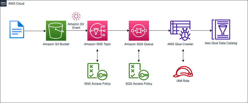
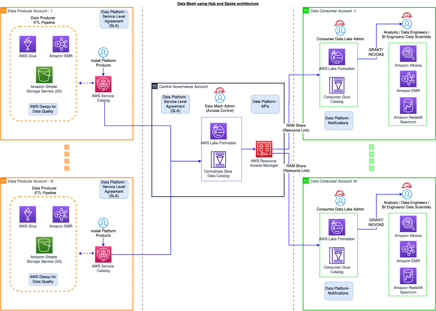
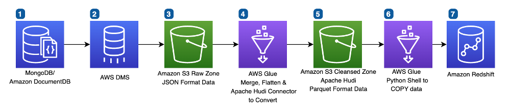
The following diagram describes the high-level architecture for our solution. We ingest the TPC-DS (store_sales) dataset from the source S3 bucket in CSV format and write it to the target S3 bucket using AWS Glue in Hudi format. We can query the Hudi tables on Amazon S3 using Amazon Athena and AWS Glue Studio Notebooks.

The following diagram illustrates the relationships between our tables.

For our post, we use the following tables from the TPC-DS dataset: one fact table, store_sales, and the dimension tables store, item, and date_dim. The following table summarizes the table row counts.

Table Approximate Row Counts
store_sales 2.8 billion
store 1,000
item 300,000
date_dim 73,000

Set up the environment

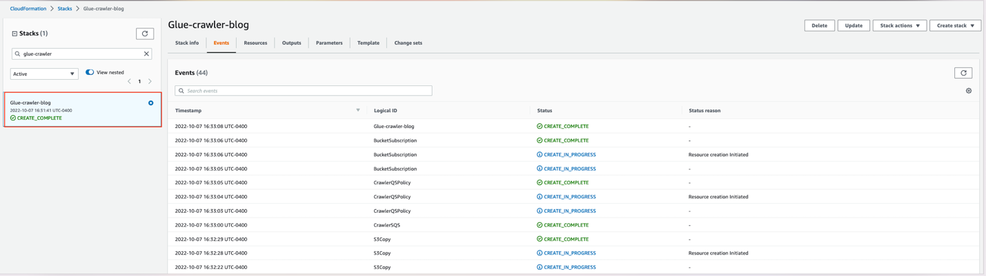
After you sign in to your test AWS account, launch the provided AWS CloudFormation template by choosing Launch Stack:

Launch Button

This template configures the following resources:

  • AWS Glue jobs hudi_bulk_insert, hudi_upsert_cow, and hudi_bulk_insert_dim. We use these jobs for the use cases covered in this post.
  • An S3 bucket to store the output of the AWS Glue job runs.
  • AWS Identity and Access Management (IAM) roles and policies with appropriate permissions.

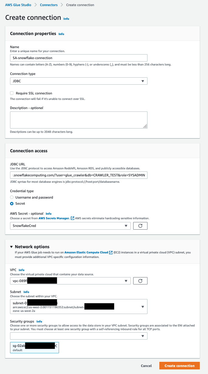
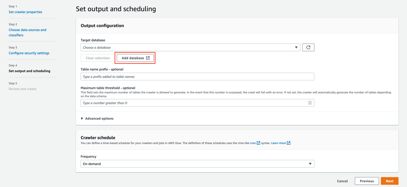
Before you run the AWS Glue jobs, you need to subscribe to the AWS Glue Apache Hudi Connector (latest version: 0.10.1). The connector is available on AWS Marketplace. Follow the connector installation and activation process from the AWS Marketplace link, or refer to Process Apache Hudi, Delta Lake, Apache Iceberg datasets at scale, part 1: AWS Glue Studio Notebook to set it up.

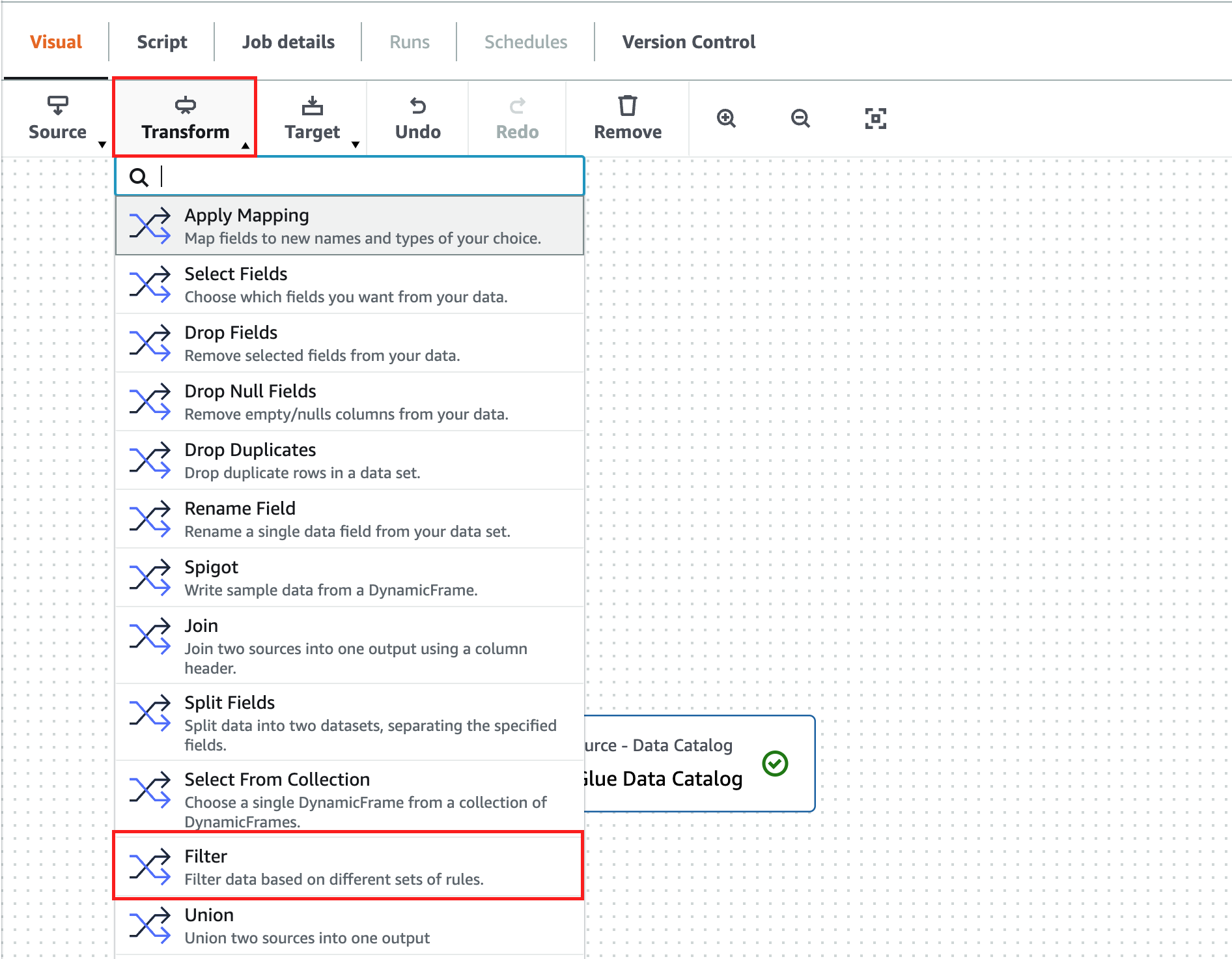
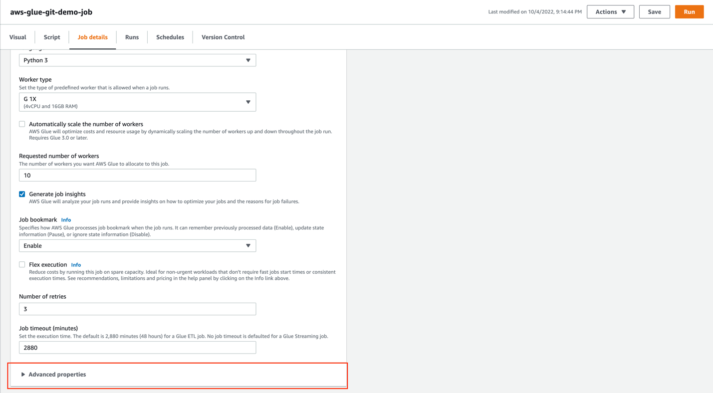
After you create the Hudi connection, add the connector name to all the AWS Glue scripts under Advanced properties.

Bulk insert job

To run the bulk insert job, choose the job hudi_bulk_insert on the AWS Glue console.

The job parameters as shown in the following screenshot are added as part of the CloudFormation stack setup. You can use different values to create CoW partitioned tables with different bulk insert options.

The parameters are as follows:

  • HUDI_DB_NAME – The database in the AWS Glue Data Catalog where the catalog table is created.
  • HUDI_INIT_SORT_OPTION – The options for bulk_insert include GLOBAL_SORT, which is the default. Other options include NONE and PARTITION_SORT.
  • HUDI_TABLE_NAME – The table name prefix that you want to use to identify the table created. In the code, we append the sort option to the name you specify in this parameter.
  • OUTPUT_BUCKET – The S3 bucket created through the CloudFormation stack where the Hudi table datasets are written. The bucket name format is <account number><bucket name>. The bucket name is the one given while creating the CloudFormation stack.
  • CATEGORY_ID – The default for this parameter is ALL, which processes categories of test data in a single AWS Glue job. To test the parallel on the same table, change the parameter value to one of categories from 3, 5, or 8 for the dataset that we use for each parallel AWS Glue job.

Upsert job for the CoW table

To run the upsert job, choose the job hudi_upsert_cow on the AWS Glue console.

The following job parameters are added as part of the CloudFormation stack setup. You can run upsert and delete operations on CoW partitioned tables with different bulk insert options based on the values provided for these parameters.

  • OUTPUT-BUCKET – The same value as the previous job parameter.
  • HUDI_TABLE_NAME – The name of the table created in your AWS Glue Data Catalog.
  • HUDI_DB_NAME – The same value as the previous job parameter. The default value is Default.

Bulk insert job for the Dimension tables

To test the queries on the CoW tables, the fact table that is created using the bulk insert operation needs supplemental dimensional tables. This AWS Glue job has to be run before you can test the TPC queries provided later in this post. To run this job, choose hudi_bulk_insert_dim on the AWS Glue console and use the parameters shown in the following screenshot.

The parameters are as follows:

  • OUTPUT-BUCKET – The same value as the previous job parameter.
  • HUDI_INIT_SORT_OPTION – The options for bulk_insert include GLOBAL_SORT, which is the default. Other available options are NONE and PARTITION_SORT.
  • HUDI_DB_NAME – The Hudi database name. Default is the default value.

Hudi design considerations

In this section, we walk you through a few use cases to demonstrate the difference in the outcome for different settings and operations.

Data migration use case

In Apache Hudi, you ingest the data into CoW or MoR tables types using either insert, upsert, or bulk insert operations. Data migration initiatives often involve one-time initial loads into the target datastore, and we recommend using the bulk insert operation for initial loads.

The bulk insert option provides the same semantics as insert, while implementing a sort-based data writing algorithm, which can scale very well for several hundred TBs of initial load. However, this just does a best-effort job at sizing files vs. guaranteeing file sizes like inserts and upserts do. Also, the primary keys aren’t sorted during the insert, therefore it’s not advised to use insert during the initial data load. By default, a Bloom index is created for the table, which enables faster lookups for upsert and delete operations.

Bulk insert has the following three sort options, which have different outcomes.

  • GLOAL_SORT – Sorts the record key for the entire dataset before writing.
  • PARTITION_SORT – Applies only to partitioned tables. In this option, the record key is sorted within each partition, and the insert time is faster than the default sort.
  • NONE – Doesn’t sort data before writing.

For testing the bulk insert with the three sort options, we use the following AWS Glue job configuration, which is part of the script hudi_bulk_insert:

  • AWS Glue version: 3.0
  • AWS Glue worker type: G1.X
  • Number of AWS Glue workers: 200
  • Input file: TPC-DS/2.13/1TB/store_sales
  • Input file format: CSV (TPC-DS)
  • Number of input files: 1,431
  • Number of rows in the input dataset: Approximately 2.8 billion

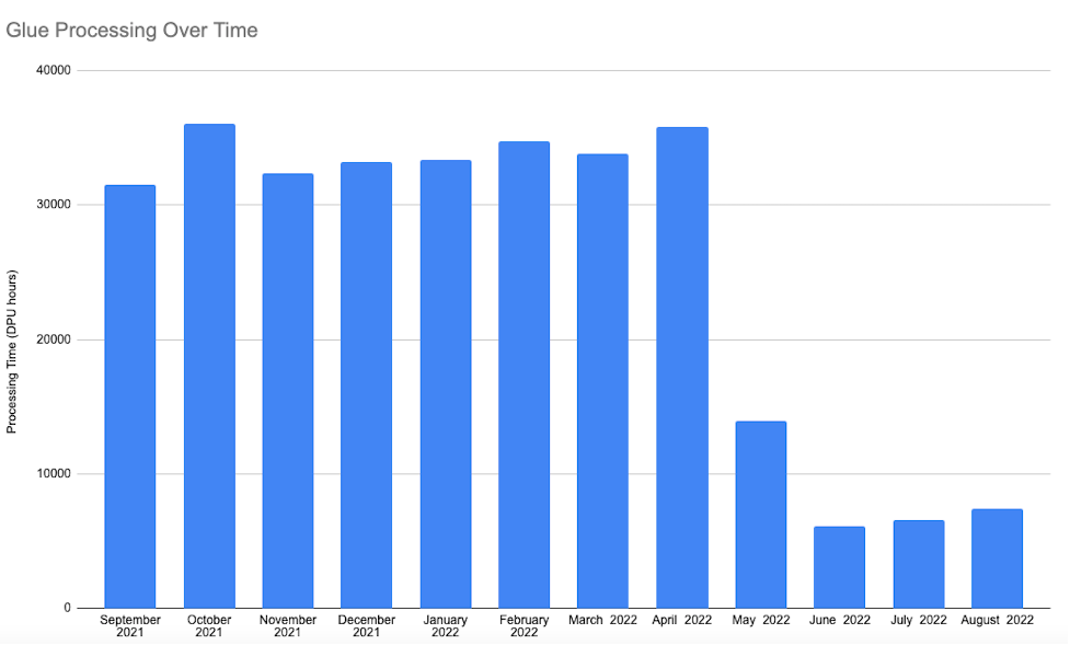
The following charts illustrate the behavior of the bulk insert operations with GLOBAL_SORT, PARTITION_SORT, and NONE as sort options for a CoW table. The statistics in the charts are created by using an average of 10 bulk insert operation runs for each sort option.

Because bulk insert does a best-effort job to pack the data in files, you see a different number of files created with different sort options.

We can observe the following:

  • Bulk insert with GLOBAL_SORT has the least number of files, because Hudi tried to create the optimal sized files. However, it takes the most time.
  • Bulk insert with NONE as the sort option has the fastest write time, but resulted in a greater number of files.
  • Bulk insert with PARTITION_SORT also has a faster write time compared to GLOBAL SORT, but also results in a greater number of files.

Based on these results, although GLOBAL_SORT takes more time to ingest the data, it creates a smaller number of files, which has better upsert and read performance.

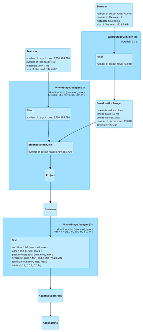
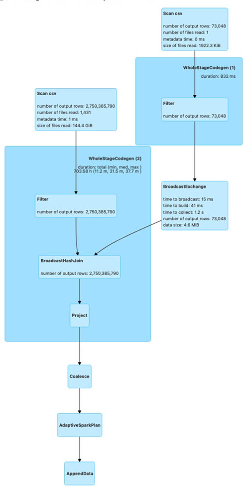
The following diagrams illustrate the Spark run plans for the bulk_insert operation using various sort options.

The first shows the Spark run plan for bulk_insert when the sort option is PARTITION_SORT.

The next is the Spark run plan for bulk_insert when the sort option is NONE.

The last is the Spark run plan for bulk_insert when the sort option is GLOBAL_SORT.

The Spark run plan for bulk_insert with GLOBAL_SORT involves shuffling of data to create optimal sized files. For the other two sort options, data shuffling isn’t involved. As a result, bulk_insert with GLOBAL_SORT takes more time compared to the other sort options.

To test the bulk insert with various bulk insert sort data options on a partitioned table, modify the Hudi AWS Glue job (hudi_bulk_insert) parameter --HUDI_INIT_SORT_OPTION.

We change the parameter --HUDI_INIT_SORT_OPTION to PARTITION_SORT or NONE to test the bulk insert with different data sort options. You need to run the job hudi_bulk_insert_dim, which loads the rest of the tables needed to test the SQL queries.

Now, look at the query performance difference between these three options. For query runtime, we ran two TPC-DS queries (q52.sql and q53.sql, as shown in the following query snippets) using interactive session with AWS Glue Studio Notebook with the following notebook configuration to compare the results.

  • AWS Glue version: 3.0
  • AWS Glue worker type: G1.X
  • Number of AWS Glue workers: 50

Before executing the following queries, replace the table names in the queries with the tables you generate in your account.
q52

SELECT
  dt.d_year,
  item.i_brand_id brand_id,
  item.i_brand brand,
  sum(ss_ext_sales_price) ext_price
FROM date_dim dt, store_sales, item
WHERE dt.d_date_sk = store_sales.ss_sold_date_sk
  AND store_sales.ss_item_sk = item.i_item_sk
  AND item.i_manager_id = 1
  AND dt.d_moy = 11
  AND dt.d_year = 2000
GROUP BY dt.d_year, item.i_brand, item.i_brand_id
ORDER BY dt.d_year, ext_price DESC, brand_id
LIMIT 100
SELECT *
FROM
  (SELECT
    i_manufact_id,
    sum(ss_sales_price) sum_sales,
    avg(sum(ss_sales_price))
    OVER (PARTITION BY i_manufact_id) avg_quarterly_sales
  FROM item, store_sales, date_dim, store
  WHERE ss_item_sk = i_item_sk AND
    ss_sold_date_sk = d_date_sk AND
    ss_store_sk = s_store_sk AND
    d_month_seq IN (1200, 1200 + 1, 1200 + 2, 1200 + 3, 1200 + 4, 1200 + 5, 1200 + 6,
                          1200 + 7, 1200 + 8, 1200 + 9, 1200 + 10, 1200 + 11) AND
    ((i_category IN ('Books', 'Children', 'Electronics') AND

As you can see in the following chart, the performance of the GLOBAL_SORT table outperforms NONE and PARTITION_SORT due to a smaller number of files created in the bulk insert operation.

Ongoing replication use case

For ongoing replication, updates and deletes usually come from transactional databases. As you saw in the previous section, the bulk operation with GLOBAL_SORT took the most time and the operation with NONE took the least time. When you anticipate a higher volume of updates and deletes on an ongoing basis, the sort option is critical for your write performance.

To illustrate the ongoing replication using Apache Hudi upsert and delete operations, we tested using the following configuration:

  • AWS Glue version: 3.0
  • AWS Glue worker type: G1.X
  • Number of AWS Glue workers: 100

To test the upsert and delete operations, we use the store_sales CoW table, which was created using the bulk insert operation in the previous section with all three sort options. We make the following changes:

  • Insert data into a new partition (month 1 and year 2004) using the existing data from month 1 of year 2002 with a new primary key; total of 32,164,890 records
  • Update the ss_list_price column by $1 for the existing partition (month 1 and year 2003); total of 5,997,571 records
  • Delete month 5 data for year 2001; total of 26,997,957 records

The following chart illustrates the runtimes for the upsert operation for the CoW table with different sort options used during the bulk insert.

As you can see from the test run, the runtime of the upsert is higher for NONE and PARTITION_SORT CoW tables. The Bloom index, which is created by default during the bulk insert operation, enables faster lookup for upsert and delete operations.

To test the upsert and delete operations on a CoW table for tables with different data sort options, modify the AWS Glue job (hudi_upsert_cow) parameter HUDI_TABLE_NAME to the desired table, as shown in the following screenshot.

For workloads where updates are performed on the most recent partitions, a Bloom index works fine. For workloads where the update volume is less but the updates are spread across partitions, a simple index is more efficient. You can specify the index type while creating the Hudi table by using the parameter hoodie.index.type. Both the Bloom index and simple index enforce uniqueness of table keys within a partition. If you need uniqueness of keys for the entire table, you must create a global Bloom index or global simple index based on the update workloads.

Multi-tenant partitioned design use case

In this section, we cover Hudi optimistic concurrency using a multi-tenant table design, where each tenant data is stored in a separate table partition. In a real-world scenario, you may encounter a business need to process different tenant data simultaneously, such as a strict SLA to make the data available for downstream consumption as quickly as possible. Without Hudi optimistic concurrency, you can’t have concurrent writes to the same Hudi table. In such a scenario, you can speed up the data writes using Hudi optimistic concurrency when each job operates on a different table dataset. In our multi-tenant table design using Hudi optimistic concurrency, you can run concurrent jobs, where each job writes data to a separate table partition.

For AWS Glue, you can implement Hudi optimistic concurrency using an Amazon DynamoDB lock provider, which was introduced with Apache Hudi 0.10.0. The initial bulk insert script has all the configurations needed to allow multiple writes. The role being used for AWS Glue needs to have DynamoDB permissions added to make it work. For more information about concurrency control and alternatives for lock providers, refer to Concurrency Control.

To simulate concurrent writes, we presume your tenant is based on the category field from the TPC DC test dataset and accordingly partitioned based on the category id field (i_category_id). Let’s modify the script hudi_bulk_insert to run an initial load for different categories. You need to configure your AWS Glue job to run concurrently based on the Maximum concurrency parameter, located under the advanced properties. We describe the Hudi configuration parameters that are needed in the appendix at the end of this post.

The TPC-DS dataset includes data from years 1998–2003. We use i_catagory_id as the tenant ID. The following screenshot shows the distribution of data for multiple tenants (i_category_id). In our testing, we load the data for i_category_id values 3, 5, and 8.

The AWS Glue job hudi_bulk_insert is designed to insert data into specific partitions based on the parameter CATEGORY_ID. If bulk insert job for dimension tables is not run before you need to run the job hudi_bulk_insert_dim, which loads the rest of the tables needed to test the SQL queries.

Now we run three concurrent jobs, each with respective values 3, 5, and 8 to simulate concurrent writes for multiple tenants. The following screenshot illustrates the AWS Glue job parameter to modify for CATEGORY_ID.

We used the following AWS Glue job configuration for each of the three parallel AWS Glue jobs:

  • AWS Glue version: 3.0
  • AWS Glue worker type: G1.X
  • Number of AWS Glue workers: 100
  • Input file: TPC-DS/2.13/1TB/store_sales
  • Input file format: CSV (TPC-DS)

The following screenshot shows all three concurrent jobs started around the same time for three categories, which loaded 867 million rows (50.1 GB of data) into the store_sales table. We used the GLOBAL_SORT option for all three concurrent AWS Glue jobs.

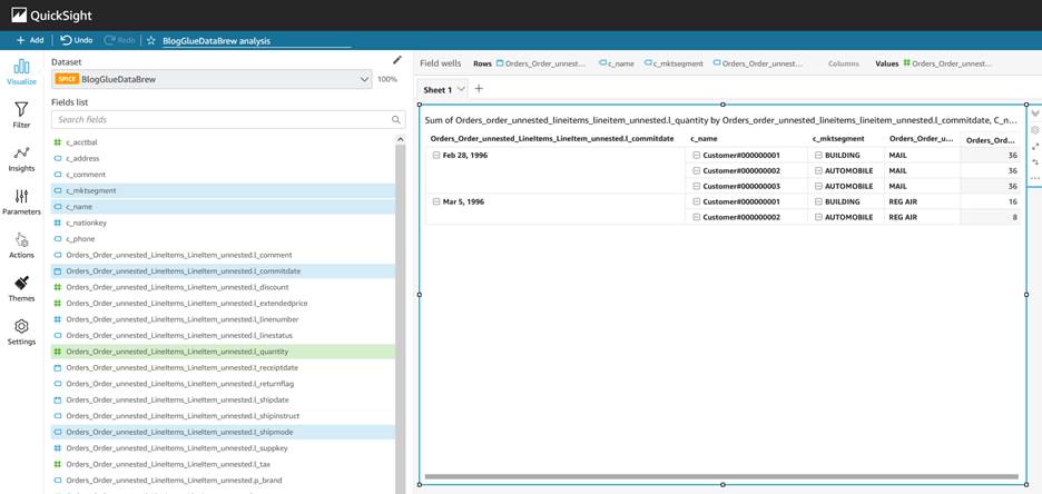
The following screenshot shows the data from the Hudi table where all three concurrent writers inserted data into different partitions, which is illustrated by different colors. All the AWS Glue jobs were run in US Central Time zone (UTC -5). The _hoodie_commit_time is in UTC.

The first two results highlighted in blue corresponds to the AWS Glue job CATEGORY_ID = 3, which had the start time of 09/27/2022 21:23:39 US CST (09/28/2022 02:23:39 UTC).

The next two results highlighted in green correspond to the AWS Glue job CATEGORY_ID = 8, which had the start time of 09/27/2022 21:23:50 US CST (09/28/2022 02:23:50 UTC).

The last two results highlighted in green correspond to the AWS Glue job CATEGORY_ID = 5, which had the start time of 09/27/2022 21:23:44 US CST (09/28/2022 02:23:44 UTC).

The sample data from the Hudi table has _hoodie_commit_time values corresponding to the AWS Glue job run times.

As you can see, we were able to load data into multiple partitions of the same Hudi table concurrently using Hudi optimistic concurrency.

Key findings

As the results show, bulk_insert with GLOBAL_SORT scales well for loading TBs of data in the initial load process. This option is recommended for use cases that require frequent changes after a large migration. Also, when query performance is critical in your use case, we recommend the GLOBAL_SORT option because of the smaller number of files being created with this option.

PARTITION_SORT has better performance for data load compared to GLOBAL_SORT, but it generates a significantly larger number of files, which negatively impacts query performance. You can use this option when the query involves a lot of joins between partitioned tables on record key columns.

The NONE option doesn’t sort the data, but it’s useful when you need the fastest initial load time and requires minimal updates, with the added capability of supporting record changes.

Clean up

When you’re done with this exercise, complete the following steps to delete your resources and stop incurring costs:

  1. On the Amazon S3 console, empty the buckets created by the CloudFormation stack.
  2. On the CloudFormation console, select your stack and choose Delete.

This cleans up all the resources created by the stack.

Conclusion

In this post, we covered some of the Hudi concepts that are important for design decisions. We used AWS Glue and the TPC-DS dataset to collect the results of different use cases for comparison. You can learn from the use cases covered in this post to make the key design decisions, particularly when you’re at the early stage of Apache Hudi adoption. You can go through the steps in this post to start a proof of concept using AWS Glue and Apache Hudi.

References

Appendix

The following table summarizes the Hudi configuration parameters that are needed.

Configuration Value Description Required
hoodie.write.
concurrency.mode
optimistic_concurrency_control Property to turn on optimistic concurrency control. Yes
hoodie.cleaner.
policy.failed.writes
LAZY Property to turn on optimistic concurrency control. Yes
hoodie.write.
lock.provider
org.apache.
hudi.client.
transaction.lock.
DynamoDBBasedLockProvider
Lock provider implementation to use. Yes
hoodie.write.
lock.dynamodb.table
<String> The DynamoDB table name to use for acquiring locks. If the table doesn’t exist, it will be created. You can use the same table across all your Hudi jobs operating on the same or different tables. Yes
hoodie.write.
lock.dynamodb.partition_key
<String> The string value to be used for the locks table partition key attribute. It must be a string that uniquely identifies a Hudi table, such as the Hudi table name. Yes: ‘tablename’
hoodie.write.
lock.dynamodb.region
<String> The AWS Region in which the DynamoDB locks table exists, or must be created. Yes:
Default: us-east-1
hoodie.write.
lock.dynamodb.billing_mode
<String> The DynamoDB billing mode to be used for the locks table while creating. If the table already exists, then this doesn’t have an effect. Yes: Default
PAY_PER_REQUEST
hoodie.write.
lock.dynamodb.endpoint_url
<String> The DynamoDB URL for the Region where you’re creating the table. Yes: dynamodb.us-east-1.amazonaws.com
hoodie.write.
lock.dynamodb.read_capacity
<Integer> The DynamoDB read capacity to be used for the locks table while creating. If the table already exists, then this doesn’t have an effect. No: Default 20
hoodie.write.
lock.dynamodb.
write_capacity
<Integer> The DynamoDB write capacity to be used for the locks table while creating. If the table already exists, then this doesn’t have an effect. No: Default 10

About the Authors

About the author Amit MaindolaAmit Maindola is a Data Architect focused on big data and analytics at Amazon Web Services. He helps customers in their digital transformation journey and enables them to build highly scalable, robust, and secure cloud-based analytical solutions on AWS to gain timely insights and make critical business decisions.

About the author Srinivas KandiSrinivas Kandi is a Data Architect with focus on data lake and analytics at Amazon Web Services. He helps customers to deploy data analytics solutions in AWS to enable them with prescriptive and predictive analytics.

About the author Amit MaindolaMitesh Patel is a Principal Solutions Architect at AWS. His main area of depth is application and data modernization. He helps customers to build scalable, secure and cost effective solutions in AWS.

Build incremental crawls of data lakes with existing Glue catalog tables

Post Syndicated from Leonardo Gomez original https://aws.amazon.com/blogs/big-data/build-incremental-crawls-of-data-lakes-with-existing-glue-catalog-tables/

AWS Glue includes crawlers, a capability that make discovering datasets simpler by scanning data in Amazon Simple Storage Service (Amazon S3) and relational databases, extracting their schema, and automatically populating the AWS Glue Data Catalog, which keeps the metadata current. This reduces the time to insight by making newly ingested data quickly available for analysis with your preferred analytics and machine learning (ML) tools.

Previously, you could reduce crawler cost by using Amazon S3 Event Notifications to incrementally crawl changes on Data Catalog tables created by crawler. Today, we’re extending this support to crawling and updating Data Catalog tables that are created by non-crawler methods, such as using data pipelines. This crawler feature can be useful for several use cases, such as following:

  • You currently have a data pipeline to create AWS Glue Data Catalog tables and want to offload detection of partition information from the data pipeline to a scheduled crawler
  • You have an S3 bucket with event notifications enabled and want to continuously catalog new changes and prevent creation of new tables in case of ill-formatted files that break the partition detection
  • You have manually created Data Catalog tables and want to run incremental crawls on new file additions instead of running full crawls due to long crawl times

To accomplish incremental crawling, you can configure Amazon S3 Event Notifications to be sent to an Amazon Simple Queue Service (Amazon SQS) queue. You can then use the SQS queue as a source to identify changes and can schedule or run an AWS Glue crawler with Data Catalog tables as a target. With each run of the crawler, the SQS queue is inspected for new events. If no new events are found, the crawler stops. If events are found in the queue, the crawler inspects their respective folders, processes through built-in classifiers (for CSV, JSON, AVRO, XML, and so on), and determines the changes. The crawler then updates the Data Catalog with new information, such as newly added or deleted partitions or columns. This feature reduces the cost and time to crawl large and frequently changing Amazon S3 data.

This post shows how to create an AWS Glue crawler that supports Amazon S3 event notification on existing Data Catalog tables using the new crawler UI and an AWS CloudFormation template.

Overview of solution

To demonstrate how the new AWS Glue crawler performs incremental updates, we use the Toronto parking tickets dataset—specifically data about parking tickets issued in the city of Toronto between 2019–2020. The goal is to create a manual dataset as well as its associated metadata tables in AWS Glue, followed by an event-based crawler that detects and implements changes to the manually created datasets and catalogs.

As mentioned before, instead of crawling all the subfolders on Amazon S3, we use an Amazon S3 event-based approach. This helps improve the crawl time by using Amazon S3 events to identify the changes between two crawls by listing all the files from the subfolder that triggered the event instead of listing the full Amazon S3 target. To accomplish this, we create an S3 bucket, an event-based crawler, an Amazon Simple Storage Service (Amazon SNS) topic, and an SQS queue. The following diagram illustrates our solution architecture.

Prerequisites

For this walkthrough, you should have the following prerequisites:

If the AWS account you use to follow this post uses Lake Formation to manage permissions on the AWS Glue Data Catalog, make sure that you log in as a user with access to create databases and tables. For more information, refer to Implicit Lake Formation permissions.

Launch your CloudFormation stack

To create your resources for this use case, complete the following steps:

  1. Launch your CloudFormation stack in us-east-1:
  2. For Stack name, enter a name for your stack .
  3. For paramBucketName, enter a name for your S3 bucket (with your account number).
  4. Choose Next.
  5. Select I acknowledge that AWS CloudFormation might create IAM resources with custom names.
  6. Choose Create stack.

Wait for the stack formation to finish provisioning the requisite resources. When you see the CREATE_COMPLETE status, you can proceed to the next steps.

Additionally, note down the ARN of the SQS queue to use at a later point.

Query your Data Catalog

Next, we use Amazon Athena to confirm that the manual tables have been created in the Data Catalog, as part of the CloudFormation template.

  1. On the Athena console, choose Launch query editor.
  2. For Data source, choose AwsDataCatalog.
  3. For Database, choose torontoparking.

    The tickets table should appear in the Tables section.

    Now you can query the table to see its contents.
  4. You can write your own query, or choose Preview Table on the options menu.

    This writes a simple SQL query to show us the first 10 rows.
  5. Choose Run to run the query.

As we can see in the query results, the database and table for 2019 parking ticket data have been created and partitioned.

Create the Amazon S3 event crawler

The next step is to create the crawler that detects and crawls only on incrementally updated tables.

  1. On the AWS Glue console, choose Crawlers in the navigation pane.
  2. Choose Create crawler.
  3. For Name, enter a name.
  4. Choose Next.

    Now we need to select the data source for the crawler.
  5. Select Yes to indicate that our data is already mapped to our AWS Glue Data Catalog.
  6. Choose Add tables.
  7. For Database, choose torontoparking and for Tables, choose tickets.
  8. Select Crawl based on events.
  9. For Include SQS ARN, enter the ARN you saved from the CloudFormation stack outputs.
  10. Choose Confirm.

    You should now see the table populated under Glue tables, with the parameter set as Recrawl by event.
  11. Choose Next.
  12. For Existing IAM role, choose the IAM role created by the CloudFormation template (GlueCrawlerTableRole).
  13. Choose Next.
  14. For Frequency, choose On demand.

    You also have the option of choosing a schedule on which the crawler will run regularly.
  15. Choose Next.
  16. Review the configurations and choose Create crawler.

    Now that the crawler has been created, we add the 2020 ticketing data to our S3 bucket so that we can test our new crawler. For this step, we use the AWS Command Line Interface (AWS CLI)
  17. To add this data, use the following command:
    aws s3 cp s3://aws-bigdata-blog/artifacts/gluenewcrawlerui2/source/year=2020/Parking_Tags_Data_2020.000.csv s3://glue-table-crawler-blog-<YOURACCOUNTNUMBER>/year=2020/Parking_Tags_Data_2020.000.csv

After successful completion of this command, your S3 bucket should contain the 2020 ticketing data and your crawler is ready to run. The terminal should return the following:

copy: s3://aws-bigdata-blog/artifacts/gluenewcrawlerui2/source/year=2020/Parking_Tags_Data_2020.000.csv to s3://glue-table-crawler-blog-<YOURACCOUNTNUMBER>/year=2020/Parking_Tags_Data_2020.000.csvRun the crawler and verify the updates

Run the crawler and verify the updates

Now that the new folder has been created, we run the crawler to detect the changes in the table and partitions.

  1. Navigate to your crawler on the AWS Glue console and choose Run crawler.

    After running the crawler, you should see that it added the 2020 data to the tickets table.
  2. On the Athena console, we can ensure that the Data Catalog has been updated by adding a where year = 2020 filter to the query.

AWS CLI option

You can also create the crawler using the AWS CLI. For more information, refer to create-crawler.

Clean up

To avoid incurring future charges, and to clean up unused roles and policies, delete the resources you created: the CloudFormation stack, S3 bucket, AWS Glue crawler, AWS Glue database, and AWS Glue table.

Conclusion

You can use AWS Glue crawlers to discover datasets, extract schema information, and populate the AWS Glue Data Catalog. In this post, we provided a CloudFormation template to set up AWS Glue crawlers to use Amazon S3 event notifications on existing Data Catalog tables, which reduces the time and cost needed to incrementally process table data updates in the Data Catalog.

With this feature, incremental crawling can now be offloaded from data pipelines to the scheduled AWS Glue crawler, reducing cost. This alleviates the need for full crawls, thereby reducing crawl times and Data Processing Units (DPUs) required to run the crawler. This is especially useful for customers that have S3 buckets with event notifications enabled and want to continuously catalog new changes.

To learn more about this feature, refer to Accelerating crawls using Amazon S3 event notifications.

Special thanks to everyone who contributed to this crawler feature launch: Theo Xu, Jessica Cheng, Arvin Mohanty, and Joseph Barlan.


About the authors

Leonardo Gómez is a Senior Analytics Specialist Solutions Architect at AWS. Based in Toronto, Canada, he has over a decade of experience in data management, helping customers around the globe address their business and technical needs.

Aayzed Tanweer is a Solutions Architect working with startup customers in the FinTech space, with a special focus on analytics services. Originally hailing from Toronto, he recently moved to New York City, where he enjoys eating his way through the city and exploring its many peculiar nooks and crannies.

Sandeep Adwankar is a Senior Technical Product Manager at AWS. Based in the California Bay Area, he works with customers around the globe to translate business and technical requirements into products that enable customers to improve how they manage, secure, and access data.

Code versioning using AWS Glue Studio and GitHub

Post Syndicated from Leonardo Gomez original https://aws.amazon.com/blogs/big-data/code-versioning-using-aws-glue-studio-and-github/

AWS Glue now offers integration with Git, an open-source version control system widely used across the developer community. Thanks to this integration, you can incorporate your existing DevOps practices on AWS Glue jobs. AWS Glue is a serverless data integration service that helps you create jobs based on Apache Spark or Python to perform extract, transform, and load (ETL) tasks on datasets of almost any size.

Git integration in AWS Glue works for all AWS Glue job types, both visual and code-based. It offers built-in integration with both GitHub and AWS CodeCommit, and makes it easier to use automation tools like Jenkins and AWS CodeDeploy to deploy AWS Glue jobs. AWS Glue Studio’s visual editor now also supports parameterizing data sources and targets for transparent deployments between environments.

Overview of solution

To demonstrate how to integrate AWS Glue Studio with a code hosting platform for version control and collaboration, we use the Toronto parking tickets dataset, specifically the data about parking tickets issued in the city of Toronto in 2019. The goal is to create a job to filter parking tickets based on a specific category and push the code to a GitHub repo for version control. After the job is uploaded on the repository, we make some changes to the code and pull the changes back to the AWS Glue job.

Prerequisites

For this walkthrough, you should have the following prerequisites:

If the AWS account you use to follow this post uses AWS Lake Formation to manage permissions on the AWS Glue Data Catalog, make sure that you log in as a user with access to create databases and tables. For more information, refer to Implicit Lake Formation permissions.

Launch your CloudFormation stack

To create your resources for this use case, complete the following steps:

  1. Launch your CloudFormation stack in us-east-1:
  2. Under Parameters, for paramBucketName, enter a name for your S3 bucket (include your account number).
  3. Select I acknowledge that AWS CloudFormation might create IAM resources with custom names.
  4. Choose Create stack.
  5. Wait until the creation of the stack is complete, as shown on the AWS CloudFormation console.

Launching this stack creates AWS resources. You need the following resources from the Outputs tab for the next steps:

  • CFNGlueRole – The IAM role to run AWS Glue jobs
  • S3Bucket – The name of the S3 bucket to store solution-related files
  • CFNDatabaseBlog – The AWS Glue database to store the table related to this post
  • CFNTableTickets – The AWS Glue table to use as part of the sample job

Configure the GitHub repository

We use GitHub as the source control system for this post. In order to use it, you need a GitHub account. After the account is created, you need to create following components:

  • GitHub repository – Create a repository and name it glue-ver-log. For instructions, refer to Create a repo.
  • Branch – Create a branch and name it develop. For instructions, refer to Managing branches.
  • Personal access token – For instructions, refer to Creating a personal access token. Make sure to keep the personal access token handy because you use it in later steps.

Create an AWS Glue Studio job

Now that the infrastructure is set up, let’s author an AWS Glue job in our account. Complete the following steps:

  1. On the AWS Glue console, choose Jobs in the navigation pane.
  2. Select Visual job with blank canvas and choose Create.
  3. Enter a name for the job using the title editor. For example, aws-glue-git-demo-job.
  4. On the Visual tab, choose Source and then choose AWS Glue Data Catalog

  5. For Database, choose torontoparking and for Table, choose tickets.
  6. Choose Transform and then Filter.
  7. Add a filter by infraction_description and set the value to PARK ON PRIVATE PROPERTY.
  8. Choose Target and then choose Amazon S3.
  9. For Format, choose Parquet.
  10. For S3 Target Location, enter s3://glue-version-blog-YOUR ACOUNT NUMBER/output/.
  11. For Data Catalog update options, select Do not update the Data Catalog.
  12. Go to the Script tab to verify that a script has been generated.
  13. Go to the Job Details tab to make sure that the role GlueBlogRole is selected and leave everything else with the default values.

    Because the catalog table names in the production and development environment may be different, AWS Glue Studio now allows you to parameterize visual jobs. To do so, perform the following steps:
  14. On the Job details tab, scroll to the Job parameters section under Advanced properties.
  15. Create the --source.database.name parameter and set the value to torontoparking.
  16. Create the --souce.table.name parameter and set the value to tickets.
  17. Go to the Visual tab and choose the AWS Glue Data Catalog node.Notice that under each of the database and table selection options is a new expandable section called Use runtime parameters.
  18. The run time parameters are auto populated with the parameters previously created. Clicking on the Apply button will apply the default values for these parameters.
  19. Go to the Script tab to review the script.AWS Glue Studio code generation automatically picks up the parameters to resolve and then makes the appropriate references in the script so that the parameters can be used.
    Now the job is ready to be pushed into the develop branch of our version control system.
  20. On the Version Control tab, for Version control system, choose Github.
  21. For Personal access token, enter your GitHub token.
  22. For Repository owner, enter the owner of your GitHub account.
  23. In the Repository configuration section, for Repository, choose glue-ver-blog.
  24. For Branch, choose develop.
  25. For Folder, leave it blank.
  26. Choose Save to save the job.

Push to the repository

Now the job can be pushed to the remote repository.

  1. On the Actions menu, choose Push to repository.
  2. Choose Confirm to confirm the operation.

    After the operation succeeds, the page reloads to reflect the latest information from the version control system. A notification shows the latest available commit and links you to the commit on GitHub.
  3. Choose the commit link to go to the repository on GitHub.

You have successfully created your first commit to GitHub from AWS Glue Studio!

Pull from the repository

Now that we have committed the AWS Glue job to GitHub, it’s time to see how we can pull changes using AWS Glue Studio. For this demo, we make a small modification in our example job using the GitHub UI and then pull the changes using AWS Glue Studio.

  1. On GitHub, choose the develop branch.
  2. Choose the aws-glue-git-demo-job folder.
  3. Choose the aws-glue-git-demo-job.json file.
  4. Choose the edit icon.
  5. Set the MaxRetries parameter to 1.
  6. Choose Commit changes.
  7. Return to the AWS Glue console and on the Actions menu, choose Pull from repository.
  8. Choose Confirm.

Notice that the commit ID has changed.

On the Job details tab, you can see that the value for Number of retries is 1.

Clean up

To avoid incurring future charges, and to clean up unused roles and policies, delete the resources you created: the datasets, CloudFormation stack, S3 bucket, AWS Glue job, AWS Glue database, and AWS Glue table.

Conclusion

This post showed how to integrate AWS Glue with GitHub, but this is only the beginning—now you can use the most popular functionalities offered by Git.

To learn more and get started using the AWS Glue Studio Git integration, refer to Configuring Git integration in AWS Glue.


About the authors

Leonardo Gómez is a Senior Analytics Specialist Solutions Architect at AWS. Based in Toronto, Canada, he has over a decade of experience in data management, helping customers around the globe address their business and technical needs.

Daiyan Alamgir is a Principal Frontend Engineer on AWS Glue based in New York. He leads the AWS Glue UI team and is focused on building interactive web-based applications for data analysts and engineers to address their data integration use cases.