Post Syndicated from Flora Wu original https://aws.amazon.com/blogs/big-data/use-apache-iceberg-in-a-data-lake-to-support-incremental-data-processing/
Apache Iceberg is an open table format for very large analytic datasets, which captures metadata information on the state of datasets as they evolve and change over time. It adds tables to compute engines including Spark, Trino, PrestoDB, Flink, and Hive using a high-performance table format that works just like a SQL table. Iceberg has become very popular for its support for ACID transactions in data lakes and features like schema and partition evolution, time travel, and rollback.
Apache Iceberg integration is supported by AWS analytics services including Amazon EMR, Amazon Athena, and AWS Glue. Amazon EMR can provision clusters with Spark, Hive, Trino, and Flink that can run Iceberg. Starting with Amazon EMR version 6.5.0, you can use Iceberg with your EMR cluster without requiring a bootstrap action. In early 2022, AWS announced general availability of Athena ACID transactions, powered by Apache Iceberg. The recently released Athena query engine version 3 provides better integration with the Iceberg table format. AWS Glue 3.0 and later supports the Apache Iceberg framework for data lakes.
In this post, we discuss what customers want in modern data lakes and how Apache Iceberg helps address customer needs. Then we walk through a solution to build a high-performance and evolving Iceberg data lake on Amazon Simple Storage Service (Amazon S3) and process incremental data by running insert, update, and delete SQL statements. Finally, we show you how to performance tune the process to improve read and write performance.
How Apache Iceberg addresses what customers want in modern data lakes
More and more customers are building data lakes, with structured and unstructured data, to support many users, applications, and analytics tools. There is an increased need for data lakes to support database like features such as ACID transactions, record-level updates and deletes, time travel, and rollback. Apache Iceberg is designed to support these features on cost-effective petabyte-scale data lakes on Amazon S3.
Apache Iceberg addresses customer needs by capturing rich metadata information about the dataset at the time the individual data files are created. There are three layers in the architecture of an Iceberg table: the Iceberg catalog, the metadata layer, and the data layer, as depicted in the following figure (source).
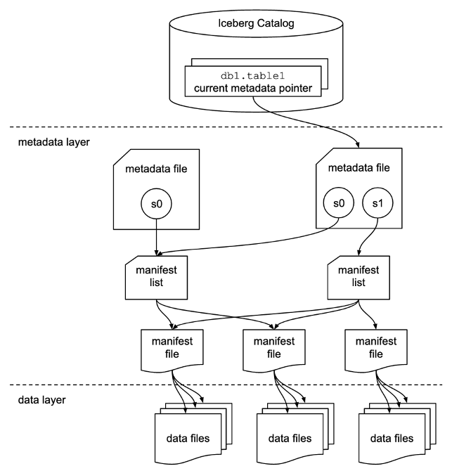
The Iceberg catalog stores the metadata pointer to the current table metadata file. When a select query is reading an Iceberg table, the query engine first goes to the Iceberg catalog, then retrieves the location of the current metadata file. Whenever there is an update to the Iceberg table, a new snapshot of the table is created, and the metadata pointer points to the current table metadata file.
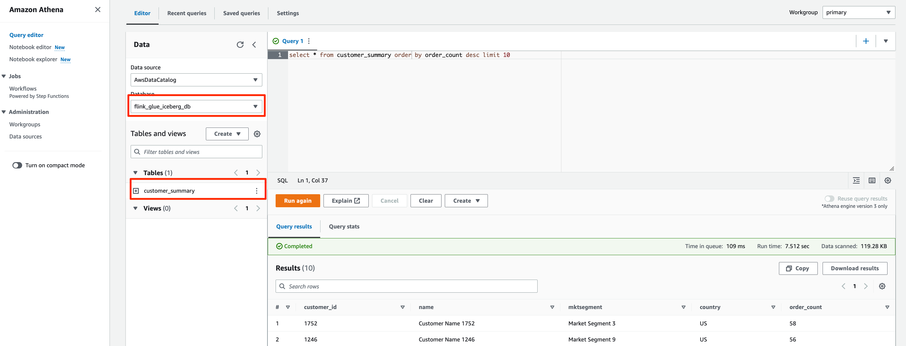
The following is an example Iceberg catalog with AWS Glue implementation. You can see the database name, the location (S3 path) of the Iceberg table, and the metadata location.

The metadata layer has three types of files: the metadata file, manifest list, and manifest file in a hierarchy. At the top of the hierarchy is the metadata file, which stores information about the table’s schema, partition information, and snapshots. The snapshot points to the manifest list. The manifest list has the information about each manifest file that makes up the snapshot, such as location of the manifest file, the partitions it belongs to, and the lower and upper bounds for partition columns for the data files it tracks. The manifest file tracks data files as well as additional details about each file, such as the file format. All three files work in a hierarchy to track the snapshots, schema, partitioning, properties, and data files in an Iceberg table.
The data layer has the individual data files of the Iceberg table. Iceberg supports a wide range of file formats including Parquet, ORC, and Avro. Because the Iceberg table tracks the individual data files instead of only pointing to the partition location with data files, it isolates the writing operations from reading operations. You can write the data files at any time, but only commit the change explicitly, which creates a new version of the snapshot and metadata files.
Solution overview
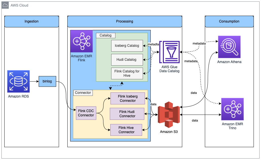
In this post, we walk you through a solution to build a high-performing Apache Iceberg data lake on Amazon S3; process incremental data with insert, update, and delete SQL statements; and tune the Iceberg table to improve read and write performance. The following diagram illustrates the solution architecture.

To demonstrate this solution, we use the Amazon Customer Reviews dataset in an S3 bucket (s3://amazon-reviews-pds/parquet/). In real use case, it would be raw data stored in your S3 bucket. We can check the data size with the following code in the AWS Command Line Interface (AWS CLI):
The total object count is 430, and total size is 47.4 GiB.
To set up and test this solution, we complete the following high-level steps:
- Set up an S3 bucket in the curated zone to store converted data in Iceberg table format.
- Launch an EMR cluster with appropriate configurations for Apache Iceberg.
- Create a notebook in EMR Studio.
- Configure the Spark session for Apache Iceberg.
- Convert data to Iceberg table format and move data to the curated zone.
- Run insert, update, and delete queries in Athena to process incremental data.
- Carry out performance tuning.
Prerequisites
To follow along with this walkthrough, you must have an AWS account with an AWS Identity and Access Management (IAM) role that has sufficient access to provision the required resources.
Set up the S3 bucket for Iceberg data in the curated zone in your data lake
Choose the Region in which you want to create the S3 bucket and provide a unique name:
Launch an EMR cluster to run Iceberg jobs using Spark
You can create an EMR cluster from the AWS Management Console, Amazon EMR CLI, or AWS Cloud Development Kit (AWS CDK). For this post, we walk you through how to create an EMR cluster from the console.
- On the Amazon EMR console, choose Create cluster.
- Choose Advanced options.
- For Software Configuration, choose the latest Amazon EMR release. As of January 2023, the latest release is 6.9.0. Iceberg requires release 6.5.0 and above.
- Select JupyterEnterpriseGateway and Spark as the software to install.
- For Edit software settings, select Enter configuration and enter
[{"classification":"iceberg-defaults","properties":{"iceberg.enabled":true}}]. - Leave other settings at their default and choose Next.

- For Hardware, use the default setting.
- Choose Next.
- For Cluster name, enter a name. We use
iceberg-blog-cluster. - Leave the remaining settings unchanged and choose Next.
- Choose Create cluster.

Create a notebook in EMR Studio
We now walk you through how to create a notebook in EMR Studio from the console.
- On the IAM console, create an EMR Studio service role.
- On the Amazon EMR console, choose EMR Studio.
- Choose Get started.
The Get started page appears in a new tab.
- Choose Create Studio in the new tab.
- Enter a name. We use iceberg-studio.
- Choose the same VPC and subnet as those for the EMR cluster, and the default security group.
- Choose AWS Identity and Access Management (IAM) for authentication, and choose the EMR Studio service role you just created.
- Choose an S3 path for Workspaces backup.
- Choose Create Studio.
- After the Studio is created, choose the Studio access URL.
- On the EMR Studio dashboard, choose Create workspace.
- Enter a name for your Workspace. We use
iceberg-workspace. - Expand Advanced configuration and choose Attach Workspace to an EMR cluster.
- Choose the EMR cluster you created earlier.
- Choose Create Workspace.
- Choose the Workspace name to open a new tab.
In the navigation pane, there is a notebook that has the same name as the Workspace. In our case, it is iceberg-workspace.
- Open the notebook.
- When prompted to choose a kernel, choose Spark.
Configure a Spark session for Apache Iceberg
Use the following code, providing your own S3 bucket name:
This sets the following Spark session configurations:
- spark.sql.catalog.demo – Registers a Spark catalog named demo, which uses the Iceberg Spark catalog plugin.
- spark.sql.catalog.demo.catalog-impl – The demo Spark catalog uses AWS Glue as the physical catalog to store Iceberg database and table information.
- spark.sql.catalog.demo.warehouse – The demo Spark catalog stores all Iceberg metadata and data files under the root path defined by this property:
s3://iceberg-curated-blog-data. - spark.sql.extensions – Adds support to Iceberg Spark SQL extensions, which allows you to run Iceberg Spark procedures and some Iceberg-only SQL commands (you use this in a later step).
- spark.sql.catalog.demo.io-impl – Iceberg allows users to write data to Amazon S3 through S3FileIO. The AWS Glue Data Catalog by default uses this FileIO, and other catalogs can load this FileIO using the io-impl catalog property.
Convert data to Iceberg table format
You can use either Spark on Amazon EMR or Athena to load the Iceberg table. In the EMR Studio Workspace notebook Spark session, run the following commands to load the data:
After you run the code, you should find two prefixes created in your data warehouse S3 path (s3://iceberg-curated-blog-data/reviews.db/all_reviews): data and metadata.
Process incremental data using insert, update, and delete SQL statements in Athena
Athena is a serverless query engine that you can use to perform read, write, update, and optimization tasks against Iceberg tables. To demonstrate how the Apache Iceberg data lake format supports incremental data ingestion, we run insert, update, and delete SQL statements on the data lake.
Navigate to the Athena console and choose Query editor. If this is your first time using the Athena query editor, you need to configure the query result location to be the S3 bucket you created earlier. You should be able to see that the table reviews.all_reviews is available for querying. Run the following query to verify that you have loaded the Iceberg table successfully:
Process incremental data by running insert, update, and delete SQL statements:
Performance tuning
In this section, we walk through different ways to improve Apache Iceberg read and write performance.
Configure Apache Iceberg table properties
Apache Iceberg is a table format, and it supports table properties to configure table behavior such as read, write, and catalog. You can improve the read and write performance on Iceberg tables by adjusting the table properties.
For example, if you notice that you write too many small files for an Iceberg table, you can config the write file size to write fewer but bigger size files, to help improve query performance.
| Property | Default | Description |
| write.target-file-size-bytes | 536870912 (512 MB) | Controls the size of files generated to target about this many bytes |
Use the following code to alter the table format:
Partitioning and sorting
To make a query run fast, the less data read the better. Iceberg takes advantage of the rich metadata it captures at write time and facilitates techniques such as scan planning, partitioning, pruning, and column-level stats such as min/max values to skip data files that don’t have match records. We walk you through how query scan planning and partitioning work in Iceberg and how we use them to improve query performance.
Query scan planning
For a given query, the first step in a query engine is scan planning, which is the process to find the files in a table needed for a query. Planning in an Iceberg table is very efficient, because Iceberg’s rich metadata can be used to prune metadata files that aren’t needed, in addition to filtering data files that don’t contain matching data. In our tests, we observed Athena scanned 50% or less data for a given query on an Iceberg table compared to original data before conversion to Iceberg format.
There are two types of filtering:
- Metadata filtering – Iceberg uses two levels of metadata to track the files in a snapshot: the manifest list and manifest files. It first uses the manifest list, which acts as an index of the manifest files. During planning, Iceberg filters manifests using the partition value range in the manifest list without reading all the manifest files. Then it uses selected manifest files to get data files.
- Data filtering – After selecting the list of manifest files, Iceberg uses the partition data and column-level stats for each data file stored in manifest files to filter data files. During planning, query predicates are converted to predicates on the partition data and applied first to filter data files. Then, the column stats like column-level value counts, null counts, lower bounds, and upper bounds are used to filter out data files that can’t match the query predicate. By using upper and lower bounds to filter data files at planning time, Iceberg greatly improves query performance.
Partitioning and sorting
Partitioning is a way to group records with the same key column values together in writing. The benefit of partitioning is faster queries that access only part of the data, as explained earlier in query scan planning: data filtering. Iceberg makes partitioning simple by supporting hidden partitioning, in the way that Iceberg produces partition values by taking a column value and optionally transforming it.
In our use case, we first run the following query on the Iceberg table not partitioned. Then we partition the Iceberg table by the category of the reviews, which will be used in the query WHERE condition to filter out records. With partitioning, the query could scan much less data. See the following code:
Run the following select statement on the non-partitioned all_reviews table vs. the partitioned table to see the performance difference:
The following table shows the performance improvement of data partitioning, with about 50% performance improvement and 70% less data scanned.
| Dataset Name | Non-Partitioned Dataset | Partitioned Dataset |
| Runtime (seconds) | 8.20 | 4.25 |
| Data Scanned (MB) | 131.55 | 33.79 |
Note that the runtime is the average runtime with multiple runs in our test.
We saw good performance improvement after partitioning. However, this can be further improved by using column-level stats from Iceberg manifest files. In order to use the column-level stats effectively, you want to further sort your records based on the query patterns. Sorting the whole dataset using the columns that are often used in queries will reorder the data in such a way that each data file ends up with a unique range of values for the specific columns. If these columns are used in the query condition, it allows query engines to further skip data files, thereby enabling even faster queries.
Copy-on-write vs. read-on-merge
When implementing update and delete on Iceberg tables in the data lake, there are two approaches defined by the Iceberg table properties:
- Copy-on-write – With this approach, when there are changes to the Iceberg table, either updates or deletes, the data files associated with the impacted records will be duplicated and updated. The records will be either updated or deleted from the duplicated data files. A new snapshot of the Iceberg table will be created and pointing to the newer version of data files. This makes the overall writes slower. There might be situations that concurrent writes are needed with conflicts so retry has to happen, which increases the write time even more. On the other hand, when reading the data, there is no extra process needed. The query will retrieve data from the latest version of data files.
- Merge-on-read – With this approach, when there are updates or deletes on the Iceberg table, the existing data files will not be rewritten; instead new delete files will be created to track the changes. For deletes, a new delete file will be created with the deleted records. When reading the Iceberg table, the delete file will be applied to the retrieved data to filter out the delete records. For updates, a new delete file will be created to mark the updated records as deleted. Then a new file will be created for those records but with updated values. When reading the Iceberg table, both the delete and new files will be applied to the retrieved data to reflect the latest changes and produce the correct results. So, for any subsequent queries, an extra step to merge the data files with the delete and new files will happen, which will usually increase the query time. On the other hand, the writes might be faster because there is no need to rewrite the existing data files.
To test the impact of the two approaches, you can run the following code to set the Iceberg table properties:
Run the update, delete, and select SQL statements in Athena to show the runtime difference for copy-on-write vs. merge-on-read:
The following table summarizes the query runtimes.
| Query | Copy-on-Write | Merge-on-Read | ||||
| UPDATE | DELETE | SELECT | UPDATE | DELETE | SELECT | |
| Runtime (seconds) | 66.251 | 116.174 | 97.75 | 10.788 | 54.941 | 113.44 |
| Data scanned (MB) | 494.06 | 3.07 | 137.16 | 494.06 | 3.07 | 137.16 |
Note that the runtime is the average runtime with multiple runs in our test.
As our test results show, there are always trade-offs in the two approaches. Which approach to use depends on your use cases. In summary, the considerations come down to latency on the read vs. write. You can reference the following table and make the right choice.
| . | Copy-on-Write | Merge-on-Read |
| Pros | Faster reads | Faster writes |
| Cons | Expensive writes | Higher latency on reads |
| When to use | Good for frequent reads, infrequent updates and deletes or large batch updates | Good for tables with frequent updates and deletes |
Data compaction
If your data file size is small, you might end up with thousands or millions of files in an Iceberg table. This dramatically increases the I/O operation and slows down the queries. Furthermore, Iceberg tracks each data file in a dataset. More data files lead to more metadata. This in turn increases the overhead and I/O operation on reading metadata files. In order to improve the query performance, it’s recommended to compact small data files to larger data files.
When updating and deleting records in Iceberg table, if the read-on-merge approach is used, you might end up with many small deletes or new data files. Running compaction will combine all these files and create a newer version of the data file. This eliminates the need to reconcile them during reads. It’s recommended to have regular compaction jobs to impact reads as little as possible while still maintaining faster write speed.
Run the following data compaction command, then run the select query from Athena:
The following table compares the runtime before vs. after data compaction. You can see about 40% performance improvement.
| Query | Before Data Compaction | After Data Compaction |
| Runtime (seconds) | 97.75 | 32.676 seconds |
| Data scanned (MB) | 137.16 M | 189.19 M |
Note that the select queries ran on the all_reviews table after update and delete operations, before and after data compaction. The runtime is the average runtime with multiple runs in our test.
Clean up
After you follow the solution walkthrough to perform the use cases, complete the following steps to clean up your resources and avoid further costs:
- Drop the AWS Glue tables and database from Athena or run the following code in your notebook:
- On the EMR Studio console, choose Workspaces in the navigation pane.
- Select the Workspace you created and choose Delete.
- On the EMR console, navigate to the Studios page.
- Select the Studio you created and choose Delete.
- On the EMR console, choose Clusters in the navigation pane.
- Select the cluster and choose Terminate.
- Delete the S3 bucket and any other resources that you created as part of the prerequisites for this post.
Conclusion
In this post, we introduced the Apache Iceberg framework and how it helps resolve some of the challenges we have in a modern data lake. Then we walked you though a solution to process incremental data in a data lake using Apache Iceberg. Finally, we had a deep dive into performance tuning to improve read and write performance for our use cases.
We hope this post provides some useful information for you to decide whether you want to adopt Apache Iceberg in your data lake solution.
About the Authors
 Flora Wu is a Sr. Resident Architect at AWS Data Lab. She helps enterprise customers create data analytics strategies and build solutions to accelerate their businesses outcomes. In her spare time, she enjoys playing tennis, dancing salsa, and traveling.
 Daniel Li is a Sr. Solutions Architect at Amazon Web Services. He focuses on helping customers develop, adopt, and implement cloud services and strategy. When not working, he likes spending time outdoors with his family.


 Kachi Odoemene is an Applied Scientist at AWS AI. He builds AI/ML solutions to solve business problems for AWS customers.
 Taylor McNally is a Deep Learning Architect at Amazon Machine Learning Solutions Lab. He helps customers from various industries build solutions leveraging AI/ML on AWS. He enjoys a good cup of coffee, the outdoors, and time with his family and energetic dog.
 Austin Welch is a Data Scientist in the Amazon ML Solutions Lab. He develops custom deep learning models to help AWS public sector customers accelerate their AI and cloud adoption. In his spare time, he enjoys reading, traveling, and jiu-jitsu.


 AWS and Hugging Face collaborate to make generative AI more accessible and cost-efficient – This previous week, we announced an expanded collaboration between AWS and
 AWS Pi Day – Join me on March 14 for the third annual


 Dhiraj Thakur is a Solutions Architect with Amazon Web Services. He works with AWS customers and partners to provide guidance on enterprise cloud adoption, migration, and strategy. He is passionate about technology and enjoys building and experimenting in the analytics and AI/ML space.
 Rajdip Chaudhuri is Solutions Architect with Amazon Web Services specializing in data and analytics. He enjoys working with AWS customers and partners on data and analytics requirements. In his spare time, he enjoys soccer.


 Sandeep Adwankar is a Senior Technical Product Manager at AWS. Based in the California Bay Area, he works with customers around the globe to translate business and technical requirements into products that enable customers to improve how they manage, secure, and access data.
 Srividya Parthasarathy is a Senior Big Data Architect on the AWS Lake Formation team. She enjoys building data mesh solutions and sharing them with the community.
 Olivia Michele is a Data Scientist Lead at Ruparupa, where she has worked in a variety of data roles over the past 5 years, including building and integrating Ruparupa data systems with AWS to improve user experience with data and reporting tools. She is passionate about turning raw information into valuable actionable insights and delivering value to the company.
 Dariswan Janweri P. is a Data Engineer at Ruparupa. He considers challenges or problems as interesting riddles and finds satisfaction in solving them, and even more satisfaction by being able to help his colleagues and friends, “two birds one stone.” He is excited to be a major player in Indonesia’s technology transformation.
 Adrianus Budiardjo Kurnadi is a Senior Solutions Architect at Amazon Web Services Indonesia. He has a strong passion for databases and machine learning, and works closely with the Indonesian machine learning community to introduce them to various AWS Machine Learning services. In his spare time, he enjoys singing in a choir, reading, and playing with his two children.
 Nico Anandito is an Analytics Specialist Solutions Architect at Amazon Web Services Indonesia. He has years of experience working in data integration, data warehouses, and big data implementation in multiple industries. He is certified in AWS data analytics and holds a master’s degree in the data management field of computer science.


 SaiKiran Reddy Aenugu is a Data Architect in the Amazon Web Services (AWS) Data Lab. He has 10 years of experience implementing data loading, transformation, and visualization processes. SaiKiran currently helps organizations in North America to adopt modern data architectures such as data lakes and data mesh. He has experience in the retail, airline, and finance sectors.
 Narendra Merla is a Data Architect in the Amazon Web Services (AWS) Data Lab. He has 12 years of experience in designing and productionalizing both real-time and batch-oriented data pipelines and building data lakes on both cloud and on-premises environments. Narendra currently helps organizations in North America to build and design robust data architectures, and has experience in the telecom and finance sectors.


 Unzip the


 Siva Manickam is the Director of Enterprise Architecture, Integrations, Digital Research & Development at Vyaire Medical Inc. In this role, Mr. Manickam is responsible for the company’s corporate functions (Enterprise Architecture, Enterprise Integrations, Data Engineering) and produce function (Digital Innovation Research and Development).
 Prahalathan M is the Data Integration Architect at Vyaire Medical Inc. In this role, he is responsible for end-to-end enterprise solutions design, architecture, and modernization of integrations and data platforms using AWS cloud-native services.
 Deenbandhu Prasad is a Senior Analytics Specialist at AWS, specializing in big data services. He is passionate about helping customers build modern data architecture on the AWS Cloud. He has helped customers of all sizes implement data management, data warehouse, and data lake solutions.


 Subhro Bose is a Senior Data Architect in Emergent Technologies and Intelligence Platform in Amazon. He loves solving science problems with emergent technologies such as AI/ML, big data, quantum, and more to help businesses across different industry verticals succeed within their innovation journey. In his spare time, he enjoys playing table tennis, learn theories of environmental economics and explore the best muffins across the city.
 Ketan Karalkar is a Big Data Solutions Consultant at AWS. He has nearly 2 decades of experience helping customers design and build data analytics, and database solutions. He believes in using technology as an enabler to solve real life business problems.
 Eva Fang is a Data Scientist within Professional Services in AWS. She is passionate about using the technology to provide value to customers and achieve business outcomes. She is based in London, in her spare time, she likes to watch movies and musicals.
 Payal Singh is a Partner Solutions Architect at Amazon Web Services, focused on the Serverless platform. She is responsible for helping partner and customers modernize and migrate their applications to AWS.


 Igor Alekseev is a Senior Partner Solution Architect at AWS in Data and Analytics domain. In his role Igor is working with strategic partners helping them build complex, AWS-optimized architectures. Prior joining AWS, as a Data/Solution Architect he implemented many projects in Big Data domain, including several data lakes in Hadoop ecosystem. As a Data Engineer he was involved in applying AI/ML to fraud detection and office automation.
 Avinash Kolluri is a Senior Solutions Architect at AWS. He works across Amazon Alexa and Devices to architect and design modern distributed solutions. His passion is to build cost-effective and highly scalable solutions on AWS. In his spare time, he enjoys cooking fusion recipes and traveling.
 Vipul Verma is a Sr.Software Engineer at Amazon.com. He has been with Amazon since 2015,solving real-world challenges through technology that directly impact and improve the life of Amazon customers. In his spare time, he enjoys hiking.
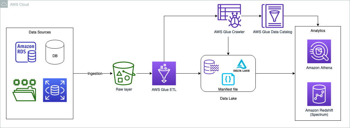


 Praveen Allam is a Solutions Architect at AWS. He helps customers design scalable, better cost-perfromant enterprise-grade applications using the AWS Cloud. He builds solutions to help organizations make data-driven decisions.
 Vivek Singh is Senior Solutions Architect with the AWS Data Lab team. He helps customers unblock their data journey on the AWS ecosystem. His interest areas are data pipeline automation, data quality and data governance, data lakes, and lake house architectures.


 Akira Ajisaka is a Senior Software Development Engineer on the AWS Glue team. He likes open-source software and distributed systems. In his spare time, he enjoys playing both arcade and console games.
 Noritaka Sekiyama is a Principal Big Data Architect on the AWS Glue team. He is responsible for building software artifacts to help customers. In his spare time, he enjoys cycling with his new road bike.
 Savio Dsouza is a Software Development Manager on the AWS Glue team. His teams work on building and innovating in distributed compute systems and frameworks, namely on Apache Spark.


 Gonzalo Herreros is a Senior Big Data Architect on the AWS Glue team.
 Michael Benattar is a Senior Software Engineer on the AWS Glue Studio team. He has led the design and implementation of the custom visual transform feature.