Tag Archives: Customer Solutions

Amazon Identity Services uses Amazon QuickSight to empower partners with self-serve data discovery

2023-01-03 Siamak Ziraknejad

Post Syndicated from Siamak Ziraknejad original https://aws.amazon.com/blogs/big-data/amazon-identity-services-uses-amazon-quicksight-to-empower-partners-with-self-serve-data-discovery/

Amazon Identity Services is responsible for the way Amazon customers—buyers, sellers, developers—identify themselves on Amazon. Our team also manages customers’ core account information, such as names and delivery addresses. Our mission is to deliver the most intuitive, convenient, and secure authentication experience. We’re in charge of account security for Amazon, worldwide, on all device surfaces.

Identity systems make millions of security decisions per second. We ingest datasets at a large scale—processing 9 TB per hour—and produce analytical datasets that grow by billions of rows per hour. Our core business metrics within the Amazon Identity Services team are built on top of these datasets, which we use for leadership meetings, product launch decisions, metric movement investigations, and discovering new innovation opportunities to simplify security experiences for our customers.

In this post, we discuss how we use Amazon QuickSight to empower partners with self-serve data discovery.

Inaccessible insights block data-driven decisions

The sheer volume of our datasets made gathering insights a slow process. Not only that, but datasets weren’t accessible to a wide audience outside our team, such as partners, program managers, product managers, and so on. As a result, Business Intelligence Engineers (BIEs) spent a lot of time writing ad hoc queries, which then took a long time to run. When the insights were ready, BIEs were tasked with answering questions via manual processes that didn’t scale.

We chose QuickSight to not only speed up our processing times, but to create efficiencies with self-serve insight access via analyses (exploration and authoring) and dashboards for consumption. With partners and stakeholders having the ability to access insights without assistance, our BIEs were able to shift focus from ad hoc requests to more impactful projects that were a better use of their skills and expertise.

In the following sections, we discuss what we were looking for in BI capabilities, and how QuickSight satisfied those requirements for our team.

Removing the middle person with QuickSight

Imagine being the pilot of a commercial airline, navigating in cloudy conditions. You know your destination lies ahead, but you can’t see it; you have to rely on your dashboard of instruments to navigate so you’ll arrive safely. It’s similar when working on large-scale consumer products. Although our team gathers anecdotes and reviews feedback to form hypotheses on what our customers need, only by analyzing data at scale can we truly understand customer problems and design appropriate solutions.

The status quo that positioned our BIEs between stakeholders and the insights that were needed required a manual, error-prone process, with a time-to-insight that could take weeks. Even more problematic was that insights were limited to what the requestor envisioned. There was no flexibility to explore and visualize data with a simple drag-and-drop UI. This inability to explore and interact with available data meant stakeholders didn’t know the best questions to ask. Our team needed to make data more accessible to partner teams and non-BIE users, and we needed that access to be fast, intuitive, and to provide a single, indisputable source of truth.

With our research into BI tool options, we were looking for the following:

Accessible insights – We needed to ensure users from all levels of technical experience would be able to access and understand the insights provided to them
Speed – With an ingestion rate of 9 TB of data per hour, we needed our BI tool to be fast and reliable
Security – Built-in row-level and column-level security would give us the ability to provide on-demand access to thousands of users across AWS

The first option we considered had a lot of great features, but it wouldn’t scale without a server. The next option we looked at was very capable in a lot of areas, but it wouldn’t be as accessible for non-BIE users, and it also required a team to manage a server. QuickSight was a great fit because it’s not only serverless, but also has enough visualization capabilities to make it useful for self-service data.

QuickSight also offered seamless integration with Amazon Redshift, and the ability to publish our business metrics to QuickSight SPICE (Super-fast, Parallel, In-memory Calculation Engine), its robust in-memory engine. SPICE performs rapid advanced calculations and serves data. What we love most about SPICE is that it greatly reduces time-to-insight, supports column-level security for staying in compliance, and most importantly it’s super fast for data exploration within analyses.

Self-service data discovery just a few clicks away

Publishing our metrics to QuickSight SPICE enabled us to create pre-authored dashboards, and empowered users to create their own analytical content via analyses. Our technical program managers have all been trained on how to use QuickSight to create visualizations, whereas our BIE team members are dedicating their time to creating better datasets. Our non-tech partners and product managers no longer need to depend on a BIE to get answers to their questions, because they can create analyses and query billions of records with a drag-and-drop interface to instantly visualize data.

The following screen shot shows what our year-to-date visualization looks like, with all sensitive data redacted.

The BIE time saved as a result of stakeholders getting self-service answers can now be invested in building richer and better quality datasets, creating a virtuous cycle to help accelerate our ability to adapt and improve to meet our customers’ needs.

Another important benefit of using QuickSight was that we centralized a semantic layer, unifying the language we speak across departments by publishing authoritative datasets in SPICE with proper access control. Because the data was easy to use and accessible with pre-calculated metrics, our partner teams didn’t have to re-invent the metric definitions. To ensure everyone stays on the same page, we publish all documentation to internal wikis.

More efficient business reviews with paginated reports and Amazon QuickSight Q

Our north star is to completely automate our periodic business review processes, similar to how the AWS Analytics Sales team is currently using QuickSight Q in their monthly business reviews. Because Q enables simple querying of data in real time via natural language, we can reduce the time it takes to author analytical content, eliminate redundant manual work, and simplify interactivity with data.

With QuickSight, we are automating all the dashboard and analyses generation for the business reviews. Doing so enables us to focus more on generating insights and conducting relevant investigations every month, rather than spending time and energy querying for data. Specifically, the new paginated report object type enables us to produce highly formatted content for leadership and formal reviews.

To learn more about how you can embed customized data visuals, interactive dashboards, and natural language querying into any application, visit Amazon QuickSight Embedded.

About the Authors

Siamak Ziraknejad leads the technical product management team for Amazon Identity Services. His team formulates the technical product strategy and plans for account security (authentication and authorization across all surfaces, worldwide) and the consumer identity foundations for all Amazon programs and products (entitlement management, benefit sharing, and personalization).

Abhinav Mehta is a Senior Product Manager (Technical) with the Amazon Identity Services team. He is focused on the product strategy and innovations for fast and secure authentication methods at Amazon.

Clickedu uses Amazon QuickSight Embedded to empower school administrators with key educational institution health insights

2022-12-23 Ignasi Nogués

Post Syndicated from Ignasi Nogués original https://aws.amazon.com/blogs/big-data/clickedu-uses-amazon-quicksight-embedded-to-empower-school-administrators-with-key-educational-institution-health-insights/

This is a guest post by Ignasi Nogués and Georgina Valls from Clickedu.

With more than 1.5 million unique users across 700 schools and core values that include connectivity, reliability, and innovation, Clickedu is the leading educational platform in Spain. Offering both a school administration system and a digital learning environment, Clickedu is one of the most comprehensive education tools in the European market for K–12 schools. Founded in 2000, Clickedu was acquired by Finland-based Sanoma Learning Group, a leading European learning and media company, in 2019.

Having originally started as an IT company, Clickedu has always been focused on providing products and services designed specifically for the education sector. Through continuous partnership with school administrators and education professionals, our development process is firmly rooted in listening to feedback and making prioritization decisions based on what customers tell us is most important to them. Because schools are the central focus of our research and development efforts, our service and product quality standards remain high.

Our mission is to help schools invest their time in educational objectives, with as little time as possible dedicated to bureaucratic tasks. To help administrators in human resources (HR), finance, and academic departments make more strategic, data-driven decisions across networks of educational centers, we launched Clickedu Analytics. This product provides data analysis and presents insights in easy-to-understand dashboards with insightful visualizations. When researching business intelligence (BI) tools that would meet our needs for what we wanted Clickedu Analytics to do, we needed look no further than Amazon QuickSight.

In this post, we discuss why we chose QuickSight and will cover some of the post-implementation outcomes.

Connecting the dots with data

Clickedu provides a cloud-based school platform that includes academic, administrative, and economic management tools and a virtual learning management system (LMS) with a connection to digital books and free content. For administrators, Clickedu’s software provides an interface to manage teachers, tutors, and heads of studies, as well as a communication environment for messaging families.

With so many data points spanning the full scope of the platform’s centralized capabilities across HR, finance, and academics, the untapped potential in that data presented a huge opportunity. We set out with the goal of building a BI experience that would enable us to quickly and efficiently analyze that data, visualize the results, and use those insights to better serve our customers.

The following screenshot shows a dashboard visualization of student distribution based on several different factors.

Clickedu QuickSight dashboard image

With dashboards built specifically to surface helpful information, school administrators are better able to make informed decisions based on clear, easy-to-understand insights. Reports can be generated to show academic results, pre-registrations, absences, etc., and all of it can be filtered by school year, institution, center, stage, courses, and classes.

Thanks to the information QuickSight delivers via Clickedu Analytics, our HR teams can see how many teachers in a group are likely to retire soon, or academic teams can see how language qualifications are progressing. Having fast, easy access to key insights like these help us be more proactive in identifying areas that might need attention before they become issues that demand a reaction.

Visibility to spot trends

The biggest challenge our customers were facing was a lack of visibility into aggregate data points that impacted several schools within a group. Speed, agility, and responsiveness are crucial when it comes to spotting trends in data points that signal issues in need of attention or wins deserving of celebration. Prior to implementing QuickSight, it would take time and resources to research whether something identified at one school was also showing up in the data points for the others. Now, administrators have full visibility to all relevant data across an entire network of schools with just a few clicks on their Clickedu Analytics dashboards.

Simple, serverless, scalable

After reviewing several other BI vendor products and evaluating the pros and cons of each, Amazon QuickSight was chosen as our Clickedu Analytics BI tool for these reasons.

Simple integration – We use Amazon Redshift as our data warehouse. We also work with AWS Glue as an extract, transform, and load (ETL) tool and Amazon SageMaker as a development environment. Adding Quicksight to our established mix of AWS services was a fast, simple, seamless process.
Serverless – Because our AWS services are in the cloud, we don’t have to download or maintain any software; there’s no heavy lifting on our end.
Scalable – QuickSight automatically scales resources based on usage and consumption, which takes one more task off the list of things we’d otherwise need to monitor and adjust.
User-friendly – QuickSight’s intuitive interface means anyone can access insights, regardless of their tech background or aptitude.
Embeddability – Being able to embed QuickSight directly into our existing product interfaces has enabled us to create valuable data products that allow both Clickedu and our customers to create visualizations of economic, academic, and HR data in an aggregate model.

Being able to export reports into PDFs, add new datasets, and the ease of combining with third-party data all contributed to swaying our decision to QuickSight.

Coming soon to Clickedu Analytics

QuickSight has empowered us to bring our Clickedu Analytics platform to the next level in providing the visibility and scalability we need to best serve our customers. We’re very excited to continue to iterate on what we’ve built with plans to expand access from the school groups and institutions who are currently using Clickedu Analytics to have it available to all schools that are in need of data management solutions.

Looking to the future, we see potential to do more with QuickSight in the learning management system (LMS) space. We are considering Amazon QuickSight Q, a machine learning-powered natural language capability that gives anyone in an organization the ability to ask business questions in natural language and receive accurate answers with relevant visualizations instantly without needing to go back to the dashboard author. There is ample potential to implement QuickSight Q as a means of querying and receiving information on our digital content.

To learn more about how you can embed customized data visuals, interactive dashboards, and natural language querying into any application, visit Amazon QuickSight Embedded.

To learn more about Clickedu, Spain’s leading platform for school administration, visit www.clickedu.net.

About the Authors

Ignasi Nogués is the founder and the CTO of Clickedu. He is, by definition, a big entrepreneur and a dreamer. He drove the company since 2000 to success due to hard work. He always wants to take the next step.

Georgina Valls is the Marketing Manager of Clickedu. She is a hardworker, dedicated to letting others know about Clickedu and its capabilities. As the daughter of teachers, she is very passionate about creating a brighter future in education.

Unlock the power of EC2 Graviton with GitLab CI/CD and EKS Runners

2022-12-23 Michael Fischer

Post Syndicated from Michael Fischer original https://aws.amazon.com/blogs/devops/unlock-the-power-of-ec2-graviton-with-gitlab-ci-cd-and-eks-runners/

Many AWS customers are using GitLab for their DevOps needs, including source control, and continuous integration and continuous delivery (CI/CD). Many of our customers are using GitLab SaaS (the hosted edition), while others are using GitLab Self-managed to meet their security and compliance requirements.

Customers can easily add runners to their GitLab instance to perform various CI/CD jobs. These jobs include compiling source code, building software packages or container images, performing unit and integration testing, etc.—even all the way to production deployment. For the SaaS edition, GitLab offers hosted runners, and customers can provide their own runners as well. Customers who run GitLab Self-managed must provide their own runners.

In this post, we’ll discuss how customers can maximize their CI/CD capabilities by managing their GitLab runner and executor fleet with Amazon Elastic Kubernetes Service (Amazon EKS). We’ll leverage both x86 and Graviton runners, allowing customers for the first time to build and test their applications both on x86 and on AWS Graviton, our most powerful, cost-effective, and sustainable instance family. In keeping with AWS’s philosophy of “pay only for what you use,” we’ll keep our Amazon Elastic Compute Cloud (Amazon EC2) instances as small as possible, and launch ephemeral runners on Spot instances. We’ll demonstrate building and testing a simple demo application on both architectures. Finally, we’ll build and deliver a multi-architecture container image that can run on Amazon EC2 instances or AWS Fargate, both on x86 and Graviton.

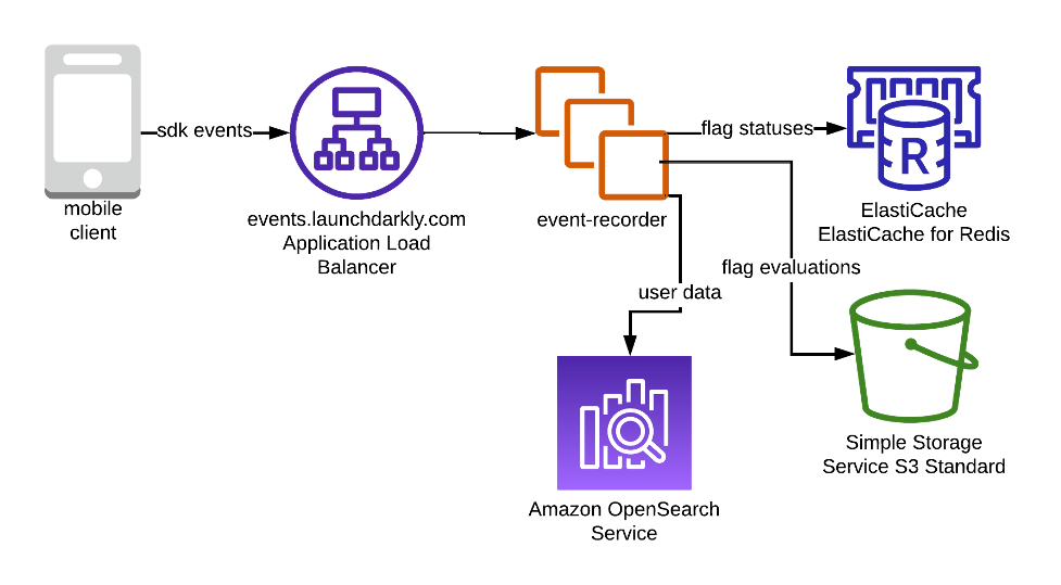
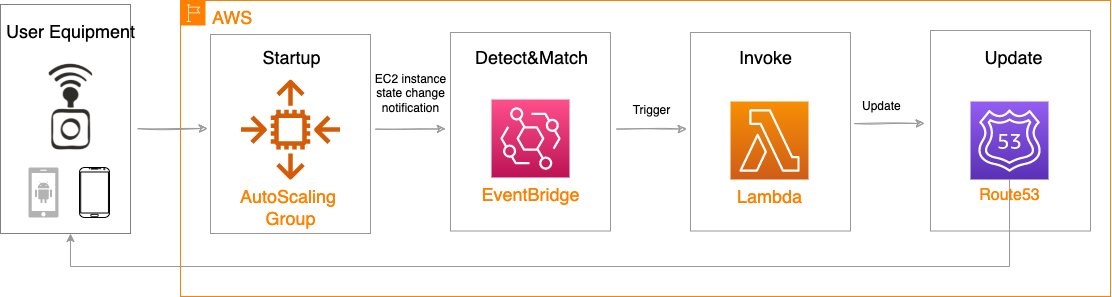
Figure 1. Managed GitLab runner architecture overview.

Let’s go through the components:

Runners

A runner is an application to which GitLab sends jobs that are defined in a CI/CD pipeline. The runner receives jobs from GitLab and executes them—either by itself, or by passing it to an executor (we’ll visit the executor in the next section).

In our design, we’ll be using a pair of self-hosted runners. One runner will accept jobs for the x86 CPU architecture, and the other will accept jobs for the arm64 (Graviton) CPU architecture. To help us route our jobs to the proper runner, we’ll apply some tags to each runner indicating the architecture for which it will be responsible. We’ll tag the x86 runner with x86, x86-64, and amd64, thereby reflecting the most common nicknames for the architecture, and we’ll tag the arm64 runner with arm64.

Currently, these runners must always be running so that they can receive jobs as they are created. Our runners only require a small amount of memory and CPU, so that we can run them on small EC2 instances to minimize cost. These include t4g.micro for Graviton builds, or t3.micro or t3a.micro for x86 builds.

To save money on these runners, consider purchasing a Savings Plan or Reserved Instances for them. Savings Plans and Reserved Instances can save you up to 72% over on-demand pricing, and there’s no minimum spend required to use them.

Kubernetes executors

In GitLab CI/CD, the executor’s job is to perform the actual build. The runner can create hundreds or thousands of executors as needed to meet current demand, subject to the concurrency limits that you specify. Executors are created only when needed, and they are ephemeral: once a job has finished running on an executor, the runner will terminate it.

In our design, we’ll use the Kubernetes executor that’s built into the GitLab runner. The Kubernetes executor simply schedules a new pod to run each job. Once the job completes, the pod terminates, thereby freeing the node to run other jobs.

The Kubernetes executor is highly customizable. We’ll configure each runner with a nodeSelector that makes sure that the jobs are scheduled only onto nodes that are running the specified CPU architecture. Other possible customizations include CPU and memory reservations, node and pod tolerations, service accounts, volume mounts, and much more.

Scaling worker nodes

For most customers, CI/CD jobs aren’t likely to be running all of the time. To save cost, we only want to run worker nodes when there’s a job to run.

To make this happen, we’ll turn to Karpenter. Karpenter provisions EC2 instances as soon as needed to fit newly-scheduled pods. If a new executor pod is scheduled, and there isn’t a qualified instance with enough capacity remaining on it, then Karpenter will quickly and automatically launch a new instance to fit the pod. Karpenter will also periodically scan the cluster and terminate idle nodes, thereby saving on costs. Karpenter can terminate a vacant node in as little as 30 seconds.

Karpenter can launch either Amazon EC2 on-demand or Spot instances depending on your needs. With Spot instances, you can save up to 90% over on-demand instance prices. Since CI/CD jobs often aren’t time-sensitive, Spot instances can be an excellent choice for GitLab execution pods. Karpenter will even automatically find the best Spot instance type to speed up the time it takes to launch an instance and minimize the likelihood of job interruption.

Deploying our solution

To deploy our solution, we’ll write a small application using the AWS Cloud Development Kit (AWS CDK) and the EKS Blueprints library. AWS CDK is an open-source software development framework to define your cloud application resources using familiar programming languages. EKS Blueprints is a library designed to make it simple to deploy complex Kubernetes resources to an Amazon EKS cluster with minimum coding.

The high-level infrastructure code – which can be found in our GitLab repo – is very simple. I’ve included comments to explain how it works.

// All CDK applications start with a new cdk.App object.
const app = new cdk.App();

// Create a new EKS cluster at v1.23. Run all non-DaemonSet pods in the 
// `kube-system` (coredns, etc.) and `karpenter` namespaces in Fargate
// so that we don't have to maintain EC2 instances for them.
const clusterProvider = new blueprints.GenericClusterProvider({
  version: KubernetesVersion.V1_23,
  fargateProfiles: {
    main: {
      selectors: [
        { namespace: 'kube-system' },
        { namespace: 'karpenter' },
      ]
    }
  },
  clusterLogging: [
    ClusterLoggingTypes.API,
    ClusterLoggingTypes.AUDIT,
    ClusterLoggingTypes.AUTHENTICATOR,
    ClusterLoggingTypes.CONTROLLER_MANAGER,
    ClusterLoggingTypes.SCHEDULER
  ]
});

// EKS Blueprints uses a Builder pattern.
blueprints.EksBlueprint.builder()
  .clusterProvider(clusterProvider) // start with the Cluster Provider
  .addOns(
    // Use the EKS add-ons that manage coredns and the VPC CNI plugin
    new blueprints.addons.CoreDnsAddOn('v1.8.7-eksbuild.3'),
    new blueprints.addons.VpcCniAddOn('v1.12.0-eksbuild.1'),
    // Install Karpenter
    new blueprints.addons.KarpenterAddOn({
      provisionerSpecs: {
        // Karpenter examines scheduled pods for the following labels
        // in their `nodeSelector` or `nodeAffinity` rules and routes
        // the pods to the node with the best fit, provisioning a new
        // node if necessary to meet the requirements.
        //
        // Allow either amd64 or arm64 nodes to be provisioned 
        'kubernetes.io/arch': ['amd64', 'arm64'],
        // Allow either Spot or On-Demand nodes to be provisioned
        'karpenter.sh/capacity-type': ['spot', 'on-demand']
      },
      // Launch instances in the VPC private subnets
      subnetTags: {
        Name: 'gitlab-runner-eks-demo/gitlab-runner-eks-demo-vpc/PrivateSubnet*'
      },
      // Apply security groups that match the following tags to the launched instances
      securityGroupTags: {
        'kubernetes.io/cluster/gitlab-runner-eks-demo': 'owned'      
      }
    }),
    // Create a pair of a new GitLab runner deployments, one running on
    // arm64 (Graviton) instance, the other on an x86_64 instance.
    // We'll show the definition of the GitLabRunner class below.
    new GitLabRunner({
      arch: CpuArch.ARM_64,
      // If you're using an on-premise GitLab installation, you'll want
      // to change the URL below.
      gitlabUrl: 'https://gitlab.com',
      // Kubernetes Secret containing the runner registration token
      // (discussed later)
      secretName: 'gitlab-runner-secret'
    }),
    new GitLabRunner({
      arch: CpuArch.X86_64,
      gitlabUrl: 'https://gitlab.com',
      secretName: 'gitlab-runner-secret'
    }),
  )
  .build(app, 
         // Stack name
         'gitlab-runner-eks-demo');
The GitLabRunner class is a HelmAddOn subclass that takes a few parameters from the top-level application:
// The location and name of the GitLab Runner Helm chart
const CHART_REPO = 'https://charts.gitlab.io';
const HELM_CHART = 'gitlab-runner';

// The default namespace for the runner
const DEFAULT_NAMESPACE = 'gitlab';

// The default Helm chart version
const DEFAULT_VERSION = '0.40.1';

export enum CpuArch {
    ARM_64 = 'arm64',
    X86_64 = 'amd64'
}

// Configuration parameters
interface GitLabRunnerProps {
    // The CPU architecture of the node on which the runner pod will reside
    arch: CpuArch
    // The GitLab API URL 
    gitlabUrl: string
    // Kubernetes Secret containing the runner registration token (discussed later)
    secretName: string
    // Optional tags for the runner. These will be added to the default list 
    // corresponding to the runner's CPU architecture.
    tags?: string[]
    // Optional Kubernetes namespace in which the runner will be installed
    namespace?: string
    // Optional Helm chart version
    chartVersion?: string
}

export class GitLabRunner extends HelmAddOn {
    private arch: CpuArch;
    private gitlabUrl: string;
    private secretName: string;
    private tags: string[] = [];

    constructor(props: GitLabRunnerProps) {
        // Invoke the superclass (HelmAddOn) constructor
        super({
            name: `gitlab-runner-${props.arch}`,
            chart: HELM_CHART,
            repository: CHART_REPO,
            namespace: props.namespace || DEFAULT_NAMESPACE,
            version: props.chartVersion || DEFAULT_VERSION,
            release: `gitlab-runner-${props.arch}`,
        });

        this.arch = props.arch;
        this.gitlabUrl = props.gitlabUrl;
        this.secretName = props.secretName;

        // Set default runner tags
        switch (this.arch) {
            case CpuArch.X86_64:
                this.tags.push('amd64', 'x86', 'x86-64', 'x86_64');
                break;
            case CpuArch.ARM_64:
                this.tags.push('arm64');
                break;
        }
        this.tags.push(...props.tags || []); // Add any custom tags
    };

    // `deploy` method required by the abstract class definition. Our implementation
    // simply installs a Helm chart to the cluster with the proper values.
    deploy(clusterInfo: ClusterInfo): void | Promise<Construct> {
        const chart = this.addHelmChart(clusterInfo, this.getValues(), true);
        return Promise.resolve(chart);
    }

    // Returns the values for the GitLab Runner Helm chart
    private getValues(): Values {
        return {
            gitlabUrl: this.gitlabUrl,
            runners: {
                config: this.runnerConfig(), // runner config.toml file, from below
                name: `demo-runner-${this.arch}`, // name as seen in GitLab UI
                tags: uniq(this.tags).join(','),
                secret: this.secretName, // see below
            },
            // Labels to constrain the nodes where this runner can be placed
            nodeSelector: {
                'kubernetes.io/arch': this.arch,
                'karpenter.sh/capacity-type': 'on-demand'
            },
            // Default pod label
            podLabels: {
                'gitlab-role': 'manager'
            },
            // Create all the necessary RBAC resources including the ServiceAccount
            rbac: {
                create: true
            },
            // Required resources (memory/CPU) for the runner pod. The runner
            // is fairly lightweight as it's a self-contained Golang app.
            resources: {
                requests: {
                    memory: '128Mi',
                    cpu: '256m'
                }
            }
        };
    }

    // This string contains the runner's `config.toml` file including the
    // Kubernetes executor's configuration. Note the nodeSelector constraints 
    // (including the use of Spot capacity and the CPU architecture).
    private runnerConfig(): string {
        return `
  [[runners]]
    [runners.kubernetes]
      namespace = "{{.Release.Namespace}}"
      image = "ubuntu:16.04"
    [runners.kubernetes.node_selector]
      "kubernetes.io/arch" = "${this.arch}"
      "kubernetes.io/os" = "linux"
      "karpenter.sh/capacity-type" = "spot"
    [runners.kubernetes.pod_labels]
      gitlab-role = "runner"
      `.trim();
    }
}

For security reasons, we store the GitLab registration token in a Kubernetes Secret – never in our source code. For additional security, we recommend encrypting Secrets using an AWS Key Management Service (AWS KMS) key that you supply by specifying the encryption configuration when you create your Amazon EKS cluster. It’s a good practice to restrict access to this Secret via Kubernetes RBAC rules.

To create the Secret, run the following command:

# These two values must match the parameters supplied to the GitLabRunner constructor
NAMESPACE=gitlab
SECRET_NAME=gitlab-runner-secret
# The value of the registration token.
TOKEN=GRxxxxxxxxxxxxxxxxxxxxxx

kubectl -n $NAMESPACE create secret generic $SECRET_NAME \
        --from-literal="runner-registration-token=$TOKEN" \
        --from-literal="runner-token="

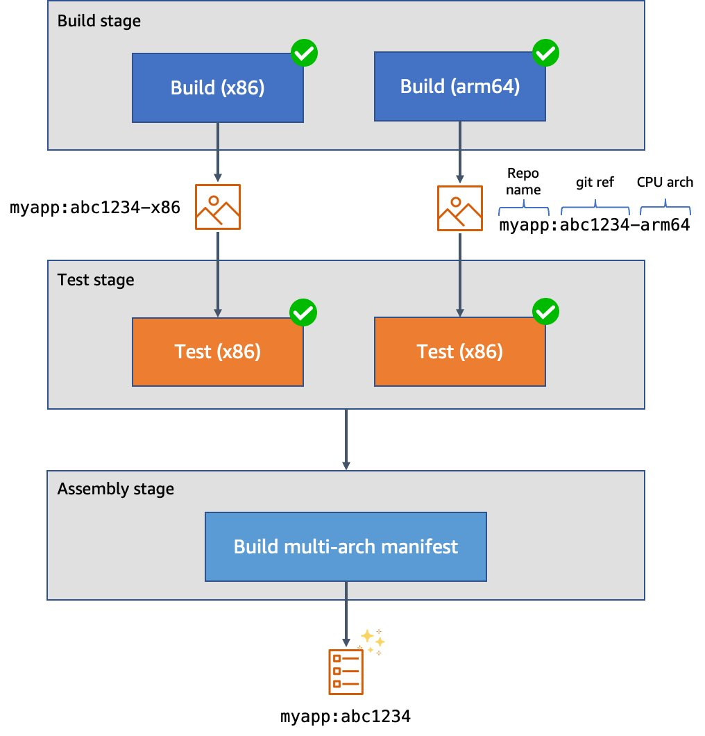
Building a multi-architecture container image

Now that we’ve launched our GitLab runners and configured the executors, we can build and test a simple multi-architecture container image. If the tests pass, we can then upload it to our project’s GitLab container registry. Our application will be pretty simple: we’ll create a web server in Go that simply prints out “Hello World” and prints out the current architecture.

Find the source code of our sample app in our GitLab repo.

In GitLab, the CI/CD configuration lives in the .gitlab-ci.yml file at the root of the source repository. In this file, we declare a list of ordered build stages, and then we declare the specific jobs associated with each stage.

Our stages are:

The build stage, in which we compile our code, produce our architecture-specific images, and upload these images to the GitLab container registry. These uploaded images are tagged with a suffix indicating the architecture on which they were built. This job uses a matrix variable to run it in parallel against two different runners – one for each supported architecture. Furthermore, rather than using docker build to produce our images, we use Kaniko to build them. This lets us build our images in an unprivileged container environment and improve the security posture considerably.
The test stage, in which we test the code. As with the build stage, we use a matrix variable to run the tests in parallel in separate pods on each supported architecture.

The assembly stage, in which we create a multi-architecture image manifest from the two architecture-specific images. Then, we push the manifest into the image registry so that we can refer to it in future deployments.

Figure 2. Example CI/CD pipeline for multi-architecture images.

Here’s what our top-level configuration looks like:

variables:
  # These are used by the runner to configure the Kubernetes executor, and define
  # the values of spec.containers[].resources.limits.{memory,cpu} for the Pod(s).
  KUBERNETES_MEMORY_REQUEST: 1Gi
  KUBERNETES_CPU_REQUEST: 1

# List of stages for jobs, and their order of execution  
stages:    
  - build
  - test
  - create-multiarch-manifest
Here’s what our build stage job looks like. Note the matrix of variables which are set in BUILD_ARCH as the two jobs are run in parallel:
build-job:
  stage: build
  parallel:
    matrix:              # This job is run twice, once on amd64 (x86), once on arm64
    - BUILD_ARCH: amd64
    - BUILD_ARCH: arm64
  tags: [$BUILD_ARCH]    # Associate the job with the appropriate runner
  image:
    name: gcr.io/kaniko-project/executor:debug
    entrypoint: [""]
  script:
    - mkdir -p /kaniko/.docker
    # Configure authentication data for Kaniko so it can push to the
    # GitLab container registry
    - echo "{\"auths\":{\"${CI_REGISTRY}\":{\"auth\":\"$(printf "%s:%s" "${CI_REGISTRY_USER}" "${CI_REGISTRY_PASSWORD}" | base64 | tr -d '\n')\"}}}" > /kaniko/.docker/config.json
    # Build the image and push to the registry. In this stage, we append the build
    # architecture as a tag suffix.
    - >-
      /kaniko/executor
      --context "${CI_PROJECT_DIR}"
      --dockerfile "${CI_PROJECT_DIR}/Dockerfile"
      --destination "${CI_REGISTRY_IMAGE}:${CI_COMMIT_SHORT_SHA}-${BUILD_ARCH}"

Here’s what our test stage job looks like. This time we use the image that we just produced. Our source code is copied into the application container. Then, we can run make test-api to execute the server test suite.

build-job:
  stage: build
  parallel:
    matrix:              # This job is run twice, once on amd64 (x86), once on arm64
    - BUILD_ARCH: amd64
    - BUILD_ARCH: arm64
  tags: [$BUILD_ARCH]    # Associate the job with the appropriate runner
  image:
    # Use the image we just built
    name: "${CI_REGISTRY_IMAGE}:${CI_COMMIT_SHORT_SHA}-${BUILD_ARCH}"
  script:
    - make test-container

Finally, here’s what our assembly stage looks like. We use Podman to build the multi-architecture manifest and push it into the image registry. Traditionally we might have used docker buildx to do this, but using Podman lets us do this work in an unprivileged container for additional security.

create-manifest-job:
  stage: create-multiarch-manifest
  tags: [arm64] 
  image: public.ecr.aws/docker/library/fedora:36
  script:
    - yum -y install podman
    - echo "${CI_REGISTRY_PASSWORD}" | podman login -u "${CI_REGISTRY_USER}" --password-stdin "${CI_REGISTRY}"
    - COMPOSITE_IMAGE=${CI_REGISTRY_IMAGE}:${CI_COMMIT_SHORT_SHA}
    - podman manifest create ${COMPOSITE_IMAGE}
    - >-
      for arch in arm64 amd64; do
        podman manifest add ${COMPOSITE_IMAGE} docker://${COMPOSITE_IMAGE}-${arch};
      done
    - podman manifest inspect ${COMPOSITE_IMAGE}
    # The composite image manifest omits the architecture from the tag suffix.
    - podman manifest push ${COMPOSITE_IMAGE} docker://${COMPOSITE_IMAGE}

Trying it out

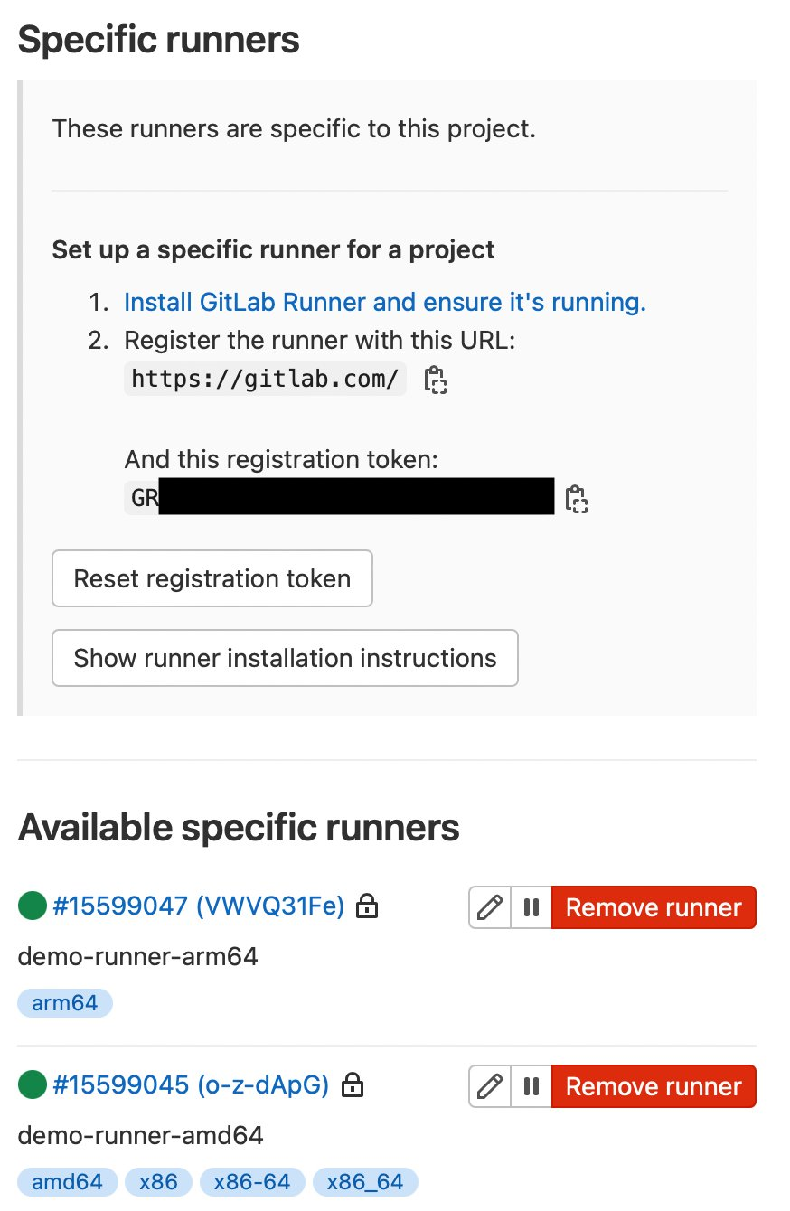
I’ve created a public test GitLab project containing the sample source code, and attached the runners to the project. We can see them at Settings > CI/CD > Runners:

Figure 3. GitLab runner configurations.

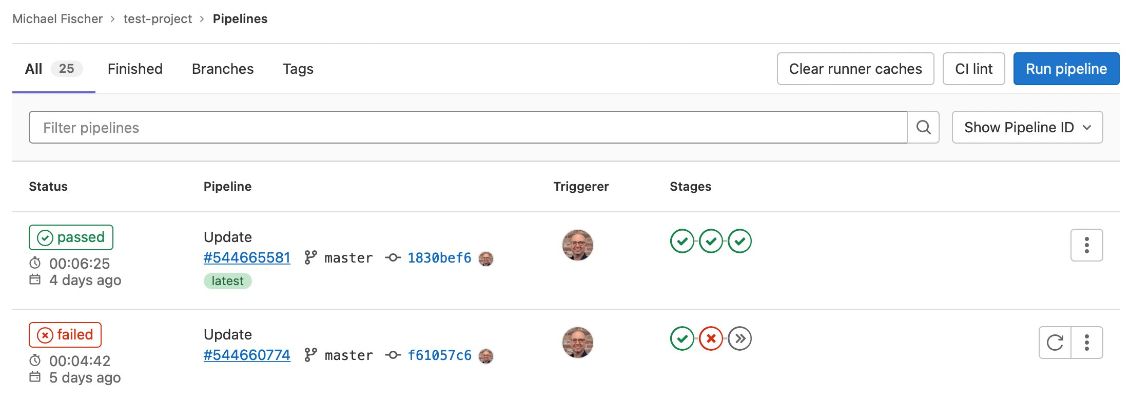
Here we can also see some pipeline executions, where some have succeeded, and others have failed.

Figure 4. GitLab sample pipeline executions.

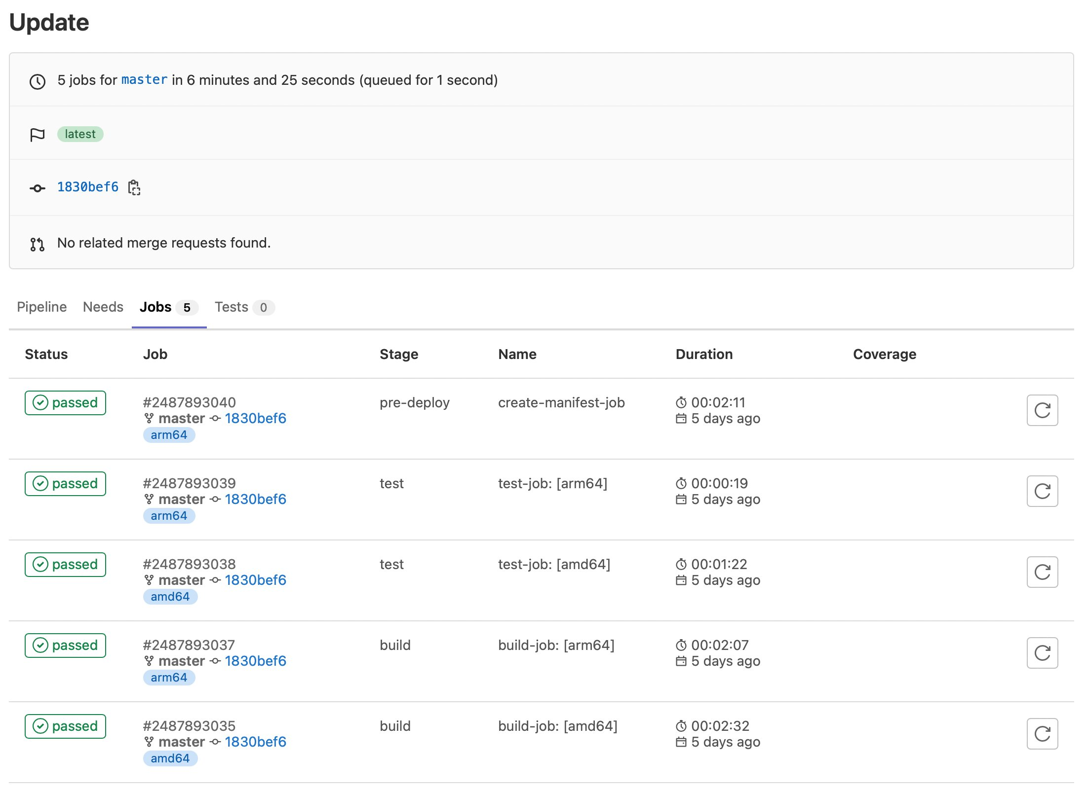
We can also see the specific jobs associated with a pipeline execution:

Figure 5. GitLab sample job executions.

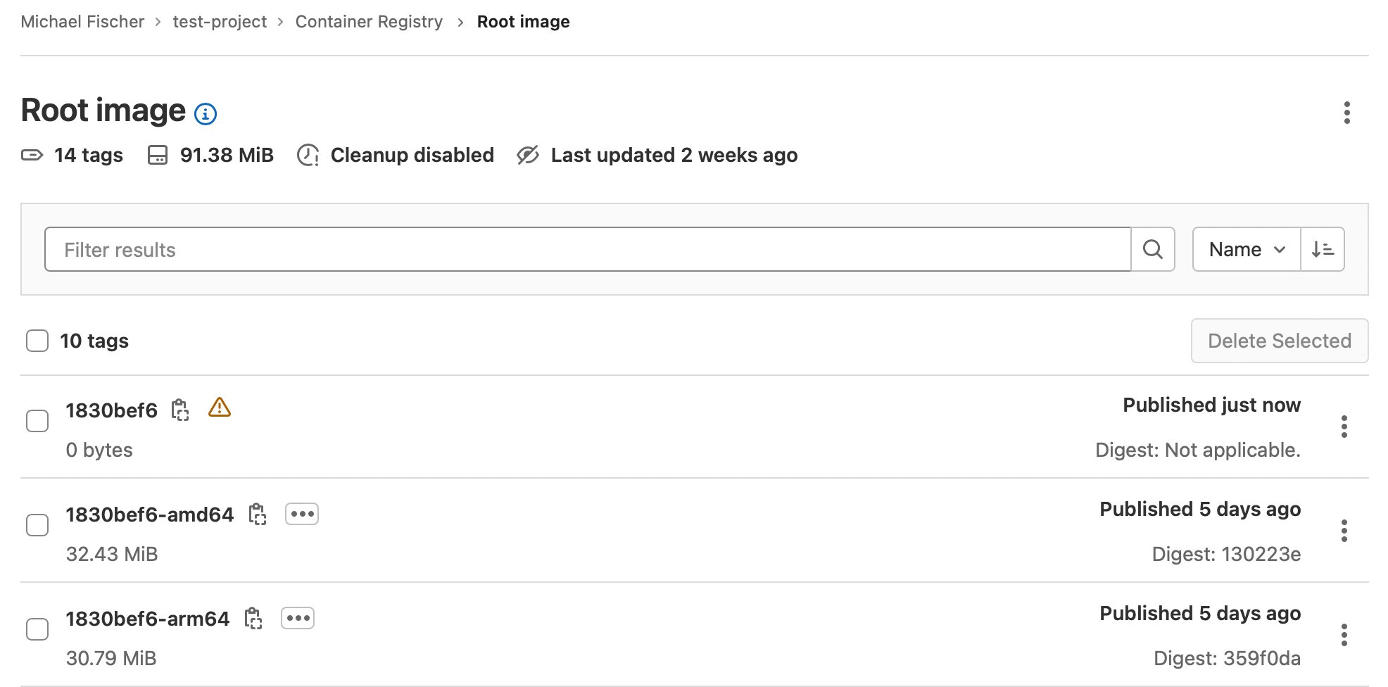
Finally, here are our container images:

Figure 6. GitLab sample container registry.

Conclusion

In this post, we’ve illustrated how you can quickly and easily construct multi-architecture container images with GitLab, Amazon EKS, Karpenter, and Amazon EC2, using both x86 and Graviton instance families. We indexed on using as many managed services as possible, maximizing security, and minimizing complexity and TCO. We dove deep on multiple facets of the process, and discussed how to save up to 90% of the solution’s cost by using Spot instances for CI/CD executions.

Find the sample code, including everything shown here today, in our GitLab repository.

Building multi-architecture images will unlock the value and performance of running your applications on AWS Graviton and give you increased flexibility over compute choice. We encourage you to get started today.

About the author:

Multi-branch pipeline management and infrastructure deployment using AWS CDK Pipelines

2022-12-22 Iris Kraja

Post Syndicated from Iris Kraja original https://aws.amazon.com/blogs/devops/multi-branch-pipeline-management-and-infrastructure-deployment-using-aws-cdk-pipelines/

This post describes how to use the AWS CDK Pipelines module to follow a Gitflow development model using AWS Cloud Development Kit (AWS CDK). Software development teams often follow a strict branching strategy during a solutions development lifecycle. Newly-created branches commonly need their own isolated copy of infrastructure resources to develop new features.

CDK Pipelines is a construct library module for continuous delivery of AWS CDK applications. CDK Pipelines are self-updating: if you add application stages or stacks, then the pipeline automatically reconfigures itself to deploy those new stages and/or stacks.

The following solution creates a new AWS CDK Pipeline within a development account for every new branch created in the source repository (AWS CodeCommit). When a branch is deleted, the pipeline and all related resources are also destroyed from the account. This GitFlow model for infrastructure provisioning allows developers to work independently from each other, concurrently, even in the same stack of the application.

Solution overview

The following diagram provides an overview of the solution. There is one default pipeline responsible for deploying resources to the different application environments (e.g., Development, Pre-Prod, and Prod). The code is stored in CodeCommit. When new changes are pushed to the default CodeCommit repository branch, AWS CodePipeline runs the default pipeline. When the default pipeline is deployed, it creates two AWS Lambda functions.

These two Lambda functions are invoked by CodeCommit CloudWatch events when a new branch in the repository is created or deleted. The Create Lambda function uses the boto3 CodeBuild module to create an AWS CodeBuild project that builds the pipeline for the feature branch. This feature pipeline consists of a build stage and an optional update pipeline stage for itself. The Destroy Lambda function creates another CodeBuild project which cleans all of the feature branch’s resources and the feature pipeline.

Figure 1. Architecture diagram.

Prerequisites

Before beginning this walkthrough, you should have the following prerequisites:

An AWS account
AWS CDK installed
Python3 installed
Jq (JSON processor) installed
Basic understanding of continuous integration/continuous development (CI/CD) Pipelines

Initial setup

Download the repository from GitHub:

# Command to clone the repository
git clone https://github.com/aws-samples/multi-branch-cdk-pipelines.git
cd multi-branch-cdk-pipelines

Create a new CodeCommit repository in the AWS Account and region where you want to deploy the pipeline and upload the source code from above to this repository. In the config.ini file, change the repository_name and region variables accordingly.

Make sure that you set up a fresh Python environment. Install the dependencies:

pip install -r requirements.txt

Run the initial-deploy.sh script to bootstrap the development and production environments and to deploy the default pipeline. You’ll be asked to provide the following parameters: (1) Development account ID, (2) Development account AWS profile name, (3) Production account ID, and (4) Production account AWS profile name.

sh ./initial-deploy.sh --dev_account_id <YOUR DEV ACCOUNT ID> --
dev_profile_name <YOUR DEV PROFILE NAME> --prod_account_id <YOUR PRODUCTION
ACCOUNT ID> --prod_profile_name <YOUR PRODUCTION PROFILE NAME>

Default pipeline

In the CI/CD pipeline, we set up an if condition to deploy the default branch resources only if the current branch is the default one. The default branch is retrieved programmatically from the CodeCommit repository. We deploy an Amazon Simple Storage Service (Amazon S3) Bucket and two Lambda functions. The bucket is responsible for storing the feature branches’ CodeBuild artifacts. The first Lambda function is triggered when a new branch is created in CodeCommit. The second one is triggered when a branch is deleted.

if branch == default_branch:
    
...

    # Artifact bucket for feature AWS CodeBuild projects
    artifact_bucket = Bucket(
        self,
        'BranchArtifacts',
        encryption=BucketEncryption.KMS_MANAGED,
        removal_policy=RemovalPolicy.DESTROY,
        auto_delete_objects=True
    )
...
    # AWS Lambda function triggered upon branch creation
    create_branch_func = aws_lambda.Function(
        self,
        'LambdaTriggerCreateBranch',
        runtime=aws_lambda.Runtime.PYTHON_3_8,
        function_name='LambdaTriggerCreateBranch',
        handler='create_branch.handler',
        code=aws_lambda.Code.from_asset(path.join(this_dir, 'code')),
        environment={
            "ACCOUNT_ID": dev_account_id,
            "CODE_BUILD_ROLE_ARN": iam_stack.code_build_role.role_arn,
            "ARTIFACT_BUCKET": artifact_bucket.bucket_name,
            "CODEBUILD_NAME_PREFIX": codebuild_prefix
        },
        role=iam_stack.create_branch_role)


    # AWS Lambda function triggered upon branch deletion
    destroy_branch_func = aws_lambda.Function(
        self,
        'LambdaTriggerDestroyBranch',
        runtime=aws_lambda.Runtime.PYTHON_3_8,
        function_name='LambdaTriggerDestroyBranch',
        handler='destroy_branch.handler',
        role=iam_stack.delete_branch_role,
        environment={
            "ACCOUNT_ID": dev_account_id,
            "CODE_BUILD_ROLE_ARN": iam_stack.code_build_role.role_arn,
            "ARTIFACT_BUCKET": artifact_bucket.bucket_name,
            "CODEBUILD_NAME_PREFIX": codebuild_prefix,
            "DEV_STAGE_NAME": f'{dev_stage_name}-{dev_stage.main_stack_name}'
        },
        code=aws_lambda.Code.from_asset(path.join(this_dir,
                                                  'code')))

Then, the CodeCommit repository is configured to trigger these Lambda functions based on two events:

(1) Reference created

# Configure AWS CodeCommit to trigger the Lambda function when a new branch is created
repo.on_reference_created(
    'BranchCreateTrigger',
    description="AWS CodeCommit reference created event.",
    target=aws_events_targets.LambdaFunction(create_branch_func))

(2) Reference deleted

# Configure AWS CodeCommit to trigger the Lambda function when a branch is deleted
repo.on_reference_deleted(
    'BranchDeleteTrigger',
    description="AWS CodeCommit reference deleted event.",
    target=aws_events_targets.LambdaFunction(destroy_branch_func))

Lambda functions

The two Lambda functions build and destroy application environments mapped to each feature branch. An Amazon CloudWatch event triggers the LambdaTriggerCreateBranch function whenever a new branch is created. The CodeBuild client from boto3 creates the build phase and deploys the feature pipeline.

Create function

The create function deploys a feature pipeline which consists of a build stage and an optional update pipeline stage for itself. The pipeline downloads the feature branch code from the CodeCommit repository, initiates the Build and Test action using CodeBuild, and securely saves the built artifact on the S3 bucket.

The Lambda function handler code is as follows:

def handler(event, context):
    """Lambda function handler"""
    logger.info(event)

    reference_type = event['detail']['referenceType']

    try:
        if reference_type == 'branch':
            branch = event['detail']['referenceName']
            repo_name = event['detail']['repositoryName']

            client.create_project(
                name=f'{codebuild_name_prefix}-{branch}-create',
                description="Build project to deploy branch pipeline",
                source={
                    'type': 'CODECOMMIT',
                    'location': f'https://git-codecommit.{region}.amazonaws.com/v1/repos/{repo_name}',
                    'buildspec': generate_build_spec(branch)
                },
                sourceVersion=f'refs/heads/{branch}',
                artifacts={
                    'type': 'S3',
                    'location': artifact_bucket_name,
                    'path': f'{branch}',
                    'packaging': 'NONE',
                    'artifactIdentifier': 'BranchBuildArtifact'
                },
                environment={
                    'type': 'LINUX_CONTAINER',
                    'image': 'aws/codebuild/standard:4.0',
                    'computeType': 'BUILD_GENERAL1_SMALL'
                },
                serviceRole=role_arn
            )

            client.start_build(
                projectName=f'CodeBuild-{branch}-create'
            )
    except Exception as e:
        logger.error(e)

Create branch CodeBuild project’s buildspec.yaml content:

version: 0.2
env:
  variables:
    BRANCH: {branch}
    DEV_ACCOUNT_ID: {account_id}
    PROD_ACCOUNT_ID: {account_id}
    REGION: {region}
phases:
  pre_build:
    commands:
      - npm install -g aws-cdk && pip install -r requirements.txt
  build:
    commands:
      - cdk synth
      - cdk deploy --require-approval=never
artifacts:
  files:
    - '**/*'

Destroy function

The second Lambda function is responsible for the destruction of a feature branch’s resources. Upon the deletion of a feature branch, an Amazon CloudWatch event triggers this Lambda function. The function creates a CodeBuild Project which destroys the feature pipeline and all of the associated resources created by that pipeline. The source property of the CodeBuild Project is the feature branch’s source code saved as an artifact in Amazon S3.

The Lambda function handler code is as follows:

def handler(event, context):
    logger.info(event)
    reference_type = event['detail']['referenceType']

    try:
        if reference_type == 'branch':
            branch = event['detail']['referenceName']
            client.create_project(
                name=f'{codebuild_name_prefix}-{branch}-destroy',
                description="Build project to destroy branch resources",
                source={
                    'type': 'S3',
                    'location': f'{artifact_bucket_name}/{branch}/CodeBuild-{branch}-create/',
                    'buildspec': generate_build_spec(branch)
                },
                artifacts={
                    'type': 'NO_ARTIFACTS'
                },
                environment={
                    'type': 'LINUX_CONTAINER',
                    'image': 'aws/codebuild/standard:4.0',
                    'computeType': 'BUILD_GENERAL1_SMALL'
                },
                serviceRole=role_arn
            )

            client.start_build(
                projectName=f'CodeBuild-{branch}-destroy'
            )

            client.delete_project(
                name=f'CodeBuild-{branch}-destroy'
            )

            client.delete_project(
                name=f'CodeBuild-{branch}-create'
            )
    except Exception as e:
        logger.error(e)

Destroy the branch CodeBuild project’s buildspec.yaml content:

version: 0.2
env:
  variables:
    BRANCH: {branch}
    DEV_ACCOUNT_ID: {account_id}
    PROD_ACCOUNT_ID: {account_id}
    REGION: {region}
phases:
  pre_build:
    commands:
      - npm install -g aws-cdk && pip install -r requirements.txt
  build:
    commands:
      - cdk destroy cdk-pipelines-multi-branch-{branch} --force
      - aws cloudformation delete-stack --stack-name {dev_stage_name}-{branch}
      - aws s3 rm s3://{artifact_bucket_name}/{branch} --recursive

Create a feature branch

On your machine’s local copy of the repository, create a new feature branch using the following git commands. Replace user-feature-123 with a unique name for your feature branch. Note that this feature branch name must comply with the CodePipeline naming restrictions, as it will be used to name a unique pipeline later in this walkthrough.

# Create the feature branch
git checkout -b user-feature-123
git push origin user-feature-123

The first Lambda function will deploy the CodeBuild project, which then deploys the feature pipeline. This can take a few minutes. You can log in to the AWS Console and see the CodeBuild project running under CodeBuild.

Figure 2. AWS Console – CodeBuild projects.

After the build is successfully finished, you can see the deployed feature pipeline under CodePipelines.

Figure 3. AWS Console – CodePipeline pipelines.

The Lambda S3 trigger project from AWS CDK Samples is used as the infrastructure resources to demonstrate this solution. The content is placed inside the src directory and is deployed by the pipeline. When visiting the Lambda console page, you can see two functions: one by the default pipeline and one by our feature pipeline.

Figure 4. AWS Console – Lambda functions.

Destroy a feature branch

There are two common ways for removing feature branches. The first one is related to a pull request, also known as a “PR”. This occurs when merging a feature branch back into the default branch. Once it’s merged, the feature branch will be automatically closed. The second way is to delete the feature branch explicitly by running the following git commands:

# delete branch local
git branch -d user-feature-123

# delete branch remote
git push origin --delete user-feature-123

The CodeBuild project responsible for destroying the feature resources is now triggered. You can see the project’s logs while the resources are being destroyed in CodeBuild, under Build history.

Figure 5. AWS Console – CodeBuild projects.

Cleaning up

To avoid incurring future charges, log into the AWS console of the different accounts you used, go to the AWS CloudFormation console of the Region(s) where you chose to deploy, and select and click Delete on the main and branch stacks.

Conclusion

This post showed how you can work with an event-driven strategy and AWS CDK to implement a multi-branch pipeline flow using AWS CDK Pipelines. The described solutions leverage Lambda and CodeBuild to provide a dynamic orchestration of resources for multiple branches and pipelines.
For more information on CDK Pipelines and all the ways it can be used, see the CDK Pipelines reference documentation.

About the authors:

AWS Specialist Insights Team uses Amazon QuickSight to provide operational insights across the AWS Worldwide Specialist Organization

2022-12-22 David Adamson

Post Syndicated from David Adamson original https://aws.amazon.com/blogs/big-data/aws-specialist-insights-team-uses-amazon-quicksight-to-provide-operational-insights-across-the-aws-worldwide-specialist-organization/

The AWS Worldwide Specialist Organization (WWSO) is a team of go-to-market experts that support strategic services, customer segments, and verticals at AWS. Working together, the Specialist Insights Team (SIT) and the Finance, Analytics, Science, and Technology team (FAST) support WWSO in acquiring, securing, and delivering information and business insights at scale by working with the broader AWS community (Sales, Business Units, Finance) enabling data-driven decisions to be made.

SIT is made up of analysts who bring deep knowledge of the business intelligence (BI) stack to support the WWSO business. Some analysts work across multiple areas, whereas others are deeply knowledgeable in their specific verticals, but all are technically proficient in BI tools and methodologies. The team’s ability to combine technical and operational knowledge, in partnership with domain experts within WWSO, helps us build a common, standard data platform that can be used throughout AWS.

Untapped potential in data availability

One of the ongoing challenges for the team was how to turn the 2.1 PB of data inside the data lake into actionable business intelligence that can drive actions and verifiable outcomes. The resources needed to translate the data, analyze it, and succinctly articulate what the data shows had been a blocker of our ability to be agile and responsive to our customers.

After reviewing several vendor products and evaluating the pros and cons of each, Amazon QuickSight was chosen to replace our existing legacy BI solution. It not only satisfied all of the criteria necessary to provide actionable insights across WWSO business but allows us to scale securely across tens of thousands of users at AWS.

In this post, we discuss what influenced the decision to implement QuickSight, and will detail some of the benefits our team has seen since implementation.

Legacy tool deprecation

The legacy BI solution presented a number of challenges, starting with scaling, complex governance, and siloed reporting. This resulted in poor performance, cumbersome development processes, multiple versions of truth, and high costs. Ultimately, the legacy BI solution had significant barriers to widespread adoption, including long time to insights, lack of trust, low innovation, and return-on-investment (ROI) justification.

After the decision was made to deprecate the previous BI tool our team had been using to provide reports and insights to the organization, the team began to make preparations for the impending switch. We met with analysts across the specialist organization to gather feedback on what they’d like to see in the next iteration of reporting capabilities. Based on that feedback, and with guidance from our leadership teams, the following criteria needed to be met in our next BI tool:

Accessible insights – To ensure users with varying levels of technical aptitude could understand the information, the insights format needed to be easy to understand.
Speed – With millions of records, processing speed needed to be lightning fast, and we also didn’t want to invest a lot of time in technical implementation or user education training.
Cost – Being a frugal company, we needed to ensure that our BI solution would not only do what we needed it to do but that it wouldn’t blow up our budget.
Security – Built-in row-level security, and a custom solution developed internally, had the ability to give access to thousands of users across AWS.

Among other considerations that ultimately influenced the decision to use QuickSight was that it’s a fully managed service, which meant no need to maintain a separate server or manage any upgrades. Because our team handles sensitive data, security was also top of mind. QuickSight passed that test as well; we were able to implement fine-grained security measures and saw no trade-off in performance.

A simple, speedy, single source of truth

With such a wide variety of teams needing access to the data and insights our team provides, our BI solution needed to be user-friendly and intuitive without the need for extensive training or convoluted instructions. With millions of records used to generate insights on sales pipelines, revenue, headcount, etc., queries could become quite complex. To meet our first top priority for accessible insights, we were looking for a combination of easy-to-operate and easy-to-understand visualizations.

Once our QuickSight implementation was complete, near-real-time, actionable insights with informative visuals were just a few clicks away. We were impressed by how simple it was to get at-a-glance insights that told data-driven stories about the key performance indicators that were most important to our stakeholder community. For business-critical metrics, we’re able to set up alerts that trigger emails to owners when certain thresholds are met, providing peace of mind that nothing important will slip through the cracks.

With the goal of migrating 400+ dashboards from the legacy BI solution over to QuickSight successfully, there were three critical components that we had to get right. Not only did we need to have the right technology, we also needed to set up the right processes while also keeping change management—from a people perspective—top of mind.

This migration project provided us with an opportunity to standardize our data, ensuring that we have a uniform source of truth that enables efficiency, as well as governed access and self-service across the company. In the spirit of working smarter (not harder), we kickstarted the migration in parallel with the data standardization project.

We started by establishing clear organization goals for alignment and a solid plan from start to finish. Next steps were to focus on row-level security design and evolution to ensure that we can provide governance and security at scale. To ensure success, we first piloted migrating 35+ dashboards and 500+ users. We then established a core technical team whose focus was to be experts at QuickSight and migrate another 400+ dashboards, 4,000+ users, and 60,0000+ impressions. The technical team also trained other members of the team to bring everyone along on the change management journey. We were able to complete the migration in 18 months across thousands of users.

With the base in place, we shifted focus to move from foundational business metrics to machine learning (ML) based insights and outcomes to help drive data-driven actions.

The following screenshot shows an example of what one of our QuickSight dashboards looks like, though the numbers do not reflect real values; this is test data.

With speed being next on our list of key criteria, we were delighted to learn more about how QuickSight works. SPICE, an acronym for Super-fast, Parallel, In-memory Calculation Engine, is the robust engine that QuickSight uses to rapidly perform advanced calculations and serve data. The query runtimes and dashboard development speed were both appreciably faster in comparison to other data visualization tools we had used, where we’d need to wait for it to process every time we added a new calculation or a new field to the visual. The dashboard load times were also noticeably faster than the load times from our previous BI tool; most load in under 5 seconds, compared to several minutes with the previous BI tool.

Another benefit of having chosen QuickSight is that there has been a significant reduction in the number of disagreements over data definitions or questions about discrepancies between reports. With standardized SPICE datasets built in QuickSight, we can now offer data as a service to the organization, creating a single source of truth for our insights shared across the organization. This saved the organization hours of time investigating unanswered questions, enabling us to be more agile and responsive, which makes us better able to serve our customers.

Dashboards are just the beginning

We’re very happy with QuickSight’s performance and scalability, and we are very excited to improve and expand on the solid reporting foundation we’ve begun to build. Having driven adoption from 50 percent to 83 percent, as well as seeing a 215 percent growth in views and a 157 percent growth in users since migrating to QuickSight, it’s clear we made the right choice.

We were intrigued by a recent post by Amy Laresch and Kellie Burton, AWS Analytics sales team uses QuickSight Q to save hours creating monthly business reviews. Based on what we learned from that post, we also plan to test out and eventually implement Amazon QuickSight Q, a ML powered natural language capability that gives anyone in the organization the ability to ask business questions in natural language and receive accurate answers with relevant visualizations. We’re also considering integrations with Amazon SageMaker and Amazon Honeycode-built apps for write back.

To learn more, visit Amazon QuickSight.

About the Authors

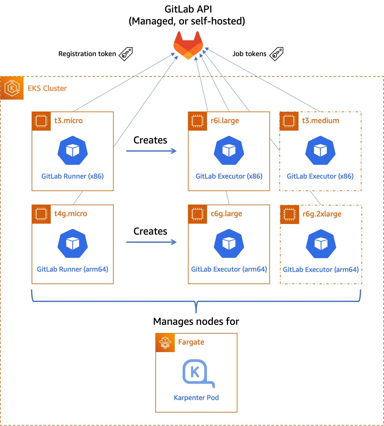
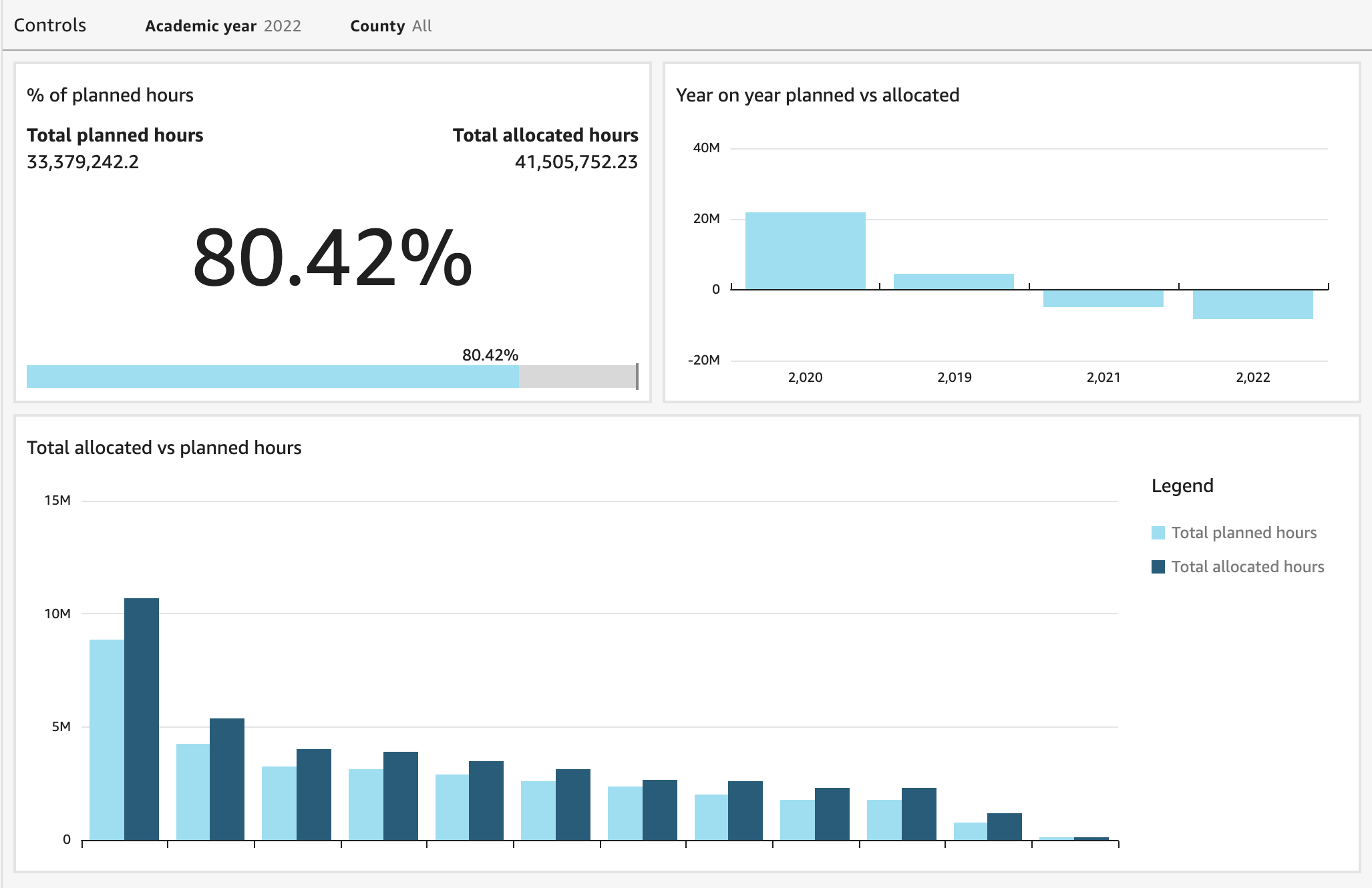
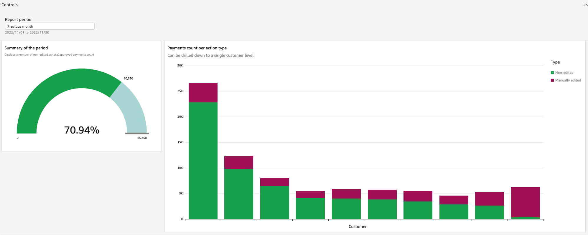
David Adamson is the head of WWSO Insights. He is leading the team on the journey to a data driven organization that delivers insightful, actionable data products to WWSO and shared in partnership with the broader AWS organization. In his spare time, he likes to travel across the world and can be found in his back garden, weather permitting exploring and photography the night sky.

Yash Agrawal is an Analytics Lead at Amazon Web Services. Yash’s role is to define the analytics roadmap, develop standardized global dashboards & deliver insightful analytics solutions for stakeholders across AWS.

Addis Crooks-Jones is a Sr. Manager of Business Intelligence Engineering at Amazon Web Services Finance, Analytics and Science Team (FAST). She is responsible for partnering with business leaders in the World Wide Specialist Organization to build a culture of data to support strategic initiatives. The technology solutions developed are used globally to drive decision making across AWS. When not thinking about new plans involving data, she like to be on adventures big and small involving food, art and all the fun people in her life.

Graham Gilvar is an Analytics Lead at Amazon Web Services. He builds and maintains centralized QuickSight dashboards, which enable stakeholders across all WWSO services to interlock and make data driven decisions. In his free time, he enjoys walking his dog, golfing, bowling, and playing hockey.

Shilpa Koogegowda is the Sales Ops Analyst at Amazon Web Services and has been part of the WWSO Insights team for the last two years. Her role involves building standardized metrics, dashboards and data products to provide data and insights to the customers.

Enabling load-balancing of non-HTTP(s) traffic on AWS Wavelength

2022-12-22 Sheila Busser

Post Syndicated from Sheila Busser original https://aws.amazon.com/blogs/compute/enabling-load-balancing-of-non-https-traffic-on-aws-wavelength/

This blog post is written by Jack Chen, Telco Solutions Architect, and Robert Belson, Developer Advocate.

AWS Wavelength embeds AWS compute and storage services within 5G networks, providing mobile edge computing infrastructure for developing, deploying, and scaling ultra-low-latency applications. AWS recently introduced support for Application Load Balancer (ALB) in AWS Wavelength zones. Although ALB addresses Layer-7 load balancing use cases, some low latency applications that get deployed in AWS Wavelength Zones rely on UDP-based protocols, such as QUIC, WebRTC, and SRT, which can’t be load-balanced by Layer-7 Load Balancers. In this post, we’ll review popular load-balancing patterns on AWS Wavelength, including a proposed architecture demonstrating how DNS-based load balancing can address customer requirements for load-balancing non-HTTP(s) traffic across multiple Amazon Elastic Compute Cloud (Amazon EC2) instances. This solution also builds a foundation for automatic scale-up and scale-down capabilities for workloads running in an AWS Wavelength Zone.

Load balancing use cases in AWS Wavelength

In the AWS Regions, customers looking to deploy highly-available edge applications often consider Amazon Elastic Load Balancing (Amazon ELB) as an approach to automatically distribute incoming application traffic across multiple targets in one or more Availability Zones (AZs). However, at the time of this publication, AWS-managed Network Load Balancer (NLB) isn’t supported in AWS Wavelength Zones and ALB is being rolled out to all AWS Wavelength Zones globally. As a result, this post will seek to document general architectural guidance for load balancing solutions on AWS Wavelength.

As one of the most prominent AWS Wavelength use cases, highly-immersive video streaming over UDP using protocols such as WebRTC at scale often require a load balancing solution to accommodate surges in traffic, either due to live events or general customer access patterns. These use cases, relying on Layer-4 traffic, can’t be load-balanced from a Layer-7 ALB. Instead, Layer-4 load balancing is needed.

To date, two infrastructure deployments involving Layer-4 load balancers are most often seen:

Amazon EC2-based deployments: Often the environment of choice for earlier-stage enterprises and ISVs, a fleet of EC2 instances will leverage a load balancer for high-throughput use cases, such as video streaming, data analytics, or Industrial IoT (IIoT) applications
Amazon EKS deployments: Customers looking to optimize performance and cost efficiency of their infrastructure can leverage containerized deployments at the edge to manage their AWS Wavelength Zone applications. In turn, external load balancers could be configured to point to exposed services via NodePort objects. Furthermore, a more popular choice might be to leverage the AWS Load Balancer Controller to provision an ALB when you create a Kubernetes Ingress.

Regardless of deployment type, the following design constraints must be considered:

Target registration: For load balancing solutions not managed by AWS, seamless solutions to load balancer target registration must be managed by the customer. As one potential solution, visit a recent HAProxyConf presentation, Practical Advice for Load Balancing at the Network Edge.
Edge Discovery: Although DNS records can be populated into Amazon Route 53 for each carrier-facing endpoint, DNS won’t deterministically route mobile clients to the most optimal mobile endpoint. When available, edge discovery services are required to most effectively route mobile clients to the lowest latency endpoint.
Cross-zone load balancing: Given the hub-and-spoke design of AWS Wavelength, customer-managed load balancers should proxy traffic only to that AWS Wavelength Zone.

Solution overview – Amazon EC2

In this solution, we’ll present a solution for a highly-available load balancing solution in a single AWS Wavelength Zone for an Amazon EC2-based deployment. In a separate post, we’ll cover the needed configurations for the AWS Load Balancer Controller in AWS Wavelength for Amazon Elastic Kubernetes Service (Amazon EKS) clusters.

The proposed solution introduces DNS-based load balancing, a technique to abstract away the complexity of intelligent load-balancing software and allow your Domain Name System (DNS) resolvers to distribute traffic (equally, or in a weighted distribution) to your set of endpoints.

Our solution leverages the weighted routing policy in Route 53 to resolve inbound DNS queries to multiple EC2 instances running within an AWS Wavelength zone. As EC2 instances for a given workload get deployed in an AWS Wavelength zone, Carrier IP addresses can be assigned to the network interfaces at launch.

Through this solution, Carrier IP addresses attached to AWS Wavelength instances are automatically added as DNS records for the customer-provided public hosted zone.

To determine how Route 53 responds to queries, given an arbitrary number of records of a public hosted zone, Route53 offers numerous routing policies:

Simple routing policy – In the event that you must route traffic to a single resource in an AWS Wavelength Zone, simple routing can be used. A single record can contain multiple IP addresses, but Route 53 returns the values in a random order to the client.

Weighted routing policy – To route traffic more deterministically using a set of proportions that you specify, this policy can be selected. For example, if you would like Carrier IP A to receive 50% of the traffic and Carrier IP B to receive 50% of the traffic, we’ll create two individual A records (one for each Carrier IP) with a weight of 50 and 50, respectively. Learn more about Route 53 routing policies by visiting the Route 53 Developer Guide.

The proposed solution leverages weighted routing policy in Route 53 DNS to route traffic to multiple EC2 instances running within an AWS Wavelength zone.

Reference architecture

The following diagram illustrates the load-balancing component of the solution, where EC2 instances in an AWS Wavelength zone are assigned Carrier IP addresses. A weighted DNS record for a host (e.g., www.example.com) is updated with Carrier IP addresses.

When a device makes a DNS query, it will be returned to one of the Carrier IP addresses associated with the given domain name. With a large number of devices, we expect a fair distribution of load across all EC2 instances in the resource pool. Given the highly ephemeral mobile edge environments, it’s likely that Carrier IPs could frequently be allocated to accommodate a workload and released shortly thereafter. However, this unpredictable behavior could yield stale DNS records, resulting in a “blackhole” – routes to endpoints that no longer exist.

Time-To-Live (TTL) is a DNS attribute that specifies the amount of time, in seconds, that you want DNS recursive resolvers to cache information about this record.

In our example, we should set to 30 seconds to force DNS resolvers to retrieve the latest records from the authoritative nameservers and minimize stale DNS responses. However, a lower TTL has a direct impact on cost, as a result of increased number of calls from recursive resolvers to Route53 to constantly retrieve the latest records.

The core components of the solution are as follows:

EC2 Launch Template – specifies instance configuration information, such as the Amazon Machine Image (AMI), Amazon Elastic Block Storage (Amazon EBS)type and size, and Elastic Network Interface (ENI) attachment with a Carrier IP association, instance tags, among other attributes.
AWS Auto Scaling Group– a collection of EC2 instances logically grouped together for the purpose of automatic scaling.

Alongside the services above in the AWS Wavelength Zone, the following services are also leveraged in the AWS Region:

AWS Lambda – a serverless event-driven function that makes API calls to the Route 53 service to update DNS records.
Amazon EventBridge– a serverless event bus that reacts to EC2 instance lifecycle events and invokes the Lambda function to make DNS updates.
Route 53– cloud DNS service with a domain record pointing to AWS Wavelength-hosted resources.

In this post, we intentionally leave the specific load balancing software solution up to the customer. Customers can leverage various popular load balancers available on the AWS Marketplace, such as HAProxy and NGINX. To focus our solution on the auto-registration of DNS records to create functional load balancing, this solution is designed to support stateless workloads only. To support stateful workloads, sticky sessions – a process in which routes requests to the same target in a target group – must be configured by the underlying load balancer solution and are outside of the scope of what DNS can provide natively.

Automation overview

Using the aforementioned components, we can implement the following workflow automation:

Amazon CloudWatch alarm can trigger the Auto Scaling group Scale out or Scale in event by adding or removing EC2 instances. Eventbridge will detect the EC2 instance state change event and invoke the Lambda function. This function will update the DNS record in Route53 by either adding (scale out) or deleting (scale in) a weighted A record associated with the EC2 instance changing state.

Configuration of the automatic auto scaling policy is out of the scope of this post. There are many auto scaling triggers that you can consider using, based on predefined and custom metrics such as memory utilization. For the demo purposes, we will be leveraging manual auto scaling.

In addition to the core components that were already described, our solution also utilizes AWS Identity and Access Management (IAM) policies and CloudWatch. Both services are key components to building AWS Well-Architected solutions on AWS. We also use AWS Systems Manager Parameter Store to keep track of user input parameters. The deployment of the solution is automated via AWS CloudFormation templates. The Lambda function provided should be uploaded to an AWS Simple Storage Service (Amazon S3) bucket.

Amazon Virtual Private Cloud (Amazon VPC), subnets, Carrier Gateway, and Route Tables are foundational building blocks for AWS-based networking infrastructure. In our deployment, we are creating a new VPC, one subnet in an AWS Wavelength zone of your choice, a Carrier Gateway, and updating the route table for this subnet to point the default route to the Carrier Gateway.

Deployment prerequisites

The following are prerequisites to deploy the described solution in your account:

Access to an AWS Wavelength zone. If your account is not allow-listed to use AWS Wavelength zones, then opt-in to AWS Wavelength zones here.
Public DNS Hosted Zone hosted in Route 53. You must have access to a registered public domain to deploy this solution. The zone for this domain should be hosted in the same account where you plan to deploy AWS Wavelength workloads.
If you don’t have a public domain, then you can register a new one. Note that there will be a service charge for the domain registration.
Amazon S3 bucket. For the Lambda function that updates DNS records in Route 53, store the source code as a .zip file in an Amazon S3 bucket.
Amazon EC2 Key pair. You can use an existing Key pair for the deployment. If you don’t have a KeyPair in the region where you plan to deploy this solution, then create one by following these instructions.
4G or 5G-connected device. Although the infrastructure can be deployed independent of the underlying connected devices, testing the connectivity will require a mobile device on one of the Wavelength partner’s networks. View the complete list of Telecommunications providers and Wavelength Zone locations to learn more.

Conclusion

In this post, we demonstrated how to implement DNS-based load balancing for workloads running in an AWS Wavelength zone. We deployed the solution that used the EventBridge Rule and the Lambda function to update DNS records hosted by Route53. If you want to learn more about AWS Wavelength, subscribe to AWS Compute Blog channel here.

Visma InSchool uses Amazon QuickSight to meet varied business intelligence needs with employees and customers

2022-12-21 Vasily Ulianko

Post Syndicated from Vasily Ulianko original https://aws.amazon.com/blogs/big-data/visma-inschool-uses-amazon-quicksight-to-meet-varied-business-intelligence-needs-with-employees-and-customers/

This is a guest post by Vasily Ulianko and Per Brandser from Visma InSchool.

Located in Europe and Latin America, with headquarters in Norway, Visma has a bold vision to shape the future of society through technology. To do that, we provide business-critical software solutions for over 1 million customers across the Nordics, Benelux, Central and Eastern Europe, and Latin America. We are most interested in solving business problems with cutting-edge technology. We specialize in serverless technologies, optimization techniques, and data analytics, primarily focusing on building solutions for accounting, invoicing, procurement, and school administration.

Our solutions help simplify and streamline administrative tasks. From resource management, admissions, and documentation to financial management and generating diplomas, municipalities, and counties depend on the solutions Visma provides to make their schools run more efficiently.

Digitizing school operations is one of our most important social missions. Our goal is to contribute to making everyday work easier for school administrators and staff. Our flagship product for school administration, Visma InSchool, is a comprehensive system used by students, teachers, parents and administrators, for everything from planning school timetables to issuing diplomas. To make all information available anywhere, and at any time, through a single log in, we have built Visma InSchool to be a holistic system that lives in the cloud. Visma InSchool team uses Amazon QuickSight for business intelligence (BI) needs. `

The path to QuickSight

When we first started considering BI tools, a different solution was available to us through our company’s parent organization. That option, however, was two times more expensive per writer account, was harder to send the data to, and had a clunky and outdated user interface. Worse still, the amount of data that could be stored was also subject to external constraints.

The number of drawbacks with that solution would be more of a hindrance than an aid. We prioritize innovation, agility, and flexibility. We wanted to be in full control of the data source connections, user privileges, and data storage constraints. Researching other tools and what they offered that matched our requirements led us to QuickSight.

We started small, piloting QuickSight first with our product development teams, giving them the user experience they’d need to answer questions about our data from product and business owners. Due to the power of visualizing key actionable data, it didn’t take long before QuickSight was adopted and embraced by other departments.

Complex plans with simple solutions

One of the more difficult challenges for school administrators is developing plans for the upcoming school year. Not only do lesson plans need to be made for each class, but it’s crucial for administrators to have an early understanding of how many teachers will be available in comparison to what the school’s needs are and what those numbers mean in terms of financial impact. Through Personnel Planning functionality, Visma InSchool helps each school identify any discrepancies between existing teaching staff and what’s needed, which helps plan for both the recruitment and redundancy process.

We present school administrators with an automated timetable optimization view, offering extensive editing capabilities via Visma InSchool.

School administrators can now create well-organized lesson schedules that take into account the number of teachers, room availability, required teaching hours, and more.

The schools have to plan the lessons to cover the required hours for each subject in accordance with each individual student’s education program. QuickSight allows us to aggregate the data from this planning process, providing us with a high-level overview that offers the ability to drill down to the county and school levels. This gives our product and consulting teams the tools necessary to guide customers through their school-year planning process.

Automation saves time for school administrators and staff

When we initially started looking at QuickSight, our original intention was simply to use it for visualizations related to Visma InSchool product usage. The more we learned about its capabilities, however, the more we discovered other ways where QuickSight could deliver value. QuickSight has helped us streamline and automate several processes that have not only improved efficiency but saved our customers time and money as well.

The status quo for salary payments to teachers involved manual accounting and pay calculations. We felt confident that automation could reduce the time spent on these tasks, and we created a plan to test that theory. We set the percentage of payments sent to the payroll system without any manual adjustments as our North Star metric. We automated calculations of variable elements that went into each payment before it was sent to payroll. Tracking the statistics to measure the number of customers who were using automated salary calculations compared with those who weren’t was key in understanding the time spent on manual processes.

Based on the data collected during this experiment, our consultants were able to advocate for the use of automated workflows among users. Not only did automation save time for school administrators and their staff, but it also helped product developers measure how useful it would be to research and develop new opportunities for automation.

One solution for all our needs

Different teams have different challenges, and there are often different approaches to solving them. One of the things that we love about QuickSight is its flexibility, which allows us to customize whatever we need based on each team’s specific priorities.

This is a brief overview of how our teams and our customers are using QuickSight every day:

Product management – Our product management team uses QuickSight to track and measure key metrics, such as the number of timetables being published, the number of salary records created, and whether formative assessments are being created. Having these key metrics on hand, the product management team can experiment with hypotheses that help them improve the product, moving it in the right direction for what will be most helpful to our customers.
Support – To help with critical warnings, our support consultants use QuickSight dashboards, which are updated hourly to proactively contact customers and escalate the problem to the relevant team before a customer submits a support ticket.
Consulting – Our consulting teams use the data to tailor their consulting services and inform their training sessions and workshops with school administrators.
Engineering – Our engineering teams use QuickSight to receive production error reports, allowing them to visualize usage statistics as well as discrepancies among different but related datasets.
Customers – Our customers are most interested in the user base and sign-in statistics, as well as key results of school work, e.g., statistics on issued diplomas at the end of the academic year.

Yet another reason why we love QuickSight is how simple and seamless it is to integrate with our existing architecture. We are using a set of Amazon Aurora databases that back our system microservices, housing around 4 TB of data in more than 1,000 tables. With so much that can go wrong with integrating systems, not having to worry about any of that with our QuickSight implementation was a major plus. Simple setup and a flexible, usage-based pricing model made QuickSight the best choice for us.

QuickSight for dashboards and reports is just the beginning

We’ve had QuickSight for about 3 years now and have no regrets. Having been built by Amazon and accessible via the cloud, we rest easy knowing that it will continue to evolve and improve. Not having to worry about upgrades or maintenance is another upside to QuickSight; there have been several releases with new features and capabilities since we’ve been customers, and each one has brought an improved user experience.

In the future, we are planning to use Amazon QuickSight Embedded to deliver targeted BI information, interactive dashboards, and customized data visuals directly to our customers via Visma InSchool. As Norwegian counties manage their schools, they want insights and statistics across the schools in their county, which we can embed in their UI. Schools want information about their data and about teachers and students to make better decisions on adjustments and strategy. Empowering our customers with near-real-time information to make data-driven decisions is our goal, and we’re confident we can achieve it with QuickSight.

About the Authors

Vasily Ulianko is a Director of Engineering in Visma InSchool, leading the development and operations, focusing on building strong engineering culture and solid system design.

Per Brandser is a Product Strategy Manager in Visma InSchool. Mainly focusing on coaching our Product Managers on vision, product strategy and product discovery methodology, Per is a promoter of data driven product management.

Leverages uses Amazon QuickSight to drive valuable and effective customer engagement with embedded market trends and insights

2022-12-21 Tomotaka Inoue

Post Syndicated from Tomotaka Inoue original https://aws.amazon.com/blogs/big-data/leverages-uses-amazon-quicksight-to-drive-valuable-and-effective-customer-engagement-with-embedded-market-trends-and-insights/

This is a guest post from Tomotaka Inoue, Data Analyst at Leverages.

Founded in 2005, Leverages offers job staffing and web tools—Levtech and Levwell—for the IT and healthcare industries, serving both companies seeking talent and job seekers who are in the market for their next role. Inspired by a data point showing a proportional correlation between productivity and job change frequency, the company saw an opportunity to combine that insight with its passion for improving work environments for engineers. Providing a platform that enables skilled workers to easily find and pursue new opportunities meant a win-win for workers and companies alike.

The Levtech platform is a job search engine designed to not only effectively match companies with IT talent but also helps engineers and developers manage contracts, ensuring documentation is centralized for easy access. Levtech’s specialization for engineer and developer audiences has made it a hit within the IT freelance market.

Driving valuable and effective engagement with customers

One of the more challenging aspects of meeting customer needs within a human resources capacity comes in appropriately balancing priorities without the risk of missing opportunities for valuable engagement. On the higher-touch end of the spectrum, users who are actively engaged to both recruit and pursue open roles are necessarily high on the priority list. We want them to have a great experience and to be happy with the end result when the role is filled. But how do we maintain a less intrusive but still valuable level of engagement with users who are registered on the platform but are not actively recruiting or seeking right now?

To make those lower-touch engagements valuable and effective, Leverages wanted to provide Levtech users with access to market trend data related to their areas of expertise. By providing this data via a dashboard that’s embedded directly into Levtech, not only do we provide valuable information to registered users, but doing so also enables recruiters to become more valuable partners when not-currently-active job seekers become active. By having access to market trend data, recommendations can be made, e.g., “The demand for skill X is increasing. Therefore, by acquiring this skill, more companies would be interested in you.” When determining which business intelligence platform would best serve our needs to provide this data to our Levtech users, we turned to Amazon QuickSight.

In this post, we discuss what influenced our decision to implement QuickSight Embedded, as well as some of the benefits we’ve seen since then.

Finding the right embedded analytics solution

The only constant in technology is that things are always changing. As job seekers, engineers and developers often have little data to keep a pulse on which skills and experiences are in the highest demand. For recruiters, it’s challenging to gain visibility into how large or small the talent pool is for candidates who possess those in-demand skills or have had extensive experience in certain areas. Answering questions like these was the primary motivation for choosing QuickSight to help bring expanded functionality and increased value to Levtech.

When determining what our new business intelligence solution needed to have, we had three top priorities.

Rich embedding features. Anonymous embedding was a key differentiator for us, enabling us to quickly launch because there were no user management or single sign-on (SSO) requirements.
Easy to use. Analysis tools are useless if they’re not intuitive and user-friendly. With QuickSight, we were able to create beautiful dashboards very quickly.
Cost-effective. Because QuickSight is serverless and offers session-based, on-demand pricing, it was a perfect fit for our budget.

One of our favorite things about QuickSight is that nondevelopers can update visuals on a dashboard. We often get requests from users that they want to see data from different angles, using a variety of charts. With other tools, making adjustments like that would require development resources with deep coding expertise to ensure the implementation was done correctly. With QuickSight, users of all technical ability levels can make updates without needing to rely on development resources.

The following screenshot shows an example of one of our dashboards.

Leverages QuickSight dashboard

Demystifying business decisions with data

In today’s world of lightning-fast communication, it’s more important than ever to be vigilant in using data to drive decisions. For the IT freelance community—both companies and job seekers—having immediate access to the data they need to make sound decisions is invaluable. For the companies we serve, dashboards can be built to show summaries of registered engineers within our database, their salary ranges, skill trends, how many job seekers there are, and more. Engineers and developers can access dashboards showing summaries of available positions, the number of freelance positions, skill requirements, etc.

For Leverages, QuickSight is helping to improve our sales and marketing efficiency because the QuickSight Embedded SDK helps reduce the time it takes to gather insights. We can now filter the actions Levtech users are making to discover data points, e.g., more companies are searching for Java engineers. Those insights can help inform not only talent suggestions but marketing campaigns as well.

Fast, efficient, intuitive embedded analytics in two days

By embedding QuickSight into Levtech, we have been able to offer thousands of users a fast, efficient, intuitive experience in accessing the data they need to make key decisions about their companies and their careers. Not only is QuickSight easy to use, implementation is exceptionally fast. Other tools we considered quoted us several months to get up and running, whereas our QuickSight implementation was done in just two business days.

To learn more about how you can embed customized data visuals, interactive dashboards, and natural language querying into any application, visit Amazon QuickSight Embedded.

About the Author

Tomotaka Inoue is a data analyst at Leverages. Tomotaka analyzes Levtech’s data and suggests about the strategy and marketing.

A modern approach to implementing the serverless Customer Data Platform

2022-12-19 Larry Bell

Post Syndicated from Larry Bell original https://aws.amazon.com/blogs/architecture/a-modern-approach-to-implementing-the-serverless-customer-data-platform-cdp/

When building a Customer Data Platform (CDP), advertising and marketing Independent Software Vendors (ISVs) face a unique set of challenges. The ISV can help organizations with the heavy lifting required to build, secure, and maintain near real-time, high volume CDPs. However, architecting CDPs using traditional on-premises technologies can introduce multiple complexities and can limit deployment options. One strategy that may address these complexities is to use serverless technologies.

Serverless technologies feature automatic scaling, built-in high availability, and a pay-for-use billing model to increase agility, optimize costs, and reduce infrastructure management tasks such as capacity provisioning and patching. Using tools such as CloudFormation, each layer of the serverless CDP can be deployed on-demand in an independent manner to maximize portability and optimize performance.

A Software as a Service (SaaS) CDP usually has significantly more data in a multi-tenant environment than a single instance of a CDP. Clients of a SaaS solution need to continually expand across different channels, and often across many AWS Regions. In some cases, an ISV might have an existing infrastructure that was built before some of these modern capabilities and techniques were mature. Today, an ISV can build or even modernize an existing CDP and gain huge benefits from a serverless implementation.

This blog post explores how to use serverless technologies for the CDP. A modern, serverless CDP architecture can enable the ISV and the client companies to deliver in weeks instead of months, and provide a resilient infrastructure that supports agility and global deployment while maximizing operational efficiency and optimizing cost. This frees up technical resources to focus on differentiated product development instead of managing servers.

Serverless implementation of a CDP on AWS

A serverless architecture uses AWS services that don’t require the configuration of a server to provide an implementation. Serverless technology allows you to focus more time on rapidly building different components of the marketing CDP. The benefits of a CDP include the collection, aggregation, and organization of customer data sources. Implementing the CDP using serverless technology reduces the need to focus on managing infrastructure while reducing time to market, increasing agility, and resulting in cost optimization. Figure 1 is an architecture diagram that describes how various data sources can be prepared for consumption in the component based Customer Data Platform.

Figure 1. Marketing CDP reference on AWS

Source systems of customer data include customer interactions, clickstreams and call center logs.
Data from customer touchpoints is ingested into the marketing customer data platform (CDP) data lake using Amazon Kinesis, Amazon AppFlow, Amazon EKS and an Amazon API Gateway.
Ingested data is sent – in its original, immutable format – to an Amazon Simple Storage Service (Amazon S3) Raw Zone bucket
Raw data is then transformed into efficient data formats – such as Parquet or Avro – and moved to a Clean Zone Amazon S3 bucket.
CDP processing and pipeline orchestration is conducted using purpose-built data processing components and transformation libraries through AWS Step Functions and then Amazon Personalize, AWS Lambda, and AWS Glue.
Data in the Amazon S3 Curated Zone is now ready for post-CDP-processing consumption and is organized by subject areas, segments, and profiles.
The analytics layer uses Amazon Redshift, Amazon QuickSight, Amazon SageMaker and Amazon Athena to natively integrate with the Curated Zone for analytics, dashboards, ad hoc reporting, and ML purposes.
Customer data is then aggregated across platforms and published using customer APIs for consumption using Amazon DynamoDB and an Amazon API Gateway.
Amazon Pinpoint and Amazon Connect are used to activate multiple customer channels such as mobile push, voice, and email for targeted marketing communications.
Using AWS Lake Formation, fine-grained access controls can be enforced on catalog tables, columns, and rows on the data lake.
The resulting catalog in AWS Glue helps you manage both business and technical metadata, with versioning, at scale.

Serverless implementation for ingestion

There are several methods of ingesting customer data, both internal to a customer and from external sources. Serverless options for ingestion could provide benefits to an ISV like cost or agility but it depends upon the use case. Examining serverless options for ingestion should be part of any modernization effort. If the CDP needs to stream data sources and ingest that data in near-real time, the ISV can use Amazon Kinesis. If you want a more traditional extract, transform, and load (ETL) tool, AWS Glue offers a serverless option to generate code that can be customized. AWS Glue DataBrew offers a visual data preparation tool. For more advanced governance and control, you can use AWS Lake Formation. To ingest sources using an API, the Amazon API Gateway provides a serverless approach. If you need more control over the ingestion, the use of customized scripts in Amazon AppFlow or Amazon Managed Streaming for Apache Kafka (Amazon MSK) can provide a solution.

Serverless storage implementation

Amazon Simple Storage Service (Amazon S3) provides a serverless, cost-effective solution for virtually unbounded amounts of storage and read-write bandwidth. As per the reference architecture, there are three purpose-specific zones:

A raw zone containing the original, immutable version of data
A trusted zone which can be used as a working area to combine, enhance and clean the data
A refined zone containing data ready for consumption by users and applications

This structure allows the improvement of customer data and profiles, and provides the ability to integrate various data sources and a structure that allows customer data to be recreated in a manner consistent with changing business rules.

Serverless cataloging implementation

The cataloging services provide a grouping of the elements contained in structured and unstructured data sources that is intuitive and easy to understand, similar to a single relational database. AWS Glue Data Catalog gives logical structure to the data lake by allowing users to define tables and columns on top of Amazon S3 data sets. This serverless solution integrates with other analytics tools to enable data discovery and consistent usage. Fine-grained governance and access can also be enforced by AWS Lake Formation.

Serverless processing

There are great choices for implementing processing, using serverless technologies. A CDP platform can package code and run on demand without servers using AWS Lambda or AWS Step Functions depending up the complexity of the processing pipeline. These services can enable complex processing on customer data and profiles. Amazon SageMaker is a great serverless choice for incorporating artificial Intelligence / machine learning into your processing stream. For processing using big data techniques Amazon EMR Serverless is a good serverless option.

Serverless implementation for consumption

Analytics for the CDP provides several serverless technologies that enable different types of insights. For interactive SQL queries that integrate with our serverless AWS Glue Catalog, there is Amazon Athena. Athena provides SQL access to various data source, and can also use federated query functionality to connect to third-party sources, even if that data is sitting on another cloud or in a vendor’s environment. Athena can also work as an interface (middleware) to other reporting solutions.

If performance is a concern, Amazon Redshift is fast, petabyte-scale data warehouse solution that has a serverless option and fully integrates with these solutions. For a data visualization tool that can be embedded in your application or work as a standalone portal, examine Amazon QuickSight.

To enable collaboration, many use cases can use Amazon API Gateway to securely publish and expose API endpoints for consuming applications. This allows data to be shared from a single source of truth to consumers that use customer data for their processes. Most customers want to activate their customer data through marketing or advertising campaigns. To activate marketing communication over voice, email, text, or in-app messaging, you can use a serverless service called Amazon Pinpoint. For an omnichannel contact center support, we recommend Amazon Connect, which uses AI/ML and the CDP data to analyze customer sentiment, implement chatbots, and authenticate voice callers.

Serverless implementation for governance

AWS Lake Formation simplifies the process of configuring and securing access to the CDP. It can help orchestrate processing and ingestion, as well as enforcing fine-grained access controls on data catalogs. Other services such as AWS Glue DataBrew or Amazon Macie can identify and help mitigate exposure of Personally identifiable information (PII). AWS Config enables you to assess, audit, and evaluate the configurations of your AWS resources to automate the evaluation of recorded configurations against desired configurations.

Conclusion

This post described just some of the serverless solutions that are managed by AWS that allow you to build a modern, low-cost, data lake-centric CDP architecture in an accelerated manner. A decoupled, component-driven architecture lets you start small and quickly add new services to each independent component of the CDP. Use the Data Analytics Lens for guidance on designing, deploying, and architecting your analytics solution workloads in the AWS Cloud. Using this framework, you will learn the architectural best practices for designing and operating reliable, secure, efficient, and cost-effective systems in the cloud. Follow the links in this article to learn more about the services available in AWS that can help you build a serverless CDP.

AWS Marketplace Seller Insights team uses Amazon QuickSight Embedded to empower sellers with actionable business insights

2022-12-16 Snigdha Sahi

Post Syndicated from Snigdha Sahi original https://aws.amazon.com/blogs/big-data/aws-marketplace-seller-insights-team-uses-amazon-quicksight-embedded-to-empower-sellers-with-actionable-business-insights/

AWS Marketplace enables independent software vendors (ISVs), data providers, and consulting partners to sell software, services, and data to millions of AWS customers. Working in partnership with the AWS Partner Network (APN), AWS Marketplace helps ISVs and partners build, market and sell their AWS offerings by providing crucial business, technical, and marketing support.

The AWS Marketplace Seller Insights team helps AWS sellers scale their businesses by providing reports, data feeds, and insights. We share this data directly with sellers through the AWS Marketplace Management Portal (AMMP). In 2013, we launched the first version of reporting insights, delivered monthly via static CSV files. To improve the customer experience, the next iteration of reporting upgrades was launched in 2020 and provided more granular data, refreshed daily and delivered via feeds.

We’ve spent the past few months working closely with the QuickSight team and are excited to now offer AWS Marketplace sellers public preview access to two new Amazon QuickSight dashboards. QuickSight improves the reporting experience for AWS Marketplace sellers by making it easy for users to monitor key metrics, perform ad hoc analysis, and quickly get business insights from data at any time and on any device.

In this post, we discuss our decision to implement QuickSight Embedded, as well as some of the benefits to AWS Marketplace sellers.

Data agility is a key differentiator

Making informed decisions is a business-critical function for successful organizations. Being able to quickly view performance trends and adjust strategies accordingly can make all the difference between hitting or missing business goals. Investing time, effort, and resources in technical data integrations, or creating pivot tables and charts from downloaded raw data, means a slower response rate to analyze shifts in performance trends. The more agile we can be in providing fast, efficient access to key performance indicators, the better positioned AWS Marketplace sellers can be to take action based on what their data tells them.

After reviewing customer feedback on their reporting experience, several trends emerged in what would be most helpful to them. First, sellers wanted a visual representation of their data. Second, though some wanted data feeds available to integrate AWS Marketplace data into their own business intelligence tools, others wanted to be able to access and review data without needing to invest technical business intelligence bandwidth in integrating feeds to create more user-friendly reports. Finally, they wanted the ability to easily filter the data, as well as the option to download it. In researching options to provide the reporting experience AWS Marketplace sellers wanted, we found that QuickSight was a perfect fit.

Doing more with data

Billed Revenue and the Collections & Disbursements are two new QuickSight dashboards embedded directly into the AWS Marketplace Management Portal (AMMP), accessed via the Insights tab. These dashboards—pre-built with 10+ controls or filters, 15+ visualizations, and powered by daily refreshed data—provide a visual reporting experience for revenue recognition and disbursements tracking.

The following screenshot shows what the dashboards look like in the Finance operations section on the Insights tab within the AMMP.

The dashboards are divided into several sections:

Controls provides filters to refine your dashboard data.
Date Range Filter provides the ability to filter dashboard data based on the dates.
Metrics, Trends, and Breakdowns all provide detailed analytics to understand business performance.
Granular data provides the option to download the raw data from the dashboard by clicking on the table and choosing the Export to CSV option.

For quick help, sellers can select the Info button to view the side navigation panel with tips on how to use the dashboard. They can also reach out to our team by selecting Contact us from the Info panel.

Improving the customer experience

The Billed Revenue dashboard now reflects changes within 24 hours of a customer being billed or refunded—a major improvement over the 45 days it once took to access this data from the legacy AMMP Billed Revenue report. Similarly, the Collections & Disbursements dashboard provides disbursement information within 24 hours of AWS sending funds to sellers, whereas it used to take up to 4 days from the legacy AMMP Disbursement Report.

Our team’s decision to go with QuickSight was the direct result of a clear alignment between what our sellers told us they wanted and what QuickSight offered. With QuickSight Embedded dashboards, AWS Marketplace sellers now have a visual representation of their data that doesn’t require time or resources dedicated to technical integration implementations, and they can quickly and easily manipulate the data via filters, or they can download it to a CSV if that’s their preference. Embedded dashboards simplify the viewing, analyzing, and tracking of key business metrics and trends related to financial operations. Being able to easily show each seller only their relevant data (using row-level security) provides us with the flexibility we need, with the peace of mind of knowing everything is secure. AWS Marketplace data is hosted in an Amazon Redshift cluster; QuickSight’s seamless integration into Amazon Redshift made it a fantastic choice.

Data-driven decisions with QuickSight

Embedding these new QuickSight dashboards into the AMMP has enabled us to provide at-a-glance metrics to AWS Marketplace sellers in a faster, more efficient, and far more user-friendly way than ever before. QuickSight has made a significant impact on how quickly sellers can access their data, which helps them respond faster to shifting trends.

To learn more about how you can embed customized data visuals, interactive dashboards, and natural language querying into any application, visit Amazon QuickSight Embedded.

About the Authors

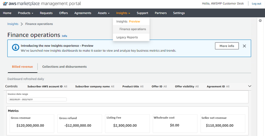
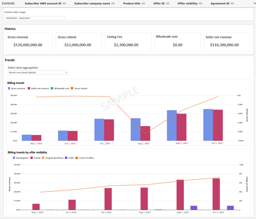
Snigdha Sahi is a Senior Product Manager (Technical) with Amazon Web Services (AWS) Marketplace. She has diverse work experience across product management, product development and management consulting. A technology enthusiast, she loves brainstorming and building products that are intuitive and easy to use. In her spare time, she enjoys hiking, solving Sudoku and listening to music.

Vincent Larchet is a Principal Software Development Engineer on the AWS Marketplace team based in Vancouver, BC. Outside of work, he is a passionate wood worker and DIYer.

Organize your AWS Serverless code to prevent merge conflicts

2022-12-16 Mark Curtis

Post Syndicated from Mark Curtis original https://aws.amazon.com/blogs/devops/organize-your-aws-serverless-code-to-prevent-merge-conflicts/

How do you prevent the most common merge conflicts when your team is working on a Serverless application? How do you make sure that your team stays productive and avoids large merge issues while trying to update the same crucial files simultaneously? –The answer to both questions is code organization! You can use cfn-include and swagger-cli to organize, collaborate, and maintain a large serverless application as well as support a large or decentralized development team.

Real life inspiration

WRAP Technologies Inc. (WRAP) creates advanced technologies for the protection and security of public safety. Their WRAP Reality product allows law enforcement agencies to train their officers using virtual reality-based scenarios.

Too many cooks in the kitchen

When multiple developers collaborate on a serverless architecture built with AWS CloudFormation, and its extensions such as the AWS Serverless Application Model (SAM), the nature of specifying resources in both the template.yaml and the optional OpenAPI.yaml specification for Amazon API Gateway leads to merge conflicts, such as the one demonstrated in the following figure where two developers are adding different API endpoints at the same time. These conflicts detract from the developer’s time and agility. Furthermore, navigating and maintaining the long template files required for a larger serverless architecture slows development as the developer scans large files to find a particular resource definition.

Figure 1. The frustrating merge conflicts.

By refactoring and organizing the CloudFormation and OpenAPI files, your development team can realize several benefits:

Improve developer efficiency by decomposing large, hard-to-manage files into a series of well-organized and single-purpose files.
Enhance developer productivity by allowing each developer to have ownership of their own code, thereby reducing the need to coordinate merges with teammates.
Eliminate potential merge issues for files that generate the most conflicts during the development of a typical Serverless API application.

Rapid development

WRAP partnered with AWS to develop and host the backend for their new officer training management platform. This entirely new platform was developed, completed, and available for use in a matter of months. Moreover, it’s a collaboration of developers spread across multiple teams worldwide, all contributing to the same code base. By instituting the norms and techniques of this post, WRAP created a large and maintainable serverless application with minimal developer code collisions.

Development of the WRAP Reality training management system was accomplished using CloudFormation for defining Infrastructure as Code (IaC), and an Amazon API Gateway OpenAPI specification for defining API contracts. The development team for the WRAP Reality training management service leveraged agile development for expediency, including the GitHub Flow branching strategy. However, since project contributors were not co-located, several considerations were put in place to make sure of consistency and speed of code development:

The API specifications and contracts were defined in OpenAPI (Swagger) specifications early in the development process, clearly defining the project structure up front, and allowing developers to independently build infrastructure components.
The two code assets central to the entire project – the CloudFormation template and the OpenAPI Specification – were decomposed into small, easily manageable components. This enabled components to be organized in a way that enhanced development productivity and practically eliminated the inevitable merge conflicts that come with large source code files that are being modified on a daily basis.

The development process was accelerated by utilizing OpenAPI integrations with AWS Services, as well as techniques for managing the OpenAPI specification and Cloudformation Template files.

Sample project

To demonstrate these techniques, we’ll explore the following sample project comprised of API endpoints for “widget” management, available on GitHub. This project provides the following end points:

/widget PUT: Creation of a new widget
/widget GET: Retrieval of a new widget
/reports/color GET: Retrieval of a set of widgets based on the widget color
/reports/filterpage GET: Retrieval of widgets based on specified filters

The overall architecture of the application is shown in the following diagram:

Figure 2. Architecture Diagram

The application comprises:

Amazon API Gateway is a fully-managed service that makes it easy for developers to create, publish, maintain, monitor, and secure APIs at any scale. In this example, API Gateway serves as the web service for the API endpoints. The mapping of data to and from the API endpoints to the Lambda functions is formally defined by an OpenAPI specification file.
AWS Lambda is a serverless compute service that lets you run code without provisioning or managing servers, creating workload-aware cluster scaling logic, maintaining event integrations, or managing runtimes. In this example, four Lambda functions are used to service each of the four API calls.
Amazon DynamoDB is a key-value and document database that delivers single-digit millisecond performance at any scale. DynamoDB is used as a persistent data store for widgets and associated properties.

OpenAPI and AWS service integration

When using API Gateway, developers have the option of using proxy Lambda integrations, or formally defining the API interface in an OpenAPI yaml file. The OpenAPI specification can be leveraged to document the API prior to development, and the example/mock features of the OpenAPI specification facilitates concurrent development by quickly establishing a working infrastructure to build upon. Furthermore, API documentation can be automatically generated from the OpenAPI specification.

As the number of endpoints increases, the OpenAPI specification file can grow in size, reaching thousands of lines of code that must be updated and maintained regularly by multiple developers. To aid in management and usability, the OpenAPI file can be decomposed into separate files for endpoints, responses, fields, and schemas.

Start with a “skeleton” file as an entry point for the OpenAPI definition, and then add a separate file for the definition of each endpoint or construct. For example, the sample project entry point is api/apiSkeleton.yaml, which contains the global definitions and effectively defines a simple list of endpoints and the reference ($ref) file path to each endpoint’s definition.

The application comprises:

/reports/color:
    $ref: './paths/reports/reportsColor.yaml'

  /reports/filterpage:
    $ref: './paths/reports/reportsFilterPage.yaml'

Diving into a file referenced by an endpoint, we see that it contains all of the specification details for that endpoint. Looking at the reportsColor.yaml file reveals the full endpoint specification for /reports/color:

get:
  description: Get widgets by color
  parameters:
    - in: path
      $ref: '../../requestParameters/color.yaml'
  responses:
    200:
      description: Get All the Widgets of a color
      content:
        application/json:
          schema:
            $ref: '../../schemas/widgetList.yaml'
    . . .

In turn, this endpoint specification can include further references to yaml files defining common parameters, schemas, and even full gateway responses. For example, color.yaml defines the color path variable:

  type: string
    description: "The widget's color"
    example: "Red"

To paraphrase a common catch phrase, “With a great many files, comes a great responsibility for organization.” To this end, we offer the following organizational structure as a start. Place all of the related API specifications in an “api” subfolder of your project. Have child subfolders for field, metadata, and gateway response definition files. Then, create child subfolder trees for each branch of your endpoints that mirror the endpoint paths. This will result in a highly-organized directory structure, as seen in the sample project:

├── api
│   ├── apiSkeleton.yaml
│   ├── fields
│   │   ├── color.yaml
│   │   ├── metadata
│   │   │   ├── count.yaml
│   │   │   ├── message.yaml
│   │   └── widgetname.yaml
│   ├── gatewayResponses
│   │   ├── error.yaml
│   │   └── notFound.yaml
│   ├── paths
│   │   ├── reports
│   │   │   ├── reportsColor.yaml
│   │   │   └── reportsFilterPage.yaml
│   │   └── widget
│   │       ├── widgetPut.yaml
│   │       └── widgetWidgetnameGet.yaml

We still need a consolidated single OpenAPI file to provide to CloudFormation during deployment to AWS. Therefore, the multiple files are combined and validated using the swagger-cli bundle command, resulting in a single file for deployment. The bundle command must be executed before a CloudFormation build. This command can also be included as a shortcut in the Makefile as the “buildOpenApi” command:

swagger-cli bundle -o api/api.yaml --dereference --t yaml  api/apiSkeleton.yaml

make buildOpenApi

Once compiled, api/api.yaml is then used normally for API Gateway integrations and as a Postman API Collection import. As api/api.yaml is dynamically compiled, it’s included in .gitignore and not checked in to AWS CodeCommit.

cfn-include and nested stacks

The CloudFormation template that defines the infrastructure for even a simple service can grow to considerable length, perhaps thousands of lines. This presents challenges from a support and continued development perspective, as specific code locations become difficult to find and merge conflicts become commonplace.

CloudFormation Nested Stacks are a method of breaking a large CloudFormation template into separate templates. When there are clear delineations between groups of resources in a stack breaking it into separate nested stacks makes sense. There is also a 500 resource limit in a single CloudFormation stack and in order to go above that nested or separate stacks are necessary. Depending on the complexity of the architecture and frequency of updates however, the Nested Stacks can also become large. Furthermore, in a serverless architecture, the logical separation of architecture layers into separate stacks may not be direct, for example when a Lambda function is triggered by an event sent to an EventBridge event bus, then that Lambda function sends a different event back to the same event bus.

In these cases, CloudFormation templates can be decomposed to further leverage cfn-include . With this technique, the top-level CloudFormation template becomes a skeleton file which contains the stack parameters, global specifications, a list of resource names without properties, and the outputs. The properties of each resource are contained in separate files, referenced by an ‘include’ directive.
CloudFormation template organization

To organize your CloudFormation template, deconstruct the template into one-file-per-resource, with one main “skeleton” file as the main entry point. This skeleton file contains the full parameters, global section, conditions, and output specification. The resources are specified by resource name in this skeleton file, and then an ‘include’ directive points to the file that contains the body of the resource declaration. See the following example of the main skeleton file with two resources:

AWSTemplateFormatVersion: '2010-09-09'
Transform: AWS::Serverless-2016-10-31
Description: >
  Widget API Service
Globals:
  Function:
    Handler: app.lambda_handler
    Runtime: python3.8
Resources:

    WidgetApi:
        !Include ./resources/apigw/widgetApiGW.yaml

    WidgetDdbTable:
        !Include ./resources/dynamodb/widgetDdbTable.yaml

Then, the resource files contain the properties of that specific resource. For example, widgetApiGW.yaml defines an API Gateway:

Type: AWS::Serverless::Api
    Properties:
      DefinitionBody:
        Fn::Transform:
          Name: AWS::Include
          Parameters:
            Location: api/api.yaml
      EndpointConfiguration:
        Type: REGIONAL
      StageName: prod
      TracingEnabled: true

This approach has the benefit of breaking the CloudFormation template into multiple small files, while still maintaining a top-level holistic view. The resource definitions, which normally comprise the majority of the content and can cause merge conflicts, are moved out of the main template.

For organization, you can create a directory in your project to contain the CloudFormation scripts. This directory also contains the entry-point skeleton file. Create further sub-folders for resources, and then further folders by resource type and architecture. We found that placing applicable AWS Identity and Access Management (IAM) role resource definitions in the same folder with the applied resource facilitated easier navigation. For example:

├── cloudformation
│   ├── resources
│   │   ├── apigw
│   │   │   └── widgetApiGW.yaml
│   │   ├── dynamodb
│   │   │   └── widgetDdbTable.yaml
│   │   └── lambda
│   │       ├── layers
│   │       │   └── lambdaDDBEnv.yaml
│   │       ├── reports
│   │       │   ├── reportsColorLambda.yaml
│   │       │   └── reportsColorLambdaRole.yaml
│   │       └── widget
│   │           ├── widgetGetLambda.yaml
│   │           └── widgetGetLambdaRole.yaml
│   └── templateSkeleton.yaml

The files must be reconstituted to a single template.yaml for CloudFormation build and deployment. This is accomplished with the cfn-include command. A convenience command can optionally be included in the Makefile.

cfn-include --yaml  cloudFormation/templateSkeleton.yaml > template.yaml

make buildTemplate

As the final template.yaml file is dynamically compiled, it’s included in .gitignore and not checked in to CodeCommit.

Conclusion

This post demonstrates techniques used by WRAP and AWS to rapidly develop and maintain key files in an Serverless architecture. The techniques discussed in this post allowed the WRAP and AWS team to do the following:

Improve developer efficiency by decomposing large, hard-to-manage files into a series of well-organized and single purpose files.
Enhance developer productivity by allowing each developer to have ownership of their own piece of the code without having to coordinate with teammates.
Eliminate potential merge issues on the files that typically generate the most conflicts during the development of a typical Serverless API application.

Applying these techniques was one of the key factors in the rapid development of the WRAP Reality training framework.

About the Authors:

LaunchDarkly’s journey from ingesting 1 TB to 100 TB per day with Amazon Kinesis Data Streams

2022-12-15 Mike Zorn

Post Syndicated from Mike Zorn original https://aws.amazon.com/blogs/big-data/launchdarklys-journey-from-ingesting-1-tb-to-100-tb-per-day-with-amazon-kinesis-data-streams/

This post was co-written with Mike Zorn, Software Architect at LaunchDarkly as the lead author.

LaunchDarkly’s feature management platform enables customers to release features and measure their impact. As part of this platform, SDKs gather event data, and the event ingestion platform consumes and analyzes this data to measure impact. As the platform launched and customer adoption increased, we had to scale the event data pipeline to meet the demands of the business for new use cases that required zero data loss. We will explain the challenges that we ran into with the initial architecture and the advantages achieved by using Amazon Kinesis Data Streams and additional AWS services in the new architecture. We will also go into the different factors that we considered in the Amazon Kinesis Data Streams implementation for cost efficiency and performance.

Problem statement

LaunchDarkly’s mission is to fundamentally change how companies deliver software by helping them innovate faster, deploy fearlessly, and make each release a masterpiece. With LaunchDarkly, we allow customers to deploy when they want, release when they are ready, and get total control of the code to ship fast, reduce risk, and reclaim their nights and weekends.

In 2017, the event ingestion platform consisted of a fleet of web servers that would write events to several databases, as shown below, that stored event data to power several features of the LaunchDarkly product. These features allow LaunchDarkly’s customers to gain full visibility into how a feature is performing over time, optimize features through experimentation, and quickly verify their implementation. Unfortunately, all of the database writes to power these features were performed within a single process on these web servers, so if any one of these databases had an availability issue, events would queue up in memory until that process ran out of memory and crashed. Since that same database would be used to write data from each web server, all of them would eventually run out of memory and crash. This cycle would repeat itself until the database availability issue was rectified. During that time, there was a permanent loss of all of the event data that was sent by the SDKs.

Original Architecture

The current system was tolerant of some data loss as the applications that used this data was limited. But the new features and workflows had stringer requirements on data-loss prevention.

We decided to explore alternatives where all the consumers are built with isolated fault tolerance, so each consumer is independent of one another in case of any issues. We built an event-driven pipeline that would be highly durable, scalable, and also provide the ability for data replay. As a result, we scaled from ingesting about 1 TB of data a day to more than 100 TBs of data now.

Solution

The following diagram illustrates our updated design. To support the new use cases, we added Amazon Kinesis Data Streams, AWS Lambda, and Amazon Kinesis Data Firehose to the architecture.

New Architecture

The design has the following key components

Mobile client using the LaunchDarkly SDK to evaluate feature flags
Application Load Balancer distributes traffic to Amazon EC2 nodes
Amazon EC2 nodes run a go application that writes traffic to Amazon Kinesis Data Streams
Amazon Kinesis Data Streams durably persist data
AWS Lambda writes various types of data to databases
Amazon OpenSearch Service records data about users
Amazon ElastiCache records data about flag statuses
Amazon Kinesis Firehose batches flag evaluation data and writes it to Amazon S3
Amazon S3 records data about flag evaluations

Data flows from a LaunchDarkly SDK into the events API, which is backed by an Application Load Balancer (ALB). That ALB routes traffic to a fleet of Amazon EC2 servers. Those servers persist the data to Amazon Kinesis Data Streams. Data is then read out of Amazon Kinesis Data Streams by Lambda functions that transform and write the data in different formats to several databases. The design has a few properties that were very important to this use case.

Durability
Isolation
Data replay

Durability would prevent data loss when issues in data processing arose. Isolation would prevent other consumers of data from failing when one consumer had a failure. Data replay would allow us to debug data anomalies and fix them retroactively.

Amazon Kinesis Data Streams satisfies these three properties. Data written to Amazon Kinesis Data Streams is persisted durably until the data ages out of the stream. Amazon Kinesis Data Streams allows for consumer isolation: each consumer maintains its own iterator position, so consumers can process data from a stream independently of one another. Finally, Amazon Kinesis Data Streams make data replay possible because consumers can set their shard iterator position to be in the past. For example, a consumer can be configured to start reading at 1 hour in the past if the last hour of data needs to be replayed.

A few additional technologies were considered that would allow us to achieve these design properties. Amazon Simple Notification Service (Amazon SNS) combined with Amazon Simple Queue Service (Amazon SQS) would allow for a system with durability and isolation. Data replay was not available out of the box and needed custom implementation to support this feature.

Apache Kafka was also considered, but in spite of the fact that it satisfies these design properties, it was not adopted because the team did not have prior experience with Apache Kafka. Amazon Kinesis Data Streams satisfies these design properties, and it is fully managed, which reduces the need to worry about a lack of operational expertise.

Amazon Kinesis Data Streams implementation deep dive

Before we started our Amazon Kinesis Data Streams implementation, during our initial proof-of-concept phase, we learned that although Amazon Kinesis Data Streams is fully managed, there are some aspects that need to be taken into consideration when implementing it at scale.

Costs
Client error handling

Amazon Kinesis Data Streams on-demand costs are proportional to the data volume put into the stream. However, if traffic is relatively even and predictable, provisioned throughput billing is more economical. Under provisioned throughput billing, customers also will be billed for put payloads, which is essentially an extra cost, especially if there are a number of small records. Since LaunchDarkly’s use case had predictable, even traffic, provisioned throughput was used. However, we had a small record size (about 100 bytes on average), so it was important to implement batching in order to control costs.

Kinesis Producer Library (KPL) supports a variety of languages, and if you use any of those, you can rely on that to efficiently batch records for you. However, since LaunchDarkly uses Go for backend applications, we had custom code because Go as a producer was not supported by KPL. Our solution was to batch data so that it was close to 25 kB (the size of a put payload). We did this by using protocol buffers and concatenating them together inside of a record.

Client errors occur when the application that writes to Amazon Kinesis Data Streams fails to write data successfully. These are important to minimize, and there are a few factors to consider to achieve that. First, design your application so that there are as few failure modes as possible in the final write path. In our application, we authenticate a request, check the value of some feature flags, and write the data to the Amazon Kinesis Data Stream. We optimized our code to not perform any database queries or network requests before the data is written to Amazon Kinesis Data Streams to avoid any query/call failures, which can cause data loss. Another step to implement is to increase the number of retries in the AWS SDK (we use 10). This way, if there’s a transient issue writing data to Amazon Kinesis Data Streams, the data will have a better likelihood of being persisted. Finally, having a coarse-grained rate limit is important if you’re using provisioned streams. Sometimes end producers will inadvertently configure an SDK to send incredible amounts of data to our system. In these scenarios, we have a rate limiter to prevent a single tenant from consuming too much of our provisioned capacity.

After we figured out how to address all these issues, we proceeded to migrate to the new architecture in two phases.

The first was to send our data into Amazon Kinesis Data Streams. The second was to move our consumer workload from our Amazon EC2 servers to AWS Lambda. For both of these phases, we used LaunchDarkly feature flag with a percentage rollout to gradually ramp up traffic to the new architecture.

The first phase, sending data to Amazon Kinesis Data Streams, went very smoothly. The batching mechanism worked as expected, and our throughput was also as expected. One thing that we had not expected was an increase in data transfer costs out of our virtual private cloud (VPC). By default, your Amazon Kinesis Data Streams traffic will go through your VPC’s network address translation (NAT) gateway. The charges are based on the data volume that flows through the NAT gateways. To reduce these costs, the design was optimized to configure a AWS Private Link endpoint in each Availability Zone where the Amazon EC2 application is hosted. This design optimization minimizes data transfer costs.

The second phase, moving the workload to AWS Lambda, did not go quite as smoothly. It turns out that dramatically changing the concurrency of a workload from tens of servers to hundreds of Lambda execution contexts can have some unintended consequences. In Amazon EC2, we aggregated our flag evaluation data on each host and flushed a file to Amazon S3 once a minute. In AWS Lambda, this aggregation became about 20 times less effective because of the increased concurrency. To overcome the issue of too many files for our downstream data processing systems to handle, we used Amazon Kinesis Data Firehose. We used it to automatically batch data into files in Amazon S3. Once we integrated that service into the architecture, we were able to migrate our entire workload to AWS Lambda.

Based on LaunchDarkly’s experience, Amazon Kinesis Data Streams are a good option for event data processing use cases. Once events are durably persisted in Amazon Kinesis Data Streams, stream consumers are easy to create, and event retention is managed for you. If you’re considering using Amazon Kinesis Data Streams, there are a few things you should account for in your implementation.

Configure AWS Private Link endpoints to reduce data transfer costs.
Use the KPL or implement your own record batching so that payloads are close to 25 kB.
Use rate limits to ensure you do not exceed provisioned capacity (if you aren’t using on-demand streams).
Increase retry counts to ensure data is written.

Conclusion

This system has been in production for over 3 years now, and we are very happy with it. It’s scaled from ingesting about 1 TB per day in 2018 to more than 100 TB per day now. Through that growth, this system has proven to be reliable, performant, and cost-effective. The system has maintained 99.99 percent availability and 99.99999 percent durability of data. End-to-end processing times have been within 30 s. Costs have scaled with increased usage, but they are well within our budget for this workload.

We hope that this post can guide you to build your event processing and analytics pipeline on top of Amazon Kinesis Data Streams while leveraging the power of fully managed technologies to not only accelerate business goals but also have a flexible system that onboards new use cases and features with ease.

About the Authors

Mike Zorn is a Software Architect at LaunchDarkly. He’s helped LaunchDarkly’s infrastructure scale from a hundred million feature flag evaluations a day to the tens of trillions of evaluations that are served nowadays. He’s been in the software industry for over a decade, working at organizations ranging from the federal government to small startups.

Chinmayi Narasimhadevara is a Solutions Architect focused on Analytics and Machine Learning at Amazon Web Services. She has over 15 years of experience in information technology. She helps AWS customers build advanced, highly scalable, and performant solutions.

AWS Analytics sales team uses QuickSight Q to save hours creating monthly business reviews

2022-12-13 Amy Laresch

Post Syndicated from Amy Laresch original https://aws.amazon.com/blogs/big-data/aws-analytics-sales-team-uses-quicksight-q-to-save-hours-creating-monthly-business-reviews/

The AWS Analytics sales team is a group of subject-matter experts who work to enable customers to become more data driven through the use of our native analytics services like Amazon Athena, Amazon Redshift, and Amazon QuickSight. Every month, each sales leader is responsible for reporting on observations and trends in their business. To support their observations, the leaders track key metrics for their region as part of their monthly business review (MBR).

Today, sales leaders use a QuickSight dashboard to analyze these key metrics. Establishing a baseline is a time-intensive process that requires navigating various tabs and filters. To save time, analytics sales managers for the Americas regions have been eager to ask QuickSight Q, in their own business language, questions like “Who are my top customers by month-over-month revenue?” or “How much did Customer X spend on Amazon Redshift this month compared with last?”

Rather than manually filtering their views to understand the underlying signals, they now use the native capabilities of QuickSight Q, resulting in many hours saved per leader.

These sales leaders can instead focus on “why it happened” and “what’s coming next” (spoiler alert: Q supports “why?” and forecast questions).

Since each leader reports on the same metrics each month, they would like to save each QuickSight Q answer, curated for their region, so they can focus on growing their business. With QuickSight Q pinboards, they can do just that. They can pin visuals for one-click access to frequently asked questions. Every time the dataset updates, the visual will reflect the latest data, all of which gets rendered in seconds because of SPICE (Super-fast, Parallel, In-memory Calculation Engine).

The features explored in this post are part of Amazon QuickSight Q. Powered by machine learning (ML), Q uses natural language processing to answer your business questions quickly. If you’re an existing QuickSight user, be sure that the Q add-on is enabled. For steps on how to do this, see Getting started with Amazon QuickSight Q.

Personalized data for sales managers

Kellie Burton, Sr. QuickSight Solutions Architect, and Amy Laresch, a Product Manager for QuickSight Q, worked with sales leaders Patrick Callahan, US West, and Jeff Pratt, US Central, to build a QuickSight Q topic for Americas Analytics revenue. A topic is a collection of one or more datasets that represents a subject area that business users can ask questions about. The Americas Analytics topic is built on a revenue dataset that is protected with row-level security (RLS), so any question asked is restricted by the same rules.

To keep the topic focused and avoid potential language ambiguity, Kellie and Amy used copies of previous MBR deliverables to understand what measures, dimensions, and calculated fields were required in the topic. With QuickSight Q automated data prep, the calculated fields were automatically added to the topic, so the topic authors did not have to recreate them. With Q, readers could ask questions like “year-to-date (YTD) YoY % for us-west analytics by segment” to get the exact table view that Patrick includes in his MBR. During a usability session, the authors worked with Jeff and Patrick to ask Q each required question and save it to their pinboard.

After opening his completed pinboard, Jeff said, “Wow, that is really cool. It answers all the questions I write the MBR for in my own custom pinboard. A report that used to take me 2-3 hours to pull together will now only take me 5 minutes.” With the extra time, he’s energized to focus more on the story behind the data and planning for future.

Patrick shared Jeff’s sentiment saying, “This will be awesome for next month when I write my MBR. What previously took a couple of hours, I can now do in a few minutes. Now I can spend more time working to deliver my customer’s outcomes.”

Completed sales pinboard showing visualizations like a bar chart for top 10 customers, using sample data from the Software Sales sample topic

Sample pinboard for a sales leader for the Americas region with mock data (from the Software Sales sample topic)

Once you have an answer to a question, you might want to understand why that happened. This is where Q Why questions come into play.

Why questions

Understanding why is critical to making data-backed decisions to delight your customers and grow your business. For example, in this Software Sales sample topic, I asked Q for monthly revenue and noticed a drop in October 2022.

Amazon QuickSight Q displaying a monthly revenue trend line chart

Mock data from the Software Sales sample topic

I ask Q, “Why?” and see four key drivers: Customer Contact, Country, Product, and Industry.

Amazon QuickSight Q Why visual displaying four key drivers for why revenue dropped in October 2022

Next, I change Country to Region to see the impact at a higher level.

Amazon QuickSight Q Why visual with dropdown open to change a key driver

Forecast questions

Next, I can ask Q for a forecast that uses ML and factors, like seasonality, to predict the trend.

Amazon QuickSight Q forecast question showing trend for revenue

With pinboards, why questions, and forecast questions, QuickSight Q not only saves significant time and energy but delivers insights that previously required the help of an analyst or data scientist. Reflecting on the project, Kellie shared, “It’s been fun building on the bleeding edge of analytics. I’m so excited to see what Q will do in 2023!”

To learn more, watch What’s New for Readers with Amazon QuickSight Q and What’s New for Authors with Amazon QuickSight Q.

About the authors

Amy Laresch is a product manager for Amazon QuickSight Q. She is passionate about analytics and is focused on delivering the best experience for every QuickSight Q reader. Check out her videos on the @AmazonQuickSight YouTube channel for best practices and to see what’s new for QuickSight Q.

Kellie Burton is a Sr. Solutions Architect for Amazon QuickSight with over 25 years of experience in business analytics helping customers across a variety of industries. Kellie has a passion for helping customers harness the power of their data to uncover insights to make decisions.

Scaling AWS Outposts rack deployments with ACE racks

2022-12-13 Sheila Busser

Post Syndicated from Sheila Busser original https://aws.amazon.com/blogs/compute/scaling-aws-outposts-rack-deployments-with-ace-racks/

This blog post is written by Eric Vasquez, Specialist Hybrid Edge Solutions Architect, and Paul Scherer, Senior Network Service Tech.

Overview

AWS Outposts brings managed, monitored AWS infrastructure, compute, and storage to your on-premises environment. It provides the same AWS APIs, and console experience you would get within the AWS Region to which the Outpost is homed to. You may already have an Outposts rack. An Outpost can consist of one or more racks creating a pool of consumable resources as a single logical Outpost. In this post, we will introduce you to an Aggregation, Core, Edge (ACE) rack.

Depending on your familiarity with the Outpost family, you might have already heard about an ACE rack. An ACE rack serves as an aggregation point for multi-rack Outpost deployments. ACE racks reduce the physical networking port requirements as well as the logical interfaces needed, while allowing for connectivity between multiple racks in your logical Outpost. ACE racks are recommended for customers with planned deployments beyond three racks excluding the ACE rack itself.

We recommend that all customers leverage an ACE rack if planning expansions beyond three racks in the long-term, even if the initial deployment is a single rack. An ACE rack contains four routers, and these routers can connect to either two or four customer upstream devices. For the best redundancy, reliability, and resiliency, we recommend deploying an ACE rack to four upstream customer devices.

ACE racks support 10G, 40G, and 100G connections to a customer network. However, 100G connections between each ACE router to a customer device are recommended.

Outpost extension from region and ACE rack deployment in a 15 rack Outpost configuration

Each Outposts rack comes standard with redundant Outpost networking devices, power supplies, and two top-of-rack patch panels which serve as demarcation points between the Outpost rack and your customer networking device (CND). For the remainder of this post, we’ll refer to the Outpost Networking Devices as OND and customer switches/routers as CND. The Outpost rack ONDs form Border Gateway Protocol (BGP) neighbor relationships with either your CND or the ACE rack using point-to-point (P2P) Virtual LAN (VLAN) interfaces.

For Outposts installation without an ACE rack, each Outposts OND connects to your LAN using single-mode or multi-mode fiber with LC connectors supporting 1G, 10G, 40G, or 100G connectivity. We provide flexibility for the CNDs and allow either Layer 2 or Layer 3 devices, including firewalls. Each OND uses a single LACP port channel that carries 2 VLAN point-to-points virtual interfaced (VIF)to establish 2 BGP relationships over the port channel to your upstream CND and aggregate total bandwidth. This results in each Outpost rack requiring a minimum of two physical uplinks, but as a general best practice we recommend two-per-device for a total of four uplinks, along with two LACP port channels and 4 VLAN to establish point-to-points (P2P) BGP peering’s. Note that the IP’s used in the following diagram are just examples.

Outpost Service link and Local Gateway VLAN

As we continue to expand rack deployments, so will the number of physical uplinks and VLAN interfaces required for the added OND to a CND. When we introduce the ACE rack, the OND is no longer attached to your CND. Instead, it goes directly to ACE devices, which provide at least one uplink to your network switch/router. In this topology, AWS owns the VLAN interface allocation and configuration between compute rack OND and the ACE routers.

Let’s cover the potential downsides to a multi-rack installation without an ACE rack. In this case, we have a three-rack Outpost deployment, with one uplink (two per rack) from each rack OND to the CND. This would require you to provide: six physical ports on your devices, six fiber cables,12 VLAN VIFs, 12 P2P subnets potentially exhausting 24 ips, and six port channels.

In comparison to a three-rack install that sits behind an ACE rack, you provide fewer physical network ports on your devices, fewer fiber cabling uplinks, fewer VLAN VIFs, fewer port channels, and fewer P2P’s. Each ACE router will have its own LACP port channel with 2x VLAN VIFs in each channel (the same as an Outposts Networking Devices (OND) <> Customer connection). The following table highlights the advantages in using an ACE rack when running a multi-rack Outpost, which becomes more desirable as you continue to scale.

	2-Rack Outpost Installation		3-Rack Outpost Installation		4-Rack Outpost Installation
Requirement	Without ACE	With ACE	Without ACE	With ACE	Without ACE	With ACE
Physical Ports	4	4	6	4	8	4
Fiber Cables	4	4	6	4	8	4
LACP Port Channels	4	4	6	4	8	4
VLAN VIFs	8	8	12	8	16	8
P2P Subnets	8	8	12	8	16	8

ACE VS Non-ACE Rack Components Comparison

Furthermore, you should consider the additional weight, and power requirements that an ACE rack introduces when planning for multi-rack deployments. In addition to initial kVA requirements for the Outpost racks you must account for the resources required for an ACE rack. An ACE rack consumes up to 10kVA of power and weighs up to 705 lbs. Carefully planning additional capacity for these resources with your AWS account team will be critical for a successful deployment.

Similar to an Outpost rack, an ACE rack deployment is monitored by AWS. The rack provides telemetry data transmitted over a set of VPN tunnels back to the anchor points in the Region to which the Outpost is homed. This allows AWS to monitor the rack for hardware failures, performance degradation, and other alarm conditions including Links, Interfaces going down, and BGP drops.

As part of the Outpost ordering process, AWS will work closely with you to determine the location for install, power availability on-site, and the network configuration of both the Outposts rack and ACE rack. This includes BGP configuration, and the Customer Owned IP Address (CoIP), which is the pool of IP addresses for route advertisements back to your CND. The COIP pool allows resources inside your Outpost rack to communicate with on-premises resources and vice-versa. Another connectivity option would be the Direct VPC Routing (DVR) where we advertise VPC subnets associated with your LGW to your on-premises networks. Outposts uses a networking connectivity back to the Region for management purposes called the service link (SL). The SL is an encrypted set of VPN connections used whenever the Outpost communicates with your chosen home Region.

Conclusion

This post addresses the most common questions surrounding ACE racks, how an ACE rack can be deployed, and why an ACE rack would be leveraged for a multi-Outpost rack deployment. In this post, we demonstrated how an ACE rack serves as a consolidation point in your on-premises environment, making multi-rack deployments scalable, while reducing complexity and physical port allocation for connectivity between an Outpost and your LAN. In addition, we described how you can get this process started. If you want to learn more about Outposts fundamentals and how you can build your applications with AWS services using Outposts for hybrid cloud deployments you can learn more check out the Outposts user guide.

Using Workflows to Build, Test, and Deploy with Amazon CodeCatalyst

2022-12-13 Kumar Karra

Post Syndicated from Kumar Karra original https://aws.amazon.com/blogs/devops/using-workflows-to-build-test-and-deploy-with-amazon-codecatalyst/

Amazon CodeCatalyst workflows are continuous integration and continuous delivery (CI/CD) pipelines that enable you to easily build, test and deploy applications. CodeCatalyst was announced at re:Invent 2022 and is currently in preview.

Introduction:

I recently read The Unicorn Project, the follow-up to the bestselling title The Phoenix Project from Gene Kim. After a few years at Amazon, I had forgotten how some companies write software, but it all came back to me as I read. In the book, the main character, Maxine, struggles with a complicated software development lifecycle (SLDC) after joining a new team. Some of the challenges she encounters include:

Continually delivering high-quality updates is complicated and slow
Collaborating efficiently with others is challenging
Managing application environments is increasingly complex
Setting up a new project is a time consuming chore

Amazon CodeCatalyst can help address all of these issues. CodeCatalyst is an integrated DevOps service that makes it easy for development teams to quickly build and deliver applications on AWS. Over the next few weeks, my colleagues and I will release a series of blog posts describing the individual features of CodeCatalyst and how they will help you overcome the challenges that Maxine encountered in The Unicorn Project. In this first post, I focus on Workflows and address the first bullet above, “continually delivering high-quality updates is complicated and slow”.

CodeCatalyst Workflows help you reliably deliver high-quality application updates frequently, quickly and securely. CodeCatalyst uses a visual editor — or if you prefer YAML — to quickly assemble and configure actions to compose workflows that automate your CI/CD pipeline, test reporting and other manual processes. Workflows use provisioned compute, lambda compute, custom container images and a managed build infrastructure to scale execution easily without sacrificing flexibility

Prerequisites

If you would like to follow along with this walkthrough, you will need to:

Have an AWS Builder ID for signing in to CodeCatalyst.
Belong to a space and have the space administrator role assigned to you in that space. For more information, see Creating a space in CodeCatalyst, Managing members of your space, and Space administrator role.
Have an AWS account associated with your space and have the IAM role in that account. For more information about the role and role policy, see Creating a CodeCatalyst service role.

Walkthrough

For this walkthrough, I am going use the Modern Three-tier Web Application blueprint. A CodeCatalyst blueprint provides a template for a new project. If you would like to follow along, you can launch the blueprint as described in Creating a project in Amazon CodeCatalyst. This will deploy the architecture shown below.

Figure 1. Modern Three-tier Web Application architecture including a presentation, application and data layer

Once the new project is launched, navigate to CI/CD > Workflows. You will see two workflows listed. Click on ApplicationDeploymentPipeline and you will be presented with the workflow pictured below. The workflow consists of six actions: 1) ensures that CDK is configured in the account; 2) builds the backend, written in Python, including unit tests; 3) deploys the backend to either AWS Lambda or AWS Fargate depending on which you selected when you launched the project; 4) runs a series of integration tests on the deployed backend; 5) builds the frontend, written with Vue, including unit tests; and finally, 6) deploys the frontend to Amazon Simple Storage Service (Amazon S3) and Amazon CloudFront.

Figure 2. Six step Workflow described in the prior paragraph

Let’s look at a few of these actions. If you click on each action you will see details about the workflow execution. For example, I clicked on build_backend. On the logs tab, I can see the build action executes a series of steps. In this example, pip installs requirements and then pytest and coverage run a series of unit test. If this had been a compiled language — like Java or .NET — there would have been a build step as well.

Figure 3. Logs from the build action including pip, pytest, and coverage

If I switch to the Reports tab, I see the result of the unit tests as well as code and branch coverage. In each case the test has exceeded the pass rate, indicated by the black bar on the graph. If they had not, the build would have failed.

Figure 4. Results of the unit tests including code and branch coverage

Next, let’s examine how the workflow is defined by clicking on the Edit button in the top right corner of the screen. If the editor opens in YAML mode, switch to Visual mode using the toggle above the code. If I click on WorkflowSource, I see that the Workflow is triggered by a push to the main branch. I could add additional triggers. CodeCatalyst supports triggering on Push or Pull Request. In addition, I can trigger off multiple branches, including wildcards (e.g. “release-.*”). Finally, I can trigger branches when only some files in a repository change (e.g. "src/.*")

Figure 5. Trigger configuration showing various options

Now, let’s look at the build_frontend action. This is a build action, similar to the build_backend action you looked at earlier. On the Configure tab I can see the Shell commands that will be executed during the build. Remember that the frontend is written using Vue. Here I can see npm install used to install dependencies, npm run test:unit used to run tests, and finally npm run build-only to build the Single Page App (SPA). The resulting artifacts are passed to subsequent actions in the Workflow.

Figure 6. Shell commands run in the build action

Next, let’s look at the integration_test action. A managed test action is very similar to a build action, defining a series of commands to execute. On the configuration tab (not shown), I can see that this action is again running pytest. Switching to the Outputs tab, I see that CodeCatalyst is configured to automatically discover the test reports generated by pytest and other test frameworks. In addition, I have defined a minimum pass rate of 100%. This means that the workflow should fail if any of the integration tests fail.

Figure 7. Test report configuration dialog including success criteria

Finally, let’s examine the deploy_frontend action. Note that all of the actions you have looked at so far include a series of commands to run in their configuration. While these actions are highly flexible, CodeCatalyst also supports purpose built actions. The cdk-deploy action is an example of this. As the name implies, this action deploys AWS Cloud Development Kit (CDK) resources. I could have called cdk deploy from the shell commands in a build action. However, using the purpose built action is easier. CodeCatalyst supports many purpose build actions developed by AWS as well as third parties. Click on the + sign in the top left corner of the screen to see a few examples. In addition, CodeCatalyst supports GitHub actions, but that is a topic for another post.

Cleanup

If you have been following along with this workflow, you should delete the resources you deployed so you do not continue to incur charges (See pricing page for more details). First, delete the two stacks that CDK deployed using the AWS CloudFormation console in the AWS account you associated when you launched the blueprint. These stacks will have names like mysfitsXXXXXWebStack and mysfitsXXXXXAppStack. Second, delete the project from CodeCatalyst by navigating to Project settings and clicking the Delete project button.

Conclusion

In this post, you learned how CodeCatalyst can help you rapidly assemble automation workflows by configuring composable, pre-built actions into CI/CD pipelines. I examined actions to build, test and deploy both frontend and backend applications. In future posts, I will discuss how CodeCatalyst can address the rest of the challenges Maxine encountered in The Unicorn Project.

About the authors:

The AWS Customer Data Platform: overview and architecture

2022-12-12 Larry Bell

Post Syndicated from Larry Bell original https://aws.amazon.com/blogs/architecture/aws-customer-data-platform-overview-and-architecture/

The deprecation of digital consumer identifiers, such as third-party cookies and mobile advertising IDs, and the rapid growth of data from expanding consumer touchpoints, has created challenges in identifying, managing, and reaching customers in digital channels. Organizations must rethink their strategies for collecting and storing customer data. Customer Data Platforms (CDPs) collect, aggregate, and organize customer data sources, and create individual centralized customer profiles to better manage and understand customers.

Independent Software Vendors (ISVs) in the advertising and marketing industry vertical can aid many companies in achieving these goals. The ISVs can help organizations with the heavy lifting required to build, secure, govern, and maintain near real-time, high volume CDPs. However, building these types of vendor solutions, that support a large number of customers, data volumes, and use cases, is a complex undertaking with often unforeseen challenges.

This post examines the logical architecture of the CDP to provide guidance to help reduce complexity, increase agility, improve operational excellence, and optimize cost. Although the material can benefit advanced marketers evaluating building a CDP, the intent of this post is to provide guidance to those ISVs that are facing these challenges for multiple clients.

Marketing CDP logical architecture

The principal challenge of the CDP architecture is to integrate data from many disparate sources and types. Envision a data lake-centric approach based on a layered architecture where the sources of customer data flow through six logical layers: Ingestion; Processing; Storage; Unified Governance (and Security); Cataloging; and Consumption.

A layered, component-oriented architecture promotes separation of concerns, decoupling of tasks, and the flexibility required to build each component consistent with best practices. These components provide the agility necessary to quickly integrate new data sources and support new analytics or product capabilities. The components are depicted in the image below in the conceptual logical model of the marketing CDP and are then described in this post.

Figure 1: Marketing CDP logical architecture

CDP components

Logical ingestion layer

The ingestion layer is responsible for collecting data across various customer touchpoints. It provides the ability to connect with internal and external data sources. It can ingest batch, near real-time, and real-time data into the storage layer. This layer aggregates data from multiple source systems and therefore elevates the marketing CDP as the primary repository of marketing and advertising data across an organization. Sources can include cloud or on-premise data sources, streaming data, file stores, third-party Software as a Service (SaaS) connectors and APIs. Separating this component into three layers reduces complexity while providing agility to the process.

Logical storage layer

A scalable, flexible, resilient, and reliable storage layer is critical to the value proposition of a marketing CDP. It consists of three distinct storage areas:

Raw Zone – Contains ingested data in its original, immutable format, which can be used to source additional attributes in the future. It can also be used to restore data in certain disaster recovery scenarios. This layer acts as an immutable record of what has happened/been observed historically so that we can use that immutable data to generate a source of fact.
Clean Zone – Contains the first transformation of raw data, including conversions to an efficient data format such as Parquet or Avro, as well as basic data quality validations. This layer also acts as an ad-hoc layer to develop answers to unknown question in reasonable time frames so that they can be migrated to the curated zone.
Curated Zone – Contains data, organized by subject area, that is ready for consumption by users and applications For a marketing CDP, this includes identity resolution, data enrichment, customer segmentation, and aggregation.

Automated data archival can be configured individually for each layer, and aligned to compliance requirements set by the organization. Access to these layers is controlled at a granular level to ensure a secure and collaborative data exchange and exploration.

Logical cataloging layer

The cataloging layer provides a centralized governance control, including mechanisms for data access control, versioning, and metadata exploration. It provides the ability to track the schema and the partitioning of datasets. This layer makes the datasets discoverable. The Governance capabilities of the Catalog ensure standardization for audit purposes.

Logical processing layer

This layer is responsible for transforming data into a consumable state by applying business rules for data validation, identity resolution, segmentation, normalization, profile aggregation, and machine learning (ML) processing. This layer comprises custom application logic. The compute resources for this layer are designed to scale independently from storage to handle large data volumes; support schema-on-read, support partitioned data and diverse data formats; and orchestrate event-based data processing pipelines.

Logical consumption layer

The consumption layer is responsible for providing scalable tools to gain insights from the vast amount of data in the marketing CDP.

Analytics layer – Enables consumption by all user personas through several purpose-built analytics tools that support analysis methods, including ad-hoc SQL queries, batch analytics, business intelligence (BI) dashboards and ML-based insights. Components in this layer should support schema-on-read, data partitioning, and a variety of formats.
Data collaboration layer – Consists of data clean rooms where organizations can aggregate customer data from different marketing channels or lines of business, and combine it with first-party data to gain insights while enforcing security, anonymization, and compliance controls.
Activation layer – This layer integrates customer profiles with the organization. It can also integrate with third-party SaaS providers in the advertising and marketing industry, and is capable of enriching data sets for consumption.

Logical security and governance layer

The Security and Governance layer is responsible for providing mechanisms for access control, encryption, auditing, and data privacy. CDP platforms must securely organize and control the flow of customer event and attribute data. The CDP must manage data, regardless of ingestion method, to unify that data to unique customer profiles, centralizing audience segmentation, and forwarding data to your purpose-built data stores.

Privacy regulations, which often vary by region or country, make it necessary to focus on collecting only the vital data for your marketing efforts. The CDP must align to a standards-based security process. There must be procedures in place to audit data collection, follow least privilege data access, and avoid data silos.

A marketing CDP must include the following security and governance aspects:

Encryption at rest – Data must be persisted in encrypted format to protect it from unauthorized access.
Encryption in transit – To protect data in transit, encryption protocols such as TLS and certificates to create a secure HTTPS connection to make API requests.
Key management – Keys must be managed securely because they grant access to data.
Secrets management – Secrets, such as application passwords and login credentials, must be protected from unintended access.
Fine-grained access controls – Control data access to only those users that have the right to see the data.
Data archival – Users need to take advantage of storage tiers and data lifecycle policies, which automatically move data to lower cost tiers over time, based on expected access patterns.
Auditing – It is critical to monitor and record all activity within the environment with the goal of being able to analyze activity down to individual API call level.
Data masking – It is important to allow users the ability to automatically detect and optionally mask, substitute, or encrypt/decrypt Personally Identifiable Information (PII). This helps outputs of the CDP to comply with such standards as HIPAA and GDPR.
Compliance programs – Compliance frameworks such as SOC2, GDPR, CCPA, and others can be attested by tying together governance-focused, audit-friendly service features with applicable compliance or audit standards.

Conclusion: Using the CDP to better manage customers

In this post, we reviewed a logical CDP data architecture that addresses several complexities at scale, using a decoupled, component-driven architecture. The Data Analytics Lens can provide further guidance when designing, deploying, and architecting analytics solution workloads. In addition, ISVs should consider a serverless model for implementation, which helps optimize cost and scalability while reducing the required maintenance on the system.

Configuration driven dynamic multi-account CI/CD solution on AWS

2022-12-12 Anshul Saxena

Post Syndicated from Anshul Saxena original https://aws.amazon.com/blogs/devops/configuration-driven-dynamic-multi-account-ci-cd-solution-on-aws/

Many organizations require durable automated code delivery for their applications. They leverage multi-account continuous integration/continuous deployment (CI/CD) pipelines to deploy code and run automated tests in multiple environments before deploying to Production. In cases where the testing strategy is release specific, you must update the pipeline before every release. Traditional pipeline stages are predefined and static in nature, and once the pipeline stages are defined it’s hard to update them. In this post, we present a configuration driven dynamic CI/CD solution per repository. The pipeline state is maintained and governed by configurations stored in Amazon DynamoDB. This gives you the advantage of automatically customizing the pipeline for every release based on the testing requirements.

By following this post, you will set up a dynamic multi-account CI/CD solution. Your pipeline will deploy and test a sample pet store API application. Refer to Automating your API testing with AWS CodeBuild, AWS CodePipeline, and Postman for more details on this application. New code deployments will be delivered with custom pipeline stages based on the pipeline configuration that you create. This solution uses services such as AWS Cloud Development Kit (AWS CDK), AWS CloudFormation, Amazon DynamoDB, AWS Lambda, and AWS Step Functions.

Solution overview

The following diagram illustrates the solution architecture:

The image represents the solution workflow, highlighting the integration of the AWS components involved.

Figure 1: Architecture Diagram

Users insert/update/delete entry in the DynamoDB table.
The Step Function Trigger Lambda is invoked on all modifications.
The Step Function Trigger Lambda evaluates the incoming event and does the following:
1. On insert and update, triggers the Step Function.
2. On delete, finds the appropriate CloudFormation stack and deletes it.
Steps in the Step Function are as follows:
1. Collect Information (Pass State) – Filters the relevant information from the event, such as repositoryName and referenceName.
2. Get Mapping Information (Backed by CodeCommit event filter Lambda) – Retrieves the mapping information from the Pipeline config stored in the DynamoDB.
3. Deployment Configuration Exist? (Choice State) – If the StatusCode == 200, then the DynamoDB entry is found, and Initiate CloudFormation Stack step is invoked, or else StepFunction exits with Successful.
4. Initiate CloudFormation Stack (Backed by stack create Lambda) – Constructs the CloudFormation parameters and creates/updates the dynamic pipeline based on the configuration stored in the DynamoDB via CloudFormation.

Code deliverables

The code deliverables include the following:

AWS CDK app – The AWS CDK app contains the code for all the Lambdas, Step Functions, and CloudFormation templates.
sample-application-repo – This directory contains the sample application repository used for deployment.
automated-tests-repo– This directory contains the sample automated tests repository for testing the sample repo.

Deploying the CI/CD solution

Clone this repository to your local machine.
Follow the README to deploy the solution to your main CI/CD account. Upon successful deployment, the following resources should be created in the CI/CD account:
1. A DynamoDB table
2. Step Function
3. Lambda Functions
Navigate to the Amazon Simple Storage Service (Amazon S3) console in your main CI/CD account and search for a bucket with the name: cloudformation-template-bucket-<AWS_ACCOUNT_ID>. You should see two CloudFormation templates (templates/codepipeline.yaml and templates/childaccount.yaml) uploaded to this bucket.
Run the childaccount.yaml in every target CI/CD account (Alpha, Beta, Gamma, and Prod) by going to the CloudFormation Console. Provide the main CI/CD account number as the “CentralAwsAccountId” parameter, and execute.
Upon successful creation of Stack, two roles will be created in the Child Accounts:
1. ChildAccountFormationRole
2. ChildAccountDeployerRole

Pipeline configuration

Make an entry into devops-pipeline-table-info for the Repository name and branch combination. A sample entry can be found in sample-entry.json.

The pipeline is highly configurable, and everything can be configured through the DynamoDB entry.

The following are the top-level keys:

RepoName: Name of the repository for which AWS CodePipeline is configured.
RepoTag: Name of the branch used in CodePipeline.
BuildImage: Build image used for application AWS CodeBuild project.
BuildSpecFile: Buildspec file used in the application CodeBuild project.
DeploymentConfigurations: This key holds the deployment configurations for the pipeline. Under this key are the environment specific configurations. In our case, we’ve named our environments Alpha, Beta, Gamma, and Prod. You can configure to any name you like, but make sure that the entries in json are the same as in the codepipeline.yaml CloudFormation template. This is because there is a 1:1 mapping between them. Sub-level keys under DeploymentConfigurations are as follows:

EnvironmentName. This is the top-level key for environment specific configuration. In our case, it’s Alpha, Beta, Gamma, and Prod. Sub level keys under this are:
- <Env>AwsAccountId: AWS account ID of the target environment.
- Deploy<Env>: A key specifying whether or not the artifact should be deployed to this environment. Based on its value, the CodePipeline will have a deployment stage to this environment.
- ManualApproval<Env>: Key representing whether or not manual approval is required before deployment. Enter your email or set to false.
- Tests: Once again, this is a top-level key with sub-level keys. This key holds the test related information to be run on specific environments. Each test based on whether or not it will be run will add an additional step to the CodePipeline. The tests’ related information is also configurable with the ability to specify the test repository, branch name, buildspec file, and build image for testing the CodeBuild project.

Execute

Make an entry into the devops-pipeline-table-info DynamoDB table in the main CI/CD account. A sample entry can be found in sample-entry.json. Make sure to replace the configuration values with appropriate values for your environment. An explanation of the values can be found in the Pipeline Configuration section above.
After the entry is made in the DynamoDB table, you should see a CloudFormation stack being created. This CloudFormation stack will deploy the CodePipeline in the main CI/CD account by reading and using the entry in the DynamoDB table.

Customize the solution for different combinations such as deploying to an environment while skipping for others by updating the pipeline configurations stored in the devops-pipeline-table-info DynamoDB table. The following is the pipeline configured for the sample-application repository’s main branch.

The image represents the dynamic CI/CD pipeline deployed in your account.

Figure 2: Dynamic Multi-Account CI/CD Pipeline

Clean up your dynamic multi-account CI/CD solution and related resources

To avoid ongoing charges for the resources that you created following this post, you should delete the following:

The pipeline configuration stored in the DynamoDB
The CloudFormation stacks deployed in the target CI/CD accounts
The AWS CDK app deployed in the main CI/CD account
Empty and delete the retained S3 buckets.

Conclusion

This configuration-driven CI/CD solution provides the ability to dynamically create and configure your pipelines in DynamoDB. IDEMIA, a global leader in identity technologies, adopted this approach for deploying their microservices based application across environments. This solution created by AWS Professional Services allowed them to dynamically create and configure their pipelines per repository per release. As Kunal Bajaj, Tech Lead of IDEMIA, states, “We worked with AWS pro-serve team to create a dynamic CI/CD solution using lambdas, step functions, SQS, and other native AWS services to conduct cross-account deployments to our different environments while providing us the flexibility to add tests and approvals as needed by the business.”

About the authors:

How Blueshift integrated their customer data environment with Amazon Redshift to unify and activate customer data for marketing

2022-12-08 Vijay Chitoor

Post Syndicated from Vijay Chitoor original https://aws.amazon.com/blogs/big-data/how-blueshift-integrated-their-customer-data-environment-with-amazon-redshift-to-unify-and-activate-customer-data-for-marketing/

This post was co-written with Vijay Chitoor, Co-Founder & CEO, and Mehul Shah, Co-Founder and CTO from the Blueshift team, as the lead authors.

Blueshift is a San Francisco-based startup that helps marketers deliver exceptional customer experiences on every channel, delivering relevant personalized marketing. Blueshift’s SmartHub Customer Data Platform (CDP) empowers marketing teams to activate their first-party customer data to drive 1:1 personalization on owned (email, mobile) and paid (Google, Facebook, and so on) website and customer (CX) channels.

In this post, Blueshift’s founding team discuss how they used Amazon Redshift Data API to integrate data from their customer’s Amazon Redshift data warehouse with their CDP environment to help marketers activate their enterprise data and drive growth for their businesses.

Business need

In today’s omnichannel world, marketing teams at modern enterprises are being tasked with engaging customers on multiple channels. To successfully deliver intelligent customer engagement, marketers need to operate with a 360 degree view of their customers that takes into account various types of data, including customer behavior, demographics, consent and preferences, transactions, data from human assisted and digital interactions, and more. However, unifying this data and making it actionable for marketers is often a herculean task. Now, for the first time, with the integration of Blueshift with Amazon Redshift, companies can use more data than ever for intelligent cross-channel engagement.

Amazon Redshift is a fast, fully managed cloud data warehouse. Tens of thousands of customers use Amazon Redshift as their analytics infrastructure. Users such as data analysts, database developers, and data scientists use SQL to analyze their data in Amazon Redshift data warehouses. Amazon Redshift provides a web-based query editor in addition to supporting connectivity via ODBC/JDBC or the Redshift Data API.

Blueshift aims at empowering business users to unlock data in such data warehouses and activate audiences with personalized journeys for segmentation, 1:1 messaging, website, mobile, and paid media use cases. Moreover, Blueshift can help combine this data in Amazon Redshift data warehouses with real-time website and mobile data for real-time profiles and activation, enabling this data to be used by marketers in these businesses.

Although the data in Amazon Redshift is incredibly powerful, marketers are unable to use it in it’s original form for customer engagement for a variety of reasons. Firstly, querying the data requires knowledge of query languages like SQL, which marketers aren’t necessarily adept at. Furthermore, marketers need to combine the data in the warehouse with additional sources of data that are critical for customer engagement, including real-time events (for example, a website page viewed by a customer), as well as channel-level permissions and identity.

With the new integration, Blueshift customers can ingest multidimensional data tables from Amazon Redshift (for example, a customer table, transactions table, and product catalog table) into Blueshift to build a single customer view that is accessible by marketers. The bi-directional integration also ensures that predictive data attributes computed in Blueshift, as well as campaign engagement data from Blueshift, are written back into Amazon Redshift tables, enabling technology and analytics teams to have a comprehensive view of the data.

In this post, we describe how Blueshift integrates with Amazon Redshift. We highlight the bi-directional integration with data flowing from a customer’s Amazon Redshift data warehouse to Blueshift’s CDP environment and vice versa. These mechanisms are facilitated through the use of the Redshift Data API.

Solution overview

The integration between the two environments is achieved through a connector. We discuss the connector’s core components in this section. Blueshift uses a hybrid approach using Redshift S3 UNLOAD, Redshift S3 COPY, and the Redshift Data API to simplify the integration between Blueshift and Amazon Redshift, thereby facilitating the data needs to empower marketing teams. The following flow diagram shows the overview of the solution.

Blueshift uses container technology to ingest and process data. The data ingestion and egress containers are scaled up and down depending on the amount of data being processed. One of the key design tenets was to simplify the design by not having to manage connections or active connection pools. The Redshift Data API supports a HTTP-based SQL interface without the need for actively managing connections. As depicted in the process flow, the Redshift Data API lets you access data from Amazon Redshift with various types of traditional, cloud-native, containerized, serverless web service-based applications and event-driven applications. The Blueshift application includes a mix of programming languages, including Ruby (for the customer-facing dashboard), Go (for container workloads), and Python (for data science workloads). The Redshift Data API supports bindings in Python, Go, Java, Node.js, PHP, Ruby, and C++, which makes it simple for developer teams to integrate quickly.

With the Redshift Data API integration in place in Blueshift’s application, IT users from Blueshift customers can set up and validate the data connection, and subsequently Blueshift’s business users (marketers) can seamlessly extract value from data by developing insights and putting those insights into action for the customer data housed in AWS Redshift seamlessly. Therefore, the process developed by Blueshift using the Redshift Data API significantly lowers the barrier for entry for new users without needing data warehousing experience or ongoing IT dependencies for the business user.

The solution architecture depicted in the following figure shows how the various components of the CDP environment and Amazon Redshift integrate to provide the the end-to-end solution.

shows how the various components of the CDP environment and Amazon Redshift integrate to provide the the end-to-end solution

Prerequisites

In this section, we describe the requirements of the integration solution between the two infrastructures. A typical data implementation with customers involves data from Amazon Redshift ingesting into the Blueshift CDP environment. This ingestion mechanism must accommodate different data types, such as the following:

Customer CRM data (user identifiers and various CRM fields). A typical range for data volume to be supported for this data type is 50–500 GB ingested once initially.
Real-time behavior or events data (for example, playing or pausing a movie).
Transactions data, such as subscription purchases. Typical data volumes ingested daily for events and transactions are in the 500 GB – 1 TB range.
Catalog content (for example, a list of shows or movies for discovery), which is typically about 1 GB in size ingested daily.

The integration also needs to support Blueshift’s CDP platform environment to export data to Amazon Redshift. This includes data such as campaign activities like emails being viewed, which can run into tens of TB, and segment or user exports to support a list of users that are part of a segment definition, typically 50–500 GB exported daily.

Integrate Amazon Redshift with data applications

Amazon Redshift provides several ways to quickly integrate data applications.

For the initial data loads, Blueshift uses Redshift S3 UNLOAD to dump Amazon Redshift data into Amazon Simple Storage Service (Amazon S3). Blueshift natively uses Amazon S3 as a persistent object store and supports bulk ingestion and export from Amazon S3. Data loads from Amazon S3 are ingested in parallel and cut down on data load times, enabling Blueshift clients to quickly onboard.

For incremental data ingestion, Blueshift data import jobs track the last time an import was run, and import new rows of data that have been added or updated since the previous import ran. Blueshift stays in sync with changes (updates or inserts) to the Amazon Redshift data warehouse using the Redshift Data API. Blueshift uses the last_updated_at column in Amazon Redshift tables to determine new or updated rows and subsequently ingest those using the Redshift Data API. Blueshift’s data integration cron job syncs data in near-real time using the Redshift Data API by polling for updates on a regular cadence (for example, every 10 minutes, hourly, or daily). The cadence can be tuned depending on data freshness requirements.

The following table summarizes the integration types.

Integration type	Integration mechanism	Advantage
Initial data ingestion from Amazon Redshift to Blueshift	Redshift S3 UNLOAD command	Initial data is exported from Amazon Redshift via Amazon S3 to allow faster parallel loads into Blueshift using the Amazon Redshift UNLOAD command.
Incremental data ingestion from Amazon Redshift to Blueshift	Redshift Data API	Incremental data changes are synchronized using the Redshift Data API in near-real time.
Data export from Blueshift to Amazon Redshift	Redshift S3 COPY command	Blueshift natively stores campaign activity and segment data in Amazon S3, which is loaded into Amazon Redshift using the Redshift S3 COPY command.

Redshift supports numerous out-of-the-box mechanisms to provide data access. Blueshift was able to cut down the data onboarding time for clients by using a hybrid approach of integrating with Amazon Redshift with Redshift S3 UNLOAD, the Redshift Data API, and Redshift S3 COPY. Blueshift is able to cut down the initial data load time, as well as be updated in near-real time with changes in Amazon Redshift and vice versa.

Conclusion

In this post, we showed how Blueshift integrated with the Redshift Data API to ingest customer data. This integration was seamless and demonstrated how straightforward the Redshift Data API makes integration with external applications, such as Blueshift’s CDP environment for marketing, with Amazon Redshift. The outlined use cases in this post are just a few examples of how to use the Redshift Data API to simplify interactions between users and Amazon Redshift clusters.

Now go build and integrate Amazon Redshift with Blueshift.

About the authors

Vijay Chittoor is the CEO & co-founder of Blueshift. Vijay has a wealth of experience in AI, marketing technology and e-commerce domains. Vijay was previously the co-founder & CEO of Mertado (acquired by Groupon to become Groupon Goods), and an early team member at Kosmix (acquired by Walmart to become @WalmartLabs). A former consultant with McKinsey & Co., Vijay is a graduate of Harvard Business School’s MBA Program. He also holds Bachelor’s and Master’s degrees in Electrical Engineering from the Indian Institute of Technology, Bombay.

Mehul Shah is co-Founder & CTO at Blueshift. Previously, he was a co-founder & CTO at Mertado, which was acquired by Groupon to become Groupon Goods. Mehul was an early employee at Kosmix that was acquired by Walmart to become @WalmartLabs. Mehul is a Y Combinator alumni and a graduate of University of Southern California. Mehul is a co-inventor of 12+ patents, and coaches a middle school robotics team.

Manohar Vellala is a Senior Solutions Architect at AWS working with digital native customers on their cloud native journey. He is based in San Francisco Bay Area and is passionate about helping customers build modern applications that can take the full advantage of the cloud. Prior to AWS he worked at H2O.ai where he helped customers build ML models. His interests are Storage, Data Analytics and AI/ML.

Prashant Tyagi joined AWS in September 2020, where he now manages the solutions architecture team focused on enabling digital native businesses. Prashant worked previously at ThermoFisher Scientific, and GE Digital where he held roles as Sr. Director for their Digital Transformation initiatives. Prashant has enabled digital transformation for customers in the Life Sciences and other industry verticals. He has experience in IoT, Data Lakes and AI/ML technical domains. He lives in the bay area in California.

Gain visibility into your Amazon MSK cluster by deploying the Conduktor Platform

2022-12-07 Stéphane Maarek

Post Syndicated from Stéphane Maarek original https://aws.amazon.com/blogs/big-data/gain-visibility-into-your-amazon-msk-cluster-by-deploying-the-conduktor-platform/

This is a guest post by AWS Data Hero and co-founder of Conduktor, Stephane Maarek.

Deploying Apache Kafka on AWS is now easier, thanks to Amazon Managed Streaming for Apache Kafka (Amazon MSK). In a few clicks, it provides you with a production-ready Kafka cluster on which you can run your applications and create data streams.

Apache Kafka is an open-source project, and no official user interfaces are available. The lack of visibility into Apache Kafka is a factor in the slow development of applications.

The recent announcement of the Conduktor Platform makes Amazon MSK operations simple, and you can solve Kafka issues end to end with solutions for testing, monitoring, data quality, governance, and security.

You can use the Conduktor Platform to monitor both types of MSK clusters, provisioned and serverless. In this post, we demonstrate how to use AWS Identity and Access Management (IAM) based security to administer our MSK cluster.

Solution overview

We look at how we can deploy the Conduktor Platform on Amazon MSK in a production-ready deployment so you can try it out today.

The solution is fully serverless and customizable. Everything is deployed using AWS CloudFormation templates.

The source code and CloudFormation templates used in this post are available in the GitHub repo.

To implement this solution, we complete the following high-level steps:

Deploy a CloudFormation template to create our customized Docker image for the Conduktor Platform using AWS CodeBuild.
Optionally, deploy an MSK cluster in provisioned or serverless mode using a CloudFormation template.
Deploy the Conduktor Platform as an AWS Fargate container against our MSK cluster using a CloudFormation template.

Create a customized configuration for the Conduktor Platform

The Conduktor Platform uses a YAML configuration file to define the cluster connection endpoints. Therefore, we must create a customized Docker image of the Conduktor Platform that is able to connect to a cluster on Amazon MSK with a customized YAML file. For this, we use CodeBuild, and we store our configuration files in Amazon Simple Storage Service (Amazon S3). The final image is stored in Amazon Elastic Container Registry (Amazon ECR). The following diagram illustrates this workflow.

Deploy the first CloudFormation template to create the following resources:
- An S3 bucket to store our configuration files.
- An ECR repository to store our final Docker image.
- A CodeBuild project to build that Docker image.
- An IAM role and policy to allow CodeBuild to perform the build.

Now we need to upload our files into Amazon S3.

Upload the following files:
- The file buildspec.yml, which is used by CodeBuild to build our primary Docker image.
- The Dockerfile, which contains instructions on how to build our final Docker image.
- The folder conduktor-platform-config (as is), which contains the configuration files to connect to Amazon MSK.

At this stage, you can customize the conduktor-platform.yaml file, allowing you to connect to one MSK cluster:

Alternatively, you can connect to multiple MSK clusters or external ones by specifying multiple Kafka bootstrap servers, as shown in the following code. You can also use the same configuration file to specify the schema registry URL, Kafka Connect connection details, and SSO.

A single-Region Conduktor Platform deployment can work for multi-Region MSK clusters, although natural latency is expected. For latency-sensitive usage, you can deploy this solution in every Region in which you’re using Amazon MSK.

After uploading the files and configurations in your S3 bucket, let’s run CodeBuild to generate a new image.

On the CodeBuild console, navigate to the project and choose Start build.

The build should complete in about 3 minutes.

The final image is pushed to Amazon ECR thanks to the script hosted in our build-spec.yml script run by CodeBuild. We’re now done with our first step. Your Conduktor Platform setup can now fully connect to your MSK cluster.

Start the MSK cluster

If you already have an MSK cluster set up with IAM access control, you can skip this step. If not, you can create one using the provided CloudFormation template.

From the MSK cluster (the new one or existing one), retrieve two essential pieces of information:

The bootstrap servers connection string, which is accessed by choosing Client Information
The MSK security group ID (see the following screenshot)

We use IAM access control so that we only need to use IAM policies to connect to our cluster.

If you’re using another security mechanism (such as SASL/SCRAM), you need to modify the Conduktor configuration files with the right properties, upload them back into Amazon S3, and rebuild the Conduktor image using CodeBuild.

Conduktor supports every single Kafka authentication method, including the ones supported by Amazon MSK: IAM access control, mutual TLS authentication, and user name/password using SASL/SCRAM.

Deploy the Conduktor Platform on Amazon ECS with Fargate

The last step is to deploy the Conduktor Platform. For this, we prefer running serverless solutions using Amazon Elastic Container Service (Amazon ECS) with Fargate. This allows you to right-size your containers in the future in case your usage of Conduktor grows over time.

Conduktor stores persistent data in the /var/conduktor file system folder, to store configuration, cache computation results, store logs, and run an internal database (for example, if you start creating data masking rules). For the persistence layer, we use Amazon Elastic File System (Amazon EFS), an elastic network file system that can be mounted on Fargate to provide a persistence layer.

Finally, we expose our Fargate container through an Application Load Balancer, giving us a public static DNS endpoint to expose the Conduktor Platform and giving us complete control over the network security to access the Conduktor Platform. The following diagram illustrates our architecture.

Deploy the Conduktor Platform on Amazon ECS with Fargate

We deploy our last CloudFormation file and specify some important parameters:

MSKBookstrapServersURL – This parameter is necessary to tell Conduktor which MSK cluster to connect to
MSKSecurityGroupID – The MSK security group is necessary to allow the template to add a security group ingress rule to it, thereby allowing our ECS task
PublicSubnetIDs – The public subnet IDs are for your Application Load Balancer
SubnetIDs – The subnet IDs are for your ECS task and can be the same subnets or private subnets (as long as they have access to the MSK cluster and the other public subnets)
VpcID – This is the VPC you’re deploying to

After deploying the template, on the Output tab of the stack, you can find the Application Load Balancer URL.

We use this URL and log in to the Conduktor Platform with the user name [email protected] and password password. These login credentials can be changed using the YAML configuration file, and you can even enable SSO and LDAP.

On the Conduktor console, you can start creating topics, producing data, consuming data, and much more! AWS Glue Schema Registry support is coming soon, and Confluent Schema Registry compatibility is already available.

Clean up

To clean up your AWS account, perform the following steps in order:

Delete the third CloudFormation template (3 – create ECS Service.yaml).
Delete the second CloudFormation template (2 – create MSK cluster.yaml).
Empty the contents of your S3 bucket.
Delete all your images in your ECR repository.
Delete the first CloudFormation template (1 – base conduktor.yaml).

Conclusion

You can use the Conduktor Platform against as many MSK clusters as desired by editing the file conduktor-platform.yaml. You can even connect to your clusters running elsewhere, for example on Amazon Elastic Compute Cloud (Amazon EC2).

On our roadmap, we’re working on a complete integration with Amazon MSK, including AWS Glue Schema Registry support, Amazon MSK Connect support, and complete monitoring capabilities.

The Conduktor Platform offers a limited free tier with no time limit. Head to Conduktor’s Get Started page and create an account to start using the Platform alongside MSK clusters today.

About the Author

Stéphane Maarek is the co-founder of Conduktor. He is also the lead instructor on Udemy for learning Apache Kafka and AWS Certifications, having taught these technologies to over 1.5 million learners. Through Conduktor, he wants to democratize access to Apache Kafka and make its usage seamless and enterprise-ready.

Email delta cost usage report in a multi-account organization using AWS Lambda

2022-12-05 Ashutosh Dubey

Post Syndicated from Ashutosh Dubey original https://aws.amazon.com/blogs/architecture/email-delta-cost-usage-report-in-a-multi-account-organization-using-aws-lambda/

Overview of solution

AWS Organizations gives customers the ability to consolidate their billing across accounts. This reduces billing complexity and centralizes cost reporting to a single account. These reports and cost information are available only to users with billing access to the primary AWS account.

In many cases, there are members of senior leadership or finance decision makers who don’t have access to AWS accounts, and therefore depend on individuals or additional custom processes to share billing information. This task becomes specifically complicated when there is a complex account organization structure in place.

In such cases, you can email cost reports periodically and automatically to these groups or individuals using AWS Lambda. In this blog post, you’ll learn how to send automated emails for AWS billing usage and consumption drifts from previous days.

Solution architecture

Figure 1. Account structure and architecture diagram

AWS provides the Cost Explorer API to enable you to programmatically query data for cost and usage of AWS services. This solution uses a Lambda function to query aggregated data from the API, format that data and send it to a defined list of recipients.

Amazon EventBridge (Amazon CloudWatch Events) is configured to cue the Lambda function at a specific time.
The function uses the AWS Cost Explorer API to fetch the cost details for each account.
The Lambda function calculates the change in cost over time and formats the information to be sent in an email.
The formatted information is passed to Amazon Simple Email Service (Amazon SES).
The report is emailed to the recipients configured in the environment variables of the function.

Prerequisites

For this walkthrough, you should have the following prerequisites:

An AWS account with Cost Explorer enabled.
AWS user or role with permissions to deploy the AWS CloudFormation template.
Valid email IDs to receive email notifications.

Walkthrough

Download the AWS CloudFormation template from this link: AWS CloudFormation template
Once downloaded, open the template in your favorite text editor
Update account-specific variables in the template. You need to update the tuple, dictionary, display list, and display list monthly sections of the script for all the accounts which you want to appear in the daily report email. Refer to Figure 2 for an example of some dummy account IDs and email IDs.

A screenshot showing account IDs in AWS Lambda

Figure 2. Account IDs in AWS Lambda

Optionally, locate “def send_report_email” in the template. The subject variable controls the subject line of the email. This can be modified to something meaningful to the recipients.

After these changes are made according to your requirements, you can deploy the CloudFormation template:

Log in to the Cloud Formation console.
Choose Create Stack. From the dropdown, choose With new resources (standard).
On the next screen under Specify Template, choose Upload a template file.
Click Choose file. Choose the local template you modified earlier, then choose Next.
Fill out the parameter fields with valid email address. For SchduleExpression, use a valid Cron expression for when you would like the report sent. Choose Next.
Here is an example for a cron schedule: 18 11 * * ? *
(This example cron expression sets the schedule to send every day at 11:18 UTC time.)
This creates the Lambda function and needed AWS Identity and Access Management (AWS IAM) roles.

You will now need to make a few modifications to the created resources.

Log in to the IAM console.
Choose Roles.
Locate the role created by the CloudFormation template called “daily-services-usage-lambdarole”
Under the Permissions tab, choose Add Permissions. From the dropdown., choose Attach Policy.
In the search bar, search for “Billing”.
Select the check box next to the AWS Managed Billing Policy and then choose Attach Policy.
Log in to the AWS Lambda console.
Choose the DailyServicesUsage function.
Choose the Configuration tab.
In the options that appear, choose General Configuration.
Choose the Edit button.
Change the timeout option to 10 seconds, because the default of three seconds may not be enough time to run the function to retrieve the cost details from multiple accounts.
Choose Save.
Still under the General Configuration tab, choose the Permissions option and validate the execution role.
The edited IAM execution role should display the Resource details for which the access has been gained. Figure 3 shows that the allow actions to aws-portal for Billing, Usage, PaymentMethods, and ViewBilling are enabled. If the Resource summary does not show these permissions, the IAM role is likely not correct. Go back to the IAM console and confirm that you updated the correct role with billing access.

A screenshot of the AWS Lambda console showing Lambda role permissions

Figure 3. Lambda role permissions

Optionally, in the left navigation pane, choose Environment variables. Here you will see the email recipients you configured in the Cloud Formation template. If changes are needed to the list in the future, you can add or remove recipients by editing the environment variables. You can skip this step if you’re satisfied with the parameters you specified earlier.

Next, you will create a few Amazon SES identities for the email addresses that were provided as environment variables for the sender and recipients:

Log in to the SES console.
Under Configuration, choose Verified Identities.
Choose Create Identity.
Choose the identity type Email Address, fill out the Email address field with the sender email, and choose Create Identify.
Repeat this step for all receiver emails.

The email IDs included will receive an email for the confirmation. Once confirmed, the status shows as verified in the Verified Identities tab of the SES console. The verified email IDs will start receiving the email with the cost reports.

Amazon EventBridge (CloudWatch) event configuration

To configure events:

1. Go to the Amazon EventBridge console.
2. Choose Create rule.
3. Fill out the rule details with meaningful descriptions.
4. Under Rule Type, choose Schedule.
5. Schedule the cron pattern from when you would like the report to run.

Figure 4 shows that the highlighted rule is configured to run the Lambda function every 24 hours.

A screenshot of the Amazon EventBridge console showing an EventBridge rule

Figure 4. EventBridge rule

An example AWS Daily Cost Report email

From: [email protected] (the email ID mentioned as “sender”)
Sent: Tuesday, April 12, 2022 1:43 PM
To: [email protected] (the email ID mentioned as “receiver”)
Subject: AWS Daily Cost Report for Selected Accounts (the subject of email as set in the Lambda function)

Figure 5 shows the first part of the cost report. It provides the cost summary and delta of the cost variance percentage compare to the previous day. You can also see the trend based on the last seven days from the same table. This helps in understanding a pattern around cost and usage.

This summary is broken down per account, and then totaled, in order to help you understand the accounts contributing to the cost changes. The daily change percentages are also color coded to highlight significant variations.

Figure 5. AWS Daily Cost Report email body part 1

The second part of the report in the email provides the service-related cost breakup for each account configured in the Account dictionary section of the function. This is a further drilldown report; you will get these for all configured accounts.

Figure 6. AWS Daily Cost Report email body part 2

Cleanup

Delete the Amazon CloudFormation stack.
Delete the identities on Amazon SES.
Delete the Amazon EventBridge (CloudWatch) event rule.

Conclusion

The blog demonstrates how you can automatically and seamlessly share your AWS accounts’ billing and change information with your leadership and finance teams daily (or on any schedule you choose). While the solution was designed for accounts that are part of an organization in the service AWS organizations, it could also be deployed in a standalone account without making any changes. This allows information sharing without the need to provide account access to the recipients, and avoids any dependency on other manual processes. As a next step, you can also store these reports in Amazon Simple Storage Service (Amazon S3), generate a historical trend summary for consumption, and continue making informed decisions.

Inaccessible insights block data-driven decisions

Removing the middle person with QuickSight

Self-service data discovery just a few clicks away

More efficient business reviews with paginated reports and Amazon QuickSight Q

About the Authors

Connecting the dots with data

Visibility to spot trends

Simple, serverless, scalable

Coming soon to Clickedu Analytics

About the Authors

Runners

Kubernetes executors

Scaling worker nodes

Deploying our solution

Building a multi-architecture container image

Trying it out

Conclusion

Solution overview

Prerequisites

Initial setup

Default pipeline

Lambda functions

Create function

Destroy function

Create a feature branch

Destroy a feature branch

Cleaning up

Conclusion

Untapped potential in data availability

Legacy tool deprecation

A simple, speedy, single source of truth

Dashboards are just the beginning

About the Authors

Load balancing use cases in AWS Wavelength

Solution overview – Amazon EC2

Reference architecture

Automation overview

Deployment prerequisites

Conclusion

The path to QuickSight

Complex plans with simple solutions

Automation saves time for school administrators and staff

One solution for all our needs

QuickSight for dashboards and reports is just the beginning

About the Authors

Driving valuable and effective engagement with customers

Finding the right embedded analytics solution

Demystifying business decisions with data

Fast, efficient, intuitive embedded analytics in two days

About the Author

Serverless implementation of a CDP on AWS

Serverless implementation for ingestion

Serverless storage implementation

Serverless cataloging implementation

Serverless processing

Serverless implementation for consumption

Serverless implementation for governance

Conclusion

Further reading

Data agility is a key differentiator

Doing more with data

Improving the customer experience

Data-driven decisions with QuickSight

About the Authors

Real life inspiration

Too many cooks in the kitchen

Rapid development

Sample project

OpenAPI and AWS service integration

cfn-include and nested stacks

Conclusion

Problem statement

Solution

Amazon Kinesis Data Streams implementation deep dive

Conclusion

About the Authors

Personalized data for sales managers

Why questions

Forecast questions

About the authors