Tag Archives: Customer Solutions

AWS Local Zones and AWS Outposts, choosing the right technology for your edge workload

Post Syndicated from Sheila Busser original https://aws.amazon.com/blogs/compute/aws-local-zones-and-aws-outposts-choosing-the-right-technology-for-your-edge-workload/

This blog post is written by Joe Sacco, Senior Technical Account Manager.

The AWS Global Cloud Infrastructure includes 30 Launched Regions, 96 Availability Zones (AZs), 410+ Points of Presence with 400+ Edge Locations, and 13 Regional Edge Caches.  With over 200 AWS services, most customer workloads can run in the AWS Regions. However, for some location-sensitive workloads with low-latency or data residency requirements, and when an AWS Region isn’t close enough, AWS offers two additional infrastructure options: AWS Local Zones and AWS Outposts. Although Local Zones and Outposts solve for similar problems, we’ll review use cases as well as the services and features available that can help you decide which offering best suits your needs.

Let’s start with an overview of Local Zones and Outposts.

What are Local Zones?

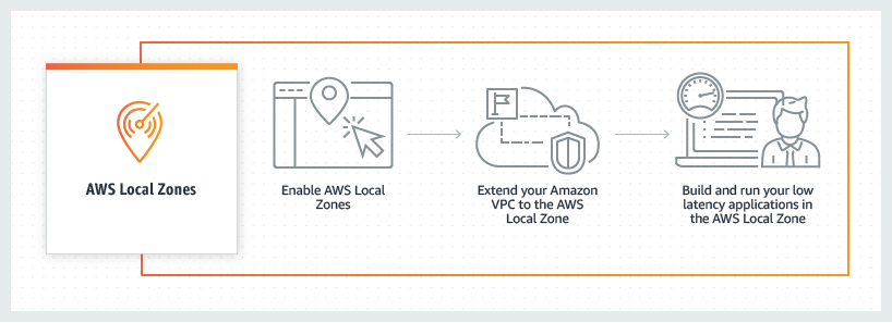
Local Zones are a new type of infrastructure deployment that places AWS compute, storage, database, and other select AWS services in large metropolitan areas closer to end users. This gives you access to single-digit millisecond latency with the use of AWS Direct Connect and the ability to meet data residency requirements. Local Zones are also connected to their parent Region via AWS’s redundant and high bandwidth private network. This gives applications running in Local Zones fast, secure, and seamless access to a complete list of services in the parent Region.

Unlike Outposts, which you deploy within your datacenter or a co-location of your choice, Local Zones are owned, managed, and operated by AWS. Local Zones eliminate the need for you to manage power, connectivity, and capacity. Furthermore, you can provision workloads on a Local Zone from your AWS Management Console just as you would for AZs and Regions today.

AWS Local Zones how it worksWhat is Outposts?

Outposts is a family of fully managed solutions delivering AWS infrastructure and services to virtually any on-premises or edge location for a truly consistent hybrid experience. Outposts lets you run some AWS services locally and connect to a broad range of services available in the local AWS Region. Outposts comes in two types of offerings: Outposts rack and Outposts servers, with which you can run applications and workloads on-premises using the same AWS infrastructure, services, tools, and APIs as in AWS Regions.

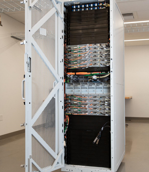
The Outposts rack is available as an industry standard 42U form factor. It provides the same AWS infrastructure, services, tools, and APIs to your data center or co-location space  that you would find in an AWS Region.

Outposts Rack

The Outposts servers come in a 1U or 2U form factor and are designed for locations that have limited space or smaller capacity requirements. Both support different compute instances, as detailed in the Outposts servers feature page.

Outposts ServersCustomer use cases

Now that we have an overview of both Local Zones and Outposts service offerings, let’s dive into use cases, the differences between them, and how your business can leverage each to accomplish your workloads requirements.

Low latency

Customers today require low latency computing for workloads, such as medical imaging, transaction processing for Enterprise Resource Planning (ERP) applications, enterprise migration with hybrid architecture, real-time multiplayer gaming, telco network function virtualization, and regulated gaming workloads.

Outposts can meet ultra-low latency requirements. This is accomplished by bringing AWS services on premises and to the edge at Outpost Sites. An Outpost site is the physical location where your Outpost operates, and it can be local within one of your data centers or at a co-location facility of your choice.

When accessing from within the same metro, Local Zones will provide you with a low, single millisecond latency experience when communicating with your applications. Latency between Local Zones and AWS Regions or Local Zones and on-premises environments varies, and these will depend on how close the nearest Local Zone is as well as the type of modality used for the connection (Public Internet, VPN, and AWS Direct Connect). You should always choose the closest Local Zone location to achieve the lowest possible latency. For use cases such as mobile gaming, you can utilize Local Zones by deploying your applications to a Local Zone location nearest to your end users. Local Zones are generally available in 17 metros across the US, 4 outside the US, and we are continuing to launch Local Zones in 30 cities across 25 countries. Check out updates for more general availability of Local Zones.

Data residency

On occasion, data must remain in a specific geographic region for regulatory or information security reasons. Healthcare and other regulated industries, such as financial services or Oil & Gas, have specific data residency requirements.

Outposts helps meet a customer’s data residency requirements because it’s installed on premises and essentially brings AWS to where the data currently resides. This allows you to pick and control where your workloads run, and where your data will stay. Check out the full list of countries and territories where Outposts is available on the FAQs page of Outposts rack and the FAQs page of Outposts servers.

Local Zones bring AWS closer or within a customer’s geographic boundary in a fully AWS owned and operated mode. Although Local Zones can help meet data residency use cases in some scenarios, data residency requirements vary depending on the jurisdictions. Therefore, you should work closely with your compliance and information security teams when choosing the Local Zone location in which to deploy your regulated workloads.

Migration and modernization

When trying to migrate to the cloud and modernize your stack, some workloads can be challenging. Often there are on-premises applications which are difficult to move into Regions due to latency-sensitive system intermittencies between their various components. As dependencies arise, you may choose to segment these migrations into smaller pieces. Then this will require latency-sensitive connectivity between the various parts of the application.

Outposts and Local Zones both allow for a gradual migration and modernization of your stack. You can choose to migrate parts of their workloads while still maintaining latency-sensitive connectivity between components until the entirety is ready to move.

Factors in selecting Local Zones or Outposts

Choosing between Local Zones and Outposts will depend on the following factors, and you should examine all of them together when selecting a service for your use case.

  1. Latency requirements

Local Zones can achieve low single millisecond latency when accessing within the same metro. On the other hand, Outposts can achieve ultra-low latency requirements when deployed within your datacenter or at a co-location facility of your choice. When selecting one over the other, you must work backward from your goal and workload requirements.

If you’re conducting a migration and modernization strategy which requires ultra-low latency between a workloads application and database tiers that are difficult to migrate to the AWS Regions, then Outposts would be the right solution for you.

Alternatively, if your workload involves streaming live broadcasts to end users which requires low single millisecond latency, but your end users are located where an AWS Region isn’t available, then Local Zones distributed across various metros would work best to serve your content.

  1. Availability of services needed to support your workload

Local Zones and Outposts differ with their list of supported AWS services, and you must review your workload’s service requirements when determining the best fit for you. For example, if a customer has a computer vision workload that requires storing and retrieving large volumes of images locally using Amazon Simple Storage Service (Amazon S3), then Outposts and certain Local Zones meet this requirement while other Local Zones don’t. Learn how you can use Amazon S3 on Outposts for computer vision workloads.

Outposts rack and servers support different sets of AWS services locally. You can view comparisons between them, or visit the Outposts servers and Outposts rack feature sites for more details.

Local Zones’ features vary depending on the location in which you choose to deploy. You can view more details and a full list of supported features and services per location on our Local Zones features page.

  1. Investment and management of infrastructure on-premises

Management of the infrastructure and prerequisites are another factor when considering which AWS service best suits your needs.

Outposts is ordered through AWS, and it requires installation in a customer’s on-premises datacenter or co-location provider of their choice. Outposts rack installation is handled by AWS, while Outposts servers installation is done by the customer or a third-party of their choosing. There are power and redundant networking requirements for the Outpost Site, as well as a required subscription to AWS Enterprise Support or On-Ramp Support.

Local Zones infrastructure is fully-managed by AWS, including the power, networking, and capacity. This reduces operational management as well as the overhead cost for customers. An Enterprise support agreement isn’t required to utilize Local Zones.

You should always choose Regions or Local Zones if your use case allows, and use Outposts when a Region or Local Zone isn’t a good fit. If both Outposts and Local Zones fit a customer’s use case and requirements, then Local Zones will be the preferred choice.

  1. Regulations, compliance, and information security

If a Local Zone is either unavailable or unable to meet your residency requirements within your geographic boundary consider Outposts, which can be deployed to a data center or co-location facility of your choice. Data residency requirements can be a factor based on your industry and the regulations to which your workload must adhere. Furthermore, you should work closely with your compliance and information security teams when choosing between Local Zones or Outposts.

Conclusion

Whether you’re dealing with latency-sensitive applications, data residency requirements, or a migration and modernization strategy, AWS provides options and flexibility for you to leverage the same AWS infrastructure, services, APIs, and tools to metro areas and on-premises locations with Local Zones and Outposts.

The decision of which technology to use will depend on several factors that we discussed above. You must work across teams within your organization to make sure that the latency requirements (low single millisecond latency within a metro for Local Zones vs the ultra low latency of Outposts when deployed close to or within your datacenter), data reseidency needs, installation prerequisites, and availability of services to support your workload are met.

Once these factors are taken into account, and you have made a choice, visit our product pages for Outposts and Local Zones with information on how you can get started.

Journey to adopt Cloud-Native DevOps platform Series #1: OfferUp modernized DevOps platform with Amazon EKS and Flagger to accelerate time to market

Post Syndicated from Purna Sanyal original https://aws.amazon.com/blogs/devops/journey-to-adopt-cloud-native-devops-platform-series-1-offerup-modernized-devops-platform-with-amazon-eks-and-flagger-to-accelerate-time-to-market/

In this two part series, we discuss the challenges faced by OfferUp, a Digital Native customer, to meet business growth and time-to-market. Their journey involved modernizing their existing DevOps platform, from the traditional monolith virtual machine (VM) based architecture to modern containerized architecture and running cloud-native applications for secured progressive delivery to accelerate time to market. This series will provide strategies, architecture patterns, and technical steps you can adopt to become more agile and innovative like OfferUp has.

OfferUp engineers were using the homegrown DevOps platform to build and release new services on the marketplace platform. In this first post, we discuss the key challenges encountered by OfferUp engineers with the existing DevOps platform, as well as how OfferUp modernized its DevOps platform with Amazon Elastic Kubernetes Service (Amazon EKS) and Flagger, automating production releases with progressive delivery techniques for faster time-to-market with new products and services. Amazon EKS is a managed container service to run and scale Kubernetes applications in the cloud or on-premises.

Previous DevOps architecture

OfferUp is a leading online and mobile customer to customer (C2C) marketplace where users can both buy and sell goods on the platform. Users can browse and purchase products from a broad range of categories, including furniture, clothing, sports equipment, toys, and many more. As a mobile-first company, OfferUp puts a great deal of emphasis on in-person communication between buyers and sellers.

OfferUp built a home grown, self-managed DevOps platform. This platform used a set of manual processes and third-party applications that allows both developers and operations engineers to build and deploy code to a production environment. The DevOps pipeline included topic areas such as source code control, continuous integration/continuous delivery (CI/CD), microservices, as well as development and test Methodologies. The following diagram depicts the previous architecture of OfferUp’s DevOps platform, which was self-managed on Amazon Elastic Compute Cloud (Amazon EC2).

Figure 1: Previous DevOps architecture of OfferUp

OfferUp used GitHub for code repositories. Once the source code was committed in the code repository, Jenkins pulled the source code from code repositories on a scheduled or on-demand basis and built Amazon Machine Images (AMI). The built image was deployed in production by a  custom built deployment tool, Vanaheim, which supports one-box canary deployment and full roll-out deployment strategies. The DevOps engineers used to manually create a deployment job in the Vanaheim portal and then manually monitor the test success rate and service metrics to detect any impact from the deployment. Once the success rate was reached, a full production roll out was performed from the Vanaheim portal.

Key challenges with previous DevOps pipeline

In 2020, OfferUp experienced significant transaction volume growth on its Marketplace platform with the increase of its user base. With OfferUp’s acquisition of LetGo in 2020, there was a need to build a scalable DevOps platform to support future integration and organic growth. The previous DevOps platform, designed and deployed over seven years ago, had reached the limits of its scalability, and could no longer keep up with the platform’s growth. The previous architecture was expensive to run and had a complex infrastructure that made it difficult to upgrade and add new features.

The following key factors drove the push for modernization:

  • Manual verification was required to check if the code was correctly deployed in one of the servers in production, and if the deployment was right in one server, then it was rolled out to other production servers. Full Rollout to production wasn’t automated due to frequent failures requiring manual rollbacks.
  • The previous platform required a longer deployment time (1–2 hours) due to the authoritative batch process, which sometimes caused delays in releasing and testing of new features.
  • The self-managed nature of the Jenkins and Vanaheim clusters was consuming far too much engineering time. Most of the institutional knowledge of this legacy platform was lost over the years and it didn’t align with OfferUp’s philosophy of small DevOps engineering teams. Innovation had stalled partly due to the difficulty of simultaneously upgrading the DevOps platform and releasing new features.

DevOps platform automation with Flagger and Gloo Ingress Controller on Amazon EKS

A key requirement for the next-generation system was that the new architecture would reduce the operational burden on engineering teams, deployment lifecycle, and total cost of ownership. OfferUp evaluated multiple managed container orchestration platforms for its DevOps Platform. It finally selected Amazon EKS for high availability, reducing the average time to deploy a change to the stack from hours to just a few minutes and reducing the complexity in managing and upgrading the Kubernetes cluster. On the Amazon EKS platform, OfferUp uses Flagger, a progressive delivery tool that automates the release process for applications running on Kubernetes. Flagger implements several deployment strategies (Canary releases, A/B testing, and Blue/Green mirroring) using the Gloo Edge ingress controller for traffic routing. Datadog is used as an observability service for monitoring the health of the deployments and effectively managing the canary to progressive delivery. For release analysis, Flagger runs a query on Datadog logs and uses Slack for alerting and notifications. The cloud native technology components of the architecture are described as follows:

Kubernetes and Amazon EKS – Kubernetes is an open-source system for automating the deployment, scaling, and management of containerized applications. Kubernetes is a graduate project in the CNCF. Amazon EKS is a fully-managed, certified Kubernetes conformant service that simplifies the process of building, securing, operating, and maintaining Kubernetes clusters on AWS. Amazon EKS integrates with core AWS services, such as Amazon CloudWatch, Auto Scaling Groups, and AWS Identity and Access Management (IAM) to provide a seamless experience for monitoring, scaling, and load balancing your containerized applications.

Helm – Helm manage Kubernetes applications. Helm Charts define, install, and upgrade even the most complex Kubernetes application. Charts are easy to create, version, share, and publish. If Kubernetes were an operating system, then Helm would be the package manager. Helm is a graduate project in the CNCF and is maintained by the Helm community.

Flagger – Flagger is a progressive delivery tool that automates the release process for applications running on Kubernetes. Flagger implements a control loop that gradually shifts traffic to the canary while measuring key performance indicators such as HTTP requests success rate, requests average duration, and pods health. Based on the set thresholds, a canary is either promoted or aborted and its analysis is pushed to a Slack channel. Flagger became a CNCF project – part of the Flux family of GitOps tools.

Gloo EdgeGloo Edge is a feature-rich, Kubernetes-native ingress controller. Gloo Edge is exceptional in its function-level routing; its support for legacy apps, microservices, and serverless; its discovery capabilities; and its tight integration with leading open-source projects. Gloo Edge is uniquely designed to support hybrid applications, in which multiple technologies, architectures, protocols, and clouds can coexist.

Observability platformDatadog’s integrations with Kubernetes, Docker, and AWS will let you track the full range of Amazon EKS metrics, as well as logs and performance data from your cluster and applications. Datadog gives you comprehensive coverage of your dynamic infrastructure and applications with features like auto discovery to track services across containers, sophisticated graphing, and alerting options.

Modernized DevOps architecture

In the new architecture, OfferUp uses Github as a version control tool and Github actions as their CI/CD tool. On every Pull request, tests are run, artifacts are built and stored in the JFrog Artifactory, and docker Images are stored in the Amazon Elastic Container Registry (Amazon ECR). Separate deployment pipelines are triggered based on the environment (dev, staging, and production) of choice. Flagger detects any changes in the version of the application and gradually shifts production traffic to the canary. It measures the requests success rate and average response duration metrics from Datadog to decide full rollout in production. For an application deployment, a canary promotion can be defined using Flagger’s custom resource. Flagger rolls back the deployment when the success rate falls below the defined desired success rate metrics.

Figure 2: Modernized DevOps architecture of OfferUp

With the modernized DevOps platform, OfferUp moved from monolithic to microservice architecture where  front-end applications and GraphQL runs on the Amazon EKS cluster. The production cluster runs 110 services and 650+ pods on 60 nodes. The cluster scales up to 100 nodes with Amazon Auto Scaling group based on the traffic pattern. On the networking front, the cluster has a private endpoint and uses both VPC CNI plugin, and the CoreDNS add-on. There are four Amazon EKS clusters, one each for the production, test, utility, and the staging environments. OfferUp has a plan to explore Karpenter open-source autoscaling project, and it will move new applications to the Amazon EKS cluster, allowing the total node counts to scale up to 200.

Benefits of modernized architecture

The new architecture helped OfferUp make  automated decisions to deploy new releases and improve the time to market while reducing unplanned production downtime

  • Faster deployments and Quicker rollbacks – The new architecture reduces the Service Deployment time from one hour down to five minutes, and automates rollback time to five minutes from the manual rollback time of one hour.
  • Automate deployment of new releases – The lack of canary deployment processes in the previous architecture required OfferUp engineers to manually intervene to validate the deployment status, which led to administrative overhead and production outages. The canary deployments take care of the traffic shifting by automatically measuring the requests’ success rate and latency metrics from Datadog and subsequently release the service to production. Deployments are automatically rolled back when the success rate falls below the defined success rate metric thresholds.
  • Simplified Configuration – Configuration has been simplified drastically and integrated within the CI/CD pipeline in the new architecture, thereby reducing configuration complexity, eliminating manual processes, and saving Developers time.
  • More time to Focus on Innovation – With fully automated progressive delivery, the developers no longer need to spend time testing and releasing source code in production. Similarly, migrating from a Self-managed DevOps platform to the Managed Amazon EKS services lowered the DevOps platform’s infrastructure management burden on the engineering team. This helps developers spend more time focusing on building and testing new features and innovations.
  • Cost reduction – Moving from self-managed Amazon EC2-based architecture to the Amazon EKS cluster reduced the cost of operations through shared nodes and improved pod density. The previous architecture was using 200 nodes of Amazon EC2 instances. The same workload was moved to a 50 nodes Amazon EKS cluster. Furthermore, custom applications (Vanaheim and Jenkins) were retired, further reducing the costs.

Conclusion

In this post, you see how OfferUp embarked on the journey to modernize its DevOps platform to support its growth and developers’ velocity. The key factors that drove the modernization decisions were the ability to scale the platform to support the automated testing of features in production, the faster release of new features, cost reduction, and to facilitate future innovation. The modernized DevOps platform on Amazon EKS also decreased the ongoing operational support burden for engineers, and the scalability of the design opens up a lot of headroom for growth.

We encourage you to look into modernizing your existing CI/CD pipeline on Amazon EKS with the Flagger progressive delivery mechanism. Amazon EKS removes the undifferentiated heavy lifting of managing and updating the Kubernetes cluster. Managed node groups automate the provisioning and lifecycle management of worker nodes in an Amazon EKS cluster, which greatly simplifies operational activities, such as new Kubernetes version deployments.

In the next part of the series, you’ll discover how to implement Flagger and Gloo Edge Ingress Controller on Amazon EKS to automate the release process for applications running on Kubernetes.

Further Reading

Journey to adopt Cloud-Native DevOps platform Series #2: Progressive delivery on Amazon EKS with Flagger and Gloo Edge Ingress Controller

About the authors:

Purna Sanyal

Purna Sanyal is a technology enthusiast and an architect at AWS, helping digital native customers solve their business problems with successful adoption of cloud native architecture. He provides technical thought leadership, architecture guidance, and conducts PoCs to enable customers’ digital transformation. He is also passionate about building innovative solutions around Kubernetes, database, analytics, and machine learning.

Alan Liu

Alan Liu is Sr Director of Engineering at OfferUp. He is a technology enthusiast and he worked across a wide variety of industry. He is highly effective, adaptable, scalable, experienced leader with a proven record.

Monitoring shared AWS Outposts rack capacity

Post Syndicated from Sheila Busser original https://aws.amazon.com/blogs/compute/monitoring-shared-aws-outposts-rack-capacity/

This post is written by Adam Imeson, Sr. Hybrid Edge Specialist Solutions Architect.

AWS Outposts rack is a fully-managed service that offers the same AWS infrastructure, APIs, tools, and a subset of AWS services to any data center, colocation space, or on-premises facility for a consistent hybrid experience. Outposts rack is ideal for workloads that require low latency, access to on-premises systems, local data processing, data residency, and migration of applications with local system interdependencies.

An Outpost is a pool of AWS compute and storage capacity deployed at a customer site. In an Outposts rack deployment, an Outpost may comprise of one or more racks connected together at the site. It’s common for customers to order their Outpost in a dedicated account and then integrate with their multi-account organizational architecture by sharing the Outpost via AWS Resource Access Manager (AWS RAM). This post will explain how to set up cross-account Amazon CloudWatch metrics so that disparate stakeholders within your organization can effectively monitor your Outpost’s capacity to meet their specific needs.

Overview

The AWS account that you use to order an Outpost owns that Outpost. This includes all metrics and health events pertaining to that Outpost. Many customers must integrate Outposts into their multi-account environments, as discussed in the “Best practices: AWS Outposts in a multi-account AWS environment” posts (part 1 and part 2). This post will go into more detail on how to monitor Outposts in these environments.

The nuance here stems from the different ways to share access to AWS resources. AWS RAM allows infrastructure resources to be shared across multiple accounts. Then, the consumer accounts can launch resources on the infrastructure as though they owned it. AWS Identity and Access Management (IAM) allows customers to modify a given account’s permissions such that users in other accounts can make AWS API calls that affect the given account.

An Outpost provides infrastructure resources, so customers can share Outposts via AWS RAM. CloudWatch metrics about Outposts are data which customers retrieve using AWS API calls, so customers can share access to those metrics using IAM.

In a typical customer’s AWS Organization, there are two cases to consider. First, when the customer is sharing an Outpost to multiple development accounts, each account needs to view metrics relevant to the Outpost so that the development accounts can deploy and operate their applications.Diagram depicting an Outpost that a customer has shared to three different accounts using RAM. The three different accounts each have a different application deployed in them.

Second, when the customer has several accounts that each own different Outposts, the customer’s centralized monitoring account needs to track metrics relevant to each of the Outposts.

Diagram depicting three accounts that each own a separate Outpost, with all three accounts sharing Outpost metrics to CloudWatch in the customer’s central monitoring account.

This post will explain strategies for both cases.

Customers must monitor the health of the Outpost’s connection to its regional control plane (the Outpost’s service link), as an Outpost is an extension of an AWS Availability Zone (AZ) and is designed to be connected to an AZ at all times. The health of the Outpost’s service link is a crucial variable when application owners are diagnosing disruptions to their application, and also when infrastructure owners are diagnosing disruptions to a site. Customers can monitor their service link’s status with the ConnectedStatus metric.

Customers also must monitor their Outposts’ current capacity. Outposts necessarily have a limited capacity footprint when compared to an AWS Region. Application owners must make informed decisions about capacity as they scale their apps over time or respond to occasional hardware failures. Infrastructure owners also must maintain a holistic view of capacity across all of the Outposts for which they are responsible so that they can plan for capacity expansion over time. Customers can monitor their Outposts’ capacity using the various capacity metrics that Outposts provide.

For an overview of how to set up a capacity dashboard and capacity-based CloudWatch alarms within a single account, see “Monitoring AWS Outposts capacity.” This post will expand on the single-account strategy by introducing cross-account capabilities. See also “Cross-Account Cross-Region Dashboards with Amazon CloudWatch.” These two posts provide practical walkthroughs for setting up the metric flows explained below.

Setting up Outposts metric permissions for your organization

This post assumes that you have multiple Outposts in different accounts that are all part of the same Organization. You’re sharing these Outposts into accounts that development teams use to deploy and operate their applications. You also have a centralized monitoring account where your infrastructure team tracks various metrics across all accounts. Your Organization might look something like this:

A base diagram depicting six AWS accounts with different names. Outpost Account 1 contains an Outpost. Outpost Account 2 contains a different Outpost. Monitoring Account contains Amazon CloudWatch. Accounts A through C contain Applications A through C respectively.

The first Outpost is shared to Accounts A and B, and the second Outpost is only shared to Account B. This is just an example of how a customer might set up their environment so that Application A can deploy on Outpost 1, and Application B can deploy on both Outpost 1 and 2.

The same base diagram of the six AWS accounts as before, with arrows added to depict AWS RAM resource shares. Outpost Account 1 shares its Outpost to Accounts A and B. Outpost Account 2 shares its Outpost to Account B.

To enable centralized monitoring, each account shares CloudWatch metrics with the central monitoring account as described in “Cross-Account Cross-Region Dashboards with Amazon CloudWatch.”

The same base diagram of the six AWS accounts, with arrows added to depict CloudWatch metrics being shared from all five of the other accounts to the Monitoring Account.

Now there are application accounts which can launch on the desired Outposts, and all of the accounts are sharing metrics with the central monitoring account. The team responsible for procuring and managing the Outposts can now set up dashboards in the central monitoring account in accordance with “Monitoring AWS Outposts capacity” to get a holistic view of capacity. This is valuable for capacity planning as applications naturally grow over time.

However, this may not be sufficient for operations. Consider that each application team needs to understand how much capacity is available on the Outpost that they’re using. This is crucial for teams operating highly available applications to maintain awareness of whether they still have N+1 capacity available on the Outpost to use in the event of a hardware failure. This is also important for planning expansions to the application ahead of time, as application teams have the best understanding of the future needs of their applications. Finally, application teams can use the metrics to track the operational health of the Outpost, which is crucial for root-causing any application disruptions.

You can implement this by sharing CloudWatch metrics from the Outpost accounts to the application accounts which are consuming the Outposts’ capacity, as shown in the following diagram.

The same base diagram of the six AWS accounts, with arrows depicting CloudWatch metrics being shared. Outpost Account 1 is sharing CloudWatch metrics to Accounts A and B. Outpost Account 2 is sharing CloudWatch metrics to Account B.

Walkthrough

Log in to your application account and navigate to the CloudWatch console. Open the Settings menu and choose Configure.

Screenshot of the CloudWatch Console’s Settings menu.

Scroll to the bottom. In the View cross-account cross-region section, choose Edit.

Screenshot of the Cross-account cross-region sub-menu in the CloudWatch console.

Choose your preferred account selection method from the three options and choose Save changes. I recommend the Custom account selector option, as it strikes a good balance between a simple setup and ease of use. If you choose this option, then input the Outpost owner account’s account ID and a human-readable name for the account. This name will appear in the drop-down when you’re using the CloudWatch console to view metrics from other accounts later.

Screenshot of the Cross-account cross-region sub-menu in the CloudWatch console, with the “Custom account selector” option selected and “123456789012 Outpost owner account” in the input field.

Your application account is now prepared to view metrics from the Outpost owner account. Now log in to the account that owns the Outpost and navigate to the CloudWatch console. You still need to share the Outpost’s metrics to the application account. Open the Settings page again, and choose Configure in the Cross-account cross-region section as before. This time, choose Share data in the Share your CloudWatch data section:

Screenshot of the Cross-account cross-region sub-menu in the CloudWatch console, with the “Share data” button circled in red in the “Share your CloudWatch data” section.

Choose Add account and input the application account’s account ID. Then scroll to the bottom of the page and choose Launch CloudFormation template.

Screenshot of the “Share your CloudWatch data sub-menu in the CloudWatch console. The “Specific accounts” option in the “Sharing” section is highlighted, and the sample account ID “234567890123” is typed into the input field.

The AWS CloudFormation template will create the CloudWatch-CrossAccountSharingRole. This role gives CloudWatch read access to the AWS account that you specified, the application account. You can view and modify this role using the IAM console if you want to. For example, you might adjust the role to allow read access to an entire Organizational Unit (OU).

Now, log back in to the application account and navigate to the CloudWatch console. Choose All metrics in the left-side menu. In the Metrics section, select the Outpost owner account from the drop-down.

Screenshot of the CloudWatch console’s “All metrics” sub-page. The account selection drop-down is circled in red in the “Metrics” subsection.

You can now view the metrics from the Outpost owner account and incorporate them into the dashboards in the application account. Now the application teams can track the Outposts’ ConnectedStatus metrics to be alerted on any disconnections from the region, and they can track the Outposts’ capacity metrics as well. It’s a best practice to alarm on Outpost capacity metrics once a consumption threshold defined by business needs has been breached.

Conclusion

Outposts rack allows customers to deploy AWS infrastructure into virtually any data center, colocation space, or on-premises facility. Outposts are tied to the AWS account that ordered them, and customers can share Outposts among AWS accounts within the same Organization. When multiple teams within a customer’s Organization are interacting with the same Outpost, that introduces additional monitoring surface area for capacity and service health. This post explains how customers can accommodate their teams’ different needs by sharing Outposts metrics around their Organization along with their Outposts. As best practices, customers should share their Outposts capacity and ConnectedStatus metrics to teams who are running applications on Outposts. Customers’ operations teams should also work with their stakeholders to define a maximum capacity utilization threshold for a given Outpost and alarm on that threshold.

BloomIP Automatically Identifies production issues with Amazon DevOps Guru

Post Syndicated from David Ernst original https://aws.amazon.com/blogs/devops/bloomip-automatically-identifies-production-issues-with-amazon-devops-guru/

Operational excellence is critical for BloomIP’s customers. In this post, you will see how we built a solution to automate the detection of trends and issues in production workloads by implementing Amazon DevOps Guru for our clients.

BloomIP ensures your business is ready for what’s ahead, with security, scalability, performance, and cost control. We are cloud solutions partner that gets to know both the people and processes in your business.

The Challenge

Identifying operational issues within applications and services is time-consuming. This requires developers and cloud engineers to spend valuable time manually debugging using multiple tools. We needed to quickly identify any operational issues related to our clients applications, including any load balancer errors or user delays in accessing their application. Ensuring the application is up and running during certain times of the day is crucial to the success of our client’s business. We needed to identify any downtime or performance patterns and quickly address any related issues.

Analyzing an AWS environment after any incident requires a combination of tools such as Amazon CloudWatch, AWS Config, AWS CloudTrail, AWS CloudFormation, and AWS X-Ray. We spend hours pouring over the information in each tool to try to identify patterns and troubleshooting steps. Still, identifying issues that correlate between those tools is a manual process.

Automating Identification of Operational Issues

To address the challenges of tedious and manual processes of analyzing different tools to identify patterns, we implemented Amazon DevOps Guru  for many of our clients. Amazon DevOps Guru helps us automatically ingests all related data from the services mentioned above and applies Machine Learning techniques to analyze and recommend fixes for abnormal behaviors. Amazon DevOps Guru organizes its findings into reactive and proactive insights.

We capture Amazon DevOps Guru Insights as events using Amazon EventBridg, and send them to an  Amazon SNS Topic, which then notifies us via email and Slack.

Architecture diagram showing a typical 3 tier web app using AWS services and integrating the application with Amazon DevOps Guru, Amazon Eventbridge and Amazon SNS Topic to send send notifications via Email and Slack

Figure 1. Architecture diagram

Results

BloomIP is leveraging DevOps Guru to scale its operations across multiple customers. Amazon DevOps Guru was easy to enable; it provides us with a single console experience to search and visualize operational data. In addition to detecting anomalies, we can see graphs and timelines related to the numerous anomalous metrics and more contextual information such as relevant events and log snippets. This helps us quickly understand the anomaly scope. Because it integrates data across multiple sources such as Amazon CloudWatch, AWS Config, AWS CloudTrail, AWS CloudFormation, and AWS X-Ray, Amazon DevOps Guru reduces the need for us to use numerous tools.

“We were looking at a way to effortlessly scale our observability needs across multiple clients while ensuring we had the proper coverage. DevOps Guru gives us additional insight and assurance by quickly pointing out anomalies in our client’s environments. With ML-powered recommendations, DevOps Guru has allowed us to remediate repeated production issues automatically. ” – Joshua Haynes, Director of Engineering, BloomIP

Conclusion

Amazon DevOps Guru provides BloomIP with a streamlined approach to visualize operational data by integrating data across multiple sources supporting Amazon CloudWatch, AWS Config, AWS CloudTrail, AWS CloudFormation, and AWS X-Ray and reduces the need to use multiple tools. DevOps Guru gives you a single-console dashboard to look for and visualize anomalies in your operational data.

Start monitoring your AWS applications with AWS DevOps Guru today using this link

About the authors:

David Ernst

David is a Sr. Specialist Solution Architect – DevOps, with 20+ years of experience in designing and implementing software solutions for various industries. David is an automation enthusiast and works with AWS customers to design, deploy, and manage their AWS workloads/architectures.

Abdullahi Olaoye

Abdullahi is a Senior Cloud Architect at AWS Professional Services where he works with customers of different scales to design and build IT solutions that solve business challenges. When he’s not working, he enjoys spending time with his family, traveling and learning history of different varieties through documentaries and podcasts.

Implement row-level access control in a multi-tenant environment with Amazon Redshift

Post Syndicated from Siva Bangaru original https://aws.amazon.com/blogs/big-data/implement-row-level-access-control-in-a-multi-tenant-environment-with-amazon-redshift/

This is a guest post co-written with Siva Bangaru and Leon Liu from ADP.

ADP helps organizations of all types and sizes by providing human capital management (HCM) solutions that unite HR, payroll, talent, time, tax, and benefits administration. ADP is a leader in business outsourcing services, analytics, and compliance expertise. ADP’s unmatched experience, deep insights, and cutting-edge technology have transformed human resources from a back-office administrative function to a strategic business advantage.

People Analytics powered by ADP DataCloud is an application that provides analytics and enhanced insights to ADP’s clients. It delivers a guided analytics experience that make it easy for you to create, use, and distribute tailored analytics for your organization. ADP People Analytics’s streamlined, configurable dashboards can help you identify potential issues in key areas, like overtime, turnover, compensation, and much more.

ADP provides this analytics experience to thousands of clients today. Securing customers’ data is a top priority for ADP. The company requires the highest security standards when implementing a multi-tenant analytics platform on Amazon Redshift.

ADP DataCloud integrates with Amazon Redshift row-level security (RLS) to implement granular data entitlements and enforce the access restrictions on their tables in Amazon Redshift.

In this post, we discuss how the ADP DataCloud team implemented Amazon Redshift RLS on the foundation of role-based access control (RBAC) to simplify managing privileges required in a multi-tenant environment, and also enabled and enforced access to granular data entitlements in business terms.

The ADP DataCloud team had the following key requirements and challenges:

  • Support a multi-tenant application to enforce a logical separation of each tenant’s data rows
  • Support dynamic provisioning of new tenants
  • Minimal impact on performance

Row-level security in Amazon Redshift

Amazon Redshift is a fully managed, petabyte-scale data warehouse service in the cloud. One of the challenges with security is that enterprises want to provide fine-grained access control at the row level for sensitive data. This can be done by creating views or using different databases and schemas for different users. However, this approach isn’t scalable and becomes complex to maintain over time, especially when supporting multi-tenant environments.

In early 2022, Amazon Redshift released row-level security, which is built on the foundation of role-based access control. RLS allows you to control which users or roles can access specific records of data within tables, based on security policies that are defined at the database object level. This new RLS capability in Amazon Redshift enables you to dynamically filter existing rows of data in a table along with session context variable setting capabilities to dynamically assign the appropriate tenant configuration. This is in addition to column-level access control, where you can grant users permissions to a subset of columns. Now you can combine column-level access control with RLS policies to further restrict access to particular rows of visible columns. Refer to Achieve fine-grained data security with row-level access control in Amazon Redshift for additional details.

Solution overview

As part of ADP’s key requirements to support a multi-tenant data store wherein a single table holds data of multiple tenants, enforcement of security policies to ensure no cross-tenant data access is of paramount importance. One obvious way to ensure this is by creating database users for each tenant and implementing RLS policies to filter a single tenant’s data as per the logged-in user. But this can be tedious and become cumbersome to maintain as the number of tenants grow by the thousands.

This post presents another way to handle this use case by combining session context variables and RLS policies on tables to filter a single tenant’s data, thereby easing the burden of creating and maintaining thousands of database users. In fact, a single database user is all that is needed to connect and query different tenant’s data in different sessions from a multi-tenant table by setting different values to a session context variable in each session, as shown in the following diagram.

Let’s start by covering the high-level implementation steps. Consider there is a database user in Amazon Redshift app_user (which is neither a super user, nor has the sys:secadmin role granted, nor has the IGNORE RLS system privilege granted via another role). The user app_user owns a schema with the same name and all objects in it. The following is a typical multi-tenant table employee in the app_user schema with some sample records shown in the table:

CREATE TABLE app_user.employee (
    tenant_id varchar(50) not null,
    id varchar(50) not null,
    name varchar(200),
    email varchar(200),
    ssn char(9),
    constraint employee_pkey primary key (tenant_id,id)	
);
TENANT_ID ID NAME EMAIL SSN
T0001 E4646 Andy . XXXXXXXXX
T0001 E4689 Bob . XXXXXXXXX
T0001 E4691 Christina . XXXXXXXXX
T0002 E4733 Peter . XXXXXXXXX
T0002 E4788 Quan . XXXXXXXXX
T0002 E4701 Rose . XXXXXXXXX
T0003 E5699 Diana . XXXXXXXXX
T0003 E5608 Emily . XXXXXXXXX
T0003 E5645 Florence . XXXXXXXXX

To implement that, the following steps are required:

  1. Create a RLS policy on a column using a predicate that is set using a session context variable.
  2. Enable RLS at the table level and attach the RLS policy on the table.
  3. Create a stored procedure that sets the session context variable used in the RLS policy predicate.
  4. Connect and call the stored procedure to set the session context variable and query the table.

Now RLS can be enabled on this table in such a way that whenever app_user queries the employee table, the user will either see no rows or retrieve only rows specific to single tenant despite being the owner of the table.

An administrator, such as app_admin, either a super user or a user that has the sys:secadmin role, can enforce this as follows:

  1. Create a RLS policy that attaches a tenant_id predicate using a session context variable:
    create rls policy tenant_policy
    with (tenant_id varchar(50))
    using (tenant_id = current_setting('app_context.tenant_id'));

  2. Enable RLS and attach the policy on the employee table:
    alter table app_user.employee row level security on;
    
    attach rls policy tenant_policy on app_user.employee to public;

  3. Create a stored procedure to set the tenant_id in a session variable and grant access to app_user:
    create or replace procedure app_admin.set_app_context
    (p_tenant_id in varchar)
    	language plpgsql
    as $$ 	
    declare
    		v_tenant_id  varchar(50);
    begin
        reset all;   
    	v_tenant_id := set_config('app_context.tenant_id',p_tenant_id,false);	
    end;
     $$
    ;
    
    grant execute on app_admin. set_app_context(varchar) to app_user;

  4. Connect to app_user and call the stored procedure to set the session context variable:
    call app_admin.set_app_context('T0001');

When this setup is complete, whenever tenants are connecting to ADP Analytics dashboards, it connects as app_user and runs stored procedures by passing tenant_id, which sets the session context variable using the tenant ID. In this case, when requests come to connect and query the employee table, the user will experience the following scenarios:

  • No data is retrieved if current_setting('app_context.tenant_id') is not set or is null
  • Data is retrieved if current_setting('app_context.tenant_id') is set by calling the app_admin.set_app_context(varchar) procedure to a value that exists in the employee table (for example, app_admin.set_app_context(‘T0001’))

No data is retrieved if current_setting('app_context.tenant_id') is set to a value that doesn’t exist in the employee table (for example, app_admin.set_app_context(‘T9999’))

Validate RLS by examining query plans

Now let’s review the preceding scenarios by running an explain plan and observing how RLS works for the test setup. If a query contains a table that is subject to RLS policies, EXPLAIN displays a special RLS SecureScan node. Amazon Redshift also logs the same node type to the STL_EXPLAIN system table. EXPLAIN doesn’t reveal the RLS predicate that applies to the employee table. To view an explain plan with RLS predicate details, the EXPLAIN RLS system privilege is granted to app_user via a role.

In this first scenario, tenant_id wasn’t set by the stored procedure and was passed as a null value, therefore below select statement returns no rows .

=> select count(1),tenant_id from employee group by 2;

count | tenant_id

-------+-------------

(0 rows)

Explain plan output shows the filter as NULL:

=> explain select count(1),tenant_id from employee group by 2;

QUERY PLAN

--------------------------------------------------------------------------------

XN HashAggregate (cost=0.10..0.11 rows=4 width=20)

-> XN RLS SecureScan employee (cost=0.00..0.08 rows=4 width=20)

-> XN Result (cost=0.00..0.04 rows=4 width=20)

One-Time Filter: NULL::boolean

-> XN Seq Scan on employee (cost=0.00..0.04 rows=4 width=20)

(5 rows)

In the second scenario, tenant_id was set by the stored procedure and passed as a value of T0001, therefore returning only corresponding rows as shown in the explain plan output:

Call stored procedure to set the session context variable as ‘T0001’ and then run the select :

=> call app_admin.set_app_context('T0001');

=> select count(1),tenant_id from employee group by 2;
 count |   tenant_id
-------+------------------
     3 | T0001
(1 row)

Explain plan output shows the filter on tenant_id as ‘T0001’

=> explain select count(1),tenant_id from employee group by 2;
                                QUERY PLAN
--------------------------------------------------------------------------
 XN HashAggregate  (cost=0.07..0.07 rows=1 width=20)
   ->  XN RLS SecureScan employee  (cost=0.00..0.06 rows=1 width=20)
         ->  XN Seq Scan on employee  (cost=0.00..0.05 rows=1 width=20)
               Filter: ((tenant_id)::text = 'T0001'::text)
(4 rows)

In the third scenario, a non-existing tenant_id was set by the stored procedure, therefore returning no rows:

=> call app_admin.set_app_context('T9999');

=> select count(1),tenant_id from employee group by 2;
 count | tenant_id
-------+-------------
(0 rows)


=> explain select count(1),tenant_id from employee group by 2;
                                QUERY PLAN
--------------------------------------------------------------------------
 XN HashAggregate  (cost=0.07..0.07 rows=1 width=20)
   ->  XN RLS SecureScan employee  (cost=0.00..0.06 rows=1 width=20)
         ->  XN Seq Scan on employee  (cost=0.00..0.05 rows=1 width=20)
               Filter: ((tenant_id)::text = 'T9999'::text)
(4 rows)

Another key point is that you can apply the same policy to multiple tables as long as they have the column (tenant_id varchar(50)) defined with the same data type, because RLS polices are strongly typed in Amazon Redshift. Similarly, you can combine multiple RLS policies defined using different session context variables or other relevant column predicates and attach them to a single table.

Also, this RLS implementation doesn’t need any changes when a new tenant’s data is added to the table, because it can be queried by simply setting the new tenant’s identifier in the session context variable that is used to define the filter predicate inside the RLS policy. A tenant to its corresponding identifier mapping is typically done during an application’s tenant onboarding process and is generally maintained in a separate metastore, which is also referred to during each tenant’s login to get the tenant’s identifier. With that, thousands of tenants could be provisioned without needing to change any policy in Amazon Redshift. In our testing, we found no performance impact by tenants after RLS was implemented.

Conclusion

In this post, we demonstrated how the ADP DataCloud team implemented row-level security in a multi-tenant environment for thousands of customers using Amazon Redshift RLS and session context variables. For more information about RLS best practices, refer to Amazon Redshift security overview.

Try out RLS for your future Amazon Redshift implementations, and feel free to leave a comment about your use cases and experience.


About the authors

Siva Bangaru is a Database Architect at ADP. He has more than 13 years of experience with technical expertise on design, development, administration, and performance tuning of database solutions for a variety of OLAP and OLTP use cases on multiple database engines like Oracle, Amazon Aurora PostgreSQL, and Amazon Redshift.

Leon Liu is a Chief Architect at ADP. He has over 20 years of experience with enterprise application framework, architecture, data warehouses, and big data real-time processing.

Neha Daudani is a Solutions Architect at AWS. She has 15 years of experience in the data and analytics space. She has enabled clients on various projects on enterprise data warehouses, data governance, data visualization, master data management, data modeling, and data migration for clients to use business intelligence and analytics in business growth and operational efficiency.

Rohit Bansal is an Analytics Specialist Solutions Architect at AWS. He specializes in Amazon Redshift and works with customers to build next-generation analytics solutions using other AWS Analytics services.

Our guide to AWS Compute at re:Invent 2022

Post Syndicated from Sheila Busser original https://aws.amazon.com/blogs/compute/our-guide-to-aws-compute-at-reinvent-2022/

This blog post is written by Shruti Koparkar, Senior Product Marketing Manager, Amazon EC2.

AWS re:Invent is the most transformative event in cloud computing and it is starting on November 28, 2022. AWS Compute team has many exciting sessions planned for you covering everything from foundational content, to technology deep dives, customer stories, and even hands on workshops. To help you build out your calendar for this year’s re:Invent, let’s look at some highlights from the AWS Compute track in this blog. Please visit the session catalog for a full list of AWS Compute sessions.

Learn what powers AWS Compute

AWS offers the broadest and deepest functionality for compute. Amazon Elastic Cloud Compute (Amazon EC2) offers granular control for managing your infrastructure with the choice of processors, storage, and networking.

The AWS Nitro System is the underlying platform for our all our modern EC2 instances. It enables AWS to innovate faster, further reduce cost for our customers, and deliver added benefits like increased security and new instance types.

Discover the benefits of AWS Silicon

AWS has invested years designing custom silicon optimized for the cloud. This investment helps us deliver high performance at lower costs for a wide range of applications and workloads using AWS services.

  • Explore the AWS journey into silicon innovation with our “CMP201: Silicon Innovation at AWS” session. We will cover some of the thought processes, learnings, and results from our experience building silicon for AWS Graviton, AWS Nitro System, and AWS Inferentia.
  • To learn about customer-proven strategies to help you make the move to AWS Graviton quickly and confidently while minimizing uncertainty and risk, attend “CMP410: Framework for adopting AWS Graviton-based instances”.

 Explore different use cases

Amazon EC2 provides secure and resizable compute capacity for several different use-cases including general purpose computing for cloud native and enterprise applications, and accelerated computing for machine learning and high performance computing (HPC) applications.

High performance computing

  • HPC on AWS can help you design your products faster with simulations, predict the weather, detect seismic activity with greater precision, and more. To learn how to solve world’s toughest problems with extreme-scale compute come join us for “CMP205: HPC on AWS: Solve complex problems with pay-as-you-go infrastructure”.
  • Single on-premises general-purpose supercomputers can fall short when solving increasingly complex problems. Attend “CMP222: Redefining supercomputing on AWS” to learn how AWS is reimagining supercomputing to provide scientists and engineers with more access to world-class facilities and technology.
  • AWS offers many solutions to design, simulate, and verify the advanced semiconductor devices that are the foundation of modern technology. Attend “CMP320: Accelerating semiconductor design, simulation, and verification” to hear from ARM and Marvel about how they are using AWS to accelerate EDA workloads.

Machine Learning

Cost Optimization

Hear from our customers

We have several sessions this year where AWS customers are taking the stage to share their stories and details of exciting innovations made possible by AWS.

Get started with hands-on sessions

Nothing like a hands-on session where you can learn by doing and get started easily with AWS compute. Our speakers and workshop assistants will help you every step of the way. Just bring your laptop to get started!

You’ll get to meet the global cloud community at AWS re:Invent and get an opportunity to learn, get inspired, and rethink what’s possible. So build your schedule in the re:Invent portal and get ready to hit the ground running. We invite you to stop by the AWS Compute booth and chat with our experts. We look forward to seeing you in Las Vegas!

How Etleap and Amazon Redshift Serverless optimize costs for ETL

Post Syndicated from Caius Brindescu original https://aws.amazon.com/blogs/big-data/how-etleap-and-amazon-redshift-serverless-optimize-costs-for-etl/

Amazon Redshift Serverless lets you avoid managing infrastructure while only paying for what you use. Etleap provides data integration software that is natively built on AWS. It’s an AWS Advanced Technology Partner with the AWS Data & Analytics Competency and Amazon Redshift Service Ready designation.

In this post, we share how you can minimize the usage of resources for some workload patterns and maximize savings while seamlessly managing data pipelines. We illustrate an example of how Redshift Serverless and Etleap’s load synchronization feature can reduce active Redshift Serverless time, further optimizing extract, transform, and load (ETL) costs.

Introduction to Redshift Serverless

Redshift Serverless makes it easy to run and scale analytics in seconds without the need to set up and manage data warehouse clusters. With Redshift Serverless, you pay for the compute only when the data warehouse is in use. This is ideal when it’s difficult to predict compute needs such as variable workloads, periodic workloads with idle time, and steady-state workloads with spikes. As your demand evolves with new workloads and more concurrent users, Redshift Serverless automatically provisions the right compute resources, and your data warehouse scales seamlessly and automatically.

You can create a Redshift Serverless data warehouse either using the default settings or custom settings. Redshift Serverless creates a default workgroup and associates that to the default namespace. You can also create multiple Redshift Serverless endpoints per AWS account and Region using namespaces and workgroups.

A namespace is a collection of database objects and users, with properties such as database name and password, permissions, and encryption and security. The following screenshot shows an example of a namespace configuration on the Redshift Serverless console.

Namespace-Amazon Redshift Serverless

A workgroup is a collection of compute resources, which includes network and security settings. Workgroup configuration allows you to create a private or public serverless endpoint that you can use to connect with your applications. The following screenshot shows an example workgroup on the Redshift Serverless console.

Workgroup - Amazon Redshift Serverless

When the Redshift Serverless endpoint is available, choose Query data to launch the Amazon Redshift Query Editor v2 to create database objects, load data, and analyze and visualize data. You can also connect to Redshift Serverless endpoints using your preferred SQL client tools via Amazon Redshift JDBC/ODBC drivers.

With Redshift Serverless, you pay separately for the compute and storage you use. Compute capacity is measured in Redshift Processing Units (RPUs), and you pay for the workloads in RPU-hours with a minimum charge of 60 seconds, metered on a per-second basis. Data lake queries are also part of the same RPU-hours, and Redshift Serverless doesn’t charge separately for the per-TB based pricing of Amazon Redshift Spectrum. The default base capacity is 128 RPUs, but you can adjust it from 32 RPUs to 512 RPUs in units of 8 using the Redshift Serverless console. For storage, you pay for data stored in Amazon Redshift-managed storage and storage used for manual snapshots, similar to what you would pay with Amazon Redshift provisioned RA3 instances.

To control your costs, you can specify usage limits and define actions that Amazon Redshift automatically takes if those limits are reached. You can specify usage limits in RPU-hours and associated with a daily, weekly, or monthly duration. Setting higher usage limits can improve the overall throughput of the system, especially for workloads that need to handle high concurrency while maintaining consistently high performance.

Why Etleap customers need Redshift Serverless

Etleap gives customers robust and flexible pipelines without the hassle of coding and managing infrastructure. Redshift Serverless has a similar benefit, letting you run Amazon Redshift without worrying about provisioning and maintaining data warehouse.

With the close Etleap-AWS integration, you can get started working with multiple data sources in Redshift Serverless in minutes.

Redshift Serverless can also reduce users’ costs because it automatically scales data warehouse capacity up and down to match usage and only charges when the serverless instance is active. ETL workloads are often batch-based and characterized by spikes, so the dynamic scaling of Redshift Serverless reduces unnecessary costs.

The following diagram illustrates this solution architecture.

Etleap Integration with Amazon Redshift Serverless

Etleap uses Amazon Database Migration Service (AWS DMS), Amazon EMR, and Amazon Simple Storage Service (Amazon S3) to process data from databases, files, applications, and streams into Redshift Serverless.

Optimize costs for Redshift Serverless

One of the main sources of cost savings when using Redshift Serverless comes from its auto-pausing feature. When a Redshift Serverless instance is idle, it will auto-pause and you aren’t charged during this period of inactivity.

However, high frequency ETL pipelines (such as those from streams or CDC sources) can constantly resume the Redshift Serverless instance, negating the cost benefit. To maximize the advantages of the auto-pausing feature of Redshift Serverless, Etleap provides the option of load synchronization. As shown in the following figure, this reduces the number of load batches, thereby lowering active Redshift Serverless instance time and cost.

Etleap Load Synchronization

It sometimes makes sense to maximize the frequency of data ingestion, but not all use cases justify the higher cost of an always-on Amazon Redshift instance. Etleap users can set their load frequency at a cost-efficient once-per-hour or as frequently as every 5 minutes.

Amazon Redshift users typically run some SQL transformations after data is loaded in the warehouse. Etleap’s models feature lets you define the SQL transformations and their dependencies and control when these transformations are run. As with data loading, however, if these aren’t designed thoughtfully, there is a risk that models will trigger updates that unnecessarily wake up an idle Redshift Serverless instance, negating the cost savings of the Redshift Serverless auto-pausing feature.

To avoid this, Etleap schedules the models to update immediately after all the dependent tables have been updated. This maximizes the instance usage while it’s awake and allows it to pause when the loads and updates have completed.

Cost savings example

Let’s illustrate the cost savings benefits of Redshift Serverless by means of an example. A customer has set a 1-hour load synchronization schedule and has 100 pipelines and 10 models. Although by default Redshift Serverless has a provisioned base capacity of 128 RPUs, a provisioned base capacity of 32 RPUs is sufficient for the load requirements of this example. A typical average load time for Etleap customers into Amazon Redshift is 6 seconds. In Etleap, we perform a maximum of five loads at a time to avoid overloading the Redshift Serverless instance.

Here is an example of how the sequence would work for the pipelines:

  1. When the hourly schedule triggers, Etleap begins the extraction and transformation of source data for all pipelines with new data to process.
  2. After all the pipelines have finished extraction and transformation, Etleap begins to load the data into Amazon Redshift. This resumes the serverless instance. At an average of 6 seconds per load and five loads running in parallel, it takes 120 seconds to load all the pipelines (100 / 5 pipeline cycles * 6 seconds each).
  3. When the load is complete, Etleap triggers the model updates. A typical model in Etleap takes about 130 seconds to update. As with loads, Etleap limits models to five simultaneous updates to reduce the load on the Redshift Serverless instance. Therefore, updating all 10 models takes 260 seconds of total instance run time (130 seconds * 10/5 model cycles).
  4. At this point, you’re being charged for 380 seconds of active workload, and Redshift Serverless will become idle after some time.

Additionally, Etleap runs daily vacuum operations on applicable tables to minimize storage and improve query efficiency. The length of this process depends on the tables and the number of updates and deletes. For a customer with this amount of pipeline volume, 20 minutes is a typical length of time to vacuum the tables, adding that much daily runtime for the instance.

This results in a total daily runtime of 172 minutes ((380 seconds * 24 daily cycles / 60) + 20 minutes), which translates into a cost of $34.40 per day for a 32 RPU serverless instance. This is 88% lower cost than a comparable Amazon Redshift provisioned environment without the benefits of Etleap and Redshift Serverless: an always-on provisioned Amazon Redshift cluster with similar performance (1 year reserved instance pricing for 16 ra3.xlplus nodes running 24 hours/day).

Other ETL optimizations on Etleap using Redshift Serverless

Etleap natively supports Redshift Serverless by updating its ETL solution to ensure you can continue to seamlessly ingest diverse data sources.

Redshift Serverless offers new system views that are used for tracking and managing ingestion, and Etleap utilizes these new system views to natively handle tracking ingestion loads and vacuuming operations in their platform. For example, Etleap uses sys_query_history to determine which loads are in progress or complete, and thereby helps avoid double loading a batch.

Redshift Serverless automatically initiates optimizations such as sort and vacuum in the background and doesn’t charge for these automatic optimizations. As a best practice, after Etleap load synchronization, Etleap periodically runs the vacuum function on applicable tables, which reduces storage and improves query performance. Etleap uses the vacuum_sort_benefit column in svv_table_info, which provides the statistics for each table, informing which would benefit from vacuuming.

Summary

In this post, we described how Redshift Serverless frees you from managing data warehouse infrastructure and reduces costs. In particular, we illustrated a data integration pattern where Etleap can ensure further cost savings through its load synchronization feature by optimally choosing a cost-efficient once-per-hour load frequency. Although this proves to be an optimal solution for uses cases where you prefer cost efficiency over real-time data insights, Etleap also allows you to set the load frequency as low as 5 minutes for use cases where near-real-time data insights are important.

Start using Redshift Serverless to run and scale analytics without having to manage data warehouse infrastructure and take advantage of further cost savings through Etleap’s load synchronization feature. To get started with Etleap, start a free trial  or request a tailored demo.


About the Authors

Caius Brindescu is an engineer at Etleap with over 4 years of experience in developing ETL software. In addition to development work, he helps customers make the most out of Etleap and Amazon Redshift. He holds a PhD from Oregon State University and one AWS certification (Big Data – Specialty).

Maneesh Sharma is a Senior Database Engineer at AWS with more than a decade of experience designing and implementing large-scale data warehouse and analytics solutions. He collaborates with various Amazon Redshift Partners and customers to drive better integration.

Sathisan Vannadil is a Senior Partner Solutions Architect at Amazon Web Services (AWS). His primary focus is on helping independent software vendor (ISV) partners design and build solutions at scale on AWS. Prior to AWS, Sathisan held diverse technical positions and has over 20 years of experience in the field of data and analytics.

Amazon Alexa Audio migrates business intelligence to Amazon QuickSight for faster performance

Post Syndicated from Weijia Shou original https://aws.amazon.com/blogs/big-data/amazon-alexa-audio-migrates-business-intelligence-to-amazon-quicksight-for-faster-performance/

The Amazon Alexa Audio Data & Insights (AUDI) team strives to make business intelligence (BI) accessible for engineers across Amazon Alexa Audio. Amazon Alexa Audio helps you stay entertained with your favorite music, podcasts, books, and radio from providers such as Amazon Music, Spotify, and iHeart Radio. The AUDI team manages dashboards and reports to help Amazon Alexa Audio teams pull metrics, derive insights, and perform deep-dive analyses. To support the performance of business-critical activities, the team sought a fast, high-performing BI solution so that it could improve the user experience.

The AUDI team turned to AWS and migrated its dashboards to Amazon QuickSight, a fully managed, cloud-native BI service powered by machine learning. By moving its dashboards to QuickSight, the AUDI team reduced load times by a factor of 25, from 2–5 minutes to only 5–10 seconds. This has made it simpler than ever for Amazon Alexa Audio to quickly harness BI insights.

“Our users were blown away at how fast Amazon QuickSight loaded our dashboards,” says Kani Singaravel, BI manager at Amazon Alexa Audio. “It’s pretty sleek and very simple to use, which is why we love it.”

Image showing charts and graphs that illustrates how Amazon QuickSight presents data visualizations.

Delivering BI insights across Amazon Alexa

The AUDI team delivers nimble BI insights for the Amazon Alexa Audio organization, harnessing data to generate weekly, monthly, quarterly, and exception-based business reports. To support the needs of the users who rely on the BI service, the AUDI team needed a faster, higher-performing solution. Previously, it would take several minutes to load dashboards and view insights, and Amazon Alexa Audio teams required lower latency to perform their important work.

After recognizing these challenges, the AUDI team began to explore advanced BI options on AWS.

“We chose to migrate to AWS after we received a lot of complaints about latency,” says Weijia Shou, BI engineer at Amazon Alexa Audio. “This decision also aligned well with our usage of other AWS tools.”

In February 2022, with the goal of quickly accessing key insights, the team chose Amazon QuickSight as its preferred BI service and began to migrate its dashboards.

Reducing costs and latency on Amazon QuickSight

From research to launch, the AUDI team’s first dashboard migration took 2 months to complete. As of July 2022, it has migrated more than 10 dashboards to Amazon QuickSight.

“The first dashboard that we migrated was the Alexa Audio Summary Trend dashboard, which covers more than 80% of the use cases in our organization,” Shou says. “After that pilot migration, we saw a great improvement on latency from our dashboard.”

The team saw a more than 25-times improvement in latency, reducing dashboard loading times from 2–5 minutes to only 5–10 seconds.

To achieve this acceleration in performance, the AUDI team took advantage of the Super-fast, Parallel, In-Memory Calculation Engine (SPICE) in-memory data store in Amazon QuickSight. SPICE is a purpose-built query engine that offers consistently fast performance and automatically scales to meet high concurrency needs during peak periods, such as weekday mornings or end-of-month reporting cycles. When data is imported into SPICE, it’s converted into a highly optimized, proprietary format. Dashboard queries are then powered by SPICE, providing fast performance for dashboard users across Amazon Alexa Audio and shielding the underlying data source from the intensity of traffic generated by interactive dashboard queries. SPICE data can be refreshed on a schedule or by one-time API calls.

On Amazon QuickSight, the AUDI team has vastly accelerated its querying time for the BI service, which is used by over 300 employees. “The new dashboard is much faster, so we can quickly understand how we’re tracking against our goals and key engagement metrics,” says Blake N., Senior Product Manager at Amazon Alexa International. In addition to improving speed and performance, the AUDI team has also reduced its expenses. Because Amazon QuickSight has a pay-as-you-go pricing structure, it’s much more cost effective than other BI tools on the market.

Accelerating data-driven decision-making on AWS

By migrating BI dashboards to Amazon QuickSight, the AUDI team has made it simpler and faster for hundreds of Amazon Alexa Audio engineers to access the information that they need to make critical decisions in their roles. In the future, the team will continue the migration, and plans to build new dashboards on Amazon QuickSight as it launches innovative new features and services.

“Amazon QuickSight has been a critical migration for our business,” says LeAnn Lorbiecki, senior manager at Amazon Alexa Audio. “Previously, the latency made our dashboards unusable and challenged our ability to make data-driven decisions quickly on behalf of our customers, products, and overall business. The work on this migration was an incredible team effort with returns seen very quickly.”


About the authors

Weijia Shou is a Business Intelligence Engineer II at Amazon Alexa Audio Data & Insights team. She led the Alexa Audio migration of reporting dashboards to AWS QuickSight. Weijia is passionate about building scalable solutions and tools to accelerate data-driven decision making.

Kani Singaravel is a Business Intelligence Manager at Alexa Audio, where she enjoys working with the team to solve customer problems and challenges using data analytics.

How GoDaddy built a data mesh to decentralize data ownership using AWS Lake Formation

Post Syndicated from Ankit Jhalaria original https://aws.amazon.com/blogs/big-data/how-godaddy-built-a-data-mesh-to-decentralize-data-ownership-using-aws-lake-formation/

This is a guest post co-written with Ankit Jhalaria from GoDaddy.

GoDaddy is empowering everyday entrepreneurs by providing all the help and tools to succeed online. With more than 20 million customers worldwide, GoDaddy is the place people come to name their idea, build a professional website, attract customers, and manage their work.

GoDaddy is a data-driven company, and getting meaningful insights from data helps them drive business decisions to delight their customers. In 2018, GoDaddy began a large infrastructure revamp and partnered with AWS to innovate faster than ever before to meet the needs of its customer growth around the world. As part of this revamp, the GoDaddy Data Platform team wanted to set the company up for long-term success by creating a well-defined data strategy and setting goals to decentralize the ownership and processing of data.

In this post, we discuss how GoDaddy uses AWS Lake Formation to simplify security management and data governance at scale, and enable data as a service (DaaS) supporting organization-wide data accessibility with cross-account data sharing using a data mesh architecture.

The challenge

In the vast ocean of data, deriving useful insights is an art. Prior to the AWS partnership, GoDaddy had a shared Hadoop cluster on premises that various teams used to create and share datasets with other analysts for collaboration. As the teams grew, copies of data started to grow in the Hadoop Distributed File System (HDFS). Several teams started to build tooling to manage this challenge independently, duplicating efforts. Managing permissions on these data assets became harder. Making data discoverable across a growing number of data catalogs and systems is something that had started to become a big challenge. Although the cost of storage these days is relatively inexpensive, when there are several copies of the same data asset available, it makes it harder for analysts to efficiently and reliably use the data available to them. Business analysts need robust pipelines on key datasets that they rely upon to make business decisions.

Solution overview

In GoDaddy’s data mesh hub and spoke model, a central data catalog contains information about all the data products that exist in the company. In AWS terminology, this is the AWS Glue Data Catalog. The data platform team provides APIs, SDKs, and Airflow Operators as components that different teams use to interact with the catalog. Activities such as updating the metastore to reflect a new partition for a given data product, and occasionally running MSCK repair operations, are all handled in the central governance account, and Lake Formation is used to secure access to the Data Catalog.

The data platform team introduced a layer of data governance that ensures best practices for building data products are followed throughout the company. We provide the tooling to support data engineers and business analysts while leaving the domain experts to run their data pipelines. With this approach, we have well-curated data products that are intuitive and easy to understand for our business analysts.

A data product refers to an entity that powers insights for analytical purposes. In simple terms, this could refer to an actual dataset pointing to a location in Amazon Simple Storage Service (Amazon S3). Data producers are responsible for the processing of data and creating new snapshots or partitions depending on the business needs. In some cases, data is refreshed every 24 hours, and other cases, every hour. Data consumers come to the data mesh to consume data, and permissions are managed in the central governance account through Lake Formation. Lake Formation uses AWS Resource Access Manager (AWS RAM) to send resource shares to different consumer accounts to be able to access the data from the central governance account. We go into details about this functionality later in the post.

The following diagram illustrates the solution architecture.

Solution architecture illustrated

Defining metadata with the central schema repository

Data is only useful if end-users can derive meaningful insights from it—otherwise, it’s just noise. As part of onboarding with the data platform, a data producer registers their schema with the data platform along with relevant metadata. This is reviewed by the data governance team that ensures best practices for creating datasets are followed. We have automated some of the most common data governance review items. This is also the place where producers define a contract about reliable data deliveries, often referred to as Service Level Objective (SLO). After a contract is in place, the data platform team’s background processes monitor and send out alerts when data producers fail to meet their contract or SLO.

When managing permissions with Lake Formation, you register the Amazon S3 location of different S3 buckets. Lake Formation uses AWS RAM to share the named resource.

When managing resources with AWS RAM, the central governance account creates AWS RAM shares. The data platform provides a custom AWS Service Catalog product to accept AWS RAM shares in consumer accounts.

Having consistent schemas with meaningful names and descriptions makes the discovery of datasets easy. Every data producer who is a domain expert is responsible for creating well-defined schemas that business users use to generate insights to make key business decisions. Data producers register their schemas along with additional metadata with the data lake repository. Metadata includes information about the team responsible for the dataset, such as their SLO contract, description, and contact information. This information gets checked into a Git repository where automation kicks in and validates the request to make sure it conforms to standards and best practices. We use AWS CloudFormation templates to provision resources. The following code is a sample of what the registration metadata looks like.

Sample code of what the registration metadata looks like

As part of the registration process, automation steps run in the background to take care of the following on behalf of the data producer:

  • Register the producer’s Amazon S3 location of the data with Lake Formation – This allows us to use Lake Formation for fine-grained access to control the table in the AWS Glue Data Catalog that refers to this location as well as to the underlying data.
  • Create the underlying AWS Glue database and table – Based on the schema specified by the data producer along with the metadata, we create the underlying AWS Glue database and table in the central governance account. As part of this, we also use table properties of AWS Glue to store additional metadata to use later for analysis.
  • Define the SLO contract – Any business-critical dataset needs to have a well-defined SLO contract. As part of dataset registration, the data producer defines a contract with a cron expression that gets used by the data platform to create an event rule in Amazon EventBridge. This rule triggers an AWS Lambda function to watch for deliveries of the data and triggers an alert to the data producer’s Slack channel if they breach the contract.

Consuming data from the data mesh catalog

When a data consumer belonging to a given line of business (LOB) identifies the data product that they’re interested in, they submit a request to the central governance team containing their AWS account ID that they use to query the data. The data platform provides a portal to discover datasets across the company. After the request is approved, automation runs to create an AWS RAM share with the consumer account covering the AWS Glue database and tables mapped to the data product registered in the AWS Glue Data Catalog of the central governance account.

The following screenshot shows an example of a resource share.

Example of a resource share

The consumer data lake admin needs to accept the AWS RAM share and create a resource link in Lake Formation to start querying the shared dataset within their account. We automated this process by building an AWS Service Catalog product that runs in the consumer’s account as a Lambda function that accepts shares on behalf of consumers.

When the resource linked datasets are available in the consumer account, the consumer data lake admin provides grants to IAM users and roles mapping to data consumers within the account. These consumers (application or user persona) can now query the datasets using AWS analytics services of their choice like Amazon Athena and Amazon EMR based on the access privileges granted by the consumer data lake admin.

Day-to-day operations and metrics

Managing permissions using Lake Formation is one part of the overall ecosystem. After permissions have been granted, data producers create new snapshots of the data at a certain cadence that can vary from every 15 minutes to a day. Data producers are integrated with the data platform APIs that informs the platform about any new refreshes of the data. The data platform automatically writes a 0-byte _SUCCESS file for every dataset that gets refreshed, and notifies the subscribed consumer account via an Amazon Simple Notification Service (Amazon SNS) topic in the central governance account. Consumers use this as a signal to trigger their data pipelines and processes to start processing newer version of the data utilizing an event-driven approach.

There are over 2,000 data products built on the GoDaddy data mesh on AWS. Every day, there are thousands of updates to the AWS Glue metastore in the central data governance account. There are hundreds of data producers generating data every hour in a wide array of S3 buckets, and thousands of data consumers consuming data across a wide array of tools, including Athena, Amazon EMR, and Tableau from different AWS accounts.

Business outcomes

With the move to AWS, GoDaddy’s Data Platform team laid the foundations to build a modern data platform that has increased our velocity of building data products and delighting our customers. The data platform has successfully transitioned from a monolithic platform to a model where ownership of data has been decentralized. We accelerated the data platform adoption to over 10 lines of business and over 300 teams globally, and are successfully managing multiple petabytes of data spread across hundreds of accounts to help our business derive insights faster.

Conclusion

GoDaddy’s hub and spoke data mesh architecture built using Lake Formation simplifies security management and data governance at scale, to deliver data as a service supporting company-wide data accessibility. Our data mesh manages multiple petabytes of data across hundreds of accounts, enabling decentralized ownership of well-defined datasets with automation in place, which helps the business discover data assets quicker and derive business insights faster.

This post illustrates the use of Lake Formation to build a data mesh architecture that enables a DaaS model for a modernized enterprise data platform. For more information, see Design a data mesh architecture using AWS Lake Formation and AWS Glue.


About the Authors

Ankit Jhalaria is the Director Of Engineering on the Data Platform at GoDaddy. He has over 10 years of experience working in big data technologies. Outside of work, Ankit loves hiking, playing board games, building IoT projects, and contributing to open-source projects.

Harsh Vardhan is an AWS Solutions Architect, specializing in Analytics. He has over 6 years of experience working in the field of big data and data science. He is passionate about helping customers adopt best practices and discover insights from their data.

Kyle Tedeschi is a Principal Solutions Architect at AWS. He enjoys helping customers innovate, transform, and become leaders in their respective domains. Outside of work, Kyle is an avid snowboarder, car enthusiast, and traveler.

How ENGIE automates the deployment of Amazon Athena data sources on Microsoft Power BI

Post Syndicated from Amine Belhabib original https://aws.amazon.com/blogs/big-data/how-engie-automates-the-deployment-of-amazon-athena-data-sources-on-microsoft-power-bi/

ENGIE—one of the largest utility providers in France and a global player in the zero-carbon energy transition—produces, transports, and deals in electricity, gas, and energy services. With 160,000 employees worldwide, ENGIE is a decentralized organization and operates 25 business units with a high level of delegation and empowerment. ENGIE’s decentralized global customer base had accumulated lots of data, and it required a smarter, unique approach and solution to align its initiatives and provide data that is ingestible, organizable, governable, sharable, and actionable across its global business units.

ENGIE built an enterprise data repository named the Common Data Hub to align its customers and business units around the same solution. ENGIE used AWS to create the Common Data Hub, a custom solution built using a globally distributed data lake and analytics solutions on AWS. The Common Data Hub empowers teams to innovate by simplifying data access and delivering a comprehensive set of analytics tools, such as Amazon QuickSight, Microsoft Power BI, Tableau, and more.

In 2018, the company’s business leadership decided to accelerate its digital transformation through data and innovation by becoming a data-driven company.

“Amazon Athena is a key service in the ENGIE data ecosystem. It makes it easy to analyze data in a serverless manner so there is no infrastructure to manage. We used Athena to quickly build operational dashboards and get insight and high business value from the data available in our data lake.”

– Gregory Wolowiec, chief technology officer at ENGIE

ENGIE uses Microsoft Power BI to create dashboards and leverages the power of Amazon Athena through the out-of-the-box connector for Microsoft Power BI in which, complete raw data sets are not downloaded to the user’s workstation. While users create or interact with a visualization, Microsoft Power BI works with Athena to dynamically query the underlying data source so that they are always viewing current data.

In a previous blog post, you learned how to manually configure all the required infrastructure to create Microsoft Power BI dashboards using Athena with Microsoft Power BI DirectQuery enabled. ENGIE automated the creation and configuration of the Athena connections on Microsoft Power BI Gateway and Microsoft Power BI Online to be able to scale and reduce the manual overhead. In this post, you learn how ENGIE is doing it today.

Solution overview

The following diagram illustrates the solution architecture to automate the creation and configuration of the Athena connections on Microsoft Power BI Gateway and Microsoft Power BI Online.

As described in the previous blog post, the AWS CloudFormation stack deploys two Amazon Elastic Compute Cloud (Amazon EC2) instances in a private subnet in an Amazon Virtual Private Cloud (Amazon VPC): one instance is used for Microsoft Power BI Desktop, and the other is used for the Microsoft Power BI on-premises data gateway. This stack uses t3.2xlarge instances because they have the minimal hardware requirements recommended. You can increase or decrease the EC2 instance type depending on the performance of the gateway.

Additionally, the CloudFormation template creates an AWS Glue table that gives you access to the dataset. It creates an AWS Lambda function as an AWS CloudFormation custom resource that updates all the partitions in the AWS Glue table.

In addition to the architecture presented in the previous blog post, this stack creates multiple AWS Systems Manager documents to configure the Athena data sources on Microsoft Power BI Gateway and on Microsoft Power BI Online. The Systems Manager documents are run by another Lambda function that is triggered when we create or delete an entry on Amazon DynamoDB.

From the security standpoint, all resources are deployed within an Amazon VPC (a logically isolated virtual network), and it uses Amazon VPC endpoints to communicate between resources within your Amazon VPC and AWS services without the need of crossing an internet gateway, NAT gateway, VPN connection, or AWS Direct Connect. Additionally, the Microsoft Power BI on-premises data gateway doesn’t require inbound connections. Additionally, authentication with Athena is done on Microsoft Power BI Desktop and on the Microsoft Power BI on-premises data gateway using AWS Identity and Access Management (IAM) profile.

The daily estimated cost of this architecture is $18 USD, mainly driven by the EC2 instances.

Walkthrough overview

For this post, we step through a use case using the data from the 2015 New York City Taxi Records dataset hosted on the Registry of Open Data on AWS. The data is already stored in an Amazon Simple Storage Service (Amazon S3) bucket in Apache Parquet format and is partitioned. For more information about optimizing your Athena queries, see Top 10 Performance Tuning Tips for Amazon Athena.

First, you deploy the CloudFormation stack with all the infrastructure required. Then, you use AWS Systems Manager Session Manager (see Starting a session (Systems Manager console)) and any remote desktop client to configure the Microsoft Power BI instance in order to create and publish your dashboard. Complete the following steps:

  1. Deploy the CloudFormation stack.
  2. On the EC2 instance that has the name tag PowerBiDesktop, install and configure the Simba Athena ODBC driver and Microsoft Power BI Desktop.
  3. Create your dashboard on Microsoft Power BI Desktop and publish it.
  4. On the EC2 instance that has the name tag PowerBiGateway, install the Simba Athena ODBC driver and Microsoft Power BI on-premises data gateway.
  5. Create Athena resources on the Microsoft Power BI Gateway instance and data source on Microsoft Power BI Online.
  6. View your report on Microsoft Power BI Online.
  7. Remove data source on Microsoft Power BI Online and Athena resources on the Microsoft Power BI Gateway instance.

Prerequisites

For this walkthrough, you should have the following prerequisites:

Create resources and prepare your environment

Deploy the CloudFormation stack by choosing Launch stack:

BDB-2063-launch-cloudformation-stack

Keep note of the gateway name, because you use it later when configuring the Microsoft Power BI on-premises data gateway.

After you deploy the CloudFormation stack, you prepare your environment following the steps in the relevant sections from Creating dashboards quickly on Microsoft Power BI using Amazon Athena:

  • Logging in to your Microsoft Power BI Desktop instance – Access to your instance without a bastion
  • Installing and configuring Microsoft Power BI Desktop – Install the required software on the desktop
  • Creating an Athena connection on Microsoft Power BI Desktop – Configure the New York City taxi data source connection
  • Creating your dashboard on Microsoft Power BI Desktop and publishing it – Send the structure of your report to Microsoft Power BI Online
  • Logging in to your Microsoft Power BI on-premises data gateway instance – Install the required software on your gateway

Install and configure the Athena-enabled Microsoft Power BI on-premises data gateway

To set up your on-premises data gateway, complete the following steps:

  1. Download and install the latest Athena ODBC driver for Windows 64-bit.
  2. Download the Microsoft Power BI on-premises data gateway standard mode and launch the installer.
  3. For your gateway, choose On-premises data gateway (recommended).
  4. Accept the default values and choose Install.
  5. When the installer asks you to sign in, enter the email address associated with the Microsoft Power BI Pro tenant that doesn’t require MFA. (This should be the same user name and password that you provided when you launched the CloudFormation stack.)
  6. Choose Sign in.
  7. If asked to register a new gateway or migrate, restore, or take over an existing gateway, choose Register a new gateway.
  8. Give your gateway a name (use the same gateway name passed as a parameter when deploying the CloudFormation stack) and provide a recovery key.
  9. Choose Configure.

You should see a green check mark indicating the gateway is online and ready to be used.

Create Athena resources automatically on the Microsoft Power BI Gateway instance and Microsoft Power BI Online

To automate this process, you insert an entry on DynamoDB. The entry’s attributes have the DSN properties and the users that are allowed to use the data source on Microsoft Power BI Online.

  1. Launch AWS CloudShell from the AWS Management Console using either of the following methods:
    • Choose the CloudShell icon on the console navigation bar.
    • Enter cloudshell in the Find Services box and then choose the CloudShell option.
  2. Enter the following script:
    echo '#!/bin/bash
    
    stack_name=$1
    dsn_name=$2
    users=$3
    
    role_arn=$(aws cloudformation describe-stacks --stack-name $stack_name --query "Stacks[0].Outputs[?OutputKey=='\''DataProjectRoleArn'\''].OutputValue" --output text)
    aws_region=$(aws cloudformation describe-stacks --stack-name $stack_name --query "Stacks[0].Outputs[?OutputKey=='\''AWSRegion'\''].OutputValue" --output text)
    athena_bucket=$(aws cloudformation describe-stacks --stack-name $stack_name --query "Stacks[0].Outputs[?OutputKey=='\''AthenaOutputS3Bucket'\''].OutputValue" --output text)
    
    aws dynamodb put-item --table-name PowerbiBlogTable --item "{\"Name\":{\"S\":\"${dsn_name}\"}, \"AWSProfile\":{\"S\":\"${role_arn}\"}, \"AWSRegion\":{\"S\":\"${aws_region}\"}, \"Workgroup\":{\"S\":\"athena-powerbi-aws-blog\"}, \"S3OutputLocation\":{\"S\":\"${athena_bucket}\"}, \"S3OutputEncOption\":{\"S\":\"SSE_S3\"}, \"AuthenticationType\":{\"S\":\"IAM Profile\"}, \"Users\":{\"S\":\"${users}\"}}"
    ' > create_record.sh

  3. Give run permission on the created script:
    chmod u+x create_record.sh

  4. Run the script, passing as parameters your CloudFormation stack name, the DSN name that you want to create, and the users that you want to attach to the dataset (you can pass multiple users separated by a comma without spaces). For example:
    ./create_record.sh PbiGwStack taxiconnection [email protected]

This script inserts an entry with all the required properties in your DynamoDB table. When a new entry is added to DynamoDB, an event is captured by Amazon DynamoDB Streams and a Lambda function is triggered to run a Systems Manager document. The last document runs two scripts on the instance: the first one creates a new Athena ODBC DSN, and the second script creates a new data source on Microsoft Power BI Online.

View your report on Microsoft Power BI

To view your report, complete the following steps:

  1. Choose the workspace where you saved your report.
  2. On the Datasets + dataflows tab, locate the dataset, which has the same name as your report (for example, taxireport) and choose the options icon (three dots).
  3. Choose Settings.
  4. Choose Discover Data Sources.
  5. Expand Gateway Connection.
  6. Choose your gateway.
  7. For Maps to, choose taxiconnection.
  8. Choose Apply.
  9. Return to the workspace where you saved your report.
  10. On the Content tab, choose your report (taxireport).

You can now see your report online using the most recent data.

Remove Athena resources automatically on Microsoft Power BI Online and on the Microsoft Power BI Gateway instance

To automate this process, you remove an entry from the DynamoDB table. The entry’s attributes have the DSN properties and the users that are allowed to use the data source on Microsoft Power BI Online.

  1. Launch CloudShell.
  2. Enter the following script:
    echo '#!/bin/bash
    
    dsn_name=$1
    
    aws dynamodb delete-item --table-name PowerbiBlogTable --key "{\"Name\":{\"S\":\"${dsn_name}\"}}"' > delete_record.sh

  3. Give run permission on the created script:
    chmod u+x delete_record.sh

  4. Run the script, passing as parameters the DSN name that you want to delete. For example:
    ./delete_record.sh taxiconnection

This command removes an item from your DynamoDB table. When an entry is deleted from DynamoDB, an event is captured by DynamoDB Streams and a Lambda function is triggered to run a Systems Manager document. The last document runs two scripts on the instance: the first one removes the data source on Microsoft Power BI Online, and the second script removes the Athena ODBC DSN.

Clean up

To avoid incurring future charges, delete the CloudFormation stack and the resources that you deployed as part of this post.

Conclusion

ENGIE discovered significant value by using AWS services on top of Microsoft Power BI, enabling its global business units to analyze data in more productive ways. This post presented how ENGIE automated the process of creating reports using Athena with Microsoft Power BI.

The first part of the post described the architecture components and how to successfully create a dashboard using the NYC taxi dataset. The stack deployed uses only one EC2 instance for the Microsoft Power BI on-premises data gateway, but in production, you should consider creating a high-availability cluster of gateway installations, ideally in different Availability Zones.

The second part of this post deployed a demo environment and walked you through the steps to automate Athena data sources to be used on Microsoft Power BI. On the GitHub repository, you can find more scripts to help you to manage the users from your data sources on Microsoft Power BI and more.

For native access to your data in AWS without any downloads or servers, be sure to also check out Amazon QuickSight.


About the authors

Amine Belhabib is Hand-On Cloud Core Service Manager at ENGIE/ ENGIE IT. Innovative Cloud Surfer, helping ENGIE entities to accelerate their digital transformation and cloud first adoption strategy by designing, building, managing group cloud products and patterns in a use cases driven approach.

Armando Segnini is a Senior Data Architect with AWS Professional Services. He spends his time building scalable big data and analytics solutions for AWS Enterprise and Strategic customers. Armando also loves to travel with his family all around the world and take pictures of the places he visits.

Xavier Naunay is a Data Architect with AWS Professional Services. He is part of the AWS ProServe team, helping enterprise customers solve complex problems using AWS services. In his free time, he is either traveling or learning about technology and other cultures.

Amine El Mallem is a Senior Data/ML Ops Engineer in AWS Professional Services. He works with customers to design, automate, and build solutions on AWS for their business needs.

Anouar Zaaber is a Senior Engagement Manager in AWS Professional Services. He leads internal AWS, external partners, and customer teams to deliver AWS Cloud services that enable customers to realize their business outcomes.

Share and publish your Snowflake data to AWS Data Exchange using Amazon Redshift data sharing

Post Syndicated from Raks Khare original https://aws.amazon.com/blogs/big-data/share-and-publish-your-snowflake-data-to-aws-data-exchange-using-amazon-redshift-data-sharing/

Amazon Redshift is a fully managed, petabyte-scale data warehouse service in the cloud. You can start with just a few hundred gigabytes of data and scale to a petabyte or more. Today, tens of thousands of AWS customers—from Fortune 500 companies, startups, and everything in between—use Amazon Redshift to run mission-critical business intelligence (BI) dashboards, analyze real-time streaming data, and run predictive analytics. With the constant increase in generated data, Amazon Redshift customers continue to achieve successes in delivering better service to their end-users, improving their products, and running an efficient and effective business.

In this post, we discuss a customer who is currently using Snowflake to store analytics data. The customer needs to offer this data to clients who are using Amazon Redshift via AWS Data Exchange, the world’s most comprehensive service for third-party datasets. We explain in detail how to implement a fully integrated process that will automatically ingest data from Snowflake into Amazon Redshift and offer it to clients via AWS Data Exchange.

Overview of the solution

The solution consists of four high-level steps:

  1. Configure Snowflake to push the changed data for identified tables into an Amazon Simple Storage Service (Amazon S3) bucket.
  2. Use a custom-built Redshift Auto Loader to load this Amazon S3 landed data to Amazon Redshift.
  3. Merge the data from the change data capture (CDC) S3 staging tables to Amazon Redshift tables.
  4. Use Amazon Redshift data sharing to license the data to customers via AWS Data Exchange as a public or private offering.

The following diagram illustrates this workflow.

Solution Architecture Diagram

Prerequisites

To get started, you need the following prerequisites:

Configure Snowflake to track the changed data and unload it to Amazon S3

In Snowflake, identify the tables that you need to replicate to Amazon Redshift. For the purpose of this demo, we use the data in the TPCH_SF1 schema’s Customer, LineItem, and Orders tables of the SNOWFLAKE_SAMPLE_DATA database, which comes out of the box with your Snowflake account.

  1. Make sure that the Snowflake external stage name unload_to_s3 created in the prerequisites is pointing to the S3 prefix s3-redshift-loader-sourcecreated in the previous step.
  2. Create a new schema BLOG_DEMO in the DEMO_DB database:CREATE SCHEMA demo_db.blog_demo;
  3. Duplicate the Customer, LineItem, and Orders tables in the TPCH_SF1 schema to the BLOG_DEMO schema:
    CREATE TABLE CUSTOMER AS 
    SELECT * FROM snowflake_sample_data.tpch_sf1.CUSTOMER;
    CREATE TABLE ORDERS AS
    SELECT * FROM snowflake_sample_data.tpch_sf1.ORDERS;
    CREATE TABLE LINEITEM AS 
    SELECT * FROM snowflake_sample_data.tpch_sf1.LINEITEM;

  4. Verify that the tables have been duplicated successfully:
    SELECT table_catalog, table_schema, table_name, row_count, bytes
    FROM INFORMATION_SCHEMA.TABLES
    WHERE TABLE_SCHEMA = 'BLOG_DEMO'
    ORDER BY ROW_COUNT;

    unload-step-4

  5. Create table streams to track data manipulation language (DML) changes made to the tables, including inserts, updates, and deletes:
    CREATE OR REPLACE STREAM CUSTOMER_CHECK ON TABLE CUSTOMER;
    CREATE OR REPLACE STREAM ORDERS_CHECK ON TABLE ORDERS;
    CREATE OR REPLACE STREAM LINEITEM_CHECK ON TABLE LINEITEM;

  6. Perform DML changes to the tables (for this post, we run UPDATE on all tables and MERGE on the customer table):
    UPDATE customer 
    SET c_comment = 'Sample comment for blog demo' 
    WHERE c_custkey between 0 and 10; 
    UPDATE orders 
    SET o_comment = 'Sample comment for blog demo' 
    WHERE o_orderkey between 1800001 and 1800010; 
    UPDATE lineitem 
    SET l_comment = 'Sample comment for blog demo' 
    WHERE l_orderkey between 3600001 and 3600010;
    MERGE INTO customer c 
    USING 
    ( 
    SELECT n_nationkey 
    FROM snowflake_sample_data.tpch_sf1.nation s 
    WHERE n_name = 'UNITED STATES') n 
    ON n.n_nationkey = c.c_nationkey 
    WHEN MATCHED THEN UPDATE SET c.c_comment = 'This is US based customer1';

  7. Validate that the stream tables have recorded all changes:
    SELECT * FROM CUSTOMER_CHECK; 
    SELECT * FROM ORDERS_CHECK; 
    SELECT * FROM LINEITEM_CHECK;

    For example, we can query the following customer key value to verify how the events were recorded for the MERGE statement on the customer table:

    SELECT * FROM CUSTOMER_CHECK where c_custkey = 60027;

    We can see the METADATA$ISUPDATE column as TRUE, and we see DELETE followed by INSERT in the METADATA$ACTION column.
    unload-val-step-7

  8. Run the COPY command to offload the CDC from the stream tables to the S3 bucket using the external stage name unload_to_s3.In the following code, we’re also copying the data to S3 folders ending with _stg to ensure that when Redshift Auto Loader automatically creates these tables in Amazon Redshift, they get created and marked as staging tables:
    COPY INTO @unload_to_s3/customer_stg/
    FROM (select *, sysdate() as LAST_UPDATED_TS from demo_db.blog_demo.customer_check)
    FILE_FORMAT = (TYPE = PARQUET)
    OVERWRITE = TRUE HEADER = TRUE;

    COPY INTO @unload_to_s3/customer_stg/
    FROM (select *, sysdate() as LAST_UPDATED_TS from demo_db.blog_demo.customer_check)
    FILE_FORMAT = (TYPE = PARQUET)
    OVERWRITE = TRUE HEADER = TRUE;

    COPY INTO @unload_to_s3/lineitem_stg/ 
    FROM (select *, sysdate() as LAST_UPDATED_TS from demo_db.blog_demo.lineitem_check) 
    FILE_FORMAT = (TYPE = PARQUET) 
    OVERWRITE = TRUE HEADER = TRUE;

  9. Verify the data in the S3 bucket. There will be three sub-folders created in the s3-redshift-loader-source folder of the S3 bucket, and each will have .parquet data files.unload-step-9-valunload-step-9-val
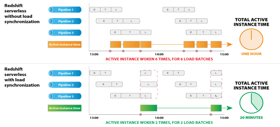
You can also automate the preceding COPY commands using tasks, which can be scheduled to run at a set frequency for automatic copy of CDC data from Snowflake to Amazon S3.
  10. Use the ACCOUNTADMIN role to assign the EXECUTE TASK privilege. In this scenario, we’re assigning the privileges to the SYSADMIN role:
    USE ROLE accountadmin;
    GRANT EXECUTE TASK, EXECUTE MANAGED TASK ON ACCOUNT TO ROLE sysadmin;

  11. Use the SYSADMIN role to create three separate tasks to run three COPY commands every 5 minutes: USE ROLE sysadmin;
    /* Task to offload Customer CDC table */ 
    CREATE TASK sf_rs_customer_cdc 
    WAREHOUSE = SMALL 
    SCHEDULE = 'USING CRON 5 * * * * UTC' 
    AS 
    COPY INTO @unload_to_s3/customer_stg/ 
    FROM (select *, sysdate() as LAST_UPDATED_TS from demo_db.blog_demo.customer_check) 
    FILE_FORMAT = (TYPE = PARQUET) 
    OVERWRITE = TRUE 
    HEADER = TRUE;
    /*Task to offload Orders CDC table */ 
    CREATE TASK sf_rs_orders_cdc 
    WAREHOUSE = SMALL 
    SCHEDULE = 'USING CRON 5 * * * * UTC' 
    AS 
    COPY INTO @unload_to_s3/orders_stg/ 
    FROM (select *, sysdate() as LAST_UPDATED_TS from demo_db.blog_demo.orders_check)
    FILE_FORMAT = (TYPE = PARQUET)
    OVERWRITE = TRUE HEADER = TRUE;

    /* Task to offload Lineitem CDC table */ 
    CREATE TASK sf_rs_lineitem_cdc 
    WAREHOUSE = SMALL 
    SCHEDULE = 'USING CRON 5 * * * * UTC' 
    AS 
    COPY INTO @unload_to_s3/lineitem_stg/ 
    FROM (select *, sysdate() as LAST_UPDATED_TS from demo_db.blog_demo.lineitem_check)
    FILE_FORMAT = (TYPE = PARQUET)
    OVERWRITE = TRUE HEADER = TRUE;

    When the tasks are first created, they’re in a SUSPENDED state.

  12. Alter the three tasks and set them to RESUME state:
    ALTER TASK sf_rs_customer_cdc RESUME;
    ALTER TASK sf_rs_orders_cdc RESUME;
    ALTER TASK sf_rs_lineitem_cdc RESUME;

  13. Validate that all three tasks have been resumed successfully: SHOW TASKS;unload-setp-13-valNow the tasks will run every 5 minutes and look for new data in the stream tables to offload to Amazon S3.As soon as data is migrated from Snowflake to Amazon S3, Redshift Auto Loader automatically infers the schema and instantly creates corresponding tables in Amazon Redshift. Then, by default, it starts loading data from Amazon S3 to Amazon Redshift every 5 minutes. You can also change the default setting of 5 minutes.
  14. On the Amazon Redshift console, launch the query editor v2 and connect to your Amazon Redshift cluster.
  15. Browse to the dev database, public schema, and expand Tables.
    You can see three staging tables created with the same name as the corresponding folders in Amazon S3.
  16. Validate the data in one of the tables by running the following query:SELECT * FROM "dev"."public"."customer_stg";unload-step-16-val

Configure the Redshift Auto Loader utility

The Redshift Auto Loader makes data ingestion to Amazon Redshift significantly easier because it automatically loads data files from Amazon S3 to Amazon Redshift. The files are mapped to the respective tables by simply dropping files into preconfigured locations on Amazon S3. For more details about the architecture and internal workflow, refer to the GitHub repo.

We use an AWS CloudFormation template to set up Redshift Auto Loader. Complete the following steps:

  1. Launch the CloudFormation template.
  2. Choose Next.
    autoloader-step-2
  3. For Stack name, enter a name.
  4. Provide the parameters listed in the following table.

    CloudFormation Template Parameter Allowed Values Description
    RedshiftClusterIdentifier Amazon Redshift cluster identifier Enter the Amazon Redshift cluster identifier.
    DatabaseUserName Database user name in the Amazon Redshift cluster The Amazon Redshift database user name that has access to run the SQL script.
    DatabaseName S3 bucket name The name of the Amazon Redshift primary database where the SQL script is run.
    DatabaseSchemaName Database name in Amazon Redshift The Amazon Redshift schema name where the tables are created.
    RedshiftIAMRoleARN Default or the valid IAM role ARN attached to the Amazon Redshift cluster The IAM role ARN associated with the Amazon Redshift cluster. Your default IAM role is set for the cluster and has access to your S3 bucket, leave it at the default.
    CopyCommandOptions Copy option; default is delimiter ‘|’ gzip

    Provide the additional COPY command data format parameters.

    If InitiateSchemaDetection = Yes, then the process attempts to detect the schema and automatically set the suitable copy command options.

    In the event of failure on schema detection or when InitiateSchemaDetection = No, then this value is used as the default COPY command options to load data.

    SourceS3Bucket S3 bucket name The S3 bucket where the data is stored. Make sure the IAM role that is associated to the Amazon Redshift cluster has access to this bucket.
    InitiateSchemaDetection Yes/No

    Set to Yes to dynamically detect the schema prior to file load and create a table in Amazon Redshift if it doesn’t exist already. If a table already exists, then it won’t drop or recreate the table in Amazon Redshift.

    If schema detection fails, the process uses the default COPY options as specified in CopyCommandOptions.

    The Redshift Auto Loader uses the COPY command to load data into Amazon Redshift. For this post, set CopyCommandOptions as follows, and configure any supported COPY command options:

    delimiter '|' dateformat 'auto' TIMEFORMAT 'auto'

    autoloader-input-parameters

  5. Choose Next.
  6. Accept the default values on the next page and choose Next.
  7. Select the acknowledgement check box and choose Create stack.
    autoloader-step-7
  8. Monitor the progress of the Stack creation and wait until it is complete.
  9. To verify the Redshift Auto Loader configuration, sign in to the Amazon S3 console and navigate to the S3 bucket you provided.
    You should see a new directory s3-redshift-loader-source is created.
    autoloader-step-9

Copy all the data files exported from Snowflake under s3-redshift-loader-source.

Merge the data from the CDC S3 staging tables to Amazon Redshift tables

To merge your data from Amazon S3 to Amazon Redshift, complete the following steps:

  1. Create a temporary staging table merge_stg and insert all the rows from the S3 staging table that have metadata_action as INSERT, using the following code. This includes all the new inserts as well as the update.
    CREATE TEMP TABLE merge_stg 
    AS
    SELECT * FROM
    (
    SELECT *, DENSE_RANK() OVER (PARTITION BY c_custkey ORDER BY last_updated_ts DESC
    ) AS rnk
    FROM customer_stg WHERE rnk = 1 AND metadata$action = 'INSERT'

    The preceding code uses a window function DENSE_RANK() to select the latest entries for a given c_custkey by assigning a rank to each row for a given c_custkey and arrange the data in descending order using last_updated_ts. We then select the rows with rnk=1 and metadata$action = ‘INSERT’ to capture all the inserts.

  2. Use the S3 staging table customer_stg to delete the records from the base table customer, which are marked as deletes or updates:
    DELETE FROM customer 
    USING customer_stg 
    WHERE customer.c_custkey = customer_stg.c_custkey;

    This deletes all the rows that are present in the CDC S3 staging table, which takes care of rows marked for deletion and updates.

  3. Use the temporary staging table merge_stg to insert the records marked for updates or inserts:
    INSERT INTO customer 
    SELECT c_custkey, c_name, c_address, c_nationkey, c_phone, c_acctbal, c_mktsegment, c_comment 
    FROM merge_stg;

  4. Truncate the staging table, because we have already updated the target table:truncate customer_stg;
  5. You can also run the preceding steps as a stored procedure:
    CREATE OR REPLACE PROCEDURE merge_customer()
    AS $$
    BEGIN
    /*CREATING TEMP TABLE TO GET THE MOST LATEST RECORDS FOR UPDATES/NEW INSERTS*/
    CREATE TEMP TABLE merge_stg AS
    SELECT * FROM
    (
    SELECT *, DENSE_RANK() OVER (PARTITION BY c_custkey ORDER BY last_updated_ts DESC ) AS rnk
    FROM customer_stg
    )
    WHERE rnk = 1 AND metadata$action = 'INSERT';
    /* DELETING FROM THE BASE TABLE USING THE CDC STAGING TABLE ALL THE RECORDS MARKED AS DELETES OR UPDATES*/
    DELETE FROM customer
    USING customer_stg
    WHERE customer.c_custkey = customer_stg.c_custkey;
    /*INSERTING NEW/UPDATED RECORDS IN THE BASE TABLE*/ 
    INSERT INTO customer
    SELECT c_custkey, c_name, c_address, c_nationkey, c_phone, c_acctbal, c_mktsegment, c_comment
    FROM merge_stg;
    truncate customer_stg;
    END;
    $$ LANGUAGE plpgsql;

    For example, let’s look at the before and after states of the customer table when there’s been a change in data for a particular customer.

    The following screenshot shows the new changes recorded in the customer_stg table for c_custkey = 74360.
    merge-process-new-changes
    We can see two records for a customer with c_custkey=74360 one with metadata$action as DELETE and one with metadata$action as INSERT. That means the record with c_custkey was updated at the source and these changes need to be applied to the target customer table in Amazon Redshift.

    The following screenshot shows the current state of the customer table before these changes have been merged using the preceding stored procedure:
    merge-process-current-state

  6. Now, to update the target table, we can run the stored procedure as follows: CALL merge_customer()The following screenshot shows the final state of the target table after the stored procedure is complete.
    merge-process-after-sp

Run the stored procedure on a schedule

You can also run the stored procedure on a schedule via Amazon EventBridge. The scheduling steps are as follows:

  1. On the EventBridge console, choose Create rule.
    sp-schedule-1
  2. For Name, enter a meaningful name, for example, Trigger-Snowflake-Redshift-CDC-Merge.
  3. For Event bus, choose default.
  4. For Rule Type, select Schedule.
  5. Choose Next.
    sp-schedule-step-5
  6. For Schedule pattern, select A schedule that runs at a regular rate, such as every 10 minutes.
  7. For Rate expression, enter Value as 5 and choose Unit as Minutes.
  8. Choose Next.
    sp-schedule-step-8
  9. For Target types, choose AWS service.
  10. For Select a Target, choose Redshift cluster.
  11. For Cluster, choose the Amazon Redshift cluster identifier.
  12. For Database name, choose dev.
  13. For Database user, enter a user name with access to run the stored procedure. It uses temporary credentials to authenticate.
  14. Optionally, you can also use AWS Secrets Manager for authentication.
  15. For SQL statement, enter CALL merge_customer().
  16. For Execution role, select Create a new role for this specific resource.
  17. Choose Next.
    sp-schedule-step-17
  18. Review the rule parameters and choose Create rule.

After the rule has been created, it automatically triggers the stored procedure in Amazon Redshift every 5 minutes to merge the CDC data into the target table.

Configure Amazon Redshift to share the identified data with AWS Data Exchange

Now that you have the data stored inside Amazon Redshift, you can publish it to customers using AWS Data Exchange.

  1. In Amazon Redshift, using any query editor, create the data share and add the tables to be shared:
    CREATE DATASHARE salesshare MANAGEDBY ADX;
    ALTER DATASHARE salesshare ADD SCHEMA tpch_sf1;
    ALTER DATASHARE salesshare ADD TABLE tpch_sf1.customer;

    ADX-step1

  2. On the AWS Data Exchange console, create your dataset.
  3. Select Amazon Redshift datashare.
    ADX-step3-create-datashare
  4. Create a revision in the dataset.
    ADX-step4-create-revision
  5. Add assets to the revision (in this case, the Amazon Redshift data share).
    ADX-addassets
  6. Finalize the revision.
    ADX-step-6-finalizerevision

After you create the dataset, you can publish it to the public catalog or directly to customers as a private product. For instructions on how to create and publish products, refer to NEW – AWS Data Exchange for Amazon Redshift

Clean up

To avoid incurring future charges, complete the following steps:

  1. Delete the CloudFormation stack used to create the Redshift Auto Loader.
  2. Delete the Amazon Redshift cluster created for this demonstration.
  3. If you were using an existing cluster, drop the created external table and external schema.
  4. Delete the S3 bucket you created.
  5. Delete the Snowflake objects you created.

Conclusion

In this post, we demonstrated how you can set up a fully integrated process that continuously replicates data from Snowflake to Amazon Redshift and then uses Amazon Redshift to offer data to downstream clients over AWS Data Exchange. You can use the same architecture for other purposes, such as sharing data with other Amazon Redshift clusters within the same account, cross-accounts, or even cross-Regions if needed.


About the Authors

Raks KhareRaks Khare is an Analytics Specialist Solutions Architect at AWS based out of Pennsylvania. He helps customers architect data analytics solutions at scale on the AWS platform.

Ekta Ahuja is a Senior Analytics Specialist Solutions Architect at AWS. She is passionate about helping customers build scalable and robust data and analytics solutions. Before AWS, she worked in several different data engineering and analytics roles. Outside of work, she enjoys baking, traveling, and board games.

Tahir Aziz is an Analytics Solution Architect at AWS. He has worked with building data warehouses and big data solutions for over 13 years. He loves to help customers design end-to-end analytics solutions on AWS. Outside of work, he enjoys traveling
and cooking.

Ahmed Shehata is a Senior Analytics Specialist Solutions Architect at AWS based on Toronto. He has more than two decades of experience helping customers modernize their data platforms, Ahmed is passionate about helping customers build efficient, performant and scalable Analytic solutions.

Fulfillment by Amazon uses Amazon QuickSight to deliver key reporting insights to Amazon Marketplace sellers

Post Syndicated from Ravi Kiran Nidadavolu original https://aws.amazon.com/blogs/big-data/fulfillment-by-amazon-uses-amazon-quicksight-to-deliver-key-reporting-insights-to-amazon-marketplace-sellers/

Fulfillment by Amazon logoFulfillment by Amazon (FBA) was launched in 2006, allowing businesses to outsource shipping to Amazon. With this fulfillment option, Amazon stores, picks, packs, ships, and delivers the products to customer as well as handling the customer service and returns for those orders.

Within Seller Central, a website where sellers can monitor their Amazon sales activity, the FBA Reporting team manages Report Central and the associated reporting APIs accessed by FBA sellers. Report Central offers 60+ downloadable reports to help sellers make data-driven decisions across inventory, sales, payments, customer concessions, removals and global shipping services.

The FBA Reporting team receives millions of report download requests from hundreds of thousands of users, in a multi-tenant fashion, every month. Tasked with ensuring speed, efficiency, and user-friendliness in the reports that sellers need to track their business operations, we turned to Amazon QuickSight.

In this post, we discuss what influenced the decision to implement QuickSight Embedded, as well as some of the benefits to FBA sellers.

Customer obsession drives innovation

Prior to implementing QuickSight Embedded, sellers had to create visuals within the limitations of their preferred spreadsheet program, which meant additional work and manual step-by-step processes to get the data out of Report Central and into whichever tools would be used. In some cases, it also meant additional cost to FBA sellers, depending on the analytics tools they were using.

To address this pain point for FBA sellers, we began researching, comparing, and contrasting our options. Initially, we considered building our own analytics tool, but decided against it due to concerns with the effort needed for long-term maintenance, upgrades, and the time investment necessary before we’d be able to bring innovative insights to customers. Once the decision was made to move forward with implementing an existing analytics solution, we began researching QuickSight, a fast, easy-to-use, cloud-powered business analytics service that makes it easy for all users to build visualizations, perform ad hoc analysis, and quickly get business insights from their data, any time, on any device.

The following screenshot shows examples of visuals created by Sales Trend data.

QuickSight enabled the us to provide data access to sellers via a QuickSight dashboard embedded directly into Seller Central.

The FBA Sales Analytics dashboard provides sellers with a summarized view of how their sales are trending over a specified time period. Sellers can filter the content on the page by SKU (or multiple SKUs), Marketplace, and time period. They can also define the granularity of the data: daily, weekly, or monthly. The analytics page includes 1 year of historical data. There are three major components:

  • Sales Fulfilled Chart – A chart showing the trend of fulfilled sales over the specified time period, with year-over-year comparisons. The granularity of the data is determined by the filter selection (daily, weekly, monthly). Sellers can hover over any data point on the chart to see a pop-up with details. They can also download the data to a CSV file.
  • Summary Table – This table displays a comparison of Sales Fulfilled ($) and Units Fulfilled reports, based on the selected filters. It also displays the year-over-year variance.
  • Top Selling SKUs – This shows details about the top-selling SKUs (based on total sales) and the year-over-year variance per SKU, and also includes a link to drill down per SKU.

With QuickSight, we are able to provide sellers with useful visualizations of sales-related data, allowing them to quickly and easily identify trends and track the impact of their actions, without needing to spend extra time and resources creating data visualizations via more manual processes.

Partnering with QuickSight has also enabled us to offer more detail and flexibility to sellers, allowing them to change the period of time for the data they’d like to review, filter based on useful controls, and drill down into whichever areas are most helpful for them.

Analytics at the speed of business

The primary motivation for our choosing QuickSight was that it not only provided a faster, more efficient, and less expensive experience for FBA sellers, but it also did most of the heavy lifting, freeing our team up to focus more of our time on product and dashboard design. One of the benefits of QuickSight being an Amazon product is that accessing data stored in Amazon Redshift, Amazon Relational Database Service (Amazon RDS), Amazon Athena, and other AWS services is a seamless, automatic experience.

The visual editor and toolkit provided by QuickSight allows us to make updates to established dashboards, and even create entirely new dashboards, in a matter of hours. Agility fosters experimentation with changes to visual elements by quickly copying a dashboard, tweaking it, soliciting feedback from stakeholders, and implementing it. The effort reduction from embedding QuickSight’s analytical capabilities allows our team to launch updates and features much faster.

Improving the status quo with QuickSight

By embedding QuickSight into Seller Central, we have been able to offer hundreds of thousands of FBA sellers year-over-year comparison information. QuickSight has allowed our team to iterate and launch updates more quickly, without having to worry about scaling or maintaining infrastructure resources.

Currently underway is an initiative to launch more dashboards to provide insights into inventory trends.

To learn more about how you can embed customized data visuals, interactive dashboards and natural language querying into any application, visit Amazon QuickSight Embedded.


About the Author

Ravi Kiran Nidadavolu is a Software Development Manager with Fulfillment by Amazon.

Introducing the price-capacity-optimized allocation strategy for EC2 Spot Instances

Post Syndicated from Sheila Busser original https://aws.amazon.com/blogs/compute/introducing-price-capacity-optimized-allocation-strategy-for-ec2-spot-instances/

This blog post is written by Jagdeep Phoolkumar, Senior Specialist Solution Architect, Flexible Compute and Peter Manastyrny, Senior Product Manager Tech, EC2 Core.

Amazon EC2 Spot Instances are unused Amazon Elastic Compute Cloud (Amazon EC2) capacity in the AWS Cloud available at up to a 90% discount compared to On-Demand prices. One of the best practices for using EC2 Spot Instances is to be flexible across a wide range of instance types to increase the chances of getting the aggregate compute capacity. Amazon EC2 Auto Scaling and Amazon EC2 Fleet make it easy to configure a request with a flexible set of instance types, as well as use a Spot allocation strategy to determine how to fulfill Spot capacity from the Spot Instance pools that you provide in your request.

The existing allocation strategies available in Amazon EC2 Auto Scaling and Amazon EC2 Fleet are called “lowest-price” and “capacity-optimized”. The lowest-price allocation strategy allocates Spot Instance pools where the Spot price is currently the lowest. Customers told us that in some cases the lowest-price strategy picks the Spot Instance pools that are not optimized for capacity availability and results in more frequent Spot Instance interruptions. As an improvement over lowest-price allocation strategy, in August 2019 AWS launched the capacity-optimized allocation strategy for Spot Instances, which helps customers tap into the deepest Spot Instance pools by analyzing capacity metrics. Since then, customers have seen a significantly lower interruption rate with capacity-optimized strategy when compared to the lowest-price strategy. You can read more about these customer stories in the Capacity-Optimized Spot Instance Allocation in Action at Mobileye and Skyscanner blog post. The capacity-optimized allocation strategy strictly selects the deepest pools. Therefore, sometimes it can pick high-priced pools even when there are low-priced pools available with marginally less capacity. Customers have been telling us that, for an optimal experience, they would like an allocation strategy that balances the best trade-offs between lowest-price and capacity-optimized.

Today, we’re excited to share the new price-capacity-optimized allocation strategy that makes Spot Instance allocation decisions based on both the price and the capacity availability of Spot Instances. The price-capacity-optimized allocation strategy should be the first preference and the default allocation strategy for most Spot workloads.

This post illustrates how the price-capacity-optimized allocation strategy selects Spot Instances in comparison with lowest-price and capacity-optimized. Furthermore, it discusses some common use cases of the price-capacity-optimized allocation strategy.

Overview

The price-capacity-optimized allocation strategy makes Spot allocation decisions based on both capacity availability and Spot prices. In comparison to the lowest-price allocation strategy, the price-capacity-optimized strategy doesn’t always attempt to launch in the absolute lowest priced Spot Instance pool. Instead, price-capacity-optimized attempts to diversify as much as possible across the multiple low-priced pools with high capacity availability. As a result, the price-capacity-optimized strategy in most cases has a higher chance of getting Spot capacity and delivers lower interruption rates when compared to the lowest-price strategy. If you factor in the cost associated with retrying the interrupted requests, then the price-capacity-optimized strategy becomes even more attractive from a savings perspective over the lowest-price strategy.

We recommend the price-capacity-optimized allocation strategy for workloads that require optimization of cost savings, Spot capacity availability, and interruption rates. For existing workloads using lowest-price strategy, we recommend price-capacity-optimized strategy as a replacement. The capacity-optimized allocation strategy is still suitable for workloads that either use similarly priced instances, or ones where the cost of interruption is so significant that any cost saving is inadequate in comparison to a marginal increase in interruptions.

Walkthrough

In this section, we illustrate how the price-capacity-optimized allocation strategy deploys Spot capacity when compared to the other two allocation strategies. The following example configuration shows how Spot capacity could be allocated in an Auto Scaling group using the different allocation strategies:

{
    "AutoScalingGroupName": "myasg ",
    "MixedInstancesPolicy": {
        "LaunchTemplate": {
            "LaunchTemplateSpecification": {
                "LaunchTemplateId": "lt-abcde12345"
            },
            "Overrides": [
                {
                    "InstanceRequirements": {
                        "VCpuCount": {
                            "Min": 4,
                            "Max": 4
                        },
                        "MemoryMiB": {
                            "Min": 0,
                            "Max": 16384
                        },
                        "InstanceGenerations": [
                            "current"
                        ],
                        "BurstablePerformance": "excluded",
                        "AcceleratorCount": {
                            "Max": 0
                        }
                    }
                }
            ]
        },
        "InstancesDistribution": {
            "OnDemandPercentageAboveBaseCapacity": 0,
            "SpotAllocationStrategy": "spot-allocation-strategy"
        }
    },
    "MinSize": 10,
    "MaxSize": 100,
    "DesiredCapacity": 60,
    "VPCZoneIdentifier": "subnet-a12345a,subnet-b12345b,subnet-c12345c"
}

First, Amazon EC2 Auto Scaling attempts to balance capacity evenly across Availability Zones (AZ). Next, Amazon EC2 Auto Scaling applies the Spot allocation strategy using the 30+ instances selected by attribute-based instance type selection, in each Availability Zone. The results after testing different allocation strategies are as follows:

  • Price-capacity-optimized strategy diversifies over multiple low-priced Spot Instance pools that are optimized for capacity availability.
  • Capacity-optimize strategy identifies Spot Instance pools that are only optimized for capacity availability.
  • Lowest-price strategy by default allocates the two lowest priced Spot Instance pools that aren’t optimized for capacity availability

To find out how each allocation strategy fares regarding Spot savings and capacity, we compare ‘Cost of Auto Scaling group’ (number of instances x Spot price/hour for each type of instance) and ‘Spot interruptions rate’ (number of instances interrupted/number of instances launched) for each allocation strategy. We use fictional numbers for the purpose of this post. However, you can use the Cloud Intelligence Dashboards to find the actual Spot Saving, and the Amazon EC2 Spot interruption dashboard to log Spot Instance interruptions. The example results after a 30-day period are as follows:

Allocation strategy

Instance allocation

Cost of Auto Scaling group

Spot interruptions rate

price-capacity-optimized

40 c6i.xlarge

20 c5.xlarge

$4.80/hour 3%

capacity-optimized

60 c5.xlarge

$5.00/hour

2%

lowest-price

30 c5a.xlarge

30 m5n.xlarge

$4.75/hour

20%

As per the above table, with the price-capacity-optimized strategy, the cost of the Auto Scaling group is only 5 cents (1%) higher, whereas the rate of Spot interruptions is six times lower (3% vs 20%) than the lowest-price strategy. In summary, from this exercise you learn that the price-capacity-optimized strategy provides the optimal Spot experience that is the best of both the lowest-price and capacity-optimized allocation strategies.

Common use-cases of price-capacity-optimized allocation strategy

Earlier we mentioned that the price-capacity-optimized allocation strategy is recommended for most Spot workloads. To elaborate further, in this section we explore some of these common workloads.

Stateless and fault-tolerant workloads

Stateless workloads that can complete ongoing requests within two minutes of a Spot interruption notice, and the fault-tolerant workloads that have a low cost of retries, are the best fit for the price-capacity-optimized allocation strategy. This category has workloads such as stateless containerized applications, microservices, web applications, data and analytics jobs, and batch processing.

Workloads with a high cost of interruption

Workloads that have a high cost of interruption associated with an expensive cost of retries should implement checkpointing to lower the cost of interruptions. By using checkpointing, you make the price-capacity-optimized allocation strategy a good fit for these workloads, as it allocates capacity from the low-priced Spot Instance pools that offer a low Spot interruptions rate. This category has workloads such as long Continuous Integration (CI), image and media rendering, Deep Learning, and High Performance Compute (HPC) workloads.

Conclusion

We recommend that customers use the price-capacity-optimized allocation strategy as the default option. The price-capacity-optimized strategy helps Amazon EC2 Auto Scaling groups and Amazon EC2 Fleet provision target capacity with an optimal experience. Updating to the price-capacity-optimized allocation strategy is as simple as updating a single parameter in an Amazon EC2 Auto Scaling group and Amazon EC2 Fleet.

To learn more about allocation strategies for Spot Instances, visit the Spot allocation strategies documentation page.

Running AI-ML Object Detection Model to Process Confidential Data using Nitro Enclaves

Post Syndicated from Sheila Busser original https://aws.amazon.com/blogs/compute/running-ai-ml-object-detection-model-to-process-confidential-data-using-nitro-enclaves/

This blog post was written by, Antoine Awad, Solutions Architect, Kevin Taylor, Senior Solutions Architect and Joel Desaulniers, Senior Solutions Architect.

Machine Learning (ML) models are used for inferencing of highly sensitive data in many industries such as government, healthcare, financial, and pharmaceutical. These industries require tools and services that protect their data in transit, at rest, and isolate data while in use. During processing, threats may originate from the technology stack such as the operating system or programs installed on the host which we need to protect against. Having a process that enforces the separation of roles and responsibilities within an organization minimizes the ability of personnel to access sensitive data. In this post, we walk you through how to run ML inference inside AWS Nitro Enclaves to illustrate how your sensitive data is protected during processing.

We are using a Nitro Enclave to run ML inference on sensitive data which helps reduce the attack surface area when the data is decrypted for processing. Nitro Enclaves enable you to create isolated compute environments within Amazon EC2 instances to protect and securely process highly sensitive data. Enclaves have no persistent storage, no interactive access, and no external networking. Communication between your instance and your enclave is done using a secure local channel called a vsock. By default, even an admin or root user on the parent instance will not be able to access the enclave.

Overview

Our example use-case demonstrates how to deploy an AI/ML workload and run inferencing inside Nitro Enclaves to securely process sensitive data. We use an image to demonstrate the process of how data can be encrypted, stored, transferred, decrypted and processed when necessary, to minimize the risk to your sensitive data. The workload uses an open-source AI/ML model to detect objects in an image, representing the sensitive data, and returns a summary of the type of objects detected. The image below is used for illustration purposes to provide clarity on the inference that occurs inside the Nitro Enclave. It was generated by adding bounding boxes to the original image based on the coordinates returned by the AI/ML model.

Image of airplanes with bounding boxes

Figure 1 – Image of airplanes with bounding boxes

To encrypt this image, we are using a Python script (Encryptor app – see Figure 2) which runs on an EC2 instance, in a real-world scenario this step would be performed in a secure environment like a Nitro Enclave or a secured workstation before transferring the encrypted data. The Encryptor app uses AWS KMS envelope encryption with a symmetrical Customer Master Key (CMK) to encrypt the data.

Image Encryption with AWS KMS using Envelope Encryption

Figure 2 – Image Encryption with AWS KMS using Envelope Encryption

Note, it’s also possible to use asymmetrical keys to perform the encryption/decryption.

Now that the image is encrypted, let’s look at each component and its role in the solution architecture, see Figure 3 below for reference.

  1. The Client app reads the encrypted image file and sends it to the Server app over the vsock (secure local communication channel).
  2. The Server app, running inside a Nitro Enclave, extracts the encrypted data key and sends it to AWS KMS for decryption. Once the data key is decrypted, the Server app uses it to decrypt the image and run inference on it to detect the objects in the image. Once the inference is complete, the results are returned to the Client app without exposing the original image or sensitive data.
  3. To allow the Nitro Enclave to communicate with AWS KMS, we use the KMS Enclave Tool which uses the vsock to connect to AWS KMS and decrypt the encrypted key.
  4. The vsock-proxy (packaged with the Nitro CLI) routes incoming traffic from the KMS Tool to AWS KMS provided that the AWS KMS endpoint is included on the vsock-proxy allowlist. The response from AWS KMS is then sent back to the KMS Enclave Tool over the vsock.

As part of the request to AWS KMS, the KMS Enclave Tool extracts and sends a signed attestation document to AWS KMS containing the enclave’s measurements to prove its identity. AWS KMS will validate the attestation document before decrypting the data key. Once validated, the data key is decrypted and securely returned to the KMS Tool which securely transfers it to the Server app to decrypt the image.

Solution architecture diagram for this blog post

Figure 3 – Solution architecture diagram for this blog post

Environment Setup

Prerequisites

Before we get started, you will need the following prequisites to deploy the solution:

  1. AWS account
  2. AWS Identity and Access Management (IAM) role with appropriate access

AWS CloudFormation Template

We are going to use AWS CloudFormation to provision our infrastructure.

  1. Download the CloudFormation (CFN) template nitro-enclave-demo.yaml. This template orchestrates an EC2 instance with the required networking components such as a VPC, Subnet and NAT Gateway.
  2. Log in to the AWS Management Console and select the AWS Region where you’d like to deploy this stack. In the example, we select Canada (Central).
  3. Open the AWS CloudFormation console at: https://console.aws.amazon.com/cloudformation/
  4. Choose Create Stack, Template is ready, Upload a template file. Choose File to select nitro-enclave-demo.yaml that you saved locally.
  5. Choose Next, enter a stack name such as NitroEnclaveStack, choose Next.
  6. On the subsequent screens, leave the defaults, and continue to select Next until you arrive at the Review step
  7. At the Review step, scroll to the bottom and place a checkmark in “I acknowledge that AWS CloudFormation might create IAM resources with custom names.” and click “Create stack”
  8. The stack status is initially CREATE_IN_PROGRESS. It will take around 5 minutes to complete. Click the Refresh button periodically to refresh the status. Upon completion, the status changes to CREATE_COMPLETE.
  9. Once completed, click on “Resources” tab and search for “NitroEnclaveInstance”, click on its “Physical ID” to navigate to the EC2 instance
  10. On the Amazon EC2 page, select the instance and click “Connect”
  11. Choose “Session Manager” and click “Connect”

EC2 Instance Configuration

Now that the EC2 instance has been provisioned and you are connected to it, follow these steps to configure it:

  1. Install the Nitro Enclaves CLI which will allow you to build and run a Nitro Enclave application:
    sudo amazon-linux-extras install aws-nitro-enclaves-cli -y
    sudo yum install aws-nitro-enclaves-cli-devel -y
    
  2. Verify that the Nitro Enclaves CLI was installed successfully by running the following command:
    nitro-cli --version

    Nitro Enclaves CLI

  3. To download the application from GitHub and build a docker image, you need to first install Docker and Git by executing the following commands:
    sudo yum install git -y
    sudo usermod -aG ne ssm-user
    sudo usermod -aG docker ssm-user
    sudo systemctl start docker && sudo systemctl enable docker
    

Nitro Enclave Configuration

A Nitro Enclave is an isolated environment which runs within the EC2 instance, hence we need to specify the resources (CPU & Memory) that the Nitro Enclaves allocator service dedicates to the enclave.

  1. Enter the following commands to set the CPU and Memory available for the Nitro Enclave allocator service to allocate to your enclave container:
    ALLOCATOR_YAML=/etc/nitro_enclaves/allocator.yaml
    MEM_KEY=memory_mib
    DEFAULT_MEM=20480
    sudo sed -r "s/^(\s*${MEM_KEY}\s*:\s*).*/\1${DEFAULT_MEM}/" -i "${ALLOCATOR_YAML}"
    sudo systemctl start nitro-enclaves-allocator.service && sudo systemctl enable nitro-enclaves-allocator.service
    
  2. To verify the configuration has been applied, run the following command and note the values for memory_mib and cpu_count:
    cat /etc/nitro_enclaves/allocator.yaml

    Enclave Configuration File

Creating a Nitro Enclave Image

Download the Project and Build the Enclave Base Image

Now that the EC2 instance is configured, download the workload code and build the enclave base Docker image. This image contains the Nitro Enclaves Software Development Kit (SDK) which allows an enclave to request a cryptographically signed attestation document from the Nitro Hypervisor. The attestation document includes unique measurements (SHA384 hashes) that are used to prove the enclave’s identity to services such as AWS KMS.

  1. Clone the Github Project
    cd ~/ && git clone https://github.com/aws-samples/aws-nitro-enclaves-ai-ml-object-detection.git
  2. Navigate to the cloned project’s folder and build the “enclave_base” image:
    cd ~/aws-nitro-enclaves-ai-ml-object-detection/enclave-base-image
    sudo docker build ./ -t enclave_base

    Note: The above step will take approximately 8-10 minutes to complete.

Build and Run The Nitro Enclave Image

To build the Nitro Enclave image of the workload, build a docker image of your application and then use the Nitro CLI to build the Nitro Enclave image:

  1. Download TensorFlow pre-trained model:
    cd ~/aws-nitro-enclaves-ai-ml-object-detection/src
    mkdir -p models/faster_rcnn_openimages_v4_inception_resnet_v2_1 && cd models/
    wget -O tensorflow-model.tar.gz https://tfhub.dev/google/faster_rcnn/openimages_v4/inception_resnet_v2/1?tf-hub-format=compressed
    tar -xvf tensorflow-model.tar.gz -C faster_rcnn_openimages_v4_inception_resnet_v2_1
  2. Navigate to the use-case folder and build the docker image for the application:
    cd ~/aws-nitro-enclaves-ai-ml-object-detection/src
    sudo docker build ./ -t nitro-enclave-container-ai-ml:latest
  3. Use the Nitro CLI to build an Enclave Image File (.eif) using the docker image you built in the previous step:
    sudo nitro-cli build-enclave --docker-uri nitro-enclave-container-ai-ml:latest --output-file nitro-enclave-container-ai-ml.eif
  4. The output of the previous step produces the Platform configuration registers or PCR hashes and a nitro enclave image file (.eif). Take note of the PCR0 value, which is a hash of the enclave image file.Example PCR0:
    {
        "Measurements": {
            "PCR0": "7968aee86dc343ace7d35fa1a504f955ee4e53f0d7ad23310e7df535a187364a0e6218b135a8c2f8fe205d39d9321923"
            ...
        }
    }
  5. Launch the Nitro Enclave container using the Enclave Image File (.eif) generated in the previous step and allocate resources to it. You should allocate at least 4 times the EIF file size for enclave memory. This is necessary because the tmpfs filesystem uses half of the memory and the remainder of the memory is used to uncompress the initial initramfs where the application executable resides. For CPU allocation, you should allocate CPU in full cores i.e. 2x vCPU for x86 hyper-threaded instances.
    In our case, we are going to allocate 14GB or 14,366 MB for the enclave:

    sudo nitro-cli run-enclave --cpu-count 2 --memory 14336 --eif-path nitro-enclave-container-ai-ml.eif

    Note: Allow a few seconds for the server to boot up prior to running the Client app in the below section “Object Detection using Nitro Enclaves”.

Update the KMS Key Policy to Include the PCR0 Hash

Now that you have the PCR0 value for your enclave image, update the KMS key policy to only allow your Nitro Enclave container access to the KMS key.

  1. Navigate to AWS KMS in your AWS Console and make sure you are in the same region where your CloudFormation template was deployed
  2. Select “Customer managed keys”
  3. Search for a key with alias “EnclaveKMSKey” and click on it
  4. Click “Edit” on the “Key Policy”
  5. Scroll to the bottom of the key policy and replace the value of “EXAMPLETOBEUPDATED” for the “kms:RecipientAttestation:PCR0” key with the PCR0 hash you noted in the previous section and click “Save changes”

AI/ML Object Detection using a Nitro Enclave

Now that you have an enclave image file, run the components of the solution.

Requirements Installation for Client App

  1. Install the python requirements using the following command:
    cd ~/aws-nitro-enclaves-ai-ml-object-detection/src
    pip3 install -r requirements.txt
  2. Set the region that your CloudFormation stack is deployed in. In our case we selected Canada (Centra)
    CFN_REGION=ca-central-1
  3. Run the following command to encrypt the image using the AWS KMS key “EnclaveKMSKey”, make sure to replace “ca-central-1” with the region where you deployed your CloudFormation template:
    python3 ./envelope-encryption/encryptor.py --filePath ./images/air-show.jpg --cmkId alias/EnclaveKMSkey --region $CFN_REGION
  4. Verify that the output contains: file encrypted? True
    Note: The previous command generates two files: an encrypted image file and an encrypted data key file. The data key file is generated so we can demonstrate an attempt from the parent instance at decrypting the data key.

Launching VSock Proxy

Launch the VSock Proxy which proxies requests from the Nitro Enclave to an external endpoint, in this case, to AWS KMS. Note the file vsock-proxy-config.yaml contains a list of endpoints which allow-lists the endpoints that an enclave can communicate with.

cd ~/aws-nitro-enclaves-ai-ml-object-detection/src
vsock-proxy 8001 "kms.$CFN_REGION.amazonaws.com" 443 --config vsock-proxy-config.yaml &

Object Detection using Nitro Enclaves

Send the encrypted image to the enclave to decrypt the image and use the AI/ML model to detect objects and return a summary of the objects detected:

cd ~/aws-nitro-enclaves-ai-ml-object-detection/src
python3 client.py --filePath ./images/air-show.jpg.encrypted | jq -C '.'

The previous step takes around a minute to complete when first called. Inside the enclave, the server application decrypts the image, runs it through the AI/ML model to generate a list of objects detected and returns that list to the client application.

Parent Instance Credentials

Attempt to Decrypt Data Key using Parent Instance Credentials

To prove that the parent instance is not able to decrypt the content, attempt to decrypt the image using the parent’s credentials:

cd ~/aws-nitro-enclaves-ai-ml-object-detection/src
aws kms decrypt --ciphertext-blob fileb://images/air-show.jpg.data_key.encrypted --region $CFN_REGION

Note: The command is expected to fail with AccessDeniedException, since the parent instance is not allowed to decrypt the data key.

Cleaning up

  1. Open the AWS CloudFormation console at: https://console.aws.amazon.com/cloudformation/.
  2. Select the stack you created earlier, such as NitroEnclaveStack.
  3. Choose Delete, then choose Delete Stack.
  4. The stack status is initially DELETE_IN_PROGRESS. Click the Refresh button periodically to refresh its status. The status changes to DELETE_COMPLETE after it’s finished and the stack name no longer appears in your list of active stacks.

Conclusion

In this post, we showcase how to process sensitive data with Nitro Enclaves using an AI/ML model deployed on Amazon EC2, as well as how to integrate an enclave with AWS KMS to restrict access to an AWS KMS CMK so that only the Nitro Enclave is allowed to use the key and decrypt the image.

We encrypt the sample data with envelope encryption to illustrate how to protect, transfer and securely process highly sensitive data. This process would be similar for any kind of sensitive information such as personally identifiable information (PII), healthcare or intellectual property (IP) which could also be the AI/ML model.

Dig deeper by exploring how to further restrict your AWS KMS CMK using additional PCR hashes such as PCR1 (hash of the Linux kernel and bootstrap), PCR2 (Hash of the application), and other hashes available to you.

Also, try our comprehensive Nitro Enclave workshop which includes use-cases at different complexity levels.

Reducing Your Organization’s Carbon Footprint with Amazon CodeGuru Profiler

Post Syndicated from Isha Dua original https://aws.amazon.com/blogs/devops/reducing-your-organizations-carbon-footprint-with-codeguru-profiler/

It is crucial to examine every functional area when firms reorient their operations toward sustainable practices. Making informed decisions is necessary to reduce the environmental effect of an IT stack when creating, deploying, and maintaining it. To build a sustainable business for our customers and for the world we all share, we have deployed data centers that provide the efficient, resilient service our customers expect while minimizing our environmental footprint—and theirs. While we work to improve the energy efficiency of our datacenters, we also work to help our customers improve their operations on the AWS cloud. This two-pronged approach is based on the concept of the shared responsibility between AWS and AWS’ customers. As shown in the diagram below, AWS focuses on optimizing the sustainability of the cloud, while customers are responsible for sustainability in the cloud, meaning that AWS customers must optimize the workloads they have on the AWS cloud.

Figure 1. Shared responsibility model for sustainability

Figure 1. Shared responsibility model for sustainability

Just by migrating to the cloud, AWS customers become significantly more sustainable in their technology operations. On average, AWS customers use 77% fewer servers, 84% less power, and a 28% cleaner power mix, ultimately reducing their carbon emissions by 88% compared to when they ran workloads in their own data centers. These improvements are attributable to the technological advancements and economies of scale that AWS datacenters bring. However, there are still significant opportunities for AWS customers to make their cloud operations more sustainable. To uncover this, we must first understand how emissions are categorized.

The Greenhouse Gas Protocol organizes carbon emissions into the following scopes, along with relevant emission examples within each scope for a cloud provider such as AWS:

  • Scope 1: All direct emissions from the activities of an organization or under its control. For example, fuel combustion by data center backup generators.
  • Scope 2: Indirect emissions from electricity purchased and used to power data centers and other facilities. For example, emissions from commercial power generation.
  • Scope 3: All other indirect emissions from activities of an organization from sources it doesn’t control. AWS examples include emissions related to data center construction, and the manufacture and transportation of IT hardware deployed in data centers.

From an AWS customer perspective, emissions from customer workloads running on AWS are accounted for as indirect emissions, and part of the customer’s Scope 3 emissions. Each workload deployed generates a fraction of the total AWS emissions from each of the previous scopes. The actual amount varies per workload and depends on several factors including the AWS services used, the energy consumed by those services, the carbon intensity of the electric grids serving the AWS data centers where they run, and the AWS procurement of renewable energy.

At a high level, AWS customers approach optimization initiatives at three levels:

  • Application (Architecture and Design): Using efficient software designs and architectures to minimize the average resources required per unit of work.
  • Resource (Provisioning and Utilization): Monitoring workload activity and modifying the capacity of individual resources to prevent idling due to over-provisioning or under-utilization.
  • Code (Code Optimization): Using code profilers and other tools to identify the areas of code that use up the most time or resources as targets for optimization.

In this blogpost, we will concentrate on code-level sustainability improvements and how they can be realized using Amazon CodeGuru Profiler.

How CodeGuru Profiler improves code sustainability

Amazon CodeGuru Profiler collects runtime performance data from your live applications and provides recommendations that can help you fine-tune your application performance. Using machine learning algorithms, CodeGuru Profiler can help you find your most CPU-intensive lines of code, which contribute the most to your scope 3 emissions. CodeGuru Profiler then suggests ways to improve the code to make it less CPU demanding. CodeGuru Profiler provides different visualizations of profiling data to help you identify what code is running on the CPU, see how much time is consumed, and suggest ways to reduce CPU utilization. Optimizing your code with CodeGuru profiler leads to the following:

  • Improvements in application performance
  • Reduction in cloud cost, and
  • Reduction in the carbon emissions attributable to your cloud workload.

When your code performs the same task with less CPU, your applications run faster, customer experience improves, and your cost reduces alongside your cloud emission. CodeGuru Profiler generates the recommendations that help you make your code faster by using an agent that continuously samples stack traces from your application. The stack traces indicate how much time the CPU spends on each function or method in your code—information that is then transformed into CPU and latency data that is used to detect anomalies. When anomalies are detected, CodeGuru Profiler generates recommendations that clearly outline you should do to remediate the situation. Although CodeGuru Profiler has several visualizations that help you visualize your code, in many cases, customers can implement these recommendations without reviewing the visualizations. Let’s demonstrate this with a simple example.

Demonstration: Using CodeGuru Profiler to optimize a Lambda function

In this demonstration, the inefficiencies in a AWS Lambda function will be identified by CodeGuru Profiler.

Building our Lambda Function (10mins)

To keep this demonstration quick and simple, let’s create a simple lambda function that display’s ‘Hello World’. Before writing the code for this function, let’s review two important concepts. First, when writing Python code that runs on AWS and calls AWS services, two critical steps are required:

The Python code lines (that will be part of our function) that execute these steps listed above are shown below:

import boto3 #this will import AWS SDK library for Python
VariableName = boto3.client('dynamodb’) #this will create the AWS SDK service client

Secondly, functionally, AWS Lambda functions comprise of two sections:

  • Initialization code
  • Handler code

The first time a function is invoked (i.e., a cold start), Lambda downloads the function code, creates the required runtime environment, runs the initialization code, and then runs the handler code. During subsequent invocations (warm starts), to keep execution time low, Lambda bypasses the initialization code and goes straight to the handler code. AWS Lambda is designed such that the SDK service client created during initialization persists into the handler code execution. For this reason, AWS SDK service clients should be created in the initialization code. If the code lines for creating the AWS SDK service client are placed in the handler code, the AWS SDK service client will be recreated every time the Lambda function is invoked, needlessly increasing the duration of the Lambda function during cold and warm starts. This inadvertently increases CPU demand (and cost), which in turn increases the carbon emissions attributable to the customer’s code. Below, you can see the green and brown versions of the same Lambda function.

Now that we understand the importance of structuring our Lambda function code for efficient execution, let’s create a Lambda function that recreates the SDK service client. We will then watch CodeGuru Profiler flag this issue and generate a recommendation.

  1. Open AWS Lambda from the AWS Console and click on Create function.
  2. Select Author from scratch, name the function ‘demo-function’, select Python 3.9 under runtime, select x86_64 under Architecture.
  3. Expand Permissions, then choose whether to create a new execution role or use an existing one.
  4. Expand Advanced settings, and then select Function URL.
  5. For Auth type, choose AWS_IAM or NONE.
  6. Select Configure cross-origin resource sharing (CORS). By selecting this option during function creation, your function URL allows requests from all origins by default. You can edit the CORS settings for your function URL after creating the function.
  7. Choose Create function.
  8. In the code editor tab of the code source window, copy and paste the code below:
#invocation code
import json
import boto3

#handler code
def lambda_handler(event, context):
  client = boto3.client('dynamodb') #create AWS SDK Service client’
  #simple codeblock for demonstration purposes  
  output = ‘Hello World’
  print(output)
  #handler function return

  return output

Ensure that the handler code is properly indented.

  1. Save the code, Deploy, and then Test.
  2. For the first execution of this Lambda function, a test event configuration dialog will appear. On the Configure test event dialog window, leave the selection as the default (Create new event), enter ‘demo-event’ as the Event name, and leave the hello-world template as the Event template.
  3. When you run the code by clicking on Test, the console should return ‘Hello World’.
  4. To simulate actual traffic, let’s run a curl script that will invoke the Lambda function every 0.2 seconds. On a bash terminal, run the following command:
while true; do curl {Lambda Function URL]; sleep 0.06; done

If you do not have git bash installed, you can use AWS Cloud 9 which supports curl commands.

Enabling CodeGuru Profiler for our Lambda function

We will now set up CodeGuru Profiler to monitor our Lambda function. For Lambda functions running on Java 8 (Amazon Corretto), Java 11, and Python 3.8 or 3.9 runtimes, CodeGuru Profiler can be enabled through a single click in the configuration tab in the AWS Lambda console.  Other runtimes can be enabled following a series of steps that can be found in the CodeGuru Profiler documentation for Java and the Python.

Our demo code is written in Python 3.9, so we will enable Profiler from the configuration tab in the AWS Lambda console.

  1. On the AWS Lambda console, select the demo-function that we created.
  2. Navigate to Configuration > Monitoring and operations tools, and click Edit on the right side of the page.

  1.  Scroll down to Amazon CodeGuru Profiler and click the button next to Code profiling to turn it on. After enabling Code profiling, click Save.

Note: CodeGuru Profiler requires 5 minutes of Lambda runtime data to generate results. After your Lambda function provides this runtime data, which may need multiple runs if your lambda has a short runtime, it will display within the Profiling group page in the CodeGuru Profiler console. The profiling group will be given a default name (i.e., aws-lambda-<lambda-function-name>), and it will take approximately 15 minutes after CodeGuru Profiler receives the runtime data for this profiling group to appear. Be patient. Although our function duration is ~33ms, our curl script invokes the application once every 0.06 seconds. This should give profiler sufficient information to profile our function in a couple of hours. After 5 minutes, our profiling group should appear in the list of active profiling groups as shown below.

Depending on how frequently your Lambda function is invoked, it can take up to 15 minutes to aggregate profiles, after which you can see your first visualization in the CodeGuru Profiler console. The granularity of the first visualization depends on how active your function was during those first 5 minutes of profiling—an application that is idle most of the time doesn’t have many data points to plot in the default visualization. However, you can remedy this by looking at a wider time period of profiled data, for example, a day or even up to a week, if your application has very low CPU utilization. For our demo function, a recommendation should appear after about an hour. By this time, the profiling groups list should show that our profiling group now has one recommendation.

Profiler has now flagged the repeated creation of the SDK service client with every invocation.

From the information provided, we can see that our CPU is spending 5x more computing time than expected on the recreation of the SDK service client. The estimated cost impact of this inefficiency is also provided. In production environments, the cost impact of seemingly minor inefficiencies can scale very quickly to several kilograms of CO2 and hundreds of dollars as invocation frequency, and the number of Lambda functions increase.

CodeGuru Profiler integrates with Amazon DevOps Guru, a fully managed service that makes it easy for developers and operators to improve the performance and availability of their applications. Amazon DevOps Guru analyzes operational data and application metrics to identify behaviors that deviate from normal operating patterns. Once these operational anomalies are detected, DevOps Guru presents intelligent recommendations that address current and predicted future operational issues. By integrating with CodeGuru Profiler, customers can now view operational anomalies and code optimization recommendations on the DevOps Guru console. The integration, which is enabled by default, is only applicable to Lambda resources that are supported by CodeGuru Profiler and monitored by both DevOps Guru and CodeGuru.

We can now stop the curl loop (Control+C) so that the Lambda function stops running. Next, we delete the profiling group that was created when we enabled profiling in Lambda, and then delete the Lambda function or repurpose as needed.

Conclusion

Cloud sustainability is a shared responsibility between AWS and our customers. While we work to make our datacenter more sustainable, customers also have to work to make their code, resources, and applications more sustainable, and CodeGuru Profiler can help you improve code sustainability, as demonstrated above. To start Profiling your code today, visit the CodeGuru Profiler documentation page. To start monitoring your applications, head over to the Amazon DevOps Guru documentation page.

About the authors:

Isha Dua

Isha Dua is a Senior Solutions Architect based in San Francisco Bay Area. She helps AWS Enterprise customers grow by understanding their goals and challenges, and guiding them on how they can architect their applications in a cloud native manner while making sure they are resilient and scalable. She’s passionate about machine learning technologies and Environmental Sustainability.

Christian Tomeldan

Christian Tomeldan is a DevOps Engineer turned Solutions Architect. Operating out of San Francisco, he is passionate about technology and conveys that passion to customers ensuring they grow with the right support and best practices. He focuses his technical depth mostly around Containers, Security, and Environmental Sustainability.

Ifeanyi Okafor

Ifeanyi Okafor is a Product Manager with AWS. He enjoys building products that solve customer problems at scale.

Architecting near real-time personalized recommendations with Amazon Personalize

Post Syndicated from Raghavarao Sodabathina original https://aws.amazon.com/blogs/architecture/architecting-near-real-time-personalized-recommendations-with-amazon-personalize/

Delivering personalized customer experiences enables organizations to improve business outcomes such as acquiring and retaining customers, increasing engagement, driving efficiencies, and improving discoverability. Developing an in-house personalization solution can take a lot of time, which increases the time it takes for your business to launch new features and user experiences.

In this post, we show you how to architect near real-time personalized recommendations using Amazon Personalize and AWS purpose-built data services.  We also discuss key considerations and best practices while building near real-time personalized recommendations.

Building personalized recommendations with Amazon Personalize

Amazon Personalize makes it easy for developers to build applications capable of delivering a wide array of personalization experiences, including specific product recommendations, personalized product re-ranking, and customized direct marketing.

Amazon Personalize provisions the necessary infrastructure and manages the entire machine learning (ML) pipeline, including processing the data, identifying features, using the most appropriate algorithms, and training, optimizing, and hosting the models. You receive results through an Application Programming Interface (API) and pay only for what you use, with no minimum fees or upfront commitments.

Figure 1 illustrates the comparison of Amazon Personalize with the ML lifecycle.

Machine learning lifecycle vs. Amazon Personalize

Figure 1. Machine learning lifecycle vs. Amazon Personalize

First, provide the user and items data to Amazon Personalize. In general, there are three steps for building near real-time recommendations with Amazon Personalize:

  1. Data preparation: Preparing data is one of the prerequisites for building accurate ML models and analytics, and it is the most time-consuming part of an ML project. There are three types of data you use for modeling on Amazon Personalize:
    • An Interactions data set captures the activity of your users, also known as events. Examples include items your users click on, purchase, or watch. The events you choose to send are dependent on your business domain. This data set has the strongest signal for personalization, and is the only mandatory data set.
    • An Items data set includes details about your items, such as price point, category information, and other essential information from your catalog. This data set is optional, but very useful for scenarios such as recommending new items.
    • A Users data set includes details about the users, such as their location, age, and other details.
  2. Train the model with Amazon Personalize: Amazon Personalize provides recipes, based on common use cases for training models. A recipe is an Amazon Personalize algorithm prepared for a given use case. Refer to Amazon Personalize recipes for more details. The four types of recipes are:
    • USER_PERSONALIZATION: Recommends items for a user from a catalog. This is often included on a landing page.
    • RELATED_ITEM: Suggests items similar to a selected item on a detail page.
    • PERSONALZIED_RANKING: Re-ranks a list of items for a user within a category or in within search results.
    • USER_SEGMENTATION: Generates segments of users based on item input data. You can use this to create a targeted marketing campaign for particular products by brand.
  3. Get near real-time recommendations: Once your model is trained, a private personalization model is hosted for you. You can then provide recommendations for your users through a private API.

Figure 2 illustrates a high-level overview of Amazon Personalize:

Figure 2. Building recommendations with Amazon Personalize

Figure 2. Building recommendations with Amazon Personalize

Near real-time personalized recommendations reference architecture

Figure 3 illustrates how to architect near real-time personalized recommendations using Amazon Personalize and AWS purpose-built data services.

Reference architecture for near real-time recommendations

Figure 3. Near real-time recommendations reference architecture

Architecture flow:

  1. Data preparation: Start by creating a dataset group, schemas, and datasets representing your items, interactions, and user data.
  2. Train the model: After importing your data, select the recipe matching your use case, and then create a solution to train a model by creating a solution version.
    Once your solution version is ready, you can create a campaign for your solution version. You can create a campaign for every solution version that you want to use for near real-time recommendations.
    In this example architecture, we’re just showing a single solution version and campaign. If you were building out multiple personalization use cases with different recipes, you could create multiple solution versions and campaigns from the same datasets.
  3. Get near real-time recommendations: Once you have a campaign, you can integrate calls to the campaign in your application. This is where calls to the GetRecommendations or GetPersonalizedRanking APIs are made to request near real-time recommendations from Amazon Personalize.
    • The approach you take to integrate recommendations into your application varies based on your architecture but it typically involves encapsulating recommendations in a microservice or AWS Lambda function that is called by your website or mobile application through a RESTful or GraphQL API interface.
    • Near real-time recommendations support the ability to adapt to each user’s evolving interests. This is done by creating an event tracker in Amazon Personalize.
    • An event tracker provides an endpoint that allows you to stream interactions that occur in your application back to Amazon Personalize in near real-time. You do this by using the PutEvents API.
    • Again, the architectural details on how you integrate PutEvents into your application varies, but it typically involves collecting events using a JavaScript library in your website or a native library in your mobile apps, and making API calls to stream them to your backend. AWS provides the AWS Amplify framework that can be integrated into your web and mobile apps to handle this for you.
    • In this example architecture, you can build an event collection pipeline using  Amazon API Gateway, Amazon Kinesis Data Streams, and Lambda to receive and forward interactions to Amazon Personalize.
    • The Event Tracker performs two primary functions. First, it persists all streamed interactions so they will be incorporated into future retraining of your model. This also how Amazon Personalize cold starts new users. When a new user visits your site, Amazon Personalize will recommend popular items. After you stream in an event or two, Amazon Personalize immediately starts adjusting recommendations.

Key considerations and best practices

  1. For all use cases, your interactions data must have a minimum 1000 interaction records from users interacting with items in your catalog. These interactions can be from bulk imports, streamed events, or both, and a minimum 25 unique user IDs with at least two interactions for each.
  2. Metadata fields (user or item) can be used for training, filters, or both.
  3. Amazon Personalize supports the encryption of your imported data. You can specify a role allowing Amazon Personalize to use an AWS Key Management Service (AWS KMS) key to decrypt your data, or use the Amazon Simple Storage Service (Amazon S3) AES-256 server-side default encryption.
  4. You can re-train Amazon Personalize deployments based on how much interaction data you generate on a daily basis. A good rule is to re-train your models once every week or two as needed.
  5. You can apply business rules for personalized recommendations using filters. Refer to Filtering recommendations and user segments for more details.

Conclusion

In this post, we showed you how to build near real-time personalized recommendations using Amazon Personalize and AWS purpose-built data services. With the information in this post, you can now build your own personalized recommendations for your applications.

Read more and get started on building personalized recommendations on AWS:

Why Signeasy chose AWS Serverless to build their SaaS dashboard

Post Syndicated from Venkatramana Ameth Achar original https://aws.amazon.com/blogs/architecture/why-signeasy-chose-aws-serverless-to-build-their-saas-dashboard/

Signeasy is a leading eSignature company that offers an easy-to-use, cross-platform and cloud-based eSignature and document transaction management software as a service (SaaS) solution for businesses. Over 43,000 companies worldwide use Signeasy to digitize and streamline business workflows. In this blog, you will learn why and how Signeasy used AWS Serverless to create a SaaS dashboard for their tenants.

Signeasy’s SaaS tenants asked for an easier way to get insights into tenant usage data on Signeasy’s eSignature platform. To address that, Signeasy built a self-service usage metrics dashboard for their SaaS tenant using AWS Serverless.

Usage reports

What was it like before the self-service dashboard experience? In the past, tenants requested Signeasy to share their usage metrics through support channels or emails. The Signeasy support team compiled the reports and then emailed the report back to the tenant to service the request. This was a repetitive manual task. It involved querying a database, fetching and collating the results into an Excel table to be emailed to the tenant. The turnaround time on these manual reports was eight hours.

The following table illustrates the report format (with example data) that the tenants received through email.

Archives usage reports

Figure 1. Archived usage reports

The design

Signeasy deliberated numerous aspects and arrived at the following design considerations:

  • Enhance tenant experience — Provide the reports to tenants on-demand, using a self-service mechanism.
  • Scalable aggregation queries — The reports ran aggregation queries on usage data within a time range on a relational database management system (RDBMS). Signeasy considered moving to a data store that has the scalability to store and run aggregation queries on millions of records.
  • Agility — Signeasy wanted to build the module in a time-bound manner and deliver it to tenants as quickly as possible.
  • Reduce infrastructure management — The load on the reports infrastructure that stores and processes data increases linearly in relation to the count of usage reports requested. This meant an increase in the undifferentiated heavy lifting of infrastructure management tasks such as capacity management and patching.

With the design considerations and constraints called out, Signeasy began to look for the suitable solution. Signeasy decided to build their usage reports on a serverless architecture. They chose AWS Serverless, because it offers scalable compute and database, application integration capabilities, automatic scaling, and a pay-for-use billing model. This reduces infrastructure management tasks such as capacity provisioning and patching. Refer to the following diagram to see how Signeasy augmented their existing SaaS with self-service usage reports.

Architecture of self-service usage reports

Architecture diagram depicting the data flow of the self-service usage reports

Figure 2. Architecture diagram depicting the data flow of the self-service usage reports

  1. Signeasy’s tenant users log in to the Signeasy portal to authenticate their tenant identity.
  2. The Signeasy portal uses a combination of tenant ID and user ID in JSON Web Tokens (JWT) to distinguish one tenant user from another when storing and processing documents.
  3. The documents are stored in Amazon Simple Storage Service (Amazon S3).
  4. The users’ actions are stored in the transactional database on Amazon Relational Database Service (Amazon RDS).
  5. The user actions are also written as messages into message queue on Amazon Simple Queue Service (Amazon SQS). Signeasy used the queue to loosely couple their existing microservices on Amazon Elastic Kubernetes Service (Amazon EKS) with the new serverless part of the stack.
  6. This allows Signeasy to asynchronously process the messages in Amazon SQS with minimal changes to the existing microservices on EKS.
  7. The messages are processed by a report writer service (Python script) on AWS Lambda and written to the reports database on Amazon Timestream. The reports database on Timestream stores metadata attributes such as user ID and signature document ID, signature document sent, signature request received, document signed, and signature request cancelled or declined, and timestamp of the data point. To view usage reports, the tenant administrators navigate to the Reports section of the Signeasy portal and select Usage Reports.
  8. The usage reports request from the (tenant) Web Client on the browser is an API call to Amazon API Gateway.
  9. API Gateway works as a front door for the backend reports service running on a separate Lambda function.
  10. The reports service on Lambda uses the user ID from login details to query the Amazon Timestream database to generate the report and send it back to the web client through the API Gateway. The report is immediately available for the administrator to view, which is a huge improvement from having to wait for eight hours before this self-service feature was made available to their SaaS tenants.

Following is a mock-up of the Usage Reports dashboard:

A mockup of the Usage Reports page of the Signeasy portal

Figure 3. A mock-up of the Usage Reports page of the Signeasy portal

So, how did AWS Serverless help Signeasy?

Amazon SQS persists messages up to 14 days, and enables retry functionality for message processed in Lambda. Lambda is an event-driven serverless compute service that manages deployment and runs code, with logging and monitoring through Amazon CloudWatch. The integration of API Gateway with Lambda helped Signeasy easily deploy and manage the backend processing logic for the reports service. As usage of the reports grew, Timestream continued to scale, without the need to re-architect their application. Signeasy continued to use SQL to query data within the reports database on Timestream in a cost optimized manner.

Signeasy used AWS Serverless for its functionality without the undifferentiated heavy lifting of infrastructure management tasks such as capacity provisioning and patching. Signeasy’s support team is now more focused on higher-level organizational needs such as customer engagements, quarterly business reviews, and signature and payment related issues instead of managing infrastructure.

Conclusion

  • Going from eight hours to on-demand self-service (0 hours) response time for usage reports is a huge improvement in their SaaS tenant experience.
  • The AWS Serverless services scale out and in to meet customer needs. Signeasy pays only for what they use, and they don’t run compute infrastructure 24/7 in anticipation of requests throughout the day.
  • Signeasy’s support and customer success teams have repurposed their time toward higher value customer engagements vs. capacity, or patch management.
  • Development time for the Usage Reports dashboard was two weeks.

Further reading

How Hudl built a cost-optimized AWS Glue pipeline with Apache Hudi datasets

Post Syndicated from Indira Balakrishnan original https://aws.amazon.com/blogs/big-data/how-hudl-built-a-cost-optimized-aws-glue-pipeline-with-apache-hudi-datasets/

This is a guest blog post co-written with Addison Higley and Ramzi Yassine from Hudl.

Hudl Agile Sports Technologies, Inc. is a Lincoln, Nebraska based company that provides tools for coaches and athletes to review game footage and improve individual and team play. Its initial product line served college and professional American football teams. Today, the company provides video services to youth, amateur, and professional teams in American football as well as other sports, including soccer, basketball, volleyball, and lacrosse. It now serves 170,000 teams in 50 different sports around the world. Hudl’s overall goal is to capture and bring value to every moment in sports.

Hudl’s mission is to make every moment in sports count. Hudl does this by expanding access to more moments through video and data and putting those moments in context. Our goal is to increase access by different people and increase context with more data points for every customer we serve. Using data to generate analytics, Hudl is able to turn data into actionable insights, telling powerful stories with video and data.

To best serve our customers and provide the most powerful insights possible, we need to be able to compare large sets of data between different sources. For example, enriching our MongoDB and Amazon DocumentDB (with MongoDB compatibility) data with our application logging data leads to new insights. This requires resilient data pipelines.

In this post, we discuss how Hudl has iterated on one such data pipeline using AWS Glue to improve performance and scalability. We talk about the initial architecture of this pipeline, and some of the limitations associated with this approach. We also discuss how we iterated on that design using Apache Hudi to dramatically improve performance.

Problem statement

A data pipeline that ensures high-quality MongoDB and Amazon DocumentDB statistics data is available in our central data lake, and is a requirement for Hudl to be able to deliver sports analytics. It’s important to maintain the integrity of the data between MongoDB and Amazon DocumentDB transactional data with the data lake capturing changes in near-real time along with upserts to records in the data lake. Because Hudl statistics are backed by MongoDB and Amazon DocumentDB databases, in addition to a broad range of other data sources, it’s important that relevant MongoDB and Amazon DocumentDB data is available in a central data lake where we can run analytics queries to compare statistics data between sources.

Initial design

The following diagram demonstrates the architecture of our initial design.

Intial Ingestion Pipeline Design

Let’s discuss the key AWS services of this architecture:

  • AWS Data Migration Service (AWS DMS) allowed our team to move quickly in delivering this pipeline. AWS DMS gives our team a full snapshot of the data, and also offers ongoing change data capture (CDC). By combining these two datasets, we can ensure our pipeline delivers the latest data.
  • Amazon Simple Storage Service (Amazon S3) is the backbone of Hudl’s data lake because of its durability, scalability, and industry-leading performance.
  • AWS Glue allows us to run our Spark workloads in a serverless fashion, with minimal setup. We chose AWS Glue for its ease of use and speed of development. Additionally, features such as AWS Glue bookmarking simplified our file management logic.
  • Amazon Redshift offers petabyte-scale data warehousing. Amazon Redshift provides consistently fast performance, and easy integrations with our S3 data lake.

The data processing flow includes the following steps:

  1. Amazon DocumentDB holds the Hudl statistics data.
  2. AWS DMS gives us a full export of statistics data from Amazon DocumentDB, and ongoing changes in the same data.
  3. In the S3 Raw Zone, the data is stored in JSON format.
  4. An AWS Glue job merges the initial load of statistics data with the changed statistics data to give a snapshot of statistics data in JSON format for reference, eliminating duplicates.
  5. In the S3 Cleansed Zone, the JSON data is normalized and converted to Parquet format.
  6. AWS Glue uses a COPY command to insert Parquet data into Amazon Redshift consumption base tables.
  7. Amazon Redshift stores the final table for consumption.

The following is a sample code snippet from the AWS Glue job in the initial data pipeline:

from awsglue.context import GlueContext 
from pyspark.sql.session import SparkSession

spark = SparkSession.builder.getOrCreate() 
spark_context = spark.sparkContext 
gc = GlueContext(spark_context)
   full_df = read_full_data()#Load entire dataset from S3 Cleansed Zone


cdc_df = read_cdc_data() # Read new CDC data which represents delta in the source MongoDB/DocumentDB


joined_df = full_df.join(cdc_df, '_id', 'full_outer') #Calculate final snapshot by joining the existing data with delta


result = joined_df.filter((joined_df.Op != 'D') | (joined_df.Op.isNull())) .select(coalesce(cdc_df._doc, full_df._doc).alias('_doc'))

gc.write_dynamic_frame.from_options(frame=DynamicFrame.fromDF(result, gc) , connection_type = "s3", connection_options = {"path": output_path}, format = "parquet", transformation_ctx = "ctx4")

Challenges

Although this initial solution met our need for data quality, we felt there was room for improvement:

  • The pipeline was slow – The pipeline ran slowly (over 2 hours) because for each batch, the whole dataset was compared. Every record had to be compared, flattened, and converted to Parquet, even when only a few records were changed from the previous daily run.
  • The pipeline was expensive – As the data size grew daily, the job duration also grew significantly (especially in step 4). To mitigate the impact, we needed to allocate more AWS Glue DPUs (Data Processing Units) to scale the job, which led to higher cost.
  • The pipeline limited our ability to scale – Hudl’s data has a long history of rapid growth with increasing customers and sporting events. Given this trend, our pipeline needed to run as efficiently as possible to handle only changing datasets to have predictable performance.

New design

The following diagram illustrates our updated pipeline architecture.

Although the overall architecture looks roughly the same, the internal logic in AWS Glue was significantly changed, along with addition of Apache Hudi datasets.

In step 4, AWS Glue now interacts with Apache HUDI datasets in the S3 Cleansed Zone to upsert or delete changed records as identified by AWS DMS CDC. The AWS Glue to Apache Hudi connector helps convert JSON data to Parquet format and upserts into the Apache HUDI dataset. Retaining the full documents in our Apache HUDI dataset allows us to easily make schema changes to our final Amazon Redshift tables without needing to re-export data from our source systems.

The following is a sample code snippet from the new AWS Glue pipeline:

from awsglue.context import GlueContext 
from pyspark.sql.session import SparkSession

spark = SparkSession.builder.getOrCreate() 
spark_context = spark.sparkContext 
gc = GlueContext(spark_context)

upsert_conf = {'className': 'org.apache.hudi', '
hoodie.datasource.hive_sync.use_jdbc': 'false', 
'hoodie.datasource.write.precombine.field': 'write_ts', 
'hoodie.datasource.write.recordkey.field': '_id', 
'hoodie.table.name': 'glue_table', 
'hoodie.consistency.check.enabled': 'true', 
'hoodie.datasource.hive_sync.database': 'glue_database', 'hoodie.datasource.hive_sync.table': 'glue_table', 'hoodie.datasource.hive_sync.enable': 'true', 'hoodie.datasource.hive_sync.support_timestamp': 'true', 'hoodie.datasource.hive_sync.sync_as_datasource': 'false', 
'path': 's3://bucket/prefix/', 'hoodie.compact.inline': 'false', 'hoodie.datasource.hive_sync.partition_extractor_class':'org.apache.hudi.hive.NonPartitionedExtractor, 'hoodie.datasource.write.keygenerator.class': 'org.apache.hudi.keygen.NonpartitionedKeyGenerator', 'hoodie.upsert.shuffle.parallelism': 200, 
'hoodie.datasource.write.operation': 'upsert', 
'hoodie.cleaner.policy': 'KEEP_LATEST_COMMITS', 
'hoodie.cleaner.commits.retained': 10 }

gc.write_dynamic_frame.from_options(frame=DynamicFrame.fromDF(cdc_upserts_df, gc, "cdc_upserts_df"), connection_type="marketplace.spark", connection_options=upsert_conf)

Results

With this new approach using Apache Hudi datasets with AWS Glue deployed after May 2022, the pipeline runtime was predictable and less expensive than the initial approach. Because we only handled new or modified records by eliminating the full outer join over the entire dataset, we saw an 80–90% reduction in runtime for this pipeline, thereby reducing costs by 80–90% compared to the initial approach. The following diagram illustrates our processing time before and after implementing the new pipeline.

Conclusion

With Apache Hudi’s open-source data management framework, we simplified incremental data processing in our AWS Glue data pipeline to manage data changes at the record level in our S3 data lake with CDC from Amazon DocumentDB.

We hope that this post will inspire your organization to build AWS Glue pipelines with Apache Hudi datasets that reduce cost and bring performance improvements using serverless technologies to achieve your business goals.


About the authors

Addison Higley is a Senior Data Engineer at Hudl. He manages over 20 data pipelines to help ensure data is available for analytics so Hudl can deliver insights to customers.

Ramzi Yassine is a Lead Data Engineer at Hudl. He leads the architecture, implementation of Hudl’s data pipelines and data applications, and ensures that our data empowers internal and external analytics.

Swagat Kulkarni is a Senior Solutions Architect at AWS and an AI/ML enthusiast. He is passionate about solving real-world problems for customers with cloud-native services and machine learning. Swagat has over 15 years of experience delivering several digital transformation initiatives for customers across multiple domains, including retail, travel and hospitality, and healthcare. Outside of work, Swagat enjoys travel, reading, and meditating.

Indira Balakrishnan is a Principal Solutions Architect in the AWS Analytics Specialist SA Team. She is passionate about helping customers build cloud-based analytics solutions to solve their business problems using data-driven decisions. Outside of work, she volunteers at her kids’ activities and spends time with her family.

How SOCAR built a streaming data pipeline to process IoT data for real-time analytics and control

Post Syndicated from DoYeun Kim original https://aws.amazon.com/blogs/big-data/how-socar-built-a-streaming-data-pipeline-to-process-iot-data-for-real-time-analytics-and-control/

SOCAR is the leading Korean mobility company with strong competitiveness in car-sharing. SOCAR has become a comprehensive mobility platform in collaboration with Nine2One, an e-bike sharing service, and Modu Company, an online parking platform. Backed by advanced technology and data, SOCAR solves mobility-related social problems, such as parking difficulties and traffic congestion, and changes the car ownership-oriented mobility habits in Korea.

SOCAR is building a new fleet management system to manage the many actions and processes that must occur in order for fleet vehicles to run on time, within budget, and at maximum efficiency. To achieve this, SOCAR is looking to build a highly scalable data platform using AWS services to collect, process, store, and analyze internet of things (IoT) streaming data from various vehicle devices and historical operational data.

This in-car device data, combined with operational data such as car details and reservation details, will provide a foundation for analytics use cases. For example, SOCAR will be able to notify customers if they have forgotten to turn their headlights off or to schedule a service if a battery is running low. Unfortunately, the previous architecture didn’t enable the enrichment of IoT data with operational data and couldn’t support streaming analytics use cases.

AWS Data Lab offers accelerated, joint-engineering engagements between customers and AWS technical resources to create tangible deliverables that accelerate data and analytics modernization initiatives. The Build Lab is a 2–5-day intensive build with a technical customer team.

In this post, we share how SOCAR engaged the Data Lab program to assist them in building a prototype solution to overcome these challenges, and to build the basis for accelerating their data project.

Use case 1: Streaming data analytics and real-time control

SOCAR wanted to utilize IoT data for a new business initiative. A fleet management system, where data comes from IoT devices in the vehicles, is a key input to drive business decisions and derive insights. This data is captured by AWS IoT and sent to Amazon Managed Streaming for Apache Kafka (Amazon MSK). By joining the IoT data to other operational datasets, including reservations, car information, device information, and others, the solution can support a number of functions across SOCAR’s business.

An example of real-time monitoring is when a customer turns off the car engine and closes the car door, but the headlights are still on. By using IoT data related to the car light, door, and engine, a notification is sent to the customer to inform them that the car headlights should be turned off.

Although this real-time control is important, they also want to collect historical data—both raw and curated data—in Amazon Simple Storage Service (Amazon S3) to support historical analytics and visualizations by using Amazon QuickSight.

Use case 2: Detect table schema change

The first challenge SOCAR faced was existing batch ingestion pipelines that were prone to breaking when schema changes occurred in the source systems. Additionally, these pipelines didn’t deliver data in a way that was easy for business analysts to consume. In order to meet the future data volumes and business requirements, they needed a pattern for the automated monitoring of batch pipelines with notification of schema changes and the ability to continue processing.

The second challenge was related to the complexity of the JSON files being ingested. The existing batch pipelines weren’t flattening the five-level nested structure, which made it difficult for business users and analysts to gain business insights without any effort on their end.

Overview of solution

In this solution, we followed the serverless data architecture to establish a data platform for SOCAR. This serverless architecture allowed SOCAR to run data pipelines continuously and scale automatically with no setup cost and without managing servers.

AWS Glue is used for both the streaming and batch data pipelines. Amazon Kinesis Data Analytics is used to deliver streaming data with subsecond latencies. In terms of storage, data is stored in Amazon S3 for historical data analysis, auditing, and backup. However, when frequent reading of the latest snapshot data is required by multiple users and applications concurrently, the data is stored and read from Amazon DynamoDB tables. DynamoDB is a key-value and document database that can support tables of virtually any size with horizontal scaling.

Let’s discuss the components of the solution in detail before walking through the steps of the entire data flow.

Component 1: Processing IoT streaming data with business data

The first data pipeline (see the following diagram) processes IoT streaming data with business data from an Amazon Aurora MySQL-Compatible Edition database.

Whenever a transaction occurs in two tables in the Aurora MySQL database, this transaction is captured as data and then loaded into two MSK topics via AWS Database Management (AWS DMS) tasks. One topic conveys the car information table, and the other topic is for the device information table. This data is loaded into a single DynamoDB table that contains all the attributes (or columns) that exist in the two tables in the Aurora MySQL database, along with a primary key. This single DynamoDB table contains the latest snapshot data from the two DB tables, and is important because it contains the latest information of all the cars and devices for the lookup against the streaming IoT data. If the lookup were done on the database directly with the streaming data, it would impact the production database performance.

When the snapshot is available in DynamoDB, an AWS Glue streaming job runs continuously to collect the IoT data and join it with the latest snapshot data in the DynamoDB table to produce the up-to-date output, which is written into another DynamoDB table.

The up-to-date data in DynamoDB is used for real-time monitoring and control that SOCAR’s Data Analytics team performs for safety maintenance and fleet management. This data is ultimately consumed by a number of apps to perform various business activities, including route optimization, real-time monitoring for oil consumption and temperature, and to identify a driver’s driving pattern, tire wear and defect detection, and real-time car crash notifications.

Component 2: Processing IoT data and visualizing the data in dashboards

The second data pipeline (see the following diagram) batch processes the IoT data and visualizes it in QuickSight dashboards.

There are two data sources. The first is the Aurora MySQL database. The two database tables are exported into Amazon S3 from the Aurora MySQL cluster and registered in the AWS Glue Data Catalog as tables. The second data source is Amazon MSK, which receives streaming data from AWS IoT Core. This requires you to create a secure AWS Glue connection for an Apache Kafka data stream. SOCAR’s MSK cluster requires SASL_SSL as a security protocol (for more information, refer to Authentication and authorization for Apache Kafka APIs). To create an MSK connection in AWS Glue and set up connectivity, we use the following CLI command:

aws glue create-connection —connection-input
'{"Name":"kafka-connection","Description":"kafka connection example",
"ConnectionType":"KAFKA",
"ConnectionProperties":{
"KAFKA_BOOTSTRAP_SERVERS":"<server-ip-addresses>",
"KAFKA_SSL_ENABLED":"true",
// "KAFKA_CUSTOM_CERT": "s3://bucket/prefix/cert.pem",
"KAFKA_SECURITY_PROTOCOL" : "SASL_SSL",
"KAFKA_SKIP_CUSTOM_CERT_VALIDATION":"false",
"KAFKA_SASL_MECHANISM": "SCRAM-SHA-512",
"KAFKA_SASL_SCRAM_USERNAME": "<username>",
"KAFKA_SASL_SCRAM_PASSWORD: "<password>"
},
"PhysicalConnectionRequirements":
{"SubnetId":"subnet-xxx","SecurityGroupIdList":["sg-xxx"],"AvailabilityZone":"us-east-1a"}}'

Component 3: Real-time control

The third data pipeline processes the streaming IoT data in millisecond latency from Amazon MSK to produce the output in DynamoDB, and sends a notification in real time if any records are identified as an outlier based on business rules.

AWS IoT Core provides integrations with Amazon MSK to set up real-time streaming data pipelines. To do so, complete the following steps:

  1. On the AWS IoT Core console, choose Act in the navigation pane.
  2. Choose Rules, and create a new rule.
  3. For Actions, choose Add action and choose Kafka.
  4. Choose the VPC destination if required.
  5. Specify the Kafka topic.
  6. Specify the TLS bootstrap servers of your Amazon MSK cluster.

You can view the bootstrap server URLs in the client information of your MSK cluster details. The AWS IoT rule was created with the Kafka topic as an action to provide data from AWS IoT Core to Kafka topics.

SOCAR used Amazon Kinesis Data Analytics Studio to analyze streaming data in real time and build stream-processing applications using standard SQL and Python. We created one table from the Kafka topic using the following code:

CREATE TABLE table_name (
column_name1 VARCHAR,
column_name2 VARCHAR(100),
column_name3 VARCHAR,
column_name4 as TO_TIMESTAMP (`time_column`, 'EEE MMM dd HH:mm:ss z yyyy'),
 WATERMARK FOR column AS column -INTERVAL '5' SECOND
)
PARTITIONED BY (column_name5)
WITH (
'connector'= 'kafka',
'topic' = 'topic_name',
'properties.bootstrap.servers' = '<bootstrap servers shown in the MSK client info dialog>',
'format' = 'json',
'properties.group.id' = 'testGroup1',
'scan.startup.mode'= 'earliest-offset'
);

Then we applied a query with business logic to identify a particular set of records that need to be alerted. When this data is loaded back into another Kafka topic, AWS Lambda functions trigger the downstream action: either load the data into a DynamoDB table or send an email notification.

Component 4: Flattening the nested structure JSON and monitoring schema changes

The final data pipeline (see the following diagram) processes complex, semi-structured, and nested JSON files.

This step uses an AWS Glue DynamicFrame to flatten the nested structure and then land the output in Amazon S3. After the data is loaded, it’s scanned by an AWS Glue crawler to update the Data Catalog table and detect any changes in the schema.

Data flow: Putting it all together

The following diagram illustrates our complete data flow with each component.

Let’s walk through the steps of each pipeline.

The first data pipeline (in red) processes the IoT streaming data with the Aurora MySQL business data:

  1. AWS DMS is used for ongoing replication to continuously apply source changes to the target with minimal latency. The source includes two tables in the Aurora MySQL database tables (carinfo and deviceinfo), and each is linked to two MSK topics via AWS DMS tasks.
  2. Amazon MSK triggers a Lambda function, so whenever a topic receives data, a Lambda function runs to load data into DynamoDB table.
  3. There is a single DynamoDB table with columns that exist from the carinfo table and the deviceinfo table of the Aurora MySQL database. This table consists of all the data from two tables and stores the latest data by performing an upsert operation.
  4. An AWS Glue job continuously receives the IoT data and joins it with data in the DynamoDB table to produce the output into another DynamoDB target table.
  5. This target table contains the final data, which includes all the device and car status information from the IoT devices as well as metadata from the Aurora MySQL table.

The second data pipeline (in green) batch processes IoT data to use in dashboards and for visualization:

  1. The car and reservation data (in two DB tables) is exported via a SQL command from the Aurora MySQL database with the output data available in an S3 bucket. The folders that contain data are registered as an S3 location for the AWS Glue crawler and become available via the AWS Glue Data Catalog.
  2. The MSK input topic continuously receives data from AWS IoT. Each car has a number of IoT devices, and each device captures data and sends it to an MSK input topic. The Amazon MSK S3 sink connector is configured to export data from Kafka topics to Amazon S3 in JSON formats. In addition, the S3 connector exports data by guaranteeing exactly-once delivery semantics to consumers of the S3 objects it produces.
  3. The AWS Glue job runs in a daily batch to load the historical IoT data into Amazon S3 and into two tables (refer to step 1) to produce the output data in an Enriched folder in Amazon S3.
  4. Amazon Athena is used to query data from Amazon S3 and make it available as a dataset in QuickSight for visualizing historical data.

The third data pipeline (in blue) processes streaming IoT data from Amazon MSK with millisecond latency to produce the output in DynamoDB and send a notification:

  1. An Amazon Kinesis Data Analytics Studio notebook powered by Apache Zeppelin and Apache Flink is used to build and deploy its output as a Kinesis Data Analytics application. This application loads data from Amazon MSK in real time, and users can apply business logic to select particular events coming from the IoT real-time data, for example, the car engine is off and the doors are closed, but the headlights are still on. The particular event that users want to capture can be sent to another MSK topic (Outlier) via the Kinesis Data Analytics application.
  2. Amazon MSK triggers a Lambda function, so whenever a topic receives data, a Lambda function runs to send an email notification to users that are subscribed to an Amazon Simple Notification Service (Amazon SNS) topic. An email is published using an SNS notification.
  3. The Kinesis Data Analytics application loads data from AWS IoT, applies business logic, and then loads it into another MSK topic (output). Amazon MSK triggers a Lambda function when data is received, which loads data into a DynamoDB Append table.
  4. Amazon Kinesis Data Analytics Studio is used to run SQL commands for ad hoc interactive analysis on streaming data.

The final data pipeline (in yellow) processes complex, semi-structured, and nested JSON files, and sends a notification when a schema evolves.

  1. An AWS Glue job runs and reads the JSON data from Amazon S3 (as a source), applies logic to flatten the nested schema using a DynamicFrame, and pivots out array columns from the flattened frame.
  2. The output is stored in Amazon S3 and is automatically registered to the AWS Glue Data Catalog table.
  3. Whenever there is a new attribute or change in the JSON input data at any level in the nested structure, the new attribute and change are captured in Amazon EventBridge as an event from the AWS Glue Data Catalog. An email notification is published using Amazon SNS.

Conclusion

As a result of the four-day Build Lab, the SOCAR team left with a working prototype that is custom fit to their needs, gaining a clear path to production. The Data Lab allowed the SOCAR team to build a new streaming data pipeline, enrich IoT data with operational data, and enhance the existing data pipeline to process complex nested JSON data. This establishes a baseline architecture to support the new fleet management system beyond the car-sharing business.


About the Authors

DoYeun Kim is the Head of Data Engineering at SOCAR. He is a passionate software engineering professional with 19+ years experience. He leads a team of 10+ engineers who are responsible for the data platform, data warehouse and MLOps engineering, as well as building in-house data products.

SangSu Park is a Lead Data Architect in SOCAR’s cloud DB team. His passion is to keep learning, embrace challenges, and strive for mutual growth through communication. He loves to travel in search of new cities and places.

YoungMin Park is a Lead Architect in SOCAR’s cloud infrastructure team. His philosophy in life is-whatever it may be-to challenge, fail, learn, and share such experiences to build a better tomorrow for the world. He enjoys building expertise in various fields and basketball.

Younggu Yun is a Senior Data Lab Architect at AWS. He works with customers around the APAC region to help them achieve business goals and solve technical problems by providing prescriptive architectural guidance, sharing best practices, and building innovative solutions together. In his free time, his son and he are obsessed with Lego blocks to build creative models.

Vicky Falconer leads the AWS Data Lab program across APAC, offering accelerated joint engineering engagements between teams of customer builders and AWS technical resources to create tangible deliverables that accelerate data analytics modernization and machine learning initiatives.

Enrich VPC Flow Logs with resource tags and deliver data to Amazon S3 using Amazon Kinesis Data Firehose

Post Syndicated from Chaitanya Shah original https://aws.amazon.com/blogs/big-data/enrich-vpc-flow-logs-with-resource-tags-and-deliver-data-to-amazon-s3-using-amazon-kinesis-data-firehose/

VPC Flow Logs is an AWS feature that captures information about the network traffic flows going to and from network interfaces in Amazon Virtual Private Cloud (Amazon VPC). Visibility to the network traffic flows of your application can help you troubleshoot connectivity issues, architect your application and network for improved performance, and improve security of your application.

Each VPC flow log record contains the source and destination IP address fields for the traffic flows. The records also contain the Amazon Elastic Compute Cloud (Amazon EC2) instance ID that generated the traffic flow, which makes it easier to identify the EC2 instance and its associated VPC, subnet, and Availability Zone from where the traffic originated. However, when you have a large number of EC2 instances running in your environment, it may not be obvious where the traffic is coming from or going to simply based on the EC2 instance IDs or IP addresses contained in the VPC flow log records.

By enriching flow log records with additional metadata such as resource tags associated with the source and destination resources, you can more easily understand and analyze traffic patterns in your environment. For example, customers often tag their resources with resource names and project names. By enriching flow log records with resource tags, you can easily query and view flow log records based on an EC2 instance name, or identify all traffic for a certain project.

In addition, you can add resource context and metadata about the destination resource such as the destination EC2 instance ID and its associated VPC, subnet, and Availability Zone based on the destination IP in the flow logs. This way, you can easily query your flow logs to identify traffic crossing Availability Zones or VPCs.

In this post, you will learn how to enrich flow logs with tags associated with resources from VPC flow logs in a completely serverless model using Amazon Kinesis Data Firehose and the recently launched Amazon VPC IP Address Manager (IPAM), and also analyze and visualize the flow logs using Amazon Athena and Amazon QuickSight.

Solution overview

In this solution, you enable VPC flow logs and stream them to Kinesis Data Firehose. This solution enriches log records using an AWS Lambda function on Kinesis Data Firehose in a completely serverless manner. The Lambda function fetches resource tags for the instance ID. It also looks up the destination resource from the destination IP using the Amazon EC2 API and IPAM, and adds the associated VPC network context and metadata for the destination resource. It then stores the enriched log records in an Amazon Simple Storage Service (Amazon S3) bucket. After you have enriched your flow logs, you can query, view, and analyze them in a wide variety of services, such as AWS Glue, Athena, QuickSight, Amazon OpenSearch Service, as well as solutions from the AWS Partner Network such as Splunk and Datadog.

The following diagram illustrates the solution architecture.

Architecture

The workflow contains the following steps:

  1. Amazon VPC sends the VPC flow logs to the Kinesis Data Firehose delivery stream.
  2. The delivery stream uses a Lambda function to fetch resource tags for instance IDs from the flow log record and add it to the record. You can also fetch tags for the source and destination IP address and enrich the flow log record.
  3. When the Lambda function finishes processing all the records from the Kinesis Data Firehose buffer with enriched information like resource tags, Kinesis Data Firehose stores the result file in the destination S3 bucket. Any failed records that Kinesis Data Firehose couldn’t process are stored in the destination S3 bucket under the prefix you specify during delivery stream setup.
  4. All the logs for the delivery stream and Lambda function are stored in Amazon CloudWatch log groups.

Prerequisites

As a prerequisite, you need to create the target S3 bucket before creating the Kinesis Data Firehose delivery stream.

If using a Windows computer, you need PowerShell; if using a Mac, you need Terminal to run AWS Command Line Interface (AWS CLI) commands. To install the latest version of the AWS CLI, refer to Installing or updating the latest version of the AWS CLI.

Create a Lambda function

You can download the Lambda function code from the GitHub repo used in this solution. The example in this post assumes you are enabling all the available fields in the VPC flow logs. You can use it as is or customize per your needs. For example, if you intend to use the default fields when enabling the VPC flow logs, you need to modify the Lambda function with the respective fields. Creating this function creates an AWS Identity and Access Management (IAM) Lambda execution role.

To create your Lambda function, complete the following steps:

  1. On the Lambda console, choose Functions in the navigation pane.
  2. Choose Create function.
  3. Select Author from scratch.
  4. For Function name, enter a name.
  5. For Runtime, choose Python 3.8.
  6. For Architecture, select x86_64.
  7. For Execution role, select Create a new role with basic Lambda permissions.
  8. Choose Create function.

Create Lambda Function

You can then see code source page, as shown in the following screenshot, with the default code in the lambda_function.py file.

  1. Delete the default code and enter the code from the GitHub Lambda function aws-vpc-flowlogs-enricher.py.
  2. Choose Deploy.

VPC Flow Logs Enricher function

To enrich the flow logs with additional tag information, you need to create an additional IAM policy to give Lambda permission to describe tags on resources from the VPC flow logs.

  1. On the IAM console, choose Policies in the navigation pane.
  2. Choose Create policy.
  3. On the JSON tab, enter the JSON code as shown in the following screenshot.

This policy gives the Lambda function permission to retrieve tags for the source and destination IP and retrieve the VPC ID, subnet ID, and other relevant metadata for the destination IP from your VPC flow log record.

  1. Choose Next: Tags.

Tags

  1. Add any tags and choose Next: Review.

  1. For Name, enter vpcfl-describe-tag-policy.
  2. For Description, enter a description.
  3. Choose Create policy.

Create IAM Policy

  1. Navigate to the previously created Lambda function and choose Permissions in the navigation pane.
  2. Choose the role that was created by Lambda function.

A page opens in a new tab.

  1. On the Add permissions menu, choose Attach policies.

Add Permissions

  1. Search for the vpcfl-describe-tag-policy you just created.
  2. Select the vpcfl-describe-tag-policy and choose Attach policies.

Create the Kinesis Data Firehose delivery stream

To create your delivery stream, complete the following steps:

  1. On the Kinesis Data Firehose console, choose Create delivery stream.
  2. For Source, choose Direct PUT.
  3. For Destination, choose Amazon S3.

Kinesis Firehose Stream Source and Destination

After you choose Amazon S3 for Destination, the Transform and convert records section appears.

  1. For Data transformation, select Enable.
  2. Browse and choose the Lambda function you created earlier.
  3. You can customize the buffer size as needed.

This impacts on how many records the delivery stream will buffer before it flushes it to Amazon S3.

  1. You can also customize the buffer interval as needed.

This impacts how long (in seconds) the delivery stream will buffer the incoming records from the VPC.

  1. Optionally, you can enable Record format conversion.

If you want to query from Athena, it’s recommended to convert it to Apache Parquet or ORC and compress the files with available compression algorithms, such as gzip and snappy. For more performance tips, refer to Top 10 Performance Tuning Tips for Amazon Athena. In this post, record format conversion is disabled.

Transform and Conver records

  1. For S3 bucket, choose Browse and choose the S3 bucket you created as a prerequisite to store the flow logs.
  2. Optionally, you can specify the S3 bucket prefix. The following expression creates a Hive-style partition for year, month, and day:

AWSLogs/year=!{timestamp:YYYY}/month=!{timestamp:MM}/day=!{timestamp:dd}/

  1. Optionally, you can enable dynamic partitioning.

Dynamic partitioning enables you to create targeted datasets by partitioning streaming S3 data based on partitioning keys. The right partitioning can help you to save costs related to the amount of data that is scanned by analytics services like Athena. For more information, see Kinesis Data Firehose now supports dynamic partitioning to Amazon S3.

Note that you can enable dynamic partitioning only when you create a new delivery stream. You can’t enable dynamic partitioning for an existing delivery stream.

Destination Settings

  1. Expand Buffer hints, compression and encryption.
  2. Set the buffer size to 128 and buffer interval to 900 for best performance.
  3. For Compression for data records, select GZIP.

S3 Buffer settings

Create a VPC flow log subscription

Now you create a VPC flow log subscription for the Kinesis Data Firehose delivery stream you created.

Navigate to AWS CloudShell or Terminal/PowerShell for a Mac or Windows computer and run the following AWS CLI command to enable the subscription. Provide your VPC ID for the parameter --resource-ids and delivery stream ARN for the parameter --log-destination.

aws ec2 create-flow-logs \ 
--resource-type VPC \ 
--resource-ids vpc-0000012345f123400d \ 
--traffic-type ALL \ 
--log-destination-type kinesis-data-firehose \ 
--log-destination arn:aws:firehose:us-east-1:123456789101:deliverystream/PUT-Kinesis-Demo-Stream \ 
--max-aggregation-interval 60 \ 
--log-format '${account-id} ${action} ${az-id} ${bytes} ${dstaddr} ${dstport} ${end} ${flow-direction} ${instance-id} ${interface-id} ${log-status} ${packets} ${pkt-dst-aws-service} ${pkt-dstaddr} ${pkt-src-aws-service} ${pkt-srcaddr} ${protocol} ${region} ${srcaddr} ${srcport} ${start} ${sublocation-id} ${sublocation-type} ${subnet-id} ${tcp-flags} ${traffic-path} ${type} ${version} ${vpc-id}'

If you’re running CloudShell for the first time, it will take a few seconds to prepare the environment to run.

After you successfully enable the subscription for your VPC flow logs, it takes a few minutes depending on the intervals mentioned in the setup to create the log record files in the destination S3 folder.

To view those files, navigate to the Amazon S3 console and choose the bucket storing the flow logs. You should see the compressed interval logs, as shown in the following screenshot.

S3 destination bucket

You can download any file from the destination S3 bucket on your computer. Then extract the gzip file and view it in your favorite text editor.

The following is a sample enriched flow log record, with the new fields in bold providing added context and metadata of the source and destination IP addresses:

{'account-id': '123456789101',
 'action': 'ACCEPT',
 'az-id': 'use1-az2',
 'bytes': '7251',
 'dstaddr': '10.10.10.10',
 'dstport': '52942',
 'end': '1661285182',
 'flow-direction': 'ingress',
 'instance-id': 'i-123456789',
 'interface-id': 'eni-0123a456b789d',
 'log-status': 'OK',
 'packets': '25',
 'pkt-dst-aws-service': '-',
 'pkt-dstaddr': '10.10.10.11',
 'pkt-src-aws-service': 'AMAZON',
 'pkt-srcaddr': '52.52.52.152',
 'protocol': '6',
 'region': 'us-east-1',
 'srcaddr': '52.52.52.152',
 'srcport': '443',
 'start': '1661285124',
 'sublocation-id': '-',
 'sublocation-type': '-',
 'subnet-id': 'subnet-01eb23eb4fe5c6bd7',
 'tcp-flags': '19',
 'traffic-path': '-',
 'type': 'IPv4',
 'version': '5',
 'vpc-id': 'vpc-0123a456b789d',
 'src-tag-Name': 'test-traffic-ec2-1', 'src-tag-project': ‘Log Analytics’, 'src-tag-team': 'Engineering', 'dst-tag-Name': 'test-traffic-ec2-1', 'dst-tag-project': ‘Log Analytics’, 'dst-tag-team': 'Engineering', 'dst-vpc-id': 'vpc-0bf974690f763100d', 'dst-az-id': 'us-east-1a', 'dst-subnet-id': 'subnet-01eb23eb4fe5c6bd7', 'dst-interface-id': 'eni-01eb23eb4fe5c6bd7', 'dst-instance-id': 'i-06be6f86af0353293'}

Create an Athena database and AWS Glue crawler

Now that you have enriched the VPC flow logs and stored them in Amazon S3, the next step is to create the Athena database and table to query the data. You first create an AWS Glue crawler to infer the schema from the log files in Amazon S3.

  1. On the AWS Glue console, choose Crawlers in the navigation pane.
  2. Choose Create crawler.

Glue Crawler

  1. For Name¸ enter a name for the crawler.
  2. For Description, enter an optional description.
  3. Choose Next.

Glue Crawler properties

  1. Choose Add a data source.
  2. For Data source¸ choose S3.
  3. For S3 path, provide the path of the flow logs bucket.
  4. Select Crawl all sub-folders.
  5. Choose Add an S3 data source.

Add Data source

  1. Choose Next.

Data source classifiers

  1. Choose Create new IAM role.
  2. Enter a role name.
  3. Choose Next.

Configure security settings

  1. Choose Add database.
  2. For Name, enter a database name.
  3. For Description, enter an optional description.
  4. Choose Create database.

Create Database

  1. On the previous tab for the AWS Glue crawler setup, for Target database, choose the newly created database.
  2. Choose Next.

Set output and scheduling

  1. Review the configuration and choose Create crawler.

Create crawler

  1. On the Crawlers page, select the crawler you created and choose Run.

Run crawler

You can rerun this crawler when new tags are added to your AWS resources, so that they’re available for you to query from the Athena database.

Run Athena queries

Now you’re ready to query the enriched VPC flow logs from Athena.

  1. On the Athena console, open the query editor.
  2. For Database, choose the database you created.
  3. Enter the query as shown in the following screenshot and choose Run.

Athena query

The following code shows some of the sample queries you can run:

Select * from awslogs where "dst-az-id"='us-east-1a'
Select * from awslogs where "src-tag-project"='Log Analytics' or "dst-tag-team"='Engineering' 
Select "srcaddr", "srcport", "dstaddr", "dstport", "region", "az-id", "dst-az-id", "flow-direction" from awslogs where "az-id"='use1-az2' and "dst-az-id"='us-east-1a'

The following screenshot shows an example query result of the source Availability Zone to the destination Availability Zone traffic.

Athena query result

You can also visualize various charts for the flow logs stored in the S3 bucket via QuickSight. For more information, refer to Analyzing VPC Flow Logs using Amazon Athena, and Amazon QuickSight.

Pricing

For pricing details, refer to Amazon Kinesis Data Firehose pricing.

Clean up

To clean up your resources, complete the following steps:

  1. Delete the Kinesis Data Firehose delivery stream and associated IAM role and policies.
  2. Delete the target S3 bucket.
  3. Delete the VPC flow log subscription.
  4. Delete the Lambda function and associated IAM role and policy.

Conclusion

This post provided a complete serverless solution architecture for enriching VPC flow log records with additional information like resource tags using a Kinesis Data Firehose delivery stream and Lambda function to process logs to enrich with metadata and store in a target S3 file. This solution can help you query, analyze, and visualize VPC flow logs with relevant application metadata because resource tags have been assigned to resources that are available in the logs. This meaningful information associated with each log record wherever the tags are available makes it easy to associate log information to your application.

We encourage you to follow the steps provided in this post to create a delivery stream, integrate with your VPC flow logs, and create a Lambda function to enrich the flow log records with additional metadata to more easily understand and analyze traffic patterns in your environment.


About the Authors

Chaitanya Shah is a Sr. Technical Account Manager with AWS, based out of New York. He has over 22 years of experience working with enterprise customers. He loves to code and actively contributes to AWS solutions labs to help customers solve complex problems. He provides guidance to AWS customers on best practices for their AWS Cloud migrations. He is also specialized in AWS data transfer and in the data and analytics domain.

Vaibhav Katkade is a Senior Product Manager in the Amazon VPC team. He is interested in areas of network security and cloud networking operations. Outside of work, he enjoys cooking and the outdoors.