Post Syndicated from Dhrubajyoti Mukherjee original https://aws.amazon.com/blogs/big-data/how-volkswagen-autoeuropa-built-a-data-solution-with-a-robust-governance-framework-simplifying-access-to-quality-data-using-amazon-datazone/
This is a joint post co-authored with Martin Mikoleizig from Volkswagen Autoeuropa.
This second post of a two-part series that details how Volkswagen Autoeuropa, a Volkswagen Group plant, together with AWS, built a data solution with a robust governance framework using Amazon DataZone to become a data-driven factory. Part 1 of this series focused on the customer challenges, overall solution architecture and solution features, and how they helped Volkswagen Autoeuropa overcome their challenges. This post dives into the technical details, highlighting the robust data governance framework that enables ease of access to quality data using Amazon DataZone.
At Amazon, we work backward, a systematic way to vet ideas and create new products. The key tenet of this approach is to start by defining the customer experience, then iteratively work backward from that point until the team achieves clarity of thought around what to build. The first section of this post discusses how we aligned the technical design of the data solution with the data strategy of Volkswagen Autoeuropa. Next, we detail the governance guardrails of the Volkswagen Autoeuropa data solution. Finally, we highlight the key business outcomes.
Aligning the solution with the data strategy
At an early stage of the project, the Volkswagen Autoeuropa and AWS team identified that a data mesh architecture for the data solution aligns with the Volkswagen Autoeuropa’s vision of becoming a data-driven factory. With this in mind, the team implemented the following steps:
- Define data domains – In a workshop, the team identified the data landscape and its distribution in Volkswagen Autoeuropa. Next, the team grouped the data assets of the organization along the lines of business and defined the data domains. Because Volkswagen Autoeuropa is at an early stage of their data mesh journey, defining data domains along the lines of business is the recommended approach. As the data solution evolves, Volkswagen Autoeuropa might consider other criteria such as business subdomains to define data domains. The team defined more than five data domains, such as production, quality, logistics, planning, and finance.
- Identify pioneer cases – The team identified the pioneer use cases that onboard the data solution first, to validate its business value. The team identified two use cases. The first use case helps predict test results during the car assembly process. The second use case enables the creation of reports containing shop floor key metrics for different management levels. The following criteria were considered to identify these use cases:
- Use cases that deliver measurable business value for Volkswagen Autoeuropa.
- Use cases with high AWS maturity.
- Use cases whose requirements can be met with the first release version of the data solution.
- Onboard key data products – The team identified the key data products that enabled these two use cases and aligned to onboard them into the data solution. These data products belonged to data domains such as production, finance, and logistics. In addition, the team aligned on business metadata attributes that would help with data discovery. The data products are classified as either source-based data or consumer-based data. Source-based data is the unaltered, raw data that is generated from source systems (for example, quality data, safety data) and is useful for other business use cases. Consumer-based data is the aggregated and transformed data from source systems. Reuse of consumer-based data saves cost in extract, transform, and load (ETL) implementation and system maintenance.
In addition to the preceding steps, the team established a data quality framework to improve the quality of the data product registered in the data solution. The following table shows the mapping of the data mesh-based solution components to Amazon DataZone and AWS Glue features. The table also provides generic examples of the components in the automotive industry.
| Data Solution Components | AWS Service Features | Generic Examples |
| Data domains | Amazon DataZone projects and Amazon DataZone domain units | Production, logistics |
| Use cases | Amazon DataZone projects | Smart manufacturing, predictive maintenance |
| Data products | Amazon DataZone assets | Sales data, sensor data |
| Business metadata | Amazon DataZone glossaries and metadata forms | Data product owner information, data refresh frequency |
| Data quality framework | AWS Glue Data Quality | A quality score of 92% |
Empowering teams with a governance framework
This section discusses the governance framework that was put in place to empower the teams at Volkswagen Autoeuropa by enhancing their analytics journey. It highlights the guardrails that enable ease of access to quality data.
Business metadata
Business metadata helps users understand the context of the data, which can lead to increased trust in the data. Moreover, establishing a common set of attributes of the data products promotes a consistent experience for the users. In addition to the business context, at Volkswagen Autoeuropa, the metadata includes information related to data classification and if the data contains personally identifiable information (PII). The data solution uses Amazon DataZone glossaries and metadata forms to provide business context to their data. Apart from the previous benefits, using the appropriate keywords in Amazon DataZone glossary terms and metadata forms can help with the search and filtering capability of data products in the Amazon DataZone data portal.
Data quality framework
The data quality framework is a comprehensive solution designed to streamline the process of data quality checks and publishing a quality score. It uses AWS Glue Data Quality to generate recommendation rulesets, run orchestrated jobs, store results, and send notifications. This framework can be seamlessly integrated into an AWS Glue job, providing a quality score for data pipeline jobs. The quality score of a data product is published in the Amazon DataZone data portal for consumers to evaluate. The key components of the solution are as follows:
- Recommendation ruleset generation – The framework generates tailored rulesets based on metadata from the AWS Glue Data Catalog table, providing relevant and comprehensive quality checks.
- Orchestrated job execution – Jobs are run in AWS Step Functions to perform data quality checks using the generated rulesets against data sources, evaluating data quality based on defined rules and criteria.
- Result storage and notification – Results, including quality scores, quality status, and rulesets checked, are stored in an Amazon Simple Storage Service (Amazon S3) bucket, maintaining a historical record. End-users receive notifications with relevant details.
- Data quality score publishing – The quality scores are published in the Amazon DataZone data portal, enabling consumers to access and evaluate data quality.
- Subscription and quality score requirements – Consumers can subscribe to data sources or targets based on their desired quality score thresholds, making sure they receive data that meets their specific needs and standards.
- Integration and extensibility – The framework is designed for seamless integration into existing AWS Glue jobs or data pipelines and provides a flexible and extensible architecture for customization and enhancement.
Federated governance
Federated governance empowers producer and consumer teams to operate independently while adhering to a central governance model. For the data solution at Volkswagen Autoeuropa, this meant a centralized team defined the governance guardrails and decentralized data teams employed those guardrails. The following are a few examples of how the team established federated governance in Volkswagen Autoeuropa:
- Management of Amazon DataZone glossaries and metadata forms – In this mechanism, the Volkswagen Autoeuropa IT team defined the Amazon DataZone glossaries and metadata forms in a central manner. The data teams used them to publish the data assets in the Amazon DataZone. This provides consistency of business metadata across the organization. The following figure explains the process.

The workflow in the Amazon DataZone data portal consists of the following steps:

-
- The data solution administrator belonging to the Volkswagen Autoeuropa IT team aligns with stakeholders such as data producers, data consumers, and source system owners, and maintains the business metadata using the Amazon DataZone glossaries and metadata forms.
- The producer project teams use the Amazon DataZone glossary terms and fill the Amazon DataZone metadata forms to enrich the inventory assets.
- After the business metadata is populated, the team publishes the assets in the Amazon DataZone data portal.
- Management of Amazon DataZone project membership – In this scenario, the management of Amazon DataZone project membership is delegated to a designated administrator of the project. The following figure explains the process.

The workflow consists of the following steps:

-
- The data solution administrator belonging to the Volkswagen Autoeuropa IT team provisions the Amazon DataZone project and environment using automation. The data solution administrator is the owner of the project.
- The data solution administrator delegates the management of the Amazon DataZone project membership to a designated administrator by assigning the owner role.
- The Amazon DataZone project administrator assigns the contributor role to eligible users.
- The users access the Amazon DataZone project and its assets from the Amazon DataZone data portal.
Authentication and authorization
The Amazon DataZone portal supports two types of authorizations: AWS Identity and Access Management (IAM) roles and AWS IAM Identity Center users. The data solution supports both of these authorization methods. The choice of authentication mechanism is a function of the type of authorization used for Amazon DataZone.
For IAM role authorization, an IAM role is created for each user, incorporating a prefix. Each data solution user role has a permission to list the Amazon DataZone domains (datazone:ListDomains) and to get the data portal login URL (datazone:GetIamPortalLoginUrl) in the Amazon DataZone AWS account. For reasons that are out of scope for this post, there could only be three SAML federated roles in an AWS account in the customer environment. As such, the team didn’t have a dedicated SAML federated role for each Amazon DataZone user. The data solution user role implemented a trust policy allowing the user’s AWS Security Token Service (AWS STS) federated user session principal Amazon Resource Name (ARN). If you don’t have limitations on the number of SAML federated roles per AWS account, you can make all data solution user roles SAML federated roles and update the trust policy accordingly.
For IAM Identity Center authorization, the configuration is done either at the AWS Organizations level or AWS account level in IAM Identity Center. Because there are currently no APIs available for identity source configuration in IAM Identity Center, the team followed the appropriate instructions to configure the identity source on the AWS Management Console.
After the chosen authorization option is activated, Amazon DataZone administrators grant the IAM principals (IAM role or IAM Identity Center user) access to the Amazon DataZone portal. For more details, refer to Manage users in the Amazon DataZone console.
Business outcomes
Volkswagen Autoeuropa and AWS established an iterative mechanism to enable the continuous growth of the data solution. This iterative improvement is expressed as a flywheel as shown in the following figure.

The outcome of each component of the flywheel powers the next component, creating a virtuous cycle. The data solution flywheel consists of five components:
- Data solution growth – The primary focus of the flywheel is to accelerate the growth of the data solution. This growth is measured by metrics such as number of data products, number of use cases onboarded into the solution, and number of users.
- Enhancing user experience – This component focuses on enhancing the user experience of the data solution. One way to measure the user experience is through user feedback surveys.
- Data solution use cases – Improved, positive user experience with the data solution contributes to the increased number of use cases that want to onboard the data solution.
- Data producers and consumers – As the number of use cases increases, so does the number of data producers and consumers. Data producers make data available to power the use cases. Data consumers use the data to drive the use cases.
- Selection of data products – After data producers onboard the data solution, they publish the assets in the Amazon DataZone data portal. This leads to a larger selection of data products. This, in turn, creates a positive experience for the data solution users.
In addition to the previous components, the positive user experience is reinforced by improving governance guardrails, increasing number of reusable assets, and maximizing operational excellence.
As of writing this post, Volkswagen Autoeuropa reduced the time to discover data from days to minutes using the data solution. This led to approximately 384 times improvement in data discovery time. Data access took several weeks before the Volkswagen Autoeuropa and AWS collaboration. With the help of the data solution powered by Amazon DataZone, the data access time was reduced to minutes. Overall, the data solution resulted in regaining between 48 hours and weeks of customer productivity over the course of a month.
The data solution powered by Amazon DataZone is driving measurable business impact for Volkswagen Autoeuropa. It enables Volkswagen Autoeuropa to deliver digital use cases faster, with less effort, and a higher overall quality. Volkswagen Autoeuropa believes that Amazon DataZone will be key in their journey to become a data-driven factory and to leverage AI.
Conclusion
This post explored how Volkswagen Autoeuropa built a robust and scalable data solution using Amazon DataZone. The first step was to align the solution with Volkswagen Autoeuropa’s overarching data strategy to drive business value.
The establishment of a comprehensive governance framework was central to this effort. This framework encompasses key components, such as business metadata, data quality, federated governance, access controls, and security, which maintain the trustworthiness and reliability of Volkswagen Autoeuropa’s data assets. The post highlighted the Volkswagen Autoeuropa data solution flywheel, showcasing how the solution enabled improved decision-making, increased operational efficiency, and accelerated digital transformation initiatives across the organization.
The data solution built at Volkswagen Autoeuropa is one of the first implementations within the Volkswagen Group and is a blueprint for other Volkswagen production plants.
“This project is a blueprint for other Volkswagen production plants. By involving the AWS team and using Amazon DataZone, we are able to govern our data centrally and make it accessible in an automated and secure way.”
– Daniel Madrid, Head of IT, Volkswagen Autoeuropa.
If you’re looking to harness the power of data mesh to drive innovation and business value within your organization, we’ve got you covered. In Strategies for building a data mesh-based enterprise solution on AWS, we dive deep into the key considerations and current recommendations to establish a robust, scalable, and well-governed data mesh on AWS. This documentation covers everything from aligning your data mesh with overall business strategy to implementing the data mesh strategy framework.
To get hands-on experience with real-world code examples, see our GitHub repository. This open source project provides a step-by-step blueprint for constructing a data mesh architecture using the powerful capabilities of Amazon DataZone, AWS Cloud Development Kit (AWS CDK), and AWS CloudFormation.
About the Authors
 Dhrubajyoti Mukherjee is a Cloud Infrastructure Architect with a strong focus on data strategy, data analytics, and data governance at AWS. He uses his deep expertise to provide guidance to global enterprise customers across industries, helping them build scalable and secure AWS solutions that drive meaningful business outcomes. Dhrubajyoti is passionate about creating innovative, customer-centric solutions that enable digital transformation, business agility, and performance improvement. An active contributor to the AWS community, Dhrubajyoti authors AWS Prescriptive Guidance publications, blog posts, and open source artifacts, sharing his insights and best practices with the broader community. Outside of work, Dhrubajyoti enjoys spending quality time with his family and exploring nature through his love of hiking mountains.
 Ravi Kumar is a Data Architect and Analytics expert at AWS, where he finds immense fulfilment in working with data. His days are dedicated to designing and analyzing complex data systems, uncovering valuable insights that drive business decisions. Outside of work, he unwinds by listening to music and watching movies, activities that allow him to recharge after a long day of data wrangling.
 Martin Mikoleizig studied mechanical engineering and production technology at the RWTH Aachen University before starting to work in Dr. h.c. Ing. F. Porsche AG 2015 as a production planner for the engine assembly. Over several years as a Project Manager on Testing Technology for new engine models, he also introduced several innovations like human-machine collaborations and intelligent assistance systems. Starting in 2017, he was responsible for the shop floor IT team of the module lines in Zuffenhausen before he became responsible for the planning of the E-Drive assembly at Porsche. Additionally, he was responsible for the Digitalisation Strategy of the Production Ressort at Porsche. In October 2022, he was assigned to Volkswagen Autoeuropa in Portugal in the role of a Digital Transformation Manager for the plant, driving the digital transformation towards a data-driven factory.
 Weizhou Sun is a Lead Architect at AWS, specializing in digital manufacturing solutions and IoT. With extensive experience in Europe, she has enhanced operational efficiencies, reducing latency and increasing throughput. Weizhou’s expertise includes industrial computer vision, predictive maintenance, and predictive quality, consistently delivering top performance and client satisfaction. A recognized thought leader in IoT and remote driving, she has contributed to business growth through innovations and open source work. Committed to knowledge sharing, Weizhou mentors colleagues and contributes to practice development. Known for her problem-solving skills and customer focus, she delivers solutions that exceed expectations. In her free time, Weizhou explores new technologies and fosters a collaborative culture.
 Ajinkya Patil is a Senior Security Architect with AWS Professional Services, specializing in security consulting for customers in the automotive industry. Since joining AWS in 2019, he has played a key role in helping automotive companies design and implement robust security solutions on AWS. Ajinkya is an active contributor to the AWS community, having presented at AWS re:Inforce and authored articles for the AWS Security Blog and AWS Prescriptive Guidance. Outside of his professional pursuits, Ajinkya is passionate about travel and photography, often capturing the diverse landscapes he encounters on his journeys.
 Adjoa Taylor has over 20 years of experience in industrial manufacturing, providing industry and technology consulting services, digital transformation, and solution delivery. Currently, Adjoa leads Product Centric Digital Transformation, enabling customers in solving complex manufacturing problems using smart factory and industry-leading transformation mechanisms. Most recently, she drives value with AI/ML and generative AI use cases for the plant floor. Adjoa is an experienced leader, having spent over 20 years of her career delivering projects in countries throughout North America, Latin America, Europe, and Asia. Adjoa brings deep experience across multiple business segments with a focus on business outcome-driven solutions. Adjoa is passionate about helping customers solve problems while realizing the art of the possible through implementing value-based solutions.


 Samir Patel is a Senior Data Architect at Amazon Web Services, where he specializes in OpenSearch, data analytics, and cutting-edge generative AI technologies. Samir works directly with enterprise customers to design and build customized solutions catered to their data analytics and cybersecurity needs. When not immersed in technical work, Samir pursues his passion for outdoor activities, including hiking, pickleball, and grilling with family and friends.
 Sesha Sanjana Mylavarapu is an Associate Data Lake Consultant at AWS Professional Services. She specializes in cloud-based data management and collaborates with enterprise clients to design and implement scalable data lakes. She has a strong interest in data analytics and enjoys assisting customers solve their business and technical challenges. Beyond her professional pursuits, Sanjana enjoys hiking, playing guitar, and is passionate about teaching yoga.
 Vivek Gautam is a Senior Data Architect with specialization in data analytics at AWS Professional Services. He works with enterprise customers building data products, analytics platforms, streaming, and search solutions on AWS. When not building and designing data products, Vivek is a food enthusiast who also likes to explore new travel destinations and go on hikes.


 Dhrubajyoti Mukherjee is a Cloud Infrastructure Architect with a strong focus on data strategy, data analytics, and data governance at Amazon Web Services (AWS). He uses his deep expertise to provide guidance to global enterprise customers across industries, helping them build scalable and secure AWS solutions that drive meaningful business outcomes. Dhrubajyoti is passionate about creating innovative, customer-centric solutions that enable digital transformation, business agility, and performance improvement. An active contributor to the AWS community, Dhrubajyoti authors AWS Prescriptive Guidance publications, blog posts, and open-source artifacts, sharing his insights and best practices with the broader community. Outside of work, Dhrubajyoti enjoys spending quality time with his family and exploring nature through his love of hiking mountains.
 Ravi Kumar is a Data Architect and Analytics expert at Amazon Web Services; he finds immense fulfillment in working with data. His days are dedicated to designing and analyzing complex data systems, uncovering valuable insights that drive business decisions. Outside of work, he unwinds by listening to music and watching movies, activities that allow him to recharge after a long day of data wrangling.
 Martin Mikoleizig studied mechanical engineering and production technology at the RWTH Aachen University before starting to work in Dr. h.c. Ing. F. Porsche AG 2015 as a production planner for the engine assembly. In several years as a Project Manager on Testing Technology for new engine models he also introduced several innovations like human-machine-collaborations and intelligent assistance systems. From 2017, he was responsible for the Shopfloor IT team of the module lines in Zuffenhausen before he became responsible for the Planning of the E-Drive assembly at Porsche. Beside this he was responsible for the Digitalisation Strategy of the Production Ressort at Porsche. Since October 2022, he has been assigned to Volkswagen Autoeuropa in Portugal in the role of a Digital Transformation Manager for the plant driving the Digital Transformation towards a Data Driven Factory.
 Weizhou Sun is a Lead Architect at Amazon Web Services, specializing in digital manufacturing solutions and IoT. With extensive experience in Europe, she has enhanced operational efficiencies, reducing latency and increasing throughput. Weizhou’s expertise includes Industrial Computer Vision, predictive maintenance, and predictive quality, consistently delivering top performance and client satisfaction. A recognized thought leader in IoT and remote driving, she has contributed to business growth through innovations and open-source work. Committed to knowledge sharing, Weizhou mentors colleagues and contributes to practice development. Known for her problem-solving skills and customer focus, she delivers solutions that exceed expectations. In her free time, Weizhou explores new technologies and fosters a collaborative culture.
 Shameka Almond is an Advisory Consultant at Amazon Web Services. She works closely with enterprise customers to help them better understand the business impact and value of implementing data solutions, including data governance best practices. Shameka has over a decade of wide-ranging IT experience in the manufacturing and aerospace industries, and the nonprofit sector. She has supported several data governance initiatives, helping both public and private organizations identify opportunities for improvement and increased efficiency. Outside of the office she enjoys hosting large family gatherings, and supporting community outreach events dedicated to introducing students in K-12 to STEM.
 Adjoa Taylor has over 20 years of experience in industrial manufacturing, providing industry and technology consulting services, digital transformation, and solution delivery. Currently Adjoa leads Product Centric Digital Transformation, enabling customers to solve complex manufacturing problems by leveraging Smart Factory and Industry leading transformation mechanisms. Most recently driving value with AI/ML and generative AI use-cases for the plant floor. Adjoa is an experienced leader spending over 20 years of her career delivering projects in countries throughout North America, Latin America, Europe, and Asia. Through prior roles, Adjoa brings deep experience across multiple business segments with a focus on business outcome driven solutions. Adjoa is passionate about helping customers solve problems while realizing the art of the possible via the right impacting value-based solution.


 Shaheer Mansoor is a Senior Machine Learning Engineer at AWS, where he specializes in developing cutting-edge machine learning platforms. His expertise lies in creating scalable infrastructure to support advanced AI solutions. His focus areas are MLOps, feature stores, data lakes, model hosting, and generative AI.
 Anoop Kumar K M is a Data Architect at AWS with focus in the data and analytics area. He helps customers in building scalable data platforms and in their enterprise data strategy. His areas of interest are data platforms, data analytics, security, file systems and operating systems. Anoop loves to travel and enjoys reading books in the crime fiction and financial domains.
 Sreenivas Nettem is a Lead Database Consultant at AWS Professional Services. He has experience working with Microsoft technologies with a specialization in SQL Server. He works closely with customers to help migrate and modernize their databases to AWS.


 Ruben Simon is a Head of Product for BMW’s Cloud Data Hub, the company’s largest data platform. He is passionate about driving digital transformation in aata, analytics, and AI, and thrives on collaborating with international teams. Outside the office, Ruben cherishes family time and has a keen interest in continual learning.
 Khalid Al Khalili is a Data Architect at BMW Group, leading the architecture of the Cloud Data Hub, BMW’s central platform for data innovation. He is a strong advocate for creating seamless data experiences, transforming complex requirements into efficient, user-friendly solutions. When he’s not building new features, Khalid enjoys collaborating with his peers and cross-functional teams to advance and shape BMW’s data strategy, ensuring it stays ahead in a rapidly evolving landscape.
 Florian Seidel is a Global Solutions Architect specializing in the automotive sector at AWS. He guides strategic customers in harnessing the full potential of cloud technologies to drive innovation in the automotive industry. With a passion for analytics, machine learning, AI, and resilient distributed systems, Florian helps transform cutting-edge concepts into practical solutions. When not architecting cloud strategies, he enjoys cooking for family and friends and experimenting with electronic music production.
 Aishwarya Lakshmi Krishnan is a Senior Customer Solutions Manager with AWS Automotive. She is passionate about solving business problems using generative AI and cloud based technologies.
 Durga Mishra is a Principal solutions architect at AWS. Outside of work, Durga enjoys spending time building new things and spend time with family and loves to hike on Appalachian trails and spend time in nature.

 Asser Moustafa is a Principal Worldwide Specialist Solutions Architect at AWS, based in Dallas, Texas, USA. He partners with customers worldwide, advising them on all aspects of their data architectures, migrations, and strategic data visions to help organizations adopt cloud-based solutions, maximize the value of their data assets, modernize legacy infrastructures, and implement cutting-edge capabilities like machine learning and advanced analytics. Prior to joining AWS, Asser held various data and analytics leadership roles, completing an MBA from New York University and an MS in Computer Science from Columbia University in New York. He is passionate about empowering organizations to become truly data-driven and unlock the transformative potential of their data.
 Pinar Yasar is the Data Engineering Manager at Getir. Her passion is to accelerate self-service analytics for her internal customers and build highly scalable and cost-effective solutions in the cloud.


 Navnit Shukla serves as an AWS Specialist Solutions Architect with a focus on analytics. He possesses a strong enthusiasm for assisting clients in discovering valuable insights from their data. Through his expertise, he constructs innovative solutions that empower businesses to arrive at informed, data-driven choices. Notably, Navnit Shukla is the accomplished author of the book titled “Data Wrangling on AWS.” He can be reached via
  Mike Mosher is s Senior Principal Cloud Platform Network Architect at a multi-national financial credit reporting company. He has more than 16 years of experience in on-premises and cloud networking and is passionate about building new architectures on the cloud that serve customers and solve problems. Outside of work, he enjoys time with his family and traveling back home to the mountains of Colorado.


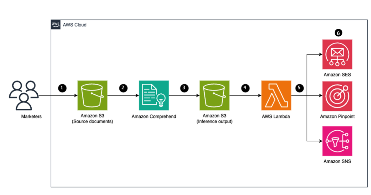


 Figure 8: Amazon Comprehend – Endpoint settings


