Post Syndicated from Julien Lafaye original https://aws.amazon.com/blogs/big-data/how-cfm-built-a-well-governed-and-scalable-data-engineering-platform-using-amazon-emr-for-financial-features-generation/
This post is co-written with Julien Lafaye from CFM.
Capital Fund Management (CFM) is an alternative investment management company based in Paris with staff in New York City and London. CFM takes a scientific approach to finance, using quantitative and systematic techniques to develop the best investment strategies. Over the years, CFM has received many awards for their flagship product Stratus, a multi-strategy investment program that delivers decorrelated returns through a diversified investment approach while seeking a risk profile that is less volatile than traditional market indexes. It was first opened to investors in 1995. CFM assets under management are now $13 billion.
A traditional approach to systematic investing involves analysis of historical trends in asset prices to anticipate future price fluctuations and make investment decisions. Over the years, the investment industry has grown in such a way that relying on historical prices alone is not enough to remain competitive: traditional systematic strategies progressively became public and inefficient, while the number of actors grew, making slices of the pie smaller—a phenomenon known as alpha decay. In recent years, driven by the commoditization of data storage and processing solutions, the industry has seen a growing number of systematic investment management firms switch to alternative data sources to drive their investment decisions. Publicly documented examples include the usage of satellite imagery of mall parking lots to estimate trends in consumer behavior and its impact on stock prices. Using social network data has also often been cited as a potential source of data to improve short-term investment decisions. To remain at the forefront of quantitative investing, CFM has put in place a large-scale data acquisition strategy.
As the CFM Data team, we constantly monitor new data sources and vendors to continue to innovate. The speed at which we can trial datasets and determine whether they are useful to our business is a key factor of success. Trials are short projects usually taking up to a several months; the output of a trial is a buy (or not-buy) decision if we detect information in the dataset that can help us in our investment process. Unfortunately, because datasets come in all shapes and sizes, planning our hardware and software requirements several months ahead has been very challenging. Some datasets require large or specific compute capabilities that we can’t afford to buy if the trial is a failure. The AWS pay-as-you-go model and the constant pace of innovation in data processing technologies enable CFM to maintain agility and facilitate a steady cadence of trials and experimentation.
In this post, we share how we built a well-governed and scalable data engineering platform using Amazon EMR for financial features generation.
AWS as a key enabler of CFM’s business strategy
We have identified the following as key enablers of this data strategy:
- Managed services – AWS managed services reduce the setup cost of complex data technologies, such as Apache Spark.
- Elasticity – Compute and storage elasticity removes the burden of having to plan and size hardware procurement. This allows us to be more focused on the business and more agile in our data acquisition strategy.
- Governance – At CFM, our Data teams are split into autonomous teams that can use different technologies based on their requirements and skills. Each team is the sole owner of its AWS account. To share data to our internal consumers, we use AWS Lake Formation with LF-Tags to streamline the process of managing access rights across the organization.
Data integration workflow
A typical data integration process consists of ingestion, analysis, and production phases.
CFM usually negotiates with vendors a download method that is convenient for both parties. We see a lot of possibilities for exchanging data (HTTPS, FPT, SFPT), but we’re seeing a growing number of vendors standardizing around Amazon Simple Storage Service (Amazon S3).
CFM data scientists then look up the data and build features that can be used in our trading models. The bulk of our data scientists are heavy users of Jupyter Notebook. Jupyter notebooks are interactive computing environments that allow users to create and share documents containing live code, equations, visualizations, and narrative text. They provide a web-based interface where users can write and run code in different programming languages, such as Python, R, or Julia. Notebooks are organized into cells, which can be run independently, facilitating the iterative development and exploration of data analysis and computational workflows.
We invested a lot in polishing our Jupyter stack (see, for example, the open source project Jupytext, which was initiated by a former CFM employee), and we are proud of the level of integration with our ecosystem that we have reached. Although we explored the option of using AWS managed notebooks to streamline the provisioning process, we have decided to continue hosting these components on our on-premises infrastructure for the current timeline. CFM internal users appreciate the existing development environment and switching to an AWS managed environment would imply a change to their habits, and a temporary drop in productivity.
Exploration of small datasets is entirely feasible within this Jupyter environment, but for large datasets, we have identified Spark as the go-to solution. We could have deployed Spark clusters in our data centers, but we have found that Amazon EMR considerably reduces the time to deploy said clusters and provides many interesting features, such as ARM support through AWS Graviton processors, auto scaling capabilities, and the ability to provision transient clusters.
After a data scientist has written the feature, CFM deploys a script to the production environment that refreshes the feature as new data comes in. These scripts often run in a relatively short amount of time because they only require processing a small increment of data.
Interactive data exploration workflow
CFM’s data scientists’ preferred way of interacting with EMR clusters is through Jupyter notebooks. Having a long history of managing Jupyter notebooks on premises and customizing them, we opted to integrate EMR clusters into our existing stack. The user workflow is as follows:
- The user provisions an EMR cluster through the AWS Service Catalog and the AWS Management Console. Users can also use API calls to do this, but usually prefer using the Service Catalog interface. You can choose various instance types that include different combinations of CPU, memory, and storage, giving you the flexibility to choose the appropriate mix of resources for your applications.
- The user starts their Jupyter notebook instance and connects to the EMR cluster.
- The user interactively works on the data using the notebook.
- The user shuts down the cluster through the Service Catalog.
Solution overview
The connection between the notebook and the cluster is achieved by deploying the following open source components:
- Apache Livy – This service that provides a REST interface to a Spark driver running on an EMR cluster.
- Sparkmagic – This set of Jupyter magics provides a straightforward way to connect to the cluster and send PySpark code to the cluster through the Livy endpoint.
- Sagemaker-studio-analytics-extension – This library provides a set of magics to integrate analytics services (such as Amazon EMR) into Jupyter notebooks. It is used to integrate Amazon SageMaker Studio notebooks and EMR clusters (for more details, see Create and manage Amazon EMR Clusters from SageMaker Studio to run interactive Spark and ML workloads – Part 1). Having the requirement to use our own notebooks, we initially didn’t benefit from this integration. To help us, the Amazon EMR service team made this library available on PyPI and guided us in setting it up. We use this library to facilitate the connection between the notebook and the cluster and to forward the user permissions to the clusters through runtime roles. These runtime roles are then used to access the data instead of instance profile roles assigned to the Amazon Elastic Compute Cloud (Amazon EC2) instances that are part of the cluster. This allows more fine-grained access control on our data.
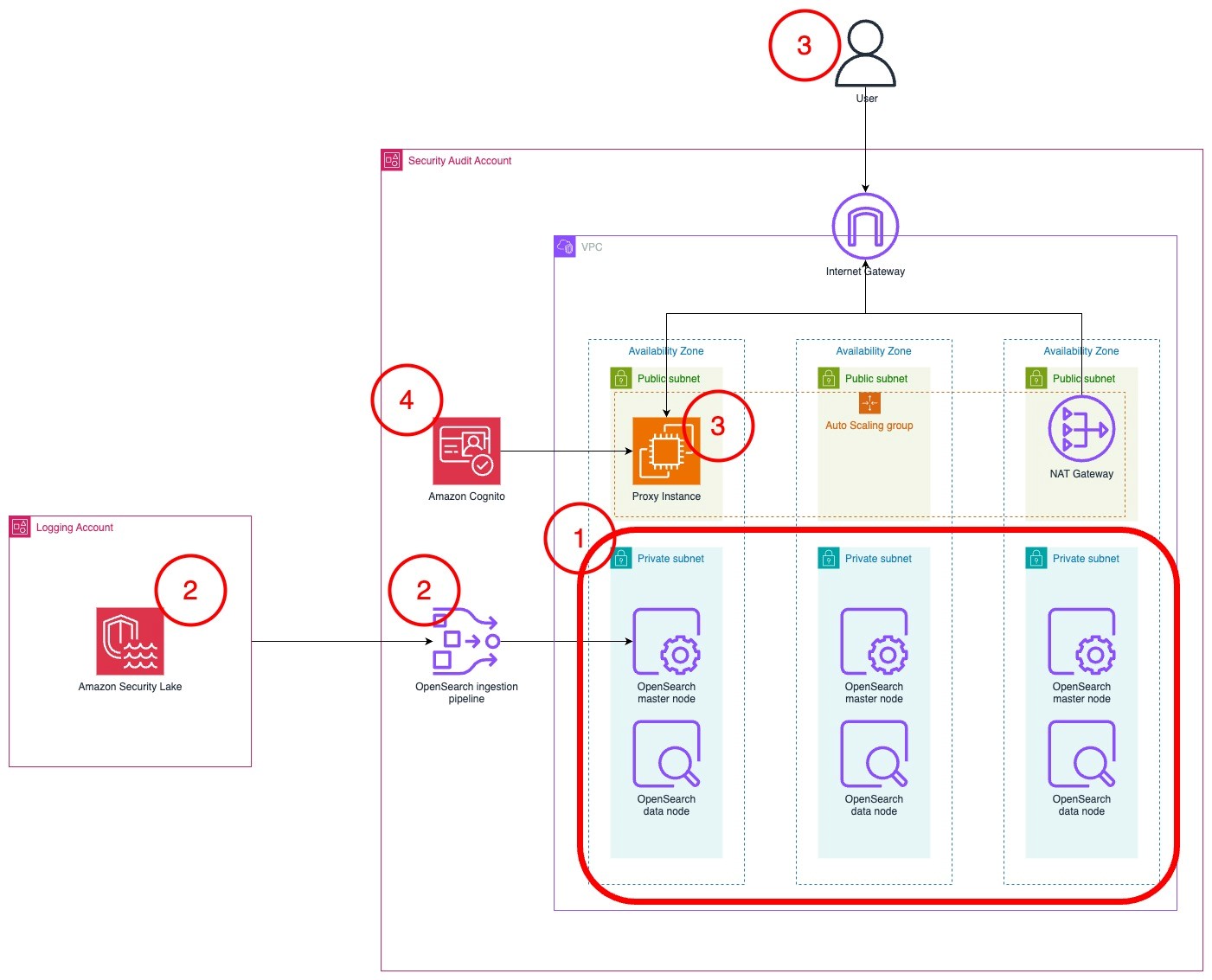
The following diagram illustrates the solution architecture.

Set up Amazon EMR on an EC2 cluster with the GetClusterSessionCredentials API
A runtime role is an AWS Identity and Access Management (IAM) role that you can specify when you submit a job or query to an EMR cluster. The EMR get-cluster-session-credentials API uses a runtime role to authenticate on EMR nodes based on the IAM policies attached runtime role (we document the steps to enable for the Spark terminal; a similar approach can be expanded for Hive and Presto). This option is generally available in all AWS Regions and the recommended release to use is emr-6.9.0 or later.
Connect to Amazon EMR on the EC2 cluster from Jupyter Notebook with the GCSC API
Jupyter Notebook magic commands provide shortcuts and extra functionality to the notebooks in addition to what can be done with your kernel code. We use Jupyter magics to abstract the underlying connection from Jupyter to the EMR cluster; the analytics extension makes the connection through Livy using the GCSC API.
On your Jupyter instance, server, or notebook PySpark kernel, install the following extension, load the magics, and create a connection to the EMR cluster using your runtime role:
Production with Amazon EMR Serverless
CFM has implemented an architecture based on dozens of pipelines: data is ingested from data on Amazon S3 and transformed using Amazon EMR Serverless with Spark; resulting datasets are published back to Amazon S3.
Each pipeline runs as a separate EMR Serverless application to avoid resource contention between workloads. Individual IAM roles are assigned to each EMR Serverless application to apply least privilege access.
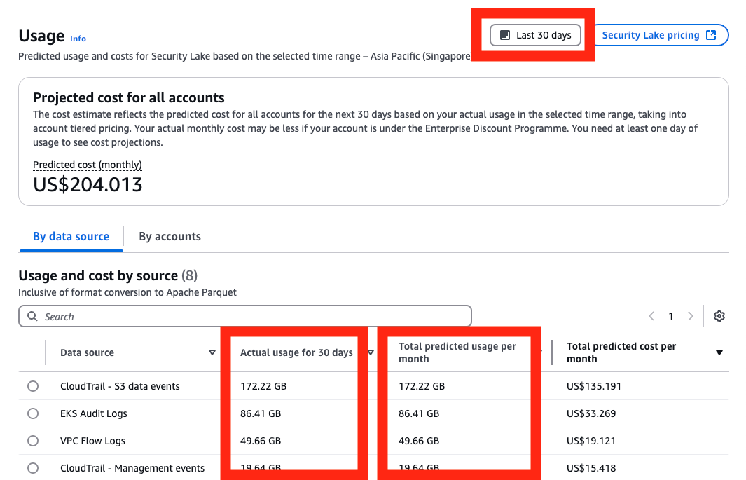
To control costs, CFM uses EMR Serverless automatic scaling combined with the maximum capacity feature (which defines the maximum total vCPU, memory, and disk capacity that can be consumed collectively by all the jobs running under this application). Finally, CFM uses an AWS Graviton architecture to optimize even more cost and performance (as highlighted in the screenshot below).

After some iterations, the user produces a final script that is put in production. For early deployments, we relied on Amazon EMR on EC2 to run those scripts. Based on user feedback, we iterated and investigated for opportunities to reduce cluster startup times. Cluster startups could take up to 8 minutes for a runtime requiring a fraction of that time, which impacted the user experience. Also, we wanted to reduce the operational overhead of starting and stopping EMR clusters.
Those are the reasons why we switched to EMR Serverless a few months after its initial release. This move was surprisingly straightforward because it didn’t require any tuning and worked instantly. The only drawback we have seen is the requirement to update AWS tools and libraries in our software stacks to incorporate all the EMR features (such as AWS Graviton); on the other hand, it led to reduced startup time, reduced costs, and better workload isolation.
At this stage, CFM data scientists can perform analytics and extract value from raw data. Resulting datasets are then published to our data mesh service across our organization to allow our scientists to work on prediction models. In the context of CFM, this requires a strong governance and security posture to apply fine-grained access control to this data. This data mesh approach allows CFM to have a clear view from an audit standpoint on dataset usage.
Data governance with Lake Formation
A data mesh on AWS is an architectural approach where data is treated as a product and owned by domain teams. Each team uses AWS services like Amazon S3, AWS Glue, AWS Lambda, and Amazon EMR to independently build and manage their data products, while tools like the AWS Glue Data Catalog enable discoverability. This decentralized approach promotes data autonomy, scalability, and collaboration across the organization:
- Autonomy – At CFM, like at most companies, we have different teams with difference skillsets and different technology needs. Enabling teams to work autonomously was a key parameter in our decision to move to a decentralized model where each domain would live in its own AWS account. Another advantage was improved security, particularly the ability to contain the potential impact area in the event of credential leaks or account compromises. Lake Formation is key in enabling this kind of model because it streamlines the process of managing access rights across accounts. In the absence of Lake Formation, administrators would have to make sure that resource policies and user policies align to grant access to data: this is usually considered complex, error-prone, and hard to debug. Lake Formation makes this process a lot less complicated.
- Scalability – There are no blockers that prevent other organization units from joining the data mesh structure, and we expect more teams to join the effort of refining and sharing their data assets.
- Collaboration – Lake Formation provides a sound foundation for making data products discoverable by CFM internal consumers. On top of Lake Formation, we developed our own Data Catalog portal. It provides a user-friendly interface where users can discover datasets, read through the documentation, and download code snippets (see the following screenshot). The interface is tailor-made for our work habits.

Lake Formation documentation is extensive and provides a collection of ways to achieve a data governance pattern that fits every organization requirement. We made the following choices:
- LF-Tags – We use LF-Tags instead of named resource permissioning. Tags are associated to resources, and personas are given the permission to access all resources with a certain tag. This makes scaling the process of managing rights straightforward. Also, this is an AWS recommended best practice.
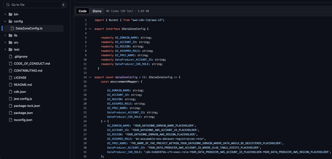
- Centralization – Databases and LF-Tags are managed in a centralized account, which is managed by a single team.
- Decentralization of permissions management – Data producers are allowed to associate tags to the datasets they are responsible for. Administrators of consumer accounts can grant access to tagged resources.
Conclusions
In this post, we discussed how CFM built a well-governed and scalable data engineering platform for financial features generation.
Lake Formation provides a solid foundation for sharing datasets across accounts. It removes the operational complexity of managing complex cross-account access through IAM and resource policies. For now, we only use it to share assets created by data scientists, but plan to add new domains in the near future.
Lake Formation also seamlessly integrates with other analytics services like AWS Glue and Amazon Athena. The ability to provide a comprehensive and integrated suite of analytics tools to our users is a strong reason for adopting Lake Formation.
Last but not least, EMR Serverless reduced operational risk and complexity. EMR Serverless applications start in less than 60 seconds, whereas starting an EMR cluster on EC2 instances typically takes more than 5 minutes (as of this writing). The accumulation of those earned minutes effectively eliminated any further instances of missed delivery deadlines.
If you’re looking to streamline your data analytics workflow, simplify cross-account data sharing, and reduce operational overhead, consider using Lake Formation and EMR Serverless in your organization. Check out the AWS Big Data Blog and reach out to your AWS team to learn more about how AWS can help you use managed services to drive efficiency and unlock valuable insights from your data!
About the Authors
 Julien Lafaye is a director at Capital Fund Management (CFM) where he is leading the implementation of a data platform on AWS. He is also heading a team of data scientists and software engineers in charge of delivering intraday features to feed CFM trading strategies. Before that, he was developing low latency solutions for transforming & disseminating financial market data. He holds a Phd in computer science and graduated from Ecole Polytechnique Paris. During his spare time, he enjoys cycling, running and tinkering with electronic gadgets and computers.
 Matthieu Bonville is a Solutions Architect in AWS France working with Financial Services Industry (FSI) customers. He leverages his technical expertise and knowledge of the FSI domain to help customer architect effective technology solutions that address their business challenges.
 Joel Farvault is Principal Specialist SA Analytics for AWS with 25 years’ experience working on enterprise architecture, data governance and analytics, mainly in the financial services industry. Joel has led data transformation projects on fraud analytics, claims automation, and Master Data Management. He leverages his experience to advise customers on their data strategy and technology foundations.


 Rajkumar Irudayaraj is a Senior Product Director at Salesforce with over 20 years of experience in data platforms and services, with a passion for delivering data-powered experiences to customers.
 Sriram Sethuraman is a Senior Manager in Salesforce Data Cloud product management. He has been building products for over 9 years using big data technologies. In his current role at Salesforce, Sriram works on Zero Copy integration with major data lake partners and helps customers deliver value with their data strategies.
 Jason Berkowitz is a Senior Product Manager with AWS Lake Formation. He comes from a background in machine learning and data lake architectures. He helps customers become data-driven.
 Ravi Bhattiprolu is a Senior Partner Solutions Architect at AWS. Ravi works with strategic ISV partners, Salesforce and Tableau, to deliver innovative and well-architected products and solutions that help joint customers achieve their business and technical objectives.
 Avijit Goswami is a Principal Solutions Architect at AWS specialized in data and analytics. He supports AWS strategic customers in building high-performing, secure, and scalable data lake solutions on AWS using AWS managed services and open source solutions. Outside of his work, Avijit likes to travel, hike, watch sports, and listen to music.
 Ife Stewart is a Principal Solutions Architect in the Strategic ISV segment at AWS. She has been engaged with Salesforce Data Cloud over the last 2 years to help build integrated customer experiences across Salesforce and AWS. Ife has over 10 years of experience in technology. She is an advocate for diversity and inclusion in the technology field.
 Michael Chess is a Technical Product Manager at AWS Lake Formation. He focuses on improving data permissions across the data lake. He is passionate about enabling customers to build and optimize their data lakes to meet stringent security requirements.
 Mike Patterson is a Senior Customer Solutions Manager in the Strategic ISV segment at AWS. He has partnered with Salesforce Data Cloud to align business objectives with innovative AWS solutions to achieve impactful customer experiences. In his spare time, he enjoys spending time with his family, sports, and outdoor activities.


 Diego Colombatto is a Senior Partner Solutions Architect at AWS. He brings more than 15 years of experience in designing and delivering Digital Transformation projects for enterprises. At AWS, Diego works with partners and customers advising how to leverage AWS technologies to translate business needs into solutions.
 Angel Conde Manjon is a Sr. EMEA Data & AI PSA, based in Madrid. He has previously worked on research related to Data Analytics and Artificial Intelligence in diverse European research projects. In his current role, Angel helps partners develop businesses centered on Data and AI.
 Tiziano Curci is a Manager, EMEA Data & AI PDS at AWS. He leads a team that works with AWS Partners (G/SI and ISV), to leverage the most comprehensive set of capabilities spanning databases, analytics and machine learning, to help customers unlock the through power of data through an end-to-end data strategy.

 Abhishek Pan is a Sr. Specialist SA-Data working with AWS India Public sector customers. He engages with customers to define data-driven strategy, provide deep dive sessions on analytics use cases, and design scalable and performant analytical applications. He has 12 years of experience and is passionate about databases, analytics, and AI/ML. He is an avid traveler and tries to capture the world through his lens.
 Gourang Harhare is a Senior Solutions Architect at AWS based in Pune, India. With a robust background in large-scale design and implementation of enterprise systems, application modernization, and cloud native architectures, he specializes in AI/ML, serverless, and container technologies. He enjoys solving complex problems and helping customer be successful on AWS. In his free time, he likes to play table tennis, enjoy trekking, or read books
 Kevin Phillips is a Neptune Specialist Solutions Architect working in the UK. He has 20 years of development and solutions architectural experience, which he uses to help support and guide customers. He has been enthusiastic about evangelizing graph databases since joining the Amazon Neptune team, and is happy to talk graph with anyone who will listen.
 Sandeep Varma is a principal in ZS’s Pune, India, office with over 25 years of technology consulting experience, which includes architecting and delivering innovative solutions for complex business problems leveraging AI and technology. Sandeep has been critical in driving various large-scale programs at ZS Associates. He was the founding member the Big Data Analytics Centre of Excellence in ZS and currently leads the Enterprise Service Center of Excellence. Sandeep is a thought leader and has served as chief architect of multiple large-scale enterprise big data platforms. He specializes in rapidly building high-performance teams focused on cutting-edge technologies and high-quality delivery.

 Hardeep Randhawa is a Senior Manager – Big Data & Analytics, Solution Architecture at HPE, recognized for stewarding enterprise-scale programs and deployments. He has led a recent Big Data EAP (Enterprise Analytics Platform) build with one of the largest global SAP HANA/S4 implementations at HPE.
 Abhay Kumar is a Lead Data Engineer in Aruba Supply Chain Analytics and manages the Cloud Infrastructure for the Application at HPE. With 11+ years of experience in the IT industry domains like banking, supply chain and Abhay has a strong background in Cloud Technologies, Data Analytics, Data Management, and Big Data systems. In his spare time, he likes reading, exploring new places and watching movies.
 Ritesh Chaman is a Senior Technical Account Manager at Amazon Web Services. With 14 years of experience in the IT industry, Ritesh has a strong background in Data Analytics, Data Management, Big Data systems and Machine Learning. In his spare time, he loves cooking, watching sci-fi movies, and playing sports.
 Sushmita Barthakur is a Senior Solutions Architect at Amazon Web Services, supporting Enterprise customers architect their workloads on AWS. With a strong background in Data Analytics and Data Management, she has extensive experience helping customers architect and build Business Intelligence and Analytics Solutions, both on-premises and the cloud. Sushmita is based out of Tampa, FL and enjoys traveling, reading and playing tennis.


 Rajkumar Irudayaraj is a Senior Product Director at Salesforce with over 20 years of experience in data platforms and services, with a passion for delivering data-powered experiences to customers.
 Jason Berkowitz is a Senior Product Manager with AWS Lake Formation. He comes from a background in machine learning and data lake architectures. He helps customers become data-driven.
 Michael Chess is a Technical Product Manager at AWS Lake Formation. He focuses on improving data permissions across the data lake. He is passionate about ensuring customers can build and optimize their data lakes to meet stringent security requirements.
 Mike Patterson is a Senior Customer Solutions Manager in the Strategic ISV segment at AWS. He has partnered with Salesforce Data Cloud to align business objectives with innovative AWS solutions to achieve impactful customer experiences. In his spare time, he enjoys spending time with his family, sports, and outdoor activities.


 Hemant Aggarwal is a senior Data Engineer at Kaplan India Pvt Ltd, helping in developing and managing ETL pipelines leveraging AWS and process/strategy development for the team.
 Naveen Kambhoji is a Senior Manager at Kaplan Inc. He works with Data Engineers at Kaplan for building data lakes using AWS Services. He is the facilitator for the entire migration process. His passion is building scalable distributed systems for efficiently managing data on cloud.Outside work, he enjoys travelling with his family and exploring new places.
 Jimy Matthews is an AWS Solutions Architect, with expertise in AI/ML tech. Jimy is based out of Boston and works with enterprise customers as they transform their business by adopting the cloud and helps them build efficient and sustainable solutions. He is passionate about his family, cars and Mixed martial arts.


 Nofar Diamant is a software team lead at AppsFlyer with a current focus on fraud protection. Before diving into this realm, she led the Retargeting team at AppsFlyer, which is the subject of this post. In her spare time, Nofar enjoys sports and is passionate about mentoring women in technology. She is dedicated to shifting the industry’s gender demographics by increasing the presence of women in engineering roles and encouraging them to succeed.
 Matan Safri is a backend developer focusing on big data in the Retargeting team at AppsFlyer. Before joining AppsFlyer, Matan was a backend developer in IDF and completed an MSC in electrical engineering, majoring in computers at BGU university. In his spare time, he enjoys wave surfing, yoga, traveling, and playing the guitar.
 Michael Pelts is a Principal Solutions Architect at AWS. In this position, he works with major AWS customers, assisting them in developing innovative cloud-based solutions. Michael enjoys the creativity and problem-solving involved in building effective cloud architectures. He also likes sharing his extensive experience in SaaS, analytics, and other domains, empowering customers to elevate their cloud expertise.
 Orgad Kimchi is a Senior Technical Account Manager at Amazon Web Services. He serves as the customer’s advocate and assists his customers in achieving cloud operational excellence focusing on architecture, AI/ML in alignment with their business goals.


 Bandana Das is a Senior Data Architect at Amazon Web Services and specializes in data and analytics. She builds event-driven data architectures to support customers in data management and data-driven decision-making. She is also passionate about enabling customers on their data management journey to the cloud.
 Anirban Saha is a DevOps Architect at AWS, specializing in architecting and implementation of solutions for customer challenges in the automotive domain. He is passionate about well-architected infrastructures, automation, data-driven solutions and helping make the customer’s cloud journey as seamless as possible. Personally, he likes to keep himself engaged with reading, painting, language learning and traveling.
 Chandana Keswarkar is a Senior Solutions Architect at AWS, who specializes in guiding automotive customers through their digital transformation journeys by using cloud technology. She helps organizations develop and refine their platform and product architectures and make well-informed design decisions. In her free time, she enjoys traveling, reading, and practicing yoga.
 Sindi Cali is a ProServe Associate Consultant with AWS Professional Services. She supports customers in building data driven applications in AWS.
 Clarisa Tavolieri is a Software Engineering graduate with qualifications in Business, Audit, and Strategy Consulting. With an extensive career in the financial and tech industries, she specializes in data management and has been involved in initiatives ranging from reporting to data architecture. She currently serves as the Global Head of Cyber Data Management at Zurich Group. In her role, she leads the data strategy to support the protection of company assets and implements advanced analytics to enhance and monitor cybersecurity tools.
 Austin Rappeport is a Computer Engineer who graduated from the University of Illinois Urbana/Champaign in 2011 with a focus in Computer Security. After graduation, he worked for the Federal Energy Regulatory Commission in the Office of Electric Reliability, working with the North American Electric Reliability Corporation’s Critical Infrastructure Protection Standards on both the audit and enforcement side, as well as standards development. Austin currently works for Zurich Insurance as the Global Head of Detection Engineering and Automation, where he leads the team responsible for using Zurich’s security tools to detect suspicious and malicious activity and improve internal processes through automation.
 Samantha Gignac is a Global Security Architect at Zurich Insurance. She graduated from Ferris State University in 2014 with a Bachelor’s degree in Computer Systems & Network Engineering. With experience in the insurance, healthcare, and supply chain industries, she has held roles such as Storage Engineer, Risk Management Engineer, Vulnerability Management Engineer, and SOC Engineer. As a Cybersecurity Architect, she designs and implements secure network systems to protect organizational data and infrastructure from cyber threats.
 Claire Sheridan is a Principal Solutions Architect with Amazon Web Services working with global financial services customers. She holds a PhD in Informatics and has more than 15 years of industry experience in tech. She loves traveling and visiting art galleries.
 Jake Obi is a Principal Security Consultant with Amazon Web Services based in South Carolina, US, with over 20 years’ experience in information technology. He helps financial services customers improve their security posture in the cloud. Prior to joining Amazon, Jake was an Information Assurance Manager for the US Navy, where he worked on a large satellite communications program as well as hosting government websites using the public cloud.
 Srikanth Daggumalli is an Analytics Specialist Solutions Architect in AWS. Out of 18 years of experience, he has over a decade of experience in architecting cost-effective, performant, and secure enterprise applications that improve customer reachability and experience, using big data, AI/ML, cloud, and security technologies. He has built high-performing data platforms for major financial institutions, enabling improved customer reach and exceptional experiences. He is specialized in services like cross-border transactions and architecting robust analytics platforms.
 Freddy Kasprzykowski is a Senior Security Consultant with Amazon Web Services based in Florida, US, with over 20 years’ experience in information technology. He helps customers adopt AWS services securely according to industry best practices, standards, and compliance regulations. He is a member of the Customer Incident Response Team (CIRT), helping customers during security events, a seasoned speaker at AWS re:Invent and AWS re:Inforce conferences, and a contributor to open source projects related to AWS security.


 Çağrı Çakır is the Lead Software Engineer for the PostNL IoT platform, where he manages the architecture that processes billions of events each day. As an AWS Certified Solutions Architect Professional, he specializes in designing and implementing event-driven architectures and stream processing solutions at scale. He is passionate about harnessing the power of real-time data, and dedicated to optimizing operational efficiency and innovating scalable systems.
 Özge Kavalcı works as Senior Solution Engineer for the PostNL IoT platform and loves to build cutting-edge solutions that integrate with the IoT landscape. As an AWS Certified Solutions Architect, she specializes in designing and implementing highly scalable serverless architectures and real-time stream processing solutions that can handle unpredictable workloads. To unlock the full potential of real-time data, she is dedicated to shaping the future of IoT integration.
 Amit Singh works as a Senior Solutions Architect at AWS with enterprise customers on the value proposition of AWS, and participates in deep architectural discussions to make sure solutions are designed for successful deployment in the cloud. This includes building deep relationships with senior technical individuals to enable them to be cloud advocates. In his free time, he likes to spend time with his family and learn more about everything cloud.
 Lorenzo Nicora works as Senior Streaming Solutions Architect at AWS helping customers across EMEA. He has been building cloud-centered, data-intensive systems for several years, working in the finance industry both through consultancies and for fintech product companies. He has used open-source technologies extensively and contributed to several projects, including Apache Flink.

 Adam McCarthy is the EMEA Tech Leader for Healthcare and Life Sciences Startups at AWS. He has over 15 years’ experience researching and implementing machine learning, HPC, and scientific computing environments, especially in academia, hospitals, and drug discovery.

 Balaram Mathukumilli is Director, Enterprise Data Services at DISH Wireless. He is deeply passionate about Data and Analytics solutions. With 20+ years of experience in Enterprise and Cloud transformation, he has worked across domains such as PayTV, Media Sales, Marketing and Wireless. Balaram works closely with the business partners to identify data needs, data sources, determine data governance, develop data infrastructure, build data analytics capabilities, and foster a data-driven culture to ensure their data assets are properly managed, used effectively, and are secure
 Viswanatha Vellaboyana, a Solutions Architect at DISH Wireless, is deeply passionate about Data and Analytics solutions. With 20 years of experience in enterprise and cloud transformation, he has worked across domains such as Media, Media Sales, Communication, and Health Insurance. He collaborates with enterprise clients, guiding them in architecting, building, and scaling applications to achieve their desired business outcomes.
 Keerthi Kambam is a Senior Engineer at DISH Network specializing in AWS Services. She builds scalable data engineering and analytical solutions for dish customer faced applications. She is passionate about solving complex data challenges with cloud solutions.
 Raks Khare is a Senior Analytics Specialist Solutions Architect at AWS based out of Pennsylvania. He helps customers across varying industries and regions architect data analytics solutions at scale on the AWS platform. Outside of work, he likes exploring new travel and food destinations and spending quality time with his family.
 Adi Eswar has been a core member of the AI/ML and Analytics Specialist team, leading the customer experience of customer’s existing workloads and leading key initiatives as part of the Analytics Customer Experience Program and Redshift enablement in AWS-TELCO customers. He spends his free time exploring new food, cultures, national parks and museums with his family.
 Shirin Bhambhani is a Senior Solutions Architect at AWS. She works with customers to build solutions and accelerate their cloud migration journey. She enjoys simplifying customer experiences on AWS.
 Vinayak Rao is a Senior Customer Solutions Manager at AWS. He collaborates with customers, partners, and internal AWS teams to drive customer success, delivery of technical solutions, and cloud adoption.