When we built AWS Glue interactive sessions, our goal was to make AWS Glue as interactive as running local Python from a notebook. We mostly succeeded. With a straightforward Python package and a Jupyter notebook, you could execute remotely against the AWS Glue ephemeral Spark backend. The Livy-based approach was ahead of its time, but it had limitations from its REST-based protocol. Running local PySpark unlocked powerful integrated development environment (IDE) features such as debugging and linting, so your environment could understand the code and help you develop Spark applications more quickly. Customers would often split their development work. They used local Spark (or Docker containers) to develop in an IDE on a small amount of data, then switched to AWS Glue interactive sessions to validate scaling and tuning against the full dataset.
With modern PySpark releases came a new protocol: Apache Spark Connect. Spark Connect bridges the gap between these two worlds: you develop in local Python, but execute on AWS Glue against actual data. Today, AWS Glue interactive sessions support Spark Connect natively. You can connect from any environment that supports the PySpark remote() API, including VS Code, PyCharm, Amazon SageMaker Unified Studio notebooks, and standalone Python applications. You don’t need to install specialized kernels or manage cluster infrastructure.
What Spark Connect changes
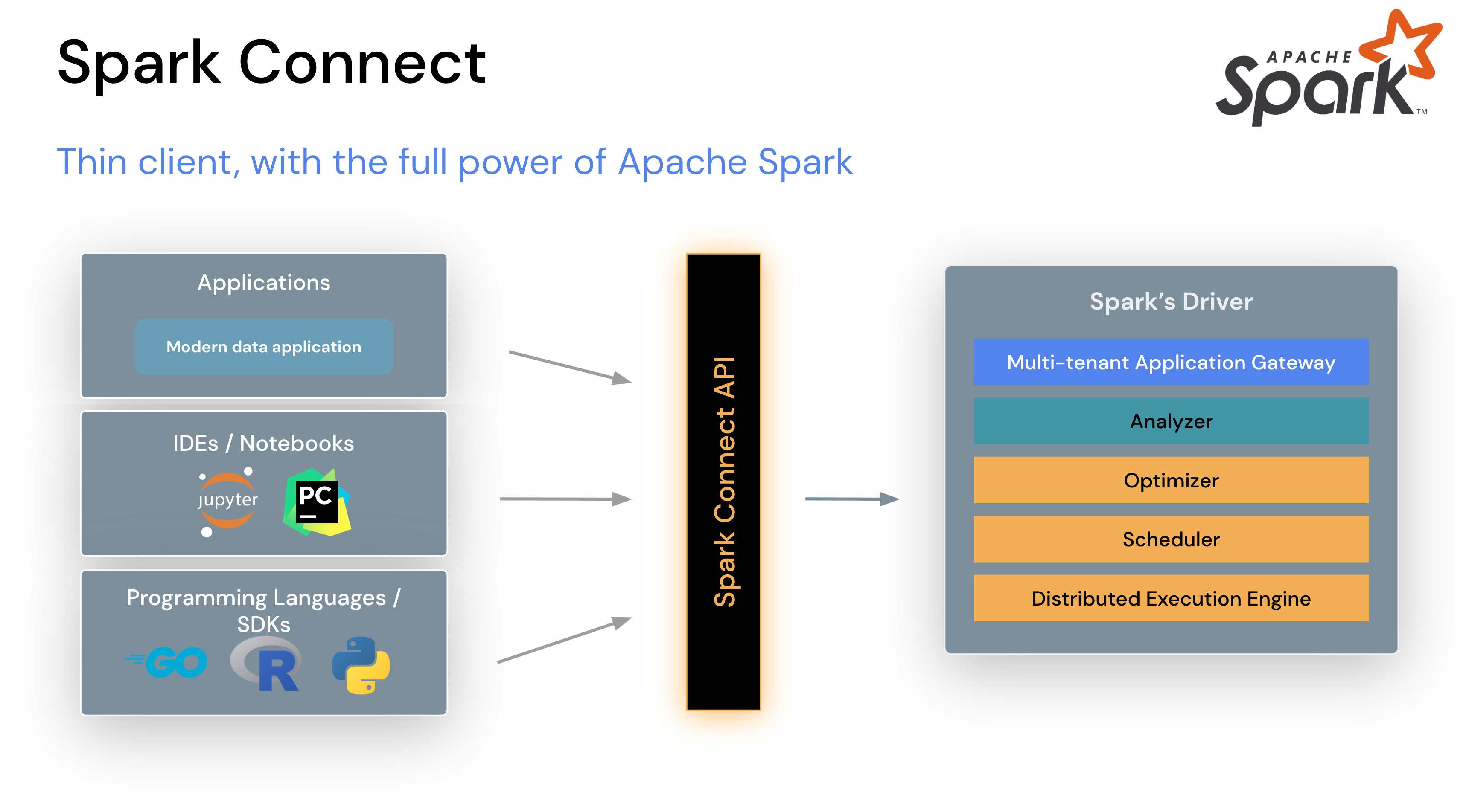
Spark Connect, introduced in Spark 3.4, decouples the Spark client from the server through a lightweight gRPC protocol. Instead of running your driver program on the cluster, your IDE communicates with a remote Spark server through a thin client layer. This architecture unlocks the key workflow improvement: you develop locally and execute remotely.
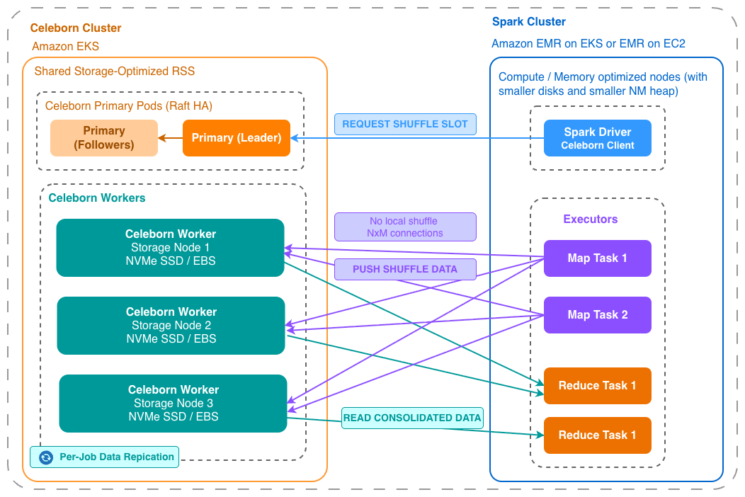
Spark Connect architecture — thin client with the full power of Apache Spark
With Spark Connect support in AWS Glue interactive sessions, you get:
IDE freedom – Use VS Code, PyCharm, JupyterLab, or any Python environment. No kernel installation required.
Programmatic access – Build Spark into your Python applications and automation scripts with a standard SparkSession.builder.remote() call.
Serverless execution – AWS Glue provisions and manages the Spark cluster. You pay only for the data processing units (DPUs) consumed while your session is active.
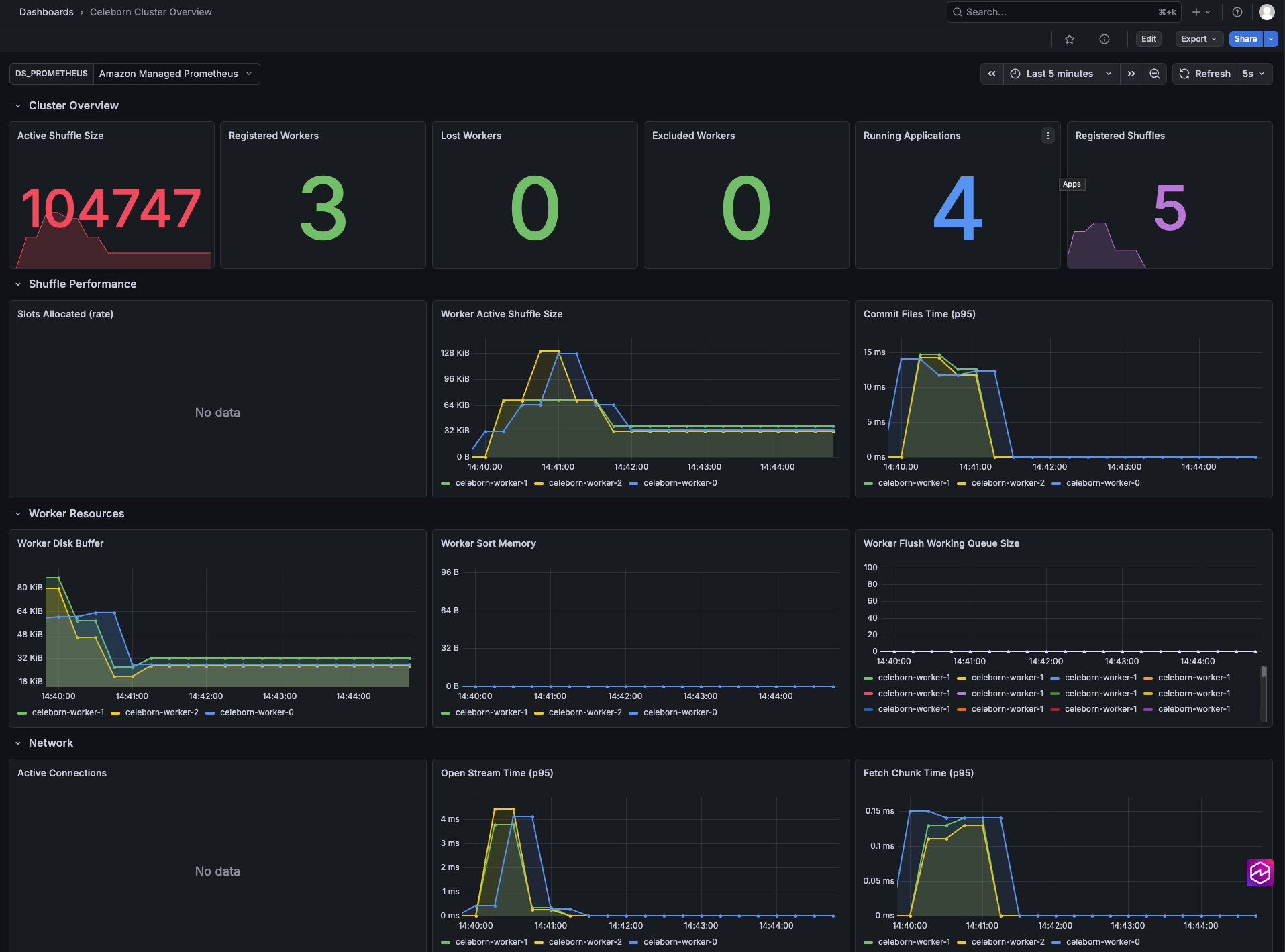
Spark Connect monitoring – The Spark Live UI now includes a dedicated Connect tab showing active Spark Connect sessions and operations alongside the existing Jobs, Stages, and Executors views.
Getting started with SageMaker Unified Studio
Amazon SageMaker Unified Studio provides the most direct path to Spark Connect on AWS Glue. The notebook environment handles session creation, endpoint retrieval, and token refresh automatically, so no connection boilerplate is required.
Prerequisite: You need an Amazon SageMaker Unified Studio project to use this workflow. If you don’t have one, create a project in your SageMaker Unified Studio domain first.
To connect to an AWS Glue Spark Connect session:
Sign in to SageMaker Unified Studio, choose your project, and create or open a Notebook.
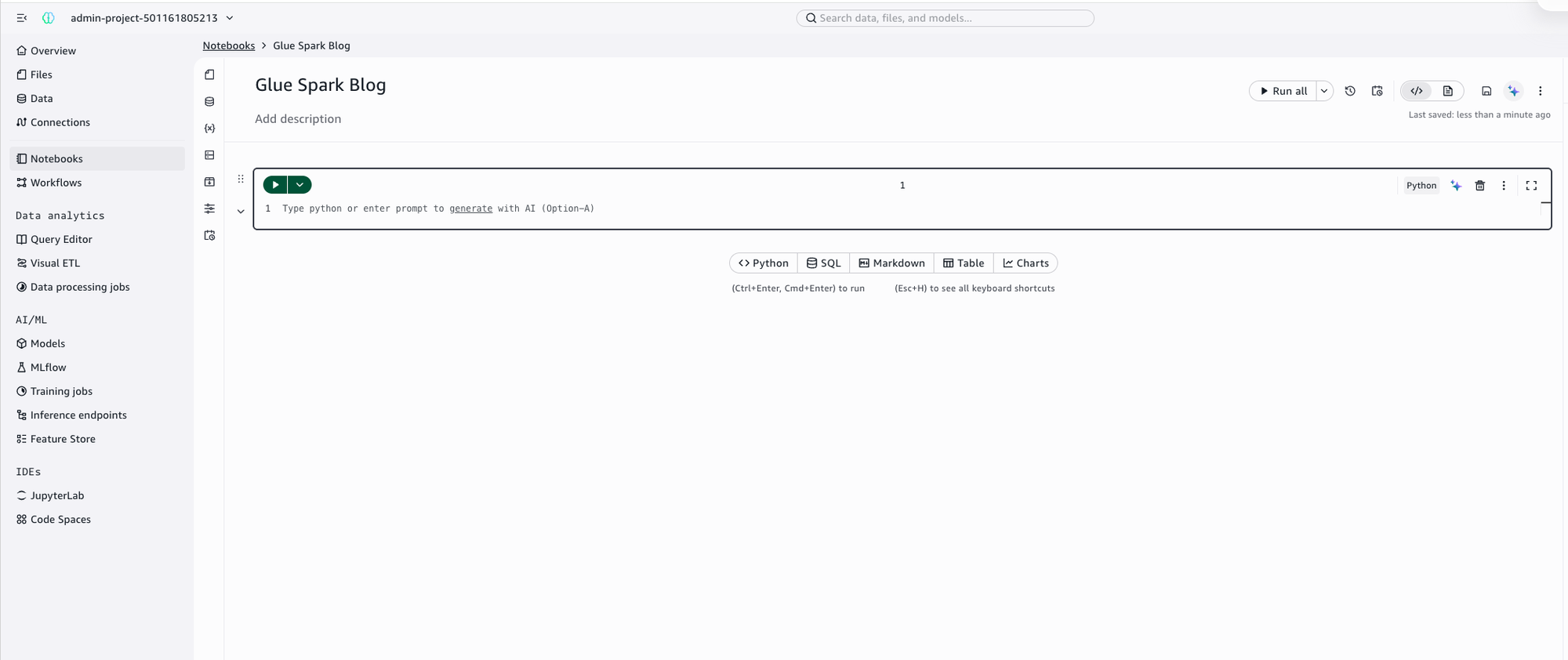
A notebook open in SageMaker Unified Studio
Choose the compute icon in the left toolbar to open the Compute environment panel. Expand the Spark section.
The Compute environment panel with the Spark dropdown list
Select a Glue Spark connection. Depending on your SageMaker domain configuration, you will see either default.spark or named connections such as project.spark.compatibility. Select the appropriate Glue (Spark) connection and choose Apply.
Connected to Glue Spark Connect — running spark.version returns ‘3.5.6-amzn-1’
After you make your selection, you’re connected. The spark session object is available natively. No imports or configuration are needed. Start running PySpark immediately:
spark.sql("SHOW DATABASES").show()
The session manages itself in the background, including automatic token refresh.
Using the sagemaker_studio SDK
The sagemaker-studio Python package extends the Spark Connect experience beyond SageMaker Unified Studio notebooks into local IDEs, continuous integration and continuous delivery (CI/CD) pipelines, and any Python environment. The sparkutils module handles session initialization and connection configuration in a single call. You get the same streamlined experience as in the notebook, anywhere you run Python:
from sagemaker_studio import sparkutils
# Initialize a Glue Spark Connect session using your project connection
spark = sparkutils.init(connection_name="default.spark")
# Run queries immediately
spark.sql("SHOW DATABASES").show()
You can also use sparkutils.get_spark_options() to retrieve pre-configured Java Database Connectivity (JDBC) options for reading and writing to data sources through your project connections. Supported sources include Amazon Redshift, Amazon Aurora, and Amazon DocumentDB (with MongoDB compatibility):
# Get connection options for a Redshift connection in your project
options = sparkutils.get_spark_options("my_redshift_connection")
# Read from Redshift via Spark Connect
df = spark.read.format("jdbc").options(**options).option("dbtable", "analytics.orders").load()
df.show()
Within SageMaker Unified Studio, the sagemaker-studio SDK is native to the environment. The spark session and sparkutils are available without installation. For local IDE use, install it with pip install sagemaker-studio and configure credentials through an AWS named profile or boto3 session.
How it works
Spark Connect sessions in AWS Glue use a three-step workflow:
Create a session – Call the CreateSession API with SessionType set to SPARK_CONNECT. The session provisions in approximately 30 seconds.
Retrieve the endpoint – Call GetSessionEndpoint to receive a sc:// gRPC endpoint URL and a time-limited authentication token.
Connect with PySpark – Pass the endpoint and token to SparkSession.builder.remote() and start running Spark operations.
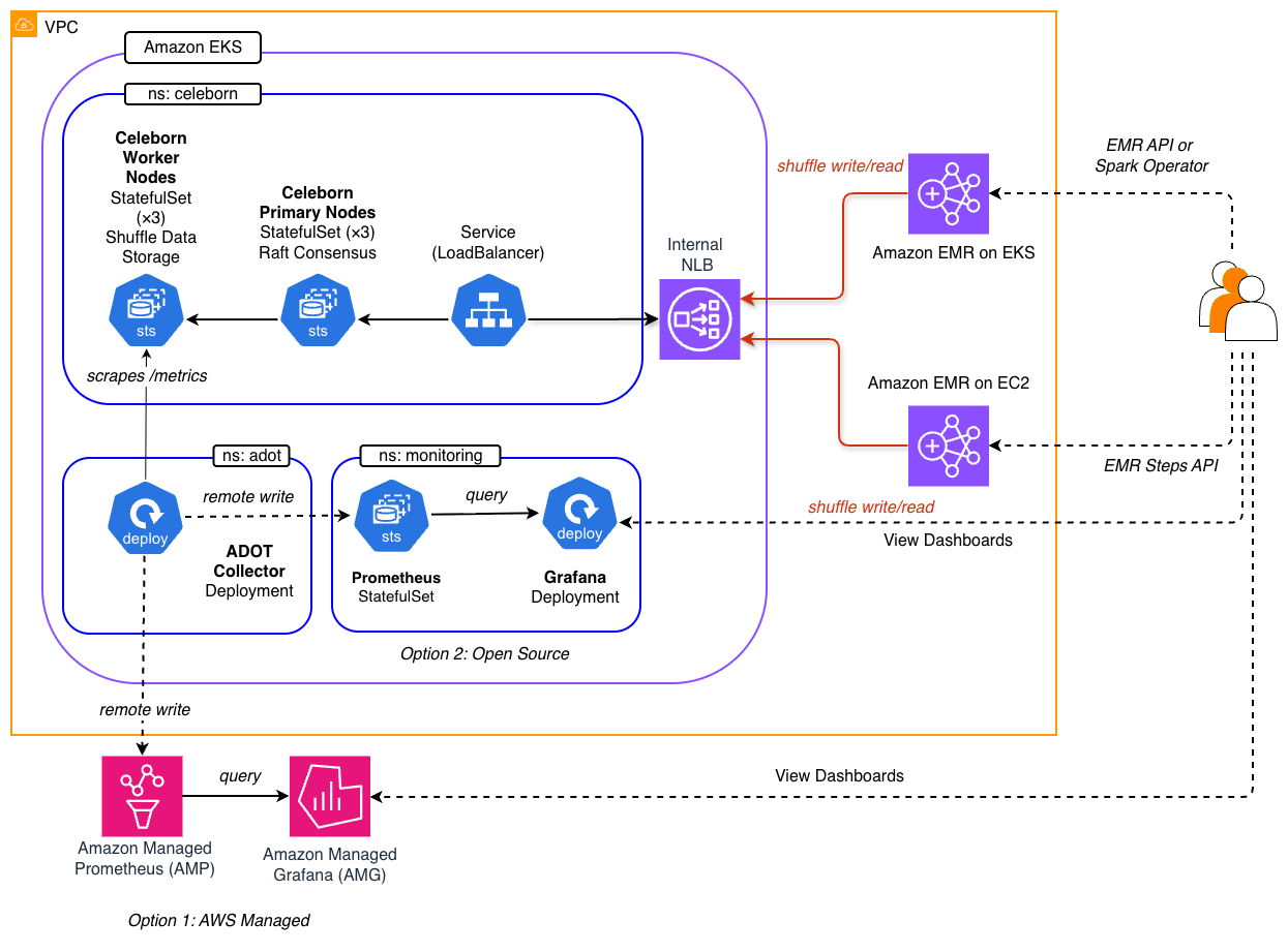
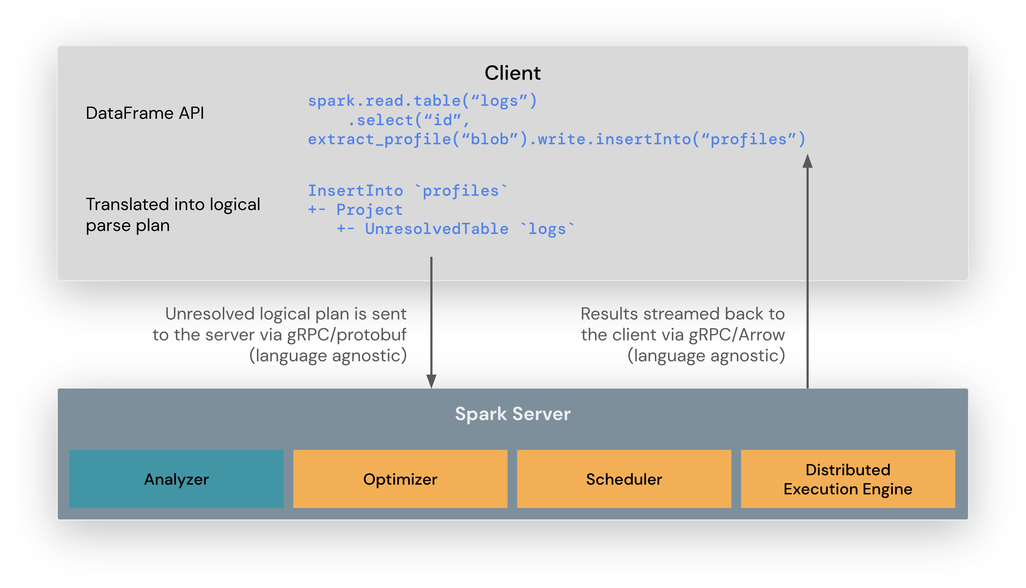
Spark Connect protocol flow — DataFrame API translated to logical plan, sent via gRPC/protobuf, results streamed back via gRPC/Arrow
Connecting with the low-level API
Some environments don’t have the sagemaker-studio SDK, such as custom containers, AWS Lambda functions, or non-Python toolchains. In these environments, or if you’re not using SageMaker Unified Studio, you can use the AWS SDK (Boto3) to manage sessions directly. The following example demonstrates the full workflow:
import time, boto3, urllib.parse
from pyspark.sql import SparkSession
glue = boto3.client("glue", region_name="us-east-1")
# 1. Create a Spark Connect session
session_id = "my-spark-connect-session"
glue.create_session(
Id=session_id,
Role="arn:aws:iam::123456789012:role/GlueServiceRole",
Command={"Name": "glueetl"},
GlueVersion="5.1",
SessionType="SPARK_CONNECT",
DefaultArguments={"--enable-spark-live-ui": "true"},
)
# 2. Wait for the session to reach READY
while True:
status = glue.get_session(Id=session_id)["Session"]["Status"]
if status == "READY":
break
time.sleep(5)
# 3. Get the Spark Connect endpoint
sc = glue.get_session_endpoint(SessionId=session_id)["SparkConnect"]
endpoint_url = sc["Url"]
auth_token = sc["AuthToken"]
# 4. Connect with PySpark
encoded_token = urllib.parse.quote(auth_token, safe="")
connection_string = f"{endpoint_url}:443/;use_ssl=true;x-aws-proxy-auth={encoded_token}"
spark = SparkSession.builder.remote(connection_string).getOrCreate()
spark.sql("SELECT 1 + 1 AS result").show()
Monitoring with Spark Live UI
When you enable the Spark Live UI at session creation, you gain access to a real-time dashboard showing:
Jobs and Stages – Track active, completed, and failed jobs with stage-level metrics.
Executors – Monitor memory usage, shuffle data, and executor health.
SQL – Inspect query plans and execution details.
Connect tab – View active Spark Connect sessions and operations (specific to Spark Connect).
Access the dashboard through the GetDashboardUrl API or directly from the AWS Glue console.
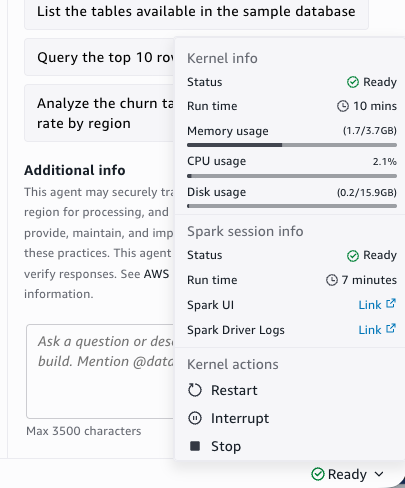
In SageMaker Unified Studio, no API call is needed. Choose Ready in the notebook status bar to open the kernel info popover. From there, open the Spark UI link for the live dashboard or Spark Driver Logs for real-time log output.
Image showing “Ready” in the status bar to access Spark UI and Driver Logs directly from the notebook
Token refresh
Authentication tokens expire after 30 minutes. In SageMaker Unified Studio, this is handled automatically. For programmatic use, you can use a background thread to keep the connection alive. The following helper reconnects transparently before the token expires:
import threading, time, boto3, urllib.parse
from pyspark.sql import SparkSession
class GlueSparkConnect:
"""Maintains a SparkSession with automatic token refresh."""
def __init__(self, session_id, region="us-east-1", refresh_margin=300):
self.session_id = session_id
self.glue = boto3.client("glue", region_name=region)
self.refresh_margin = refresh_margin # seconds before expiry to refresh
self._lock = threading.Lock()
self.spark = self._connect()
self._start_refresh_loop()
def _connect(self):
sc = self.glue.get_session_endpoint(SessionId=self.session_id)["SparkConnect"]
encoded_token = urllib.parse.quote(sc["AuthToken"], safe="")
remote_url = f"{sc['Url']}:443/;use_ssl=true;x-aws-proxy-auth={encoded_token}"
self._token_expiry = sc["AuthTokenExpirationTime"].timestamp()
return SparkSession.builder.remote(remote_url).getOrCreate()
def _start_refresh_loop(self):
def _loop():
while True:
sleep_for = max(self._token_expiry - time.time() - self.refresh_margin, 30)
time.sleep(sleep_for)
with self._lock:
self.spark = self._connect()
t = threading.Thread(target=_loop, daemon=True)
t.start()
# Usage
session = GlueSparkConnect("my-spark-connect-session")
session.spark.sql("SELECT 1 + 1 AS result").show()
The background thread sleeps until 5 minutes before token expiry, then transparently reconnects. Because the daemon thread exits when your script ends, there is no cleanup required.
Getting started
To start using Spark Connect with AWS Glue interactive sessions:
Grant your AWS Identity and Access Management (IAM) identity permissions for glue:CreateSession, glue:GetSession, and glue:GetSessionEndpoint.
Create a session with --session-type SPARK_CONNECT and connect from your preferred environment.
VPC note: If you connect to AWS Glue interactive sessions through a virtual private cloud (VPC) endpoint, add the new Spark Connect endpoint (com.amazonaws.{region}.glue.sessions) to your VPC configuration. Existing AWS Glue VPC endpoints don’t cover Spark Connect traffic.
For detailed instructions, see Connecting to a Spark Connect session in the AWS Glue Developer Guide.
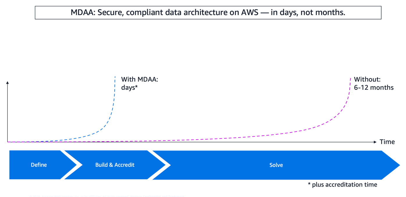
Modern Data Architecture Accelerator (MDAA) is an open source framework that replaces infrastructure code with concise YAML configuration, so your team can deploy a governed, production-ready data architecture, reducing deployment time from months to weeks (depending on complexity and team experience).
Organizations building modern data architecture on AWS face a critical challenge: deploying production-ready, governed infrastructure traditionally requires 6–12 months of custom development, thousands of lines of infrastructure code, and continuous remediation cycles to maintain security and compliance. Governance is often added incrementally, treated as an afterthought that creates compliance gaps and engineering rework.
MDAA addresses this by replacing infrastructure code with concise YAML configuration, achieving up to 97.6 percent code reduction (from approximately 1,800 lines of AWS CloudFormation to 45 lines of MDAA YAML) while embedding governance from the start. The complete Governed Lakehouse Starter Kit deploys 491 AWS resources across 12 stacks from approximately 450 lines of YAML configuration, representing a 66x verbosity ratio where each line automatically expands into production-ready infrastructure.
In this post, we explore how MDAA transforms data architecture development from months of manual coding to production-ready deployment through configuration-driven infrastructure and embedded governance, examine a real customer transformation, and provide a clear implementation pathway for your own data modernization journey.
Customer use case and challenge
A university system office needed to modernize its analytics architecture across 17 campuses while managing sensitive educational data. Their third-party dependency created bottlenecks that slowed feature implementation from weeks to months, and their IT team lacked the cloud skillsets to build modern infrastructure independently.
With MDAA, they achieved:
95 percent reduction in time-to-value for dashboard and feature implementation (from weeks to hours).
17 campuses integrated into a unified, secure architecture.
7.2TB of data and over 8,000 dashboards migrated successfully.
Significant cost savings by removing third-party dependencies and reducing license costs.
Enhanced security posture for external stakeholders accessing sensitive educational data.
The team used MDAA to implement a modernization strategy with continuous integration and continuous delivery (CI/CD) for automated deployment. The architecture now supports rapid response to stakeholder requests while maintaining strict data governance through AWS Lake Formation.
Their transformation demonstrates what becomes possible when governance is embedded from launch rather than added incrementally, moving from months-long manual development to weeks of production-ready deployment through configuration-driven infrastructure.
Solution: MDAA and its value propositions
MDAA’s capabilities stem from its modular, composable architecture. The accelerator provides over 40 pre-built modules that encapsulate AWS best practices for security, governance, and operational excellence. Organizations describe the outcomes they want in MDAA-specific YAML configuration files (not CloudFormation or Terraform YAML) and the accelerator automatically translates these configurations into AWS Cloud Development Kit (AWS CDK) constructs, which then deploy via CloudFormation with embedded governance.
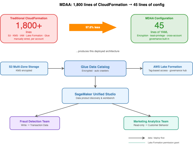
Configuration over code. The MDAA framework takes a fundamentally different approach: describe the outcomes you want in YAML, and the accelerator deploys production-ready infrastructure with embedded governance. Consider deploying a governed data lake where fraud detection teams need write access to transaction data, while marketing analytics teams require read-only access to customer behavior data. Traditional approaches require over 1,800 lines of CloudFormation across Amazon Simple Storage Service (Amazon S3) buckets, AWS Key Management Service (AWS KMS) keys, AWS Identity and Access Management (IAM) policies, and Lake Formation permissions. With MDAA, the same governed data lake is expressed in 45 lines of configuration, a 97.6 percent reduction, while helping you apply encryption, least-privilege access, and cross-account governance as built-in defaults.
The configuration deploys multi-zone S3 storage with KMS encryption, Lake Formation permissions with tag-based access control (TBAC) enabled, Amazon SageMaker Unified Studio for data product discovery, and encrypted AWS Glue Data Catalog with automated crawlers. All permissions flow through Lake Formation rather than individual IAM policies.
Embedded governance from day one. Governance is declared in YAML and deployed alongside infrastructure from the first run. Fine-grained access controls, encrypted data catalogs, data quality validation, audit trails, and sensitive data classification are all part of the same configuration. MDAA’s Governed Lakehouse starter kit defines an entire governed data architecture in roughly 450 lines of YAML, which produces approximately 29,700 lines of CloudFormation across 12 stacks (a 98.5 percent reduction in infrastructure code).
Modular, composable architecture. Each module is purpose-built to handle a specific capability within the data architecture. Modules communicate through AWS Systems Manager Parameter Store, passing resource identifiers (Amazon Resource Names (ARNs), IDs, and names) between stacks. This approach removes hardcoded dependencies. A KMS key created in one module can be referenced by another through parameter resolution, with all dependencies resolved automatically at deployment time.
The diagram illustrates the deployed architecture and team-level access flow that MDAA generates from the 45-line configuration.
Progressive architecture patterns. MDAA provides four reference architecture patterns that align to progressive stages of data infrastructure maturity:
Basic Data Lake deploys a governed data lake with built-in security controls, data quality checks, centralized metadata management using AWS Lake Formation and AWS Glue.
Data Science Platform extends the data lake with Amazon SageMaker notebooks, feature stores, and machine learning (ML) pipelines so data science teams can experiment and train models on governed data.
SageMaker Unified Studio adds a single interface for analytics and ML collaboration, connecting data engineers, analysts, and data scientists in one workspace.
Generative AI Platform layers Amazon Bedrock and Retrieval Augmented Generation (RAG) capabilities on top of your existing data foundation, so teams can build generative AI applications grounded in enterprise data.
Each pattern builds the one before it. You can start with the Basic Data Lake and adopt additional patterns as your team’s needs grow. MDAA’s modular design means you add capabilities without rearchitecting what you already deployed.
The infrastructure is versioned through GitHub, repeatable across environments, and auditable through comprehensive AWS CloudTrail logging. Data engineers focus on data pipelines and business logic while MDAA manages infrastructure complexity and governance integration. This represents the fundamental shift: from writing infrastructure code to describing the outcomes you want through configuration, with governance embedded from the start.
Use case of MDAA: Governed data architecture
DataOps teams spend significant time on governance tasks, including permissions management, compliance validation, and access control, rather than building pipelines and analytics. These aren’t data problems, they’re governance problems that consume engineering capacity meant for higher-value work. MDAA addresses this at the architectural level. Governance is declared in YAML and deployed alongside infrastructure from the first run.
The following sections walk through how each governance module works in practice.
Publish, discover, subscribe, and consume data products between business units: SageMaker Unified Studio
Amazon SageMaker Unified Studio provides a governed data catalog where data producers publish data products, and consumers discover and subscribe to them. Your deployment with MDAA includes a pre-configured domain, blueprints (managed and custom), projects, and environment profiles, all defined in a single configuration file:
Behind this configuration, MDAA deploys an Amazon SageMaker Unified Studio domain with dedicated KMS keys, execution and provisioning roles, and single sign-on group profiles for team access. Data producers tag and publish assets with metadata, ownership, and classification. Consumers browse a searchable catalog, see only authorized assets, and request access through a governed workflow. Cross-account and cross-business-unit data sharing flows through a subscription model, ensuring every access grant is tracked, auditable, and revocable.
Use case of MDAA: Restricting access to cardholder data using Lake Formation
AWS Lake Formation provides fine-grained access control at database and table levels, removing manual IAM policy management. MDAA deploys AWS Lake Formation with pre-configured settings that disable IAMAllowedPrincipals, the critical governance setting that ensures all permissions flow through centralized governance:
That last flag is the single most important governance setting in the platform. Without it, an IAM principal with glue:GetTable can read tables in the catalog, bypassing the entire access control model. Most manual setups miss this or defer it.
With the data lake configuration, you declare roles and access policies in YAML where admins get full control, engineers get read access to curated data, extract, transform, and load (ETL) roles get scoped write access, and MDAA compiles them into the correct S3 bucket policies and Lake Formation registrations.
Use case of MDAA: Ensuring data integrity with AWS Glue Data Quality
AWS Glue Data Quality runs automated validation rulesets continuously as part of the pipeline, not as periodic batch checks. MDAA’s data quality module supports over 15 built-in rule types, from completeness and uniqueness checks to statistical thresholds and data freshness validation:
Quality metrics flow into Amazon CloudWatch for real-time alerting. If anomalies are detected, automated workflows quarantine affected records and alert data engineering teams before issues reach downstream consumers.
Protecting metadata at rest: AWS Glue Data Catalog encryption
Table schemas, column names, and partition structures can reveal sensitive information about an organization’s data architecture, even without access to the underlying data. AWS Glue Catalog Encryption secures metadata at rest using AWS KMS-managed keys. MDAA configures catalog encryption by default, so schema definitions and connection passwords are encrypted from initial deployment without requiring manual key management setup. Access to catalog metadata follows the same Lake Formation governance controls applied to the data itself, so teams see only the schemas that they’re authorized to query.
Auditing every data access event: CloudTrail integration
Every data access event must be logged and attributable to a specific identity. Without a complete audit trail, demonstrating compliance during a regulatory review becomes a manual, error-prone process. AWS CloudTrail captures API-level activity across the data infrastructure, recording who accesses what data, when, and from which service. MDAA configures CloudTrail integration by default, so audit logging is active from initial deployment rather than added retroactively. Log data flows into a centralized, tamper-resistant store, giving compliance teams a single location to query access history across all business units and accounts.
Identifying sensitive data automatically: Macie integration
In large environments, sensitive information spreads across dozens of S3 buckets through pipelines, transforms, and ad hoc data drops, and self-reporting data owners consistently produce gaps. Amazon Macie uses machine learning to automatically discover and classify sensitive data in S3, surfacing findings at the object level without manual tagging. MDAA configures Macie across your S3 buckets during deployment, routing findings to Amazon EventBridge where automated workflows can alert owners or trigger remediation.
Together, these controls form a layered defense: Lake Formation governs access to cataloged data, Glue Data Quality validates integrity on arrival, and Macie identifies sensitive data that lands outside governed pipelines to reduce compliance risk.
Multi-account data mesh
MDAA provides extensive support for multi-account data mesh setups, with decentralized data ownership across business units and centralized governance. The data mesh starter kit supports cross-account data product publishing and consumption, allowing organizations to scale data sharing while maintaining consistent security and compliance controls.
Technical implementation
Ready to deploy your modern data architecture? Here are the resources to get started:
MDAA Implementation Guide provides detailed instructions for deploying all starter packages, including architecture patterns, configuration examples, security best practices, and troubleshooting guidance.
MDAA Hands-on Workshop offers step-by-step guided implementation with AWS experts. The workshop covers configuration management best practices, implementation patterns, hands-on labs with real-world scenarios, and cleanup instructions.
Organizations approach MDAA from different starting points. Some modernize existing data architectures, migrating from on-premises infrastructure or legacy cloud architectures. Others build new architectures for artificial intelligence and machine learning (AI/ML) initiatives or generative AI applications. Financial services organizations require PCI-DSS compliance from day one. Healthcare organizations need controls that can help support HIPAA. Each journey benefits from MDAA’s configuration-driven approach and embedded governance.
Conclusion
MDAA transforms data architecture development from months of manual coding to production-ready deployment. Configuration-driven infrastructure reduces development time by 40–60 percent while embedding governance from the start. The university system’s 95 percent reduction in time-to-value demonstrates the outcome: organizations deploy secure, compliant, governed data architectures in weeks rather than months.
Financial services organizations can deploy architectures to help them align with PCI-DSS compliance requirements using Lake Formation access controls, Glue Data Quality validation, SageMaker Unified Studio data discovery, comprehensive CloudTrail audit trails, and automated Macie data classification, all inherited from configuration rather than built manually.
Data architecture journeys need not follow six-month timelines with governance added incrementally. MDAA provides an alternative: describe the outcomes you want through YAML configuration, inherit pre-validated security controls, and deploy production-ready infrastructure with comprehensive governance from initial deployment.
Security and compliance is a shared responsibility between AWS and the customer. For more information, see the AWS Shared Responsibility Model.
Need help or have questions? Contact AWS ProServe for personalized guidance on selecting the right package and deployment strategy for your organization.
Amazon Redshift recently announced the general availability of a new Graviton-powered instance called RG. Built on Amazon’s own Graviton processors, RG delivers:
Up to 2.2x faster performance for data warehouse workloads compared to RA3.
Up to 2.4x faster for Iceberg queries and 1.5x faster for Parquet queries through an integrated vectorized data lake engine.
No per-TB scan charges for data lake queries, eliminating the Amazon Redshift Spectrum cost applied on RA3 clusters.
30 percent lower cost per vCPU compared to RA3.
RG is both faster and cheaper. While cloud vendors typically charge more for faster performance or newer generation hardware, Amazon Redshift delivers better performance at lower cost.
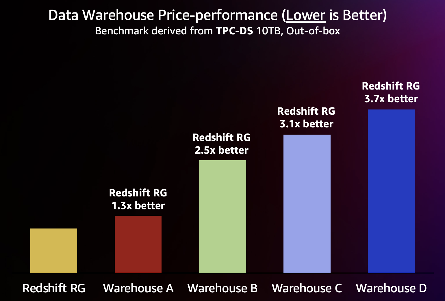
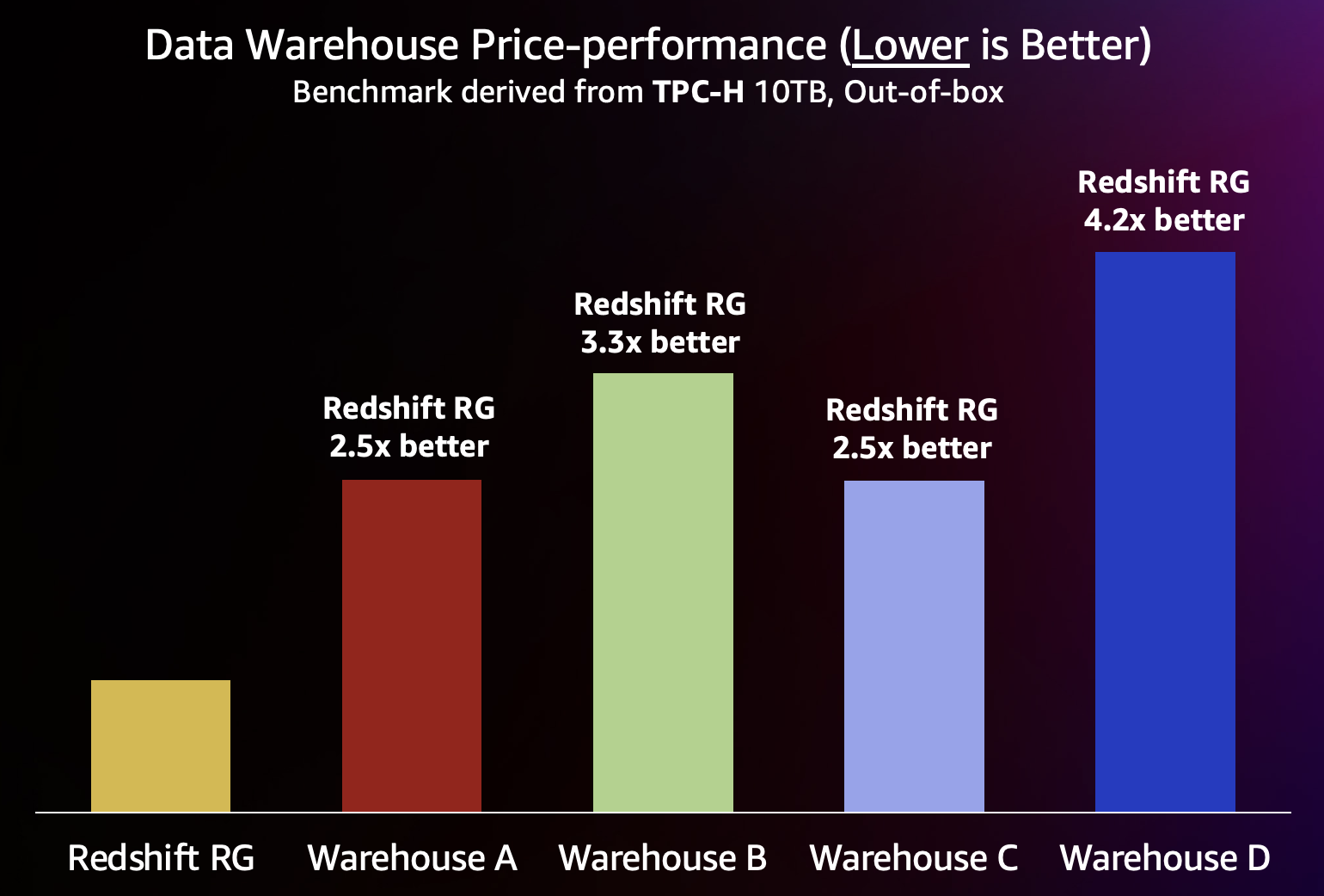
In this post, we describe the innovations that make RG instances so much faster. We also share benchmark results showing that RG delivers up to 4.2x better price-performance than other leading data warehouses.
What makes RG so fast
The new RG instances are built from the ground up to take advantage of Graviton processors. The vectorized engine of Amazon Redshift is optimized with Graviton-based single instruction, multiple data (SIMD) kernels to deliver accelerated, parallelized execution for analytics workloads. Operations like predicate evaluations over Parquet encodings use Graviton vector comparison, table lookup, and vector manipulation intrinsics. To support these increased processing speeds, RG instances use custom-built Nitro SSDs. This lets RG use faster local storage as a caching layer for Amazon Redshift Managed Storage (RMS), data lake scans, and intermediate result sets for computations that can’t fit in memory. RG’s JIT (Just-In-Time) Analyze feature also collects statistics from data lake files automatically as queries run, so the optimizer can produce significantly better query plans. Together, these represent innovation across the entire stack: hardware acceleration with Graviton, vectorized execution with SIMD kernels, high-speed storage with Nitro SSDs, and intelligent query planning with JIT Analyze.
These optimizations, coupled with RG’s purpose-built high-performance vectorized data lake engine, combine to make Amazon Redshift’s new RG instances up to 2.2x faster than RA3 for analytics workloads at 30 percent lower cost.
Purpose-built high-performance vectorized data lake engine
With RA3, data lake queries offloaded scans to a separate compute fleet known as Amazon Redshift Spectrum. Because data lake queries ran on this separate compute, additional overhead was introduced to transfer query metadata and results between RA3 clusters and the Spectrum fleet. Amazon Redshift RG instances include a completely new built-in scan layer designed from the ground up for data lakes. This new scan layer includes a purpose-built I/O subsystem that incorporates smart prefetch capabilities to reduce data latency. The new scan layer is also optimized to process Apache Parquet files, the most commonly used file format for Iceberg, through fast vectorized scans that use SIMD kernels optimized for Graviton. The scan layer includes sophisticated data pruning mechanisms that operate at both partition and file levels, which significantly reduces the volume of data that needs to be scanned. This pruning capability works with the smart prefetch system to create a coordinated approach that maximizes efficiency throughout the entire data retrieval process.
The new purpose-built vectorized data lake engine is up to 2.4x faster than RA3 for Iceberg queries and 1.5x faster than RA3 for Parquet queries.
Because this new vectorized data lake engine integrates directly with the core execution engine of Amazon Redshift, new performance optimizations are possible compared to RA3. With this architecture, data lake queries on RG now benefit from fast local data caching, improved bloom filters, vectorized Parquet scans, and advanced filtering and pruning.
RG also solves a common problem customers face when querying data in the lake: open-format files like Iceberg in Amazon Simple Storage Service (Amazon S3) often lack useful metadata and statistics, which makes it difficult to run a SQL query optimally.
Statistics are metadata about your data, such as distinct value counts, min/max values, distribution patterns, and row counts. The query optimizer uses this information to choose the most efficient way to run a query. For example, when joining two tables, the optimizer needs to know how many unique values each side produces to pick the right join strategy. Without statistics, it has to guess, which often leads to slower joins and unnecessary data movement across nodes. This is where Amazon Redshift’s new feature called JIT (Just-In-Time) Analyze comes in. RG instances automatically fetch and store statistics of your Iceberg files as queries run, so Amazon Redshift can choose query execution strategies that are far more optimized than it could without these statistics.
These improvements make scans of Iceberg and Parquet data much faster than RA3. Removing Amazon Redshift Spectrum compute also means RG instances remove the $5/TB cost for data lake queries, which makes data lake queries cheaper and costs predictable. This is a triple win for data lake price-performance: faster performance, lower compute cost, and no per-TB scan cost.
Faster insights from faster data loads
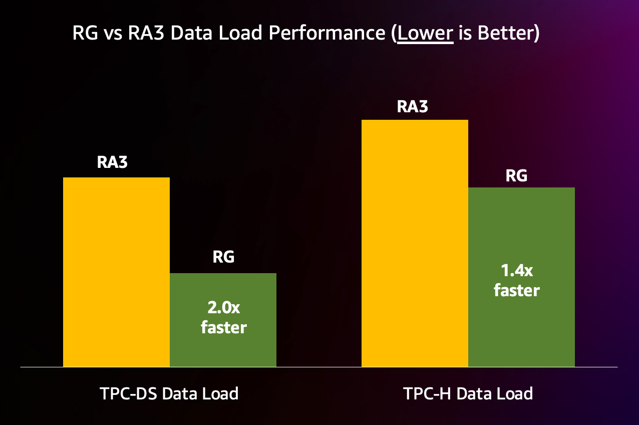
Amazon Redshift RG’s fast I/O and Graviton-optimized engine result in faster data loads compared to RA3. To measure this improved performance, we ran the data ingestion step of 10TB TPC-DS and TPC-H on equivalently sized RA3 and RG clusters. RG ingested the TPC-DS dataset 2x faster and the TPC-H dataset 1.4x faster, as shown in the following figure.
The new Graviton-based RG instances are up to 2.0x faster for data loads compared to RA3 instances. This means workloads can see the latest data sooner, and users and agents can get up-to-date insights faster. This faster ingestion on RG comes at 30 percent lower cost compared to RA3, resulting in up to 2.9x better price-performance for data loads compared to RA3 instances.
What customers are saying
Amazon Redshift customers are already seeing performance and cost benefits of switching to RG. Southwest Airlines and tombola tested their business-critical workloads, and found they could get better performance and save on cost:
Southwest Airlines
“Amazon Redshift RG instances have the potential to deliver meaningful business impact for Southwest Airlines. Based on initial testing in our development environment, our data warehouse workloads run 50–60% faster, and data lake analytics are 45% faster—enabling teams to get insights sooner, respond to operational conditions faster, and make data‑driven decisions with less latency. These early results are encouraging, and we are excited to validate and scale these improvements in production. All of this comes without per‑terabyte Spectrum scanning charges, delivering 30% lower cost than RA3 at a time when fuel prices continue to pressure industry margins!!”
— Sean Lynch, Vice President, Data and Architecture, Southwest Airlines
tombola
“The new Graviton-based Amazon Redshift RG instances delivered 1.8x–2x faster write throughput and up to 2.2x faster read speeds compared to RA3 across a diverse set of batch and analytical jobs — enabling us to process 40% more within the same window. Compressed ETL cycles, accelerated time-to-insight, and decision-making no longer bottlenecked by the pipeline — together, these translated directly into fresher data reaching our analysts and business teams sooner. What made this even more compelling was a concurrent 30% reduction in compute spend alongside the gains — delivering more for less is a rare outcome, and one worth highlighting. In a volume-heavy gaming industry at tombola, where query latency and cost compound at scale, this has been one of the more impactful platform decisions we’ve made this year.”
— Akshay Srinivasan, Data Engineer, tombola
Qoala
“After migrating our Amazon Redshift cluster from RA3 to the new Graviton-based RG instances, we saw 60–70% faster query processing times across our BI and analytics workloads. As a growing insurtech platform handling millions of policy transactions, faster time-to-insight means our data team can deliver dashboards and reports to the business sooner. We moved to a larger node configuration to accommodate future growth, and the performance gains far exceeded the incremental investment – making this one of the most impactful infrastructure decisions we’ve made this year.”
— Umar Abdul Aziz, VP of Data, Qoala
Performance results
To see how RG stacks up, we ran benchmarks derived from the industry-standard TPC-DS and TPC-H benchmarks at 10TB scale on the new Amazon Redshift RG instances and on leading alternative data warehouses. These benchmarks are designed to run queries of various operational requirements and complexities, such as ad hoc, reporting, iterative online analytical processing (OLAP), and data mining. We sized each data warehouse at approximately the same on-demand cost ($32/hr) and ran three power runs of each benchmark out of the box, with no special tuning or manual customization. The results are shown in the following charts.
The new RG instance leads, and by a large margin. Better price-performance means better performance and lower cost.
Conclusion
Amazon Redshift RG instances are the next generation of analytics engine, delivering high performance for data warehouse and data lake workloads. Because RG supports all the same workloads and features as RA3, getting started is straightforward. See our migration guide for how to upgrade and start getting better performance at lower cost.
Find the best price-performance for your workloads
The benchmarks used in this post are derived from the industry-standard TPC-DS and TPC-H benchmarks, and have the following characteristics:
We use the schema and data unmodified from TPC-DS and TPC-H.
The queries are generated using the official TPC-DS and TPC-H kits with query parameters generated using the default random seed of the kits. TPC-approved query variants are used for a warehouse if the warehouse doesn’t support the SQL dialect of the default queries.
The test includes the 99 TPC-DS SELECT queries and 22 TPC-H SELECT queries. It doesn’t include maintenance and throughput steps.
Three power runs were run, and the best run is taken for each data warehouse.
Price-performance is calculated as the cost per hour (USD) divided by 3,600 seconds/hour times the benchmark geomean in seconds, which is equivalent to the geomean cost per query. The latest published on-demand pricing is used for all data warehouses.
We call this the Cloud Data Warehouse benchmark, and you can reproduce the preceding benchmark results using the scripts, queries, and data available in our GitHub repository. It’s derived from the TPC-DS benchmarks as described in this post, and as such isn’t comparable to published TPC-DS results, because the results of our tests don’t comply with the official specification.
Onboard analytics workloads at scale with Amazon Redshift’s improved remote table data definition language (DDL), materialized view improvements, and concurrency scaling enhancements for zero-ETL and auto-copy.
As organizations scale their analytics capabilities, they need the ability to add workloads without disrupting production operation or being constrained by the resources of a single data warehouse. In this post, we introduce new capabilities of Amazon Redshift that enhance our multi-warehouse and scaling capabilities: remote materialized view (MV) operations, remote table DDL support, and concurrency scaling enhancements for zero-ETL and S3 event integration. These features help you build more scalable, performant decentralized analytics architectures on Amazon Redshift.
Let us review how these new features enable you to run analytics at scale.
New remote materialized view operations
Amazon Redshift now classifies CREATE MATERIALIZED VIEW as a user workload, enabling concurrency scaling to execute MV logic on additional warehouses during resource contention. This ensures queries consistently benefit from MV performance advantages, even under heavy load.
Amazon Redshift now supports creating MVs on remote data shares, allowing customers who share data across Redshift warehouses to leverage MV performance benefits on both local and shared data.
ALTER TABLE ALTER DISTSTYLE operations now work on remote warehouses through concurrency scaling and data sharing. You can dynamically optimize data distribution across distributed environments, improving query performance and resource utilization without requiring data migration. This is especially valuable for data engineers fine-tuning performance across multiple warehouses and administrators adapting to changing query patterns.
ALTER TABLE APPEND operations now extend to remote warehouses through concurrency scaling and data sharing. This consolidates data across distributed environments, so you can efficiently combine tables without complex data movement or extract, transform, and load (ETL) processes. Organizations managing dynamic table operations across multiple environments can maintain data consistency while reducing operational overhead.
With these new concurrency scaling capabilities, you can maintain consistent data freshness without compromising existing warehouse performance. This eliminates the traditional trade-off between analytics and data loading. Apart from turning on concurrency scaling, no additional changes are required to take advantage of these features.
Customer use cases
This section covers two industry use cases: the first for a financial services customer and the second for a gaming industry customer.
Financial services use case
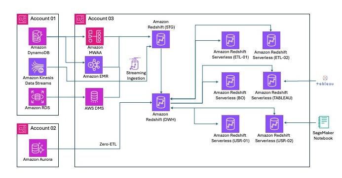
The following is a sample architecture for a large financial services customer with global operations. This customer uses a multi-warehouse architecture built on Amazon Redshift.
The staging (STG) warehouse serves as a raw zone for data from various sources, like the bronze layer of a medallion architecture. This warehouse also cleanses and standardizes the raw data to the silver layer and makes it available for further processing. The STG warehouse uses MVs to process millions of nested JSON messages and extract attributes into scalar columnar Amazon Redshift tables.
CREATE MATERIALIZED VIEW rawdb.fsi.customer_orders_raw
distkey(c_custkey) sortkey(c_custkey) AS (
SELECT c_custkey,
o.o_orderstatus,
o.o_totalprice,
o_idx
FROM customer_orders_lineitem c,
c.c_orders o AT o_idx
);
REFRESH MATERIALIZED VIEW rawdb.fsi.customer_orders_raw;
The DWH warehouse serves as the primary Amazon Redshift instance and gold layer, providing data to consuming applications like Business Objects and Tableau. The zero-ETL concurrency scaling improvements provide consistent data freshness even when zero-ETL ingestion spikes occur alongside heavy DWH workloads. The DWH MVs provide fast access to aggregated data for Tableau extracts and Business Objects live reports. The DWH warehouse takes advantage of concurrency scaling when multiple MVs need to be refreshed on the DWH instance.
CREATE MATERIALIZED VIEW bodb.final.customer_churn_tbl
AS (
SELECT state,
account_length,
area_code,
total_charge/account_length AS average_daily_spend,
cust_serv_calls/account_length AS average_daily_cases,
churn
FROM custdb.final.customer_activity_all
);
REFRESH MATERIALIZED VIEW bodb.final.customer_churn_tbl;
The ETL01/02 warehouses serve as dedicated compute environments for running project-specific ETL jobs, while the USR01/02 warehouses handle user workloads such as ad-hoc analysis or model building from dbt. When new objects are required by user workloads, they are created and maintained on the remote producer warehouse (DWH).
ALTER TABLE salesdb.final.sales_report_all
ALTER DISTKEY sales_id;
ALTER TABLE APPEND salesdb.final.sales_report_all
FROM stagingdb.sales.sales_2026_02;
Gaming industry use case
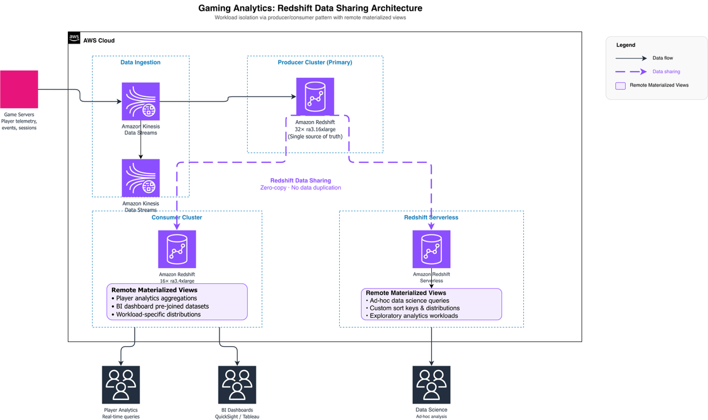
A leading gaming company has built their entire analytics infrastructure on AWS, with their analytics team managing data streaming from games, data warehousing, and business intelligence tools. They standardized Amazon Redshift across the organization, migrating off Vertica running on Amazon Elastic Compute Cloud (Amazon EC2). After overcoming early challenges with cluster resize operations, the team became strong advocates for Amazon Redshift and now runs their primary production cluster on 32 ra3.16xlarge nodes.
As their data ingestion pipeline grew, query workloads began competing with data ingestion processes, creating performance bottlenecks. Rather than scaling up their primary cluster, they implemented a workload isolation strategy using Amazon Redshift data sharing. The customer launched a second 16-node ra3.4xlarge cluster as a data share consumer, with the primary cluster serving as the producer. This architecture allowed them to migrate consumption workloads to the consumer cluster while the producer focused on data ingestion, effectively supporting growth without increasing the primary cluster size.
Recognizing the advantages of this distributed architecture, the gaming company expanded their approach by migrating workloads to Amazon Redshift Serverless, further using the data sharing model for workload isolation. Amazon Redshift’s remote materialized view capability allowed the gaming company to create materialized views directly on the data shared by the producer cluster. Each consumer cluster could now build materialized views optimized for its specific workload patterns. This created pre-aggregated datasets, custom join strategies, and workload-specific data distributions, without impacting the producer cluster’s performance or requiring data duplication. The producer warehouse maintains data distribution and sorting strategies designed for generic enterprise needs, providing consistent data quality across all consumers. Meanwhile, consumer warehouses used remote materialized views to fine-tune query performance for their distinct analytical requirements, whether supporting real-time player analytics, business intelligence dashboards, or ad-hoc data science workloads. This distributed approach to data consumption optimization proved essential for the gaming company. It delivered fast query performance across diverse analytical workloads while maintaining a single source of truth in the producer cluster and avoiding the operational overhead of managing redundant data copies.
Best practices
To get the most out of these new capabilities, consider the following best practices:
Enable concurrency scaling on your Amazon Redshift clusters and Serverless workgroups to allow ETLs and user queries to run even faster, providing consistent report and dashboard performance.
Set up usage limits for concurrency scaling on both Amazon Redshift provisioned clusters and Serverless workgroups by configuring an appropriate MaxRPU setting. This helps you avoid unexpected additional costs. For more information, see the Amazon Redshift usage limits documentation.
Use remote MVs to offload resource-intensive MV creation and refresh operations from your primary warehouse to remote data share clusters.
Conclusion
In this post, we walked through the new MV refresh features, remote table DDL capabilities, and expanded concurrency scaling support for zero-ETL and S3 auto-copy. These features help you move beyond the constraints of a single warehouse. They are particularly valuable for organizations managing distributed data architectures that require dynamic table management across multiple environments while maintaining data consistency and adapting quickly to changing workloads. To get started, make sure you are running the latest Amazon Redshift version. Then visit the Amazon Redshift documentation to learn more about concurrency scaling, data sharing, and materialized views.
The AWS Customer Incident Response Team (AWS CIRT) encounters patterns that repeat across engagements when helping customers respond to security incidents. We’re passionate about making sure that information is accessible so that everyone can improve their security posture and their organization’s resilience to disruption. The primary method we use to share this information is the Threat Technique Catalog for AWS (TTC). The latest update to the catalog for June 2026 focuses on container security, organization-level trust, and compute hijacking. Each new entry reflects something we’ve encountered in practice, and each provides straightforward mitigation. This post breaks down what changed, why it matters, and what you can do about it today.
What we’re seeing
We’ve added five new entries to the TTC.
EKS workload modification
Amazon Elastic Kubernetes Service (Amazon EKS) gives teams powerful orchestration capabilities. We’re seeing threat actors who have obtained Kubernetes credentials or an AWS Identity and Access Management (IAM) role with EKS permissions modify running workloads—altering container images, injecting sidecar containers, or changing pod specifications to introduce malicious code into a deployment.
Nothing new is created. The workload already exists, it might be running in production, and by modifying it in place the threat actor inherits the network access, service account permissions, and data access the legitimate workload already had. Without admission controllers or image verification, these changes can go unnoticed until the impact shows up downstream. Enforcing image signing through admission controllers, restricting workload changes with Kubernetes role-based access control (RBAC), and enabling Amazon GuardDuty EKS Protection to surface anomalous cluster activity all reduce this risk. For more information, see EKS Modification – Workload Integrity Degradation.
Exploit public-facing application – EKS
Publicly exposed Kubernetes API servers and misconfigured ingress controllers continue to be an entry point we see exploited. This technique captures threat actors targeting the customer-deployed workloads running on Amazon EKS—not EKS itself—and their exposure to the internet.
The pattern starts with an exposed service and an application-level weakness, then pivots from the compromised pod toward broader cluster access. When inside a pod, a threat actor can query the instance metadata service, read mounted service account tokens, or move laterally across the cluster network. Limiting public exposure of the Kubernetes API server, applying network policies to restrict pod-to-pod communication, and running workloads with least-privilege service accounts reduce the risk of this technique succeeding. For more information about this technique, see Exploit Public-Facing Application.
Assume root into organization member account
AWS Organizations centralizes trust across member accounts, and that trust runs in one direction—from the management account downward. We’ve observed threat actors who compromise a management account—or gain sufficient privilege within one—use that position to assume root access into member accounts using sts:AssumeRoot. Because the trust is inherent to the organization structure, this can avoid the access controls a member account administrator has configured.
With root access to a member account, a threat actor can disable security controls, delete resources, change billing configurations, and establish persistence that survives remediation focused on IAM principals. We strongly encourage implementing service control policies (SCPs) that restrict which principals can call sts:AssumeRoot and under what conditions, and monitoring for sts:AssumeRoot calls in AWS CloudTrail. For more information, see Assume Root into Organization Member Account.
Compute hijacking – EKS
Compute hijacking remains one of the most common motivations we see behind unauthorized access, and Amazon EKS clusters are increasingly the target. Threat actors deploy cryptocurrency mining or other compute-intensive workloads inside compromised clusters, consuming customer resources and generating unexpected cost.
What sets EKS-based hijacking apart is scale. In clusters without resource quotas, a single compromised service account can consume all available capacity across nodes. The workloads use legitimate-looking images pulled from public registries, which makes image scanning alone insufficient. Setting resource quotas and limit ranges, restricting which registries workloads can pull from, and enabling Amazon GuardDuty EKS Protection to flag mining behavior provides effective detection. For more information, see Resource Hijacking: Compute Hijacking – EKS.
Invite accounts to unknown organization
A threat actor with access to a standalone account—or one they’ve removed from its legitimate organization—invites it into an organization they control. After the account joins, it falls under the threat actor’s governance. The threat actor’s organization can apply SCPs that restrict the legitimate owner’s actions, gain visibility into the account’s resources through organizational services, and access consolidated billing information. The legitimate owner finds themselves locked out of their own governance controls. Monitoring organizations:InviteAccountToOrganization and organizations:AcceptHandshake, and implementing SCPs that prevent accounts from leaving their legitimate organization are important preventive measures. For more information, see Modify Cloud Resource Hierarchy: Invite Accounts to Unknown Organization.
What’s updated
We’ve refreshed three existing entries. S3 Object Collectionnow captures additional API calls used for bulk data staging from Amazon Simple Storage Service (Amazon S3), with refined detection guidance and mitigations that use recent Amazon S3 security features. Compute Hijacking – ECSadds methods threat actors use to deploy unauthorized tasks in Amazon Elastic Container Service (Amazon ECS), including abuse of overly permissive task execution roles. Role Assumption and Federated Access has been expanded to cover new cross-account role assumption variations and identity provider manipulation, with sharper guidance for distinguishing legitimate federated access from unauthorized use.
The current trend
This June update reflects a clear trend: threat actors are increasingly targeting container orchestration platforms and using organizational trust relationships to their advantage. The container techniques show that as organizations adopt Kubernetes at scale, the attack surface grows with it. The organization-level techniques show that threat actors understand organizational trust relationships.
The common thread is that every one of these techniques operates within the boundaries of legitimate functionality. Modifying a workload, assuming cross-account trust, and joining an organization are all expected actions in healthy environments.. Detection, then, depends entirely on context: the principal, the timing, and the sequence of events that follows.
The Threat Technique Catalog for AWS is designed to help with this. We encourage teams to review the relevant entries and assess whether their current monitoring would catch these patterns:
Unexpected modifications to EKS workload specifications
Pod deployments that use unsigned container images
sts:AssumeRoot calls into member accounts
Unbounded compute consumption in your EKS clusters that could be prevented by resource quotas
Unexpected organization invitations to your accounts
Each of the threats leaves traces in AWS CloudTrail and Kubernetes audit logs, and the TTC provides specific guidance on what to watch for and how to respond.
Looking ahead
The Threat Technique Catalog for AWS exists because we believe the patterns we observe during security engagements shouldn’t stay behind closed doors. When we see techniques repeating across customers, the most effective thing we can do is document them and make that knowledge available so you can act on it before you’re in the middle of an incident.
This June update adds five new entries and updates three existing ones, and the catalog will continue to evolve. Our team updates it based on what we’re seeing in the real world when helping customers respond to security events. We encourage security teams to review the catalog, incorporate its techniques into threat modeling exercises, and use it as a shared vocabulary for discussing cloud-specific threats.
When your game server needs both a managed identity provider and its own session system, players face a broken experience if authentication forces a redirect or stalls gameplay. Dual-token authentication for Nakama game servers with Amazon Cognito solves this by connecting two independent session systems, each with its own token lifecycle, without interrupting the player. This post shows you how.
Amazon Cognito handles player identity and Nakama manages game sessions. Cognito issues a JWT, a server-side Go hook validates it and exchanges the verified identity for a Nakama session token. Each token is validated independently on every request. The pattern applies to game servers such as Nakama that support runtime authentication hooks.
The infrastructure wraps Nakama in a default-closed routing layer. Amazon CloudFront serves as the single HTTPS entry point, AWS WAF filters traffic at the edge, an Application Load Balancer (ALB) enforces an explicit route allow-list for HTTP, and a Network Load Balancer (NLB) handles WebSocket TCP passthrough. Nakama runs on Amazon Elastic Container Service (Amazon ECS) on AWS Fargate. In this post, we cover the Cognito configuration, the Go hook, the Terraform infrastructure, and the WebSocket lifecycle controls.
In this post, you learn how to:
Configure an Amazon Cognito User Pool for SRP-based game client authentication with no client secret.
Implement a Go runtime hook that validates Cognito JWTs and bridges player identity to Nakama sessions.
Set up a default-closed routing layer using Amazon CloudFront, an ALB, and an NLB.
Manage the WebSocket connection lifecycle under the NLB TCP idle timeout model.
Solution overview
The architecture has four layers for authenticating and routing traffic.
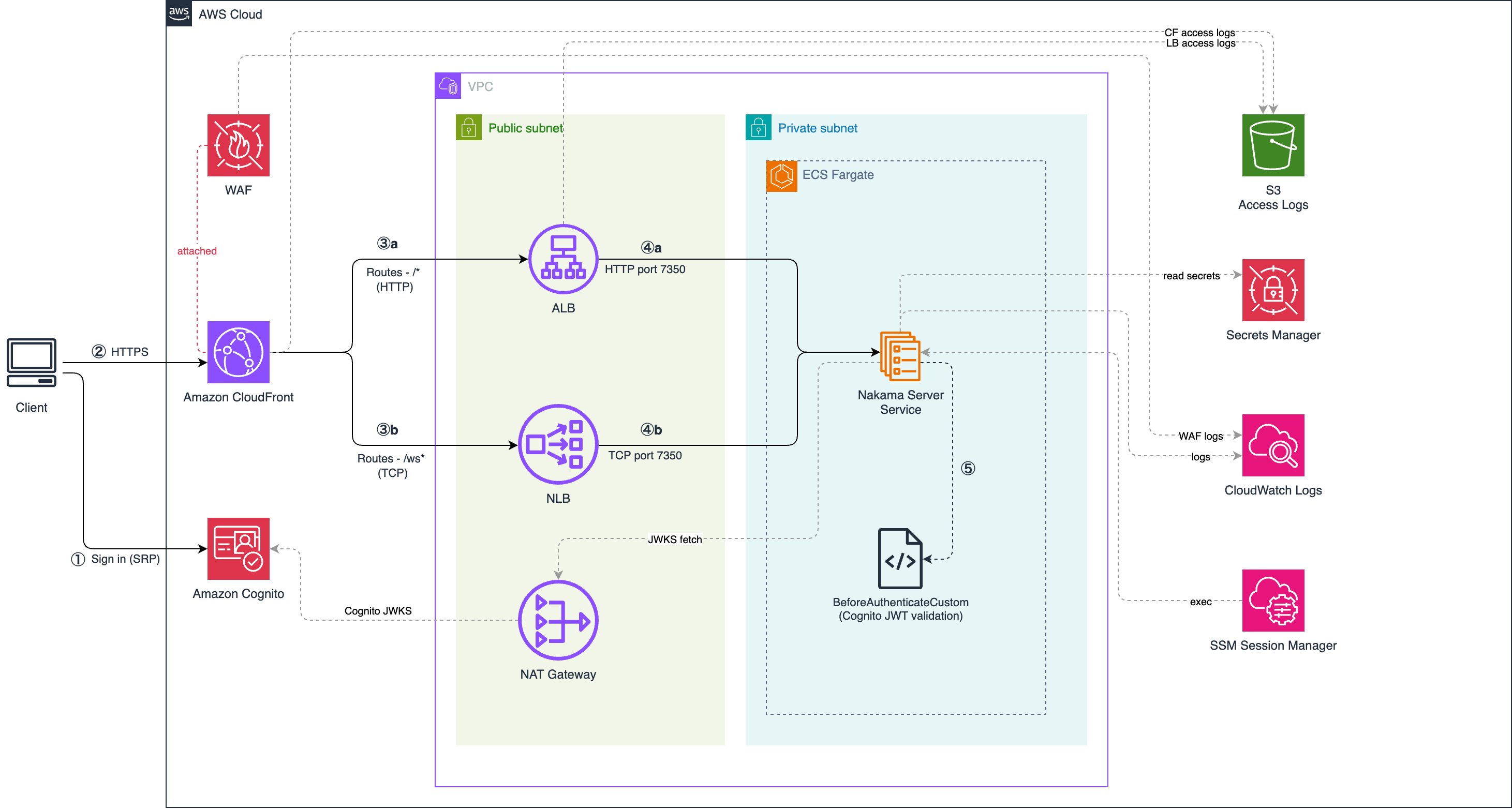
The following diagram shows the architecture. Amazon CloudFront is the single entry point, routing HTTP API traffic through an Application Load Balancer (ALB) to Nakama on Amazon ECS, and WebSocket traffic through a Network Load Balancer (NLB) via TCP passthrough.
Figure 1. Dual-token authentication architecture for Nakama on AWS.
Traffic flows through the system in six steps:
Client → Amazon Cognito — The player authenticates using USER_SRP_AUTH. The password never leaves the client. Amazon Cognito returns a JWT access token.
Client → Amazon CloudFront — Requests enter via Amazon CloudFront (HTTPS). AWS WAF inspects traffic at the edge before it reaches the origin.
CloudFront → ALB (port 80) — /* HTTP API traffic. The ALB is security-group locked to the CloudFront managed prefix list only.
CloudFront → NLB (port 7350) — /ws* WebSocket traffic. The NLB performs TCP passthrough with no HTTP inspection.
ALB → Amazon ECS (Nakama) — For auth requests: the BeforeAuthenticateCustom Go hook validates the Cognito JWT and extracts the sub claim as the Nakama user ID. For other API calls: Nakama validates its own session token.
NLB → Amazon ECS (Nakama) — Persistent WebSocket connection. Nakama validates the session token from the token query parameter at connect time.
Why two load balancers
The ALB and NLB serve different purposes and cannot be combined into one.
The ALB operates at the HTTP layer (Layer 7). It reads the path, applies listener rules, and returns 403 for unlisted routes.
The NLB operates at the TCP layer (Layer 4) and passes the raw stream to Nakama unchanged. Nakama receives the WebSocket upgrade directly from the client, validates the session token, and manages the connection lifecycle end-to-end.
Amazon CloudFront routes /ws* to the NLB and everything else to the ALB, so each connection type gets the appropriate handling behind a single HTTPS endpoint.
Prerequisites
Before you deploy this solution, make sure you have:
The repository includes a browser-based test app (/app) that demonstrates the full sign-up, sign-in, and Nakama token exchange flow.
Authenticate players with Amazon Cognito
Amazon Cognito provides a managed user directory that issues JWTs without requiring you to run your own identity server or store credentials. The game server validates the JWT independently on each request, with no callback to Cognito needed. This decouples identity from game sessions: Cognito owns the player’s identity, Nakama owns the game session, and neither system depends on the other at runtime.
Players self-register by calling the Cognito SignUp API from the game client. The User Pool verifies their email before the account becomes active. After sign-in, Cognito returns a JWT access token containing the player’s sub claim (a UUID), which becomes the Nakama user ID in the next step.
Authentication uses the USER_SRP_AUTH flow. The password never leaves the client device. The User Pool App Client is configured as a public client with no client secret, since your game client runs in the browser or a native app where any embedded secret is extractable. With SRP, no secret is needed; security comes from the protocol itself.
After a successful sign-in, Amazon Cognito returns a JWT access token. This token carries the player’s identity claims and is signed with an RSA key pair unique to your User Pool. The sub claim — a UUID generated by Cognito — uniquely identifies the player and becomes the Nakama user ID in the next step.
The auth Terraform module configures the App Client with generate_secret=false and permits only ALLOW_USER_SRP_AUTH and ALLOW_REFRESH_TOKEN_AUTH flows. The resulting JWT access token is short-lived (1 hour by default) and carries the sub, iss, exp, and client_id claims that the Go hook validates in the next step.
Bridge Cognito identity to Nakama sessions
Nakama’s server-side runtime supports Go plugins exclusively. The hook in this section is written in Go using Nakama’s runtime.Initializer interface. This is a constraint of the Nakama runtime model.
Once the client has a Cognito JWT, it needs a Nakama session token to make game API calls.
Validate the Cognito JWT in the Go hook
The game server cannot trust the identity claim sent by the client directly. Any client can forge a user ID. JWT validation cryptographically proves the identity was issued by Cognito, preventing player impersonation.
The hook performs five checks in order: token format, algorithm (RS256 only), signature against the JWKS, expiry, and issuer/audience matching your specific User Pool.
func validateCognitoJWT(token string, env map[string]string) (string, error) {
parts := strings.Split(token, ".")
if len(parts) != 3 {
return "", runtime.NewError("invalid token format", 3)
}
// Parse the header to get the key ID (kid)
var header struct {
Kid string `json:"kid"`
Alg string `json:"alg"`
}
headerBytes, _ := base64.RawURLEncoding.DecodeString(parts[0])
json.Unmarshal(headerBytes, &header)
if header.Alg != "RS256" {
return "", runtime.NewError("unsupported algorithm: "+header.Alg, 3)
}
// Fetch the public key from the JWKS cache
pubKey, err := jwksCache.getKey(header.Kid)
if err != nil {
return "", runtime.NewError("token validation failed", 16)
}
// Verify the RSA signature
hash := sha256.Sum256([]byte(parts[0] + "." + parts[1]))
signatureBytes, _ := base64.RawURLEncoding.DecodeString(parts[2])
if err := rsa.VerifyPKCS1v15(pubKey, crypto.SHA256, hash[:], signatureBytes); err != nil {
return "", runtime.NewError("invalid token signature", 16)
}
// Validate claims: expiry, issuer, audience
if time.Now().Unix() > claims.Exp { return "", runtime.NewError("token expired", 16) }
if claims.Iss != expectedIssuer || claims.ClientID != env["COGNITO_CLIENT_ID"] {
return "", runtime.NewError("invalid issuer or audience", 16)
}
return claims.Sub, nil // sub claim becomes the Nakama user ID
}
Security note: The hook never trusts the identity string sent by the client. It discards it and overwrites the Nakama user ID with the sub claim from the validated JWT. A client that sends a forged sub cannot impersonate another player — the hook ignores the body value entirely.
Cache JWKS keys with thundering herd protection
Amazon Cognito rotates its signing keys periodically. The hook caches keys with a 1-hour TTL. A 30-second re-fetch guard prevents multiple goroutines from calling the JWKS endpoint simultaneously when the cache expires.
func (c *JWKSCache) refresh() error {
c.mu.Lock()
defer c.mu.Unlock()
// Thundering herd protection: if another goroutine already
// refreshed within the last 30s, use the updated cache
if time.Since(c.fetched) < 30*time.Second {
return nil
}
// ... fetch and parse JWKS from Cognito endpoint
}
Register the hook
The hook registers itself in InitModule, the entry point called by Nakama when the plugin loads:
func InitModule(ctx context.Context, logger runtime.Logger, db *sql.DB,
nk runtime.NakamaModule, initializer runtime.Initializer) error {
if err := initializer.RegisterBeforeAuthenticateCustom(beforeAuthenticateCustom); err != nil {
return fmt.Errorf("failed to register hook: %w", err)
}
logger.Info("Cognito JWT validation hook registered")
return nil
}
When the client calls POST /v2/account/authenticate/custom with the Cognito JWT as the id field, Nakama calls beforeAuthenticateCustom before processing the request. If the JWT is valid, the hook sets in.Account.Id = sub and returns. Nakama creates or links the account and returns a session token to the client.
If your server is not Nakama, for example, Colyseus, Photon, or a custom WebSocket server, implement the same five checks (algorithm, signature, expiry, issuer, audience) in your server’s middleware or plugin language. The JWKS endpoint and JWT structure follow the OIDC standard, so any OIDC-compliant identity provider (not only Amazon Cognito) works with this pattern.
Deploy the infrastructure
The infrastructure is organized into six Terraform modules: network (Amazon Virtual Private Cloud (Amazon VPC), subnets, security groups), compute (Amazon ECS cluster, ALB, NLB, Amazon Elastic Container Registry (Amazon ECR)), auth (Cognito User Pool), cdn (CloudFront distribution), waf-cloudfront (AWS WAF Web ACL), and ops (IAM, AWS Systems Manager access). A bootstrap module creates the S3 state backend and AWS Key Management Service (AWS KMS) key before the main deployment.
Deploy with:
# One-time: provision the Terraform state backend
cd terraform/bootstrap && terraform init && terraform apply
# Deploy everything
cd terraform && terraform init -backend-config=config/backend-dev.hcl
make deploy
make deploy builds and pushes the Nakama container image to Amazon ECR, then runs terraform apply. The image tag auto-increments from the latest tag in ECR.
ALB routing: explicit allow list
The ALB default listener action returns 403. Only the paths in the following table reach Nakama. Requests to unlisted paths are rejected before they reach the game server.
Priority
Path
Target
Purpose
1
/healthcheck
Nakama port 7350
Health monitoring
2
/v2/account/authenticate/*
Nakama port 7350
Session bridge: Go hook validates JWT
10
/v2/*
Nakama port 7350
Nakama REST API v2
11
/v1/*
Nakama port 7350
Nakama RPC (v1)
Default
*
403 Forbidden
Request never reaches Nakama
The default-403 posture means a misconfigured client or a scanner probing arbitrary paths gets a 403 at the ALB, not an error from the game server. This limits the attack surface to the explicitly listed API surface.
Security group chain
The network layer enforces two security group rules:
The ALB security group allows inbound only from the CloudFront managed prefix list. As an additional application-layer check, CloudFront sends a shared secret in the X-CloudFront-Secret header on every request; ALB listener rules reject any request missing the correct value with a 403. The NLB security group applies the same CloudFront managed prefix list restriction at Layer 4.
The NLB security group allows inbound TCP 7350 only from the CloudFront managed prefix list. The ECS task security group allows inbound port 7350 only from the ALB security group (HTTP API) and from the NLB security group (WebSocket).
Together, the routing and security group chain means the only path to Nakama is: Internet → CloudFront → AWS WAF → ALB or NLB → ECS. No hop can be skipped.
Manage the WebSocket connection lifecycle
The NLB TCP passthrough model creates a lifecycle challenge: the NLB drops idle TCP flows after 350 seconds (the AWS default, not configurable). If a player’s connection sits idle, the NLB closes the underlying TCP connection while Nakama still holds an open socket.
The following table describes the four controls that handle this:
Control
Value
Purpose
NLB TCP idle timeout
350s
NLB drops idle TCP flows. Cannot be changed.
Nakama ping interval
10s
Nakama sends a WebSocket ping every 10s, keeping the TCP flow active.
Nakama pong wait
20s
If the client does not respond to a ping within 20s, Nakama closes the connection.
token_expiry_sec
7200
Nakama rejects session tokens older than 2 hours at connect time.
single_socket
true
A new connection from the same user kills the previous one, preventing stale sessions.
The ping/pong keepalive
The 10-second ping interval is the key control. Nakama sends a WebSocket ping frame every 10 seconds on each active connection. The client responds with a pong. This keeps the NLB TCP flow alive well within the 350-second idle timeout. If the client goes silent, Nakama detects the missing pong within 20 seconds and closes the socket cleanly.
Session expiry at connect time
The NLB performs TCP passthrough, so there is no opportunity to inspect HTTP headers or validate the session token at the network layer. Nakama validates the session token from the token query parameter when the WebSocket upgrade request arrives. A token older than token_expiry_sec is rejected and the connection is closed before any game messages are processed.
Single socket enforcement
single_socket: true verifies that when a player opens a second connection (after a network drop and reconnect, for example) the server closes the first connection. Without this, a player’s Nakama state can be split across two concurrent connections if the client does not cleanly close the first one.
The four-layer model (keepalive, timeout, session expiry at connect, one-connection-per-user enforcement) applies to any real-time server behind an NLB TCP passthrough: Colyseus, Photon, custom WebSocket backends, or any game server that manages persistent connections. If your server does not have built-in ping/pong, implement application-level heartbeat messages that serve the same role.
Security note: The session token travels as a query parameter (?token=...) in the WebSocket upgrade URL. Query parameters appear in server access logs, load balancer logs, Amazon CloudFront logs, and browser history. Mitigations: all connections use TLS (token encrypted in transit), session tokens are short-lived (2 hours), and single_socket invalidates old connections on reconnect. For production deployments, consider log redaction policies for the token parameter.
Clean up
To avoid ongoing AWS charges, destroy all resources when you no longer need them.
Destroy the main infrastructure first:
cd terraform && terraform destroy
Then destroy the Terraform state backend:
cd terraform/bootstrap && terraform destroy
Confirm resources are removed by running terraform state list (should return empty) or checking the AWS Management Console.
Conclusion
In this post, you implemented a dual-token authentication architecture for a Nakama game server on AWS. Amazon Cognito handles player identity through JWT validation; a Go runtime hook bridges verified identity into Nakama sessions; and the infrastructure enforces a routing layer where HTTP API traffic passes through an Application Load Balancer with an explicit allow list and WebSocket connections reach Nakama directly through a Network Load Balancer TCP passthrough.
The four-layer WebSocket lifecycle model can be applied to real-time game servers behind an NLB TCP passthrough, not Nakama exclusively.
For production deployments, consider these next steps:
This is a guest blog post co-written by Adiascar Cisneros, from Tableau at Salesforce.
Integrating Tableau with Amazon Redshift Serverless gives you high-performance analytics with serverless scaling and minimal capacity planning. Although automatic scaling handles warehouse management for you, optimization requires a strategic approach to data modeling, security, and query management.
In this post, we provide a guide to help you use Tableau’s Relationships and Amazon Redshift Serverless architecture to deliver sub-second insights while maximizing every Redshift Processing Unit (RPU). We also provide guidance on five key areas: data model architecture for optimal query performance, security configuration and access control, performance optimization through smart configuration, cost management strategies, and query and join optimization techniques.
Prerequisites
Before implementing these optimization strategies, make sure you have:
Tableau Desktop (version 2022.1 or later) or Tableau Server deployed.
An active Amazon Redshift Serverless workspace.
AWS Identity and Access Management (IAM) permissions to configure authentication and access controls.
Network connectivity configured between your Tableau environment and Amazon Redshift Serverless.
The native Amazon Redshift driver installed.
Building the foundation
The success of any analytics system begins with its data model. True scalability starts with the end-user experience. Your data model is more than a storage structure. It’s the foundation of dashboard responsiveness. By aligning your database design in Amazon Redshift with your analytical requirements, you empower Tableau to generate highly efficient queries, reducing costs and keeping your users engaged with the data.
When connecting to Amazon Redshift, we recommend using Tableau’s logical data model, specifically Relationships. With Relationship, you can preserve the native level of detail for each table, so Tableau can perform join culling and dynamically query only the specific tables needed for a particular visualization.
When designing your Amazon Redshift schema, implement a well-structured star or snowflake schema, or one big denormalized table where appropriate. This allows Tableau to optimize query execution automatically. Modern Amazon Redshift deployments benefit significantly from Automatic Table Optimization (ATO), which uses AI and machine learning (ML) to continuously monitor and adjust sort keys and distribution keys. To take advantage of ATO, keep sort keys and distribution styles at their default AUTO setting when you create tables. ATO then continuously monitors workload patterns and adjusts keys to improve query performance.
Start by implementing Relationships in your existing workbooks to take advantage of join culling and improved query performance.
Securing your connection
Native database drivers provide enhanced security features and better integration with Amazon Redshift capabilities compared to generic ODBC or JDBC alternatives.
The integrity of your analytics relies on the quality of the connection between your platforms. Use the native Amazon Redshift driver rather than generic ODBC or JDBC alternatives. The native driver is specifically engineered to use the advanced capabilities of Amazon Redshift and supports modern security protocols, such as AWS IAM Identity Center, out of the box. By prioritizing the native driver, you verify that your connection uses the latest security patches and performance optimizations, establishing a hardened and efficient entry point for your data. For more information, see Integrate Tableau and Okta with Amazon Redshift using AWS IAM Identity Center.
Connection stability for high-scale environments
In Amazon Redshift, cursors are used to retrieve a result set from a query and process the data row-by-row or in smaller chunks rather than loading the entire set into memory at once. For high-scale environments, stable connections depend on how you handle large result sets. In some high-volume scenarios, Amazon Redshift cursors can introduce resource overhead that impacts user concurrency. Monitor your workload and, if necessary, fine-tune your connection configurations using Tableau Data Customization (TDC) files. TDC files are XML configuration files that customize how Tableau connects to your database. Specifically, validate whether disabling cursors improves throughput.
Important: This configuration loads the entire dataset into memory. For large datasets, this might cause performance degradation or out-of-memory errors. Evaluate your dataset size and business requirements before you turn on this setting. This is a key step in tuning your deployment, helping verify that your Amazon Redshift resources remain available and responsive for secure, ad-hoc analysis.
Security best practices
Follow security best practices while deploying Amazon Redshift Serverless. Configure security groups to control inbound access from Tableau Server and Desktop IP ranges. IAM authentication must be the primary method, complemented by SSL/TLS encryption for all connections.
For authorization, implement a layered security model:
Apply explicit GRANT statements.
Create distinct database roles aligned with business functions.
Use Amazon Redshift system-defined roles judiciously.
Apply dynamic data masking for sensitive data.
Conduct regular security audits to support ongoing protection.
Audit your current connection types and migrate to the native Amazon Redshift driver if you’re using ODBC or JDBC connections.
Enhancing performance through smart configuration
Smart configuration spans how much data you query, where you push complex logic, how you design dashboards, and how you tune connections. The following sections cover each area.
Managing data volume
To maximize workbook efficiency, start by rigorously managing your data volume. Although Amazon Redshift handles large datasets well, your dashboard should query only what is strictly necessary. Use Tableau Hyper Extracts for production environments to provide a consistent, high-speed cache that offloads repetitive query processing from Amazon Redshift. If a live connection is required, strictly limit your data intake by using Data Source Filters and hiding all unused fields. This helps verify that Tableau generates leaner queries, significantly reducing network latency and processing time.
Shifting complexity to the database
Next, shift the burden of complexity away from the visualization layer. Materialize calculations within your extracts or push complex logic (especially row-level string manipulations and regex) directly down to the Amazon Redshift database level. By pre-calculating these values before the user ever loads the dashboard, you eliminate expensive runtime processing.
Simplify your logic within Tableau by using native features like CASE statements or Sets rather than complex IF/THEN statements. Testing shows these methods perform significantly faster for grouping dimensions.
Streamlining dashboard design
Additionally, optimize the rendering process by streamlining your dashboard design:
Limit the number of visualizations per dashboard.
Prioritize fixed-size dashboards to maximize server-side caching effectiveness.
Avoid high-cardinality filters (fields with thousands of unique values).
Don’t use the ‘Show Only Relevant Values’ setting on large datasets, because it forces the system to run extra background queries that slow down your dashboard.
Connection and parameter tuning
Optimize Tableau’s performance by enabling connection pooling tailored to your concurrent user count. Configure datetime handling and parallel query execution settings to match your workload patterns.
You can enhance the automatic resource management of Amazon Redshift Serverless through parameter optimization. Key parameters include:
Set enable_result_cache_for_session to OFF during development to verify you’re testing against live query performance, not cached results. Set it to ON in production.
Choosing between extracts and live queries is a foundational architectural decision. We recommend a hybrid approach tailored to specific use cases rather than a one-size-fits-all policy.
When to use live queries
Live queries are best for real-time analytics. They use Amazon Redshift Serverless automatic scaling to query massive datasets in place. Use this approach for:
Keep in mind that live connections rely entirely on the database’s performance, so optimizing your Amazon Redshift tables and using materialization techniques within the database is important for maintaining interactivity.
When to use extracts
For scenarios when data is static or where query performance is critical, Tableau Hyper Extracts provide a high-speed cache that shifts the processing load from Amazon Redshift to Tableau’s data engine. This is valuable for dashboards with complex calculations (such as row-level string manipulations or heavy aggregations) where an extract can pre-materialize results, effectively baking in the logic before the user ever loads the view. By using extracts for these heavy workloads, you reduce the compute load on Amazon Redshift, lowering costs while delivering sub-second response times to end users.
Right-sizing your extracts
To maximize efficiency, right-size your extracts for your dashboard’s specific needs:
Avoid the SELECT * mentality.
Use data source filters to limit rows.
Hide unused fields to remove redundant columns.
For higher-level analysis, aggregate your data during the extract process. For example, summarize daily transactions into monthly trends to significantly reduce file size and query time.
Schedule refreshes during off-peak hours.
Use incremental updates to add only new rows, minimizing Amazon Redshift RPU usage and network overhead.
Balance performance and cost by aligning your connection choice with business freshness requirements and data complexity. Monitor usage patterns to refine this balance over time.
Star schema query and join optimization
Optimize your star schema joins and queries to reduce execution time and compute costs by using Tableau Relationships. Relationships keep tables separate, allowing Tableau to automatically query only the necessary tables for the fields in the view. Relationships are more flexible and often perform better than joins because they don’t force a row-level merge on all fields.
Inefficient joins and poorly optimized queries force Amazon Redshift to scan unnecessary data, increasing both query execution time and compute costs.
Query optimization best practices
Avoid Custom SQL, which forces Tableau to wrap queries in complex sub-selects. Instead, connect directly to tables or views to let the database optimizer function effectively.
Define primary and foreign keys in your Amazon Redshift schema to allow Tableau to assume referential integrity.
Important: Amazon Redshift does not enforce primary or foreign key constraints. They are informational only, and the query optimizer uses them to generate more efficient execution plans. You’re responsible for data integrity at the application or ETL layer. For more information, see Defining constraints. Assume Referential Integrity is a Tableau setting that tells the engine to trust defined key relationships without validating them at query time, reducing query complexity.
Use Materialized Views to pre-compute heavy aggregations, which reduces execution time for frequently accessed data patterns. For example, create materialized views for common date-based aggregations or customer-level summaries.
Optimize Amazon Redshift Serverless by denormalizing data to minimize complex joins. After you apply these changes, use Tableau’s Performance Recorder to regularly validate your query speeds and identify bottlenecks.
Cost optimization and monitoring
Amazon Redshift Serverless charges in RPU-hours on a per-second basis (60-second minimum), so you only pay for the workloads you run.
Optimizing query volumes and resource usage helps you control Amazon Redshift Serverless costs and maintain predictable spending. To help control compute costs, optimize Tableau queries before they reach Amazon Redshift by using Data Source Filters and ‘Hide All Unused Fields.’ This forces the generation of lean SELECT statements that scan only the necessary rows and columns. Because Amazon Redshift Serverless scales resources based on workload, reducing data volume and complexity at the Tableau source layer can help lower RPU consumption and costs.
Tableau Hyper Extracts act as a cost buffer for high-traffic dashboards. By extracting data into Tableau’s in-memory engine, database costs are typically incurred during scheduled refreshes rather than for every individual user interaction. For live connections, maximize Tableau’s caching architecture by setting server cache policies to “Refresh less often,” ensuring that repetitive dashboard views are served instantly from memory and avoid redundant, billable queries.
Monitoring and alerting
Monitor RPU usage patterns and set billing alerts to maintain cost control:
Combine query result caching with strategic scheduling for resource-intensive tasks.
Use scaling event data and query patterns to define thresholds.
Set up Amazon CloudWatch alarms for RPU consumption spikes.
This post covered key optimization strategies for Tableau and Amazon Redshift Serverless integration: data model architecture using Relationships, security configuration with native drivers and AWS IAM, performance optimization through extracts and smart configuration, cost management with RPU monitoring, and query optimization techniques.
As AI-driven optimization evolves, staying informed about Amazon Redshift AI features and best practices, including Tableau Pulse, is key. Regularly review your configuration, performance, and security to verify that your Tableau and Amazon Redshift Serverless integration remains secure, cost-effective, and high-performing.
Optimization is an ongoing, iterative process. To keep your environment optimized, regularly review your settings, monitor performance, and adapt as workload patterns evolve. This approach maintains a cost-effective analytics environment that scales with your organization.
Ready to build a secure, high-performance analytics solution that delivers both speed and cost efficiency? Visit the Salesforce and AWS partnership webpage to start scaling your insights today.
Sign-in resource-based policies and RCPs support several security objectives: restricting console sign-in to corporate networks, limiting which principals can sign-in to the console, and applying consistent network perimeter controls across an entire AWS Organizations organization.
In this post, we walk through a common use case: a financial services company restricting console access to its corporate network for regulatory compliance. We show you how to implement this using a sign-in resource-based policy for a single account, verify the controls with AWS CloudTrail, and explain how these policies integrate with AWS Management Console Private Access and the broader AWS data perimeter framework.
Restricting console sign-in access to a corporate network
Consider a financial services company that requires access to AWS Management Console sign-in to originate from the corporate network. The company has the following requirements:
Users sign in to the console only from the corporate VPN, office network, or customer VPC.
Sign-in attempts from personal networks, public Wi-Fi, or other unexpected locations must be denied.
A designated principal should retain access from any network to prevent lockout.
All sign-in attempts (allowed and denied) must be logged to CloudTrail for compliance evidence.
In the steps that follow, we show you how to create a resource-based policy to enforce these requirements on a single account.
Permission to manage Sign-in resource policies. Attach the AWS managed policyAWSSignInResourcePolicyManagementor grant permissions to the following actions to respective principals:
Most resource-based policies require the author to input the full policy document (JSON statements). A Sign-in resource permission statement is different: you provide parameters, and AWS Sign-In generates the policy for you.
The following command provides your corporate IP range, your VPC, and an excluded principal as parameters. AWS Sign-In uses these parameters to generate a policy that restricts console sign-in to those networks, while letting the excluded principal sign in from any network. You control the parameter values, not the policy structure. You can review the generated policy at any time with the get-resource-policy command.
Note: Creating resource permission statements has no effect until console authorization is enabled in Step 2, so you can review the complete policy before it takes effect. Write operations must target us-east-1.
To create resource permission statements
1. Open your terminal and ensure you have the latest AWS CLI installed. 2. Run the following command, replacing the placeholder values <my-vpc>, <my-vpc-region>, <my-corporate-cidr>, and <excluded-IAM-principal-arn> with your specific configuration:
The generated policy contains four statements, grouped into two pairs. The first pair restricts access by network source—it denies any principal making a request from outside your corporate IP range (<my-corporate-cidr>) or your VPC (<my-vpc>). The second pair restricts which AWS Region your VPC can target—it denies requests originating from <my-vpc> unless they are directed at <my-vpc-region>. This Region binding is necessary because VPC IDs are only unique within a single Region.
AWS Sign-In evaluates these policies in two phases: before authentication and after authentication. The post-authentication evaluation repeats each time the console session requests new credentials. Within each pair, one statement covers the pre-authentication phase and one covers the post-authentication phase.
The pre-authentication statement evaluates the signin:Authenticate action. Since the principal is not yet authenticated in this phase, the statement uses the signin:PrincipalArn condition key to exempt your excluded principal. This key supports all principal types: root user, AWS Identity and Access Management (IAM) user, federated user, and role.
The post-authentication statement evaluates the signin:AuthorizeOAuth2Access and signin:CreateOAuth2Token actions. AWS Sign-In evaluates these actions after authentication, when it issues the tokens that establish the console session. These actions do not support the signin:PrincipalArn key. Instead, they use aws:PrincipalArn, which resolves to the authenticated principal.
Step 2: Turn on sign-in policy enforcement for your account
This step turns on enforcement of the policy you created in Step 1. Until you run this step, the resource permission statements you created in Step 1 have no effect.
5. Turn on enforcement of sign-in policies using the following command:
Now that enforcement is active, sign-in attempts are evaluated against your resource-based policy. Verify the behavior by testing sign-in from different network conditions.
Scenario 1: Allowed sign-in from the corporate network
A principal signing in from the allowed corporate IP range or VPC succeeds normally. The CloudTrail event shows ConsoleLogin:Success
Example CloudTrail event details for successful console sign-in:
Scenario 2: Denied sign-in from an unexpected network
A principal signing in from a network other than the allowed IP address range or a VPC endpoint attached to the source VPC, is blocked. The CloudTrail event shows ConsoleLogin: Failure with an error message identifying the policy that caused the denial:
Example CloudTrail event details for failed console sign-in:
{
"userIdentity": {
"type": "IAMUser",
"accountId": "123456789123",
"accessKeyId": "",
"userName": "Dev1"
},
"eventTime": "2026-06-09T19:20:38Z",
"eventSource": "signin.amazonaws.com",
"eventName": "ConsoleLogin",
"awsRegion": "us-east-1",
"sourceIPAddress": "198.51.100.76",
"userAgent": "Mozilla/5.0 (Macintosh; Intel Mac OS X 10_15_7) AppleWebKit/537.36 (KHTML, like Gecko) Chrome/148.0.0.0 Safari/537.36",
"errorCode": "AccessDenied",
"errorMessage": "Authorization denied because of a resource-based policy",
"requestParameters": null,
"responseElements": {
"ConsoleLogin": "Failure"
},
"eventID": "d88a7543-ae89-4186-b1b6-d3116413f2ee",
"readOnly": false,
"eventType": "AwsConsoleSignIn",
"managementEvent": true,
"recipientAccountId": "123456789123",
"eventCategory": "Management"
}
The error message field shows the policy type that caused the denial: “Authorization denied because of a resource-based policy”.
Scaling with RCPs
The steps above apply a Sign-in resource-based policy to a single account. For organizations managing many accounts, RCPs offer a better path: they can be attached at the organization, OU, or account level in AWS Organizations and apply automatically to every account in scope. To view an RCP example, see here .
When a sign-in to the console is denied because of an RCP, the error message field shows the denial as “Authorization denied because of a resource control policy”.
Extending with Console Private Access and data perimeters
The sign-in resource-based policy you created controls which networks can reach your account’s sign-in flow. AWS Management Console Private Access adds a complementary control: from within your network, it limits console access to a known set of AWS accounts, preventing sign-in to unexpected AWS accounts.
Together, these capabilities contribute to a data perimeter for console access:
Network perimeter: Sign-in resource-based policies and RCPs restrict console sign-in to expected networks (corporate IP ranges, VPCs).
Identity perimeter: Sign-in resource-based policy and RCP ensure only trusted identities can sign in to the console. Console VPC endpoint policy and Sign-in VPC endpoint policy ensure only trusted identities can use the console from your VPC.
Resource perimeter: Sign-in VPC endpoint policy and Console VPC endpoint policy restrict which AWS accounts are reachable from your network.
By using sign-in resource-based policies and RCPs, you can restrict AWS Management Console access to expected networks. These controls are available at no additional cost in all AWS commercial Regions.
When a player in Turkey, Brazil, or India tries to log in, they expect a verification code on their phone within seconds. If it doesn’t arrive, that’s a lost session, a support ticket, or worse, a player who doesn’t come back. For gaming studios operating across 100+ countries, delivering those SMS messages reliably is a complex operational challenge involving country-specific regulations, carrier registrations, and routing rules that can change overnight.
This post shares practical lessons from a real-world migration of a global gaming SMS platform from Amazon Simple Notification Service (Amazon SNS) to AWS End User Messaging. You’ll learn how to use resource sharing to avoid months of re-registration, how to build a country inventory that survives regulatory changes, and how to avoid the operational pitfalls that surface only when you migrate production traffic across accounts. Although the examples here are drawn from gaming, the operational challenges are universal. Any organization delivering SMS at international scale will face the same complexities, whether your users are players, customers, or patients.
Why gaming studios migrate SMS accounts
Before diving into the how, it’s worth understanding the why. Gaming studios commonly need to move SMS workloads between AWS accounts for several reasons:
Security and scope isolation — Separating messaging infrastructure from game servers and backend services into a dedicated account reduces the impact of a security incident in either environment.
Organizational changes — Studio acquisitions, team restructuring, or moving from a shared corporate account to a studio-owned account.
Service evolution — Migrating from Amazon SNS (which supports SMS as one of many pub/sub capabilities) to AWS End User Messaging (purpose-built for SMS/MMS/voice with features like phone pools, protect configurations, and event destinations)
Compliance boundaries — Isolating messaging resources to meet data residency or audit requirements.
Whatever the reason, the challenge is the same: you have a working global SMS setup with phone numbers, Sender IDs, short codes, and carrier registrations spread across dozens of countries, and you need to move it without disrupting millions of players’ 2FA flows.
Resource sharing: A faster migration path
The traditional approach would be to re-register every origination identity (that is, phone numbers, Sender IDs, short codes, see Choosing an origination identity) in the consuming account from scratch. For a global gaming platform, this is impractical:
The single most important preparation step is building a complete inventory of your SMS footprint, country by country. AWS publishes a comprehensive reference table listing supported countries, origination identity types, and registration requirements.
This inventory becomes invaluable for future account transitions, incident response, and onboarding new team members.
Plan for regulatory change, not just today’s rules
The global SMS regulatory landscape is not static. It’s tightening. Countries that previously had relaxed requirements are increasingly introducing mandatory Sender ID registration, content filtering, and message format restrictions. A migration is the ideal time to future-proof your setup, not just replicate what worked yesterday.
For help navigating the registration process for specific countries, see Registration support.
In April 2026, Turkey’s Information and Communications Technologies Authority (BTK) began enforcing a regulation that blocks all international A2P SMS messages containing URLs, hyperlinks, or shortened links. For gaming studios that include account recovery links, promotional URLs, or support links in their SMS messages, this type of regulatory change can mean immediate delivery failure to an entire market.
This type of regulatory shift is becoming more common:
Optional to mandatory Sender ID registration. Australia is mandating Sender ID registration with ACMA by mid-2026. AWS now supports Australia sender ID registration directly through the EUM console.
Content template registration. India requires DLT registration through TRAI, and China requires message template pre-registration through AWS Support.

Content filtering and URL restrictions. Carriers in multiple markets are implementing automated filtering that rejects messages containing URLs or specific patterns, even from registered senders. Your country inventory shouldn’t just document what works today. It should also track regulatory change dates, upcoming requirements, content restrictions, and your fallback plan for each market. For each country, ask: “If the rules change tomorrow, how quickly can we adapt?” If the answer is weeks, that country should have a fallback channel (email, push notification) ready to activate immediately.
Lessons learned: What can go wrong at scale
Even with careful planning, migrating global SMS infrastructure surfaces unexpected issues. The following sections cover the most common pitfalls we encountered.
Sender ID case sensitivity
As documented by AWS, Sender ID values are case-sensitive at the carrier and aggregator level. In countries with mandatory registration (Turkey, UK, India, Australia), carriers might perform exact-match validation. If your application sends STUDIONAME but the carrier has StudioName on file, the message can be rejected.
The AWS End User Messaging console displays all Sender IDs in uppercase regardless of registration casing, which is something to watch out for. Always verify casing against the Registrations section of the console, which preserves the original value. Countries can also begin enforcing stricter matching overnight as regulations tighten, turning previously-working messages into failures.
What to watch for:
Test delivery to countries with mandatory Sender ID registration before rolling out any casing changes globally.
Phone pools are the recommended way to manage origination identities (that is, phone numbers, Sender IDs, short codes, see Choosing an origination identity) at scale with AWS End User Messaging. A pool automatically selects the appropriate identity based on the destination country code, handling failover between identities for the same country.
Plan ahead: Inventory your origination identities before creating your pool, and request the quota increase before you start associating resources. Hitting the quota mid-migration creates unnecessary delays.
Batch your RAM sharing operations
When sharing a large number of origination identities through RAM (50+), the RAM API creates resource-based policies on each shared resource. The order of operations matters: add the consuming account (principal) to the resource share first, then add resources incrementally. If you create a resource share with hundreds of resources and then add the consuming account afterward, RAM attempts to set resource-based policies on all resources simultaneously. This is the most common trigger for throttling at scale. In severe cases, this throttling can result in resources with empty or corrupted resource policies, making them inaccessible to the consuming account until manually remediated.
Best practice:
Add the consuming account (principal) to the resource share before adding any resources. Batch resource associations in groups of 10 or fewer.
After each batch, verify that all resources have reached ASSOCIATED status.
From the consuming account, confirm that shared resources are visible using the describe-* CLI commands with the --owner SHARED flag.
Retain AWS CloudTrail logs for troubleshooting if any associations don’t complete as expected.
If you suspect corrupted policies, verify the resource policies on affected resources and re-associate them individually.
Not everything transfers through RAM
RAM sharing covers the “what you send with”: phone numbers, Sender IDs, pools, and opt-out lists. But several critical components are account-specific and must be recreated in the consuming account:
Note on Protect Configurations: Protect Configurations apply at three levels: account default, configuration set, and per-message. A common mistake when setting up a consuming account is checking only the account-level default and missing a restriction at the configuration set level, resulting in unexpectedly blocked destination countries. When recreating your configuration in the consuming account, verify protect settings at all three levels.
Production mode requirement: Both the sharing account and the consuming account must be in Production mode. If the consuming account is still in the SMS sandbox, it can only send messages to verified destination phone numbers, which means shared production-ready resources cannot be used for real-world traffic. Verify production status in the consuming account before beginning your migration.
One tip worth highlighting: The registration process for certain countries’ message templates (notably China) is handled through AWS Support cases. After the registration is approved, retain a copy of the approved template details, the case correspondence, and the registration parameters. Support case history might not be accessible indefinitely. If you need to re-register in a new account later, having your own records of what was approved and the exact template content saves significant time.
Countries without Sender ID support
Not every country supports Sender IDs. If your phone pool is configured with Sender IDs and a message is routed to a country that doesn’t support them (for example, Belgium or Puerto Rico), the delivery will fail, and the error might not clearly indicate that the issue is Sender ID incompatibility.
Build an exclusion list: For countries that don’t support Sender IDs you have two options:
Route those messages through a different origination identity (long code or short code) if available.
Exclude those countries from Sender ID routing and allow them to fall back to shared routes.
The country capabilities table is your definitive reference for which countries support which origination identity types.
The “hidden fallback” discovery
A common surprise during migration is that your existing setup might have been silently falling back to shared routes in countries where you assumed you had branded Sender ID delivery. When SMS is sent through Amazon SNS with automatic origination identity selection, the service quietly falls back to shared routes (often displaying “NOTICE” as the Sender ID) if no registered identity is available for the destination country.
This fallback is invisible in normal operations. Messages still deliver, and unless you’re checking the Sender ID displayed on the recipient’s device, there’s no visible indication. But when you migrate to a phone pool with explicit Sender ID routing, these gaps become visible as delivery failures.
Before migrating, audit your actual delivery patterns, not just your configuration. Check delivery reports for countries where you expect branded Sender ID delivery and verify that the Sender ID displayed matches your brand, not “NOTICE” or a generic shared route.
Operational recommendations
The following practices help you avoid disruptions during migration and maintain reliable delivery afterward.
Have a fallback channel ready during migration
Before you begin migrating traffic, ensure you have an alternative authentication channel (typically email-based 2FA) ready to activate on short notice per-country. When an issue is detected, disable SMS for that country and fall back to email while you investigate, rather than leaving players locked out.
Build your country registry
Maintain a living document that tracks what you have (identity type, registration status, exact casing, account location), what you chose and why, what gaps exist (countries relying on shared routes), and registration details (approval dates, case references, template content). This registry is your migration playbook.
Before scaling traffic, test delivery to representative countries from each category: mandatory Sender ID registration, no Sender ID support, optional Sender IDs, message template registration, and carrier-specific content restrictions. A successful test to the US doesn’t validate your Turkey configuration.
Conclusion
Global SMS for gaming works reliably until something needs to change. Migrations, account restructuring, and service upgrades expose the complexity that was previously hidden behind automatic fallbacks and “it just works” behavior.
In this post, we covered how to use RAM sharing to avoid months of re-registration, how to build a country inventory that accounts for regulatory change, and how to navigate the operational pitfalls of migrating production SMS traffic across accounts. The key takeaways:
Know your country landscape before you start. The country capabilities table is your starting point, but build your own registry with registration details, exact Sender ID values, and decision rationale.
Respect the details. Case sensitivity, phone pool quotas, RAM batching limits, non-shareable resources, and record retention can each independently block your migration.
Monitor from day one and plan for regulatory change. Set up delivery tracking before sending production traffic, and track what’s changing in each market.
What matters to players is that their verification code arrives in seconds, every time, regardless of location. The operational discipline described in this post helps make that happen and keeps it working through whatever infrastructure changes come next. Although this post is framed around gaming, the lessons apply broadly. Whether your users are players, shoppers, or account holders, reliable global SMS delivery requires the same operational rigor.
Financial services organizations increasingly run analytical workloads across multiple systems. For example, customers typically store transaction records in Snowflake for its concurrency handling during peak volumes, while they store risk scores, customer profiles, and behavioral signals on AWS. To bridge that divide, practitioners have had to stitch together manual exports, custom extract, transform, and load (ETL) code, and external business intelligence (BI) tools to query both sources, cache expensive aggregations, and visualize results.
Amazon SageMaker Data Agent now closes these gaps with three new capabilities in Amazon SageMaker Unified Studio notebooks: SQL analytics on Snowflake data sources, materialized view management, and interactive charting. Practitioners can use them together to query Snowflake alongside AWS data, pre-compute and schedule repeated aggregations, and create interactive visualizations from natural language prompts in a single notebook, without writing boilerplate code or switching tools.
In this post, we describe the challenges these capabilities address, introduce each one, and walk through a fraud analytics scenario that demonstrates them working together in an end-to-end investigation workflow.
Challenges with fraud detection
Fraud analytics teams working in SageMaker Unified Studio notebooks encounter several recurring friction points that slow their path from alert to insight:
Querying across AWS and third-party warehouses. Customers store transaction data in Snowflake and maintain risk scores and customer profiles on AWS. SageMaker Data Agent supported SQL generation for AWS-native engines: Amazon Athena, Amazon Redshift, Apache Spark, and DuckDB. However, it didn’t yet generate Snowflake-dialect SQL. This created a gap for customers working with data distributed across both AWS services and Snowflake. Analysts had to write Snowflake SQL manually and export results as CSV files to join with AWS data. The process consumed 1–2 hours before any actual investigation could begin.
Rich visualization requires coding expertise. When analysts want to plot query results, they must write Python code using packages like matplotlib, seaborn, or plotly. They must choose the right chart type, format axes, handle data transformations, and debug rendering issues. For fraud teams whose expertise is in investigation rather than data visualization code, each chart becomes a detour: either learn the package interface, ask an engineer for help, or export to an external BI tool. This slows the exploratory cycle that fraud investigations depend on, where every new angle (time-of-day patterns, category breakdowns, geographic clusters) ideally takes seconds, not minutes of code iteration.
Expensive repeated queries with no caching. Fraud signal queries flag transactions that exceed a customer’s historical average and compute risk-score distributions by merchant category. These queries re-scan entire tables on each execution. A team running the same aggregation every morning over millions of rows pays the full compute cost each time, with no mechanism to pre-compute results or schedule automatic refreshes. For fraud teams, this means investigations start with a 30-minute wait for queries that ran identically yesterday.
These three friction points (accessing data across platforms, visualizing it interactively, and operationalizing repeated analyses) are what the new Data Agent capabilities address together.
What’s new in Data Agent
Snowflake connectivity
SageMaker Data Agent can now connect to Snowflake data warehouses through connections registered in Amazon SageMaker Unified Studio. The agent discovers available Snowflake databases, browses schemas progressively (databases → schemas → tables → columns), and generates Snowflake-dialect SQL, including Snowflake-specific syntax like FLATTEN, VARIANT column access, and semi-structured data handling. Analysts query Snowflake tables alongside AWS data sources from a single notebook conversation, and the agent handles dialect differences automatically: Snowflake SQL for extraction, Spark SQL for Amazon Simple Storage Service (Amazon S3) Tables operations, with no manual translation required.
Materialized view management
Data Agent now creates and manages materialized views through natural language prompts. Analysts describe the aggregation they want, for example, “create a materialized view that flags transactions where risk_score is above 0.7, refreshed every 6 hours,” and the agent generates the Spark SQL DDL, including SCHEDULE REFRESH syntax. Materialized views store pre-computed results in Apache Iceberg format for fast repeated access, turning expensive full-table scans into sub-second queries. Supported operations include create, refresh, drop, describe, and scheduled refresh. When asked, Data Agent can also analyze notebook query patterns and recommend which queries would benefit from materialization.
Interactive charting
Instead of generating matplotlib code that produces static images, Data Agent now creates native interactive chart cells powered by Vega-Lite. Supported chart types include bar, line, scatter, pie, area, heatmap, and more. Charts render inline in the notebook with hover tooltips, zoom, and filtering. Analysts can reconfigure them through the sidebar or by typing inline instructions like “change this to a heatmap showing volume by hour and category.” This removes the cycle of modifying Python plotting code or exporting to an external BI tool every time the analysis needs a different view.
Detecting fraud patterns across Snowflake and AWS: a walkthrough
Solution overview
In this section, we walk through how these three capabilities work together in a realistic fraud investigation. A fraud analytics lead at a mid-size fintech processes a high volume of card transactions daily. Customers store transaction data in Snowflake and maintain customer risk profiles on AWS.
This morning, the real-time alerting system flagged an unusual spike in declined transactions from a cluster of new accounts, all purchasing high-value electronics. The analyst suspects a fraud ring using synthetic identities, fabricated customer profiles that pass initial verification but share telltale patterns like similar device fingerprints or overlapping IP ranges. The analyst has three goals:
Confirm the fraud ring hypothesis. Determine whether the flagged accounts share device fingerprints, IP ranges, or behavioral patterns indicating coordinated fraud.
Quantify the exposure. Calculate total fraudulent transaction volume and identify all affected accounts, not only the ones that triggered today’s alert.
Set up ongoing monitoring. Create a reusable, auto-refreshing query so the team catches the next ring faster.
The analyst wants to do all of this without leaving the SageMaker notebook, without writing boilerplate data-engineering code, and within a single morning standup cycle so the investigations team can be briefed by noon.
How Data Agent approaches this analysis
Data Agent is context-aware. It discovers your actual table names, column schemas, and data source connections through Amazon SageMaker Unified Studio rather than requiring you to specify them manually. It generates SQL in the correct dialect for each source (Snowflake SQL for Snowflake, Spark SQL for S3 Tables) and operates within your existing AWS Identity and Access Management (IAM) permissions boundaries.
You interact with Data Agent in two modes: the Agent Panel for multi-step investigations like the example walkthrough that follows, where each prompt builds on previous context, and inline interactions for quick adjustments like “change this to a heatmap” directly on a chart cell.
Prerequisites
Before starting this walkthrough, verify that you have:
A Snowflake account with a warehouse and USAGE grants on the database and schemas you want to query.
A Snowflake connection registered in your SageMaker Unified Studio project.
An S3 Tables catalog in your project containing customer data (or equivalent AWS-hosted tables for joining with Snowflake data).
A notebook open in SageMaker Unified Studio with Data Agent available in the chat panel.
Step 1: Explore Snowflake transaction data
What the analyst wants: Before investigating the fraud ring, the analyst must understand what data is available in Snowflake and verify recent transactions are accessible. The schema isn’t memorized (the payments team manages these tables), so Data Agent needs to discover the structure.
In the SageMaker notebook Agent Panel, the analyst types:
“Show me a preview of transactions over $500 for the last 24 hours. I’m looking for repeated high-value purchases that might indicate synthetic identity fraud.”
What Data Agent does for you: Data Agent discovers the Snowflake connection through SageMaker Unified Studio, browses the available databases, and locates PAYMENTS_DB → CARD_TRANSACTIONS schema → transactions table. It surfaces the column structure (transaction_id, customer_id, amount, merchant_category, transaction_timestamp, device_fingerprint, ip_address) so the analyst can confirm the right data is available without writing a single DESCRIBE TABLE statement.
Data Agent then generates a Snowflake-dialect SQL query to preview the last 24 hours of high-value transactions (amount > $500), returning hundreds of results. The preview immediately reveals what was suspected: alongside legitimate high-value purchases (mortgage payments, business supplies), there are clusters of electronics purchases at similar price points from different customer_id values but the same device_fingerprint, a classic synthetic identity pattern.
Figure 1: Data Agent querying Snowflake transaction data and generating equivalent code in the cell.
Figure 2: Displaying results when the notebook cell runs.
Step 2: Land Snowflake data into S3 Tables and join with risk profiles
What the analyst wants: Pulling historical high-value transactions into S3 Tables makes this data available for downstream analysis, including the materialized view that will cross-reference risk profiles automatically.
“Load the last 90 days of transactions where amount is greater than 500 into S3 Tables.”
What Data Agent does for you: Data Agent queries Snowflake to extract a large volume of high-value transactions from the last 90 days, converts the result to a PySpark DataFrame, creates an Apache Iceberg table at payments.fraud_analytics.high_value_transactions, and writes all the rows. Data Agent stores the transaction data (transaction_id, customer_id, amount, merchant_category, transaction_timestamp, device_fingerprint, ip_address) as Iceberg in S3 Tables, allowing you to query it entirely on AWS.
Data Agent handles the cross-source complexity: Snowflake-dialect SQL for extraction, automatic schema inference for the Iceberg table, and PySpark for the write. The analyst didn’t write a single line of ETL code.
Figure 3: Sending a prompt to land Snowflake transactions into an S3 Tables catalog.
Figure 4: Reading data from Snowflake using code Data Agent generated.
Figure 5: Data Agent creating a new cell to create an S3 Tables Iceberg table and populate it with the Snowflake data.
Step 3: Create a materialized view for ongoing fraud monitoring
What the analyst wants: The pattern is confirmed, but re-running this expensive join across two tables every morning isn’t sustainable. A pre-computed view that automatically refreshes and surfaces transactions from high-risk customers means tomorrow’s investigation starts with answers instead of queries (goal #3, ongoing monitoring).
“Create a materialized view called mv_fraud_signals that joins high_value_transactions with customer_risk_profiles, flagging transactions where risk_score is above 0.7. Refresh it every 6 hours.”
What Data Agent does for you: Data Agent browses the S3 Tables catalog to discover both tables and their schemas, generates the Spark SQL DDL with SCHEDULE REFRESH EVERY 6 HOURS, and creates an INNER JOIN on customer_id with a risk_score > 0.7 filter. The resulting materialized view contains only the high-risk subset of transactions, and subsequent queries against it return significantly faster compared to a full table scan.
Data Agent can also recommend materialized views when asked. If the analyst prompts “analyze my notebook and suggest which queries would benefit from materialized views,” Data Agent examines query patterns and suggests candidates. This is useful when a team runs the same expensive aggregations repeatedly without realizing a materialized view would help.
Figure 6: Data Agent creates a new cell to create the materialized view.
Figure 7: Data Agent adds code to query the newly created materialized view.
Step 4: Visualize fraud patterns with interactive charting
What the analyst wants: The data is ready, but the investigations team needs a clear visual story by noon to see which merchant categories are targeted and what time of day the fraud occurs, so they can build detection rules. The team needs interactive charts that can be explored on the fly, not static matplotlib images that need regenerating every time someone asks “what about category X?”
“Show me a scatter plot of flagged transactions: amount vs risk_score, colored by merchant_category.”
What Data Agent does for you: Data Agent queries the materialized view, generates a Vega-Lite specification, and renders an interactive scatter plot directly in the notebook cell, with no matplotlib code and no BI tool export. Hovering over any point reveals the transaction details. A dense cluster immediately stands out: Electronics & Computers transactions with risk scores between 0.75–0.95, all in the $950–$1,000 range.
Figures 8, 9, and 10: Data Agent creates a scatter plot showing a dense cluster of Electronics transactions in the $950–$1,000 range with risk scores between 0.75–.95.
The analyst follows up with a second prompt to explore temporal patterns:
“Change this to a heatmap showing transaction volume by hour of day and merchant category.”
What Data Agent does for you: Data Agent generates a new heatmap visualization from the same materialized view. The heatmap reveals that Business Supplies and Mortgage Payments maintain steady transaction volumes throughout the day. However, Electronics shows a distinctly uneven temporal distribution, with noticeable volume dips during early morning hours (midnight to 5 AM) and late evening. This variability, absent in legitimate purchase categories, is a signal the detection rules team can act on immediately.
Figures 11 and 12: Data Agent creates a heat map to show transaction volume by hour of day and merchant category, revealing uneven temporal distribution in high-risk categories.
From insight to action
This investigation, from Snowflake connection to visual evidence, streamlined a workflow that previously required significant time across multiple tools. The analyst shares the notebook link with the investigations team, who confirm a fraud ring of dozens of synthetic identities responsible for significant fraudulent purchases. The temporal pattern, uneven Electronics transaction distribution with off-hours variability, is added to the company’s real-time detection rules that same afternoon.
The materialized view continues refreshing every 6 hours. The next morning, it flags three new accounts matching the same pattern, caught within hours of their first transaction instead of days.
Why SageMaker Data Agent for fraud analytics
This walkthrough demonstrates three new capabilities working together:
SQL analytics on Snowflake data sources removed the CSV export and manual ETL that consumed half of the investigation time.
Materialized view management turned a one-time query into persistent, auto-refreshing monitoring, transforming reactive investigations into proactive detection.
Interactive charting kept the entire analysis in the notebook, removing the BI tool context switch and making the inline exploration that revealed the Electronics temporal anomaly possible.
For the team, the combined effect is a reduction in time-to-insight, allowing faster fraud pattern analysis. This means daily fraud pattern reviews instead of weekly, and an investigation workflow that’s reproducible. The notebook itself serves as documentation for compliance and audit purposes.
Cleanup
The walkthrough creates notebook cells, SQL queries, and materialized views in your SageMaker Unified Studio session. To remove the generated cells, delete them from your notebook or delete the notebook itself.
If you created resources specifically for this walkthrough, remove the following to avoid ongoing charges:
Materialized view. In the notebook Agent Panel, prompt: “Drop the materialized view mv_fraud_signals.” This removes the Iceberg table from S3 Tables and cancels the scheduled refresh. Alternatively, run the Spark SQL statement DROP MATERIALIZED VIEW payments.fraud_analytics.mv_fraud_signals directly.
Landed Iceberg tables. Drop any tables created during the data landing step (for example, payments.fraud_analytics.high_value_transactions) by prompting Data Agent or running DROP TABLE in a Spark SQL cell. This removes the data from S3 Tables and the underlying Amazon Simple Storage Service (Amazon S3) storage.
SageMaker Unified Studio domain. If you created a domain solely for this walkthrough, delete it to stop incurring charges. Refer to the SageMaker Unified Studio administration guide for deletion steps.
Amazon S3 storage. Verify that dropping the materialized view and Iceberg tables removed the associated S3 objects. If residual Iceberg metadata files remain in your S3 Tables bucket, delete them manually.
Snowflake compute. No persistent Snowflake resources are created. Queries use your existing warehouse. Review your Snowflake query history to estimate the compute credits consumed during the walkthrough.
Conclusion
In this post, we walked through three new capabilities in Amazon SageMaker Data Agent for notebooks: Snowflake connectivity, materialized views, and native interactive charting. Using a fraud analytics scenario, we demonstrated how these features work together. We connected to a Snowflake warehouse to explore transaction data, landed results into S3 Tables and joined them with AWS-hosted risk profiles, created a materialized view for ongoing fraud monitoring, and visualized patterns with interactive charts that revealed temporal anomalies in Electronics transactions linked to dozens of synthetic identities.
These capabilities are available now in Amazon SageMaker Unified Studio. To get started, open a notebook in your SageMaker Unified Studio domain and begin a conversation with Data Agent in the chat panel.
This is a guest post by Rafael Ribeiro and Moe Haidar, at Nexthink, in partnership with AWS.
Nexthink is the leader in digital employee experience, helping enterprises improve how employees interact with technology in the workplace. The company gives IT teams real-time visibility into endpoint performance, application usage, and employee sentiment across millions of devices worldwide.
At the heart of Nexthink’s innovation is Spark, an autonomous artificial intelligence (AI) agent that automates IT support. Spark resolves IT issues for employees, from troubleshooting application crashes to resetting configurations and running remediation scripts. Rather than routing tickets or providing scripted responses, the agent takes direct action, achieving a 77% resolution rate at first contact without human escalation.
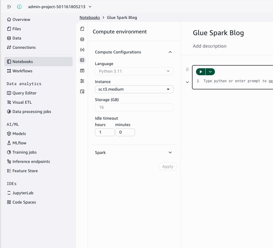
Spark operates at enterprise scale, deployed across 12 AWS Regions to serve global customers with low-latency responses.
In this post, we explore how Nexthink combined Amazon OpenSearch Service vector search, Amazon Bedrock, and infrastructure as code to power the Spark agent’s retrieval layer.
The challenge: Why vector search for AI agents?
For an AI agent to autonomously resolve IT issues, it must quickly retrieve the most relevant context from a vast knowledge base. Traditional keyword search falls short because:
Semantic understanding matters: An employee asking “my laptop is running slow” should match articles about “system performance optimization” even without exact keyword overlap.
Accurate retrieval drives correct outcomes: The quality of an AI agent’s response is only as good as the context it retrieves. When the agent pulls the right documentation, scripts, and historical resolutions, it produces accurate, safe actions. When retrieval is imprecise, the consequences can be severe. An agent acting on the wrong context could run destructive commands like rm -rf *, wipe critical data, or apply an incorrect fix that escalates the problem. Accurate vector search is the guardrail that keeps autonomous agents grounded in verified, relevant knowledge.
Speed is critical: Enterprise users expect near-instant responses, so retrieval must run in sub-second time across millions of documents.
This led Nexthink to implement Amazon OpenSearch Service with vector search capabilities, using Amazon Titan Text Embeddings V2 through Amazon Bedrock for embedding generation. With this architecture, Spark performs semantic search across all knowledge sources, retrieving contextually relevant information that drives accurate, autonomous issue resolution.
High-level architecture
The following diagram illustrates the high-level architecture of Nexthink’s Spark agent implementation with Amazon OpenSearch Service.
Architecture components
Amazon Elastic Kubernetes Service (Amazon EKS) hosts the Spark agent, which interprets user queries, retrieves relevant context, and runs autonomous resolutions. With container orchestration, the agent scales horizontally across Nexthink’s 12 AWS Regions while maintaining consistent response times. The agent communicates with Amazon OpenSearch Service to perform semantic searches, retrieving the most contextually relevant documentation and automation scripts for each user’s issue.
Amazon OpenSearch Service functions as the central vector store, providing the k-Nearest Neighbors (k-NN) capabilities required for semantic search. OpenSearch Service stores document embeddings (dense vector representations of text content) alongside traditional metadata fields. When the AI agent submits a query, OpenSearch Service performs approximate nearest neighbor (ANN) searches to find documents with semantically similar embeddings, even when exact keywords don’t match. This vector search capability, combined with the proven scalability and managed infrastructure of OpenSearch Service, makes it well suited for AI agent architectures that require fast, accurate context retrieval.
Amazon Bedrock provides the foundation models used to generate text embeddings. Nexthink uses Amazon Titan Text Embeddings V2, hosted on Amazon Bedrock, to convert both documents and queries into dense vector representations. OpenSearch Service integrates natively with Amazon Bedrock through the OpenSearch ML Connector, which handles embedding generation at both index and query time.
Data ingestion pipeline
A critical component of any AI agent architecture is the data ingestion pipeline. This mechanism transforms raw documents into searchable, semantically indexed content in OpenSearch Service. For Spark, the pipeline must handle diverse data sources while automatically generating vector embeddings for semantic search.
Step 1: Staging and preprocessing layer
Staging layer in Amazon S3
Knowledge bases (KBs) are staged in Amazon Simple Storage Service (Amazon S3) before being processed through the ingestion pipeline. Amazon S3 provides durable storage, versioning capabilities, and integration with OpenSearch Service ingestion mechanisms. When documentation updates occur, new versions are uploaded to Amazon S3, which triggers the ingestion pipeline to reprocess and re-embed the content.
Event-driven streaming with Apache Kafka
IT tickets, agent interactions, and remote actions are processed through Apache Kafka for reliable message delivery during traffic spikes. Its consumer group model lets the ingestion pipeline scale horizontally based on event volume.
Step 2: Embedding generation during indexing time
Nexthink uses ingest pipelines inside OpenSearch Service to process the data at ingestion time, including generating text embeddings. When documents are sent to OpenSearch Service, the text_embedding processor inside the ingest pipeline automatically invokes the machine learning (ML) Connector to generate embeddings.
The ML Connector is the OpenSearch Service built-in framework for integrating external ML services. It handles request signing between OpenSearch Service and Amazon Bedrock, parses the Amazon Bedrock response to extract embeddings, maps them to index fields, and manages retries on failure. This eliminated the need for custom integration code and accelerated Nexthink’s time to market.
The following ingestion pipeline configuration demonstrates how to configure the text_embedding processor.
model_id: References the registered ML model connected to Amazon Bedrock.
field_map: Maps the source text field (content) to the target embedding field (content_embedding).
Step 3: Embeddings and data structure in OpenSearch Service
Nexthink stores embeddings alongside textual and metadata information in their k-NN index. For the vector field, they use Hierarchical Navigable Small World (HNSW) with the Lucene engine, as shown in the following example.
Enterprise AI agent deployments must address a critical challenge: making sure that users only access data they’re authorized to see. For Nexthink, serving multiple enterprise customers from a shared infrastructure requires robust multi-tenant security. Each customer’s knowledge base, automation scripts, and support tickets must remain isolated while the shared vector index continues to perform well.
The following diagram illustrates the search flow from user query to ranked results.
Tenant management
Nexthink stores information about each tenant inside the tenant_id field. This design lets permission filters run efficiently alongside vector similarity searches. Additionally, Nexthink stores the tenant_id as a keyword type in the index mapping shared previously, so that filtering runs without the overhead of text analysis. Instead of pre-filtering with k-NN queries through a score script filter, the OpenSearch engine uses an intelligent decision-based approach for k-NN filtering called efficient filtering.
Neural query example with efficient filtering
OpenSearch’s neural search simplifies vector search by handling embedding generation as part of the query itself. Instead of requiring the application to call an embedding model separately and then submit a raw k-NN query with a vector, a neural query accepts plain text and uses the registered ML Connector to generate the embedding on the fly. As a result, the Spark agent can send natural-language queries directly to OpenSearch Service without any client-side embedding logic.
The following query demonstrates how Nexthink combines neural search with tenant isolation through efficient filtering in OpenSearch Service.
bool.must: Contains the neural search clause that performs semantic matching against document embeddings.
bool.filter: Applies the tenant isolation constraint, so that only documents belonging to customer-123 are returned.
Nexthink’s contribution to the technical community
A key principle in Nexthink’s architecture is treating infrastructure as code. With deployments spanning 12 AWS Regions, manual provisioning would be error-prone and time-consuming. Therefore, Nexthink uses several infrastructure as code (IaC) technologies, including Terraform, to provision resources.
Although the Terraform provider supports core OpenSearch Service resources like indices and index templates, it lacked support for some of the ML Commons resources required to integrate Amazon Bedrock:
ML Connectors: Required to establish connections to external ML services like Amazon Bedrock.
ML Model Groups: Needed to organize and manage related models.
ML Models: Required to register models that use the connectors.
Without these resources, Nexthink initially relied on workarounds using local-exec provisioners and null_resource blocks to call the OpenSearch Service API directly. This approach was fragile, difficult to maintain, and didn’t integrate well with Terraform’s state management.
Contributing back
Rather than maintaining a private fork indefinitely, Nexthink chose to contribute their custom Terraform resources back to the OpenSearch Project community. This decision aligned with their engineering values to help other organizations implement similar architectures and contribute to the broader community.
Open source contribution links
The Terraform provider contributions are being added to the official OpenSearch project repository:
Pull Request: Add support for ML Connector, ML Model Group, and ML Model resources #280.
Feature Request: Contribution – Support for ML resources #281.
These contributions let any organization provision OpenSearch Service ML resources with Terraform, which streamlines the deployment of AI agent architectures that integrate with Amazon Bedrock or other ML services.
Conclusion
Nexthink’s implementation of Amazon OpenSearch Service for the Spark agent demonstrates how vector search capabilities can power autonomous IT support at enterprise scale. By combining semantic search with multi-tenant security and infrastructure as code practices, Nexthink achieved a 77% resolution rate at first contact, so that employees can resolve IT issues without human escalation.
Get started
Ready to build your own AI agent with vector search capabilities? Here are your next steps:
The combination of Amazon OpenSearch Service, Amazon Bedrock, and infrastructure as code practices provides a foundation for building intelligent, context-aware AI agents that deliver business value.
With Private Networking for Amazon MQ for RabbitMQ, your brokers can establish outbound connections to private resources in your VPC without exposing those resources publicly. This post explains how the feature works and walks you through setting it up.
Amazon MQ for RabbitMQ brokers could previously only reach external destinations over the public internet. If you used a private Lightweight Directory Access Protocol (LDAP) server for broker authentication, you had to expose that server publicly. If you wanted to federate messages between private brokers, you needed workarounds like Network Load Balancers with IP allowlisting, as described in Implementing Federation on Amazon MQ for RabbitMQ Private Brokers. Private Networking removes those constraints.
You can connect your broker to private identity providers, other Amazon MQ for RabbitMQ brokers, or self-hosted RabbitMQ brokers running in private subnets. Combined with cross-Region networking services like AWS Transit Gateway, you can extend these connections across AWS Regions and accounts, with traffic staying on the AWS private network.
You create a VPC Lattice resource gateway in a VPC that can reach your private destination. You then create a VPC Lattice resource configuration that defines the destination, such as an IP address or Domain Name System (DNS) name. You add the resource configuration to a RAM resource share and associate the resource share with your broker through the UpdateBroker API operation. After rebooting the broker, the network path is active and your broker can reach the private destination.
The broker does not need to be private. A publicly accessible broker works the same way.
What you can connect to
Private Networking supports three use cases.
Private identity providers
If you use an LDAP server or other identity provider for RabbitMQ authentication, you no longer need to expose it publicly. Create a resource configuration pointing to your identity provider, associate it with your broker, and use the DNS name returned by the DescribeSharedResources API operation in place of the public endpoint. Follow the existing guidance for setting up an identity provider, substituting the private DNS name.
Self-hosted RabbitMQ brokers
You can use Shovel or Federation to connect your Amazon MQ for RabbitMQ broker to a self-hosted RabbitMQ broker running in a private subnet. Create a resource configuration pointing to the self-hosted broker and use the DNS name from the DescribeSharedResources API operation in your Shovel or Federation configuration.
You can federate or shovel messages between two Amazon MQ for RabbitMQ brokers using Private Networking. Create a resource configuration pointing to the destination broker’s endpoint and specify that same endpoint as the custom domain name on the resource configuration. This helps to verify that the DNS name resolves correctly and Transport Layer Security (TLS) peer verification succeeds.
This extends to brokers in different AWS Regions and different AWS accounts. By combining Private Networking with cross-Region networking services like AWS Transit Gateway or VPC peering, you can build a fully private federation or shovel path between brokers, with no public endpoints required.
DNS names and custom domains
Each resource configuration can include a custom domain name. If you add a verified domain, that domain resolves to the private destination. If you do not add a verified domain, Amazon MQ provides a DNS name for the broker’s private connection. Retrieve this DNS name with the DescribeSharedResources API operation.
If you specify an unverified domain on a resource configuration, it is ignored. The broker’s private connection receives a private DNS name instead, which you can retrieve with the DescribeSharedResources API operation.
Note: If you are running RabbitMQ 4, review this section before configuring Shovel or Federation connections.
RabbitMQ 4 enforces TLS certificate peer verification by default for Shovel and Federation connections. RabbitMQ 3 does not enforce this by default. When using Private Networking, the DNS name that Amazon MQ assigns to the private connection will not match the TLS certificate of the destination, which causes peer verification to fail.
The recommended approach is to specify the destination broker’s endpoint (for example, b-a1b2c3d4-5678-90ab-cdef-EXAMPLE11111.mq.us-east-1.on.aws) as the custom domain name on the resource configuration. This exception only applies to Amazon MQ for RabbitMQ broker endpoints. You cannot use an unverified domain for self-hosted brokers. Specifying the Amazon MQ endpoint causes the DNS name to match the destination’s TLS certificate, and peer verification succeeds. This approach works regardless of your RabbitMQ version and avoids the issue entirely.
Getting started
To get started with Private Networking for Amazon MQ for RabbitMQ, follow these steps.
Create a VPC Lattice resource gateway in a VPC that can reach your private destination. Make sure the resource gateway’s security group allows outbound traffic to your destination on the required port (for example, port 5671 for AMQPS (AMQP over TLS) or port 636 for LDAPS (LDAP over TLS)). The resource gateway must share at least one Availability Zone with the broker. Cluster brokers cover multiple Availability Zones, so this is satisfied. For single-instance brokers, verify the Availability Zone overlap.
Create a VPC Lattice resource configuration pointing to your private destination (IP address or DNS name). If you’re connecting to another Amazon MQ broker, specify the destination broker’s endpoint as the custom domain name on the resource configuration, as shown in the following figure.Figure 1: VPC Lattice resource configuration showing the custom domain name field and resource definition populated with the Amazon MQ broker endpoint.
Add the resource configuration to a RAM resource share. The resource share must allow external principals, as shown in the following figure.Figure 2: RAM resource share configuration with the Allow external principals option selected.
Associate the resource share with your broker by editing the broker and adding the resource share. You can also do this using the update-broker command with the AWS CLI. You must pass the entire list of resource share ARNs you want on the broker. This is a put operation, not an add or remove operation.
The associated RAM resource share appears as shown in the following figure.
Figure 3: Network settings view with associated RAM resource shares.
Select the resource share in the Associated RAM resource shares section. The network status of each shared resource is displayed in the Shared resources section, as shown in the following figure.
Figure 4: RAM resource share selection showing the network status of each shared resource.
Reboot the broker from the AWS Management Console or the AWS CLI to create the network path:
Use the DNS name returned in the output in your Shovel, Federation, or identity provider configuration. Adding new resource configurations to an existing RAM resource share does not automatically update the broker. You must call update-broker and reboot the broker for the new resource configurations to take effect.
Cleaning up
Private Networking uses VPC Lattice and PrivateLink resources that incur ongoing charges. If you no longer need the private connection:
Call update-broker with the resource share removed from the list (or an empty list to remove all), then reboot the broker.
After the broker reboot completes and the resources are no longer in use, delete the VPC Lattice resource configuration and resource gateway.
Optionally, remove the Amazon MQ account principal from the RAM resource share. This principal may still be in use if other brokers are associated with the same resource share, so only remove it if no other brokers depend on it.
If you created a new Amazon MQ for RabbitMQ broker for this walkthrough and no longer need it, delete the broker from the Amazon MQ console or with the delete-broker command.
Operational behavior: Resource access and reboots
Removing a VPC Lattice resource configuration from a RAM resource share while the broker is actively using it revokes access immediately, with no reboot required. Removing a principal from a RAM resource share has the same effect: brokers associated through that principal lose access to the resources in the share immediately. These are intentional security behaviors managed by RAM and VPC Lattice.
Adding new resource configurations to an existing resource share does not take effect automatically. You must call update-broker and reboot the broker for the new resource configurations to take effect. This is by design. It helps verify that changes to a resource share only reach the broker when someone with broker management permissions explicitly triggers the update, providing clear security separation between share management and broker management.
Private Networking is available for Amazon MQ for RabbitMQ brokers in all the AWS Regions where Amazon VPC Lattice is available. Amazon MQ for ActiveMQ brokers do not support this feature.
Pricing
Private Networking uses Amazon VPC Lattice and AWS PrivateLink. Data processing and data transfer charges apply to traffic sent through the private connection. There is an Amazon MQ pricing of $0.01 per GB of data processed through the resource endpoint. For details, see the Amazon MQ pricing page, VPC Lattice pricing page and AWS PrivateLink pricing page.
Conclusion
In this post, we explained how Private Networking for Amazon MQ for RabbitMQ works and walked through the setup process. Whether you’re securing a private identity provider, federating messages between brokers, or connecting to self-hosted RabbitMQ, your broker can now reach private destinations without exposing them publicly.
When a security event occurs in your Amazon Web Services (AWS) environment, rapid response is critical. However security teams often struggle with time-consuming, manual processes that slow down investigations. Analysts must recall complex AWS Command Line Interface (AWS CLI) syntax for multiple services, manually correlate findings across Amazon GuardDuty, AWS CloudTrail, and other security tools, and document every investigation step for compliance requirements. They make critical decisions under pressure while active threats continue. For analysts without deep AWS expertise, these challenges are even more pronounced, creating bottlenecks in your security operations.
Kiro is an AI-powered coding assistant that helps users write, understand, and optimize code through integrated development environment (IDE) and command line integrations. Beyond traditional development tasks, it offers AWS-specific expertise including architecture guidance, best practices, cost optimization recommendations, and service documentation navigation. Kiro CLI puts Kiro’s full capabilities in your terminal, making it a natural fit for security operations workflows. For example, with built-in tools, Kiro CLI can be used to help with investigation of a GuardDuty finding—it will propose the appropriate AWS CLI commands, explain what each command does, and wait for your approval before executing. This approach lets you focus on analyzing threats rather than figuring out how to investigate them.
This blog post demonstrates how to use Kiro CLI to conduct a security investigation following the AWS Security Incident Response Guide framework. This framework organizes incident response into five phases:
Preparation: Having the right tools and processes in place before an incident occurs
Detection and analysis: Identifying security events and understanding their scope
Containment: Limiting the impact of an incident and preventing further damage
Eradication and recovery: Removing threats and restoring normal operations
Post-incident activity: Learning from incidents to improve future response
You’ll see how you can use Kiro CLI to triage GuardDuty findings, assess impacted Amazon Elastic Compute Cloud (Amazon EC2) resources, analyze AWS CloudTrail logs, and generate remediation scripts. By the end of this post, you’ll learn how to use Kiro CLI to run security investigations in minutes rather than hours — without skipping steps.
Prerequisites
Before getting started, confirm you have the following:
AWS CLI: Configure using one of the methods in Configuring settings for the AWS CLI. Kiro CLI uses the default AWS CLI profile (or the profile specified by the AWS_PROFILE environment variable) to interact with AWS resources and will request your approval before executing any actions.
Solution overview
To show Kiro CLI in action, we investigate a GuardDuty finding end to end — following the AWS Security Incident Response Guide framework through the following steps.
Discovery: Retrieve and analyze a high-severity GuardDuty finding
Knowledge capture: Create reusable investigation workflows through steering files
Throughout this investigation, Kiro CLI will propose commands, explain their purpose, wait for approval, and automatically document findings—transforming an inefficient manual process into a guided, efficient workflow.
Kiro CLI combines AI reasoning with deep AWS knowledge to analyze security findings, correlate evidence across services, and propose appropriate AWS CLI commands at each step of an investigation. While this AI-powered approach accelerates investigations, it’s important to validate outputs and recommendations before taking action. The specific commands and analysis shown in this walkthrough are examples—your results will vary based on your specific findings and environment configuration.
The investigation: From alert to resolution
In this section, we walk you through the phases of an investigation, from discovery through analysis.
Discovery: A high-severity GuardDuty finding
Our investigation began with a GuardDuty finding requiring immediate attention. Rather than manually constructing AWS CLI commands, we used Kiro CLI’s natural language interface:
I need to investigate GuardDuty finding 58cddb4e8705cde3f595ef5805f50491 in us-east-1. Please help me understand this finding by checking the finding details, resource details, and threat details. For each investigation step, propose the AWS CLI command, explain what information we'll get, and wait for my confirmation before showing the next command. Document everything in a findings.md file in the current directory, including finding summary, investigation steps, evidence collected, and remediation guidance. Structure it for both technical and executive audiences.
This single prompt establishes the entire investigation framework, as shown in Figure 1. By requesting step-by-step approval, we maintain control while benefiting from AI guidance. The documentation requirement helps ensure that we’re building an audit trail in real-time for compliance requirements.
Figure 1: Kiro CLI interface showing the initial investigation prompt and proposed first command to retrieve GuardDuty detector ID and finding details
Kiro CLI proposed retrieving the detector ID and complete finding details. After approval, it executed the commands and revealed critical information, as shown in Figure 2.Key findings:
Type: CryptoCurrency:EC2/BitcoinTool.B!DNS
Severity: HIGH (8.0)
Instance: i-05447e6dacd0a7e7e (m5.xlarge)
Threat: 617 DNS queries to pool.minergate.com
Timeline: Started 9 minutes after instance launch
We can see that it took 9 minutes from instance launch to mining activity, which suggests automated event rather than manual action. This timeline information, automatically extracted and highlighted by Kiro CLI, helps security teams understand event patterns.
Figure 2: GuardDuty finding details showing HIGH severity cryptocurrency mining detection with threat indicators and timeline
Resource and scope analysis
Kiro CLI proposed investigating the EC2 instance configuration, security groups, IAM permissions, and checking for additional findings. This proactive suggestion demonstrates Kiro CLI’s understanding of security investigation workflows, it knows that understanding the potential impact requires examining not just what the unauthorized user did, but what might possibly be a next step in a typical threat scenario.
The following information is also shown in Figure 3.
Instance configuration: Kiro CLI retrieved the instance details, revealing:
Amazon Linux 2023 AMI
Instance Metadata Service version 2 (IMDSv2) required (good security posture)
Public IP address with unrestricted outbound access
IAM instance profile attached
Security group assessment: Kiro CLI analyzed the security group rules and identified:
No inbound rules
Unrestricted outbound access to 0.0.0.0/0, enabling mining traffic
IAM permission analysis: Kiro CLI examined the instance profile and attached role policies, uncovering a critical security risk:
Critical finding: AdministratorAccess policy attached to the EC2 instance profile
Full AWS account access from compromised instance
Potential for complete account takeover
While the observed activity is cryptocurrency mining, the attached AdministratorAccess policy means the unauthorized user could have exfiltrated data, created backdoors, or compromised other resources. This highlights why least-privilege IAM policies are critical. Even if an instance is compromised, limited permissions help reduce the potential impact.
Figure 3: Kiro CLI’s instance configuration summary highlighting the AdministratorAccess policy, unrestricted outbound access, and multiple concurrent security findings
Scope assessment: Kiro CLI checked for additional unexpected activity and discovered seven security findings on this single instance, indicating a multi-vector attack, as shown in Figure 4.
Figure 4: Kiro CLI’s summary highlighting a multi-vector attack.
Figure 5: Kiro CLI’s summary of the investigation and recommendations for immediate actions.
Instance isolation: Kiro CLI produced commands to create an isolation security group with no inbound or outbound rules (as shown in Figure 6), then applied it to the compromised instance. This containment step stops new connections without destroying evidence. However, it’s important to understand that security groups are stateful and use connection tracking. When you change security group rules, existing connections aren’t immediately interrupted and continue to allow packets until they time out.
This means that if an unauthorized user has an active connection to the instance, that connection might persist temporarily even after applying the isolation security group. For immediate interruption of all traffic including active connections, consider also implementing network access control lists (NACLs), which are stateless and don’t track connection state. Unlike security groups, NACLs can immediately break existing connections when rules are applied. While NACLs operate at the subnet level (broader scope than instance-level security groups), they provide an additional layer of defense that helps ensure network isolation.
This scenario illustrates an important principle: while AI-powered tools such as Kiro CLI can help you respond more quickly by generating appropriate commands, it’s critical to keep a human in the loop who understands these nuances. Kiro CLI might not have complete information about edge cases, so security professionals should validate recommendations and consider additional controls based on their expertise and the specific threat scenario.
Figure 6: Instance successfully isolated with confirmation showing no inbound or outbound rules, blocking all network traffic including command-and-control (C&C) communications and mining activity
Privilege revocation: Kiro CLI generated commands to attach a deny-all policy to the compromised IAM role (as shown in Figure 7). The AI assistant explained that even though the AdministratorAccess policy remains attached, the deny-all policy takes precedence because of the evaluation logic used by IAM, where explicit denies always override any allows. This immediately revoked all permissions while preserving the original configuration for forensic analysis.
Figure 7: IAM credentials revocation confirmation with current status checklist showing network isolated, IAM credentials revoked, and forensic snapshot pending
Evidence preservation
Before making mutating changes, Kiro CLI recommended creating a forensic snapshot of the compromised instance’s Amazon EBS volume (as shown in figure 8). This step can be missed when teams are under pressure to contain an active threat, but it’s critical for post-incident analysis and potential legal proceedings.
Memory preservation decision: We chose to leave the instance running in its isolated state rather than stopping it immediately. Stopping an EC2 instance results in loss of volatile memory containing forensic evidence such as running processes, network connections, loaded malware, and encryption keys. By maintaining the instance in an isolated security group with all network access blocked, we neutralized the threat while preserving the ability to conduct deeper forensic investigation if needed.
Volatile memory often contains evidence that explains how an event occurred, malware binaries, decryption keys, or command-and-control (C&C) communications that disappear when an instance stops. This decision point illustrates the balance between immediate threat elimination and thorough investigation.
Capturing volatile memory requires specialized tools and techniques. For Linux instances, LiME (Linux Memory Extractor) can capture physical memory, while Windows instances can use tools like Winpmem. After being captured, memory dumps can be analyzed using Volatility, an open source memory forensics framework. Forensics tools should be pre-installed on your systems to avoid changes being made during the evidence gathering process. AWS provides guidance on automating forensic kernel module builds for Amazon Linux EC2 instances to streamline this process.
Figure 8: Forensic snapshot creation confirmation with proper tagging including purpose, incident ID, and severity for evidence preservation
CloudTrail analysis
To understand the full scope of compromise, we asked Kiro CLI to analyze CloudTrail logs. The AI assistant identified available CloudTrail trails and proposed queries to find any API calls made from the compromised instance using its temporary credentials (as shown in Figure 9).
CloudTrail analysis is often the most time-consuming part of incident investigation, requiring analysts to construct complex queries and correlate events across time. Kiro CLI automates this process, immediately identifying the relevant log sources and proposing appropriate queries.
Figure 9: Kiro CLI identifying available CloudTrail trails and proposing targeted queries
Kiro CLI found no unexpected API calls originating from the instance credentials—no IAM users created, no S3 buckets accessed, and no secrets stolen. The event appeared limited to cryptocurrency mining activity conducted through DNS queries, with no evidence of data exfiltration or lateral movement.
Figure 10: Investigation results from Kiro CLI
This shows the value of thorough CloudTrail analysis: even when initial findings suggest a contained threat, confirming the absence of broader compromise is essential before closing an investigation.
Building proactive defenses
The AWS Security Incident Response Guide emphasizes that preparation is the foundation of effective incident response. With the immediate threat contained, we used Kiro CLI to strengthen our preparation phase by establishing automated alerting for future incidents.
As shown in Figure 11, we used natural language to request
Set up a notification system that sends an email to [email] for any high severity or higher severity findings.
Kiro CLI understood the requirement and proposed a multi-step solution involving Amazon SNS and EventBridge:
Create an SNS topic for GuardDuty alerts
Subscribe an email address to the topic
Create an EventBridge rule to trigger on high-severity findings (severity greater than or equal to 7.0)
Configure the SNS topic as the EventBridge target
Grant EventBridge permissions to publish to the SNS topic
Building automated alerting requires understanding multiple AWS services, their interactions, and correct configuration syntax. Kiro CLI translates a straightforward natural language request into a complete, production-ready solution.
Auto-correction and testing: When setting up complex integrations, commands can fail because of permission issues, incorrect Amazon Resource Name (ARN) references, or malformed JSON policies. Kiro CLI automatically detects these failures and proposes corrected commands.
Figure 11: Notification system setup completion showing SNS topic created, EventBridge rule configured, and confirmation that notifications will trigger on HIGH and CRITICAL severity findings
You can also prompt Kiro CLI to test the setup: Test this notification system to verify it’s working correctly. Kiro CLI will verify that the SNS subscription is confirmed, check that the EventBridge rule is properly configured, validate IAM permissions, identify any misconfigurations, and publish a test event to verify end-to-end functionality. This intelligent error handling means security teams can confidently deploy automation without manual troubleshooting.
Creating reusable investigation workflows
With the immediate threat contained and proactive defenses in place, we then used Kiro CLI to create a reusable steering file that codifies this investigation workflow for future incidents. Steering files are Markdown files stored in .kiro/steering/ that act as persistent memory for Kiro CLI, helping security teams capture institutional knowledge and standardize response procedures. To share them across your team, add them to a Git repository or publish them to your documentation system like Confluence — the same places you’d keep any other runbook.
We recommend running the full investigation and generating the steering file in the same Kiro CLI session. This way, the steering file captures the exact steps, commands, and decisions from your investigation. Navigate the process the way that fits your organization — the steering file will reflect your workflow, not a generic template.
We asked Kiro CLI:
Create a steering file that captures this GuardDuty investigation workflow so future analysts can follow the same systematic approach.
Kiro CLI generated a detailed steering file at .kiro/steering/guardduty-incident-response.md that includes:
Investigation phases aligned with the AWS Security Incident Response Guide
AWS CLI command patterns for GuardDuty, Amazon EC2, IAM, and CloudTrail
Documentation requirements and approval gates
Containment, eradication, and evidence preservation procedures
This is the example steering file that was created by Kiro cli:
---
inclusion: manual
---
# GuardDuty Incident Response Workflow
This steering file guides systematic investigation of GuardDuty findings following AWS Security Incident Response Guide best practices.
## Investigation Phases
### Detection and Analysis
1. Retrieve GuardDuty finding details using finding ID
2. Extract finding type, severity, affected resources, and threat indicators
3. Document timeline of events (instance launch, threat detection)
### Resource Analysis
4. Investigate EC2 instance configuration (AMI, IMDS version, network access)
5. Analyze security group rules (inbound/outbound access)
6. Review IAM permissions attached to instance profile
7. Check for additional findings on the same resource
### Containment
8. Create isolation security group with no inbound/outbound rules
9. Apply isolation security group to compromised instance
10. Create forensic snapshot before making destructive changes
11. Preserve volatile memory by keeping instance running if forensic analysis needed
### Eradication
12. Revoke excessive IAM permissions
13. Document all actions in findings.md with technical and executive summaries
### Analysis
14. Query CloudTrail for API calls from compromised instance credentials
15. Assess scope of compromise and potential lateral movement
## Documentation Requirements
- Finding summary with severity and type
- Investigation steps with timestamps
- Evidence collected (security groups, IAM policies, CloudTrail logs)
- Remediation actions taken
- Recommendations for prevention
## AWS CLI Command Patterns
- GuardDuty: `aws guardduty get-findings`
- EC2: `aws ec2 describe-instances`, `aws ec2 describe-security-groups`
- IAM: `aws iam get-instance-profile`, `aws iam list-attached-role-policies`
- CloudTrail: `aws cloudtrail lookup-events`
## Approval Gates
Always propose commands with explanations before execution and wait for approval.
Traditional incident response playbooks are static documents that quickly become outdated. Kiro CLI steering files are executable playbooks that guide AI-assisted investigations with consistency while remaining flexible enough to adapt to specific scenarios. Steering files stay current because updating them is part of the workflow, not a separate task. When you adjust your investigation process, ask Kiro CLI to update the steering file at the end of the session. It captures your changes, and you share the updated version with the team through Git or Confluence — everyone works from the latest version.
Conclusion
Security incidents require accurate and rapid response, but traditional investigation workflows create bottlenecks that extend mean time to respond (MTTR). By following the framework provided by the AWS Security Incident Response Guide and using Kiro CLI’s AI-powered capabilities, you can transform incident response from reactive to proactive, well-documented operations.
In this post, we demonstrated how Kiro CLI accelerates each phase of the incident response lifecycle—from initial detection and analysis through containment, eradication, and recovery. You learned how to use natural language prompts to investigate GuardDuty findings, analyze compromised resources, implement containment measures, preserve forensic evidence, and establish automated alerting for future incidents. The steering file capability helps your team embed hard-won expertise in reusable workflows that benefit analysts at all skill levels.
Whether you’re investigating alerts, building defenses, or documenting procedures, Kiro CLI provides the expertise and automation to respond faster, learn continuously, build better defenses, and document thoroughly. When commands fail or configurations are wrong, Kiro CLI identifies the issue and corrects it, reducing time spent troubleshooting.
If you have feedback about this post, submit comments in the Comments section below.
In this blog post you’ll learn how to detect and prevent subdomain takeover – a tactic where threat actors exploit dangling DNS records to redirect traffic to attacker-controlled resources. We’ll explain the issue, how the situation arises, and how you can use various AWS features and services to help mitigate the impact of this tactic.
Under the shared responsibility model, securing configurations in the cloud is your responsibility. AWS supports you through strong defaults, guidance in the Security Pillar of the Well-Architected Framework, and security services to help you meet that responsibility. The AWS Customer Incident Response Team (AWS CIRT) also monitors for new and trending tactics that threat actors use to exploit specific customer configurations, so that you can make informed design decisions and improve your response plans.
AWS CIRT has observed threat actors actively scanning for public DNS CNAME records that point to resources that no longer exist, looking for subdomain takeover opportunities.
Note: The subdomain takeover tactic does not leverage vulnerabilities of AWS services. It exploits a dangling DNS record to redirect traffic to an attacker-controlled resource.
Quick DNS Primer
CNAME Records: A CNAME (Canonical Name) record is a DNS entry that points one domain name to another. For example, api.example.com can be configured to point to api.example.s3-website-us-east-1.amazonaws.com. This feature of DNS enables users to configure a memorable, human-friendly domain name while the actual resource lives at a longer, machine-generated AWS hostname. A security issue emerges when the target resource is deleted but the CNAME record pointing to it remains – creating a “dangling” record.
Dangling Records: When a resource (like an S3 bucket) is deleted but the DNS record pointing to it is left behind, that DNS record becomes “dangling”, pointing to a resource that no longer exists. For resources in globally shared namespaces, threat actors can potentially reclaim the name of your deleted resource and serve malicious content through your DNS record.
What is subdomain takeover?
A subdomain is a prefix added to a domain that allows you to organize access to your resources. A subdomain takeover occurs when you delete the underlying resource and a threat actor creates a new resource with the same name to take advantage of the DNS records still pointing to it.
A subdomain takeover is possible when a CNAME record points to an AWS resource that uses a globally shared DNS namespace where the resource name can be chosen by any AWS customer. The following AWS resources meet these criteria:
Amazon S3 (global namespace): Bucket names like mybucket.s3.amazonaws.com are globally unique and can be claimed by any account if the bucket is deleted. Note: S3 buckets created with account regional namespaces (launched March 2026) are scoped to your account and are not subject to this issue.
Amazon CloudFront: Distribution domain names like d111111abcdef8.cloudfront.net are assigned by AWS and cannot be chosen by an attacker. However, if you delete a distribution and another customer creates one that happens to receive the same domain name, a dangling CNAME could resolve to their content.
AWS Elastic Beanstalk: Environment names like myapp.elasticbeanstalk.com are globally unique and can be claimed by any account if the environment is terminated.
Resources like Amazon VPC, Amazon EC2 instances, or private hosted zones are not subject to this tactic because they do not expose globally claimable DNS namespaces.
You create a DNS CNAME record pointing to your S3 website endpoint. The subdomain subdomain.example.com now resolves to subdomain.example.s3-website-us-east-1.amazonaws.com, which serves content from the S3 bucket named subdomain.example. If your team deletes the bucket and forgets to delete the DNS record, users that navigate to the site will see an error stating that the bucket doesn’t exist. However, at this point, if a threat actor sees this error and moves in to claim the bucket name, they will be able to set up their own site that users will see when they navigate to the subdomain.example.com site.
Figure 1 shows an S3 bucket named subdomain.example (a globally unique bucket name) configured to host a static website, with the S3 website endpoint subdomain.example.s3-website-us-east-1.amazonaws.com.
Figure 1: S3 bucket configured as a static website
As shown in Figure 2, we use Amazon Route 53 to create a CNAME record to resolve to our Amazon domain name; to give users a friendly name and so they do not have to remember the long S3 website name in URLs.
Figure 2: DNS Resolver configured with CNAME record pointing to origin bucket
The customer’s AWS administrator decides to stop serving content from the S3 bucket and deletes it, as shown in Figure 3.
Figure 3: Resource deleted without removing the CNAME record
With the S3 bucket deleted and the CNAME record still in place, the DNS record is now dangling. A threat actor identifies this situation and creates a new S3 bucket with the same global name subdomain.example in an AWS account that the threat actor controls, as shown in Figure 4. The threat actor can now serve content from this new bucket, including potentially malicious content. End users remain unaware of this switch and continue to access subdomain.example.com, trusting the content because it appears to originate from a URL they recognize.
Figure 4: Subdomain takeover happens
Potential impacts of a sub-domain takeover
Consider these potential impacts:
Reputation risk: There is a potential risk to your organization’s reputation, because you don’t control the content being served from the threat actor’s site that your DNS record points to.
Potential exposure to phishing campaigns: Users within your organization might have the subdomain bookmarked in their browser, not knowing the resource is no longer available, then unsuspectingly navigate to the site that now hosts malware or is used to phish user credentials.
Blocking: If the subdomain is flagged by security vendors for malicious activity, it could impact your business operations.
Financial loss: Subdomain takeover incidents can result in a financial impact due to the potential disruption to service delivery as you deal with the event.
Proactive detection
AWS Config for proactive detection
For proactive detection, you can use AWS Config to continuously monitor your Route 53 CNAME records and verify that the target resources exist in your account.
Prerequisite: This approach requires AWS Config recorder to be enabled for the resource types you want to monitor (S3 buckets, CloudFront distributions, Elastic Beanstalk environments). If Config isn’t recording a resource type, it won’t appear in the inventory check. For more information, see Setting up AWS Config with the console.
Why use AWS Config inventory instead of DNS resolution checks?
A common approach is to check whether a CNAME resolves to a valid endpoint. However, this method has a critical flaw: if an attacker has already claimed the resource, DNS resolution will succeed – to their resource, not yours. You would have no indication that you don’t own what’s responding.
By querying AWS Config’s recorded configuration items, you’re checking whether the resource exists in your account inventory, not just whether something responds at that DNS name. This approach correctly identifies dangling CNAMEs even after a takeover has occurred.
Implementation approach:
Account-level vs. organization-level scope
The reference implementation queries AWS Config inventory within a single account. This means that if a CNAME record in Account A points to a resource that legitimately exists in Account B within the same AWS organization, the rule will flag it as NON_COMPLIANT.
For organizations that share resources across accounts, you can modify the solution to use an AWS Config Aggregator, which queries resource inventory across all accounts in your organization. This is similar to how IAM Access Analyzer supports both account-level and organization-level scopes. To use this approach, you need an organization-level Config Aggregator already configured, and the Lambda function’s IAM role needs the config:SelectAggregateResourceConfig permission.
We recommend starting with account-level scope for simplicity, then expanding to organization-level if your environment includes cross-account resource sharing.
The main idea is to create a custom AWS Config rule that queries your Route 53 hosted zones for CNAME records, then parses each CNAME target to determine whether it points to a known AWS resource pattern such as S3, CloudFront, or Elastic Beanstalk. For each match, the rule cross-references the target against your AWS Config inventory to verify that the resource actually exists in your account. If the resource isn’t found, the rule marks the CNAME record as NON_COMPLIANT, surfacing it for review.
The Config rule should focus on known AWS resource patterns:
Note: CNAME records pointing to external third-party services are outside the scope of this detection mechanism, as those resources won’t appear in your AWS Config inventory.
NON_COMPLIANT findings from your Config rule can be routed to AWS Security Hub for centralized visibility, or trigger SNS notifications to alert your security team.
Figure 5: Dangling DNS Detection Solution
Reference implementation:
We’ve published a complete implementation of this detection approach as an open-source solution. The solution deploys a Lambda function that discovers CNAME records across all your Route 53 hosted zones and uses pattern matching to identify targets pointing to S3, CloudFront, and Elastic Beanstalk. It then queries your AWS Config inventory to verify whether each target resource still exists in your account. When a dangling record is detected, the solution generates a HIGH severity finding in Security Hub and can optionally send SNS notifications to alert your security team. A CloudWatch metrics dashboard is also included for ongoing compliance tracking.
Deployment:
# Clone the repository
git clone https://github.com/aws-samples/sample-dangling-dns-detection
cd sample-dangling-dns-detection
# Build the Lambda deployment package
./scripts/package.sh
# Upload to S3
aws s3 cp dist/dangling-dns-detection.zip s3://YOUR_BUCKET/
# Deploy the CloudFormation stack
aws cloudformation deploy \
--template-file infrastructure/template.yaml \
--stack-name dangling-dns-detection \
--parameter-overrides \
LambdaCodeS3Bucket=YOUR_BUCKET \
EvaluationFrequency=TwentyFour_Hours \
--capabilities CAPABILITY_NAMED_IAM
The stack creates an AWS Config custom rule that runs on your specified schedule (default: every 24 hours), evaluating all CNAME records and reporting compliance status.
Mitigating the effects
Mitigating subdomain takeover requires both preventive procedures and responsive capabilities.
Prevention: Standard operating procedure
The most effective mitigation is a standard operating procedure for resource deprovisioning that ensures DNS records are removed before the underlying resource:
Within your DNS zone, delete the CNAME record that points to the fully qualified domain name (FQDN) of the resource that you plan to deprovision.
Wait for the DNS TTL to expire before deleting the resource. DNS resolvers cache records for the duration of the TTL (for example, a TTL of 3600 means resolvers may serve the old record for up to one hour). If you delete the resource before the TTL expires, a threat actor could claim the resource name while cached CNAME entries are still directing traffic to it.
Deprovision the resource that you no longer want to use.
Run a DNS check of the CNAME record that you removed to verify that the resource is no longer resolving.
Key principle: Always delete DNS first, wait for the TTL to expire, then delete the resource. This order eliminates the window where a dangling record could be exploited.
Prevention: S3 account regional namespaces
As mentioned earlier, AWS introduced account regional namespaces for Amazon S3 general purpose buckets in March 2026. While this is a meaningful step toward mitigating the S3-specific takeover vector, there are important operational limitations to be aware of:
Existing buckets are unaffected. Buckets already created in the global namespace cannot be migrated to an account regional namespace. The bucket names remain globally unique and claimable by anyone if the bucket is deleted.
Global namespace is still the default. When creating a new bucket through the console, CLI, or SDK, the global namespace remains the default selection. Users who aren’t aware of the new option will continue creating globally-scoped buckets.
Existing IaC templates require updates. Existing infrastructure-as-code templates (CloudFormation, CDK, Terraform) that don’t explicitly opt in to the account regional namespace will continue provisioning buckets in the global namespace. For CloudFormation, this means setting the BucketNamespace property to account-regional. For other IaC tools, consult their documentation for the equivalent configuration. Organizations need to audit and update their templates to opt in.
For these reasons, the dangling DNS detection approach described in this post remains critical – particularly for organizations with existing S3 infrastructure, and for CloudFront, and Elastic Beanstalk resources where no equivalent namespace scoping exists.
Response: Notification and remediation
When a dangling DNS record is detected, the reference solution described in the Detection section automatically creates a HIGH severity finding in AWS Security Hub and reports the CNAME record as NON_COMPLIANT in AWS Config. If you provide an SNS topic ARN during deployment, the solution also sends notifications to alert your security or operations team via email, Slack, or other channels. For production environments, consider a human-in-the-loop workflow where these notifications are reviewed by a team member who approves the DNS record deletion before it’s executed. This prevents accidental deletion of legitimate records during transient issues.
The reference solution also includes a CloudWatch dashboard for tracking compliance status and evaluation metrics over time, giving your team ongoing visibility into DNS health across your hosted zones.
Note: Fully automated remediation (auto-deleting DNS records) carries risk – a false positive could disrupt legitimate services. We recommend starting with detection and notification, then evaluating automation based on your detection accuracy and operational maturity.
Conclusion
Subdomain takeover is a preventable misconfiguration that can have significant impact on your organization. A layered defense approach provides the best protection:
Prevention: Implement a standard operating procedure that deletes DNS records before deprovisioning the underlying resource.
Detection: Use AWS Config custom rules to proactively identify CNAME records pointing to resources that no longer exist in your account.
Response: Configure notifications through SNS or Security Hub so your team can respond quickly when dangling records are detected.
Monitoring: Maintain ongoing visibility through CloudWatch dashboards to track DNS health and compliance status.
The key insight is that good DNS hygiene – knowing when your CNAME records point to a nonexistent resource – is your first line of defense. Automated detection through AWS Config provides a safety net when operational procedures fail. And if you detect an issue, having a playbook ready to enact your response can lower the impact and your mean time to recovery.
If you have feedback about this post, submit comments in the Comments section below.
This post is co-authored with Sathish Kumar and Christopher Chan from Samsung ecommerce.
In high-traffic ecommerce, achieving real-time pricing is critical to prevent price inconsistency. Pricing inconsistency creates cart shock and erodes trust. This isn’t broken software, it’s a symptom of architectural latency that you can address using AWS Lambda Response Streaming and Amazon CloudFront for systems aggregating data from multiple backend sources.
In this post, we walk through the legacy architecture challenges, the stateless streaming solution, key implementation patterns, and performance results—a pattern you can apply if you’re building high-traffic APIs that aggregate data from multiple backend sources.
Samsung.com is Samsung’s primary direct-to-consumer channel, selling smartphones, TVs, appliances, and accessories, each with multiple variants, offers, and regional pricing. This complexity makes real-time price accuracy especially important.
Samsung’s All Deals and Product Finder pages showcase these products during high-traffic events like Black Friday. To maintain low latency for these high-density Product Listing Pages (PLPs) and comparison tables, the legacy infrastructure relied on asynchronous caching, which introduced a desynchronization gap where the cached price drifted from the authoritative pricing engine.
Problem: Legacy middleware caching created a 1-hour desynchronization gap between the authoritative pricing engine and customer-facing pages.
Our approach: We dismantled the stateful Data Aggregation (DA) architecture and built a real-time Bulk Arbitration Engine (a stateless orchestration layer that queries the Pricing Engine directly at request time) using AWS Lambda Response Streaming and Amazon CloudFront edge caching.
Challenge: The Data Aggregation trap
When product listing pages need to display pricing for over 30 item combinations simultaneously, the latency of calling the Pricing Engine for each item combination individually becomes untenable. To solve this, we built a backend for frontend (BFF) service to do a “Data Aggregation. This DA service was designed to decouple the frontend from the heavy Pricing Engine.
It relied on a scheduled Cron Worker that ran hourly to fetch the entire product catalog. The worker would then precompute prices for every possible permutation of products and store them in a local cache.
While this improved read speeds, it created two significant failures:
1. The Permutation Explosion – The DA service had to precompute every combination just in case a customer viewed it.
The Math: 30 products × (Variants × Offers × Add-ons) = Thousands of records per page
Storage Impact: Cache grew exponentially with each new product variant added
Waste: Most precomputed combinations were never requested
2. The Synchronization Lag – Because the Cron job ran only once per hour, price changes (for example, flash sales) lagged significantly. Customers continued to see old prices until the next scheduled sync.
Business Impact: Flash sales showed incorrect old pricing until the next run time
Customer Trust: Cart shock when checkout price differed from product page price
Competitive Disadvantage: Competitors with real-time pricing gained market share
Legacy Data Aggregation architecture
Architecture diagram showing the legacy Data Aggregation layer between the Pricing Engine and CloudFront CDN.
Figure 1: Legacy Data Aggregation (DA) ArchitectureThe legacy system relied on a scheduled Cron job, creating a distinct “Desynchronization Layer” between the Authority (Pricing) and the Customer. Precomputation of all product permutations consumed significant storage and compute resources.
The solution: Stateless streaming architecture
Intermediate layers storing data will eventually diverge from the source, so we collaborated with our AWS Technical Account Manager (TAM) and service teams to architect a new solution: the Bulk Arbitration Engine, a stateless orchestration layer that queries the Pricing Engine directly at request time.
The new architecture follows a Pass-Through pattern:
1. Client Request: The browser requests prices for 30 specific SKUs using a single HTTP GET request.
2. Streaming Orchestration: An AWS Lambda function fans out these 30 requests to the Pricing Engine in parallel.
3. Immediate Response: As the Pricing Engine returns data, the Lambda streams it immediately to the client without buffering.
Why Lambda Response Streaming?
We evaluated several alternatives before settling on this approach:
Traditional request-response pattern (buffered) – A standard Lambda invocation buffers the full response before returning it to the client, which negates the latency benefit of parallel fan-out. For 30 concurrent SKU lookups, this added seconds of wait time.
EC2 with improved caching – This was the legacy approach. Caching layers will eventually drift from the source of truth, which was the core problem we needed to solve.
Lambda Response Streaming – This was the only option that let us fan out requests in parallel, stream results as they arrived (reducing time-to-first-byte), and remain fully stateless with no intermediate cache to maintain or invalidate.
New stateless streaming architecture
Architecture diagram showing the stateless streaming solution with CloudFront connected directly to Lambda.
Figure 2: Stateless Streaming ArchitectureThe new architecture eliminates the middleware cache. A high-performance stream connects the user directly to the pricing source of truth. CloudFront edge locations cache the response for 95% of traffic, while remaining requests go directly to Lambda for real-time pricing.
Implementation walkthrough
Transitioning to this new architecture required solving two specific technical constraints regarding CDN behavior and cold starts. We implemented the solution in three steps.
Step 1: Implementing the streaming handler
The core of our solution is the Node.js Lambda handler wrapped in awslambda.streamifyResponse(). This allows us to pipe data through a transformation and compression stream directly to the client as it becomes available.
We used a custom NDJSONTransform to convert pricing objects into newline-delimited JSON (NDJSON), allowing the browser to parse and render each price as it arrives rather than waiting for the complete response.
// Lambda Handler with Response Streaming
// File: lambda-handler.js
import * as awslambda from "aws-lambda";
import * as zlib from "zlib";
import { pipeline } from "stream/promises";
import { NDJSONTransform } from "./transforms/ndjson-transform.js";
// Constants
const PROCESSING_MODE = process.env.PROCESSING_MODE || "MODE_QUERYSTRING";
const MODE_QUERYSTRING = "MODE_QUERYSTRING";
// The Handler MUST be wrapped in streamifyResponse() to enable streaming
export const handler = awslambda.streamifyResponse(
async (event, responseStream, _context) => {
try {
if (PROCESSING_MODE === MODE_QUERYSTRING) {
// Set response metadata with status code and headers
const httpResponseMetadata = {
statusCode: 200,
headers: {
"Content-Type": "application/x-ndjson",
"Content-Encoding": "gzip",
"Cache-Control": "public, max-age=300", // 5 min cache
"X-Custom-Header": "lambda-streaming",
},
};
responseStream = awslambda.HttpResponseStream.from(
responseStream,
httpResponseMetadata
);
const ndjsonTransform = new NDJSONTransform();
// Create gzip stream with fast compression level (Z_BEST_SPEED = Level 1)
// Level 1 prioritizes speed over compression ratio for real-time responses
const gzip = zlib.createGzip({
level: zlib.constants.Z_BEST_SPEED,
});
// Process the request, writing to the gzip stream
await processRequestUsingQueryString(event, ndjsonTransform, _context);
// Pipeline: Transform → Compress → Send
await pipeline(ndjsonTransform, gzip, responseStream);
}
// ... error handling
} catch (error) {
console.error("Lambda streaming error:", error);
responseStream.destroy();
} finally {
await flushMetrics().catch(console.error);
}
}
);
Helper function to fan-out the requests in parallel:
// Process request: fan out SKU lookups in parallel
async function processRequestUsingQueryString(event, ndjsonTransform, context) {
try {
// Parse query string to extract SKU list
const queryString = event.rawQueryString || "";
const skus = parseCompressedQueryString(queryString);
// Fetch pricing in parallel using Promise.all
const pricingPromises = skus.map((sku) =>
fetchPricingForSKU(sku).catch((err) => ({
sku: sku.id,
error: err.message,
}))
);
const pricingResults = await Promise.all(pricingPromises);
// Emit each result as a separate NDJSON line
for (const result of pricingResults) {
ndjsonTransform.write(result);
}
ndjsonTransform.end();
} catch (error) {
ndjsonTransform.destroy(error);
}
}
The handler also uses helper functions for parsing the compressed query string (parseCompressedQueryString), fetching individual SKU prices with connection pooling (fetchPricingForSKU), and flushing metrics to Amazon CloudWatch (flushMetrics).
Key implementation details:
awslambda.streamifyResponse() wraps the handler so it streams data in real time instead of waiting for the full response from the pricing engine.
NDJSONTransform converts objects to newline-delimited JSON (one object per line)
GZIP (GNU zip) compression with Z_BEST_SPEED (Level 1) prioritizes speed over compression ratio
pipeline() handles error propagation and stream cleanup
Response headers include Cache-Control for CloudFront caching
Step 2: Compressing the request data into a GET request
We needed to send complex request data (30 SKUs, context metadata) to the API.
Constraint: CloudFront and standard HTTP specs treat POST requests as non-idempotent, meaning they are not cacheable by default.
Our approach: We developed a dense, compressed query string format to fit the complex request data into a standard GET request. Format: g=group1(p=SKU-A:1:p=SKU-B:2)…
This allowed us to strictly use GET requests, keeping the request URI within standard length limits (~800 bytes) while carrying the same data as a 3-4KB JSON body.
Client-Side Code: Building the Compressed Query String
// Client-side: Building the compressed query string format
// File: pricing-client.js
/**
* Builds a compressed query string for bulk pricing requests
* Format: g=group1(p=SKU-A:1:p=SKU-B:2:p=SKU-C:3)
* @param {Array} skus - Array of SKU objects with { id, variant }
* @param {Object} context - Customer context { customerId, region, sessionId }
* @returns {string} Compressed query string
*/
function buildPricingQueryString(skus, context = {}) {
if (!skus || skus.length === 0) {
throw new Error("SKUs array cannot be empty");
}
if (skus.length > 30) {
throw new Error("Maximum 30 SKUs per request. Split into multiple batches.");
}
// Build SKU portion: p=SKU-001:1:p=SKU-002:2
const skuParts = skus
.map((sku) => {
const variant = sku.variant || 1;
return `p=${sku.id}:${variant}`;
})
.join(":");
// Build context portion (optional)
let contextPart = "";
if (context && Object.keys(context).length > 0) {
const contextStr = Object.entries(context)
.map(([key, value]) => `${key}=${value}`)
.join(":");
contextPart = `:c=${contextStr}`;
}
// Final format: g=group1(p=SKU-A:1:p=SKU-B:2:c=customerId=123:region=US-EAST-1)
return `g=group1(${skuParts}${contextPart})`;
}
/**
* Fetches pricing data with streaming NDJSON response parsing
* Core pattern: read chunks, split by newlines, parse each line as JSON
*/
async function fetchPricingStream(skus, options = {}) {
const queryString = buildPricingQueryString(skus);
const url = `${options.baseUrl}?${queryString}`;
const response = await fetch(url, {
method: "GET",
headers: { Accept: "application/x-ndjson" },
});
// Stream the response using the ReadableStream API
const reader = response.body.getReader();
const decoder = new TextDecoder();
const pricingData = [];
let buffer = "";
while (true) {
const { done, value } = await reader.read();
if (done) break;
// Decode chunk and append to buffer
buffer += decoder.decode(value, { stream: true });
// Split by newlines (NDJSON format: one JSON object per line)
const lines = buffer.split("\n");
// Keep the last incomplete line in buffer
buffer = lines.pop() || "";
// Parse each complete line as a JSON object
for (const line of lines) {
if (line.trim()) {
const pricingObject = JSON.parse(line);
pricingData.push(pricingObject);
// Optional: update UI immediately as each price arrives
if (options.onChunk) {
options.onChunk(pricingObject);
}
}
}
}
reader.releaseLock();
return pricingData;
}
On page load, the client calls fetchPricingStream with up to 30 SKUs and an onChunk callback that updates each product’s DOM (Document Object Model) element as pricing chunks arrive. Helper functions handle updating individual price elements, displaying variant information, and gracefully degrading with a user-friendly message if pricing is temporarily unavailable.
Step 3: Configuring CloudFront for uncacheable requests
To allow CloudFront to cache these complex GET requests effectively, we configured a precise Cache Policy that includes all query strings and specific headers.
The CloudFront distribution itself is configured with HTTPS-only viewer protocol, the cache policy and origin request policy as shown in the preceding section, and points to the Lambda as its origin through HTTPS.
Cache policy highlights:
5-minute default TTL balances freshness and cache efficiency
Query strings included in cache key (different SKU combos = separate cache entries)
5–30 minute TTL range provides flexibility for different content
Performance optimization results
We optimized the system through four distinct phases, testing each configuration with K6 load test scripts (500 concurrent users, 30 items per request) to simulate high-traffic events like Black Friday.
Phase 1: The baseline (Global VPN)
We tested our initial proof-of-concept with the default network configuration, where all outbound traffic (including requests to AWS services like Lambda) was routed through a global VPN, forcing traffic onto the public network and back into the AWS backbone, adding unnecessary network hops and delays. The Lambda used a standard buffered response with no compression. The results were suboptimal (4,500ms P90) because connection overhead dominated the request.
DNS resolution: approximately 50 ms
TCP handshake: approximately 100 ms
TLS negotiation: approximately 150 ms
Total connection overhead: approximately 300 ms per call
This overhead created a massive bottleneck for latency before business logic even ran.
Phase 2: Amazon VPC Peering and warm starts
To remove the network penalty, we acted on two fronts:
First: Moved the Lambda inside an Amazon Virtual Private Cloud (Amazon VPC) peered directly to the pricing origin, cutting DNS and TLS overhead to near zero for internal calls.
Second: Enabled Provisioned Concurrency for Lambda to remove the 500–1000 ms cold start latency.
With these changes, P90 latency dropped to 1,000 ms, a 4.5x improvement, but still not real-time enough.
Phase 3: HTTP/2 and GZIP compression
The remaining bottleneck was the sheer size of the data transfer. We targeted two optimizations:
HTTP/2 Multiplexing: Enabled HTTP/2 multiplexing to reuse a single TCP connection for the 30 parallel SKU lookups, saving seconds of cumulative handshake time.
GZIP Compression: Applied GZIP compression (Level 1 / Z_BEST_SPEED), which reduced the response size by 76 percent (170KB → 40KB).
These two optimizations brought P90 latency down to 218 ms.
Phase 4: Production (edge caching)
In the final phase, we layered CloudFront edge caching on top of the optimized Lambda. Because we had successfully converted our request data to a GET request (Step 2), we could now cache the computed prices for 95 percent of incoming traffic.The final P90 latency landed at 50 ms.In practice, the 95 percent cache hit ratio means only 1 in 20 requests actually invokes the Lambda function; the rest are served directly from CloudFront edge locations closest to the customer. During peak events like Black Friday, this translates to millions of requests served at edge speed without touching the origin, keeping both latency and compute costs minimal.
Performance metrics table
Metric
Phase 1 (Baseline)
Phase 2 (VPC)
Phase 3 (HTTP/2)
Phase 4 (Production)
P50 Latency
1,670 ms
501 ms
176 ms
35 ms
P90 Latency
4,500 ms
1,000 ms
218 ms
50 ms
P99 Latency
5,100 ms
2,400 ms
500 ms
150 ms
Cache Hit Ratio
<1%
<1%
<1%
95%
Response Size
170 KB
170 KB
40 KB
40 KB
Concurrent Users
500
500
500
500
P90 Improvement vs Baseline
1x
4.5x
20x
90x
The following chart shows P90 latency improvements across each optimization phase.
Latency improvements across four optimization phases.
K6 load test configuration:
// A sample K6 load test script
import http from 'k6/http';
import { check } from 'k6';
export let options = {
stages: [
{ duration: '2m', target: 100 }, // Ramp up
{ duration: '5m', target: 500 }, // Stay at 500 concurrent users
{ duration: '2m', target: 0 }, // Ramp down
],
thresholds: {
http_req_duration: ['p(90)<100', 'p(99)<500'], // P90 < 100ms, P99 < 500ms
},
};
export default function () {
const url = 'https://api.example.com/pricing?g=group1(p=SKU-001:1:p=SKU-002:2:...)';
const res = http.get(url);
check(res, {
'status is 200': (r) => r.status === 200,
'response has content': (r) => r.body.length > 0,
});
}
Resilience, scale, and security considerations
Beyond latency, we designed the system to handle failure gracefully, scale under load, and protect data in transit.
Batching limits
The 30-item limit per request is intentional. If a page requires more (for example, 50 items), the client logic splits them into multiple parallel batches.–We chose 30 because of the following:
Lambda execution time under 5 seconds
Prevents timeout issues during high latency
Balances parallel requests vs. Lambda concurrency limits
Typical product listing pages show 20–30 items
async function fetchLargePricingBatch(skus) {
const BATCH_SIZE = 30;
const batches = [];
// Split into 30-item chunks
for (let i = 0; i < skus.length; i += BATCH_SIZE) {
batches.push(skus.slice(i, i + BATCH_SIZE));
}
// Fetch all batches in parallel
const results = await Promise.all(
batches.map((batch) =>
fetchPricingStream(batch, { timeout: 30000 })
)
);
// Flatten results
return results.flat();
}
Partial failures
The streaming architecture is resilient. If pricing for one item fails, the stream doesn’t crash; it continues processing the remaining items, so the user still sees a mostly complete page.
Partial failure handling:
async function processRequestUsingQueryString(event, ndjsonTransform, context) {
const skus = parseCompressedQueryString(event.rawQueryString);
for (const sku of skus) {
try {
const pricing = await fetchPricingForSKU(sku);
ndjsonTransform.write(pricing);
} catch (error) {
// Emit error object but continue processing other SKUs
ndjsonTransform.write({
sku: sku.id,
variant: sku.variant,
error: error.message,
timestamp: new Date().toISOString(),
});
}
}
ndjsonTransform.end();
}
Data protection
While constructing the query string on the client exposes the request structure, this data (SKUs, variants) is already public. The actual pricing logic and business rules remain securely protected within the Pricing Engine.
Data in transit encrypted with TLS 1.3.
Amazon VPC endpoint connection to pricing engine (no internet exposure).
No sensitive data logged (PII, pricing algorithms excluded).
Stale pricing forces engineering teams to choose between freshness and scale. With the Data Aggregation pattern, we attempted to maintain both but compromised on data integrity due to the lag inherent in scheduled synchronization.By using AWS Lambda Response Streaming and Amazon CloudFront, we removed the need for a synchronization layer entirely. The result is a system that delivers the 50 ms latency required for a smooth user experience while supporting price consistency between the product page and checkout.
Beyond performance, this architecture significantly reduced operational footprint: compute fleet shrank from over 100 auto-scaled instances during peak events to only 5–10 Lambda functions, lowering maintenance and operational costs. This outcome was the result of close collaboration between Samsung’s ecommerce engineering team, our AWS Technical Account Manager (TAM), and the Lambda and CloudFront service teams, who helped architect the solution, review design decisions, and guide Samsung through production readiness. This technique applies to similar high-traffic data aggregation scenarios: product catalogs, inventory systems, recommendation engines, or services that combine multiple backend responses in real-time.
To get started, identify your highest-latency aggregation endpoints, evaluate whether your request data can be converted to cacheable GET requests and implement Lambda Response Streaming for a single endpoint before migrating your full API
Healthcare providers manage millions of paper medical records that remain disconnected from modern clinical systems. Clinicians make decisions without full patient histories, organizations spend millions on manual data entry, and critical information stays trapped in formats that modern applications can’t read. The technical challenge is clear: how do you transform unstructured, scanned documents into standardized, interoperable health data at scale, without building custom machine learning (ML) models or hand-coding document parsers for every form type.
In this post, you learn how to build an automated, serverless pipeline that converts scanned PDF medical records into FHIR R4-compliant data using Amazon Bedrock Data Automation and AWS HealthLake. We walk through the architecture, explain how each AWS service connects to the next, show you what the pipeline looks like when it runs, and get you deployed in under 20 minutes. For advanced configuration, troubleshooting, and customization options, see the GitHub repository.
The challenge with paper medical records
Healthcare organizations face a compounding problem. Paper records don’t only create storage challenges, they create care gaps. When a patient arrives at a new facility, clinicians often proceed with incomplete information because retrieving and interpreting historical records takes too long. Manual digitization is expensive, error-prone, and doesn’t scale.
The solution requires more than scanning documents. It requires extracting structured, clinically meaningful data and storing it in a format that integrates with existing systems. That’s where Fast Healthcare Interoperability Resources (FHIR) comes in. FHIR is the healthcare industry’s standard for exchanging electronic health information.
Solution overview
This solution uses an event-driven, serverless architecture to automate the full journey from PDF upload to queryable FHIR data. No custom machine learning models or manual template configuration are required.
AWS services used:
Amazon Bedrock Data Automation (BDA): Extracts over 50 structured clinical fields from scanned PDFs using advanced AI capabilities, including patient demographics, diagnoses with ICD-10 codes, medications, vital signs, and lab results.
AWS Lambda: Two serverless functions orchestrate the pipeline: a BDA Trigger function that fires when a PDF is uploaded, and a FHIR Processor function that converts extracted JSON into FHIR R4 format.
Amazon Simple Storage Service (Amazon S3): Input and output buckets with event notifications drive the pipeline automatically, with no polling or scheduled jobs required.
AWS HealthLake: A FHIR R4-compliant, HIPAA-eligible data store that validates, indexes, and exposes data through standard FHIR API endpoints.
AWS CloudFormation: Provisions the entire infrastructure as code in a single automated deployment (approximately 15–20 minutes).
Amazon CloudWatch and AWS CloudTrail: Provide end-to-end monitoring, logging, and audit trails across all pipeline components.
Important: This solution is a demonstration sample designed for use with synthetic data only. It’s not production-ready for real Protected Health Information (PHI) without additional HIPAA security controls. See the Security considerations section before deploying in any environment with real patient data.
Architecture
Figure 1: End-to-end architecture showing the event-driven pipeline from PDF upload to FHIR-compliant data storage
The pipeline runs in three phases, each building on the last.
Phase 1: Infrastructure deployment
AWS CloudFormation provisions all required resources in a single stack: Amazon S3 input and output buckets, two Lambda functions, AWS Identity and Access Management (IAM) roles with least-privilege permissions, AWS KMS keys, CloudWatch log groups, and an AWS HealthLake FHIR R4 datastore. The entire environment, including all service-to-service permissions, is version-controlled and repeatable.
Phase 2: Event-driven data processing
The processing pipeline is fully event-driven. No scheduler or orchestration service is required. Each step triggers the next automatically:
PDF Upload → S3 Input Bucket
S3 Event → Triggers BDA Lambda function
BDA Processing → Extracts over 50 clinical fields with confidence scores
JSON Storage → S3 Output Bucket
S3 Event → Triggers FHIR Processor Lambda function
HealthLake Import → Automatic NDJSON ingestion and validation
FHIR API Access → Query using HealthLake endpoints
Phase 3: Query and analytics
After the data is in AWS HealthLake, it’s immediately queryable using standard FHIR R4 API endpoints. Python scripts authenticate using AWS Signature Version 4 (SigV4) and support searches by patient, condition, medication, or lab result type.
How the services connect
Understanding the service interconnections is key to customizing or extending this solution.
Amazon S3 as the pipeline backbone
Amazon S3 plays a dual role: it’s both the entry point for raw PDFs and the handoff layer between processing stages. Amazon S3 event notifications remove the need for polling. When a PDF lands in the input bucket, the BDA Lambda fires immediately. When BDA writes its JSON output to the output bucket, the FHIR Processor Lambda fires automatically. This decoupled design means that each stage can scale independently.
Amazon Bedrock Data Automation as the intelligence layer
BDA serves as the intelligence layer. When Lambda triggers the extraction job, BDA retrieves the PDF from Amazon S3 and applies a custom medical blueprint, which is a schema defining the over 50 clinical fields to extract. The service understands document structure without requiring templates or training data. Each extracted field is returned with a confidence score (0.0–1.0), which the FHIR Processor Lambda uses to apply validation thresholds before conversion.
AWS Lambda as the transformation layer
The two Lambda functions are intentionally narrow in scope:
The BDA Trigger Lambda receives the Amazon S3 event, constructs the BDA API call, and submits the processing job.
The FHIR Processor Lambda reads BDA’s JSON output, maps each extracted field to the appropriate FHIR R4 resource type, assembles a FHIR Bundle, exports it as NDJSON, and triggers an AWS HealthLake import job.
This separation of concerns makes each function independently testable and replaceable.
AWS HealthLake as the FHIR data store
AWS HealthLake receives the NDJSON import, validates each resource against the FHIR R4 specification, creates relationships between resources (for example, linking Condition resources to their Patient), indexes data for efficient querying, and generates unique FHIR resource IDs. The result is a fully queryable FHIR data store accessible through authenticated API calls.
IAM roles as the security fabric
Each service communicates with the next using IAM roles with least-privilege permissions. There are no hardcoded credentials and no overly broad policies. Lambda functions assume roles that grant only the specific actions they need (for example, bedrock-data-automation:InvokeDataAutomationAsync and s3:GetObject for the BDA Trigger Lambda).
Walkthrough
This walkthrough takes you from prerequisites through deployment and verification.
Prerequisites
Before deploying, confirm you have the following:
Required software:
Python 3.10 or later.
Poetry (Python dependency management).
AWS Command Line Interface (AWS CLI) configured with appropriate credentials.
You need IAM permissions for the following services:
Amazon Bedrock Data Automation.
AWS CloudFormation (create, update, and delete stacks).
Amazon S3 (create buckets, upload and download objects).
AWS Lambda (create and update functions).
AWS Identity and Access Management (IAM) (create roles and policies).
AWS HealthLake (create data stores).
Supported AWS Regions:
This solution currently supports us-east-1 (US East N. Virginia) and us-west-2 (US West Oregon) only. These are the Regions where Amazon Bedrock Data Automation is available.
Deploy the pipeline
Deployment takes approximately 15–20 minutes. Run the following four commands to go from zero to a fully deployed pipeline:
# 1. Clone the repository and install dependencies
git clone <repository-url>
cd Medical-Record-Digitization-and-FHIR-Integration-Pipeline
poetry install
# 2. Configure your environment
poetry run python src/utils/setup_env.py
# 3. Deploy the CloudFormation stack (approximately 15 minutes)
poetry run python src/automation/deploy.py
# 4. Verify deployment
aws cloudformation describe-stacks \
--stack-name bda-medical-records-stack \
--query 'Stacks[0].StackStatus'
# Expected output: "CREATE_COMPLETE"
The deployment creates the following resources:
Amazon Bedrock Data Automation blueprint and project (custom medical records schema with over 50 fields).
Amazon S3 input and output buckets with automatic event notifications.
Two AWS Lambda functions (BDA Trigger and FHIR Processor).
AWS HealthLake FHIR R4 data store.
AWS Identity and Access Management (IAM) roles and policies with least-privilege permissions.
Amazon CloudWatch log groups for all Lambda executions.
For manual environment configuration, advanced deployment options, and troubleshooting, see the GitHub repository.
See it in action
After it’s deployed, upload a sample medical record to trigger the full pipeline. You can use the sample provided in the GitHub repository.
# Get your input bucket name from the CloudFormation stack output
INPUT_BUCKET=$(aws cloudformation describe-stacks \
--stack-name bda-medical-records-stack \
--query 'Stacks[0].Outputs[?OutputKey==`InputBucketName`].OutputValue' \
--output text)
# Upload a sample PDF (use the synthetic records included in the repository)
aws s3 cp samples/medical-record-sample.pdf s3://$INPUT_BUCKET/
# Track BDA processing jobs
poetry run python src/utils/track_bda_jobs.py
Within 2–3 minutes, Amazon Bedrock Data Automation processes the PDF and the FHIR Processor Lambda imports the results into HealthLake. View the extracted data:
After ingestion, query your data using the interactive FHIR query interface:
poetry run python src/utils/query_medical_data.py
Supported FHIR query patterns:
# Search by patient name
Patient?name=Wilkins
# Get conditions for a specific patient
Condition?patient=Patient/47ef817a-9826-4498-b693-2af5eb2b5250
# Get lab results only
Observation?category=laboratory
# Get vital signs only
Observation?category=vital-signs
# Get all medications
MedicationRequest
This is a demonstration sample for synthetic data only. Do not use with real Protected Health Information (PHI) without implementing the controls listed in the following sections.
Security controls included in this sample:
IAM roles with least-privilege permissions.
Amazon S3 bucket access controls (private by default).
AWS KMS encryption for AWS HealthLake data at rest.
AWS service-to-service authorization using IAM roles.
Amazon CloudWatch logging for audit trails.
Additional controls required for production PHI workloads:
AWS HealthLake is a HIPAA Eligible Service. Customers must review the AWS Shared Responsibility Model to understand their security and compliance obligations. Before processing real patient data, implement the following:
AWS Business Associate Addendum (BAA): Required under HIPAA before processing PHI on AWS.
Amazon Virtual Private Cloud (Amazon VPC) isolation: Lambda functions and AWS HealthLake in private subnets with AWS PrivateLink.
The following estimates apply to testing with approximately 100 medical records per month in the US West (Oregon) Region:
Service
Usage
Estimated monthly cost
Amazon Bedrock Data Automation
100 pages (approximately $0.20–$0.30/page)
$20–$30
AWS HealthLake
5 GB storage + 100 queries
$15–$20
AWS Lambda
200 invocations (512 MB, approximately 30s avg)
$5–$10
Amazon S3
1 GB storage + 200 requests
$1–$2
AWS KMS
1 customer managed key
$1
Total approximately $50–$100/month
For production workloads processing 10,000 records per month, expect costs in the range of $2,000–$3,000/month. The primary cost drivers are BDA (charged per page), HealthLake (charged per search request), and VPC endpoints (hourly PrivateLink charges in production deployments).
Cost optimization tips:
Delete the CloudFormation stack when not actively testing: aws cloudformation delete-stack --stack-name bda-medical-records-stack.
Set up AWS Budgets alerts to catch unexpected costs early.
Monitor Lambda duration in CloudWatch to optimize function execution time.
Clean up
To avoid ongoing charges, delete the CloudFormation stack when you’re done:
For cleanup of manually created Amazon Bedrock Data Automation projects and S3 bucket contents, see the GitHub repository.
What’s next
After you deploy, you can extend this foundation to:
Integrate with existing electronic health records (EHR) systems through FHIR APIs.
Build analytics dashboards using Amazon Quick Sight.
Add natural language search with Amazon Kendra.
Add Amazon Simple Queue Service (Amazon SQS) as a buffer between Amazon S3 events and the BDA Trigger Lambda to handle burst uploads and manage BDA concurrency limits at scale.
Orchestrate with AWS Step Functions for error handling, retry logic, and routing low-confidence extractions to human review.
Implement real-time, high-volume processing with Amazon Kinesis Data Streams for continuous ingestion from multiple sources.
Conclusion
In this post, you saw how Amazon Bedrock Data Automation, AWS Lambda, Amazon S3, and AWS HealthLake work together to automate the transformation of scanned medical records into FHIR R4-compliant data. The event-driven architecture removes manual data entry, scales without custom machine learning models, and makes historical records accessible to modern care delivery systems.
Key takeaways:
Amazon Bedrock Data Automation extracts over 50 structured clinical fields from PDFs without template configuration.
AWS Lambda orchestrates the pipeline with two focused, event-driven functions.
Amazon S3 event notifications decouple each stage, so each can scale independently.
AWS HealthLake validates, indexes, and exposes FHIR R4 data through standard APIs.
Security controls are the customer’s responsibility under the AWS Shared Responsibility Model.
To explore the full source code, advanced configuration options, and customization guidance, visit the GitHub repository.
Additional resources
For more information, see the following additional resources:
This solution is intended for educational purposes using synthetic data. Review the security considerations and consult your compliance team before deploying in any environment with real patient data.
Today, AWS is announcing support for Spark Connect on Amazon EMR Serverless with EMR release 7.13 (Apache Spark 3.5.6) and later versions. You can now build and debug Spark applications from your preferred local environment while running full-scale Spark operations on EMR Serverless.
Previously, code that worked on a local machine might break in production because of environment mismatches, dependency conflicts, or unexpected data patterns. The only way to catch it was a deploy-and-check cycle. With the Spark Connect feature, you can develop Spark code from a supported local environment, such as an IDE (for example, VS Code or PyCharm), Jupyter notebooks, Amazon SageMaker Unified Studio (SMUS) Data Notebooks, Amazon Q Developer, or Kiro. There are no clusters to provision, no code to repackage, and no deploy-and-check loop. Your local Python session can stay local as usual while Spark operations are automatically routed to a remote Spark server for execution.
Each Spark Connect session has its own AWS resource with a unique ARN, enabling per‑session AWS Identity and Access Management (AWS IAM) permissions, tag‑based cost allocation, audit through AWS CloudTrail, and session-specific configuration overrides. This gives teams finer control over who runs what, at what cost. You also get real-time visibility through the Spark UI, persistent session history, and a dedicated interface to monitor and manage active and completed sessions.
Spark Connect uses a client-server architecture that separates application code from the Spark engine. The client, a lightweight PySpark library running on a local environment, sends Spark operations over a secure gRPC/TLS connection to a Spark Connect server running on EMR Serverless. Then the server runs that Spark code on EMR Serverless as compute. Finally, it returns results to your local session.
Your local machine doesn’t need Spark installed, doesn’t need direct access to the data, and doesn’t need to be sized for the workload. Because the client is a compact library, you can embed Spark operations in your Python applications that support PySpark. This includes web services, dashboards, and automation scripts. For example, a development team can add Spark-powered analytics directly into a FastAPI backend or a Streamlit dashboard, treating Spark like a database driver rather than a separate batch system. These capabilities extend Spark Connect use cases beyond traditional notebook and IDE development, since the compute-intensive processing happens on the server – EMR Serverless side. This allows you to use pandas, matplotlib, and your team’s internal Python libraries on your laptop or in your embedded clients, without installing those libraries on EMR Serverless.
With Spark Connect server sessions running on EMR Serverless, you pay for compute only while your session is active. When inactive, you’re not paying. EMR Serverless automatically scales compute up and down based on workload demands through dynamic resource allocation (DRA), eliminating the need to predict capacity ahead of time. For teams that run Spark Connect sessions regularly, you can configure pre-initialized capacity on your EMR Serverless application for faster session startup times. Additionally, your Spark Connect sessions have access to the full suite of EMR Serverless features, including AWS Graviton processors for cost optimization and secure VPC connectivity to your data sources. You also get access to custom images with flexibility and integrated observability through Amazon CloudWatch and the Spark UI.
Getting started
Getting started with Spark Connect on EMR Serverless takes three steps: create an application, start a session, and connect from your IDE.
Note: The resources created in this quick start incur charges while active. Make sure to follow the cleanup steps at the end of this tutorial to avoid ongoing charges.
Prerequisites
In addition to the required job runtime IAM role, these additional permissions are needed: emr-serverless:StartSession, GetSession, GetSessionEndpoint, TerminateSession, GetResourceDashboard, and iam:PassRole on the runtime role.
An existing EMR Serverless application running emr-7.13.0 or later, with interactiveConfiguration.sessionEnabled = true.
boto3 version 1.43.0 or later to access the latest EMR Serverless session APIs.
Step 1: Create an EMR Serverless application with Spark Connect enabled
Open the Amazon EMR console and navigate to EMR Serverless.
Choose Get started. A pop-up appears. Choose Create and launch EMR Studio.
This takes you to the Create application page.
Enter a Name for your application (for example, spark-connect-app).
For Type, select Spark.
For Release version, select emr-7.13.0 or later.
For Architecture, choose x86_64 (default). This is compatible with most third-party tools and libraries.
Under Application setup options, select Use default settings for interactive workloads. This automatically sets interactiveConfiguration.sessionEnabled = true.
Next, start a session and obtain the Spark Connect endpoint.
Provide an IAM execution role that grants the session access to your data, such as reading data from an Amazon S3 bucket or querying the AWS Glue Data Catalog. This is the same type of role used for EMR Serverless batch jobs.
# Start a session with your execution role
$ROLE_ARN="YOUR_ROLE" # example: arn:aws:iam::123456789012:role/EMRServerlessSessionRole
SESSION_ID=$(aws emr-serverless start-session \
--application-id $APP_ID \
--execution-role-arn $ROLE_ARN \
--query sessionId \
--output text)
# Get the session endpoint
aws emr-serverless get-session-endpoint \
--application-id $APP_ID \
--session-id $SESSION_ID
The get-session-endpoint response includes a secure endpoint URL and an authentication token. All communication between your local environment and EMR Serverless is encrypted using TLS. Treat the token as a sensitive credential. Consider using AWS Secrets Manager to store and retrieve tokens programmatically. The authentication token is time-limited to 1 hour, so for long-running sessions we recommend that you refresh it periodically.
Step 3: Connect from your local IDE
Use the returned endpoint URL and authentication token to connect to the Spark Connect server.
The connection URL uses the sc:// protocol, which is the Spark Connect standard. The use_ssl=true parameter supports encrypted communications over TLS, so your data and credentials are protected in transit.
from pyspark.sql import SparkSession
# Use the endpoint and auth token from get-session-endpoint
session_endpoint="<endpoint-from-get-session-endpoint>"
auth_token="<authToken-from-get-session-endpoint>"
spark_connect_url = (
f"sc://{session_endpoint}:443/;use_ssl=true;x-aws-proxy-auth={auth_token}"
)
spark = SparkSession.builder \
.remote(spark_connect_url) \
.getOrCreate()
# Query data in your S3 data lake
df = spark.sql("SELECT * FROM my_catalog.my_database.my_table")
df.show()
# Run transformations at scale
df.groupBy("category").count().orderBy("count", ascending=False).show()
spark.stop()
Once connected, Spark operations you write in your IDE can be run on EMR Serverless. For debugging, you can pause the execution at breakpoints, inspect variables, and step through your transformations locally while EMR Serverless processes your data on remote, scalable infrastructure.
Sessions remain active for a configurable idle timeout (1 hour by default). If your connection drops, the session continues running, allowing you to reconnect without losing your work. You can also access the live Spark UI through the GetResourceDashboard API to monitor queries, stages, and executors in real time. After the session ends, the Spark History Server remains available for post-run analysis.
Clean up resources
If the 1-hour session idle timeout does not meet your needs, you can manually remove sessions to avoid ongoing costs. Note that terminating an active session will immediately stop you running Spark operations. Before doing that, verify all your critical data processing is completed, and results are saved.
# 1. Stop the active session
aws emr-serverless terminate-session \
--application-id $APP_ID \
--session-id $SESSION_ID
# 2. Stop the application
aws emr-serverless stop-application --application-id $APP_ID
Use cases
Spark Connect on EMR Serverless supports a wide range of development workflows. The following are some of the most popular use cases, including but not limited to:
Interactive ETL development — Build and test data pipelines interactively, validating transformations against full-scale datasets before promoting them to production as batch jobs.
SageMaker Unified Studio (SMUS)Data Notebooks — Run interactive PySpark sessions directly from SMUS Data Notebooks connected to EMR Serverless through Spark Connect.
Direct S3 and JDBC access without a catalog — Connect directly to S3 files and JDBC data sources without needing a metastore or catalog configuration.
Amazon S3 Tables with federated catalog — Access S3 Tables as a federated Glue Data Catalog source, combining Iceberg features with serverless Spark execution.
dbt-spark — Run dbt-spark adapter against EMR Serverless via Spark Connect, allowing analytics engineers to develop and test transformations locally with dbt framework while using EMR Serverless as the remote Spark engine.
Exploratory data analysis and feature engineering — Analyze production-scale data from your preferred notebook environment instead of using sampled subsets, helping you catch data quality issues earlier.
Compute standardization — Standardize EMR Serverless as the Spark backend while giving you the flexibility to use preferred local tools, version control, and CI/CD workflows.
These use cases work across multiple client surfaces: IDEs, Jupyter notebooks, dbt-spark, and AI coding agents. Because Spark Connect is an open Apache Spark standard, the same PySpark code typically works across different Spark backends by changing the connection endpoint.
Availability and pricing
Spark Connect on EMR Serverless is now available with Apache Spark 3.5.6 on Amazon EMR release 7.13 and higher in all AWS Regions where EMR Serverless is available. There is no additional charge for using Spark Connect. You pay for the EMR Serverless compute resources (vCPU, memory, and storage) consumed during your session, the same pricing model as EMR Serverless batch jobs.
Conclusion
Spark Connect on EMR Serverless bridges the gap between local development and production-scale execution. Build and debug PySpark applications from your preferred environment (IDE, notebook, dbt, or AI coding agent) while EMR Serverless handles automatic scaling, per-session cost visibility, and infrastructure management behind the scenes. With ARN-addressable sessions, fine-grained IAM permissions, tag-based cost allocation, and per-session configuration overrides, your team gets the controls they need without sacrificing flexibility.
Get started today with EMR release 7.13.0 (Spark 3.5.6). Follow the step-by-step tutorial in the EMR Serverless Developer Guide to create your first Spark Connect session and experience interactive, serverless PySpark development firsthand.
As data volumes grow and pipelines become more complex, you need an engine that handles semi-structured data natively, supports streaming state without operational overhead, and allows you to develop interactively against production-scale compute. Spark 4.0 addresses these three challenges that slow modern data teams: wrangling semi-structured data, managing streaming state, and bridging the gap between interactive development and production-scale execution. With VARIANT data type, state-management improvements, and Spark Connect availability in Spark 4.0, you can now handle these workloads with less code, fewer operational trade-offs, and faster iteration cycles, all on Amazon EMR optimized runtime, which runs Spark workloads up to 4.5× faster than open-source Apache Spark.
With this general availability announcement, Spark 4.0 is now supported across Amazon EMR Serverless, Amazon EMR on EC2, and Amazon EMR on EKS deployment options. In this post, you’ll learn about key Spark 4.0 capabilities now available on Amazon EMR including Spark Connect, the Variant data type, SQL scripting, Python API improvements, and streaming enhancements, along with infrastructure changes in the new emr-spark-8.0 release.
New features in GA
Apache Spark 4.0 introduces several capabilities that are now generally available on Amazon EMR.
Spark Connect
Most Spark development is iterative and disconnected from production. You write code locally, test it against a sample, then package and deploy it to a cluster. It often fails due to data issues at scale, environment mismatches, or dependency conflicts. The feedback loop is slow, and the gap between development and production is where most time is lost.
Spark Connect closes that gap by introducing a decoupled client-server architecture that changes how your application communicates with Spark. In previous versions, your application code and the Spark driver ran inside the same JVM process, meaning issues in your application code could destabilize the Spark driver and disrupt the entire session. Your application runs as a lightweight client that submits logical plans to a Spark server over gRPC. The server handles execution independently. Your client doesn’t require a local Spark installation, a JVM, and doesn’t need to run on a cluster node. It only needs connectivity to the server endpoint.
With Amazon EMR, this means you can write PySpark from your preferred IDE (VS Code, PyCharm), Jupyter notebooks, Amazon SageMaker Unified Studio Data Notebooks, Amazon Q Developer, or Kiro, and Spark Connect routes your DataFrame transformations and SQL queries to Amazon EMR for execution over a secure connection.You can set breakpoints, inspect variables, and step through transformations while your data is processed on serverless compute, catching issues during development instead of after deployment. There are no clusters to provision, no code to repackage, and no infrastructure to manage.
This architecture also improves session resilience. A client-side failure doesn’t affect the Spark server, so other workloads continue to run without disruption. Spark Connect is an open Apache Spark standard. The same PySpark code works across different Spark backends by changing the connection endpoint.
For example, connecting to Amazon EMR Serverless from your local IDE takes minimal lines of spark code:
from pyspark.sql import SparkSession
spark = SparkSession.builder \
.remote("sc://<endpoint>:443/;use_ssl=true;x-aws-proxy-auth=") \
.getOrCreate()
df = spark.sql("SELECT * FROM my_catalog.my_database.my_table")
df.groupBy("category").count().show()
On Amazon EMR Serverless, start a session to retrieve your endpoint and auth token, then connect remotely using the standard sc:// protocol. Every Spark operation executes on Amazon EMR Serverless while your code stays local.
The following video showcases Spark Connect and Variant features together.
This section covers the VARIANT data type and Apache Iceberg V3 support. These two additions improve how you store and query semi-structured data.
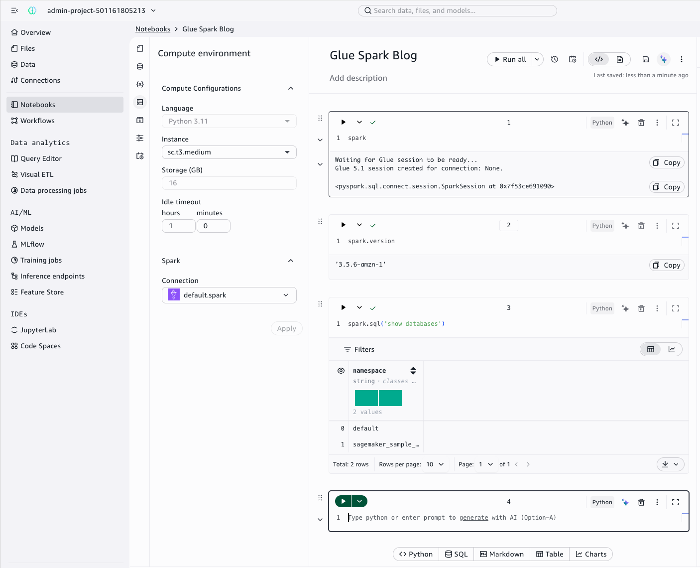
Apache Iceberg V3 support
Amazon EMR has supported Apache Iceberg V3 since Amazon EMR release 7.x, introducing capabilities such as deletion vectors and row lineage. With Spark 4.0 on Amazon EMR, that support deepens unlocking capabilities that had a hard dependency on Spark 4.0 itself, including VARIANT column storage and unknown type handling. For teams running data lakehouse workloads, the table format underneath your data determines how efficiently it is stored, how reliably it evolves, and how safely multiple tools can read and write it simultaneously.
What this means for your workloads:
VARIANT and Iceberg working together: VARIANT columns can now be stored natively in Iceberg V3 tables, combining efficient semi-structured data storage with Iceberg’s schema evolution and time travel capabilities. This eliminates the pipeline complexity of upfront schema definitions.
More efficient partitioning: Multi-argument transforms accept multiple input columns in a single partition expression, such as range (order_date, product_category), giving you finer control over data layout. They produce a single composite key instead of separate columns whose cartesian product can explode partition count. The result is less data scanned, faster queries, and lower compute costs for high volume workloads.
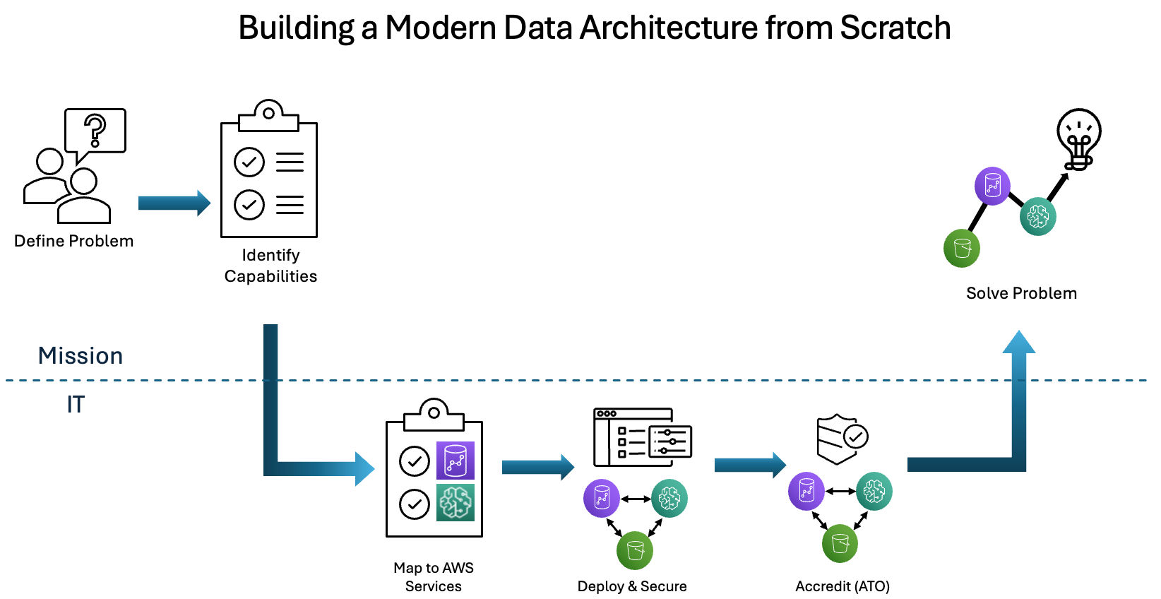
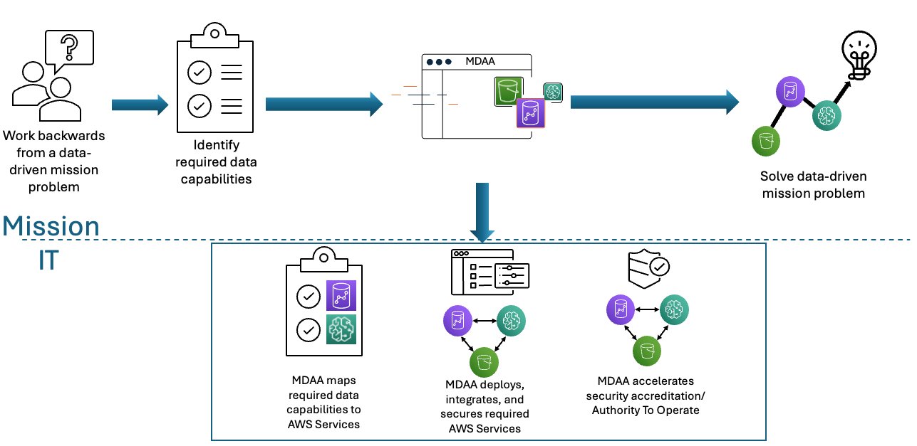
Safer schema evolution: Unknown type handling ensures that older readers do not break when newer writers introduce new column types, reducing coordination overhead across teams and tools during upgrades.
Fine-grained access control (FGAC): Column-level and row-level permissions are now available through AWS Lake Formation, giving you governed access control at a granular level across your Iceberg tables, no custom access logic required.
Variant data type
The new VARIANT data type, supported through Apache Iceberg v3, brings native support for semi-structured JSON data directly into Spark SQL. This matters most when you don’t control the data being written because platform teams and shared services often receive data from partners and upstream teams with unpredictable or evolving structures.
Without VARIANT, handling semi-structured data meant accepting real tradeoffs: defining schemas upfront that broke when data evolved, storing everything as strings with heavy parsing costs on every read, or building wide tables with nullable columns that wasted storage on empty fields. The most realistic option was breaking nested structures apart into separate columns before running queries. This ETL step added latency, increased storage costs, and broke every time an upstream team added or removed fields from their data feed.
VARIANT eliminates the process entirely. Data stays nested and is queryable with variant_get(), without a separate ETL pipeline. You ingest without defining a schema first and apply structure at query time.
For example, querying nested fields is now a single expression:
SELECT
variant_get(payload, '$.user.name') AS user_name,
variant_get(payload, '$.event.type') AS event_type,
variant_get(payload, '$.event.timestamp') AS event_timestamp
FROM VALUES
(PARSE_JSON('{"user":{"name":"Alice"},"event":{"type":"click","timestamp":"2025-03-01"}}'))
AS t(payload)
WHERE variant_get(payload, '$.event.timestamp') > '2025-01-01';
Reduced pipeline fragility: Schema changes no longer break ingestion. Data lands as-is, and you apply structure at query time based on what each analysis needs, without upstream coordination.
Improved query performance: Optimized storage format enables efficient access to nested fields without parsing overhead, so queries run faster even on deeply nested payloads.
Better storage efficiency: Compact encoding eliminates the waste of NULL-heavy wide tables, reducing storage costs for semi-structured data at scale.
VARIANT is especially well-suited where schemas are unpredictable or evolving: IoT and sensor data with device-specific payloads, logging and telemetry with variable event structures, and API responses and webhooks from third-party services where the schema changes without notice.
SQL enhancements
You can now write and maintain Spark pipelines using the same standard SQL you already know, no Spark-specific functions or syntax required. Apache Spark 4.0 expands ANSI SQL compliance so that functions behave consistently, opening Spark to anyone who can write SQL rather than requiring Spark specialists.
Standard SQL syntax such as OFFSET, LIMIT ... OFFSET, and lateral column aliases now work as expected. For example:
-- Standard OFFSET syntax now supported
SELECT id, name
FROM VALUES (1, 'Alice'), (2, 'Bob'), (3, 'Carol'), (4, 'Dave') AS t(id, name)
ORDER BY id
LIMIT 2 OFFSET 1;
-- Lateral column aliases work inline
SELECT amount * 1.1 AS adjusted, adjusted * 0.08 AS tax
FROM VALUES (100.0), (200.0), (350.0) AS t(amount);
Beyond syntax, SQL scripting brings procedural logic directly into Spark SQL. You can now use variables, IF/ELSE conditionals, loops, and multi-statement blocks without switching to Python or JVM-based languages. Before SQL scripting, multi-step workflows (such as ETL logic with conditional branching or iterative data quality checks) required wrapping SQL statements in Python or Scala to handle control flow. SQL scripting removes that dependency. SQL-native teams can author and maintain these workflows entirely in SQL.
Key benefits:
Simplified ETL workflows: Multi-step transformation logic that previously required an external language can now live entirely in SQL, reducing code complexity and making pipelines easier to build and maintain.
Lower barrier for SQL-native teams: Teams that primarily work in SQL no longer need to context-switch into Python or Scala to implement conditional logic or iterative processing. The entire pipeline stays in SQL.
Python advances
Earlier versions of Spark required Python users to step outside Python at two key points: building custom data connectors required Java or Scala, and diagnosing UDF performance lacked built-in visibility. Spark 4.0 addresses both directly, removing the two biggest blockers for organizations where Python is the primary language.
Python Data Source API
With the Python Data Source API, you can build custom, reusable data connectors in Python without any JVM or Scala code. Custom connectors participate in Spark’s query optimization, including predicate pushdown and schema inference. This matters when your data system only has a Python client, or when your team does not have Java or Scala expertise: you can now wrap any custom format or external source as a Spark DataFrame source or sink without leaving Python.
Spark 4.0 also introduces polymorphic Python UDTFs (User-Defined Table Functions) that can return different schema shapes depending on input, with an analyze() method that produces a schema dynamically based on parameters. This is particularly useful for processing varying JSON schemas or splitting inputs into a variable set of outputs.
If you’re ingesting data from a REST API with a Python client, you can implement a custom Spark data source entirely in Python, register it, and use it directly in Spark SQL or the DataFrame API. What previously required a Scala developer and a custom JVM connector can now be built and maintained by your Python team running the pipeline.
Python UDF enhancement
Python UDF profiling provides built-in visibility into execution time, serialization overhead, and memory usage at the individual UDF level without external tooling. Additionally, it enables performance or memory profiling depending on what you need to diagnose.
Arrow-based vectorized UDF support reduces serialization overhead between Python and the JVM using a columnar format, replacing row-at-a-time processing with batch-oriented columnar exchange.
Together, these give you a complete optimization loop: build custom connectors in Python, profile your UDF performance, and optimize with confidence.
Practical benefits for Python teams:
Lower barrier for Python teams: Custom data connectors no longer require Java or Scala knowledge. If your data system has a Python client, you can build a production-grade Spark connector entirely in Python.
Flexible data transformation: Polymorphic UDTFs let your functions adapt to varying input schemas dynamically, reducing the need to write and maintain multiple transformation functions for different data shapes.
Faster UDF optimization: Built-in profiling surfaces exactly where execution time and memory are being spent at the UDF level, replacing guesswork with direct visibility and making performance tuning significantly faster.
Streaming enhancements
This section covers improvements to state management and observability in structured streaming workloads.
Queryable state for structured streaming
Structured streaming jobs maintain state continuously (running totals, session windows, aggregated counts). However, in earlier versions of Spark that state was locked inside the running job. Inspecting it meant stopping the stream or manually parsing checkpoint files. For production workloads, this created real operational risk: teams had no way to verify whether state was correct, corrupted, or drifting without taking the job down.
Time-sensitive applications faced an additional problem: timers in Spark streaming only fired when new data arrived, so a five-minute heartbeat timeout could silently miss its window if no data came in, making applications like heartbeat monitoring and session tracking unreliable by design.
Spark 4.0 changes this. The new transformWithState API provides deterministic timer execution because timers fire on schedule regardless of data arrival patterns. It also delivers automatic state TTL to prevent unbounded growth, schema evolution without restarting from a new checkpoint, and state observability for mid-stream debugging. External systems can now read live aggregated state from a running streaming job without interrupting it. State is accessible as a DataFrame, queryable during development, verifiable in unit tests, and inspectable during production incidents without touching the running stream.
This is backed by three improvements working together. First, the transformWithState operator replaces mapGroupsWithState from earlier Spark versions (which had limited timer support and no TTL-based cleanup). Second, the state data source reader exposes streaming state as a queryable DataFrame. Lastly, RocksDB changelog checkpointing improvements address throughput bottlenecks in high-volume stateful workloads.
Consider a fleet of 100,000 IoT sensors across manufacturing facilities, each requiring an alert within 30 seconds of going offline. The sensors track heartbeat state per device, managing independent timers, handling late data, and cleaning up decommissioned devices at scale had no clean solution in earlier Spark versions. The transformWithState operator handles all of this natively, and queryable state lets your operations team inspect live device state in real time without stopping the stream:
# Timers fire on schedule regardless of data arrival, making heartbeat monitoring reliable
alerts = events_df.groupBy("device_id").transformWithState(
HeartbeatMonitor(),
outputStructType=StructType([
StructField("device_id", StringType()),
StructField("alert", StringType())
]),
outputMode="Append"
)
Combined with Amazon EMR Serverless, which scales compute automatically based on workload demands, you can deploy stateful streaming pipelines without managing clusters or predicting capacity.
Benefits:
Real-time operational visibility: Live streaming state is now accessible externally without interrupting the job, powering dashboards and monitoring systems that reflect current aggregations.
Faster debugging: State values can be queried directly as a DataFrame, making it significantly easier to diagnose production incidents and verify correctness during development.
Better performance at scale: RocksDB checkpointing improvements reduce bottlenecks in high-throughput stateful workloads, improving reliability for long-running streaming jobs.
What’s new in the emr-spark-8.0 release
Beyond the Spark 4.0 capabilities covered in the preceding sections, the emr-spark-8.0 release introduces infrastructure and runtime changes that simplify how you deploy, patch, and manage Amazon EMR workloads. The release focuses exclusively on Spark, reducing the surface area you need to patch and test.
Fewer components to patch and test
The emr-spark-8.0 release includes Apache Spark 4.0, Apache Iceberg 1.10, Apache Hudi 1.0.2, Delta Lake 4.0, and connectors for Amazon DynamoDB, Amazon Kinesis, Amazon Redshift, and Amazon Simple Storage Service (Amazon S3) (via the S3A connector). Apache Livy and JupyterEnterpriseGateway are available as opt-in components on Amazon EMR on EC2. If your workloads require Apache Flink, Trino, Presto, or other execution engines, you can continue to use Amazon EMR 7.x releases.
Simplified patch management
You can specify emr-spark-8.0.x when creating a cluster or application, and Amazon EMR will automatically select the latest patch version. For example, emr-spark-8.0.1, emr-spark-8.0.2, and so on as patches are released. This “.x” wildcard is supported through AWS APIs and AWS Command Line Interface (AWS CLI). On Amazon EMR on EKS and Amazon EMR Serverless, new jobs automatically run on the latest Amazon Linux patches, so you no longer need to track date-based version tags.
Latest Python, Java, and Scala runtimes
The release ships with modernized runtimes: Python 3.11 as the default, with support for Python 3.12 and 3.13. Java 17 is the default, with Java 21 also available. Both are provided through Amazon Corretto. Scala 2.13 is the supported Scala runtime.
If you are migrating from Spark 3.5 to Spark 4.0, the Apache Spark upgrade agent for Amazon EMR can accelerate your migration by analyzing existing applications and identifying changes needed for Spark 4.0 compatibility. For more information, see the upgrade guidance.
If your workflows use Apache Pig, Apache Oozie, JupyterHub, Apache Zeppelin, or Hue, you can continue to use Amazon EMR 7.x releases. These components are not included in emr-spark-8.0. For interactive Spark development, use Amazon EMR Studio, with Apache Livy and JupyterEnterpriseGateway available on Amazon EMR on EC2.
For the complete list of supported components and configurations, see the Amazon EMR release guide.
Get started
Spark 4.0 is now available across Amazon EMR on EC2, Amazon EMR on EKS, and Amazon EMR Serverless. To begin, choose your deployment model and follow the relevant getting started guide:
Spark 4.0 on Amazon EMR delivers improvements across query validation, semi-structured data handling, Python development, and streaming observability. ANSI SQL mode catches invalid operations at query time rather than silently propagating nulls downstream, and SQL scripting removes the need to context-switch between SQL and Python for complex ETL logic. The VARIANT data type eliminates parsing overhead for semi-structured JSON workloads and can now be stored natively in Iceberg V3 tables with fine-grained access control at the column and row level. Queryable streaming state gives you live visibility into running jobs without interruption, and Spark Connect lets you develop against Amazon EMR from Jupyter notebooks, Amazon SageMaker Unified Studio Data Notebooks, Amazon Q Developer, Kiro, or your preferred IDE without managing cluster connectivity.
Enabling security tooling is the starting point. Making it operational—where findings drive decisions, response times are measurable, and your security posture improves week over week—is where most organizations struggle.
This blog post provides a phased maturity roadmap for organizations that have already enabled AWS Security Hub and Amazon GuardDuty. These two services form the foundation of a cloud-centered security operations capability on AWS. Security Hub provides centralized security posture management and aggregates findings from multiple AWS security services, while GuardDuty provides intelligent threat detection by continuously monitoring for malicious activity and unauthorized behavior. For any production or enterprise AWS environment, having both services enabled across all accounts and AWS Regions is a baseline expectation; not because they’re optional add-ons, but because effective security operations require both the ability to detect threats and the ability to understand your overall security posture. If you haven’t yet enabled them, the Security Hub documentation and GuardDuty documentation provide setup guidance, including multi-account deployment with AWS Organizations.
Customers consistently tell us that while individual AWS security service documentation is thorough, what’s missing is a consolidated operational playbook—one resource that ties the services together into a working security operations practice with clear phases, progression criteria, and an operational cadence. That’s the gap this post fills. Rather than covering how each feature works (the documentation does that well), this post focuses on when and why to use each capability, and how to build the organizational habits that make them effective.
What follows is a six-phase roadmap for moving from these services are active to these services are driving our security operations. Each phase builds on the previous one, and each is designed to deliver tangible, measurable improvement.
Phase 0: Assess your current state
Goal: Understand what’s working before changing anything.
Estimated timeline: 1–2 weeks
Move to Phase 1 when: You have a documented current-state assessment covering all the following items.
Before introducing new processes or automation, establish a clear picture of the current environment. This assessment informs every decision that follows.
Actions:
Findings inventory: Review existing active GuardDuty findings to determine how many there are, the severity distribution, and how old the oldest findings are. A large backlog of untouched HIGH or CRITICAL findings that have been sitting for weeks is a strong signal about where to focus first.
Security Hub score baseline: Determine your current compliance score against AWS Foundational Security Best Practices (FSBP) and The CIS AWS Foundations Benchmark. Check to see which standards are enabled; if multiple standards are enabled, review for overlapping standards (creating noise) or unused standards.
Multi-account and multi-Region check: Look to see if GuardDuty is enabled in every account and every Region, or only in Regions with active workloads. Threat actors frequently operate in Regions that organizations don’t actively monitor. Also check to see if Security Hub aggregation is configured with a delegated administrator account or if each account is being managed independently.
Integration check: Determine if GuardDuty findings are flowing into Security Hub and if Amazon Inspector and Amazon Macie are enabled and feeding findings in. Without integration, Security Hub might be only surfacing its own compliance checks.
Notification check: See if there’s an Amazon EventBridge rule configured for notifications and if so, how findings are being routed and to whom. Know if notifications are being sent using an Amazon Simple Notification Service (Amazon SNS) topic or a chat channel integration. Without a clear notification and response workflow, findings can accumulate silently in the console with no one looking at them.
Deliverable: A one-page current state assessment that identifies what’s enabled, what’s flowing where, who’s looking at it, and what’s in the existing backlog.
Phase 1: Reduce the noise
Goal: Make the signal meaningful before asking anyone to act on it.
Estimated timeline: 2–3 weeks
Move to Phase 2 when: Remaining findings represent items requiring real decisions, compliance scores reflect actual posture, and you can articulate why every suppression rule and disabled control exists.
This is the single most important phase. If this step is skipped in favor of jumping straight to automation, the result is automated chaos. Alert fatigue is the primary reason security tooling is ignored, and addressing it first is what makes everything that follows sustainable.
GuardDuty tuning:
Create suppression rules for known-benign findings. The goal is to suppress activity you’ve already evaluated and accepted—such as expected traffic from corporate egress IPs (based on trusted IP lists), internal tools that trigger DNS-based findings, or internet-facing resources that naturally receive port scanning. The principle: if you’ve investigated a finding and it’s expected, suppress it so your team can focus on what matters.
Triage every active HIGH and CRITICAL finding into three categories: needs immediate investigation (real threat, not yet reviewed), true positive, already addressed (archive using workflow status), or false positive or expected behavior (create a suppression rule). Every finding must be categorized into one of these three states.
Review GuardDuty protection plans and enable any that are relevant but not yet active. Organizations that enabled GuardDuty years ago might not have activated protection plans released since then (such as Runtime Monitoring, Malware Protection, RDS Protection, and Lambda Protection). Evaluate each against your workload profile and enable what applies.
Security Hub tuning:
Disable controls that aren’t relevant to the environment. This is the highest-value quick win. If a service isn’t in use, disable its controls. If a control is addressed by an alternative solution, disable it. A 47% compliance score where half the failures are irrelevant trains teams to ignore the dashboard entirely. See the Security Hub controls reference for the full list.
Choose a primary standard. AWS Foundational Security Best Practices is a strong default. The CIS AWS Foundations Benchmark adds value when there’s a specific compliance mandate. Avoid enabling PCI DSS or NIST 800-53 standards unless there’s a reporting requirement—they add significant volume without proportional signal for most organizations.
Configure cross-Region aggregation to the delegated administrator account if not already in place. A single aggregated view eliminates the need to check findings across multiple Regional consoles.
Use the workflow status field operationally. Findings should progress from NEW to NOTIFIED to RESOLVED or SUPPRESSED. If everything remains in NEW indefinitely, the system carries no operational meaning.
Deliverable: A tuned environment where remaining findings represent items that require real decisions. Compliance scores should now reflect your organization’s actual security posture rather than noise.
Phase 2: Build the notification and routing layer
Goal: Get the right findings to the right people at the right time.
Estimated timeline: 2–3 weeks
Move to Phase 3 when: CRITICAL and HIGH findings reach the security team within minutes, MEDIUM findings create tracked tickets, and notifications include enriched context. No action is taken until a person or an automation is informed that something needs attention.
Architecture: Security Hub to EventBridge rule to routing logic to destination
Tiered notification strategy:
CRITICAL
Page on-call immediately
PagerDuty or Opsgenie
15 minutes
HIGH
Alert security team channel
Slack or Teams channel and ticket creation
4 hours
MEDIUM
Create ticket for review
Jira or ServiceNow
48 hours
LOW or INFORMATIONAL
Batch digest
Weekly email summary or dashboard review
Next review cycle
Key design decisions:
Route from Security Hub, not individual services. Because findings from GuardDuty, Inspector, Macie, and Security Hub compliance checks all aggregate in Security Hub, build your EventBridge rules there for centralized management.
Create a fast path for the most dangerous finding types. Certain GuardDuty findings, particularly those involving credential exfiltration, cryptocurrency activity, trojans, and active compromises, warrant a separate, faster routing path that bypasses normal triage. Identify these based on your threat model and the GuardDuty finding types reference.
Enrich notifications before delivery. A raw JSON finding in a chat channel provides little actionable context. Use an AWS Lambda function to format notifications with the information responders need: account alias, Region, Amazon Resource Name (ARN), finding type, severity, a console deep link, and a plain-language description. The Security Hub CloudWatch Events integration guide describes the event format.
Deliverable: A working notification pipeline where CRITICAL and HIGH findings reach the security team within minutes, MEDIUM findings create tracked work items, and LOW and INFORMATIONAL findings are batched for periodic review.
Phase 3: Build automated remediation for high-confidence findings
Goal: For findings where the correct response is deterministic, remove the human from the loop.
Estimated timeline: 3–4 weeks
Move to Phase 4 when: At least 3–5 high-confidence finding types have automated responses deployed with audit trails, and the team has established a process for evaluating new auto-remediation candidates.
The guiding principle: Only auto-remediate when all three conditions are met: the finding is high-confidence, the response is deterministic, and the blast radius of the automated action is limited. Automated remediation must not create the risk of a production outage.
Decision framework:
Confidence level
High – no false positive risk
Medium – context-dependent
Low – requires investigation
Response complexity
Single, well-defined action
Multiple steps or judgment calls
Requires forensic analysis
Blast radius
Limited to one resource
Could affect dependent services
Production-wide impact
Rollback difficulty
Straightforward to reverse
Moderate effort to reverse
Difficult or impossible to reverse
Common auto-remediation categories:
Instance isolation for confirmed compromise findings (cryptocurrency mining, malware, and trojans): Replace the security group, snapshot volumes for forensics, and notify.
Credential revocation for confirmed credential compromise: Attach deny-all policies, revoke sessions, and deactivate access keys as appropriate to the credential type.
Compliance drift correction for deterministic misconfigurations: Re-enable Amazon Simple Storage Service (Amazon S3) Block Public Access, revoke overly permissive security group rules, and re-enable AWS CloudTrail logging.
Notification-only escalation for findings that require human judgment before action: Amazon Elastic Block Store (Amazon EBS) encryption gaps (require migration) and access key rotation (requires coordination with the key owner).
For implementation, AWS provides Security Hub Automated Response and Remediation (SHARR), a solution that includes pre-built remediation playbooks deployed as AWS Step Functions workflows triggered by EventBridge. This is a strong starting point—evaluate the provided playbooks, enable the ones that fit, and extend with custom remediations as needed.
Note: For findings that recur because the environment lacks preventive guardrails, the best long-term response is often a service control policy (SCP) that prevents the misconfiguration from occurring in the first place. Phase 5 covers this preventive controls layer.
Deliverable: A library of automated and semi-automated remediation runbooks with full audit trails, and a documented decision framework the team uses to evaluate new auto-remediation candidates.
Phase 4: Build the operational rhythm
Goal: Turn security findings management into a sustained organizational practice, not a one-time cleanup.
Estimated timeline: 4–6 weeks to establish, then ongoing
Move to Phase 5 when: The weekly cadence has been running consistently for at least 8 weeks, monthly metrics show positive trends, and the first quarterly review has been completed.
This is where many organizations stall, and it’s the most important phase in the entire roadmap. The technology is working, the notifications are flowing, automated remediations are firing, but there’s no organizational habit built around it. Without this phase, everything you’ve built in Phases 0–3 will gradually decay. Suppression rules will go stale, new team members won’t know the system exists, and findings will start accumulating again. The operational rhythm is what converts a security tooling deployment into a security operations practice.
Weekly security review (30 minutes)
Attendees: Security team lead, cloud platform team representative, rotating engineering lead from an application team
Why the rotating engineering lead matters: Security findings don’t exist in a vacuum; they’re generated by workloads that engineering teams own. Rotating an engineering representative through this meeting accomplishes three things: it builds security awareness across the organization, ensures findings are routed to people with the context to resolve them, and creates organizational accountability beyond the security team.
Agenda template:
5 minutes
Compliance score trend – Review Security Hub scores by account and standard. Is the trend improving, declining, or flat? If declining, why?
Security lead
Identified regression areas
5 minutes
Critical and high findings review – Walk through new HIGH and CRITICAL GuardDuty findings from the past week. Are there any that need immediate escalation?
Security lead
Escalation actions assigned
10 minutes
Top five failing controls – Identify the five Security Hub controls with the most failures. Assign an owner and a target date for each.
Platform lead
Owners and dates documented
5 minutes
Automation review – Did any auto-remediations fire this week? Did they work correctly? Were there any false triggers?
Security lead
Automation adjustments queued
5 minutes
Tuning decisions – Are new suppression rules needed based on this week’s findings? Are any new finding types candidates for auto-remediation?
All
Tuning backlog updated
Running the meeting effectively:
Keep a running document (such as a wiki page or shared document) that captures decisions and action items week over week. This becomes your institutional memory.
If the compliance score hasn’t moved in over 3 weeks, that’s a signal. Either the assigned work isn’t happening, or the remaining findings are genuinely difficult to address. Both need to be discussed.
Track action items from previous weeks. A review that generates action items but never follows up on them will lose credibility and attendance quickly.
Escalation procedures
Define clear escalation paths before they’re needed:
CRITICAL finding not acknowledged within the SLA
Auto-escalate to security team manager
15 minutes after SLA breach
HIGH finding not resolved within the SLA
Escalate to finding owner’s manager
4 hours after SLA breach
Compliance score drops more than 5 points in a week
Escalate to cloud platform team lead for investigation
Next business day
Auto-remediation failure
Page security on-call
Immediate
New finding type not covered by existing runbooks
Add to weekly review agenda for triage and runbook development
Next weekly review
Monthly metrics report
Compile these metrics monthly and review them with security and engineering leadership. The goal is to tell a story about whether the organization’s security posture is improving, stable, or degrading, and why.
Mean time to acknowledge (MTTA) for CRITICAL findings
Are findings being seen promptly?
Decreasing month over month
Mean time to resolve (MTTR) for CRITICAL and HIGH findings
Are findings being acted on?
Decreasing month over month
Security Hub compliance score by standard, by account
What is the posture trend over time?
Increasing month over month
Number of active GuardDuty findings by severity
Is the backlog growing or shrinking?
Decreasing for HIGH and CRITICAL
Findings auto-remediated compared to manually resolved
Is automation delivering value?
Auto-remediation ratio increasing
Number of suppressed findings (with quarterly justification review)
Is noise being managed, or are problems being hidden?
Stable or decreasing
New findings introduced compared to resolved this month
Is the organization getting ahead or falling behind?
More finding resolved than introduced
SLA adherence rate by severity
Are response commitments being met?
More than 95% for CRITICAL, and more than 90% for HIGH
Building the dashboard: Use Amazon CloudWatch dashboards for real-time operational visibility or Amazon QuickSight connected to Security Hub findings through Amazon Security Lake for historical trend analysis and executive reporting. The dashboard should be visible to—and regularly viewed by—everyone in the weekly review, not locked in a security team tool.
Quarterly reviews
The quarterly review is a deeper inspection of the system itself; not just the findings, but the machinery processing them.
Quarterly review checklist:
Suppression rules audit: Review every active suppression rule to determine if the underlying condition is still present and the suppression is still justified. Document the review outcome for each rule.
Disabled controls audit: Review every disabled Security Hub control. Check that the justification is still valid and if the environment changed (for example, a service that wasn’t in use is now in use).
Automation audit: Review AWS Identity and Access Management (IAM) roles used by remediation functions and verify least privilege. Review execution logs for any anomalies or failures that weren’t caught.
New capabilities review: Evaluate newly released GuardDuty protection plans and Security Hub controls from that quarter. AWS releases new detection and compliance capabilities regularly. If you’re not reviewing them quarterly, you’re accumulating blind spots.
Process effectiveness review: Determine if the weekly meeting is well-attended and if action items are being completed. Make sure SLAs are being met. If attendance, action item completion, and SLA compliance aren’t where they should be, explore structural changes to address the gaps.
Operational maturity scoring
Use this rubric to assess the maturity of your operational rhythm itself. Score each dimension 1–3 and use the total to track progress over time.
Review cadence
One time reviews when someone remembers
Weekly review happens, but attendance is inconsistent
Weekly review is consistently attended with documented outcomes
Metrics tracking
No metrics captured
Metrics are collected monthly but not acted on
Metrics drive decisions and declining trends trigger specific actions
Finding ownership
Findings sit in queue with no owner
Findings are assigned to teams but SLAs aren’t tracked
Every finding has an owner, SLAs are tracked, and breaches are escalated
Automation management
Set-and-forget automations
Automation logs are reviewed periodically
Automation is reviewed weekly, and new candidates are evaluated continuously
Tuning lifecycle
Suppression rules created but never reviewed
Annual review of suppressions and disabled controls
Quarterly reviews with documented justification for every rule
Cross-team engagement
Security team works in isolation
Platform team participates
Engineering teams actively participate and own remediation
Scoring (revisit quarterly):
Beginning: 6–9
Established: 10–14
Optimized: 15–18
Deliverable: A documented operational cadence with clear ownership (consider a RACI matrix), metrics dashboards, escalation procedures, and a continuous improvement loop. The cadence should survive team member turnover—if it depends on one person remembering to run it, it’s not yet operational.
Phase 5: Mature the architecture
Goal: Fill remaining gaps and build toward a comprehensive security operations capability. Estimated timeline: Ongoing. Prioritize based on organizational risk profile and compliance requirements.
Amazon Inspector integration: Enable Amazon Inspector for Amazon Elastic Compute Cloud (Amazon EC2) instances, Lambda functions, and Amazon Elastic Container Registry (Amazon ECR) container images. Findings flow into Security Hub automatically, adding vulnerability management alongside threat detection and posture management. Prioritize this if you have Amazon EC2 or container workloads without an existing vulnerability scanning solution.
Amazon Macie: Enable Amazon Macie for S3 buckets containing potentially sensitive data. Particularly important for organizations with compliance requirements around personally identifiable information (PII), protected health information (PHI), or Payment Card Industry (PCI) data. Configure automated sensitive data discovery and route findings to Security Hub.
Amazon Security Lake: Amazon Security Lake centralizes security-relevant logs in OCSF format for long-term retention, forensic investigation, and threat hunting. This is valuable when you need historical analysis beyond the Security Hub retention window, or when feeding a third-party Security Information and Event Management (SIEM) tool.
Preventive controls layer: Convert recurring detective findings into preventive policies. Use SCPs to prevent disabling GuardDuty, Security Hub, and CloudTrail, IAM permission boundaries on developer roles, AWS WAF on public endpoints, and AWS Network Firewall for VPC traffic inspection. The pattern is to make recurring misconfigurations impossible to introduce.
Incident response readiness: Have incident response playbooks referencing specific GuardDuty finding types, pre-built forensics infrastructure (isolated VPC, forensic AMIs, and pre-configured IAM roles), regular tabletop exercises, and AWS CloudFormation templates to deploy isolation infrastructure on demand. See the AWS Security Incident Response Guide for a comprehensive framework.
Conclusion
In this post, I provided a six-phase roadmap for operationalizing Security Hub and GuardDuty and showed that it isn’t a single project, but a progression. Phase 0 and Phase 1 can typically be completed in 3–5 weeks and deliver immediate clarity. Phases 2 and 3 build the response infrastructure that turns findings into action over the following 5–7 weeks. Phase 4 is what makes everything sustainable and is where you should invest the most attention. And Phase 5 expands the aperture from Security Hub and GuardDuty into a comprehensive security operations capability.
If you walked away from this post and did one thing, run the Phase 0 assessment this week. That single deliverable tells you exactly where to focus next. Use the following self-assessment checklist to identify your current phase, then focus on the next one. A tuned environment with working notifications and a weekly review cadence is dramatically more effective than a fully featured but neglected deployment. Start where you are, reduce the noise, build the habits, and iterate. To learn more, explore the AWS Security Hub User Guide, the Amazon GuardDuty User Guide, and the AWS Security Incident Response Guide. If you’ve implemented a similar operational cadence, or have questions about any phase, share your experience in the comments.
Self-assessment checklist
Phase 0
We know how many active GuardDuty findings exist across all accounts
☐
We know our current Security Hub compliance score
☐
We know whether GuardDuty is enabled in every account and region
☐
We know who (if anyone) is reviewing findings today
☐
Phase 1
GuardDuty suppression rules exist for known-benign activity
☐
Irrelevant Security Hub controls have been disabled with documented justification
☐
All active HIGH and CRITICAL findings have been triaged
☐
Security Hub compliance scores reflect actual posture, not noise
☐
Phase 2
HIGH and CRITICAL findings generate real-time notifications to the security team
☐
MEDIUM findings automatically create tracked work items
☐
Notifications include enriched context (account alias, resource ARN, and console link)
☐
Phase 3
At least three high-confidence finding types trigger automated remediation
☐
Auto-remediation actions have full audit trails
☐
Remediation runbooks are documented and version-controlled
☐
Phase 4
A weekly security review meeting occurs with defined attendees and agenda
☐
MTTA and MTTR are tracked monthly for CRITICAL and HIGH findings
☐
Suppression rules and disabled controls are reviewed quarterly
☐
Security metrics trend positively over the past 3 months
☐
Phase 5
Amazon Inspector, Macie, or Security Lake are integrated
Modern web applications require robust security controls to protect user data and application resources. Authentication and authorization are two fundamental pillars of application security that answer critical questions: Who are you? and What are you allowed to do? Implementing these controls correctly can be challenging for developers, especially when building data-intensive applications with frameworks like Streamlit (an open-source Python framework for building interactive web applications) or when requiring fine-grained access control. Key challenges include protecting access to application resources, implementing application identity with multi-factor authentication (MFA), and implementing usage-based controls.
In this post, you will learn how to build fine-grained access controls for a sample Streamlit application using Amazon Cognito for authentication and Amazon Verified Permissions with Cedar policies for authorization. This architecture provides enterprise-grade security with minimal development effort, so you can focus on your application’s core functionality. You will learn how to reduce development time for secure applications, implement enterprise-grade authentication, through proper access management, and scale security with growing user bases.
Security architecture overview
The reference architecture follows a layered security design with four key components; separating identity verification, authorization evaluation, application logic, and enforcement boundaries. By assigning clear responsibilities to each layer, the architecture limits blast radius and ensures that a failure in any single control does not compromise the overall system.
Authentication layer: Amazon Cognito handles user authentication with secure credential validation and JSON web tokens (JWTs). It provides built-in password policies, account lockout protection, and session management.
Authorization layer: Verified Permissions uses the Cedar policy engine to evaluate fine-grained access requests based on centrally stored policies.
Application layer: The Streamlit frontend integrates with both services, managing user sessions and enforcing access controls in the user interface.
Security boundaries: Multiple layers of security controls protect against unauthorized access, privilege escalation, authentication verification, authorization checks, and input validation.
This separation of concerns enables authentication and authorization to function as complementary security controls, following defense-in-depth principles. Figure 1 illustrates the end-to-end authentication and authorization workflow, showing how a user’s sign-in request flows through Amazon Cognito for identity verification, then through Verified Permissions for Cedar policy-based access decisions, before the application enforces the result.
Figure 1: Solution architecture and workflow
The following workflow demonstrates how the three architecture layers work together: the authentication layer (steps 1–3) handles identity verification using Amazon Cognito, the authorization layer (steps 4–6) evaluates Cedar policies using Verified Permissions, and the application layer (steps 7–8) enforces the decision in Streamlit.
The user sends a sign-in request, which is submitted through Streamlit
The request is authenticated by Amazon Cognito
An access token is sent back to Streamlit
An authorization request is sent to Verified Permissions
The Cedar policy engine evaluates the request
A decision is sent back by the policy engine
The instruction to allow or deny is sent back to Streamlit
If the instruction is to allow, access is provided
Understanding authorization with Cedar
While authentication establishes user identity, authorization determines what actions users can perform. Verified Permissions provides a scalable authorization service based on Cedar, a policy language specifically designed for fine-grained access control.
Cedar policies follow a structured format that defines who can perform which actions on what resources. Let’s examine the anatomy of a Cedar policy:
permit(
principal == ?principal,
action == application::Action::"ViewGrade",
resource == ?resource
) when {
principal has role == "Student" &&
resource.student == principal.entityId
};
Policy components
Effect: permitor forbid determines whether the policy allows or denies access
Principal: The entity (user) making the request, represented by ?principal as a variable
Action: The operation being performed, scoped to your application namespace
Resource: The target of the action, also represented as a variable
Conditions: The when clause contains logical expressions that must evaluate to true
Advanced Cedar policy patterns
This section describes commonly used Cedar policy patterns for implementing fine-grained authorization with Amazon Verified Permissions. The examples illustrate how to model ownership, role-based access, hierarchical permissions, and administrative controls in real-world applications
Resource ownership control
This pattern helps ensure that users can only access resources they own:
permit(
principal == ?principal,
action == application::Action::"ViewGrade",
resource == ?resource
) when {
principal has role == "Student" &&
resource.student == principal.entityId
};
What it does – This policy allows students to view only their own grades by:
Checking that the user has the Student role
Verifying that the grade resource’s student attribute matches the student’s entityId
Preventing students from accessing other students’ grades while allowing access to their own academic performance
Role-based access with resource type
This pattern grants access based on role and resource type:
permit(
principal == ?principal,
action == application::Action::"EditCourse",
resource == ?resource
) when {
principal has role == "Faculty" &&
resource has resourceType == "Course" &&
resource.instructor == principal.entityId
};
What it does – This policy allows faculty members to edit courses they teach by:
Verifying the user has the Faculty role
Confirming the resource is of type Course
Verifying that the course’s instructor attribute matches the faculty member’s entityId
Restricting faculty to modify only their own courses, not courses taught by other instructors
Hierarchical authorization
This pattern allows department heads to manage faculty in their department:
permit(
principal == ?principal,
action == application::Action::"ManageFaculty",
resource == ?resource
) when {
principal has role == "DepartmentHead" &&
resource has role == "Faculty" &&
resource.department == principal.department
};
What it does – This policy implements departmental hierarchy controls by:
Requiring the user to be a DepartmentHead
Verifying the resource is a faculty member
Matching the faculty member’s department with the department head’s department
Preventing department heads from managing faculty in other departments
Administrative override
This pattern provides emergency access with proper justification:
permit(
principal == ?principal,
action == ?action,
resource == ?resource
) when {
principal has role == "Administrator" &&
context has emergencyAccess == true &&
context has justification
};
What it does – This policy provides emergency access capabilities by:
Allowing administrators to perform any action on any resource
Requiring an emergency access flag to be set to true
Requiring a justification for emergency access
Supporting accountability through required documentation while enabling emergency operations
Cedar policy evaluation flow
Understanding how policies are evaluated helps design effective authorization systems. Figure 2 shows a common evaluation pattern for an academic scenario
Note: A policy match evaluates to the policy’s effect (permit or forbid). Forbid policies take precedence: if any forbid policy matches, access is denied regardless of permit policies.
Figure 2: Policy evaluation process
The policy evaluation process follows these steps:
User attempts to access a protected resource
Application sends an authorization request to Verified Permissions
Verified Permissions retrieves applicable Cedar policies from the policy store
The Cedar policy engine evaluates each policy against the request
If any forbid policy matches, access is denied immediately
If any permit policy matches and no forbid policies match, access is allowed
If no policies match, access is denied by default
The evaluation result (ALLOW or DENY) is returned to the application
Application enforces the authorization decision
Cedar policy language
Cedar is an Amazon open source policy language designed for fine-grained authorization. Every policy defines who (principal) can perform what action on which resource under what conditions, as shown in Figure 3.
Figure 3: Cedar policy definitions
Policy interaction
The following table shows how different policies interact in complex scenarios where multiple policies could apply:
Scenario
Student policy
Faculty policy
Department head policy
Admin policy
Student accessing own grade
Permit
N/A
N/A
Override
Faculty editing course
N/A
Permit
N/A
Override
Department head managing faculty
N/A
N/A
Permit
Override
Emergency admin access
N/A
N/A
N/A
Permit
Legend:
Permit – Policy allows access
N/A – Policy doesn’t apply
Override – Emergency admin access
The preceding table shows how each role’s policy applies to different scenarios, with admin access having override capabilities across most situations except for emergency admin access where it’s the primary permit authority. The Override column specifically indicates that the administrator’s emergency access policy can supersede other role-specific policies, but only when the emergencyAccess context flag is explicitly set and a justification is provided. This is not an automatic override.
Policy optimization tips:
Order conditions by likelihood of success – Place the most frequently true conditions first in your when clause to enable short-circuit evaluation. For example, check role before resource ownership, because role mismatches are caught earlier. See Cedar best practices.
Use indexed attributes for faster lookups – Use entity attributes that Verified Permissions indexes natively (entityId, role, resource type) as primary conditions. Best practices for designing an authorization model
Cache policy evaluations when appropriate
Monitor evaluation metrics and performance
Real-world application: Academic system
Consider an academic system with different user roles and their corresponding permissions:
Student: View own grades
Policy helps ensure students can only access grade resources where they are listed as the student
The policy verifies the student’s role and matches the resource owner to the principal’s entity ID
Faculty: Edit course content, manage grades
Policy allows faculty to edit courses they teach
Faculty can view and modify grades for students in their courses
Teaching assistant (TA): Grade management and course support
Policy permits TAs to manage grades for courses they assist with
Access is limited to specific courses assigned to the TA
Department head: Manage faculty assignments
Policy allows department heads to manage faculty in their department
Access is scoped to the department hierarchy
Administrator: System-wide access
Policy provides emergency access with proper justification
Administrative actions are logged and audited
Prerequisites
To implement the preceding Academic system application, you need an active AWS account, Python 3.8 or later, basic Streamlit knowledge, and AWS Identity and Access Management (IAM) permissions for Amazon Cognito and Verified Permissions.
./deploy-demo-environment.sh
Do you want to start the demo now? (Y/N): Y
This provisions an Amazon Cognito user pool, a Verified Permissions policy store, and any sample resources needed for the demo.
Verify the login screen:
Figure 4: Verify login credentials
Demo walkthrough and shut down: Interact with the demo and test the policies and features. When you’re ready to exit, press Ctrl+C to shut down and stop.
Define your Cedar policies: Start with basic policies and gradually add complexity as you understand the evaluation model.
Implement authentication: Integrate Amazon Cognito authentication into your application with proper error handling.
Add authorization checks: Implement authorization checks at critical access points in your application. For authentication, implement proper error handling for expired tokens, failed MFA challenges, and account lockouts. Use the Amazon Cognito built-in token refresh flow. For authorization, place Verified Permissions checks at every API endpoint and UI component that accesses protected resources.
Test thoroughly: Create test scenarios for each user role and permission combination.
When implementing this architecture, follow these best practices to support security:
Layer your security controls: Use both authentication and authorization as complementary controls rather than relying on a single mechanism.
Follow least privilege principles: Grant only the permissions needed for specific user roles. Start with minimal permissions and add more as needed.
Implement proper session management: Set appropriate token expiration and refresh policies. Amazon Cognito handles much of this automatically, but you should configure timeouts based on your security requirements.
Validate all inputs: Sanitize user inputs to prevent injection attacks. Don’t rely on client-side validation alone.
Monitor authentication events: Set up logging and alerts for suspicious activities such as repeated failed login attempts or unusual access patterns.
Conduct regular security reviews: Periodically audit your policies and security configurations to verify they still meet your requirements and follow current best practices.
Implement secure error handling: Avoid information disclosure through error messages. Provide helpful feedback to users without revealing system details that could aid attackers.
Conclusion
Implementing proper authentication and authorization is critical for application security. By using Amazon Cognito and Amazon Verified Permissions, you can build robust security controls without complex custom code. Through this approach, you can implement enterprise-grade authentication with minimal effort, define and enforce fine-grained authorization policies, scale your security controls as your application grows, and centrally manage and audit security policies.
To get started with your implementation, create your AWS resources including an Amazon Cognito user pool and Verified Permissions policy store. Define your Cedar policies based on your application’s access requirements. Integrate authentication and authorization checks into your application flow. Test thoroughly with different user roles and access scenarios. Finally, monitor and refine your security controls based on usage patterns.
If you have feedback about this post, submit comments in the Comments section below.
The collective thoughts of the interwebz
Manage Consent
To provide the best experiences, we use technologies like cookies to store and/or access device information. Consenting to these technologies will allow us to process data such as browsing behavior or unique IDs on this site. Not consenting or withdrawing consent, may adversely affect certain features and functions.
Functional
Always active
The technical storage or access is strictly necessary for the legitimate purpose of enabling the use of a specific service explicitly requested by the subscriber or user, or for the sole purpose of carrying out the transmission of a communication over an electronic communications network.
Preferences
The technical storage or access is necessary for the legitimate purpose of storing preferences that are not requested by the subscriber or user.
Statistics
The technical storage or access that is used exclusively for statistical purposes.The technical storage or access that is used exclusively for anonymous statistical purposes. Without a subpoena, voluntary compliance on the part of your Internet Service Provider, or additional records from a third party, information stored or retrieved for this purpose alone cannot usually be used to identify you.
Marketing
The technical storage or access is required to create user profiles to send advertising, or to track the user on a website or across several websites for similar marketing purposes.