Post Syndicated from Himshikha Gupta original https://aws.amazon.com/blogs/big-data/cluster-manager-communication-simplified-with-remote-publication/
Amazon OpenSearch Service has taken a significant leap forward in scalability and performance with the introduction of support for 1,000-node OpenSearch Service domains capable of handling 500,000 shards with OpenSearch Service version 2.17. This breakthrough is made possible by multiple features, including Remote Publication, which introduces an innovative cluster state publication mechanism that enhances scalability, availability, and durability. It uses the remote cluster state feature as the base. This feature provides durability and makes sure metadata is not lost even when the majority of the cluster manager nodes fail permanently. By using a remote store for cluster state publication, OpenSearch Service can now support clusters with a higher number of nodes and shards.
The cluster state is an internal data structure that contains cluster information. The elected cluster manager node manages this state. It’s distributed to follower nodes through the transport layer and stored locally on each node. A follower node can be a data node, a coordinator node or a non-elected cluster manager node. However, as the cluster grows, publishing the cluster state over the transport layer becomes challenging. The increasing size of the cluster state consumes more network bandwidth and blocks transport threads during publication. This can impact scalability and availability. This post explains cluster state publication, Remote Publication, and their benefits in improving durability, scalability, and availability.
How did cluster state publication work before Remote Publication?
The elected cluster manager node is responsible for maintaining and distributing the latest OpenSearch cluster state to all the follower nodes. The cluster state updates when you create indexes and update mappings, or when internal actions like shard relocations occur. Distribution of the updates follows a two-phase process: publish and commit. In the publish phase, the cluster manager sends the updated state to the follower nodes and saves a copy locally. After a majority (more than half) of the eligible cluster manager nodes acknowledge this update, the commit phase begins, where the follower nodes are instructed to apply the new state.
To optimize performance, the elected cluster manager sends only the changes since the last update, referred to as the diff state, reducing data transfer. However, if a folllower node is out of sync or new to the cluster, it might reject the diff state. In such cases, the cluster manager sends the full cluster state to those follower nodes.
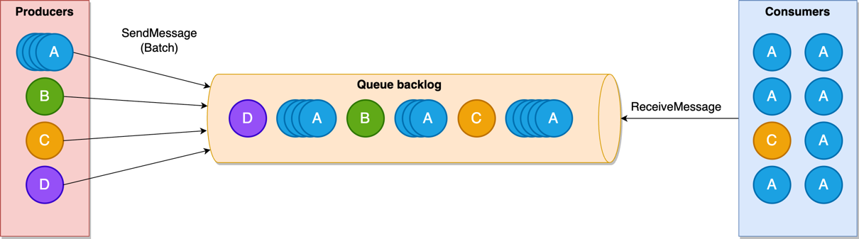
The following diagram depicts the cluster state publication flow.
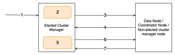
The workflow consists of the following steps:
- The user invokes an admin API such as create index.
- The elected cluster manager node computes the cluster state for the admin API request.
- The elected cluster manager node sends the cluster state publish request to follower nodes.
- The follower nodes respond with an acknowledgement to the publish request.
- The elected cluster manager node persists the cluster state to the disk.
- The elected cluster manager node sends the commit request to follower nodes.
- The follower nodes respond with an acknowledgement to the commit request.
We’ve observed stable cluster operations with this publication flow up to 200 nodes or 75,000 shards. However, as the cluster state grows in size with more indexes, shards, and nodes, it starts consuming high network bandwidth and blocking transport threads for a longer duration during publication. Additionally, it becomes CPU and memory intensive for the elected cluster manager to transmit to the follower nodes, often impacting publication latency. The increased latency can lead to a high pending task count on the elected cluster manager. This can cause request timeouts, or in severe cases, cluster manager failure, creating a cluster outage.
Using a remote store for cluster state publication improved availability and scalability
With Remote Publication, cluster state updates are transmitted through an Amazon Simple Storage Service (Amazon S3) bucket as the remote store, rather than transmitting the state over the transport layer. When the elected cluster manager updates the cluster state, it uploads the new state to Amazon S3 in addition to persisting on disk. The cluster manager uploads a manifest file, which keeps track of the entities and which entities changed from their previous state. Similarly, follower nodes download the manifest from Amazon S3 and can decide if it needs the full state or only changed entities. This has two benefits: reduced cluster manager resource usage and faster transport thread availability.
Creating new domains or upgrading from existing OpenSearch Service versions to 2.17 or above, or applying the service patch to an existing 2.17 or above domain, enables Remote Publication by default, This provides seamless migration with the remote state. This is enabled by default for SLA clusters, with or without remote-backed storage. Let’s dive into some details of this design and understand how it works internally.
How is the remote store modeled for scalability?
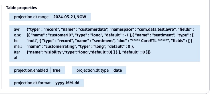
Having scalable and efficient Amazon S3 storage is essential for Remote Publication to work seamlessly. The cluster state has multiple entities, which get updated at different frequencies. For example, cluster node data only changes if a new node joins the cluster or an old node leaves the cluster, which usually happens during blue/green deployments or node replacements. However, shard allocation can change multiple times a day based on index creations, rollovers, or internal service triggered relocations. The storage schema needs to be able to handle these entities in a way that a change in one entity doesn’t impact another entity. A manifest file keeps track of the entities. Each cluster state entity has its own separate file, like one for templates, one for cluster settings, one for cluster nodes, and so on. For entities that scale with the number of indexes, like index metadata and index shard allocation, per-index files are created to make sure changes in an index can be uploaded and downloaded independently. The manifest file keeps track of paths to these individual entity files. The following code shows a sample manifest file. It contains the details of the granular cluster state entities’ files uploaded to Amazon S3 along with some basic metadata.
In addition to keeping track of cluster state components, the manifest file also keeps track of what entities changed compared to the last state, which is the diff manifest. In the preceding code, diff manifest has a section for metadata diff and routing table diff. This signifies that between these two versions of the cluster state, these entities have changed.
We also keep a separate shard diff file specifically for shard allocation. Because multiple shards for different indexes can be relocated in a single cluster state update, having this shard diff file further reduces the number of files to download.
This configuration provides the following benefits:
- Separate files help prevent bloating a single document
- Per-index files reduces the number of updates and effectively reduces the network bandwidth usage, because most updates affect only a few indexes
- Having a diff tracker makes downloads on nodes efficient because only limited data needs to be downloaded
To support the scale and high request rate to Amazon S3, we use Amazon S3 pre-partitioning, so we can scale proportionally with the number of clusters and indexes. For managing storage size, an asynchronous scheduler is added, which cleans up stale files and keeps only the last 10 recently updated documents. After a cluster is deleted, a domain sweeper job removes the files for that cluster after a few days.
Remote Publication overview
Now that you understand how cluster state is persisted in Amazon S3, let’s see how it is used during the publication workflow. When a cluster state update occurs, the elected cluster manager uploads changed entities to Amazon S3 in parallel, with the number of concurrent uploads determined by a fixed thread pool. It then updates and uploads a manifest file with diff details and file paths.
During the publish phase, the elected cluster manager sends the manifest path, term, and version to follower nodes using a new remote transport action. When the elected cluster manager changes, the newly elected cluster manager increments the term which signifies the number of times a new cluster manager election has occurred. The elected cluster manager increments the cluster state version when the cluster state is updated. You can use these two components to identify cluster state progression and make sure nodes operate with the same understanding of the cluster’s configuration. The follower nodes download the manifest, determine if they need a full state or just the diff, and then download the required files from Amazon S3 in parallel. After the new cluster state is computed, follower nodes acknowledge the elected cluster manager.
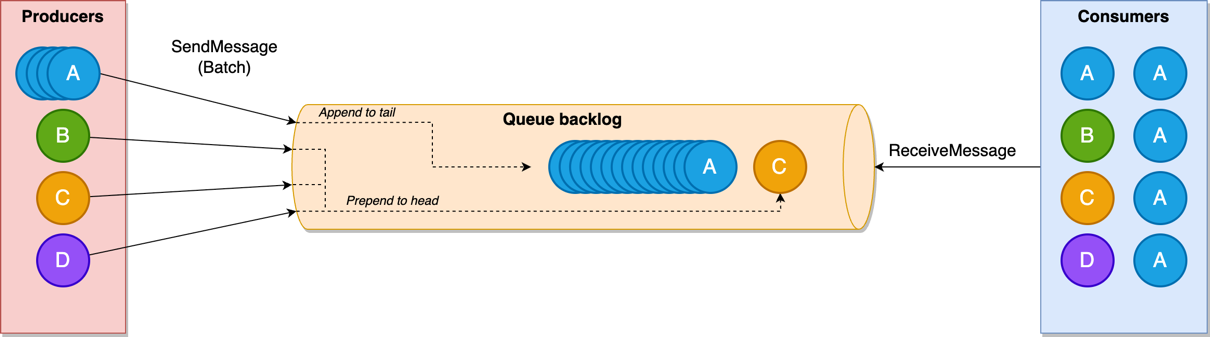
In the commit phase, the elected cluster manager updates the manifest, marking it as committed, and instructs follower nodes to commit the new cluster state. This process provides efficient distribution of cluster state updates, especially in large clusters, by minimizing direct data transfer between nodes and using Amazon S3 for storage and retrieval. The following diagram depicts the Remote Publication flow when an index creation triggers a cluster state update.
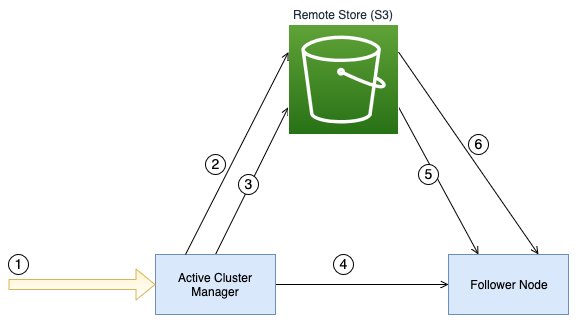
The workflow consists of the following steps:
- The user invokes an admin API such as create index.
- The elected cluster manager node uploads the index metadata and routing table files in parallel to the configured remote store.
- The elected cluster manager node uploads the manifest file containing the details of the metadata files to the remote store.
- The elected cluster manager sends the remote manifest file path to the follower nodes.
- The follower node downloads the manifest file from the remote store.
- The follower nodes download the index metadata and routing table files from the remote store in parallel.
Failure detection in publication
Remote Publication brings in a significant change to how publication works and how the cluster state is managed. Issues in file creation, publication, or downloading and creating cluster state on follower nodes can have a potential impact on the cluster. To make sure the new flow works as expected, a checksum validation is added to the publication flow. On the elected cluster manager, after creating a new cluster state, a checksum is created for individual entities and the overall cluster state and added to the manifest. On follower nodes, after the cluster state is created after download, a checksum is created again and matched against the checksum from the manifest. A mismatch in checksums means the cluster state on the follower node is different from that on the elected cluster manager. In the default mode, the service only logs which entity is failing the checksum match and lets the cluster state persist. For further debugging, checksum match supports different modes, where it can download the complete state and find the diff between two states in trace mode, or fail the publication request in failure mode.
Recovery from failures
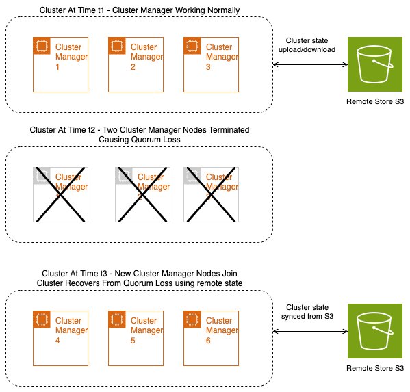
With remote state, quorum loss is recovered by using the cluster state from the remote store. Without remote state, the cluster manager might lose metadata, leading to data loss for your cluster. However, the cluster manager can now use the last persisted state to help prevent metadata loss in the cluster. The following diagram illustrates the states of a cluster before a quorum loss, during a quorum loss, and after the quorum loss recovery happens using a remote store.
Benefits
In this section, we discuss some of the solution benefits.
Scalability and availability
Remote Publication significantly reduces the CPU, memory, and network overhead for the elected cluster manager when transmitting the state to the follower nodes. Additionally, transport threads responsible for sending publish requests to follower nodes are made available more quickly, because the remote publish request size is smaller. The publication request size remains consistent irrespective of the cluster state size, giving consistent publication performance. This enhancement enables OpenSearch Service to support larger clusters of up to 1,000 nodes and a higher number of shards per node, without overwhelming the elected cluster manager. With reduced load on the cluster manager, its availability improves, so it can more efficiently serve admin API requests.
Durability
With the cluster state being persisted to Amazon S3, we get Amazon S3 durability. Clusters suffering quorum loss due to replacement of cluster manager nodes can hydrate with the remote cluster state and recover from quorum loss. Because Amazon S3 has the last committed cluster state, there is no data loss on recovery.
Cluster state publication performance
We tested the elected cluster manager performance in a 1,000-node domain containing 500,000 shards. We compared two versions: the new Remote Publication system vs. the older cluster state publication system. Both clusters were operated with the same workload for a few hours. The following are some key observations:
- Cluster state publication time reduced from an average of 13 seconds to 4 seconds, which is a three-fold improvement
- Network out reduced from an average of 4 GB to 3 GB
- Elected cluster manager resource utilization showed significant improvement, with JVM dropping from an average of 40% to 20% and CPU dropping from 50% to 40%
We tested on a 100-node cluster as well and saw performance improvements with the increase in the size of the cluster state. With 50,000 shards, the uncompressed cluster state size increased to 600 MB. The following observations were made during cluster state update when compared to a cluster without Remote Publication:
- Max network out traffic reduced from 11.3 GB to 5.7 GB (approximately 50%)
- Average elected cluster manager JVM usage reduced from 54% to 35%
- Average elected cluster manager CPU reduced from 33% to 20%
Contributing to open source
OpenSearch is an open source, community-driven software. You can find code for the Remote Publication feature in the project’s GitHub repository. Some of the notable GitHub pull requests have been added inline to the preceding text. You can find the RFCs for remote state and remote state publication in the project’s GitHub repository. A more comprehensive list of pull requests is attached in the meta issues for remote state, remote publication, and remote routing table.
Looking ahead
The new Remote Publication architecture enables teams to build additional features and optimizations using the remote store:
- Faster recovery after failures – With the new architecture, we have the last successful cluster state in Amazon S3, which can be downloaded on the new cluster manager. At the time of writing, only cluster metadata gets restored on recovery and then the elected cluster manager tries to build shard allocation by contacting the data nodes. This takes up a lot of CPU and memory for both the cluster manager and data nodes, in addition to the time taken to collate the data to build the allocation table. With the last successful shard allocation available in Amazon S3, the elected cluster manager can download the data, build the allocation table locally, and then update the cluster state to the follower nodes, making recovery faster and less resource-intensive.
- Lazy loading – The cluster state entities can be loaded as needed instead of all at once. This approach reduces the average memory usage on a follower node and is expected to speed up cluster state publication.
- Node-specific metadata – At present, every follower node downloads and loads the entire cluster state. However, we can optimize this by modifying the logic so that a data node only downloads the index metadata and routing table for the indexes it contains.
- Optimize cluster state downloads – There is an opportunity to optimize the downloading of cluster state entities. We are exploring compression and serialization techniques to minimize the amount of data transmitted.
- Restoring to an older state – The service keeps the cluster state for the last 10 updates. This can be used to restore the cluster to a previous state in case the state gets corrupted.
Conclusion
Remote Publication makes cluster state publication faster and more robust, significantly improving cluster scalability, reliability, and recovery capabilities, potentially reducing customer incidents and operational overhead. This change in architecture enables further improvements in elected cluster manager performance and making domains more durable, especially for larger domains where cluster manager operations become heavy as the number of indexes and nodes increase. We encourage you to upgrade to the latest version to take advantage of these improvements and share your experience with our community.
About the authors
 Himshikha Gupta is a Senior Engineer with Amazon OpenSearch Service. She is excited about scaling challenges with distributed systems. She is an active contributor to OpenSearch, focused on shard management and cluster scalability
 Sooraj Sinha is a software engineer at Amazon, specializing in Amazon OpenSearch Service since 2021. He has worked on multiple core components of OpenSearch, including indexing, cluster management, and cross-cluster replication. His contributions have focused on improving the availability, performance, and durability of OpenSearch.
 Jon Handler is Director of Solutions Architecture for Search Services at Amazon Web Services, based in Palo Alto, CA. Jon works closely with OpenSearch and Amazon OpenSearch Service, providing help and guidance to a broad range of customers who have generative AI, search, and log analytics workloads for OpenSearch. Prior to joining AWS, Jon’s career as a software developer included four years of coding a large-scale, eCommerce search engine. Jon holds a Bachelor of the Arts from the University of Pennsylvania, and a Master of Science and a Ph. D. in Computer Science and Artificial Intelligence from Northwestern University.
 Arjun Kumar Giri is a Principal Engineer at AWS working on the OpenSearch Project. He primarily works on OpenSearch’s artificial intelligence and machine learning (AI/ML) and semantic search features. He is passionate about AI, ML, and building scalable systems.
 Siddhant Gupta is a Senior Product Manager (Technical) at AWS, spearheading AI innovation within the OpenSearch Project from Hyderabad, India. With a deep understanding of artificial intelligence and machine learning, Siddhant architects features that democratize advanced AI capabilities, enabling customers to harness the full potential of AI without requiring extensive technical expertise. His work seamlessly integrates cutting-edge AI technologies into scalable systems, bridging the gap between complex AI models and practical, user-friendly applications.
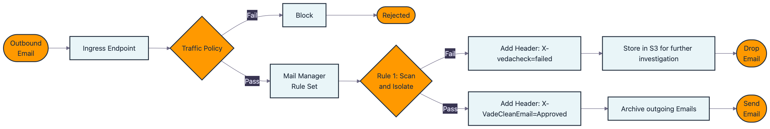
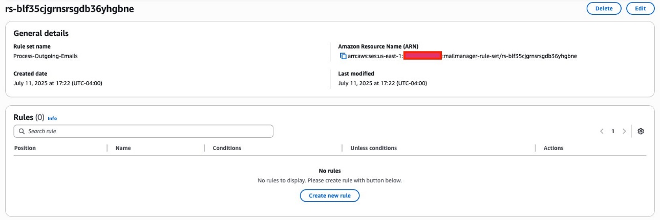
 After your ingress endpoint is created, note down the following details from the General details section:
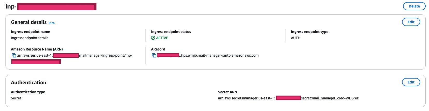
 Smita Singh is a Senior Solutions Architect at AWS. She focuses on defining technical strategic vision and works on architecture, design, and implementation of modern, scalable platforms for large-scale global enterprises and SaaS providers. She is a data, analytics, and generative AI enthusiast and is passionate about building innovative, highly scalable, resilient, fault-tolerant, self-healing, multi-tenant platform solutions and accelerators.
 Dipayan Sarkar is a Specialist Solutions Architect for Analytics at AWS, where he helps customers modernize their data platform using AWS analytics services. He works with customers to design and build analytics solutions, enabling businesses to make data-driven decisions.
 Ezat Karimi is a Senior Solutions Architect at AWS, based in Austin, TX. Ezat specializes in designing and delivering modernization solutions and strategies for database applications. Working closely with multiple AWS teams, Ezat helps customers migrate their database workloads to the AWS Cloud.
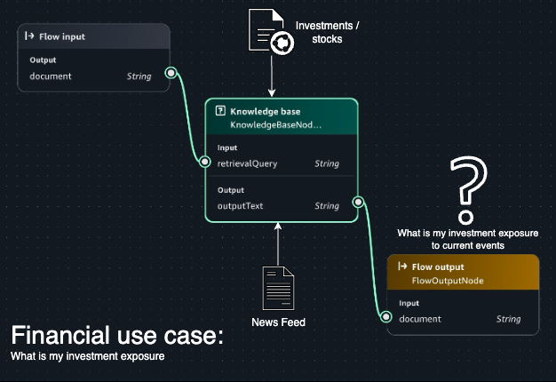
 Amit Maindola is a Senior Data Architect focused on data engineering, analytics, and AI/ML at Amazon Web Services. He helps customers in their digital transformation journey and enables them to build highly scalable, robust, and secure cloud-based analytical solutions on AWS to gain timely insights and make critical business decisions.
 Arghya Banerjee is a Sr. Solutions Architect at AWS in the San Francisco Bay Area, focused on helping customers adopt and use the AWS Cloud. He is focused on big data, data lakes, streaming and batch analytics services, and generative AI technologies.
 Melody Yang is a Principal Analytics Architect for Amazon EMR at AWS. She is an experienced analytics leader working with AWS customers to provide best practice guidance and technical advice in order to assist their success in data transformation. Her areas of interests are open-source frameworks and automation, data engineering and DataOps.
 Gaurav Parekh is a Solutions Architect at AWS, specializing in generative AI and data analytics, with extensive experience building production AI systems on AWS.
 Mohammad Sabeel Mohammad Sabeel is a Senior Cloud Support Engineer at Amazon Web Services (AWS) with over 14 years of experience in Information Technology (IT). As a member of the Technical Field Community (TFC) Analytics team, he is a Subject matter expert in Analytics services AWS Glue, Amazon Managed Workflows for Apache Airflow (MWAA), and Amazon Athena services. Sabeel provides expert guidance and technical support to enterprise and strategic customers, helping them optimize their data analytics solutions and overcome complex challenges. With deep subject matter expertise he enables organizations to build scalable, efficient, and cost-effective data processing pipelines.
 Indira Balakrishnan Indira Balakrishnan is a Principal Solutions Architect in the Amazon Web Services (AWS) Analytics Specialist Solutions Architect (SA) Team. She helps customers build cloud-based Data and AI/ML solutions to address business challenges. With over 25 years of experience in Information Technology (IT), Indira actively contributes to the AWS Analytics Technical Field community, supporting customers across various Domains and Industries. Indira participates in Women in Engineering and Women at Amazon tech groups to encourage girls to pursue STEM path to enter careers in IT. She also volunteers in early career mentoring circles.

 Michael Torio is an Associate Specialist Solutions Architect at AWS focused on Amazon OpenSearch Service based out of Mountain View, CA. Michael enjoys helping customers leverage cloud technologies to solve their business challenges.
 Arjun Nambiar is a Product Manager with Amazon OpenSearch Service. He focuses on ingestion technologies that enable ingesting data from a wide variety of sources into Amazon OpenSearch Service at scale. Arjun is interested in large-scale distributed systems and cloud-centered technologies, and is based out of Seattle, Washington.
 Noritaka Sekiyama is a Principal Big Data Architect with AWS Analytics services. He’s responsible for building software artifacts to help customers. In his spare time, he enjoys cycling on his road bike.
 Tomohiro Tanaka is a Senior Cloud Support Engineer at Amazon Web Services. He’s passionate about helping customers use Apache Iceberg for their data lakes on AWS. In his free time, he enjoys a coffee break with his colleagues and making coffee at home.
 Peter Tsai is a Software Development Engineer at AWS, where he enjoys solving challenges in the design and performance of the AWS Glue runtime. In his leisure time, he enjoys hiking and cycling.
 Matt Su is a Senior Product Manager on the AWS Glue team. He enjoys helping customers uncover insights and make better decisions using their data with AWS Analytics services. In his spare time, he enjoys skiing and gardening.
 Sean McGeehan is a Software Development Engineer at AWS, where he builds features for the AWS Glue fulfillment system. In his leisure time, he explores his home of Philadelphia and work city of New York.


 Naohisa Takahashi is a Senior Cloud Support Engineer on the AWS Support Engineering team. He supports customers resolve technical issues and launch systems. In his spare time, he plays board games with his friends.
 Noritaka Sekiyama is a Principal Big Data Architect with AWS Analytics services. He’s responsible for building software artifacts to help customers. In his spare time, he enjoys cycling on his road bike.
 Iris Tian is a UX designer on the Amazon SageMaker Unified Studio team. She designs intuitive, end-to-end experiences that simplify and streamline workflows across data processing and orchestration. In her spare time, she enjoys snowboarding and visiting museums.
 Regan Baum is a Senior Software Development Engineer on the Amazon SageMaker Unified Studio team. She designs, implements, and maintains features that enable customers to manage their workflows in SageMaker Unified Studio. Outside of work, she enjoys hiking and running.
 Yuhang Huang is a Software Development Manager on the Amazon SageMaker Unified Studio team. He leads the engineering team to design, build, and operate scheduling and orchestration capabilities in SageMaker Unified Studio. In his free time, he enjoys playing tennis.
 Gal Heyne is a Senior Technical Product Manager for AWS Analytics services with a strong focus on AI/ML and data engineering. She is passionate about developing a deep understanding of customers’ business needs and collaborating with engineers to design simple-to-use data products.


 Neeraj Kaushik is an Open Group Certified Distinguish Architect at IBM with two decades of experience in client-facing delivery roles. His experience spans several industries, including travel and transportation, banking, retail, education, healthcare, and anti-human trafficking. As a trusted advisor, he works directly with the client executive and architects on business strategy to define a technology roadmap. As a hands-on Chief Architect AWS Professional Certified Solution Architect, AWS Certified Machine Learning Specialist and Natural Language Processing Expert, he has led multiple complex cloud modernization programs and AI initiatives.
 Jay Pandya is a Senior Partner Solutions Architect in the Global Systems Integrator (GSI) team at Amazon Web Services (AWS). He has over 30 years of IT experience and is helping and providing guidance to AWS GSI partners to build, design, and architect agile, scalable, highly available, and secure solutions on AWS. Outside of the office, Jay enjoys spending time with his family and traveling, and he is an aviation enthusiast and avid sports and Formula 1 fan.
 Vijay Gokarn is a Senior Solution Architect at IBM with extensive experience across industries including financial services, healthcare, industrial, retail, and travel and hospitality. He leads complex AWS transformation initiatives, drawing on his hands-on expertise as an AWS Certified Solutions Architect Associate. Vijay specializes in serverless architectures, event-driven systems, and enterprise modernization. As a skilled architect and team leader, he has delivered impactful solutions in cloud modernization, digital banking, and intelligent automation. His passion lies in bridging business strategy with technical execution to drive scalable digital transformation.
 Subhash Sharma is Sr. Partner Solutions Architect at AWS. He has more than 25 years of experience in delivering distributed, scalable, highly available, and secured software products using Microservices, AI/ML, the Internet of Things (IoT), and Blockchain using a DevSecOps approach. In his spare time, Subhash likes to spend time with family and friends, hike, walk on beach, and watch TV.


 Swapna Bandla is a Senior Solutions Architect in the AWS Analytics Specialist SA Team. Swapna has a passion towards understanding customers data and analytics needs and empowering them to develop cloud-based well-architected solutions. Outside of work, she enjoys spending time with her family.
 Austin Groeneveld is a Streaming Specialist Solutions Architect at Amazon Web Services (AWS), based in the San Francisco Bay Area. In this role, Austin is passionate about helping customers accelerate insights from their data using the AWS platform. He is particularly fascinated by the growing role that data streaming plays in driving innovation in the data analytics space. Outside of his work at AWS, Austin enjoys watching and playing soccer, traveling, and spending quality time with his family.


 Bharav Patel is a Specialist Solution Architect, Analytics at Amazon Web Services. He primarily works on Amazon OpenSearch Service and helps customers with key concepts and design principles of running OpenSearch workloads on the cloud. Bharav likes to explore new places and try out different cuisines.