Tag Archives: launch

Heads Up – AWS News Blog RSS Feed Change

Post Syndicated from Jeff Barr original https://aws.amazon.com/blogs/aws/heads-up-aws-news-blog-rss-feed-change/

TL;DR – If you are using the ancient Feedburner feed for this blog, please change to the new one (https://aws.amazon.com/blogs/aws/feed/) ASAP.

Back in the early days of AWS, I paid a visit to the Chicago headquarters of a cool startup called FeedBurner. My friend Matt Shobe demo’ed their new product to me and showed me how “burning” a raw RSS feed could add value to it in various ways. Upon my return to Seattle I promptly burned the RSS feed of the original (TypePad-hosted) version of this blog, and shared that feed for many years.

FeedBurner has served us well over the years, but its time has passed. The company was acquired many years ago and the new owners are now putting the product into maintenance mode.

While the existing feed will continue to work for the foreseeable future, I would like to encourage you to use the one directly generated by this blog instead. Simply update your feed reader to refer to https://aws.amazon.com/blogs/aws/feed/ .

Jeff;

In the Works – AWS Region in Tel Aviv, Israel

Post Syndicated from Jeff Barr original https://aws.amazon.com/blogs/aws/in-the-works-aws-region-in-tel-aviv-israel/

We launched three AWS Regions (Italy, South Africa, and Japan) in the last 12 months, and are working on regions in Australia, Indonesia, Spain, India, Switzerland, and the United Arab Emirates.

Tel Aviv, Israel in the Works
Today I am happy to announce that the AWS Israel (Tel Aviv) Region is in the works and will open in the first half of 2023. This region will have three Availability Zones and will give AWS customers in Israel the ability to run workloads and store data that must remain in-country.

There are 81 Availability Zones within 25 AWS Regions in operation today, with 21 more Availability Zones and seven announced regions (including this one) underway.

As is always the case with an AWS Region, each of the Availability Zones will be a fully isolated part of the AWS infrastructure. The AZs in this region will be connected together via high-bandwidth, low-latency network connections over dedicated, fully redundant metro fiber. This connectivity supports applications that need synchronous replication between AZs for availability or redundancy. You can take a peek at the AWS Global Infrastructure page to learn more about how we design and build regions and AZs.

AWS in Israel
I first visited Israel in 2013 and have been back several (but definitely not enough) times since then. I have spoken at several AWS Summits and visited many of early customers in the area. Today, AWS has the following resources on the ground in Israel:

Israel is also home to Annapurna Labs, an Amazon.com subsidiary that is responsible for developing much of the innovative hardware that powers AWS.

In addition, the government of Israel announced that it has selected AWS as the primary cloud provider for the Nimbus Project. As part of this project, government ministries and subsidiaries in Israel will use cloud computing to power a digital transformation and to provide new digital services for the citizens of Israel.

Stay Tuned
We’ll announce the opening of the AWS Israel (Tel Aviv) Region in a forthcoming blog post, so be sure to stay tuned!

Jeff;


Now Open Third Availability Zone in the AWS China (Beijing) Region

Post Syndicated from Jeff Barr original https://aws.amazon.com/blogs/aws/now-open-third-availability-zone-in-the-aws-china-beijing-region/

I made my first trip to China in late 2008. I was able to speak to developers and entrepreneurs and to get a sense of the then-nascent market for cloud computing. With over 900 million Internet users as of 2020 (according to a recent report from China Internet Network Information Center), China now has the largest user base in the world.

A limited preview of the China (Beijing) Region was launched in 2013 and brought to general availability in 2016. A year later the AWS China (Ningxia) Region launched. In order to comply with China’s legal and regulatory requirements, we collaborated with local Chinese partners. These partners have the proper telecom licenses to provide cloud services in Mainland China. Today, developers can deploy cloud-based applications inside of using the same APIs, protocols, services, and operational practices used by our customers in other parts of the world. This commonality has been particularly attractive to multinational companies that can take advantage of their existing AWS experience when they expand their cloud infrastructure into Mainland China.

Third Availability Zone in Beijing
Today I am happy to announce that we are adding a third Availability Zone (AZ) to the China (Beijing) Region operated by Sinnet in order to support the demands of our growing customer base in China. As is the case with all AWS Availability Zones, this one encompasses one or more discrete data centers in separate facilities, each with redundant power, networking, and connectivity. With this launch, both AWS Regions in China offer three AZs and allow customers to build applications that are scalable, fault-tolerant, and highly available.

AWS Customers in the Beijing Region
Many enterprise customers in China are using the China (Beijing) Region to support their digital transformations. For example:

Yantai Shinho was founded in 1992 and now manufactures 13 popular condiments. They now have a presence in over 100 countries and supply products that tens of millions of families enjoy. They are already using the region to support their front-end and big data efforts, and plan to make use of the additional architectural options made possible by the new AZ.

Kingdee International Software Group was founded in 1993 and now provides corporate management and cloud services for more than 6.8 million enterprises and government organizations. They now have over 8,000 employees AND are committed to changing the way that hundreds of millions of people work.

As I noted earlier, our multinational customers are using the AWS Regions in China to expand their global presence. Here are a few examples:

Australian independent software vendor Canva offers its design-on-demand application to 150 million active users in 190 countries. They launched their Chinese products in August 2018, and have since built in into a first-class design platform that includes tens of millions of high-resolution pictures, Chinese fonts, original templates, and more. Chinese users have already created over 50 million designs on the Canva.cn platform.

Swire is a 200 year old business group that spans the aviation, beverage, food, industrial, marine services, and property industries. Their Swire Coca-Cola division has the exclusive right to manufacture, market, and distribute Coca-Cola products in eleven Chinese provinces, the Shanghai Municipality, Hong Kong, Taiwan, and part of the Western United States — a total customer base of 728 million people. Swire Coca-Cola’s systems primarily operate in the China (Beijing) Region and will soon make use of the third AZ.

Finally, startups are using the region to power their fast-growing businesses:

CraiditX applies machine learning technology originally developed for search engines to the financial services industry. Established in 2015, they use behavioral language processing, natural language processing, neural networks, and integrated modeling to build risk management systems.

Founded in 2016, Momenta is a Chinese startup that is building a “brain” for autonomous vehicles. Powered by deep learning and data-driven path planning, they are working on autonomous driving for passenger vehicles and full autonomy for mobile service vehicles, all deployed in the China (Beijing) Region.

81 and 25
This launch raises the global AWS footprint to a total of 81 Availability Zones across 25 geographic regions, with plans to launch 18 additional Availability Zones and six more regions in Australia, India, Indonesia, Spain, Switzerland, and United Arab Emirates (UAE).

–Jeff, with lots of help from Lillian Shao;

PS – The operator and service provider for the AWS China (Beijing) Region is Beijing Sinnet Technology Co., Ltd. The operator and service provider for the AWS China (Ningxia) Region is Ningxia Western Cloud Data Technology Co., Ltd.

Introducing the newest AWS Heroes – June, 2021

Post Syndicated from Ross Barich original https://aws.amazon.com/blogs/aws/introducing-the-newest-aws-heroes-june-2021/

We at AWS continue to be impressed by the passion AWS enthusiasts have for knowledge sharing and supporting peer-to-peer learning in tech communities. A select few of the most influential and active community leaders in the world, who truly go above and beyond to create content and help others build better & faster on AWS, are recognized as AWS Heroes.

Today we are thrilled to introduce the newest AWS Heroes, including the first Heroes based in Perú and Ukraine:

Anahit Pogosova – Tampere, Finland

Data Hero Anahit Pogosova is a Lead Cloud Software Engineer at Solita. She has been architecting and building software solutions with various customers for over a decade. Anahit started working with monolithic on-prem software, but has since moved all the way to the cloud, nowadays focusing mostly on AWS Data and Serverless services. She has been particularly interested in the AWS Kinesis family and how it integrates with AWS Lambda. You can find Anahit speaking at various local and international events, such as AWS meetups, AWS Community Days, ServerlessDays, and Code Mesh. She also writes about AWS on Solita developers’ blog and has been a frequent guest on various podcasts.

Anurag Kale – Gothenburg, Sweden

Data Hero Anurag Kale is a Cloud Consultant at Cybercom Group. He has been using AWS professionally since 2017 and holds the AWS Solutions Architect – Associate certification. He is a co-organizer of the AWS User Group Pune; helping host and organize AWS Community Day Pune 2020 and AWS Community Day India 2020 – Virtual Edition. Anurag’s areas of interest include Amazon DynamoDB, relational databases, serverless data pipelines, data analytics, Infrastructure as Code, and sustainable cloud solutions. He is an active advocate of DynamoDB and Amazon Aurora, and has spoken at various national and international events such as AWS Community Day Nordics 2020 and various AWS Meetups.

Arseny Zinchenko – Kiev, Ukraine

Container Hero Arseny Zinchenko has over 15 years in IT, and currently works as a DevOps Team Lead and Data Security Officer at BetterMe Inc., a leading health & fitness mobile publisher. Since 2011 Arseny has used his blog to share expertise about DevOps, system administration, containerization, and cloud computing. Currently he is focused primary on Amazon Elastic Kubernetes Service (EKS) and security solutions provided by AWS. He is a member of the biggest Ukranian DevOps community, UrkOps, where he helps others to build their best with AWS and containers. where he helps others to build their best with AWS and containers. He also helps implement DevOps methodology in their organizations by using Amazon CloudFormation and AWS managed services like Amazon RDS, Amazon Aurora, and EKS.

Azmi Mengü – Istanbul, Turkey

Community Hero Azmi Mengü is a Sr. Software Engineer on the Infrastructure Team at Armut / HomeRun. He has over 5 years of AWS cloud development experience and has expertise in serverless, containers, data, and storage services. Since 2019, Azmi has been on the organizing committee of the Cloud and Serverless Turkey community. He co-organized and acted as a speaker at over 50 physical and online events during this time. He actively writes blog posts about developing serverless, container, and IaC technologies on AWS. Azmi also co-organized the first-ever ServerlessDays Istanbul in Turkey and AWS Community Day Turkey events.

Carlos Cortez – Lima, Perú

Community Hero Carlos Cortez is the founder and leader of AWS User Group Perú and Founder and CTO of CENNTI, which helps Peruvian companies in their difficult journey to the cloud and the development of Machine Learning solutions. The two biggest AWS events in Perú, AWS Community Day Lima 2019 and AWS UG Perú Conference in 2021, were organized by Carlos. He is the owner of the first AWS Podcast in Latam, “Imperio Cloud” and “Al día con AWS”. He loves to create content for emerging technologies, which is why he created DeepFridays to educate people in Reinforcement Learning.

Chris Miller – Santa Cruz, USA

Machine Learning Hero Chris Miller is an entrepreneur, inventor, and CEO of Cloud Brigade. After winning the 2019 AWS DeepRacer Summit race in Santa Clara, he founded the Santa Cruz DeepRacer Meetup group. Chris has worked with AWS AI/ML product teams with DeepLens and DeepRacer on projects including The Poopinator, and What’s in my Fridge. He prides himself on being a technical founder with experience across a broad range of disciplines, which has led to a lot of crazy projects in competitions and hackathons, such as an automated beer brewery, animatronic ventriloquist dummy, and his team even won a Cardboard Boat Race!

Gert Leenders – Brussels, Belgium

DevTools Hero Gert Leenders started his career as a developer in 2001. Eight years ago, his focus shifted entirely towards AWS. Today, he’s an AWS Cloud Solution Architect helping teams build and deploy cloud-native applications and manage their cloud infrastructure. On his blog, Gert emphasizes hidden gems in AWS developer tools and day-to-day topics for cloud engineers like logging, debugging, error handling and Infrastructure as Code. He also often shares code on GitHub.

Lei Wu – Beijing, China

Machine Learning Hero Lei Wu is head of the machine learning team at FreeWheel. He enjoys sharing technology with others, and he publishes many Chinese language tech blogs at infoQ, covering machine learning, big data, and distributed computing systems. Lei works hard to promote deep learning adoption with AWS services wherever he can, including talks at Spark Summit China, World Artificial Intelligence Conference, AWS Innovate AI/ML edition, and AWS re:Invent where he shared FreeWheel’s best practices on deep learning with Amazon SageMaker.

Hidetoshi Matsui – Hamamatsu, Japan

Serverless Hero Hidetoshi Matsui is a developer at Startup Technology Inc. and a member of the Japan AWS User Group (JAWS-UG). On “builders.flash,” a web magazine for developers run by AWS Japan, the articles he has contributed are among the most viewed pages on the site since 2020. His most impactful achievement is the construction of a distribution site for JAWS-UG’s largest event, JAWS DAYS 2021 re:Connect. He made full use of various AWS services to build a low-latency and scalable distribution system with a serverless architecture and smooth streaming video viewing for nearly 4000 participants.

Philipp Schmid – Nuremberg, Germany

Machine Learning Hero Philipp Schmid is a Machine Learning & Tech Lead at Hugging Face, working to democratize artificial intelligence through open source and open science. He has extensive experience in deep learning, deploying NLP models into production using AWS Lambda, and is an avid advocate of Amazon SageMaker to simplify machine learning, such as “Distributed Training: Train BART/T5 for Summarization using Transformers and Amazon SageMaker.” He loves to share his knowledge on AI and NLP at various meetups such as Data Science on AWS, and on his technical Blog.

Simone Merlini – Milan, Italy

Community Hero Simone Merlini is CEO and CTO at beSharp. In 2012 he co-founded the first AWS User Group in Italy, and he’s currently the organizer of the AWS User Group Milan. He’s also actively involved in the development of Leapp, an open-source project for managing and securing Cloud access in multi-account environments. Simone is also the editor in chief and writer for Proud2beCloud, a blog aimed to share highly specialized AWS knowledge to enable the adoption of cloud technologies.

Virginie Mathivet – Lyon, France

Machine Learning Hero Virginie Mathivet has been leading the DataSquad team at TeamWork since 2017, focused on Data and Artificial Intelligence. Their purpose is to make the most of their clients’ data, via Data Science or Data Engineering / Big Data, mainly on AWS. Virginie regularly participates in conferences and writes books and articles, both for the public (introduction to AI) and for an informed audience (technical subjects). She also campaigns for a better visibility of women in the digital industry and for diversity in the data professions. Her favorite cloud service? Amazon SageMaker of course!

Walid A. Shaari – Dhahran, Saudi Arabia

Container Hero Walid A. Shaari is the community lead for the Dammam Cloud-native AWS User Group, working closely with CNCF ambassadors, K8saraby, and AWS MENA community leaders to enable knowledge sharing, collaboration, and networking. He helped organize the first AWS Community Day – MENA 2020. Walid also maintains GitHub content for Certified Kubernetes Administrators (CKA) and Certified Kubernetes Security Specialists (CKS), and holds several active professional certifications: AWS Certified Associate Solutions Architect, Certified Kubernetes Administrator, Certified Kubernetes Application Developer, Red Hat Certified Architect level IV, and more.


If you’d like to learn more about the new Heroes, or connect with a Hero near you, please visit the AWS Hero website.

Ross;

Amazon Redshift ML Is Now Generally Available – Use SQL to Create Machine Learning Models and Make Predictions from Your Data

Post Syndicated from Danilo Poccia original https://aws.amazon.com/blogs/aws/amazon-redshift-ml-is-now-generally-available-use-sql-to-create-machine-learning-models-and-make-predictions-from-your-data/

With Amazon Redshift, you can use SQL to query and combine exabytes of structured and semi-structured data across your data warehouse, operational databases, and data lake. Now that AQUA (Advanced Query Accelerator) is generally available, you can improve the performance of your queries by up to 10 times with no additional costs and no code changes. In fact, Amazon Redshift provides up to three times better price/performance than other cloud data warehouses.

But what if you want to go a step further and process this data to train machine learning (ML) models and use these models to generate insights from data in your warehouse? For example, to implement use cases such as forecasting revenue, predicting customer churn, and detecting anomalies? In the past, you would need to export the training data from Amazon Redshift to an Amazon Simple Storage Service (Amazon S3) bucket, and then configure and start a machine learning training process (for example, using Amazon SageMaker). This process required many different skills and usually more than one person to complete. Can we make it easier?

Today, Amazon Redshift ML is generally available to help you create, train, and deploy machine learning models directly from your Amazon Redshift cluster. To create a machine learning model, you use a simple SQL query to specify the data you want to use to train your model, and the output value you want to predict. For example, to create a model that predicts the success rate for your marketing activities, you define your inputs by selecting the columns (in one or more tables) that include customer profiles and results from previous marketing campaigns, and the output column you want to predict. In this example, the output column could be one that shows whether a customer has shown interest in a campaign.

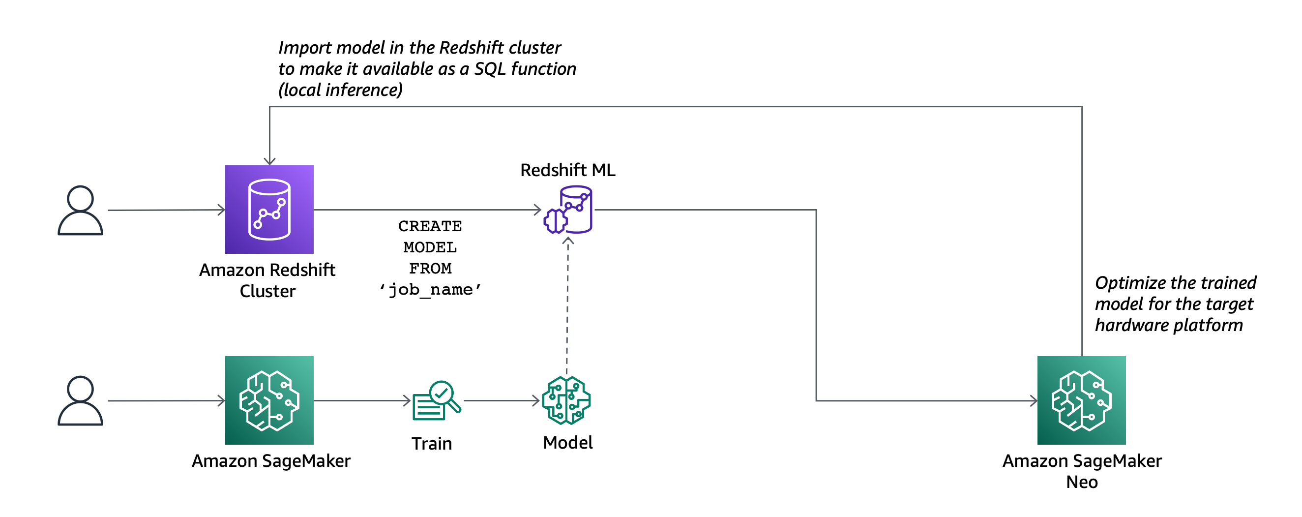
After you run the SQL command to create the model, Redshift ML securely exports the specified data from Amazon Redshift to your S3 bucket and calls Amazon SageMaker Autopilot to prepare the data (pre-processing and feature engineering), select the appropriate pre-built algorithm, and apply the algorithm for model training. You can optionally specify the algorithm to use, for example XGBoost.

Architectural diagram.

Redshift ML handles all of the interactions between Amazon Redshift, S3, and SageMaker, including all the steps involved in training and compilation. When the model has been trained, Redshift ML uses Amazon SageMaker Neo to optimize the model for deployment and makes it available as a SQL function. You can use the SQL function to apply the machine learning model to your data in queries, reports, and dashboards.

Redshift ML now includes many new features that were not available during the preview, including Amazon Virtual Private Cloud (VPC) support. For example:

Architectural diagram.

  • You can also create SQL functions that use existing SageMaker endpoints to make predictions (remote inference). In this case, Redshift ML is batching calls to the endpoint to speed up processing.

Before looking into how to use these new capabilities in practice, let’s see the difference between Redshift ML and similar features in AWS databases and analytics services.

ML Feature Data Training
from SQL
Predictions
using SQL Functions
Amazon Redshift ML

Data warehouse

Federated relational databases

S3 data lake (with Redshift Spectrum)

Yes, using
Amazon SageMaker Autopilot
Yes, a model can be imported and executed inside the Amazon Redshift cluster, or invoked using a SageMaker endpoint.
Amazon Aurora ML Relational database
(compatible with MySQL or PostgreSQL)
No

Yes, using a SageMaker endpoint.

A native integration with Amazon Comprehend for sentiment analysis is also available.

Amazon Athena ML

S3 data lake

Other data sources can be used through Athena Federated Query.

No Yes, using a SageMaker endpoint.

Building a Machine Learning Model with Redshift ML
Let’s build a model that predicts if customers will accept or decline a marketing offer.

To manage the interactions with S3 and SageMaker, Redshift ML needs permissions to access those resources. I create an AWS Identity and Access Management (IAM) role as described in the documentation. I use RedshiftML for the role name. Note that the trust policy of the role allows both Amazon Redshift and SageMaker to assume the role to interact with other AWS services.

From the Amazon Redshift console, I create a cluster. In the cluster permissions, I associate the RedshiftML IAM role. When the cluster is available, I load the same dataset used in this super interesting blog post that my colleague Julien wrote when SageMaker Autopilot was announced.

The file I am using (bank-additional-full.csv) is in CSV format. Each line describes a direct marketing activity with a customer. The last column (y) describes the outcome of the activity (if the customer subscribed to a service that was marketed to them).

Here are the first few lines of the file. The first line contains the headers.

age,job,marital,education,default,housing,loan,contact,month,day_of_week,duration,campaign,pdays,previous,poutcome,emp.var.rate,cons.price.idx,cons.conf.idx,euribor3m,nr.employed,y 56,housemaid,married,basic.4y,no,no,no,telephone,may,mon,261,1,999,0,nonexistent,1.1,93.994,-36.4,4.857,5191.0,no
57,services,married,high.school,unknown,no,no,telephone,may,mon,149,1,999,0,nonexistent,1.1,93.994,-36.4,4.857,5191.0,no
37,services,married,high.school,no,yes,no,telephone,may,mon,226,1,999,0,nonexistent,1.1,93.994,-36.4,4.857,5191.0,no
40,admin.,married,basic.6y,no,no,no,telephone,may,mon,151,1,999,0,nonexistent,1.1,93.994,-36.4,4.857,5191.0,no

I store the file in one of my S3 buckets. The S3 bucket is used to unload data and store SageMaker training artifacts.

Then, using the Amazon Redshift query editor in the console, I create a table to load the data.

CREATE TABLE direct_marketing (
	age DECIMAL NOT NULL, 
	job VARCHAR NOT NULL, 
	marital VARCHAR NOT NULL, 
	education VARCHAR NOT NULL, 
	credit_default VARCHAR NOT NULL, 
	housing VARCHAR NOT NULL, 
	loan VARCHAR NOT NULL, 
	contact VARCHAR NOT NULL, 
	month VARCHAR NOT NULL, 
	day_of_week VARCHAR NOT NULL, 
	duration DECIMAL NOT NULL, 
	campaign DECIMAL NOT NULL, 
	pdays DECIMAL NOT NULL, 
	previous DECIMAL NOT NULL, 
	poutcome VARCHAR NOT NULL, 
	emp_var_rate DECIMAL NOT NULL, 
	cons_price_idx DECIMAL NOT NULL, 
	cons_conf_idx DECIMAL NOT NULL, 
	euribor3m DECIMAL NOT NULL, 
	nr_employed DECIMAL NOT NULL, 
	y BOOLEAN NOT NULL
);

I load the data into the table using the COPY command. I can use the same IAM role I created earlier (RedshiftML) because I am using the same S3 bucket to import and export the data.

COPY direct_marketing 
FROM 's3://my-bucket/direct_marketing/bank-additional-full.csv' 
DELIMITER ',' IGNOREHEADER 1
IAM_ROLE 'arn:aws:iam::123412341234:role/RedshiftML'
REGION 'us-east-1';

Now, I create the model straight form the SQL interface using the new CREATE MODEL statement:

CREATE MODEL direct_marketing
FROM direct_marketing
TARGET y
FUNCTION predict_direct_marketing
IAM_ROLE 'arn:aws:iam::123412341234:role/RedshiftML'
SETTINGS (
  S3_BUCKET 'my-bucket'
);

In this SQL command, I specify the parameters required to create the model:

  • FROM – I select all the rows in the direct_marketing table, but I can replace the name of the table with a nested query (see example below).
  • TARGET – This is the column that I want to predict (in this case, y).
  • FUNCTION – The name of the SQL function to make predictions.
  • IAM_ROLE – The IAM role assumed by Amazon Redshift and SageMaker to create, train, and deploy the model.
  • S3_BUCKET – The S3 bucket where the training data is temporarily stored, and where model artifacts are stored if you choose to retain a copy of them.

Here I am using a simple syntax for the CREATE MODEL statement. For more advanced users, other options are available, such as:

  • MODEL_TYPE – To use a specific model type for training, such as XGBoost or multilayer perceptron (MLP). If I don’t specify this parameter, SageMaker Autopilot selects the appropriate model class to use.
  • PROBLEM_TYPE – To define the type of problem to solve: regression, binary classification, or multiclass classification. If I don’t specify this parameter, the problem type is discovered during training, based on my data.
  • OBJECTIVE – The objective metric used to measure the quality of the model. This metric is optimized during training to provide the best estimate from data. If I don’t specify a metric, the default behavior is to use mean squared error (MSE) for regression, the F1 score for binary classification, and accuracy for multiclass classification. Other available options are F1Macro (to apply F1 scoring to multiclass classification) and area under the curve (AUC). More information on objective metrics is available in the SageMaker documentation.

Depending on the complexity of the model and the amount of data, it can take some time for the model to be available. I use the SHOW MODEL command to see when it is available:

SHOW MODEL direct_marketing

When I execute this command using the query editor in the console, I get the following output:

Console screenshot.

As expected, the model is currently in the TRAINING state.

When I created this model, I selected all the columns in the table as input parameters. I wonder what happens if I create a model that uses fewer input parameters? I am in the cloud and I am not slowed down by limited resources, so I create another model using a subset of the columns in the table:

CREATE MODEL simple_direct_marketing
FROM (
        SELECT age, job, marital, education, housing, contact, month, day_of_week, y
 	  FROM direct_marketing
)
TARGET y
FUNCTION predict_simple_direct_marketing
IAM_ROLE 'arn:aws:iam::123412341234:role/RedshiftML'
SETTINGS (
  S3_BUCKET 'my-bucket'
);

After some time, my first model is ready, and I get this output from SHOW MODEL. The actual output in the console is in multiple pages, I merged the results here to make it easier to follow:

Console screenshot.

From the output, I see that the model has been correctly recognized as BinaryClassification, and F1 has been selected as the objective. The F1 score is a metrics that considers both precision and recall. It returns a value between 1 (perfect precision and recall) and 0 (lowest possible score). The final score for the model (validation:f1) is 0.79. In this table I also find the name of the SQL function (predict_direct_marketing) that has been created for the model, its parameters and their types, and an estimation of the training costs.

When the second model is ready, I compare the F1 scores. The F1 score of the second model is lower (0.66) than the first one. However, with fewer parameters the SQL function is easier to apply to new data. As is often the case with machine learning, I have to find the right balance between complexity and usability.

Using Redshift ML to Make Predictions
Now that the two models are ready, I can make predictions using SQL functions. Using the first model, I check how many false positives (wrong positive predictions) and false negatives (wrong negative predictions) I get when applying the model on the same data used for training:

SELECT predict_direct_marketing, y, COUNT(*)
  FROM (SELECT predict_direct_marketing(
                   age, job, marital, education, credit_default, housing,
                   loan, contact, month, day_of_week, duration, campaign,
                   pdays, previous, poutcome, emp_var_rate, cons_price_idx,
                   cons_conf_idx, euribor3m, nr_employed), y
          FROM direct_marketing)
 GROUP BY predict_direct_marketing, y;

The result of the query shows that the model is better at predicting negative rather than positive outcomes. In fact, even if the number of true negatives is much bigger than true positives, there are much more false positives than false negatives. I added some comments in green and red to the following screenshot to clarify the meaning of the results.

Console screenshot.

Using the second model, I see how many customers might be interested in a marketing campaign. Ideally, I should run this query on new customer data, not the same data I used for training.

SELECT COUNT(*)
  FROM direct_marketing
 WHERE predict_simple_direct_marketing(
           age, job, marital, education, housing,
           contact, month, day_of_week) = true;

Wow, looking at the results, there are more than 7,000 prospects!

Console screenshot.

Availability and Pricing
Redshift ML is available today in the following AWS Regions: US East (Ohio), US East (N Virginia), US West (Oregon), US West (San Francisco), Canada (Central), Europe (Frankfurt), Europe (Ireland), Europe (Paris), Europe (Stockholm), Asia Pacific (Hong Kong) Asia Pacific (Tokyo), Asia Pacific (Singapore), Asia Pacific (Sydney), and South America (São Paulo). For more information, see the AWS Regional Services list.

With Redshift ML, you pay only for what you use. When training a new model, you pay for the Amazon SageMaker Autopilot and S3 resources used by Redshift ML. When making predictions, there is no additional cost for models imported into your Amazon Redshift cluster, as in the example I used in this post.

Redshift ML also allows you to use existing Amazon SageMaker endpoints for inference. In that case, the usual SageMaker pricing for real-time inference applies. Here you can find a few tips on how to control your costs with Redshift ML.

To learn more, you can see this blog post from when Redshift ML was announced in preview and the documentation.

Start getting better insights from your data with Redshift ML.

Danilo

Getting Started with Amazon ECS Anywhere – Now Generally Available

Post Syndicated from Channy Yun original https://aws.amazon.com/blogs/aws/getting-started-with-amazon-ecs-anywhere-now-generally-available/

Since Amazon Elastic Container Service (Amazon ECS) was launched in 2014, AWS has released other options for running Amazon ECS tasks outside of an AWS Region such as AWS Wavelength, an offering for mobile edge devices or AWS Outposts, a service that extends to customers’ environments using hardware owned and fully managed by AWS.

But some customers have applications that need to run on premises due to regulatory, latency, and data residency requirements or the desire to leverage existing infrastructure investments. In these cases, customers have to install, operate, and manage separate container orchestration software and need to use disparate tooling across their AWS and on-premises environments. Customers asked us for a way to manage their on-premises containers without this added complexity and cost.

Following Jeff’s preannouncement last year, I am happy to announce the general availability of Amazon ECS Anywhere, a new capability in Amazon ECS that enables customers to easily run and manage container-based applications on premises, including virtual machines (VMs), bare metal servers, and other customer-managed infrastructure.

With ECS Anywhere, you can run and manage containers on any customer-managed infrastructure using the same cloud-based, fully managed, and highly scalable container orchestration service you use in AWS today. You no longer need to prepare, run, update, or maintain your own container orchestrators on premises, making it easier to manage your hybrid environment and leverage the cloud for your infrastructure by installing simple agents.

ECS Anywhere provides consistent tooling and APIs for all container-based applications and the same Amazon ECS experience for cluster management, workload scheduling, and monitoring both in the cloud and on customer-managed infrastructure. You can now enjoy the benefits of reduced cost and complexity by running container workloads such as data processing at edge locations on your own hardware maintaining reduced latency, and in the cloud using a single, consistent container orchestrator.

Amazon ECS Anywhere – Getting Started
To get started with ECS Anywhere, register your on-premises servers or VMs (also referred to as External instances) in the ECS cluster. The AWS Systems Manager Agent, Amazon ECS container agent, and Docker must be installed on these external instances. Your external instances require an IAM role that permits them to communicate with AWS APIs. For more information, see Required IAM permissions in the ECS Developer Guide.

To create a cluster for ECS Anywhere, on the Create Cluster page in the ECS console, choose the Networking Only template. This option is for use with either AWS Fargate or external instance capacity. We recommend that you use the AWS Region that is geographically closest to the on-premises servers you want to register.

This creates an empty cluster to register external instances. On the ECS Instances tab, choose Register External Instances to get activation codes and an installation script.

On the Step 1: External instances activation details page, in Activation key duration (in days), enter the number of days the activation key should remain active. The activation key can be used for up to 1,000 activations. In Number of instances, enter the number of external instances you want to register to your cluster. In Instance role, enter the IAM role to associate with your external instances.

Choose Next step to get a registration command.

On the Step 2: Register external instances page, copy the registration command. Run this command on the external instances you want to register to your cluster.

Paste the registration command in your on-premise servers or VMs. Each external instance is then registered as an AWS Systems Manager managed instance, which is then registered to your Amazon ECS clusters.

Both x86_64 and ARM64 CPU architectures are supported. The following is a list of supported operating systems:

  • CentOS 7, CentOS 8
  • RHEL 7
  • Fedora 32, Fedora 33
  • openSUSE Tumbleweed
  • Ubuntu 18, Ubuntu 20
  • Debian 9, Debian 10
  • SUSE Enterprise Server 15

When the ECS agent has started and completed the registration, your external instance will appear on the ECS Instances tab.

You can also add your external instances to the existing cluster. In this case, you can see both Amazon EC2 instances and external instances are prefixed with mi-* together.

Now that the external instances are registered to your cluster, you are ready to create a task definition. Amazon ECS provides the requiresCompatibilities parameter to validate that the task definition is compatible with the the EXTERNAL launch type when creating your service or running your standalone task. The following is an example task definition:

{
	"requiresCompatibilities": [
		"EXTERNAL"
	],
	"containerDefinitions": [{
		"name": "nginx",
		"image": "public.ecr.aws/nginx/nginx:latest",
		"memory": 256,
		"cpu": 256,
		"essential": true,
		"portMappings": [{
			"containerPort": 80,
			"hostPort": 8080,
			"protocol": "tcp"
		}]
	}],
	"networkMode": "bridge",
	"family": "nginx"
}

You can create a task definition in the ECS console. In Task Definition, choose Create new task definition. For Launch type, choose EXTERNAL and then configure the task and container definitions to use external instances.

On the Tasks tab, choose Run new task. On the Run Task page, for Cluster, choose the cluster to run your task definition on. In Number of tasks, enter the number of copies of that task to run with the EXTERNAL launch type.

Or, on the Services tab, choose Create. Configure service lets you specify copies of your task definition to run and maintain in a cluster. To run your task in the registered external instance, for Launch type, choose EXTERNAL. When you choose this launch type, load balancers, tag propagation, and service discovery integration are not supported.

The tasks you run on your external instances must use the bridge, host, or none network modes. The awsvpc network mode isn’t supported. For more information about each network mode, see Choosing a network mode in the Amazon ECS Best Practices Guide.

Now you can run your tasks and associate a mix of EXTERNAL, FARGATE, and EC2 capacity provider types with the same ECS service and specify how you would like your tasks to be split across them.

Things to Know
Here are a couple of things to keep in mind:

Connectivity: In the event of loss of network connectivity between the ECS agent running on the on-premises servers and the ECS control plane in the AWS Region, existing ECS tasks will continue to run as usual. If tasks still have connectivity with other AWS services, they will continue to communicate with them for as long as the task role credentials are active. If a task launched as part of a service crashes or exits on its own, ECS will be unable to replace it until connectivity is restored.

Monitoring: With ECS Anywhere, you can get Amazon CloudWatch metrics for your clusters and services, use the CloudWatch Logs driver (awslogs) to get your containers’ logs, and access the ECS CloudWatch event stream to monitor your clusters’ events.

Networking: ECS external instances are optimized for running applications that generate outbound traffic or process data. If your application requires inbound traffic, such as a web service, you will need to employ a workaround to place these workloads behind a load balancer until the feature is supported natively. For more information, see Networking with ECS Anywhere.

Data Security: To help customers maintain data security, ECS Anywhere only sends back to the AWS Region metadata related to the state of the tasks or the state of the containers (whether they are running or not running, performance counters, and so on). This communication is authenticated and encrypted in transit through Transport Layer Security (TLS).

ECS Anywhere Partners
ECS Anywhere integrates with a variety of ECS Anywhere partners to help customers take advantage of ECS Anywhere and provide additional functionality for the feature. Here are some of the blog posts that our partners wrote to share their experiences and offerings. (I am updating this article with links as they are published.)

Now Available
Amazon ECS Anywhere is now available in all commercial regions except AWS China Regions where ECS is supported. With ECS Anywhere, there are no minimum fees or upfront commitments. You pay per instance hour for each managed ECS Anywhere task. ECS Anywhere free tier includes 2200 instance hours per month for six months per account for all regions. For more information, see the pricing page.

To learn more, see ECS Anywhere in the Amazon ECS Developer Guide. Please send feedback to the AWS forum for Amazon ECS or through your usual AWS Support contacts.

Get started with the Amazon ECS Anywhere today.

Channy

Update. Watch a cool demo of ECS Anywhere to operate a Raspberry Pi cluster at home office and read its deep-dive blog post.

Introducing Amazon Kinesis Data Analytics Studio – Quickly Interact with Streaming Data Using SQL, Python, or Scala

Post Syndicated from Danilo Poccia original https://aws.amazon.com/blogs/aws/introducing-amazon-kinesis-data-analytics-studio-quickly-interact-with-streaming-data-using-sql-python-or-scala/

The best way to get timely insights and react quickly to new information you receive from your business and your applications is to analyze streaming data. This is data that must usually be processed sequentially and incrementally on a record-by-record basis or over sliding time windows, and can be used for a variety of analytics including correlations, aggregations, filtering, and sampling.

To make it easier to analyze streaming data, today we are pleased to introduce Amazon Kinesis Data Analytics Studio.

Now, from the Amazon Kinesis console you can select a Kinesis data stream and with a single click start a Kinesis Data Analytics Studio notebook powered by Apache Zeppelin and Apache Flink to interactively analyze data in the stream. Similarly, you can select a cluster in the Amazon Managed Streaming for Apache Kafka console to start a notebook to analyze data in Apache Kafka streams. You can also start a notebook from the Kinesis Data Analytics Studio console and connect to custom sources.

Architectural diagram.

In the notebook, you can interact with streaming data and get results in seconds using SQL queries and Python or Scala programs. When you are satisfied with your results, with a few clicks you can promote your code to a production stream processing application that runs reliably at scale with no additional development effort.

For new projects, we recommend that you use the new Kinesis Data Analytics Studio over Kinesis Data Analytics for SQL Applications. Kinesis Data Analytics Studio combines ease of use with advanced analytical capabilities, which makes it possible to build sophisticated stream processing applications in minutes. Let’s see how that works in practice.

Using Kinesis Data Analytics Studio to Analyze Streaming Data
I want to get a better understanding of the data sent by some sensors to a Kinesis data stream.

To simulate the workload, I use this random_data_generator.py Python script. You don’t need to know Python to use Kinesis Data Analytics Studio. In fact, I am going to use SQL in the following steps. Also, you can avoid any coding and use the Amazon Kinesis Data Generator user interface (UI) to send test data to Kinesis Data Streams or Kinesis Data Firehose. I am using a Python script to have finer control over the data that is being sent.

import datetime
import json
import random
import boto3

STREAM_NAME = "my-input-stream"


def get_random_data():
    current_temperature = round(10 + random.random() * 170, 2)
    if current_temperature > 160:
        status = "ERROR"
    elif current_temperature > 140 or random.randrange(1, 100) > 80:
        status = random.choice(["WARNING","ERROR"])
    else:
        status = "OK"
    return {
        'sensor_id': random.randrange(1, 100),
        'current_temperature': current_temperature,
        'status': status,
        'event_time': datetime.datetime.now().isoformat()
    }


def send_data(stream_name, kinesis_client):
    while True:
        data = get_random_data()
        partition_key = str(data["sensor_id"])
        print(data)
        kinesis_client.put_record(
            StreamName=stream_name,
            Data=json.dumps(data),
            PartitionKey=partition_key)


if __name__ == '__main__':
    kinesis_client = boto3.client('kinesis')
    send_data(STREAM_NAME, kinesis_client)

This script sends random records to my Kinesis data stream using JSON syntax. For example:

{'sensor_id': 77, 'current_temperature': 93.11, 'status': 'OK', 'event_time': '2021-05-19T11:20:00.978328'}
{'sensor_id': 47, 'current_temperature': 168.32, 'status': 'ERROR', 'event_time': '2021-05-19T11:20:01.110236'}
{'sensor_id': 9, 'current_temperature': 140.93, 'status': 'WARNING', 'event_time': '2021-05-19T11:20:01.243881'}
{'sensor_id': 27, 'current_temperature': 130.41, 'status': 'OK', 'event_time': '2021-05-19T11:20:01.371191'}

From the Kinesis console, I select a Kinesis data stream (my-input-stream) and choose Process data in real time from the Process drop-down. In this way, the stream is configured as a source for the notebook.

Console screenshot.

Then, in the following dialog box, I create an Apache Flink – Studio notebook.

I enter a name (my-notebook) and a description for the notebook. The AWS Identity and Access Management (IAM) permissions to read from the Kinesis data stream I selected earlier (my-input-stream) are automatically attached to the IAM role assumed by the notebook.

Console screenshot.

I choose Create to open the AWS Glue console and create an empty database. Back in the Kinesis Data Analytics Studio console, I refresh the list and select the new database. It will define the metadata for my sources and destinations. From here, I can also review the default Studio notebook settings. Then, I choose Create Studio notebook.

Console screenshot.

Now that the notebook has been created, I choose Run.

Console screenshot.

When the notebook is running, I choose Open in Apache Zeppelin to get access to the notebook and write code in SQL, Python, or Scala to interact with my streaming data and get insights in real time.

In the notebook, I create a new note and call it Sensors. Then, I create a sensor_data table describing the format of the data in the stream:

%flink.ssql

CREATE TABLE sensor_data (
    sensor_id INTEGER,
    current_temperature DOUBLE,
    status VARCHAR(6),
    event_time TIMESTAMP(3),
    WATERMARK FOR event_time AS event_time - INTERVAL '5' SECOND
)
PARTITIONED BY (sensor_id)
WITH (
    'connector' = 'kinesis',
    'stream' = 'my-input-stream',
    'aws.region' = 'us-east-1',
    'scan.stream.initpos' = 'LATEST',
    'format' = 'json',
    'json.timestamp-format.standard' = 'ISO-8601'
)

The first line in the previous command tells to Apache Zeppelin to provide a stream SQL environment (%flink.ssql) for the Apache Flink interpreter. I can also interact with the streaming data using a batch SQL environment (%flink.bsql), or Python (%flink.pyflink) or Scala (%flink) code.

The first part of the CREATE TABLE statement is familiar to anyone who has used SQL with a database. A table is created to store the sensor data in the stream. The WATERMARK option is used to measure progress in the event time, as described in the Event Time and Watermarks section of the Apache Flink documentation.

The second part of the CREATE TABLE statement describes the connector used to receive data in the table (for example, kinesis or kafka), the name of the stream, the AWS Region, the overall data format of the stream (such as json or csv), and the syntax used for timestamps (in this case, ISO 8601). I can also choose the starting position to process the stream, I am using LATEST to read the most recent data first.

When the table is ready, I find it in the AWS Glue Data Catalog database I selected when I created the notebook:

Console screenshot.

Now I can run SQL queries on the sensor_data table and use sliding or tumbling windows to get a better understanding of what is happening with my sensors.

For an overview of the data in the stream, I start with a simple SELECT to get all the content of the sensor_data table:

%flink.ssql(type=update)

SELECT * FROM sensor_data;

This time the first line of the command has a parameter (type=update) so that the output of the SELECT, which is more than one row, is continuously updated when new data arrives.

On the terminal of my laptop, I start the random_data_generator.py script:

$ python3 random_data_generator.py

At first I see a table that contains the data as it comes. To get a better understanding, I select a bar graph view. Then, I group the results by status to see their average current_temperature, as shown here:

Notebook screenshot.

As expected by the way I am generating these results, I have different average temperatures depending on the status (OK, WARNING, or ERROR). The higher the temperature, the greater the probability that something is not working correctly with my sensors.

I can run the aggregated query explicitly using a SQL syntax. This time, I want the result computed on a sliding window of 1 minute with results updated every 10 seconds. To do so, I am using the HOP function in the GROUP BY section of the SELECT statement. To add the time to the output of the select, I use the HOP_ROWTIME function. For more information, see how group window aggregations work in the Apache Flink documentation.

%flink.ssql(type=update)

SELECT sensor_data.status,
       COUNT(*) AS num,
       AVG(sensor_data.current_temperature) AS avg_current_temperature,
       HOP_ROWTIME(event_time, INTERVAL '10' second, INTERVAL '1' minute) as hop_time
  FROM sensor_data
 GROUP BY HOP(event_time, INTERVAL '10' second, INTERVAL '1' minute), sensor_data.status;

This time, I look at the results in table format:

Notebook screenshot.

To send the result of the query to a destination stream, I create a table and connect the table to the stream. First, I need to give permissions to the notebook to write into the stream.

In the Kinesis Data Analytics Studio console, I select my-notebook. Then, in the Studio notebooks details section, I choose Edit IAM permissions. Here, I can configure the sources and destinations used by the notebook and the IAM role permissions are updated automatically.

Console screenshot.

In the Included destinations in IAM policy section, I choose the destination and select my-output-stream. I save changes and wait for the notebook to be updated. I am now ready to use the destination stream.

In the notebook, I create a sensor_state table connected to my-output-stream.

%flink.ssql

CREATE TABLE sensor_state (
    status VARCHAR(6),
    num INTEGER,
    avg_current_temperature DOUBLE,
    hop_time TIMESTAMP(3)
)
WITH (
'connector' = 'kinesis',
'stream' = 'my-output-stream',
'aws.region' = 'us-east-1',
'scan.stream.initpos' = 'LATEST',
'format' = 'json',
'json.timestamp-format.standard' = 'ISO-8601');

I now use this INSERT INTO statement to continuously insert the result of the select into the sensor_state table.

%flink.ssql(type=update)

INSERT INTO sensor_state
SELECT sensor_data.status,
    COUNT(*) AS num,
    AVG(sensor_data.current_temperature) AS avg_current_temperature,
    HOP_ROWTIME(event_time, INTERVAL '10' second, INTERVAL '1' minute) as hop_time
FROM sensor_data
GROUP BY HOP(event_time, INTERVAL '10' second, INTERVAL '1' minute), sensor_data.status;

The data is also sent to the destination Kinesis data stream (my-output-stream) so that it can be used by other applications. For example, the data in the destination stream can be used to update a real-time dashboard, or to monitor the behavior of my sensors after a software update.

I am satisfied with the result. I want to deploy this query and its output as a Kinesis Analytics application. To do so, I need to provide an S3 location to store the application executable.

In the configuration section of the console, I edit the Deploy as application configuration settings. There, I choose a destination bucket in the same region and save changes.

Console screenshot.

I wait for the notebook to be ready after the update. Then, I create a SensorsApp note in my notebook and copy the statements that I want to execute as part of the application. The tables have already been created, so I just copy the INSERT INTO statement above.

From the menu at the top right of my notebook, I choose Build SensorsApp and export to Amazon S3 and confirm the application name.

Notebook screenshot.

When the export is ready, I choose Deploy SensorsApp as Kinesis Analytics application in the same menu. After that, I fine-tune the configuration of the application. I set parallelism to 1 because I have only one shard in my input Kinesis data stream and not a lot of traffic. Then, I run the application, without having to write any code.

From the Kinesis Data Analytics applications console, I choose Open Apache Flink dashboard to get more information about the execution of my application.

Apache Flink console screenshot.

Availability and Pricing
You can use Amazon Kinesis Data Analytics Studio today in all AWS Regions where Kinesis Data Analytics is generally available. For more information, see the AWS Regional Services List.

In Kinesis Data Analytics Studio, we run the open-source versions of Apache Zeppelin and Apache Flink, and we contribute changes upstream. For example, we have contributed bug fixes for Apache Zeppelin, and we have contributed to AWS connectors for Apache Flink, such as those for Kinesis Data Streams and Kinesis Data Firehose. Also, we are working with the Apache Flink community to contribute availability improvements, including automatic classification of errors at runtime to understand whether errors are in user code or in application infrastructure.

With Kinesis Data Analytics Studio, you pay based on the average number of Kinesis Processing Units (KPU) per hour, including those used by your running notebooks. One KPU comprises 1 vCPU of compute, 4 GB of memory, and associated networking. You also pay for running application storage and durable application storage. For more information, see the Kinesis Data Analytics pricing page.

Start using Kinesis Data Analytics Studio today to get better insights from your streaming data.

Danilo

AWS Lambda Extensions Are Now Generally Available – Get Started with Your Favorite Operations Tools Today

Post Syndicated from Channy Yun original https://aws.amazon.com/blogs/aws/getting-started-with-using-your-favorite-operational-tools-on-aws-lambda-extensions-are-now-generally-available/

In October 2020, we announced the preview of AWS Lambda extensions, which you can use to easily integrate Lambda functions with your favorite tools for monitoring, observability, security, and governance.

Today, I’m happy to announce the general availability of AWS Lambda Extensions which comes with new performance improvements and an expanded set of partners. As part of the GA release, we have enabled functions to send responses as soon as the function code is complete without waiting for the included extensions to finish. This enables extensions to perform activities like sending telemetry to a preferred destination after the function’s response has been returned. We also welcome extensions from new partners: Imperva, Instana, Sentry, Site24x7, and the AWS Distro for OpenTelemetry.

You can use Lambda extensions for use cases such as capturing diagnostic information before, during, and after function invocation; automatically instrumenting your code without needing code changes; fetching configuration settings or secrets before the function invocation; detecting and alerting on function activity through security agents; and sending telemetry to custom destinations such as Amazon Simple Storage Service (Amazon S3), Amazon Kinesis, Amazon Elasticsearch Service directly and asynchronously from your Lambda functions.

Customers are drawn to the vision of Serverless. The reduced operational responsibility frees them up to focus on their business problems. To help customers monitor, observe, secure, and govern their functions, AWS Lambda provides native integrations for logs and metrics through Amazon CloudWatch, tracing through AWS X-Ray, tracking configuration changes through AWS Config, and recording API calls through AWS CloudTrail In addition, AWS Lambda partners provide tools for application management, API integration, deployment, monitoring, and security.

AWS Lambda extensions provide a simple way to extend the Lambda execution environment, which is where your function code is executed. AWS customers, partners, and the open source community can use the new Lambda Extensions API to build their own extensions, which are companion processes that augment the capabilities of Lambda functions. To learn how to build your own extensions, see the Building Extensions for AWS Lambda – In preview blog post. The post also includes information about changes to the Lambda lifecycle.

How AWS Lambda Extensions Works
AWS Lambda extensions are designed to be the easiest way to plug in the tools you use today without complex installation or configuration management. You can add tools to your functions using Lambda layers or include them in the image for functions deployed as container images.

Lambda extensions use the Extensions API to register for function and execution environment lifecycle events. In response to these events, extensions can start new processes or run logic. Lambda extensions can also use the Runtime Logs API to subscribe to a stream of the same logs that the Lambda service sends to Amazon CloudWatch directly from the Lambda execution environment. Lambda streams the logs to the extension, and the extension can then process, filter, and send the logs to any preferred destination.

Most customers will use Lambda extensions without needing to know about the capabilities of the Extensions API. You can just consume capabilities of an extension by configuring the options in your Lambda functions.

How to Use Lambda Extensions
You can install and manage extensions using the Lambda console, the AWS Command Line Interface (CLI), or infrastructure as code (IaC) services and tools such as AWS CloudFormation, AWS Serverless Application Model (AWS SAM), and Terraform.

To use Lambda extensions to integrate existing tools with your Lambda functions, choose your a Lambda function and on the Configuration tab, choose Monitoring and Operations tools.

On the Extensions page, you can find available extensions from AWS Lambda partners. Choose an extension to view its installation instructions.

AWS Lambda Extensions Partners
At this launch, Lambda extensions integrate with these AWS Lambda partners who have provided the following information to introduce their extensions. (I am updating this article with links as they are published.)

  • AppDynamics provides end-to-end transaction tracing for AWS Lambda. With the AppDynamics extension, it is no longer mandatory for developers to include the AppDynamics tracer as a dependency in their function code, making tracing transactions across hybrid architectures even simpler.
  • Coralogix is a log analytics and cloud security platform that empowers thousands of companies to improve security and accelerate software delivery, allowing you to get deep insights without paying for the noise. Coralogix can now read Lambda function logs and metrics directly, without using CloudWatch or Amazon S3, reducing the latency, and cost of observability.
  • The Datadog extension brings comprehensive, real-time visibility to your serverless applications. Combined with Datadog’s integration with AWS, you get metrics, traces, and logs to help you monitor, detect, and resolve issues at any scale. The Datadog extension makes it easier than ever to get telemetry from your serverless workloads.
  • The Dynatrace extension makes it even easier to bring AWS Lambda metrics and traces into the Dynatrace platform for intelligent observability and automatic root cause detection. Get comprehensive, end-to-end observability with the flip of a switch and no code changes.
  • Epsagon helps you monitor, troubleshoot, and lower the cost of your Lambda functions. Epsagon’s extension reduces the overhead of sending traces to the Epsagon service, with minimal performance impact to your function.
  • HashiCorp Vault allows you to secure, store, and tightly control access to your application’s secrets and sensitive data. With the Vault extension, you can now authenticate and securely retrieve dynamic secrets before your Lambda function is invoked.
  • Honeycomb is a powerful observability tool that helps you debug your entire production app stack. Honeycomb’s extension decreases the overhead, latency, and cost of sending events to the Honeycomb service, while increasing reliability.
  • Instana Enterprise Observability Platform ingests performance metrics, traces requests, and profiles processes to make observability work for the enterprise. The Instana Lambda extension offers modification-free, low latency tracing of Lambda functions backed by their real-time Enterprise Observability Platform.
  • Imperva Serverless Protection protects organizations from vulnerabilities created by misconfigured apps and code-level security risks in serverless computing environments. The Imperva extension enables customers to easily embed additional security in their DevOps processes for serverless applications without requiring any code changes, leading to faster time to market.
  • Lumigo provides a monitoring and observability platform for serverless and microservices applications. The Lumigo extension enables the new Lumigo Lambda Profiler to see a breakdown of function resources, including CPU, memory, and network metrics. Use the extension to receive actionable insights to reduce Lambda runtime duration and cost, fix bottlenecks, and increase efficiency.
  • Check Point CloudGuard provides full lifecycle security for serverless applications. The CloudGuard extension enables Function Self Protection data aggregation as an out-of-process extension, providing detection and alerting on application layer attacks.
  • New Relic enables you to efficiently monitor, troubleshoot, and optimize your Lambda functions. New Relic’s extension allows you send your Lambda service platform logs directly to New Relic’s unified observability platform, allowing you to quickly visualize data with minimal latency and cost.
  • Thundra provides an application debugging, observability and security platform for serverless, container and virtual machine (VM) workloads. The Thundra extension adds asynchronous telemetry reporting functionality to the Thundra agents, getting rid of network latency.
  • Splunk offers an enterprise-grade cloud monitoring solution for real-time full-stack visibility at scale. The Splunk extension provides a simplified runtime-independent interface to collect high-resolution observability data with minimal overhead. Monitor, manage, and optimize the performance and cost of your serverless applications with Splunk Observability solutions.
  • Sentry’s extension enables developers to monitor code health. From error tracking to performance monitoring, developers can see issues more clearly, solve them quicker, and continuously stay informed about the health of their applications, all without making code changes.
  • Site24x7 provides a performance monitoring solution for DevOps and IT operations. The Site24x7 extension enables real-time observability into your Lambda functions. It enables you to monitor critical Lambda metrics and function executions logs and optimize execution time and performance.
  • The Sumo Logic extension enables you to get instant visibility into the health and performance of your mission-critical applications using AWS Lambda. With this extension and Sumo Logic’s continuous intelligence platform, you can now ensure that all your Lambda functions are running as expected by analyzing function, platform, and extension logs to quickly identify and remediate errors and exceptions.

Here are Lambda extensions from AWS services:

  • AWS AppConfig helps you manage, store, and safely deploy application configurations to your hosts at runtime. The AWS AppConfig extension integrates Lambda and AWS AppConfig seamlessly. Lambda functions have simple access to external configuration settings quickly and easily. Developers can now dynamically change their Lambda function’s configuration safely using robust validation features.
  • Amazon CodeGuru Profiler helps developers improve application performance and reduce costs by pinpointing an application’s most expensive line of code. It provides recommendations for improving code to save money. The Lambda integration removes the need to change any code or redeploy packages.
  • Amazon CloudWatch Lambda Insights enables you to efficiently monitor, troubleshoot, and optimize Lambda functions. The Lambda Insights extension simplifies the collection, visualization, and investigation of detailed compute performance metrics, errors, and logs. You can more easily isolate and correlate performance problems to optimize your Lambda environments.
  • AWS Distro for OpenTelemetry is a secure, production-ready, AWS-supported distribution of the OpenTelemetry project. The Lambda extension runs the OpenTelemetry collector and enables functions to send trace data to AWS monitoring services such as AWS X-Ray and to any destination such as Honeycomb and Lightstep that supports OpenTelemetry Protocol (OTLP) using the OTLP exporter.

To get started with Lambda extensions, use the links provided to install these extensions.

Things to Know
Here are a couple of things to keep in mind:

Pricing: Extensions share the same billing model as Lambda functions and you are charged for compute time used in all phases of the Lambda lifecycle. For function invocations, you pay for requests served and the compute time used to run your code and all extensions, together, in 1ms increments. To learn more about billing for extensions, visit the Lambda FAQs page.

Performance: Lambda extensions might impact the performance of your function because they share resources such as CPU, memory, and storage with the function, and because extensions are initialized before function code. For example, if an extension performs compute-intensive operations, you might see your function’s execution duration increase because the extension and your function code share the same CPU resources.

Because Lambda uses allocates proportional CPU power based on the memory setting, you might see increased execution and initialization duration at lower memory settings as more processes compete for the same CPU resources. You can use CloudWatch metrics such as PostRuntimeExecutionDuration to measure the extra time the extension takes after the function execution and MaxMemoryUsed to measure the increase in memory used.

Available Now
The performance improvements announced as part of GA are currently in US East (N. Virginia), Europe (Ireland), and Europe (Milan) Regions. (Update. AWS Lambda Extensions are now generally available in all commercial regions.)

You can also build your own extensions. To learn how to build extensions, see the Lambda Extensions API in the AWS Lambda Developer Guide. You can send feedback through the AWS forum for AWS Lambda or through your usual AWS Support contacts.

Channy

Update. Watch a quick introductory video and a deep dive playlist about AWS Lambda Extensions for more information.

New – Amazon Elastic Block Store Local Snapshots on AWS Outposts

Post Syndicated from Channy Yun original https://aws.amazon.com/blogs/aws/new-amazon-elastic-block-store-local-snapshots-on-aws-outposts/

Today I am happy to announce that AWS Outposts customers can now make local snapshots of their Amazon Elastic Block Store (EBS) volumes, making it easy to meet data residency and local backup requirements. AWS Outposts is a fully managed service that extends AWS infrastructure, services, APIs, and tools to virtually any datacenter, co-location space, or on-premises facility for a truly consistent hybrid experience. Until now, Amazon EBS snapshots on Outposts were stored by default on Amazon Simple Storage Service (S3) in the AWS Region. If your Outpost is provisioned with Amazon S3 on Outposts, now you have the option to store your snapshots locally on your Outpost.

Customers use AWS Outposts to support applications that need to run on-premises due to low latency, local data processing, or data residency requirements. Customers looking to use AWS services in countries where no AWS Region exists today can opt to run their applications on Outposts. Sometimes data needs to remain in a particular country, state, or municipality for regulatory, contractual, or information security reasons. These customers need the data for snapshots and Amazon Machine Image (AMI) to be stored locally on Outposts to operate their applications. In addition, some of our customers could also see value for workloads that need low latency access to local backups.

EBS Local Snapshots on Outposts is a new capability that enables snapshots and AMI data to be stored locally on Amazon S3 on Outposts. Now you can create and manage EBS Local Snapshots on Outposts through the AWS Management Console, AWS Command Line Interface (CLI), and AWS SDKs. You can also continue to take snapshots of EBS volumes on Outposts, which are stored in S3 in the associated parent Region.

How to Get Started With EBS Local Snapshots on Outposts
To get started, visit the AWS Outposts Management Console to order an Outposts configuration that includes your selected EBS and Amazon S3 storage capacity (EBS snapshots use Amazon S3 on Outposts to store snapshots), or you can add S3 storage to your existing Outposts. EBS Local Snapshots are enabled on Outposts provisioned with Amazon S3 on Outposts.

To create a local EBS snapshot on Outposts, go to the EBS volume console and select the volume you want to create a snapshot from. Click the Actions button, then select Create Snapshot in the dropdown menu.

You can create a snapshot either in the AWS Region or your Outposts when you choose the Snapshot destination. The AWS Region snapshot uses Amazon S3 in the region and the AWS Outposts snapshot uses S3 storage on Outposts for storing the snapshots. Amazon S3 on Outposts is a new storage class, which is designed to durably and redundantly store data on Outposts. Note that due to its scale, Amazon S3 in a region offers higher durability than S3 on Outposts.

You can call CreateSnapshot with the outpost-arn parameter set to the Outposts ARN that uniquely identifies your installation. If data residency is not a concern, you can also get the CreateSnapshot API to create the snapshot in the parent AWS Region by specifying AWS Region as the destination.

$ aws ec2 create-snapshot \
     --volume-id vol-1234567890abcdef0 \
     --outpost-arn arn:aws:outposts:us-east-1:123456789012:outpost/op-1a2b3c \ 
	 --description "local snapshots in outpost"

You can also use commands for the AWS Command Line Interface (CLI) and AWS SDKs e.g. CreateSnapshots, DescribeSnapshot, CopySnapshot, and DeleteSnapshot to manage snapshots on Outposts, and use Amazon Data Lifecycle Manager to automate snapshots management on Outposts. All local snapshots on Outposts are Encrypted by Default (EBD).

You can set IAM policies for data residency of your snapshots. The policy example below will enforce data residency on the Outposts by denying CreateSnapshot(s) calls to create snapshots in the region from outpost volumes.

{
   "Version":"2012-10-17",
   "Statement":[
      {
         "Effect":"Deny",
         "Action":[
            "ec2:CreateSnapshot",
            "ec2:CreateSnapshots"
         ],
         "Resource":"arn:aws:ec2:us-west-2::snapshot/*",
         "Condition":{
            "StringEquals":{
               "ec2:SourceOutpostArn":"arn:aws:outposts:us-west-2:1234567890:outpost/op-1a2b3c"
            },
            "Null":{
               "ec2:OutpostArn":"true"
            }
         }
      },
      {
         "Effect":"Allow",
         "Action":[
            "ec2:CreateSnapshot",
            "ec2:CreateSnapshots"
         ],
         "Resource":"*"
      }
   ]
}

You can audit your own data residency compliance by calling the DescribeSnapshots API that will return the snapshot’s storage location. All creation, update, and copy operations are logged in AWS CloudTrail audit logs.

You can copy AMI snapshots from the AWS Region to your Outposts and register them as AMI to launch your EC2 instances on Outposts.

Also, you can do this via simple AWS Command Line Interface (CLI) commands as follows:

$ aws ec2 copy-snapshot \
     --region us-west-2 \
     --source-region us-west-2 \
     --source-snapshot-id snap-1 \
     --destination-outpost-arn arn:aws:outposts:us-west-2:123456789012:outpost/op-1a2b3c \ 
	 --description "This is my copied snapshot."

Now you can register the snapshot as a local AMI for launching your EC2 instances on your Outposts.

$ aws ec2 register-image \
    --root-device-name /dev/sda1 \
    --block-device-mappings '[ \
       {"DeviceName": "/dev/sda1", "Ebs" :{"VolumeSize":100, "SnapshotId":"snap-1-copy"}}]'

You can also copy your regional AMIs to Outposts using the copy-image command. Specify the ID of the AMI to copy, the source Region, and the ARN of the destination Outpost.

$ aws ec2 copy-image \
       --source-region us-west-2 \
	   --source-image-id ami-1234567890abcdef0  \
	   --name "Local AMI copy"  \
	   --destination-outpost-arn arn:aws:outposts:us-west-2:123456789012:outpost/op-1a2b3c

Copying of local snapshots on Outposts to the parent AWS Region is not supported. In scenarios where data residency is required, you can only create local snapshots or copy snapshots from the parent Region. To ensure your data residency requirements are met on AWS Outposts, I recommend you refer to whitepapers such as AWS Policy Perspectives: Data Residency and Addressing Data Residency Requirements with AWS Outposts, and confirm and work closely with your compliance and security teams.

CloudEndure Migration and Disaster Recovery services, offered by AWS, allow customers to migrate or replicate workloads for recovery purposes into AWS from physical, virtual, or cloud-based sources. Up until now, if customers selected an Outposts device as a migration or recovery target, the snapshot data had to be copied to a public region before being copied back into the Outposts device. This led to increased cutover and recovery times, as well as other data transfer impacts.

With the newly launched availability of EBS Local Snapshots on Outposts, you can migrate, replicate and recover workloads from any sources directly into Outposts, or between Outposts devices, without requiring the EBS snapshot data to go through a public region, leading to lower latencies, greater performance, and reduced costs. Supported use cases related to Outposts for migration and disaster recovery include: from on-premises to Outposts, from public AWS Regions into Outposts, from Outposts into public AWS Regions, and between two Outposts devices. Learn more about CloudEndure Migration and CloudEndure Disaster Recovery.

Available Now
Amazon EBS Local Snapshots on AWS Outposts is available for all Outposts provisioned with S3 on Outposts. To learn more, take a look at the documentation. Please send feedback to the AWS Outposts team, your usual AWS support contacts, or Outposts partners.

Learn all the details about AWS Outposts and get started today.

Channy

Understanding memory usage in your Java application with Amazon CodeGuru Profiler

Post Syndicated from Fernando Ciciliati original https://aws.amazon.com/blogs/devops/understanding-memory-usage-in-your-java-application-with-amazon-codeguru-profiler/

“Where has all that free memory gone?” This is the question we ask ourselves every time our application emits that dreaded OutOfMemoyError just before it crashes. Amazon CodeGuru Profiler can help you find the answer.

Thanks to its brand-new memory profiling capabilities, troubleshooting and resolving memory issues in Java applications (or almost anything that runs on the JVM) is much easier. AWS launched the CodeGuru Profiler Heap Summary feature at re:Invent 2020. This is the first step in helping us, developers, understand what our software is doing with all that memory it uses.

The Heap Summary view shows a list of Java classes and data types present in the Java Virtual Machine heap, alongside the amount of memory they’re retaining and the number of instances they represent. The following screenshot shows an example of this view.

Amazon CodeGuru Profiler heap summary view example

Figure: Amazon CodeGuru Profiler Heap Summary feature

Because CodeGuru Profiler is a low-overhead, production profiling service designed to be always on, it can capture and represent how memory utilization varies over time, providing helpful visual hints about the object types and the data types that exhibit a growing trend in memory consumption.

In the preceding screenshot, we can see that several lines on the graph are trending upwards:

  • The red top line, horizontal and flat, shows how much memory has been reserved as heap space in the JVM. In this case, we see a heap size of 512 MB, which can usually be configured in the JVM with command line parameters like -Xmx.
  • The second line from the top, blue, represents the total memory in use in the heap, independent of their type.
  • The third, fourth, and fifth lines show how much memory space each specific type has been using historically in the heap. We can easily spot that java.util.LinkedHashMap$Entry and java.lang.UUID display growing trends, whereas byte[] has a flat line and seems stable in memory usage.

Types that exhibit constantly growing trend of memory utilization with time deserve a closer look. Profiler helps you focus your attention on these cases. Associating the information presented by the Profiler with your own knowledge of your application and code base, you can evaluate whether the amount of memory being used for a specific data type can be considered normal, or if it might be a memory leak – the unintentional holding of memory by an application due to the failure in freeing-up unused objects. In our example above, java.util.LinkedHashMap$Entry and java.lang.UUIDare good candidates for investigation.

To make this functionality available to customers, CodeGuru Profiler uses the power of Java Flight Recorder (JFR), which is now openly available with Java 8 (since OpenJDK release 262) and above. The Amazon CodeGuru Profiler agent for Java, which already does an awesome job capturing data about CPU utilization, has been extended to periodically collect memory retention metrics from JFR and submit them for processing and visualization via Amazon CodeGuru Profiler. Thanks to its high stability and low overhead, the Profiler agent can be safely deployed to services in production, because it is exactly there, under real workloads, that really interesting memory issues are most likely to show up.

Summary

For more information about CodeGuru Profiler and other AI-powered services in the Amazon CodeGuru family, see Amazon CodeGuru. If you haven’t tried the CodeGuru Profiler yet, start your 90-day free trial right now and understand why continuous profiling is becoming a must-have in every production environment. For Amazon CodeGuru customers who are already enjoying the benefits of always-on profiling, this new feature is available at no extra cost. Just update your Profiler agent to version 1.1.0 or newer, and enable Heap Summary in your agent configuration.


Happy profiling!

New – AWS Transfer Family support for Amazon Elastic File System

Post Syndicated from Channy Yun original https://aws.amazon.com/blogs/aws/new-aws-transfer-family-support-for-amazon-elastic-file-system/

AWS Transfer Family provides fully managed Secure File Transfer Protocol (SFTP), File Transfer Protocol (FTP) over TLS, and FTP support for Amazon Simple Storage Service (S3), enabling you to seamlessly migrate your file transfer workflows to AWS.

Today I am happy to announce AWS Transfer Family now also supports file transfers to Amazon Elastic File System (EFS) file systems as well as Amazon S3. This feature enables you to easily and securely provide your business partners access to files stored in Amazon EFS file systems. With this launch, you now have the option to store the transferred files in a fully managed file system and reduce your operational burden, while preserving your existing workflows that use SFTP, FTPS, or FTP protocols.

Amazon EFS file systems are accessible within your Amazon Virtual Private Cloud (VPC) and VPC connected environments. With this launch, you can securely enable third parties such as your vendors, partners, or customers to access your files over the supported protocols at scale globally, without needing to manage any infrastructure. When you select Amazon EFS as the data store for your AWS Transfer Family server, the transferred files are readily available to your business-critical applications running on Amazon Elastic Compute Cloud (EC2), as well as to containerized and serverless applications run using AWS services such as Amazon Elastic Container Service (ECS), Amazon Elastic Kubernetes Service (EKS), AWS Fargate, and AWS Lambda.

Using Amazon EFS – Getting Started
To get started in your existing Amazon EFS file system, make sure the POSIX identities you assign for your SFTP/FTPS/FTP users are owners of the files and directories you want to provide access to. You will provide access to that Amazon EFS file system through a resource-based policy. Your role also needs to establish a trust relationship. This trust relationship allows AWS Transfer Family to assume the AWS Identity and Access Management (IAM) role to access your bucket so that it can service your users’ file transfer requests.

You will also need to make sure you have created a mount target for your file system. In the example below, the home directory is owned by userid 1234 and groupid 5678.

$ mkdir home/myname
$ chown 1234:5678 home/myname

When you create a server in the AWS Transfer Family console, select Amazon EFS as your storage service in the Step 4 section Choose a domain.

When the server is enabled and in an online state, you can add users to your server. On the Servers page, select the check box of the server that you want to add a user to and choose Add user.

In the User configuration section, you can specify the username, uid (e.g. 1234), gid (e.g 5678), IAM role, and Amazon EFS file system as user’s home directory. You can optionally specify a directory within the file system which will be the user’s landing directory. You use a service-managed identity type – SSH keys. If you want to use password type, you can use a custom option with AWS Secrets Manager.

Amazon EFS uses POSIX IDs which consist of an operating system user id, group id, and secondary group id to control access to a file system. When setting up your user, you can specify the username, user’s POSIX configuration, and an IAM role to access the EFS file system. To learn more about configuring ownership of sub-directories in EFS, visit the documentation.

Once the users have been configured, you can transfer files using the AWS Transfer Family service by specifying the transfer operation in a client. When your user authenticates successfully using their file transfer client, it will be placed directly within the specified home directory, or root of the specified EFS file system.

$ sftp [email protected]

sftp> cd /fs-23456789/home/myname
sftp> ls -l
-rw-r--r-- 1 3486 1234 5678 Jan 04 14:59 my-file.txt
sftp> put my-newfile.txt
sftp> ls -l
-rw-r--r-- 1 3486 1234 5678 Jan 04 14:59 my-file.txt
-rw-r--r-- 1 1002 1234 5678 Jan 04 15:22 my-newfile.txt

Most of SFTP/FTPS/FTP commands are supported in the new EFS file system. You can refer to a list of available commands for FTP and FTPS clients in the documentation.

Command Amazon S3 Amazon EFS
cd Supported Supported
ls/dir Supported Supported
pwd Supported Supported
put Supported Supported
get Supported Supported including resolving symlinks
rename Supported (only file) Supported (file or folder)
chown Not supported Supported (root only)
chmod Not supported Supported (root only)
chgrp Not supported Supported (root or owner only)
ln -s Not supported Not supported
mkdir Supported Supported
rm Supported Supported
rmdir Supported (non-empty folders only) Supported
chmtime Not Supported Supported

You can use Amazon CloudWatch to track your users’ activity for file creation, update, delete, read operations, and metrics for data uploaded and downloaded using your server. To learn more on how to enable CloudWatch logging, visit the documentation.

Available Now
AWS Transfer Family support for Amazon EFS file systems is available in all AWS Regions where AWS Transfer Family is available. There are no additional AWS Transfer Family charges for using Amazon EFS as the storage backend. With Amazon EFS storage, you pay only for what you use. There is no need to provision storage in advance and there are no minimum commitments or up-front fees.

To learn more, take a look at the FAQs and the documentation. Please send feedback to the AWS forum for AWS Transfer Family or through your usual AWS support contacts.

Learn all the details about AWS Transfer Family to access Amazon EFS file systems and get started today.

Channy;

Optimizing AWS Lambda cost and performance using AWS Compute Optimizer

Post Syndicated from Chad Schmutzer original https://aws.amazon.com/blogs/compute/optimizing-aws-lambda-cost-and-performance-using-aws-compute-optimizer/

This post is authored by Brooke Chen, Senior Product Manager for AWS Compute Optimizer, Letian Feng, Principal Product Manager for AWS Compute Optimizer, and Chad Schmutzer, Principal Developer Advocate for Amazon EC2

Optimizing compute resources is a critical component of any application architecture. Over-provisioning compute can lead to unnecessary infrastructure costs, while under-provisioning compute can lead to poor application performance.

Launched in December 2019, AWS Compute Optimizer is a recommendation service for optimizing the cost and performance of AWS compute resources. It generates actionable optimization recommendations tailored to your specific workloads. Over the last year, thousands of AWS customers reduced compute costs up to 25% by using Compute Optimizer to help choose the optimal Amazon EC2 instance types for their workloads.

One of the most frequent requests from customers is for AWS Lambda recommendations in Compute Optimizer. Today, we announce that Compute Optimizer now supports memory size recommendations for Lambda functions. This allows you to reduce costs and increase performance for your Lambda-based serverless workloads. To get started, opt in for Compute Optimizer to start finding recommendations.

Overview

With Lambda, there are no servers to manage, it scales automatically, and you only pay for what you use. However, choosing the right memory size settings for a Lambda function is still an important task. Computer Optimizer uses machine-learning based memory recommendations to help with this task.

These recommendations are available through the Compute Optimizer console, AWS CLI, AWS SDK, and the Lambda console. Compute Optimizer continuously monitors Lambda functions, using historical performance metrics to improve recommendations over time. In this blog post, we walk through an example to show how to use this feature.

Using Compute Optimizer for Lambda

This tutorial uses the AWS CLI v2 and the AWS Management Console.

In this tutorial, we setup two compute jobs that run every minute in AWS Region US East (N. Virginia). One job is more CPU intensive than the other. Initial tests show that the invocation times for both jobs typically last for less than 60 seconds. The goal is to either reduce cost without much increase in duration, or reduce the duration in a cost-efficient manner.

Based on these requirements, a serverless solution can help with this task. Amazon EventBridge can schedule the Lambda functions using rules. To ensure that the functions are optimized for cost and performance, you can use the memory recommendation support in Compute Optimizer.

In your AWS account, opt in to Compute Optimizer to start analyzing AWS resources. Ensure you have the appropriate IAM permissions configured – follow these steps for guidance. If you prefer to use the console to opt in, follow these steps. To opt in, enter the following command in a terminal window:

$ aws compute-optimizer update-enrollment-status --status Active

Once you enable Compute Optimizer, it starts to scan for functions that have been invoked for at least 50 times over the trailing 14 days. The next section shows two example scheduled Lambda functions for analysis.

Example Lambda functions

The code for the non-CPU intensive job is below. A Lambda function named lambda-recommendation-test-sleep is created with memory size configured as 1024 MB. An EventBridge rule is created to trigger the function on a recurring 1-minute schedule:

import json
import time

def lambda_handler(event, context):
  time.sleep(30)
  x=[0]*100000000
  return {
    'statusCode': 200,
    'body': json.dumps('Hello World!')
  }

The code for the CPU intensive job is below. A Lambda function named lambda-recommendation-test-busy is created with memory size configured as 128 MB. An EventBridge rule is created to trigger the function on a recurring 1-minute schedule:

import json
import random

def lambda_handler(event, context):
  random.seed(1)
  x=0
  for i in range(0, 20000000):
    x+=random.random()

  return {
    'statusCode': 200,
    'body': json.dumps('Sum:' + str(x))
  }

Understanding the Compute Optimizer recommendations

Compute Optimizer needs a history of at least 50 invocations of a Lambda function over the trailing 14 days to deliver recommendations. Recommendations are created by analyzing function metadata such as memory size, timeout, and runtime, in addition to CloudWatch metrics such as number of invocations, duration, error count, and success rate.

Compute Optimizer will gather the necessary information to provide memory recommendations for Lambda functions, and make them available within 48 hours. Afterwards, these recommendations will be refreshed daily.

These are recent invocations for the non-CPU intensive function:

Recent invocations for the non-CPU intensive function

Function duration is approximately 31.3 seconds with a memory setting of 1024 MB, resulting in a duration cost of about $0.00052 per invocation. Here are the recommendations for this function in the Compute Optimizer console:

Recommendations for this function in the Compute Optimizer console

The function is Not optimized with a reason of Memory over-provisioned. You can also fetch the same recommendation information via the CLI:

$ aws compute-optimizer \
  get-lambda-function-recommendations \
  --function-arns arn:aws:lambda:us-east-1:123456789012:function:lambda-recommendation-test-sleep
{
    "lambdaFunctionRecommendations": [
        {
            "utilizationMetrics": [
                {
                    "name": "Duration",
                    "value": 31333.63587049883,
                    "statistic": "Average"
                },
                {
                    "name": "Duration",
                    "value": 32522.04,
                    "statistic": "Maximum"
                },
                {
                    "name": "Memory",
                    "value": 817.67049838188,
                    "statistic": "Average"
                },
                {
                    "name": "Memory",
                    "value": 819.0,
                    "statistic": "Maximum"
                }
            ],
            "currentMemorySize": 1024,
            "lastRefreshTimestamp": 1608735952.385,
            "numberOfInvocations": 3090,
            "functionArn": "arn:aws:lambda:us-east-1:123456789012:function:lambda-recommendation-test-sleep:$LATEST",
            "memorySizeRecommendationOptions": [
                {
                    "projectedUtilizationMetrics": [
                        {
                            "name": "Duration",
                            "value": 30015.113193697029,
                            "statistic": "LowerBound"
                        },
                        {
                            "name": "Duration",
                            "value": 31515.86878891883,
                            "statistic": "Expected"
                        },
                        {
                            "name": "Duration",
                            "value": 33091.662123300975,
                            "statistic": "UpperBound"
                        }
                    ],
                    "memorySize": 900,
                    "rank": 1
                }
            ],
            "functionVersion": "$LATEST",
            "finding": "NotOptimized",
            "findingReasonCodes": [
                "MemoryOverprovisioned"
            ],
            "lookbackPeriodInDays": 14.0,
            "accountId": "123456789012"
        }
    ]
}

The Compute Optimizer recommendation contains useful information about the function. Most importantly, it has determined that the function is over-provisioned for memory. The attribute findingReasonCodes shows the value MemoryOverprovisioned. In memorySizeRecommendationOptions, Compute Optimizer has found that using a memory size of 900 MB results in an expected invocation duration of approximately 31.5 seconds.

For non-CPU intensive jobs, reducing the memory setting of the function often doesn’t have a negative impact on function duration. The recommendation confirms that you can reduce the memory size from 1024 MB to 900 MB, saving cost without significantly impacting duration. The new duration cost per invocation saves approximately 12%.

The Compute Optimizer console validates these calculations:

Compute Optimizer console validates these calculations

These are recent invocations for the second function which is CPU-intensive:

Recent invocations for the second function which is CPU-intensive

The function duration is about 37.5 seconds with a memory setting of 128 MB, resulting in a duration cost of about $0.000078 per invocation. The recommendations for this function appear in the Compute Optimizer console:

recommendations for this function appear in the Compute Optimizer console

The function is also Not optimized with a reason of Memory under-provisioned. The same recommendation information is available via the CLI:

$ aws compute-optimizer \
  get-lambda-function-recommendations \
  --function-arns arn:aws:lambda:us-east-1:123456789012:function:lambda-recommendation-test-busy
{
    "lambdaFunctionRecommendations": [
        {
            "utilizationMetrics": [
                {
                    "name": "Duration",
                    "value": 36006.85851551957,
                    "statistic": "Average"
                },
                {
                    "name": "Duration",
                    "value": 38540.43,
                    "statistic": "Maximum"
                },
                {
                    "name": "Memory",
                    "value": 53.75978407557355,
                    "statistic": "Average"
                },
                {
                    "name": "Memory",
                    "value": 55.0,
                    "statistic": "Maximum"
                }
            ],
            "currentMemorySize": 128,
            "lastRefreshTimestamp": 1608725151.752,
            "numberOfInvocations": 741,
            "functionArn": "arn:aws:lambda:us-east-1:123456789012:function:lambda-recommendation-test-busy:$LATEST",
            "memorySizeRecommendationOptions": [
                {
                    "projectedUtilizationMetrics": [
                        {
                            "name": "Duration",
                            "value": 27340.37604781184,
                            "statistic": "LowerBound"
                        },
                        {
                            "name": "Duration",
                            "value": 28707.394850202432,
                            "statistic": "Expected"
                        },
                        {
                            "name": "Duration",
                            "value": 30142.764592712556,
                            "statistic": "UpperBound"
                        }
                    ],
                    "memorySize": 160,
                    "rank": 1
                }
            ],
            "functionVersion": "$LATEST",
            "finding": "NotOptimized",
            "findingReasonCodes": [
                "MemoryUnderprovisioned"
            ],
            "lookbackPeriodInDays": 14.0,
            "accountId": "123456789012"
        }
    ]
}

For this function, Compute Optimizer has determined that the function’s memory is under-provisioned. The value of findingReasonCodes is MemoryUnderprovisioned. The recommendation is to increase the memory from 128 MB to 160 MB.

This recommendation may seem counter-intuitive, since the function only uses 55 MB of memory per invocation. However, Lambda allocates CPU and other resources linearly in proportion to the amount of memory configured. This means that increasing the memory allocation to 160 MB also reduces the expected duration to around 28.7 seconds. This is because a CPU-intensive task also benefits from the increased CPU performance that comes with the additional memory.

After applying this recommendation, the new expected duration cost per invocation is approximately $0.000075. This means that for almost no change in duration cost, the job latency is reduced from 37.5 seconds to 28.7 seconds.

The Compute Optimizer console validates these calculations:

Compute Optimizer console validates these calculations

Applying the Compute Optimizer recommendations

To optimize the Lambda functions using Compute Optimizer recommendations, use the following CLI command:

$ aws lambda update-function-configuration \
  --function-name lambda-recommendation-test-sleep \
  --memory-size 900

After invoking the function multiple times, we can see metrics of these invocations in the console. This shows that the function duration has not changed significantly after reducing the memory size from 1024 MB to 900 MB. The Lambda function has been successfully cost-optimized without increasing job duration:

Console shows the metrics from recent invocations

To apply the recommendation to the CPU-intensive function, use the following CLI command:

$ aws lambda update-function-configuration \
  --function-name lambda-recommendation-test-busy \
  --memory-size 160

After invoking the function multiple times, the console shows that the invocation duration is reduced to about 28 seconds. This matches the recommendation’s expected duration. This shows that the function is now performance-optimized without a significant cost increase:

Console shows that the invocation duration is reduced to about 28 seconds

Final notes

A couple of final notes:

  • Not every function will receive a recommendation. Compute optimizer only delivers recommendations when it has high confidence that these recommendations may help reduce cost or reduce execution duration.
  • As with any changes you make to an environment, we strongly advise that you test recommended memory size configurations before applying them into production.

Conclusion

You can now use Compute Optimizer for serverless workloads using Lambda functions. This can help identify the optimal Lambda function configuration options for your workloads. Compute Optimizer supports memory size recommendations for Lambda functions in all AWS Regions where Compute Optimizer is available. These recommendations are available to you at no additional cost. You can get started with Compute Optimizer from the console.

To learn more visit Getting started with AWS Compute Optimizer.


Amazon Location – Add Maps and Location Awareness to Your Applications

Post Syndicated from Jeff Barr original https://aws.amazon.com/blogs/aws/amazon-location-add-maps-and-location-awareness-to-your-applications/

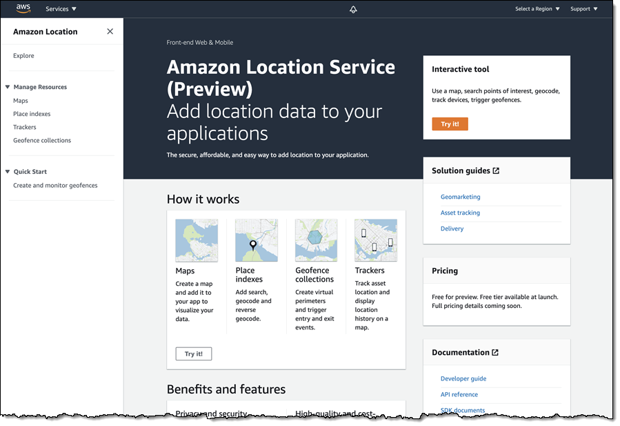
We want to make it easier and more cost-effective for you to add maps, location awareness, and other location-based features to your web and mobile applications. Until now, doing this has been somewhat complex and expensive, and also tied you to the business and programming models of a single provider.

Introducing Amazon Location Service
Today we are making Amazon Location available in preview form and you can start using it today. Priced at a fraction of common alternatives, Amazon Location Service gives you access to maps and location-based services from multiple providers on an economical, pay-as-you-go basis.

You can use Amazon Location Service to build applications that know where they are and respond accordingly. You can display maps, validate addresses, perform geocoding (turn an address into a location), track the movement of packages and devices, and much more. You can easily set up geofences and receive notifications when tracked items enter or leave a geofenced area. You can even overlay your own data on the map while retaining full control.

You can access Amazon Location Service from the AWS Management Console, AWS Command Line Interface (CLI), or via a set of APIs. You can also use existing map libraries such as Mapbox GL and Tangram.

All About Amazon Location
Let’s take a look at the types of resources that Amazon Location Service makes available to you, and then talk about how you can use them in your applications.

MapsAmazon Location Service lets you create maps that make use of data from our partners. You can choose between maps and map styles provided by Esri and by HERE Technologies, with the potential for more maps & more styles from these and other partners in the future. After you create a map, you can retrieve a tile (at one of up to 16 zoom levels) using the GetMapTile function. You won’t do this directly, but will use Mapbox GL, Tangram, or another library instead.

Place Indexes – You can choose between indexes provided by Esri and HERE. The indexes support the SearchPlaceIndexForPosition function which returns places, such as residential addresses or points of interest (often known as POI) that are closest to the position that you supply, while also performing reverse geocoding to turn the position (a pair of coordinates) into a legible address. Indexes also support the SearchPlaceIndexForText function, which searches for addresses, businesses, and points of interest using free-form text such as an address, a name, a city, or a region.

Trackers –Trackers receive location updates from one or more devices via the BatchUpdateDevicePosition function, and can be queried for the current position (GetDevicePosition) or location history (GetDevicePositionHistory) of a device. Trackers can also be linked to Geofence Collections to implement monitoring of devices as they move in and out of geofences.

Geofence Collections – Each collection contains a list of geofences that define geographic boundaries. Here’s a geofence (created with geojson.io) that outlines a park near me:

Amazon Location in Action
I can use the AWS Management Console to get started with Amazon Location and then move on to the AWS Command Line Interface (CLI) or the APIs if necessary. I open the Amazon Location Service Console, and I can either click Try it! to create a set of starter resources, or I can open up the navigation on the left and create them one-by-one. I’ll go for one-by-one, and click Maps:

Then I click Create map to proceed:

I enter a Name and a Description:

Then I choose the desired map and click Create map:

The map is created and ready to be added to my application right away:

Now I am ready to embed the map in my application, and I have several options including the Amplify JavaScript SDK, the Amplify Android SDK, the Amplify iOS SDK, Tangram, and Mapbox GL (read the Developer Guide to learn more about each option).

Next, I want to track the position of devices so that I can be notified when they enter or exit a given region. I use a GeoJSON editing tool such as geojson.io to create a geofence that is built from polygons, and save (download) the resulting file:

I click Create geofence collection in the left-side navigation, and in Step 1, I add my GeoJSON file, enter a Name and Description, and click Next:

Now I enter a Name and a Description for my tracker, and click Next. It will be linked to the geofence collection that I just created:

The next step is to arrange for the tracker to send events to Amazon EventBridge so that I can monitor them in CloudWatch Logs. I leave the settings as-is, and click Next to proceed:

I review all of my choices, and click Finalize to move ahead:

The resources are created, set up, and ready to go:

I can then write code or use the CLI to update the positions of my devices:

$ aws location batch-update-device-position \
   --tracker-name MyTracker1 \
   --updates "DeviceId=Jeff1,Position=-122.33805,47.62748,SampleTime=2020-11-05T02:59:07+0000"

After I do this a time or two, I can retrieve the position history for the device:

$ aws location get-device-position-history \
  -tracker-name MyTracker1 --device-id Jeff1
------------------------------------------------
|           GetDevicePositionHistory           |
+----------------------------------------------+
||               DevicePositions              ||
|+---------------+----------------------------+|
||  DeviceId     |  Jeff1                     ||
||  ReceivedTime |  2020-11-05T02:59:17.246Z  ||
||  SampleTime   |  2020-11-05T02:59:07Z      ||
|+---------------+----------------------------+|
|||                 Position                 |||
||+------------------------------------------+||
|||  -122.33805                              |||
|||  47.62748                                |||
||+------------------------------------------+||
||               DevicePositions              ||
|+---------------+----------------------------+|
||  DeviceId     |  Jeff1                     ||
||  ReceivedTime |  2020-11-05T03:02:08.002Z  ||
||  SampleTime   |  2020-11-05T03:01:29Z      ||
|+---------------+----------------------------+|
|||                 Position                 |||
||+------------------------------------------+||
|||  -122.43805                              |||
|||  47.52748                                |||
||+------------------------------------------+||

I can write Amazon EventBridge rules that watch for the events, and use them to perform any desired processing. Events are published when a device enters or leaves a geofenced area, and look like this:

{
  "version": "0",
  "id": "7cb6afa8-cbf0-e1d9-e585-fd5169025ee0",
  "detail-type": "Location Geofence Event",
  "source": "aws.geo",
  "account": "123456789012",
  "time": "2020-11-05T02:59:17.246Z",
  "region": "us-east-1",
  "resources": [
    "arn:aws:geo:us-east-1:123456789012:geofence-collection/MyGeoFences1",
    "arn:aws:geo:us-east-1:123456789012:tracker/MyTracker1"
  ],
  "detail": {
        "EventType": "ENTER",
        "GeofenceId": "LakeUnionPark",
        "DeviceId": "Jeff1",
        "SampleTime": "2020-11-05T02:59:07Z",
        "Position": [-122.33805, 47.52748]
  }
}

Finally, I can create and use place indexes so that I can work with geographical objects. I’ll use the CLI for a change of pace. I create the index:

$ aws location create-place-index \
  --index-name MyIndex1 --data-source Here

Then I query it to find the addresses and points of interest near the location:

$ aws location search-place-index-for-position --index-name MyIndex1 \
  --position "[-122.33805,47.62748]" --output json \
  |  jq .Results[].Place.Label
"Terry Ave N, Seattle, WA 98109, United States"
"900 Westlake Ave N, Seattle, WA 98109-3523, United States"
"851 Terry Ave N, Seattle, WA 98109-4348, United States"
"860 Terry Ave N, Seattle, WA 98109-4330, United States"
"Seattle Fireboat Duwamish, 860 Terry Ave N, Seattle, WA 98109-4330, United States"
"824 Terry Ave N, Seattle, WA 98109-4330, United States"
"9th Ave N, Seattle, WA 98109, United States"
...

I can also do a text-based search:

$ aws location search-place-index-for-text --index-name MyIndex1 \
  --text Coffee --bias-position "[-122.33805,47.62748]" \
  --output json | jq .Results[].Place.Label
"Mohai Cafe, 860 Terry Ave N, Seattle, WA 98109, United States"
"Starbucks, 1200 Westlake Ave N, Seattle, WA 98109, United States"
"Metropolitan Deli and Cafe, 903 Dexter Ave N, Seattle, WA 98109, United States"
"Top Pot Doughnuts, 590 Terry Ave N, Seattle, WA 98109, United States"
"Caffe Umbria, 1201 Westlake Ave N, Seattle, WA 98109, United States"
"Starbucks, 515 Westlake Ave N, Seattle, WA 98109, United States"
"Cafe 815 Mercer, 815 9th Ave N, Seattle, WA 98109, United States"
"Victrola Coffee Roasters, 500 Boren Ave N, Seattle, WA 98109, United States"
"Specialty's, 520 Terry Ave N, Seattle, WA 98109, United States"
...

Both of the searches have other options; read the Geocoding, Reverse Geocoding, and Search to learn more.

Things to Know
Amazon Location is launching today as a preview, and you can get started with it right away. During the preview we plan to add an API for routing, and will also do our best to respond to customer feedback and feature requests as they arrive.

Pricing is based on usage, with an initial evaluation period that lasts for three months and lets you make numerous calls to the Amazon Location APIs at no charge. After the evaluation period you pay the prices listed on the Amazon Location Pricing page.

Amazon Location is available in the US East (N. Virginia), US East (Ohio), US West (Oregon), Europe (Ireland), and Asia Pacific (Tokyo) Regions.

Jeff;


New –  FreeRTOS Long Term Support to Provide Years of Feature Stability

Post Syndicated from Channy Yun original https://aws.amazon.com/blogs/aws/new-freertos-long-term-support-to-provide-years-of-feature-stability/

Today, I’m particularly happy to announce FreeRTOS Long Term Support (LTS). FreeRTOS is an open source, real-time operating system for microcontrollers that makes small, low-power edge devices easy to program, deploy, secure, connect, and manage. LTS releases offer a more stable foundation than standard releases as manufacturers deploy and later update devices in the field. As we have planned, LTS is now included in the FreeRTOS kernel and a set of FreeRTOS libraries needed for embedded and IoT applications, and for securely connecting microcontroller-based (MCU) devices to the cloud.

Embedded developers at original equipment manufacturers (OEMs) and MCU vendors using FreeRTOS to build long-lived applications on IoT devices now get the predictability and feature stability of an LTS release without compromising access to critical security updates. The FreeRTOS 202012.00 LTS release applies to the FreeRTOS kernel, connectivity libraries (FreeRTOS+TCP, coreMQTT, coreHTTP), security library (PKCS #11 implementation), and AWS library (AWS IoT Device Shadow).

We will provide security updates and critical bug fixes for all these libraries until December 31, 2022.

Benefits of FreeRTOS LTS
Embedded developers at OEMs who want to use FreeRTOS libraries for their long-lived applications want to benefit from security updates and bug fixes in the latest FreeRTOS mainline releases. Mainline releases can introduce both new features and critical fixes, which may increase time and effort for users to include only fixes.

An LTS release provides years of feature stability of included libraries. With an LTS release, any update will not change public APIs, file structure, or build processes that could require changes to your application. Security updates and critical bug fixes will be backported at least until Dec 31, 2022. LTS releases contain updates that only address critical issues including security vulnerabilities. Therefore, the integration of LTS releases is less disruptive to customers’ development and integration efforts as they approach and move into production. For MCU vendors, this means reduced effort in integrating a stable code base and faster time to market with vendors’ latest libraries.

Available Now
The FreeRTOS 202012.00 LTS release is available now to download. To learn more, visit FreeRTOS LTS and the documentation. Please send us feedback on the Github repository and the forum of FreeRTOS.

Channy

Announcing AWS IoT Greengrass 2.0 – With an Open Source Edge Runtime and New Developer Capabilities

Post Syndicated from Channy Yun original https://aws.amazon.com/blogs/aws/announcing-aws-iot-greengrass-2-0-with-an-open-source-edge-runtime-and-new-developer-capabilities/

I am happy to announce AWS IoT Greengrass 2.0, a new version of AWS IoT Greengrass that makes it easy for device builders to build, deploy, and manage intelligent device software. AWS IoT Greengrass 2.0 provides an open source edge runtime, a rich set of pre-built software components, tools for local software development, and new features for managing software on large fleets of devices.


AWS IoT Greengrass 2.0 edge runtime is now open source under an Apache 2.0 license, and available on Github. Access to the source code allows you to more easily integrate your applications, troubleshoot problems, and build more reliable and performant applications that use AWS IoT Greengrass.

You can add or remove pre-built software components based on your IoT use case and your device’s CPU and memory resources. For example, you can choose to include pre-built AWS IoT Greengrass components such as stream manager only when you need to process data streams with your application, or machine learning components only when you want to perform machine learning inference locally on your devices.

The AWS IoT Greengrass IoT Greengrass 2.0 includes a new command-line interface (CLI) that allows you to locally develop and debug applications on your device. In addition, there is a new local debug console that helps you visually debug applications on your device. With these new capabilities, you can rapidly develop and debug code on a test device before using the cloud to deploy to your production devices.

AWS IoT Greengrass 2.0 is also integrated with AWS IoT thing groups, enabling you to easily organize your devices in groups and manage application deployments across your devices with features to control rollout rates, timeouts, and rollbacks.

AWS IoT Greengrass 2.0 – Getting Started
Device builders can use AWS IoT Greengrass 2.0 by going to the AWS IoT Greengrass console where you can find a download and install command that you run on your device. Once the installer is downloaded to the device, you can use it to install Greengrass software with all essential features, register the device as an AWS IoT Thing, and create a simple “hello world” software component in less than 10 minutes.

To get started in the AWS IoT Greengrass console, you first register a test device by clicking Set up core device. You assign the name and group of your core device. To deploy to only the core device, select No group. In the next step, install the AWS IoT Greengrass Core software in your device.

When the installer completes, you can find your device in the list of AWS IoT Greengrass Core devices on the Core devices page.

AWS IoT Greengrass components enable you to develop and deploy software to your AWS IoT Greengrass Core devices. You can write your application functionality and bundle it as a private component for deployment. AWS IoT Greengrass also provides public components, which provide pre-built software for common use cases that you can deploy to your devices as you develop your device software. When you finish developing the software for your component, you can register it with AWS IoT Greengrass. Then, you can deploy and run the component on your AWS IoT Greengrass Core devices.


To create a component, click the Create component button on the Components page. You can use a recipe or import an AWS Lambda function. The component recipe is a YAML or JSON file that defines the component’s details, dependencies, compatibility, and lifecycle. To learn about the specifications, visit the recipe reference guide.

Here is an example of a YAML recipe.

When you finish developing your component, you can add it to a deployment configuration to deploy to one or more core devices. To create a new deployment or configure the components to deploy to core devices, click the Create button on the Deployments page. You can deploy to a core device or a thing group as a target, and select the components to deploy. The deployment includes the dependencies for each component that you select.


You can edit the version and parameters of selected components and advanced settings such as the rollout configuration, which defines the rate at which the configuration deploys to the target devices; timeout configuration, which defines the duration that each device has to apply the deployment; or cancel configuration, which defines when to automatically stop the deployment.

Moving to AWS IoT Greengrass 2.0
Existing devices running AWS IoT Greengrass 1.x will continue to run without any changes. If you want to take advantage of new AWS IoT Greengrass 2.0 features, you will need to move your existing AWS IoT Greengrass 1.x devices and workloads to AWS IoT Greengrass 2.0. To learn how to do this, visit the migration guide.

After you move your 1.x applications over, you can start adding components to your applications using new version 2 features, while leaving your version 1 code as-is until you decide to update them.

AWS IoT Greengrass 2.0 Partners
At launch, industry-leading partners NVIDIA and NXP have qualified a number of their devices for AWS IoT Greengrass 2.0:

See all partner device listings in the AWS Partner Device Catalog. To learn about getting your device qualified, visit the AWS Device Qualification Program.

Available Now
AWS IoT Greengrass 2.0 is available today. Please see the AWS Region table for all the regions where AWS IoT Greengrass is available. For more information, see the developer guide.

Starting today, to help you evaluate, test, and develop with this new release of AWS IoT Greengrass, the first 1,000 devices in your account will not incur any AWS IoT Greengrass charges until December 31, 2021. For pricing information, check out the AWS IoT Greengrass pricing page.

Give it a try, and please send us feedback through your usual AWS Support contacts or the AWS forum for AWS IoT Greengrass.

Learn all the details about AWS IoT Greengrass 2.0 and get started with the new version today.

Channy

New – AWS IoT Core for LoRaWAN to Connect, Manage, and Secure LoRaWAN Devices at Scale

Post Syndicated from Channy Yun original https://aws.amazon.com/blogs/aws/new-aws-iot-core-for-lorawan-to-connect-manage-and-secure-lorawan-devices-at-scale/

Today, I am happy to announce AWS IoT Core for LoRaWAN, a new fully-managed feature that allows AWS IoT Core customers to connect and manage wireless devices that use low-power long-range wide area network (LoRaWAN) connectivity with the AWS Cloud.

Using AWS IoT Core for LoRaWAN, customers can now set up a private LoRaWAN network by connecting their own LoRaWAN devices and gateways to the AWS Cloud – without developing or operating a LoRaWAN Network Server (LNS) by themselves. The LNS is required to manage LoRaWAN devices and gateways’ connection to the cloud; gateways serve as a bridge and carry device data to and from the LNS, usually over Wi-Fi or Ethernet.

This allows customers to eliminate the undifferentiated work and operational burden of managing an LNS, and enables them to easily and quickly connect and secure LoRaWAN device fleets at scale.

Combined with the long range and deep in-building coverage provided by LoRa technology, AWS IoT Core now enables customers to accelerate IoT application development using AWS services and acting on the data generated easily from connected LoRaWAN devices.

Customers – mostly enterprises – need to develop IoT applications using devices that transmit data over long range (1-3 miles of urban coverage or up to 10 miles for line-of-sight) or through the walls and floors of buildings, for example for real-time asset tracking at airports, remote temperature monitoring in buildings, or predictive maintenance of industrial equipment. Such applications also require devices to be optimized for low-power consumption, so that batteries can last several years without replacement, thus making the implementation cost-effective. Given the extended coverage of LoRaWAN connectivity, it is attractive to enterprises for these use cases, but setting up LoRaWAN connectivity in a privately managed site requires customers to operate an LNS.

With AWS IoT Core for LoRaWAN, you can connect LoRaWAN devices and gateways to the cloud with a few simple steps in the AWS IoT Management Console, thus speeding up the network setup time, and connect off-the-shelf LoRaWAN devices, without any requirement to modify embedded software, for a plug and play experience.

AWS IoT Core for LoRaWAN – Getting Started
Getting started with a LoRaWAN network setup is easy. You can find AWS IoT Core for LoRaWAN qualified gateways and developer kits from the AWS Partner Device Catalog. AWS qualified gateways and developer kits are pre-tested and come with a step by step guide from the manufacturer on how to connect it with AWS IoT Core for LoRaWAN.

With AWS IoT Core console, you can register the gateways by providing a gateway’s unique identifier (provided by the gateway vendor) and selecting LoRa frequency band. For registering devices, you can input device credentials (identifiers and security keys provided by the device vendor) on the console.

Each device has a Device Profile that specifies the device capabilities and boot parameters the LNS requires to set up LoRaWAN radio access service. Using the console, you can select a pre-populated Device Profile or create a new one.

A destination automatically routes messages from LoRaWAN devices to AWS IoT Rules Engine. Once a destination is created, you can use it to map multiple LoRaWAN devices to the same IoT rule. You can write rules using simple SQL queries, to transform and act on the device data, like converting data from proprietary binary to JSON format, raising alerts, or routing it to other AWS services like Amazon Simple Storage Service (S3). From the console, you can also query metrics for connected devices and gateways to troubleshoot connectivity issues.

Available Now
AWS IoT Core for LoRaWAN is available today in US East (N. Virginia) and Europe (Ireland) Regions. With pay-as-you-go pricing and no monthly commitments, you can connect and scale LoRaWAN device fleets reliably, and build applications with AWS services quickly and efficiently. For more information, see the pricing page.

To get started, buy an AWS qualified LoRaWAN developer kit and and launch Getting Started experience in the AWS Management Console. To learn more, visit the developer guide. Give this a try, and please send us feedback either through your usual AWS Support contacts or the AWS forum for AWS IoT.

Learn all the details about AWS IoT Core for LoRaWAN and get started with the new feature today.

Channy

Join the Preview – Amazon Managed Service for Prometheus (AMP)

Post Syndicated from Jeff Barr original https://aws.amazon.com/blogs/aws/join-the-preview-amazon-managed-service-for-prometheus-amp/

Observability is an essential aspect of running cloud infrastructure at scale. You need to know that your resources are healthy and performing as expected, and that your system is delivering the desired level of performance to your customers.

A lot of challenges arise when monitoring container-based applications. First, because container resources are transient and there are lots of metrics to watch, the monitoring data has strikingly high cardinality. In plain language this means that there are lots of unique values, which can make it harder to define a space-efficient storage model and to create queries that return meaningful results. Second, because a well-architected container-based system is composed using a large number of moving parts, ingesting, processing, and storing the monitoring data can become an infrastructure challenge of its own.

Prometheus is a leading open-source monitoring solution with an active developer and user community. It has a multi-dimensional data model that is a great fit for time series data collected from containers.

Introducing Amazon Managed Service for Prometheus (AMP)
Today we are launching a preview of Amazon Managed Service for Prometheus (AMP). This fully-managed service is 100% compatible with Prometheus. It supports the same metrics, the same PromQL queries, and can also make use of the 150+ Prometheus exporters. AMP runs across multiple Availability Zones for high availability, and is powered by CNCF Cortex for horizontal scalability. AMP will easily scale to ingest, store, and query millions of time series metrics.

The preview includes support for Amazon Elastic Kubernetes Service (EKS) and Amazon Elastic Container Service (ECS). It can also be used to monitor your self-managed Kubernetes clusters that are running in the cloud or on-premises.

Getting Started with Amazon Managed Service for Prometheus (AMP)
After joining the preview, I open the AMP Console, enter a name for my AMP workspace, and click Create to get started (API and CLI support is also available):

My workspace is active within a minute or so. The console provides me with the endpoints that I can use to write data to my workspace, and to issue queries:

It also provides guidance on how to configure an existing Prometheus server to send metrics to the AMP workspace:

I can also use AWS Distro for OpenTelemetry to scrape Prometheus metrics and send them to my AMP workspace.

Once I have stored some metrics in my workspace, I can run PromQL queries and I can use Grafana to create dashboards and other visualizations. Here’s a sample Grafana dashboard:

Join the Preview
As noted earlier, we’re launching Amazon Managed Service for Prometheus (AMP) in preview form and you are welcome to try it out today.

We’ll have more info (and a more detailed blog post) at launch time.

Jeff;

New – AWS Systems Manager Consolidates Application Management

Post Syndicated from Steve Roberts original https://aws.amazon.com/blogs/aws/new-aws-systems-manager-consolidates-application-management/

A desire for consolidated, and simplified operational oversight isn’t limited to just cloud infrastructure. Increasingly, customers ask us for a “single pane of glass” approach for also monitoring and managing their application portfolios.

These customers tell us that detection and investigation of application issues takes additional time and effort, due to the typical use of multiple consoles, tools, and sources of information such as resource usage metrics, logs, and more, to enable their DevOps engineers to obtain context about the application issue under investigation. Here, an “application” means not just the application code but also the logical group of resources that act as a unit to host the application, along with ownership boundaries for operators, and environments such as development, staging, and production.

Today, I’m pleased to announce a new feature of AWS Systems Manager, called Application Manager. Application Manager aggregates operational information from multiple AWS services and Systems Manager capabilities into a single console, making it easier to view operational data for your applications.

To make it even more convenient, the service can automatically discover your applications. Today, auto-discovery is available for applications running in AWS CloudFormation stacks and Amazon Elastic Kubernetes Service (EKS) clusters, or launched using AWS Launch Wizard. Applications can also be discovered from Resource Groups.

A particular benefit of automated discovery is that application components and resources are automatically kept up-to-date on an ongoing basis, but you can also always revise applications as needed by adding or deleting components manually.

With applications discovered and consolidated into a single console, you can more easily diagnose operational issues and resolve them with minimal time and effort. Automated runbooks targeting an application component or resource can be run to help remediate operational issues. For any given application, you can select a resource and explore relevant details without needing to leave the console.

For example, the application can surface Amazon CloudWatch logs, operational metrics, AWS CloudTrail logs, and configuration changes, removing the need to engage with multiple tools or consoles. This means your on-call engineers can understand issues more quickly and reduce the time needed to resolve them.

Exploring an Application with Application Manager
I can access Application Manager from the Systems Manager home page. Once open, I get an overview of my discovered applications and can see immediately that there are some alarms, without needing to switch context to the Amazon CloudWatch console, and some operations items (“OpsItems”) that I might need to pay attention to. I can also switch to the Applications tab to view the collections of applications, or I can click the buttons in the Applications panel for the collection I’m interested in.

Screenshot of the <span title="">Application Manager</span> overview page

In the screenshot below, I’ve navigated to a sample application and again, have indicators showing that alarms have raised. The various tabs enable me to drill into more detail to view resources used by the application, config resource and rules compliance, monitoring alarms, logs, and automation runbooks associated with the application.

Screenshot of application components and overview

Clicking on the Alarm indicator takes me into the Monitoring tab, and it shows that the ConsumedWriteCapacityUnits alarm has been raised. I can change the timescale to zero in on when the event occurred, or I can use the View recent alarms dashboard link to jump into the Amazon CloudWatch Alarms console to view more detail.

Screenshot of alarms on the <span title="">Application Manager</span> Monitoring tab

The Logs tab shows me a consolidated list of log groups for the application, and clicking a log group name takes me directly to the CloudWatch Logs where I can inspect the log streams, and take advantage of Log Insights to dive deeper by querying the log data.

OpsItems shows me operational issues associated with the resources of my application, and enables me to indicate the current status of the issue (open, in progress, resolved). Below, I am marking investigation of a stopped EC2 instance as in progress.

Screenshot of <span title="">Application Manager</span> OpsItems tab

Finally, Runbooks shows me automation documents associated with the application and their execution status. Below, it’s showing that I ran the AWS-RestartEC2Instance automation document to restart the EC2 instance that was stopped, and I would now resolve the issue logged in the OpsItems tab.

Screenshot of <span title="">Application Manager</span>'s Runbooks tab

Consolidating this information into a single console gives engineers a single starting location to monitor and investigate issues arising with their applications, and automatic discovery of applications and resources makes getting started simple. AWS Systems Manager Application Manager is available today, at no extra charge, in all public AWS Regions where Systems Manager is available.

Learn more about Application Manager and get started at AWS Systems Manager.

— Steve

New – AWS Systems Manager Fleet Manager

Post Syndicated from Steve Roberts original https://aws.amazon.com/blogs/aws/new-aws-systems-manager-fleet-manager/

Organizations, and their systems administrators, routinely face challenges in managing increasingly diverse portfolios of IT infrastructure across cloud and on-premises environments. Different tools, consoles, services, operating systems, procedures, and vendors all contribute to complicate relatively common, and related, management tasks. As workloads are modernized to adopt Linux and open-source software, those same systems administrators, who may be more familiar with GUI-based management tools from a Windows background, have to continually adapt and quickly learn new tools, approaches, and skill sets.

AWS Systems Manager is an operational hub enabling you to manage resources on AWS and on-premises. Available today, Fleet Manager is a new console based experience in Systems Manager that enables systems administrators to view and administer their fleets of managed instances from a single location, in an operating-system-agnostic manner, without needing to resort to remote connections with SSH or RDP. As described in the documentation, managed instances includes those running Windows, Linux, and macOS operating systems, in both the AWS Cloud and on-premises. Fleet Manager gives you an aggregated view of your compute instances regardless of where they exist.

All that’s needed, whether for cloud or on-premises servers, is the Systems Manager agent installed on each server to be managed, some AWS Identity and Access Management (IAM) permissions, and AWS Key Management Service (KMS) enabled for Systems Manager‘s Session Manager. This makes it an easy and cost-effective approach for remote management of servers running in multiple environments without needing to pay the licensing cost of expensive management tools you may be using today. As noted earlier, it also works with instances running macOS. With the agent software and permissions set up, Fleet Manager enables you to explore and manage your servers from a single console environment. For example, you can navigate file systems, work with the registry on Windows servers, manage users, and troubleshoot logs (including viewing Windows event logs) and monitor common performance counters without needing the Amazon CloudWatch agent to be installed.

Exploring an Instance With Fleet Manager
To get started exploring my instances using Fleet Manager, I first head to the Systems Manager console. There, I select the new Fleet Manager entry on the navigation toolbar. I can also select the Managed Instances option – Fleet Manager replaces Managed Instances going forward, but the original navigation toolbar entry will be kept for backwards compatibility for a short while. But, before we go on to explore my instances, I need to take you on a brief detour.

When you select Fleet Manager, as with some other views in Systems Manager, a check is performed to verify that a role, named AmazonSSMRoleForInstancesQuickSetup, exists in your account. If you’ve used other components of Systems Manager in the past, it’s quite possible that it does. The role is used to permit Systems Manager to access your instances on your behalf and if the role exists, then you’re directed to the requested view. If however the role doesn’t exist, you’ll first be taken to the Quick Setup view. This in itself will trigger creation of the role, but you might want to explore the capabilities of Quick Setup, which you can also access any time from the navigation toolbar.

Quick Setup is a feature of Systems Manager that you can use to set up specific configuration items, such as the Systems Manager and CloudWatch agents on your instances (and keep them up-to-date), and also IAM roles permitting access to your resources for Systems Manager components. For this post, all the instances I’m going to use already have the required agent set up, including the role permissions, so I’m not going to discuss this view further but I encourage you to check it out. I also want to remind you that to take full advantage of Fleet Manager‘s capabilities you first need to have KMS encryption enabled for your instances and secondly, the role attached to your Amazon Elastic Compute Cloud (EC2) instances must have the kms:Decrypt role permission included, referencing the key you selected when you enabled KMS encryption. You can enable encryption, and select the KMS key, using the Preferences section of the Session Manager console, and of course you can set up the role permission in the IAM console.

That’s it for the diversion; if you have the role already, as I do, you’ll now be at the Managed instances list view. If you’re at Quick Setup instead, simply click the Fleet Manager navigation button once more.

The Managed instances view shows me all of my instances, in the cloud or on-premises, that I can access. Selecting an instance, in this case an EC2 Windows instance launched using AWS Elastic Beanstalk, and clicking Instance actions presents me with a menu of options. The options (less those specific to Windows) are available for my Amazon Linux instance too, and for instances running macOS I can use the View file system option.

Screenshot of <span title="">Fleet Manager</span>'s Managed instances view

The File system view displays a read-only view onto the file system of the selected instance. This can be particularly useful for viewing text-based log files, for example, where I can preview up to 10,000 lines of a log file and even tail it to view changes as the log updates. I used this to open and tail an IIS web server log on my Windows Server instance. Having selected the instance, I next select View file system from the Instance actions dropdown (or I can click the Instance ID to open a view onto that instance and select File system from the menu displayed on the instance view).

Having opened the file system view for my instance, I navigate to the folder on the instance containing the IIS web server logs.

Screenshot of <span title="">Fleet Manager</span>'s File system view

Selecting a log file, I then click Actions and select Tail file. This opens a view onto the log file contents, which updates automatically as new content is written.

Screenshot of tailing a log file in <span title="">Fleet Manager</span>

As I mentioned, the File system view is also accessible for macOS-based instances. For example, here is a screenshot of viewing the Applications folder on an EC2 macOS instance.

Screenshot of macOS file system view in <span title="">Fleet Manager</span>

Next, let’s examine the Performance counters view, which is available for both Windows and Linux instances. This view displays CPU, memory, network traffic, and disk I/O and will be familiar to Windows users from Task Manager. The metrics shown reflect the guest OS metrics, whereas EC2 instance metrics you may be used to relate to the hypervisor. On this particular instance I’ve deployed an ASP.NET Core 5 application, which generates a varying length collection of Fibonacci numbers on page refresh. Below is a snapshot of the counters, after I’ve put the instance under a small amount of load. The view updates automatically every 5 seconds.

Screenshot of <span title="">Fleet Manager</span>'s Performance Counters view

There are more views available than I have space for in this post. Using the Windows Registry view, I can view and edit the registry on the selected Windows instance. Windows event logs gives me access to the Application and Service logs, and common Windows logs such as System, Setup, Security, etc. With Users and groups I can manage users or groups, including assignment of users to groups (again for both Windows and Linux instances). For all views, Fleet Manager enables me to use a single and convenient console.

Getting Started
AWS Systems Manager Fleet Manager is available today for use with managed instances running Windows, Linux, and macOS. Information on pricing, for this and other Systems Manager features, can be found at this page.

Learn more, and get started with Fleet Manager today, at AWS Systems Manager.

— Steve

Introducing AWS Systems Manager Change Manager

Post Syndicated from Sébastien Stormacq original https://aws.amazon.com/blogs/aws/introducing-systems-manager-change-manager/

Because you are constantly listening to the feedback from your customer, you are iterating, innovating, and improving your applications and infrastructures. You continually modify your IT systems in the cloud. And let’s face it, changing something in a working system risks breaking things or introducing side effects that are sometimes unpredictable; it doesn’t matter how many tests you do. On the other hand, not making changes is stasis, followed by irrelevance, followed by death.

This is why organizations of all sizes and types have embraced a culture of controlling changes. Some organizations adopt change management processes such as the ones defined in ITIL v4. Some have adopted DevOps’ Continuous Deployment, or other methods. In any case, to support your change management processes, it is important to have tools.

Today, we are launching AWS Systems Manager Change Manager, a new change management capability for AWS Systems Manager. It simplifies the way ops engineers track, approve, and implement operational changes to their application configurations and infrastructures.

Using Change Manager has two primary advantages. First, it can improve the safety of changes made to application configurations and infrastructures, reducing the risk of service disruptions. It makes operational changes safer by tracking that only approved changes are being implemented. Secondly, it is tightly integrated with other AWS services, such as AWS Organizations and AWS Single Sign-On, or the integration with the Systems Manager change calendar and Amazon CloudWatch alarms.

Change Manager provides accountability with a consistent way to report and audit changes made across your organization, their intent, and who approved and implemented them.

Change Manager works across AWS Regions and multiple AWS accounts. It works closely with Organizations and AWS SSO to manage changes from a central point and to deploy them in a controlled way across your global infrastructure.

Terminology
You can use AWS Systems Manager Change Manager on a single AWS account, but most of the time, you will use it in a multi-account configuration.

The way you manage changes across multiple AWS accounts depends on how these accounts are linked together. Change Manager uses the relationships between your accounts defined in AWS Organizations. When using Change Manager, there are three types of accounts:

  • The management account – also known as the “main account” or “root account.” The management account is the root account in an AWS Organizations hierarchy. It is the management account by virtue of this fact.
  • The delegated administrator account – A delegated administrator account is an account that has been granted permission to manage other accounts in Organizations. In the Change Manager context, this is the account from which change requests will be initiated. You will typically log in to this account to manage templates and change requests. Using a delegated administrators account allows you to limit connections made to the root account. It also allows you to enforce a least privileges policy by using a specific subset of permissions required by the changes.
  • The member accounts – Member accounts are accounts that are not the management account or a delegated administrator account, but are still included in Organizations. In my mental model for Change Manager, these would be the accounts that hold the resources where changes are deployed. A delegated administrator account would initiate a change request that would impact resources in a member account. System administrators are discouraged from logging directly into these accounts.

Let’s see how you can use AWS Systems Manager Change Manager by taking a short walk-through demo.

One-Time Configuration
In this scenario, I show you how to use Change Manager with multiple AWS accounts linked together with Organizations. If you are not interested in the one-time configuration, jump to the Create a Change Request section below.

There are four one-time configuration actions to take before using Change Manager: one action in the root account and three in the delegated administrator account. In the root account, I use Quick Setup to define my delegated administrator account and initially configure permissions on the accounts. In the delegated administrator account, you define your source of user identities, you define what users have permissions to approve change templates, and you define a change request template.

First, I ensure I have an Organization in place and my AWS accounts are organized in Organizational Units (OU). For the purpose of this simple example, I have three accounts: the root account, the delegated administrator account in the management OU and a member account in the managed OU. When ready, I use Quick Setup on the root account to configure my accounts. There are multiple paths leading to Quick Setup; for this demo, I use the blue banner on top of the Quick Setup console, and I click Setup Change Manager.

Change Manager Quick Setup


On the Quick Setup page, I enter the ID of the delegated administrator account if I haven’t defined it already. Then I choose the permissions boundaries I grant to the delegated administrator account to perform changes on my behalf. This is the maximum permissions Change Manager receives to make changes. I will further restrict this permission set when I create change requests in a few minutes. In this example, I grant Change Manager permissions to call any ec2 API. This effectively authorizes Change Manager to only run changes related to EC2 instances.

Change Manager Quick Setup

Lower on the screen, I choose the set of accounts that are targets for my changes. I choose between Entire organization or Custom to select one or multiple OUs.

Change Manager Quick Setup 2

After a while, Quick Setup finishes configuring my AWS accounts permission and I can move to the second part of the one-time setup.

Change Manager Quick Setup 3

Second, I switch to my delegated administrator account. Change Manager asks me how I manage users in my organization: with AWS Identity and Access Management (IAM) or AWS Single Sign-On? This defines where Change Manager pulls user identities when I choose approvers. This is a one-time configuration option. This can be changed at any time in the Change Manager Settings page.

Change Manager Settings

Third, on the same page, I define an Amazon Simple Notification Service (SNS) topic to receive notifications about template reviews. This channel is notified any time a template is created or modified, to let template approvers review and approve templates. I also define the IAM (or SSO) user with permission to approve change templates (more about these in one minute).

Change Manager Template Reviewers

Optionally, you can use the existing AWS Systems Manager Change Calendar to define the periods where changes are not authorized, such as marketing events or holiday sales.

Finally, I define a change template. Every change request is created from a template. Templates define common parameters for all change requests based on them, such as the change request approvers, the actions to perform, or the SNS topic to send notifications of progress. You can enforce the review and approval of templates before they can be used. It makes sense to create multiple templates to handle different type of changes. For example, you can create one template for standard changes, and one for emergency changes that overrides the change calendar. Or you can create different templates for different types of automation run books (documents).

To help you to get started, we created a template for you: the “Hello World” template. You can use it as a starting point to create a change request and test out your approval flow.

At any time, I can create my own template. Let’s imagine my system administrator team is frequently restarting EC2 instances. I create a template allowing them to create change requests to restart one or multiple instances. Using the delegated administrator account, I navigate to the Change Manager management console and click Create template.

Change Manager Create Template

In a nutshell, a template defines the list of authorized actions, where to send notifications and who can approve the change request. Actions are an AWS Systems Manager runbook. Emergency change templates allow change requests to bypass the change calendar I wrote about earlier. Under Runbook Options, I choose one or multiple runbooks allowed to run. For this example, I choose the AWS EC2RestartInstance runbook.

I use the console to create the template, but templates are defined internally as YAML. I can edit the YAML using the Editor tab, or when I am using the AWS Command Line Interface (CLI) or API. This means I can version control them just like the rest of my infrastructure (as code).Change Manager Create Template part 1

Just below, I document my template using text formatted as markdown format. I use this section to document the defining characteristics of the template and provide any necessary instructions, such as back-out procedures, to the requestor.

Change Manager Template Documentation

I scroll down that page and click Add Approver to define approvers. Approvers can be individual users or groups. The list of approvers are defined either at the template level or in the change request itself. I also choose to create an SNS topic to inform approvers when any requests are created that require their approval.

In the Monitoring section I select the alarm that, when active, stops any change based on this template, and initiate a rollback.

In the Notifications section, I select or create another SNS topic so I’m notified when status changes for this template occur.

Change Manager Create Template part 2

Once I am done, I save the template and submit it for review.

Change Manager Submit Template for Review

Templates have to be reviewed and approved before they can be used. To approve the template, I connect the console as the template_approver user I defined earlier. As template_approver user, I see pending approvals on the Overview tab. Or, I navigate to the Templates tab, select the template I want to review. When I am done reviewing it, I click Approve.

Change Manager Approve Template

Voila, now we’re ready to create change requests based on this template. Remember that all the preceding steps are one-time configurations and can be amended at any time. When existing templates are modified, the changes go through a review and approval process again.

Create a Change Request
To create a change request on any account linked to the Organization, I open a AWS Systems Manager Change Manager console from the delegated administrator account and click Create request.

Change Manager Create Request

I choose the template I want to use and click Next.

Change Manager Select Template I enter a name for this change request. The change is initiated immediately after all approvals are granted, or I specify an optional scheduled time. When the template allows me, I choose the approver for this change. In this example, the approver is defined by the template and cannot be changed. I click Next.

Change Manager Create CR part 1

On the next screen, there are multiple important configuration options, relating to the actual execution of the change:

  • Target location – lets me define on which target AWS accounts and AWS Region I want to run this change.
  • Deployment target – lets me define which resources are the target of this change. One EC2 instance? Or multiple ones identified by their tags, their resources groups, a list of instance IDs, or all EC2 instances.
  • Runbook parameters – lets me define the parameters I want to pass to my runbook, if any.
  • Execution role – lets me define the set of permissions I grant the System Manager to deploy with this change. The permission set must have service changemanagement.ssm.amazonaws.com as principal for the trust policy. Selecting a role allows me to grant the Change Manager runtime a different permission set than the one I have.

Here is an example allowing Change Manager to stop an EC2 instance (you can scope it down to a specific AWS account, specific Region, or specific instances):

{
    "Version": "2012-10-17",
    "Statement": [
        {
            "Effect": "Allow",
            "Action": [
                "ec2:StartInstances",
                "ec2:StopInstances"
            ],
            "Resource": "*",
        },
        {
            "Effect": "Allow",
            "Action": "ec2:DescribeInstances",
            "Resource": "*"
        }
    ]
}

And the associated trust policy:

{
  "Version": "2012-10-17",
  "Statement": [
    {
      "Effect": "Allow",
      "Principal": {
        "Service": "changemanagement.ssm.aws.internal"
      },
      "Action": "sts:AssumeRole"
    }
  ]
}

When I am ready, I click Next. On the last page, I review my data entry and click Submit for approval.

At this stage, the approver receives a notification, based on the SNS topic configured in the template. To continue this demo, I sign out of the console and sign in again as the cr_approver user, which I created, with permission to view and approve change requests.

As the cr_approver user, I navigate to the console, review the change request, and click Approve.

Change Manager Review Change Request

The change request status switches to scheduled, and eventually turns green to Success. At any time, I can click the change request to get the status, and to collect errors, if any.

Change Manager Dashboard with Succeeded Request

I click on the change request to see the details. In particular, the Timeline tab shows the history of this CR.

Change Management CR Timeline

Availability and Pricing
AWS Systems Manager Change Manager is available today in all commercial AWS Regions, except mainland China. The pricing is based on two dimensions: the number of change requests you submit and the total number of API calls made. The number of change requests you submit will be the main cost factor. We will charge $0.29 per change request. Check the pricing page for more details.

You can evaluate Change Manager for free for 30 days, starting on your first change request.

As usual, let us know what you think and let’s get started today

— seb