Part 2: Rethinking cache purge with a new architecture

Post Syndicated from Zaidoon Abd Al Hadi original http://blog.cloudflare.com/rethinking-cache-purge-architecture/

Part 2: Rethinking cache purge with a new architecture

Part 2: Rethinking cache purge with a new architecture

In Part 1: Rethinking Cache Purge, Fast and Scalable Global Cache Invalidation, we outlined the importance of cache invalidation and the difficulties of purging caches, how our existing purge system was designed and performed, and we gave a high level overview of what we wanted our new Cache Purge system to look like.

It’s been a while since we published the first blog post and it’s time for an update on what we’ve been working on. In this post we’ll be talking about some of the architecture improvements we’ve made so far and what we’re working on now.

Cache Purge end to end

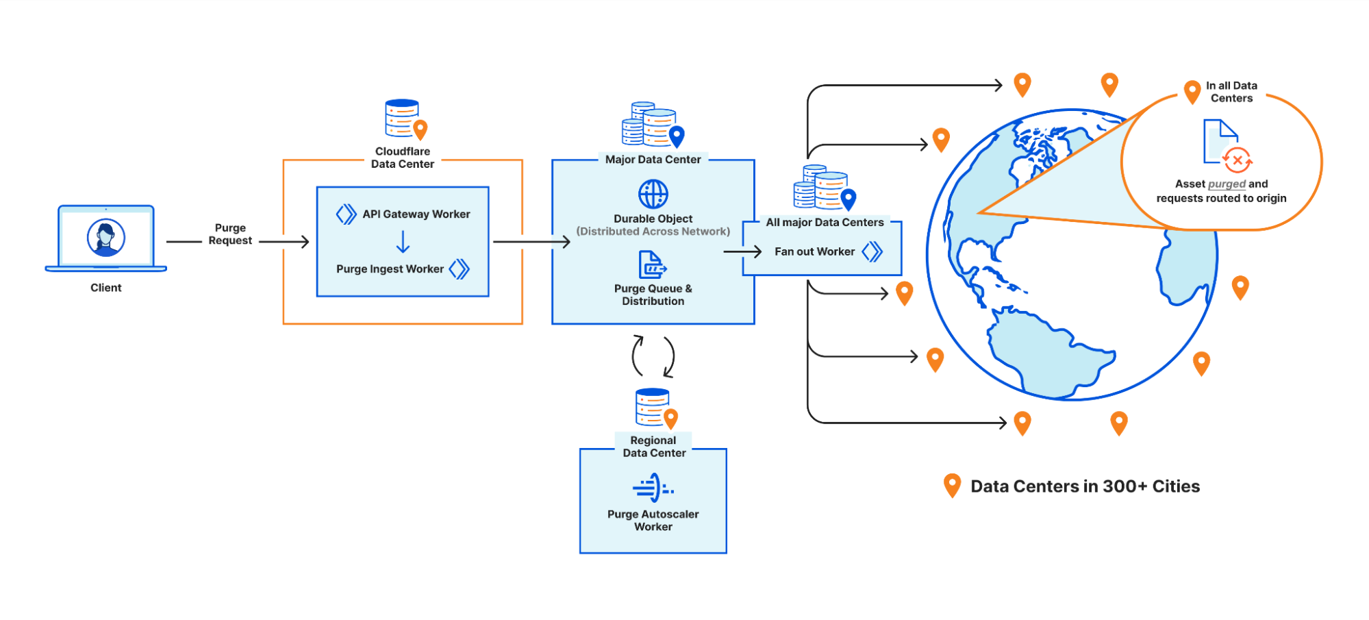
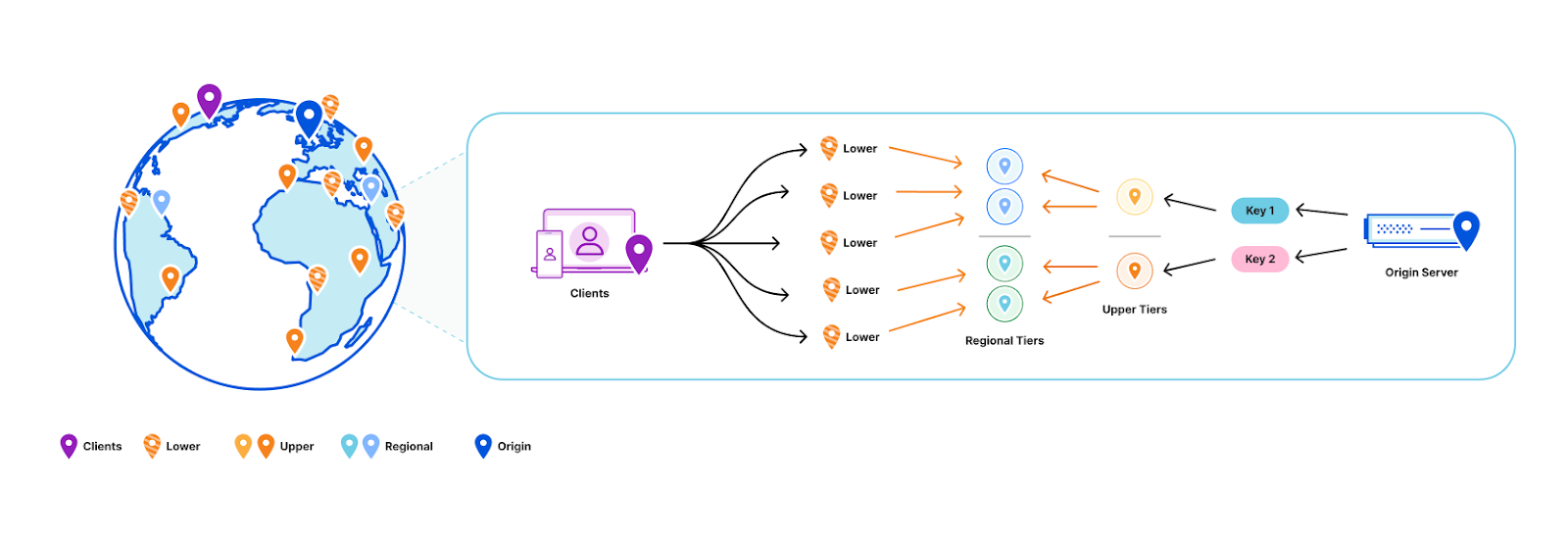
We touched on the high level design of what we called the “coreless” purge system in part 1, but let’s dive deeper into what that design encompasses by following a purge request from end to end:

Part 2: Rethinking cache purge with a new architecture

Step 1: Request received locally

An API request to Cloudflare is routed to the nearest Cloudflare data center and passed to an API Gateway worker. This worker looks at the request URL to see which service it should be sent to and forwards the request to the appropriate upstream backend. Most endpoints of the Cloudflare API are currently handled by centralized services, so the API Gateway worker is often just proxying requests to the nearest “core” data center which have their own gateway services to handle authentication, authorization, and further routing. But for endpoints which aren’t handled centrally the API Gateway worker must handle authentication and route authorization, and then proxy to an appropriate upstream. For cache purge requests that upstream is a Purge Ingest worker in the same data center.

Step 2: Purges tested locally

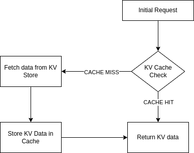
The Purge Ingest worker evaluates the purge request to make sure it is processible. It scans the URLs in the body of the request to see if they’re valid, then attempts to purge the URLs from the local data center’s cache. This concept of local purging was a new step introduced with the coreless purge system allowing us to capitalize on existing logic already used in every data center.

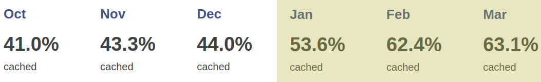
By leveraging the same ownership checks our data centers use to serve a zone’s normal traffic on the URLs being purged, we can determine if those URLs are even cacheable by the zone. Currently more than 50% of the URLs we’re asked to purge can’t be cached by the requesting zones, either because they don’t own the URLs (e.g. a customer asking us to purge https://cloudflare.com) or because the zone’s settings for the URL prevent caching (e.g. the zone has a “bypass” cache rule that matches the URL). All such purges are superfluous and shouldn’t be processed further, so we filter them out and avoid broadcasting them to other data centers freeing up resources to process more legitimate purges.

On top of that, generating the cache key for a file isn’t free; we need to load zone configuration options that might affect the cache key, apply various transformations, et cetera. The cache key for a given file is the same in every data center though, so when we purge the file locally we now return the generated cache key to the Purge Ingest worker and broadcast that key to other data centers instead of making each data center generate it themselves.

Step 3: Purges queued for broadcasting

Part 2: Rethinking cache purge with a new architecture

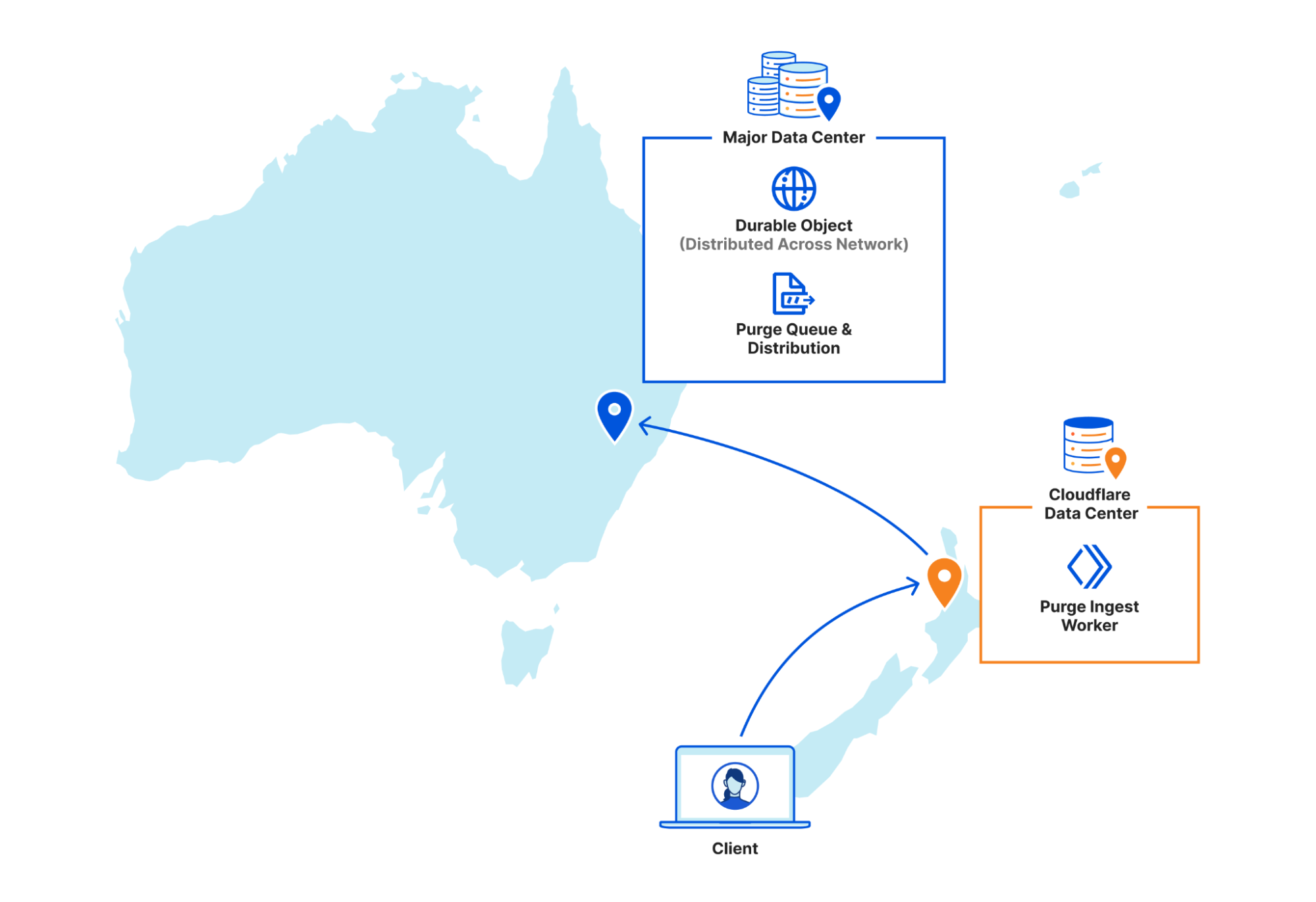
Once the local purge is done the Purge Ingest worker forwards the purge request with the cache key obtained from the local cache to a Purge Queue worker. The queue worker is a Durable Object worker using its persistent state to hold a queue of purges it receives and pointers to how far along in the queue each data center in our network is in processing purges.

The queue is important because it allows us to automatically recover from a number of scenarios such as connectivity issues or data centers coming back online after maintenance. Having a record of all purges since an issue arose lets us replay those purges to a data center and “catch up”.

But Durable Objects are globally unique, so having one manage all global purges would have just moved our centrality problem from a core data center to wherever that Durable Object was provisioned. Instead we have dozens of Durable Objects in each region, and the Purge Ingest worker looks at the load balancing pool of Durable Objects for its region and picks one (often in the same data center) to forward the request to. The Durable Object will write the purge request to its queue and immediately loop through all the data center pointers and attempt to push any outstanding purges to each.

While benchmarking our performance we found our particular workload exhibited a “goldilocks zone” of throughput to a given Durable Object. On script startup we have to load all sorts of data like network topology and data center health–then refresh it continuously in the background–and as long as the Durable Object sees steady traffic it stays active and we amortize those startup costs. But if you ask a single Durable Object to do too much at once like send or receive too many requests, the single-threaded runtime won’t keep up. Regional purge traffic fluctuates a lot depending on local time of day, so there wasn’t a static quantity of Durable Objects per region that would let us stay within the goldilocks zone of enough requests to each to keep them active but not too many to keep them efficient. So we built load monitoring into our Durable Objects, and a Regional Autoscaler worker to aggregate that data and adjust load balancing pools when we start approaching the upper or lower edges of our efficiency goldilocks zone.

Step 4: Purges broadcast globally

Part 2: Rethinking cache purge with a new architecture

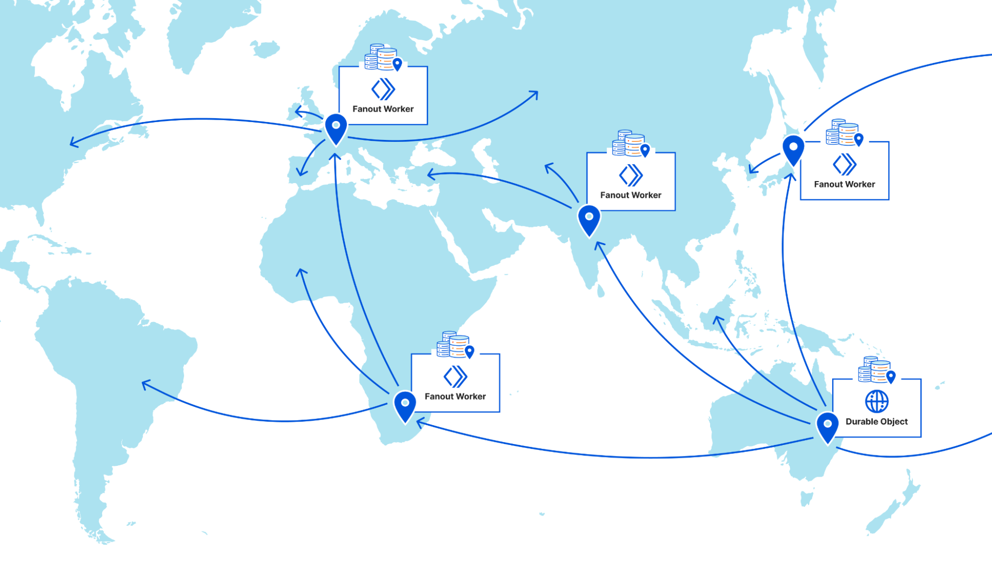
Once a purge request is queued by a Purge Queue worker it needs to be broadcast to the rest of Cloudflare’s data centers to be carried out by their caches. The Durable Objects will broadcast purges directly to all data centers in their region, but when broadcasting to other regions they pick a Purge Fanout worker per region to take care of their region’s distribution. The fanout workers manage queues of their own as well as pointers for all of their region’s data centers, and in fact they share a lot of the same logic as the Purge Queue workers in order to do so. One key difference is fanout workers aren’t Durable Objects; they’re normal worker scripts, and their queues are purely in memory as opposed to being backed by Durable Object state. This means not all queue worker Durable Objects are talking to the same fanout worker in each region. Fanout workers can be dropped and spun up again quickly by any metal in the data center because they aren’t canonical sources of state. They maintain queues and pointers for their region but all of that info is also sent back downstream to the Durable Objects who persist that data themselves, reliably.

But what does the fanout worker get us? Cloudflare has hundreds of data centers all over the world, and as we mentioned above we benefit from keeping the number of incoming and outgoing requests for a Durable Object fairly low. Sending purges to a fanout worker per region means each Durable Object only has to make a fraction of the requests it would if it were broadcasting to every data center directly, which means it can process purges faster.

On top of that, occasionally a request will fail to get where it was going and require retransmission. When this happens between data centers in the same region it’s largely unnoticeable, but when a Durable Object in Canada has to retry a request to a data center in rural South Africa the cost of traversing that whole distance again is steep. The data centers elected to host fanout workers have the most reliable connections in their regions to the rest of our network. This minimizes the chance of inter-regional retries and limits the latency imposed by retries to regional timescales.

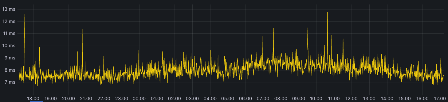
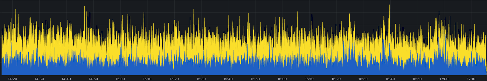
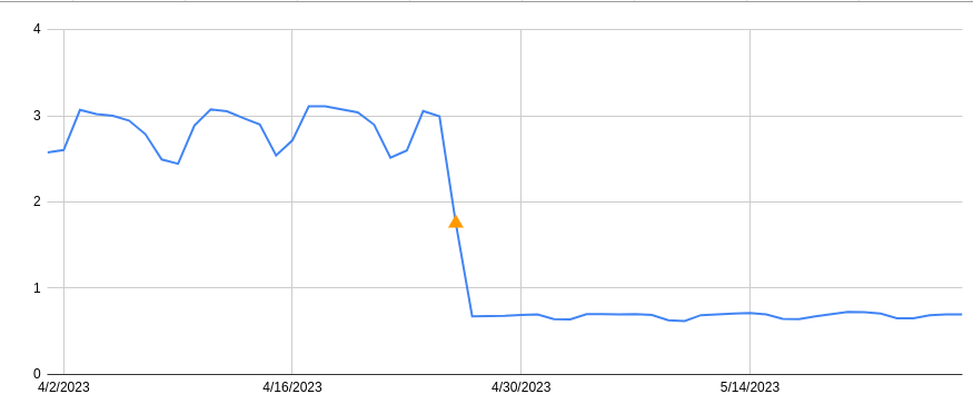
The introduction of the Purge Fanout worker was a massive improvement to our distribution system, reducing our end-to-end purge latency by 50% on its own and increasing our throughput threefold.

Current status of coreless purge

We are proud to say our new purge system has been in production serving purge by URL requests since July 2022, and the results in terms of latency improvements are dramatic. In addition, flexible purge requests (purge by tag/prefix/host and purge everything) share and benefit from the new coreless purge system’s entrypoint workers before heading to a core data center for fulfillment.

The reason flexible purge isn’t also fully coreless yet is because it’s a more complex task than “purge this object”; flexible purge requests can end up purging multiple objects–or even entire zones–from cache. They do this through an entirely different process that isn’t coreless compatible, so to make flexible purge fully coreless we would have needed to come up with an entirely new multi-purge mechanism on top of redesigning distribution. We chose instead to start with just purge by URL so we could focus purely on the most impactful improvements, revamping distribution, without reworking the logic a data center uses to actually remove an object from cache.

This is not to say that the flexible purges haven’t benefited from the coreless purge project. Our cache purge API lets users bundle single file and flexible purges in one request, so the API Gateway worker and Purge Ingest worker handle authorization, authentication and payload validation for flexible purges too. Those flexible purges get forwarded directly to our services in core data centers pre-authorized and validated which reduces load on those core data center auth services. As an added benefit, because authorization and validity checks all happen at the edge for all purge types users get much faster feedback when their requests are malformed.

Next steps

While coreless cache purge has come a long way since the part 1 blog post, we’re not done. We continue to work on reducing end-to-end latency even more for purge by URL because we can do better. Alongside improvements to our new distribution system, we’ve also been working on the redesign of flexible purge to make it fully coreless, and we’re really excited to share the results we’re seeing soon. Flexible cache purge is an incredibly popular API and we’re giving its refresh the care and attention it deserves.

Spotlight on Zero Trust: We’re fastest and here’s the proof

Post Syndicated from David Tuber original http://blog.cloudflare.com/spotlight-on-zero-trust/

Spotlight on Zero Trust: We're fastest and here's the proof

Spotlight on Zero Trust: We're fastest and here's the proof

In January and in March we posted blogs outlining how Cloudflare performed against others in Zero Trust. The conclusion in both cases was that Cloudflare was faster than Zscaler and Netskope in a variety of Zero Trust scenarios. For Speed Week, we’re bringing back these tests and upping the ante: we’re testing more providers against more public Internet endpoints in more regions than we have in the past.

For these tests, we tested three Zero Trust scenarios: Secure Web Gateway (SWG), Zero Trust Network Access (ZTNA), and Remote Browser Isolation (RBI). We tested against three competitors: Zscaler, Netskope, and Palo Alto Networks. We tested these scenarios from 12 regions around the world, up from the four we’d previously tested with. The results are that Cloudflare is the fastest Secure Web Gateway in 42% of testing scenarios, the most of any provider. Cloudflare is 46% faster than Zscaler, 56% faster than Netskope, and 10% faster than Palo Alto for ZTNA, and 64% faster than Zscaler for RBI scenarios.

In this blog, we’ll provide a refresher on why performance matters, do a deep dive on how we’re faster for each scenario, and we’ll talk about how we measured performance for each product.

Performance is a threat vector

Performance in Zero Trust matters; when Zero Trust performs poorly, users disable it, opening organizations to risk. Zero Trust services should be unobtrusive when the services become noticeable they prevent users from getting their job done.

Zero Trust services may have lots of bells and whistles that help protect customers, but none of that matters if employees can’t use the services to do their job quickly and efficiently. Fast performance helps drive adoption and makes security feel transparent to the end users. At Cloudflare, we prioritize making our products fast and frictionless, and the results speak for themselves. So now let’s turn it over to the results, starting with our secure web gateway.

Cloudflare Gateway: security at the Internet

A secure web gateway needs to be fast because it acts as a funnel for all of an organization’s Internet-bound traffic. If a secure web gateway is slow, then any traffic from users out to the Internet will be slow. If traffic out to the Internet is slow, users may see web pages load slowly, video calls experience jitter or loss, or generally unable to do their jobs. Users may decide to turn off the gateway, putting the organization at risk of attack.

In addition to being close to users, a performant web gateway needs to also be well-peered with the rest of the Internet to avoid slow paths out to websites users want to access. Many websites use CDNs to accelerate their content and provide a better experience. These CDNs are often well-peered and embedded in last mile networks. But traffic through a secure web gateway follows a forward proxy path: users connect to the proxy, and the proxy connects to the websites users are trying to access. If that proxy isn’t as well-peered as the destination websites are, the user traffic could travel farther to get to the proxy than it would have needed to if it was just going to the website itself, creating a hairpin, as seen in the diagram below:

Spotlight on Zero Trust: We're fastest and here's the proof

A well-connected proxy ensures that the user traffic travels less distance making it as fast as possible.

To compare secure web gateway products, we pitted the Cloudflare Gateway and WARP client against Zscaler, Netskope, and Palo Alto which all have products that perform the same functions. Cloudflare users benefit from Gateway and Cloudflare’s network being embedded deep into last mile networks close to users, being peered with over 12,000 networks. That heightened connectivity shows because Cloudflare Gateway is the fastest network in 42% of tested scenarios:

Spotlight on Zero Trust: We're fastest and here's the proof

Number of testing scenarios where each provider is fastest for 95th percentile HTTP Response time (higher is better)
Provider Scenarios where this provider is fastest
Cloudflare 48
Zscaler 14
Netskope 10
Palo Alto Networks 42

This data shows that we are faster to more websites from more places than any of our competitors. To measure this, we look at the 95th percentile HTTP response time: how long it takes for a user to go through the proxy, have the proxy make a request to a website on the Internet, and finally return the response. This measurement is important because it’s an accurate representation of what users see. When we look at the 95th percentile across all tests, we see that Cloudflare is 2.5% faster than Palo Alto Networks, 13% faster than Zscaler, and 6.5% faster than Netskope.

95th percentile HTTP response across all tests
Provider 95th percentile response (ms)
Cloudflare 515
Zscaler 595
Netskope 550
Palo Alto Networks 529

Cloudflare wins out here because Cloudflare’s exceptional peering allows us to succeed in places where others were not able to succeed. We are able to get locally peered in hard-to-reach places on the globe, giving us an edge. For example, take a look at how Cloudflare performs against the others in Australia, where we are 30% faster than the next fastest provider:

Spotlight on Zero Trust: We're fastest and here's the proof

Cloudflare establishes great peering relationships in countries around the world: in Australia we are locally peered with all of the major Australian Internet providers, and as such we are able to provide a fast experience to many users around the world. Globally, we are peered with over 12,000 networks, getting as close to end users as we can to shorten the time requests spend on the public Internet. This work has previously allowed us to deliver content quickly to users, but in a Zero Trust world, it shortens the path users take to get to their SWG, meaning they can quickly get to the services they need.

Previously when we performed these tests, we only tested from a single Azure region to five websites. Existing testing frameworks like Catchpoint are unsuitable for this task because performance testing requires that you run the SWG client on the testing endpoint. We also needed to make sure that all of the tests are running on similar machines in the same places to measure performance as well as possible. This allows us to measure the end-to-end responses coming from the same location where both test environments are running.

In our testing configuration for this round of evaluations, we put four VMs in 12 cloud regions side by side: one running Cloudflare WARP connecting to our gateway, one running ZIA, one running Netskope, and one running Palo Alto Networks. These VMs made requests every five minutes to the 11 different websites mentioned below and logged the HTTP browser timings for how long each request took. Based on this, we are able to get a user-facing view of performance that is meaningful. Here is a full matrix of locations that we tested from, what websites we tested against, and which provider was faster:

Endpoints
SWG Regions Shopify Walmart Zendesk ServiceNow Azure Site Slack Zoom Box M365 GitHub Bitbucket
East US Cloudflare Cloudflare Palo Alto Networks Cloudflare Palo Alto Networks Cloudflare Palo Alto Networks Cloudflare
West US Palo Alto Networks Palo Alto Networks Cloudflare Cloudflare Palo Alto Networks Cloudflare Palo Alto Networks Cloudflare
South Central US Cloudflare Cloudflare Palo Alto Networks Cloudflare Palo Alto Networks Cloudflare Palo Alto Networks Cloudflare
Brazil South Cloudflare Palo Alto Networks Palo Alto Networks Palo Alto Networks Zscaler Zscaler Zscaler Palo Alto Networks Cloudflare Palo Alto Networks Palo Alto Networks
UK South Cloudflare Palo Alto Networks Palo Alto Networks Palo Alto Networks Palo Alto Networks Palo Alto Networks Palo Alto Networks Cloudflare Palo Alto Networks Palo Alto Networks Palo Alto Networks
Central India Cloudflare Cloudflare Cloudflare Palo Alto Networks Palo Alto Networks Cloudflare Cloudflare Cloudflare
Southeast Asia Cloudflare Cloudflare Cloudflare Cloudflare Palo Alto Networks Cloudflare Cloudflare Cloudflare
Canada Central Cloudflare Cloudflare Palo Alto Networks Cloudflare Cloudflare Palo Alto Networks Palo Alto Networks Palo Alto Networks Zscaler Cloudflare Zscaler
Switzerland North netskope Zscaler Zscaler Cloudflare netskope netskope netskope netskope Cloudflare Cloudflare netskope
Australia East Cloudflare Cloudflare netskope Cloudflare Cloudflare Cloudflare Cloudflare Cloudflare
UAE Dubai Zscaler Zscaler Cloudflare Cloudflare Zscaler netskope Palo Alto Networks Zscaler Zscaler netskope netskope
South Africa North Palo Alto Networks Palo Alto Networks Palo Alto Networks Zscaler Palo Alto Networks Palo Alto Networks Palo Alto Networks Palo Alto Networks Zscaler Palo Alto Networks Palo Alto Networks

Blank cells indicate that tests to that particular website did not report accurate results or experienced failures for over 50% of the testing period. Based on this data, Cloudflare is generally faster, but we’re not as fast as we’d like to be. There are still some areas where we need to improve, specifically in South Africa, UAE, and Brazil. By Birthday Week in September, we want to be the fastest to all of these websites in each of these regions, which will bring our number up from fastest in 54% of tests to fastest in 79% of tests.

To summarize, Cloudflare’s Gateway is still the fastest SWG on the Internet. But Zero Trust isn’t all about SWG. Let’s talk about how Cloudflare performs in Zero Trust Network Access scenarios.

Instant (Zero Trust) access

Access control needs to be seamless and transparent to the user: the best compliment for a Zero Trust solution is for employees to barely notice it’s there. Services like Cloudflare Access protect applications over the public Internet, allowing for role-based authentication access instead of relying on things like a VPN to restrict and secure applications. This form of access management is more secure, but with a performant ZTNA service, it can even be faster.

Cloudflare outperforms our competitors in this space, being 46% faster than Zscaler, 56% faster than Netskope, and 10% faster than Palo Alto Networks:

Spotlight on Zero Trust: We're fastest and here's the proof

Zero Trust Network Access P95 HTTP Response times
Provider P95 HTTP response (ms)
Cloudflare 1252
Zscaler 2388
Netskope 2974
Palo Alto Networks 1471

For this test, we created applications hosted in three different clouds in 12 different locations: AWS, GCP, and Azure. However, it should be noted that Palo Alto Networks was the exception, as we were only able to measure them using applications hosted in one cloud from two regions due to logistical challenges with setting up testing: US East and Singapore.

For each of these applications, we created tests from Catchpoint that accessed the application from 400 locations around the world. Each of these Catchpoint nodes attempted two actions:

  • New Session: log into an application and receive an authentication token
  • Existing Session: refresh the page and log in passing the previously obtained credentials

We like to measure these scenarios separately, because when we look at 95th percentile values, we would almost always be looking at new sessions if we combined new and existing sessions together. For the sake of completeness though, we will also show the 95th percentile latency of both new and existing sessions combined.

Cloudflare was faster in both US East and Singapore, but let’s spotlight a couple of regions to delve into. Let’s take a look at a region where resources are heavily interconnected equally across competitors: US East, specifically Ashburn, Virginia.

In Ashburn, Virginia, Cloudflare handily beats Zscaler and Netskope for ZTNA 95th percentile HTTP Response:

95th percentile HTTP Response times (ms) for applications hosted in Ashburn, VA
AWS East US Total (ms) New Sessions (ms) Existing Sessions (ms)
Cloudflare 2849 1749 1353
Zscaler 5340 2953 2491
Netskope 6513 3748 2897
Palo Alto Networks
Azure East US
Cloudflare 1692 989 1169
Zscaler 5403 2951 2412
Netskope 6601 3805 2964
Palo Alto Networks
GCP East US
Cloudflare 2811 1615 1320
Zscaler
Netskope 6694 3819 3023
Palo Alto Networks 2258 894 1464

You might notice that Palo Alto Networks looks to come out ahead of Cloudflare for existing sessions (and therefore for overall 95th percentile). But these numbers are misleading because Palo Alto Networks’ ZTNA behavior is slightly different than ours, Zscaler’s, or Netskope’s. When they perform a new session, it does a full connection intercept and returns a response from its processors instead of directing users to the login page of the application they are trying to access.

This means that Palo Alto Networks' new session response times don’t actually measure the end-to-end latency we’re looking for. Because of this, their numbers for new session latency and total session latency are misleading, meaning we can only meaningfully compare ourselves to them for existing session latency. When we look at existing sessions, when Palo Alto Networks acts as a pass-through, Cloudflare still comes out ahead by 10%.

This is true in Singapore as well, where Cloudflare is 50% faster than Zscaler and Netskope, and also 10% faster than Palo Alto Networks for Existing Sessions:

95th percentile HTTP Response times (ms) for applications hosted in Singapore
AWS Singapore Total (ms) New Sessions (ms) Existing Sessions (ms)
Cloudflare 2748 1568 1310
Zscaler 5349 3033 2500
Netskope 6402 3598 2990
Palo Alto Networks
Azure Singapore
Cloudflare 1831 1022 1181
Zscaler 5699 3037 2577
Netskope 6722 3834 3040
Palo Alto Networks
GCP Singapore
Cloudflare 2820 1641 1355
Zscaler 5499 3037 2412
Netskope 6525 3713 2992
Palo Alto Networks 2293 922 1476

One critique of this data could be that we’re aggregating the times of all Catchpoint nodes together at P95, and we’re not looking at the 95th percentile of Catchpoint nodes in the same region as the application. We looked at that, too, and Cloudflare’s ZTNA performance is still better. Looking at only North America-based Catchpoint nodes, Cloudflare performs 50% better than Netskope, 40% better than Zscaler, and 10% better than Palo Alto Networks at P95 for warm connections:

Spotlight on Zero Trust: We're fastest and here's the proof

Zero Trust Network Access 95th percentile HTTP Response times for warm connections with testing locations in North America
Provider P95 HTTP response (ms)
Cloudflare 810
Zscaler 1290
Netskope 1351
Palo Alto Networks 871

Finally, one thing we wanted to show about our ZTNA performance was how well Cloudflare performed per cloud per region. This below chart shows the matrix of cloud providers and tested regions:

Fastest ZTNA provider in each cloud provider and region by 95th percentile HTTP Response
AWS Azure GCP
Australia East Cloudflare Cloudflare Cloudflare
Brazil South Cloudflare Cloudflare N/A
Canada Central Cloudflare Cloudflare Cloudflare
Central India Cloudflare Cloudflare Cloudflare
East US Cloudflare Cloudflare Cloudflare
South Africa North Cloudflare Cloudflare N/A
South Central US N/A Cloudflare Zscaler
Southeast Asia Cloudflare Cloudflare Cloudflare
Switzerland North N/A N/A Cloudflare
UAE Dubai Cloudflare Cloudflare Cloudflare
UK South Cloudflare Cloudflare netskope
West US Cloudflare Cloudflare N/A

There were some VMs in some clouds that malfunctioned and didn’t report accurate data. But out of 30 available cloud regions where we had accurate data, Cloudflare was the fastest ZT provider in 28 of them, meaning we were faster in 93% of tested cloud regions.

To summarize, Cloudflare also provides the best experience when evaluating Zero Trust Network Access. But what about another piece of the puzzle: Remote Browser Isolation (RBI)?

Remote Browser Isolation: a secure browser hosted in the cloud

Remote browser isolation products have a very strong dependency on the public Internet: if your connection to your browser isolation product isn’t good, then your browser experience will feel weird and slow. Remote browser isolation is extraordinarily dependent on performance to feel smooth and seamless to the users: if everything is fast as it should be, then users shouldn’t even notice that they’re using browser isolation.

For this test, we’re again pitting Cloudflare against Zscaler. While Netskope does have an RBI product, we were unable to test it due to it requiring a SWG client, meaning we would be unable to get full fidelity of testing locations like we would when testing Cloudflare and Zscaler. Our tests showed that Cloudflare is 64% faster than Zscaler for remote browsing scenarios: Here’s a matrix of fastest provider per cloud per region for our RBI tests:

Fastest RBI provider in each cloud provider and region by 95th percentile HTTP Response
AWS Azure GCP
Australia East Cloudflare Cloudflare Cloudflare
Brazil South Cloudflare Cloudflare Cloudflare
Canada Central Cloudflare Cloudflare Cloudflare
Central India Cloudflare Cloudflare Cloudflare
East US Cloudflare Cloudflare Cloudflare
South Africa North Cloudflare Cloudflare
South Central US Cloudflare Cloudflare
Southeast Asia Cloudflare Cloudflare Cloudflare
Switzerland North Cloudflare Cloudflare Cloudflare
UAE Dubai Cloudflare Cloudflare Cloudflare
UK South Cloudflare Cloudflare Cloudflare
West US Cloudflare Cloudflare Cloudflare

This chart shows the results of all of the tests run against Cloudflare and Zscaler to applications hosted on three different clouds in 12 different locations from the same 400 Catchpoint nodes as the ZTNA tests. In every scenario, Cloudflare was faster. In fact, no test against a Cloudflare-protected endpoint had a 95th percentile HTTP Response of above 2105 ms, while no Zscaler-protected endpoint had a 95th percentile HTTP response of below 5000 ms.

To get this data, we leveraged the same VMs to host applications accessed through RBI services. Each Catchpoint node would attempt to log into the application through RBI, receive authentication credentials, and then try to access the page by passing the credentials. We look at the same new and existing sessions that we do for ZTNA, and Cloudflare is faster in both new sessions and existing session scenarios as well.

Gotta go fast(er)

Our Zero Trust customers want us to be fast not because they want the fastest Internet access, but because they want to know that employee productivity won’t be impacted by switching to Cloudflare. That doesn’t necessarily mean that the most important thing for us is being faster than our competitors, although we are. The most important thing for us is improving our experience so that our users feel comfortable knowing we take their experience seriously. When we put out new numbers for Birthday Week in September and we’re faster than we were before, it won’t mean that we just made the numbers go up: it means that we are constantly evaluating and improving our service to provide the best experience for our customers. We care more that our customers in UAE have an improved experience with Office365 as opposed to beating a competitor in a test. We show these numbers so that we can show you that we take performance seriously, and we’re committed to providing the best experience for you, wherever you are.

It’s never been easier to migrate thanks to Cloudflare’s new Migration Hub

Post Syndicated from Sam Marsh original http://blog.cloudflare.com/turpentine-v2-migration-program/

It's never been easier to migrate thanks to Cloudflare's new Migration Hub

It's never been easier to migrate thanks to Cloudflare's new Migration Hub

We understand the pain points associated with CDN migrations. That's why in late 2021 we introduced Turpentine, a project to  the process of translating the old Varnish Configuration Language (VCL) into Cloudflare Workers with just a push of a button. After nearly two years of testing and user feedback, we’ve tailored the migration processes for different user groups.

Today, we are thrilled to relaunch Turpentine, and introduce Cloudflare's new Migration Hub. The Migration Hub serves as a one-stop-shop for all migration needs, featuring brand-new migration guides that bring transparency and simplicity to the process.

We also know that a large number of customers aren't comfortable doing migrations themselves. Years of built up business logic makes unpacking and translating CDN configurations between different vendors difficult and locks businesses into subpar products and services. To help these customers we have established a Professional Services group to ensure smooth migrations for customers transitioning to Cloudflare’s first-class products. Going forward, we plan to continue to invest resources in Turpentine to ensure that moving to any part of Cloudflare is easy and you have the help you need.

Why choose Cloudflare?

Cloudflare has gained immense popularity among businesses seeking to improve website performance, security, and reliability. The demand for Cloudflare's CDN services has skyrocketed, with an ever-increasing number of companies wanting to use our services to help protect their web properties. It became evident that a more streamlined approach was needed to empower customers to self-guide through the onboarding process if they wanted.

That’s why we’ve shipped guides to help bring transparency to the migration process, compare Cloudflare's Rules or Workers to VCL or XML configurations, and provide mappings of different products between vendors. This resource serves as a repository of information and step-by-step guidance for those seeking to move to Cloudflare. These guides are designed to empower customers to take control of their onboarding journey by providing them with the tools and resources they need to understand how to successfully implement Cloudflare's first-class products without needing to talk to anyone.

As new features and enhancements are introduced to Cloudflare, the landing page will be updated to reflect these changes.

However, undertaking the onboarding process independently can be daunting for some businesses. We understand that every organization is unique, with specific requirements and challenges. To address this concern, Cloudflare has established a dedicated Professional Services team. This team of experts works closely with customers, taking the time to understand their environments, assess their needs, and provide tailored guidance and support throughout the migration process. With the help of the professional services team, businesses can transition to Cloudflare being guided by an experienced team to ensure a timely, smooth and successful migration. Using the Migration Hub, you can get in contact with the Professional Services team to help your migration journey.

Whether you prefer self-guided exploration or expert guidance, the Cloudflare Migration Hub has everything you need to make your migration journey a success.

Self-serve guides

Our commitment to transparency and empowering our customers led us to create comprehensive public-facing guides that provide valuable insights into how CDN products compare and overlap. With these guides, you can gain a clear understanding of the features and capabilities offered by Cloudflare, and how they map between CDN offerings you might be more familiar with.

It's never been easier to migrate thanks to Cloudflare's new Migration Hub
Example of mapping Fastly products to Cloudflare

The migration guides include product maps that show how you can match Cloudflare features to Akamai or Fastly features and how to configure them. Using this information, migration should just be about matching up rules and implementing instead of translating feature names between vendors or fiddling with ChatGPT prompts to correctly (or incorrectly!) translate code from one vendor to the other. There are also numerous examples of how certain configurations have been accomplished with code examples that help customers configure and understand their current configuration and translate them into Cloudflare products, easily. Check them out here.

Not only that, but Cloudflare’s commitment to providing numerous free tools across our network means anyone can sign-up and get access to much of our platform without needing to talk to anyone. We believe in giving you the tools and knowledge you need to navigate the migration and testing process independently, while knowing that our support is just a click away whenever you need it.

Let us do it for you with Professional Services

It's never been easier to migrate thanks to Cloudflare's new Migration Hub

We're also incredibly excited to introduce our dedicated team of migration experts, known as Professional Services, who are here to assist you throughout the entire process. The Professional Service team will work closely with you, offering their expertise and guiding you through each step to ensure a seamless transition onto Cloudflare’s products.

Too often, we meet with customers who have been intimidated by the complexity of their current CDN vendor. They had help setting it up by a third party and have experienced the nervousness of trying to change things without knowing what impacts it could have downstream. This is compounded by different CDNs using different terminology for essentially the same concepts.

Professional Services is here to help guide your onboarding experience and cut through that uncertainty.

From providing in-depth knowledge about the migration process and tooling to addressing any specific challenges you may encounter, our Professional Services team is committed to making your migration experience as smooth and efficient as possible. With Cloudflare's Professional Services, you can confidently embark on your migration journey, knowing that our experts will handle the complexities while empowering you to drive the migration process forward.

Success Stories

By leveraging Cloudflare's migration solutions, numerous businesses have achieved remarkable results, including improved performance, enhanced security, and streamlined pricing. These success stories serve as a testament to the effectiveness and reliability of Cloudflare's migration offerings.

Improve cost and performance by migrating to Cloudflare

A mobile communications leader successfully migrated its public website, after 20 years with Akamai, to Cloudflare for a better digital experience plus >20% cost savings.

The company’s decision to decentralize purchasing of CDN services illuminated the high cost of using Akamai for its public-facing websites.

A short proof-of-concept of Cloudflare Application Performance suite resulted in measurable cost savings and performance improvements. It was also determined the flexibility to integrate additional Cloudflare tools, like Workers for serverless compute offerings, would enable the organization to scale further when ready.

Avoid reliability concerns by migrating to Cloudflare

A UK sporting giant with a devoted international fan community was deeply concerned about their spikey traffic associated with game days. Often these matches saw 10x the normal website traffic. Unfortunately, incumbent vendors weren’t up for the challenge of providing the performance and uptime reliability to their fans during these game day traffic spikes.

After migrating to Cloudflare, the results spoke for themselves. In one 24-hour match day, the site received over 11 million requests. Cloudflare’s cache served over 93% of them with eaze while providing a 100% uptime guarantee.

Get started today

We invite you to visit our Migration Hub and explore our comprehensive offerings.

Migrating from one CDN to another can be a daunting task, but with Cloudflare's Migration Hub and Professional Services, the process becomes more straightforward and hassle-free. We are committed to empowering our customers with the resources, support, and expertise needed to transition smoothly to Cloudflare's advanced solutions.

Workers KV is faster than ever with a new architecture

Post Syndicated from Charles Burnett original http://blog.cloudflare.com/faster-workers-kv-architecture/

Workers KV is faster than ever with a new architecture

Workers KV is faster than ever with a new architecture

We’re excited to announce a significant performance improvement coming to Workers KV, focused on dramatically improving cold read performance and reducing latency, even for long tail access patterns.

Developers using KV have seen great performance on hot reads, but ask why their 95th percentile latency — often on a key (or set of keys) that hadn’t been accessed recently or in that region — was higher than expected. We took this feedback to heart: we’ve been working feverishly on a new caching layer for KV behind the scenes, which enables customers to achieve much more frequent hot reads, reduced worst case latency times, better flexibility and control over cache TTLs, and much faster consistency over our previous iterations, and it’s now live for all KV users.

The best part? Developers using KV don’t need to change anything to benefit from this increased performance.

What is Workers KV?

Workers KV is a key value store designed for read heavy use-cases and applications powered by Cloudflare’s network. KV’s focus on read-heavy use-cases allows it to serve hot (cached) reads in milliseconds, which makes it ideal for storing per-application or customer configuration data, routing configuration, multivariate (A/B testing) configurations, and even small asset data that you need to serve quickly.  Anything that you can serialize and need quickly you can store in KV, all the way up to 25 MiB worth of data per each individual key, with no cap on total data stored.

The problem

KV might be optimized for read-heavy workloads, but it’s critical that writes are globally available quickly enough that they’re useful for your application. Under typical conditions, the convergence delay for an eventually consistent system like KV is approximately one minute, globally: a write from one location should be able to be observed by all readers. Typical conditions are great, but typical unfortunately didn’t mean “always”. It could take significant time to restore global consistency where regions like North America and Europe are reading the same value. We needed to improve not just the average convergence, but the worst case as well.

Speaking of consistency, setting a long cache Time to Live (cacheTTL) for reads would result in a situation where you won’t notice a write for the entire cacheTTL duration, as the existing cached data had not timed out yet. This means you have to trade off read latency for infrequently accessed keys against noticing writes. Developers using KV have been consistent in their feedback: a higher cache TTL should improve performance, but not multiply the time it takes for KV to converge on a write to that key.

Lastly, our cold read times also left room for improvement. While cache hits are fast in KV, a cache miss would result in a request being routed all the way to our storage backends. While this is slow for everyone, it was particularly slow for folks in regions not immediately in the US or EU.This is poor performance that doesn’t represent what we can achieve with our global presence.

Our solution

A new horizontally scaled tiered cache

We’ve revamped Workers KV to be powered by a new tiered cache implementation. This implementation is written as a Worker service. We reuse the Dynamic Dispatch infrastructure developed for Workers for Platforms which lets us jump from our old KV worker into our new caching service within hundreds of microseconds. Importantly, this means we don’t impact cache hit performance to implement this new transparent caching layer. We leverage the same infrastructure powering Smart Placement to implement the tiering.

Before we re-designed KV, our topology looked like this:

Workers KV is faster than ever with a new architecture
All data centers in Cloudflare’s network can reach out to the origin in the event of a cache miss or to do a background refresh.

Cache TTL and efficiency

Our design goal was clear and ambitious: “can we relax honoring the cacheTTL constraint without violating it”? While this seems contradictory, the motivation is clear: we want to minimize the need to communicate with our storage backends while honoring the user-facing semantics of the cacheTTL setting, as it can have security implications if violated (e.g. if you use it to store and validate security tokens). Answering this design question also manages to simultaneously solve many of the problems outlined earlier.

Comparing existing solutions

First, let’s look at the design constraints for two eventually consistent storage systems at Cloudflare: Quicksilver and Tiered CDN.

Quicksilver gives us global consistency within seconds using a push architecture to replicate the data across all machines at Cloudflare. That architecture however doesn’t scale for Workers KV’s needs, which can have terabytes of data just within one namespace. This would be too much to replicate to every single data center.

By comparison, the tiered CDN cache is a pull mechanism where each hop pulls a more recent version of the asset into the local cache on access. That scales better because we only use storage for assets that are accessed, which works well with most use-cases where the vast majority of data is never retrieved. However, a pull based architecture is insufficient because it can only let us aggregate traffic across broader regions but we still can’t decouple how long we serve from the cache from the cacheTTL.

Push based architectures let us know when an asset is updated and enable scalable storage. By blending the properties of both systems, we can decouple how long we store the assets in cache from the cacheTTL. And that’s exactly what we did: KV now uses a hybrid push/pull caching layer where data centers closest to customers will pull from the regional data centers that are a little bit farther away. Writes will broadcast to all regional data centers that a key has been updated, so that the regional data center will remove that key from the local cache.

Workers KV is faster than ever with a new architecture
Traditional regional tiered cache topology

We can solve this problem by taking advantage of the fact that we semantically understand the write operations that are happening within Workers KV:

  1. Workers KV doesn’t have one data center per region as might be typical for your zone in a Cloudflare CDN regional tiered cache topology. Instead, each key in a KV namespace is deterministically assigned a data center by performing a weighted rendezvous hash. The rendezvous hash ensures that load is distributed equally across the region and outages result in optimal shifts of traffic.
  2. When the data center closest to a customer has a miss, it computes the regional data center affinity and provides that information to our Smart Placement infrastructure. When a regional tier misses, we repeat this process except using data centers in the KV origin region.
  3. Finally, a miss at the upper tier exits to our storage nodes located in that origin region.

When we do a write, we only purge (invalidate) the key from the regional and upper tier data centers. This is a fixed number of data centers in our network regardless of how many data centers we add, which ensures that we aren’t reducing cache hit rates as our network continues to grow Compared with a global purge that delivers the event to every data center in our network, because we only need to deliver this purge to a random fixed set of data centers in our network, our aggregate write capacity for Workers KV automatically scales horizontally as we add more data centers.

Workers KV is faster than ever with a new architecture
All lower-tier data centers will reach out to a regional tier responsible for a given key in the event of a cache miss. If the regional tier doesn’t have the content, the regional tier will then ask an upper-tier out of region for the content. On a write for a given key, the responsible regional and upper tiers have that key deleted from cache.

Why do we call this a hybrid topology? The data centers closest to customers pull from the regional data centers as normal, but we automatically push invalidation events to the regional tier data centers on every write. That way, those customer data center pulls know to get an updated value when there is one. This means that while the cacheTTL parameter controls the caching behavior closest to the customer, it’s treated as a suggestion at best at the regional and upper tiers.

This way we’ve combined the push design principles behind Quicksilver, which delivers global consistency within seconds, with the pull-based design of our CDN tiered caching which can scale to handle “infinite” size workloads and prioritizes the assets that are most frequently accessed.

Visualizing it

It can be a bit hard to follow what’s happening in the new caching layer since there’s so many moving parts.

Here’s a video of a simplified version of how it works:

Small yellow balls represent KV read requests, larger green balls represent read responses. A larger purple ball represents a KV write request, while a read response ball represents a KV write response. Teal balls represent purge requests being broadcast. The “E” is a data center that doesn’t participate as a regional tier. The R represents the regional tier for key N while O is the upper tier for key N.

Decoupled cache TTL and consistency parameters

As a refresher, the objects written to KV can specify a cacheTTL: by default this is set to 1 minute, which is also the minimum acceptable value. This means that if an asset has been in the cache for longer than a minute, we bypass the cache and read instead from our durable storage nodes. In order to prevent eyeballs noticing origin fetches every minute, we implement stale while revalidate logic in our caching layer that automatically refreshes from the storage nodes in the background as requests come in.

Workers KV is faster than ever with a new architecture
Here’s an example from a Worker that’s constantly reading the same key

Notice the absence of any spikes indicating a cache miss? You’d expect to see them regularly every minute or so in the tens or even hundreds of milliseconds when the cacheTTL should expire. The reason this doesn’t happen is because as the expiry time is approaching, a background request to the storage nodes occurs and the cache is updated with an expiry time one more minute into the future; thus the asset in cache is never too stale and eyeball requests are always served from cache. Let’s take a look at requests to our storage layer before and after adding tiering:

Workers KV is faster than ever with a new architecture
Yellow is the estimated number of requests that would have occurred to origin without the new caching layer. Blue is the number of requests we’re making now.

The above chart is for a system with conservative parameters set. The upper tier doesn’t store the data for much longer than the cacheTTL currently and the upper tier will itself still do a background refresh probabilistically even though it doesn’t actually need to since we see all writes.

The new caching layer we’ve built inherits the old background refresh mechanism and expands on it. The first thing we did is decouple the background refresh period from the cacheTTL as a separate parameter (also defaulting to 1 minute). This means that even if you set a cacheTTL for 1 hour, KV will still check every minute from the regional tier to see if the value has been updated. If the data you’re storing within KV doesn’t have strict requirements on stale reads (think a key that’s accessed once every 10 minutes but needs to honor a write within 1 minute like security tokens), then you can increase the cacheTTL so that infrequently accessed keys stick around in the cache without changing the observed consistency.

Consistency improvements

Speaking of consistency, we’ve improved the worst case performance of that as well. Historically, we’ve had a background system that crawls all data in the storage nodes to figure out which region has the most up to date value and update accordingly. This gives us complete consistency coverage, but could take a significant amount of time to confirm. We would also periodically check both backends to see if network conditions had changed to pick the primary storage region to use for a given customer-close data center. Of course inconsistencies would be resolved then, but in practice this happens randomly, and at a low probability that won’t typically catch any meaningful values served inconsistently.

With the new caching layer all this changes. Since we’re now only reading keys on first access or after a write, we have enough storage capacity that we can check both backends on every read. When a customer requests data, we make a call to each origin data center, with the fastest response being returned immediately to reduce read latency. If the other data center has a newer value than what was returned first, we synchronize both data centers and notify our caching layer to purge that key from all regional data centers. If the other data center instead has an older value, we just synchronize the data centers without purging since we served the latest value. This means that even if our data centers are inconsistent, readers will notice new values much more quickly.

Latency improvements

Here’s the latency improvement at 10% rollout on a logarithmic x-axis:

Workers KV is faster than ever with a new architecture

Architecture that just gets better

This is just the start of what we can do. We now have a solid foundation for making further improvements, including making our best case reads even faster. We’ll be working on cutting out parts of our traditional stack that add unnecessary latency, and adding new high performance features that were too difficult to integrate otherwise. We can also explore features like setting the consistency TTL parameter for sub one minute consistency for additional cost. Similarly, we could create a best effort global purge feature if you want to choose to signal writes that way. Finally, we’re looking at exposing this new caching layer as a general Worker binding anyone can use within a Worker in front of their own service or to put in front of their Worker. If these sound like the killer features you need, please reach out to us if you’re interested in trying them out.

What next?

Developers don’t have to do anything to benefit from KV’s new performance improvements. We are currently in the process of rolling out our new architecture, and you don’t have to redeploy your Worker or change the way you use KV to benefit.

Workers KV is a natural fit for any application built on top of our Workers platform. We provide a native API that enables any Worker script to read, write, list, and manageyour Workers KV storage. You can also interact with Workers KV directly via our REST API from any client that can make a HTTP request, and the Cloudflare Dashboard provides an easy way to create, list, and delete keys to be used with the rest of your Workers setup.

Regardless of how you use Workers KV, it will be faster than ever before. We’re excited to see what you build with us, and you can dive into our documentation to start building with it.

How Kinsta used Workers and Workers KV to improve cache hit rates by 56%

Post Syndicated from Steven Bonisteel (Guest Author) original http://blog.cloudflare.com/how-kinsta-used-workers-and-workers-kv-to-improve-cache-hit-rates/

How Kinsta used Workers and Workers KV to improve cache hit rates by 56%

This is a guest post by Kinsta about their use of our platform.

How Kinsta used Workers and Workers KV to improve cache hit rates by 56%

At Kinsta, we’re obsessed with speed: Our Application Hosting, Database Hosting and Managed WordPress Hosting services all run on the Google Cloud Platform’s fastest Premium Tier Network and C2 Machines, and we rely on Cloudflare to keep the pedal to the metal for tens of thousands of customers who want to deliver their content around the world with speed and security.

While making that happen, we’ve learned a thing or two about using Cloudflare Workers and Workers KV to provide optimized caching rules for static and dynamic content.

In early 2023, we doubled down on Cloudflare cache wrangling, making caches more responsive to client-side configuration changes while also shifting the heavy lifting behind broadcasting feature updates away from our admins on the backend and into Cloudflare Workers. A key result was a dramatic increase in the share of customer data successfully cached, increasing 56.3% between October 2022 and March 2023.

How Kinsta used Workers and Workers KV to improve cache hit rates by 56%

Cloudflare Workers and Workers KV allow us to programmatically customize every request and response with minimal effort and lower latency. We no longer need to deploy changes to hundreds of thousands of containers when we want to implement new features; we can replicate or implement the feature with Workers and deploy it everywhere with a few commands and clicks, saving us days of work and maintenance.

Request routing with Workers KV and Workers

Every Kinsta-hosted domain is a key, and its value contains at least the core settings, like the origin's IP and port, and a unique random ID. With this data easily available in Workers KV, we can use Workers to analyze, manipulate, and route requests to their expected backend. We also use Workers KV to store customer optimization options like Polish, Image Resizing, and Auto Minify.

To route requests to custom IPs and ports, we use resolveOverride, a Cloudflare-specific Request property. Here's an example:

<pre><code class="language-javascript">
// Assign KV values to variables
const { customBackend } = kvdata.kinstaConf;

// Override the backend
cf.resolveOverride = customBackend;
</code></pre>

However, while Workers KV worked well to route requests, we soon noticed inconsistent responses in our cache. Sometimes a customer activated Polish and, due to Workers KV's one-minute cache, new requests arrived before Workers KV fully propagated the change, causing us to cache non-optimized assets. When this happened, the client had to clear their cache again manually. Not the ideal scenario. Clients got frustrated, and we wasted API operations and GCP bandwidth, constantly purging caches.

Cache key is the key

Since we always read the domain's Workers KV data, we realized we could route requests and customize the cache key, appending things like the domain's ID and features that could affect the asset, like Polish. Today, our cache key is heavily customized to quickly reflect every client's change in our panel or API. By modifying the cache key using Workers KV's data, nobody needs to worry about clearing the cache anymore. As soon as Workers KV propagates the changes, the cache key also changes and we request and cache a fresh asset.

The easiest way to customize the cache key is to append query params to it. For example:

<pre><code class="language-javascript">
let cacheKey = `${request.url}?custom-cache-param-polish=lossy`
</code></pre>

Of course, you need to check the URL for existing parameters to determine which connector to use — ? or & — and ensure you are using a unique identifier.

Then, you can use this new cache key to save the response with Cache API or Fetch — or both.

Workers KV Cache

Workers KV operations are affordable, but the numbers can pile up when you trigger billions of reading operations daily.

Thanks to our cache key customization, we realized we could cache the Workers KV data with Cache API, saving on reading operations and possibly lowering the latency by avoiding multiple Workers KV GET requests per visitor. Since the cached response is now based on the request's URL combined with KV data, we no longer need to worry about caching stale content.

How Kinsta used Workers and Workers KV to improve cache hit rates by 56%

However, unlike many applications, we can't cache Workers KV for extended periods. Kinsta's customers are constantly trying new features, changing Polish and Auto Minify settings, sometimes excluding pages or extensions from being cached, and they want to see their changes in production as soon as possible.

That's when we decided to microcache our Workers KV data — caching dynamic or constantly-changed content for a very short period of time, usually less than 60 seconds.

It’s pretty simple to implement your own Workers KV caching logic. For example:

<pre><code class="language-javascript">
const handleKVCache = async (event, myCustomDomain) => {
  // Try to get KV from cache first
  const cache = caches.default;
  let site_data = await cache.match( `https://${myCustomDomain}/some-string-ID-kv-data/` );

  // Valid KV cache match
  if (site_data && site_data.status === 200) {
    // ... modify your cached data if necessary, then return it
    return site_data;
  }

  // Invalid cache (expired, miss, etc), get data from KV namespace
  site_data = await KV_NAMESPACE.get(myCustomDomain.toLowerCase());
  
  // Cache valid KV responses with Cache API
  if (site_data) {
    let kvResponse = new Response(JSON.stringify(site_data), {status: 200});
    kvResponse.headers.set("Cache-Control", "public, s-maxage=30");
    event.waitUntil(cache.put(`https://${myCustomDomain}/some-string-ID-kv-data/`, kvResponse));
  }
  
  return site_data;
};
</code></pre>

(Optionally, you could use FlareUtils' BetterKV.)

At Kinsta, we implemented a 30-second cache TTL for Workers KV data, decreasing read operations by about 80%.

How Kinsta used Workers and Workers KV to improve cache hit rates by 56%
Read operations

Learn more

Want to learn more about Workers and Workers KV? Check out the Cloudflare Workers KV developer documentation, or read our dedicated homepage.

Cyber Asset Attack Surface Management 101

Post Syndicated from Rapid7 original https://blog.rapid7.com/2023/06/21/cyber-asset-attack-surface-management-101/

Understanding CAASM

Cyber Asset Attack Surface Management 101

This article was written by Ethan Smart, Co-Founder and Chief Solution Architect, appNovi (a Rapid7 integration partner).

It’s essential for security and IT teams to have a comprehensive view and control of their cyber assets. This is why Cyber Asset Attack Surface Management (CAASM) has received so much attention from security practitioners and leaders.

According to Gartner, “CAASM tools use API integrations to connect with existing data sources of the organization. These tools then continuously monitor and analyze detected vulnerabilities to drill down the most critical threats to the business and prioritize necessary remediation and mitigation actions for improved cyber security.”

CAASM provides a unified view of all cyber assets to identify exposed assets and potential security gaps through data integration, conversion, and analytics. It is intended to be authoritative source of asset information complete with ownership, network, and business context for IT and security teams.

Security teams integrate CAASM with existing workflows to automate security control gap analysis, prioritization, and remediation processes. These integration outcomes boost efficiency and break down operational silos between teams and their tools. Common key performance indicators of CAASM are asset visibility, endpoint agent coverage, SLAs, and MTTR.

It’s important to understand assets are more than devices and infrastructure. In a Security Operations Center (SOC), assets include users, applications, and application code. Recognizing the interconnectedness of these assets is key to enhancing the SOC’s capabilities. For example, consider a scenario where 1,000 servers have the same vulnerability. Assessing each one individually would be incredibly time-consuming. CAASM enriches cyber asset data to automate the majority of analysis.

For example, when you understand only eight of the 1,000 servers are internet-facing, and of those only two are exposed through the necessary port and protocol for exploitation of the vulnerability, you know which assets have the highest contextual exposure, which are exploitable, and which should be addressed first.

In this blog, we’ll cover how security teams can leverage their existing tech stack for Cyber Asset Attack Surface Management.

Understanding the Attack Surface

Comprehensive attack surface management hinges on a comprehensive understanding of everything that is a target for attackers. In a sprawling enterprise environment, there’s an abundance of assets distributed across different networks (e.g. cloud, SDN, on-prem), each with its own set of monitoring and alerting tools. When these security tools don’t interoperate or mesh with one another, security teams lack a complete picture of the attack surface. This fragmented understanding results in the continued siloing of teams and tools and inhibits effective data sharing.

One of the oldest adages in cybersecurity is complexity is the enemy of security—and complexity increases when teams recognize assets as more than devices. Assets are more than just computers and servers connecting on the network, as those assets are used to support applications to drive revenue. Applications also use code, which can be used by multiple applications. Users are assets that operate the business using technology. This complex asset tracking and relationship mapping spans network connections, application and code ownership, and the dependencies and indirect dependencies between applications.

CAASM emerged to address this complexity. CAASM is founded through the consolidation of existing data from all the different network and security tools. For example, by integrating Rapid7’s portfolio of products with a security data integration and visualization solution like appNovi, organizations can achieve and maintain full visibility across their entire connected network—including on-prem, Software Defined Network (SDN), and hybrid cloud.

Using CAASM, organizations can leverage analytics to refine search results, identify trends, or disseminate specific information to defined groups or individuals. One common use case with appNovi is identifying vulnerable application servers contextually exposed for exploitation and identifying owners based on login telemetry and notifying the server owner and security. This integrated approach delivers comprehensive attack surface visibility and mapping to enable organizations to address risks and manage vulnerabilities more efficiently. When analytics are coupled with automation tools, such as orchestrators, the SOC is able to focus on threat hunting and less on data analysis. Common examples include asset inventory management and security control gap analysis.

Cyber Asset Inventory and Mapping

To manage the attack surface proficiently, it’s essential to discover and map an organization’s assets accurately and with the greatest level of detail. Organizations that use Rapid7’s Insight Platform already identify network infrastructure to pinpoint active devices, open ports, and running services. When combined with your other tools’ data through the enrichment capabilities of appNovi, Rapid7’s InsightVM integrates with the entire network and security tech stack to reveal overlooked assets, those that were inadvertently deployed without endpoint detection and response (EDR) agents, and those that require a prioritized response.

Telemetry data can also be leveraged from Rapid7’s InsightIDR to enrich asset data to understand network connections, ownership, and user activity. This relationship and connection mapping supports establishing the relationships between assets and their relevance to applications. With an automated and continuously updated asset inventory enriched by telemetry, IT and security teams not only gain visibility but also develop a comprehensive understanding of each asset’s dependencies and business significance.

Risk Assessment and Prioritization Based on Exposure

Vulnerability scanners and agents help you understand what devices and their software are vulnerable. For teams today to understand the exposure of their vulnerable devices requires sifting through large amounts of network log data. This time-consuming process often inhibits the ability to prioritize devices based on their network contextual exposure. But when telemetry sources are abstracted and converged with cyber asset data, contextual exposure analysis becomes a simple and automated analysis. That’s why data convergence in appNovi with Rapid7’s platform compiles network, asset, and vulnerability data into a comprehensive and easily accessible format.

This powerful data management capability means teams efficiently and accurately identify the devices that are the most vulnerable and exposed to both external threats and lateral movement from within the network. With this level of enrichment, security teams can quickly identify the handful of assets that require immediate prioritization to support an effective remediation strategy.

Identifying and Managing New Assets

Monitoring the attack surface involves leveraging a diverse set of tools to identify new assets within an organization’s digital ecosystem. It is vital to utilize comprehensive asset discovery tools, vulnerability scanners, and other solutions to gain a holistic view of the digital infrastructure.

However, some infrastructure is ephemeral or may be inaccessible to all monitoring tools, in which case telemetry data sources and other SIEM data can be used to identify new assets. This aggregation, enrichment, and analysis can feed into other actions whether it be as simple as email notifications of results or triggering specific automated actions.

Creating Closed-Loop Remediation

When an authoritative source of detailed asset data is established standard searches can be run to provide consistent results and define specific outcomes. As an example, many organizations want to prioritize appropriate EDR agent and Rapid7 IDR agent installations across their application infrastructure.

To achieve this functionality, security teams define what constitutes appropriate security controls and search for all assets that do not meet the criteria. The results can trigger playbooks or workflows to create automated remediation notifications. In instances where orchestrators can install agents, those assets without agents can be automatically remediated in a self-healing loop.

By integrating Rapid7’s platform with appNovi, businesses gain actionable insights into the changes that occur across their attack surface with the ability to implement streamlined remediation.

Best Practices for Cyber Asset Attack Surface Management

Maintaining a robust attack surface management initiative is essential—automating as much of it as possible is what will result in efficiencies for the SOC. There are several best practices for organizations that want to undertake the initiative to uplevel security operations with Cyber Asset Attack Surface Management.

Different data, same problem
Rarely is all data in the same format. Even more rarely does all data provide the same match values of assets. For CAASM to be effective, ingestion and data convergence must facilitate data normalization through abstraction. This needs to be done through unique identifiers. Without integrated data feeds that support the wide variety of data structures and vendor nuances, you’ll end up back in an Excel spreadsheet that effectively only saves you a SIEM query.

Less is hard
There are many different data points about assets. All the asset attributes must converge into a single asset profile. Without this capability, security teams will be sifting through duplicate records providing two different perspectives on the same asset which often leads to partial resolution or inaction. To be effective, the SOC needs a high-fidelity source of data and not several incomplete profiles of the same asset.

Where is it?
Complete asset inventories are helpful to satiate compliance requirements, but without context, all assets will be viewed based on an objective data point. Because you have network data, you should be able to apply your network context to it and make the asset subjective. An external-facing asset with a medium risk is more important than a high risk asset buried behind several network security controls. Your tools already monitor and have network and business context—that telemetry and enrichment need to extend to assets.

What is it?
Every enterprise has applications. Few know how many they have deployed in their network. Using application data sources can help delineate and track application servers and what they are direct and indirect dependencies of. The business importance of an asset helps not only in prioritization, but telemetry such as logins can expedite ownership identification.

Conclusion

By leveraging the power of CAASM, organizations can overcome the complexity of asset tracking and relationship mapping, optimize their security workflows, and effectively manage the evolving threat landscape. The tooling already exists, all that’s required is the integration and data convergence capabilities for you to uplevel the SOC.

Watch appNovi’s video on CAASM capabilities with Rapid7 today to understand this comprehensive and proactive approach to cybersecurity.

Forward Zabbix Events to Event-Driven Ansible and Automate your Workflows

Post Syndicated from Aleksandr Kotsegubov original https://blog.zabbix.com/forward-zabbix-events-to-event-driven-ansible-and-automate-your-workflows/25893/

Zabbix is highly regarded for its ability to integrate with a variety of systems right out of the box. That list of systems has recently been expanded with the addition of Event-Driven Ansible. Bringing Zabbix and Event-Driven Ansible together lets you completely automate your IT processes, with Zabbix being the source of events and Ansible serving as the executor. This article will explore in detail how to send events from Zabbix to Event-Driven Ansible.

What is Event-Driven Ansible?

Currently available in developer preview, Event-Driven Ansible is an event-based automation solution that automatically matches each new event to the conditions you specified. This eliminates routine tasks and lets you spend your time on more important issues. And because it’s a fully automated system, it doesn’t get sick, take lunch breaks, or go on vacation – by working around the clock, it can speed up important IT processes.

Sending an event from Zabbix to Event-Driven Ansible

From the Zabbix side, the implementation is a media type that uses a webhook – a tool that’s already familiar to most users. This solution allows you to take advantage of the flexibility of setting up alerts from Zabbix using actions. This media type is delivered to Zabbix out of the box, and if your installation doesn’t have it, you can import it yourself from our integrations page.

On the Event-Driven Ansible side, the webhook plugin from the ansible.eda standard collection is used. If your system doesn’t have this collection, you can get it by running the following command:

ansible-galaxy collection install ansible.eda

Let’s look at the process of sending events in more detail with the diagram below.

From the Zabbix side:
  1. An event is created in Zabbix.

  2. The Zabbix server checks the created event according to the conditions in the actions. If all the conditions in an action configured to send an event to Event-Driven Ansible are met, the next step (running the operations configured in the action) is executed. 

  3. Sending through the “Event-Driven Ansible” media type is configured as an operation. The address specified by the service user for the “Event-Driven Ansible” media is taken as the destination.

  4. The media type script processes all the information about the event, generates a JSON, and sends it to Event-Driven Ansible.

From the Ansible side:
  1. An event sent from Zabbix arrives at the specified address and port. The webhook plugin listens on this port.

  2. After receiving an event, ansible-rulebook starts checking the conditions in order to find a match between the received event and the set of rules in ansible-rulebook.

  3. If the conditions for any of the rules match the incoming event, then the ansible-rulebook performs the specified action. It can be either a single command or a playbook launch.

Let’s look at the setup process from each side.

Sending events from Zabbix

Setting up sending alerts is described in detail on the Zabbix – Ansible integration page. Here are the basic steps:

  1. Import the media type of the required version if it is not present in your system.

  2. Create a service user. Select “Event-Driven Ansible” as the media and specify the address of your server and the port which the webhook plugin will listen in on as the destination in the format xxx.xxx.xxx.xxx:port. This article will use the value 5001 as the port. This value will still be needed to configure ansible-rulebook.

  3. Configure an action to send notifications. As an operation, specify sending via “Event-Drive Ansible.” Specify the service user created in the previous step as the recipient.

Receiving events in Event-Driven Ansible

First things first – you need to have an eda-server installed. You can find detailed installation and configuration instructions here.

After installing an eda-server, you can make your first ansible-rulebook. To do this, you need to create a file with the “yml” extension. Call it zabbix-test.yml and put the following code in it:

---
- name: Zabbix test rulebook
  hosts: all
  sources:
    - ansible.eda.webhook:
        host: 0.0.0.0
        port: 5001
  rules:
    - name: debug
      condition: event.payload is defined
      action:
        debug:

Ansible-rulebook, as you may have noticed, uses the yaml format. In this case, it has 4 parameters – name, hosts, source, and rules.

Name and Host parameters

The first 2 parameters are typical for Ansible users. The name parameter contains the name of the ansible-rulebook. The hosts parameter specifies which hosts the ansible-rulebook applies to. Hosts are usually listed in the inventory file. You can learn more about the inventory file in the ansible documentation. The most interesting options are source and rules, so let’s take a closer look at them.

Source parameter

The source parameter specifies the origin of events for the ansible-rulebook. In this case, the ansible.eda.webhook plugin is specified as the event source. This means that after the start of the ansible-rulebook, the webhook plugin starts listening in on the port to receive the event. This also means that it needs 2 parameters to work:

  1. Parameter “host” – a value of 0.0.0.0 used to receive events from all addresses.
  2. Parameter “port” – with 5001 as the value. This plugin will accept all incoming messages received on this particular port. The value of the port parameter must match the port you specified when creating the service user in Zabbix.
Rules parameter

The rules parameter contains a set of rules with conditions for matching with an incoming event. If the condition matches the received event, then the action specified in the actions section will be performed. Since this ansible-rulebook is only for reference, it is enough to specify only one rule. For simplicity, you can use event.payload is defined as a condition. This simple condition means that the rule will check for the presence of the “event.payload” field in the incoming event. When you specify debug in the action, ansible-rulebook will show you the full text of the received event. With debug you can also understand which fields will be passed in the event and set the conditions you need.

The name, host, source parameters only affect the event source. In our case, the webhook plugin will always be the event source. Accordingly, these parameters will not change and in all the following examples they will be skipped. As an example, only the value of the rules parameter will be specified.

To start your ansible-rulebook you can use the command:

ansible-rulebook --rulebook /path/to/your/rulebook/zabbix-test.yml –verbose

The line Waiting for events in the output indicates that the ansible-rulebook has successfully loaded and is ready to receive events.

Examples 

Ansible-rulebook provides a wide variety of opportunities for handling incoming events. We will look into some of the possible conditions and scenarios for using ansible-rulebook, but please remember that a more detailed list of all supported conditions and examples can be found on the official documentation page. For a general understanding of the principles of working with ansible-rulebook, please read the documentation.

Let’s see how to build conditions for precise event filtering in more detail with a few examples.

Example #1

You need to run a playbook to change the NGINX configuration at the Berlin office when you receive an event from Zabbix. The host is in three groups:

  1. Linux servers
  2. Web servers
  3. Berlin.

And it has 3 tags:

  1. target: nginx
  2. class: software
  3. component: configuration.

You can see all these parameters in the diagram below:

On the left side you can see a host with configured monitoring. To determine whether an event belongs to a given rule, you will work with two fields – host groups and tags. These parameters will be used to determine whether the event belongs to the required server and configuration. According to the diagram, all event data is sent to the media type script to generate and send JSON. On the Ansible side, the webhook receives an event with JSON from Zabbix and passes it to the ansible-rulebook to check the conditions. If the event matches all the conditions, the ansible-rulebook starts the specified action. In this case, it’s the start of the playbook.

In accordance with the specified settings for host groups and tags, the event will contain information as in the block below. However, only two fields from the output are needed – “host_groups” and “event_tags.”

{
    ...,
    "host_groups": [
        "Berlin",
        "Linux servers",
        "Web servers"],
    "event_tags": {
        "class": ["os"],
        "component": ["configuration"],
        "target": ["nginx"]},
    ...
}
Search by host groups

First, you need to determine that the host is a web server. You can understand this by the presence of the “Web servers” group in the host in the diagram above. The second point that you can determine according to the scheme is that the host also has the group “Berlin” and therefore refers to the office in Berlin. To filter the event on the Event-Driven Ansible side, you need to build a condition by checking for the presence of two host groups in the received event – “Web servers” and “Berlin.” The “host_groups” field in the resulting JSON is a list, which means that you can use the is select construct to find an element in the list.

Search by tag value

The third condition for the search applies if this event belongs to a configuration. You can understand this by the fact that the event has a “component” tag with a value of “configuration.” However, the event_tags field in the resulting JSON is worth looking at in more detail. It is a dictionary containing tag names as keys, and because of that, you can refer to each tag separately on the Ansible side. What’s more, each tag will always contain a list of tag values, as tag names can be duplicated with different values. To search by the value of a tag, you can refer to a specific tag and use the is select construction for locating an element in the list.

To solve this example, specify the following rules block in ansible-rulebook:

  rules:
    - name: Run playbook for office in Berlin
      condition: >-
        event.payload.host_groups is select("==","Web servers") and
        event.payload.host_groups is select("==","Berlin") and
        event.payload.event_tags.component is select("==","configuration")
      action:
        run_playbook:
          name: deploy-nginx-berlin.yaml
Solution

The condition field contains 3 elements, and you can see all conditions on the right side of the diagram. In all three cases, you can use the is select construct and check if the required element is in the list.

The first two conditions check for the presence of the required host groups in the list of groups in “event.payload.host_groups.” In the diagram, you can see with a green dotted line how the first two conditions correspond to groups on the host in Zabbix. According to the condition of the example, this host must belong to both required groups, meaning that you need to set the logical operation and between the two conditions.

In the last condition, the event_tags field is a dictionary. Therefore, you can refer to the tag by specifying its name in the “event.payload.event_tags.component“ path and check for the presence of “configuration” among the tag values. In the diagram, you can see the relationship between the last condition and the tags on the host with a dotted line.

Since all three conditions must match according to the condition of the example, you once again need to put the logical operation and between them.

Action block

Let’s analyze the action block. If both conditions match, the ansible-rulebook will perform the specified action. In this case, that means the launch of the playbook using the run_playbook construct. Next, the name block contains the name of the playbook to run: deploy-nginx-berlin.yaml.

Example #2

Here is an example using the standard template Docker by Zabbix agent 2. For events triggered by “Container {#NAME}: Container has been stopped with error code”, the administrator additionally configured an action to send it to Event-Driven Ansible as well. Let’s assume that in the case of stopping the container “internal_portal” with the status “137”, its restart requires preparation, with the logic of that preparation specified in the playbook.

There are more details in the diagram above. On the left side, you can see a host with configured monitoring. The event from the example will have many parameters, but you will work with two – operational data and all tags of this event. According to the general concept, all this data will go into the media type script, which will generate JSON for sending to Event-Driven Ansible. On the Ansible side, the ansible-rulebook checks the received event for compliance with the specified conditions. If the event matches all the conditions, the ansible-rulebook starts the specified action, in this case, the start of the playbook.

In the block below you can see part of the JSON to send to Event-Driven Ansible. To solve the task, you need to be concerned only with two fields from the entire output: “event_tags” and “operation_data”:

{
    ...,
    "event_tags": {
        "class": ["software"],
        "component": ["system"],
        "container": ["/internal_portal"],
        "scope": ["availability"],
        "target": ["docker"]},
    "operation_data": "Exit code: 137",
    ...
}
Search by tag value

The first step is to determine that the event belongs to the required container. Its name is displayed in the “container” tag, so you need to add a condition to search for the name of the container “/internal_portal” in the tag. However, as discussed in the previous example, the event_tags field in the resulting JSON is a dictionary containing tag names as keys. By referring to the key to a specific tag, you can get a list of its values. Since tags can be repeated with different values, you can get all the values of this tag by key in the received JSON, and this field will always be a list. Therefore, to search by value, you can always refer to a specific tag and use the is select construction.

Search by operational data field

The second step is to check the exit code. According to the trigger settings, this information is displayed in the operational data and passed to Event-Driven Ansible in the “operation_data” field. This field is a string, and you need to check with a regular expression if this field contains the value “Exit code: 137.” On the ansible-rulebook side, the is regex construct will be used to search for a regular expression.

To solve this example, specify the following rules block in ansible-rulebook:

  rules:
    - name: Run playbook for container "internal_portal"
      condition: >-
        event.payload.event_tags.container is select("==","/internal_portal") and
        event.payload.operation_data is regex("Exit code.*137")
      action:
        run_playbook:
          name: restart_internal_portal.yaml
Solution

In the first condition, the event_tags field is a dictionary and you are referring to a specific tag, so the final path will contain the tag name, including “event.payload.event_tags.container.” Next, using the is select construct, the list of tag values is checked. This allows you to check that the required “internal_portal” container is present as the value of the tag. If you refer to the diagram, you can see the green dotted line relationship between the condition in the ansible-rulebook and the tags in the event from the Zabbix side.

In the second condition, access the event.payload.operation_data field using the is regex construct and the regular expression “Exit code.*137.” This way you check for the presence of the status “137” as a value. You can also see he link between the green dotted line of the condition on the ansible-rulebook side and the operational data of the event in Zabbix in the diagram.

Since both conditions must match, you can specify the and logical operation between the conditions.

Action block

Taking a look at the action block, if both conditions match, the ansible-rulebook will perform the specified action. In this case, it’s the launch of the playbook using the run_playbook construct. Next, the name block contains the name of the playbook to run:restart_internal_portal.yaml.

Conclusion

It’s clear that both tools (and especially their interconnected work) are great for implementing automation. Zabbix is a powerful monitoring solution, and Ansible is a great orchestration software. Both of these tools complement each other, creating an excellent tandem that takes on all routine tasks. This article has shown how to send events from Zabbix to Event-Driven Ansible and how to configure it on each side, and it has also proven that it’s not as difficult as it might initially seem. But remember – we’ve only looked at the simplest examples. The rest depends only on your imagination.

Questions

Q: How can I get the full list of fields in an event?

A: The best way is to make an ansible-rulebook with action “debug” and condition “event.payload is defined.” In this case, all events from Zabbix will be displayed. This example is described in the section “Receiving Events in Event-Driven Ansible.”

Q: Does the list of sent fields depend on the situation?

A: No. The list of fields in the sent event is always the same. If there are no objects in the event, the field will be empty. The case with tags is a good example – the tags may not be present in the event, but the “tags” field will still be sent.

Q: What events can be sent from Zabbix to Event-Drive Ansible?

A: In the current version (Zabbix 6.4)n, only trigger-based events and problems can be sent.

Q: Is it possible to use the values of received events in the ansible-playbook?

A: Yes. On the ansible-playbook side, you can get values using the ansible_eda namespace. To access the values in an event, you need to specify ansible_eda.event.

For example, to display all the details of an event, you can use:

  tasks:
    - debug:
        msg: "{{ ansible_eda.event }}"

To get the name of the container from example #2 of this article, you can use the following code:

  tasks:
    - debug:
        msg: "{{ ansible_eda.event.payload.event_tags.container }}"

The post Forward Zabbix Events to Event-Driven Ansible and Automate your Workflows appeared first on Zabbix Blog.

Как да си извадим ЕЗОК без да се кланяме на гишета?

Post Syndicated from original https://yurukov.net/blog/2023/elektronna-ezok/

Наскоро обещах да опиша процеса на вадене на Европейска здравноосигурителна карта (ЕЗОК). Днес я получих, така че го проиграх и мога да споделя. Нека започна с това как тръгна всичко. Ако не ви се чете, може да прескочите към указанията.

Миналата година имахме няколко пътувания в чужбина със семейството и реших, че е добра идея да ни извадя ЕЗОК. До онзи момент не ми се беше налагало, защото до тогава живеехме в Германия, а там всеки здравноосигурен получава карта, която освен за лекарите, болниците и други здравни специалисти в страната се използва и като карта от европейската система. Та отворих съответния сайт на НЗОК и открих, че „нормалният“ начин е да се подаде хартиено заявление в районното на касата или „за улеснение“ – в някой от офисите на ДСК.

Можеше да го направя, но тъй като обичам да си причинявам трудности за едната идея, реших да ги накарам да спазят закона. Според Закона за електронно управление са длъжни да предоставят всичките си услуги в електронен формат. За НЗОК няма изключение тъй като въпреки настояването им не са по „специален закон“, който да ги освобождава.

Та изтеглих тогавашния формуляр, попълних го дигитално, подписах го с електронен подпис и го пратих през Системата за сигурно електронно връчване (ССЕВ). Това беше февруари 2022. В рамките на следващите доста седмици си обменяхме съобщения, откази и опровержения. Те настояваха, че това не важи за тях, че министерството е виновно за наредбата, че не могат така, защото разбираш ли наредбата им вързва ръцете, както и че не могат да приемат така заявлението, защото нямали процес. Отговорих им, че това няма никакво значение тъй като наредбата не може да отмени закон и да си направят процес щом са наясно, че такъв липсва.

В крайна сметка след няколко поправки приеха заявлението. Може да е имало връзка със споменаването на санкциите предвидени в закона и ясната представа кой беше ресорен министър тогава. Нека да го отдадем по-добре на това, че разумът е надделял.

Звъннаха ми скоро след това да мина през централното управление да си взема лично картата. Отидох в уречения час, казах кой съм на неизменната някак за институциите ни охрана и зачаках. Излезе шефката на ПР-ите им да ми благодари за търпението и прочие. След нея излезе друга служителка, която ми даде да подпиша протокол и ми даде картата.

Докато подписвах им подхвърлих, че се надявам да са наясно, че сега вече „това тук“ ще е процеса. Увериха ме, че не, няма да е, но работят по електронна услуга и до „лятото“ ще е готова. Имали работна група, която само изчиствала „някои неща“. Аз друго чух после, но както и да е.

Веднага след това извадих по идентичен начин ЕЗОК на всички в семейството. На децата прикачих само снимка на акта за раждане и подписахме документа с електронните подписи и на двамата родители. Получихме ги отново скоро след това. Бяха само объркали едното име, но го оправиха за ден.

Разпитах и се оказва, че изглежда съм първият, който си издава такава карта по изцяло електронен път. След като писах в Twitter още хора го пробваха и поне двама споделиха, че са успели.

Тази година се наложи да обновя моята карта и тръгнах по същия начин. Открих, че на страницата им е променен формуляра. Както и ги предупредих – точно това, което направих преди година, се превърна в процеса. Добавили са обаче една важна подробност – при подаване електронно може да получиш картата чрез куриер. Съдейки по промените на сайта и новия документ, въвели са го най-рано през декември 2022, а най-вероятно са го качили на сайта чак март.

Друга подробност е, че от 8-ми юли ДСК спират да посредничат с издаването на картите (благодаря на Ирина Марудина, че го откри това), а страницата на специалния сайт на НЗОК за ЕЗОК с местата за издаване към този момент изцяло липсва.

Ето какъв е новият процес:

Картите за децата се издават за 5 години, а за възрастни – за година. Заявление за преиздаване на карта може да подадете най-рано 25 дни преди да изтече настоящата. Иначе трябвало да се подаде заявление за анулиране на картата и едва тогава заявление за нова. Защо така и защо само година – „не е грешка, така дава системата, господине„.

Първо ви трябва електронен подпис и регистрация в ССЕВ. Последното е добра идея по принцип. Това поне докато най-накрая не се въведе електронната идентичност и си извадим лична карта с такава. Трябва също да може да подписвате PDF документи.

Второ, сваляте заявлението и го попълвате направо в документа. Има две уловки – много малко място са оставили за адреса и ако не ви стига, напишете го в съобщението в ССЕВ. Второто е, че са пропуснали да направят възможност да отбележите вида осигуряване. Не знам защо го искат щом могат, а и трябва да го проверяват служебно. Може да го пропуснете. Не забравяйте да проверите имената си на латиница и ЕГН-то.

Трето, отбелязвате, че искате да получите картата с куриер. За София струваше 3.24 лв. Има възможност за доставяне в чужбина, но не знам колко ще струва и колко време ще отнеме.

Четвърто, подписвате документа с електронния подпис. Аз конкретно сложих правоъгълника на мястото за подпис до датата, но не би трябвало да има значение. За дете да подпишат и двамата родители.

Пето, отваряте ССЕВ, пишете си адреса за кореспонденция в съобщението (ако има нужда) и прикачвате подписания документ. Тук пак има две важни подробности. Едната е, че за адресант трябва да изберете службата на НЗОК по постоянен адрес. Втората е, че трябва в текста на съобщението да добавите, че не прикачвате снимка на личната карта, защото според собствената им наредба тя се иска само за справка на изписването на имената, а и по закон са длъжни да проверяват такива неща по служебен път. Ще си спестите време да го пишете като ви я искат. За дете прикачете все пак акт за раждане.

Шесто, чакате. Трябва да ви отговорят с входящ номер. Ако не – напомнете им. Срокът е две седмици, при мен отне 9 дни. Ако оспорят, че нямат такава практика или каквото и да е, насочете ги към НЗОК да се информират и отделно пишете на НЗОК да си говорят с хората.

Птичка пролет не прави, но пак е нещо

Почуда буди защо картите се издават само за година. Обяснението им беше, че всеки е длъжен да има здравна застраховка, но ако някой спре да плаща вноските, така се намалявала щетата на касата. Т.е. картата се преиздава постоянно в случай, че нямате здравна застраховка и вече нямате право на такава.

Защо въобще имаме нужда от карта, а не ни се издава просто номер през приложение или дори мейл? Тогава може да го сменят всеки месец, ако искат. Обяснението тук беше, че в евродирективата имало изискване за физическа карта с определени атрибути. Те затова.

Процесът, макар и наистина минал в електронна услуга извършвана изцяло дистанционно, все още следва мисленето на бюрократ, а не удобството на издържащите самата каса. Заявлението е абсолютно ненужно. Достатъчно е едно ЕГН, което така или иначе го има в електронния подпис и дори в ССЕВ при пращане на съобщение. Може просто през ССЕВ да се пусне съобщение „искам ЕЗОК, пратете на този адрес“ и НЗОК ще има всички данни, за да направи проверките и да направи нова. Преиздаването също може да се автоматизира при известен осигурителен статус и адрес.

Но това са неща, които трудно може да се очакват от администрацията като цяло, а особено от НЗОК. В този случай наистина са се постарали предвид какво знаем и очакваме от тях. Критиката ми за подпомагане на източването на средствата за здраве и особено в контекста за лечение на тежко болни деца си остава. Една електронна услуга повече няма да изчисти имиджа им при все още абсурдния процес на кандидатстване и облагодетелстване на определени посредници и болници.

И не на последно място – има смисъл да се правят такива неща, да се изисква и натиска да се спазва закона.

The post Как да си извадим ЕЗОК без да се кланяме на гишета? first appeared on Блогът на Юруков.

New – Amazon EC2 Hpc7g Instances Powered by AWS Graviton3E Processors Optimized for High Performance Computing Workloads

Post Syndicated from Channy Yun original https://aws.amazon.com/blogs/aws/new-amazon-ec2-hpc7g-instances-powered-by-aws-graviton3e-processors-optimized-for-high-performance-computing-workloads/

At AWS re:Invent 2022, Adam Selipsky, CEO of AWS, explained high performance computing (HPC) workloads typically can either be compute-intensive, compute- and networking-intensive, or data- and memory-intensive in his keynote.

Compute workloads include weather forecasting, computational fluid dynamics, and financial options pricing. To help with this, you have Amazon EC2 Hpc6a instances, which deliver up to 65 percent better price performance over comparable compute optimized x86-based instances.

Other HPC workloads require modeling the performance of complex structures—things like wind turbines, concrete buildings, and industrial equipment. Without enough data and memory, these models can take days or weeks to run in a cost-effective way. The Amazon EC2 Hpc6id instance is designed to deliver leading price performance for data and memory-intensive HPC workloads with higher memory bandwidth per core, faster local solid-state drive (SSD) storage, and enhanced networking with Elastic Fabric Adapter (EFA).

Announcing Amazon EC2 Hpc7g Instances
Compute-intensive HPC workloads such as weather forecasting, computational fluid dynamics, and financial options pricing also require more network performance, even better price performance, and greater energy efficiency.

Today we are announcing the general availability of Amazon EC2 Hpc7g instances, a new purpose-built instance type for tightly coupled compute and network-intensive HPC workloads.

Hpc7g instances are powered by AWS Graviton3E processors that provide up to two times better floating-point performance and 200 Gbps dedicated EFA bandwidth than EC2 C6gn instances powered by AWS Graviton2 processors and are up to 60 percent more energy efficient than comparable x86 instances.

Here’s a quick infographic that shows you how the Hpc7g instances and the Graviton3E processors compare to previous instances and processors:

Hpc7g instances feature sizes of up to 64 cores of the latest AWS custom Graviton3E CPUs with 128 GiB RAM. Here are the detailed specs:

Instance Name
CPUs RAM (GiB)
EFA Network Bandwidth (Gbps) Attached Storage
hpc7g.4xlarge 16 128 Up to 200 EBS Only
hpc7g.8xlarge 32 128 Up to 200 EBS Only
hpc7g.16xlarge 64 128 Up to 200 EBS Only

Hpc7g instances are the most cost-efficient option to scale your HPC clusters on AWS. If you are considering migrating your largest HPC workloads requiring tens of thousands of cores at scale to AWS, you can take advantage of up to 200 Gbps EFA bandwidth to reduce the latency and run message passing interface (MPI) applications on parallel computing architectures while ensuring minimized power consumption on Hpc7g instances.

You can choose to use smaller sizes of Hpc7g instances to pick a lower number of cores and evenly distribute memory and network resources across the remaining cores to increase per-core performance to help reduce software licensing costs.

You can also use Hpc7g instances with AWS ParallelCluster to offer a complete HPC run-time environment that spans both x86 and arm64 instance types, giving you the flexibility to run different workload types within the same HPC cluster. You can compare and contrast performance, thus making it easier to find out what’s best for you and enabling easier porting of your workload.

Customer Story
The Water Institute is an independent, non-profit applied research organization that works across disciplines to advance science and develop integrated methods used to solve complex environmental and societal challenges.

They benchmarked the Hpc7g instances with 200 Gbps EFA using the Advanced Circulation (ADCIRC) model. ADCIRC is deployed throughout many US government agencies to simulate the movement of water due to astronomic tides, riverine flows, and atmospheric forces, including hurricanes and it is often used for real-time forecasting applications and design studies.

The model run for this application is targeted at Southern Louisiana and is the basis for most of the analysis conducted there including levee design, planning studies, and real-time hurricane storm surge forecasting applications. The left graphic above shows the full extent of the domain, while to the right of that, the high-resolution area targeted at Southern Louisiana shows flooding around the levees in New Orleans during a simulation of Hurricane Katrina.

The model contains 1.6 million vertices and 3 million elements. It’s these parameters that affect the computational complexity of the simulations. The simulations depict 18 days of astronomic tide, river inflows, and atmospheric wind and pressure forcing.

The Water Institute benchmarked against many of the instance types that would be useful for their workload types at AWS, including c6gn.16xlarge, hpc7g.16xlarge, hpc6a.48xlarge, and hpc6id.36xlarge.

The Hpc7g instance shows more than 40 percent better performance than the C6gn instance and has comparable performance to other high performance x86 instance types but with a better price-to-performance ratio. With Hpc7g instances, the Water Institute can lower its costs while maintaining the performance levels they expect.

RIKEN, who has built the powerful supercomputer, FUGAKU using arm64, is collaborating with AWS to create a virtual Fugaku using Hpc7g with Graviton3E to support Japanese manufacturers’ increasing demand for compute power. RIKEN has already confirmed that multiple Fugaku applications provide excellent performance on the AWS Graviton3E processor in the AWS cloud environment.

Also, Siemens has optimized the scalability of Simcenter STAR-CCM+ across a broad range of CPU and GPU instances on AWS. This technology is supported on Linux and available through Arm-based EC2 instances or the Fugaku supercomputer.

To hear more voices of customers and partners such as Ansys, Arup, CERFACS, ESI, Jij, ParTec, Rescale, and TotalCAE, see the Hpc7g instances page.

Now Available
Amazon EC2 Hpc7g instances are now generally available in the US East (N. Virginia) Region for purchase in On-Demand, Reserved Instance, and Savings Plan form.

To learn more, see the Amazon EC2 Hpc7g instances page. Give it a try, and please send feedback to AWS re:Post for High Performance Compute or through your usual AWS support contacts.

Channy

New Amazon EC2 C7gn Instances: Graviton3E Processors and Up To 200 Gbps Network Bandwidth

Post Syndicated from Jeff Barr original https://aws.amazon.com/blogs/aws/new-amazon-ec2-c7gn-instances-graviton3e-processors-and-up-to-200-gbps-network-bandwidth/

The C7gn instances that we previewed last year are now available and you can start using them today. The instances are designed for your most demanding network-intensive workloads (firewalls, virtual routers, load balancers, and so forth), data analytics, and tightly-coupled cluster computing jobs. They are powered by AWS Graviton3E processors and support up to 200 Gbps of network bandwidth.

Here are the specs:

Instance Name vCPUs
Memory
Network Bandwidth
EBS Bandwidth
c7gn.medium 1 2 GiB up to 25 Gbps up to 10 Gbps
c7gn.large 2 4 GiB up to 30 Gbps up to 10 Gbps
c7gn.xlarge 4 8 GiB up to 40 Gbps up to 10 Gbps
c7gn.2xlarge 8 16 GiB up to 50 Gbps up to 10 Gbps
c7gn.4xlarge 16 32 GiB 50 Gbps up to 10 Gbps
c7gn.8xlarge 32 64 GiB 100 Gbps up to 20 Gbps
c7gn.12xlarge 48 96 GiB 150 Gbps up to 30 Gbps
c7gn.16xlarge 64 128 GiB 200 Gbps up to 40 Gbps

The increased network bandwidth is made possible by the new 5th generation AWS Nitro Card. As another benefit, these instances deliver the lowest Elastic Fabric Adapter (EFA) latency of any current EC2 instance.

Here’s a quick infographic that shows you how the C7gn instances and the Graviton3E processors compare to previous instances and processors:

As you can see, the Graviton3E processors deliver substantially higher memory bandwidth and compute performance than the Graviton2 processors, along with higher vector instruction performance than the Graviton3 processors.

C7gn instances are available in the US East (Ohio, N. Virginia), US West (Oregon), and Europe (Ireland) AWS Regions in On-Demand, Reserved Instance, Spot, and Savings Plan form. Dedicated Instances and Dedicated Hosts are also available.

Jeff;

Learn how to streamline and secure your SaaS applications at AWS Applications Innovation Day

Post Syndicated from Phil Goldstein original https://aws.amazon.com/blogs/aws/learn-how-to-streamline-and-secure-your-saas-applications-at-aws-applications-innovation-day/

Companies continue to adopt software as a service (SaaS) applications at a rapid clip, with recent research showing that the average SaaS portfolio now has at least 200 applications. While organizations purchase these purpose-built tools to make their employees more productive, they now must contend with growing security complexities, context switching, and data silos.

If your company faces these issues, or you want to avoid them in the future, join us on Tuesday, June 27, for a free-to-attend online event AWS Applications Innovation Day. AWS will stream the event simultaneously across multiple platforms, including LinkedIn Live, Twitter, YouTube, and Twitch. You can also join us in person in Seattle to hear from Dilip Kumar, Vice President of AWS Applications and an executive panel with AWS Partners Splunk, Asana, and Okta.

Join us for Applications Innovation Day June 27, 2023.

Applications Innovation Day is designed to give you the tools you need to improve how your organization uses and secures SaaS applications. Sessions throughout the day will show you how you can secure data while providing your employees with the best tools for the job. You’ll also learn how to support the right mix of applications to improve workforce collaboration, and how to use generative artificial intelligence securely and effectively to improve insights and enhance employee productivity.

We’ll start the virtual broadcast with a keynote from Dilip Kumar, Vice President of AWS Applications, who will discuss the way we use and govern SaaS applications at AWS. He’ll also discuss how we’ll make it easier to deploy purpose-built SaaS applications like Asana, Okta, Splunk, Zoom, and others across your business, including the announcement of some exciting new innovations from AWS.

AWS product leaders will present technical breakout sessions during the day on the productivity and security aspects of managing a SaaS application tech stack. Sessions will cover a wide range of topics, including how the nature of productivity at work is changing, how AI is transforming SaaS applications and collaboration, how you can improve your security observability across your applications, and how you can create custom analytics on SaaS application activity.

Overall, the event is a great opportunity for security leaders, IT administrators and operations leaders, and anyone leading digital workplace and transformation initiatives to learn how to better leverage and govern SaaS applications.

To register for AWS Applications Innovation Day, simply go to the event page.

[$] Backporting XFS fixes to stable

Post Syndicated from original https://lwn.net/Articles/934941/

Backporting fixes to stable kernels is an ongoing process that, in general,
is handled by the stable maintainers or the developers of the fixes.
However, due
to some unhappiness in the XFS development
community with the process of handling stable fixes for that filesystem,
a different process has come about for backporting XFS patches to the
stable kernels. The three developers doing that work, Leah Rumancik, Amir
Goldstein, and Chandan Babu Rajendra, led a plenary session at the
2023 Linux Storage, Filesystem,
Memory-Management and BPF Summit
(with Rajendra
participating remotely) to discuss that process.

Stream VPC Flow Logs to Datadog via Amazon Kinesis Data Firehose

Post Syndicated from Chaitanya Shah original https://aws.amazon.com/blogs/big-data/stream-vpc-flow-logs-to-datadog-via-amazon-kinesis-data-firehose/

It’s common to store the logs generated by customer’s applications and services in various tools. These logs are important for compliance, audits, troubleshooting, security incident responses, meeting security policies, and many other purposes. You can perform log analysis on these logs to understand users’ application behavior and patterns to make informed decisions.

When running workloads on Amazon Web Services (AWS), you need to analyze Amazon Virtual Private Cloud (Amazon VPC) Flow Logs to track the IP traffic going to and from the network interfaces for the workloads in their VPC. Analyzing VPC flow logs helps you understand how your applications are communicating over the VPC network and acts as a main source of information to the network in your VPC.

You can easily deliver data to supported destinations using the Amazon Kinesis Data Firehose integration with VPC flow logs. Kinesis Data Firehose is a fully managed service for delivering near-real-time streaming data to various destinations for storage and performing near-real-time analytics. With its extensible data transformation capabilities, you can also streamline log processing and log delivery pipelines into a single Kinesis Data Firehose delivery stream. You can perform analytics on VPC flow logs delivered from your VPC using the Kinesis Data Firehose integration with Datadog as a destination.

Datadog is a monitoring and security platform and AWS Partner Network (APN) Advanced Technology Partner with AWS Competencies in AWS Cloud Operations, DevOps, Migration, Security, Networking, Containers, and Microsoft Workloads, along with many others.

Datadog enables you to easily explore and analyze logs to gain deeper insights into the state of your applications and AWS infrastructure. You can analyze all your AWS service logs while storing only the ones you need, generate metrics from aggregated logs to uncover, and send alerts about trends in your AWS services.

In this post, you learn how to integrate VPC flow logs with Kinesis Data Firehose and deliver it to Datadog.

Solution overview

This solution uses native integration of VPC flow logs streaming to Kinesis Data Firehose. We use a Kinesis Data Firehose delivery stream to buffer the streamed VPC flow logs to a Datadog destination endpoint in your Datadog account. You can use these logs with Datadog Log Management and Datadog Cloud SIEM to analyze the health, performance, and security of your cloud resources.

The following diagram illustrates the solution architecture.

We walk you through the following high-level steps:

  1. Link your AWS account with your Datadog account.
  2. Create the Kinesis Data Firehose stream where VPC service streams the flow logs.
  3. Create the VPC flow log subscription to Kinesis Data Firehose.
  4. Visualize VPC flow logs in the Datadog dashboard.

The account ID 123456781234 used in this post is a dummy account. It is used only for demonstration purposes.

Prerequisites

You should have the following prerequisites:

Link your AWS account with your Datadog account for AWS integration

Follow the instructions provided on the Datadog website for AWS Integration. To configure log archiving and enrich the log data sent from your AWS account with useful context, link the accounts. When you complete the linking setup, proceed to the following step.

Create a Kinesis Data Firehose stream

Now that your Datadog integration with AWS is complete, you can create a Kinesis Data Firehose delivery stream where VPC Flow Logs are streamed by following these steps:

  1. On the Amazon Kinesis console, choose Kinesis Data Firehose in the navigation pane.
  2. Choose Create delivery stream.
  3. Choose Direct PUT as the source.
  4. Set Destination as Datadog.
    Create delivery stream
  1. For Delivery stream name, enter PUT-DATADOG-DEMO.
  2. Keep Data transformation set to Disabled under Transform records.
  3. In Destination settings, for HTTP endpoint URL, choose the desired log’s HTTP endpoint based on your Region and Datadog account configuration.
    Kinesis delivery stream configuration
  4. For API key, enter your Datadog API key.

This allows your delivery stream to publish VPC Flow logs to the Datadog endpoint. API keys are unique to your organization. An API key is required by the Datadog Agent to submit metrics and events to Datadog.

  1. Set Content encoding to GZIP to reduce the size of data transferred.
  2. Set the Retry duration to 60.You can change the Retry duration value if you need to. This depends on the request handling capacity of the Datadog endpoint.
    Kinesis destination settings
    Under Buffer hints, Buffer size and Buffer interval are set with default values for Datadog integration.
    Kinesis buffer settings
  1. Under Backup settings, as mentioned in the prerequisites, choose the S3 bucket that you created to store failed logs and backup with specific prefix.
  2. Under S3 buffer hints section, set Buffer size to 5 and Buffer interval to 300.

You can change the S3 buffer size and interval based on your requirements.

  1. Under S3 compression and encryption, select GZIP for Compression for data records or another compression method of your choice.

Compressing data reduces the required storage space.

  1. Select Disabled for Encryption of the data records. You can enable encryption of the data records to secure access to your logs.
    Kinesis stream backup settings
  1. Optionally, in Advanced settings, select Enable server-side encryption for source records in delivery stream.
    You can use AWS managed keys or a CMK managed by you for the encryption type.
  1. Enable CloudWatch error logging.
  2. Choose Create or update IAM role, which is created by Kinesis Data Firehose as part of this stream.
    Kinesis stream Advanced settings
  1. Choose Next.
  2. Review your settings.
  3. Choose Create delivery stream.

Create a VPC flow logs subscription

Create a VPC flow logs subscription for the Kinesis Data Firehose delivery stream you created in the previous step:

  1. On the Amazon VPC console, choose Your VPCs.
  2. Select the VPC that you to create the flow log for.
  3. On the Actions menu, choose Create flow log.
    AWS VPCs
  1. Select All to send all flow log records to the Firehose destination.

If you want to filter the flow logs, you could alternatively select Accept or Reject.

  1. For Maximum aggregation interval, select 10 minutes or the minimum setting of 1 minute if you need the flow log data to be available for near-real-time analysis in Datadog.
  2. For Destination, select Send to Kinesis Data Firehose in the same account if the delivery stream is set up on the same account where you create the VPC flow logs.

If you want to send the data to a different account, refer to Publish flow logs to Kinesis Data Firehose.

  1. Choose an option for Log record format:
  2. If you leave Log record format as the AWS default format, the flow logs are sent as version 2 format.
  3. Alternatively, you can specify the custom fields for flow logs to capture and send it to Datadog.

For more information on log format and available fields, refer to Flow log records.

  1. Choose Create flow log.
    Create VPC Flow log

Now let’s explore the VPC flow logs in Datadog.

Visualize VPC flow logs in the Datadog dashboard

In the Logs Search option in the navigation pane, filter to source:vpc. The VPC flow logs from your VPC are in the Datadog Log Explorer and are automatically parsed so you can analyze your logs by source, destination, action, or other attributes.

Datadog Logs Dashboard

Clean up

After you test this solution, delete all the resources you created to avoid incurring future charges. Refer to the following links for instructions for deleting the resources:

Conclusion

In this post, we walked through a solution of how to integrate VPC flow logs with a Kinesis Data Firehose delivery stream, deliver it to a Datadog destination with no code, and visualize it in a Datadog dashboard. With Datadog, you can easily explore and analyze logs to gain deeper insights into the state of your applications and AWS infrastructure.

Try this new, quick, and hassle-free way of sending your VPC flow logs to a Datadog destination using Kinesis Data Firehose.


About the Author

Chaitanya Shah - AWS Chaitanya Shah is a Sr. Technical Account Manager(TAM) with AWS, based out of New York. He has over 22 years of experience working with enterprise customers. He loves to code and actively contributes to the AWS solutions labs to help customers solve complex problems. He provides guidance to AWS customers on best practices for their AWS Cloud migrations. He is also specialized in AWS data transfer and the data and analytics domain.

Accelerate data science feature engineering on transactional data lakes using Amazon Athena with Apache Iceberg

Post Syndicated from Vivek Gautam original https://aws.amazon.com/blogs/big-data/accelerate-data-science-feature-engineering-on-transactional-data-lakes-using-amazon-athena-with-apache-iceberg/

Amazon Athena is an interactive query service that makes it easy to analyze data in Amazon Simple Storage Service (Amazon S3) and data sources residing in AWS, on-premises, or other cloud systems using SQL or Python. Athena is built on open-source Trino and Presto engines, and Apache Spark frameworks, with no provisioning or configuration effort required. Athena is serverless, so there is no infrastructure to manage, and you pay only for the queries that you run.

Apache Iceberg is an open table format for very large analytic datasets. It manages large collections of files as tables, and it supports modern analytical data lake operations such as record-level insert, update, delete, and time travel queries. Athena supports read, time travel, write, and DDL queries for Apache Iceberg tables that use the Apache Parquet format for data and the AWS Glue Data Catalog for their metastore.

Feature engineering is a process of identifying and transforming raw data (images, text files, videos, and so on), backfilling missing data, and adding one or more meaningful data elements to provide context so a machine learning (ML) model can learn from it. Data labeling is required for various use cases, including forecasting, computer vision, natural language processing, and speech recognition.

Combined with the capabilities of Athena, Apache Iceberg delivers a simplified workflow for data scientists to create new data features without needing to copy or recreate the entire dataset. You can create features using standard SQL on Athena without using any other service for feature engineering. Data scientists can reduce the time spent preparing and copying datasets, and instead focus on data feature engineering, experimentation, and analyzing data at scale.

In this post, we review the benefits of using Athena with the Apache Iceberg open table format and how it simplifies common feature engineering tasks for data scientists. We demonstrate how Athena can convert an existing table in Apache Iceberg format, then add columns, delete columns, and modify the data in the table without recreating or copying the dataset, and use these capabilities to create new features on Apache Iceberg tables.

Solution overview

Data scientists are generally accustomed to working with large datasets. Datasets are usually stored in either JSON, CSV, ORC, or Apache Parquet format, or similar read-optimized formats for fast read performance. Data scientists often create new data features, and backfill such data features with aggregated and ancillary data. Historically, this task was accomplished by creating a view on top of the table with the underlying data in Apache Parquet format, where such columns and data were added at runtime or by creating a new table with additional columns. Although this workflow is well-suited for many use cases, it’s inefficient for large datasets, because data would need to be generated at runtime or datasets would need to be copied and transformed.

Athena has introduced ACID (Atomicity, Consistency, Isolation, Durability) transaction capabilities that add INSERT, UPDATE, DELETE, MERGE, and time travel operations built on Apache Iceberg tables. These capabilities enable data scientists to create new data features and drop existing data features on existing datasets without worrying about copying or transforming the dataset or abstracting it with a view. Data scientists can focus on feature engineering work and avoid copying and transforming the datasets.

The Athena Iceberg UPDATE operation writes Apache Iceberg position delete files and newly updated rows as data files in the same transaction. You can make record corrections via a single UPDATE statement.

With the release of Athena engine version 3, the capabilities for Apache Iceberg tables are enhanced with the support for operations such as CREATE TABLE AS SELECT (CTAS) and MERGE commands that streamline the lifecycle management of your Iceberg data. CTAS makes it fast and efficient to create tables from other formats such as Apache Paquet, and MERGE INTO conditional updates, deletes, or inserts rows into an Iceberg table. A single statement can combine update, delete, and insert actions.

Prerequisites

Set up an Athena workgroup with Athena engine version 3 to use CTAS and MERGE commands with an Apache Iceberg table. To upgrade your existing Athena engine to version 3 in your Athena workgroup, follow the instructions in Upgrade to Athena engine version 3 to increase query performance and access more analytics features or refer to Changing the engine version in the Athena console.

Dataset

For demonstration, we use an Apache Parquet table that contains several million records of randomly distributed fictitious sales data from the last several years stored in an S3 bucket. Download the dataset, unzip it to your local computer, and upload it to your S3 bucket. In this post, we uploaded our dataset to s3://sample-iceberg-datasets-xxxxxxxxxxx/sampledb/orders_and_customers/.

The following table shows the layout for the table customer_orders.

Column Name Data Type Description
orderkey string Order number for the order
custkey string Customer identification number
orderstatus string Status of the order
totalprice string Total price of the order
orderdate string Date of the order
orderpriority string Priority of the order
clerk string Name of the clerk who processed the order
shippriority string Priority on the shipping
name string Customer name
address string Customer address
nationkey string Customer nation key
phone string Customer phone number
acctbal string Customer account balance
mktsegment string Customer market segment

Perform feature engineering

As a data scientist, we want to perform feature engineering on the customer orders data by adding calculated one year total purchases and one year average purchases for each customer in the existing dataset. For demonstration purposes, we created the customer_orders table in the sampledb database using Athena as shown in the following DDL command. (You can use any of your existing datasets and follow the steps mentioned in this post.) The customer_orders dataset was generated and stored in the S3 bucket location s3://sample-iceberg-datasets-xxxxxxxxxxx/sampledb/orders_and_customers/ in Parquet format. This table is not an Apache Iceberg table.

CREATE EXTERNAL TABLE sampledb.customer_orders(
  `orderkey` string, 
  `custkey` string, 
  `orderstatus` string, 
  `totalprice` string, 
  `orderdate` string, 
  `orderpriority` string, 
  `clerk` string, 
  `shippriority` string, 
  `name` string, 
  `address` string, 
  `nationkey` string, 
  `phone` string, 
  `acctbal` string, 
  `mktsegment` string)
ROW FORMAT SERDE 
  'org.apache.hadoop.hive.ql.io.parquet.serde.ParquetHiveSerDe' 
STORED AS INPUTFORMAT 
  'org.apache.hadoop.hive.ql.io.parquet.MapredParquetInputFormat' 
OUTPUTFORMAT 
  'org.apache.hadoop.hive.ql.io.parquet.MapredParquetOutputFormat'
LOCATION
  's3://sample-iceberg-datasets-xxxxxxxxxxx/sampledb/orders_and_customers/'
TBLPROPERTIES (
  'classification'='parquet');

Validate the data in the table by running a query:

SELECT * 
from sampledb.customer_orders 
limit 10;

We want to add new features to this table to get a deeper understanding of customer sales, which can result in faster model training and more valuable insights. To add new features to the dataset, convert the customer_orders Athena table to Apache Iceberg table on Athena. Issue a CTAS query statement to create a new table with Apache Iceberg format from the customer_orders table. While doing so, a new feature is added to get the total purchase amount in the past year (max year of the dataset) by each customer.

In the following CTAS query, a new column named one_year_sales_aggregate with the default value as 0.0 of data type double is added and table_type is set to ICEBERG:

CREATE TABLE  sampledb.customers_orders_aggregate
WITH (table_type = 'ICEBERG',
   format = 'PARQUET', 
   location = 's3://sample-iceberg-datasets-xxxxxxxxxxxx/sampledb/customer_orders_aggregate', 
   is_external = false
   ) 
AS 
SELECT 
orderkey,
custkey,
orderstatus,
totalprice,
orderdate, 
orderpriority, 
clerk, 
shippriority, 
name, 
address, 
nationkey, 
phone, 
acctbal, 
mktsegment,
0.0 as one_year_sales_aggregate
from sampledb.customer_orders;

Issue the following query to verify the data in the Apache Iceberg table with the new column one_year_sales_aggregate values as 0.0:

SELECT custkey, totalprice, one_year_sales_aggregate 
from sampledb.customers_orders_aggregate 
limit 10;

We want to populate the values for the new feature one_year_sales_aggregate in the dataset to get the total purchase amount for each customer based on their purchases in the past year (max year of the dataset). Issue a MERGE query statement to the Apache Iceberg table using Athena to populate values for the one_year_sales_aggregate feature:

MERGE INTO sampledb.customers_orders_aggregate coa USING 
    (select custkey, 
            date_format(CAST(orderdate as date), '%Y ') as    orderdate, 
            sum(CAST(totalprice as double)) as one_year_sales_aggregate
    FROM sampledb.customers_orders_aggregate o
    where date_format(CAST(o.orderdate as date), '%Y ') = (select date_format(max(CAST(orderdate as date)), '%Y ') from sampledb.customers_orders_aggregate)
    group by custkey, date_format(CAST(orderdate as date), '%Y ')) sales_one_year_agg
    ON (coa.custkey = sales_one_year_agg.custkey)
    WHEN MATCHED
        THEN UPDATE SET one_year_sales_aggregate = sales_one_year_agg.one_year_sales_aggregate;

Issue the following query to validate the updated value for total spend by each customer in the past year:

SELECT custkey, totalprice, one_year_sales_aggregate
from sampledb.customers_orders_aggregate limit 10;

We decide to add another feature onto an existing Apache Iceberg table to compute and store the average purchase amount in the past year by each customer. Issue an ALTER query statement to add a new column to an existing table for feature one_year_sales_average:

ALTER TABLE sampledb.customers_orders_aggregate
ADD COLUMNS (one_year_sales_average double);

Before populating the values to this new feature, you can set the default value for the feature one_year_sales_average to 0.0. Using the same Apache Iceberg table on Athena, issue an UPDATE query statement to populate the value for the new feature as 0.0:

UPDATE sampledb.customers_orders_aggregate
SET one_year_sales_average = 0.0;

Issue the following query to verify the updated value for average spend by each customer in the past year is set to 0.0:

SELECT custkey, orderdate, totalprice, one_year_sales_aggregate, one_year_sales_average 
from sampledb.customers_orders_aggregate 
limit 10;

Now we want to populate the values for the new feature one_year_sales_average in the dataset to get the average purchase amount for each customer based on their purchases in the past year (max year of the dataset). Issue a MERGE query statement to the existing Apache Iceberg table on Athena using the Athena engine to populate values for the feature one_year_sales_average:

MERGE INTO sampledb.customers_orders_aggregate coa USING 
    (select custkey, 
            date_format(CAST(orderdate as date), '%Y') as orderdate, 
            avg(CAST(totalprice as double)) as one_year_sales_average
    FROM sampledb.customers_orders_aggregate o
    where date_format(CAST(o.orderdate as date), '%Y') = (select date_format(max(CAST(orderdate as date)), '%Y') from sampledb.customers_orders_aggregate)
    group by custkey, date_format(CAST(orderdate as date), '%Y')) sales_one_year_avg
    ON (coa.custkey = sales_one_year_avg.custkey)
    WHEN MATCHED
        THEN UPDATE SET one_year_sales_average = sales_one_year_avg.one_year_sales_average;

Issue the following query to verify the updated values for average spend by each customer:

SELECT custkey, orderdate, totalprice, one_year_sales_aggregate, one_year_sales_average 
from sampledb.customers_orders_aggregate 
limit 10;

Once additional data features have been added to the dataset, data scientists generally proceed to train ML models and make inferences using Amazon Sagemaker or equivalent toolset.

Conclusion

In this post, we demonstrated how to perform feature engineering using Athena with Apache Iceberg. We also demonstrated using the CTAS query to create an Apache Iceberg table on Athena from an existing dataset in Apache Parquet format, adding new features in an existing Apache Iceberg table on Athena using the ALTER query, and using UPDATE and MERGE query statements to update the feature values of existing columns.

We encourage you to use CTAS queries to create tables quickly and efficiently, and use the MERGE query statement to synchronize tables in one step to simplify data preparations and update tasks when transforming the features using Athena with Apache Iceberg. If you have comments or feedback, please leave them in the comments section.


About the Authors

Vivek Gautam is a Data Architect with specialization in data lakes at AWS Professional Services. He works with enterprise customers building data products, analytics platforms, and solutions on AWS. When not building and designing modern data platforms, Vivek is a food enthusiast who also likes to explore new travel destinations and go on hikes.

Mikhail Vaynshteyn is a Solutions Architect with Amazon Web Services. Mikhail works with healthcare and life sciences customers to build solutions that help improve patients’ outcomes. Mikhail specializes in data analytics services.

Naresh Gautam is a Data Analytics and AI/ML leader at AWS with 20 years of experience, who enjoys helping customers architect highly available, high-performance, and cost-effective data analytics and AI/ML solutions to empower customers with data-driven decision-making. In his free time, he enjoys meditation and cooking.

Harsha Tadiparthi is a specialist Principal Solutions Architect, Analytics at AWS. He enjoys solving complex customer problems in databases and analytics and delivering successful outcomes. Outside of work, he loves to spend time with his family, watch movies, and travel whenever possible.

Detecting Scene Changes in Audiovisual Content

Post Syndicated from Netflix Technology Blog original https://netflixtechblog.com/detecting-scene-changes-in-audiovisual-content-77a61d3eaad6

Avneesh Saluja, Andy Yao, Hossein Taghavi

Introduction

When watching a movie or an episode of a TV show, we experience a cohesive narrative that unfolds before us, often without giving much thought to the underlying structure that makes it all possible. However, movies and episodes are not atomic units, but rather composed of smaller elements such as frames, shots, scenes, sequences, and acts. Understanding these elements and how they relate to each other is crucial for tasks such as video summarization and highlights detection, content-based video retrieval, dubbing quality assessment, and video editing. At Netflix, such workflows are performed hundreds of times a day by many teams around the world, so investing in algorithmically-assisted tooling around content understanding can reap outsized rewards.

While segmentation of more granular units like frames and shot boundaries is either trivial or can primarily rely on pixel-based information, higher order segmentation¹ requires a more nuanced understanding of the content, such as the narrative or emotional arcs. Furthermore, some cues can be better inferred from modalities other than the video, e.g. the screenplay or the audio and dialogue track. Scene boundary detection, in particular, is the task of identifying the transitions between scenes, where a scene is defined as a continuous sequence of shots that take place in the same time and location (often with a relatively static set of characters) and share a common action or theme.

In this blog post, we present two complementary approaches to scene boundary detection in audiovisual content. The first method, which can be seen as a form of weak supervision, leverages auxiliary data in the form of a screenplay by aligning screenplay text with timed text (closed captions, audio descriptions) and assigning timestamps to the screenplay’s scene headers (a.k.a. sluglines). In the second approach, we show that a relatively simple, supervised sequential model (bidirectional LSTM or GRU) that uses rich, pretrained shot-level embeddings can outperform the current state-of-the-art baselines on our internal benchmarks.

Figure 1: a scene consists of a sequence of shots.

Leveraging Aligned Screenplay Information

Screenplays are the blueprints of a movie or show. They are formatted in a specific way, with each scene beginning with a scene header, indicating attributes such as the location and time of day. This consistent formatting makes it possible to parse screenplays into a structured format. At the same time, a) changes made on the fly (directorial or actor discretion) or b) in post production and editing are rarely reflected in the screenplay, i.e. it isn’t rewritten to reflect the changes.

Figure 2: screenplay elements, from The Witcher S1E1.

In order to leverage this noisily aligned data source, we need to align time-stamped text (e.g. closed captions and audio descriptions) with screenplay text (dialogue and action² lines), bearing in mind a) the on-the-fly changes that might result in semantically similar but not identical line pairs and b) the possible post-shoot changes that are more significant (reordering, removing, or inserting entire scenes). To address the first challenge, we use pre trained sentence-level embeddings, e.g. from an embedding model optimized for paraphrase identification, to represent text in both sources. For the second challenge, we use dynamic time warping (DTW), a method for measuring the similarity between two sequences that may vary in time or speed. While DTW assumes a monotonicity condition on the alignments³ which is frequently violated in practice, it is robust enough to recover from local misalignments and the vast majority of salient events (like scene boundaries) are well-aligned.

As a result of DTW, the scene headers have timestamps that can indicate possible scene boundaries in the video. The alignments can also be used to e.g., augment audiovisual ML models with screenplay information like scene-level embeddings, or transfer labels assigned to audiovisual content to train screenplay prediction models.

Figure 3: alignments between screenplay and video via time stamped text for The Witcher S1E1.

A Multimodal Sequential Model

The alignment method above is a great way to get up and running with the scene change task since it combines easy-to-use pretrained embeddings with a well-known dynamic programming technique. However, it presupposes the availability of high-quality screenplays. A complementary approach (which in fact, can use the above alignments as a feature) that we present next is to train a sequence model on annotated scene change data. Certain workflows in Netflix capture this information, and that is our primary data source; publicly-released datasets are also available.

From an architectural perspective, the model is relatively simple — a bidirectional GRU (biGRU) that ingests shot representations at each step and predicts if a shot is at the end of a scene.⁴ The richness in the model comes from these pretrained, multimodal shot embeddings, a preferable design choice in our setting given the difficulty in obtaining labeled scene change data and the relatively larger scale at which we can pretrain various embedding models for shots.

For video embeddings, we leverage an in-house model pretrained on aligned video clips paired with text (the aforementioned “timestamped text”). For audio embeddings, we first perform source separation to try and separate foreground (speech) from background (music, sound effects, noise), embed each separated waveform separately using wav2vec2, and then concatenate the results. Both early and late-stage fusion approaches are explored; in the former (Figure 4a), the audio and video embeddings are concatenated and fed into a single biGRU, and in the latter (Figure 4b) each input modality is encoded with its own biGRU, after which the hidden states are concatenated prior to the output layer.

Figure 4a: Early Fusion (concatenate embeddings at the input).
Figure 4b: Late Fusion (concatenate prior to prediction output).

We find:

  • Our results match and sometimes even outperform the state-of-the-art (benchmarked using the video modality only and on our evaluation data). We evaluate the outputs using F-1 score for the positive label, and also relax this evaluation to consider “off-by-n” F-1 i.e., if the model predicts scene changes within n shots of the ground truth. This is a more realistic measure for our use cases due to the human-in-the-loop setting that these models are deployed in.
  • As with previous work, adding audio features improves results by 10–15%. A primary driver of variation in performance is late vs. early fusion.
  • Late fusion is consistently 3–7% better than early fusion. Intuitively, this result makes sense — the temporal dependencies between shots is likely modality-specific and should be encoded separately.

Conclusion

We have presented two complementary approaches to scene boundary detection that leverage a variety of available modalities — screenplay, audio, and video. Logically, the next steps are to a) combine these approaches and use screenplay features in a unified model and b) generalize the outputs across multiple shot-level inference tasks, e.g. shot type classification and memorable moments identification, as we hypothesize that this path would be useful for training general purpose video understanding models of longer-form content. Longer-form content also contains more complex narrative structure, and we envision this work as the first in a series of projects that aim to better integrate narrative understanding in our multimodal machine learning models.

Special thanks to Amir Ziai, Anna Pulido, and Angie Pollema.

Footnotes

  1. Sometimes referred to as boundary detection to avoid confusion with image segmentation techniques.
  2. Descriptive (non-dialogue) lines that describe the salient aspects of a scene.
  3. For two sources X and Y, if a) shot a in source X is aligned to shot b in source Y, b) shot c in source X is aligned to shot d in source Y, and c) shot c comes after shot a in X, then d) shot d has to come after shot b in Y.
  4. We experiment with adding a Conditional Random Field (CRF) layer on top to enforce some notion of global consistency, but found it did not improve the results noticeably.


Detecting Scene Changes in Audiovisual Content was originally published in Netflix TechBlog on Medium, where people are continuing the conversation by highlighting and responding to this story.

The collective thoughts of the interwebz