Post Syndicated from original https://lwn.net/Articles/930903/
Security updates have been issued by Fedora (python-sentry-sdk) and Ubuntu (python-django and ruby2.3, ruby2.5, ruby2.7).
Post Syndicated from original https://lwn.net/Articles/930903/
Security updates have been issued by Fedora (python-sentry-sdk) and Ubuntu (python-django and ruby2.3, ruby2.5, ruby2.7).
Post Syndicated from original https://www.backblaze.com/blog/backblaze-drive-stats-for-q1-2023/
A long time ago in a galaxy far, far away, we started collecting and storing Drive Stats data. More precisely it was 10 years ago, and the galaxy was just Northern California, although it has expanded since then (as galaxies are known to do). During the last 10 years, a lot has happened with the where, when, and how of our Drive Stats data, but regardless, the Q1 2023 drive stats data is ready, so let’s get started.
As of the end of Q1 2023, Backblaze was monitoring 241,678 hard drives (HDDs) and solid state drives (SSDs) in our data centers around the world. Of that number, 4,400 are boot drives, with 3,038 SSDs and 1,362 HDDs. The failure rates for the SSDs are analyzed in the SSD Edition: 2022 Drive Stats review.
Today, we’ll focus on the 237,278 data drives under management as we review their quarterly and lifetime failure rates as of the end of Q1 2023. We also dig into the topic of average age of failed hard drives by drive size, model, and more. Along the way, we’ll share our observations and insights on the data presented and, as always, we look forward to you doing the same in the comments section at the end of the post.
Let’s start with reviewing our data for the Q1 2023 period. In that quarter, we tracked 237,278 hard drives used to store customer data. For our evaluation, we removed 385 drives from consideration as they were used for testing purposes or were drive models which did not have at least 60 drives. This leaves us with 236,893 hard drives grouped into 30 different models to analyze.

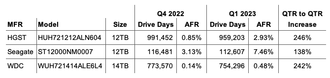
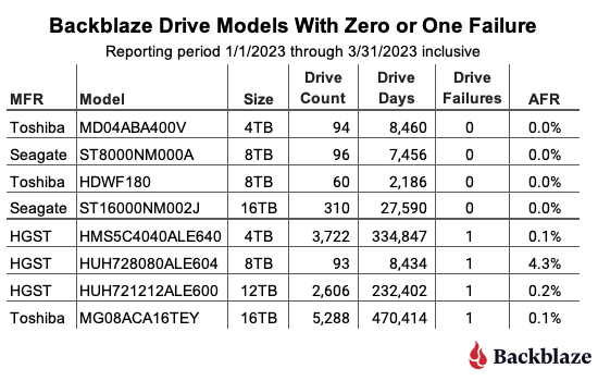
When reviewing the table, any drive model with less than 50,000 drive days for the quarter does not have enough data to be statistically relevant for that period. That said, for two of the drive models listed, posting zero failures is not new. The 16TB Seagate (model: ST16000NM002J) had zero failures last quarter as well, and the 8TB Seagate (model: ST8000NM000A) has had zero failures since it was first installed in Q3 2022, a lifetime AFR of 0%.
The charts below summarize the Q1 2023 data first by Drive Size and then by manufacturer.

While we included all of the drive sizes we currently use, both the 6TB and 10TB drive sizes consist of one model for each and each has a limited number of drive days in the quarter: 79,651 for the 6TB drives and 105,443 for the 10TB drives. Each of the remaining drive sizes has at least 2.2 million drive days, making their quarterly annualized failure rates more reliable.
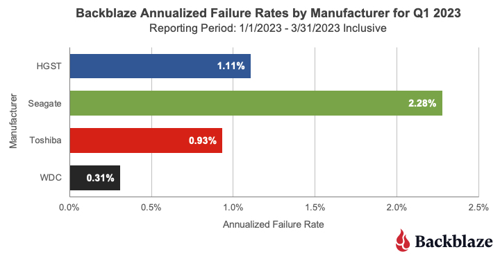
This chart combines all of the manufacturer’s drive models regardless of their age. In our case, many of the older drive models are from Seagate and that helps drive up their overall AFR. For example, 60% of the 4TB drives are from Seagate and are, on average, 89 months old, and over 95% of the 8TB drives in production are from Seagate and they are, on average, over 70 months old. As we’ve seen when we examined hard drive life expectancy using the Bathtub Curve, older drives have a tendency to fail more often.
That said, there are outliers out there like our intrepid fleet of 6TB Seagate drives which have an average age of 95.4 months and have a Q1 2023 AFR of 0.92% and a lifetime AFR of 0.89% as we’ll see later in this report.
Recently the folks at Blocks & Files published an article outlining the average age of a hard drive when it failed. The article was based on the work of Timothy Burlee at Secure Data Recovery. To summarize, the article found that for the 2,007 failed hard drives analyzed, the average age at which they failed was 1,051 days, or two years and 10 months. We thought this was an interesting way to look at drive failure, and we wanted to know what we would find if we asked the same question of our Drive Stats data. They also determined the current pending sector count for each failed drive, but today we’ll focus on the average age of drive failure.
The article didn’t specify how they collected the amount of time a drive was operational before it failed but we’ll assume they used the SMART 9 raw value for power-on hours. Given that, our first task was to round up all of the failed drives in our dataset and record the power-on hours for each drive. That query produced a list of 18,605 drives which failed between April 10, 2013 and March 30, 2023, inclusive.
For each failed drive we recorded the date, serial_number, model, drive_capacity, failure, and SMART 9 raw value. A sample is below.
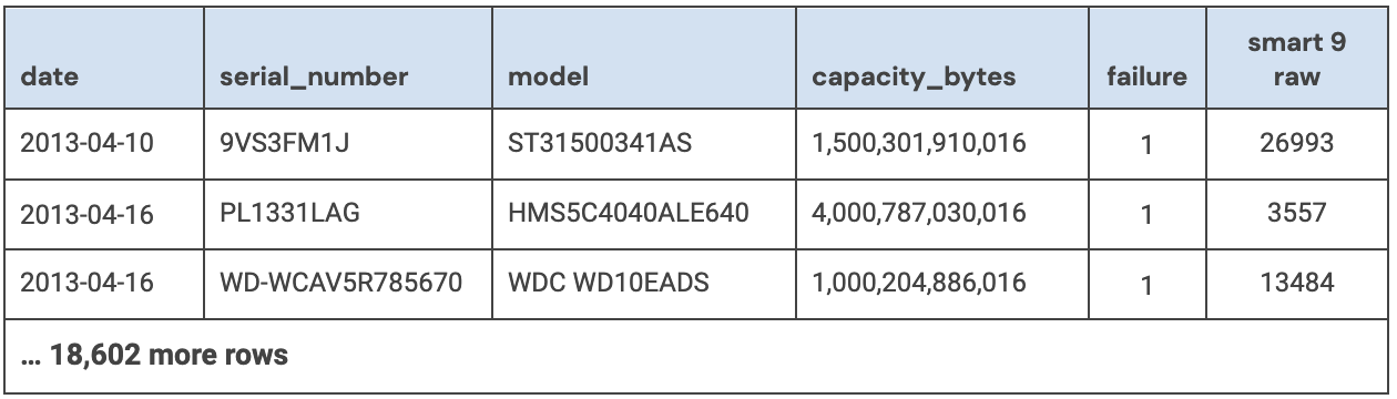
To start the data cleanup process, we first removed 1,355 failed boot drives from the dataset, leaving us with 17,250 data drives.
We then removed 95 drives for one of the following reasons:
In both of these cases, the drives in question were not in a good state when the data was collected and as such any other data collected could be unreliable.
We are left with 17,155 failed drives to analyze. When we compute the average age at which this cohort of drives failed we get 22,360 hours, which is 932 days, or just over two years and six months. This is reasonably close to the two years and 10 months from the Blocks & Files article, but before we confirm their numbers let’s dig into our results a bit more.
Our Drive Stats dataset contains drive failures for 72 drive models, and that number does not include boot drives. To make our table a bit more manageable we’ve limited the list to those drive models which have recorded 50 or more failures. The resulting list contains 30 models which we’ve sorted by average failure age:
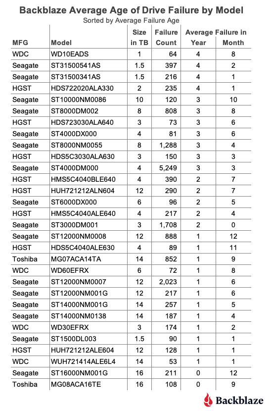
As one would expect, there are drive models above and below our overall failure average age of two years and six months. One observation is that the average failure age of many of the smaller sized drive models (1TB, 1.5TB, 2TB, etc.) is higher than our overall average of two years and six months. Conversely, for many larger sized drive models (12TB, 14TB, etc.) the average failure age was below the average. Before we reach any conclusions, let’s see what happens if we review the average failure age by drive size as shown below.
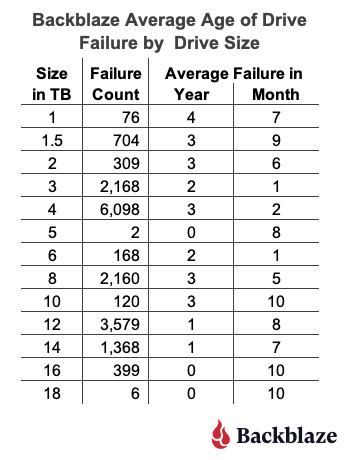
This chart seems to confirm the general trend that the average failure age of smaller drive models is higher than larger drive models.
At this point you might start pondering whether technologies in larger drives such as the additional platters, increased areal density, or even the use of helium would impact the average failure age of these drives. But as the unflappable Admiral Ackbar would say:
The trap is that the dataset for the smaller sized drive models is, in our case, complete—there are no more 1TB, 1.5TB, 2TB, 3TB, or even 5TB drives in operation in our dataset. On the contrary, most of the larger sized drive models are still in operation and therefore they “haven’t finished failing yet.” In other words, as these larger drives continue to fail over the coming months and years, they could increase or decrease the average failure age of that drive model.
One way to move forward at this point is to limit our computations to only those drive models which are no longer in operation in our data centers. When we do this, we find we have 35 drive models consisting of 3,379 drives that have a failed average age of two years and seven months.
Trap or not, our results are consistent with the Blocks & Files article as their failed average age of two years and 10 months for their dataset. It will be interesting to see how this comparison holds up over time as more drive models in our dataset finish their Backblaze operational life.
The second way to look at drive failure is to view the problem from the life expectancy point of view instead. This approach takes a page from bioscience and utilizes Kaplan-Meier techniques to produce life expectancy (aka survival) curves for different cohorts, in our case hard drive models. We used such curves previously in our Hard Drive Life Expectancy and Bathtub Curve blog posts. This approach allows us to see the failure rate over time and helps answer questions such as, “If I bought a drive today, what are the chances it will survive x years?”
We have three different, but similar, values for average failure age of hard drives, and they are as follows:
| Source | Failed Drive Count | Average Failed Age |
|---|---|---|
| Secure Data Recovery | 2,007 failed drives | 2 years, 10 months |
| Backblaze | 17,155 failed drives (all models) | 2 years, 6 months |
| Backblaze | 3,379 failed drives (only drive models no longer in production) | 2 years, 7 months |
When we first saw the Secure Data Recovery average failed age we thought that two years and 10 months was too low. We were surprised by what our data told us, but a little math never hurt anyone. Given we are always adding additional failed drives to our dataset, and retiring drive models along the way, we will continue to track the average failed age of our drive models and report back if we find anything interesting.
As of March 31, 2023, we were tracking 237,278 hard drives. For our lifetime analysis, we removed 385 drives that were only used for testing purposes or did not have at least 60 drives. This leaves us with 236,893 hard drives grouped into 30 different models to analyze for the lifetime table below.

The lifetime AFR for all the drives listed above is 1.40%. That is a slight increase from the previous quarter of 1.39%. The lifetime AFR number for all of our hard drives seems to have settled around 1.40%, although each drive model has its own unique AFR value.
For the past 10 years we’ve been capturing and storing the Drive Stats data which is the source of the lifetime AFRs listed in the table above. But, why keep track of the data at all? Well, besides creating this report each quarter, we use the data internally to help run our business. While there are many other factors which go into the decisions we make, the Drive Stats data helps to surface potential issues sooner, allows us to take better informed drive related actions, and overall adds a layer of confidence in the drive-based decisions we make.
The complete dataset used to create the information used in this review is available on our Hard Drive Test Data page. You can download and use this data for free for your own purpose. All we ask are three things: 1) you cite Backblaze as the source if you use the data, 2) you accept that you are solely responsible for how you use the data, and 3) you do not sell this data to anyone; it is free.
If you want the tables and charts used in this report, you can download the .zip file from Backblaze B2 Cloud Storage which contains an Excel file with a tab for each table or chart.
Good luck and let us know if you find anything interesting.
The post Backblaze Drive Stats for Q1 2023 appeared first on Backblaze Blog | Cloud Storage & Cloud Backup.
Post Syndicated from Bruce Schneier original https://www.schneier.com/blog/archives/2023/05/large-language-models-and-elections.html
Earlier this week, the Republican National Committee released a video that it claims was “built entirely with AI imagery.” The content of the ad isn’t especially novel—a dystopian vision of America under a second term with President Joe Biden—but the deliberate emphasis on the technology used to create it stands out: It’s a “Daisy” moment for the 2020s.
We should expect more of this kind of thing. The applications of AI to political advertising have not escaped campaigners, who are already “pressure testing” possible uses for the technology. In the 2024 presidential election campaign, you can bank on the appearance of AI-generated personalized fundraising emails, text messages from chatbots urging you to vote, and maybe even some deepfaked campaign avatars. Future candidates could use chatbots trained on data representing their views and personalities to approximate the act of directly connecting with people. Think of it like a whistle-stop tour with an appearance in every living room. Previous technological revolutions—railroad, radio, television, and the World Wide Web—transformed how candidates connect to their constituents, and we should expect the same from generative AI. This isn’t science fiction: The era of AI chatbots standing in as avatars for real, individual people has already begun, as the journalist Casey Newton made clear in a 2016 feature about a woman who used thousands of text messages to create a chatbot replica of her best friend after he died.
The key is interaction. A candidate could use tools enabled by large language models, or LLMs—the technology behind apps such as ChatGPT and the art-making DALL-E—to do micro-polling or message testing, and to solicit perspectives and testimonies from their political audience individually and at scale. The candidates could potentially reach any voter who possesses a smartphone or computer, not just the ones with the disposable income and free time to attend a campaign rally. At its best, AI could be a tool to increase the accessibility of political engagement and ease polarization. At its worst, it could propagate misinformation and increase the risk of voter manipulation. Whatever the case, we know political operatives are using these tools. To reckon with their potential now isn’t buying into the hype—it’s preparing for whatever may come next.
On the positive end, and most profoundly, LLMs could help people think through, refine, or discover their own political ideologies. Research has shown that many voters come to their policy positions reflexively, out of a sense of partisan affiliation. The very act of reflecting on these views through discourse can change, and even depolarize, those views. It can be hard to have reflective policy conversations with an informed, even-keeled human discussion partner when we all live within a highly charged political environment; this is a role almost custom-designed for LLM. In US politics, it is a truism that the most valuable resource in a campaign is time. People are busy and distracted. Campaigns have a limited window to convince and activate voters. Money allows a candidate to purchase time: TV commercials, labor from staffers, and fundraising events to raise even more money. LLMs could provide campaigns with what is essentially a printing press for time.
If you were a political operative, which would you rather do: play a short video on a voter’s TV while they are folding laundry in the next room, or exchange essay-length thoughts with a voter on your candidate’s key issues? A staffer knocking on doors might need to canvass 50 homes over two hours to find one voter willing to have a conversation. OpenAI charges pennies to process about 800 words with its latest GPT-4 model, and that cost could fall dramatically as competitive AIs become available. People seem to enjoy interacting with chatbots; Open’s product reportedly has the fastest-growing user base in the history of consumer apps.
Optimistically, one possible result might be that we’ll get less annoyed with the deluge of political ads if their messaging is more usefully tailored to our interests by AI tools. Though the evidence for microtargeting’s effectiveness is mixed at best, some studies show that targeting the right issues to the right people can persuade voters. Expecting more sophisticated, AI-assisted approaches to be more consistently effective is reasonable. And anything that can prevent us from seeing the same 30-second campaign spot 20 times a day seems like a win.
AI can also help humans effectuate their political interests. In the 2016 US presidential election, primitive chatbots had a role in donor engagement and voter-registration drives: simple messaging tasks such as helping users pre-fill a voter-registration form or reminding them where their polling place is. If it works, the current generation of much more capable chatbots could supercharge small-dollar solicitations and get-out-the-vote campaigns.
And the interactive capability of chatbots could help voters better understand their choices. An AI chatbot could answer questions from the perspective of a candidate about the details of their policy positions most salient to an individual user, or respond to questions about how a candidate’s stance on a national issue translates to a user’s locale. Political organizations could similarly use them to explain complex policy issues, such as those relating to the climate or health care or…anything, really.
Of course, this could also go badly. In the time-honored tradition of demagogues worldwide, the LLM could inconsistently represent the candidate’s views to appeal to the individual proclivities of each voter.
In fact, the fundamentally obsequious nature of the current generation of large language models results in them acting like demagogues. Current LLMs are known to hallucinate—or go entirely off-script—and produce answers that have no basis in reality. These models do not experience emotion in any way, but some research suggests they have a sophisticated ability to assess the emotion and tone of their human users. Although they weren’t trained for this purpose, ChatGPT and its successor, GPT-4, may already be pretty good at assessing some of their users’ traits—say, the likelihood that the author of a text prompt is depressed. Combined with their persuasive capabilities, that means that they could learn to skillfully manipulate the emotions of their human users.
This is not entirely theoretical. A growing body of evidence demonstrates that interacting with AI has a persuasive effect on human users. A study published in February prompted participants to co-write a statement about the benefits of social-media platforms for society with an AI chatbot configured to have varying views on the subject. When researchers surveyed participants after the co-writing experience, those who interacted with a chatbot that expressed that social media is good or bad were far more likely to express the same view than a control group that didn’t interact with an “opinionated language model.”
For the time being, most Americans say they are resistant to trusting AI in sensitive matters such as health care. The same is probably true of politics. If a neighbor volunteering with a campaign persuades you to vote a particular way on a local ballot initiative, you might feel good about that interaction. If a chatbot does the same thing, would you feel the same way? To help voters chart their own course in a world of persuasive AI, we should demand transparency from our candidates. Campaigns should have to clearly disclose when a text agent interacting with a potential voter—through traditional robotexting or the use of the latest AI chatbots—is human or automated.
Though companies such as Meta (Facebook’s parent company) and Alphabet (Google’s) publish libraries of traditional, static political advertising, they do so poorly. These systems would need to be improved and expanded to accommodate user-level differentiation in ad copy to offer serviceable protection against misuse.
A public, anonymized log of chatbot conversations could help hold candidates’ AI representatives accountable for shifting statements and digital pandering. Candidates who use chatbots to engage voters may not want to make all transcripts of those conversations public, but their users could easily choose to share them. So far, there is no shortage of people eager to share their chat transcripts, and in fact, an online database exists of nearly 200,000 of them. In the recent past, Mozilla has galvanized users to opt into sharing their web data to study online misinformation.
We also need stronger nationwide protections on data privacy, as well as the ability to opt out of targeted advertising, to protect us from the potential excesses of this kind of marketing. No one should be forcibly subjected to political advertising, LLM-generated or not, on the basis of their Internet searches regarding private matters such as medical issues. In February, the European Parliament voted to limit political-ad targeting to only basic information, such as language and general location, within two months of an election. This stands in stark contrast to the US, which has for years failed to enact federal data-privacy regulations. Though the 2018 revelation of the Cambridge Analytica scandal led to billions of dollars in fines and settlements against Facebook, it has so far resulted in no substantial legislative action.
Transparency requirements like these are a first step toward oversight of future AI-assisted campaigns. Although we should aspire to more robust legal controls on campaign uses of AI, it seems implausible that these will be adopted in advance of the fast-approaching 2024 general presidential election.
Credit the RNC, at least, with disclosing that their recent ad was AI-generated—a transparent attempt at publicity still counts as transparency. But what will we do if the next viral AI-generated ad tries to pass as something more conventional?
As we are all being exposed to these rapidly evolving technologies for the first time and trying to understand their potential uses and effects, let’s push for the kind of basic transparency protection that will allow us to know what we’re dealing with.
This essay was written with Nathan Sanders, and previously appeared on the Atlantic.
EDITED TO ADD (5/12): Better article on the “daisy” ad.
Post Syndicated from James Beswick original https://aws.amazon.com/blogs/compute/extending-a-serverless-event-driven-architecture-to-existing-container-workloads/
This post is written by Dhiraj Mahapatro, Principal Specialist SA, and Sascha Moellering, Principal Specialist SA, and Emily Shea, WW Lead, Integration Services.
Many serverless services are a natural fit for event-driven architectures (EDA), as events invoke them and only run when there is an event to process. When building in the cloud, many services emit events by default and have built-in features for managing events. This combination allows customers to build event-driven architectures easier and faster than ever before.
The insurance claims processing sample application in this blog series uses event-driven architecture principles and serverless services like AWS Lambda, AWS Step Functions, Amazon API Gateway, Amazon EventBridge, and Amazon SQS.
When building an event-driven architecture, it’s likely that you have existing services to integrate with the new architecture, ideally without needing to make significant refactoring changes to those services. As services communicate via events, extending applications to new and existing microservices is a key benefit of building with EDA. You can write those microservices in different programming languages or running on different compute options.
This blog post walks through a scenario of integrating an existing, containerized service (a settlement service) to the serverless, event-driven insurance claims processing application described in this blog post.
The sample application uses a front-end to sign up a new user and allow the user to upload images of their car and driver’s license. Once signed up, they can file a claim and upload images of their damaged car. Previously, it did not yet integrate with a settlement service for completing the claims and settlement process.
In this scenario, the settlement service is a brownfield application that runs Spring Boot 3 on Amazon ECS with AWS Fargate. AWS Fargate is a serverless, pay-as-you-go compute engine that lets you focus on building container applications without managing servers.
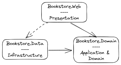
The Spring Boot application exposes a REST endpoint, which accepts a POST request. It applies settlement business logic and creates a settlement record in the database for a car insurance claim. Your goal is to make settlement work with the new EDA application that is designed for claims processing without re-architecting or rewriting. Customer, claims, fraud, document, and notification are the other domains that are shown as blue-colored boxes in the following diagram:

The application uses AWS Cloud Development Kit (CDK) to build the stack. With CDK, you get the flexibility to create modular and reusable constructs imperatively using your language of choice. The sample application uses TypeScript for CDK.
The following project structure enables you to build different bounded contexts. Event-driven architecture relies on the choreography of events between domains. The object oriented programming (OOP) concept of CDK helps provision the infrastructure to separate the domain concerns while loosely coupling them via events.
You break the higher level CDK constructs down to these corresponding domains:
Application and infrastructure code are present in each domain. This project structure creates a seamless way to add new domains like settlement with its application and infrastructure code without affecting other areas of the business.
With the preceding structure, you can use the settlement-service.ts CDK construct inside claims-processing-stack.ts:
const settlementService = new SettlementService(this, "SettlementService", {
  bus,
});
The only information the SettlementService construct needs to work is the EventBridge custom event bus resource that is created in the claims-processing-stack.ts.
To run the sample application, follow the setup steps in the sample application’s README file.
The settlement domain provides a REST service to the rest of the organization. A Docker containerized Spring Boot application runs on Amazon ECS with AWS Fargate. The following sequence diagram shows the synchronous request-response flow from an external REST client to the service:

A request to the HTTP API endpoint looks like:
curl --location <settlement-api-endpoint-from-cloudformation-output> \
--header 'Content-Type: application/json' \
--data '{
  "customerId": "06987bc1-1234-1234-1234-2637edab1e57",
  "claimId": "60ccfe05-1234-1234-1234-a4c1ee6fcc29",
  "color": "green",
  "damage": "bumper_dent"
}'
The response from the API call is:
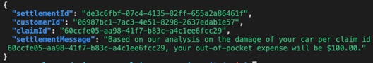
You can learn more here about optimizing Spring Boot applications on AWS Fargate.
To integrate the settlement service, you must update the service to receive and emit events asynchronously. The core logic of the settlement service remains the same. When you file a claim, upload damaged car images, and the application detects no document fraud, the settlement domain subscribes to Fraud.Not.Detected event and applies its business logic. The settlement service emits an event back upon applying the business logic.
The following sequence diagram shows a new interface in settlement to work with EDA. The settlement service subscribes to events that a producer emits. Here, the event producer is the fraud service that puts an event in an EventBridge custom event bus.

Settlement.Finalized.The rest of the architecture consumes this Settlement.Finalized event.
Schema enforces a contract between a producer and a consumer. A consumer expects the exact structure of the event payload every time an event arrives. EventBridge provides schema registry and discovery to maintain this contract. The consumer (the settlement service) can download the code bindings and use them in the source code.
Enable schema discovery in EventBridge before downloading the code bindings and using them in your repository. The code bindings provide a marshaller that unmarshals the incoming event from SQS queue to a plain old Java object (POJO) FraudNotDetected.java. You download the code bindings using the choice of your IDE. AWS Toolkit for IntelliJ makes it convenient to download and use them.

The final architecture for the settlement service with REST and event-driven architecture looks like:
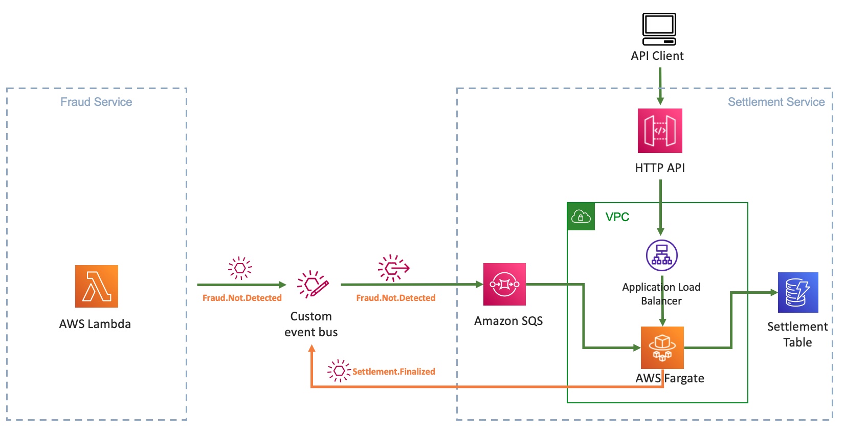
With the new capability to handle events, the Spring Boot application now supports both the REST endpoint and the event-driven architecture by running the same business logic through different interfaces. In this example scenario, as the event-driven architecture matures and the rest of the organization adopts it, the need for the POST endpoint to save a settlement may diminish. In the future, you can deprecate the endpoint and fully rely on polling messages from the SQS queue.
You start with using an ALB and Fargate service CDK ECS pattern:
const loadBalancedFargateService = new ecs_patterns.ApplicationLoadBalancedFargateService(
  this,
  "settlement-service",
  {
    cluster: cluster,
    taskImageOptions: {
      image: ecs.ContainerImage.fromDockerImageAsset(asset),
      environment: {
        "DYNAMODB_TABLE_NAME": this.table.tableName
      },
      containerPort: 8080,
      logDriver: new ecs.AwsLogDriver({
        streamPrefix: "settlement-service",
        mode: ecs.AwsLogDriverMode.NON_BLOCKING,
        logRetention: RetentionDays.FIVE_DAYS,
      })
    },
    memoryLimitMiB: 2048,
    cpu: 1024,
    publicLoadBalancer: true,
    desiredCount: 2,
    listenerPort: 8080
  });
To adapt to EDA, you update the resources to retrofit the SQS queue to receive messages and EventBridge to put events. Add new environment variables to the ApplicationLoadBalancerFargateService resource:
environment: {
  "SQS_ENDPOINT_URL": queue.queueUrl,
  "EVENTBUS_NAME": props.bus.eventBusName,
  "DYNAMODB_TABLE_NAME": this.table.tableName
}
Grant the Fargate task permission to put events in the custom event bus and consume messages from the SQS queue:
props.bus.grantPutEventsTo(loadBalancedFargateService.taskDefinition.taskRole);
queue.grantConsumeMessages(loadBalancedFargateService.taskDefinition.taskRole);
When you transition the settlement service to become fully event-driven, you do not need the HTTP API endpoint and ALB anymore, as SQS is the source of events.
A better alternative is to use QueueProcessingFargateService ECS pattern for the Fargate service. The pattern provides auto scaling based on the number of visible messages in the SQS queue, besides CPU utilization. In the following example, you can also add two capacity provider strategies while setting up the Fargate service: FARGATE_SPOT and FARGATE. This means, for every one task that is run using FARGATE, there are two tasks that use FARGATE_SPOT. This can help optimize cost.
const queueProcessingFargateService = new ecs_patterns.QueueProcessingFargateService(this, 'Service', {
  cluster,
  memoryLimitMiB: 1024,
  cpu: 512,
  queue: queue,
  image: ecs.ContainerImage.fromDockerImageAsset(asset),
  desiredTaskCount: 2,
  minScalingCapacity: 1,
  maxScalingCapacity: 5,
  maxHealthyPercent: 200,
  minHealthyPercent: 66,
  environment: {
    "SQS_ENDPOINT_URL": queueUrl,
    "EVENTBUS_NAME": props?.bus.eventBusName,
    "DYNAMODB_TABLE_NAME": tableName
  },
  capacityProviderStrategies: [
    {
      capacityProvider: 'FARGATE_SPOT',
      weight: 2,
    },
    {
      capacityProvider: 'FARGATE',
      weight: 1,
    },
  ],
});
This pattern abstracts the automatic scaling behavior of the Fargate service based on the queue depth.
Running the application
To test the application, follow How to use the Application after the initial setup. Once complete, you see that the browser receives a Settlement.Finalized event:
{
  "version": "0",
  "id": "e2a9c866-cb5b-728c-ce18-3b17477fa5ff",
  "detail-type": "Settlement.Finalized",
  "source": "settlement.service",
  "account": "123456789",
  "time": "2023-04-09T23:20:44Z",
  "region": "us-east-2",
  "resources": [],
  "detail": {
    "settlementId": "377d788b-9922-402a-a56c-c8460e34e36d",
    "customerId": "67cac76c-40b1-4d63-a8b5-ad20f6e2e6b9",
    "claimId": "b1192ba0-de7e-450f-ac13-991613c48041",
    "settlementMessage": "Based on our analysis on the damage of your car per claim id b1192ba0-de7e-450f-ac13-991613c48041, your out-of-pocket expense will be $100.00."
  }
}
The stack creates a custom VPC and other related resources. Be sure to clean up resources after usage to avoid the ongoing cost of running these services. To clean up the infrastructure, follow the clean-up steps shown in the sample application.
The blog explains a way to integrate existing container workload running on AWS Fargate with a new event-driven architecture. You use EventBridge to decouple different services from each other that are built using different compute technologies, languages, and frameworks. Using AWS CDK, you gain the modularity of building services decoupled from each other.
This blog shows an evolutionary architecture that allows you to modernize existing container workloads with minimal changes that still give you the additional benefits of building with serverless and EDA on AWS.
The major difference between the event-driven approach and the REST approach is that you unblock the producer once it emits an event. The event producer from the settlement domain that subscribes to that event is loosely coupled. The business functionality remains intact, and no significant refactoring or re-architecting effort is required. With these agility gains, you may get to the market faster
The sample application shows the implementation details and steps to set up, run, and clean up the application. The app uses ECS Fargate for a domain service, but you do not limit it to just Fargate. You can also bring container-based applications running on Amazon EKS similarly to event-driven architecture.
Learn more about event-driven architecture on Serverless Land.
Post Syndicated from original https://lwn.net/Articles/930368/
The LWN.net Weekly Edition for May 4, 2023 is available.
Post Syndicated from Suresh Babu original https://aws.amazon.com/blogs/devops/integrating-devops-guru-insights-with-cloudwatch-dashboard/
Many customers use Amazon CloudWatch dashboards to monitor applications and often ask how they can integrate Amazon DevOps Guru Insights in order to have a unified dashboard for monitoring. This blog post showcases integrating DevOps Guru proactive and reactive insights to a CloudWatch dashboard by using Custom Widgets. It can help you to correlate trends over time and spot issues more efficiently by displaying related data from different sources side by side and to have a single pane of glass visualization in the CloudWatch dashboard.
Amazon DevOps Guru is a machine learning (ML) powered service that helps developers and operators automatically detect anomalies and improve application availability. DevOps Guru’s anomaly detectors can proactively detect anomalous behavior even before it occurs, helping you address issues before they happen; detailed insights provide recommendations to mitigate that behavior.
Amazon CloudWatch dashboard is a customizable home page in the CloudWatch console that monitors multiple resources in a single view. You can use CloudWatch dashboards to create customized views of the metrics and alarms for your AWS resources.
This post will help you to create a Custom Widget for Amazon CloudWatch dashboard that displays DevOps Guru Insights. A custom widget is part of your CloudWatch dashboard that calls an AWS Lambda function containing your custom code. The Lambda function accepts custom parameters, generates your dataset or visualization, and then returns HTML to the CloudWatch dashboard. The CloudWatch dashboard will display this HTML as a widget. In this post, we are providing sample code for the Lambda function that will call DevOps Guru APIs to retrieve the insights information and displays as a widget in the CloudWatch dashboard. The architecture diagram of the solution is below.

Figure 1: Reference architecture diagram
We are providing two options to deploy the solution – using the AWS console and AWS CloudFormation. The first section has instructions to deploy using the AWS console followed by instructions for using CloudFormation. The key difference is that we will create one Widget while using the Console, but three Widgets are created when we use AWS CloudFormation.
We will first create a Lambda function that will retrieve the DevOps Guru insights. We will then modify the default IAM role associated with the Lambda function to add DevOps Guru permissions. Finally we will create a CloudWatch dashboard and add a custom widget to display the DevOps Guru insights.

Figure 2a: Create Lambda Function

Figure 2b: Create Lambda Function
// SPDX-License-Identifier: MIT-0
// CloudWatch Custom Widget sample: displays count of Amazon DevOps Guru Insights
const aws = require('aws-sdk');

const DOCS = `## DevOps Guru Insights Count
Displays the total counts of Proactive and Reactive Insights in DevOps Guru.
`;

async function getProactiveInsightsCount(DevOpsGuru, StartTime, EndTime) {
    let NextToken = null;
    let proactivecount=0;

    do {
        const args = { StatusFilter: { Any : { StartTimeRange: { FromTime: StartTime, ToTime: EndTime }, Type: 'PROACTIVE'  }}}
        const result = await DevOpsGuru.listInsights(args).promise();
        console.log(result)
        NextToken = result.NextToken;
        result.ProactiveInsights.forEach(res => {
        console.log(result.ProactiveInsights[0].Status)
        proactivecount++;
        });
        } while (NextToken);
    return proactivecount;
}

async function getReactiveInsightsCount(DevOpsGuru, StartTime, EndTime) {
    let NextToken = null;
    let reactivecount=0;

    do {
        const args = { StatusFilter: { Any : { StartTimeRange: { FromTime: StartTime, ToTime: EndTime }, Type: 'REACTIVE'  }}}
        const result = await DevOpsGuru.listInsights(args).promise();
        NextToken = result.NextToken;
        result.ReactiveInsights.forEach(res => {
        reactivecount++;
        });
        } while (NextToken);
    return reactivecount;
}

function getHtmlOutput(proactivecount, reactivecount, region, event, context) {

    return `DevOps Guru Proactive Insights<br><font size="+10" color="#FF9900">${proactivecount}</font>
    <p>DevOps Guru Reactive Insights</p><font size="+10" color="#FF9900">${reactivecount}`;
}

exports.handler = async (event, context) => {
    if (event.describe) {
        return DOCS;
    }
    const widgetContext = event.widgetContext;
    const timeRange = widgetContext.timeRange.zoom || widgetContext.timeRange;
    const StartTime = new Date(timeRange.start);
    const EndTime = new Date(timeRange.end);
    const region = event.region || process.env.AWS_REGION;
    const DevOpsGuru = new aws.DevOpsGuru({ region });

    const proactivecount = await getProactiveInsightsCount(DevOpsGuru, StartTime, EndTime);
    const reactivecount = await getReactiveInsightsCount(DevOpsGuru, StartTime, EndTime);

    return getHtmlOutput(proactivecount, reactivecount, region, event, context);

};
Figure 3: Lambda Function Source Code

Figure 4: Lambda function execution role

Figure 5: IAM Role Update

Figure 6: IAM Role Policy Update

Figure 7: Create New CloudWatch dashboard

Figure 8: Add widget

Figure 9: Custom Widget Selection

Figure 10: Create Custom Widget
You may skip this step and move to future scope section if you have already created the resources using AWS Console.
In this step we will show you how to deploy the solution using AWS CloudFormation. AWS CloudFormation lets you model, provision, and manage AWS and third-party resources by treating infrastructure as code. Customers define an initial template and then revise it as their requirements change. For more information on CloudFormation stack creation refer to this blog post.
The following resources are created.
To deploy the solution by using the CloudFormation template
It takes approximately 2-3 minutes for the provisioning to complete. After the status is “Complete”, proceed to validate the resources as listed below.
Now that the stack creation has completed successfully, you should validate the resources that were created.
With the appropriate time-range setup on CloudWatch Dashboard, you will be able to navigate through the insights that have been generated from DevOps Guru on the CloudWatch Dashboard.
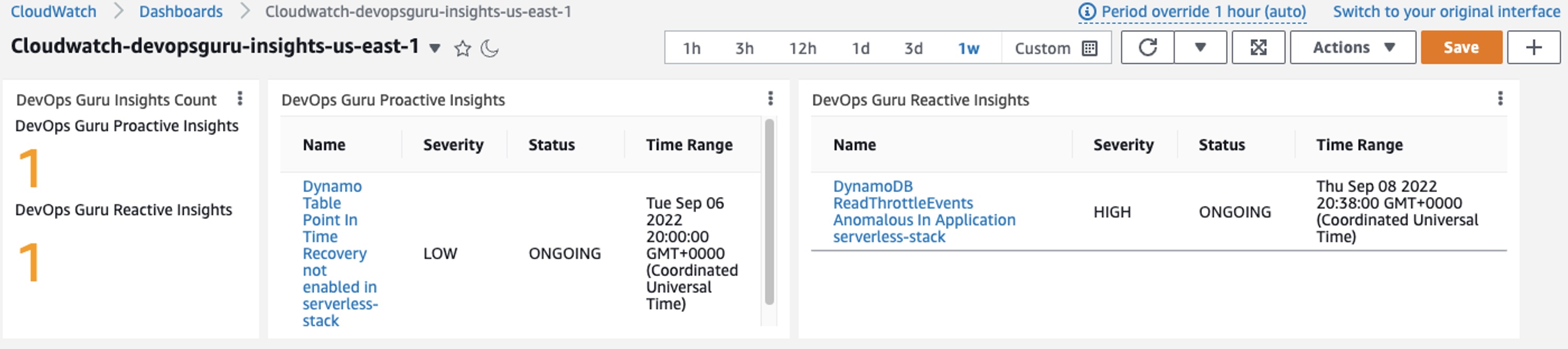
Figure 11: DevOpsGuru Insights in Cloudwatch Dashboard
For cost optimization, after you complete and test this solution, clean up the resources. You can delete them manually if you used the AWS Console or by deleting the AWS CloudFormation stack called devopsguru-cloudwatch-dashboard if you used AWS CloudFormation.
For more information on deleting the stacks, see Deleting a stack on the AWS CloudFormation console.
This blog post outlined how you can integrate DevOps Guru insights into a CloudWatch Dashboard. As a customer, you can start leveraging CloudWatch Custom Widgets to include DevOps Guru Insights in an existing Operational dashboard.
AWS Customers are now using Amazon DevOps Guru to monitor and improve application performance. You can start monitoring your applications by following the instructions in the product documentation. Head over to the Amazon DevOps Guru console to get started today.
To learn more about AIOps for Serverless using Amazon DevOps Guru check out this video.
Post Syndicated from Jakub Oleksy original https://github.blog/2023-05-03-github-availability-report-april-2023/
In April, we experienced four incidents that resulted in degraded performance across GitHub services. This report also sheds light into three March incidents that resulted in degraded performance across GitHub services.
March 27 12:25 UTC (lasting 1 hour and 33 minutes)
On March 27 at 12:14 UTC, users began to see degraded experience with Git Operations, GitHub Issues, pull requests, GitHub Actions, GitHub API requests, GitHub Codespaces, and GitHub Pages. We publicly statused Git Operations 11 minutes later, initially to yellow, followed by red for other impacted services. Full functionality was restored at 13:17 UTC.
The cause was traced to a change in a frequently-used database query. The query alteration was part of a larger infrastructure change that had been rolled out gradually, starting in October 2022, then more quickly beginning February 2023, completing on March 20, 2023. The change increased the chance of lock contention, leading to increased query times and eventual resource exhaustion during brief load spikes, which caused the database to crash. An initial automatic failover solved this seamlessly, but the slow query continued to cause lock contention and resource exhaustion, leading to a second failover that did not complete. Mitigation took longer than usual because manual intervention was required to fully recover.
The query causing lock tension was disabled via feature flag, and then refactored. We have added additional monitoring of relevant database resources so as not to reach resource exhaustion, and detect similar issues earlier in our staged rollout process. Additionally, we have enhanced our query evaluation procedures related to database lock contention, along with improved documentation and training material.
March 29 14:21 UTC (lasting 4 hour and 57 minutes)
On March 29 at 14:10 UTC, users began to see a degraded experience with GitHub Actions with their workflows not progressing. Engineers initially statused GitHub Actions nine minutes later. GitHub Actions started recovering between 14:57 UTC and 16:47 UTC before degrading again. GitHub Actions fully recovered the queue of backlogged workflows at 19:03 UTC.
We determined the cause of the impact to be a degraded database cluster. Contributing factors included a new load source from a background job querying that database cluster, maxed out database transaction pools, and underprovisioning of vtgate proxy instances that are responsible for query routing, load balancing, and sharding. The incident was mitigated through throttling of job processing and adding capacity, including overprovisioning to speed processing of the backlogged jobs.
After the incident, we identified that the pool, found_rows_pool managed by the vtgate layer, was overwhelmed and unresponsive. This pool became flooded and stuck due to contention between inserting data into and reading data from the tables in the database. This contention led to us being unable to progress any new queries across our database cluster.
The health of our database clusters is a top priority for us and we have taken steps to reduce contentious queries on our cluster over the last few weeks. We also have taken multiple actions from what we learned in this incident to improve our telemetry and alerting to allow us to identify and act on blocking queries faster. We are carefully monitoring the cluster health and are taking a close look into each component to identify any additional repair items or adjustments we can make to improve long-term stability.
March 31 01:07 UTC (lasting 2 hours)
On March 31 at 00:06 UTC, a small percentage of users started to receive consistent 500 error responses on pull request files pages. At 01:07 UTC, the support team escalated reports from customers to engineering who identified the cause and statused yellow nine minutes later. The fix was deployed to all production hosts by 02:07 UTC.
We determined the source of the bug to be a notification to promote a new feature. Only repository admins who had not enabled the new feature or dismissed the notification were impacted. An expiry date in the configuration of this notification was set incorrectly, which caused a constant that was still referenced in code to no longer be available.
We have taken steps to avoid similar issues in the future by auditing the expiry dates of existing notices, preventing future invalid configurations, and improving test coverage.
April 18 09:28 UTC (lasting 11 minutes)
On April 18 at 09:22 UTC, users accessing any issues or pull request related entities experienced consistent 5xx responses. Engineers publicly statused pull requests to red and issues six minutes later. At 09:33 UTC, the root cause self-healed and traffic recovered. The impact resulted in an 11 minute outage of access to issues and pull request related artifacts. After fully validating traffic recovery, we statused green for issues at 09:42 UTC.
The root cause of this incident was a planned change in our database infrastructure to minimize the impact of unsuccessful deployments. As part of the progressive rollout of this change, we deleted nodes that were taking live traffic. When these nodes were deleted, there was an 11 minute window where requests to this database cluster failed. The incident was resolved when traffic automatically switched back to the existing nodes.
This planned rollout was a rare event. In order to avoid similar incidents, we have taken steps to review and improve our change management process. We are updating our monitoring and observability guidelines to check for traffic patterns prior to disruptive actions. Furthermore, we’re adding additional review steps for disruptive actions. We have also implemented a new checklist for change management for these types of infrequent administrative changes that will prompt the primary operator to document the change and associated risks along with mitigation strategies.
April 26 23:26 UTC (lasting 1 hour and 04 minutes)
On April 26 at 23:26 UTC, we were notified of an outage with GitHub Copilot. We resolved the incident at 00:29 UTC.
Due to the recency of this incident, we are still investigating the contributing factors and will provide a more detailed update in next month’s report.
April 27 08:59 UTC (lasting 57 minutes)
On April 26 at 08:59 UTC, we were notified of an outage with GitHub Packages. We resolved the incident at 09:56 UTC.
Due to the recency of this incident, we are still investigating the contributing factors and will provide a more detailed update in next month’s report.
April 28 12:26 UTC (lasting 19 minutes)
On April 28 at 12:26 UTC, we were notified of degraded availability for GitHub Codespaces. We resolved the incident at 12:45 UTC.
Due to the recency of this incident, we are still investigating the contributing factors and will provide a more detailed update in next month’s report.
Please follow our status page for real-time updates on status changes. To learn more about what we’re working on, check out the GitHub Engineering Blog.
Post Syndicated from Steve Roberts original https://aws.amazon.com/blogs/aws/introducing-bobs-used-books-a-new-real-world-net-sample-application/
Today, I’m happy to announce that a new open-source sample application, a fictitious used books eCommerce store we call Bob’s Used Books, is available for .NET developers working with AWS. The .NET advocacy and development teams at AWS talk to customers regularly and, during those conversations, often receive requests for more in-depth samples. Customers tell us that, while small code snippets serve well to illustrate the mechanics of an API, their development teams also need and want to make use of fuller, more real-world samples to understand better how to construct modern applications for the cloud. Today’s sample application release is in response to those requests.
Bob’s Used Books is a sample eCommerce application built using ASP.NET Core version 6 and represents an initial modernization of a typical on-premises custom application. Representing a first stage of modernization, the application uses modern cross-platform .NET, enabling it to run on both Windows and Linux systems in the cloud. It’s typical of what many .NET developers are just now going through, porting their own applications from .NET Framework to .NET using freely available tools from AWS such as the Toolkit for .NET Refactoring and the Porting Assistant for .NET.

Sample application features
Customers of our fictional bookstore can browse and search on the store for used books and view details on selected books such as price, condition, genre, and more:


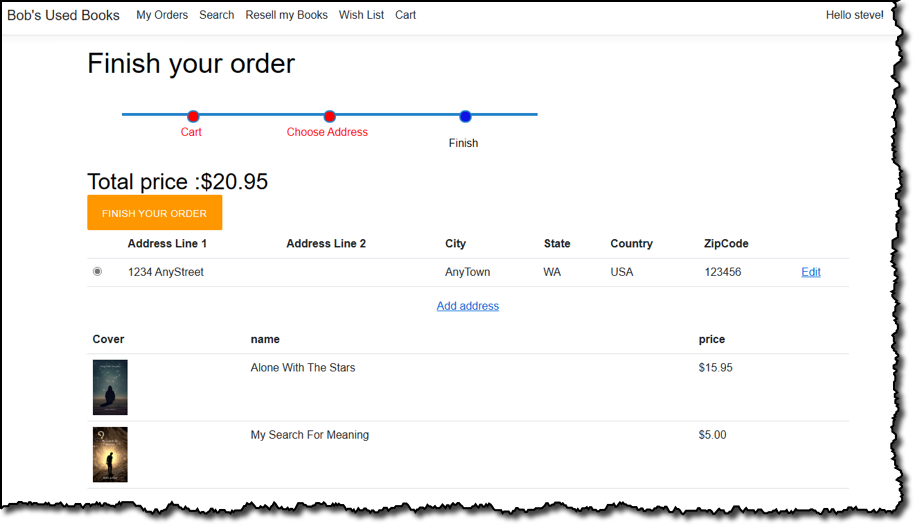
Just like a real e-commerce store, customers can add books to a shopping cart, pending subsequent checkout, or to a personal wish list. When the time comes to purchase, the customer can start the checkout process, which will encourage them to sign in if they are an existing customer or sign up during the process.
In this sample application, the bookstore’s staff uses the same web application to manage inventory and customer orders. Role-based authentication is used to determine whether it’s a staff member signing in, in which case they can view an administrative portal, or a regular store customer. For staff, having accessed the admin portal, they start with a dashboard view that summarizes pending, in-process, or completed orders and the state of the store’s inventory:

Staff can edit inventory to add new books, complete with cover images, or adjust stock levels. From the same dashboard, staff can also view and process pending orders.

Not shown here, but something I think is pretty cool, is a simulated workflow where customers can re-sell their books through the store. This involves the customer submitting an application, the store admin evaluating and deciding whether to purchase from the customer, the customer “posting” the book to the store if accepted, and finally the admin adding the book into inventory and reimbursing the customer. Remember, this is all fictional, however—no actual financial transactions take place!
Application architecture
The bookstore sample didn’t start as a .NET Framework-based application that needed porting to .NET, but it does use a monolithic MVC (model-view-controller) application design, typical of the .NET Framework development era (and still in use today). It also uses a single Microsoft SQL Server database to contain inventory, shopping cart, user data, and more.
When fully deployed to AWS, the application makes use of several services. These provide resources to host the application, provide configuration to the running application, and also provide useful functionality to the running code, such as image verification:
The application is a starting point to showcase further modernization opportunities in the future, such as adopting purpose-built databases instead of using a single relational database, decomposing the monolith to use microservices (for the latter, AWS provides the Microservice Extractor for .NET), and more. The .NET development, advocacy, and solution architect teams here at AWS are quite excited at the opportunities for new content, using this sample, to illustrate those modernization opportunities in the upcoming months. And, as the sample is open-source, we’re also interested to see where the .NET development community takes it regarding modernization.
Running the application
My colleague Brad Webber, a Solutions Architect at AWS, has written the first in a series of technical blog posts we’ll be publishing about the sample. You’ll find these on the new .NET on AWS blog channel. In his first post, you’ll learn more about how to run or debug the application on your own machine as well as deploy it completely to the AWS cloud.
The application uses SQL Server Express localdb instance for its database needs when running outside the cloud, which means you do currently need to be using a Windows machine to run or debug. Launch profiles, accessible from Visual Studio, Visual Studio Code, or JetBrains Rider (all on Windows), are used to select how the application runs (for example, with no or some cloud resources):
Deploying the Sample to AWS
You can also deploy the entire application to the AWS Cloud, in this case, to virtual machines in Amazon Elastic Compute Cloud (Amazon EC2) with a SQL Server Express database instance in Amazon Relational Database Service (RDS). The deployment uses resources compatible with the AWS Free Tier but do note, however, that you may still incur charges if you exceed the Free Tier limits. Unlike running the application on your own machine, which requires Windows because of the localdb dependency, you can deploy the application to AWS from any machine, including those running macOS and Linux. Once again, a CDK project is included in the repository to get you started, and Brad’s blog post goes into more detail on these steps so I won’t repeat them here.
Using virtual machines in the cloud is often a first step in modernizing on-premises applications because of similarity with an on-premises server setup, hence the reason for supporting Amazon EC2 deployments out-of-the-box. In the future, we’ll be adding content showing how to deploy the application to container services on AWS, such as AWS App Runner, Amazon Elastic Container Service (Amazon ECS), and Amazon Elastic Kubernetes Service (EKS).
Next steps
The Bob’s Used Books sample application is available now on GitHub. We encourage you, if you’re a .NET developer working on AWS and looking for a deeper, more real-world sample, to clone the repository and take the application for a spin. We’re also curious about what modernization journeys you would decide to take with the application, which will help us create future content for the sample. Let us know in the issues section of the repository. And if you want to contribute to the sample, we welcome contributions!
Post Syndicated from Prashant Agrawal original https://aws.amazon.com/blogs/big-data/amazon-opensearch-service-now-supports-99-99-availability-using-multi-az-with-standby/
Customers use Amazon OpenSearch Service for mission-critical applications and monitoring. But what happens when OpenSearch Service itself is unavailable? If your ecommerce search is down, for example, you’re losing revenue. If you’re monitoring your application with OpenSearch Service, and it becomes unavailable, your ability to detect, diagnose, and repair issues with your application is diminished. In these cases, you may suffer lost revenue, customer dissatisfaction, reduced productivity, or even damage to your organization’s reputation.
OpenSearch Service offers an SLA of three 9s (99.9%) availability when following best practices. However, following those practices is complicated, and can require knowledge of and experience with OpenSearch’s data deployment and management, along with an understanding of how OpenSearch Service interacts with AWS Availability Zones and networking, distributed systems, OpenSearch’s self-healing capabilities, and its recovery methods. Furthermore, when an issue arises, such as a node becoming unresponsive, OpenSearch Service recovers by recreating the missing shards (data), causing a potentially large movement of data in the domain. This data movement increases resource usage on the cluster, which can impact performance. If the cluster is not sized properly, it can experience degraded availability, which defeats the purpose of provisioning the cluster across three Availability Zones.
Today, AWS is announcing the new deployment option Multi-AZ with Standby for OpenSearch Service, which helps you offload some of that heavy lifting in terms of high frequency monitoring, fast failure detection, and quick recovery from failure, and keeps your domains available and performant even in the event of an infrastructure failure. With Multi-AZ with Standby, you get 99.99% availability with consistent performance for a domain.
In this post, we discuss the benefits of this new option and how to configure your OpenSearch cluster with Multi-AZ with Standby.
The OpenSearch Service team has incorporated years of experience running tens of thousands of domains for our customers into the Multi-AZ with Standby feature. When you adopt Multi-AZ with Standby, OpenSearch Service creates a cluster across three Availability Zones, with each Availability Zone containing a complete copy of data in the cluster. OpenSearch Service then puts one Availability Zone into standby mode, routing all queries to the other two Availability Zones. When it detects a hardware-related failure, OpenSearch Service promotes nodes from the standby pool to become active in less than a minute. When you use Multi-AZ with Standby, OpenSearch Service doesn’t need to redistribute or recreate data from missing nodes. As a result, cluster performance is unaffected, removing the risk of degraded availability.
Multi-AZ with Standby requires the following prerequisites:
Refer to Sizing Amazon OpenSearch Service domains for guidance on sizing your domain and dedicated cluster manager nodes.
You can use Multi-AZ with Standby when you create a new domain, or you can add it to an existing domain. If you’re creating a new domain using the AWS Management Console, you can create it with Multi-AZ with Standby by either selecting the new Easy create option or the traditional Standard create option. You can update existing domains to use Multi-AZ with Standby by editing their domain configuration.
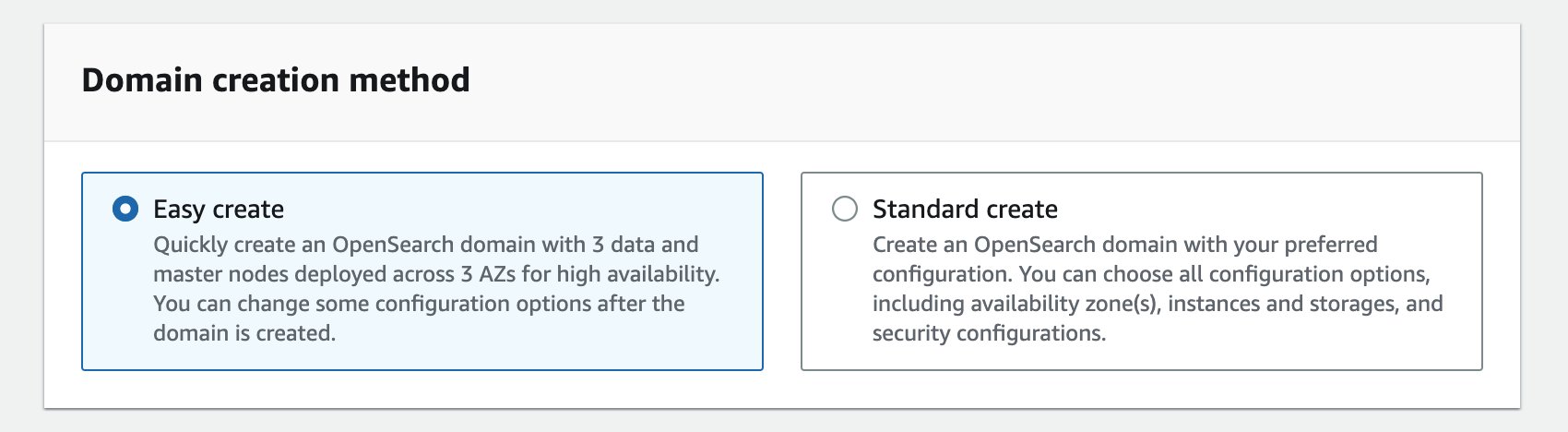
The Easy create option, as the name suggests, makes creating a domain easier by defaulting to best practice choices for most of the configuration (the majority of which can be altered later). The domain will be set up for high availability from the start and deployed as Multi-AZ with Standby.

While choosing the data nodes, you should choose three (or a multiple of three) data nodes so that they are equally distributed across each of the Availability Zones. The Data nodes table on the OpenSearch Service console provides a visual representation of the data notes, showing that one of the Availability Zones will be put on standby.

Similarly, while selecting the cluster manager (master) node, consider the number of data nodes, indexes, and shards that you plan to have before deciding the instance size.
After the domain is created, you can check its deployment type on the OpenSearch Service console under Cluster configuration, as shown in the following screenshot.

While creating an index, make sure that the number of copies (primary and replica) are multiples of three. If you don’t specify the number of replicas, the service will default to two. This is important so that there is at least one copy of the data in each Availability Zone. We recommend using an index template or similar for logs workloads.
OpenSearch Service distributes the nodes and data copies equally across the three Availability Zones. During normal operations, the standby nodes don’t receive any search requests. The two active Availability Zones respond to all the search requests. However, data is replicated to these standby nodes to ensure you have a full copy of the data in each Availability Zone at all times.
OpenSearch Service continuously monitors the domain for events like node failure, disk failure, or Availability Zone failure. In the event of an infrastructure failure like an Availability Zone failure, OpenSearch Services promotes the standby nodes to active while the impacted Availability Zone recovers. Impact (if any) is limited to the in-flight requests as traffic is weighed away from the impacted Availability Zone in less a minute.
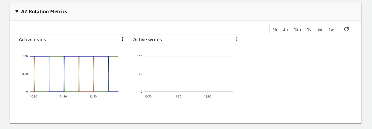
You can check the status of the domain, data node metrics for both active and standby, and Availability Zone rotation metrics on the Cluster health tab. The following screenshots show the cluster health and metrics for data nodes such as CPU utilization, JVM memory pressure, and storage.


The following screenshot of the AZ Rotation Metrics section (you can find this under Cluster health tab) shows the read and write status of the Availability Zones. OpenSearch Service rotates the standby Availability Zone every 30 minutes to ensure the system is running and ready to respond to events. Availability Zones responding to traffic have a read value of 1, and the standby Availability Zone has a value of 0.
Several improvements and guardrails have been made for this feature that offer higher availability and maintain performance. Some static limits have been applied that are specifically related to the number of shards per node, number of shards for a domain, and the size of a shard. OpenSearch Service also enables Auto-Tune by default. Multi-AZ with Standby restricts the storage to GP3- or SSD-backed instances for the most cost-effective and performant storage options. Additionally, we’re introducing an advanced traffic shaping mechanism that will detect rogue queries, which further enhances the reliability of the domain.
We recommend evaluating your domain infrastructure needs based on your workload to achieve high availability and performance.
Multi-AZ with Standby is now available on OpenSearch Service in all AWS Regions globally where OpenSearch service is available, except US West (N. California), and AWS GovCloud (US-Gov-East, US-Gov-West). Try it out and send your feedback to AWS re:Post for Amazon OpenSearch Service or through your usual AWS support contacts.
 Prashant Agrawal is a Sr. Search Specialist Solutions Architect with Amazon OpenSearch Service. He works closely with customers to help them migrate their workloads to the cloud and helps existing customers fine-tune their clusters to achieve better performance and save on cost. Before joining AWS, he helped various customers use OpenSearch and Elasticsearch for their search and log analytics use cases. When not working, you can find him traveling and exploring new places. In short, he likes doing Eat → Travel → Repeat.
 Rohin Bhargava is a Sr. Product Manager with the Amazon OpenSearch Service team. His passion at AWS is to help customers find the correct mix of AWS services to achieve success for their business goals.
Post Syndicated from original https://lwn.net/Articles/930509/
The Python packaging picture is generally a bit murky; there are lots of
different stakeholders, with disparate wishes and needs, which all adds up
to a fairly large set of multi-faceted problems. Back in the first three
months of the year, we looked at various
discussions around packaging, some of which are still ongoing.
A packaging
summit was held at PyCon 2023 to bring some of the
participants of those discussions together in one room. One of its sessions
was on adding
a namespaces feature to the Python Package
Index (PyPI). It provides a look into some of the
difficulties that
can arise, especially when trying to accommodate a long legacy of existing
practices, which is often a millstone around the neck of those trying to
make packaging improvements.
Post Syndicated from Rapid7 original https://blog.rapid7.com/2023/05/03/cloud-security-strategies-for-manufacturing/

The manufacturing industry is in limbo as organizations shift to cloud services. Many organizations are transitioning services to the cloud, but the vast majority maintain hybrid network environments that lean heavily on on-prem elements. During the pandemic, some companies were forced to expand their cloud services quickly to keep up with an influx of end users accessing network services remotely. However, few manufacturers are really pursuing a cloud-first approach.
This leaves most manufacturing organizations struggling to address issues of visibility in their hybrid cloud environments. There’s also a growing concern about compliance in the industry, with manufacturers setting internal standards to provide crucial oversight for themselves and their third-party partners. All of this is occurring during an industry-wide push to implement smart factory initiatives and a persistent IT/OT skills gap in manufacturing organizations.
An effective cloud security strategy is key for manufacturing companies. As they transition their services, implementing cloud security will ensure they’re able to monitor their growing attack surfaces, establish the necessary auditing processes and assessments for compliance, and support smart factory initiatives.
Ensuring consistent production is paramount for manufacturing organizations. Cloud security strategy for this industry enables hybrid networks to function without disruption, while still supporting developing compliance regulations and smart factory initiatives. Without an effective cloud security strategy, manufacturers jeopardize their entire hybrid network as well as the operational elements and software integral to their manufacturing processes. Let’s look at a few of the obstacles keeping manufacturers from implementing an effective cloud security strategy.
The manufacturing industry is unique in that organizations are not only monitoring an environment populated with their own cloud and on-prem elements, but they’re also tasked with tracking the elements of the third-party vendors that they partner with. These additional endpoints increase the overall attack surface and can be tricky to secure.
Lack of visibility into the cloud applications and elements in a manufacturing company’s network impacts root-cause analysis, anomaly detection, and the other processes that affect availability, performance, and security across the entire network.
Network disruptions often translate to supply chain issues that can affect production and availability. This ultimately translates to lost revenue and negatively impacts a manufacturer’s brand reputation. In fact, in a Supply Chain Resilience Report, 16.7% of business owners reported a “severe loss of income” due to a supply chain disruption. The report also revealed that the average cost of a disruption was around $610,000 dollars. Cloud security strategy, then, should include visibility across the entire infrastructure as well as third-party dependencies and the necessary context to bring clarity to third-party risk.
Unlike other highly regulated industries like healthcare and financial services, manufacturing organizations don’t have much external guidance when it comes to cloud compliance. In the absence of government regulation, manufacturing companies need a way to validate network configurations and changes in their cloud applications and infrastructure.
The lack of compliance standards for cloud applications prevents many manufacturers from properly deploying cloud-controlled elements, as well as detecting and remediating issues. This leads to system-wide vulnerabilities and greater exposure in the threat landscape. For example, without proper compliance standards in place, an organization may fail to update their service-level agreements (SLAs) or security patches in their cloud environments, which can be exploited by malicious threat actors.
Manufacturing organizations require a cloud security strategy that includes automated detection and remediation assistance, as well as support in adopting and implementing the few regulatory recommendations available, such as those set forth by the National Institute of Standards and Technology (NIST).
According to a Gartner survey, 64% of IT executives view talent shortages as the most significant barrier to adoption of emerging technologies. In the manufacturing industry, this translates specifically to a lack of IT/OT specialist knowledge on network teams.
IT/OT refers to the integration of information technology (IT) systems with operational technology (OT) systems. This particular combination of systems is used by manufacturing organizations to balance cloud network infrastructure that controls information and data with industrial equipment, assets, and processes.
Without specialist knowledge of these systems and how they interact, manufacturers struggle with IT and OT silos that lead to system disruption, downtime, and increased vulnerability. Manufacturers often misunderstand that OT systems are critical to their production process, but not necessarily the source of risk in their infrastructure. IT systems, however, may represent a smaller point of entry to their system, but pose a much larger risk as they connect to the larger OT systems. To combat this, manufacturers need a toolkit that will fill this skill gap on their teams, automate processes for increased efficiency, and consolidate data to break down silos between teams.
When looking to build a strong cloud security strategy, manufacturers should focus their efforts in the following areas:
Though the transition to cloud services is slower in the manufacturing industry, it is still an inevitability. Consequently, the best way for manufacturing organizations to adequately protect their cloud infrastructure, and by extension their overall environment, is to focus on visibility.
Visibility reduces risk and allows companies to effectively monitor their attack surfaces. This begins with manufacturers collecting monitoring data from across their cloud infrastructure. Drawing connections between the data, end-user experiences, and supply chain interaction can help manufacturers find weak or vulnerable points in their cloud infrastructure.
The right cloud security tools will help teams continuously monitor both public cloud and container environments. Manufacturers also need real-time visibility and context to find and fix issues quickly. InsightCloudSec offers all of these features and more to manufacturing companies—effectively eliminating network blind spots and giving teams the confidence they need to move forward with their cloud initiatives.
Many manufacturers struggle with finding and adopting regulatory best practices in their cloud environments. While NIST offers guidance on network security, and the Center for Internet Security (CIS) offers frameworks and CIS Benchmarks, many manufacturers are unsure of which guidelines make the most sense for their organization’s needs. Moreover, manufacturers need guidance on how to implement compliance monitoring, which ensures that their cloud elements are operating securely.
Without compliance, manufacturers are essentially managing their cloud environments in the dark, with little governance on how to deploy applications, configure their cloud environments, and update their elements. This can lead to lapsed security updates and serious vulnerabilities that increase risk across the entire infrastructure.
Enter cloud compliance solutions. These tools can enable manufacturing organizations to automate compliance monitoring and management. For example, InsightCloudSec checks an organization’s multi-cloud environments against dozens of industry and regulatory best practices. Moreover, cloud compliance solutions enable manufacturers to customize external compliance checks to sync with internal compliance regulations. This eliminates frustration and false alarms.
Teams can also take advantage of InsightCloudSec’s embedded automation, which automatically detects compliance drift and returns cloud environments to a secure state within 60 seconds.
Manufacturing teams struggling to hire and retain skilled IT workers often find themselves with a gap in IT/OT oversight. This gap can result in greater silos between IT and OT teams, which can disrupt smart factory initiatives and the adoption of cloud services, and lead to increased unchecked system vulnerabilities.
After all, it’s hard to contextualize risk without a complete understanding of IT/OT cloud elements and how risk in one arena affects the other. Instead of an organization redoubling their hiring efforts or overwhelming their existing team members, managed services allow manufacturers to effectively outsource this role and add a virtual IT/OT specialist to their team.
Rapid7’s managed services team offers regular assessments, handles the operational requirements of incident detection and response, and performs vulnerability scanning. This frees up crucial time for IT/OT teams and streamlines the scanning and reporting process, which encourages greater collaboration. Contextualization, or the process of analyzing threats and gathering relevant supplemental information, is simple with Rapid7’s InsightVM. InsightVM works in partnership with SCADAfence to assess vulnerabilities and leverage insight into OT networks to accurately prioritize risk.
Establishing cloud security strategies in manufacturing organizations often seems like an insurmountable task. Common struggles of visibility, compliance, and IT/OT knowledge gaps plague manufacturing companies who are transitioning to cloud services. This can lead to network blind spots, slowdowns, and increased risk.
Building a toolkit of cloud security solutions can help manufacturers reduce their overall risk in the cloud and optimize their performance by improving internal compliance. Making the most of this toolkit requires specialized knowledge, but leveraging managed services enables manufacturing organizations to streamline reporting and assessments without hiring additional in-house staff.
Manufacturing organizations are evolving to keep up with production demands, changing technology, and an ever-broadening threat landscape. By strengthening cloud security, manufacturing companies can focus on providing a superb product, assured that their cloud environment is secure. Get in touch with us to learn more about how Rapid7 is helping manufacturing companies navigate security during every phase of the cloud transition process.
Post Syndicated from Damon Cortesi original https://aws.amazon.com/blogs/big-data/build-deploy-and-run-spark-jobs-on-amazon-emr-with-the-open-source-emr-cli-tool/
Today, we’re pleased to introduce the Amazon EMR CLI, a new command line tool to package and deploy PySpark projects across different Amazon EMR environments. With the introduction of the EMR CLI, you now have a simple way to not only deploy a wide range of PySpark projects to remote EMR environments, but also integrate with your CI/CD solution of choice.
In this post, we show how you can use the EMR CLI to create a new PySpark project from scratch and deploy it to Amazon EMR Serverless in one command.
The EMR CLI is an open-source tool to help improve the developer experience of developing and deploying jobs on Amazon EMR. When you’re just getting started with Apache Spark, there are a variety of options with respect to how to package, deploy, and run jobs that can be overwhelming or require deep domain expertise. The EMR CLI provides simple commands for these actions that remove the guesswork from deploying Spark jobs. You can use it to create new projects or alongside existing PySpark projects.
In this post, we walk through creating a new PySpark project that analyzes weather data from the NOAA Global Surface Summary of Day open dataset. We’ll use the EMR CLI to do the following:
For this walkthrough, you should have the following prerequisites:
us-east-1 Regionus-east-1 RegionIf you don’t already have an existing EMR Serverless application, you can use the following AWS CloudFormation template or use the emr bootstrap command after you’ve installed the CLI.
![]()
You can find the source for the EMR CLI in the GitHub repo, but it’s also distributed via PyPI. It requires Python version >= 3.7 to run and is tested on macOS, Linux, and Windows. To install the latest version, use the following command:
You should now be able to run the emr --help command and see the different subcommands you can use:
If you didn’t already create an EMR Serverless application, the bootstrap command can create a sample environment for you and a configuration file with the relevant settings. Assuming you used the provided CloudFormation stack, set the following environment variables using the information on the Outputs tab of your stack. Set the Region in the terminal to us-east-1 and set a few other environment variables we’ll need along the way:
We use us-east-1 because that’s where the NOAA GSOD data bucket is. EMR Serverless can access S3 buckets and other AWS resources in the same Region by default. To access other services, configure EMR Serverless with VPC access.
Next, we use the emr init command to initialize a default PySpark project for us in the provided directory. The default templates create a standard Python project that uses pyproject.toml to define its dependencies. In this case, we use Pandas and PyArrow in our script, so those are already pre-populated.
After the project is initialized, you can run cd my-project or open the my-project directory in your code editor of choice. You should see the following set of files:
Note that we also have a Dockerfile here. This is used by the package command to ensure that our project dependencies are built on the right architecture and operating system for Amazon EMR.
If you use Poetry to manage your Python dependencies, you can also add a --project-type poetry flag to the emr init command to create a Poetry project.
If you already have an existing PySpark project, you can use emr init --dockerfile to create the Dockerfile necessary to package things up.
Now that we’ve got our sample project created, we need to package our dependencies, deploy the code to Amazon S3, and start a job on EMR Serverless. With the EMR CLI, you can do all of that in one command. Make sure to run the command from the my-project directory:
This command performs several actions:
You should now see the following output in your terminal as the job begins running in EMR Serverless:
And that’s it! If you want to run the same code on Amazon EMR on Amazon Elastic Compute Cloud (Amazon EC2), you can replace --application-id with --cluster-id j-11111111. The CLI will take care of sending the right spark-submit commands to your EMR cluster.
Now let’s walk through some of the other commands.
PySpark projects can be packaged in numerous ways, from a single .py file to a complex Poetry project with various dependencies. The EMR CLI can help consistently package your projects without having to worry about the details.
For example, if you have a single .py file in your project directory, the package command doesn’t need to do anything. If, however, you have multiple .py files in a typical Python project style, the emr package command will zip these files up as a package that can later be uploaded to Amazon S3 and provided to your PySpark job using the --py-files option. If you have third party dependencies defined in pyproject.toml, emr package will create a virtual environment archive and start your EMR job with the spark.archive option.
The EMR CLI also supports Poetry for dependency management and packaging. If you have a Poetry project with a corresponding poetry.lock file, there’s nothing else you need to do. The emr package command will detect your poetry.lock file and automatically build the project using the Poetry Bundle plugin. You can use a Poetry project in two ways:
emr init command. The commands take a --project-type poetry option that create a Poetry project for you:
emr init --dockerfile option, which creates a Dockerfile that is automatically used when you run emr package.Finally, as noted earlier, the EMR CLI provides you a default Dockerfile based on Amazon Linux 2 that you can use to reliably build package artifacts that are compatible with different EMR environments.
The emr deploy command takes care of copying the necessary artifacts for your project to Amazon S3, so you don’t have to worry about it. Regardless of how the project is packaged, emr deploy will copy the resulting files to your Amazon S3 location of choice.
One use case for this is with CI/CD pipelines. Sometimes you want to deploy a specific version of code to Amazon S3 to be used in your data pipelines. With emr deploy, this is as simple as changing the --s3-code-uri parameter.
For example, let’s assume you’ve already packaged your project using the emr package command. Most CI/CD pipelines allow you to access the git tag. You can use that as part of the emr deploy command to deploy a new version of your artifacts. In GitHub actions, this is github.ref_name, and you can use this in an action to deploy a versioned artifact to Amazon S3. See the following code:
In your downstream jobs, you could then update the location of your entry point files to point to this new location when you’re ready, or you can use the emr run command discussed in the next section.
Let’s take a quick look at the emr run command. We’ve used it before to package, deploy, and run in one command, but you can also use it to run on already-deployed artifacts. Let’s look at the specific options:
If you want to run your code on EMR Serverless, the emr run command takes an --application-id and --job-role parameters. If you want to run on EMR on EC2, you only need the --cluster-id option.
Required for both options are --entry-point and --s3-code-uri. --entry-point is the main script that will be called by Amazon EMR. If you have any dependencies, --s3-code-uri is where they get uploaded to using the emr deploy command, and the EMR CLI will build the relevant spark-submit properties pointing to these artifacts.
There are a few different ways to customize the job:
spark-submit options like --conf spark.jars or othersstdout in your terminal after the job is completeAs we’ve seen before, --build invokes both the package and deploy commands. This makes it easier to iterate on local development when your code still needs to run remotely. You can simply use the same emr run command over and over again to build, deploy, and run your code in your environment of choice.
The EMR CLI is under active development. Updates are currently in progress to support Amazon EMR on EKS and allow for the creation of local development environments to make local iteration of Spark jobs even easier. Feel free to contribute to the project in the GitHub repository.
To avoid incurring future charges, stop or delete your EMR Serverless application. If you used the CloudFormation template, be sure to delete your stack.
With the release of the EMR CLI, we’ve made it easier for you to deploy and run Spark jobs on EMR Serverless. The utility is available as open source on GitHub. We’re planning a host of new functionalities; if there are specific requests you have, feel free to file an issue or open a pull request!
 Damon is a Principal Developer Advocate on the EMR team at AWS. He’s worked with data and analytics pipelines for over 10 years and splits his team between splitting service logs and stacking firewood.
Post Syndicated from Channy Yun original https://aws.amazon.com/blogs/aws/new-set-up-your-aws-notifications-in-one-place/
Today we are launching AWS User Notifications, a single place in the AWS console to set up and view AWS notifications across multiple AWS accounts, Regions, and services.
You can centrally set up and view notifications from over 100 AWS services, such as Amazon Simple Storage Service (Amazon S3) objects events, Amazon Elastic Compute Cloud (Amazon EC2) instance state changes, AWS Health Dashboard events, Amazon CloudWatch alarms, or AWS Support case updates in a consistent, human-friendly format. You can also configure delivery channels—email, chat, and push notifications to the AWS console mobile app, where you can receive these notifications.
Alternatively, you can view notifications in the AWS Management Console by clicking the bell icon!

Choose See all notifications to find all your configured notifications in the Notification Center. You can filter notifications in your accounts by services, display a detailed notification view with human-readable messages, and access deep links to the relevant console resource pages.

Configure Notifications the Way You Want
To receive your notifications, set up notification configurations. If this is your first time using the service, you will be prompted to first set up at least one notification hub.
Notification hubs are the Regions your notifications are stored and processed in or replicated to. You are required to select at least one notification hub before you can create notification configurations. You can also edit notification hubs from Notification hubs in the navigation pane.
Currently, you can select up to three Regions.

Next, choose Notification configurations and Create notification configuration to specify what event will generate a notification. You can select the services, create event rules that you want to be notified about, and set up how often you are notified in your communication channels.

Next, enter a name and description for your configuration. Here is an example to get all notifications for Amazon EC2 instance state changes.

In the Event rules section, use the Pattern builder to create one or more event rules to specify which events generate notifications. Choose your AWS service name as the event source, the type of events as the source of the matching pattern, and the Regions the events will be sourced from.

You can select any Amazon EventBridge events, like CloudWatch alarm state change, and configure them to generate notifications. Currently, more than 100 AWS services emit events to Amazon EventBridge.
Optionally, use the Advanced filter to further customize the event rules using a JSON format with EventBridge event patterns. For example, you can create a rule to only generate notifications for EC2 instances with the production tag.
{
    "detail": {
    "tag": ["production"]
     }
}
You can also define the cadence of when you want to receive the notifications. Choose either Receive fewer notifications only to receive a few daily notifications or Reduce notification delivery time to get high-priority notifications.

Configure delivery channels where you want the notifications to be sent, such as specific email addresses or AWS Chatbot. You can get notifications in chat clients like Slack and Amazon Chime via AWS Chatbot. Also, you can enable push notifications in the AWS Console Mobile Application as one of the delivery channels.

Choose Create notification configuration after reviewing your configuration and confirming the details.

If you would like to receive notifications from multiple accounts, see the instructions for Sending and receiving Amazon EventBridge events between AWS accounts in the Amazon EventBridge User Guide. Once you’ve completed setting up a receiver account, create a notification configuration that reacts to events.
Now Available
AWS User Notifications are now available in US East (Ohio), US East (N. Virginia), US West (N. California), US West (Oregon), Asia Pacific (Mumbai), Asia Pacific (Osaka), Asia Pacific (Seoul), Asia Pacific (Singapore), Asia Pacific (Sydney), Asia Pacific (Tokyo), Canada (Central), Europe (Frankfurt), Europe (Ireland), Europe (London), Europe (Paris), Europe (Stockholm), and South America (São Paulo) Regions, and you can start using it today.
To use User Notifications in Regions added after March 2019, such as Africa (Cape Town), Asia Pacific (Hong Kong), Asia Pacific (Hyderabad), Asia Pacific (Jakarta), Asia Pacific (Melbourne), Europe (Milan), Europe (Spain), Europe (Zurich), Middle East (Bahrain), and Middle East (UAE), enable them in your account. To learn more, see Managing AWS Regions in the AWS Reference guide.
For more information, see the AWS User Notifications Guide, and please send feedback to AWS re:Post for AWS User Notifications or through your usual AWS support contacts.
– Channy
Post Syndicated from Vamsi Vikash Ankam original https://aws.amazon.com/blogs/security/how-to-scan-your-aws-lambda-functions-with-amazon-inspector/
Amazon Inspector is a vulnerability management and application security service that helps improve the security of your workloads. It automatically scans applications for vulnerabilities and provides you with a detailed list of security findings, prioritized by their severity level, as well as remediation instructions. In this blog post, we’ll introduce new features from Amazon Inspector that can help you improve the security posture of your AWS Lambda functions.
At re:Invent 2022, Amazon Inspector announced the ability to perform automated security scans of the application package dependencies and associated layers in your Lambda functions. This adds to the existing ability to scan Amazon Elastic Compute Cloud (Amazon EC2) instances and container images in the Amazon Elastic Container Registry (Amazon ECR). The list of operating systems and programming languages that are supported for scanning is available in the Amazon Inspector documentation. On February 28, 2023, Amazon Inspector also announced a new feature, in public preview, to scan your application code in Lambda functions for vulnerabilities. This new feature uses the Detector Library from Amazon CodeGuru to scan your Lambda code. For more details on how the service scans your code, see the Amazon Inspector documentation.
Security is the top priority at AWS. For Lambda, our serverless compute offering, we released a whitepaper that goes into more detail about the security underpinnings of the service. It is important to highlight some differences in the model between infrastructure services such as Amazon EC2 and serverless options such as Lambda. Given the serverless nature of Lambda, besides the infrastructure, AWS also manages the Firecracker microVM software patches, the execution environment, and runtimes. Meanwhile, customers are responsible for using AWS Identity and Access Management (IAM) to create roles and permissions for their Lambda functions and for securing their code that is used with Lambda.
Let’s go over the steps for activating Amazon Inspector.
First, if you’re an existing Amazon Inspector customer, you can enable the new Lambda features from the Amazon Inspector console.
You can also activate Amazon Inspector in a multi-account environment by enabling it from the Amazon Inspector delegated administrator account.
If you’re a new Amazon Inspector customer, we encourage you to try the service by enabling the 15-day free trial, which includes both Lambda function standard scanning and, if available in your Region, code scanning. Figure 1 shows how the Account Management section of the Amazon Inspector console will look, after you enable both features for Lambda. You also have the ability to exclude Lambda functions from being scanned by using AWS tags, as explained in the Amazon Inspector documentation.
Note: The Export CSV button in Figure 1 will be displayed only when you are logged in as the designated Inspector delegated administrator in the Region.

Figure 1: Amazon Inspector account management area
Let’s see these features in action.
You won’t see Lambda functions in the findings if there are no potential vulnerabilities detected by Amazon Inspector. Amazon Inspector discovers eligible Lambda functions in near real time when it is deployed to Lambda and automatically scans the function code and dependencies. For more details on how Lambda functions are scanned, see the Amazon Inspector documentation.
As an example, we will walk through a simple Node.js 12 application. Figure 2 shows a sample Lambda function for which Amazon Inspector generated findings.

Figure 2: Lambda function finding summary
Amazon Inspector found three findings marked with a severity rating of High or Medium, shown in Figure 3. Amazon Inspector detects software vulnerabilities in Lambda functions and categorizes them as type Package Vulnerability (a vulnerable package in Lambda functions or associated layers) or Code Vulnerability (code vulnerabilities in custom code written by a developer – this does not include third-party dependencies, because these are covered under package vulnerabilities). The three findings in Figure 3 are of type Package Vulnerability, and when you choose the Common Vulnerabilities and Exposures (CVE) title, you can find more details about the vulnerability and its status

Figure 3: Amazon Inspector findings for a sample Lambda function
Each Lambda function can have up to five layers (at the time of this writing). A layer is a .zip file archive that can contain additional code or data. Amazon Inspector will also scan the functions’ available layers, and the findings from these scans will be available on the Layers tab, as shown in Figure 4.

Figure 4: Amazon Inspector findings for Lambda Layers
Amazon Inspector sources the data for its vulnerability intelligence database from more than 50 data feeds to generate its CVE findings. Let’s dive deeper into one finding from the sample application—for instance, the CVE-2021-43138-async package shown in Figure 5. The description of the CVE gives a high-level overview of the vulnerability, along with a CVE score to determine the severity.

Figure 5: CVE-2021-43138 finding details
The Amazon Inspector score assigned to the vulnerability will be affected by details such as whether an exploit is available. Amazon Inspector also uses the network reachability of the function as one of its score parameters. This helps you triage your findings appropriately to focus on the functions that could be most vulnerable.
Amazon Inspector will also provide you with remediation instructions for the vulnerable package, if available. In Figure 6, the recommendation to address this particular finding is to upgrade the async package to 3.2.2 to mitigate the vulnerability.

Figure 6: Remediation instructions for the sample application finding
Now let’s look at the new code scanning feature of Amazon Inspector. With this release, Amazon Inspector reviews the security and quality of the code written in your Lambda functions. To do this, the service uses the Amazon CodeGuru Detector Library, which has trained data across millions of code reviews, to generate findings. Amazon Inspector scans the Lambda function code to detect security flaws like cross-site scripting, injection flaws, data leaks, log injection, OS command injections, and other risk categories in the OWASP Top 10 and CWE Top 25. When you enable code scanning, you can focus on building your application while also following current security recommendations. At the time of this writing, Amazon Inspector supports scanning Java, Node.js, Python, and Go Lambda runtimes. For a full list of supported programming language runtimes, see the Amazon Inspector documentation.
As a demonstration of the Amazon Inspector code scanning feature, let’s take the simple Python Lambda function shown following, which accidentally overrides the Lambda reserved environment variables and also has an open-to-all socket connection.
Overriding reserved environment variables might lead to unexpected behavior or failure of the Lambda function. You can learn more about this vulnerability by reviewing the Detector Library documentation. Similarly, a socket connection without an IP address opens the connection to all entities, allowing the function code to potentially access public IPv4 addresses from within the code. There can be external dependencies in your code, which might reuse the insecure socket connection. To learn more about insecure socket binds, see the Detector Library documentation.
As shown in Figure 7, Amazon Inspector automatically detects these vulnerabilities and tags them as Code Vulnerability, which indicates that the vulnerability is in the code of the function, and not in one of the code-dependent libraries. You can see more details for these new finding types under the By Lambda function section of the Amazon Inspector console. You can filter the results based on the function name to see the active vulnerabilities. For this particular function, Amazon Inspector found two vulnerabilities.

Figure 7: Code Vulnerability sample findings
Similar to other finding types, Amazon Inspector tagged the vulnerability based on its severity level, which can help you to triage findings. Let’s focus on the High severity vulnerability in Figure 8 to learn how you can remediate the issue. Selecting the finding reveals additional details, like the name of the detector, the vulnerability location, and remediation details.

Figure 8: Code Vulnerability finding details
Now let’s see how you can remediate these vulnerabilities according to the suggested remediation. The code is attempting to change the function handler. AWS recommends that you don’t try to override reserved Lambda environment variables, because this can lead to unexpected results. For this case, we recommend that you delete line 8 from the sample code shown here and instead update the Lambda function handler name by using the runtime settings configuration in the Lambda console, as shown in Figure 9.

Figure 9: Lambda function runtime settings
To address the second finding, we also updated the function by passing an IP address when binding to a socket, according to the recommendations that were included in the finding. Amazon Inspector will automatically detect the changes that are made to fix the issues, and change the status of the finding to closed, as shown in Figure 10. By changing the findings filter to Show all, you can see active and closed findings.

Figure 10: Findings summary after remediation
You can create more complex workflows by using the Amazon Inspector integration with Amazon EventBridge to manually or automatically respond to findings by creating various playbooks to respond to unique events. These findings will also be routed to AWS Security Hub for a centralized view of your Amazon Inspector findings in your AWS accounts and Regions.
Pricing for Lambda standard scanning is available on the Amazon Inspector pricing page. During the public preview, the code scanning feature will be available at no additional cost.
In this blog post, we introduced two new Amazon Inspector features that scan your Lambda function application package dependencies, as well as your application code, for security vulnerabilities. With these new features, you can strengthen your security posture by scanning for code security vulnerabilities such as injection flaws, data leaks, and unsanitized input, according to current AWS security recommendations. We encourage you to test Lambda function scanning in your own environment by enabling the free trial for Amazon Inspector and following the steps in the Amazon Inspector documentation.
If you have feedback about this post, submit comments in the Comments section below. If you have questions about this post, start a new thread on the Security, Identity, & Compliance re:Post or contact AWS Support.
Want more AWS Security news? Follow us on Twitter.
Post Syndicated from Igor Alekseev original https://aws.amazon.com/blogs/big-data/compose-your-etl-jobs-for-mongodb-atlas-with-aws-glue/
In today’s data-driven business environment, organizations face the challenge of efficiently preparing and transforming large amounts of data for analytics and data science purposes. Businesses need to build data warehouses and data lakes based on operational data. This is driven by the need to centralize and integrate data coming from disparate sources.
At the same time, operational data often originates from applications backed by legacy data stores. Modernizing applications requires a microservice architecture, which in turn necessitates the consolidation of data from multiple sources to construct an operational data store. Without modernization, legacy applications may incur increasing maintenance costs. Modernizing applications involves changing the underlying database engine to a modern document-based database like MongoDB.
These two tasks (building data lakes or data warehouses and application modernization) involve data movement, which uses an extract, transform, and load (ETL) process. The ETL job is a key functionality to having a well-structured process in order to succeed.
AWS Glue is a serverless data integration service that makes it straightforward to discover, prepare, move, and integrate data from multiple sources for analytics, machine learning (ML), and application development. MongoDB Atlas is an integrated suite of cloud database and data services that combines transactional processing, relevance-based search, real-time analytics, and mobile-to-cloud data synchronization in an elegant and integrated architecture.
By using AWS Glue with MongoDB Atlas, organizations can streamline their ETL processes. With its fully managed, scalable, and secure database solution, MongoDB Atlas provides a flexible and reliable environment for storing and managing operational data. Together, AWS Glue ETL and MongoDB Atlas are a powerful solution for organizations looking to optimize how they build data lakes and data warehouses, and to modernize their applications, in order to improve business performance, reduce costs, and drive growth and success.
In this post, we demonstrate how to migrate data from Amazon Simple Storage Service (Amazon S3) buckets to MongoDB Atlas using AWS Glue ETL, and how to extract data from MongoDB Atlas into an Amazon S3-based data lake.
In this post, we explore the following use cases:
AWS Glue comes handy in these cases with the pay-as-you-go model and its ability to run complex transformations across huge datasets. Developers can use AWS Glue Studio to efficiently create such data pipelines.
The following diagram shows the data extraction workflow from MongoDB Atlas into an S3 bucket using the AWS Glue Studio.

In order to implement this architecture, you will need a MongoDB Atlas cluster, an S3 bucket, and an AWS Identity and Access Management (IAM) role for AWS Glue. To configure these resources, refer to the prerequisite steps in the following GitHub repo.
The following figure shows the data load workflow from an S3 bucket into MongoDB Atlas using AWS Glue.

The same prerequisites are needed here: an S3 bucket, IAM role, and a MongoDB Atlas cluster.
The following steps describe how to load data from the S3 bucket into MongoDB Atlas using an AWS Glue job. The extraction process from MongoDB Atlas to Amazon S3 is very similar, with the exception of the script being used. We call out the differences between the two processes.

The following screenshot shows a code snippet for loading data into the MongoDB Atlas cluster.
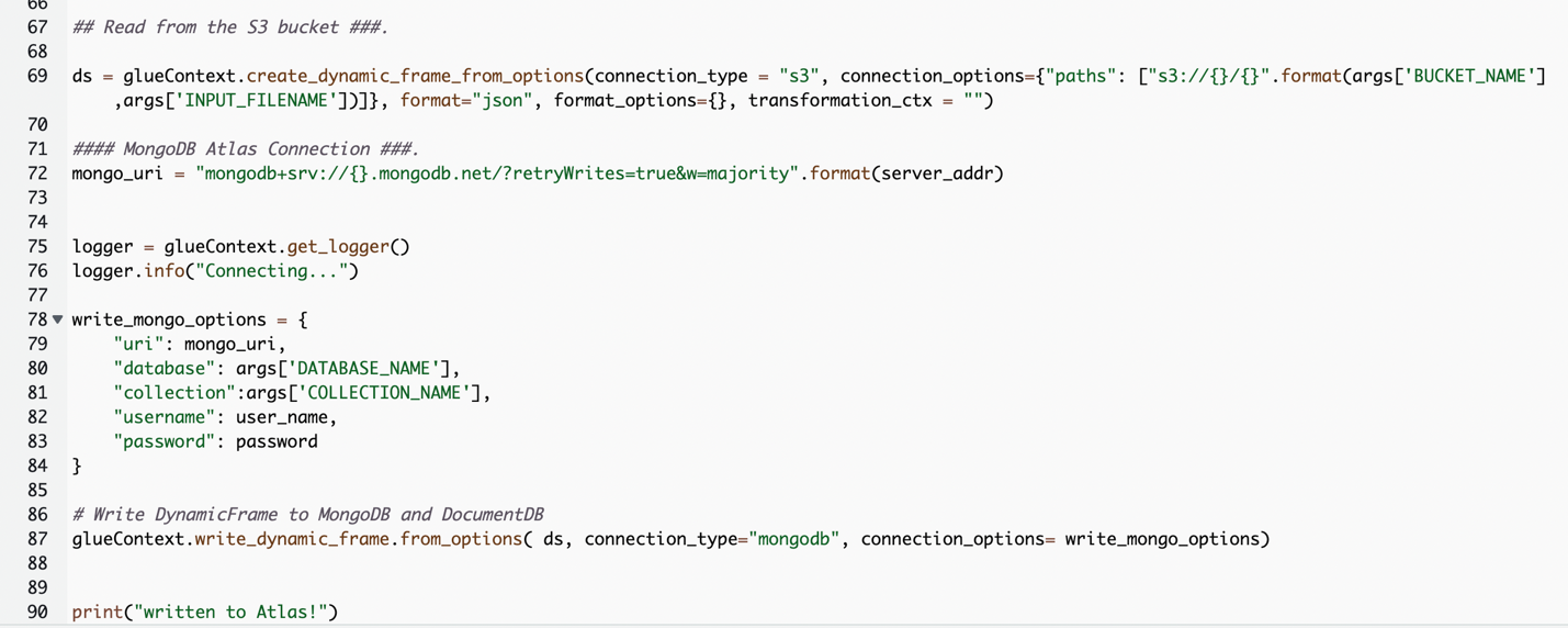
The code uses AWS Secrets Manager to retrieve the MongoDB Atlas cluster name, user name, and password. Then, it creates a DynamicFrame for the S3 bucket and file name passed to the script as parameters. The code retrieves the database and collection names from the job parameters configuration. Finally, the code writes the DynamicFrame to the MongoDB Atlas cluster using the retrieved parameters.
For more details, refer to Configure an IAM role for your ETL job.
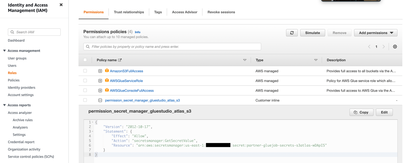


The following screenshot shows the results of a successful data load from an Amazon S3 bucket into the MongoDB Atlas cluster. The data is now available for queries in the MongoDB Atlas UI.
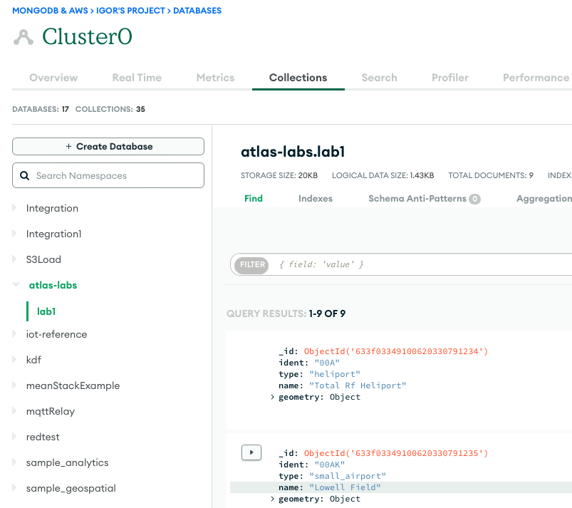
The following screenshot shows that the job ran successfully, with additional details such as links to the CloudWatch logs.

In this post, we described how to extract and ingest data to MongoDB Atlas using AWS Glue.
With AWS Glue ETL jobs, we can now transfer the data from MongoDB Atlas to AWS Glue-compatible sources, and vice versa. You can also extend the solution to build analytics using AWS AI and ML services.
To learn more, refer to the GitHub repository for step-by-step instructions and sample code. You can procure MongoDB Atlas on AWS Marketplace.

Igor Alekseev is a Senior Partner Solution Architect at AWS in Data and Analytics domain. In his role Igor is working with strategic partners helping them build complex, AWS-optimized architectures. Prior joining AWS, as a Data/Solution Architect he implemented many projects in Big Data domain, including several data lakes in Hadoop ecosystem. As a Data Engineer he was involved in applying AI/ML to fraud detection and office automation.
 Babu Srinivasan is a Senior Partner Solutions Architect at MongoDB. In his current role, he is working with AWS to build the technical integrations and reference architectures for the AWS and MongoDB solutions. He has more than two decades of experience in Database and Cloud technologies . He is passionate about providing technical solutions to customers working with multiple Global System Integrators(GSIs) across multiple geographies.
Post Syndicated from BeardedTinker original https://www.youtube.com/watch?v=MOJQU5zyoIY
Post Syndicated from Younggu Yun original https://aws.amazon.com/blogs/big-data/how-socar-handles-large-iot-data-with-amazon-msk-and-amazon-elasticache-for-redis/
This is a guest blog post co-written with SangSu Park and JaeHong Ahn from SOCAR.
As companies continue to expand their digital footprint, the importance of real-time data processing and analysis cannot be overstated. The ability to quickly measure and draw insights from data is critical in today’s business landscape, where rapid decision-making is key. With this capability, businesses can stay ahead of the curve and develop new initiatives that drive success.
This post is a continuation of How SOCAR built a streaming data pipeline to process IoT data for real-time analytics and control. In this post, we provide a detailed overview of streaming messages with Amazon Managed Streaming for Apache Kafka (Amazon MSK) and Amazon ElastiCache for Redis, covering technical aspects and design considerations that are essential for achieving optimal results.
SOCAR is the leading Korean mobility company with strong competitiveness in car-sharing. SOCAR wanted to design and build a solution for a new Fleet Management System (FMS). This system involves the collection, processing, storage, and analysis of Internet of Things (IoT) streaming data from various vehicle devices, as well as historical operational data such as location, speed, fuel level, and component status.
This post demonstrates a solution for SOCAR’s production application that allows them to load streaming data from Amazon MSK into ElastiCache for Redis, optimizing the speed and efficiency of their data processing pipeline. We also discuss the key features, considerations, and design of the solution.
SOCAR operates about 20,000 cars and is planning to include other large vehicle types such as commercial vehicles and courier trucks. SOCAR has deployed in-car devices that capture data using AWS IoT Core. This data was then stored in Amazon Relational Database Service (Amazon RDS). The challenge with this approach included inefficient performance and high resource usage. Therefore, SOCAR looked for purpose-built databases tailored to the needs of their application and usage patterns while meeting the future requirements of SOCAR’s business and technical requirements. The key requirements for SOCAR included achieving maximum performance for real-time data analytics, which required storing data in an in-memory data store.
After careful consideration, ElastiCache for Redis was selected as the optimal solution due to its ability to handle complex data aggregation rules with ease. One of the challenges faced was loading data from Amazon MSK into the database, because there was no built-in Kafka connector and consumer available for this task. This post focuses on the development of a Kafka consumer application that was designed to tackle this challenge by enabling performant data loading from Amazon MSK to Redis.
Extracting valuable insights from streaming data can be a challenge for businesses with diverse use cases and workloads. That’s why SOCAR built a solution to seamlessly bring data from Amazon MSK into multiple purpose-built databases, while also empowering users to transform data as needed. With fully managed Apache Kafka, Amazon MSK provides a reliable and efficient platform for ingesting and processing real-time data.
The following figure shows an example of the data flow at SOCAR.
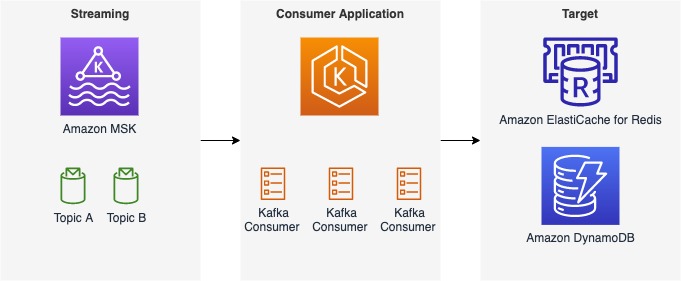
This architecture consists of three components:
Although this post focuses on a specific use case with ElastiCache for Redis as the target database and a single topic called gps, the consumer application we describe can handle additional topics and messages, as well as different streaming sources and target databases such as Amazon DynamoDB. Our post covers the most important aspects of the consumer application, including its features and components, design considerations, and a detailed guide to the code implementation.
The consumer application comprises three main parts that work together to consume, transform, and load messages from Amazon MSK into a target database. The following diagram shows an example of data transformations in the handler component.

The details of each component are as follows:
This connection has three features:
Note the following design considerations for the consumer application:
The producer of this solution is AWS IoT Core, which sends out messages into a topic called gps. The target database of this solution is ElastiCache for Redis. ElastiCache for Redis a fast in-memory data store that provides sub-millisecond latency to power internet-scale, real-time applications. Built on open-source Redis and compatible with the Redis APIs, ElastiCache for Redis combines the speed, simplicity, and versatility of open-source Redis with the manageability, security, and scalability from Amazon to power the most demanding real-time applications.
The target location can be either another database or storage depending on the use case and workload. SOCAR uses Amazon EKS to operate the containerized solution to achieve scalability, performance, and flexibility. Amazon EKS is a managed Kubernetes service to run Kubernetes in the AWS Cloud. Amazon EKS automatically manages the availability and scalability of the Kubernetes control plane nodes responsible for scheduling containers, managing application availability, storing cluster data, and other key tasks.
For the programming language, the SOCAR team decided to use the Go Programming language, utilizing both the AWS SDK for Go and a Goroutine, a lightweight logical or virtual thread managed by the Go runtime, which makes it easy to manage multiple threads. The AWS SDK for Go simplifies the use of AWS services by providing a set of libraries that are consistent and familiar for Go developers.
In the following sections, we walk through the steps to implement the solution:
For this walkthrough, you should have the following:
In this example, we use a topic called gps, and the consumer includes a Kafka client that receives messages from the topic. SOCAR created a struct and built a consumer (called NewConsumer in the code) to make it extendable. With this approach, any additional parameters and rules can be added easily.
To authenticate with Amazon MSK, SOCAR uses IAM. Because SOCAR already uses IAM to authenticate other resources, such as Amazon EKS, it uses the same IAM role (aws_msk_iam_v2) to authenticate clients for both Amazon MSK and Apache Kafka actions.
The following code creates the consumer:
The loader function, represented by the Loader struct, is responsible for loading messages to the target location, which in this case is ElastiCache for Redis. The NewLoader function initializes a new instance of the Loader struct with a logger and a Redis cluster client, which is used to communicate with the ElastiCache cluster. The redis.NewClusterClient object is initialized using the NewRedisClient function, which uses IAM to authenticate the client for Redis actions. This ensures secure and authorized access to the ElastiCache cluster. The Loader struct also contains the Close method to close the Kafka reader and free up resources.
The following code creates a loader:
A handler is used to include business rules and data transformation logic that prepares data before loading it into the target location. It acts as a bridge between a consumer and a loader. In this example, the topic name is cars.gps.json, and the message includes two keys, lng and lat, with data type Float64. The business logic can be defined in a function like handlerFuncGpsToRedis and then applied as follows:
Now you have created the consumer, loader, and handler. The next step is to build a consumer application using them. In a consumer application, you read messages from your stream with a consumer, transform them using a handler, and then load transformed messages into a target location with a loader. These three components are parameterized in a consumer application function such as the one shown in the following code:
To achieve maximum parallelism, SOCAR containerizes the consumer application and deploys it into multiple pods on Amazon EKS. Each consumer application contains a unique consumer, loader, and handler. For example, if you need to receive messages from a single topic with five partitions, you can deploy five identical consumer applications, each running in its own pod. Similarly, if you have two topics with three partitions each, you should deploy two consumer applications, resulting in a total of six pods. It’s a best practice to run one consumer application per topic, and the number of pods should match the number of partitions to enable concurrent message processing. The pod number can be specified in the Kubernetes deployment configuration
There are two stages in the Dockerfile. The first stage is the builder, which installs build tools and dependencies, and builds the application. The second stage is the runner, which uses a smaller base image (Alpine) and copies only the necessary files from the builder stage. It also sets the appropriate user permissions and runs the application. It’s also worth noting that the builder stage uses a specific version of the Golang image, while the runner stage uses a specific version of the Alpine image, both of which are considered to be lightweight and secure images.
The following code is an example of the Dockerfile:
In this post, we discussed SOCAR’s approach to building a consumer application that enables IoT real-time streaming from Amazon MSK to target locations such as ElastiCache for Redis. We hope you found this post informative and useful. Thank you for reading!
 SangSu Park is the Head of Operation Group at SOCAR. His passion is to keep learning, embrace challenges, and strive for mutual growth through communication. He loves to travel in search of new cities and places.
 JaeHong Ahn is a DevOps Engineer in SOCAR’s cloud infrastructure team. He is dedicated to promoting collaboration between developers and operators. He enjoys creating DevOps tools and is committed to using his coding abilities to help build a better world. He loves to cook delicious meals as a private chef for his wife.
 Younggu Yun works at AWS Data Lab in Korea. His role involves helping customers across the APAC region meet their business objectives and overcome technical challenges by providing prescriptive architectural guidance, sharing best practices, and building innovative solutions together.
Post Syndicated from Rohit Kumar original https://www.servethehome.com/nvidia-connectx-7-400gbe-and-ndr-infiniband-adapter-review-from-pny-supermicro-intel-sapphire-rapids/
We take a look at the NVIDIA ConnectX-7 400GbE and NDR Infiniband adapter to get wild performance from a low-profile PCIe Gen5 card
The post NVIDIA ConnectX-7 400GbE and NDR Infiniband Adapter Review from PNY appeared first on ServeTheHome.
Post Syndicated from James Beswick original https://aws.amazon.com/blogs/compute/patterns-for-building-an-api-to-upload-files-to-amazon-s3/
This blog is written by Thomas Moore, Senior Solutions Architect and Josh Hart, Senior Solutions Architect.
Applications often require a way for users to upload files. The traditional approach is to use an SFTP service (such as the AWS Transfer Family), but this requires specific clients and management of SSH credentials. Modern applications instead need a way to upload to Amazon S3 via HTTPS. Typical file upload use cases include:
If you have control over the application that sends the uploads, then you can integrate with the AWS SDK from within the browser with a framework such as AWS Amplify. To learn more, read Allowing external users to securely and directly upload files to Amazon S3.
Often you must provide end users direct access to upload files via an endpoint. You could build a bespoke service for this purpose, but this results in more code to build, maintain, and secure.
This post explores three different approaches to securely upload content to an Amazon S3 bucket via HTTPS without the need to build a dedicated API or client application.
The simplest option is to use API Gateway to proxy an S3 bucket. This allows you to expose S3 objects as REST APIs without additional infrastructure. By configuring an S3 integration in API Gateway, this allows you to manage authentication, authorization, caching, and rate limiting more easily.
This pattern allows you to implement an authorizer at the API Gateway level and requires no changes to the client application or caller. The limitation with this approach is that API Gateway has a maximum request payload size of 10 MB. For step-by-step instructions to implement this pattern, see this knowledge center article.
This is an example implementation (you can deploy this from Serverless Land):

The second pattern uses S3 presigned URLs, which allow you to grant access to S3 objects for a specific period, after which the URL expires. This time-bound access helps prevent unauthorized access to S3 objects and provides an additional layer of security.
They can be used to control access to specific versions or ranges of bytes within an object. This granularity allows you to fine-tune access permissions for different users or applications, and ensures that only authorized parties have access to the required data.
This avoids the 10 MB limit of API Gateway as the API is only used to generate the presigned URL, which is then used by the caller to upload directly to S3. Presigned URLs are straightforward to generate and use programmatically, but it does require the client to make two separate requests: one to generate the URL and one to upload the object. To learn more, read Uploading to Amazon S3 directly from a web or mobile application.
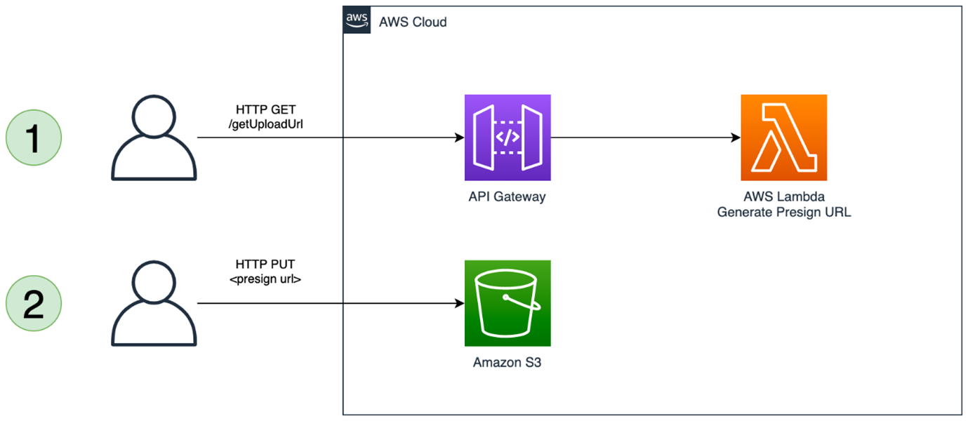
This pattern is limited by the 5GB maximum request size of the S3 Put Object API call. One way to work around this limit with this pattern is to leverage S3 multipart uploads. This requires that the client split the payload into multiple segments and send a separate request for each part.
This adds some complexity to the client and is used by libraries such as AWS Amplify that abstract away the multipart upload implementation. This allows you to upload objects up to 5TB in size. For more details, see uploading large objects to Amazon S3 using multipart upload and transfer acceleration.
An example of this pattern is available on Serverless Land.
The final pattern leverages Amazon CloudFront instead of API Gateway. CloudFront is primarily a content delivery network (CDN) that caches and delivers content from an S3 bucket or other origin. However, CloudFront can also be used to upload data to an S3 bucket. Without any additional configuration, this would essentially make the S3 bucket publicly writable. To secure the solution so that only authenticated users can upload objects, you can use a Lambda@Edge function to verify the users’ permissions.
The maximum size of the object that you can upload with this pattern is 5GB. If you need to upload files larger than 5GB, then you must use multipart uploads. To implement this, deploy the example Serverless Land pattern:

This pattern uses an origin access identity (OAI) to limit access to the S3 bucket to only come from CloudFront. The default OAI has s3:GetObject permission, which is changed to s3:PutObject to allow uploads explicitly and prevent and read operations:
{
    "Version": "2008-10-17",
    "Id": "PolicyForCloudFrontPrivateContent",
    "Statement": [
        {
            "Sid": "1",
            "Effect": "Allow",
            "Principal": {
                "AWS": "arn:aws:iam::cloudfront:user/CloudFront Origin Access Identity <origin access identity ID>"
            },
            "Action": [
                "s3:PutObject"
            ],
            "Resource": "arn:aws:s3::: DOC-EXAMPLE-BUCKET/*"
        }
    ]
}
As CloudFront is not used to cache content, the managed cache policy is set to CachingDisabled.
There are multiple options for implementing the authorization in the Lambda@Edge function. The sample repository uses an Amazon Cognito authorizer that validates a JSON Web Token (JWT) sent as an HTTP authorization header.
Using a JWT is secure as it implies this token is dynamically vended by an Identity Provider, such as Amazon Cognito. This does mean that the caller needs a mechanism to obtain this JWT token. You are in control of this authorizer function, and the exact implementation depends on your use-case. You could instead use an API Key or integrate with an alternate identity provider such as Auth0 or Okta.
Lambda@Edge functions do not currently support environment variables. This means that the configuration parameters are dynamically resolved at runtime. In the example code, AWS Systems Manager Parameter Store is used to store the Amazon Cognito user pool ID and app client ID that is required for the token verification. For more details on how to choose where to store your configuration parameters, see Choosing the right solution for AWS Lambda external parameters.
To verify the JWT token, the example code uses the aws-jwt-verify package. This supports JWTs issued by Amazon Cognito and third-party identity providers.
The Serverless Land pattern uses an Amazon Cognito identity provider to do authentication in the Lambda@Edge function. This code snippet shows an example using a pre-shared key for basic authorization:
import json

def lambda_handler(event, context):

    print(event)

    response = event["Records"][0]["cf"]["request"]
    headers = response["headers"]

    if 'authorization' not in headers or headers['authorization'] == None:
        return unauthorized()

    if headers['authorization'] == 'my-secret-key':
        return request

    return response

def unauthorized():
    response = {
            'status': "401",
            'statusDescription': 'Unauthorized',
            'body': 'Unauthorized'
        }
    return response
The Lambda function is associated with the CloudFront distribution by creating a Lambda trigger. The CloudFront event is set Viewer request to meaning the function is invoked in reaction to PUT events from the client.
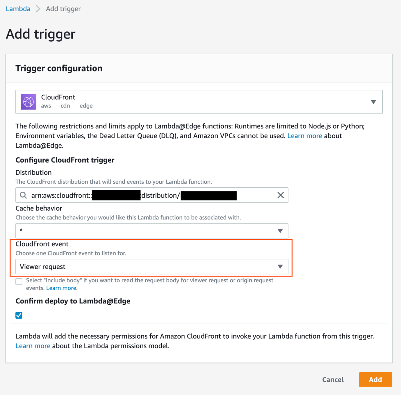
The solution can be tested with an API testing client, such as Postman. In Postman, issue a PUT request to https://<your-cloudfront-domain>/<object-name> with a binary payload as the body. You receive a 401 Unauthorized response.
Next, add the Authorization header with a valid token and submit the request again. For more details on how to obtain a JWT from Amazon Cognito, see the README in the repository. Now the request works and you receive a 200 OK message.
To troubleshoot, the Lambda function logs to Amazon CloudWatch Logs. For Lambda@Edge functions, look for the logs in the Region closest to the request, and not the same Region as the function.
The Lambda@Edge function in this example performs basic authorization. It validates the user has access to the requested resource. You can perform any custom authorization action here. For example, in a multi-tenant environment, you could restrict the prefix so that specific tenants only have permission to write to their own prefix, and validate the requested object name in the function.
Additionally, you could implement controls traditionally performed by the API Gateway such as throttling by tenant or user. Another use for the function is to validate the file type. If users can only upload images, you could validate the content-length to ensure the images are a certain size and the file extension is correct.
Which option you choose depends on your use case. This table summarizes the patterns discussed in this blog post:
| API Gateway as a proxy | Presigned URLs with API Gateway | CloudFront with Lambda@Edge | |
| Max Object Size | 10 MB | 5 GB (5 TB with multipart upload) | 5 GB |
| Client Complexity | Single HTTP Request | Multiple HTTP Requests | Single HTTP Request |
| Authorization Options | Amazon Cognito, IAM, Lambda Authorizer | Amazon Cognito, IAM, Lambda Authorizer | Lambda@Edge |
| Throttling | API Key throttling | API Key throttling | Custom throttling |
Each of the available methods has its strengths and weaknesses and the choice of which one to use depends on your specific needs. The maximum object size supported by S3 is 5 TB, regardless of which method you use to upload objects. Additionally, some methods have more complex configuration that requires more technical expertise. Considering these factors with your specific use-case can help you make an informed decision on the best API option for uploading to S3.
For more serverless learning resources, visit Serverless Land.
Post Syndicated from Geographics original https://www.youtube.com/watch?v=XTEnwdQaVyI