Tag Archives: Amazon EMR

How Paytm modernized their data pipeline using Amazon EMR

Post Syndicated from Rajat Bhardwaj original https://aws.amazon.com/blogs/big-data/how-paytm-modernized-their-data-pipeline-using-amazon-emr/

This post was co-written by Rajat Bhardwaj, Senior Technical Account Manager at AWS and Kunal Upadhyay, General Manager at Paytm.

Paytm is India’s leading payment platform, pioneering the digital payment era in India with 130 million active users. Paytm operates multiple lines of business, including banking, digital payments, bill recharges, e-wallet, stocks, insurance, lending and mobile gaming. At Paytm, the Central Data Platform team is responsible for turning disparate data from multiple business units into insights and actions for their executive management and merchants, who are small, medium or large business entities accepting payments from the Paytm platforms.

The Data Platform team modernized their legacy data pipeline with AWS services. The data pipeline collects data from different sources and runs analytical jobs, generating approximately 250K reports per day, which are consumed by Paytm executives and merchants. The legacy data pipeline was set up on premises using a proprietary solution and didn’t utilize the open-source Hadoop stack components such as Spark or Hive. This legacy setup was resource-intensive, having high CPU and I/O requirements. Analytical jobs took approximately 8–10 hours to complete, which often led to Service Level Agreements (SLA) breaches. The legacy solution was also prone to outages due to higher than expected hardware resource consumption. Its hardware and software limitations impacted the ability of the system to scale during peak load. Data models used in the legacy setup processed the entire data every time, which led to an increased processing time.

In this post, we demonstrate how the Paytm Central Data Platform team migrated their data pipeline to AWS and modernized it using Amazon EMR, Amazon Simple Storage Service (Amazon S3) and underlying AWS Cloud infrastructure along with Apache Spark. We optimized the hardware usage and reduced the data analytical processing, resulting in shorter turnaround time to generate insightful reports, all while maintaining operational stability and scale irrespective of the size of daily ingested data.

Overview of solution

The key to modernizing a data pipeline is to adopt an optimal incremental approach, which helps reduce the end-to-end cycle to analyze the data and get meaningful insights from it. To achieve this state, it’s vital to ingest incremental data in the pipeline, process delta records and reduce the analytical processing time. We configured the data sources to inherit the unchanged records and tuned the Spark jobs to only analyze the newly inserted or updated records. We used temporal data columns to store the incremental datasets until they’re processed. Data intensive Spark jobs are configured in incremental on-demand deduplicating mode to process the data. This helps to eliminate redundant data tuples from the data lake and reduces the total data volume, which saves compute and storage capacity. We also optimized the scanning of raw tables to restrict the scans to only the changed record set which reduced scanning time by approximately 90%. Incremental data processing also helps to reduce the total processing time.

At the time of this writing, the existing data pipeline has been operationally stable for 2 years. Although this modernization was vital, there is a risk of an operational outage while the changes are being implemented. Data skewing needs to be handled in the new system by an appropriate scaling strategy. Zero downtime is expected from the stakeholders because the reports generated from this system are vital for Paytm’s CXO, executive management and merchants on a daily basis.

The following diagram illustrates the data pipeline architecture.

Benefits of the solution

The Paytm Central Data Office team, comprised of 10 engineers, worked with the AWS team to modernize the data pipeline. The team worked for approximately 4 months to complete this modernization and migration project.

Modernizing the data pipeline with Amazon EMR 6.3 helped efficiently scale the system at a lower cost. Amazon EMR managed scaling helped reduce the scale-in and scale-out time and increase the usage of Amazon Elastic Compute Cloud (Amazon EC2) Spot Instances for running the Spark jobs. Paytm is now able to utilize a Spot to On-Demand ratio of 80:20, resulting in higher cost savings. Amazon EMR managed scaling also helped automatically scale the EMR cluster based on YARN memory usage with the desired type of EC2 instances. This approach eliminates the need to configure multiple Amazon EMR scaling policies tied to specific types of EC2 instances as per the compute requirements for running the Spark jobs.

In the following sections, we walk through the key tasks to modernize the data pipeline.

Migrate over 400 TB of data from the legacy storage to Amazon S3

Paytm team built a proprietary data migration application with the open-source AWS SDK for Java for Amazon S3 using the Scala programming language. This application can connect with multiple cloud providers , on-premises data centers and migrate the data to a central data lake built on Amazon S3.

Modernize the transformation jobs for over 40 data flows

Data flows are defined in the system for ingesting raw data, preprocessing the data and aggregating the data that is used by the analytical jobs for report generation. Data flows are developed using Scala programming language on Apache Spark. We use an Azkaban batch workflow job scheduler for ordering and tracking the Spark job runs. Workflows are created on Amazon EMR to schedule these Spark jobs multiple times during a day. We also implemented Spark optimizations to improve the operational efficiency for these jobs. We use Spark broadcast joins to handle the data skewness, which can otherwise lead to data spillage, resulting in extra storage needs. We also tuned the Spark jobs to avoid a  large number of small files, which is a known problem with Spark if not handled effectively. This is mainly because Spark is a parallel processing system and data loading is done through multiple tasks where each task can load into multiple partition. Data-intensive jobs are run using Spark stages.

The following is the code snippet for the Scala jobs:

nodes:
  - name: jobC
    type: noop
    # jobC depends on jobA and jobB
    dependsOn:
      - jobA
      - jobB

  - name: jobA
    type: command
    config:
      command: echo "This is an echoed text."

  - name: jobB
    type: command
    config:
      command: pwd

Validate the data

Accuracy of the data reports is vital for the modern data pipeline. The modernized pipeline has additional data reconciliation steps to improve the correctness of data across the platform. This is achieved by having greater programmatic control over the processed data. We could only reconcile data for the legacy pipeline after the entire data processing was complete. However, the modern data pipeline enables all the transactions to be reconciled at every step of the transaction, which gives granular control for data validation. It also helps isolate the cause of any data processing errors. Automated tests were done before go-live to compare the data records generated by the legacy vs. the modern system to ensure data sanity. These steps helped ensure the overall sanity of the processed data by the new system. Deduplication of data is done frequently via on-demand queries to eliminate redundant data, thereby reducing the processing time. As an example, if there are transactions which are already consumed by the end clients but still a part of the data-set, these can be eliminated by the deduplication, resulting in processing of only the newer transactions for the end client consumption.

The following sample query uses Spark SQL for on-demand deduplication of raw data at the reporting layer:

Insert over table  <<table>>
select col1,col2,col3 ---...coln 
from (select t.*
            ,row_number() over(order by col) as rn 
      from <<table>>
     ) t
where rn = 1

What we achieved as part of the modernization

With the new data pipeline, we reduced the compute infrastructure by 400% which helps to save  compute cost. The earlier legacy stack was running on over 6,000 virtual cores. Optimization techniques helped to run the same system at an improved scale, with approximately 1,500 virtual cores. We are able to reduce the compute and storage capacity for 400 TB of data and 40 data flows after migrating to Amazon EMR. We also achieved Spark optimizations, which helped to reduce the runtime of the jobs by 95% (from 8–10 hours to 20–30 minutes), CPU consumption by 95%, I/O by 98% and overall computation time by 80%. The incremental data processing approach helped to scale the system despite data skewness, which wasn’t the case with the legacy solution.

Conclusion

In this post, we showed how Paytm modernized their data lake and data pipeline using Amazon EMR, Amazon S3, underlying AWS Cloud infrastructure and Apache Spark. Choice of these cloud & big-data technologies helped to address the challenges for operating a big data pipeline because the type and volume of data from disparate sources adds complexity to the analytical processing.

By partnering with AWS, the Paytm Central Data Platform team created a modern data pipeline in a short amount of time. It provides reduced data analytical times with astute scaling capabilities, generating high-quality reports for the executive management and merchants on a daily basis.

As next steps, do a deep dive bifurcating the data collection and data processing stages for your data pipeline system. Each stage of the data pipeline should be appropriately designed and scaled to reduce the processing time while maintaining integrity of the reports generated as an output.

If you have feedback about this post, submit comments in the Comments section below.


About the Authors

Rajat Bhardwaj is a Senior Technical Manager with Amazon Web Services based in India, having 23 years of work experience with multiple roles in software development, telecom, and cloud technologies. He works along with AWS Enterprise customers, providing advocacy and strategic technical guidance to help plan and build solutions using AWS services and best practices. Rajat is an avid runner, having competed several half and full marathons in recent years.

Kunal Upadhyay is a General Manager with Paytm Central Data Platform team based out of Bengaluru, India. Kunal has 16 years of experience in big data, distributed computing, and data intelligence. When not building software, Kunal enjoys travel and exploring the world, spending time with friends and family.

Access Apache Livy using a Network Load Balancer on a Kerberos-enabled Amazon EMR cluster

Post Syndicated from Bharat Gamini original https://aws.amazon.com/blogs/big-data/access-apache-livy-using-a-network-load-balancer-on-a-kerberos-enabled-amazon-emr-cluster/

Amazon EMR is a cloud big data platform for running large-scale distributed data processing jobs, interactive SQL queries, and machine learning (ML) applications using open-source analytics frameworks such as Apache Spark, Apache Hive, and Presto. Amazon EMR supports Kerberos for authentication; you can enable Kerberos on Amazon EMR and put the cluster in a private subnet to maximize security.

To access the cluster, the best practice is to use a Network Load Balancer (NLB) to expose only specific ports, which are access-controlled via security groups. By default, the NLB prevents Kerberos ticket authentication to any Amazon EMR service.

Apache Livy is a service that enables easy interaction with a Spark cluster over a REST interface. It enables easy submission of Spark jobs or snippets of Spark code, synchronous or asynchronous result retrieval, as well as SparkContext management, all via a simple REST interface or an RPC client library.

In this post, we discuss how to provide Kerberos ticket access to Livy for external systems like Airflow and Notebooks using an NLB. You can apply this process to other Amazon EMR services beyond Livy, such as Trino and Hive.

Solution overview

The following are the high-level steps required:

  1. Create an EMR cluster with Kerberos security configuration.
  2. Create an NLB with required listeners and target groups.
  3. Update the Kerberos Key Distribution Center (KDC) to create a new service principal and keytab changes.
  4. Update the Livy configuration file.
  5. Verify Livy is accessible via the NLB.
  6. Run the Python Livy test case.

Prerequisites

The advanced configuration presented in this post assumes familiarity with Amazon EMR, Kerberos, Livy, Python and bash.

Create an EMR cluster

Create the Kerberos security configuration using the AWS Command Line Interface (AWS CLI) as follows (this creates the KDC on the EMR primary node):

aws emr create-security-configuration --name kdc-security-config --security-configuration '{
   "EncryptionConfiguration":{
      "InTransitEncryptionConfiguration":{
         "TLSCertificateConfiguration":{
            "CertificateProviderType":"PEM",
            "S3Object":"s3://${conf_bucket}/${certs.zip}"
         }
      },
      "AtRestEncryptionConfiguration":{
         "S3EncryptionConfiguration":{
            "EncryptionMode":"SSE-S3"
         }
      },
      "EnableInTransitEncryption":true,
      "EnableAtRestEncryption":true
   },
   "AuthenticationConfiguration":{
      "KerberosConfiguration":{
         "Provider":"ClusterDedicatedKdc",
         "ClusterDedicatedKdcConfiguration":{
            "TicketLifetimeInHours":24
         }
      }
   }
}'

It’s a security best practice to keep passwords in AWS Secrets Manager. You can use a bash function like the following as the argument to the --kerberos-attributes option so no passwords are stored in the launch script or command line. The function outputs the required JSON for the --kerberos-attributes option after retrieving the password from Secrets Manager.

krbattrs() { # Pull the KDC password from Secrets Manager without saving to disk or var
cat << EOF
  {
    "Realm": "EC2.INTERNAL",
    "KdcAdminPassword": "$(aws secretsmanager get-secret-value \
        --secret-id KDCpasswd  |jq -r .SecretString)"
  }
EOF
}

Create the cluster using the AWS CLI as follows:

aws emr create-cluster \
  --name "<your-cluster-name>" \
  --release-label emr-6.4.0 \
  --log-uri "s3://<your-log-bucket>" \
  --applications Name=Hive Name=Spark \
  --ec2-attributes "KeyName=<your-key-name>,SubnetId=<your-private-subnet>" \
  --instance-groups InstanceGroupType=MASTER,InstanceCount=1,InstanceType=m3.xlarge InstanceGroupType=CORE,InstanceCount=1,InstanceType=m3.xlarge \
  --security-configuration <kdc-security-config> \
  --kerberos-attributes $(krbattrs) \
  --use-default-roles

Create an NLB

Create an internet-facing NLB with TCP listeners in your VPC and subnet. An Internet-facing load balancer routes requests from clients to targets over the internet.  Conversely, an Internal NLB routes requests to targets using private IP addresses. For instructions, refer to Create a Network Load Balancer.

The following screenshot shows the listener details.

Create target groups and register the EMR primary instance (Livy3) and KDC instance (KDC3). For this post, these instances are the same; use the respective instances if KDC is running on a different instance.

The KDC and EMR security groups must allow the NLB’s private IP address to access ports 88 and 8998, respectively. You can find the NLB’s private IP address by searching the elastic network interfaces for the NLB’s name. For access control instructions, refer to this article on the knowledge center. Now that the security groups allow access, the NLB health check should pass, but Livy isn’t usable via the NLB until you make further changes (detailed in the following sections). The NLB is actually being used as a proxy to access Livy rather than doing any load balancing.

Update the Kerberos KDC

The KDC used by the Livy service must contain a new HTTP Service Principal Name (SPN) using the public NLB host name.

  • You can create the new principle from the EMR primary host using the full NLB public host name:
sudo kadmin.local addprinc HTTP/[email protected]

Replace the fully qualified domain name (FQDN) and Kerberos realm as needed. Ensure the NLB hostname is all lowercase.

After the new SPN exists, you create two keytabs containing that SPN. The first keytab is for the Livy service. The second keytab, which must use the same KVNO number as the first keytab, is for the Livy client.

  • Create Livy service keytab as follows:
sudo kadmin.local ktadd -norandkey -k /etc/livy2.keytab livy/[email protected]
sudo kadmin.local ktadd -norandkey -k /etc/livy2.keytab HTTP/[email protected]
sudo chown livy:livy /etc/livy2.keytab
sudo chmod 600 /etc/livy2.keytab
sudo -u livy klist -e -kt /etc/livy2.keytab

Note the key version number (KVNO) for the HTTP principal in the output of the preceding klist command. The KVNO numbers for the HTTP principal must match the KVNO numbers in the user keytab. Copy the livy2.keytab file to the EMR cluster Livy host if it’s not already there.

  • Create a user or client keytab as follows:
sudo kadmin.local ktadd -norandkey -k /var/tmp/user1.keytab [email protected]
sudo kadmin.local ktadd -norandkey -k /var/tmp/user1.keytab HTTP/[email protected]

Note the -norandkey option used when adding the SPN. That preserves the KVNO created in the preceding livy2.keytab.

  • Copy the user1.keytab to the client machine running the Python test case as user1.

Replace the FQDN, realm, and keytab path as needed.

Update the Livy configuration file

The primary change on the EMR cluster primary node running the Livy service is to the /etc/livy/conf/livy.conf file. You change the authentication principal that Livy uses, as well as the associated Kerberos keytab created earlier.

  • Make the following changes to the livy.conf file with sudo:
livy.server.auth.kerberos.principal = HTTP/[email protected]
livy.server.auth.kerberos.keytab = /etc/livy2.keytab

Don’t change the livy.server.launch.kerberos.* values.

  • Restart and verify the Livy service:
sudo systemctl restart livy-server
sudo systemctl status livy-server
  • Verify the Livy port is listening:
sudo lsof -Pi :8998

COMMAND PID USER FD TYPE DEVICE SIZE/OFF NODE NAME
java 30106 livy 196u IPv6 224853844 0t0 TCP *:8998 (LISTEN)

You can automate these steps (modifying the KDC and Livy config file) by adding a step to the EMR cluster. For more information, refer to Tutorial: Configure a cluster-dedicated KDC.

Verify Livy is accessible via the NLB

You can now use user1.keytab to authenticate against the Livy REST endpoint. Copy the user1.keytab you created earlier to the host and user login, which run the Livy test case. The host running the test case must be configured to connect to the modified KDC.

  • Create a Linux user (user1) on client host and EMR cluster.

If the client host has a terminal available that the user can run commands in, you can use the following commands to verify network connectivity to Livy before running the actual Livy Python test case.

  • Verify the NLB host and port are reachable (no data will be returned by the nc command):
$ nc -vz mynlb-a0ac4b07f9f7f0a1.elb.us-west-2.amazonaws.com 8998
Ncat: Version 7.50 ( https://nmap.org/ncat )
Ncat: Connected to 44.242.1.1:8998.
Ncat: 0 bytes sent, 0 bytes received in 0.02 seconds.
  • Create a TLS connection, which returns the server’s TLS certificate and TCP packets:
openssl s_client -connect mynlb-a0ac4b07f9f7f0a1.elb.us-west-2.amazonaws.com:8998

If the openssl command doesn’t return a TLS server certificate, the rest of the verification doesn’t succeed. You may have a proxy or firewall interfering with the connection. Investigate your network environment, resolve the issue, and repeat the openssl command to ensure connectivity.

  • Verify the Livy REST endpoint using curl. This verifies Livy REST but not Spark.
kinit -kt user1.keytab [email protected]
curl -k -u : --negotiate https://mynlb-a0ac4b07f9f7f0a1.elb.us-west-2.amazonaws.com:8998/sessions
{"from":0,"total":0,"sessions":[]}

curl arguments:
  "-k"   - Ignore secure connection check
  "-u :" - Use user name and passwords from environment
  "--negotiate" – Enables negotiate(SPNEGO) authentication

Run the Python Livy test case

The Livy test case is a simple Python3 script named livy-verify.py. You can run this script from a client machine to run Spark commands via Livy using the NLB. The script is as follows:

#!/usr/bin/env python3
# pylint: disable=invalid-name,no-member

"""
Verify Livy (REST) service using pylivy module, install req modules or use PEX:
  sudo yum install python3-devel
  sudo python3 -m pip install livy==0.8.0 requests==2.27.1 requests_gssapi==1.2.3
  https://pypi.org/project/requests-gssapi/

Kerberos authN implicitly uses TGT from kinit in users login env
"""

import shutil
import requests
from requests_gssapi import HTTPSPNEGOAuth
from livy import LivySession

# Disable ssl-warnings for self-signed certs when testing
requests.packages.urllib3.disable_warnings()

# Set the base URI(use FQDN and TLS) to target a Livy service
# Redefine remote_host to specify the remote Livy hostname to connect to
remote_host="mynlb-a0ac4b07f9f7f0a1.elb.us-west-2.amazonaws.com"
livy_uri = "https://" + remote_host + ":8998"

def livy_session():
    ''' Connect to Livy (REST) and run trivial pyspark command '''
    sconf = {"spark.master": "yarn", "spark.submit.deployMode": "cluster"}

    if shutil.which('kinit'):
        kauth = HTTPSPNEGOAuth()
        # Over-ride with an explicit user principal
        #kauth = HTTPSPNEGOAuth(principal="[email protected]")
        print("kinit found, kauth using Krb cache")
    else:
        kauth = None
        print("kinit NOT found, kauth set to None")

    with LivySession.create(livy_uri, verify=False, auth=kauth, spark_conf=sconf) as ls:
        ls.run("rdd = sc.parallelize(range(100), 2)")
        ls.run("rdd.take(3)")

    return 'LivySession complete'

def main():
    """ Starting point """
    livy_session()

if __name__ == '__main__':
    main()

The test case requires the new SPN to be in the user’s Kerberos ticket cache. To get the service principal into the Kerberos cache, use the kinit command with the -S option:

kinit -kt user1.keytab -S HTTP/[email protected] [email protected]

Note the SPN and the User Principal Name (UPN) are both used in the kinit command.

The Kerberos cache should look like the following code, as revealed by the klist command:

klist
Ticket cache: FILE:/tmp/krb5cc_1001
Default principal: [email protected]

Valid starting Expires Service principal
01/20/2022 01:38:06 01/20/2022 11:38:06 HTTP/[email protected]
renew until 01/21/2022 01:38:06

Note the HTTP service principal in the klist ticket cache output.

After the SPN is in the cache as verified by klist, you can run the following command to verify that Livy accepts the Kerberos ticket and runs the simple PySpark script. It generates a simple array, [0,1,2], as the output. The preceding Python script has been copied to the /var/tmp/user1/ folder in this example.

/var/tmp/user1/livy-verify.py
kinit found, kauth using TGT
[0, 1, 2]

It can take a minute or so to generate the result. Any authentication errors will happen in seconds. If the test in the new environment generates the preceding array, the Livy Kerberos configuration has been verified.

Any other client program that needs to have Livy access must be a Kerberos client of the KDC that generated the keytabs. It must also have a client keytab (such as user1.keytab or equivalent) and the service principal key in its Kerberos ticket cache.

In some environments, a simple kinit as follows may be sufficient:

kdestroy
kinit -kt user1.keytab [email protected]

Summary

If you have an existing EMR cluster running Livy and using Kerberos (even in a private subnet), you can add an NLB to connect to the Livy service and still authenticate with Kerberos. For simplicity, we used a cluster-dedicated KDC in this post, but you can use any KDC architecture option supported by Amazon EMR. This post documented all the KDC and Livy changes to make it work; the script and procedure have been run successfully in multiple environments. You can modify the Python script as needed and try running the verification script in your environment.

For more details about the systems and processes described in this post, refer to the following:


About the Authors

John Benninghoff is a AWS Professional Services Sr. Data Architect, focused on Data Lake architecture and implementation.

Bharat Gamini is a Data Architect focused on Big Data & Analytics at Amazon Web Services. He helps customers architect and build highly scalable, robust and secure cloud-based analytical solutions on AWS. Besides family time, he likes watching movies and sports.

Amazon EMR on Amazon EKS provides up to 61% lower costs and up to 68% performance improvement for Spark workloads

Post Syndicated from Melody Yang original https://aws.amazon.com/blogs/big-data/amazon-emr-on-amazon-eks-provides-up-to-61-lower-costs-and-up-to-68-performance-improvement-for-spark-workloads/

Amazon EMR on Amazon EKS is a deployment option offered by Amazon EMR that enables you to run Apache Spark applications on Amazon Elastic Kubernetes Service (Amazon EKS) in a cost-effective manner. It uses the EMR runtime for Apache Spark to increase performance so that your jobs run faster and cost less.

Amazon EMR on Amazon EKS is a deployment option offered by Amazon EMR that enables you to run Apache Spark applications on Amazon Elastic Kubernetes Service (Amazon EKS) in a cost-effective manner. It uses the EMR runtime for Apache Spark to increase performance so that your jobs run faster and cost less.

In our benchmark tests using TPC-DS datasets at 3 TB scale, we observed that Amazon EMR on EKS provides up to 61% lower costs and up to 68% improved performance compared to running open-source Apache Spark on Amazon EKS via equivalent configurations. In this post, we walk through the performance test process, share the results, and discuss how to reproduce the benchmark. We also share a few techniques to optimize job performance that could lead to further cost-optimization for your Spark workloads.

How does Amazon EMR on EKS reduce cost and improve performance?

The EMR runtime for Spark is a performance-optimized runtime for Apache Spark that is 100% API compatible with open-source Apache Spark. It’s enabled by default with Amazon EMR on EKS. It helps run Spark workloads faster, leading to lower running costs. It includes multiple performance optimization features, such as Adaptive Query Execution (AQE), dynamic partition pruning, flattening scalar subqueries, bloom filter join, and more.

In addition to the cost benefit brought by the EMR runtime for Spark, Amazon EMR on EKS can take advantage of other AWS features to further optimize cost. For example, you can run Amazon EMR on EKS jobs on Amazon Elastic Compute Cloud (Amazon EC2) Spot Instances, providing up to 90% cost savings when compared to On-Demand Instances. Also, Amazon EMR on EKS supports Arm-based Graviton EC2 instances, which creates a 15% performance improvement and up to 30% cost savings when compared a Graviton2-based M6g to M5 instance type.

The recent graceful executor decommissioning feature makes Amazon EMR on EKS workloads more robust by enabling Spark to anticipate Spot Instance interruptions. Without the need to recompute or rerun impacted Spark jobs, Amazon EMR on EKS can further reduce job costs via critical stability and performance improvements.

Additionally, through container technology, Amazon EMR on EKS offers more options to debug and monitor Spark jobs. For example, you can choose Spark History Server, Amazon CloudWatch, or Amazon Managed Prometheus and Amazon Managed Grafana (for more details, refer to the Monitoring and Logging workshop). Optionally, you can use familiar command line tools such as kubectl to interact with a job processing environment and observe Spark jobs in real time, which provides a fail-fast and productive development experience.

Amazon EMR on EKS supports multi-tenant needs and offers application-level security control via a job execution role. It enables seamless integrations to other AWS native services without a key-pair set up in Amazon EKS. The simplified security design can reduce your engineering overhead and lower the risk of data breach. Furthermore, Amazon EMR on EKS handles security and performance patches so you can focus on building your applications.

Benchmarking

This post provides an end-to-end Spark benchmark solution so you can get hands-on with the performance test process. The solution uses unmodified TPC-DS data schema and table relationships, but derives queries from TPC-DS to support the Spark SQL test case. It is not comparable to other published TPC-DS benchmark results.

Key concepts

Transaction Processing Performance Council-Decision Support (TPC-DS) is a decision support benchmark that is used to evaluate the analytical performance of big data technologies. Our test data is a TPC-DS compliant dataset based on the TPC-DS Standard Specification, Revision 2.4 document, which outlines the business model and data schema, relationship, and more. As the whitepaper illustrates, the test data contains 7 fact tables and 17 dimension tables, with an average of 18 columns. The schema consists of essential retailer business information, such as customer, order, and item data for the classic sales channels: store, catalog, and internet. This source data is designed to represent real-world business scenarios with common data skews, such as seasonal sales and frequent names. Additionally, the TPC-DS benchmark offers a set of discrete scaling points (scale factors) based on the approximate size of the raw data. In our test, we chose the 3 TB scale factor, which produces 17.7 billion records, approximately 924 GB compressed data in Parquet file format.

Test approach

A single test session consists of 104 Spark SQL queries that were run sequentially. To get a fair comparison, each session of different deployment types, such as Amazon EMR on EKS, was run three times. The average runtime per query from these three iterations is what we analyze and discuss in this post. Most importantly, it derives two summarized metrics to represent our Spark performance:

  • Total execution time – The sum of the average runtime from three iterations
  • Geomean – The geometric mean of the average runtime

 Test results

In the test result summary (see the following figure), we discovered that the Amazon EMR-optimized Spark runtime used by Amazon EMR on EKS is approximately 2.1 times better than the open-source Spark on Amazon EKS in geometric mean and 3.5 times faster by the total runtime.

The following figure breaks down the performance summary by queries. We observed that EMR runtime for Spark was faster in every query compared to open-source Spark. Query q67 was the longest query in the performance test. The average runtime with open-source Spark was 1019.09 seconds. However, it took 150.02 seconds with Amazon EMR on EKS, which is 6.8 times faster. The highest performance gain in these long-running queries was q72—319.70 seconds (open-source Spark) vs. 26.86 seconds (Amazon EMR on EKS), a 11.9 times improvement.

Test cost

Amazon EMR pricing on Amazon EKS is calculated based on the vCPU and memory resources used from the time you start to download your EMR application Docker image until the Amazon EKS pod terminates. As a result, you don’t pay any Amazon EMR charges until your application starts to run, and you only pay for the vCPU and memory used during a job—you don’t pay for the full amount of compute resources in an EC2 instance.

Overall, the estimated benchmark cost in the US East (N. Virginia) Region is $22.37 per run for open-source Spark on Amazon EKS and $8.70 per run for Amazon EMR on EKS – that’s 61% cheaper due to the 68% quicker job runtime. The following table provides more details.

Benchmark Job Runtime (Hour) Estimated Cost Total EC2 Instance Total vCPU Total Memory (GiB) Root Device (EBS)
Amazon EMR on EKS 0.68 $8.70 6 216 432 20 GiB gp2
Open-Source Spark on Amazon EKS 2.13 $22.37 6 216 432 20 GiB gp2

Amazon EMR on Amazon EC2

(1 primary and 5 core nodes)

0.80 $8.80 6 196 424 20 GiB gp2

The cost estimate doesn’t account for Amazon Simple Storage Service (Amazon S3) storage, or PUT and GET requests. The Amazon EMR on EKS uplift calculation is based on the hourly billing information provided by AWS Cost Explorer.

Cost breakdown

The following is the cost breakdown for the Amazon EMR on EKS job ($8.70): 

  • Total uplift on vCPU – (126.93 * $0.01012) = (total number of vCPU used * per vCPU-hours rate) = $1.28
  • Total uplift on memory – (258.7 * $0.00111125) = (total amount of memory used * per GB-hours rate) = $0.29
  • Total Amazon EMR uplift cost – $1.57
  • Total Amazon EC2 cost – (6 * $1.728 * 0.68) = (number of instances * c5d.9xlarge hourly rate * job runtime in hour) = $7.05
  • Other costs – ($0.1 * 0.68) + ($0.1/730 * 20 * 6 * 0.68) = (shared Amazon EKS cluster charge per hour * job runtime in hour) + (EBS per GB-hourly rate * root EBS size * number of instances * job runtime in hour) = $0.08 

The following is the cost breakdown for the open-source Spark on Amazon EKS job ($22.37): 

  • Total Amazon EC2 cost – (6 * $1.728 * 2.13) = (number of instances * c5d.9xlarge hourly rate * job runtime in hour) = $22.12
  • Other costs – ($0.1 * 2.13) + ($0.1/730 * 20 * 6 * 2.13) = (shared EKS cluster charge per hour * job runtime in hour) + (EBS per GB-hourly rate * root EBS size * number of instances * job runtime in hour) = $0.25

The following is the cost breakdown for the Amazon EMR on Amazon EC2 ($8.80):

  • Total Amazon EMR cost – (5 * $0.27 * 0.80) + (1 * $0.192 * 0.80) = (number of core nodes * c5d.9xlarge Amazon EMR price * job runtime in hour) + (number of primary nodes * m5.4xlarge Amazon EMR price * job runtime in hour) = $1.23
  • Total Amazon EC2 cost – (5 * $1.728 * 0.80) + (1 * $0.768 * 0.80) = (number of core nodes * c5d.9xlarge instance price * job runtime in hour) + (number of primary nodes * m5.4xlarge instance price * job runtime in hour) = $7.53
  • Other Cost – ($0.1/730 * 20 GiB * 6 * 0.80) + ($0.1/730 * 256 GiB * 1 * 0.80) = (EBS per GB-hourly rate * root EBS size * number of instances * job runtime in hour) + (EBS per GB-hourly rate * default EBS size for m5.4xlarge * number of instances * job runtime in hour) = $0.041

Benchmarking considerations

In this section, we share some techniques and considerations for the benchmarking.

Set up an Amazon EKS cluster with Availability Zone awareness

Our Amazon EKS cluster configuration looks as follows:

apiVersion: eksctl.io/v1alpha5
kind: ClusterConfig
metadata:
  name: $EKSCLUSTER_NAME
  region: us-east-1
availabilityZones:["us-east-1a"," us-east-1b"]  
managedNodeGroups: 
  - name: mn-od
    availabilityZones: ["us-east-1b"] 

In the cluster configuration, the mn-od managed node group is assigned to the single Availability Zone b, where we run the test against.

Availability Zones are physically separated by a meaningful distance from other Availability Zones in the same AWS Region. This produces round trip latency between two compute instances located in different Availability Zones. Spark implements distributed computing, so exchanging data between compute nodes is inevitable when performing data joins, windowing, and aggregations across multiple executors. Shuffling data between multiple Availability Zones adds extra latency to the network I/O, which therefore directly impacts Spark performance. Additionally, when data is transferred between two Availability Zones, data transfer charges apply in both directions.

For this benchmark, which is a time-sensitive workload, we recommend running in a single Availability Zone and using On-Demand instances (not Spot) to have a dedicated compute resource. In an existing Amazon EKS cluster, you may have multiple instance types and a Multi-AZ setup. You can use the following Spark configuration to achieve the same goal:

--conf spark.kubernetes.node.selector.eks.amazonaws.com/capacityType=ON_DEMAND
--conf spark.kubernetes.node.selector.topology.kubernetes.io/zone=us-east-1b

Use instance store volume to increase disk I/O

Spark data shuffle, the process of reading and writing intermediate data to disk, is a costly operation. Besides the network I/O speed, Spark demands high performant disk to support a large amount of data redistribution activities. I/O operations per second (IOPS) is an equally important measure to baseline Spark performance. For instance, the SQL queries 23a, 23b, 50, and 93 are shuffle-intensive Spark workloads in TPC-DS, so choosing an optimal storage strategy can significantly shorten their runtime. General speaking, the recommended options are either attaching multiple EBS disk volumes per node in Amazon EKS or using the d series EC2 instance type, which offers high disk I/O performance within a compute family (for example, c5d.9xlarge is the d series in the c5 compute optimized family).

The following table summarizes the hardware specification we used:

Instance On-Demand Hourly Price vCPU Memory (GiB) Instance Store Networking Performance (Gbps) 100% Random Read IOPS Write IOPS
c5d.9xlarge $1.73 36 72 1 x 900GB NVMe SSD 10 350,000 170,000

To simplify our hardware configuration, we chose the AWS Nitro System EC2 instance type c5d.9xlarge, which comes with a NVMe-based SSD instance store volume. As of this writing, the built-in NVMe SSD disk requires less effort to set up and provides optimal disk performance we need. In the following code, the one-off preBoostrapCommand is triggered to mount an instance store to a node in Amazon EKS:

managedNodeGroups: 
  - name: mn-od
    preBootstrapCommands:
      - "sleep 5; sudo mkfs.xfs /dev/nvme1n1;sudo mkdir -p /local1;sudo echo /dev/nvme1n1 /local1 xfs defaults,noatime 1 2 >> /etc/fstab"
      - "sudo mount -a"
      - "sudo chown ec2-user:ec2-user /local1"

Run as a predefined job user, not a root user

For security, it’s not recommended to run Spark jobs as a root user. But how can you access the NVMe SSD volume mounted to the Amazon EKS cluster as a non-root Spark user?

An init container is created for each Spark driver and executor pods in order to set the volume permission and control the data access. Let’s check out the Spark driver pod via the kubectl exec command, which allows us execute into the running container and have an interactive session. We can observe the following:

  • The init container is called volume-permission.
  • The SSD disk is called /ossdata1. The Spark driver has stored some data to the disk.
  • The non-root Spark job user is called hadoop.

This configuration is provided in a format of a pod template file for Amazon EMR on EKS, so you can dynamically tailor job pods when Spark configuration doesn’t support your needs. Be aware that the predefined user’s UID in the EMR runtime for Spark is 999, but it’s set to 1000 in open-source Spark. The following is a sample Amazon EMR on EKS driver pod template:

apiVersion: v1
kind: Pod
spec:
  nodeSelector:
    app: sparktest
  volumes:
    - name: spark-local-dir-1
      hostPath:
        path: /local1  
  initContainers:  
  - name: volume-permission
    image: public.ecr.aws/y4g4v0z7/busybox
    # grant volume access to "hadoop" user with uid 999
    command: ['sh', '-c', 'mkdir /data1; chown -R 999:1000 /data1'] 
    volumeMounts:
      - name: spark-local-dir-1
        mountPath: /data1
  containers:
  - name: spark-kubernetes-driver
    volumeMounts:
      - name: spark-local-dir-1
        mountPath: /data1

In the job submission, we map the pod templates via the Spark configuration:

"spark.kubernetes.driver.podTemplateFile": "s3://'$S3BUCKET'/pod-template/driver-pod-template.yaml",
"spark.kubernetes.executor.podTemplateFile": "s3://'$S3BUCKET'/pod-template/executor-pod-template.yaml",

Spark on k8s operator is a popular tool to deploy Spark on Kubernetes. Our open-source Spark benchmark uses the tool to submit the job to Amazon EKS. However, the Spark operator currently doesn’t support file-based pod template customization, due to the way it operates. So we embed the disk permission setup into the job definition, as in the example on GitHub.

Disable dynamic resource allocation and enable Adaptive Query Execution in your application

Spark provides a mechanism to dynamically adjust compute resources based on workload. This feature is called dynamic resource allocation. It provides flexibility and efficiency to manage compute resources. For example, your application may give resources back to the cluster if they’re no longer used, and may request them again later when there is demand. It’s quite useful when your data traffic is unpredictable and an elastic compute strategy is needed at your application level. While running the benchmarking, our source data volume (3 TB) is certain and the jobs were run on a fixed-size Spark cluster that consists of six EC2 instances. You can turn off the dynamic allocation in EMR on EC2 as shown in the following code, because it doesn’t suit our purpose and might add latency to the test result. The rest of Spark deployment options, such as Amazon EMR on EKS, has the dynamic allocation off by default, so we can ignore these settings.

--conf spark.dynamicAllocation.enabled=false 
--conf spark.shuffle.service.enabled=false

Dynamic resource allocation is a different concept from automatic scaling in Amazon EKS, such as the Cluster Autoscaler. Disabling the dynamic allocation feature only fixes our 6-node Spark cluster size per job, but doesn’t stop the Amazon EKS cluster from expanding or shrinking automatically. It means our Amazon EKS cluster is still able to scale between 1 and 30 EC2 instances, as configured in the following code:

managedNodeGroups: 
  - name: mn-od
    availabilityZones: ["us-east-1b"] 
    instanceType: c5d.9xlarge
    minSize: 1
    desiredCapacity: 1
    maxSize: 30

Spark Adaptive Query Execution (AQE) is an optimization technique in Spark SQL since Spark 3.0. It dynamically re-optimizes the query execution plan at runtime, which supports a variety of optimizations, such as the following:

  • Dynamically switch join strategies
  • Dynamically coalesce shuffle partitions
  • Dynamically handle skew joins

The feature is enabled by default in EMR runtime for Spark, but disabled by default in open-source Apache Spark 3.1.2. To provide the fair comparison, make sure it’s set in the open-source Spark benchmark job declaration:

  sparkConf:
    # Enable AQE
    "spark.sql.adaptive.enabled": "true"
    "spark.sql.adaptive.localShuffleReader.enabled": "true"
    "spark.sql.adaptive.coalescePartitions.enabled": "true"
    "spark.sql.adaptive.skewJoin.enabled": "true"

Walkthrough overview

With these considerations in mind, we run three Spark jobs in Amazon EKS. This helps us compare Spark 3.1.2 performance in various deployment scenarios. For more details, check out the GitHub repository.

In this walkthrough, we show you how to do the following:

  • Produce a 3 TB TPC-DS complaint dataset
  • Run a benchmark job with the open-source Spark operator on Amazon EKS
  • Run the same benchmark application with Amazon EMR on EKS

We also provide information on how to benchmark with Amazon EMR on Amazon EC2.

Prerequisites

Install the following tools for the benchmark test:

Provision resources

The provision script creates the following resources:

  • A new Amazon EKS cluster
  • Amazon EMR on EKS enabler
  • The required AWS Identity and Access Management (IAM) roles
  • The S3 bucket emr-on-eks-nvme-${ACCOUNTID}-${AWS_REGION}, referred to as <S3BUCKET> in the following steps

The provisioning process takes approximately 30 minutes.

  1. Download the project with the following command:
    git clone https://github.com/aws-samples/emr-on-eks-bencharmk.git
    cd emr-on-eks-bencharmk

  2. Create a test environment (change the Region if necessary):
    export EKSCLUSTER_NAME=eks-nvme
    export AWS_REGION=us-east-1
    
    ./provision.sh

Modify the script if needed for testing against an existing Amazon EKS cluster. Make sure the existing cluster has the Cluster Autoscaler and Spark Operator installed. Examples are provided by the script.

  1. Validate the setup:
    # should return results
    kubectl get pod -n oss | grep spark-operator
    kubectl get pod -n kube-system | grep nodescaler

Generate TPC-DS test data (optional)

In this optional task, you generate TPC-DS test data in s3://<S3BUCKET>/BLOG_TPCDS-TEST-3T-partitioned. The process takes approximately 80 minutes.

The job generates TPC-DS compliant datasets with your preferred scale. In this case, it creates 3 TB of source data (approximately 924 GB compressed) in Parquet format. We have pre-populated the source dataset in the S3 bucket blogpost-sparkoneks-us-east-1 in Region us-east-1. You can skip the data generation job if you want to have a quick start.

Be aware of that cross-Region data transfer latency will impact your benchmark result. It’s recommended to generate the source data to your S3 bucket if your test Region is different from us-east-1.

  1. Start the job:
    kubectl apply -f examples/tpcds-data-generation.yaml

  2. Monitor the job progress:
    kubectl get pod -n oss
    kubectl logs tpcds-data-generation-3t-driver -n oss

  3. Cancel the job if needed:
    kubectl delete -f examples/tpcds-data-generation.yaml

The job runs in the namespace oss with a service account called oss in Amazon EKS, which grants a minimum permission to access the S3 bucket via an IAM role. Update the example .yaml file if you have a different setup in Amazon EKS.

Benchmark for open-source Spark on Amazon EKS

Wait until the data generation job is complete, then update the default input location parameter (s3://blogpost-sparkoneks-us-east-1/blog/BLOG_TPCDS-TEST-3T-partitioned) to your S3 bucket in the tpcds-benchmark.yaml file.. Other parameters in the application can also be adjusted. Check out the comments in the yaml file for details. This process takes approximately 130 minutes.

If the data generation job is skipped, run the following steps without waiting.

  1. Start the job:
    kubectl apply -f examples/tpcds-benchmark.yaml

  2. Monitor the job progress:
    kubectl get pod -n oss
    kubectl logs tpcds-benchmark-oss-driver -n oss

  3. Cancel the job if needed:
    kubectl delete -f examples/tpcds-benchmark.yaml

The benchmark application outputs a CSV file capturing runtime per Spark SQL query and a JSON file with query execution plan details. You can use the collected metrics and execution plans to compare and analyze performance between different Spark runtimes (open-source Apache Spark vs. EMR runtime for Spark).

Benchmark with Amazon EMR on EKS

Wait for the data generation job finish before starting the benchmark for Amazon EMR on EKS. Don’t forget to change the input location (s3://blogpost-sparkoneks-us-east-1/blog/BLOG_TPCDS-TEST-3T-partitioned) to your S3 bucket. The output location is s3://<S3BUCKET>/EMRONEKS_TPCDS-TEST-3T-RESULT. If you use the pre-populated TPC-DS dataset, start the Amazon EMR on EKS benchmark without waiting. This process takes approximately 40 minutes.

  1. Start the job (change the Region if necessary):
    export EMRCLUSTER_NAME=emr-on-eks-nvme
    export AWS_REGION=us-east-1
    
    ./examples/emr6.5-benchmark.sh

Amazon EKS offers multi-tenant isolation and optimized resource allocation features, so it’s safe to run two benchmark tests in parallel on a single Amazon EKS cluster.

  1. Monitor the job progress in real time:
    kubectl get pod -n emr
    #run the command then search "execution time" in the log to analyze individual query's performance
    kubectl logs YOUR_DRIVER_POD_NAME -n emr spark-kubernetes-driver

  2. Cancel the job (get the IDs from the cluster list on the Amazon EMR console):
    aws emr-containers cancel-job-run --virtual-cluster-id <YOUR_VIRTUAL_CLUSTER_ID> --id <YOUR_JOB_ID>

The following are additional useful commands:

#Check volume status
kubectl exec -it YOUR_DRIVER_POD_NAME -c spark-kubernetes-driver -n emr -- df -h

#Login to a running driver pod
kubectl exec -it YOUR_DRIVER_POD_NAME -c spark-kubernetes-driver -n emr – bash

#Monitor compute resource usage
watch "kubectl top node"

Benchmark for Amazon EMR on Amazon EC2

Optionally, you can use the same benchmark solution to test Amazon EMR on Amazon EC2. Download the benchmark utility application JAR file from a running Kubernetes container, then submit a job via the Amazon EMR console. More details are available in the GitHub repository.

Clean up

To avoid incurring future charges, delete the resources generated if you don’t need the solution anymore. Run the following cleanup script (change the Region if necessary):

cd emr-on-eks-bencharmk

export EKSCLUSTER_NAME=eks-nvme
export AWS_REGION=us-east-1

./deprovision.sh

Conclusion

Without making any application changes, we can run Apache Spark workloads faster and cheaper with Amazon EMR on EKS when compared to Apache Spark on Amazon EKS. We used a benchmark solution running on a 6-node c5d.9xlarge Amazon EKS cluster and queried a TPC-DS dataset at 3 TB scale. The performance test result shows that Amazon EMR on EKS provides up to 61% lower costs and up to 68% performance improvement over open-source Spark 3.1.2 on Amazon EKS.

If you’re wondering how much performance gain you can achieve with your use case, try out the benchmark solution or the EMR on EKS Workshop. You can also contact your AWS Solution Architects, who can be of assistance alongside your innovation journey.


About the Authors

Melody Yang is a Senior Big Data Solution Architect for Amazon EMR at AWS. She is an experienced analytics leader working with AWS customers to provide best practice guidance and technical advice in order to assist their success in data transformation. Her areas of interests are open-source frameworks and automation, data engineering and DataOps.

Kinnar Kumar Sen is a Sr. Solutions Architect at Amazon Web Services (AWS) focusing on Flexible Compute. As a part of the EC2 Flexible Compute team, he works with customers to guide them to the most elastic and efficient compute options that are suitable for their workload running on AWS. Kinnar has more than 15 years of industry experience working in research, consultancy, engineering, and architecture.

How SailPoint solved scaling issues by migrating legacy big data applications to Amazon EMR on Amazon EKS

Post Syndicated from Richard Li original https://aws.amazon.com/blogs/big-data/how-sailpoint-solved-scaling-issues-by-migrating-legacy-big-data-applications-to-amazon-emr-on-amazon-eks/

This post is co-written with Richard Li from SailPoint.

SailPoint Technologies is an identity security company based in Austin, TX. Its software as a service (SaaS) solutions support identity governance operations in regulated industries such as healthcare, government, and higher education. SailPoint distinguishes multiple aspects of identity as individual identity security services, including cloud governance, SaaS management, access risk governance, file access management, password management, provisioning, recommendations, and separation of duties, as well as access certification, access insights, access modeling, and access requests.

In this post, we share how SailPoint updated its platform for big data operations, and solved scaling issues by migrating legacy big data applications to Amazon EMR on Amazon EKS.

The challenge with the legacy data environment

SailPoint acquired a SaaS software platform that processes and analyzes identity, resource, and usage data from multiple cloud providers, and provides access insights, usage analysis, and access risk analysis. The original design criteria of the platform was focused on serving small to medium-sized companies. To quickly process these analytics insights, many of these processing workloads were done inside many microservices through streaming connections.

After acquisition, we set a goal to expand the platform’s capability to handle customers with large cloud footprints over multiple cloud providers, sometime over hundreds or even thousands of accounts producing large amount of cloud event data.

The legacy architecture has a simplistic approach for data processing, as shown in the following diagram. We were processing the vast majority of event data in-service and directly ingested into Amazon Relational Database Service (Amazon RDS), which we then merged with a graph database to form the final view..

We needed to convert this into a scalable process that could handle customers of any size. To address this challenge, we had to quickly introduce a big data processing engine in the platform.

How migrating to Amazon EMR on EKS helped solve this challenge

When evaluating the platform for our big data operations, several factors made Amazon EMR on EKS a top choice.

The amount of event data we receive at any given time is generally unpredictable. To stay cost-effective and efficient, we need a platform that is capable of scaling up automatically when the workload increases to reduce wait time, and can scale down when the capacity is no longer needed to save cost. Because our existing application workloads are already running on an Amazon Elastic Kubernetes Service (Amazon EKS) cluster with the cluster autoscaler enabled, running Amazon EMR on EKS on top of our existing EKS cluster fits this need.

Amazon EMR on EKS can safely coexist on an EKS cluster that is already hosting other workloads, be contained within a specified namespace, and have controlled access through use of Kubernetes role-based access control and AWS Identity and Access Management (IAM) roles for service accounts. Therefore, we didn’t have to build new infrastructures just for Amazon EMR. We simply linked up Amazon EMR on EKS with our existing EKS cluster running our application workloads. This reduced the amount of DevOps support needed, and significantly sped up our implementation and deployment timeline.

Unlike Amazon EMR on Amazon Elastic Compute Cloud (Amazon EC2), because our EKS cluster spans over multiple Availability Zones, we can control Spark pods placements using Kubernetes’s pod scheduling and placement strategy to achieve higher fault tolerance.

With the ability to create and use custom images in Amazon EMR on EKS, we could also utilize our existing container-based application build and deployment pipeline for our Amazon EMR on EKS workload without any modifications. This also gave us additional benefit in reducing job startup time because we package all job scripts as well as all dependencies with the image, without having to fetch them at runtime.

We also utilize AWS Step Functions as our core workflow engine. The native integration of Amazon EMR on EKS with Step Functions is another bonus where we didn’t have to build custom code for job dispatch. Instead, we could utilize the Step Functions native integration to seamlessly integrate Amazon EMR jobs with our existing workflow, with very little effort.

In merely 5 months, we were able to go from design, to proof of concept, to rolling out phase 1 of the event analytics processing. This vastly improved our event analytics processing capability by extending horizontal scalability, which gave us the ability to take customers with significantly larger cloud footprints than the legacy platform was designed for.

During the development and rollout of the platform, we also found that the Spark History Server provided by Amazon EMR on EKS was very useful in terms of helping us identify performance issues and tune the performance of our jobs.

As of this writing, the phase 1 rollout, which includes the event processing component of the core analytics processing, is complete. We’re now expanding the platform to migrate additional components onto Amazon EMR on EKS. The following diagram depicts our future architecture with Amazon EMR on EKS when all phases are complete.

In addition, to improve performances and reduce costs, we’re currently testing the Spark dynamic resource allocation support of Amazon EMR on EKS. This would automatically scale up and down the job executors based on load, and therefore boost performance when needed and reduce cost when the workload is low. Furthermore, we’re investigating the possibility to reduce the overall cost and increase performance by utilizing the pod template feature that would allow us to seamlessly transition our Amazon EMR job workload to AWS Graviton based instances.

Conclusion

With Amazon EMR on EKS, we can now onboard new customers and process vast amounts of data in a cost-effective manner, which we couldn’t do with our legacy environment. We plan to expand our Amazon EMR on EKS footprint to handle all our transform and load data analytics processes.


About the Authors

Richard Li is a senior staff software engineer on the SailPoint Technologies Cloud Access Management team.

Janak Agarwal is a product manager for Amazon EMR on Amazon EKS at AWS.

Kiran Guduguntla is a WW Go-to-Market Specialist for Amazon EMR at AWS. He works with AWS customers across the globe to strategize, build, develop, and deploy modern data analytics solutions.

Best practices to optimize data access performance from Amazon EMR and AWS Glue to Amazon S3

Post Syndicated from Noritaka Sekiyama original https://aws.amazon.com/blogs/big-data/best-practices-to-optimize-data-access-performance-from-amazon-emr-and-aws-glue-to-amazon-s3/

Customers are increasingly building data lakes to store data at massive scale in the cloud. It’s common to use distributed computing engines, cloud-native databases, and data warehouses when you want to process and analyze your data in data lakes. Amazon EMR and AWS Glue are two key services you can use for such use cases. Amazon EMR is a managed big data framework that supports several different applications, including Apache Spark, Apache Hive, Presto, Trino, and Apache HBase. AWS Glue Spark jobs run on top of Apache Spark, and distribute data processing workloads in parallel to perform extract, transform, and load (ETL) jobs to enrich, denormalize, mask, and tokenize data on a massive scale.

For data lake storage, customers typically use Amazon Simple Storage Service (Amazon S3) because it’s secure, scalable, durable, and highly available. Amazon S3 is designed for 11 9’s of durability and stores over 200 trillion objects for millions of applications around the world, making it the ideal storage destination for your data lake. Amazon S3 averages over 100 million operations per second, so your applications can easily achieve high request rates when using Amazon S3 as your data lake.

This post describes best practices to achieve the performance scaling you need when analyzing data in Amazon S3 using Amazon EMR and AWS Glue. We specifically focus on optimizing for Apache Spark on Amazon EMR and AWS Glue Spark jobs.

Optimizing Amazon S3 performance for large Amazon EMR and AWS Glue jobs

Amazon S3 is a very large distributed system, and you can scale to thousands of transactions per second in request performance when your applications read and write data to Amazon S3. Amazon S3 performance isn’t defined per bucket, but per prefix in a bucket. Your applications can achieve at least 3,500 PUT/COPY/POST/DELETE or 5,500 GET/HEAD requests per second per prefix in a bucket. Additionally, there are no limits to the number of prefixes in a bucket, so you can horizontally scale your read or write performance using parallelization. For example, if you create 10 prefixes in an S3 bucket to parallelize reads, you could scale your read performance to 55,000 read requests per second. You can similarly scale writes by writing data across multiple prefixes.

You can scale performance by utilizing automatic scaling in Amazon S3 and scan millions of objects for queries run over petabytes of data. Amazon S3 automatically scales in response to sustained new request rates, dynamically optimizing performance. While Amazon S3 is internally optimizing for a new request rate, you receive HTTP 503 request responses temporarily until the optimization completes:

AmazonS3Exception: Please reduce your request rate. (Service: Amazon S3; Status Code: 503; Error Code: SlowDown)

Such situations require the application to retry momentarily, but after Amazon S3 internally optimizes performance for the new request rate, all requests are generally served without retries. One such situation is when multiple workers in distributed compute engines such as Amazon EMR and AWS Glue momentarily generate a high number of requests to access data under the same prefix.

When using Amazon EMR and AWS Glue to process data in Amazon S3, you can employ certain best practices to manage request traffic and avoid HTTP Slow Down errors. Let’s look at some of these strategies.

Best practices to manage HTTP Slow Down responses

You can use the following approaches to take advantage of the horizontal scaling capability in Amazon S3 and improve the success rate of your requests when accessing Amazon S3 data using Amazon EMR and AWS Glue:

  • Modify the retry strategy for Amazon S3 requests
  • Adjust the number of Amazon S3 objects processed
  • Adjust the number of concurrent Amazon S3 requests

We recommend choosing and applying the options that fit best for your use case to optimize data processing on Amazon S3. In the following sections, we describe best practices of each approach.

Modify the retry strategy for Amazon S3 requests

This is the easiest way to avoid HTTP 503 Slow Down responses and improve the success rate of your requests. To access Amazon S3 data, both Amazon EMR and AWS Glue use the EMR File System (EMRFS), which retries Amazon S3 requests with jitters when it receives 503 Slow Down responses. To improve the success rate of your Amazon S3 requests, you can adjust your retry strategy by configuring certain properties. In Amazon EMR, you can configure parameters in your emrfs-site configuration. In AWS Glue, you can configure the parameters in job parameters. You can adjust your retry strategy in the following ways:

  • Increase the EMRFS default retry limit – By default, EMRFS uses an exponential backoff strategy to retry requests to Amazon S3. The default EMRFS retry limit is 15. However, you can increase this limit when you create a new cluster, on a running cluster, or at application runtime. To increase the retry limit, you can change the value of the fs.s3.maxRetries parameter. Note that you may experience longer job duration if you set a higher value for this parameter. We recommend experimenting with different values, such as 20 as a starting point, confirm the duration overhead of the jobs for each value, and then adjust this parameter based on your requirement.
  • For Amazon EMR, use the AIMD retry strategy – With Amazon EMR versions 6.4.0 and later, EMRFS supports an alternative retry strategy based on an additive-increase/multiplicative-decrease (AIMD) model. This strategy can be useful in shaping the request rate from large clusters. Instead of treating each request in isolation, this mode keeps track of the rate of recent successful and throttled requests. Requests are limited to a rate determined from the rate of recent successful requests. This decreases the number of throttled requests, and therefore the number of attempts needed per request. To enable the AIMD retry strategy, you can set the fs.s3.aimd.enabled property to true. You can further refine the AIMD retry strategy using the advanced AIMD retry settings.

Adjust the number of Amazon S3 objects processed

Another approach is to adjust the number of Amazon S3 objects processed so you have fewer requests made concurrently. When you lower the number of objects to be processed in a job, you use fewer Amazon S3 requests, thereby lowering the request rate or transactions per second (TPS) required for each job. Note the following considerations:

  • Preprocess the data by aggregating multiple smaller files into fewer, larger chunks – For example, use s3-dist-cp or an AWS Glue compaction blueprint to merge a large number of small files (generally less than 64 MB) into a smaller number of optimally sized files (such as 128–512 MB). This approach reduces the number of requests required, while simultaneously improving the aggregate throughput to read and process data in Amazon S3. You may need to experiment to arrive at the optimal size for your workload, because creating extremely large files can reduce the parallelism of the job.
  • Use partition pruning to scan data under specific partitions – In Apache Hive and Hive Metastore-compatible applications such as Apache Spark or Presto, one table can have multiple partition folders. Partition pruning is a technique to scan only the required data in a specific partition folder of a table. It’s useful when you want to read a specific portion from the entire table. To take advantage of predicate pushdown, you can use partition columns in the WHERE clause in Spark SQL or the filter expression in a DataFrame. In AWS Glue, you can also use a partition pushdown predicate when creating DynamicFrames.
  • For AWS Glue, enable job bookmarks – You can use AWS Glue job bookmarks to process continuously ingested data repeatedly. It only picks unprocessed data from the previous job run, thereby reducing the number of objects read or retrieved from Amazon S3.
  • For AWS Glue, enable bounded executionsAWS Glue bounded execution is a technique to only pick unprocessed data, with an upper bound on the dataset size or the number of files to be processed. This is another way to reduce the number of requests made to Amazon S3.

Adjust the number of concurrent Amazon S3 requests

To adjust the number of Amazon S3 requests to have fewer concurrent reads per prefix, you can configure Spark parameters. By default, Spark populates 10,000 tasks to list prefixes when creating Spark DataFrames. You may experience Slow Down responses, especially when you read from a table with highly nested prefix structures. In this case, it’s a good idea to configure Spark to limit the number of maximum listing parallelism by decreasing the parameter spark.sql.sources.parallelPartitionDiscovery.parallelism (the default is 10000).

To have fewer concurrent write requests per prefix, you can use the following techniques:

  • Reduce the number of Spark RDD partitions before writes – You can do this by using df.repartition(n) or df.coalesce(n) in DataFrames. For Spark SQL, you can also use query hints like REPARTITION or COALESCE. You can see the number of tasks (=RDD partitions) on the Spark UI.
  • For AWS Glue, group the input data – If the datasets are made up of small files, we recommend grouping the input data because it reduces the number of RDD partitions, and reduces the number of Amazon S3 requests to write the files.
  • Use the EMRFS S3-optimized committer – The EMRFS S3-optimized committer is used by default in Amazon EMR 5.19.0 and later, and AWS Glue 3.0. In AWS Glue 2.0, you can configure it in the job parameter --enable-s3-parquet-optimized-committer. The committer uses Amazon S3 multipart uploads instead of renaming files, and it usually reduces the number of HEAD/LIST requests significantly.

The following are other techniques to adjust the Amazon S3 request rate in Amazon EMR and AWS Glue. These options have the net effect of reducing parallelism of the Spark job, thereby reducing the probability of Amazon S3 Slow Down responses, although it can lead to longer job duration. We recommend testing and adjusting these values for your use case.

  • Reduce the number of concurrent jobs – Start with the most read/write heavy jobs. If you configured cross-account access for Amazon S3, keep in mind that other accounts might also be submitting jobs to the prefix.
  • Reduce the number of concurrent Spark tasks – You have several options:
    • For Amazon EMR, set the number of Spark executors (for example, the spark-submit option --num-executors and Spark parameter spark.executor.instance).
    • For AWS Glue, set the number of workers in the NumberOfWorkers parameter.
    • For AWS Glue, change the WorkerType parameter to a smaller one (for example, G.2X to G.1X).
    • Configure Spark parameters:
      • Decrease the number of spark.default.parallelism.
      • Decrease the number of spark.sql.shuffle.partitions.
      • Increase the number of spark.task.cpus (the default is 1) to allocate more CPU cores per Spark task.

Conclusion

In this post, we described the best practices to optimize data access from Amazon EMR and AWS Glue to Amazon S3. With these best practices, you can easily run Amazon EMR and AWS Glue jobs by taking advantage of Amazon S3 horizontal scaling, and process data in a highly distributed way at a massive scale.

For further guidance, please reach out to AWS Premium Support.

Appendix A: Configure CloudWatch request metrics

To monitor Amazon S3 requests, you can enable request metrics in Amazon CloudWatch for the bucket. Then, define a filter for the prefix. For a list of useful metrics to monitor, see Monitoring metrics with Amazon CloudWatch. After you enable metrics, use the data in the metrics to determine which of the aforementioned options is best for your use case.

Appendix B: Configure Spark parameters

To configure Spark parameters in Amazon EMR, there are several options:

  • spark-submit command – You can pass Spark parameters via the --conf option.
  • Job script – You can set Spark parameters in the SparkConf object in the job script codes.
  • Amazon EMR configurations – You can configure Spark parameters via API using Amazon EMR configurations. For more information, see Configure Spark.

To configure Spark parameters in AWS Glue, you can configure AWS Glue job parameters using key --conf with value like spark.hadoop.fs.s3.maxRetries=50.

To set multiple configs, configure your job parameters using key --conf with value like spark.hadoop.fs.s3.maxRetries=50 --conf spark.task.cpus=2.


About the Authors

Noritaka Sekiyama is a Principal Big Data Architect on the AWS Glue team. He is passionate about releasing AWS Glue connector custom blueprints and other software artifacts to help customers build their data lakes. In his spare time, he enjoys watching hermit crabs with his children.

Aditya Kalyanakrishnan is a Senior Product Manager on the Amazon S3 team at AWS. He enjoys learning from customers about how they use Amazon S3 and helping them scale performance. Adi’s based in Seattle, and in his spare time enjoys hiking and occasionally brewing beer.

New features from Apache Hudi 0.9.0 on Amazon EMR

Post Syndicated from Kunal Gautam original https://aws.amazon.com/blogs/big-data/new-features-from-apache-hudi-0-9-0-on-amazon-emr/

Apache Hudi is an open-source transactional data lake framework that greatly simplifies incremental data processing and data pipeline development. It does this by providing transaction support and record-level insert, update, and delete capabilities on data lakes on Amazon Simple Storage Service (Amazon S3) or Apache HDFS. Apache Hudi is integrated with open-source big data analytics frameworks, such as Apache Spark, Apache Hive, Presto, and Trino. Furthermore, Apache Hudi lets you maintain data in Amazon S3 or Apache HDFS in open formats such as Apache Parquet and Apache Avro.

Common use cases where we see customers use Apache Hudi are as follows:

  • To simplify data ingestion pipelines that deal with late-arriving or updated records from streaming and batch data sources.
  • To ingest data using Change Data Capture (CDC) from transactional systems.
  • To implement data-deletion pipelines to comply with data privacy regulations, e.g., GDPR (General Data Protection Regulation) compliance. Conforming to GDPR is a necessity of today’s modern data architectures, which includes the features of “right to erasure” or “right to be forgotten”, and it can be implemented using Apache Hudi capabilities in place of deletes and updates.

We are excited to announce that Apache Hudi 0.9.0 is available on Amazon EMR 5.34 and EMR 6.5.0. This is a major release, which includes Spark SQL DML and DDL support as its highlight, along with several other writer/reader side improvements. The 3x query performance improvement that we observe over Hudi 0.6.0 is especially remarkable so if you are looking to implement a transactional data lake with record level upserts and deletes or are using an older version of Hudi, this is a great version to use. In this post, we’ll focus on the following new features and improvements that come with the 0.9.0 release:

  • Spark SQL DML and DDL Support: Explore Spark SQL DML and DDL support.
  • Performance Improvements: Explore the performance improvements and new performance related features introduced on the writer and query side.
  • Additional Features: Explore additional useful features, such as Amazon DynamoDB-based locks for Optimistic Concurrency Control (OCC), delete partitions operation, etc.

Spark SQL DML and DDL support

The most exciting new feature is that Apache Hudi 0.9.0 adds support for DDL/DMLs using Spark SQL. This takes a huge step toward making Hudi more easily accessible, operable by all people (non-engineers, analysts, etc.). Moreover, it enables existing datasets to be easily migrated to Apache Hudi tables, and it takes a step closer to a low-code paradigm using Spark SQL DML and DDL hence eliminating the need to write scala/python code.

Users can now create tables using CREATE TABLE....USING HUDI and CREATE TABLE .. AS SELECT SQL statements to directly manage tables in AWS Glue catalog.

Then, users can use INSERT, UPDATE, MERGE INTO, and DELETE SQL statements to manipulate data. The INSERT OVERWRITE statement can be used to overwrite existing data in the table or partition for existing batch ETL pipelines.

Let’s run through a quick example where we create a Hudi table amazon_customer_review_hudi resembling the schema of Amazon Customer reviews Public Dataset and perform the following activities:

  • Pre-requisite: Create Amazon Simple Storage Service (S3) Buckets s3://EXAMPLE-BUCKET and s3://EXAMPLE-BUCKET-1
  • Create a partitioned Hudi table amazon_product_review_hudi
  • Create a source Hudi table amazon_customer_review_parquet_merge_source with contents that will be merged with the amazon_product_review_hudi table
  • Insert data into amazon_customer_review_parquet_merge_source and amazon_product_review_hudi as well as perform a merge operation by reading the data from
    amazon_customer_review_parquet_merge_source and merging with the Hudi table amazon_product_review_hudi
  • Perform a delete operation on amazon_customer_review_hudi over the previously inserted records

Configure Spark Session

We use the following script via EMR studio notebook, to configure Spark Session to work with Apache Hudi DML and DDL support. The following examples demonstrate how to launch the interactive Spark shell, use Spark submit, or use Amazon EMR Notebooks to work with Hudi on Amazon EMR. We recommend launching your EMR cluster with the following Apache Livy configuration:

[
    {
        "Classification": "livy-conf",
        "Properties": {
            "livy.file.local-dir-whitelist": "/usr/lib/hudi"
        }
    }
]

The above configuration lets you directly refer to the local /usr/lib/hudi/hudi-spark-bundle.jar on the EMR leader node while configuring the Spark session. Alternatively, you can also copy /usr/lib/hudi/hudi-spark-bundle.jar over to an HDFS location and refer to that while initializing Spark session. Here is a command for initializing the Spark session from a notebook:

%%configure -f
{
    "conf" : {
        "spark.jars":"file:///usr/lib/hudi/hudi-spark-bundle.jar",
        "spark.serializer":"org.apache.spark.serializer.KryoSerializer",
        "spark.sql.extensions":"org.apache.spark.sql.hudi.HoodieSparkSessionExtension"
    }
}

Create a Table

Let’s create the following Apache Hudi tables amazon_customer_review_hudi and amazon_customer_review_parquet_merge_source

amazon_customer_review_hudi and amazon_customer_review_parquet_merge_source

%%sql 

/****************************
Create a HUDI table having schema same as of Amazon customer reviews table containing selected columns 
*****************************/

-- Hudi 0.9.0 configuration https://hudi.apache.org/docs/configurations
-- Hudi configurations can be set in options block as hoodie.datasource.hive_sync.assume_date_partitioning = 'false',


create table if not exists amazon_customer_review_hudi
    ( marketplace string, 
      review_id string, 
      customer_id string,
      product_title string,
      star_rating int,
      timestamp long ,
      review_date date,
      year string,
      month string ,
      day string
      )
      using hudi
      location 's3://EXAMPLE-BUCKET/my-hudi-dataset/'
      options ( 
      type = 'cow',  
      primaryKey = 'review_id', 
      preCombineField = 'timestamp',
      hoodie.datasource.write.hive_style_partitioning = 'true'
      )
      partitioned by (year,month,day);
      

-- Change Location 's3://EXAMPLE-BUCKET/my-hudi-dataset/' to appropriate S3 bucket you have created in your AWS account

%%sql 
/****************************
Create amazon_customer_review_parquet_merge_source  to be used as source for merging into amazon_customer_review_hudi.
The table contains deleteRecord column to track if deletion of record is needed
*****************************/


create table if not exists amazon_customer_review_parquet_merge_source 
       (
        marketplace string, 
        review_id string, 
        customer_id string,
        product_title string,
        star_rating int,
        review_date date,
        deleteRecord string
       )
       STORED AS PARQUET
       LOCATION 's3://EXAMPLE-BUCKET-1/toBeMergeData/'


-- Change Location (s3://EXAMPLE-BUCKET-1/toBeMergeData/') to appropriate S3 bucket you have created in your AWS account

For comparison if, amazon_customer_review_hudi was to be created using programmatic approach the PySpark sample code is as follows.

# Create a DataFrame
inputDF = spark.createDataFrame(
    [
         ("Italy", "11", "1111", "table", 5, 1648126827, "2015/05/02", "2015", "05", "02"),
         ("Spain", "22", "2222", "chair", 5, 1648126827, "2015/05/02", "2015", "05", "02")        
    ],
    ["marketplace", "review_id", "customer_id", "product_title", "star_rating", "timestamp", "review_date", "year", "month", "day" ]
)

# Print Schema of inputDF 
inputDF.printSchema()

# Specify common DataSourceWriteOptions in the single hudiOptions variable
hudiOptions = {
"hoodie.table.name": "amazon_customer_review_hudi",
"hoodie.datasource.write.recordkey.field": "review_id",
"hoodie.datasource.write.partitionpath.field": "year,month,day",
"hoodie.datasource.write.precombine.field": "timestamp",
"hoodie.datasource.write.hive_style_partitioning": "true", 
"hoodie.datasource.hive_sync.enable": "true",
"hoodie.datasource.hive_sync.table": " amazon_customer_review_hudi",
"hoodie.datasource.hive_sync.partition_fields": "year,month,day",
"hoodie.datasource.hive_sync.partition_extractor_class": "org.apache.hudi.hive.MultiPartKeysValueExtractor"
}


# Create Hudi table and insert data into my_hudi_table_1 hudi table at the S3 location specified 
inputDF.write \
       .format("org.apache.hudi")\
       .option("hoodie.datasource.write.operation", "insert")\
       .options(**hudiOptions)\
       .mode("append")\
       .save("s3://EXAMPLE-BUCKET/my-hudi-dataset/") 

Insert data into the Hudi tables

Let’s insert records into the table amazon_customer_review_parquet_merge_source to be used for the merge operation. This includes inserting a row for fresh insert, update, and delete.

%%sql 

/****************************
 Insert a record into amazon_customer_review_parquet_merge_source for deletion 
*****************************/

-- The record will be deleted from amazon_customer_review_hudi after merge as deleteRecord  is set to yes

insert into amazon_customer_review_parquet_merge_source
    select
    'italy',
    '11',
    '1111',
    'table',
     5,
    TO_DATE(CAST(UNIX_TIMESTAMP('2015/05/02', 'yyyy/MM/dd') AS TIMESTAMP)) as  review_date,
    'yes' 


%%sql
/****************************
 Insert a record into amazon_customer_review_parquet_merge_source used for update
*****************************/

-- The record will be updated from amazon_customer_review_hudi with new Star rating and product_title after merge

insert into amazon_customer_review_parquet_merge_source
    select
    'spain',
    '22',
    '2222',
    'Relaxing chair',
     4,
    TO_DATE(CAST(UNIX_TIMESTAMP('2015/05/02', 'yyyy/MM/dd') AS TIMESTAMP)) as  review_date,
    'no' 


%%sql
/****************************
 Insert a record into amazon_customer_review_parquet_merge_source for insert 
*****************************/

-- The record will be inserted into amazon_customer_review_hudi after merge 

insert into amazon_customer_review_parquet_merge_source
    select
    'uk',
    '33',
    '3333',
    'hanger',
     3,
    TO_DATE(CAST(UNIX_TIMESTAMP('2015/05/02', 'yyyy/MM/dd') AS TIMESTAMP)) as  review_date,
    'no' 

Now let’s insert records into the amazon_customer_review_hudi table used as the destination table for the merge operation.

%%sql

/****************************
 Insert a record into amazon_customer_review_hudi table for deletion after merge 
*****************************/

-- Spark SQL date time functions https://spark.apache.org/docs/latest/api/sql/index.html#date_add

insert into amazon_customer_review_hudi 
    select 
    'italy',
    '11',
    '1111',
    'table',
     5,
    unix_timestamp(current_timestamp()) as timestamp,
    TO_DATE(CAST(UNIX_TIMESTAMP('2015/05/02', 'yyyy/MM/dd') AS TIMESTAMP)) as  review_date,
    date_format(date '2015-05-02', "yyyy") as year, 
    date_format(date '2015-05-02', "MM") as month,
    date_format(date '2015-05-02', "dd") as day  


%%sql
/****************************
 Insert a record into amazon_customer_review_hudi table for update after merge 
*****************************/

insert into  amazon_customer_review_hudi
    select 
    'spain',
    '22',
    '2222',
    'chair ',
     5,
    unix_timestamp(current_timestamp()) as timestamp,
    TO_DATE(CAST(UNIX_TIMESTAMP('2015/05/02', 'yyyy/MM/dd') AS TIMESTAMP)) as  review_date,
    date_format(date '2015-05-02', "yyyy") as year, 
    date_format(date '2015-05-02', "MM") as month,
    date_format(date '2015-05-02', "dd") as day  

Merge into

Let’s perform the merge from amazon_customer_review_parquet_merge_source into amazon_customer_review_hudi.

%%sql 

/*************************************
MergeInto : Merge Source Into Traget 
**************************************/

-- Source amazon_customer_review_parquet_merge_source 
-- Taget amazon_customer_review_hudi

merge into amazon_customer_review_hudi as target
using ( 
        select
        marketplace, 
        review_id, 
        customer_id,
        product_title,
        star_rating,
        review_date,
        deleteRecord,
        date_format(review_date, "yyyy") as year,
        date_format(review_date, "MM") as month,
        date_format(review_date, "dd") as day
        from amazon_customer_review_parquet_merge_source ) source
on target.review_id = source.review_id 
when matched and deleteRecord != 'yes' then 

update set target.timestamp = unix_timestamp(current_timestamp()),  
target.star_rating = source.star_rating, 
target.product_title = source.product_title

when matched and deleteRecord = 'yes' then delete

when not matched then insert 
      ( target.marketplace, 
        target.review_id, 
        target.customer_id,
        target.product_title,
        target.star_rating,
        target.timestamp ,
        target.review_date,
        target.year ,
        target.month  ,
        target.day
      ) 
      values
      (
        source.marketplace,
        source.review_id, 
        source.customer_id,
        source.product_title,
        source.star_rating,
        unix_timestamp(current_timestamp()),
        source.review_date,
        source.year , 
        source.month ,
        source.day 
       )

Considerations and Limitations

  • The merge-on condition can only be applied on primary key as of now.
    -- The merge condition is possible only on primary keys
    on target.review_id = source.review_id
  • Support for partial updates is supported for the Copy on Write (CoW) table, but it isn’t supported for the Merge on Read (MoR) tables.
  • The target table’s fields cannot be the right-value of the update expression for the MoR table:
    -- The update will result in an error as target columns are present on right hand side of the expression
    update set target.star_rating =  target.star_rating +1 

Delete a Record

Now let’s delete the inserted record.

%%sql

/*************************************
Delete the inserted record from amazon_customer_review_hudi table 
**************************************/
Delete from amazon_customer_review_hudi where review_id == '22'


%%sql 
/*************************************
Query the deleted record from amazon_customer_review_hudi table 
**************************************/
select * from amazon_customer_review_hudi where review_id == '22'

Schema Evolution

Hudi supports common schema evolution scenarios, such as adding a nullable field or promoting the datatype of a field. Let’s add a new column ssid (type int) to existing amazon_customer_review_hudi table, and insert a record with extra column. Hudi allows for querying both old and new data with the updated table schema.

%%sql

/*************************************
Adding a new column name ssid of type int to amazon_customer_review_hudi table
**************************************/

ALTER TABLE amazon_customer_review_hudi ADD COLUMNS (ssid int)

%%sql
/*************************************
Adding a new record to altered table amazon_customer_review_hudi 
**************************************/
insert into amazon_customer_review_hudi
    select 
    'germany',
    '55',
    '5555',
    'car',
     5,
    unix_timestamp(current_timestamp()) as timestamp,
    TO_DATE(CAST(UNIX_TIMESTAMP('2015/05/02', 'yyyy/MM/dd') AS TIMESTAMP)) as  review_date,
    10 as ssid,
    date_format(date '2015-05-02', "yyyy") as year, 
    date_format(date '2015-05-02', "MM") as month,
    date_format(date '2015-05-02', "dd") as day  

%%sql 
/*************************************
Promoting ssid type from int to long  
**************************************/
ALTER TABLE amazon_customer_review_hudi CHANGE COLUMN ssid ssid long


%%sql 
/*************************************
Querying data from amazon_customer_review_hudi table
**************************************/
select * from amazon_customer_review_hudi where review_id == '55'

Spark Performance Improvements

Query Side Improvements

Apache Hudi tables are now registered with the metastore as Spark Data Source tables. This enables Spark SQL queries on Hudi tables to use Spark’s native Parquet Reader in case of Copy on Write tables, and Hudi’s custom MergeOnReadSnapshotRelation in case of Merge on Read tables. Therefore, it no longer depends on Hive Input Format fallback within Spark, which isn’t as maintained and efficient as Spark’s native readers. This unlocks many optimizations, such as the use of Spark’s native parquet readers, and implementing Hudi’s own Spark FileIndex implementation. The File Index helps improve file listing performance via optimized caching, support for partition pruning, as well as the ability to list files via Hudi metadata table (instead of listing directly from Amazon S3). In addition, Hudi now supports time travel query via Spark data source, which lets you query snapshot of the dataset as of a historical time instant.

Other important things to note are:

  • Configurations such as spark.sql.hive.convertMetastoreParquet=false and mapreduce.input.pathFilter.class=org.apache.hudi.hadoop.HoodieROTablePathFilter are no longer needed while querying via Spark SQL.
  • Now you can use a non-globbed query path when querying Hudi datasets via Data Source API. This lets you query the table via base path without having to specify * in the query path.

We ran a performance benchmark derived from the 3 TB scale TPC-DS benchmark to determine the query performance improvements for Hudi 0.9.0 on EMR 6.5.0, relative to Hudi 0.6.0 on EMR 6.2.0 (at the beginning of 2021) for Copy on Write tables. The queries were run on 5-node c5.9xlarge EMR clusters.

In terms of Geometric Mean, the queries with Hudi 0.9.0 are three times faster than they were with Hudi 0.6.0. The following graphs compare the total aggregate runtime and geometric mean of runtime for all of the queries in the TPC-DS 3 TB query dataset between the two Amazon EMR/Hudi releases (lower is better):

Hudi-0.9 TPC-DS-1

In terms of Geometric Mean the queries with Hudi 0.9.0 are 3 times faster than they were with Hudi 0.6.0.

Writer side improvements

Virtual Keys Support

Apache Hudi maintains metadata by adding additional columns to the datasets. This lets it support upsert/delete operations and various capabilities around it, such as incremental queries, compaction, etc. These metadata columns (namely _hoodie_commit_time, _hoodie_record_key, _hoodie_partition_path, _hoodie_file_name and _hoodie_commit_seqno) let Hudi uniquely identify a record, the partition/file in which a record exists, and the latest commit that updated a record.

However, generating and maintaining these metadata columns increases the storage footprint for Hudi tables on disk. Some of these columns, such as _hoodie_record_key and _hoodie_partition_path, can be constructed from other data columns already stored in the datasets. Apache Hudi 0.9.0 has introduced support for Virtual Keys. This lets users disable the generation of these metadata columns, and instead depend on actual data columns to construct the record key/partition paths dynamically using appropriate key generators. This helps in reducing the storage footprint, as well as improving ingestion time. However, this feature comes with the following caveats:

  • This is only meant to be used for Append Only / Immutable data. It can’t be used for use cases requiring upserts and deletes, which requires metadata columns such as _hoodie_record_key and _hoodie_partition_path for bloom indexes to work.
  • Incremental queries will not be supported, because they need _hoodie_commit_time to filter records written/updated at a specific time.
  • Once this feature is enabled, it can’t be turned off for an existing table.

The feature is turned off by default, and it can be enabled by setting hoodie.populate.meta.fields to false. We measured the write performance and storage footprint improvements using Bulk Insert with public Amazon Customer Reviews dataset. Here is the code snippet that we used:

import org.apache.hudi.DataSourceWriteOptions
import org.apache.hudi.config.HoodieWriteConfig
import org.apache.spark.sql.SaveMode

var srcPath = "s3://amazon-reviews-pds/parquet/"
var tableName = "amazon_reviews_table"
var tablePath = "s3://<bucket>/<prefix>/" + tableName

val inputDF = spark.read.format("parquet").load(srcPath)

inputDF.write.format("hudi")
 .option(HoodieWriteConfig.TABLE_NAME, tableName)
 .option(DataSourceWriteOptions.OPERATION_OPT_KEY, DataSourceWriteOptions.BULK_INSERT_OPERATION_OPT_VAL)
 .option(DataSourceWriteOptions.TABLE_TYPE_OPT_KEY, DataSourceWriteOptions.COW_TABLE_TYPE_OPT_VAL)
 .option(DataSourceWriteOptions.RECORDKEY_FIELD_OPT_KEY, "review_id")
 .option(DataSourceWriteOptions.PARTITIONPATH_FIELD_OPT_KEY, "product_category") 
 .option(DataSourceWriteOptions.PRECOMBINE_FIELD_OPT_KEY, "review_date")
 .option("hoodie.populate.meta.fields", "<true/false>")
 .mode(SaveMode.Overwrite)
 .save(tablePath)

The experiment was run on a four node c4.2xlarge EMR cluster (one leader, three core). We observed a 10.63% improvement in the write runtime performance, and a 8.67% reduction in storage footprint with virtual keys enabled. The following graph compares the bulk insert runtime and table size with and without virtual keys (lower is better):

BDB-2071-Virtual_key_1

BDB-2071-Virtual_key_2” width=

Timeline Server-based Marker Mechanism

Apache Hudi supports the automatic cleaning up of uncommitted data written during write operations. This cleaning is supported by generating marker files corresponding to each data file, which serves as a method to track data files of interest rather than having to scan the entire table by listing all of the files. Although the existing marker mechanism is much more efficient than scanning the entire table for uncommitted data files, it can still have a performance impact for Amazon S3 data lakes. For example, writing a significant number of marker files (one per-data file) and then deleting them following a successful commit could take a non-trivial amount of time, sometimes in the order of several minutes. In addition, it has the potential to hit Amazon S3 throttling limits when a significant number of data/marker files are being written concurrently.

Apache Hudi 0.9.0 introduces a new timeline server based implementation of this marker mechanism. This makes it more efficient for Amazon S3 workloads by improving the overall write performance, as well as significantly decreasing the probability of hitting Amazon S3 throttle limits. The new mechanism uses Hudi’s timeline server component as a central place for processing all of the marker creation/deletion requests (from all executors), which allows for batching of these requests and reducing the number of requests to Amazon S3. Therefore, users with Amazon S3 data lakes can leverage this to improve write operations performance and avoid throttling due to marker files management. It would be especially impactful for scenarios where a significant number of data files (e.g., 10k or more) are being written.

This new mechanism is not enabled by default, and it can be enabled by setting hoodie.write.markers.type to timeline_server_based, for the write operation. For more details about the feature, refer to this blog post by the Apache Hudi community.

Additional Improvements

DynamoDB-based Locking

Optimistic Concurrency Control was one of the major features introduced with Apache Hudi 0.8.0 to allow multiple concurrent writers to ingest data into the same Hudi table. The feature requires acquiring locks for which either Zookeeper (default on EMR) or Hive Metastore could be used. However, these lock providers require all of the writers to be running on the same cluster on which the Zookeeper/Hive Metastore is running.

Apache Hudi 0.9.0 on Amazon EMR has introduced DynamoDB as a lock provider. This would let multiple writers running across different clusters ingest data into the same Hudi table. This feature was originally added to Hudi 0.9.0 on Amazon EMR, and it contributed back to open source Hudi in version 0.10.0. To configure this, the following properties should be set:

Configuration Value Description Required
hoodie.write.lock.provider org.apache.hudi.client.
transaction.lock.
DynamoDBBasedLockProvider
Lock Provider implementation to be used Yes
hoodie.write.lock.dynamodb.
table
<String> DynamoDB table name to be used for acquiring locks. If the table doesn’t exist, it will be created. The same table can be used across all of your Hudi jobs operating on the same or different tables Yes
hoodie.write.lock.dynamodb.
partition_key
<String> String Value to be used for the locks table partition key attribute. It must be a string that uniquely identifies a Hudi table, such as the Hudi table name No. Default: Hudi Table Name
hoodie.write.lock.dynamodb.
region
<String> AWS Region in which the DynamoDB locks table exists, or must be created.

No. Default:

us-east-1

hoodie.write.lock.dynamodb.
billing_mode
<String> DynamoDB billing mode to be used for the locks table while creating. If the table already exists, then this doesn’t have an effect No. Default:
PAY_PER_REQUEST
hoodie.write.lock.dynamodb.
read_capacity
<Integer> DynamoDB read capacity to be used for the locks table while creating. If the table already exists, then this doesn’t have an effect No. Default: 20
hoodie.write.lock.dynamodb.
write_capacity
<Integer> DynamoDB write capacity to be used for the locks table while creating. If the table already exists, then this doesn’t have an effect No. Default: 10

Furthermore, Optimistic Concurrency Control must be enabled via the following:

hoodie.write.concurrency.mode = optimistic_concurrency_control
hoodie.cleaner.policy.failed.writes = LAZY

You can seamlessly configure these properties at the cluster level, using EMR Configurations API with hudi-defaults classification, to avoid having to configure it with every job.

Delete partitions

Apache Hudi 0.9.0 introduces a DELETE_PARTITION operation for its Spark Data Source API that can be leveraged to delete partitions. Here is a scala example of how to leverage this operation:

import org.apache.hudi.DataSourceWriteOptions
import org.apache.hudi.config.HoodieWriteConfig
import org.apache.spark.sql.SaveMode

val deletePartitionDF = spark.emptyDataFrame

deletePartitionDF.write.format("hudi")
 .option(HoodieWriteConfig.TABLE_NAME, "<table name>")
 .option(DataSourceWriteOptions.OPERATION_OPT_KEY, DataSourceWriteOptions.DELETE_PARTITION_OPERATION_OPT_VAL)
 .option(DataSourceWriteOptions.PARTITIONS_TO_DELETE.key(), "<partition_value1>,<partition_value2>")
 .option(DataSourceWriteOptions.TABLE_TYPE_OPT_KEY, DataSourceWriteOptions.COW_TABLE_TYPE_OPT_VAL)
 .option(DataSourceWriteOptions.RECORDKEY_FIELD_OPT_KEY, "<record key(s)>")
 .option(DataSourceWriteOptions.PARTITIONPATH_FIELD_OPT_KEY, "<partition field(s)>") 
 .option(DataSourceWriteOptions.PRECOMBINE_FIELD_OPT_KEY, "<precombine key>")
 .mode(SaveMode.Append)
 .save("<table path>")

However, there is a known issue:

  • Hive Sync fails when performed along with DELETE_PARTITION operation because of a bug. Hive Sync will succeed for any future insert/upsert/delete operation performed following the delete partition operation. This bug has been fixed in Hudi release 0.10.0.

Asynchronous Clustering

Apache Hudi 0.9.0 introduces support for asynchronous clustering via Spark structured streaming sink and Delta Streamer. This lets users continue ingesting data into the data lake, while the clustering service continues to run in the background to reorganize data for improved query performance and optimal file sizes. This is made possible with the Optimistic Concurrency Control feature introduced in Hudi 0.8.0. Currently, clustering can only be scheduled for partitions that aren’t receiving any concurrent updates. Additional details on how to get started with this feature can be found in this blog post.

Conclusion

In this post, we shared some of the new and exciting features in Hudi 0.9.0 available on Amazon EMR versions 5.34 and 6.5.0 and later. These new features enable the ability for data pipelines to be built solely with SQL statements, thereby making it easier to build transactional data lakes on Amazon S3.

As a next step, for a hands on experience on Hudi 0.9.0 on EMR, try out the notebook here on EMR Studio using Amazon EMR version 6.5.0 and let us know your feedback.


About the Authors

Kunal Gautam is a Senior Big Data Architect at Amazon Web Services. Having experience in building his own Startup and working along with enterprises, he brings a unique perspective to get people, business and technology work in tandem for customers. He is passionate about helping customers in their digital transformation journey and enables them to build scalable data and advance analytics solutions to gain timely insights and make critical business decisions. In his spare time, Kunal enjoys Marathons, Tech Meetups and Meditation retreats.

Gabriele Cacciola is a Senior Data Architect working for the Professional Service team with Amazon Web Services. Coming from a solid Startup experience, he currently helps enterprise customers across EMEA implement their ideas, innovate using the latest tech and build scalable data and analytics solutions to make critical business decisions. In his free time, Gabriele enjoys football and cooking.

Udit Mehrotra is a software development engineer at Amazon Web Services and an Apache Hudi PMC member/committer. He works on cutting-edge features of Amazon EMR and is also involved in open-source projects such as Apache Hudi, Apache Spark, Apache Hadoop, and Apache Hive. In his spare time, he likes to play guitar, travel, binge watch, and hang out with friends.

Up to 15 times improvement in Hive write performance with the Amazon EMR Hive zero-rename feature

Post Syndicated from Suthan Phillips original https://aws.amazon.com/blogs/big-data/up-to-15-times-improvement-in-hive-write-performance-with-the-amazon-emr-hive-zero-rename-feature/

Our customers use Apache Hive on Amazon EMR for large-scale data analytics and extract, transform, and load (ETL) jobs. Amazon EMR Hive uses Apache Tez as the default job execution engine, which creates Directed Acyclic Graphs (DAGs) to process data. Each DAG can contain multiple vertices from which tasks are created to run the application in parallel. Their final output is written to Amazon Simple Storage Service (Amazon S3).

Hive initially writes data to staging directories and then move it to the final location after a series of rename operations. This design of Hive renames supports task failure recovery, such as rescheduling the failed task with another attempt, running speculative execution, and recovering from a failed job attempt. These move and rename operations don’t have a significant performance impact in HDFS because it’s only a metadata operation when compared to Amazon S3 where the performance can degrade significantly based on the number of files written.

This post discusses the new optimized committer for Hive in Amazon EMR and also highlights its impressive performance by running a TPCx-BB performance benchmark and comparing it with the Hive default commit logic.

How Hive commit logic works

By default, Apache Hive manages the task and job commit phase and doesn’t have support for pluggable Hadoop output committers, which you can use to customize Hive’s file commit behavior.

In its current state, the rename operation with Hive-managed and external tables happens in three places:

  • Task commit – The output of task attempts is stored in its own staging directory. In the task commit phase, they’re renamed and moved to a task-specific staging directory.
  • Job commit – In this phase, the final output is generated from the output of all committed tasks of a job attempt. Task-specific staging directories are renamed and moved to the job commit staging directory.
  • Move task – The job commit staging directory is renamed or moved to the final table directory.

The impact of these rename operations is more significant on Hive jobs writing a large number of files.

Hive EMRFS S3-optimized committer

To mitigate the slowdown in write performance due to renames, we added support for output committers in Hive. We developed a new output committer, the Hive EMRFS S3-optimized committer, to avoid Hive rename operations. This committer directly writes the data to the output location, and the file commit happens only at the end of the job to ensure that it is resilient to job failures.

It modifies the default Hive file naming convention from <task_id>_<attempt_id>_<copy_n> to <task_id>_<attempt_id>_<copy_n>-<query_id>. For example, after an insert query in a Hive table, the output file is generated as 000000_0-hadoop_20210714130459_ba7c23ec-5695-4947-9d98-8a40ef759222-1 instead of 000000_0, where the suffix is the combination of user_name, timestamp, and UUID, which forms the query ID.

Performance evaluation

We ran the TPCx-BB Express Benchmark tests with and without the new committer and evaluated the write performance improvement.

The following graph shows performance improvement measured as total runtime of the queries. With the new committer, the runtime is better(lower).

This optimization is for Hive writes and hence the majority of improvement occurred in the load test, which is the writing phase of the benchmark. We observed an approximate 15-times reduction in runtime. However, we didn’t see much improvement in the power test and throughput test because each query is just writing a single file to the final table.

The benchmark used in this post is derived from the industry-standard TPCx-BB benchmark, and has the following characteristics:

  • The schema and data are used unmodified from TPCx-BB.
  • The scale factor used is 1000.
  • The queries are used unmodified from TPCx-BB.
  • The suite has three tests: the load test is the process of building of test database and is write heavy; the power test determines the maximum speed the system takes to run all the queries; and the Throughput test runs the queries in concurrent streams. The run elapsed times are used as the primary metric.
  • The power tests and throughput tests include 25 out of 30 queries. The five queries for machine learning workloads were excluded.

Note that this is derived from the TPCx-BB benchmark, and as such is not comparable to published TPCx-BB results, as the results of our tests do not comply with the specification.

Understanding performance impact with different data sizes and number of files

To benchmark the performance impact with variable data sizes and number of files, we also evaluated the following INSERT OVERWRITE query over the store_sales table from the TPC-DS dataset with additional variations, such as size of data (1 GB, 5 GB, 10 GB, 25 GB, 50 GB, 100 GB), number of files, and number of partitions:

SET partitions=100.0
SET files_per_partition=10;

CREATE TABLE store_sales_simple_test
(ss_sold_time_sk int, ss_item_sk int, ss_customer_sk int,
ss_cdemo_sk int, ss_hdemo_sk int, ss_addr_sk int,
ss_store_sk int, ss_promo_sk int, ss_ticket_number bigint,
ss_quantity int, ss_wholesale_cost decimal(7,2),
ss_list_price decimal(7,2), ss_sales_price decimal(7,2),
ss_ext_discount_amt decimal(7,2),
ss_ext_sales_price decimal(7,2),
ss_ext_wholesale_cost decimal(7,2),
ss_ext_list_price decimal(7,2), ss_ext_tax decimal(7,2),
ss_coupon_amt decimal(7,2), ss_net_paid decimal(7,2),
ss_net_paid_inc_tax decimal(7,2),
ss_net_profit decimal(7,2), ss_sold_date_sk int)
PARTITIONED BY (part_key int)
STORED AS ORC
LOCATION 's3://<bucket>/<table_location>';

Insert overwrite table store_sales_simple_test
select * , FLOOR(RAND()*${partitions}) as part_key
from store_sales distribute by part_key, FLOOR(RAND()*${files_per_partition});

The results show that the number of files written is the critical factor for performance improvement when using this new committer in comparison to the default Hive commit logic.

In the following graph, the y-axis denotes the speedup (total time taken with rename / total time taken by query with committer), and the x-axis denotes the data size.

Enabling the feature

To enable Amazon EMR Hive to use HiveEMRFSOptimizedCommitter to commit data as the default for all Hive-managed and external tables, use the following hive-site configuration starting with EMR 6.5.0 or EMR 5.34.0 clusters:

[
  {
    "classification": "hive-site",
    "properties": {
      "hive.blobstore.use.output-committer": "true"
    }
  }
]

The new committer is not compatible with the hive.exec.parallel=true setting. Be sure to not enable both settings at the same time in Amazon EMR 6.5.0. In future EMR releases, parallel execution will automatically be disabled when the new Hive committer is used.

Limitations

This committer will not be used and default Hive commit logic will be applied in the following scenarios:

  • When merge small files (hive.merge.tezfiles) is enabled
  • When using Hive ACID tables
  • When partitions are distributed across file systems such as HDFS and Amazon S3

Summary

The Hive EMRFS S3-optimized committer improves write performance compared to the default Hive commit logic, eliminating Amazon S3 renames. You can use this feature starting with Amazon EMR 6.5.0 and Amazon EMR 5.34.0.

Stay tuned for additional updates on new features and further improvements in Apache Hive on Amazon EMR.


About the Authors

Suthan Phillips works with customers to provide them architectural guidance and helps them achieve performance enhancements for complex applications on Amazon EMR. In his spare time, he enjoys hiking and exploring the Pacific Northwest.

Aditya Shah is a Software Development Engineer at AWS. He is interested in Databases and Data warehouse engines and has worked on distributed filesystem, ACID compliance and metadata management of Apache Hive. When not thinking about data, he is browsing pages of internet to sate his appetite for random trivia and is a movie geek at heart.

Syed Shameerur Rahman is a software development engineer at Amazon EMR. He is interested in highly scalable, distributed computing. He is an active contributor of open source projects like Apache Hive, Apache Tez, Apache ORC and has contributed important features and optimizations. During his free time, he enjoys exploring new places and food.

How Cynamics built a high-scale, near-real-time, streaming AI inference system using AWS

Post Syndicated from Aviv Yehezkel original https://aws.amazon.com/blogs/big-data/how-cynamics-built-a-high-scale-near-real-time-streaming-ai-inference-system-using-aws/

This post is co-authored by Dr. Yehezkel Aviv, Co-Founder and CTO of Cynamics and Sapir Kraus, Head of Engineering at Cynamics.

Cynamics provides a new paradigm of cybersecurity — predicting attacks long before they hit by collecting small network samples (less than 1%), inferring from them how the full network (100%) behaves, and predicting threats using unique AI breakthroughs. The sample approach allows Cynamics to be generic, agnostic, and work for any client’s network architecture, no matter how messy the mix between legacy, private, and public clouds. Furthermore, the solution is scalable and provides full cover to the client’s network, no matter how large it is in volume and size. Moreover, because any network gateway (physical or virtual, legacy or cloud) supports one of the standard sampling protocols and APIs, Cynamics doesn’t require any installation of appliances nor agents, as well as no network changes and modifications, and the onboarding usually takes less than an hour.

In the crowded cybersecurity market, Cynamics is the first-ever solution based on small network samples, which has been considered a hard and unsolved challenge in academia (our academic paper “Network anomaly detection using transfer learning based on auto-encoders loss normalization” was recently presented in ACM CCS AISec 2021) and industry to this day.

The problem Cynamics faced

Early in the process, with the growth of our customer base, we were required to seamlessly support the increased scale and network throughput by our unique AI algorithms. We faced a few different challenges:

  • How can we perform near-real-time analysis on our streaming clients’ incoming data into our AI inference system to predict threats and attacks?
  • How can we seamlessly auto scale our solution to be cost-efficient with no impact on the platform ingestion rate?
  • Because many of our customers are from the public sector, how can we do this while supporting both AWS commercial and government environments (GovCloud)?

This post shows how we used AWS managed services and in particular Amazon Kinesis Data Streams and Amazon EMR to build a near-real-time streaming AI inference system serving hundreds of production customers in both AWS commercial and government environments, while seamlessly auto scaling.

Overview of solution

The following diagram illustrates our solution architecture:

To provide a cost-efficient, highly available solution that scales easily with user growth, while having no impact on near-real-time performance, we turned to Amazon EMR.

We currently process over 50 million records per day, which translates to just over 5 billion flows, and keeps growing on a daily basis. Using Amazon EMR along with Kinesis Data Streams provided the scalability we needed to achieve inference times of just a few seconds.

Although this technology was new to us, we minimized our learning curve by turning to the available guides from AWS for best practices on scale, partitioning, and resource management.

Workflow

Our workflow contains the following steps:

  1. Flow samples are sent by the client’s network devices directly to the Cynamics cloud. A network flow (or connection) is a set of packets with the same five-tuple ID: source-IP-address, destination-IP-address, source-port, destination-port, and protocol.
  2. The samples are analyzed by Network Load Balancers, which forward them into an auto scaling group of stateless flow transformers running on Graviton-powered Amazon Elastic Compute Cloud (Amazon EC2) instances. With Graviton-based processors in the flow transformers, we reduced our operational costs by over 30%.
  3. The flows are transformed to the Cynamics data format and enriched with additional information from Cynamics’ databases and in-house sources such as IP resolutions, intelligence, and reputation.

The following figures show the network scale for a single flow transformer machine over a week. The first figure illustrates incoming network packets for a single flow transformer machine.

The following shows outcoming network packets for a single flow transformer machine.

The following shows incoming network bytes for a single flow transformer machine.

The following shows outcoming network bytes for a single flow transformer machine.

  1. The flows are sent using Kinesis Data Streams to the real-time analysis engine.
  2. The Amazon EMR-based real-time engine consumes records in a few seconds batches using Yarn/Spark. The sampling rate of each client is dynamically tuned according to its throughput to ensure a fixed incoming data rate for all clients. We achieved this using Amazon EMR Managed Scaling with a custom policy (available with Amazon EMR versions 5.30.1 and later), which allows us to scale EMR nodes in or out based on Amazon CloudWatch metrics, with two different rules for scale-out and scale-in. The metric we created is based on the Amazon EMR running time, because our real-time AI threat detection runs on a sliding window interval of a few seconds.
    1. The scale-out policy tracks the average running time over a period of 10 minutes, and scales the EMR nodes if it’s longer than 95% of the required interval. This allows us to prevent processing delays.
    2. Similarly, the scale-in policy uses the same metric but measures the average over a 30-minute period, and scales the cluster accordingly. This enables us to optimize cluster costs and reduce the number of EMR nodes in off-hours.
  3. To optimize and seamlessly scale our AI inference calls, these were made available through an ALB and another auto scaling group of servers (AI model-service).
  4. We use Amazon DynamoDB as a fast and highly available states table.

The following figure shows the number of records processed by the Kinesis data stream over a single day.

The following shows the Kinesis data streams records rate per minute.

AI predictions and threat detections are sent to continued processing and alerting, and are saved in Amazon DocumentDB (with MongoDB compatibility).

Conclusion

With the approach described in this post, Cynamics has been providing threat prediction based on near-real-time analysis of its unique AI algorithms for a constantly growing customer base in a seamless and automatically scalable way. Since first implementing the solution, we’ve managed to easily and linearly scale our architecture, and were able to further optimize our costs by transitioning to Graviton-based processors in the flow transformers, which reduced over 30% of our flow transformers costs.

We’re considering the following next steps:

  • An automatic machine learning lifecycle using an Amazon SageMaker Studio pipeline, which includes the following steps:
  • Additional cost reduction by moving the EMR instances to be Graviton-based as well, which should yield an additional 20% reduction.

About the Authors

Dr. Yehezkel Aviv is the co-founder and CTO of Cynamics, leading the company innovation and technology. Aviv holds a PhD in Computer Science from the Technion, specializing in cybersecurity, AI, and ML.

Sapir Kraus is Head of Engineering at Cynamics, where his core focus is managing the software development lifecycle. His responsibilities also include software architecture and providing technical guidance to team members. Outside of work, he enjoys roasting coffee and barbecuing.

Omer Haim is a Startup Solutions Architect at Amazon Web Services. He helps startups with their cloud journey, and is passionate about containers and ML. In his spare time, Omer likes to travel, and occasionally game with his son.

Doing more with less: Moving from transactional to stateful batch processing

Post Syndicated from Tom Jin original https://aws.amazon.com/blogs/big-data/doing-more-with-less-moving-from-transactional-to-stateful-batch-processing/

Amazon processes hundreds of millions of financial transactions each day, including accounts receivable, accounts payable, royalties, amortizations, and remittances, from over a hundred different business entities. All of this data is sent to the eCommerce Financial Integration (eCFI) systems, where they are recorded in the subledger.

Ensuring complete financial reconciliation at this scale is critical to day-to-day accounting operations. With transaction volumes exhibiting double-digit percentage growth each year, we found that our legacy transactional-based financial reconciliation architecture proved too expensive to scale and lacked the right level of visibility for our operational needs.

In this post, we show you how we migrated to a batch processing system, built on AWS, that consumes time-bounded batches of events. This not only reduced costs by almost 90%, but also improved visibility into our end-to-end processing flow. The code used for this post is available on GitHub.

Legacy architecture

Our legacy architecture primarily utilized Amazon Elastic Compute Cloud (Amazon EC2) to group related financial events into stateful artifacts. However, a stateful artifact could refer to any persistent artifact, such as a database entry or an Amazon Simple Storage Service (Amazon S3) object.

We found this approach resulted in deficiencies in the following areas:

  • Cost – Individually storing hundreds of millions of financial events per day in Amazon S3 resulted in high I/O and Amazon EC2 compute resource costs.
  • Data completeness – Different events flowed through the system at different speeds. For instance, while a small stateful artifact for a single customer order could be recorded in a couple of seconds, the stateful artifact for a bulk shipment containing a million lines might require several hours to update fully. This made it difficult to know whether all the data had been processed for a given time range.
  • Complex retry mechanisms – Financial events were passed between legacy systems using individual network calls, wrapped in a backoff retry strategy. Still, network timeouts, throttling, or traffic spikes could result in some events erroring out. This required us to build a separate service to sideline, manage, and retry problematic events at a later date.
  • Scalability – Bottlenecks occurred when different events competed to update the same stateful artifact. This resulted in excessive retries or redundant updates, making it less cost-effective as the system grew.
  • Operational support – Using dedicated EC2 instances meant that we needed to take valuable development time to manage OS patching, handle host failures, and schedule deployments.

The following diagram illustrates our legacy architecture.

Transactional-based legacy architecture

Evolution is key

Our new architecture needed to address the deficiencies while preserving the core goal of our service: update stateful artifacts based on incoming financial events. In our case, a stateful artifact refers to a group of related financial transactions used for reconciliation. We considered the following as part of the evolution of our stack:

  • Stateless and stateful separation
  • Minimized end-to-end latency
  • Scalability

Stateless and stateful separation

In our transactional system, each ingested event results in an update to a stateful artifact. This became a problem when thousands of events came in all at once for the same stateful artifact.

However, by ingesting batches of data, we had the opportunity to create separate stateless and stateful processing components. The stateless component performs an initial reduce operation on the input batch to group together related events. This meant that the rest of our system could operate on these smaller stateless artifacts and perform fewer write operations (fewer operations means lower costs).

The stateful component would then join these stateless artifacts with existing stateful artifacts to produce an updated stateful artifact.

As an example, imagine an online retailer suddenly received thousands of purchases for a popular item. Instead of updating an item database entry thousands of times, we can first produce a single stateless artifact that summaries the latest purchases. The item entry can now be updated one time with the stateless artifact, reducing the update bottleneck. The following diagram illustrates this process.

Batch visualization

Minimized end-to-end latency

Unlike traditional extract, transform, and load (ETL) jobs, we didn’t want to perform daily or even hourly extracts. Our accountants need to be able to access the updated stateful artifacts within minutes of data arriving in our system. For instance, if they had manually sent a correction line, they wanted to be able to check within the same hour that their adjustment had the intended effect on the targeted stateful artifact instead of waiting until the next day. As such, we focused on parallelizing the incoming batches of data as much as possible by breaking down the individual tasks of the stateful component into subcomponents. Each subcomponent could run independently of each other, which allowed us to process multiple batches in an assembly line format.

Scalability

Both the stateless and stateful components needed to respond to shifting traffic patterns and possible input batch backlogs. We also wanted to incorporate serverless compute to better respond to scale while reducing the overhead of maintaining an instance fleet.

This meant we couldn’t simply have a one-to-one mapping between the input batch and stateless artifact. Instead, we built flexibility into our service so the stateless component could automatically detect a backlog of input batches and group multiple input batches together in one job. Similar backlog management logic was applied to the stateful component. The following diagram illustrates this process.

Batch scalability

Current architecture

To meet our needs, we combined multiple AWS products:

  • AWS Step Functions – Orchestration of our stateless and stateful workflows
  • Amazon EMR – Apache Spark operations on our stateless and stateful artifacts
  • AWS Lambda – Stateful artifact indexing and orchestration backlog management
  • Amazon ElastiCache – Optimizing Amazon S3 request latency
  • Amazon S3 – Scalable storage of our stateless and stateful artifacts
  • Amazon DynamoDB – Stateless and stateful artifact index

The following diagram illustrates our current architecture.

Current architecture

The following diagram shows our stateless and stateful workflow.

Flowchart

The AWS CloudFormation template to render this architecture and corresponding Java code is available in the following GitHub repo.

Stateless workflow

We used an Apache Spark application on a long-running Amazon EMR cluster to simultaneously ingest input batch data and perform reduce operations to produce the stateless artifacts and a corresponding index file for the stateful processing to use.

We chose Amazon EMR for its proven highly available data-processing capability in a production setting and also its ability to horizontally scale when we see increased traffic loads. Most importantly, Amazon EMR had lower cost and better operational support when compared to a self-managed cluster.

Stateful workflow

Each stateful workflow performs operations to create or update millions of stateful artifacts using the stateless artifacts. Similar to the stateless workflows, all stateful artifacts are stored in Amazon S3 across a handful of Apache Spark part-files. This alone resulted in a huge cost reduction, because we significantly reduced the number of Amazon S3 writes (while using the same amount of overall storage). For instance, storing 10 million individual artifacts using the transactional legacy architecture would cost $50 in PUT requests alone, whereas 10 Apache Spark part-files would cost only $0.00005 in PUT requests (based on $0.005 per 1,000 requests).

However, we still needed a way to retrieve individual stateful artifacts, because any stateful artifact could be updated at any point in the future. To do this, we turned to DynamoDB. DynamoDB is a fully managed and scalable key-value and document database. It’s ideal for our access pattern because we wanted to index the location of each stateful artifact in the stateful output file using its unique identifier as a primary key. We used DynamoDB to index the location of each stateful artifact within the stateful output file. For instance, if our artifact represented orders, we would use the order ID (which has high cardinality) as the partition key, and store the file location, byte offset, and byte length of each order as separate attributes. By passing the byte-range in Amazon S3 GET requests, we can now fetch individual stateful artifacts as if they were stored independently. We were less concerned about optimizing the number of Amazon S3 GET requests because the GET requests are over 10 times cheaper than PUT requests.

Overall, this stateful logic was split across three serial subcomponents, which meant that three separate stateful workflows could be operating at any given time.

Pre-fetcher

The following diagram illustrates our pre-fetcher subcomponent.

Prefetcher architecture

The pre-fetcher subcomponent uses the stateless index file to retrieve pre-existing stateful artifacts that should be updated. These might be previous shipments for the same customer order, or past inventory movements for the same warehouse. For this, we turn once again to Amazon EMR to perform this high-throughput fetch operation.

Each fetch required a DynamoDB lookup and an Amazon S3 GET partial byte-range request. Due to the large number of external calls, fetches were highly parallelized using a thread pool contained within an Apache Spark flatMap operation. Pre-fetched stateful artifacts were consolidated into an output file that was later used as input to the stateful processing engine.

Stateful processing engine

The following diagram illustrates the stateful processing engine.

Stateful processor architecture

The stateful processing engine subcomponent joins the pre-fetched stateful artifacts with the stateless artifacts to produce updated stateful artifacts after applying custom business logic. The updated stateful artifacts are written out across multiple Apache Spark part-files.

Because stateful artifacts could have been indexed at the same time that they were pre-fetched (also called in-flight updates), the stateful processor also joins recently processed Apache Spark part-files.

We again used Amazon EMR here to take advantage of the Apache Spark operations that are required to join the stateless and stateful artifacts.

State indexer

The following diagram illustrates the state indexer.

State Indexer architecture

This Lambda-based subcomponent records the location of each stateful artifact within the stateful part-file in DynamoDB. The state indexer also caches the stateful artifacts in an Amazon ElastiCache for Redis cluster to provide a performance boost in the Amazon S3 GET requests performed by the pre-fetcher.

However, even with a thread pool, a single Lambda function isn’t powerful enough to index millions of stateful artifacts within the 15-minute time limit. Instead, we employ a cluster of Lambda functions. The state indexer begins with a single coordinator Lambda function, which determines the number of worker functions that are needed. For instance, if 100 part-files are generated by the stateful processing engine, then the coordinator might assign five part-files for each of the 20 Lambda worker functions to work on. This method is highly scalable because we can dynamically assign more or fewer Lambda workers as required.

Each Lambda worker then performs the ElastiCache and DynamoDB writes for all the stateful artifacts within each assigned part-file in a multi-threaded manner. The coordinator function monitors the health of each Lambda worker and restarts workers as needed.

Distributed Lambda architecture

Orchestration

We used Step Functions to coordinate each of the stateless and stateful workflows, as shown in the following diagram.

Step Function Workflow

Every time a new workflow step ran, the step was recorded in a DynamoDB table via a Lambda function. This table not only maintained the order in which stateful batches should be run, but it also formed the basis of the backlog management system, which directed the stateless ingestion engine to group more or fewer input batches together depending on the backlog.

We chose Step Functions for its native integration with many AWS services (including triggering by an Amazon CloudWatch scheduled event rule and adding Amazon EMR steps) and its built-in support for backoff retries and complex state machine logic. For instance, we defined different backoff retry rates based on the type of error.

Conclusion

Our batch-based architecture helped us overcome the transactional processing limitations we originally set out to resolve:

  • Reduced cost – We have been able to scale to thousands of workflows and hundreds of million events per day using only three or four core nodes per EMR cluster. This reduced our Amazon EC2 usage by over 90% when compared with a similar transactional system. Additionally, writing out batches instead of individual transactions reduced the number of Amazon S3 PUT requests by over 99.8%.
  • Data completeness guarantees – Because each input batch is associated with a time interval, when a batch has finished processing, we know that all events in that time interval have been completed.
  • Simplified retry mechanisms – Batch processing means that failures occur at the batch level and can be retried directly through the workflow. Because there are far fewer batches than transactions, batch retries are much more manageable. For instance, in our service, a typical batch contains about two million entries. During a service outage, only a single batch needs to be retried, as opposed to two million individual entries in the legacy architecture.
  • High scalability – We’ve been impressed with how easy it is to scale our EMR clusters on the fly if we detect an increase in traffic. Using Amazon EMR instance fleets also helps us automatically choose the most cost-effective instances across different Availability Zones. We also like the performance achieved by our Lambda-based state indexer. This subcomponent not only dynamically scales with no human intervention, but has also been surprisingly cost-efficient. A large portion of our usage has fallen within the free tier.
  • Operational excellence – Replacing traditional hosts with serverless components such as Lambda allowed us to spend less time on compliance tickets and focus more on delivering features for our customers.

We are particularly excited about the investments we have made moving from a transactional-based system to a batch processing system, especially our shift from using Amazon EC2 to using serverless Lambda and big data Amazon EMR services. This experience demonstrates that even services originally built on AWS can still achieve cost reductions and improve performance by rethinking how AWS services are used.

Inspired by our progress, our team is moving to replace many other legacy services with serverless components. Likewise, we hope that other engineering teams can learn from our experience, continue to innovate, and do more with less.

Find the code used for this post in the following GitHub repository.

Special thanks to development team: Ryan Schwartz, Abhishek Sahay, Cecilia Cho, Godot Bian, Sam Lam, Jean-Christophe Libbrecht, and Nicholas Leong.


About the Authors


Tom Jin is a Senior Software Engineer for eCommerce Financial Integration (eCFI) at Amazon. His interests include building large-scale systems and applying machine learning to healthcare applications. He is based in Vancouver, Canada and is a fan of ocean conservation.

Karthik Odapally is a Senior Solutions Architect at AWS supporting our Gaming Customers. He loves presenting at external conferences like AWS Re:Invent, and helping customers learn about AWS. His passion outside of work is to bake cookies and bread for family and friends here in the PNW. In his spare time, he plays Legend of Zelda (Link’s Awakening) with his 4 yr old daughter.

How Belcorp decreased cost and improved reliability in its big data processing framework using Amazon EMR managed scaling

Post Syndicated from Diego Benavides original https://aws.amazon.com/blogs/big-data/how-belcorp-decreased-cost-and-improved-reliability-in-its-big-data-processing-framework-using-amazon-emr-managed-scaling/

This is a guest post by Diego Benavides and Luis Bendezú, Senior Data Architects, Data Architecture Direction at Belcorp.

Belcorp is one of the main consumer packaged goods (CPG) companies providing cosmetics products in the region for more than 50 years, allocated to around 13 countries in North, Central, and South America (AMER). Born in Peru and with its own product factory in Colombia, Belcorp always stayed ahead of the curve and adapted its business model according to customer needs and strengthened its strategy with technological trends, providing each time a better customer experience. Focused on this, Belcorp began to implement its own data strategy encouraging the use of data for decision-making. Based on this strategy, the Belcorp data architecture team designed and implemented a data ecosystem allowing business and analytics teams to consume functional data that they use to generate hypotheses and insights that are materialized in better marketing strategies or novel products. This post aims to detail a series of continuous improvements carried out during 2021 in order to reduce the number of platform incidents reported at the end of 2020, optimize SLAs required by the business, and be more cost-efficient when using Amazon EMR, resulting in up to 30% savings for the company.

To stay ahead of the curve, stronger companies have built a data strategy that allows them to improve main business strategies, or even create new ones, using data as a main driver. As one of the main consumer packaged goods (CPG) companies in the region, Belcorp is not an exception—in recent years we have been working to implement data-driven decision-making.

We know that all good data strategy is aligned to business objectives and based on main business use cases. Currently, all our team efforts are focused on the final consumers, and almost all business initiatives are related to hyper-personalization, pricing, and customer engagement.

To support these initiatives, the data architecture department provides data services like data integration, only one source of truth, data governance and data quality frameworks, data availability, data accessibility, and optimized time to market, according to business requirements like other big companies. To provide minimal capabilities to support all these services, we needed a scalable, flexible, and cost-efficient data ecosystem. Belcorp started this adventure a couple of years ago using AWS services like Amazon Elastic Compute Cloud (Amazon EC2), AWS Lambda, AWS Fargate, Amazon EMR, Amazon DynamoDB, and Amazon Redshift, which currently feed our main analytical solutions with data.

As we were growing, we had to continually improve our architecture design and processing framework in regards to data volume and more complex data solution requirements. We also had to adopt quality and monitoring frameworks in order to guarantee data integrity, data quality, and service level agreements (SLAs). As you can expect, it’s not an easy task, and requires its own strategy. At the beginning of 2021 and due to critical incidents we were finding, operational stability was affected, directly impacting business outcomes. Billing was also impacted, due to more new complex workloads being included, which caused an unexpected increase in platform costs. In response, we decided to focus on three challenges:

  • Operational stability
  • Cost-efficiency
  • Service level agreements

This post details some action points we carried out during 2021 over Belcorp’s data processing framework based on Amazon EMR. We also discuss how these actions helped us face the challenges previously mentioned, and also provide economic savings to Belcorp, which was the data architecture team’s main contribution to the company.

Overview of solution

Belcorp’s data ecosystem is composed by seven key capability pillars (as shown in the following diagram) that define our architectural design and give us more or less technological flexible options. Our data platform can be classified as a part of the second generation of data platforms, as mentioned by Zhamak Dehghani in How to Move Beyond a Monolithic Data Lake to a Distributed Data Mesh. In fact, it has all the limitations and restrictions of a Lakehouse approach as mentioned in the paper Lakehouse: A New Generation of Open Platforms that Unify Data Warehousing and Advanced Analytics .

Belcorp’s data platform supports two main use cases. On one side, it provides data to be consumed using visualization tools, encouraging self-service. On the other side, it provides functional data to end-users, like data scientists or data analysts, through distributed data warehouses and object storage more suited to advanced analytical practices.

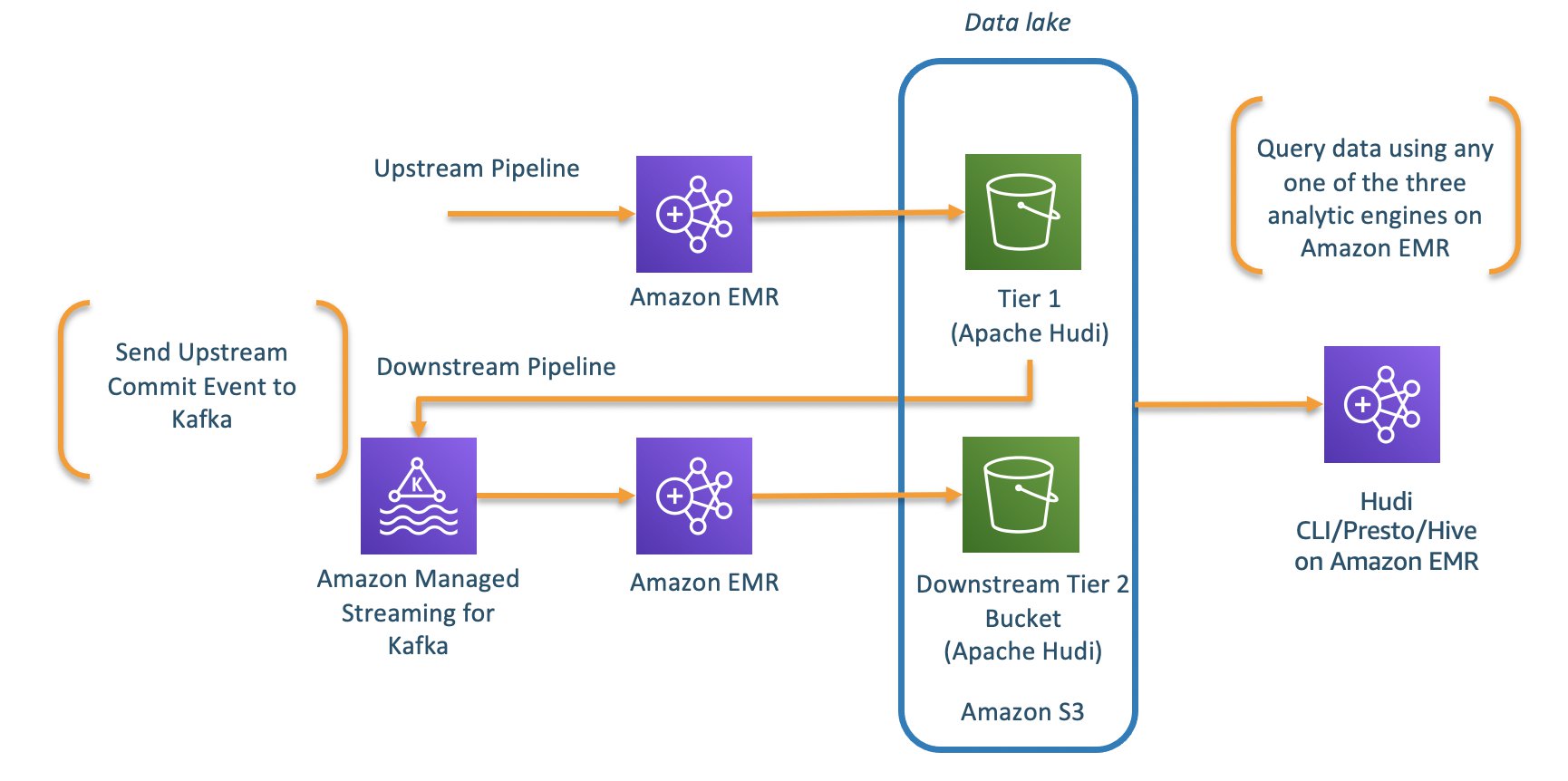
The following reference design explains the main two layers in charge of providing functional data for these use cases. The data processing layer is composed of two sub-layers. The first is Belcorp’s Data Lake Integrator, which is a built-in, in-house Python solution with a set of API REST services in charge of organizing all the data workloads and data stages inside the analytics repositories. It also works as a point of control to distribute resources to be allocated for each Amazon EMR Spark job. The processing sub-layer is mainly composed of the EMR cluster, which is in charge of orchestrating, tracking, and maintaining all the Spark jobs developed using a Scala framework.

For the persistent repository layer, we use Amazon Simple Storage Service (Amazon S3) object storage as a data repository for analytics workloads, where we have designed a set of data stages that have operational and functional purposes based on the reference architecture design. Discussing the repository design in more depth is out of scope for this post, but we must note that it covers all the common challenges related to data availability, data accessibility, data consistency, and data quality. In addition, it achieves all Belcorp’s needs required by its business model, despite all limitations and restrictions we inherit by the design previously mentioned.

We can now move our attention to the main purpose of this post.

As we mentioned, we experienced critical incidents (some of which existed before) and unexpected cost increases at the beginning of 2021, which motivated us to take action. The following table lists some of the main issues that attracted our attention.

Reported Incidents Impact
Delay in Spark jobs on Amazon EMR Core workloads take a long time
Delay in Amazon EMR nodes auto scaling Workloads take a long time
Increase in Amazon EMR computational usage per node Unexpected cost increase
Lost resource containers Workloads process a huge data crash
Overestimated memory and CPUs Unexpected cost increase

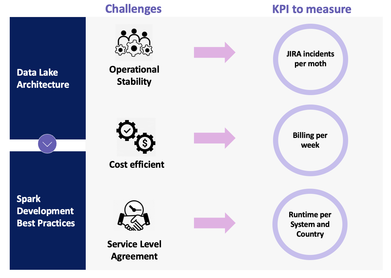
To face these issues, we decided to change strategies and started to analyze each issue in order to identify the cause. We defined two action lines based on three challenges that the leaders wanted us to work on. The following figure summarizes these lines and challenges.

The data lake architecture action line refers to all the architectural gaps and deprecated features that we determined as part of the main problems that were generating the incidents. The Spark development best practices action line is related to the developed Spark data solution that had been causing instability due to bad practices during the development lifecycle. Focusing on these action lines, our leaders defined three challenges in order to decrease the number of incidents and guarantee the quality of the service we provide: operational stability, cost-efficiency, and SLAs.

Based on these challenges, we defined three KPIs to measure the success of the project. Jira incidents allow us to validate that our changes are having a positive impact; billing per week shows the leaders that part of the changes we applied will gradually optimize cost; and runtime provides the business users with a better time to market.

Next, we defined the next steps and how to measure progress. Based on our monitoring framework, we determined that almost all incidents that arose were related to the data processing and persistent repository layers. Then we had to decide how to solve them. We could make reactive fixes in order to achieve operational stability and not have an impact on business, or we could change our usual way of working, analyze each issue, and provide a final solution to optimize our framework. As you can guess, we decided to change our way of working.

We performed a preliminary analysis to determine the main impacts and challenges. We then proposed the following actions and improvements based on our action lines:

  • Data lake architecture – We redesigned the EMR cluster; we’re now using core and task nodes
  • Spark development best practices – We optimized Spark parameters (RAM memory, cores, CPUs, and executor number)

In the next section, we explain in detail the actions and improvements proposed in order to achieve our goals.

Actions and improvements

As we mentioned in the previous section, the analysis made by the architecture team resulted in a list of actions and improvements that would help us face three challenges: operational stability, a cost-efficient data ecosystem, and SLAs.

Before going further, it’s a good time to provide more details about the Belcorp data processing framework. We built it based on Apache Spark using the Scala programming language. Our data processing framework is a set of scalable, parameterizable, and reusable Scala artifacts that provide development teams with a powerful tool to implement complex data pipelines, achieving the most complex business requirements using Apache Spark technology. Through the Belcorp DevOps framework, we deploy each artifact to several non-production environments. Then we promote into production, where the EMR cluster launches all the routines using the Scala artifacts that reference each conceptual area inside the analytical platform. This part of the cycle provides the teams with some degree of flexibility and agility. However, we forgot, for a moment, the quality of the software we were developing using Apache Spark technology.

In this section, we dive into the actions and improvements we applied in order to optimize the Belcorp data processing framework and improve the architecture.

Redesigning the EMR cluster

The current design and implementation of the Belcorp data lake is not the first version. We’re currently in version 2.0, and from the beginning of the first implementation until now, we’ve tried different EMR cluster designs to implement the data processing layer. Initially, we used a fixed cluster with four nodes (as shown in the following figure), but when the auto scaling capability was launched and Belcorp’s data workloads increased, we decided to move it there to optimize resource usage and costs. However, an auto scaled EMR cluster has different options too. You can choose between core and task nodes with a minimal and maximum number of each. In addition, you can select On-Demand or Spot Instances. You can also implement an optimized allocation strategy using EMR instance fleets to reduce the probability of Spot Instance loss. For more information about Amazon EMR resources allocation strategies, see Spark enhancements for elasticity and resiliency on Amazon EMR and Optimizing Amazon EMR for resilience and cost with capacity-optimized Spot Instances.

We tested all these capabilities, but we found some problems.

First, although AWS offers many capabilities and functionalities around Amazon EMR, if you don’t have some degree of knowledge about the technology that you want to use, you may encounter many issues as the use cases arise. As we mentioned, we decided to use the Apache Spark data processing engine through Amazon EMR as a part of Belcorp data ecosystem, but we faced many issues. Whenever an incident appeared, it motivated the data architect team in charge to fix it, as a part of the operational and support tasks. Almost all these reactive fixes were related to changing Amazon EMR configuration to try different alternatives in order to efficiently solve these incidents.

We figured out that almost all incidents were related to resource allocation, so we tested many configuration options such as instance types, increasing the number of nodes, customized rules for auto scaling, and fleet strategies. This last option was used to reduce node loss. At the end of 2020, we validated that an EMR cluster with automatic scaling enabled with a minimum capacity of three On-Demand core nodes 24/7 and the ability to scale up to 25 On-Demand core nodes provided us with a stable data processing platform. At the beginning of 2021, more complex Spark jobs were deployed as a part of the data processing routines inside the EMR cluster, causing operational instability again. In addition, the billing was increasing unexpectedly, which alerted leaders whose team needed to redesign the EMR cluster in order to keep healthy operational stability and optimize the costs.

We soon realized that it was possible to reduce up to 40% of the current billing using Spot Instances, instead of keeping all core nodes in On-Demand consumption. Another infrastructure optimization that we wanted to apply was to replace a number of core nodes with task nodes, because almost all Belcorp data workloads are memory-intensive and use Amazon S3 to read the source data and write the result dataset. The question here was how to do that without losing the benefits of the current design. To answer this question, we had the guidance of the AWS Account Team and our AWS Analytics and Big Data Specialist SA, in order to clarify questions about the following:

  • Apache Spark implementation in Amazon EMR
  • Core and task node best practices for production environments
  • Spot Instance behavior in Amazon EMR

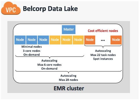
We definitely recommend addressing these three main points before applying any changes because, according to our previous experience, making modifications in the dark can lead to costly and underperforming Amazon EMR implementation. With that in mind, we redesigned the EMR cluster to utilize EMR managed scaling, which automatically resizes your cluster for best performance at the lowest possible cost. We defined a maximum of 28 capacity units with three On-Demand core nodes always on (24/7) in order to support data workloads during the day. We then set an auto scaling limit of six On-Demand cores in order to provide minimal HDFS capabilities to support the remaining 22 task nodes composed of Spot Instances. This final configuration is based on advice from AWS experts that we have at least one core node to support six task nodes, keeping a 1:6 ratio. The following table summarizes our cluster design.

Cluster Scaling Policy Amazon EMR Managed Scaling Enabled
Minimum node units (MinimumCapacityUnits) 3
Maximum node units (a) 28
On-demand limit (MaximumOnDemandCapacityUnits) 6
Maximum core nodes (MaximumCoreCapacityUnits) 6
Instance type m4.10xlarge
Number of primary nodes 1
Primary node instance type m4.4xlarge

The following figure illustrates our updated and current cluster design.

Tuning Spark parameters

As any good book about Apache Spark can tell you, Spark parameter tuning is the main topic you need to look into before deploying a Spark application in production.

Adjusting Spark parameters is the task of setting up the resources (CPUs, memory, and the number of executors) to each Spark application. In this post, we don’t focus on driver instance resources; we focus on the executors because that’s the main issue we found inside Belcorp’s implementation.

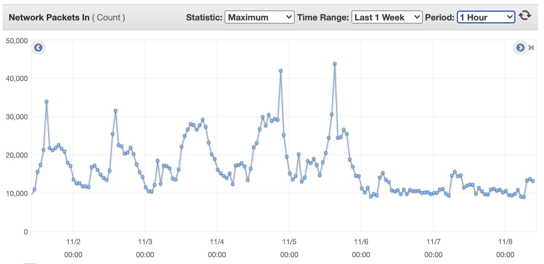
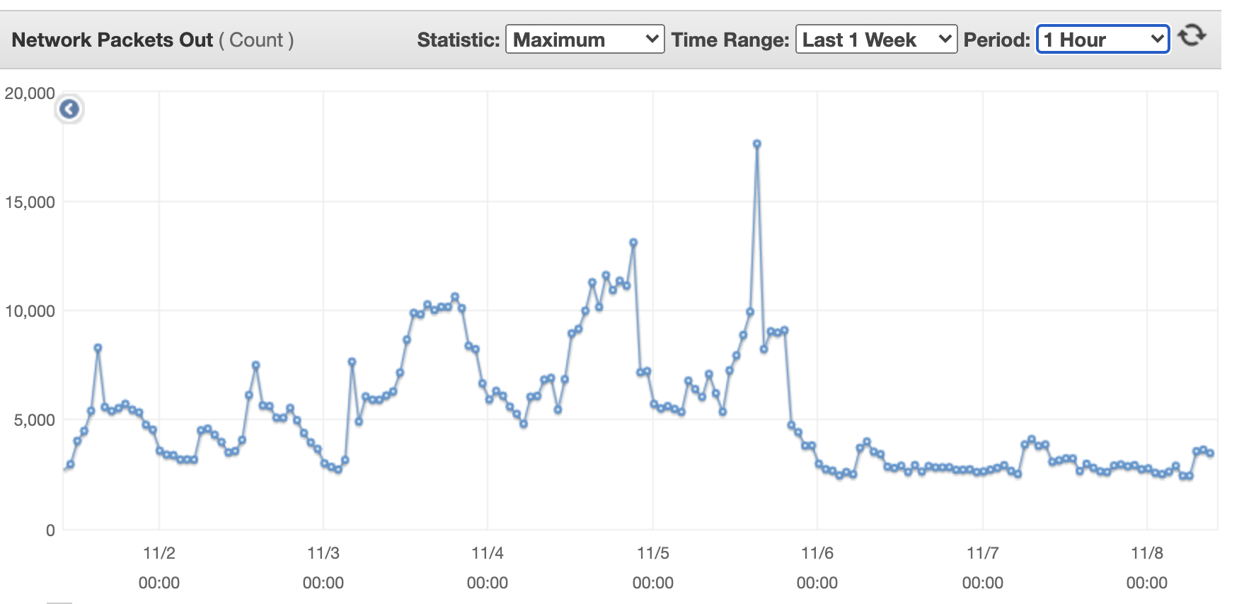
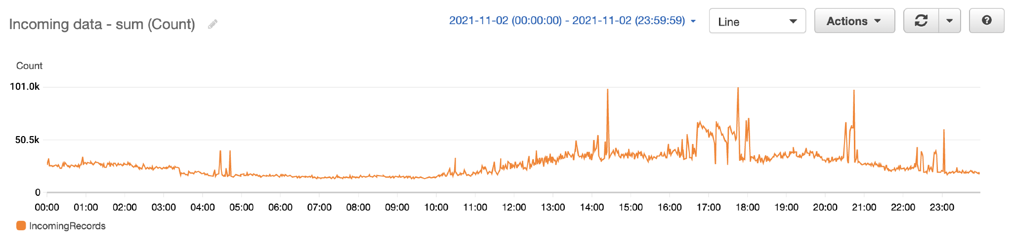
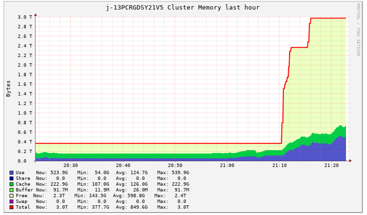
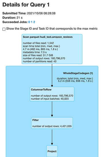
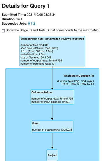
After we applied improvements around join operation and cache strategies in Spark application development, we realized that some of those applications were assigned with overestimated resources in the EMR cluster. That means Spark applications assigned resources, but only 30% of the resources were used. The following Ganglia report illustrates the overestimation of resource allocation for one Spark application job, which we captured during one of our tests.

A big consequence of this behavior was the massive deployment of EMR nodes that weren’t being properly utilized. That means that numerous nodes were provisioned because of the auto scaling feature required by a Spark application submit, but much of the resources of these nodes were kept free. We show a basic example of this later in this section.

With this evidence, we began to suspect that we needed to adjust the Spark parameters of some of our Spark applications.

As we mentioned in previous sections, as part of the Belcorp data ecosystem, we built a Data Pipelines Integrator, which has the main responsibility of maintaining centralized control of the runs of each Spark application. To do that, it uses a JSON file containing the Spark parameter configuration and performs each spark-submit using Livy service, as shown in the following example code:

'/usr/lib/spark/bin/spark-submit' '--class' 'LoadToFunctional' '--conf' 'spark.executor.instances=62' '--conf' 'spark.executor.memory=17g' '--conf' 'spark.yarn.maxAppAttempts=2' '--conf' 'spark.submit.deployMode=cluster' '--conf' 'spark.master=yarn' '--conf' 'spark.executor.cores=5' 's3://<bucket-name>/FunctionalLayer.jar' '--system' 'CM' '--country' 'PE' '--current_step' 'functional' '--attempts' '1' '--ingest_attributes' '{"FileFormat": "zip", "environment": "PRD", "request_origin": "datalake_integrator", "next_step": "load-redshift"}' '--fileFormat' 'zip' '--next_step' 'load-redshift'

This JSON file contains the Spark parameter configuration of each Spark application related to an internal system and country we submit to the EMR cluster. In the following example, CM is the name of the system and PE is the country code that the data comes from:

"systems" : {
  "CM" : {
    "PE" : { 
      "params" : {"executorCores": 15, "executorMemory": "45g", "numExecutors": 50 },
      "conf" : { "spark.sql.shuffle.partitions" :120 }
    }
}

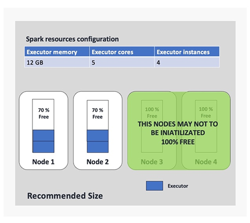
The problem with this approach is that as we add more applications, the management of these configuration files becomes more complex. In addition, we had a lot of Spark applications set up with a default configuration that was defined a long time ago when workloads were less expensive. So, it was expected that some things would change. One example of a Spark application with uncalibrated parameters is shown in the following figure (we use four executor instances only for the example). In this example, we realized we were allocating executors with a lot of resources without following any of the Spark best practices. This was causing the provisioning of fat executors (using Spark slang) allocating each of those in at least one node. That means that if we define a Spark application to be submitted using 10 executors, we require at least 10 nodes of the cluster and use 10 nodes for only one run, which was very expensive for us.

When you deal with Spark parameter tuning challenges, it’s always a good idea to follow expert advice. Perhaps one of the most important pieces of advice is related to the number of executor cores you should use in one Spark application. Experts suggest that an executor should have up to four or five cores. We were familiar with this restriction because we formerly developed Spark applications in the Hadoop ecosystem because of Hadoop File Systems I/O restrictions. That is, if we have more cores configured for one executor, we perform more I/O operations in a single HDFS data node, and it’s well known that HDFS degrades due to high concurrency. This constraint isn’t a problem if we use Amazon S3 as storage, but the suggestion remains due to the overload of the JVM. Remember, while you have more operational tasks, like I/O operations, the JVM of each executor has more work to do, so the JVM is degraded.

With these facts and previous findings, we realized that for some of our Spark applications, we were using only 30% of the assigned resources. We needed to recalibrate the Spark job parameters in order to allocate only the best-suited resources and significantly reduce the overuse of EMR nodes. The following figure provides an example of the benefits of this improvement, where we can observe a 50% of node reduction based on our earlier configuration.

We used the following optimized parameters to optimize the Spark application related to the CM system:

"systems" : {
  "CM" : {
    "PE" : { 
      "params" : {"executorCores": 5, "executorMemory": "17g", "numExecutors": 62 },
      "conf" : { "spark.sql.shuffle.partitions" :120 }
    }
}

Results

In this post, we wanted to share the success story of our project to improve the Belcorp data ecosystem, based on two lines of actions and three challenges defined by leaders using AWS data technologies and in-house platforms.

We were clear about our objectives from the beginning based on the defined KPIs, so we’ve been able to validate that the number of JIRA incidents reported at the end of May 2021 had a notable reduction. The following figures shows a reduction of up to 75% in respect to previous months, highlighting March as a critical peak.

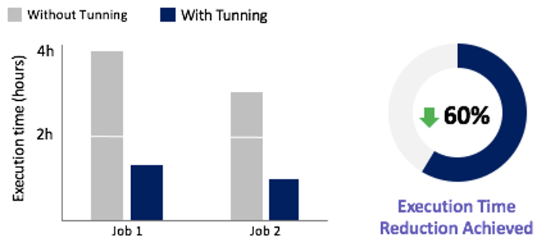
Based on this incident reduction, we figured out that almost all Spark job routines running in the EMR cluster benefitted from a runtime optimization, including the two most complex Spark jobs, with a reduction up to 60%, as shown in the following figure.

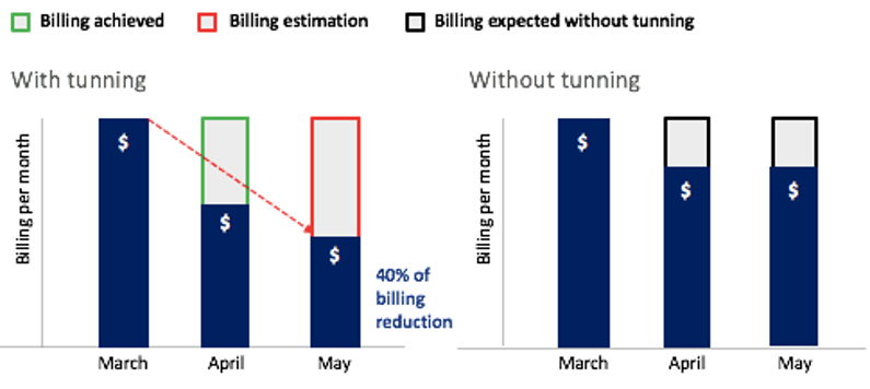
Perhaps the most important contribution of the improvements made by the team is directly related to the billing per week. For example, Amazon EMR redesigning, the join operation improvements, cache best practices applied, and Spark parameter tuning—all of these produced a notable reduction in the use of cluster resources. As we know, Amazon EMR calculates billing based on the time that the cluster nodes have been on, regardless of whether they do any work. So, when we optimized EMR cluster usage, we optimized the costs we were generating as well. As shown in the following figure, only in 2 months, between March and May, we achieved a billing reduction of up to 40%. We estimate that we will save up to 26% of the annual billing that would have been generated without the improvements.

Conclusion and next steps

The data architecture team is in charge of the Belcorp data ecosystem’s continuous improvements, and we’re always being challenged to achieve a best-in-class architecture, craft better architectural solution designs, optimize cost, and create the most automated, flexible, and scalable frameworks.

At the same time, we’re thinking about the future of this data ecosystem—how we can adapt to new business needs, generate new business models, and address current architectural gaps. We’re working now on the next generation of the Belcorp data platform, based on novel approaches like data products, data mesh, and lake houses. We believe these new approaches and concepts are going to help us to cover our current architectural gaps in the second generation of our data platform design. Additionally, it’s going to help us better organize the business and development teams in order to obtain greater agility during the development cycle. We’re thinking of data solutions as a data product, and providing teams with a set of technological components and automated frameworks they can use as building blocks.

Acknowledgments

We would like to thank our leaders, especially Jose Israel Rico, Corporate Data Architecture Director, and Venkat Gopalan, Chief Technology, Data and Digital Officer, who inspire us to be customer centric, insist on the highest standards, and support every technical decision based on a stronger knowledge of the state of the art.


About the Authors

Diego Benavides is the Senior Data Architect of Belcorp in charge of the design, implementation, and the continuous improvement of the Global and Corporate Data Ecosystem Architecture. He has experience working with big data and advanced analytics technologies across many industry areas like telecommunication, banking, and retail.

Luis Bendezú works as a Senior Data Engineer at Belcorp. He’s in charge of continuous improvements and implementing new data lake features using a number of AWS services. He also has experience as a software engineer, designing APIs, integrating many platforms, decoupling applications, and automating manual jobs.

Mar Ortiz is a bioengineer who works as a Solutions Architect Associate at AWS. She has experience working with cloud compute and diverse technologies like media, databases, compute, and distributed architecture design.

Raúl Hugo is an AWS Sr. Solutions Architect with more than 12 years of experience in LATAM financial companies and global telco companies as a SysAdmin, DevOps engineer, and cloud specialist.

New features from Apache Hudi 0.7.0 and 0.8.0 available on Amazon EMR

Post Syndicated from Udit Mehrotra original https://aws.amazon.com/blogs/big-data/new-features-from-apache-hudi-0-7-0-and-0-8-0-available-on-amazon-emr/

Apache Hudi is an open-source transactional data lake framework that greatly simplifies incremental data processing and data pipeline development by providing record-level insert, update, and delete capabilities. This record-level capability is helpful if you’re building your data lakes on Amazon Simple Storage Service (Amazon S3) or Hadoop Distributed File System (HDFS). You can use it to comply with data privacy regulations and simplify data ingestion pipelines that deal with late-arriving or updated records from streaming data sources, or to ingest data using change data capture (CDC) from transactional systems. Apache Hudi is integrated with open-source big data analytics frameworks like Apache Spark, Apache Hive, Presto, and Trino. It allows you to maintain data in Amazon S3 or HDFS in open formats like Apache Parquet and Apache Avro.

Starting with release version 5.28.0, Amazon EMR installs the Hudi component by default when you install Spark, Hive, Presto, or Trino. Since the inclusion of Apache Hudi within Amazon EMR, there has been several improvements and bug fixes that have been added to Apache Hudi. Apache Hudi graduated as a top-level Apache project on June 2020.

In this post, we provide a summary of some of the key new features and capabilities included since Apache Hudi release versions 0.7.0 and 0.8.0. These new features and capabilities of Hudi are available since Amazon EMR releases 5.33.0 and 6.3.0:

  • Clustering
  • Metadata-based file listing
  • Amazon CloudWatch integration
  • Optimistic Concurrency Control
  • Amazon EMR configuration support and improvements
  • Apache Flink integration
  • Kafka commit callbacks
  • Other improvements

Clustering

We see more use cases that need high throughput ingestion to data lakes. However, faster data ingestion often leads to smaller data file sizes that often adversely affects query performance, because a large number of small files increases the costly I/O operations required to return results. Another concern that we see is that the organization of data during ingestion is different from the organization that would be most efficient when querying the data. For example, it’s convenient to ingest ecommerce orders by OrderDate as they come in, but when queried, it’s better if orders for a single customer are stored together.

Apache Hudi version 0.7.0 introduces a new feature that allows you to cluster the Hudi tables. Clustering in Hudi is a framework that provides a pluggable strategy to change and reorganize the data layout while also optimizing the file sizes. With clustering, you can now optimize query performance without having to trade-off data ingest throughput.

You can use clustering to rewrite the data using different methods as per the different use case requirements:

  • Improve query performance with data locality – This changes the data layout on disk by sorting the data on one or many user-specified columns. With this approach, we can improve query performance by using the Parquet file format’s ability to perform predicate push-down and skip the unwanted files and Parquet row groups. This strategy can also control the file size to avoid small files.
  • Improve data freshness – This requirement assumes that the data locality is not important or taken care of already at the time of ingestion. It’s ideal for use cases where fresh data is important, where data is ingested using several small files and stitched or merged later using the clustering framework.

You can run the clustering table service asynchronously or synchronously. It also introduces the new action type REPLACE, which identifies the clustering action in the Hudi metadata timeline.

In the following example, we create two Copy on Write (CoW) Hudi tables: amazon_reviews and amazon_reviews_clustered using Amazon EMR release version 6.3.0.

We use spark-shell to create the Hudi tables. Start the Spark shell by running the following on the Amazon EMR primary node:

spark-shell --conf "spark.serializer=org.apache.spark.serializer.KryoSerializer" --conf "spark.sql.hive.convertMetastoreParquet=false" --jars /usr/lib/hudi/hudi-spark-bundle.jar

We then create the Hudi table amazon_reviews using the BULK_INSERT operation and without clustering enabled:

import org.apache.hudi.DataSourceWriteOptions
import org.apache.hudi.config.HoodieWriteConfig
import org.apache.hudi.HoodieDataSourceHelpers
import org.apache.spark.sql.SaveMode

val srcPath = "s3://amazon-reviews-pds/parquet/"
val tableName = "amazon_reviews"
val tablePath = "s3://emr-hudi-test-data/hudi/hudi_080/" + tableName

val inputDF = spark.read.format("parquet").load(srcPath)

inputDF.write.format("hudi")
  .option(HoodieWriteConfig.TABLE_NAME, tableName)
  .option(DataSourceWriteOptions.OPERATION_OPT_KEY, DataSourceWriteOptions.BULK_INSERT_OPERATION_OPT_VAL)
  .option(DataSourceWriteOptions.TABLE_TYPE_OPT_KEY, DataSourceWriteOptions.COW_TABLE_TYPE_OPT_VAL)
  .option(DataSourceWriteOptions.RECORDKEY_FIELD_OPT_KEY, "review_id")
  .option(DataSourceWriteOptions.PARTITIONPATH_FIELD_OPT_KEY, "product_category")
  .option(DataSourceWriteOptions.PRECOMBINE_FIELD_OPT_KEY, "review_date")
  .option(DataSourceWriteOptions.HIVE_SYNC_ENABLED_OPT_KEY, "true")
  .option(DataSourceWriteOptions.HIVE_DATABASE_OPT_KEY, "hudi_test")
  .option(DataSourceWriteOptions.HIVE_TABLE_OPT_KEY, tableName)
 .option(DataSourceWriteOptions.HIVE_PARTITION_FIELDS_OPT_KEY, "product_category")
.option(DataSourceWriteOptions.HIVE_PARTITION_EXTRACTOR_CLASS_OPT_KEY, "org.apache.hudi.hive.MultiPartKeysValueExtractor")
  .mode(SaveMode.Overwrite)
  .save(tablePath)

We then create the Hudi table amazon_reviews_clustered using BULK_INSERT operation and inline clustering enabled and sorted by columns star_rating and total_votes:

import org.apache.hudi.DataSourceWriteOptions
import org.apache.hudi.config.HoodieWriteConfig
import org.apache.hudi.config.HoodieClusteringConfig
import org.apache.hudi.HoodieDataSourceHelpers
import org.apache.spark.sql.SaveMode

val srcPath = "s3://amazon-reviews-pds/parquet/"
val tableName = "amazon_reviews_clustered"
val tablePath = "s3://emr-hudi-test-data/hudi/hudi_080/" + tableName

val inputDF = spark.read.format("parquet").load(srcPath)

inputDF.write
  .format("hudi")
  .option(HoodieWriteConfig.TABLE_NAME, tableName)
  .option(DataSourceWriteOptions.OPERATION_OPT_KEY, DataSourceWriteOptions.BULK_INSERT_OPERATION_OPT_VAL)
  .option(DataSourceWriteOptions.TABLE_TYPE_OPT_KEY, DataSourceWriteOptions.COW_TABLE_TYPE_OPT_VAL)
  .option(DataSourceWriteOptions.RECORDKEY_FIELD_OPT_KEY, "review_id")
  .option(DataSourceWriteOptions.PARTITIONPATH_FIELD_OPT_KEY, "product_category")
  .option(DataSourceWriteOptions.PRECOMBINE_FIELD_OPT_KEY, "review_date")
  .option(HoodieClusteringConfig.INLINE_CLUSTERING_PROP, "true")
.option(HoodieClusteringConfig.INLINE_CLUSTERING_MAX_COMMIT_PROP, "0")
  .option(HoodieClusteringConfig.CLUSTERING_TARGET_PARTITIONS, "43")
  .option(HoodieClusteringConfig.CLUSTERING_MAX_NUM_GROUPS, "100")
.option(HoodieClusteringConfig.CLUSTERING_SORT_COLUMNS_PROPERTY, "star_rating,total_votes")
  .option(DataSourceWriteOptions.HIVE_SYNC_ENABLED_OPT_KEY, "true")
  .option(DataSourceWriteOptions.HIVE_DATABASE_OPT_KEY, "hudi_test")
  .option(DataSourceWriteOptions.HIVE_TABLE_OPT_KEY, tableName)
 .option(DataSourceWriteOptions.HIVE_PARTITION_FIELDS_OPT_KEY, "product_category")
.option(DataSourceWriteOptions.HIVE_PARTITION_EXTRACTOR_CLASS_OPT_KEY, "org.apache.hudi.hive.MultiPartKeysValueExtractor")
  .mode(SaveMode.Overwrite)
  .save(tablePath)

Let’s query these two tables and validate performance difference. To validate the performance, we will use Spark SQL CLI – a convenient tool to run the Hive metastore service in local mode and execute queries input from the command line. To start the Spark SQL CLI, we execute the following command:

spark-sql --conf "spark.serializer=org.apache.spark.serializer.KryoSerializer" —conf "spark.hadoop.mapreduce.input.pathFilter.class=org.apache.hudi.hadoop.HoodieROTablePathFilter" —jars /usr/lib/hudi/hudi-spark-bundle.jar

We restart the Spark SQL CLI (spark-sql) session between each run in order to avoid caching or warm executors, which may impact query performance.

Let’s run the query against the non-clustered Hudi table by running the following in the spark-sql interface:

spark-sql> USE hudi_test;
spark-sql> select review_id from amazon_reviews where star_rating > 3 and total_votes > 10;

Let’s also run the same query on our clustered table from the spark-sql interface:

spark-sql> USE hudi_test;
spark-sql> select review_id from amazon_reviews_clustered where star_rating > 3 and total_votes > 10;

Let’s compare the underlying file scan performance for the two different Hudi tables. The following screenshot is the output from the Spark UI, which shows the changes in the files scanned for the same number of output rows. First we see the files scanned for the unclustered Hudi table.

Next, we see the files scanned for the clustered Hudi table.

The number of files scanned by Spark dropped from 1,542 files for the unclustered Hudi dataset to 85 files for the clustered Hudi dataset for the exact same data. Also, the number of records scanned reduced from 160,796,570 to 78,845,795.

We compared the performance of the preceding query for the amazon_reviews (non-clustered) and amazon_reviews_clustered (clustered) Hudi dataset, across Spark SQL, Hive, and PrestoDB. The cluster configuration used was 1 leader (m5.4xlarge) and 2 cores (m5.4xlarge).

The following chart provides the query performance comparison using different engines for the Hudi table, which are unclustered, and for the Hudi table, which is clustered.

We found that with clustering enabled for the Hudi table, the query performance increased for all three query engines, ranging from 28% to 63%. The following table provides the details for the query performance for the Hudi table, both with clustering enabled and disabled.

Query Engine Non-clustered Table Clustered Table Query Runtime Improvement
Time (in seconds) Time (in seconds)
Spark SQL 21.6 15.4 28.7 %
Hive 96.3 47 51.3 %
PrestoDB 11.7 4.3 63.25 %

Metadata-based file listing

Hudi write operations like compaction, cleaning, and global index, as well as queries, perform a file system listing to get the current view of the partitions and files in the dataset. For small datasets, this shouldn’t impact the performance drastically. However, when working with large data, this listing operation can impact the performance negatively when reading the files. For example, with HDFS as the underlying data store, the list operation for a large number of files or partitions can overwhelm HDFS NameNode and affect the stability of job. In cases where Amazon S3 is used as the underlying data store, O(N) calls for N partitions with a large number of files is time-consuming and can also result in throttling errors.

With Apache Hudi version 0.7.0, you can change this behavior by enabling metadata-based listing for Hudi tables. This partitions and files list is stored in an internal metadata table, which is implemented using a Hudi Merge on Read (MoR) table. This metadata table can take all the advantages of the Hudi MoR table, which includes the capability of low-latency updates, and the ability to atomically commit metadata updates and easily roll back if write fails. It also makes it easy to keep metadata in sync with the Hudi table because both use a timeline for traceability. This index of the file list is stored using HFiles for base and log file format for delta updates. The HFile format allows point-lookups of specific records based on record key. The goal is to reduce O(N) list calls for N partitions to O(1) get call to read the metadata.

We compared query performance for a Hudi dataset with metadata listing enabled vs. not enabled. For this example, we used a larger dataset of 3 TB with Amazon EMR release version 6.3.0. We used the following code snippet to create the metadata enabled and not enabled dataset by setting the HoodieMetadataConfig.METADATA_ENABLE_PROP (hoodie.metadata.enable) config:

val srcPath = "s3://gbrahmi-demo/3-tb-data_store_sales-parquet/"
val tableName = "tpcds_store_sales_3TB_hudi_080"
val tablePath = "s3://emr-hudi-test-data/hudi/hudi_080/" + tableName

val inputDF = spark.read.format("parquet").load(srcPath)

inputDF.write
  .format("hudi")
  .option(HoodieWriteConfig.TABLE_NAME, tableName)
  .option(HoodieMetadataConfig.METADATA_ENABLE_PROP, "true")
  .option(DataSourceWriteOptions.OPERATION_OPT_KEY, DataSourceWriteOptions.BULK_INSERT_OPERATION_OPT_VAL)
  .option(DataSourceWriteOptions.TABLE_TYPE_OPT_KEY, DataSourceWriteOptions.COW_TABLE_TYPE_OPT_VAL)
  .option(DataSourceWriteOptions.RECORDKEY_FIELD_OPT_KEY, "ss_item_sk,ss_ticket_number")
  .option(DataSourceWriteOptions.PARTITIONPATH_FIELD_OPT_KEY, "ss_sold_date_sk")
  .option(DataSourceWriteOptions.PRECOMBINE_FIELD_OPT_KEY, "ss_ticket_number")
  .option(DataSourceWriteOptions.KEYGENERATOR_CLASS_OPT_KEY, "org.apache.hudi.keygen.ComplexKeyGenerator")
  .option(DataSourceWriteOptions.HIVE_SYNC_ENABLED_OPT_KEY, "true")
  .option(DataSourceWriteOptions.HIVE_DATABASE_OPT_KEY, "hudi_test")
  .option(DataSourceWriteOptions.HIVE_TABLE_OPT_KEY, tableName)
 .option(DataSourceWriteOptions.HIVE_PARTITION_FIELDS_OPT_KEY, "ss_sold_date_sk")
.option(DataSourceWriteOptions.HIVE_PARTITION_EXTRACTOR_CLASS_OPT_KEY, "org.apache.hudi.hive.MultiPartKeysValueExtractor")
  .mode(SaveMode.Overwrite)
  .save(tablePath)

On the query engine side, we can enable it via the following methods:

  • Spark data source:
    spark.read.format("hudi")
      .option(HoodieMetadataConfig.METADATA_ENABLE_PROP, "true")
      .load(tablePath + "/*")

  • Spark SQL CLI:
    spark-sql --conf "spark.hadoop.hoodie.metadata.enable=true"
     --jars /usr/lib/hudi/hudi-spark-bundle.jar

  • Hive:
    hive> SET hoodie.metadata.enable = true;

  • PrestoDB:
    presto:default> set session hive.prefer_metadata_to_list_hudi_files=true;

We used the following query to compare query performance via Hive and PrestoDB:

select count(*) from tpcds_store_sales_3TB_hudi_080 where ss_quantity > 50;

The following chart provides the query performance comparison.

We found that with metadata listing, query execution runtime decreased by around 25% for the Hive engine, and by around 32% for PrestoDB. The following table provides the details of query execution runtime with and without metadata listing.

Query Engine Metadata Disabled Metadata Enabled Query Runtime Improvement
Time (in seconds) Time (in seconds)
Hive 415.28533 310.02367 25.35%
Presto 72 48.6 32.50%

Metadata listing considerations

With Hudi 0.7.0 and 0.8.0, you may not observe noticeable improvements for queries via Spark SQL (with metadata listing), because Hudi relies on Spark’s InMemoryFileIndex to do the actual file listing and can’t use the metadata. You may observe improvements because HoodieROPathFilter uses the metadata for its filtering. However, with Hudi release 0.9.0, we’re introducing a custom FileIndex implementation for Hudi to use metadata for file listing instead of relying on Spark. Therefore, from 0.9.0, you will observe noticeable performance improvements for Spark SQL queries.

Amazon CloudWatch integration

Apache Hudi provides MetricsReporter implementations like JmxMetricsReporter, MetricsGraphiteReporter, and DatadogMetricsReporter, which you can use to publish metrics to user-specified sinks. Amazon EMR, with its release 6.4.0 having Hudi 0.8.0, has introduced CloudWatchMetricsReporter, which you can use to publish these metrics to Amazon CloudWatch. It helps publish Hudi writer metrics like commit duration, rollback duration, file-level metrics (number of files added or deleted per commit), record-level metrics (records inserted or updated per commit) and partition-level metrics (partitions inserted or updated per commit). This is useful in debugging Hudi jobs, as well as making decisions around cluster scaling.

You can enable the CloudWatch metric via the following configurations:

hoodie.metrics.on = true
hoodie.metrics.reporter.type = CLOUDWATCH

The following table summarizes additional configurations that you can change if needed.

Configuration Description Value
hoodie.metrics.cloudwatch.report.period.seconds Frequency (in seconds) at which to report metrics to CloudWatch Default value is 60 seconds, which is fine for the default 1-minute resolution offered by CloudWatch
hoodie.metrics.cloudwatch.metric.prefix Prefix to be added to each metric name Default value is empty (no prefix)
hoodie.metrics.cloudwatch.namespace CloudWatch namespace under which metrics are published Default value is Hudi
hoodie.metrics.cloudwatch.maxDatumsPerRequest Maximum number of datums to be included in one request to CloudWatch Default value is 20, which is same as the CloudWatch default

The following screenshot shows some of the metrics published for a particular Hudi table, including the type of metric and its name. These are dropwizard metrics; gauge represents the exact value at a point in time, and counter represents a simple incrementing or decrementing integer.

The following graph of the gauge metric represents the total records written to a table over time.

The following graph of the counter metric represents the number of commits increasing over time.

Optimistic Concurrency Control

A major feature that has been introduced with Hudi 0.8.0, and available since Amazon EMR release 6.4.0, is Optimistic Concurrency Control (OCC) to enable multiple writers to concurrently ingest data into the same Hudi table. This is file-level OCC, which means that for any two commits (or writers) happening to the same table at the same time, both are allowed to succeed if they don’t have writes to overlapping files. The feature requires acquiring locks, for which you can use either Zookeeper or HiveMetastore. For more information about the guarantees provided, see Concurrency Control.

Amazon EMR clusters have Zookeeper installed, which you can use as a lock provider to perform concurrent writes from the same cluster. To make it easier to use, Amazon EMR preconfigures the lock provider in the newly introduced /etc/hudi/conf/hudi-defaults.conf file (see the next section) via the following properties:

hoodie.write.lock.provider=org.apache.hudi.client.transaction.lock.ZookeeperBasedLockProvider
hoodie.write.lock.zookeeper.url=<EMR Zookeeper URL>
hoodie.write.lock.zookeeper.port=<EMR Zookeeper Port>
hoodie.write.lock.zookeeper.base_path=/hudi

Although the lock provider is preconfigured, enabling of OCC still needs to be handled by the users either via Hudi job options or at cluster level via the Amazon EMR Configurations API:

hoodie.write.concurrency.mode = optimistic_concurrency_control
hoodie.cleaner.policy.failed.writes = LAZY (Performs cleaning of failed writes lazily instead of inline with every write)
hoodie.write.lock.zookeeper.lock_key = <Key to uniquely identify the Hudi table> (Table Name is a good option)

Amazon EMR configuration support and improvements

Amazon EMR release 6.4.0 has introduced the ability to configure and reconfigure Hudi via the configurations feature. Hudi configurations that are needed across jobs and tables can now be configured at cluster level via the hudi-defaults classification or /etc/hudi/conf/hudi-defaults.conf file, similar to other applications like Spark and Hive. The following code is an example of the hudi-defaults classification to enable metadata-based listing and CloudWatch metrics:

[{
  "Classification": "hudi-defaults",
  "Properties": {
    "hoodie.metadata.enable": "true",
    "hoodie.metadata.insert.parallelism": "3000",
    "hoodie.metrics.on": "true",
    "hoodie.metrics.reporter.type": "CLOUDWATCH"
  }
}]

Amazon EMR automatically configures suitable defaults for a few configs, to improve the user experience by removing the need for customers having to pass them:

  • HIVE_URL_OPT_KEY is configured to the cluster’s Hive server URL and no longer needs to be specified. This is particularly useful when running a job in Spark cluster mode, where users previously had to determine and themselves specify the Amazon EMR primary IP.
  • HBase specific configurations, which are useful for using HBase index with Hudi.
  • Zookeeper lock provider specific configuration, as discussed under concurrency control, which makes it easier to use OCC.

Additional changes have been introduced to reduce the number of configurations that users need to pass, and to infer automatically where possible:

Apache Flink integration

Apache Hudi started off with a very tight integration with Apache Spark. With release version 0.7.0, we now have integrations available to ingest data using Apache Flink. It required decoupling Spark from the internal table format, writers, and table services code in a way that can be used by other evolving engines in the industry like Flink.

Hudi 0.7.0 provides initial Flink support via HooodieFlinkStreamer, which you can use to write CoW tables by streaming data from a Kafka topic using Apache Flink. For example, you can use the following Flink command to start reading the topic ExampleTopic from the Kafka brokers broker-1, broker-2, and broker-3 running on port 9092:

./bin/flink run -c org.apache.hudi.HoodieFlinkStreamer \
  -m yarn-cluster -d -yjm 1024 -ytm 1024 -p 4 -ys 3 \
  -ynm hudi_on_flink_example \
  /usr/lib/hudi/hudi-flink-bundle.jar \
  --kafka-topic ExampleTopic \
  --kafka-group-id <kafka-group-id> \
  --kafka-bootstrap-servers broker-1:9092,broker-2:9092,broker-3:9092 \
  --table-type COPY_ON_WRITE \
  --target-table hudi_flink_table \
  --target-base-path s3://emr-hudi-test-data/hudi/hudi_070/hudi_flink_table \
  --props hdfs:///hudi/flink/config/hudi-jobConf.properties \
  --checkpoint-interval 6000 \
  --flink-checkpoint-path hdfs:///hudi/hudi-flink-checkpoint-dir

With Hudi 0.8.0, there have been major improvements in Flink integration performance and scalability, as well as the introduction of new features like SQL connector for both source and sink, writer for MoR, batch reader for CoW and MoR, streaming reader for MoR, and state-backed indexing with bootstrap support. For more information about Flink integration design, see Apache Hudi meets Apache Flink. To get started with Flink SQL, see Flink Guide.

Kafka commit callbacks

The previous version (0.6.0) of Apache Hudi introduced write commit callback functionality. With this functionality, Hudi can send a callback message every time a successful commit arrives to the Hudi dataset. The write commit callback supported HTTP method in the previous release. With Apache Hudi release version 0.7.0, Hudi now supports write commit callback for Kafka as well. Using Kafka for sending the callback messages for every successful commit can now enable you to build asynchronous data pipelines or business processing logic every time the Hudi dataset sees a new commit. You can now build incremental ETL pipelines for processing new events that arrive in the Hudi data lake.

The implementation of Kafka commit callback uses HoodieWriteCommitKafkaCallback as the hoodie.write.commit.callback.class. Besides setting the commit callback class, you can also set up additional parameters for the Kafka bootstrap servers and the topic configurations.

The following is a code snippet where commit callback messages are published to the Kafka topic ExampleTopic hosted on the Kafka brokers b-1.demo-hudi.xxxxxx.xxx.kafka.us-east-1.amazonaws.com, b-2.demo-hudi.xxxxxx.xxx.kafka.us-east-1.amazonaws.com, and b-3.demo-hudi.xxxxxx.xxx.kafka.us-east-1.amazonaws.com when writing to a Hudi dataset:

import org.apache.hudi.QuickstartUtils._
import scala.collection.JavaConversions._
import org.apache.spark.sql.SaveMode._
import org.apache.hudi.DataSourceReadOptions._
import org.apache.hudi.DataSourceWriteOptions._
import org.apache.hudi.config.HoodieWriteConfig._
 
val tableName = "trips_data_kafka_callback"
val tablePath = "s3://gbrahmi-sample-bucket/hudi-dataset/hudi_kafka_callback/" + tableName
 
val dataGen = new DataGenerator(Array("2021/05/01"))
val updates = convertToStringList(dataGen.generateInserts(10))
 
val df = spark.read.json(spark.sparkContext.parallelize(updates, 1))
 
df.write.format("hudi").
  option(TABLE_NAME, tableName).
  option(PRECOMBINE_FIELD_OPT_KEY, "ts").
  option(RECORDKEY_FIELD_OPT_KEY, "uuid").
  option("hoodie.write.commit.callback.on", "true").
  option("hoodie.write.commit.callback.class", "org.apache.hudi.utilities.callback.kafka.HoodieWriteCommitKafkaCallback").
  option("hoodie.write.commit.callback.kafka.bootstrap.servers", "b-1.demo-hudi.xxxxxx.xxx.kafka.us-east-1.amazonaws.com:9092,b-2.demo-hudi.xxxxxx.xxx.kafka.us-east-1.amazonaws.com:9092,b-3.demo-hudi.xxxxxx.xxx.kafka.us-east-1.amazonaws.com:9092").
  option("hoodie.write.commit.callback.kafka.topic", "ExampleTopic").
  option("hoodie.write.commit.callback.kafka.acks", "all").
  option("hoodie.write.commit.callback.kafka.retries", 3).
  mode(Append).
  save(tablePath)

The following is how the messages appear in your Kafka topic:

{"commitTime":"20210508210230","tableName":"trips_data_kafka_callback","basePath":"s3:// gbrahmi-sample-bucket/hudi-dataset/hudi_kafka_callback/trips_data_kafka_callback"}

A downstream pipeline can now easily query these events from Kafka and process the incremental data into derived Hudi tables.

Other improvements

Besides the aforementioned improvements, there have been some additional changes worth mentioning. On the writer side, there are the following improvements:

  • Support for Spark 3 – Support for writing and querying the data using Apache Spark 3 is now available with Apache Hudi 0.7.0 onwards. This works with Scala 2.12 bundle for hudi-spark-bundle.
  • Insert overwrite and insert overwrite table write operations – Apache Hudi 0.7.0 introduces two new operations, insert_overwrite and insert_overwrite_table, to support batch ETL jobs where an entire table or partition is overwritten during each execution. You can use these operations instead of the upsert operation, and it’s must cheaper to run.
  • Delete partitions – The new API is now available since 0.7.0 to delete an entire partition. This helps avoid the use of record-level deletes.
  • Java writer support – Hudi 0.7.0 introduced Java-based writing support via the HoodieJavaWriteClient class.

Similarly, on the query integration side, there have been the following improvements:

  • Structured streaming reads – Hudi 0.8.0 introduced a Spark structured streaming source implementation via the HoodieStreamSource class. You can use it to support streaming reads from Hudi tables.
  • Incremental query on MoR – Since Hudi 0.7.0, we now have incremental query support for MoR tables, which you can use to incrementally pull data by downstream applications.

Conclusion

The new features introduced in Apachi Hudi enable you to build decoupled solutions by using features like Kafka commit callback and Flink integration with Apache Hudi with Amazon EMR. You can also improve your overall performance of the Hudi data lake by using the capabilities of clustering and metadata tables.


About the Authors

Udit Mehrotra is a software development engineer at Amazon Web Services and an Apache Hudi PMC member/committer. He works on cutting-edge features of Amazon EMR and is also involved in open-source projects such as Apache Hudi, Apache Spark, Apache Hadoop, and Apache Hive. In his spare time, he likes to play guitar, travel, binge watch, and hang out with friends.

Gagan Brahmi is a Specialist Solutions Architect focused on Big Data & Analytics at Amazon Web Services. Gagan has over 16 years of experience in information technology. He helps customers architect and build highly scalable, performant, and secure cloud-based solutions on AWS.

How Goldman Sachs built persona tagging using Apache Flink on Amazon EMR

Post Syndicated from Balasubramanian Sakthivel original https://aws.amazon.com/blogs/big-data/how-goldman-sachs-built-persona-tagging-using-apache-flink-on-amazon-emr/

The Global Investment Research (GIR) division at Goldman Sachs is responsible for providing research and insights to the firm’s clients in the equity, fixed income, currency, and commodities markets. One of the long-standing goals of the GIR team is to deliver a personalized experience and relevant research content to their research users. Previously, in order to customize the user experience for their various types of clients, GIR offered a few distinct editions of their research site that were provided to users based on broad criteria. However, GIR did not have any way to create a personally curated content flow at the individual user level. To provide this functionality, GIR wanted to implement a system to actively filter the content that is recommended to their users on a per-user basis, keyed on characteristics such as the user’s job title or working region. Having this kind of system in place would both improve the user experience and simplify the workflows of GIR’s research users, by reducing the amount of time and effort required to find the research content that they need.

The first step towards achieving this is to directly classify GIR’s research users based on their profiles and readership. To that end, GIR created a system to tag users with personas. Each persona represents a type or classification that individual users can be tagged with, based on certain criteria. For example, GIR has a series of personas for classifying a user’s job title, and a user tagged with the “Chief Investment Officer” persona will have different research content highlighted and have a different site experience compared to one that is tagged with the “Corporate Treasurer” persona. This persona-tagging system can both efficiently carry out the data operations required for tagging users, as well as have new personas created as needed to fit use cases as they emerge.

In this post, we look at how GIR implemented this system using Amazon EMR.

Challenge

Given the number of contacts (i.e., millions) and the growing number of publications maintained in GIR’s research data store, creating a system for classifying users and recommending content is a scalability challenge. A newly created persona could potentially apply to almost every contact, in which case a tagging operation would need to be performed on several million data entries. In general, the number of contacts, the complexity of the data stored per contact, and the amount of criteria for personalization can only increase. To future-proof their workflow, GIR needed to ensure that their solution could handle the processing of large amounts of data as an expected and frequent case.

GIR’s business goal is to support two kinds of workflows for classification criteria: ad hoc and ongoing. An ad hoc criteria causes users that currently fit the defining criteria condition to immediately get tagged with the required persona, and is meant to facilitate the one-time tagging of specific contacts. On the other hand, an ongoing criteria is a continuous process that automatically tags users with a persona if a change to their attributes causes them to fit the criteria condition. The following diagram illustrates the desired personalization flow:

In the rest of this post, we focus on the design and implementation of GIR’s ad hoc workflow.

Apache Flink on Amazon EMR

To meet GIR’s scalability demands, they determined that Amazon EMR was the best fit for their use case, being a managed big data platform meant for processing large amounts of data using open source technologies such as Apache Flink. Although GIR evaluated a few other options that addressed their scalability concerns (such as AWS Glue), GIR chose Amazon EMR for its ease of integration into their existing systems and possibility to be adapted for both batch and streaming workflows.

Apache Flink is an open source big data distributed stream and batch processing engine that efficiently processes data from continuous events. Flink offers exactly-once guarantees, high throughput and low latency, and is suited for handling massive data streams. Also, Flink provides many easy-to-use APIs and mitigates the need for the programmer to worry about failures. However, building and maintaining a pipeline based on Flink comes with operational overhead and requires considerable expertise, in addition to provisioning physical resources.

Amazon EMR empowers users to create, operate, and scale big data environments such as Apache Flink quickly and cost-effectively. We can optimize costs by using Amazon EMR managed scaling to automatically increase or decrease the cluster nodes based on workload. In GIR’s use case, their users need to be able to trigger persona-tagging operations at any time, and require a predictable completion time for their jobs. For this, GIR decided to launch a long-running cluster, which allows multiple Flink jobs to be submitted simultaneously to the same cluster.

Ad hoc persona-tagging infrastructure and workflow

The following diagram illustrates the architecture of GIR’s ad hoc persona-tagging workflow on the AWS Cloud.

This is a broad overview, and the specifics of networking and security between components are out of scope for this post.

At a high level, we can discuss GIR’s workflow in four parts:

  1. Upload the Flink job artifacts to the EMR cluster.
  2. Trigger the Flink job.
  3. Within the Flink job, transform and then store user data.
  4. Continuous monitoring.

You can interact with Flink on Amazon EMR via the Amazon EMR console or the AWS Command Line Interface (AWS CLI). After launching the cluster, GIR used the Flink API to interact with and submit work to the Flink application. The Flink API provided a bit more functionality and was much easier to invoke from an AWS Lambda application.

The end goal of the setup is to have a pipeline where GIR’s internal users can freely make requests to update contact data (which in this use case is tagging or untagging contacts with various personas), and then have the updated contact data uploaded back to the GIR contact store.

Upload the Flink job artifacts to Amazon EMR

GIR has a GitLab project on-premises for managing the contents of their Flink job. To trigger the first part of their workflow and deploy a new version of the Flink job onto the cluster, a GitLab pipeline is run that first creates a .zip file containing the Flink job JAR file, properties, and config files.

The preceding diagram depicts the sequence of events that occurs in the job upload:

  1. The GitLab pipeline is manually triggered when a new Flink job should be uploaded. This transfers the .zip file containing the Flink job to an Amazon Simple Storage Service (Amazon S3) bucket on the GIR AWS account, labeled as “S3 Deployment artifacts”.
  2. A Lambda function (“Upload Lambda”) is triggered in response to the create event from Amazon S3.
  3. The function first uploads the Flink job JAR to the Amazon EMR Flink cluster, and retrieves the application ID for the Flink session.
  4. Finally, the function uploads the application properties file to a specific S3 bucket (“S3 Flink Job Properties”).

Trigger the Flink job

The second part of the workflow handles the submission of the actual Flink job to the cluster when job requests are generated. GIR has a user-facing web app called Personalization Workbench that provides the UI for carrying out persona-tagging operations. Admins and internal Goldman Sachs users can construct requests to tag or untag contacts with personas via this web app. When a request is submitted, a data file is generated that contains the details of the request.

The steps of this workflow are as follows:

  1. Personalization Workstation submits the details of the job request to the Flink Data S3 bucket, labeled as “S3 Flink data”.
  2. A Lambda function (“Run Lambda”) is triggered in response to the create event from Amazon S3.
  3. The function first reads the job properties file uploaded in the previous step to get the Flink job ID.
  4. Finally, the function makes an API call to run the required Flink job.

Process data

Contact data is processed according to the persona-tagging requests, and the transformed data is then uploaded back to the GIR contact store.

The steps of this workflow are as follows:

  1. The Flink job first reads the application properties file that was uploaded as part of the first step.
  2. Next, it reads the data file from the second workflow that contains the contact and persona data to be updated. The job then carries out the processing for the tagging or untagging operation.
  3. The results are uploaded back to the GIR contact store.
  4. Finally, both successful and failed requests are written back to Amazon S3.

Continuous monitoring

The final part of the overall workflow involves continuous monitoring of the EMR cluster in order to ensure that GIR’s tagging workflow is stable and that the cluster is in a healthy state. To ensure that the highest level of security is maintained with their client data, GIR wanted to avoid unconstrained SSH access to their AWS resources. Being constrained from accessing the EMR cluster’s primary node directly via SSH meant that GIR initially had no visibility into the EMR primary node logs or the Flink web interface.

By default, Amazon EMR archives the log files stored on the primary node to Amazon S3 at 5-minute intervals. Because this pipeline serves as a central platform for processing many ad hoc persona-tagging requests at a time, it was crucial for GIR to build a proper continuous monitoring system that would allow them to promptly diagnose any issues with the cluster.

To accomplish this, GIR implemented two monitoring solutions:

  • GIR installed an Amazon CloudWatch agent onto every node of their EMR cluster via bootstrap actions. The CloudWatch agent collects and publishes Flink metrics to CloudWatch under a custom metric namespace, where they can be viewed on the CloudWatch console. GIR configured the CloudWatch agent configuration file to capture relevant metrics, such as CPU utilization and total running EMR instances. The result is an EMR cluster where metrics are emitted to CloudWatch at a much faster rate than waiting for periodic S3 log flushes.
  • They also enabled the Flink UI in read-only mode by fronting the cluster’s primary node with a network load balancer and establishing connectivity from the Goldman Sachs on-premises network. This change allowed GIR to gain direct visibility into the state of their running EMR cluster and in-progress jobs.

Observations, challenges faced, and lessons learned

The personalization effort marked the first-time adoption of Amazon EMR within GIR. To date, hundreds of personalization criteria have been created in GIR’s production environment. In terms of web visits and clickthrough rate, site engagement with GIR personalized content has gradually increased since the implementation of the persona-tagging system.

GIR faced a few noteworthy challenges during development, as follows:

Restrictive security group rules

By default, Amazon EMR creates its security groups with rules that are less restrictive, because Amazon EMR can’t anticipate the specific custom settings for ingress and egress rules required by individual use cases. However, proper management of the security group rules is critical to protect the pipeline and data on the cluster. GIR used custom-managed security groups for their EMR cluster nodes and included only the needed security group rules for connectivity, in order to fulfill this stricter security posture.

Custom AMI

There were challenges in ensuring that the required packages were available when using custom Amazon Linux AMIs for Amazon EMR. As part of Goldman Sachs development SDLC controls, any Amazon Elastic Compute Cloud (Amazon EC2) instances on Goldman Sachs-owned AWS accounts are required to use internal Goldman Sachs-created AMIs. When GIR began development, the only compliant AMI that was available under this control was a minimal AMI based on the publicly available Amazon Linux 2 minimal AMI (amzn2-ami-minimal*-x86_64-ebs). However, Amazon EMR recommends using the full default Amazon 2 Linux AMI because it has all the necessary packages pre-installed. This resulted in various start up errors with no clear indication of the missing libraries.

GIR worked with AWS support to identify and resolve the issue by comparing the minimal and full AMIs, and installing the 177 missing packages individually (see the appendix for the full list of packages). In addition, various AMI-related files had been set to read-only permissions by the Goldman Sachs internal AMI creation process. Restoring these permissions to full read/write access allowed GIR to successfully start up their cluster.

Stalled Flink jobs

During GIR’s initial production rollout, GIR experienced an issue where their EMR cluster failed silently and caused their Lambda functions to time out. On further debugging, GIR found this issue to be related to an Akka quarantine-after-silence timeout setting. By default, it was set to 48 hours, causing the clusters to refuse more jobs after that time. GIR found a workaround by setting the value of akka.jvm-exit-on-fatal-error to false in the Flink config file.

Conclusion

In this post, we discussed how the GIR team at Goldman Sachs set up a system using Apache Flink on Amazon EMR to carry out the tagging of users with various personas, in order to better curate content offerings for those users. We also covered some of the challenges that GIR faced with the setup of their EMR cluster. This represents an important first step in providing GIR’s users with complete personalized content curation based on their individual profiles and readership.

Acknowledgments

The authors would like to thank the following members of the AWS and GIR teams for their close collaboration and guidance on this post:

  • Elizabeth Byrnes, Managing Director, GIR
  • Moon Wang, Managing Director, GIR
  • Ankur Gurha, Vice President, GIR
  • Jeremiah O’Connor, Solutions Architect, AWS
  • Ley Nezifort, Associate, GIR
  • Shruthi Venkatraman, Analyst, GIR

About the Authors

Balasubramanian Sakthivel is a Vice President at Goldman Sachs in New York. He has more than 16 years of technology leadership experience and worked on many firmwide entitlement, authentication and personalization projects. Bala drives the Global Investment Research division’s client access and data engineering strategy, including architecture, design and practices to enable the lines of business to make informed decisions and drive value. He is an innovator as well as an expert in developing and delivering large scale distributed software that solves real world problems, with demonstrated success envisioning and implementing a broad range of highly scalable platforms, products and architecture.

Victor Gan is an Analyst at Goldman Sachs in New York. Victor joined the Global Investment Research division in 2020 after graduating from Cornell University, and has been responsible for developing and provisioning cloud infrastructure for GIR’s user entitlement systems. He is focused on learning new technologies and streamlining cloud systems deployments.

Manjula Nagineni is a Solutions Architect with AWS based in New York. She works with major Financial service institutions, architecting, and modernizing their large-scale applications while adopting AWS cloud services. She is passionate about designing big data workloads cloud-natively. She has over 20 years of IT experience in Software Development, Analytics and Architecture across multiple domains such as finance, manufacturing and telecom.


Appendix

GIR ran the following command to install the missing AMI packages:

yum install -y libevent.x86_64 python2-botocore.noarch \

device-mapper-event-libs.x86_64 bind-license.noarch libwebp.x86_64 \

sgpio.x86_64 rsync.x86_64 perl-podlators.noarch libbasicobjects.x86_64 \

langtable.noarch sssd-client.x86_64 perl-Time-Local.noarch dosfstools.x86_64 \

attr.x86_64 perl-macros.x86_64 hwdata.x86_64 gpm-libs.x86_64 libtirpc.x86_64 \

device-mapper-persistent-data.x86_64 libconfig.x86_64 setserial.x86_64 \

rdate.x86_64 bc.x86_64 amazon-ssm-agent.x86_64 virt-what.x86_64 zip.x86_64 \

lvm2-libs.x86_64 python2-futures.noarch perl-threads.x86_64 \

dmraid-events.x86_64 bridge-utils.x86_64 mdadm.x86_64 ec2-net-utils.noarch \

kbd.x86_64 libtiff.x86_64 perl-File-Path.noarch quota-nls.noarch \

libstoragemgmt-python.noarch man-pages-overrides.x86_64 python2-rsa.noarch \

perl-Pod-Usage.noarch psacct.x86_64 libnl3-cli.x86_64 \

libstoragemgmt-python-clibs.x86_64 tcp_wrappers.x86_64 yum-utils.noarch \

libaio.x86_64 mtr.x86_64 teamd.x86_64 hibagent.noarch perl-PathTools.x86_64 \

libxml2-python.x86_64 dmraid.x86_64 pm-utils.x86_64 \

amazon-linux-extras-yum-plugin.noarch strace.x86_64 bzip2.x86_64 \

perl-libs.x86_64 kbd-legacy.noarch perl-Storable.x86_64 perl-parent.noarch \

bind-utils.x86_64 libverto-libevent.x86_64 ntsysv.x86_64 yum-langpacks.noarch \

libjpeg-turbo.x86_64 plymouth-core-libs.x86_64 perl-threads-shared.x86_64 \

kernel-tools.x86_64 bind-libs-lite.x86_64 screen.x86_64 \

perl-Text-ParseWords.noarch perl-Encode.x86_64 libcollection.x86_64 \

xfsdump.x86_64 perl-Getopt-Long.noarch man-pages.noarch pciutils.x86_64 \

python2-s3transfer.noarch plymouth-scripts.x86_64 device-mapper-event.x86_64 \

json-c.x86_64 pciutils-libs.x86_64 perl-Exporter.noarch libdwarf.x86_64 \

libpath_utils.x86_64 perl.x86_64 libpciaccess.x86_64 hunspell-en-US.noarch \

nfs-utils.x86_64 tcsh.x86_64 libdrm.x86_64 awscli.noarch cryptsetup.x86_64 \

python-colorama.noarch ec2-hibinit-agent.noarch usermode.x86_64 rpcbind.x86_64 \

perl-File-Temp.noarch libnl3.x86_64 generic-logos.noarch python-kitchen.noarch \

words.noarch kbd-misc.noarch python-docutils.noarch hunspell-en.noarch \

dyninst.x86_64 perl-Filter.x86_64 libnfsidmap.x86_64 kpatch-runtime.noarch \

python-simplejson.x86_64 time.x86_64 perl-Pod-Escapes.noarch \

perl-Pod-Perldoc.noarch langtable-data.noarch vim-enhanced.x86_64 \

bind-libs.x86_64 boost-system.x86_64 jbigkit-libs.x86_64 binutils.x86_64 \

wget.x86_64 libdaemon.x86_64 ed.x86_64 at.x86_64 libref_array.x86_64 \

libstoragemgmt.x86_64 libteam.x86_64 hunspell.x86_64 python-daemon.noarch \

dmidecode.x86_64 perl-Time-HiRes.x86_64 blktrace.x86_64 bash-completion.noarch \

lvm2.x86_64 mlocate.x86_64 aws-cfn-bootstrap.noarch plymouth.x86_64 \

parted.x86_64 tcpdump.x86_64 sysstat.x86_64 vim-filesystem.noarch \

lm_sensors-libs.x86_64 hunspell-en-GB.noarch cyrus-sasl-plain.x86_64 \

perl-constant.noarch libini_config.x86_64 python-lockfile.noarch \

perl-Socket.x86_64 nano.x86_64 setuptool.x86_64 traceroute.x86_64 \

unzip.x86_64 perl-Pod-Simple.noarch langtable-python.noarch jansson.x86_64 \

pystache.noarch keyutils.x86_64 acpid.x86_64 perl-Carp.noarch GeoIP.x86_64 \

python2-dateutil.noarch systemtap-runtime.x86_64 scl-utils.x86_64 \

python2-jmespath.noarch quota.x86_64 perl-HTTP-Tiny.noarch ec2-instance-connect.noarch \

vim-common.x86_64 libsss_idmap.x86_64 libsss_nss_idmap.x86_64 \

perl-Scalar-List-Utils.x86_64 gssproxy.x86_64 lsof.x86_64 ethtool.x86_64 \

boost-date-time.x86_64 python-pillow.x86_64 boost-thread.x86_64 yajl.x86_64

New – Create and Manage EMR Clusters and Spark Jobs with Amazon SageMaker Studio

Post Syndicated from Sean M. Tracey original https://aws.amazon.com/blogs/aws/new-create-and-manage-emr-clusters-and-spark-jobs-with-amazon-sagemaker-studio/

Today, we’re very excited to offer three new enhancements to our Amazon SageMaker Studio service.

As of now, users of SageMaker Studio can create, terminate, manage, discover, and connect to Amazon EMR clusters running within a single AWS account and in shared accounts across an organization—all directly from SageMaker Studio. Furthermore, SageMaker Studio Notebook users can able to utilize SparkUI to monitor and debug Spark jobs running on an Amazon EMR cluster—directly from the SageMaker Studio Notebooks!

The story so far…
Before today, SageMaker Studio users had some ability to find and connect with EMR clusters, provided that they were running in the same account as SageMaker Studio. While useful in many circumstances, if a cluster did not exist that would suit the requirements of the model or analysis being run, then data scientists would have to leave their development environment and manually configure a cluster that suited their needs. As well as being disruptive to workflow of data scientists, there are no guarantees that the data scientists would have either the permissions or depth of knowledge required to provision a cluster that would enable them to continue with their work. Additionally, being restricted to creating and managing clusters in a single account could become prohibitive in organizations working across many AWS accounts.

What’s new?
Data scientists can:

  • Discover, manage, create, terminate, and connect to Amazon EMR clusters from within SageMaker Studio
  • Utilize “templates” – a new way to configure and provision clusters for your workload needs with support from seasoned DevOps practitioners
  • Connect to, debug, and monitor Spark jobs running on an Amazon EMR cluster from within a SageMaker Studio Notebook

Creating, Connecting to, and Managing EMR Clusters

Connecting to an EMR Cluster from a SageMaker Studio Notebook

With the ability to connect to and manage EMR clusters from within SageMaker Studio, data scientists no longer have to leave their familiar environment to create, configure and provision the EMR clusters where they run their workloads.

Introducing Templates
A template is a collection of off-the-shelf cluster configurations optimized for numerous workloads. Templates can be created and managed by DevOps administrators and made available through the AWS Service Catalog to data scientists within SageMaker Studio. This lets them quickly spin up a cluster to meet their needs, all while safe in the knowledge that a trusted DevOps admin has correctly configured a cluster per the project’s requirements. Furthermore, this lets data scientists get on with the work they do best, and it gives DevOps administrators within these teams greater ability to manage the types of provisioned infrastructure.

Managing EMR Clusters from within SageMaker Studio Notebooks

Directly Connect to and monitor Spark Jobs
Finally, to make the job of data scientists even simpler, we’ve built the ability to connect to, debug, and monitor Spark jobs running on an Amazon EMR cluster from within a SageMaker Studio Notebook. Before now, to access the monitoring UI of a Spark Job, one needed to configure secure tunnels and web proxies to gain direct access to currently executing jobs, adding friction to the workflow of a data scientist trying to observe and debug their workloads. Now, with these new features, users will have one-click access directly from the interface that they already know. This enables them to build and put their workloads to work, rather than spending time on configuring infrastructure and workloads.

Connecting to a Spark Job from within a SageMaker Studio Notebook

These new features let data scientists can use a simple, consistent UI to provision and manage infrastructure as needed without ever having to leave SageMaker Studio or dive into the minutiae of the provisioning of such hardware – Moreover, they won’t have to spend time configuring proxies and SSH tunnels to debug and monitor ongoing Spark jobs.

Find out more
These features are generally available in all AWS Regions where SageMaker Studio is available, and there are no additional charges to use this capability. For complete information on pricing and regional availability, please refer to the SageMaker Studio pricing page .

To learn more, see our documentation.

Announcing Amazon EMR Serverless (Preview): Run big data applications without managing servers

Post Syndicated from Damon Cortesi original https://aws.amazon.com/blogs/big-data/announcing-amazon-emr-serverless-preview-run-big-data-applications-without-managing-servers/

Today we’re happy to announce Amazon EMR Serverless, a new option in Amazon EMR that makes it easy and cost-effective for data engineers and analysts to run petabyte-scale data analytics in the cloud. With EMR Serverless, you can run applications built using open-source frameworks such as Apache Spark, Hive, and Presto, without having to configure, manage, optimize, or secure clusters. EMR Serverless automatically provisions and scales the compute and memory resources required by your applications, and you only pay for the resources that your applications use.

In this post, we discuss the benefits of EMR Serverless, walk you through the core concepts of EMR Serverless and how you can use it, and show you a quick demo.

Overview of EMR Serverless

Tens of thousands of customers use Amazon EMR, a managed service for running open-source analytics frameworks such as Apache Spark, Hive, and Presto, for large-scale data analytics applications. With Amazon EMR, you can provision clusters of any size in minutes. Amazon EMR automatically installs and configures the frameworks you choose, and provides a performance-optimized runtime that is compatible with and over twice as fast as standard open-source.

Amazon EMR customers have full control over cluster configuration. The ability to customize clusters allows you to optimize for cost and performance based on workload requirements. For example, you can use Amazon Elastic Compute Cloud (Amazon EC2) memory optimized instances to run SQL workloads with low latency, or use the EC2 Graviton2-based instances to improve performance. You can also use EC2 Spot Instances, which are integrated in Amazon EMR so that you can take advantage of unused EC2 capacity in the AWS Cloud to obtain instances at up to a 90% discount compared to On-Demand prices. If you run your applications on Kubernetes, you can use Amazon EMR on Amazon EKS to run your Amazon EMR analytics applications on Amazon Elastic Kubernetes Service (Amazon EKS) clusters.

However, tuning clusters for optimal cost and performance requires engineers to have deep knowledge of the underlying analytics frameworks. Furthermore, the specific compute and memory resources needed to optimally run applications depend on various factors, such as the schedule and complexity of data processing jobs and the volume of data being processed. When these characteristics change over time, you need to reevaluate and reconfigure clusters. In addition, administrators have to secure and monitor the clusters to ensure that they’re compliant with corporate security policies, and adjust security settings each time the cluster is reconfigured. Many customers don’t need this level of customization and control, and want a simpler way to process data using open-source frameworks on the Amazon EMR performance-optimized runtime.

With this in mind, we built EMR Serverless. With EMR Serverless, you can get all the benefits of running Amazon EMR, but with a serverless environment. We had the following goals in mind when we built EMR Serverless:

  • Provide a simpler experience – EMR Serverless is simple to use because you don’t have to configure, optimize, operate, or secure clusters. You don’t have to worry about instance types or cluster sizes, or about applying OS patches. You simply specify the framework and version that you want to use for your application, and submit your data processing jobs. You still get all the benefits that you expect out of Amazon EMR—open-source compatibility, open-source version currency, and performance-optimized runtime—but without the need to manage clusters.
  • No need to guess cluster sizes – EMR Serverless eliminates the need to right-size clusters for varying jobs and data sizes. With EMR Serverless, you create an application using an open-source framework version, and submit jobs to the application. EMR Serverless automatically adds and removes workers at different stages of processing your job. As a result, you don’t have to reconfigure when data volumes change, and you only pay for what your jobs require. You can control costs by specifying the minimum and maximum number of concurrent workers, and the VCPU and memory per worker.
  • Retain Amazon EMR’s performance-optimized runtime and open-source currency – EMR Serverless includes the Amazon EMR performance-optimized runtime for Apache Spark, Hive, and Presto. The Amazon EMR runtime is API-compatible and over twice as fast as standard open-source, so your jobs run faster and incur less compute costs.
  • Seamless integration with EMR Studio – EMR Serverless includes EMR Studio, which provides fully managed serverless Jupyter Notebooks and familiar open-source tools such as Spark UI and Tez UI to help you develop, visualize, and debug your applications.
  • Automatic and fine-grained scaling – EMR Serverless automatically scales up workers at each stage of processing your job and scales them down when they’re not required. You’re charged for aggregate vCPU, memory, and storage resources used from the time a worker starts running until it stops, rounded up to the nearest second with a 1-minute minimum. For example, your job may require 10 workers for the first 10 minutes of processing the job, and 50 workers for the next 5 minutes. With fine-grained automatic scaling, you only incur cost for 10 workers for 10 minutes and 50 workers for 5 minutes. As a result, you don’t have to pay for underutilized resources.
  • Resilience to Availability Zone failures – EMR Serverless is a Regional service. When you submit jobs to an EMR Serverless application, it can run in any Availability Zone in the Region. A job is run in a single Availability Zone to avoid performance implications of network traffic across Availability Zones. In case an Availability Zone is impaired, a job submitted to your EMR Serverless application is automatically run in a different (healthy) Availability Zone. When using resources in a private VPC, EMR Serverless recommends you specify the private VPC configuration for multiple Availability Zones so that EMR Serverless can automatically select a healthy Availability Zone.
  • Enable shared applications – When you submit jobs to an EMR Serverless application, you can specify the AWS Identity and Access Management (IAM) role that must be used by the job to access AWS resources such as Amazon Simple Storage Service (Amazon S3) objects. As a result, different IAM principals can run jobs on a single EMR Serverless application, and each job can only access the AWS resources that the IAM principal is allowed to access. This enables you to set up scenarios where a single application with a pre-initialized pool of workers is made available to multiple tenants wherein each tenant can submit jobs using a different IAM role but use the common pool of pre-initialized workers to immediately process requests.
  • Enable interactive applications – Interactive applications that allow data scientists and analysts to run interactive SQL queries for data exploration require a fast response time to user requests. For such interactive applications, EMR Serverless allows you to pre-initialize a pool of workers. You can start your EMR Serverless application and pre-initialize the pool of workers as soon as a user starts the application, and stop the application to stop workers when no interactive users are active. If processing user requests requires more workers than what have been pre-initialized, EMR Serverless automatically adds more workers up to the maximum concurrent limits that you specify. Therefore, by controlling the number of workers to pre-initialize and the maximum concurrent workers, you can optimize user experience and cost for your interactive applications.
  • Make it easy to switch from one deployment model to another – The same Amazon EMR releases are provided for applications using EMR clusters, Amazon EMR on EKS, and EMR Serverless. When you build an application using an Amazon EMR release (for example a Spark job using Amazon EMR release 6.4), you can choose to run it on an EMR cluster, Amazon EMR on EKS, or EMR Serverless without having to rewrite the application. This allows you to build applications for a given framework version, and retain the flexibility to change the deployment model based on future operational needs.

Core concepts

In this section, we discuss the core concepts in EMR Serverless: applications, jobs, workers, and pre-initialized workers.

Application

With EMR Serverless, you can create one or more applications that use open-source analytics frameworks. To create an application, you specify the open-source framework that you want to use (for example, Apache Spark or Apache Hive), the Amazon EMR release for the open-source framework version (for example, Amazon EMR release 6.4, which corresponds to Apache Spark 3.1.2), and a name for your application. After you create an application, you can submit data processing jobs or interactive requests to your application.

The following are a few examples where you may want to create multiple applications:

  • To use different open-source frameworks (for example, Hive or Spark)
  • To use different versions of open-source frameworks for different use cases (for example, use a newer version of Spark for a new application without having to upgrade older applications)
  • To perform A/B testing when upgrading from one version to another (for example, migrating from Spark 2.4 to Spark 3.1)
  • To maintain separate logical environments for test and production scenarios
  • To provide separate logical environments for different teams with independent cost controls and usage tracking
  • To logically separate different line-of-business applications (for example, finance vs. marketing)

Job

A job is a request submitted to an EMR Serverless application that is asynchronously run and tracked through completion. You can run multiple jobs concurrently in an application.

Workers

An EMR Serverless application internally uses workers to run your jobs. By default, each application uses workers with 4 VCPU, 30 memory, and 20 GB of local storage per worker. You have the ability to customize this configuration.

Pre-initialized workers

EMR Serverless provides an optional feature to pre-initialize workers when your application starts up, so that the workers are ready to process requests immediately when a job is submitted to the application. Pre-initialized workers allow you to maintain a warm pool of workers for the application so that it can provide a sub-second response to start processing requests.

Common usage patterns applied to EMR Serverless

Now let’s examine some common usage scenarios and how EMR Serverless provides you a simple solution.

Pattern #1: Data pipelines

Data pipelines are the backbone of your analytics workloads. A common pattern with data pipelines is to start a cluster, run a job, and stop the cluster when the job is complete. Because data is separated from compute, the inputs and outputs for each job are persisted separately from the cluster (for example, in Amazon S3). These steps are frequently automated using workflow orchestration applications such as Apache Airflow. You can also use AWS services such as AWS Step Functions and AWS Managed Workflows for Apache Airflow (Amazon MWAA) to create such workflows.

Although automating these steps isn’t complex, data engineers have to spend time determining the appropriate EC2 instance and cluster size. They have to determine the Availability Zone where the cluster is run, and handle failover. They have to test their applications when adopting OS updates. When data sizes change over time, they have to resize clusters, or use features like Amazon EMR managed scaling that automatically resize clusters. EMR Serverless provides a simpler solution by eliminating the need for you to handle these scenarios. You simply choose the open-source framework and version for your application, and submit jobs. You don’t have to worry about instance selection, cluster sizes, cluster startup, cluster resize, stopping nodes, Availability Zone failover, or OS updates.

Pattern #2: Shared clusters

Another common pattern is for teams to use a shared long-running cluster to run multiple jobs. In this case, engineers implement queues in Apache YARN for different workloads on a common cluster, and set up rules to automatically scale the cluster up or down based on overall workload. With Amazon EMR on EC2 clusters, you can use Amazon EMR managed scaling, a feature that automatically scales clusters up or down depending on the workload. With EMR Serverless, workers are assigned to each job when required, so your jobs get the resources they need. Moreover, because you only pay for the workers that your jobs require, you don’t incur cost for over-provisioned resources. Finally, because each job can specify the IAM role that should be used to access AWS resources when running the job, you don’t have to set up complex configurations to manage queues and permissions.

Pattern #3: Interactive workloads

A third pattern of use is when teams keep a cluster of instances available to support interactive analysis. In this case, the cluster is set up and initialized with applications that wait for interactive user requests. Applications are pre-initialized so that they can immediately start processing user requests and provide an interactive user experience. EMR Serverless enables this scenario without requiring you to manage clusters. You can specify the number of workers that you want to pre-initialize when you start an EMR Serverless application. Subsequently, when users submit requests, the pre-initialized workers can be used to immediately process user requests. If processing the user requests requires more workers than what you have chosen to pre-initialize, EMR Serverless automatically adds more workers (up to the maximum concurrent limit that you specify). When the requests are processed, EMR Serverless automatically reverts back to maintaining the pre-initialized workers that you specified. You can control when the pre-initialized workers start by controlling when to start and stop your EMR Serverless application. For example, you can start your application when users begin interactive analysis and turn it off when there are no user requests and the application remains idle.

Demo

Conclusion

In this post, we discussed the core concepts and common usage patterns of EMR Serverless, and showed you a quick demo. EMR Serverless is in Preview, in which you can run workloads using Spark 3.1.2 and Hive 2.0 using the API, AWS Command Line Interface (AWS CLI), and SDK. Sign up for now, and for more information, see EMR Serverless documentation.


About the Authors

Damon Cortesi is a Principal Developer Advocate with Amazon Web Services.

Mehul Y. Shah is the GM for Amazon EMR.

Abhishek Sinha is a Principal Product Manager at Amazon Web Services.

Provide data reliability in Amazon Redshift at scale using Great Expectations library

Post Syndicated from Faizan Ahmed original https://aws.amazon.com/blogs/big-data/provide-data-reliability-in-amazon-redshift-at-scale-using-great-expectations-library/

Ensuring data reliability is one of the key objectives of maintaining data integrity and is crucial for building data trust across an organization. Data reliability means that the data is complete and accurate. It’s the catalyst for delivering trusted data analytics and insights. Incomplete or inaccurate data leads business leaders and data analysts to make poor decisions, which can lead to negative downstream impacts and subsequently may result in teams spending valuable time and money correcting the data later on. Therefore, it’s always a best practice to run data reliability checks before loading the data into any targets like Amazon Redshift, Amazon DynamoDB, or Amazon Timestream databases.

This post discusses a solution for running data reliability checks before loading the data into a target table in Amazon Redshift using the open-source library Great Expectations. You can automate the process for data checks via the extensive built-in Great Expectations glossary of rules using PySpark, and it’s flexible for adding or creating new customized rules for your use case.

Amazon Redshift is a cloud data warehouse solution and delivers up to three times better price-performance than other cloud data warehouses. With Amazon Redshift, you can query and combine exabytes of structured and semi-structured data across your data warehouse, operational database, and data lake using standard SQL. Amazon Redshift lets you save the results of your queries back to your Amazon Simple Storage Service (Amazon S3) data lake using open formats like Apache Parquet, so that you can perform additional analytics from other analytics services like Amazon EMR, Amazon Athena, and Amazon SageMaker.

Great Expectations (GE) is an open-source library and is available in GitHub for public use. It helps data teams eliminate pipeline debt through data testing, documentation, and profiling. Great Expectations helps build trust, confidence, and integrity of data across data engineering and data science teams in your organization. GE offers a variety of expectations developers can configure. The tool defines expectations as statements describing verifiable properties of a dataset. Not only does it offer a glossary of more than 50 built-in expectations, it also allows data engineers and scientists to write custom expectation functions.

Use case overview

Before performing analytics or building machine learning (ML) models, cleaning data can take up a lot of time in the project cycle. Without automated and systematic data quality checks, we may spend most of our time cleaning data and hand-coding one-off quality checks. As most data engineers and scientists know, this process can be both tedious and error-prone.

Having an automated quality check system is critical to project efficiency and data integrity. Such systems help us understand data quality expectations and the business rules behind them, know what to expect in our data analysis, and make communicating the data’s intricacies much easier. For example, in a raw dataset of customer profiles of a business, if there’s a column for date of birth in format YYYY-mm-dd, values like 1000-09-01 would be correctly parsed as a date type. However, logically this value would be incorrect in 2021, because the age of the person would be 1021 years, which is impossible.

Another use case could be to use GE for streaming analytics, where you can use AWS Database Migration Service (AWS DMS) to migrate a relational database management system. AWS DMS can export change data capture (CDC) files in Parquet format to Amazon S3, where these files can then be cleansed by an AWS Glue job using GE and written to either a destination bucket for Athena consumption or the rows can be streamed in AVRO format to Amazon Kinesis or Kafka.

Additionally, automated data quality checks can be versioned and also bring benefit in the form of optimal data monitoring and reduced human intervention. Data lineage in an automated data quality system can also indicate at which stage in the data pipeline the errors were introduced, which can help inform improvements in upstream systems.

Solution architecture

This post comes with a ready-to-use blueprint that automatically provisions the necessary infrastructure and spins up a SageMaker notebook that walks you step by step through the solution. Additionally, it enforces the best practices in data DevOps and infrastructure as code. The following diagram illustrates the solution architecture.

The architecture contains the following components:

  1. Data lake – When we run the AWS CloudFormation stack, an open-source sample dataset in CSV format is copied to an S3 bucket in your account. As an output of the solution, the data destination is an S3 bucket. This destination consists of two separate prefixes, each of which contains files in Parquet format, to distinguish between accepted and rejected data.
  2. DynamoDB – The CloudFormation stack persists data quality expectations in a DynamoDB table. Four predefined column expectations are populated by the stack in a table called redshift-ge-dq-dynamo-blog-rules. Apart from the pre-populated rules, you can add any rule from the Great Expectations glossary according to the data model showcased later in the post.
  3. Data quality processing – The solution utilizes a SageMaker notebook instance powered by Amazon EMR to process the sample dataset using PySpark (v3.1.1) and Great Expectations (v0.13.4). The notebook is automatically populated with the S3 bucket location and Amazon Redshift cluster identifier via the SageMaker lifecycle config provisioned by AWS CloudFormation.
  4. Amazon Redshift – We create internal and external tables in Amazon Redshift for the accepted and rejected datasets produced from processing the sample dataset. The external dq_rejected.monster_com_rejected table, for rejected data, uses Amazon Redshift Spectrum and creates an external database in the AWS Glue Data Catalog to reference the table. The dq_accepted.monster_com table is created as a regular Amazon Redshift table by using the COPY command.

Sample dataset

As part of this post, we have performed tests on the Monster.com job applicants sample dataset to demonstrate the data reliability checks using the Great Expectations library and loading data into an Amazon Redshift table.

The dataset contains nearly 22,000 different sample records with the following columns:

  • country
  • country_code
  • date_added
  • has_expired
  • job_board
  • job_description
  • job_title
  • job_type
  • location
  • organization
  • page_url
  • salary
  • sector
  • uniq_id

For this post, we have selected four columns with inconsistent or dirty data, namely organization, job_type, uniq_id, and location, whose inconsistencies are flagged according to the rules we define from the GE glossary as described later in the post.

Prerequisites

For this solution, you should have the following prerequisites:

  • An AWS account if you don’t have one already. For instructions, see Sign Up for AWS.
  • For this post, you can launch the CloudFormation stack in the following Regions:
    • us-east-1
    • us-east-2
    • us-west-1
    • us-west-2
  • An AWS Identity and Access Management (IAM) user. For instructions, see Create an IAM User.
  • The user should have create, write, and read access for the following AWS services:
  • Familiarity with Great Expectations and PySpark.

Set up the environment

Choose Launch Stack to start creating the required AWS resources for the notebook walkthrough:

For more information about Amazon Redshift cluster node types, see Overview of Amazon Redshift clusters. For the type of workflow described in this post, we recommend using the RA3 Instance Type family.

Run the notebooks

When the CloudFormation stack is complete, complete the following steps to run the notebooks:

  1. On the SageMaker console, choose Notebook instances in the navigation pane.

This opens the notebook instances in your Region. You should see a notebook titled redshift-ge-dq-EMR-blog-notebook.

  1. Choose Open Jupyter next to this notebook to open the Jupyter notebook interface.

You should see the Jupyter notebook file titled ge-redshift.ipynb.

  1. Choose the file to open the notebook and follow the steps to run the solution.

Run configurations to create a PySpark context

When the notebook is open, make sure the kernel is set to Sparkmagic (PySpark). Run the following block to set up Spark configs for a Spark context.

Create a Great Expectations context

In Great Expectations, your data context manages your project configuration. We create a data context for our solution by passing our S3 bucket location. The S3 bucket’s name, created by the stack, should already be populated within the cell block. Run the following block to create a context:

from great_expectations.data_context.types.base import DataContextConfig,DatasourceConfig,S3StoreBackendDefaults
from great_expectations.data_context import BaseDataContext

bucket_prefix = "ge-redshift-data-quality-blog"
bucket_name = "ge-redshift-data-quality-blog-region-account_id"
region_name = '-'.join(bucket_name.replace(bucket_prefix,'').split('-')[1:4])
dataset_path=f"s3://{bucket_name}/monster_com-job_sample.csv"
project_config = DataContextConfig(
    config_version=2,
    plugins_directory=None,
    config_variables_file_path=None,
    datasources={
        "my_spark_datasource": {
            "data_asset_type": {
                "class_name": "SparkDFDataset",//Setting dataset type to Spark
                "module_name": "great_expectations.dataset",
            },
            "spark_config": dict(spark.sparkContext.getConf().getAll()) //Passing Spark Session configs,
            "class_name": "SparkDFDatasource",
            "module_name": "great_expectations.datasource"
        }
    },
    store_backend_defaults=S3StoreBackendDefaults(default_bucket_name=bucket_name)//
)
context = BaseDataContext(project_config=project_config)

For more details on creating a GE context, see Getting started with Great Expectations.

Get GE validation rules from DynamoDB

Our CloudFormation stack created a DynamoDB table with prepopulated rows of expectations. The data model in DynamoDB describes the properties related to each dataset and its columns and the number of expectations you want to configure for each column. The following code describes an example of the data model for the column organization:

{
 "id": "job_reqs-organization", 
 "dataset_name": "job_reqs", 
 "rules": [ //list of expectations to apply to this column
  {
   "kwargs": {
    "result_format": "SUMMARY|COMPLETE|BASIC|BOOLEAN_ONLY" //The level of detail of the result
   },
   "name": "expect_column_values_to_not_be_null",//name of GE expectation   "reject_msg": "REJECT:null_values_found_in_organization"
  }
 ],
 "column_name": "organization"
}

The code contains the following parameters:

  • id – Unique ID of the document
  • dataset_name – Name of the dataset, for example monster_com
  • rules – List of GE expectations to apply:
    • kwargs – Parameters to pass to an individual expectation
    • name – Name of the expectation from the GE glossary
    • reject_msg – String to flag for any row that doesn’t pass this expectation
  • column_name – Name of dataset column to run the expectations on

Each column can have one or more expectations associated that it needs to pass. You can also add expectations for more columns or to existing columns by following the data model shown earlier. With this technique, you can automate verification of any number of data quality rules for your datasets without performing any code change. Apart from its flexibility, what makes GE powerful is the ability to create custom expectations if the GE glossary doesn’t cover your use case. For more details on creating custom expectations, see How to create custom Expectations.

Now run the cell block to fetch the GE rules from the DynamoDB client:

  1. Read the monster.com sample dataset and pass through validation rules.

After we have the expectations fetched from DynamoDB, we can read the raw CSV dataset. This dataset should already be copied to your S3 bucket location by the CloudFormation stack. You should see the following output after reading the CSV as a Spark DataFrame.

To evaluate whether a row passes each column’s expectations, we need to pass the necessary columns to a Spark user-defined function. This UDF evaluates each row in the DataFrame and appends the results of each expectation to a comments column.

Rows that pass all column expectations have a null value in the comments column.

A row that fails at least one column expectation is flagged with the string format REJECT:reject_msg_from_dynamo. For example, if a row has a null value in the organization column, then according to the rules defined in DynamoDB, the comments column is populated by the UDF as REJECT:null_values_found_in_organization.

The technique with which the UDF function recognizes a potentially erroneous column is done by evaluating the result dictionary generated by the Great Expectations library. The generation and structure of this dictionary is dependent upon the keyword argument of result_format. In short, if the count of unexpected column values of any column is greater than zero, we flag that as a rejected row.

  1. Split the resulting dataset into accepted and rejected DataFrames.

Now that we have all the rejected rows flagged in the source DataFrame within the comments column, we can use this property to split the original dataset into accepted and rejected DataFrames. In the previous step, we mentioned that we append an action message in the comments column for each failed expectation in a row. With this fact, we can select rejected rows that start with the string REJECT (alternatively, you can also filter by non-null values in the comments column to get the accepted rows). When we have the set of rejected rows, we can get the accepted rows as a separate DataFrame by using the following PySpark except function.

Write the DataFrames to Amazon S3.

Now that we have the original DataFrame divided, we can write them both to Amazon S3 in Parquet format. We need to write the accepted DataFrame without the comments column because it’s only added to flag rejected rows. Run the cell blocks to write the Parquet files under appropriate prefixes as shown in the following screenshot.

Copy the accepted dataset to an Amazon Redshift table

Now that we have written the accepted dataset, we can use the Amazon Redshift COPY command to load this dataset into an Amazon Redshift table. The notebook outlines the steps required to create a table for the accepted dataset in Amazon Redshift using the Amazon Redshift Data API. After the table is created successfully, we can run the COPY command.

Another noteworthy point to mention is that one of the advantages that we witness due to the data quality approach described in this post is that the Amazon Redshift COPY command doesn’t fail due to schema or datatype errors for the columns, which have clear expectations defined that match the schema. Similarly, you can define expectations for every column in the table that satisfies the schema constraints and can be considered a dq_accepted.monster_com row.

Create an external table in Amazon Redshift for rejected data

We need to have the rejected rows available to us in Amazon Redshift for comparative analysis. These comparative analyses can help inform upstream systems regarding the quality of data being collected and how they can be corrected to improve the overall quality of data. However, it isn’t wise to store the rejected data on the Amazon Redshift cluster, particularly for large tables, because it occupies extra disk space and increase cost. Instead, we use Redshift Spectrum to register an external table in an external schema in Amazon Redshift. The external schema lives in an external database in the AWS Glue Data Catalog and is referenced by Amazon Redshift. The following screenshot outlines the steps to create an external table.

Verify and compare the datasets in Amazon Redshift.

12,160 records got processed successfully out of a total of 22,000 from the input dataset, and were loaded to the monster_com table under the dq_accepted schema. These records successfully passed all the validation rules configured in DynamoDB.

A total 9,840 records got rejected due to breaking of one or more rules configured in DynamoDB and loaded to the monster_com_rejected table in the dq_rejected schema. In this section, we describe the behavior of each expectation on the dataset.

  • Expect column values to not be null in organization – This rule is configured to reject a row if the organization is null. The following query returns the sample of rows, from the dq_rejected.monster_com_rejected table, that are null in the organization column, with their reject message.
  • Expect column values to match the regex list in job_type – This rule expects the column entries to be strings that can be matched to either any of or all of a list of regular expressions. In our use case, we have only allowed values that match a pattern within [".*Full.*Time", ".*Part.*Time", ".*Contract.*"].
  • The following query shows rows that are rejected due to an invalid job type.

Most of the records were rejected with multiple reasons, and all those mismatches are captured under the comments column.

  • Expect column values to not match regex for uniq_id – Similar to the previous rule, this rule aims to reject any row whose value matches a certain pattern. In our case, that pattern is having an empty space (\s++) in the primary column uniq_id. This means we consider a value to be invalid if it has empty spaces in the string. The following query returned an invalid format for uniq_id.
  • Expect column entries to be strings with a length between a minimum value and a maximum value (inclusive) – A length check rule is defined in the DynamoDB table for the location column. This rule rejects values or rows if the length of the value violates the specified constraints. The following
  • query returns the records that are rejected due to a rule violation in the location column.

You can continue to analyze the other columns’ predefined rules from DynamoDB or pick any rule from the GE glossary and add it to an existing column. Rerun the notebook to see the result of your data quality rules in Amazon Redshift. As mentioned earlier, you can also try creating custom expectations for other columns.

Benefits and limitations

The efficiency and efficacy of this approach is delineated from the fact that GE enables automation and configurability to an extensive degree when compared with other approaches. A very brute force alternative to this could be writing stored procedures in Amazon Redshift that can perform data quality checks on staging tables before data is loaded into main tables. However, this approach might not be scalable because you can’t persist repeatable rules for different columns, as persisted here in DynamoDB, in stored procedures (or call DynamoDB APIs), and would have to write and store a rule for each column of every table. Furthermore, to accept or reject a row based on a single rule requires complex SQL statements that may result in longer durations for data quality checks or even more compute power, which can also incur extra costs. With GE, a data quality rule is generic, repeatable, and scalable across different datasets.

Another benefit of this approach, related to using GE, is that it supports multiple Python-based backends, including Spark, Pandas, and Dask. This provides flexibility across an organization where teams might have skills in different frameworks. If a data scientist prefers using Pandas to write their ML pipeline feature quality test, then a data engineer using PySpark can use the same code base to extend those tests due to the consistency of GE across backends.

Furthermore, GE is written natively in Python, which means it’s a good option for engineers and scientists who are more used to running their extract, transform, and load (ETL) workloads in PySpark in comparison to frameworks like Deequ, which is natively written in Scala over Apache Spark and fits better for Scala use cases (the Python interface, PyDeequ, is also available). Another benefit of using GE is the ability to run multi-column unit tests on data, whereas Deequ doesn’t support that (as of this writing).

However, the approach described in this post might not be the most performant in some cases for full table load batch reads for very large tables. This is due to the serde (serialization/deserialization) cost of using UDFs. Because the GE functions are embedded in PySpark UDFs, the performance of these functions is slower than native Spark functions. Therefore, this approach gives the best performance when integrated with incremental data processing workflows, for example using AWS DMS to write CDC files from a source database to Amazon S3.

Clean up

Some of the resources deployed in this post, including those deployed using the provided CloudFormation template, incur costs as long as they’re in use. Be sure to remove the resources and clean up your work when you’re finished in order to avoid unnecessary cost.

Go to the CloudFormation console and click the ‘delete stack’ to remove all resources.

The resources in the CloudFormation template are not production ready. If you would like to use this solution in production, enable logging for all S3 buckets and ensure the solution adheres to your organization’s encryption policies through EMR Security Best Practices.

Conclusion

In this post, we demonstrated how you can automate data reliability checks using the Great Expectations library before loading data into an Amazon Redshift table. We also showed how you can use Redshift Spectrum to create external tables. If dirty data were to make its way into the accepted table, all downstream consumers such as business intelligence reporting, advanced analytics, and ML pipelines can get affected and produce inaccurate reports and results. The trends of such data can generate wrong leads for business leaders while making business decisions. Furthermore, flagging dirty data as rejected before loading into Amazon Redshift also helps reduce the time and effort a data engineer might have to spend in order to investigate and correct the data.

We are interested to hear how you would like to apply this solution for your use case. Please share your thoughts and questions in the comments section.


About the Authors

Faizan Ahmed is a Data Architect at AWS Professional Services. He loves to build data lakes and self-service analytics platforms for his customers. He also enjoys learning new technologies and solving, automating, and simplifying customer problems with easy-to-use cloud data solutions on AWS. In his free time, Faizan enjoys traveling, sports, and reading.

Bharath Kumar Boggarapu is a Data Architect at AWS Professional Services with expertise in big data technologies. He is passionate about helping customers build performant and robust data-driven solutions and realize their data and analytics potential. His areas of interests are open-source frameworks, automation, and data architecting. In his free time, he loves to spend time with family, play tennis, and travel.

Improve Amazon Athena query performance using AWS Glue Data Catalog partition indexes

Post Syndicated from Noritaka Sekiyama original https://aws.amazon.com/blogs/big-data/improve-amazon-athena-query-performance-using-aws-glue-data-catalog-partition-indexes/

The AWS Glue Data Catalog provides partition indexes to accelerate queries on highly partitioned tables. In the post Improve query performance using AWS Glue partition indexes, we demonstrated how partition indexes reduce the time it takes to fetch partition information during the planning phase of queries run on Amazon EMR, Amazon Redshift Spectrum, and AWS Glue extract, transform, and load (ETL) jobs.

We’re pleased to announce Amazon Athena support for AWS Glue Data Catalog partition indexes. You can use the same indexes configured for Amazon EMR, Redshift Spectrum, and AWS Glue ETL jobs with Athena to reduce query planning times for highly partitioned tables, which is common in most data lakes on Amazon Simple Storage Service (Amazon S3).

In this post, we describe how to set up partition indexes and perform a few sample queries to demonstrate the performance improvement on Athena queries.

Set up resources with AWS CloudFormation

To help you get started quickly, we provide an AWS CloudFormation template, the same template we used in a previous post. You can review and customize it to suit your needs. Some of the resources this stack deploys incur costs when in use.

The CloudFormation template generates the following resources:

If you’re using AWS Lake Formation permissions, you need to make sure that the IAM user or role running AWS CloudFormation has the required permissions to create a database on the AWS Glue Data Catalog.

The tables created by the CloudFormation template use sample data located in an S3 public bucket. The data is partitioned by the columns year, month, day, and hour. There are 367,920 partition folders in total, and each folder has a single file in JSON format that contains an event similar to the following:

{
  "id": "95c4c9a7-4718-4031-9e79-b56b72220fbc",
  "value": 464.22130592811703
}

To create your resources, complete the following steps:

  1. Sign in to the AWS CloudFormation console.
  2. Choose Launch Stack:
  3. Choose Next.
  4. For DatabaseName, leave as the default.
  5. Choose Next.
  6. On the next page, choose Next.
  7. Review the details on the final page and select I acknowledge that AWS CloudFormation might create IAM resources.
  8. Choose Create.

Stack creation can take up to 5 minutes. When the stack is complete, you have two Data Catalog tables: table_with_index and table_without_index. Both tables point to the same S3 bucket, as mentioned previously, which holds data for more than 42 years (1980–2021) in 367,920 partitions. Each partition folder includes a data.json file containing the event data. In the following sections, we demonstrate how the partition indexes improve query performance with these tables using an example that represents large datasets in a data lake.

Set up partition indexes

You can create up to three partition indexes per table for new and existing tables. If you want to create a new table with partition indexes, you can include a list of PartitionIndex objects with the CreateTable API call. To add a partition index to an existing table, use the CreatePartitionIndex API call. You can also perform these actions from the AWS Glue console.

Let’s configure a new partition index for the table table_with_index we created with the CloudFormation template.

  1. On the AWS Glue console, choose Tables.
  2. Choose the table table_with_index.
  3. Choose Partitions and indices.
  4. Choose Add new index.
  5. For Index name, enter year-month-day-hour.
  6. For Selected keys from schema, select year, month, day, and hour. Make that you choose each column in this order, and confirm that Partition key for each column is correctly configured as follows:
    1. year: Partition (0)
    2. month: Partition (1)
    3. day: Partition (2)
    4. hour: Partition (3)
  7. Choose Add index.

The Status column of the newly created partition index shows as Creating. We need to wait for the partition index to be Active before it can be used by query engines. It should take about 1 hour to process and build the index for 367,920 partitions.

When the partition index is ready for table_with_index, you can use it when querying with Athena. For table_without_index, you should expect to see no change in query latency because no partition indexes were configured.

Enable partition filtering

To enable partition filtering in Athena, you need to update the table properties as follows:

  1. On the AWS Glue console, choose Tables.
  2. Choose the table table_with_index.
  3. Choose Edit table.
  4. Under Table properties, add the following:
    1. Keypartition_filtering.enabled
    2. Valuetrue
  5. Choose Apply.

Alternatively, you can set this parameter by running an ALTER TABLE SET PROPERTIES query in Athena:

ALTER TABLE partition_index.table_with_index
SET TBLPROPERTIES ('partition_filtering.enabled' = 'true')

Query tables using Athena

Now that your table has filtering enabled for Athena, let’s query both tables to see the performance differences.

First, query the table without using the partition index. In the Athena query editor, enter the following query:

SELECT count(*), sum(value) 
FROM partition_index.table_without_index 
WHERE year='2021' AND month='04' AND day='01'

The following screenshot shows the query took 44.9 seconds.

Next, query the table with using the partition index. You need to use the columns that are configured for the indexes in the WHERE clause to gain these performance benefits. Run the following query:

SELECT count(*), sum(value) 
FROM partition_index.table_with_index 
WHERE year='2021' AND month='04' AND day='01'

The following screenshot shows the query took just 1.3 seconds to complete, which is significantly faster than the table without indexes.

Query planning is the phase where the table and partition metadata are fetched from the AWS Glue Data Catalog. With partition indexes enabled, retrieving only the partitions required by the query can be done more efficiently and therefore quicker. Let’s retrieve the execution details of each query by using the AWS Command Line Interface (AWS CLI) to compare planning statistics.

The following is the query execution details for the query that ran against a table without partition indexes:

$ aws athena get-query-execution --query-execution-id 5e972df6-11f8-467a-9eea-77f509a23573 --query QueryExecution.Statistics --output table
--------------------------------------------
|             GetQueryExecution            |
+---------------------------------+--------+
|  DataScannedInBytes             |  1782  |
|  EngineExecutionTimeInMillis    |  44914 |
|  QueryPlanningTimeInMillis      |  44451 |
|  QueryQueueTimeInMillis         |  278   |
|  ServiceProcessingTimeInMillis  |  47    |
|  TotalExecutionTimeInMillis     |  45239 |
+---------------------------------+--------+

The following is the query execution details for a query that ran against a table with partition indexes:

% aws athena get-query-execution --query-execution-id 31d0b4ae-ae8d-4836-b20b-317fa9d9b79a --query QueryExecution.Statistics --output table
-------------------------------------------
|            GetQueryExecution            |
+---------------------------------+-------+
|  DataScannedInBytes             |  1782 |
|  EngineExecutionTimeInMillis    |  1361 |
|  QueryPlanningTimeInMillis      |  384  |
|  QueryQueueTimeInMillis         |  190  |
|  ServiceProcessingTimeInMillis  |  58   |
|  TotalExecutionTimeInMillis     |  1609 |
+---------------------------------+-------+

QueryPlanningTimeInMillis represents the number of milliseconds that Athena took to plan the query processing flow. This includes the time spent retrieving table partitions from the data source. Because the query engine performs the query planning, the query planning time is a subset of engine processing time.

Comparing the stats for both queries, we can see that QueryPlanningTimeInMillis is significantly lower in the query using partition indexes. It went from 44 seconds to 0.3 seconds when using partition indexes. The improvement in query planning resulted in a faster overall query runtime, going from 45 seconds to 1.3 seconds—a 35 times greater performance improvement.

Clean up

Now to the final step, cleaning up the resources:

  1. Delete the CloudFormation stack.
  2. Confirm both tables have been deleted from the AWS Glue Data Catalog.

Conclusion

At AWS, we strive to improve the performance of our services and our customers’ experience. The AWS Glue Data Catalog is a fully managed, Apache Hive compatible metastore that enables a wide range of big data, analytics, and machine learning services, like Athena, Amazon EMR, Redshift Spectrum, and AWS Glue ETL, to access data in the data lake. Athena customers can now further reduce query latency by enabling partition indexes for your tables in Amazon S3. Using partition indexes can improve the efficiency of retrieving metadata for highly partitioned tables ranging in the tens and hundreds of thousands and millions of partitions.

You can learn more about AWS Glue Data Catalog partition indexes in Working with Partition Indexes, and more about Athena best practices in Best Practices When Using Athena with AWS Glue.


About the Author

Noritaka Sekiyama is a Principal Big Data Architect on the AWS Glue team. He is passionate about architecting fast-growing data platforms, diving deep into distributed big data software like Apache Spark, building reusable software artifacts for data lakes, and sharing the knowledge in AWS Big Data blog posts. In his spare time, he enjoys having and watching killifish, hermit crabs, and grubs with his children.

Now Available: Updated guidance on the Data Analytics Lens for AWS Well-Architected Framework

Post Syndicated from Wallace Printz original https://aws.amazon.com/blogs/big-data/now-available-updated-guidance-on-the-data-analytics-lens-for-aws-well-architected-framework/

Nearly all businesses today require some form of data analytics processing, from auditing user access to generating sales reports. For all your analytics needs, the Data Analytics Lens for AWS Well-Architected Framework provides prescriptive guidance to help you assess your workloads and identify best practices aligned to the AWS Well-Architected Pillars: Operational Excellence, Security, Reliability, Performance Efficiency, and Cost Optimization. Today, we’re pleased to announce a completely revised and updated version of the Data Analytics Lens whitepaper.

Self-assess with Well-Architected design principles

The updated version of the Data Analytics Lens whitepaper has been revised to provide guidance to CxOs as well as all data personas. Within each of the five Well-Architected Pillars, we provide top-level design principles for CxOs to quickly identify areas for teams and fundamental rules that analytics workloads designers should follow. Each design principle is followed by a series of questions and best practices that architects and system designers can use to perform self-assessments. Additionally, the Data Analytics Lens includes suggestions that prescriptively explain steps to implement best practices useful for implementation teams.

For example, the Security Pillar design principle “Control data access” works with the best practice to build user identity solutions that uniquely identify people and systems. The associated suggestion for this best practice is to centralize workforce identities, which details how to use this principle and includes links to more documentation on the suggestion.

“Building Data Analytics platform or workloads is one of the complex architecture patterns. It involves multi-layered approach such as Data Ingestion, Data Landing, Transformation Layer, Analytical/Insight and Reporting. Choices of technology and service for each of these layers are wide. The AWS Well-Architected Analytics Lens helps us to design and validate with great confidence against each of the pillars. Now Cognizant Architects can perform assessments using the Data Analytics Lens to validate and help build secure, scalable and innovative data solutions for customers.”

– Supriyo Chakraborty, Principal Architect & Head of Data Engineering Guild, Cognizant Germany
– Somasundaram Janavikulam, Cloud Enterprise Architect & Well Architected Partner Program Lead, Cognizant

In addition to performing your own assessment, AWS can provide a guided experience through reviewing your workload with a Well-Architected Framework Review engagement. For customers building data analytics workloads with AWS Professional Services, our teams of Data Architects can perform assessments using the Data Analytics Lens during the project engagements. This provides you with an objective assessment of your workloads and guidance on future improvements. The integration is available now for customers of the AWS Data Lake launch offering, with additional Data Analytics offerings coming in 2022. Reach out to your AWS Account Team if you’d like to know more about these guided Reviews.

Updated architectural patterns and scenarios

In this version of the Data Analytics Lens, we have also revised the discussion of data analytics patterns and scenarios to keep up with the industry and modern data analytics practices. Each scenario includes sections on characteristics that help you plan when developing systems for that scenario, a reference architecture to visualize and explain how the components work together, and configuration notes to help you properly configure your solution.

This version covers the following topics:

  • Building a modern data architecture (formerly Lake House Architecture)
  • Organize around data domains by delivering data as a product using a data mesh
  • Efficiently and securely provide batch data processing
  • Use streaming ingest and stream processing for real-time workloads
  • Build operational analytics systems to improve business processes and performance
  • Provide data visualization securely and cost-effectively at scale

Changed from the first release, the machine learning and tenant analytics scenarios have been migrated to a separate Machine Learning Lens whitepaper and SaaS Lens whitepaper.

Conclusion

We expect this updated version will provide better guidance to validate your existing architectures, as well as provide recommendations for any gaps that identified.

For more information about building your own Well-Architected systems using the Data Analytics Lens, see the Data Analytics Lens whitepaper.

Special thanks to everyone across the AWS Solution Architecture and Data Analytics communities who contributed. These contributions encompassed diverse perspectives, expertise, and experiences in developing the new AWS Well-Architected Data Analytics Lens.


About the Authors

Wallace Printz is a Senior Solutions Architect based in Austin, Texas. He helps customers across Texas transform their businesses in the cloud. He has a background in semiconductors, R&D, and machine learning.

Indira Balakrishnan is a Senior Solutions Architect in the AWS Analytics Specialist SA Team. She is passionate about helping customers build cloud-based analytics solutions to solve their business problems using data-driven decisions. Outside of work, she volunteers at her kids’ activities and spends time with her family.

How Parametric Built Audit Surveillance using AWS Data Lake Architecture

Post Syndicated from Raghavarao Sodabathina original https://aws.amazon.com/blogs/architecture/how-parametric-built-audit-surveillance-using-aws-data-lake-architecture/

Parametric Portfolio Associates (Parametric), a wholly owned subsidiary of Morgan Stanley, is a registered investment adviser. Parametric provides investment advisory services to individual and institutional investors around the world. Parametric manages over 100,000 client portfolios with assets under management exceeding $400B (as of 9/30/21).

As a registered investment adviser, Parametric is subject to numerous regulatory requirements. The Parametric Compliance team conducts regular reviews on the firm’s portfolio management activities. To accomplish this, the organization needs both active and archived audit data to be readily available.

Parametric’s on-premises data lake solution was based on an MS-SQL server. They used an Apache Hadoop platform for their data storage, data management, and analytics. Significant gaps existed with the on-premises solution, which complicated audit processes. They were spending a large amount of effort on system maintenance, operational management, and software version upgrades. This required expensive consulting services and challenges with keeping the maintenance windows updated. This limited their agility, and also impacted their ability to derive more insights and value from their data. In an environment of rapid growth, adoption of more sophisticated analytics tools and processes has been slower to evolve.

In this blog post, we will show how Parametric implemented their Audit Surveillance Data Lake on AWS with purpose-built fully managed analytics services. With this solution, Parametric was able to respond to various audit requests within hours rather than days or weeks. This resulted in a system with a cost savings of 5x, with no data growth. Additionally, this new system can seamlessly support a 10x data growth.

Audit surveillance platform

The Parametric data management office (DMO) was previously running their data workloads using an on-premises data lake, which ran on the Hortonworks data platform of Apache Hadoop. This platform wasn’t up to date, and Parametric’s hardware was reaching end-of-life. Parametric was faced with a decision to either reinvest in their on-premises infrastructure or modernize their infrastructure using a modern data analytics platform on AWS. After doing a detailed cost/benefit analysis, the DMO calculated a 5x cost savings by using AWS. They decided to move forward and modernize with AWS due to these cost benefits, in addition to elasticity and security features.

The PPA compliance team asked the DMO to provide an enterprise data service to consume data from a data lake. This data was destined for downstream applications and ad-hoc data querying capabilities. It was accessed via standard JDBC tools and user-friendly business intelligence dashboards. The goal was to ensure that seven years of audit data would be readily available.

The DMO team worked with AWS to conceptualize an audit surveillance data platform architecture and help accelerate the implementation. They attended a series of AWS Immersion Days focusing on AWS fundamentals, Data Lakes, Devops, Amazon EMR, and serverless architectures. They later were involved in a four-day AWS Data Lab with AWS SMEs to create a data lake. The first use case in this Lab was creating the Audit Surveillance system on AWS.

Audit surveillance architecture on AWS

The following diagram shows the Audit Surveillance data lake architecture on AWS by using AWS purpose-built analytics services.

Figure 1. Audit Surveillance data lake architecture diagram

Figure 1. Audit Surveillance data lake architecture diagram

Architecture flow

  1. User personas: As first step, the DMO team identified three user personas for the Audit Surveillance system on AWS.
    • Data service compliance users who would like to consume audit surveillance data from the data lake into their respective applications through an enterprise data service.
    • Business users who would like to create business intelligence dashboards using a BI tool to audit data for compliance needs.
    • Complaince IT users who would like to perform ad-hoc queries on the data lake to perform analytics using an interactive query tool.
  2. Data ingestion: Data is ingested into Amazon Simple Storage Service (S3) from different on-premises data sources by using AWS Lake Formation blueprints. AWS Lake Formation provides workflows that define the data source and schedule to import data into the data lake. It is a container for AWS Glue crawlers, jobs, and triggers that are used to orchestrate the process to load and update the data lake.
  3. Data storage: Parametric used Amazon S3 as a data storage to build an Audit Surveillance data lake, as it has unmatched 11 nines of durability and 99.99% availability. The existing Hadoop storage was replaced with Amazon S3. The DMO team created a drop zone (raw), an analytics zone (transformed), and curated (enriched) storage layers for their data lake on AWS.
  4. Data cataloging: AWS Glue Data Catalog was the central catalog used to store and manage metadata for all datasets hosted in the Audit Surveillance data lake. The existing Hadoop metadata store was replaced with AWS Glue Data Catalog. AWS services such as AWS Glue, Amazon EMR, and Amazon Athena, natively integrate with AWS Glue Data Catalog.
  5. Data processing: Amazon EMR and AWS Glue process the raw data and places it into analytics zones (transformed) and curated zones (enriched) S3 buckets. Amazon EMR was used for big data processing and AWS Glue for standard ETL processes. AWS Lambda and AWS Step Functions were used to initiate monitoring and ETL processes.
  6. Data consumption: After Audit Surveillance data was transformed and enriched, the data was consumed by various personas within the firm as follows:
    • AWS Lambda and Amazon API Gateway were used to support consumption for data service compliance users.
    • Amazon QuickSight was used to create business intelligence dashboards for compliance business users.
    • Amazon Athena was used to query transformed and enriched data for compliance IT users.
  7. Security: AWS Key Management Service (KMS) customer managed keys were used for encryption at rest, and TLS for encryption at transition. Access to the encryption keys is controlled using AWS Identity and Access Management (IAM) and is monitored through detailed audit trails in AWS CloudTrail. Amazon CloudWatch was used for monitoring, and thresholds were created to determine when to send alerts.
  8. Governance: AWS IAM roles were attached to compliance users that permitted the administrator to grant access. This was only given to approved users or programs that went through authentication and authorization through AWS SSO. Access is logged and permissions can be granted or denied by the administrator. AWS Lake Formation is used for fine-grained access controls to grant/revoke permissions at the database, table, or column-level access.

Conclusion

The Parametric DMO team successfully replaced their on-premises Audit Surveillance Data Lake. They now have a modern, flexible, highly available, and scalable data platform on AWS, with purpose-built analytics services.

This change resulted in a 5x cost savings, and provides for a 10x data growth. There are now fast responses to internal and external audit requests (hours rather than days or weeks). This migration has given the company access to a wider breadth of AWS analytics services, which offers greater flexibility and options.

Maintaining the on-premises data lake would have required significant investment in both hardware upgrade costs and annual licensing and upgrade vendor consulting fees. Parametric’s decision to migrate their on-premises data lake has yielded proven cost benefits. And it has introduced new functions, service, and capabilities that were previously unavailable to Parametric DMO.

You may also achieve similar efficiencies and increase scalability by migrating on-premises data platforms into AWS. Read more and get started on building Data Lakes on AWS.

Copy large datasets from Google Cloud Storage to Amazon S3 using Amazon EMR

Post Syndicated from Andrew Lee original https://aws.amazon.com/blogs/big-data/copy-large-datasets-from-google-cloud-storage-to-amazon-s3-using-amazon-emr/

Many organizations have data sitting in various data sources in a variety of formats. Even though data is a critical component of decision-making, for many organizations this data is spread across multiple public clouds. Organizations are looking for tools that make it easy and cost-effective to copy large datasets across cloud vendors. With Amazon EMR and the Hadoop file copy tools Apache DistCp and S3DistCp, we can migrate large datasets from Google Cloud Storage (GCS) to Amazon Simple Storage Service (Amazon S3).

Apache DistCp is an open-source tool for Hadoop clusters that you can use to perform data transfers and inter-cluster or intra-cluster file transfers. AWS provides an extension of that tool called S3DistCp, which is optimized to work with Amazon S3. Both these tools use Hadoop MapReduce to parallelize the copy of files and directories in a distributed manner. Data migration between GCS and Amazon S3 is possible by utilizing Hadoop’s native support for S3 object storage and using a Google-provided Hadoop connector for GCS. This post demonstrates how to configure an EMR cluster for DistCp and S3DistCP, goes over the settings and parameters for both tools, performs a copy of a test 9.4 TB dataset, and compares the performance of the copy.

Prerequisites

The following are the prerequisites for configuring the EMR cluster:

  1. Install the AWS Command Line Interface (AWS CLI) on your computer or server. For instructions, see Installing, updating, and uninstalling the AWS CLI.
  2. Create an Amazon Elastic Compute Cloud (Amazon EC2) key pair for SSH access to your EMR nodes. For instructions, see Create a key pair using Amazon EC2.
  3. Create an S3 bucket to store the configuration files, bootstrap shell script, and the GCS connector JAR file. Make sure that you create a bucket in the same Region as where you plan to launch your EMR cluster.
  4. Create a shell script (sh) to copy the GCS connector JAR file and the Google Cloud Platform (GCP) credentials to the EMR cluster’s local storage during the bootstrapping phase. Upload the shell script to your bucket location: s3://<S3 BUCKET>/copygcsjar.sh. The following is an example shell script:
#!/bin/bash
sudo aws s3 cp s3://<S3 BUCKET>/gcs-connector-hadoop3-latest.jar /tmp/gcs-connector-hadoop3-latest.jar
sudo aws s3 cp s3://<S3 BUCKET>/gcs.json /tmp/gcs.json
  1. Download the GCS connector JAR file for Hadoop 3.x (if using a different version, you need to find the JAR file for your version) to allow reading of files from GCS.
  2. Upload the file to s3://<S3 BUCKET>/gcs-connector-hadoop3-latest.jar.
  3. Create GCP credentials for a service account that has access to the source GCS bucket. The credentials should be named json and be in JSON format.
  4. Upload the key to s3://<S3 BUCKET>/gcs.json. The following is a sample key:
{
   "type":"service_account",
   "project_id":"project-id",
   "private_key_id":"key-id",
   "private_key":"-----BEGIN PRIVATE KEY-----\nprivate-key\n-----END PRIVATE KEY-----\n",
   "client_email":"service-account-email",
   "client_id":"client-id",
   "auth_uri":"https://accounts.google.com/o/oauth2/auth",
   "token_uri":"https://accounts.google.com/o/oauth2/token",
   "auth_provider_x509_cert_url":"https://www.googleapis.com/oauth2/v1/certs",
   "client_x509_cert_url":"https://www.googleapis.com/robot/v1/metadata/x509/service-account-email"
}
  1. Create a JSON file named gcsconfiguration.json to enable the GCS connector in Amazon EMR. Make sure the file is in the same directory as where you plan to run your AWS CLI commands. The following is an example configuration file:
[
   {
      "Classification":"core-site",
      "Properties":{
         "fs.AbstractFileSystem.gs.impl":"com.google.cloud.hadoop.fs.gcs.GoogleHadoopFS",
         "google.cloud.auth.service.account.enable":"true",
         "google.cloud.auth.service.account.json.keyfile":"/tmp/gcs.json",
         "fs.gs.status.parallel.enable":"true"
      }
   },
   {
      "Classification":"hadoop-env",
      "Configurations":[
         {
            "Classification":"export",
            "Properties":{
               "HADOOP_USER_CLASSPATH_FIRST":"true",
               "HADOOP_CLASSPATH":"$HADOOP_CLASSPATH:/tmp/gcs-connector-hadoop3-latest.jar"
            }
         }
      ]
   },
   {
      "Classification":"mapred-site",
      "Properties":{
         "mapreduce.application.classpath":"/tmp/gcs-connector-hadoop3-latest.jar"
      }
   }
]

Launch and configure Amazon EMR

For our test dataset, we start with a basic cluster consisting of one primary node and four core nodes for a total of five c5n.xlarge instances. You should iterate on your copy workload by adding more core nodes and check on your copy job timings in order to determine the proper cluster sizing for your dataset.

  1. We use the AWS CLI to launch and configure our EMR cluster (see the following basic create-cluster command):
aws emr create-cluster \
--name "My First EMR Cluster" \
--release-label emr-6.3.0 \
--applications Name=Hadoop \
--ec2-attributes KeyName=myEMRKeyPairName \
--instance-type c5n.xlarge \
--instance-count 5 \
--use-default-roles

  1. Create a custom bootstrap action to be performed at cluster creation to copy the GCS connector JAR file and GCP credentials to the EMR cluster’s local storage. You can add the following parameter to the create-cluster command to configure your custom bootstrap action:
--bootstrap-actions Path="s3://<S3 BUCKET>/copygcsjar.sh"

Refer to Create bootstrap actions to install additional software for more details about this step.

  1. To override the default configurations for your cluster, you need to supply a configuration object. You can add the following parameter to the create-cluster command to specify the configuration object:
--configurations file://gcsconfiguration.json

Refer to Configure applications when you create a cluster for more details on how to supply this object when creating the cluster.

Putting it all together, the following code is an example of a command to launch and configure an EMR cluster that can perform migrations from GCS to Amazon S3:

aws emr create-cluster \
--name "My First EMR Cluster" \
--release-label emr-6.3.0 \
--applications Name=Hadoop \
--ec2-attributes KeyName=myEMRKeyPairName \
--instance-type c5n.xlarge \
--instance-count 5 \
--use-default-roles \
--bootstrap-actions Path="s3:///copygcsjar.sh" \
--configurations file://gcsconfiguration.json

Submit S3DistCp or DistCp as a step to an EMR cluster

You can run the S3DistCp or DistCp tool in several ways.

When the cluster is up and running, you can SSH to the primary node and run the command in a terminal window, as mentioned in this post.

You can also start the job as part of the cluster launch. After the job finishes, the cluster can either continue running or be stopped. You can do this by submitting a step directly via the AWS Management Console when creating a cluster. Provide the following details:

  • Step type – Custom JAR
  • NameS3DistCp Step
  • JAR locationcommand-runner.jar
  • Argumentss3-dist-cp --src=gs://<GCS BUCKET>/ --dest=s3://<S3 BUCKET>/
  • Action of failure – Continue

We can always submit a new step to the existing cluster. The syntax here is slightly different than in previous examples. We separate arguments by commas. In the case of a complex pattern, we shield the whole step option with single quotation marks:

aws emr add-steps \
--cluster-id j-ABC123456789Z \
--steps 'Name=LoadData,Jar=command-runner.jar,ActionOnFailure=CONTINUE,Type=CUSTOM_JAR,Args=s3-dist-cp,--src=gs://<GCS BUCKET>/, --dest=s3://<S3 BUCKET>/'

DistCp settings and parameters

In this section, we optimize the cluster copy throughput by adjusting the number of maps or reducers and other related settings.

Memory settings

We use the following memory settings:

-Dmapreduce.map.memory.mb=1536
-Dyarn.app.mapreduce.am.resource.mb=1536

Both parameters determine the size of the map containers that are used to parallelize the transfer. Setting this value in line with the cluster resources and the number of maps defined is key to ensuring efficient memory usage. You can calculate the number of launched containers by using the following formula:

Total number of launched containers = Total memory of cluster / Map container memory

Dynamic strategy settings

We use the following dynamic strategy settings:

-Ddistcp.dynamic.max.chunks.tolerable=4000
-Ddistcp.dynamic.split.ratio=3 -strategy dynamic

The dynamic strategy settings determine how DistCp splits up the copy task into dynamic chunk files. Each of these chunks is a subset of the source file listing. The map containers then draw from this pool of chunks. If a container finishes early, it can get another unit of work. This makes sure that containers finish the copy job faster and perform more work than slower containers. The two tunable settings are split ratio and max chunks tolerable. The split ratio determines how many chunks are created from the number of maps. The max chunks tolerable setting determines the maximum number of chunks to allow. The setting is determined by the ratio and the number of maps defined:

Number of chunks = Split ratio * Number of maps
Max chunks tolerable must be > Number of chunks

Map settings

We use the following map setting:

-m 640

This determines the number of map containers to launch.

List status settings

We use the following list status setting:

-numListstatusThreads 15

This determines the number of threads to perform the file listing of the source GCS bucket.

Sample command

The following is a sample command when running with 96 core or task nodes in the EMR cluster:

hadoop distcp
-Dmapreduce.map.memory.mb=1536 \
-Dyarn.app.mapreduce.am.resource.mb=1536 \
-Ddistcp.dynamic.max.chunks.tolerable=4000 \
-Ddistcp.dynamic.split.ratio=3 \
-strategy dynamic \
-update \
-m 640 \
-numListstatusThreads 15 \
gs://<GCS BUCKET>/ s3://<S3 BUCKET>/

S3DistCp settings and parameters

When running large copies from GCS using S3DistCP, make sure you have the parameter fs.gs.status.parallel.enable (also shown earlier in the sample Amazon EMR application configuration object) set in core-site.xml. This helps parallelize getFileStatus and listStatus methods to reduce latency associated with file listing. You can also adjust the number of reducers to maximize your cluster utilization. The following is a sample command when running with 24 core or task nodes in the EMR cluster:

s3-dist-cp -Dmapreduce.job.reduces=48 --src=gs://<GCS BUCKET>/--dest=s3://<S3 BUCKET>/

Testing and performance

To test the performance of DistCp with S3DistCp, we used a test dataset of 9.4 TB (157,000 files) stored in a multi-Region GCS bucket. Both the EMR cluster and S3 bucket were located in us-west-2. The number of core nodes that we used in our testing varied from 24–120.

The following are the results of the DistCp test:

  • Workload – 9.4 TB and 157,098 files
  • Instance types – 1x c5n.4xlarge (primary), c5n.xlarge (core)
Nodes Throughput Transfer Time Maps
24 1.5GB/s 100 mins 168
48 2.9GB/s 53 mins 336
96 4.4GB/s 35 mins 640
120 5.4GB/s 29 mins 840

The following are the results of the S3DistCp test:

  • Workload – 9.4 TB and 157,098 files
  • Instance types – 1x c5n.4xlarge (primary), c5n.xlarge (core)
Nodes Throughput Transfer Time Reducers
24 1.9GB/s 82 mins 48
48 3.4GB/s 45 mins 120
96 5.0GB/s 31 mins 240
120 5.8GB/s 27 mins 240

The results show that S3DistCP performed slightly better than DistCP for our test dataset. In terms of node count, we stopped at 120 nodes because we were satisfied with the performance of the copy. Increasing nodes might yield better performance if required for your dataset. You should iterate through your node counts to determine the proper number for your dataset.

Using Spot Instances for task nodes

Amazon EMR supports the capacity-optimized allocation strategy for EC2 Spot Instances for launching Spot Instances from the most available Spot Instance capacity pools by analyzing capacity metrics in real time. You can now specify up to 15 instance types in your EMR task instance fleet configuration. For more information, see Optimizing Amazon EMR for resilience and cost with capacity-optimized Spot Instances.

Clean up

Make sure to delete the cluster when the copy job is complete unless the copy job was a step at the cluster launch and the cluster was set up to stop automatically after the completion of the copy job.

Conclusion

In this post, we showed how you can copy large datasets from GCS to Amazon S3 using an EMR cluster and two Hadoop file copy tools: DistCp and S3DistCp.

We also compared the performance of DistCp with S3DistCp with a test dataset stored in a multi-Region GCS bucket. As a follow-up to this post, we will run the same test on Graviton instances to compare the performance/cost of the latest x86 based instances vs. Graviton 2 instances.

You should conduct your own tests to evaluate both tools and find the best one for your specific dataset. Try copying a dataset using this solution and let us know your experience by submitting a comment or starting a new thread on one of our forums.


About the Authors

Hammad Ausaf is a Sr Solutions Architect in the M&E space. He is a passionate builder and strives to provide the best solutions to AWS customers.

Andrew Lee is a Solutions Architect on the Snap Account, and is based in Los Angeles, CA.