Post Syndicated from Anshuman Varshney original https://aws.amazon.com/blogs/big-data/how-gameskraft-uses-amazon-redshift-data-sharing-to-support-growing-analytics-workloads/
This post is co-written by Anshuman Varshney, Technical Lead at Gameskraft.
Gameskraft is one of India’s leading online gaming companies, offering gaming experiences across a variety of categories such as rummy, ludo, poker, and many more under the brands RummyCulture, Ludo Culture, Pocket52, and Playship. Gameskraft holds the Guinness World Record for organizing the world’s largest online rummy tournament, and is one of India’s first gaming companies to build an ISO certified platform.
Amazon Redshift is a fully managed data warehousing service that offers both provisioned and serverless options, making it more efficient to run and scale analytics without having to manage your data warehouse. Amazon Redshift enables you to use SQL to analyze structured and semi-structured data across data warehouses, operational databases, and data lakes, using AWS-designed hardware and machine learning (ML) to deliver the best price-performance at scale.
In this post, we show how Gameskraft used Amazon Redshift data sharing along with concurrency scaling and WLM optimization to support its growing analytics workloads.
Amazon Redshift use case
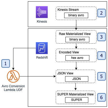
Gameskraft used Amazon Redshift RA3 instances with Redshift Managed Storage (RMS) for their data warehouse. The upstream data pipeline is a robust system that integrates various data sources, including Amazon Kinesis and Amazon Managed Streaming for Apache Kafka (Amazon MSK) for handling clickstream events, Amazon Relational Database Service (Amazon RDS) for delta transactions, and Amazon DynamoDB for delta game-related information. Additionally, data is extracted from vendor APIs that includes data related to product, marketing, and customer experience. All of this diverse data is then consolidated into the Amazon Simple Storage Service (Amazon S3) data lake before being uploaded to the Redshift data warehouse. These upstream data sources constitute the data producer components.
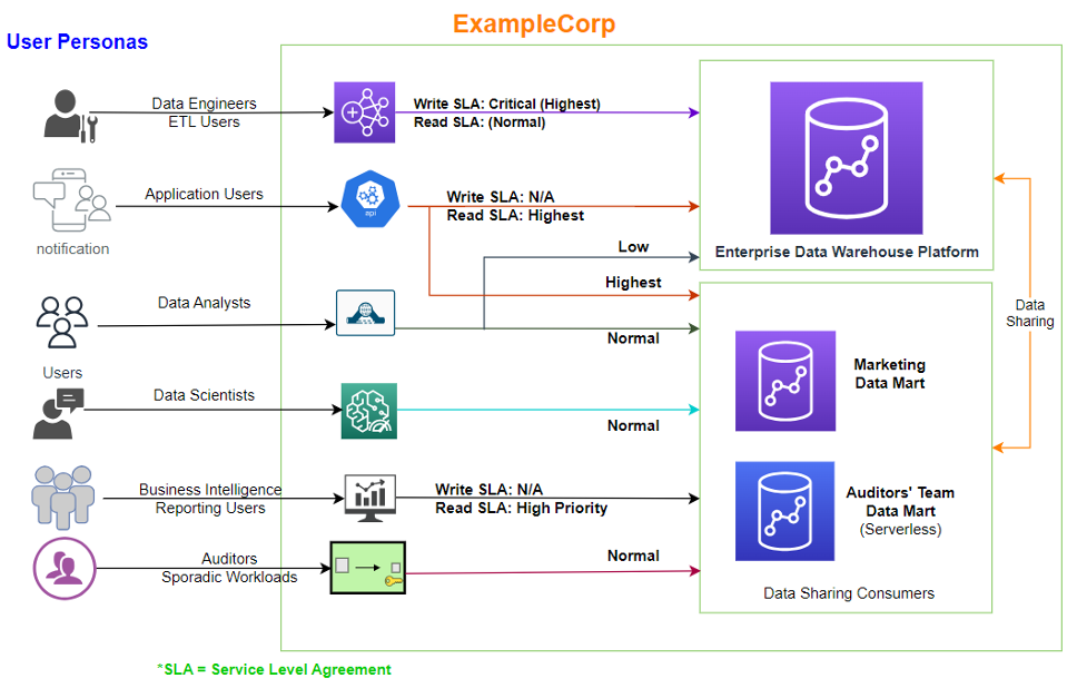
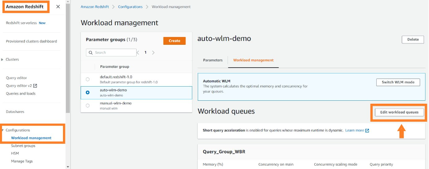
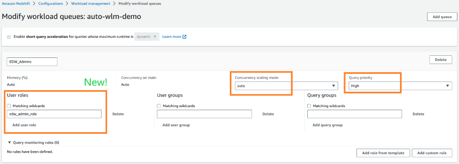
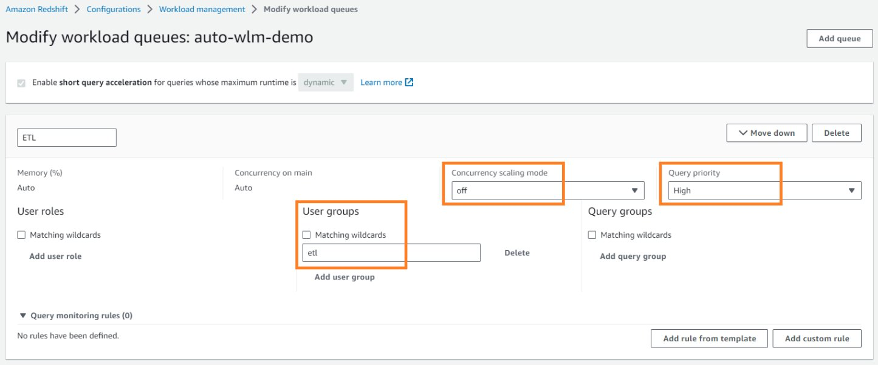
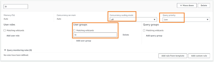
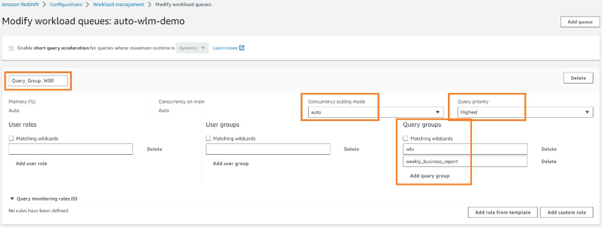
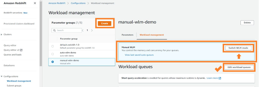
Gameskraft used Amazon Redshift workload management (WLM) to manage priorities within workloads, with higher priority being assigned to the extract, transform, and load (ETL) queue that runs critical jobs for data producers. The downstream consumers consist of business intelligence (BI) tools, with multiple data science and data analytics teams having their own WLM queues with appropriate priority values.
As Gameskraft’s portfolio of gaming products increased, it led to an approximate five-times growth of dedicated data analytics and data science teams. Consequently, there was a fivefold rise in data integrations and a fivefold increase in ad hoc queries submitted to the Redshift cluster. These query patterns and concurrency were unpredictable in nature. Also, over time the number of BI dashboards (both scheduled and live) increased, which contributed to more queries being submitted to the Redshift cluster.
With this growing workload, Gameskraft was observing the following challenges:
- Increase in critical ETL job runtime
- Increase in query wait time in multiple queues
- Impact of unpredictable ad hoc query workloads across other queues in the cluster
Gameskraft was looking for a solution that would help them mitigate all these challenges, and provide flexibility to scale ingestion and consumption workload processing independently. Gameskraft was also looking for a solution that would cater to their unpredictable future growth.
Solution overview
Gameskraft tackled these challenges in a phased manner using Amazon Redshift concurrency scaling, Amazon Redshift data sharing, Amazon Redshift Serverless, and Redshift provisioned clusters.
Amazon Redshift concurrency scaling lets you easily support thousands of concurrent users and concurrent queries, with consistently fast query performance. As concurrency increases, Amazon Redshift automatically adds query processing power in seconds to process queries without any delays. When the workload demand subsides, this extra processing power is automatically removed, so you pay only for the time when concurrency scaling clusters are in use. Amazon Redshift offers 1 hour of free concurrency scaling credits per active cluster per day, allowing you to accumulate 30 hours of free credits per month.
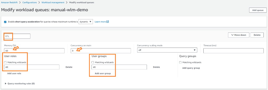
Gameskraft enabled concurrency scaling in selective WLM queues to ease the query wait time in those queues during peak usage and also helped reduce ETL query runtime. In the prior setup, we maintained four specialized queues for ETL, ad hoc queries, BI tools, and data science. To prevent blockages for other processes, we imposed minimal query timeouts using query monitoring rules (QMR). However, both the ETL and BI tools queues were persistently occupied, impacting the performance of the remaining queues.
Concurrency scaling helped alleviate query wait time in the ad hoc query queue. Still, the challenge of downstream consumption workloads (like ad hoc queries) impacting ingestion persisted, and Gameskraft was looking for a solution to manage these workloads independently.
The following table summarizes the workload management configuration prior to the solution implementation.
| Queue | Usage | Concurrency Scaling Mode | Concurrency on Main / Memory % | Query Monitoring Rules |
etl |
For ingestion from multiple data integration | off | auto | Stop action on: Query runtime (seconds) > 2700 |
report |
For scheduled reporting purposes | off | auto | Stop action on: Query runtime (seconds) > 600 |
datascience |
For data science workloads | off | auto | Stop action on: Query runtime (seconds) > 300 |
readonly |
For ad hoc and day-to-day analysis | auto | auto | Stop action on: Query runtime (seconds) > 120 |
bi_tool |
For BI tools | auto | auto | Stop action on: Query runtime (seconds) > 300 |
To achieve flexibility in scaling, Gameskraft used Amazon Redshift data sharing. Amazon Redshift data sharing allows you to extend the ease of use, performance, and cost benefits offered by a single cluster to multi-cluster deployments while being able to share data. Data sharing enables instant, granular, and fast data access across Amazon Redshift data warehouses without the need to copy or move it. Data sharing provides live access to data so that users always observe the most up-to-date and consistent information as it’s updated in the data warehouse. You can securely share live data across provisioned clusters, serverless endpoints within AWS account, across AWS accounts, and across AWS Regions.
Data sharing builds on Redshift Managed Storage (RMS), which underpins RA3 provisioned clusters and serverless workgroups, allowing multiple warehouses to query the same data with separate isolated compute. Queries accessing shared data run on the consumer cluster and read data from RMS directly without impacting the performance of the producer cluster. You can now rapidly onboard workloads with diverse data access patterns and SLA requirements and not be concerned about resource contention.
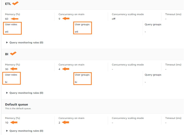
We chose to run all ETL workloads in the primary producer cluster to manage ETL independently. We used data sharing to share read-only access to data with a data science serverless workgroup, a BI provisioned cluster, an ad hoc query provisioned cluster, and a data integration serverless workgroup. Teams using these separate compute resources could then query the same data without copying the data between the producer and consumer. Additionally, we introduced concurrency scaling to the consumer queues, prioritizing BI tools, and extended the timeout for the remaining queues. These modifications notably enhanced overall efficiency and throughput.
The following table summarizes the new workload management configuration for the producer cluster.
| Queue | Usage | Concurrency Scaling Mode | Concurrency on Main / Memory % | Query Monitoring Rules |
etl |
For ingestion from multiple data integration | auto | auto | Stop action on: Query runtime (seconds) > 3600 |
The following table summarizes the new workload management configuration for the consumer cluster.
| Queue | Usage | Concurrency Scaling Mode | Concurrency on Main / Memory % | Query Monitoring Rules |
report |
For scheduled reporting purposes | off | auto | Stop action on: Query runtime (seconds) > 1200 Query queue time (seconds) > 1800 Spectrum scan row count (rows) > 100000 Spectrum scan (MB) > 3072 |
datascience |
For data science workloads | off | auto | Stop action on: Query runtime (seconds) > 600 Query queue time (seconds) > 1800 Spectrum scan row count (rows) > 100000 Spectrum scan (MB) > 3072 |
readonly |
For ad hoc and day-to-day analysis | auto | auto | Stop action on: Query runtime (seconds) > 900 Query queue time (seconds) > 3600 Spectrum scan (MB) > 3072 Spectrum scan row count (rows) > 100000 |
bi_tool_live |
For live BI tools | auto | auto | Stop action on: Query runtime (seconds) > 900 Query queue time (seconds) > 1800 Spectrum scan (MB) > 1024 Spectrum scan row count (rows) > 1000 |
bi_tool_schedule |
For scheduled BI tools | auto | auto | Stop action on: Query runtime (seconds) > 1800 Query queue time (seconds) > 3600 Spectrum scan (MB) > 1024 Spectrum scan row count (rows) > 1000 |
Solution implementation
Gameskraft is dedicated to maintaining uninterrupted system operations, prioritizing seamless solutions over downtime. In pursuit of this principle, strategic measures were undertaken to ensure a smooth migration process towards enabling data sharing, which included the following steps:
- Planning:
- Replicating users and groups to the consumer, to mitigate potential access complications for analytics, data science, and BI teams.
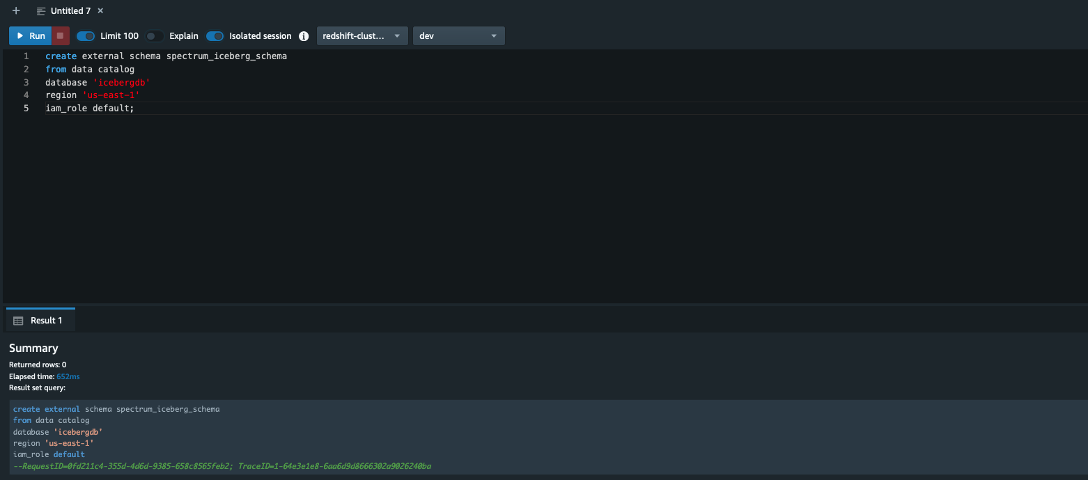
- Establishing a comprehensive setup within the consumers, encompassing essential components like external schemas for Amazon Redshift Spectrum.
- Fine-tuning WLM configurations tailored to the consumer’s requirements.
- Implementation:
- Introducing insightful monitoring dashboards in Grafana for CPU utilization, read/write throughputs, IOPS, and latencies specific to the consumer cluster, enhancing oversight capabilities.
- Changing all interleaved key tables on the producer cluster to compound sortkey tables to seamlessly transition data.
- Creating an external schema from the data share database on the consumer, mirroring that of the producer cluster with identical names. This approach minimizes the need for making query adjustments in multiple locations.
- Testing:
- Conducting an internal week-long regression testing and auditing process to meticulously validate all data points by running the same workload and twice the workload.
- Final changes:
- Updating the DNS record for the cluster endpoint, which included replacing the consumer cluster’s endpoint to the same domain as the producer cluster’s endpoint, to streamline connections and avoid making changes in multiple places.
- Ensuring data security and access control by revoking group and user privileges from the producer cluster.
The following diagram illustrates the Gameskraft Amazon Redshift data sharing architecture.

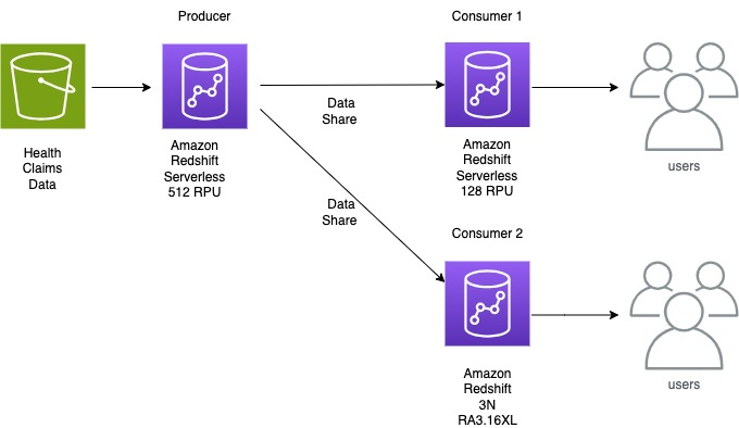
The following diagram illustrates the Amazon Redshift data sharing architecture with multiple consumer clusters.

With data sharing implementation, Gameskraft was able to isolate the producer and consumer workloads. Data sharing also provided the flexibility to independently scale the producer and consumer data warehouses.
The implementation of the overall solution helped Gameskraft support more frequent data refresh (43% reduction in overall job runtime) for its ETL workload, which runs on the producer cluster, along with capabilities to support a growing (five-times increase in users, BI workloads, and ad hoc queries) and unpredictable consumer workload.
The following dashboards show some of the critical ETL pipeline runtimes (before solution implementation and after solution implementation).
The first shows the delta P1/P2/P3 job runs before and after solution implementation (duration in minutes).

The following shows the daily event ETL P1/P2/P3 job runs before and after solution implementation (duration in minutes).

Key considerations
Gameskraft embraces a modern data architecture, with the data lake residing in Amazon S3. To grant seamless access to the data lake, we use the innovative capabilities of Redshift Spectrum, which is a bridge between the data warehouse (Amazon Redshift) and data lake (Amazon S3). It allows you to perform data transformations and analysis directly on data stored in Amazon S3, without having to duplicate the data into your Redshift cluster.
Gameskraft had a couple of key learnings while implementing this data sharing solution:
- First, as of this writing, Amazon Redshift data sharing doesn’t support adding external schemas, tables, or late-binding views on external tables to the data share. To enable this, we have created an external schema as a pointer to AWS Glue database. The same AWS Glue database is referenced in the external schema on the consumer side.
- Second, Amazon Redshift doesn’t support sharing tables with interleaved sort keys and views that refer to tables with interleaved sort keys. Due to the presence of interleaved sort keys across numerous tables and views, a prerequisite for inclusion into the data share involves revising the sort key configuration to use compound sort key.
Conclusion
In this post, we saw how Gameskraft used data sharing and concurrency scaling in Amazon Redshift with a producer and consumer cluster architecture to achieve the following:
- Reduce query wait time for all queues in the producer and consumer
- Scale the producer and consumer independently based on workload and queue requirements
- Improve ETL pipeline performance and the data refresh cycle to support more frequent refreshes in the producer cluster
- Onboard more queues and workloads (BI tools queue, data integration queue, data science queue, downstream team’s queue, ad hoc query queue) in the consumer without impacting the ETL pipeline in the producer cluster
- Flexibility to use multiple consumers with a mix of provisioned Redshift cluster and Redshift Serverless
These Amazon Redshift features and architecture can help support a growing and unpredictable analytics workload.
About the Authors
 Anshuman Varshney is Technical Lead at Gameskraft with a background in both backend and data engineering. He has a proven track record of leading and mentoring cross-functional teams to deliver high-performance, scalable solutions. Apart from work, he relishes moments with his family, indulges in cinematic experiences, and seizes every opportunity to explore new destinations through travel.
 Prafulla Wani is an Amazon Redshift Specialist Solution Architect at AWS. He works with AWS customers on analytics architecture designs and Amazon Redshift proofs of concept. In his spare time, he plays chess with his son.
 Saurov Nandy is a Solutions Architect at AWS. He works with AWS customers to design and implement solutions that solve complex business problems. In his spare time, he likes to explore new places and indulge in photography and video editing.
 Shashank Tewari is a Senior Technical Account Manager at AWS. He helps AWS customers optimize their architectures to achieve performance, scale, and cost efficiencies. In his spare time, he likes to play video games with his kids. During vacations, he likes to trek on mountains and take up adventure sports.

 Preshen Goobiah is the Lead Machine Learning Engineer for the Feature Platform at Capitec. He is focused on designing and building Feature Store components for enterprise use. In his spare time, he enjoys reading and traveling.
 Johan Olivier is a Senior Machine Learning Engineer for Capitec’s Model Platform. He is an entrepreneur and problem-solving enthusiast. He enjoys music and socializing in his spare time.
 Sudipta Bagchi is a Senior Specialist Solutions Architect at Amazon Web Services. He has over 12 years of experience in data and analytics, and helps customers design and build scalable and high-performant analytics solutions. Outside of work, he loves running, traveling, and playing cricket. Connect with him on
  Syed Humair is a Senior Analytics Specialist Solutions Architect at Amazon Web Services (AWS). He has over 17 years of experience in enterprise architecture focusing on Data and AI/ML, helping AWS customers globally to address their business and technical requirements. You can connect with him on
  Vuyisa Maswana is a Senior Solutions Architect at AWS, based in Cape Town. Vuyisa has a strong focus on helping customers build technical solutions to solve business problems. He has supported Capitec in their AWS journey since 2019.
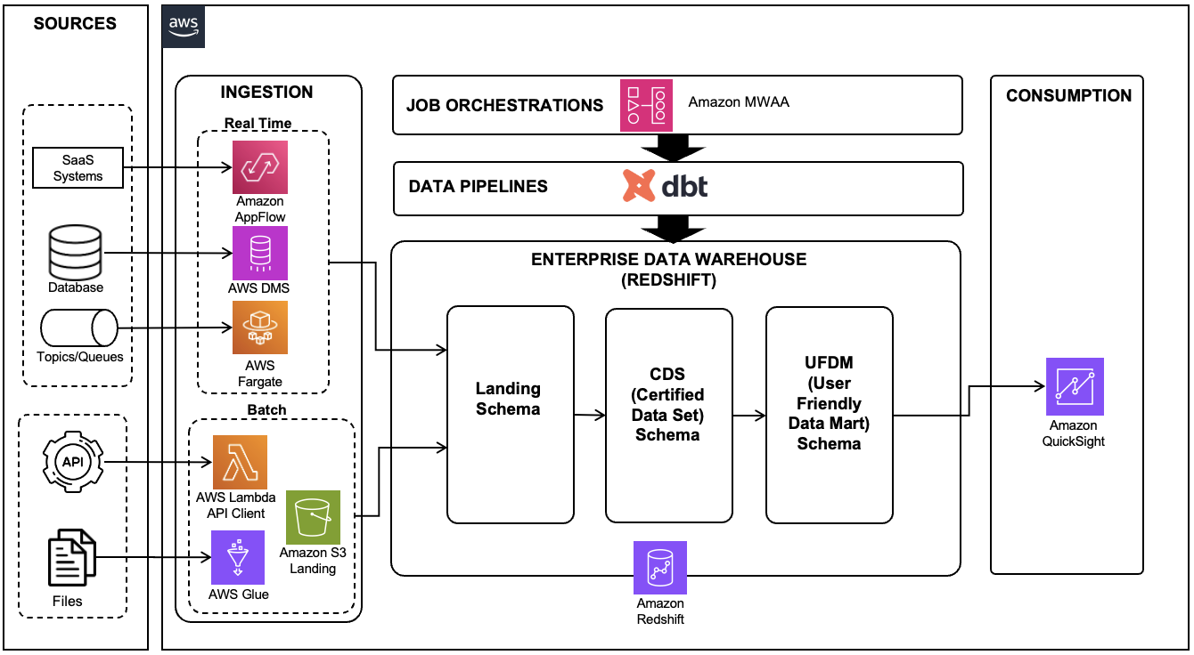


 Prantik Gachhayat is an Enterprise Architect at Infosys having experience in various technology fields and business domains. He has a proven track record helping large enterprises modernize digital platforms and delivering complex transformation programs. Prantik specializes in architecting modern data and analytics platforms in AWS. Prantik loves exploring new tech trends and enjoys cooking.
 Ashutosh Dubey is a Senior Partner Solutions Architect and Global Tech leader at Amazon Web Services based out of New Jersey, USA. He has extensive experience specializing in the Data and Analytics and AIML field including generative AI, contributed to the community by writing various tech contents, and has helped Fortune 500 companies in their cloud journey to AWS.

 Rajiv Arora is a Director of Clinical Data Science at Gilead Sciences with over 20 years of experience in the industry. He is responsible for the multi-modal data platform for the development organization and supports all statistical and predictive analytical infrastructure for RWE and Advanced Analytical functions.
 Ritesh Kumar Sinha is an Analytics Specialist Solutions Architect based out of San Francisco. He has helped customers build scalable data warehousing and big data solutions for over 16 years. He loves to design and build efficient end-to-end solutions on AWS. In his spare time, he loves reading, walking, and doing yoga.
 Raks Khare is an Analytics Specialist Solutions Architect at AWS based out of Pennsylvania. He helps customers architect data analytics solutions at scale on the AWS platform.
 Brent Strong is a Senior Solutions Architect in the Healthcare and Life Sciences team at AWS. He has more than 15 years of experience in the industry, focusing on data and analytics and DevOps. At AWS, he works closely with large Life Sciences customers to help them deliver new and innovative treatments.
 Phil Bates is a Senior Analytics Specialist Solutions Architect at AWS with over 25 years of data warehouse experience.


 Phil Bates is a Senior Analytics Specialist Solutions Architect at AWS. He has more than 25 years of experience implementing large-scale data warehouse solutions. He is passionate about helping customers through their cloud journey and using the power of ML within their data warehouse.


 Stefan Gromoll is a Senior Performance Engineer with Amazon Redshift team where he is responsible for measuring and improving Redshift performance. In his spare time, he enjoys cooking, playing with his three boys, and chopping firewood.
 Aamer Shah is a Senior Engineer in the Amazon Redshift Service team.
 Sanket Hase is a Software Development Manager in the Amazon Redshift Service team.
 Orestis Polychroniou is a Principal Engineer in the Amazon Redshift Service team.


 Anirban Sinha is a Senior Technical Account Manager at AWS. He is passionate about building scalable data warehouses and big data solutions working closely with customers. He works with large ISVs customers, in helping them build and operate secure, resilient, scalable, and high-performance SaaS applications in the cloud.
 Gaurav Singh is a Senior Solutions Architect at AWS, specializing in AI/ML and Generative AI. Based in Pune, India, he focuses on helping customers build, deploy, and migrate ML production workloads to SageMaker at scale. In his spare time, Gaurav loves to explore nature, read, and run.

 Sakti Mishra is a Principal Solutions Architect at AWS, where he helps customers modernize their data architecture and define their end-to-end data strategy, including data security, accessibility, governance, and more. He is also the author of the book
  Bhavana Chirumamilla is a Senior Resident Architect at AWS with a strong passion for data and machine learning operations. She brings a wealth of experience and enthusiasm to help enterprises build effective data and ML strategies. In her spare time, Bhavana enjoys spending time with her family and engaging in various activities such as traveling, hiking, gardening, and watching documentaries.
 Sheela Sonone is a Senior Resident Architect at AWS. She helps AWS customers make informed choices and trade-offs about accelerating their data, analytics, and AI/ML workloads and implementations. In her spare time, she enjoys spending time with her family—usually on tennis courts.
 Daniel Bruno is a Principal Resident Architect at AWS. He had been building analytics and machine learning solutions for over 20 years and splits his time helping customers build data science programs and designing impactful ML products.


 Mykhailo Kondak is a Database Engineer in the AWS Database Migration Service team at AWS. He uses his experience with different database technologies to help Amazon customers to move their on-premises data warehouses and big data workloads to the AWS Cloud. In his spare time, he plays soccer.
 Illia Kravtsov is a Database Engineer on the AWS Database Migration Service team. He has over 10 years of experience in data warehouse development with Teradata and other massively parallel processing (MPP) databases.
 Michael Soo is a Principal Database Engineer in the AWS Database Migration Service. He builds products and services that help customers migrate their database workloads to the AWS Cloud.
 M Mehrtens has been working in distributed systems engineering throughout their career, working as a Software Engineer, Architect, and Data Engineer. In the past, M has supported and built systems to process terrabytes of streaming data at low latency, run enterprise Machine Learning pipelines, and created systems to share data across teams seamlessly with varying data toolsets and software stacks. At AWS, they are a Sr. Solutions Architect supporting US Federal Financial customers.
 Sindhu Achuthan is a Sr. Solutions Architect with Federal Financials at AWS. She works with customers to provide architectural guidance on analytics solutions using AWS Glue, Amazon EMR, Amazon Kinesis, and other services. Outside of work, she loves DIYs, to go on long trails, and yoga.
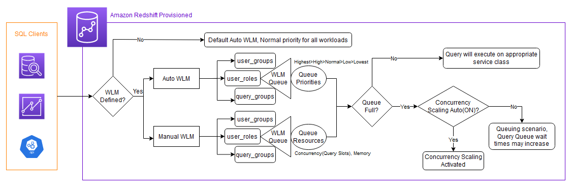


 Rohit Vashishtha is a Senior Analytics Specialist Solutions Architect at AWS based in Dallas, Texas. He has over 17 years of experience architecting, building, leading, and maintaining big data platforms. Rohit helps customers modernize their analytic workloads using the breadth of AWS services and ensures that customers get the best price/performance with utmost security and data governance.
 Harshida Patel is a Principal specialist SA with AWS.
 Nita Shah is an Analytics Specialist Solutions Architect at AWS based out of New York. She has been building data warehouse solutions for over 20 years and specializes in Amazon Redshift. She is focused on helping customers design and build enterprise-scale well-architected analytics and decision support platforms.
 Yanzhu Ji is a Product Manager in the Amazon Redshift team. She has experience in product vision and strategy in industry-leading data products and platforms. She has outstanding skill in building substantial software products using web development, system design, database, and distributed programming techniques. In her personal life, Yanzhu likes painting, photography, and playing tennis.


 Milind Oke is a Data Warehouse Specialist Solutions Architect based out of New York. He has been building data warehouse solutions for over 15 years and specializes in Amazon Redshift.
 Satesh Sonti is a Sr. Analytics Specialist Solutions Architect based out of Atlanta, specialized in building enterprise data platforms, data warehousing, and analytics solutions. He has over 17 years of experience in building data assets and leading complex data platform programs for banking and insurance clients across the globe.
 Kiran Chinta is a Software Development Manager at Amazon Redshift. He leads a strong team in query processing, SQL language, data security, and performance. Kiran is passionate about delivering products that seamlessly integrate with customers’ business applications with the right ease of use and performance. In his spare time, he enjoys reading and playing tennis.
 Huichen Liu is a software development engineer on the Amazon Redshift query processing team. She focuses on query optimization, statistics and SQL language features. In her spare time, she enjoys hiking and photography.


 Satish Sathiya is a Senior Product Engineer at Amazon Redshift. He is an avid big data enthusiast who collaborates with customers around the globe to achieve success and meet their data warehousing and data lake architecture needs.


 Ziad WALI is an Acceleration Lab Solutions Architect at Amazon Web Services. He has over 10 years of experience in databases and data warehousing where he enjoys building reliable, scalable and efficient solutions. Outside of work, he enjoys sports and spending time in nature.