Post Syndicated from Suthan Phillips original https://aws.amazon.com/blogs/big-data/part-1-build-your-apache-hudi-data-lake-on-aws-using-amazon-emr/
Apache Hudi is an open-source transactional data lake framework that greatly simplifies incremental data processing and data pipeline development. It does this by bringing core warehouse and database functionality directly to a data lake on Amazon Simple Storage Service (Amazon S3) or Apache HDFS. Hudi provides table management, instantaneous views, efficient upserts/deletes, advanced indexes, streaming ingestion services, data and file layout optimizations (through clustering and compaction), and concurrency control, all while keeping your data in open-source file formats such as Apache Parquet and Apache Avro. Furthermore, Apache Hudi is integrated with open-source big data analytics frameworks, such as Apache Spark, Apache Hive, Apache Flink, Presto, and Trino.
In this post, we cover best practices when building Hudi data lakes on AWS using Amazon EMR. This post assumes that you have the understanding of Hudi data layout, file layout, and table and query types. The configuration and features can change with new Hudi versions; the concept of this post applies to Hudi versions of 0.11.0 (Amazon EMR release 6.7), 0.11.1 (Amazon EMR release 6.8) and 0.12.1 (Amazon EMR release 6.9).
Specify the table type: Copy on Write Vs. Merge on Read
When we write data into Hudi, we have the option to specify the table type: Copy on Write (CoW) or Merge on Read (MoR). This decision has to be made at the initial setup, and the table type can’t be changed after the table has been created. These two table types offer different trade-offs between ingest and query performance, and the data files are stored differently based on the chosen table type. If you don’t specify it, the default storage type CoW is used.
The following table summarizes the feature comparison of the two storage types.
| CoW |
MoR |
| Data is stored in base files (columnar Parquet format). |
Data is stored as a combination of base files (columnar Parquet format) and log files with incremental changes (row-based Avro format). |
| COMMIT: Each new write creates a new version of the base files, which contain merged records from older base files and newer incoming records. Each write adds a commit action to the timeline, and each write atomically adds a commit action to the timeline, guaranteeing a write (and all its changes) entirely succeed or get entirely rolled back. |
DELTA_COMMIT: Each new write creates incremental log files for updates, which are associated with the base Parquet files. For inserts, it creates a new version of the base file similar to CoW. Each write adds a delta commit action to the timeline. |
| Write |
| In case of updates, write latency is higher than MoR due to the merge cost because it needs to rewrite the entire affected Parquet files with the merged updates. Additionally, writing in the columnar Parquet format (for CoW updates) is more latent in comparison to the row-based Avro format (for MoR updates). |
No merge cost for updates during write time, and the write operation is faster because it just appends the data changes to the new log file corresponding to the base file each time. |
| Compaction isn’t needed because all data is directly written to Parquet files. |
Compaction is required to merge the base and log files to create a new version of the base file. |
| Higher write amplification because new versions of base files are created for every write. Write cost will be O(number of files in storage modified by the write). |
Lower write amplification because updates go to log files. Write cost will be O(1) for update-only datasets and can get higher when there are new inserts. |
| Read |
| CoW table supports snapshot query and incremental queries. |
MoR offers two ways to query the same underlying storage: ReadOptimized tables and Near-Realtime tables (snapshot queries).
ReadOptimized tables support read-optimized queries, and Near-Realtime tables support snapshot queries and incremental queries.
|
| Read-optimized queries aren’t applicable for CoW because data is already merged to base files while writing. |
Read-optimized queries show the latest compacted data, which doesn’t include the freshest updates in the not yet compacted log files. |
| Snapshot queries have no merge cost during read. |
Snapshot queries merge data while reading if not compacted and therefore can be slower than CoW while querying the latest data. |
CoW is the default storage type and is preferred for simple read-heavy use cases. Use cases with the following characteristics are recommended for CoW:
- Tables with a lower ingestion rate and use cases without real-time ingestion
- Use cases requiring the freshest data with minimal read latency because merging cost is taken care of at the write phase
- Append-only workloads where existing data is immutable
MoR is recommended for tables with write-heavy and update-heavy use cases. Use cases with the following characteristics are recommended for MoR:
- Faster ingestion requirements and real-time ingestion use cases.
- Varying or bursty write patterns (for example, ingesting bulk random deletes in an upstream database) due to the zero-merge cost for updates during write time
- Streaming use cases
- Mix of downstream consumers, where some are looking for fresher data by paying some additional read cost, and others need faster reads with some trade-off in data freshness
For streaming use cases demanding strict ingestion performance with MoR tables, we suggest running the table services (for example, compaction and cleaning) asynchronously, which is discussed in the upcoming Part 3 of this series.
For more details on table types and use cases, refer to How do I choose a storage type for my workload?
Select the record key, key generator, preCombine field, and record payload
This section discusses the basic configurations for the record key, key generator, preCombine field, and record payload.
Record key
Every record in Hudi is uniquely identified by a Hoodie key (similar to primary keys in databases), which is usually a pair of record key and partition path. With Hoodie keys, you can enable efficient updates and deletes on records, as well as avoid duplicate records. Hudi partitions have multiple file groups, and each file group is identified by a file ID. Hudi maps Hoodie keys to file IDs, using an indexing mechanism.
A record key that you select from your data can be unique within a partition or across partitions. If the selected record key is unique within a partition, it can be uniquely identified in the Hudi dataset using the combination of the record key and partition path. You can also combine multiple fields from your dataset into a compound record key. Record keys cannot be null.
Key generator
Key generators are different implementations to generate record keys and partition paths based on the values specified for these fields in the Hudi configuration. The right key generator has to be configured depending on the type of key (simple or composite key) and the column data type used in the record key and partition path columns (for example, TimestampBasedKeyGenerator is used for timestamp data type partition path). Hudi provides several key generators out of the box, which you can specify in your job using the following configuration.
| Configuration Parameter |
Description |
Value |
hoodie.datasource.write.keygenerator.class |
Key generator class, which generates the record key and partition path |
Default value is SimpleKeyGenerator |
The following table describes the different types of key generators in Hudi.
| Key Generators |
Use-case |
SimpleKeyGenerator |
Use this key generator if your record key refers to a single column by name and similarly your partition path also refers to a single column by name. |
ComplexKeyGenerator |
Use this key generator when record key and partition paths comprise multiple columns. Columns are expected to be comma-separated in the config value (for example, "hoodie.datasource.write.recordkey.field" : “col1,col4”). |
GlobalDeleteKeyGenerator |
Use this key generator when you can’t determine the partition of incoming records to be deleted and need to delete only based on record key. This key generator ignores the partition path while generating keys to uniquely identify Hudi records.
When using this key generator, set the config hoodie.[bloom|simple|hbase].index.update.partition.path to false in order to avoid redundant data written to the storage.
|
NonPartitionedKeyGenerator |
Use this key generator for non-partitioned datasets because it returns an empty partition for all records. |
TimestampBasedKeyGenerator |
Use this key generator for a timestamp data type partition path. With this key generator, the partition path column values are interpreted as timestamps. The record key is the same as before, which is a single column converted to string. If using TimestampBasedKeyGenerator, a few more configs need to be set. |
CustomKeyGenerator |
Use this key generator to take advantage of the benefits of SimpleKeyGenerator, ComplexKeyGenerator, and TimestampBasedKeyGenerator all at the same time. With this you can configure record key and partition paths as a single field or a combination of fields. This is helpful if you want to generate nested partitions with each partition key of different types (for example, field_3:simple,field_5:timestamp). For more information, refer to CustomKeyGenerator. |
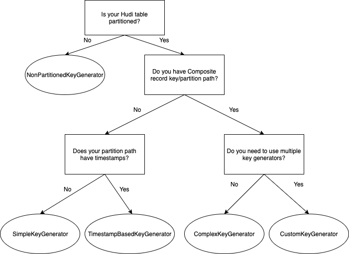
The key generator class can be automatically inferred by Hudi if the specified record key and partition path require a SimpleKeyGenerator or ComplexKeyGenerator, depending on whether there are single or multiple record key or partition path columns. For all other cases, you need to specify the key generator.
The following flow chart explains how to select the right key generator for your use case.

PreCombine field
This is a mandatory field that Hudi uses to deduplicate the records within the same batch before writing them. When two records have the same record key, they go through the preCombine process, and the record with the largest value for the preCombine key is picked by default. This behavior can be customized through custom implementation of the Hudi payload class, which we describe in the next section.
The following table summarizes the configurations related to preCombine.
| Configuration Parameter |
Description |
Value |
hoodie.datasource.write.precombine.field |
The field used in preCombining before the actual write. It helps select the latest record whenever there are multiple updates to the same record in a single incoming data batch. |
The default value is ts. You can configure it to any column in your dataset that you want Hudi to use to deduplicate the records whenever there are multiple records with the same record key in the same batch. Currently, you can only pick one field as the preCombine field.
Select a column with the timestamp data type or any column that can determine which record holds the latest version, like a monotonically increasing number.
|
hoodie.combine.before.upsert |
During upsert, this configuration controls whether deduplication should be done for the incoming batch before ingesting into Hudi. This is applicable only for upsert operations. |
The default value is true. We recommend keeping it at the default to avoid duplicates. |
hoodie.combine.before.delete |
Same as the preceding config, but applicable only for delete operations. |
The default value is true. We recommend keeping it at the default to avoid duplicates. |
hoodie.combine.before.insert |
When inserted records share the same key, the configuration controls whether they should be first combined (deduplicated) before writing to storage. |
The default value is false. We recommend setting it to true if the incoming inserts or bulk inserts can have duplicates. |
Record payload
Record payload defines how to merge new incoming records against old stored records for upserts.
The default OverwriteWithLatestAvroPayload payload class always overwrites the stored record with the latest incoming record. This works fine for batch jobs and most use cases. But let’s say you have a streaming job and want to prevent the late-arriving data from overwriting the latest record in storage. You need to use a different payload class implementation (DefaultHoodieRecordPayload) to determine the latest record in storage based on an ordering field, which you provide.
For example, in the following example, Commit 1 has HoodieKey 1, Val 1, preCombine10, and in-flight Commit 2 has HoodieKey 1, Val 2, preCombine 5.

If using the default OverwriteWithLatestAvroPayload, the Val 2 version of the record will be the final version of the record in storage (Amazon S3) because it’s the latest version of the record.
If using DefaultHoodieRecordPayload, it will honor Val 1 because the Val 2’s record version has a lower preCombine value (preCombine 5) compared to Val 1’s record version, while merging multiple versions of the record.
You can select a payload class while writing to the Hudi table using the configuration hoodie.datasource.write.payload.class.
Some useful in-built payload class implementations are described in the following table.
| Payload Class |
Description |
OverwriteWithLatestAvroPayload (org.apache.hudi.common.model.OverwriteWithLatestAvroPayload) |
Chooses the latest incoming record to overwrite any previous version of the records. Default payload class. |
DefaultHoodieRecordPayload (org.apache.hudi.common.model.DefaultHoodieRecordPayload) |
Uses hoodie.payload.ordering.field to determine the final record version while writing to storage. |
EmptyHoodieRecordPayload (org.apache.hudi.common.model.EmptyHoodieRecordPayload) |
Use this as payload class to delete all the records in the dataset. |
AWSDmsAvroPayload (org.apache.hudi.common.model.AWSDmsAvroPayload) |
Use this as payload class if AWS DMS is used as source. It provides support for seamlessly applying changes captured via AWS DMS. This payload implementation performs insert, delete, and update operations on the Hudi table based on the operation type for the CDC record obtained from AWS DMS. |
Partitioning
Partitioning is the physical organization of files within a table. They act as virtual columns and can impact the max parallelism we can use on writing.
Extremely fine-grained partitioning (for example, over 20,000 partitions) can create excessive overhead for the Spark engine managing all the small tasks, and can degrade query performance by reducing file sizes. Also, an overly coarse-grained partition strategy, without clustering and data skipping, can negatively impact both read and upsert performance with the need to scan more files in each partition.
Right partitioning helps improve read performance by reducing the amount of data scanned per query. It also improves upsert performance by limiting the number of files scanned to find the file group in which a specific record exists during ingest. A column frequently used in query filters would be a good candidate for partitioning.
For large-scale use cases with evolving query patterns, we suggest coarse-grained partitioning (such as date), while using fine-grained data layout optimization techniques (clustering) within each partition. This opens the possibility of data layout evolution.
By default, Hudi creates the partition folders with just the partition values. We recommend using Hive style partitioning, in which the name of the partition columns is prefixed to the partition values in the path (for example, year=2022/month=07 as opposed to 2022/07). This enables better integration with Hive metastores, such as using msck repair to fix partition paths.
To support Apache Hive style partitions in Hudi, we have to enable it in the config hoodie.datasource.write.hive_style_partitioning.
The following table summarizes the key configurations related to Hudi partitioning.
| Configuration Parameter |
Description |
Value |
hoodie.datasource.write.partitionpath.field |
Partition path field. This is a required configuration that you need to pass while writing the Hudi dataset. |
There is no default value set for this. Set it to the column that you have determined for partitioning the data. We recommend that it doesn’t cause extremely fine-grained partitions. |
hoodie.datasource.write.hive_style_partitioning |
Determines whether to use Hive style partitioning. If set to true, the names of partition folders follow <partition_column_name>=<partition_value> format. |
Default value is false. Set it to true to use Hive style partitioning. |
hoodie.datasource.write.partitionpath.urlencode |
Indicates if we should URL encode the partition path value before creating the folder structure. |
Default value is false. Set it to true if you want to URL encode the partition path value. For example, if you’re using the data format “yyyy-MM-dd HH:mm:ss“, the URL encode needs to be set to true because it will result in an invalid path due to :. |
Note that if the data isn’t partitioned, you need to specifically use NonPartitionedKeyGenerator for the record key, which is explained in the previous section. Additionally, Hudi doesn’t allow partition columns to be changed or evolved.
Choose the right index
After we select the storage type in Hudi and determine the record key and partition path, we need to choose the right index for upsert performance. Apache Hudi employs an index to locate the file group that an update/delete belongs to. This enables efficient upsert and delete operations and enforces uniqueness based on the record keys.
Global index vs. non-global index
When picking the right indexing strategy, the first decision is whether to use a global (table level) or non-global (partition level) index. The main difference between global vs. non-global indexes is the scope of key uniqueness constraints. Global indexes enforce uniqueness of the keys across all partitions of a table. The non-global index implementations enforce this constraint only within a specific partition. Global indexes offer stronger uniqueness guarantees, but they come with a higher update/delete cost, for example global deletes with just the record key need to scan the entire dataset. HBase indexes are an exception here, but come with an operational overhead.

For large-scale global index use cases, use an HBase index or record-level index (available in Hudi 0.13) because for all other global indexes, the update/delete cost grows with the size of the table, O(size of the table).
When using a global index, be aware of the configuration hoodie[bloom|simple|hbase].index.update.partition.path, which is already set to true by default. For existing records getting upserted to a new partition, enabling this configuration will help delete the old record in the old partition and insert it in the new partition.
Hudi index options
After picking the scope of the index, the next step is to decide which indexing option best fits your workload. The following table explains the indexing options available in Hudi as of 0.11.0.
| Indexing Option |
How It Works |
Characteristic |
Scope |
| Simple Index |
Performs a join of the incoming upsert/delete records against keys extracted from the involved partition in case of non-global datasets and the entire dataset in case of global or non-partitioned datasets. |
Easiest to configure. Suitable for basic use cases like small tables with evenly spread updates. Even for larger tables where updates are very random to all partitions, a simple index is the right choice because it directly joins with interested fields from every data file without any initial pruning, as compared to Bloom, which in the case of random upserts adds additional overhead and doesn’t give enough pruning benefits because the Bloom filters could indicate true positive for most of the files and end up comparing ranges and filters against all these files. |
Global/Non-global |
| Bloom Index (default index in EMR Hudi) |
Employs Bloom filters built out of the record keys, optionally also pruning candidate files using record key ranges. Bloom filter is stored in the data file footer while writing the data. |
More efficient filter compared to simple index for use cases like late-arriving updates to fact tables and deduplication in event tables with ordered record keys such as timestamp. Hudi implements a dynamic Bloom filter mechanism to reduce false positives provided by Bloom filters.
In general, the probability of false positives increases with the number of records in a given file. Check the Hudi FAQ for Bloom filter configuration best practices.
|
Global/Non-global |
| Bucket Index |
It distributes records to buckets using a hash function based on the record keys or subset of it. It uses the same hash function to determine which file group to match with incoming records. New indexing option since hudi 0.11.0. |
Simple to configure. It has better upsert throughput performance compared to the Bloom filter. As of Hudi 0.11.1, only fixed bucket number is supported. This will no longer be an issue with the upcoming consistent hashing bucket index feature, which can dynamically change bucket numbers. |
Non-global |
| HBase Index |
The index mapping is managed in an external HBase table. |
Best lookup time, especially for large numbers of partitions and files. It comes with additional operational overhead because you need to manage an external HBase table. |
Global |
Use cases suitable for simple index
Simple indexes are most suitable for workloads with evenly spread updates over partitions and files on small tables, and also for larger tables with dimension kind of workloads because updates are random to all partitions. A common example is a CDC pipeline for a dimension table. In this case, updates end up touching a large number of files and partitions. Therefore, a join with no other pruning is most efficient.
Use cases suitable for Bloom index
Bloom indexes are suitable for most production workloads with uneven update distribution across partitions. For workloads with most updates to recent data like fact tables, Bloom filter rightly fits the bill. It can be clickstream data collected from an ecommerce site, bank transactions in a FinTech application, or CDC logs for a fact table.
When using a Bloom index, be aware of the following configurations:
hoodie.bloom.index.use.metadata – By default, it is set to false. When this flag is on, the Hudi writer gets the index metadata information from the metadata table and doesn’t need to open Parquet file footers to get the Bloom filters and stats. You prune out the files by just using the metadata table and therefore have improved performance for larger tables.hoodie.bloom.index.prune.by.ranges– Enable or disable range pruning based on use case. By default, it’s already set to true. When this flag is on, range information from files is used to speed up index lookups. This is helpful if the selected record key is monotonously increasing. You can set any record key to be monotonically increasing by adding a timestamp prefix. If the record key is completely random and has no natural ordering (such as UUIDs), it’s better to turn this off, because range pruning will only add extra overhead to the index lookup.
Use cases suitable for bucket index
Bucket indexes are suitable for upsert use cases on huge datasets with a large number of file groups within partitions, relatively even data distribution across partitions, and can achieve relatively even data distribution on the bucket hash field column. It can have better upsert performance in these cases due to no index lookup involved as file groups are located based on a hashing mechanism, which is very fast. This is totally different from both simple and Bloom indexes, where an explicit index lookup step is involved during write. The buckets here has one-one mapping with the hudi file group and since the total number of buckets (defined by hoodie.bucket.index.num.buckets(default – 4)) is fixed here, it can potentially lead to skewed data (data distributed unevenly across buckets) and scalability (buckets can grow over time) issues over time. These issues will be addressed in the upcoming consistent hashing bucket index, which is going to be a special type of bucket index.
Use cases suitable for HBase index
HBase indexes are suitable for use cases where ingestion performance can’t be met using the other index types. These are mostly use cases with global indexes and large numbers of files and partitions. HBase indexes provide the best lookup time but come with large operational overheads if you’re already using HBase for other workloads.
For more information on choosing the right index and indexing strategies for common use cases, refer to Employing the right indexes for fast updates, deletes in Apache Hudi. As you have already seen, Hudi index performance depends heavily on the actual workload. We encourage you to evaluate different indexes for your workload and choose the one which is best suited for your use case.
Migration guidance
With Apache Hudi growing in popularity, one of the fundamental challenges is to efficiently migrate existing datasets to Apache Hudi. Apache Hudi maintains record-level metadata to perform core operations such as upserts and incremental pulls. To take advantage of Hudi’s upsert and incremental processing support, you need to add Hudi record-level metadata to your original dataset.
Using bulk_insert
The recommended way for data migration to Hudi is to perform a full rewrite using bulk_insert. There is no look-up for existing records in bulk_insert and writer optimizations like small file handling. Performing a one-time full rewrite is a good opportunity to write your data in Hudi format with all the metadata and indexes generated and also potentially control file size and sort data by record keys.
You can set the sort mode in a bulk_insert operation using the configuration hoodie.bulkinsert.sort.mode. bulk_insert offers the following sort modes to configure.
| Sort Modes |
Description |
NONE |
No sorting is done to the records. You can get the fastest performance (comparable to writing parquet files with spark) for initial load with this mode. |
GLOBAL_SORT |
Use this to sort records globally across Spark partitions. It is less performant in initial load than other modes as it repartitions data by partition path and sorts it by record key within each partition. This helps in controlling the number of files generated in the target thereby controlling the target file size. Also, the generated target files will not have overlapping min-max values for record keys which will further help speed up index look-ups during upserts/deletes by pruning out files based on record key ranges in bloom index. |
PARTITION_SORT |
Use this to sort records within Spark partitions. It is more performant for initial load than Global_Sort and if your Spark partitions in the data frame are already fairly mapped to the Hudi partitions (dataframe is already repartitioned by partition column), using this mode would be preferred as you can obtain records sorted by record key within each partition. |
We recommend to use Global_Sort mode if you can handle the one-time cost. The default sort mode is changed from Global_Sort to None from EMR 6.9 (Hudi 0.12.1). During bulk_insert with Global_Sort, two configurations control the sizes of target files generated by Hudi.
| Configuration Parameter |
Description |
Value |
hoodie.bulkinsert.shuffle.parallelism |
The number of files generated from the bulk insert is determined by this configuration. The higher the parallelism, the more Spark tasks processing the data. |
Default value is 200. To control file size and achieve maximum performance (more parallelism), we recommend setting this to a value such that the files generated are equal to the hoodie.parquet.max.file.size. If you make parallelism really high, the max file size can’t be honored because the Spark tasks are working on smaller amounts of data. |
hoodie.parquet.max.file.size |
Target size for Parquet files produced by Hudi write phases. |
Default value is 120 MB. If the Spark partitions generated with hoodie.bulkinsert.shuffle.parallelism are larger than this size, it splits it and generates multiple files to not exceed the max file size. |
Let’s say we have a 100 GB Parquet source dataset and we’re bulk inserting with Global_Sort into a partitioned Hudi table with 10 evenly distributed Hudi partitions. We want to have the preferred target file size of 120 MB (default value for hoodie.parquet.max.file.size). The Hudi bulk insert shuffle parallelism should be calculated as follows:
- The total data size in MB is 100 * 1024 = 102400 MB
hoodie.bulkinsert.shuffle.parallelism should be set to 102400/120 = ~854
Please note that in reality even with Global_Sort, each spark partition can be mapped to more than one hudi partition and this calculation should only be used as a rough estimate and can potentially end up with more files than the parallelism specified.
Using bootstrapping
For customers operating at scale on hundreds of terabytes or petabytes of data, migrating your datasets to start using Apache Hudi can be time-consuming. Apache Hudi provides a feature called bootstrap to help with this challenge.
The bootstrap operation contains two modes: METADATA_ONLY and FULL_RECORD.
FULL_RECORD is the same as full rewrite, where the original data is copied and rewritten with the metadata as Hudi files.
The METADATA_ONLY mode is the key to accelerating the migration progress. The conceptual idea is to decouple the record-level metadata from the actual data by writing only the metadata columns in the Hudi files generated while the data isn’t copied over and stays in its original location. This significantly reduces the amount of data written, thereby improving the time to migrate and get started with Hudi. However, this comes at the expense of read performance, which involves the overhead merging Hudi files and original data files to get the complete record. Therefore, you may not want to use it for frequently queried partitions.
You can pick and choose these modes at partition level. One common strategy is to tier your data. Use FULL_RECORD mode for a small set of hot partitions, which are accessed frequently, and METADATA_ONLY for a larger set of cold partitions.
Consider the following:
Catalog sync
Hudi supports syncing Hudi table partitions and columns to a catalog. On AWS, you can either use the AWS Glue Data Catalog or Hive metastore as the metadata store for your Hudi tables. To register and synchronize the metadata with your regular write pipeline, you need to either enable hive sync or run the hive_sync_tool or AwsGlueCatalogSyncTool command line utility.
We recommend enabling the hive sync feature with your regular write pipeline to make sure the catalog is up to date. If you don’t expect a new partition to be added or the schema changed as part of each batch, then we recommend enabling hoodie.datasource.meta_sync.condition.sync as well so that it allows Hudi to determine if hive sync is necessary for the job.
If you have frequent ingestion jobs and need to maximize ingestion performance, you can disable hive sync and run the hive_sync_tool asynchronously.
If you have the timestamp data type in your Hudi data, we recommend setting hoodie.datasource.hive_sync.support_timestamp to true to convert the int64 (timestamp_micros) to the hive type timestamp. Otherwise, you will see the values in bigint while querying data.
The following table summarizes the configurations related to hive_sync.
| Configuration Parameter |
Description |
Value |
hoodie.datasource.hive_sync.enable |
To register or sync the table to a Hive metastore or the AWS Glue Data Catalog. |
Default value is false. We recommend setting the value to true to make sure the catalog is up to date, and it needs to be enabled in every single write to avoid an out-of-sync metastore. |
hoodie.datasource.hive_sync.mode |
This configuration sets the mode for HiveSynctool to connect to the Hive metastore server. For more information, refer to Sync modes. |
Valid values are hms, jdbc, and hiveql. If the mode isn’t specified, it defaults to jdbc. Hms and jdbc both talk to the underlying thrift server, but jdbc needs a separate jdbc driver. We recommend setting it to ‘hms’, which uses the Hive metastore client to sync Hudi tables using thrift APIs directly. This helps when using the AWS Glue Data Catalog because you don’t need to install Hive as an application on the EMR cluster (because it doesn’t need the server). |
hoodie.datasource.hive_sync.database |
Name of the destination database that we should sync the Hudi table to. |
Default value is default. Set this to the database name of your catalog. |
hoodie.datasource.hive_sync.table |
Name of the destination table that we should sync the Hudi table to. |
In Amazon EMR, the value is inferred from the Hudi table name. You can set this config if you need a different table name. |
hoodie.datasource.hive_sync.support_timestamp |
To convert logical type TIMESTAMP_MICROS as hive type timestamp. |
Default value is false. Set it to true to convert to hive type timestamp. |
hoodie.datasource.meta_sync.condition.sync |
If true, only sync on conditions like schema change or partition change. |
Default value is false. |
Writing and reading Hudi datasets, and its integration with other AWS services
There are different ways you can write the data to Hudi using Amazon EMR, as explained in the following table.
| Hudi Write Options |
Description |
| Spark DataSource |
You can use this option to do upsert, insert, or bulk insert for the write operation.
Refer to Work with a Hudi dataset for an example of how to write data using DataSourceWrite.
|
| Spark SQL |
You can easily write data to Hudi with SQL statements. It eliminates the need to write Scala or PySpark code and adopt a low-code paradigm. |
| Flink SQL, Flink DataStream API |
If you’re using Flink for real-time streaming ingestion, you can use the high-level Flink SQL or Flink DataStream API to write the data to Hudi. |
| DeltaStreamer |
DeltaStreamer is a self-managed tool that supports standard data sources like Apache Kafka, Amazon S3 events, DFS, AWS DMS, JDBC, and SQL sources, built-in checkpoint management, schema validations, as well as lightweight transformations. It can also operate in a continuous mode, in which a single self-contained Spark job can pull data from source, write it out to Hudi tables, and asynchronously perform cleaning, clustering, compactions, and catalog syncing, relying on Spark’s job pools for resource management. It’s easy to use and we recommend using it for all the streaming and ingestion use cases where a low-code approach is preferred. For more information, refer to Streaming Ingestion. |
| Spark structured streaming |
For use cases that require complex data transformations of the source data frame written in Spark DataFrame APIs or advanced SQL, we recommend the structured streaming sink. The streaming source can be used to obtain change feeds out of Hudi tables for streaming or incremental processing use cases. |
| Kafka Connect Sink |
If you standardize on the Apache Kafka Connect framework for your ingestion needs, you can also use the Hudi Connect Sink. |
Refer to the following support matrix for query support on specific query engines. The following table explains the different options to read the Hudi dataset using Amazon EMR.
| Hudi Read options |
Description |
| Spark DataSource |
You can read Hudi datasets directly from Amazon S3 using this option. The tables don’t need to be registered with Hive metastore or the AWS Glue Data Catalog for this option. You can use this option if your use case doesn’t require a metadata catalog. Refer to Work with a Hudi dataset for example of how to read data using DataSourceReadOptions. |
| Spark SQL |
You can query Hudi tables with DML/DDL statements. The tables need to be registered with Hive metastore or the AWS Glue Data Catalog for this option. |
| Flink SQL |
After the Flink Hudi tables have been registered to the Flink catalog, they can be queried using the Flink SQL. |
| PrestoDB/Trino |
The tables need to be registered with Hive metastore or the AWS Glue Data Catalog for this option. This engine is preferred for interactive queries. There is a new Trino connector in upcoming Hudi 0.13, and we recommend reading datasets through this connector when using Trino for performance benefits. |
| Hive |
The tables need to be registered with Hive metastore or the AWS Glue Data Catalog for this option. |
Apache Hudi is well integrated with AWS services, and these integrations work when AWS Glue Data Catalog is used, with the exception of Athena, where you can also use a data source connector to an external Hive metastore. The following table summarizes the service integrations.
Conclusion
This post covered best practices for configuring Apache Hudi data lakes using Amazon EMR. We discussed the key configurations in migrating your existing dataset to Hudi and shared guidance on how to determine the right options for different use cases when setting up Hudi tables.
The upcoming Part 2 of this series focuses on optimizations that can be done on this setup, along with monitoring using Amazon CloudWatch.
About the Authors
 Suthan Phillips is a Big Data Architect for Amazon EMR at AWS. He works with customers to provide best practice and technical guidance and helps them achieve highly scalable, reliable and secure solutions for complex applications on Amazon EMR. In his spare time, he enjoys hiking and exploring the Pacific Northwest.
 Dylan Qu is an AWS solutions architect responsible for providing architectural guidance across the full AWS stack with a focus on Data Analytics, AI/ML and DevOps.


 (IDMC) is an AI-powered, metadata-driven, persona-based, cloud-native platform to empower data professionals with a comprehensive and cohesive cloud data management capabilities to discover, catalog, ingest, cleanse, integrate, govern, secure, prepare, and master data.


 Leon Liu is a Chief Architect at ADP. He has over 20 years of experience with enterprise application framework, architecture, data warehouses, and big data real-time processing.


 Suthan Phillips is a Big Data Architect for Amazon EMR at AWS. He works with customers to provide best practice and technical guidance and helps them achieve highly scalable, reliable and secure solutions for complex applications on Amazon EMR. In his spare time, he enjoys hiking and exploring the Pacific Northwest.
 Dylan Qu is an AWS solutions architect responsible for providing architectural guidance across the full AWS stack with a focus on Data Analytics, AI/ML and DevOps.


 Srikanth Baheti is a Specialized World Wide Sr. Solution Architect for Amazon QuickSight. He started his career as a consultant and worked for multiple private and government organizations. Later he worked for PerkinElmer Health and Sciences & eResearch Technology Inc, where he was responsible for designing and developing high traffic web applications, highly scalable and maintainable data pipelines for reporting platforms using AWS services and Serverless computing.
 Raji Sivasubramaniam is a Sr. Solutions Architect at AWS, focusing on Analytics. Raji is specialized in architecting end-to-end Enterprise Data Management, Business Intelligence and Analytics solutions for Fortune 500 and Fortune 100 companies across the globe. She has in-depth experience in integrated healthcare data and analytics with wide variety of healthcare datasets including managed market, physician targeting and patient analytics.


 Theo Tolv is a Senior Analytics Architect based in Stockholm, Sweden. He’s worked with small and big data for most of his career, and has built applications running on AWS since 2008. In his spare time he likes to tinker with electronics and read space opera.
 Bruce Ross is a Senior Solutions Architect at AWS in the New York Area. Bruce is the Lens Leader for the Well-Architected Framework. He has been involved in IT and Content Development for over 20 years. He is an avid sailor and angler, and enjoys R&B, jazz, and classical music.


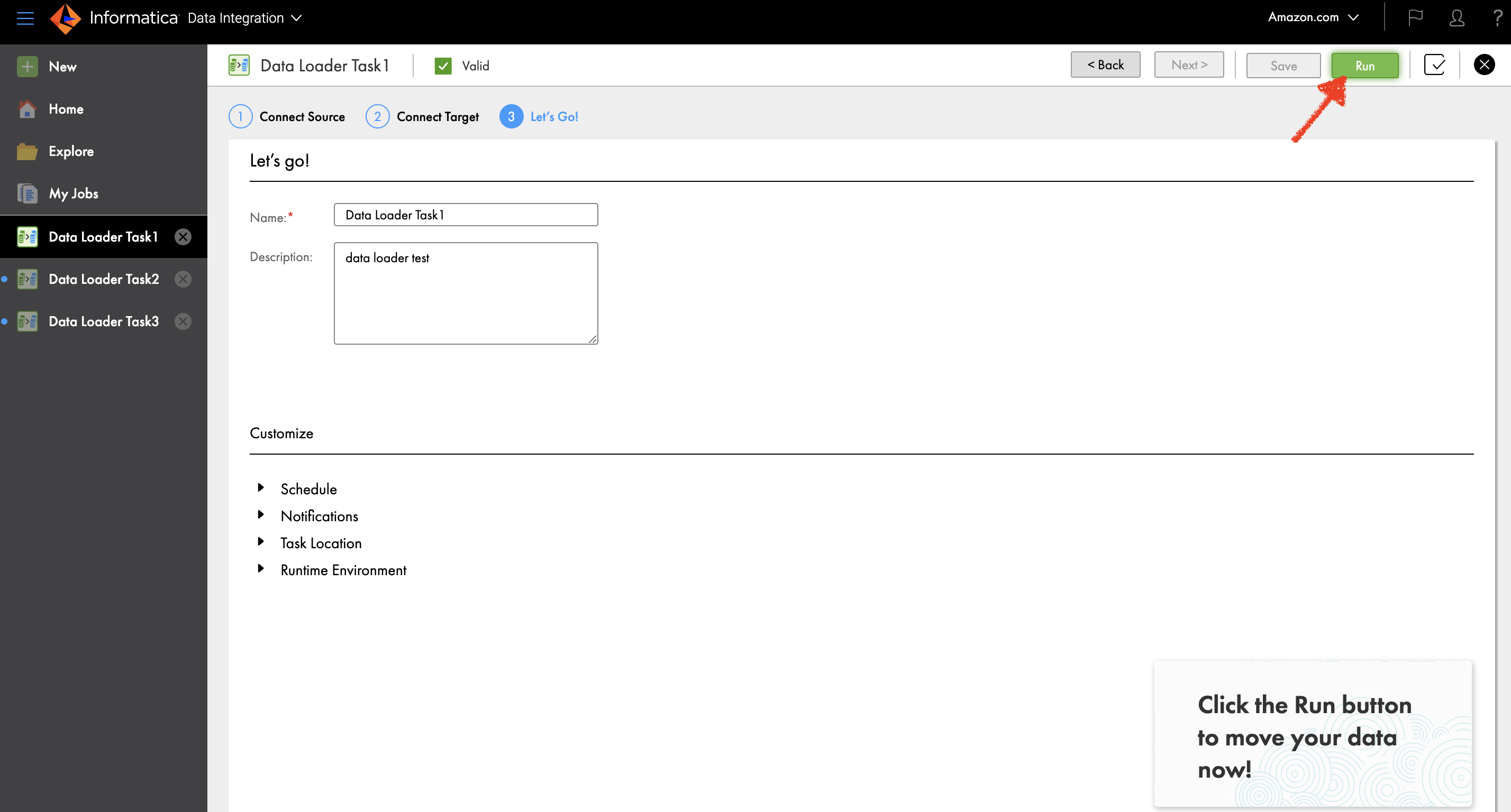
 You can also automate the preceding COPY commands using tasks, which can be scheduled to run at a set frequency for automatic copy of CDC data from Snowflake to Amazon S3.
 Now the tasks will run every 5 minutes and look for new data in the stream tables to offload to Amazon S3.As soon as data is migrated from Snowflake to Amazon S3, Redshift Auto Loader automatically infers the schema and instantly creates corresponding tables in Amazon Redshift. Then, by default, it starts loading data from Amazon S3 to Amazon Redshift every 5 minutes. You can also