Tag Archives: AWS Glue

Data preparation using an Amazon RDS for MySQL database with AWS Glue DataBrew

Post Syndicated from Dhiraj Thakur original https://aws.amazon.com/blogs/big-data/data-preparation-using-an-amazon-rds-for-mysql-database-with-aws-glue-databrew/

With AWS Glue DataBrew, data analysts and data scientists can easily access and visually explore any amount of data across their organization directly from their Amazon Simple Storage Service (Amazon S3) data lake, Amazon Redshift data warehouse, or Amazon Aurora and Amazon Relational Database Service (Amazon RDS) databases. You can choose from over 250 built-in functions to merge, pivot, and transpose the data without writing code.

Now, with added support for JDBC-accessible databases, DataBrew also supports additional data stores, including PostgreSQL, MySQL, Oracle, and Microsoft SQL Server. In this post, we use DataBrew to clean data from an RDS database, store the cleaned data in an S3 data lake, and build a business intelligence (BI) report.

Use case overview

For our use case, we use three datasets:

  • A school dataset that contains school details like school ID and school name
  • A student dataset that contains student details like student ID, name, and age
  • A student study details dataset that contains student study time, health, country, and more

The following diagram shows the relation of these tables.

For our use case, this data is collected by a survey organization after an annual exam, and updates are made in Amazon RDS for MySQL using a Java script-based frontend application. We join the tables to create a single view and create aggregated data through a series of data preparation steps, and the business team uses the output data to create BI reports.

Solution overview

The following diagram illustrates our solution architecture. We use Amazon RDS to store data, DataBrew for data preparation, Amazon Athena for data analysis with standard SQL, and Amazon QuickSight for business reporting.

The workflow includes the following steps:
  1. Create a JDBC connection for RDS and a DataBrew project. DataBrew does the transformation to find the top performing students across all the schools considered for analysis.
  2. The DataBrew job writes the final output to our S3 output bucket.
  3. After the output data is written, we can create external tables on top of it with Athena create table statements and load partitions with MCSK REPAIR commands.
  4. Business users can use QuickSight for BI reporting, which fetches data through Athena. Data analysts can also use Athena to analyze the complete refreshed dataset.

Prerequisites

To complete this solution, you should have an AWS account.

Prelab setup

Before beginning this tutorial, make sure you have the required permissions to create the resources required as part of the solution.

For our use case, we use three mock datasets. You can download the DDL code and data files from GitHub.

  1. Create the RDS for MySQL instance to capture the student health data.
  2. Make sure you have set up the correct security group for Amazon RDS. For more information, see Setting Up a VPC to Connect to JDBC Data Stores.
  3. Create three tables: student_tbl, study_details_tbl, and school_tbl. You can use DDLsql to create the database objects.
  4. Upload the student.csv, study_details.csv, and school.csv files in their respective tables. You can use student.sql, study_details.sql, and school.sql to insert the data in the tables.

Create an Amazon RDS connection

To create your Amazon RDS connection, complete the following steps:

  1. On the DataBrew console, choose Datasets.
  2. On the Connections tab, choose Create connection.

  1. For Connection name, enter a name (for example, student_db-conn).
  2. For Connection type, select JDBC.
  3. For Database type, choose MySQL.

  1. Provide other parameters like RDS endpoint, port, database name, and database login credentials.

  1. In the Network options section, choose the VPC, subnet, and security group of your RDS instance.
  2. Choose Create connection.

Create your datasets

We have three tables in Amazon RDS: school_tbl, student_tbl, and study_details_tbl. To use these tables, we first need to create a dataset for each table.

To create the datasets, complete the following steps (we walk you through creating the school dataset):

  1. On the Datasets page of the DataBrew console, choose Connect new dataset.

  1. For Dataset name, enter school-dataset.
  2. Choose the connection you created (AwsGlueDatabrew-student-db-conn).
  3. For Table name, enter school_tbl.
  4. Choose Create dataset.

  1. Repeat these steps for the student_tbl and study_details_tbl tables, and name the new datasets student-dataset and study-detail-dataset, respectively.

All three datasets are available to use on the Datasets page.

Create a project using the datasets

To create your DataBrew project, complete the following steps:

  1. On the DataBrew console, choose Projects.
  2. Choose Create project.
  3. For Project Name, enter my-rds-proj.
  4. For Attached recipe, choose Create new recipe.

The recipe name is populated automatically.

  1. For Select a dataset, select My datasets.
  2. For Dataset name, select study-detail-dataset.

  1. For Role name, choose your AWS Identity and Access management (IAM) role to use with DataBrew.
  2. Choose Create project.

You can see a success message along with our RDS study_details_tbl table with 500 rows.

After the project is opened, a DataBrew interactive session is created. DataBrew retrieves sample data based on your sampling configuration selection.

Open an Amazon RDS project and build a transformation recipe

In a DataBrew interactive session, you can cleanse and normalize your data using over 250 built-in transforms. In this post, we use DataBrew to identify top performing students by performing a few transforms and finding students who got marks greater than or equal to 60 in the last annual exam.

First, we use DataBrew to join all three RDS tables. To do this, we perform the following steps:

  1. Navigate to the project you created.
  2. Choose Join.

  1. For Select dataset, choose student-dataset.
  2. Choose Next.

  1. For Select join type, select Left join.
  2. For Join keys, choose student_id for Table A and deselect student_id for Table B.
  3. Choose Finish.

Repeat the steps for school-dataset based on the school_id key.

  1. Choose MERGE to merge first_name and last_name.
  2. Enter a space as a separator.
  3. Choose Apply.

We now filter the rows based on marks value greater than or equal to 60 and add the condition as a recipe step.

  1. Choose FILTER.

  1. Provide the source column and filter condition and choose Apply.

The final data shows the top performing students’ data who had marks greater than or equal to 60.

Run the DataBrew recipe job on the full data

Now that we have built the recipe, we can create and run a DataBrew recipe job.

  1. On the project details page, choose Create job.
  2. For Job name¸ enter top-performer-student.

For this post, we use Parquet as the output format.

  1. For File type, choose PARQUET.
  2. For S3 location, enter the S3 path of the output folder.

  1. For Role name, choose an existing role or create a new one.
  2. Choose Create and run job.

  1. Navigate to the Jobs page and wait for the top-performer-student job to complete.

  1. Choose the Destination link to navigate to Amazon S3 to access the job output.

Run an Athena query

Let’s validate the aggregated table output in Athena by running a simple SELECT query. The following screenshot shows the output.

Create reports in QuickSight

Now let’s do our final step of the architecture, which is creating BI reports through QuickSight by connecting to the Athena aggregated table.

  1. On the QuickSight console, choose Athena as your data source.

  1. Choose the database and catalog you have in Athena.
  2. Select your table.
  3. Choose Select.

Now you can create a quick report to visualize your output, as shown in the following screenshot.

If QuickSight is using SPICE storage, you need to refresh the dataset in QuickSight after you receive notification about the completion of the data refresh. We recommend using SPICE storage to get better performance.

Clean up

Delete the following resources that might accrue cost over time:

  • The RDS instance
  • The recipe job top-performer-student
  • The job output stored in your S3 bucket
  • The IAM roles created as part of projects and jobs
  • The DataBrew project my-rds-proj and its associated recipe my-rds-proj-recipe
  • The DataBrew datasets

Conclusion

In this post, we saw how to create a JDBC connection for an RDS database. We learned how to use this connection to create a DataBrew dataset for each table, and how to reuse this connection multiple times. We also saw how we can bring data from Amazon RDS into DataBrew and seamlessly apply transformations and run recipe jobs that refresh transformed data for BI reporting.


About the Author

Dhiraj Thakur is a Solutions Architect with Amazon Web Services. He works with AWS customers and partners to provide guidance on enterprise cloud adoption, migration, and strategy. He is passionate about technology and enjoys building and experimenting in the analytics and AI/ML space.

Incremental data matching using AWS Lake Formation and AWS Glue

Post Syndicated from Shehzad Qureshi original https://aws.amazon.com/blogs/big-data/incremental-data-matching-using-aws-lake-formation/

AWS Lake Formation provides a machine learning (ML) capability (FindMatches transform) to identify duplicate or matching records in your dataset, even when the records don’t have a common unique identifier and no fields match exactly. Customers across many industries have come to rely on this feature for linking datasets like patient records, customer databases, and TV shows. The initial release of the FindMatches transform identified matching records within a single dataset. When you had a new dataset, you had to merge it with the existing clean dataset and rerun matching against the complete merged dataset.

We’re excited to announce the Lake Formation FindMatches incremental matching feature (Find Incremental Matches), which enables you to effortlessly match to incremental records against existing matched datasets.

In this post, you learn how to use the Find Incremental Matches capability to match prospects data with existing customer datasets for the marketing department of a fictional company. The dataset used for this post is synthetically generated.

Overview of solution

The marketing department of our fictional company is responsible for organizing promotion campaigns every month and developing communications content to promote services and product to prospects (potential new customers). A list of prospects is generated by multiple internal business processes and also from multiple third-party services.

At end of each month, the marketing team ends up with hundreds of thousands of prospects. Now the team has the herculean task of identifying unique prospects by removing duplicates and existing customers from the list.

The prospect list purchased from the third-party service doesn’t have any common unique identifiers like Social Security number (SSN) or driver’s license, which makes these tasks arduous to do manually.

You can use the ML capabilities of Lake Formation to address this challenge. The Find Incremental Matches transform enables you to identify duplicate or matching records in your dataset, even when the records don’t have a common unique identifier and no fields match exactly.

Specifically, the new incremental match capability provides the flexibility to match hundreds of thousands of new prospects with the existing database of prospects and customers without merging the two databases. Moreover, by conducting matches only between the new and existing datasets, the Find Incremental Matches optimization reduces computation time, which also reduces cost.

The following screenshot shows a sample of the existing customers dataset.

The following screenshot shows a sample of the incremental prospect dataset.

In this post, you perform the following steps for incremental matching:

  1. Run an AWS Glue extract, transform, and load (ETL) job for initial matching.
  2. Run an AWS Glue ETL job for incremental matching.
  3. Verify output data from Amazon Simple Storage Service (Amazon S3) with Amazon Athena.

The first step of initial matching is mandatory in order to perform incremental matching.

Prerequisites

To create resources for incremental matching in AWS Glue, launch the following AWS CloudFormation stack in the us-east-1 Region:

This stack creates the following resources:

  • A S3 bucket that stores the input and outputs of matching
  • The AWS Glue database marketing-demo
  • AWS Glue tables for existing and incremental customers:
    • existing_customers – Raw customer data
    • cleaned_existing_customers – Matched and cleaned customer data. This is the output generated by InitialMatching job.
    • incremental_prospects – New incremental prospects data for matching
    • unique_prospects – Final output of unique prospects as required by this post’s use case
  • The AWS Glue ML transform incremental-match-blog-transform
  • AWS Glue Jobs for initial matching and incremental matching:
    • InitialMatching – For matching and transforming existing_customers to cleaned_existing_customers
    • IncrementalMatching – For incrementally matching new prospects data with cleaned_existing_customers and identifying unique prospects
  • IAM roles

Run an AWS Glue ETL job for initial matching

Before we perform the incremental matching, we need to clean the existing customer datasets by running an AWS Glue ETL job:

  1. On the AWS Glue console, choose Jobs in the navigation pane.
  2. Select the job InitialMatching.
  3. On the Action menu, choose Run job.

This job uses the FindMatches transformation to identify unique and matched customers from the existing_customers table and writes it to the cleaned_existing_customers table. The transform adds another column named match_id to identify matching records in the output. Rows with the same match_id are considered matching records.

The cleaned_existing_customers table becomes the primary customer data table and incremental customer data is matched against this table.

Run an AWS Glue ETL job for incremental matching

To perform the incremental matching, complete the following steps:

  1. On the AWS Glue console, choose Jobs in the navigation pane.
  2. Select the job IncrementalMatching.
  3. On the Action menu, choose Run job.

In comparison to the initial FindMatches scripts, the following changes are added to read data from the incremental customers table (lines 24 and 27) and call the incremental matching API (line 30):

L6
import com.amazonaws.services.glue.ml.FindIncrementalMatches

L22
val existingCustomersSource = glueContext.getCatalogSource(database = "marketing-demo", 
							   tableName = "cleaned_existing_customers", 
							   redshiftTmpDir = "", 
							   transformationContext = "existingCustomersSource").getDynamicFrame()

L24
val incrementalProspectsSource = glueContext.getCatalogSource(database = "marketing-demo", 
							      tableName = "incremental_prospects", 
							      redshiftTmpDir = "", 
							      transformationContext = "incrementalProspectsSource").getDynamicFrame()

L26
val existingCustomers = existingCustomersSource.resolveChoice(choiceOption = Some(ChoiceOption("MATCH_CATALOG")), 
							      database = Some("marketing-demo"), 
							      tableName = Some("cleaned_existing_customers"), 
							      transformationContext = "existingCustomers")

L27
val incrementalProspects = incrementalProspectsSource.resolveChoice(choiceOption = Some(ChoiceOption("MATCH_CATALOG")), 
								    database = Some("marketing-demo"), 
								    tableName = Some("incremental_prospects"), 
								    transformationContext = "incrementalProspects")

L30
val incrementalMatchesResult = FindIncrementalMatches.apply(existingFrame = existingCustomers, 
					   		    incrementalFrame = incrementalProspects, 
					   		    transformId = args("tansform_id"), 
					   		    transformationContext = "findIncrementalMatches")

The DynamicFrame incrementalMatchesResult contains both matched and unmatched records from the incremental prospects dataset. Matching is done both within the prospects dataset and against the existing customer dataset. In the script, the DynamicFrame incrementalMatchesResult is further processed to filter and store the unique prospects from the incremental dataset (lines 37–53).

The job takes a few minutes to complete with 10 worker nodes. When the job is complete, you can find the matched records in the target S3 path specified in the script.

Create an AWS Glue job bookmark

Because the incremental matching targets the datasets that are received at certain intervals and joins with the existing dataset to generate output, we highly recommend you enable AWS Glue job bookmarks when you create the job. This way, when the new incremental dataset is available, you can schedule the job to run and don’t need to make any change in the ETL script.

  1. On the AWS Glue console, choose Jobs in the navigation pane.
  2. Select the job IncrementalMatching.
  3. On the Action menu, choose Edit job.
  4. Under Advanced properties, for Job bookmark, choose Enable.
  5. Choose Save.

When a new prospect dataset arrives, you only need to upload it to the bucket of incremental dataset and run the incremental matching job you have created. AWS Glue job bookmarks track both the existing and incremental data that has already been processed during your previous job run, so the job automatically reads the cleaned customer dataset generated by the previous job and the newly added incremental prospect dataset. The incremental matching job writes the output to the same target S3 path.

Verify the output

To review the unique prospects identified by the IncrementalMatching job, complete the following steps:

  1. On the Athena console, make sure you’re in the correct Region.
  2. Choose AwsGlueDataCatalog as your data source and marketing_demo as the database.
  3. Create the following query:
    SELECT * FROM "marketing_demo"."unique_prospects";

  4. Choose Run query.

The Results window shows all the unique customers from the incremental customer dataset.

Pricing

In Region us-east-1, the total runtime is approximately 7 minutes for both the jobs. We configured these jobs to run with 10 workers with the standard worker type, resulting in a total cost of $1.47. Pricing can vary by region. For more information, see AWS Glue pricing.

Conclusion

This post showed how you can incrementally match a new prospect dataset against an existing customer dataset using the Lake Formation FindMatches transform in order to identify unique prospects. You can use a similar process to identify duplicates and matched records from the incremental dataset, and it’s especially useful in the use case of product matching and fraud detection.

To learn more, see the AWS Glue PySpark or Scala documentation. Please send any feedback to the AWS Glue Discussion Forums or through your usual AWS Support contacts.


About the Authors

Shehzad Qureshi is a Senior Software Engineer at Amazon Web Services.


Bin Pang is a software development engineer at Amazon Web Services.


Deenbandhu Prasad is a Senior Analytics Specialist at AWS, specializing in big data services. He is passionate about helping customers build modern data platforms on the AWS Cloud. He has helped customers of all sizes implement data management, data warehouse, and data lake solutions.

Create a secure data lake by masking, encrypting data, and enabling fine-grained access with AWS Lake Formation

Post Syndicated from Shekar Tippur original https://aws.amazon.com/blogs/big-data/create-a-secure-data-lake-by-masking-encrypting-data-and-enabling-fine-grained-access-with-aws-lake-formation/

You can build data lakes with millions of objects on Amazon Simple Storage Service (Amazon S3) and use AWS native analytics and machine learning (ML) services to process, analyze, and extract business insights. You can use a combination of our purpose-built databases and analytics services like Amazon EMR, Amazon Elasticsearch Service (Amazon ES), and Amazon Redshift as the right tool for your specific job and benefit from optimal performance, scale, and cost.

In this post, you learn how to create a secure data lake using AWS Lake Formation for processing sensitive data. The data (simulated patient metrics) is ingested through a serverless pipeline to identify, mask, and encrypt sensitive data before storing it securely in Amazon S3. After the data has been processed and stored, you use Lake Formation to define and enforce fine-grained access permissions to provide secure access for data analysts and data scientists.

Target personas

The proposed solution focuses on the following personas, with each one having different level of access:

  • Cloud engineer – As the cloud infrastructure engineer, you implement the architecture but may not have access to the data itself or to define access permissions
  • secure-lf-admin – As a data lake administrator, you configure the data lake setting and assign data stewards
  • secure-lf-business-analyst – As a business analyst, you shouldn’t be able to access sensitive information
  • secure-lf-data-scientist – As a data scientist, you shouldn’t be able to access sensitive information

Solution overview

We use the following AWS services for ingesting, processing, and analyzing the data:

  • Amazon Athena is an interactive query service that can query data in Amazon S3 using standard SQL queries using tables in an AWS Glue Data Catalog. The data can be accessed via JDBC for further processing such as displaying in business intelligence (BI) dashboards.
  • Amazon CloudWatch is a monitoring and observability service that provides you with data and actionable insights to monitor your applications, respond to system-wide performance changes, and more. The logs from AWS Glue jobs and AWS Lambda functions are saved in CloudWatch logs.
  • Amazon Comprehend is a natural language processing (NLP) service that uses ML to uncover information in unstructured data.
  • Amazon DynamoDB is a NoSQL database that delivers single-digit millisecond performance at any scale and is used to avoid processing duplicates files.
  • AWS Glue is a serverless data preparation service that makes it easy to extract, transform, and load (ETL) data. An AWS Glue job encapsulates a script that reads, processes, and writes data to a new schema. This solution uses Python3.6 AWS Glue jobs for ETL processing.
  • AWS IoT provides the cloud services that connect your internet of things (IoT) devices to other devices and AWS Cloud services.
  • Amazon Kinesis Data Firehose is the easiest way to reliably load streaming data into data lakes, data stores, and analytics services.
  • AWS Lake Formation makes it easy to set up, secure, and manage your data lake. With Lake Formation, you can discover, cleanse, transform, and ingest data into your data lake from various sources; define fine-grained permissions at the database, table, or column level; and share controlled access across analytic, ML, and ETL services.
  • Amazon S3 is a scalable object storage service that hosts the raw data files and processed files in the data lake for millisecond access.

You can enhance the security of your sensitive data with the following methods:

  • Implement encryption at rest using AWS Key Management Service (AWS KMS) and customer managed encryption keys
  • Instrument AWS CloudTrail and audit logging
  • Restrict access to AWS resources based on the least privilege principle

Architecture overview

The solution emulates diagnostic devices sending Message Queuing Telemetry Transport (MQTT) messages onto an AWS IoT Core topic. We use Kinesis Data Firehose to preprocess and stage the raw data in Amazon S3. We then use AWS Glue for ETL to further process the data by calling Amazon Comprehend to identify any sensitive information. Finally, we use Lake Formation to define fine-grained permissions that restrict access to business analysts and data scientists who use Athena to query the data.

The following diagram illustrates the architecture for our solution.

Prerequisites

To follow the deployment walkthrough, you need an AWS account. Use us-east-1 or us-west-2 as your Region.

For this post, make sure you don’t have Lake Formation enabled in your AWS account.

Stage the data

Download the zipped archive file to use for this solution and unzip the files locally. patient.csv file is dummy data created to help demonstrate masking, encryption, and granting fine-grained access. The send-messages.sh script randomly generates simulated diagnostic data to represent body vitals. AWS Glue job uses glue-script.py script to perform ETL that detects sensitive information, masks/encrypt data, and populates curated table in AWS Glue catalog.

Create an S3 bucket called secure-datalake-scripts-<ACCOUNT_ID> via the Amazon S3 console. Upload the scripts and CSV files to this location.

Deploy your resources

For this post, we use AWS CloudFormation to create our data lake infrastructure.

  1. Choose Launch Stack:
  2. Select I acknowledge that AWS CloudFormation might create IAM resources with custom names before deploying.

The stack takes approximately 5 minutes to complete.

The following screenshot shows the key-values the stack created. We use the TestUserPassword parameter for the Lake Formation personas to sign in to the AWS Management Console.

Load the simulation data

Sign in to the AWS CloudShell console and wait for the terminal to start.

Stage the send-messages.sh script by running the Amazon S3 copy command:

aws s3 cp s3://secure-datalake-scripts-<ACCOUNT_ID>/send-messages.sh

Run your script by using the following command:

sh send-messages.sh.

The script runs for a few minutes and emits 300 messages. This sends MQTT messages to the secure_iot_device_analytics topic, filtered using IoT rules, processed using Kinesis Data Firehose, and converted to Parquet format. After a minute, data starts showing up in the raw bucket.

Run the AWS Glue ETL pipeline

Run AWS Glue workflow (secureGlueWorkflow) from the AWS Glue console; you can also schedule to run this using CloudWatch. It takes approximately 10 minutes to complete.

The AWS Glue job that is triggered as part of the workflow (ProcessSecureData) joins the patient metadata and patient metrics data. See the following code:

# Join Patient metadata and patient metrics dataframe
combined_df=Join.apply(patient_metadata, patient_metrics, 'PatientId', 'pid', transformation_ctx = "combined_df")

The ensuing dataframe contains sensitive information like FirstName, LastName, DOB, Address1, Address2, and AboutYourself. AboutYourself is freeform text entered by the patient during registration. In the following code snippet, the detect_sensitive_info function calls the Amazon Comprehend API to identify personally identifiable information (PII):

# Apply groupBy to get unique  AboutYourself records
group=combined_df.toDF().groupBy("pid","DOB", "FirstName", "LastName", "Address1", "Address2", "AboutYourself").count()
# Apply detect_sensitive_info to get the redacted string after masking  PII data
df_with_about_yourself = Map.apply(frame = group_df, f = detect_sensitive_info)
# Apply encryption to the identified fields
df_with_about_yourself_encrypted = Map.apply(frame = group_df, f = encrypt_rows)

Amazon Comprehend returns an object that has information about the entity name and entity type. Based on your needs, you can filter the entity types that need to be masked.

These fields are masked, encrypted, and written to their respective S3 buckets where fine-grained access controls are applied via Lake Formation:

  • Masked datas3://secure-data-lake-masked-<ACCOUNT_ID>
    secure-dl-masked-data/
  • Encrypted datas3://secure-data-lake-masked-<ACCOUNT_ID>
    secure-dl-encrypted-data/
  • Curated datas3://secure-data-lake-<ACCOUNT_ID>
    secure-dl-curated-data/

Now that the tables have been defined, we review permissions using Lake Formation.

Enable Lake Formation fine-grained access

To enable fine-grained access, we first add a Lake Formation admin user.

  1. On the Lake Formation console, select Add other AWS users or roles.
  2. On the drop-down menu, choose secure-lf-admin.
  3. Choose Get started.
  4. In the navigation pane, choose Settings.
  5. On the Data Catalog Settings page, deselect Use only IAM access control for new databases and Use only IAM access control for new tables in new databases.
  6. Choose Save.

Grant access to different personas

Before we grant permissions to different user personas, let’s register the S3 locations in Lake Formation so these personas can access S3 data without granting access through AWS Identity and Access Management (IAM).

  1. On the Lake Formation console, choose Register and ingest in the navigation pane.
  2. Choose Data lake locations.
  3. Choose Register location.
  4. Find and select each of the following S3 buckets and choose Register location:
    1. s3://secure-raw-bucket-<ACCOUNT_ID>/temp-raw-table
    2. s3://secure-data-lake-masked-<ACCOUNT_ID>/secure-dl-encrypted-data
    3. s3://secure-data-lake-<ACCOUNT_ID>/secure-dl-curated-data
    4. s3://secure-data-lake-masked-<ACCOUNT_ID>/secure-dl-masked-data

We’re now ready to grant access to our different users.

Grant read-only access to all the tables to secure-lf-admin

First, we grant read-only access to all the tables for the user secure-lf-admin.

  1. Sign in to the console with secure-lf-admin (use the password value for TestUserPassword from the CloudFormation stack) and make sure you’re in the same Region.
  2. Navigate to AWS Lake Formation console
  3. Under Data Catalog, choose Databases.
  4. Select the database secure-db.
  5. On the Actions drop-down menu, choose Grant.
  6. Select IAM users and roles.
  7. Choose the role secure-lf-admin.
  8. Under Policy tags or catalog resources, select Named data catalog resources.
  9. For Database, choose the database secure-db.
  10. For Tables, choose All tables.
  11. Under Permissions, select Table permissions.
  12. For Table permissions, select Super.
  13. Choose Grant.
  14. Choosesecure_dl_curated_data table.
  15. On the Actions drop-down menu, chose View permissions.
  16. Check IAMAllowedPrincipals and select Revoke and click on Revoke button.

You can confirm your user permissions on the Data Permissions page.

Grant read-only access to secure-lf-business-analyst

Now we grant read-only access to certain encrypted columns to the user secure-lf-business-analyst.

  1. On the Lake Formation console, under Data Catalog, choose Databases.
  2. Select the database secure-db and choose View tables.
  3. Select the table secure_dl_encrypted_data.
  4. On the Actions drop-down menu, choose Grant.
  5. Select IAM users and roles.
  6. Choose the role secure-lf-business-analyst.
  7. Under Permissions, select Column-based permissions.
  8. Choose the following columns:
    1. count
    2. address1_encrypted
    3. firstname_encrypted
    4. address2_encrypted
    5. dob_encrypted
    6. lastname_encrypted
  9. For Grantable permissions, select Select.
  10. Choose Grant.
  11. Chose secure_dl_encrypted_data table.
  12. On the Actions drop-down menu, chose View permissions.
  13. Check IAMAllowedPrincipals and select Revoke and click on Revoke button.

You can confirm your user permissions on the Data Permissions page.

Grant read-only access to secure-lf-data-scientist

Lastly, we grant read-only access to masked data to the user secure-lf-data-scientist.

  1. On the Lake Formation console, under Data Catalog, choose Databases.
  2. Select the database secure-db and choose View tables.
  3. Select the table secure_dl_masked_data.
  4. On the Actions drop-down menu, choose Grant.
  5. Select IAM users and roles.
  6. Choose the role secure-lf-data-scientist.
  7. Under Permissions, select Table permissions.
  8. For Table permissions, select Select.
  9. Choose Grant.
  10. Under Data Catalog, chose Tables.
  11. Chose secure_dl_masked_data table.
  12. On the Actions drop-down menu, chose View permissions.
  13. Check IAMAllowedPrincipals and select Revoke and click on Revoke button.

You can confirm your user permissions on the Data Permissions page.

Query the data lake using Athena from different personas

To validate the permissions of different personas, we use Athena to query against the S3 data lake.

Make sure you set the query result location to the location created as part of the CloudFormation stack (secure-athena-query-<ACCOUNT_ID>). The following screenshot shows the location information in the Settings section on the Athena console.

You can see all the tables listed under secure-db.

  1. Sign in to the console with secure-lf-admin (use the password value for TestUserPassword from the CloudFormation stack) and make sure you’re in the same Region.
  2. Navigate to Athena Console.
  3. Run a SELECT query against the secure_dl_curated_data

The user secure-lf-admin should see all the columns with encryption or masking.

Now let’s validate the permissions of secure-lf-business-analyst user.

  1. Sign in to the console with secure-lf-business-analyst.
  2. Navigate to Athena console.
  3. Run a SELECT query against the secure_dl_encrypted_data table.

The secure-lf-business-analyst user can only view the selected encrypted columns.

Lastly, let’s validate the permissions of secure-lf-data-scientist.

  1. Sign in to the console with secure-lf-data-scientist.
  2. Run a SELECT query against the secure_dl_masked_data table.

The secure-lf-data-scientist user can only view the selected masked columns.

If you try to run a query on different tables, such as secure_dl_curated_data, you get an error message for insufficient permissions.

Clean up

To avoid unexpected future charges, delete the CloudFormation stack.

Conclusion

In this post, we presented a potential solution for processing and storing sensitive data workloads in an S3 data lake. We demonstrated how to build a data lake on AWS to ingest, transform, aggregate, and analyze data from IoT devices in near-real time. This solution also demonstrates how you can mask and encrypt sensitive data, and use fine-grained column-level security controls with Lake Formation, which benefits those with a higher level of security needs.

Lake Formation recently announced the preview for row-level access; and you can sign up for the preview now!


About the Authors

Shekar Tippur is an AWS Partner Solutions Architect. He specializes in machine learning and analytics workloads. He has been helping partners and customers adopt best practices and discover insights from data.


Ramakant Joshi is an AWS Solution Architect, specializing in the analytics and serverless domain. He has over 20 years of software development and architecture experience, and is passionate about helping customers in their cloud journey.


Navnit Shukla is AWS Specialist Solution Architect, Analytics, and is passionate about helping customers uncover insights from their data. He has been building solutions to help organizations make data-driven decisions.

Design a data mesh architecture using AWS Lake Formation and AWS Glue

Post Syndicated from Nivas Shankar original https://aws.amazon.com/blogs/big-data/design-a-data-mesh-architecture-using-aws-lake-formation-and-aws-glue/

Organizations of all sizes have recognized that data is one of the key enablers to increase and sustain innovation, and drive value for their customers and business units. They are eagerly modernizing traditional data platforms with cloud-native technologies that are highly scalable, feature-rich, and cost-effective. As you look to make business decisions driven by data, you can be agile and productive by adopting a mindset that delivers data products from specialized teams, rather than through a centralized data management platform that provides generalized analytics.

In this post, we describe an approach to implement a data mesh using AWS native services, including AWS Lake Formation and AWS Glue. This approach enables lines of business (LOBs) and organizational units to operate autonomously by owning their data products end to end, while providing central data discovery, governance, and auditing for the organization at large, to ensure data privacy and compliance.

Benefits of a data mesh model

A centralized model is intended to simplify staffing and training by centralizing data and technical expertise in a single place, to reduce technical debt by managing a single data platform, and to reduce operational costs. Data platform groups, often part of central IT, are divided into teams based on the technical functions of the platform they support. For instance, one team may own the ingestion technologies used to collect data from numerous data sources managed by other teams and LOBs. A different team might own data pipelines, writing and debugging extract, transform, and load (ETL) code and orchestrating job runs, while validating and fixing data quality issues and ensuring data processing meets business SLAs. However, managing data through a central data platform can create scaling, ownership, and accountability challenges, because central teams may not understand the specific needs of a data domain, whether due to data types and storage, security, data catalog requirements, or specific technologies needed for data processing.

You can often reduce these challenges by giving ownership and autonomy to the team who owns the data, best allowing them to build data products, rather than only being able to use a common central data platform. For instance, product teams are responsible for ensuring the product inventory is updated regularly with new products and changes to existing ones. They’re the domain experts of the product inventory datasets. If a discrepancy occurs, they’re the only group who knows how to fix it. Therefore, they’re best able to implement and operate a technical solution to ingest, process, and produce the product inventory dataset. They own everything leading up to the data being consumed: they choose the technology stack, operate in the mindset of data as a product, enforce security and auditing, and provide a mechanism to expose the data to the organization in an easy-to-consume way. This reduces overall friction for information flow in the organization, where the producer is responsible for the datasets they produce and is accountable to the consumer based on the advertised SLAs.

This data-as-a-product paradigm is similar to Amazon’s operating model of building services. Service teams build their services, expose APIs with advertised SLAs, operate their services, and own the end-to-end customer experience. This is distinct from the world where someone builds the software, and a different team operates it. The end-to-end ownership model has enabled us to implement faster, with better efficiency, and to quickly scale to meet customers’ use cases. We aren’t limited by centralized teams and their ability to scale to meet the demands of the business. Each service we build stands on the shoulders of other services that provide the building blocks. The analogy in the data world would be the data producers owning the end-to-end implementation and serving of data products, using the technologies they selected based on their unique needs. At AWS, we have been talking about the data-driven organization model for years, which consists of data producers and consumers. This model is similar to those used by some of our customers, and has been eloquently described recently by Zhamak Dehghani of Thoughtworks, who coined the term data mesh in 2019.

Solution overview

In this post, we demonstrate how the Lake House Architecture is ideally suited to help teams build data domains, and how you can use the data mesh approach to bring domains together to enable data sharing and federation across business units. This approach can enable better autonomy and a faster pace of innovation, while building on top of a proven and well-understood architecture and technology stack, and ensuring high standards for data security and governance.

The following are key points when considering a data mesh design:

  • Data mesh is a pattern for defining how organizations can organize around data domains with a focus on delivering data as a product. However, it may not be the right pattern for every customer.
  • A Lake House approach and the data lake architecture provide technical guidance and solutions for building a modern data platform on AWS.
  • The Lake House approach with a foundational data lake serves as a repeatable blueprint for implementing data domains and products in a scalable way.
  • The manner in which you utilize AWS analytics services in a data mesh pattern may change over time, but still remains consistent with the technological recommendations and best practices for each service.

The following are data mesh design goals:

  • Data as a product – Each organizational domain owns their data end to end. They’re responsible for building, operating, serving, and resolving any issues arising from the use of their data. Data accuracy and accountability lies with the data owner within the domain.
  • Federated data governance – Data governance ensures data is secure, accurate, and not misused. The technical implementation of data governance such as collecting lineage, validating data quality, encrypting data at rest and in transit, and enforcing appropriate access controls can be managed by each of the data domains. However, central data discovery, reporting, and auditing is needed to make it simple for users to find data and for auditors to verify compliance.
  • Common Access – Data must be easily consumable by subject matter personas like data analysts and data scientists, as well as purpose-built analytics and machine learning (ML) services like Amazon Athena, Amazon Redshift, and Amazon SageMaker. To do that, data domains must expose a set of interfaces that make data consumable while enforcing appropriate access controls and audit tracking.

The following are user experience considerations:

  • Data teams own their information lifecycle, from the application that creates the original data, through to the analytics systems that extract and create business reports and predictions. Through this lifecycle, they own the data model, and determine which datasets are suitable for publication to consumers.
  • Data domain producers expose datasets to the rest of the organization by registering them with a central catalog. They can choose what to share, for how long, and how consumers can interact with it. They’re also responsible for maintaining the data and making sure it’s accurate and current.
  • Data domain consumers or individual users should be given access to data through a supported interface, like a data API, that can ensure consistent performance, tracking, and access controls.
  • All data assets are easily discoverable from a single central data catalog. The data catalog contains the datasets registered by data domain producers, including supporting metadata such as lineage, data quality metrics, ownership information, and business context.
  • All actions taken with data, usage patterns, data transformation, and data classifications should be accessible through a single, central place. Data owners, administrators, and auditors should able to inspect a company’s data compliance posture in a single place.

Let’s start with a high-level design that builds on top of the data mesh pattern. As seen in the following diagram, it separates consumers, producers, and central governance to highlight the key aspects discussed previously. However, a data domain may represent a data consumer, a data producer, or both.

The objective for this design is to create a foundation for building data platforms at scale, supporting the objectives of data producers and consumers with strong and consistent governance. The AWS approach to designing a data mesh identifies a set of general design principles and services to facilitate best practices for building scalable data platforms, ubiquitous data sharing, and enable self-service analytics on AWS.

Expanding on the preceding diagram, we provide additional details to show how AWS native services support producers, consumers, and governance. Each data domain, whether a producer, consumer, or both, is responsible for its own technology stack. However, using AWS native analytics services with the Lake House Architecture offers a repeatable blueprint that your organization can use as you scale your data mesh design. Having a consistent technical foundation ensures services are well integrated, core features are supported, scale and performance are baked in, and costs remain low.

A data domain: producer and consumer

A data mesh design organizes around data domains. Each data domain owns and operates multiple data products with its own data and technology stack, which is independent from others. Data domains can be purely producers, such as a finance domain that only produces sales and revenue data for domains to consumers, or a consumer domain, such as a product recommendation service that consumes data from other domains to create the product recommendations displayed on an ecommerce website. In addition to sharing, a centralized data catalog can provide users with the ability to more quickly find available datasets, and allows data owners to assign access permissions and audit usage across business units.

A producer domain resides in an AWS account and uses Amazon Simple Storage Service (Amazon S3) buckets to store raw and transformed data. It maintains its own ETL stack using AWS Glue to process and prepare the data before being cataloged into a Lake Formation Data Catalog in their own account. Similarly, the consumer domain includes its own set of tools to perform analytics and ML in a separate AWS account. The central data governance account is used to share datasets securely between producers and consumers. It’s important to note that sharing is done through metadata linking alone. Data isn’t copied to the central account, and ownership remains with the producer. The central catalog makes it easy for any user to find data and to ask the data owner for access in a single place. They can then use their tool of choice inside of their own environment to perform analytics and ML on the data.

The following diagram illustrates the end-to-end workflow.

The workflow from producer to consumer includes the following steps:

  1. Data source locations hosted by the producer are created within the producer’s AWS Glue Data Catalog and registered with Lake Formation.
  2. When a dataset is presented as a product, producers create Lake Formation Data Catalog entities (database, table, columns, attributes) within the central governance account. This makes it easy to find and discover catalogs across consumers. However, this doesn’t grant any permission rights to catalogs or data to all accounts or consumers, and all grants are be authorized by the producer.
  3. The central Lake Formation Data Catalog shares the Data Catalog resources back to the producer account with required permissions via Lake Formation resource links to metadata databases and tables.
  4. Lake Formation permissions are granted in the central account to producer role personas (such as the data engineer role) to manage schema changes and perform data transformations (alter, delete, update) on the central Data Catalog.
  5. Producers accept the resource share from the central governance account so they can make changes to the schema at a later time.
  6. Data changes made within the producer account are automatically propagated into the central governance copy of the catalog.
  7. Based on a consumer access request, and the need to make data visible in the consumer’s AWS Glue Data Catalog, the central account owner grants Lake Formation permissions to a consumer account based on direct entity sharing, or based on tag based access controls, which can be used to administer access via controls like data classification, cost center, or environment.
  8. Lake Formation in the consumer account can define access permissions on these datasets for local users to consume. Users in the consumer account, like data analysts and data scientists, can query data using their chosen tool such as Athena and Amazon Redshift.

Build data products

Data domain producers ingest data into their respective S3 buckets through a set of pipelines that they manage, own, and operate. Producers are responsible for the full lifecycle of the data under their control, and for moving data from raw data captured from applications to a form that is suitable for consumption by external parties. AWS Glue is a serverless data integration and preparation service that offers all the components needed to develop, automate, and manage data pipelines at scale, and in a cost-effective way. It provides a simple-to-use interface that organizations can use to quickly onboard data domains without needing to test, approve, and juggle vendor roadmaps to ensure all required features and integrations are available.

Central data governance

The central data governance account stores a data catalog of all enterprise data across accounts, and provides features allowing producers to register and create catalog entries with AWS Glue from all their S3 buckets. No data (except logs) exists in this account. Lake Formation centrally defines security, governance, and auditing policies in one place, enforces those policies for consumers across analytics applications, and only provides authorization and session token access for data sources to the role that is requesting access. Lake Formation also provides uniform access control for enterprise-wide data sharing through resource shares with centralized governance and auditing.

Common access

Each consumer obtains access to shared resources from the central governance account in the form of resource links. These are available in the consumer’s local Lake Formation and AWS Glue Data Catalog, allowing database and table access that can be managed by consumer admins. After access is granted, consumers can access the account and perform different actions with the following services:

  • Athena acts as a consumer and runs queries on data registered using Lake Formation. Lake Formation verifies that the workgroup AWS Identity and Access Management (IAM) role principal has the appropriate Lake Formation permissions to the database, table, and Amazon S3 location as appropriate for the query. If the principal has access, Lake Formation vends temporary credentials to Athena, and the query runs. Authentication is granted through IAM roles or users, or web federated identities using SAML or OIDC. For more information, see How Athena Accesses Data Registered With Lake Formation.
  • Amazon SageMaker Data Wrangler allows you to quickly select data from multiple data sources, such as Amazon S3, Athena, Amazon Redshift, Lake Formation, and Amazon SageMaker Feature Store. You can also write queries for data sources and import data directly into SageMaker from various file formats, such as CSV files, Parquet files, and database tables. Authentication is granted through IAM roles in the consumer account. For more information, see Prepare ML Data with Amazon SageMaker Data Wrangler.
  • Amazon Redshift Spectrum allows you to register external schemas from Lake Formation, and provides a hierarchy of permissions to control access to Amazon Redshift databases and tables in a Data Catalog. If the consumer principal has access, Lake Formation vends temporary credentials to Redshift Spectrum tables, and the query runs. Authentication is granted through IAM roles or users, or web federated identities using SAML or OIDC. For more information, see Using Redshift Spectrum with AWS Lake Formation.
  • Amazon QuickSight via Athena integrates with Lake Formation permissions. If you’re querying data with Athena, you can use Lake Formation to simplify how you secure and connect to your data from QuickSight. Lake Formation adds to the IAM permissions model by providing its own permissions model that is applied to AWS analytics and ML services. Authentication is granted through IAM roles that are mapped to QuickSight user permissions. For more information, see Authorizing Connections Through AWS Lake Formation.
  • Amazon EMR Studio and EMR notebooks allow running Spark SQL against Lake Formation’s tables backed by a SAML authority. Beginning with Amazon EMR31.0, you can launch a cluster that integrates with Lake Formation. Authentication is granted through IAM roles or users, or web federated identities using SAML or OIDC. For more information, see Integrate Amazon EMR with AWS Lake Formation.

With this design, you can connect multiple data lake houses to a centralized governance account that stores all the metadata from each environment. The strength of this approach is that it integrates all the metadata and stores it in one meta model schema that can be easily accessed through AWS services for various consumers. You can extend this architecture to register new data lake catalogs and share resources across consumer accounts. The following diagram illustrates a cross-account data mesh architecture.

Conclusion

A data mesh approach provides a method by which organizations can share data across business units. Each domain is responsible for the ingestion, processing, and serving of their data. They are data owners and domain experts, and are responsible for data quality and accuracy. This is similar to how microservices turn a set of technical capabilities into a product that can be consumed by other microservices. Implementing a data mesh on AWS is made simple by using managed and serverless services such as AWS Glue, Lake Formation, Athena, and Redshift Spectrum to provide a wellunderstood, performant, scalable, and cost-effective solution to integrate, prepare, and serve data.

One customer who used this data mesh pattern is JPMorgan Chase. For more information, see How JPMorgan Chase built a data mesh architecture to drive significant value to enhance their enterprise data platform.

Lake Formation offers the ability to enforce data governance within each data domain and across domains to ensure data is easily discoverable and secure, and lineage is tracked and access can be audited. The Lake House Architecture provides an ideal foundation to support a data mesh, and provides a design pattern to ramp up delivery of producer domains within an organization. Each domain has autonomy to choose their own tech stack, but is governed by a federated security model that can be administered centrally, providing best practices for security and compliance, while allowing high agility within the domain.


About the Authors

Nivas Shankar is a Principal Data Architect at Amazon Web Services. He helps and works closely with enterprise customers building data lakes and analytical applications on the AWS platform. He holds a master’s degree in physics and is highly passionate about theoretical physics concepts.


Roy Hasson is the Global Business Development Lead of Analytics and Data Lakes at AWS. He works with customers around the globe to design solutions to meet their data processing, analytics, and business intelligence needs. Roy is big Manchester United fan, cheering his team on and hanging out with his family.


Zach Mitchell is a Sr. Big Data Architect. He works within the product team to enhance understanding between product engineers and their customers while guiding customers through their journey to develop data lakes and other data solutions on AWS analytics services.


Ian Meyers is a Sr. Principal Product Manager for AWS Database Services. He works with many of AWS largest customers on emerging technology needs, and leads several data and analytics initiatives within AWS including support for Data Mesh.


The AWS Data Lake Team members are Chanu Damarla, Sanjay Srivastava, Natacha Maheshe, Roy Ben-Alta, Amandeep Khurana, Jason Berkowitz, David Tucker, and Taz Sayed.

Building a Showback Dashboard for Cost Visibility with Serverless Architectures

Post Syndicated from Peter Chung original https://aws.amazon.com/blogs/architecture/building-a-showback-dashboard-for-cost-visibility-with-serverless-architectures/

Enterprises with centralized IT organizations and multiple lines of businesses frequently use showback or chargeback mechanisms to hold their departments accountable for their technology usage and costs. Chargeback involves actually billing a department for the cost of their division’s usage. Showback focuses on visibility to make the department more cost conscientious and encourage operational efficiency.

Building a showback mechanism can be potentially challenging for business and financial analysts of an AWS Organization. You may not have the scripting or data engineering skills needed to coordinate workflows and build reports at scale. Although you can use AWS Cost Explorer as starting point, you may want greater customizability, larger datasets beyond a one-year period, and more of a business intelligence (BI) experience.

In this post, we discuss the benefits of building a showback dashboard using the AWS Cost and Usage Report (AWS CUR). You can track costs by cost center, business unit, or project using managed services. Using a showback strategy, you can consolidate and present costs to a business unit to show resource use over a set period of time for your entire AWS Organization. Building this solution with managed services allows you to spend time understanding your costs rather than maintaining the underlying infrastructure.

This solution highlights AWS Glue DataBrew to prepare your data into the appropriate format for dashboards. We recommend DataBrew because it provides a no-code environment for data transformation. It allows anyone to create dashboards similar to those built in the Cloud Intelligence Dashboards Workshop for your Organization.

Figure 1. QuickSight showback dashboard using CUR data transformed by Glue DataBrew and leveraging QuickSight insights

Figure 1. QuickSight showback dashboard using CUR data transformed by Glue DataBrew and leveraging QuickSight insights

Tags for cost allocation

The success of your showback dashboard partially depends on your cost allocation tagging strategy. Typically, customers use business tags such as cost center, business unit, or project to associate AWS costs with traditional financial reporting dimensions within their organization.

The CUR supports the ability to break down AWS costs by tag. For example, if a group of resources are labeled with the same tag, you’ll be able to see the total cost and usage of that group of resources. Read more about Tagging Best Practices to develop a tagging strategy for your organization.

A serverless data workflow for showback dashboards

You can build showback dashboards with managed services such as Amazon QuickSight, without the need to write any code or manage any servers.

Figure 2. A serverless architecture representing data workflow

Figure 2. A serverless architecture representing data workflow

AWS automatically delivers the data you need for showback dashboards through the CUR. Once this data arrives in an Amazon Simple Storage Service (S3) bucket, you can transform the data without the need to write any code by using DataBrew. You can also automatically identify the data schema, and catalog the data’s properties to run queries using Amazon Athena. Lastly, you can visualize the results by publishing and sharing dashboards to key stakeholders within your organization using Amazon QuickSight.

The key benefits of this approach are:

  • Automatic data delivery
  • No-code data transformation
  • Automatic cataloging and querying
  • Serverless data visualization

Let’s take a look at each in more detail.

Automatic data delivery

The CUR is the source for historical cost and usage data. The CUR provides the most comprehensive set of cost and usage data available and will include your defined cost allocation tags for your entire Organization. You configure CUR to deliver your billing data to an Amazon S3 bucket at the payer account level. This will consolidate data for all linked accounts. After delivery starts, Amazon updates the CUR files at least once a day.

No-code data transformation

You can use DataBrew to transform the data in the Amazon S3 bucket aggregating cost and usage according to your tagging strategy. DataBrew summarizes your data for discovery. You can also run transformations called “jobs” in DataBrew without writing any code, using over 250 built-in transforms. Figures 3 through 5 show several job examples.

Figure 3. DataBrew recipe action: rename column

Figure 3. DataBrew recipe action: rename column

Figure 4. DataBrew recipe action: Create column from function

Figure 4. DataBrew recipe action: Create column from function

Figure 5. DataBrew recipe action: fill missing values

Figure 5. DataBrew recipe action: fill missing values

For a full list of columns available in CUR, review the CUR Data Dictionary. Following is a list of relevant columns for an executive summary showback dashboard:

  • bill_billing_period_start_date
  • line_item_usage_account_id
  • line_item_line_item_type
  • product_product_name
  • product_product_family
  • product_product_transfer_type
  • savings_plan_savings_plan_effective cost
  • reservation_effective_cost
  • line_item_unblended_cost

Based on data refresh and business requirements, DataBrew can run a job on a recurring basis (for example, every 12 hours). This can be run at a particular time of day, or as defined by a valid CRON expression. This helps you automate your transformation workflows.

Automatic cataloging and querying

You can use a Glue crawler to automatically classify your data to determine the data’s format, schema, and associated properties. The crawlers write metadata to an AWS Glue Data Catalog to help data users find the data they need.

With the results in Amazon S3, and the metadata in the Glue Data Catalog, you can run standard SQL to queries with Athena. This will help you make more informed business decisions by tracking financial metrics and optimizing costs. This is done directly in Amazon S3 without having to move around data. Using standard SQL, you can create views that aggregate cost and usage by your defined tags.

Serverless data visualization

You can use Amazon QuickSight to create and share dashboards with your teams for cost visibility. QuickSight provides native integration with Athena and S3, and lets you easily create and publish interactive BI dashboards that include ML-powered insights. When building a showback dashboard such as the example in Figure 1, QuickSight authors create visuals and publish interactive dashboards.

Readers log in using your preferred authentication mechanism to view the shared dashboard. You can then filter data based on billing periods, account number, or cost allocation tags. You can also drill down to details using a web browser or mobile app.

Conclusion

In this blog, we’ve discussed designing and building a data transformation process and a showback dashboard. This gives you highly granular cost visualization without having to provision and manage any servers. You can use managed services such as AWS Glue DataBrew, Amazon Athena, and Amazon QuickSight to crawl, catalog, analyze, and visualize your data.

We recommend defining your organization tagging strategy to be able to view costs by tags. You can then get started by creating Cost and Usage Reports. With the data in Amazon S3, you can use the services described in this post to transform the data that works for your business. Additionally, you can get started today by experimenting with the Cloud Intelligence Dashboards Workshop. This workshop provides examples of visualizations that you can build using native AWS services on top of your Cost and Usage Report. You will be able to get cost, usage, and operational insights about your AWS Cloud usage.

Design patterns for an enterprise data lake using AWS Lake Formation cross-account access

Post Syndicated from Satish Sarapuri original https://aws.amazon.com/blogs/big-data/design-patterns-for-an-enterprise-data-lake-using-aws-lake-formation-cross-account-access/

In this post, we briefly walk through the most common design patterns adapted by enterprises to build lake house solutions to support their business agility in a multi-tenant model using the AWS Lake Formation cross-account feature to enable a multi-account strategy for line of business (LOB) accounts to produce and consume data from your data lake.

A modern data platform enables a community-driven approach for customers across various industries, such as manufacturing, retail, insurance, healthcare, and many more, through a flexible, scalable solution to ingest, store, and analyze customer domain-specific data to generate the valuable insights they need to differentiate themselves. Building a data lake on Amazon Simple Storage Service (Amazon S3), together with AWS analytic services, sets you on a path to become a data-driven organization.

Overview of Lake House Architecture on AWS

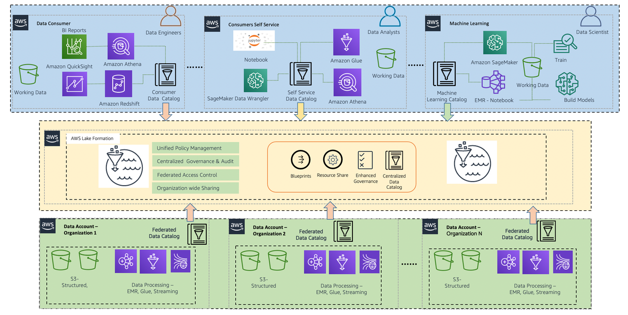
You can deploy data lakes on AWS to ingest, process, transform, catalog, and consume analytic insights using the AWS suite of analytics services, including Amazon EMR, AWS Glue, Lake Formation, Amazon Athena, Amazon QuickSight, Amazon Redshift, Amazon Elasticsearch Service (Amazon ES), Amazon Relational Database Service (Amazon RDS), Amazon SageMaker, and Amazon S3. These services provide the foundational capabilities to realize your data vision, in support of your business outcomes. You can deploy a common data access and governance framework across your platform stack, which aligns perfectly with our own Lake House Architecture.

Large enterprise customers require a scalable data lake with a unified access enforcement mechanism to support their analytics workload. For this, you want to use a single set of single sign-on (SSO) and AWS Identity and Access Management (IAM) mappings to attest individual users, and define a single set of fine-grained access controls across various services. The AWS Lake House Architecture encompasses a single management framework; however, the current platform stack requires that you implement workarounds to meet your security policies without compromising on the ability to drive automation, data proliferation, or scale.

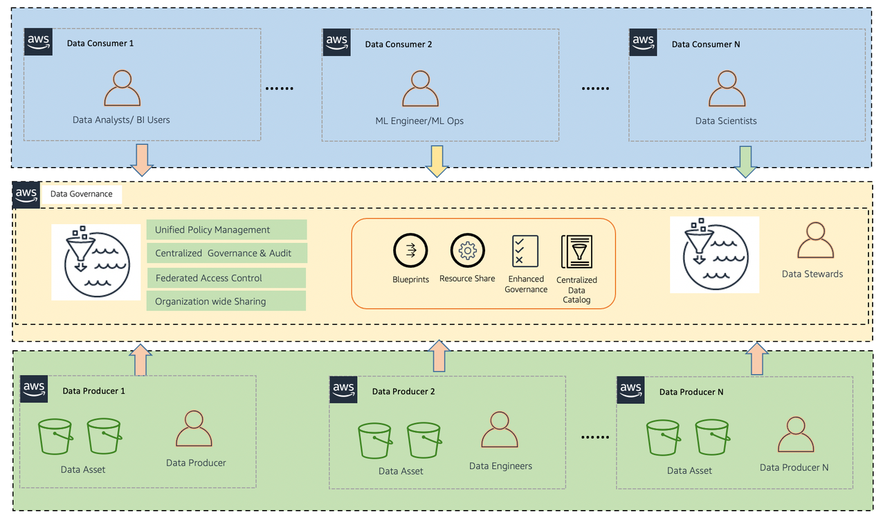
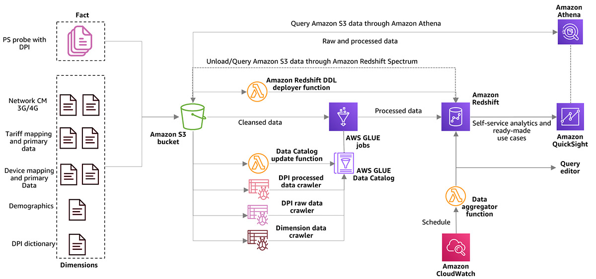
The following diagram illustrates the Lake House architecture.

Lake Formation serves as the central point of enforcement for entitlements, consumption, and governing user access. Furthermore, you may want to minimize data movements (copy) across LOBs and evolve on data mesh methodologies, which is becoming more and more prominent.

Most typical architectures consist of Amazon S3 for primary storage; AWS Glue and Amazon EMR for data validation, transformation, cataloging, and curation; and Athena, Amazon Redshift, QuickSight, and SageMaker for end users to get insight.

Introduction to Lake Formation

Lake Formation is a fully managed service that makes it easy to build, secure, and manage data lakes. Lake Formation simplifies and automates many of the complex manual steps that are usually required to create data lakes. These steps include collecting, cleansing, moving, and cataloging data, and securely making that data available for analytics and ML.

Lake Formation provides its own permissions model that augments the IAM permissions model. This centrally defined permissions model enables fine-grained access to data stored in data lakes through a simple grant or revoke mechanism, much like a relational database management system (RDBMS). Lake Formation permissions are enforced at the table and column level (row level in preview) across the full portfolio of AWS analytics and ML services, including Athena and Amazon Redshift.

With the new cross-account feature of Lake Formation, you can grant access to other AWS accounts to write and share data to or from the data lake to other LOB producers and consumers with fine-grained access. Data lake data (S3 buckets) and the AWS Glue Data Catalog are encrypted with AWS Key Management Service (AWS KMS) customer master keys (CMKs) for security purposes.

Common lake house design patterns using Lake Formation

A typical lake house infrastructure has three major components:

  • Data producer – Publishes the data into the data lake
  • Data consumer – Consumes that data out from the data lake and runs predictive and business intelligence (BI) insights
  • Data platform – Provides infrastructure and an environment to store data assets in the form of a layer cake such as landing, raw, and curated (conformance) data, and establishes security controls between producers and consumers

Although you can construct a data platform in multiple ways, the most common pattern is a single-account strategy, in which the data producer, data consumer, and data lake infrastructure are all in the same AWS account. There is no consensus if using a single account or multiple accounts most of the time is better, but because of the regulatory, security, performance trade-off, we have seen customers adapting to a multi-account strategy in which data producers and data consumers are in different accounts and the data lake is operated from a central, shared account.

This raised the concern of how to manage the data access controls across multiple accounts that are part of the data analytics platform to enable seamless ingestion for producers as well as improved business autonomy and agility for the needs of consumers.

With the general availability of the Lake Formation cross-account feature, the ability to manage data-driven access controls is simplified and offers an RDBMS style of managing data lake assets for producers and consumers.

You can drive your enterprise data platform management using Lake Formation as the central location of control for data access management by following various design patterns that balance your company’s regulatory needs and align with your LOB expectation. The following table summarizes different design patterns.

Design Type Lake Formation Glue Data Catalog Storage (Amazon S3) Compute
Centralized Centralized Centralized Centralized De-Centralized
De-Centralized De-Centralized Centralized De- Centralized De-Centralized

We explain each design pattern in more detail, with examples, in the following sections.\

Terminology

We use the following terms throughout this post when discussing data lake design patterns:

  • LOB – The line of business, such as inventory, marketing, or manufacturing
  • Enterprise data lake account (EDLA) – A centralized AWS account for data lake storage with a centralized AWS Glue Data Catalog and Lake Formation
  • Producer – The process or application producing data for its LOB
  • Consumer – The consumer of the LOB data via AWS services (such as Athena, AWS Glue, Amazon EMR, Amazon Redshift Spectrum, AWS Lambda, and QuickSight)

Centralized data lake design

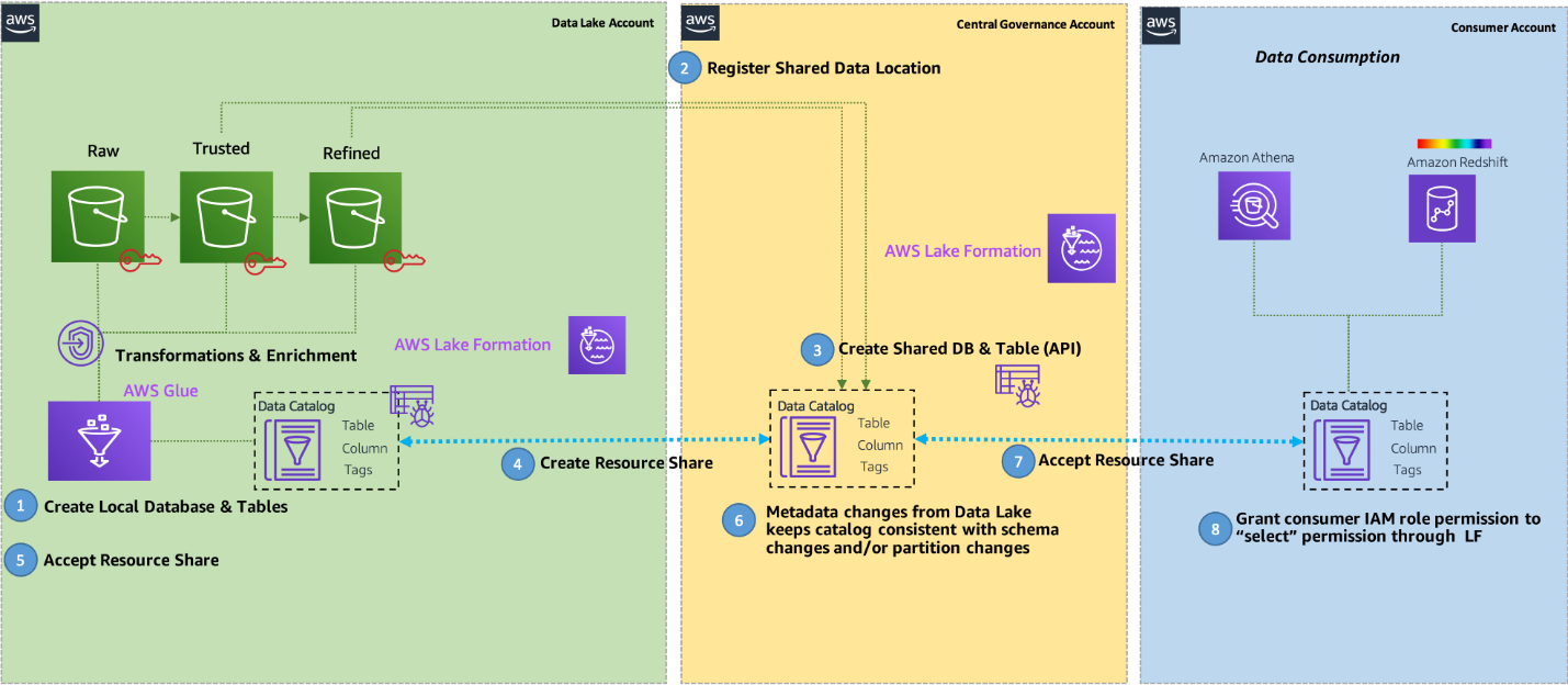
In a centralized data lake design pattern, the EDLA is a central place to store all the data in S3 buckets along with a central (enterprise) Data Catalog and Lake Formation. The respective LOB producer and consumer accounts have all the required compute to write and read data in and from the central EDLA data, and required fine-grained access is performed using the Lake Formation cross-account feature. That’s why this architecture pattern (see the following diagram) is called a centralized data lake design pattern.

For this post, we use one LOB as an example, which has an AWS account as a producer account that generates data, which can be from on-premises applications or within an AWS environment. This account uses its compute (in this case, AWS Glue) to write data into its respective AWS Glue database. The database is created in the central EDLA where all S3 data is stored using the database link created with the Lake Formation cross-account feature. The same LOB consumer account consumes data from the central EDLA via Lake Formation to perform advanced analytics using services like AWS Glue, Amazon EMR, Redshift Spectrum, Athena, and QuickSight, using the consumer AWS account compute. The following section provides an example.

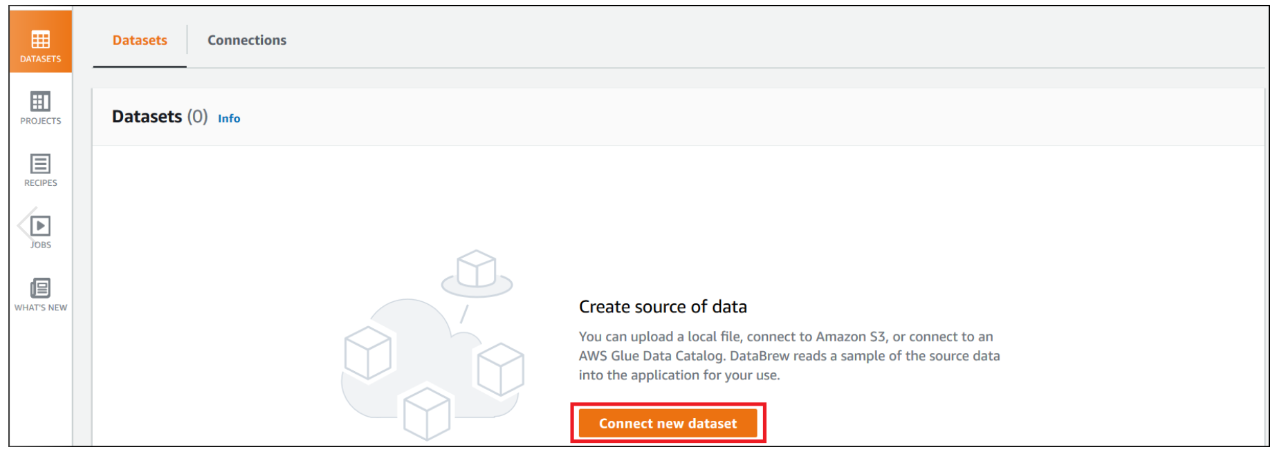
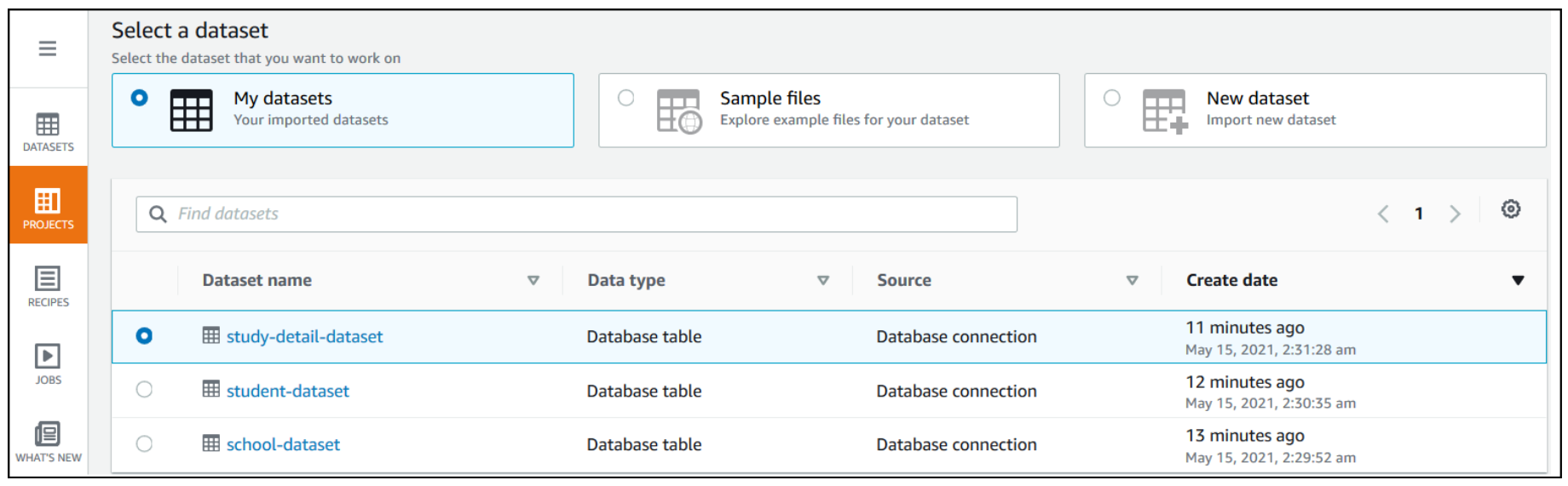
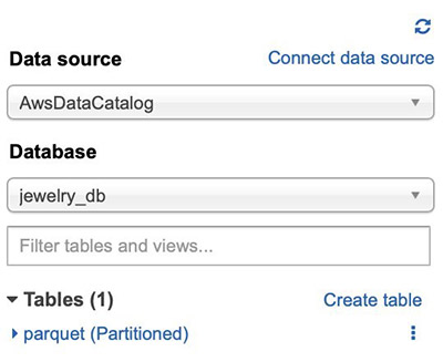
Create your database, tables and register S3 locations

In the EDLA, complete the following steps:

  1. Register the EDLA S3 bucket path in Lake Formation.
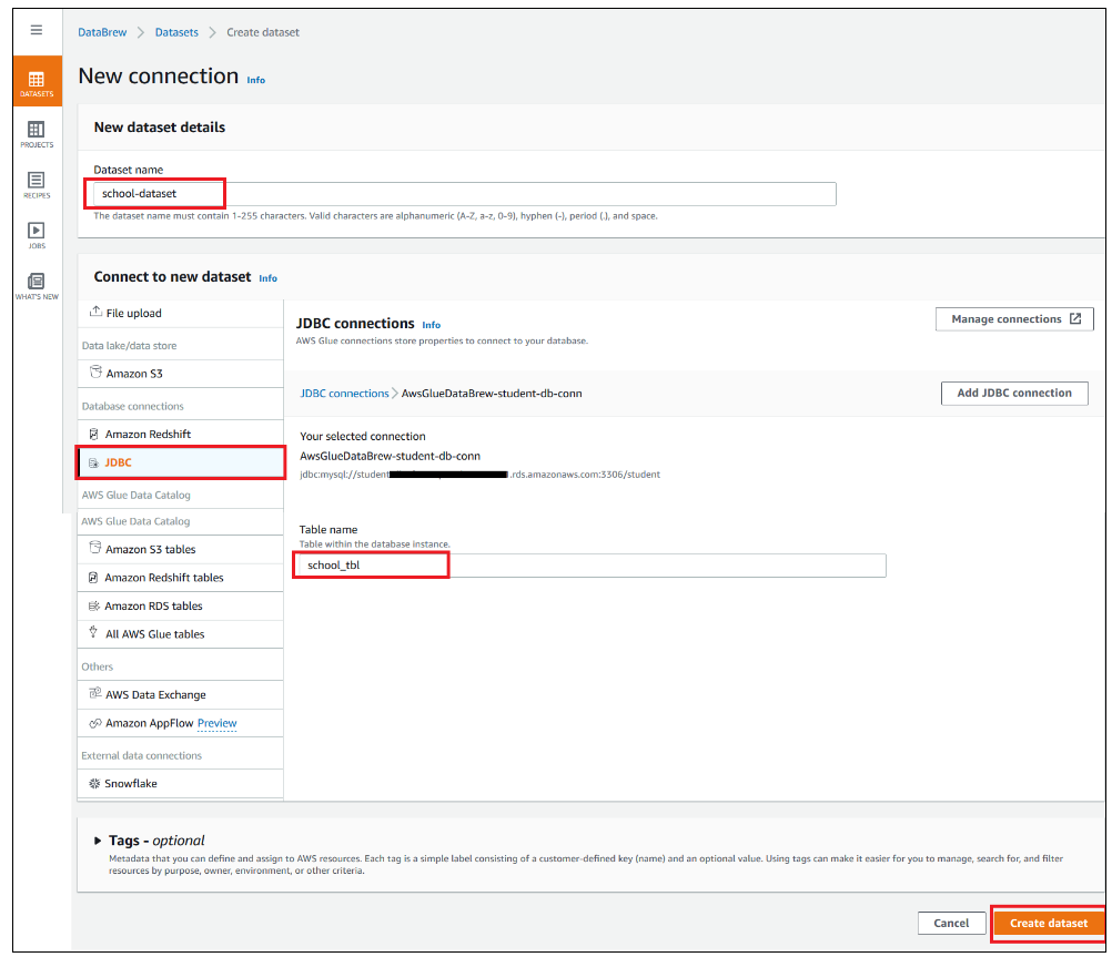
  2. Create a database called edla_lob_a, which points to the EDLA S3 bucket for LOB-A.

  3. Create a customer table in this edla_lob_a database , which points to the EDLA S3 bucket.

The LOB-A producer account can directly write or update data into tables, and create, update, or delete partitions using the LOB-A producer account compute via the Lake Formation cross-account feature.

You can trigger the table creation process from the LOB-A producer AWS account via Lambda cross-account access.

Grant Lake Formation cross-account access

Grant full access to the LOB-A producer account to write, update, and delete data into the EDLA S3 bucket via AWS Glue tables.

If your EDLA and producer accounts are part of same AWS organization, you should see the accounts on the list. If not, you need to enter the AWS account number manually as an external AWS account.

The following screenshot shows the granted permissions in the EDLA for the LOB-A producer account.


When you grant permissions to another account, Lake Formation creates resource shares in AWS Resource Access Manager (AWS RAM) to authorize all the required IAM layers between the accounts. To validate a share, sign in to the AWS RAM console as the EDLA and verify the resources are shared.

The first time you create a share, you see three resources:

  • The AWS Glue Data Catalog in the EDLA
  • The database containing the tables you shared
  • The table resource itself

You only need one share per resource, so multiple database shares only require a single Data Catalog share, and multiple table shares within the same database only require a single database share.

For the share to appear in the catalog of the receiving account (in our case the LOB-A account), the AWS RAM admin must accept the share by opening the share on the Shared With Me page and accepting it.

If both accounts are part of the same AWS organization and the organization admin has enabled automatic acceptance on the Settings page of the AWS Organizations console, then this step is unnecessary.

If your EDLA Data Catalog is encrypted with a KMS CMK, make sure to add your LOB-A producer account root user as the user for this key, so the LOB-A producer account can easily access the EDLA Data Catalog for read and write permissions with its local IAM KMS policy. Data encryption keys don’t need any additional permissions, because the LOB accounts use the Lake Formation role associated with the registration to access objects in Amazon S3.

When you sign in with the LOB-A producer account to the AWS RAM console, you should see the EDLA shared database details, as in the following screenshot.

Create a database resource link in the LOB-A producer account

Resource links are pointers to the original resource that allow the consuming account to reference the shared resource as if it were local to the account. As a pointer, resource links mean that any changes are instantly reflected in all accounts because they all point to the same resource. No sync is necessary for any of this and no latency occurs between an update and its reflection in any other accounts.

  1. Create a resource link to the shared Data Catalog database from the EDLA called shared_edla_lob_a.
  2. Grant full access to the AWS Glue role in the LOB-A producer account for this newly created shared database link from the EDLA so a producer AWS Glue job can create, update, and delete tables and partitions.

You need to perform two grants: one on the database shared link and one on the target to the AWS Glue job role. Granting on the link allows it to be visible to end-users. Data-level permissions are granted on the target itself.

  1. Create an AWS Glue job using this role to create and write data into the EDLA database and S3 bucket location.

The AWS Glue table and S3 data are in a centralized location for this architecture, using the Lake Formation cross-account feature.

This completes the configuration of the LOB-A producer account remotely writing data into the EDLA Data Catalog and S3 bucket. You can create and share the rest of the required tables for this LOB using the Lake Formation cross-account feature.

Because your LOB-A producer created an AWS Glue table and wrote data into the Amazon S3 location of your EDLA, the EDLA admin can access this data and share the LOB-A database and tables to the LOB-A consumer account for further analysis, aggregation, ML, dashboards, and end-user access.

Share the database to the LOB-A consumer account

In the EDLA, you can share the LOB-A AWS Glue database and tables (edla_lob_a, which contains tables created from the LOB-A producer account) to the LOB-A consumer account (in this case, the entire database is shared).

Next, go to the LOB-A consumer account to accept the resource share in AWS RAM.

Accepting the shared database in AWS RAM of the LOB-A consumer account

Sign in with the LOB-A consumer account to the AWS RAM console. You should see the EDLA shared database details.

Accept this resource share request so you can create a resource link in the LOB-A consumer account.

Create a database resource link in the LOB-A consumer account

Create a resource link to a shared Data Catalog database from the EDLA as consumer_edla_lob_a.

Now, grant full access to the AWS Glue role in the LOB-A consumer account for this newly created shared database link from the EDLA so the consumer account AWS Glue job can perform SELECT data queries from those tables. You need to perform two grants: one on the database shared link and one on the target to the AWS Glue job role.

A grant on the resource link allows a user to describe (or see) the resource link, which allows them to point engines such as Athena at it for queries. A grant on the target grants permissions to local users on the original resource, which allows them to interact with the metadata of the table and the data behind it. Permissions of DESCRIBE on the resource link and SELECT on the target are the minimum permissions necessary to query and interact with a table in most engines.

Create an AWS Glue job using this role to read tables from the consumer database that is shared from the EDLA and for which S3 data is also stored in the EDLA as a central data lake store. This data is accessed via AWS Glue tables with fine-grained access using the Lake Formation cross-account feature.

This completes the process of granting the LOB-A consumer account remote access to data for further analysis.

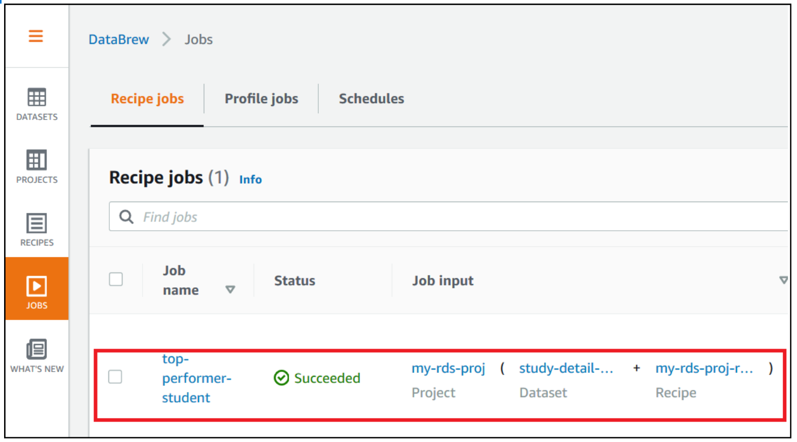
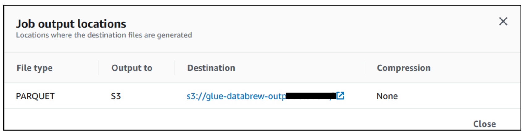
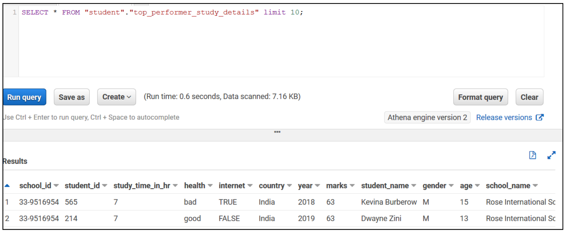
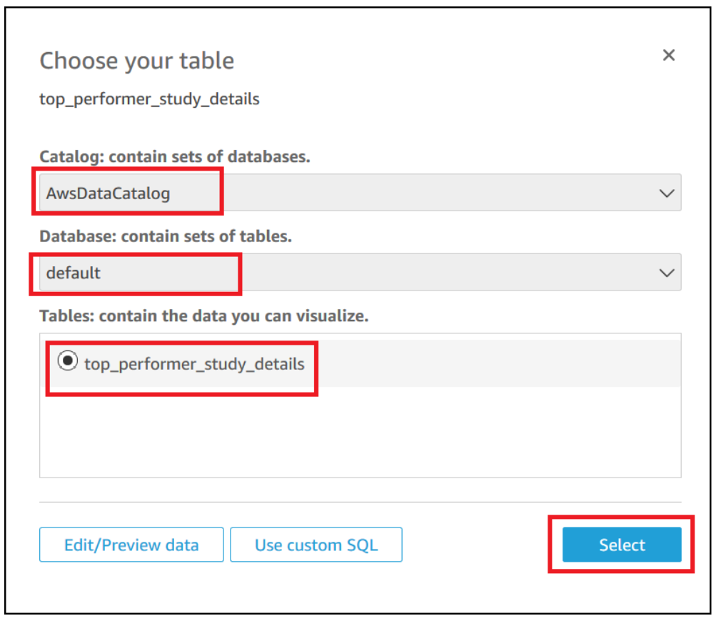
This data can be accessed via Athena in the LOB-A consumer account. LOB-A consumers can also access this data using QuickSight, Amazon EMR, and Redshift Spectrum for other use cases.


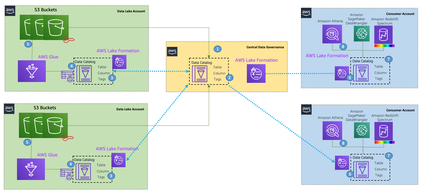
De-centralized data lake design

In the de-centralized design pattern, each LOB AWS account has local compute, an AWS Glue Data Catalog, and a Lake Formation along with its local S3 buckets for its LOB dataset and a central Data Catalog for all LOB-related databases and tables, which also has a central Lake Formation where all LOB-related S3 buckets are registered in EDLA.

EDLA manages all data access (read and write) permissions for AWS Glue databases or tables that are managed in EDLA. It grants the LOB producer account write, update, and delete permissions on the LOB database via the Lake Formation cross-account share. It also grants read permissions to the LOB consumer account. The respective LOB’s local data lake admins grant required access to their local IAM principals.

Refer to the earlier details on how to share database, tables, and table columns from EDLA to the producer and consumer accounts via Lake Formation cross-account sharing via AWS RAM and resource links.

Each LOB account (producer or consumer) also has its own local storage, which is registered in the local Lake Formation along with its local Data Catalog, which has a set of databases and tables, which are managed locally in that LOB account by its Lake Formation admins.

Clean up

To avoid incurring future charges, delete the resources that were created as part of this exercise.

Delete the S3 buckets in the following accounts:

  • Producer account
  • EDLA account
  • Consumer account (if any)

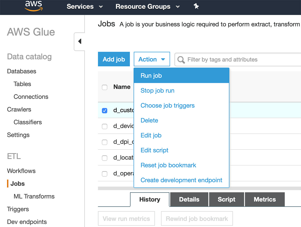
Delete the AWS Glue jobs in the following accounts:

  • Producer account
  • Consumer account (if any)

Lake Formation limitations

This solution has the following limitations:

  • The spark-submit action on Amazon EMR is not currently supported
  • AWS Glue Context does not yet support column-level fine-grained permissions granted via the Lake Formation

Conclusion

This post describes how you can design enterprise-level data lakes with a multi-account strategy and control fine-grained access to its data using the Lake Formation cross-account feature. This can help your organization build highly scalable, high-performance, and secure data lakes with easy maintenance of its related LOBs’ data in a single AWS account with all access logs and grant details.


About the Authors

Satish Sarapuri is a Data Architect, Data Lake at AWS. He helps enterprise-level customers build high-performance, highly available, cost-effective, resilient, and secure data lakes and analytics platform solutions, which includes streaming and batch ingestions into the data lake. In his spare time, he enjoys spending time with his family and playing tennis.


UmaMaheswari Elangovan is a Principal Data Lake Architect at AWS. She helps enterprise and startup customers adopt AWS data lake and analytic services, and increases awareness on building a data-driven community through scalable, distributed, and reliable data lake infrastructure to serve a wide range of data users, including but not limited to data scientists, data analysts, and business analysts. She also enjoys mentoring young girls and youth in technology by volunteering through nonprofit organizations such as High Tech Kids, Girls Who Code, and many more.


Zach Mitchell is a Sr. Big Data Architect. He works within the product team to enhance understanding between product engineers and their customers while guiding customers through their journey to develop data lakes and other data solutions on AWS analytics services.


Architecting Persona-centric Data Platform with On-premises Data Sources

Post Syndicated from Raghavarao Sodabathina original https://aws.amazon.com/blogs/architecture/architecting-persona-centric-data-platform-with-on-premises-data-sources/

Many organizations are moving their data from silos and aggregating it in one location. Collecting this data in a data lake enables you to perform analytics and machine learning on that data. You can store your data in purpose-built data stores, like a data warehouse, to get quick results for complex queries on structured data.

In this post, we show how to architect a persona-centric data platform with on-premises data sources by using AWS purpose-built analytics services and Apache NiFi. We will also discuss Lake House architecture on AWS, which is the next evolution from data warehouse and data lake-based solutions.

Data movement services

AWS provides a wide variety of services to bring data into a data lake:

You may want to bring on-premises data into the AWS Cloud to take advantage of AWS purpose-built analytics services, derive insights, and make timely business decisions. Apache NiFi is an open source tool that enables you to move and process data using a graphical user interface.

For this use case and solution architecture, we use Apache NiFi to ingest data into Amazon S3 and AWS purpose-built analytics services, based on user personas.

Building persona-centric data platform on AWS

When you are building a persona-centric data platform for analytics and machine learning, you must first identify your user personas. Who will be using your platform? Then choose the appropriate purpose-built analytics services. Envision a data platform analytics architecture as a stack of seven layers:

  1. User personas: Identify your user personas for data engineering, analytics, and machine learning
  2. Data ingestion layer: Bring the data into your data platform and data lineage lifecycle view, while ingesting data into your storage layer
  3. Storage layer: Store your structured and unstructured data
  4. Cataloging layer: Store your business and technical metadata about datasets from the storage layer
  5. Processing layer: Create data processing pipelines
  6. Consumption layer: Enable your user personas for purpose-built analytics
  7. Security and Governance: Protect your data across the layers

Reference architecture

The following diagram illustrates how to architect a persona-centric data platform with on-premises data sources by using AWS purpose-built analytics services and Apache NiFi.

Figure 1. Example architecture for persona-centric data platform with on-premises data sources

Figure 1. Example architecture for persona-centric data platform with on-premises data sources

Architecture flow:

    1. Identify user personas: You must first identify user personas to derive insights from your data platform. Let’s start with identifying your users:
      • Enterprise data service users who would like to consume data from your data lake into their respective applications.
      • Business users who would like to like create business intelligence dashboards by using your data lake datasets.
      • IT users who would like to query data from your data lake by using traditional SQL queries.
      • Data scientists who would like to run machine learning algorithms to derive recommendations.
      • Enterprise data warehouse users who would like to run complex SQL queries on your data warehouse datasets.
    2. Data ingestion layer: Apache NiFi scans the on-premises data stores and ingest the data into your data lake (Amazon S3). Apache NiFi can also transform the data in transit. It supports both Extract, Transform, Load (ETL) and Extract, Load, Transform (ELT) data transformations. Apache NiFi also supports data lineage lifecycle while ingesting data into Amazon S3.
    3. Storage layer: For your data lake storage, we recommend using Amazon S3 to build a data lake. It has unmatched 11 nines of durability and 99.99% availability. You can also create raw, transformed, and enriched storage layers depending upon your use case.
    4. Cataloging layer: AWS Lake Formation provides the central catalog to store and manage metadata for all datasets hosted in the data lake by AWS Glue Data Catalog. AWS services such as AWS Glue, Amazon EMR, and Amazon Athena natively integrate with Lake Formation. They automate discovering and registering dataset metadata into the Lake Formation catalog.
    5. Processing layer: Amazon EMR processes your raw data and places them into a new S3 bucket. Use AWS Glue DataBrew and AWS Glue to process the data as needed.
    6. Consumption layer or persona-centric analytics: Once data is transformed:
      • AWS Lambda and Amazon API Gateway will allow you to develop data services for enterprise data service users
      • You can develop user-friendly dashboards for your business users using Amazon QuickSight
      • Use Amazon Athena to query transformed data for your IT users
      • Your data scientists can utilize AWS Glue DataBrew to clean and normalize the data and Amazon SageMaker for machine learning models
      • Your enterprise data warehouse users can use Amazon Redshift to derive business intelligence
    7. Security and governance layer: AWS IAM provides users, groups, and role-level identity, in addition to the ability to configure coarse-grained access control for resources managed by AWS services in all layers. AWS Lake Formation provides fine-grained access controls and you can grant/revoke permissions at the database- or table- or column-level access.

Lake House architecture on AWS

The vast majority of data lakes are built on Amazon S3. At the same time, customers are leveraging purpose-built analytics stores that are optimized for specific use cases. Customers want the freedom to move data between their centralized data lakes and the surrounding purpose-built analytics stores. And they want to get insights with speed and agility in a seamless, secure, and compliant manner. We call this modern approach to analytics the Lake House architecture.

Figure 2. Lake House architecture on AWS

Figure 2. Lake House architecture on AWS

Refer to the whitepaper Derive Insights from AWS Lake house for various design patterns to derive persona-centric analytics by using the AWS Lake House approach. Check out the blog post Build a Lake House Architecture on AWS  for a Lake House reference architecture on AWS.

Conclusion

In this post, we show you how to build a persona-centric data platform on AWS with a seven-layered approach. This uses Apache NiFi as a data ingestion tool and AWS purpose-built analytics services for persona-centric analytics and machine learning. We have also shown how to build persona-centric analytics by using the AWS Lake House approach.

With the information in this post, you can now build your own data platform on AWS to gain faster and deeper insights from your data. AWS provides you the broadest and deepest portfolio of purpose-built analytics and machine learning services to support your business needs.

Read more and get started on building a data platform on AWS:

Using AppStream 2.0 to Deliver PACS and Image Analysis in Clinical Trials

Post Syndicated from Chris Fuller original https://aws.amazon.com/blogs/architecture/using-appstream-2-0-to-deliver-pacs-and-image-analysis-in-clinical-trials/

Hospitals and clinical trial sites manage sensitive patient data. They are often required to grant remote access to custom Windows-based applications for patient record review and medical image analysis. This typically requires providing physicians and staff with remote access to on-premises workstations over VPN, with some flavor of remote desktop software. This can be both costly and inefficient, since it requires licensing custom 3rd party remote access tools, configuring network access for each researcher, and training individuals at each site for every trial. In combination with other AWS services, Amazon AppStream 2.0 can be used to build better workflows. Applications delivered via AppStream 2.0 can be used to review patient data, such as medical images, videos, and patient records. At the same time, this approach offers greater protection of patient data, without the cost and complexity of a remote desktop solution. In this blog, we will present a high-level architecture and several example use cases for leveraging AppStream 2.0 for medical image analysis.

Background – managing patient data security

Picture archiving and communications systems (PACS) and vendor neutral archives (VNAs) are used extensively for storing and managing medical images and related metadata. These systems are critical for sharing images among modern medical teams collaborating on patient care. Furthermore, researchers and clinicians can access images from PACS and view them at a workstation in an office or clinic setting.

While data sharing is critical for healthcare and research workflows, HIPAA-covered entities are responsible for protecting patient’s personally identifiable information (PII) as protected health information (PHI). As such, HIPAA-covered entities are bound to protect any information about a patient’s healthcare, health status, and payment history for services.

Data sovereignty leads to further complications. Clinical trials play an essential role in vouching for the safety and efficacy of medical products and innovations. The increasing transparency in clinical trial data makes sharing this information among researchers, clinicians, patients, and trial subjects possible. However, this also makes it a challenge to maintain stakeholder’s control over their data. With laws like General Data Protection Regulation (GDPR) and the emphasis on data localization, data sovereignty is interpreted based on the location of the data. Further, regulations like 21 CFR Part 11 impose strict guidelines on data protection, authentication, and validation for any FDA-regulated entity or use case.

If you are a healthcare organization or software provider, you understand the struggle to innovate and drive change, while maintaining your security and compliance posture for your applications. Your end users (physicians, radiologists, researchers, and remote operators) require IT environments that are easily accessible and can automatically scale globally on demand.

The network of professionals involved in image management and review is widely distributed, yet applications for review and analysis are still largely desktop-based. This means that a common use case for the healthcare industry is to use desktop applications from anywhere. Let’s use the following example to look more closely into a use case where AppStream 2.0 is helpful.

Data flow through the image management architecture

In this use case, the hospital’s on-premises systems are connected to the AWS Cloud using a private network connection, such as AWS Direct Connect, or an AWS Site-to-Site VPN. The images and files generated from the PACS server and the Electronic Medical Record (EMR) server are placed on an Amazon Simple Storage Service (Amazon S3). Amazon S3 is an object storage service that offers scalability, availability, security, and performance. All of the images and files are read from a secure S3 bucket, accessible only by the PACS. They are then de-identified and written back to a separate bucket accessible by other systems for review.

In our workflow, text-based PII is extracted from the images using Amazon Comprehend Medical. Amazon Rekognition helps to identify and detect “burned-in” PHI data (text that is actually part of the image). In addition, Amazon Rekognition can assist with entity identification within images. For example, in a batch of thousands of shoulder MRIs, Amazon Rekognition can identify a knee. Amazon SageMaker is an end-to-end machine learning platform that enables trial administrators and data management teams to prepare training data. It can also be used to build machine learning models quickly with pre-built algorithms.  With Amazon SageMaker notebooks, the resulting de-identified image and text are written to the S3 bucket, and can then be used by the desktop applications.

AppStream 2.0 is a fully managed application streaming service that provides users with instant access to desktop applications from anywhere, regardless of what device is being used for access. An AppStream 2.0 image builder is used to install, add, and test your applications, and then create a software image or package. The software image contains applications that you can stream to your users. Default Windows and application settings allow your users to get started with their applications quickly. A fleet consists of fleet instances (also known as streaming instances) that run the software image that you specify. A stack consists of an associated fleet, user access policies, and storage configurations. A streaming instance (also known as a fleet instance) is an Amazon EC2 instance that is made available to a single user for application streaming.

Secure user interactions for image analysis and review

We’ve covered secure storage and anonymization of the image data that’s managed by the PACS, with images residing in Amazon S3. The next challenge is to provide secure, role-based access to those images for review by physicians, radiologists, or researchers. However, many of the applications used for image review and annotation are proprietary desktop applications that only run on specific operating systems. Traditionally, reviewers access these applications via remote desktop sessions to an on-premises workstation. This creates cost, management, network security, and data privacy concerns for the application hosts. Using Amazon AppStream 2.0, we can provide secure access to these proprietary applications in the cloud.

Authentication and access to the applications is as follows:

  • When end users sign in with the provided AppStream 2.0 URL, they are authenticated against Active Directory.
  • After the users are authenticated, the browser receives a Security Assertion Markup Language (SAML) assertion as an authentication response from Amazon Cognito, which controls access to AWS resources.
  • The response is then posted by the browser to the AWS sign-in SAML endpoint. Temporary security credentials are issued after the assertion and the embedded attributes are validated.
  • The temporary credentials are then used to create the sign-in URL.
  • The user is redirected to the AppStream 2.0 streaming session and is granted access permissions based on the role assigned to them. After this, they can log into the AppStream 2.0 instance and access their applications.

The application configurations are stored as persistent data using Amazon FSx, which can provide every user a unique storage drive within AppStream 2.0 streaming sessions. A user will have permissions to access only their directory. The drive is automatically mounted at the start of a streaming session. Files added or updated to the drive are automatically persisted between streaming sessions.

Figure 1. Architecture for managing, anonymizing, and analyzing medical image data

Figure 1. Architecture for managing, anonymizing, and analyzing medical image data

Conclusion

In our high-level use case, we reviewed how a combination of AWS services can be used to increase efficiency and reduce cost. While managing and reviewing patient data using custom applications such as PACS or image viewers, AWS services also provide an improved end user experience. This architecture provides a scalable, reliable, and secure foundation to develop your solution, leveraging the image analysis applications you already use. Your applications are available through a standard web browser, and you can manage users, access, and data with existing Active Directory group memberships and credentials.

AppStream 2.0 manages the AWS resources required to host and run your applications, scales automatically, and provides access to users on demand. AWS services can be managed using configuration as code best practices through AWS CloudFormation. CloudFormation lets you define text-based templates used to spin up cloud architectures. In a more complex setup, AWS Glue, Amazon CloudWatch, and AWS CloudTrail configured with a centralized logging account can be added to achieve 21 CFR Part 11 and GxP compliance.

For additional information, check out the following resources or contact your AWS account manager.

Field Notes: Develop Data Pre-processing Scripts Using Amazon SageMaker Studio and an AWS Glue Development Endpoint

Post Syndicated from Sam Mokhtari original https://aws.amazon.com/blogs/architecture/field-notes-develop-data-pre-processing-scripts-using-amazon-sagemaker-studio-and-an-aws-glue-development-endpoint/

This post was co-written with Marcus Rosen, a Principal  – Machine Learning Operations with Rio Tinto, a global mining company. 

Data pre-processing is an important step in setting up Machine Learning (ML) projects for success. Many AWS customers use Apache Spark on AWS Glue or Amazon EMR to run data pre-processing scripts while using Amazon SageMaker to build ML models.  To develop spark scripts in AWS Glue, you can create an environment called a Glue Development (Dev) Endpoint that lets you author and test your data pre-processing scripts iteratively. When you’re satisfied with the results of your development, you can create a Glue ETL job that runs the final script as part of your automation framework.

With the introduction of Amazon SageMaker Studio in AWS re:Invent 2020, you can now use a single web-based IDE to spin up a notebook and perform all ML development steps. These include data pre-processing, ML model training, ML model deployment and monitoring.

This post walks you through how to connect a SageMaker Studio notebook to an AWS Glue Dev Endpoint, so you can use a single tool to iteratively develop both data pre-processing scripts and ML models.

Solution Overview

The following diagram shows the components that are used in this solution.

  • First, we use an AWS CloudFormation template to set up the required networking components (for example, VPC, subnets).
  • Then, we create an AWS Glue Dev Endpoint and use a security group to allow SageMaker Studio to securely access the endpoint.
  • Finally, we create a studio domain and use a SparkMagic kernel to connect to the AWS Glue Dev Endpoint and run spark scripts.

In the Amazon SageMaker Studio notebook, SparkMagic will call a REST API against a Livy server running on the AWS Glue Dev Endpoint. Apache Livy is a service that enables interaction with a remote Spark cluster over a REST API.


The following diagram shows the components that are used in this solution. We use an AWS CloudFormation template to set up the required ntworking components (for example, VPC, subnets).

Set up the VPC

You can use the following CloudFormation template to set up the environment needed for this solution.

launch stack button

This template deploys the following resources in your account:

  • A new VPC, with both public and private subnet.
  • VPC endpoints for the following resources:
  • Security groups for SageMaker Studio, Glue endpoint and VPC endpoints
  • SageMaker Service IAM role
  • AWS Glue Dev Endpoint IAM role
  • Set up the AWS Glue Dev Endpoint

Set up AWS Glue Dev Endpoint

Review this Developer Guide: Adding a Development Endpoint for instructions to create an AWS Glue Dev Endpoint.

Note: you must use the AWS Glue Dev Endpoint IAM role provisioned by the CloudFormation template.

  • In the Networking section, select Choose a VPC, subnet, and security groups.

Then choose the VPC glue security group, which you provisioned through the CloudFormation template.

The AWS Glue Dev Endpoint needs to be secured with an SSH public key, which should be generated within your local environment. An SSH key pair (public/private) can be generated using the ssh-keygen on Linux or using PuTTYgen on Windows.

Glue Dev Endpoint screenshot

The final review page looks similar to the following screenshot.

Final review page

Once the AWS Glue Dev Endpoint is in Ready status, keep note of its private IP address (Glue -> ETL -> Dev Endpoints). You will use this IP for the Livy port forwarding.

Set up SageMaker Studio

We recommend launching the SageMaker Studio resource by following the instructions in Securing Amazon SageMaker Studio connectivity using a private VPC .

Follow these steps when you provision the SageMaker Studio resources:

  • Select Standard setup with the AWS Identity and Access Management (IAM) authentication method.
  • Attach a SageMaker Service IAM role, created by the CloudFormation template, to SageMaker Studio.
  • Under Network and storage, select the same VPC and private subnet as the AWS Glue endpoint.
  • For the Network Access for Studio option, select VPC Only — SageMaker Studio will use your VPC. Direct internet access is disabled.

Then ensure that the security group with the self-referencing rule is attached. Also, check your other required security groups are attached for SageMaker Studio from the CloudFormation template output.

Connect the SageMaker Studio notebook to the AWS Glue Dev Endpoint

Once you launch the SageMaker Studio and you add the users. Follow these steps to connect the SageMaker Studio notebook to the AWS Glue Dev Endpoint:

  1. Open the Studio and go to the launcher page (by pressing the “+” icon on the top-left of the page.
  2. Under Notebooks and compute resources, select SparkMagic in the dropdown menu and select Notebook.
  3. Then open another launcher page, select SparkMagic in the same dropdown menu and select Image terminal. One thing to note is that the SparkMagic app will take some time to initialize. Proceed once the apps are in Ready status (2-3 minutes).

Notebooks and compute resources screenshot

4. Upload the private key into SparkMagic Image terminal. In other words, copy the private key to “.ssh” directory and update its permissions using “chmod 400”.

Note: the private key is corresponding to the public key used when you create the AWS Glue Dev Endpoint.

5. Now, you need to achieve port forwarding of the Livy service in order for SparkMagic kernel to be able to connect to the AWS Glue Dev Endpoint.  You run the following command in the image terminal:

/usr/bin/ssh -4 -N -o ServerAliveInterval=60 -o ServerAliveCountMax=3 -o StrictHostKeyChecking=no -i /root/.ssh/{PRIVATE_KEY} -L 8998:169.254.76.1:8998 glue@{GLUE_ENDPOINT_PRIVATE_IP_ADDRESS}

The command consists of:

  • {PRIVATE_KEY} is the private key file name that you copied into .ssh directory.
  • {GLUE_ENDPOINT_PRIVATE_IP_ADDRESS} is the private IP address of the AWS Glue Dev Endpoint.
  • “8998” is the Livy port we are using for port forwarding.
  • “169.254.76.1” is the remote IP address defined by AWS Glue, this IP address does not change.

Note: Keep this terminal open and the SSH command running in order to keep the Livy session active.

6. Go to the SparkMagic notebook and restart the kernel, by going to the top menu and selecting Kernel > Restart Kernel.

7. Once the notebook kernel is restarted, the connection between the Studio Notebook and the AWS Glue Dev Endpoint is ready. To test the integration, you can run the following example command to list the tables in the AWS Glue Data Catalog.

spark.sql("show tables").show()

To test the integration, you can run the following command to list the tables in the Glue Data Catalog

Cleaning up

To avoid incurring future charges, delete the resources you created:

Conclusion

Our customers needed a single web-based IDE to spin up a notebook and perform all ML development steps including data pre-processing, ML model training, ML model deployment and monitoring. This blog post demonstrated how you can configure a SageMaker Studio notebook and connect to AWS Glue Dev Endpoint. This provides a framework for you to use  when developing both data preprocessing scripts and ML models.

To learn more about how to develop data pre-processing scripts and ML models in Amazon SageMaker, you can check out the examples in this repository.

Field Notes provides hands-on technical guidance from AWS Solutions Architects, consultants, and technical account managers, based on their experiences in the field solving real-world business problems for customers.


Building a Cloud-based OLAP Cube and ETL Architecture with AWS Managed Services

Post Syndicated from Peter Chung original https://aws.amazon.com/blogs/architecture/building-a-cloud-based-olap-cube-and-etl-architecture-with-aws-managed-services/

For decades, enterprises used online analytical processing (OLAP) workloads to answer complex questions about their business by filtering and aggregating their data. These complex queries were compute and memory-intensive. This required teams to build and maintain complex extract, transform, and load (ETL) pipelines to model and organize data, oftentimes with commercial-grade analytics tools.

In this post, we discuss building a cloud-based OLAP cube and ETL architecture that will yield faster results at lower costs without sacrificing performance by:

  • Connecting your on-premises database to the cloud for data profiling, discovery, and transformation
  • Running OLAP workloads without costly third-party software licenses, dedicated infrastructure, or the need to migrate data
  • Using AWS Glue Data Catalog, Amazon Athena, Amazon QuickSight, and Amazon SageMaker to catalog and visualize data with machine learning (ML)

Data analytics pipeline with AWS Managed Services

The proposed architecture in Figure 1 relies on AWS Managed Services. AWS Glue DataBrew is a no-code data transformation service that you can use to quickly build your transformation jobs. AWS Glue crawlers collect metadata from the transformed data and catalogs it for analytics and visualization using Athena and QuickSight. SageMaker will build, train, and deploy ML models.

This architecture will help you get answers from your data to your users as fast as possible without needing to migrate your data to AWS. There is no coding required, so you can leverage data transformation, cataloging, analytics, and ML quickly.

Figure 1. Example architecture using AWS Managed Services

Figure 1. Example architecture using AWS Managed Services

Benefits of AWS Managed Services for data analytics

Immediate connectivity to on-premises databases

The example architecture in Figure 1 begins with an online transaction processing (OLTP) database running in your corporate data center. Figure 2 shows how you can establish a Java database connectivity (JDBC) connection from the OLTP database to DataBrew running in AWS to run OLAP workloads. DataBrew supports data sources using JDBC for common data stores such as Microsoft SQL Server, MySQL, Oracle, and PostgreSQL.

DataBrew - JDBC connection to data source

Figure 2. DataBrew – JDBC connection to data source

Automatic data discovery

Figures 3 through 6 show how DataBrew summarizes your data for discovery. You can profile your data to understand patterns and detect anomalies. You can also run transformations called “jobs” in DataBrew without writing any code using over 250 built-in transforms.

DataBrew - dataset profiling overview

Figure 3. DataBrew – dataset profiling overview


DataBrew - data correlation patterns

Figure 4. DataBrew – data correlation patterns


DataBrew - data points distribution

Figure 5. DataBrew – data points distribution

No-code data transformation and cataloging

To run OLAP-type transactions, you can create jobs based on the transformation steps shown in Figure 6. These steps collectively are referred to as DataBrew recipes. These recipe results can be run as a job and outputted to an Amazon Simple Storage Service (Amazon S3) bucket.

A DataBrew project user interface view with sample data and transformation functions

Figure 6. A DataBrew project user interface view with sample data and transformation functions

Scheduled DataBrew jobs act similarly to scheduled ETL pipelines in OLAP. Based on data refresh and business requirements, DataBrew can run a job on a recurring basis (for example, every 12 hours). This can be run at a particular time of day, or as defined by a valid CRON expression. This helps you automate your transformation workflows.

The OLAP catalog is a set of metadata that sits between the actual OLAP data stored and applications. To create a Data Catalog, you can use AWS Glue crawlers to automatically classify your data to determine the data’s format, schema, and associated properties. Figure 7 shows the results of a crawler’s results written to Data Catalog as metadata to help data users find the data they need.

AWS Glue crawler metadata table output of column names and data types

Figure 7. AWS Glue crawler metadata table output of column names and data types

Data analytics without third-party software licenses

You can run analytics on your data by referring to the metadata definitions in the Data Catalog as references to the actual data in Amazon S3 using Athena. Athena is well suited for running one-time queries using standard SQL to query the transformed data directly in Amazon S3 without having to move data around. Athena is serverless, so there is no infrastructure to manage, and you pay only for the queries that you run.

Enterprises often supplement their OLAP workloads with separate visualization and business intelligence (BI) tools. These tools often come with their own licensing, server management, and security considerations.

You can visualize curated data using QuickSight, a scalable, serverless, embeddable, ML-powered BI service. QuickSight lets you easily create and publish interactive BI dashboards that include ML-powered insights, as shown in Figure 8. These dashboards can be shared with other users and embedded within your own applications.

A sample of data visualization options with Amazon QuickSight

Figure 8. A sample of data visualization options with Amazon QuickSight

Finally, you can incorporate ML workloads to OLAP workloads using SageMaker. In the past, ML workloads were often expensive, resource-intensive, and inaccessible. SageMaker provides a fully managed ML service to quickly and easily build and train ML models and directly deploy them into a production-ready hosted environment.

Conclusion

In this post, we show you how to connect your on-premises database using a JDBC connection to DataBrew for data profiling, discovery, and transformation. We looked at how you can use DataBrew recipes and jobs to run OLAP workloads without costly third-party software licenses, dedicated infrastructure, or the need to migrate any data. We also looked at AWS capabilities in data cataloging, visualization, and machine learning using Data Catalog, Athena, QuickSight, and SageMaker without having to manage any servers.

Laying the foundation to modernize an analytics workflow is critical for many enterprises that are looking to reduce the time it takes to understand their business. With AWS, you can perform enterprise-scale analytics with our portfolio of analytics services.


Hydrate your data lake with SaaS application data using Amazon AppFlow

Post Syndicated from Ninad Phatak original https://aws.amazon.com/blogs/big-data/hydrate-your-data-lake-with-saas-application-data-using-amazon-appflow/

Organizations today want to make data-driven decisions. The data could lie in multiple source systems, such as line of business applications, log files, connected devices, social media, and many more. As organizations adopt software as a service (SaaS) applications, data becomes increasingly fragmented and trapped in different “data islands.” To make decision-making easier, organizations are building data lakes, which is a centralized repository that allows you to store all your structured and unstructured data at any scale. You can store your data as is, without having to first structure the data, and run different types of analytics—from dashboards and visualizations to big data processing, ad hoc analytics, and machine learning (ML) to guide better decisions.

AWS provides services such as AWS Glue, AWS Lake Formation, Amazon Database Migration Service (AWS DMS), and many third-party solutions on AWS Marketplace to integrate data from various source systems into the Amazon Simple Storage Service (Amazon S3) data lake. If you’re using SaaS applications like Salesforce, Marketo, Slack, and ServiceNow to run your business, you may need to integrate data from these sources into your data lake. You likely also want to easily integrate these data sources without writing or managing any code. This is precisely where you can use Amazon AppFlow.

Amazon AppFlow is a fully managed integration service that enables you to securely transfer data between SaaS applications like Salesforce, Marketo, Slack, and ServiceNow and AWS services like Amazon S3 and Amazon Redshift. With Amazon AppFlow, you can run data flows at nearly any scale at the frequency you choose—on a schedule, in response to a business event in real time, or on demand. You can configure data transformations such as data masking and concatenation of fields as well as validate and filter data (omitting records that don’t fit a criteria) to generate rich, ready-to-use data as part of the flow itself, without additional steps. Amazon AppFlow automatically encrypts data in motion, and optionally allows you to restrict data from flowing over the public internet for SaaS applications that are integrated with AWS PrivateLink, reducing exposure to security threats. For a complete list of all the SaaS applications that can be integrated with Amazon AppFlow, see Amazon AppFlow integrations.

In this post, we look at how to integrate data from Salesforce into a data lake and query the data via Amazon Athena. Amazon AppFlow recently announced multiple new capabilities such as availability of APIs and integration with AWS CloudFormation. We take advantage of these new capabilities and deploy the solution using a CloudFormation template.

Solution architecture

The following diagram depicts the architecture of the solution that we deploy using AWS CloudFormation.

As seen in the diagram, we use Amazon AppFlow to integrate data from Salesforce into a data lake on Amazon S3. We then use Athena to query this data with the table definitions residing in the AWS Glue Data Catalog.

Deploy the solution with AWS CloudFormation

We use AWS CloudFormation to deploy the solution components in your AWS account. Choose an AWS Region for deployment where the following services are available:

  • Amazon AppFlow
  • AWS Glue
  • Amazon S3
  • Athena

You need to meet the following prerequisites before deploying the solution:

  • Have a Salesforce account with credentials authorized to pull data using APIs.
  • If you’re deploying the stack in an account using the Lake Formation permission model, validate the following settings:
    • The AWS Identity and Access Management (IAM) user used to deploy the stack is added as a data lake administrator under Lake Formation, or the IAM user used to deploy the stack has IAM privileges to create databases in the AWS Glue Data Catalog.
    • The Data Catalog settings under Lake Formation are configured to use only IAM access control for new databases and new tables in new databases. This makes sure that all access to the newly created databases and tables in the Data Catalog are controlled solely using IAM permissions. The following screenshot shows the Data catalog settings page on the Lake Formation console, where you can set these permissions.

These Lake Formation settings are required so that all permissions to the Data Catalog objects are controlled using IAM only.

Although you need these Lake Formation settings for the CloudFormation stack to deploy properly, in a production setting we recommend you use Lake Formation to govern access to the data in the data lake. For more information about Lake Formation, see What Is AWS Lake Formation?

We now deploy the solution and the following components:

  • An Amazon AppFlow flow to integrate Salesforce account data into Amazon S3
  • An AWS Glue Data Catalog database
  • An AWS Glue crawler to crawl the data pulled into Amazon S3 so that it can be queried using Athena.
  1. On the Amazon AppFlow console, on the Connections page, choose Create connection.
  2. For Connection name, enter a name for your connection.
  3. Choose Continue.

You’re redirected to the Salesforce login page, where you enter your Salesforce account credentials.

  1. Enter the appropriate credentials and grant OAuth2 access to the Amazon AppFlow client in the next step, after which a new connector profile is set up in your AWS account.
  2. To deploy the remaining solution components, choose Launch Stack:
  3. For Stack name, enter an appropriate name for the CloudFormation stack.
  4. For Parameters, enter the name of the Salesforce connection you created.
  5. Choose Next.
  6. Follow through the CloudFormation stack creation wizard, leaving rest of the default values unchanged.
  7. On the final page, select I acknowledge that AWS CloudFormation might create IAM resources with custom names.
  8. Choose Create stack.
  9. Wait for the stack status to change to CREATE_COMPLETE.
  10. On the Outputs tab of the stack, record the name of the S3 bucket.

Run the flow

The CloudFormation stack has deployed a flow named SFDCAccount. Open the flow to see the configuration. The flow has been configured to do the following:

  • Pull the account object from your Salesforce account into a S3 bucket. The flow pulls certain attributes from the object in Parquet format.
  • Mask the last five digits of the phone number associated with the Salesforce account.
  • Build a validation on the Account ID field that ignores the record if the value is NULL.

Make sure that all these attributes pulled by the flow are part of your account object in Salesforce. Make any additional changes that you may want to the flow and save the flow.

  1. Run the flow by choosing Run flow.
  2. When the flow is complete, navigate to the S3 bucket created by the CloudFormation stack to confirm its contents.

The Salesforce account data is stored in Parquet format in the SFDCData/SFDCAccount/ folder in the S3 bucket.

  1. On the AWS Glue console, run the crawler AppFlowGlueCrawler.

This crawler has been created by the CloudFormation stack and is configured to crawl the S3 bucket and create a table in the appflowblogdb database in the Data Catalog.

When the crawler is complete, a table named SFDCAccount exists in the appflowblogdb database.

  1. On the Athena console, run the following query:
    Select * from appflowblogdb.SFDCAccount limit 10;

The output shows the data pulled by the Amazon AppFlow flow into the S3 bucket.

Clean up

When you’re done exploring the solution, complete the following steps to clean up the resources deployed by AWS CloudFormation:

  1. Empty the S3 bucket created by the CloudFormation stack.
  2. Delete the CloudFormation stack.

Conclusion

In this post, we saw how you can easily set up an Amazon AppFlow flow to integrate data from Salesforce into your data lake. Amazon Appflow allows you to integrate data from many other SaaS applications into your data lake. After the data lands in Amazon S3, you can take it further for downstream processing using services like Amazon EMR and AWS Glue. You can then use the data in the data lake for multiple analytics use cases ranging from dashboards to ad hoc analytics and ML.


About the Authors

Ninad Phatak is a Principal Data Architect at Amazon Development Center India. He specializes in data engineering and datawarehousing technologies and helps customers architect their analytics use cases and platforms on AWS.


Vinay Kondapi is Head of product for Amazon AppFlow. He specializes in Application and data integration with SaaS products at AWS.


Improve query performance using AWS Glue partition indexes

Post Syndicated from Noritaka Sekiyama original https://aws.amazon.com/blogs/big-data/improve-query-performance-using-aws-glue-partition-indexes/

While creating data lakes on the cloud, the data catalog is crucial to centralize metadata and make the data visible, searchable, and queryable for users. With the recent exponential growth of data volume, it becomes much more important to optimize data layout and maintain the metadata on cloud storage to keep the value of data lakes.

Partitioning has emerged as an important technique for optimizing data layout so that the data can be queried efficiently by a variety of analytic engines. Data is organized in a hierarchical directory structure based on the distinct values of one or more columns. Over time, hundreds of thousands of partitions get added to a table, resulting in slow queries. To speed up query processing of highly partitioned tables cataloged in AWS Glue Data Catalog, you can take advantage of AWS Glue partition indexes.

Partition indexes are available for queries in Amazon EMRAmazon Redshift Spectrum, and AWS Glue extract, transform, and load (ETL) jobs (Spark DataFrame). When partition indexes are enabled on the heavily partitioned AWS Glue Data Catalog tables, all these query engines are accelerated. You can add partition indexes to both new tables and existing tables. This post demonstrates how to utilize partition indexes, and discusses the benefit you can get with partition indexes when working with highly partitioned data.

Partition indexes

AWS Glue partition indexes are an important configuration to reduce overall data transfers and processing, and reduce query processing time. In the AWS Glue Data Catalog, the GetPartitions API is used to fetch the partitions in the table. The API returns partitions that match the expression provided in the request. If no partition indexes are present on the table, all the partitions of the table are loaded, and then filtered using the query expression provided by the user in the GetPartitions request. The query takes more time to run as the number of partitions increase on a table with no indexes. With an index, the GetPartitions request tries to fetch a subset of the partitions instead of loading all the partitions in the table.

The following are key benefits of partition indexes:

  • Increased query performance
  • Increased concurrency as a result of fewer GetPartitions API calls
  • Cost savings:
    • Analytic engine cost (query performance is related to the charges in Amazon EMR and AWS Glue ETL)
    • AWS Glue Data Catalog API request cost

Setting up resources with AWS CloudFormation

This post provides an AWS CloudFormation template for a quick setup. You can review and customize it to suit your needs. Some of the resources that this stack deploys incur costs when in use.

The CloudFormation template generates the following resources:

If you’re using AWS Lake Formation permissions, you need to ensure that the IAM user or role running AWS CloudFormation has the required permissions (to create a database on the Data Catalog).

The tables use sample data located in an Amazon Simple Storage Service (Amazon S3) public bucket. Initially, no partition indexes are configured in these AWS Glue Data Catalog tables.

To create your resources, complete the following steps:

  1. Sign in to the CloudFormation console.
  2. Choose Launch Stack:
  3. Choose Next.
  4. For DatabaseName, leave as the default.
  5. Choose Next.
  6. On the next page, choose Next.
  7. Review the details on the final page and select I acknowledge that AWS CloudFormation might create IAM resources.
  8. Choose Create.

Stack creation can take up to 5 minutes. When the stack is completed, you have two Data Catalog tables: table_with_index and table_without_index. Both tables point to the same S3 bucket, and the data is highly partitioned based on yearmonthday, and hour columns for more than 42 years (1980-2021). In total, there are 367,920 partitions, and each partition has one JSON file, data.json. In the following sections, you see how the partition indexes work with these sample tables.

Setting up a partition index on the AWS Glue console

You can create partition indexes at any time. If you want to create a new table with partition indexes, you can make the CreateTable API call with a list of PartitionIndex objects. If you want to add a partition index to an existing table, make the CreatePartitionIndex API call. You can also perform these actions on the AWS Glue console. You can create up to three partition indexes on a table.

Let’s configure a new partition index for the table table_with_index we created with the CloudFormation template.

  1. On the AWS Glue console, choose Tables.
  2. Choose the table table_with_index.
  3. Choose Partitions and indices.
  4. Choose Add new index.
  5. For Index name, enter year-month-day-hour.
  6. For Selected keys from schema, select year, month, day, and hour.
  7. Choose Add index.

The Status column of the newly created partition index shows the status as Creating. Wait for the partition index to be Active. The process takes about 1 hour because more number of partitions longer it takes for index creation and we have 367,920 partitions on this table.

Now the partition index is ready for the table table_with_index. You can use this index from various analytic engines when you query against the table. You see default behavior in the table table_without_index because no partition indexes are configured for this table.

You can follow (or skip) any of the following sections based on your interest.

Making a GetPartitions API call with an expression

Before we use the partition index from various query engines, let’s try making the GetPartitions API call using AWS Command Line Interface (AWS CLI) to see the difference. The AWS CLI get-partitions command makes multiple GetPartitions API calls if needed. In this section, we simply use the time command to compare the duration for each table, and use the debug logging to compare the number of API calls for each table.

  1. Run the get-partitions command against the table table_without_index with the expression year='2021' and month='04' and day='01':
    $ time aws glue get-partitions --database-name partition_index --table-name table_without_index --expression "year='2021' and month='04' and day='01'"
    ...
    real    3m57.438s
    user    0m2.872s
    sys    0m0.248s
    

The command took about 4 minutes. Note that you used only three partition columns out of four.

  1. Run the same command with debug logging to get the number of the GetPartitionsAPI calls:
    $ aws glue get-partitions --database-name partition_index --table-name table_without_index --expression "year='2021' and month='04' and day='01'" --debug 2>get-partitions-without-index.log
    $ cat get-partitions-without-index.log | grep x-amz-target:AWSGlue.GetPartitions | wc -l
         737

There were 737 GetPartitions API calls when the partition indexes aren’t used.

  1. Next, run the get-partitions command against table_with_index with the same expression:
    $ time aws glue get-partitions --database-name partition_index --table-name table_with_index --expression "year='2020' and month='07' and day='01' and hour='09'"
    ...
    real    0m2.697s
    user    0m0.442s
    sys    0m0.163s

The command took just 2.7 seconds. You can see how quickly the required partitions were returned.

  1. Run the same command with debug logging to get the number of the GetPartitionsAPI calls:
    $ aws glue get-partitions --database-name partition_index --table-name table_with_index --expression "year='2021' and month='04' and day='01'" --debug 2>get-partitions-with-index.log
    $ cat get-partitions-with-index.log | grep x-amz-target:AWSGlue.GetPartitions | wc -l
           4
    

There were only four GetPartitions API calls when the partition indexes are used.

Querying a table using Apache Spark on Amazon EMR

In this section, we explore querying a table using Apache Spark on Amazon EMR.

  1. Launch a new EMR cluster with Apache Spark.

For instructions, see Setting Up Amazon EMR. You need to specify the AWS Glue Data Catalog as the metastore. In this example, we use the default EMR cluster (release: emr-6.2.0, three m5.xlarge nodes).

  1. Connect to the EMR node using SSH.
  2. Run the spark-sql command on the EMR node to start an interactive shell for Spark SQL:
    $ spark-sql

  3. Run the following SQL against partition_index.table_without_index:
    spark-sql> SELECT count(*), sum(value) FROM partition_index.table_without_index WHERE year='2021' AND month='04' AND day='01';
    24    13840.894731640636
    Time taken: 35.518 seconds, Fetched 1 row(s)

The query took 35 seconds. Even though you aggregated records only in the specific partition, the query took so long because there are many partitions and the GetPartitions API call takes time.

Now let’s run the same query against table_with_index to see how much benefit the partition index introduces.

  1. Run the following SQL against partition_index.table_with_index:
    spark-sql> SELECT count(*), sum(value) FROM partition_index.table_with_index WHERE year='2021' AND month='04' AND day='01';
    24    13840.894731640636
    Time taken: 2.247 seconds, Fetched 1 row(s)

The query took just 2 seconds. The reason for the difference in query duration is because the number of GetPartitions calls is smaller because of the partition index.

The following chart shows the granular metrics for query planning time without and with the partition index. The query planning time with the index is far less than that without the index.

For more information about comparing metrics in Apache Spark, see Appendix 2 at the end of this post.

Querying a table using Redshift Spectrum

To query with Redshift Spectrum, complete the following steps:

  1. Launch a new Redshift cluster.

You need to configure an IAM role for the cluster to utilize Redshift Spectrum and the Amazon Redshift query editor. Choose dc2.large, 1 node in this example. You need to launch the cluster in the us-east-1 Region because you need to place your cluster in the same Region as the bucket location.

  1. Connect with the Redshift query editor. For instructions, see Querying a database using the query editor.
  2. Create an external schema for the partition_index database to use it in Redshift Spectrum: (replace <your IAM role ARN> with your IAM role ARN).
    create external schema spectrum from data catalog 
    database 'partition_index' 
    iam_role '<your IAM role ARN>'
    create external database if not exists;

  3. Run the following SQL against spectrum_schema.table_without_index:
    SELECT count(*), sum(value) FROM spectrum.table_without_index WHERE year='2021' AND month='04' AND day='01'

The following screenshot shows our output.

The query took more than 3 minutes.

  1. Run the following SQL against spectrum_schema.table_with_index:
    SELECT count(*), sum(value) FROM spectrum.table_with_index WHERE year='2021' AND month='04' AND day='01'

The following screenshot shows our output.

The query for the table using indexes took just 8 seconds, which is much faster than the table without indexes.

Querying a table using AWS Glue ETL

Let’s launch an AWS Glue development endpoint and an Amazon SageMaker notebook.

  1. Open the AWS Glue console, choose Dev endpoints.
  2. Choose Add endpoint.
  3. For Development endpoint name, enter partition-index.
  4. For IAM role, choose your IAM role.

For more information about roles, see Managing Access Permissions for AWS Glue Resources.

  1. For Worker type under Security configuration, script libraries, and job parameters (optional), choose 1X.
  2. For Number of workers, enter 4.
  3. For Dependent jar path, enter s3://crawler-public/json/serde/json-serde.jar.
  4. Select Use Glue data catalog as the Hive metastore under Catalog options (optional).
  5. Choose Next.
  6. For Networking, leave as is (by default, Skip networking configuration is selected), and choose Next.
  7. For Add an SSH public key (Optional), leave it blank, and choose Next.
  8. Choose Finish.
  9. Wait for the development endpoint partition-index to show as READY.

The endpoint may take up to 10 minutes to be ready.

  1. Select the development endpoint partition-index, and choose Create SageMaker notebook on the Actions
  2. For Notebook name, enter partition-index.
  3. Select Create an IAM role.
  4. For IAM role, enter partition-index.
  5. Choose Create notebook.
  6. Wait for the notebook aws-glue-partition-index to show the status as Ready.

The notebook may take up to 3 minutes to be ready.

  1. Select the notebook aws-glue-partition-index, and choose Open notebook.
  2. Choose Sparkmagic (PySpark)on the New
  3. Enter the following code snippet against table_without_index, and run the cell:
    %%time
    %%sql
    SELECT count(*), sum(value) FROM partition_index.table_without_index WHERE year='2021' AND month='04' AND day='01'

The following screenshot shows our output.

The query took 3 minutes.

  1. Enter the following code snippet against partition_index.table_with_index, and run the cell:
    %%time
    %%sql
    SELECT count(*), sum(value) FROM partition_index.table_with_index WHERE year='2021' AND month='04' AND day='01'

The following screenshot shows our output.

The cell took just 7 seconds. The query for the table using indexes is faster than the table without indexes.

Cleaning up

Now to the final step, cleaning up the resources:

  1. Delete the CloudFormation stack. 
  2. Delete the EMR cluster.
  3. Delete the Amazon Redshift cluster.
  4. Delete the AWS Glue development endpoint and SageMaker notebook.

Conclusion

In this post, we explained how to use partition indexes and how they accelerate queries in various query engines. If you have several millions of partitions, the performance benefit is significantly more. You can learn about partition indexes more deeply in Working with Partition Indexes.


Appendix 1: Setting up a partition index using AWS CLI

If you prefer using the AWS CLI, run the following create-partition-index command to set up a partition index:

$ aws glue create-partition-index --database-name partition_index --table-name table_with_index --partition-index Keys=year,month,day,hour,IndexName=year-month-day-hour

To get the status of the partition index, run the following get-partition-indexes command:

$ aws glue get-partition-indexes --database-name partition_index --table-name table_with_index
{
    "PartitionIndexDescriptorList": [
        {
            "IndexName": "year-month-day-hour",
            "Keys": [
                {
                    "Name": "year",
                    "Type": "string"
                },
                {
                    "Name": "month",
                    "Type": "string"
                },
                {
                    "Name": "day",
                    "Type": "string"
                },
                {
                    "Name": "hour",
                    "Type": "string"
                }
            ],
            "IndexStatus": "CREATING"
        }
    ]
}

Appendix 2: Comparing breakdown metrics in Apache Spark

If you’re interested in comparing the breakdown metrics for query planning time, you can register a SQL listener with the following Scala code snippet:

spark.listenerManager.register(new org.apache.spark.sql.util.QueryExecutionListener {
  override def onSuccess(funcName: String, qe: org.apache.spark.sql.execution.QueryExecution, durationNs: Long): Unit = {
    val metricMap = qe.tracker.phases.mapValues { ps => ps.endTimeMs - ps.startTimeMs }
    println(metricMap.toSeq)
  }
  override def onFailure(funcName: String, qe: org.apache.spark.sql.execution.QueryExecution, exception: Exception): Unit = {}
})

If you use spark-shell, you can register the listener as follows:

$ spark-shell
...
scala> spark.listenerManager.register(new org.apache.spark.sql.util.QueryExecutionListener {
     |   override def onSuccess(funcName: String, qe: org.apache.spark.sql.execution.QueryExecution, durationNs: Long): Unit = {
     |     val metricMap = qe.tracker.phases.mapValues { ps => ps.endTimeMs - ps.startTimeMs }
     |     println(metricMap.toSeq)
     |   }
     |   override def onFailure(funcName: String, qe: org.apache.spark.sql.execution.QueryExecution, exception: Exception): Unit = {}
     | })

Then run the same query without using the index to get the breakdown metrics:

scala> spark.sql("SELECT count(*), sum(value) FROM partition_index.table_without_index WHERE year='2021' AND month='04' AND day='01'").show()
Vector((planning,208), (optimization,29002), (analysis,4))
+--------+------------------+
|count(1)|        sum(value)|
+--------+------------------+
|      24|13840.894731640632|
+--------+------------------+

In this example, we use the same setup for the EMR cluster (release: emr-6.2.0, three m5.xlarge nodes). The console has additional line:

Vector((planning,208), (optimization,29002), (analysis,4)) 

Apache Spark’s query planning mechanism has three phases: analysis, optimization, and physical planning (shown as just planning). This line means that the query planning took 4 milliseconds in analysis, 29,002 milliseconds in optimization, and 208 milliseconds in physical planning.

Let’s try running the same query using the index:

scala> spark.sql("SELECT count(*), sum(value) FROM partition_index.table_with_index WHERE year='2021' AND month='04' AND day='01'").show()
Vector((planning,7), (optimization,608), (analysis,2))                          
+--------+------------------+
|count(1)|        sum(value)|
+--------+------------------+
|      24|13840.894731640634|
+--------+------------------+

The query planning took 2 milliseconds in analysis, 608 milliseconds in optimization, and 7 milliseconds in physical planning.


About the Authors

Noritaka Sekiyama is a Senior Big Data Architect at AWS Glue and AWS Lake Formation. He is passionate about big data technology and open source software, and enjoys building and experimenting in the analytics area.


Sachet Saurabh is a Senior Software Development Engineer at AWS Glue and AWS Lake Formation. He is passionate about building fault tolerant and reliable distributed systems at scale.


Vikas Malik is a Software Development Manager at AWS Glue. He enjoys building solutions that solve business problems at scale. In his free time, he likes playing and gardening with his kids and exploring local areas with family.


Build a data quality score card using AWS Glue DataBrew, Amazon Athena, and Amazon QuickSight

Post Syndicated from Nitin Aggarwal original https://aws.amazon.com/blogs/big-data/build-a-data-quality-score-card-using-aws-glue-databrew-amazon-athena-and-amazon-quicksight/

Data quality plays an important role while building an extract, transform, and load (ETL) pipeline for sending data to downstream analytical applications and machine learning (ML) models. The analogy “garbage in, garbage out” is apt at describing why it’s important to filter out bad data before further processing. Continuously monitoring data quality and comparing it with predefined target metrics helps you comply with your governance frameworks.

In November 2020, AWS announced the general availability of AWS Glue DataBrew, a new visual data preparation tool that helps you clean and normalize data without writing code. This reduces the time it takes to prepare data for analytics and ML by up to 80% compared to traditional approaches to data preparation.

In this post, we walk through a solution in which we apply various business rules to determine the quality of incoming data and separate good and bad records. Furthermore, we publish a data quality score card using Amazon QuickSight and make records available for further analysis.

Use case overview

For our use case, we use a public dataset that is available for download at Synthetic Patient Records with COVID-19. It contains 100,000 synthetic patient records in CSV format. Data hosted within SyntheticMass has been generated by SyntheaTM, an open-source patient population simulation made available by The MITRE Corporation.

When we unzip the 100k_synthea_covid19_csv.zip file, we see the following CSV files:

  • Allergies.csv
  • Careplans.csv
  • Conditions.csv
  • Devices.csv
  • Encounters.csv
  • Imaging_studies.csv
  • Immunizations.csv
  • Medications.csv
  • Observations.csv
  • Organizations.csv
  • Patients.csv
  • Payer_transitions.csv
  • Payers.csv
  • Procedures.csv
  • Providers.csv
  • Supplies.csv

We perform the data quality checks categorized by the following data quality dimensions:

  • Completeness
  • Consistency
  • Integrity

For our use case, these CSV files are maintained by your organization’s data ingestion team, which uploads the updated CSV file to Amazon Simple Storage Service (Amazon S3) every week. The good and bad records are separated through a series of data preparation steps, and the business team uses the output data to create business intelligence (BI) reports.

Architecture overview

The following architecture uses DataBrew for data preparation and building key KPIs, Amazon Athena for data analysis with standard SQL, and QuickSight for building the data quality score card.

The workflow includes the following steps:

  1. The ingestion team receives CSV files in an S3 input bucket every week.
  2. The DataBrew job scheduled to run every week triggers the recipe job.
  3. DataBrew processes the input files and generates output files that contain additional fields depending on the recipe job logic.
  4. After the output data is written, we create external table on top of it by creating and running an AWS Glue crawler.
  5. The good and bad records are separated by creating views on top of the external table.
  6. Data analysts can use Athena to analyze good and bad records.
  7. The records can also be separated directly using QuickSight calculated fields.
  8. We use QuickSight to create the data quality score card in the form of a dashboard, which fetches data through Athena.

Prerequisites

Before beginning this tutorial, make sure you have the required permissions to create the resources required as part of the solution.

Additionally, create the S3 input and output buckets to capture the data, and upload the input data into the input bucket.

Create DataBrew datasets

To create a DataBrew dataset for the patient data, complete the following steps:

  1. On the DataBrew console, choose Datasets.
  2. Choose Connect new dataset.
  3. For Dataset name, enter a name (for this post, Patients).
  4. For Enter your source from S3, enter the S3 path of the patients input CSV.
  5. Choose Create Dataset.

Repeat these steps to create datasets for other CSV files, such as encounters, conditions, and so on.

Create a DataBrew project

To create a DataBrew project for marketing data, complete the following steps:

  1. On the DataBrew console, choose Projects.
  2. Choose Create a project.
  3. For Project name, enter a name (for this post, patients-data-quality).
  4. For Select a dataset, select My datasets.
  5. Select the patients dataset.
  6. Under Permissions, for Role name, choose an AWS Identity and Access Management (IAM) role that allows DataBrew to read from your Amazon S3 input location.

You can choose a role if you already created one, or create a new one. For more information, see Adding an IAM role with data resource permissions.

  1. Wait till the dataset is loaded (about 1–2 minutes).
  2. To make a consistency check, choose Birthdate.
  3. On the Create menu, choose Flag column.
  4. Under Create column, for Values to flag, select Custom value.
  5. For Source column, choose BIRTHDATE.
  6. For Values to flag, enter the regular expression (?:(?:18|19|20)[0-9]{2}).
  7. For Flag values as, choose Yes or no.
  8. For Destination column, enter BIRTHDATE_flagged.

The new column BIRTHDATE_FLAGGED now displays Yes for a valid four-digit year within BIRTHDATE.

  1. To create a completeness check, repeat the preceding steps to create a DRIVERS_FLAGGED column by choosing the DRIVERS column to mark missing values.
  2. To create an integrity check, choose the JOIN transformation.
  3. Choose the encounters dataset and choose Next.
  4. For Select join type, select Left join.
  5. For Join keys, choose Id for Table A and Patient for Table B.
  6. Under Column list, unselect all columns from Table B except for Patient.
  7. Choose Finish.
  8. Choose the Patient column and create another flag column PATIENTS_FLAG to mark missing values from the Patient column.

For our use case, we created three new columns to demonstrate data quality checks for data quality dimensions in scope (consistency, completeness, and integrity), but you can integrate additional transformations on the same or additional columns as needed.

  1. After you finish applying all your transformations, choose Publish on the recipe.
  2. Enter a description of the recipe version and choose Publish.

Create a DataBrew job

Now that our recipe is ready, we can create a job for it, which gets invoked through our AWS Lambda functions.

  1. On the DataBrew console, choose Jobs.
  2. Choose Create a job.
  3. For Job name¸ enter a name (for example, patient-data-quality).

Your recipe is already linked to the job.

  1. Under Job output settings¸ for File type, choose your final storage format (for this post, we choose CSV).
  2. For S3 location, enter your final S3 output bucket path.
  3. For Compression, choose the compression type you want to apply (for this post, we choose None).
  4. For File output storage, select Replace output files for each job run.

We choose this option because our use case is to publish a data quality score card for every new set of data files.

  1. Under Permissions, for Role name¸ choose your IAM role.
  2. Choose Create and run job.

Create an Athena table

If you’re familiar with Apache Hive, you may find creating tables on Athena to be familiar. You can create tables by writing the DDL statement on the query editor, or by using the wizard or JDBC driver. To use the query editor, enter the following DDL statement to create a table:

CREATE EXTERNAL TABLE `blog_output`(
  `id` string, 
  `birthdate` string, 
  `birthdate_flagged` string, 
  `deathdate` string, 
  `ssn` string, 
  `drivers` string, 
  `drivers_flagged` string, 
  `passport` string, 
  `prefix` string, 
  `first` string, 
  `last` string, 
  `suffix` string, 
  `maiden` string, 
  `marital` string, 
  `race` string, 
  `ethnicity` string, 
  `gender` string, 
  `birthplace` string, 
  `address` string, 
  `city` string, 
  `state` string, 
  `county` string, 
  `zip` bigint, 
  `lat` double, 
  `lon` double, 
  `healthcare_expenses` double, 
  `healthcare_coverage` double, 
  `patient` string, 
  `patient_flagged` string)
ROW FORMAT DELIMITED 
  FIELDS TERMINATED BY ',' 
STORED AS INPUTFORMAT 
  'org.apache.hadoop.mapred.TextInputFormat' 
OUTPUTFORMAT 
  'org.apache.hadoop.hive.ql.io.HiveIgnoreKeyTextOutputFormat'
LOCATION
  's3://<your-bucket>/blog_output/';

Let’s validate the table output in Athena by running a simple SELECT query. The following screenshot shows the output.

Create views to filter good and bad records (optional)

To create a good records view, enter the following code:

CREATE OR REPLACE VIEW good_records AS
SELECT * FROM "databrew_blog"."blog_output"
where 
birthdate_flagged = 'Yes' AND
drivers_flagged = 'No' AND
patient_flagged = 'No'

To create a bad records view, enter the following code:

CREATE OR REPLACE VIEW bad_records AS
SELECT * FROM "databrew_blog"."blog_output"
where 
birthdate_flagged = 'No' OR
drivers_flagged = 'Yes' OR 
patient_flagged = 'Yes'

Now you have the ability to query the good and bad records in Athena using these views.

Create a score card using QuickSight

Now let’s complete our final step of the architecture, which is creating a data quality score card through QuickSight by connecting to the Athena table.

  1. On the QuickSight console, choose Athena as your data source.
  2. For Data source name, enter a name.
  3. Choose Create data source.
  4. Choose your catalog and database.
  5. Select the table you have in Athena.
  6. Choose Select.

Now you have created a dataset.

To build the score card, you add calculated fields by editing the dataset blog_output.

  1. Locate your dataset.
  2. Choose Edit dataset.
  3. Choose Add calculated field.
  4. Add the field DQ_Flag with value ifelse({birthdate_flagged} = 'No' OR {drivers_flagged} = 'Yes' OR {patient_flagged} = 'Yes' , 'Invalid', 'Valid').

Similarly, add other calculated fields.

  1. Add the field % Birthdate Invalid Year with value countIf({birthdate_flagged}, {birthdate_flagged} = 'No')/count({birthdate_flagged}).
  2. Add the field % Drivers Missing with value countIf({drivers_flagged}, {drivers_flagged} = 'Yes')/count({drivers_flagged}).
  3. Add the field % Patients missing encounters with value countIf({patient_flagged}, {patient_flagged} = 'Yes')/count({patient_flagged}).
  4. Add the field % Bad records with the value countIf({DQ_Flag}, {DQ_Flag} = 'Invalid')/count({DQ_Flag}).

Now we create the analysis blog_output_analysis.

  1. Change the format of the calculated fields to display the Percent format.
  2. Start adding visuals by choosing Add visual on the + Add menu.

Now you can create a quick report to visualize your data quality score card, as shown in the following screenshot.

If QuickSight is using SPICE storage, you need to refresh the dataset in QuickSight after you receive notification about the completion of the data refresh. If the QuickSight report is running an Athena query for every request, you might see a “table not found” error when data refresh is in progress. We recommend using SPICE storage to get better performance.

Cleaning up

To avoid incurring future charges, delete the resources created during this walkthrough.

Conclusion

This post explains how to create a data quality score card using DataBrew, Athena queries, and QuickSight.

This gives you a great starting point for using this solution with your datasets and applying business rules to build a complete data quality framework to monitor issues within your datasets. We encourage you to use various built-in transformations to get the maximum value for your project.


About the Authors

Nitin Aggarwal is a Senior Solutions Architect at AWS, where helps digital native customers with architecting data analytics solutions and providing technical guidance on various AWS services. He brings more than 16 years of experience in software engineering and architecture roles for various large-scale enterprises.


Gaurav Sharma is a Solutions Architect at AWS. He works with digital native business customers providing architectural guidance on AWS services.


Vivek Kumar is a Solutions Architect at AWS. He works with digital native business customers providing architectural guidance on AWS services.

Monitor data quality in your data lake using PyDeequ and AWS Glue

Post Syndicated from Joan Aoanan original https://aws.amazon.com/blogs/big-data/monitor-data-quality-in-your-data-lake-using-pydeequ-and-aws-glue/

In our previous post, we introduced PyDeequ, an open-source Python wrapper over Deequ, which enables you to write unit tests on your data to ensure data quality. The use case we ran through was on static, historical data, but most datasets are dynamic, so how can you quantify how your data is changing and detect anomalous changes over time?

At Amazon, we’ve leveraged PyDeequ on AWS Glue to address this problem. AWS Glue is a serverless data integration service that allows you to easily prepare and combine your data for analytics, machine learning (ML), and application development. AWS Glue enables data engineers to build extract, transform, and load (ETL) workflows with ease. By using PyDeequ with AWS Glue, you can create a metrics repository on your data and check for anomalous changes over time inside your ETL workflows. In this post, we share this design pattern with you.

Use cases of PyDeequ on AWS Glue include:

  • Identifying and counting mismatched schema items and then immediately correcting them
  • Reviewing your incoming data with standard or custom, predefined analytics before storing it for big data validation
  • Tracking changes in data distribution by using a data quality metric file
  • Immediately identifying and creating useful constraints based on data distribution

The post describes the implementation process and provides a step-by-step tutorial of tracking changes in data quality. It walks you through an example of transforming a large dataset to identify the seasonality of the trends over time. Next, you create, sort, and load a metrics repository using PyDeequ, which allows you to persist your analysis over time. Finally, you create an alert that notifies you when a data point is outside the forecasted range.

Where are the Anomalies?

It can be difficult to immediately find anomalies within your incoming data stream over time. PyDeequ makes it easier to identify changes in data distribution by creating a metrics repository. The repository allows you to store and load a variety of anomaly checks to compare current and past metric values. For this post, you learn about the Holt Winters anomaly detection strategy, one of the various anomaly detection strategies that PyDeequ provides. The Holt Winters model forecasts future datasets based on a repeated periodical pattern (seasonality), a trend (slope), and the average between two corresponding time points.

You can apply the Holt Winters method in many different use cases, such as the following:

  • Business problem – Identifying a shift in the demand of a product
  • Data pattern – Input data deviates from trend and seasonality
  • Business analysis – Detecting changes in profits over time

To demonstrate this anomaly detection strategy, you use the AWS Customer Reviews Dataset, a collection of over 130 million reviews written in Amazon.com marketplace from 1995–2015. Specifically, you narrow down the dataset to focus on the total votes in the jewelry subset from 2013–2015. A graph of this data shows a tight correlation and seasonality with more engagement throughout the winter holidays. However, by 2015, the correlation deviates.

The following graph illustrates February 2015 as divergent from the previous years, with nearly 30% more engagement in votes.

How can we detect similar events like these in new data?

With PyDeequ, you can easily identify anomalies without any visuals. February 2015 is outside the calculated forecast range; therefore, PyDeequ flags the data point as anomalous. This post demonstrates using PyDeequ’s anomaly detection to get email notifications for anomalous events, which look like the following screenshot.

Solution architecture

With Amazon Athena and an AWS Glue crawler, you can create an AWS Glue Data Catalog to access the Amazon Simple Storage Service (Amazon S3) data source. This allows the data to be easily queried for usage downstream. You can use an Amazon SageMaker notebook with a configured AWS Glue development endpoint to interact with your AWS Glue ETL jobs. We configure our AWS Glue ETL jobs to use PyDeequ to store results in Amazon S3, and use Amazon Simple Notification Service (Amazon SNS) to notify administrators of any anomalies.

The following diagram illustrates this architecture.

Solution overview

To implement this solution, you complete the following high-level steps:

  1. Create an SNS topic.
  2. Upload PyDeequ and Deequ to Amazon S3.
  3. Create an AWS Identity and Access Management (IAM) role for AWS Glue.
  4. Crawl, query, and create your dataset.
  5. Transform the dataset into a table.
  6. Create an AWS Glue development endpoint.
  7. Create a SageMaker notebook to interface with the endpoint.
  8. Create a new AWS Glue session.
  9. Extract the table.
  10. Transform the table.
  11. Use PyDeequ to detect anomalous data points.

Create an SNS topic

Complete the following steps to create your SNS topic:

  1. On the Amazon SNS console, choose Topics.
  2. Choose Create topic.
  3. For Type, choose Standard.
  4. For Name, enter jewelry_hw.
  5. For Display name, enter Holt Winters Anomaly Example.
  6. Choose Create Topic.
  7. On the details page for the topic you just created, under Subscription, choose Create subscription.
  8. For Protocol, choose Email.
  9. For Endpoint, enter the email you want to receive the notification.
  10. Choose Create subscription. An email is sent to the entered endpoint.
  11. Open the email message and choose Confirm subscription.

Upload PyDeequ and Deequ to Amazon S3

In this step, you create an S3 bucket and upload PyDeequ and Deequ.

  1. On the Amazon S3 console, create a new bucket. We reference it as <__YOUR_BUCKET__> throughout this post.
  2. Inside your bucket, create a folder called dependencies.
  3. Download the deequ-1.0.3.jar file.
  4. Create a .zip file for PyDeequ by compressing the folder that contains the __init__.py file.
  5. Upload the Deequ and PyDeequ file to your dependencies folder.

If you’re on a *nix operating system or have the AWS Command Line Interface (AWS CLI) configured, you can use the following code:

$ wget https://repo1.maven.org/maven2/com/amazon/deequ/deequ/1.0.3/deequ-1.0.3.jar 
$ git clone https://github.com/awslabs/python-deequ.git
$ cd python-deequ && zip -r ../pydeequ.zip pydeequ && cd ../
$ aws s3 cp deequ-1.0.3.jar s3://<__YOUR_BUCKET__>/dependencies/
$ aws s3 cp pydeequ.zip s3://<__YOUR_BUCKET__>/dependencies/

Create an IAM role for AWS Glue

You now create an IAM role for AWS Glue and attach the required policies.

  1. On the IAM console, choose Roles.
  2. Choose Create a role.
  3. For Trusted entity, choose AWS Service.
  4. For Use case, choose Glue.
  5. Choose Next.
  6. Add the following policies to the role:
    1. AWSGlueServiceRole
    2. AWSGlueConsoleSageMakerNotebookFullAccess
  7. Add an inline policy to the role with the following JSON code.

Be sure to replace the resource values in the code. If you’re unsure what your Athena query outputs location is in Amazon S3, you can find it on the Settings tab on the Athena console.

{
    "Version": "2012-10-17",
    "Statement": [
        {
            "Effect": "Allow",
            "Action": [
                "s3:Put*",
                "s3:Get*",
                "s3:Create*",
                "s3:Delete*"
            ],
            "Resource": [
                "arn:aws:s3:::<__YOUR_BUCKET__>/*",
                "arn:aws:s3:::<__ATHENA_QUERY_OUTPUTS_BUCKET__>/*",
                "arn:aws:s3:::amazon-reviews-pds/parquet/*"
            ]
        },
        {
            "Effect": "Allow",
            "Action": "sns:Publish",
            "Resource": "arn:aws:sns:*:*:jewelry_hw"
        }
    ]
}

Crawl, query, and create the dataset

First, you use an AWS Glue crawler to add the AWS Customer Reviews Dataset to the Data Catalog.

  1. On the Athena console, choose Connect Data Source.
  2. For Choose where your data is located, select Query data in Amazon S3.
  3. For Choose a metadata catalog, select AWS Glue data catalog.
  4. Choose Set up a crawler in AWS Glue to retrieve schema information automatically.
  5. Choose Connect to AWS Glue.
  6. For Crawler Name, enter jewelry_dataset_crawler.
  7. Choose Next.
  8. Choose Next again.
  9. For Crawler Source Type, choose Data stores.
  10. For Repeat crawls of S3 data stores, choose Crawl all folders.
  11. Choose Next.
  12. For Choose a data store, choose S3.
  13. For Crawl data in, select Specified path in another account.
  14. For Include path, enter: s3://amazon-reviews-pds/parquet/.
  15. Choose Next.
  16. In the Choose an IAM role section, select Choose an existing IAM role.
  17. Choose the IAM role we created earlier.
  18. Choose Next.
  19. Under Frequency, choose Run on Demand.

Alternatively, to test incoming data in the Data Catalog, you can change the frequency of the crawler.

  1. Choose Next.
  2. For Database, choose Add Database and enter jewelry_db.
  3. Choose Next.
  4. Review the crawler properties and choose Finish.
  5. Run the data crawler.

Transform the dataset into a table

Next, we transform the AWS Customer Reviews Dataset into a table with Athena.

  1. On the Athena console, under Database, choose the jewelry_db table.

The table parquet(Partitioned) should be listed under Tables. If the database doesn’t show up, choose the refresh icon above Connect data source.

Now let’s create a second table from this dataset. This table includes three columns, which contain where data has a product category jewelry and the marketplace is US. We use US as a filter to closely match holiday seasonal trends.

  1. Enter the following query:
    /*Athena jewelry dataset*/
    CREATE TABLE jewelry_db.jewelry_dataset
    WITH (
    format='PARQUET'
    ) AS
    SELECT total_votes, year,
    Date_FORMAT(review_date,
    '%Y-%c-01') AS review_date
    FROM parquet
    WHERE product_category = 'Jewelry' AND marketplace = 'US'
    ORDER BY review_date DESC

  2. Choose Run Query.

Under Tables, a new data table has been added called jewelry_dataset.

Create an AWS Glue development endpoint

To create your AWs Glue development endpoint, complete the following steps:

  1. On the AWS Glue console, choose Dev Endpoints.
  2. Choose Add endpoint.
  3. For Development endpoint name, enter jewelry_hw_example.
  4. In the IAM role section, select Choose an existing IAM role and choose the IAM role we created earlier.
  5. Under Python Library Path, choose the folder icon to navigate to the pydeequ.zip file in your S3 bucket.
  6. Under Dependent Jars Path, choose the folder icon to select the deequ-1.0.3.jar file in your S3 bucket.
  7. For AWS Glue Version, choose Spark 2.4, Python 3 (Glue Version 1.0).
  8. Choose Next.
  9. Review your settings and choose Finish.

Create a SageMaker notebook to interface with our endpoint

You’re redirected to the dev endpoint page. Under Provisioning Status, it currently says Provisioning. Wait until that changes to Ready. This may take more than 5 minutes.

  1. On the AWS Glue console, choose Notebooks.
  2. Choose Create notebook.
  3. For Notebook name, enter jewelry-hw.
  4. For Attach to development endpoint, choose jewelry_hw_example.
  5. Select Create an IAM Role.
  6. For IAM role, enter a name for your role.
  7. Choose Create notebook.

Now we can do our data analysis! You can walk through the following sections in your newly created SageMaker notebook.

Create an AWS Glue session

To create your AWS Glue session, complete the following steps:

  1. In your SageMaker notebook instance, choose New.
  2. Choose Sparkmagic (PySpark).

This creates a new notebook for you with a Sparkmagic (PySpark) kernel.

  1. Create an AWS Glue session using the following code:
    import sys
    from awsglue.utils import getResolvedOptions
    from pyspark.context import SparkContext
    from awsglue.context import GlueContext
    
    glueContext = GlueContext(SparkContext.getOrCreate())
    
    session = glueContext.spark_session
    
    # UPDATE ME:
    topic_arn = "<__SNS_TOPIC_ARN__>"
    s3_bucket = "<__S3_BUCKET_NAME__>"
    region = "<__REGION_YOUR_DEV_ENDPOINT_AND_SNS_TOPIC_ARE_IN__>"

Extract the table

You extract the data table jewelry_dataset and turn it into to a DataFrame so that it can be used with PyDeequ. Next, you use the dropDuplicates method to remove any potential duplicates within the dataset. See the following code:

jewelry_dyf = glueContext.create_dynamic_frame.from_catalog(database="jewelry_db", table_name="jewelry_dataset")
jewelry_df = jewelry_dyf.toDF()
jewelry_df.dropDuplicates()

The following screenshot shows your output.

Transform the table

We can further simply the jewelry_df table by using the date_format method to change the column to only show the month and year of total_votes. Afterwards, we can filter jewelry_df2 by year to contain only the two columns needed. See the following code:

import pyspark.sql.functions as f

jewelry_df2 = jewelry_df.withColumn('review_date', f.date_format('review_date', 'yyyy/M'))\
.orderBy('review_date', ascending = False)

df_2013 = jewelry_df2.filter("year ='2013'").select("review_date","total_votes")
df_2014 = jewelry_df2.filter("year ='2013'").select("review_date","total_votes")
df_2015 = jewelry_df2.filter("year ='2013'").select("review_date","total_votes")

We can use df_2013.show(10) to see an iteration of what our data table looks like before iterating through PyDeequ. The following screenshot shows our output.

Use PyDeequ to detect anomalous data points

For this post, we demonstrate detecting anomalous data points with the FileSystemMetricsRepository class. A metrics repository is stored in JSON format to be used as a data quality report over time in Amazon S3, HDFS, or in memory. The variable s3_write_path is where you want your JSON file to be stored within Amazon S3. See the following code:

s3_write_path = f"s3://{s3_bucket}/tmp/holt_winters_tutorial.json"
import pydeequ
from pydeequ.repository import *
metricsRepository = FileSystemMetricsRepository(session,s3_write_path)

We now load the 2013–2014 dataset into metrics.

If your dataset is collected monthly, and follows an annual seasonal trend, use the MetricInterval.Monthly and SeriesSeasonality.Yearly metrics. This selection requires you to collect at least 25 data points. The initial 24 data points are monthly values from 2013–2014, which we use to create the Holt Winters model. The values in 2015 are the forecasted points, which could can concede an anomalous value.

As shown in the following code, we create a for loop that iterates through df_2013. We use month to create a date to later help us query values from df_2013. The filter method allows us create a df data frame that contains the total_votes values by month (for this post, the first iteration is a table of values from January 2013).

Next, each set of metrics that we computed needs be indexed by a ResultKey, which contains a timestamp and supports arbitrary tags in the form of key-value pairs.

Finally, we create a VerificationSuite. We make PyDeequ write and store our metrics in Amazon S3 by adding the useRepository and saveOrAppendResult method. Then we add Holt Winters with a Sum analyzer to calculate monthly total_votes. See the following code:

from pydeequ.verification import *

for year in ['2013','2014']:
    for month in range(1,13):
        date = f"\'{year}/{month}\'"
        df = df_2013.filter(f"review_date = {date}")

        key_tags = {'tag':  date}
        result_key_2013 = ResultKey(session, ResultKey.current_milli_time(), key_tags)

        jewelry_result = VerificationSuite(session).onData(df)\
            .useRepository(metricsRepository) \
            .saveOrAppendResult(result_key_2013) \
            .addAnomalyCheck(HoltWinters(MetricInterval.Monthly, SeriesSeasonality.Yearly), Sum('total_votes'))\
            .run()

Great! We have created the trend for the Holt Winters algorithm. Now it’s time to detect any anomalies within 2015.

Create another Holt Winters anomaly check similar to the 2013–2014 dataset, except  iterate only to August (because the dataset only goes to August of 2015). For each month, we check for an anomaly using jewelry_result.status. If it’s not a success, that means an anomaly has been detected. Collect the constraint_message to see the error value. Use publish to create an SNS notification. Include the topicArn that we created in Amazon SNS, a Message, subject, and MessageAttribute. If an anomaly has been detected, break out of the loop. See the following code:

# Use AWS SNS 
import boto3 
import json

# Topic for AWS SNS 
snsClient = boto3.client('sns', region_name = region)

for month in range(1,9):
    date = "\'2015" +'/'+str(month)+"\'"
    df = df_2015.filter("review_date =" + date)
    key_tags = {'tag':  date}
    result_key_2015 = ResultKey(session, ResultKey.current_milli_time(), key_tags)

    jewelry_result = VerificationSuite(session).onData(df)\
        .useRepository(metricsRepository) \
        .saveOrAppendResult(result_key_2015) \
        .addAnomalyCheck(HoltWinters(MetricInterval.Monthly, SeriesSeasonality.Yearly), Sum('total_votes'))\
        .run()
    
    df = VerificationResult.checkResultsAsDataFrame(session, jewelry_result)
    
    if (jewelry_result.status != "Success"):
        print("Anomaly for total_votes has been detected")
        print(date)
        message = df.select("constraint_message").collect()
        response = snsClient.publish(TopicArn = topic_arn,
                             Message = "anomaly detected in data frame: \n" + json.dumps(message),
                             Subject = "Anomaly Detected in the jewelry dataset:"+ date,
                             MessageAttributes = {"TransactionType":
                                            {"DataType": "String.Array", "StringValue": "Anomaly Detected in Glue"}})
        break

After completing this tutorial, you should receive an email notification stating an anomaly has been detected for February 2015. This coincides with our hypothesis that PyDeequ will flag the same anomaly from the graph!

More on using AWS Glue and PyDeequ

This post shows how you can start exploring anomaly detection with PyDeequ. This simple tutorial is just the beginning of what you can do with AWS Glue. To add to this tutorial, you can create a time-based schedule for jobs and crawlers to run every time a dataset is appended.

Alternatively, you can use the different modules provided by PyDeequ and its tutorials, or the use case examples provided at the beginning of this post to further understand the dataset.

Resource cleanup

Clean up the resources created in this post when you’re finished:

Conclusion

This post demonstrates the basics of detecting anomalies using PyDeequ and AWS Glue. Anomaly detection relies on the metrics repository file. This repository can easily be stored within Amazon S3, HDFS, or in memory as a JSON object for future test usage and AWS Glue ETL jobs. In addition to AWS Glue, PyDeequ can function within Amazon EMR and SageMaker in order to best handle the needs of your data pipeline.

This approach allows you to improve the quality and your own knowledge of your dataset. You can also apply this tool to a variety of business scenarios. The contents of this tutorial are for demonstration purposes and not production workloads. Be sure to follow security best practices for handling data at rest and in transit when you adapt PyDeequ into your workflows.


About the Authors

Joan Aoanan is a ProServe Consultant at AWS. With her B.S. Mathematics-Computer Science degree from Gonzaga University, she is interested in integrating her interests in math and science with technology.


Veronika Megler, PhD, is Principal Data Scientist for Amazon.com Consumer Packaging. Until recently she was the Principal Data Scientist for AWS Professional Services. She enjoys adapting innovative big data, AI, and ML technologies to help companies solve new problems, and to solve old problems more efficiently and effectively. Her work has lately been focused more heavily on economic impacts of ML models and exploring causality.


Calvin Wang is a Data Scientist at AWS AI/ML. He holds a B.S. in Computer Science from UC Santa Barbara and loves using machine learning to build cool stuff.


Integrating Datadog data with AWS using Amazon AppFlow for intelligent monitoring

Post Syndicated from Gopalakrishnan Ramaswamy original https://aws.amazon.com/blogs/big-data/integrating-datadog-data-with-aws-using-amazon-appflow-for-intelligent-monitoring/

Infrastructure and operation teams are often challenged with getting a full view into their IT environments to do monitoring and troubleshooting. New monitoring technologies are needed to provide an integrated view of all components of an IT infrastructure and application system.

Datadog provides intelligent application and service monitoring by bringing together data from servers, databases, containers, and third-party services in the form of a software as a service (SaaS) offering. It provides operations and development professionals the ability to measure application and infrastructure performance, visualize metrics with the help of a unified dashboard and create alerts and notifications.

Amazon AppFlow is a fully managed service that provides integration capabilities by enabling you to transfer data between SaaS applications like Datadog, Salesforce, Marketo, and Slack and AWS services like Amazon Simple Storage Service (Amazon S3) and Amazon Redshift. It provides capabilities to transform, filter, and validate data to generate enriched and usable data in a few easy steps.

In this post, I walk you through the process of extracting log data from Datadog, using Amazon AppFlow and storing it in Amazon S3, and querying it with Amazon Athena.

Solution overview

The following diagram shows the flow of our solution.

The following diagram shows the flow of our solution.

The Datadog Agent is a lightweight software that can be installed in many different platforms, either directly or as a containerized version. It collects events and metrics from hosts and sends them to Datadog. Amazon AppFlow extracts the log data from Datadog and stores it in Amazon S3, which is then queried using Athena.

To implement the solution, you complete the following steps:

  1. Install and configure the Datadog Agent.
  2. Create a new Datadog application key.
  3. Create an Amazon AppFlow connection for Datadog.
  4. Create a flow in Amazon AppFlow.
  5. Run the flow and query the data.

Prerequisites

The walkthrough requires the following:

  • An AWS account
  • A Datadog account

Installing and configuring the Datadog Agent

The Datadog Agent is lightweight software installed on your hosts. With additional setup, the Agent can report live processes, logs, and traces. The Agent needs an API key, which is used to associate the Agent’s data with your organization. Complete the following steps to install and configure the Datadog Agent:

  1. Create a Datadog account if you haven’t already.
  2. Login to your account.
  3. Under Integrations, choose APIs.
  4. Copy the API key.
  5. Download the Datadog Agent software for the selected platform.
  6. Install the Agent on the hosts using the API key you copied.

Collecting logs is disabled by default in Datadog Agent. To enable Agent log collection and configure a custom log collection, perform the following steps on your host:

  1. Update the Datadog Agent’s main configuration file (datadog.yaml) with the following code:
    logs_enabled: true

In Windows this file is in C:\ProgramData\Datadog.

  1. Create custom log collection by customizing the conf.yaml file.

For example in Windows this file would be in the path C:\ProgramData\Datadog\conf.d\win32_event_log.d. The following code is a sample entry in the conf.yaml file that enables collection of Windows security events:

logs:
  - type: windows_event
    channel_path: Security
    source: Security
    service: windowsOS
    sourcecategory: windowsevent

Getting the Datadog application key

The application keys in conjunction with your organization’s API key give you full access to Datadog’s programmatic API. Application keys are associated with the user account that created them. The application key is used to log all requests made to the API. Get your application key with the following steps:

  1. Login into your Datadog account.
  2. Under Integrations, choose APIs.
  3. Expand Application Keys.
  4. For Application key name, enter a name.
  5. Choose Create Application key.

Creating an Amazon AppFlow connection for Datadog

A connection defines the source or destination to use in a flow. To create a new connection for Datadog, complete the following steps:

  1. On the Amazon AppFlow console, in the navigation pane, choose Connections. 
  2. For Connectors, choose Datadog.
  3. Choose Create Connection.
  4. For API key and Application Key, enter the keys procured from the previous steps.
  5. For Connection Name, enter a name; for example, myappflowconnection.
  6. Choose Connect.

Choose Connect.

Creating a flow in Amazon AppFlow

After you create the data connection, you can create a flow that uses the connection and defines the destination, data mapping, transformation, and filters.

Creating an S3 bucket

Create an S3 bucket as your Amazon AppFlow transfer destination.

  1. On the Amazon S3 console, choose Create bucket.
  2. Enter a name for your bucket; for example, mydatadoglogbucket.
  3. Ensure that Block all public access is selected.
  4. Enable bucket versioning and encryption (optional).
  5. Choose Create bucket.
  6. Enable Amazon S3 server access logging (optional).

Configuring the flow source

After you create the Datadog agent and the S3 bucket, complete the following steps to create a flow:

  1. On the Amazon AppFlow console, in the navigation pane, choose Flows.
  2. Choose Create flow.
  3. For Flow name, enter a name for your flow; for example mydatadogflow.
  4. For Source name, choose Datadog.
  5. For Choose Datadog connection, choose the connection created earlier.
  6. For Choose Datadog object, choose Logs.

For Choose Datadog object, choose Logs.

Choosing a destination

In the Destination details section, provide the following information:

  1. For Destination name, Choose Amazon S3.
  2. For Bucket details, choose the name of the S3 bucket created earlier.

This step create a folder with the flow name you specified within the bucket to store the logs.

This step creates a folder with the flow name you specified within the bucket to store the logs.

Additional settings

You can provide additional settings for data format (JSON, CSV, Parquet), data transfer preference, filename preference, flow trigger and transfer mode. Leave all settings as default:

  • For Data format preference, choose JSON format.
  • For Data transfer preference, choose No aggregation.
  • For Filename preference, choose No timestamp.
  • For Folder structure preference, choose No timestamped folder.

Adding a flow trigger

Flows can be run on a schedule, based on an event or on demand. For this post, we choose Run on demand.

Mapping data fields

You can map manually or using a CSV file. This determines how data is transferred from source to destination. You can apply transformations like concatenation, masking, and truncation to the mappings.

  1. In the Map data fields section, for Mapping method, choose Manually map fields.
  2. For Source field name, choose Map all fields directly.
  3. Choose Next.Choose Next.

Validation

You can add validation to perform certain actions based on conditions on field values.

  1. In the Validations section, for Field name choose Content.
  2. For Condition, choose Values are missing or null.
  3. For Action, choose Ignore record.For Action, choose Ignore record.

Filters

Filters specify which records to transfer. You can add multiple filters with criterion. For the Datadog data source, it’s mandatory to specify filters for Date_Range and Query. The format for specifying filter query for metrics and logs are different.

  1. In the Add filters section, for Field name, choose Date_Range.
  2. For Condition, choose is between.
  3. For Criterion 1 and Criterion 2, enter start and end dates for log collection.
  4. Choose Add filter.
  5. For your second filter, for Field name, choose
  6. For Condition, enter host:<yourhostname> AND service:(windowsOS OR LinuxOS).
  7. Choose Save.

Choose Save.

The service names specified in the filter should have Datadog logs enabled (refer to the earlier step when you installed and configured the Datadog Agent).

The following are some examples of the filter Query for metrics:

  • load.1{*} by {host}
  • avg:system.cpu.idle{*}
  • avg:system.cpu.system{*}
  • avg:system.cpu.user{*}
  • avg:system.cpu.guest{*}
  • avg:system.cpu.user{host:yourhostname}

The following are some examples of the filter Query for logs:

  • service:servicename
  • host:myhostname
  • host:hostname1 AND service:(servicename1 OR servicename2) 

Running the Flow and querying the data

If a flow is based on a trigger, you can activate or deactivate it. If it’s on demand, it must be run each time data needs to be transferred. When you run the flow, the logs or metrics are pulled into files residing in Amazon S3. The data is in the form of a nested JSON in this example. Use AWS Glue and Athena to create a schema and query the log data.

Querying data with Athena

When the Datadog data is in AWS, there are a host of possibilities to store, process, integrate with other data sources, and perform advanced analytics. One such method is to use Athena to query the data directly from Amazon S3.

  1. On the AWS Glue console, in the navigation pane, choose Databases.
  2. Choose Add database.
  3. For Database name, enter a name such as mydatadoglogdb.
  4. Choose Create.
  5. In the navigation pane, choose Crawlers.
  6. Choose Add Crawler.
  7. For Crawler name, enter a name, such as mylogcrawler.
  8. Choose Next.
  9. For Crawler source type, select Data stores.
  10. Choose Next.
  11. In the Add a data store section, choose S3 for the data store.
  12. Enter the path to the S3 folder that has the log files; for example s3://mydatadoglogbucket/logfolder/.
  13. In the Choose an IAM role section, select Create an IAM role and provide a name.
  14. For Frequency select Run on demand.
  15. In the Configure the crawler’s output section, for Database, select the database created previously.
  16. Choose Next.
  17. Review and choose Finish.
  18. When the crawler’s status changes to Active, select it and choose Run Crawler.

When the crawler finishes running, it creates the tables and populates them with data based on the schema it infers from the JSON log files.

  1. On the Athena console, choose Settings.
  2. Select an S3 bucket and folder where Athena results are stored.
  3. In the Athena query window, enter the following query:
    select * 
    from mydatadoglogdb.samplelogfile
    where content.attributes.level = 'Information'
    

  4. Choose Run Query.

This sample query gets all the log entries where the level is Information. We’re traversing a nested JSON object in the Athena query, simply with a dot notation.

Summary

In this post, I demonstrated how we can bring Datadog data into AWS. Doing so opens a host of opportunities to use the tools available in AWS to drive advance analytics and monitoring while integrating with data from other sources.

With Amazon AppFlow, you can integrate applications in a few minute, transfer data at massive scale, and enrich the data as it flows, using mapping, merging, masking, filtering, and validation. For more information about integrating SaaS applications and AWS, see Amazon AppFlow.


About the Author

Gopalakrishnan Ramaswamy is a Solutions Architect at AWS based out of India with extensive background in database, analytics, and machine learning. He helps customers of all sizes solve complex challenges by providing solutions using AWS products and services. Outside of work, he likes the outdoors, physical activities and spending time with friends and family.

Amazon MSK backup for Archival, Replay, or Analytics

Post Syndicated from Rohit Yadav original https://aws.amazon.com/blogs/architecture/amazon-msk-backup-for-archival-replay-or-analytics/

Amazon MSK is a fully managed service that helps you build and run applications that use Apache Kafka to process streaming data. Apache Kafka is an open-source platform for building real-time streaming data pipelines and applications. With Amazon MSK, you can use native Apache Kafka APIs to populate data lakes. You can also stream changes to and from databases, and power machine learning and analytics applications.

Amazon MSK simplifies the setup, scaling, and management of clusters running Apache Kafka. MSK manages the provisioning, configuration, and maintenance of resources for a highly available Kafka clusters. It is fully compatible with Apache Kafka and supports familiar community-build tools such as MirrorMaker 2.0, Kafka Connect and Kafka streams.

Introduction

In the past few years, the volume of data that companies must ingest has increased significantly. Information comes from various sources, like transactional databases, system logs, SaaS platforms, mobile, and IoT devices. Businesses want to act as soon as the data arrives. This has resulted in increased adoption of scalable real-time streaming solutions. These solutions scale horizontally to provide the needed throughput to process data in real time, with milliseconds of latency. Customers have adopted Amazon MSK as a top choice of streaming platforms. Amazon MSK gives you the flexibility to retain topic data for longer term (default 7 days). This supports replay, analytics, and machine learning based use cases. When IT and business systems are producing and processing terabytes of data per hour, it can become expensive to store, manage, and retrieve data. This has led to legacy data archival processes moving towards cheaper, reliable, and long-term storage solutions like Amazon Simple Storage Service (S3).

Following are some of the benefits of archiving Amazon MSK topic data to Amazon S3:

  1. Reduced Cost – You only must retain the data in the cluster based on your Recovery Point Objective (RPO). Any historical data can be archived in Amazon S3 and replayed if necessary.
  2. Integration with Enterprise Data Lake – Since your data is available in S3, you can now integrate with other data analytics services like Amazon EMR, AWS Glue, Amazon Athena, to run data aggregation and analytics. For example, you can build reports to visualize month over month changes.
  3. Optimize Machine Learning Workloads – Machine learning applications will be able to train new models and improve predictions using historical streams of data available in Amazon S3. This also enables better integration with Amazon Machine Learning services.
  4. Compliance – Long-term data archival for regulatory and security compliance.
  5. Backloading data to other systems – Ability to rebuild data into other application environments such as pre-prod, testing, and more.

There are many benefits to using Amazon S3 as long-term storage for Amazon MSK topics. Let’s dive deeper into the recommended architecture for this pattern. We will present an architecture to back up Amazon MSK topics to Amazon S3 in real time. In addition, we’ll demonstrate some of the use cases previously mentioned.

Architecture

The diagram following illustrates the architecture for building a real-time archival pipeline to archive Amazon MSK topics to S3. This architecture uses an AWS Lambda function to process records from your Amazon MSK cluster when the cluster is configured as an event source. As a consumer, you don’t need to worry about infrastructure management or scaling with Lambda. You only pay for what you consume, so you don’t pay for over-provisioned infrastructure.

To create an event source mapping, you can add your Amazon MSK cluster in a Lambda function trigger. The Lambda service internally polls for new records or messages from the event source, and then synchronously invokes the target Lambda function. Lambda reads the messages in batches from one or more partitions and provides these to your function as an event payload. The function then processes records, and sends the payload to an Amazon Kinesis Data Firehose delivery stream. We use Kinesis Data Firehose delivery stream because it can natively batch, compress, transform, and encrypt your events before loading to S3.

In this architecture, Kinesis Data Firehose delivers the records received from Lambda in Gzip file to Amazon S3. These files are partitioned in hive style format by Kinesis Data Firehose:

data/year = yyyy/month = MM/day = dd/hour = HH

Figure 1. Archival Architecture

Figure 1. Archival Architecture

Let’s review some of the possible solutions that can be built on this archived data.

Integration with Enterprise Data Lake

The architecture diagram following shows how you can integrate the archived data in Amazon S3 with your Enterprise Data Lake. Since the data files are prefixed in hive style format, you can partition and store the Data Catalog in AWS Glue. With partitioning in place, you can perform optimizations like partition pruning, which enables predicate pushdown for improved performance of your analytics queries. You can also use AWS Data Analytics services like Amazon EMR and AWS Glue for batch analytics. Amazon Athena can be used to run serverless SQL-like interactive queries on visualization and data.

Data currently gets stored in JSON files. Following are some of the services/tools that can be integrated with your archive for reporting, analytics, visualization, and machine learning requirements.

Figure 2. Analytics Architecture

Figure 2. Analytics Architecture

Cloning data into other application environments

There are use cases where you would want to use this data to clone other application environments using this archive.

These clusters could be used for testing or debugging purposes. You could decide to use only a subset of your data from the archive. Let’s say you want to debug an issue beyond the configured retention period, but not replicate all the data to your testing environment. With archived data in S3, you can build downstream jobs to filter data that can be loaded into a new Amazon MSK cluster. The following diagram highlights this pattern:

Figure 3. Replay Architecture

Figure 3. Replay Architecture

Ready for a Test Drive

To help you get started, we would like to introduce an AWS Solution: AWS Streaming Data Solution for Amazon MSK (scroll down and see Option 3 tab). There is a single-click AWS CloudFormation template, which can assist you in quickly provisioning resources. This will get your real-time archival pipeline for Amazon MSK up and running quickly. This solution shortens your development time by removing or reducing the need for you to:

  • Model and provision resources using AWS CloudFormation
  • Set up Amazon CloudWatch alarms, dashboards, and logging
  • Manually implement streaming data best practices in AWS

This solution is data and logic agnostic, enabling you to start with boilerplate code and start customizing quickly. After deployment, use this solution’s monitoring capabilities to transition easily to production.

Conclusion

In this post, we explained the architecture to build a scalable, highly available real-time archival of Amazon MSK topics to long term storage in Amazon S3. The architecture was built using Amazon MSK, AWS Lambda, Amazon Kinesis Data Firehose, and Amazon S3. The architecture also illustrates how you can integrate your Amazon MSK streaming data in S3 with your Enterprise Data Lake.

Using AWS DevOps Tools to model and provision AWS Glue workflows

Post Syndicated from Nuatu Tseggai original https://aws.amazon.com/blogs/devops/provision-codepipeline-glue-workflows/

This post provides a step-by-step guide on how to model and provision AWS Glue workflows utilizing a DevOps principle known as infrastructure as code (IaC) that emphasizes the use of templates, source control, and automation. The cloud resources in this solution are defined within AWS CloudFormation templates and provisioned with automation features provided by AWS CodePipeline and AWS CodeBuild. These AWS DevOps tools are flexible, interchangeable, and well suited for automating the deployment of AWS Glue workflows into different environments such as dev, test, and production, which typically reside in separate AWS accounts and Regions.

AWS Glue workflows allow you to manage dependencies between multiple components that interoperate within an end-to-end ETL data pipeline by grouping together a set of related jobs, crawlers, and triggers into one logical run unit. Many customers using AWS Glue workflows start by defining the pipeline using the AWS Management Console and then move on to monitoring and troubleshooting using either the console, AWS APIs, or the AWS Command Line Interface (AWS CLI).

Solution overview

The solution uses COVID-19 datasets. For more information on these datasets, see the public data lake for analysis of COVID-19 data, which contains a centralized repository of freely available and up-to-date curated datasets made available by the AWS Data Lake team.

Because the primary focus of this solution showcases how to model and provision AWS Glue workflows using AWS CloudFormation and CodePipeline, we don’t spend much time describing intricate transform capabilities that can be performed in AWS Glue jobs. As shown in the Python scripts, the business logic is optimized for readability and extensibility so you can easily home in on the functions that aggregate data based on monthly and quarterly time periods.

The ETL pipeline reads the source COVID-19 datasets directly and writes only the aggregated data to your S3 bucket.

The solution exposes the datasets in the following tables:

Table Name Description Dataset location Provider
countrycode Lookup table for country codes s3://covid19-lake/static-datasets/csv/countrycode/ Rearc
countypopulation Lookup table for the population of each county s3://covid19-lake/static-datasets/csv/CountyPopulation/ Rearc
state_abv Lookup table for US state abbreviations s3://covid19-lake/static-datasets/json/state-abv/ Rearc
rearc_covid_19_nyt_data_in_usa_us_counties Data on COVID-19 cases at US county level s3://covid19-lake/rearc-covid-19-nyt-data-in-usa/csv/us-counties/ Rearc
rearc_covid_19_nyt_data_in_usa_us_states Data on COVID-19 cases at US state level s3://covid19-lake/rearc-covid-19-nyt-data-in-usa/csv/us-states/ Rearc
rearc_covid_19_testing_data_states_daily Data on COVID-19 cases at US state level s3://covid19-lake/rearc-covid-19-testing-data/csv/states_daily/ Rearc
rearc_covid_19_testing_data_us_daily US total test daily trend s3://covid19-lake/rearc-covid-19-testing-data/csv/us_daily/ Rearc
rearc_covid_19_testing_data_us_total_latest US total tests s3://covid19-lake/rearc-covid-19-testing-data/csv/us-total-latest/ Rearc
rearc_covid_19_world_cases_deaths_testing World total tests s3://covid19-lake/rearc-covid-19-world-cases-deaths-testing/ Rearc
rearc_usa_hospital_beds Hospital beds and their utilization in the US s3://covid19-lake/rearc-usa-hospital-beds/ Rearc
world_cases_deaths_aggregates Monthly and quarterly aggregate of the world s3://<your-S3-bucket-name>/covid19/world-cases-deaths-aggregates/ Aggregate

Prerequisites

This post assumes you have the following:

  • Access to an AWS account
  • The AWS CLI (optional)
  • Permissions to create a CloudFormation stack
  • Permissions to create AWS resources, such as AWS Identity and Access Management (IAM) roles, Amazon Simple Storage Service (Amazon S3) buckets, and various other resources
  • General familiarity with AWS Glue resources (triggers, crawlers, and jobs)

Architecture

The CloudFormation template glue-workflow-stack.yml defines all the AWS Glue resources shown in the following diagram.

architecture diagram showing ETL process

Figure: AWS Glue workflow architecture diagram

Modeling the AWS Glue workflow using AWS CloudFormation

Let’s start by exploring the template used to model the AWS Glue workflow: glue-workflow-stack.yml

We focus on two resources in the following snippet:

  • AWS::Glue::Workflow
  • AWS::Glue::Trigger

From a logical perspective, a workflow contains one or more triggers that are responsible for invoking crawlers and jobs. Building a workflow starts with defining the crawlers and jobs as resources within the template and then associating it with triggers.

Defining the workflow

This is where the definition of the workflow starts. In the following snippet, we specify the type as AWS::Glue::Workflow and the property Name as a reference to the parameter GlueWorkflowName.

Parameters:
  GlueWorkflowName:
    Type: String
    Description: Glue workflow that tracks all triggers, jobs, crawlers as a single entity
    Default: Covid_19

Resources:
  Covid19Workflow:
    Type: AWS::Glue::Workflow
    Properties: 
      Description: Glue workflow that tracks specified triggers, jobs, and crawlers as a single entity
      Name: !Ref GlueWorkflowName

Defining the triggers

This is where we define each trigger and associate it with the workflow. In the following snippet, we specify the property WorkflowName on each trigger as a reference to the logical ID Covid19Workflow.

These triggers allow us to create a chain of dependent jobs and crawlers as specified by the properties Actions and Predicate.

The trigger t_Start utilizes a type of SCHEDULED, which means that it starts at a defined time (in our case, one time a day at 8:00 AM UTC). Every time it runs, it starts the job with the logical ID Covid19WorkflowStarted.

The trigger t_GroupA utilizes a type of CONDITIONAL, which means that it starts when the resources specified within the property Predicate have reached a specific state (when the list of Conditions specified equals SUCCEEDED). Every time t_GroupA runs, it starts the crawlers with the logical ID’s CountyPopulation and Countrycode, per the Actions property containing a list of actions.

  TriggerJobCovid19WorkflowStart:
    Type: AWS::Glue::Trigger
    Properties:
      Name: t_Start
      Type: SCHEDULED
      Schedule: cron(0 8 * * ? *) # Runs once a day at 8 AM UTC
      StartOnCreation: true
      WorkflowName: !Ref GlueWorkflowName
      Actions:
        - JobName: !Ref Covid19WorkflowStarted

  TriggerCrawlersGroupA:
    Type: AWS::Glue::Trigger
    Properties:
      Name: t_GroupA
      Type: CONDITIONAL
      StartOnCreation: true
      WorkflowName: !Ref GlueWorkflowName
      Actions:
        - CrawlerName: !Ref CountyPopulation
        - CrawlerName: !Ref Countrycode
      Predicate:
        Conditions:
          - JobName: !Ref Covid19WorkflowStarted
            LogicalOperator: EQUALS
            State: SUCCEEDED

Provisioning the AWS Glue workflow using CodePipeline

Now let’s explore the template used to provision the CodePipeline resources: codepipeline-stack.yml

This template defines an S3 bucket that is used as the source action for the pipeline. Any time source code is uploaded to a specified bucket, AWS CloudTrail logs the event, which is detected by an Amazon CloudWatch Events rule configured to start running the pipeline in CodePipeline. The pipeline orchestrates CodeBuild to get the source code and provision the workflow.

For more information on any of the available source actions that you can use with CodePipeline, such as Amazon S3, AWS CodeCommit, Amazon Elastic Container Registry (Amazon ECR), GitHub, GitHub Enterprise Server, GitHub Enterprise Cloud, or Bitbucket, see Start a pipeline execution in CodePipeline.

We start by deploying the stack that sets up the CodePipeline resources. This stack can be deployed in any Region where CodePipeline and AWS Glue are available. For more information, see AWS Regional Services.

Cloning the GitHub repo

Clone the GitHub repo with the following command:

$ git clone https://github.com/aws-samples/provision-codepipeline-glue-workflows.git

Deploying the CodePipeline stack

Deploy the CodePipeline stack with the following command:

$ aws cloudformation deploy \
--stack-name codepipeline-covid19 \
--template-file cloudformation/codepipeline-stack.yml \
--capabilities CAPABILITY_NAMED_IAM \
--no-fail-on-empty-changeset \
--region <AWS_REGION>

When the deployment is complete, you can view the pipeline that was provisioned on the CodePipeline console.

CodePipeline console showing the deploy pipeline in failed state

Figure: CodePipeline console

The preceding screenshot shows that the pipeline failed. This is because we haven’t uploaded the source code yet.

In the following steps, we zip and upload the source code, which triggers another (successful) run of the pipeline.

Zipping the source code

Zip the source code containing Glue scripts, CloudFormation templates, and Buildspecs file with the following command:

$ zip -r source.zip . -x images/\* *.history* *.git* *.DS_Store*

You can omit *.DS_Store* from the preceding command if you are not a Mac user.

Uploading the source code

Upload the source code with the following command:

$ aws s3 cp source.zip s3://covid19-codepipeline-source-<AWS_ACCOUNT_ID>-<AWS_REGION>

Make sure to provide your account ID and Region in the preceding command. For example, if your AWS account ID is 111111111111 and you’re using Region us-west-2, use the following command:

$ aws s3 cp source.zip s3://covid19-codepipeline-source-111111111111-us-west-2

Now that the source code has been uploaded, view the pipeline again to see it in action.

CodePipeline console showing the deploy pipeline in success state

Figure: CodePipeline console displaying stage “Deploy” in-progress

Choose Details within the Deploy stage to see the build logs.

CodeBuild console displaying build logs

Figure: CodeBuild console displaying build logs

To modify any of the commands that run within the Deploy stage, feel free to modify: deploy-glue-workflow-stack.yml

Try uploading the source code a few more times. Each time it’s uploaded, CodePipeline starts and runs another deploy of the workflow stack. If nothing has changed in the source code, AWS CloudFormation automatically determines that the stack is already up to date. If something has changed in the source code, AWS CloudFormation automatically determines that the stack needs to be updated and proceeds to run the change set.

Viewing the provisioned workflow, triggers, jobs, and crawlers

To view your workflows on the AWS Glue console, in the navigation pane, under ETL, choose Workflows.

Glue console showing workflows

Figure: Navigate to Workflows

To view your triggers, in the navigation pane, under ETL, choose Triggers.

Glue console showing triggers

Figure: Navigate to Triggers

To view your crawlers, under Data Catalog, choose Crawlers.

Glue console showing crawlers

Figure: Navigate to Crawlers

To view your jobs, under ETL, choose Jobs.

Glue console showing jobs

Figure: Navigate to Jobs

Running the workflow

The workflow runs automatically at 8:00 AM UTC. To start the workflow manually, you can use either the AWS CLI or the AWS Glue console.

To start the workflow with the AWS CLI, enter the following command:

$ aws glue start-workflow-run --name Covid_19 --region <AWS_REGION>

To start the workflow on the AWS Glue console, on the Workflows page, select your workflow and choose Run on the Actions menu.

Glue console run workflow

Figure: AWS Glue console start workflow run

To view the run details of the workflow, choose the workflow on the AWS Glue console and choose View run details on the History tab.

Glue console view run details of a workflow

Figure: View run details

The following screenshot shows a visual representation of the workflow as a graph with your run details.

Glue console showing visual representation of the workflow as a graph.

Figure: AWS Glue console displaying details of successful workflow run

Cleaning up

To avoid additional charges, delete the stack created by the CloudFormation template and the contents of the buckets you created.

1. Delete the contents of the covid19-dataset bucket with the following command:

$ aws s3 rm s3://covid19-dataset-<AWS_ACCOUNT_ID>-<AWS_REGION> --recursive

2. Delete your workflow stack with the following command:

$ aws cloudformation delete-stack --stack-name glue-covid19 --region <AWS_REGION>

To delete the contents of the covid19-codepipeline-source bucket, it’s simplest to use the Amazon S3 console because it makes it easy to delete multiple versions of the object at once.

3. Navigate to the S3 bucket named covid19-codepipeline-source-<AWS_ACCOUNT_ID>- <AWS_REGION>.

4. Choose List versions.

5. Select all the files to delete.

6. Choose Delete and follow the prompts to permanently delete all the objects.

S3 console delete all object versions

Figure: AWS S3 console delete all object versions

7. Delete the contents of the covid19-codepipeline-artifacts bucket:

$ aws s3 rm s3://covid19-codepipeline-artifacts-<AWS_ACCOUNT_ID>-<AWS-REGION> --recursive

8. Delete the contents of the covid19-cloudtrail-logs bucket:

$ aws s3 rm s3://covid19-cloudtrail-logs-<AWS_ACCOUNT_ID>-<AWS-REGION> --recursive

9. Delete the pipeline stack:

$ aws cloudformation delete-stack --stack-name codepipeline-covid19 --region <AWS-REGION>

Conclusion

In this post, we stepped through how to use AWS DevOps tooling to model and provision an AWS Glue workflow that orchestrates an end-to-end ETL pipeline on a real-world dataset.

You can download the source code and template from this Github repository and adapt it as you see fit for your data pipeline use cases. Feel free to leave comments letting us know about the architectures you build for your environment. To learn more about building ETL pipelines with AWS Glue, see the AWS Glue Developer Guide and the AWS Data Analytics learning path.

About the Authors

Nuatu Tseggai

Nuatu Tseggai is a Cloud Infrastructure Architect at Amazon Web Services. He enjoys working with customers to design and build event-driven distributed systems that span multiple services.

Suvojit Dasgupta

Suvojit Dasgupta is a Sr. Customer Data Architect at Amazon Web Services. He works with customers to design and build complex data solutions on AWS.

Data monetization and customer experience optimization using telco data assets: Part 1

Post Syndicated from Vikas Omer original https://aws.amazon.com/blogs/big-data/part-1-data-monetization-and-customer-experience-optimization-using-telco-data-assets/

The landscape of the telecommunications industry is changing rapidly. For telecom service providers (TSPs), revenue from core voice and data services continues to shrink due to regulatory pressure and emerging OTT players that offer an attractive alternative. Despite increasing demand from customers for bandwidth, speed, and efficiency, TSPs are finding that ROI from implementing new access technologies like 5G are unsubstantial.

To overcome the risk of being relegated to a utility or dumb pipe, TSPs today are looking to diversify, adopting alternative business models to generate new revenue streams.

In recent times, adopting customer experience (CX) and data monetization initiatives has been a key theme across all industries. Although many Tier-1 TSPs are leading this transformation by using new technologies to improve CX and improve profitability, many TSPs have yet to embark on this challenging but rewarding journey.

Building and implementing a CX management and data monetization strategy

Data monetization is often misunderstood as making dollars by selling data, but what it really means is to drive revenue by increasing the top line or the bottom line. It can be tangible or intangible, internal or external, or by making use of data assets.

According to Gartner, most data and analytics leaders are looking to increase investments in business intelligence (BI) and analytics (see the following study results).

The preceding visualization is from “The 2019 CIO Agenda: Securing a New Foundation for Digital Business”, published October 15, 2018.

Although the external monetization opportunities are limited due to strict regulations, a plethora of opportunities exist for TSPs to monetize data both internally (regulated but much less compared to external) and externally via a marketplace (highly regulated). If TSPs can shift their mindsets from selling data to focus on using data insights for monetization and improving CX, they can adopt a significant number of use cases to realize an immediate positive impact.

Tapping and utilizing insights around customer behavior acts like a Swiss Army Knife for businesses. You can use these insights to drive CX, hyper-personalization and localization, micro-segmentation, subscriber retention, loyalty and rewards programs, network planning and optimization, internal and external data monetization, and more. The following are some use cases that can be driven using CX and data monetization strategies:

  • Segmentation/micro-segmentation (cross-sell, up-sell, targeted advertising, enhanced market locator); for example:
    • Identify targets for consuming baby products or up-selling a kids-related TV channel
    • Identify females in the age range of 18-35 to target for high-end beauty products or apparels

You can build hundreds of such segments.

  • Personalized loyalty and reward programs (incentivize customers with what they like). For example, movie tickets or discounts for a movie lover, or food coupons and deals for a food lover.
  • CX-driven network optimization (allocate more resources to streaming hotspots with high-value customers).
  • Identifying potential partners for joint promotions. For example, bundling device offers with a music app subscription.
  • Hyper-personalization. For example, personalized recommendations for on-portal apps and websites.
  • Next best action and next best offer. For example, intelligent bundling and packaging of offerings.

Challenges with driving CX and data monetization

In this digital era, TSPs consider data analytics a strategic pillar in their quest to evolve into a true data-driven organization. Although many TSPs are harnessing the power of data to drive and improve CX, there are technological gaps and challenges to baseline and formulate internal and external data monetization strategies. Some of these challenges include:

  • Non-overlapping technology investments for CX and data monetization due to misaligned business and IT initiatives
  • Huge CAPEX requirements to process massive volumes of data
  • Inability to unearth hidden insights due to siloed data initiatives
  • Inability to marry various datasets together due to missing pieces around data standardization techniques
  • Lack of user-friendly tools and techniques to discover, ingest, process, correlate, analyze, and consume the data
  • Inability to experiment and innovate with agility and low cost

In this two-part series, I demonstrate a working solution with an AWS CloudFormation template for how a TSP can use existing data assets to generate new revenue streams and improve and personalize CX using AWS services. I also include key pieces of information around data standardization, baselining an analytics data model to marry different datasets in the data warehouse, self-service analytics, metadata search, and media dictionary framework.

In this post, you deploy the stack using a CloudFormation template and follow simple steps to transform, enrich, and bring multiple datasets together so that they can be correlated and queried.

In part 2, you learn how advanced business users can query enriched data and derive meaningful insights using Amazon Redshift and Amazon Redshift Spectrum or Amazon Athena, enable self-service analytics for business users, and publish ready-made dashboards via Amazon QuickSight.

Solution overview

The main ingredient of this solution is Packet Switch (PS) probe data embedded with a deep packet inspection (DPI) engine, which can reveal a lot of information about user interests and usage behavior. This data is transformed and enriched with DPI media and device dictionaries, along with other standard telco transformations to deduce insights, profile and micro-segment subscribers. Enriched data is made available along with other transformed dimensional attributes (CRM, subscriptions, media, carrier, device and network configuration management) for rich slicing and dicing.

For example, the following QuickSight visualizations depict a use case to identity music lovers ages 18-55 with Apple devices. You can also generate micro-segments by capturing the top X subscribers by consumption or adding KPIs like recency and frequency.

The following diagram illustrates the workflow of the solution.

For this post, AWS CloudFormation sets up the required folder structure in Amazon Simple Storage Service (Amazon S3) and provides sample data and dictionary file. Most of the data included as part of the CloudFormation template is dummy and is as follows:

  • CRM
  • Subscription and subscription mapping
  • Network 3G & 4G configuration management
  • Operator PLMN
  • DPI and device dictionary
  • PS probe data

Descriptions of all the input datasets and attributes are available with AWS Glue Data Catalog tables and as part of Amazon Redshift metadata for all tables in Amazon Redshift.

The workflow for this post includes the following steps:

  1. Catalog all the files in the AWS Glue Data Catalog using the following AWS Glue data crawlers:
    1. DPI data crawler (to crawl incoming PS probe DPI data)
    2. Dimension data crawler (to crawl all dimension data)
  2. Update attribute descriptions in the Data Catalog (this step is optional).
  3. Create Amazon Redshift schema, tables, procedures, and metadata using an AWS Lambda
  4. Process each data source file using separate AWS Glue Spark jobs. These jobs enrich, transform, and apply business filtering rules before ingesting data into an Amazon Redshift cluster.
  5. Trigger Amazon Redshift hourly and daily aggregation procedures using Lambda functions to aggregate data from the raw table into hourly and daily tables.

Part 2 includes the following steps:

  1. Catalog the processed raw, aggregate, and dimension data in the Data Catalog using the DPI processed data crawler.
  2. Interactively query data directly from Amazon S3 using Amazon Athena.
  3. Enable self-service analytics using QuickSight to prepare and publish insights based on data residing in the Amazon Redshift cluster.

The workflow can change depending on the complexity of the environment and your use case, but the fundamental idea remains the same. For example, your use case could be processing PS probe DPI data in real time rather than in batch mode, keeping hot data in Amazon Redshift, storing cold and historical data on Amazon S3, or archiving data in Amazon S3 Glacier for regulatory compliance. Amazon S3 offers several storage classes designed for different use cases. You can move the data among these different classes based on Amazon S3 lifecycle properties. For more information, see Amazon S3 Storage Classes.

Prerequisites

For this walkthrough, you should have the following prerequisites:

For more information about AWS Regions and where AWS services are available, see Region Table.

Creating your resources with AWS CloudFormation

To get started, create your resources with the following CloudFormation stack.

  1. Click the Launch Stack button below:
  2. Leave the parameters at their default, with the following exceptions:
    1. Enter RedshiftPassword and S3BucketNameParameter parameters, which aren’t populated by default.
    2. An Amazon S3 bucket name is globally unique, so enter a unique bucket name for S3BucketNameParameter.

The following screenshot shows the parameters for our use case.

  1. Choose Next.
  2. Select I acknowledge that AWS CloudFormation might create IAM resources with custom names.
  3. Choose Create stack.

It takes approximately 10 minutes to deploy the stack. For more information about the key resources deployed through the stack, see Data Monetization and Customer Experience(CX)Optimization using telco data assets: Amazon CloudFormation stack details. You can view all the resources on the AWS CloudFormation console. For instructions, see Viewing AWS CloudFormation stack data and resources on the AWS Management Console.

The CloudFormation stack we provide in this post serves as a baseline and is not a production-grade solution.

Building a Data Catalog using AWS Glue

You start by discovering sample data stored on Amazon S3 through an AWS Glue crawler. For more information, see Populating the AWS Glue Data Catalog. To catalog data, complete the following steps:

  1. On the AWS Glue console, in the navigation pane, choose Crawlers.
  2. Select DPIRawDataCrawler and choose Run crawler.
  3. Select DimensionDataCrawler and choose Run crawler.
  4. Wait for the crawlers to show the status Stopping.

The tables added against the DimensionDataCrawler and DPIRawDataCrawler crawlers should show 9 and 1, respectively.

  1. In the navigation pane, choose Tables.
  2. Verify the following 10 tables are created under the cemdm database:
    • d_crm_demographics
    • d_device
    • d_dpi_dictionary
    • d_network_cm_3g
    • d_network_cm_4g
    • d_operator_plmn
    • d_tac
    • d_tariff_plan
    • d_tariff_plan_desc
    • raw_dpi_incoming

Updating attribute descriptions in the Data Catalog

The AWS Glue Data Catalog has a comment field to store the metadata under each table in the AWS Glue database. Anybody who has access to this database can easily understand attributes coming from different data sources through metadata provided in the comment field. The CloudFormation stack includes a CSV file that contains a description of all the attributes from the source files. This file is used to update the comment field for all the Data Catalog tables this stack deployed. This step is not mandatory to proceed with the workflow. However, if you want to update the comment field against each table, complete the following steps:

  1. On the Lambda console, in the navigation pane, choose Functions.
  2. Choose the GlueCatalogUpdate
  3. Configure a test event by choosing Configure test events.
  4. For Event name, enter Test.
  5. Choose Create.
  6. Choose Test.

You should see a message that the test succeeded, which implies that the Data Catalog attribute description is complete.

Attributes of the table under the Data Catalog database should now have descriptions in the Comment column. For example, the following screenshot shows the d_operator_plmn table.

Creating Amazon Redshift schema, tables, procedures, and metadata

To create schema, tables, procedures, and metadata in Amazon Redshift, complete the following steps:

  1. On the Lambda console, in the navigation pane, choose Functions.
  2. Choose the RedshiftDDLCreation
  3. Choose Configure test events.
  4. For Event name, enter Test.
  5. Choose Create.
  6. Choose Test.

You should see a message that the test succeeded, which means that the schema, table, procedures, and metadata generation is complete.

Running AWS Glue ETL jobs

AWS Glue provides the serverless, scalable, and distributed processing capability to transform and enrich your datasets. To run AWS Glue extract, transform, and load (ETL) jobs, complete the following steps:

  1. On the AWS Glue console, in the navigation pane, choose Jobs.
  2. Select the following jobs (one at a time) and choose Run job from Action
    • d_customer_demographics
    • d_device
    • d_dpi_dictionary
    • d_location
    • d_operator_plmn
    • d_tac
    • d_tariff_plan
    • d_tariff_plan_desc
    • f_dpi_enrichment

You can run all these jobs in parallel.

All dimension data jobs should finish successfully within 3 minutes, and the fact data enrichment job should finish within 5 minutes.

  1. Verify the jobs are complete by selecting each job and checking Run status on the History tab.

Aggregating hourly and daily DPI data in Amazon Redshift

To aggregate hourly and daily sample data in Amazon Redshift using Lambda functions, complete the following steps:

  1. On the Lambda console, in the navigation pane, choose Functions.
  2. Choose the RedshiftDPIHourlyAgg function.
  3. Choose Configure test events.
  4. For Event name, enter Test.
  5. Choose Create.
  6. Choose Test.

You should see a message that the test succeeded, which means that hourly aggregation is complete.

  1. In the navigation pane, choose Functions.
  2. Choose the RedshiftDPIDailyAgg function.
  3. Choose Configure test events.
  4. For Event name, enter Test.
  5. Choose Create.
  6. Choose Test.

You should see a message that the test succeeded, which means that daily aggregation is complete.

Both hourly and daily Lambda functions are hardcoded with the date and hour to aggregate the sample data. To make them generic, there are a few commented lines of code that need to be uncommented and a few lines to be commented. Both functions are also equipped with offset parameters to decide how far back in time you want to do the aggregations. However, this isn’t required for this walkthrough.

You can schedule these functions with CloudWatch. However, this is not required for this walkthrough.

So far, we have completed the following:

  1. Deployed the CloudFormation stack.
  2. Cataloged sample raw data by running DimensionDataCrawler and DPIRawDataCrawler AWS Glue crawlers.
  3. Updated attribute descriptions in the AWS Glue Data Catalog by running the GlueCatalogUpdate Lambda function.
  4. Created Amazon Redshift schema, tables, stored procedures, and metadata through the RedshiftDDLCreation Lambda function.
  5. Ran all AWS Glue ETL jobs to transform raw data and load it into their respective Amazon Redshift tables.
  6. Aggregated hourly and daily data from enriched raw data into hourly and daily Amazon Redshift tables by running the RedshiftDPIHourlyAgg and RedshiftDPIDailyAgg Lambda functions.

Cleaning up

If you don’t plan to proceed to the part 2 of this series, and want to avoid incurring future charges, delete the resources you created by deleting the CloudFormation stack.

Conclusion

In this post, I demonstrated how you can easily transform, enrich, and bring multiple telco datasets together in an Amazon Redshift data warehouse cluster. You can correlate these datasets to produce multi-dimensional insights from several angles, like subscriber, network, device, subscription, roaming, and more.

In part 2 of this series, I demonstrate how you can enable data analysts, scientists, and advanced business users to query data from Amazon Redshift or Amazon S3 directly.

As always, AWS welcomes feedback. This is a wide space to explore, so reach out to us if you want a deep dive into building this solution and more on AWS. Please submit comments or questions in the comments section.


About the Author

Vikas Omer is an analytics specialist solutions architect at Amazon Web Services. Vikas has a strong background in analytics, customer experience management (CEM), and data monetization, with over 11 years of experience in the telecommunications industry globally. With six AWS Certifications, including Analytics Specialty, he is a trusted analytics advocate to AWS customers and partners. He loves traveling, meeting customers, and helping them become successful in what they do.

Developing, testing, and deploying custom connectors for your data stores with AWS Glue

Post Syndicated from Bo Li original https://aws.amazon.com/blogs/big-data/developing-testing-and-deploying-custom-connectors-for-your-data-stores-with-aws-glue/

AWS Glue is a serverless data integration service that makes it easy to discover, prepare, and combine data for analytics, machine learning, and application development. AWS Glue already integrates with various popular data stores such as the Amazon Redshift, RDS, MongoDB, and Amazon S3. Organizations continue to evolve and use a variety of data stores that best fit their applications and data requirements. We recently announced general availability of AWS Glue custom connectors, which makes it easy to discover and integrate with variety of additional data sources, such as SaaS applications and your custom data sources. With just a few clicks, you can search and select connectors from the AWS Marketplace and begin your data preparation workflow in minutes. We are also releasing a new framework to develop, validate, and deploy your own custom connectors (bring your own connectors / BYOC).

In this blog post, we go over three key aspects of AWS Glue custom connectors. First, we introduce the two mechanisms using which you can plug in a custom connector by either subscribing from AWS Marketplace or bring your own connector into Glue Spark jobs. Second, we describe the three interfaces based on Apache Spark DataSource, Amazon Athena Federated Query, and JDBC, which you can use to develop a custom connector with the released Glue Spark runtime.  Finally, we get deeper into the development process, and describe how Glue Spark runtime interfaces simplify data integration by offering powerful features that are built-in for Glue custom connectors. These features include job bookmarks for incremental loads of your data, at-source data filtering with SQL queries, partitioned execution for data parallelism, data type mapping, advanced Spark and built-in AWS Glue data transformations, integration with AWS Secrets Manager to securely store authentication credentials, AWS Glue Data Catalog for storing connections and table metadata. Glue custom connectors are also supported with AWS Glue Studio that enables visual authoring of your data integration jobs.

These data sources cover the following categories:

This post introduces two mechanisms to use custom connectors with AWS Glue Spark runtime and AWS Glue Studio console. First, we go over the user experience for seamless discovery and subscription to custom connectors developed by AWS Glue partners that are hosted on AWS Marketplace. Next, we go deeper into the five simple steps to develop and test your own connectors with AWS Glue Spark runtime, and deploy them into your production Apache Spark applications for ETL and analytics workloads that run on AWS Glue.

AWS Glue custom connectors: AWS Marketplace and BYOC

You can use an AWS Glue connector available on AWS Marketplace or bring your own connector (BYOC) and plug it into AWS Glue Spark runtime. This is in addition to the native connectors available with AWS Glue.

Connectors available on AWS Marketplace

As we make AWS Glue custom connectors generally available today, we have an ecosystem of Glue connectors listed on AWS Marketplace available from different AWS Glue partners, big data architects, and third-party developers. The following posts go into more detail on using some of these connectors for different use cases with AWS Glue:

BYOC connector example

Customers and application developers also need a method to develop connectors for custom data stores. The next section describes the end-to-end process to develop and test a custom connector using the AWS Glue Spark runtime library and interfaces locally.

After testing and validating, you can package and deploy the custom connector using the BYOC workflow in AWS Glue Studio. For instructions on deploying and using the Snowflake connector with AWS Glue jobs as a BYOC custom connector, see Performing data transformations using Snowflake and AWS Glue.

AWS Glue Spark runtime connector interfaces

AWS Glue Spark runtime offers three interfaces to plug in custom connectors built for existing frameworks: the Spark DataSource API, Amazon Athena Data Source API, or Java JDBC API. The following code snippets show how you can plug in these connectors into AWS Glue Spark runtime without any changes.

For connectors subscribed from AWS Marketplace, use the following code:

Datasource = glueContext.create_dynamic_frame.from_options(connection_type = "marketplace.spark|athena|jdbc", connection_options = {"dbTable":"Account","connectionName":"my-marketplace-connection"}, transformation_ctx = "DataSource0)

For custom connectors developed and deployed with AWS Glue, use the following code:

Datasource = glueContext.create_dynamic_frame.from_options(connection_type = "custom.spark|athena|jdbc", connection_options = {"dbTable":"Account","connectionName":"my-custom-connection"}, transformation_ctx = "DataSource0")

The following table summarizes the interfaces you need to implement for connectivity with AWS Glue Spark runtime using the Spark DataSource API.

Interfaces Description
DataSourceV2 The base interface for Spark DataSource v2 API.
ReadSupport A mix-in interface for DataSourceV2 for the connector to provide data reading ability and scan the data from the data source.
DataSourceReader A data source reader that is created by ReadSupport to scan the data from this data source. It also supports reading actual schema and generating a list of InputPartition for parallel reads from Spark executors.
InputPartition Each InputPartition is responsible for creating a data reader to read data into one RDD partition. InputPartitions are serialized and sent to executors, then the reader is created on executors to do the actual reading.
InputPartitionReader Responsible for reading data into an RDD partition.

The following table summarizes the interfaces you need to implement for connectivity with AWS Glue Spark runtime using the Athena Data Source API.

Interfaces Description
MetadataHandler
doGetSplits Splits up the reads required to scan the requested batch of partitions.
doListSchemaNames Gets the list of schemas (databases) that this source contains.
doGetTable Gets a definition (such as field names, types, and descriptions) of a table.
doListTables Gets the list of tables that this source contains.
getPartitions Gets the partitions that must be read from the request table.
RecordHandler
doReadRecords Reads the row data associated with the provided split.

The following diagram shows the class structure for the three interfaces and their execution on Spark drivers to read metadata and Spark executors to read data from the underlying datasource. The classes shown in pink are the ones that need to be implemented as part of the connector. Classes shown in green are already implemented as part of the Glue Spark runtime.

Steps to develop a custom connector

In the following sections, we describe how to develop, test, and validate an AWS Glue custom connector. We also show how to deploy the connectors to AWS Glue jobs using the AWS Glue Studio console.

Implementing the solution includes the following 5 high-level steps:

  1. Download and install AWS Glue Spark runtime, and review sample connectors.
  2. Develop using the required connector interface.
  3. Build, test, and validate your connector locally.
  4. Package and deploy the connector on AWS Glue.
  5. Use AWS Glue Studio to author a Spark application with the connector.

Downloading and installing AWS Glue Spark runtime and reviewing sample connectors

The first step to developing a connector is to install the Glue Spark runtime from Maven and refer to AWS Glue sample connectors on AWS Glue GitHub repository.

Developing and testing using the required connector interface

As discussed earlier, you can develop AWS Glue custom connectors with one of the following interfaces:

  • Spark DataSource
  • Athena Federated Query
  • JDBC

In this section, we walk you through each interface.

Spark DataSource interface

We use a simple example to illustrate the development of an AWS Glue custom connector with the Spark DataSource interface. You can also find intermediate and complex examples for developing connectors with more functionality for different data sources.

This solution implements a DataSourceReader that returns predefined data as InputPartitions stored in-memory with a given schema. The following interfaces need to be implemented for DataSourceReader. The DataSourceReader implementation runs on the Spark driver and plans the execution of Spark executors reading the data in InputPartitions:

class Reader implements DataSourceReader {
        public StructType readSchema() { ... }
        
        public List<InputPartition<InternalRow>> planInputPartitions() { ... }
}

The InputPartitions are read in parallel by different Spark executors using the InputPartitionReader implementation, which returns the records in Spark’s InternalRow format. The InputPartitionReader is essentially implemented to return an iterator of the records scanned from the underlying data store. Refer the following code:

class SimpleInputPartitionReader implements InputPartitionReader<InternalRow> {
    public boolean next() { ... }

    public InternalRow get() { ... }

    public void close() throws IOException { ... }
}

The second connector example shows how to use an Amazon S3 client to read the data in CSV format from an S3 bucket and path supplied as reader options. The third connector example shows how to use a JDBC driver to read data from a MySQL source. It also shows how to push down a SQL query to filter records at source and authenticate with the user name and password supplied as reader options.

You can plug the connectors based on the Spark DataSource API into AWS Glue Spark runtime as follows. You need to supply the connection_type for custom.spark and an AWS Glue catalog connection containing the reader options, such as user name and password. AWS Glue Spark runtime automatically converts the data source into a Glue DynamicFrame. The following code is an example to plug in the Elasticsearch Spark connector:

Datasource = glueContext.create_dynamic_frame.from_options(connection_type = "custom.spark", connection_options = {"path": "test", "es.nodes": "https://search-glue-etl-job-xxx.us-east-1.es.amazonaws.com","es.net.http.auth.user": "user","es.net.http.auth.pass": "pwd","es.port": "443","es.nodes.wan.only": "true" ,"connectionName":"my-custom-es-connection"}, transformation_ctx = "DataSource0")

AWS Glue Studio provides a visual ETL console that can also auto-generate the preceding code to construct a DynamicFrame for a deployed Spark connector (as described later in this post).

Athena Federated Query interface

AWS Glue Spark runtime also supports connectors developed with the Athena connector interface for federated queries. Similar to the Spark DataSource API, it requires implementation of two key handler interfaces: MetadataHandler and RecordHandler.

The MetadataHandler implementation runs on the Spark driver and contains the functions required to compute the schema, tables, and table partitions, and plan the actual scan by splitting the reads of individual partitions into different splits. See the following code:

public class MyMetadataHandler extends MetadataHandler{
       ListSchemasResponse doListSchemaNames(BlockAllocator allocator, ListSchemasRequest request) { … }

       ListTablesResponse doListTables(BlockAllocator allocator, ListTablesRequest request) { … }

       GetTableResponse doGetTable(BlockAllocator allocator, GetTableRequest request) { … }

       void getPartitions(BlockWriter blockWriter, GetTableLayoutRequest request, QueryStatusChecker queryStatusChecker) { … }

       GetSplitsResponse doGetSplits(BlockAllocator allocator, GetSplitsRequest request) { … }
}

The RecordHandler implements the reader to scan the data from the underlying data store associated with the split contained in the ReadRecordsRequest structure.

AWS Glue custom connectors uses the Athena RecordHandler interface, but it do not need the BlockSpiller implementation or use AWS Lambda to read the data from the underlying data store. Instead, the implementation directly runs inline within each Spark executor to return the records as Apache Arrow column vector batches. Refer the following code:

public class MyRecordHandlerextends RecordHandler{

void readWithConstraint(ConstraintEvaluator constraints, BlockSpiller spiller, ReadRecordsRequest recordsRequest, QueryStatusChecker queryStatusChecker){…}
}

AWS Glue Spark runtime can convert records returned by plugging in an Athena connector to an AWS Glue DynamicFrame as follows:

Datasource = glueContext.create_dynamic_frame.from_options(connection_type = "custom.athena", connection_options = {"tableName":"table","schemaName":"schema","connectionName":"my-custom-athena-connection"}, transformation_ctx = "DataSource0")

JDBC interface

AWS Glue Spark runtime also allows you to plug in any connector compliant with the JDBC interface. It allows you to pass in any connection option available with the JDBC connector as follows:

Datasource = glueContext.create_dynamic_frame.from_options(connection_type = "custom.jdbc", connection_options = {"dbTable":"Account","connectionName":"my-custom-jdbc-connection"}, transformation_ctx = "DataSource0")

Advanced ETL and analytics with AWS Glue

AWS Glue Spark runtime also provides different features supported out-of-the-box with the custom connectors to enable advanced extract, data transformations, and load.

AWS Glue Studio for visual authoring of ETL jobs

Data type mapping

You can type cast the columns while reading them from the underlying data store itself. For example, a dataTypeMapping of {"INTEGER":"STRING"} casts all integer columns to string while parsing the records and constructing the DynamicFrame. This also helps you cast columns to types of your choice. Refer the following code:

DataSource0 = glueContext.create_dynamic_frame.from_options(connection_type = "custom.jdbc", connection_options = {"dataTypeMapping":{"INTEGER":"STRING"}", connectionName":"test-connection-snowflake-jdbc"}, transformation_ctx = "DataSource0")

Partitioning for parallel reads

AWS Glue allows you to read data in parallel from the data store by partitioning it on a column by specifying the partitionColumn, lowerBound, upperBound, and numPartitions. This allows you to use data parallelism and multiple Spark executors allocated for the Spark application. Refer the following code, which reads data from Snowflake using 4 Spark executors in parallel. Data is partitioned across executors uniformly along the id column in the range [0, 200]:

DataSource0 = glueContext.create_dynamic_frame.from_options(connection_type = "custom.jdbc", connection_options = {"upperBound":"200","numPartitions":"4","partitionColumn":"id","lowerBound":"0","connectionName":"my-connection-snowflake"}, transformation_ctx = "DataSource0")

Glue Data Catalog connections

You can encapsulate all your connection properties with Glue Data Catalog connections and supply the connection name as follows. Integration with Glue Data Catalog connections allows you to use the same connection properties across multiple calls in a single Spark application or across different applications. See the following code:

DataSource = glueContext.create_dynamic_frame.from_options(connection_type = "custom.jdbc", connection_options = {"connectionName":"my-connection-snowflake"}, transformation_ctx = "DataSource0")

Secrets Manager for credentials

The Data Catalog connection can also contain a secretId corresponding to a secret stored in AWS Secrets Manager that can be used to securely gather authentication and credentials information at runtime. For more details on using a secretId on the AWS Glue Studio console, see Adding connectors to AWS Glue Studio. secretId can also be specified within the ETL script as follows.

DataSource = glueContext.create_dynamic_frame.from_options(connection_type = "custom.jdbc", connection_options = {"connectionName":"my-connection-snowflake", "secretId"-> "my-secret-id"}, transformation_ctx = "DataSource0")

Secret Id can be used to store credentials for different authentication mechanisms that your connector can support such as username/password, access keys, and OAuth.

SQL queries at source: Filtering with row predicates and column projections

AWS Glue Spark runtime allows you to push down SQL queries to filter data at source with row predicates and column projections. This allows you to load filtered data faster from data stores that support pushdowns. An example SQL query pushed down to a JDBC data source is SELECT id, name, department FROM department WHERE id < 200. Refer the following code:

DataSource = glueContext.create_dynamic_frame.from_options(connection_type = "custom.jdbc", connection_options = {"query":"SELECT id, name, department FROM department WHERE id < 200","connectionName":"my-connection-snowflake "}, transformation_ctx = "DataSource0")

Job bookmarks

AWS Glue job bookmarks allows for incremental loading of data from JDBC sources. It keeps track of the last processed record from the data store and processes new data records in subsequent AWS Glue job runs. Job bookmarks use the primary key as the default column as the bookmark key if it increases or decreases sequentially. Refer the following code that uses a transformation_ctx with job bookmarks enabled for the job:

DataSource0 = glueContext.create_dynamic_frame.from_options(connection_type = "custom.jdbc", connection_options = {"connectionName":"test-connection-snowflake-jdbc"}, transformation_ctx = "DataSource0")

AWS Glue transformations

AWS Glue offers more than 35 commonly used data transformation operations with DynamicFrames and Spark DataFrames. These transforms allow you to get insights from your data and prepare it for further analytics using hundreds of available Spark SQL functions. These transformations include popular functions for schema manipulation, projecting columns, and performing joins across different data sources; transforming data with map, split, and explode; flattening nested datasets with relationalize and unnest; group and aggregate records; and run arbitrary SQL on datasets.

VPC support for networking

AWS Glue jobs allow you to securely connect to your data stores within a private VPC subnet. You can also enable a NAT (Network Address Translation) gateway within a VPC to access both VPC resources and public internet.

Building, testing, and validating your connector locally

After developing the connector for your favorite data store with the interface of your choice, you can follow the instructions to build the connector using Maven by doing a maven install. This builds the connector and installs the resulting JAR into your local Maven repository. You can now include this JAR in the class path of your IDE or AWS Glue Spark runtime downloaded from Maven.

After you build and import the JAR, you can test it locally by plugging it in AWS Glue Spark runtime and writing a validation test. We provide sample validation tests in the AWS Glue’s GitHub repository. These cover several scenarios for both local testing and validation on the AWS Glue job system. The following table lists the validation tests, the functionality they test, and the associated interfaces.

Test Name Description JDBC Spark Athena
DataSourceTest Tests connector connectivity and reading functionality. x x x
ReadWriteTest Tests reading and writing end-to-end workflow. x x x
CatalogConnectionTest Tests catalog connection integration. x x x
DataSchemaTest Tests data schema from reading with the connector. x x x
SecretsManagerTest Tests Secrets Manager integration. x x
DataSinkTest Tests connector connectivity and writing functionality x x
ColumnPartitioningTest Tests connector column partitioning functionality. x
FilterPredicateTest Tests connector filter predicate functionality. x
JDBCUrlTest Tests connector extra parameters for JDBC Url functionality. x
DbtableQueryTest Tests connector dbTable and query option functionality. x
DataTypeMappingTest Tests connector custom data type mapping functionality. x

Functionality such as AWS Glue job bookmarks that allow incremental loads can be tested on the AWS Glue job system only. We also provide a Python script to run all tests together as a suite on the AWS Glue job system.

Packaging and deploying the connector on AWS Glue

We now discuss how you can package your connector and deploy it on AWS Glue using the BYOC workflow:

  1. Package the custom connector as a JAR and upload the JAR file to an Amaon S3 bucket in your account.
  2. Follow the flow to create a custom connector referencing the JAR in Amazon S3 from AWS Glue Studio.
  3. Instantiate a connection for that connector and create an AWS Glue job using it.

For step-by-step instructions on the BYOC workflow, see Creating custom connectors.

Alternatively, we also provide the scripts and instructions for you to share the connector publicly using AWS Marketplace for a price or free. For instructions on subscribing to the connector, see Subscribing to AWS Marketplace connectors.

Using AWS Glue Studio to author a Spark application

After you create a connection for using a BYOC or AWS Marketplace – AWS Glue connector, you can follow the instructions to visually author a Spark ETL application with AWS Glue Studio. These instructions are available here for Job Authoring with custom connectors. Following are screenshots from AWS Glue Studio:

Connectors on AWS Marketplace

Connectors on AWS Marketplace

Visually author Glue jobs using connectors with AWS Glue Studio

Step 1 – Select a connector

Following are screenshots from AWS Glue Studio:

Step 2 – Visually author the job using the associated connection

Conclusion

You can use two different mechanisms to use custom connectors with AWS Glue Spark runtime and AWS Glue Studio console. In this post, we discussed the user experience for seamless discovery and subscription to custom connectors, and walked you through developing and testing your own connectors with AWS Glue Spark runtime, and deploying them into your production Apache Spark applications for ETL and analytics workloads that run on AWS Glue.

Build a custom connector yourself or try one on AWS Marketplace with AWS Glue Studio.

If you would like to partner or add a new Glue connector to AWS Marketplace, please reach out to us at [email protected]

Resources

For additional resources, see the following:


About the Authors

Bo Li is a software engineer in AWS Glue and devoted to designing and building end-to-end solutions to address customer’s data analytic and processing needs with cloud-based data-intensive technologies.


Yubo Xu is a Sofware Development Engineer on the AWS Glue team. His main focus is to improve the stability and efficiency of Spark runtime for AWS Glue and the easiness to connect to various data sources. Outside of work, he enjoys reading books and hiking the trails in the Bay area with his dog, Luffy, a one-year old Shiba Inu.


Xiaoxi Liu is a software engineer at AWS Glue team. Her passion is building scalable distributed systems for efficiently managing big data on cloud and her concentrations are distributed system, big data and cloud computing


Mohit Saxena is a Software Development Manager at AWS Glue. His team works on Glue’s Spark runtime to enable new customer use cases for efficiently managing data lakes on AWS and optimize Apache Spark for performance and reliability.

Performing data transformations using Snowflake and AWS Glue

Post Syndicated from Srinivas Kesanapally original https://aws.amazon.com/blogs/big-data/performing-data-transformations-using-snowflake-and-aws-glue/

In the connected world, data is getting generated from many different sources in a wide variety of data formats. Enterprises are looking for tools to ingest from these evolving data sources as well as programmatically customize the ingested data to meet their data warehousing needs. You also need solutions that help you quickly meet your business needs without provisioning any hardware or software resources, keeping costs low with the pay-as-you-use model.

AWS Glue is serverless data integration service that makes it easy to discover, prepare, and combine data for analytics, machine learning (ML), and application development. AWS Glue provides all the capabilities needed for data integration and analyzes your data in minutes instead of weeks or months.

To further support wide variety of use cases, AWS Glue has launched a new capability at AWS re:Invent 2020 to support custom third party connectors that will help users to easily orchestrate data integration workflow visually using AWS Glue Studio in minutes with just few clicks. AWS Glue Customer Connectors help users to search and select connectors from the AWS Marketplace or bring their own connectors.  Using this new feature, users can easily connect to Snowflake with few clicks using their own Snowflake connector and start orchestrating the data pipeline in minutes.

In this post, we go over how to unify your datasets in your Amazon Simple Storage Service (Amazon S3) data lake with data in Snowflake and read and transform it using AWS Glue. Though not addressed in this post, you can also read data from Amazon S3, perform transformations on it using AWS Glue, persist it into Snowflake by customizing the generated AWS Glue script.

Solution overview

The following architecture diagram shows how AWS Glue connects to Snowflake for data preparation.

The following architecture diagram shows how AWS Glue connects to Snowflake for data preparation.

You upload the Snowflake JDBC connector JAR file into your S3 bucket and define an AWS Identity and Access Management (IAM) role that has permissions to read from this bucket, write to a destination S3 bucket, and run AWS Glue jobs. Then, you define your credentials to connect to Snowflake either in AWS Secrets Manager or define it on the AWS Glue Studio console, and create a job that can load the JAR file from your S3 bucket and connect to Snowflake to get the data and save it to the defined S3 bucket location. With the same JDBC connection, you also can read data from your S3 bucket and write to Snowflake.

Creating a custom connector

To implement this solution, you first create a custom connector.

  1. On the AWS Glue Studio console, under Connectors, choose Create custom connector.

On the AWS Glue Studio console, under Connectors, choose Create custom connector.

  1. For Connector S3 URL, enter the S3 location where you uploaded the Snowflake JDBC connector JAR file.
  2. For Name, enter a name (for this post, we enter snowflake-jdbc-connector).
  3. For Connector type, choose JDBC.
  4. For Class name, enter the Snowflake JDBC driver class name, snowflake.client.jdbc.SnowflakeDriver.
  5. For JDBC URL base, enter the following URL (provide your own account): jdbc:snowflake://<snowflake account info> /?user=${Username}&password=${Password}&warehouse=${warehouse}.
  6. For URL parameter delimiter, Enter &.
  7. Choose Create connector.

8. Choose Create connector.

Creating a connection

To create a JDBC connection to Snowflake, complete the following steps:

  1. On the Connectors page, select the connector.
  2. Choose Create connection.

Choose Create connection.

  1. For Name, enter a name, such as snowflake-glue-jdbc-connection.
  2. For Description, enter a meaningful description to identify the connection.
  3. For JDBC URL format, choose default.

You have an option to enter a user name and password or use Secrets Manager to store your encrypted credentials.

  1. For this post, for Data source credentials, select Use a secret.
  2. For Secret, choose your secret.
  3. For Additional URL parameters, provide the following parameters needed to run a SQL statement in Snowflake:
    1. warehouse – Virtual Snowflake warehouse to use to run the query. Replace {warehouse} with a valid value.
    2. db – The Snowflake database name.
    3. schema – The Snowflake database schema.
  4. Verify that the JDBC URL is well formed.

Verify that the JDBC URL is well formed.

Creating a job

You’re now ready to define the job using this connection.

  1. On the Connectors page, select your connection.
  2. Choose Create job.

Choose Create job.

  1. For Name, enter a name (for this post, we enter untitled job).
  2. For Description, enter a meaningful description for the job.
  3. For IAM Role, choose the role that has access to the target S3 location where job is writing to and the source location from where it’s loading the Snowflake JDBC JAR file and also to run the AWS Glue job (use the AWS Glue service role).
  4. Use the default options for Type, Glue version, Language, Worker type, Number of workers, Number of retries, and Job timeout.
  5. For Job bookmark, choose Disable.

For Job bookmark, choose Disable.

  1. Save the job.
  2. On the Visual tab, go to the Data Source properties-connector tab to specify the table or query to read from Snowflake.
  3. Choose Save.

Choose Save.

  1. In the Visual tab, choose the + icon to create a new S3 node for the destination.
  2. On the Node properties tab, pay close attention to choose the node as Target node.

On the Node properties tab, pay close attention to choose the node as Target node.

  1. On the Data target properties tab, define the S3 bucket location to where AWS Glue is writing the results to.

On the Data target properties tab, define the S3 bucket location to where AWS Glue is writing the results to.

  1. Add an Apply Mapping transformation to map Snowflake column name to destination column

Add an Apply Mapping transformation to map Snowflake column name to destination column

  1. Save your settings.
  2. On the Script tab, look at the script generated by AWS Glue for verification.

On the Script tab, look at the script generated by AWS Glue for verification.

  1. Run the job and validate that the table data is successfully stored in the specified S3 bucket location

In the following screenshot, I upload three records from my employee table in Snowflake into my S3 bucket.

In the following screenshot, I upload three records from my employee table in Snowflake into my S3 bucket.

The following screenshot shows that my S3 bucket has the data from Snowflake.

The following screenshot shows that my S3 bucket has the data from Snowflake.

Conclusion

In this post, you went over how AWS Glue Console integration with Snowflake has simplified the process of connecting to Snowflake and apply transformations on it without writing a single line of code and you also learnt how to define Snowflake connection parameters in AWS Glue, connect to Snowflake from AWS Glue, read from Snowflake using AWS Glue and apply transformations to meet your business needs.


About the Author

Srinivas Kesanapally  is a principal partner solution architect at AWS and has over 25 years of experience in working with database and analytics products from traditional to modern database vendors and has helped many large technology companies in designing data analytics solutions as well as led engineering teams involved in modernizing data analytic platforms.