Tag Archives: AWS Glue

How Amazon Transportation Service enabled near-real-time event analytics at petabyte scale using AWS Glue with Apache Hudi

Post Syndicated from Madhavan Sriram original https://aws.amazon.com/blogs/big-data/how-amazon-transportation-service-enabled-near-real-time-event-analytics-at-petabyte-scale-using-aws-glue-with-apache-hudi/

This post is co-written with Madhavan Sriram and Diego Menin from Amazon Transportation Services (ATS).

The transportation and logistics industry covers a wide range of services, such as multi-modal transportation, warehousing, fulfillment, freight forwarding, and delivery. At Amazon Transportation Service (ATS), the lifecycle of the shipment is digitally tracked and appended to tens of tracking updates on average. Those tracking updates are vital to kick off events through the shipment operational and billing lifecycle, including delay identification and route optimization. They are also the base for the customer and consumer tracking experience through the different touchpoints.

In this post, we discuss how ATS enabled near-real-time event analytics at petabyte scale using Apache Hudi tables created by AWS Glue Spark jobs.

ATS was looking for ways to securely and cost-efficiently manage and derive analytical insights over petabyte-sized datasets, with data coming in from different sources at different paces, and stored over different storage solutions. You can gain deeper and richer insights when you bring together all your relevant data of all structures and types, from all sources, to analyze.

One of the main challenges that our data engineering team at ATS faced was bringing together all the data arriving in real time, and building a holistic view for our customers and partners. The majority of the orders placed through Amazon, one of the world’s largest online retailers, are operationalized by ATS for the transportation and logistics. ATS provides the business accurate and timely package delivery. ATS operations generate data at petabyte scale, so having the data available at their fingertips provides innumerable opportunities to improve operations through data-driven decision-making.

Apache Hudi is an open-source data management framework used to simplify incremental data processing and data pipeline development. This framework more efficiently manages business requirements like data lifecycles and improves data quality. Hudi enables you to manage data at the record level in Amazon Simple Storage Service (Amazon S3) data lakes to simplify change data capture (CDC) and streaming data ingestion at petabyte scale, and helps handle data privacy use cases requiring record-level updates and deletes.
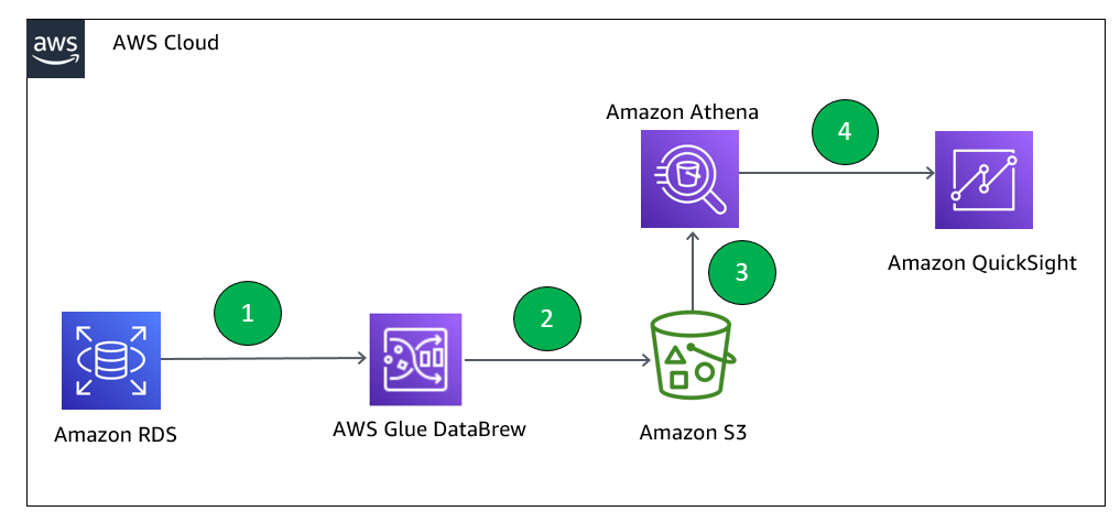
Solution overview

One of the biggest challenges ATS faced was handling data at petabyte scale with the need for constant inserts, updates, and deletes with minimal time delay, which reflects real business scenarios and package movement to downstream data consumers.

Their traditional data warehouses couldn’t scale to the size of the data nor the frequency of data ingestion. They needed to scale to hundreds of GBs of data across multiple data ingestion sources in order to derive near-real-time data for downstream consumers to use for data analytics that powered business-critical reports, dashboards, and visualizations. The data is also used for training machine learning models with overall service level agreements (SLAs) of 15 minutes for data ingestion and processing.

In this post, we show how we ingest data in real time in the order of hundreds of GBs per hour and run inserts, updates, and deletes on a petabyte-scale data lake using Apache Hudi tables loaded using AWS Glue Spark jobs and other AWS server-less services including AWS Lambda, Amazon Kinesis Data Firehose, and Amazon DynamoDB. AWS ProServe, working closely with ATS, built a data lake comprising of Apache Hudi tables on Amazon S3 created and populated using AWS Glue. A data pipeline was created that supports inserts, updates, and deletes at petabyte scale on the Apache Hudi tables using AWS Glue. To support real-time time ingestion, ATS also implemented a real-time data ingestion pipeline based on Kinesis Data Firehose, DynamoDB, and Amazon DynamoDB Streams.

To tackle the challenges we discussed, we decided to follow the “Divide et Impera” approach, and define two separate workstreams:

  • Stream-based – We ingested data from four different data sources and 11 datasets, and performed some initial data transformation and joins steps, honoring a time window that may vary from 3 hours to 2 weeks across all workloads. The event rate might go up to thousands of events per second, and events might have duplicates, arrive late, or not be in the correct order. Our objective was to understand in real time the transit status of a given package or truck, capture the current status of ATS operations in real time, and extend the current stream-based solution to offload and supplement the current extract, transform, and load (ETL) solution, based on Amazon Redshift.
  • Data lake – We wanted the ability to store petabytes of data and allow for merges between historical data (petabytes) with newly ingested data. The data retention policy extends to up to 5 years, which brings increased costs and reduces performance significantly. Our team requires access to near-real-time data (less than 15 minutes) from stream-based ingestion, with full GDPR compliance. Our objective was to merge stream-based ingested data files to derive a holistic view of the dataset at a certain point in time, with an SLA of under 15 minutes. Data lineage capabilities would also be nice to have.

Stream-based solution

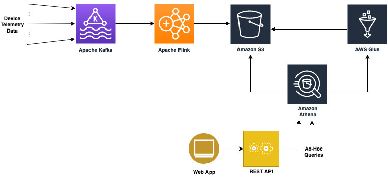
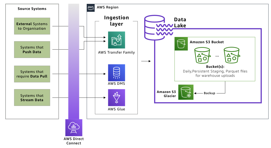
The following diagram illustrates the architecture of our stream-based solution.

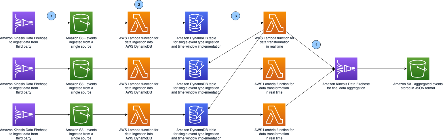
The flow of the solution is as follows:

  1. Data is ingested from various sources in separate Firehose data streams, collected for up to 15 minutes and stored in S3 buckets.
  2. Upon the arrival of every new file in Amazon S3, a Lambda function is triggered to insert data into a DynamoDB table associated with a specific data source or datasets.
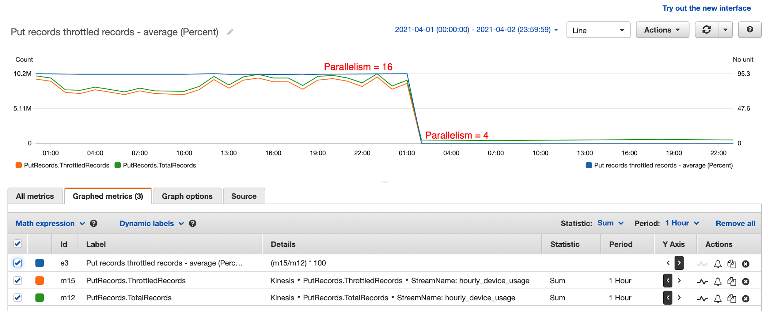
  3. With DynamoDB Streams, we trigger a second Lambda function that aggregates data in real time across the different DynamoDB tables by performing real-time DynamoDB table lookups. The ETL window is enforced using DynamoDB item TTL, so data is automatically deleted from the table after the TTL period expires.
  4. After it’s transformed, data is collected in Amazon S3 passing through a Firehose delivery stream and is ready to be ingested into our data lake.

The solution allows us to do the following:

  • Ingest data in parallel, in real time, and at the desired scale from all the data sources
  • Scale on demand, and with minimal human operational overhead; this is achieved using an AWS Serverless technology stack
  • Implement our desired time window on a per-item base, reducing costs and the total amount of data stored
  • Implement ETL using Lambda functions in Python, thereby providing a tighter grasp over expressing the business logic
  • Access data on Amazon S3 before it’s ingested into our data lake, and allow customers and partners to consume data in raw format if needed

The data present in Amazon S3 represents the starting point for a seamless data lake integration.
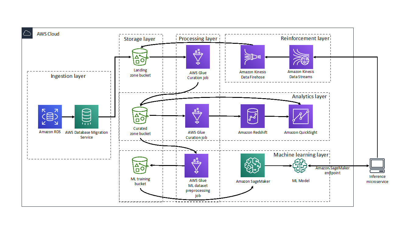
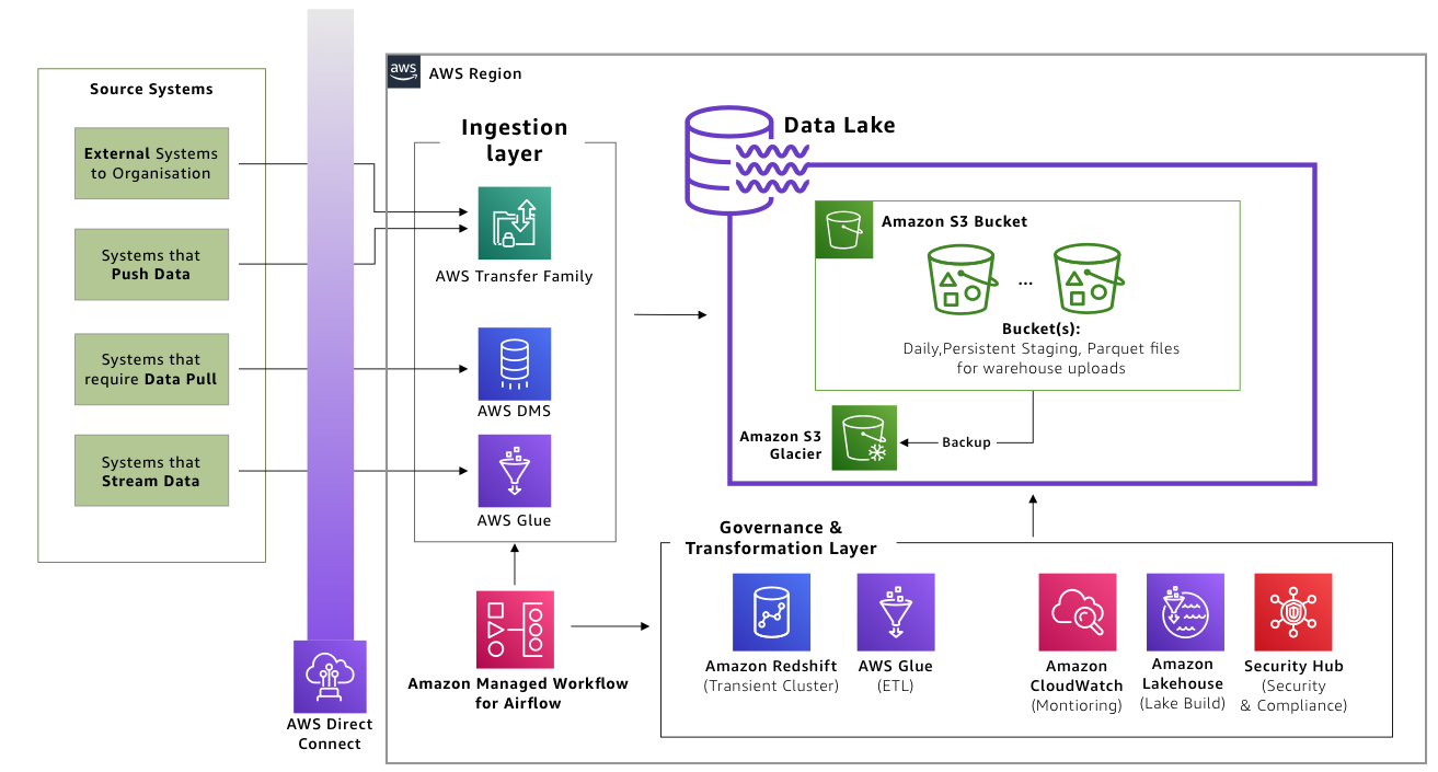
Data lake ingestion

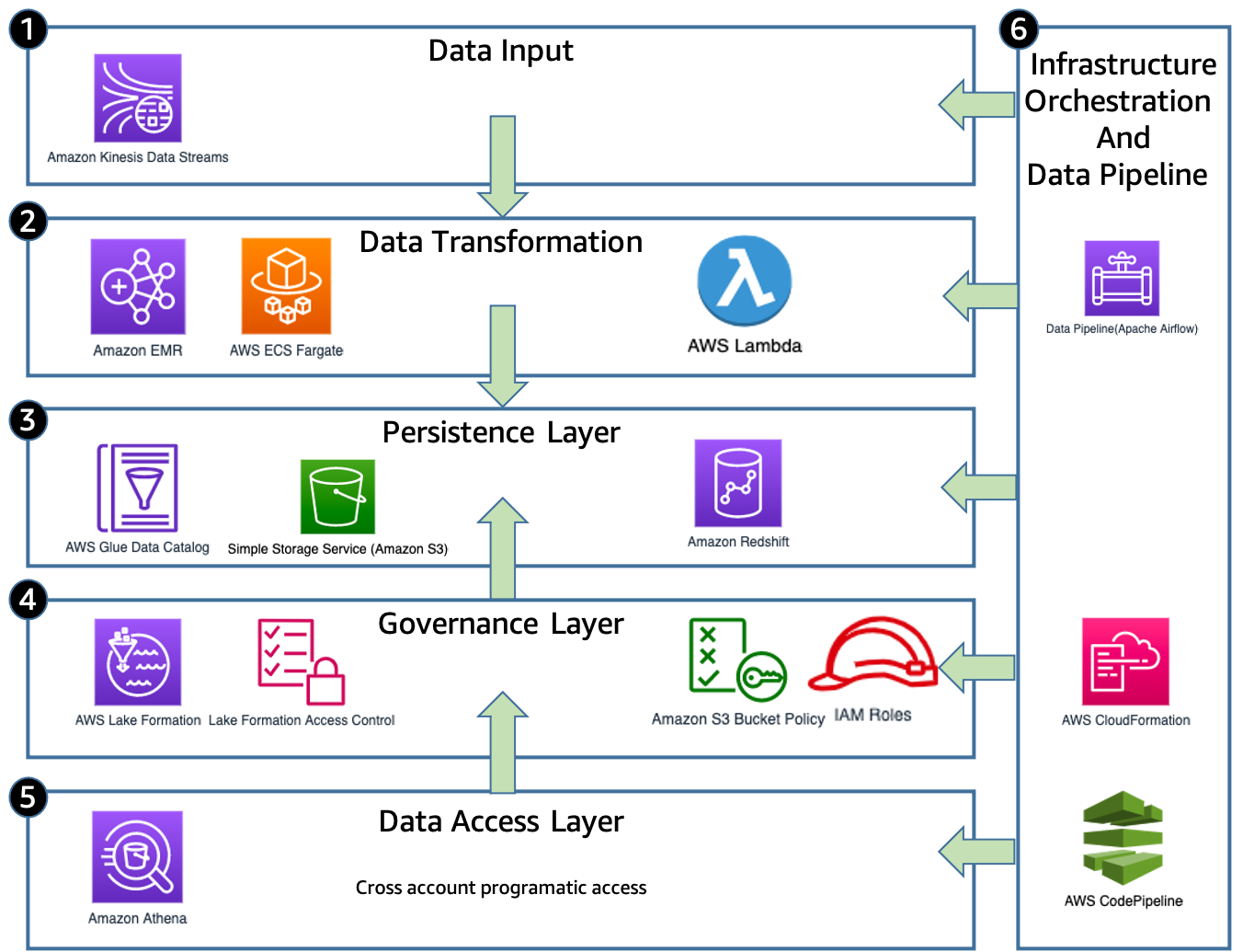
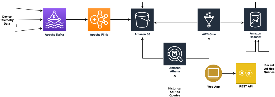
Moving into our data lake, the following diagram illustrates our architecture for data lake ingestion.

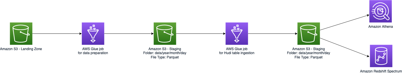
The core implementation in this architecture is the AWS Glue Spark ingestion job for the Hudi table; it represents the entry point for the incremental data processing pipeline.

AWS Glue Spark job runs with a concurrency of 1 and contains the logic for upsert and delete sequentially applied on the Hudi table. The sequencing of delete after upsert in the AWS Glue Spark job ensures, deletes are applied after upsert and the data consistency is maintained even in case of job reruns.

To use Apache Hudi v0.7 on AWS Glue jobs using PySpark, we imported the following libraries in the AWS Glue jobs, extracted locally from the master node of Amazon EMR:

  • hudi-spark-bundle_2.11-0.7.0-amzn-1.jar
  • spark-avro_2.11-2.4.7-amzn-1.jar

We recommend using Glue 3.0 with Hudi 0.9.0 connector rather than importing Hudi v0.7 jar files from EMR, for seamless integration and have more capabilities and features.

Before we insert data the Hudi table, we prepare it for push. To optimize for incremental merge, we take a fixed lookup window based on business use case considerations. We start by reading historical data in a given time window. See the following code:

# HUDI DATA READ
read_options = {
  'hoodie.datasource.query.type': 'snapshot'
}


# HUDI DATAFRAME  created  from target Hudi Table on S3
hudi_df = spark. \
  read. \
  format("hudi"). \
  options(*read_options). \
  load(config['target'] + "////*")

# Read Historical data set, load(basePath) use "/partitionKey=partitionValue" folder structure for Spark auto partition discovery

# input_df is the INCREMENT DATAFRAME created from incrementally ingested data on S3
input_df = spark.read.format("csv"). options(header='true').load(config['incremental_path'])


window_year, window_month, window_day = year_month_day_window()
window_filter_clause = "year >= {} AND month >= {} and day >= {}".format(window_year, window_month, window_day)

# We merge it with the incoming newly available data: 

# Data from Hudi Table on S3, because our use case is global, id is unique else id + partitionPath = unique.
hudi_s3_df = hudi_df.select(col("node_id"),col("container_label"),col(config['sort_key'])).filter(window_filter_clause)

# Perform a left outer join between new data (input_df) and data present in S3 Hudi. (hudi_s3_df)
hudi_join_df = input_df.alias("incomingData").join(hudi_s3_df.alias("S3HudiData"), (input_df.node_id == hudi_s3_df.node_id) & (input_df.container_label == hudi_s3_df.container_label), "leftouter")

# As it's a Left Outer join, there might bew new records which aren't present on S3 Hudi. 

hudi_new_df = hudi_join_df.filter(col("S3HudiData.last_update_row_epoch_seconds").isNull()).drop(col("S3HudiData.node_id")).drop(col("S3HudiData.container_label")).drop(col("S3HudiData.last_update_row_epoch_seconds"))

# As it's a Left Outer join, Select the records where input_df.last_update_time > hudi_s3_df.last_update_time. 

hudi_updated_df = hudi_join_df.filter(col("S3HudiData.last_update_row_epoch_seconds").isNotNull() & (col("incomingData.last_update_row_epoch_seconds") > col("S3HudiData.last_update_row_epoch_seconds"))).drop(col("S3HudiData.node_id")).drop(col("S3HudiData.container_label")).drop(col("S3HudiData.last_update_row_epoch_seconds"))
hudi_final_df = hudi_new_df.union(hudi_updated_df)

#  After we prepare the data to be pushed in the Hudi table, we implement the Hudi table update using the following code:

(hudi_final_df.write.format(HUDI_FORMAT)
.option(TABLE_NAME, config['hudi_table_name'])
.option(RECORDKEY_FIELD_OPT_KEY, config["primary_key"])
.option(PARTITIONPATH_FIELD_OPT_KEY,config["partition_keys"])
.option(KEYGENERATOR_CLASS_OPT_KEY, COMPLEX_KEYGENERATOR_CLASS_OPT_VAL)
.option(PRECOMBINE_FIELD_OPT_KEY, config["sort_key"])
.option(OPERATION_OPT_KEY, UPSERT_OPERATION_OPT_VAL)
.option(UPSERT_PARALLELISM, 1500)
.option('hoodie.payload.ordering.field',config["sort_key"])
.option(PAYLOAD_CLASS_OPT_KEY,'org.apache.hudi.common.model.DefaultHoodieRecordPayload')
.option(HIVE_PARTITION_FIELDS_OPT_KEY, config["partition_keys"])
.option(HIVE_DATABASE_OPT_KEY,config['hudi_database'])
.option(HIVE_TABLE_OPT_KEY,config['hudi_table_name'])
.option(HIVE_SYNC_ENABLED_OPT_KEY,"true")
.option(HIVE_JDBC_SYNC,"false")
.option(HIVE_PARTITION_EXTRACTOR_CLASS_OPT_KEY, MULTIPART_KEYS_EXTRACTOR_CLASS_OPT_VAL)
.option('hoodie.datasource.write.hive_style_partitioning', 'true')
# To switch to Global Bloom index, set the following configuration as GLOBAL_BLOOM.
.option('hoodie.index.type', 'GLOBAL_SIMPLE') 
.option('hoodie.simple.index.update.partition.path', 'true')
.option('hoodie.global.simple.index.parallelism', '500')
.mode("append")
.save(config['target']))

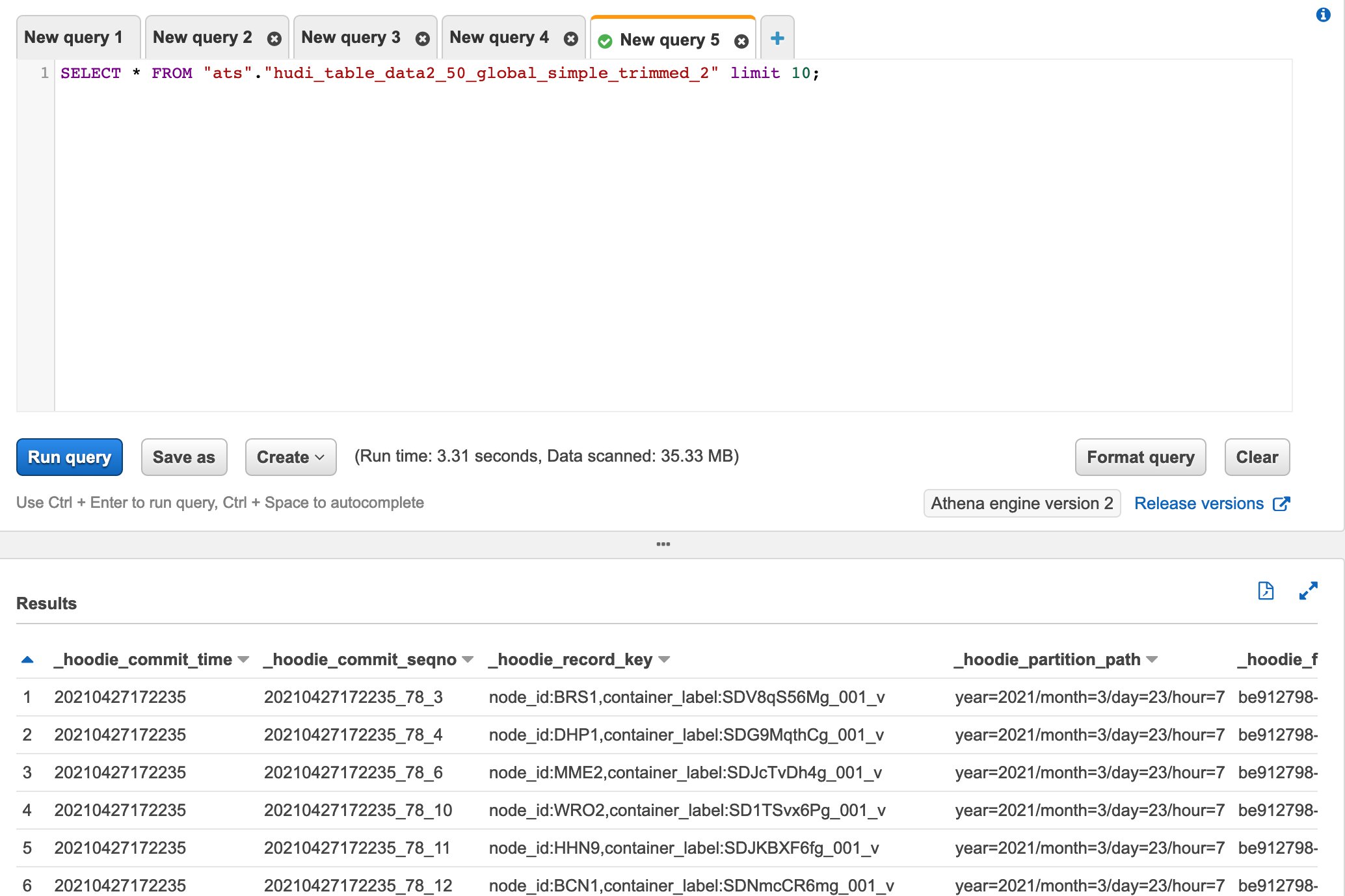
In the preceding code, config is a dictionary that includes all the Apache Hudi configurations. The AWS Glue Data Catalog is automatically synched after Hudi table creation, as part of the Glue job, reflecting the Amazon S3 partition structure. We can now query the data using Amazon Athena or Amazon Redshift Spectrum.

To comply with our strict internal ingestion SLA, we had to dedicate special attention to employing the right Hudi indexes and defining the right table type. For the latter, we analyzed the type of workload. Due to the analytic nature of the datasets and use case, we identified that the right configuration would be to use a COPY_ON_WRITE table, even if that was a compromise on the write performances but enhanced read performance.

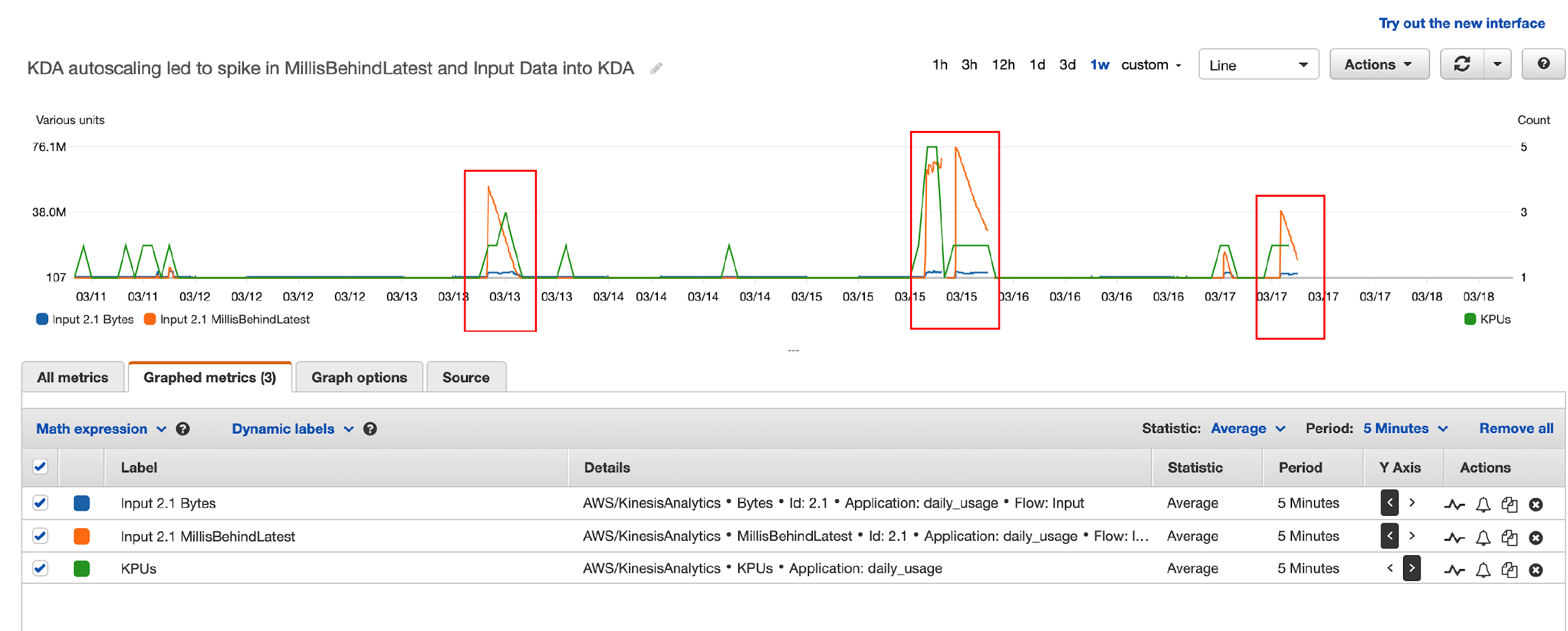
For the former, we went through an experimentation phase. We started with a GLOBAL_BLOOM index, identifying an initial non-linear pattern for data writing performances.

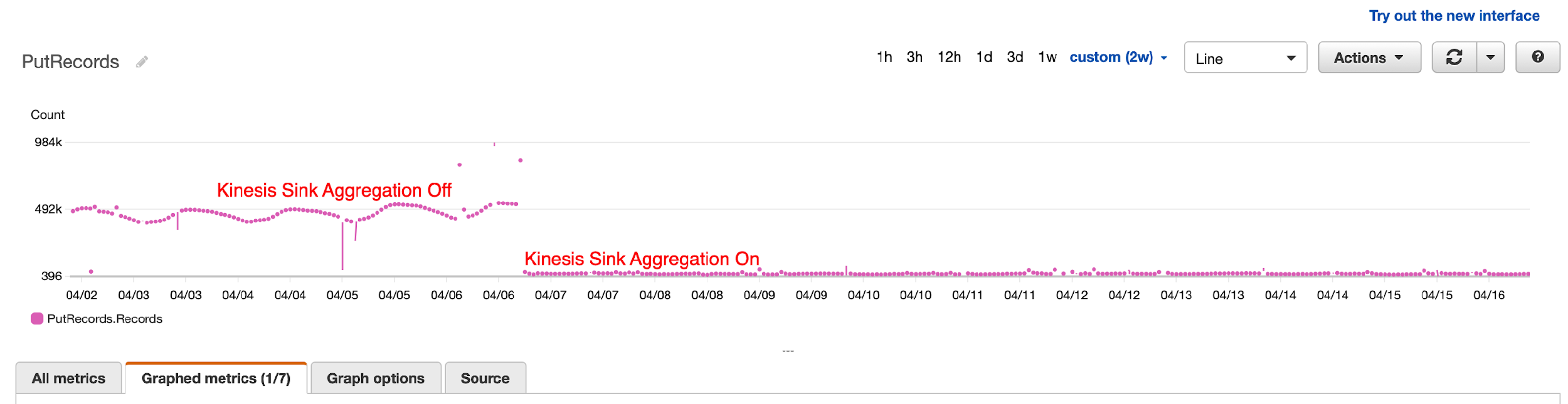
Given the randomness and the time window specified for the input data, we have encountered a significant number of false positives, leading to reading the entire dataset back for comparison. Moreover, GLOBAL_BLOOM keeps increasing linearly corresponding to the data size, whereas GLOBAL_SIMPLE doesn’t bring this overhead (with a fixed lookup window) as can be observed in the diagram.

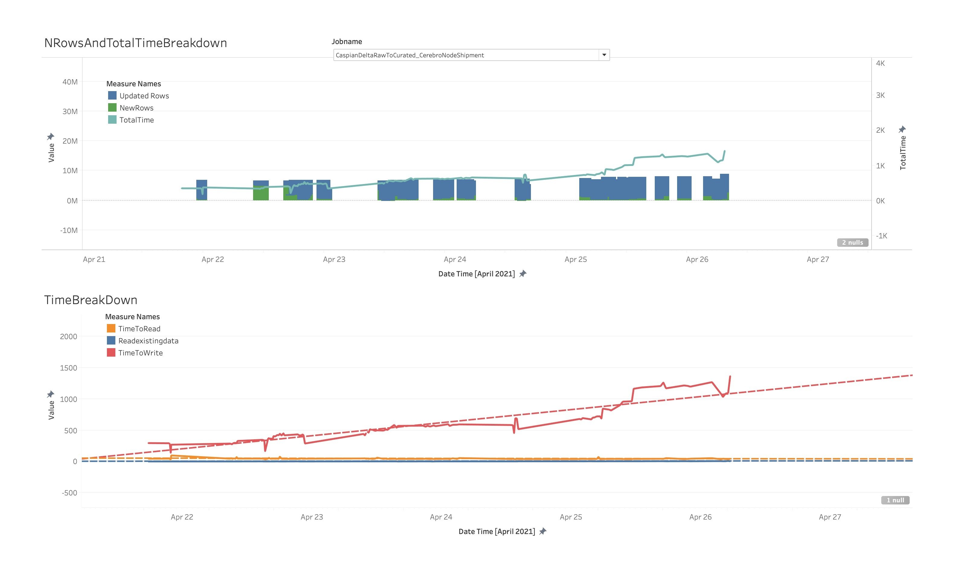
The graph represents the Total Time taken by Glue Hudi job(X-axis) over days (Y axis) as incoming data is merged with the historical data.  leveraging GLOBAL_BLOOM.  The graph in upper half, shows when same data was merged consecutively over days, non-linear time increase was observed. Lower half graph indicates Linear increase with a steep slope when new incoming data was merged with historical data.

GLOBAL_BLOOM wasn’t appropriate for our use case as the historical data spanned back to 5 years, and Glue job will not be able to meet the SLA demands. At this point, we investigated GLOBAL_SIMPLE indexes, reaching the expected performance patterns.

Our data lake solution allows us to do the following:

  • Ingest data files in a petabyte-scale data lake, with a 15-minute ingestion SLA from the moment we receive the data
  • Read the data at Peta Byte scale by leveraging Amazon S3 partitions (created by Glue jobs and mapped to Hudi partition logic) and faster lookups by using Hudi indexes
  • Use Hudi data lineage capabilities
  • Reduce costs for data storage, infrastructure maintenance, and development
  • Manage data governance using AWS Lake Formation, which allows partners and customers to query the data using their own tools, while allowing ATS to retain control over our data

Conclusion

In this post, we highlighted how ATS built a real-time fully serverless data ingestion platform, scaling up to thousands of events per second and merging with petabyte- sized historical data stored in a data lake in near-real time.

We built a petabyte-scale data lake solution based on Apache Hudi and AWS Glue that allows us to share our data within 15 minutes from ingestion with our partners and consumers, while retaining complete control over our data and automatically offloading costs for data consumption. This provides linear performance as data grows over time.

About Amazon Transportation Service

Amazon Transportation Service (ATS) is the middle mile of the transportation network of Amazon, connecting the fulfillment centers at one end and the delivery stations and post offices at the other end. We enable packages that are ordered and packaged from fulfillment centers that traverse across the European continent to be delivered in the final delivery station that does the house-to-house delivery.


About the Authors

Madhavan Sriram is a Manager, Data Science who comes with a wide experience across multiple enterprise organisations in the space of Big Data and Machine Learning technologies. He currently leads the Data Technology and Products team within Amazon Transportation Services (ATS) and builds data-intensive products for the transportation network within Amazon. In his free time, Madhavan enjoys photography and poetry.

Diego Menin is a Senior Data Engineer within the Data Technology and Products team. He comes with a wide experience across startups and enterprises with deep AWS expertise to develop scalable cloud-based data and analytics products. Within Amazon, he is the architect of Amazon’s transportation data lake and working heavily on streaming data and integration mechanisms with downstream applications through the data lake.

Gabriele Cacciola is a Senior Data Architect working for the Professional Service team with Amazon Web Services. Coming from a solid Startup experience, he currently helps enterprise customers across EMEA implement their ideas, innovate using the latest tech and build scalable data and analytics solutions to make critical business decisions. In his free time, Gabriele enjoys football and cooking.

Kunal Gautam is a Senior Big Data Architect at Amazon Web Services. Having experience in building his own Startup and working along with enterprises, he brings a unique perspective to get people, business and technology work in tandem for customers. He is passionate about helping customers in their digital transformation journey and enables them to build scalable data and advance analytics solutions to gain timely insights and make critical business decisions. In his spare time, Kunal enjoys Marathons, Tech Meetups and Meditation retreats.

Field Notes: How to Build an AWS Glue Workflow using the AWS Cloud Development Kit

Post Syndicated from Michael Hamilton original https://aws.amazon.com/blogs/architecture/field-notes-how-to-build-an-aws-glue-workflow-using-the-aws-cloud-development-kit/

Many customers use AWS Glue workflows to build and orchestrate their ETL (extract-transform-load) pipelines directly in the AWS Glue console using the visual tool to author workflows. This can be time consuming, harder to version control, and error prone due to manual configurations, when compared to managing your workflows as code. To improve your operational excellence, consider deploying the entire AWS Glue ETL pipeline using the AWS Cloud Development Kit (AWS CDK).

In this blog post, you will learn how to build an AWS Glue workflow using Amazon Simple Storage Service (Amazon S3), various components of AWS Glue, AWS Secrets Manager, Amazon Redshift, and the AWS CDK.

Architecture overview

In this architecture, you will use the AWS CDK to deploy your data sources, ETL scripts, AWS Glue workflow components, and an Amazon Redshift cluster for analyzing the transformed data.

AWS Glue workflow architecture

Figure 1. AWS Glue workflow architecture

It is common for customers to pre-aggregate data before sending it downstream to analytical engines, like Amazon Redshift, because table joins and aggregations are computationally expensive. The AWS Glue workflow will join COVID-19 case data, and COVID-19 hiring data together on their date columns in order to run correlation analysis on the final dataset. The datasets may seem arbitrary, but we wanted to offer a way to better understand the impacts COVID-19 had on jobs in the United States. The takeaway here is to use this as a blueprint for automating the deployment of data analytic pipelines for the data of interest to your business.

After the AWS CDK application is deployed, it will begin creating all of the resources required to build the complete workflow. When it completes, the components in the architecture will be created, and the AWS Glue workflow will be ready to start. In this blog post, you start workflows manually, but they can be configured to start on a scheduled time or from a workflow trigger.

The workflow is programmed to dynamically pull the raw data from the Registry of Open Data on AWS where you can find the Covid-19 case data and the Hiring Data respectively.

Prerequisites

This blog post uses an AWS CDK stack written in TypeScript and AWS Glue jobs written in Python. Follow the instructions in the AWS CDK Getting Started guide to set up your environment, before you proceed to deployment.

In addition to setting up your environment, you need to clone the Git repository, which contains the AWS CDK scripts and Python ETL scripts used by AWS Glue. The ETL scripts will be deployed to Amazon S3 by the AWS CDK stack as assets, and referenced by the AWS Glue jobs as part of the AWS Glue Workflow.

You should have the following prerequisites:

Deployment

After you have cloned the repository, navigate to the glue-cdk-blog/lib folder and open the blog-glue-workflow-stack.ts file. This is the AWS CDK script used to deploy all necessary resources to build your AWS Glue workflow. The blog-redshift-vpc-stack.ts contains the necessary resources to deploy the Amazon Redshift cluster, connections, and permissions. The glue-cdk-blog/lib/assets folder also contains the AWS Glue job scripts. These files are uploaded to Amazon S3 by the AWS CDK when you bootstrap.

You won’t review the individual lines of code in the script in this blog post, but if you are unfamiliar with any of the AWS CDK level 1 or level 2 constructs used in the sample, you can review what each construct does with the AWS CDK documentation. Familiarize yourself with the script you cloned and anticipate what resources will be deployed. Then, deploy both stacks and verify your initial findings.

After your environment is configured, and the packages and modules installed, deploy the AWS CDK stack and assets in two commands.

  1. Bootstrap the AWS CDK stack to create an S3 bucket in the predefined account that will contain the assets.

cdk bootstrap

  1. Deploy the AWS CDK stacks.

cdk deploy --all

Verify that both of these commands have completed successfully, and remediate any failures returned. Upon successful completion, you’re ready to start the AWS Glue workflow that was just created. You can find the AWS CDK commands reference in the AWS CDK Toolkit commands documentation, and help with Troubleshooting common AWS CDK issues you may encounter.

Walkthrough

Prior to initiating the AWS Glue workflow, explore the resources the AWS CDK stacks just deployed to your account.

  1. Log in to the AWS Management Console and the AWS CDK account.
  2. Navigate to Amazon S3 in the AWS console (you should see an S3 bucket with the name prefix of cdktoolkit-stagingbucket-xxxxxxxxxxxx).
  3. Review the objects stored in the bucket in the assets folder. These are the .py files used by your AWS Glue jobs. They were uploaded to the bucket when you issued the AWS CDK bootstrap command, and referenced within the AWS CDK script as the scripts to use for the AWS Glue jobs. When retrieving data from multiple sources, you cannot always control the naming convention of the sourced files. To solve this and create better standardization, you will use a job within the AWS Glue workflow to copy these scripts to another folder and rename them with a more meaningful name.
  4. Navigate to Amazon Redshift in the AWS console and verify your new cluster. You can use the Amazon Redshift Query Editor within the console to connect to the cluster and see that you have an empty database called db-covid-hiring. The Amazon Redshift cluster and networking resources were created by the redshift_vpc_stack which are listed here:
    • VPC, subnet and security group for Amazon Redshift
    • Secrets Manager secret
    • AWS Glue connection and S3 endpoint
    • Amazon Redshift cluster
  1. Navigate to AWS Glue in the AWS console and review the following new resources created by the workflow_stack CDK stack:
    • Two crawlers to crawl the data in S3
    • Three AWS Glue jobs used within the AWS Glue workflow
    • Five triggers to initiate AWS Glue jobs and crawlers
    • One AWS Glue workflow to manage the ETL orchestration
  1. All of these resources could have been deployed within a single stack, but this is intended to be a simple example on how to share resources across multiple stacks. The AWS Identity and Access Management (IAM) role that AWS Glue uses to run the ETL jobs in the workflow_stack, is also used by Secrets Manager for Amazon Redshift in the redshift_vpc_stack. Inspect the /bin/blog-glue-workflow-stack.ts file to further understand cross stack resource sharing.

By performing these steps, you have deployed all of the AWS Glue resources necessary to perform common ETL tasks. You then combined the resources to create an orchestration of tasks using an AWS Glue workflow. All of this was done using IaC with AWS CDK. Your workflow should look like Figure 2.

AWS Glue console showing the workflow created by the CDK

Figure 2. AWS Glue console showing the workflow created by the CDK

As mentioned earlier, you could have started your workflow using a scheduled cron trigger, but you initiated the workflow manually so you had time to review the resources the workflow_stack CDK deployed, prior to initiation of the workflow. Now that you have reviewed the resources, validate your workflow by initiating it and verifying it runs successfully.

  1. From within the AWS Glue console, select Workflows under ETL.
  2. Select the workflow named glue-workflow, and then select Run from the actions listbox.
  3. You can verify the status of the workflow by viewing the run details under the History tab.
  4. Your job will take approximately 15 minutes to successfully complete, and your history should look like Figure 3.
AWS Glue console showing the workflow as completed after the run

Figure 3. AWS Glue console showing the workflow as completed after the run

The workflow performs the following tasks:

  1. Prepares the ETL scripts by copying the files in the S3 asset bucket to a new folder and renames them with a more relevant name.
  2. Initiates a crawler to crawl the raw source data as csv files and adds tables to the Glue Data Catalog.
  3. Runs a Python script to perform some ETL tasks on the .csv files and converts them to parquet files.
  4. Crawls the parquet files and adds them to the Glue Data Catalog.
  5. Loads the parquet files into a DynamicFrame and runs an Amazon Redshift COPY command to load the data into the Amazon Redshift database.

After the workflow completes, you can query and perform analytics on the data that was populated in Amazon Redshift. Open the Amazon Redshift Query Editor and run a simple SELECT statement to query the covid_hiring_table which is the joined Covid-19 case data and hiring data (see Figure 4).

Amazon Redshift query editor showing the data that the workflow loaded into the Redshift tables

Figure 4. Amazon Redshift query editor showing the data that the workflow loaded into the Redshift tables

Cleaning up

Some resources, like S3 buckets and Amazon DynamoDB tables, must be manually emptied and deleted through the console to be fully removed. To clean up the deployment, delete all objects in the AWS CDK asset bucket in Amazon S3 by using the AWS console to empty the bucket, and then run cdk destroy –all to delete the resources the AWS CDK stacks created in your account. Finally, if you don’t plan on using AWS CloudFormation assets in this account in the future, you will need to delete the AWS CDK asset stack within the CloudFormation console to remove the AWS CDK asset bucket.

Conclusion

In this blog post, you learned how to automate the deployment of AWS Glue workflows using the AWS CDK. This further enhances your continuous integration and delivery (CI/CD) data pipelines by automating the deployment of the ETL jobs and AWS Glue workflow orchestration, providing an efficient, fast, and repeatable way to build and deploy AWS Glue workflows at scale.

Although AWS CDK primarily supports level 1 constructs for most AWS Glue resources, new constructs are added continually. See the AWS CDK API Reference for updates, prior to authoring your stacks, for AWS Glue level 2 construct support. You can find the code used in this blog post in this GitHub repository, and the AWS CDK in TypeScript reference to the AWS CDK namespace.

We hope this blog post helps enrich your work through the skills gained of automating the creation of Glue Workflows, enabling you to quickly build and deploy your own ETL pipelines and run analytical models that power your business.

Field Notes provides hands-on technical guidance from AWS Solutions Architects, consultants, and technical account managers, based on their experiences in the field solving real-world business problems for customers.

How NortonLifelock built a serverless architecture for real-time analysis of their VPN usage metrics

Post Syndicated from Madhu Nunna original https://aws.amazon.com/blogs/big-data/how-nortonlifelock-built-a-serverless-architecture-for-real-time-analysis-of-their-vpn-usage-metrics/

This post presents a reference architecture and optimization strategies for building serverless data analytics solutions on AWS using Amazon Kinesis Data Analytics. In addition, this post shows the design approach that the engineering team at NortonLifeLock took to build out an operational analytics platform that processes usage data for their VPN services, consuming petabytes of data across the globe on a daily basis.

NortonLifeLock is a global cybersecurity and internet privacy company that offers services to millions of customers for device security, and identity and online privacy for home and family. NortonLifeLock believes the digital world is only truly empowering when people are confident in their online security. NortonLifeLock has been an AWS customer since 2014.

For any organization, the value of operational data and metrics decreases with time. This lost value can equate to lost revenue and wasted resources. Real-time streaming analytics helps capture this value and provide new insights that can create new business opportunities.

AWS offers a rich set of services that you can use to provide real-time insights and historical trends. These services include managed Hadoop infrastructure services on Amazon EMR as well as serverless options such as Kinesis Data Analytics and AWS Glue.

Amazon EMR also supports multiple programming options for capturing business logic, such as Spark Streaming, Apache Flink, and SQL.

As a customer, it’s important to understand organizational capabilities, project timelines, business requirements, and AWS service best practices in order to define an optimal architecture from performance, cost, security, reliability, and operational excellence perspectives (the five pillars of the AWS Well-Architected Framework).

NortonLifeLock is taking a methodical approach to real-time analytics on AWS while using serverless technology to deliver on key business drivers such as time to market and total cost of ownership. In addition to NortonLifeLock’s implementation, this post provides key lessons learned and best practices for rapid development of real-time analytics workloads.

Business problem

NortonLifeLock offers a VPN product as a freemium service to users. Therefore, they need to enforce usage limits in real time to stop freemium users from using the service when their usage is over the limit. The challenge for NortonLifeLock is to do this in a reliable and affordable fashion.

NortonLifeLock runs its VPN infrastructure in almost all AWS Regions. Migrating to AWS from smaller hosting vendors has greatly improved user experience and VPN edge server performance, including a reduction in connection latency, time to connect and connection errors, faster upload and download speed, and more stability and uptime for VPN edge servers.

VPN usage data is collected by VPN edge servers and uploaded to backend stats servers every minute and persisted in backend databases. The usage information serves multiple purposes:

  • Displaying how much data a device has consumed for the past 30 days.
  • Enforcing usage limits on freemium accounts. When a user exhausts their free quota, that user is unable to connect through VPN until the next free cycle.
  • Analyzing usage data by the internal business intelligence (BI) team based on time, marketing campaigns, and account types, and using this data to predict future growth, ability to retain users, and more.

Design challenge

NortonLifeLock had the following design challenges:

  • The solution must be able to simultaneously satisfy both real-time and batch analysis.
  • The solution must be economical. NortonLifeLock VPN has hundreds of thousands of concurrent users, and if a user’s usage information is persisted as it comes in, it results in tens of thousands of reads and writes per second and tens of thousands of dollars a month in database costs.

Solution overview

NortonLifeLock decided to split storage into two parts by storing usage data in Amazon DynamoDB for real-time access and in Amazon Simple Storage Service (Amazon S3) for analysis, which addresses real-time enforcement and BI needs. Kinesis Data Analytics aggregates and loads data to Amazon S3 and DynamoDB. With Amazon Kinesis Data Streams and AWS Lambda as consumers of Kinesis Data Analytics, the implementation of user and device-level aggregations was simplified.

To keep costs down, user usage data was aggregated by the hour and persisted in DynamoDB. This spread hundreds of thousands of writes over an hour and reduced DynamoDB cost by 30 times.

Although increasing aggregation might not be an option for other problem domains, it’s acceptable in this case because it’s not necessary to be precise to the minute for user usage, and it’s acceptable to calculate and enforce the usage limit every hour.

The following diagram illustrates the high-level architecture. The solution is broken into three logical parts:

  • End-users – Real-time queries from devices to display current usage information (how much data is used daily)
  • Business analysts – Query historical usage information through Amazon Athena to extract business insights
  • Usage limit enforcement – Usage data ingestion and aggregation in real time

The solution has the following workflow:

  1. Usage data is collected by a VPN edge server and sends it to the backend service through Application Load Balancer.
  2. A single usage data record sent by the VPN edge server contains usage data for many users. A stats splitter splits the message into individual usage stats per user and forwards the message to Kinesis Data Streams.
  3. Usage data is consumed by both the legacy stats processor and the new Apache Flink application developed and deployed on Kinesis Data Analytics.
  4. The Apache Flink application carries out the following tasks:
    1. Aggregate device usage data hourly and send the aggregated result to Amazon S3 and the outgoing Kinesis data stream, which is picked up by a Lambda function that persists the usage data in DynamoDB.
    2. Aggregate device usage data daily and send the aggregated result to Amazon S3.
    3. Aggregate account usage data hourly and forward the aggregated results to the outgoing data stream, which is picked up by a Lambda function that checks if account usage is over the limit for that account. If account usage is over the limit, the function forwards the account information to another Lambda function, via Amazon Simple Queue Service (Amazon SQS), to cut off access on that account.

Design journey

NortonLifeLock needed a solution that was capable of real-time streaming and batch analytics. Kinesis Data Analysis fits this requirement because of the following key features:

  • Real-time streaming and batch analytics for data aggregation
  • Fully managed with a pay-as-you-go model
  • Auto scaling

NortonLifeLock needed Kinesis Data Analytics to do the following:

  • Aggregate customer usage data per device hourly and send results to Kinesis Data Streams (ultimately to DynamoDB) and the data lake (Amazon S3)
  • Aggregate customer usage data per account hourly and send results to Kinesis Data Streams (ultimately to DynamoDB and Lambda, which enforces usage limit)
  • Aggregate customer usage data per device daily and send results to the data lake (Amazon S3)

The legacy system processes usage data from an incoming Kinesis data stream, and they plan to use Kinesis Data Analytics to consume and process production data from the same stream. As such, NortonLifeLock started with SQL applications on Kinesis Data Analytics.

First attempt: Kinesis Data Analytics for SQL

Kinesis Data Analytics with SQL provides a high-level SQL-based abstraction for real-time stream processing and analytics. It’s configuration driven and very simple to get started. NortonLifeLock was able to create a prototype from scratch, get to production, and process the production load in less than 2 weeks. The solution met 90% of the requirements, and there were alternates for the remaining 10%.

However, they started to receive “read limit exceeded” alerts from the source data stream, and the legacy application was read throttled. With Amazon Support’s help, they traced the issues to the drastic reversal of the Kinesis Data Analytics MillisBehindLatest metric in Kinesis record processing. This was correlated to the Kinesis Data Analytics auto scaling events and application restarts, as illustrated by the following diagram. The highlighted areas show the correlation between spikes due to autoscaling and reversal of MillisBehindLatest metrics.

Here’s what happened:

  • Kinesis Data Analytics for SQL scaled up KPU due to load automatically, and the Kinesis Data Analytics application was restarted (part of scaling up).
  • Kinesis Data Analytics for SQL supports the at least once delivery model and uses checkpoints to ensure no data loss. But it doesn’t support taking a snapshot and restoring from the snapshot after a restart. For more details, see Delivery Model for Persisting Application Output to an External Destination.
  • When the Kinesis Data Analytics for SQL application was restarted, it needed to reprocess data from the beginning of the aggregation window, resulting in a very large number of duplicate records, which led to a dramatic increase in the Kinesis Data Analytics MillisBehindLatest metric.
  • To catch up with incoming data, Kinesis Data Analytics started re-reading from the Kinesis data stream, which led to over-consumption of read throughput and the legacy application being throttled.

In summary, Kinesis Data Analytics for SQL’s duplicates record processing on restarts, no other means to eliminate duplicates, and limited ability to control auto scaling led to this issue.

Although they found Kinesis Data Analytics for SQL easy to get started, these limitations demanded other alternatives. NortonLifeLock reached out to the Kinesis Data Analytics team and discussed the following options:

  • Option 1 – AWS was planning to release a new service, Kinesis Data Analytics Studio for SQL, Python, and Scala, which addresses these limitations. But this service was still a few months away (this service is now available, launched May 27, 2021).
  • Option 2 – The alternative was to switch to Kinesis Data Analytics for Apache Flink, which also provides the necessary tools to address all their requirements.

Second attempt: Kinesis Data Analytics for Apache Flink

Apache Flink has a comparatively steep learning curve (we used Java for streaming analytics instead of SQL), and it took about 4 weeks to build the same prototype, deploy it to Kinesis Data Analytics, and test the application in production. NortonLifeLock had to overcome a few hurdles, which we document in this section along with the lessons learned.

Challenge 1: Too many writes to outgoing Kinesis data stream

The first thing they noticed was that the write threshold on the outgoing Kinesis data stream was greatly exceeded. Kinesis Data Analytics was attempting to write 10 times the amount of expected data to the data stream, with 95% of data throttled.

After a lengthy investigation, it turned out that having too much parallelism in the Kinesis Data Analytics application led to this issue. They had followed default recommendations and set parallelism to 12 and it scaled up to 16. This means that every hour, 16 separate threads were attempting to write to the destination data stream simultaneously, leading to massive contention and writes throttled. These threads attempted to retry continuously, until all records were written to the data stream. This resulted in 10 times the amount of data processing attempted, even though only one tenth of the writes eventually succeeded.

The solution was to reduce parallelism to 4 and disable auto scaling. In the preceding diagram, the percentage of throttled records dropped to 0 from 95% after they reduced parallelism to 4 in the Kinesis Data Analytics application. This also greatly improved KPU utilization and reduced Kinesis Data Analytics cost from $50 a day to $8 a day.

Challenge 2: Use Kinesis Data Analytics sink aggregation

After tuning parallelism, they still noticed occasional throttling by Kinesis Data Streams because of the number of records being written, not record size. To overcome this, they turned on Kinesis Data Analytics sink aggregation to reduce the number of records being written to the data stream, and the result was dramatic. They were able to reduce the number of writes by 1,000 times.

Challenge 3: Handle Kinesis Data Analytics Flink restarts and the resulting duplicate records

Kinesis Data Analytics applications restart because of auto scaling or recovery from application or task manager crashes. When this happens, Kinesis Data Analytics saves a snapshot before shutdown and automatically reloads the latest snapshot and picks up where the work was left off. Kinesis Data Analytics also saves a checkpoint every minute so no data is lost, guaranteeing exactly-once processing.

However, when the Kinesis Data Analytics application shut down in the middle of sending results to Kinesis Data Streams, it doesn’t guarantee exactly-once data delivery. In fact, Flink only guarantees at least once delivery to Kinesis Data Analytics sink, meaning that Kinesis Data Analytics guarantees to send a record at least once, which leads to duplicate records sent when Kinesis Data Analytics is restarted.

How were duplicate records handled in the outgoing data stream?

Because duplicate records aren’t handled by Kinesis Data Analytics when sinks do not have exactly-once semantics, the downstream application must deal with the duplicate records. The first question you should ask is whether it’s necessary to deal with the duplicate records. Maybe it’s acceptable to tolerate duplicate records in your application? This, however, is not an option for NortonLifeLock, because no user wants to have their available usage taken twice within the same hour. So, logic had to be built in the application to handle duplicate usage records.

To deal with duplicate records, you can employ a strategy in which the application saves an update timestamp along with the user’s latest usage. When a record comes in, the application reads existing daily usage and compares the update timestamp against the current time. If the difference is less than a configured window (50 minutes if the aggregation window is 60 minutes), the application ignores the new record because it’s a duplicate. It’s acceptable for the application to potentially undercount vs. overcount user usage.

How were duplicate records handled in the outgoing S3 bucket?

Kinesis Data Analytics writes temporary files in Amazon S3 before finalizing and removing them. When Kinesis Data Analytics restarts, it attempts to write new S3 files, and potentially leaves behind temporary S3 files because of restart. Because Athena ignores all temporary S3 files, no further is action needed. If your BI tools take temporary S3 files into consideration, you have to configure the Amazon S3 lifecycle policy to clean up temporary S3 files after a certain time.

Conclusion

NortonLifelock has been successfully running a Kinesis Data Analytics application in production since May 2021. It provides several key benefits. VPN users can now keep track of their usage in near-real time. BI analysts can get timely insights that are used for targeted sales and marketing campaigns, and upselling features and services. VPN usage limits are enforced in near-real time, thereby optimizing the network resources. NortonLifelock is saving tens of thousands of dollars each month with this real-time streaming analytics solution. And this telemetry solution is able to keep up with petabytes of data flowing through their global VPN service, which is seeing double-digit monthly growth.

To learn more about Kinesis Data Analytics and getting started with serverless streaming solutions on AWS, please see Developer Guide for Studio, the easiest way to build Apache Flink applications in SQL, Python, Scala in a notebook interface.


About the Authors

Lei Gu has 25 years of software development experience and the architect for three key Norton products, Norton Secure Backup, VPN and Norton Family. He is passionate about cloud transformation and most recently spoke about moving from Cassandra to Amazon DynamoDB at AWS re:Invent 2019. Check out his Linkedin profile at https://www.linkedin.com/in/leigu/.

Madhu Nunna is a Sr. Solutions Architect at AWS, with over 20 years of experience in networks and cloud, with the last two years focused on AWS Cloud. He is passionate about Analytics and AI/ML. Outside of work, he enjoys hiking and reading books on philosophy, economics, history, astronomy and biology.

Hybrid Cloud Architectures Using Self-hosted Apache Kafka and AWS Glue

Post Syndicated from Brandon Rubadou original https://aws.amazon.com/blogs/architecture/hybrid-cloud-architectures-using-self-hosted-apache-kafka-and-aws-glue/

Using analytics to gain insights from a variety of datasets is key to successful transformation. There are many options to consider to realize the full value and potential of our data in a hybrid cloud infrastructure. Common practice is to route data produced from on-premises to a central repository or data lake. Here it can be consumed by multiple applications.

You can use an Apache Kafka cluster for data movement from on-premises to the data lake, using Amazon Simple Storage Service (Amazon S3). But you must either replicate the topics onto a cloud cluster, or develop a custom connector to read and copy the topics to Amazon S3. This presents a challenge for many customers.

This blog presents another option; an architecture solution leveraging AWS Glue.

Kafka and ETL processing

Apache Kafka is an open-source distributed event streaming platform used by thousands of companies for high-performance data pipelines, streaming analytics, data integration, and mission-critical applications. You can use Kafka clusters as a system to move data between systems. Producers typically publish data (or push) to a Kafka topic, where an application can consume it. Consumers are usually custom applications that feed data into respective target applications. These targets can be a data warehouse, an Amazon OpenSearch Service cluster, or others.

AWS Glue offers the ability to create jobs that will extract, transform, and load (ETL) data. This allows you to consume from many sources, such as from Apache Kafka, Amazon Kinesis Data Streams, or Amazon Managed Streaming for Apache Kafka (Amazon MSK). The jobs cleanse and transform the data, and then load the results into Amazon S3 data lakes or JDBC data stores.

Hybrid solution and architecture design

In most cases, the first step in building a responsive and manageable architecture is to review the data itself. For example, if we are processing insurance policy data from a financial organization, our data may contain fields that identify customer data. These can be account ID, an insurance claim identifier, and the dollar amount of the specific claim. Glue provides the ability to change any of these field types into the expected data lake schema type for processing.

Figure 1. Data flow - Source to data lake target

Figure 1. Data flow – Source to data lake target

Next, AWS Glue must be configured to connect to the on-premises Kafka server (see Figure 1). Private and secure connectivity to the on-premises environment can be established via AWS Direct Connect or a VPN solution. Traffic from the Amazon Virtual Private Cloud (Amazon VPC) is allowed to access the cluster directly. You can do this by creating a three-step streaming ETL job:

  1. Create a Glue connection to the on-premises Kafka source
  2. Create a Data Catalog table
  3. Create an ETL job, which saves to an S3 data lake

Configuring AWS Glue

  1. Create a connection. Using AWS Glue, create a secure SSL connection in the Data Catalog using the predefined Kafka connection type. Enter the hostname of the on-premises cluster and use the custom-managed certificate option for additional security. If you are in a development environment, you are required to generate a self-signed SSL certificate. Use your Kafka SSL endpoint to connect to Glue. (AWS Glue also supports client authentication for Apache Kafka streams.)
  2. Specify a security group. To allow AWS Glue to communicate between its components, specify a security group with a self-referencing inbound rule for all TCP ports. By creating this rule, you can restrict the source to the same security group in the Amazon VPC. Ensure you check the default security group for your VPC, as it could have a preconfigured self-referencing inbound rule for ALL traffic.
  3. Create the Data Catalog. Glue can auto-create the data schema. Since it’s a simple flat file, use the schema detection function of Glue. Set up the Kafka topic and refer to the connection.
  4. Define the job properties. Create the AWS Identity and Access Management (IAM) role to allow Glue to connect to S3 data. Select an S3 bucket and format. In this case, we use CSV and enable schema detection.

The Glue job can be scheduled, initiated manually, or by using an event driven architecture. Note that Glue does not yet support the “test connection” option within the console. Make sure you set the “Job Timeout” and enter a duration in minutes because the default value is blank.

When the job runs, it pulls the latest topics from the source on-premises Kafka cluster. Glue supports checkpoints to ensure that all source data is processed. By default, AWS Glue processes and writes out data in 100-second windows. This allows data to be processed efficiently and permits aggregations to be performed on data arriving later. You can modify this window size to increase timeliness or aggregation accuracy. AWS Glue streaming jobs use checkpoints rather than job bookmarks to track the data that has been read. AWS Glue bills hourly for streaming ETL jobs only while they are running.

Now that the connection is complete and the job is created, we can format the source data needed for the data lake. AWS Glue offers a set of built-in transforms that you can use to process your data using your ETL script. The transformed data is then placed in S3, where it can be leveraged as part of a larger data lake environment.

Many additional steps can be taken to render even more value from the information. For example, one team may choose to use a business intelligence tool like Amazon QuickSight to visualize and embed the data into an internal dashboard. Another team may want to use event driven architectures to notify financial analysts and initiate downstream actions when specific types of data are discovered. There are endless opportunities that should be determined by the business needs.

Summary

In this blog post, we have given an overview of an architecture that provides hybrid cloud data integration and analytics capability. Once the data is transformed and hosted in the S3 data lake, we can provide secure, reliable access to gain valuable insights. This solution allows for a variety of different producers and consumers, with the ability to handle increasing volumes of data.

AWS Glue along with Apache Kafka will ensure that your on-premises workloads are tightly integrated with your larger data lake solution.

If you have questions, post your thoughts in the comments section.

For further reading:

Emerging Solutions for Operations Research on AWS

Post Syndicated from Randy DeFauw original https://aws.amazon.com/blogs/architecture/emerging-solutions-for-operations-research-on-aws/

Operations research (OR) uses mathematical and analytical tools to arrive at optimal solutions for complex business problems like workforce scheduling. The mathematical techniques used to solve these problems, such as linear programming and mixed-integer programming, require the use of optimization software (solvers).  There are several popular and powerful solvers available, ranging from commercial options like IBM CPLEX to open-source packages like ORTools. While these solvers incorporate decades of algorithmic expertise and can solve large and complex problems effectively, they have some scalability limitations.

In this post, we’ll describe three alternatives that you can consider for solving OR problems (see Figure 1). None of these are as general purpose as traditional solvers, but they should be on your “emerging technologies” radar.

Figure 1. OR optimization options

Figure 1. OR optimization options

These include:

  1. A traditional solver running on a compute platform
  2. Reinforcement and machine learning (ML) algorithms running on Amazon SageMaker
  3. A quantum computing algorithm running on Amazon Braket. Experiments are collected in Amazon DynamoDB and the results are visualized in Amazon Elasticsearch Service.

A reference problem and solution

Let’s start with a reference problem and solve it with a traditional solver. We’ll tackle an inventory management issue (see Figure 2). We have a sales depot that supplies products for local sales outlets. For the depot’s Region, there are seven weeks of historical sales data for each product. We also know how much each product costs and for how much it can be sold. Finally, we know the overall weekly capacity of the depot. This depends on logistical constraints like the size of the warehouse and transportation availability. This scenario is loosely based on the Grupo Bimbo retailer’s Kaggle competition and dataset.

Figure 2. Sales depot inventory management scenario

Figure 2. Sales depot inventory management scenario

Our job is to place an inventory order to restock our sales depot each week. We quantify our work through a reward function. We want to maximize our revenue:

revenue = (sale price * number of units sold)

(Note that the sample dataset does not include cost of goods sold, only sale price.)

We use these constraints:

total units sold <= depot capacity
0 <= quantity sold of any given item <= forecasted demand for that item

There are many possible solutions to this problem. Using ORTools, we get an average reward (profit) of about $5,700, in about 1,000 simulations.

We can make the scenario slightly more realistic by acknowledging that our sales forecasts are not perfect. After we get the solution from the solver, we can penalize the reward (profit) by subtracting the cost of unsold goods. With this approach, we get a reward of about $2,450.

Solving OR problems with reinforcement learning

An alternative approach to the traditional solver is reinforcement learning (RL). RL is a field of ML that handles problems where the right answer is not immediately known, like playing a game of chess. RL fits our sales depot scenario, because we don’t know how well we will do until after we place the order and are able to view a week of sales activity.

Our sales depot problem resembles a knapsack problem. This is a common OR pattern where we want to fill a container (in this case, our sales depot) with as many items as possible until capacity is reached. Each item has a value (sales price) and a weight (cost). In RL we have to translate this into an observation space, an action space, a state, and a reward (see Figure 3).

The observation space is what our purchasing agent sees. This includes our depot capacity, the sales price, and the forecasted demand. The action space is what our agent can do. In the simplest case, it’s the number of each item to order for the depot, each week. The state is what the agent sees right now, and we model that as the sales results from last week. Finally, the reward function is our profit equation.

One important distinction between OR solvers and RL is that we can’t easily enforce hard constraints in RL. We can limit the amount of an individual product we purchase each week, but we can’t enforce an overall limit on the number of items purchased. We may exceed the capacity of our depot. The simplest way to handle that is to enforce a penalty. There are more sophisticated techniques available, such as interpreting our action as the percentage of budget to spend on each item. But let’s illustrate the simple case here.

Using an RL algorithm from the Ray RLLib package, our reward was $7,000 on average, including penalties for ordering too much of any given item.

Figure 3. Translating OR problem to RL

Figure 3. Translating OR problem to RL

Solving OR problems with machine learning

It’s possible to model a knapsack problem using ML rather than RL in some cases, and there are simple reference implementations available. The design assumes that we know, or can accurately estimate the reward for a given week. With our simple scenario, we can compute the reward using estimates of future sales. We can use this in a custom loss function to train a neural network.

Solving OR problems with quantum computing

Quantum computers are fundamentally different than the computers most of us use. The appeal of quantum computers is that they can tackle some types of problems much more efficiently than standard computers. Quantum computers can, in theory, solve prime number factoring for decryption in orders of magnitude faster than a standard computer. But they are still in their infancy and limited to the size of problem they can handle, due to hardware limitations.

D-Wave Systems, which make some of the types of quantum computers available through Amazon Braket, has a solver called QBSolv. QBSolv works on a specific type of optimization problem called quadratic unconstrained binary optimization (QUBO). It breaks large problems into smaller pieces that a quantum computer can handle. There is a reference pattern for translating a knapsack problem to a QUBO problem.

Running the sales depot problem through QBSolv on Amazon Braket and using a subset of the data, I was able to obtain a reward of $900. When I tried to run on the full dataset, I was not able to complete the decomposition step, likely due to a hardware limitation.

Conclusion

In this blog post, I review OR problems and traditional OR solvers. I then discussed three alternative approaches, RL, ML, and quantum computing. Each of these alternatives has drawbacks and none is a general-purpose replacement for traditional OR solvers.

However, RL and ML are potentially more scalable because you can train those solutions on a cluster of machines, rather than running an OR solver on a single machine. RL agents can also learn from experience, giving them flexibility to handle scenarios that may be difficult to incorporate into an OR solver. Quantum computing solutions are promising but the current state of the art for quantum computers limits their application to small-scale problems at the moment. All of these alternatives can potentially derive a solution more quickly than an OR solver.

Further Reading:

How MOIA built a fully automated GDPR compliant data lake using AWS Lake Formation, AWS Glue, and AWS CodePipeline

Post Syndicated from Leonardo Pêpe original https://aws.amazon.com/blogs/big-data/how-moia-built-a-fully-automated-gdpr-compliant-data-lake-using-aws-lake-formation-aws-glue-and-aws-codepipeline/

This is a guest blog post co-written by Leonardo Pêpe, a Data Engineer at MOIA.

MOIA is an independent company of the Volkswagen Group with locations in Berlin and Hamburg, and operates its own ride pooling services in Hamburg and Hanover. The company was founded in 2016 and develops mobility services independently or in partnership with cities and existing transport systems. MOIA’s focus is on ride pooling and the holistic development of the software and hardware for it. In October 2017, MOIA started a pilot project in Hanover to test a ride pooling service, which was brought into public operation in July 2018. MOIA covers the entire value chain in the area of ​​ride pooling. MOIA has developed a ridesharing system to avoid individual car traffic and use the road infrastructure more efficiently.

In this post, we discuss how MOIA uses AWS Lake Formation, AWS Glue, and AWS CodePipeline to store and process gigabytes of data on a daily basis to serve 20 different teams with individual user data access and implement fine-grained control of the data lake to comply with General Data Protection Regulation (GDPR) guidelines. This involves controlling access to data at a granular level. The solution enables MOIA’s fast pace of innovation to automatically adapt user permissions to new tables and datasets as they become available.

Background

Each MOIA vehicle can carry six passengers. Customers interact with the MOIA app to book a trip, cancel a trip, and give feedback. The highly distributed system prepares multiple offers to reach their destination with different pickup points and prices. Customers select an option and are picked up from their chosen location. All interactions between the customers and the app, as well as all the interactions between internal components and systems (the backend’s and vehicle’s IoT components), are sent to MOIA’s data lake.

Data from the vehicle, app, and backend must be centralized to have the synchronization between trips planned and implemented, and then to collect passenger feedback. To provide different pricing and routing options, MOIA needed centralized data. MOIA decided to build and secure its Amazon Simple Storage Service (Amazon S3) based Data Lake using AWS Lake Formation.

Different MOIA teams that includes Data Analysts, Data Scientists and Data Engineers need to access centralized data from different sources for the development and operations of the application workloads. It’s a legal requirement to control the access and format of the data to these different teams. The app development team needs to understand customer feedback in an anonymized way, pricing-related data must be accessed only by the business analytics team, vehicle data is meant to be used only by the vehicle maintenance team, and the routing team needs access to customer location and destination.

Architecture overview

The following diagram illustrates MOIA solution architecture.

The solution has the following components:

  1. Data input – The apps, backend, and IoT devices are continuously streaming event messages via Amazon Kinesis Data Streams in a nested information in a JSON format.
  2. Data transformation – When the raw data is received, the data pipeline orchestrator (Apache Airflow) starts the data transformation jobs to meet requirements for respective data formats. Amazon EMR, AWS Lambda, or AWS Fargate cleans, transforms, and loads the events in the S3 data lake.
  3. Persistence layer – After the data is transformed and normalized, AWS Glue crawlers classify the data to determine the format, schema, and associated properties. They group data into tables or partitions and write metadata to the AWS Glue Data Catalog based on the structured partitions created in Amazon S3. The data is written on Amazon S3 partitioned by its event type and timestamp so it can be easily accessed via Amazon Athena and the correct permissions can be applied using Lake Formation. The crawlers are run at a fixed interval in accordance with the batch jobs, so no manual runs are required.
  4. Governance layer – Access on the data lake is managed using the Lake Formation governance layer. MOIA uses Lake Formation to centrally define security, governance, and auditing policies in one place. These policies are consistently implemented, which eliminates the need to manually configure them across security services like AWS Identity and Access Management (IAM), AWS Key Management Service (AWS KMS), storage services like Amazon S3, or analytics and machine learning (ML) services like Amazon Redshift, Athena, Amazon EMR for Apache Spark. Lake Formation reduces the effort in configuring policies across services and provides consistent assistance for GDPR requirements and compliance. When a user makes a request to access Data Catalog resources or underlying data from the data lake, for the request to succeed, it must pass permission checks by both IAM and Lake Formation. Lake Formation permissions control access to Data Catalog resources, Amazon S3 locations, and the underlying data at those locations. User permissions to the data on the table, row, or column level are defined in Lake Formation, so that users only access the data if they’re authorized.
  5. Data access layer – After the flattened and structured data is available to be accessed by the data analysts, scientists, and engineers they can use Amazon Redshift or Athena to perform SQL analysis, or AWS Data Wrangler and Apache Spark to perform programmatic analysis and build ML use cases.
  6. Infrastructure orchestration and data pipeline – After the data is ingested and transformed, the infrastructure orchestration layer (CodePipeline and Lake Formation) creates or updates the governance layer with the proper and predefined permissions periodically every hour (see more about the automation in the governance layer later in this post).

Governance challenge

MOIA wants to evolve their ML models for routing, demand prediction, and business models continuously. This requires MOIA to constantly review models and update them, therefore power users such as data administrators and engineers frequently redesign the table schemas in the AWS Glue Data Catalog as part of the data engineering workflow. This highly dynamic metadata transformation requires an equally dynamic governance layer pipeline that can assign the right user permissions to all tables and adapt to these changes transparently without disruptions to end-users. Due to GDPR requirements, there is no room for error, and manual work is required to assign the right permissions according to GDPR compliance on the tables in the data lake with many terabytes of data. Without automation, many developers are needed for administration; this adds human error into the workflows, which is not acceptable. Manual administration and access management isn’t a scalable solution. MOIA needed to innovate faster with GDPR compliance with a small team of developers.

Data schema and data structure often changes at MOIA, resulting in new tables being created in the data lake. To guarantee that new tables inherit the permissions granted to the same group of users who already have access to the entire database, MOIA uses an automated process that grants Lake Formation permission to newly created tables, columns, and databases, as described in the next section.

Solution overview

The following diagram illustrates the continuous deployment loop using AWS CloudFormation.

The workflow contains the following steps:

  1. MOIA data scientists and engineers create or modify new tables to evolve the business and ML models. This results in new tables or changes in the existing schema of the table.
  2. The data pipeline is orchestrated via Apache Airflow, which controls the whole cycle of ingestion, cleansing, and data transformation using Spark jobs (as shown in Step 1). When the data is in its desired format and state, Apache Airflow triggers the AWS Glue crawler job to discover the data schema in the S3 bucket and add the new partitions to the Data Catalog. Apache Airflow also triggers CodePipeline to assign the right permissions on all the tables.
  3. Apache Airflow triggers CodePipeline every hour, which uses MOIA’s libraries to discover the new tables, columns, and databases, and grants Lake Formation permissions in the AWS CloudFormation template for all tables, including new and modified. This orchestration layer ensures Lake Formation permissions are granted. Without this step, nobody can access new tables, and new data isn’t visible to data scientists, business analysts, and others who need it.
  4. MOIA uses Stacker and Troposphere to identify all the tables, assign the tables the right permissions, and deploy the CloudFormation stack. Troposphere is the infrastructure as code (IaC) framework that renders the CloudFormation templates, and stacker helps with the parameterization and deployment of the templates on AWS. Stacker also helps produce reusable templates in the form of blueprints as pure Python code, which can be easily parameterized using YAML files. The Python code uses Boto3 clients to lookup the Data Catalog and search for databases and tables.
  5. The stacker blueprint libraries developed by MOIA (which internally use Boto3 and troposphere) are used to discover newly created databases or tables in the Data Catalog.
  6. A Permissions configuration file allows MOIA to predefine data lake tables (Can be a wildcard indicating all tables available in one database) and specific personas who have access to these tables. These roles are split into different categories called lake personas, and have specific access levels. Example lake personas include data domain engineers, data domain technical users, data administrators, and data analysts. Users and their permissions are defined in the file. In case access to personally identifiable information (PII) data is granted, the GDPR officer ensures that a record of processing activities is in place and the usage of personal data is documented according to the law.
  7. MOIA uses stacker to read the predefined permissions file, and uses the customized stacker blueprints library containing the logic to assign permissions to lake personas for each of the tables discovered in Step 5.
  8. The discovered and modified tables are matched with predefined permissions in Step 6 and Step 7. Stacker uses YAML format as the input for the CloudFormation template parameters to define users and data access permissions. These parameters are related to the user’s roles and define access to the tables. Based on this, MOIA creates a customized stacker that creates AWS CloudFormation resources dynamically. The following are the example stacks in AWS CloudFormation:
    1. data-lake-domain-database – Holds all resources that are relevant during the creation of the database, which includes lake permissions at the database level that allow the domain database admin personas to perform operations in the database.
    2. data-lake-domain-crawler – Scans Amazon S3 constantly to discover and create new tables and updates.
    3. data-lake-lake-table-permissions – Uses Boto3 combined with troposphere to list the available tables and grant lake permissions to the domain roles that access it.

This way, new CloudFormation templates are created, containing permissions for new or modified tables. This process guarantees a fully automated governance layer for the data lake. The generated CloudFormation template contains Lake Formation permission resources for each table, database, or column. The process of managing Lake Formation permissions on Data Catalog databases, tables, and columns is simplified by granting Data Catalog permissions using the Lake Formation tag-based access control method. The advantage of generating a CloudFormation template is audibility. When the new version of the CloudFormation stack is prepared with an access control set on new or modified tables, administrators can compare that stack with the older version to discover newly prepared and modified tables. MOIA can view the differences via the AWS CloudFormation console before new stack deployment.

  1. Either the CloudFormation stack is deployed in the account with the right permissions for all users, or a stack deployment failure notice is sent to the developers via a Slack channel (Step 10). This ensures the visibility in the deployment process and failed pipelines in permission assignment.
  2. Whenever the pipeline fails, MOIA receives the notification via Slack so the engineers can promptly fix the errors. This loop is very important to guarantee that whenever the schema changes, those changes are reflected in the data lake without manual intervention.
  3. Following this automated pipeline, all the tables are assigned right permissions.

Benefits

This solution delivers the following benefits:

  • Automated enforcement of data access permissions allows people to access the data without manual interventions in a scalable way. With automation, 1,000 hours of manual work are saved every year.
  • The GDPR team does the assessment internally every month. The GDPR team constantly provides guidance and approves each change in permissions. This audit trail for records of processing activities is automated with the help of Lake Formation (otherwise it needs a dedicated human resource).
  • The automated workflow of permission assignment is integrated into existing CI/CD processes, resulting in faster onboarding of new teams, features, and dataset releases. An average of 48 releases are done each month (including major and minor version releases and new event types). Onboarding new teams and forming internal new teams is very easy now.
  • This solution enables you to create a data lake using IaC processes that are easy and GDPR-compliant.

Conclusion

MOIA has created scalable, automated, and versioned permissions with a GDPR-supported, governed data lake using Lake Formation. This solution helps them bring new features and models to market faster, and reduces administrative and repetitive tasks. MOIA can focus on 48 average releases every month, contributing to a great customer experience and new data insights.


About the Authors

Leonardo Pêpe is a Data Engineer at MOIA. With a strong background in infrastructure and application support and operations, he is immersed in the DevOps philosophy. He’s helping MOIA build automated solutions for its data platform and enabling the teams to be more data-driven and agile. Outside of MOIA, Leonardo enjoys nature, Jiu-Jitsu and martial arts, and explores the good of life with his family.


Sushant Dhamnekar is a Solutions Architect at AWS. As a trusted advisor, Sushant helps automotive customers to build highly scalable, flexible, and resilient cloud architectures, and helps them follow the best practices around advanced cloud-based solutions. Outside of work, Sushant enjoys hiking, food, travel, and CrossFit workouts.


Shiv Narayanan is Global Business Development Manager for Data Lakes and Analytics solutions at AWS. He works with AWS customers across the globe to strategize, build, develop and deploy modern data platforms. Shiv loves music, travel, food and trying out new tech.

Create a custom Amazon S3 Storage Lens metrics dashboard using Amazon QuickSight

Post Syndicated from Jignesh Gohel original https://aws.amazon.com/blogs/big-data/create-amazon-s3-storage-lens-metrics-dashboard-amazon-quicksight/

Companies use Amazon Simple Storage Service (Amazon S3) for its flexibility, durability, scalability, and ability to perform many things besides storing data. This has led to an exponential rise in the usage of S3 buckets across numerous AWS Regions, across tens or even hundreds of AWS accounts. To optimize costs and analyze security posture, Amazon S3 Storage Lens provides a single view of object storage usage and activity across your entire Amazon S3 storage. S3 Storage Lens includes an embedded dashboard to understand, analyze, and optimize storage with over 29 usage and activity metrics, aggregated for your entire organization, with drill-downs for specific accounts, Regions, buckets, or prefixes. In addition to being accessible in a dashboard on the Amazon S3 console, the raw data can also be scheduled for export to an S3 bucket.

For most customers, the S3 Storage Lens dashboard will cover all your needs. However, you may require specialized views of your S3 Storage Lens metrics, including combining data across multiple AWS accounts, or with external data sources. For such cases, you can use Amazon QuickSight, which is a scalable, serverless, embeddable, machine learning (ML)-powered business intelligence (BI) service built for the cloud. QuickSight lets you easily create and publish interactive BI dashboards that include ML-powered insights.

In this post, you learn how to use QuickSight to create simple customized dashboards to visualize S3 Storage Lens metrics. Specifically, this solution demonstrates two customization options:

  • Combining S3 Storage Lens metrics with external sources and being able to filter and visualize the metrics based on one or multiple accounts
  • Restricting users to view Amazon S3 metrics data only for specific accounts

You can further customize these dashboards based on your needs.

Solution architecture

The following diagram shows the high-level architecture of this solution. In addition to S3 Storage Lens and QuickSight, we use other AWS Serverless services like AWS Glue and Amazon Athena.

Solution Architecture for Amazon S3 Storage Lens custom metrics

The data flow includes the following steps:

  1. S3 Storage Lens collects the S3 metrics and exports them daily to a user-defined S3 bucket. Note that first we need to activate S3 Storage Lens from the Amazon S3 console and configure it to export the file either in CSV or Apache Parquet format.
  2. An AWS Glue crawler scans the data from the S3 bucket and populates the AWS Glue Data Catalog with tables. It automatically infers schema, format, and data types from the S3 bucket.
  3. You can schedule the crawler to run at regular intervals to keep metadata, table definitions, and schemas in sync with data in the S3 bucket. It automatically detects new partitions in Amazon S3 and adds the partition’s metadata to the AWS Glue table.
  4. Athena performs the following actions:
    • Uses the table populated by the crawler in Data Catalog to fetch the schema.
    • Queries and analyzes the data in Amazon S3 directly using standard SQL.
  5. QuickSight performs the following actions:
    • Uses the Athena connector to import the Amazon S3 metrics data.
    • Fetches the external data from a custom CSV file.

To demonstrate this, we have a sample CSV file that contains the mapping of AWS account numbers to team names owning these accounts. QuickSight combines these datasets using the data source join feature.

  1. When the combined data is available in QuickSight, users can create custom analysis and dashboards, apply appropriate QuickSight permissions, and share dashboards with other users.

At a high level, this solution requires you to complete the following steps:

  1. Enable S3 Storage Lens in your organization’s payer account or designate a member account. For instructions to have a member account as a delegated administrator, see Enabling a delegated administrator account for Amazon S3 Storage Lens.
  2. Set up an AWS Glue crawler, which populates the Data Catalog to query S3 Storage Lens data using Athena.
  3. Use QuickSight to import data (using the Athena connector) and create custom visualizations and dashboards that can be shared across multiple QuickSight users or groups.

Enable and configure the S3 Storage Lens dashboard

S3 Storage Lens includes an interactive dashboard available on the Amazon S3 console. It shows organization-wide visibility into object storage usage, activity trends, and makes actionable recommendations to improve cost-efficiency and apply data protection best practices. First you need to activate S3 Storage Lens via the Amazon S3 console. After it’s enabled, you can access an interactive dashboard containing preconfigured views to visualize storage usage and activity trends, with contextual recommendations. Most importantly, it also provides the ability to export metrics in CSV or Parquet format to an S3 bucket of your choice for further use. We use this export metrics feature in our solution. The following steps provide details on how you can enable this feature in your account.

  1. On the Amazon S3 console, under Storage Lens in the navigation pane, choose Dashboards.
  2. Choose Create dashboard.

Create S3 Storage Dashboard

  1. Provide the appropriate details in the Create dashboard
    • Make sure to select Include all accounts in your organization, Include Regions, and Include all Regions.

S3 Storage Lens Dashboard Configure

S3 Storage Lens has two tiers: Free metrics, which is free of charge, automatically available for all Amazon S3 customers, and contains 15 usage-related metrics; and Advanced metrics and recommendations, which has an additional charge, but includes all 29 usage and activity metrics with 15-month data retention, and contextual recommendations. For this solution, we select Free metrics. If you need additional metrics, you may select Advanced metrics.

  1. For Metrics export, select Enable.
  2. For Choose and output format, select Apache Parquet.
  3. For Destination bucket, select This account.
  4. For Destination, enter your S3 bucket path.

S3 Storage Lens Metrics Export Configuration

We highly recommend following security best practices for the S3 bucket you use, along with server-side encryption available with export. You can use an Amazon S3 key (SSE-S3) or AWS Key Management Service key (SSE-KMS) as encryption key types.

  1. Choose Create dashboard.

The data population process can take up to 48 hours. Proceed to the next steps only after the dashboard is available.

Set up the AWS Glue crawler

AWS Glue is serverless, fully managed extract, transform, and load (ETL) service that makes it simple and cost-effective to categorize your data, clean it, enrich it, and move it reliably between various data stores and data streams. AWS Glue consists of a central metadata repository known as the AWS Glue Data Catalog, an ETL engine, and a flexible scheduler that handles dependency resolution, job monitoring, and retries. We can use the AWS Glue to discover data, transform it, and make it available for search and querying. The AWS Glue Data Catalog is an index to the location, schema, and runtime metrics of your data. Athena uses this metadata definition to query data available in Amazon S3 using simple SQL statements.

The AWS Glue crawler populates the Data Catalog with tables from various sources, including Amazon S3. When the crawler runs, it classifies data to determine the format, schema, and associated properties of the raw data, performs grouping of data into tables or partitions, and writes metadata to the Data Catalog. You can configure the crawler to run at specific intervals to make sure the Data Catalog is in sync with the underlying source data.

For our solution, we use these services to catalog and query exported S3 Storage Lens metrics data. First, we create the crawler via the AWS Glue console. For the purpose of this example, we provide an AWS CloudFormation template that deploys the required AWS resources. This template creates the CloudFormation stack with three AWS resources in your AWS account:

When you create your stack with the CloudFormation template, provide the following information:

  • AWS Glue database name
  • AWS Glue crawler name
  • S3 URL path pointing to the reports folder where S3 Storage Lens has exported metrics data. For example, s3://[Name of the bucket]/StorageLens/o-lcpjprs6wq/s3-storage-lense-parquet-v1/V_1/reports/.

After the stack is complete, navigate to the AWS Glue console and confirm that a new crawler job is listed on the Crawlers page. When the crawler runs for the first time, it creates the table reports in the Data Catalog. The Data Catalog may need to be periodically refreshed, so this job is configured to run every day at midnight to sync the data. You can change this configuration to your desired schedule.

After the crawler job runs, we can confirm that the data is accessible using the following query in Athena (make sure to run this query in the database provided in the CloudFormation template):

select * from reports limit 10

Running this query should return results similar to the following screenshot.

Query Results

Create a QuickSight dashboard

When the data is available to access using Athena, we can use QuickSight to create customized analytics and publish dashboards across multiple users. This process involves creating a new QuickSight dataset, creating the analysis using this dataset, creating the dashboard, and configuring user permissions and security.

To get started, you must be signed in to QuickSight using the same payer account. If you’re signing into QuickSight for the first time, you’re prompted to complete the initial signup process (for example, choosing QuickSight Enterprise Edition). You’re also required to provide QuickSight access to your S3 bucket and Athena. For instructions on adding permissions, see Insufficient Permissions When Using Athena with Amazon QuickSight.

  1. In the QuickSight navigation pane, choose Datasets.
  2. Choose New dataset and select Athena.

QuickSight Create Dataset

  1. For Data source name, enter a name.
  2. Choose Create data source.

QuickSight create Athena Dataset

  1. For Catalog, choose AwsDataCatalog.
  2. For Database, choose the AWS Glue database that contains the table for S3 Storage Lens.
  3. For Tables, select your table (for this post, reports).

QuickSight table selection

  1. Choose Edit dataset and choose the query mode SPICE.
  2. Change the format of report_date and dt to Date.
  3. Choose Save.

We can use the cross data source join feature in QuickSight to connect external data sources to the S3 Storage Lens dataset. For this example, let’s say we want to visualize the number of S3 buckets mapped to the internal teams. This data is external to S3 Storage Lens and stored in a CSV file, which contains the mapping between the account numbers and internal team names.

Account to Team Mapping

  1. To import this data into our existing dataset, choose Add data.

QuickSight add external data

  1. Choose Upload a file to import the CSV file to the dataset.

QuickSight Upload External File

We’re redirected to the join configuration screen. From here, we can configure the join type and join clauses to connect these two data sources. For more information about the cross data source join functionality, see Joining across data sources on Amazon QuickSight.

  1. For this example, we need to perform the left join on columns aws_account_number (from the reports table) and Account (from the Account-to-Team-mapping table). This left join returns all records from the reports table and matching records from Account-to-Team-mapping.
  2. Choose Apply after selecting this configuration.

QuickSight DataSet Join

  1. Choose Save & visualize.

From here, you can create various analyses and visualizations on the imported datasets. For instructions on creating visualizations, see Creating an Amazon QuickSight Visual. We provide a sample template you can use to get the basic dashboard. This dashboard provides metrics for total Amazon S3 storage size, object count, S3 bucket by internal team, and more. It also allows authorized users to filter the metrics based on accounts and report dates. This is a simple report that can be further customized based on your needs.

Quicksight Final Dashboard

S3 Storage Lens’s IAM security policies don’t apply to imported data into QuickSight. So before you share this dashboard with anyone, one might want to restrict access according to the security requirement and business role of the user. For a comprehensive set of security features, see AWS Security in Amazon QuickSight. For implementation examples, see Applying row-level and column-level security on Amazon QuickSight dashboards. In our example, instead of all users having access to view S3 Storage Lens data for all accounts, you might want to restrict user access to only specific accounts.

QuickSight provides a feature called row-level security that can restrict user access to only a subset of table rows (or records). You can base the selection of these subsets of rows on filter conditions defined on specific columns.

For our current example, we want to allow user access to view the Amazon S3 metrics dashboard only for a few accounts. For this, we can use the column aws_account_number as filter criteria with account number values. We can implement this by creating a CSV file with columns named UserName and aws_account_number, and adding the rows for users and a list of account numbers (comma-separated). In the following example file, we have added a sample value for the user awslabs-qs-1 with a specific account. This means that user awslabs-qs-1 can only see the rows (or records) that match with the corresponding aws_account_number values specified in the permission CSV.

QuickSight Permissions file

For instructions on applying a permission rule file, see Using Row-Level Security (RLS) to Restrict Access to a Dataset.

You can further customize this QuickSight analysis to produce additional visualizations, apply additional permissions, and publish it to enterprise users and groups with various levels of security.

Conclusion

Harnessing the knowledge of S3 Storage Lens metrics with other custom data enables you to discover anomalies and identify cost-efficiencies across accounts. In this post, we used serverless components to build a workflow to use this data for real-time visualization. You can use this workflow to scale up and design an enterprise-level solution with a multi-account strategy and control fine-grained access to its data using the QuickSight row-level security feature.


About the Authors

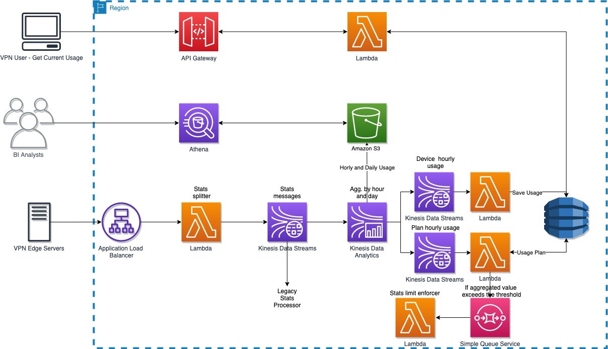
Jignesh Gohel is a Technical Account Manager at AWS. In this role, he provides advocacy and strategic technical guidance to help plan and build solutions using best practices, and proactively keep customers’ AWS environments operationally healthy. He is passionate about building modular and scalable enterprise systems on AWS using serverless technologies. Besides work, Jignesh enjoys spending time with family and friends, traveling and exploring the latest technology trends.


Suman Koduri is a Global Category Lead for Data & Analytics category in AWS Marketplace. He is focused towards business development activities to further expand the presence and success of Data & Analytics ISVs in AWS Marketplace.  In this role, he leads the scaling, and evolution of new and existing ISVs, as well as field enablement and strategic customer advisement for the same. In his spare time, he loves running half marathon’s and riding his motorcycle.

How to Accelerate Building a Lake House Architecture with AWS Glue

Post Syndicated from Raghavarao Sodabathina original https://aws.amazon.com/blogs/architecture/how-to-accelerate-building-a-lake-house-architecture-with-aws-glue/

Customers are building databases, data warehouses, and data lake solutions in isolation from each other, each having its own separate data ingestion, storage, management, and governance layers. Often these disjointed efforts to build separate data stores end up creating data silos, data integration complexities, excessive data movement, and data consistency issues. These issues are preventing customers from getting deeper insights. To overcome these issues and easily move data around, a Lake House approach on AWS was introduced.

In this blog post, we illustrate the AWS Glue integration components that you can use to accelerate building a Lake House architecture on AWS. We will also discuss how to derive persona-centric insights from your Lake House using AWS Glue.

Components of the AWS Glue integration system

AWS Glue is a serverless data integration service that facilitates the discovery, preparation, and combination of data. It can be used for analytics, machine learning, and application development. AWS Glue provides all of the capabilities needed for data integration. So you can start analyzing your data and putting it to use in minutes, rather than months.

The following diagram illustrates the various components of the AWS Glue integration system.

Figure 1. AWS Glue integration components

Figure 1. AWS Glue integration components

Connect – AWS Glue allows you to connect to various data sources anywhere

Glue connector: AWS Glue provides built-in support for the most commonly used data stores. You can use Amazon Redshift, Amazon RDS, Amazon Aurora, Microsoft SQL Server, MySQL, MongoDB, or PostgreSQL using JDBC connections. AWS Glue also allows you to use custom JDBC drivers in your extract, transform, and load (ETL) jobs. For data stores that are not natively supported such as SaaS applications, you can use connectors. You can also subscribe to several connectors offered in the AWS Marketplace.

Glue crawlers: You can use a crawler to populate the AWS Glue Data Catalog with tables. A crawler can crawl multiple data stores in a single pass. Upon completion, the crawler creates or updates one or more tables in your Data Catalog. Extract, transform, and load (ETL) jobs that you define in AWS Glue use these Data Catalog tables as sources and targets.

Catalog – AWS Glue simplifies data discovery and governance

Glue Data Catalog: The Data Catalog serves as the central metadata catalog for the entire data landscape.

Glue Schema Registry: The AWS Glue Schema Registry allows you to centrally discover, control, and evolve data stream schemas. With AWS Glue Schema Registry, you can manage and enforce schemas on your data streaming applications.

Data quality – AWS Glue helps you author and monitor data quality rules

Glue DataBrew: AWS Glue DataBrew allows data scientists and data analysts to clean and normalize data. You can use a visual interface, reducing the time it takes to prepare data by up to 80%. With Glue DataBrew, you can visualize, clean, and normalize data directly from your data lake, data warehouses, and databases.

Curate data: You can use either Glue development endpoint or AWS Glue Studio to curate your data.

AWS Glue development endpoint is an environment that you can use to develop and test your AWS Glue scripts. You can choose either Amazon SageMaker notebook or Apache Zeppelin notebook as an environment.

AWS Glue Studio is a new visual interface for AWS Glue that supports extract-transform-and-load (ETL) developers. You can author, run, and monitor AWS Glue ETL jobs. You can now use a visual interface to compose jobs that move and transform data, and run them on AWS Glue.

AWS Data Exchange makes it easy for AWS customers to securely exchange and use third-party data in AWS. This is for data providers who want to structure their data across multiple datasets or enrich their products with additional data. You can publish additional datasets to your products using the AWS Data Exchange.

Deequ is an open-source data quality library developed internally at Amazon, for data quality. It provides multiple features such as automatic constraint suggestions and verification, metrics computation, and data profiling.

Build a Lake House architecture faster, using AWS Glue

Figure 2 illustrates how you can build a Lake House using AWS Glue components.

Figure 2. Building lake house architectures with AWS Glue

Figure 2. Building Lake House architectures with AWS Glue

The architecture flow follows these general steps:

  1. Glue crawlers scan the data from various data sources and populate the Data Catalog for your Lake House.
  2. The Data Catalog serves as the central metadata catalog for the entire data landscape.
  3. Once data is cataloged, fine-grained access control is applied to the tables through AWS Lake Formation.
  4. Curate your data with business and data quality rules by using Glue Studio, Glue development endpoints, or Glue DataBrew. Place transformed data in a curated Amazon S3 for purpose built analytics downstream.
  5. Facilitate data movement with AWS Glue to and from your data lake, databases, and data warehouse by using Glue connections. Use AWS Glue Elastic views to replicate the data across the Lake House.

Derive persona-centric insights from your Lake House using AWS Glue

Many organizations want to gather observations from increasingly larger volumes of acquired data. These insights help them make data-driven decisions with speed and agility. They must use a central data lake, a ring of purpose-built data services, and data warehouses based on persona or job function.

Figure 3 illustrates the Lake House inside-out data movement with AWS Glue DataBrew, Amazon Athena, Amazon Redshift, and Amazon QuickSight to perform persona-centric data analytics.

Figure 3. Lake house persona-centric data analytics using AWS Glue

Figure 3. Lake House persona-centric data analytics using AWS Glue

This shows how Lake House components serve various personas in an organization:

  1. Data ingestion: Data is ingested to Amazon Simple Storage Service (S3) from different sources.
  2. Data processing: Data curators and data scientists use DataBrew to validate, clean, and enrich the data. Amazon Athena is also used to run improvised queries to analyze the data in the lake. The transformation is shared with data engineers to set up batch processing.
  3. Batch data processing: Data engineers or developers set up batch jobs in AWS Glue and AWS Glue DataBrew. Jobs can be initiated by an event, or can be scheduled to run periodically.
  4. Data analytics: Data/Business analysts can now analyze prepared dataset in Amazon Redshift or in Amazon S3 using Athena.
  5. Data visualizations: Business analysts can create visuals in QuickSight. Data curators can enrich data from multiple sources. Admins can enforce security and data governance. Developers can embed QuickSight dashboard in applications.

Conclusion

Using a Lake House architecture will help you get persona-centric insights quickly from all of your data based on user role or job function. In this blog post, we describe several AWS Glue components and AWS purpose-built services that you can use to build Lake House architectures on AWS. We have also presented persona-centric Lake House analytics architecture using AWS Glue, to help you derive insights from your Lake House.

Read more and get started on building Lake House Architectures on AWS.

How MEDHOST’s cardiac risk prediction successfully leveraged AWS analytic services

Post Syndicated from Pandian Velayutham original https://aws.amazon.com/blogs/big-data/how-medhosts-cardiac-risk-prediction-successfully-leveraged-aws-analytic-services/

MEDHOST has been providing products and services to healthcare facilities of all types and sizes for over 35 years. Today, more than 1,000 healthcare facilities are partnering with MEDHOST and enhancing their patient care and operational excellence with its integrated clinical and financial EHR solutions. MEDHOST also offers a comprehensive Emergency Department Information System with business and reporting tools. Since 2013, MEDHOST’s cloud solutions have been utilizing Amazon Web Services (AWS) infrastructure, data source, and computing power to solve complex healthcare business cases.

MEDHOST can utilize the data available in the cloud to provide value-added solutions for hospitals solving complex problems, like predicting sepsis, cardiac risk, and length of stay (LOS) as well as reducing re-admission rates. This requires a solid foundation of data lake and elastic data pipeline to keep up with multi-terabyte data from thousands of hospitals. MEDHOST has invested a significant amount of time evaluating numerous vendors to determine the best solution for its data needs. Ultimately, MEDHOST designed and implemented machine learning/artificial intelligence capabilities by leveraging AWS Data Lab and an end-to-end data lake platform that enables a variety of use cases such as data warehousing for analytics and reporting.

Since you’re reading this post, you may also be interested in the following:

Getting started

MEDHOST’s initial objectives in evaluating vendors were to:

  • Build a low-cost data lake solution to provide cardiac risk prediction for patients based on health records
  • Provide an analytical solution for hospital staff to improve operational efficiency
  • Implement a proof of concept to extend to other machine learning/artificial intelligence solutions

The AWS team proposed AWS Data Lab to architect, develop, and test a solution to meet these objectives. The collaborative relationship between AWS and MEDHOST, AWS’s continuous innovation, excellent support, and technical solution architects helped MEDHOST select AWS over other vendors and products. AWS Data Lab’s well-structured engagement helped MEDHOST define clear, measurable success criteria that drove the implementation of the cardiac risk prediction and analytical solution platform. The MEDHOST team consisted of architects, builders, and subject matter experts (SMEs). By connecting MEDHOST experts directly to AWS technical experts, the MEDHOST team gained a quick understanding of industry best practices and available services allowing MEDHOST team to achieve most of the success criteria at the end of a four-day design session. MEDHOST is now in the process of moving this work from its lower to upper environment to make the solution available for its customers.

Solution

For this solution, MEDHOST and AWS built a layered pipeline consisting of ingestion, processing, storage, analytics, machine learning, and reinforcement components. The following diagram illustrates the Proof of Concept (POC) that was implemented during the four-day AWS Data Lab engagement.

Ingestion layer

The ingestion layer is responsible for moving data from hospital production databases to the landing zone of the pipeline.

The hospital data was stored in an Amazon RDS for PostgreSQL instance and moved to the landing zone of the data lake using AWS Database Migration Service (DMS). DMS made migrating databases to the cloud simple and secure. Using its ongoing replication feature, MEDHOST and AWS implemented change data capture (CDC) quickly and efficiently so MEDHOST team could spend more time focusing on the most interesting parts of the pipeline.

Processing layer

The processing layer was responsible for performing extract, tranform, load (ETL) on the data to curate them for subsequent uses.

MEDHOST used AWS Glue within its data pipeline for crawling its data layers and performing ETL tasks. The hospital data copied from RDS to Amazon S3 was cleaned, curated, enriched, denormalized, and stored in parquet format to act as the heart of the MEDHOST data lake and a single source of truth to serve any further data needs. During the four-day Data Lab, MEDHOST and AWS targeted two needs: powering MEDHOST’s data warehouse used for analytics and feeding training data to the machine learning prediction model. Even though there were multiple challenges, data curation is a critical task which requires an SME. AWS Glue’s serverless nature, along with the SME’s support during the Data Lab, made developing the required transformations cost efficient and uncomplicated. Scaling and cluster management was addressed by the service, which allowed the developers to focus on cleaning data coming from homogenous hospital sources and translating the business logic to code.

Storage layer

The storage layer provided low-cost, secure, and efficient storage infrastructure.

MEDHOST used Amazon S3 as a core component of its data lake. AWS DMS migration tasks saved data to S3 in .CSV format. Crawling data with AWS Glue made this landing zone data queryable and available for further processing. The initial AWS Glue ETL job stored the parquet formatted data to the data lake and its curated zone bucket. MEDHOST also used S3 to store the .CSV formatted data set that will be used to train, test, and validate its machine learning prediction model.

Analytics layer

The analytics layer gave MEDHOST pipeline reporting and dashboarding capabilities.

The data was in parquet format and partitioned in the curation zone bucket populated by the processing layer. This made querying with Amazon Athena or Amazon Redshift Spectrum fast and cost efficient.

From the Amazon Redshift cluster, MEDHOST created external tables that were used as staging tables for MEDHOST data warehouse and implemented an UPSERT logic to merge new data in its production tables. To showcase the reporting potential that was unlocked by the MEDHOST analytics layer, a connection was made to the Redshift cluster to Amazon QuickSight. Within minutes MEDHOST was able to create interactive analytics dashboards with filtering and drill-down capabilities such as a chart that showed the number of confirmed disease cases per US state.

Machine learning layer

The machine learning layer used MEDHOST’s existing data sets to train its cardiac risk prediction model and make it accessible via an endpoint.

Before getting into Data Lab, the MEDHOST team was not intimately familiar with machine learning. AWS Data Lab architects helped MEDHOST quickly understand concepts of machine learning and select a model appropriate for its use case. MEDHOST selected XGBoost as its model since cardiac prediction falls within regression technique. MEDHOST’s well architected data lake enabled it to quickly generate training, testing, and validation data sets using AWS Glue.

Amazon SageMaker abstracted underlying complexity of setting infrastructure for machine learning. With few clicks, MEDHOST started Jupyter notebook and coded the components leading to fitting and deploying its machine learning prediction model. Finally, MEDHOST created the endpoint for the model and ran REST calls to validate the endpoint and trained model. As a result, MEDHOST achieved the goal of predicting cardiac risk. Additionally, with Amazon QuickSight’s SageMaker integration, AWS made it easy to use SageMaker models directly in visualizations. QuickSight can call the model’s endpoint, send the input data to it, and put the inference results into the existing QuickSight data sets. This capability made it easy to display the results of the models directly in the dashboards. Read more about QuickSight’s SageMaker integration here.

Reinforcement layer

Finally, the reinforcement layer guaranteed that the results of the MEDHOST model were captured and processed to improve performance of the model.

The MEDHOST team went beyond the original goal and created an inference microservice to interact with the endpoint for prediction, enabled abstracting of the machine learning endpoint with the well-defined domain REST endpoint, and added a standard security layer to the MEDHOST application.

When there is a real-time call from the facility, the inference microservice gets inference from the SageMaker endpoint. Records containing input and inference data are fed to the data pipeline again. MEDHOST used Amazon Kinesis Data Streams to push records in real time. However, since retraining the machine learning model does not need to happen in real time, the Amazon Kinesis Data Firehose enabled MEDHOST to micro-batch records and efficiently save them to the landing zone bucket so that the data could be reprocessed.

Conclusion

Collaborating with AWS Data Lab enabled MEDHOST to:

  • Store single source of truth with low-cost storage solution (data lake)
  • Complete data pipeline for a low-cost data analytics solution
  • Create an almost production-ready code for cardiac risk prediction

The MEDHOST team learned many concepts related to data analytics and machine learning within four days. AWS Data Lab truly helped MEDHOST deliver results in an accelerated manner.


About the Authors

Pandian Velayutham is the Director of Engineering at MEDHOST. His team is responsible for delivering cloud solutions, integration and interoperability, and business analytics solutions. MEDHOST utilizes modern technology stack to provide innovative solutions to our customers. Pandian Velayutham is a technology evangelist and public cloud technology speaker.


George Komninos is a Data Lab Solutions Architect at AWS. He helps customers convert their ideas to a production-ready data product. Before AWS, he spent 3 years at Alexa Information domain as a data engineer. Outside of work, George is a football fan and supports the greatest team in the world, Olympiacos Piraeus.

Simplify data discovery for business users by adding data descriptions in the AWS Glue Data Catalog

Post Syndicated from Karim Hammouda original https://aws.amazon.com/blogs/big-data/simplify-data-discovery-for-business-users-by-adding-data-descriptions-in-the-aws-glue-data-catalog/

In this post, we discuss how to use AWS Glue Data Catalog to simplify the process for adding data descriptions and allows data analysts to access, search, and discover this cataloged metadata with BI tools.

In this solution, we use AWS Glue Data Catalog, to break the silos between cross-functional data producer teams, sometimes also known as domain data experts, and business-focused consumer teams that author business intelligence (BI) reports and dashboards.

Since you’re reading this post, you may also be interested in the following:

Data democratization and the need for self-service BI

To be able to extract insights and get value out of organizational-wide data assets, data consumers like data analysts need to understand the meaning of existing data assets. They rely on data platform engineers to perform such data discovery tasks on their behalf.

Although data platform engineers can programmatically extract and obtain some technical and operational metadata, such as database and table names and sizes, column schemas, and keys, this metadata is primarily used for organizing and manipulating data inside the data lake. They still rely on source data domain experts to gain more knowledge about the meaning of the data, its business context, and classification. It becomes more challenging when data domain experts tend to prioritize operational-critical requests and delay the analytical-related ones.

Such a cycled dependency, as illustrated in the following figure, can delay the organizational strategic vision for implementing a self-service data analytics platform to reduce the time of the data-to-insights process.

Solution overview

The Data Catalog fundamentally holds basic information about the actual data stored in various data sources, including but not limited to Amazon Simple Storage Service (Amazon S3), Amazon Relational Database Service (Amazon RDS), and Amazon Redshift. Information like data location, format, and columns schema can be automatically discovered and stored as tables, where each table specifies a single data store.

Throughout this post, we see how we can use the Data Catalog to make it easy for domain experts to add data descriptions, and for data analysts to access this metadata with BI tools.

First, we use the comment field in Data Catalog schema tables to store data descriptions with more business meaning. Comment fields aren’t like the other schema table fields (such as column name, data type, and partition key), which are typically populated automatically by an AWS Glue crawler.

We also use Amazon AI/ML capabilities to initially identify the description of each data entity. One way to do that is by using the Amazon Comprehend text analysis API. When we provide a sample of values for each data entity type, Amazon Comprehend natural language processing (NLP) models can identify a standard range of data classification, and we can use this as a description for identified data entities.

Next, because we need to identify entities unique to our domain or organization, we can use custom named entity recognition (NER) in Amazon Comprehend to add more metadata that is related to our business domain. One way to train custom NER models is to use Amazon SageMaker Ground Truth; for more information, see Developing NER models with Amazon SageMaker Ground Truth and Amazon Comprehend.

For this post, we use a dataset that has a table schema defined as per TPC-DS, and was generated using a data generator developed as part of AWS Analytics Reference Architecture code samples.

In this example, Amazon Comprehend API recognizes PII-related fields like Aid as a MAC address. While the none PII-related fields like Estatus, aren’t recognized. Therefore, the user enters a custom description manually, and we use the custom NER to automatically populate those fields, as shown in the following diagram.


After we add data meanings, we need to expose all the metadata captured in the Data Catalog to various data consumers. This can be done two different ways:

We can also use the latter method to expose the Data Catalog to BI authors comprehending data analyses and dashboards using Amazon QuickSight, so we use the second method for this post.

We do this by defining an Athena dataset that queries the information_schema and allows BI authors to use the QuickSight capability of text search filter to search and discover data using its business meaning (see the following diagram).

Solution details

The core part of this solution is done using AWS Glue jobs. We use two AWS Glue jobs, which are responsible for calling Amazon Comprehend APIs and updating the AWS Glue Data Catalog with added data descriptions accordingly.

The first job (Glue_Comprehend_Job) performs the first stage of detection using the Amazon Comprehend Detect PII API, and the second job (Glue_Comprehend_Custom) uses Amazon Comprehend custom entity recognition for entities labeled by domain experts. The following diagram illustrates this workflow.

We describe the details of each stage in the upcoming sections.

You can integrate this workflow into your existing data processing pipeline, which might be orchestrated with AWS services like AWS Step Functions, Amazon Managed Workflows for Apache Airflow (Amazon MWAA), AWS Glue workflows, or any third-party orchestrator.

The workflow can complement AWS Glue crawler functionality and inherit the same logic for scheduling and running crawlers. On the other end, we can query the updated Data Catalog with data descriptions via Athena (see the following diagram).

To show an end-to-end implementation of this solution, we have adopted a choreographically built architecture with additional AWS Lambda helper functions, which communicate between AWS services, triggering the AWS Glue crawler and AWS Glue jobs.

Stage-one: Enrich the Data Catalog with a standard built-in Amazon Comprehend entity detector

To get started, Choose   to launch a CloudFormation stack.

Define unique S3 bucket name and on the CloudFormation console, accept default values for the parameters.

This CloudFormation stack consists of the following:

  • An AWS Identity Access Management (IAM) role called Lambda-S3-Glue-comprehend.
  • An S3 bucket with a bucket name that can be defined based on preference.
  • A Lambda function called trigger_data_cataloging. This function is automatically triggered when any CSV file is uploaded to the folder row_data inside our S3 bucket. Then it creates an AWS Glue database if one doesn’t exist, and creates and runs an AWS Glue crawler called glue_crawler_comprehend.
  • An AWS Glue job called Glue_Comprehend_Job, which calls Amazon Comprehend APIs and updates the AWS Glue Data Catalog table accordingly.
  • A Lambda function called Glue_comprehend_workflow, which is triggered when the AWS Glue Crawler successfully finishes and calls the AWS Glue job Glue_Comprehend_Job.

To test the solution, create a prefix called row_data under the S3 bucket created from the CF stack, then upload the customer dataset sample to the prefix.

The first Lambda function is triggered to run the subsequent AWS Glue crawler and AWS Glue job to get data descriptions using Amazon Comprehend, and it updates the comment section of the dataset created in the AWS Glue Data Catalog.

Stage-two: Use Amazon Comprehend custom entity recognition

Amazon Comprehend was able to detect some of the entity types within the customer sample dataset. However, for the remaining undetected fields, we can get help from a domain data expert to label a sample dataset using Ground Truth. Then we use the labeled data output to train a custom NER model and rerun the AWS Glue job to update the comment column with a customized data description.

Train an Amazon Comprehend custom entity recognition model

One way to train Amazon Comprehend custom entity recognizers is to get augmented manifest information using Ground Truth to label the data. Ground Truth has a built-in NER task for creating labeling jobs so domain experts can identify entities in text. To learn more about how to create the job, see Named Entity Recognition.

As an example, we tagged three labels entities: customer information ID, current level of education, and customer credit rating. The domain experts get a web interface like one shown in the following screenshot to label the dataset.

We can use the output of the labeling job to train an Amazon Comprehend custom entity recognition model using the augmented manifest.

The augmented manifest option requires a minimum of 1,000 custom entity recognition samples. Another option can be to use a CSV file that contains the annotations of the entity lists for the training dataset. The required format depends on the type of CSV file that we provide. In this post, we use the CSV entity lists option with two sample files:

To create the training job, we can use the Amazon Comprehend console, the AWS Command Line Interface (AWS CLI), or the Amazon Comprehend API. For this post, we use the API to programmatically create a training Lambda function using the AWS SDK for Python, as shown on GitHub.

The training process can take approximately 15 minutes. When the training process is complete, choose the recognizer and make a note of the recognizer ARN, which we use in the next step.

Run custom entity recognition inference

When the training job is complete, create an Amazon Comprehend analysis job using the console or APIs as shown on GitHub.

The process takes approximately 10 minutes, and again we need to make a note of the output job file.

Create an AWS Glue job to update the Data Catalog

Now that we have the Amazon Comprehend inference output, we can use the following AWS CLI command to create an AWS Glue job that updates the Data Catalog Comment fields for this dataset with customized data description.

Download the AWS Glue job script from the GitHub repo, upload to the S3 bucket created from the CF Stack in stage-1, and run the following AWS CLI command:

aws glue create-job 
--name "Glue_Comprehend_Job_custom_entity" 
--role "Lambda-S3-Glue-comprehend" 
--command '{"Name" : "pythonshell", "ScriptLocation" : "s3://<Your S3 bucket>/glue_comprehend_workflow_custom.py","PythonVersion":"3"}'
--default-arguments '{"--extra-py-files": "s3://aws-bigdata-blog/artifacts/simplify-data-discovery-for-business-users/blog/python/library/boto3-1.17.70-py2.py3-none-any.whl" }'

After you create the AWS Glue job, edit the job script and update the bucket and key name variables with the output data location of the Amazon Comprehend analysis jobs and run the AWS Glue job. See the following code:

bucket ="<Bucket Name>"
key = "comprehend_output/<Random number>output/output.tar.gz"

When the job is complete, it updates the Data Catalog with customized data descriptions.

Expose Data Catalog data to data consumers for search and discovery

Data consumers that prefer using SQL can use Athena to run queries against the information_schema.columns table, which includes the comment field of the Data Catalog. See the following code:

SELECT table_catalog,
         table_schema,
         table_name,
         column_name,
         data_type,
         comment
FROM information_schema.columns
WHERE comment LIKE '%customer%'
AND table_name = 'row_data_row_data'

The following screenshot shows our query results.

The query searches all schema columns that might have any data meanings that contain customer; it returns crating, which contains customer in the comment field.

BI authors can use text search instead of SQL to search for data meanings of data stored in an S3 data lake. This can be done by setting up a visual layer on top of Athena inside QuickSight.

QuickSight is scalable, serverless, embeddable, and machine learning (ML) powered BI tool that is deeply integrated with other AWS services.

BI development in QuickSight is organized as a stack of datasets, analyses, and dashboards. We start by defining a dataset from a list of various integrated data sources. On top of this dataset, we can design multiple analyses to uncover hidden insights and trends in the dataset. Finally, we can publish these analyses as dashboards, which is the consumable form that can be shared and viewed across different business lines and stakeholders.

We want to help the BI authors while designing analyses to get a better knowledge of the datasets they’re working on. To do so, we first need to connect to the data source where the metadata is stored, in this case the Athena table information_schema.columns, so we create a dataset to act as a Data Catalog view inside QuickSight.

QuickSight offers different modes of querying data sources, which is decided as part of the dataset creation process. The first mode is called direct query, in which the fetching query runs directly against the external data source. The second mode is a caching layer called QuickSight Super-fast Parallel In-memory Calculation Engine (SPICE), which improves performance when data is shared and retrieved by various BI authors. In this mode, the data is stored locally and can be reused multiple times, instead of running queries against the data source every time the data needs to be retrieved. However, as with all caching solutions, you must take data volume limits into consideration while choosing datasets to be stored in SPICE.

In our case, we choose to keep the Data Catalog dataset in SPICE, because the volume of the dataset is relatively small and won’t consume a lot of SPICE resources. However, we need to decide if we want to refresh the data cached in SPICE. The answer depends on how frequently the data schema and Data Catalog change, but in any case we can use the built-in scheduling within QuickSight to refresh SPICE at the desired interval. For information about triggering a refresh in an event-based manner, see Event-driven refresh of SPICE datasets in Amazon QuickSight.

After we create the Data Catalog view as a dataset inside QuickSight stored in SPICE, we can use row-level security to restrict the access to this dataset. Each BI author has access with respect to their privileges for columns they can view metadata for.

Next, we see how we can allow BI authors to search through data descriptions populated in the comment field of the Data Catalog dataset. QuickSight offers features like filters, parameters, and controls to add more flexibility into QuickSight analyses and dashboards.

Finally, we use the QuickSight capability to add more than one dataset within an analysis view to allow BI authors to switch between the metadata for the dataset and the actual dataset. This allows the BI authors to self-serve, reducing dependency on data platform engineers to decide which columns they should use in their analyses.

To set up a simple Data Catalog search and discovery inside QuickSight, complete the following steps:

  1. On the QuickSight console, choose Datasets in the navigation pane.
  2. Choose New dataset.
  3. For New data sources, choose Amazon Athena.
  4. Name the dataset Data Catalog.
  5. Choose Create data source.
  6. For Choose your table, choose Use custom SQL.
  7. For Enter custom SQL query, name the query Data Catalog Query.
  8. Enter the following query:
SELECT * FROM information_schema.columns
  1. Choose Confirm query.
  2. Select Import to QuickSight SPICE for quicker analytics.
  3. Choose Visualize.

Next, we design an analysis on the dataset we just created to access the Data Catalog through Athena.

When we choose Visualize, we’re redirected to the QuickSight workspace to start designing our analysis.

  1. Under Visual types, choose Table.
  2. Under Fields list, add table_name, column_name, and comment to the Values field well.

Next, we use the filter control feature to allow users to perform text search for data descriptions.

  1. In the navigation pane, choose Filter.
  2. Choose the plus sign (+) to access the Create a new filter list.
  3. On the list of columns, choose comment to be the filter column.
  4. From the options menu (…) on the filter, choose Add to sheet.

We should be able to see a new control being added into our analysis to allow users to search the comment field.

Now we can start a text search for data descriptions that contain customer, where QuickSight shows the list of fields matching the search criteria and provides table and column names accordingly.

Alternatively, we can use parameters to be associated with the filter control if needed, for example to connect one dashboard to another. For more information, see the GitHub repo.

Finally, BI authors can switch between the metadata view that we just created and the actual Athena table view (row_all_row_data), assuming it’s already imported (if not, we can use the same steps from earlier to import the new dataset).

  1. In the navigation pane, choose Visualize.
  2. Choose the pen icon to add, edit, replace, or remove datasets.
  3. Choose Add dataset.
  4. Add row_all_row_data.
  5. Choose Select.

BI authors can now switch between data and metadata datasets.

They now have a metadata view along with the actual data view, so they can better understand the meaning of each column in the dataset they’re working on, and they can read any comment that can be passed from other teams within the organization without needing to do this manually.

Conclusion

In this post, we showed how to build a quick workflow using AWS Glue and Amazon AI/ML services to complement the AWS Glue crawler functionality. You can integrate this workflow into a typical AWS Glue data cataloging and processing pipeline to achieve alignment between cross-functional teams by simplifying and automating the process of adding data descriptions in the Data Catalog. This is an important step in data discovery, and the topic will be covered more in upcoming posts.

This solution is also a step towards implementing data privacy and protection regimes such as the Health Insurance Portability and Accountability Act (HIPAA) and General Data Protection Regulation (GDPR) by identifying sensitive data types like PII and enforcing access polices.

You can find the source code from this post on GitHub and use it to build your own solution. For more information about NER models, see Developing NER models with Amazon SageMaker Ground Truth and Amazon Comprehend.


About the Authors

Karim Hammouda is a Specialist Solutions Architect for Analytics at AWS with a passion for data integration, data analysis, and BI. He works with AWS customers to design and build analytics solutions that contribute to their business growth. In his free time, he likes to watch TV documentaries and play video games with his son.


Ahmed Raafat is a Senior Solutions Architect at Amazon Web Services, with a passion for machine learning solutions. Ahmed acts as a trusted advisor for many AWS enterprise customers to support and accelerate their cloud journey.

­­­­­­Introducing AWS Glue 3.0 with optimized Apache Spark 3.1 runtime for faster data integration

Post Syndicated from Noritaka Sekiyama original https://aws.amazon.com/blogs/big-data/introducing-aws-glue-3-0-with-optimized-apache-spark-3-1-runtime-for-faster-data-integration/

In August 2020, we announced the availability of AWS Glue 2.0. AWS Glue 2.0 reduced job startup times by 10x, enabling customers to reali­­ze an average of 45% cost savings on their extract, transform, and load (ETL) jobs. The fast start time allows customers to easily adopt AWS Glue for batching, micro-batching, and streaming use cases. In the last year, AWS Glue has evolved from an ETL service to a serverless data integration service, offering all the required capabilities needed to build, operate and scale a modern data platform. The following are some of the use cases you can accomplish with AWS Glue:

  • Move data to and from a broad variety of data sources and software as a service (SaaS) applications using AWS Glue custom connectors
  • Populate a central AWS Glue Data Catalog using AWS Glue crawlers, which are capable of inferring the schema, detecting data drift, and keeping the metadata up to date easily and quickly
  • Build and share reusable data pipelines running on AWS Glue workflows using custom blueprints
  • Process data in near-real time using event-driven workflows and AWS Glue streaming.
  • Visually clean and prepare data for analysis using AWS Glue DataBrew
  • Visually author AWS Glue ETL jobs in AWS Glue Studio to simplify how you build, maintain and monitor data pipelines.

Today, we are pleased to announce AWS Glue version 3.0.  AWS Glue 3.0 introduces a performance-optimized Apache Spark 3.1 runtime for batch and stream processing. The new engine speeds up data ingestion, processing and integration allowing you to hydrate your data lake and extract insights from data quicker.

AWS Glue version 3.0 highlights

Performance-optimized Spark runtime based on open-source Apache Spark 3.1.1 and enhanced with innovative optimizations developed by the AWS Glue and Amazon EMR teams. These optimizations accelerate data integration and query processing with advanced techniques, such as SIMD based vectorized readers developed in native language (C++), in-memory columnar formats for processing, optimized shuffles, partition coalescing, and Spark’s adaptive query execution. The AWS Glue 3.0 runtime is built with upgraded JDBC drivers for all AWS Glue native sources, including MySQL, Microsoft SQL Server, Oracle, PostgreSQL, and MongoDB, to enable simpler, faster, and secure integration with new versions of database engines.

Faster read and write access with the AWS Glue 3.0 runtime to Amazon Simple Storage Service (Amazon S3) using vectorized readers and Amazon S3 optimized output committers. These optimizations improve Spark application performance for popular customer workloads reading row-based formats such as CSV and writing to columnar formats such as Apache Parquet.

Faster and efficient partition pruning with the AWS Glue 3.0 runtime when analyzing large, highly partitioned tables managed AWS Glue Data Catalog. For highly partitioned datasets, partition pruning can significantly reduce the cost of catalog partition listing and query planning by filtering out unnecessary partitions using partition indexes.

Fine-grained access control with the AWS Glue 3.0 runtime for your batch jobs using AWS Lake Formation. You can now access your data at the database, table, column, row, and cell-level using resource names and Lake Formation tag attributes (available in preview).

ACID transactions offered with the AWS Glue 3.0 runtime for Lake Formation Governed Tables and query acceleration with automatic file compaction on your data lake (available in preview).

Improved user experience for monitoring, debugging, and tuning Spark applications. Spark 3.1.1 enables an improved Spark UI experience that includes new Spark executor memory metrics and Spark Structured Streaming metrics that are useful for AWS Glue streaming jobs.

With AWS Glue 3.0, you continue to benefit from reduced startup latency, which improves overall job execution times and makes job and pipeline development more interactive. AWS Glue 3.0 Spark jobs are billed per second, with a 1-minute minimum, similar to AWS Glue 2.0.

Getting started with AWS Glue 3.0

You can start using AWS Glue 3.0 via AWS Glue Studio, the AWS Glue console, the latest AWS SDK, and the AWS Command Line Interface (AWS CLI).

To start using AWS Glue 3.0 in AWS Glue Studio, choose the version Glue 3.0 – Supports spark 3.1, Scala 2, Python 3.

To migrate your existing AWS Glue jobs from AWS Glue 0.9, 1.0, and 2.0 to AWS Glue 3.0, see Migrating AWS Glue jobs to AWS Glue version 3.0.

Performance of AWS Glue 3.0

AWS Glue 3.0 speeds up your Spark applications in addition to offering reduced startup latencies. The following benchmark shows the performance improvements between AWS Glue 3.0 and AWS Glue 2.0 for a popular customer workload to convert large datasets from CSV to Apache Parquet format. The comparison uses the largest store_sales table in the TPC-DS benchmark dataset (3 TB). All Spark jobs run on warm 60 G.2X workers. All values in store_sales table are numeric. We compare performance with schema enforcement, casting values into numeric data type and without schema enforcement, casting them to string type. Enforcing schema to numeric types allows for compact in-memory representations and faster deserialization. No schema enforcement allows for flexibility with string types.

AWS Glue 3.0 speeds up performance by as much as 2.4 times compared to AWS Glue 2.0 with the use of vectorized readers, which are implemented in C++. It also uses micro-parallel SIMD CPU instructions for faster data parsing, tokenization and indexing. Additionally, it reads data into in-memory columnar formats based on Apache Arrow for improved memory bandwidth utilization and direct conversion to columnar storage format such as Apache Parquet.

Conclusion

In this post, we introduced a faster, more efficient AWS Glue engine based on Apache Spark 3.1 that includes innovative features to enable your jobs to run faster and reduce costs. With only minor changes to your job configurations and scripts, you can start using AWS Glue 3.0 today. To learn more about new features, library versions, and dependencies in AWS Glue 3.0, see Migrating AWS Glue jobs to AWS Glue version 3.0.


About the Authors

Noritaka Sekiyama is a Senior Big Data Architect on the AWS Glue team. He is passionate about architecting fast-growing data platforms, diving deep into distributed big data softwares like Apache Spark, building reusable software artifacts for data lakes, and sharing the knowledge in AWS Big Data blog posts.


Neil Gupta is a Software Development Engineer on the AWS Glue team. He enjoys tackling big data problems and learning more about distributed systems.


XiaoRun Yu is a Software Development Engineer on the AWS Glue team.


Rajendra Gujja is a Software Development Engineer on the AWS Glue team. He is passionate about distributed computing and everything and anything about the data.


Mohit Saxena is a Software Engineering Manager on the AWS Glue team. His team works on distributed systems for efficiently managing data lakes on AWS and optimizes Apache Spark for performance and reliability.


Kinshuk Pahare is a Principal Product Manager on the AWS Glue team.

How Comcast uses AWS to rapidly store and analyze large-scale telemetry data

Post Syndicated from Asser Moustafa original https://aws.amazon.com/blogs/big-data/how-comcast-uses-aws-to-rapidly-store-and-analyze-large-scale-telemetry-data/

This blog post is co-written by Russell Harlin from Comcast Corporation.

Comcast Corporation creates incredible technology and entertainment that connects millions of people to the moments and experiences that matter most. At the core of this is Comcast’s high-speed data network, providing tens of millions of customers across the country with reliable internet connectivity. This mission has become more important now than ever.

This post walks through how Comcast used AWS to rapidly store and analyze large-scale telemetry data.

Background

At Comcast, we’re constantly looking for ways to gain new insights into our network and improve the overall quality of service. Doing this effectively can involve scaling solutions to support analytics across our entire network footprint. For this particular project, we wanted an extensible and scalable solution that could process, store, and analyze telemetry reports, one per network device every 5 minutes. This data would then be used to help measure quality of experience and determine where network improvements could be made.

Scaling big data solutions is always challenging, but perhaps the biggest challenge of this project was the accelerated timeline. With 2 weeks to deliver a prototype and an additional month to scale it, we knew we couldn’t go through the traditional bake-off of different technologies, so we had to either go with technologies we were comfortable with or proven managed solutions.

For the data streaming pipeline, we already had the telemetry data coming in on an Apache Kafka topic, and had significant prior experience using Kafka combined with Apache Flink to implement and scale streaming pipelines, so we decided to go with what we knew. For the data storage and analytics, we needed a suite of solutions that could scale quickly, had plenty of support, and had an ecosystem of well-integrated tools to solve any problem that might arise. This is where AWS was able to meet our needs with technologies like Amazon Simple Storage Service (Amazon S3), AWS Glue, Amazon Athena, and Amazon Redshift.

Initial architecture

Our initial prototype architecture for the data store needed to be fast and simple so that we could unblock the development of the other elements of the budding telemetry solution. We needed three key things out of it:

  • The ability to easily fetch raw telemetry records and run more complex analytical queries
  • The capacity to integrate seamlessly with the other pieces of the pipeline
  • The possibility that it could serve as a springboard to a more scalable long-term solution

The first instinct was to explore solutions we used in the past. We had positive experiences with using nosql databases, like Cassandra, to store and serve raw data records, but it was clear these wouldn’t meet our need for running ad hoc analytical queries. Likewise, we had experience with more flexible RDBMs, like Postgres, for handling more complicated queries, but we knew that those wouldn’t scale to meet our requirement to store tens to hundreds of billions of rows. Therefore, any prototyping with one of these approaches would be considered throwaway work.

After moving on from these solutions, we quickly settled on using Amazon S3 with Athena. Amazon S3 provides low-cost storage with near-limitless scaling, so we knew we could store as much historical data as required and Athena would provide serverless, on-demand querying of our data. Additionally, Amazon S3 is known to be a launching pad to many other data store solutions both inside and outside the AWS ecosystem. This was perfect for the exploratory prototyping phase.

Integrating it into the rest of our pipeline would also prove simple. Writing the data to Amazon S3 from our Flink job was straightforward and could be done using the readily available Flink streaming file sink with an Amazon S3 bucket as the destination. When the data was available in Amazon S3, we ran AWS Glue to index our Parquet-formatted data and generate schemas in the AWS Glue metastore for searching using Athena with standard SQL.

The following diagram illustrates this architecture.

Using Amazon S3 and Athena allowed us to quickly unblock development of our Flink pipeline and ensure that the data being passed through was correct. Additionally, we used the AWS SDK to connect to Athena from our northbound Golang microservice and provide REST API access to our data for our custom web application. This allowed us to prove out an end-to-end solution with almost no upfront cost and very minimal infrastructure.

Updated architecture

As application and service development proceeded, it became apparent that Amazon Athena performed for developers running ad hoc queries, but wasn’t going to work as a long-term responsive backend for our microservices and user interface requirements.

One of the primary use cases of this solution was to look at device-level telemetry reports for a period of time and plot and track different aspects of their quality of experience. Because this most often involves solving problems happening in the now, we needed an improved data store for the most recent hot data.

This led us to Amazon Redshift. Amazon Redshift requires loading the data into a dedicated cluster and formulating a schema tuned for your use cases.

The following diagram illustrates this updated architecture.

Data loading and storage requirements

For loading and storing the data in Amazon Redshift, we had a few fundamental requirements:

  • Because our Amazon Redshift solution would be for querying data to troubleshoot problems happening as recent as the current hour, we needed to minimize the latency of the data load and keep up with our scale while doing it. We couldn’t live with nightly loads.
  • The pipeline had to be robust and recover from failures automatically.

There’s a lot of nuance that goes into making this happen, and we didn’t want to worry about handling these basic things ourselves, because this wasn’t where we were going to add value. Luckily, because we were already loading the data into Amazon S3, AWS Glue ETL satisfied these requirements and provided a fast, reliable, and scalable solution to do periodic loads from our Amazon S3 data store to our Amazon Redshift cluster.

A huge benefit of AWS Glue ETL is that it provides many opportunities to tune your ETL pipeline to meet your scaling needs. One of our biggest challenges was that we write multiple files to Amazon S3 from different regions every 5 minutes, which results in many small files. If you’re doing infrequent nightly loads, this may not pose a problem, but for our specific use case, we wanted to load data at least every hour and multiple times an hour if possible. This required some specific tuning of the default ETL job:

  • Amazon S3 list implementation – This allows the Spark job to handle files in batches and optimizes reads for a large number of files, preventing out of memory issues.
  • Pushdown predicates – This tells the load to skip listing any partitions in Amazon S3 that you know won’t be a part of the current run. For frequent loads, this can mean skipping a lot of unnecessary file listing during each job run.
  • File grouping – This allows the read from Amazon S3 to group files together in batches when reading from Amazon S3. This greatly improves performance when reading from a large number of small files.
  • AWS Glue 2.0 – When we were starting our development, only AWS Glue 1.0 was available, and we’d frequently see Spark cluster start times of over 10 minutes. This becomes problematic if you want to run the ETL job more frequently because you have to account for the cluster startup time in your trigger timings. When AWS Glue 2.0 came out, those start times consistently dropped to under 1 minute and they became a afterthought.

With these tunings, as well as increasing the parallelism of the job, we could meet our requirement of loading data multiple times an hour. This made relevant data available for analysis sooner.

Modeling, distributing, and sorting the data

Aside from getting the data into the Amazon Redshift cluster in a timely manner, the next consideration was how to model, distribute, and sort the data when it was in the cluster. For our data, we didn’t have a complex setup with tens of tables requiring extensive joins. We simply had two tables: one for the device-level telemetry records and one for records aggregated at a logical grouping.

The bulk of the initial query load would be centered around serving raw records from these tables to our web application. These types of raw record queries aren’t difficult to handle from a query standpoint, but do present challenges when dealing with tens of millions of unique devices and a report granularity of 5 minutes. So we knew we had to tune the database to handle these efficiently. Additionally, we also needed to be able to run more complex ad hoc queries, like getting daily summaries of each table so that higher-level problem areas could be more easily tracked and spotted in the network. These queries, however, were less time sensitive and could be run on an ad hoc, batch-like basis where responsiveness wasn’t as important.

The schema fields themselves were more or less one-to-one mappings from the respective Parquet schemas. The challenge came, however, in picking partition keys and sorting columns. For partition keys, we identified a logical device grouping column present in both our tables as the one column we were likely to join on. This seemed like a natural fit to partition on and had good enough cardinality that our distribution would be adequate.

For the sorting keys, we knew we’d be searching by the device identifier and the logical grouping; for the respective tables, and we knew we’d be searching temporally. So the primary identifier column of each table and the timestamp made sense to sort on. The documented sort key order suggestion was to use the timestamp column as the first value in the sort key, because it could provide dataset filtering on a specific time period. This initially worked well enough and we were able to get a performance improvement over Athena, but as we scaled and added more data, our raw record retrieval queries were rapidly slowing down. To help with this, we made two adjustments.

The first adjustment came with a change to the sort key. The first part of this involved swapping the order of the timestamp and the primary identifier column. This allowed us to filter down to the device and then search through the range of timestamps on just that device, skipping over all irrelevant devices. This provided significant performance gains and cut our raw record query times by several multiples. The second part of the sort key adjustment involved adding another column (a node-level identifier) to the beginning of the sort key. This allowed us to have one more level of data filtering, which further improved raw record query times.

One trade-off made while making these sort key adjustments was that our more complex aggregation queries had a noticeable decline in performance. This was because they were typically run across the entire footprint of devices and could no longer filter as easily based on time being the first column in the sort key. Fortunately, because these were less frequent and could be run offline if necessary, this performance trade-off was considered acceptable.

If the frequency of these workloads increases, we can use materialized views in Amazon Redshift, which can help avoid unnecessary reruns of the complex aggregations if minimal-to-no data changes in the underlying base tables have occurred since the last run.

The final adjustment was cluster scaling. We chose to use the Amazon Redshift next-generation RA3 nodes for a number of benefits, but three especially key benefits:

  • RA3 clusters allow for practically unlimited storage in our cluster.
  • The RA3 ability to scale storage and compute independently paired really well with our expectations and use cases. We fully expected our Amazon Redshift storage footprint to continue to grow, as well as the number, shape, and sizes of our use cases and users, but data and workloads wouldn’t necessarily grow in lockstep. Being able to scale the cluster’s compute power independent of storage (or vice versa) was a key technical requirement and cost-optimization for us.
  • RA3 clusters come with Amazon Redshift managed storage, which places the burden on Amazon Redshift to automatically situate data based on its temperature for consistently peak performance. With managed storage, hot data was cached on a large local SSD cache in each node, and cold data was kept in the Amazon Redshift persistent store on Amazon S3.

After conducting performance benchmarks, we determined that our cluster was under-powered for the amount of data and workloads it was serving, and we would benefit from greater distribution and parallelism (compute power). We easily resized our Amazon Redshift cluster to double the number of nodes within minutes, and immediately saw a significant performance boost. With this, we were able to recognize that as our data and workloads scaled, so too should our cluster.

Looking forward, we expect that there will be a relatively small population of ad hoc and experimental workloads that will require access to additional datasets sitting in our data lake, outside of Amazon Redshift in our data lake—workloads similar to the Athena workloads we previously observed. To serve that small customer base, we can leverage Amazon Redshift Spectrum, which empowers users to run SQL queries on external tables in our data lake, similar to SQL queries on any other table within Amazon Redshift, while allowing us to keep costs as lean as possible.

This final architecture provided us with the solid foundation of price, performance, and flexibility for our current set of analytical use cases—and, just as important, the future use cases that haven’t shown themselves yet.

Summary

This post details how Comcast leveraged AWS data store technologies to prototype and scale the serving and analysis of large-scale telemetry data. We hope to continue to scale the solution as our customer base grows. We’re currently working on identifying more telemetry-related metrics to give us increased insight into our network and deliver the best quality of experience possible to our customers.


About the Authors

Russell Harlin is a Senior Software Engineer at Comcast based out of the San Francisco Bay Area. He works in the Network and Communications Engineering group designing and implementing data streaming and analytics solutions.


Asser Moustafa is an Analytics Specialist Solutions Architect at AWS based out of Dallas, Texas. He advises customers in the Americas on their Amazon Redshift and data lake architectures and migrations, starting from the POC stage to actual production deployment and maintenance


Amit Kalawat is a Senior Solutions Architect at Amazon Web Services based out of New York. He works with enterprise customers as they transform their business and journey to the cloud.

How GE Healthcare modernized their data platform using a Lake House Architecture

Post Syndicated from Krishna Prakash original https://aws.amazon.com/blogs/big-data/how-ge-healthcare-modernized-their-data-platform-using-a-lake-house-architecture/

GE Healthcare (GEHC) operates as a subsidiary of General Electric. The company is headquartered in the US and serves customers in over 160 countries. As a leading global medical technology, diagnostics, and digital solutions innovator, GE Healthcare enables clinicians to make faster, more informed decisions through intelligent devices, data analytics, applications, and services, supported by its Edison intelligence platform.

GE Healthcare’s legacy enterprise analytics platform used a traditional Postgres based on-premise data warehouse from a big data vendor to run a significant part of its analytics workloads. The data warehouse is key for GE Healthcare; it enables users across units to gather data and generate the daily reports and insights required to run key business functions. In the last few years, the number of teams accessing the cluster increased by almost three times, with twice the initial number of users running four times the number of daily queries for which the cluster had been designed. The legacy data warehouse wasn’t able to scale to support GE Healthcare’s business needs and would require significant investment to maintain, update, and secure.

Searching for a modern data platform

After working for several years in a database-focused approach, the rapid growth in the data made the GEHC’s on-prem system unviable from a cost and maintenance perspective. This presented GE Healthcare with an opportunity to take a holistic look at the emerging and strategic needs for data and analytics. With this in mind, GE Healthcare decided to adopt a Lake House Architecture using AWS services:

  • Use Amazon Simple Storage Service (Amazon S3) to store raw enterprise and event data
  • Use familiar SQL statements to combine and process data across all data stores in Amazon S3 and Amazon Redshift
  • Apply the “best fit” concept of using the appropriate AWS technology to meet specific business needs

Architecture

The following diagram illustrates GE Healthcare’s architecture.

Choosing Amazon Redshift for the enterprise cloud data warehouse

Choosing the right data store is just as important as how you collect the data for analytics. Amazon Redshift provided the best value because it was easy to launch, access, and store data, and could scale to meet our business needs on demand. The following are a few additional reasons for why GE Healthcare made Amazon Redshift our cloud data warehouse:

  • The ability to store petabyte-scale data in Amazon S3 and query the data in Amazon S3 and Amazon Redshift with little preprocessing was important because GE Healthcare’s data needs are expanding at a significant pace.
  • The AWS based strategy provides financial flexibility. GE Healthcare moved from a fixed cost/fixed asset on-premises model to a consumption-based model. In addition, the total cost of ownership (TCO) of the AWS based architecture was less than the solution it was replacing.
  • Native integration with the AWS Analytics ecosystem made it easier to handle end-to-end analytics workflows without friction. GE Healthcare took a hybrid approach to extract, transform, and load (ETL) jobs by using a combination of AWS Glue, Amazon Redshift SQL, and stored procedures based on complexity, scale, and cost.
  • The resilient platform makes recovery from failure easier, with errors further down the pipeline less likely to affect production environments because all historical data is on Amazon S3.
  • The idea of a Lake House Architecture is that taking a one-size-fits-all approach to analytics eventually leads to compromises. It’s not simply about integrating a data lake with a data warehouse, but rather about integrating a data lake, a data warehouse, and purpose-built data stores and enabling unified governance and easy data movement. (For more information about the Lake House Architecture, see Harness the power of your data with AWS Analytics.)
  • It’s easy to implement new capabilities to support emerging business needs such as artificial intelligence, machine learning, graph databases, and more because of the extensive product capabilities of AWS and the Amazon Redshift Lake House Architecture.

Implementation steps and best practices

As part of this journey, GE Healthcare partnered with AWS Professional Services to accelerate their momentum. AWS Professional Services was instrumental in following the Working Backwards (WB) process, which is Amazon’s customer-centric product development process.

Here’s how it worked:

  • AWS Professional Services guided GE Healthcare and partner teams through the Lake House Architecture, sharing AWS standards and best practices.
  • The teams accelerated Amazon Redshift stored procedure migration, including data structure selection and table design.
  • The teams delivered performant code at scale to enable a timely go live.
  • They implemented a framework for batch file extract to support downstream data consumption via a data as a service (DaaS) solution.

Conclusion

Modernizing to a Lake House Architecture with Amazon Redshift allowed GEHC to speed up, innovate faster, and better solve customers’ needs. At the time of writing, GE Healthcare workloads are running at full scale in production. We retired our on-premises infrastructure. Amazon Redshift RA3 instances with managed storage enabled us to scale compute and storage separately based on our customers’ needs. Furthermore, with the concurrency scaling feature of Amazon Redshift, we don’t have to worry about peak times affecting user performance any more. Amazon Redshift scales out and in automatically.

We also look forward to realizing the benefits of Amazon Redshift data sharing and AQUA (Advanced Query Accelerator) for Amazon Redshift as we continue to increase the performance and scale of our Amazon Redshift data warehouse. We appreciate AWS’s continual innovation on behalf of its customers.


About the Authors

Krishna Prakash (KP) Bhat is a Sr. Director in Data & Analytics at GE Healthcare. In this role, he’s responsible for architecture and data management of data and analytics solutions within GE Healthcare Digital Technologies Organization. In his spare time, KP enjoys spending time with family. Connect him on LinkedIn.


Suresh Patnam is a Solutions Architect at AWS, specialized in big data and AI/ML. He works with customers in their journey to the cloud with a focus on big data, data lakes, and AI/ML. In his spare time, Suresh enjoys playing tennis and spending time with his family. Connect him on LinkedIn.

Benefits of Modernizing On-premise Analytics with an AWS Lake House

Post Syndicated from Vikas Nambiar original https://aws.amazon.com/blogs/architecture/benefits-of-modernizing-on-premise-analytics-with-an-aws-lake-house/

Organizational analytics systems have shifted from running in the background of IT systems to being critical to an organization’s health.

Analytics systems help businesses make better decisions, but they tend to be complex and are often not agile enough to scale quickly. To help with this, customers upgrade their traditional on-premises online analytic processing (OLAP) databases to hyper converged infrastructure (HCI) solutions. However, these systems incur operational overhead, are limited by proprietary formats, have limited elasticity, and tie customers into costly and inhibiting licensing agreements. These all bind an organization’s growth to the growth of the appliance provider.

In this post, we provide you a reference architecture and show you how an AWS lake house will help you overcome the aforementioned limitations. Our solution provides you the ability to scale, integrate with multiple sources, improve business agility, and help future proof your analytics investment.

High-level architecture for implementing an AWS lake house

Lake house architecture uses a ring of purpose-built data consumers and services centered around a data lake. This approach acknowledges that a one-size-fits-all approach to analytics eventually leads to compromises. These compromises can include agility associated with change management and impact of different business domain reporting requirements on the data from a central platform. As such, simply integrating a data lake with a data warehouse is not sufficient.

Each step in Figure 1 needs to be de-coupled to build a lake house.

Data flow in a lake house

Figure 1. Data flow in a lake house


High-level design for an AWS lake house implementation

Figure 2. High-level design for an AWS lake house implementation

Building a lake house on AWS

These steps summarize building a lake house on AWS:

  1. Identify source system extraction capabilities to define an ingestion layer that loads data into a data lake.
  2. Build data ingestion layer using services that support source systems extraction capabilities.
  3. Build a governance and transformation layer to manipulate data.
  4. Provide capability to consume and visualize information via purpose-built consumption/value layer.

This lake house architecture provides you a de-coupled architecture. Services can be added, removed, and updated independently when new data sources are identified like data sources to enrich data via AWS Data Exchange. This can happen while services in the purpose-built consumption layer address individual business unit requirements.

Building the data ingestion layer

Services in this layer work directly with the source systems based on their supported data extraction patterns. Data is then placed into a data lake.

Figure 3 shows the following services to be included in this layer:

  • AWS Transfer Family for SFTP integrates with source systems to extract data using secure shell (SSH), SFTP, and FTPS/FTP. This service is for systems that support batch transfer modes and have no real-time requirements, such as external data entities.
  • AWS Glue connects to real-time data streams to extract, load, transform, clean, and enrich data.
  • AWS Database Migration Service (AWS DMS) connects and migrates data from relational databases, data warehouses, and NoSQL databases.
Ingestion layer against source systems

Figure 3. Ingestion layer against source systems

Services in this layer are managed services that provide operational excellence by removing patching and upgrade overheads. Being managed services, they will also detect extraction spikes and scale automatically or on-demand based on your specifications.

Building the data lake layer

A data lake built on Amazon Simple Storage Service (Amazon S3) provides the ideal target layer to store, process, and cycle data over time. As the central aspect of the architecture, Amazon S3 allows the data lake to hold multiple data formats and datasets. It can also be integrated with most if not all AWS services and third-party applications.

Figure 4 shows the following services to be included in this layer:

  • Amazon S3 acts as the data lake to hold multiple data formats.
  • Amazon S3 Glacier provides the data archiving and long-term backup storage layer for processed data. It also reduces the amount of data indexed by transformation layer services.
Figure 4. Data lake integrated to ingestion layer

Figure 4. Data lake integrated to ingestion layer

The data lake layer provides 99.999999999% data durability and supports various data formats, allowing you to future proof the data lake. Data lakes on Amazon S3 also integrate with other AWS ecosystem services (for example, AWS Athena for interactive querying or third-party tools running off Amazon Elastic Compute Cloud (Amazon EC2) instances).

Defining the governance and transformation layer

Services in this layer transform raw data in the data lake to a business consumable format, along with providing operational monitoring and governance capabilities.

Figure 5 shows the following services to be included in this layer:

  1. AWS Glue discovers and transforms data, making it available for search and querying.
  2. Amazon Redshift (Transient) functions as an extract, transform, and load (ETL) node using RA3 nodes. RA3 nodes can be paused outside ETL windows. Once paused, Amazon Redshift’s data sharing capability allows for live data sharing for read purposes, which reduces costs to customers. It also allows for creation of separate, smaller read-intensive business intelligence (BI) instances from the larger write-intensive ETL instances required during ETL runs.
  3. Amazon CloudWatch monitors and observes your enabled services. It integrates with existing IT service management and change management systems such as ServiceNow for alerting and monitoring.
  4. AWS Security Hub implements a single security pane by aggregating, organizing, and prioritizing security alerts from services used, such as Amazon GuardDuty, Amazon Inspector, Amazon Macie, AWS Identity and Access Management (IAM) Access Analyzer, AWS Systems Manager, and AWS Firewall Manager.
  5. Amazon Managed Workflows for Apache Airflow (MWAA) sequences your workflow events to ingest, transform, and load data.
  6. Amazon Lake Formation standardizes data lake provisioning.
  7. AWS Lambda runs custom transformation jobs if required, or developed over a period of time that hold custom business logic IP.
Governance and transformation layer prepares data in the lake

Figure 5. Governance and transformation layer prepares data in the lake

This layer provides operational isolation wherein least privilege access control can be implemented to keep operational staff separate from the core services. It also lets you implement custom transformation tasks using Lambda. This allows you to consistently build lakes across all environments and single view of security via AWS Security Hub.

Building the value layer

This layer generates value for your business by provisioning decoupled, purpose-built visualization services, which decouples business units from change management impacts of other units.

Figure 6 shows the following services to be included in this value layer:

  1. Amazon Redshift (BI cluster) acts as the final store for data processed by the governance and transformation layer.
  2. Amazon Elasticsearch Service (Amazon ES) conducts log analytics and provides real-time application and clickstream analysis, including for data from previous layers.
  3. Amazon SageMaker prepares, builds, trains, and deploys machine learning models that provide businesses insights on possible scenarios such as predictive maintenance, churn predictions, demand forecasting, etc.
  4. Amazon QuickSight acts as the visualization layer, allowing business and support resources users to create reports, dashboards accessible across devices and embedded into other business applications, portals, and websites.
Value layer with services for purpose-built consumption

Figure 6. Value layer with services for purpose-built consumption

Conclusion

By using services managed by AWS as a starting point, you can build a data lake house on AWS. This open standard based, pay-as-you-go data lake will help future proof your analytics platform. With the AWS data lake house architecture provided in this post, you can expand your architecture, avoid excessive license costs associated with proprietary software and infrastructure (along with their ongoing support costs). These capabilities are typically unavailable in on-premises OLAP/HCI based data analytics platforms.

Related information

Improving Retail Forecast Accuracy with Machine Learning

Post Syndicated from Soonam Jose original https://aws.amazon.com/blogs/architecture/improving-retail-forecast-accuracy-with-machine-learning/

The global retail market continues to grow larger and the influx of consumer data increases daily. The rise in volume, variety, and velocity of data poses challenges with demand forecasting and inventory planning. Outdated systems generate inaccurate demand forecasts. This results in multiple challenges for retailers. They are faced with over-stocking and lost sales, and often have to rely on increased levels of safety stock to avoid losing sales.

A recent McKinsey study indicates that AI-based forecasting improves forecasting accuracy by 10–20 percent. This translates to revenue increases of 2–3 percent. An accurate forecasting system can also help determine ideal inventory levels and better predict the impact of sales promotions. It provides a single view of demand across all channels and a better customer experience overall.

In this blog post, we will show you how to build a reliable retail forecasting system. We will use Amazon Forecast, and an AWS-vetted solution called Improving Forecast Accuracy with Machine Learning. This is an AWS Solutions Implementation that automatically produces forecasts and generates visualization dashboards. This solution can be extended to use cases across a variety of industries.

Improving Forecast Accuracy solution architecture

This post will illustrate a retail environment that has an SAP S/4 HANA system for overall enterprise resource planning (ERP). We will show a forecasting solution based on Amazon Forecast to predict demand across product categories. The environment also has a unified platform for customer experience provided by SAP Customer Activity Repository (CAR). Replenishment processes are driven by SAP Forecasting and Replenishment (F&R), and SAP Fiori apps are used to manage forecasts.

The solution is divided into four parts: Data extraction and preparation, Forecasting and monitoring, Data visualization, and Forecast import and utilization in SAP.

Figure 1. Notional architecture for improving forecasting accuracy solution and SAP integration

Figure 1. Notional architecture for improving forecasting accuracy solution and SAP integration

­­Data extraction and preparation

Historical demand data such as sales, web traffic, inventory numbers, and resource demand are extracted from SAP and uploaded to Amazon Simple Storage Service (S3). There are multiple ways to extract data from an SAP system into AWS. As part of this architecture, we will use operational data provisioning (ODP) extraction. ODP acts as a data source for OData services, enabling REST-based integrations with external applications. The ODP-Based Data Extraction via OData document details this approach. The steps involved are:

  1. Create a data source using transaction RSO2, allow Change Data Capture for specific data to be extracted
  2. Create an OData service using transaction SEGW
  3. Create a Data model for ODP extraction, which refers to the defined data source, then register the service
  4. Initiate the service from SAP gateway client
  5. In the AWS Management Console, create an AWS Lambda function to extract data and upload to S3. Check out the sample extractor code using Python, referenced in the blog Building data lakes with SAP on AWS

Related data that can potentially affect demand levels can be uploaded to Amazon S3. These could include seasonal events, promotions, and item price. Additional item metadata, such as product descriptions, color, brand, size may also be uploaded. Amazon Forecast provides built-in related time series data for holidays and weather. These three components together form the forecast inputs.

Forecasting and monitoring

An S3 event notification will be initiated when new datasets are uploaded to the input bucket. This in turn, starts an AWS Step Functions state machine. The state machine combines a series of AWS Lambda functions that build, train, and deploy machine learning models in Amazon Forecast. All AWS Step Functions logs are sent to Amazon CloudWatch. Administrators will be notified with the results of the AWS Step Functions through Amazon Simple Notification Service (SNS).

An AWS Glue job combines raw forecast input data, metadata, predictor backtest exports, and forecast exports. These all go into an aggregated view of forecasts in an S3 bucket. It is then translated to the format expected by the External Forecast import interface. Amazon Athena can be used to query forecast output in S3 using standard SQL queries.

Data visualization

Amazon QuickSight analyses can be created on a per-forecast basis. This provides users with forecast output visualization across hierarchies and categories of forecasted items. It also displays item-level accuracy metrics. Dashboards can be created from these analyses and shared within the organization. Additionally, data scientists and developers can prepare and process data, and evaluate Forecast outputs using an Amazon SageMaker Notebook Instance.

Forecast import and utilization in SAP

Amazon Forecast outputs located in Amazon S3 will be imported into the Unified Demand Forecast (UDF) module within the SAP Customer Activity Repository (CAR). You can read here about how to import external forecasts. An AWS Lambda function will be initiated when aggregated forecasts are uploaded to the S3 bucket. The Lambda function performs a remote function call (RFC) to the SAP system through the official SAP JCo Library. The SAP RFC credentials and connection information may be stored securely inside AWS Secrets Manager and read on demand to establish connectivity.

Once imported, forecast values from the solution can be retrieved by SAP Forecasting and Replenishment (F&R). They will be consumed as an input to replenishment processes, which consist of requirements calculation and­­­­­ requirement quantity optimization. SAP F&R calculates requirements based on the forecast, the current stock, and the open purchase orders. The requirement quantity then may be improved in accordance with optimization settings defined in SAP F&R.

­­­

Additionally, you have the flexibly to adjust the system forecast as required by the demand situation or analyze forecasts via respective SAP Fiori Apps.

Sample use case: AnyCompany Stores, Inc.

To illustrate how beneficial this solution can be for retail organizations, let’s consider AnyCompany Stores, Inc. This is a hypothetical customer and leader in the retailer industry with 985 stores across the United States. They struggle with issues stemming from their existing forecasting implementation. That implementation only understands certain categories and does not factor in the entire product portfolio. Additionally, it is limited to available demand history and does not consider related information that may affect forecasts. AnyCompany Stores is looking to improve their demand forecasting system.

Using Improving Forecast Accuracy with Machine Learning, AnyCompany Stores can easily generate AI-based forecasts at appropriate quantiles to address sensitivities associated with respective product categories. This mitigates inconsistent inventory buys, overstocks, out-of-stocks, and margin erosion. The solution also considers all relevant related data in addition to the historical demand data. This ensures that generated forecasts are accurate for each product category.

The generated forecasts may be used to complement existing forecasting and replenishment processes. With an improved forecasting solution, AnyCompany Stores will be able to meet demand, while holding less inventory and improving customer experience. This also helps ensure that potential demand spikes are accurately captured, so staples will always be in stock. Additionally, the company will not overstock expensive items with short shelf lives that are likely to spoil.

Conclusion

In this post, we explored how to implement an accurate retail forecasting solution using a ready-to-deploy AWS Solution. We use generated forecasts to drive inventory replenishment optimization and improve customer experience. The solution can be extended to inventory, workforce, capacity, and financial planning.

We showcase one of the ways in which Improving Forecast Accuracy with Machine Learning may be extended for a use case in the retail industry. If your organization would like to improve business outcomes with the power of forecasting, explore customizing this solution to fit your unique needs.

Further reading:

Build a serverless event-driven workflow with AWS Glue and Amazon EventBridge

Post Syndicated from Noritaka Sekiyama original https://aws.amazon.com/blogs/big-data/build-a-serverless-event-driven-workflow-with-aws-glue-and-amazon-eventbridge/

Customers are adopting event-driven-architectures to improve the agility and resiliency of their applications. As a result, data engineers are increasingly looking for simple-to-use yet powerful and feature-rich data processing tools to build pipelines that enrich data, move data in and out of their data lake and data warehouse, and analyze data. AWS Glue is a serverless data integration service that makes it easy to discover, prepare, and combine data for analytics, machine learning, and application development. AWS Glue provides all the capabilities needed for data integration so that you can start analyzing your data and putting it to use in minutes instead of months.

Data integration jobs have varying degrees of priority and time sensitivity. For example, you can use batch processing to process weekly sales data but in some cases, data needs to be processed immediately. Fraud detection applications, for example, require near-real-time processing of security logs. Or if a partner uploads product information to your Amazon Simple Storage Service (Amazon S3) bucket, it needs to be processed right away to ensure that your website has the latest product information.

This post discusses how to configure AWS Glue workflows to run based on real-time events. You no longer need to set schedules or build complex solutions to trigger jobs based on events; AWS Glue event-driven workflows manage it all for you.

Get started with AWS Glue event-driven workflows

As a business requirement, most companies need to hydrate their data lake and data warehouse with data in near-real time. They run their pipelines on a schedule (hourly, daily, or even weekly) or trigger the pipeline through an external system. It’s difficult to predict the frequency at which upstream systems generate data, which makes it difficult to plan and schedule ETL pipelines to run efficiently. Scheduling ETL pipelines to run too frequently can be expensive, whereas scheduling pipelines to run infrequently can lead to making decisions based on stale data. Similarly, triggering pipelines from an external process can increase complexity, cost, and job startup time.

AWS Glue now supports event-driven workflows, a capability that lets developers start AWS Glue workflows based on events delivered by Amazon EventBridge. With this new feature, you can trigger a data integration workflow from any events from AWS services, software as a service (SaaS) providers, and any custom applications. For example, you can react to an S3 event generated when new buckets are created and when new files are uploaded to a specific S3 location. In addition, if your environment generates many events, AWS Glue allows you to batch them either by time duration or by the number of events. Event-driven workflows make it easy to start an AWS Glue workflow based on real-time events.

To get started, you simply create a new AWS Glue trigger of type EVENT and place it as the first trigger in your workflow. You can optionally specify a batching condition. Without event batching, the AWS Glue workflow is triggered every time an EventBridge rule matches which may result in multiple concurrent workflow runs. In some environments, starting many concurrent workflow runs could lead to throttling, reaching service quota limits, and potential cost overruns. This can also result in workflow execution failures in case the concurrency limit specified on the workflow and the jobs within the workflow do not match. Event batching allows you to configure the number of events to buffer or the maximum elapsed time before firing the particular trigger. Once the batching condition is met, a workflow run is started. For example, you can trigger your workflow when 100 files are uploaded in S3 or 5 minutes after the first upload. We recommend configuring event batching to avoid too many concurrent workflow runs, and optimize resource usage and cost.

Overview of the solution

In this post, we walk through a solution to set up an AWS Glue workflow that listens to S3 PutObject data events captured by AWS CloudTrail. This workflow is configured to run when five new files are added or the batching window time of 900 seconds expires after first file is added. The following diagram illustrates the architecture.

The steps in this solution are as follows:

  1. Create an AWS Glue workflow with a starting trigger of EVENT type and configure the batch size on the trigger to be five and batch window to be 900 seconds.
  2. Configure Amazon S3 to log data events, such as PutObject API calls to CloudTrail.
  3. Create a rule in EventBridge to forward the PutObject API events to AWS Glue when they are emitted by CloudTrail.
  4. Add an AWS Glue event-driven workflow as a target to the EventBridge rule.
  5. To start the workflow, upload files to the S3 bucket. Remember you need to have at least five files before the workflow is triggered.

Deploy the solution with AWS CloudFormation

For a quick start of this solution, you can deploy the provided AWS CloudFormation stack. This creates all the required resources in your account.

The CloudFormation template generates the following resources:

  • S3 bucket – This is used to store data, CloudTrail logs, job scripts, and any temporary files generated during the AWS Glue ETL job run.
  • CloudTrail trail with S3 data events enabled – This enables EventBridge to receive PutObject API call data on specific bucket.
  • AWS Glue workflow – A data processing pipeline that is comprised of a crawler, jobs, and triggers. This workflow converts uploaded data files into Apache Parquet format.
  • AWS Glue database – The AWS Glue Data Catalog database that is used to hold the tables created in this walkthrough.
  • AWS Glue table – The Data Catalog table representing the Parquet files being converted by the workflow.
  • AWS Lambda function – This is used as an AWS CloudFormation custom resource to copy job scripts from an AWS Glue-managed GitHub repository and an AWS Big Data blog S3 bucket to your S3 bucket.
  • IAM roles and policies – We use the following AWS Identity and Access Management (IAM) roles:
    • LambdaExecutionRole – Runs the Lambda function that has permission to upload the job scripts to the S3 bucket.
    • GlueServiceRole – Runs the AWS Glue job that has permission to download the script, read data from the source, and write data to the destination after conversion.
    • EventBridgeGlueExecutionRole – Has permissions to invoke the NotifyEvent API for an AWS Glue workflow.

To launch the CloudFormation stack, complete the following steps:

  1. Sign in to the AWS CloudFormation console.
  2. Choose Launch Stack:

  1. Choose Next.
  2. For S3BucketName, enter the unique name of your new S3 bucket.
  3. For WorkflowName, DatabaseName, and TableName, leave as the default.
  4. Choose Next.

  1. On the next page, choose Next.
  2. Review the details on the final page and select I acknowledge that AWS CloudFormation might create IAM resources.
  3. Choose Create.

It takes a few minutes for the stack creation to complete; you can follow the progress on the Events tab.

By default, the workflow runs whenever a single file is uploaded to the S3 bucket, resulting in a PutObject API call. In the next section, we configure the event batching to change this behavior.

Review the AWS Glue trigger and add event batching conditions

The CloudFormation template provisioned an AWS Glue workflow including a crawler, jobs, and triggers. The first trigger in the workflow is configured as an event-based trigger. Next, we update this trigger to batch five events or wait for 900 seconds after the first event before it starts the workflow.

Before we make any changes, let’s review the trigger on the AWS Glue console:

  1. On the AWS Glue console, under ETL, choose Triggers.
  2. Choose <Workflow-name>_pre_job_trigger.
  3. Choose Edit.

We can see the trigger’s type is set to EventBridge event, which means it’s an event-based trigger. Let’s change the event batching condition to run the workflow after five files are uploaded to Amazon S3.

  1. For Number of events, enter 5.
  2. For Time delay (sec), enter 900.
  3. Choose Next.

  1. On the next screen, under Choose jobs to trigger, leave as the default and choose Next.
  2. Choose Finish.

Review the EventBridge rule

The CloudFormation template created an EventBridge rule to forward S3 PutObject API events to AWS Glue. Let’s review the configuration of the EventBridge rule:

  1. On the EventBridge console, under Events, choose Rules.
  2. Choose s3_file_upload_trigger_rule-<CloudFormation-stack-name>.
  3. Review the information in the Event pattern section.

The event pattern shows that this rule is triggered when an S3 object is uploaded to s3://<bucket_name>/data/products_raw/. CloudTrail captures the PutObject API calls made and relays them as events to EventBridge.

  1. In the Targets section, you can verify that this EventBridge rule is configured with an AWS Glue workflow as a target.

Trigger the AWS Glue workflow by uploading files to Amazon S3

To test your workflow, we upload files to Amazon S3 using the AWS Command Line Interface (AWS CLI). If you don’t have the AWS CLI, see Installing, updating, and uninstalling the AWS CLI.

Let’s upload some small files to your S3 bucket.

  1. Run the following command to upload the first file to your S3 bucket:
$ echo '{"product_id": "00001", "product_name": "Television", "created_at": "2021-06-01"}' > product_00001.json
$ aws s3 cp product_00001.json s3://<bucket-name>/data/products_raw/
  1. Run the following command to upload the second file:
$ echo '{"product_id": "00002", "product_name": "USB charger", "created_at": "2021-06-02"}' > product_00002.json
$ aws s3 cp product_00002.json s3://<bucket-name>/data/products_raw/
  1. Run the following command to upload the third file:
$ echo '{"product_id": "00003", "product_name": "USB charger", "created_at": "2021-06-03"}' &gt; product_00003.json<br />
$ aws s3 cp product_00003.json s3://<bucket-name>/data/products_raw/
  1. Run the following command to upload the fourth file:
$ echo '{"product_id": "00004", "product_name": "USB charger", "created_at": "2021-06-04"}' &gt; product_00004.json<br />
$ aws s3 cp product_00004.json s3://<bucket-name>/data/products_raw/

These events didn’t trigger the workflow because it didn’t meet the batch condition of five events.

  1. Run the following command to upload the fifth file:
$ echo '{"product_id": "00005", "product_name": "USB charger", "created_at": "2021-06-05"}' > product_00005.json
$ aws s3 cp product_00005.json s3://<bucket-name>/data/products_raw/

Now the five JSON files have been uploaded to Amazon S3.

Verify the AWS Glue workflow is triggered successfully

Now the workflow should be triggered. Open the AWS Glue console to validate that your workflow is in the RUNNING state.

To view the run details, complete the following steps:

  1. On the History tab of the workflow, choose the current or most recent workflow run.
  2. Choose View run details.

When the workflow run status changes to Completed, let’s see the converted files in your S3 bucket.

  1. Switch to the Amazon S3 console, and navigate to your bucket.

You can see the Parquet files under s3://<bucket-name>/data/products/.

Congratulations! Your workflow ran successfully based on S3 events triggered by uploading files to your bucket. You can verify everything works as expected by running a query against the generated table using Amazon Athena.

Verify the metrics for the EventBridge rule

Optionally, you can use Amazon CloudWatch metrics to validate the events were sent to the AWS Glue workflow.

  1. On the EventBridge console, in the navigation pane, choose Rules.
  2. Select your EventBridge rule s3_file_upload_trigger_rule-<Workflow-name> and choose Metrics for the rule.

When the target workflow is invoked by the rule, the metrics Invocations and TriggeredRules are published.

The metric FailedInvocations is published if the EventBridge rule is unable to trigger the AWS Glue workflow. In that case, we recommend you check the following configurations:

  • Verify the IAM role provided to the EventBridge rule allows the glue:NotifyEvent permission on the AWS Glue workflow.
  • Verify the trust relationship on the IAM role provides the events.amazonaws.com service principal the ability to assume the role.
  • Verify the starting trigger on your target AWS Glue workflow is an event-based trigger.

Clean up

Now to the final step, cleaning up the resources. Delete the CloudFormation stack to remove any resources you created as part of this walkthrough.

Conclusion

AWS Glue event-driven workflows enable data engineers to easily build event driven ETL pipelines that respond in near-real time, delivering fresh data to business users. In this post, we demonstrated how to configure a rule in EventBridge to forward events to AWS Glue. We also saw how to create an event-based trigger that either immediately, or after a set number of events or period of time, starts a Glue ETL workflow. Migrating your existing AWS Glue workflows to make them event-driven is easy. This can be simply done by replacing the first trigger in the workflow to be of type EVENT and adding this workflow as a target to an EventBridge rule that captures events of your interest.

For more information about event-driven AWS Glue workflows, see Starting an AWS Glue Workflow with an Amazon EventBridge Event.


About the Authors

Noritaka Sekiyama is a Senior Big Data Architect on the AWS Glue and AWS Lake Formation team. In his spare time, he enjoys playing with his children. They are addicted to grabbing crayfish and worms in the park, and putting them in the same jar to observe what happens.


Karan Vishwanathan is a Software Development Engineer on the AWS Glue team. He enjoys working on distributed systems problems and playing golf.


Keerthi Chadalavada is a Software Development Engineer on the AWS Glue team. She is passionate about building fault tolerant and reliable distributed systems at scale.

Data preparation using an Amazon RDS for MySQL database with AWS Glue DataBrew

Post Syndicated from Dhiraj Thakur original https://aws.amazon.com/blogs/big-data/data-preparation-using-an-amazon-rds-for-mysql-database-with-aws-glue-databrew/

With AWS Glue DataBrew, data analysts and data scientists can easily access and visually explore any amount of data across their organization directly from their Amazon Simple Storage Service (Amazon S3) data lake, Amazon Redshift data warehouse, or Amazon Aurora and Amazon Relational Database Service (Amazon RDS) databases. You can choose from over 250 built-in functions to merge, pivot, and transpose the data without writing code.

Now, with added support for JDBC-accessible databases, DataBrew also supports additional data stores, including PostgreSQL, MySQL, Oracle, and Microsoft SQL Server. In this post, we use DataBrew to clean data from an RDS database, store the cleaned data in an S3 data lake, and build a business intelligence (BI) report.

Use case overview

For our use case, we use three datasets:

  • A school dataset that contains school details like school ID and school name
  • A student dataset that contains student details like student ID, name, and age
  • A student study details dataset that contains student study time, health, country, and more

The following diagram shows the relation of these tables.

For our use case, this data is collected by a survey organization after an annual exam, and updates are made in Amazon RDS for MySQL using a Java script-based frontend application. We join the tables to create a single view and create aggregated data through a series of data preparation steps, and the business team uses the output data to create BI reports.

Solution overview

The following diagram illustrates our solution architecture. We use Amazon RDS to store data, DataBrew for data preparation, Amazon Athena for data analysis with standard SQL, and Amazon QuickSight for business reporting.

The workflow includes the following steps:
  1. Create a JDBC connection for RDS and a DataBrew project. DataBrew does the transformation to find the top performing students across all the schools considered for analysis.
  2. The DataBrew job writes the final output to our S3 output bucket.
  3. After the output data is written, we can create external tables on top of it with Athena create table statements and load partitions with MCSK REPAIR commands.
  4. Business users can use QuickSight for BI reporting, which fetches data through Athena. Data analysts can also use Athena to analyze the complete refreshed dataset.

Prerequisites

To complete this solution, you should have an AWS account.

Prelab setup

Before beginning this tutorial, make sure you have the required permissions to create the resources required as part of the solution.

For our use case, we use three mock datasets. You can download the DDL code and data files from GitHub.

  1. Create the RDS for MySQL instance to capture the student health data.
  2. Make sure you have set up the correct security group for Amazon RDS. For more information, see Setting Up a VPC to Connect to JDBC Data Stores.
  3. Create three tables: student_tbl, study_details_tbl, and school_tbl. You can use DDLsql to create the database objects.
  4. Upload the student.csv, study_details.csv, and school.csv files in their respective tables. You can use student.sql, study_details.sql, and school.sql to insert the data in the tables.

Create an Amazon RDS connection

To create your Amazon RDS connection, complete the following steps:

  1. On the DataBrew console, choose Datasets.
  2. On the Connections tab, choose Create connection.

  1. For Connection name, enter a name (for example, student_db-conn).
  2. For Connection type, select JDBC.
  3. For Database type, choose MySQL.

  1. Provide other parameters like RDS endpoint, port, database name, and database login credentials.

  1. In the Network options section, choose the VPC, subnet, and security group of your RDS instance.
  2. Choose Create connection.

Create your datasets

We have three tables in Amazon RDS: school_tbl, student_tbl, and study_details_tbl. To use these tables, we first need to create a dataset for each table.

To create the datasets, complete the following steps (we walk you through creating the school dataset):

  1. On the Datasets page of the DataBrew console, choose Connect new dataset.

  1. For Dataset name, enter school-dataset.
  2. Choose the connection you created (AwsGlueDatabrew-student-db-conn).
  3. For Table name, enter school_tbl.
  4. Choose Create dataset.

  1. Repeat these steps for the student_tbl and study_details_tbl tables, and name the new datasets student-dataset and study-detail-dataset, respectively.

All three datasets are available to use on the Datasets page.

Create a project using the datasets

To create your DataBrew project, complete the following steps:

  1. On the DataBrew console, choose Projects.
  2. Choose Create project.
  3. For Project Name, enter my-rds-proj.
  4. For Attached recipe, choose Create new recipe.

The recipe name is populated automatically.

  1. For Select a dataset, select My datasets.
  2. For Dataset name, select study-detail-dataset.

  1. For Role name, choose your AWS Identity and Access management (IAM) role to use with DataBrew.
  2. Choose Create project.

You can see a success message along with our RDS study_details_tbl table with 500 rows.

After the project is opened, a DataBrew interactive session is created. DataBrew retrieves sample data based on your sampling configuration selection.

Open an Amazon RDS project and build a transformation recipe

In a DataBrew interactive session, you can cleanse and normalize your data using over 250 built-in transforms. In this post, we use DataBrew to identify top performing students by performing a few transforms and finding students who got marks greater than or equal to 60 in the last annual exam.

First, we use DataBrew to join all three RDS tables. To do this, we perform the following steps:

  1. Navigate to the project you created.
  2. Choose Join.

  1. For Select dataset, choose student-dataset.
  2. Choose Next.

  1. For Select join type, select Left join.
  2. For Join keys, choose student_id for Table A and deselect student_id for Table B.
  3. Choose Finish.

Repeat the steps for school-dataset based on the school_id key.

  1. Choose MERGE to merge first_name and last_name.
  2. Enter a space as a separator.
  3. Choose Apply.

We now filter the rows based on marks value greater than or equal to 60 and add the condition as a recipe step.

  1. Choose FILTER.

  1. Provide the source column and filter condition and choose Apply.

The final data shows the top performing students’ data who had marks greater than or equal to 60.

Run the DataBrew recipe job on the full data

Now that we have built the recipe, we can create and run a DataBrew recipe job.

  1. On the project details page, choose Create job.
  2. For Job name¸ enter top-performer-student.

For this post, we use Parquet as the output format.

  1. For File type, choose PARQUET.
  2. For S3 location, enter the S3 path of the output folder.

  1. For Role name, choose an existing role or create a new one.
  2. Choose Create and run job.

  1. Navigate to the Jobs page and wait for the top-performer-student job to complete.

  1. Choose the Destination link to navigate to Amazon S3 to access the job output.

Run an Athena query

Let’s validate the aggregated table output in Athena by running a simple SELECT query. The following screenshot shows the output.

Create reports in QuickSight

Now let’s do our final step of the architecture, which is creating BI reports through QuickSight by connecting to the Athena aggregated table.

  1. On the QuickSight console, choose Athena as your data source.

  1. Choose the database and catalog you have in Athena.
  2. Select your table.
  3. Choose Select.

Now you can create a quick report to visualize your output, as shown in the following screenshot.

If QuickSight is using SPICE storage, you need to refresh the dataset in QuickSight after you receive notification about the completion of the data refresh. We recommend using SPICE storage to get better performance.

Clean up

Delete the following resources that might accrue cost over time:

  • The RDS instance
  • The recipe job top-performer-student
  • The job output stored in your S3 bucket
  • The IAM roles created as part of projects and jobs
  • The DataBrew project my-rds-proj and its associated recipe my-rds-proj-recipe
  • The DataBrew datasets

Conclusion

In this post, we saw how to create a JDBC connection for an RDS database. We learned how to use this connection to create a DataBrew dataset for each table, and how to reuse this connection multiple times. We also saw how we can bring data from Amazon RDS into DataBrew and seamlessly apply transformations and run recipe jobs that refresh transformed data for BI reporting.


About the Author

Dhiraj Thakur is a Solutions Architect with Amazon Web Services. He works with AWS customers and partners to provide guidance on enterprise cloud adoption, migration, and strategy. He is passionate about technology and enjoys building and experimenting in the analytics and AI/ML space.

Incremental data matching using AWS Lake Formation and AWS Glue

Post Syndicated from Shehzad Qureshi original https://aws.amazon.com/blogs/big-data/incremental-data-matching-using-aws-lake-formation/

AWS Lake Formation provides a machine learning (ML) capability (FindMatches transform) to identify duplicate or matching records in your dataset, even when the records don’t have a common unique identifier and no fields match exactly. Customers across many industries have come to rely on this feature for linking datasets like patient records, customer databases, and TV shows. The initial release of the FindMatches transform identified matching records within a single dataset. When you had a new dataset, you had to merge it with the existing clean dataset and rerun matching against the complete merged dataset.

We’re excited to announce the Lake Formation FindMatches incremental matching feature (Find Incremental Matches), which enables you to effortlessly match to incremental records against existing matched datasets.

In this post, you learn how to use the Find Incremental Matches capability to match prospects data with existing customer datasets for the marketing department of a fictional company. The dataset used for this post is synthetically generated.

Overview of solution

The marketing department of our fictional company is responsible for organizing promotion campaigns every month and developing communications content to promote services and product to prospects (potential new customers). A list of prospects is generated by multiple internal business processes and also from multiple third-party services.

At end of each month, the marketing team ends up with hundreds of thousands of prospects. Now the team has the herculean task of identifying unique prospects by removing duplicates and existing customers from the list.

The prospect list purchased from the third-party service doesn’t have any common unique identifiers like Social Security number (SSN) or driver’s license, which makes these tasks arduous to do manually.

You can use the ML capabilities of Lake Formation to address this challenge. The Find Incremental Matches transform enables you to identify duplicate or matching records in your dataset, even when the records don’t have a common unique identifier and no fields match exactly.

Specifically, the new incremental match capability provides the flexibility to match hundreds of thousands of new prospects with the existing database of prospects and customers without merging the two databases. Moreover, by conducting matches only between the new and existing datasets, the Find Incremental Matches optimization reduces computation time, which also reduces cost.

The following screenshot shows a sample of the existing customers dataset.

The following screenshot shows a sample of the incremental prospect dataset.

In this post, you perform the following steps for incremental matching:

  1. Run an AWS Glue extract, transform, and load (ETL) job for initial matching.
  2. Run an AWS Glue ETL job for incremental matching.
  3. Verify output data from Amazon Simple Storage Service (Amazon S3) with Amazon Athena.

The first step of initial matching is mandatory in order to perform incremental matching.

Prerequisites

To create resources for incremental matching in AWS Glue, launch the following AWS CloudFormation stack in the us-east-1 Region:

This stack creates the following resources:

  • A S3 bucket that stores the input and outputs of matching
  • The AWS Glue database marketing-demo
  • AWS Glue tables for existing and incremental customers:
    • existing_customers – Raw customer data
    • cleaned_existing_customers – Matched and cleaned customer data. This is the output generated by InitialMatching job.
    • incremental_prospects – New incremental prospects data for matching
    • unique_prospects – Final output of unique prospects as required by this post’s use case
  • The AWS Glue ML transform incremental-match-blog-transform
  • AWS Glue Jobs for initial matching and incremental matching:
    • InitialMatching – For matching and transforming existing_customers to cleaned_existing_customers
    • IncrementalMatching – For incrementally matching new prospects data with cleaned_existing_customers and identifying unique prospects
  • IAM roles

Run an AWS Glue ETL job for initial matching

Before we perform the incremental matching, we need to clean the existing customer datasets by running an AWS Glue ETL job:

  1. On the AWS Glue console, choose Jobs in the navigation pane.
  2. Select the job InitialMatching.
  3. On the Action menu, choose Run job.

This job uses the FindMatches transformation to identify unique and matched customers from the existing_customers table and writes it to the cleaned_existing_customers table. The transform adds another column named match_id to identify matching records in the output. Rows with the same match_id are considered matching records.

The cleaned_existing_customers table becomes the primary customer data table and incremental customer data is matched against this table.

Run an AWS Glue ETL job for incremental matching

To perform the incremental matching, complete the following steps:

  1. On the AWS Glue console, choose Jobs in the navigation pane.
  2. Select the job IncrementalMatching.
  3. On the Action menu, choose Run job.

In comparison to the initial FindMatches scripts, the following changes are added to read data from the incremental customers table (lines 24 and 27) and call the incremental matching API (line 30):

L6
import com.amazonaws.services.glue.ml.FindIncrementalMatches

L22
val existingCustomersSource = glueContext.getCatalogSource(database = "marketing-demo", 
							   tableName = "cleaned_existing_customers", 
							   redshiftTmpDir = "", 
							   transformationContext = "existingCustomersSource").getDynamicFrame()

L24
val incrementalProspectsSource = glueContext.getCatalogSource(database = "marketing-demo", 
							      tableName = "incremental_prospects", 
							      redshiftTmpDir = "", 
							      transformationContext = "incrementalProspectsSource").getDynamicFrame()

L26
val existingCustomers = existingCustomersSource.resolveChoice(choiceOption = Some(ChoiceOption("MATCH_CATALOG")), 
							      database = Some("marketing-demo"), 
							      tableName = Some("cleaned_existing_customers"), 
							      transformationContext = "existingCustomers")

L27
val incrementalProspects = incrementalProspectsSource.resolveChoice(choiceOption = Some(ChoiceOption("MATCH_CATALOG")), 
								    database = Some("marketing-demo"), 
								    tableName = Some("incremental_prospects"), 
								    transformationContext = "incrementalProspects")

L30
val incrementalMatchesResult = FindIncrementalMatches.apply(existingFrame = existingCustomers, 
					   		    incrementalFrame = incrementalProspects, 
					   		    transformId = args("tansform_id"), 
					   		    transformationContext = "findIncrementalMatches")

The DynamicFrame incrementalMatchesResult contains both matched and unmatched records from the incremental prospects dataset. Matching is done both within the prospects dataset and against the existing customer dataset. In the script, the DynamicFrame incrementalMatchesResult is further processed to filter and store the unique prospects from the incremental dataset (lines 37–53).

The job takes a few minutes to complete with 10 worker nodes. When the job is complete, you can find the matched records in the target S3 path specified in the script.

Create an AWS Glue job bookmark

Because the incremental matching targets the datasets that are received at certain intervals and joins with the existing dataset to generate output, we highly recommend you enable AWS Glue job bookmarks when you create the job. This way, when the new incremental dataset is available, you can schedule the job to run and don’t need to make any change in the ETL script.

  1. On the AWS Glue console, choose Jobs in the navigation pane.
  2. Select the job IncrementalMatching.
  3. On the Action menu, choose Edit job.
  4. Under Advanced properties, for Job bookmark, choose Enable.
  5. Choose Save.

When a new prospect dataset arrives, you only need to upload it to the bucket of incremental dataset and run the incremental matching job you have created. AWS Glue job bookmarks track both the existing and incremental data that has already been processed during your previous job run, so the job automatically reads the cleaned customer dataset generated by the previous job and the newly added incremental prospect dataset. The incremental matching job writes the output to the same target S3 path.

Verify the output

To review the unique prospects identified by the IncrementalMatching job, complete the following steps:

  1. On the Athena console, make sure you’re in the correct Region.
  2. Choose AwsGlueDataCatalog as your data source and marketing_demo as the database.
  3. Create the following query:
    SELECT * FROM "marketing_demo"."unique_prospects";

  4. Choose Run query.

The Results window shows all the unique customers from the incremental customer dataset.

Pricing

In Region us-east-1, the total runtime is approximately 7 minutes for both the jobs. We configured these jobs to run with 10 workers with the standard worker type, resulting in a total cost of $1.47. Pricing can vary by region. For more information, see AWS Glue pricing.

Conclusion

This post showed how you can incrementally match a new prospect dataset against an existing customer dataset using the Lake Formation FindMatches transform in order to identify unique prospects. You can use a similar process to identify duplicates and matched records from the incremental dataset, and it’s especially useful in the use case of product matching and fraud detection.

To learn more, see the AWS Glue PySpark or Scala documentation. Please send any feedback to the AWS Glue Discussion Forums or through your usual AWS Support contacts.


About the Authors

Shehzad Qureshi is a Senior Software Engineer at Amazon Web Services.


Bin Pang is a software development engineer at Amazon Web Services.


Deenbandhu Prasad is a Senior Analytics Specialist at AWS, specializing in big data services. He is passionate about helping customers build modern data platforms on the AWS Cloud. He has helped customers of all sizes implement data management, data warehouse, and data lake solutions.

Create a secure data lake by masking, encrypting data, and enabling fine-grained access with AWS Lake Formation

Post Syndicated from Shekar Tippur original https://aws.amazon.com/blogs/big-data/create-a-secure-data-lake-by-masking-encrypting-data-and-enabling-fine-grained-access-with-aws-lake-formation/

You can build data lakes with millions of objects on Amazon Simple Storage Service (Amazon S3) and use AWS native analytics and machine learning (ML) services to process, analyze, and extract business insights. You can use a combination of our purpose-built databases and analytics services like Amazon EMR, Amazon Elasticsearch Service (Amazon ES), and Amazon Redshift as the right tool for your specific job and benefit from optimal performance, scale, and cost.

In this post, you learn how to create a secure data lake using AWS Lake Formation for processing sensitive data. The data (simulated patient metrics) is ingested through a serverless pipeline to identify, mask, and encrypt sensitive data before storing it securely in Amazon S3. After the data has been processed and stored, you use Lake Formation to define and enforce fine-grained access permissions to provide secure access for data analysts and data scientists.

Target personas

The proposed solution focuses on the following personas, with each one having different level of access:

  • Cloud engineer – As the cloud infrastructure engineer, you implement the architecture but may not have access to the data itself or to define access permissions
  • secure-lf-admin – As a data lake administrator, you configure the data lake setting and assign data stewards
  • secure-lf-business-analyst – As a business analyst, you shouldn’t be able to access sensitive information
  • secure-lf-data-scientist – As a data scientist, you shouldn’t be able to access sensitive information

Solution overview

We use the following AWS services for ingesting, processing, and analyzing the data:

  • Amazon Athena is an interactive query service that can query data in Amazon S3 using standard SQL queries using tables in an AWS Glue Data Catalog. The data can be accessed via JDBC for further processing such as displaying in business intelligence (BI) dashboards.
  • Amazon CloudWatch is a monitoring and observability service that provides you with data and actionable insights to monitor your applications, respond to system-wide performance changes, and more. The logs from AWS Glue jobs and AWS Lambda functions are saved in CloudWatch logs.
  • Amazon Comprehend is a natural language processing (NLP) service that uses ML to uncover information in unstructured data.
  • Amazon DynamoDB is a NoSQL database that delivers single-digit millisecond performance at any scale and is used to avoid processing duplicates files.
  • AWS Glue is a serverless data preparation service that makes it easy to extract, transform, and load (ETL) data. An AWS Glue job encapsulates a script that reads, processes, and writes data to a new schema. This solution uses Python3.6 AWS Glue jobs for ETL processing.
  • AWS IoT provides the cloud services that connect your internet of things (IoT) devices to other devices and AWS Cloud services.
  • Amazon Kinesis Data Firehose is the easiest way to reliably load streaming data into data lakes, data stores, and analytics services.
  • AWS Lake Formation makes it easy to set up, secure, and manage your data lake. With Lake Formation, you can discover, cleanse, transform, and ingest data into your data lake from various sources; define fine-grained permissions at the database, table, or column level; and share controlled access across analytic, ML, and ETL services.
  • Amazon S3 is a scalable object storage service that hosts the raw data files and processed files in the data lake for millisecond access.

You can enhance the security of your sensitive data with the following methods:

  • Implement encryption at rest using AWS Key Management Service (AWS KMS) and customer managed encryption keys
  • Instrument AWS CloudTrail and audit logging
  • Restrict access to AWS resources based on the least privilege principle

Architecture overview

The solution emulates diagnostic devices sending Message Queuing Telemetry Transport (MQTT) messages onto an AWS IoT Core topic. We use Kinesis Data Firehose to preprocess and stage the raw data in Amazon S3. We then use AWS Glue for ETL to further process the data by calling Amazon Comprehend to identify any sensitive information. Finally, we use Lake Formation to define fine-grained permissions that restrict access to business analysts and data scientists who use Athena to query the data.

The following diagram illustrates the architecture for our solution.

Prerequisites

To follow the deployment walkthrough, you need an AWS account. Use us-east-1 or us-west-2 as your Region.

For this post, make sure you don’t have Lake Formation enabled in your AWS account.

Stage the data

Download the zipped archive file to use for this solution and unzip the files locally. patient.csv file is dummy data created to help demonstrate masking, encryption, and granting fine-grained access. The send-messages.sh script randomly generates simulated diagnostic data to represent body vitals. AWS Glue job uses glue-script.py script to perform ETL that detects sensitive information, masks/encrypt data, and populates curated table in AWS Glue catalog.

Create an S3 bucket called secure-datalake-scripts-<ACCOUNT_ID> via the Amazon S3 console. Upload the scripts and CSV files to this location.

Deploy your resources

For this post, we use AWS CloudFormation to create our data lake infrastructure.

  1. Choose Launch Stack:
  2. Select I acknowledge that AWS CloudFormation might create IAM resources with custom names before deploying.

The stack takes approximately 5 minutes to complete.

The following screenshot shows the key-values the stack created. We use the TestUserPassword parameter for the Lake Formation personas to sign in to the AWS Management Console.

Load the simulation data

Sign in to the AWS CloudShell console and wait for the terminal to start.

Stage the send-messages.sh script by running the Amazon S3 copy command:

aws s3 cp s3://secure-datalake-scripts-<ACCOUNT_ID>/send-messages.sh

Run your script by using the following command:

sh send-messages.sh.

The script runs for a few minutes and emits 300 messages. This sends MQTT messages to the secure_iot_device_analytics topic, filtered using IoT rules, processed using Kinesis Data Firehose, and converted to Parquet format. After a minute, data starts showing up in the raw bucket.

Run the AWS Glue ETL pipeline

Run AWS Glue workflow (secureGlueWorkflow) from the AWS Glue console; you can also schedule to run this using CloudWatch. It takes approximately 10 minutes to complete.

The AWS Glue job that is triggered as part of the workflow (ProcessSecureData) joins the patient metadata and patient metrics data. See the following code:

# Join Patient metadata and patient metrics dataframe
combined_df=Join.apply(patient_metadata, patient_metrics, 'PatientId', 'pid', transformation_ctx = "combined_df")

The ensuing dataframe contains sensitive information like FirstName, LastName, DOB, Address1, Address2, and AboutYourself. AboutYourself is freeform text entered by the patient during registration. In the following code snippet, the detect_sensitive_info function calls the Amazon Comprehend API to identify personally identifiable information (PII):

# Apply groupBy to get unique  AboutYourself records
group=combined_df.toDF().groupBy("pid","DOB", "FirstName", "LastName", "Address1", "Address2", "AboutYourself").count()
# Apply detect_sensitive_info to get the redacted string after masking  PII data
df_with_about_yourself = Map.apply(frame = group_df, f = detect_sensitive_info)
# Apply encryption to the identified fields
df_with_about_yourself_encrypted = Map.apply(frame = group_df, f = encrypt_rows)

Amazon Comprehend returns an object that has information about the entity name and entity type. Based on your needs, you can filter the entity types that need to be masked.

These fields are masked, encrypted, and written to their respective S3 buckets where fine-grained access controls are applied via Lake Formation:

  • Masked datas3://secure-data-lake-masked-<ACCOUNT_ID>
    secure-dl-masked-data/
  • Encrypted datas3://secure-data-lake-masked-<ACCOUNT_ID>
    secure-dl-encrypted-data/
  • Curated datas3://secure-data-lake-<ACCOUNT_ID>
    secure-dl-curated-data/

Now that the tables have been defined, we review permissions using Lake Formation.

Enable Lake Formation fine-grained access

To enable fine-grained access, we first add a Lake Formation admin user.

  1. On the Lake Formation console, select Add other AWS users or roles.
  2. On the drop-down menu, choose secure-lf-admin.
  3. Choose Get started.
  4. In the navigation pane, choose Settings.
  5. On the Data Catalog Settings page, deselect Use only IAM access control for new databases and Use only IAM access control for new tables in new databases.
  6. Choose Save.

Grant access to different personas

Before we grant permissions to different user personas, let’s register the S3 locations in Lake Formation so these personas can access S3 data without granting access through AWS Identity and Access Management (IAM).

  1. On the Lake Formation console, choose Register and ingest in the navigation pane.
  2. Choose Data lake locations.
  3. Choose Register location.
  4. Find and select each of the following S3 buckets and choose Register location:
    1. s3://secure-raw-bucket-<ACCOUNT_ID>/temp-raw-table
    2. s3://secure-data-lake-masked-<ACCOUNT_ID>/secure-dl-encrypted-data
    3. s3://secure-data-lake-<ACCOUNT_ID>/secure-dl-curated-data
    4. s3://secure-data-lake-masked-<ACCOUNT_ID>/secure-dl-masked-data

We’re now ready to grant access to our different users.

Grant read-only access to all the tables to secure-lf-admin

First, we grant read-only access to all the tables for the user secure-lf-admin.

  1. Sign in to the console with secure-lf-admin (use the password value for TestUserPassword from the CloudFormation stack) and make sure you’re in the same Region.
  2. Navigate to AWS Lake Formation console
  3. Under Data Catalog, choose Databases.
  4. Select the database secure-db.
  5. On the Actions drop-down menu, choose Grant.
  6. Select IAM users and roles.
  7. Choose the role secure-lf-admin.
  8. Under Policy tags or catalog resources, select Named data catalog resources.
  9. For Database, choose the database secure-db.
  10. For Tables, choose All tables.
  11. Under Permissions, select Table permissions.
  12. For Table permissions, select Super.
  13. Choose Grant.
  14. Choosesecure_dl_curated_data table.
  15. On the Actions drop-down menu, chose View permissions.
  16. Check IAMAllowedPrincipals and select Revoke and click on Revoke button.

You can confirm your user permissions on the Data Permissions page.

Grant read-only access to secure-lf-business-analyst

Now we grant read-only access to certain encrypted columns to the user secure-lf-business-analyst.

  1. On the Lake Formation console, under Data Catalog, choose Databases.
  2. Select the database secure-db and choose View tables.
  3. Select the table secure_dl_encrypted_data.
  4. On the Actions drop-down menu, choose Grant.
  5. Select IAM users and roles.
  6. Choose the role secure-lf-business-analyst.
  7. Under Permissions, select Column-based permissions.
  8. Choose the following columns:
    1. count
    2. address1_encrypted
    3. firstname_encrypted
    4. address2_encrypted
    5. dob_encrypted
    6. lastname_encrypted
  9. For Grantable permissions, select Select.
  10. Choose Grant.
  11. Chose secure_dl_encrypted_data table.
  12. On the Actions drop-down menu, chose View permissions.
  13. Check IAMAllowedPrincipals and select Revoke and click on Revoke button.

You can confirm your user permissions on the Data Permissions page.

Grant read-only access to secure-lf-data-scientist

Lastly, we grant read-only access to masked data to the user secure-lf-data-scientist.

  1. On the Lake Formation console, under Data Catalog, choose Databases.
  2. Select the database secure-db and choose View tables.
  3. Select the table secure_dl_masked_data.
  4. On the Actions drop-down menu, choose Grant.
  5. Select IAM users and roles.
  6. Choose the role secure-lf-data-scientist.
  7. Under Permissions, select Table permissions.
  8. For Table permissions, select Select.
  9. Choose Grant.
  10. Under Data Catalog, chose Tables.
  11. Chose secure_dl_masked_data table.
  12. On the Actions drop-down menu, chose View permissions.
  13. Check IAMAllowedPrincipals and select Revoke and click on Revoke button.

You can confirm your user permissions on the Data Permissions page.

Query the data lake using Athena from different personas

To validate the permissions of different personas, we use Athena to query against the S3 data lake.

Make sure you set the query result location to the location created as part of the CloudFormation stack (secure-athena-query-<ACCOUNT_ID>). The following screenshot shows the location information in the Settings section on the Athena console.

You can see all the tables listed under secure-db.

  1. Sign in to the console with secure-lf-admin (use the password value for TestUserPassword from the CloudFormation stack) and make sure you’re in the same Region.
  2. Navigate to Athena Console.
  3. Run a SELECT query against the secure_dl_curated_data

The user secure-lf-admin should see all the columns with encryption or masking.

Now let’s validate the permissions of secure-lf-business-analyst user.

  1. Sign in to the console with secure-lf-business-analyst.
  2. Navigate to Athena console.
  3. Run a SELECT query against the secure_dl_encrypted_data table.

The secure-lf-business-analyst user can only view the selected encrypted columns.

Lastly, let’s validate the permissions of secure-lf-data-scientist.

  1. Sign in to the console with secure-lf-data-scientist.
  2. Run a SELECT query against the secure_dl_masked_data table.

The secure-lf-data-scientist user can only view the selected masked columns.

If you try to run a query on different tables, such as secure_dl_curated_data, you get an error message for insufficient permissions.

Clean up

To avoid unexpected future charges, delete the CloudFormation stack.

Conclusion

In this post, we presented a potential solution for processing and storing sensitive data workloads in an S3 data lake. We demonstrated how to build a data lake on AWS to ingest, transform, aggregate, and analyze data from IoT devices in near-real time. This solution also demonstrates how you can mask and encrypt sensitive data, and use fine-grained column-level security controls with Lake Formation, which benefits those with a higher level of security needs.

Lake Formation recently announced the preview for row-level access; and you can sign up for the preview now!


About the Authors

Shekar Tippur is an AWS Partner Solutions Architect. He specializes in machine learning and analytics workloads. He has been helping partners and customers adopt best practices and discover insights from data.


Ramakant Joshi is an AWS Solution Architect, specializing in the analytics and serverless domain. He has over 20 years of software development and architecture experience, and is passionate about helping customers in their cloud journey.


Navnit Shukla is AWS Specialist Solution Architect, Analytics, and is passionate about helping customers uncover insights from their data. He has been building solutions to help organizations make data-driven decisions.