Tag Archives: machine learning

How to improve visibility into AWS WAF with anomaly detection

Post Syndicated from Cyril Soler original https://aws.amazon.com/blogs/security/how-to-improve-visibility-into-aws-waf-with-anomaly-detection/

When your APIs are exposed on the internet, they naturally face unpredictable traffic. AWS WAF helps protect your application’s API against common web exploits, such as SQL injection and cross-site scripting. In this blog post, you’ll learn how to automatically detect anomalies in the AWS WAF metrics to improve your visibility into AWS WAF activity, identify malicious activity, and simplify your investigations. The service that this solution uses to detect anomalies is Amazon Lookout for Metrics.

Lookout for Metrics is a service you can use to monitor business or operational metrics such as successful or failed HTTP requests and detect anomalies by using machine learning (ML). You can configure Lookout for Metrics to monitor different data sources that contain AWS WAF metrics, including Amazon CloudWatch. Lookout for Metrics can also take actions such as publishing findings in AWS Security Hub.

Solution overview

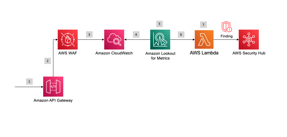
The solution in this blog post uses Amazon API Gateway to serve a simple REST API. AWS WAF protects API Gateway with AWS Managed Rules for AWS WAF. Amazon Lookout for Metrics actively detects unusual patterns in AWS WAF rule actions and sends a finding to Security Hub when suspicious activity is detected. Figure 1 shows the solution architecture.

Because AWS WAF integrates with Application Load Balancer, Amazon CloudFront distributions, or AWS AppSync GraphQL APIs, this solution also applies to these services.
 

Figure 1: Solution architecture

Figure 1: Solution architecture

The workflow of the solution is as follows:

  1. An HTTP request reaches the API Gateway endpoint.
  2. AWS WAF analyzes the HTTP request using the configured rules.
  3. Amazon CloudWatch collects action metrics for each rule that is configured in AWS WAF.
  4. Amazon Lookout for Metrics monitors CloudWatch metrics, selects the best ML algorithm, and trains the ML model.
  5. Lookout for Metrics detects outliers and provides a severity score to diagnose the issue.
  6. Lookout for Metrics invokes an AWS Lambda function when an anomaly is detected.
  7. The Lambda function sends a finding to Security Hub for further analysis.

Let’s take a detailed look at the AWS services that you will use in this solution.

Amazon API Gateway

Amazon API Gateway is a serverless API management service that supports mock integrations for API methods. This is the easiest and the most cost-effective way to implement this solution. But you can also use Amazon CloudFront, AWS AppSync GraphQL API, and Application Load Balancer to implement this solution in your workload.

AWS WAF

AWS WAF is a web application firewall you can associate with API Gateway for REST APIs, Amazon CloudFront, AWS AppSync for GraphQL API, or Application Load Balancer. AWS WAF is integrated with other AWS services such as CloudWatch. AWS WAF uses rules to detect common web exploits in the incoming HTTP requests. You can configure your own rules, or use managed rulesets from AWS or from a third-party vendor. In this solution, you use AWS Managed Rules, which contains the CrossSiteScripting_QUERYARGUMENTS rule.

Amazon CloudWatch

Amazon CloudWatch is a monitoring and observability service. CloudWatch receives specific metrics from AWS WAF every 5 minutes. In particular, for each AWS WAF rule, CloudWatch provides PassedRequests, BlockedRequests, and CountedRequests metrics.

Amazon Lookout for Metrics

Amazon Lookout for Metrics uses machine learning (ML) algorithms to automatically detect and diagnose anomalies in your metrics. By using CloudWatch metrics as a data source for Lookout for Metrics, you can apply one of the Lookout for Metrics ML models to detect anomalies in a faster way. In addition, you can provide feedback on detected anomalies to help improve the model accuracy over time. Lookout for Metrics is available in the US East (Ohio), US East (N. Virginia), US West (Oregon), Asia Pacific (Singapore), Asia Pacific (Sydney), Asia Pacific (Tokyo), Europe (Frankfurt), Europe (Ireland), and Europe (Stockholm) AWS Regions.

AWS Lambda

In this solution, you use an AWS Lambda function as an alert mechanism for Lookout for Metrics. When the machine learning model detects an outlier, it invokes the Lambda function, which implements a custom code. The Lambda function then imports the anomaly as a finding to Security Hub.

AWS Security Hub

In this solution, you use AWS Security Hub as a centralized way to manage security findings. This integration has the advantage of providing a common place for the security team to diagnose security findings from various sources, and uniformly integrates with your existing Security Information and Event Management (SIEM) system.

Prerequisites

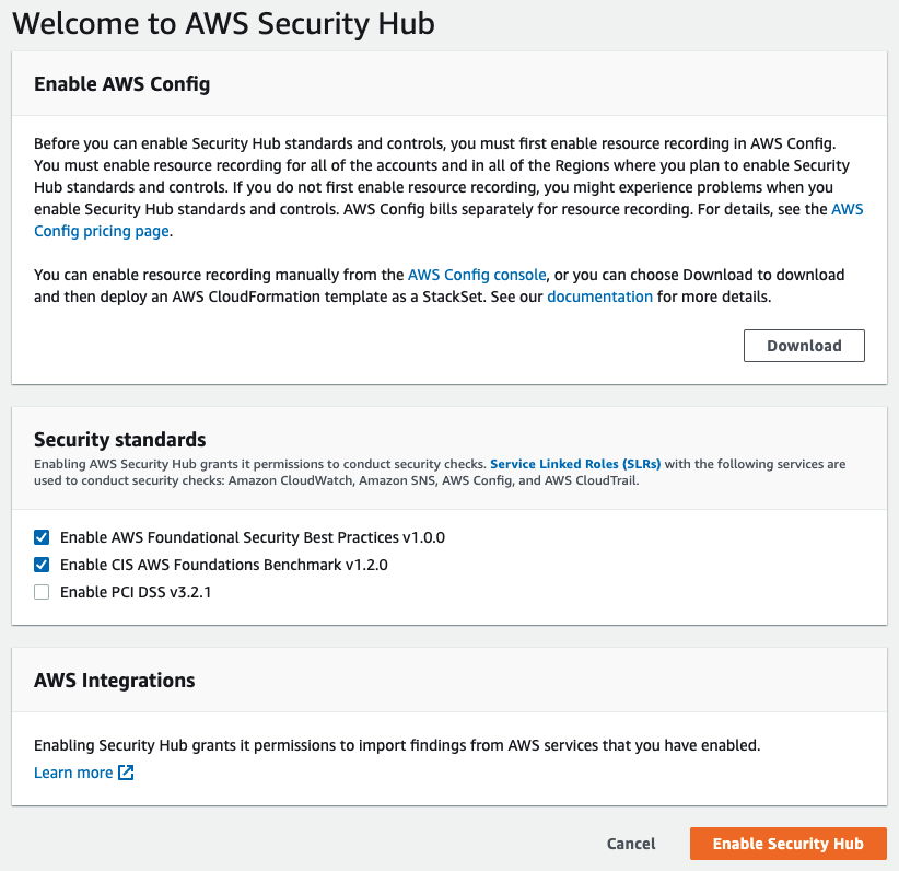
This solution uses Security Hub to collect anomaly detection findings. Before you deploy the solution, you need to enable Security Hub in your AWS account by following the instructions provided in to enable Security Hub manually. After you enable Security Hub, you can optionally select the security standards that are relevant for your workload, as shown in Figure 2.
 

Figure 2: Manually enabling Security Hub in the AWS Management Console

Figure 2: Manually enabling Security Hub in the AWS Management Console

Deploy the solution

A ready-to-use solution is provided as an AWS Cloud Development Kit (AWS CDK) application in the AWS WAF Anomaly Detection CDK project GitHub code repository. You can clone the GitHub repository and deploy the application by using the AWS CDK for Python.

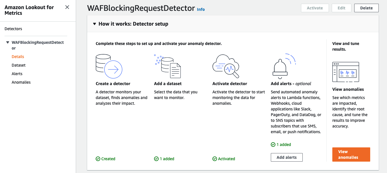
Important: After you successfully deploy the solution, you should activate the Lookout for Metrics detector. This is not done as part of the CDK deployment. To activate the detector, in the AWS Management Console navigate to Amazon Lookout for Metrics, select the detector the solution created (WAFBlockingRequestDetector), and choose Activate. Alternatively, you can use the following AWS command to activate your detector.

aws lookoutmetrics activate-anomaly-detector --anomaly-detector-arn arn:aws:lookoutmetrics:<REGION_ID>:<ACCOUNT_ID>:AnomalyDetector:WAFBlockingRequestDetector

If you don’t want to run the CDK application, you can implement the same solution by using the AWS Management Console. In the following sections, I’ll go through the manual steps you can follow to achieve this.

Create an API to demonstrate the solution

First, you need an HTTP endpoint to protect. AWS WAF is integrated with CloudFront, Application Load Balancer, API Gateway, and AWS AppSync GraphQL API. In this blog post, I recommend a REST API Gateway because it’s a fully managed service to create and manage APIs. In addition, API Gateway provides a mechanism to implement mock APIs.

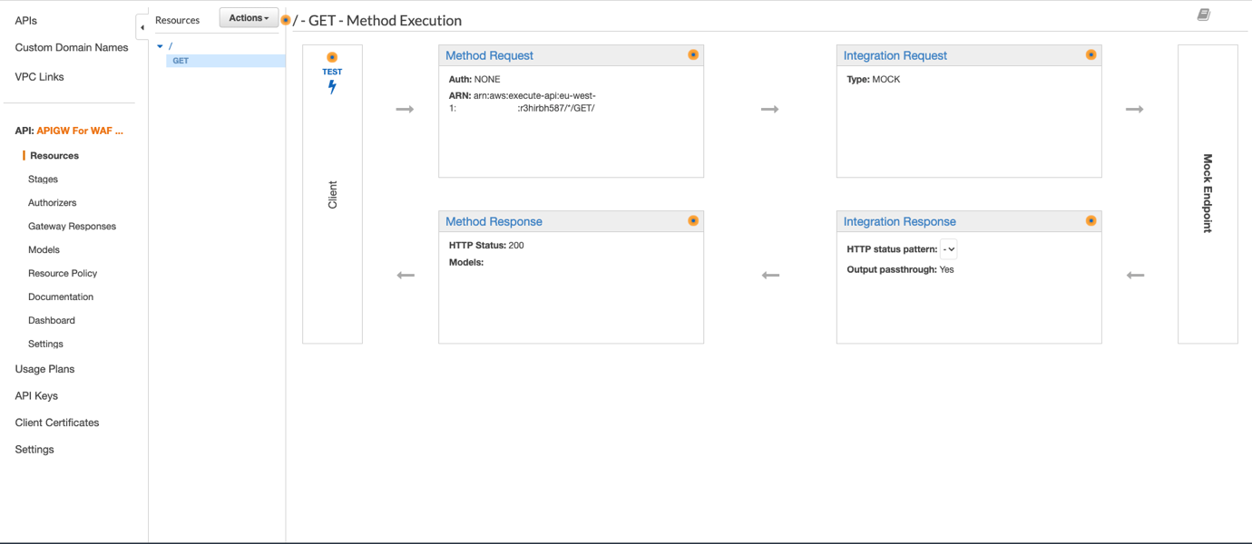
To build a REST API, follow the instructions for creating a REST API in Amazon API Gateway. After you create the API, create a GET method at the API root level and associate it to a mock endpoint, as shown in Figure 3. This is just enough to return an HTTP 200 status code to any GET requests.
 

Figure 3: Creating an API with mock integration

Figure 3: Creating an API with mock integration

Finally, deploy the API under the “prod” stage and keep all the default settings.

Create an AWS WAF web ACL to deploy the managed rules

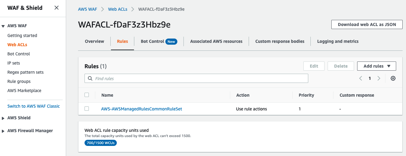
Now that you’ve created an API in API Gateway, you need to create an AWS WAF web access control list (web ACL) by following the instructions in Creating a web ACL. A web ACL is the top-level configuration object of AWS WAF. This is the collection of AWS WAF rules that you will apply to your API. API Gateway is a regional service, so make sure to create a web ACL in the same AWS Region as the API. After you create the web ACL, add the Core rule set (CRS) rule group from AWS Managed Rules, also called AWSManagedRulesCommonRuleSet, as shown in Figure 4. This rule group contains the CrossSiteScripting_QUERYARGUMENTS rule, which you will use later to demonstrate the anomaly detection.
 

Figure 4: Adding AWSManagedRulesCommonRuleSet to the AWS WAF web ACL

Figure 4: Adding AWSManagedRulesCommonRuleSet to the AWS WAF web ACL

By observing Web ACL rule capacity units used, you can see that the Core rule set is consuming 700 web ACL capacity units (WCUs). The maximum capacity for a web ACL is 1,500, which is sufficient for most use cases. If you need more capacity, contact the AWS Support Center.

Associate the web ACL with the API deployment

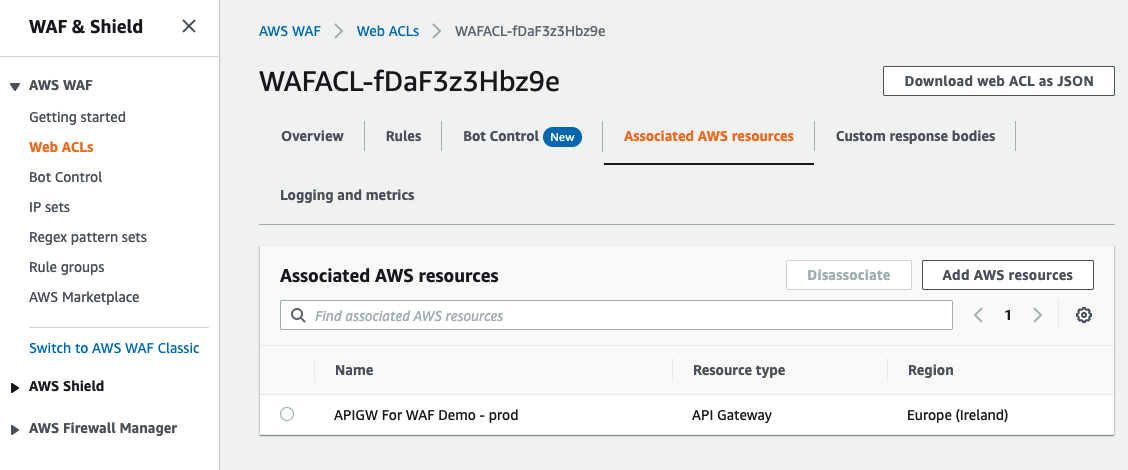
After you create the web ACL, you associate it with the API. To do this, in the AWS WAF console, navigate to the web ACL you just created. On the Associated AWS resources tab, choose Add AWS resources. When prompted, choose the API you created earlier, and then choose Add.
 

Figure 5: Associating the web ACL with the API

Figure 5: Associating the web ACL with the API

Create a Lambda function to forward the anomaly to Security Hub

It’s useful to get visibility into the anomalies that are detected by the solution, and there are various ways to do that. In this solution, you provide such visibility as findings to Security Hub. Security Hub provides a centralized place to manage different findings from your AWS solutions. It also provides graphical tools to help with diagnostics.

You use a Lambda function that receives each anomaly and imports them into Security Hub. You can find the lookout_alarm Lambda function on GitHub, or follow the instructions to build a Lambda function with Python. You will use this Lambda function to provide additional context enrichment in the finding.

import boto3

securityHub = boto3.client('securityhub')

def lambda_handler(event, context):
    # submit the finding to Security Hub
    result = securityHub.batch_import_findings(Findings = [...])

Before you use this Lambda function, make sure you enable Security Hub.

Create the Lookout for Metrics detector, dataset, and alarm

Now you have an API that is protected by an AWS WAF web ACL. You also have configured a way to integrate with Security Hub through a Lambda function. The next step is to create a Lookout for Metrics detector and connect all these elements together. The key concepts and terminology of Lookout for Metrics are:

  • Detector – A Lookout for Metrics resource that monitors a dataset and identifies anomalies.
  • Dataset – The detector’s copy of the data that Lookout for Metrics is analyzing.
  • Alert – A mechanism to send a notification or initiate a processing workflow when the detector finds an anomaly.

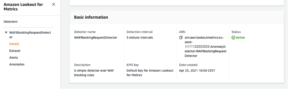
First, follow the instructions to create a detector. The only information you need to provide is a name and an interval. The interval is the amount of time between two analyses. Your choice of the interval depends upon criteria such as the metrics you are processing, or the retention time of your data. For more information on the detector interval, see Lookout for Metrics quotas. In the example in Figure 6, I chose an interval of 5 minutes, which is the minimum.
 

Figure 6: Creating an Amazon Lookout for Metrics detector

Figure 6: Creating an Amazon Lookout for Metrics detector

After you create the detector, follow the instructions to configure a dataset that uses CloudWatch as a data source. Select Create a role in the service role, choose Next, and enter the following parameters:

  • For the CloudWatch namespace, choose AWS/WAFV2.
  • For Dimensions, choose Region, Rule, and WebACL.
  • For Measure, choose BlockedRequests.
  • For Aggregation function, choose SUM.

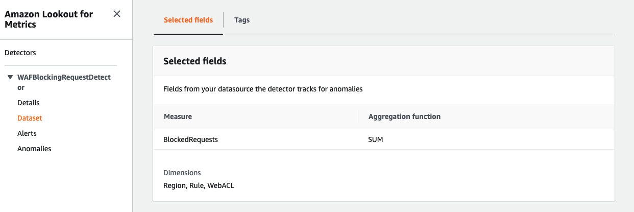
Figure 7 shows the data source fields that the detector will check for anomalies.
 

Figure 7: Creating an Amazon Lookout for Metrics dataset

Figure 7: Creating an Amazon Lookout for Metrics dataset

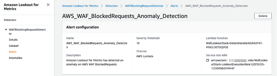
Next, create a Lookout for Metrics alert to invoke the Lambda function. To do so, follow the instructions for working with alerts. You provide a name, a channel (the Lambda function), and a severity threshold. One of the main advantages of Lookout for Metrics is the scoring of the detected anomaly, which indicates the severity. Anomalies have a score from 0 to 100. You can set up different alerts with different thresholds that are associated to the same detector. This way, you can provide alerts for different severity levels. In the example in Figure 8, I created a single alert with a severity threshold of 10.
 

Figure 8: Creating an Amazon Lookout for Metrics alert

Figure 8: Creating an Amazon Lookout for Metrics alert

The last steps are to activate the detector and configure Lookout for Metrics to select a ML model and train it. To do so, choose Activate on the detector details page.
 

Figure 9: Activating the Amazon Lookout for Metrics detector

Figure 9: Activating the Amazon Lookout for Metrics detector

Why does this solution use Lookout for Metrics anomaly detection?

Amazon CloudWatch offers native anomaly detection on a given metric. This function is useful to apply statistical and ML algorithms that continuously analyze metrics, determine normal baselines, and identify anomalies with minimal user intervention.

Lookout for Metrics provides a more sophisticated version of anomaly detection, which makes it the better choice for this solution. Lookout for Metrics automatically supports a collection of ML algorithms. For example, no one algorithm works for all kinds of data, so Lookout for Metrics inspects the data and applies the right ML algorithm to the right data to accurately detect anomalies. In addition, Lookout for Metrics groups concurrent anomalies into logical groups, and sends a single alert for the anomaly group rather than separate alerts, so you can see the full picture. Finally, Lookout for Metrics allows you to provide feedback on the detected anomalies, which AWS uses to continuously improve the accuracy and performance of the models.

Publish the value zero in CloudWatch metrics

The reporting criteria for AWS WAF metrics is a nonzero value. This means that the BlockedRequests metric isn’t updated if AWS WAF isn’t blocking any requests. In the absence of real HTTP traffic, typically in a testing environment, the value zero must be published. In production, because AWS WAF is actively blocking illegitimate requests, this publication is not required. To train the ML model in the absence of blocked requests, you need to publish the value zero by calling the PutMetricData CloudWatch API method every 5 minutes.

In my example, I selected a 5-minute period to be aligned with the Lookout for Metrics interval. It’s possible to publish a zero value every five minutes by using the CloudWatch metrics API, as shown following. The zero value doesn’t impact the SUM and ensures that at least one value is published every five minutes. You can use the cloudwatch_zero Lambda function on GitHub to publish the value zero by using the AWS SDK for Python.

import boto3

cloudwatch = boto3.client('cloudwatch')

def lambda_handler(event, context):

    result = cloudwatch.put_metric_data(
        Namespace='AWS/WAFV2',
        MetricData=[{
                'MetricName': 'BlockedRequests',
                'Dimensions': [...],
                'Value': 0
        }]
    )

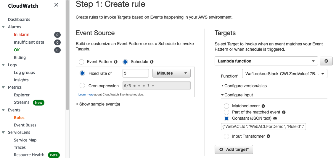
To create a CloudWatch Events rule to schedule the call every 5 minutes

  1. Navigate to the CloudWatch Event console and choose Create Rule.
  2. Choose Schedule, keep the 5-minute default interval, and choose Add target.
  3. Select the name of the function you previously created, expand the Configure input section.
  4. Choose Constant (JSON text), as shown in Figure 10. In the text field, paste the following configuration:
    {"WebACLId":"WebACLForWAFDemo","RuleId":"AWS-AWSManagedRulesCommonRuleSet"}
    

  5. Choose Configure details.
  6. Enter a name for your rule, and then choose Create rule.


Figure 10: Creating a CloudWatch Events rule scheduled every 5 minutes

Figure 10: Creating a CloudWatch Events rule scheduled every 5 minutes

Training time

Before the activated detector attempts to find anomalies, it uses data from several intervals to learn. If no historical data is available, the training process takes approximately one day for a five-minute interval. When you first deploy this solution, you have no historical data in CloudWatch for your AWS WAF resources, and you’re facing a cold start of Lookout for Metrics anomaly detection. Because the Lookout for Metrics detector interval is set to 5 minutes, you have to wait for 25 hours before being able to detect an anomaly. If you deploy the solution against an AWS WAF resource that’s been in production for days, you’ll have a reduced training time.

Test the anomaly detection

After 25 hours, Lookout for Metrics correctly selects an ML model that fits your metrics behavior, and correctly trains it based on your actual data. You can then start to test the anomaly detection. You can use a simple curl command, injecting a JavaScript alert() call in a query parameter as described in the AWS WAF documentation, to invoke the CrossSiteScripting_QUERYARGUMENTS managed rule. Make sure to inject a significant number of requests to ensure detection of blocked requests anomalies.

for i in {1..150}
do
  curl https://<api_gateway_endpoint>?test=%3Cscript%3Ealert%28%22hello%22%29%3C%2Fscript%3E
done

After you run the injection script, wait for the system to detect the anomaly. The CloudWatch BlockedRequests metric takes up to 5 minutes to update, and Lookout for Metrics is configured to detect anomalies in the CloudWatch data every 5 minutes. For those reasons, it can take 10 minutes to detect the simulated anomaly.

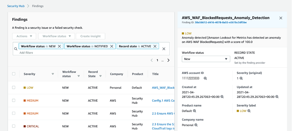
After detection and processing time, the finding is visible in Security Hub. To view the finding, go to the AWS Management Console, choose Services, choose Security Hub, and then choose Findings.
 

Figure 11: AWS Security Hub findings

Figure 11: AWS Security Hub findings

In Figure 11, you can see the new finding, coming from Lookout for Metrics, with a Low severity and an anomaly score of 100. You can use the remediation field to open the Lookout for Metrics console, where you can give feedback on the anomaly detection to improve the model for future detections.
 

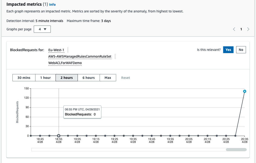
Figure 12: Lookout for Metrics console, Finding view

Figure 12: Lookout for Metrics console, Finding view

Figure 12 shows the Lookout for Metrics graphical interface, where you can see the metrics related to the finding. The previous injection script impacted only one metric, but the same setup works to observe anomalies that arise between two or more metrics together. This feature makes diagnosis of issues easier.

For each of the impacted metrics, to confirm that the anomaly is relevant, choose the Yes button next to Is this relevant? above the graph.

Extend the solution

The solution in this post detects anomalies in the AWS WAF blocked request behavior. But you can also configure AWS WAF rule actions to count your requests instead of blocking them. This is usually done on legacy systems or for some particular rules of a managed ruleset that present an incompatibility with your workload. When you configure the rule action as a count, you increase the need for a comprehensive observability approach. By implementing anomaly detection against counted requests, this solution will help you to achieve better observability for your system.

Concerning the remediation, it’s possible to modify this solution by integrating it with different AWS services. As an example, you can integrate the anomaly detection with your own SIEM system, or simply notify your security team distribution list by using Amazon Simple Notification Service (Amazon SNS).

AWS WAF provides additional information in its logs, such as the IP address for the client. To detect anomalies in AWS WAF logs, you can ingest the AWS WAF logs to Amazon Simple Storage Service (Amazon S3), and then use Lookout for Metrics with Amazon S3 as a data source.

Conclusion

AWS WAF is integrated with CloudWatch and provides metrics for passed requests, blocked requests, or counted requests. With Lookout for Metrics, you can detect unexpected behavior in CloudWatch metrics by using a machine learning (ML) model. In this blog, I showed you how to integrate both services to provide AWS WAF with an ML-based anomaly detection mechanism. ML is a way to gain more visibility into your AWS WAF behavior. In addition, you can easily be notified when the system detects abnormal levels of blocked (or counted) requests, in order to take the right remediation action.

If you have feedback about this post, submit comments in the Comments section below. If you have questions about this post, start a new thread on the AWS WAF forum or contact AWS Support.

Want more AWS Security how-to content, news, and feature announcements? Follow us on Twitter.

Author

Cyril Soler

Cyril is a Senior Solutions Architect at AWS, working with Spain-based enterprises. His interests include security and data protection. He has been passionate about computer science since he was 7. When he’s far from a keyboard, he enjoys mechanics. Cyril holds a Master’s degree from Polytech Marseille, School of Engineering.

IoT gets a machine learning boost, from edge to cloud

Post Syndicated from Ashley Whittaker original https://www.raspberrypi.org/blog/iot-gets-a-machine-learning-boost-from-edge-to-cloud/

Today, it’s easy to run Edge Impulse machine learning on any operating system, like Raspberry Pi OS, and on every cloud, like Microsoft’s Azure IoT. Evan Rust, Technology Ambassador for Edge Impulse, walks us through it.

Building enterprise-grade IoT solutions takes a lot of practical effort and a healthy dose of imagination. As a foundation, you start with a highly secure and reliable communication between your IoT application and the devices it manages. We picked our favorite integration, the Microsoft Azure IoT Hub, which provides us with a cloud-hosted solution backend to connect virtually any device. For our hardware, we selected the ubiquitous Raspberry Pi 4, and of course Edge Impulse, which will connect to both platforms and extend our showcased solution from cloud to edge, including device authentication, out-of-box device management, and model provisioning.

From edge to cloud – getting started 

Edge machine learning devices fall into two categories: some are able to run very simple models locally, and others have more advanced capabilities that allow them to be more powerful and have cloud connectivity. The second group is often expensive to develop and maintain, as training and deploying models can be an arduous process. That’s where Edge Impulse comes in to help to simplify the pipeline, as data can be gathered remotely, used effortlessly to train models, downloaded to the devices directly from the Azure IoT Hub, and then run – fast.

This reference project will serve you as a guide for quickly getting started with Edge Impulse on Raspberry Pi 4 and Azure IoT, to train a model that detects lug nuts on a wheel and sends alerts to the cloud.

Setting up the hardware

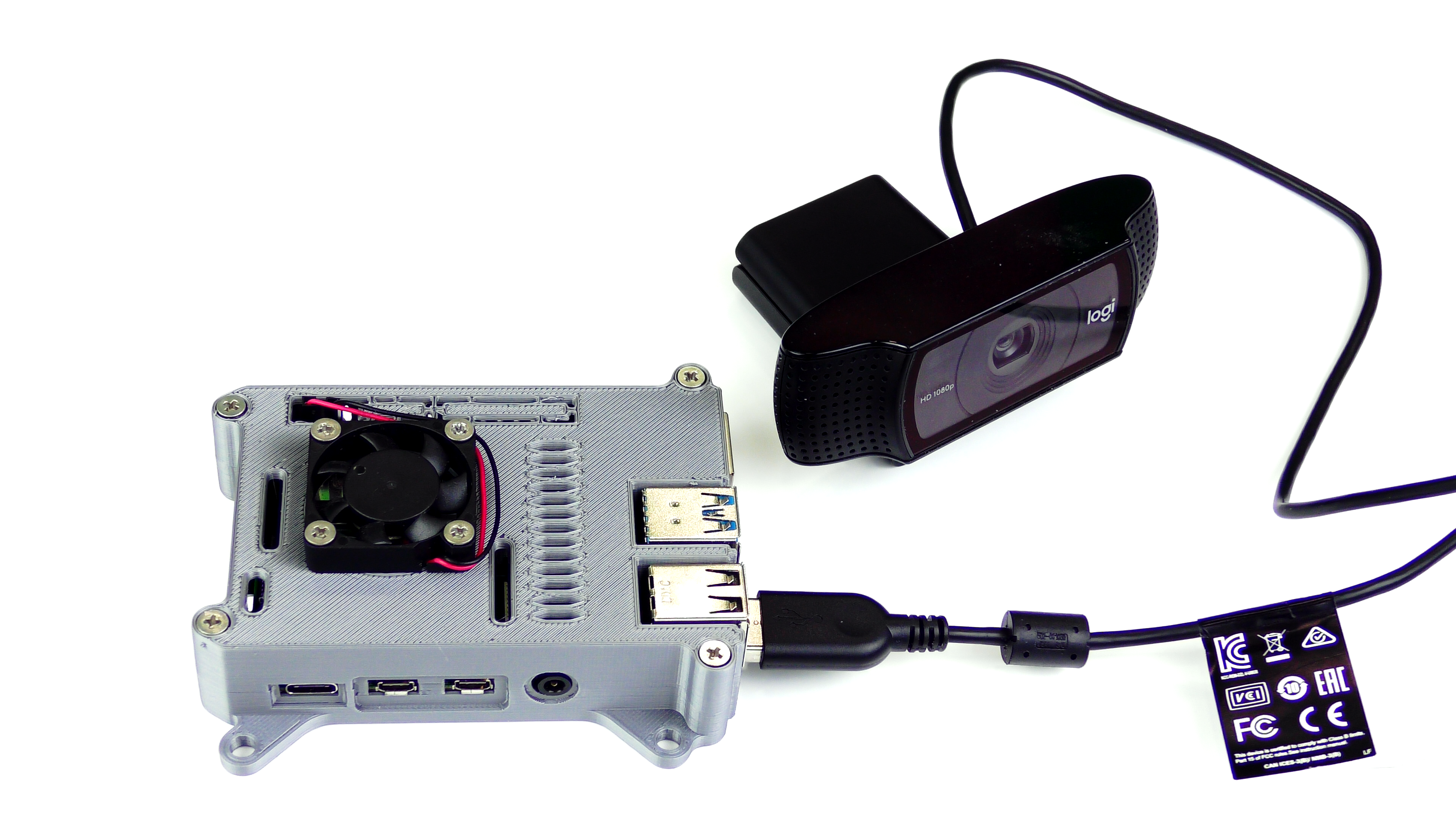
Hardware setup for Edge Impulse Machine Learning
Raspberry Pi 4 forms the base for the Edge Impulse machine learning setup

To begin, you’ll need a Raspberry Pi 4 with an up-to-date Raspberry Pi OS image which can be found here. After flashing this image to an SD card and adding a file named wpa_supplicant.conf

ctrl_interface=DIR=/var/run/wpa_supplicant GROUP=netdev
update_config=1
country=<Insert 2 letter ISO 3166-1 country code here>

network={
	ssid="<Name of your wireless LAN>"
	psk="<Password for your wireless LAN>"
}

along with an empty file named ssh (both within the /boot directory), you can go ahead and power up the board. Once you’ve successfully SSH’d into the device with 

$ ssh pi@<IP_ADDRESS>

and the password raspberry, it’s time to install the dependencies for the Edge Impulse Linux SDK. Simply run the next three commands to set up the NodeJS environment and everything else that’s required for the edge-impulse-linux wizard:

$ curl -sL https://deb.nodesource.com/setup_12.x | sudo bash -
$ sudo apt install -y gcc g++ make build-essential nodejs sox gstreamer1.0-tools gstreamer1.0-plugins-good gstreamer1.0-plugins-base gstreamer1.0-plugins-base-apps
$ npm config set user root && sudo npm install edge-impulse-linux -g --unsafe-perm

Since this project deals with images, we’ll need some way to capture them. The wizard supports both the Pi Camera modules and standard USB webcams, so make sure to enable the camera module first with 

$ sudo raspi-config

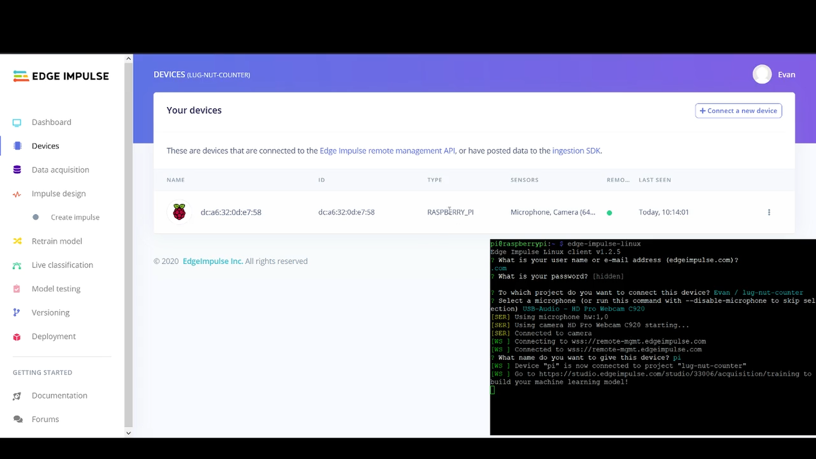
if you plan on using one. With that completed, go to the Edge Impulse Studio and create a new project, then run the wizard with 

$ edge-impulse-linux

and make sure your device appears within the Edge Impulse Studio’s device section after logging in and selecting your project.

Edge Impulse Machine Learning screengrab

Capturing your data

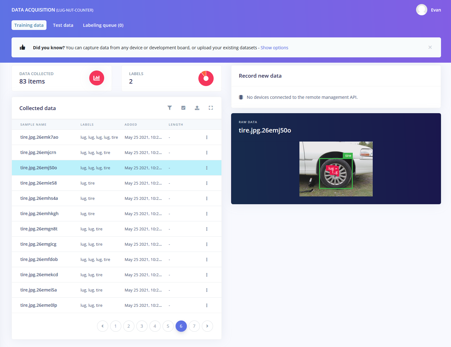
Training accurate machine learning models requires feeding plenty of varied data, which means a lot of images are required. For this use case, I captured around 50 images of a wheel that had lug nuts on it. After I was done, I headed to the Labeling queue in the Data Acquisition page and added bounding boxes around each lug nut within every image, along with every wheel.

Edge Impulse Machine Learning screengrab

To add some test data, I went back to the main Dashboard page and clicked the Rebalance dataset button, which moves 20% of the training data to the test data bin. 

Training your models

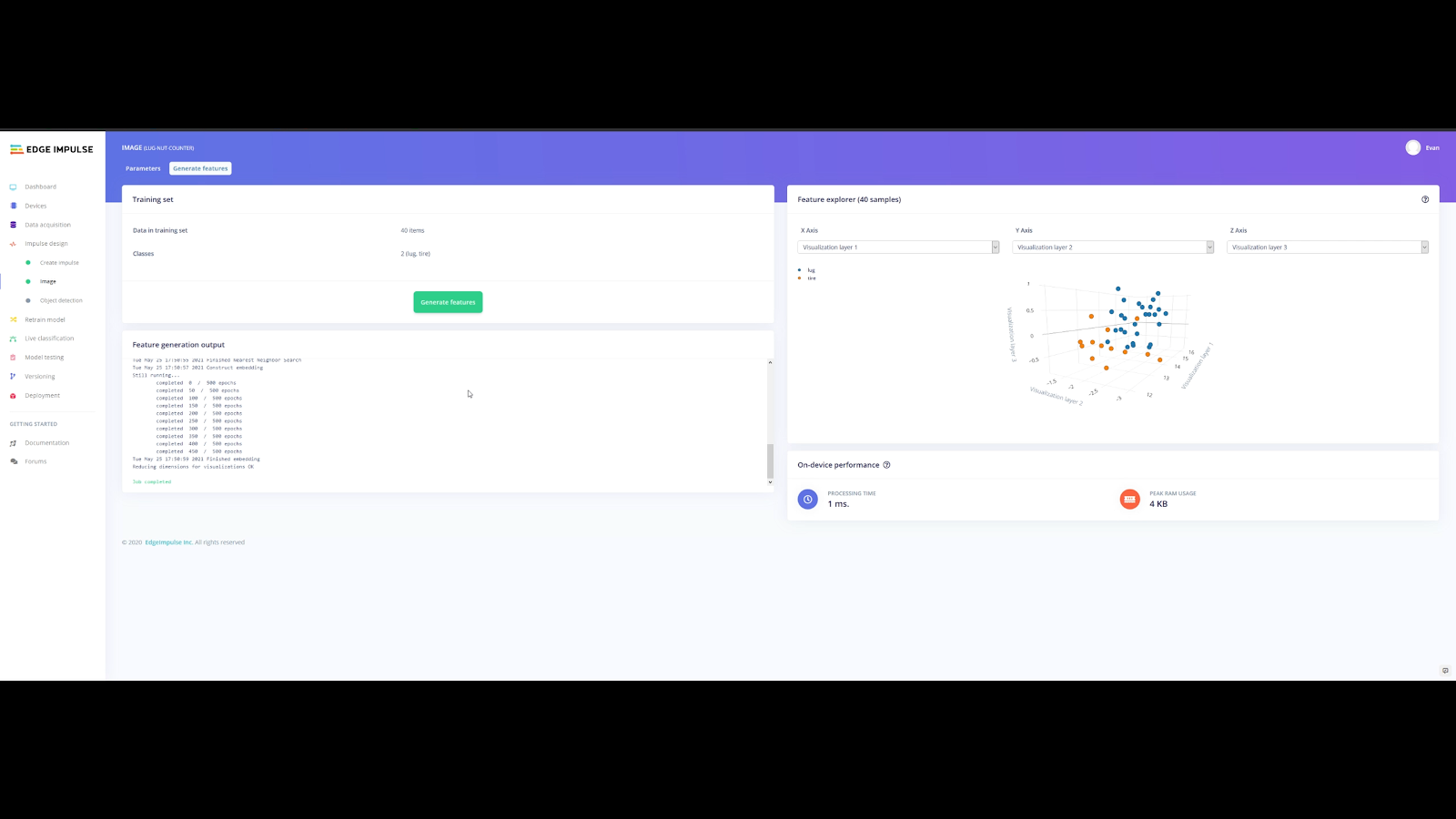
So now that we have plenty of training data, it’s time to do something with it, namely train a model. The first block in the impulse is an Image Data block, and it scales each image to a size of 320 by 320 pixels. Next, image data is fed to the Image processing block which takes the raw RGB data and derives features from it.

Edge Impulse Machine Learning screengrab

Finally, these features are sent to the Transfer Learning Object Detection model which learns to recognize the objects. I set my model to train for 30 cycles at a learning rate of .15, but this can be adjusted to fine-tune the accuracy.

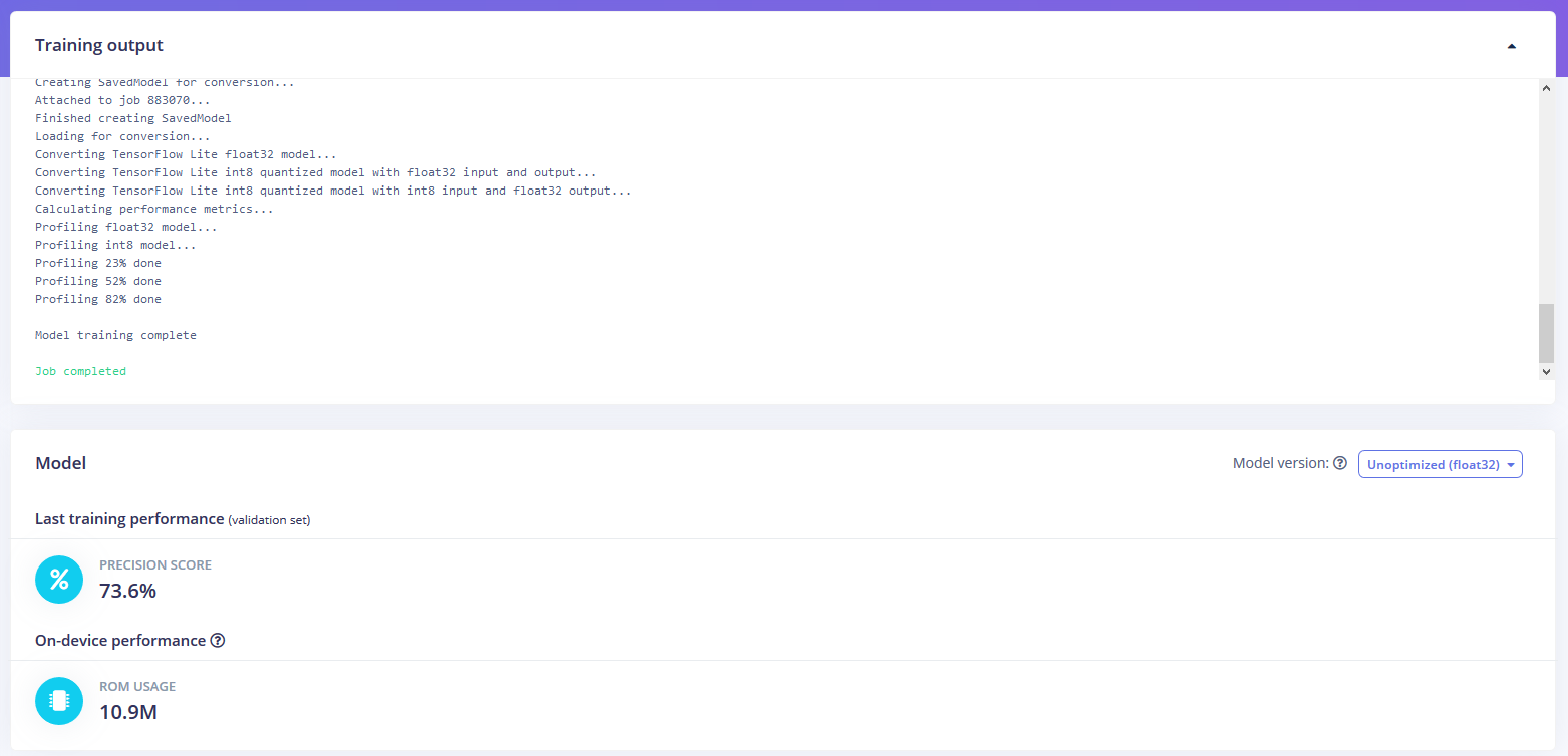
As you can see from the screenshot below, the model I trained was able to achieve an initial accuracy of 35.4%, but after some fine-tuning, it was able to correctly recognize objects at an accuracy of 73.5%.

Edge Impulse Machine Learning screengrab

Testing and deploying your models

In order to verify that the model works correctly in the real world, we’ll need to deploy it to our Raspberry Pi 4. This is a simple task thanks to the Edge Impulse CLI, as all we have to do is run 

$ edge-impulse-linux-runner

which downloads the model and creates a local webserver. From here, we can open a browser tab and visit the address listed after we run the command to see a live camera feed and any objects that are currently detected. 

Integrating your models with Microsoft Azure IoT 

With the model working locally on the device, let’s add an integration with an Azure IoT Hub that will allow our Raspberry Pi to send messages to the cloud. First, make sure you’ve installed the Azure CLI and have signed in using az login. Then get the name of the resource group you’ll be using for the project. If you don’t have one, you can follow this guide on how to create a new resource group. After that, return to the terminal and run the following commands to create a new IoT Hub and register a new device ID:

$ az iot hub create --resource-group <your resource group> --name <your IoT Hub name>
$ az extension add --name azure-iot
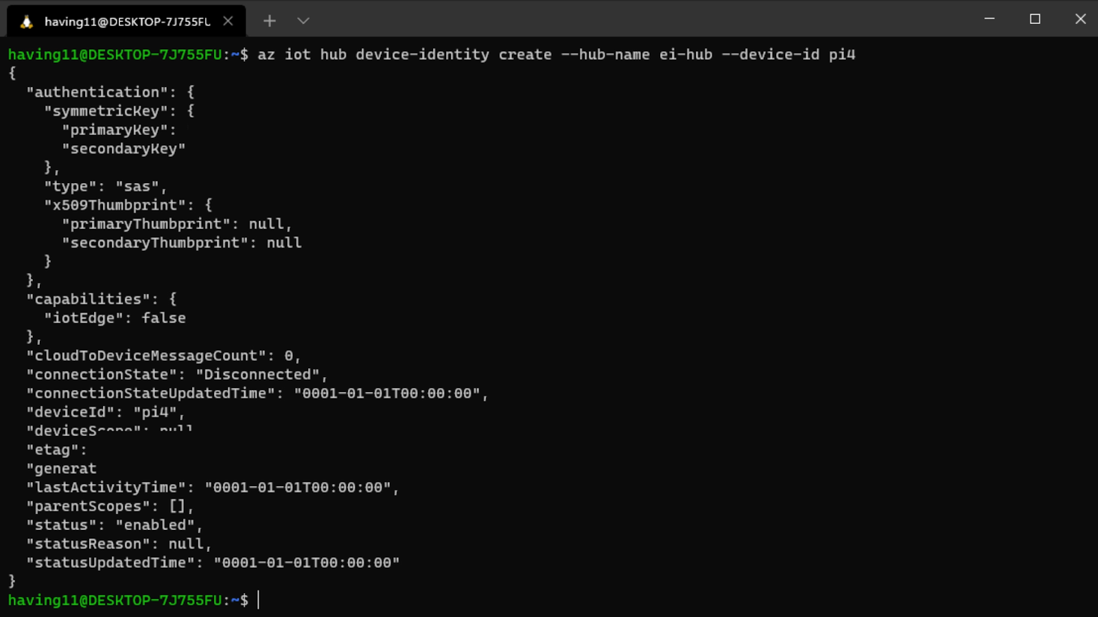
$ az iot hub device-identity create --hub-name <your IoT Hub name> --device-id <your device id>

Retrieve the connection string with 

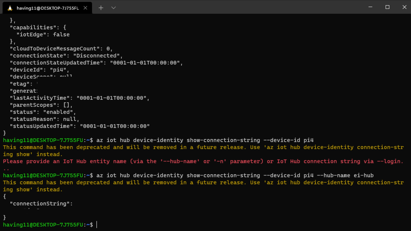
$ az iot hub device-identity connection-string show --device-id <your device id> --hub-name <your IoT Hub name>
Edge Impulse Machine Learning screengrab

and set it as an environment variable with 

$ export IOTHUB_DEVICE_CONNECTION_STRING="<your connection string here>" 

in your Raspberry Pi’s SSH session, as well as 

$ pip install azure-iot-device

to add the necessary libraries. (Note: if you do not set the environment variable or pass it in as an argument, the program will not work!) The connection string contains the information required for the device to establish a connection with the IoT Hub service and communicate with it. You can then monitor output in the Hub with 

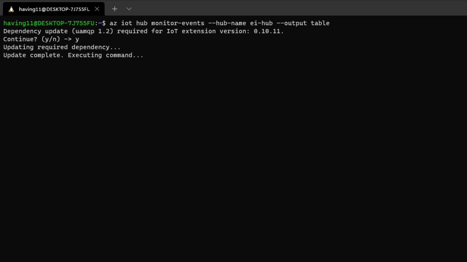
$ az iot hub monitor-events --hub-name <your IoT Hub name> --output table

 or in the Azure Portal.

To make sure it works, download and run this example to make sure you can see the test message. For the second half of deployment, we’ll need a way to customize how our model is used within the code. Thankfully, Edge Impulse provides a Python SDK for this purpose. Install it with 

$ sudo apt-get install libatlas-base-dev libportaudio0 libportaudio2 libportaudiocpp0 portaudio19-dev
$ pip3 install edge_impulse_linux -i https://pypi.python.org/simple

There’s some simple code that can be found here on Github, and it works by setting up a connection to the Azure IoT Hub and then running the model.

Edge Impulse Machine Learning screengrab

Once you’ve either downloaded the zip file or cloned the repo into a folder, get the model file by running

$ edge-impulse-linux-runner --download modelfile.eim

inside of the folder you just created from the cloning process. This will download a file called modelfile.eim. Now, run the Python program with 

$ python lug_nut_counter.py ./modelfile.eim -c <LUG_NUT_COUNT>

where <LUG_NUT_COUNT> is the correct number of lug nuts that should be attached to the wheel (you might have to use python3 if both Python 2 and 3 are installed).

Now whenever a wheel is detected the number of lug nuts is calculated. If this number falls short of the target, a message is sent to the Azure IoT Hub.

And by only sending messages when there’s something wrong, we can prevent an excess amount of bandwidth from being taken due to empty payloads.

The possibilities are endless

Imagine utilizing object detection for an industrial task such as quality control on an assembly line, or identifying ripe fruit amongst rows of crops, or detecting machinery malfunction, or remote, battery-powered inferencing devices. Between Edge Impulse, hardware like Raspberry Pi, and the Microsoft Azure IoT Hub, you can design endless models and deploy them on every device, while authenticating each and every device with built-in security.

You can set up individual identities and credentials for each of your connected devices to help retain the confidentiality of both cloud-to-device and device-to-cloud messages, revoke access rights for specific devices, transmit code and services between the cloud and the edge, and benefit from advanced analytics on devices running offline or with intermittent connectivity. And if you’re really looking to scale your operation and enjoy a complete dashboard view of the device fleets you manage, it is also possible to receive IoT alerts in Microsoft’s Connected Field Service from Azure IoT Central – directly.

Feel free to take the code for this project hosted here on GitHub and create a fork or add to it.

The complete project is available here. Let us know your thoughts at [email protected]. There are no limits, just your imagination at work.

The post IoT gets a machine learning boost, from edge to cloud appeared first on Raspberry Pi.

Deter package thieves from your porch with Raspberry Pi

Post Syndicated from Ashley Whittaker original https://www.raspberrypi.org/blog/deter-package-thieves-from-your-porch-with-raspberry-pi/

This Raspberry Pi-based build aims to deter porch pirates from stealing packages left at your front door. In recent times, we’ve all relied on home-delivered goods more than ever, and more often than not we ask our delivery drivers to stash our package somewhere if we’re not home, leaving them vulnerable to thieves.

Watch the full build video: ‘Fighting porch pirates with artificial intelligence (and flour)’

Flashing lights, sirens, flour and sprinklers

When internet shopper and AI project maker Ryder had a package stolen from his porch, he wanted to make sure that didn’t happen again. He figured that package stealers would be deterred by blaring sirens and flashing red lights. He also went one step further, wanting to hamper the thief’s escape with motion-activated water sprinklers and a blast of flour ready to catch them as they run away.

package thief running away
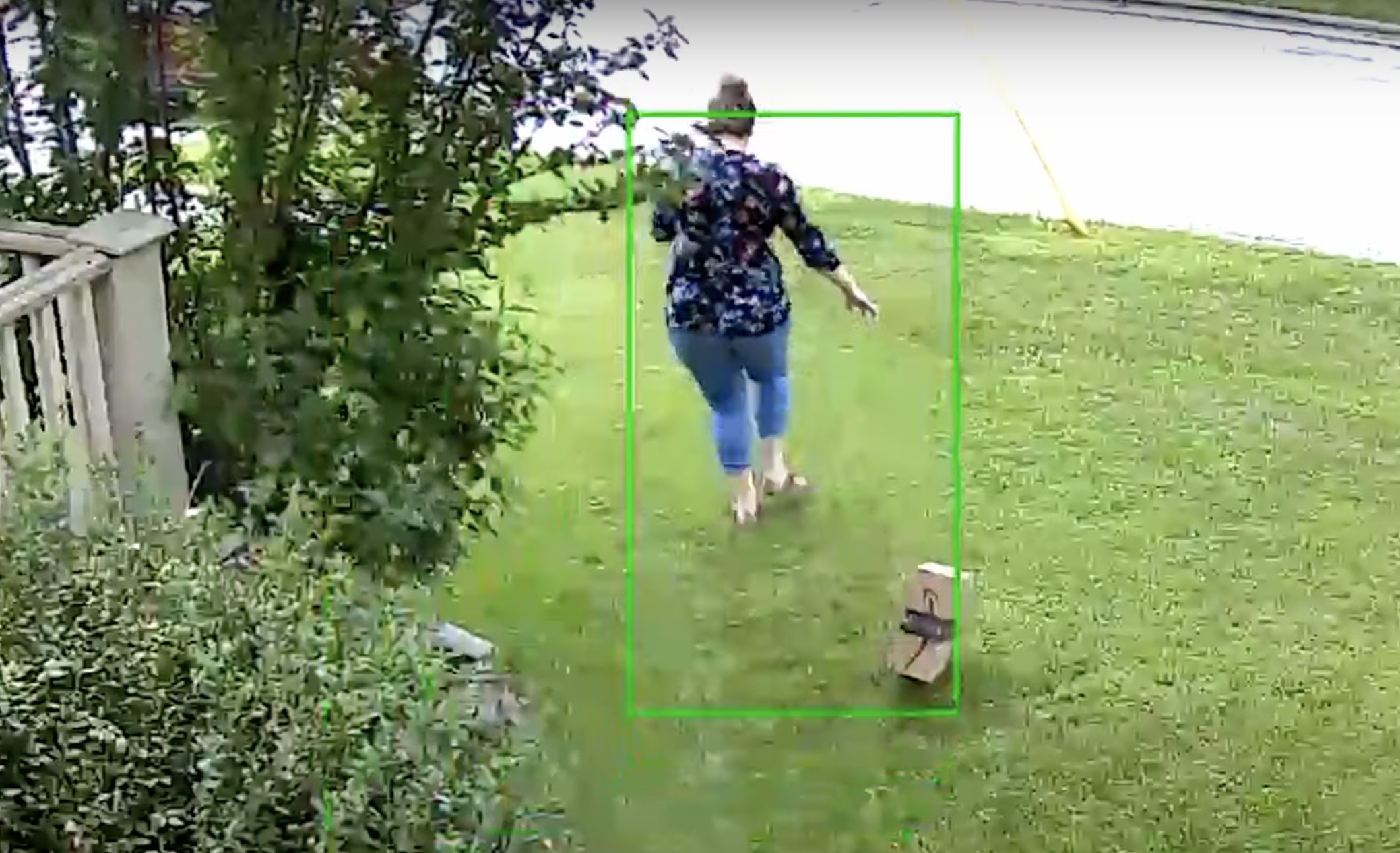
A would-be package thief dropping their swag and running away from the sprinkler

A simple motion detector wouldn’t work because it would set off Ryder’s booby traps whenever an unsuspecting cat or legitimate visitor happened across his porch, or if Ryder himself arrived home and didn’t fancy a watery flour bath. So some machine learning and a Python script needed to be employed.

How does it catch package thieves?

inside the package thief build
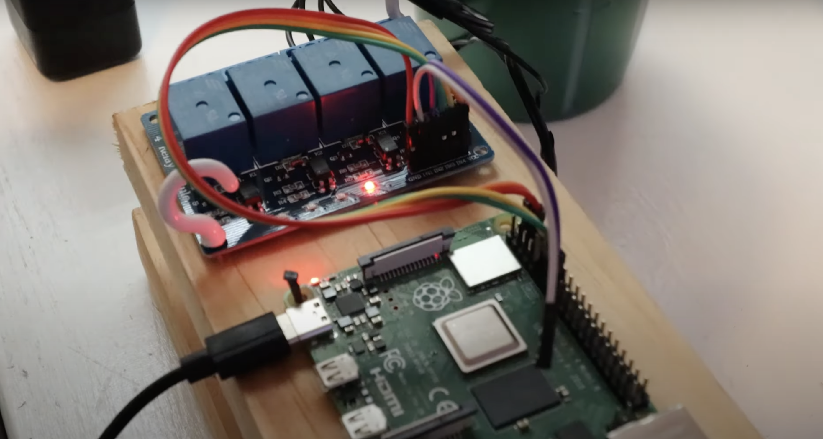
It’s what’s on the inside that counts. Us. We’re on the inside.

The camera keeps an eye on Ryder’s porch and is connected wirelessly to a Raspberry Pi 4, which works with a custom TensorFlow machine learning model trained to recognise when a package is or isn’t present. If the system detects a package, it gets ready to deploy the anti-thief traps. The Raspberry Pi sets everything off if it detects that someone other than Ryder has removed the package from the camera’s view.

And Ryder had an interesting technique to train the machine learning model to recognise him:

If you want to make your own anti-porch pirate device, Ryder has shared everything you need on GitHub.

Wanna see some cool dogs?

We can always rely on Ryder Calm Down’s YouTube channel for unique and quasi-bonkers builds.

If you’re not familiar with Ryder’s dog-detecting (and happiness-boosting) build, check it out below. We also blogged about this project when we needed a good dopamine boost during lockdown.

The post Deter package thieves from your porch with Raspberry Pi appeared first on Raspberry Pi.

Educating young people in AI, machine learning, and data science: new seminar series

Post Syndicated from Sue Sentance original https://www.raspberrypi.org/blog/ai-machine-learning-data-science-education-seminars/

A recent Forbes article reported that over the last four years, the use of artificial intelligence (AI) tools in many business sectors has grown by 270%. AI has a history dating back to Alan Turing’s work in the 1940s, and we can define AI as the ability of a digital computer or computer-controlled robot to perform tasks commonly associated with intelligent beings.

A woman explains a graph on a computer screen to two men.
Recent advances in computing technology have accelerated the rate at which AI and data science tools are coming to be used.

Four key areas of AI are machine learning, robotics, computer vision, and natural language processing. Other advances in computing technology mean we can now store and efficiently analyse colossal amounts of data (big data); consequently, data science was formed as an interdisciplinary field combining mathematics, statistics, and computer science. Data science is often presented as intertwined with machine learning, as data scientists commonly use machine learning techniques in their analysis.

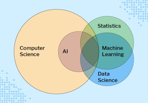
Venn diagram showing the overlaps between computer science, AI, machine learning, statistics, and data science.
Computer science, AI, statistics, machine learning, and data science are overlapping fields. (Diagram from our forthcoming free online course about machine learning for educators)

AI impacts everyone, so we need to teach young people about it

AI and data science have recently received huge amounts of attention in the media, as machine learning systems are now used to make decisions in areas such as healthcare, finance, and employment. These AI technologies cause many ethical issues, for example as explored in the film Coded Bias. This film describes the fallout of researcher Joy Buolamwini’s discovery that facial recognition systems do not identify dark-skinned faces accurately, and her journey to push for the first-ever piece of legislation in the USA to govern against bias in the algorithms that impact our lives. Many other ethical issues concerning AI exist and, as highlighted by UNESCO’s examples of AI’s ethical dilemmas, they impact each and every one of us.

Three female teenagers and a teacher use a computer together.
We need to make sure that young people understand AI technologies and how they impact society and individuals.

So how do such advances in technology impact the education of young people? In the UK, a recent Royal Society report on machine learning recommended that schools should “ensure that key concepts in machine learning are taught to those who will be users, developers, and citizens” — in other words, every child. The AI Roadmap published by the UK AI Council in 2020 declared that “a comprehensive programme aimed at all teachers and with a clear deadline for completion would enable every teacher confidently to get to grips with AI concepts in ways that are relevant to their own teaching.” As of yet, very few countries have incorporated any study of AI and data science in their school curricula or computing programmes of study.

A teacher and a student work on a coding task at a laptop.
Our seminar speakers will share findings on how teachers can help their learners get to grips with AI concepts.

Partnering with The Alan Turing Institute for a new seminar series

Here at the Raspberry Pi Foundation, AI, machine learning, and data science are important topics both in our learning resources for young people and educators, and in our programme of research. So we are delighted to announce that starting this autumn we are hosting six free, online seminars on the topic of AI, machine learning, and data science education, in partnership with The Alan Turing Institute.

A woman teacher presents to an audience in a classroom.
Everyone with an interest in computing education research is welcome at our seminars, from researchers to educators and students!

The Alan Turing Institute is the UK’s national institute for data science and artificial intelligence and does pioneering work in data science research and education. The Institute conducts many different strands of research in this area and has a special interest group focused on data science education. As such, our partnership around the seminar series enables us to explore our mutual interest in the needs of young people relating to these technologies.

This promises to be an outstanding series drawing from international experts who will share examples of pedagogic best practice […].

Dr Matt Forshaw, The Alan Turing Institute

Dr Matt Forshaw, National Skills Lead at The Alan Turing Institute and Senior Lecturer in Data Science at Newcastle University, says: “We are delighted to partner with the Raspberry Pi Foundation to bring you this seminar series on AI, machine learning, and data science. This promises to be an outstanding series drawing from international experts who will share examples of pedagogic best practice and cover critical topics in education, highlighting ethical, fair, and safe use of these emerging technologies.”

Our free seminar series about AI, machine learning, and data science

At our computing education research seminars, we hear from a range of experts in the field and build an international community of researchers, practitioners, and educators interested in this important area. Our new free series of seminars runs from September 2021 to February 2022, with some excellent and inspirational speakers:

  • Tues 7 September: Dr Mhairi Aitken from The Alan Turing Institute will share a talk about AI ethics, setting out key ethical principles and how they apply to AI before discussing the ways in which these relate to children and young people.
  • Tues 5 October: Professor Carsten Schulte, Yannik Fleischer, and Lukas Höper from Paderborn University in Germany will use a series of examples from their ProDaBi programme to explore whether and how AI and machine learning should be taught differently from other topics in the computer science curriculum at school. The speakers will suggest that these topics require a paradigm shift for some teachers, and that this shift has to do with the changed role of algorithms and data, and of the societal context.
  • Tues 3 November: Professor Matti Tedre and Dr Henriikka Vartiainen from the University of Eastern Finland will focus on machine learning in the school curriculum. Their talk will map the emerging trajectories in educational practice, theory, and technology related to teaching machine learning in K-12 education.
  • Tues 7 December: Professor Rose Luckin from University College London will be looking at the breadth of issues impacting the teaching and learning of AI.
  • Tues 11 January: We’re delighted that Dr Dave Touretzky and Dr Fred Martin (Carnegie Mellon University and University of Massachusetts Lowell, respectively) from the AI4K12 Initiative in the USA will present some of the key insights into AI that the researchers hope children will acquire, and how they see K-12 AI education evolving over the next few years.
  • Tues 1 February: Speaker to be confirmed

How you can join our online seminars

All seminars start at 17:00 UK time (18:00 Central European Time, 12 noon Eastern Time, 9:00 Pacific Time) and take place in an online format, with a presentation, breakout discussion groups, and a whole-group Q&A.

Sign up now and we’ll send you the link to join on the day of each seminar — don’t forget to put the dates in your diary!

In the meantime, you can explore some of our educational resources related to machine learning and data science:

The post Educating young people in AI, machine learning, and data science: new seminar series appeared first on Raspberry Pi.

Hiding Malware in ML Models

Post Syndicated from Bruce Schneier original https://www.schneier.com/blog/archives/2021/07/hiding-malware-in-ml-models.html

Interesting research: “EvilModel: Hiding Malware Inside of Neural Network Models”.

Abstract: Delivering malware covertly and detection-evadingly is critical to advanced malware campaigns. In this paper, we present a method that delivers malware covertly and detection-evadingly through neural network models. Neural network models are poorly explainable and have a good generalization ability. By embedding malware into the neurons, malware can be delivered covertly with minor or even no impact on the performance of neural networks. Meanwhile, since the structure of the neural network models remains unchanged, they can pass the security scan of antivirus engines. Experiments show that 36.9MB of malware can be embedded into a 178MB-AlexNet model within 1% accuracy loss, and no suspicious are raised by antivirus engines in VirusTotal, which verifies the feasibility of this method. With the widespread application of artificial intelligence, utilizing neural networks becomes a forwarding trend of malware. We hope this work could provide a referenceable scenario for the defense on neural network-assisted attacks.

News article.

Protecting Personal Data in Grab’s Imagery

Post Syndicated from Grab Tech original https://engineering.grab.com/protecting-personal-data-in-grabs-imagery

Image Collection Using KartaView

Starting a few years ago, we realised the strong demand to better understand the streets where our drivers and clients go, with the purpose to better fulfil their needs and also to be able to quickly adapt ourselves to the rapidly changing environment in the Southeast Asia cities.

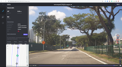
One way to fulfil that demand was to create an image collection platform named KartaView which is Grab Geo’s platform for geotagged imagery. It empowers collection, indexing, storage, retrieval of imagery, and map data extraction.

KartaView is a public, partially open-sourced product, used both internally and externally by the OpenStreetMap community and other users. As of 2021, KartaView has public imagery in over 100 countries with various coverage degrees, and 60+ cities of Southeast Asia. Check it out at www.kartaview.com.

Figure 1 - KartaView platform
Figure 1 – KartaView platform

Why Image Blurring is Important

Many incidental people and licence plates are in the collected images, whose privacy is a serious concern. We deeply respect all of them and consequently, we are using image obfuscation as the most effective anonymisation method for ensuring privacy protection.

Because manually annotating the regions in the picture where faces and licence plates are located is impractical, this problem should be solved using machine learning and engineering techniques. Hence we detect and blur all faces and licence plates which could be considered as personal data.

Figure 2 - Sample blurred picture
Figure 2 – Sample blurred picture

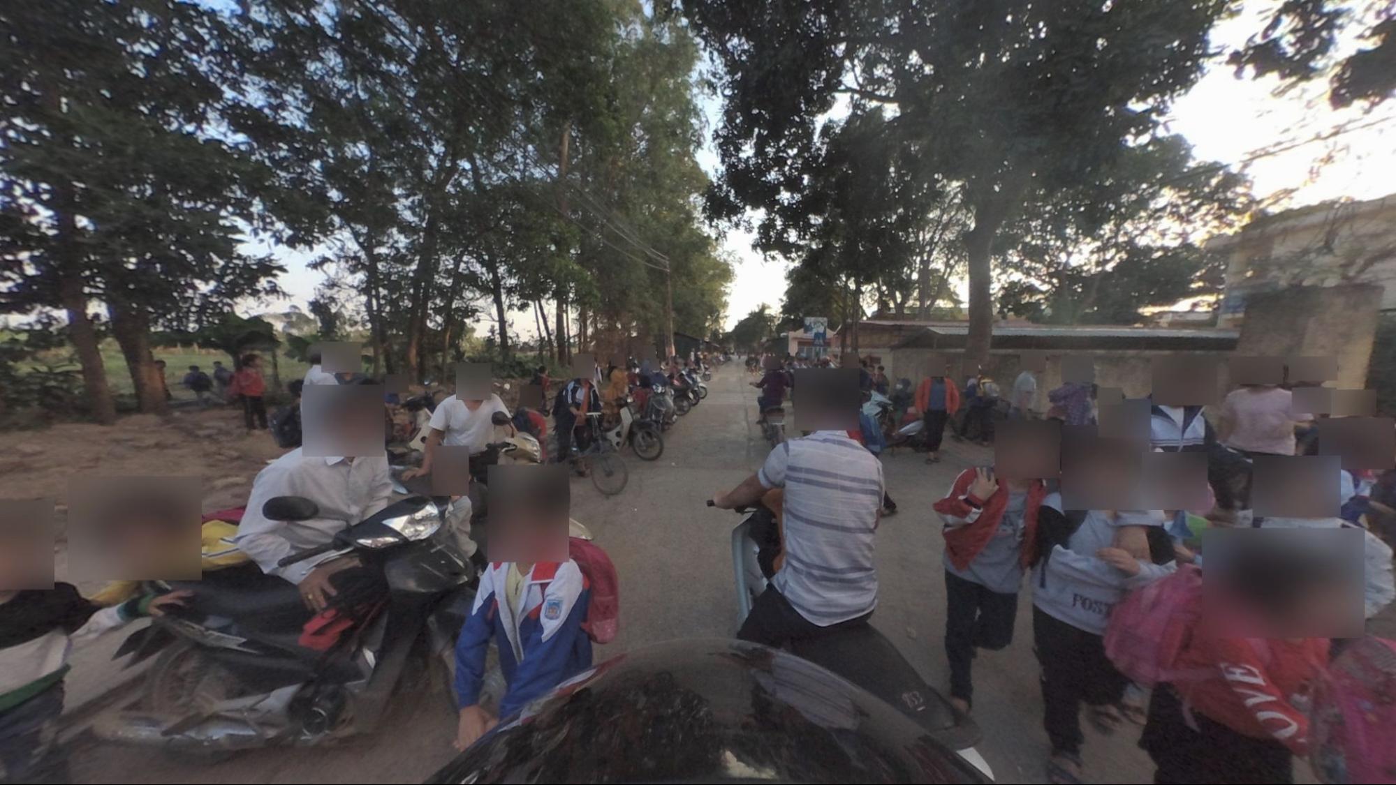
In our case, we have a wide range of picture types: regular planar, very wide and 360 pictures in equirectangular format collected with 360 cameras. Also, because we are collecting imagery globally, the vehicle types, licence plates, and human environments are quite diverse in appearance, and are not handled well by off-the-shelf blurring software. So we built our own custom blurring solution which yielded higher accuracy and better cost-efficiency overall with respect to blurring of personal data.

Figure 3 - Example of equirectangular image where personal data has to be blurred
Figure 3 – Example of equirectangular image where personal data has to be blurred

Behind the scenes, in KartaView, there are a set of cool services which are able to derive useful information from the pictures like image quality, traffic signs, roads, etc. A big part of them are using deep learning algorithms which potentially can be negatively affected by running them over blurred pictures. In fact, based on the assessment we have done so far, the impact is extremely low, similar to the one reported in a well known study of face obfuscation in ImageNet [9].

Outline of Grab’s Blurring Process

Roughly, the processing steps are the following:

  1. Transform each picture into a set of planar images. In this way, we further process all pictures, whatever the format they had, in the same way.
  2. Use an object detector able to detect all faces and licence plates in a planar image having a standard field of view.
  3. Transform the coordinates of the detected regions into original coordinates and blur those regions.
Figure 4 - Picture’s processing steps [8]
Figure 4 – Picture’s processing steps [8]

In the following section, we are going to describe in detail the interesting aspects of the second step, sharing the challenges and how we were solving them. Let’s start with the first and most important part, the dataset.

Dataset

Our current dataset consists of images from a wide range of cameras, including normal perspective cameras from mobile phones, wide field of view cameras and also 360 degree cameras.

It is the result of a series of data collections contributed by Grab’s data tagging teams, which may contain 2 classes of dataset that are of interest for us: FACE and LICENSE_PLATE.

The data was collected using Grab internal tools, stored in queryable databases, making it a system that gives the possibility to revisit the data and correct it if necessary, but also making it possible for data engineers to select and filter the data of interest.

Dataset Evolution

Each iteration of the dataset was made to address certain issues discovered while having models used in a production environment and observing situations where the model lacked in performance.

Dataset v1 Dataset v2 Dataset v3
Nr. images 15226 17636 30538
Nr. of labels 64119 86676 242534

If the first version was basic, containing a rough tagging strategy we quickly noticed that it was not detecting some special situations that appeared due to the pandemic situation: people wearing masks.

This led to another round of data annotation to include those scenarios.
The third iteration addressed a broader range of issues:

  • Small regions of interest (objects far away from the camera)
  • Objects in very dark backgrounds
  • Rotated objects or even upside down
  • Variation of the licence plate design due to images from different countries and regions
  • People wearing masks
  • Faces in the mirror – see below the mirror of the motorcycle
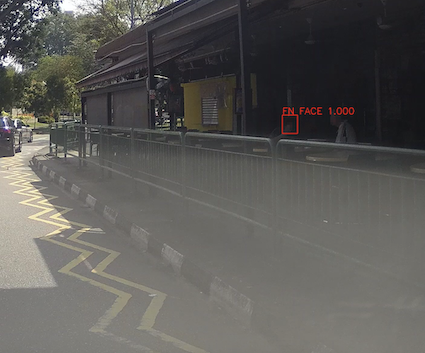
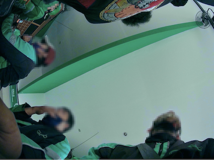
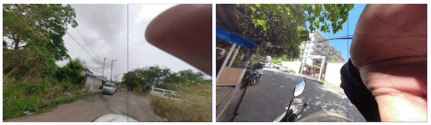
  • But the main reason was because of a scenario where the recording, at the start or end (but not only), had close-ups of the operator who was checking the camera. This led to images with large regions of interest containing the camera operator’s face – too large to be detected by the model.

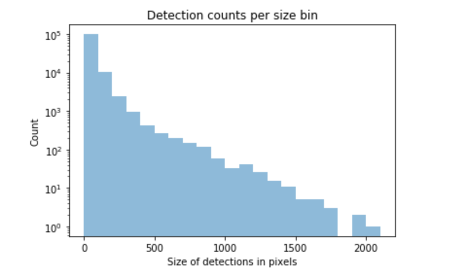
An investigation in the dataset structure, by splitting the data into bins based on the bbox sizes (in pixels), made something clear: the dataset was unbalanced.

We made bins for tag sizes with a stride of 100 pixels and went up to the max present in the dataset which accounted for 1 sample of size 2000 pixels. The majority of the labels were small in size and the higher we would go with the size, the less tags we would have. This made it clear that we would need more targeted annotations for our dataset to try to balance it.

All these scenarios required the tagging team to revisit the data multiple times and also change the tagging strategy by including more tags that were considered at a certain limit. It also required them to pay more attention to small details that may have been missed in a previous iteration.

Data Splitting

To better understand the strategy chosen for splitting the data we need to also understand the source of the data. The images come from different devices that are used in different geo locations (different countries) and are from a continuous trip recording. The annotation team used an internal tool to visualise the trips image by image and mark the faces and licence plates present in them. We would then have access to all those images and their respective metadata.

The chosen ratios for splitting are:

  • Train 70%
  • Validation 10%
  • Test 20%
Number of train images 12733
Number of validation images 1682
Number of test images 3221
Number of labeled classes in train set 60630
Number of labeled classes in validation set 7658
Number of of labeled classes in test set 18388

The split is not so trivial as we have some requirements and need to complete some conditions:

  • An image can have multiple tags from one or both classes but must belong to just one subset.
  • The tags should be split as close as possible to the desired ratios.
  • As different images can belong to the same trip in a close geographical relation we need to force them in the same subset, thus avoiding similar tags in train and test subsets, resulting in incorrect evaluations.

Data Augmentation

The application of data augmentation plays a crucial role while training the machine learning model. There are mainly three ways in which data augmentation techniques can be applied. They are:

  1. Offline data augmentation – enriching a dataset by physically multiplying some of its images and applying modifications to them.
  2. Online data augmentation – on the fly modifications of the image during train time with configurable probability for each modification.
  3. Combination of both offline and online data augmentation.

In our case, we are using the third option which is the combination of both.

The first method that contributes to offline augmentation is a method called image view splitting. This is necessary for us due to different image types: perspective camera images, wide field of view images, 360 degree images in equirectangular format. All these formats and field of views with their respective distortions would complicate the data and make it hard for the model to generalise it and also handle different image types that could be added in the future.

For this we defined the concept of image views which are an extracted portion (view) of an image with some predefined properties. For example, the perspective projection of 75 by 75 degrees field of view patches from the original image.

Here we can see a perspective camera image and the image views generated from it:

Figure 5 - Original image
Figure 5 – Original image
Figure 6 - Two image views generated
Figure 6 – Two image views generated

The important thing here is that each generated view is an image on its own with the associated tags. They also have an overlapping area so we have a possibility to contain the same tag in two views but from different perspectives. This brings us to an indirect outcome of the first offline augmentation.

The second method for offline augmentation is the oversampling of some of the images (views). As mentioned above, we faced the problem of an unbalanced dataset, specifically we were missing tags that occupied high regions of the image, and even though our tagging teams tried to annotate as many as they could find, these were still scarce.

As our object detection model is an anchor-based detector, we did not even have enough of them to generate the anchor boxes correctly. This could be clearly seen in the accuracy of the previous trained models, as they were performing poorly on bins of big sizes.

By randomly oversampling images that contained big tags, up to a minimum required number, we managed to have better anchors and increase the recall for those scenarios. As described below, the chosen object detector for blurring was YOLOv4 which offers a large variety of online augmentations. The online augmentations used are saturation, exposure, hue, flip and mosaic.

Model

As of summer of 2021, the “to go” solution for object detection in images are convolutional neural networks (CNN), being a mature solution able to fulfil the needs efficiently.

Architecture

Most CNN based object detectors have three main parts: Backbone, Neck and (Dense or Sparse Prediction) Heads. From the input image, the backbone extracts features which can be combined in the neck part to be used by the prediction heads to predict object bounding-boxes and their labels.

Figure 7 - Anatomy of one and two-stage object detectors [1]
Figure 7 – Anatomy of one and two-stage object detectors [1]

The backbone is usually a CNN classification network pretrained on some dataset, like ImageNet-1K. The neck combines features from different layers in order to produce rich representations for both large and small objects. Since the objects to be detected have varying sizes, the topmost features are too coarse to represent smaller objects, so the first CNN based object detectors were fairly weak in detecting small sized objects. The multi-scale, pyramid hierarchy is inherent to CNNs so [2] introduced the Feature Pyramid Network which at marginal costs combines features from multiple scales and makes predictions on them. This or improved variants of this technique is used by most detectors nowadays. The head part does the predictions for bounding boxes and their labels.

YOLO is part of the anchor-based one-stage object detectors family being developed originally in Darknet, an open source neural network framework written in C and CUDA. Back in 2015 it was the first end-to-end differentiable network of this kind that offered a joint learning of object bounding boxes and their labels.

One reason for the big success of newer YOLO versions is that the authors carefully merged new ideas into one architecture, the overall speed of the model being always the north star.

YOLOv4 introduces several changes to its v3 predecessor:

  • Backbone – CSPDarknet53: YOLOv3 Darknet53 backbone was modified to use Cross Stage Partial Network (CSPNet [5]) strategy, which aims to achieve richer gradient combinations by letting the gradient flow propagate through different network paths.
  • Multiple configurable augmentation and loss function types, so called “Bag of freebies”, which by changing the training strategy can yield higher accuracy without impacting the inference time.
  • Configurable necks and different activation functions, they call “Bag of specials”.

Insights

For this task, we found that YOLOv4 gave a good compromise between speed and accuracy as it has doubled the speed of a more accurate two-stage detector while maintaining a very good overall precision/recall. For blurring, the main metric for model selection was the overall recall, while precision and intersection over union (IoU) of the predicted box comes second as we want to catch all personal data even if some are wrong. Having a multitude of possibilities to configure the detector architecture and train it on our own dataset we conducted several experiments with different configurations for backbones, necks, augmentations and loss functions to come up with our current solution.

We faced challenges in training a good model as the dataset posed a large object/box-level scale imbalance, small objects being over-represented in the dataset. As described in [3] and [4], this affects the scales of the estimated regions and the overall detection performance. In [3] several solutions are proposed for this out of which the SPP [6] blocks and PANet [7] neck used in YOLOv4 together with heavy offline data augmentation increased the performance of the actual model in comparison to the former ones.

As we have evaluated the model; it still has some issues:

  • Occlusion of the object, either by the camera view, head accessories or other elements:

These cases would need extra annotation in the dataset, just like the faces or licence plates that are really close to the camera and occupy a large region of interest in the image.

  • As we have a limited number of annotations of close objects to the camera view, the model has incorrectly learnt this, sometimes producing false positives in these situations:

Again, one solution for this would be to include more of these scenarios in the dataset.

What’s Next?

Grab spends a lot of effort ensuring privacy protection for its users so we are always looking for ways to further improve our related models and processes.

As far as efficiency is concerned, there are multiple directions to consider for both the dataset and the model. There are two main factors that drive the costs and the quality: further development of the dataset for additional edge cases (e.g. more training data of people wearing masks) and the operational costs of the model.

As the vast majority of current models require a fully labelled dataset, this puts a large work effort on the Data Entry team before creating a new model. Our dataset increased 4x for it’s third version, still there is room for improvement as described in the Dataset section.

As Grab extends its operation in more cities, new data is collected that has to be processed, this puts an increased focus on running detection models more efficiently.

Directions to pursue to increase our efficiency could be the following:

  • As plenty of unlabelled data is available from imagery collection, a natural direction to explore is self-supervised visual representation learning techniques to derive a general vision backbone with superior transferring performance for our subsequent tasks as detection, classification.
  • Experiment with optimisation techniques like pruning and quantisation to get a faster model without sacrificing too much on accuracy.
  • Explore new architectures: YOLOv5, EfficientDet or Swin-Transformer for Object Detection.
  • Introduce semi-supervised learning techniques to improve our model performance on the long tail of the data.

References

  1. Alexey Bochkovskiy et al.. YOLOv4: Optimal Speed and Accuracy of Object Detection. arXiv:2004.10934v1
  2. Tsung-Yi Lin et al. Feature Pyramid Networks for Object Detection. arXiv:1612.03144v2
  3. Kemal Oksuz et al.. Imbalance Problems in Object Detection: A Review. arXiv:1909.00169v3
  4. Bharat Singh, Larry S. Davis. An Analysis of Scale Invariance in Object Detection – SNIP. arXiv:1711.08189v2
  5. Chien-Yao Wang et al. CSPNet: A New Backbone that can Enhance Learning Capability of CNN. arXiv:1911.11929v1
  6. Kaiming He et al. Spatial Pyramid Pooling in Deep Convolutional Networks for Visual Recognition. arXiv:1406.4729v4
  7. Shu Liu et al. Path Aggregation Network for Instance Segmentation. arXiv:1803.01534v4
  8. http://blog.nitishmutha.com/equirectangular/360degree/2017/06/12/How-to-project-Equirectangular-image-to-rectilinear-view.html
  9. Kaiyu Yang et al. Study of Face Obfuscation in ImageNet: arxiv.org/abs/2103.06191
  10. Zhenda Xie et al. Self-Supervised Learning with Swin Transformers. arXiv:2105.04553v2

Join Us

Grab is the leading superapp platform in Southeast Asia, providing everyday services that matter to consumers. More than just a ride-hailing and food delivery app, Grab offers a wide range of on-demand services in the region, including mobility, food, package and grocery delivery services, mobile payments, and financial services across 428 cities in eight countries.

Powered by technology and driven by heart, our mission is to drive Southeast Asia forward by creating economic empowerment for everyone. If this mission speaks to you, join our team today!

Hosting Hugging Face models on AWS Lambda for serverless inference

Post Syndicated from Chris Munns original https://aws.amazon.com/blogs/compute/hosting-hugging-face-models-on-aws-lambda/

This post written by Eddie Pick, AWS Senior Solutions Architect – Startups and Scott Perry, AWS Senior Specialist Solutions Architect – AI/ML

Hugging Face Transformers is a popular open-source project that provides pre-trained, natural language processing (NLP) models for a wide variety of use cases. Customers with minimal machine learning experience can use pre-trained models to enhance their applications quickly using NLP. This includes tasks such as text classification, language translation, summarization, and question answering – to name a few.

First introduced in 2017, the Transformer is a modern neural network architecture that has quickly become the most popular type of machine learning model applied to NLP tasks. It outperforms previous techniques based on convolutional neural networks (CNNs) or recurrent neural networks (RNNs). The Transformer also offers significant improvements in computational efficiency. Notably, Transformers are more conducive to parallel computation. This means that Transformer-based models can be trained more quickly, and on larger datasets than their predecessors.

The computational efficiency of Transformers provides the opportunity to experiment and improve on the original architecture. Over the past few years, the industry has seen the introduction of larger and more powerful Transformer models. For example, BERT was first published in 2018 and was able to get better benchmark scores on 11 natural language processing tasks using between 110M-340M neural network parameters. In 2019, the T5 model using 11B parameters achieved better results on benchmarks such as summarization, question answering, and text classification. More recently, the GPT-3 model was introduced in 2020 with 175B parameters and in 2021 the Switch Transformers are scaling to over 1T parameters.

One consequence of this trend toward larger and more powerful models is an increased barrier to entry. As the number of model parameters increases, as does the computational infrastructure that is necessary to train such a model. This is where the open-source Hugging Face Transformers project helps.

Hugging Face Transformers provides over 30 pretrained Transformer-based models available via a straightforward Python package. Additionally, there are over 10,000 community-developed models available for download from Hugging Face. This allows users to use modern Transformer models within their applications without requiring model training from scratch.

The Hugging Face Transformers project directly addresses challenges associated with training modern Transformer-based models. Many customers want a zero administration ML inference solution that allows Hugging Face Transformers models to be hosted in AWS easily. This post introduces a low touch, cost effective, and scalable mechanism for hosting Hugging Face models for real-time inference using AWS Lambda.

Overview

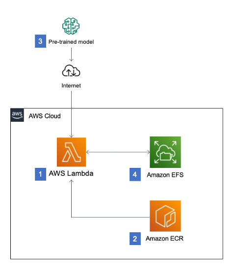
Our solution consists of an AWS Cloud Development Kit (AWS CDK) script that automatically provisions container image-based Lambda functions that perform ML inference using pre-trained Hugging Face models. This solution also includes Amazon Elastic File System (EFS) storage that is attached to the Lambda functions to cache the pre-trained models and reduce inference latency.Solution architecture

In this architectural diagram:

  1. Serverless inference is achieved by using Lambda functions that are based on container image
  2. The container image is stored in an Amazon Elastic Container Registry (ECR) repository within your account
  3. Pre-trained models are automatically downloaded from Hugging Face the first time the function is invoked
  4. Pre-trained models are cached within Amazon Elastic File System storage in order to improve inference latency

The solution includes Python scripts for two common NLP use cases:

  • Sentiment analysis: Identifying if a sentence indicates positive or negative sentiment. It uses a fine-tuned model on sst2, which is a GLUE task.
  • Summarization: Summarizing a body of text into a shorter, representative text. It uses a Bart model that was fine-tuned on the CNN / Daily Mail dataset.

For simplicity, both of these use cases are implemented using Hugging Face pipelines.

Prerequisites

The following is required to run this example:

Deploying the example application

  1. Clone the project to your development environment:
    git clone https://github.com/aws-samples/zero-administration-inference-with-aws-lambda-for-hugging-face.git
  2. Install the required dependencies:
    pip install -r requirements.txt
  3. Bootstrap the CDK. This command provisions the initial resources needed by the CDK to perform deployments:
    cdk bootstrap
  4. This command deploys the CDK application to its environment. During the deployment, the toolkit outputs progress indications:
    $ cdk deploy

Testing the application

After deployment, navigate to the AWS Management Console to find and test the Lambda functions. There is one for sentiment analysis and one for summarization.

To test:

  1. Enter “Lambda” in the search bar of the AWS Management Console:Console Search
  2. Filter the functions by entering “ServerlessHuggingFace”:Filtering functions
  3. Select the ServerlessHuggingFaceStack-sentimentXXXXX function:Select function
  4. In the Test event, enter the following snippet and then choose Test:Test function
{
   "text": "I'm so happy I could cry!"
}

The first invocation takes approximately one minute to complete. The initial Lambda function environment must be allocated and the pre-trained model must be downloaded from Hugging Face. Subsequent invocations are faster, as the Lambda function is already prepared and the pre-trained model is cached in EFS.Function test results

The JSON response shows the result of the sentiment analysis:

{
  "statusCode": 200,
  "body": {
    "label": "POSITIVE",
    "score": 0.9997532367706299
  }
}

Understanding the code structure

The code is organized using the following structure:

├── inference
│ ├── Dockerfile
│ ├── sentiment.py
│ └── summarization.py
├── app.py
└── ...

The inference directory contains:

  • The Dockerfile used to build a custom image to be able to run PyTorch Hugging Face inference using Lambda functions
  • The Python scripts that perform the actual ML inference

The sentiment.py script shows how to use a Hugging Face Transformers model:

import json
from transformers import pipeline

nlp = pipeline("sentiment-analysis")

def handler(event, context):
    response = {
        "statusCode": 200,
        "body": nlp(event['text'])[0]
    }
    return response

For each Python script in the inference directory, the CDK generates a Lambda function backed by a container image and a Python inference script.

CDK script

The CDK script is named app.py in the solution’s repository. The beginning of the script creates a virtual private cloud (VPC).

vpc = ec2.Vpc(self, 'Vpc', max_azs=2)

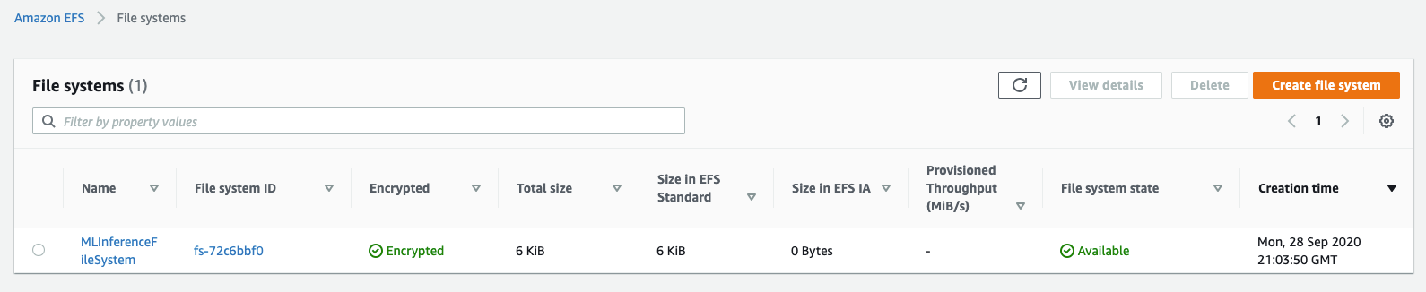
Next, it creates the EFS file system and an access point in EFS for the cached models:

        fs = efs.FileSystem(self, 'FileSystem',
                            vpc=vpc,
                            removal_policy=cdk.RemovalPolicy.DESTROY)
        access_point = fs.add_access_point('MLAccessPoint',
                                           create_acl=efs.Acl(
                                               owner_gid='1001', owner_uid='1001', permissions='750'),
                                           path="/export/models",
                                           posix_user=efs.PosixUser(gid="1001", uid="1001"))>

It iterates through the Python files in the inference directory:

docker_folder = os.path.dirname(os.path.realpath(__file__)) + "/inference"
pathlist = Path(docker_folder).rglob('*.py')
for path in pathlist:

And then creates the Lambda function that serves the inference requests:

            base = os.path.basename(path)
            filename = os.path.splitext(base)[0]
            # Lambda Function from docker image
            function = lambda_.DockerImageFunction(
                self, filename,
                code=lambda_.DockerImageCode.from_image_asset(docker_folder,
                                                              cmd=[
                                                                  filename+".handler"]
                                                              ),
                memory_size=8096,
                timeout=cdk.Duration.seconds(600),
                vpc=vpc,
                filesystem=lambda_.FileSystem.from_efs_access_point(
                    access_point, '/mnt/hf_models_cache'),
                environment={
                    "TRANSFORMERS_CACHE": "/mnt/hf_models_cache"},
            )

Adding a translator

Optionally, you can add more models by adding Python scripts in the inference directory. For example, add the following code in a file called translate-en2fr.py:

import json
from transformers 
import pipeline

en_fr_translator = pipeline('translation_en_to_fr')

def handler(event, context):
    response = {
        "statusCode": 200,
        "body": en_fr_translator(event['text'])[0]
    }
    return response

Then run:

$ cdk synth
$ cdk deploy

This creates a new endpoint to perform English to French translation.

Cleaning up

After you are finished experimenting with this project, run “cdk destroy” to remove all of the associated infrastructure.

Conclusion

This post shows how to perform ML inference for pre-trained Hugging Face models by using Lambda functions. To avoid repeatedly downloading the pre-trained models, this solution uses an EFS-based approach to model caching. This helps to achieve low-latency, near real-time inference. The solution is provided as infrastructure as code using Python and the AWS CDK.

We hope this blog post allows you to prototype quickly and include modern NLP techniques in your own products.

The Future of Machine Learning and Cybersecurity

Post Syndicated from Bruce Schneier original https://www.schneier.com/blog/archives/2021/06/the-future-of-machine-learning-and-cybersecurity.html

The Center for Security and Emerging Technology has a new report: “Machine Learning and Cybersecurity: Hype and Reality.” Here’s the bottom line:

The report offers four conclusions:

  • Machine learning can help defenders more accurately detect and triage potential attacks. However, in many cases these technologies are elaborations on long-standing methods — not fundamentally new approaches — that bring new attack surfaces of their own.
  • A wide range of specific tasks could be fully or partially automated with the use of machine learning, including some forms of vulnerability discovery, deception, and attack disruption. But many of the most transformative of these possibilities still require significant machine learning breakthroughs.
  • Overall, we anticipate that machine learning will provide incremental advances to cyber defenders, but it is unlikely to fundamentally transform the industry barring additional breakthroughs. Some of the most transformative impacts may come from making previously un- or under-utilized defensive strategies available to more organizations.
  • Although machine learning will be neither predominantly offense-biased nor defense-biased, it may subtly alter the threat landscape by making certain types of strategies more appealing to attackers or defenders.

Building a Hyper Self-Service, Distributed Tracing and Feedback System for Rule & Machine Learning (ML) Predictions

Post Syndicated from Grab Tech original https://engineering.grab.com/building-hyper-self-service-distributed-tracing-feedback-system

Introduction

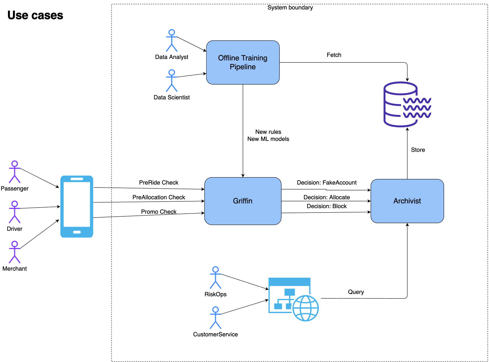
In Grab, the Trust, Identity, Safety, and Security (TISS) is a team of software engineers and AI developers working on fraud detection, login identity check, safety issues, etc. There are many TISS services, like grab-fraud, grab-safety, and grab-id. They make billions of business decisions daily using the Griffin rule engine, which determines if a passenger can book a trip, get a food promotion, or if a driver gets a delivery booking.

There is a natural demand to log down all these important business decisions, store them and query them interactively or in batches. Data analysts and scientists need to use the data to train their machine learning models. RiskOps and customer service teams can query the historical data and help consumers.

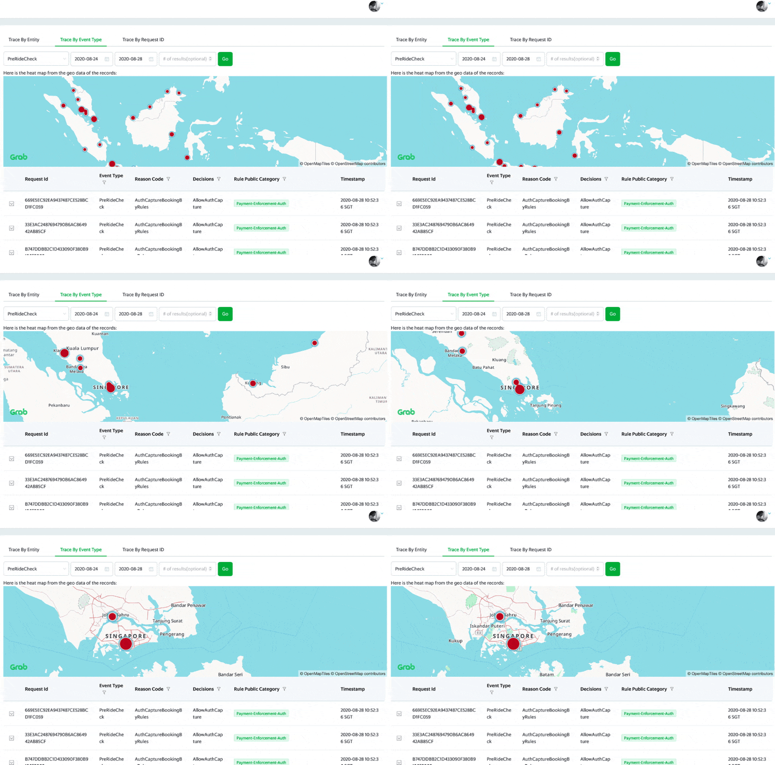
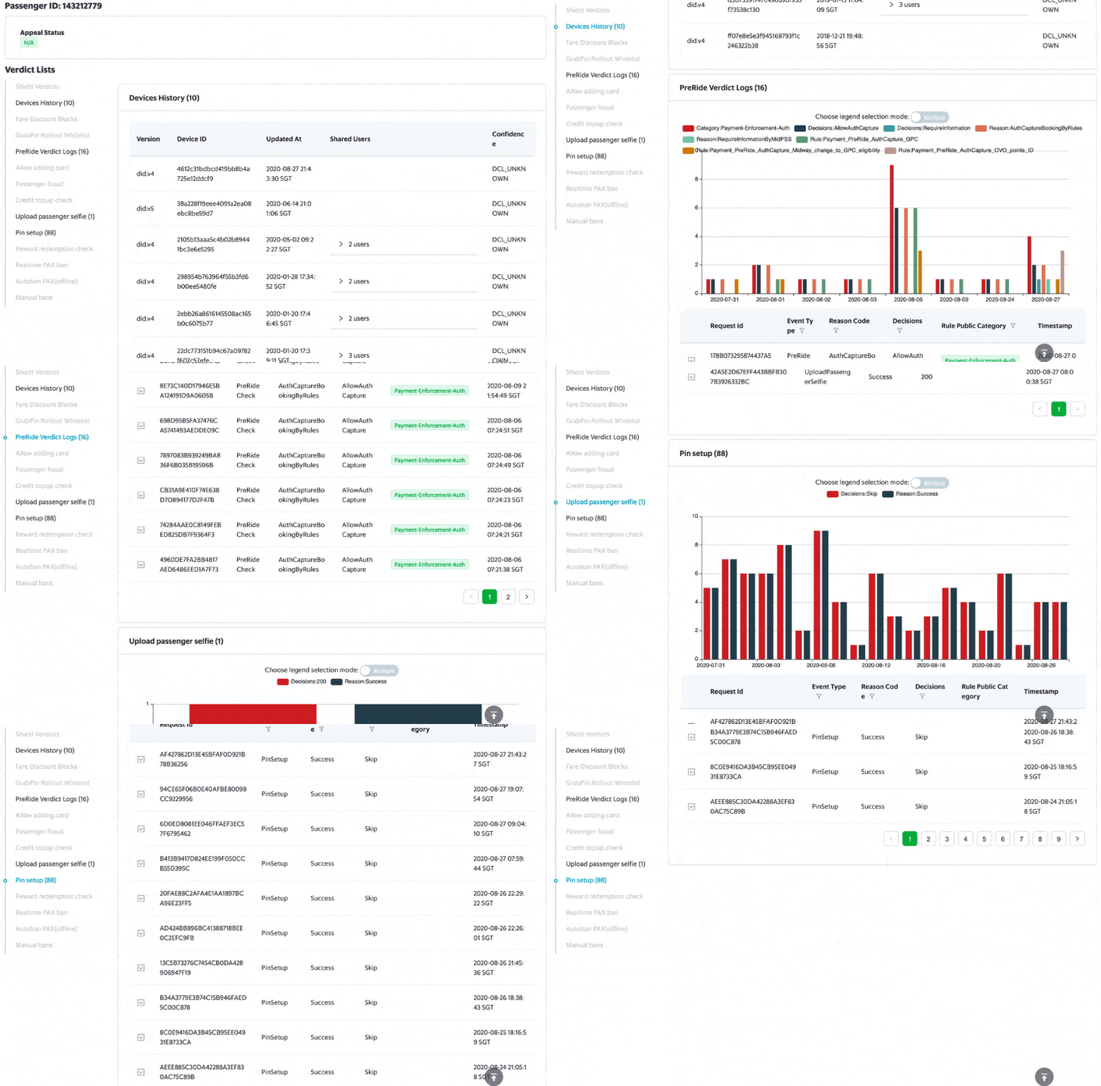
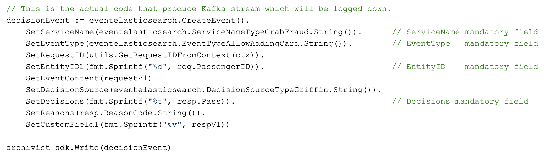
That’s where Archivist comes in; it is a new tracing, statistics and feedback system for rule and machine learning-based predictions. It is reliable and performant. Its innovative data schema is flexible for storing events from different business scenarios. Finally, it provides a user-friendly UI, which has access control for classified data.

Here are the impacts Archivist has already made:

  • Currently, there are 2 teams with a total of 5 services and about 50 business scenarios using Archivist. The scenarios include fraud prevention (e.g. DriverBan, PassengerBan), payment checks (e.g. PayoutBlockCheck, PromoCheck), and identity check events like PinTrigger.
  • It takes only a few minutes to onboard a new business scenario (event type), by using the configuration page on the user portal. Previously, it took at least 1 to 2 days.
  • Each day, Archivist logs down 80 million logs to the ElasticSearch cluster, which is about 200GB of data.
  • Each week, Customer Experience (CE)/Risk Ops goes to the user portal and checks Archivist logs for about 2,000 distinct customers. They can search based on numerous dimensions such as the Passenger/DriverID, phone number, request ID, booking code and payment fingerprint.

Background

Each day, TISS services make billions of business decisions (predictions), based on the Griffin rule engine and ML models.

After the predictions are made, there are still some tough questions for these services to answer.

  • If Risk Ops believes a prediction is false-positive, a consumer could be banned. If this happens, how can consumers or Risk Ops report or feedback this information to the new rule and ML model training quickly?
  • As CustomService/Data Scientists investigating any tickets opened due to TISS predictions/decisions, how do you know which rules and data were used? E.g. why the passenger triggered a selfie, or why a booking was blocked.
  • After Data Analysts/Data Scientists (DA/DS) launch a new rule/model, how can they track the performance in fine-granularity and in real-time? E.g. week-over-week rule performance in a country or city.
  • How can DA/DS access all prediction data for data analysis or model training?
  • How can the system keep up with Grab’s business launch speed, with maximum self-service?

Problem

To answer the questions above, TISS services previously used company-wide Kibana to log predictions.  For example, a log looks like: PassengerID:123,Scenario:PinTrigger,Decision:Trigger,.... This logging method had some obvious issues:

  • Logs in plain text don’t have any structure and are not friendly to ML model training as most ML models need processed data to make accurate predictions.
  • Furthermore, there is no fine-granularity access control for developers in Kibana.
  • Developers, DA and DS have no access control while CEs have no access at all. So CE cannot easily see the data and DA/DS cannot easily process the data.

To address all the Kibana log issues, we developed ActionTrace, a code library with a well-structured data schema. The logs, also called documents, are stored in a dedicated ElasticSearch cluster with access control implemented. However, after using it for a while, we found that it still needed some improvements.

  1. Each business scenario involves different types of entities and ActionTrace is not fully self-service. This means that a lot of development work was needed to support fast-launching business scenarios. Here are some examples:
    • The main entities in the taxi business are Driver and Passenger,

    • The main entities in the food business can be Merchant, Driver and Consumer.

    All these entities will need to be manually added into the ActionTrace data schema.

  2.  Each business scenario may have their own custom information logged. Because there is no overlap, each of them will correspond to a new field in the data schema. For example:
    • For any scenario involving payment, a valid payment method and expiration date is logged.
    • For the taxi business, the geohash is logged.
  3.   To store the log data from ActionTrace, different teams need to set up and manage their own ElasticSearch clusters. This increases hardware and maintenance costs.

  4. There was a simple Web UI created for viewing logs from ActionTrace, but there was still no access control in fine granularity.

Solution

We developed Archivist, a new tracing, statistics, and feedback system for ML/rule-based prediction events. It’s centralised, performant and flexible. It answers all the issues mentioned above, and it is an improvement over all the existing solutions we have mentioned previously.

The key improvements are:

  • User-defined entities and custom fields
    • There are no predefined entity types. Users can define up to 5 entity types (E.g. PassengerId, DriverId, PhoneNumber, PaymentMethodId, etc.).
    • Similarly, there are a limited number of custom data fields to use, in addition to the common data fields shared by all business scenarios.
  • A dedicated service shared by all other services
    • Each service writes its prediction events to a Kafka stream. Archivist then reads the stream and writes to the ElasticSearch cluster.
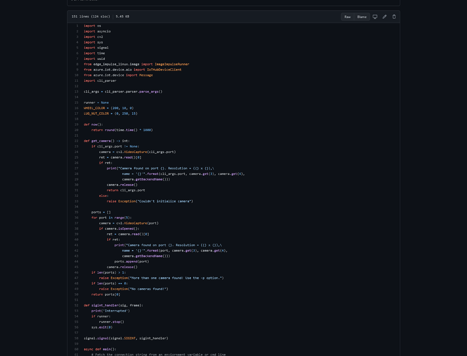
    • The data writes are buffered, so it is easy to handle traffic surges in peak time.
    • Different services share the same Elastic Cloud Enterprise (ECE) cluster, but they create their own daily file indices so the costs can be split fairly.
  • Better support for data mining, prediction stats and feedback
    • Kafka stream data are simultaneously written to AWS S3. DA/DS can use the PrestoDB SQL query engine to mine the data.
    • There is an internal web portal for viewing Archivist logs. Customer service teams and Ops can use no-risk data to address CE tickets, while DA, DS and developers can view high-risk data for code/rule debugging.
  • A reduction of development days to support new business launches
    • Previously, it took a week to modify and deploy the ActionTrace data schema. Now, it only takes several minutes to configure event schemas in the user portal.
  • Saves time in RiskOps/CE investigations
    • With the new web UI which has access control in place, the different roles in the company, like Customer service and Data analysts, can access the Archivist events with different levels of permissions.
    • It takes only a few clicks for them to find the relevant events that impact the drivers/passengers.

Architecture Details

Archivist’s system architecture is shown in the diagram below.

Archivist system architecture
  • Different services (like fraud-detection, safety-allocation, etc.) use a simple SDK to write data to a Kafka stream (the left side of the diagram).
  • In the centre of Archivist is an event processor. It reads data from Kafka, and writes them to ElasticSearch (ES).
  • The Kafka stream writes to the Amazon S3 data lake, so DA/DS can use the Presto SQL query engine to query them.
  • The user portal (bottom right) can be used to view the Archivist log and update configurations. It also sends all the web requests to the API Handler in the centre.

The following diagram shows how internal and external users use Archivist as well as the interaction between the Griffin rule engine and Archivist.

Archivist use cases
Archivist use cases

Flexible Event Schema

In Archivist, a prediction/decision is called an event. The event schema can be divided into 3 main parts conceptually.

  1. Data partitioning: Fields like service_name and event_type categorise data by services and business scenarios.
    Field name Type Example Notes
    service_name string GrabFraud Name of the Service
    event_type string PreRide PaxBan/SafeAllocation
  2. Business decision making: request_id, decisions, reasons, event_content are used to record the business decision, the reason and the context (E.g. The input features of machine learning algorithms).
    Field name Type Example Notes
    request_id string a16756e8-efe2-472b-b614-ec6ae08a5912 a 32-digit id for web requests
    event_content string Event context
    decisions [string] [“NotAllowBook”, “SMS”] A list
    reasons string json payload string of the response from engine.
  3. Customisation: Archivist provides user-defined entities and custom fields that we feel are sufficient and flexible for handling different business scenarios.
    Field name Type Example Notes
    entity_type_1 string Passenger
    entity_id_1 string 12151
    entity_type_2 string Driver
    entity_id_2 string 341521-rdxf36767
    string
    entity_id_5 string
    custom_field_type_1 string “MessageToUser”
    custom_field_1 string “please contact Ops” User defined fields
    custom_field_type_2 “Prediction rule:”
    custom_field_2 string “ML rule: 123, version:2”
    string
    custom_field_6 string

A User Portal to Support Querying, Prediction Stats and Feedback

DA, DS, Ops and CE can access the internal user portal to see the prediction events, individually and on an aggregated city level.

A snapshot of the Archivist logs showing the aggregation of the data in each city

There are graphs on the portal, showing the rule/model performance on individual customers over a period of time.

Rule performance on a customer over a period of time

How to Use Archivist for Your Service

If you want to get onboard Archivist, the coding effort is minimal. Here is an example of a code snippet to log an event:

Code snippet to log an event

Lessons

During the implementation of Archivist, we learnt some things:

  • A good system needs to support multi-tenants from the beginning. Originally, we thought we could use just one Kafka stream, and put all the documents from different teams into one ElasticSearch (ES) index. But after one team insisted on keeping their data separately from others, we created more Kafka streams and ES indexes. We realised that this way, it’s easier for us to manage data and share the cost fairly.
  • Shortly after we launched Archivist, there was an incident where the ES data writes were choked. Because each document write is a goroutine, the number of goroutines increased to 400k and the memory usage reached 100% within minutes. We added a patch (2 lines of code) to limit the maximum number of goroutines in our system. Since then, we haven’t had any more severe incidents in Archivist.

Join Us

Grab is the leading superapp platform in Southeast Asia, providing everyday services that matter to consumers. More than just a ride-hailing and food delivery app, Grab offers a wide range of on-demand services in the region, including mobility, food, package and grocery delivery services, mobile payments, and financial services across 428 cities in eight countries.

Powered by technology and driven by heart, our mission is to drive Southeast Asia forward by creating economic empowerment for everyone. If this mission speaks to you, join our team today!

How We Improved Agent Chat Efficiency with Machine Learning

Post Syndicated from Grab Tech original https://engineering.grab.com/how-we-improved-agent-chat-efficiency-with-ml

In previous articles (see Grab’s in-house chat platform, workforce routing), we shared how chat has grown to become one of the primary channels for support in the last few years.

With continuous chat growth and a new in-house tool, helping our agents be more efficient and productive was key to ensure a faster support time for our users and scale chat even further.
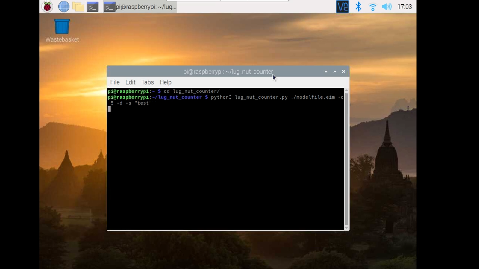
Starting from the analysis on the usage of another third-party tool as well as some shadowing sessions, we realised that building a templated-based feature wouldn’t help. We needed to offer personalisation capabilities, as our consumer support specialists care about their writing style and tone, and using templates often feels robotic.

We decided to build a machine learning model, called SmartChat, which offers contextual suggestions by leveraging several sources of internal data, helping our chat specialists type much faster, and hence serving more consumers.

In this article, we are going to explain the process from problem discovery to design iterations, and share how the model was implemented from both a data science and software engineering perspective.

How SmartChat Works

Diving Deeper into the Problem

Agent productivity became a key part in the process of scaling chat as a channel for support.

After splitting chat time into all its components, we noted that agent typing time represented a big portion of the chat support journey, making it the perfect problem to tackle next.

After some analysis on the usage of the third-party chat tool, we found out that even with functionalities such as canned messages, 85% of the messages were still free typed.

Hours of shadowing sessions also confirmed that the consumer support specialists liked to add their own flair. They would often use the template and adjust it to their style, which took more time than just writing it on the spot. With this in mind, it was obvious that templates wouldn’t be too helpful, unless they provided some degree of personalisation.
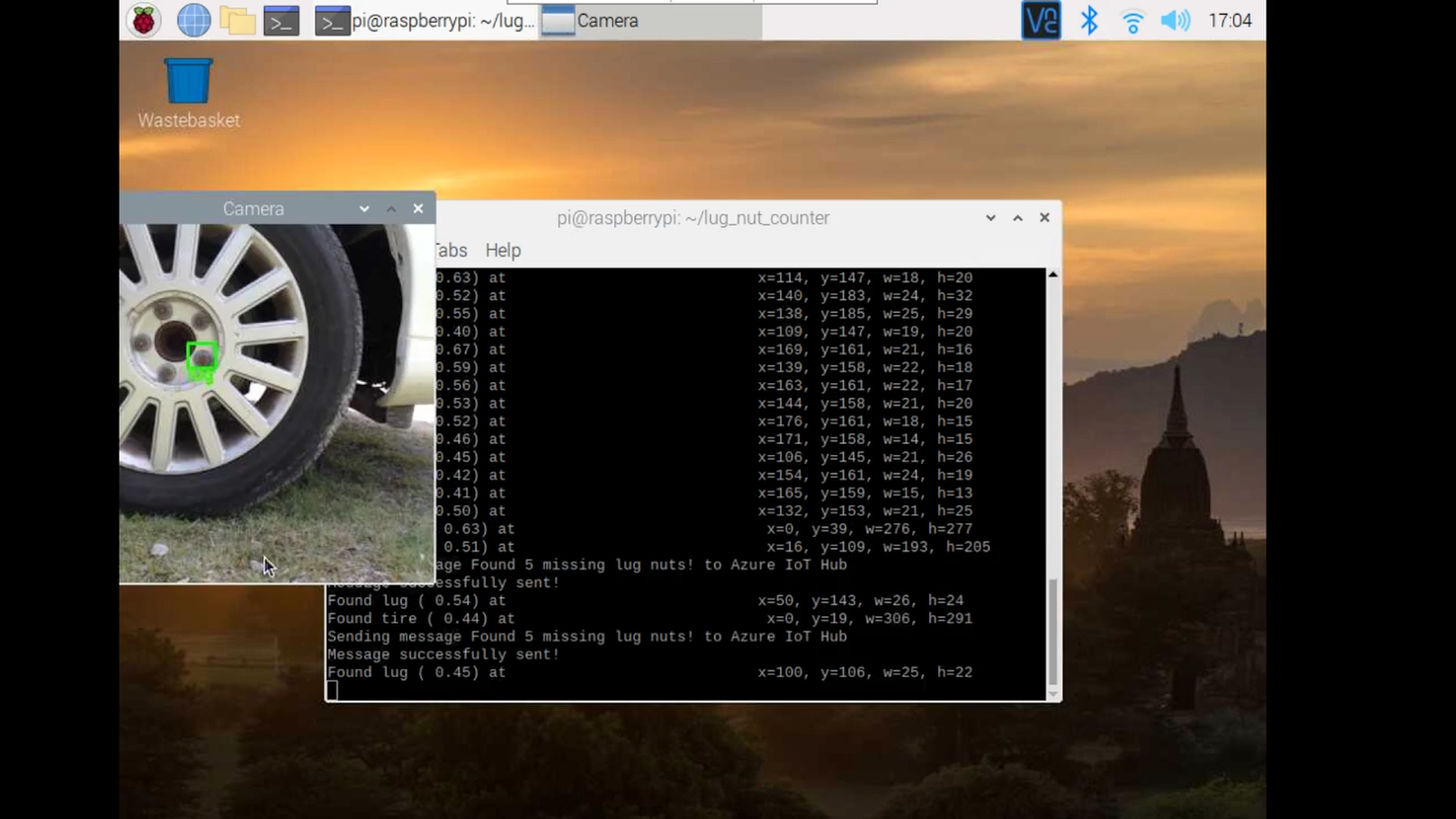
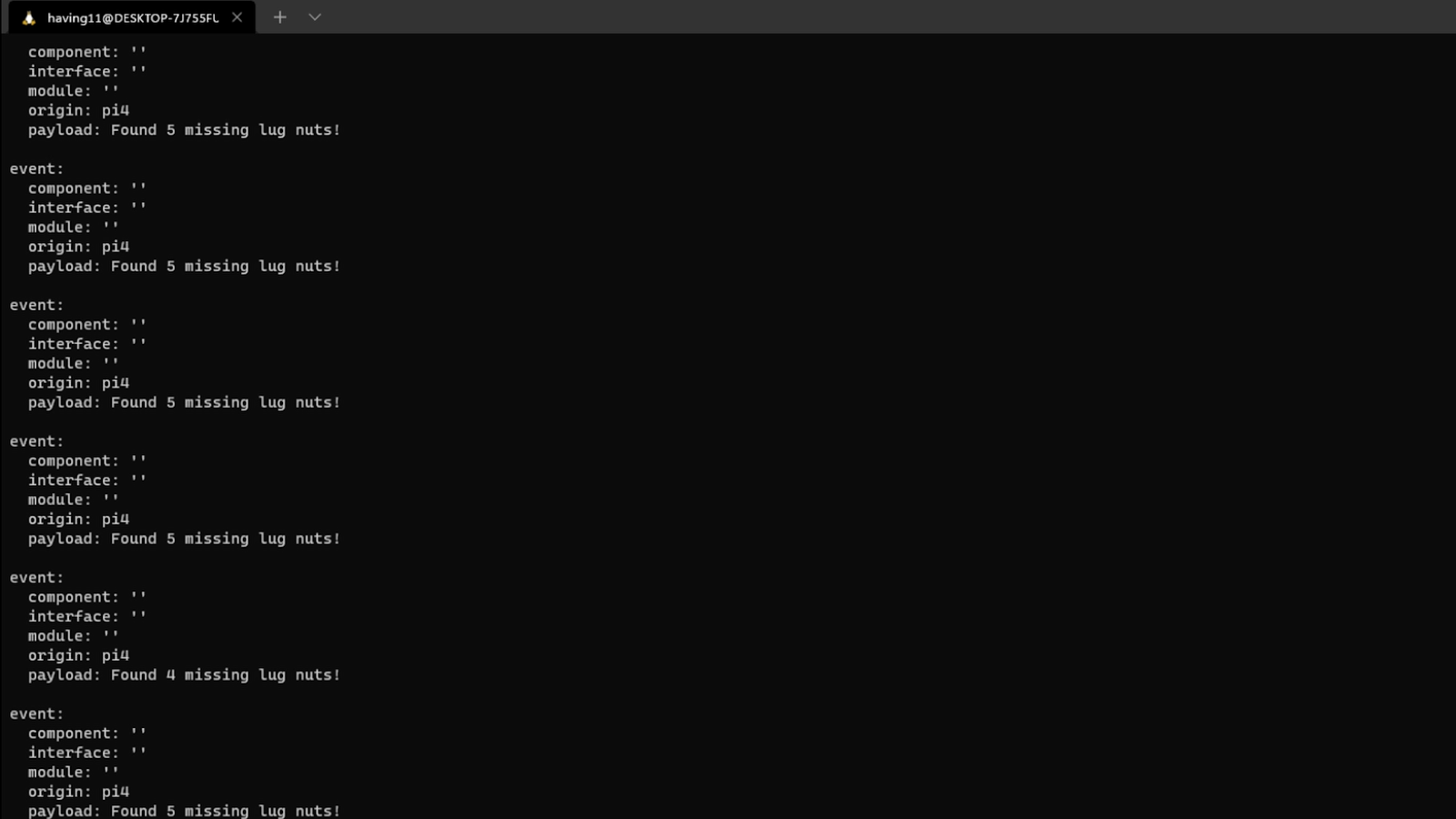
We needed something that reduces typing time and also:

  • Allows some degree of personalisation, so that answers don’t seem robotic and repeated.
  • Works with multiple languages and nuances, considering Grab operates in 8 markets, even some of the English markets have some slight differences in commonly used words.
  • It’s contextual to the problem and takes into account the user type, issue reported, and even the time of the day.
  • Ideally doesn’t require any maintenance effort, such as having to keep templates updated whenever there’s a change in policies.

Considering the constraints, this seemed to be the perfect candidate for a machine learning-based functionality, which predicts sentence completion by considering all the context about the user, issue and even the latest messages exchanged.

Usability is Key

To fulfil the hypothesis, there are a few design considerations:

  1. Minimising the learning curve for agents.
  2. Avoiding visual clutter if recommendations are not relevant.

To increase the probability of predicting an agent’s message, one of the design explorations is to allow agents to select the top 3 predictions (Design 1). To onboard agents, we designed a quick tip to activate SmartChat using keyboard shortcuts.

By displaying the top 3 recommendations, we learnt that it slowed agents down as they started to read all options even if the recommendations were not helpful. Besides, by triggering this component upon every recommendable text, it became a distraction as they were forced to pause.

In our next design iteration, we decided to leverage and reuse the interaction of SmartChat from a familiar platform that agents are using – Gmail’s Smart Compose. As agents are familiar with Gmail, the learning curve for this feature would be less steep. For first time users, agents will see a “Press tab” tooltip, which will activate the text recommendation. The tooltip will disappear after 5 times of use.

To relearn the shortcut, agents can hover over the recommended text.

How We Track Progress

Knowing that this feature would come in multiple iterations, we had to find ways to track how well we were doing progressively, so we decided to measure the different components of chat time.

We realised that the agent typing time is affected by:

  • Percentage of characters saved. This tells us that the model predicted correctly, and also saved time. This metric should increase as the model improves.
  • Model’s effectiveness. The agent writes the least number of characters possible before getting the right suggestion, which should decrease as the model learns.
  • Acceptance rate. This tells us how many messages were written with the help of the model. It is a good proxy for feature usage and model capabilities.
  • Latency. If the suggestion is not shown in about 100-200ms, the agent would not notice the text and keep typing.

Architecture

The architecture involves support specialists initiating the fetch suggestion request, which is sent for evaluation to the machine learning model through API gateway. This ensures that only authenticated requests are allowed to go through and also ensures that we have proper rate limiting applied.

We have an internal platform called Catwalk, which is a microservice that offers the capability to execute machine learning models as a HTTP service. We used the Presto query engine to calculate and analyse the results from the experiment.

Designing the Machine Learning Model

I am sure all of us can remember an experiment we did in school when we had to catch a falling ruler. For those who have not done this experiment, feel free to try it at home! The purpose of this experiment is to define a ballpark number for typical human reaction time (equations also included in the video link).

Typically, the human reaction time ranges from 100ms to 300ms, with a median of about 250ms (read more here). Hence, we decided to set the upper bound for SmartChat response time to be 200ms while deciding the approach. Otherwise, the experience would be affected as the agents would notice a delay in the suggestions. To achieve this, we had to manage the model’s complexity and ensure that it achieves the optimal time performance.

Taking into consideration network latencies, the machine learning model would need to churn out predictions in less than 100ms, in order for the entire product to achieve a maximum 200ms refresh rate.

As such, a few key components were considered:

  • Model Tokenisation
    • Model input/output tokenisation needs to be implemented along with the model’s core logic so that it is done in one network request.
    • Model tokenisation needs to be lightweight and cheap to compute.
  • Model Architecture
    • This is a typical sequence-to-sequence (seq2seq) task so the model needs to be complex enough to account for the auto-regressive nature of seq2seq tasks.
    • We could not use pure attention-based models, which are usually state of the art for seq2seq tasks, as they are bulky and computationally expensive.
  • Model Service
    • The model serving platform should be executed on a low-level, highly performant framework.

Our proposed solution considers the points listed above. We have chosen to develop in Tensorflow (TF), which is a well-supported framework for machine learning models and application building.

For Latin-based languages, we used a simple whitespace tokenizer, which is serialisable in the TF graph using the tensorflow-text package.

import tensorflow_text as text

tokenizer = text.WhitespaceTokenizer()

For the model architecture, we considered a few options but eventually settled for a simple recurrent neural network architecture (RNN), in an Encoder-Decoder structure:

  • Encoder
    • Whitespace tokenisation
    • Single layered Bi-Directional RNN
    • Gated-Recurrent Unit (GRU) Cell
  • Decoder

    • Single layered Uni-Directional RNN
    • Gated-Recurrent Unit (GRU) Cell
  • Optimisation
    • Teacher-forcing in training, Greedy decoding in production
    • Trained with a cross-entropy loss function
    • Using ADAM (Kingma and Ba) optimiser

Features

To provide context for the sentence completion tasks, we provided the following features as model inputs:

  • Past conversations between the chat agent and the user
  • Time of the day
  • User type (Driver-partners, Consumers, etc.)
  • Entrypoint into the chat (e.g. an article on cancelling a food order)

These features give the model the ability to generalise beyond a simple language model, with additional context on the nature of contact for support. Such experiences also provide a better user experience and a more customised user experience.

For example, the model is better aware of the nature of time in addressing “Good {Morning/Afternoon/Evening}” given the time of the day input, as well as being able to interpret meal times in the case of food orders. E.g. “We have contacted the driver, your {breakfast/lunch/dinner} will be arriving shortly”.

Typeahead Solution for the User Interface

With our goal to provide a seamless experience in showing suggestions to accepting them, we decided to implement a typeahead solution in the chat input area. This solution had to be implemented with the ReactJS library, as the internal web-app used by our support specialist for handling chats is built in React.

There were a few ways to achieve this:

  1. Modify the Document Object Model (DOM) using Javascript to show suggestions by positioning them over the input HTML tag based on the cursor position.
  2. Use a content editable div and have the suggestion span render conditionally.

After evaluating the complexity in both approaches, the second solution seemed to be the better choice, as it is more aligned with the React way of doing things: avoid DOM manipulations as much as possible.

However, when a suggestion is accepted we would still need to update the content editable div through DOM manipulation. It cannot be added to React’s state as it creates a laggy experience for the user to visualise what they type.

Here is a code snippet for the implementation:

import React, { Component } from 'react';
import liveChatInstance from './live-chat';

export class ChatInput extends Component {
 constructor(props) {
   super(props);
   this.state = {
     suggestion: '',
   };
 }

 getCurrentInput = () => {
   const { roomID } = this.props;
   const inputDiv = document.getElementById(`input_content_${roomID}`);
   const suggestionSpan = document.getElementById(
     `suggestion_content_${roomID}`,
   );

   // put the check for extra safety in case suggestion span is accidentally cleared
   if (suggestionSpan) {
     const range = document.createRange();
     range.setStart(inputDiv, 0);
     range.setEndBefore(suggestionSpan);
     return range.toString(); // content before suggestion span in input div
   }
   return inputDiv.textContent;
 };

 handleKeyDown = async e => {
   const { roomID } = this.props;
   // tab or right arrow for accepting suggestion
   if (this.state.suggestion && (e.keyCode === 9 || e.keyCode === 39)) {
     e.preventDefault();
     e.stopPropagation();
     this.insertContent(this.state.suggestion);
     this.setState({ suggestion: '' });
   }
   const parsedValue = this.getCurrentInput();
   // space
   if (e.keyCode === 32 && !this.state.suggestion && parsedValue) {
     // fetch suggestion
     const prediction = await liveChatInstance.getSmartComposePrediction(
       parsedValue.trim(), roomID);
     this.setState({ suggestion: prediction })
   }
 };

 insertContent = content => {
   // insert content behind cursor
   const { roomID } = this.props;
   const inputDiv = document.getElementById(`input_content_${roomID}`);
   if (inputDiv) {
     inputDiv.focus();
     const sel = window.getSelection();
     const range = sel.getRangeAt(0);
     if (sel.getRangeAt && sel.rangeCount) {
       range.insertNode(document.createTextNode(content));
       range.collapse();
     }
   }
 };

 render() {
   const { roomID } = this.props;
   return (
     <div className="message_wrapper">
       <div
         id={`input_content_${roomID}`}
         role={'textbox'}
         contentEditable
         spellCheck
         onKeyDown={this.handleKeyDown}
       >
         {!!this.state.suggestion.length && (
           <span
             contentEditable={false}
             id={`suggestion_content_${roomID}`}
           >
             {this.state.suggestion}
           </span>
         )}
       </div>
     </div>
   );
 }
}

The solution uses the spacebar as the trigger for fetching the suggestion from the ML model and stores them in a React state. The ML model prediction is then rendered in a dynamically rendered span.

We used the window.getSelection() and range APIs to:

  • Find the current input value
  • Insert the suggestion
  • Clear the input to type a new message

The implementation has also considered the following:

  • Caching. API calls are made on every space character to fetch the prediction. To reduce the number of API calls, we also cached the prediction until it differs from the user input.
  • Recover placeholder. There are data fields that are specific to the agent and consumer, such as agent name and user phone number, and these data fields are replaced by placeholders for model training. The implementation recovers the placeholders in the prediction before showing it on the UI.
  • Control rollout. Since rollout is by percentage per country, the implementation has to ensure that only certain users can access predictions from their country chat model.
  • Aggregate and send metrics. Metrics are gathered and sent for each chat message.

Results

The initial experiment results suggested that we managed to save 20% of characters, which improved the efficiency of our agents by 12% as they were able to resolve the queries faster. These numbers exceeded our expectations and as a result, we decided to move forward by rolling SmartChat out regionally.

What’s Next?

In the upcoming iteration, we are going to focus on non-Latin language support, caching, and continuous training.

Non-Latin Language Support and Caching

The current model only works with Latin languages, where sentences consist of space-separated words. We are looking to provide support for non-Latin languages such as Thai and Vietnamese. The result would also be cached in the frontend to reduce the number of API calls, providing the prediction faster for the agents.

Continuous Training

The current machine learning model is built with training data derived from historical chat data. In order to teach the model and improve the metrics mentioned in our goals, we will enhance the model by letting it learn from data gathered in day-to-day chat conversations. Along with this, we are going to train the model to give better responses by providing more context about the conversations.

Seeing how effective this solution has been for our chat agents, we would also like to expose this to the end consumers to help them express their concerns faster and improve their overall chat experience.


Special thanks to Kok Keong Matthew Yeow, who helped to build the architecture and implementation in a scalable way.
—-

Join Us

Grab is the leading superapp platform in Southeast Asia, providing everyday services that matter to consumers. More than just a ride-hailing and food delivery app, Grab offers a wide range of on-demand services in the region, including mobility, food, package and grocery delivery services, mobile payments, and financial services across 428 cities in eight countries.

Powered by technology and driven by heart, our mission is to drive Southeast Asia forward by creating economic empowerment for everyone. If this mission speaks to you, join our team today!

Machine learning and depth estimation using Raspberry Pi

Post Syndicated from David Plowman original https://www.raspberrypi.org/blog/machine-learning-and-depth-estimation-using-raspberry-pi/

One of our engineers, David Plowman, describes machine learning and shares news of a Raspberry Pi depth estimation challenge run by ETH Zürich (Swiss Federal Institute of Technology).

Spoiler alert – it’s all happening virtually, so you can definitely make the trip and attend, or maybe even enter yourself.

What is Machine Learning?

Machine Learning (ML) and Artificial Intelligence (AI) are some of the top engineering-related buzzwords of the moment, and foremost among current ML paradigms is probably the Artificial Neural Network (ANN).

They involve millions of tiny calculations, merged together in a giant biologically inspired network – hence the name. These networks typically have millions of parameters that control each calculation, and they must be optimised for every different task at hand.

This process of optimising the parameters so that a given set of inputs correctly produces a known set of outputs is known as training, and is what gives rise to the sense that the network is “learning”.

A popular type of ANN used for processing images is the Convolutional Neural Network. Many small calculations are performed on groups of input pixels to produce each output pixel

Machine Learning frameworks

A number of well known companies produce free ML frameworks that you can download and use on your own computer. The network training procedure runs best on machines with powerful CPUs and GPUs, but even using one of these pre-trained networks (known as inference) can be quite expensive.

One of the most popular frameworks is Google’s TensorFlow (TF), and since this is rather resource intensive, they also produce a cut-down version optimised for less powerful platforms. This is TensorFlow Lite (TFLite), which can be run effectively on Raspberry Pi.

Depth estimation

ANNs have proven very adept at a wide variety of image processing tasks, most notably object classification and detection, but also depth estimation. This is the process of taking one or more images and working out how far away every part of the scene is from the camera, producing a depth map.

Here’s an example:

Depth estimation example using a truck

The image on the right shows, by the brightness of each pixel, how far away the objects in the original (left-hand) image are from the camera (darker = nearer).

We distinguish between stereo depth estimation, which starts with a stereo pair of images (taken from marginally different viewpoints; here, parallax can be used to inform the algorithm), and monocular depth estimation, working from just a single image.

The applications of such techniques should be clear, ranging from robots that need to understand and navigate their environments, to the fake bokeh effects beloved of many modern smartphone cameras.

Depth Estimation Challenge

C V P R conference logo with dark blue background and the edge of the earth covered in scattered orange lights connected by white lines

We were very interested then to learn that, as part of the CVPR (Computer Vision and Pattern Recognition) 2021 conference, Andrey Ignatov and Radu Timofte of ETH Zürich were planning to run a Monocular Depth Estimation Challenge. They are specifically targeting the Raspberry Pi 4 platform running TFLite, and we are delighted to support this effort.

For more information, or indeed if any technically minded readers are interested in entering the challenge, please visit:

The conference and workshops are all taking place virtually in June, and we’ll be sure to update our blog with some of the results and models produced for Raspberry Pi 4 by the competing teams. We wish them all good luck!

The post Machine learning and depth estimation using Raspberry Pi appeared first on Raspberry Pi.

Resource leak detection in Amazon CodeGuru Reviewer

Post Syndicated from Pranav Garg original https://aws.amazon.com/blogs/devops/resource-leak-detection-in-amazon-codeguru/

This post discusses the resource leak detector for Java in Amazon CodeGuru Reviewer. CodeGuru Reviewer automatically analyzes pull requests (created in supported repositories such as AWS CodeCommit, GitHub, GitHub Enterprise, and Bitbucket) and generates recommendations for improving code quality. For more information, see Automating code reviews and application profiling with Amazon CodeGuru. This blog does not describe the resource leak detector for Python programs that is now available in preview.

What are resource leaks?

Resources are objects with a limited availability within a computing system. These typically include objects managed by the operating system, such as file handles, database connections, and network sockets. Because the number of such resources in a system is limited, they must be released by an application as soon as they are used. Otherwise, you will run out of resources and you won’t be able to allocate new ones. The paradigm of acquiring a resource and releasing it is also followed by other categories of objects such as metric wrappers and timers.

Resource leaks are bugs that arise when a program doesn’t release the resources it has acquired. Resource leaks can lead to resource exhaustion. In the worst case, they can cause the system to slow down or even crash.

Starting with Java 7, most classes holding resources implement the java.lang.AutoCloseable interface and provide a close() method to release them. However, a close() call in source code doesn’t guarantee that the resource is released along all program execution paths. For example, in the following sample code, resource r is acquired by calling its constructor and is closed along the path corresponding to the if branch, shown using green arrows. To ensure that the acquired resource doesn’t leak, you must also close r along the path corresponding to the else branch (the path shown using red arrows).

A resource must be closed along all execution paths to prevent resource leaks

Often, resource leaks manifest themselves along code paths that aren’t frequently run, or under a heavy system load, or after the system has been running for a long time. As a result, such leaks are latent and can remain dormant in source code for long periods of time before manifesting themselves in production environments. This is the primary reason why resource leak bugs are difficult to detect or replicate during testing, and why automatically detecting these bugs during pull requests and code scans is important.

Detecting resource leaks in CodeGuru Reviewer

For this post, we consider the following Java code snippet. In this code, method getConnection() attempts to create a connection in the connection pool associated with a data source. Typically, a connection pool limits the maximum number of connections that can remain open at any given time. As a result, you must close connections after their use so as to not exhaust this limit.

 1     private Connection getConnection(final BasicDataSource dataSource, ...)
               throws ValidateConnectionException, SQLException {
 2         boolean connectionAcquired = false;
 3         // Retrying three times to get the connection.
 4         for (int attempt = 0; attempt < CONNECTION_RETRIES; ++attempt) {
 5             Connection connection = dataSource.getConnection();
 6             // validateConnection may throw ValidateConnectionException
 7             if (! validateConnection(connection, ...)) {
 8                 // connection is invalid
 9                 DbUtils.closeQuietly(connection);
10             } else {
11                 // connection is established
12                 connectionAcquired = true;
13                 return connection;
14             }
15         }
16         return null;
17     }

At first glance, it seems that the method getConnection() doesn’t leak connection resources. If a valid connection is established in the connection pool (else branch on line 10 is taken), the method getConnection() returns it to the client for use (line 13). If the connection established is invalid (if branch on line 7 is taken), it’s closed in line 9 before another attempt is made to establish a connection.

However, method validateConnection() at line 7 can throw a ValidateConnectionException. If this exception is thrown after a connection is established at line 5, the connection is neither closed in this method nor is it returned upstream to the client to be closed later. Furthermore, if this exceptional code path runs frequently, for instance, if the validation logic throws on a specific recurring service request, each new request causes a connection to leak in the connection pool. Eventually, the client can’t acquire new connections to the data source, impacting the availability of the service.

A typical recommendation to prevent resource leak bugs is to declare the resource objects in a try-with-resources statement block. However, we can’t use try-with-resources to fix the preceding method because this method is required to return an open connection for use in the upstream client. The CodeGuru Reviewer recommendation for the preceding code snippet is as follows:

“Consider closing the following resource: connection. The resource is referenced at line 7. The resource is closed at line 9. The resource is returned at line 13. There are other execution paths that don’t close the resource or return it, for example, when validateConnection throws an exception. To prevent this resource leak, close connection along these other paths before you exit this method.”

As mentioned in the Reviewer recommendation, to prevent this resource leak, you must close the established connection when method validateConnection() throws an exception. This can be achieved by inserting the validation logic (lines 7–14) in a try block. In the finally block associated with this try, the connection must be closed by calling DbUtils.closeQuietly(connection) if connectionAcquired == false. The method getConnection() after this fix has been applied is as follows:

private Connection getConnection(final BasicDataSource dataSource, ...) 
        throws ValidateConnectionException, SQLException {
    boolean connectionAcquired = false;
    // Retrying three times to get the connection.
    for (int attempt = 0; attempt < CONNECTION_RETRIES; ++attempt) {
        Connection connection = dataSource.getConnection();
        try {
            // validateConnection may throw ValidateConnectionException
            if (! validateConnection(connection, ...)) {
                // connection is invalid
                DbUtils.closeQuietly(connection);
            } else {
                // connection is established
                connectionAcquired = true;
                return connection;
            }
        } finally {
            if (!connectionAcquired) {
                DBUtils.closeQuietly(connection);
            }
        }
    }
    return null;
}

As shown in this example, resource leaks in production services can be very disruptive. Furthermore, leaks that manifest along exceptional or less frequently run code paths can be hard to detect or replicate during testing and can remain dormant in the code for long periods of time before manifesting themselves in production environments. With the resource leak detector, you can detect such leaks on objects belonging to a large number of popular Java types such as file streams, database connections, network sockets, timers and metrics, etc.

Combining static code analysis with machine learning for accurate resource leak detection

In this section, we dive deep into the inner workings of the resource leak detector. The resource leak detector in CodeGuru Reviewer uses static analysis algorithms and techniques. Static analysis algorithms perform code analysis without running the code. These algorithms are generally prone to high false positives (the tool might report correct code as having a bug). If the number of these false positives is high, it can lead to alarm fatigue and low adoption of the tool. As a result, the resource leak detector in CodeGuru Reviewer prioritizes precision over recall— the findings we surface are resource leaks with a high accuracy, though CodeGuru Reviewer could potentially miss some resource leak findings.

The main reason for false positives in static code analysis is incomplete information available to the analysis. CodeGuru Reviewer requires only the Java source files and doesn’t require all dependencies or the build artifacts. Not requiring the external dependencies or the build artifacts reduces the friction to perform automated code reviews. As a result, static analysis only has access to the code in the source repository and doesn’t have access to its external dependencies. The resource leak detector in CodeGuru Reviewer combines static code analysis with a machine learning (ML) model. This ML model is used to reason about external dependencies to provide accurate recommendations.

To understand the use of the ML model, consider again the code above for method getConnection() that had a resource leak. In the code snippet, a connection to the data source is established by calling BasicDataSource.getConnection() method, declared in the Apache Commons library. As mentioned earlier, we don’t require the source code of external dependencies like the Apache library for code analysis during pull requests. Without access to the code of external dependencies, a pure static analysis-driven technique doesn’t know whether the Connection object obtained at line 5 will leak, if not closed. Similarly, it doesn’t know that DbUtils.closeQuietly() is a library function that closes the connection argument passed to it at line 9. Our detector combines static code analysis with ML that learns patterns over such external function calls from a large number of available code repositories. As a result, our resource leak detector knows that the connection doesn’t leak along the following code path:

  • A connection is established on line 5
  • Method validateConnection() returns false at line 7
  • DbUtils.closeQuietly() is called on line 9

This suppresses the possible false warning. At the same time, the detector knows that there is a resource leak when the connection is established at line 5, and validateConnection() throws an exception at line 7 that isn’t caught.

When we run CodeGuru Reviewer on this code snippet, it surfaces only the second leak scenario and makes an appropriate recommendation to fix this bug.

The ML model used in the resource leak detector has been trained on a large number of internal Amazon and GitHub code repositories.

Responses to the resource leak findings

Although closing an open resource in code isn’t difficult, doing so properly along all program paths is important to prevent resource leaks. This can easily be overlooked, especially along exceptional or less frequently run paths. As a result, the resource leak detector in CodeGuru Reviewer has observed a relatively high frequency, and has alerted developers within Amazon to thousands of resource leaks before they hit production.

The resource leak detections have witnessed a high developer acceptance rate, and developer feedback towards the resource leak detector has been very positive. Some of the feedback from developers includes “Very cool, automated finding,” “Good bot :),” and “Oh man, this is cool.” Developers have also concurred that the findings are important and need to be fixed.

Conclusion

Resource leak bugs are difficult to detect or replicate during testing. They can impact the availability of production services. As a result, it’s important to automatically detect these bugs early on in the software development workflow, such as during pull requests or code scans. The resource leak detector in CodeGuru Reviewer combines static code analysis algorithms with ML to surface only the high confidence leaks. It has a high developer acceptance rate and has alerted developers within Amazon to thousands of leaks before those leaks hit production.

Automating Recommendation Engine Training with Amazon Personalize and AWS Glue

Post Syndicated from Alexander Spivak original https://aws.amazon.com/blogs/architecture/automating-recommendation-engine-training-with-amazon-personalize-and-aws-glue/

Customers from startups to enterprises observe increased revenue when personalizing customer interactions. Still, many companies are not yet leveraging the power of personalization, or, are relying solely on rule-based strategies. Those strategies are effort-intensive to maintain and not effective. Common reasons for not launching machine learning (ML) based personalization projects include: the complexity of aggregating and preparing the datasets, gaps in data science expertise and the lack of trust regarding the quality of ML recommendations.

This blog post demonstrates an approach for product recommendations to mitigate those concerns using historical datasets. To get started with your personalization journey, you don’t need ML expertise or a data lake. The following serverless end-to-end architecture involves aggregating and transforming the required data, as well as automatically training an ML-based recommendation engine.

I will outline the architectural production-ready setup for personalized product recommendations based on historical datasets. This is of interest to data analysts who look for ways to bring an existing recommendation engine to production, as well as solutions architects new to ML.

Solution Overview

The two core elements to create a proof-of-concept for ML-based product recommendations are:

  1. the recommendation engine and,
  2. the data set to train the recommendation engine.

Let’s start with the recommendation engine first, and work backwards to the corresponding data needs.

Product recommendation engine

To create the product recommendation engine, we use Amazon Personalize. Amazon Personalize differentiates three types of input data:

  1. user events called interactions (user events like views, signups or likes),
  2. item metadata (description of your items: category, genre or availability), and
  3. user metadata (age, gender, or loyalty membership).

An interactions dataset is typically the minimal requirement to build a recommendation system. Providing user and item metadata datasets improves recommendation accuracy, and enables cold starts, item discovery and dynamic recommendation filtering.

Most companies already have existing historical datasets to populate all three input types. In the case of retail companies, the product order history is a good fit for interactions. In the case of the media and entertainment industry, the customer’s consumption history maps to the interaction dataset. The product and media catalogs map to the items dataset and the customer profiles to the user dataset.

Amazon Personalize: from datasets to a recommendation API

Amazon Personalize: from datasets to a recommendation API

The Amazon Personalize Deep Dive Series provides a great introduction into the service and explores the topics of training, inference and operations. There are also multiple blog posts available explaining how to create a recommendation engine with Amazon Personalize and how to select the right metadata for the engine training. Additionally, the Amazon Personalize samples repository in GitHub showcases a variety of topics: from getting started with Amazon Personalize, up to performing a POC in a Box using existing datasets, and, finally, automating the recommendation engine with MLOps. In this post, we focus on getting the data from the historical data sources into the structure required by Amazon Personalize.

Creating the dataset

While manual data exports are a quick way to get started with one-time datasets for experiments, we use AWS Glue to automate this process. The automated approach with AWS Glue speeds up the proof of concept (POC) phase and simplifies the process to production by:

  • easily reproducing dataset exports from various data sources. This are used to iterate with other feature sets for recommendation engine training.
  • adding additional data sources and using those to enrich existing datasets
  • efficiently performing transformation logic like column renaming and fuzzy matching out of the box with code generation support.

AWS Glue is a serverless data integration service that is scalable and simple to use. It provides all of the capabilities needed for data integration and supports a wide variety of data sources: Amazon S3 buckets, JDBC connectors, MongoDB databases, Kafka, and Amazon Redshift, the AWS data warehouse. You can even make use of data sources living outside of your AWS environment, e.g. on-premises data centers or other services outside of your VPC. This enables you to perform a data-driven POC even when the data is not yet in AWS.

Modern application environments usually combine multiple heterogeneous database systems, like operational relational and NoSQL databases, in addition to, the BI-powering data warehouses. With AWS Glue, we orchestrate the ETL (extract, transform, and load) jobs to fetch the relevant data from the corresponding data sources. We then bring it into a format that Amazon Personalize understands: CSV files with pre-defined column names hosted in an Amazon S3 bucket.

Each dataset consists of one or multiple CSV files, which can be uniquely identified by an Amazon S3 prefix. Additionally, each dataset must have an associated schema describing the structure of your data. Depending on the dataset type, there are required and pre-defined fields:

  • USER_ID (string) and one additional metadata field for the users dataset

  • ITEM_ID (string) and one additional metadata field for the items dataset
  • USER_ID (string), ITEM_ID (string), TIMESTAMP (long; as Epoch time) for the interactions dataset

The following graph presents a high-level architecture for a retail customer, who has a heterogeneous data store landscape.

Using AWS Glue to export datasets from heterogeneous data sources to Amazon S3

Using AWS Glue to export datasets from heterogeneous data sources to Amazon S3

To understand how AWS Glue connects to the variety of data sources and allows transforming the data into the required format, we need to drill down into the AWS Glue concepts and components.

One of the key components of AWS Glue is the AWS Glue Data Catalog: a persistent metadata store containing table definitions, connection information, as well as, the ETL job definitions.
The tables are metadata definitions representing the structure of the data in the defined data sources. They do not contain any data entries from the sources but solely the structure definition. You can create a table either manually or automatically by using AWS Glue Crawlers.

AWS Glue Crawlers scan the data in the data sources, extract the schema information from it, and store the metadata as tables in the AWS Glue Data Catalog. This is the preferred approach for defining tables. The crawlers use AWS Glue Connections to connect to the data sources. Each connection contains the properties that are required to connect to a particular data store. The connections will be also used later by the ETL jobs to fetch the data from the data sources.

AWS Glue Crawlers also help to overcome a challenge frequently appearing in microservice environments. Microservice architectures are frequently operated by fully independent and autonomous teams. This means that keeping track of changes to the data source format becomes a challenge. Based on a schedule, the crawlers can be triggered to update the metadata for the relevant data sources in the AWS Glue Data Catalog automatically. To detect cases when a schema change would break the ETL job logic, you can combine the CloudWatch Events emitted by AWS Glue on updating the Data Catalog tables with an AWS Lambda function or a notification send via the Amazon Simple Notification Service (SNS).

The AWS Glue ETL jobs use the defined connections and the table information from the Data Catalog to extract the data from the described sources, apply the user-defined transformation logic and write the results into a data sink. AWS Glue can automatically generate code for ETL jobs to help perform a variety of useful data transformation tasks. AWS Glue Studio makes the ETL development even simpler by providing an easy-to-use graphical interface that accelerates the development and allows designing jobs without writing any code. If required, the generated code can be fully customized.

AWS Glue supports Apache Spark jobs, written either in Python or in Scala, and Python Shell jobs. Apache Spark jobs are optimized to run in a highly scalable, distributed way dealing with any amount of data and are a perfect fit for data transformation jobs. The Python Shell jobs provide access to the raw Python execution environment, which is less scalable but provides a cost-optimized option for orchestrating AWS SDK calls.

The following diagram visualizes the interaction between the components described.

The basic concepts of populating your Data Catalog and processing ETL dataflow in AWS Glue

The basic concepts of populating your Data Catalog and processing ETL dataflow in AWS Glue

For each Amazon Personalize dataset type, we create a separate ETL job. Since those jobs are independent, they also can run in parallel. After all jobs have successfully finished, we can start the recommendation engine training. AWS Glue Workflows allow simplifying data pipelines by visualizing and monitoring complex ETL activities involving multiple crawlers, jobs, and triggers, as a single entity.

The following graph visualizes a typical dataset export workflow for training a recommendation engine, which consists of:

  • a workflow trigger being either manual or scheduled
  • a Python Shell job to remove the results of the previous export workflow from S3
  • a trigger firing when the removal job is finished and initiating the parallel execution of the dataset ETL jobs
  • the three Apache Spark ETL jobs, one per dataset type
  • a trigger firing when all three ETL jobs are finished and initiating the training notification job
  • a Python Shell job to initiate a new dataset import or a full training cycle in Amazon Personalize (e.g. by triggering the MLOps pipeline using the AWS SDK)


AWS Glue workflow for extracting the three datasets and triggering the training workflow of the recommendation engine

AWS Glue workflow for extracting the three datasets and triggering the training workflow of the recommendation engine

Combining the data export and the recommendation engine

In the previous sections, we discussed how to create an ML-based recommendation engine and how to create the datasets for the training of the engine. In this section, we combine both parts of the solution leveraging an adjusted version of the MLOps pipeline solution available on GitHub to speed up the iterations on new solution versions by avoiding manual steps. Moreover, automation means new items can be put faster into production.

The MLOps pipeline uses a JSON file hosted in an S3 bucket to describe the training parameters for Amazon Personalize. The creation of a new parameter file version triggers a new training workflow orchestrated in a serverless manner using AWS Step Functions and AWS Lambda.

To integrate the Glue data export workflow described in the previous section, we also enable the Glue workflow to trigger the training pipeline. Additionally, we manipulate the pipeline to read the parameter file as the first pipeline step. The resulting architecture enables an automated end-to-end set up from dataset export up to the recommendation engine creation.

End-to-end architecture combining the data export with AWS Glue, the MLOps training workflow and Amazon Personalize

End-to-end architecture combining the data export with AWS Glue, the MLOps training workflow, and Amazon Personalize

The architecture for the end-to-end data export and recommendation engine creation solution is completely serverless. This makes it highly scalable, reliable, easy to maintain, and cost-efficient. You pay only for what you consume. For example, in the case of the data export, you pay only for the duration of the AWS Glue crawler executions and ETL jobs. These are only need to run to iterate with a new dataset.

The solution is also flexible in terms of the connected data sources. This architecture is also recommended for use cases with a single data source. You can also start with a single data store and enrich the datasets on-demand with additional data sources in future iterations.

Testing the quality of the solution

A common approach to validate the quality of the solution is the A/B testing technique, which is widely used to measure the efficacy of generated recommendations. Based on the testing results, you can iterate on the recommendation engine by optimizing the underlying datasets and models. The high degree of automation increases the speed of iterations and the resiliency of the end-to-end process.

Conclusion

In this post, I presented a typical serverless architecture for a fully automated, end-to-end ML-based recommendation engine leveraging available historical datasets. As you begin to experiment with ML-based personalization, you will unlock value currently hidden in the data. This helps mitigate potential concerns like the lack of trust in machine learning and you can put the resulting engine into production.

Start your personalization journey today with the Amazon Personalize code samples and bring the engine to production with the architecture outlined in this blog. As a next step, you can involve recording real-time events to update the generated recommendations automatically based on the event data.


Supporting content decision makers with machine learning

Post Syndicated from Netflix Technology Blog original https://netflixtechblog.com/supporting-content-decision-makers-with-machine-learning-995b7b76006f

by Melody Dye*, Chaitanya Ekanadham*, Avneesh Saluja*, Ashish Rastogi
* contributed equally

Netflix is pioneering content creation at an unprecedented scale. Our catalog of thousands of films and series caters to 195M+ members in over 190 countries who span a broad and diverse range of tastes. Content, marketing, and studio production executives make the key decisions that aspire to maximize each series’ or film’s potential to bring joy to our subscribers as it progresses from pitch to play on our service. Our job is to support them.

The commissioning of a series or film, which we refer to as a title, is a creative decision. Executives consider many factors including narrative quality, relation to the current societal context or zeitgeist, creative talent relationships, and audience composition and size, to name a few. The stakes are high (content is expensive!) as is the uncertainty of the outcome (it is difficult to predict which shows or films will become hits). To mitigate this uncertainty, executives throughout the entertainment industry have always consulted historical data to help characterize the potential audience of a title using comparable titles, if they exist. Two key questions in this endeavor are:

  • Which existing titles are comparable and in what ways?
  • What audience size can we expect and in which regions?

The increasing vastness and diversity of what our members are watching make answering these questions particularly challenging using conventional methods, which draw on a limited set of comparable titles and their respective performance metrics (e.g., box office, Nielsen ratings). This challenge is also an opportunity. In this post we explore how machine learning and statistical modeling can aid creative decision makers in tackling these questions at a global scale. The key advantage of these techniques is twofold. First, they draw on a much wider range of historical titles (spanning global as well as niche audiences). Second, they leverage each historical title more effectively by isolating the components (e.g., thematic elements) that are relevant for the title in question.

Our approach is rooted in transfer learning, whereby performance on a target task is improved by leveraging model parameters learned on a separate but related source task. We define a set of source tasks that are loosely related to the target tasks represented by the two questions above. For each source task, we learn a model on a large set of historical titles, leveraging information such as title metadata (e.g., genre, runtime, series or film) as well as tags or text summaries curated by domain experts describing thematic/plot elements. Once we learn this model, we extract model parameters constituting a numerical representation or embedding of the title. These embeddings are then used as inputs to downstream models specialized on the target tasks for a smaller set of titles directly relevant for content decisions (Figure 1). All models were developed and deployed using metaflow, Netflix’s open source framework for bringing models into production.

To assess the usefulness of these embeddings, we look at two indicators: 1) Do they improve the performance on the target task via downstream models? And just as importantly, 2) Are they useful to our creative partners, i.e. do they lend insight or facilitate apt comparisons (e.g., revealing that a pair of titles attracts similar audiences, or that a pair of countries have similar viewing behavior)? These considerations are key in informing subsequent lines of research and innovation.

Figure 1: Similar title identification and audience sizing can be supported by a common learned title embedding.

Similar titles

In entertainment, it is common to contextualize a new project in terms of existing titles. For example, a creative executive developing a title might wonder: Does this teen movie have more of the wholesome, romantic vibe ofTo All the Boys I’ve Loved Before or more of the dark comedic bent of The End of the F***ing World? Similarly, a marketing executive refining her “elevator pitch” might summarize a title with: “The existential angst of Eternal Sunshine of the Spotless Mind meets the surrealist flourishes of The One I Love.”

To make these types of comparisons even richer we “embed” titles in a high-dimensional space or “similarity map,” wherein more similar titles appear closer together with respect to a spatial distance metric such as Euclidean distance. We can then use this similarity map to identify clusters of titles that share common elements (Figure 2), as well as surface candidate similar titles for an unlaunched title.

Notably, there is no “ground truth” about what is similar: embeddings optimized on different source tasks will yield different similarity maps. For example, if we derive our embeddings from a model that classifies genre, the resulting map will minimize the distance between titles that are thematically similar (Figure 2). By contrast, embeddings derived from a model that predicts audience size will align titles with similar performance characteristics. By offering multiple views into how a given title is situated within the broader content universe, these similarity maps offer a valuable tool for ideation and exploration for our creative decision makers.

Figure 2: T-SNE visualization of embeddings learned from content categorization task.

Transfer learning for audience sizing

Another crucial input for content decision makers is an estimate of how large the potential audience will be (and ideally, how that audience breaks down geographically). For example, knowing that a title will likely drive a primary audience in Spain along with sizable audiences in Mexico, Brazil, and Argentina would aid in deciding how best to promote it and what localized assets (subtitles, dubbings) to create ahead of time.

Predicting the potential audience size of a title is a complex problem in its own right, and we leave a more detailed treatment for the future. Here, we simply highlight how embeddings can be leveraged to help tackle this problem. We can include any combination of the following as features in a supervised modeling framework that predicts audience size in a given country:

  • Embedding of a title
  • Embedding of a country we’d like to predict audience size in
  • Audience sizes of past titles with similar embeddings (or some aggregation of them)
Figure 3: How we can use transfer-learned embeddings to help with demand prediction.

As an example, if we are trying to predict the audience size of a dark comedic title in Brazil, we can leverage the aforementioned similarity maps to identify similar dark comedies with an observed audience size in Brazil. We can then include these observed audience sizes (or some weighted average based on similarity) as features. These features are interpretable (they are associated with known titles and one can reason/debate about whether those titles’ performances should factor into the prediction) and significantly improve prediction accuracy.

Learning embeddings

How do we produce these embeddings? The first step is to identify source tasks that will produce useful embeddings for downstream model consumption. Here we discuss two types of tasks: supervised and self-supervised.

Supervised

A major motivation for transfer learning is to “pre-train” model parameters by first learning them on a related source task for which we have more training data. Inspecting the data we have on hand, we find that for any title on our service with sufficient viewing data, we can (1) categorize the title based on who watched it (a.k.a. “content category”) and (2) observe how many subscribers watched it in each country (“audience size”). From this title-level information, we devise the following supervised learning tasks:

  • {metadata, tags, summaries} → content category
  • {metadata, tags, summaries, country} → audience size in country

When implementing specific solutions to these tasks, two important modeling decisions we need to make are selecting a) a suitable method (“encoder”) for converting title-level features (metadata, tags, summaries) into an amenable representation for a predictive model and b) a model (“predictor”) that predicts labels (content category, audience size) given an encoded title. Since our goal is to learn somewhat general-purpose embeddings that can plug into multiple use cases, we generally prefer parameter-rich models for the encoder and simpler models for the predictor.

Our choice of encoder (Figure 4) depends on the type of input. For text-based summaries, we leverage pre-trained models like BERT to provide context-dependent word embeddings that are then run through a recurrent neural network style architecture, such as a bidirectional LSTM or GRU. For tags, we directly learn tag representations by considering each title as a tag collection, or a “bag-of-tags”. For audience size models where predictions are country-specific, we also directly learn country embeddings and concatenate the resulting embedding to the tag or summary-based representation. Essentially, conversion of each tag and country to its resulting embedding is done via a lookup table.

Likewise, the predictor depends on the task. For category prediction, we train a linear model on top of the encoder representation, apply a softmax operation, and minimize the negative log likelihood. For audience size prediction, we use a single hidden-layer feedforward neural network to minimize the mean squared error for a given title-country pair. Both the encoder and predictor models are optimized via backpropagation, and the representation produced by the optimized encoder is used in downstream models.

Figure 4: encoder architectures to handle various kinds of title-related inputs. For text summaries, we first convert each word to its context-dependent representation via BERT or a related model, followed by a biGRU to convert the sequence of embeddings to a single (final-state) representation. For tags, we compute the average tag representation (since each title is associated with multiple tags).

Self-supervised

Knowledge graphs are abstract graph-based data structures which encode relations (edges) between entities (nodes). Each edge in the graph, i.e. head-relation-tail triple, is known as a fact, and in this way a set of facts (i.e. “knowledge”) results in a graph. However, the real power of the graph is the information contained in the relational structure.

At Netflix, we apply this concept to the knowledge contained in the content universe. Consider a simplified graph whose nodes consist of three entity types: {titles, books, metadata tags} and whose edges encode relationships between them (e.g., “Apocalypse Now is based on Heart of Darkness” ; “21 Grams has a storyline around moral dilemmas”) as illustrated in Figure 5. These facts can be represented as triples (h, r, t), e.g. (Apocalypse Now, based_on, Heart of Darkness), (21 Grams, storyline, moral dilemmas). Next, we can craft a self-supervised learning task where we randomly select edges in the graph to form a test set, and condition on the rest of the graph to predict these missing edges. This task, also known as link prediction, allows us to learn embeddings for all entities in the graph. There are a number of approaches to extract embeddings and our current approach is based on the TransE algorithm. TransE learns an embedding F that minimizes the average Euclidean distance between (F(h) + F(r)) and F(t).

Figure 5: Left: Illustration of a graph relating titles, books, and thematic elements to each other. Right: Illustration of translational embeddings in which the sum of the head and relation embeddings approximates the tail embedding.

The self-supervision is crucial since it allows us to train on titles both on and off our service, expanding the training set considerably and unlocking more gains from transfer learning. The resulting embeddings can then be used in the aforementioned similarity models and audience sizing models models.

Epilogue

Making great content is hard. It involves many different factors and requires considerable investment, all for an outcome that is very difficult to predict. The success of our titles is ultimately determined by our members, and we must do our best to serve their needs given the tools and data we have. We identified two ways to support content decision makers: surfacing similar titles and predicting audience size, drawing from various areas such as transfer learning, embedding representations, natural language processing, and supervised learning. Surfacing these types of insights in a scalable manner is becoming ever more crucial as both our subscriber base and catalog grow and become increasingly diverse. If you’d like to be a part of this effort, please contact us!.


Supporting content decision makers with machine learning was originally published in Netflix TechBlog on Medium, where people are continuing the conversation by highlighting and responding to this story.

re:Invent 2020 Liveblog: Andy Jassy Keynote

Post Syndicated from Jeff Barr original https://aws.amazon.com/blogs/aws/reinvent-2020-liveblog-andy-jassy-keynote/

I’m always ready to try something new! This year, I am going to liveblog Andy Jassy‘s AWS re:Invent keynote address, which takes place from 8 a.m. to 11 a.m. on Tuesday, December 1 (PST). I’ll be updating this post every couple of minutes as I watch Andy’s address from the comfort of my home office. Stay tuned!

Jeff;


Split-Second Phantom Images Fool Autopilots

Post Syndicated from Bruce Schneier original https://www.schneier.com/blog/archives/2020/10/split-second-phantom-images-fool-autopilots.html

Researchers are tricking autopilots by inserting split-second images into roadside billboards.

Researchers at Israel’s Ben Gurion University of the Negev … previously revealed that they could use split-second light projections on roads to successfully trick Tesla’s driver-assistance systems into automatically stopping without warning when its camera sees spoofed images of road signs or pedestrians. In new research, they’ve found they can pull off the same trick with just a few frames of a road sign injected on a billboard’s video. And they warn that if hackers hijacked an internet-connected billboard to carry out the trick, it could be used to cause traffic jams or even road accidents while leaving little evidence behind.

[…]

In this latest set of experiments, the researchers injected frames of a phantom stop sign on digital billboards, simulating what they describe as a scenario in which someone hacked into a roadside billboard to alter its video. They also upgraded to Tesla’s most recent version of Autopilot known as HW3. They found that they could again trick a Tesla or cause the same Mobileye device to give the driver mistaken alerts with just a few frames of altered video.

The researchers found that an image that appeared for 0.42 seconds would reliably trick the Tesla, while one that appeared for just an eighth of a second would fool the Mobileye device. They also experimented with finding spots in a video frame that would attract the least notice from a human eye, going so far as to develop their own algorithm for identifying key blocks of pixels in an image so that a half-second phantom road sign could be slipped into the “uninteresting” portions.

The paper:

Abstract: In this paper, we investigate “split-second phantom attacks,” a scientific gap that causes two commercial advanced driver-assistance systems (ADASs), Telsa Model X (HW 2.5 and HW 3) and Mobileye 630, to treat a depthless object that appears for a few milliseconds as a real obstacle/object. We discuss the challenge that split-second phantom attacks create for ADASs. We demonstrate how attackers can apply split-second phantom attacks remotely by embedding phantom road signs into an advertisement presented on a digital billboard which causes Tesla’s autopilot to suddenly stop the car in the middle of a road and Mobileye 630 to issue false notifications. We also demonstrate how attackers can use a projector in order to cause Tesla’s autopilot to apply the brakes in response to a phantom of a pedestrian that was projected on the road and Mobileye 630 to issue false notifications in response to a projected road sign. To counter this threat, we propose a countermeasure which can determine whether a detected object is a phantom or real using just the camera sensor. The countermeasure (GhostBusters) uses a “committee of experts” approach and combines the results obtained from four lightweight deep convolutional neural networks that assess the authenticity of an object based on the object’s light, context, surface, and depth. We demonstrate our countermeasure’s effectiveness (it obtains a TPR of 0.994 with an FPR of zero) and test its robustness to adversarial machine learning attacks.

Pay as you go machine learning inference with AWS Lambda

Post Syndicated from James Beswick original https://aws.amazon.com/blogs/compute/pay-as-you-go-machine-learning-inference-with-aws-lambda/

This post is courtesy of Eitan Sela, Senior Startup Solutions Architect.

Many customers want to deploy machine learning models for real-time inference, and pay only for what they use. Using Amazon EC2 instances for real-time inference may not be cost effective to support sporadic inference requests throughout the day.

AWS Lambda is a serverless compute service with pay-per-use billing. However, ML frameworks like XGBoost are too large to fit into the 250 MB application artifact size limit, or the 512 MB /tmp space limit. While you can store the packages in Amazon S3 and download to Lambda (up to 3 GB), this can increase the cost.

To address this, Lambda functions can now mount an Amazon Elastic File System (EFS). This is a scalable and elastic NFS file system storing data within and across multiple Availability Zones (AZ) for high availability and durability.

With this new capability, it’s now easier to use Python packages in Lambda that require storage space to load models and other dependencies.

In this blog post, I walk through how to:

  • Create an EFS file system and an Access Point as an application-specific entry point.
  • Provision an EC2 instance, mount EFS using the Access Point, and train a breast cancer XGBoost ML model. XGBoost, Python packages, and the model are saved on the EFS file system.
  • Create a Lambda function that loads the Python packages and model from EFS, and performs the prediction based on a test event.

Create an Amazon EFS file system with an Access Point

Configuring EFS for Lambda is straight-forward. I show how to do this in the AWS CloudFormation but you can also use the AWS CLI, AWS SDK, and AWS Serverless Application Model (AWS SAM).

EFS file systems are created within a customer VPC, so Lambda functions using the EFS file system must have access to the same VPC.

You can deploy the AWS CloudFormation stack located on this GitHub repository.

The stack includes the following:

  • Create a VPC with public subnet.
  • Create an EFS file system
  • Create an EFS Access Point
  • Create an EC2 in the VPC

It can take up to 10 minutes for the CloudFormation stack to create the resources. After the resource creation is complete, navigate to the EFS console to see the new file system.

EFS console

Navigate to the Access Points panel to see a new Access Point with the File system ID from the previous page.

Access Points panel

Note the Access Point ID and File System ID for the following sections.

Launch an Amazon EC2 instance to train a breast cancer model

In this section, you install Python packages on the EFS file system, after mounting it to EC2. You then train the breast cancer model, and save the model in the EFS file system used by the Lambda function.

The machine learning framework you use for this function is XGBoost. This is an optimized distributed gradient boosting library designed to be highly efficient, flexible, and portable. XGBoost is one of the most popular machine learning algorithms.

Navigate to the EC2 console to see the new EC2 instance created from the CloudFormation stack. This is an Amazon Linux 2 c5.large EC2 instance named ‘xgboost-for-serverless-inference-cfn-ec2’. In the instance details, you see that the security group is configured to allow inbound SSH access (for connecting to the instance).

Security Groups on instances page

Mount the EFS file system on the EC2

Connect to the instance using SSH and mount the EFS file system previously created by using the Access Point:

  1. Install amazon-efs-utils tools:
    sudo yum -y install amazon-efs-utils
  2. Create a directory to mount EFS into:
    mkdir efs
  3. Mount the EFS file system using the Access Point:
    sudo mount -t efs -o tls,accesspoint=<Access point ID> <File system ID>:/ efs

Console output

Install Python, pip and required packages

  1. Install Python and pip:
    sudo yum -y install python37
    curl -O https://bootstrap.pypa.io/get-pip.py
    python3 get-pip.py --user
  2. Verify the installation:
    python3 --version
    pip3 --version
  3. Create a requirements.txt file containing the dependencies:
    xgboost==1.1.1
    pandas
    sklearn
    joblib
  4. Install the Python packages using the requirements file:
    pip3 install -t efs/lib/ -r requirements.txt

    Note: using bursting throughput mode with EFS File system, this action can take up to 10 minutes.
  5. Set the Python path to refer to the installed packages directory of EFS file system:
    export PYTHONPATH=/home/ec2-user/efs/lib/

Train the breast cancer model

The breast cancer model predicts whether the breast mass is a malignant tumor or benign by looking at features computed from a digitized image of a fine needle aspirate of a breast mass.

The data used to train the model consists of the diagnosis in addition to the 10 real-valued features that are computed for each cell nucleus. Such features include radius, texture, perimeter, area, smoothness, compactness, concavity, concave points, symmetry, and fractal dimension. The prediction returned by the model is either “B” for benign or “M” for malignant. This sample project uses the public Breast Cancer Wisconsin (Diagnostic) dataset.

After installing the required Python packages, train a XGBoost model on the breast cancer dataset:

  1. Create a bc_xgboost_train.py file containing the Python code needed to train a breast cancer XGBoost model. Download the code here.
  2. Start the training of the model:python3 bc_xgboost_train.pyYou see the following message:Console outputThe model file bc-xgboost-model is created in the root directory.
  3. Create a new directory on the EFS file system and copy the XGBoost breast cancer model:
    mkdir efs/model
    cp bc-xgboost-model efs/model/
  4. Check you have the required Python packages and the model on the EFS file system:
    ls efs/model/ efs/lib/

    You see all the Python packages installed previously in the lib directory, and the model file in the model directory.
  5. Review the total size of lib Python packages directory:
    du -sh efs/lib/

You can see that the total size of lib directory is 534 MB. This is a larger package size than was allowed before EFS for Lambda.

Building a serverless machine learning inference using Lambda

In this section, you use the EFS file system previously configured for the Lambda function to import the required libraries and load the model.

Using EFS with Lambda

The AWS SAM template creates the Lambda function, mount the EFS Access Point created earlier, and both IAM roles required.

It takes several minutes for the AWS SAM CLI to create the Lambda function. After, navigate to the Lambda console to see the created Lambda function.

Lambda console

In the Lambda function configuration, you see the environment variables, and basic settings, such as runtime, memory, and timeout.

Lambda function configuration

Further down, you see that the Lambda function has the VPC access configured, and the file system is mounted.

Lambda VPC configuration

Test your Lambda function

  1. In the Lambda console, select Configure test events from the Test events dropdown.
  2. For Event Name, enter InferenceTestEvent.
  3. Copy the event JSON from here and paste in the dialog box.Confiigure test event
  4. Choose Create. After saving, you see InferenceTestEvent in the Test list. Now choose Test.

You see the Lambda function inference result, log output, and duration:

Lambda function result

Conclusion

In this blog post, you train an XGBoost breast cancer model using Python packages installed on an Amazon EFS file system. You create an AWS Lambda function that loads the Python packages and the model from EFS file system, and perform the predictions.

Now you know how to call a machine learning model inference using a Lambda function. To learn more about other real-world examples, see:

AWS Architecture Monthly Magazine: Robotics

Post Syndicated from Annik Stahl original https://aws.amazon.com/blogs/architecture/architecture-monthly-magazine-robotics/

Architecture Monthly: RoboticsSeptember’s issue of AWS Architecture Monthly issue is all about robotics. Discover why iRobot, the creator of your favorite (though maybe not your pet’s favorite) little robot vacuum, decided to move its mission-critical platform to the serverless architecture of AWS. Learn how and why you sometimes need to test in a virtual environment instead of a physical one. You’ll also have the opportunity to hear from technical experts from across the robotics industry who came together for the AWS Cloud Robotics Summit in August.

Our expert this month, Matt Hansen (who has dreamed of building robots since he was a teen), gives us his outlook for the industry and explains why cloud will be an essential part of that.

In September’s Robotics issue

  • Ask an Expert: Matt Hansen, Principle Solutions Architect
  • Blog: Testing a PR2 Robot in a Simulated Hospital
  • Case Study: iRobot
  • Blog: Introduction to Automatic Testing of Robotics Applications
  • Case Study: Multiply Labs Uses AWS RoboMaker to Manufacture Individualized Medicines
  • Demos & Videos: AWS Cloud Robotics Summit (August 18-19, 2020)
  • Related Videos: iRobot and ZS Associates

Survey opportunity

This month, we’re also asking you to take a 10-question survey about your experiences with this magazine. The survey is hosted by an external company (Qualtrics), so the below survey button doesn’t lead to our website. Please note that AWS will own the data gathered from this survey, and we will not share the results we collect with survey respondents. Your responses to this survey will be subject to Amazon’s Privacy Notice. Please take a few moments to give us your opinions.

How to access the magazine

We hope you’re enjoying Architecture Monthly, and we’d like to hear from you—leave us star rating and comment on the Amazon Kindle Newsstand page or contact us anytime at [email protected].