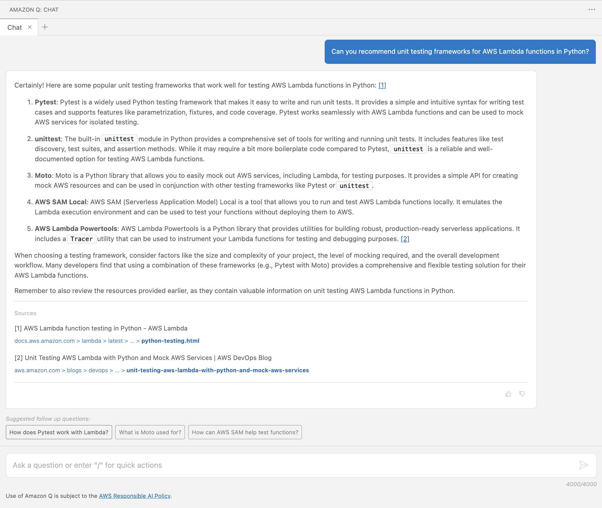
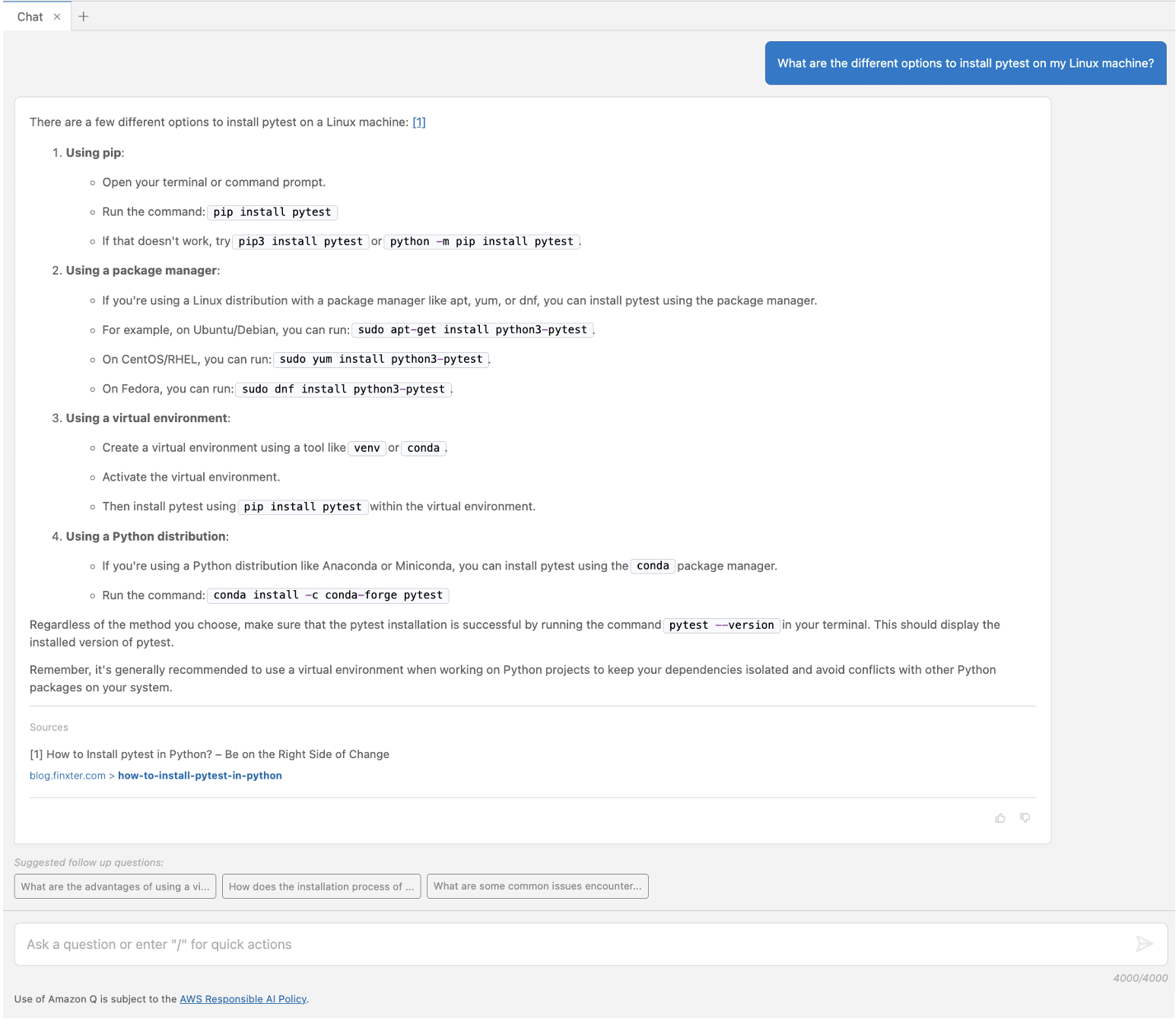
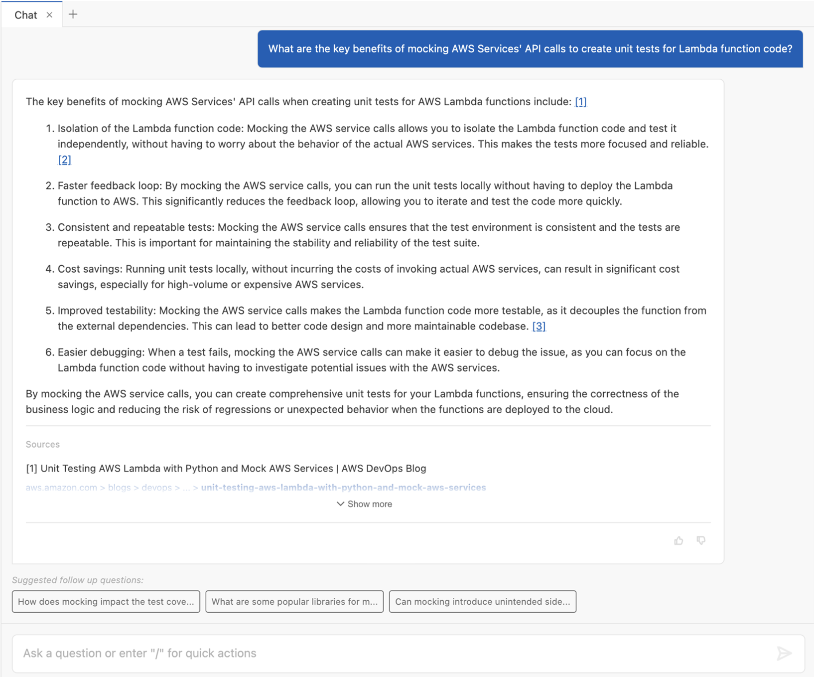
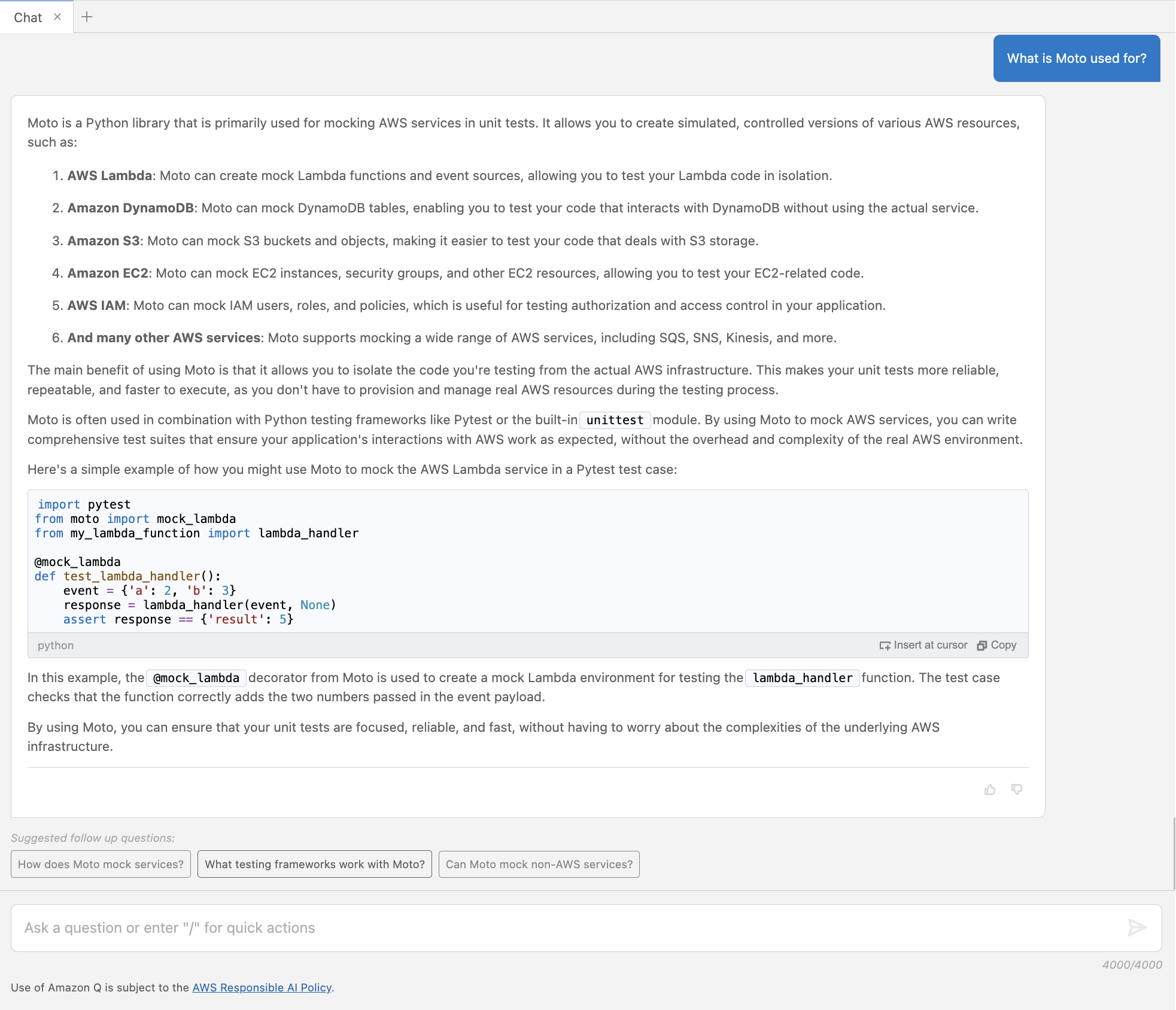
Tag Archives: Technical How-to

Securely validate business application resilience with AWS FIS and IAM

Post Syndicated from Dr. Rudolf Potucek original https://aws.amazon.com/blogs/devops/securely-validate-business-application-resilience-with-aws-fis-and-iam/

To avoid high costs of downtime, mission critical applications in the cloud need to achieve resilience against degradation of cloud provider APIs and services.

In 2021, AWS launched AWS Fault Injection Simulator (FIS), a fully managed service to perform fault injection experiments on workloads in AWS to improve their reliability and resilience. At the time of writing, FIS allows to simulate degradation of Amazon Elastic Compute Cloud (EC2) APIs using API fault injection actions and thus explore the resilience of workflows where EC2 APIs act as a fault boundary. 

In this post we show you how to explore additional fault boundaries in your applications by selectively denying access to any AWS API. This technique is particularly useful for fully managed, “black box” services like Amazon Simple Storage Service (S3) or Amazon Simple Queue Service (SQS) where a failure of read or write operations is sufficient to simulate problems in the service. This technique is also useful for injecting failures in serverless applications without needing to modify code. While similar results could be achieved with network disruption or modifying code with feature flags, this approach provides a fine granular degradation of an AWS API without the need to re-deploy and re-validate code.

Overview

We will explore a common application pattern: user uploads a file, S3 triggers an AWS Lambda function, Lambda transforms the file to a new location and deletes the original:

S3 upload and transform logical workflow: User uploads file to S3, upload triggers AWS Lambda execution, Lambda writes transformed file to a new bucket and deletes original. Workflow can be disrupted at file deletion.

Figure 1. S3 upload and transform logical workflow: User uploads file to S3, upload triggers AWS Lambda execution, Lambda writes transformed file to a new bucket and deletes original. Workflow can be disrupted at file deletion.

We will simulate the user upload with an Amazon EventBridge rate expression triggering an AWS Lambda function which creates a file in S3:

S3 upload and transform implemented demo workflow: Amazon EventBridge triggers a creator Lambda function, Lambda function creates a file in S3, file creation triggers AWS Lambda execution on transformer function, Lambda writes transformed file to a new bucket and deletes original. Workflow can be disrupted at file deletion.

Figure 2. S3 upload and transform implemented demo workflow: Amazon EventBridge triggers a creator Lambda function, Lambda function creates a file in S3, file creation triggers AWS Lambda execution on transformer function, Lambda writes transformed file to a new bucket and deletes original. Workflow can be disrupted at file deletion.

Using this architecture we can explore the effect of S3 API degradation during file creation and deletion. As shown, the API call to delete a file from S3 is an application fault boundary. The failure could occur, with identical effect, because of S3 degradation or because the AWS IAM role of the Lambda function denies access to the API.

To inject failures we use AWS Systems Manager (AWS SSM) automation documents to attach and detach IAM policies at the API fault boundary and FIS to orchestrate the workflow.

Each Lambda function has an IAM execution role that allows S3 write and delete access, respectively. If the processor Lambda fails, the S3 file will remain in the bucket, indicating a failure. Similarly, if the IAM execution role for the processor function is denied the ability to delete a file after processing, that file will remain in the S3 bucket.

Prerequisites

Following this blog posts will incur some costs for AWS services. To explore this test application you will need an AWS account. We will also assume that you are using AWS CloudShell or have the AWS CLI installed and have configured a profile with administrator permissions. With that in place you can create the demo application in your AWS account by downloading this template and deploying an AWS CloudFormation stack:

git clone https://github.com/aws-samples/fis-api-failure-injection-using-iam.git
cd fis-api-failure-injection-using-iam
aws cloudformation deploy --stack-name test-fis-api-faults --template-file template.yaml --capabilities CAPABILITY_NAMED_IAM

Fault injection using IAM

Once the stack has been created, navigate to the Amazon CloudWatch Logs console and filter for /aws/lambda/test-fis-api-faults. Under the EventBridgeTimerHandler log group you should find log events once a minute writing a timestamped file to an S3 bucket named fis-api-failure-ACCOUNT_ID. Under the S3TriggerHandler log group you should find matching deletion events for those files.

Once you have confirmed object creation/deletion, let’s take away the permission of the S3 trigger handler lambda to delete files. To do this you will attach the FISAPI-DenyS3DeleteObject  policy that was created with the template:

ROLE_NAME=FISAPI-TARGET-S3TriggerHandlerRole
ROLE_ARN=$( aws iam list-roles --query "Roles[?RoleName=='${ROLE_NAME}'].Arn" --output text )
echo Target Role ARN: $ROLE_ARN

POLICY_NAME=FISAPI-DenyS3DeleteObject
POLICY_ARN=$( aws iam list-policies --query "Policies[?PolicyName=='${POLICY_NAME}'].Arn" --output text )
echo Impact Policy ARN: $POLICY_ARN

aws iam attach-role-policy \
  --role-name ${ROLE_NAME}\
  --policy-arn ${POLICY_ARN}

With the deny policy in place you should now see object deletion fail and objects should start showing up in the S3 bucket. Navigate to the S3 console and find the bucket starting with fis-api-failure. You should see a new object appearing in this bucket once a minute:

S3 bucket listing showing files not being deleted because IAM permissions DENY file deletion during FIS experiment.

Figure 3. S3 bucket listing showing files not being deleted because IAM permissions DENY file deletion during FIS experiment.

If you would like to graph the results you can navigate to AWS CloudWatch, select “Logs Insights“, select the log group starting with /aws/lambda/test-fis-api-faults-S3CountObjectsHandler, and run this query:

fields @timestamp, @message
| filter NumObjects >= 0
| sort @timestamp desc
| stats max(NumObjects) by bin(1m)
| limit 20

This will show the number of files in the S3 bucket over time:

AWS CloudWatch Logs Insights graph showing the increase in the number of retained files in S3 bucket over time, demonstrating the effect of the introduced failure.

Figure 4. AWS CloudWatch Logs Insights graph showing the increase in the number of retained files in S3 bucket over time, demonstrating the effect of the introduced failure.

You can now detach the policy:

ROLE_NAME=FISAPI-TARGET-S3TriggerHandlerRole
ROLE_ARN=$( aws iam list-roles --query "Roles[?RoleName=='${ROLE_NAME}'].Arn" --output text )
echo Target Role ARN: $ROLE_ARN

POLICY_NAME=FISAPI-DenyS3DeleteObject
POLICY_ARN=$( aws iam list-policies --query "Policies[?PolicyName=='${POLICY_NAME}'].Arn" --output text )
echo Impact Policy ARN: $POLICY_ARN

aws iam detach-role-policy \
  --role-name ${ROLE_NAME}\
  --policy-arn ${POLICY_ARN}

We see that newly written files will once again be deleted but the un-processed files will remain in the S3 bucket. From the fault injection we learned that our system does not tolerate request failures when deleting files from S3. To address this, we should add a dead letter queue or some other retry mechanism.

Note: if the Lambda function does not return a success state on invocation, EventBridge will retry. In our Lambda functions we are cost conscious and explicitly capture the failure states to avoid excessive retries.

Fault injection using SSM

To use this approach from FIS and to always remove the policy at the end of the experiment, we first create an SSM document to automate adding a policy to a role. To inspect this document, open the SSM console, navigate to the “Documents” section, find the FISAPI-IamAttachDetach document under “Owned by me”, and examine the “Content” tab (make sure to select the correct region). This document takes the name of the Role you want to impact and the Policy you want to attach as parameters. It also requires an IAM execution role that grants it the power to list, attach, and detach specific policies to specific roles.

Let’s run the SSM automation document from the console by selecting “Execute Automation”. Determine the ARN of the FISAPI-SSM-Automation-Role from CloudFormation or by running:

POLICY_NAME=FISAPI-DenyS3DeleteObject
POLICY_ARN=$( aws iam list-policies --query "Policies[?PolicyName=='${POLICY_NAME}'].Arn" --output text )
echo Impact Policy ARN: $POLICY_ARN

Use FISAPI-SSM-Automation-Role, a duration of 2 minutes expressed in ISO8601 format as PT2M, the ARN of the deny policy, and the name of the target role FISAPI-TARGET-S3TriggerHandlerRole:

Image of parameter input field reflecting the instructions in blog text.

Figure 5. Image of parameter input field reflecting the instructions in blog text.

Alternatively execute this from a shell:

ASSUME_ROLE_NAME=FISAPI-SSM-Automation-Role
ASSUME_ROLE_ARN=$( aws iam list-roles --query "Roles[?RoleName=='${ASSUME_ROLE_NAME}'].Arn" --output text )
echo Assume Role ARN: $ASSUME_ROLE_ARN

ROLE_NAME=FISAPI-TARGET-S3TriggerHandlerRole
ROLE_ARN=$( aws iam list-roles --query "Roles[?RoleName=='${ROLE_NAME}'].Arn" --output text )
echo Target Role ARN: $ROLE_ARN

POLICY_NAME=FISAPI-DenyS3DeleteObject
POLICY_ARN=$( aws iam list-policies --query "Policies[?PolicyName=='${POLICY_NAME}'].Arn" --output text )
echo Impact Policy ARN: $POLICY_ARN

aws ssm start-automation-execution \
  --document-name FISAPI-IamAttachDetach \
  --parameters "{
      \"AutomationAssumeRole\": [ \"${ASSUME_ROLE_ARN}\" ],
      \"Duration\": [ \"PT2M\" ],
      \"TargetResourceDenyPolicyArn\": [\"${POLICY_ARN}\" ],
      \"TargetApplicationRoleName\": [ \"${ROLE_NAME}\" ]
    }"

Wait two minutes and then examine the content of the S3 bucket starting with fis-api-failure again. You should now see two additional files in the bucket, showing that the policy was attached for 2 minutes during which files could not be deleted, and confirming that our application is not resilient to S3 API degradation.

Permissions for injecting failures with SSM

Fault injection with SSM is controlled by IAM, which is why you had to specify the FISAPI-SSM-Automation-Role:

Visual representation of IAM permission used for fault injections with SSM. It shows the SSM execution role permitting access to use SSM automation documents as well as modify IAM roles and policies via the SSM document. It also shows the SSM user needing to have a pass-role permission to grant the SSM execution role to the SSM service.

Figure 6. Visual representation of IAM permission used for fault injections with SSM.

This role needs to contain an assume role policy statement for SSM to allow assuming the role:

      AssumeRolePolicyDocument:
        Statement:
          - Action:
             - 'sts:AssumeRole'
            Effect: Allow
            Principal:
              Service:
                - "ssm.amazonaws.com"

The role also needs to contain permissions to describe roles and their attached policies with an optional constraint on which roles and policies are visible:

          - Sid: GetRoleAndPolicyDetails
            Effect: Allow
            Action:
              - 'iam:GetRole'
              - 'iam:GetPolicy'
              - 'iam:ListAttachedRolePolicies'
            Resource:
              # Roles
              - !GetAtt EventBridgeTimerHandlerRole.Arn
              - !GetAtt S3TriggerHandlerRole.Arn
              # Policies
              - !Ref AwsFisApiPolicyDenyS3DeleteObject

Finally the SSM role needs to allow attaching and detaching a policy document. This requires

  1. an ALLOW statement
  2. a constraint on the policies that can be attached
  3. a constraint on the roles that can be attached to

In the role we collapse the first two requirements into an ALLOW statement with a condition constraint for the Policy ARN. We then express the third requirement in a DENY statement that will limit the '*' resource to only the explicit role ARNs we want to modify:

          - Sid: AllowOnlyTargetResourcePolicies
            Effect: Allow
            Action:  
              - 'iam:DetachRolePolicy'
              - 'iam:AttachRolePolicy'
            Resource: '*'
            Condition:
              ArnEquals:
                'iam:PolicyARN':
                  # Policies that can be attached
                  - !Ref AwsFisApiPolicyDenyS3DeleteObject
          - Sid: DenyAttachDetachAllRolesExceptApplicationRole
            Effect: Deny
            Action: 
              - 'iam:DetachRolePolicy'
              - 'iam:AttachRolePolicy'
            NotResource: 
              # Roles that can be attached to
              - !GetAtt EventBridgeTimerHandlerRole.Arn
              - !GetAtt S3TriggerHandlerRole.Arn

We will discuss security considerations in more detail at the end of this post.

Fault injection using FIS

With the SSM document in place you can now create an FIS template that calls the SSM document. Navigate to the FIS console and filter for FISAPI-DENY-S3PutObject. You should see that the experiment template passes the same parameters that you previously used with SSM:

Image of FIS experiment template action summary. This shows the SSM document ARN to be used for fault injection and the JSON parameters passed to the SSM document specifying the IAM Role to modify and the IAM Policy to use.

Figure 7. Image of FIS experiment template action summary. This shows the SSM document ARN to be used for fault injection and the JSON parameters passed to the SSM document specifying the IAM Role to modify and the IAM Policy to use.

You can now run the FIS experiment and after a couple minutes once again see new files in the S3 bucket.

Permissions for injecting failures with FIS and SSM

Fault injection with FIS is controlled by IAM, which is why you had to specify the FISAPI-FIS-Injection-EperimentRole:

Visual representation of IAM permission used for fault injections with FIS and SSM. It shows the SSM execution role permitting access to use SSM automation documents as well as modify IAM roles and policies via the SSM document. It also shows the FIS execution role permitting access to use FIS templates, as well as the pass-role permission to grant the SSM execution role to the SSM service. Finally it shows the FIS user needing to have a pass-role permission to grant the FIS execution role to the FIS service.

Figure 8. Visual representation of IAM permission used for fault injections with FIS and SSM. It shows the SSM execution role permitting access to use SSM automation documents as well as modify IAM roles and policies via the SSM document. It also shows the FIS execution role permitting access to use FIS templates, as well as the pass-role permission to grant the SSM execution role to the SSM service. Finally it shows the FIS user needing to have a pass-role permission to grant the FIS execution role to the FIS service.

This role needs to contain an assume role policy statement for FIS to allow assuming the role:

      AssumeRolePolicyDocument:
        Statement:
          - Action:
              - 'sts:AssumeRole'
            Effect: Allow
            Principal:
              Service:
                - "fis.amazonaws.com"

The role also needs permissions to list and execute SSM documents:

            - Sid: RequiredReadActionsforAWSFIS
              Effect: Allow
              Action:
                - 'cloudwatch:DescribeAlarms'
                - 'ssm:GetAutomationExecution'
                - 'ssm:ListCommands'
                - 'iam:ListRoles'
              Resource: '*'
            - Sid: RequiredSSMStopActionforAWSFIS
              Effect: Allow
              Action:
                - 'ssm:CancelCommand'
              Resource: '*'
            - Sid: RequiredSSMWriteActionsforAWSFIS
              Effect: Allow
              Action:
                - 'ssm:StartAutomationExecution'
                - 'ssm:StopAutomationExecution'
              Resource: 
                - !Sub 'arn:aws:ssm:${AWS::Region}:${AWS::AccountId}:automation-definition/${SsmAutomationIamAttachDetachDocument}:$DEFAULT'

Finally, remember that the SSM document needs to use a Role of its own to execute the fault injection actions. Because that Role is different from the Role under which we started the FIS experiment, we need to explicitly allow SSM to assume that role with a PassRole statement which will expand to FISAPI-SSM-Automation-Role:

            - Sid: RequiredIAMPassRoleforSSMADocuments
              Effect: Allow
              Action: 'iam:PassRole'
              Resource: !Sub 'arn:aws:iam::${AWS::AccountId}:role/${SsmAutomationRole}'

Secure and flexible permissions

So far, we have used explicit ARNs for our guardrails. To expand flexibility, we can use wildcards in our resource matching. For example, we might change the Policy matching from:

            Condition:
              ArnEquals:
                'iam:PolicyARN':
                  # Explicitly listed policies - secure but inflexible
                  - !Ref AwsFisApiPolicyDenyS3DeleteObject

or the equivalent:

            Condition:
              ArnEquals:
                'iam:PolicyARN':
                  # Explicitly listed policies - secure but inflexible
                  - !Sub 'arn:${AWS::Partition}:iam::${AWS::AccountId}:policy/${FullPolicyName}

to a wildcard notation like this:

            Condition:
              ArnEquals:
                'iam:PolicyARN':
                  # Wildcard policies - secure and flexible
                  - !Sub 'arn:${AWS::Partition}:iam::${AWS::AccountId}:policy/${PolicyNamePrefix}*'

If we set PolicyNamePrefix to FISAPI-DenyS3 this would now allow invoking FISAPI-DenyS3PutObject and FISAPI-DenyS3DeleteObject but would not allow using a policy named FISAPI-DenyEc2DescribeInstances.

Similarly, we could change the Resource matching from:

            NotResource: 
              # Explicitly listed roles - secure but inflexible
              - !GetAtt EventBridgeTimerHandlerRole.Arn
              - !GetAtt S3TriggerHandlerRole.Arn

to a wildcard equivalent like this:

            NotResource: 
              # Wildcard policies - secure and flexible
              - !Sub 'arn:${AWS::Partition}:iam::${AWS::AccountId}:role/${RoleNamePrefixEventBridge}*'
              - !Sub 'arn:${AWS::Partition}:iam::${AWS::AccountId}:role/${RoleNamePrefixS3}*'
and setting RoleNamePrefixEventBridge to FISAPI-TARGET-EventBridge and RoleNamePrefixS3 to FISAPI-TARGET-S3.

Finally, we would also change the FIS experiment role to allow SSM documents based on a name prefix by changing the constraint on automation execution from:

            - Sid: RequiredSSMWriteActionsforAWSFIS
              Effect: Allow
              Action:
                - 'ssm:StartAutomationExecution'
                - 'ssm:StopAutomationExecution'
              Resource: 
                # Explicitly listed resource - secure but inflexible
                # Note: the $DEFAULT at the end could also be an explicit version number
                # Note: the 'automation-definition' is automatically created from 'document' on invocation
                - !Sub 'arn:aws:ssm:${AWS::Region}:${AWS::AccountId}:automation-definition/${SsmAutomationIamAttachDetachDocument}:$DEFAULT'

to

            - Sid: RequiredSSMWriteActionsforAWSFIS
              Effect: Allow
              Action:
                - 'ssm:StartAutomationExecution'
                - 'ssm:StopAutomationExecution'
              Resource: 
                # Wildcard resources - secure and flexible
                # 
                # Note: the 'automation-definition' is automatically created from 'document' on invocation
                - !Sub 'arn:aws:ssm:${AWS::Region}:${AWS::AccountId}:automation-definition/${SsmAutomationDocumentPrefix}*'

and setting SsmAutomationDocumentPrefix to FISAPI-. Test this by updating the CloudFormation stack with a modified template:

aws cloudformation deploy --stack-name test-fis-api-faults --template-file template2.yaml --capabilities CAPABILITY_NAMED_IAM

Permissions governing users

In production you should not be using administrator access to use FIS. Instead we create two roles FISAPI-AssumableRoleWithCreation and FISAPI-AssumableRoleWithoutCreation for you (see this template). These roles require all FIS and SSM resources to have a Name tag that starts with FISAPI-. Try assuming the role without creation privileges and running an experiment. You will notice that you can only start an experiment if you add a Name tag, e.g. FISAPI-secure-1, and you will only be able to get details of experiments and templates that have proper Name tags.

If you are working with AWS Organizations, you can add further guard rails by defining SCPs that control the use of the FISAPI-* tags similar to this blog post.

Caveats

For this solution we are choosing to attach policies instead of permission boundaries. The benefit of this is that you can attach multiple independent policies and thus simulate multi-step service degradation. However, this means that it is possible to increase the permission level of a role. While there are situations where this might be of interest, e.g. to simulate security breaches, please implement a thorough security review of any fault injection IAM policies you create. Note that modifying IAM Roles may trigger events in your security monitoring tools.

The AttachRolePolicy and DetachRolePolicy calls from AWS IAM are eventually consistent, meaning that in some cases permission propagation when starting and stopping fault injection may take up to 5 minutes each.

Cleanup

To avoid additional cost, delete the content of the S3 bucket and delete the CloudFormation stack:

# Clean up policy attachments just in case
CLEANUP_ROLES=$(aws iam list-roles --query "Roles[?starts_with(RoleName,'FISAPI-')].RoleName" --output text)
for role in $CLEANUP_ROLES; do
  CLEANUP_POLICIES=$(aws iam list-attached-role-policies --role-name $role --query "AttachedPolicies[?starts_with(PolicyName,'FISAPI-')].PolicyName" --output text)
  for policy in $CLEANUP_POLICIES; do
    echo Detaching policy $policy from role $role
    aws iam detach-role-policy --role-name $role --policy-arn $policy
  done
done
# Delete S3 bucket content
ACCOUNT_ID=$( aws sts get-caller-identity --query Account --output text )
S3_BUCKET_NAME=fis-api-failure-${ACCOUNT_ID}
aws s3 rm --recursive s3://${S3_BUCKET_NAME}
aws s3 rb s3://${S3_BUCKET_NAME}
# Delete cloudformation stack
aws cloudformation delete-stack --stack-name test-fis-api-faults
aws cloudformation wait stack-delete-complete --stack-name test-fis-api-faults

Conclusion 

AWS Fault Injection Simulator provides the ability to simulate various external impacts to your application to validate and improve resilience. We’ve shown how combining FIS with IAM to selectively deny access to AWS APIs provides a generic path to explore fault boundaries across all AWS services. We’ve shown how this can be used to identify and improve a resilience problem in a common S3 upload workflow. To learn about more ways to use FIS, see this workshop.

About the authors:

Dr. Rudolf Potucek

Dr. Rudolf Potucek is Startup Solutions Architect at Amazon Web Services. Over the past 30 years he gained a PhD and worked in different roles including leading teams in academia and industry, as well as consulting. He brings experience from working with academia, startups, and large enterprises to his current role of guiding startup customers to succeed in the cloud.

Rudolph Wagner

Rudolph Wagner is a Premium Support Engineer at Amazon Web Services who holds the CISSP and OSCP security certifications, in addition to being a certified AWS Solutions Architect Professional. He assists internal and external Customers with multiple AWS services by using his diverse background in SAP, IT, and construction.

Configure ADFS Identity Federation with Amazon QuickSight

Post Syndicated from Adeleke Coker original https://aws.amazon.com/blogs/big-data/configure-adfs-identity-federation-with-amazon-quicksight/

Amazon QuickSight Enterprise edition can integrate with your existing Microsoft Active Directory (AD), providing federated access using Security Assertion Markup Language (SAML) to dashboards. Using existing identities from Active Directory eliminates the need to create and manage separate user identities in AWS Identity Access Management (IAM). Federated users assume an IAM role when access is requested through an identity provider (IdP) such as Active Directory Federation Service (AD FS) based on AD group membership. Although, you can connect AD to QuickSight using AWS Directory Service, this blog focuses on federated logon to QuickSight Dashboards.

With identity federation, your users get one-click access to Amazon QuickSight applications using their existing identity credentials. You also have the security benefit of identity authentication by your IdP. You can control which users have access to QuickSight using your existing IdP. Refer to Using identity federation and single sign-on (SSO) with Amazon QuickSight for more information.

In this post, we demonstrate how you can use a corporate email address as an authentication option for signing in to QuickSight. This post assumes you have an existing Microsoft Active Directory Federation Services (ADFS) configured in your environment.

Solution overview

While connecting to QuickSight from an IdP, your users initiate the sign-in process from the IdP portal. After the users are authenticated, they are automatically signed in to QuickSight. After QuickSight checks that they are authorized, your users can access QuickSight.

The following diagram shows an authentication flow between QuickSight and a third-party IdP. In this example, the administrator has set up a sign-in page to access QuickSight. When a user signs in, the sign-in page posts a request to a federation service that complies with SAML 2.0. The end-user initiates authentication from the sign-in page of the IdP. For more information about the authentication flow, see Initiating sign-on from the identity provider (IdP).

QuickSight IdP flow

The solution consists of the following high-level steps:

  1. Create an identity provider.
  2. Create IAM policies.
  3. Create IAM roles.
  4. Configure AD groups and users.
  5. Create a relying party trust.
  6. Configure claim rules.
  7. Configure QuickSight single sign-on (SSO).
  8. Configure the relay state URL for QuickStart.

Prerequisites

The following are the prerequisites to build the solution explained in this post:

  • An existing or newly deployed AD FS environment.
  • An AD user with permissions to manage AD FS and AD group membership.
  • An IAM user with permissions to create IAM policies and roles, and administer QuickSight.
  • The metadata document from your IdP. To download it, refer to Federation Metadata Explorer.

Create an identity provider

To add your IdP, complete the following steps:

  1. On the IAM console, choose Identity providers in the navigation pane.
  2. Choose Add provider.
  3. For Provider type¸ select SAML.
  4. For Provider name, enter a name (for example, QuickSight_Federation).
  5. For Metadata document, upload the metadata document you downloaded as a prerequisite.
  6. Choose Add provider.
  7. Copy the ARN of this provider to use in a later step.

Add IdP in IAM

Create IAM policies

In this step, you create IAM policies that allow users to access QuickSight only after federating their identities. To provide access to QuickSight and also the ability to create QuickSight admins, authors (standard users), and readers, use the following policy examples.

The following code is the author policy:

{
    "Statement": [
        {
            "Action": [
                "quicksight:CreateUser"
            ],
            "Effect": "Allow",
            "Resource": [
                "*"
            ]
        }
    ],
    "Version": "2012-10-17"
}

The following code is the reader policy:

{ 
"Version": "2012-10-17", 
"Statement": [ 
{ 
"Effect": "Allow",
"Action": "quicksight:CreateReader", 
"Resource": "*" 
} 
] 
}

The following code is the admin policy:

{
    "Statement": [
        {
            "Action": [
                "quicksight:CreateAdmin"
            ],
            "Effect": "Allow",
            "Resource": [
                "*"
            ]
        }
    ],
    "Version": "2012-10-17"
}

Create IAM roles

You can configure email addresses for your users to use when provisioning through your IdP to QuickSight. To do this, add the sts:TagSession action to the trust relationship for the IAM role that you use with AssumeRoleWithSAML. Make sure the IAM role names start with ADFS-.

  1. On the IAM console, choose Roles in the navigation pane.
  2. Choose Create new role.
  3. For Trusted entity type, select SAML 2.0 federation.
  4. Choose the SAML IdP you created earlier.
  5. Select Allow programmatic and AWS Management Console access.
  6. Choose Next.
    Create IAM Roles
  7. Choose the admin policy you created, then choose Next.
  8. For Name, enter ADFS-ACCOUNTID-QSAdmin.
  9. Choose Create.
  10. On the Trust relationships tab, edit the trust relationships as follows so you can pass principal tags when users assume the role (provide your account ID and IdP):
{
    "Version": "2012-10-17",
    "Statement": [
        {
            "Effect": "Allow",
            "Principal": {
                "Federated": "arn:aws:iam::ACCOUNTID:saml-provider/Identity_Provider"
            },
            "Action":[ "sts:AssumeRoleWithSAML",
	 "sts:TagSession"],
            "Condition": {
                "StringEquals": {
                    "SAML:aud": "https://signin.aws.amazon.com/saml"
                },
                "StringLike": {
                    "aws:RequestTag/Email": "*"
                }
            }
            }
    ]
}
  1. Repeat this process for the role ADFS-ACCOUNTID-QSAuthor and attach the author IAM policy.
  2. Repeat this process for the role ADFS-ACCOUNTID-QSReader and attach the reader IAM policy.

Configure AD groups and users

Now you need to create AD groups that determine the permissions to sign in to AWS. Create an AD security group for each of the three roles you created earlier. Note that the group name should follow same format as your IAM role names.

One approach for creating the AD groups that uniquely identify the IAM role mapping is by selecting a common group naming convention. For example, your AD groups would start with an identifier, for example AWS-, which will distinguish your AWS groups from others within the organization. Next, include the 12-digit AWS account number. Finally, add the matching role name within the AWS account. You should do this for each role and corresponding AWS account you wish to support with federated access. The following screenshot shows an example of the naming convention we use in this post.

AD Groups

Later in this post, we create a rule to pick up AD groups starting with AWS-, the rule will remove AWS-ACCOUNTID- from AD groups name to match the respective IAM role, which is why we use this naming convention here.

Users in Active Directory can subsequently be added to the groups, providing the ability to assume access to the corresponding roles in AWS. You can add AD users to the respective groups based on your business permissions model. Note that each user must have an email address configured in Active Directory.

Create a relying party trust

To add a relying party trust, complete the following steps:

  1. Open the AD FS Management Console.
  2. Choose (right-click) Relying Party Trusts, then choose Add Relying Party Trust.
    Add Relying Party Trust
  3. Choose Claims aware, then choose Start.
  4. Select Import data about the relying party published online or on a local network.
  5. For Federation metadata address, enter https://signin.aws.amazon.com/static/saml-metadata.xml.
  6. Choose Next.
    ADFS Wizard Data Source
  7. Enter a descriptive display name, for example Amazon QuickSight Federation, then choose Next.
  8. Choose your access control policy (for this post, Permit everyone), then choose Next.
    ADFS Access Control
  9. In the Ready to Add Trust section, choose Next.
    ADFS Ready to Add
  10. Leave the defaults, then choose Close.

Configure claim rules

In this section, you create claim rules that identify accounts, set LDAP attributes, get the AD groups, and match them to the roles created earlier. Complete the following steps to create the claim rules for NameId, RoleSessionName, Get AD Groups, Roles, and (optionally) Session Duration:

  1. Select the relying party trust you just created, then choose Edit Claim Issuance Policy.
  2. Add a rule called NameId with the following parameters:
    1. For Claim rule template, choose Transform an Incoming Claim.
    2. For Claim rule name, enter NameId
    3. For Incoming claim type, choose Windows account name.
    4. For Outgoing claim type, choose Name ID.
    5. For Outgoing name ID format, choose Persistent Identifier.
    6. Select Pass through all claim values.
    7. Choose Finish.
      NameId
  3. Add a rule called RoleSessionName with the following parameters:
    1. For Claim rule template, choose Send LDAP Attributes as Claims.
    2. For Claim rule name, enter RoleSessionName.
    3. For Attribute store, choose Active Directory.
    4. For LDAP Attribute, choose E-Mail-Addresses.
    5. For Outgoing claim type, enter https://aws.amazon.com/SAML/Attributes/RoleSessionName.
    6. Add another E-Mail-Addresses LDAP attribute and for Outgoing claim type, enter https://aws.amazon.com/SAML/Attributes/PrincipalTag:Email.
    7. Choose OK.
      RoleSessionName
  4. Add a rule called Get AD Groups with the following parameters:
    1. For Claim rule template, choose Send Claims Using a Custom Rule.
    2. For Claim rule name, enter Get AD Groups
    3. For Custom Rule, enter the following code:
      c:[Type == "http://schemas.microsoft.com/ws/2008/06/identity/claims/windowsaccountname", Issuer == "AD AUTHORITY"] => add(store = "Active Directory", types = ("http://temp/variable"), query = ";tokenGroups;{0}", param = c.Value);

    4. Choose OK.
      Get AD Groups
  1. Add a rule called Roles with the following parameters:
    1. For Claim rule template, choose Send Claims Using a Custom Rule.
    2. For Claim rule name, enter Roles
    3. For Custom Rule, enter the following code (provide your account ID and IdP):
      c:[Type == "http://temp/variable", Value =~ "(?i)^AWS-ACCOUNTID"]=> issue(Type = "https://aws.amazon.com/SAML/Attributes/Role", Value = RegExReplace(c.Value, "AWS-ACCOUNTID-", "arn:aws:iam:: ACCOUNTID:saml-provider/your-identity-provider-name,arn:aws:iam:: ACCOUNTID:role/ADFS-ACCOUNTID-"));

    4. Choose Finish.Roles

Optionally, you can create a rule called Session Duration. This configuration determines how long a session is open and active before users are required to reauthenticate. The value is in seconds. For this post, we configure the rule for 8 hours.

  1. Add a rule called Session Duration with the following parameters:
    1. For Claim rule template, choose Send Claims Using a Custom Rule.
    2. For Claim rule name, enter Session Duration.
    3. For Custom Rule, enter the following code:
      => issue(Type = "https://aws.amazon.com/SAML/Attributes/SessionDuration", Value = "28800");

    4. Choose Finish.Session Duration

You should be able to see these five claim rules, as shown in the following screenshot.
All Claims Rules

  1. Choose OK.
  2. Run the following commands in PowerShell on your AD FS server:
Set-AdfsProperties -EnableIdPInitiatedSignonPage $true

Set-AdfsProperties -EnableRelayStateForIdpInitiatedSignOn $true
  1. Stop and start the AD FS service from PowerShell:
net stop adfssrv

net start adfssrv

Configure E-mail Syncing

With QuickSight Enterprise edition integrated with an IdP, you can restrict new users from using personal email addresses. This means users can only log in to QuickSight with their on-premises configured email addresses. This approach allows users to bypass manually entering an email address. It also ensures that users can’t use an email address that might differ from the email address configured in Active Directory.

QuickSight uses the preconfigured email addresses passed through the IdP when provisioning new users to your account. For example, you can make it so that only corporate-assigned email addresses are used when users are provisioned to your QuickSight account through your IdP. When you configure email syncing for federated users in QuickSight, users who log in to your QuickSight account for the first time have preassigned email addresses. These are used to register their accounts.

To configure E-mail syncing for federated users in QuickSight, complete the following steps:

  1. Log in to your QuickSight dashboard with a QuickSight administrator account.
  2. Choose the profile icon.
    QuickSight SSO
  3. On the drop-down menu, choose on Manage QuickSight.
  4. In the navigation pane, choose Single sign-on (SSO).
  5. For Email Syncing for Federated Users, select ON, then choose Enable in the pop-up window.
  6. Choose Save.SSO Configuration

Configure the relay state URL for QuickStart

To configure the relay state URL, complete the following steps (revise the input information as needed to match your environment’s configuration):

  1. Use the ADFS RelayState Generator to generate your URL.
  2. For IDP URL String, enter https://ADFSServerEndpoint/adfs/ls/idpinitiatedsignon.aspx.
  3. For Relying Party Identifier, enter urn:amazon:webservices or https://signin.aws.amazon.com/saml.
  4. For Relay State/Target App, enter your authenticated users to access. In this case, it’s https://quicksight.aws.amazon.com.
  5. Choose Generate URL.RelayState Generator
  6. Copy the URL and load it in your browser.

You should be presented with a login to your IdP landing page.

ADFS Logon Page

Make sure the user logging in has an email address attribute configured in Active Directory. A successful login should redirect you to the QuickSight dashboard after authentication. If you’re not redirected to the QuickSight dashboard page, make sure you ran the commands listed earlier after you configured your claim rules.

Summary

In this post, we demonstrated how to configure federated identities to a QuickSight dashboard and ensure that users can only sign in with preconfigured email address in your existing Active Directory.

We’d love to hear from you. Let us know what you think in the comments section.


About the Author

Adeleke Coker is a Global Solutions Architect with AWS. He helps customers globally accelerate workload deployments and migrations at scale to AWS. In his spare time, he enjoys learning, reading, gaming and watching sport events.

How Vanguard made their technology platform resilient and efficient by building cross-Region replication for Amazon Kinesis Data Streams

Post Syndicated from Raghu Boppanna original https://aws.amazon.com/blogs/big-data/how-vanguard-made-their-technology-platform-resilient-and-efficient-by-building-cross-region-replication-for-amazon-kinesis-data-streams/

This is a guest post co-written with Raghu Boppanna from Vanguard. 

At Vanguard, the Enterprise Advice line of business improves investor outcomes through digital access to superior, personalized, and affordable financial advice. They made it possible, in part, by driving economies of scale across the globe for investors with a highly resilient and efficient technical platform. Vanguard opted for a multi-Region architecture for this workload to help protect against impairments of Regional services. For high availability purposes, there is a need to make the data used by the workload available not just in the primary Region, but also in the secondary Region with minimal replication lag. In the event of a service impairment in the primary Region, the solution should be able to fail over to the secondary Region with as little data loss as possible and the ability to resume data ingestion.

Vanguard Cloud Technology Office and AWS partnered to build an infrastructure solution on AWS that met their resilience requirements. The multi-Region solution enables a robust fail-over mechanism, with built-in observability and recovery. The solution also supports streaming data from multiple sources to different Kinesis data streams. The solution is currently being rolled out to the different lines of business teams to improve the resilience posture of their workloads.

The use case discussed here requires Change Data Capture (CDC) to stream data from a remote data source (mainframe DB2) to Amazon Kinesis Data Streams, because the business capability depends on this data. Kinesis Data Streams is a fully managed, massively scalable, durable, and low-cost streaming service that can continuously capture and stream large amounts of data from multiple sources, and makes the data available for consumption within milliseconds. The service is built to be highly resilient and uses multiple Availability Zones to process and store data.

The solution discussed in this post explains how AWS and Vanguard innovated to build a resilient architecture to meet their high availability goals.

Solution overview

The solution uses AWS Lambda to replicate data from Kinesis data streams in the primary Region to a secondary Region. In the event of any service impairment impacting the CDC pipeline, the failover process promotes the secondary Region to primary for the producers and consumers. We use Amazon DynamoDB global tables for replication checkpoints that allows to resume data streaming from the checkpoint and also maintains a primary Region configuration flag that prevents an infinite replication loop of the same data back and forth.

The solution also provides the flexibility for Kinesis Data Streams consumers to use the primary or any secondary Region within the same AWS account.

The following diagram illustrates the reference architecture.

Let’s look at each component in detail:

  1. CDC processor (producer) – In this reference architecture, the producer is deployed on Amazon Elastic Compute Cloud (Amazon EC2) in both the primary and secondary Regions, and is active in the primary Region and on standby mode in the secondary Region. It captures CDC data from the external data source (like a DB2 database as shown in the architecture above), and streams to Kinesis Data Streams in the primary Region. Vanguard uses a 3rd party tool Qlik Replicate as their CDC Processor. It produces a well-formed payload including the DB2 commit timestamp to the Kinesis data stream, in addition to the actual row data from the remote data source. (example-stream-1 in this example). The following code is a sample payload containing only the primary key of the record that changed and the commit timestamp (for simplicity, the rest of the table row data is not shown below):
    {
        "eventSource": "aws:kinesis",
        "kinesis": 
        {
             "ApproximateArrivalTimestamp": "Mon July 18 20:00:00 UTC 2022",
             "SequenceNumber": "49544985256907370027570885864065577703022652638596431874",
             "PartitionKey": "12349999",
             "KinesisSchemaVersion": "1.0",
             "Data": "eyJLZXkiOiAxMjM0OTk5OSwiQ29tbWl0VGltZXN0YW1wIjogIjIwMjItMDctMThUMjA6MDA6MDAifQ=="
        },
        "eventId": "shardId-000000000000:49629136582982516722891309362785181370337771525377097730",
        "invokeIdentityArn": "arn:aws:iam::6243876582:role/kds-crr-LambdaRole-1GZWP67437SD",
        "eventName": "aws:kinesis:record",
        "eventVersion": "1.0",
        "eventSourceARN": "arn:aws:kinesis:us-east-1:6243876582:stream/kds-stream-1/consumer/kds-crr:6243876582",
        "awsRegion": "us-east-1"
    }

    The Base64 decoded value of Data is as follows. The actual Kinesis record would contain the entire row data of the table row that changed, in addition to the primary key and the commit timestamp.

    {"Key": 12349999,"CommitTimestamp": "2022-07-18T20:00:00"}

    The CommitTimestamp in the Data field is used in the replication checkpoint and is critical to accurately track how much of the stream data has been replicated to the secondary Region. The checkpoint can then be used to facilitate a CDC processor (producer) failover and accurately resume producing data from the replication checkpoint timestamp onwards.

    The alternative to using a remote data source CommitTimestamp (if unavailable) is to use the ApproximateArrivalTimestamp (which is the timestamp when the record is actually written to the data stream).

  2. Cross-Region replication Lambda function – The function is deployed to both primary and secondary Regions. It’s set up with an event source mapping to the data stream containing CDC data. The same function can be used to replicate data of multiple streams. It’s invoked with a batch of records from Kinesis Data Streams and replicates the batch to a target replication Region (which is provided via the Lambda configuration environment). For cost considerations, if the CDC data is actively produced into the primary Region only, the reserved concurrency of the function in the secondary Region can be set to zero, and modified during regional failover. The function has AWS Identity and Access Management (IAM) role permissions to do the following:
    • Read and write to the DynamoDB global tables used in this solution, within the same account.
    • Read and write to Kinesis Data Streams in both Regions within the same account.
    • Publish custom metrics to Amazon CloudWatch in both Regions within the same account.
  3. Replication checkpoint – The replication checkpoint uses the DynamoDB global table in both the primary and secondary Regions. It’s used by the cross-Region replication Lambda function to persist the commit timestamp of the last replication record as the replication checkpoint for every stream that is configured for replication. For this post, we create and use a global table called kdsReplicationCheckpoint.
  4. Active Region config – The active Region uses the DynamoDB global table in both primary and secondary Regions. It uses the native cross-Region replication capability of the global table to replicate the configuration. It’s pre-populated with data about which is the primary Region for a stream, to prevent replication back to the primary Region by the Lambda function in the standby Region. This configuration may not be required if the Lambda function in the standby Region has a reserved concurrency set to zero, but can serve as a safety check to avoid infinite replication loop of the data. For this post, we create a global table called kdsActiveRegionConfig and put an item with the following data:
    {
     "stream-name": "example-stream-1",
     "active-region" : "us-east-1"
    }
    
  5. Kinesis Data Streams – The stream to which the CDC processor produces the data. For this post, we use a stream called example-stream-1 in both the Regions, with the same shard configuration and access policies.

Sequence of steps in cross-Region replication

Let’s briefly look at how the architecture is exercised using the following sequence diagram.

The sequence consists of the following steps:

  1. The CDC processor (in us-east-1) reads the CDC data from the remote data source.
  2. The CDC processor (in us-east-1) streams the CDC data to Kinesis Data Streams (in us-east-1).
  3. The cross-Region replication Lambda function (in us-east-1) consumes the data from the data stream (in us-east-1). The enhanced fan-out pattern is recommended for dedicated and increased throughput for cross-Region replication.
  4. The replicator Lambda function (in us-east-1) validates its current Region with the active Region configuration for the stream being consumed, with the help of the kdsActiveRegionConfig DynamoDB global tableThe following sample code (in Java) can help illustrate the condition being evaluated:
    // Fetch the current AWS Region from the Lambda function’s environment
    String currentAWSRegion = System.getenv(“AWS_REGION”);
    // Read the stream name from the first Kinesis Record once for the entire batch being processed. This is done because we are reusing the same Lambda function for replicating multiple streams.
    String currentStreamNameConsumed = kinesisRecord.getEventSourceARN().split(“:”)[5].split(“/”)[1];
    // Build the DynamoDB query condition using the stream name
    Map<String, Condition> keyConditions = singletonMap(“streamName”, Condition.builder().comparisonOperator(EQ).attributeValueList(AttributeValue.builder().s(currentStreamNameConsumed).build()).build());
    // Query the DynamoDB Global Table
    QueryResponse queryResponse = ddbClient.query(QueryRequest.builder().tableName("kdsActiveRegionConfig").keyConditions(keyConditions).attributesToGet(“ActiveRegion”).build());
  5. The function evaluates the response from DynamoDB with the following code:
    // Evaluate the response
    if (queryResponse.hasItems()) {
           AttributeValue activeRegionForStream = queryResponse.items().get(0).get(“ActiveRegion”);
           return currentAWSRegion.equalsIgnoreCase(activeRegionForStream.s());
    }
  6. Depending on the response, the function takes the following actions:
    1. If the response is true, the replicator function produces the records to Kinesis Data Streams in us-east-2 in a sequential manner.
      • If there is a failure, the sequence number of the record is tracked and the iteration is broken. The function returns the list of failed sequence numbers. By returning the failed sequence number, the solution uses the feature of Lambda checkpointing to be able to resume processing of a batch of records with partial failures. This is useful when handling any service impairments, where the function tries to replicate the data across Regions to ensure stream parity and no data loss.
      • If there are no failures, an empty list is returned, which indicates the batch was successful.
    2. If the response is false, the replicator function returns without performing any replication. To reduce the cost of the Lambda invocations, you can set the reserved concurrency of the function in the DR Region (us-east-2) to zero. This will prevent the function from being invoked. When you failover, you can update this value to an appropriate number based on the CDC throughput and set the reserved concurrency of the function in us-east-1 to zero to prevent it from executing unnecessarily.
  7. After all the records are produced to Kinesis Data Streams in us-east-2, the replicator function checkpoints to the kdsReplicationCheckpoint DynamoDB global table (in us-east-1) with the following data:
    { "streamName": "example-stream-1", "lastReplicatedTimestamp": "2022-07-18T20:00:00" }
    
  8. The function returns after successfully processing the batch of records.

Performance considerations

The performance expectations of the solution should be understood with respect to the following factors:

  • Region selection – The replication latency is directly proportional to the distance being traveled by the data, so understand your Region selection
  • Velocity – The incoming velocity of the data or the volume of data being replicated
  • Payload size – The size of the payload being replicated

Monitor the Cross-Region replication

It’s recommended to track and observe the replication as it happens. You can tailor the Lambda function to publish custom metrics to CloudWatch with the following metrics at the end of every invocation. Publishing these metrics to both the primary and secondary Regions helps protect yourself from impairments affecting observability in the primary Region.

  • Throughput – The current Lambda invocation batch size
  • ReplicationLagSeconds – The difference between the current timestamp (after processing all the records) and the ApproximateArrivalTimestamp of the last record that was replicated

The following example CloudWatch metric graph shows the average replication lag was 2 seconds with a throughput of 100 records replicated from us-east-1 to us-east-2.

Common failover strategy

During any impairments impacting the CDC pipeline in the primary Region, business continuity or disaster recovery needs may dictate a pipeline failover to the secondary (standby) Region. This means a couple of things need to be done as part of this failover process:

  • If possible, stop all the CDC tasks in the CDC processor tool in us-east-1.
  • The CDC processor must be failed over to the secondary Region, so that it can read the CDC data from the remote data source while operating out of the standby Region.
  • The kdsActiveRegionConfig DynamoDB global table needs to be updated. For instance, for the stream example-stream-1 used in our example, the active Region is changed to us-east-2:
{
"stream-name": "example-stream-1",
"active-Region" : "us-east-2"
}
  • All the stream checkpoints need to be read from the kdsReplicationCheckpoint DynamoDB global table (in us-east-2), and the timestamps from each of the checkpoints are used to start the CDC tasks in the producer tool in us-east-2 Region. This minimizes the chances of data loss and accurately resumes streaming the CDC data from the remote data source from the checkpoint timestamp onwards.
  • If using reserved concurrency to control Lambda invocations, set the value to zero in the primary Region(us-east-1) and to a suitable non-zero value in the secondary Region(us-east-2).

Vanguard’s multi-step failover strategy

Some of the third-party tools that Vanguard uses have a two-step CDC process of streaming data from a remote data source to a destination. Vanguard’s tool of choice for their CDC processor follows this two-step approach:

  1. The first step involves setting up a log stream task that reads the data from the remote data source and persists in a staging location.
  2. The second step involves setting up individual consumer tasks that read data from the staging location—which could be on Amazon Elastic File System (Amazon EFS) or Amazon FSx, for example—and stream it to the destination. The flexibility here is that each of these consumer tasks can be triggered to stream from different commit timestamps. The log stream task usually starts reading data from the minimum of all the commit timestamps used by the consumer tasks.

Let’s look at an example to explain the scenario:

  • Consumer task A is streaming data from a commit timestamp 2022-07-19T20:00:00 onwards to example-stream-1.
  • Consumer task B is streaming data from a commit timestamp 2022-07-19T21:00:00 onwards to example-stream-2.
  • In this situation, the log stream should read data from the remote data source from the minimum of the timestamps used by the consumer tasks, which is 2022-07-19T20:00:00.

The following sequence diagram demonstrates the exact steps to run during a failover to us-east-2 (the standby Region).

The steps are as follows:

  1. The failover process is triggered in the standby Region (us-east-2 in this example) when required. Note that the trigger can be automated using comprehensive health checks of the pipeline in the primary Region.
  2. The failover process updates the kdsActiveRegionConfig DynamoDB global table with the new value for the Region as us-east-2 for all the stream names.
  3. The next step is to fetch all the stream checkpoints from the kdsReplicationCheckpoint DynamoDB global table (in us-east-2).
  4. After the checkpoint information is read, the failover process finds the minimum of all the lastReplicatedTimestamp.
  5. The log stream task in the CDC processor tool is started in us-east-2 with the timestamp found in Step 4. It begins reading CDC data from the remote data source from this timestamp onwards and persists them in the staging location on AWS.
  6. The next step is to start all the consumer tasks to read data from the staging location and stream to the destination data stream. This is where each consumer task is supplied with the appropriate timestamp from the kdsReplicationCheckpoint table according to the streamName to which the task streams the data.

After all the consumer tasks are started, data is produced to the Kinesis data streams in us-east-2. From there on, the process of cross-Region replication is the same as described earlier – the replication Lambda function in us-east-2 starts replicating data to the data stream in us-east-1.

The consumer applications reading data from the streams are expected to be idempotent to be able to handle duplicates. Duplicates can be introduced in the stream due to many reasons, some of which are called out below.

  • The Producer or the CDC Processor introduces duplicates into the stream while replaying the CDC data during a failover
  • DynamoDB Global Table uses asynchronous replication of data across Regions and if the kdsReplicationCheckpoint table data has a replication lag, the failover process may potentially use an older checkpoint timestamp to replay the CDC data.

Also, consumer applications should checkpoint the CommitTimestamp of the last record that was consumed. This is to facilitate better monitoring and recovery.

Path to maturity: Automated recovery

The ideal state is to fully automate the failover process, reducing time to recover and meeting the resilience Service Level Objective (SLO). However, in most organizations, the decision to fail over, fail back, and trigger the failover requires manual intervention in assessing the situation and deciding the outcome. Creating scripted automation to perform the failover that can be run by a human is a good place to start.

Vanguard has automated all of the steps of failover, but still have humans make the decision on when to invoke it. You can customize the solution to meet your needs and depending on the CDC processor tool you use in your environment.

Conclusion

In this post, we described how Vanguard innovated and built a solution for replicating data across Regions in Kinesis Data Streams to make the data highly available. We also demonstrated a robust checkpoint strategy to facilitate a Regional failover of the replication process when needed. The solution also illustrated how to use DynamoDB global tables for tracking the replication checkpoints and configuration. With this architecture, Vanguard was able to deploy workloads depending on the CDC data to multiple Regions to meet business needs of high availability in the face of service impairments impacting CDC pipelines in the primary Region.

If you have any feedback please leave a comment in the Comments section below.


About the authors

Raghu Boppanna works as an Enterprise Architect at Vanguard’s Chief Technology Office. Raghu specializes in Data Analytics, Data Migration/Replication including CDC Pipelines, Disaster Recovery and Databases. He has earned several AWS Certifications including AWS Certified Security – Specialty & AWS Certified Data Analytics – Specialty.

Parameswaran V Vaidyanathan is a Senior Cloud Resilience Architect with Amazon Web Services. He helps large enterprises achieve the business goals by architecting and building scalable and resilient solutions on the AWS Cloud.

Richa Kaul is a Senior Leader in Customer Solutions serving Financial Services customers. She is based out of New York. She has extensive experience in large scale cloud transformation, employee excellence, and next generation digital solutions. She and her team focus on optimizing value of cloud by building performant, resilient and agile solutions. Richa enjoys multi sports like triathlons, music, and learning about new technologies.

Mithil Prasad is a Principal Customer Solutions Manager with Amazon Web Services. In his role, Mithil works with Customers to drive cloud value realization, provide thought leadership to help businesses achieve speed, agility, and innovation.

Control access to Amazon OpenSearch Service Dashboards with attribute-based role mappings

Post Syndicated from Stefan Appel original https://aws.amazon.com/blogs/big-data/control-access-to-amazon-opensearch-service-dashboards-with-attribute-based-role-mappings/

Federated users of Amazon OpenSearch Service often need access to OpenSearch Dashboards with roles based on their user profiles. OpenSearch Service fine-grained access control maps authenticated users to OpenSearch Search roles and then evaluates permissions to determine how to handle the user’s actions. However, when an enterprise-wide identity provider (IdP) manages the users, the mapping of users to OpenSearch Service roles often needs to happen dynamically based on IdP user attributes. One option to map users is to use OpenSearch Service SAML integration and pass user group information to OpenSearch Service. Another option is Amazon Cognito role-based access control, which supports rule-based or token-based mappings. But neither approach supports arbitrary role mapping logic. For example, when you need to interpret multivalued user attributes to identify a target role.

This post shows how you can implement custom role mappings with an Amazon Cognito pre-token generation AWS Lambda trigger. For our example, we use a multivalued attribute provided over OpenID Connect (OIDC) to Amazon Cognito. We show how you are in full control of the mapping logic and process of such a multivalued attribute for AWS Identity and Access Management (IAM) role lookups. Our approach is generic for OIDC-compatible IdPs. To make this post self-contained, we use the Okta IdP as an example to walk through the setup.

Overview of solution

The provided solution intercepts the OICD-based login process to OpenSearch Dashboards with a pre-token generation Lambda function. The login to OpenSearch Dashboards with a third-party IdP and Amazon Cognito as an intermediary consists of several steps:

  1. First, the initial user request to OpenSearch Dashboard is redirected to Amazon Cognito.
  2. Amazon Cognito redirects the request to the IdP for authentication.
  3. After the user authenticates, the IdP sends the identity token (ID token) back to Amazon Cognito.
  4. Amazon Cognito invokes a Lambda function that modifies the obtained token. We use an Amazon DynamoDB table to perform role mapping lookups. The modified token now contains the IAM role mapping information.
  5. Amazon Cognito uses this role mapping information to map the user to the specified IAM role and provides the role credentials.
  6. OpenSearch Service maps the IAM role credentials to OpenSearch roles and applies fine-grained permission checks.

The following architecture outlines the login flow from a user’s perspective.

Scope of solution

On the backend, OpenSearch Dashboards integrates with an Amazon Cognito user pool and an Amazon Cognito identity pool during the authentication flow. The steps are as follows:

  1. Authenticate and get tokens.
  2. Look up the token attribute and IAM role mapping and overwrite the Amazon Cognito attribute.
  3. Exchange tokens for AWS credentials used by OpenSearch dashboards.

The following architecture shows this backend perspective to the authentication process.

Backend authentication flow

In the remainder of this post, we walk through the configurations necessary for an authentication flow in which a Lambda function implements custom role mapping logic. We provide sample Lambda code for the mapping of multivalued OIDC attributes to IAM roles based on a DynamoDB lookup table with the following structure.

OIDC Attribute Value IAM Role
["attribute_a","attribute_b"] arn:aws:iam::<aws-account-id>:role/<role-name-01>
["attribute_a","attribute_x"] arn:aws:iam::<aws-account-id>:role/<role-name-02>

The high-level steps of the solution presented in this post are as follows:

  1. Configure Amazon Cognito authentication for OpenSearch Dashboards.
  2. Add IAM roles for mappings to OpenSearch Service roles.
  3. Configure the Okta IdP.
  4. Add a third-party OIDC IdP to the Amazon Cognito user pool.
  5. Map IAM roles to OpenSearch Service roles.
  6. Create the DynamoDB attribute-role mapping table.
  7. Deploy and configure the pre-token generation Lambda function.
  8. Configure the pre-token generation Lambda trigger.
  9. Test the login to OpenSearch Dashboards.

Prerequisites

For this walkthrough, you should have the following prerequisites:

  • An AWS account with an OpenSearch Service domain.
  • A third-party IdP that supports OpenID Connect and adds a multivalued attribute in the authorization token. For this post, we use attributes_array as this attribute’s name and Okta as an IdP provider. You can create an Okta Developer Edition free account to test the setup.

Configure Amazon Cognito authentication for OpenSearch Dashboards

The modification of authentication tokens requires you to configure the OpenSearch Service domain to use Amazon Cognito for authentication. For instructions, refer to Configuring Amazon Cognito authentication for OpenSearch Dashboards.

The Lambda function implements custom role mappings by setting the cognito:preferred_role claim (for more information, refer to Role-based access control). For the correct interpretation of this claim, set the Amazon Cognito identity pool to Choose role from token. The Amazon Cognito identity pool then uses the value of the cognito:preferred_role claim to select the correct IAM role. The following screenshot shows the required settings in the Amazon Cognito identity pool that is created during the configuration of Amazon Cognito authentication for OpenSearch Service.

Cognito role mapping configuration

Add IAM roles for mappings to OpenSearch roles

IAM roles used for mappings to OpenSearch roles require a trust policy so that authenticated users can assume them. The trust policy needs to reference the Amazon Cognito identity pool created during the configuration of Amazon Cognito authentication for OpenSearch Service. Create at least one IAM role with a custom trust policy. For instructions, refer to Creating a role using custom trust policies. The IAM role doesn’t require the attachment of a permission policy. For a sample trust policy, refer to Role-based access control.

Configure the Okta IdP

In this section, we describe the configuration steps to include a multivalued attribute_array attribute in the token provided by Okta. For more information, refer to Customize tokens returned from Okta with custom claims. We use the Okta UI to perform the configurations. Okta also provides an API that you can use to script and automate the setup.

The first step is adding the attributes_array attribute to the Okta user profile.

  1. Use Okta’s Profile Editor under Directory, Profile Editor.
  2. Select User (default) and then choose Add Attribute.
  3. Add an attribute with a display name and variable name attributes_array of type string array.

The following screenshot shows the Okta default user profile after the custom attribute has been added.

Okta user profile editor

  1. Next, add attributes_array attribute values to users using Okta’s user management interface under Directory, People.
  2. Select a user and choose Profile.
  3. Choose Edit and enter attribute values.

The following screenshot shows an example of attributes_array attribute values within a user profile.

Okta user attributes array

The next step is adding the attributes_array attribute to the ID token that is generated during the authentication process.

  1. On the Okta console, choose Security, API and select the default authorization server.
  2. Choose Claims and choose Add Claim to add the attributes_array attribute as part of the ID token.
  3. As the scope, enter openid and as the attribute value, enter user.attributes_array.

This references the previously created attribute in a user’s profile.

Add claim to ID token

  1. Next, create an application for the federation with Amazon Cognito. For instructions, refer to How do I set up Okta as an OpenID Connect identity provider in an Amazon Cognito user pool.

The last step assigns the Okta application to Okta users.

  1. Navigate to Directory, People, select a user, and choose Assign Applications.
  2. Select the application you created in the previous step.

Add a third-party OIDC IdP to the Amazon Cognito user pool

We are implementing the role mapping based on the information provided in a multivalued OIDC attribute. The authentication token needs to include this attribute. If you followed the previously described Okta configuration, the attribute is automatically added to the ID token of a user. If you used another IdP, you might have to request the attribute explicitly. For this, add the attribute name to the Authorized scopes list of the IdP in Amazon Cognito.

For instructions on how to set up the federation between a third-party IdP and an Amazon Cognito user pool and how to request additional attributes, refer to Adding OIDC identity providers to a user pool. For a detailed walkthrough for Okta, refer to How do I set up Okta as an OpenID Connect identity provider in an Amazon Cognito user pool.

After requesting the token via OIDC, you need to map the attribute to an Amazon Cognito user pool attribute. For instructions, refer to Specifying identity provider attribute mappings for your user pool. The following screenshot shows the resulting configuration on the Amazon Cognito console.

Amazon Cognito user pool attribute mapping

Map IAM roles to OpenSearch Service roles

Upon login, OpenSearch Service maps users to an OpenSearch Service role based on the IAM role ARN set in the cognito:preferred_role claim by the pre-token generation Lambda trigger. This requires a role mapping in OpenSearch Service. To add such role mappings to IAM backend roles, refer to Mapping roles to users. The following screenshot shows a role mapping on the OpenSearch Dashboards console.

Amazon OpenSearch Service role mappings

Create the attribute-role mapping table

For this solution, we use DynamoDB to store mappings of users to IAM roles. For instructions, refer to Create a table and define a partition key named Key of type String. You need the table name in the subsequent step to configure the Lambda function.

The next step is writing the mapping information into the table. A mapping entry consists of the following attributes:

  • Key – A string that contains attribute values in comma-separated alphabetical order
  • RoleArn – A string with the IAM role ARN to which the attribute value combination should be mapped

For details on how to add data to a DynamoDB table, refer to Write data to a table using the console or AWS CLI.

For example, if the previously configured OIDC attribute attributes_array contains three values, attribute_a, attribute_b, and attribute_c, the entry in the mapping table looks like table line 1 in the following screenshot.

Amazon DynamoDB table with attribute-role mappings

Deploy and configure the pre-token generation Lambda function

A Lambda function implements the custom role mapping logic. The Lambda function receives an Amazon Cognito event as input and extracts attribute information out of it. It uses the attribute information for a lookup in a DynamoDB table and retrieves the value for cognito:preferred_role. Follow the steps in Getting started with Lambda to create a Node.js Lambda function and insert the following source code:

const AWS = require("aws-sdk");
const tableName = process.env.TABLE_NAME;
const unauthorizedRoleArn = process.env.UNAUTHORIZED_ROLE;
const userAttributeArrayName = process.env.USER_POOL_ATTRIBUTE;
const dynamodbClient = new AWS.DynamoDB({apiVersion: "2012-08-10"});
exports.lambdaHandler = handlePreTokenGenerationEvent

async function handlePreTokenGenerationEvent (event, context) {
    var sortedAttributeList = getSortedAttributeList(event);
    var lookupKey = sortedAttributeList.join(',');
    var roleArn = await lookupIAMRoleArn(lookupKey);
    appendResponseWithPreferredRole(event, roleArn);
    return event;
}

function getSortedAttributeList(event) {
    return JSON.parse(event['request']['userAttributes'][userAttributeArrayName]).sort();
}

async function lookupIAMRoleArn(key) {
    var params = {
        TableName: tableName,
        Key: {
          'Key': {S: key}
        },
        ProjectionExpression: 'RoleArn'
      };
    try {
        let item = await dynamodbClient.getItem(params).promise();
        return item['Item']['RoleArn']['S'];
    } catch (e){
        console.log(e);
        return unauthorizedRoleArn; 
    }
}

function appendResponseWithPreferredRole(event, roleArn){
    event.response = {
        'claimsOverrideDetails': {
            'groupOverrideDetails': {
                'preferredRole': roleArn
            }
        }
    };
}

The Lambda function expects three environment variables. Refer to Using AWS Lambda environment variables for instructions to add the following entries:

  • TABLE_NAME – The name of the previously created DynamoDB table. This table is used for the lookups.
  • UNAUTHORIZED_ROLE – The ARN of the IAM role that is used when no mapping is found in the lookup table.
  • USER_POOL_ATTRIBUTE – The Amazon Cognito user pool attribute used for the IAM role lookup. In our example, this attribute is named custom:attributes_array.

The following screenshot shows the final configuration.

AWS Lamba function configuration

The Lambda function needs permissions to access the DynamoDB lookup table. Set permissions as follows: attach the following policy to the Lambda execution role (for instructions, refer to Lambda execution role) and provide the Region, AWS account number, and DynamoDB table name:

{
    "Statement": [
        {
            "Action": [
                "dynamodb:GetItem",
                "dynamodb:Scan",
                "dynamodb:Query",
                "dynamodb:BatchGetItem",
                "dynamodb:DescribeTable"
            ],
            "Resource": [
                "arn:aws:dynamodb:<region>:<accountid>:table/<table>",
                "arn:aws:dynamodb:<region>:<accountid>:table/<table>/index/*"
            ],
            "Effect": "Allow"
        }
    ]
}

The configuration of the Lambda function is now complete.

Configure the pre-token generation Lambda trigger

As final step, add a pre-token generation trigger to the Amazon Cognito user pool and reference the newly created Lambda function. For details, refer to Customizing user pool workflows with Lambda triggers. The following screenshot shows the configuration.

Amazon Cognito pre-token generation trigger configuration

This step completes the setup; Amazon Cognito now maps users to OpenSearch Service roles based on the values provided in an OIDC attribute.

Test the login to OpenSearch Dashboards

The following diagram shows an exemplary login flow and the corresponding screenshots for an Okta user user1 with a user profile attribute attribute_array and value: ["attribute_a", "attribute_b", "attribute_c"].

Testing of solution

Clean up

To avoid incurring future charges, delete the OpenSearch Service domain, Amazon Cognito user pool and identity pool, Lambda function, and DynamoDB table created as part of this post.

Conclusion

In this post, we demonstrated how to set up a custom mapping to OpenSearch Service roles using values provided via an OIDC attribute. We dynamically set the cognito:preferred_role claim using an Amazon Cognito pre-token generation Lambda trigger and a DynamoDB table for lookup. The solution is capable of handling dynamic multivalued user attributes, but you can extend it with further application logic that goes beyond a simple lookup. The steps in this post are a proof of concept. If you plan to develop this into a productive solution, we recommend implementing Okta and AWS security best practices.

The post highlights just one use case of how you can use Amazon Cognito support for Lambda triggers to implement custom authentication needs. If you’re interested in further details, refer to How to Use Cognito Pre-Token Generation trigger to Customize Claims In ID Tokens.


About the Authors

Portrait StefanStefan Appel is a Senior Solutions Architect at AWS. For 10+ years, he supports enterprise customers adopt cloud technologies. Before joining AWS, Stefan held positions in software architecture, product management, and IT operations departments. He began his career in research on event-based systems. In his spare time, he enjoys hiking and has walked the length of New Zealand following Te Araroa.

Portrait ModoodModood Alvi is Senior Solutions Architect at Amazon Web Services (AWS). Modood is passionate about digital transformation and is committed helping large enterprise customers across the globe accelerate their adoption of and migration to the cloud. Modood brings more than a decade of experience in software development, having held various technical roles within companies like SAP and Porsche Digital. Modood earned his Diploma in Computer Science from the University of Stuttgart.

Improve collaboration between teams by using AWS CDK constructs

Post Syndicated from Joerg Woehrle original https://aws.amazon.com/blogs/devops/improve-collaboration-between-teams-by-using-aws-cdk-constructs/

There are different ways to organize teams to deliver great software products. There are companies that give the end-to-end responsibility for a product to a single team, like Amazon’s Two-Pizza teams, and there are companies where multiple teams split the responsibility between infrastructure (or platform) teams and application development teams. This post provides guidance on how collaboration efficiency can be improved in the case of a split-team approach with the help of the AWS Cloud Development Kit (CDK).

The AWS CDK is an open-source software development framework to define your cloud application resources. You do this by using familiar programming languages like TypeScript, Python, Java, C# or Go. It allows you to mix code to define your application’s infrastructure, traditionally expressed through infrastructure as code tools like AWS CloudFormation or HashiCorp Terraform, with code to bundle, compile, and package your application.

This is great for autonomous teams with end-to-end responsibility, as it helps them to keep all code related to that product in a single place and single programming language. There is no need to separate application code into a different repository than infrastructure code with a single team, but what about the split-team model?

Larger enterprises commonly split the responsibility between infrastructure (or platform) teams and application development teams. We’ll see how to use the AWS CDK to ensure team independence and agility even with multiple teams involved. We’ll have a look at the different responsibilities of the participating teams and their produced artifacts, and we’ll also discuss how to make the teams work together in a frictionless way.

This blog post assumes a basic level of knowledge on the AWS CDK and its concepts. Additionally, a very high level understanding of event driven architectures is required.

Team Topologies

Let’s first have a quick look at the different team topologies and each team’s responsibilities.

One-Team Approach

In this blog post we will focus on the split-team approach described below. However, it’s still helpful to understand what we mean by “One-Team” Approach: A single team owns an application from end-to-end. This cross-functional team decides on its own on the features to implement next, which technologies to use and how to build and deploy the resulting infrastructure and application code. The team’s responsibility is infrastructure, application code, its deployment and operations of the developed service.

If you’re interested in how to structure your AWS CDK application in a such an environment have a look at our colleague Alex Pulver’s blog post Recommended AWS CDK project structure for Python applications.

Split-Team Approach

In reality we see many customers who have separate teams for application development and infrastructure development and deployment.

Infrastructure Team

What I call the infrastructure team is also known as the platform or operations team. It configures, deploys, and operates the shared infrastructure which other teams consume to run their applications on. This can be things like an Amazon SQS queue, an Amazon Elastic Container Service (Amazon ECS) cluster as well as the CI/CD pipelines used to bring new versions of the applications into production.
It is the infrastructure team’s responsibility to get the application package developed by the Application Team deployed and running on AWS, as well as provide operational support for the application.

Application Team

Traditionally the application team just provides the application’s package (for example, a JAR file or an npm package) and it’s the infrastructure team’s responsibility to figure out how to deploy, configure, and run it on AWS. However, this traditional setup often leads to bottlenecks, as the infrastructure team will have to support many different applications developed by multiple teams. Additionally, the infrastructure team often has little knowledge of the internals of those applications. This often leads to solutions which are not optimized for the problem at hand: If the infrastructure team only offers a handful of options to run services on, the application team can’t use options optimized for their workload.

This is why we extend the traditional responsibilities of the application team in this blog post. The team provides the application and additionally the description of the infrastructure required to run the application. With “infrastructure required” we mean the AWS services used to run the application. This infrastructure description needs to be written in a format which can be consumed by the infrastructure team.

While we understand that this shift of responsibility adds additional tasks to the application team, we think that in the long term it is worth the effort. This can be the starting point to introduce DevOps concepts into the organization. However, the concepts described in this blog post are still valid even if you decide that you don’t want to add this responsibility to your application teams. The boundary of who is delivering what would then just move more into the direction of the infrastructure team.

To be successful with the given approach, the two teams need to agree on a common format on how to hand over the application, its infrastructure definition, and how to bring it to production. The AWS CDK with its concept of Constructs provides a perfect means for that.

Primer: AWS CDK Constructs

In this section we take a look at the concepts the AWS CDK provides for structuring our code base and how these concepts can be used to fit a CDK project into your team topology.

Constructs

Constructs are the basic building block of an AWS CDK application. An AWS CDK application is composed of multiple constructs which in the end define how and what is deployed by AWS CloudFormation.

The AWS CDK ships with constructs created to deploy AWS services. However, it is important to understand that you are not limited to the out-of-the-box constructs provided by the AWS CDK. The true power of AWS CDK is the possibility to create your own abstractions on top of the default constructs to create solutions for your specific requirement. To achieve this you write, publish, and consume your own, custom constructs. They codify your specific requirements, create an additional level of abstraction and allow other teams to consume and use your construct.

We will use a custom construct to separate the responsibilities between the the application and the infrastructure team. The application team will release a construct which describes the infrastructure along with its configuration required to run the application code. The infrastructure team will consume this construct to deploy and operate the workload on AWS.

How to use the AWS CDK in a Split-Team Setup

Let’s now have a look at how we can use the AWS CDK to split the responsibilities between the application and infrastructure team. I’ll introduce a sample scenario and then illustrate what each team’s responsibility is within this scenario.

Scenario

Our fictitious application development team writes an AWS Lambda function which gets deployed to AWS. Messages in an Amazon SQS queue will invoke the function. Let’s say the function will process orders (whatever this means in detail is irrelevant for the example) and each order is represented by a message in the queue.

The application development team has full flexibility when it comes to creating the AWS Lambda function. They can decide which runtime to use or how much memory to configure. The SQS queue which the function will act upon is created by the infrastructure team. The application team does not have to know how the messages end up in the queue.

With that we can have a look at a sample implementation split between the teams.

Application Team

The application team is responsible for two distinct artifacts: the application code (for example, a Java jar file or an npm module) and the AWS CDK construct used to deploy the required infrastructure on AWS to run the application (an AWS Lambda Function along with its configuration).

The lifecycles of these artifacts differ: the application code changes more frequently than the infrastructure it runs in. That’s why we want to keep the artifacts separate. With that each of the artifacts can be released at its own pace and only if it was changed.

In order to achieve these separate lifecycles, it is important to notice that a release of the application artifact needs to be completely independent from the release of the CDK construct. This fits our approach of separate teams compared to the standard CDK way of building and packaging application code within the CDK construct.

But how will this be done in our example solution? The team will build and publish an application artifact which does not contain anything related to CDK.
When a CDK Stack with this construct is synthesized it will download the pre-built artifact with a given version number from AWS CodeArtifact and use it to create the input zip file for a Lambda function. There is no build of the application package happening during the CDK synth.

With the separation of construct and application code, we need to find a way to tell the CDK construct which specific version of the application code it should fetch from CodeArtifact. We will pass this information to the construct via a property of its constructor.

For dependencies on infrastructure outside of the responsibility of the application team, I follow the pattern of dependency injection. Those dependencies, for example a shared VPC or an Amazon SQS queue, are passed into the construct from the infrastructure team.

Let’s have a look at an example. We pass in the external dependency on an SQS Queue, along with details on the desired appPackageVersion and its CodeArtifact details:

export interface OrderProcessingAppConstructProps {
    queue: aws_sqs.Queue,
    appPackageVersion: string,
    codeArtifactDetails: {
        account: string,
        repository: string,
        domain: string
    }
}

export class OrderProcessingAppConstruct extends Construct {

    constructor(scope: Construct, id: string, props: OrderProcessingAppConstructProps) {
        super(scope, id);

        const lambdaFunction = new lambda.Function(this, 'OrderProcessingLambda', {
            code: lambda.Code.fromDockerBuild(path.join(__dirname, '..', 'bundling'), {
                buildArgs: {
                    'PACKAGE_VERSION' : props.appPackageVersion,
                    'CODE_ARTIFACT_ACCOUNT' : props.codeArtifactDetails.account,
                    'CODE_ARTIFACT_REPOSITORY' : props.codeArtifactDetails.repository,
                    'CODE_ARTIFACT_DOMAIN' : props.codeArtifactDetails.domain
                }
            }),
            runtime: lambda.Runtime.NODEJS_16_X,
            handler: 'node_modules/order-processing-app/dist/index.lambdaHandler'
        });
        const eventSource = new SqsEventSource(props.queue);
        lambdaFunction.addEventSource(eventSource);
    }
}

Note the code lambda.Code.fromDockerBuild(...): We use AWS CDK’s functionality to bundle the code of our Lambda function via a Docker build. The only things which happen inside of the provided Dockerfile are:

  • the login into the AWS CodeArtifact repository which holds the pre-built application code’s package
  • the download and installation of the application code’s artifact from AWS CodeArtifact (in this case via npm)

If you are interested in more details on how you can build, bundle and deploy your AWS CDK assets I highly recommend a blog post by my colleague Cory Hall: Building, bundling, and deploying applications with the AWS CDK. It goes into much more detail than what we are covering here.

Looking at the example Dockerfile we can see the two steps described above:

FROM public.ecr.aws/sam/build-nodejs16.x:latest

ARG PACKAGE_VERSION
ARG CODE_ARTIFACT_AWS_REGION
ARG CODE_ARTIFACT_ACCOUNT
ARG CODE_ARTIFACT_REPOSITORY

RUN aws codeartifact login --tool npm --repository $CODE_ARTIFACT_REPOSITORY --domain $CODE_ARTIFACT_DOMAIN --domain-owner $CODE_ARTIFACT_ACCOUNT --region $CODE_ARTIFACT_AWS_REGION
RUN npm install order-processing-app@$PACKAGE_VERSION --prefix /asset

Please note the following:

  • we use --prefix /asset with our npm install command. This tells npm to install the dependencies into the folder which CDK will mount into the container. All files which should go into the output of the docker build need to be placed here.
  • the aws codeartifact login command requires credentials with the appropriate permissions to proceed. In case you run this on for example AWS CodeBuild or inside of a CDK Pipeline you need to make sure that the used role has the appropriate policies attached.

Infrastructure Team

The infrastructure team consumes the AWS CDK construct published by the application team. They own the AWS CDK Stack which composes the whole application. Possibly this will only be one of several Stacks owned by the Infrastructure team. Other Stacks might create shared infrastructure (like VPCs, networking) and other applications.

Within the stack for our application the infrastructure team consumes and instantiates the application team’s construct, passes any dependencies into it and then deploys the stack by whatever means they see fit (e.g. through AWS CodePipeline, GitHub Actions or any other form of continuous delivery/deployment).

The dependency on the application team’s construct is manifested in the package.json of the infrastructure team’s CDK app:

{
  "name": "order-processing-infra-app",
  ...
  "dependencies": {
    ...
    "order-app-construct" : "1.1.0",
    ...
  }
  ...
}

Within the created CDK Stack we see the dependency version for the application package as well as how the infrastructure team passes in additional information (like e.g. the queue to use):

export class OrderProcessingInfraStack extends cdk.Stack {
  constructor(scope: Construct, id: string, props?: cdk.StackProps) {
    super(scope, id, props);   

    const orderProcessingQueue = new Queue(this, 'order-processing-queue');

    new OrderProcessingAppConstruct(this, 'order-processing-app', {
       appPackageVersion: "2.0.36",
       queue: orderProcessingQueue,
       codeArtifactDetails: { ... }
     });
  }
}

Propagating New Releases

We now have the responsibilities of each team sorted out along with the artifacts owned by each team. But how do we propagate a change done by the application team all the way to production? Or asked differently: how can we invoke the infrastructure team’s CI/CD pipeline with the updated artifact versions of the application team?

We will need to update the infrastructure team’s dependencies on the application teams artifacts whenever a new version of either the application package or the AWS CDK construct is published. With the dependencies updated we can then start the release pipeline.

One approach is to listen and react to events published by AWS CodeArtifact via Amazon EventBridge. On each release AWS CodeArtifact will publish an event to Amazon EventBridge. We can listen to that event, extract the version number of the new release from its payload and start a workflow to update either our dependency on the CDK construct (e.g. in the package.json of our CDK application) or a update the appPackageVersion which the infrastructure team passes into the consumed construct.

Here’s how a release of a new app version flows through the system:

A release of the application package triggers a change and deployment of the infrastructure team's CDK Stack

Figure 1 – A release of the application package triggers a change and deployment of the infrastructure team’s CDK Stack

  1. The application team publishes a new app version into AWS CodeArtifact
  2. CodeArtifact triggers an event on Amazon EventBridge
  3. The infrastructure team listens to this event
  4. The infrastructure team updates its CDK stack to include the latest appPackageVersion
  5. The infrastructure team’s CDK Stack gets deployed

And very similar the release of a new version of the CDK Construct:

A release of the application team's CDK construct triggers a change and deployment of the infrastructure team's CDK Stack

Figure 2 – A release of the application team’s CDK construct triggers a change and deployment of the infrastructure team’s CDK Stack

  1. The application team publishes a new CDK construct version into AWS CodeArtifact
  2. CodeArtifact triggers an event on Amazon EventBridge
  3. The infrastructure team listens to this event
  4. The infrastructure team updates its dependency to the latest CDK construct
  5. The infrastructure team’s CDK Stack gets deployed

We will not go into the details on how such a workflow could look like, because it’s most likely highly custom for each team (think of different tools used for code repositories, CI/CD). However, here are some ideas on how it can be accomplished:

Updating the CDK Construct dependency

To update the dependency version of the CDK construct the infrastructure team’s package.json (or other files used for dependency tracking like pom.xml) needs to be updated. You can build automation to checkout the source code and issue a command like npm install sample-app-construct@NEW_VERSION (where NEW_VERSION is the value read from the EventBridge event payload). You then automatically create a pull request to incorporate this change into your main branch. For a sample on what this looks like see the blog post Keeping up with your dependencies: building a feedback loop for shared librares.

Updating the appPackageVersion

To update the appPackageVersion used inside of the infrastructure team’s CDK Stack you can either follow the same approach outlined above, or you can use CDK’s capability to read from an AWS Systems Manager (SSM) Parameter Store parameter. With that you wouldn’t put the value for appPackageVersion into source control, but rather read it from SSM Parameter Store. There is a how-to for this in the AWS CDK documentation: Get a value from the Systems Manager Parameter Store. You then start the infrastructure team’s pipeline based on the event of a change in the parameter.

To have a clear understanding of what is deployed at any given time and in order to see the used parameter value in CloudFormation I’d recommend using the option described at Reading Systems Manager values at synthesis time.

Conclusion

You’ve seen how the AWS Cloud Development Kit and its Construct concept can help to ensure team independence and agility even though multiple teams (in our case an application development team and an infrastructure team) work together to bring a new version of an application into production. To do so you have put the application team in charge of not only their application code, but also of the parts of the infrastructure they use to run their application on. This is still in line with the discussed split-team approach as all shared infrastructure as well as the final deployment is in control of the infrastructure team and is only consumed by the application team’s construct.

About the Authors

Picture of the author Joerg Woehrle As a Solutions Architect Jörg works with manufacturing customers in Germany. Before he joined AWS in 2019 he held various roles like Developer, DevOps Engineer and SRE. With that Jörg enjoys building and automating things and fell in love with the AWS Cloud Development Kit.
Picture of the author Mohamed Othman Mo joined AWS in 2020 as a Technical Account Manager, bringing with him 7 years of hands-on AWS DevOps experience and 6 year as System operation admin. He is a member of two Technical Field Communities in AWS (Cloud Operation and Builder Experience), focusing on supporting customers with CI/CD pipelines and AI for DevOps to ensure they have the right solutions that fit their business needs.

How to use granular geographic match rules with AWS WAF

Post Syndicated from Mohit Mysore original https://aws.amazon.com/blogs/security/how-to-use-granular-geographic-match-rules-with-aws-waf/

In November 2022, AWS introduced support for granular geographic (geo) match conditions in AWS WAF. This blog post demonstrates how you can use this new feature to customize your AWS WAF implementation and improve the security posture of your protected application.

AWS WAF provides inline inspection of inbound traffic at the application layer. You can use AWS WAF to detect and filter common web exploits and bots that could affect application availability or security, or consume excessive resources. Inbound traffic is inspected against web access control list (web ACL) rules. A web ACL rule consists of rule statements that instruct AWS WAF on how to inspect a web request.

The AWS WAF geographic match rule statement functionality allows you to restrict application access based on the location of your viewers. This feature is crucial for use cases like licensing and legal regulations that limit the delivery of your applications outside of specific geographic areas.

AWS recently released a new feature that you can use to build precise geographic rules based on International Organization for Standardization (ISO) 3166 country and area codes. With this release, you can now manage access at the ISO 3166 region level. This capability is available across AWS Regions where AWS WAF is offered and for all AWS WAF supported services. In this post, you will learn how to use this new feature with Amazon CloudFront and Elastic Load Balancing (ELB) origin types.

Summary of concepts

Before we discuss use cases and setup instructions, make sure that you are familiar with the following AWS services and concepts:

  • Amazon CloudFront: CloudFront is a web service that gives businesses and web application developers a cost-effective way to distribute content with low latency and high data transfer speeds.
  • Amazon Simple Storage Service (Amazon S3): Amazon S3 is an object storage service built to store and retrieve large amounts of data from anywhere.
  • Application Load Balancer: Application Load Balancer operates at the request level (layer 7), routing traffic to targets—Amazon Elastic Compute Cloud (Amazon EC2) instances, IP addresses, and Lambda functions—based on the content of the request.
  • AWS WAF labels: Labels contain metadata that can be added to web requests when a rule is matched. Labels can alter the behavior or default action of managed rules.
  • ISO (International Organization for Standardization) 3166 codes: ISO codes are internationally recognized codes that designate for every country and most of the dependent areas a two- or three-letter combination. Each code consists of two parts, separated by a hyphen. For example, in the code AU-QLD, AU is the ISO 3166 alpha-2 code for Australia, and QLD is the subdivision code of the state or territory—in this case, Queensland.

How granular geo labels work

Previously, geo match statements in AWS WAF were used to allow or block access to applications based on country of origin of web requests. With updated geographic match rule statements, you can control access at the region level.

In a web ACL rule with a geo match statement, AWS WAF determines the country and region of a request based on its IP address. After inspection, AWS WAF adds labels to each request to indicate the ISO 3166 country and region codes. You can use labels generated in the geo match statement to create a label match rule statement to control access.

AWS WAF generates two types of labels based on origin IP or a forwarded IP configuration that is defined in the AWS WAF geo match rule. These labels are the country and region labels.

By default, AWS WAF uses the IP address of the web request’s origin. You can instruct AWS WAF to use an IP address from an alternate request header, like X-Forwarded-For, by enabling forwarded IP configuration in the rule statement settings. For example, the country label for the United States with origin IP and forwarded IP configuration are awswaf:clientip:geo:country:US and awswaf:forwardedip:geo:country:US, respectively. Similarly, the region labels for a request originating in Oregon (US) with origin and forwarded IP configuration are awswaf:clientip:geo:region:US-OR and awswaf:forwardedip:geo:region:US-OR, respectively.

To demonstrate this AWS WAF feature, we will outline two distinct use cases.

Use case 1: Restrict content for copyright compliance using AWS WAF and CloudFront

Licensing agreements might prevent you from distributing content in some geographical locations, regions, states, or entire countries. You can deploy the following setup to geo-block content in specific regions to help meet these requirements.

In this example, we will use an AWS WAF web ACL that is applied to a CloudFront distribution with an S3 bucket origin. The web ACL contains a geo match rule to tag requests from Australia with labels, followed by a label match rule to block requests from the Queensland region. All other requests with source IP originating from Australia are allowed.

To configure the AWS WAF web ACL rule for granular geo restriction

  1. Follow the steps to create an Amazon S3 bucket and CloudFront distribution with the S3 bucket as origin.
  2. After the CloudFront distribution is created, open the AWS WAF console.
  3. In the navigation pane, choose Web ACLs, select Global (CloudFront) from the dropdown list, and then choose Create web ACL.
  4. For Name, enter a name to identify this web ACL.
  5. For Resource type, choose the CloudFront distribution that you created in step 1, and then choose Add.
  6. Choose Next.
  7. Choose Add rules, and then choose Add my own rules and rule groups.
  8. For Name, enter a name to identify this rule.
  9. For Rule type, choose Regular rule.
  10. Configure a rule statement for a request that matches the statement Originates from a Country and select the Australia (AU) country code from the dropdown list.
  11. Set the IP inspection configuration parameter to Source IP address.
  12. Under Action, choose Count, and then choose Add Rule.
  13. Create a new rule by following the same actions as in step 7 and enter a name to identify the rule.
  14. For Rule type, choose Regular rule.
  15. Configure a rule statement for a request that matches the statement Has a Label and enter awswaf:clientip:geo:region:AU-QLD for the match key.
  16. Set the action to Block and choose Add rule.
  17. For Actions, keep the default action of Allow.
  18. For Amazon CloudWatch metrics, select the AWS WAF rules that you created in steps 8 and 14.
  19. For Request sampling options, choose Enable sampled requests, and then choose Next.
  20. Review and create the web ACL rule.

After the web ACL is created, you should see the web ACL configuration, as shown in the following figures. Figure 1 shows the geo match rule configuration.

Figure 1: Web ACL rule configuration

Figure 1: Web ACL rule configuration

Figure 2 shows the Queensland regional geo restriction.

Figure 2: Queensland regional geo restriction - web ACL configuration<

Figure 2: Queensland regional geo restriction – web ACL configuration<

The setup is now complete—you have a web ACL with two regular rules. The first rule matches requests that originate from Australia and adds geographic labels automatically. The label match rule statement inspects requests with Queensland granular geo labels and blocks them. To understand where requests are originating from, you can configure logging on the AWS WAF web ACL.

You can test this setup by making requests from Queensland, Australia, to the DNS name of the CloudFront distribution to invoke a block. CloudFront will return a 403 error, similar to the following example.

$ curl -IL https://abcdd123456789.cloudfront.net
HTTP/2 403 
server: CloudFront
date: Tue, 21 Feb 2023 22:06:25 GMT
content-type: text/html
content-length: 919
x-cache: Error from cloudfront
via: 1.1 abcdd123456789.cloudfront.net (CloudFront)
x-amz-cf-pop: SYD1-C1

As shown in these test results, requests originating from Queensland, Australia, are blocked.

Use case 2: Allow incoming traffic from specific regions with AWS WAF and Application Load Balancer

We recently had a customer ask us how to allow traffic from only one region, and deny the traffic from other regions within a country. You might have similar requirements, and the following section will explain how to achieve that. In the example, we will show you how to allow only visitors from Washington state, while disabling traffic from the rest of the US.

This example uses an AWS WAF web ACL applied to an application load balancer in the US East (N. Virginia) Region with an Amazon EC2 instance as the target. The web ACL contains a geo match rule to tag requests from the US with labels. After we enable forwarded IP configuration, we will inspect the X-Forwarded-For header to determine the origin IP of web requests. Next, we will add a label match rule to allow requests from the Washington region. All other requests from the United States are blocked.

To configure the AWS WAF web ACL rule for granular geo restriction

  1. Follow the steps to create an internet-facing application load balancer in the US East (N. Virginia) Region.
  2. After the application load balancer is created, open the AWS WAF console.
  3. In the navigation pane, choose Web ACLs, and then choose Create web ACL in the US east (N. Virginia) Region.
  4. For Name, enter a name to identify this web ACL.
  5. For Resource type, choose the application load balancer that you created in step 1 of this section, and then choose Add.
  6. Choose Next.
  7. Choose Add rules, and then choose Add my own rules and rule groups.
  8. For Name, enter a name to identify this rule.
  9. For Rule type, choose Regular rule.
  10. Configure a rule statement for a request that matches the statement Originates from a Country in, and then select the United States (US) country code from the dropdown list.
  11. Set the IP inspection configuration parameter to IP address in Header.
  12. Enter the Header field name as X-Forwarded-For.
  13. For Match, choose Fallback for missing IP address. Web requests without a valid IP address in the header will be treated as a match and will be allowed.
  14. Under Action, choose Count, and then choose Add Rule.
  15. Create a new rule by following the same actions as in step 7 of this section, and enter a name to identify the rule.
  16. For Rule type, choose Regular rule.
  17. Configure a rule statement for a request that matches the statement Has a Label, and for the match key, enter awswaf:forwardedip:geo:region:US-WA.
  18. Set the action to Allow and add choose Add Rule.
  19. For Default web ACL action for requests that don’t match any rules, set the Action to Block.
  20. For Amazon CloudWatch metrics, select the AWS WAF rules that you created in steps 8 and 14 of this section.
  21. For Request sampling options, choose Enable sampled requests, and then choose Next.
  22. Review and create the web ACL rule.

After the web ACL is created, you should see the web ACL configuration, as shown in the following figures. Figure 3 shows the geo match rule

Figure 3: Geo match rule

Figure 3: Geo match rule

Figure 4 shows the Washington regional geo restriction.

Figure 4: Washington regional geo restriction - web ACL configuration

Figure 4: Washington regional geo restriction – web ACL configuration

The following is a JSON representation of the rule:

{
  "Name": "WashingtonRegionAllow",
  "Priority": 1,
  "Statement": {
    "LabelMatchStatement": {
      "Scope": "LABEL",
      "Key": "awswaf:forwardedip:geo:region:US-WA"
    }
  },
  "Action": {
    "Allow": {}
  },
  "VisibilityConfig": {
    "SampledRequestsEnabled": true,
    "CloudWatchMetricsEnabled": true,
    "MetricName": "USRegionalRestriction"
  }
}

The setup is now complete—you have a web ACL with two regular rules. The first rule matches requests that originate from the US after inspecting the origin IP in the X-Forwarded-For header, and adds geographic labels. The label match rule statement inspects requests with the Washington region granular geo labels and allows these requests.

If a user makes a web request from outside of the Washington region, the request will be blocked and a HTTP 403 error response will be returned, similar to the following.

curl -IL https://GeoBlock-1234567890.us-east-1.elb.amazonaws.com
HTTP/1.1 403 Forbidden
Server: awselb/2.0
Date: Tue, 21 Feb 2023 22:07:54 GMT
Content-Type: text/html
Content-Length: 118
Connection: keep-alive

Conclusion

AWS WAF now supports the ability to restrict traffic based on granular geographic labels. This gives you further control based on geographic location within a country.

In this post, we demonstrated two different use cases that show how this feature can be applied with CloudFront distributions and application load balancers. Note that, apart from CloudFront and application load balancers, this feature is supported by other origin types that are supported by AWS WAF, such as Amazon API Gateway and Amazon Cognito.

If you have feedback about this post, submit comments in the Comments section below. If you have questions about this post, start a new thread on the AWS WAF re:Post or contact AWS Support.

Want more AWS Security news? Follow us on Twitter.

Mohit Mysore

Mohit Mysore

Mohit is a Technical Account Manager with over 5 years of experience working with AWS Customers. He is passionate about network and system administration. Outside work, He likes to travel, watch soccer and F1 and spend time with his family.

Maintaining Code Quality with Amazon CodeCatalyst Reports

Post Syndicated from Imtranur Rahman original https://aws.amazon.com/blogs/devops/maintaining-code-quality-with-amazon-codecatalyst-reports/

Amazon CodeCatalyst reports contain details about tests that occur during a workflow run. You can create tests such as unit tests, integration tests, configuration tests, and functional tests. You can use a test report to help troubleshoot a problem during a workflow.

Introduction

In prior posts in this series, I discussed reading The Unicorn Project, by Gene Kim, and how the main character, Maxine, struggles with a complicated Software Development Lifecycle (SDLC) after joining a new team. One of the challenges she encounters is the difficulties in shipping secure, functioning code without an automated testing mechanism. To quote Gene Kim, “Without automated testing, the more code we write, the more money it takes for us to test.”

Software Developers know that shipping vulnerable or non-functioning code to a production environment is to be avoided at all costs; the monetary impact is high and the toll it takes on team morale can be even greater. During the SDLC, developers need a way to easily identify and troubleshoot errors in their code.

In this post, I will focus on how developers can seamlessly run tests as a part of workflow actions as well as configure unit test and code coverage reports with Amazon CodeCatalyst. I will also outline how developers can access these reports to gain insights into their code quality.

Prerequisites

If you would like to follow along with this walkthrough, you will need to:

Walkthrough

As with the previous posts in the CodeCatalyst series, I am going to use the Modern Three-tier Web Application blueprint. Blueprints provide sample code and CI/CD workflows to help you get started easily across different combinations of programming languages and architectures. To follow along, you can re-use a project you created previously, or you can refer to a previous post that walks through creating a project using the Three-tier blueprint.

Once the project is deployed, CodeCatalyst opens the project overview. This view shows the content of the README file from the project’s source repository, workflow runs, pull requests, etc. The source repository and workflow are created for me by the project blueprint. To view the source code, I select Code → Source Repositories from the left-hand navigation bar. Then, I select the repository name link from the list of source repositories.

Figure 1. List of source repositories including Mythical Mysfits source code.

Figure 1. List of source repositories including Mythical Mysfits source code.

From here I can view details such as the number of branches, workflows, commits, pull requests and source code of this repo. In this walkthrough, I’m focused on the testing capabilities of CodeCatalyst. The project already includes unit tests that were created by the blueprint so I will start there.

From the Files list, navigate to web → src → components→ __tests__ → TheGrid.spec.js. This file contains the front-end unit tests which simply check if the strings “Good”, “Neutral”, “Evil” and “Lawful”, “Neutral”, “Chaotic” have rendered on the web page. Take a moment to examine the code. I will use these tests throughout the walkthrough.

Figure 2. Unit test for the front-end that test strings have been rendered properly.

Figure 2. Unit test for the front-end that test strings have been rendered properly. 

Next, I navigate to the  workflow that executes the unit tests. From the left-hand navigation bar, select CI/CD → Workflows. Then, find ApplicationDeploymentPipeline, expand Recent runs and select  Run-xxxxx . The Visual tab shows a graphical representation of the underlying YAML file that makes up this workflow. It also provides details on what started the workflow run, when it started,  how long it took to complete, the source repository and whether it succeeded.

Figure 3. The Deployment workflow open in the visual designer.

Figure 3. The Deployment workflow open in the visual designer.

Workflows are comprised of a source and one or more actions. I examined test reports for the back-end in a prior post. Therefore, I will focus on the front-end tests here. Select the build_and_test_frontend action to view logs on what the action ran, its configuration details, and the reports it generated. I’m specifically interested in the Unit Test and Code Coverage reports under the Reports tab:

Figure 4. Reports tab showing line and branch coverage.

Figure 4. Reports tab showing line and branch coverage.

Select the report unitTests.xml (you may need to scroll). Here, you can see an overview of this specific report with metrics like pass rate, duration, test suites, and the test cases for those suites:

Figure 5. Detailed report for the front-end tests

Figure 5. Detailed report for the front-end tests.

This report has passed all checks.  To make this report more interesting, I’ll intentionally edit the unit test to make it fail. First, navigate back to the source repository and open web → src → components→ __tests__→TheGrid.spec.js. This test case is looking for the string “Good” so change it to say “Best” instead and commit the changes.

Figure 6. Front-End Unit Test Code Change.

Figure 6. Front-End Unit Test Code Change.

This will automatically start a new workflow run. Navigating back to CI/CD →  Workflows, you can see a new workflow run is in progress (takes ~7 minutes to complete).

Once complete, you can see that the build_and_test_frontend action failed. Opening the unitTests.xml report again, you can see that the report status is in a Failed state. Notice that the minimum pass rate for this test is 100%, meaning that if any test case in this unit test ever fails, the build fails completely.

There are ways to configure these minimums which will be explored when looking at Code Coverage reports. To see more details on the error message in this report, select the failed test case.

Figure 7. Failed Test Case Error Message.

Figure 7. Failed Test Case Error Message.

As expected, this indicates that the test was looking for the string “Good” but instead, it found the string “Best”. Before continuing, I return to the TheGrid.spec.js file and change the string back to “Good”.

CodeCatalyst also allows me to specify code and branch coverage criteria. Coverage is a metric that can help you understand how much of your source was tested. This ensures source code is properly tested before shipping to a production environment. Coverage is not configured for the front-end, so I will examine the coverage of the back-end.

I select Reports on the left-hand navigation bar, and open the report called backend-coverage.xml. You can see details such as line coverage, number of lines covered, specific files that were scanned, etc.

Figure 8. Code Coverage Report Succeeded.

Figure 8. Code Coverage Report Succeeded.

The Line coverage minimum is set to 70% but the current coverage is 80%, so it succeeds. I want to push the team to continue improving, so I will edit the workflow to raise the minimum threshold to 90%. Navigating back to CI/CD → Workflows → ApplicationDeploymentPipeline, select the Edit button. On the Visual tab, select build_backend. On the Outputs tab, scroll down to Success Criteria and change Line Coverage to 90%.

Figure 9. Configuring Code Coverage Success Criteria.

Figure 9. Configuring Code Coverage Success Criteria.

On the top-right, select Commit. This will push the changes to the repository and start a new workflow run. Once the run has finished, navigate back to the Code Coverage report. This time, you can see it reporting a failure to meet the minimum threshold for Line coverage.

Figure 10. Code Coverage Report Failed.

There are other success criteria options available to experiment with. To learn more about success criteria, see Configuring success criteria for tests.

Cleanup

If you have been following along with this workflow, you should delete the resources you deployed so you do not continue to incur charges. First, delete the two stacks that CDK deployed using the AWS CloudFormation console in the AWS account you associated when you launched the blueprint. These stacks will have names like mysfitsXXXXXWebStack and mysfitsXXXXXAppStack. Second, delete the project from CodeCatalyst by navigating to Project settings and choosing Delete project.

Summary

In this post, I demonstrated how Amazon CodeCatalyst can help developers quickly configure test cases, run unit/code coverage tests, and generate reports using CodeCatalyst’s workflow actions. You can use these reports to adhere to your code testing strategy as a software development team. I also outlined how you can use success criteria to influence the outcome of a build in your workflow.  In the next post, I will demonstrate how to configure CodeCatalyst workflows and integrate Software Composition Analysis (SCA) reports. Stay tuned!

About the authors:

Imtranur Rahman

Imtranur Rahman is an experienced Sr. Solutions Architect in WWPS team with 14+ years of experience. Imtranur works with large AWS Global SI partners and helps them build their cloud strategy and broad adoption of Amazon’s cloud computing platform.Imtranur specializes in Containers, Dev/SecOps, GitOps, microservices based applications, hybrid application solutions, application modernization and loves innovating on behalf of his customers. He is highly customer obsessed and takes pride in providing the best solutions through his extensive expertise.

Wasay Mabood

Wasay is a Partner Solutions Architect based out of New York. He works primarily with AWS Partners on migration, training, and compliance efforts but also dabbles in web development. When he’s not working with customers, he enjoys window-shopping, lounging around at home, and experimenting with new ideas.

How to monitor and query IAM resources at scale – Part 2

Post Syndicated from Michael Chan original https://aws.amazon.com/blogs/security/how-to-monitor-and-query-iam-resources-at-scale-part-2/

In this post, we continue with our recommendations for using AWS Identity and Access Management (IAM) APIs. In part 1 of this two-part series, we described how you could create IAM resources and use them soon after for authorization decisions. We also described options for monitoring and responding to IAM resource changes for entire accounts. Now, in part 2 of this post, we’ll cover the API throttling behavior of IAM and AWS Security Token Service (AWS STS) and how you can effectively plan your usage of these APIs. We’ll also cover the features of IAM that enable you to right-size the permissions granted to principals in your organization and assess external access to your resources.

Increase your usage of IAM APIs

If you’re a developer or a security engineer, you might find yourself writing more and more automation that interacts with IAM APIs. Other engineers, teams, or applications might also call the IAM APIs within the same account or cross-account. Over time, anyone calling the APIs in your account incrementally increases the number of requests per second. If so, IAM might send a “Rate exceeded” error that indicates you have exceeded a certain threshold of API calls per second. This is called API throttling.

Understand IAM API throttling

API throttling occurs when you exceed the call rate limits for an API. AWS uses API throttling to limit requests to a service. Like many AWS services, IAM limits API requests to maintain the performance of the service, and to ensure fair usage across customers. IAM and AWS STS independently implement a token bucket algorithm for throttling, in which a bucket of virtual tokens is refilled every second. Each token represents a non-throttled API call that you can make. The number of tokens that a bucket holds and the refill rate depends on the API. For each IAM API, a number of token buckets might apply.

We refer to this simply as rate-limiting criteria. Essentially, there are several rate-limiting criteria that are considered when evaluating whether a customer is generating more traffic than the service allows. The following are some examples of these criteria:

  • The account where the API is called
  • The account for read or write APIs (depending on whether the API is a read or write operation)
  • The account from which AssumeRole was called prior to the API call (for example, third-party cross-account calls)
  • The account from which AssumeRole was called prior to the API call for read APIs
  • The API and organization where the API is called

Understand STS API throttling

Although IAM has criteria pertaining to the account from which AssumeRole was called, IAM has its own API rate limits that are distinct from AWS STS. Therefore, the preceding criteria are IAM-specific and are separate from the throttling that can occur if you call STS APIs. IAM is also a global service, and the limits are not Region-aware. In contrast, while STS has a single global endpoint, every Region has its own STS endpoint with its own limits.

The STS rate-limiting criteria pertain to each account and endpoint for API calls. For example, if you call the AssumeRole API against the sts.ap-northeast-1.amazonaws.com endpoint, STS will evaluate the rate-limiting criteria associated with that account and the ap-northeast-1 endpoint. Other STS API requests that you perform under the same account and endpoint will also count towards these criteria. However, if you make a request from the same account to a different regional endpoint or the global endpoint, that request will count against different criteria.

Note: AWS recommends that you use the STS regional endpoints instead of the STS global endpoint. Regional endpoints have several benefits, including redundancy and reduced latency. To learn more about other benefits, see Managing AWS STS in an AWS Region.

How multiple criteria affect throttling

The preceding examples show the different ways that IAM and STS can independently limit requests. Limits might be applied at the account level and across read or write APIs. More than one rate-limiting criterion is typically associated with an API call, with each request counted against each rate-limiting criterion independently. This means that if the requests-per-second exceeds the applicable criteria, then API throttling occurs and returns a rate-limiting error.

How to address IAM and STS API throttling

In this section, we’ll walk you through some strategies to reduce IAM and STS API throttling.

Query for top callers

With AWS CloudTrail Lake, your organization can aggregate, store, and query events recorded by CloudTrail for auditing, security investigation, and operational troubleshooting. To monitor API throttling, you can run a simple query that identifies the top callers of IAM and STS.

For example, you can make a SQL-based query in the CloudTrail console to identify the top callers of IAM, as shown in Figure 1. This query includes the API count, API event name, and more that are made to IAM (shown under eventSource). In this example, the top result is a call to GetServiceLastAccessedDetails, which occurred 163 times. The result includes the account ID and principal ID that made those requests.

Figure 1: Example AWS CloudTrail Lake query

Figure 1: Example AWS CloudTrail Lake query

You can enable AWS CloudTrail Lake for all accounts in your organization. For more information, see Announcing AWS CloudTrail Lake – a managed audit and security Lake. For sample queries, including top IAM actions by principal, see cloud-trail-lake-query-samples in our aws-samples GitHub repository.

Know when you exceed API call rate limits

To reduce call throttling, you need to know when you exceed a rate limit. You can identify when you are being throttled by catching the RateLimitExceeded exception in your API calls. Or, you can send your application logs to Amazon CloudWatch Logs and then configure a metric filter to record each time that throttling occurs, for later analysis or notification. Ideally, you should do this across your applications, and log this information centrally so that you can investigate whether calls from a specific account (such as your central monitoring account) are affecting API availability across your other accounts by exceeding a rate-limiting criterion in those accounts.

Call your APIs with a less aggressive retry strategy

In the AWS SDKs, you can use the existing retry library and provide a custom base for the initial sleep done between API calls. For example, you can set a custom configuration for the backoff or edit the defaults directly. The default SDK_DEFAULT_THROTTLED_BASE_DELAY is 500 milliseconds (ms) in the relevant Java SDK file, but if you’re experiencing throttling consistently, we recommend a minimum 1000 ms for the throttled base delay. You can change this value or implement a custom configuration through the PredefinedBackoffStrategies.SDKDefaultBackoffStrategy() class, which is referenced in the same file. As another example, in the Javascript SDK, you can edit the base retry of the retryDelayOptions configuration in the AWS.Config class, as described in the documentation.

The difference between making these changes and using the SDK defaults is that the custom base provides a less aggressive retry. You shouldn’t retry multiple requests that are throttled during the same one-second window. If the API has other applicable rate-limiting criteria, you can potentially exceed those limits as well, preventing other calls in your account from performing requests. Lastly, be careful that you don’t implement your own retry or backoff logic on top of the SDK retry or backoff logic because this could make throttling worse — instead, you should override the SDK defaults.

Reduce the number of requests by using max items

For some APIs, you can increase the number of items returned by a single API call. Consider the example of the GetServiceLastAccessedDetails API. This API returns a lot of data, but the results are truncated by default to 100 items, ordered alphabetically by the service namespace. If the number of items returned is greater than 100, then the results are paginated, and you need to make multiple requests to retrieve the paginated results individually. But if you increase the value of the MaxItems parameter, you can decrease the number of requests that you need to make to obtain paginated results.

AWS has hundreds of services, so you should set the value of the MaxItems parameter no higher than your application can handle (the response size could be large). At the time of our testing, the results were no longer truncated when this value was 300. For this particular API, IAM might return fewer results, even when more results are available. This means that your code still needs to check whether the results are paginated and make an additional request if paginated results are available.

Consistent use of the MaxItems parameter across AWS APIs can help reduce your total number of API requests. The MaxItems parameter is also available through the GetOrganizationsAccessReport operation, which defaults to 100 items but offers a maximum of 1000 items, with the same caveat that fewer results might be returned, so check for paginated results.

Smooth your high burst traffic

In the table from part 1 of this post, we stated that you should evaluate IAM resources every 24 hours. However, if you use a simple script to perform this check, you could initiate a throttling event. Consider the following fictional example:

As a member of ExampleCorp’s Security team, you are working on a task to evaluate the company’s IAM resources through some custom evaluation scripts. The scripts run in a central security account. ExampleCorp has 1000 accounts. You write automation that assumes a role in every account to run the GetAccountAuthorizationDetails API call. Everything works fine during development on a few accounts, but you later build a dashboard to graph the data. To get the results faster for the dashboard, you update your code to run concurrently every hour. But after this change, you notice that many requests result in the throttling error “Rate exceeded.” Other security teams see “Rate exceeded” errors in their application logs, too.

Can you guess what happened? When you tried to make the requests faster, you used concurrency to make the requests run in parallel. By initiating this large number of requests simultaneously, you exceeded the rate-limiting criteria for the security account from which the sts:AssumeRole action was called prior to the GetAccountAuthorizationDetails API call.

To address scenarios like this, we recommend that you set your own client-side limitations when you need to make a large number of API requests. You can spread these calls out so that they happen sequentially and avoid large spikes. For example, if you run checks every 24 hours, make sure that the calls don’t happen at exactly midnight. Figure 2 shows two different ways to distribute API volume over time:

Figure 2: Call volume that periodically spikes compared to evenly-distributed call volume

Figure 2: Call volume that periodically spikes compared to evenly-distributed call volume

The graph on the left represents a large, recurring API call volume, with calls occurring at roughly the same time each day—such as 1000 requests at midnight every 24 hours. However, if you intend to make these 1000 requests consistently every 24 hours, you can spread them out over the 24-hour period. This means that you could make about 41 requests every hour, so that 41 accounts are queried at 00:00 UTC, another 41 the next hour, and so on. By using this strategy, you can make these requests blend into your other traffic, as shown in the graph on the right, rather than create large spikes. In summary, your automation scheduler should avoid large spikes and distribute API requests evenly over the 24-hour period. Using queues such as those provided by Amazon Simple Queue Service (Amazon SQS) can also help, and when errors are identified, you can put them in a dead letter queue to try again later.

Some IAM APIs have rate-limiting criteria for API requests made from the account from which the AssumeRole was called prior to the call. We recommend that you serially iterate over the accounts in your organization to avoid throttling. To continue with our example, you should iterate the 41 accounts one-by-one each hour, rather than running 41 calls at once, to reduce spikes in your request rates.

Recommendations specific to STS

You can adjust how you use AWS STS to reduce your number of API calls. When you write code that calls the AssumeRole API, you can reuse the returned credentials for future requests because the credentials might still be valid. Imagine that you have an event-driven application running in a central account that assumes a role in a target account and does an API call for each event that occurs in that account. You should consider reusing the credentials returned by the AssumeRole call for each subsequent call in the target account, especially if calls in the central accounts are being throttled. You can do this for AssumeRole calls because there is no service-side limit to the number of credentials that you can create and use. Whether it’s one credential or many, you need to use and store these carefully. You can also adjust the role session duration, which determines how long the role’s credentials are valid. This value can be up to 12 hours, depending on the maximum session duration configured on the role. If you reuse short-term credentials or adjust the session duration, make sure that you evaluate these changes from a security perspective as you optimize your use of STS to reduce API call volume.

Use case #3: Pare down permissions for least-privileged access

Let’s assume that you want to evaluate your organization’s IAM resources with some custom evaluation scripts. AWS has native functionality that can reduce your need for a custom solution. Let’s take a look at some of these that can help you accomplish these goals.

Identify unintended external sharing

To identify whether resources in your accounts, such as IAM roles and S3 buckets, have been shared with external entities, you can use IAM Access Analyzer instead of writing your own checks. With IAM Access Analyzer, you can identify whether resources are accessible outside your account or even your entire organization. Not only can you identify these resources on-demand, but IAM Access Analyzer proactively re-analyzes resources when their policies change, and reports new findings. This can help you feel confident that you will be notified of new external sharing of supported resources, so that you can act quickly to investigate. For more details, see the IAM Access Analyzer user guide.

Right-size permissions

You can also use IAM Access Analyzer to help right-size the permissions policies for key roles in your accounts. IAM Access Analyzer has a policy generation feature that allows you to generate a policy by analyzing your CloudTrail logs to identify actions used from over 140 services. You can compare this generated policy with the existing policy to see if permissions are unused, and if so, remove them.

You can perform policy generation through the API or the IAM console. For example, you can use the console to navigate to the role that you want to analyze, and then choose Generate policy to start analyzing the actions used over a specified period. Actions that are missing from the generated policy are permissions that can be potentially removed from the existing policy, after you confirm your changes with those who administer the IAM role. To learn more about generating policies based on CloudTrail activity, see IAM Access Analyzer makes it easier to implement least privilege permissions by generating IAM policies based on access activity.

Conclusion

In this two-part series, you learned more about how to use IAM so that you can test and query IAM more efficiently. In this post, you learned about the rate-limiting criteria for IAM and STS, to help you address API throttling when increasing your usage of these services. You also learned how IAM Access Analyzer helps you identify unintended resource sharing while also generating policies that serve as a baseline for principals in your account. In part 1, you learned how to quickly create IAM resources and use them when refining permissions. You also learned how to get information about IAM resources and respond to IAM changes through the various services integrated with IAM. Lastly, when calling IAM directly, you learned about bulk APIs, which help you efficiently retrieve the state of your principals and policies. We hope these posts give you valuable insights about IAM to help you better monitor, review, and secure access to your AWS cloud environment!

If you have feedback about this post, submit comments in the Comments section below. If you have questions about this post, start a new thread on the Security, Identity, & Compliance re:Post or contact AWS Support.

Want more AWS Security news? Follow us on Twitter.

Michael Chan

Michael Chan

Michael is a Senior Solutions Architect for AWS Identity who has advised financial services and global customers of AWS. He enjoys understanding customer problems with identity and access management and helping them solve their security issues at scale.

Author photo

Joshua Du Lac

Josh is a Senior Manager of Security Solutions Architects at AWS. Based out of Texas, he has advised dozens of enterprise, global, and financial services customers to accelerate their journey to the cloud while improving their security along the way. Outside of work, Josh enjoys searching for the best tacos in Texas and practicing his handstands.

How to monitor and query IAM resources at scale – Part 1

Post Syndicated from Michael Chan original https://aws.amazon.com/blogs/security/how-to-monitor-and-query-iam-resources-at-scale-part-1/

In this two-part blog post, we’ll provide recommendations for using AWS Identity and Access Management (IAM) APIs, and we’ll share useful details on how IAM works so that you can use it more effectively. For example, you might be creating new IAM resources such as roles and policies through automation and notice a delay for resource propagations. Or you might be building a custom cloud security monitoring solution that uses IAM APIs to evaluate the security and compliance of your AWS accounts, and you want to know how to do that without exceeding limits. Although these are just a few example use cases, the insights described in this post are intended to help you avoid anti-patterns when building scalable cloud services that use IAM APIs.

In this post, we describe how to create IAM resources and use them soon after for authorization decisions. We also describe options for monitoring and responding to IAM resource changes for entire accounts. In part 2, we’ll cover the API throttling behavior of IAM and AWS Security Token Service (AWS STS) and how you can effectively plan your usage of these APIs. Let’s dive in!

Use case 1: Create IAM resources and attempt to use them immediately

If you’re a cloud developer, you create and use IAM resources when you develop applications on AWS. For your application to interact with AWS services, you need to grant IAM permissions to your application. Your application—whether it runs on AWS Lambda, Amazon Elastic Compute Cloud (Amazon EC2), or another service—will need an associated IAM role and policy that provide the necessary permissions.

Imagine that you want to create least privilege policies for your application. You begin by deploying new or updated IAM resources, such as roles and policies, along with your application updates, and you automate this process to speed up testing and development.

During development, you begin removing unnecessary policy permissions, with your automation testing the updated permissions. However, you notice that some of your updates do not immediately take effect. The following sections address why this occurs and provide insights to help you architect for other scenarios.

Understand the IAM control plane and data plane

Let’s first learn more about the control plane and data plane in IAM. The control plane involves operations to create, read, update, and delete IAM resources, and it’s how you get the current state of IAM. When you invoke IAM APIs, you interact with the control plane. This includes any API that falls under the iam:* namespace. The data plane, in contrast, consists of the authorization system that is used at scale to grant access to the broader set of AWS services and resources. This includes the AWS STS APIs, which have their own sts:* namespace.

When you call the IAM control plane APIs to create, update, or delete resources, you can expect a read-after-write consistent response. This means that you can retrieve (read) the resource and its latest updates immediately after it’s written. In contrast, the IAM data plane, where authorizations occur, is eventually consistent. This means that there will be a delay for IAM resource changes, such as updates to roles and policies, to propagate and reflect in the authorizations that follow. The delay can be several seconds or longer. Because of this, you need to allow for propagation time when you test changes to IAM resources. To learn more about the control plane and data plane of IAM, see Resilience in AWS Identity and Access Management.

Note: Because calls to AWS APIs rely on IAM to check permissions, the availability and scalability of the data plane are paramount. In 2011, the “can the caller do this?” function handled a couple of thousand requests per second. Today, as new services continue to launch and the number of AWS customers increases, AWS Identity handles over half a billion API calls per second worldwide, and the number is growing. Eventually consistent design enables the IAM data plane to maintain the high availability and low latency needed to evaluate permissions on AWS.

This is why when architecting your application, we recommend that you don’t depend on control plane actions such as resource updates for critical parts of your application’s workflow. Instead, you should architect to take advantage of the data plane, which includes STS and the authorization system of IAM. In the next section, we describe how you can do this.

Test permissions with STS scope-down policies

IAM role sessions have a feature called a session policy, which takes effect immediately when a role is assumed. This is an optional policy that you can provide to scope down the role’s existing identity policies, with the permissions being the intersection of the role’s identity-based policies and the session policy. By using session policies, you get specific, scoped-down credentials from a single pre-existing role without having to create new roles or identity policies for each particular session’s use case. You can use session policies for your application or when you test which least privilege policies are best for your application.

Let’s walk through an example of when to use session policies for permissions testing. Imagine that you need permissions that require very specific, fine-grained conditions to attain your ideal least privilege policy. You might iterate on the policy several times, making updates and testing the changes over and over again. If you update a policy attached to a role, you need to wait for these changes to propagate to the IAM data plane. But if you instead specify a scope-down policy when assuming the pre-existing role prior to testing, you can immediately test and observe the effects of your permissions changes. Immediate testing is possible because your role and its original policy have already propagated to the data plane, enabling you to iterate over various scoped-down session policies that operate against the IAM data plane.

Use STS session policies to assume a role with the AWS CLI

There are two ways to provide a session policy during the AssumeRole process: you can provide an inline policy document or the Amazon Resource Names (ARNs) of managed session policies. The following example shows how to do this through the AWS Command Line Interface (AWS CLI), by passing in a policy document along with the AssumeRole call. If you use this example policy, make sure to replace <123456789012> and <DOC-EXAMPLE-BUCKET> with your own information.

$ aws sts assume-role \
 --role-arn arn:aws:iam::<123456789012>:role/s3-full-access
 --role-session-name getobject-only-exco
 --policy '{ "Version": "2012-10-17", "Statement": [ { "Action": [ "s3:GetObject" ], "Effect": "Allow", "Resource": "arn:aws:s3::: <DOC-EXAMPLE-BUCKET>/*" } ] }'

In this example, we provide a previously created role ARN named s3-full-access, which provides full access to Amazon Simple Storage Service (Amazon S3). We can further restrict the role’s permissions by supplying a policy with the optional --policy option. The inline policy document only allows the GetObject request against the S3 bucket named <DOC-EXAMPLE-BUCKET>. The effective permissions for the returned session are the intersection of the role’s identity-based policies and our provided session policy. Therefore, the role session’s permissions are limited to only performing the GetObject request against the <DOC-EXAMPLE-BUCKET>.

Note: The combined size of the passed inline policy document and all passed managed policy ARN characters cannot exceed 2,048 characters. You can reduce the size of the JSON policy document by removing unnecessary whitespace and shortening or removing tags associated with your session.

To learn more about session permissions, see Create fine-grained session permissions using IAM managed policies. In part two of this post, we will describe how you can use role sessions when you need to provide credentials at a high rate.

Use case 2: Monitor and respond to IAM resources for entire accounts

You might need to periodically audit the state of your IAM resources, such as roles and policies, including whether these IAM resources have changed, in a single account or across your entire organization. For example, you might want to check whether roles have overly broad access to actions and resources. Or you might want to monitor IAM resource creation and updates to respond to security-relevant permission changes. In this section, you will learn how to choose the right tool for auditing and monitoring IAM resources across accounts. You will learn about the AWS services that support this use case, the benefits of polling compared to event-based architectures, and powerful APIs that aggregate common information.

Respond to configuration changes with an event-driven approach

Sometimes you might need to perform actions relatively quickly based on IAM changes. For example, you might need to check if a trust policy for a newly created or updated role allows cross-account access. In cases like this, you can use AWS Config rules, AWS CloudTrail, or Amazon EventBridge to detect state changes and perform actions based on these state changes. You can use AWS Config rules to evaluate whether a resource complies with the conditions that you specify. If it doesn’t comply, you can provide a workflow to remediate the non-compliance. With CloudTrail, you can monitor your account’s API calls, and log API calls for your accounts with AWS Organizations integration. EventBridge works closely with CloudTrail and helps you create rules that match incoming events and send them to targets, such as Lambda, where your code can perform analysis or automated remediation. You can even filter out events from your accounts and send them to a central account’s event bus for processing. For an example of how to use EventBridge with IAM Access Analyzer to remediate cross-account access in a role’s trust policy, see Automate resolution for IAM Access Analyzer cross-account access findings on IAM roles. Which feature you choose depends on whether you need to monitor one account or all accounts in your organization, as well as which solution you are more comfortable building with.

One caveat to an event-driven approach is that if many events occur over a short period and your application responds to each event with an IAM API call of its own, you could eventually be throttled by IAM. To address this, you can queue up your responding API calls, distribute them over a longer period, or aggregate them to reduce API call volume. For example, if some of your calls are write APIs (such as UpdateAssumeRolePolicy or CreatePolicyVersion) or read APIs (such as GetRole or GetRolePolicy), you can call them serially with a delay between calls. If you need the latest status on a large number of principals and policies, you can call IAM bulk APIs such as GetAccountAuthorizationDetails, which will return data to you for principals and policies and their relationships in your organization. This approach helps you avoid throttling and querying the IAM control plane with unnecessary and redundant API calls. You will learn more about throttling and how to address it in part two of this post.

Retrieve point-in-time resource information with AWS Config

AWS Config helps you assess, audit, and evaluate the configuration of your AWS resources. It also offers multi-account, multi-Region data aggregation and is integrated with AWS Organizations. With AWS Config, you can create rules that detect and respond to changes. AWS Config also keeps an inventory of AWS resource configurations that you can query through its API, so that you don’t need to make direct API calls to each resource’s service. AWS Config also offers the ability to return the status of resources from multiple accounts and AWS Regions. As shown in Figure 1, you can use the AWS Config console to run a simple SQL-like statement for details on the IAM roles in your entire organization.

Figure 1: Run a query on IAM roles in AWS Config

Figure 1: Run a query on IAM roles in AWS Config

The preceding results also show associated resources, such as the inline and attached policies for the IAM roles. Alternatively, you can obtain these results from the SDK or CLI. The following query that uses the CLI is equivalent to the preceding query that uses the console. If you use this query, make sure to replace DOC-EXAMPLE-CONFIG-AGGREGATOR> with your AWS Config aggregator.

aws configservice select-aggregate-resource-config
--configuration-aggregator-name <DOC-EXAMPLE-CONFIG-AGGREGATOR>
--expression "SELECT accountId, resourceId, resourceName, resourceType, tags, configuration.attachedManagedPolicies, configuration.rolePolicyList WHERE resourceType = 'AWS::IAM::Role'"

Here is the response (note that we’ve adjusted the formatting to make it more readable):

{
  "accountId": "123456789012",
  "resourceId": "AROAI3X5HCEQIIEXAMPLE",
  "configuration": { 
    "attachedManagedPolicies": [
      {     
        "policyArn": "arn:aws:iam::aws:policy/service-role/AWSLambdaBasicExecutionRole",
        "policyName": "AWSLambdaBasicExecutionRole"
      },    
      {     
        "policyArn": "arn:aws:iam::123456789012:policy/mchan-test-cloudtrail-post-to-SNS",
        "policyName": "mchan-test-cloudtrail-post-to-SNS"
      }     
      ],    
    "rolePolicyList": []
  },
  "resourceName": "lambda-cloudtrail-notifications",
  "tags": [],
  "resourceType": "AWS::IAM::Role"
}

The preceding command returns the details of roles in your organization’s accounts, including the full policy document for the associated inline policy. It also returns the customer-managed policy names and their ARNs, for which you can view the policy documents and versions by using the BatchGetResourceConfig API. Note that AWS Config doesn’t provide the AWS-managed policy documents. However, these are common across accounts, and we will show you how to query that data later in this section.

To query the status of roles in your organization, you need to have AWS Config enabled in each account. You also need an aggregator to monitor your accounts with your organization’s management account or a delegated administrator account. For more details on how to set up AWS Config, see the AWS Config developer guide. After you set up AWS Config, you can periodically call the AWS Config APIs to get a snapshot of the current or prior state of your resources. Furthermore, you can periodically pull the snapshot records and evaluate this information in other tools outside of AWS Config. So before you directly use the IAM APIs to get IAM information, consider using AWS Config—this is what it’s for!

Retrieve IAM resource information directly from IAM

As previously noted, AWS Config can give you a bulk view of your AWS and IAM resources. Additionally, CloudTrail and EventBridge can detect AWS and IAM resource changes and help you act on them. If you need data from IAM beyond what these services offer, you can query the IAM APIs directly to get the latest information on your resources.

A few key APIs can help you audit IAM resources more efficiently, especially in bulk. The first is GetAccountAuthorizationDetails, which enables you to retrieve the principals in your account, their associated inline policy documents (if any), attached managed policies, and their relationships to each other. This API reduces the need to individually call ListRolePolicies and ListAttachedRolePolicies for each role in an account. GetAccountAuthorizationDetails also returns the role trust policy document for roles in the results. Finally, GetAccountAuthorizationDetails allows you to filter the result set. For example, if you don’t need information relating to groups or AWS managed policies, you can exclude these from the API response. You can do this by using the filter parameter to only include the details that you need at the time.

Another useful API is GenerateServiceLastAccessedDetails. This API gives you details about when an IAM resource (user, group, role, or policy) was last used in an attempt to access AWS services. You can use this API to identify roles that are unused and remove them if you don’t need them. IAM Access Analyzer, which you will learn about later in this post, also uses the same information.

The following table summarizes the key APIs that you can use, rather than building your own code that loops for this information individually.

Type of information API How to use the API Frequency of use
User list and user detail GetAccountAuthorizationDetails Pass User to the filter parameter When needed, per account
User’s inline policy User’s inline policy GetAccountAuthorizationDetails Pass User to the filter parameter When needed, per account
User’s attached managed policies GetAccountAuthorizationDetails Pass User to the filter parameter When needed, per account
Role list and role detail GetAccountAuthorizationDetails Pass Role to the filter parameter When needed, per account
Role trust policy GetAccountAuthorizationDetails Pass Role to the filter parameter When needed, per account
Role’s inline policy GetAccountAuthorizationDetails Pass Role to the filter parameter When needed, per account
Role’s attached managed policies GetAccountAuthorizationDetails Pass Role to the filter parameter When needed, per account
Role last used GetAccountAuthorizationDetails Pass Role to the filter parameter When needed, per account
Group list and group detail GetAccountAuthorizationDetails Pass Group to the filter parameter When needed, per account
Group’s inline policy GetAccountAuthorizationDetails Pass Group to the filter parameter When needed, per account
Group’s attached managed policies GetAccountAuthorizationDetails Pass Group to the filter parameter When needed, per account
AWS customer managed policies GetAccountAuthorizationDetails Pass LocalManagedPolicy to the filter parameter When needed, per account
AWS managed policies GetAccountAuthorizationDetails Pass LocalManagedPolicy to the filter parameter 24 hours recommended, globally (once for all accounts within an AWS partition)
Policy versions GetAccountAuthorizationDetails Pass either LocalManagedPolicy or WSManagedPolicy to the filter parameter 24 hours recommended, per account
Services access attempts by an IAM resource GetServiceLastAccessedDetails Submit a job through the GenerateServiceLastAccessedDetails API, which returns a JobId; then retrieve the results after the job completes. Spread total number of requests evenly across 24 hours
Actions access attempts by an IAM resource GetServiceLastAccessedDetails Submit a job through the GenerateServiceLastAccessedDetails API which returns a JobId; then retrieve the results after the job completes. Pass ACTION_LEVEL as the required Granularity parameter. Spread total number of requests evenly across 24 hours

Note: In the table, we suggest that you perform some of these API requests once every 24 hours as a starting point. You might prefer to perform your own analysis at a longer time interval, such as every 48 hours, but we don’t recommend requesting it more often than every 24 hours because these resources (and therefore the details in the responses) don’t change often. These APIs are suitable for periodic, point-in-time collection of information. If you need faster detection of information from GetAccountAuthorizationDetails, consider whether AWS Config rules or EventBridge will fit your needs. For GetServiceLastAccessedDetails, recent activity usually appears within four hours, so more frequent requests are unlikely to provide much value.

Use of these APIs can help you avoid writing code that loops through results to make individual read API calls for each principal, policy, and policy version in an account, which could result in tens of thousands of API requests and call throttling. Instead of iterating over each resource, you should use solutions that return bulk data, such as GetAccountAuthorizationDetails, AWS Config, or an AWS Partner Network solution. However, if you’re experiencing throttling, you will learn some practical considerations on how to handle that later in this post.

Inspect IAM resources across multiple accounts and organizations

Your use case might require that you inspect IAM resources across multiple accounts in your organization. Or perhaps you are an independent software vendor and need to build a software-as-a-service tool to evaluate IAM resources across many organizations. The following considerations can help you address use cases like these.

AWS Organizations integration

Previously, you learned of the benefits of the “service last accessed data” that the GenerateServiceLastAccessedDetails and GetServiceLastAccessedDetails APIs provide. But what if you want to pull this data for multiple accounts in your organization? IAM has bulk APIs that support querying this data across your entire organization, so you don’t need to assume a role in each account to generate the request. To generate a report for entities (organization root, organizational unit, or account) or policies in your organization, use the GenerateOrganizationsAccessReport operation, which returns a JobId that is passed as a parameter to the GetOrganizationsAccessReport operation to check if the report has been generated. When the job status is marked complete, you can retrieve the report.

AWS managed policies

Many customers use AWS managed policies because they align to common job functions. AWS creates and administers these policies, which have their own ARNs, such as arn:aws:iam::aws:policy/AWSCodeCommitPowerUser. AWS managed policies are available for every account, and they are the same for every account. AWS updates them when new services and API operations are introduced. Updated policies are recorded and visible as a new version, so you only need to query for the current AWS managed policies once per evaluation cycle, rather than once per account. Therefore, if you’re evaluating hundreds or thousands of accounts, you shouldn’t include the AWS managed policies and their policy versions in your query. Doing so would result in thousands of redundant API requests and could cause throttling. Instead, you can query the AWS managed policies once and then reuse the results across your analysis and evaluation by caching the results for a period of time (for example, every 24 hours) in your application before requesting them again to check for updates. Because AWS managed policies are available through the GetAccountAuthorizationDetails API, you don’t need to query for the AWS managed policies or their versions as a separate action.

Multi-account limits

The preceding table lists the frequency of API requests as “per account” in many places. If you’re calling IAM APIs by assuming a role in other accounts from a central account, some IAM APIs have rate-limiting criteria that apply to API requests performed from the assuming account (the central account). To query data from multiple accounts, we recommend that you serially iterate over the accounts one-by-one to avoid throttling. You’ll learn more about this strategy, as well as throttling, in part 2 of this blog post.

Conclusion

In this post, you learned about different aspects of IAM and best practices to test and query IAM efficiently. With STS session policies, you can test different policies to help achieve least privilege access. With AWS Config, EventBridge, CloudTrail, and CloudTrail Lake, you can audit your IAM resources and respond to changes while reducing the number of IAM API calls that you make. If you need to call IAM directly, you can use IAM bulk APIs for more efficient retrieval of your resource state. You can learn more about IAM and best practices in part 2 of blog post: How to monitor and query IAM resources at scale – Part 2.

If you have feedback about this post, submit comments in the Comments section below. If you have questions about this post, start a new thread on the Security, Identity, & Compliance re:Post or contact AWS Support.

Want more AWS Security news? Follow us on Twitter.

Michael Chan

Michael Chan

Michael is a Senior Solutions Architect for AWS Identity who has advised financial services and global customers of AWS. He enjoys understanding customer problems with identity and access management and helping them solve their security issues at scale.

Author photo

Joshua Du Lac

Josh is a Senior Manager of Security Solutions Architects at AWS. Based out of Texas, he has advised dozens of enterprise, global, and financial services customers to accelerate their journey to the cloud while improving their security along the way. Outside of work, Josh enjoys searching for the best tacos in Texas and practicing his handstands.

Build a data storytelling application with Amazon Redshift Serverless and Toucan

Post Syndicated from Louis Hourcade original https://aws.amazon.com/blogs/big-data/build-a-data-storytelling-application-with-amazon-redshift-serverless-and-toucan/

This post was co-written with Django Bouchez, Solution Engineer at Toucan.

Business intelligence (BI) with dashboards, reports, and analytics remains one of the most popular use cases for data and analytics. It provides business analysts and managers with a visualization of the business’s past and current state, helping leaders make strategic decisions that dictate the future. However, customers continue to ask for better ways to tell stories with their data, and therefore increase the adoption rate of their BI tools.

Most BI tools on the market provide an exhaustive set of customization options to build data visualizations. It might appear as a good idea, but ultimately burdens business analysts that need to navigate through endless possibilities before building a report. Analysts are not graphic designers, and a poorly designed data visualization can hide the insight it’s intended to convey, or even mislead the viewer. To realize more value from your data, you should focus on building data visualizations that tell stories, and are easily understandable by your audience. This is where guided analytics helps. Instead of presenting unlimited options for customization, it intentionally limits choice by enforcing design best practices. The simplicity of a guided experience enables business analysts to spend more time generating actual insight rather than worrying about how to present them.

This post illustrates the concept of guided analytics and shows you how you can build a data storytelling application with Amazon Redshift Serverless and Toucan, an AWS Partner. Toucan natively integrates with Redshift Serverless, which enables you to deploy a scalable data stack in minutes without the need to manage any infrastructure component.

Amazon Redshift is a fully managed cloud data warehouse service that enables you to analyze large amounts of structured and semi-structured data. Amazon Redshift can scale from a few gigabytes to a petabyte-scale data warehouse, and AWS recently announced the global availability of Redshift Serverless, making it one of the best options for storing data and running ad hoc analytics in a scalable and cost-efficient way.

With Redshift Serverless, you can get insights on your data by running standalone SQL queries or by using data visualizations tools such as Amazon QuickSight, Toucan, or other third-party options without having to manage your data warehouse infrastructure.

Toucan is a cloud-based guided analytics platform built with one goal in mind: reduce the complexity of bringing data insights to business users. For this purpose, Toucan provides a no-code and comprehensive user experience at every stage of the data storytelling application, which includes data connection, building the visualization, and distribution on any device.

If you’re in a hurry and want to see what you can do with this integration, check out Shark attacks visualization with AWS & Toucan, where Redshift Serverless and Toucan help in understanding the evolution of shark attacks in the world.

Overview of solution

There are many BI tools in the market, each providing an ever-increasing set of capabilities and customization options to differentiate from the competition. Paradoxically, this doesn’t seem to increase the adoption rate of BI tools in enterprises. With more complex tools, data owners spend time building fancy visuals, and tend to add as much information as possible in their dashboards instead of providing a clear and simple message to business users.

In this post, we illustrate the concept of guided analytics by putting ourselves in the shoes of a data engineer that needs to communicate stories to business users with data visualizations. This fictional data engineer has to create dashboards to understand how shark attacks evolved in the last 120 years. After loading the shark attacks dataset in Redshift Serverless, we guide you in using Toucan to build stories that provide a better understanding of shark attacks through time. With Toucan, you can natively connect to datasets in Redshift Serverless, transform the data with a no-code interface, build storytelling visuals, and publish them for business users. The shark attacks visualization example illustrates what you can achieve by following instructions in this post.

Additionally, we have recorded a video tutorial that explains how to connect Toucan with Redshift Serverless and start building charts.

Solution architecture

The following diagram depicts the architecture of our solution.

Architecture diagram

We use an AWS CloudFormation stack to deploy all the resources you need in your AWS account:

  • Networking components – This includes a VPC, three public subnets, an internet gateway, and a security group to host the Redshift Serverless endpoint. In this post, we use public subnets to facilitate data access from external sources such as Toucan instances. In this case, the data in Redshift Serverless is still protected by the security group that restricts incoming traffic, and by the database credentials. For a production workload, it is recommended to keep traffic in the Amazon network. For that, you can set the Redshift Serverless endpoints in private subnets, and deploy Toucan in your AWS account through the AWS Marketplace.
  • Redshift Serverless components – This includes a Redshift Serverless namespace and workgroup. The Redshift Serverless workspace is publicly accessible to facilitate the connection from Toucan instances. The database name and the administrator user name are defined as parameters when deploying the CloudFormation stack, and the administrator password is created in AWS Secrets Manager. In this post, we use database credentials to connect to Redshift Serverless, but Toucan also supports connection with AWS credentials and AWS Identity and Access Management (IAM) profiles.
  • Custom resources – The CloudFormation stack includes a custom resource, which is an AWS Lambda function that loads shark attacks data automatically in your Redshift Serverless database when the CloudFormation stack is created.
  • IAM roles and permissions – Finally, the CloudFormation stack includes all IAM roles associated with services previously mentioned to interact with other AWS resources in your account.

In the following sections, we provide all the instructions to connect Toucan with your data in Redshift Serverless, and guide you to build your data storytelling application.

Sample dataset

In this post, we use a custom dataset that lists all known shark attacks in the world, starting from 1900. You don’t have to import the data yourself; we use the Amazon Redshift COPY command to load the data when deploying the CloudFormation stack. The COPY command is one the fastest and most scalable methods to load data into Amazon Redshift. For more information, refer to Using a COPY command to load data.

The dataset contains 4,900 records with the following columns:

  • Date
  • Year
  • Decade
  • Century
  • Type
  • Zone_Type
  • Zone
  • Country
  • Activity
  • Sex
  • Age
  • Fatal
  • Time
  • Species
  • href (a PDF link with the description of the context)
  • Case_Number

Prerequisites

For this solution, you should have the following prerequisites:

  • An AWS account. If you don’t have one already, see the instructions in Sign Up for AWS.
  • An IAM user or role with permissions on AWS resources used in this solution.
  • A Toucan free trial to build the data storytelling application.

Set up the AWS resources

You can launch the CloudFormation stack in any Region where Redshift Serverless is available.

  1. Choose Launch Stack to start creating the required AWS resources for this post:

  1. Specify the database name in Redshift Serverless (default is dev).
  2. Specify the administrator user name (default is admin).

You don’t have to specify the database administrator password because it’s created in Secrets Manager by the CloudFormation stack. The secret’s name is AWS-Toucan-Redshift-Password. We use the secret value in subsequent steps.

Test the deployment

The CloudFormation stack takes a few minutes to deploy. When it’s complete, you can confirm the resources were created. To access your data, you need to get the Redshift Serverless database credentials.

  1. On the Outputs tab for the CloudFormation stack, note the name of the Secrets Manager secret.

BDB-2389temp

  1. On the Secrets Manager console, navigate to the Amazon Redshift database secret and choose Retrieve secret value to get the database administrator user name and password.

  1. To make sure your Redshift Serverless database is available and contains the shark attacks dataset, open the Redshift Serverless workgroup on the Amazon Redshift console and choose Query data to access the query editor.
  2. Also note the Redshift Serverless endpoint, which you need to connect with Toucan.

  1. In the Amazon Redshift query editor, run the following SQL query to view the shark attacks data:
SELECT * FROM "dev"."public"."shark_attacks";

Redshift Query Editor v2

Note that you need to change the name of the database in the SQL query if you change the default value when launching the CloudFormation stack.

You have configured Redshift Serverless in your AWS account and uploaded the shark attacks dataset. Now it’s time to use this data by building a storytelling application.

Launch your Toucan free trial

The first step is to access Toucan platform through the Toucan free trial.

Fill the form and complete the signup steps. You then arrive in the Storytelling Studio, in Staging mode. Feel free to explore what has been already created.

Toucan Home page

Connect Redshift Serverless with Toucan

To connect Redshift Serverless and Toucan, complete the following steps:

  1. Choose Datastore at the bottom of the Toucan Storytelling Studio.
  2. Choose Connectors.

Toucan is natively integrated with Redshift Serverless with AnyConnect.

  1. Search for the Amazon Redshift connector, and complete the form with the following information:
    • Name – The name of the connector in Toucan.
    • Host – Your Redshift Serverless endpoint.
    • Port – The listening port of your Amazon Redshift database (5439).
    • Default Database – The name of the database to connect to (dev by default, unless edited in the CloudFormation stack parameters).
    • Authentication Method – The authentication mechanism to connect to Redshift Serverless. In this case, we use database credentials.
    • User – The user name to use for authentication with Redshift Serverless (admin by default, unless edited in the CloudFormation stack parameters).
    • Password – The password to use for authentication with Redshift Serverless (you should retrieve it from Secrets Manager; the secret’s name is AWS-Toucan-Redshift-Password).

Toucan connection

Create a live query

You are now connected to Redshift Serverless. Complete the following steps to create a query:

  1. On the home page, choose Add tile to create a new visualization.

Toucan new tile

  1. Choose the Live Connections tab, then choose the Amazon Redshift connector you created in the previous step.

Toucan Live Connection

The Toucan trial guides you in building your first live query, in which you can transform your data without writing code using the Toucan YouPrep module.

For instance, as shown in the following screenshot, you can use this no-code interface to compute the sum of fatal shark attacks by activities, get the top five, and calculate the percentage of the total.

Toucan query data

Build your first chart

When your data is ready, choose the Tile tab and complete the form that helps you build charts.

For example, you can configure a leaderboard of the five most dangerous activities, and add a highlight for activities with more than 100 attacks.

Choose Save Changes to save your work and go back to the home page.

Toucan chart builder

Publish and share your work

Until this stage, you have been working in working in Staging mode. To make your work available to everyone, you need to publish it into Production.

On the bottom right of the home page, choose the eye icon to preview your work by putting yourself in the shoes of your future end-users. You can then choose Publish to make your work available to all.

Toucan publish

Toucan also offers multiple embedding options to make your charts easier for end-users to access, such as mobile and tablet.

Toucan multi devices

Following these steps, you connected to Redshift Serverless, transformed the data with the Toucan no-code interface, and built data visualizations for business end-users. The Toucan trial guides you in every stage of this process to help you get started.

Redshift Serverless and Toucan guided analytics provide an efficient approach to increase the adoption rate of BI tools by decreasing infrastructure work for data engineers, and by simplifying dashboard understanding for business end-users. This post only covered a small part of what Redshift Serverless and Toucan offer, so feel free to explore other functionalities in the Amazon Redshift Serverless documentation and Toucan documentation.

Clean up

Some of the resources deployed in this post through the CloudFormation template incur costs as long as they’re in use. Be sure to remove the resources and clean up your work when you’re finished in order to avoid unnecessary cost.

On the CloudFormation console, choose Delete stack to remove all resources.

Conclusion

This post showed you how to set up an end-to-end architecture for guided analytics with Redshift Serverless and Toucan.

This solution benefits from the scalability of Redshift Serverless, which enables you to store, transform, and expose data in a cost-efficient way, and without any infrastructure to manage. Redshift Serverless natively integrates with Toucan, a guided analytics tool designed to be used by everyone, on any device.

Guided analytics focuses on communicating stories through data reports. By setting intentional constraints on customization options, Toucan makes it easy for data owners to build meaningful dashboards with a clear and concise message for end-users. It works for both your internal and external customers, on an unlimited number of use cases.

Try it now with our CloudFormation template and a free Toucan trial!


About the Authors


Louis
Louis Hourcade
is a Data Scientist in the AWS Professional Services team. He works with AWS customer across various industries to accelerate their business outcomes with innovative technologies. In his spare time he enjoys running, climbing big rocks, and surfing (not so big) waves.


Benjamin
Benjamin Menuet
is a Data Architect with AWS Professional Services. He helps customers develop big data and analytics solutions to accelerate their business outcomes. Outside of work, Benjamin is a trail runner and has finished some mythic races like the UTMB.


Xavier
Xavier Naunay
is a Data Architect with AWS Professional Services. He is part of the AWS ProServe team, helping enterprise customers solve complex problems using AWS services. In his free time, he is either traveling or learning about technology and other cultures.


Django
Django Bouchez
is a Solution Engineer at Toucan. He works alongside the Sales team to provide support on technical and functional validation and proof, and is also helping R&D demo new features with Cloud Partners like AWS. Outside of work, Django is a homebrewer and practices scuba diving and sport climbing.

Using Porting Advisor for Graviton

Post Syndicated from Sheila Busser original https://aws.amazon.com/blogs/compute/using-porting-advisor-for-graviton/

This blog post is written by Ryan Doty Solutions Architect , AWS and Vishal Manan Sr. SSA, EC2 Graviton , AWS.

Introduction

AWS customers recognize that Graviton-based EC2 instances deliver price-performance benefits but many are concerned about the effort to port existing applications. Porting code from one architecture to another can result in a substantial investment in time and effort. AWS has worked continuously to improve the migration process for customers. We recently introduced the Porting Advisor for Graviton as a tool to further simplify the migration process. In this blog, we’ll walk you through how to use Porting Advisor for Graviton so that you can learn how to use it.

Porting Advisor for Graviton is an open-source, command-line tool that analyzes source code and generates a report highlighting missing or outdated libraries and code constructs that may require modification and provides a user with alternative recommendations. It helps customers and developers accelerate their transition to Graviton-based Amazon EC2 instances by reducing the iterative process of identifying and resolving source code and library dependencies. This blog post will provide you with a step-by-step implementation on how to use Porting Advisor for Graviton. At the end of the blog, you will be able to run Porting Advisor for Graviton on your source code tree, generating findings that will help simplify the effort required to port your application.

Porting Advisor for Graviton scans for potentially unsupported or non-portable arm64 code in source code trees. The tool only scans source code files for the programming languages C/C++, Fortran, Go 1.11+, Java 8+, Python 3+, and dependency files such as project/requirements.txt file(s). Most importantly the Porting Advisor doesn’t make any code modifications, API-level recommendations, or send data back to AWS.

You can utilize Porting Advisor for Graviton either as a Python script or compiled into a binary and run on x86-64 or arm64 systems. Therefore, it can be easily implemented as part of your build processes.

Expected Results

Porting Advisor for Graviton reports the following issues:

  1. Inline assembly with no corresponding arm64 inline assembly.
  2. Assembly source files with no corresponding arm64 assembly source files.
  3. Missing arm64 architecture detection in autoconf config.guess scripts.
  4. Linking against libraries that aren’t available on the arm64 architecture.
  5. Use  architecture specific intrinsics.
  6. Preprocessor errors that trigger when compiling on arm64.
  7. Usages of old Visual C++ runtime (Windows specific).

Compiler specific code guarded by compiler specific pre-defined macros is detected, but not reported by default. The following cross-compile specific issues are detected, but not reported by default:

  • Architecture detection that depends on the host rather than the target.
  • Use of build artifacts in the build process.

Skillsets needed for using the tool

Porting Advisor for Graviton is designed to be easy to use. Users though should be versed in the following skills in order to take advantage of the recommendations the tool provides:

  • An understanding of the build system – project requirements and dependencies, versioning, etc.
  • Basic scripting language skills around Python, PowerShell/Bash.
  • Understanding hardware (inline assembly for C/C++) or compiler specific (intrinsic for C/C++) constructs when applicable.
  • The ability to follow best practices in the AWS Graviton Technical Guide for code optimization.

How to use Porting Advisor for Graviton

Prerequisites

The tool requires a minimum version of Python 3.10 and Java (8+ to be installed). The installation of Java is also optional and only required if you want to scan JAR files for native method calls. You can run the tool on a Windows/Linux/MacOS machine, or in an EC2 instance. I will show case usage on Windows and Amazon Linux 2(AL2) running on an EC2 instance. It supports both arm64 and x86-64 processors.

You don’t need to be on an arm64-based processor to run the tool.

The tool doesn't need a lot of CPU Horsepower and even a system with few processors will do

You can run the tool as a Python script or an executable. The executable requires extra steps to build. However, it can be used on another machine without the need to install Python packages.

You must copy the complete “dist” folder for it to work, as there are libraries that are present in that folder along with the executable.

Porting Advisor for Graviton can be run as a binary or as a script. You must run the script to generate the binaries

./porting-advisor-linux-x86_64 ~/my/path/to/my/repo --output report.html 
./porting-advisor-linux-x86_64.exe ../test/CppCode/inline_assembly --output report.html

Running Porting Advisor for Graviton as an executable

The first step is to build the executable.

Building the executable

The first step is to set up the Python Environment. If you run into any errors building the binary, see the Troubleshooting section for more details.

Building the binary on Windows

Building Porting Advisor using Powershell

Building Porting Advisor binary

Building the binary on Linux/Mac

Using shell script to build on Linux or macOS

Porting Advisor binary saved in dist folder

Running the binary

Here you can see how you can run the tool on Linux as a binary for a C++ project.

Porting advisor binary run on a C++ codebase with 350 files

The “dist” folder will have the executable.

Running Porting Advisor for Graviton as a script

Enable the Python environment for the following:

Linux/Mac:

$. python3 -m venv .venv
$. source .venv/bin/activate

PowerShell:

PS> python -m venv .venv
PS> .\.venv\Scripts\Activate.ps1

The following shows how the tool would work on Windows when run as a script:

Running Porting Advisor on Windows as a powershell script

Running the Porting Advisor for Graviton on Linux as a Script

Setting up Python environment to run the Porting Advisor as a script

Running Porting Advisor on Linux as a script

Output of the Porting Advisor for Graviton

The Porting Advisor for Graviton requires the directory parameter to point to the folder where your source code lives. If there are multiple locations, then you can run the tool as part of the script.

If no output file is supplied only standard output will be produced. The following is the output of the tool in HTML format. The first line shows the total files scanned.

  1. If no issues are found, then you’ll see an output like the following:

Results of Porting Advisor run on C++ code with 2836 files with no issues found

  1. With x86-64 specific intrinsics, such as _bswap64, you’ll see it flagged. arm64 specific intrinsics won’t be flagged. Therefore, if your code has arm64 specific intrinsics, then the porting advisor will only flag x86-64 to arm64 and not vice versa. The primary goal of the tool is determining the arm64 readiness of your code.

Porting Advisor reporting inline assembly files in C++ code

  1. The scanner typically looks for source code files only, but it can also look for assembly files with *.s extensions. An example of a file with the C++ code with inline assembly code is as follows:

Porting Advisor reporting use of intrinsics in C++ code

  1. The tool has pointed out errors such as a preprocessor error and architecture-specific intrinsic usage errors.

Porting Advisor results run on C++ code pointing out missing preprocessor macros for arm64 and x86-64 specific intrinsics

Next steps

If you don’t see any issues reported by the tool, then you are in good shape for doing the port. If no issues are reported it does not guarantee that it will work as port. Porting Advisor for Graviton is a tool used best as a helper. Regardless of the issues reported by the tool, we still highly suggest testing the application thoroughly.

As a good practice, we recommend that you use the latest version of your libraries.

Based on the issue, you can consider further actions. For Compiler intrinsic errors, we recommend studying Intel and arm64 intrinsics.

Once you’ve migrated your code and are using Gravition, you can start to look at taking steps to optimize your performance. If you’re interested in doing that please look at our Getting Started Guide.

If you run into any issues, then see our CONTRIBUTING file.

FAQs

  1. How fast is the tool? The tool is able to scan 4048 files in 1.18 seconds.

On an arm64 Based Instance:

Porting Advisor scans 4048 files in 1.18 seconds

  1. False Positives?

This tool scans all files in a source tree, regardless of whether they are included by the build system or not. Therefore, it may misreport issues in files that appear in the source tree but are excluded by the build system. Currently, the tool supports the following languages/dependencies: C/C++, Fortran, Go 1.11+, Java 8+, and Python 3+.

For example: You may have legacy code using Python version 2.7 that is in the source tree but isn’t being used. The tool will scan the code base and point out issues in that particular codebase even though you may not be using that piece of code.  To mitigate, either  remove that folder from the source code or ignore the error pointed by the tool.

  1. I see mention of Ruby and .Net in the Open source tool, but they don’t work on my tool.

Ruby and .Net haven’t been implemented yet, but please consider contributing to it and open an issue requesting support. If you need support then see our CONTRIBUTING file.

Troubleshooting

Errors that you may encounter while building the tool binary:

PyInstaller needs a shared version of libraries.

  1. Python 3.10+ not having shared libraries for use by the PyInstaller tool.

Building Porting Advisor binaries

Pyinstaller failed at building binary and suggesting building Python configure script with --enable-shared on Linux or --enable-framework on macOS

The fix for this is to build your version of Python(3.10+) with the right flags:

./configure --enable-optimizations --enable-shared

If the two flags don’t work together, try doing the build with each flag enabled sequentially.

pyinstaller tool needs python configure script with --enable-shared and enable-optimizations flag

  1. Incorrect Python version (version less than 3.10).If you aren’t on the correct version of Python:

You will get errors similar to the ones here:

Python version on host is 3.7.15 which is less than the recommended version

If you want to run the tool in an EC2 instance on Amazon Linux 2(AL2), then you could try upgrading/installing Python 3.10 as pointed out here.

If you run into any issues, then see our CONTRIBUTING file.

Trying to run Porting Advisor as script will result in Syntax errors on Python version less than 3.10

Conclusion

Porting Advisor for Graviton helps customers quantify the amount of work that is required to port an application. It accelerates your ability to transition to Graviton-based Amazon EC2 instances by reducing the iterative process of identifying and resolving source code and library dependencies.

Resources

To learn how to migrate your workloads to Graviton-based instances, see the AWS Graviton Technical Guide GitHub Repository and AWS Graviton Transition Guide. To get started with Graviton-based Amazon EC2 instances, see the AWS Management Console, AWS Command Line Interface (AWS CLI), and AWS SDKs.

Some other resources include:

How to use AWS Private Certificate Authority short-lived certificate mode

Post Syndicated from Zachary Miller original https://aws.amazon.com/blogs/security/how-to-use-aws-private-certificate-authority-short-lived-certificate-mode/

AWS Private Certificate Authority (AWS Private CA) is a highly available, fully managed private certificate authority (CA) service that you can use to create CA hierarchies and issue private X.509 certificates. You can use these private certificates to establish endpoints for TLS encryption, cryptographically sign code, authenticate users, and more.

Based on customer feedback for prorated certificate pricing options, AWS Private CA now offers short-lived certificate mode, a lower cost mode of AWS Private CA that is designed to issue short-lived certificates. In this blog post, we will compare the original general-purpose and new short-lived CA modes and discuss use cases for each of them.

The general-purpose mode of AWS Private CA supports certificates of any validity period. The addition of short-lived CA mode is intended to facilitate use cases where you want certificates with a short validity period, defined as 7 days or less. Keep in mind this doesn’t mean that the root CA certificate must also be short lived. Although a typical root CA certificate is valid for 10 years, you can customize the certificate validity period for CAs in either mode when you install the CA certificate.

You select the CA mode when you create a certificate authority. The CA mode cannot be changed for an existing CA. Both modes (general-purpose and short-lived) have distinct pricing for the different use cases that they support.

The short-lived CA mode offers an accessible pricing model for customers who need to issue certificates with a short-term validity period. You can use these short-lived certificates for on-demand AWS workloads and align the validity of the certificate with the lifetime of the certificate holder. For example, if you’re using certificate-based authentication for a virtual workstation that is rebuilt each day, you can configure your certificates to expire after 24 hours.

In this blog post, we will compare the two CA modes, examine their pricing models, and discuss several potential use cases for short-lived certificates. We will also provide a walkthrough that shows you how to create a short-lived mode CA by using the AWS Command Line Interface (AWS CLI). To create a short-lived mode CA using the AWS Management Console, see Procedure for creating a CA (console).

Comparing general-purpose mode CAs to short-lived mode CAs

You might be wondering, “How is the short-lived CA mode different from the general-purpose CA mode? I can already create certificates with a short validity period by using AWS Private CA.” The key difference between these two CA modes is cost. Short-lived CA mode is priced to better serve use cases where you reissue private certificates frequently, such as for certificate-based authentication (CBA).

With CBA, users can authenticate once and then seamlessly access resources, including Amazon WorkSpaces and Amazon AppStream 2.0, without re-entering their credentials. This use case demonstrates the security value of short-lived certificates. A short validity period for the certificate reduces the impact of a compromised certificate because the certificate can only be used for authentication during a small window before it’s automatically invalidated. This method of authentication is useful for customers who are looking to adopt a Zero Trust security strategy.

Before the release of the short-lived CA mode, using AWS Private CA for CBA could be cost prohibitive for some customers. This is because CBA needs a new certificate for each user at regular intervals, which can require issuing a high volume of certificates. The best practice for CBA is to use short-lived CA mode, which can issue certificates at a lower cost that can be used to authenticate a user and then expire shortly afterward.

Let’s take a closer look at the pricing models for the two CA modes that are available when you use AWS Private CA.

Pricing model comparison

You can issue short-lived certificates from both the general-purpose and short-lived CA modes of AWS Private CA. However, the general-purpose mode CAs incur a monthly charge of $400 per CA. The cost of issuing certificates from a general-purpose mode CA is based on the number of certificates that you issue per month, per AWS Region.

The following table shows the pricing tiers for certificates issued by AWS Private CA by using a general-purpose mode CA.

Number of private certificates created each month (per Region) Price (per certificate)
1–1,000 $0.75 USD
1,001–10,000 $0.35 USD
10,001 and above $0.001 USD

The short-lived mode CA will only incur a monthly charge of $50 per CA. The cost of issuing certificates from a short-lived mode CA is the same regardless of the volume of certificates issued: $0.058 per certificate. This pricing structure is more cost effective than general-purpose mode if you need to frequently issue new, short-lived certificates for a use case like certificate-based authentication. Figure 1 compares costs between modes at different certificate volumes.

Figure 1: Cost comparison of AWS Private CA modes

Figure 1: Cost comparison of AWS Private CA modes

It’s important to note that if you already issue a high volume of certificates each month from AWS Private CA, the short-lived CA mode might not be more cost effective than the general-purpose mode. Consider a customer who has one CA and issues 80,000 certificates per month using the general-purpose CA mode: This will incur a total monthly cost of $4,370. A breakdown of the total cost per month in this scenario is as follows.

1 private CA x 400 USD per month = 400 USD per month for operation of AWS Private CA

Tiered price for 80,000 issued certificates:
1,000 issued certificates x 0.75 USD = 750 USD
9,000 issued certificates x 0.35 USD = 3,150 USD
70,000 issued certificates x 0.001 USD = 70 USD
Total tier cost: 750 USD + 3,150 USD + 70 USD = 3,970 USD per month for certificates issued
400 USD for instances + 3,970 USD for certificate issued = 4,370 USD
Total cost (monthly): 4,370 USD

Now imagine that same customer chose to use a short-lived mode CA to issue the same number of private certificates. Although the cost per month of the short-lived mode CA instance is lower, the price of issuing short-lived certificates would still be greater than the 70,000 certificates issued at a cost of $0.001 with the general-purpose mode CA. The total cost of issuing this many certificates from a single short-lived mode CA is $4,690. A breakdown of the total cost per month in this scenario is as follows.

1 private CA x 50 USD per month = 50 USD per month for operation of AWS Private CA (short-lived CA mode)

Price for 80,000 issued certificates (short-lived CA mode):
80,000 issued certificates x 0.058 USD = 4,640 USD
50 USD for instances + 4,640 USD for certificate issued = 4,690 USD
Total cost (monthly): 4,690 USD

At very high volumes of certificate issuance, the short-lived CA mode is not as cost effective as the general-purpose CA mode. It’s important to consider the volume of certificates that your organization will be issuing when you decide which CA mode to use. Figure 1 shows the cost difference at various volumes of certificate issuance. This difference will vary based on the number of certificates issued, as well as the number of CAs that your organization used.

You should also evaluate the various use cases that your organization has for using private certificates. For example, private certificates that are used to terminate TLS traffic typically have a validity of a year or more, meaning that the short-lived CA mode could not facilitate this use case. The short-lived CA mode can only issue certificates with a validity of 7 days or less.

However, you can create multiple private CAs and select the appropriate certificate authority mode for each CA based on your requirements. We recommend that you evaluate your use cases and estimate your certificate volume when you consider which CA mode to use.

In general, you should use the new short-lived CA mode for use cases where you require certificates with a short validity period (less than 7 days) and you are not planning to issue more than 75,000 certificates per month. You should use the general-purpose CA mode for scenarios where you need to issue certificates with a validity period of more than 7 days, or when you need short-lived certificates but will be issuing very high volumes of certificates each month (for example, over 75,000).

Use cases

The short-lived certificate feature was initially developed for certificate-based authentication with Amazon WorkSpaces and Amazon AppStream 2.0. For a step-by-step guide on how to configure certificate-based authentication for Amazon Workspaces, see How to configure certificate-based authentication for Amazon WorkSpaces. However, there are other ways to get value from the AWS Private CA short-lived CA mode, which we will describe in the following sections.

IAM Roles Anywhere

For customers who use AWS Identity and Access Management (IAM) Roles Anywhere, you might want to reduce the time period for which a certificate can be used to retrieve temporary credentials to assume an IAM role. If you frequently issue X.509 certificates to servers outside of AWS for use with IAM Roles Anywhere, and you want to use short-lived certificates, the pricing model for short-lived CA mode will be more cost effective in most cases (see Figure 1).

Short-lived credentials are useful for administrative personas that have broad permissions to AWS resources. For instance, you might use IAM Roles Anywhere to allow an entity outside AWS to assume an IAM role with the AdministratorAccess AWS managed policy attached. To help manage the risk of this access pattern, we want the certificate to expire relatively quickly, which reduces the time period during which a compromised certificate could potentially be used to authenticate to a highly privileged IAM role.

Furthermore, IAM Roles Anywhere requires that you manually upload a certificate revocation list (CRL), and does not support the CRL and Online Certificate Status Protocol (OCSP) mechanisms that are native to AWS Private CA. Using short-lived certificates is a way to reduce the impact of a potential credential compromise without needing to configure revocation for IAM Roles Anywhere. The need for certificate revocation is greatly reduced if the certificates are only valid for a single day and can’t be used to retrieve temporary credentials to assume an IAM role after the certificate expires.

Mutual TLS between workloads

Consider a highly sensitive workload running on Amazon Elastic Kubernetes Service (Amazon EKS). AWS Private CA supports an open-source plugin for cert-manager, a widely adopted solution for TLS certificate management in Kubernetes, that offers a more secure CA solution for Kubernetes containers. You can use cert-manager and AWS Private CA to issue certificates to identify cluster resources and encrypt data in transit with TLS.

If you use mutual TLS (mTLS) to protect network traffic between Kubernetes pods, you might want to align the validity period of the private certificates with the lifetime of the pods. For example, if you rebuild the worker nodes for your EKS cluster each day, you can issue certificates that expire after 24 hours and configure your application to request a new short-lived certificate before the current certificate expires.

This enables resource identification and mTLS between pods without requiring frequent revocation of certificates that were issued to resources that no longer exist. As stated previously, this method of issuing short-lived certificates is possible with the general-purpose CA mode—but using the new short-lived CA mode makes this use case more cost effective for customers who issue fewer than 75,000 certificates each month.

Create a short-lived mode CA by using the AWS CLI

In this section, we show you how to use the AWS CLI to create a new private certificate authority with the usage mode set to SHORT_LIVED_CERTIFICATE. If you don’t specify a usage mode, AWS Private CA creates a general-purpose mode CA by default. We won’t use a form of revocation, because the short-lived CA mode makes revocation less useful. The certificates expire quickly as part of normal operations. For more examples of how to create CAs with the AWS CLI, see Procedure for creating a CA (CLI). For instructions to create short-lived mode CAs with the AWS console, see Procedure for creating a CA (Console).

This walkthrough has the following prerequisites:

  1. A terminal with the .aws configuration directory set up with a valid default Region, endpoint, and credentials. For information about configuring your AWS CLI environment, see Configuration and credential file settings.
  2. An AWS Identity and Access Management (IAM) user or role that has permissions to create a certificate authority by using AWS Private CA.
  3. A certificate authority configuration file to supply when you create the CA. This file provides the subject details for the CA certificate, as well as the key and signing algorithm configuration.

    Note: We provide an example CA configuration file, but you will need to modify this example to meet your requirements.

To use the create-certificate-authority command with the AWS CLI

  1. We will use the following ca_config.txt file to create the certificate authority. You will need to modify this example to meet your requirements.
    {
       "KeyAlgorithm":"RSA_2048",
       "SigningAlgorithm":"SHA256WITHRSA",
       "Subject":{
          "Country":"US",
          "Organization":"Example Corp",
          "OrganizationalUnit":"Sales",
          "State":"WA",
          "Locality":"Seattle",
          "CommonName":"Example Root CA G1"
       }
    }

  2. Enter the following command to create a short-lived mode root CA by using the parameters supplied in the ca_config.txt file.

    Note: Make sure that ca_config.txt is located in your current directory, or specify the full path to the file.

    aws acm-pca create-certificate-authority \
    --certificate-authority-configuration file://ca_config.txt \
    --certificate-authority-type "ROOT" \
    --usage-mode SHORT_LIVED_CERTIFICATE \
    --tags Key=usageMode,Value=SHORT_LIVED_CERTIFICATE

  3. Use the describe-certificate-authority command to view the status of your new root CA. The status will show Pending_Certificate, until you install a self-signed root CA certificate. You will need to replace the certificate authority Amazon Resource Name (ARN) in the following command with your own CA ARN.

    sh-4.2$ aws acm-pca describe-certificate-authority --certificate-authority-arn arn:aws:acm-pca:region:account:certificate-authority/CA_ID

    The output of this command is as follows:

    {
        "CertificateAuthority": {
            "Arn": "arn:aws:acm-pca:region:account:certificate-authority/CA_ID",
            "OwnerAccount": "account",
            "CreatedAt": "2022-11-02T23:12:46.916000+00:00",
            "LastStateChangeAt": "2022-11-02T23:12:47.779000+00:00",
            "Type": "ROOT",
            "Status": "PENDING_CERTIFICATE",
            "CertificateAuthorityConfiguration": {
                "KeyAlgorithm": "RSA_2048",
                "SigningAlgorithm": "SHA256WITHRSA",
                "Subject": {
                    "Country": "US",
                    "Organization": "Example Corp",
                    "OrganizationalUnit": "Sales",
                    "State": "WA",
                    "CommonName": "Example Root CA G1",
                    "Locality": "Seattle"
                }
            },
            "RevocationConfiguration": {
                "CrlConfiguration": {
                    "Enabled": false
                },
                "OcspConfiguration": {
                    "Enabled": false
                }
            },
            "KeyStorageSecurityStandard": "FIPS_140_2_LEVEL_3_OR_HIGHER",
            "UsageMode": "SHORT_LIVED_CERTIFICATE"
        }
    }

  4. Generate a certificate signing request for your root CA certificate by running the following command. Make sure to replace the certificate authority ARN in the command with your own CA ARN.

    aws acm-pca get-certificate-authority-csr \
    --certificate-authority-arn arn:aws:acm-pca:region:account:certificate-authority/CA_ID \
    --output text > ca.csr

  5. Using the ca.csr file from the previous step as the argument for the --csr parameter, issue the root certificate with the following command. Make sure to replace the certificate authority ARN in the command with your own CA ARN.

    aws acm-pca issue-certificate \
    --certificate-authority-arn arn:aws:acm-pca:region:account:certificate-authority/CA_ID \
    --csr fileb://ca.csr \
    --signing-algorithm SHA256WITHRSA \
    --template-arn arn:aws:acm-pca:::template/RootCACertificate/V1 \
    --validity Value=10,Type=YEARS

  6. The response will include the CertificateArn for the issued root CA certificate. Next, use your CA ARN and the certificate ARN provided in the response to retrieve the certificate by using the get-certificate CLI command, as follows.

    aws acm-pca get-certificate \
    --certificate-authority-arn arn:aws:acm-pca:region:account:certificate-authority/CA_ID \
    --certificate-arn arn:aws:acm-pca:region:account:certificate-authority/CA_ID/certificate/CERTIFICATE_ID \
    --output text > cert.pem

  7. Notice that we created a new file, cert.pem, that contains the certificate we retrieved in the previous command. We will import this certificate to our short-lived mode root CA by running the following command. Make sure to replace the certificate authority ARN in the command with your own CA ARN.

    aws acm-pca import-certificate-authority-certificate \
    --certificate-authority-arn arn:aws:acm-pca:region:account:certificate-authority/CA_ID \
    --certificate fileb://cert.pem

  8. Check the status of your short-lived mode CA again by using the describe-certificate-authority command. Make sure to replace the certificate authority ARN in the following command with your own CA ARN.

    sh-4.2$ aws acm-pca describe-certificate-authority \
    > --certificate-authority-arn arn:aws:acm-pca:region:account:certificate-authority/CA_ID \
    > --output json

    The output of this command is as follows:

    {
        "CertificateAuthority": {
            "Arn": "arn:aws:acm-pca:region:account:certificate-authority/CA_ID",
            "OwnerAccount": "account",
            "CreatedAt": "2022-11-02T23:12:46.916000+00:00",
            "LastStateChangeAt": "2022-11-02T23:39:23.482000+00:00",
            "Type": "ROOT",
            "Serial": "serial",
            "Status": "ACTIVE",
            "NotBefore": "2022-11-02T22:34:50+00:00",
            "NotAfter": "2032-11-02T23:34:50+00:00",
            "CertificateAuthorityConfiguration": {
                "KeyAlgorithm": "RSA_2048",
                "SigningAlgorithm": "SHA256WITHRSA",
                "Subject": {
                    "Country": "US",
                    "Organization": "Example Corp",
                    "OrganizationalUnit": "Sales",
                    "State": "WA",
                    "CommonName": "Example Root CA G1",
                    "Locality": "Seattle"
                }
            },
            "RevocationConfiguration": {
                "CrlConfiguration": {
                    "Enabled": false
                },
                "OcspConfiguration": {
                    "Enabled": false
                }
            },
            "KeyStorageSecurityStandard": "FIPS_140_2_LEVEL_3_OR_HIGHER",
            "UsageMode": "SHORT_LIVED_CERTIFICATE"
        }
    }

  9. Great! As shown in the output from the preceding command, the new short-lived mode root CA has a status of ACTIVE, meaning it can now issue certificates. This certificate authority will be able to issue end-entity certificates that have a validity period of up to 7 days, as shown in the UsageMode: SHORT_LIVED_CERTIFICATE parameter.

Conclusion

In this post, we introduced the short-lived CA mode that is offered by AWS Private CA, explained how it differs from the general-purpose CA mode, and compared the pricing models for both CA modes. We also provided some recommendations for choosing the appropriate CA mode based on your certificate issuance volume and use cases. Finally, we showed you how to create a short-lived mode CA by using the AWS CLI.

Get started using AWS Private CA, and consult the AWS Private CA User Guide for more details on the short-lived CA mode.

If you have feedback about this post, submit comments in the Comments section below. If you have questions about this post, start a new thread on the AWS Certificate Manager re:Post or contact AWS Support.

Want more AWS Security news? Follow us on Twitter.

Zach Miller

Zach Miller

Zach is a Senior Security Specialist Solutions Architect at AWS. His background is in data protection and security architecture, focused on a variety of security domains, including cryptography, secrets management, and data classification. Today, he is focused on helping enterprise AWS customers adopt and operationalize AWS security services to increase security effectiveness and reduce risk.

Rushir Patel

Rushir Patel

Rushir is a Senior Security Specialist at AWS focused on data protection and cryptography services. His goal is to make complex topics simple for customers and help them adopt better security practices. Prior to AWS, he worked in security product management, engineering, and operations roles.

Trevor Freeman

Trevor Freeman

Trevor is an innovative and solutions-oriented Product Manager at Amazon Web Services, focusing on AWS Private CA. With over 20 years of experience in software and service development, he became an expert in Cloud Services, Security, Enterprise Software, and Databases. Being adept in product architecture and quality assurance, Trevor takes great pride in providing exceptional customer service.

Detecting solar panel damage with Amazon Rekognition Custom Labels

Post Syndicated from Ramakant Joshi original https://aws.amazon.com/blogs/architecture/detecting-solar-panel-damage-with-amazon-rekognition-custom-labels/

Enterprises perform quality control to ensure products meet production standards and avoid potential brand reputation damage. As the cost of sensors decreases and connectivity increases, industries adopt real-time imagery analysis to detect quality issues.

At the same time, artificial intelligence (AI) advancements enable advanced automation, reduce overall cost and project time, and produce accurate defect detection results in manufacturing plants. As these technologies mature, AI-driven inspections are more common outside of the plant environment.

Overview of solution

This post describes our SOLVED (Solar Roving Eye Detector) project leveraging machine learning (ML) to identify damaged solar panels using Amazon Rekognition Custom Labels and alert operators to take corrective action.

As solar adoption increases, so does the need to detect panel damage. Applying AWS-managed AI services is a simpler, more cost-effective approach than human solar panel inspection or custom-built production applications.

Customers can capture and process videos from the field and build effective computer vision models without creating a dedicated data science team. This approach can be generalized for use cases across industries to detect defects in wind turbines, cell phone towers, automotive parts, and other field components.

Amazon Rekognition Custom Labels builds off of existing service capabilities already trained to identify the objects and scenes in millions of cross-category images. You upload a small set of training images—typically a few hundred or less—into our console. The solution automatically loads and inspects the training data, selects the right ML algorithms, trains a model, and provides model performance metrics. You can then integrate your custom model into your applications through the Amazon Rekognition Custom Labels API.

Walkthrough

This post introduces the SOLVED project featured at the re:Invent 2021 Builders Fair. It will:

  • Review the need for solar panel damage detection
  • Discuss a cloud-based approach to ingest, store, process, analyze, and detect damaged solar panels
  • Present a diagram streaming videos from a Raspberry Pi, storing them on Amazon Simple Storage Service (Amazon S3), processing them using an AWS video-on-demand solution, and inferring damage using Amazon Rekognition
  • Introduce a console to mimic an operation center for appropriate action
  • Demonstrate the integration of AWS IoT Core with a Philips Hue bulb for operator alerts

Prerequisites

Before getting started, review the following prerequisites for this solution:

The SOLVED project

The SOLVED project leverages ML to identify damaged solar panels using Amazon Rekognition Custom Labels. It involves four steps:

  1. Data ingestion: Live solar panel video ingested from moving rover into an Amazon S3 bucket
  2. Pre-processing: Captured video split into thumbnail images
  3. Processing and visualization: ML models making real-time inferences to identify defective panels with a dashboard to review images and prediction scores
  4. Alerting: Defective panels result in notification sent through MQTT messages to light a smart bulb

Figure 1 shows the SOLVED project system architecture.

The SOLVED project system architecture

Figure 1. The SOLVED project system architecture

Installation steps

Let’s review each of the steps in this use case.

Data ingestion

The data ingestion layer of the SOLVED project consists of a continuous video stream captured as a rover moves through a field of solar panels.

We used a Freenove 4WD Smart Car rover with Raspberry Pi. The mounted camera captures video as it moves through the field. We installed an Amazon Kinesis Video Streams Producer on the Pi and streamed the live video to a Kinesis Video Stream named reinventbuilder2021.

Figure 2 shows the Kinesis Video Stream setup window for reinventbuilder2021.

Kinesis Video Stream setup for reinventbuilder2021

Figure 2. Kinesis Video Stream setup for reinventbuilder2021

To start streaming, use the following steps.

  1. Create a new Kinesis Video Stream using this Amazon Kinesis Video Streams Developer Guide
  2. Make a note of the Amazon Resource Name (ARN)
  3. On the Pi, access the command prompt and use aws sts get-session-token for temporary credentials. The IAM user should have the permissions for Kinesis Video Streams PutMedia.
  4. Set the following environment variables:
    export AWS_DEFAULT_REGION="us-east-1"
    export AWS_ACCESS_KEY_ID="xxxxx"
    export AWS_SECRET_ACCESS_KEY="yyyyy"
    export AWS_SESSION_TOKEN=“zzzzz”
  5. Start the streamer using the following command:
    cd ~/amazon-kinesis-video-streams-producer-sdk-cpp/build
    ./kvs_gstreamer_sample reinventbuilder2021
  6. Validate the captured stream by viewing the Media playback on the console.

Figure 3 shows the video stream console, including the Media playback option.

Video stream console with Media playback option

Figure 3. Video stream console with Media playback option

There are two ways to clip video snippets, which we’ll do next.

You can use the Download clip button on the video stream console as shown in Figure 4.

Choose your video streaming clip duration

Figure 4. Choose your video streaming clip duration

Alternately, you can use a script from the following command line:

ONE_MIN_AGO=$(date -v -30S -u "+%FT%T+0000")
NOW=$(date -u "+%FT%T+0000")

FILE_NAME=reinventbuilder-solved-$RANDOM.mp4
echo $FILE_NAME
S3_PATH=s3://videoondemandsplitter-source-e6lyof9qjv1j/

aws kinesis-video-archived-media get-clip --endpoint-url $KVS_DATA_ENDPOINT \
--stream-name reinventbuilder2021 \
--clip-fragment-selector "FragmentSelectorType=SERVER_TIMESTAMP,TimestampRange={StartTimestamp=$ONE_MIN_AGO,EndTimestamp=$NOW}" \
$FILE_NAME

echo "Running get-clip for stream"

sleep 45

aws s3 cp $FILE_NAME $S3_PATH
echo "copying file $FILE_NAME TO $S3_PATH"

The clip is available in the Amazon S3 source folder created using AWS CloudFormation, as shown in Figure 5.

Access your clip in the Amazon S3 source folder

Figure 5. Access your clip in the Amazon S3 source folder

Pre-processing

To process the video, we leverage Video on Demand at AWS. This solution encodes video files with AWS Elemental MediaConvert. Out of the box, it:

1. Automatically transcodes videos uploaded to Amazon S3 into formats suitable for playback on a range of devices using MediaConvert
2. Customizes MediaConvert job settings by uploading a custom file and using different settings per input
3. Stores transcoded files in a destination Amazon S3 bucket and uses CloudFront to deliver them to end viewers
4. Provides outputs including input file metadata, job settings, and output details in addition to transcoded video. These outputs are stored in a separate JSON file, available for further processing

For our use case, we used the frame capture feature to create a set of thumbnails from the source videos. The thumbnails are stored in the Amazon S3 bucket with the video output.

To deploy this solution, use the CloudFormation stack.

Processing and visualization

Every trained ML model requires quality training data. We began with publicly available solar panel images that were categorized as “good” or “defective” and uploaded the images to an Amazon S3 bucket into corresponding folders.

Next, we configured Amazon Rekognition Custom Labels with the folders to indicate the labels to use in training and deploying the model. Using the rover images, we tested the model.

We used the rover to record videos of good and damaged solar panels over an extended period and label the outcome favorably. The video was then split into individual frames using MediaConvert, giving us a well-labeled dataset that we trained our model with using Amazon Rekognition Custom Labels.

We used the model endpoint to infer outcomes on solar panels with varying damage footprints across multiple locations. AWS Elemental Mediaconvert expedited the process of curating the training set, and creating the model and endpoint using Amazon Rekognition was straightforward.

As shown in Figure 6, we used a training set of 7,000 images with an even mix of good and damaged panels.

A training set of images

Figure 6. A training set of images

Examples of good panel images are depicted in Figure 7.

Good panel images

Figure 7. Good panel images

Examples of damaged panel images are depicted in Figure 8.

Damaged panel images

Figure 8. Damaged panel images

In this use case, 90 percent model accuracy was achieved.

To visualize the results, we leveraged AWS Amplify to provide an operator interface to identify the damaged panels.

Figure 9 shows screenshots from the operator dashboard with output from the Amazon Custom Labels Rekognition model for good and defective panels.

Operator dashboard in AWS Amplify

Figure 9. Operator dashboard in AWS Amplify

Alerting

Maintenance teams must be notified of defective panels to take corrective action. To create alerts, we configured AWS IoT Core to send MQTT messages to a Philips Hue smart bulb, with red bulbs indicating defective panels. To set up the Philips Hue API, use the How to develop for Hue guide.

For example, here’s the API to change color:

PUT https://192.xx.xx.xx/api/xxxxxxx/lights/1/state

{"on":true, "sat":254, "bri":254,"hue":20000} 

turns color to green

{"on":true, "sat":254, "bri":254,"hue":1000}

turns to red.

We set up a client on the Pi that listens on an AWS IoT Core MQTT topic and makes an API request to Philips Hue.

To connect a device to AWS IoT, complete these steps:

  1. Create an IoT thing, a device certificate, and an AWS IoT policy. An AWS IoT thing represents a physical device (in this case, Raspberry Pi) and contains static device metadata, as shown in Figure 10.
    AWS IoT Thing

    Figure 10. AWS IoT Thing

    2. Create a device certificate, required to connect to and authenticate with AWS IoT. An example is shown in Figure 11.

Device certificate

Figure 11. Device certificate

3. Associate an AWS IoT policy with each device certificate. They determine which AWS IoT resources the device can access. In this case, we allowed iot.*, giving the device access to all IoT resources, as shown in Figure 12.

IoT policy

Figure 12. IoT policy

Devices and other clients use an AWS IoT root CA certificate to authenticate the server they’re communicating with. For more on how devices authenticate with AWS IoT Core, see Server authentication in the AWS IoT Core Developer Guide. Copy the certificate chain to the Raspberry Pi.

For communication with the Philips Hue, we used the Qhue wrapper as shown in Figure 13.

Qhue wrapper

Figure 13. Qhue wrapper

The authors presented a demo of this solution at re:Invent 2021 Builder’s Fair.

Author demo at re:Invent 2021 Builder's Fair

Figure 14. Author demo at re:Invent 2021 Builder’s Fair

Clean up

If you used the CloudFormation stack, delete it to avoid unexpected future charges. Delete Amazon S3 buckets and terminate Amazon Rekognition jobs to stop accruing charges.

Conclusion

Amazon Rekognition helps customers collect images in the field and apply AI-based analysis to interpret the condition of assets within the images.

In this post, you learned how to configure the Kinesis Video Stream producer on a Raspberry Pi to upload captured videos to Amazon Kinesis Video streams. You also learned how to save video streams to Amazon S3 and leverage the Video on Demand at AWS solution.

Using AWS MediaConvert, we transcoded the videos and create a set of thumbnails from the source videos. We then used Amazon Rekognition Custom Labels to train and deploy models for solar panel damage detection. Finally, we configured AWS IoT core to send MQTT messages to a Philips Hue smart bulb for notifications.

In this post, we presented a serverless architecture on AWS to detect defective solar panels. The reference architecture diagram is adaptable to solve inspection and damage detection problems across other industries.

Automate replication of relational sources into a transactional data lake with Apache Iceberg and AWS Glue

Post Syndicated from Luis Gerardo Baeza original https://aws.amazon.com/blogs/big-data/automate-replication-of-relational-sources-into-a-transactional-data-lake-with-apache-iceberg-and-aws-glue/

Organizations have chosen to build data lakes on top of Amazon Simple Storage Service (Amazon S3) for many years. A data lake is the most popular choice for organizations to store all their organizational data generated by different teams, across business domains, from all different formats, and even over history. According to a study, the average company is seeing the volume of their data growing at a rate that exceeds 50% per year, usually managing an average of 33 unique data sources for analysis.

Teams often try to replicate thousands of jobs from relational databases with the same extract, transform, and load (ETL) pattern. There is lot of effort in maintaining the job states and scheduling these individual jobs. This approach helps the teams add tables with few changes and also maintains the job status with minimum effort. This can lead to a huge improvement in the development timeline and tracking the jobs with ease.

In this post, we show you how to easily replicate all your relational data stores into a transactional data lake in an automated fashion with a single ETL job using Apache Iceberg and AWS Glue.

Solution architecture

Data lakes are usually organized using separate S3 buckets for three layers of data: the raw layer containing data in its original form, the stage layer containing intermediate processed data optimized for consumption, and the analytics layer containing aggregated data for specific use cases. In the raw layer, tables usually are organized based on their data sources, whereas tables in the stage layer are organized based on the business domains they belong to.

This post provides an AWS CloudFormation template that deploys an AWS Glue job that reads an Amazon S3 path for one data source of the data lake raw layer, and ingests the data into Apache Iceberg tables on the stage layer using AWS Glue support for data lake frameworks. The job expects tables in the raw layer to be structured in the way AWS Database Migration Service (AWS DMS) ingests them: schema, then table, then data files.

This solution uses AWS Systems Manager Parameter Store for table configuration. You should modify this parameter specifying the tables you want to process and how, including information such as primary key, partitions, and the business domain associated. The job uses this information to automatically create a database (if it doesn’t already exist) for every business domain, create the Iceberg tables, and perform the data loading.

Finally, we can use Amazon Athena to query the data in the Iceberg tables.

The following diagram illustrates this architecture.

Solution architecture

This implementation has the following considerations:

  • All tables from the data source must have a primary key to be replicated using this solution. The primary key can be a single column or a composite key with more than one column.
  • If the data lake contains tables that don’t need upserts or don’t have a primary key, you can exclude them from the parameter configuration and implement traditional ETL processes to ingest them into the data lake. That’s outside of the scope of this post.
  • If there are additional data sources that need to be ingested, you can deploy multiple CloudFormation stacks, one to handle each data source.
  • The AWS Glue job is designed to process data in two phases: the initial load that runs after AWS DMS finishes the full load task, and the incremental load that runs on a schedule that applies change data capture (CDC) files captured by AWS DMS. Incremental processing is performed using an AWS Glue job bookmark.

There are nine steps to complete this tutorial:

  1. Set up a source endpoint for AWS DMS.
  2. Deploy the solution using AWS CloudFormation.
  3. Review the AWS DMS replication task.
  4. Optionally, add permissions for encryption and decryption or AWS Lake Formation.
  5. Review the table configuration on Parameter Store.
  6. Perform initial data loading.
  7. Perform incremental data loading.
  8. Monitor table ingestion.
  9. Schedule incremental batch data loading.

Prerequisites

Before starting this tutorial, you should already be familiar with Iceberg. If you’re not, you can get started by replicating a single table following the instructions in Implement a CDC-based UPSERT in a data lake using Apache Iceberg and AWS Glue. Additionally, set up the following:

Set up a source endpoint for AWS DMS

Before we create our AWS DMS task, we need to set up a source endpoint to connect to the source database:

  1. On the AWS DMS console, choose Endpoints in the navigation pane.
  2. Choose Create endpoint.
  3. If your database is running on Amazon RDS, choose Select RDS DB instance, then choose the instance from the list. Otherwise, choose the source engine and provide the connection information either through AWS Secrets Manager or manually.
  4. For Endpoint identifier, enter a name for the endpoint; for example, source-postgresql.
  5. Choose Create endpoint.

Deploy the solution using AWS CloudFormation

Create a CloudFormation stack using the provided template. Complete the following steps:

  1. Choose Launch Stack:
  2. Choose Next.
  3. Provide a stack name, such as transactionaldl-postgresql.
  4. Enter the required parameters:
    1. DMSS3EndpointIAMRoleARN – The IAM role ARN for AWS DMS to write data into Amazon S3.
    2. ReplicationInstanceArn – The AWS DMS replication instance ARN.
    3. S3BucketStage – The name of the existing bucket used for the stage layer of the data lake.
    4. S3BucketGlue – The name of the existing S3 bucket for storing AWS Glue scripts.
    5. S3BucketRaw – The name of the existing bucket used for the raw layer of the data lake.
    6. SourceEndpointArn – The AWS DMS endpoint ARN that you created earlier.
    7. SourceName – The arbitrary identifier of the data source to replicate (for example, postgres). This is used to define the S3 path of the data lake (raw layer) where data will be stored.
  5. Do not modify the following parameters:
    1. SourceS3BucketBlog – The bucket name where the provided AWS Glue script is stored.
    2. SourceS3BucketPrefix – The bucket prefix name where the provided AWS Glue script is stored.
  6. Choose Next twice.
  7. Select I acknowledge that AWS CloudFormation might create IAM resources with custom names.
  8. Choose Create stack.

After approximately 5 minutes, the CloudFormation stack is deployed.

Review the AWS DMS replication task

The AWS CloudFormation deployment created an AWS DMS target endpoint for you. Because of two specific endpoint settings, the data will be ingested as we need it on Amazon S3.

  1. On the AWS DMS console, choose Endpoints in the navigation pane.
  2. Search for and choose the endpoint that begins with dmsIcebergs3endpoint.
  3. Review the endpoint settings:
    1. DataFormat is specified as parquet.
    2. TimestampColumnName will add the column last_update_time with the date of creation of the records on Amazon S3.

AWS DMS endpoint settings

The deployment also creates an AWS DMS replication task that begins with dmsicebergtask.

  1. Choose Replication tasks in the navigation pane and search for the task.

You will see that the Task Type is marked as Full load, ongoing replication. AWS DMS will perform an initial full load of existing data, and then create incremental files with changes performed to the source database.

On the Mapping Rules tab, there are two types of rules:

  • A selection rule with the name of the source schema and tables that will be ingested from the source database. By default, it uses the sample database provided in the prerequisites, dms_sample, and all tables with the keyword %.
  • Two transformation rules that include in the target files on Amazon S3 the schema name and table name as columns. This is used by our AWS Glue job to know to which tables the files in the data lake correspond.

To learn more about how to customize this for your own data sources, refer to Selection rules and actions.

AWS mapping rules

Let’s change some configurations to finish our task preparation.

  1. On the Actions menu, choose Modify.
  2. In the Task Settings section, under Stop task after full load completes, choose Stop after applying cached changes.

This way, we can control the initial load and incremental file generation as two different steps. We use this two-step approach to run the AWS Glue job once per each step.

  1. Under Task logs, choose Turn on CloudWatch logs.
  2. Choose Save.
  3. Wait about 1 minute for the database migration task status to show as Ready.

Add permissions for encryption and decryption or Lake Formation

Optionally, you can add permissions for encryption and decryption or Lake Formation.

Add encryption and decryption permissions

If your S3 buckets used for the raw and stage layers are encrypted using AWS Key Management Service (AWS KMS) customer managed keys, you need to add permissions to allow the AWS Glue job to access the data:

Add Lake Formation permissions

If you’re managing permissions using Lake Formation, you need to allow your AWS Glue job to create your domain’s databases and tables through the IAM role GlueJobRole.

  1. Grant permissions to create databases (for instructions, refer to Creating a Database).
  2. Grant SUPER permissions to the default database.
  3. Grant data location permissions.
  4. If you create databases manually, grant permissions on all databases to create tables. Refer to Granting table permissions using the Lake Formation console and the named resource method or Granting Data Catalog permissions using the LF-TBAC method according to your use case.

After you complete the later step of performing the initial data load, make sure to also add permissions for consumers to query the tables. The job role will become the owner of all the tables created, and the data lake admin can then perform grants to additional users.

Review table configuration in Parameter Store

The AWS Glue job that performs the data ingestion into Iceberg tables uses the table specification provided in Parameter Store. Complete the following steps to review the parameter store that was configured automatically for you. If needed, modify according to your own needs.

  1. On the Parameter Store console, choose My parameters in the navigation pane.

The CloudFormation stack created two parameters:

  • iceberg-config for job configurations
  • iceberg-tables for table configuration
  1. Choose the parameter iceberg-tables.

The JSON structure contains information that AWS Glue uses to read data and write the Iceberg tables on the target domain:

  • One object per table – The name of the object is created using the schema name, a period, and the table name; for example, schema.table.
  • primaryKey – This should be specified for every source table. You can provide a single column or a comma-separated list of columns (without spaces).
  • partitionCols – This optionally partitions columns for target tables. If you don’t want to create partitioned tables, provide an empty string. Otherwise, provide a single column or a comma-separated list of columns to be used (without spaces).
  1. If you want to use your own data source, use the following JSON code and replace the text in CAPS from the template provided. If you’re using the sample data source provided, keep the default settings:
{
    "SCHEMA_NAME.TABLE_NAME_1": {
        "primaryKey": "ONLY_PRIMARY_KEY",
        "domain": "TARGET_DOMAIN",
        "partitionCols": ""
    },
    "SCHEMA_NAME.TABLE_NAME_2": {
        "primaryKey": "FIRST_PRIMARY_KEY,SECOND_PRIMARY_KEY",
        "domain": "TARGET_DOMAIN",
        "partitionCols": "PARTITION_COLUMN_ONE,PARTITION_COLUMN_TWO"
    }
}
  1. Choose Save changes.

Perform initial data loading

Now that the required configuration is finished, we ingest the initial data. This step includes three parts: ingesting the data from the source relational database into the raw layer of the data lake, creating the Iceberg tables on the stage layer of the data lake, and verifying results using Athena.

Ingest data into the raw layer of the data lake

To ingest data from the relational data source (PostgreSQL if you are using the sample provided) to our transactional data lake using Iceberg, complete the following steps:

  1. On the AWS DMS console, choose Database migration tasks in the navigation pane.
  2. Select the replication task you created and on the Actions menu, choose Restart/Resume.
  3. Wait about 5 minutes for the replication task to complete. You can monitor the tables ingested on the Statistics tab of the replication task.

AWS DMS full load statistics

After some minutes, the task finishes with the message Full load complete.

  1. On the Amazon S3 console, choose the bucket you defined as the raw layer.

Under the S3 prefix defined on AWS DMS (for example, postgres), you should see a hierarchy of folders with the following structure:

  • Schema
    • Table name
      • LOAD00000001.parquet
      • LOAD0000000N.parquet

AWS DMS full load objects created on S3

If your S3 bucket is empty, review Troubleshooting migration tasks in AWS Database Migration Service before running the AWS Glue job.

Create and ingest data into Iceberg tables

Before running the job, let’s navigate the script of the AWS Glue job provided as part of the CloudFormation stack to understand its behavior.

  1. On the AWS Glue Studio console, choose Jobs in the navigation pane.
  2. Search for the job that starts with IcebergJob- and a suffix of your CloudFormation stack name (for example, IcebergJob-transactionaldl-postgresql).
  3. Choose the job.

AWS Glue ETL job review

The job script gets the configuration it needs from Parameter Store. The function getConfigFromSSM() returns job-related configurations such as source and target buckets from where the data needs to be read and written. The variable ssmparam_table_values contain table-related information like the data domain, table name, partition columns, and primary key of the tables that needs to be ingested. See the following Python code:

# Main application
args = getResolvedOptions(sys.argv, ['JOB_NAME', 'stackName'])
SSM_PARAMETER_NAME = f"{args['stackName']}-iceberg-config"
SSM_TABLE_PARAMETER_NAME = f"{args['stackName']}-iceberg-tables"

# Parameters for job
rawS3BucketName, rawBucketPrefix, stageS3BucketName, warehouse_path = getConfigFromSSM(SSM_PARAMETER_NAME)
ssm_param_table_values = json.loads(ssmClient.get_parameter(Name = SSM_TABLE_PARAMETER_NAME)['Parameter']['Value'])
dropColumnList = ['db','table_name', 'schema_name','Op', 'last_update_time', 'max_op_date']

The script uses an arbitrary catalog name for Iceberg that is defined as my_catalog. This is implemented on the AWS Glue Data Catalog using Spark configurations, so a SQL operation pointing to my_catalog will be applied on the Data Catalog. See the following code:

catalog_name = 'my_catalog'
errored_table_list = []

# Iceberg configuration
spark = SparkSession.builder \
    .config('spark.sql.warehouse.dir', warehouse_path) \
    .config(f'spark.sql.catalog.{catalog_name}', 'org.apache.iceberg.spark.SparkCatalog') \
    .config(f'spark.sql.catalog.{catalog_name}.warehouse', warehouse_path) \
    .config(f'spark.sql.catalog.{catalog_name}.catalog-impl', 'org.apache.iceberg.aws.glue.GlueCatalog') \
    .config(f'spark.sql.catalog.{catalog_name}.io-impl', 'org.apache.iceberg.aws.s3.S3FileIO') \
    .config('spark.sql.extensions', 'org.apache.iceberg.spark.extensions.IcebergSparkSessionExtensions') \
    .getOrCreate()

The script iterates over the tables defined in Parameter Store and performs the logic for detecting if the table exists and if the incoming data is an initial load or an upsert:

# Iteration over tables stored on Parameter Store
for key in ssm_param_table_values:
    # Get table data
    isTableExists = False
    schemaName, tableName = key.split('.')
    logger.info(f'Processing table : {tableName}')

The initialLoadRecordsSparkSQL() function loads initial data when no operation column is present in the S3 files. AWS DMS adds this column only to Parquet data files produced by the continuous replication (CDC). The data loading is performed using the INSERT INTO command with SparkSQL. See the following code:

sqltemp = Template("""
    INSERT INTO $catalog_name.$dbName.$tableName  ($insertTableColumnList)
    SELECT $insertTableColumnList FROM insertTable $partitionStrSQL
""")
SQLQUERY = sqltemp.substitute(
    catalog_name = catalog_name, 
    dbName = dbName, 
    tableName = tableName,
    insertTableColumnList = insertTableColumnList[ : -1],
    partitionStrSQL = partitionStrSQL)

logger.info(f'****SQL QUERY IS : {SQLQUERY}')
spark.sql(SQLQUERY)

Now we run the AWS Glue job to ingest the initial data into the Iceberg tables. The CloudFormation stack adds the --datalake-formats parameter, adding the required Iceberg libraries to the job.

  1. Choose Run job.
  2. Choose Job Runs to monitor the status. Wait until the status is Run Succeeded.

Verify the data loaded

To confirm that the job processed the data as expected, complete the following steps:

  1. On the Athena console, choose Query Editor in the navigation pane.
  2. Verify AwsDataCatalog is selected as the data source.
  3. Under Database, choose the data domain that you want to explore, based on the configuration you defined in the parameter store. If using the sample database provided, use sports.

Under Tables and views, we can see the list of tables that were created by the AWS Glue job.

  1. Choose the options menu (three dots) next to the first table name, then choose Preview Data.

You can see the data loaded into Iceberg tables. Amazon Athena review initial data loaded

Perform incremental data loading

Now we start capturing changes from our relational database and applying them to the transactional data lake. This step is also divided in three parts: capturing the changes, applying them to the Iceberg tables, and verifying the results.

Capture changes from the relational database

Due to the configuration we specified, the replication task stopped after running the full load phase. Now we restart the task to add incremental files with changes into the raw layer of the data lake.

  1. On the AWS DMS console, select the task we created and ran before.
  2. On the Actions menu, choose Resume.
  3. Choose Start task to start capturing changes.
  4. To trigger new file creation on the data lake, perform inserts, updates, or deletes on the tables of your source database using your preferred database administration tool. If using the sample database provided, you could run the following SQL commands:
UPDATE dms_sample.nfl_stadium_data_upd
SET seatin_capacity=93703
WHERE team = 'Los Angeles Rams' and sport_location_id = '31';

update  dms_sample.mlb_data 
set bats = 'R'
where mlb_id=506560 and bats='L';

update dms_sample.sporting_event 
set start_date  = current_date 
where id=11 and sold_out=0;
  1. On the AWS DMS task details page, choose the Table statistics tab to see the changes captured.
    AWS DMS CDC statistics
  2. Open the raw layer of the data lake to find a new file holding the incremental changes inside every table’s prefix, for example under the sporting_event prefix.

The record with changes for the sporting_event table looks like the following screenshot.

AWS DMS objects migrated into S3 with CDC

Notice the Op column in the beginning identified with an update (U). Also, the second date/time value is the control column added by AWS DMS with the time the change was captured.

CDC file schema on Amazon S3

Apply changes on the Iceberg tables using AWS Glue

Now we run the AWS Glue job again, and it will automatically process only the new incremental files since the job bookmark is enabled. Let’s review how it works.

The dedupCDCRecords() function performs deduplication of data because multiple changes to a single record ID could be captured within the same data file on Amazon S3. Deduplication is performed based on the last_update_time column added by AWS DMS that indicates the timestamp of when the change was captured. See the following Python code:

def dedupCDCRecords(inputDf, keylist):
    IDWindowDF = Window.partitionBy(*keylist).orderBy(inputDf.last_update_time).rangeBetween(-sys.maxsize, sys.maxsize)
    inputDFWithTS = inputDf.withColumn('max_op_date', max(inputDf.last_update_time).over(IDWindowDF))
    
    NewInsertsDF = inputDFWithTS.filter('last_update_time=max_op_date').filter("op='I'")
    UpdateDeleteDf = inputDFWithTS.filter('last_update_time=max_op_date').filter("op IN ('U','D')")
    finalInputDF = NewInsertsDF.unionAll(UpdateDeleteDf)

    return finalInputDF

On line 99, the upsertRecordsSparkSQL() function performs the upsert in a similar fashion to the initial load, but this time with a SQL MERGE command.

Review the applied changes

Open the Athena console and run a query that selects the changed records on the source database. If using the provided sample database, use one the following SQL queries:

SELECT * FROM "sports"."nfl_stadiu_data_upd"
WHERE team = 'Los Angeles Rams' and sport_location_id = 31
LIMIT 1;

Amazon Athena review cdc data loaded

Monitor table ingestion

The AWS Glue job script is coded with simple Python exception handling to catch errors during processing a specific table. The job bookmark is saved after each table finishes processing successfully, to avoid reprocessing tables if the job run is retried for the tables with errors.

The AWS Command Line Interface (AWS CLI) provides a get-job-bookmark command for AWS Glue that provides insight into the status of the bookmark for each table processed.

  1. On the AWS Glue Studio console, choose the ETL job.
  2. Choose the Job Runs tab and copy the job run ID.
  3. Run the following command on a terminal authenticated for the AWS CLI, replacing <GLUE_JOB_RUN_ID> on line 1 with the value you copied. If your CloudFormation stack is not named transactionaldl-postgresql, provide the name of your job on line 2 of the script:
jobrun=<GLUE_JOB_RUN_ID>
jobname=IcebergJob-transactionaldl-postgresql
aws glue get-job-bookmark --job-name jobname --run-id $jobrun

In this solution, when a table processing causes an exception, the AWS Glue job will not fail according to this logic. Instead, the table will be added into an array that is printed after the job is complete. In such scenario, the job will be marked as failed after it tries to process the rest of the tables detected on the raw data source. This way, tables without errors don’t have to wait until the user identifies and solves the problem on the conflicting tables. The user can quickly detect job runs that had issues using the AWS Glue job run status, and identify which specific tables are causing the problem using the CloudWatch logs for the job run.

  1. The job script implements this feature with the following Python code:
# Performed for every table
        try:
            # Table processing logic
        except Exception as e:
            logger.info(f'There is an issue with table: {tableName}')
            logger.info(f'The exception is : {e}')
            errored_table_list.append(tableName)
            continue
        job.commit()
if (len(errored_table_list)):
    logger.info('Total number of errored tables are ',len(errored_table_list))
    logger.info('Tables that failed during processing are ', *errored_table_list, sep=', ')
    raise Exception(f'***** Some tables failed to process.')

The following screenshot shows how the CloudWatch logs look for tables that cause errors on processing.

AWS Glue job monitoring with logs

Aligned with the AWS Well-Architected Framework Data Analytics Lens practices, you can adapt more sophisticated control mechanisms to identify and notify stakeholders when errors appear on the data pipelines. For example, you can use an Amazon DynamoDB control table to store all tables and job runs with errors, or using Amazon Simple Notification Service (Amazon SNS) to send alerts to operators when certain criteria is met.

Schedule incremental batch data loading

The CloudFormation stack deploys an Amazon EventBridge rule (disabled by default) that can trigger the AWS Glue job to run on a schedule. To provide your own schedule and enable the rule, complete the following steps:

  1. On the EventBridge console, choose Rules in the navigation pane.
  2. Search for the rule prefixed with the name of your CloudFormation stack followed by JobTrigger (for example, transactionaldl-postgresql-JobTrigger-randomvalue).
  3. Choose the rule.
  4. Under Event Schedule, choose Edit.

The default schedule is configured to trigger every hour.

  1. Provide the schedule you want to run the job.
  2. Additionally, you can use an EventBridge cron expression by selecting A fine-grained schedule.
    Amazon EventBridge schedule ETL job
  3. When you finish setting up the cron expression, choose Next three times, and finally choose Update Rule to save changes.

The rule is created disabled by default to allow you to run the initial data load first.

  1. Activate the rule by choosing Enable.

You can use the Monitoring tab to view rule invocations, or directly on the AWS Glue Job Run details.

Conclusion

After deploying this solution, you have automated the ingestion of your tables on a single relational data source. Organizations using a data lake as their central data platform usually need to handle multiple, sometimes even tens of data sources. Also, more and more use cases require organizations to implement transactional capabilities to the data lake. You can use this solution to accelerate the adoption of such capabilities across all your relational data sources to enable new business use cases, automating the implementation process to derive more value from your data.


About the Authors

Luis Gerardo BaezaLuis Gerardo Baeza is a Big Data Architect in the Amazon Web Services (AWS) Data Lab. He has 12 years of experience helping organizations in the healthcare, financial and education sectors to adopt enterprise architecture programs, cloud computing, and data analytics capabilities. Luis currently helps organizations across Latin America to accelerate strategic data initiatives.

SaiKiran Reddy AenuguSaiKiran Reddy Aenugu is a Data Architect in the Amazon Web Services (AWS) Data Lab. He has 10 years of experience implementing data loading, transformation, and visualization processes. SaiKiran currently helps organizations in North America to adopt modern data architectures such as data lakes and data mesh. He has experience in the retail, airline, and finance sectors.

Narendra MerlaNarendra Merla is a Data Architect in the Amazon Web Services (AWS) Data Lab. He has 12 years of experience in designing and productionalizing both real-time and batch-oriented data pipelines and building data lakes on both cloud and on-premises environments. Narendra currently helps organizations in North America to build and design robust data architectures, and has experience in the telecom and finance sectors.

How to visualize IAM Access Analyzer policy validation findings with QuickSight

Post Syndicated from Mostefa Brougui original https://aws.amazon.com/blogs/security/how-to-visualize-iam-access-analyzer-policy-validation-findings-with-quicksight/

In this blog post, we show you how to create an Amazon QuickSight dashboard to visualize the policy validation findings from AWS Identity and Access Management (IAM) Access Analyzer. You can use this dashboard to better understand your policies and how to achieve least privilege by periodically validating your IAM roles against IAM best practices. This blog post walks you through the deployment for a multi-account environment using AWS Organizations.

Achieving least privilege is a continuous cycle to grant only the permissions that your users and systems require. To achieve least privilege, you start by setting fine-grained permissions. Then, you verify that the existing access meets your intent. Finally, you refine permissions by removing unused access. To learn more, see IAM Access Analyzer makes it easier to implement least privilege permissions by generating IAM policies based on access activity.

Policy validation is a feature of IAM Access Analyzer that guides you to author and validate secure and functional policies with more than 100 policy checks. You can use these checks when creating new policies or to validate existing policies. To learn how to use IAM Access Analyzer policy validation APIs when creating new policies, see Validate IAM policies in CloudFormation templates using IAM Access Analyzer. In this post, we focus on how to validate existing IAM policies.

Approach to visualize IAM Access Analyzer findings

As shown in Figure 1, there are four high-level steps to build the visualization.

Figure 1: Steps to visualize IAM Access Analyzer findings

Figure 1: Steps to visualize IAM Access Analyzer findings

  1. Collect IAM policies

    To validate your IAM policies with IAM Access Analyzer in your organization, start by periodically sending the content of your IAM policies (inline and customer-managed) to a central account, such as your Security Tooling account.

  2. Validate IAM policies

    After you collect the IAM policies in a central account, run an IAM Access Analyzer ValidatePolicy API call on each policy. The API calls return a list of findings. The findings can help you identify issues, provide actionable recommendations to resolve the issues, and enable you to author functional policies that can meet security best practices. The findings are stored in an Amazon Simple Storage Service (Amazon S3) bucket. To learn about different findings, see Access Analyzer policy check reference.

  3. Visualize findings

    IAM Access Analyzer policy validation findings are stored centrally in an S3 bucket. The S3 bucket is owned by the central (hub) account of your choosing. You can use Amazon Athena to query the findings from the S3 bucket, and then create a QuickSight analysis to visualize the findings.

  4. Publish dashboards

    Finally, you can publish a shareable QuickSight dashboard. Figure 2 shows an example of the dashboard.

    Figure 2: Dashboard overview

    Figure 2: Dashboard overview

Design overview

This implementation is a serverless job initiated by Amazon EventBridge rules. It collects IAM policies into a hub account (such as your Security Tooling account), validates the policies, stores the validation results in an S3 bucket, and uses Athena to query the findings and QuickSight to visualize them. Figure 3 gives a design overview of our implementation.

Figure 3: Design overview of the implementation

Figure 3: Design overview of the implementation

As shown in Figure 3, the implementation includes the following steps:

  1. A time-based rule is set to run daily. The rule triggers an AWS Lambda function that lists the IAM policies of the AWS account it is running in.
  2. For each IAM policy, the function sends a message to an Amazon Simple Queue Service (Amazon SQS) queue. The message contains the IAM policy Amazon Resource Name (ARN), and the policy document.
  3. When new messages are received, the Amazon SQS queue initiates the second Lambda function. For each message, the Lambda function extracts the policy document and validates it by using the IAM Access Analyzer ValidatePolicy API call.
  4. The Lambda function stores validation results in an S3 bucket.
  5. An AWS Glue table contains the schema for the IAM Access Analyzer findings. Athena natively uses the AWS Glue Data Catalog.
  6. Athena queries the findings stored in the S3 bucket.
  7. QuickSight uses Athena as a data source to visualize IAM Access Analyzer findings.

Benefits of the implementation

By implementing this solution, you can achieve the following benefits:

  • Store your IAM Access Analyzer policy validation results in a scalable and cost-effective manner with Amazon S3.
  • Add scalability and fault tolerance to your validation workflow with Amazon SQS.
  • Partition your evaluation results in Athena and restrict the amount of data scanned by each query, helping to improve performance and reduce cost.
  • Gain insights from IAM Access Analyzer policy validation findings with QuickSight dashboards. You can use the dashboard to identify IAM policies that don’t comply with AWS best practices and then take action to correct them.

Prerequisites

Before you implement the solution, make sure you’ve completed the following steps:

  1. Install a Git client, such as GitHub Desktop.
  2. Install the AWS Command Line Interface (AWS CLI). For instructions, see Installing or updating the latest version of the AWS CLI.
  3. If you plan to deploy the implementation in a multi-account environment using Organizations, enable all features and enable trusted access with Organizations to operate a service-managed stack set.
  4. Get a QuickSight subscription to the Enterprise edition. When you first subscribe to the Enterprise edition, you get a free trial for four users for 30 days. Trial authors are automatically converted to month-to-month subscription upon trial expiry. For more details, see Signing up for an Amazon QuickSight subscription, Amazon QuickSight Enterprise edition and the Amazon QuickSight Pricing Calculator.

Note: This implementation works in accounts that don’t have AWS Lake Formation enabled. If Lake Formation is enabled in your account, you might need to grant Lake Formation permissions in addition to the implementation IAM permissions. For details, see Lake Formation access control overview.

Walkthrough

In this section, we will show you how to deploy an AWS CloudFormation template to your central account (such as your Security Tooling account), which is the hub for IAM Access Analyzer findings. The central account collects, validates, and visualizes your findings.

To deploy the implementation to your multi-account environment

  1. Deploy the CloudFormation stack to your central account.

    Important: Do not deploy the template to the organization’s management account; see design principles for organizing your AWS accounts. You can choose the Security Tooling account as a hub account.

    In your central account, run the following commands in a terminal. These commands clone the GitHub repository and deploy the CloudFormation stack to your central account.

    # A) Clone the repository
    git clone https://github.com/aws-samples/visualize-iam-access-analyzer-policy-validation-findings.git
      # B) Switch to the repository's directory cd visualize-iam-access-analyzer-policy-validation-findings
      # C) Deploy the CloudFormation stack to your central security account (hub). For <AWSRegion> enter your AWS Region without quotes. make deploy-hub aws-region=<AWSRegion>

    If you want to send IAM policies from other member accounts to your central account, you will need to make note of the CloudFormation stack outputs for SQSQueueUrl and KMSKeyArn when the deployment is complete.

    make describe-hub-outputs aws-region=<AWSRegion>

  2. Switch to your organization’s management account and deploy the stack sets to the member accounts. For <SQSQueueUrl> and <KMSKeyArn>, use the values from the previous step.
    # Create a CloudFormation stack set to deploy the resources to the member accounts.
      make deploy-members SQSQueueUrl=<SQSQueueUrl> KMSKeyArn=<KMSKeyArn< aws-region=<AWSRegion>

To deploy the QuickSight dashboard to your central account

  1. Make sure that QuickSight is using the IAM role aws-quicksight-service-role.
    1. In QuickSight, in the navigation bar at the top right, choose your account (indicated by a person icon) and then choose Manage QuickSight.
    2. On the Manage QuickSight page, in the menu at the left, choose Security & Permissions.
    3. On the Security & Permissions page, under QuickSight access to AWS services, choose Manage.
    4. For IAM role, choose Use an existing role, and then do one of the following:
      • If you see a list of existing IAM roles, choose the role

        arn:aws:iam::<account-id>:role/service-role/aws-quicksight-service-role.

      • If you don’t see a list of existing IAM roles, enter the IAM ARN for the role in the following format:

        arn:aws:iam::<account-id>:role/service-role/aws-quicksight-service-role.

    5. Choose Save.
  2. Retrieve the QuickSight users.
    # <aws-region> your Quicksight main Region, for example eu-west-1
    # <account-id> The ID of your account, for example 123456789012
    # <namespace-name> Quicksight namespace, for example default.
    # You can list the namespaces by using aws quicksight list-namespaces --aws-account-id <account-id>
      aws quicksight list-users --region <aws-region> --aws-account-id <account-id> --namespace <namespace-name>

  3. Make a note of the user’s ARN that you want to grant permissions to list, describe, or update the QuickSight dashboard. This information is found in the arn element. For example, arn:aws:quicksight:us-east-1:111122223333:user/default/User1
  4. To launch the deployment stack for the QuickSight dashboard, run the following command. Replace <quicksight-user-arn> with the user’s ARN from the previous step.
    make deploy-dashboard-hub aws-region=<AWSRegion> quicksight-user-arn=<quicksight-user-arn>

Publish and share the QuickSight dashboard with the policy validation findings

You can publish your QuickSight dashboard and then share it with other QuickSight users for reporting purposes. The dashboard preserves the configuration of the analysis at the time that it’s published and reflects the current data in the datasets used by the analysis.

To publish the QuickSight dashboard

  1. In the QuickSight console, choose Analyses and then choose access-analyzer-validation-findings.
  2. (Optional) Modify the visuals of the analysis. For more information, see Tutorial: Modify Amazon QuickSight visuals.
  3. Share the QuickSight dashboard.
    1. In your analysis, in the application bar at the upper right, choose Share, and then choose Publish dashboard.
    2. On the Publish dashboard page, choose Publish new dashboard as and enter IAM Access Analyzer Policy Validation.
    3. Choose Publish dashboard. The dashboard is now published.
  4. On the QuickSight start page, choose Dashboards.
  5. Select the IAM Access Analyzer Policy Validation dashboard. IAM Access Analyzer policy validation findings will appear within the next 24 hours.

    Note: If you don’t want to wait until the Lambda function is initiated automatically, you can invoke the function that lists customer-managed policies and inline policies by using the aws lambda invoke AWS CLI command on the hub account and wait one to two minutes to see the policy validation findings:

    aws lambda invoke –function-name access-analyzer-list-iam-policy –invocation-type Event –cli-binary-format raw-in-base64-out –payload {} response.json

  6. (Optional) To export your dashboard as a PDF, see Exporting Amazon QuickSight analyses or dashboards as PDFs.

To share the QuickSight dashboard

  1. In the QuickSight console, choose Dashboards and then choose IAM Access Analyzer Policy Validation.
  2. In your dashboard, in the application bar at the upper right, choose Share, and then choose Share dashboard.
  3. On the Share dashboard page that opens, do the following:
    1. For Invite users and groups to dashboard on the left pane, enter a user email or group name in the search box. Users or groups that match your query appear in a list below the search box. Only active users and groups appear in the list.
    2. For the user or group that you want to grant access to the dashboard, choose Add. Then choose the level of permissions that you want them to have.
  4. After you grant users access to a dashboard, you can copy a link to it and send it to them.

For more details, see Sharing dashboards or Sharing your view of a dashboard.

Your teams can use this dashboard to better understand their IAM policies and how to move toward least-privilege permissions, as outlined in the section Validate your IAM roles of the blog post Top 10 security items to improve in your AWS account.

Clean up

To avoid incurring additional charges in your accounts, remove the resources that you created in this walkthrough.

Before deleting the CloudFormation stacks and stack sets in your accounts, make sure that the S3 buckets that you created are empty. To delete everything (including old versioned objects) in a versioned bucket, we recommend emptying the bucket through the console. Before deleting the CloudFormation stack from the central account, delete the Athena workgroup.

To delete remaining resources from your AWS accounts

  1. Delete the CloudFormation stack from your central account by running the following command. Make sure to replace <AWSRegion> with your own Region.
    make delete-hub aws-region=<AWSRegion>

  2. Delete the CloudFormation stack set instances and stack sets by running the following command using your organization’s management account credentials. Make sure to replace <AWSRegion> with your own Region.
    make delete-stackset-instances aws-region=<AWSRegion>
      # Wait for the operation to finish. You can check its progress on the CloudFormation console.
      make delete-stackset aws-region=<AWSRegion>

  3. Delete the QuickSight dashboard by running the following command using the central account credentials. Make sure to replace <AWSRegion> with your own Region.
    make delete-dashboard aws-region=<AWSRegion>

  4. To cancel your QuickSight subscription and close the account, see Canceling your Amazon QuickSight subscription and closing the account.

Conclusion

In this post, you learned how to validate your existing IAM policies by using the IAM Access Analyzer ValidatePolicy API and visualizing the results with AWS analytics tools. By using the implementation, you can better understand your IAM policies and work to reach least privilege in a scalable, fault-tolerant, and cost-effective way. This will help you identify opportunities to tighten your permissions and to grant the right fine-grained permissions to help enhance your overall security posture.

To learn more about IAM Access Analyzer, see previous blog posts on IAM Access Analyzer.

To download the CloudFormation templates, see the visualize-iam-access-analyzer-policy-validation-findings GitHub repository. For information about pricing, see Amazon SQS pricing, AWS Lambda pricing, Amazon Athena pricing and Amazon QuickSight pricing.

If you have feedback about this post, submit comments in the Comments section below. If you have questions about this post, start a new thread on the AWS Security, Identity, & Compliance re:Post.

Want more AWS Security news? Follow us on Twitter.

Mostefa Brougui

Mostefa Brougui

Mostefa is a Sr. Security Consultant in Professional Services at Amazon Web Services. He works with AWS enterprise customers to design, build, and optimize their security architecture to drive business outcomes.

Tobias Nickl

Tobias Nickl

Tobias works in Professional Services at Amazon Web Services as a Security Engineer. In addition to building custom AWS solutions, he advises AWS enterprise customers on how to reach their business objectives and accelerate their cloud transformation.

Monitor Apache HBase on Amazon EMR using Amazon Managed Service for Prometheus and Amazon Managed Grafana

Post Syndicated from Anubhav Awasthi original https://aws.amazon.com/blogs/big-data/monitor-apache-hbase-on-amazon-emr-using-amazon-managed-service-for-prometheus-and-amazon-managed-grafana/

Amazon EMR provides a managed Apache Hadoop framework that makes it straightforward, fast, and cost-effective to run Apache HBase. Apache HBase is a massively scalable, distributed big data store in the Apache Hadoop ecosystem. It is an open-source, non-relational, versioned database that runs on top of the Apache Hadoop Distributed File System (HDFS). It’s built for random, strictly consistent, real-time access for tables with billions of rows and millions of columns. Monitoring HBase clusters is critical in order to identify stability and performance bottlenecks and proactively preempt them. In this post, we discuss how you can use Amazon Managed Service for Prometheus and Amazon Managed Grafana to monitor, alert, and visualize HBase metrics.

HBase has built-in support for exporting metrics via the Hadoop metrics subsystem to files or Ganglia or via JMX. You can either use AWS Distro for OpenTelemetry or Prometheus JMX exporters to collect metrics exposed by HBase. In this post, we show how to use Prometheus exporters. These exporters behave like small webservers that convert internal application metrics to Prometheus format and serve it at /metrics path. A Prometheus server running on an Amazon Elastic Compute Cloud (Amazon EC2) instance collects these metrics and remote writes to an Amazon Managed Service for Prometheus workspace. We then use Amazon Managed Grafana to create dashboards and view these metrics using an Amazon Managed Service for Prometheus workspace as its data source.

This solution can be extended to other big data platforms such as Apache Spark and Apache Presto that also use JMX to expose their metrics.

Solution overview

The following diagram illustrates our solution architecture.

Solution Architecture

This post uses an AWS CloudFormation template to perform below actions:

  1. Install an open-source Prometheus server on an EC2 instance.
  2. Create appropriate AWS Identity and Access Management (IAM) roles and security group for the EC2 instance running the Prometheus server.
  3. Create an EMR cluster with an HBase on Amazon S3 configuration.
  4. Install JMX exporters on all EMR nodes.
  5. Create additional security groups for the EMR master and worker nodes to connect with the Prometheus server running on the EC2 instance.
  6. Create a workspace in Amazon Managed Service for Prometheus.

Prerequisites

To implement this solution, make sure you have the following prerequisites:

aws emr create-default-roles

Deploy the CloudFormation template

Deploy the CloudFormation template in the us-east-1 Region:

Launch Stack

It will take 15–20 minutes for the template to complete. The template requires the following fields:

  • Stack Name – Enter a name for the stack
  • VPC – Choose an existing VPC
  • Subnet – Choose an existing subnet
  • EMRClusterName – Use EMRHBase
  • HBaseRootDir – Provide a new HBase root directory (for example, s3://hbase-root-dir/).
  • MasterInstanceType – Use m5x.large
  • CoreInstanceType – Use m5x.large
  • CoreInstanceCount – Enter 2
  • SSHIPRange – Use <your ip address>/32 (you can go to https://checkip.amazonaws.com/ to check your IP address)
  • EMRKeyName – Choose a key pair for the EMR cluster
  • EMRRleaseLabel – Use emr-6.9.0
  • InstanceType – Use the EC2 instance type for installing the Prometheus server

cloud formation parameters

Enable remote writes on the Prometheus server

The Prometheus server is running on an EC2 instance. You can find the instance hostname in the CloudFormation stack’s Outputs tab for key PrometheusServerPublicDNSName.

  1. SSH into the EC2 instance using the key pair:
    ssh -i <sshKey.pem> ec2-user@<Public IPv4 DNS of EC2 instance running Prometheus server>

  2. Copy the value for Endpoint – remote write URL from the Amazon Managed Service for Prometheus workspace console.

  1. Edit remote_write url in /etc/prometheus/conf/prometheus.yml:
sudo vi /etc/prometheus/conf/prometheus.yml

It should look like the following code:

  1. Now we need to restart the Prometheus server to pick up the changes:
sudo systemctl restart prometheus

Enable Amazon Managed Grafana to read from an Amazon Managed Service for Prometheus workspace

We need to add the Amazon Managed Prometheus workspace as a data source in Amazon Managed Grafana. You can skip directly to step 3 if you already have an existing Amazon Managed Grafana workspace and want to use it for HBase metrics.

  1. First, let’s create a workspace on Amazon Managed Grafana. You can follow the appendix to create a workspace using the Amazon Managed Grafana console or run the following API from your terminal (provide your role ARN):
aws grafana create-workspace \
--account-access-type CURRENT_ACCOUNT \
--authentication-providers AWS_SSO \
--permission-type CUSTOMER_MANAGED \
--workspace-data-sources PROMETHEUS \
--workspace-name emr-metrics \
--workspace-role-arn <role-ARN> \
--workspace-notification-destinations SNS
  1. On the Amazon Managed Grafana console, choose Configure users and select a user you want to allow to log in to Grafana dashboards.

Make sure your IAM Identity Center user type is admin. We need this to create dashboards. You can assign the viewer role to all the other users.

  1. Log in to the Amazon Managed Grafana workspace URL using your admin credentials.
  2. Choose AWS Data Sources in the navigation pane.

  1. For Service, choose Amazon Managed Service for Prometheus.

  1. For Regions, choose US East (N. Virginia).

Create an HBase dashboard

Grafana labs has an open-source dashboard that you can use. For example, you can follow the guidance from the following HBase dashboard. Start creating your dashboard and chose the import option. Provide the URL of the dashboard or enter 12722 and choose Load. Make sure your Prometheus workspace is selected on the next page. You should see HBase metrics showing up on the dashboard.

Key HBase metrics to monitor

HBase has a wide range of metrics for HMaster and RegionServer. The following are a few important metrics to keep in mind.

HMASTER Metric Name Metric Description
. hadoop_HBase_numregionservers Number of live region servers
. hadoop_HBase_numdeadregionservers Number of dead region servers
. hadoop_HBase_ritcount Number of regions in transition
. hadoop_HBase_ritcountoverthreshold Number of regions that have been in transition longer than a threshold time (default: 60 seconds)
. hadoop_HBase_ritduration_99th_percentile Maximum time taken by 99% of the regions to remain in transition state
REGIONSERVER Metric Name Metric Description
. hadoop_HBase_regioncount Number of regions hosted by the region server
. hadoop_HBase_storefilecount Number of store files currently managed by the region server
. hadoop_HBase_storefilesize Aggregate size of the store files
. hadoop_HBase_hlogfilecount Number of write-ahead logs not yet archived
. hadoop_HBase_hlogfilesize Size of all write-ahead log files
. hadoop_HBase_totalrequestcount Total number of requests received
. hadoop_HBase_readrequestcount Number of read requests received
. hadoop_HBase_writerequestcount Number of write requests received
. hadoop_HBase_numopenconnections Number of open connections at the RPC layer
. hadoop_HBase_numactivehandler Number of RPC handlers actively servicing requests
Memstore . .
. hadoop_HBase_memstoresize Total memstore memory size of the region server
. hadoop_HBase_flushqueuelength Current depth of the memstore flush queue (if increasing, we are falling behind with clearing memstores out to Amazon S3)
. hadoop_HBase_flushtime_99th_percentile 99th percentile latency for flush operation
. hadoop_HBase_updatesblockedtime Number of milliseconds updates have been blocked so the memstore can be flushed
Block Cache . .
. hadoop_HBase_blockcachesize Block cache size
. hadoop_HBase_blockcachefreesize Block cache free size
. hadoop_HBase_blockcachehitcount Number of block cache hits
. hadoop_HBase_blockcachemisscount Number of block cache misses
. hadoop_HBase_blockcacheexpresshitpercent Percentage of the time that requests with the cache turned on hit the cache
. hadoop_HBase_blockcachecounthitpercent Percentage of block cache hits
. hadoop_HBase_blockcacheevictioncount Number of block cache evictions in the region server
. hadoop_HBase_l2cachehitratio Local disk-based bucket cache hit ratio
. hadoop_HBase_l2cachemissratio Bucket cache miss ratio
Compaction . .
. hadoop_HBase_majorcompactiontime_99th_percentile Time in milliseconds taken for major compaction
. hadoop_HBase_compactiontime_99th_percentile Time in milliseconds taken for minor compaction
. hadoop_HBase_compactionqueuelength Current depth of the compaction request queue (if increasing, we are falling behind with storefile compaction)
. flush queue length Number of flush operations waiting to be processed in the region server (a higher number indicates flush operations are slow)
IPC Queues . .
. hadoop_HBase_queuesize Total data size of all RPC calls in the RPC queues in the region server
. hadoop_HBase_numcallsingeneralqueue Number of RPC calls in the general processing queue in the region server
. hadoop_HBase_processcalltime_99th_percentile 99th percentile latency for RPC calls to be processed in the region server
. hadoop_HBase_queuecalltime_99th_percentile 99th percentile latency for RPC calls to stay in the RPC queue in the region server
JVM and GC . .
. hadoop_HBase_memheapusedm Heap used
. hadoop_HBase_memheapmaxm Total heap
. hadoop_HBase_pausetimewithgc_99th_percentile Pause time in milliseconds
. hadoop_HBase_gccount Garbage collection count
. hadoop_HBase_gctimemillis Time spent in garbage collection, in milliseconds
Latencies . .
. HBase.regionserver.<op>_<measure> Operation latencies, where <op> is Append, Delete, Mutate, Get, Replay, or Increment, and <measure> is min, max, mean, median, 75th_percentile, 95th_percentile, or 99th_percentile
. HBase.regionserver.slow<op>Count Number of operations we thought were slow, where <op> is one of the preceding list
Bulk Load . .
. Bulkload_99th_percentile hadoop_HBase_bulkload_99th_percentile
I/O . .
. FsWriteTime_99th_percentile hadoop_HBase_fswritetime_99th_percentile
. FsReadTime_99th_percentile hadoop_HBase_fsreadtime_99th_percentile
Exceptions . .
. exceptions.RegionTooBusyException .
. exceptions.callQueueTooBig .
. exceptions.NotServingRegionException .

Considerations and limitations

Note the following when using this solution:

  • You can set up alerts on Amazon Managed Service for Prometheus and visualize them in Amazon Managed Grafana.
  • This architecture can be easily extended to include other open-source frameworks such as Apache Spark, Apache Presto, and Apache Hive.
  • Refer to the pricing details for Amazon Managed Service for Prometheus and Amazon Managed Grafana.
  • These scripts are for guidance purposes only and aren’t ready for production deployments. Make sure to perform thorough testing.

Clean up

To avoid ongoing charges, delete the CloudFormation stack and workspaces created in Amazon Managed Grafana and Amazon Managed Service for Prometheus.

Conclusion

In this post, you learned how to monitor EMR HBase clusters and set up dashboards to visualize key metrics. This solution can serve as a unified monitoring platform for multiple EMR clusters and other applications. For more information on EMR HBase, see Release Guide and HBase Migration whitepaper.


Appendix

Complete the following steps to create a workspace on Amazon Managed Grafana:

  1. Log in to the Amazon Managed Grafana console and choose Create workspace.

  1. For Authentication access, select AWS IAM Identity Center.

If you don’t have IAM Identity Center enabled, refer to Enable IAM Identity Center.

  1. Optionally, to view Prometheus alerts in your Grafana workspace, select Turn Grafana alerting on.

  1. On the next page, select Amazon Managed Service for Prometheus as the data source.

  1. After the workspace is created, assign users to access Amazon Managed Grafana.

  1. For a first-time setup, assign admin privileges to the user.

You can add other users with only viewer access.

Make sure you are able to log in to the Grafana workspace URL using your IAM Identity Center user credentials.


About the Author

Anubhav Awasthi is a Sr. Big Data Specialist Solutions Architect at AWS. He works with customers to provide architectural guidance for running analytics solutions on Amazon EMR, Amazon Athena, AWS Glue, and AWS Lake Formation.

Improve security of Amazon RDS master database credentials using AWS Secrets Manager

Post Syndicated from Vinod Santhanam original https://aws.amazon.com/blogs/security/improve-security-of-amazon-rds-master-database-credentials-using-secrets-manager/

Amazon Relational Database Service (Amazon RDS) makes it simpler to set up, operate, and scale a relational database in the AWS Cloud. AWS Secrets Manager helps you manage, retrieve, and rotate database credentials, API keys, and other secrets.

Amazon RDS now offers integration with Secrets Manager to manage master database credentials. You no longer have to manage master database credentials, such as creating a secret in Secrets Manager or setting up rotation, because Amazon RDS does it for you.

In this blog post, you will learn how to set up an Amazon RDS database instance and use the Secrets Manager integration to manage master database credentials. You will also learn how to set up alternating users rotation for application credentials.

Benefits of the integration

Managing Amazon RDS master database credentials with Secrets Manager provides the following benefits:

  • Amazon RDS automatically generates and helps secure master database credentials, so that you don’t have to do the heavy lifting of securely managing credentials.
  • Amazon RDS automatically stores and manages database credentials in Secrets Manager.
  • Amazon RDS rotates database credentials regularly without requiring application changes.
  • Secrets Manager helps to secure database credentials from human access and plaintext view.
  • Secrets Manager allows retrieval of database credentials using its API or the console.
  • Secrets Manager allows fine-grained control of access to database credentials in secrets using AWS Identity and Access Management (IAM).
  • You can separate database encryption from credentials encryption with different AWS Key Management Service (AWS KMS) keys.
  • You can monitor access to database credentials with AWS CloudTrail and Amazon CloudWatch.

Walkthrough

In this blog post, we’ll show you how to use the console to do the following:

  • Manage master database credentials for new Amazon RDS instances in Secrets Manager. We will use the MySQL engine, but you can also use this process for other Amazon RDS database engines.
  • Use the managed master database secret to set up alternating users rotation for a new database user.

Manage Amazon RDS master database credentials in Secrets Manager

In this section, you will create a database instance with Secrets Manager integration.

To manage Amazon RDS master database credentials in Secrets Manager:

  1. Open the Amazon RDS console and choose Create database.
  2. For Choose a database creation method, choose Standard create.
  3. In Engine options, for Engine type, choose MySQL.
  4. In Settings, under Credentials Settings, select Manage master credentials in AWS Secrets Manager.
    Figure 1: Select Secrets Manager integration

    Figure 1: Select Secrets Manager integration

  5. You will have the option to encrypt the managed master database credentials. In this example, we will use the default KMS key.
    Figure 2: Choose KMS key

    Figure 2: Choose KMS key

  6. (Optional) Choose other settings to meet your requirements. For more information, see Settings for DB instances.
  7. Choose Create Database, and wait a few minutes for the database to be created.
  8. After the database is created, from the Instances dashboard in the Amazon RDS console, navigate to your new Amazon RDS instance.
  9. Choose the Configuration tab, and under Master Credentials ARN, you will find the secret that contains your master database credentials.

Create a new database user by using the master database credentials

In this section you will learn how to create and secure a credential that could be used in your application to connect to the database. You will learn how to access the master database credentials and use the master database credentials to create and set up rotation on child (application) credentials.

To create a new database user by using the master database credentials

  1. Retrieve the master database credentials from Secrets Manager as follows:
    1. Choose the Configuration tab of your RDS instance dashboard, and under Master Credentials ARN, choose Manage in Secrets Manager to open your managed master database secret in Secrets Manager.
      Figure 3: View DB configuration

      Figure 3: View DB configuration

    2. You can see that Amazon RDS has added some system tags to the secret and that rotation is turned on by default.
      Figure 4: View secret details

      Figure 4: View secret details

    3. To see the password, in the Secret value section, choose Retrieve secret value.

    Note: Your applications can retrieve these credentials by using the AWS Command Line Interface (AWS CLI) or AWS SDK if they have IAM permission to read the secret.

  2. In MySQL Workbench, log in to your Amazon RDS database as the master database by using the credentials that you just retrieved from the secret. For more information, see Connecting to a DB instance running the MySQL database engine.
  3. For the master database, create a new database user with the permissions that you want by running the following SQL command. Make sure to replace <password> with your own information, and make sure to use a strong password.

    CREATE USER 'child'@'%' IDENTIFIED by <password>;

For more information about creating users, see the MySQL documentation.

Set up alternating users rotation for the new database user

In this section, you will learn how to use the master database credential to set up multi-user rotation for application credentials.

To set up alternating users rotation

  1. In the Secrets Manager console, under Secrets, choose Store a new secret.
  2. For Secret type, select Credentials for Amazon RDS database.
  3. In the Credentials section, enter the username and password of the new database user.
  4. In the Database section, select your Amazon RDS instance, and then choose Next, as shown in Figure 5.
    Figure 5: Select the RDS instance

    Figure 5: Select the RDS instance

  5. On the Configure secret page, give the secret a name and description. No other configuration is needed.
  6. On the Configure rotation – optional page, turn on Automatic rotation.
    Figure 6: Select automatic rotation

    Figure 6: Select automatic rotation

  7. In the Rotation schedule section, configure the rotation schedule according to your needs.
  8. In the Rotation function section, do the following:
    1. Enter a descriptive name for the Lambda function that will be created.
    2. For Use separate credentials to rotate this secret, select Yes.
    3. For Secrets, choose the master database secret that was created by Amazon RDS.

      Note: To find the name of your master database secret, in the Amazon RDS console, on your Amazon RDS instance details page, choose the Configuration tab and then see the Master Credentials ARN.

    Figure 7: Select separate credentials for rotation

    Figure 7: Select separate credentials for rotation

  9. Choose Next, and then on the Review page, choose Store.

It will take a few minutes for the Secrets Manager workflow to set up the rotation Lambda function before the new database user secret is ready to be rotated.

To check that rotation is enabled

  1. In the Secrets Manager console, navigate to the new database user secret.
    Figure 8: View the child secret

    Figure 8: View the child secret

  2. In the Rotation configuration section, verify that Rotation status is Enabled.
    Figure 9: Verify the rotation status

    Figure 9: Verify the rotation status

For more details and troubleshooting on this process, see Set up alternating users rotation for AWS Secrets Manager.

Clean up the resources

By deleting the Amazon RDS instance, you will automatically clean up the managed master database credential secret.

To delete the Amazon RDS instance

  1. Open the Amazon RDS console.
  2. From the navigation pane, choose Databases and then select the DB cluster to be modified.
  3. Choose Actions, and then choose Modify Cluster.
  4. Choose Disable deletion protection, and then choose Continue.
  5. Choose Apply immediately.
  6. From the Actions dropdown, choose Delete.
  7. (Optional) Use the menu to create final snapshots or automated backups of your Amazon RDS instance.
    Figure 10: Create snapshots and backups

    Figure 10: Create snapshots and backups

  8. When you’re ready, enter delete me.

For more information, see Deleting a DB instance.

To clean up alternating users rotation on the new database user secret

  1. In the Secrets Manager console, open the new database user secret.
    Figure 11: Select child secret

    Figure 11: Select child secret

  2. In the Rotation configuration section, choose the Lambda rotation function.
    Figure 12: View the rotation function

    Figure 12: View the rotation function

  3. In the Lambda console, under Application, select the application.
    Figure 13: Open application

    Figure 13: Open application

  4. On the Deployments tab, choose CloudFormation stack.
  5. Choose Delete and then follow the Delete menu steps. You might need to navigate to the root stack and choose Delete again. You might also need to disable termination protection for the stack. The console will guide you through that.
    Figure 14: Choose delete

    Figure 14: Choose delete

  6. Now that you have cleaned up rotation for the new database user secret, you need to delete the child secret. Navigate to the Secrets Manager console and select the secret that you want to delete.
  7. In the Actions dropdown, select Delete secret to delete the secret.
    Figure 15: Delete child secret

    Figure 15: Delete child secret

Summary

Amazon RDS integration with Secrets Manager helps you better secure and manage master DB credentials. This integration helps you store the credentials when the DB instances are created and eliminates the effort for you to set up credential rotation.

In this blog post, you learned how to do the following:

  1. Set up an Amazon RDS instance that uses Secrets Manager to store the master database credentials
  2. View the credentials in Secrets Manager and confirm that rotation is set up
  3. Use the master database credentials to create database user credentials
  4. Set up alternating users rotation on database user credentials

Additional resources

For instructions on how to create database users for other Amazon RDS engine types, see the following resources:

 
If you have feedback about this post, submit comments in the Comments section below. If you have questions about this post, contact AWS Support.

Want more AWS Security news? Follow us on Twitter.

Vinod Santhanam

Vinod Santhanam

Vinod is a Senior Technical Program Manager at AWS. He has over 17 years of experience in designing and developing software. He currently works with other AWS platform teams to build secure features for customers. Outside of work, he enjoys biking and exploring the beautiful trails and mountains in Pacific Northwest.

Adithya Solai

Adithya Solai

Adithya is a Software Development Engineer working on core backend features for AWS Secrets Manager. He graduated from the University of Maryland — College Park with a B.S. in Computer Science. He is passionate about social work in education. He enjoys reading, chess, and hip-hop/r&b music.

Using GitHub Actions with Amazon CodeCatalyst

Post Syndicated from Dr. Rahul Sharad Gaikwad original https://aws.amazon.com/blogs/devops/using-github-actions-with-amazon-codecatalyst/

An Amazon CodeCatalyst workflow is an automated procedure that describes how to build, test, and deploy your code as part of a continuous integration and continuous delivery (CI/CD) system. You can use GitHub Actions alongside native CodeCatalyst actions in a CodeCatalyst workflow.

Introduction:

In a prior post in this series, Using Workflows to Build, Test, and Deploy with Amazon CodeCatalyst, I discussed creating CI/CD pipelines in CodeCatalyst and how that relates to The Unicorn Project’s main protagonist, Maxine. CodeCatalyst workflows help you reliably deliver high-quality application updates frequently, quickly, and securely. CodeCatalyst allows you to quickly assemble and configure actions to compose workflows that automate your CI/CD pipeline, test reporting, and other manual processes. Workflows use provisioned compute, Lambda compute, custom container images, and a managed build infrastructure to scale execution easily without sacrificing flexibility. In this post, I will return to workflows and discuss running GitHub Actions alongside native CodeCatalyst actions.

Prerequisites

If you would like to follow along with this walkthrough, you will need to:

Walkthrough

As with the previous posts in the CodeCatalyst series, I am going to use the Modern Three-tier Web Application blueprint. Blueprints provide sample code and CI/CD workflows to help you get started easily across different combinations of programming languages and architectures. To follow along, you can re-use a project you created previously, or you can refer to a previous post that walks through creating a project using the Three-tier blueprint.

As the team has grown, I have noticed that code quality has decreased. Therefore, I would like to add a few additional tools to validate code quality when a new pull request is submitted. In addition, I would like to create a Software Bill of Materials (SBOM) for each pull request so I know what components are used by the code. In the previous post on workflows, I focused on the deployment workflow. In this post, I will focus on the OnPullRequest workflow. You can view the OnPullRequest pipeline by expanding CI/CD from the left navigation, and choosing Workflows. Next, choose OnPullRequest and you will be presented with the workflow shown in the following screenshot. This workflow runs when a new pull request is submitted and currently uses Amazon CodeGuru to perform an automated code review.

OnPullRequest Workflow with CodeGuru code review

Figure 1. OnPullRequest Workflow with CodeGuru code review

While CodeGuru provides intelligent recommendations to improve code quality, it does not check style. I would like to add a linter to ensure developers follow our coding standards. While CodeCatalyst supports a rich collection of native actions, this does not currently include a linter. Fortunately, CodeCatalyst also supports GitHub Actions. Let’s use a GitHub Action to add a linter to the workflow.

Select Edit in the top right corner of the Workflow screen. If the editor opens in YAML mode, switch to Visual mode using the toggle above the code. Next, select “+ Actions” to show the list of actions. Then, change from Amazon CodeCatalyst to GitHub using the dropdown. At the time this blog was published, CodeCatalyst includes about a dozen curated GitHub Actions. Note that you are not limited to the list of curated actions. I’ll show you how to add GitHub Actions that are not on the list later in this post. For now, I am going to use Super-Linter to check coding style in pull requests. Find Super-Linter in the curated list and click the plus icon to add it to the workflow.

Super-Linter action with add icon

Figure 2. Super-Linter action with add icon

This will add a new action to the workflow and open the configuration dialog box. There is no further configuration needed, so you can simply close the configuration dialog box. The workflow should now look like this.

Workflow with the new Super-Linter action

Figure 3. Workflow with the new Super-Linter action

Notice that the actions are configured to run in parallel. In the previous post, when I discussed the deployment workflow, the steps were sequential. This made sense since each step built on the previous step. For the pull request workflow, the actions are independent, and I will allow them to run in parallel so they complete faster. I select Validate, and assuming there are no issues, I select Commit to save my changes to the repository.

While CodeCatalyst will start the workflow when a pull request is submitted, I do not have a pull request to submit. Therefore, I select Run to test the workflow. A notification at the top of the screen includes a link to view the run. As expected, Super Linter fails because it has found issues in the application code. I click on the Super Linter action and review the logs. Here are few issues that Super Linter reported regarding app.py used by the backend application. Note that the log has been modified slightly to fit on a single line.

/app.py:2:1: F401 'os' imported but unused
/app.py:2:1: F401 'time' imported but unused
/app.py:2:1: F401 'json' imported but unused
/app.py:2:10: E401 multiple imports on one line
/app.py:4:1: F401 'boto3' imported but unused
/app.py:6:9: E225 missing whitespace around operator
/app.py:8:1: E402 module level import not at top of file
/app.py:10:1: E402 module level import not at top of file
/app.py:15:35: W291 trailing whitespace
/app.py:16:5: E128 continuation line under-indented for visual indent
/app.py:17:5: E128 continuation line under-indented for visual indent
/app.py:25:5: E128 continuation line under-indented for visual indent
/app.py:26:5: E128 continuation line under-indented for visual indent
/app.py:33:12: W292 no newline at end of file

With Super-Linter working, I turn my attention to creating a Software Bill of Materials
(SBOM). I am going to use OWASP CycloneDX to create the SBOM. While there is a GitHub Action for CycloneDX, at the time I am writing this post, it is not available from the list of curated GitHub Actions in CodeCatalyst. Fortunately, CodeCatalyst is not limited to the curated list. I can use most any GitHub Action in CodeCatalyst. To add a GitHub Action that is not in the curated list, I return to edit mode, find GitHub Actions in the list of curated actions, and click the plus icon to add it to the workflow.

Figure 4. GitHub Action with add icon

Figure 4. GitHub Action with add icon

CodeCatalyst will add a new action to the workflow and open the configuration dialog box. I choose the Configuration tab and use the pencil icon to change the Action Name to Software-Bill-of-Materials. Then, I scroll down to the configuration section, and change the GitHub Action YAML. Note that you can copy the YAML from the GitHub Actions Marketplace, including the latest version number. In addition, the CycloneDX action expects you to pass the path to the Python requirements file as an input parameter.

GitHub Action YAML configuration

Figure 5. GitHub Action YAML configuration

Since I am using the generic GitHub Action, I must tell CodeCatalyst which artifacts are produced by the action and should be collected after execution. CycloneDX creates an XML file called bom.xml which I configure as an artifact. Note that a CodeCatalyst artifact is the output of a workflow action, and typically consists of a folder or archive of files. You can share artifacts with subsequent actions.

Artifact configuration with the path to bom.xml

Figure 6. Artifact configuration with the path to bom.xml

Once again, I select Validate, and assuming there are no issues, I select Commit to save my changes to the repository. I now have three actions that run in parallel when a pull request is submitted: CodeGuru, Super-Linter, and Software Bill of Materials.

Figure 7. Workflow including the software bill of materials

Figure 7. Workflow including the software bill of materials

As before, I select Run to test my workflow and click the view link in the notification. As expected, the workflow fails because Super-Linter is still reporting issues. However, the new Software Bill of Materials has completed successfully. From the artifacts tab I can download the SBOM.

Figure 8. Artifacts tab listing code review and SBOM

Figure 8. Artifacts tab listing code review and SBOM

The artifact is a zip archive that includes the bom.xml created by CycloneDX. This includes, among other information, a list of components used in the backend application.

    <components>
        <component type="library" bom-ref="7474f0f6-8aa2-46db-bebf-a7648cff84e1">
            <name>Jinja2</name>
            <version>3.1.2</version>
            <purl>pkg:pypi/[email protected]</purl>
        </component>
        <component type="library" bom-ref="fad0708b-d007-4f98-a80c-056b136015df">
            <name>aws-cdk-lib</name>
            <version>2.43.0</version>
            <purl>pkg:pypi/[email protected]</purl>
        </component>
        <component type="library" bom-ref="23e3aaae-b4e1-4f3b-b026-fcd298c9cb9b">
            <name>aws-cdk.aws-apigatewayv2-alpha</name>
            <version>2.43.0a0</version>
            <purl>pkg:pypi/[email protected]</purl>
        </component>
        <component type="library" bom-ref="d283cf17-9125-422c-b55c-cabb64d18f79">
            <name>aws-cdk.aws-apigatewayv2-integrations-alpha</name>
            <version>2.43.0a0</version>
            <purl>pkg:pypi/[email protected]</purl>
        </component>
        <component type="library" bom-ref="0f095c84-c9e9-4d6c-a4ed-c4a6c7605426">
            <name>aws-cdk.aws-lambda-python-alpha</name>
            <version>2.43.0a0</version>
            <purl>pkg:pypi/[email protected]</purl>
        </component>
        <component type="library" bom-ref="b248b85b-ba27-4796-bcdf-6bd82ad47295">
            <name>constructs</name>
            <version>&gt;=10.0.0,&lt;11.0.0</version>
            <purl>pkg:pypi/constructs@%3E%3D10.0.0%2C%3C11.0.0</purl>
        </component>
        <component type="library" bom-ref="72b1da33-19c2-4b5c-bd58-7f719dafc28a">
            <name>simplejson</name>
            <version>3.17.6</version>
            <purl>pkg:pypi/[email protected]</purl>
        </component>
    </components>

The workflow is now enforcing code quality and generating a SBOM like I wanted. Note that while this is a great start, there is still room for improvement. First, I could collect reports generated by the actions in my workflow, and define success criteria for code quality. Second, I could scan the SBOM for known security vulnerabilities using a Software Composition Analysis (SCA) solution. I will be covering this in a future post in this series.

Cleanup

If you have been following along with this workflow, you should delete the resources you deployed so you do not continue to incur charges. First, delete the two stacks that CDK deployed using the AWS CloudFormation console in the AWS account you associated when you launched the blueprint. These stacks will have names like mysfitsXXXXXWebStack and mysfitsXXXXXAppStack. Second, delete the project from CodeCatalyst by navigating to Project settings and choosing Delete project.

Conclusion

In this post, you learned how to add GitHub Actions to a CodeCatalyst workflow. I used GitHub Actions alongside native CodeCatalyst actions in my workflow. I also discussed adding actions from both the curated list of actions and others not in the curated list. Read the documentation to learn more about using GitHub Actions in CodeCatalyst.

About the authors:

Dr. Rahul Gaikwad

Dr. Rahul is a DevOps Lead Consultant at AWS. He helps customers to migrate and modernize workloads to AWS Cloud with a special focus on DevOps and IaC. He is passionate about building innovative solutions using technology and enjoys collaborating with customers and peers. He contributes to open-source community projects. Outside of work, Rahul has completed Ph.D. in AIOps and he enjoys travelling and spending time with his family.

Anirudh Sharma

Anirudh is a Cloud Support Engineer 2 with an extensive background in DevOps offerings at AWS, he is also a Subject Matter Expert in AWS ElasticBeanstalk and AWS CodeDeploy services. He loves helping customers and learning new services and technologies. He also loves travelling and has a goal to visit Japan someday, is a Golden State Warriors fan and loves spending time with his family.

Navdeep Pareek

Navdeep is Lead Migration Consultant at AWS. He helps customer to migrate and modernize customer workloads to AWS Cloud and have specialisation in automation, DevOps. In his spare time, he enjoys travelling, cooking and spending time with family and friends.

­­Use fuzzy string matching to approximate duplicate records in Amazon Redshift

Post Syndicated from Sean Beath original https://aws.amazon.com/blogs/big-data/use-fuzzy-string-matching-to-approximate-duplicate-records-in-amazon-redshift/

Amazon Redshift is a fully managed, petabyte-scale data warehouse service in the cloud. Amazon Redshift enables you to run complex SQL analytics at scale and performance on terabytes to petabytes of structured and unstructured data, and make the insights widely available through popular business intelligence (BI) and analytics tools.

It’s common to ingest multiple data sources into Amazon Redshift to perform analytics. Often, each data source will have its own processes of creating and maintaining data, which can lead to data quality challenges within and across sources.

One challenge you may face when performing analytics is the presence of imperfect duplicate records within the source data. Answering questions as simple as “How many unique customers do we have?” can be very challenging when the data you have available is like the following table.

Name Address Date of Birth
Cody Johnson 8 Jeffery Brace, St. Lisatown 1/3/1956
Cody Jonson 8 Jeffery Brace, St. Lisatown 1/3/1956

Although humans can identify that Cody Johnson and Cody Jonson are most likely the same person, it can be difficult to distinguish this using analytics tools. This identification of duplicate records also becomes nearly impossible when working on large datasets across multiple sources.

This post presents one possible approach to addressing this challenge in an Amazon Redshift data warehouse. We import an open-source fuzzy matching Python library to Amazon Redshift, create a simple fuzzy matching user-defined function (UDF), and then create a procedure that weights multiple columns in a table to find matches based on user input. This approach allows you to use the created procedure to approximately identify your unique customers, improving the accuracy of your analytics.

This approach doesn’t solve for data quality issues in source systems, and doesn’t remove the need to have a wholistic data quality strategy. For addressing data quality challenges in Amazon Simple Storage Service (Amazon S3) data lakes and data pipelines, AWS has announced AWS Glue Data Quality (preview). You can also use AWS Glue DataBrew, a visual data preparation tool that makes it easy for data analysts and data scientists to clean and normalize data to prepare it for analytics.

Prerequisites

To complete the steps in this post, you need the following:

The following AWS CloudFormation stack will deploy a new Redshift Serverless endpoint and an S3 bucket for use in this post.

BDB-2063-launch-cloudformation-stack

All SQL commands shown in this post are available in the following notebook, which can be imported into the Amazon Redshift Query Editor V2.

Overview of the dataset being used

The dataset we use is mimicking a source that holds customer information. This source has a manual process of inserting and updating customer data, and this has led to multiple instances of non-unique customers being represented with duplicate records.

The following examples show some of the data quality issues in the dataset being used.

In this first example, all three customers are the same person but have slight differences in the spelling of their names.

id name age address_line1 city postcode state
1 Cody Johnson 80 8 Jeffrey Brace St. Lisatown 2636 South Australia
101 Cody Jonson 80 8 Jeffrey Brace St. Lisatown 2636 South Australia
121 Kody Johnson 80 8 Jeffrey Brace St. Lisatown 2636 South Australia

In this next example, the two customers are the same person with slightly different addresses.

id name age address_line1 city postcode state
7 Angela Watson 59 3/752 Bernard Follow Janiceberg 2995 Australian Capital Territory
107 Angela Watson 59 752 Bernard Follow Janiceberg 2995 Australian Capital Territory

In this example, the two customers are different people with the same address. This simulates multiple different customers living at the same address who should still be recognized as different people.

id name age address_line1 city postcode state
6 Michael Hunt 69 8 Santana Rest St. Jessicamouth 2964 Queensland
106 Sarah Hunt 69 8 Santana Rest St. Jessicamouth 2964 Queensland

Load the dataset

First, create a new table in your Redshift Serverless endpoint and copy the test data into it by doing the following:

  1. Open the Query Editor V2 and log in using the admin user name and details defined when the endpoint was created.
  2. Run the following CREATE TABLE statement:
    create table customer (
        id smallint, 
        urid smallint,
        name varchar(100),
        age smallint,
        address_line1 varchar(200),
        city varchar(100),
        postcode smallint,
        state varchar(100)
    )
    ;

    Screenshot of CREATE TABLE statement for customer table being run successfully in Query Editor V2

  3. Run the following COPY command to copy data into the newly created table:
    copy customer (id, name, age, address_line1, city, postcode, state)
    from ' s3://redshift-blogs/fuzzy-string-matching/customer_data.csv'
    IAM_ROLE default
    FORMAT csv
    REGION 'us-east-1'
    IGNOREHEADER 1
    ;

  4. Confirm the COPY succeeded and there are 110 records in the table by running the following query:
    select count(*) from customer;

    Screenshot showing the count of records in the customer table is 110. Query is run in Query Editor V2

Fuzzy matching

Fuzzy string matching, more formally known as approximate string matching, is the technique of finding strings that match a pattern approximately rather than exactly. Commonly (and in this solution), the Levenshtein distance is used to measure the distance between two strings, and therefore their similarity. The smaller the Levenshtein distance between two strings, the more similar they are.

In this solution, we exploit this property of the Levenshtein distance to estimate if two customers are the same person based on multiple attributes of the customer, and it can be expanded to suit many different use cases.

This solution uses TheFuzz, an open-source Python library that implements the Levenshtein distance in a few different ways. We use the partial_ratio function to compare two strings and provide a result between 1–100. If one of the strings matches perfectly with a portion of the other, the partial_ratio function will return 100.

Weighted fuzzy matching

By adding a scaling factor to each of our column fuzzy matches, we can create a weighted fuzzy match for a record. This is especially useful in two scenarios:

  • We have more confidence in some columns of our data than others, and therefore want to prioritize their similarity results.
  • One column is much longer than the others. A single character difference in a long string will have much less impact on the Levenshtein distance than a single character difference in a short string. Therefore, we want to prioritize long string matches over short string matches.

The solution in this post applies weighted fuzzy matching based on user input defined in another table.

Create a table for weight information

This reference table holds two columns; the table name and the column mapping with weights. The column mapping is held in a SUPER datatype, which allows JSON semistructured data to be inserted and queried directly in Amazon Redshift. For examples on how to query semistructured data in Amazon Redshift, refer to Querying semistructured data.

In this example, we apply the largest weight to the column address_line1 (0.5) and the smallest weight to the city and postcode columns (0.1).

Using the Query Editor V2, create a new table in your Redshift Serverless endpoint and insert a record by doing the following:

  1. Run the following CREATE TABLE statement:
    CREATE TABLE ref_unique_record_weight_map(table_name varchar(100), column_mapping SUPER);

  2. Run the following INSERT statement:
    INSERT INTO ref_unique_record_weight_map VALUES (
        'customer',
        JSON_PARSE('{
        "colmap":[
        {
            "colname": "name",
            "colweight": 0.3
        },
        {
            "colname": "address_line1",
            "colweight": 0.5
        },
        {
            "colname": "city",
            "colweight": 0.1
        },
        {
            "colname": "postcode",
            "colweight": 0.1
        }
        ]
    }')
    );

  3. Confirm the mapping data has inserted into the table correctly by running the following query:
    select * from ref_unique_record_weight_map;

    Screenshot showing the result of querying the ref_unique_record_weight_map table in Query Editor V2

  4. To check all weights for the customer table add up to 1 (100%), run the following query:
    select  cm.table_name, 
            sum(colmap.colweight) as total_column_weight 
    from    ref_unique_record_weight_map cm, cm.column_mapping.colmap colmap 
    where   cm.table_name = 'customer'
    group by cm.table_name;

    Screenshot showing the total weight applied to the customer table is 1.0

User-defined functions

With Amazon Redshift, you can create custom scalar user-defined functions (UDFs) using a Python program. A Python UDF incorporates a Python program that runs when the function is called and returns a single value. In addition to using the standard Python functionality, you can import your own custom Python modules, such as the module described earlier (TheFuzz).

In this solution, we create a Python UDF to take two input values and compare their similarity.

Import external Python libraries to Amazon Redshift

Run the following code snippet to import the TheFuzz module into Amazon Redshift as a new library. This makes the library available within Python UDFs in the Redshift Serverless endpoint. Make sure to provide the name of the S3 bucket you created earlier.

CREATE OR REPLACE LIBRARY thefuzz LANGUAGE plpythonu 
FROM 's3://<your-bucket>/thefuzz.zip' 
IAM_ROLE default;

Create a Python user-defined function

Run the following code snippet to create a new Python UDF called unique_record. This UDF will do the following:

  1. Take two input values that can be of any data type as long as they are the same data type (such as two integers or two varchars).
  2. Import the newly created thefuzz Python library.
  3. Return an integer value comparing the partial ratio between the two input values.
CREATE OR REPLACE FUNCTION unique_record(value_a ANYELEMENT, value_b ANYELEMENT) 
RETURNS INTEGER IMMUTABLE
AS
$$
    from thefuzz import fuzz

    return fuzz.partial_ratio(value_a, value_b)
$$ LANGUAGE plpythonu;

You can test the function by running the following code snippet:

select unique_record('Cody Johnson'::varchar, 'Cody Jonson'::varchar)

The result shows that these two strings are have a similarity value of 91%.

Screenshot showing that using the created function on the Cody Johnson/Cody Jonson name example provides a response of 91

Now that the Python UDF has been created, you can test the response of different input values.

Alternatively, you can follow the amazon-redshift-udfs GitHub repo to install the f_fuzzy_string_match Python UDF.

Stored procedures

Stored procedures are commonly used to encapsulate logic for data transformation, data validation, and business-specific logic. By combining multiple SQL steps into a stored procedure, you can reduce round trips between your applications and the database.

In this solution, we create a stored procedure that applies weighting to multiple columns. Because this logic is common and repeatable regardless of the source table or data, it allows us to create the stored procedure once and use it for multiple purposes.

Create a stored procedure

Run the following code snippet to create a new Amazon Redshift stored procedure called find_unique_id. This procedure will do the following:

  1. Take one input value. This value is the table you would like to create a golden record for (in our case, the customer table).
  2. Declare a set of variables to be used throughout the procedure.
  3. Check to see if weight data is in the staging table created in previous steps.
  4. Build a query string for comparing each column and applying weights using the weight data inserted in previous steps.
  5. For each record in the input table that doesn’t have a unique record ID (URID) yet, it will do the following:
    1. Create a temporary table to stage results. This temporary table will have all potential URIDs from the input table.
    2. Allocate a similarity value to each URID. This value specifies how similar this URID is to the record in question, weighted with the inputs defined.
    3. Choose the closest matched URID, but only if there is a >90% match.
    4. If there is no URID match, create a new URID.
    5. Update the source table with the new URID and move to the next record.

This procedure will only ever look for new URIDs for records that don’t already have one allocated. Therefore, rerunning the URID procedure multiple times will have no impact on the results.

CREATE OR REPLACE PROCEDURE find_unique_id(table_name varchar(100)) AS $$
DECLARE
    unique_record RECORD;
    column_info RECORD;

    column_fuzzy_comparison_string varchar(MAX) := '0.0';
    max_simularity_value decimal(5,2) := 0.0;

    table_check varchar(100);
    temp_column_name varchar(100);
    temp_column_weight decimal(5,2);
    unique_record_id smallint := 0;
BEGIN
    /* 
        Check the ref_unique_record_weight_map table to see if there is a mapping record for the provided table.
        If there is no table, raise an exception
    */
    SELECT INTO table_check cm.table_name from ref_unique_record_weight_map cm where cm.table_name = quote_ident(table_name);
    IF NOT FOUND THEN
        RAISE EXCEPTION 'Input table ''%'' not found in mapping object', table_name;
        RETURN;
    END IF;

    /*
        Build query to be used to compare each column using the mapping record in the ref_unique_record_weight_map table.
        For each column specified in the mapping object, append a weighted comparison of the column
    */
    FOR column_info IN (
        select  colmap.colname::varchar(100) column_name, 
                colmap.colweight column_weight 
        from    ref_unique_record_weight_map cm, cm.column_mapping.colmap colmap 
        where   cm.table_name = quote_ident(table_name)
    ) LOOP
        temp_column_name = column_info.column_name;
        temp_column_weight = column_info.column_weight;
        
        column_fuzzy_comparison_string = column_fuzzy_comparison_string || 
            ' + unique_record(t1.' || 
            temp_column_name || 
            '::varchar, t2.' || 
            temp_column_name || 
            '::varchar)*' || 
            temp_column_weight;
    END LOOP;

    /* Drop temporary table if it exists */
    EXECUTE 'DROP TABLE IF EXISTS #unique_record_table';

    /*
        For each record in the source table that does not have a Unique Record ID (URID):
            1. Create a new temporary table holding all possible URIDs for this record (i.e. all URIDs that have are present). 
                Note: This temporary table will only be present while the simularity check is being calculated
            2. Update each possible URID in the temporary table with it's simularity to the record being checked
            3. Find the most simular record with a URID
                3a. If the most simular record is at least 90% simular, take it's URID (i.e. this is not a unique record, and matches another in the table)
                3b. If there is no record that is 90% simular, create a new URID (i.e. this is a unique record)
            4. Drop the temporary table in preparation for the next record
    */
    FOR unique_record in EXECUTE 'select * from ' || table_name || ' where urid is null order by id asc' LOOP

        RAISE INFO 'test 1';

        /* Create temporary table */
        EXECUTE '
            CREATE TABLE #unique_record_table AS 
            SELECT id, urid, 0.0::decimal(5,2) as simularity_value 
            FROM ' || table_name || '
            where urid is not null
            ';

        /* Update simularity values in temporary table */
        EXECUTE '
            UPDATE #unique_record_table  
            SET simularity_value = round(calc_simularity_value,2)::decimal(5,2)
            FROM (
                SELECT ' || column_fuzzy_comparison_string || ' as calc_simularity_value,
                        t2.id as upd_id
                FROM ' || table_name || ' t1
                INNER JOIN ' || table_name || ' t2
                ON t1.id <> t2.id
                AND t1.id = ' || quote_literal(unique_record.id) || '
                ) t
            WHERE t.upd_id = id
            ';

        /* Find largest simularity value */
        SELECT INTO max_simularity_value simularity_value FROM (
            SELECT  MAX(simularity_value) as simularity_value 
            FROM    #unique_record_table
        );

        /* If there is a >90% similar match, choose it's URID. Otherwise, create a new URID */
        IF max_simularity_value > 90 THEN
            SELECT INTO unique_record_id urid FROM (
                SELECT urid
                FROM #unique_record_table
                WHERE simularity_value = max_simularity_value
            );
        ELSE 
            EXECUTE 'select COALESCE(MAX(urid)+1,1) FROM ' || table_name INTO unique_record_id;
        END IF;
        
        /* Update table with new URID value */
        EXECUTE 'UPDATE ' || table_name || ' SET urid = ' || quote_literal(unique_record_id) || ' WHERE id = ' || quote_literal(unique_record.id);

        /* Drop temporary table and repeat process */
        EXECUTE 'DROP TABLE #unique_record_table';

        max_simularity_value = 0.0;
    END LOOP;

END;
$$ LANGUAGE plpgsql;

Now that the stored procedure has been created, create the unique record IDs for the customer table by running the following in the Query Editor V2. This will update the urid column of the customer table.

CALL find_unique_id('customer'); 
select * from customer;

Screenshot showing the customer table now has values inserted in the URID column

When the procedure has completed its run, you can identify what duplicate customers were given unique IDs by running the following query:

select * 
from customer
where urid in (
    select urid 
    from customer 
    group by urid 
    having count(*) > 1
    )
order by urid asc
;

Screenshot showing the records that have been identified as duplicate records

From this you can see that IDs 1, 101, and 121 have all been given the same URID, as have IDs 7 and 107.

Screenshot showing the result for IDs 1, 101, and 121

Screenshot showing the result for IDs 7, and 107

The procedure has also correctly identified that IDs 6 and 106 are different customers, and they therefore don’t have the same URID.

Screenshot showing the result for IDs 6, and 106

Clean up

To avoid incurring future reoccurring charges, delete all files in the S3 bucket you created. After you delete the files, go to the AWS CloudFormation console and delete the stack deployed in this post. This will delete all created resources.

Conclusion

In this post, we showed one approach to identifying imperfect duplicate records by applying a fuzzy matching algorithm in Amazon Redshift. This solution allows you to identify data quality issues and apply more accurate analytics to your dataset residing in Amazon Redshift.

We showed how you can use open-source Python libraries to create Python UDFs, and how to create a generic stored procedure to identify imperfect matches. This solution is extendable to provide any functionality required, including adding as a regular process in your ELT (extract, load, and transform) workloads.

Test the created procedure on your datasets to investigate the presence of any imperfect duplicates, and use the knowledge learned throughout this post to create stored procedures and UDFs to implement further functionality.

If you’re new to Amazon Redshift, refer to Getting started with Amazon Redshift for more information and tutorials on Amazon Redshift. You can also refer to the video Get started with Amazon Redshift Serverless for information on starting with Redshift Serverless.


About the Author

Sean Beath is an Analytics Solutions Architect at Amazon Web Services. He has experience in the full delivery lifecycle of data platform modernisation using AWS services and works with customers to help drive analytics value on AWS.

Automate schema evolution at scale with Apache Hudi in AWS Glue

Post Syndicated from Subhro Bose original https://aws.amazon.com/blogs/big-data/automate-schema-evolution-at-scale-with-apache-hudi-in-aws-glue/

In the data analytics space, organizations often deal with many tables in different databases and file formats to hold data for different business functions. Business needs often drive table structure, such as schema evolution (the addition of new columns, removal of existing columns, update of column names, and so on) for some of these tables in one business function that requires other business functions to replicate the same. This post focuses on such schema changes in file-based tables and shows how to automatically replicate the schema evolution of structured data from table formats in databases to the tables stored as files in cost-effective way.

AWS Glue is a serverless data integration service that makes it easy to discover, prepare, and combine data for analytics, machine learning (ML), and application development. In this post, we show how to use Apache Hudi, a self-managing database layer on file-based data lakes, in AWS Glue to automatically represent data in relational form and manage their schema evolution at scale using Amazon Simple Storage Service (Amazon S3), AWS Database Migration Service (AWS DMS), AWS Lambda, AWS Glue, Amazon DynamoDB, Amazon Aurora, and Amazon Athena to automatically identify schema evolution and apply it to manage data load at petabyte scale.

Apache Hudi supports ACID transactions and CRUD operations on a data lake. This lays the foundation of a data lake architecture by enabling transaction support and schema evolution and management, decoupling storage from compute, and ensuring support for accessibility through business intelligence (BI) tools. In this post, we implement an architecture to build a transactional data lake built on the aforementioned Hudi features.

Solution overview

This post assumes a scenario where multiple tables are present in a source database, and we want to replicate any schema changes in any of those tables in Apache Hudi tables in the data lake. It uses the native support for Apache Hudi on AWS Glue for Apache Spark.

In this post, the schema evolution of source tables in the Aurora database is captured via the AWS DMS incremental load or change data capture (CDC) mechanism, and the same schema evolution is replicated in Apache Hudi tables stored in Amazon S3. Apache Hudi tables are discovered by the AWS Glue Data Catalog and queried by Athena. An AWS Glue job, supported by an orchestration pipeline using Lambda and a DynamoDB table, takes care of the automated replication of schema evolution in the Apache Hudi tables.

We use Aurora as a sample data source, but any data source that supports Create, Read, Update, and Delete (CRUD) operations can replace Aurora in your use case.

The following diagram illustrates our solution architecture.

The flow of the solution is as follows:

  1. Aurora, as a sample data source, contains a RDBMS table with multiple rows, and AWS DMS does the full load of that data to an S3 bucket (which we call the raw bucket). We expect that you may have multiple source tables, but for demonstration purposes, we only use one source table in this post.
  2. We trigger a Lambda function with the source table name as an event so that the corresponding parameters of the source table are read from DynamoDB. To schedule this operation for specific time intervals, we schedule Amazon EventBridge to trigger the Lambda with the table name as a parameter.
  3. There are many tables in the source database, and we want to run one AWS Glue job for each source table for simplicity in operations. Because we use each AWS Glue job to update each Apache Hudi table, this post uses a DynamoDB table to hold the configuration parameters used by each AWS Glue job for each Apache Hudi table. The DynamoDB table contains each Apache Hudi table name, corresponding AWS Glue job name, AWS Glue job status, load status (full or delta), partition key, record key, and schema to pass to the corresponding table’s AWS Glue Job. The values in the DynamoDB table are static values.
  4. To trigger each AWS Glue job (10 G.1X DPUs) in parallel to run an Apache Hudi specific code to insert data in the corresponding Hudi tables, Lambda passes each Apache Hudi table specific parameters read from DynamoDB to each AWS Glue job. The source data comes from tables in the Aurora source database via AWS DMS with full load and incremental load or CDC.

Create resources with AWS CloudFormation

We provide an AWS CloudFormation template to create the following resources:

  • Lambda and DynamoDB as the data load management orchestrators
  • S3 buckets for the raw, refined zone, and assets for holding code for schema evolution
  • An AWS Glue job to update the Hudi tables and perform schema evolution, both forward- and backward-compatible

The Aurora table and AWS DMS replication instance is not provisioned via this stack. For instructions to set up Aurora, refer to Creating an Amazon Aurora DB cluster.

Launch the following stack and provide your stack name.

eu-west-1

Schema evolution

To access your Aurora database, refer to How do I connect to my Amazon RDS for MySQL instance by using MySQL Workbench. Then complete the following steps:

  1. Create a table named object following the queries in the Aurora database and change its schema so that we can see the schema evolution is reflected at the data lake level:
create database db;
create table db.object ( 
object_name varchar(255),
object_description varchar(255),
new_column_add varchar(255), 
new_field_1 varchar(255), 
object_id int);
insert into object 
values("obj1","Object-1","","",1);

After you create the stacks, some manual steps are needed to prepare the solution end to end.

  1. Create an AWS DMS instance, AWS DMS endpoints, and AWS DMS task with the following configurations:
    • Add dataFormat as Parquet in the target endpoint.
    • Point the target endpoint of AWS DMS to the raw bucket, which is formatted as raw-bucket-<account_number>-<region_name>, and the folder name should be POC.
  2. Start the AWS DMS task.
  3. Create a test event in the HudiLambda Lambda function with the content of the event JSON as POC.db and save it.
  4. Run the Lambda function.

In this post, the schema evolution is reflected through Hudi Hive sync in AWS Glue. You don’t alter queries separately in the data lake.

Now we complete the following steps to change the schema at the source. Trigger the Lambda function after each step to generate a file in the POC/db/object folder within the raw bucket. AWS DMS almost instantly picks up the schema changes and reports to the raw bucket.

  1. Add a column called test_column to the source table object in your Aurora database:
alter table db.object add column test_column int after object_name;
insert into object 
values("obj2",22,"test-2","","",2);
  1. Rename the column new_field_1 to new_field_2 in the source table object:
alter table db.object change new_field_1 new_field_2 varchar(10);
insert into object 
values("obj3",33,"test-3","","new-3",3);

The column new_field_1 is expected to stay in the Hudi table but without any new values being populated to it anymore.

  1. Delete the column new_field_2 from the source table object:
alter table db.object drop column new_field_2;
insert into object 
values("obj4",44,"test-4","",4);

Similar to the previous operation, the column new_field_2 is expected to stay in the Hudi table but without any new values being populated to it anymore.

If you already have AWS Lake Formation data permissions set up in your account, you may encounter permission issues. In that case, grant full permission (Super) to the default database (before triggering the Lambda function) and all tables in the POC.db database (after the load is complete).

Review the results

When the aforementioned run happens after schema changes, the following results are generated in the refined bucket. We can view the Apache Hudi tables with its contents in Athena. To set up Athena, refer to Getting started.

The table and the database are available in the AWS Glue Data Catalog and ready for browsing the schema.

Before the schema change, the Athena results look like the following screenshot.

After you add the column test_column and insert a value in the test_column field in the object table in the Aurora database, the new column (test_column) is reflected in its corresponding Apache Hudi table in the data lake.

The following screenshot shows the results in Athena.

After you rename the column new_field_1 to new_field_2 and insert a value in the new_field_2 field in the object table, the renamed column (new_field_2) is reflected in its corresponding Apache Hudi table in the data lake, and new_field_1 remains in the schema, having no new value populated to the column.

The following screenshot shows the results in Athena.

After you delete the column new_field_2 in the object table and insert or update any values under any columns in the object table, the deleted column (new_field_2) remains in the corresponding Apache Hudi table schema, having no new value populated to the column.

The following screenshot shows the results in Athena.

Clean up

When you’re done with this solution, delete the sample data in the raw and refined S3 buckets and delete the buckets.

Also, delete the CloudFormation stack to remove all the service resources used in this solution.

Conclusion

This post showed how to implement schema evolution with an open-source solution using Apache Hudi in an AWS environment with an orchestration pipeline.

You can explore the different configurations of AWS Glue to change the AWS Glue job structures and implement it for your data analytics and other use cases.


About the Authors

Subhro Bose is a Senior Data Architect in Emergent Technologies and Intelligence Platform in Amazon. He loves solving science problems with emergent technologies such as AI/ML, big data, quantum, and more to help businesses across different industry verticals succeed within their innovation journey. In his spare time, he enjoys playing table tennis, learn theories of environmental economics and explore the best muffins across the city.

Ketan Karalkar is a Big Data Solutions Consultant at AWS. He has nearly 2 decades of experience helping customers design and build data analytics, and database solutions. He believes in using technology as an enabler to solve real life business problems.

Eva Fang is a Data Scientist within Professional Services in AWS. She is passionate about using the technology to provide value to customers and achieve business outcomes. She is based in London, in her spare time, she likes to watch movies and musicals.