Tag Archives: Technical How-to

Optimize traffic costs of Amazon MSK consumers on Amazon EKS with rack awareness

2025-07-30 Austin Groeneveld

Post Syndicated from Austin Groeneveld original https://aws.amazon.com/blogs/big-data/optimize-traffic-costs-of-amazon-msk-consumers-on-amazon-eks-with-rack-awareness/

Are you incurring significant cross Availability Zone traffic costs when running an Apache Kafka client in containerized environments on Amazon Elastic Kubernetes Service (Amazon EKS) that consume data from Amazon Managed Streaming for Apache Kafka (Amazon MSK) topics?

If you’re not familiar with Apache Kafka’s rack awareness feature, we strongly recommend starting with the blog post on how to Reduce network traffic costs of your Amazon MSK consumers with rack awareness for an in-depth explanation of the feature and how Amazon MSK supports it.

Although the solution described in that post uses an Amazon Elastic Compute Cloud (Amazon EC2) instance deployed in a single Availability Zone to consume messages from an Amazon MSK topic, modern cloud-native architectures demand more dynamic and scalable approaches. Amazon EKS has emerged as a leading platform for deploying and managing distributed applications. The dynamic nature of Kubernetes introduces unique implementation challenges compared to static client deployments. In this post, we walk you through a solution for implementing rack awareness in consumer applications that are dynamically deployed across multiple Availability Zones using Amazon EKS.

Here’s a quick recap of some key Apache Kafka terminology from the referenced blog. An Apache Kafka client consumer will register to read against a topic. A topic is the logical data structure that Apache Kafka organizes data into. A topic is segmented into a single or many partitions. Partitions are the unit of parallelism in Apache Kafka. Amazon MSK provides high availability by replicating each partition of a topic across brokers in different Availability Zones. Because there are replicas of each partition that reside across the different brokers that make up your MSK cluster, Amazon MSK also tracks whether a replica partition is in sync with the most recent data for that partition. This means there is one partition that Amazon MSK recognizes as containing the most up-to-date data, and this is known as the leader partition. The collection of replicated partitions is called in-sync replicas. This list of in-sync replicas is used internally when the cluster needs to elect a new leader partition if the current leader were to become unavailable.

When consumer applications read from a topic, the Apache Kafka protocol facilitates a network exchange to determine which broker currently has the leader partition that the consumer needs to read from. This means that the consumer could be told to read from a broker in a different Availability Zone than itself, leading to cross-zone traffic charge in your AWS account. To help optimize this cost, Amazon MSK supports the rack awareness feature, using which clients can ask an Amazon MSK cluster to provide a replica partition to read from, within the same Availability Zone as the client, even if it isn’t the current leader partition. The cluster accomplishes this by checking for an in-sync replica on a broker within the same Availability Zone as the consumer.

The challenge with Kafka clients on Amazon EKS

In Amazon EKS, the underlying units of computes are EC2 instances that are abstracted as Kubernetes nodes. The nodes are organized into node groups for ease of management, scaling, and grouping of applications on certain EC2 instance types. As a best practice for resilience, the nodes in a node group are spread across multiple Availability Zones. Amazon EKS uses the underlying Amazon EC2 metadata about the Availability Zone that it’s located in, and it injects that information into the node’s metadata during node configuration. In particular, the Availability Zone (AZ ID) is injected into the node metadata.

When an application is deployed in a Kubernetes Pod on Amazon EKS, it goes through a process of binding to a node that meets the pod’s requirements. As shown in the following diagram, when you deploy client applications on Amazon EKS, the pod for the application can be bound to a node with available capacity in any Availability Zone. Also, the pod doesn’t automatically inherit the Availability Zone information from the node that it’s bound to, a piece of information necessary for rack awareness. The following architecture diagram illustrates Kafka consumers running on Amazon EKS without rack awareness.

AWS Cloud architecture showing MSK brokers, EKS pods, and EC2 instances in three Availability Zones

To set the client configuration for rack awareness, the pod needs to know what Availability Zone it’s located in, dynamically, as it is bound to a node. During its lifecycle, the same pod can be evicted from the node it was bound to previously and moved to a node in a different Availability Zone, if the matching criteria permit that. Making the pod aware of its Availability Zone dynamically sets the rack awareness parameter client.rack during the initialization of the application container that is encapsulated in the pod.

After rack awareness is enabled on the MSK cluster, what happens if the broker in the same Availability Zone as the client (hosted on Amazon EKS or elsewhere) becomes unavailable? The Apache Kafka protocol is designed to support a distributed data storage system. Assuming customers follow the best practice of implementing a replication factor > 1, Apache Kafka can dynamically reroute the consumer client to the next available in-sync replica on a different broker. This resilience remains consistent even after implementing nearest replica fetching, or rack awareness. Enabling rack awareness optimizes the networking exchange to prefer a partition within the same Availability Zone, but it doesn’t compromise the consumer’s ability to operate if the nearest replica is unavailable.

In this post, we walk you through an example of how to use the Kubernetes metadata label, topology.k8s.aws/zone-id, assigned to each node by Amazon EKS, and use an open source policy engine, Kyverno, to deploy a policy that mutates the pods that are in the binding state to dynamically inject the node’s AZ ID into the pod’s metadata as an annotation, as depicted in the following diagram. This annotation, in turn, is used by the container to create an environment variable that is assigned the pod’s annotated AZ ID information. The environment variable is then used in the container postStart lifecycle hook to generate the Kafka client configuration file with rack awareness setting. The following architecture diagram illustrates Kafka consumers running on Amazon EKS with rack awareness.

AWS architecture with MSK, EKS, Kyverno, and EC2 across three Availability Zones, detailing topology

Solution Walkthrough

Prerequisites

For this walkthrough, we use AWS CloudShell to run the scripts that are provided inline as you progress. For a smooth experience, before getting started, make sure to have kubectl and eksctl installed and configured in the AWS CloudShell environment, following the installation instructions for Linux (amd64). Helm is also required to be install on AWS CloudShell, using the instructions for Linux.

Also, check if the envsubst tool is installed in your CloudShell environment by invoking:

which envsubst

If the tool isn’t installed, you can install it using the command:

sudo dnf -y install gettext-devel

We also assume you already have an MSK cluster deployed in an Amazon Virtual Private Cloud (VPC) in three Availability Zones with the name MSK-AZ-Aware. In this walkthrough, we use AWS Identity and Access Management (IAM) authentication for client access control to the MSK cluster. If you’re using a cluster in your account with a different name, replace the instances of MSK-AZ-Aware in the instructions.

We follow the same MSK cluster configuration mentioned in the Rack Awareness blog mentioned previously, with some modifications. (Ensure you’ve set replica.selector.class = org.apache.kafka.common.replica.RackAwareReplicaSelector for the reasons discussed there). In our configuration, we add one line: num.partitions = 6. Although not mandatory, this ensures that topics that are automatically created will have multiple partitions to support clearer demonstrations in subsequent sections.

Finally, we use the Amazon MSK Data Generator with the following configuration:

{
"name": "msk-data-generator",
    "config": {
    "connector.class": "com.amazonaws.mskdatagen.GeneratorSourceConnector",
    "genkp.MSK-AZ-Aware-Topic.with": "#{Internet.uuid}",
    "genv.MSK-AZ-Aware-Topic.product_id.with": "#{number.number_between '101','200'}",
    "genv.MSK-AZ-Aware-Topic.quantity.with": "#{number.number_between '1','5'}",
    "genv.MSK-AZ-Aware-Topic.customer_id.with": "#{number.number_between '1','5000'}"
    }
}

Running the MSK Data Generator with this configuration will automatically create a six-partition topic named MSK-AZ-Aware-Topic on our cluster for us, and it will push data to that topic. To follow along with the walkthrough, we recommend and assume that you deploy the MSK Data Generator to create the topic and populate it with simulated data.

Create the EKS cluster

The first step is to install an EKS cluster in the same Amazon VPC subnets as the MSK cluster. You can modify the name of the MSK cluster by changing that environment variable MSK_CLUSTER_NAME if your cluster is created with a different name than suggested. You can also change the Amazon EKS cluster name by changing EKS_CLUSTER_NAME.

The environment variables that we define here are used throughout the walkthrough.

The last step is to update the kubeconfig with an entry for the EKS cluster:

AWS_ACCOUNT=$(aws sts get-caller-identity --output text --query Account)
export AWS_ACCOUNT
export AWS_REGION=${AWS_DEFAULT_REGION}
export MSK_CLUSTER_NAME=MSK-AZ-Aware
export EKS_CLUSTER_NAME=EKS-AZ-Aware
export EKS_CLUSTER_SIZE=3
export K8S_VERSION=1.32
export POD_ID_VERSION=1.3.5
 
MSK_BROKER_SG=$(aws kafka list-clusters \
  --query  'ClusterInfoList[?ClusterName==`'${MSK_CLUSTER_NAME}'`].BrokerNodeGroupInfo.SecurityGroups'  \
  --output text | xargs)
export MSK_BROKER_SG

MSK_BROKER_CLIENT_SUBNETS=$(aws kafka list-clusters \
  --query  'ClusterInfoList[?ClusterName==`'${MSK_CLUSTER_NAME}'`].BrokerNodeGroupInfo.ClientSubnets'  \
  --output text | xargs)
export MSK_BROKER_CLIENT_SUBNETS
 
VPC_ID=$(aws ec2 describe-subnets \
  --subnet-ids "$(echo "${MSK_BROKER_CLIENT_SUBNETS}" | cut -d' ' -f1)" \
  --query 'Subnets[0].VpcId' \
  --output text)
export VPC_ID

EKS_SUBNETS=$(echo ${MSK_BROKER_CLIENT_SUBNETS} | sed 's/ \+/,/g')
export EKS_SUBNETS

# Create a minimal config file for encrypted node volumes
cat > eks-config.yaml << EOF
apiVersion: eksctl.io/v1alpha5
kind: ClusterConfig
metadata:
  name: ${EKS_CLUSTER_NAME}
  region: ${AWS_REGION}
  version: "${K8S_VERSION}"
vpc:
  id: "${VPC_ID}"
  subnets:
    public:
$(for subnet in ${MSK_BROKER_CLIENT_SUBNETS}; do
  AZ=$(aws ec2 describe-subnets --subnet-ids "$subnet" --query 'Subnets[0].AvailabilityZone' --output text)
  echo "      $AZ: { id: $subnet }"
done)
nodeGroups:
  - name: ng1
    instanceType: m5.xlarge
    desiredCapacity: ${EKS_CLUSTER_SIZE}
    minSize: ${EKS_CLUSTER_SIZE}
    maxSize: ${EKS_CLUSTER_SIZE}
    securityGroups:
      attachIDs: ["${MSK_BROKER_SG}"]
    volumeSize: 100
    volumeType: gp3
    volumeEncrypted: true
EOF

eksctl create cluster -f eks-config.yaml

aws eks update-kubeconfig \
  --region "${AWS_REGION}" \
  --name ${EKS_CLUSTER_NAME}

Next, you need to create an IAM policy, MSK-AZ-Aware-Policy, to allow access from the Amazon EKS pods to the MSK cluster. Note here that we’re using MSK-AZ-Aware as the cluster name.

Create a file, msk-az-aware-policy.json, with the IAM policy template:

cat > msk-az-aware-policy.json << EOF
{
    "Version": "2012-10-17",
    "Statement": [
        {
            "Effect": "Allow",
            "Action": [
                "kafka-cluster:Connect",
                "kafka-cluster:AlterCluster",
                "kafka-cluster:DescribeCluster",
                "kafka-cluster:DescribeClusterDynamicConfiguration",
                "kafka-cluster:AlterClusterDynamicConfiguration"
            ],
            "Resource": [
                "arn:aws:kafka:${AWS_REGION}:${AWS_ACCOUNT}:cluster/${MSK_CLUSTER_NAME}/*"
            ]
        },
        {
            "Effect": "Allow",
            "Action": [
                "kafka-cluster:*Topic*",
                "kafka-cluster:WriteData",
                "kafka-cluster:ReadData"
            ],
            "Resource": [
                "arn:aws:kafka:${AWS_REGION}:${AWS_ACCOUNT}:topic/${MSK_CLUSTER_NAME}/*"
            ]
        },
        {
            "Effect": "Allow",
            "Action": [
                "kafka-cluster:AlterGroup",
                "kafka-cluster:DescribeGroup"
            ],
            "Resource": [
                "arn:aws:kafka:${AWS_REGION}:${AWS_ACCOUNT}:group/${MSK_CLUSTER_NAME}/*"
            ]
        }
    ]
}
EOF

To create the IAM policy, use the following command. It first replaces the placeholders in the policy file with values from relevant environment variables, and then creates the IAM policy:

envsubst < msk-az-aware-policy.json | \
xargs -0 -I {} aws iam create-policy \
            --policy-name MSK-AZ-Aware-Policy \
            --policy-document {}

Configure EKS Pod Identity

Amazon EKS Pod Identity offers a simplified experience for obtaining IAM permissions for pods on Amazon EKS. This requires installing an add-on Amazon EKS Pod Identity Agent to the EKS cluster:

eksctl create addon \
  --cluster ${EKS_CLUSTER_NAME} \
  --name eks-pod-identity-agent \
  --version ${POD_ID_VERSION}

Confirm that the add-on has been installed and its status is ACTIVE and that the status of all the pods associated with the add-on is Running.

eksctl get addon \
  --cluster ${EKS_CLUSTER_NAME} \
  --region "${AWS_REGION}" \
  --name eks-pod-identity-agent -o json

kubectl get pods \
  -n kube-system \
  -l app.kubernetes.io/instance=eks-pod-identity-agent

After you’ve installed the add-on, you need to create a pod identity association between a Kubernetes service account and the IAM policy created earlier:

eksctl create podidentityassociation \
  --namespace kafka-ns \
  --service-account-name kafka-sa \
  --role-name EKS-AZ-Aware-Role \
  --permission-policy-arns arn:aws:iam::"${AWS_ACCOUNT}":policy/MSK-AZ-Aware-Policy \
  --cluster ${EKS_CLUSTER_NAME} \
  --region "${AWS_REGION}"

Install Kyverno

Kyverno is an open source policy engine for Kubernetes that allows for validation, mutation, and generation of Kubernetes resources using policies written in YAML, thus simplifying the enforcement of security and compliance requirements. You need to install Kyverno to dynamically inject metadata into the Amazon EKS pods as they enter the binding state to inform them of Availability Zone ID.

In AWS CloudShell, create a file named kyverno-values.yaml. This file defines the Kubernetes RBAC permissions for Kyverno’s Admission Controller to read Amazon EKS node metadata because the default Kyverno (v. 1.13 onwards) settings don’t allow this:

cat > kyverno-values.yaml << EOF
admissionController:
  rbac:
    clusterRole:
      extraResources:
        - apiGroups:
            - ""
          resources:
            - "nodes"
          verbs:
            - get
            - list
            - watch
EOF

After this file is created, you can install Kyverno using helm and providing the values file created in the previous step:

helm repo add kyverno https://kyverno.github.io/kyverno/
helm repo update

helm install kyverno kyverno/kyverno \
  -n kyverno \
  --create-namespace \
  --version 3.3.7 \
  -f kyverno-values.yaml

Starting with Kyverno v 1.13, the Admission Controller is configured to ignore the AdmissionReview requests for pods in binding state. This needs to be changed by editing the Kyverno ConfigMap:

kubectl -n kyverno edit configmap kyverno

The kubectl edit command uses the default editor configured in your environment (in our case Linux VIM).

This will open the ConfigMap in a text editor.

As highlighted in the following screenshot, [Pod/binding,*,*] should be removed from the resourceFilters field for the Kyverno Admission Controller to process AdmissionReview requests for pods in binding state.

Kubernetes YAML configuration detailing Kyverno policy resource filters and cluster roles

If Linux VIM is your default editor, you can delete the entry using VIM command 18x, meaning delete (or cut) 18 characters from the current cursor position. Save the modified configuration using the VIM command :wq, meaning write (or save) the file and quit.

After deleting, the resourceFilters field should look similar to the following screenshot.

Kubernetes YAML configuration with ReplicaSet resource filter highlighted for Kyverno policy management

If you have a different editor configured in your environment, follow the appropriate steps to achieve a similar outcome.

Configure Kyverno policy

You need to configure the policy that will make the pods rack aware. This policy is adapted from the suggested approach in the Kyverno blog post, Assigning Node Metadata to Pods. Create a new file with the name kyverno-inject-node-az-id.yaml:

cat > kyverno-inject-node-az-id.yaml  << EOF
apiVersion: kyverno.io/v2beta1
kind: ClusterPolicy
metadata:
  name: inject-node-az-id
spec:
  background: false
  rules:
    - name: inject-node-az-id
      match:
        any:
        - resources:
            kinds:
            - Pod/binding
      context:
      - name: node
        variable:
          jmesPath: request.object.target.name
          default: ''
      - name: node_az_id
        apiCall:
          urlPath: "/api/v1/nodes/{{node}}"
          jmesPath: "metadata.labels.\"topology.k8s.aws/zone-id\" || 'empty'"
      mutate:
        patchStrategicMerge:
          metadata:
            annotations:
              node_az_id: "{{ node_az_id }}"
EOF

It instructs Kyverno to watch for pods in binding state. After Kyverno receives the AdmissionReview request for a pod, it sets the variable node to the name of the node to which the pod is being bound. It also sets another variable node_az_id to the Availability Zone ID by calling the Kubernetes API /api/v1/nodes/node to get the node metadata label topology.k8s.aws/zone-id. Finally, it defines a mutate rule to inject the obtained AZ ID into the pod’s metadata as an annotation node_az_id.
After you’ve created the file, apply the policy using the following command:

kubectl apply -f kyverno-inject-node-az-id.yaml

Deploy a pod without rack awareness

Now let’s visualize the problem statement. To do this, connect to one of the EKS pods and check how it interacts with the MSK cluster when you run a Kafka consumer from the pod.

First, get the bootstrap string of the MSK cluster. Look up the Amazon Resource Names (ARNs) of the MSK cluster:

MSK_CLUSTER_ARN=$(
    aws kafka list-clusters \
      --query 'ClusterInfoList[?ClusterName==`'${MSK_CLUSTER_NAME}'`].ClusterArn' \
      --output text)
export MSK_CLUSTER_ARN

Using the cluster ARN, you can get the bootstrap string with the following command:

BOOTSTRAP_SERVER_LIST=$(
    aws kafka get-bootstrap-brokers \
        --cluster-arn "${MSK_CLUSTER_ARN}" \
        --query 'BootstrapBrokerStringSaslIam' \
        --output text)
export BOOTSTRAP_SERVER_LIST

Create a new file named kafka-no-az.yaml:

cat > kafka-no-az.yaml << EOF
apiVersion: v1
kind: Namespace
metadata:
 name: kafka-ns
---
apiVersion: v1
kind: ServiceAccount
metadata:
 name: kafka-sa
 namespace: kafka-ns
automountServiceAccountToken: false
---
apiVersion: apps/v1
kind: Deployment
metadata:
  name: kafka-no-az
  namespace: kafka-ns
  labels:
    app: kafka-no-az
  annotations:
    node_az_id: ''
spec:
  replicas: 3
  selector:
    matchLabels:
      app: kafka-no-az
  template:
    metadata:
      labels:
        app: kafka-no-az
    spec:
      serviceAccountName: kafka-sa
      containers:
      - image: bitnami/kafka:3.8.0
        name: kafka-no-az
        command: ["/bin/sh", "-ec", "while :; do echo '.'; sleep 5 ; done"]
        env:
        - name: BootstrapServerString
          value: ${BOOTSTRAP_SERVER_LIST}
        - name: MSK_TOPIC
          value: "MSK-AZ-Aware-Topic"
        - name: KAFKA_HOME
          value: /opt/bitnami/kafka
        - name: KAFKA_BIN
          value: /opt/bitnami/kafka/bin
        - name: KAFKA_CONFIG
          value: /opt/bitnami/kafka/config
        - name: KAFKA_LIBS
          value: /opt/bitnami/kafka/libs
        - name: KAFKA_LOG4J_OPTS
          value: "-Dlog4j.configuration=file:/opt/bitnami/kafka/config/log4j.properties"
        lifecycle:
          postStart:
            exec:
              command: 
              - "sh"
              - "-c"
              - |
                export KAFKA_HOME=/opt/bitnami/kafka
                export KAFKA_BIN=\${KAFKA_HOME}/bin
                export KAFKA_CONFIG=\${KAFKA_HOME}/config
                cat > \${KAFKA_CONFIG}/client.properties << EOF1
                security.protocol=SASL_SSL
                sasl.mechanism=AWS_MSK_IAM
                sasl.jaas.config=software.amazon.msk.auth.iam.IAMLoginModule required;
                sasl.client.callback.handler.class=software.amazon.msk.auth.iam.IAMClientCallbackHandler
                EOF1
                
                cat >> \${KAFKA_CONFIG}/log4j.properties << EOF2
                #
                # Enable logging of Kafka Client to stderr
                #
                log4j.rootLogger=WARN, stderr
                log4j.logger.org.apache.kafka.clients.consumer.internals.AbstractFetch=DEBUG
                log4j.appender.stderr=org.apache.log4j.ConsoleAppender
                log4j.appender.stderr.layout=org.apache.log4j.PatternLayout
                log4j.appender.stderr.layout.ConversionPattern=[%d] %p %m (%c)%n
                log4j.appender.stderr.Target=System.err
                EOF2
                cd \${KAFKA_HOME}/libs
                /usr/bin/curl -sS -L https://github.com/aws/aws-msk-iam-auth/releases/download/v2.2.0/aws-msk-iam-auth-2.2.0-all.jar --output \${KAFKA_LIBS}/aws-msk-iam-auth-2.2.0-all.jar
EOF

This pod manifest doesn’t make use of the Availability Zone ID injected into the metadata annotation and hence doesn’t add client.rack to the client.properties configuration.

Deploy the pods using the following command:

kubectl apply -f kafka-no-az.yaml

Run the following command to confirm that the pods have been deployed and are in the Running state:

kubectl -n kafka-ns get pods

Select a pod id from the output of the previous command, and connect to it using:

kubectl -n kafka-ns exec -it POD_ID -- sh

Run the Kafka consumer:

"${KAFKA_BIN}"/kafka-console-consumer.sh \
  --bootstrap-server  "${BootstrapServerString}" \
  --consumer.config  "${KAFKA_CONFIG}"/client.properties \
  --topic "${MSK_TOPIC}" \
  --from-beginning /tmp/non-rack-aware-consumer.log 2>&1 &

This command will dump all the resulting logs into the file, non-rack-aware-consumer.log. There’s a lot of information in those logs, and we encourage you to open them and take a deeper look. Next, examine the EKS pod in action. To do this, run the following command to tail the file to view fetch request results to the MSK cluster. You’ll notice a handful of meaningful logs to review as the consumer access various partitions of the Kafka topic:

grep -E "DEBUG.*Added read_uncommitted fetch request for partition MSK-AZ-Aware-Topic-[0-9]+" /tmp/rack-aware-consumer.log | tail -5

Observe your log output, which should look similar to the following:

[2025-03-12 23:59:05,308] DEBUG [Consumer clientId=console-consumer, groupId=console-consumer-24102] Added read_uncommitted fetch request for partition MSK-AZ-Aware-Topic-3 at position FetchPosition{offset=100, offsetEpoch=Optional[0], currentLeader=LeaderAndEpoch{leader=Optional[b-2.mskazaware.hxrzlh.c6.kafka.us-east-1.amazonaws.com:9098 (id: 2 rack: use1-az6)], epoch=0}} to node b-2.mskazaware.hxrzlh.c6.kafka.us-east-1.amazonaws.com:9098 (id: 2 rack: use1-az6) (org.apache.kafka.clients.consumer.internals.AbstractFetch)
[2025-03-12 23:59:05,308] DEBUG [Consumer clientId=console-consumer, groupId=console-consumer-24102] Added read_uncommitted fetch request for partition MSK-AZ-Aware-Topic-0 at position FetchPosition{offset=83, offsetEpoch=Optional[0], currentLeader=LeaderAndEpoch{leader=Optional[b-2.mskazaware.hxrzlh.c6.kafka.us-east-1.amazonaws.com:9098 (id: 2 rack: use1-az6)], epoch=0}} to node b-2.mskazaware.hxrzlh.c6.kafka.us-east-1.amazonaws.com:9098 (id: 2 rack: use1-az6) (org.apache.kafka.clients.consumer.internals.AbstractFetch)
[2025-03-12 23:59:05,542] DEBUG [Consumer clientId=console-consumer, groupId=console-consumer-24102] Added read_uncommitted fetch request for partition MSK-AZ-Aware-Topic-5 at position FetchPosition{offset=100, offsetEpoch=Optional[0], currentLeader=LeaderAndEpoch{leader=Optional[b-1.mskazaware.hxrzlh.c6.kafka.us-east-1.amazonaws.com:9098 (id: 1 rack: use1-az4)], epoch=0}} to node b-1.mskazaware.hxrzlh.c6.kafka.us-east-1.amazonaws.com:9098 (id: 1 rack: use1-az4) (org.apache.kafka.clients.consumer.internals.AbstractFetch)
[2025-03-12 23:59:05,542] DEBUG [Consumer clientId=console-consumer, groupId=console-consumer-24102] Added read_uncommitted fetch request for partition MSK-AZ-Aware-Topic-2 at position FetchPosition{offset=107, offsetEpoch=Optional[0], currentLeader=LeaderAndEpoch{leader=Optional[b-1.mskazaware.hxrzlh.c6.kafka.us-east-1.amazonaws.com:9098 (id: 1 rack: use1-az4)], epoch=0}} to node b-1.mskazaware.hxrzlh.c6.kafka.us-east-1.amazonaws.com:9098 (id: 1 rack: use1-az4) (org.apache.kafka.clients.consumer.internals.AbstractFetch)
[2025-03-12 23:59:05,720] DEBUG [Consumer clientId=console-consumer, groupId=console-consumer-24102] Added read_uncommitted fetch request for partition MSK-AZ-Aware-Topic-4 at position FetchPosition{offset=84, offsetEpoch=Optional[0], currentLeader=LeaderAndEpoch{leader=Optional[b-3.mskazaware.hxrzlh.c6.kafka.us-east-1.amazonaws.com:9098 (id: 3 rack: use1-az2)], epoch=0}} to node b-3.mskazaware.hxrzlh.c6.kafka.us-east-1.amazonaws.com:9098 (id: 3 rack: use1-az2) (org.apache.kafka.clients.consumer.internals.AbstractFetch)
[2025-03-12 23:59:05,720] DEBUG [Consumer clientId=console-consumer, groupId=console-consumer-24102] Added read_uncommitted fetch request for partition MSK-AZ-Aware-Topic-1 at position FetchPosition{offset=85, offsetEpoch=Optional[0], currentLeader=LeaderAndEpoch{leader=Optional[b-3.mskazaware.hxrzlh.c6.kafka.us-east-1.amazonaws.com:9098 (id: 3 rack: use1-az2)], epoch=0}} to node b-3.mskazaware.hxrzlh.c6.kafka.us-east-1.amazonaws.com:9098 (id: 3 rack: use1-az2) (org.apache.kafka.clients.consumer.internals.AbstractFetch)
[2025-03-12 23:59:05,811] DEBUG [Consumer clientId=console-consumer, groupId=console-consumer-24102] Added read_uncommitted fetch request for partition MSK-AZ-Aware-Topic-3 at position FetchPosition{offset=100, offsetEpoch=Optional[0], currentLeader=LeaderAndEpoch{leader=Optional[b-2.mskazaware.hxrzlh.c6.kafka.us-east-1.amazonaws.com:9098 (id: 2 rack: use1-az6)], epoch=0}} to node b-2.mskazaware.hxrzlh.c6.kafka.us-east-1.amazonaws.com:9098 (id: 2 rack: use1-az6) (org.apache.kafka.clients.consumer.internals.AbstractFetch)
[2025-03-12 23:59:05,811] DEBUG [Consumer clientId=console-consumer, groupId=console-consumer-24102] Added read_uncommitted fetch request for partition MSK-AZ-Aware-Topic-0 at position FetchPosition{offset=83, offsetEpoch=Optional[0], currentLeader=LeaderAndEpoch{leader=Optional[b-2.mskazaware.hxrzlh.c6.kafka.us-east-1.amazonaws.com:9098 (id: 2 rack: use1-az6)], epoch=0}} to node b-2.mskazaware.hxrzlh.c6.kafka.us-east-1.amazonaws.com:9098 (id: 2 rack: use1-az6) (org.apache.kafka.clients.consumer.internals.AbstractFetch)

You’ve now connected to a specific pod in the EKS cluster and run a Kafka consumer to read from the MSK topic without rack awareness. Remember that this pod is running within a single Availability Zone.

Reviewing the log output, you find rack: values as use1-az2, use1-az4, and use1-az6 as the pod makes calls to different partitions of the topic. These rack values represent the Availability Zone IDs that our brokers are running within. This means that our EKS pod is creating networking connections to brokers across three different Availability Zones, which would be accruing networking charges in our account.

Also notice that you have no way to check which node, and therefore Availability Zone, this EKS pod is running in. You can observe in the logs that it’s calling to MSK brokers in different Availability Zones, but there is no way to know which broker is in the same Availability Zone as the EKS pod you’ve connected to. Delete the deployment when you’re done:

kubectl -n kafka-ns delete -f kafka-no-az.yaml

Deploy a pod with rack awareness

Now that you have experienced the consumer behavior without rack awareness, you need to inject the Availability Zone ID to make your pods rack-aware.

Create a new file named kafka-az-aware.yaml:

cat > kafka-az-aware.yaml << EOF
apiVersion: v1
kind: Namespace
metadata:
 name: kafka-ns
---
apiVersion: v1
kind: ServiceAccount
metadata:
 name: kafka-sa
 namespace: kafka-ns
automountServiceAccountToken: false
---
apiVersion: apps/v1
kind: Deployment
metadata:
  name: kafka-az-aware
  namespace: kafka-ns
  labels:
    app: kafka-az-aware
  annotations:
    node_az_id: ''
spec:
  replicas: 3
  selector:
    matchLabels:
      app: kafka-az-aware
  template:
    metadata:
      labels:
        app: kafka-az-aware
    spec:
      serviceAccountName: kafka-sa
      containers:
      - image: bitnami/kafka:3.8.0
        name: kafka-az-aware
        command: ["/bin/sh", "-ec", "while :; do echo '.'; sleep 5 ; done"]
        env:
        - name: BootstrapServerString
          value: ${BOOTSTRAP_SERVER_LIST}
        - name: MSK_TOPIC
          value: "MSK-AZ-Aware-Topic"
        - name: KAFKA_HOME
          value: /opt/bitnami/kafka
        - name: KAFKA_BIN
          value: /opt/bitnami/kafka/bin
        - name: KAFKA_CONFIG
          value: /opt/bitnami/kafka/config
        - name: KAFKA_LIBS
          value: /opt/bitnami/kafka/libs
        - name: KAFKA_LOG4J_OPTS
          value: "-Dlog4j.configuration=file:/opt/bitnami/kafka/config/log4j.properties"
        - name: NODE_AZ_ID
          valueFrom:
            fieldRef:
              fieldPath: metadata.annotations['node_az_id']
        lifecycle:
          postStart:
            exec:
              command: 
              - "sh"
              - "-c"
              - |
                export KAFKA_HOME=/opt/bitnami/kafka
                export KAFKA_BIN=\${KAFKA_HOME}/bin
                export KAFKA_CONFIG=\${KAFKA_HOME}/config
                cat > \${KAFKA_CONFIG}/client.properties << EOF1
                security.protocol=SASL_SSL
                sasl.mechanism=AWS_MSK_IAM
                sasl.jaas.config=software.amazon.msk.auth.iam.IAMLoginModule required;
                sasl.client.callback.handler.class=software.amazon.msk.auth.iam.IAMClientCallbackHandler
                EOF1
                if [ \$NODE_AZ_ID ]
                then
                  echo "client.rack=\$NODE_AZ_ID" >> \${KAFKA_CONFIG}/client.properties
                fi
                
                cat >> \${KAFKA_CONFIG}/log4j.properties << EOF2
                #
                # Enable logging of Kafka Client to stderr
                #
                log4j.rootLogger=WARN, stderr
                log4j.logger.org.apache.kafka.clients.consumer.internals.AbstractFetch=DEBUG
                log4j.appender.stderr=org.apache.log4j.ConsoleAppender
                log4j.appender.stderr.layout=org.apache.log4j.PatternLayout
                log4j.appender.stderr.layout.ConversionPattern=[%d] %p %m (%c)%n
                log4j.appender.stderr.Target=System.err
                EOF2
                
                /usr/bin/curl -sS -L https://github.com/aws/aws-msk-iam-auth/releases/download/v2.2.0/aws-msk-iam-auth-2.2.0-all.jar --output \${KAFKA_LIBS}/aws-msk-iam-auth-2.2.0-all.jar
EOF

As you can observe, the pod manifest defines an environment variable NODE_AZ_ID, assigning it the value from the pod’s own metadata annotation node_az_id that was injected by Kyverno. The manifest then uses the pod’s postStart lifecycle script to add client.rack into the client.properties configuration, setting it equal to the value in the environment variable NODE_AZ_ID.

Deploy the pods using the following command:

kubectl apply -f kafka-az-aware.yaml

Run the following command to confirm that the pods have been deployed and are in the Running state:

kubectl -n kafka-ns get pods

Verify that Availability Zone Ids have been injected into the pods

for pod in $(kubectl -n kafka-ns get pods --field-selector=status.phase==Running -o=name | grep "pod/kafka-az-aware-" | xargs)
do
  kubectl -n kafka-ns get "$pod" -o yaml | grep "node_az_id:"
done

Your output should look similar to:

node_az_id: use1-az2
node_az_id: use1-az4
node_az_id: use1-az6

Or:

AWS CloudShell showing Kafka namespace pods and node assignments in Kubernetes cluster

Select a pod id from the output of the get pods command and shell-in to it.

kubectl -n kafka-ns exec -it POD_ID -- sh

The output of the get $pod command matches the order of results from the get pods command. This matching will help you understand what Availability Zone your pod is running in so you can compare it to log outputs later.

After you’ve connected to your pod, run the Kafka consumer:

"${KAFKA_BIN}"/kafka-console-consumer.sh \
  --bootstrap-server  "${BootstrapServerString}" \
  --consumer.config  "${KAFKA_CONFIG}"/client.properties \
  --topic "${MSK_TOPIC}" \
  --from-beginning /tmp/non-rack-aware-consumer.log 2>&1 &

Similar to before, this command will dump all the resulting logs into the file, rack-aware-consumer.log. You create a new file so there’s no overlap between the Kafka consumers you’ve run. There’s a lot of information in those logs, and we encourage you to open them and take a deeper look. If you want to see the rack awareness of your EKS pod in action, run the following command to tail the file to view fetch request results to the MSK cluster. You can observe a handful of meaningful logs to review here as the consumer access various partitions of the Kafka topic:

grep -E "DEBUG.*Added read_uncommitted fetch request for partition MSK-AZ-Aware-Topic-[0-9]+" /tmp/rack-aware-consumer.log | tail -5

Observe your log output, which should look similar to the following:

[2025-03-13 00:47:51,695] DEBUG [Consumer clientId=console-consumer, groupId=console-consumer-86303] Added read_uncommitted fetch request for partition MSK-AZ-Aware-Topic-5 at position FetchPosition{offset=527, offsetEpoch=Optional[0], currentLeader=LeaderAndEpoch{leader=Optional[b-1.mskazaware.hxrzlh.c6.kafka.us-east-1.amazonaws.com:9098 (id: 1 rack: use1-az4)], epoch=0}} to node b-2.mskazaware.hxrzlh.c6.kafka.us-east-1.amazonaws.com:9098 (id: 2 rack: use1-az6) (org.apache.kafka.clients.consumer.internals.AbstractFetch)
[2025-03-13 00:47:51,695] DEBUG [Consumer clientId=console-consumer, groupId=console-consumer-86303] Added read_uncommitted fetch request for partition MSK-AZ-Aware-Topic-4 at position FetchPosition{offset=509, offsetEpoch=Optional[0], currentLeader=LeaderAndEpoch{leader=Optional[b-3.mskazaware.hxrzlh.c6.kafka.us-east-1.amazonaws.com:9098 (id: 3 rack: use1-az2)], epoch=0}} to node b-2.mskazaware.hxrzlh.c6.kafka.us-east-1.amazonaws.com:9098 (id: 2 rack: use1-az6) (org.apache.kafka.clients.consumer.internals.AbstractFetch)
[2025-03-13 00:47:51,695] DEBUG [Consumer clientId=console-consumer, groupId=console-consumer-86303] Added read_uncommitted fetch request for partition MSK-AZ-Aware-Topic-3 at position FetchPosition{offset=527, offsetEpoch=Optional[0], currentLeader=LeaderAndEpoch{leader=Optional[b-2.mskazaware.hxrzlh.c6.kafka.us-east-1.amazonaws.com:9098 (id: 2 rack: use1-az6)], epoch=0}} to node b-2.mskazaware.hxrzlh.c6.kafka.us-east-1.amazonaws.com:9098 (id: 2 rack: use1-az6) (org.apache.kafka.clients.consumer.internals.AbstractFetch)
[2025-03-13 00:47:51,695] DEBUG [Consumer clientId=console-consumer, groupId=console-consumer-86303] Added read_uncommitted fetch request for partition MSK-AZ-Aware-Topic-2 at position FetchPosition{offset=522, offsetEpoch=Optional[0], currentLeader=LeaderAndEpoch{leader=Optional[b-1.mskazaware.hxrzlh.c6.kafka.us-east-1.amazonaws.com:9098 (id: 1 rack: use1-az4)], epoch=0}} to node b-2.mskazaware.hxrzlh.c6.kafka.us-east-1.amazonaws.com:9098 (id: 2 rack: use1-az6) (org.apache.kafka.clients.consumer.internals.AbstractFetch)
[2025-03-13 00:47:51,695] DEBUG [Consumer clientId=console-consumer, groupId=console-consumer-86303] Added read_uncommitted fetch request for partition MSK-AZ-Aware-Topic-1 at position FetchPosition{offset=533, offsetEpoch=Optional[0], currentLeader=LeaderAndEpoch{leader=Optional[b-3.mskazaware.hxrzlh.c6.kafka.us-east-1.amazonaws.com:9098 (id: 3 rack: use1-az2)], epoch=0}} to node b-2.mskazaware.hxrzlh.c6.kafka.us-east-1.amazonaws.com:9098 (id: 2 rack: use1-az6) (org.apache.kafka.clients.consumer.internals.AbstractFetch)
[2025-03-13 00:47:51,695] DEBUG [Consumer clientId=console-consumer, groupId=console-consumer-86303] Added read_uncommitted fetch request for partition MSK-AZ-Aware-Topic-0 at position FetchPosition{offset=520, offsetEpoch=Optional[0], currentLeader=LeaderAndEpoch{leader=Optional[b-2.mskazaware.hxrzlh.c6.kafka.us-east-1.amazonaws.com:9098 (id: 2 rack: use1-az6)], epoch=0}} to node b-2.mskazaware.hxrzlh.c6.kafka.us-east-1.amazonaws.com:9098 (id: 2 rack: use1-az6) (org.apache.kafka.clients.consumer.internals.AbstractFetch)

For each log line, you can now observe two rack: values. The first rack: value shows the current leader, the second rack: shows the rack that is being used to fetch messages.

For example, look at MSK-AZ-Aware-Topic-5. The leader is identified as rack: use1-az4, but the fetch request is sent to use1-az6 as indicated by to node b-2.mskazaware.hxrzlh.c6.kafka.us-east-1.amazonaws.com:9098 (id: 2 rack: use1-az6) (org.apache.kafka.clients.consumer.internals.AbstractFetch)

You’ll notice something similar in all other log lines. The fetch is always to the broker in use1-az6, which maps to our expectation, given the pod we connected to was in this Availability Zone.

Congratulations! You’re consuming from the closest replica on Amazon EKS.

Clean Up

Delete the deployment when finished:

kubectl -n kafka-ns delete -f kafka-az-aware.yaml

To delete the EKS Pod Identity association:

eksctl delete podidentityassociation \
--cluster ${EKS_CLUSTER_NAME} \
--namespace kafka-ns \
--service-account-name kafka-sa

To delete the IAM policy:

aws iam delete-policy \
  --policy-arn arn:aws:iam::"${AWS_ACCOUNT}":policy/MSK-AZ-Aware-Policy

To delete the EKS cluster:

eksctl delete cluster -n ${EKS_CLUSTER_NAME} --disable-nodegroup-eviction

If you followed along with this post using the Amazon MSK Data Generator, be sure to delete your deployment so it’s no longer attempting to generate and send data after you delete the rest of your resources.

Clean up will depend on which deployment option you used. To read more about the deployment options and the resources created for the Amazon MSK Data Generator, refer to Getting Started in the GitHub repository.

Creating an MSK cluster was a prerequisite of this post, and if you’d like to clean up the MSK cluster as well, you can use the following command:

aws kafka delete-cluster --cluster-arn "${MSK_CLUSTER_ARN}"

There is no additional cost to using AWS CloudShell, but if you’d like to delete your shell, refer to the Delete a shell session home directory in the AWS CloudShell User Guide.

Conclusion

Apache Kafka nearest replica fetching, or rack awareness, is a strategic cost-optimization technique. By implementing it for Amazon MSK consumers on Amazon EKS, you can significantly reduce cross-zone traffic costs while maintaining robust, distributed streaming architectures. Open source tools such as Kyverno can simplify complex configuration challenges and drive meaningful savings.The solution we’ve demonstrated provides a powerful, repeatable approach to dynamically injecting Availability Zone information into Kubernetes pods, optimize Kafka consumer routing, and minimize reduce transfer costs.

Additional resources

To learn more about rack awareness with Amazon MSK, refer to Reduce network traffic costs of your Amazon MSK consumers with rack awareness.

About the authors

Austin Groeneveld is a Streaming Specialist Solutions Architect at Amazon Web Services (AWS), based in the San Francisco Bay Area. In this role, Austin is passionate about helping customers accelerate insights from their data using the AWS platform. He is particularly fascinated by the growing role that data streaming plays in driving innovation in the data analytics space. Outside of his work at AWS, Austin enjoys watching and playing soccer, traveling, and spending quality time with his family.

Farooq Ashraf is a Senior Solutions Architect at AWS, specializing in SaaS, Generative AI, and MLOps. He is passionate about blending multi-tenant SaaS concepts with Cloud services to innovate scalable solutions for the digital enterprise, and has several blog posts, and workshops to his credit.

Automate data lineage in Amazon SageMaker using AWS Glue Crawlers supported data sources

2025-07-30 Mohit Dawar

Post Syndicated from Mohit Dawar original https://aws.amazon.com/blogs/big-data/automate-data-lineage-in-amazon-sagemaker-using-aws-glue-crawlers-supported-data-sources/

The next generation of Amazon SageMaker is the center for all your data, analytics, and AI. Bringing together widely adopted Amazon Web Services (AWS) machine learning (ML) and analytics capabilities, it delivers an integrated experience for analytics and AI with unified access to all your data. From Amazon SageMaker Unified Studio, a single data and AI development environment, you can access your data and use a suite of powerful tools for data processing, SQL analytics, model development, training and inference, and generative AI development.

With data lineage, now part of Amazon SageMaker Catalog, you can centralize lineage metadata of your data assets in a single place. You can track the flow of data over time, determining a clear understanding of where it originated, how it has changed, and its usage across the business. By providing this level of transparency, data lineage helps data consumers gain trust that the data is correct and compliant for their use cases. With data lineage captured at the table, column, and job level, data producers can conduct impact analysis of changes in their data pipelines and respond to data issues when needed, for example, when a column in the resulting dataset is missing the quality required by the business.

Data lineage is a powerful tool that can transform how organizations understand and manage their data flows. In this post, we explore its real-world impact through the lens of an ecommerce company striving to boost their bottom line.

To illustrate this practical application, we walk you through how you can use the prebuilt integration between SageMaker Catalog and AWS Glue crawlers to automatically capture lineage for data assets stored in Amazon Simple Storage Service (Amazon S3) and Amazon DynamoDB. Using this workflow, you can capture lineage automatically from additional data sources using AWS Glue crawlers. Refer to the Data lineage support matrix in the SageMaker Unified Studio User Guide for supported sources. We also use SageMaker Unified Studio to navigate these data assets and learn about their origin, transformations, and dependencies, thanks to the lineage metadata captured using the AWS Glue crawlers.

Key features of the SageMaker Catalog lineage graph

In SageMaker Unified Studio, you can explore and discover data assets of your organization suited for your use case. As you dive into these data assets, you can learn more about its business context, schema, quality, and lineage. When you decide to work with a subset of these assets, you can subscribe to them in a self-service fashion and start working with them. For more detail, visit Data discovery, subscription, and consumption in the SageMaker Unified Studio User Guide.

SageMaker Studio provides a visual lineage graph that shows how a data asset has evolved from its source through transformations to its final state. This helps data scientists, engineers, and analysts answer key questions such as:

Where did this data come from?
What transformations has it gone through?
Which downstream assets will be impacted by a change?

With this level of visibility, teams can perform faster impact analysis, find the root cause of data quality issues, and ensure models are built on trusted data. It also supports better collaboration so users can confidently use and share data across the organization. The following screenshot shows how SageMaker Unified Studio visualizes data lineage, making it straightforward to trace data flow and understand dependencies.

Column-level lineage – You can expand column-level lineage when available in dataset nodes. This automatically shows relationships with upstream or downstream dataset nodes if source column information is available.
Column search – If the dataset has more than 10 columns, the node presents pagination to navigate to columns not initially presented. To quickly view a particular column, you can search on the dataset node that lists only the searched column.
Details pane – Each lineage node captures and displays the following details:
- Every dataset node has three tabs: LINEAGE, SCHEMA, and HISTORY. The HISTORY tab lists the different versions of lineage event captured for that node.
- The job node has a details pane to display job details with the tabs Job info and History. The details pane also captures queries or expressions run as part of the job.
View dataset nodes only – If you want to filter out the job nodes, you can choose the open view control icon in the graph viewer and toggle the display dataset nodes only, which will remove all the job nodes from the graph and let you navigate only the dataset nodes.
Version tabs – All lineage nodes in Amazon DataZone data lineage will have versioning, captured as history, based on lineage events captured. You can view lineage at a selected timestamp that opens a new tab on the lineage page to help compare or contrast between the different timestamps.

You can try some of these features as you explore the data assets of this post. To learn more on data lineage in SageMaker, we encourage you to dive deep into the Data lineage in Amazon SageMaker Unified Studio.

Solution overview

Imagine a scenario where an ecommerce company aims to optimize conversion rates and enhance customer experience by gaining deeper insights into the customer journey. They need to connect the dots between user interactions and actual purchases, but with data scattered across multiple sources, where do they begin? This is where data lineage becomes invaluable. To perform their analysis, they need data from two primary sources:

Clickstream data stored in Amazon S3 (in JSON or Parquet format)
Transactional order data stored as items in Amazon DynamoDB

To make these datasets discoverable across the business, you need to:

Create a project in SageMaker Unified Studio that will be used to source and manage the datasets
Enable data lineage capture in the SageMaker Unified Studio project
Set up the resources for this use case, which includes an AWS Glue data source (set up in SageMaker Unified Studio) and AWS Glue crawler (set up in AWS Glue)
Run the AWS Glue crawler to catalog the datasets in AWS Glue Data Catalog
Source the metadata of the data assets into the SageMaker Catalog by running the data source
Use SageMaker Unified Studio to navigate through the lineage of the data assets and visualize their origin
Understand how schema evolution is captured in the data asset’s lineage

Prerequisites

To complete the steps on this post, you need an SageMaker Unified Studio domain already deployed in your AWS account. To get started quickly in a testing environment, we suggest creating your SageMaker domain using the quick setup option as explained in Create an Amazon SageMaker Unified Studio domain – quick setup.

Solution steps

To capture data lineage for AWS Glue tables managed with AWS Glue crawlers using SageMaker Unified Studio, complete the steps in the following sections.

Set up a SageMaker project with SQL capability

In SageMaker Unified Studio, a project profile defines an uber template for projects in your Amazon SageMaker unified domain. By setting up a project with the right tooling (project profile), you will provision resources you can use to work with data, which might include cataloging it in SageMaker, transforming it into new data assets, analyzing it to drive business value, or even use it for ML or AI applications.

To demonstrate data lineage effectively, we use SageMaker SQL analytics project profile for a streamlined setup. Although this profile offers comprehensive data analytics capabilities, we focus specifically on two key components:

AWS Glue database – A lakehouse for storing and managing technical metadata
Data source job – Automatically collects and tracks metadata into SageMaker Catalog

We’ve chosen this profile to bypass complex manual configurations so we can focus on the core concepts of data lineage.

To create a new project in your SageMaker domain using the SQL analytics project profile, follow the steps detailed in SQL analytics project profile. Keep all default configurations when creating the project.

After creating your project in SageMaker Studio, you’ll unlock powerful data lineage capabilities that make tracking and understanding your data flows intuitive. Through the data sourcing feature, you can easily monitor how data moves from source to the AWS Glue database. This visibility becomes particularly valuable when debugging data issues—you can quickly trace data back to its source, understand how changes impact downstream processes, and identify affected analyses or reports. Next, populate the AWS Glue database with sample data to observe these features in action and demonstrate how they can streamline your data operations.

For further guidance on how to access the details of the new SageMaker project, refer to Get project details. After you access the data source details, in the Database name field, take note of the AWS Glue database name associated to the SageMaker project.

Enable data lineage capture in the SageMaker project’s data source

To enable lineage capture, follow these steps:

Expand the Actions menu, then choose Edit data source.
Go to the connections and select Import data lineage to configure lineage capture from the source, as shown in the following screenshot.
Make other changes to the data source fields as desired, then choose Save.

Enabling lineage will make sure the data source job will capture lineage in the next run.

Deploy resources for the use case

Follow these steps:

To deploy the resources required for this post, download the AWS CloudFormation template amazon-datazone-examples in the AWS Samples GitHub repository. Deploy it in your AWS account.

For further guidance on how to deploy a CloudFormation stack, refer to Create a stack from the CloudFormation console. You need to provide a Stack name and the name of the AWS GlueDatabaseName associated to the project of your SageMaker domain, as shown in the following screenshot.

Choose Next.

The template will deploy the following resources:

A S3 bucket with a sample file of clickstream data. The bucket name and location of the file will follow the path pattern s3://ecomm-analytics-<ACCOUNT_ID>-<REGION>/clickstream/<YYYY>/<MM>/<DD>/data.json. The file will contain a sample record with the following structure:

{
    "session_id": "abc123",
    "user_id": "u789",
    "event_type": "product_view",
    "product_id": "prod456",
    "timestamp": "2025-06-04T09:23:12Z"
}

A DynamoDB table with a sample item of order data (transactions). The table will be named OrderTransactionTable. The sample item will have the following structure:

{
    "order_id": "ord789",
    "user_id": "u789",
    "product_id": "prod456",
    "order_total": 79.99,
    "order_timestamp": "2025-06-04T09:27:10Z"
}

An AWS Glue crawler configured to crawl the S3 bucket and DynamoDB table deployed as part of the stack and store the metadata in the AWS Glue database associated to the SageMaker project. You can access the crawler’s details in the AWS console, as shown in the following screenshot.

Two AWS Identity and Access Management (IAM) roles for loading the source data into Amazon S3 and DynamoDB and to use when running the AWS Glue crawler.

Run the AWS Glue crawler

The AWS Glue crawler deployed in the previous step will allow you to capture metadata from the two data sources, Amazon S3 and DynamoDB, and store it in AWS Glue Data Catalog, specifically in the database associated to the SageMaker project. After the metadata is stored, it will be accessible to SageMaker.

Before running the crawler, you need to provide AWS Lake Formation permissions to the IAM role that the AWS Glue crawler will use to interact with your data source and target AWS Glue database. The following command will grant the permissions needed for the crawler to store metadata into the AWS Glue database of the SageMaker project.

To invoke this command, we recommend using AWS CloudShell on the AWS console as explained in AWS CloudShell Concepts. Update the <REGION>, <ACCOUNT_ID> and <GLUE_DATABASE_NAME> placeholders with the right values for your AWS Region, AWS account ID, and name of the AWS Glue database associated to the SageMaker project.

aws lakeformation grant-permissions \
  --region  \
  --principal DataLakePrincipalIdentifier=arn:aws:iam:::role/glue-crawler-role \ 
  --permissions CREATE_TABLE \
  --resource '{ "Database": { "Name": "" } }'

Next, run the AWS Glue Crawler on the AWS console. After the crawler successfully finishes, two new tables, clickstream and ordertransactiontable, will be created in the AWS Glue database associated to the SageMaker project. Refer to Viewing crawler results and details to learn more about AWS Glue crawler results.

Source metadata from the AWS Glue database into SageMaker

To source metadata from data assets in the AWS Glue database, including their lineage, into SageMaker, use the data source that was deployed as part of the SageMaker project creation.

To run the data source, go to the data source details page.
Choose Run. (Data sources can be scheduled to run as well, however, for this demonstration we trigger a manual run).

After the data source run is complete, metadata from both data assets in the AWS Glue database will be imported into the SageMaker domain as the project’s inventory assets. You can find the details of the data source run from within SageMaker Unified Studio, which include:

The data assets from the AWS Glue database that were ingested into SageMaker.
The status of the data lineage import for each data asset, which includes an event ID for traceability. This lineage event ID can be used to debug inconsistencies in the resulting lineage graph. You can use the GetLineageEvent API to retrieve the raw payload of the lineage event.

Visualizing the data lineage graph of the data assets in SageMaker Unified Studio

With SageMaker Unified Studio, you have a single place to manage and discover data assets. When accessing a data asset published in the SageMaker central catalog or in your project’s own inventory, you can dive into the asset’s metadata, which includes its schema, business description, custom metadata forms, quality, lineage, and more. To visualize the lineage graph of each data asset of this post, follow these steps:

In SageMaker Studio, navigate to the Assets section of the SageMaker project details page and choose INVENTORY
Select the asset that you want to explore. You can also access the asset directly from the data source run by selecting the asset name.
To view the lineage graph of the data asset up to its origin, shown in the following screenshots, choose the LINEAGE tab.
- For clickstream table (Sourced from S3)

- For order transactions table (Sourced from DynamoDB)

With lineage, you can now confirm that the data originated from sources such as Amazon S3 and Amazon DynamoDB and understand how it has been transformed along the way. Because of this end-to-end visibility, you can trust the data, make informed decisions, and provide compliance with confidence. The lineage graph captures essential metadata that forms the foundation of lineage tracking.

This includes table schemas, column definitions and their data types.
Column-level lineage becomes particularly powerful in this context. Imagine your clickstream’s AWS Glue table powers an Amazon QuickSight dashboard analyzing customer purchase patterns and notice discrepancies in your revenue reports. With column lineage, you can instantly trace the source of those columns.
This granular visibility not only accelerates debugging but also proves invaluable during schema changes, as we show in the following section by changing the source schema.
The crawler details such as crawlerRunId (present in the source identifier of the lineage node) and crawler start and end times can be used to debug which crawler runs updated the table.

Understanding your data asset’s schema evolution through lineage in SageMaker Unified Studio

Imagine the order transactions source in DynamoDB was updated with new information. Because this source powers an Amazon QuickSight report for the customer using the AWS Glue database table, it’s important for consumers to know what changes in the data pipeline updated the report.

Edit the DynamoDB table item with additional columns to learn how lineage graph can be used to view historical updates:

{
    "order_id": "ord789",
    "user_id": "u789",
    "product_id": "prod456",
    "order_total": 79.99,
    "order_timestamp": "2025-06-04T09:27:10Z",
	"customerSegment": "new-customer",
    "conversionSource": "primeDayEmailCampaign"
}

Enter the OrderTransactionsCrawler Glue crawler again on the AWS console. After completion, you’ll notice that it updated the ordertransactiontable AWS Glue table, as shown in the following screenshot.

Run again the data source associated to the project in SageMaker Unified Studio to import the latest metadata into the SageMaker Catalog. After completion, you’ll notice the data source updated the ordertransactiontable data asset in the SageMaker Catalog, as shown in the following screenshot.

This section explores how lineage can be useful to track the updates.

Navigate to the ordertransactiontable data asset in SageMaker Catalog by selecting it from the data source run and choose the LINEAGE tab, as shown in the following screenshot.

Notice how the new columns are available in the lineage graph. A new crawler run ID is present as the source identifier of the crawler lineage node. The history tab shows multiple crawler runs. You can navigate to check the state of the system during the first run.

Cleanup

After you’re done, we recommend to cleaning up the resources created for this post to avoid unintended charges:

Delete the inventory assets that were cataloged in the SageMaker project’s inventory, as explained in Delete an Amazon SageMaker Unified Studio asset.
Delete the SageMaker project that was created as part of this post, as explained in Delete a project.
Delete the CloudFormation stack that was deployed as part of this post, as explained in Delete a stack from the CloudFormation console.
The S3 bucket created as part of the CloudFormation stack will remain after its deletion because it contains a data file in it. Empty and delete the bucket, as explained in Deleting a general purpose bucket.

Conclusion

In this post, you were able to explore the data lineage capabilities of Amazon SageMaker, specifically when working with AWS Glue crawlers. You learned how you can set up an AWS Glue crawler to infer metadata from data assets in multiple sources such as Amazon S3 and DynamoDB and store it the AWS Glue Data Catalog. You also imported this metadata, including data lineage, into Amazon SageMaker through the data source capability of a SageMaker project. Finally, you explored the resulting lineage graph of data assets in SageMaker Unified Studio and saw some of the functionalities available to understand the origin path of them, understand how columns are transformed, and what impact looks like when performing changes to any step of the pipeline.We encourage you to now test the capabilities you explored in this post with your own data. By following the pattern presented in this post, many customers have been able to achieve governance of their data lake and lakehouse platforms on top of Amazon SageMaker with data lineage and more.

About the authors

Mohit Dawar is a Senior Software Engineer at Amazon Web Services (AWS) working on Amazon DataZone. Over the past 3 years, he has led efforts around the core metadata catalog, generative AI–powered metadata curation, and lineage visualization. He enjoys working on large-scale distributed systems, experimenting with AI to improve user experience, and building tools that make data governance feel effortless. Connect with him on LinkedIn: Mohit Dawar.

Jose Romero is a Senior Solutions Architect for Startups at Amazon Web Services (AWS) based in Austin, TX, US. He is passionate about helping customers architect modern platforms at scale for data, AI, and ML. As a former senior architect in AWS Professional Services, he enjoys building and sharing solutions for common complex problems so that customers can accelerate their cloud journey and adopt best practices. Connect with him on LinkedIn: Jose Romero.

Troubleshooting Elastic Beanstalk Environments with Amazon Q Developer CLI

2025-07-29 Adarsh Suresh

Post Syndicated from Adarsh Suresh original https://aws.amazon.com/blogs/devops/troubleshooting-elastic-beanstalk-environments-with-amazon-q-developer-cli/

Introduction

Developers working with AWS find AWS Elastic Beanstalk to be an invaluable service which makes it straightforward to deploy and run web applications without worrying about the underlying infrastructure. You simply upload your application code, and Elastic Beanstalk automatically handles the details of capacity provisioning, load balancing, scaling, and monitoring, which allows you to focus on writing code.

With the release of the Amazon Q Developer’s new enhanced CLI agent, we’ve already seen how Q CLI can be used to transform the approach to the software development process.

In addition to software development, developers and DevOps teams may spend most of their time on operational tasks such as deploying and testing their code on multiple environments, including troubleshooting any deployment related failures or application health issues. Q CLI’s new agentic features can be used to significantly simplify this process by helping you identify and resolve operational issues in a more efficient manner.

When troubleshooting Elastic Beanstalk environment issues, Q CLI becomes a go-to companion. When environments show degraded health or deployment failures, developers can use Q CLI to quickly investigate without having to navigate through multiple AWS console pages or parse multiple logs manually.

For instance, when facing deployment failures, you can run q chat to start a new conversation and describe the issue. Q CLI can help analyze instance logs, check environment configurations, and identify misconfigurations in applications. It can pull relevant error messages from Elastic Beanstalk logs and suggest specific fixes based on the error patterns it recognizes.

When dealing with health issues, developers can ask Q CLI to check their environment’s status, resource utilization, and recent events. It can identify if an application is experiencing out of memory problems, connectivity issues, or dependency related failures. Q CLI can also examine application logs to find recurring errors that might be causing health degradation.

What developers appreciate most is how Q CLI connects the dots between different AWS services. If an Elastic Beanstalk environment is having issues because of an underlying Amazon VPC configuration issue or Amazon S3 permission issue, Q CLI can identify these connections and provide holistic solutions.

The time savings are significant – what used to take hours of investigation across multiple AWS console pages now takes minutes with targeted Q CLI queries. This has dramatically improved developers’ ability to maintain healthy environments and quickly resolve issues when they arise.

Below, we’ll take you through some examples of how you can use Q CLI to troubleshoot some of the issues that you may face while managing Elastic Beanstalk environments.

Solution Walkthrough

Prerequisites

If you’d like to follow along on your own machine, please make sure you complete the following prerequisites:

An AWS account with Elastic Beanstalk access
Basic familiarity with Elastic Beanstalk concepts (environments, applications, deployments)
AWS CLI installed and configured with appropriate permissions to access Elastic Beanstalk resources, and collect logs
AWS Q Developer CLI installed and setup
EB CLI installed and setup (optional)
Elastic Beanstalk environments created for troubleshooting

Now let’s dive into troubleshooting specific Elastic Beanstalk issues with Q CLI. All the scenarios below were tested with Amazon Q Developer CLI with a Pro tier subscription as it provides higher request limits, but is not required for the purposes of this demo.

Troubleshooting environment health

Let’s consider an Elastic Beanstalk environment running Node.js 22 AL2023, to which we’re going to deploy a new application version. After deploying a new application version to our Node.js based elastic beanstalk environment, we noticed that its health status changed to a “Warning” state with the following message visible in the environment events:

100% of requests failing with HTTP 5xx errors

Figure 1. EB Dashboard showing the Warning health state, along with the reason for the health status

This event message could be a result of a number of issues, including but not limited to Nodejs application failures, reverse proxy configuration issues, resource utilization issues etc.

Let’s use Q CLI to help us investigate further. We’ll initiate a new conversation with the agent by running q chat, and ask the following question:

Why is my beanstalk environment nodejs-app in us-east-1 unhealthy? Check the logs if required, and recommend steps to resolve the issue

Note that we’ve disabled all confirmations for q chat using the /tools trust-all option as we’re using a development environment, but this is generally not recommended as it can lead to unexpected changes.

As you can see, the Q CLI agent is able to use the AWS CLI tool to describe the environment details, its health status and retrieve the tail logs for further analysis. It then parses through the log file to identify the source of the issue, all without requiring additional prompts.

As we can see from the below image, the Q CLI agent was able to parse the logs and identify that the Nodejs application is running on port 3000, but the Nginx proxy is attempting to establish a connection to the application on port 8080 (which is the default forwarding port for Nodejs based elastic beanstalk environments), resulting in HTTP requests failing with a 502 response.

Figure 2. Q CLI solution for port issue

As requested in the prompt, the Q CLI agent also provides multiple ways to implement the recommended solution, along with specific steps or commands for each option. In this specific case, Q CLI correctly advised us to update the elastic beanstalk environment’s configuration to use port 3000 and shared multiple approaches to apply the recommended changes.

Environment creation failures

Here, we’re trying to create a new Elastic Beanstalk environment in a new VPC, but the environment creation fails with the following error message as we can see in the screenshot below:

The EC2 instances failed to communicate with AWS Elastic Beanstalk, either because of configuration problems with the VPC or a failed EC2 instance. Check your VPC configuration and try launching the environment again.

Figure 3. EB events describing the VPC connectivity issue

Now, let’s ask Q CLI to help us investigate this specific issue. We will issue the following prompt to Q CLI with the environment’s name and region, along with the specific error message that is observed:

The beanstalk environment "Dev-env" in the us-west-2 region failed to launch successfully with the following error:

The EC2 instances failed to communicate with AWS Elastic Beanstalk, either because of configuration problems with the VPC or a failed EC2 instance. Check your VPC configuration and try launching the environment again.

Check the environment configuration and recommend steps to resolve the issue.

Here, Q CLI is able to use the given context to invoke relevant AWS CLI commands to check and verify the elastic beanstalk environment’s configuration, including its underlying resources such as the VPC, subnets, route table, security groups and related resources.

Figure 4. Q CLI identified network configuration issues

After retrieving the required information, Q CLI was able to identify the source of the issue. The subnets configured for the elastic beanstalk environment’s EC2 instances do not have outbound internet access, due to which they are unable to communicate with the AWS service endpoints.

As seen in the following screenshot, Q CLI then goes on to recommend multiple solutions to resolve the issue, specifically highlighting the more secure options recommended for production vs other options that are simpler to manage but may not be as secure.

Figure 5. Q CLI solutions for resolving network configuration issues

We can see how using Q CLI here results in significant time saved during troubleshooting as it quickly and efficiently verifies the relevant underlying resource configurations, hence removing the need for the developer to manually identify and check multiple AWS resource configurations.

Command Execution Failures

In this next scenario, we’re attempting to deploy a python application to an elastic beanstalk environment, using a Python 3.13 based solution stack. We noticed that the deployment fails with the following error message, visible in the environment events:

Command failed on instance. Return code: 1 Output: Engine execution has encountered an error.

Let’s ask Q CLI to help us identify and resolve the issue, with the following prompt:

The deployment to the beanstalk environment "modern-python" in the us-east-1 region failed with the error "Command failed on instance". Check the environment details, and logs if required, and recommend steps to resolve the issu

Here, we see how Q CLI can also help with troubleshooting application or dependencies related issues. By checking the environment events and the tail logs, Q CLI was able to identify the source of the deployment failure due to the “Jinja” package that was specified in the requirements.txt file. It correctly advises us to use a newer version of the “Jinja2” package, which is compatible with Python 3.13.

It also goes on to give us recommendations and steps on testing the changes locally before updating the requirements.txt and creating a new application version to be used for the deployment.

Figure 6. Q CLI identified the reason for command failure and provides solutions

Using EB CLI with Amazon Q Developer CLI

To wrap this up, we will demonstrate the benefits of using Q CLI in your development environment, along with EB CLI.

EB CLI enables developers to deploy applications to Elastic Beanstalk with a simple eb deploy command, handling environment provisioning, artifact packaging, and configuration as code. It integrates with Git for version tracking and supports local testing through eb local run, making it ideal for CI/CD pipelines and iterative development workflows.

In this scenario, we have another application deployment that failed. We will use Q CLI to troubleshoot this issue by initiating a new q chat from the same directory where the application files are located, which also has EB CLI installed and setup using the command eb init.

Figure 7. Q CLI prompt to troubleshoot the python deployment issue

As you can see above, we’ve used the following prompt:

The latest deployment to the beanstalk environment "modern-python" in the us-east-1 region failed, and the environment is in a Degraded health state. Check the environment details and logs if required, and recommend steps to resolve the issue.

Q CLI was able to check the relevant logs and identify the following error causing the deployment failure:

ModuleNotFoundError: no module named ‘app’

Because the q chat conversation was initiated from the directory containing the application files, Q CLI is also able to view my application files, and identify the solution to the problem, suggesting that main python file name is application.py, not app.py, and therefore, the Procfile needs to be updated accordingly.

Figure 8. Q CLI identifies the reason for deployment failure, and recommends updating the Procfile

Finally, because we already have EB CLI initiated in this directory with the application files, we can use Q CLI to automatically make the required changes to the Procfile and update the elastic beanstalk environment, all with just the following natural language prompt:

Update the Procfile with the recommended corrections, and deploy to the beanstalk environment

As seen above, Q CLI is able to update the Procfile with the necessary changes and use the eb deploy EB CLI command to deploy the changes to the elastic beanstalk environment.

These examples demonstrate how Amazon Q Developer’s CLI agent supercharges your operational and troubleshooting tasks throughout the entire development process when used in your CLI environment.

Best Practices for Troubleshooting Elastic Beanstalk with Amazon Q Developer CLI

Be specific in your questions: Include environment name, region, and specific symptoms to help Q CLI provide more targeted assistance.
Allow Amazon Q to access logs: When prompted, allow Amazon Q to retrieve and analyze logs for more accurate troubleshooting.
Implement suggested fixes incrementally: If Amazon Q suggests multiple solutions, implement them one at a time to identify which one resolves the issue.
Use caution with the /tools trust-all flag: This flag bypasses confirmation prompts during the troubleshooting. Review the security considerations and use with caution in production environments.

Cleaning up

If you’ve created any Elastic Beanstalk environments, please terminate them if they’re no longer being used to avoid incurring charges for unused AWS resources.

Conclusion

Amazon Q Developer CLI is a powerful tool for troubleshooting Elastic Beanstalk environments, capable of quickly identifying and helping resolve common issues. By leveraging Q CLI’s ability to analyze logs, check environment status, and provide targeted solutions, you can significantly reduce the time and effort required to troubleshoot Elastic Beanstalk problems.

Try Amazon Q Developer CLI today and see how quickly you can resolve Elastic Beanstalk issues. Transform hours of log parsing and console navigation into minutes of focused problem-solving with Amazon Q Developer CLI. Start with a simple q chat command and let AI-powered assistance transform your operational workflows. Install the CLI agent now and experience firsthand how conversational AI can help you maintain healthier Elastic Beanstalk environments with less effort!

About the Authors

How to automatically disable users in AWS Managed Microsoft AD based on GuardDuty findings

2025-07-28 Tim Kingdon

Post Syndicated from Tim Kingdon original https://aws.amazon.com/blogs/security/how-to-automatically-disable-users-in-aws-managed-microsoft-ad-based-on-guardduty-findings/

Organizations are facing an increasing number of security threats, especially in the form of compromised user accounts. Manually monitoring and acting on suspicious activities is not only time-consuming but also prone to human error. The lack of automated responses to security incidents can lead to disastrous consequences, such as data breaches and financial loss.

In this blog post, I show you how to detect suspicious events using Amazon GuardDuty and create an automation from those findings to disable user accounts in AWS Directory Service for Microsoft Active Directory.

This post addresses scenarios where, for example, you have a web server that uses a Microsoft Active Directory user account (service account) to access an application or database resources on other servers, and you want to automate disabling the user account if suspicious activity is detected.

I walk you through how to deploy Microsoft Active Directory in AWS Directory Services, set up GuardDuty to monitor Amazon Elastic Compute Cloud (Amazon EC2) instances, and configure Amazon EventBridge with AWS Step Functions to trigger AWS Systems Manager Run Command to obtain the username and disable the user in Active Directory.

Solution overview

In this example, shown in Figure 1, you deploy a test EC2 instance and enable GuardDuty runtime monitoring. Findings will trigger an EventBridge rule that executes a Step Functions state machine, which runs two Systems Manager Run Command documents that discover the username and disable that user using the directory administration EC2 instance.

Figure 1: Solution architecture

GuardDuty

GuardDuty is an automated threat detection service that continuously monitors for suspicious activity and unauthorized behavior to protect your AWS accounts, workloads, and data stored in Amazon Simple Storage Service (Amazon S3).

To activate GuardDuty:

Go to GuardDuty on the AWS Management Console.
1. If you’re activating GuardDuty for the first time, under Try threat detection with GuardDuty, select All Features and then choose Get Started.
2. If you’ve used GuardDuty before, select Runtime Monitoring and then choose Enable under Runtime Monitoring.
Figure 2: GuardDuty Runtime Monitoring enabled with EC2 monitoring

AWS Managed Microsoft AD

AWS Managed Microsoft AD provides a fully managed service for Microsoft Active Directory (AD) in the AWS Cloud. When you create your directory, AWS deploys two domain controllers in separate Availability Zones that are exclusively yours for high availability. For use cases that require even higher resilience and performance in a specific AWS Region or during specific hours, you can scale AWS Managed Microsoft AD by deploying additional domain controllers to meet your needs. These domain controllers can help load balance, increase overall performance, or provide additional nodes to protect against temporary availability issues. Using AWS Managed Microsoft AD, you can define the correct number of domain controllers for your directory based on your use case.

To deploy a new AWS Managed Microsoft AD:

Go to the Directory Service console.
Choose Set up directory and select AWS Managed Microsoft AD.
Select Standard Edition and enter a Directory DNS name and password.
Select a virtual private cloud (VPC), for this example use the Default VPC.
Choose Create directory.

Directory administration EC2 instance

This directory administration EC2 instance will be used to control the Microsoft Active Directory using AWS Systems Manager.

To deploy the directory administration EC2 instance:

If you have deployed a new directory, you might need to wait 20–45 minutes until the directory status is Active.
Select the Directory ID.
Choose Actions and select Launch directory Administration EC2 Instance, using the default options.

Alternatively, you can build your own Windows EC2 instances with a role that has the AmazonSSMManagedInstanceCore policy, join it to the Active Directory domain, and install Active Directory management tools.

To remotely connect to the directory administration EC2 instance:

Go to the Systems Manager console.
Open Fleet Manager from the navigation pane.
Select the Node ID for the instance with the name ending managementInstance.
Choose Node Actions (top right), select Connect, and then choose Connect with Remote Desktop.
Enter the username admin and the directory password that you set earlier.

Create a test Active Directory user

You will use this test user account to sign in to an EC2 instance and initiate a command that simulates suspicious activity that results in this account being disabled.

To use the directory administration EC2 instance to create a test user on the Active Directory:

From the management EC2 instance, open the start menu, select Windows Administrative Tools and then open Active Directory Users and Computers.
Browse to your Domain, the Domain OU, and then the Users OU, right-click and choose New and then select User.
Create a TestUser user, making sure that you don’t select Account is disabled.

Create a privileged domain service account

You will create this domain user account with delegated permissions to be used by Systems Manager Windows Service.

To use the directory administration EC2 instance to create a service account in AD:

From the management EC2 instance, open the start menu, select Windows Administrative Tools, and then open Active Directory Users and Computers.
Browse to your Domain, the Domain OU, and then the Users OU. Right-click and select New, and then select User
Create an SSMService user, making sure that you don’t select Account is disabled.

To delegate permission to the service account in AD:

Right-click on the Users OU and select Delegate Control.
Choose Next on the Delegation of Control Wizard.
Add the new service user you created earlier and choose Next.
Select Create a custom task to delegate and choose Next.
Select Only the following objects in the folder and select User Objects, then choose Next.
Select General and Property-specific to show the permissions, select Read userAccountControl and Write userAccountControl (near the end of the list), then choose Next and Finish.

To add a service account to the local administrators group:

From the management EC2 instance, open the start menu, select Windows Administrative Tools, and then open Computer Management.
Browse to Local Users and Groups, then to Groups.
Right-click on Administrators and select Properties.
Choose Add to add the new service user you created earlier and choose OK.

Configure Systems Manager

Configure Systems Manager on the directory administration EC2 instance with permission to manage the Active Directory.

To configure Systems Manager:

From the management EC2 instance from the Start Menu, select Windows Administrative Tools, and then open Services.
Locate the Amazon SSM Agent, right-click, and select Properties.
Select the Log On tab and select This account.
Within This account enter the privileged domain username you created earlier followed by @ and then the domain name, for example [email protected]. Enter your password and choose OK.

Figure 3: Microsoft Windows Services showing Systems Manager Agent settings
Choose OK on the This account has been granted Log On As A Service right and The new logon name will not take effect until you stop and restart the service popups.
Right-click Amazon SSM Agent and select Restart.

Systems Manager Run Command

Run Command is a feature of Systems Manager that can remotely and securely manage the configuration of your managed nodes. You can use Run Command to automate common administrative tasks and perform one-time configuration changes at scale. You can use Run Command from the console, the AWS Command Line Interface (AWS CLI), AWS Tools for PowerShell, or the AWS SDKs. Run Command is offered at no additional cost.

To create a Run Command document with a PowerShell command to disable domain user accounts:

Go to the AWS Systems Manager console.
Select Documents under Change Management Tools.
Choose Create document and select Command or Session.
Enter a name, for example DisableADUser.
Select document type Command.

Select YAML and then enter the following code:

---
schemaVersion: "2.2"
description: "Disable AD Users"
parameters:
  UserName:
    type: String
    description: "(Required) The username to disable."
mainSteps:
- action: "aws:runPowerShellScript"
  name: "DisableUser"
  inputs:
    runCommand:
    - "import-module activedirectory"
    - "$disableuser = get-aduser {{ UserName }} | select-object -ExpandProperty DistinguishedName"
    - "dsmod user $disableuser -disabled yes"

Choose Create document.

To create a Run Command document with a bash command to find a username from a UserID:

Follow steps 1–3 from the previous procedure.
Enter a name, for example GetUsernameFromID.
Select document type Command.

Select YAML and then enter the following code:

---
description: "Get Username from Linux"
schemaVersion: "2.2"
parameters:
  UserId:
    type: String
    description: "(Required) The User ID to find."
    default: "1000"
mainSteps:
- action: aws:runShellScript
  name: GetLinuxUsername
  precondition:
    StringEquals:
    - platformType
    - Linux
  inputs:
    timeoutSeconds: 7200
    runCommand:
      - "#!/bin/bash"
      - "#"
      - "UserName=$(id -nu {{ UserId }})"
      - "if [[ $UserName == *'@'* ]]; then"
      - "echo ${UserName%@*} "
      - "else if [[ $UserName == *'\\'* ]]; then"
      - "echo $UserName | sed 's/.*\\\\//g'"
      - "fi"
      - "fi"
  outputs:
    - Name: output
      Selector: $.Payload.output
      Type: String

Choose Create document.

Step Functions

Step Functions is a serverless orchestration service that you can use to coordinate multiple AWS services, microservices, and third-party integrations into business-critical applications. Step Functions is widely used for orchestrating complex workflows, such as loan processing, fraud detection, risk management, and compliance processes. By breaking down these processes into a series of steps, Step Functions provides a clear overview and control of the entire workflow. This helps make sure that it executes each stage correctly and in the right order. One of the critical aspects of using Step Functions in regulated industries is the importance of security and data protection.

By the end of this section, your state machine should have a sequential flow that starts with a choice that defaults to No UserID found and with the UserID present, includes the steps Find Username, Wait, Get Username, and Disable AD User. If it doesn’t, you can drag the actions into the correct order or change the next state associated with each action. Alternatively, copy this state machine definition JSON and import it directly into Step Functions.

To create a Step Functions state machine to execute the Systems Manager Run Commands:

Go to the Step Functions console.
Choose Get Started.
Choose Create your own.
Enter a name for the state machine, select Standard, and choose Continue.
Select JSONPath as the state machine query language.
From the navigation pane, search for and add the Pass action by dragging the action to the center window.
Add the Systems Manager: SendCommand Action for Finding the Username using Run Command.

Select the SendCommand, change the state name to Find Username, and then enter the following code into API Parameters on the right side of the screen.

{
  "DocumentName": "GetUsernameFromID",
  "Parameters": {
    "UserId.$": "States.Array(States.JsonToString($.detail.service.runtimeDetails.process.euid))"
  },
  "Targets": [
    {
      "Key": "InstanceIds",
      "Values.$": "States.Array($.detail.resource.instanceDetails.instanceId)"
    }
  ]
}

With SendCommand selected, select the Input/Output tab, select Add original input to output using ResultPath, select Combine original input with result, and enter the following:
```
$.RunCommand.State
```
Add a Wait Action and set the number of seconds to wait before resuming the execution to 5 seconds.
Add a Systems Manager: GetCommandInvocation action, which will get the Username value from Run Command and change the state name to Get Username, then enter the following API Parameters.
```
{
  "CommandId.$": "$.RunCommand.State.Command.CommandId",
  "InstanceId.$": "$.detail.resource.instanceDetails.instanceId"
}
```
On the Input/Output tab, select Transform result with ResultSelector and enter the following:
```
{
  "StandardOutputContent.$": "States.StringSplit($.StandardOutputContent,'\n')"
}
```
Add a Systems Manager: SendCommand action which will disable the Active Directory user using Run Command. Change the state name to Disable AD User then enter the following API Parameters, changing the InstanceIds value to the ID of your Active Directory Management server.
```
{
  "DocumentName": "DisableADUser",
  "Parameters": {
    "UserName.$": "$.StandardOutputContent"
  },
  "Targets": [
    {
      "Key": "InstanceIds",
      "Values": [
        "i-0b22a22eec53b9321"
      ]
    }
  ]
}
```
Add a Choice action, choose the pencil icon next to Rule #1, choose Edit conditions, enter the variable $.detail.service.runtimeDetails.process.euid, select operator is present, value true, leave Not as blank, and choose Save Conditions.
Re-arrange the state machine layout to the same structure as displayed in Figure 4, with a sequential flow that starts with a choice that defaults to No UserID found and with the UserID present includes the steps Find Username, Wait, Get Username, and Disable AD User.

Figure 4: Step Functions state machine structure
Choose Create (top right) and then Confirm to create the step function state machine.

To add permissions to enable the State Machine to run System Manager commands:

Within the newly created state machine, choose Config (top center).
Choose View in IAM, under Permissions, Execution role.
Choose Add permissions, Attach Polices (center right).
Search for and select AmazonSSMAutomationRole and choose Add permission.

EventBridge

EventBridge helps developers build event-driven architectures (EDA) by connecting loosely coupled publishers and consumers using event routing, filtering, and transformation. To create an EventBridge rule that triggers the Systems Manger Run Command document you created earlier:

Go to the Amazon EventBridge console and select Create rule with EventBridge Rule.
Enter a name, for example GuardDutyDisableADuser.
Select Rule with an event pattern and choose Next.
Under the Event pattern JSON window, choose Edit pattern and enter the following:
```
{
  "source": ["aws.guardduty"],
  "detail-type": ["GuardDuty Finding"]
}
```
Choose Next.
Select AWS Service.
Select Step Functions state machine as the target.
Select the state machine you created earlier, for example MyStateMachine-A123456789.
Choose Next twice and choose Create rule

Create a test EC2 instance

To generate alerts on GuardDuty, you create a domain joined Linux EC2 instance. For this example, you’ll use two separate EC2 instances so you can monitor for activity from each instance within GuardDuty and use EventBridge to create automations.

To create an AWS Identity and Access Management (IAM) role to permit the EC2 instance to join the AD:

Go to the IAM console.
Select Policies from the navigation pane.
Choose Create policy (top right).

Select Policy editor JSON, enter the following code and choose Next.

{
"Version": "2012-10-17",
"Statement": [
	{
		"Effect": "Allow",
		"Action": [
			"secretsmanager:GetSecretValue",
			"secretsmanager:DescribeSecret"
			],
		"Resource": "*"
	}
	]
}

Enter the Policy name, for example SecretsManagerGetSecrets, and choose Create policy.
Select Roles from navigation pane.
Choose Create role (top right).
Select AWS service and choose EC2 from the service or use case selection, then choose Next.
Search for and select the following policies and choose Next
- AmazonSSMDirectoryServiceAccess
- AmazonSSMManagedInstanceCore
- SecretsManagerGetSecrets (created earlier)
Enter the role name, for example EC2DomainJoin, and choose Create role.

To create a secret that will be used to store privileged credentials used to join EC2 instances to the domain:

Go to the Secrets Manager console.
Select Store a new secret.
Select Other type of secret.
Add the following keys with the corresponding value of a domain username and password that have permissions to join computers to the domain:
1. awsSeamlessDomainUsername
2. awsSeamlessDomainPassword
Choose Next.
Enter the following secret name, replacing <d-1234567890> with your directory ID.
```
aws/directory-services/<d-1234567890>/seamless-domain-join
```
Choose Next twice, then Store.

For more information more, see Seamlessly joining an Amazon EC2 Linux instance to your AWS Managed Microsoft AD Active Directory.

To create a domain joined EC2 instance for testing this GuardDuty automation:

Go to the Amazon EC2 console.
Select Instances from navigation pane.
Choose Launch Instances.
Select Amazon Linux AMI.
Select an existing Key Pair or create a new key pair.
Scroll to the bottom and select Advanced details.
Within Domain join directory, select the domain
Within IAM instance profile, select the EC2DomainJoin role that you created earlier.
Choose Launch Instance.

Testing

To simulate a threat, use a GuardDuty test domain that GuardDuty will recognize as a command and control server.

Go to the Amazon EC2 console.
Choose Instances from the navigation pane.
Select the test EC2 instance that you created earlier.
Choose Connect, select the Session Manager tab, and choose Connect
Authenticate with your test user by entering su followed by the test user with the domain name that you created earlier. For example su [email protected], then enter the password.
Enter the command curl guarddutyc2activityb.com.
- You will receive an error because the page won’t resolve, but GuardDuty will have detected suspicious events.
Go to the GuardDuty console and select Findings from the navigation pane.
Within 3–5 minutes, you should see a high severity finding for Backdoor:EC2/C&CActivity.B!DNS.

Note: You must archive the GuardDuty finding before re-running this test, because the EventBridge rule only runs once against a GuardDuty finding with the same details. To archive the finding, select the check box next to the Backdoor:EC2/C&CActivity.B!DNS finding, choose Actions (top right), and select Archive.

Figure 5: GuardDuty simulated findings

If you go back to Active Directory Users and Computers on the Directory Administration EC2 instance, you should see that the Test User is now disabled. You can enable the user by right-clicking on the user and selecting Enable Account.

Figure 6: Active Directory Users and Computers showing the disabled test use

Conclusion

In this post, you learned how to deploy AWS Managed AD, Systems Manager Run Command, EventBridge, Step Functions, and GuardDuty to monitor for suspicious events and disable the associated Active Directory user account.

You can expand this scenario by creating Run Command documents that reset Active Directory passwords, disable computer accounts, or Active Directory tasks supported by Microsoft PowerShell. Additionally, you can add steps within the Step Functions state machine to notify administrators through Amazon Simple Notification Service (Amazon SNS) or add additional checks with AWS Lambda.

Although this post uses AWS Managed Microsoft AD, the same functionality can be achieved with a manual deployment of Active Directory on Amazon EC2 or on-premises, either by using an EC2 instance joined to the Active Directory domain with the Active Directory administration tools installed or by installing Systems Manager agent onto a management server on-premises.

If you have feedback about this post, submit comments in the Comments section below. If you have questions about this post, start a new thread on AWS re:Post GuardDuty or contact AWS Support.

Optimize industrial IoT analytics with Amazon Data Firehose and Amazon S3 Tables with Apache Iceberg

2025-07-25 Ashok Padmanabhan

Post Syndicated from Ashok Padmanabhan original https://aws.amazon.com/blogs/big-data/optimize-industrial-iot-analytics-with-amazon-data-firehose-and-amazon-s3-tables-with-apache-iceberg/

Manufacturing organizations are racing to digitize their operations through Industry 4.0 initiatives. A key challenge they face is capturing, processing, and analyzing real-time data from industrial equipment to enable data-driven decision making.Modern manufacturing facilities generate massive amounts of real-time data from their production lines. Capturing this valuable data requires a two-tier architecture: first, an edge device that understands industrial protocols collects data directly from the shop floor sensors. Then, these edge gateways securely buffer and transmit the data to AWS Cloud, providing reliability during network interruptions.

In this post, we show how to use AWS service integrations to minimize custom code while providing a robust platform for industrial data ingestion, processing, and analytics. By using Amazon S3 Tables and its built-in optimizations, you can maximize query performance and minimize costs without additional infrastructure setup. Additionally, AWS IoT Greengrass supports VPC endpoints, and you can securely communicate between the edge gateway (hosted on premises) and AWS.

Solution overview

Let’s consider a manufacturing line with and equipment sensors capturing flow rate, temperature, and pressure. To perform analysis on this data, you ingest real-time streaming data from these sensors into the AWS environment using an edge gateway. After data lands in AWS, you can use various analytics services to gain insights.

To demonstrate the data flow from the edge to the cloud, we have assets, machines, and tools publish data using MQTT. Optionally, we use a simulated edge device that publishes data to a local MQTT endpoint. We use an edge gateway with an AWS IoT Greengrass V2 edge runtime to stream data through Amazon Data Firehose in the cloud to S3 Tables.

The following diagram illustrates the solution architecture.

Fig 1 : High Level Architecture

The workflow consists of the following steps:

Collect data from Internet of Things (IoT) sensors and stream real-time data from edge devices to the AWS Cloud using AWS IoT Greengrass.
Ingest, transform, and land data in near real time using Data Firehose, with the Firehose component on AWS IoT Greengrass, and S3 Tables integration.
Store and organize the tabular data using S3 Tables, which provides purpose-built storage for Apache Iceberg format with a simple, performant, and cost-effective querying solution.
Query and analyze the tabular data using Amazon Athena.

The edge data flow consists of the following key components:

IoT device to local MQTT broker – A simulated device used to generate data for the purposes of this post. In a typical production implementation, this would be your equipment or gateway that supports MQTT. IoT devices can publish messages to a local MQTT broker (Moquette) running on AWS IoT Greengrass.
MQTT bridge – The MQTT bridge component relays messages between:
- MQTT broker (where client devices communicate)
- Local AWS IoT Greengrass publish/subscribe (IPC)
Local PubSub (custom) component – This component completes the following tasks:
- Subscribes to the local IPC messages.
- Forwards messages to the kinesisfirehose/message topic.
- Uses the IPC interface to subscribe to messages.
Firehose component – The Firehose component subscribes to the kinesisfirehose/message topic. The component then streams the data to Data Firehose in the cloud. It uses QoS 1 for reliable message delivery.

You can scale this solution to multiple edge locations, so you have a seamless view of data across multiple locations of the manufacturing site, as a low-code solution.In the following sections, we walk through the steps to configure the cloud data ingestion flow:

Create an S3 Tables bucket and enable integration with AWS analytics services.
Create a namespace in the table bucket using the AWS Command Line Interface (AWS CLI).
Create a table in the table bucket with the defined schema using the AWS CLI.
Create an AWS Identity and Access Management (IAM) role for Data Firehose with necessary permissions.
Configure AWS Lake Formation permissions:
- Grant Super permissions on specific tables for the Data Firehose role.
Set up a Data Firehose stream:
- Choose Direct PUT as the source and Iceberg tables as the destination.
- Configure the destination settings with database and table names.
- Specify an Amazon Simple Storage Service (Amazon S3) bucket for error output.
- Associate the IAM role created earlier.
Verify and query data using Athena:
- Grant Lake Formation permissions for Athena access.
- Query the table to verify data ingestion.

Prerequisites

You must have the following prerequisites:

An AWS account
The required IAM privileges to launch AWS IoT Greengrass on an edge gateway (or another supported device)
An Amazon Elastic Compute Cloud (Amazon EC2) instance with a supported operating system to perform a proof of concept

Install AWS IoT Greengrass on the edge gateway

For instructions to install AWS IoT Greengrass, refer to Install the AWS IoT Greengrass Core software. After you complete the installation, you will have a core device provisioned, as shown in the following screenshot. The status of the device says Healthy, which means that your account is able to communicate with the device successfully.

For a proof of concept, you can use an Ubuntu-based EC2 instance as your edge gateway.

Fig 2: Greengrass Core Device

Provision a Data Firehose stream

For detailed steps on setting up Data Firehose to deliver data to Iceberg tables, refer to Deliver data to Apache Iceberg Tables with Amazon Data Firehose. For S3 Tables integration, refer to Build a data lake for streaming data with Amazon S3 Tables and Amazon Data Firehose.

Because you’re using AWS IoT Greengrass to stream data, you can skip the Kinesis Data Generator steps mentioned in these tutorials. The data will instead flow from your edge devices through the Greengrass components to Data Firehose.After you complete these steps, you will have a Firehose stream and S3 Tables bucket, as shown in the following screenshot. Note the Amazon Resource Name (ARN) of the Firehose stream to use in subsequent steps.

Fig 3: Amazon Data Firehose Stream

Deploy the Greengrass components

Complete the following steps to configure and deploy the Greengrass components. For more details, refer to Create deployments.

Use the following configuration to enable message routing from local MQTT to the AWS IoT Greengrass PubSub component. Note the topic in the code. This is the MQTT topic where the devices will send the data to.

{
  "reset": [""],
  "merge": {
    "mqttTopicMapping": {
      "HelloWorldIotCoreMapping": {
        "topic": "clients/#",
        "source": "LocalMqtt",
        "target": "Pubsub"
      }
    }
  }
}

Use the following configuration to deploy the Firehose component. Use the Firehose stream ARN that you noted earlier.

{
"reset": [""],
"merge": {
   "lambdaExecutionParameters": {
     "EnvironmentVariables": {
       "DEFAULT_DELIVERY_STREAM_ARN": "arn:aws:firehose:us-east-1:<<account-id>>:deliverystream/<<stream name>>"
         }
     },
   "containerMode": "NoContainer"
      }
}

Use the following configuration to deploy the legacy subscription router component (Note that this is a dependent component to the Firehose component):

{
"reset": [""],
"merge": {
   "subscriptions": {
      "aws-greengrass-kinesisfirehose": {
          "id": "aws-greengrass-kinesisfirehose",
          "source": "component:aws.greengrass.KinesisFirehose",
          "subject": "kinesisfirehose/message/status",
         "target": "cloud"
                  }
           }
         }
}

Create and deploy a custom PubSub component. You can use the following sample code snippet in your preferred language to deploy as a Greengrass component. You can use gdk to create custom components.

{
"reset": [""],
"merge": {
   "subscriptions": {
      "aws-greengrass-kinesisfirehose": {
         "id": "aws-greengrass-kinesisfirehose",
        "source": "component:aws.greengrass.KinesisFirehose",
        "subject": "kinesisfirehose/message/status",
          "target": "cloud"
        }
        }
    }
       }

After you deploy the components, you will see them on the Components tab of your core device.

Fig 4: AWS IoT Greengrass components

Ingest data

In this step, you ingest the data from your device to AWS IoT Greengrass, which will subsequently land in Data Firehose. Complete the following steps:

From your edge device that is MQTT aware, or your edge gateway, publish the data to the topic defined earlier ( client/#). For example, we publish the data to the client/devices/telemetry MQTT topic.
If you want to do this as a proof of concept, refer to Create a virtual device with Amazon EC2 to create a sample IoT device.

The following code is a sample payload for our example:

PAYLOAD="{
\"device_id\": \"$DEVICE_ID\",
\"timestamp\": \"$TIMESTAMP\",
\"temperature\": $TEMPERATURE,
\"pressure\": $PRESSURE,
\"flow_rate\": $FLOW_RATE,
\"vibration\": $VIBRATION,
\"motor_speed\": $MOTOR_SPEED,
\"status\": \"$STATUS\",
\"battery\": $((RANDOM % 30 + 70 )),
}"

For additional details on how to publish messages from a sample device, refer to Just-in-time provisioning.

The MQTT bridge component will route the payload from the MQTT topic (client/devices/telemetry) to an IPC topic by the same name. The custom component that you deployed earlier will listen to the IPC topic client/devices/telemetry and publish to the IPC topic kinesisfirehose/message. The message must follow the structure described in Input data.

Validate the data in Athena

You can now query the data published from the edge IoT device using Athena. On the Athena console, find the catalog and database that you set up, and run the following query:SELECT * FROM <<database>>."device_telemetry" limit 10;You should see the data displayed as shown in the following screenshot. Note the database and table name that you had defined as part of the “Provision a Data Firehose” stream step.

Fig 5: Validate Data in Athena

Scale out the solution

In the preceding sections, we showed how multiple equipments can ingest data into the cloud using a single Greengrass edge gateway device. Because manufacturing locations are distributed in a real-world scenario, you might set up Greengrass devices at other sites and publish the data to the same Firehose stream. This makes sure the data from different sites is landed into a single S3 bucket, is partitioned appropriately (Device_Id in our example), and can be queried seamlessly.

Clean up

After you validate the results, you can delete the following resources to avoid incurring additional costs:

Delete the EC2 Ubuntu instance you created for your proof of concept.
Delete the Firehose delivery stream and associated resources.
Drop the Athena tables created for querying the data.
Delete the S3 Tables bucket you provisioned.

Conclusion

In this post, we showed how to set up a scalable edge-to-cloud near real-time data ingestion framework using AWS IoT Greengrass and start performing analytics on the data within AWS services using a low-code approach. We demonstrated how to optimize the data storage into Iceberg format with S3 Tables, and transform the streaming data before it lands on the storage layer using Data Firehose. We also discussed how you can scale this solution horizontally across multiple manufacturing locations (plants or sites) to create a low-code solution to analyze data in near real time.

To learn more, refer to the following resources:

About the authors

Joyson Neville Lewis is a Sr. Conversational AI Architect with AWS Professional Services. Joyson worked as a Software/Data engineer before diving into the Conversational AI and Industrial IoT space. He assists AWS customers to materialize their AI visions using Voice Assistant/Chatbot and IoT solutions.

Anil Vure is a Sr. IoT Data Architect with AWS Professional services. Anil has extensive experience building large-scale data platforms and works with manufacturing customers designing high-speed data ingestion systems.

Ashok Padmanabhan is a Sr. IoT Data Architect with AWS Professional Services. Ashok primarily works with manufacturing and automotive customers to design and build Industry 4.0 solutions.

Use Databricks Unity Catalog Open APIs for Spark workloads on Amazon EMR

2025-07-25 Venkat Viswanathan

Post Syndicated from Venkat Viswanathan original https://aws.amazon.com/blogs/big-data/use-databricks-unity-catalog-open-apis-for-spark-workloads-on-amazon-emr/

This post was written with John Spencer, Sreeram Thoom, and Dipankar Kushari from Databricks.

Organizations need seamless access to data across multiple platforms and business units. A common scenario involves one team using Amazon EMR for data processing while needing to access data that another team manages in Databricks Unity Catalog. Traditionally, this would require data duplication or complex manual setups.

Although both Amazon EMR and Databricks Unity Catalog are powerful tools on their own, integrating them effectively is crucial for maintaining strong data governance, security, and operational efficiency. In this post, we demonstrate how to achieve this integration using Amazon EMR Serverless, though the approach works well with other Amazon EMR deployment options and Unity Catalog OSS.

EMR Serverless makes running big data analytics frameworks straightforward by offering a serverless option that automatically provisions and manages the infrastructure required to run big data applications. Teams can run Apache Spark and other workloads without the complexity of cluster management, while providing cost-effective scaling based on actual workload demands and seamless integration with AWS services and security controls.

Databricks Unity Catalog serves as a unified governance solution for data and AI assets, providing centralized access control and auditing capabilities. It enables fine-grained permissions across workspaces and cloud platforms, while supporting comprehensive metadata management and data discovery across the organization, and can complement governance tools like AWS Lake Formation.

To enable Amazon EMR to process data maintained in Unity Catalog, the data team traditionally copies data products across the platforms to a location accessible by Amazon EMR. The practice of data duplication not only leads to increased storage costs, but also severely impacts data quality and makes it challenging to effectively enforce same governance policies across different systems, track data lineage, enforce data retention policies, and maintain consistent access controls across the organization.

Now using Unity Catalog’s Open REST APIs, Amazon EMR customers can read from and write to Databricks Unity Catalog and Unity Catalog OSS tables using Spark, enabling cross-platform interoperability while maintaining governance and access controls across Amazon EMR and Unity Catalog.

Solution overview

In this post, we will provide an overview of EMR Spark workload integration with Databricks Unity Catalog and walk through the end-to-end process of reading from and writing to Databricks Unity Catalog tables using Amazon EMR and Spark. We show you how to configure EMR Serverless to interact with Databricks Unity Catalog, run an interactive Spark workload to access the data, and run an analysis to derive insights.

The following diagram illustrates the solution architecture.

Prerequisites

You must have the following prerequisites:

An AWS account and admin user. For instructions, see Set up an AWS account and create an administrator user.
Storage for EMR Serverless. We use an Amazon Simple Storage Service (Amazon S3) bucket to store output files and logs from the Spark workload that you will run using an EMR Serverless application. For instructions to create a bucket, see Creating a general purpose bucket.
An EMR Serverless runtime execution AWS Identity and Access Management (IAM) role. For instructions, refer to Job runtime roles for Amazon EMR Serverless, and add access to the storage bucket and storage bucket objects of the Unity Catalog’s storage data.
A Databricks account. To sign up, see Sign up for Databricks using your existing AWS account.
Access to a Databricks workspace (on AWS) with Unity Catalog configured. For instructions, see Get started with Unity Catalog.

In the following sections, we walk through the process of reading and writing to Unity Catalog with EMR Serverless.

Enable Unity Catalog for external access

Log in to your workspace as a Databricks admin and complete the following steps to configure external access to read Databricks objects:

Enable external data access for your metastore. For instructions, see Enable external data access on the metastore.
Set up a principal that will be configured with Amazon EMR for data access.
Grant the principal the privilege to configure the integration of the EXTERNAL USE SCHEMA privilege on the schema containing the objects. For instructions, see Grant a principal EXTERNAL USE SCHEMA.
For this post, we generate a Databricks personal access token (PAT) for the principal and note it down. For instructions, refer to Authorizing access to Databricks resources and Databricks personal access token authentication.

For a production deployment, store the PAT in AWS Secrets Manager. You can use it in a later step to read and write to Unity Catalog with Amazon EMR.

Configure EMR Spark to access Unity Catalog

In this walkthrough, we run PySpark interactive queries through notebooks using EMR Studio. Complete the following steps:

Open the AWS Management Console with administrator permission.
Create an EMR Studio to run interactive workloads. To create a workspace, you need to specify the S3 bucket created in the prerequisites and the minimum service role for EMR Serverless. For instructions, see Set up an EMR Studio.

For this post, we create two EMR Serverless applications. For instructions, see Creating an EMR Serverless application from the EMR Studio console.

For Iceberg tables, create an EMR Serverless application called dbx-demo-application-iceberg with version 7.8.0 or higher. Make sure to deselect Use AWS Glue Data Catalog as Metastore under Additional Configurations, Metastore configuration. Add the following Spark configuration (see Configure applications). Provide the name of the catalog in Unity Catalog that contains your tables and the URL of the Databricks workspace.

{
    "runtimeConfiguration": [
        {
            "classification": "spark-defaults",
            "properties": {
                "spark.jars": "/usr/share/aws/iceberg/lib/iceberg-spark3-runtime.jar",
                "spark.jars.packages": "io.unitycatalog:unitycatalog-spark_2.12:0.2.0",
                "spark.sql.extensions": "org.apache.iceberg.spark.extensions.IcebergSparkSessionExtensions",
                "spark.sql.defaultCatalog": "<uc-catalog-name>",
                "spark.sql.catalog.<uc-catalog-name>": "org.apache.iceberg.spark.SparkCatalog",
                "spark.sql.catalog.<uc-catalog-name>.uri": "https://<workspace-url>/api/2.1/unity-catalog/iceberg-rest",
                "spark.sql.catalog.<uc-catalog-name>.type": "rest",
                "spark.sql.catalog.<uc-catalog-name>.warehouse": "<uc-catalog-name>"
            }
        }
    ]
}

For Delta tables, create an EMR Serverless application called dbx-demo-application and version 7.8.0 or higher. Make sure to deselect Use AWS Glue Data Catalog as Metastore under Additional Configurations, Metastore configuration. Add the following Spark configuration (see Configure applications). Provide the name of the catalog in Unity Catalog that contains your tables and the URL of the Databricks workspace.

{
    "runtimeConfiguration": [
        {
            "classification": "spark-defaults",
            "properties": {
                "spark.jars": "/usr/share/aws/delta/lib/delta-spark.jar,/usr/share/aws/delta/lib/delta- storage.jar",
                "spark.jars.packages": "io.unitycatalog:unitycatalog-spark_2.12:0.2.0",
                "spark.sql.extensions": "io.delta.sql.DeltaSparkSessionExtension",
                "spark.sql.defaultCatalog": "<uc-catalog-name>",
                "spark.sql.catalog.spark_catalog": "io.unitycatalog.spark.UCSingleCatalog",
                "spark.sql.catalog.<uc-catalog-name>": "io.unitycatalog.spark.UCSingleCatalog",
                "spark.sql.catalog.<uc-catalog-name>.uri": "https://<workspace-url>/api/2.1/unity-catalog"
            }
        }
    ]
}

To set up your interactive workload with a runtime role, see Run interactive workloads with EMR Serverless through EMR Studio.

Read and write to Unity Catalog with Amazon EMR

Launch the workspace created in the previous step. Download the notebooks create-delta-table and create-iceberg-table and upload them to the EMR Studio workspace.

The create-delta-table.ipynb notebook configures the metastore properties to work with Delta tables. The create-iceberg-table.ipynb notebook configures the metastore properties to work with Iceberg tables.

Add the generated token to the session.

For a production deployment, store the PAT in Secrets Manager.

For Iceberg tables, connect to the EMR Serverless application dbx-demo-application-iceberg with the runtime role created in earlier steps under compute and run the notebook (create-iceberg-table). Select PySpark as the kernel and execute each cell in the notebook by choosing the run icon. Refer to Submit a job run or interactive workload for further details about how to run an interactive notebook.

We use the following code to create an external Iceberg table in the catalog:

CREATE SCHEMA IF NOT EXISTS customerschema;
USE SCHEMA customerschema;
CREATE TABLE IF NOT EXISTS iceberg_customer (id string, name string, country string) USING iceberg; 
insert into iceberg customer values('1','Alice','US');

For Delta tables, connect to the EMR Serverless application dbx-demo-application with the runtime role created in earlier steps and run the notebook (create-delta-table). Select PySpark as the kernel and execute each cell in the notebook by choosing the run icon. Refer to Submit a job run or interactive workload for further details about how to run an interactive notebook.

We use the following code to create an external Delta table in the catalog:

CREATE SCHEMA IF NOT EXISTS customerschema;
USE SCHEMA customerschema;
CREATE TABLE IF NOT EXISTS delta_customer (id int, name string, country string) USING delta LOCATION ‘s3://<bucket_name>/emr-dbx/external/customerschema/delta_customer’;
insert into delta_customer values(1,'Bob','US');

Verify in Databricks for both Iceberg and Delta tables

Now you can run queries in Databricks Unity Catalog to show the records inserted into the Iceberg and Delta tables from EMR Serverless:

Log in to your Databricks workspace.
Choose SQL Editor in the navigation pane.
Run queries for both Iceberg and Delta tables.
Verify the results show the same as what you saw in the Jupyter notebook in EMR Studio.

The following screenshot shows an example of querying the Iceberg table.

The following screenshot shows an example of querying the Delta table.

Clean up

Clean up the resources used in this post to avoid additional charges:

Delete the IAM roles for this post.
Delete the EMR applications and EMR Studio setup created for this post.
Delete the resources created in Unity Catalog.
Empty and then delete the S3 bucket.

Summary

In this post, we demonstrated the powerful interoperability between Amazon EMR and Databricks Unity Catalog by walking through how to enable external access to Unity Catalog, configure EMR Spark to connect seamlessly with Unity Catalog, and perform DML and DDL operations on Unity Catalog tables using EMR Serverless.

To learn more about using EMR Serverless, see Getting started with Amazon EMR Serverless. To learn more about using tools like EMR Spark with Unity Catalog, see Unity Catalog integrations.

About the authors

Venkatavaradhan (Venkat) Viswanathan is a Global Partner Solutions Architect at Amazon Web Services. Venkat is a Technology Strategy Leader in Data, AI, ML, generative AI, and Advanced Analytics. Venkat is a Global SME for Databricks and helps AWS customers design, build, secure, and optimize Databricks workloads on AWS.

Srividya Parthasarathy is a Senior Big Data Architect on the AWS Lake Formation team. She works with the product team and customers to build robust features and solutions for their analytical data platform. She enjoys building data mesh solutions and sharing them with the community.

Ramkumar Nottath is a Principal Solutions Architect at AWS focusing on Analytics services. He enjoys working with various customers to help them build scalable, reliable big data and analytics solutions. His interests extend to various technologies such as analytics, data warehousing, streaming, data governance, and machine learning. He loves spending time with his family and friends.

John Spencer is a Product Manager at Databricks, dedicated to making Unity Catalog work seamlessly with customers’ ecosystems of tools and platforms so they can easily access, govern, and use their data.

Sreeram Thoom is a Specialist Solutions Architect at Databricks helping customers design secure, scalable applications on the Data Lakehouse.

Dipankar Kushari is a specialist solutions architect at Databricks helping customer architect and build secured applications on Data Lakehouse.

Amazon OpenSearch Service 101: How many shards do I need

2025-07-25 Tom Burns

Post Syndicated from Tom Burns original https://aws.amazon.com/blogs/big-data/amazon-opensearch-service-101-how-many-shards-do-i-need/

Customers new to Amazon OpenSearch Service often ask how many shards their indexes need. An index is a collection of shards, and an index’s shard count can affect both indexing and search request efficiency. OpenSearch Service can take in large amounts of data, split it into smaller units called shards, and distribute those shards across a dynamically changing set of instances.

In this post, we provide some practical guidance for determining the ideal shard count for your use case.

Shards overview

A search engine has two jobs: create an index from a set of documents, and search that index to compute the best-matching documents. If your index is small enough, a single partition on a single machine can store that index. For larger document sets, in cases where a single machine isn’t large enough to hold the index, or in cases where a single machine can’t compute your search results effectively, the index can be split into partitions. These partitions are called shards in OpenSearch Service. Each document is routed to a shard that is calculated, by default, by using a hash of that document’s ID.

A shard is both a unit of storage and a unit of computation. OpenSearch Service distributes shards across nodes in your cluster to parallelize index storage and processing. If you add more nodes to an OpenSearch Service domain, it automatically rebalances the shards by moving them between the nodes. The following figure illustrates this process.

Diagram showing how source documents are indexed and partitioned into shards.

As storage, primary shards are distinct from one another. The document set in one shard doesn’t overlap the document set in other shards. This approach makes shards independent for storage.

As computational units, shards are also distinct from one another. Each shard is an instance of an Apache Lucene index that computes results on the documents it holds. Because all the shards comprise the index, they must function together to process each query and update request for that index. To process a query, OpenSearch Service routes the query to a data node for a primary or replica shard. Each node computes its response locally and the shard responses get aggregated for a final response. To process a write request (a document ingestion or an update to an existing document), OpenSearch Service routes the request to the appropriate shards—primary then replica. Because most writes are bulk requests, all shards of an index are typically used.

The two different types of shards

There are two kinds of shards in OpenSearch Service—primary and replica shards. In an OpenSearch index configuration, the primary shard count serves to partition data and the replica count is the number of full copies of the primary shards. For example, if you configure your index with 5 primary shards and 1 replica, you will have a total of 10 shards: 5 primary shards and 5 replica shards.

The primary shard receives writes first. The primary shard passes documents to the replica shards for indexing by default. OpenSearch Service’s O-series instances use segment replication. By default, OpenSearch Service waits for acknowledgment from replica shards before confirming a successful write operation to the client. Primary and replica shards provide redundant data storage, enhancing cluster resilience against node failures. In the following example, the OpenSearch Service domain has three data nodes. There are two indexes, green (darker) and blue (lighter), each of which has three shards. The primary for each shard is outlined in red. Each shard also has a single replica, shown with no outline.

Diagram showing how shards and replica shards are distributed between 3 Opensearch instances.

OpenSearch Service maps shards to nodes based on a number of rules. The most basic rule is that primary and replica shards are never put onto the same node. If a data node fails, OpenSearch Service automatically creates another data node and re-replicates shards from surviving nodes and redistributes them across the cluster. If primary shards fail, replica shards are promoted to primary to prevent data loss and provide continuous indexing and search operations.

So how many shards? Focus on storage first

There are three types of workloads that OpenSearch users typically maintain: search for applications, log analytics, and as a vector database. Search workloads are read-heavy and latency sensitive. They are typically tied to an application to enhance search capability and performance. A common pattern is to index the data in relational databases to give users more filtering capabilities and provide efficient full text search.

Log workloads are write-heavy and receive data continuously from applications and network devices. Typically, that data is put into a changing set of indexes, based on an indexing time period like daily or monthly depending on the use case. Instead of indexing based on time period, you can use rollover policies based on index size or document count to make sure shard sizing best practices are followed.

Vector database workloads use the OpenSearch Service k-Nearest Neighbor (k-NN) plugin to index vectors from an embedding pipeline. This enables semantic search, which measures relevance using the meaning of words rather than exactly matching the words. The embedding model from the pipeline maps multimodal data into a vector with potentially thousands of dimensions. OpenSearch Service searches across vectors to provide search results.

To determine the optimal number of shards for your workload, start with your index storage requirements. Although storage requirements can vary widely, a general guideline is to use 1:1.25 using the source data size to estimate usage. Also, compression algorithms default to performance, but can also be adjusted to reduce size. When it comes to shard sizes, consider the following based on the workload:

Search – Divide your total storage requirement by 30 GB.
- If search latency is high, use a smaller shard size (as low as 10GB), increasing the shard count and parallelism for query processing.
- Increasing the shard count reduces the amount of work at each shard (they have fewer documents to process), but also increases the amount of networking for distributing the query and gathering the response. To balance these competing concerns, examine your average hit count. If your hit count is high, use smaller shards. If your hit count is low, use larger shards.
Logs – Divide the storage requirement for your desired time period by 50 GB.
- If using an ISM policy with rollover, consider setting the min_size parameter to 50 GB.
- Increasing the shard count for logs workloads similarly improves parallelism. However, most queries for logs workloads have a small hit count, so query processing is light. Logs workloads work well with larger shard sizes, but shard smaller if your query workload is heavier.
Vector – Divide your total storage requirement by 50 GB.
- Reducing shard size (as low as 10GB) can improve search latency when your vector queries are hybrid with a heavy lexical component. Conversely, increasing shard size (as high as 75GB) can improve latency when your queries are pure vector queries.
- OpenSearch provides other optimization methods for vector databases, including vector quantization and disk-based search.
- K-NN queries behave like highly filtered search queries, with low hit counts. Therefore, larger shards tend to work well. Be prepared to shard smaller when your queries are heavier.

Don’t be afraid of using a single shard

If your index contains less than the advised shard size (30 GB for search and 50 GB otherwise), we recommend that you use a single primary shard. Although it’s tempting to add more shards thinking it will improve performance, this approach can actually be counterproductive for smaller datasets because of the added networking. Each shard you add to an index distributes the processing of requests for that index across an additional node. Performance can decrease because there is overhead for distributed operations to split and combine results across nodes when a single node can do it sufficiently.

Set the shard count

When you create an OpenSearch index, you set the primary and replica counts for that index. Because you can’t dynamically change the primary shard count of an existing index, you have to make this important configuration decision before indexing your first document.

You set the shard count using the OpenSearch create index API. For example (provide your OpenSearch Service domain endpoint URL and index name):

curl -XPUT https://<opensearch-domain-endpoint>/<index-name> -H 'Content-Type: application/json' -d \
 '{
    "settings": {
        "index" : {
            "number_of_shards": 3,
            "number_of_replicas": 1
        }
    }
 }'

If you have a single index workload, you only have to do this one time, when you create your index for the first time. If you have a rolling index workload, you create a new index regularly. Use the index template API to automate applying settings to all new indexes whose name matches the template. The following example sets the shard count for any index whose name has the prefix logs (provide your OpenSearch service endpoint domain URL and index template name):

curl -XPUT https://<opensearch-domain-endpoint>/_index_template/<template-name> -H 'Content-Type: application/json' -d \
 '{
   "index_patterns": ["logs*"],
   "template": {
        "settings": {
            "index" : {
                "number_of_shards": 3,
                "number_of_replicas": 1
            }
       }
  }
}'

Conclusion

This post outlined basic shard sizing best practices, but additional factors might influence the ideal index configuration you choose to implement in your OpenSearch Service domain.

For more information about sharding, refer to Optimize OpenSearch index shard sizes or Shard strategy. Both resources can help you better fine-tune your OpenSearch Service domain to optimize its available compute resources.

About the authors

Photo of Tom Burns Tom Burns is a Senior Cloud Support Engineer at AWS and is based in the NYC area. He is a subject matter expert in Amazon OpenSearch Service and engages with customers for critical event troubleshooting and improving the supportability of the service. Outside of work, he enjoys playing with his cats, playing board games with friends, and playing competitive games online.

Photo of Ron Miller Ron Miller is a Solutions Architect based out of NYC, supporting transportation and logistics customers. Ron works closely with AWS’s Data & Analytics specialist organization to promote and support OpenSearch. On the weekend, Ron is a shade tree mechanic and trains to complete triathlons.

Post-quantum TLS in Python

2025-07-24 Will Childs-Klein

Post Syndicated from Will Childs-Klein original https://aws.amazon.com/blogs/security/post-quantum-tls-in-python/

At Amazon Web Services (AWS), security is a top priority. Maintaining data confidentiality is a substantial component of operating environment security for AWS and our customers. Though not yet available, a cryptographically relevant quantum computer (CRQC) could be used to break public key algorithms that are used today to provide data confidentiality. To prepare for a world where CRQCs might exist, the National Institute of Standards and Technology (NIST) initiated a search for new algorithms that are robust against potential CRQCs. In August 2024, after eight years of intense scrutiny by the cryptography community, NIST selected three post-quantum cryptography (PQC) standards, including FIPS 203’s ML-KEM, to supplement and eventually replace classical public key algorithms.

A few recent AWS blog posts have discussed PQC at AWS, particularly post-quantum Transport Layer Security (PQ TLS) using ML-KEM:

In this post, we demonstrate how you can test PQ TLS in Python applications today.

Testing PQ TLS in Python

As described in detail elsewhere, AWS currently deploys PQ TLS in a hybrid configuration where a classical key exchange is used alongside ML-KEM to provide defense-in-depth for data confidentiality. ML-KEM has much larger keys than classical schemes, so hybrid TLS handshakes send and receive more data when establishing a connection. As with other protocol updates, it’s important to test hybrid TLS in your network to validate that security appliances and network devices can handle these connections appropriately. We hope that you find the provided AWS Sample useful for such tests.

To negotiate hybrid TLS, PQ-ready software is required on both ends of the connection: client and server. AWS is currently rolling out hybrid TLS on the server side transparently with no customer configuration required. On the client side, each language SDK’s story for enabling hybrid TLS will be slightly different.

The AWS SDK for Python (Boto3) relies the on the Python interpreter’s ssl module for TLS, which in turn uses the operating system’s cryptography library. For most Linux distributions, this is OpenSSL. OpenSSL recently announced support for hybrid TLS and has enabled it by default in version 3.5. However, OpenSSL 3.5 is not yet the default on most operating system distributions.

To unblock testing, we provide a container definition that installs OpenSSL 3.5 alongside a standard Python distribution, allowing Python applications to perform PQ hybrid TLS connections. The container definition also installs common packages such as boto3 and requests. We provide example Python code for basic interactions with: AWS services (using boto3 and the AWS Command Line Interface (AWS CLI)), arbitrary HTTPS endpoints (using requests), and TLS-secured TCP servers (using Python’s standard library ssl module).

In the following sections, we walk through how to use this container definition to test PQ TLS connections from Python applications to AWS services.

Build the container

You can build this container on your local machine, or you can build it in a cloud environment such as Amazon Elastic Compute Cloud (Amazon EC2) or AWS CloudShell. Note that if you want to exercise the network path between your machine and AWS, you must build and run the container locally. The only prerequisite for building the container is having Docker (or an equivalent container tool) installed. For simplicity, the following steps mostly assume that you’re running these commands in a Linux CloudShell environment.

Clone the sample repo:
git clone https://github.com/aws-samples/sample-post-quantum-tls-python
Change into the sample’s directory and build the container by executing the following command:
cd sample-post-quantum-tls-python && docker build . -t pq-tls-python

Run the container

To run the samples described earlier, execute the following:

docker run --rm \
    -e AWS_ACCESS_KEY_ID=$(aws configure get aws_access_key_id) \
    -e AWS_SECRET_ACCESS_KEY=$(aws configure get aws_secret_access_key) \
    -it pq-tls-python \
    test.sh

The preceding command assumes that you have an AWS CLI default profile with permission to call the AWS Secrets Manager ListSecrets API. With this permission, you can make a basic, read-only test call to Secrets Manager PQ-enabled API endpoints that won’t return sensitive or secret values. In CloudShell, you’ll need to set access key and secret key values with aws configure. In Amazon EC2, you can configure an instance profile and remove the access key and secret key environment.

After printing out the name and version of the cryptography library used by Python, test.sh will test hybrid TLS connections used to secure (in order):

TCP sockets using Python’s socket and ssl modules
HTTP requests using the requests library
AWS API requests using boto3 and the AWS CLI

If the tests are successful you should see the following output:

Crypto library: OpenSSL 3.5.0 8 Apr 2025
Testing ssl socket... ok
Testing requests... ok
Testing boto3... ok
Testing AWS CLI... ok

You can inspect, modify, and extend the examples in the tests/ directory as needed for your experiments. Instead of running the provided test.sh script, you can access an interactive shell with the following command.

docker run --rm -it pq-tls-python

Make sure to rebuild the container if you add or modify the files for testing.

Confirm PQ TLS negotiation

To confirm that PQ hybrid TLS is negotiated, inspect the samples’ TLS handshakes to confirm that the PQ hybrid TLS key exchange is performed. To do this, you must capture host network traffic. In CloudShell, you can do this using the following command:

sudo tcpdump -A -i docker0 -w pq_tls.pcap

This will capture TCP traffic to port 443, the standard port for TLS. Modify the command as needed if you’re capturing traffic for a non-standard port. Alternatively, if you’re running the container locally, you can perform the packet capture in Wireshark’s GUI on a local network device, such as docker0 on Linux or en0 on MacOS.

Next, run the test suite in a separate terminal using the Docker run command from Run the container. As before, you should see the success messages in your terminal, and a new file named docker_443.pcap if you’re using tcpdump. You can download this file from CloudShell to view locally in Wireshark. Specifically, look for the key_share extension in client or server Hello handshake messages. If you’re using Wireshark to view the packet capture, you can specify the display filter tls.handshake to only show handshake messages. Your packet capture should look something like Figure 1:

Figure 1: Wireshark view of packet capture

You can see in Figure 1 that X25519MLKEM768 is selected in the server Hello handshake message, showing that PQ hybrid TLS was successfully negotiated.

Conclusion

In this post, you’ve seen how to use a container definition to test PQ hybrid TLS in Python today. The linked AWS Sample shows how to establish PQ hybrid TLS connections for:

AWS API requests with boto3 or the AWS CLI
General HTTPS requests with requests
TLS-secured TCP sockets with Python’s socket and ssl modules

We encourage you to use the AWS Sample to start vetting your networks and Python applications in preparation for upcoming PQ hybrid TLS migrations. AWS is committed to supporting our customers through their migration journeys, and PQ hybrid TLS is no exception.

If you have feedback about this post, submit comments in the Comments section below. If you have questions about this post, contact AWS Support.

Implementing message prioritization with quorum queues on Amazon MQ for RabbitMQ

2025-07-23 Akhil Melakunta

Post Syndicated from Akhil Melakunta original https://aws.amazon.com/blogs/compute/implementing-message-prioritization-with-quorum-queues-on-amazon-mq-for-rabbitmq/

Quorum queues are now available on Amazon MQ for RabbitMQ from version 3.13. Quorum queues are a replicated First-In, First-Out (FIFO) queue type that uses the Raft consensus algorithm to maintain data consistency. Quorum queues on RabbitMQ version 3.13 lack one key feature compared to classic queues: message prioritization. However, RabbitMQ version 4.0 introduced support for message priority, which behaves differently than classic queue message priorities. Migrating applications from classic queues with message priority to quorum queues on Amazon MQ for RabbitMQ presents challenges for customers. This post describes the different approaches to implementing message prioritization in quorum queues in Amazon MQ for RabbitMQ.

Amazon MQ is a managed message broker service for Apache ActiveMQ and RabbitMQ that simplifies setting up and operating message brokers on AWS.

Why message prioritization matters

Modern messaging systems require handling messages differently, depending on the business priority. Some messages are more time-sensitive or critical than others and prioritizing them can enhance the efficiency and responsiveness of applications. Message prioritization allows certain messages to be processed before others, aligning with business priorities and helping to ensure that high-value or time-critical messages receive the attention they need.

Message prioritization addresses critical business challenges across multiple industries. In insurance companies, it can expedite urgent claim processing by prioritizing high-priority messages over routine policy updates, reducing settlement times. Automotive manufacturers can make sure that critical production line alerts and safety notifications take precedence over standard telemetry data, preventing costly downtime. Energy utilities can prioritize real-time grid stability alerts and outage notifications, enabling faster responses to potential blackouts. By implementing message priority, industries can direct immediate attention to time-sensitive operations while efficiently managing routine processes within existing infrastructure. By using this approach to transform their communication strategies, organizations can respond more quickly and effectively to critical events.

Classic queues compared to quorum queues message prioritization

In this section, explore the fundamental differences between classic queues and quorum queues when it comes to message prioritization capabilities. Examine how each queue type handles message priority, the built-in features available, and key considerations.

Message prioritization with classic queues

In classic queues, RabbitMQ supports message priorities ranging from 1 to 255, with 1 being the lowest priority and 255 being the highest. However, it’s generally recommended to use a smaller range (for example, 1–5) for better performance, because RabbitMQ needs to maintain an internal sub-queue for each priority from 1 up to the maximum value configured for a given queue. A wider priority range adds more CPU and memory cost, which can impact broker performance.

Priority queue behavior in classic queues:

Classic queues require x-max-priority argument to define the maximum number of priorities for a given queue
A procedure sends a message with a priority property value
Consumers don’t need special configuration to handle priorities
Messages with higher priority are delivered before messages with lower priority
Within the same priority level, messages are delivered in FIFO order
Messages without a priority property are treated as if their priority is lowest
Messages with a priority that is higher than the queue’s maximum are treated as if they were published with the maximum priority

Example Python code for classic queue implementation with message priority:

#!/usr/bin/env python
import pika
import ssl
# Set up SSL context for secure connection
context = ssl.SSLContext(ssl.PROTOCOL_TLSv1_2)
# Define credentials
credentials = pika.PlainCredentials('username', 'password') # Replace with actual credentials
# Set up connection parameters for Amazon MQ RabbitMQ broker
connection_parameters = pika.ConnectionParameters(
    host='b-example.mq.us-west-2.on.aws', # Replace with actual broker endpoint
    port=5671,
    credentials=credentials,
    ssl_options=pika.SSLOptions(context)
)
# Establish connection and create a channel
connection = pika.BlockingConnection(connection_parameters)
channel = connection.channel()
# Declare a direct exchange
# - direct exchanges route messages based on routing key
channel.exchange_declare(
    exchange='priority_exchange',
    exchange_type='direct',
)
# Declare a priority queue
# - x-max-priority=5 sets maximum priority level (0-5)
# - x-queue-type=classic specifies classic queue implementation
channel.queue_declare(
    queue='classic_priority_queue',
    arguments={
        'x-max-priority': 5,
        'x-queue-type': "classic"
    }
)
# Bind queue to exchange with routing key
# - This connects the queue to the exchange
# - Messages sent to the exchange with matching routing key will be routed to this queue
channel.queue_bind(
    queue='classic_priority_queue',
    exchange='priority_exchange',
    routing_key='priority_queue'
)
# Publish messages with different priorities
# Low priority message (priority=1)
channel.basic_publish(
    exchange='priority_exchange',
    routing_key='priority_queue',
    body='Low priority message',
    properties=pika.BasicProperties(priority=1)
)
print(" [x] Sent 'Low priority message'")
# Medium priority message (priority=2)
channel.basic_publish(
    exchange='priority_exchange',
    routing_key='priority_queue',
    body='Medium priority message',
    properties=pika.BasicProperties(priority=2)
)
print(" [x] Sent 'Medium priority message'")
# High priority message (priority=5)
channel.basic_publish(
    exchange='priority_exchange',
    routing_key='priority_queue',
    body='High priority message',
    properties=pika.BasicProperties(priority=5)
)
print(" [x] Sent 'High priority message'")
# Close the connection
connection.close()

The preceding code demonstrates message prioritization in RabbitMQ using a classic queue with built-in priority handling. The implementation connects to a RabbitMQ broker using the Python Pika library and declares a direct exchange, a classic queue with a maximum priority level of 5. Messages are then published to this single queue with explicitly assigned priority values (1 for low, 2 for medium, and 5 for high priority). When consumers fetch messages from this queue, RabbitMQ will deliver higher priority messages first.

Message prioritization with quorum queues

Unlike classic queues, quorum queues in Rabbit MQ 3.13 don’t support message prioritization natively. However, there are effective patterns that you can implement to achieve message priority with Quorum queues.

Using separate queues for different priorities

A straightforward method is to create multiple quorum queues, each dedicated to different priority levels. For example, you might have a high-priority queue and a low-priority queue. Using RabbitMQ exchange and binding key route messages to the appropriate queues based on their priority, allowing the system to process high-priority messages more promptly, as shown in the following figure.

Example to implement priority handling using separate quorum queues:

#!/usr/bin/env python
import pika
import ssl
# Set up SSL context for secure connection
context = ssl.SSLContext(ssl.PROTOCOL_TLSv1_2)
# Define credentials
credentials = pika.PlainCredentials('username', 'password') #Replace with actual credentials
# Set up connection parameters for Amazon MQ RabbitMQ broker
connection_parameters = pika.ConnectionParameters(
    host='b-example.mq.us-west-2.on.aws',
    port=5671,
    credentials=credentials,
    ssl_options=pika.SSLOptions(context)
)
# Establish connection and create a channel
connection = pika.BlockingConnection(connection_parameters)
channel = connection.channel()
# Declare a direct exchange
# - Direct exchanges route messages based on routing key
channel.exchange_declare(
    exchange='priority_exchange_qq',
    exchange_type='direct'
)
# Create separate quorum queues for different priority levels
# Low priority queue
channel.queue_declare(
    queue='low_priority_queue',
    durable=True,
    arguments={
        'x-queue-type': "quorum" 
    }
)
# Bind the low priority queue to the exchange with a specific routing key
# - This creates a rule that messages sent to 'priority_exchange' with routing_key='low_priority_1'
# - will be routed to the 'low_priority_queue'
channel.queue_bind(
    queue='low_priority_queue',
    exchange='priority_exchange_qq',
    routing_key='low_priority_1'
)
# Medium priority queue
channel.queue_declare(
    queue='medium_priority_queue',
    durable=True,
    arguments={
        'x-queue-type': "quorum" 
    }
)
# Bind the medium priority queue to the exchange with a specific routing key
# - Messages with routing_key='medium_priority_2' will be directed to the 'medium_priority_queue'
channel.queue_bind(
    queue='medium_priority_queue',
    exchange='priority_exchange_qq',
    routing_key='medium_priority_2'
)
# High priority queue
channel.queue_declare(
    queue='high_priority_queue',
    durable=True,
    arguments={
        'x-queue-type': "quorum" 
    }
)
# Bind the high priority queue to the exchange with a specific routing key
# - Messages with routing_key='high_priority_2' will be directed to the 'high_priority_queue'
channel.queue_bind(
    queue='high_priority_queue',
    exchange='priority_exchange_qq',
    routing_key='high_priority_5'
)
# Publish messages to different priority queues
print(" [x] Publishing messages to different priority queues")
# Low priority message
channel.basic_publish(
    exchange='priority_exchange_qq',  
    routing_key='low_priority_1',
    body='Low priority message'
)
print(" [x] Sent 'Low priority message'")
# Medium priority message
channel.basic_publish(
    exchange='priority_exchange_qq', 
    routing_key='medium_priority_2',
    body='Medium priority message'
)
print(" [x] Sent 'Medium priority message'")
# High priority message
channel.basic_publish(
    exchange='priority_exchange_qq', 
    routing_key='high_priority_5',
    body='High priority message'
)
print(" [x] Sent 'High priority message'")
# Close the connection
connection.close()
print(" [x] Connection closed")

The preceding code demonstrates a message prioritization approach in RabbitMQ using separate quorum queues for different priority levels (low, medium, and high). The implementation uses the Python Pika library to connect to a RabbitMQ server, a direct exchange and three separate quorum queues for different priority levels, and publish messages to different routing keys with different priority.

Custom priority logic on consumers

Implement custom logic within your application to handle messages based on their priority. For example, you can use headers or metadata to determine the priority of a message and then use this information to route messages to different queues or handle them in a specific order.

Higher priority queues should use more consumers or consumers with higher resources allocated to process messages more quickly than lower priority queues. Use the basic.qos (prefetch) method in manual acknowledgement mode on your consumers to limit the number of messages that can be out for delivery at any time and allow messages to be prioritized. basic.qos is a value a consumer sets when connecting to a queue. It indicates how many messages the consumer can handle at one time. This method is shown in the following figure.

Note: This solution implements message priority on a best-effort basis. There is a possibility that low and medium priority messages may be processed before high priority messages.

Conclusion

Message prioritization in RabbitMQ brokers on Amazon MQ has different considerations for classic and quorum queues. Using quorum queues requires a thoughtful approach because of the lack of native support for message proritization in RabbitMQ. By employing separate queues and custom logic, you can achieve effective prioritization while maintaining the high availability and consistency that quorum queues offer. Embrace these strategies to optimize your messaging infrastructure, enhance application responsiveness, and make sure that critical messages are processed in a timely manner.

We recommend that you adopt quorum queues as the preferred replicated queue type on RabbitMQ 3.13 brokers. For more details, see Amazon MQ documentation. For more information, see quorum queues.

To learn more, see Amazon MQ for Rabbit MQ.

Building resilient multi-tenant systems with Amazon SQS fair queues

2025-07-22 Maximilian Schellhorn

Post Syndicated from Maximilian Schellhorn original https://aws.amazon.com/blogs/compute/building-resilient-multi-tenant-systems-with-amazon-sqs-fair-queues/

Today, AWS introduced Amazon Simple Queue Service (Amazon SQS) fair queues, a new feature that mitigates noisy neighbor impact in multi-tenant systems. With fair queues, your applications become more resilient and easier to operate, reducing operational overhead while improving quality of service for your customers.

In distributed architectures, message queues have become the backbone of resilient system design. They act as buffers between components, allowing services to process work asynchronously and at their own pace. When a sudden traffic spike hits your application, queues prevent cascading failures by buffering work and ensuring that downstream services aren’t overwhelmed. Amazon SQS has long been a go-to solution for developers building scalable applications because it’s a fully managed serverless solution that can seamlessly scale to ingest millions of messages per second.

In this post, you learn how to use Amazon SQS fair queues and understand their inner workings through a practical example.

Overview

Many modern applications follow a multi-tenant architecture, where a single application instance serves multiple tenants. A tenant is any entity that shares resources with others. It could be a customer, client application, or request type. This approach reduces operational costs and simplifies maintenance through efficient resource utilization. One example of such shared resources are queues and their associated consumer capacity.

However, multi-tenant systems face challenges when one tenant becomes a noisy neighbor. This tenant impacts others by overutilizing your system’s resources. With queues, this tenant causes a backlog by sending a large volume of messages or by requiring longer processing time. Regular queues deliver older messages first, which increases message dwell time for all tenants in such scenarios. This makes it difficult to maintain quality of service and forces teams to over-provision resources or build complex custom solutions.

Amazon SQS fair queues help maintain low dwell time for other tenants when there is a noisy neighbor. This happens transparently without requiring changes to your existing message processing logic. You define what constitutes a tenant in your system, and Amazon SQS handles the complex orchestration of mitigating noisy neighbor impact.

How it works

Amazon SQS continually monitors the distribution of messages received but not yet deleted (in-flight) by consumers across all tenants. When the system detects an imbalance:

It identifies the noisy tenant, the one causing the queue to build a backlog.
It automatically adjusts message delivery order to prioritize messages belonging to quiet (non-noisy) tenants.
It maintains overall queue throughput.

Consider the following example that consists of a multi-tenant queue and four different tenants (A, B, C, and D).

In the steady state condition, the queue has no backlog, and in-flight messages are evenly distributed among tenants. All messages are consumed immediately when they land in the queue. The dwell time of messages is low for all tenants. Notice that not all consumer capacity is fully utilized in this steady state. The steady state condition is illustrated in the following diagram.

Figure 1: A multi-tenant queue in steady state condition

Now consider a noisy tenant scenario in which the number of messages of tenant A increases significantly and creates a backlog in the queue. Consumers are busy processing the messages mostly from tenant A, and messages from other tenants are waiting in the backlog, leading to a higher dwell time for all tenants. This noisy tenant scenario is illustrated in the following screenshot.

Figure 2: A multi-tenant queue with a noisy tenant

When a single tenant starts to occupy a significant portion of consumer resources, Amazon SQS fair queues considers this tenant as a noisy neighbor and prioritizes returning messages belonging to other tenants. This prioritization helps maintain low dwell times for quiet tenants (B, C, D), while the dwell time for tenant A’s messages will be elevated until the queue backlog is consumed—but without impacting other tenants. Fair queues are illustrated in the following diagram.

Figure 3: A multi-tenant queue with fair queues

Amazon SQS doesn’t limit the consumption rate per tenant. Consumers can receive messages from noisy neighbor tenants when there is consumer capacity and the queue has no other messages to return. Like Amazon SQS standard queues, fair queues allow virtually unlimited throughput, and there are no limits on the number of tenants you can have in your queue.

How to use

The following is a quick overview of how to get started with Amazon SQS fair queues in your applications. See the feature documentation for a detailed walkthrough. These are the high-level steps the walkthrough follows:

Enable Amazon SQS fair queues by adding a tenant identifier (MessageGroupId) to your messages
Configure Amazon CloudWatch metrics to monitor Amazon SQS fair queues behavior
You can use the example application to observe the Amazon SQS fair queues behavior with varying message volumes

Enable Amazon SQS fair queues by adding a tenant identifier (MessageGroupId) to your messages

Your message producers can add a tenant identifier by setting a MessageGroupId on an outgoing message:

// Send message with tenant identifier
SendMessageRequest request = new SendMessageRequest()
    .withQueueUrl(queueUrl)
    .withMessageBody(messageBody)
    .withMessageGroupId("tenant-123");  // Tenant identifier
sqs.sendMessage(request);

The new fairness capability will be applied automatically in all Amazon SQS standard queues for messages with the MessageGroupId property. It’s important to mention that it doesn’t require any change in the consumer code. It has no impact on API latency and doesn’t come with any throughput limitations.

Configure Amazon CloudWatch metrics to monitor Amazon SQS fair queues behavior

You can monitor Amazon SQS fair queues with Amazon CloudWatch metrics. The following terms are important in this context:

Noisy groups – A noisy message group represents a noisy neighbor tenant of a multi-tenant queue.
Quiet groups – Message groups excluding noisy groups.

When you use fair queues, Amazon SQS now emits the following additional metrics:

ApproximateNumberOfNoisyGroups
ApproximateNumberOfMessagesVisibleInQuietGroups
ApproximateNumberOfMessagesNotVisibleInQuietGroups
ApproximateNumberOfMessagesDelayedInQuietGroups
ApproximateAgeOfOldestMessageInQuietGroups

The new ApproximateNumberOfNoisyGroups metric gives the number of message groups (tenants) that are considered noisy in a fair queue. This metric helps identify the number of potential noisy neighbors in multi-tenant environments by tracking message groups consuming disproportionate resources. Use this metric to set alarms that trigger when the number of noisy groups exceeds your acceptable threshold, indicating potential queue fairness issues.

Amazon SQS already provides several standard queue-level metrics that offer approximate insights into the queue’s state, message processing, and potential bottlenecks. These metrics look at all messages in a queue. With fair queues, there’s a new set of four equivalent metrics, shown in the preceding list, that allow the exclusion of messages from noisy neighbor groups and target only quiet groups (non-noisy tenants). Hence, they all have the InQuietGroups suffix.

To monitor the effect of Amazon SQS fair queues you can compare metrics that have the InQuietGroups suffix with standard queue-level metrics. During traffic surges for a specific tenant, the general queue-level metrics might reveal increasing backlogs or older message ages. However, looking at the quiet groups in isolation, you can identify that most non-noisy message groups or tenants aren’t impacted, and you can estimate the total number of impacted message groups.

The following graph shows how the standard queue backlog metric (ApproximateNumberOfMessagesVisible) increases due to a noisy tenant while the backlog for non-noisy tenants (ApproximateNumberOfMessagesVisibleInQuietGroups) remains low.

Figure 4: Queue backlog for noisy and quiet groups

While these new metrics provide a good overview of Amazon SQS fair queues behavior, it can be beneficial to understand which specific tenant is causing the load. Use Amazon CloudWatch Contributor Insights to see metrics about the top-N contributors, the total number of unique contributors, and their usage. This is especially helpful in scenarios where you’re dealing with thousands of tenants that would otherwise lead to high-cardinality data (and cost) when emitting traditional metrics. The following screenshot shows an example of a Contributor Insights dashboard on the AWS console that visualizes the top 10 contributors based on MessageGroupId.

Figure 5: Container Insights ReceivedMessagesPerMessageGroupId dashboard

Contributor Insights creates these metrics based on data from your application log output. Let your code log the number of messages being processed, and the corresponding MessageGroupId within your application. You can find a full example in the sample application in the next section.

Example application

To make it even more straightforward to get started, we’ve prepared an example application that you can use to observe the Amazon SQS fair queues behavior with varying message volumes. You can find the source code repository, infrastructure as code (IaC), and the instructions to run the sample on the sqs-fair-queues repository on GitHub.

The example application includes a load generator to simulate multi-tenant traffic and provides an Amazon CloudWatch dashboard that displays the most important metrics to visualize fair queue behavior. The following screenshot shows an example of the dashboard.

Figure 6: CloudWatch FairQueuesDashboard

Conclusion

Amazon SQS fair queues automatically mitigates the noisy neighbor impact in multi-tenant queues. Even when one tenant generates high message volumes or requires longer processing times (that is, becomes a noisy neighbor), the feature maintains consistent message dwell times for other tenants. When you add a tenant identifier to your messages, Amazon SQS fair queues will automatically detect and mitigate noisy neighbor impact, providing fair access to the queue for other tenants.

We recommend reviewing the Amazon SQS Developer Guide to get started and exploring the sample applications to test the behavior with varying message volumes.

Optimizing vector search using Amazon S3 Vectors and Amazon OpenSearch Service

2025-07-21 Sohaib Katariwala

Post Syndicated from Sohaib Katariwala original https://aws.amazon.com/blogs/big-data/optimizing-vector-search-using-amazon-s3-vectors-and-amazon-opensearch-service/

NOTE: As of July 15, the Amazon S3 Vectors Integration with Amazon OpenSearch Service is in preview release and is subject to change.

The way we store and search through data is evolving rapidly with the advancement of vector embeddings and similarity search capabilities. Vector search has become essential for modern applications such as generative AI and agentic AI, but managing vector data at scale presents significant challenges. Organizations often struggle with the trade-offs between latency, cost, and accuracy when storing and searching through millions or billions of vector embeddings. Traditional solutions either require substantial infrastructure management or come with prohibitive costs as data volumes grow.

We now have a public preview of two integrations between Amazon Simple Storage Service (Amazon S3) Vectors and Amazon OpenSearch Service that give you more flexibility in how you store and search vector embeddings:

Cost-optimized vector storage: OpenSearch Service managed clusters using service-managed S3 Vectors for cost-optimized vector storage. This integration will support OpenSearch workloads that are willing to trade off higher latency for ultra-low cost and still want to use advanced OpenSearch capabilities (such as hybrid search, advanced filtering, geo filtering, and so on).
One-click export from S3 Vectors: One-click export from an S3 vector index to OpenSearch Serverless collections for high-performance vector search. Customers who build natively on S3 Vectors will benefit from being able to use OpenSearch for faster query performance.

By using these integrations, you can optimize cost, latency, and accuracy by intelligently distributing your vector workloads by keeping infrequent queried vectors in S3 Vectors and using OpenSearch for your most time-sensitive operations that require advanced search capabilities such as hybrid search and aggregations. Further, OpenSearch performance tuning capabilities (that is, quantization, k-nearest neighbor (knn) algorithms, and method-specific parameters) help to improve the performance with little compromise of cost or accuracy.

In this post, we walk through this seamless integration, providing you with flexible options for vector search implementation. You’ll learn how to use the new S3 Vectors engine type in OpenSearch Service managed clusters for cost-optimized vector storage and how to use one-click export from S3 Vectors to OpenSearch Serverless collections for high-performance scenarios requiring sustained queries with latency as low as 10ms. By the end of this post, you’ll understand how to choose and implement the right integration pattern based on your specific requirements for performance, cost, and scale.

Service overview

Amazon S3 Vectors is the first cloud object store with native support to store and query vectors with sub-second search capabilities, requiring no infrastructure management. It combines the simplicity, durability, availability, and cost-effectiveness of Amazon S3 with native vector search functionality, so you can store and query vector embeddings directly in S3. Amazon OpenSearch Service provides two complementary deployment options for vector workloads: Managed Clusters and Serverless Collections. Both harness Amazon OpenSearch’s powerful vector search and retrieval capabilities, though each excels in different scenarios. For OpenSearch users, the integration between S3 Vectors and Amazon OpenSearch Service offers unprecedented flexibility in optimizing your vector search architecture. Whether you need ultra-fast query performance for real-time applications or cost-effective storage for large-scale vector datasets, this integration lets you choose the approach that best fits your specific use case.

Understanding Vector Storage Options

OpenSearch Service provides multiple options for storing and searching vector embeddings, each optimized for different use cases. The Lucene engine, which is OpenSearch’s native search library, implements the Hierarchical Navigable Small World (HNSW) method, offering efficient filtering capabilities and strong integration with OpenSearch’s core functionality. For workloads requiring additional optimization options, the Faiss engine (Facebook AI Similarity Search) provides implementations of both HNSW and IVF (Inverted File Index) methods, along with vector compression capabilities. HNSW creates a hierarchical graph structure of connections between vectors, enabling efficient navigation during search, while IVF organizes vectors into clusters and searches only relevant subsets during query time. With the introduction of the S3 engine type, you now have a cost-effective option that uses Amazon S3’s durability and scalability while maintaining sub-second query performance. With this variety of options, you can choose the most suitable approach based on your specific requirements for performance, cost, and accuracy. For instance, if your application requires sub-50 ms query responses with efficient filtering, Faiss’s HNSW implementation is the best choice. Alternatively, if you need to optimize storage costs while maintaining reasonable performance, the new S3 engine type would be more appropriate.

Solution overview

In this post, we explore two primary integration patterns:

OpenSearch Service managed clusters using service-managed S3 Vectors for cost-optimized vector storage.

For customers already using OpenSearch Service domains who want to optimize costs while maintaining sub-second query performance, the new Amazon S3 engine type offers a compelling solution. OpenSearch Service automatically manages vector storage in Amazon S3, data retrieval, and cache optimization, eliminating operational overhead.

One-click export from an S3 vector index to OpenSearch Serverless collections for high-performance vector search.

For use cases requiring faster query performance, you can migrate your vector data from an S3 vector index to an OpenSearch Serverless collection. This approach is ideal for applications that require real-time response times and gives you the benefits that come with Amazon OpenSearch Serverless, including advanced query capabilities and filters, automatic scaling and high availability, and no administration. The export process automatically handles schema mapping, vector data transfer, index optimization, and connection configuration.

The following illustration shows the two integration patterns between Amazon OpenSearch Service and S3 Vectors.

Prerequisites

Before you begin, make sure you have:

An AWS account
Access to Amazon S3 and Amazon OpenSearch Service
An OpenSearch Service domain (for the first integration pattern)
Vector data stored in S3 Vectors (for the second integration pattern)

Integration pattern 1: OpenSearch Service managed cluster using S3 Vectors

To implement this pattern:

Create an OpenSearch Service Domain using OR1 instances on OpenSearch version 2.19.
1. While creating the OpenSearch Service domain, choose the Enable S3 Vectors as an engine option in the Advanced features section.
Sign in to OpenSearch Dashboards and open Dev tools. Then create your knn index and specify s3vector as the engine.

PUT my-first-s3vector-index
{
  "settings": {
    "index": {
      "knn": true
    }
  },
  "mappings": {
    "properties": {
        "my_vector1": {
          "type": "knn_vector",
          "dimension": 2,
          "space_type": "l2",
          "method": {
            "engine": "s3vector"
          }
        },
        "price": {
          "type": "float"
        }
    }
  }
}

Index your vectors using the Bulk API:

POST _bulk
{ "index": { "_index": "my-first-s3vector-index", "_id": "1" } }
{ "my_vector1": [2.5, 3.5], "price": 7.1 }
{ "index": { "_index": "my-first-s3vector-index", "_id": "3" } }
{ "my_vector1": [3.5, 4.5], "price": 12.9 }
{ "index": { "_index": "my-first-s3vector-index", "_id": "4" } }
{ "my_vector1": [5.5, 6.5], "price": 1.2 }
{ "index": { "_index": "my-first-s3vector-index", "_id": "5" } }
{ "my_vector1": [4.5, 5.5], "price": 3.7 }
{ "index": { "_index": "my-first-s3vector-index", "_id": "6" } }
{ "my_vector1": [1.5, 2.5], "price": 12.2 }

Run a knn query as usual:

GET my-first-s3vector-index/_search
{
  "size": 2,
  "query": {
    "knn": {
      "my_vector1": {
        "vector": [2.5, 3.5],
        "k": 2
      }
    }
  }
}

The following animation demonstrates steps 2-4 above.

Integration pattern 2: Export S3 vector indexes to OpenSearch Serverless

To implement this pattern:

Navigate to the AWS Management Console for Amazon S3 and select your S3 vector bucket.

Select a vector index that you want to export. Under Advanced search export, select Export to OpenSearch.

Alternatively, you can:

Navigate to the OpenSearch Service console.
Select Integrations from the navigation pane.
Here you will see a new Integration Template to Import S3 vectors to OpenSearch vector engine – preview. Select Import S3 vector index.

You will now be brought to the Amazon OpenSearch Service integration console with the Export S3 vector index to OpenSearch vector engine template pre-selected and pre-populated with your S3 vector index Amazon Resource Name (ARN). Select an existing role that has the necessary permissions or create a new service role.

Scroll down and choose Export to start the steps to create a new OpenSearch Serverless collection and copy data from your S3 vector index into an OpenSearch knn index.

You will now be taken to the Import history page in the OpenSearch Service console. Here you will see the new job that was created to migrate your S3 vector index into the OpenSearch serverless knn index. After the status changes from In Progress to Complete, you can connect to the new OpenSearch serverless collection and query your new OpenSearch knn index.

The following animation demonstrates how to connect to the new OpenSearch serverless collection and query your new OpenSearch knn index using Dev tools.

Cleanup

To avoid ongoing charges:

For Pattern 1:
- Delete the OpenSearch index using S3 vectors.
- Delete the OpenSearch Service managed cluster if no longer needed.

For Pattern 2:
- Delete the import task from the Import history section of the OpenSearch Service console. Deleting this task will remove both the OpenSearch vector collection and the OpenSearch Ingestion pipeline that was automatically created by the import task.

Conclusion

The innovative integration between Amazon S3 Vectors and Amazon OpenSearch Service marks a transformative milestone in vector search technology, offering unprecedented flexibility and cost-effectiveness for enterprises. This powerful combination delivers the best of both worlds: The renowned durability and cost efficiency of Amazon S3 merged seamlessly with the advanced AI search capabilities of OpenSearch. Organizations can now confidently scale their vector search solutions to billions of vectors while maintaining control over their latency, cost, and accuracy. Whether your priority is ultra-fast query performance with latency as low as 10ms through OpenSearch Service, or cost-optimized storage with impressive sub-second performance using S3 Vectors or implementing advanced search capabilities in OpenSearch, this integration provides the perfect solution for your specific needs. We encourage you to get started today by trying S3 Vectors engine in your OpenSearch managed clusters and testing the one-click export from S3 vector indexes to OpenSearch Serverless.

For more information, visit:

About the Authors

Sohaib Katariwala is a Senior Specialist Solutions Architect at AWS focused on Amazon OpenSearch Service based out of Chicago, IL. His interests are in all things data and analytics. More specifically he loves to help customers use AI in their data strategy to solve modern day challenges.

Mark Twomey is a Senior Solutions Architect at AWS focused on storage and data management. He enjoys working with customers to put their data in the right place, at the right time, for the right cost. Living in Ireland, Mark enjoys walking in the countryside, watching movies, and reading books.

Sorabh Hamirwasia is a senior software engineer at AWS working on the OpenSearch Project. His primary interest include building cost optimized and performant distributed systems.

Pallavi Priyadarshini is a Senior Engineering Manager at Amazon OpenSearch Service leading the development of high-performing and scalable technologies for search, security, releases, and dashboards.

Bobby Mohammed is a Principal Product Manager at AWS leading the Search, GenAI, and Agentic AI product initiatives. Previously, he worked on products across the full lifecycle of machine learning, including data, analytics, and ML features on SageMaker platform, deep learning training and inference products at Intel.

Streamline DevOps troubleshooting: Integrate CloudWatch investigations with Slack

2025-07-21 Paige Broderick

Post Syndicated from Paige Broderick original https://aws.amazon.com/blogs/devops/streamline-devops-troubleshooting-integrate-cloudwatch-investigations-with-slack/

Infrastructure alerts pose a challenge for DevOps teams, particularly when they occur outside of regular business hours. The complexity isn’t merely in receiving notifications, it lies in rapidly assessing their severity and determining the root cause. This challenge is compounded when upstream service disruptions cascade into multiple downstream alerts, creating a confusion of notifications that mask the true source of the problem. DevOps teams find themselves working backwards through a complex web of interconnected services, unsure whether to start investigating at the application, network, or infrastructure level.

To reduce resolution time and alert root cause analysis, AWS introduced CloudWatch Investigations, a generative AI-powered capability within Amazon CloudWatch. Powered by Amazon Q Developer, a generative AI–powered assistant for software development, CloudWatch investigations analyzes multiple metrics, logs, and deployment events to provide suggestions for remediation and root-cause analyses, reducing alarm resolution time. A key advantage of this feature is the ability to integrate these findings directly into Microsoft Teams and Slack, making sure developers and stakeholders receive immediate alerts when issues arise. This centralized collaboration approach enables teams to work together efficiently, reducing duplicate efforts and facilitating consistent problem-solving across the organization.

In this blog post, we will walk through how to integrate CloudWatch Investigations with Slack channels and demonstrate how to interact with investigations in Slack.

Overview of the solution

CloudWatch Investigations can be started in multiple ways, like from existing Amazon CloudWatch log insights, metrics, or alarms. To demonstrate CloudWatch Investigations functionalities, we will use CloudWatch alarms in a sample web application available in the aws-samples GitHub repository. Steps on how to deploy this web app in your AWS environment, via a CloudFormation template, can be found here. You can learn more about the architecture of the resources deployed in the AWS One Observability workshop. If you choose to deploy the sample web application, you will be responsible for all service charges associated with the CloudFormation template deployment. Alternatively, you can use existing CloudWatch alarms in your environment. Examples of common Amazon CloudWatch alarms include: MemoryUtilization, CPUUtiliziation, 5xxErrors and 4xxError. A full list of available alarms can be found here.

For this blog, we will utilize a pre-configured alarm to monitor when one of the website services, backed by an Application Load Balancer, experiences abnormal response times. When the alarm triggers, CloudWatch Investigations automatically initiates an investigation, analyzing both the current alarm state and 90 days of CloudTrail event history to generate hypotheses and determine potential root causes. The investigation insights are published to a Slack channel via Amazon Q Developer in Chat Applications and Amazon Simple Notification Service (SNS).

Figure 1. Architecture diagram of the services involved in the investigation integration in Slack

Prerequisites

Launch the Amazon CloudFormation template associated with the One Observability lab outlined in the AWS Samples GitHub.
Set up a Standard Amazon SNS topic by following the instructions outlined here. To enable CloudWatch investigations to send notifications to Slack, you must add an access policy to the Amazon SNS topic, an example can be found here.
When the topic configuration is complete, navigate to Amazon Q Developer in Chat Applications (formerly AWS Chatbot) to configure the integration between Amazon Q and Slack by following the instructions outlined here. To allow channel members to interact with the investigation in Slack, add the following permission templates to the Channel role settings: Notification Permissions, Amazon Q Permissions, and Amazon Q Operations assistant permissions. More details on these permissions can be located here.

Setting up CloudWatch Investigations

To get started, navigate to the Amazon CloudWatch console. Choose AI Operations and then Configuration.

Figure 2. Configure for this account button within the AWS Console

Before we can set up an investigation, we need to create an investigation group. This is an organizational structure to manage common properties of the investigation like retention requirements, encryption, access permissions and the SNS topic linked. Click Configure for this account and follow the prompts in the console to set up the investigation group. Detailed explanations for each prompt are located in the documentation here. For this demo, we left the default options for steps 1 and 2 of the prompts. In step 3, please select the existing SNS topic created in the prerequisites section.

Figure 3. Select SNS topic for Q Developer Operational Insights

For the investigation trigger, we will use an existing alarm created by the CloudFormation deployment mentioned at the beginning of this blog. The sample alarm is named:

ApplicationInsights/Services/AWS/ApplicationELB/TargetResponseTime/app/Servic-lista-...

and it goes into ALARM state when one of the website services, backed by an Application Load Balancer, experiences abnormal response times.

To configure this alarm to automatically start an investigation when it goes into an ALARM state:

In the CloudWatch console, choose Alarms, All alarms
Search for the alarm name and click on it
Choose Actions, Edit
Choose Next once to skip the metrics and conditions section
Choose Add investigation action and then select your investigation group as outlined in figure 4
Choose Skip to Preview and create, then choose Update alarm

Figure 4. Configure alarm to automatically start investigations

Testing the solution

At this point, we are ready to test the solution. To simulate a website traffic overload and trigger the alarm, we are going to use Amazon ECS tasks deployed as part of the sample web application. Open up CloudShell and run the following command:

PETLISTADOPTIONS_CLUSTER=$(aws ecs list-clusters | jq '.clusterArns[]|select(contains("PetList"))' -r)

TRAFFICGENERATOR_SERVICE=$(aws ecs list-services --cluster $PETLISTADOPTIONS_CLUSTER | jq '.serviceArns[]|select(contains("trafficgenerator"))' -r)

aws ecs update-service --cluster $PETLISTADOPTIONS_CLUSTER --service $TRAFFICGENERATOR_SERVICE --desired-count 5

The command will launch 5 instances of the Amazon ECS traffic generator container task. Once the tasks are running (after about 5 minutes), the ALB will become overloaded with requests, forcing the alarm into ALARM state as shown below. You should also see a new investigation created.

Figure 5. CloudWatch Alarm in ALARM state

Interacting with the investigation via Slack

Once the alarm is triggered, an investigation is initiated. Since we associated the investigation with an Amazon SNS topic and subscribed our Slack client to it, we can see a message in our Slack channel from Amazon Q as seen in figure 6.

Figure 6. Slack notification for open investigation

Within Slack, channel members can accept useful hypotheses and discard unhelpful ones by clicking on the Accept or Discard button. They can also add text-based notes of observations or evidence to the investigation by clicking on the Add Note button. Amazon Q will respond to messages within the same thread as the original investigation message. Channel members will be able to track who has accepted or discarded messages, as well as notes made about the investigation. This emphasizes the power of Slack integration, as teams can collaborate on the investigation and track who is actively working on it. It is important to note that CloudWatch Investigations uses Generative AI and may provide suggestions different from those below based on your specific account environment.

Figure 7. Accept or discard investigation suggestions from Slack

When integrated with Slack, CloudWatch Investigations can provide suggestions and root-cause hypotheses. Channel members with appropriate permissions can access metrics, charts, and additional information related to the investigation by clicking the blue header at the top of the investigation message. This link will direct users to the CloudWatch Investigations feed in the AWS console as shown below in figure 8.

Figure 8. CloudWatch Investigations in CloudWatch console.

Integrating CloudWatch Investigations with Slack or Teams channels improves developers’ visibility of arising issues and provides targeted recommendations to reduce alarm resolution time. The Accept and Discard buttons make it straightforward to track who is actively working on an investigation, fostering a culture of collaboration. The best part? The integration is quick to set up, especially with existing alarms.

Clean Up

If you launched the CloudFormation template mentioned at the beginning of this blog, the services will continue to run unless you delete them. To make sure that you are not charged for use of the resources after the demo, please follow the below steps to delete the resources created as part of the steps performed on this blog.

Remove the Amazon Q in Chat Applications Slack integration by clicking on Remove Workspace Integration and policy as explained here.
Delete Amazon SNS topic and subscription as explained here.
Remove the CloudWatch Investigations as explained here.
Delete the images under the Amazon ECR repository named cdk-…-container-assets… as explained here.
Open the CloudShell console or AWS CLI and execute the two commands below:

curl https://raw.githubusercontent.com/aws-samples/one-observability-demo/main/PetAdoptions/cdk/pet_stack/resources/destroy_stack.sh | bash

aws cloudformation delete-stack –stack-name CDKToolkit

After executing the above command, the resources of the demo should be destroyed. Look at the CloudFormation console in case of potential errors.

Conclusion

The new CloudWatch Investigations feature reduces alarm resolution time for development teams by providing actionable insights and recommendations. It is straightforward to connect investigations to a team’s primary form of communication, such as Teams or Slack, to improve notification awareness and interaction. To learn more about the capabilities of CloudWatch Investigations check out the feature announcement and documentation.

Happy investigating!

Implement monitoring for Amazon EKS with managed services

2025-07-18 Aritra Nag

Post Syndicated from Aritra Nag original https://aws.amazon.com/blogs/architecture/implement-monitoring-for-amazon-eks-with-managed-services/

In this post, we show you how to implement comprehensive monitoring for Amazon Elastic Kubernetes Service (Amazon EKS) workloads using AWS managed services. Amazon EKS offers compelling solutions with EKS Auto Mode and AWS Fargate, each designed for different use cases. This solution demonstrates building an EKS platform that combines flexible compute options with enterprise-grade observability using AWS native services and OpenTelemetry.

Modern containerized environments require observability that goes beyond basic CPU and memory metrics. Our approach addresses three critical challenges: reducing compute management complexity, closing observability gaps, and enabling metrics-driven automatic scaling that responds to real application demand rather than infrastructure utilization alone.

Architecture components

Amazon Managed Service for Prometheus is a fully managed Prometheus-compatible service that alleviates the operational overhead of running Prometheus infrastructure while providing automatic scaling to handle billions of metrics, built-in high availability across multiple Availability Zones, 150 days of metrics retention by default, and native integration with Grafana and other visualization tools.

AWS Distro for OpenTelemetry (ADOT) is a secure, enterprise-grade distribution of OpenTelemetry that provides standardized metrics, traces, and logs collection, native AWS service integration, automatic instrumentation for popular frameworks, and efficient data processing and export.

Amazon CloudWatch is a centralized logging and monitoring service offering structured log aggregation and search, custom metrics and alarms, integration with AWS services, and long-term log retention and analysis.

Solution overview

This section outlines the comprehensive monitoring solution architecture and its key components. We explore how the different AWS services work together to provide complete observability for your Amazon EKS workloads.

Our solution addresses key challenges through a comprehensive observability pipeline using Amazon Managed Service for Prometheus, AWS X-Ray, and Amazon CloudWatch; real metrics-based automatic scaling using custom Prometheus metrics instead of basic resource utilization; and cost optimization through strategic virtual private cloud (VPC) endpoints and compute mode selection.

The architecture showcases a Kubernetes environment with two distinct compute modes, each optimized for different use cases. EKS Auto Mode represents AWS’s latest approach to managed Kubernetes compute. It eliminates the need for node management by removing the requirement to configure node groups or instance types. The platform automatically scales compute resources based on your actual workload demands, ensuring you pay only for the resources your applications consume. It comes with integrated services including automatic configuration of VPC CNI, EBS CSI driver, and load balancer integration, making it ideal for general workloads and cost-optimized deployments. The Amazon EKS Auto Mode architecture (shown in the following diagram) provides zero node management with automatic scaling based on workload demands. This mode includes integrated networking, storage, and load balancing capabilities, making it ideal for general workloads and cost-optimized deployments.

Amazon EKS Auto Mode Architecture

AWS Fargate takes a different approach by providing true serverless container execution. With Fargate, you don’t need to manage any Amazon EC2 instances, as each pod runs in its own isolated compute environment. This isolation extends to billing, where costs are tracked at the individual pod level, providing granular control over your expenses. Pods can scale independently without requiring capacity planning, making Fargate particularly well-suited for security-sensitive workloads and applications requiring strict resource isolation.The Amazon EKS Fargate architecture (shown in the following diagram) offers serverless container execution with strong isolation, where each pod runs in its own compute environment. This approach works best for security-sensitive workloads and applications requiring granular cost control.

Amazon EKS Fargate Architecture

The key architectural difference lies in networking and scaling behavior. Auto Mode uses shared node networking with cluster-wide scaling decisions, whereas Fargate provides isolated pod networking with individual pod scaling.

Comprehensive observability pipeline

The following diagram illustrates the workflow of the observability pipeline.

Open Telemetry Collector Agent

The observability architecture implements the three pillars of observability using AWS native services:

Metrics collection and storage:
- Dual collection strategy combining direct Prometheus scraping and OpenTelemetry SDK
- Local Prometheus server for Horizontal Pod Autoscaler (HPA) metrics and Prometheus Adapter integration
- Amazon Managed Service for Prometheus for long-term storage and querying
- Custom metrics exposed through Kubernetes custom metrics API
Distributed tracing:
- OpenTelemetry SDK integration for automatic trace collection
- AWS Distro for OpenTelemetry (ADOT) collector for data processing
- AWS X-Ray for trace storage and service map visualization
- End-to-end transaction monitoring across microservices
Centralized logging:
- OpenTelemetry SDK for structured application logging
- FluentBit for container log collection
- CloudWatch Logs with proper retention policies
- Log correlation with traces and metrics for comprehensive debugging

The below diagram demonstrates a modern cloud-native monitoring solution that collects and analyzes performance data from containerized applications, with data flowing from the Kubernetes workloads through the metrics pipeline to CloudWatch for centralized monitoring and observability.

Amazon EKS Fargate and Auto Mode Telemetry Collection

In the following sections, we walk you through deploying the complete observability stack. We start with the foundational AWS services, then configure the collection agents, and finally instrument your applications.

Prerequisites

Before implementing this solution, you must have the following:

AWS account setup:
- AWS Command Line Interface (AWS CLI) version 2.15.0 or later
- AWS Identity and Access Management (IAM) roles with the following permissions:
Development environment:
- Node.js 18.x or later
- Python 3.9+
- Docker 24.0+
- Kubectl 1.28+
- AWS Cloud Development Kit (AWS CDK) 2.100.0 or later
Basic understanding and familiarity with the following:
- Kubernetes concepts
- AWS networking (VPC, subnets, security groups)
- Observability concepts (metrics, traces, logs)
- Containerized applications

Create the observability stack

The first step to implement the observability stack involves creating the core AWS services that will store and process your observability data using the AWS CDK:

from aws_cdk import (
    Stack,
    aws_logs as logs,
    aws_aps as aps,
    aws_iam as iam,
    RemovalPolicy,
    CfnOutput
)

class ObservabilityStack(Stack):
    def __init__(self, scope: Construct, construct_id: str, **kwargs) -> None:
        super().__init__(scope, construct_id, **kwargs)

       # Create workspace for storing Prometheus metrics
        self.prometheus_workspace = aps.CfnWorkspace(
            self, "AmpWorkspace",
            alias="eks-observability-platform"
        )

        # Create CloudWatch Log Groups for storing Application Logs
        self.app_log_group = logs.LogGroup(
            self, "ApplicationLogGroup",
            log_group_name="/aws/eks/observability/applications",
            removal_policy=RemovalPolicy.DESTROY,
            retention=logs.RetentionDays.ONE_WEEK
        )
        
        # Create Otel Log Group for OpenTelemetry Logs
        self.otel_log_group = logs.LogGroup(
            self, "OtelLogGroup",
            log_group_name="/aws/eks/observability/otel",
            removal_policy=RemovalPolicy.DESTROY,
            retention=logs.RetentionDays.ONE_WEEK
        )

Deploy the infrastructure stack using the following commands:

pip install aws-cdk-lib constructs
cdk deploy ObservabilityStack

Deploy local Prometheus for HPA

This step configures Prometheus for service discovery and remote write to Amazon Managed Service for Prometheus. The local Prometheus instance enables the HPA to access custom metrics:

prometheus_config = {
    "apiVersion": "v1",
    "kind": "ConfigMap",
    "metadata": {
        "name": "prometheus-config",
        "namespace": "monitoring"
    },
    "data": {
        "prometheus.yml": f"""
global:
  scrape_interval: 15s
  evaluation_interval: 15s

remote_write:
  - url: https://aps-workspaces.{region}.amazonaws.com/workspaces/{workspace_id}/api/v1/remote_write
    queue_config:
      max_samples_per_send: 1000
      max_shards: 200
      capacity: 2500
    sigv4:
      region: {region}

scrape_configs:
  - job_name: 'kubernetes-pods'
    kubernetes_sd_configs:
      - role: pod
    relabel_configs:
      - source_labels: [__meta_kubernetes_pod_annotation_prometheus_io_scrape]
        action: keep
        regex: true
      - source_labels: [__meta_kubernetes_pod_annotation_prometheus_io_path]
        action: replace
        target_label: __metrics_path__
        regex: (.+)
      - source_labels: [__address__, __meta_kubernetes_pod_annotation_prometheus_io_port]
        action: replace
        regex: ([^:]+)(?::\d+)?;(\d+)
        replacement: $1:$2
        target_label: __address__
"""
    }
}

Apply the configuration to your cluster:

kubectl apply -f prometheus-config.yaml

Configure the ADOT Collector

Deploy the ADOT Collector with proper AWS service integration. This collector processes telemetry data from your applications and exports it to AWS services:

apiVersion: opentelemetry.io/v1alpha1
kind: OpenTelemetryCollector
metadata:
  name: otel-collector
  namespace: opentelemetry
spec:
  config: |
    receivers:
      otlp:
        protocols:
          grpc:
            endpoint: 0.0.0.0:4317
          http:
            endpoint: 0.0.0.0:4318
      prometheus:
        config:
          scrape_configs:
            - job_name: 'kubernetes-pods'
              kubernetes_sd_configs:
                - role: pod

    processors:
      batch:
        timeout: 1s
        send_batch_size: 1024
      resource:
        attributes:
          - key: ClusterName
            value: ${CLUSTER_NAME}
            action: upsert

    exporters:
      awsxray:
        region: ${AWS_REGION}
      awscloudwatchlogs:
        region: ${AWS_REGION}
        log_group_name: "/aws/eks/observability/otel"
      prometheusremotewrite:
        endpoint: https://aps-workspaces.${AWS_REGION}.amazonaws.com/workspaces/${PROMETHEUS_WORKSPACE_ID}/api/v1/remote_write
        auth:
          authenticator: sigv4auth

    extensions:
      sigv4auth:
        region: ${AWS_REGION}

    service:
      extensions: [sigv4auth]
      pipelines:
        traces:
          receivers: [otlp]
          processors: [resource, batch]
          exporters: [awsxray]
        metrics:
          receivers: [otlp, prometheus]
          processors: [resource, batch]
          exporters: [prometheusremotewrite]
        logs:
          receivers: [otlp]
          processors: [resource, batch]
          exporters: [awscloudwatchlogs]

Deploy the collector:

kubectl apply -f adot-collector.yaml

Instrument your applications

This section shows how to instrument your applications to emit telemetry data. We cover both Python and Java applications.

Instrument a Python Flask application

The following code demonstrates how to add OpenTelemetry instrumentation to a Python Flask application:

from opentelemetry import trace, metrics
from opentelemetry.sdk.trace import TracerProvider
from opentelemetry.sdk.metrics import MeterProvider
from opentelemetry.sdk.resources import Resource
from opentelemetry.exporter.otlp.proto.grpc.trace_exporter import OTLPSpanExporter
from opentelemetry.exporter.otlp.proto.grpc.metric_exporter import OTLPMetricExporter
from opentelemetry.sdk.trace.export import BatchSpanProcessor
from opentelemetry.sdk.metrics.export import PeriodicExportingMetricReader

# Configure OpenTelemetry
resource = Resource.create({
    "service.name": "flask-app",
    "service.version": "1.0.0",
    "deployment.environment": "production"
})

# Setup tracing
trace_provider = TracerProvider(resource=resource)
otlp_trace_exporter = OTLPSpanExporter(endpoint="http://otel-collector.opentelemetry:4317")
trace_provider.add_span_processor(BatchSpanProcessor(otlp_trace_exporter))
trace.set_tracer_provider(trace_provider)
tracer = trace.get_tracer(__name__)

# Setup metrics
metric_provider = MeterProvider(resource=resource)
otlp_metric_exporter = OTLPMetricExporter(endpoint="http://otel-collector.opentelemetry:4317")
metric_provider.add_metric_reader(PeriodicExportingMetricReader(otlp_metric_exporter))
metrics.set_meter_provider(metric_provider)
meter = metrics.get_meter(__name__)

# Create application metrics
request_counter = meter.create_counter(
    name="http_requests_total",
    description="Total HTTP requests",
    unit="1"
)

@app.route('/api/users')
def users():
    with tracer.start_as_current_span("get_users") as span:
        span.set_attribute("endpoint", "api_users")
        # Record metrics
        request_counter.add(1, {"endpoint": "api_users", "status": "success"})
        return jsonify({"users": ["user1", "user2", "user3"]})

Instrument a Java application

For Java applications using Spring Boot, add the following instrumentation:

@RestController
public class ApiController {
    private final Counter httpRequestsTotal;

    public ApiController(MeterRegistry meterRegistry) {
        this.httpRequestsTotal = Counter.builder("http_requests_total")
            .description("Total HTTP requests")
            .register(meterRegistry);
    }

    @GetMapping("/api/users")
    public Map<String, Object> getUsers() {
        httpRequestsTotal.increment();
        Map<String, Object> response = new HashMap<>();
        response.put("users", Arrays.asList("user1", "user2", "user3"));
        return response;
    }
}

Build and deploy your instrumented applications to the EKS cluster with the appropriate annotations for Prometheus scraping.

Configure the Prometheus Adapter for custom metrics

The Prometheus Adapter exposes custom metrics from Prometheus to the Kubernetes custom metrics API, enabling the HPA to use application-specific metrics:

prometheus_adapter_config = """
rules:
- seriesQuery: 'http_requests_total{app="flask-app"}'
  resources:
    overrides:
      kubernetes_namespace: {resource: "namespace"}
      kubernetes_pod_name: {resource: "pod"}
  name:
    as: "flask_app_requests_rate"
  metricsQuery: 'rate(http_requests_total{app="flask-app",<<.LabelMatchers>>}[1m]) * 60'
"""

# Deploy Prometheus Adapter
prometheus_adapter_deployment = {
    "apiVersion": "apps/v1",
    "kind": "Deployment",
    "metadata": {
        "name": "prometheus-adapter",
        "namespace": "monitoring"
    },
    "spec": {
        "replicas": 1,
        "selector": {"matchLabels": {"app": "prometheus-adapter"}},
        "template": {
            "metadata": {"labels": {"app": "prometheus-adapter"}},
            "spec": {
                "containers": [{
                    "name": "prometheus-adapter",
                    "image": "k8s.gcr.io/prometheus-adapter/prometheus-adapter:v0.12.0",
                    "args": [
                        "--prometheus-url=http://prometheus-service.monitoring:9090",
                        "--config=/etc/adapter/config.yaml"
                    ]
                }]
            }
        }
    }
}

Deploy the Prometheus Adapter:

kubectl apply -f prometheus-adapter.yaml

Configure HPAs with custom metrics

Create HPAs that use custom metrics instead of basic resource utilization:

apiVersion: autoscaling/v2
kind: HorizontalPodAutoscaler
metadata:
  name: flask-app-hpa
  namespace: default
spec:
  scaleTargetRef:
    apiVersion: apps/v1
    kind: Deployment
    name: flask-app
  minReplicas: 2
  maxReplicas: 10
  metrics:
  - type: Pods
    pods:
      metric:
        name: flask_app_requests_rate
      target:
        type: AverageValue
        averageValue: "10"
  behavior:
    scaleUp:
      stabilizationWindowSeconds: 60
      policies:
      - type: Percent
        value: 100
        periodSeconds: 15
    scaleDown:
      stabilizationWindowSeconds: 300
      policies:
      - type: Percent
        value: 10
        periodSeconds: 60

Apply the HPA configuration:

kubectl apply -f hpa-custom-metrics.yaml

Monitoring and visualization

After implementing this solution, you can create custom dashboards in Amazon Managed Grafana to monitor the following:

Application performance metrics
Request rates and latencies
Resource utilization
Error rates

For dashboard examples and templates, refer to the Amazon Managed Grafana documentation. The following screenshots are examples of some of the dashboards you can build:

OpenTelemetry Prometheus Dashboard – This dashboard displays Python application performance with request rate by endpoints, response time percentiles (P50, P95, P99), CPU utilization trends, memory usage patterns, and error rates segmented by HTTP status codes.

Python App OpenTelemetry Prometheus Dashboard

Go OpenTelemetry Application Dashboard – This dashboard focuses on Go-specific metrics including HTTP request rate, active concurrent users, goroutine counts, CPU usage, and memory allocation patterns with garbage collection insights.

Go App OpenTelemetry Prometheus Dashboard

Java OTEL Sample App Monitoring – This dashboard shows JVM-specific metrics like heap memory utilization, alongside application-level metrics such as requests per second, garbage collection insights, and thread pool utilization.

Java App OpenTelemetry Prometheus Dashboard

The dashboards enable real-time application performance monitoring, infrastructure resource utilization tracking, error rate monitoring and alerting, and automatic scaling visualization and trends.

Best practices and recommendations

Choose Amazon EKS Auto Mode for the following use cases and features:

You’re building general-purpose applications that benefit from cost optimization and operational simplicity
You’re managing mixed workload types and want to use integrated AWS service features
Teams want to avoid the complexity of node management
Cost-efficiency and ease of operations are priorities for production workloads

Choose Amazon EKS with Fargate in the following scenarios:

Security isolation is paramount for your applications
You’re running batch or event-driven workloads that require strong container isolation
Your organization requires granular cost attribution at the pod level
Compliance mandates dictate complete container isolation from the underlying infrastructure

For your observability strategy, consider the following monitoring approach:

Use business metrics for HPA scaling decisions
Implement proper metric labeling for filtering and aggregation
Monitor both application and infrastructure metrics
Set up alerting based on Service Level Indicator (SLI) and Service Level Objective (SLO) definitions

Additionally, implement the following tracing approach:

Instrument critical code paths with OpenTelemetry
Use consistent trace context propagation
Monitor service dependencies through AWS X-Ray service maps
Implement proper error handling and trace sampling

Benefits of the solution

Instead of relying on basic CPU and memory metrics, this solution configures the Prometheus Adapter to expose custom metrics to the Kubernetes HPA. The HPA configuration shown in this post enables more intelligent scaling decisions based on actual application load, resulting in better resource efficiency and improved application performance. This approach allows your applications to scale based on business-relevant metrics such as request rate, queue length, or custom application metrics rather than generic infrastructure utilization. This solution offers reduced management overhead through the following features:

Fully managed – Amazon Managed Service for Prometheus eliminates infrastructure management
Automatic scaling – Built-in high availability and scaling
Integrated security – Native IAM integration
Cost-effective – Pay only for metrics ingested and stored

You also benefit from enhanced observability:

Three pillars – Complete metrics, traces, and logs coverage
Real-time monitoring – Custom metrics for intelligent automatic scaling
Correlation – Trace IDs link logs, metrics, and traces
Business metrics – Scale based on application behavior, not just infrastructure

Troubleshooting

If the ADOT Collector isn’t receiving data, troubleshoot as follows:

Verify the collector service is running: $ kubectl get pods -n opentelemetry
Check application configuration for correct endpoint URLs
Verify IAM roles have proper permissions for AWS services

If the custom metrics aren’t available in the HPA, check the following:

Confirm the Prometheus Adapter is deployed and running
Verify metrics are being scraped by Prometheus: $ kubectl port-forward svc/prometheus 9090:9090
Check the Prometheus Adapter configuration for correct metric queries

Deployment cost considerations

In this section, we provide an estimate of the cost that will incur with the preceding solutions:

Amazon Managed Service for Prometheus – $0.90 per million samples ingested + $0.03 per GB-month storage
AWS X-Ray – $5.00 per million traces recorded
Amazon CloudWatch Logs – $0.50 per GB ingested + $0.03 per GB-month storage
Amazon EKS – $73/month control plane + compute costs (Auto Mode/Fargate variable)

For a medium-scale application (5 microservices, 2 million samples/hour, 100,000 traces/day, 10 GB logs/day), the costs are as follows:|

Service	Cost
Amazon Managed Prometheus	~$80
AWS X-Ray	~$45
CloudWatch Logs	~$165
EKS Control Plane	~$73
Compute costs	~$200-400
Total	~$563-763/month

Costs are estimates based on US East (N. Virginia) pricing as of 2025 and might vary based on AWS Region, usage patterns, and AWS pricing changes. Consider the following cost optimization methods:

Sampling – Implement intelligent sampling for high-cardinality metrics
Retention – Set appropriate log retention (7–30 days for debug logs)
Monitoring – Use CloudWatch billing alarms to track spending
Regional – Deploy in single Region to minimize data transfer costs

Clean up

To avoid ongoing charges, delete the resources created in this walkthrough:

Remove IAM roles and policies created for this solution through the IAM console or AWS CLI.
Delete the AWS CDK stack:

cdk destroy ObservabilityStack

Conclusion

This solution demonstrates how organizations can achieve enterprise-grade Kubernetes deployments that balance flexibility, observability, and cost optimization. By combining Amazon EKS Auto Mode or Fargate with comprehensive AWS native observability services, teams can focus on application development while maintaining deep visibility into system performance. The real metrics-based automatic scaling approach represents a significant improvement over traditional resource-based scaling, enabling more intelligent infrastructure decisions that align with actual application behavior. Combined with the flexible compute options and modular architecture, this platform provides a robust foundation for modern containerized applications at scale. Key takeaways include:

Use AWS managed services – Reduce operational overhead with Amazon Managed Service for Prometheus and CloudWatch
Implement OpenTelemetry – Standardize observability across all applications
Custom metrics for HPA – Scale based on business metrics, not just CPU/memory
Structured logging – Enable better debugging and correlation
Security first – Implement proper IAM roles and network isolation

Organizations implementing this solution can expect reduced operational complexity, improved cost-efficiency, and enhanced visibility into their containerized applications, enabling faster development cycles and more reliable production deployments.

About the author

Deploying external boot volumes with AWS Outposts

2025-07-18 Mark Nguyen

Post Syndicated from Mark Nguyen original https://aws.amazon.com/blogs/compute/deploying-external-boot-volumes-with-aws-outposts/

Building on our previous announcement, AWS Outposts third-party storage integration for data volumes, AWS is expanding its collaboration with third-party storage solutions by introducing support for boot volumes backed by external storage arrays. In this post we show you how to boot Amazon Elastic Compute Cloud (Amazon EC2) instances on Outposts directly from NetApp on-premise enterprise array and Pure Storage FlashArray, providing greater flexibility to align your workload needs for storage.

With this enhancement, you can now:

Launch EC2 instances using boot volumes backed by compatible third-party storage arrays
Use existing storage management workflows and tools for both boot and data volumes
Take advantage of advanced features like storage efficiencies and cloning for cost reduction
Migrate compute of existing workloads that rely on external boot volumes to Outposts
Employ High Availability (HA) and Disaster Recover (DR) architectures with technologies such as NetApp’s SnapMirror or Pure Storage’s ActiveDR, enabling quick and easy recovery from failures and streamline DR processes.

The boot volume integration is enabled through AWS-provided launch Amazon Machine Images (AMIs) and sample automation scripts. Two methods are supported:

Storage Area Network boot (SANboot), which uses Pre-boot eXecution Environment (iPXE) and Internet Small Computer System Interface (iSCSI) to attach an external volume when booting.
Outposts localboot, which hydrates a local Non-Volatile Memory Express (NVMe) volume using iSCSI or NVMe-over-TCP, prior to booting.

The added third-party boot volume support further strengthens the commitment of AWS to providing flexible, enterprise-grade storage options for you while maintaining the automation tenants of the AWS experience.

SANboot solution overview

SANboot is a method of booting an EC2 instance from a block volume stored on a remote storage device. iPXE is an open source boot firmware that allows computers to boot from a network location, and when combined with iSCSI, it enables the start up of an operating system (OS) from a remote iSCSI target. In this case, the iSCSI target is a third-party storage system. The EC2 instance boots from the remote block volume as if it were a local disk. Read/write operations within the OS are written directly to the external storage array.

The instance can be shutdown and the data remains persistent on the third-party storage device. iPXE is stateless by design, thus subsequent boots must go through the full SANboot process. Snapshots of the volumes can be performed by the external storage device.

SANboot prerequisites

The following prerequisites are necessary for SANboot:

An Outposts rack or Outposts 2U server. Outposts 1U server is not supported.
An external storage system with IP reachability to the Outposts local network through a local gateway (LGW) or local network interface (LNI).
An Amazon EC2 bootable image stored as a block volume on the external storage system.
1. The block volume should be configured with an iSCSI IQN
2. At the time of this post, only Windows 2022 (or newer) and Red Hat Linux 9 are supported operating systems

(optional) Authentication credentials stored in AWS Secrets Manager if authentication is needed.

If Secrets Manager is used, your EC2 instance profile needs the following minimum required permissions:

{
    "Version": "2012-10-17",
    "Statement": [
        {
             "Sid": "SecretsManagerPermissions",
             "Effect": "Allow",
             "Action": [
                  "secretsmanager:GetSecretValue"
             ],
             "Resource": "<secret name>"
        }
    ] 
}

(optional) Use Outposts SANboot script from AWS Samples downloaded onto your management computer. Your computer must be capable of running Python scripts and connected to both the external storage system and the AWS Region.

SANboot deployment overview

The following diagram shows the workflow when launching an EC2 instance using SANboot.

Figure 1 – SANboot workflow

The Outposts must have network connectivity to the external storage system through the Outposts local network connection. Specifically, the EC2 instances must communicate to the storage system. This should be a high speed connection with low latency (recommended 10Gbps or more, and under 10ms round trip). The Outposts and storage system do not have to be on the same subnet, instead they just need IP reachability.
1. For Outposts racks, the EC2 instance connects through the LGW.
2. For Outposts 2U servers, the EC2 instance connects through the LNI.
The boot volume must be an Amazon EC2 bootable image. This includes the appropriate settings and drivers for the respective OS.
Run the SANboot automation script and follow the prompts to enter the relevant parameters for your boot volume. This information is used to populate the Multipurpose Internet Mail Extension (MIME) multipart user data that iPXE uses for its initial configuration. See the following section on SANboot script walkthrough for more information.
(optional) If iSCSI authentication is enabled, the SANboot automation script retrieves the credentials of the iSCSI target stored in Secrets Manager to be later populated to the iPXE script.
The iPXE boot AMI launches its firmware image and executes the iPXE script. This script contains the necessary information to mount the remote iSCSI block volume. This includes the iSCSI intiator settings, the IP address of the iSCSI target, the credentials, the iSCSI port, and the iSCSI IQN. The iPXE boot AMI is a relatively small image that is pulled down from the Region. The time it takes to launch the iPXE image depends on the bandwidth of the Outposts service link connection to the Region.
The iPXE firmware establishes the iSCSI connection to the target and boots the OS from the remote storage device over the local network. If applicable, then more user data information can be passed to the booting OS. The time it takes for the OS to boot depends on the speed of the local area network.

SANboot sample script walkthrough

The following diagram shows the workflow for executing the SANboot sample script.

These are the questions you step through as you run the SANboot automation script

Figure 2 – SANboot automation script walkthrough

Outposts localboot solution overview

Outposts localboot, using iSCSI or NVMe-over-TCP, is a method of booting an EC2 instance using a copy of a boot volume retrieved from a remote storage device. The original source image is not modified and remains unchanged. First, a localboot AMI is launched as a helper instance to facilitate the copying of the boot volume. The localboot instance acts as the iSCSI initiator or NVMe-over-TCP host, and mounts the remote boot volume from the third-party storage system. Then, the block volume is copied to local instance storage on the EC2 instance. The EC2 instance reboots using the local instance storage volume.

Localboot uses instance store volumes, which are ephemeral in nature. The boot volume is deleted when the EC2 instance that it is attached to is terminated or stopped. This is suitable for temporary guest desktop access or read-only workloads. Data volumes from external storage can also be mounted during the localboot process, which can be used to store data persistently.

Localboot prerequisites

The following prerequisites are necessary for localboot:

An Outposts rack or Outposts 2U server.
An external storage system with IP reachability to the Outposts local network through an LGW or LNI.
An Amazon EC2 bootable image stored as a block volume on the external storage system.
1. The block volume should be configured with an iSCSI IQN or NVMe-over-TCP NQN.
2. At the time of this post, Red Hat Linux 9 is the only supported operating system.
If using Outposts rack, instance types must have local NVMe drives to support instance store volumes. These include the C/M/R “d” type instances such as c5d, m5d, or r7d.
Boot volumes on third-party storage systems must fit within the instance store of the instance type chosen. For example, an m5d.xlarge has one 150GB NVMe SSD for the instance store. The boot volume must be under 150GB to fit within an m5d.xlarge instance store. If the boot volume is larger, then a larger instance type must be chosen, such as an m5d.2xlarge (which has a 300GB NVMe SSD).

(optional) Authentication credentials are stored in Secrets Manager if authentication is needed.

If Secrets Manager is used, your EC2 instance profile needs the following minimum required permissions:

{
    "Version": "2012-10-17",
    "Statement": [
        {
             "Sid": "SecretsManagerPermissions",
             "Effect": "Allow",
             "Action": [
                  "secretsmanager:GetSecretValue"
             ],
             "Resource": "<secret name>"
        }
    ] 
}

(optional) Outposts localboot script from AWS Samples downloaded onto your management computer. Your computer must be capable of running Python scripts and connected to both the external storage system and the Region.

Localboot deployment overview

The following diagram shows the workflow when launching an EC2 instance using localboot.

Figure 3 – Localboot workflow

Steps 1 and 2 are the same as SANboot deployment, see instructions above. Starting with step 3 for localboot:

Run the localboot automation script and follow the prompts to enter the relevant parameters for your boot volume. This information is used to populate the MIME multipart user data that the localboot instance uses to mount the external boot volume. Go to the following localboot script walkthrough. The user data contains the necessary information to mount the remote iSCSI or NVMe-over-TCP block volume.
(Optional) The localboot automation script retrieves the credentials of the external storage appliance stored in Secrets Manager.
The localboot AMI is downloaded from the Region and launched. This can take a few minutes depending on the speed of the Outposts service link connection to the Region. When booting, the localboot AMI runs the user data script to attach the boot volume from the third-party storage system.
The mounted boot volume is then copied to the local instance storage of the EC2 instance and configured as the boot partition. The time it takes to copy depends on the speed of your local network. When the copying is completed, the EC2 instance reboots using the newly configured boot partition.
A copy of the boot volume is booted as a new EC2 instance. If applicable, then more user data information (such as mounting a data volume) can be passed to the booting OS.

Outposts localboot sample script walkthrough

The following diagram shows the workflow for running the localboot sample script.

These are the questions you step through as you run the localboot automation script

Figure 4 – Localboot automation script walkthrough

Conclusion

The introduction of third-party boot volume support allows you to continue getting value from your existing investments in external shared storage by connecting these arrays with Amazon EC2 on Outposts. Both the SANboot and localboot methods allow you to integrate your existing storage solutions with AWS Outposts, enabling them to boot EC2 instances directly from NetApp on-premise enterprise storage arrays and Pure Storage FlashArray volumes. This capability not only enhances storage options for EC2 instances running on Outposts but also streamlines workload migration and offers advanced features such as storage efficiencies for boot volumes. Automated configuration scripts and AWS-provided helper AMIs allow you to maintain the seamless and automated experience expected from AWS, while also giving you the flexibility to use your preferred enterprise storage solutions. Combined with the previously announced support for data volumes, this development further demonstrates the commitment of AWS to offering flexible solutions that can integrate into your existing hybrid environments.

To speak to an Outposts expert and learn more, submit this form.

To learn more about how NetApp and Pure Storage solutions work with Outposts, read the NetApp on-premises storage arrays for AWS Outposts blog post and the Pure Storage FlashArray for AWS Outposts blog post.

GitOps continuous delivery with ArgoCD and EKS using natural language

2025-07-17 Jagdish Komakula

Post Syndicated from Jagdish Komakula original https://aws.amazon.com/blogs/devops/gitops-continuous-delivery-with-argocd-and-eks-using-natural-language/

Introduction

ArgoCD is a leading GitOps tool that empowers teams to manage Kubernetes deployments declaratively, using Git as the single source of truth. Its robust feature set, including automated sync, rollback support, drift detection, advanced deployment strategies, RBAC integration, and multi-cluster support, makes it a go-to solution for Kubernetes application delivery. However, as organizations scale, several pain points and operational challenges become apparent.

Pain Points with Traditional ArgoCD Usage

ArgoCD’s UI and CLI are designed for users with extensive technical background. Interacting with YAML manifests, understanding Kubernetes resource relationships, and troubleshooting sync errors require specialized knowledge. This limits access to GitOps workflows for less technical stakeholders and increases reliance on DevOps engineers.
Managing ArgoCD across multiple clusters or environments (using hub-spoke, per-cluster, or grouped models) introduces significant operational complexity. Teams must handle multiple ArgoCD instances, maintain consistent configuration, and coordinate deployments, which can become a bottleneck as service footprints grow.
ArgoCD excels at syncing and monitoring Kubernetes resources but lacks built-in mechanisms for pre-deployment (e.g., image scanning) or post-deployment (e.g., load testing) tasks. This forces teams to rely on external tools or custom scripts, fragmenting the deployment pipeline and increasing maintenance effort.
Promoting applications across environments (Dev → Test → Prod) is not natively streamlined. Teams must manually orchestrate or script these promotions, slowing down urgent fixes and complicating the release process.
As organizations adopt multi-cluster strategies, managing ArgoCD’s access, RBAC, and resource visibility across environments becomes cumbersome, often leading to fragmented workflows and potential security gaps.

How ArgoCD MCP Server with Amazon Q CLI addresses these challenges:

The integration of the ArgoCD MCP (Model Context Protocol) Server with Amazon Q CLI fundamentally transforms the user experience by introducing natural language interaction for GitOps operations.
With MCP, users can manage deployments, monitor application states, and perform sync or rollback operations using plain conversational language rather than technical commands or YAML. For example, a user can simply ask, “What applications are out of sync in production?” or “Sync the api-service application,” and the system executes the appropriate ArgoCD API calls in the background.
This democratizes access to GitOps, enabling less technical team members (such as QA, product managers, or support engineers) to safely interact with deployment workflows.
Natural language interfaces abstract away the complexity of multi-cluster and multi-environment management. Users can query or act on resources across clusters without memorizing resource names, namespaces, or API endpoints.
The MCP server handles authentication, session management, and robust error handling, reducing the need for manual troubleshooting and custom scripting.
The integration provides detailed feedback, intelligent endpoint handling, and comprehensive error messages, making it easier to diagnose and resolve issues. Full static type checking and environment-based configuration further enhance reliability and maintainability.
By leveraging Amazon Q CLI’s extensibility, users gain access to pre-built integrations and context-aware prompts, accelerating development and deployment workflows.
The MCP server enables AI assistants and language models to automate routine tasks, recommend actions, and even debug issues, acting as a virtual DevOps engineer. This can significantly reduce manual effort and speed up incident response.

Traditional ArgoCD vs. ArgoCD MCP Server with Amazon Q CLI

Feature/Challenge	Traditional ArgoCD	With MCP Server + Amazon Q CLI
User Interface	Technical UI/CLI, YAML required	Natural language, conversational
Access for Non-Engineers	Limited	Broad, democratized
Multi-Cluster Management	Complex, manual	Simplified, abstracted
Pre-Post Deployment Tasks	External tools/scripts needed	(Still external, but easier to invoke)
Application Promotion	Manual or scripted	Natural language, easier orchestration
Troubleshooting	Technical, error-prone	Guided, AI-assisted, detailed feedback
Automation	Scripting required	AI/agent-driven, proactive

You can perform the following actions using natural language using Amazon Q CLI integration with ArgoCD MCP server.

Application Management: List, create, update, and delete ArgoCD applications
Sync Operations: Trigger sync operations and monitor their status
Resource Tree Visualization: View the hierarchy of resources managed by applications
Health Status Monitoring: Check the health of applications and their resources
Event Tracking: View events related to applications and resources
Log Access: Retrieve logs from application workloads
Resource Actions: Execute actions on resources managed by applications

Setting Up Your Environment

Pre-requisites

Following are the pre-requisites for setting up your EKS environment to be managed by ArgoCD using Amazon Q CLI.

An AWS account with appropriate permissions
AWS CLI v2.13.0 or later
Node.js v18.0.0 or later
npm v9.0.0 or later
Amazon Q CLI v1.0.0 or later (npm install -g @aws/amazon-q-cli)
An EKS cluster (v1.27 or later) with ArgoCD v2.8 or later installed

Connecting to your EKS cluster

Use AWS CLI to update your kubeconfig

aws eks update-kubeconfig --name <cluster_name> --region <region> --role-arn <iam_role_arn>

Verify ArgoCD pods are running properly in the argocd namespace

kubectl get pods -n argocd

Access the ArgoCD server UI locally using port forwarding command

kubectl port-forward svc/blueprints-addon-argocd-server -n argocd 8080:443

Create AgroCD API Token

Access the ArgoCD UI at https://localhost:8080
Log in with the admin credentials
Navigate to User Settings > API Tokens
Click “Generate New” to create a token
Create an Amazon Q CLI MCP configuration file at .amazonq/mcp.json and update the ARGOCD_BASE_URL and ARGOCD_API_TOKEN as per your environment setup.

Integrating with Amazon Q CLI

{ 
  "mcpServers": {
    "argocd-mcp-stdio": { 
      "type": "stdio", 
      "command": "npx", 
      "args": [ 
         "argocd-mcp@latest", 
         "stdio" 
      ], 
      "env": { 
        "ARGOCD_BASE_URL": "<ARGOCD_BASE_URL>",
        "ARGOCD_API_TOKEN": "<ARGOCD_API_TOKEN>", 
        "NODE_TLS_REJECT_UNAUTHORIZED": "0" 
      } 
    } 
  }
}

Once configured, you can start using natural language commands with Amazon Q CLI to interact with your ArgoCD applications.

Managing ArgoCD applications using natural language

Listed below are some example prompts to interact with ArgoCD applications in your EKS cluster.

List ArgoCD application

Prompt: “List all ArgoCD applications in my cluster”

Amazon Q listing all ArgoCD applications in my cluster Amazon Q will use the ArgoCD MCP server to retrieve and display all applications

Create new ArgoCD application

Prompt: Create new argocd application using App name: game-2048 Repo: https://github.com/aws-ia/terraform-aws-eks-blueprints Path: patterns/gitops/getting-started-argocd/k8s. Branch: main Namespace: argocd

Amazon Q creating new argocd application using MCP Server Amazon Q will create a new application from GitRepo information provided

Viewing deployment status

Prompt: “Show me the resource tree for team-carmen app”

Amazon Q showing Resource tree of argocd application
Amazon Q will display the hierarchy of Kubernetes resources managed by the application

Synchronizing applications

Prompt: “Show me the applications that’s out of sync”

Amazon Q showing argocd out of sync applications Amazon Q will display the out of sync applications

Prompt: “Sync the application”

Amazon Q syncing argocd applications Amazon Q syncing application

Amazon Q will:

Initiate a sync operation for the specified application
Monitor the sync progress
Report the final status of the sync operation

Healthchecks and monitoring

Prompt:”Check the health of all resources in the team-geordie application”

Amazon Q showing health status of all the resources in an application

Amazon Q will:

Retrieve the health status of all resources
Identify any unhealthy components
Provide recommendations for addressing issues

Prompt: “Show me the logs for the failing pod in the team-platform application”

Amazon Q showing logs for the failing pod Amazon Q showing logs of problematic pod

Amazon Q will:

Identify problematic pods
Retrieve and display relevant logs
Highlight potential error messages

Conclusion

The integration of Amazon Q CLI with ArgoCD through the MCP server marks a transformative advancement in Kubernetes management, combining ArgoCD’s GitOps capabilities with Amazon Q’s natural language processing. By transforming complex Kubernetes operations into simple conversational interactions, this solution allows teams to focus on what truly matters – creating value for their business. Rather than spending time memorizing commands or navigating technical complexities, teams can now manage their cloud infrastructure through natural dialogue, making the cloud-native journey more accessible and efficient for everyone.Ready to transform your EKS and ArgoCD experience? It’s highly recommended to try out Amazon Q CLI integration with ArgoCD MCP and discover why DevOps teams are making it an essential part of their toolkit.

About the authors

	Jagdish Komakula is a passionate Sr. Delivery Consultant working with AWS Professional Services. With over two decades of experience in Information Technology, he helped numerous enterprise clients successfully navigate their digital transformation journeys and cloud adoption initiatives.
	Aditya Ambati, Is an experienced DevOps Engineer with 12 plus years of experience in IT. Excellent reputation for resolving problems, improving customer satisfaction, and driving overall operational improvements.
	Anand Krishna Varanasi, is a seasoned AWS builder and architect who began his career over 16 years ago. He guides customers with cutting-edge cloud technology migration strategies (the 7 Rs) and modernization. He is very passionate about the role that technology plays in bridging the present with all the possibilities for our future.

Infrastructure as code translation for serverless using AI code assistants

2025-07-16 Debasis Rath

Post Syndicated from Debasis Rath original https://aws.amazon.com/blogs/compute/infrastructure-as-code-translation-for-serverless-using-ai-code-assistants/

Serverless applications commonly use infrastructure as code (IaC) frameworks to define and manage their cloud resources. Teams choose different IaC tools based on their skills, existing tooling, or compliance needs. As applications grow, the need to shift between IaC formats may arise to adopt new features or align with evolving standards. Developers are rapidly adopting AI-powered coding assistants to help with these evolving demands. In this post, we focus on Amazon Q Developer as an example, but the guidance applies broadly to any coding assistant. Amazon Q Developer is an AI-powered assistant that helps developers with code generation, problem-solving, and development tasks within the Amazon Web Services (AWS) ecosystem. Amazon Q Developer command line interface (CLI) allows developers to convert infrastructure definitions between popular IaC frameworks. This post demonstrates how to use Amazon Q CLI to translate a serverless project from a source IaC such as Serverless Framework version 3 to an IaC framework of choice such as the AWS Serverless Application Model (AWS SAM). To make demonstration more accessible, we have chosen a low-complexity project. However, Amazon Q CLI supports bidirectional translation across multiple IaC formats. We walk through how to migrate a reference architecture to show how the process works, as shown in the following figure.

Figure 1. Architecture diagram of example AWS solution to translate

This sample project orchestrates the deployment of a REST API using Amazon API Gateway, acting as an Amazon Simple Storage Service (Amazon S3) proxy for write operations. It includes API-Key setup, basic request validator, AWS Lambda invocation on Amazon S3 events, and enables Amazon CloudWatch Logs and AWS X-Ray tracing for API Gateway and Lambda using the Powertools for Lambda developer toolkit.

Solution overview

Amazon Q Developer is trained on AWS best practices and provides an AI-powered experience through its CLI. It automates IaC translation by reducing manual effort, minimizing errors, and preserving the original intent across frameworks. The translation process follows four steps: assess, translate, test and refine, and deploy. The following figure shows this workflow.

Figure 2. Logical flow for assessment, translation, testing, and deployment

Assess: Analyze existing Serverless Framework projects for compatibility and readiness.
Translate: Convert Serverless Framework configuration into AWS SAM templates using Amazon Q Developer CLI.
Test and refine: Validate and improve translated templates to make sure of functional accuracy and best practices.
Deploy: Package and deploy the finalized AWS SAM templates to AWS environments.

Prerequisites and considerations

The following prerequisites and considerations are necessary to complete this solution.

Define custom rules to guide automation with Amazon Q Developer

Amazon Q Developer uses a rule-based model to automate tasks that is guided by user-defined rules. These rules encode your team’s standards to make sure that the automation is consistent and repeatable. You can create a library of custom rules to enforce best practices when using Amazon Q in your integrated development environment (IDE) or through the CLI. To help you get started, we’ve included a sample rules file that provides a baseline configuration. This file defines the structure of the output, sequence of the automation steps, and best practices to follow during each phase of the project. You can customize these rules to align with your organization’s architectural guidelines, security policies, or compliance needs.

Understand and categorize project complexity

Serverless projects differ in scale and structure, which directly impacts how you assess them. Smaller projects with minimal configuration and a few functions typically present fewer challenges. Larger, more complex projects can include dozens of Lambda functions, shared layers, and integrations across services such as Amazon Simple Queue Service (Amazon SQS), Amazon DynamoDB, or Amazon EventBridge. Start by categorizing the project as low, medium, or high complexity based on factors such as the number of functions, the diversity of event sources, and the presence of shared configurations. Use this categorization to prioritize and scope your assessment efforts. For complex workloads, assess individual components separately to reduce the surface area for troubleshooting and remediation.

Handle framework-specific tooling and plugins

Plugins or dependencies in different IaC frameworks extend core functionality or introduce custom behaviors. AWS SAM supports similar capabilities but in a different way. For example, you may be able to use AWS SAM, but for capabilities not found in AWS SAM, you can use AWS CloudFormation macros or Lambda-backed custom resources. During assessment, identify all active plugins and document their purpose and integration points. Evaluate whether each plugin’s functionality can be replicated using native AWS services or custom resources in AWS SAM. For common patterns—such as packaging optimizations, function warmers, or custom deploy hooks—consider using the CloudFormation macros and custom resources. When plugin functionality cannot be translated directly, annotate it in your assessment report for manual intervention. Clearly mapping each plugin’s role helps maintain parity and reduces surprises during deployment in the new environment.

With all of this you are ready to start the conversion.

Assess with Amazon Q Developer

The animated diagrams included in this post offer step-by-step visuals to explain the Amazon Q behavior throughout the workflow. Remember that you have already set rules for Amazon Q for each phase. Now your prompt to Amazon Q is clear. At this point Amazon Q has enough context to get you crisper and deterministic result. Use the following prompt to start the assessment:

Prompt

Evaluate the readiness of the Serverless Framework v3 project for 
translation to AWS SAM using the provided assessment rules.

Figure 3. Assessment step using Amazon Q Developer

After the assessment, Amazon Q Developer generates translation recommendations based on AWS best practices. It produces an evaluation_summary.md file with detailed insights, mapping guidance, and technical considerations for converting components to AWS SAM resources. The report serves as the foundation for the next step: automated translation into AWS SAM resources.

Translate using Amazon Q Developer

After completing the assessment, begin the translation using the baseline rules defined in .amazonq/rules/translation_rules.md. These rules guide the conversion and make sure of consistency with the assessment outputs. Amazon Q Developer CLI uses these rules to parse the serverless.yml file, scaffold a new project structure, and generate a complete AWS SAM template. During translation, Amazon Q Developer performs the following actions:

Converts each Lambda function into an AWS::Serverless::Function, preserving runtime, handler, memory, timeout, and environment settings.
Translates event sources such as HTTP APIs and Amazon SQS into SAM event definitions.
Maps AWS Identity and Access Management (IAM) policies and permissions into CloudFormation-compatible resources.
Removes development-only settings such as the serverless-offline plugin.

Serverless Framework v3 often uses CloudFormation orchestration and custom resources to deliver certain capabilities. For example, it may use custom resources to provision S3 bucket notifications. Amazon Q detects these patterns during assessment and translates them into explicit, well-structured AWS SAM resources. This makes sure of functional parity in the target IaC.Use the following prompt to begin the translation:

Prompt

Apply the translation rules to migrate this Serverless Framework 
v3 project into an AWS SAM project while maintaining all 
original infrastructure behavior.

Figure 4. Translation using Amazon Q Developer

After translation, Amazon Q Developer produces a complete AWS SAM project with test scripts and documentation. The project supports local testing, automated deployment, consistent resource management, and native integration with AWS tools. You also receive a development_summary.md file with a structured project overview and step-by-step testing instructions.

Amazon Q Developer replaces resources created implicitly by Serverless Framework plugins (such as Serverless Lift or custom resources for handling circular dependencies) with explicit CloudFormation definitions. To support custom or unsupported plugins, define the translation logic in .amazonq/rules/development_rules.md. Specify mappings or flag resources for manual review. This maximizes automation while highlighting exceptions early in the workflow.

Test and refine using Amazon Q Developer

Validate the translated AWS SAM application using the local testing rules defined in .amazonq/rules/local_testing_rules.md. These rules guide high-fidelity simulation and verification.

Amazon Q Developer generates test commands that use the AWS SAM CLI to replicate real-world behavior. It uses sam local invoke to test Lambda functions and sam local start-api to simulate HTTP API calls. This makes sure of the translated application behaves as expected when compared to the original Serverless Framework project.

To simulate Amazon S3 events, provision temporary S3 buckets, and instruct Amazon Q Developer to reference them during testing, it enables full end-to-end validation by combining real Amazon S3 interactions with a local function execution.Use the following prompt to begin testing:

Based on the local test rules, test the Lambda function in 
SAM project. Assume S3 bucket name is : <BUCKET_NAME>

Figure 5. Testing and refinement step using Amazon Q Developer

Use AWS SAM Accelerate with sam sync to run cloud-based integration tests in a lower environment after completing local validation. This complements early testing and helps catch runtime issues before deployment. Combining Amazon Q Developer automation with AWS SAM CLI allows you to speed up feedback cycles and make sure of functional accuracy in the cloud environment.

Deploy

The translated and tested AWS SAM application is ready, thus the final step is deployment. Using AWS SAM CLI, package and deploy the application to an AWS environment where it becomes fully operational. Begin by running the following:sam build

This command prepares the application for deployment by packaging the Lambda function code, resolving dependencies, and creating build artifacts in the .aws-sam directory.Next, deploy the application using the following:

sam deploy --guided

The --guided flag walks you through the initial configuration, such as stack name, AWS Region, and necessary capabilities such as IAM role creation. When it’s complete, CloudFormation provisions all resources defined in the template.yaml, such as Lambda functions, API Gateway endpoints, SQS queues, and IAM policies. Here is how the output looks from the deployment:

Key                 ApiGKeyId
Description         API Gateway Key ID
Value               j5u41XXXXXX

Key                 S3BucketName
Description         Name of the S3 bucket
Value               bb245-sfp-XXXXXXXXXX

Key                 ApiRootUrl
Description         Root URL of the API Gateway
Value               https://XXXXXXXX.execute-api.us-east-1.amazonaws.com/dev/api/{order_object_path+}

Key                 ProcessS3DataFunction
Description         ProcessS3Data Lambda Function ARN
Value               arn:aws:lambda:us-east-1:0123456789012:function:q-generated-stack-ProcessS3DataFunction-
jvXXXXXXXMAT

AWS SAM emphasizes explicit definitions such as resource names and parameters. Therefore, using the AWS SAM guided deployment here helps by presenting change set reviews to verify these changes.Now that you’ve translated and tested your AWS SAM application, verify its parity with the original Serverless Framework stack. Compare CloudFormation outputs—API Gateway endpoints, S3 bucket names, Lambda Amazon Resource Names (ARNs), and queue URLs—and automate integration or A/B tests to confirm functional equivalence. Then, deploy the AWS SAM version using a canary release, monitor performance and user metrics, and shift traffic gradually to minimize risk.

Cleaning up

If you no longer need the AWS resources that you created by running this example, then you can remove them by deleting the CloudFormation stack that you deployed.

To delete the CloudFormation stack, use the sam delete command:

sam delete --stack-name apigw-s3-lambda-sam-stack

Conclusion

In this post you’ve learned how Amazon Q Developer CLI can streamline the translation of IaC by using an example of migrating Serverless Framework to AWS SAM. Using AI-powered conversational interfaces and deep integration with AWS knowledge means that Amazon Q Developer substantially reduces the manual effort and potential errors involved in these translations. Comprehensive assessment, translation, testing, and deployment can be difficult to accelerate, but this can be streamlined with new generative AI tools from AWS.

For more information on Amazon Q, you can check out Amazon Q Developer. For more serverless learning resources, visit Serverless Land. To find more patterns, go directly to the Serverless Patterns Collection.

Introducing Jobs in Amazon SageMaker

2025-07-15 Chiho Sugimoto

Post Syndicated from Chiho Sugimoto original https://aws.amazon.com/blogs/big-data/introducing-jobs-in-amazon-sagemaker/

Processing large volumes of data efficiently is critical for businesses, and so data engineers, data scientists, and business analysts need reliable and scalable ways to run data processing workloads. The next generation of Amazon SageMaker is the center for all your data, analytics, and AI. Amazon SageMaker Unified Studio is a single data and AI development environment where you can find and access all of the data in your organization and act on it using the best tools across any use case.

We’re excited to announce a new data processing job experience for Amazon SageMaker. Jobs are a common concept widely used in existing AWS services such as Amazon EMR and AWS Glue. With this launch, you can now build jobs in SageMaker to process large volumes of data. Jobs can be built using your preferred tool. For example, you can create jobs from extract, transform, and load (ETL) scripts coded in the Unified Studio code editor, code interactively in a Unified Studio Notebooks, or create jobs visually using the Unified Studio Visual ETL editor. After being created, data processing jobs can be set to run on demand, scheduled using the built in scheduler, or orchestrated with SageMaker workflows. You can monitor the status of your data processing jobs and view run history showing status, logs, and performance metrics. When jobs encounter failures, you can use generative AI troubleshooting to automatically analyze errors and receive detailed recommendations to resolve issues quickly. Together, you can use these capabilities to author, manage, operate, and monitor data processing workloads across your organization. The new experience provides an experience that’s consistent with other AWS analytics services such as AWS Glue.

This post demonstrates how the new jobs experience works in SageMaker Unified Studio.

Prerequisites

To get started, you must have the following prerequisites in place:

An AWS account
A SageMaker Unified Studio domain
A SageMaker Unified Studio project with an Data analytics and AI-ML model development project profile

Example use case

A global apparel ecommerce retailer processes thousands of customer reviews daily across multiple marketplaces. They need to transform their raw review data into actionable insights to improve their product offerings and customer experience. Using SageMaker Unified Studio visual ETL editor, we’ll demonstrate how to transform raw review data into structured analytical datasets that enable market-specific performance analysis and product quality monitoring.

Create and run a visual job

In this section, you’ll create a Visual ETL Job that processes the review data from a Parquet file in Amazon Simple Storage Service Amazon S3. The job transforms the data using SQL queries and saves the results back to S3 buckets. Complete the following steps to create a Visual ETL Job:

On the SageMaker Unified Studio console, on the top menu, choose Build.
Under DATA ANALYSIS & INTEGRATION, choose Data processing jobs.
Choose Create Visual ETL Job.

You’ll be directed to the Visual ETL editor, where you can create ETL jobs. You can use this editor to design data transformation pipelines by connecting source nodes, transformation nodes, and target nodes.

On the top left, choose the plus (+) icon in the circle. Under Data sources, select Amazon S3.
Select the Amazon S3 source node and enter the following values:
1. S3 URI: s3://aws-bigdata-blog/generated_synthetic_reviews/data/product_category=Apparel/
2. Format: Parquet
Select Update node.
Choose the plus (+) icon in the circle to the right of the Amazon S3 source node. Under Transforms, select SQL query.
Enter the following query statement and select Update node.

SELECT
    marketplace,
    star_rating,
    DATE_FORMAT(review_date, 'yyyy-MM-dd') as review_date,
    COUNT(*) as review_count,
    AVG(CAST(helpful_votes as DOUBLE) / NULLIF(total_votes, 0)) as helpfulness_ratio,
    COUNT(CASE WHEN insight = 'Y' THEN 1 END) as insight_count
FROM {myDataSource}
GROUP BY
    marketplace,
    star_rating,
    DATE_FORMAT(review_date, 'yyyy-MM-dd')

Choose the plus (+) icon to the right of the SQL Query node. Under Data target, select Amazon S3.
Select the Amazon S3 target node and enter the following values:
1. S3 URI: Choose the Amazon S3 location from the project overview page and add the suffix “/output/rating_analysis/”. For example, s3://<bucket-name>/<domainId>/<projectId>/output/rating_analysis/
2. Format: Parquet
3. Compression: Snappy
4. Partition keys: review_date
5. Mode: Append
Select Update node.

Next, add another SQL query node connected to the same Amazon S3 data source. This node performs a SQL query transformations and outputs the results to a separate S3 location.

On the top left, choose the plus (+) icon in the circle. Under Transforms, select SQL query, and connect the Amazon S3 source node.
Enter the following query statement and select Update node.

SELECT 
    marketplace,
    product_id,
    product_title,
    COUNT(*) as review_count,
    AVG(star_rating) as avg_rating,
    SUM(helpful_votes) as total_helpful_votes,
    COUNT(DISTINCT customer_id) as unique_reviewers,
    COUNT(CASE WHEN insight = 'Y' THEN 1 END) as insight_count
FROM {myDataSource}
GROUP BY 
    marketplace,
    product_id,
    product_title

Choose the plus (+) icon to the right of the SQL Query node. Under Data target, select Amazon S3.
Select the Amazon S3 target node and enter the following values:
1. S3 URI: Choose the Amazon S3 location from the project overview page and add suffix “/output/product_analysis/”. For example, s3://<bucket-name>/<domainId>/<projectId>/output/product_analysis/
2. Format: Parquet
3. Compression: Snappy
4. Partition keys: marketplace
5. Mode: Append
Select Update node.

At this point, your end-to-end visual job should look like the following image. The next step is to save this job to the project and run the job.

On the top right, choose Save to project to save the draft job. You can optionally change the name and add a description.
Choose Save.
On the top right, choose Run.

This will start running your Visual ETL job. You can monitor the list of job runs by selecting View runs in the top middle of the screen.

Create and run a code based job

In addition to creating jobs through the Visual ETL Editor, you can create jobs using a code-based approach by specifying Python script or Notebook files. When you specify a Notebook file, it automatically converts to a Python script to create the job. Here, you’ll create a notebook in JupyterLab within SageMaker Unified Studio, save it to the project repository, and then create a code-based job from that notebook. First, create a Notebook.

On the SageMaker Unified Studio console, on the top menu, choose Build.
Under IDE & APPLICATIONS, select JupyterLab.
Select Python 3 under Notebook.

For the first cell, select Local Python, python, enter following code:

%%configure -n project.spark.compatibility
{
    "number_of_workers": 10,
    "session_type": "etl",
    "glue_version": "5.0",
    "worker_type": "G.1X",
    "idle_timeout": 10,
    "timeout": 1200
}

For the second cell, select PySpark, project.spark.compatibility, enter following code. This performs the same processing as the Visual ETL job you created above. Replace the S3 bucket and folder names for output_path.

import sys
from pyspark.context import SparkContext
from pyspark.sql import SparkSession

sc = SparkContext.getOrCreate()
spark = SparkSession.builder.getOrCreate()

# Create Spark session
sc = SparkContext.getOrCreate()
spark = SparkSession.builder.getOrCreate()

# Configure paths
input_path = "s3://aws-bigdata-blog/generated_synthetic_reviews/data/product_category=Apparel/"
output_path = "s3://<bucket-name>/<domainId>/<projectId>/code-job-output/results"


# Read data from S3
df = spark.read.format("parquet").load(input_path)
df.createOrReplaceTempView("reviews")

# Transform 1: Rating Analysis
rating_analysis = spark.sql("""
    SELECT 
        marketplace,
        star_rating,
        DATE_FORMAT(review_date, 'yyyy-MM-dd') as review_date,
        COUNT(*) as review_count,
        AVG(CAST(helpful_votes as DOUBLE) / NULLIF(total_votes, 0)) as helpfulness_ratio,
        COUNT(CASE WHEN insight = 'Y' THEN 1 END) as insight_count
    FROM reviews
    GROUP BY 
        marketplace,
        star_rating,
        DATE_FORMAT(review_date, 'yyyy-MM-dd')
""")

# Transform 2: Product Analysis
product_analysis = spark.sql("""
    SELECT 
        marketplace,
        product_id,
        product_title,
        COUNT(*) as review_count,
        AVG(star_rating) as avg_rating,
        SUM(helpful_votes) as total_helpful_votes,
        COUNT(DISTINCT customer_id) as unique_reviewers,
        COUNT(CASE WHEN insight = 'Y' THEN 1 END) as insight_count
    FROM reviews
    GROUP BY 
        marketplace,
        product_id,
        product_title
    HAVING 
        COUNT(*) >= 5
""")

# Write results to S3
rating_analysis.write.format("parquet") \
    .option("compression", "snappy") \
    .partitionBy("review_date") \
    .mode("append") \
    .save(f"{output_path}/rating_analysis")

product_analysis.write.format("parquet") \
    .option("compression", "snappy") \
    .partitionBy("marketplace") \
    .mode("append") \
    .save(f"{output_path}/product_analysis")

Choose the File icon to save the notebook file. Enter the name of your notebook.

Save the notebook to the project’s repository.

Choose the Git icon in the left navigation. This opens a panel where you can view the commit history and perform Git operations.
Choose the plus (+) icon next to the files you want to commit.
Enter a brief summary of the commit in the Summary text entry field. Optionally, enter a longer description of the commit in the Description text entry field.
Choose Commit.
Choose the Push committed changes icon to do a git push.

Create the Code-based Job from the Notebook file in the project repository.

On the SageMaker Unified Studio console, on the top menu, choose Build.
Under DATA ANALYSIS & INTEGRATION, choose Data processing jobs.
Choose Create job from files.
Choose Choose project files and choose Browse files.
Select the Notebook file you created and choose Select.

Here, the Python script automatically converted from your notebook file will be displayed. Review the content.

Choose Next.
For Job name, enter the name of your job.
Choose Submit to create your job.
Choose the job you created.
Choose Run job.

Convert existing Visual ETL flows to jobs

You can convert an existing visual ETL flow to a job by saving your existing Visual ETL flow to the project repository. Use the following steps to create a job from your existing visual ETL flow:

On the SageMaker Unified Studio console, on the top menu, choose Build.
Under DATA ANALYSIS & INTEGRATION, select Visual ETL editor.
Select the existing Visual ETL flow.
On the top right, choose Save to project to save the draft flow. You can optionally change the name and add a description.
Choose Save.

View jobs

You can view the list of jobs in your project on the Data processing jobs page. Jobs can be filtered by mode (Visual ETL or Code).

Monitor job runs

On each job’s detail page, you can view a list of job runs in the Job runs tab. You can filter activities by job run ID, status, start time, and end time. The Job runs list shows basic attributes such as duration, resources consumed, and instance type, along with log group names and various job parameters. You can list, compare, and explore job runs history based on various attributes.

On the individual job run details page, you can view job properties and output logs from the run. When a job fails because of an error, you can see the error message at the top of the page and examine detailed error information in the output logs.

Intelligent troubleshooting with generative AI: When jobs fail, you can take advantage of generative AI troubleshooting to resolve issues quickly. SageMaker Unified Studio’s AI-powered troubleshooting automatically analyzes job metadata, Spark event logs, error stack traces, and runtime metrics to identify root causes and provide actionable solutions. It handles both simple scenarios like missing S3 buckets, and complex performance issues such as out-of-memory exceptions. The analysis explains not just what failed, but why it failed and how to fix it, reducing troubleshooting time from hours or days to minutes.

To start the analysis, choosing Troubleshoot with AI at the top right. The troubleshooting analysis provides Root Cause Analysis identifying the specific issue, Analysis Insights explaining the error context and failure patterns, and Recommendations with step-by-step remediation actions. This expert-level analysis makes complex Spark debugging accessible to all team members, regardless of their Spark expertise.

Clean up

To avoid incurring future charges, delete the resources you created during this walkthrough:

Delete Visual ETL flows in Visual ETL editor.
Delete Data processing jobs, including Visual ETL and Code-based jobs.
Delete Output files in the S3 bucket.

Conclusion

In this post, we explored the new job experience in Amazon SageMaker Unified Studio, which brings a familiar and consistent experience for data processing and data integration tasks. This new capability streamlines your workflows by providing enhanced visibility, cost management, and seamless migration paths from AWS Glue.With the ability to create both visual and code-based jobs, monitor job runs, and set up scheduling, the new jobs experience helps you build and manage data processing and data integration tasks efficiently. Whether you’re a data engineer working on ETL processes or a data scientist preparing datasets for machine learning, the job experience in SageMaker Unified Studio provides the tools you need in a unified environment.Start exploring the new job experience today to simplify your data processing workflows and make the most of your data in Amazon SageMaker Unified Studio.

About the authors

Chiho Sugimoto is a Cloud Support Engineer on the AWS Big Data Support team. She is passionate about helping customers build data lakes using ETL workloads. She loves planetary science and enjoys studying the asteroid Ryugu on weekends.

Noritaka Sekiyama is a Principal Big Data Architect at the AWS Analytics product team. He’s responsible for designing new features in AWS products, building software artifacts, and providing architecture guidance to customers. In his spare time, he enjoys cycling on his road bike.

Matt Su is a Senior Product Manager on the AWS Glue team. He enjoys helping customers uncover insights and make better decisions using their data with AWS Analytics services. In his spare time, he enjoys skiing and gardening.

Orchestrate data processing jobs, querybooks, and notebooks using visual workflow experience in Amazon SageMaker

2025-07-15 Naohisa Takahashi

Post Syndicated from Naohisa Takahashi original https://aws.amazon.com/blogs/big-data/orchestrate-data-processing-jobs-querybooks-and-notebooks-using-visual-workflow-experience-in-amazon-sagemaker/

Automation of data processing and data integration tasks and queries is essential for data engineers and analysts to maintain up-to-date data pipelines and reports. Amazon SageMaker Unified Studio is a single data and AI development environment where you can find and access the data in your organization and act on it using the ideal tools for your use case. SageMaker Unified Studio offers multiple ways to integrate with data through the Visual ETL, Query Editor, and JupyterLab builders. SageMaker is natively integrated with Apache Airflow and Amazon Managed Workflows for Apache Airflow (Amazon MWAA), and is used to automate the workflow orchestration for jobs, querybooks, and notebooks with a Python-based DAG definition.

Today, we are excited to launch a new visual workflows builder in SageMaker Unified Studio. With the new visual workflow experience, you don’t need to code the Python DAGs manually. Instead, you can visually define the orchestration workflow in SageMaker Unified Studio, and the visual definition is automatically converted to a Python DAG definition that is supported in Airflow. This post demonstrates the new visual workflow experience in SageMaker Unified Studio.

Example use case

In this post, a fictional ecommerce company sells many different products, like books, toys, and jewelry. Customers can leave reviews and star ratings for each product so other customers can make informed decisions about what they should buy. We use a sample synthetic review dataset for demonstration purposes, which includes different products and customer reviews.In this example, we demonstrate the new visual workflow experience with a data processing job, SQL querybook, and notebook. We also identify the top 10 customers who have contributed the most helpful votes per category.The following diagram illustrates the solution architecture.

In the following sections, we show how to configure a series of components using data processing jobs, querybooks, and notebooks with SageMaker Unified Studio visual workflows. You can use sample data to extract information from the specific category, update partition metadata, and display query results in the notebook using Python code.

Prerequisites

To get started, you must have the following prerequisites:

An AWS account
A SageMaker Unified Studio domain. To use the sample data provided in this blog post, your domain should be in us-east-1 region.
A SageMaker Unified Studio project with the Data analytics and AI-ML model development project profile
A workflow environment

Create a data processing job

The first step is to create a data processing job to run visual transformations to identify top contributing customers per category. Complete the following steps to create a data processing job:

On the top menu, under Build, choose Visual ETL flow.
Choose the plus sign, and under Data sources, choose Amazon S3.
Choose the Amazon S3 source node and enter the following values:
1. S3 URI: s3://aws-bigdata-blog/generated_synthetic_reviews/data/
2. Format: Parquet
Choose Update node.
Choose the plus sign, and under Transform, choose Filter.
Choose the Filter node and enter the following values:
1. Filter Type: Global AND
2. Key: product_category
3. Operation: ==
4. Value: Books
Choose Update node.
Choose the plus sign, and under Data targets, choose Amazon S3.
Choose the S3 node and enter the following values:
1. S3 URI: Use the Amazon S3 location from the project overview page and add the suffix /data/books_synthetic_reviews/ (for example, /dzd_al0ii4pi2sqv68/awi0lzjswu0yhc/dev/data/books_synthetic_reviews/)
2. Format: Parquet
3. Compression: Snappy
4. Partition keys: marketplace
5. Mode: Overwrite
6. Update Catalog: True
7. Database: Choose your database
8. Table: books_synthetic_review
9. Include header: False
Choose Update node.

At this point, you should have an end-to-end visual flow. Now you can publish it.

Choose Save to project to save the draft flow.
Change Job name to filter-books-synthetic-review, then choose Update.

The data processing job has been successfully created.

Create a querybook

Complete the following steps to create a querybook to run a SQL query against the source table to recognize partitions:

Choose the plus sign next to the querybook tab to open new querybook.
Enter the following query and choose Save to project. The query MSCK REPAIR TABLE is prepared for recognizing partitions in the table. We don’t run this querybook yet because the querybook is designed to be triggered by a workflow.

MSCK REPAIR TABLE `books_synthetic_review`;

For Querybook title, enter QueryBook-synthetic-review-<timestamp>, then choose Save changes.

The querybook to recognize new partitions has been successfully created.

Create a notebook

Next, we create notebook to generate output and visualize the results. Complete following steps:

On the top menu, under Build, choose JupyterLab.
Choose File, New, and Notebook to create a new notebook.
Enter the following code snippets into notebook cells and save them (provide your AWS account ID, AWS Region, and S3 bucket):

import sys
!{sys.executable} -m pip install PyAthena
from sagemaker_studio import Project
from pyathena import connect
import pandas as pd

project = Project()
s3_path = f'{project.s3.root}/sys/athena/'
region = project.connection().physical_endpoints[0].aws_region
database = project.connection().catalog().databases[0].name

conn = connect(s3_staging_dir=s3_path, region_name=region)

print("Top 10 most helpful commented customer, Books category")
df = pd.read_sql(f"""
select customer_id, sum(helpful_votes) helpful_votes_sum from {database}.books_synthetic_review group by customer_id order by sum(helpful_votes) desc limit 10;
""", conn)
df

Choose File, Save Notebook.

Rename the file name, and choose Rename and Save.
Choose the Git sidebar and choose the plus sign next to the file name.

Enter the commit message and choose COMMIT.
Choose Push to Remote.

Create a workflow

Complete the following steps to create a workflow:

On the top menu, under Build, choose Workflows.
Choose Create new workflow.

Choose the plus sign, then choose Data processing job.

Choose the Data processing job node, then choose Browse jobs.
Select filter-books-synthetic-review and choose Select.

Choose the plus sign, then choose Querybook.
Choose the Querybook node, then choose Browse files.
Select QueryBook-synthetic-review-<timestamp>.sqlnb and choose Select.
Choose the plus sign, then choose Notebook.
Choose the Notebook node, then choose Browse files.
Select synthetics-review-result.ipynb and choose Select.

At this point, you should have an end-to-end visual workflow. Now you can publish it.

Choose Save to project to save the draft flow.
Change Workflow name to synthetic-review-workflow and choose Save to project.

Run the workflow

To run your workflow, complete following steps:

Choose Run on the workflow details page.

Choose View runs to see the running workflow.

When the run is complete, you can check the notebook task result by choosing the run ID (manual__<timestamp>), then choose the notebook task ID (notebook-task-xxxx).

You can find the IDs of the top 10 customers who have contributed the most helpful votes in the notebook output.

Clean up

To avoid incurring future charges, clean up the resources you created during this walkthrough:

On the workflows page, select your workflow, and under Actions, choose Delete workflow.

On the Visual ETL flows page, select filter-books-synthetics-review, and under Actions, choose Delete flow.
In Query Editor, enter and run the following SQL to drop table:

DROP TABLE `books_synthetic_review`;

In JupyterLab, in the File Browser sidebar, choose (right-click) each notebook (synthetics-review-result.ipynb and QueryBook-synthetic-review-<timestamp>.sqlnb) and choose Delete.
Commit with git and then push to the remote repository.

Conclusion

The new visual workflow editor in SageMaker Unified Studio can help you orchestrate your data integration tasks visually without requiring deep expertise in Airflow. Through the visual interface, data engineers and analysts can focus on their core tasks instead of spending time on manual workflow Python DAG code implementation.Visual workflows offer several advantages, including an intuitive visual interface for workflow design and automatic conversion of visual workflows to Python DAG definitions. The integration with Airflow and Amazon MWAA further enhances the utility, and improved monitoring capabilities provide greater visibility into workflow runs. These features contribute to reduced development time in workflow creation. Visual workflows make workflow automation easy for a variety of use cases, such as data engineers orchestrating complex ETL pipelines or analysts maintaining regular reports.We encourage you to explore visual workflows in SageMaker Unified Studio, and discover how they can streamline your data processing and analytics workflows. For more information about SageMaker Unified Studio and its features, see AWS documentation.

About the authors

Naohisa Takahashi is a Senior Cloud Support Engineer on the AWS Support Engineering team. He supports customers resolve technical issues and launch systems. In his spare time, he plays board games with his friends.

Noritaka Sekiyama is a Principal Big Data Architect with AWS Analytics services. He’s responsible for building software artifacts to help customers. In his spare time, he enjoys cycling on his road bike.

Iris Tian is a UX designer on the Amazon SageMaker Unified Studio team. She designs intuitive, end-to-end experiences that simplify and streamline workflows across data processing and orchestration. In her spare time, she enjoys snowboarding and visiting museums.

Regan Baum is a Senior Software Development Engineer on the Amazon SageMaker Unified Studio team. She designs, implements, and maintains features that enable customers to manage their workflows in SageMaker Unified Studio. Outside of work, she enjoys hiking and running.

Yuhang Huang is a Software Development Manager on the Amazon SageMaker Unified Studio team. He leads the engineering team to design, build, and operate scheduling and orchestration capabilities in SageMaker Unified Studio. In his free time, he enjoys playing tennis.

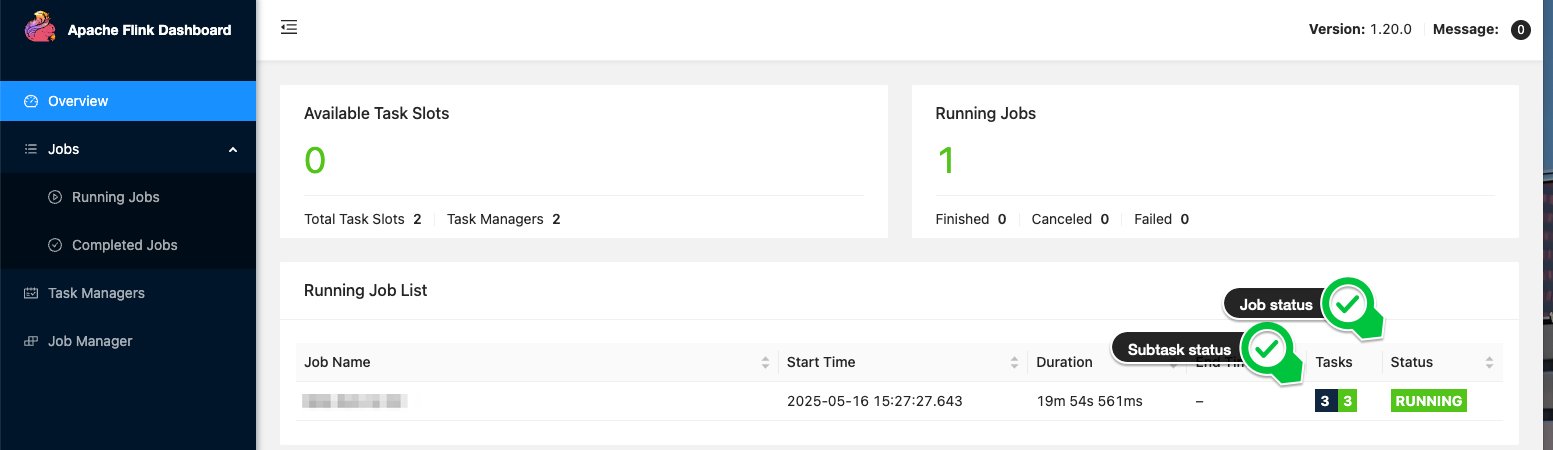
Gal Heyne is a Senior Technical Product Manager for AWS Analytics services with a strong focus on AI/ML and data engineering. She is passionate about developing a deep understanding of customers’ business needs and collaborating with engineers to design simple-to-use data products.

Modernizing SOAP applications using Amazon API Gateway and AWS Lambda

2025-07-15 Daniel Abib

Post Syndicated from Daniel Abib original https://aws.amazon.com/blogs/compute/modernizing-soap-applications-using-amazon-api-gateway-and-aws-lambda/

This post demonstrates how you can modernize legacy SOAP applications using Amazon API Gateway and AWS Lambda to create bidirectional proxy architectures that enable integration between SOAP and REST systems without disrupting existing business operations.

Many organizations today face the challenge of maintaining critical business systems that were built decades ago. These legacy applications power essential business operations despite relying on outdated technologies and integration patterns. Although complete system replacement would be ideal, practical constraints such as budget limitations, resource availability, technical complexity, and missing documentation often make modernization efforts challenging.

This post first shows proxy architecture patterns to expose a legacy SOAP server over a REST API. It then shows how to integrate a legacy SOAP client with applications using a REST API.

While SOAP and REST APIs share HTTP as their foundation, SOAP has some limitations compared to REST, like limited HTTP methods (GET/POST only) and mandatory XML formatting. REST is more flexible with multiple HTTP methods and diverse payload formats (plain text, binary, HTML, JSON, XML).

Using API Gateway and Lambda to proxy SOAP service

Consider a legacy solution that only supports SOAP. The following diagram shows the architecture for a SOAP proxy server using API Gateway and Lambda.

Figure 1: SOAP Server Proxy for modernized architecture

The proxy exposes the APIs hosted on the SOAP Server (on the right side of the image) over a REST interface. A SOAP service expects the HTTP Content-Type header set to text/xml, and a XML format payload that follows the WSDL specification defined by the server.

In the proposed architecture, the Lambda function is the core transformation engine, handling the bidirectional conversion between JSON and XML formats. Lambda functions can be developed in multiple programming languages such as Python, Node.js, Java, C#, Go, Ruby, and PowerShell, allowing you to use your existing development expertise. The serverless nature of Lambda provides automatic scaling to handle traffic spikes without needing infrastructure management or capacity planning.

API Gateway acts as the intelligent front door, managing all incoming requests and routing them appropriately. It provides enterprise-grade features such as request throttling to protect backend systems from overload, comprehensive authentication and authorization mechanisms, API key management for partner access control, request and response validation, caching capabilities for improved performance, and detailed monitoring and logging. These built-in features remove the need for custom middleware development and provide immediate operational benefits. API Gateway can receive multiple payload format such as XML, JSON, binary data, and plain text. This makes it suitable for diverse integration scenarios.

Using API Gateway and Lambda to support legacy SOAP clients

The previous section focused on exposing SOAP services over REST APIs. Organizations also face the reverse challenge where legacy SOAP client applications must access REST services. The architecture for supporting legacy SOAP clients follows a similar pattern but with reversed data flow. In this case, the legacy SOAP client sends XML-formatted requests to what it believes is a SOAP server. However, behind the scenes API Gateway and Lambda work together to translate these requests into REST API calls.

Figure 2: Legacy SOAP client modernization architecture

The legacy SOAP client application sends XML SOAP messages to API Gateway. The Lambda function receives these SOAP requests, extracts the relevant data from the XML envelope, and transforms it into JSON format for the modern REST service.

The Lambda function wraps the JSON response from the REST services into the SOAP XML format that the legacy client expects. It recreates the appropriate XML structure, SOAP headers, and ensures that the response conforms to the WSDL specification that the client application was designed to consume.

Example scenario

Let’s suppose our legacy client application needs to send a SOAP request to convert an integer number to its word form. The SOAP envelop to convert the number 1519 to its long form “one thousand, five hundred and nine” looks like this:

<?xml version="1.0" encoding="utf-8"?>
<soap:Envelope xmlns:soap="http://schemas.xmlsoap.org/soap/envelope/">
    <soap:Body> \
        <ConvertNumberToWordsSoapIn>
            <NumberToWordsRequest>1519</NumberToWordsRequest>
        </ConvertNumberToWordsSoapIn>
    </soap:Body>
</soap:Envelope>

The REST conversion service expects a JSON payload the as follownig:

jsonObject = {
	"data" : 1519
}

The following code block shows a sample Lambda function implementation for this. This function converts the SOAP XML envelop to JSON, changes the http header to application/json, and converts response from REST service to SOAP format.

var parseString = require('xml2js').parseString;
const axios = require('axios');

exports.handler = async (event, context) => {
    var valueNumber;
    
    try {
        console.log("Parsing XML string");

        // Parsing the XML to obtain data needed for conversion (number to words)
        parseString(event.body, function (err, result) {
            if (!err) {
                valueNumber = result['soap:Envelope']['soap:Body'][0]
                              ['ConvertNumberToWordsSoapIn'][0]
                              ['NumberToWordsRequest'][0];
            } else { 
                console.log (err);
                throw (err);
            }
        });
        console.log("Creating JSON for calling the service");
        // Creating JSON to call service
        var jsonObject = {
            "data" : valueNumber
        }
        
        console.log("Calling Microservice (NumberToWords)");
        const headers = { 
            'Content-Type': 'Application/json'
        };
        
        console.log ("Parameter for NumberToWords URL:" + 
                    JSON.stringify(process.env.NumberToWordMicroservice));

        // Calling numberToWords REST Server
        var resultNumberToWords = await 
            axios.post(process.env.NumberToWordMicroservice, jsonObject, { headers });
        
        // Creating the response
        console.log("Creating response XML");

        var resp =  create_response (JSON.stringify(resultNumberToWords.data.message));
        console.log("Response in XML: "+ resp);
        
        // Returning the value in XML using text/xml content type
        let response = {'statusCode': 200, headers: {"content-type": "text/xml"}, 
                        'body': JSON.stringify(resp)}
        return response;
        
    } catch (err) {
        console.log ("Error: " + err);
        let response = {'statusCode': 500, 
                        headers: {"content-type": "text/xml"}, 'body': err}
        return response;
    }
};

// Function to create a SOAP XML envelope with the result value
function create_response(numberInWords) {
  return '<?xml version="1.0" encoding="utf-8"?> \
            <soap:Envelope xmlns:soap="http://schemas.xmlsoap.org/soap/envelope/">\
            <soap:Body>\
              <m:ConvertNumberToWordsResponse xmlns:m="http://www.dataaccess.com/webservicesserver/"> \
                  <m:ConvertNumberToWordsResponseResult>' + numberInWords + '</m:ConvertNumberToWordsResponseResult> \
              </m:ConvertNumberToWordsResponse> \
            </soap:Body>\
            </soap:Envelope>';
}

With this approach, you can maintain your existing SOAP client applications without modification, allowing them to consume modern REST services. You can preserve investments in legacy client applications while gradually modernizing the overall system. This architecture is particularly valuable in scenarios where multiple legacy SOAP clients need to access the same modern REST services. This is because a single proxy can serve multiple client applications simultaneously. The serverless nature of the architecture makes sure that it scales automatically based on the number of client requests, providing cost-effective operation regardless of usage patterns.

Alternative approach using API Gateway transformation capabilities

The Lambda-based approach provides maximum flexibility and control. API Gateway also offers built-in transformation capabilities that can handle certain SOAP modernization scenarios without the need for compute resources.

The native API Gateway transformation uses Apache Velocity Template Language mapping templates. It converts the payload directly at the gateway, offering a streamlined solution for specific modernization scenarios.

The VTL approach works by defining mapping templates that handle the conversion process between different payload formats. When modernizing SOAP services, these templates can intercept REST requests with JSON payloads, restructure the data into XML format compatible with your legacy SOAP endpoints, and reverse the process for responses returning to the client.

Figure 3: API Gateway with velocity template language transformation

This gateway-native transformation strategy offers several operational advantages. You benefit from streamlined architecture because the transformation logic resides entirely within the API Gateway service. There are no other infrastructure components to manage or monitor, and the solution avoids the complexity of coordinating between multiple AWS services. Cost efficiency is another key benefit, as there are no compute charges beyond the standard API Gateway pricing.

Consider the previous example of converting a number to its word format. The VTL transformation in API Gateway will look like this:

## Parse the SOAP envelope and extract the number value
#set(\$xmlDoc = \$input.path('\$'))
#set(\$numberToWords = \$xmlDoc.Envelope.Body.ConvertNumberToWordsSoapIn.NumberToWordsRequest)

## Convert to integer if it's a string
#if(\$numberToWords.toString().matches("^\d+\$"))
  #set(\$dataValue = \$numberToWords.toInteger())
#else
  #set(\$dataValue = \$numberToWords)
#end

{
  "data": \$dataValue
}

You should consider VTL transformations when your SOAP services have predictable, stable schemas with relatively direct XML structures. This approach works particularly well for legacy systems that rarely undergo changes and have clear request-response patterns. For more dynamic environments or complex transformation requirements, the Lambda-based solution provides superior flexibility and maintainability.

Security considerations

An important consideration when working with legacy SOAP services is understanding their authentication mechanisms. SOAP protocols often implement authentication through security standards, where authentication credentials and security tokens are embedded directly within the SOAP envelope headers. This includes username tokens, digital signatures, and encryption elements that are part of the XML structure.

When SOAP envelopes contain unencrypted authentication information in the headers, the proxy architecture typically functions without more modifications. This is because the Lambda function can pass through these authentication elements transparently to the backend SOAP service. However, due to the nature of SOAP authentication being tightly integrated with the XML envelope structure, certain scenarios may need custom handling within the Lambda function.

For example, if the SOAP service uses timestamp-based authentication tokens, session management, or needs specific security header modifications, the Lambda function may need customization to properly handle, validate, or refresh these authentication elements during the JSON-to-XML transformation process. Organizations should carefully analyze their SOAP service authentication requirements to determine if more Lambda logic is needed to maintain security compliance.

Moreover, make sure that any SOAP authentication credentials processed by the Lambda function are handled securely and never logged in plain text.

Conclusion

In this post, you learned how cloud-native services can bridge the gap between legacy systems and modern application architectures, allowing you to use your existing investments while adopting contemporary development practices and technologies.

Amazon API Gateway and AWS Lambda enable organizations to create REST services that proxy legacy SOAP servers, allowing modern applications to consume legacy services through JSON payloads while preserving existing SOAP infrastructure. This serverless solution provides cost-effectiveness, automatic scaling, and reduced operational overhead while facilitating company modernization through scalable APIs without abandoning legacy software investments.

This modernization strategy allows you to gradually transition from legacy SOAP services to modern REST APIs without disrupting existing business operations. As your modernization journey progresses, you can extend this pattern to support more SOAP services or implement more sophisticated transformation logic based on your specific business requirements.

For more serverless learning resources, visit Serverless Land.

Geospatial data lakes with Amazon Redshift

2025-07-11 Jeremy Spell

Post Syndicated from Jeremy Spell original https://aws.amazon.com/blogs/big-data/geospatial-data-lakes-with-amazon-redshift/

Data lake architectures help organizations offload data from premium storage systems without losing the ability to query and analyze the data. This architecture can be useful for geospatial data, where builders might have terabytes of infrequently accessed data in their databases that they want to cost-effectively maintain. However, this requires for their data lake query engine to support geographic information systems (GIS) data types and functions.

Amazon Redshift supports querying spatial data, including the GEOMETRY and GEOGRAPHY data types and functions that are used in querying GIS systems. Additionally, Amazon Redshift lets you query geospatial data both in your data lakes on Amazon S3 and your Redshift data warehouse, giving you the choice of how you can access your data. Additionally, AWS Lake Formation and support for AWS Identity and Access Management (IAM) in Esri’s ArcGIS Pro gives you a way to securely bridge data between your geospatial data lakes and map visualization tools. You can set up, manage, and secure geospatial data lakes in the cloud with a few clicks.

In this post, we walk through how to set up a geospatial data lake using Lake Formation and query the data with ArcGIS Pro using Amazon Redshift Serverless.

Solution overview

In our example, a county public health department has used Lake Formation to secure their data lake that contains public health information (PHI) data. Epidemiologists within the county want to create a map for the clinics providing vaccination for their communities. The county’s GIS analysts need access to the data lake to create the required maps without being able to access the PHI data.

This solution uses Lake Formation tags to allow column-level access in the database to the public information that includes the clinic names, addresses, zip codes, and longitude/latitude coordinates without allowing access to the PHI data within the same tables. We use Redshift Serverless and Amazon Redshift Spectrum to access this data from ArcGIS Pro, a GIS mapping software from Esri, an AWS Partner.

The following diagram shows the architecture for this solution.

End-to-end architecture showing ArcGIS Pro data integration with AWS analytics services through Redshift connector

The following is a sample schema for this post.

`Description`	`Column Name`	`Geoproperty Tag`
`Patient ID`	`patient_id`	`No`
`Clinic ID`	`clinic_id`	`Yes`
`Address of Clinic`	`clinic_address`	`Yes`
`Clinic Zip Code`	`clinic_zip`	`Yes`
`Clinic City`	`clinic_city`	`Yes`
`First Name Patient`	`first_name`	`No`
`Last Name Patient`	`last_name`	`No`
`Patient Address`	`patient_address`	`No`
`Patient Zip Code`	`patient_zip`	`No`
`Vaccination Type`	`vaccination_type`	`No`
`Latitude of Clinic`	`clinic_lat`	`Yes`
`Longitude of Clinic`	`clinic_long`	`Yes`

In the following sections, we walk through the steps to set up the solution:

Deploy the solution infrastructure using AWS CloudFormation.
Upload a CSV with sample data to an Amazon Simple Storage Service (Amazon S3) bucket and run an AWS Glue crawler to crawl the data.
Set up Lake Formation permissions.
Configure the Amazon Redshift Query Editor v2.
Set up the schemas in Amazon Redshift.
Create a view in Amazon Redshift.
Create a local database user in ArcGIS Pro.
Connect ArcGIS Pro to the Redshift database.

Prerequisites

You should have the following prerequisites:

An AWS account
Lake Formation enabled in your target AWS Region
Familiarity with Lake Formation and setting permissions on tables
ArcGIS Pro
Network connectivity from the ArcGIS Pro client to the virtual private cloud (VPC) where Amazon Redshift resources will be deployed using either VPN or AWS Direct Connect

Set up the infrastructure with AWS CloudFormation

To create the environment for the demo, complete the following steps:

Log in to the AWS Management Console as an AWS account administrator and a Lake Formation data lake administrator—this account needs to be both an account admin and a data lake admin for the template to complete.
Open the AWS CloudFormation console
Choose Launch Stack.

The CloudFormation template creates the following components:

S3 bucket – samp-clinic-db-{ACCOUNT_ID}
AWS Glue database – samp-clinical-glue-db
AWS Glue crawler – samp-glue-crawler
Redshift Serverless workgroup – samp-clinical-rs-wg
Redshift Serverless namespace – samp-clinical-rs-ns
IAM role for Amazon Redshift – demo-RedshiftIAMRole-{UNIQUE_ID}
IAM role for AWS Glue – samp-clinical-glue-role
Lake Formation tag – geoproperty

Upload a CSV to the S3 bucket and run the AWS Glue crawler

The next step is to create a data lake in our demo environment and then use an AWS Glue crawler to populate the AWS Glue database and update the schema and metadata in the AWS Glue Data Catalog.

The CloudFormation stack created the S3 bucket we will use as well as the AWS Glue database and crawler. We have provided a fictious test dataset that will represent the patient and clinical information. Download the file and complete the following steps:

On the AWS CloudFormation console, open the stack you just launched.
On the Resources tab, choose the link to the S3 bucket.
Choose Upload and add the CSV file (data-with-geocode.csv), then choose Upload.
On the AWS Glue console, choose Crawlers in the navigation pane.
Select the crawler you created with the CloudFormation stack and choose Run.

The crawler run should only take a minute to complete, and will populate a table named clinic-sample-s3_ACCOUNT_ID with a fictious dataset.

Choose Tables in the navigation pane and open the table the crawler populated.

You will see that the dataset contains fields that contain PHI and personally identifiable information (PII).

AWS Glue table 'clinic-sample_s3' schema definition with patient and clinic fields, input/output formats, and database properties

We now have a database set up and the Data Catalog populated with the schema and metadata we will use for the rest of the demo.

Set up Lake Formation permissions

In this next set of steps, we demonstrate how to secure PHI data to maintain compliance and empower GIS analysts to work effectively. To secure the data lake, we use AWS Lake Formation. In order to properly set up Lake Formation permissions, we need to gather details on how access to the data lake is established.

The Data Catalog provides metadata and schema information that enables services to access data within the data lake. To access the data lake from ArcGIS Pro, we use the ArcGIS Pro Redshift connector, which allows a connection from ArcGIS Pro to Amazon Redshift. Amazon Redshift can access the Data Catalog and provide connectivity to the data lake. The CloudFormation template created a Redshift Serverless instance and namespace and an IAM role that we will use to configure this connection. We still need to set up Lake Formation permissions so that GIS analysts can only access publicly available fields and not those containing PHI or PII. We will assign a Lake Formation tag on the columns containing the publicly available information and assign permissions to the GIS analysts to allow access to columns with this tag.

By default, the Lake Formation configuration allows Super access to IAMAllowedPrinciples; this is to maintain backward compatibility as detailed in Changing the default settings for your data lake. To demonstrate a more secure configuration, we will remove this default configuration.

On the Lake Formation console, choose Administration in the navigation pane.
In the Data Catalog settings section, make sure Use only IAM access control for new databases and Use only IAM access control for new tables in new databases are unchecked.

AWS Data Catalog settings interface showing unchecked IAM-only access control options for new databases and tables

In the navigation pane, under Permissions, choose Data permissions.
Select IAMAllowedPrincipals and choose Revoke.
Choose Tables in the navigation pane.
Open the table clinic-sample-s3_ACCOUNT_ID and choose Edit schema.
Select the fields beginning with clinic_ and choose Edit LF-Tags.
The CloudFormation stack created a Lake Formation tag named geoproperty. Assign geoproperty as the key and true for the value on all the clinic_ fields, then choose Save.

Next, we need to grant the Amazon Redshift IAM role permission to access fields tagged with geoproperty = true.

Choose Data lake permissions, then choose Grant.
For the IAM role, choose demo-RedshiftIAMRole-UNIQUE_ID.
Select geoproperty for the key and true for the value.
Under Database permissions, select Describe, and under Table permissions, select Select and Describe.

Configure the Amazon Redshift Query Editor v2

Next, we need to perform the initial configuration of Amazon Redshift required for database operations. We use an AWS Secrets Manager secret created by the template to make sure password access is managed securely in accordance with AWS best practices.

On the Amazon Redshift console, choose Query editor v2.
When you first start Amazon Redshift, a one-time configuration for the account appears. For this post, leave the options default and choose Configure account.

For more information about these options, refer to Configuring your AWS account.

Redshift query editor configuration interface with AWS KMS encryption settings and optional S3 bucket path input

The query editor will require credentials to connect to the serverless instance; these have been created by the template and stored in Secrets Manager.

Select Other ways to connect, then select AWS Secrets Manager.
For Secret, select (Redshift-admin-credentials).
Choose Save.

Redshift connection interface displaying IAM Identity Center and AWS Secrets Manager authentication methods with credential selector

Set up schemas in Amazon Redshift

An external schema in Amazon Redshift is a feature used to reference schemas that exist in external data sources. For information on creating external schemas, see External schemas in Amazon Redshift Spectrum. We use an external schema to provide access to the data lake in Amazon Redshift. From ArcGIS Pro, we will connect to Amazon Redshift to access the geospatial data.

The IAM role used in the creation of the external schema needs to be associated with the Redshift namespace. This has already been set up by the CloudFormation template, but it’s a good practice to verify that the role is set up correctly before proceeding.

On the Redshift Serverless console, choose Namespace configuration in the navigation pane.
Choose the namespace (sample-rs-namespace).

Amazon Redshift Serverless console displaying namespace configuration with status, workgroup and creation details

On the Security and encryption tab, you should see the IAM role created by CloudFormation. If this role or the namespace isn’t present, verify the stack in AWS CloudFormation before proceeding.

Copy the ARN of the role for use in a later step.

Redshift security configuration panel showing single synchronized IAM role with complete ARN and management options

Choose Query data to return to the query editor.

Amazon Redshift Serverless interface displaying sample-rs-namespace configuration with management and query data controls

In the query editor, enter the following SQL command; be sure to replace the example role ARN with your own. This SQL command will create an external schema that uses the same Redshift role associated with our namespace to attach to the AWS Glue database.

CREATE EXTERNAL SCHEMA samp_clinic_sch_ext FROM DATA CATALOG
database 'sample-glue-database'
IAM_ROLE 'arn:aws:iam::{ACCOUNT_ID}:role/demo-RedshiftIAMRole-{UNIQUE_ID}';

In the query editor, perform a select query on sample-glue-database:

SELECT * FROM "dev"."samp_clinic_sch_ext"."clinic-sample_s3_{ACCOUNT_ID}";

Because the associated role has been granted access to columns tagged with geoproperty = true, only those fields will be returned, as shown in the following screenshot (the data in this example is fictionalized).

Query result displaying 20 medical clinics with details like name, address, and coordinates

Use the following command to create a local schema in Amazon Redshift. The external schema can’t be updated; we will use this local schema to add a geometry field with a Redshift function.

CREATE SCHEMA samp_clinic_sch_local

Create a view in Amazon Redshift

For the data to be viewable from ArcGIS Pro, we will need to create a view. Now that the schemas have been established, we can create the view that can be accessed from ArcGIS Pro.

Amazon Redshift provides many geospatial functions that can be used to create views with fields used by ArcGIS Pro to add points onto a map. We will use one of these functions because the dataset contains latitude and longitude.

Use the following SQL code in the Amazon Redshift Query Editor to create a new view named clinic_location_view. Replace {ACCOUNT_ID} with your own account ID.

CREATE
OR REPLACE VIEW "samp_clinic_sch_local"."clinic_location_view" AS
SELECT
    clinic_id as id,
    clinic_lat as lat,
    clinic_long as long,
    ST_MAKEPOINT(long, lat) as geom
FROM
    “dev”."samp_clinic_sch_ext"."clinic-sample_s3_{ACCOUNT_ID}"
WITH NO SCHEMA BINDING;

The new view that is created under your local schema will have a column named geom containing map-based points that can be used by ArcGIS Pro to add points during map creation. The points in this example are for the clinics providing vaccines. In a real-world scenario, as new clinics are built and their data is added to the data lake, their locations would be added to the map created using this data.

Create a local database user for ArcGIS Pro

For this demo, we use a database user and group to provide access for ArcGIS Pro clients. Enter the following SQL code into the Amazon Redshift Query Editor to create a database user and group:

CREATE USER dbuser with PASSWORD ‘SET_PASSWORD_HERE’;
CREATE GROUP esri_developer_group;
ALTER GROUP esri_developer_group ADD USER dbuser;

After the commands are complete, use the following code to grant permissions to the group:

GRANT USAGE ON SCHEMA samp_clinic_sch_local TO GROUP esri_developer_group;
ALTER DEFAULT PRIVILEGES IN SCHEMA samp_clinic_sch_local GRANT SELECT ON TABLES TO GROUP esri_developer_group;
GRANT SELECT ON ALL TABLES IN SCHEMA samp_clinic_sch_local TO GROUP esri_developer_group;

Connect ArcGIS Pro to the Redshift database

In order to add the database connection to ArcGIS Pro, you need the endpoint for the Redshift Serverless workgroup. You can access the endpoint information on the sample-rs-wg workgroup details page on the Redshift Serverless console. The Redshift namespaces and workgroups are listed by default, as shown in the following screenshot.

Amazon Redshift Serverless namespace and workgroup status dashboard with performance metrics

You can copy the endpoint in the General information section. This endpoint will need to modified; the :5439/dev will need to be removed when configuring the connector in ArcGIS Pro.

Amazon Redshift Serverless workgroup details showing configuration and connection information

Open ArcGIS Pro with the project file you want to add the Redshift connection to.

Make sure the Amazon Redshift ODBC connector has already been installed; this is required in order to make the connection.

On the menu, choose Insert and then Connections, Database, and New Database Connection.
For Database Platform, choose Amazon Redshift.
For Server, insert the endpoint you copied (remove everything following .com from the endpoint).
For Database, choose your database.

Amazon Redshift Serverless connection settings with server, authentication, and database fields

If your ArcGIS Pro client doesn’t have access to the endpoint, you will receive an error during this step. A network path must exist between the ArcGIS Pro client and the Redshift Serverless endpoint. You can set up the network path with Direct Connect, AWS Site-to-Site VPN, or AWS Client VPN. Although it’s not recommended for security reasons, you can also configure Amazon Redshift with a publicly available endpoint. Be sure you consult your security and network teams for best practices and policy guidance before allowing public access to your Redshift Serverless instance.

If a network path exists and you’re having issues connecting, verify the security group rules allow communication inbound from your ArcGIS Pro subnet over the port your Redshift Serverless instance is running on. The default port is 5439, but you can configure a range of ports depending on your environment; see Connecting to Amazon Redshift Serverless for more information.

If connectivity is successful, ArcGIS Pro will add the Amazon Redshift connection under Connection File Name.

Choose OK.
Choose the connection to display the view that was created to include geometry (clinic_location_view).
Choose (right-click) the view and choose Add To Current Map.

ArcGIS Pro will add the points from the view onto the map. The final map displayed has the symbology edited to use red crosses to represent the clinics instead of dots.

Professional GIS interface showing Houston metropolitan vaccination clinics with topographic base map, toolbars, and database connectivity

Clean up

After you have finished the demo, complete the following steps to clean up your resources:

On the Amazon S3 console, open the bucket created by the CloudFormation stack and delete the data-with-geocode.csv file.
On the AWS CloudFormation console, delete the demo stack to remove the resources it created.

Conclusion

In this post, we reviewed how to set up Redshift Serverless to use geospatial data contained within a data lake to enhance maps in ArcGIS Pro. This technique helps builders and GIS analysts use available datasets in data lakes and transform it in Amazon Redshift to further enrich the data before presenting it on a map. We also showed how to secure a data lake using Lake Formation, crawl a geospatial dataset with AWS Glue, and visualize the data in ArcGIS Pro.

For additional best practices for storing geospatial data in Amazon S3 and querying it with Amazon Redshift, see How to partition your geospatial data lake for analysis with Amazon Redshift. We invite you to leave feedback in the comments section.

About the authors

Jeremy Spell is a Cloud Infrastructure Architect working with Amazon Web Services (AWS) Professional Services. He enjoys architecting and building solutions for customers. In his free time Jeremy makes Texas style BBQ, and spends time with his family and church community.

Jeff Demuth is a solutions architect who joined Amazon Web Services (AWS) in 2016. He focuses on the geospatial community and is passionate about geographic information systems (GIS) and technology. Outside of work, Jeff enjoys traveling, building Internet of Things (IoT) applications, and tinkering with the latest gadgets.