Tag Archives: Technical How-to

Streamline Spark application development on Amazon EMR with the Data Solutions Framework on AWS

Post Syndicated from Vincent Gromakowski original https://aws.amazon.com/blogs/big-data/streamline-spark-application-development-on-amazon-emr-with-the-data-solutions-framework-on-aws/

Today, organizations are heavily using Apache Spark for their big data processing needs. However, managing the entire development lifecycle of Spark applications—from local development to production deployment—can be complex and time-consuming. Managing the entire code base—including application code, infrastructure provisioning, and continuous integration and delivery (CI/CD) pipelines—is sometimes not fully automated and a shared responsibility across multiple teams, which slows down release cycles. This undifferentiated heavy lifting diverts valuable resources away from core business objectives: deriving value from data.

In this post, we explore how to use Amazon EMR, the AWS Cloud Development Kit (AWS CDK), and the Data Solutions Framework (DSF) on AWS to streamline the development process, from setting up a local development environment to deploying serverless Spark infrastructure, and implementing a CI/CD pipeline for automated testing and deployment.

By adopting this approach, developers gain full control over their code and the infrastructure responsible for running it, alleviating the need for cross-team dependency. Developers can customize the infrastructure to meet specific business needs and optimize performance. Additionally, they can customize CI/CD stages to facilitate comprehensive testing, using the self-mutation capability of AWS CDK Pipelines to automatically update and refine the deployment process. This level of control not only accelerates development cycles but also enhances the reliability and efficiency of the entire application lifecycle, so developers can focus more on innovation and less on manual infrastructure management.

Solution overview

The solution consists of the following key components:

  • The local development environment to develop and test your Spark code locally
  • The infrastructure as code (IaC) that will run your Spark application in AWS environments
  • The CI/CD pipeline running end-to-end tests and deploying into the different AWS environments

In the following sections, we discuss how to set up these components.

Prerequisites

To set up this solution, you must have an AWS account with appropriate permissions, Docker and the AWS CDK CLI.

Set up the local development environment

Developing Spark applications locally can be a challenging task due to the need for a consistent and efficient environment that mirrors your production setup. With Amazon EMR, Docker, and the Amazon EMR toolkit extension for Visual Studio Code, you can quickly set up a local development environment for Spark applications, developing and testing Spark code locally, and seamlessly port it to the cloud.

The Amazon EMR toolkit for VS Code includes an “EMR: Create Local Spark Environment” command that generates a development container. This container is based on an Amazon EMR on Amazon EKS image corresponding to the Amazon EMR version you select. You can develop Spark and PySpark code locally, with full compatibility with your remote Amazon EMR environment. Additionally, the toolkit provides helpers to make it straightforward to connect to the AWS Cloud, including an Amazon EMR explorer, an AWS Glue Data Catalog explorer, and commands to run Amazon EMR Serverless jobs from VS Code.

To set up your local environment, complete the following steps:

  1. Install VS Code and the Amazon EMR Toolkit for VS Code.
  2. Install and launch Docker.
  3. Create a local Amazon EMR environment in your working directory using the command EMR: Create Local Spark Environment.

Amazon EMR Toolkit bootstrap

  1. Choose PySpark, Amazon EMR 7.5, and the AWS Region you want to use, and choose an authentication mechanism.

Amazon EMR toolkit local environment

  1. Log in to Amazon ECR with your AWS credentials using the following command so you can download the Amazon EMR image:
aws ecr get-login-password --region us-east-1 \
    | docker login \
    --username AWS \
    --password-stdin \
    12345678910.dkr.ecr.us-east-1.amazonaws.com
  1. Now you can launch your dev container using the VS Code command Dev Containers: Rebuild and Reopen in container.

The container will install the latest operating system packages and run a local Spark history server on port 18080.

local Spark history server

The container provides spark-shell, spark-sql, and pyspark from the terminal and a Jupyter Python kernel for connecting a Jupyter notebook to execute interactive Spark code.

local Jupyter notebooks

Using the Amazon EMR Toolkit, you can develop your Spark application and test it locally using Pytest—for example, to validate the business logic. You can also connect to other AWS accounts where you have your development environment.

Build the AWS CDK application with DSF on AWS

After you validate the business logic into your local Spark application, you can implement the infrastructure responsible for running your application. DSF provides AWS CDK L3 Constructs that simplify the creation of Spark-based data pipelines on EMR Serverless or Amazon EMR on EKS.

DSF provides the capability to package your local PySpark application, including the Python dependencies, into artifacts that can consumed by EMR Serverless jobs. The PySparkApplicationPackage is a construct that uses a Dockerfile to perform the packaging of dependencies into a Python virtual environment archive and then upload the archive and the PySpark entrypoint file into a secured Amazon Simple Storage Service (Amazon S3) bucket. The following diagram illustrates this architecture.

PySparkApplicationPackage L3 construct

See the following example code:

spark_app = dsf.processing.PySparkApplicationPackage(
    self,
    "SparkApp",
    entrypoint_path="./../spark/src/agg_trip_distance.py",
    application_name="TaxiAggregation",
    # Path of the Dockerfile used to package the dependencies as a Python venv
    dependencies_folder='./../spark',
    # Path of the venv archive in the docker image
    venv_archive_path="/venv-package/pyspark-env.tar.gz",
    removal_policy=RemovalPolicy.DESTROY)

You just need to provide the paths for the following:

  • The PySpark entrypoint. This is the main Python script of your Spark application.
  • The Dockerfile containing the logic for packaging a virtual environment into an archive.
  • The path of the resulting archive in the container file system.

DSF provides helpers to connect the application package to the EMR Serverless job. The PySparkApplicationPackage construct exposes properties that can directly be used into the SparkEmrServerlessJob construct parameters. This construct simplifies the configuration of a batch job using an AWS Step Functions state machine. The following diagram illustrates this architecture.

EmrServerlessJob L3 construct

The following code is an example of an EMR Serverless job:

spark_job = dsf.processing.SparkEmrServerlessJob(
    self,
    "SparkProcessingJob",
    dsf.processing.SparkEmrServerlessJobProps(
        name=f"taxi-agg-job-{Names.unique_resource_name(self)}",
        # ID of the previously created EMR Serverless runtime
        application_id=spark_runtime.application.attr_application_id,
        # The IAM role used by the EMR Job with permissions required by the application
        execution_role=processing_exec_role,
        spark_submit_entry_point=spark_app.entrypoint_uri,
        # Add the Spark parameters from the PySpark package to configure the dependencies (using venv)
        spark_submit_parameters=spark_app.spark_venv_conf + spark_params,
        removal_policy=RemovalPolicy.DESTROY,
        schedule=schedule))

Note the two parameters of SparkEmrServerlessJob that are provided by PySparkApplicationPackage:

  • entrypoint_uri, which is the S3 URI of the entrypoint file
  • spark_venv_conf, which contains the Spark submit parameters for using the Python virtual environment

DSF also provides a SparkEmrServerlessRuntime to simplify the creation of the EMR Serverless application responsible for running the job.

Deploy the Spark application using CI/CD

The final step is to implement a CI/CD pipeline that can test your Spark code and promote from dev/test/stage and then to production. DSF provides a L3 Construct that simplifies the creation of the CI/CD pipeline for your Spark applications. DSF’s implementation of the Spark CI/CD pipeline construct uses the AWS CDK built-in pipeline functionality. One of the key capabilities when using an AWS CDK pipeline is its self-mutating capability. It can update itself whenever you change its definition, avoiding the traditional chicken-and-egg problem of pipeline updates and helping developers fully control their CI/CD pipeline.

When the pipeline runs, it follows a carefully orchestrated sequence. First, it retrieves your code from your repository and synthesizes it into AWS CloudFormation templates. Before doing anything else, it examines these templates to see if you’ve made any changes to the pipeline’s own structure. If the pipeline detects that its definition has changed, it will pause its normal operation and update itself first. After the pipeline has updated itself, it will continue with its regular stages, such as deploying your application.

DSF provides an opinionated implementation of CDK Pipelines for Spark applications, where the PySpark code is automatically unit tested using Pytest and where the configuration is simplified. You only need to configure four components:

  • The CI/CD stages (testing, staging, production, and so on). This includes the AWS account ID and Region where these environments reside in.
  • The AWS CDK stack that is deployed in each environment.
  • (Optional) The integration test script that you want to run against the deployed stack.
  • The SparkEmrCICDPipeline AWS CDK construct.

The following diagram illustrates how everything works together.

SparkCICDPipeline L3 construct

Let’s dive into each of these components.

Define cross-account deployment and CI/CD stages

With the SparkEmrCICDPipeline construct, you can deploy your Spark application stack across different AWS accounts. For example, you can have a separate account for your CI/CD processes and different accounts for your staging and production environments.To set this up, first bootstrap the various AWS accounts (staging, production, and so on):

cdk bootstrap --profile <ENVIRONMENT_ACCOUNT_PROFILE> \ 
    aws://<ENVIRONMENT_ACCOUNT_ID&gt;/&lt;REGION> \ 
    --trust <CICD_ACCOUNT_ID> \ 
    --cloudformation-execution-policies "POLICY_ARN"

This step sets up the necessary resources in the environment accounts and creates a trust relationship between those accounts and the CI/CD account where the pipeline will run.Next, choose between two options to define the environments (both options require the relevant configuration in the cdk.context.json file.The first option is to use pre-defined environments, which is defined as follows:

{ 
    "staging": { 
        "account": "<STAGING_ACCOUNT_ID>", 
        "region": "<REGION>" 
    }, 
    "prod": { 
        "account": "<PROD_ACCOUNT_ID>", 
        "region": "<REGION>" 
    } 
}

Alternatively, you can use user-defined environments, which is defined as follows:

{
   "environments":[
      {
         "stageName":"<STAGE_NAME_1>",
         "account":"<STAGE_ACCOUNT_ID>",
         "region":"<REGION>",
         "triggerIntegTest":"<OPTIONAL_BOOLEAN_CAN_BE_OMMITTED>"
      },
      {
         "stageName":"<STAGE_NAME_2>",
         "account":"<STAGE_ACCOUNT_ID>",
         "region":"<REGION>",
         "triggerIntegTest":"<OPTIONAL_BOOLEAN_CAN_BE_OMMITTED>"
      },
      {
         "stageName":"<STAGE_NAME_3>",
         "account":"<STAGE_ACCOUNT_ID>",
         "region":"<REGION>",
         "triggerIntegTest":"<OPTIONAL_BOOLEAN_CAN_BE_OMMITTED>"
      }
   ]
}

Customize the stack to be deployed

Now that the environments have been bootstrapped and configured, let’s look at the actual stack that contains the resources that will be deployed in the various environments. Two classes must be implemented:

  • A class that extends the stack – This is where the resources that are going to be deployed in each of the environments are defined. This can be a normal AWS CDK stack, but it can be deployed in another AWS account depending on the environment configuration defined in the previous section.
  • A class that extends ApplicationStackFactory – This is DSF specific, and makes it possible to configure and then return the stack that is created.

The following code shows a full example:

class MyApplicationStack(cdk.Stack): 
    def __init__(self, scope, *, stage): 
        super().__init__(scope, "MyApplicationStack") 
        bucket = Bucket(self, "TestBucket",
                        auto_delete_objects=True, 
                        removal_policy=cdk.RemovalPolicy.DESTROY) 
        cdk.CfnOutput(self, "BucketName", value=bucket.bucket_name) 
        
class MyStackFactory(dsf.utils.ApplicationStackFactory): 
    def create_stack(self, scope, stage): 
        return MyApplicationStack(scope, stage=stage)

ApplicationStackFactory supports customization of the stack before returning the initialized object to be deployed by the CI/CD pipeline. You can customize your stack behavior by passing the current stage to your stack. For example, you can skip scheduling the Spark application in the integration tests stage because the integration tests trigger it manually as part of the CI/CD pipeline. For the production stage, the scheduling facilitates automatic execution of the Spark application.

Write the integration test script

The integration test script is a bash script that is triggered after the main application stack has been deployed. Inputs to the bash script can come from the AWS CloudFormation outputs of the main application stack. These outputs are mapped into environment variables that the bash script can access directly.

In the Spark CI/CD example, the application stack uses the SparkEMRServerlessJob CDK construct. This construct uses a Step Functions state machine to manage the execution and monitoring of the Spark job. The following is an example integration test bash script that we use to test that the deployed stack can run the associated Spark job successfully:

#!/bin/bash 
EXECUTION_ARN=$(aws stepfunctions start-execution --state-machine-arn $STEP_FUNCTION_ARN | jq -r '.executionArn')

while true 
do 
    STATUS=$(aws stepfunctions describe-execution --execution-arn $EXECUTION_ARN | jq -r '.status') 
    if [ $STATUS = "SUCCEEDED" ]; then 
        exit 0 
    elif [ $STATUS = "FAILED" ] || [ $STATUS = "TIMED_OUT" ] || [ $STATUS = "ABORTED" ]; then 
        exit 1 
    else 
        sleep 10
        continue 
    fi
done

The integration test scripts are executed within an AWS CodeBuild project. As part of the IntegrationTestStack, we’ve included a custom resource that periodically checks the status of the integration test script as it runs. Failure of the CodeBuild execution causes the parent pipeline (residing in the pipeline account) to fail. This helps teams only promote changes that pass all the required testing.

Bring all the components together

When you have your components ready, you can use the SparkEmrCICDPipeline to bring them together. See the following example code:

dsf.processing.SparkEmrCICDPipeline(
    self,
    "SparkCICDPipeline",
    spark_application_name="SparkTest",
    # The Spark image to use in the CICD unit tests
    spark_image=dsf.processing.SparkImage.EMR_7_5,
    # The factory class to dynamically pass the Application Stack
    application_stack_factory=SparkApplicationStackFactory(),
    # Path of the CDK python application to be used by the CICD build and deploy phases
    cdk_application_path="infra",
    # Path of the Spark application to be built and unit tested in the CICD
    spark_application_path="spark",
    # Path of the bash script responsible to run integration tests 
    integ_test_script='./infra/resources/integ-test.sh',
    # Environment variables used by the integration test script, value is the CFN output name
    integ_test_env={
        "STEP_FUNCTION_ARN": "ProcessingStateMachineArn"
    },
    # Additional permissions to give to the CICD to run the integration tests
    integ_test_permissions=[
        PolicyStatement(
            actions=["states:StartExecution", "states:DescribeExecution"
            ],
            resources=["*"]
        )
    ],
    source= CodePipelineSource.connection("your/repo", "branch",
        connection_arn="arn:aws:codeconnections:us-east-1:222222222222:connection/7d2469ff-514a-4e4f-9003-5ca4a43cdc41"
    ),
    removal_policy=RemovalPolicy.DESTROY,
)

The following elements of the code are worth highlighting:

  • With the integ_test_env parameter, you can define the environment variable mapping with the output of your application stack that’s defined in the application_stack_factory parameter
  • The integ_test_permissions parameter specifies the AWS Identity and Access Management (IAM) permissions that are attached to the CodeBuild project where the integration test script runs in
  • CDK Pipelines needs an AWS code connection Amazon Resource Name (ARN) to connect to your Git repository when you host your code

Now you can deploy the stack containing the CI/CD pipeline. This is a one-time operation because the CI/CD pipeline will dynamically be updated based on code changes that impact the CI/CD pipeline itself:

cd infra 
cdk deploy CICDPipeline

Then you can commit and push the code into the source code repository defined in the source parameter. This step triggers the pipeline and deploys the application in the configured environments. You can check the pipeline definition and status on the AWS CodePipeline console.

AWS CodePipeline

You can find the full example on the Data Solutions Framework GitHub repository.

Clean up

Follow the readme guide to delete the resources created by the solution.

Conclusion

By using Amazon EMR, the AWS CDK, DSF on AWS, and the Amazon EMR toolkit, developers can now streamline their Spark application development process. The solution described in this post helps developers gain full control over their code and infrastructure, making it possible to set up local development environments, implement automated CI/CD pipelines, and deploy serverless Spark infrastructure across multiple environments.

DSF supports other patterns, such as streaming governance and data sharing and Amazon Redshift data warehousing. The DSF roadmap is publicly available, and we look forward to your feature requests, contributions, and feedback. You can get started using DSF by following our Quick start guide.


About the authors

Jan Michael Go Tan

Jan Michael Go Tan

Jan is a Principal Solutions Architect for Amazon Web Services. He helps customers design scalable and innovative solutions with the AWS Cloud.

Vincent Gromakowski

Vincent Gromakowski

Vincent is an Analytics Specialist Solutions Architect at AWS where he enjoys solving customers’ analytics, NoSQL, and streaming challenges. He has a strong expertise on distributed data processing engines and resource orchestration platform.

Lotfi Mouhib

Lotfi Mouhib

Lotfi is a Principal Solutions Architect working for the Public Sector team with Amazon Web Services. He helps public sector customers across EMEA realize their ideas, build new services, and innovate for citizens. In his spare time, Lotfi enjoys cycling and running.

Tuning guide for AMD Amazon EC2 instances

Post Syndicated from Suyash Nadkarni original https://aws.amazon.com/blogs/compute/tuning-guide-for-amd-amazon-ec2-instances/

As organizations migrate more mission-critical workloads to the cloud, optimizing for price-performance becomes a key consideration. Amazon Elastic Compute Cloud (Amazon EC2) instances powered by AMD EPYC processors deliver high core density, large memory bandwidth, and hardware-enabled security features, making them a strong option for a wide range of compute, memory, and I/O-intensive workloads. In this post, we explain how to choose the right AMD-based Amazon EC2 instance types and describe tuning techniques that can help users improve workload efficiency. Whether you’re running simulations, large-scale analytics, or inference workloads, this post provides practical guidance for optimizing AMD-powered Amazon EC2 instance.

Amazon EC2 offers AMD-based instances built on multiple generations of AMD EPYC processors. This post focuses on optimization strategies for the 3rd and 4th generation families, which provide enhanced capabilities for compute and memory-intensive workloads.

  • 3rd generation (M6a, R6a, C6a, Hpc6a): Balances compute, memory, and storage—well-suited for analytics, web servers, and high-performance computing.
  • 4th generation (M7a, R7a, C7a, Hpc7a): Deliver up to 50% better performance over earlier AMD generations These instances introduce AVX-512 support, DDR5 memory, and Simultaneous Multithreading (SMT) turned off, SMT is a technology that allows a single physical core to run multiple threads concurrently; with SMT disabled, each virtual CPU (vCPU) maps directly to a physical core, which can improve workload isolation and consistency.

Choosing the right AMD EPYC powered Amazon EC2 instance type

Selecting the right AMD EPYC powered Amazon EC2 instance type starts with understanding how your application uses compute, memory, storage, and networking resources. Each instance family is optimized for specific workload characteristics.

Compute-intensive workloads

These workloads involve large-scale calculations, simulations, or encoding tasks, and they often need high CPU throughput and advanced instruction set support.

Recommended instances: C7a, Hpc7a, C6a, Hpc6a
Use cases: Scientific computing, financial modelling, media transcoding, encryption, machine learning (ML) inference

Big data and analytics

Applications that process and analyze large datasets benefit from high memory bandwidth and a balanced compute-to-memory ratio.

Recommended instances: R7a, M7a, R6a, M6a
Use cases: Stream processing, real-time analytics, business intelligence tools, distributed caching

Database workloads

Database workloads typically need consistent memory performance and high I/O throughput for read/write operations.

Recommended instances: R7a, M7a, R6a, M6a
Use cases: Relational databases (MySQL, PostgreSQL), NoSQL databases (MongoDB, Cassandra), in-memory databases (Redis)

Web and application servers

These applications handle variable request loads and benefit from balanced compute, memory, and network performance.

Recommended instances: C7a, M7a, C6a, M6a
Use cases: Web servers, content management systems, e-commerce platforms, API endpoints

AI/ML on CPU

ML tasks that do not need GPUs—such as inference or preprocessing—can run efficiently on CPU-based instances.

Recommended instances: M7a, R7a, C7a
Use cases: Model inference, natural language processing, computer vision, recommendation engines

High Performance Computing (HPC)

These workloads need high core counts, memory bandwidth, and low-latency networking for tightly coupled computations.

Recommended instances: Hpc7a, Hpc6a, R7a, M7a
Use cases: Computational fluid dynamics, genomics, seismic analysis, engineering simulations

Aligning your instance type with the needs of your workload helps provide predictable performance and cost efficiency. Services such as Amazon EC2 Auto Scaling and AWS Compute Optimizer can assist with ongoing instance selection and scaling decisions.

Optimizing AMD EPYC powered Amazon EC2 instances

Amazon EC2 instances powered by 4th generation AMD EPYC processors use a modular chiplet architecture, as shown in the following figure. Each processor includes multiple Core Complex Dies (CCDs), and each CCD contains one or more core complexes (CCXs). A CCX groups up to eight physical cores, with each core having 1 MB of dedicated L2 cache and all eight cores sharing a 32 MB L3 cache. These CCDs are connected to a central I/O die, which manages memory and interconnects across the chip.

Figure 1: Layout of the ‘Zen 4’ CPU die with 8 cores per die

Figure 1: Layout of the ‘Zen 4’ CPU die with 8 cores per die

The modular architecture of 4th generation AMD EPYC processors enables Amazon EC2 instances such as m7a.24xlarge and m7a.48xlarge to support high core counts-up to 96 physical cores per socket. For example:

  • m7a.24xlarge provides 96 physical cores from a single socket.
  • m7a.48xlarge spans two sockets, offering 192 physical cores.

Understanding how Amazon EC2 instance sizes map to physical processor layouts can help you optimize for performance and cache locality. Workloads that involve shared memory access or thread synchronization, such as high-performance computing or in-memory databases, can benefit from selecting instance sizes that minimize cross-socket communication and make efficient use of shared L3 cache, as shown in the following figure.

Figure 2: Layout of the ‘EPYC Chiplet’ CPU

Figure 2: Layout of the ‘EPYC Chiplet’ CPU

Amazon EC2 instances powered by 4th generation AMD EPYC processors operate with SMT turned off. In this configuration, each vCPU maps directly to a physical core, eliminating resource sharing such as execution units and cache between sibling threads. This design can reduce intra-core interference and help provide more consistent performance under certain workloads. Users can isolate threads at the core level and observe lower variability and more stable throughput for workloads, such as high-performance computing, ML inference, and transactional databases.

CPU optimizations

Tools such as htop can help identify CPU usage patterns, system load averages, and per-process resource consumption. CPU usage should be evaluated in the context of your workload and performance requirements. If usage consistently reaches 100%, then it may indicate that the workload is CPU-bound and not optimally balanced. Before modifying the instance size, enabling Auto Scaling, or switching instance families, evaluations must be conducted for the tuning opportunities that could improve performance without changing infrastructure. Load averages that regularly exceed the number of vCPUs can also signal compute saturation and may warrant further optimization.

L3 cache usage

The L3 cache is a shared, high-speed memory layer used by a group of CPU cores. On AMD-based Amazon EC2, cores are organized into L3 cache slices, each shared by a subset of cores on the same socket. Threads scheduled within the same slice can access shared data more efficiently, reducing memory latency. On 4th generation AMD instances such as m7a.2xlarge or r7a.2xlarge, all vCPUs typically map to cores within a single L3 slice, which ensures consistent cache locality. For larger sizes (for example m7a.8xlarge and above), thread pinning—assigning threads to specific physical cores—can help maintain this locality. Thread pinning can reduce performance variability in workloads with shared-memory access patterns.

You can pin threads using the taskset command:

taskset -c 0-3 ./your_application

This example pins your application to CPU cores 0 through 3. To determine which cores share the same L3 cache region, use tools such as lscpu or lstopo to inspect the system’s CPU topology. Grouping related threads on cores that share an L3 cache can improve performance consistency for workloads with frequent shared-memory access.

Docker container optimization

In containerized environments running on AMD-based Amazon EC2 instances, tuning CPU-related settings can improve workload consistency and efficiency—particularly for compute-intensive or latency-sensitive applications. Although default configurations work for many general-purpose scenarios, certain workloads may benefit from more explicit control over how CPU resources are allocated. By default, container runtimes such as Docker allow the operating system to schedule containers across any available CPU cores. This flexible scheduling can lead to variability in performance when containers move across cores that don’t share cache. To reduce this variability and improve cache efficiency, containers can be pinned to specific cores using the --cpuset-cpus flag.

docker run --cpuset-cpus="1,3" my-container

This setting restricts the container to use only the specified cores. In this example, cores 1 and 3 are used for demonstration. The actual core selection should be based on CPU topology to make sure of cache-efficient scheduling. Pinning containers to cores that share L3 cache can reduce scheduling overhead and improve consistency for workloads with shared-memory access patterns.

CPU frequency governor settings

Some operating systems adjust CPU frequency dynamically to save power. This is typically controlled by a setting called the CPU frequency governor. Although this behavior is efficient for general-purpose workloads, it may introduce latency or performance variability in compute-sensitive environments. For workloads that need consistently high CPU performance—such as high-throughput data processing, simulations, or real-time applications—we recommend setting the CPU governor to performance mode. This makes sure that the CPU runs at its maximum frequency under load, avoiding time spent ramping up from lower power states.

You can apply this setting on bare metal instances or Amazon EC2 Dedicated Hosts using the following command:

sudo cpupower frequency-set -g performance

Before applying, consider benchmarking workload performance with other CPU frequency governors (such as ondemand or schedutil) to make sure that the performance setting provides measurable benefits without unnecessary energy trade-offs.

Use architecture-specific compiler flags

When compiling performance-sensitive C or C++ applications, architecture-specific flags such as -march=znverX can unlock AMD EPYC–specific optimizations, including improved vectorization and floating-point performance. Although this is beneficial for compute-heavy workloads, it may reduce portability across architectures. To balance performance and flexibility, consider implementing runtime feature detection and dispatching an approach used by many optimized libraries to adapt behavior based on the underlying CPU.

Before using these flags, verify that your compiler version supports them and make sure that the target EC2 instance architecture matches the specified flag. For example, a binary compiled with -march=znver4 may fail with an illegal instruction error (SIGILL) if run on earlier-generation instances such as M5a.The following table outlines the appropriate flags and minimum supported compiler versions for each AMD EPYC generation:

AMD EPYC Generation -march Flag Minimum GCC Version Minimum LLVM/Clang Version
4th generation (for example M7a) znver4 GCC 12 Clang 15
3rd generation (for example M6a) znver3 GCC 11 Clang 13
2nd generation (for example M5a) znver2 GCC 9 Clang 11

The following flags are supported for GCC 11+ or LLVM Clang 13+:

# 4th Gen EPYC (M7a, R7a, C7a, Hpc7a)
-march=znver4

# 3rd Gen EPYC (M6a, R6a, C6a)
-march=znver3

# 2nd Gen EPYC (M5a, R5a, C5a)
-march=znver2

When to enable AVX-512 and VNNI instructions

4th generation AMD EPYC powered Amazon EC2 instances support advanced single instruction, multiple data (SIMD) instruction sets such as AVX2, AVX-512, and VNNI. These can improve throughput for vector-heavy workloads such as ML inference, image processing, or scientific simulations. However, these flags are generation-specific—attempting to run binaries compiled with AVX-512 on unsupported instances (for example 2nd generation M5a) may result in runtime errors such as illegal instruction (SIGILL).

When compiling C or C++ code:

gcc -mavx2 -mavx512f -O2 your_program.c -o your_program

To better understand which optimizations are applied, use the following:

-ftree-vectorizer-verbose=2 -fopt-info-vec-missed

This helps identify loops that benefit from vectorization and those that don’t. Only enable these optimizations if your workload benefits and you’ve validated compatibility with the instance generation in use. Avoid applying AVX flags indiscriminately, because it may reduce portability and increase binary complexity.

AMD Optimizing CPU Libraries

The AMD Optimizing CPU Libraries (AOCL) provide performance-tuned math libraries specifically designed for AMD EPYC processors. These libraries include optimized implementations of commonly used functions in scientific computing, engineering, and ML workloads. You can link your applications against AOCL to use processor-specific optimizations without rewriting your code. AOCL includes libraries for vector and scalar math, random number generation, FFT, BLAS, and LAPACK, among others.

Setting up AOCL

  • Set the AOCL_ROOT environment variable to point to the installation directory:
    export AOCL_ROOT=/path/to/aocl

  • Compile your application with the appropriate include and library paths:
    gcc -I$AOCL_ROOT/include -L$AOCL_ROOT/lib -lamdlibm -lm your_program.c -o your_program

  • Vector and scalar math optimization: you can enable more vectorized or scalar math tuning flags for specific workloads:
    # Vector math optimization
    gcc -lamdlibm -fveclib=AMDLIBM -lm your_program.c -o your_program
    		
    # Faster scalar math
    gcc -lamdlibm -fsclrlib=AMDLIBM -lamdlibmfast -lm your_program.c -o your_program

  • AOCL runtime profiling: AOCL supports runtime profiling, which helps developers identify which mathematical operations dominate execution time. To enable profiling, run the following:
    export AOCL_PROFILE=1
    ./your_program

After running this, a report file named aocl_profile_report.txt is generated. It provides a function-level breakdown of call counts, execution time, and thread usage. Developers can use this to focus optimization efforts on high-impact operations.

Conclusion

This post explored how to select AMD-based Amazon EC2 instance types that align with specific workload characteristics, and how to apply tuning techniques focused on CPU usage, thread placement, cache efficiency, and math library optimization. These approaches are especially relevant for compute-bound or latency-sensitive workloads where consistent performance is critical.

Ready to get started? Sign in to the AWS Management Console and launch AMD EPYC powered Amazon EC2 instances to begin optimizing your workloads today.

Accelerate your data and AI workflows by connecting to Amazon SageMaker Unified Studio from Visual Studio Code

Post Syndicated from Lauren Mullennex original https://aws.amazon.com/blogs/big-data/accelerate-your-data-and-ai-workflows-by-connecting-to-amazon-sagemaker-unified-studio-from-visual-studio-code/

Developers and machine learning (ML) engineers can now connect directly to Amazon SageMaker Unified Studio from their local Visual Studio Code (VS Code) editor. With this capability, you can maintain your existing development workflows and personalized integrated development environment (IDE) configurations while accessing Amazon Web Services (AWS) analytics and artificial intelligence and machine learning (AI/ML) services in a unified data and AI development environment. This integration provides seamless access from your local development environment to scalable infrastructure for running data processing, SQL analytics, and ML workflows. By connecting your local IDE to SageMaker Unified Studio, you can optimize your data and AI development workflows without disrupting your established development practices.

In this post, we demonstrate how to connect your local VS Code to SageMaker Unified Studio so you can build complete end-to-end data and AI workflows while working in your preferred development environment.

Solution overview

The solution architecture consists of three main components:

  • Local computer – Your development machine running VS Code with AWS Toolkit for Visual Studio Code and Microsoft Remote SSH installed. You can connect through the Toolkit for Visual Studio Code extension in VS Code by browsing available SageMaker Unified Studio spaces and selecting their target environment.
  • SageMaker Unified Studio – Part of the next generation of Amazon SageMaker, SageMaker Unified Studio is a single data and AI development where you can find and access your data and act on it using familiar AWS tools for SQL analytics, data processing, model development, and generative AI application development.
  • AWS Systems Manager – A secure, scalable remote access and management service that enables seamless connectivity between your local VS Code and SageMaker Unified Studio spaces to streamline data and AI development workflows.

The following diagram shows the interaction between your local IDE and SageMaker Unified Studio spaces.
Architecture diagram showing the connection between VS Code, SageMaker Unified Studio, and AWS SSM

Prerequisites

To try the remote IDE connection, you must have the following prerequisites:

  • Access to a SageMaker Unified Studio domain with connectivity to the internet. For domains set up in virtual private cloud (VPC)-only mode, your domain should have a route out to the internet through a proxy or a NAT gateway. If your domain is completely isolated from the internet, refer to the documentation for setting up the remote connection. If you don’t have a SageMaker Unified Studio domain, you can create one using the quick setup or manual setup option.
  • A user with SSO credentials through IAM Identity Center is required. To configure SSO user access, review the documentation.
  • Access to or can create a SageMaker Unified Studio project.
  • A JupyterLab or Code Editor compute space with a minimum instance type requirement of 8 GB of memory. In this post, we use an ml.t3.large instance. SageMaker Distribution image version 2.8 or later is supported.
  • You have the latest stable VS Code with Microsoft Remote SSH (version 0.74.0 or later), and AWS Toolkit (version 3.74.0) extension installed on your local machine.

Solution implementation

To enable remote connectivity and connect to the space from VS Code, complete the following steps. To connect to a SageMaker Unified Studio space remotely, the space must have remote access enabled.

  1. Navigate to your JupyterLab or Code Editor space. If it’s running, stop the space and choose Configure space to enable remote access, as shown in the following screenshot.
    Shows how to configure space in SageMaker Unified Studio
  2. Turn on Remote access to enable the feature and choose Save and restart, as shown in the following screenshot.
    Enable the remote access toggle in SageMaker Unified Studio space
  3. Navigate to AWS Toolkit in your local VS Code installation.
    Navigating to AWS Toolkit in VS Code
  4. On the SageMaker Unified Studio tab, choose Sign in to get started and provide your SageMaker Unified Studio domain URL, that is, https://<domain-id>.sagemaker.<region>.on.aws.
    SageMaker Unified Studio sign-in in VS Code
  5. You will be prompted to be redirected to your web browser to allow access to AWS IDE extensions. Choose Open to open a new web browser tab.
    Notification to sign-in to SageMaker Unified Studio domain
  6. Choose Allow access to connect to the project through VS Code.
    Allow access to the SageMaker Unified Studio project from VS Code
  7. You’ll receive a Request approved notification, indicating that you now have permissions to access the domain remotely.
    Approval that VS Code has access to the SageMaker Unified Studio domain

You can now navigate back to your local VS Code to access your project to continue building ETL jobs and data pipelines, training and deploying ML models, or building generative AI applications. To connect to the project for data processing and ML development, follow these steps:

  1. Choose Select a project to view your data and compute resources. All projects in the domain are listed, but you’re only allowed access to projects where you’re a project member.

    Select a project in your local VS Code

    You can only view one domain and one project at a time. To switch projects or sign out of a domain, choose the ellipsis icon.

    Viewing data and compute resources and switching projects in local VS Code

    You can also view compute and data resources that you created previously.

  2. Connect your JupyterLab or Code Editor space by selecting the connectivity icon, as shown in the following image. Note: If this option does not show as available, then you may have remote access disabled in the space. If the space is in “Stopped” state, hover over the space and choose the connect button. This should enable remote access, start the space and connect to it. If the space is in “Running” state, the space must be restarted with remote access enabled. You can do this by stopping the space and connecting to it as shown below from the toolkit.
    Connectivity icon in local VS Code

    Another VS Code window will open that is connected to your SageMaker Unified Studio space using remote SSH.

  3. Navigate to the Explorer to view your space’s notebooks, files, and scripts. From the AWS Toolkit, you can also view your data sources.
    Explorer in local VS Code after remote SSH connection showing connectivity to SageMaker Unified Studio space

Use your custom VS Code setup with SageMaker Unified Studio resources

When you connect VS Code to SageMaker Unified Studio, you keep all your personal shortcuts and customizations. For example, if you use code snippets to quickly insert common analytics and ML code patterns, these continue to work with SageMaker Unified Studio managed infrastructure.

In the following graphic, we demonstrate using analytics workflow shortcuts. The “show-databases” code snippet queries Athena to show available databases, “show-glue-tables” lists tables in AWS Glue Data Catalog, and “query-ecommerce” retrieves data using Spark SQL for analysis.

Graphic showing how to use code snippets in local VS Code to query data resources in SageMaker Unified Studio

You can also use shortcuts to automate building and training an ML model on SageMaker AI. In the below graphic, the code snippets show data processing, configuring, and launching a SageMaker AI training job. This approach demonstrates how data practitioners can maintain their familiar development setup while using managed data and AI resources in SageMaker Unified Studio.

Graphic showing how to do data processing and train a SageMaker AI job remotely in VS Code using code snippets

Disabling remote access in SageMaker Unified Studio

As an administrator, if you want to disable this feature for your users, you can enforce it by adding the following policy to your project’s IAM role:

{
    "Version": "2012-10-17",
    "Statement": [
        {
            "Sid": "DenyStartSessionForSpaces",
            "Effect": "Deny",
            "Action": [
                "sagemaker:StartSession"
            ],
            "Resource": "arn:aws:sagemaker:*:*:space/*/*"
        }
    ]
}

Clean up

SageMaker Unified Studio by default shuts down idle resources such as JupyterLab and Code Editor spaces after 1 hour. If you’ve created a SageMaker Unified Studio domain for the purposes of this post, remember to delete the domain.

Conclusion

Connecting directly to Amazon SageMaker Unified Studio from your local IDE reduces the friction of moving between local development and scalable data and AI infrastructure. By maintaining your personalized IDE configurations, this reduces the need to adapt between different development environments. Whether you’re processing large datasets, training foundation models (FMs), or building generative AI applications, you can now work from your local setup while accessing the capabilities of SageMaker Unified Studio. Get started today by connecting your local IDE to SageMaker Unified Studio to streamline your data processing workflows and accelerate your ML model development.


About the authors

Lauren Mullennex

Lauren Mullennex

Lauren is a Senior GenAI/ML Specialist Solutions Architect at AWS. She has over a decade of experience in ML, DevOps, and infrastructure. She is a published author of a book on computer vision. Outside of work, you can find her traveling and hiking with her two dogs.

Bhargava Varadharajan

Bhargava Varadharajan

Bhargava is a Senior Software Engineer at Amazon Web Services, where he develops AI & ML products like SageMaker Studio, Studio Lab, and Unified Studio. Over five years, he’s focused on transforming complex AI & ML workflows into seamless experiences. When not architecting systems at scale, Bhargava pursues his goal of exploring all 63 U.S. National Parks and seeks adventures through climbing, football, and snowboarding. His downtime is split between tinkering with DIY projects and feeding his curiosity through books

Anagha Barve

Anagha Barve

Anagha is a Software Development Manager on the Amazon SageMaker Unified Studio team.

Anchit Gupta

Anchit Gupta

Anchit is aSenior Product Manager for Amazon SageMaker Unified Studio. She focuses on delivering products that make it easier to build machine learning solutions. In her spare time, she enjoys cooking, playing board/card games, and reading.

How to build resilient SMS delivery with AWS End User Messaging

Post Syndicated from Tyler Holmes original https://aws.amazon.com/blogs/messaging-and-targeting/how-to-build-resilient-sms-delivery-with-aws-end-user-messaging/

Reliable SMS delivery is a critical requirement for many businesses. However, SMS communications can be impacted by factors outside your direct control, such as carrier availability and delivery challenges.

In this post, we explore strategies for building resilient SMS architectures using AWS End User Messaging. We discuss how to architect your SMS communications at the originator, account, and Regional levels to support high availability and seamless failover, even in the face of disruptions. This includes implementing best practices like using phone pools, dedicated originators, and multi-Region redundancy.

By understanding these strategies, you can create a resilient messaging system that keeps your mission-critical SMS flowing reliably to your customers and stakeholders, regardless of external service interruptions or carrier-specific issues.

How SMS delivery works

The process of delivering an SMS message involves a complex chain of interconnected systems. The message needs to be routed to the appropriate mobile network operator (carrier) based on the recipient’s phone number, and there are many paths the message could take. When a user sends an SMS through AWS End User Messaging, the message is routed appropriately based on the country, carrier, and originator type being used.

The inherent complexity of SMS delivery means there are numerous potential service degradation points, such as issues with an aggregator, carrier configurations, and filtering. The general availability of a mobile device can also be a factor, because it’s dependent on the current health of the network the device uses. Things as simple as weather changes or location (such as parking garages) can impact the delivery of messages and illustrates why alternate channels should be provided.

Understanding this underlying architecture is crucial for building resilient SMS systems that can withstand disruptions at different stages of the process. The following diagram shows a simplified version of how an SMS is delivered to a handset.

The need for SMS resiliency

Given the complex dependencies and potential points of degradation in the SMS delivery chain, it’s critical to architect your SMS communications for resilience. This helps make sure your messages can be delivered reliably, even when facing Regional service disruptions, carrier challenges, or other potential communication barriers.

Levels of resiliency for SMS

The following are the three levels of resiliency to consider for SMS and some potential reasons for disruption:

  • Originator-level resiliency – Carriers and other downstream entities can sometimes block or filter specific origination numbers, causing delivery issues. Originators must be configured with these downstream entities, so downstream misconfigurations might occur.
  • Account resiliency – Your primary AWS account might experience a disruption, preventing you from sending messages through that account. Account-level issues, such as reaching an account SMS spending limit or throughput, might limit your ability to send from a specific account.
  • AWS Region resiliency – Regions can experience degradation of service, and originators are tied to an account and Region when they are configured and can’t be moved.

General best practices for SMS resiliency

A phone pool, also known as a pool, is a collection of originators that share the same settings. When you send messages through a phone pool, it selects an appropriate origination identity to use for sending the message based on the country code. In general, pools will select the highest throughput originator in the pool for the country being sent to. This means that the order from first to last will be short codes, long codes, sender ID, toll-free, and finally shared routes. If one of the origination identities in the phone pool is unable to send the message, the phone pool will automatically fail over to another origination identity, which is part of the same phone pool, for that same country if there is one available.

Having a dedicated originator for each country you send to improves deliverability and allows for two-way communication if the originator supports it. Pools have a setting for shared routes in some countries, which is a pool of shared origination identities that AWS maintains. When you activate shared routes on a pool and don’t have a dedicated originator, AWS End User Messaging SMS attempts to deliver your message using one of the shared identities. The origination identity could be a sender ID, long code, or short code, and could vary within each country. These shared routes are not capable of two-way communication so they are not eligible for any use cases that require it. Deliverability on these shared routes also varies; it’s always a best practice to use a shared route as a last resort option. Using at least one dedicated originator for each destination and use case you support will improve your deliverability and the experience of your end-users. Refer to How to Manage Global Sending of SMS with AWS End User Messaging for more details on getting ready to send SMS. The post includes a template for organizing use cases and selecting originators.

AWS End User Messaging provides several options for sending Delivery Receipts (DLRs), as shown in the following diagram, including Amazon Simple Notification Service (Amazon SNS), Amazon CloudWatch Logs, and Amazon Data Firehose. If you are using a multi-Region or multi-account architecture, it’s important to centralize this data. The following GitHub repo provides a solution as a deployable starter project that builds on top of an Amazon S3 storage location and combines channel engagement and conversational data into a centralized data store. You can also optionally deploy an Amazon QuickSight dashboard to visualize the engagement data.

Using the message feedback feature of AWS End User Messaging also allows for more visible and finite message statuses. You can use signals from customers to determine if they have received the message and set the message feedback status record as delivered. Using message feedback means you don’t have to wait for the DLR to be returned and you can set your message as received and update your message metrics. Message feedback can be used for typical user actions, such as completing a workflow, clicking a link, verifying a one-time password.

When choosing a repository for your DLRs, make sure to consider your data requirements related to data consistency, tolerance for latency, performance requirements, and your unique access patterns.

Strategies for resiliency at each level

Each level at which SMS operates provides layered resiliency. You don’t need to implement all the layers; this will depend on your comfort level for complexity and increased cost. In this section, we review the resiliency strategies at each level.

Originator-level resiliency

AWS recommends provisioning a minimum of two origination number types per country in each Region you are using to provide redundancy. Different originator types often use different paths to send, so if one sending is degraded on one path, you can switch to the other. The implementation itself will depend on the countries you are sending to and the level of complexity and cost you are willing to incur, because some originators have costs associated with owning them.If you decide to have multiple originators, we recommend communicating with your end-users about the methods by which you might communicate with them. This reduces the chance of spam complaints if you need to deliver SMS with an unfamiliar originator.

Let’s explore an example of designing originator-level resiliency for the US (the general pattern is the same across different countries).The US options for originators, in order of highest to lowest throughput, are short codes, 10DLC, and toll-free numbers (TFNs). Each requires registration to be completed. Depending on your throughput needs, there are a few things we recommend when implementing resiliency in the US.

If you’re using 10DLC, we recommend getting at least one other 10DLC number that you don’t use. If you encounter a filtering or blocking event by US carriers, you can use this number to swap into your pool to continue to be able to send while you solve the problem on the blocked or filtered number. This might give you more time to fix an issue while still maintaining your ability to send. The other option, and another layer of redundancy, is to register a TFN that you could swap into your pool. Although TFNs have lower throughput, this can help you continue some level of sending while solving for the blocking issue.

If you’re using a short code, you have an added layer of redundancy because carriers don’t generally block those codes without warning. You will receive an audit and be given a chance to fix whatever issue the carriers have found with your sending. Having a second short code or using a lower throughput backup such as a 10DLC or TFN is also an option.

Account-level resiliency

There is always the chance that your primary account could be degraded in some way. Issues such as an inaccessible account or hitting a spending limit can take time to mitigate. For example, Artificially Inflated Traffic (AIT), also known as SMS pumping fraud, can cause your spending limit to be hit, shutting off your ability to send from that account. To learn more, refer to Defending Against SMS Pumping: New AWS Features to Help Combat Artificially Inflated Traffic.

You can mitigate these issues by having a secondary account in the same Region that you share your originators, pools, and opt-out lists with by using AWS Resource Access Manager (AWS RAM) to enable resource sharing. You can use AWS RAM to share some AWS End User Messaging SMS resources with other AWS accounts or through AWS Organizations. The accounts being shared to must be in the same Region as the account that owns the resources. Configuring this sharing makes it possible to send from a secondary account using the same resources in the primary account. Billing on the volume is attributed to the sending account, whereas charges for the originators are billed to the account that owns them.

Region-level resiliency

There is always the possibility of a Regional degradation of services or a downstream misconfiguration for a particular originator or Region. The only way to protect your sending against this is to configure origination numbers in at least one other Region. This way, you can fail over to a secondary Region if the primary Region experiences a degradation of service. When implementing this approach, keep the following considerations in mind:

  • If a country requires registration for SMS sending, you must complete that registration separately in each Region where you plan to use an originator for that country. You can submit the same registration for each Region, or for some originators you can specify multiple Regions at the time of registration, rather than applying twice.
  • Many countries support sender IDs, and as long as they don’t require a registration, the same sender ID can be configured in multiple Regions. This simplifies the multi-Region setup. If you need to configure many sender IDs, refer to Automating Sender ID Configuration for SMS with AWS End User Messaging APIs to learn how to automate the process of configuring sender IDs across Regions.
  • Carrier availability can also be a point of failure, so it’s important to have multiple origination numbers provisioned in each Region to avoid a single point of failure.

Although this post focuses specifically on SMS resiliency, as a general best practice for your messaging system, you should also enable alternative channels as failover or primary channels. Channels such as WhatsApp, push, voice, or email offer increased resiliency in the event of a degradation of SMS service.

Automating failover

AWS End User Messaging provides DLR data for your sent messages, which is a key piece of information you can use to automate retries and handle failures. As a protocol, SMS doesn’t guarantee delivery. Depending on the country being sent to, DLRs might take up to 72 hours to be returned or in some cases might not be returned at all. For this reason, relying on DLRs alone is not enough. You might also want to monitor the health of your Region or the AWS End User Messaging service, which can be done through the AWS Health Dashboard.

For a deep dive on managing SMS deliverability, refer to A Guide to Optimizing SMS Delivery and Best Practices, which goes into more detail on the complexities of SMS delivery and how to effectively monitor your message performance.

When it comes to automating your failover process, the DLR data provided by AWS End User Messaging can be a powerful tool. By analyzing the delivery statuses and error codes, you can build logic to automatically retry messages that fail on the first attempt. The key is to build in this automation proactively, rather than relying on manual intervention. Building your failover logic ahead of time can provide for a seamless recovery when delivery issues occur, minimizing disruption to your users.

It’s also important to remember that DLRs are fallible and might take up to 72 hours to arrive. The message feedback feature will give you more insight into message status, and you don’t have to wait for the DLR to be returned. You can set your message as received and update your message metrics based on expected user actions.

The goal is to create a resilient messaging architecture that can withstand the inevitable complexities of SMS delivery. Automating your failover process is a crucial component of that strategy.

Pros and cons of multi-Region SMS redundancy

Although implementing multi-Region redundancy can increase the reliability and resilience of your SMS communications, there are both advantages and trade-offs to consider. Evaluating the specific needs of your use cases against the added complexity and costs is important in determining the optimal approach.

The following are key benefits of having a resilient SMS architecture:

  • Increased reliability and availability of SMS communications – Having redundant originators and routing across multiple Regions strengthens your ability to withstand Regional disruptions or carrier-specific issues, so you can continue sending SMS reliably.
  • Seamless failover during outages – The ability to automatically fail over to a secondary Region when issues occur in the primary Region minimizes disruptions and keeps your SMS flowing.
  • Reduced impact of carrier-specific problems – By diversifying your origination numbers across AWS accounts and Regions, you can avoid being heavily impacted by a problem with a single carrier or originator.

However, consider the following important trade-offs:

  • Increased complexity in configuration and management – Maintaining redundant resources (originators, phone pools, opt-out lists, and so on) across multiple Regions adds complexity to your SMS architecture. A multi-Region setup requires additional configuration and ongoing maintenance.
  • Additional costs – Provisioning origination numbers, short codes, and so on in multiple Regions can incur additional costs compared to a single-Region setup. There might also be costs for cross-Region data transfers if centralizing delivery logs and event data. Centralizing DLR data from multiple Regions likely requires additional storage and processing costs.
  • Potential reputation and deliverability challenges – When failing over to a different Region, your SMS messages might come from new originators. If customers aren’t prepared for this change, they might mistake legitimate messages for spam. These spam reports can harm your overall SMS deliverability rates.

Overall, the pros of increased reliability and resilience must be weighed against the cons of higher complexity and costs. The optimal approach will depend on the criticality of the SMS use cases and your organization’s risk tolerance.

Conclusion

By implementing the layered resiliency strategies outlined in this post, you can significantly improve the reliability of your critical SMS communications. Whether you start with originator-level redundancy using phone pools or build a fully Regional-resilient architecture, proactively investing in your setup helps your messages reach your customers, even in the face of unexpected challenges.

To get started, consider the following next steps:

  • Evaluate your current SMS workloads and determine what level of resiliency is right for your business needs and risk tolerance.
  • As a first step, implement phone pools in your primary Region to protect against single-originator filtering or blocking.
  • For critical applications, set up a secondary account and use AWS RAM to share your primary originators, providing a robust layer of account-level redundancy.

To learn more, explore the AWS End User Messaging documentation and the AWS RAM User Guide. For personalized guidance, work with your AWS account team to design the optimal SMS architecture for your business.


About the author

Migrating from API keys to service account tokens in Grafana dashboards using Terraform

Post Syndicated from Majdoulina Makbal original https://aws.amazon.com/blogs/big-data/migrating-from-api-keys-to-service-account-tokens-in-grafana-dashboards-using-terraform/

With the release of Grafana 9.4, Amazon Managed Grafana added support for service accounts, which have become the recommended authentication method for applications interacting with Amazon Managed Grafana, replacing the previous API key system.

While API keys are created with a specific role that determines their level of access, service accounts offer a more flexible and maintainable approach. They support multiple tokens, can be enabled or disabled independently, and aren’t tied to individual users, allowing applications to remain authenticated even if a user is deleted. Permissions can be assigned directly to service accounts using role-based access control, simplifying management of long-lived access for non-human entities like applications or scripts.

In this blog post, we walk through how to migrate from API keys to service account tokens when automating Amazon Managed Grafana resource management. We will also show how to securely store tokens using AWS Secrets Manager and automate token rotation with AWS Lambda. All infrastructure is deployed using Terraform, though the pattern can be adapted to your infrastructure-as-code framework of choice.

What are service accounts and tokens?

A service account is designed to authenticate automated tools and systems with Amazon Managed Grafana and is intended for programmatic access. A service account token is a secure credential issued to a service account and can be used to authenticate requests to the Amazon Managed Grafana HTTP API. Multiple tokens can be associated with a single service account, and tokens can be individually revoked or rotated without affecting other services or requiring changes to user accounts.

For a deeper understanding, see the Grafana service account documentation.

Solution overview

In this solution, we show you how to create a service account, reference it in your Terraform stack, and then implement rotation of the token associated with it using Lambda and Secrets Manager as shown in the following diagram:

Workflow diagram showing automated secret management between Terraform, AWS Secrets Manager, and Grafana workspace with Lambda rotation

Architecture diagram illustrating the integration between Terraform, AWS Secrets Manager secret store, and an Amazon Managed Grafana workspace, with secret rotation functionality.

The following are the basic steps to set up the solution.

  1. Set up Amazon Managed Grafana with service accounts.
  2. Update the secret in Secrets Manager with the token value.
  3. Automate resource creation in Amazon Managed Grafana using service account tokens in Terraform.
  4. Create a service account and token in your Amazon Managed Grafana workspace.
  5. Store the token securely using Secrets Manager.
  6. Use Terraform to automate Amazon Managed Grafana resource creation with the token.
  7. Automate the rotation of the service account token.

GitHub repo for cloning the code and deploying the Terraform stack.

Prerequisites

Before starting this walkthrough, make sure that you have the following:

Solution walkthrough

Use the following steps to set up and configure the solution.

Provision resources using the Terraform stack

The full source code of the solution is in sample-migrate-from-apikeys-grafana and is deployed using Terraform.

  1. Clone the repository.
git clone https://github.com/aws-samples/sample-migrate-from-apikeys-grafana.git
  1. Initialise a Terraform project.
terraform init
  1. Create infrastructure for the secrets and the Amazon Managed Grafana instance.
terraform apply —target=aws_secretsmanager_secret.token —target=aws_grafana_workspace.grafana

This step creates the Amazon Managed Grafana workspace and the Secrets Manager secret. In the next step, you bind the workspace with AWS IAM Identity Center and generate the service account token.

Retrieve service account token from the Amazon Managed Grafana workspace

You must have administrative privileges in your Amazon Managed Grafana workspace to perform this step. This applies whether you’re using IAM Identity Center or an external identity provider for authentication.

  1. To change a user’s role in AWS IAM Identity Center (console)
    1. Open the Amazon Managed Grafana console.
    2. In the navigation pane, choose Workspaces.
    3. Select the workspace you want to manage.
    4. On the AWS IAM Identity Center, choose the Assigned users tab.
    5. Select the row of the user that you want to modify.
    6. For Action, choose the following:
      • Make admin
    7. Confirm the role change.

  1. Select the workspace URL and sign in using your credentials, you should be able to create a service account under the name grafana-sa (or the name of the variable defined in /variables.tf).

  1. Assign the Editor role to the service account to allow it to create dashboards and folders. Learn more about service account roles in the Assign roles to a service account in Grafana.
  2. After the service account is created, add a service account token to it, again the name should be similar to the one defined in /variables.tf.

Add the token to Secrets Manager and create the rest of the resources

After you complete this step, the access token will be stored in Secrets Manager and will automatically be used in the provider definition during future runs of terraform apply.

  1. Copy the service account token.

  1. Paste it into the plaintext section of the Secrets Manager secret created in the previous section

  1. With the access token stored in Secrets Manager, there is no longer a need to restrict the apply operation to the rotation module using the --target flag. Use the following code to remove the restriction.
    provider "grafana" {
      url  = "https://${aws_grafana_workspace.grafana.endpoint}"
      auth = module.grafana_sa_key_automation.grafana_sa_token
    }

Clean up

To avoid incurring future charges, use the following command to delete unused Amazon Managed Grafana service accounts and Terraform-managed resources run the cli command terraform destroy.

Security notes

To protect the security of your organization, we recommend the following best practices:

  • Always follow least privilege principles. Grant the minimum permissions needed to the service account (for example, Editor instead of Admin).
  • Make sure that Amazon Simple Queue Service (Amazon SQS) queues, Secrets Manager secrets, and Amazon CloudWatch Logs are encrypted with a customer-managed KMS key if required by your organization.
  • Rotate secrets regularly to minimize exposure.

Conclusion

In this post, we demonstrated how to migrate from API keys to Amazon Managed Grafana service account tokens using Terraform, with secure storage in AWS Secrets Manager and optional automated token rotation via AWS Lambda.This modern approach improves security, scalability, and auditing in your automation pipelines.

For more information, see the Amazon Managed Grafana service account documentation.


About the authors

Majdoulina

Majdoulina Makbal

Majdoulina is a Delivery Consultant in AWS Professional Services, specialising in AI and ML solutions. With a strong background in industrial connected services, she brings extensive experience helping organisations across diverse industries transform their business vision into technological reality. Based in Munich, she’s mastering the art of explaining transformer architectures and federated learning over a Maß at Oktoberfest.

Use the Amazon DataZone upgrade domain to Amazon SageMaker and expand to new SQL analytics, data processing, and AI uses cases

Post Syndicated from David Victoria original https://aws.amazon.com/blogs/big-data/use-the-amazon-datazone-upgrade-domain-to-amazon-sagemaker-and-expand-to-new-sql-analytics-data-processing-and-ai-uses-cases/

Amazon DataZone and Amazon SageMaker announced a new feature that allows an Amazon DataZone domain to be upgraded to the next generation of SageMaker, making the investment customers put into developing Amazon DataZone transferable to SageMaker. All content created and curated through Amazon DataZone such as assets, metadata forms, glossaries, subscriptions, and so on are available to users through Amazon SageMaker Unified Studio after the upgrade.

As an Amazon DataZone administrator, you can choose which of your domains to upgrade to SageMaker through a user interface driven experience. You can use the upgraded domain to use your existing Amazon DataZone implementation in the new SageMaker environment and expand to new SQL analytics, data processing and AI uses cases. Additionally, after the upgrade, both Amazon DataZone and SageMaker portals remain accessible. This provides administrators flexibility with user rollout of SageMaker while providing business continuity for users operating within Amazon DataZone. By upgrading to SageMaker, users can build on their investment from Amazon DataZone by using the SageMaker unified platform, which serves as a central hub for all data, analytics, and AI needs.

SageMaker delivers an integrated experience for analytics and AI with unified access to all your data. Collaborate and build faster from a unified studio using familiar Amazon Web Services (AWS) tools for model development, generative AI, data processing, and SQL analytics, accelerated by Amazon Q Developer, the most capable generative AI assistant for software development. Access all your data whether it’s stored in data lakes, data warehouses, or third-party or federated data sources, with governance built in to meet enterprise security needs.

What we hear from customers

Customers have successfully used Amazon DataZone, enabling data analysts, data engineers, and machine learning teams to collaborate around a shared data catalog. With generative AI moving to center stage, these organizations now aim to address a wider range of use cases, from interactive notebook exploration to prompt engineering for generative-AI projects. Upgrading their Amazon DataZone domains to SageMaker Unified Studio brings everyone together in one place. Data analysts, data engineers, machine learning (ML) specialists, and AI innovators can create integrated solutions on the same governed data while using the tools that best match their work. For example, one of our customers, HEMA, uses Amazon DataZone as a single solution for cataloging, discovery, sharing, and governance of their enterprise data across business domains. They are moving to SageMaker to enable more machine learning and generative AI use cases.

“The launch of the domain upgrade feature allows us to take the investment from our production Amazon DataZone deployment and utilize it in Amazon SageMaker. Organizationally, we are doing more in the generative AI space and with Amazon SageMaker we can accomplish new use cases that leverage the assets curated through Amazon DataZone. With this feature we also love that both portals remain open at the same time so that we can thoughtfully transition user populations to Amazon SageMaker.”

– Tommaso Paracciani, Head of Data & Cloud Platforms at HEMA.

“We’ve invested a lot in building our data management platform for production and logistics, using Amazon DataZone, to accelerate our digital transformation. Evolving our data management solution to use Amazon SageMaker Unified Studio means Data Analysis, Data Engineering, Machine Learning & Generative AI features can now be done from the same place. With the domain upgrade feature, it allows us to onboard to Amazon SageMaker faster by utilizing the work done from Amazon DataZone“

– Volkswagen AG

Upgrade your Amazon DataZone domain to SageMaker Unified Studio

  1. On your Amazon DataZone domain home page, a banner appears at the top announcing the new domain upgrade feature. Choose Get started on this banner to open the upgrade wizard.

  1. A summary page explains the actions the upgrade wizard will perform and what to expect while it runs. Read the information carefully, then choose Start to begin the upgrade.

  1. On the configuration screen, specify the AWS Identity and Access Management (IAM) roles and ownership for your new SageMaker Unified Studio domain:
    1. Domain execution role – The runtime role the domain assumes for SageMaker operations.
    2. Domain service role – Authorizes the service to create and manage domain resources.
    3. Root domain owner (optional) – Designates the administrators of the upgraded root domain. IAM roles cannot sign in to the SageMaker Unified Studio UI. It is helpful to have a root domain owner who can sign in to the UI to modify authorization policies for the root domain.

After selecting the appropriate roles—and, if applicable, a root owner—choose Upgrade domain to launch the upgrade.

  1. When the upgrade finishes, a confirmation banner appears at the top of the domain detail page with two items:
    1. The Amazon DataZone portal URL
    2. The Manage Amazon DataZone upgrade button. Here you can see the Amazon DataZone URL, information about the upgrade, and an option to roll back the upgrade to Amazon DataZone.

  1. Scroll to the Users section of the SageMaker Unified Studio console. All identities that belonged to your original Amazon DataZone domain—along with the root domain owner you assigned in Step 3—now appear in the new domain automatically. No additional setup is required.

  1. Use the URL provided in Step 4 to open SageMaker Unified Studio, then sign in with your existing credentials. You’ll land on the SageMaker Unified Studio home page, confirming that you’re now working in your upgraded domain.

  1. In the Projects list, choose a project that existed in your original Amazon DataZone domain and that the current user can access. Select its name to open it and confirm that every asset and permission transferred correctly to SageMaker Unified Studio.

  1. Inside the project, you can view two key areas:
    • Project Environments – Verify that every environment linked to the project has been migrated.
    • Overview – Confirm the project’s general information, including owner, description, and status.

Checking both sections helps ensure that the project moved to SageMaker Unified Studio as expected.

Conclusion

In this post, we discussed the new capability in Amazon DataZone that allows a domain to be upgraded to the next generation of Amazon SageMaker. The investment customers put into developing Amazon DataZone is now transferable to SageMaker. All content created and curated through Amazon DataZone such as assets, metadata forms, glossaries, subscriptions, and so on are available to users through SageMaker Unified Studio after the upgrade. By upgrading to SageMaker, customers build on their investment from Amazon DataZone by using the SageMaker unified platform.

To learn more, visit the domain upgrade documentation.


About the authors

David Victoria is a Senior Technical Product Manager with Amazon SageMaker at AWS. He focuses on improving administration and governance capabilities needed for customers to support their analytics systems. He is passionate about helping customers realize the most value from their data in a secure, governed manner.

Leonardo David Gomez Virahonda is a Principal Analytics Specialist Solutions Architect at AWS, with a strong focus on data governance. He helps organizations across industries implement effective governance strategies using AWS services like Amazon DataZone, AWS Glue, Lake Formation, and SageMaker Catalog. Leonardo’s work spans metadata management, data lineage, access control, and compliance—empowering customers to make their data secure, discoverable, and ready for analytics and AI. He regularly shares best practices through technical blogs, enablement content, and sessions at AWS events like re:Invent and regional Summits.

Overview of security services available in AWS Dedicated Local Zones

Post Syndicated from Lakshmi VP original https://aws.amazon.com/blogs/security/overview-of-security-services-available-in-aws-dedicated-local-zones/

 When modernizing applications, customers in regulated industries like government, financial, and research face a critical challenge: how to transform their systems while meeting strict digital sovereignty and security compliance requirements. A common misconception tied to this is that data must be moved to an AWS Region to fully use Amazon Web Services (AWS) security services.

In this blog post, we dispel that misconception by addressing how to use the following Region-based AWS security services while keeping your data within AWS Dedicated Local Zones.

Dedicated Local Zones are AWS-managed on-premises infrastructure configured for your exclusive use. They help meet specific regulatory requirements while providing cloud benefits such as elasticity, scalability, and pay-as-you-grow pricing. You can place data in your chosen location and use it with enhanced security and governance features provided by AWS to monitor and control application access while maintaining data isolation, in-country data residency, digital sovereignty, and meeting compliance requirements.

AWS Nitro System

Many organizations with strict compliance and data sovereignty requirements are understandably hesitant about moving confidential workloads to the cloud. Their concerns are legitimate and specific: they need a solution that provides independently verifiable protection and isolation from data access by privileged parties, including cloud provider personnel. These organizations also require assurance that unauthorized data access through the cloud control plane is technically impossible, not just contractually prohibited.

Perhaps most critically, they need side-channel protection to help make sure that sensitive data cannot leak through memory or other means to other hypervisor tenants sharing the same physical infrastructure. Traditional cloud security approaches often rely on operational controls and promises rather than technical impossibility, which doesn’t meet the stringent requirements these organizations face.

The AWS Nitro System, which is the foundation of AWS next generation Amazon Elastic Compute Cloud (Amazon EC2) instances that run in a Dedicated Local Zone and its parent Region, addresses each of these concerns through its architecture. This purpose-built combination of specialized hardware and software creates a secure enclave that shields your data from unauthorized access during processing on EC2 instances.

The EC2 instances that run in your Dedicated Local Zones are based on AWS Nitro System, which is designed to provide robust security for compute workloads. It uses specialized hardware and software components to help protect your data from unauthorized access during processing on Amazon EC2.

The three key components of Nitro System include a purpose-built Nitro cards, the Nitro Security Chip, and a Nitro Hypervisor. Together, these three components are designed to enforce restrictions and provide physical and logical security boundaries so that no one, including AWS employees, can access customer workloads or data running on Amazon EC2 without your explicit authorization.

The Nitro System whitepaper details how the Nitro System, by design, removes the possibility of administrator access to an EC2 instance, the overall passive communications design of the Nitro System, and the Nitro System change management process. The security design of the Nitro System has also been independently validated by the NCC Group in a public report.

AWS Key Management Service

Working with customers, we’ve noticed that one of the most persistent sources of confusion and concern isn’t just about whether their data is encrypted, but about who controls the keys that protect that encryption. Many organizations struggle with a fundamental tension: they want the operational benefits of cloud computing, but they also need to maintain strict control over their encryption keys to meet compliance requirements.

This concern is particularly acute for organizations in regulated industries, which often ask pointed questions like “Where exactly are my encryption keys stored?” and “Who can access my keys?” AWS KMS addresses this by offering multiple approaches to key management, each designed for different security and operational requirements. The service provides centralized control over the lifecycle and permissions of encryption keys, so you can create new keys whenever needed and control key management access separate from key policies

By default, Dedicated Local Zones customers can use the integration with AWS KMS in the parent Region to store and control encryption keys. You can then use these encryption keys to encrypt your data stored locally in Amazon EBS, and Amazon S3 in the Dedicated Local Zones.

If your use cases require an external encryption key store to maintain strict data sovereignty requirements, then the combination of Dedicated Local Zones and an AWS KMS external key store can provide a robust solution.

Using an external key store in Dedicated Local Zones, you can host the external hardware security module (HSM) that stores your encryption keys on-premises or colocated with your other infrastructure. By doing this, you maintain full control over the physical security and management of the HSM, while benefiting from the low-latency access and data processing capabilities of Dedicated Local Zones.

The main components of AWS KMS external key store architecture are:

  • XKS proxy server: You provision an external key store proxy (XKS proxy) server within your on-premises data center (as shown in Figure 1) or within the Dedicated Local Zones. The role of the XKS proxy is to act as the intermediary between AWS KMS and your on-premises HSM. The XKS proxy must be registered as target of a Network Load Balancer (NLB) in Region, this means that if it’s hosted on your on-premises data center, then NLB Amazon Virtual Private Cloud (Amazon VPC) must have private connectivity to the on-premises network through a site-to-site VPN or AWS Direct Connect connection.
  • On-premises HSM: You configure your on-premises HSM to securely store the root encryption keys that will be used to protect your data encryption keys.
  • External key store: You create an external key store resource in AWS KMS, which maps to your on-premises HSM through the XKS proxy.
Figure 1: AWS KMS external key store in a Dedicated Local Zone

Figure 1: AWS KMS external key store in a Dedicated Local Zone

The workflow is as follows:

  1. Amazon Simple Storage Service (Amazon S3) or Amazon Elastic Block Store (Amazon EBS) deployed locally in the Dedicated Local Zones needs to encrypt data, it requests AWS KMS to generate a new data encryption key.
  2. AWS KMS sends a request to the XKS proxy, which communicates with your on-premises HSM to generate the root key material.
  3. AWS KMS uses this root key to encrypt the data encryption key before returning it to the requesting service and stores the encrypted data encryption key alongside the encrypted data in Amazon S3 or Amazon EBS.
  4. For future encrypt/decrypt operations, the AWS service uses the previously generated and AWS KMS-encrypted data encryption key, without needing to interact with the on-premises HSM.

Note: The on-premises HSM only participates in the initial root key generation to protect the data encryption key, not in the high-volume encrypt/decrypt operations on the data itself.

This architecture delivers two key benefits:

  • You maintain complete control of your encryption keys by storing them in your data center, helping you meet security compliance requirements.
  • Dedicated Local Zones keep your data isolated in your chosen location, providing low latency for your users.

It’s important to note that using an AWS KMS external key store requires you to manage additional operational tasks beyond standard AWS KMS. To maintain continuous access to your encrypted data, you must provide 24/7 availability of your on-premises HSM, monitor XKS proxy infrastructure performance, implement robust security controls, and create backup and recovery procedures.

Because system outages can prevent access to your encrypted data, we recommend that you develop detailed operational runbooks, set up comprehensive monitoring, test your recovery procedures regularly, and maintain redundant systems where possible.

For more information about the interactions between AWS KMS and the external key store, see Announcing AWS KMS External Key Store (XKS).

Amazon Inspector

Another common concern we hear from organizations evaluating Dedicated Local Zones is whether they’ll need to compromise on security capabilities to maintain data residency. The reality is that AWS security services running in a Region, such as Amazon Inspector, are specifically designed to provide comprehensive protection while respecting your data location requirements.

Organizations running regulated applications in Dedicated Local Zones require robust protection from zero-day vulnerabilities, prioritized patch remediation, and automated vulnerability management to meet compliance requirements. Amazon Inspector addresses these needs by continuously scanning your workloads to detect software vulnerabilities and unintended network exposure without requiring data movement from your chosen location.

Amazon Inspector helps protect your workloads through two distinct scanning modes: hybrid scanning and agent-based scanning. However, for the context of this blog, let’s consider only agent-based scanning mode.

To securely meet data residency requirements in Dedicated Local Zones, enable agent-based scanning mode on AWS Systems Manager (AWS SSM)-managed instances in your account. It’s the default mode for new accounts offering enhanced security through continuous scanning, immediately responding to new common vulnerabilities and exposures (CVEs) and instance changes. It also enables deep inspection capabilities for eligible instances, providing comprehensive vulnerability assessment.

The reference architecture in Figure 2 shows:

  1. Amazon Inspector agent running on AWS SSM managed instances, keeping your application data within Dedicated Local Zones.
  2. Amazon Inspector evaluates and generates findings for detected vulnerabilities.
Figure 2: Amazon Inspector in Dedicated Local Zones

Figure 2: Amazon Inspector in Dedicated Local Zones

Amazon GuardDuty

Maintaining data sovereignty with Dedicated Local Zones doesn’t mean sacrificing advanced security capabilities. GuardDuty demonstrates how sophisticated threat detection can operate effectively while honoring strict data residency requirements.

Protecting your AI workloads from ransomware and advanced security threats requires an AI and machine learning (AL/ML)-integrated threat intelligence solution that can detect suspicious activity and respond proactively. GuardDuty uses AI/ML-based threat detection and integrated threat intelligence from AWS and leading third parties to protect your AWS accounts, workloads, and data. It continuously monitors malicious activity, delivers detailed security findings, and you can use the information it provides to respond quickly to threats.

With GuardDuty EKS Protection, monitors Kubernetes audit logs to detect threats. The key point to note is that your data is stored in your chosen location and the parent Region only processes log data.

GuardDuty Runtime Monitoring observes and analyzes operating system, networking, and file events to detect potential threats in your AWS workloads. The parent Region receives only threat reports while Dedicated Local Zones retain your data.

The reference architecture in Figure 3 shows how GuardDuty helps protect your data in a Dedicated Local Zones:

  1. GuardDuty monitors EC2 instances while your data stays in Dedicated Local Zones.
  2. GuardDuty analyzes data sources from AWS CloudTrail event logs, management events, and Amazon VPC flow logs that your AWS account captures in the Region.
Figure 3: Amazon GuardDuty in Dedicated Local Zones

Figure 3: Amazon GuardDuty in Dedicated Local Zones

AWS Certificate Manager

Organizations frequently express concern about certificate management complexity when deploying applications in Dedicated Local Zones. AWS Certificate Manager (ACM), which operates in the parent Region, addresses these challenges by serving as the primary service that customers use to provision, manage, and deploy certificates for use in both public-facing and private Dedicated Local Zones workloads.

ACM integrates seamlessly with ALBs in Dedicated Local Zones to manage your complete certificate lifecycle, as shown in Figure 4.

Figure 4: ACM in Dedicated Local Zones

Figure 4: ACM in Dedicated Local Zones

Follow these steps to implement TLS certificates in Dedicated Local Zones:

  1. Provision or import certificates through ACM in the parent Region.
  2. Associate your certificates with ALB HTTPS listeners in Dedicated Local Zones to enable secure, low-latency SSL/TLS termination near your users.

ACM renews certificates automatically, avoids manual management tasks, and maintains continuous HTTPS service availability. This integration delivers enterprise-grade security with your data residing locally in Dedicated Local Zones. It also provides enhanced performance and reduced latency through proximity to users.

AWS Shield

Business-critical applications in Dedicated Local Zones need maximum availability and responsiveness. AWS Shield Standard, a managed distributed denial of service (DDoS) protection service that runs at the AWS edge, automatically helps protect your applications by detecting and mitigating network (Layer 3) and transport (Layer 4) DDoS attacks even before they reach your workloads.

AWS CloudTrail

A common concern when deploying workloads in Dedicated Local Zones is whether organizations can maintain the same level of governance and compliance oversight they expect from traditional AWS deployments. CloudTrail demonstrates how comprehensive auditing capabilities can extend seamlessly across distributed infrastructure while respecting data residency requirements.

CloudTrail, running in the parent Region, enables governance, compliance, operational auditing, and risk auditing of your AWS account providing you aggregated and consolidated record of multisource events in a single place. This includes a detailed history of AWS API calls for your account, including API calls made using the AWS Management Console, the AWS SDKs, the command line tools, and higher-level AWS services used by the applications running in your Dedicated Local Zones. Only the logs are stored in the parent Region, while your data remains within the Dedicate Local Zones. AWS CloudTrail helps you to enable operational and risk auditing, governance, and compliance of your AWS accounts.

Conclusion

Dedicated Local Zones provide a robust solution for running regulated workloads for all industries, to meet strict data residency and digital sovereignty. Through integrated security services like AWS Nitro System, AWS KMS External Key Store, ACM, AWS Shield, Amazon GuardDuty, Amazon Inspector, and AWS CloudTrail, your organization can achieve stronger security compliance for their mission-critical applications running in AWS Dedicated Local Zones.

To learn more about implementing these security solutions in your Dedicated Local Zones deployment, contact your AWS account team.

If you have feedback about this post, submit comments in the Comments section below. If you have questions about this post, contact AWS Support.


Lakshmi VP

Lakshmi VP

Lakshmi is a Solutions Architect at AWS WWPS-Canada and specializes in hybrid edge solutions—Outposts, Local Zones and Dedicated Local Zones. With over 16 years of global supporting various industries, Lakshmi is passionate about technology and practical solutions for customers. Outside work, she enjoys watching animated movies and hiking.

Enrico Liguori

Enrico Liguori

Enrico is a Specialist Solutions Architect focused on networking and hybrid cloud. He works within the Worldwide Public Sector Solutions Architecture organization, where he leverages his expertise to design highly available, scalable, secure, and cost-effective networking and hybrid cloud solutions. When Enrico isn’t immersed in his professional responsibilities, he indulges in exploring the wonders of the underwater world through scuba diving.

Build a streaming data mesh using Amazon Kinesis Data Streams

Post Syndicated from Felix John original https://aws.amazon.com/blogs/big-data/build-a-streaming-data-mesh-using-amazon-kinesis-data-streams/

Organizations face an ever-increasing need to process and analyze data in real time. Traditional batch processing methods no longer suffice in a world where instant insights and immediate responses to market changes are crucial for maintaining competitive advantage. Streaming data has emerged as the cornerstone of modern data architectures, helping businesses capture, process, and act upon data as it’s generated.

As customers move from batch to real-time processing for streaming data, organizations are facing another challenge: scaling data management across the enterprise, because the centralized data platform can become the bottleneck. Data mesh for streaming data has emerged as a solution to address this challenge, building on the following principles:

  • Distributed domain-driven architecture – Moving away from centralized data teams to domain-specific ownership
  • Data as a product – Treating data as a first-class product with clear ownership and quality standards
  • Self-serve data infrastructure – Enabling domains to manage their data independently
  • Federated data governance – Following global standards and policies while allowing domain autonomy

A streaming mesh applies these principles to real-time data movement and processing. This mesh is a modern architectural approach that enables real-time data movement across decentralized domains. It provides a flexible, scalable framework for continuous data flow while maintaining the data mesh principles of domain ownership and self-service capabilities. A streaming mesh represents a modern approach to data integration and distribution, breaking down traditional silos and helping organizations create more dynamic, responsive data ecosystems.

AWS provides two primary solutions for streaming ingestion and storage: Amazon Managed Streaming for Apache Kafka (Amazon MSK) or Amazon Kinesis Data Streams. These services are key to building a streaming mesh on AWS. In this post, we explore how to build a streaming mesh using Kinesis Data Streams.

Kinesis Data Streams is a serverless streaming data service that makes it straightforward to capture, process, and store data streams at scale. The service can continuously capture gigabytes of data per second from hundreds of thousands of sources, making it ideal for building streaming mesh architectures. Key features include automatic scaling, on-demand provisioning, built-in security controls, and the ability to retain data for up to 365 days for replay purposes.

Benefits of a streaming mesh

A streaming mesh can deliver the following benefits:

  • Scalability – Organizations can scale from processing thousands to millions of events per second using managed scaling capabilities such as Kinesis Data Streams on-demand, while maintaining transparent operations for both producers and consumers.
  • Speed and architectural simplification – Streaming mesh enables real-time data flows, alleviating the need for complex orchestration and extract, transform, and load (ETL) processes. Data is streamed directly from source to consumers as it’s produced, simplifying the overall architecture. This approach replaces intricate point-to-point integrations and scheduled batch jobs with a streamlined, real-time data backbone. For example, instead of running nightly batch jobs to synchronize inventory data of physical goods across regions, a streaming mesh allows for instant inventory updates across all systems as sales occur, significantly reducing architectural complexity and latency.
  • Data synchronization – A streaming mesh captures source system changes one time and enables multiple downstream systems to independently process the same data stream. For instance, a single order processing stream can simultaneously update inventory systems, shipping services, and analytics platforms while maintaining replay capability, minimizing redundant integrations and providing data consistency.

The following personas have distinct responsibilities in the context of a streaming mesh:

  • Producers – Producers are responsible for generating and emitting data products into the streaming mesh. They have full ownership over the data products they generate and must make sure these data products adhere to predefined data quality and format standards. Additionally, producers are tasked with managing the schema evolution of the streaming data, while also meeting service level agreements for data delivery.
  • Consumers – Consumers are responsible for consuming and processing data products from the streaming mesh. They rely on the data products provided by producers to support their applications or analytics needs.
  • Governance – Governance is responsible for maintaining both the operational health and security of the streaming mesh platform. This includes managing scalability to handle changing workloads, enforcing data retention policies, and optimizing resource usage for efficiency. They also oversee security and compliance, enforcing proper access control, data encryption, and adherence to regulatory standards.

The streaming mesh establishes a common platform that enables seamless collaboration between producers, consumers, and governance teams. By clearly defining responsibilities and providing self-service capabilities, it removes traditional integration barriers while maintaining security and compliance. This approach helps organizations break down data silos and achieve more efficient, flexible data utilization across the enterprise.A streaming mesh architecture consists of two key constructs: stream storage and the stream processor. Stream storage serves all three key personas—governance, producers, and consumers—by providing a reliable, scalable, on-demand platform for data retention and distribution.

The stream processor is essential for consumers reading and transforming the data. Kinesis Data Streams integrates seamlessly with various processing options. AWS Lambda can read from a Kinesis data stream through event source mapping, which is a Lambda resource that reads items from the stream and invokes a Lambda function with batches of records. Other processing options include the Kinesis Client Library (KCL) for building custom consumer applications, Amazon Managed Service for Apache Flink for complex stream processing at scale, Amazon Data Firehose, and more. To learn more, refer to Read data from Amazon Kinesis Data Streams.

This combination of storage and flexible processing capabilities supports the diverse needs of multiple personas while maintaining operational simplicity.

Common access patterns for building a streaming mesh

When building a streaming mesh, you should consider data ingestion, governance, access control, storage, schema control, and processing. When implementing the components that make up the streaming mesh, you must properly address the needs of the personas defined in the previous section: producer, consumer, and governance. A key consideration in streaming mesh architectures is the fact that producers and consumers can also exist outside of AWS entirely. In this post, we examine the key scenarios illustrated in the following diagram. Although the diagram has been simplified for clarity, it highlights the most important scenarios in a streaming mesh architecture:

  • External sharing – This involves producers or consumers outside of AWS
  • Internal sharing – This involves producers and consumers within AWS, potentially across different AWS accounts or AWS Regions

Overview of internal and external sharing

Building a streaming mesh on a self-managed streaming solution that facilitates internal and external sharing can be challenging because producers and consumers require the appropriate service discovery, network connectivity, security, and access control to be able to interact with the mesh. This can involve implementing complex networking solutions such as VPN connections with authentication and authorization mechanisms to support secure connectivity. In addition, you must consider the access pattern of the consumers when building the streaming mesh.The following are common access patterns:

  • Shared data access with replay – This pattern allows multiple (standard or enhanced fan-out) consumers to access the same data stream as well as the ability to replay data as needed. For example, a centralized log stream might serve various teams: security operations for threat detection, IT operations for system troubleshooting, or development teams for debugging. Each team can access and replay the same log data for their specific needs.
  • Messaging filtering based on rules – In this pattern, you must filter the data stream, and consumers are only reading a subset of the data stream. The filtering is based on predefined rules at the column or row level.
  • Fan-out to subscribers without replay – This pattern is designed for real-time distribution of messages to multiple subscribers with each subscriber or consumer. The messages are delivered under at-most-once semantics and can be dropped or deleted after consumption. The subscribers can’t replay the events. The data is consumed by services such as AWS AppSync or other GraphQL-based APIs using WebSockets.

The following diagram illustrates these access patterns.

Streaming mesh patterns

Build a streaming mesh using Kinesis Data Streams

When building a streaming mesh that involves internal and external sharing, you can use Kinesis Data Streams. This service offers a built-in API layer that deliver secure and highly available HTTP/S endpoints accessible through the Kinesis API. Producers and consumers can securely write and read from the Kinesis Data Streams endpoints using the AWS SDK, the Amazon Kinesis Producer Library (KPL), or Kinesis Client Library (KCL), alleviating the need for custom REST proxies or additional API infrastructure.

Security is inherently integrated through AWS Identity and Access Management (IAM), supporting fine-grained access control that can be centrally managed. You can also use attribute-based access control (ABAC) with stream tags assigned to Kinesis Data Streams resources for managing access control to the streaming mesh, because ABAC is particularly helpful in complex and scaling environments. Because ABAC is attribute-based, it enables dynamic authorization for data producers and consumers in real time, automatically adapting access permissions as organizational and data requirements evolve. In addition, Kinesis Data Streams provides built-in rate limiting, request throttling, and burst handling capabilities.

In the following sections, we revisit the previously mentioned common access patterns for consumers in the context of a streaming mesh and discuss how to build the patterns using Kinesis Data Streams.

Shared data access with replay

Kinesis Data Stream has built-in support for the shared data access with replay pattern. The following diagram illustrates this access pattern, focusing on same-account, cross-account, and external consumers.

Shared access with replay

Governance

When you create your data mesh with Kinesis Data Streams, you should create a data stream with the appropriate number of provisioned shards or on-demand mode based on your throughput needs. On-demand mode should be considered for more dynamic workloads. Note that message ordering can only be guaranteed at the shard level.

Configure the data retention period of up to 365 days. The default retention period is 24 hours and can be modified using the Kinesis Data Streams API. This way, the data is retained for the specified retention period and can be replayed by the consumers. Note that there is an additional fee for long-term data retention fee beyond the default 24 hours.

To enhance network security, you can use interface VPC endpoints. They make sure the traffic between your producers and consumers residing in your virtual private cloud (VPC) and your Kinesis data streams remain private and don’t traverse the internet. To provide cross-account access to your Kinesis data stream, you can use resource policies or cross-account IAM roles. Resource-based policies are directly attached to the resource that you want to share access to, such as the Kinesis data stream, and a cross-account IAM role in one AWS account delegates specific permissions, such as read access to the Kinesis data stream, to another AWS account. At the time of writing, Kinesis Data Streams doesn’t support cross-Region access.

Kinesis Data Streams enforces quotas at the shard and stream level to prevent resource exhaustion and maintain consistent performance. Combined with shard-level Amazon CloudWatch metrics, these quotas help identify hot shards and prevent noisy neighbor scenarios that could impact overall stream performance.

Producer

You can build producer applications using the AWS SDK or the KPL. Using the KPL can facilitate the writing because it provides built-in functions such as aggregation, retry mechanisms, pre-shard rate limiting, and increased throughput. The KPL can incur an additional processing delay. You should consider integrating Kinesis Data Streams with the AWS Glue Schema Registry to centrally control discover, control, and evolve schemas and make sure produced data is continuously validated by a registered schema.

You must make sure your producers can securely connect to the Kinesis API whether from inside or outside the AWS Cloud. Your producer can potentially live in the same AWS account, across accounts, or outside of AWS entirely. Typically, you want your producers to be as close as possible to the Region where your Kinesis data stream is running to minimize latency. You can enable cross-account access by attaching a resource-based policy to your Kinesis data stream that grants producers in other AWS accounts permission to write data. At the time of writing, the KPL doesn’t support specifying a stream Amazon Resource Name (ARN) when writing to a data stream. You must use the AWS SDK to write to a cross-account data stream (for more details, see Share your data stream with another account). There are also limitations for cross-Region support if you want to produce data to Kinesis Data Streams from Data Firehose in a different Region using the direct integration.

To securely access the Kinesis data stream, producers need valid credentials. Credentials should not be stored directly in the client application. Instead, you should use IAM roles to provide temporary credentials using the AssumeRole API through AWS Security Token Service (AWS STS). For producers outside of AWS, you can also consider AWS IAM Roles Anywhere to obtain temporary credentials in IAM. Importantly, only the minimum permissions that are required to write the stream should be granted. With ABAC support for Kinesis Data Streams, specific API actions can be allowed or denied when the tag on the data stream matches the tag defined in the IAM role principle.

Consumer

You can build consumers using the KCL or AWS SDK. The KCL can simplify reading from Kinesis data streams because it automatically handles complex tasks such as checkpointing and load balancing across multiple consumers. This shared access pattern can be implemented using standard as well as enhanced fan-out consumers. In the standard consumption mode, the read throughput is shared by all consumers reading from the same shard. The maximum throughput for each shard is 2 MBps. Records are delivered to the consumers in a pull model over HTTP using the GetRecords API. Alternatively, with enhanced fan-out, consumers can use the SubscribeToShard API with data pushed over HTTP/2 for lower-latency delivery. For more details, see Develop enhanced fan-out consumers with dedicated throughput.

Both consumption methods allow consumers to specify the shard and sequence number from which to start reading, enabling data replay from different points within the retention period. Kinesis Data Streams recommends to be aware of the shard limit that is shared and use fan-out when possible. KCL 2.0 or later uses enhanced fan-out by default, and you must specifically set the retrieval mode to POLLING to use the standard consumption model. Regarding connectivity and access control, you should closely follow what is already suggested for the producer side.

Messaging filtering based on rules

Although Kinesis Data Streams doesn’t provide built-in filtering capabilities, you can implement this pattern by combining it with Lambda or Managed Service for Apache Flink. For this post, we focus on using Lambda to filter messages.

Governance and producer

Governance and producer personas should follow the best practices already defined for the shared data access with replay pattern, as described in the previous section.

Consumer

You should create a Lambda function that consumes (shared throughput or dedicated throughput) from the stream and create a Lambda event source mapping with your filter criteria. At the time of writing, Lambda supports event source mappings for Amazon DynamoDB, Kinesis Data Streams, Amazon MQ, Managed Streaming for Apache Kafka or self-managed Kafka, and Amazon Simple Queue Service (Amazon SQS). Both the ingested data records and your filter criteria for the data field must be in a valid JSON format for Lambda to properly filter the incoming messages from Kinesis sources.

When using enhanced fan-out, you configure a Kinesis dedicated-throughput consumer to act as the trigger for your Lambda function. Lambda then filters the (aggregated) records and passes only those records that meet your filter criteria.

Fan-out to subscribers without replay

When distributing streaming data to multiple subscribers without the ability to replay, Kinesis Data Streams supports an intermediary pattern that’s particularly effective for web and mobile clients needing real-time updates. This pattern introduces an intermediary service to bridge between Kinesis Data Streams and the subscribers, processing records from the data stream (using a standard or enhanced fan-out consumer model) and delivering the data records to the subscribers in real time. Subscribers don’t directly interact with the Kinesis API.

A common approach uses GraphQL gateways such as AWS AppSync, WebSockets API services like the Amazon API Gateway WebSockets API, or other suitable services that make the data available to the subscribers. The data is distributed to the subscribers through networking connections such as WebSockets.

The following diagram illustrates the access pattern of fan-out to subscribers without replay. The diagram displays the managed AWS services AppSync and API Gateway as intermediary consumer options for illustration purposes.

Fan-out without replay

Governance and producer

Governance and producer personas should follow the best practices already defined for the shared data access with replay pattern.

Consumer

This consumption model operates differently from traditional Kinesis consumption patterns. Subscribers connect through networking connections such as WebSockets to the intermediary service and receive the data records in real time without the ability to set offsets, replay historical data, or control data positioning. The delivery follows at-most-once semantics, where messages might be lost if subscribers disconnect, because consumption is ephemeral without persistence for individual subscribers. The intermediary consumer service must be designed for high performance, low latency, and resilient message distribution. Potential intermediary service implementations range from managed services such as AppSync or API Gateway to custom-built solutions like WebSocket servers or GraphQL subscription services. In addition, this pattern requires an intermediary consumer service such as Lambda that reads the data from the Kinesis data stream and immediately writes it to the intermediary service.

Conclusion

This post highlighted the benefits of a streaming mesh. We demonstrated why Kinesis Data Streams is particularly suited to facilitate a secure and scalable streaming mesh architecture for internal as well as external sharing. The reasons include the service’s built-in API layer, comprehensive security through IAM, flexible networking connection options, and versatile consumption models. The streaming mesh patterns demonstrated—shared data access with replay, message filtering, and fan-out to subscribers—showcase how Kinesis Data Streams effectively supports producers, consumers, and governance teams across internal and external boundaries.

For more information on how to get started with Kinesis Data Streams, refer to Getting started with Amazon Kinesis Data Streams. For other posts on Kinesis Data Streams, browse through the AWS Big Data Blog.


About the authors

Felix John

Felix John

Felix is a Global Solutions Architect and data streaming expert at AWS, based in Germany. He focuses on supporting global automotive & manufacturing customers on their cloud journey. Outside of his professional life, Felix enjoys playing Floorball and hiking in the mountains.

Ali Alemi

Ali Alemi

Ali is a Principal Streaming Solutions Architect at AWS. Ali advises AWS customers with architectural best practices and helps them design real-time analytics data systems which are reliable, secure, efficient, and cost-effective. Prior to joining AWS, Ali supported several public sector customers and AWS consulting partners in their application modernization journey and migration to the Cloud.

Decrease your storage costs with Amazon OpenSearch Service index rollups

Post Syndicated from Luis Tiani original https://aws.amazon.com/blogs/big-data/decrease-your-storage-costs-with-amazon-opensearch-service-index-rollups/

Amazon OpenSearch Service is a fully managed service to support search, log analytics, and generative AI Retrieval Augment Generation (RAG) workloads in the AWS Cloud. It simplifies the deployment, security, and scaling of OpenSearch clusters. As organizations scale their log analytics workloads by continuously collecting and analyzing vast amounts of data, they often struggle to maintain quick access to historical information while managing costs effectively. OpenSearch Service addresses these challenges through its tiered storage options: hot, UltraWarm, and cold storage. These storage tiers are great options to help optimize costs and offer a balance between performance and affordability, so organizations can manage their data more efficiently. Organizations can choose between these different storage tiers by keeping data in expensive hot storage for quick access or moving it to cheaper cold storage with limited accessibility. This trade-off becomes particularly challenging when organizations need to analyze both recent and historical data for compliance, trend analysis, or business intelligence.

In this post, we explore how to use index rollups in Amazon OpenSearch Service to address this challenge. This feature helps organizations efficiently manage their historical data by automatically summarizing and compressing older data while maintaining its analytical value, significantly reducing storage costs in any storage tier without sacrificing the ability to query historical information effectively.

Index rollups overview

Index rollups provide a mechanism to aggregate historical data into summarized indexes at specified time intervals. This feature is particularly useful for time series data where the granularity of older data can be reduced while maintaining meaningful analytics capabilities.

Key benefits include:

  • Reduced storage costs (varies by granularity level), for example:
    • Larger savings when aggregating from seconds to hours
    • Moderate savings when aggregating from seconds to minutes
  • Improved query performance of historical data
  • Maintained data accessibility for long-term analytics
  • Automated data summarization process

Index rollups are part of a comprehensive data management strategy. The real cost savings come from properly managing your data lifecycle in conjunction with rollups. To achieve meaningful cost reductions, you must remove or move the original data to a lower-cost storage tier after creating the rollup.

For customers already using Index State Management (ISM) to move older data to UltraWarm or cold tiers, rollups can provide significant additional benefits. By aggregating data at higher time intervals before moving it to lower-cost tiers, you can dramatically reduce the volume of data in these tiers, leading to further cost savings. This strategy is particularly effective for workloads with large amounts of time series data, typically measuring in terabytes or petabytes. The larger your data volume, the more impactful your savings will be when implementing rollups correctly.

Index rollups can be implemented using ISM policies through the OpenSearch Dashboards UI or the OpenSearch API. Index rollups require OpenSearch or Elasticsearch 7.9 or later.

The decision to use different storage tiers requires careful consideration of an organization’s specific needs, balancing the desire for cost savings with the requirement for data accessibility and performance. As data volumes continue to grow and analytics become increasingly important, finding the right storage strategy becomes crucial for businesses to remain competitive and compliant while managing their budgets effectively.

In this post, we consider a scenario with a large volume of time series data that can be aggregated using the Rollup API. With rollups, you have the flexibility to either store aggregated data in the hot tier for rapid access or aggregate and promote it to more cost-effective tiers such as UltraWarm or cold storage. This approach allows for efficient data and index lifecycle management while optimizing both performance and cost.

Index rollups are often confused with index rollovers, which are automated OpenSearch Service operations that create new indexes when specified thresholds are met, for example by age, size, or document count. This feature maintains raw data while optimizing cluster performance through controlled index growth. For example, rolling over when an index reaches 50 GB or is 30 days old.

Use cases for index rollups

Index rollups are ideal for scenarios where you need to balance storage costs with data granularity, such as:

  • Time series data that requires different granularity levels over time – For example, Internet of Things (IoT) sensor data where real-time precision matters only for the most recent data.
    • Traditional approach – It is common for users to keep all data in expensive hot storage for instant accessibility. However, this isn’t optimal for cost.
    • Recommended – Retain recent (per second) data in hot storage for immediate access. For older periods, store aggregated (hourly or daily) data using index rollups. Move or delete the higher-granularity old data from the hot tier. This balances accessibility and cost-effectiveness.
  • Historical data with cost-optimization needs – For example, system performance metrics where overall trends are more valuable than precise values over time.
    • Traditional approach – It is common for users to store all performance metrics at full granularity indefinitely, consuming excessive storage space. We don’t recommend storing data indefinitely. Implement a data retention policy based on your specific business needs and compliance requirements.
    • Recommended – Maintain detailed metrics for recent monitoring (last 30 days) and aggregate older data into hourly or daily summaries. This preserves the trend analysis capability while significantly reducing storage costs.
  • Log data with infrequent historical access and low value – For example, application error logs where detailed investigation is primarily needed for recent incidents.
    • Traditional approach – It is common for users to keep all log entries at full detail, regardless of age or access frequency.
    • Recommended – Preserve detailed logs for an active troubleshooting period (for example, 1 week) and maintain summarized error patterns and statistics for older periods. This enables historical pattern analysis while reducing storage overhead.

Schema design

A well-planned schema is crucial for successful rollup implementation. Proper schema design makes sure your rolled-up data remains valuable for analysis while maximizing storage savings. Consider the following key aspects:

  • Identify fields required for long-term analysis – Carefully select fields that provide meaningful insights over time, avoiding unnecessary data retention.
  • Define aggregation types for each field, such as min, max, sum, and average – Choose appropriate aggregation methods that preserve the analytical value of your data.
  • Determine which fields can be excluded from rollups – Reduce storage costs by omitting fields that don’t contribute to long-term analysis.
  • Consider mapping compatibility between source and target indexes – Provide successful data transition without mapping conflicts. This involves:
    • Matching data types (for example, date fields remain as date in rollups)
    • Handling nested fields appropriately
    • Ensuring all required fields are included in the rollup
    • Considering the impact of analyzed vs. non-analyzed fields
    • Incompatible mappings can lead to failed rollup jobs or incorrect data aggregation.

Functional and non-functional requirements

Before implementing index rollups, consider the following:

  • Data access patterns – When implementing data rollup strategies, it’s crucial to first analyze data access patterns, including query frequency and usage periods, to determine optimal rollup intervals. This analysis should lead to specific granularity metrics, such as deciding between hourly or daily aggregations, while establishing clear thresholds based on both data volume and query requirements. These decisions should be documented alongside specific aggregation rules for each data type.
  • Data growth rate – Storage optimization begins with calculating your current dataset size and its growth rate. This information helps quantify potential space reductions across different rollup strategies. Performance metrics, particularly expected query response times, should be defined upfront. Additionally, establish monitoring KPIs focusing on latency, throughput, and resource usage to make sure the system meets performance expectations.
  • Compliance or data retention requirements – Retention planning requires careful consideration of regulatory requirements and business needs. Develop a clear retention policy that specifies how long to keep different types of data at various granularity levels. Implement systematic processes for archiving or deleting older data and maintain detailed documentation of storage costs across different retention periods.
  • Resource utilization and planning – For successful implementation, proper cluster capacity planning is essential. This involves accurately sizing computing resources, including CPU, RAM, and storage requirements. Define specific time windows for executing rollup jobs to minimize impact on regular operations. Set clear resource utilization thresholds and implement proactive capacity monitoring. Finally, develop a scalability plan that accounts for both horizontal and vertical growth to accommodate future needs.

Operational requirements

Proper operational planning facilitates smooth ongoing management of your rollup implementation. This is essential for maintaining data reliability and system health:

  • Monitoring – You must monitor rollup jobs for their accuracy and desired results. This means implementing automated checks that validate data completeness, aggregation accuracy, and job execution status. Set up alerts for failed jobs, data inconsistencies, or when aggregation results fall outside expected ranges.
  • Scheduling hours – Schedule rollup operations during periods of low system usage, typically during off-peak hours. Document these maintenance windows clearly and communicate them to all stakeholders. Include buffer time for potential issues and establish clear procedures for what happens if a maintenance window needs to be extended.
  • Backup and recovery – OpenSearch Service takes automated snapshots of your data at 1-hour intervals. But you can define and implement comprehensive backup procedures using snapshot management functionality to support your Recovery Time Objective (RTO) and Recovery Point Objective (RPO).

Your RPO can be customized through different rollup schedules based on index patterns. This flexibility helps you define varied data loss tolerance levels according to your data’s criticality. For mission-critical indexes, you can configure more frequent rollups, while maintaining less frequent schedules for analytical data.

You can tailor RTO management in OpenSearch per index pattern through backup and replication options. For critical rollup indexes, implementing cross-cluster replication maintains up-to-date copies, significantly reducing recovery time. Other indexes might use standard backup procedures, balancing recovery speed with operational costs. This flexible approach helps you optimize both storage costs and recovery objectives based on your specific business requirements for different types of data within your OpenSearch deployment.

Before implementing rollups, audit all applications and dashboards that use the data being aggregated. Update queries and visualizations to accommodate the new data structure. Test these changes thoroughly in a staging environment to confirm they continue to provide accurate results with the rolled-up data. Create a rollback plan in case of unexpected issues with dependent applications.

In the following sections, we walk through the steps to create, run, and monitor a rollup job.

Create a rollup job

As discussed in previous sections, there are some considerations when choosing good candidates for index rollup usage. Building on this concept, identify your indexes to roll up their data and create the jobs.The following code is an example of creating a basic rollup job:

PUT /_plugins/_rollup/jobs/sensor_hourly_rollup
{
  "rollup": {
    "rollup_id": "sensor_1_hour_rollup",
    "enabled": true,
    "schedule": {
      "interval": {
        "start_time": 1746632400,        
        "period": 1,
        "unit": "hours",
        "schedule_delay": 0
      }
    },
    "description": "Rolls up sensor data 1 hourly per device_id",
    "source_index": "sensor-*",           
    "target_index": "sensor_rolled_hour",
    "page_size": 1000,
    "delay": 0,
    "continuous": true,
    "dimensions": [
      {
        "date_histogram": {
          "fixed_interval": "1h",
          "source_field": "timestamp",
          "target_field": "timestamp",
          "timezone": "UTC"
        }
      },
      {
        "terms": {
          "source_field": "device_id",
          "target_field": "device_id"
        }
      }
    ],
    "metrics": [
      {
        "source_field": "temperature",
        "metrics": [
          { "avg": {} },
          { "min": {} },
          { "max": {} }
        ]
      },
      {
        "source_field": "humidity",
        "metrics": [
          { "avg": {} },
          { "min": {} },
          { "max": {} }
        ]
      },
      {
        "source_field": "pressure",
        "metrics": [
          { "avg": {} },
          { "min": {} },
          { "max": {} }
        ]
      },
      {
        "source_field": "battery",
        "metrics": [
          { "avg": {} },
          { "min": {} },
          { "max": {} }
        ]
      }
    ]
  }
}

This rollup job processes IoT sensor data, aggregating readings from the sensor-* index pattern into hourly summaries stored in sensor_rolled_hour. It maintains device-level granularity while calculating average, minimum, and maximum values for temperature, humidity, pressure, and battery levels. The job executes hourly, processing 1,000 documents per batch.

The preceding code assumes that the device_id field is of type keyword; note that aggregation can’t be performed on the text field.

Start the rollup job

After you create the job, it will automatically be scheduled based on the job’s configuration (refer to the schedule: part of the job example code in the previous section). However, you can also trigger the job manually using the following API call:

POST _plugins/_rollup/jobs/sensor_hourly_rollup/_start

The following is an example of the results:

{
  "acknowledged": true
}

Monitor progress

Using Dev Tools, run the following command to monitor the progress:

GET _plugins/_rollup/jobs/sensor_hourly_rollup/_explain

The following is an example of the results:

{
  "sensor_hourly_rollup": {
    "metadata_id": "pCDjMZcBgTxYF90dWEfP",
    "rollup_metadata": {
      "rollup_id": "sensor_hourly_rollup",
      "last_updated_time": 1749043472416,
      "continuous": {
        "next_window_start_time": 1749043440000,
        "next_window_end_time": 1749043560000
      },
      "status": "started",
      "failure_reason": null,
      "stats": {
        "pages_processed": 374603,
        "documents_processed": 390,
        "rollups_indexed": 200,
        "index_time_in_millis": 789,
        "search_time_in_millis": 402202
      }
    }
  }
}  

The GET _plugins/_rollup/jobs/sensor_hourly_rollup/_explain command shows the current status and statistics of the sensor_hourly_rollup job. The response shows important statistics such as the number of processed documents, indexed rollups, time spent on indexing and searching, and records of any failures. The status indicates whether the job is active (started) or stopped (stopped) and shows the last processed timestamp. This information is crucial for monitoring the efficiency and health of the rollup process, helping administrators track progress, identify potential issues or bottlenecks, and confirm the job is operating as expected. Regular checks of these statistics can help in optimizing the rollup job’s performance and maintaining data integrity.

Real-world example

Let’s consider a scenario where a company collects IoT sensor data, ingesting 240 GB of data per day to an OpenSearch cluster, which totals 7.2 TB per month.

The following is an example record:

"_source": {
          "timestamp": "2024-01-01T10:00:00Z",
          "device_id": "sensor_001",
          "temperature": 26.1,
          "humidity": 43,
          "pressure": 1009.3,
          "battery": 90
}

Assume you have a time series index with the following configuration:

  • Ingest rate: 10 million documents per hour
  • Retention period: 30 days
  • Each document size: Approximately 1 KB

The total storage without rollups is as follows:

  • Per-day storage size: 10,000,000 docs per hour × ~1 KB × 24 hours per day = ~240 GB
  • Per-month storage size: 240 GB × 30 days = ~7.2 TB

The decision to implement rollups should be based on a cost-benefit analysis. Consider the following:

  • Current storage costs vs. potential savings
  • Compute costs for running rollup jobs
  • Value of granular data over time
  • Frequency of historical data access

For smaller datasets (for example, less than 50 GB/day), the benefits might be less significant. As data volumes grow, the cost savings become more compelling.

Rollup configuration

Let’s roll up the data with the following configuration:

  • From 1-minute granularity to 1-hour granularity
  • Aggregating average, min, and max, grouped by device_id
  • Reducing 60 documents per minute to 1 rollup document per minute

The new document count per hour is as follows:

  • Per-hour documents: 10,000,000/60 = 166,667 docs per hour
  • Assuming each rollup document is 2 KB (extra metadata), total rollup storage: 166,667 docs per hour × 24 hours per day × 30 days × 2KB ˜= 240 GB/month

Verify all required data exists in the new rolled index, then delete the original index to remove raw data manually or by using ISM policies (as discussed in the next section).

Execute the rollup job following the preceding instructions to aggregate data into the new rolled up index. To view your aggregated results, run the following code:

GET sensor_rolled_hour/_search
{
  "size": 0,
  "aggs": {
    "per_device": {
      "terms": {
        "field": "device_id",
        "size": 200,
        "shard_size": 200
      },
      "aggs": {
        "temperature_avg": {
          "avg": {
            "field": "temperature"
          }
        },
        "temperature_min": {
          "min": {
            "field": "temperature"
          }
        },
        "temperature_max": {
          "max": {
            "field": "temperature"
          }
        }
      }
      }
    }
  } 

The following code shows the example results:

"aggregations": {
    "per_device": {
      "doc_count_error_upper_bound": 0,
      "sum_other_doc_count": 0,
      "buckets": [
        {
          "key": "sensor_001",
          "doc_count": 98,
          "temperature_min": {
            "value": 24.100000381469727
          },
          "temperature_avg": {
            "value": 26.287754603794642
          },
          "temperature_max": {
            "value": 27.5
          }
        },
        {
          "key": "sensor_002",
          "doc_count": 98,
          "temperature_min": {
            "value": 20.600000381469727
          },
          "temperature_avg": {
            "value": 22.192856146364797
          },
          "temperature_max": {
            "value": 22.799999237060547
          }
        },...]

This document represents the rolled-up data for sensor_001 and sensor_002 during a 1-hour period. It aggregates 1 hour of sensor readings into a single record, storing minimum, average, and maximum values for temperature levels. The record includes metadata about the rollup process and timestamps for data tracking. This aggregated format significantly reduces storage requirements while maintaining essential statistical information about the sensor’s performance during that hour.

We can calculate the storage savings as follows:

  • Original storage: 7.2 TB (or 7200 GB)
  • Post-rollup storage: 240 GB
  • Storage savings: ((7.2 TB – 240 GB)/7.2 GB) × 100 = 96.67% savings

Using OpenSearch rollups as demonstrated in this example, you can achieve approximately 96% storage savings while preserving important aggregate insights.

The aggregation levels and document sizes can be customized according to your specific use case requirements.

Automate rollups with ISM

To fully realize the benefits of index rollups, automate the process using ISM policies. The following code is an example that implements a rollup strategy based on the given scenario:

PUT _plugins/_ism/policies/sensor_rollup_policy
{
  "policy": {
    "description": "Roll up sensor data and delete original",
    "default_state": "hot",
    "ism_template": {
      "index_patterns": ["sensor-*"],
      "priority": 100
    },
    "states": [
      {
        "name": "hot",
        "actions": [],
        "transitions": [
          {
            "state_name": "rollup",
            "conditions": {
              "min_index_age": "1d"
            }
          }
        ]
      },
      {
        "name": "rollup",
        "actions": [
          {
            "rollup": {
              "ism_rollup": {
                "target_index": "sensor_rolled_minutely",
                "description": "Rollup sensor data to minutely aggregations",
                "page_size": 1000,
                "dimensions": [
                  {
                    "date_histogram": {
                      "fixed_interval": "1m",
                      "source_field": "timestamp",
                      "target_field": "timestamp"
                    }
                  },
                  {
                    "terms": {
                      "source_field": "device_id",
                      "target_field": "device_id"
                    }
                  }
                ],
                "metrics": [
                  {
                    "source_field": "temperature",
                    "metrics": [{ "avg": {} }, { "min": {} }, { "max": {} }]
                  },
                  {
                    "source_field": "humidity",
                    "metrics": [{ "avg": {} }, { "min": {} }, { "max": {} }]
                  }
                ]
              }
            }
          }
        ],
        "transitions": [
          {
            "state_name": "delete",
            "conditions": {
              "min_index_age": "2d"
            }
          }
        ]
      },
      {
        "name": "delete",
        "actions": [
          {
            "delete": {}
          }
        ]
      }
    ]
  }
}

This ISM policy automates the rollup process and data lifecycle:

    1. Applies to all indexes matching the sensor-* pattern.
    2. Keeps original data in the hot state for 1 day.
    3. After 1 day, rolls up the data into minutely aggregations. Aggregates by device_id and calculates average, minimum, and maximum for temperature and humidity.
    4. Stores rolled-up data in the sensor_rolled_minutely index.
    5. Deletes the original index 2 days after rollup.

This strategy offers the following benefits:

  • Recent data is available at full granularity
  • Historical data is efficiently summarized
  • Storage is optimized by removing original data after rollup

You can monitor the policy’s execution using the following command:

GET _plugins/_ism/policies/sensor_rollup_policy

Remember to adjust the timeframes, metrics, and aggregation intervals based on your specific requirements and data patterns.

Conclusion

Index rollups in OpenSearch Service provide a powerful way to manage storage costs while maintaining valuable historical data access. By implementing a well-planned rollup strategy, organizations can achieve significant cost savings while making sure their data remains available for analysis.

To get started, take the following next steps:

  • Review your current index patterns and data retention requirements
  • Analyze your historical data volumes and access patterns
  • Start with a proof-of-concept rollup implementation in a test environment
  • Monitor performance and storage metrics to optimize your rollup strategy
  • Move the infrequently accessed data between storage tiers:
    • Delete data you’ll no longer use
    • Automate the process using ISM policies

To learn more, refer to the following resources:


About the authors

Luis Tiani

Luis Tiani

Luis is a Sr Solutions Architect at AWS. He specializes in data and analytics topics, with extensive focus on Amazon OpenSearch Service for search, log analytics, and vector environments. Tiani has helped numerous customers across financial services, DNB, SMB, and enterprise segments in their OpenSearch adoption journey, reviewing use cases and providing architecture design and cluster sizing guidance. As a Solutions Architect, he has worked with FSI customers in developing and implementing big data and data lake solutions, app modernization, cloud migrations, and AI/ML initiatives.

Muhammad Ali

Muhammad Ali

Muhammad is a Principal Analytics (APJ Tech Lead) at AWS with over 20 years of experience in the industry. He specializes in information retrieval, data analytics, and artificial intelligence, advocating an AI-first approach while helping organizations build data-driven mindsets through technology modernization and process transformation.

Srikanth Daggumalli

Srikanth Daggumalli

Srikanth is a Senior Analytics & AI Specialist Solutions Architect in AWS. He has over a decade of experience in architecting cost-effective, performant, and secure enterprise applications that improve customer reachability and experience, using big data, AI/ML, cloud, and security technologies. He has built high-performing data platforms for major financial institutions, enabling improved customer reach and exceptional experiences. He has also built many real-time streaming log analytics, SIEM, observability, and monitoring solutions to many AWS customers, including major financial institutions, enterprise, ISV, DNB, and more.

Accessing private Amazon API Gateway endpoints through custom Amazon CloudFront distribution using VPC Origins

Post Syndicated from Napoleone Capasso original https://aws.amazon.com/blogs/compute/accessing-private-amazon-api-gateway-endpoints-through-custom-amazon-cloudfront-distribution-using-vpc-origins/

Organizations can use Amazon CloudFront Virtual Private Cloud (VPC) Origins to deliver content from applications hosted in private subnets within Amazon VPC. Network traffic flows between Amazon CloudFront and Application Load Balancers (ALBs), Network Load Balancers (NLBs), or Amazon Elastic Compute Cloud (Amazon EC2) instances deployed within private subnets. This means that Amazon CloudFront can access both public and private Amazon Web Services (AWS) resources seamlessly.

This post demonstrates how you can connect CloudFront with a Private REST API in Amazon REST API Gateway using a VPC origin.

Overview

Organizations looking to enhance their application security and performance can find several key benefits in this architecture. You can use it to keep your APIs private and access them through CloudFront, implementing more security layers such as AWS Shield Advanced, geoblocking and TLSv1.3 support along with custom cipher suites. You can use this approach to engage the global CloudFront content delivery network while maintaining more control over the distribution.

Furthermore, you can enhance security controls through the built-in features of CloudFront, such as AWS WAF integration, custom SSL certificates, and field-level encryption. The VPC Origins feature eliminates any need to expose your internal resources to the public internet, which reduces your application’s potential attack surface.

Enterprises that need to maintain strict compliance requirements while delivering content globally can find this solution particularly valuable. Contain all traffic within the AWS private network to better meet your security and compliance objectives while still providing fast, reliable access to your applications.

Solution overview

You can set up CloudFront as the front door to your application and use VPC Origins integrated with an internal ALB to route traffic to Private Rest API through an execute-api VPC endpoint. All traffic between CloudFront and Private REST API remains within the AWS Private network.

The following figure provides an overview of the solution.

Figure 1: Amazon CloudFront to Private Amazon API Gateway

This diagram depicts three services running in an AWS account. The CloudFront distribution serves as the main entry point for the application. This distribution connects to an internal ALB using VPC Origins. The interface VPC endpoint execute-api is set as the target for the internal ALB to route requests to the Private Amazon API Gateway.

Solution deployment

To deploy this solution, follow the instructions in the GitHub repository and clone the repository.

The solution can be deployed in any AWS Region. Make sure to have a valid SSL certificate in AWS Certificate Manager (ACM) in the us-east-1 Region for the CloudFront distribution. All other resources must be in the same Region.

Prerequisites

For this walkthrough, the following resources are needed:

  • An Amazon VPC with at least 2 Private Subnets.
  • A Public Hosted Zone in Amazon Route 53.
  • A valid public SSL certificate in ACM in the us-east-1 Region for CloudFront and another certificate in the same Region as an ALB.
  • A custom domain name, covered by the ACM certificate for CloudFront distribution.

These are the input parameters for the solution deployment.

Walkthrough

The AWS Serverless Application Model (AWS SAM) template from the sample GitHub repository creates a secure, private networking architecture that provides controlled access to an API Gateway through CloudFront. It provisions a private API Gateway with a VPC endpoint, an internal ALB, and a CloudFront distribution. The template establishes secure communication channels by implementing private networking components, configuring SSL certificates, and setting up Route53 DNS routing. It uses custom AWS Lambda resources to dynamically manage network interfaces and security group configurations, providing a robust and flexible infrastructure for private API access, as shown in the following figure.

Figure 2: Amazon CloudFront to Private Amazon API Gateway walkthrough

Step 1: Create the CloudFront distribution and the VPC Origins

The solution creates a CloudFront distribution that enables wide range of HTTP clients by supporting HTTP2 and HTTP3, enhances your solution security by enforcing HTTPS-only traffic, and uses a custom domain with the user-provided SSL certificate.The internal ALB is configured as the origin for the CloudFront distribution, and it is created using the VPC Origins feature.

########### Cloudfront Distribution ###############
  CloudFrontDistribution:
    Type: AWS::CloudFront::Distribution
    Properties:
      DistributionConfig:
        HttpVersion: http2and3
        Comment: CloudFront Distribution with VPC Origin Integration
        Aliases: 
        - !Ref CloudFrontDomainName
        ViewerCertificate:
          AcmCertificateArn: !Ref CloudFrontCertificateARN
          MinimumProtocolVersion: TLSv1.2_2021
          SslSupportMethod: sni-only
        Origins:
        - Id: AlbOrigin
          DomainName: !GetAtt ApplicationLoadBalancer.DNSName
          VpcOriginConfig:
            OriginKeepaliveTimeout: 60
            OriginReadTimeout: 60
            VpcOriginId: !GetAtt CloudFrontVpcOrigin.Id
        Enabled: true
        DefaultCacheBehavior:
          TargetOriginId: AlbOrigin
          CachePolicyId: 83da9c7e-98b4-4e11-a168-04f0df8e2c65
          OriginRequestPolicyId: 216adef6-5c7f-47e4-b989-5492eafa07d3
          ViewerProtocolPolicy: https-only

The VPC Origins references the internal ALB, and only supports HTTPS protocol.

  ########### Cloudfront VPC Origin ###############
  CloudFrontVpcOrigin:
    Type: AWS::CloudFront::VpcOrigin
    Properties:
      VpcOriginEndpointConfig:
          Arn: !Ref ApplicationLoadBalancer
          Name: !Sub vpc-origin-${AWS::StackName}
          OriginProtocolPolicy: https-only
          OriginSSLProtocols: 
          - TLSv1.2

When the VPC Origins is created, the custom resource Lambda function adds an inbound rule to the CloudFront VPC Origin security group to allow traffic only from the CloudFront prefix list in the chosen Region.

        ec2_client.authorize_security_group_ingress(
            GroupId=cloudfront_sg_id,
            IpPermissions=[
                {
                    'IpProtocol': 'tcp',  
                    'FromPort': 443,      
                    'ToPort': 443,        
                    'PrefixListIds': [{'PrefixListId': cloudfront_prefix_id}]
                }
            ]
        )

Step 2: Create the ALB

The internal ALB is configured with an HTTPS listener using the user-provided SSL certificate. This maintains the encryption of the traffic between CloudFront and the ALB.

########### ALB Listener ###########  
  ALBListener:
    Type: AWS::ElasticLoadBalancingV2::Listener
    Properties:
      DefaultActions:
        - Type: forward
          TargetGroupArn: !Ref ALBTargetGroup
      LoadBalancerArn: !Ref ApplicationLoadBalancer
      Port: '443'
      Protocol: HTTPS
      SslPolicy: ELBSecurityPolicy-TLS-1-2-2017-01
      Certificates:
        - CertificateArn: !Ref ALBCertificateARN

The target group of the ALB points to the execute API VPC endpoint IP addresses. These IP addresses are fetched using a custom resource Lambda function.

  ########### ALB Target Group ###########
  ALBTargetGroup:
    Type: AWS::ElasticLoadBalancingV2::TargetGroup
    Properties:
      Port: 443
      Name: !Sub TargetGroup-${AWS::StackName}
      Protocol: HTTPS
      VpcId: !Ref VPCId
      Targets:
        - Id: !GetAtt GetPrivateIPs.IP0
          Port: 443
        - Id: !GetAtt GetPrivateIPs.IP1
          Port: 443
      TargetType: ip
      Matcher:
        HttpCode: '200,403'

The custom resource Lambda function fetches private IPs for given network interface IDs using the EC2 client and returns a dictionary with keys IP0 and IP1 values as the private IPs.

def fetch_interface_ips(network_interface_ids):
    """
    Fetch private IPs for given network interface IDs using ec2 client
    Returns a dictionary with keys IP0, IP1, etc. and values as the private IPs
    """
    responseData = {}
    
    # Use describe_network_interfaces instead of the resource approach
    response = ec2_client.describe_network_interfaces(
        NetworkInterfaceIds=network_interface_ids
    )
    
    for index, interface in enumerate(response['NetworkInterfaces']):
        responseData[f'IP{index}'] = interface['PrivateIpAddress']
    
    return responseData

Furthermore, the Lambda function adds an inbound rule to the internal ALB security group to allow traffic from the VPC Origin security group.

ec2_client.authorize_security_group_ingress(
            GroupId=security_group_id,
            IpPermissions=[
                {
                    'IpProtocol': 'tcp',  
                    'FromPort': 443,     
                    'ToPort': 443,  
                    'UserIdGroupPairs': [{'GroupId': cloudfront_sg_id}]
                }
            ]
        )

Step 3: Create the VPC endpoint for Private API Gateway

The execute-api VPC Endpoint is configured to route traffic from the internal ALB to the Private API Gateway. Only VPC endpoints can resolve private endpoints and route traffic securely.

  ########### execute-api VPC Endpoint ###########
  ExecuteApiVpcEndpoint:
    Type: AWS::EC2::VPCEndpoint
    Properties:
      ServiceName: !Sub "com.amazonaws.${AWS::Region}.execute-api"
      VpcId: !Ref VPCId
      SubnetIds: !Ref PrivateSubnets
      VpcEndpointType: Interface
      PrivateDnsEnabled: true
      SecurityGroupIds:
        - !Ref VpcEndpointSG 

Step 4: Create the Private API Gateway Resource Policy

The Resource Policy set up on the Private API Gateway only allows traffic from the VPC endpoint placed within the user-defined VPC.

        x-amazon-apigateway-policy:
          Version: "2012-10-17"
          Statement:
          - Effect: "Allow"
            Principal: "*"
            Action: "execute-api:Invoke"
            Resource: "execute-api:/*"
            Condition:
              StringEquals:
                aws:sourceVpce: 
                - !Ref ExecuteApiVpcEndpoint

Testing

Fetch the CloudFront URL from the Outputs section of the deployed stack and test it by using the curl command or your web browser.

curl https://{your custom domain name} 
{"message": "Hello from API GW"}

Conclusion

This post demonstrates how you can establish a secure architecture to access a Private REST API Gateway through a Private ALB, using Amazon CloudFront as the entry point for your application. The solution uses the CloudFront VPC Origins feature, a powerful capability that you can use to directly integrate CloudFront with resources that you host within your Amazon VPC. You can implement this architecture to significantly enhance your application’s security posture as you restrict access to your backend services and minimize the potential attack surface. This approach provides you with a robust and reliable method to protect your applications from unauthorized access while maintaining high availability and performance through the CloudFront global content delivery network.

Introducing enhanced AI assistance in Amazon SageMaker Unified Studio: Agentic chat, Amazon Q Developer CLI, and MCP integration

Post Syndicated from Lauren Mullennex original https://aws.amazon.com/blogs/big-data/introducing-enhanced-ai-assistance-in-amazon-sagemaker-unified-studio-agentic-chat-amazon-q-developer-cli-and-mcp-integration/

Amazon Q Developer provides generative AI assistance within Amazon SageMaker Unified Studio for data discovery, data processing, SQL analytics, and machine learning workflows. Today, we are announcing improvements to the Amazon Q Developer chat experience in SageMaker Unified Studio JupyterLab integrated development environment (IDE) and adding Amazon Q Developer in the command line in JupyterLab and Code Editor IDEs. By integrating with Model Context Protocol (MCP) servers, Amazon Q Developer is aware of your SageMaker Unified Studio project resources, including data, compute, and code, and provides personalized, relevant responses for data engineering and machine learning development. You can use this improved AI assistance to setup your development environment more quickly, and for tasks like code refactoring, file modification, and troubleshooting while maintaining transparency into how the AI assistant is acting on your behalf.

Solution implementation

In this post, we will walk through how you can use the improved Amazon Q Developer chat and the new built-in Amazon Q Developer CLI in SageMaker Unified Studio for coding ETL tasks, to fix code errors, and generate ML development workflows. Both interfaces use MCP to read files, run commands, and interact with AWS services directly from the IDE. You can also configure additional MCP servers to extend Amazon Q Developer’s capabilities with custom tools and integrations specific to your workflow.

Prerequisites

Before starting this tutorial, you must have the following prerequisites:

  • Access to a SageMaker Unified Studio domain. If you don’t have a Unified Studio domain, you can create one using the quick setup or manual setup option.
  • Access to or can create a SageMaker Unified Studio project with the All capabilities project profile enabled.
  • Access to or can create a JupyterLab or Code Editor compute space. We will walk through a JupyterLab IDE example. There is no minimum instance type requirement to use the new features. In this post, we use an ml.t3.medium instance. At launch, SageMaker Distribution images 2.9 (contains Amazon Q Developer chat and Amazon Q Developer CLI) or 3.4 (contains Amazon Q Developer CLI) are required.

Uploading the dataset to an Amazon S3 bucket

  1. Download the Diabetes 130-US hospitals dataset. This dataset contains 10 years (1999–2008) of clinical care data from 130 US hospitals and integrated delivery networks.
  2. On the Data section in the middle of your project page, choose + on the top. This opens Add data on the right.
  3. On Add data, choose Create table.
  4. Select Choose file or drag and drop the diabetic_data CSV file.
  5. Select S3/external table and complete the information in the form.
  6. Select Next to upload the dataset.

Amazon Q Developer chat

Amazon Q Developer chat in SageMaker Unified Studio is an agentic AI assistant that automatically understands your project, including data, compute resources, and code to provide highly relevant suggestions and insights. It helps you answer questions about your project, understand complex datasets, write code, and create notebooks, making it a powerful coding companion for creating ETL workflows, building ML models, or developing generative AI applications. We will walk through user personas, data engineer and ML engineer, to show how to use the Amazon Q Developer chat to do exploratory data analysis, troubleshoot code, and perform predictive analysis. Note: Amazon Q Developer code security scanning will auto-scan the code as it is being written in the IDE and provide recommendations for remediation and in some cases a code fix as well. This helps you proactively identify and remove security vulnerabilities in your codebase, both in existing codebase and in new code as you write it in the IDE.

To launch Amazon Q Developer chat:

  1. Navigate to your project. Access the JupyterLab IDE. At the time of launch, Amazon Q Developer chat is only available in the JupyterLab IDE.
  2. Choose the icon on the left for Amazon Q Developer chat. If this is the first time opening, a message displays for you to acknowledge the AWS policies for responsible AI.
  3. Enter the questions to interact with Amazon Q Developer chat. Enter over the Ask a question… line.

width="1140"

Configure additional MCP servers

You can add additional MCP servers such as the Amazon Datazone MCP server or the AWS Data Processing MCP Server for use in Amazon Q Developer chat and the Amazon Q Developer CLI. In the following steps, we add the AWS Data Processing MCP Server, an open source tool that uses MCP to simplify analytics environment setup. The AWS Data Processing MCP Server includes access to AWS Glue job statuses, Amazon Athena query results, Amazon EMR cluster metrics, and AWS Glue Data Catalog metadata. For more information on configuring MCP servers, see MCP configuration for Q Developer in the IDE.

The following are the steps to configure additional MCP servers:

  1. Navigate to Amazon Q Developer chat and select the Configure MCP servers tools icon in the upper right. You also have the option edit the configuration file located at /home/sagemaker-user/.aws/amazonq/agents/default.json to add an MCP sever in Amazon Q Developer chat. You can also navigate to /home/sagemaker-user/.aws/amazonq/mcp.json in the terminal and edit the configuration file to add an MCP server in Amazon Q Developer CLI.
    UI for configuring additional MCP server in Amazon Q Developer chat within SageMaker Studio
  2. Select the + symbol to Add new MCP server.
  3. Add the following information in the form:
  4. Select the scope: Global
  5. Name: Enter awsdp-mcp
  6. Transport: Select stdio
  7. Command: Enteruvx
  8. Arguments-optional: Enter awslabs.aws-dataprocessing-mcp-server@latest
    Configuration panel for Data Processing MCP server in Amazon Q Developer chat
  9. Choose Save.

Data engineer

As a data engineer, you might build ETL jobs and data pipelines. Amazon Q Developer chat helps reduce setup time and improves workflow efficiency by refactoring code, implementing best practices, and troubleshooting errors. Amazon Q Developer uses AI to provide code recommendations, and this is non-deterministic. The results you get might be different from the ones shown in the following examples. Example prompt:

You are a data engineer. Your responsibility is to perform descriptive and exploratory data analysis.
* Use the diabetic_data dataset in SageMaker Lakehouse.
* Find list of connections and note down their names
* Create a notebook. Use getting_started.ipynb for best practices and as an example notebook.
* Make sure to use correct connection names in cell magic commands
* Make sure to handle missing values, perform descriptive analysis, and feature analysis.
* Create a comprehensive README.md file.
* Create a new working directory under the /src directory.

Run the following steps, after the solution is created.

  1. Go to the notebook.
  2. Run the created notebook and review each section:
    • Data loading
    • Descriptive analysis
    • Correlation matrix
    • Data preprocessing such as handling missing values
    • Analyze importance of features
  3. Review the README.md file.
  4. You can make changes on the created files.
  5. You can prompt the Amazon Q Developer chat to make additional changes for you.

Data engineer's guided conversation with Amazon Q for exploratory data analysis with dataset insights
Comprehensive EDA notebook featuring Amazon Q generated code blocks, statistical analysis, and interactive visualizations

Fix errors without specifying the error

You can give instructions in a conversational way to Amazon Q Developer chat. Without the need to specify the error, Amazon Q Developer chat will access your notebook and fix the error.

  1. Open your notebook.
  2. Prompt The notebook isn’t running, can you fix it? Amazon Q Developer chat will identify the error from the notebook.
  3. Review the issue and the solution. Run the notebook again.

 Amazon Q Developer chat debugging a notebook error with solution

ML engineer

As an ML engineer, you might analyze complex datasets and run ML experiments. You can ask Amazon Q Developer chat to take on an ML engineer role and perform a predictive ML model on the dataset. Also, you can ask to take the output from the data engineer into account. Example prompt:

You are a machine learning engineer. Your responsibility is to perform predictive machine learning model on the data. The data engineer performed exploratory analysis. Use the output from the data engineer in your notebook. 
- Create a notebook to build a diabetes prediction model using Amazon SageMaker.
- Make sure to have model evaluation.
- Explain your choice for features and model selection.
- Create a comprehensive README.md file
- Do this in the working directory you created

Run the following steps, after the solution is created:

  1. Run the created notebook and review each section:
    • Note that the notebook is running successfully.
    • Amazon Q chat incorporated feature engineering section based on data engineer’s output.
  2. Four ML models (Logistic Regression, Random Forest, Gradient Boosting, and XGBoost) were identified for diabetes readmission prediction.
  3. Models were evaluated using a comprehensive metrics suite including accuracy, precision, recall, F1 score, and ROC AUC to help ensure balanced performance.
  4. Feature engineering produced critical predictors such as previous inpatient visits and medication changes, while hyperparameter tuning optimized model performance.
  5. The final implementation balances predictive power with clinical interpretability, enabling effective identification of high-risk patients.

Amazon Q chat interface showing ML model creation process
 Interactive Amazon Q session building comprehensive ML notebook with code, visualizations, and markdown explanations

Amazon Q Developer CLI

The Amazon Q Developer CLI also understands your code, data, and compute resources, but is optimized for users who prefer working in the terminal. It helps you execute and automate data processing, model training, and generative AI tasks through natural language prompts.To launch the Amazon Q Developer CLI:

  1. On the top menu of your SageMaker Unified Studio project page, choose Build, and under IDE & APPLICATIONS, choose JupyterLab.
  2. Wait for the space to be ready.
  3. From the Launcher tab, open a new terminal. Or navigate to File > New > Terminal.
  4. Enter q chat

Terminal window launching Amazon Q Developer CLI in SageMaker Studio

At launch, Anthropic’s Claude Sonnet 4 in Amazon Bedrock is the default large language model (LLM). You can choose other LLMs, depending on your AWS Region. To view the available models or change the models enter /model. MCP tools are executable functions that MCP servers expose to the Amazon Q Developer CLI. They enable Amazon Q Developer to perform actions, process data, and interact with external systems on your behalf. To view the available tools, enter /tools.

Example prompt:

Explore the datasets available in the project’s data catalog and do exploratory analysis.

Terminal window showing Amazon Q Developer CLI commands and responses

Clean up

SageMaker Unified Studio by default shuts down idle resources such as JupyterLab and Code Editor spaces after 1 hour. However, you need to delete the Amazon Simple Storage Service (Amazon S3) bucket to stop incurring additional charges. You can delete any real-time endpoints you created using the SageMaker console. For instructions, see Delete Endpoints and Resources.

Conclusion

The improved AI assistance available in JupyterLab and Code Editor IDEs in SageMaker Unified Studio helps streamline data engineering and machine learning workflows by providing answers relevant to your project files, notebooks, data, and compute. Whether you’re a data engineer building ETL pipelines, a data scientist conducting exploratory analysis, or an ML engineer developing predictive models, these features now understand what you’re working on and help you do it more efficiently. This is just the start of our agentic journey in SageMaker Unified Studio. To learn more, review the SageMaker Unified Studio User Guide. We encourage you to explore the MCP capabilities and the AWS MCP Servers repository on GitHub.


About the authors

Lauren Mullennex is a Senior GenAI/ML Specialist Solutions Architect at AWS. She has over a decade of experience in ML, DevOps, and infrastructure. She is a published author of a book on computer vision. Outside of work, you can find her traveling and hiking with her two dogs.

Siddharth Gupta is heading Generative AI within SageMaker’s Unified Experiences. His focus is on driving agentic experiences, where AI systems act autonomously on behalf of users to accomplish complex tasks. Previously, he led edge machine learning solutions at AWS. This cutting-edge work aims to revolutionize how developers and data scientists interact with AI, creating more intuitive data integrations and powerful tools for building and deploying machine learning models. An alumnus of the University of Illinois at Urbana-Champaign, he brings extensive experience from his roles at Yahoo, Glassdoor, and Twitch. You can reach out to him on LinkedIn.

Ishneet Kaur is a Software Development Manager on the Amazon SageMaker Unified Studio team. She leads the engineering team to design and build GenAI capabilities in SageMaker Unified Studio

Mohan Gandhi is a Senior Software Engineer at AWS. He has been with AWS for the last 10 years and has worked on various AWS services like Amazon EMR, Amazon EFA, and Amazon RDS. Currently, he is focused on improving the SageMaker inference experience. In his spare time, he enjoys hiking and marathons.

Mukul Prasad is a Senior Applied Science Manager in the AWS Agentic AI organization. He leads the Data Processing Agents Science team developing DevOps agents to simplify and optimize the customer journey in using AWS Big Data processing services including Amazon EMR, AWS Glue, and Amazon SageMaker Unified Studio. Outside of work, Mukul enjoys food, travel, photography, and Cricket.

Murali Narayanaswamy is a Principal Machine Learning Scientist in the Agentic AI organization in AWS working on products including Amazon Bedrock, Amazon SageMaker Unified Studio, Amazon Redshift and Amazon RDS. His research interests lie at the intersection of AI, optimization, learning and inference particularly using them to understand, model and combat noise and uncertainty in real world applications and Reinforcement Learning in practice and at scale. Broadly, he works on using ideas from online algorithms, optimization under uncertainty, control theory, game theory, artificial intelligence, graphical models and estimation theory to solve important problems at Amazon scale.

Necibe Ahat is a Senior AI/ML Specialist Solutions Architect at AWS, working with Healthcare and Life Sciences customers. Necibe helps customers to advance their generative AI and machine learning journey. She has a background in computer science with 15 years of industry experience helping customers ideate, design, build and deploy solutions at scale. She is a passionate inclusion and diversity advocate.

Vipin Mohan is a Principal Product Manager at Amazon Web Services, where he leads generative AI product strategy. He specializes in building AI/ML products, container platforms, and search technologies that serve thousands of customers. Outside of work, he mentors aspiring product managers, enjoys reading about financial investing and entrepreneurship, and loves exploring the world through the eyes of his two kids.

Accelerate AWS Glue Zero-ETL data ingestion using Salesforce Bulk API

Post Syndicated from Shashank Sharma original https://aws.amazon.com/blogs/big-data/accelerate-aws-glue-zero-etl-data-ingestion-using-salesforce-bulk-api/

Efficiently integrating and analyzing Salesforce data is essential in today’s business environment. AWS Glue Zero ETL (extract, transform, and load) now supports Salesforce Bulk API, delivering substantial performance gains compared to Salesforce REST API for large-scale data integration for targets such as Amazon SageMaker lakehouse and Amazon Redshift. You can use this enhancement to process millions of Salesforce records in minutes while efficiently handling wide-column entities with hundreds of fields. In this blog post, we show you how to use Zero-ETL powered by AWS Glue with Salesforce Bulk API to accelerate your data integration processes.

Zero-ETL represents a modern approach to data integration that eliminates the need for traditional ETL processes by establishing direct connections between data sources and destinations. Rather than explicitly extracting data, transforming it, and loading it in separate steps, Zero-ETL handles these operations in the background. Zero-ETL enables direct integration with software as a service (SaaS) applications like Salesforce, automatically synchronizing data while maintaining consistency and eliminating the complexity of manual ETL pipeline development. This approach reduces development time, maintenance overhead, and the potential for errors in data movement processes.

Solution overview

Traditionally, Zero-ETL used Salesforce REST API for data ingestion. While the REST API provides a straightforward way to interact with Salesforce data, it comes with certain limitations, especially when dealing with large datasets. These include request limits, data volume constraints, performance overhead, and concurrency limitations. As of August 2025, depending on the Salesforce edition and license type, you might be limited to between 15,000 and 100,000 API calls per 24-hour period. When retrieving large volumes of data, multiple API calls are required, leading to inefficiency and extended processing times.

To address these limitations and enhance performance, AWS Glue Zero-ETL now supports Salesforce Bulk API. The Bulk API is designed for processing large datasets, offering several advantages over the REST API. It uses asynchronous processing, so you can process much larger data volumes without timing out. Data is processed in batches, which can be parallelized for faster processing. As of August 2025, the Bulk API also has more generous limits; up to 150,000,000 API calls, which is 15,000 batches, per 24-hour period, with each batch containing up to 10,000 records. The following diagram shows a Salesforce Zero-ETL architecture ingesting data through Salesforce Bulk and REST APIs and writing to Amazon SageMaker Lakehouse (in Amazon Simple Storage Service (Amazon S3) or Apache Iceberg) or Amazon Redshift.

AWS Glue Zero-ETL architecture highlighting data flow, API processing, and analytics capabilities with performance metrics

The diagram illustrates the Zero-ETL data flow from Salesforce to AWS analytics services. Salesforce data is ingested using smart API processing, which intelligently selects between Bulk API for standard fields and REST API for compound fields. This approach is necessary because, as of now, the Salesforce Bulk API does not support compound fields (such as Address). Therefore, you must use the REST API in such cases for comprehensive data extraction. The solution supports Salesforce wide-column entities containing up to 800 fields, enabling comprehensive data integration. The processed data is then staged in an S3 bucket owned by the service team before being made available in the AWS Glue Data Catalog or Amazon Redshift, ready for analytics and machine learning applications.

AWS Glue Zero-ETL now uses the Salesforce Bulk API by default for most data integration scenarios, delivering superior performance and scalability. This approach optimizes data extraction for most use cases, particularly when dealing with large datasets. However, the solution automatically switches to the REST API when handling compound fields. Compound fields, such as addresses (which include street, city, state, postal code, and country), are automatically processed using the REST API.This intelligent API selection provides efficient processing while maintaining the performance benefits of the Bulk API for standard data extraction. This hybrid approach provides the best of both worlds: the scalability and throughput of the Bulk API for most operations, with the specialized handling capabilities of the REST API where it makes the most sense. The system handles this switch automatically, so you don’t need to worry about which API to use for different scenarios.

Performance details

After implementing Salesforce Bulk API support in AWS Glue Zero-ETL, you can see significant performance improvements that scale dramatically with data volume. To test performance benefits, we created a custom object in our Salesforce account and populated it with 10 million records. We then established a Zero-ETL integration between Salesforce and AWS Glue databases to measure data transfer performance. The most impressive gains are evident with large-scale operations: processing 10 million records now completes in 6 minutes and 20 seconds compared to 28 minutes and 53 seconds with the REST API—representing a 4.6-fold improvement in processing time in our controlled testing environment, as shown in the following figure. Performance improvements can vary depending on factors such as data volume, field complexity, network conditions, and computational resources.

Graph demonstrating Bulk API's 4.6x performance advantage over REST API when processing 10M records

Multi-entity processing scenarios, where four different Salesforce objects are processed simultaneously, demonstrate the solution’s scalability. Even with this concurrent load, 1 million records across multiple entities complete processing in under 3 minutes, showcasing the Bulk API’s superior handling of real-world data integration scenarios, as shown in the following figure.

Multi-entity comparison graph demonstrating Bulk API's 4.6x performance advantage over REST when processing 4 objects at 10M scale

This performance pattern demonstrates that the Bulk API’s asynchronous, batch-oriented architecture delivers exceptional results when handling the large-scale data volumes that enterprises typically encounter in production Salesforce integrations. The performance advantage scales directly with data volume, making it particularly valuable for organizations processing millions of records in their daily operations. As dataset size increases, the efficiency gains become increasingly pronounced, establishing the Bulk API as the optimal choice for enterprise-scale data processing requirements.Beyond the impressive performance gains with large datasets, our recent enhancements have also unlocked another critical capability: efficient processing of wide-column entities. Our performance benchmarks demonstrate this capability in action, with custom objects containing up to 800 columns and 226 KB record sizes processing in just 2 minutes and 11 seconds, while entities with 500 columns and 140 KB records complete in 2 minutes and 3 seconds, and 100-column entities with 28 KB records process in 1 minute and 56 seconds (shown in the following figure). This remarkable consistency across varying column counts and record sizes demonstrates that Zero-ETL from SaaS applications maintains excellent performance while efficiently ingesting and processing these wide-column entities, which means that you can use your complete Salesforce datasets for analytics and machine learning initiatives.

Wide column processing graph demonstrating scalable integration times from 01:56 to 02:11 minutes across increasing data volumes

Impact

The performance improvements, demonstrated by AWS Glue Zero-ETL with Salesforce Bulk API support, offer tangible benefits for businesses managing large volumes of Salesforce data. As mentioned earlier, our controlled testing, demonstrated a 4.6-fold improvement over the REST API when processing 10 million records. With these results, you can significantly reduce your data integration time windows. This faster processing allows for more frequent data updates, potentially enabling you to work with fresher data for your analytics and reporting needs. Additionally, the efficient handling of wide-column entities, such as processing custom objects with up to 800 columns in just over 2 minutes, means that you can more readily use your complete Salesforce datasets without sacrificing performance.

Prerequisites

Before implementing this solution, you need to have the following in place:

  1. A Salesforce Enterprise, Unlimited, or Performance Edition account
  2. An AWS account with administrator access
  3. Create an AWS Glue database with a name such as zero_etl_bulk_demo_db and associate the S3 bucket zeroetl-etl-bulk-demo-bucket as a location of the database.
  4. Update AWS Glue Data Catalog settings using the following IAM policy for fine-grained access control of the data catalog for zero-ETL.
  5. Create an AWS Identity and Access Management (IAM) role named zero_etl_bulk_role. The IAM role will be used by Zero-ETL to access data from your Saleforce account
  6. Create the secret zero_etl_bulk_demo_secret in AWS Secrets Manager to store Salesforce credentials.

Build and verify the zero-ETL integration

This section covers the steps required to set up a Salesforce connection and using that connection to create a Zero-ETL integration.

Step 1: Set up a connector to your Salesforce instance to enable data access

  1. Open the AWS Management Console for AWS Glue.
  2. In the navigation pane, under Data catalog, choose Connections.
  3. Choose Create Connection.
  4. In the Create Connection pane, enter Salesforce in Data Sources.
  5. Choose Salesforce.
  6. Choose Next.

AWS Glue connection creation interface highlighting Salesforce data source options

  1. Enter the Salesforce URL Instance URL
  2. For IAM service role, select the zero_etl_bulk_demo_role (created as part of the prerequisites).
  3. For Authentication Type, select the authentication type that you’re using for Salesforce. In this example, we selected Authorization Code.
  4. For AWS Secret, select the secret zero_etl_bulk_demo_secret (created as part of the prerequisites).
  5. Choose Next.

AWS Glue data connection interface for configuring Salesforce integration with security credentials

  1. In the Connection Properties section, for Name, enter zero_etl_bulk_demo_conn.
  2. Choose Next.

Successfully configured AWS Glue Salesforce connector interface with connection details

Step 2: Set up Zero-ETL integration

  1. Open the AWS Glue console.
  2. In the navigation pane, under Data catalog, choose Zero-ETL integrations.
  3. Choose Create zero-ETL integration.
  4. In the Create integration pane, enter Salesforce in Data Sources.
  5. Choose Salesforce.
  6. Choose Next.

AWS Glue integration wizard displaying Salesforce data source options with four-step configuration process


  1. Select the connection name that you created in the previous step.
  2. Select the IAM role which you created in the previous step.
  3. For Salesforce object, select the objects you want to perform the ingestion managed by Zero-ETL integration. For this post, select Opportunity.

AWS Glue Zero-ETL configuration interface displaying Salesforce connection settings and opportunity objects selection

For Namespace or Database In this example, we use the zero_etl_bulk_demo_db (from the prerequisites).

  1. For Target IAM role, select the zero_etl_demo_role (from the prerequisites).
  2. Choose Next.

AWS Glue Zero-ETL target configuration interface with data warehouse selection

  1. In the Integration details section, for Name, enter zero-etl-bulk-demo-integration.
  2. Choose Next.

AWS Glue Zero-ETL configuration interface displaying AWS-managed KMS encryption, customizable replication timing, and integration naming

  1. Review the details and choose Create and launch integration.
  2. The newly created integration will show as Active in about a minute.

AWS Glue Zero-ETL integration dashboard displaying successful creation confirmation and monitoring status

Clean up

Note that following these steps will permanently delete the resources created in this post; back up any important data before proceeding.

  1. Delete the Zero-ETL integration zero-etl-bulk-demo-integration.
  2. Delete content from the S3 bucket zeroetl-etl-bulk-demo-bucket.
  3. Delete the Data Catalog database zero_etl_bulk_demo_db.
  4. Delete the Data Catalog connection zero_etl_bulk_demo_conn.
  5. Delete the Secrets Manager secret zero_etl_bulk_demo_secret.

Conclusion

The integration of Salesforce Bulk API support in AWS Glue Zero-ETL marks a significant advancement in our data integration capabilities. By addressing the limitations of the REST API, efficiently handling wide-column entities and compound fields, and implementing robust error handling, you can now use AWS Glue Zero-ETL to ingest larger volumes of Salesforce data more efficiently.This enhancement improves performance and opens up new possibilities for your organization to use their Salesforce data for analytics, machine learning, and other data-driven initiatives. As we continue to evolve AWS Glue Zero-ETL, we remain committed to providing cutting-edge solutions that empower our customers to make the most of their data integration processes.

Learn more


About the authors

Shashank Sharma

Shashank Sharma

Shashank is an Engineering Leader within AWS Glue delivering data integration and replication solutions for enterprise customers. He leads engineering for AWS Glue Zero-ETL and Amazon AppFlow.


Shashi Shekhar

Shashi Shekhar

Shashi is a Software Engineer within AWS Glue Zero-ETL, building scalable data pipeline solutions for enterprise workloads. He is passionate about distributed systems, performance engineering, and simplifying complex data integration processes.

Building resilient multi-Region Serverless applications on AWS

Post Syndicated from Vamsi Vikash Ankam original https://aws.amazon.com/blogs/compute/building-resilient-multi-region-serverless-applications-on-aws/

Mission-critical applications demand high availability and resilience against potential disruptions. In online gaming, millions of players connect simultaneously, making availability challenges evident. When gaming platforms experience outages, players lose progress, tournaments get disrupted, and brand reputation suffers. Traditional environments often overprovision compute to address these challenges, resulting in complex setups and high infrastructure and operation costs. Modern Amazon Web Services (AWS) serverless infrastructure offers a more efficient approach. This post presents architectural best practices for building resilient serverless applications, demonstrated through a multi-Region serverless authorizer implementation.

Overview

It’s too late if you are recognizing the importance of availability only after experiencing a disaster event. Applications fail for a variety of reasons, such as infrastructure issues, code defects, configuration errors, unexpected traffic spikes, or service disruptions at a regional level. Critical business services such as authentication systems, payment processors, and real-time gaming features necessitate high availability. To minimize impact on user experience and business revenue, establish bounded recovery times for critical services during outages.

AWS serverless architectures inherently provide high availability through multi-Availability Zone (AZ) deployments and built-in scalability. These services minimize infrastructure management while operating on a pay-for-value pricing model at a Regional level. The AWS serverless pay-for-value model enables cost-effective multi-Region deployments, making it ideal for building resilient architectures.

Figure 1. Chart showing various causes of failure, their impact, and how often they happen

Figure 1. Chart showing various causes of failure, their impact, and how often they happen

The preceding chart maps failures—from common operational errors to rare catastrophic events. It guides organizations in prioritizing multi-Region recovery strategies based on the likelihood and the potential impact to the business.

Regional decisions

To determine the appropriate multi-Region approach, carefully evaluate the following factors:

  1. Evaluate if your Recovery Time Objective (RTO) and Recovery Point Objective (RPO) requirements can be met within a single Region, or if a multi-Region architecture is necessary to achieve your recovery objectives.
  2. Do the business benefits of multi-Region redundancy outweigh the operational costs of data replication, synchronization, and increased implementation cost and complexity?
  3. Evaluate if data sovereignty laws, compliance requirements, or geographic restrictions prevent data replication across specific AWS Regions.
  4. Make sure that the chosen Regions in a multi-Region solution have service compatibility, quota limits, and pricing to match your needs.

After evaluating these requirements, if organizations determine the need for multi-Region workloads, then they must choose between two architectural patterns: Active-Passive or Active-Active deployments. Each pattern offers distinct advantages and trade-offs for resilience, costs, and operational complexity.

Multi-Region deployment patterns

The following sections outline the different multi-Region deployment patterns: Active-Passive, and Active-Active.

Active-Passive

In this pattern, one AWS Region serves as the “Active” Region, handling all production traffic, while other Region(s) remain “Passive”, as shown in the following figure. Passive Region(s) replicate data and configurations from the Active Region without serving requests and are prepared to handle requests during service disruptions in the “Active” Region. Depending on application criticality, passive Regions implement varying levels of infrastructure readiness: fully deployed infrastructure (Hot Standby), partially deployed infrastructure (Warm Standby), or minimal core infrastructure (Pilot Light).

Traditional Active-Passive architectures need significant investment in idle infrastructure: load balancers, auto-scaling groups, running compute resources, and monitoring systems. Organizations can use AWS serverless applications, with their pay-for-value pricing, to pay primarily for data replication, not idle compute resources. AWS manages the underlying infrastructure, eliminating most operational overhead.

Service quotas, API limits, and concurrency settings must match between AWS Regions to provide seamless failover. AWS Lambda offers provisioned concurrency to keep functions warm and responsive, which is particularly useful for secondary Regions during failover. It helps reduce cold starts by maintaining warm execution environments, thus the system can handle sudden traffic spikes with fewer cold starts. Note that provisioned concurrency incurs compute costs regardless of usage. Consider implementing auto-scaling for provisioned concurrency based on traffic patterns to optimize costs during idle periods.

This pattern suits organizations seeking a cost-effective disaster recovery (DR) solution, because AWS serverless charges apply only when resources are actively used in the secondary Region. Managed services such as Amazon DynamoDB Global Tables and Amazon Aurora Global Database handle data replication, further streamlining the implementation. The serverless authorizer discussed later in this article demonstrates this pattern in practice.

Figure 2: Active-Passive pattern with dotted lines shows standby Regions, while Active-Active patterns serve concurrent traffic

Figure 2: Active-Passive pattern with dotted lines shows standby Regions, while Active-Active patterns serve concurrent traffic

Active-Active

In this pattern, multiple Regions actively serve traffic concurrently, distributing the load and providing rapid failover capabilities. Active-Active architectures are expensive and designed for highest availability. However, they do not inherently provide DR for all potential failure modes. This approach suits applications needing geolocation-based routing, or highest availability requirements.

Active-Active deployments need rigorous engineering to handle data synchronization and conflict resolution. Each Region must be sized to handle full application load if another Region experiences service impairments. Active users are distributed across AWS Regions, thus a disruption in the service in one Region redirects all of the traffic to the remaining Regions, which necessitates them handling the combined load. To improve application resiliency, implement retry mechanisms, circuit breakers, and fallback strategies. Plan for static stability by pre-provisioning capacity and implementing client-side caching. Services such as Amazon Route 53 with latency-based routing and Amazon DynamoDB Global Tables with strong consistency provide the foundation but need thorough testing under various failure scenarios. This blog will not cover Active-Active deployments.

Multi-Region serverless authorizer

To demonstrate the Active-Passive scenario, we build a sample application that demonstrates how to build a multi-Region serverless authorizer using Amazon API Gateway, Lambda functions, and Amazon Route53. Modern gaming and entertainment platforms host critical services such as player matchmaking, live streaming, and real-time sports analytics. These services depend on robust authorization systems—when authorization fails, players cannot join matches, viewers lose access to streams, and live events becomes inaccessible. This post demonstrates how to build a fault-tolerant, multi-Region serverless authorizer while maintaining lower costs as compared to traditional environments.

Serverless multi-Region architectures typically comprise Routing, Compute, and Data layers. When implementing multi-Region deployments, data replication across AWS Regions is essential, regardless of the compute services used. The compute layer should prioritize idempotency to make sure of safe event processing across AWS Regions. Use Powertools for Lambda for efficient idempotency handling, or implement custom solutions using unique event IDs with DynamoDB as an idempotency store. Although this post focuses on the authorizer service implementation, this pattern can be applied to build multi-Region microservices handling various critical functions, such as game session management, content delivery orchestration, user preference management, and profile services.

Demo overview

To demonstrate the multi-Region serverless authorizer operation, we can examine the workflow:

  1. The frontend application authenticates with the Identity Provider to obtain an authentication token.
  2. The authentication token is sent to a resilient multi-Region DNS endpoint, which is hosted on Route 53 in this demo.
  3. Route 53 routes the request with the token to API Gateway in the primary Region.
  4. Route 53 monitors application health using a mock Lambda function in this demo. In production environments, implement deep health checks to monitor the complete service stack.
  5. Upon successful authorization, the application receives a response. If Route 53 detects primary Region impairment, then it triggers Amazon CloudWatch alarms, which application owners can use to evaluate and approve traffic redirection to the secondary Region.
  6. New traffic routes to the API Gateway in the secondary Region after manual failover approval.
  7. Route 53 health checks continue monitoring the primary Region’s health and restores request traffic when the Region recovers.
Figure 3: Multi-Region serverless authorizer workflow with Route 53 failover between primary and secondary Regions

Figure 3: Multi-Region serverless authorizer workflow with Route 53 failover between primary and secondary Regions

The preceding figure shows the architecture, which demonstrates both failover and fallback capabilities through CloudWatch alarms and a manual approval process. This approach aligns with best practices for critical applications, where automated failover is not recommended despite being technically possible. Teams can use this approach to assess technical readiness, evaluate business impact, and make informed business decisions about timing and potential revenue implications. The demo implements a multi-Region serverless authorizer that serves as a reference architecture. Real-world implementations should carefully evaluate the failover strategies based on business criticality and operational requirements.

Testing multi-Region scenarios

The demo application hosts its frontend on Amazon Elastic Container Service (Amazon ECS). The Route 53 health check configuration in this GitHub defines key failover parameters:

  1. FailureThreshold: Specifies the number of consecutive health check failures before Route 53 marks an endpoint as unhealthy
  2. RequestInterval:
    1. Standard: 30-second interval ($0.50 per health check/month)
    2. Fast: 10-second intervals ($1.00 per health check/month)
```
Route53HealthCheck:
    Type: AWS::Route53::HealthCheck
    Properties:
      HealthCheckConfig:
        FailureThreshold: 2
        FullyQualifiedDomainName: !Ref DomainName
        Port: 443
        RequestInterval: 10
        ResourcePath: /failure
        Type: HTTPS
      HealthCheckTags:
        - Key: Environment
          Value: Production
        - Key: Name
          Value: multi-authorizer-health-check
```

The faster interval enables quicker failure detection. However, it increases health check costs through more logging, request handling, and backend compute resources. Temporary issues such as network glitches, transient errors, or third-party dependency delays may resolve within minutes. Implementing effective retry handling introduces unnecessary complexities and potential data inconsistencies. Choose the appropriate interval based on your business SLAs and cost considerations.

For testing failover scenarios, the architecture uses a mock Lambda function as the health check endpoint. We trigger CloudWatch alarms by simulating a response status code of 500 from this function, which prompts the manual failover decision process, as shown in the following figure.

Figure 4. Console screenshot showing multi-authorizer-health-check with status "Unhealthy"

Figure 4. Console screenshot showing multi-authorizer-health-check with status “Unhealthy”

DNS caching occurs at multiple levels (browser, operating system, ISP, and VPN). To observe failover behavior immediately, clear DNS resolver caches at each level

For more comprehensive resilience testing, consider implementing chaos engineering practices. You can use the chaos-lambda-extension to introduce latency or modify the function responses in a controlled manner. AWS Fault Injection Service (AWS FIS), a fully managed service, enables fault inject experiments to improve application resilience, performance, and observability. Combining these tools helps validate your multi-Region architectures under various controlled failure conditions.

Observability in multi-Region deployments

Implementing a multi-Region architecture is only the first step. Cross-Region observability necessitates monitoring Region A’s resource from Region B and the other way around. CloudWatch enables this through cross-account and cross-Region monitoring, providing consolidated logs and metrics in a single dashboard. Implement deep health checks to verify critical application functionality across AWS Regions.

Although AWS serverless services are distributed, identifying exact failures necessitates combining multiple data points. CloudWatch composite alarms help aggregate these insights, thus facilitating informed decisions. Consider implementing custom monitoring solutions for end-to-end request tracing across AWS Regions. This comprehensive view helps manage the complexity of multi-Region complexity and provides rapid responses to potential issues.

Conclusion

Building resilient multi-Region applications necessitate careful considerations of architecture patterns, costs, and operational complexities. AWS Serverless services, with their pay-for-value model, significantly reduce the challenges to implementing multi-Region architectures. The authorizer pattern demonstrated in this post shows how organizations can achieve high availability without the traditional overhead of idle infrastructure. Teams can follow these architectural patterns and best practices to build robust, cost-effective solutions that maintain service availability during service disruptions.

To learn the concepts of resilience, visit the AWS Developer Center. The complete source code for the demo used in this post is available in our GitHub repository. To expand your serverless knowledge, visit Serverless Land.

Achieve full control over your data encryption using customer managed keys in Amazon Managed Service for Apache Flink

Post Syndicated from Lorenzo Nicora original https://aws.amazon.com/blogs/big-data/achieve-full-control-over-your-data-encryption-using-customer-managed-keys-in-amazon-managed-service-for-apache-flink/

Encryption of both data at rest and in transit is a non-negotiable feature for most organizations. Furthermore, organizations operating in highly regulated and security-sensitive environments—such as those in the financial sector—often require full control over the cryptographic keys used for their workloads.

Amazon Managed Service for Apache Flink makes it straightforward to process real-time data streams with robust security features, including encryption by default to help protect your data in transit and at rest. The service removes the complexity of managing the key lifecycle and controlling access to the cryptographic material.

If you need to retain full control over your key lifecycle and access, Managed Service for Apache Flink now supports the use of customer managed keys (CMKs) stored in AWS Key Management Service (AWS KMS) for encrypting application data.

This feature helps you manage your own encryption keys and key policies, so you can meet strict compliance requirements and maintain complete control over sensitive data. With CMK integration, you can take advantage of the scalability and ease of use that Managed Service for Apache Flink offers, while meeting your organization’s security and compliance policies.

In this post, we explore how the CMK functionality works with Managed Service for Apache Flink applications, the use cases it unlocks, and key considerations for implementation.

Data encryption in Managed Service for Apache Flink

In Managed Service for Apache Flink, there are multiple aspects where data should be encrypted:

  • Data at rest directly managed by the service – Durable application storage (checkpoints and snapshots) and running application state storage (disk volumes used by RocksDB state backend) are automatically encrypted
  • Data in transit internal to the Flink cluster – Automatically encrypted using TLS/HTTPS
  • Data in transit to and at rest in external systems that your Flink application accesses – For example, an Amazon Managed Streaming for Apache Kafka (Amazon MSK) topic through the Kafka connector or calling an endpoint through a custom AsyncIO); encryption depends on the external service, user settings, and code

For data at rest managed by the service, checkpoints, snapshots, and running application state storage are encrypted by default using AWS owned keys. If your security requirements require you to directly control the encryption keys, you can use the CMK held in AWS KMS.

Key components and roles

To understand how CMKs work in Managed Service for Apache Flink, we first need to introduce the components and roles involved in managing and running an application using CMK encryption:

  • Customer managed key (CMK):
    • Resides in AWS KMS within the same AWS account as your application
    • Has an attached key policy that defines access permissions and usage rights to other components and roles
    • Encrypts both durable application storage (checkpoints and snapshots) and running application state storage
  • Managed Service for Apache Flink application:
    • The application whose storage you want to encrypt using the CMK
    • Has an attached AWS Identity and Access Management (IAM) execution role that grants permissions to access external services
    • The execution role doesn’t have to provide any specific permissions to use the CMK for encryption operations
  • Key administrator:
    • Manages the CMK lifecycle (creation, rotation, policy updates, and so on)
    • Can be an IAM user or IAM role, and used by a human operator or by automation
    • Requires administrative access to the CMK
    • Permissions are defined by the attached IAM policies and the key policy
  • Application operator:
    • Manages the application lifecycle (start/stop, configuration updates, snapshot management, and so on)
    • Can be an IAM User or IAM role, and used by a human operator or by automation
    • Requires permissions to manage the Flink application and use the CMK for encryption operations
    • Permissions are defined by the attached IAM policies and the key policy

The following diagram illustrates the solution architecture.
Actors

Enabling CMK following the principle of least privilege

When deploying applications in production environments or handling sensitive data, you should follow the principle of least privilege. CMK support in Managed Service for Apache Flink has been designed with this principle in mind, so each component receives only the minimum permissions necessary to function.

For detailed information about the permissions required by the application operator and key policy configurations, refer to Key management in Amazon Managed Service for Apache Flink. Although these policies might appear complex at first glance, this complexity is intentional and necessary. For more details about the requirements for implementing the most restrictive key management possible while maintaining functionality, refer to Least-privilege permissions.

For this post, we highlight some important points about CMK permissions:

  • Application execution role – Requires no additional permissions to use a CMK. You don’t need to change the permissions of an existing application; the service handles CMK operations transparently during runtime.
  • Application operator permissions – The operator is the user or role who controls the application lifecycle. For the permissions required to operate an application that uses CMK encryption, refer to Key management in Amazon Managed Service for Apache Flink. In addition to these permissions, an operator normally has permissions on actions with the kinesisanalytics prefix. It is a best practice to restrict these permissions to a specific application defining the Resource. The operator must also have the iam:PassRole permission to pass the service execution role to the application.

To simplify managing the permissions of the operator, we recommend creating two separate IAM policies, to be attached to the operator’s role or user:

  • A base operator policy defining the basic permissions to operate the application lifecycle without a CMK
  • An additional CMK operator policy that adds permissions to operate the application with a CMK

The following IAM policy example illustrates the permissions that should be included in the base operator policy:

{
  "Version": "2012-10-17",
  "Statement": [
    {
      "Sid": "Allow Managed Flink operations",
      "Effect": "Allow",
      "Action": "kinesisanalytics:*",
      "Resource": "arn:aws:kinesisanalytics:<region>:<account-id>:application/MyApplication"
    },
    {
      "Sid": "Allow passing service execution role",
      "Effect": "Allow",
      "Action": [
        "iam:PassRole"
      ],
      "Resource": "arn:aws:iam::<account-id>:role/MyApplicationRole"
    },
  ]
} 

Refer to Application lifecycle operator (API caller) permissions for the permissions to be included with the additional CMK operator policy.

Separating these two policies has an additional benefit of simplifying the process of setting up an application for the CMK, due to the dependencies we illustrate in the following section.

Dependencies between the key policy and CMK operator policy

If you carefully observe the operator’s permissions and the key policy explained in Create a KMS key policy, you will notice some interdependencies, illustrated by the following diagram.

Dependencies

In particular, we highlight the following:

  • CMK key policy dependencies – The CMK policy requires references to both the application Amazon Resource Name (ARN) and the key administrator or operator IAM roles or users. This policy must be defined at key creation time by the key administrator.
  • IAM policy dependencies – The operator’s IAM policy must reference both the application ARN and the CMK key itself. The operator role is responsible for various tasks, including configuring the application to use the CMK.

To properly follow the principle of least privilege, each component requires the others to exist before it can be correctly configured. This necessitates a carefully orchestrated deployment sequence.

In the following section, we demonstrate the precise order required to resolve these dependencies while maintaining security best practices.

Sequence of operations to create a new application with a CMK

When deploying a new application that uses CMK encryption, we recommend following this sequenced approach to resolve dependency conflicts while maintaining security best practices:

  1. Create the operator IAM role or user with a base policy that includes application lifecycle permissions. Do not include CMK permissions at this stage, because the key doesn’t exist yet.
  2. The operator creates the application using the default AWS owned key. Keep the application in a stopped state to prevent data creation—there should be no data at rest to encrypt during this phase.
  3. Create the key administrator IAM role or user, if not already available, with permissions to create and manage KMS keys. Refer to Using IAM policies with AWS KMS for detailed permission requirements.
  4. The key administrator creates the CMK in AWS KMS. At this point, you have the required components for the key policy: application ARN, operator IAM role or user ARN, and key administrator IAM role or user ARN.
  5. Create and attach to the operator an additional IAM policy that includes the CMK-specific permissions. See Application lifecycle operator (API caller) permissions for the complete operator policy definition.
  6. The operator can now modify the application configuration using the UpdateApplication action, to enable CMK encryption, as illustrated in the following section.
  7. The application is now ready to run with all data at rest encrypted using your CMK.

Enable the CMK with UpdateApplication

You can configure a Managed Service for Apache Flink application to use a CMK using the AWS Management Console, the AWS API, AWS Command Line Interface (AWS CLI), or infrastructure as code (IaC) tools like the AWS Cloud Development Kit (AWS CDK) or AWS CloudFormation templates.

When setting up CMK encryption in a production environment, you will probably use an automation tool rather than the console. These tools eventually use the AWS API under the hood, and the UpdateApplication action of the kinesisanalyticsv2 API in particular. In this post, we analyze the additions to the API that you can use to control the encryption configuration.

An additional top-level block ApplicationEncryptionConfigurationUpdate has been added to the UpdateApplication request payload. With this block, you can enable and disable the CMK.

You must add the following block to the UpdateApplication request:

{
  "ApplicationEncryptionConfigurationUpdate": {
    "KeyTypeUpdate": "CUSTOMER_MANAGED_KEY",
    "KeyIdUpdate": "arn:aws:kms:us-east-1:123456789012:key/01234567-99ab-cdef-0123-456789abcdef"
  }
}

The KeyIdUpdate value can be the key ARN, key ID, key alias name, or key alias ARN.

Disable the CMK

Similarly, the following requests disable the CMK, switching back to the default AWS owned key:

{
  "ApplicationEncryptionConfigurationUpdate": {
    "KeyTypeUpdate": "AWS_OWNED_KEY"
  }
}

Enable the CMK with CreateApplication

Theoretically, you can enable the CMK directly when you first create the application using the CreateApplication action.

A top-level block ApplicationEncryptionConfiguration has been added to the CreateApplication request payload, with a syntax similar to UpdateApplication.

However, due to the interdependencies described in the previous section, you will most often create an application with the default AWS owned key and later use UpdateApplication to enable the CMK.

If you omit ApplicationEncryptionConfiguration when you create the application, the default behavior is using the AWS owned key, for backward compatibility.

Sample CloudFormation templates to create IAM roles and the KMS key

The process you use to create the roles and key and configure the application to use the CMK will vary, depending on the automation you use and your approval and security processes. Any automation example we can provide will likely not fit your processes or tooling.

However, the following GitHub repository provides some example CloudFormation templates to generate some of the IAM policies and the KMS key with the correct key policy:

  • IAM policy for the key administrator – Allows managing the key
  • Base IAM policy for the operator – Allows managing the normal application lifecycle operations without the CMK
  • CMK IAM policy for the operator – Provides additional permissions required to manage the application lifecycle when the CMK is enabled
  • KMS key policy – Allows the application to encrypt and decrypt the application state and the operator to manage the application operations

CMK operations

We have described the process of creating a new Managed Service for Apache Flink application with CMK. Let’s now examine other common operations you can perform.

Changes to the encryption key become effective when the application is restarted. If you update the configuration of a running application, this causes the application to restart and the new key to be used immediately. Conversely, if you change the key of a READY (not running) application, the new key is not actually used until the application is restarted.
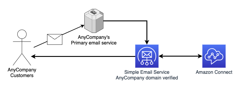
Enable a CMK on an existing application

If you have an application running with an AWS owned key, the process is similar to what we described for creating new applications. In this case, you already have a running application state and older snapshots that are encrypted using the AWS owned key.

Also, if you have a running application, you probably already have an operator role with an IAM policy that you can use to control the operator lifecycle.

The sequence of steps to enable a CMK on an existing and running application is as follows:

  1. If you don’t already have one, create a key administrator IAM role or user with permissions to create and manage keys in AWS KMS. See Using IAM policies with AWS KMS for more details about the permissions required to manage keys.
  2. The key administrator creates the CMK. The key policy references the application ARN, the operator’s ARN, and the key administrator’s role or user ARN.
  3. Create an additional IAM policy that allows the use of the CMK and attach this policy to the operator. Alternatively, modify the operator’s existing IAM policy by adding these permissions.
  4. Finally, the operator can update the application and enable the CMK.The following diagram illustrates the process that occurs when you execute an UpdateApplication action on the running application to enable a CMK.

    Enabling CMK on an existing application

    The workflow consists of the following steps:

  5. When you update the application to set up the CMK, the following happens:
    1. The application running state, at the moment it is encrypted with the AWS owned key, is saved in a snapshot while the application is stopped. This snapshot is encrypted with the default AWS owned key. The running application state storage is volatile and destroyed when the application is stopped.
    2. The application is redeployed, restoring the snapshot into the running application state.
    3. The running application state storage is now encrypted with the CMK.
  6. New snapshots created from this point on are encrypted using the CMK.
  7. You will probably want to delete all the old snapshots, including the one created automatically by the UpdateApplication that enabled the CMK, because they are all encrypted using the AWS owned key.

Rotate the encryption key

As with any cryptographic key, it’s a best practice to rotate the key periodically for enhanced security. Managed Service for Apache Flink does not support AWS KMS automatic key rotation, so you have two primary options for rotating your CMK.

Option 1: Create a new CMK and update the application

The first approach involves creating an entirely new KMS key and then updating your application configuration to use the new key. This method provides a clean separation between the old and new encryption keys, making it easier to track which data was encrypted with which key version.

Let’s assume you have a running application using CMK#1 (the current key) and want to rotate to CMK#2 (the new key) for enhanced security:

  • Prerequisites and preparation – Before initiating the key rotation process, you must update the operator’s IAM policy to include permissions for both CMK#1 and CMK#2. This dual-key access supports uninterrupted operation during the transition period. After the application configuration has been successfully updated and verified, you can safely remove all permissions to CMK#1.
  • Application update process – The UpdateApplication operation used to configure CMK#2 automatically triggers an application restart. This restart mechanism makes sure both the application’s running state and any newly created snapshots are encrypted using the new CMK#2, providing immediate security benefits from the updated encryption key.
  • Important security considerations – Existing snapshots, including the automatic snapshot created during the CMK update process, remain encrypted with the original CMK#1. For complete security hygiene and to minimize your cryptographic footprint, consider deleting these older snapshots after verifying that your application is functioning correctly with the new encryption key.

This approach provides a clean separation between old and new encrypted data while maintaining application availability throughout the key rotation process.

Option 2: Rotate the key material of the existing CMK

The second option is to rotate the cryptographic material within your existing KMS key. For a CMK used for Managed Service for Apache Flink, we recommend using on-demand key material rotation.

The benefit of this approach is simplicity: no change is required to the application configuration nor to the operator’s IAM permissions.

Important security considerations

The new encryption key is used by the Managed Service for Apache Flink application only after the next application restart. To make the new key material effective, immediately after the rotation, you need to stop and start using snapshots to preserve the application state or execute an UpdateApplication, which also forces a stop-and-restart. After the restart, you should consider deleting the old snapshots, including the one taken automatically in the last stop-and-restart.

Switch back to the AWS owned key

At any time, you can decide to switch back to using an AWS owned key. The application state is still encrypted, but using the AWS owned key instead of your CMK.

If you are using the UpdateApplication API or AWS CLI command to switch back to CMK, you must explicitly pass ApplicationEncryptionConfigurationUpdate, setting the key type to AWS_OWNED_KEY as shown in the following snippet:

{
  "ApplicationEncryptionConfigurationUpdate": {
    "KeyTypeUpdate": "AWS_OWNED_KEY"
  }
}

When you execute UpdateApplication to switch off the CMK, the operator must still have permissions on the CMK. After the application is successfully running using the AWS owned key, you can safely remove any CMK-related permissions from the operator’s IAM policy.

Test the CMK in development environments

In a production environment—or an environment containing sensitive data—you should follow the principle of least privilege and apply the restrictive permissions described so far.

However, if you want to experiment with CMKs in a development setting, such as using the console, strictly following the production process might become cumbersome. In these environments, the roles of key administrator and operator are often filled by the same person.

For testing purposes in development environments, you might want to use a permissive key policy like the following, so you can freely experiment with CMK encryption:

{
  "Version": "2012-10-17",
  "Id": "key-policy-permissive-for-dev-only",
  "Statement": [
    {
      "Sid": "Allow any KMS action to Admin",
      "Effect": "Allow",
      "Principal": {
        "AWS": "arn:aws:iam::<account-id>:role/Admin"
      },
      "Action": "kms:*",
      "Resource": "*"
    },
    {
      "Sid": "Allow any KMS action to Managed Flink",
      "Effect": "Allow",
      "Principal": { 
        "Service": [
          "kinesisanalytics.amazonaws.com",
          "infrastructure.kinesisanalytics.amazonaws.com"
        ]
      },
      "Action": [
        "kms:DescribeKey",
        "kms:Decrypt",
        "kms:GenerateDataKey",
        "kms:GenerateDataKeyWithoutPlaintext",
        "kms:CreateGrant"
      ],
      "Resource": "*"
    }
  ]
}

This policy must never be used in an environment containing sensitive data, and especially not in production.

Common caveats and pitfalls

As discussed earlier, this feature is designed to maximize security and promote best practices such as the principle of least privilege. However, this focus can introduce some corner cases you should be aware of.

The CMK must be enabled for the service to encrypt and decrypt snapshots and running state

With AWS KMS, you can disable one key at any time. If you disable the CMK while the application is running, it might cause unpredictable failures. For example, an application will not be able to restore a snapshot if the CMK used to encrypt that snapshot has been disabled. For example, if you attempt to roll back an UpdateApplication that changed the CMK, and the previous key has since been disabled, you might not be able to restore from an old snapshot. Similarly, you might not be able to restart the application from an older snapshot if the corresponding CMK is disabled.

If you encounter these scenarios, the solution is to reenable the required key and retry the operation.

The operator requires permissions to all keys involved

To perform an action on the application (such as Start, Stop, UpdateApplication, or CreateApplicationSnapshot), the operator must have permissions for all CMKs involved in that operation. AWS owned keys don’t require explicit permission.

Some operations implicitly involve two CMKs—for example, when switching from one CMK to another, or when switching from a CMK to an AWS owned key by disabling the CMK. In these cases, the operator must have permissions for both keys for the operation to succeed.

The same rule applies when rolling back an UpdateApplication action that involved multiple CMKs.

A new encryption key takes effect only after restart

A new encryption key is only used after the application is restarted. This is important when you rotate the key material for a CMK. Rotating the key material in AWS KMS doesn’t require updating the Managed Flink application’s configuration. However, you must restart the application as a separate step after rotating the key. If you don’t restart the application, it will continue to use the old encryption key for its running state and snapshots until the next restart.

For this reason, it is recommended not to enable automatic key rotation for the CMK. When automatic rotation is enabled, AWS KMS might rotate the key material at any time, but your application will not start using the new key until it is next restarted.

CMKs are only supported with Flink runtime 1.20 or later

CMKs are only supported when you are using the Flink runtime 1.20 or later. If your application is currently using an older runtime, you should upgrade to Flink 1.20 first. Managed Service for Apache Flink makes it straightforward to upgrade your existing application using the in-place version upgrade.

Conclusion

Managed Service for Apache Flink provides robust security by enabling encryption by default, protecting both the running state and persistently saved state of your applications. For organizations that require full control over their encryption keys (often due to regulatory or internal policy needs), the ability to use a CMK integrated with AWS KMS offers a new level of assurance.

By using CMKs, you can tailor encryption controls to your specific compliance requirements. However, this flexibility comes with the need for careful planning: the CMK feature is intentionally designed to enforce the principle of least privilege and strong role separation, which can introduce complexity around permissions and operational processes.

In this post, we reviewed the key steps for enabling CMKs on existing applications, creating new applications with a CMK, and managing key rotation. Each of these processes gives you greater control over your data security but also requires attention to access management and operational best practices.

To get started with CMKs and for more comprehensive guidance, refer to Key management in Amazon Managed Service for Apache Flink.


About the authors

Lorenzo Nicora

Lorenzo Nicora

Lorenzo works as Senior Streaming Solution Architect at AWS, helping customers across EMEA. He has been building cloud-centered, data-intensive systems for over 25 years, working across industries both through consultancies and product companies. He has used open-source technologies extensively and contributed to several projects, including Apache Flink, and is the maintainer of the Flink Prometheus connector.

Sofia Zilberman

Sofia Zilberman

Sofia works as a Senior Streaming Solutions Architect at AWS, helping customers design and optimize real-time data pipelines using open-source technologies like Apache Flink, Kafka, and Apache Iceberg. With experience in both streaming and batch data processing, she focuses on making data workflows efficient, observable, and high-performing.

Serverless generative AI architectural patterns – Part 2

Post Syndicated from Michael Hume original https://aws.amazon.com/blogs/compute/part-2-serverless-generative-ai-architectural-patterns/

In Part 1 of this series, we discussed three patterns and general best practices for building real-time, interactive, generative AI applications. However, not all generative AI workflows require immediate responses. This post explores two complementary approaches for non-real-time scenarios: buffered asynchronous processing for time-intensive individual requests, and batch processing for scheduled or event-driven workflows.

Buffered asynchronous processing is useful for use cases demanding time-consuming processing to yield the most precise outcomes. Consequently, these benefit from an interactive delayed request response cycle that can be achieved through a buffered asynchronous integration. Examples include generating video or music from text, conducting medical or scientific analysis and visualization, creating complete virtual worlds for gaming or the metaverse, fashion and lifestyle graphics generation, and more.

The second approach addresses a different challenge: processing extensive datasets on a schedule or when specific events occur. Examples include bulk image enhancement and optimization, weekly or monthly report generation, weekly customer review analysis, and social media content creation. These non-interactive, batch-oriented generative AI workflows necessitate repeatability, scalability, parallelism, and dependency management to manage large data volumes. The non-interactive batch implements this processing pattern.

Pattern 4: Buffered asynchronous request response

This asynchronous pattern uses event-driven architectures to enhance application scalability and reliability. This approach offers several advantages, including improved performance through concurrent processing, enhanced scalability through group processing, and better reliability through decoupled components. This pattern is particularly effective for handling high-volume requests or long-running processes.

The implementation typically involves message queuing services like Amazon Simple Queue Service (Amazon SQS) to buffer requests and manage processing loads. This pattern can be particularly effective when combined with WebSocket APIs for interactive updates, alleviating the need for client-side polling. For complex scenarios involving multiple LLM models, the multimodal fan-out pattern (refer pattern 5 below) using Amazon EventBridge or Amazon Simple Notification Service (Amazon SNS) enables parallel processing across different endpoints. This pattern can be implemented through several architectural approaches.

REST APIs with message queuing

To limit scaling challenges with your LLM endpoint, use an Amazon SQS queue to buffer messages. The frontend sends messages to Amazon API Gateway REST endpoints, which pushes them to the queue. API Gateway returns an acknowledgement and a unique identifier (the message ID) to the frontend. The middleware running on compute services like AWS Lambda, Amazon EC2 or AWS Fargate processes messages in batches, creating entries in Amazon DynamoDB for each record. It then calls LLM endpoints to generate responses, storing the results back in the DynamoDB table with the corresponding message ID. The frontend polls the API Gateway endpoint to check if the response message is generated, querying the DynamoDB table using the message ID. This pattern helps overcome the API Gateway limit of 29 seconds for the request response cycle. For an example implementation, see API Gateway REST API to SQS to Lambda to Bedrock. A similar solution can be implemented using AWS AppSync GraphQL APIs instead of Amazon API Gateway. The following diagram illustrates an example architecture.Fig 1: Buffered asynchronous request response using Amazon API integrations services and Amazon SQS queues

Fig 11: Buffered asynchronous request response using Amazon API integrations services and Amazon SQS queues

WebSocket APIs with message queuing

This is a variation of the previous pattern but uses API Gateway WebSocket APIs instead of REST endpoints. In this pattern, instead of the frontend client having to continuously poll for the response, the middleware sends back the result back to the client after it is generated. This uses WebSocket omni-channel communication to accept and respond to messages, all maintained by API Gateway. For an example implementation, refer to the aws-apigatewayv2websocket-sqs AWS Solutions Construct. The following diagram illustrates this architecture.Fig 2: Buffered asynchronous request response using Amazon API Gateway WebSocket APIs and Amazon SQS queues

Fig 12: Buffered asynchronous request response using Amazon API Gateway WebSocket APIs and Amazon SQS queues

Pattern 5: Multimodal parallel fan-out

For use cases that require interacting with multiple LLM models, data sources, or agents, you can use the messaging fan-out pattern, which distributes messages to multiple destinations in parallel. You can use Amazon EventBridge or Amazon SNS to send specific messages to target LLM endpoints or agents using rules-based message fan-out. This pattern decomposes complex tasks into sub-tasks and executes them in parallel, minimizing overall generation time. For an example implementation, see SNS to SQS fanout pattern. The following diagram illustrates the architecture.Fig 3: Multimodal parallel fan-out using Amazon API integration and messaging services

Fig 13: Multimodal parallel fan-out using Amazon API integration and messaging services

Pattern 6: Non-interactive batch processing

Non-interactive batch processing pipelines are ideal when you need to process large volumes of data efficiently without real-time user interaction, typically running on a scheduled basis to maximize resource usage and throughput. This pattern uses AWS Step Functions, AWS Glue, or other compute services to create a serverless data processing and inferencing pipeline. The data integration, transformation, and inference jobs can be triggered based on a schedule or occurrence of events. This pattern offers higher throughput, optimizes on resource usage, and enhances automation through volume processing. For an example implementation, refer to the aws-sqs-pipes-stepfunctions AWS Solutions Construct. The following diagram illustrates an example architecture.Fig 4: Non-interactive batch processing using Amazon data integration services

Fig 14: Non-interactive batch processing using Amazon data integration services

Conclusion

In this post (series), you learned six architectural patterns on building generative AI applications using AWS serverless services. These patterns implement interactive real-time, asynchronous or batch-oriented workloads without a lot of operational overhead. You can combine these patterns to deliver modern cloud native applications. Given the current trajectory of innovation in this domain, it is anticipated that further blueprints will emerge to augment or evolve these in the future.The successful deployment of production-ready generative AI applications requires careful consideration of architectural patterns and implementation approaches. You must evaluate various factors such as response time, scalability, integration needs, reliability, and user experience when selecting appropriate patterns or a combination of them.

To learn more about Serverless architectures see Serverless Land.

Serverless generative AI architectural patterns – Part 1

Post Syndicated from Michael Hume original https://aws.amazon.com/blogs/compute/serverless-generative-ai-architectural-patterns/

Organizations of all sizes and types are harnessing large language models (LLMs) and foundation models (FMs) to build generative AI applications that deliver new customer and employee experiences. Serverless computing offers the perfect solution, empowering organizations to focus on innovation, flexibility, and cost-efficiency without the complexity of infrastructure management. Organizations transitioning their experimental implementations into production-ready applications can implement proven, scalable, and maintainable software design patterns as the cornerstone of their architecture.

This two-part series explores the different architectural patterns, best practices, code implementations, and design considerations essential for successfully integrating generative AI solutions into both new and existing applications. In this post, we focus on patterns applicable for architecting real-time generative AI applications. Part 2 addresses patterns for building batch-oriented generative AI implementations using serverless services.

Separation of concerns

A fundamental principle in building robust generative AI applications is the separation of concerns, which involves dividing the application stack into three distinct components: frontend, middleware, and backend service layers. This architectural approach (as shown in the following diagram) offers multiple benefits, including reduced complexity, enhanced maintainability, and the ability to scale components independently. By implementing this separation, you can develop cross-platform solutions while maintaining the flexibility to evolve each component according to specific requirements.
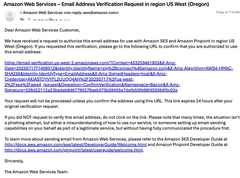
1:3 Tier Generative AI Architecture

Fig 1: 3 Tier generative AI Architecture

Although these layers are merely extensions to the traditional software stack, they do perform some specific tasks in generative AI applications.

Frontend layer

The frontend layer serves as the primary interface between end-users and the generative AI application. For organizations integrating generative AI into existing applications, this layer might already be established. The frontend handles critical responsibilities including user authentication, UI/UX presentation, and API communication. AWS provides a robust suite of serverless services to support frontend implementations, including AWS Amplify for full-stack development, Amazon CloudFront paired with Amazon Simple Storage Service (Amazon S3) for content delivery, and container services like Amazon Elastic Container Service (Amazon ECS) and Amazon Elastic Kubernetes Service (Amazon EKS) for application hosting. Specialized services such as Amazon Lex can enhance the user experience through conversational interfaces and intelligent search capabilities for building interactive chatbots.

Middleware layer

This represents the integration layer, comprising of three essential sub-layers that manage different aspects of the application logic and data flow:

  • API layer – This layer exposes backend services through various protocols, including REST, GraphQL, and WebSockets. It handles essential functions such as input validation, traffic management, and CORS support. The API layer also implements authorization and access control mechanisms, manages API versioning, and provides monitoring capabilities. It provides secure and efficient communication between the frontend and backend components while maintaining scalability and reliability. AWS managed services like Amazon API Gateway and AWS AppSync can help create an AI gateway to simplify access and API management.
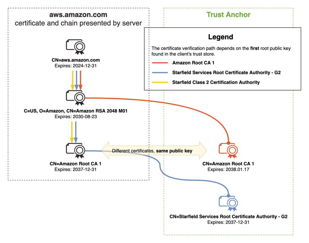
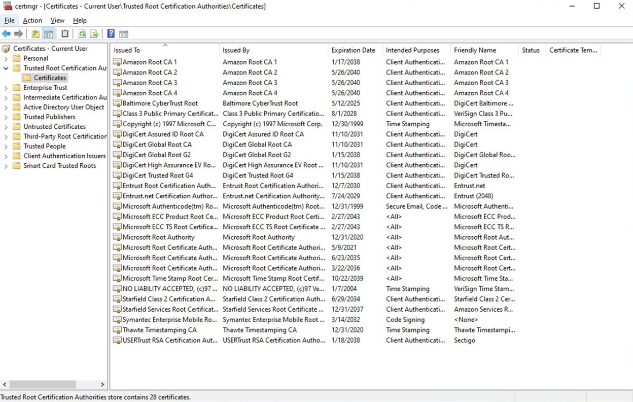
  • Prompt engineering layer – This layer encapsulates the business logic necessary for interacting with LLMs. It handles dynamic prompt generation, model selection, prompt caching, model routing, guardrails, and security enforcement. This layer implements token and context window optimization, sensitive information filtering, output content moderation, error handling, retry logic, and audit trails. By centralizing these functions, you can maintain consistent prompt strategies, enforce security, and optimize model interactions across applications. You can use Amazon DynamoDB to store prompt templates and configurations, and use Amazon Bedrock Guardrails, Amazon Bedrock prompt caching, and Amazon Bedrock Intelligent Prompt Routing to implement responsible AI safeguards, reuse of prompt prefixes, and dynamic routing, respectively.
  • Orchestration layer – This layer manages complex interactions between various system components. It coordinates external API calls and agent calls, manages vector database queries, stores user sessions and conversation histories, and maintains conversation context across multiple LLM interactions. Frameworks like LangChain and LlamaIndex are commonly used to simplify these operations and provide standardized approaches to common generative AI tasks. AWS Step Functions has direct integrations with over 220 AWS services, including Amazon Bedrock, enabling you to construct intricate generative AI workflows without incurring additional computational resources. Additionally, with Amazon Bedrock Flows, you can create complex, flexible, multi-prompt workflows to evaluate, compare, and version.

Backend services, agents, and private data sources

The backend layer forms the core of generative AI response generation powered by LLMs. It consists of hosting and invoking the LLM model, agents, knowledge bases, or a Model Context Protocol (MCP) server. Amazon Bedrock, Amazon SageMaker JumpStart, and Amazon SageMaker offer a variety of high-performing FMs from leading AI companies or the option to bring your own. You can securely run an MCP server using a containerized architecture, as described in Guidance for Deploying Model Context Protocol Servers on AWS.

Private data sources complement LLMs by providing authoritative proprietary knowledge outside of its training data. For Retrieval Augmented Generation (RAG) implementations, Amazon Kendra, Amazon OpenSearch Serverless, and Amazon Aurora PostgreSQL-Compatible Edition with the pgVector extension provide robust, scalable vector database options. For a deeper dive, please read The role of vector databases in generative AI applications on available AWS service options to store embeddings in a purpose built vector database.

Real-time applications process and deliver responses with minimal latency, enhancing the user experience and facilitating faster decision-making. In the following sections, we explore some architectural patterns that can be used to implement real-time generative AI applications.

Pattern 1: Synchronous request response

In this pattern, responses are generated and immediately delivered, while the client blocks/waits for response. Although this is simple to implement, has a predictable flow, and offers strong consistency, it suffers from blocking operations, high latency, and potential timeouts. When implemented for generative AI applications, this pattern is particularly suited for certain modalities like video or image generations. For fast LLM interactions, it can handle multiple concurrent requests while maintaining consistent performance under varying loads. This model can be implemented through several architectural approaches.

REST APIs

You can use RESTful APIs to communicate with your backend over HTTP requests. You can use REST or HTTP APIs in API Gateway or an Application Load Balancer for path-based routing to the middleware. API Gateway offers additional features like token-based authentication, custom authorizers, resource-based permissions, request/response mapping and transformation, versioning, and rate-limiting. However, with REST/HTTP APIs in API Gateway, the response must be generated within 29 seconds to meet the default integration timeout. You can extend this default limit to 5 minutes for REST APIs with a possible reduction in your AWS Region-level throttle quota for your account. For an example implementation, refer to Interact with Bedrock models from a Lambda function fronted with an API Gateway. The following diagram illustrates this architecture.

Fig 2: Synchronous REST/HTTP APIs using Amazon API Gateway

Fig 2: Synchronous REST/HTTP APIs using Amazon API Gateway

GraphQL HTTP APIs

You can use AWS AppSync as the API layer to take advantage of the benefits of GraphQL APIs. GraphQL APIs offer declarative and efficient data fetching using a typed schema definition, serverless data caching, offline data synchronization, security, and fine-grained access control. It also provides data sources and resolvers for writing business logic. If you don’t need the mutation layer, AWS AppSync can directly invoke an LLM in Amazon Bedrock. AWS AppSync integration timeout is set to 30 seconds by default and can’t be extended. If you need to perform operations that might take longer, consider implementing asynchronous patterns or breaking down the operation into smaller chunks. For an example integration, see Invoke Amazon Bedrock models from AWS AppSync HTTP resolver. The following diagram illustrates the solution architecture.

Fig 3: Synchronous GraphQL HTTP APIs using AWS AppSyncFig 3: Synchronous GraphQL HTTP APIs using AWS AppSync

Conversational chatbot interface

Amazon Lex is a service for building conversational interfaces with voice and text, offering speech recognition and language understanding capabilities. It simplifies multimodal development and enables publication of chatbots to various chat services and mobile devices. It offers native integration with Lambda to streamline chatbot development. When a Lambda function is used for fulfilment, the default response timeout is set to 30 seconds. To bypass, you can use fulfilment updates to provide periodic updates to the user, so the user knows that the chatbot is still working on their request. For an example implementation, see Enhance Amazon Connect and Lex with generative AI capabilities. The following diagram illustrates the solution architecture.

Fig 4: Synchronous conversational APIs using Amazon Lex

Fig 4: Synchronous conversational APIs using Amazon Lex

Model invocation using orchestration

AWS Step Functions enables orchestration and coordination of multiple tasks, with native integrations across AWS services like Amazon API Gateway, AWS Lambda, and Amazon DynamoDB. AWS Step Functions offers built-in features like function orchestration, branching, error handling, parallel processing, and human-in-the-loop capabilities. It also has an optimized integration with Amazon Bedrock, allowing direct invocation of Amazon Bedrock FMs from AWS Step Functions workflows. With this integration, you can accomplish the following:

  • Enrich Step Functions data processing with generative AI capabilities for tasks like text summarization, image generation, or personalization
  • Retrieve and inject up-to-date data (such as product pricing or user profiles) into LLM prompts for improved accuracy
  • Orchestrate LLM and agent calls in a customized processing chain, using the best-suited models at each stage
  • Implement human-in-the-loop interactions to moderate responses and handle hallucinations of the FM

For an example implementation using API Gateway, see Prompt chaining with Amazon API Gateway and AWS Step Functions. For an example implementation using AWS AppSync, see Prompt chaining with AWS AppSync, AWS Step Functions and Amazon Bedrock. The following diagram illustrates an example architecture.

Fig 5: Synchronous model invocations using AWS Step FunctionsFig 5: Synchronous model invocations using AWS Step Functions

Pattern 2: Asynchronous request response

This pattern provides a full-duplex, bidirectional communication channel between the client and server without clients having to wait for updates. The biggest advantages is its non-blocking nature that can handle long-running operations. However, they are more complex to implement because they require channel, message, and state management. This model can be implemented through two architectural approaches.

WebSocket APIs

The WebSocket protocol enables real-time, synchronous communication between the frontend and middleware, allowing for bidirectional, full-duplex messaging over a persistent TCP connection. This bidirectional behavior enhances client/service interactions, enabling services to push data to clients without requiring explicit requests. Using API Gateway, you can create a WebSocket APIs as a stateful frontend for an AWS service (such as Lambda or DynamoDB) or for an HTTP endpoint. The WebSocket API invokes your backend based on the content of the messages it receives from client apps. After the message is generated, the backend can send callback messages to connected clients. Each request-response cycle must complete within 29 seconds, as defined by the API Gateway integration timeout for WebSockets. The connection duration for API Gateway WebSocket APIs can be up to 2 hours with an idle connection timeout of 10 minutes—these can’t be extended. For an example implementation, refer to AI Chat with Amazon API Gateway (WebSockets), AWS Lambda and Amazon Bedrock. The following diagram illustrates an example architecture.

Fig 6: Asynchronous WebSocket APIs using Amazon API GatewayFig 6: Asynchronous WebSocket APIs using Amazon API Gateway

GraphQL WebSocket APIs

AWS AppSync can establish and maintain secure WebSocket connections for GraphQL subscription operations, enabling middleware applications to distribute data in real time from data sources to subscribers. It also supports a simple publish-subscribe model, where client frontends can listen to specific channels or topics, with AWS AppSync managing multiple temporary pub/sub channels and WebSocket connections to deliver and filter data based on the channel name. For an example implementation, refer to AI Chat with AWS AppSync (WebSockets), AWS Lambda, and Amazon Bedrock. The following diagram illustrates an example architecture.Fig 7: Asynchronous GraphQL WebSocket APIs using AWS

Fig 7: Asynchronous GraphQL WebSocket APIs using AWS

Pattern 3: Asynchronous streaming response

This streaming pattern enables real-time response flow to clients in chunks, enhancing the user experience and minimizing first response latency. This pattern uses built-in streaming capabilities in services like Amazon Bedrock (InvokeModelWithResponseStream or ConverseStream APIs) and SageMaker real-time inference, enabling applications to display results incrementally rather than waiting for complete responses. This pattern is particularly effective for applications implementing text modality such as chat interfaces and word-based content generation tools.

Implementation is achieved through the API Gateway WebSocket API or AWS AppSync WebSocket APIs or GraphQL subscriptions, with careful consideration given to timeout management and connection handling.

The following diagram illustrates the architecture of asynchronous streaming using API Gateway WebSocket APIs.Fig 8: Asynchronous streaming response using Amazon API Gateway WebSockets APIs

Fig 8: Asynchronous streaming response using Amazon API Gateway WebSockets APIs

The following diagram illustrates the architecture of asynchronous streaming using AWS AppSync WebSocket APIs.Fig 9: Asynchronous streaming response using AWS AppSync WebSocket APIs

Fig 9: Asynchronous streaming response using AWS AppSync WebSocket APIs

If you don’t need an API layer, Lambda response streaming lets a Lambda function progressively stream response payloads back to clients. For more details, see Using Amazon Bedrock with AWS Lambda. The following diagram illustrates this architecture.Fig 10: Asynchronous response using AWS Lambda response streaming

Fig 10: Asynchronous response using AWS Lambda response streaming

Conclusion

This post introduced three design patterns applicable for real-time generative AI applications: synchronous request response, asynchronous request response, and asynchronous streaming response. We also highlighted how to implement these patterns using AWS serverless services. When selecting an appropriate pattern for your implementation, it is crucial to consider the anticipated end-user experience, the existing technical stack, AWS service quotas, and the latency of your LLM responses. In Part 2, we discuss patterns for building batch-oriented generative AI implementations using AWS serverless services.

Deep dive into the Amazon Managed Service for Apache Fink application lifecycle – Part 2

Post Syndicated from Lorenzo Nicora original https://aws.amazon.com/blogs/big-data/part-2-deep-dive-into-the-amazon-managed-service-for-apache-fink-application-lifecycle/

In Part 1 of this series, we discussed fundamental operations to control the lifecycle of your Amazon Managed Service for Apache Flink application. If you are using higher-level tools such as AWS CloudFormation or Terraform, the tool will execute these operations for you. However, understanding the fundamental operations and what the service automatically does can provide some level of Mechanical Sympathy to confidently implement a more robust automation.

In the first part of this series, we focused on the happy paths. In an ideal world, failures don’t happen, and every change you deploy works perfectly. However, the real world is less predictable. Quoting Werner Vogels, Amazon’s CTO, “Everything fails, all the time.”

In this post, we explore failure scenarios that can happen during normal operations or when you deploy a change or scale the application, and how to monitor operations to detect and recover when something goes wrong.

The less happy path

A robust automation must be designed to handle failure scenarios, in particular during operations. To do that, we need to understand how Apache Flink can deviate from the happy path. Due to the nature of Flink as a stateful stream processing engine, detecting and resolving failure scenarios requires different techniques compared to other long-running applications, such as microservices or short-lived serverless functions (such as AWS Lambda).

Flink’s behavior on runtime errors: The fail-and-restart loop

When a Flink job encounters an unexpected error at runtime (an unhandled exception), the normal behavior is to fail, stop the processing, and restart from the latest checkpoint. Checkpoints allow Flink to support data consistency and no data loss in case of failure. Also, because Flink is designed for stream processing applications, which run continuously, if the error happens again, the default behavior is to keep restarting, hoping the problem is transient and the application will eventually recover the normal processing.In some cases, the problem is not transient, however. For example, when you deploy a code change that contains a bug, causing the job to fail as soon as it starts processing data, or if the expected schema doesn’t match the records in the source, causing deserialization or processing errors. The same scenario might also happen if you mistakenly changed a configuration that prevents a connector to reach the external system. In these cases, the job is stuck in a fail-and-restart loop, indefinitely, or until you actively force-stop it.

When this happens, the Managed Service for Apache Flink application status might be RUNNING, but the underlying Flink job is actually failing and restarting. The AWS Management Console gives you a hint, pointing that the application might need attention (see the following screenshot).

Application needs attention

In the following sections, we learn how to monitor the application and job status, to automatically react to this situation.

When starting or updating the application goes wrong

To understand the failure mode, let’s review what happens automatically when you start the application, or when the application restarts after you issued UpdateApplication command, as we explored in Part 1 of this series. The following diagram illustrates what happens when an application starts.

Application start process

The workflow consists of the following steps:

  1. Managed Service for Apache Flink provisions a cluster dedicated to your application.
  2. The code and configuration are submitted to the Job Manager node.
  3. The code in the main() method of your application runs, defining the dataflow of your application.
  4. Flink deploys to the Task Manager nodes the substasks that make up your job.
  5. The job and application status change to RUNNING. However, subtasks start initializing now.
  6. Subtasks restore their state, if applicable, and initialize any resources. For example, a Kafka connector’s subtask initializes the Kafka client and subscribes the topic.
  7. When all subtasks are successfully initialized, they change to RUNNING status and the job starts processing data.

To new Flink users, it can be confusing that a RUNNING status doesn’t necessarily imply the job is healthy and processing data.When something goes wrong during the process of starting (or restarting) the application, depending on the phase when the problem arises, you might observe two different types of failure modes:

  • (a) A problem prevents the application code from being deployed – Your application might encounter this failure scenario if the deployment fails as soon as the code and configuration are passed to the Job Manager (step 2 of the process), for example if the application code package is malformed. A typical error is when the JAR is missing a mainClass or if mainClass points to a class that doesn’t exist. This failure mode might also happen if the code of your main() method throws an unhandled exception (step 3). In these cases, the application fails to change to RUNNING, and reverts to READY after the attempt.
  • (b) The application is started, the job is stuck in a fail-and-restart loop – A problem might occur later in the process, after the application status has changed RUNNING. For example, after the Flink job has been deployed to the cluster (step 4 of the process), a component might fail to initialize (step 6). This might happen when a connector is misconfigured, or a problem prevents it from connecting to the external system. For example, a Kafka connector might fail to connect to the Kafka cluster because of the connector’s misconfiguration or networking issues. Another possible scenario is when the Flink job successfully initializes, but it throws an exception as soon as it starts processing data (step 7). When this happens, Flink reacts to a runtime error and might get stuck in a fail-and-restart loop.

The following diagram illustrates the sequence of application status, including the two failure scenarios just described.

Application statuses, with failure scenarios

Troubleshooting

We have examined what can go wrong during operations, in particular when you update a RUNNING application or restart an application after changing its configuration. In this section, we explore how we can act on these failure scenarios.

Roll back a change

When you deploy a change and realize something is not quite right, you normally want to roll back the change and put the application back in working order, until you investigate and fix the problem. Managed Service for Apache Flink provides a graceful way to revert (roll back) a change, also restarting the processing from the point it was stopped before applying the fault change, providing consistency and no data loss.In Managed Service for Apache Flink, there are two types of rollbacks:

  • Automatic – During an automatic rollback (also called system rollback), if enabled, the service automatically detects when the application fails to restart after a change, or when the job starts but immediately falls into a fail-and-restart loop. In these situations, the rollback process automatically restores the application configuration version before the last change was applied and restarts the application from the snapshot taken when the change was deployed. See Improve the resilience of Amazon Managed Service for Apache Flink application with system-rollback feature for more details. This feature is disabled by default. You can enable it as part of the application configuration.
  • Manual – A manual rollback API operation is like a system rollback, but it’s initiated by the user. If the application is running but you observe something not behaving as expected after applying a change, you can trigger the rollback operation using the RollbackApplication API action or the console. Manual rollback is possible when the application is RUNNING or UPDATING.

Both rollbacks work similarly, restoring the configuration version before the change and restarting with the snapshot taken before the change. This prevents data loss and brings you back to a version of the application that was working. Also, this uses the code package that was saved at the time you created the previous configuration version (the one you are rolling back to), so there is no inconsistency between code, configuration, and snapshot, even if in the meantime you have replaced or deleted the code package from the Amazon Simple Storage Service (Amazon S3) bucket.

Implicit rollback: Update with an older configuration

A third way to roll back a change is to simply update the configuration, bringing it back to what it was before the last change. This creates a new configuration version, and requires the correct version of the code package to be available in the S3 bucket when you issue the UpdateApplication command.

Why is there a third option when the service provides system rollback and the managed RollbackApplication action? Because most high-level infrastructure-as-code (IaC) frameworks such as Terraform use this strategy, explicitly overwriting the configuration. It is important to understand this possibility even though you will probably use the managed rollback if you implement your automation based on the low-level actions.

The following are two important caveats to consider for this implicit rollback:

  • You will normally want to restart the application from the snapshot that was taken before the faulty change was deployed. If the application is currently RUNNING and healthy, this is not the latest snapshot (RESTORE_FROM_LATEST_SNAPSHOT), but rather the previous one. You must set the restart from RESTORE_FROM_CUSTOM_SNAPSHOT and select the correct snapshot.
  • UpdateApplication only works if the application is RUNNING and healthy, and the job can be gracefully stopped with a snapshot. Conversely, if the application is stuck in a fail-and-restart loop, you must force-stop it first, change the configuration while the application is READY, and later start the application from the snapshot that was taken before the faulty change was deployed.

Force-stop the application

In normal scenarios, you stop the application gracefully, with the automatic snapshot creation. However, this might not be possible in some scenarios, such as if the Flink job is stuck in a fail-and-restart loop. This might happen, for example, if an external system the job uses stops working, or because the AWS Identity and Access Management (IAM) configuration was erroneously modified, removing permissions required by the job.

When the Flink job gets stuck in a fail-and-restart loop after a faulty change, your first option should be using RollbackApplication, which automatically restores the previous configuration and starts from the correct snapshot. In the rare cases you can’t stop the application gracefully or use RollbackApplication, the last resort is force-stopping the application. Force-stop uses the StopApplication command with Force=true. You can also force-stop the application from the console.

When you force-stop an application, no snapshot is taken (if that were possible, you would have been able to gracefully stop). When you restart the application, you can either skip restoring from a snapshot (SKIP_RESTORE_FROM_SNAPSHOT) or use a snapshot that was previously taken, scheduled using Snapshot Manager, or manually, using the console or CreateApplicationSnapshot API action.

We strongly recommend setting up scheduled snapshots for all production applications that you can’t afford restarting with no state.

Monitoring Apache Flink application operations

Effective monitoring of your Apache Flink applications during and after operations is crucial to verify the outcome of the operation and allow lifecycle automation to raise alarms or react, in case something goes wrong.

The main indicators you can use during operations include the FullRestarts metric (available in Amazon CloudWatch) and the application, job, and task status.

Monitoring the outcome of an operation

The simplest way to detect the outcome of an operation, such as StartApplication or UpdateApplication, is to use the ListApplicationOperations API command. This command returns a list of the most recent operations of a specific application, including maintenance events that force an application restart.

For example, to retrieve the status of the most recent operation, you can use the following command:

aws kinesisanalyticsv2 list-application-operations \
    --application-name MyApplication \
   | jq '.ApplicationOperationInfoList \
   | sort_by(.StartTime) | last'

The output will be similar to the following code:

{
  "Operation": "UpdateApplication",
  "OperationId": "12abCDeGghIlM",
  "StartTime": "2025-08-06T09:24:22+01:00",
  "EndTime": "2025-08-06T09:26:56+01:00",
  "OperationStatus": "IN_PROGRESS"
}

OperationStatus will follow the same logic as the application status reported by the console and by DescribeApplication. This means it might not detect a failure during the operator initialization or while the job starts processing data. As we have learned, these failures might put the application in a fail-and-restart loop. To detect these scenarios using your automation, you must use other techniques, which we cover in the rest of this section.

Detecting the fail-and-restart loop using the FullRestarts metric

The simplest way to detect whether the application is stuck in a fail-and-restart loop is using the fullRestarts metric, available in CloudWatch Metrics. This metric counts the number of restarts of the Flink job after you started the application with a StartApplication command or restarted with UpdateApplication.

In a healthy application, the number of full restarts should ideally be zero. A single full restart might be acceptable during deployment or planned maintenance; multiple restarts normally indicate some issue. We recommend not to trigger an alarm on a single restart, or even a couple of consecutive restarts.

The alarm should only be triggered when the application is stuck in a fail-and-restart loop. This implies checking whether several restarts have happened over a relatively short period of time. Deciding the period is not trivial, because the time the Flink job takes to restart from a checkpoint depends on the size of the application state. However, if the state of your application is lower than several GB per KPU, you can safely assume the application should start in less than a minute.

The goal is creating a CloudWatch alarm that triggers when fullRestarts keeps increasing over a time period sufficient for multiple restarts. For example, assuming your application restarts in less than 1 minute, you can create a CloudWatch alarm that relies on the DIFF math expression of the fullRestarts metric. The following screenshot shows an example of the alarm details.

CloudWatch Alarm on fullRestarts

This example is a conservative alarm, only triggering if the application keeps restarting for over 5 minutes. This means you detect the problem after at least 5 minutes. You might consider reducing the time to detect the failure earlier. However, be careful not to trigger an alarm after just one or two restarts. Occasional restarts might happen, for example during normal maintenance (patching) that is managed by the service, or for a transient error of an external system. Flink is designed to recover from these conditions with minimal downtime and no data loss.

Detecting whether the job is up and running: Monitoring application, job, and task status

We have discussed how you have different statuses: the status of the application, job, and subtask. In Managed Service for Apache Flink, the application and job status change to RUNNING when the subtasks are successfully deployed on the cluster. However, the job is not really running and processing data until all the subtasks are RUNNING.

Observing the application status during operations

The application status is visible on the console, as shown in the following screenshot.

Screenshot: Application status

In your automation, you can poll the DescribeApplication API action to observe the application status. The following command shows how to use the AWS Command Line Interface (AWS CLI) and jq command to extract the status string of an application:

aws kinesisanalyticsv2 describe-application \ 
    --application-name <your-application-name> \
    | jq -r '.ApplicationDetail.ApplicationStatus'

Observing job and subtask status

Managed Service for Apache Flink gives you access to the Flink Dashboard, which provides useful information for troubleshooting, including the status of all subtasks. The following screenshot, for example, shows a healthy job where all subtasks are RUNNING.

Job and Task status

In the following screenshot, we can see a job where subtasks are failing and restarting.

Job status: failing

In your automation, when you start the application or deploy a change, you want to be sure the job is eventually up and running and processing data. This happens when all the subtasks are RUNNING. Note that waiting for the job status to become RUNNING after an operation is not completely safe. A subtask might still fail and cause the job to restart after it was reported as RUNNING.

After you execute a lifecycle operation, your automation can poll the substasks status waiting for one of two events:

  • All subtasks report RUNNING – This indicates the operation was successful and your Flink job is up and running.
  • Any subtask reports FAILING or CANCELED – This indicates something went wrong, and the application is likely stuck in a fail-and-restart loop. You need to intervene, for example, force-stopping the application and then rolling back the change.

If you are restarting from a snapshot and the state of your application is quite big, you might observe subtasks will report INITIALIZING status for longer. During the initialization, Flink restores the state of the operator before changing to RUNNING.

The Flink REST API exposes the state of the subtasks, and can be used in your automation. In Managed Service for Apache Flink, this requires three steps:

  1. Generate a pre-signed URL to access the Flink REST API using the CreateApplicationPresignedUrl API action.
  2. Make a GET request to the /jobs endpoint of the Flink REST API to retrieve the job ID.
  3. Make a GET request to the /jobs/<job-id> endpoint to retrieve the status of the subtasks.

The following GitHub repository provides a shell script to retrieve the status of the tasks of a given Managed Service for Apache Flink application.

Monitoring subtasks failure while the job is running

The approach of polling the Flink REST API can be used in your automation, immediately after an operation, to observe whether the operation was eventually successful.

We strongly recommend not to continuously poll the Flink REST API while the job is running to detect failures. This operation is resource consuming, and might degrade performance or cause errors.

To monitor for suspicious subtask status changes during normal operations, we recommend using CloudWatch Logs instead. The following CloudWatch Logs Insights query extracts all subtask state transitions:

fields , message
| parse message /^(?<task>.+) switched from (?<fromStatus>[A-Z]+) to (?<toStatus>[A-Z]+)\./
| filter ispresent(task) and ispresent(fromStatus) and ispresent(toStatus)
| display , task, fromStatus, toStatus
| limit 10000

How Managed Service for Apache Flink minimizes processing downtime

We have seen how Flink is designed for strong consistency. To guarantee exactly-once state consistency, Flink temporarily stops the processing to deploy any changes, including scaling. This downtime is required for Flink to take a consistent copy of the application state and save it in a savepoint. After the change is deployed, the job is restarted from the savepoint, and there is no data loss. In Managed Service for Apache Flink, updates are fully managed. When snapshots are enabled, UpdateApplication automatically stops the job and uses snapshots (based on Flink’s savepoints) to retain the state.

Flink guarantees no data loss. However, your business requirements or Service Level Objectives (SLOs) might also impose a maximum delay for the data received by downstream systems, or end-to-end latency. This delay is affected by the processing downtime, or the time the job doesn’t process data to allow Flink deploying the change.With Flink, some processing downtime is unavoidable. However, Managed Service for Apache Flink is designed to minimize the processing downtime when you deploy a change.

We have seen how the service runs your application in a dedicated cluster, for complete isolation. When you issue UpdateApplication on a RUNNING application, the service prepares a new cluster with the required amount of resources. This operation might take some time. However, this doesn’t affect the processing downtime, because the service keeps the job running and processing data on the original cluster until the last possible moment, when the new cluster is ready. At this point, the service stops your job with a savepoint and restarts it on the new cluster.

During this operation, you are only charged for the number of KPU of a single cluster.

The following diagram illustrates the difference between the duration of the update operation, or the time the application status is UPDATING, and the processing downtime, observable from the job status, visible in the Flink Dashboard.

Downtime

You can observe this process, keeping both the application console and Flink Dashboard open, when you update the configuration of a running application, even with no changes. The Flink Dashboard will become temporarily unavailable when the service switches to the new cluster. Additionally, you can’t use the script we provided to check the job status for this scope. Even though the cluster keeps serving the Flink Dashboard until it’s tore down, the CreateApplicationPresignedUrl action doesn’t work while the application is UPDATING.

The processing time (the time the job is not running on either clusters) depends on the time the job takes to stop with a savepoint (snapshot) and restore the state in the new cluster. This time largely depends on the size of the application state. Data skew might also affect the savepoint time due to the barrier alignment mechanism. For a deep dive into the Flink’s barrier alignment mechanism, refer to Optimize checkpointing in your Amazon Managed Service for Apache Flink applications with buffer debloating and unaligned checkpoints, keeping in mind that savepoints are always aligned.

For the scope of your automation, you normally want to wait until the job is back up and running and processing data. You normally want to set a timeout. If both the application and job don’t return to RUNNING within this timeout, something probably went wrong and you might want to raise an alarm or force a rollback. This timeout should consider the entire update operation duration.

Conclusion

In this post, we discussed possible failure scenarios when you deploy a change or scale your application. We showed how Managed Service for Apache Flink rollback functionalities can seamlessly bring you back to a safe place after a change went wrong. We also explored how you can automate monitoring operations to observe application, job, and subtask status, and how to use the fullRestarts metric to detect when the job is in a fail-and-restart loop.

For more information, see Run a Managed Service for Apache Flink application, Implement fault tolerance in Managed Service for Apache Flink, and Manage application backups using Snapshots.


About the authors

Lorenzo Nicora

Lorenzo Nicora

Lorenzo works as Senior Streaming Solution Architect at AWS, helping customers across EMEA. He has been building cloud-centered, data-intensive systems for over 25 years, working across industries both through consultancies and product companies. He has used open-source technologies extensively and contributed to several projects, including Apache Flink, and is the maintainer of the Flink Prometheus connector.

Felix John

Felix John

Felix is a Global Solutions Architect and data streaming expert at AWS, based in Germany. He focuses on supporting global automotive & manufacturing customers on their cloud journey. Outside of his professional life, Felix enjoys playing Floorball and hiking in the mountains.

Deep dive into the Amazon Managed Service for Apache Fink application lifecycle – Part 1

Post Syndicated from Lorenzo Nicora original https://aws.amazon.com/blogs/big-data/part-1-deep-dive-into-the-amazon-managed-service-for-apache-fink-application-lifecycle/

Apache Flink is an open source framework for stream and batch processing applications. It excels in handling real-time analytics, event-driven applications, and complex data processing with low latency and high throughput. Flink is designed for stateful computation with exactly-once consistency guarantees for the application state.

Amazon Managed Service for Apache Flink is a fully managed stream processing service that you can use to run Apache Flink jobs at scale without worrying about managing clusters and provisioning resources. You can focus on implementing your application using your integrated development environment (IDE) of choice, and build and package the application using standard build and continuous integration and delivery (CI/CD) tools.

With Managed Service for Apache Flink, you can control the application lifecycle through simple AWS API actions. You can use the API to start and stop the application, and to apply any changes to the code, runtime configuration, and scale. The service takes care of managing the underlying Flink cluster, giving you a serverless experience. You can implement automation such as CI/CD pipelines with tools that can interact with the AWS API or AWS Command Line Interface (AWS CLI).

You can control the application using the AWS Management Console, AWS CLI, AWS SDK, and tools using the AWS API, such as AWS CloudFormation or Terraform. The service is not prescriptive on the automation tool you use to deploy and orchestrate the application.

Paraphrasing Jackie Stewart, the famous racing driver, you don’t need to understand how to operate a Flink cluster to use Managed Service for Apache Flink, but some Mechanical Sympathy will help you implement a robust and reliable automation.

In this two-part series, we explore what happens during an application’s lifecycle. This post covers core concepts and the application workflow during normal operations. In Part 2, we look at potential failures, how to detect them through monitoring, and ways to quickly resolve issues when they occur.

Definitions

Before examining the application lifecycle steps, we need to clarify the usage of certain terms in the context of Managed Service for Apache Flink:

  • Application – The main resource you create, control, and run in Managed Service for Apache Flink is an application.
  • Application code package – For each Managed Service for Apache Flink application, you implement the application code package (application artifact) of the Flink application code you want to run. This code is compiled and packaged along with dependencies into a JAR or a ZIP file, that you upload to an Amazon Simple Storage Service (Amazon S3) bucket.
  • Configuration – Each application has a configuration that contains the information to run it. The configuration points to the application code package in the S3 bucket and defines the parallelism, which will also determine the application resources, in terms of KPUs. It also defines security, networking, and runtime properties, which are passed to your application code at runtime.
  • Job – When you start the application, Managed Service for Apache Flink creates a dedicated cluster for you and runs your application code as a Flink job.

The following diagram shows the relationship between these concepts.

Concepts

There are two additional important concepts: checkpoints and savepoints, the mechanisms Flink uses to guarantee state consistency across failures and operations. In Managed Service for Apache Flink, both checkpoints and savepoints are fully managed.

  • Checkpoints – These are controlled by the application configuration and enabled by default with a period of 1 minute. In Managed Service for Apache Flink, checkpoints are used when a job automatically restarts after a runtime failure. They are not durable and are deleted when the application is stopped or updated and when the application automatically scales.
  • Savepoints – These are called snapshots in Managed Service for Apache Flink, and are used to persist the application state when the application is deliberately restarted by the user, due to an update or an automatic scaling event. Snapshots can be triggered by the user. Snapshots (if enabled) are also automatically used to save and restore the application state when the application is stopped and restarted, for example to deploy a change or automatically scale. Automatic use of snapshots is enabled in the application configuration (enabled by default when you create an application using the console).

Lifecycle of an application in Managed Service for Apache Flink

Starting with the happy path, a typical lifecycle of a Managed Service for Apache Flink application comprises the following steps:

  1. Create and configure a new application.
  2. Start the application.
  3. Deploy a change (update the runtime configuration, update the application code, change the parallelism to scale up or down).
  4. Stop the application.

Starting, stopping, and updating the application use snapshots (if enabled) to retain application state consistency during operations. We recommend enabling snapshots on every production and staging application, to support the persistence of the application state across operations.

In Managed Service for Apache Flink, the application lifecycle is controlled through the console, API actions in the kinesisanalyticsv2 API, or equivalent actions in the AWS CLI and SDK. On top of these fundamental operations, you can build your own automation using different tools, directly using low-level actions or using higher level infrastructure-as-code (IaC) tooling such as AWS CloudFormation or Terraform.

In this post, we refer to the low-level API actions used at each step. Any higher-level IaC tooling will use combination of these operations. Understanding these operations is fundamental to designing a robust automation.

The following diagram summarizes the application lifecycle, showing typical operations and application statuses.

Application statuses

The status of your application, READY, STARTING, RUNNING, UPDATING, and so on, can be observed on the console and using the DescribeApplication API action.

In the following sections, we analyze each lifecycle operation in more detail.

Create and configure the application

The first step is creating a new Managed Service for Apache Flink application, including defining the application configuration. You can do this in a single step using the CreateApplication action, or by creating the basic application configuration and then updating the configuration before starting it using UpdateApplication. The latter approach is what you do when you create an application from the console.

In this phase, the developer packages the application they have implemented in a JAR file (for Java) or ZIP file (for Python) and uploads it to an S3 bucket the user has previously created. The bucket name and the path to the application code package are part of the configuration you define.

When UpdateApplication or CreateApplication is invoked, Managed Service for Apache Flink takes a copy of the application code package (JAR or ZIP file) referred by the configuration. The configuration is rejected if the file pointed by the configuration doesn’t exist.

The following diagram illustrates this workflow.

Create application

Simply updating the application code package in the S3 bucket doesn’t trigger an update. You need to run UpdateApplication to make the new file visible to the service and trigger the update, even when you overwrite the code package with the same name.

Start the application

Managed Service for Apache Flink provisions resources when the application is actually running, and you only pay for the resources of running applications. You explicitly control when to start the application by issuing a StartApplication.

Managed Service for Apache Flink indexes on high availability and runs your application in a dedicated Flink cluster. When you start the application, Managed Service for Apache Flink deploys a dedicated cluster and deploys and runs the Flink job based on the configuration you defined.

When you start the application, the status of the application moves from READY, to STARTING, and then RUNNING.

The following diagram illustrates this workflow.

Start application

Managed Service for Apache Flink supports both streaming mode, the default for Apache Flink, and batch mode:

  • Streaming mode – In streaming mode, after an application is successfully started and goes into RUNNING status, it keeps running until you stop it explicitly. From this point on, the behavior on failure is automatically restarting the job from the latest checkpoint, so there is no data loss. We discuss more details about this failure scenario later in this post.
  • Batch mode – A Flink application running in batch mode behaves differently. After you start it, it goes into RUNNING status, and the job continues running until it completes the processing. At that point the job will gracefully stop, and the Managed Service for Apache Flink application goes back to READY status.

This post focuses on streaming applications only.

Update the application

In Managed Service for Apache Flink, you handle the following changes by updating the application configuration, using the console or the UpdateApplication API action:

  • Application code changes, replacing the package (JAR or ZIP file) with one containing a new version
  • Runtime properties changes
  • Scaling, which implies changing parallelism and resources (KPU) changes
  • Operational parameter changes, such as checkpoint, logging level, and monitoring setup
  • Networking configuration changes

When you modify the application configuration, Managed Service for Apache Flink creates a new configuration version, identified by a version ID number, automatically incremented at every change.

Update the code package

We mentioned how the service takes a copy of the code package (JAR or ZIP file) when you update the application configuration. The copy is associated with the new application configuration version that has been created. The service uses its own copy of the code package to start the application. You can safely replace or delete the code package after you have updated the configuration. The new package is not taken into account until you update the application configuration again.

Update a READY (not running) application

If you update an application in READY status, nothing special happens beyond creating the new configuration version that will be used the next time you start the application. However, in production, you will normally update the configuration of an application in RUNNING status to apply a change. Managed Service for Apache Flink automatically handles the operations required to update the application with no data loss.

Update a RUNNING application

To understand what happens when you update a running application, you need to remember that Flink is designed for strong consistency and exactly-once state consistency. To maintain these features when a change is applied, Flink must stop the data processing, take a copy of the application state, restart the job with the changes, and restore the state, before processing can restart.

This is a standard Flink behavior, and applies to any changes, whether it’s code changes, runtime configuration changes, or new parallelism to scale up and down. Managed Service for Apache Flink automatically orchestrates this process for you. If snapshots are enabled, the service will take a snapshot before stopping the processing and restart from the snapshot when the change is deployed. This way, the change can be deployed with zero data loss.

If snapshots are disabled, the service restarts the job with the change, but the state will be empty, like the first time you started the application. This might cause data loss. You normally don’t want this to happen, particularly in production applications.

Let’s explore a practical example, illustrated by the following diagram. For instance, when you want to deploy a code change, the following steps typically happen (in this example, we assume that snapshots are enabled, which they should be in a production application):

  1. Make changes to the application code.
  2. The build process creates the application package (JAR or ZIP file), either manually or using CI/CD automation.
  3. Upload the new application package to an S3 bucket.
  4. Update the application configuration pointing to the new application package.
  5. As soon as you successfully update the configuration, Managed Service for Apache Flink starts the operation for updating the application. The application status changes to UPDATING. The Flink job is stopped, taking a snapshot of the application state.
  6. After the changes have been applied, the application is restarted using the new configuration, which in this case includes the new application code, and the job restores the state from the snapshot. When the process is complete, the application status goes back to RUNNING.

Update application

The process is similar for changes to the application configuration. For example, you can change the parallelism to scale the application updating the application configuration, causing the application to be redeployed with the new parallelism and the amount resources (CPU, memory, local storage) based on the new number of KPU.

Update the application’s IAM role

The application configuration contains a reference to an AWS Identity and Access Management (IAM) role. In the unlikely case you want to use a different role, you can update the application configuration using UpdateApplication. The process will be the same described earlier.

However, you usually want to modify the IAM role, to add or remove permissions. This operation doesn’t use the Managed Service for Apache Flink application lifecycle and can be done at any time. No application stop and restart is required. IAM changes take effect immediately, potentially inducing a failure if, for example, you inadvertently remove a required permission. In this case, the behavior of the Flink job’s response might vary, depending on the affected component.

Stop the application

You can stop a running Managed Service for Apache Flink application using the StopApplication action or the console. The service gracefully stops the application. The state turns from RUNNING, into STOPPING, and finally into READY.

When snapshots are enabled, the service will take a snapshot of the application state when it is stopped, as shown in the following diagram.

Stop application

After you stop the application, any resource previously provisioned to run your application is reclaimed. You incur no cost while the application is not running (READY).

Start the application from a snapshot

Sometimes, you might want to stop a production application and restart it later, restarting the processing from the point it was stopped. Managed Service for Apache Flink supports starting the application from a snapshot. The snapshot saves not only the application state, but also the point in the source—the offsets in a Kafka topic, for example—where the application stopped consuming.

When snapshots are enabled, Managed Service for Apache Flink automatically takes a snapshot when you stop the application. This snapshot can be used when you restart the application.

The StartApplication API command has three restore options:

  • RESTORE_FROM_LATEST_SNAPSHOT: Restore from the latest snapshot.
  • RESTORE_FROM_CUSTOM_SNAPSHOT: Restore from a custom snapshot (you need to specify which one).
  • SKIP_RESTORE_FROM_SNAPSHOT: Skip restoring from the snapshot. The application will start with no state, as the very first time you ran it.

When you start the application for the very first time, no snapshot is available yet. Regardless of the restore option you choose, the application will start with no snapshot.

The process of starting the application from a snapshot is visualized in the following diagram.

Start application with snapshot

In production, you normally want to restore from the latest snapshot (RESTORE_FROM_LATEST_SNAPSHOT). This will automatically use the snapshot the service created when you last stopped the application.

Snapshots are based on Flink’s savepoint mechanism and maintain the exactly-once consistency of the internal state. Also, the risk of reprocessing duplicate records from the source is minimized because the snapshot is taken synchronously while the Flink job is stopped.

Start the application from an older snapshot

In Managed Service for Apache Flink, you can schedule taking periodic snapshots of a running production application, for example using the Snapshot Manager. Taking a snapshot from a running application doesn’t stop the processing and only introduces a minimal overhead (comparable to checkpointing). With the second option, RESTORE_FROM_CUSTOM_SNAPSHOT, you can restart the application back in time, using a snapshot older than the one taken on the last StopApplication.

Because the source positions—for example, the offsets in a Kafka topic—are also restored with the snapshot, the application will revert to the point the application was processing when the snapshot was taken. This will also restore the state at that exact point, providing consistency.

When you start an application from an older snapshot, there are two important considerations:

  • Only restore snapshots taken within the source system retention period – If you restore a snapshot older than the source retention, data loss might occur, and the application behavior is unpredictable.
  • Restarting from an older snapshot will likely generate duplicate output – This is often not a problem when the end-to-end system is designed to be idempotent. However, this might cause problems if you are using a Flink transactional connector, such as File System sink or Kafka sink with exactly-once guarantees enabled. Because these sinks are designed to guarantee no duplicates (preventing them at any cost), they might prevent your application from restarting from an older snapshot. There are workarounds to this operational problem, but they depend on the specific use case and are beyond the scope of this post.

Understanding what happens when you start your application

We have learned the fundamental operations in the lifecycle of an application. In Managed Service for Apache Flink, these operations are controlled by a few API actions, such as StartApplication, UpdateApplication, and StopApplication. The service controls every operation for you. You don’t have to provision or manage Flink clusters. However, a better understanding of what happens during the lifecycle will give you sufficient Mechanical Sympathy to recognize potential failure modes and implement a more robust automation.

Let’s see in detail what happens when you issue a StartApplication command on an application in READY (not running). When you issue an UpdateApplication command on a RUNNING application, the application is first stopped with a snapshot, and then restarted with the new configuration, with a process identical to what we are going to see.

Composition of a Flink cluster

To understand what happens when you start the application, we need to introduce a couple of additional concepts. A Flink cluster is comprised of two types of nodes:

  • A single Job Manager, which acts as a coordinator
  • One or more Task Managers, which do the actual data processing

In Managed Service for Apache Flink, you can see the cluster nodes in the Flink Dashboard, which you can access from the console.

Flink decomposes the data processing defined by your application code into one or more subtasks, which are distributed across the Task Manager nodes, as illustrated in the following diagram.

Component of a Flink cluster

Remember, in Managed Service for Apache Flink, you don’t need to worry about provisioning and configuring the cluster. The service provides a dedicated cluster for your application. The total amount of vCPU, memory, and local storage of Task Managers matches the number of KPU you configured.

Starting your Managed Service for Apache Flink application

Now that we’ve discussed how a Flink cluster is composed, let’s explore what happens when you issue a StartApplication command, or when the application restarts after a change has been deployed with an UpdateApplication command.

The following diagram illustrates the process. Everything is carried out automatically for you.

Start application process

The workflow consists of the following steps:

  1. A dedicated cluster, with the amount of resources you requested, based on the number of KPU, is provisioned for your application.
  2. The application code, runtime properties, and other configurations such as the application parallelism are passed to the Job Manager node, the coordinator of the cluster.
  3. The Java or Python code in the main() method of your application is executed. This generates the logical graph of operators of your application (called dataflow). Based on the dataflow you defined and the application parallelism, Flink generates the subtasks, the actual nodes Flink will execute to process your data.
  4. Flink then distributes the job’s subtasks across Task Managers, the actual worker nodes of the cluster.
  5. When the previous step succeeds, the Flink job status and the Managed Service for Apache Flink application status change to RUNNING. However, the job is still not completely running and processing data. All substasks must be initialized.
  6. Each subtask independently restores its state, if starting from a snapshot, and initializes runtime resources. For example, Flink’s Kafka source connector restores the partition assignments and offsets from the savepoint (snapshot), establishes a connection to the Kafka cluster, and subscribes to the Kafka topic. From this step onward, a Flink job will stop and restart from its last checkpoint when encountering any unhandled error. If the problem causing the error is not transient, the job keeps stopping and restarting from the same checkpoint in a loop.
  7. When all subtasks are successfully initialized and change to RUNNING status, the Flink job starts processing data and is now properly running.

Conclusion

In this post, we discussed how the lifecycle of a Managed Service for Apache Flink application is controlled by simple AWS API commands, or the equivalent using the AWS SDK or AWS CLI. If you are using high-level automation tools such as AWS CloudFormation or Terraform, the low-level actions are also abstracted away for you. The service handles the complexity of operating the Flink cluster and orchestrating the Flink job lifecycle.

However, with a better understanding of how Flink works and what the service does for you, you can implement more robust automation and troubleshoot failures.

In the Part 2, we continue examining failure scenarios that can happen during normal operations or when you deploy a change or scale the application, and how to monitor operations to detect and recover when something goes wrong.


About the authors

Lorenzo Nicora

Lorenzo Nicora

Lorenzo works as Senior Streaming Solution Architect at AWS, helping customers across EMEA. He has been building cloud-centered, data-intensive systems for over 25 years, working across industries both through consultancies and product companies. He has used open-source technologies extensively and contributed to several projects, including Apache Flink, and is the maintainer of the Flink Prometheus connector.

Felix John

Felix John

Felix is a Global Solutions Architect and data streaming expert at AWS, based in Germany. He focuses on supporting global automotive & manufacturing customers on their cloud journey. Outside of his professional life, Felix enjoys playing Floorball and hiking in the mountains.

Use account-agnostic, reusable project profiles in Amazon SageMaker to streamline governance

Post Syndicated from Ramesh H Singh original https://aws.amazon.com/blogs/big-data/use-account-agnostic-reusable-project-profiles-in-amazon-sagemaker-to-streamline-governance/

Amazon SageMaker now supports account-agnostic project profiles, so you can create reusable project templates across multiple AWS accounts and organizational units. In this post, we demonstrate how account-agnostic project profiles can help you simplify and streamline the management of SageMaker project creation while maintaining security and governance features. We walk through the technical steps to configure account-agnostic, reusable project profiles, helping you maximize the flexibility of your SageMaker deployments.

New feature: Account-agnostic project profiles

Previously, SageMaker provided the ability to create project profiles, which required selecting an AWS account and AWS Region at the time of profile creation. This feature provides you the flexibility to insert the AWS account and Region dynamically when creating projects.

SageMaker now supports generic, account-agnostic project profiles (templates) in SageMaker domains, so domain administrators can define project configurations one time and reuse them across multiple AWS accounts and Regions.

Project profiles are no longer tied to a specific AWS account or Region. Instead, platform teams can reference an account pool—a new domain entity that enables dynamic account and Region selection at the time of project creation, based on custom enterprise authorization policies or user-specific logic. This decoupling of profile definitions from static deployment settings is designed to simplify governance, reduce duplication, and accelerate onboarding across large-scale data and machine learning (ML) environments.

Account-agnostic project profiles offer the following key benefits:

  • Project creators benefit from a more flexible experience – During project creation, project creators can select from a personalized list of authorized AWS accounts and Regions, powered by custom resolution strategies or predefined account pools.
  • The feature streamlines project profile governance – This model is intended to enable organizations operating across many different accounts to scale efficiently across those accounts, while preserving organization’s centralized control and permission boundaries.

Customer spotlight

As a large data-driven organization, Bayer AG looks to harness the power of data, analytics, and ML to help researchers and engineers accelerate pharmaceutical innovation. With the ability to create account agnostic templates and reusable templates in SageMaker, the research teams at Bayer can innovate faster without platform and engineering overhead.

“At Bayer, we use Amazon SageMaker Unified Studio as a unified, governed workspace that brings together data from multiple AWS accounts—enabling our users to run analytics, build pipelines, and train models as part of their day-to-day work. With the new capability to create account-agnostic templates, our platform team can publish reusable templates once, and teams can select the right authorized AWS account at project creation—without relying on platform hand-offs. This will support faster onboarding, improved agility, and consistent governance as we scale ML across our global operations.”

— Avinash Reddy Erupaka, Principal Engineering Lead, Drug Innovation Platform, Bayer

Solution overview

For our example use case, a leading pharmaceutical company has implemented SageMaker to manage their enterprise-wide data governance initiatives. The organization faces the complex challenge of managing thousands of AWS accounts across their global operations.

To streamline this process, their platform administrator needs to develop a system of reusable project profiles that map to specific account pools, organized according to the company’s organizational structure. For instance, they’ve created a specialized Corporate HR project profile tailored to meet the Corporate HR team’s specific requirements, as well as a comprehensive Data Engineer project profile designed for data engineering teams operating across North America, Asia-Pacific, and European Regions. This strategic approach helps data engineers efficiently create new projects using these preconfigured profiles while selecting from pre-authorized account and Region combinations. This structure strikes an optimal balance between operational flexibility and enhanced security and governance features.

In the following sections, we provide a detailed, step-by-step implementation guide for this solution.

Prerequisites

For this walkthrough, you must have the following prerequisites:

  • An AWS account – If you don’t have an account, you can create one. The account should have permission to do the following:
  • SageMaker domain – For instructions, refer to Create a domain – quick setup.
  • AWS CLI installed – The AWS Command Line Interface (AWS CLI) version 2.11 or later.
  • Python installed – Python 3.8 or later (if using custom Lambda handlers).
  • IAM permissions – The following IAM permissions are required:
    • sagemaker:CreateProject
    • sagemaker:CreateProjectProfile
    • datazone:CreateAccountPool

Platform administrator tasks

The platform administrator is responsible for two key setup tasks: creating account pools and establishing project profiles associated with these pools. This section provides the steps to accomplish both crucial processes.

Create account pools

There are two ways to create account pools:

  • For static account sources, provide a list of accounts and Regions
  • For dynamic account sources, use a custom Lambda handler to authorize account and Region pair information

As of this writing, the creation, update, and deletion of account pools are only supported in the AWS CLI.

For creating account pools, use the create-account-pool command and provide the resources. We used the following commands to create account pools for our example use case. Replace the relevant values with your own resources, such as domain identifier, account, and Region.

First, create the account pool hr-accountpool with a single AWS account. In the following command, the parameter MANUAL refers to the mechanism by which an account is chosen from the pool at project creation time. Because the platform admin is manually choosing the accounts, the resolution strategy is set to MANUAL.

aws datazone create-account-pool --domain-identifier dzd_5yxxxxxxxxxxxx --name hr-accountpool --resolution-strategy MANUAL --account-source '{"accounts": [{"awsAccountId": "633xxxxxxxxx", "supportedRegions": ["us-east-1"], "awsAccountName": "HRaccount"}]}'

Next, create the account pool namer-data-engg-pool with multiple AWS accounts. Use the same code to create account pools for the EMEA and APAC Regions:

aws datazone create-account-pool --domain-identifier dzd_5yxxxxxxxxxxxx --name namer-data-engg-pool --resolution-strategy MANUAL --account-source '{"accounts": [{"awsAccountId": "633xxxxxxxxx", "supportedRegions": ["us-east-1"], "awsAccountName": "usaccount1"}, {"awsAccountId": "635xxxxxxxxx ", "supportedRegions": ["us-east-1"], "awsAccountName": "usaccount2"}]}'

You will use these account pools in subsequent steps to create project profiles.

To verify account pool creation, use the following command:

aws datazone list-account-pools --domain-identifier <domain-id>

If you have an external permissioning system, you can use the following custom Lambda command to create your account pool that will dynamically resolve during project creation:

aws datazone create-account-pool --domain-identifier dzd_cdy9yy904sxxxx --name custom- accountpool --resolution-strategy MANUAL --account-source '{"customAccountPoolHandler": {"lambdaFunctionArn": "<<Lambda ARN>>","lambdaExecutionRoleArn": "<<Lambda execution role>>"}}'

Create project profiles and account pool assignments

In this step, we establish project profiles and connect them to authorized account pools. There are three possible scenarios for setting up project profiles.

Scenario 1: Project profile associated with a single account pool

This is the simplest configuration, where one project profile is mapped to a single account pool. In the following steps, we create a project profile for the Corporate HR team and tie it to the HR account pool:

  1. On the SageMaker console, choose Domains in the navigation pane.
  2. On the Project profiles tab, choose Create.
  3. Enter a name and description for your profile.
  4. Choose an appropriate project profile template that aligns with your project’s needs.
  5. Select Choose account and region during project creation.
  6. Select Choose account pool(s) and choose the account pool you created for the HR team.
  7. Leave the remaining settings as default and choose Create project profile.
  8. On the project details page, choose Enable to activate your profile.
  9. Choose Enable in the confirmation pop-up to proceed.

You will see a success message confirming that the Corporate HR profile has been created and linked to one account pool.

On the Project profiles tab, you should now see your newly created Corporate HR profile listed among the available project profiles.

To explore further, navigate to the Corporate HR project profile and choose the Blueprints tab to see a list of available blueprints. Choose a blueprint to view its details.

On the blueprint details page, the blueprint shows as deployable to the single account pool you associated with this project profile.

Scenario 2: Project profile associated with multiple account pools

In this example, we create a project profile for a global Data Engineering team, connecting it to three Regional account pools: NAMER (North America), APAC (Asia Pacific), and EMEA (Europe, Middle East, and Africa). Complete the following steps:

  1. On the SageMaker console, choose Domains in the navigation pane.
  2. On the Project profiles tab, choose Create.
  3. Enter a name and description for your profile.
  4. Choose an appropriate project profile template that aligns with your project’s needs.
  5. Select Choose account and region during project creation.
  6. Select Choose account pool(s) and choose all three Regional pools:
    1. NAMER Data Engineering team
    2. EMEA Data Engineering team
    3. APAC Data Engineering team
  7. Leave the remaining settings as default and choose Create project profile.
  8. On the project details page, choose Enable to activate your profile.
  9. Choose Enable in the confirmation pop-up to proceed.

You will see a success message confirming the Data Engineer profile creation. The profile will show connections to all three Regional account pools.

You can find your new profile listed on the Project profiles tab.

Navigate to your project profile and choose the Blueprints tab to see a list of available blueprints. Choose a blueprint to view its details.

On the blueprint details page, the blueprint shows as deployable to the three account pools you associated with this project profile.

Scenario 3: Project profile with all associated accounts

In this scenario, we create a project profile linked to all the associated accounts for this domain. Complete the following steps:

  1. On the SageMaker console, choose Domains in the navigation pane.
  2. On the Project profiles tab, choose Create.
  3. Enter a name and description for your profile.
  4. Choose an appropriate project profile template that aligns with your project’s needs.
  5. Select Choose account and region during project creation.
  6. Select All associated accounts.
  7. Leave the remaining settings as default and choose Create project profile.

You can find your new profile listed on the Project profiles tab.

Project owner tasks

Now that the administrator has created project profiles for the account pools, project owners can log in to SageMaker to create projects for their account pools. In this section, we demonstrate the procedure to create a project using an account-agnostic project profile with a single account pool. You can use the same procedure to create projects using an account-agnostic project profile with multiple account pools.

For this scenario, Sarah from HR will create a project for the HR team, using the Corporate HR team profile that is associated with the HR account pool.

  1. On the SageMaker portal, choose Create project.
  2. Enter a name and optional description.
  3. Choose the Corporate HR project profile.
  4. Choose Continue.
  5. For Account and AWS Region, choose the HR account.
  6. Choose Continue.
  7. Review the information and choose Create project.

You can view the successfully created project.

Clean up

To clean up resources, complete the following steps:

  1. Delete the projects using the AWS CLI:
    aws sagemaker delete-project --project-name <project-name>

  2. Delete the account pools:
    aws datazone delete-account-pool --domain-identifier <domain-id> --name <pool-name>

Conclusion

In this post, we discussed how account-agnostic project profiles can help organizations simplify and streamline the management of SageMaker project creation while maintaining enhanced security and governance features. To learn more about account-agnostic project profiles in SageMaker, refer to Account pools in Amazon SageMaker Unified Studio, and demo: account-agnostic project profile in Amazon SageMaker.

About the Authors

Ramesh H Singh

Ramesh H Singh

Ramesh is a Senior Product Manager Technical (External Services) at AWS in Seattle, Washington, currently with the Amazon DataZone team. He is passionate about building high-performance ML/AI and analytics products that help enterprise customers achieve their critical goals using cutting-edge technology

Nira Jaiswal

Nira Jaiswal

Nira is a Principal Data Solutions Architect at AWS. Nira works with strategic customers to architect and deploy innovative data and analytics solutions. She excels at designing scalable, cloud-based platforms that help organizations maximize the value of their data investments. Nira is passionate about combining analytics, AI/ML, and storytelling to transform complex information into actionable insights that deliver measurable business value.

Somdeb Bhattacharjee

Somdeb Bhattacharjee

Somdeb is a Senior Solutions Architect specializing in data and analytics. He is part of the global healthcare and life sciences industry at AWS, helping his customers modernize their data platform solutions to achieve their business outcomes.

Brian Ross

Brian Ross

Brian is a Senior Software Development Manager at AWS. He is focused on creating delightful builder experiences for data, analytics and AI, and is currently building the next generation of Amazon SageMaker. He is based out of NYC and thinks you should be, too.

Deploy Apache YuniKorn batch scheduler for Amazon EMR on EKS

Post Syndicated from Suvojit Dasgupta original https://aws.amazon.com/blogs/big-data/deploy-apache-yunikorn-batch-scheduler-for-amazon-emr-on-eks/

As organizations successfully grow their Apache Spark workloads on Amazon EMR on EKS, they may seek to optimize resource scheduling to further enhance cluster utilization, minimize job queuing, and maximize performance. Although Kubernetes’ default scheduler, kube-scheduler, works well for most containerized applications, it lacks feature sets capable of managing complex big data workloads with specific requirements such as gang scheduling, resource quotas, job priorities, multi-tenancy, and hierarchical queue management. This limitation can result in inefficient resource utilization, longer job completion times, and increased operational costs for organizations running large-scale data processing workloads.

Apache YuniKorn addresses these limitations by providing a custom resource scheduler specifically designed for big data and machine learning (ML) workloads running on Kubernetes. Unlike kube-scheduler, YuniKorn offers features such as gang scheduling, making sure all containers of a Spark application start together, resource fairness amongst multiple tenants, priority and preemption capabilities, and queue management with hierarchical resource allocation. For data engineering and platform teams managing large-scale Spark workloads on Amazon EMR on EKS, YuniKorn can improve resource utilization rates, reduce job completion times, and provide improved resource allocation for multi-tenant clusters. This is particularly valuable for organizations running mixed workloads with varying resource requirements, strict SLA requirements, or complex resource sharing policies across different teams and applications.

This post explores Kubernetes scheduling fundamentals, examines the limitations of the default kube-scheduler for batch workloads, and demonstrates how YuniKorn addresses these challenges. We discuss how to deploy YuniKorn as a custom scheduler for Amazon EMR on EKS, its integration with job submissions, how to configure queues and placement rules, and how to establish resource quotas. We also show these features in action through practical Spark job examples.

Understanding Kubernetes scheduling and the need for YuniKorn

In this section, we dive into the details of Kubernetes scheduling and the need for YuniKorn.

How Kubernetes scheduling works

Kubernetes scheduling is the process of assigning pods to nodes within a cluster while considering resource requirements, scheduling constraints, and isolation constraints. The scheduler evaluates each pod individually against all schedulable worker nodes, considering multiple factors, including resource requirements such as CPU, memory and I/O requests, node affinity preferences for specific node characteristics, inter-pod affinity and anti-affinity rules that determine whether the pods should be distributed across multiple worker nodes or require colocation, taints and tolerations that dictate scheduling constraints, and Quality of Service classifications that influence scheduling priority.

The scheduling process operates through a two-phase approach. During the filtering phase, the scheduler identifies all worker nodes that could potentially host the pod by eliminating those that don’t meet the basic requirements. The scoring phase then ranks all feasible worker nodes using scoring algorithms to determine the optimal placement, ultimately selecting the highest-scoring node for pod assignment.

Default implementation of kube-scheduler

kube-scheduler serves as the Kubernetes default scheduler. This scheduler operates on a pod-by-pod basis, treating each scheduling decision as an independent operation without consideration for the broader application context.When kube-scheduler processes scheduling requests, it follows a continuous workflow. The API server is monitored for newly created pods awaiting node assignment, applies filtering logic to eliminate unsuitable worker nodes, executes its scoring algorithm to rank the remaining candidates, binds the selected pod to the optimal node, and repeats the process with the next unscheduled pod in the queue.This individual pod scheduling approach works well for microservices and web applications where each pod has fewer interdependencies. However, this design creates significant challenges when applied to distributed big data frameworks like Spark that require coordinated scheduling of multiple interdependent pods.

Challenges using kube-scheduler for batch jobs

Batch processing workloads, particularly those built on Spark, present different scheduling requirements that expose limitations in kube-scheduler algorithm. Such applications consist of multiple pods that must operate as a cohesive unit, yet kube-scheduler lacks the application-level awareness necessary to handle coordinated scheduling requirements.

Gang scheduling challenges

The most significant challenge emerges from the need for gang scheduling, where all components of a distributed application must be scheduled simultaneously. A typical Spark application requires a driver pod and multiple executor pods running in parallel to function correctly. Without YuniKorn, kube-scheduler first schedules the driver pod without knowing the total amount of resources that the driver and executors will need together. When the driver pod starts running, it attempts to spin up the required executor pods but might fail to find sufficient resources in the cluster. This sequential approach can result in the driver being scheduled successfully while some or all executor pods remain in a pending state due to insufficient cluster capacity.This partial scheduling creates a problematic scenario where the application consumes cluster resources but can’t execute meaningful work. The partially scheduled application will hold onto allocated resources indefinitely while waiting for the missing components, preventing other applications from utilizing those resources and resulting in a deadlock situation.

Resource fragmentation issues

Resource fragmentation represents another critical issue that emerges from individual pod scheduling. When multiple batch applications compete for cluster resources, the lack of coordinated scheduling leads to scenarios where sufficient total resources exist for a given application, but they become fragmented across multiple incomplete applications. This fragmentation prevents efficient resource utilization and can leave applications in perpetual pending states.

The absence of hierarchical queue management further compounds these challenges. kube-scheduler provides limited support for hierarchical resource allocation, making it difficult to implement fair sharing policies across different tenants. Organizations can’t easily establish resource quotas that guarantee minimum allocations while setting maximum limits, nor can they implement preemption policies that allow higher-priority jobs to reclaim resources from lower-priority workloads.

The Need for YuniKorn

YuniKorn addresses these batch scheduling limitations through a set of features designed for distributed computing workloads. Unlike the pod-centric approach of kube-scheduler, YuniKorn operates with application-level awareness, understanding the relationships between different components of distributed applications and making scheduling decisions accordingly. The features are as follows:

  • Gang scheduling for atomic application deployment – Gang scheduling represents YuniKorn’s advantage for batch workloads. This capability makes sure pods belonging to an application are scheduled atomically—either all components receive node assignments, or none are scheduled until sufficient resources become available. YuniKorn’s all-or-nothing approach to scheduling minimizes resource deadlocks and partial application failures that impact kube-scheduler based deployments, resulting in more predictable job execution and higher completion rates.
  • Hierarchical queue management and resource organization – YuniKorn’s queue management system provides the hierarchical resource organization that enterprise batch processing environments require. Organizations can establish multi-level queue structures that mirror their organizational hierarchy, implementing resource quotas at each level to facilitate fair resource distribution. The scheduler supports guaranteed resource allocations that provide minimum resource commitments and maximum limits that prevent a single queue from monopolizing cluster resources.
  • Dynamic resource preemption based on priority – The preemption capabilities built into YuniKorn enable dynamic resource reallocation based on job priorities and queue policies. When higher-priority applications require resources currently allocated to lower-priority workloads, YuniKorn can gracefully stop lower-priority pods and reallocate their resources, making sure critical jobs receive the resources they need without manual intervention.
  • Intelligent resource pooling and fair share distribution – Resource pooling and fair share scheduling further enhance YuniKorn’s effectiveness for batch workloads. Rather than treating each scheduling decision in isolation, YuniKorn considers the broader resource allocation landscape, implementing fair-share algorithms that facilitate equitable resource distribution across different applications and users while maximizing overall cluster utilization.

These features add to the existing capabilities of Amazon EMR on EKS by establishing an enhanced environment in which the unique requirements of distributed computing workloads are satisfied.

Solution overview

Consider HomeMax, a fictitious company operating a shared Amazon EMR on EKS cluster where three teams regularly submit Spark jobs with distinct characteristics and priorities:

  • Analytics team – Runs time-sensitive customer analysis jobs requiring immediate processing for business decisions
  • Marketing team – Executes large overnight batch jobs for campaign optimization with predictable resource patterns
  • Data science team – Runs experimental workloads with varying resource needs throughout the day for model development and research

Without proper resource scheduling, these teams face common challenges: resource contention, job failures due to partial scheduling, and inability to guarantee SLAs for critical workloads.For our YuniKorn demonstration, we configured an Amazon EMR on EKS cluster with the following specifications:

  • Amazon EKS cluster: Four worker nodes using m5.2xlarge Amazon Elastic Compute Cloud (Amazon EC2) instances
  • Per-node resources: 8 vCPUs, 32 GiB memory
  • Total cluster capacity: 32 vCPU cores and 128 GiB memory
  • Available for Spark: Approximately 30 vCPUs and approximately 120 GiB memory (after system overhead)
  • Kubernetes version: 1.30+ (required for YuniKorn 1.6.x compatibility)

The following code shows the node group configuration:

# EKS Node Group specification
NodeGroup:
  InstanceTypes:
    - m5.2xlarge
  ScalingConfig:
    MinSize: 4
    DesiredSize: 4
    MaxSize: 4
  DiskSize: 20
  AmiType: AL2023_x86_64_STANDARD

We intentionally use a fixed-capacity cluster to provide a controlled environment that showcases YuniKorn’s scheduling capabilities with consistent, predictable resources. This approach makes resource contention scenarios more apparent and demonstrates how YuniKorn resolves them.

Amazon EMR on EKS offers robust scaling capabilities through Karpenter. The principles demonstrated in this fixed environment apply equally to dynamic environments, where YuniKorn’s capabilities complement the scaling features of Amazon EMR on EKS to optimize resource utilization during peak demand periods or when scaling limits are reached.

The following diagram shows the high-level architecture of the YuniKorn scheduler running on Amazon EMR on EKS. This solution also includes a secure bastion host not shown in the architecture diagram that provides access to the EKS cluster via AWS Systems Manager (SSM) Session Manager. The bastion host is deployed in a private subnet with all necessary tools pre-installed with proper permissions for seamless cluster interaction.

In the following sections, we explore YuniKorn’s queue architecture optimized for this use case. We examine various demonstration scenarios, including gang scheduling, queue-based resource management, priority-based preemption, and fair share distribution. We walk through the process of deploying an Amazon EMR on EKS cluster, implementing the YuniKorn scheduler, configuring the specified queues, and submitting Spark jobs to showcase these scenarios.

YuniKorn integration on Amazon EMR on EKS

The integration involves three key components working together: the Amazon EMR on EKS virtual cluster configuration, YuniKorn’s admission webhook system, and job-level queue annotations.

Namespace and virtual cluster foundation

The integration begins with a dedicated Kubernetes namespace where your Amazon EMR on EKS jobs will run. In our demonstration, we use the emr namespace, created as a standard Kubernetes namespace:

apiVersion: v1
kind: Namespace
metadata:
  name: emr

The Amazon EMR on EKS virtual cluster is configured to deploy all jobs within this specific namespace. When creating the virtual cluster, you specify the namespace in the container provider configuration:

aws emr-containers create-virtual-cluster \
    --name "emr-on-eks-cluster-v" \
    --container-provider "{
        \"id\": \"my-eks-cluster\",
        \"type\": \"EKS\",
        \"info\": {
            \"eksInfo\": {
                \"namespace\": \"emr\"
            }
        }
    }"

This configuration makes sure all jobs submitted to this virtual cluster will be deployed in the emr namespace, establishing the foundation for YuniKorn integration.

The YuniKorn interception mechanism

When YuniKorn is installed using Helm, it automatically registers a MutatingAdmissionWebhook with the Kubernetes API server. This webhook acts as an interceptor that monitors pod creation events in your designated namespace. The webhook registration tells Kubernetes to call YuniKorn whenever pods are created in the emr namespace:

# YuniKorn registers this webhook configuration
apiVersion: admissionregistration.k8s.io/v1
kind: MutatingAdmissionWebhook
rules:
- operations: ["CREATE"]
  resources: ["pods"]
  namespaces: ["emr"]  # Intercepts pods in EMR namespace

This webhook is triggered by any pod creation in the emr namespace, not specifically by YuniKorn annotations. However, the webhook’s logic only modifies pods that contain YuniKorn queue annotations, leaving other pods unchanged.

End-to-end job flow

When you submit a Spark job through the Spark Operator, the following sequence occurs:

  1. Your Spark job includes YuniKorn queue annotations on both driver and executor pods:
driver:
  annotations:
    yunikorn.apache.org/queue: "root.analytics-queue"
executor:
  annotations:
    yunikorn.apache.org/queue: "root.analytics-queue"
  1. The Spark Operator processes your SparkApplication and creates individual Kubernetes pods for the driver and executors. These pods inherit the YuniKorn annotations from your job template.
  2. When the Spark Operator attempts to create pods in the emr namespace, Kubernetes calls YuniKorn’s admission webhook. The webhook examines each pod and performs the following actions:
    1. Detects pods with yunikorn.apache.org/queue annotations.
    2. Adds schedulerName: yunikorn to those pods.
    3. Leaves pods without YuniKorn annotations unchanged.

This interception means you don’t need to manually specify schedulerName: yunikorn in your Spark jobs—YuniKorn claims the pods transparently based on the presence of queue annotations.

  1. The YuniKorn scheduler receives the scheduling requests and applies the queue placement rules configured in the YuniKorn ConfigMap:
placementrules:
  - name: provided    # Uses the annotation value
    create: false.    # Doesn’t create the queue if not present
  - name: fixed       # Fallback to root.default queue
    value: root.default

The provided rule reads the yunikorn.apache.org/queue annotation and places the job in the specified queue (for example, root.analytics-queue). YuniKorn then applies gang scheduling logic, holding all pods until sufficient resources are available for the entire application, preventing the partial scheduling issues that come with kube-scheduler.

  1. After YuniKorn determines that all pods can be scheduled according to the queue’s resource guarantees and limits, it schedules all driver and executor pods. The Spark job begins execution with the guaranteed resource allocation defined in the queue configuration.

The combination of namespace-based virtual cluster configuration, admission webhook interception, and annotation-driven queue placement creates an integration that transforms Amazon EMR on EKS job scheduling without disrupting existing workflows.

YuniKorn queue architecture

To demonstrate the various YuniKorn features described in the next section, we configured three job-specific queues and a default queue representing our enterprise teams with carefully balanced resource allocations:

# Analytics Queue - Time-sensitive workloads
analytics-queue:
  guaranteed: 10 vCPUs, 38GB memory (30% of cluster)
  max: 24 vCPUs, 96GB memory (80% burst capacity)
  priority: 100 (highest)
  policy: FIFO (predictable scheduling)
# Marketing Queue - Large batch jobs
marketing-queue:
  guaranteed: 8 vCPUs, 32GB memory (25% of cluster)
  max: 24 vCPUs, 96GB memory (80% burst capacity)
  priority: 75 (medium)
  policy: Fair Share (balanced resource distribution)
# Data Science Queue - Experimental workloads
datascience-queue:
  guaranteed: 6 vCPUs, 26GB memory (20% of cluster)
  max: 24 vCPUs, 96GB memory (80% burst capacity)
  priority: 50 (lower)
  policy: Fair Share (experimental workload balancing)
# Default Queue - Fallback for unmatched jobs
default:
  guaranteed: 6 vCPUs, 26GB memory (20% of cluster)
  max: 24 vCPUs, 96GB memory (80% burst capacity)
  priority: 25 (lowest)
  policy: FIFO (predictable job submission)

Demonstration scenarios

This section outlines key YuniKorn scheduling capabilities and their corresponding Spark job submissions. These scenarios demonstrate guaranteed resource allocation and burst capacity usage. Guaranteed resources represent minimum allocations that queues can always access, but jobs might exceed these allocations when additional cluster capacity is available. The marketing-job specifically demonstrates burst capacity usage beyond its guaranteed allocation.

  • Gang scheduling – In this scenario, we submit analytics-job.py (analytics-queue, 9 total cores) and marketing-job.py (marketing-queue, 17 total cores) simultaneously. YuniKorn makes sure all pods for each job are scheduled atomically, preventing partial resource allocation that could cause job failures in our resource-constrained cluster.
  • Queue-based resource management – We run all three jobs concurrently to observe guaranteed resource allocation. YuniKorn distributes remaining capacity proportionally based on queue weights and maximum limits.
    • analytics-job.py (analytics-queue) receives guaranteed 10 vCPUs and 38 GB memory.
    • marketing-job.py (marketing-queue) receives guaranteed 8 vCPUs and 32 GB memory.
    • datascience-job.py (datascience-queue) receives guaranteed 6 vCPUs and 26 GB memory.
  • Priority-based preemption – We start datascience-job.py (datascience-queue, priority 25) and marketing-job.py (marketing-queue, priority 50) consuming cluster resources, then submit high-priority analytics-job.py (analytics-queue, priority 100). YuniKorn preempts lower-priority jobs to make sure the time-sensitive analytics workload gets its guaranteed resources, maintaining SLA compliance.
  • Fair share distribution – We submit multiple jobs to each queue when all queues have available capacity. YuniKorn applies configured fair share policies within queues—the analytics queue uses First In, First Out (FIFO) method for predictable scheduling, and the marketing and data science queues use fair sharing method for balanced resource distribution.

Source code

You can find the codebase in the AWS Samples GitHub repository.

Prerequisites

Before you deploy this solution, make sure the following prerequisites are in place:

Set up the solution infrastructure

Complete the following steps to set up the infrastructure:

  1. Clone the repository to your local machine and set the two environment variables. Replace <AWS_REGION> with the AWS Region where you want to deploy these resources.
git clone https://github.com/aws-samples/sample-emr-eks-yunikorn-scheduler.git
cd sample-emr-eks-yunikorn-scheduler
export REPO_DIR=$(pwd)
export AWS_REGION=<AWS_REGION>
  1. Execute the following script to create the infrastructure:
cd $REPO_DIR/infrastructure
./setup-infra.sh
  1. To verify successful infrastructure deployment, open the AWS CloudFormation console, choose your stack, and check the Events, Resources, and Outputs tabs for completion status, details, and list of resources created.

Deploy YuniKorn on Amazon EMR on EKS

Run the following script to deploy the Yunikorn helm chart and update the configmap with the queues and placement rules:

cd $REPO_DIR/yunikorn/
./setup-yunikorn.sh

Establish EKS cluster connectivity

Complete the following steps to establish secure connectivity to your private EKS cluster:

  1. Execute the following script in a new terminal window. This script establishes port forwarding through the bastion host to make your private EKS cluster accessible from your local machine. Keep this terminal window open and running throughout your work session. The script maintains the connection to your EKS cluster.
export REPO_DIR=$(pwd)
export AWS_REGION=<AWS_REGION>
cd $REPO_DIR/port-forward
./eks-connect.sh --start
  1. Test kubectl connectivity in the main terminal window to verify that you can successfully communicate with the EKS cluster. You should see the EKS worker nodes listed, confirming that the port forwarding is working correctly.

kubectl get nodes

Verify successful YuniKorn deployment

Complete the following steps to verify a successful deployment:

  1. List all Kubernetes objects in the yunikorn namespace:

kubectl get all -n yunikorn

You will see details like the following screenshot.

  1. Check the YuniKorn scheduler logs for configuration loading and look for queue configuration messages:
kubectl logs -n yunikorn deployment/yunikorn-scheduler --tail=50
kubectl logs -n yunikorn deployment/yunikorn-scheduler | grep -i queue
  1. Access the YuniKorn web UI by navigating to http://127.0.0.1:9889 in your browser. Port 9889 is the default port for the YuniKorn web UI.
# macOS
open http://127.0.0.1:9889
# Linux
xdg-open http://127.0.0.1:9889
# Windows
start http://127.0.0.1:9889

The following screenshots show the YuniKorn web UI with queues but no running applications.

Run Spark jobs with YuniKorn on Amazon EMR on EKS

Complete the following steps to run Spark jobs with YuniKorn on Amazon EMR on EKS:

  1. Execute the following script to set up the Spark jobs environment. The script uploads PySpark scripts to Amazon Simple Storage Service (Amazon S3) bucket locations and creates ready-to-use YAML files from templates.
cd $REPO_DIR/spark-jobs
./setup-spark-jobs.sh
  1. Submit analytics, marketing, and data science Spark jobs using the following commands. YuniKorn will place the jobs in their respective queues and allocate resources to execution. Refer to Using YuniKorn as a custom scheduler for Apache Spark on Amazon EMR on EKS for supported job submission methods with YuniKorn as a custom scheduler.
kubectl apply -f spark-operator/analytics-job.yaml
kubectl apply -f spark-operator/marketing-job.yaml
kubectl apply -f spark-operator/datascience-job.yaml
  1. Review the previous section describing different demonstration scenarios and submit the Spark jobs using various combinations to see YuniKorn scheduler’s capabilities in action. We encourage you to adjust the cores, instances, and memory parameters and explore the scheduler’s behavior by executing the jobs. We also encourage you to modify the queues’ guaranteed and max capacities in the file yunikorn/queue-config-provided.yaml, apply the changes, and submit jobs to further understand Yunikorn scheduler behavior under various circumstances.

Clean up

To avoid incurring future charges, complete the following steps to delete the resources you created:

  1. Stop the port forwarding sessions:
cd $REPO_DIR/port-forwarding
./eks-connect.sh --stop
  1. Remove all created AWS resources:
cd $REPO_DIR
./cleanup.sh

Conclusion

YuniKorn addresses the scheduling limitations of default kube-scheduler while running Spark workloads on Amazon EMR on EKS through gang scheduling, intelligent queue management, and priority-based resource allocation. This post showed how YuniKorn’s queue system enables better resource utilization, prevents job failure due to poor allocation of resources, and supports multi-tenant environments.

To get started with YuniKorn on Amazon EMR on EKS, explore the Apache YuniKorn documentation for implementation guides, review Amazon EMR on EKS best practices for optimization strategies, and engage with the YuniKorn community for ongoing support.


About the authors

Suvojit Dasgupta is a Principal Data Architect at Amazon Web Services. He leads a team of skilled engineers in designing and building scalable data solutions for diverse customers. He specializes in developing and implementing innovative data architectures to address complex business challenges.

Peter Manastyrny is a Senior Product Manager at AWS Analytics. He leads Amazon EMR on EKS, a product that makes it straightforward and efficient to run open-source data analytics frameworks such as Spark on Amazon EKS.

Matt Poland is a Senior Cloud Infrastructure Architect at Amazon Web Services. He is passionate about solving complex problems and delivering well-structured solutions for diverse customers. His expertise spans across a range of cloud technologies, providing scalable and reliable infrastructure tailored to each project’s unique challenges.

Gregory Fina is a Principal Startup Solutions Architect for Generative AI at Amazon Web Services, where he empowers startups to accelerate innovation through cloud adoption. He specializes in application modernization, with a strong focus on serverless architectures, containers, and scalable data storage solutions. He is passionate about using generative AI tools to orchestrate and optimize large-scale Kubernetes deployments, as well as advancing GitOps and DevOps practices for high-velocity teams. Outside of his customer-facing role, Greg actively contributes to open source projects, especially those related to Backstage.