Zabbix allows its users to configure custom data retention periods for different types of data – from history and trend storage periods to user session storage periods.
Data retention requirements can vary a lot between different environments. With considerations to data storage footprint and company policies, some environments might require storing months of historical data, while others are fine with storing mostly trends.
Use housekeeping settings to define custom data storage periods:
Storage periods can be defined for history, trends, events, and more
Unique storage periods can be defined for each individual item
TimescaleDB backends support native data partitioning and compression
Housekeeping for individual data types can be disabled – not recommended in production environments
Check out the video to learn how to define data storage periods on your Zabbix instance.
How to define data storage periods on your Zabbix instance:
Navigate to Configuration → Hosts and click on the Items button next to an existing host
Select any integer or float item
Set the History storage period to 30d, Trend storage period to 180d
Save the item
Navigate to Administration → General → Housekeeping
Set the Trigger data storage period to 90d
Tick the checkbox next to the Override item history period option
Set the History storage period to 90d
Navigate back to Configuration → Hosts and click on your host
Click on the Items next to your host and find the previously modified item
Click on the green i next to the History storage period
Read the override notification
Tips and best practices::
Usually, long term storage of internal, network discovery, and autoregistration events is not required
Item and trend storage periods can be overridden by global settings
Storage period will not be overridden for items that have Do not keep history or Do not keep trends enabled
An event will not be removed until the associated problem is resolved
This post is written by Ben Freiberg, Solutions Architect, and Markus Ziller, Solutions Architect.
Many developers import libraries and dependencies into their AWS Lambda functions. These dependencies can be zipped and uploaded as part of the build and deployment process but it’s often easier to use Lambda layers instead.
A Lambda layer is an archive containing additional code, such as libraries or dependencies. Layers are deployed as immutable versions, and the version number increments each time you publish a new layer. When you include a layer in a function, you specify the layer version you want to use.
Lambda layers simplify and speed up the development process by providing common dependencies and reducing the deployment size of your Lambda functions. To learn more, refer to Using Lambda layers to simplify your development process.
Many customers build Lambda layers for use across multiple Regions. But maintaining up-to-date and consistent layer versions across multiple Regions is a manual process. Layers are set as private automatically but they can be shared with other AWS accounts or shared publicly. Permissions only apply to a single version of a layer. This solution automates the creation and deployment of Lambda layers across multiple Regions from a centralized pipeline.
This diagram outlines the workflow implemented in this blog:
A CodeCommit repository contains the language-specific definition of dependencies and libraries that the layer contains, such as package.json for Node.js or requirements.txt for Python. Each commit to the main branch triggers an execution of the surrounding CodePipeline.
A CodeBuild job uses the provided buildspec.yaml to create a zipped archive containing the layer contents. CodePipeline automatically stores the output of the CodeBuild job as artifacts in a dedicated Amazon S3 bucket.
A Lambda function is invoked for each configured Region.
The function first downloads the zip archive from S3.
Next, the function creates the layer version in the specified Region with the configured permissions.
Walkthrough
The following walkthrough explains the components and how the provisioning can be automated via CDK. For this walkthrough, you need:
Clone the associated GitHub repository by running the following command in a local directory: git clone https://github.com/aws-samples/multi-region-lambda-layers
Open the repository in your preferred editor and review the contents of the src and cdk folder.
Follow the instructions in the README.md to deploy the stack.
Check the execution history of your pipeline in the AWS Management Console. The pipeline has been started once already and published a first version of the Lambda layer.
Code repository
The source code of the Lambda layers is stored in AWS CodeCommit. This is a secure, highly scalable, managed source control service that hosts private Git repositories. This example initializes a new repository as part of the CDK stack:
    const asset = new Asset(this, 'SampleAsset', {
      path: path.join(__dirname, '../../res')
    });

    const cfnRepository = new codecommit.CfnRepository(this, 'lambda-layer-source', {
      repositoryName: 'lambda-layer-source',
      repositoryDescription: 'Contains the source code for a nodejs12+14 Lambda layer.',
      code: {
        branchName: 'main',
        s3: {
          bucket: asset.s3BucketName,
          key: asset.s3ObjectKey
        }
      },
    });
This code uploads the contents of the ./cdk/res/ folder to an S3 bucket that is managed by the CDK. The CDK then initializes a new CodeCommit repository with the contents of the bucket. In this case, the repository gets initialized with the following files:
LICENSE: A text file describing the license for this Lambda layer
package.json: In Node.js, the package.json file is a manifest for projects. It defines dependencies, scripts, and metainformation about the project. The npm install command installs all project dependencies in a node_modules folder. This is where you define the contents of the Lambda layer.
The default package.json in the sample code defines a Lambda layer with the latest version of the AWS SDK for JavaScript:
To see what is included in the layer, run npm install in the ./cdk/res/ directory. This shows the files that are bundled into the Lambda layer. The contents of this folder initialize the CodeCommit repository, so delete node_modules and package-lock.json inspecting these files.
This blog post uses a new CodeCommit repository as the source but you can adapt this to other providers. CodePipeline also supports repositories on GitHub and Bitbucket. To connect to those providers, see the documentation.
CI/CD Pipeline
CodePipeline automates the process of building and distributing Lambda layers across Region for every change to the main branch of the source repository. It is a fully managed continuous delivery service that helps you automate your release pipelines for fast and reliable application and infrastructure updates. CodePipeline automates the build, test, and deploy phases of your release process every time there is a code change, based on the release model you define.
The CDK creates a pipeline in CodePipeline and configures it so that every change to the code base of the Lambda layer runs through the following three stages:
The source phase is the first phase of every run of the pipeline. It is typically triggered by a new commit to the main branch of the source repository. You can also start the source phase manually with the following AWS CLI command:
When started manually, the current head of the main branch is used. Otherwise CodePipeline checks out the code in the revision of the commit that triggered the pipeline execution.
CodePipeline stores the code locally and uses it as an output artifact of the Source stage. Stages use input and output artifacts that are stored in the Amazon S3 artifact bucket you chose when you created the pipeline. CodePipeline zips and transfers the files for input or output artifacts as appropriate for the action type in the stage.
Build
In the second phase of the pipeline, CodePipeline installs all dependencies and packages according to the specs of the targeted Lambda runtime. CodeBuild is a fully managed build service in the cloud. It reduces the need to provision, manage, and scale your own build servers. It provides prepackaged build environments for popular programming languages and build tools like npm for Node.js.
In CodeBuild, you use build specifications (buildspecs) to define what commands need to run to build your application. Here, it runs commands in a provisioned Docker image with Amazon Linux 2 to do the following:
Create the folder structure expected by Lambda Layer.
Run npm install to install all Node.js dependencies.
Package the code into a layer.zip file and define layer.zip as output of the Build stage.
The following CDK code highlights the specifications of the CodeBuild project.
In the final stage, Lambda uses layer.zip to create and publish a Lambda layer across multiple Regions. The sample code defines four Regions as targets for the distribution process:
The Distribution phase consists of n (one per Region) parallel invocations of the same Lambda function, each with userParameter.region set to the respective Region. This is defined in the CDK stack:
Each Lambda function runs the following code to publish a new Lambda layer in each Region:
const parallel = props.regionCodesToDistribute.map((region) => new codepipelineActions.LambdaInvokeAction({
      actionName: `distribute-${region}`,
      lambda: distributor,
      inputs: [buildOutput],
      userParameters: { region, layerPrincipal: props.layerPrincipal }
}));
Each Lambda function runs the following code to publish a new Lambda layer in each Region:
// Simplified code for brevity
// Omitted error handling, permission management and logging
// See code samples for full code.
export async function handler(event: any) {
// #1 Get job specific parameters (e.g. target region)
const { location } = event['CodePipeline.job'].data.inputArtifacts[0];
const { region, layerPrincipal } = JSON.parse(event["CodePipeline.job"].data.actionConfiguration.configuration.UserParameters);
// #2 Get location of layer.zip and download it locally
const layerZip = s3.getObject(/* Input artifact location*/);
const lambda = new Lambda({ region });
// #3 Publish a new Lambda layer version based on layer.zip
const layer = lambda.publishLayerVersion({
Content: {
ZipFile: layerZip.Body
},
LayerName: 'sample-layer',
CompatibleRuntimes: ['nodejs12.x', 'nodejs14.x']
})
// #4 Report the status of the operation back to CodePipeline
return codepipeline.putJobSuccessResult(..);
}
After each Lambda function completes successfully, the pipeline ends. In a production application, you likely would have additional steps after publishing. For example, it may send notifications via Amazon SNS. To learn more about other possible integrations, read Working with pipeline in CodePipeline.
Testing the workflow
With this automation, you can release a new version of the Lambda layer by changing package.json in the source repository.
Add the AWS X-Ray SDK for Node.js as a dependency to your project, by making the following changes to package.json and committing the new version to your main branch:
After committing the new version to the repository, the pipeline is triggered again. After a while, you see that an updated version of the Lambda layer is published to all Regions:
Cleaning up
Many services in this blog post are available in the AWS Free Tier. However, using this solution may incur cost and you should tear down the stack if you don’t need it anymore. Cleaning up steps are included in the readme in the repository.
Conclusion
This blog post shows how to create a centralized pipeline to build and distribute Lambda layers consistently across multiple Regions. The pipeline is configurable and allows you to adapt the Regions and permissions according to your use-case.
For more serverless learning resources, visit Serverless Land.
Our mission is to enable developers to build their applications, end to end, on our platform, and ruthlessly eliminate limitations that may get in the way. Today, we’re excited to announce you can build large, data-intensive applications on our network, all without breaking the bank; starting today, we’re dropping egress fees to zero.
More Affordable: No Egress Fees
Building more on any platform historically comes with a caveat — high data transfer cost. These costs often come in the form of egress fees. Especially in the case of data intensive workloads, egress data transfer costs can come at a high premium, depending on the provider.
What exactly are data egress fees? They are the costs of retrieving data from a cloud provider. Cloud infrastructure providers generally pay for bandwidth based on capacity, but often bill customers based on the amount of data transferred. Curious to learn more about what this means for end users? We recently wrote an analysis of AWS’ Egregious Egress — a good read if you would like to learn more about the ‘Hotel California’ model AWS has spun up. Effectively, data egress fees lock you into their platform, making you choose your provider based not on which provider has the best infrastructure for your use case, but instead choosing the provider where your data resides.
At Cloudflare, we’re working to flip the script for our customers. Our recently announced R2 Storage waives the data egress fees other providers implement for similar products. Cloudflare is a founding member of the Bandwidth Alliance, aiming to help our mutual customers overcome these data transfer fees.
We’re keeping true to our mission and, effective immediately, dropping all Egress Data Transfer fees associated with Workers Unbound and Durable Objects. If you’re using Workers Unbound today, your next bill will no longer include Egress Data Transfer fees. If you’re not using Unbound yet, now is a great time to experiment. With Workers Unbound, get access to longer CPU time limits and pay only for what you use, and don’t worry about the data transfer cost. When paired with Bandwidth Alliance partners, this is a cost-effective solution for any data intensive workloads.
More Unbound: 15 Minutes
This week has been about defining what the future of computing is going to look like. Workers are great for your latency sensitive workloads, with zero-milliseconds cold start times, fast global deployment, and the power of Cloudflare’s network. But Workers are not limited to lightweight tasks — we want you to run your heavy workloads on our platform as well. That’s why we’re announcing you can now use up to 15 minutes of CPU time on your Workers! You can run your most compute-intensive tasks on Workers using Cron Triggers. To get started, head to the Settings tab in your Worker and select the ‘Unbound’ usage model.
Once you’ve confirmed your Usage Model is Unbound, switch to the Triggers tab and click Add Cron Trigger. You’ll see a ‘Maximum Duration’ is listed, indicating whether your schedule is eligible for 15 Minute workloads.
Wait, there’s more (literally!)
That’s not all. As a platform, it is validating to see our customers want to grow even more with us, and we’ve been working to address these restrictions. That’s why, starting today, all customers will be allowed to deploy up to 100 Worker scripts. With the introduction of Services, that represents up to 100 environments per account. This higher limit will allow our customers to migrate more use cases to the Workers platform.
We’re also delighted to announce that, alongside this increase, the Workers platform will plan to support scripts larger in size. This increase will allow developers to build Workers with more libraries and new possibilities, like running Golang with WASM. Check out an example of esbuild running on a Worker, in a script that’s just over 2MB compressed. If you’re interested in larger script sizes, sign up here.
The future of cloud computing is here, and it’s on Cloudflare. Workers has always been the secure, fast serverless offering, and has recently been named a leader in the space. Now, it is even more affordable and flexible too. We can’t wait to see what ambitious projects our customers build. Developers are now better positioned than ever to deploy large and complex applications on Cloudflare. Excited to build using Workers, or get engaged with the community? Join our Discord server to keep up with the latest on Cloudflare Workers.
Two months ago we launched Cloudflare Images for everyone, and we are amazed about the adoption and the feedback we received.
Let’s start with some numbers:
More than 70 million images delivered per day on average in the week of November 5 to 12.
More than 1.5 million images have been uploaded so far, growing faster every day.
But we are just getting started and are happy to announce the release of the most requested features, first we talk about the AVIF support for Images, converting as many images as possible with AVIF results in highly compressed, fast delivered images without compromising on the quality.
Secondly we introduce blur. By blurring an image, in combination with the already supported protection of private images via signed URL, we make Cloudflare Images a great solution for previews for paid content.
For many of our customers it is important to be able to serve Images from their own domain and not only via imagedelivery.net. Here we show an easy solution for this using a custom Worker or a special URL.
Last but not least we announce the launch of new attractively priced bundles for both Cloudflare Images and Stream.
Images supports AVIF
We announced support for the new AVIF image format in Image Resizing product last year.
Last month we added AVIF support in Cloudflare Images. It compresses images significantly better than older-generation formats such as WebP and JPEG. Today, AVIF image format is supported both in Chrome and Firefox. Globally, almost 70% of users have a web browser that supports AVIF.
“Currently, JPEG is the most popular image format on the web. It’s doing remarkably well for its age, and it will likely remain popular for years to come thanks to its excellent compatibility. There have been many previous attempts at replacing JPEG, such as JPEG 2000, JPEG XR, and WebP. However, these formats offered only modest compression improvements and didn’t always beat JPEG on image quality. Compression and image quality in AVIF is better than in all of them, and by a wide margin.”1
How Cloudflare Images supports AVIF
As a reminder, image delivery is done through the Cloudflare managed imagedelivery.net domain. It is powered by Cloudflare Workers. We have the following logic to request the AVIF format based on the Accept HTTP request header:
const WEBP_ACCEPT_HEADER = /image\/webp/i;
const AVIF_ACCEPT_HEADER = /image\/avif/i;

addEventListener("fetch", (event) => {
  event.respondWith(handleRequest(event));
});

async function handleRequest(event) {
  const request = event.request;
  const url = new URL(request.url);

  const headers = new Headers(request.headers);

  const accept = headers.get("accept");

  let format = undefined;

  if (WEBP_ACCEPT_HEADER.test(accept)) {
    format = "webp";
  }

  if (AVIF_ACCEPT_HEADER.test(accept)) {
    format = "avif";
  }

  const resizingReq = new Request(url, {
    headers,
    cf: {
      image: { ..., format },
    },
  });

  return fetch(resizingReq);
}
Based on the Accept header, the logic in the Worker detects if WebP or AVIF format can be served. The request is passed to Image Resizing. If the image is available in the Cloudflare cache it will be served immediately, otherwise the image will be resized, transformed, and cached. This approach ensures that for clients without AVIF format support we deliver images in WebP or JPEG formats.
The benefit of Cloudflare Images product is that we added AVIF support without a need for customers to change a single line of code from their side.
The transformation of an image to AVIF is compute-intensive but leads to a significant benefit in file-size. We are always weighing the cost and benefits in the decision which format to serve.
It Is worth noting that all the conversions to WebP and AVIF formats happen on the request phase for image delivery at the moment. We will be adding the ability to convert images on the upload phase in the future.
Introducing Blur
One of the most requested features for Images and Image Resizing was adding support for blur. We recently added the support for blur both via URL format and with Cloudflare Workers.
Cloudflare Images uses variants. When you create a variant, you can define properties including variant name, width, height, and whether the variant should be publicly accessible. Blur will be available as a new option for variants via variant API:
Using the variant we defined via API we can fetch the image without providing a signature:
To access the protected image a valid signed URL will be required:
Lava lamps in the Cloudflare lobby. Courtesy of @mahtin
The combination of image blurring and restricted access to images could be integrated into many scenarios and provides a powerful tool set for content publishers.
The functionality to define a variant with a blur option is coming soon in the Cloudflare dashboard.
Serving images from custom domains
One important use case for Cloudflare Images customers is to serve images from custom domains. It could improve latency and loading performance by not requiring additional TLS negotiations on the client. Using Cloudflare Workers customers can add this functionality today using the following example:
For simplicity, the Workers script makes the redirect from the domain where it’s deployed to the imagedelivery.net. We assume the same format as for Cloudflare Images URLs:
The Worker could be adjusted to fit customer needs like:
Serving images from a specific domains’ path e.g. /images/
Populate account id or variant name automatically
Map Cloudflare Images to custom URLs altogether
For customers who just want the simplicity of serving Cloudflare Images from their domains on Cloudflare we will be adding the ability to serve Cloudflare Images using the following format:
Image delivery will be supported from all customer domains under the same Cloudflare account where Cloudflare Images subscription is activated. This will be available to all Cloudflare Images customers before the holidays.
Images and Stream Bundle
Creator platforms, eCommerce, and many other products have one thing in common: having an easy and accessible way to upload, store and deliver your images and videos in the best and most affordable way is vital.
We teamed up with the Stream team to create a set of bundles that make it super easy to get started with your product.
The Starter bundle is perfect for experimenting and a first MVP. For just $10 per month it is 50% cheaper than the unbundled option, and includes enough to get started:
Stream: 1,000 stored minutes and 5,000 minutes served
Images: 100,000 stored images and 500,000 images served
For larger and fast scaling applications we have the Creator Bundle for $50 per month which saves over 60% compared to the unbundled products. It includes everything to start scaling:
Stream: 10,000 stored minutes and 50,000 minutes served
Images: 500,000 stored images and 1,000,000 images served
These new bundles will be available to all customers from the end of November.
What’s next
We are not stopping here, and we already have the next features for Images lined up. One of them is Images Analytics. Having great analytics for a product is vital, and so we will be introducing analytics functionality for Cloudflare Images for all customers to be able to keep track of all images and their usage.
Next up on the Developer Spotlight is another favourite of mine. Today’s post is by Jacob Hands. Jacob operates TriTails Premium Beef, which is an online store for meat, a very perishable good. So he has a lot of unique challenges when it comes to shipping. To deal with their growth, Jacob, a developer by trade, turned to Airtable and Cloudflare Workers to automate a lot of their workflow.
One of Jacob’s quotes is one of my favourites:
“Sure, Cloudflare Workers allows you to scale to billions of requests per day, but it is also awesome for a few hundred requests a day.”
Here is Jacob talking about how it only took him a few days to put together a fully customised workflow tool by integrating Airtable and Workers. And how it saves them multiple hours every single day.
Shipping Requirements
Working at a new e-commerce business shipping perishable goods has several challenges as operations scale up. One of our biggest challenges is that daily shipping throughput is limited. Partly because of a small workspace, limiting how many employees can simultaneously pack orders, and also because despite having a requested pickup time with UPS, they often show up hours early, requiring packers to stop and scramble to meet them before they leave. Packing is also time-consuming because it’s a game of Tetris getting all products to fit with enough dry ice to keep it frozen.
This is what a regular box looks like:
Ensuring time-in-transit stays as low as possible is critical for ensuring that products stay frozen when arriving at the customer’s doorstep. Because of this requirement, avoiding packages staying in transit during the weekend is a must. We learned that the hard way after a package got delayed by a day, which wouldn’t have been too bad, but that meant it stayed in a sorting centre over the weekend, which wasn’t as pleasant.
Luckily, we caught it on time, and we were able to send a replacement set of steaks overnight and save a dinner party. But after that, we started triaging our orders to make sure that the correct packages were shipped at the right time.
Order Triage, The Hard Way
In the early days, we could pack orders after lunch and be done in an hour, but as we grew we needed to be careful about what, when, and how we ship. First, all open orders were copied to a Google Sheet. Next, the time-in-transit was manually checked for each order and added to the sheet. The sheet was then sorted by transit time (with paid priority air at the top), and each set of orders was separated into groups. Finally, the Google Sheet was printed for the packing team to work through.
Transit times are so crucial to the shipment process that they need to be on each packing slip so that the packing team knows how much dry ice and packaging each order needs. So the transit times were typed into each packing slip in Adobe Acrobat before printing. While this is a very tedious process, it is vital to ensure that each package is packed according to what they need to arrive in good condition.
Once the packing team would finish packing orders, the box weights and sizes were added to the Google Sheet based on the worksheet filled out by the packers. Next, each order label was created, individually copying weights and sizes from the Google Sheet to ShipStation, the application we use to manage logistics with our providers. Finally, the packages would be picked up and started their journey to the customer’s doorstep.
This process worked fine for ten orders, but as operations scaled up, triaging and organizing the orders became a full-time job, checking and double-checking that everything was entered correctly and that no human mistakes occurred (spoiler, they still happened!)
Automation
At first, I just wanted to automate the most tedious step: calculating transit times. This process took so long that it hindered how early the packing team could start packing orders, further limiting our throughput. Cloudflare Workers are so easy to use and get running quickly, so they seemed like a great place to start. The plan was to use =IMPORTDATA(order) in Google Sheets and eliminate that step in the process.
Automating just one thing is powerful, and it opened a flood of ideas about how our workflow could further be improved. With the first 30 minutes of daily work automated, what else could be done? That’s when I set out to automate as much of the workflow as possible, excited about the possibilities.
Triaging the Triaging
Problem-solving is often about figuring out what to prioritize, and automating this workflow is no different. Our order triaging process has many steps, and setting out to automate the entire thing at once wasn’t possible because of the limited blocks of time to work on it. Instead, I decided to only solve the highest priority problems, one step at a time. Triaging the triaging process helped me build everything needed to automate an entire workflow without it ever feeling overwhelming, and gaining efficiency each step along the way.
With the time-in-transit calculation API working, the next part I automated was getting the orders that need shipping from Shopify via the API instead of copy-pasting every time. This is where the limits of Google Sheets started to become apparent. While automation can be done in Sheets, it can quickly become a black box full of hacks. So it was time to move to a better platform, but which one?
While I had often heard of Airtable and played with it a few times since it launched in 2012, the pricing and limitations never seemed to fit any of my use cases. But with the little amount of data we needed to store at any one time, it seemed worth trying since it has an easy-to-use API and supports strict cell formats, which is much harder to do in Sheets. Airtable has an intuitive UI, and it is easy to create custom fields for each type of data needed.
Once I found out Airtable had a built-in Scripting app, it was obvious this was the right tool for the job.
Building Airtable Scripting Apps
Airtable Scripting is a powerful tool for building functionality directly within Airtable using JavaScript. Unfortunately, there are some limitations. For example, it isn’t possible to share code between different instances of the Scripting App without copying and pasting. There’s also no source control so reverting changes relies on the Undo button.
Cloudflare Workers, on the other hand, is a full developer platform. You can easily use source control, and it has a great developer experience with Wrangler and Miniflare, so testing and deploying is fast and seamless.
Airtable Scripting and Cloudflare Workers work together beautifully. Building APIs on Workers allows more complex tasks to run on the Cloudflare network. These APIs are then fetched by Airtable scripts, solving the code-sharing issue and speeding up development.
Shopify Order Importing
First, we needed to import orders from Shopify into Airtable. The API endpoint I created in Workers goes through all open orders and figures out which ones should be shipped this week. The orders are then cached in the Workers Cache API, so we can request this endpoint as much as needed without hitting Shopify API’s limits.
From there, the Airtable Scripting app checks the transit time for each order using our Workers API that makes calls to Shippo (a multi-carrier shipping API) to get time-in-transit estimates for the carrier. Finally, each row in Airtable is updated with the respective transit times, automatically sorted with priority paid air at the top, followed by the longest to the shortest transit times.
Going from an entirely manual process of getting a list of triaged orders in 45 minutes to clicking a button and having Airtable and Workers do it all for me in seconds was one of the most significant “lightbulb” moments I’ve ever had programming.
Printing Packing Slips in Order
The next big thing to tackle was the printing of packing slips. They need to be printed in the triaged order rather than in chronological order. To do so, this manually required searching for each order, but now a button in Airtable generates links to Shopify search with each batch of orders prefilled.
Printing the Order Worksheet
Of course, we just couldn’t stop there.
To keep track of orders as they are packed, we use a printed worksheet with all orders listed and columns for each order’s box size and weight. Unfortunately, Airtable does not have a good way to customize the printout of a table.
Ironically, this brought us back to Google Sheets! Since Sheets is the easiest way to format a table, it seemed like the best choice. But copying data from Airtable to Sheets is tedious. Instead, I created an API endpoint in Workers to get the data from Airtable and format it as a CSV the way we need it to look when printing. From Sheets, the IMPORTDATA function imports the day’s orders automatically when opened, ready for printing.
Sending Package Details to ShipStation
Once the packing team has finished packing and filling out the shipment worksheet, box size and weights are entered into Airtable for each order. Rather than typing these details also into ShipStation, I built an endpoint in our Workers API to set the weight and size using the ShipStation API. ShipStation order updates are done based on the ID of the order. The script first lists all open orders and then writes the order name and ID mapping for all open orders to Workers KV so that future requests to this API can avoid the ShipStation list API, which is slow and has strict limits.
Next, I built another Airtable script to send the details of each box to this API. In addition to setting the weight and size, the order is also tagged with today’s date, making it easy to identify what orders in ShipStation are ready to be labeled. Finally, the labels are created and printed in ShipStation in bulk and applied to their respective packages.
Putting it all together
So an overview of the entire system looks like this. All clients connect to Airtable and Airtable makes calls out to the Worker APIs which connect and coordinates between all third party APIs.
Why Workers and Airtable Work Well Together
While it might have been possible to build this entire workflow in Airtable, integrating Workers has made the process much easier to build, test, and reuse code both between Airtable scripts and other platforms.
Development Experience
The Airtable Scripting app makes it quick and easy to build scripts that work with the data stored in Airtable, with a decent editor and autocomplete, but it is hard to build more complex scripts in it.
Funnily enough for this project, latency and scaling weren’t all that important. But Cloudflare Workers makes development and testing incredibly easy: no excessive configuration or deployment pipelines.
Reliability and Security
We are running a business and having to babysit servers is a massive distraction that we certainly don’t need. With Workers being fully serverless I never have to worry about anything breaking because a server is down.
And we can safely store all our secrets needed to access all third-party systems with Cloudflare, with the secret environments variables. Making sure those tokens and keys are all fully encrypted and secure.
Airtable is a great database and UI in one
Building UI’s around data entry and visualisation takes a lot of time and resources. By utilizing Airtable, I built out an entire workflow without ever touching HTML, let alone front-end frameworks. Instead, I could focus solely on core business logic. Airtable’s dashboard feature also allows building reports with high-level overviews of the types of packages being sent, helping us forecast future packing supplies needed.
While building workflows in spreadsheets can feel like a hack when custom scripting gets involved, Airtable is the opposite. The extensibility and good UX have made Airtable a great tool to use going forward.
Improvements Going Forward
Now that we had the basics covered, I noticed one of the most powerful things about this setup: how easy it was to add features. I started noticing minor issues with the workflow that could be improved. For example, when an order has to be split into multiple packages, the row in Airtable has to be duplicated and have a suffix added to the order number for each order. Automating order splitting was not a priority previously, but it quickly became one of the most time-consuming parts of the process. Thirty minutes later, every row had a “Split order” button, built with another Airtable script.
Another issue was when a customer was not going to be home on a Wednesday, which meant that if the order got shipped on Monday, it would go bad sitting on their doorstep. Thankfully, adding an optional minimum ship date tag to the Workers API that gets shippable orders was quick and easy. Now, our sales team can add tags for minimum ship dates when customers are not home, and the rest of the workflow will automatically take it into account when deciding what to ship.
Conclusion
Many businesses are turning to Workers for their incredible performance and scaling to millions or billions of requests, but we couldn’t be happier with how much value we get with the few hundred Workers requests we do every day.
Cloudflare Workers, especially in combination with tools like Airtable, make it really easy to create your own internal tool, built to your exact specifications. Which will bring this capability to so many more businesses.
Cloudflare is not affiliated with Formagrid, Inc., dba Airtable. The views and opinions expressed in this blog post are solely those of the guest author and do not necessarily represent those of Cloudflare, Inc.
HTTP headers are central to how the web works. They are used for passing additional information between the client and server, such as which security permissions to apply and information about the client, allowing the correct content to be served.
Today we are announcing the immediate availability of the third action within Transform Rules, “HTTP Response Header Modification”, available for all Cloudflare plans. This new functionality provides Cloudflare users the ability to set or remove HTTP response headers as traffic returns through Cloudflare back to the client. This allows customers to enrich responses with information about how their request was handled, debugging information and even recruitment messages.
Previously, HTTP response header modification was done using a Cloudflare Worker. Today we’re introducing an easier way to do this without writing a single line of code.
Luggage tags of the World Wide Web
Think of HTTP headers as the “luggage tag” attached to your bags when you check in at the airport.
Generally, you don’t need to know what those numbers and words mean. You just know they are important in getting your suitcase from the boarding desk, to the correct airplane, and back to the correct luggage carousel at your destination.
These tags contain information about the weight of the suitcase, the destination airport code, baggage tag number, airline carrier, customs handling information, and more. These attributes are all essential, not only for ensuring that your luggage arrives at the correct destination, but also it does so in the safest, most efficient manner.
HTTP headers are the luggage tags of the Internet. They are essential to ensuring the request from your browser arrives at the correct destination, and that traffic is returned to your browser using the correct settings also in the safest, most efficient manner.
How are HTTP response headers used?
HTTP headers are set on both the ‘request’ and ‘response’ interactions; ‘request’ being when the client asks for the file and ‘response’ being what the server returns as a result. The functionality announced today pertains specifically to HTTP response headers.
HTTP response headers are used to ensure the correct data is returned to the browser along with information which helps the browser handle the data correctly. Common response headers include “Content-Type” which tells the browser the type of the content returned, e.g. “Content-Type: text/html” or “Content-Type: image/png”. Another common header is “Server:” which contains information about the software used to handle the HTTP request, e.g. “Server: cloudflare”.
Outside of basic HTTP traffic handling there are many other uses for these response headers. One such example is to improve security. Security mechanisms such as Content Security Policy (CSP), Cross Origin Resource Sharing (CORS) and HTTP Strict Transport Security (HSTS) are all implemented as response headers to improve and harden security for website visitors.
For example, the primary goal of CSP is to mitigate and report Cross-Site Scripting (XSS) attacks. XSS attacks occur when a malicious script is injected into a trusted website, allowing an attacker to use an application to send malicious code such as a browser-side script to a different end user. This script can then be used to compromise the end user’s interactions with the website or application, siphoning sensitive information such as passwords to a third party.
To prevent this, CSP is added by the website administrator as a HTTP response header. The CSP response header specifies the domains that the browser should consider to be valid sources of executable scripts. A CSP compatible browser will then only execute scripts loaded in files received from those permitted domains, ignoring all other scripts.
CSP is added to the HTTP response by setting the ‘Content-Security-Policy’ header along with the policy which is contained in the value. For example, when using NGINX, a popular web server, the administrator would have a line in the config similar to:
When the browser receives the HTTP response it will now detect the presence of the Content-Security-Policy header and act appropriately.
Dynamic modification of HTTP response headers
Ensuring these headers are present on the HTTP response is often the job of the reverse proxy — a server which sits between the client and the server whose job is, amongst many others, to enrich the HTTP response data returned to the client.
“HTTP Response Header Modification” is now available for all Cloudflare plans, within Transform Rules. It provides the ability to modify HTTP response headers before they are returned to the visitor, all within Cloudflare. This is especially important when the response is coming from an origin the administrator does not have total control over, such as a SaaS provider or other third party service.
Transform Rules allows users to modify up to ten HTTP response headers per rule using one of three options:
‘Set dynamic’ should be used when the value of a HTTP response header needs to be populated dynamically for each HTTP response. Examples include adding the Cloudflare Bot Management ‘bot score’ to each HTTP response, or the visitor’s country:
Note: These values are calculated using the corresponding HTTP request, meaning the bot score returned in the response header will be calculated based upon the HTTP request. Similarly, the ‘ip.src.country value will be the country of the website visitor, not the origin where the response was sent from.
‘Set static’ should be used to populate the value of a header with a static, literal string. This option should be used for simple header creation such as setting the CORS or CSP policies:
In both ‘set’ examples, if a header with the specified name already exists in the HTTP response, its value will be removed and replaced with the given value.
‘Remove’ is the final option, which should be used to remove all HTTP response headers with the specified name. For example, if you wanted to ensure the ‘Link’ HTTP response header was removed, you would use a rule similar to the following one:
Cloudflare functions can be used within ‘set dynamic’ header modifications. These functions include:
concat()
regex_replace()
to_string()
lower()
An example where functions are commonly used is concat() and to_string() used to take a list of different data types and concatenate to form a single header value. For example, `concat(“score=”,to_string(cf.bot_management.score))` would result in a header value like `score=85`.
Note: regular expression functions are only available for customers on Business and Enterprise plans.
Optimizing for your website
One other huge benefit of moving HTTP response header modification into Cloudflare is the level of filtering provided in the rule builder. Typically, technologies like CORS and CSP are set as response headers on the entire website — or at best — on a per-directory basis.
With Transform Rules, administrators can set headers based upon a number of parameters including the visitor’s country of origin, bot score, user agent, requested filename / file extension, request method and more.
This allows administrators the ability to implement setups such as having a stricter Content Security Policy for verified bots vs unverified bots/low bot score traffic.
Try it now
HTTP Response Header Modification can be used to improve operations, remove sensitive data, and increase security, amongst many other use cases. Try out the latest Transform Rule yourself today.
Today we’re launching the Cloudflare Developer Expert Program: an initiative to support and recognize our VIP users who build with Workers, Pages, and the entire Cloudflare developer ecosystem.
A Cloudflare Developer Expert is an early adopter of new releases, a frequent participant in feedback sessions, and an evangelist for Cloudflare products made for the larger developer community.
But first, what are the benefits of becoming a Cloudflare Developer Expert?
Early access to features (e.g., private betas)
Admission to a private community of power users
Routine calls with product managers, engineers, and developer advocates
Sponsorships for OSS work
Our best swag, of course
We have already sent invites to our first batch of power users, but if you’d like to join or want to nominate a developer, please fill out this form.
Why We Made This Program
We ship very quickly at Cloudflare.
This is because we want feedback early in development, allowing users to challenge our assumptions and validate what we’re building. In the Workers team, this strategy has been very successful.
For example, we began beta testing custom builds for Wrangler (our CLI tool) that allow you to run any JavaScript bundler you want. This was a huge release because it introduced the ES Modules syntax for the first time in Workers, significantly increasing the number of usable JavaScript packages and libraries. To get feedback before public release, we opened a private Discord channel and invited around 50 users for testing.
We were blown away by the feedback.
Our users quickly discovered edge cases that weren’t working, such as needing support for Workers Unbound. This made it easy for us to prioritize what to fix before GA. We also discovered actionable steps to improve documentation.
“The Workers team wanted our input early on for such a big release, and it really shows how seriously they’re taking developer experience,” said James Ross, CTO of Nodecraft.
After seeing the success of this small group of users, we figured it was time to make this a regular part of development.
We threw together a list of users, sent NDAs, and opened a private Discord channel for one of our biggest releases of the year: running functions directly on Cloudflare Pages.
“We’re able to ship this feature more quickly and confidently because of feedback in our Discord,” said Nevi Shah, product manager for Cloudflare Pages. “Users let us know quickly what can be better and what features they need first.”
Developers, Developers, Developers
Back in April, we launched our first Developer Week with a central focus: how to get developers to build more on Cloudflare. This included exciting releases like Cloudflare Pages and the Durable Objects open beta.
Since then, after receiving so much feedback in our Discord and other channels, we learned developers either expect their code to automatically run on Cloudflare’s infrastructure (Cloudflare Pages), or, if it’s a new technology (such as Durable Objects) they want as much direct guidance as possible to reliably get up and running. We realized involving users earlier in development allowed us to support more happy paths.
And since developers like doing things their own way, we aim to support as many happy paths as possible on our platform.
“I started developing with Cloudflare Workers shortly after it was announced. Over that time, Cloudflare has only increased its emphasis on developer experience,” said David Barratt, staff software engineer at Drizly. “The Cloudflare Developer Expert Program has been a fantastic way to have a quick feedback loop between the developers who have a lot of experience using the platform and the developers building that platform.”
Apply now!
If you are a developer who deploys with Workers, Pages, and our other tools, we want you to apply! We’re hoping to review applicants with experience deploying to production with our developer tools.
And again, Cloudflare Developer Experts get special, special care from our team.
To apply for the Cloudflare Developer Expert Program, fill out this form.
Security updates have been issued by CentOS (binutils, firefox, flatpak, freerdp, httpd, java-1.8.0-openjdk, java-11-openjdk, kernel, openssl, and thunderbird), Fedora (python-sport-activities-features, rpki-client, and vim), and Red Hat (devtoolset-10-annobin and devtoolset-10-binutils).
As your monitoring infrastructures evolve, you might hit a point when there’s no avoiding using the Zabbix API. The Zabbix API can be used to automate a particular part of your day-to-day workflow, troubleshoot your monitoring or to simply analyze or get statistics about a specific set of entities.
In this blog post, we will take a look at some of the more advanced API methods and specific method parameters and learn how they can be used to improve your API workflows.
1. Count entities with CountOutput
Let’s start with gathering some statistics. Let’s say you have to count the number of some matching entities – here we can use the CountOutput parameter. For a more advanced use case – what if we have to count the number of events for some time period? Let’s combine countOutput with time_from and time_till (in unixtime) and get the number of events created for the month of November. Let’s get all of the events for the month of November that have the Disaster severity:
Now let’s copy and paste the result of the export and import the template into another environment. It’s extremely important to remember that for this method to work exactly as we intend to, we need to include the parameters that specify the behavior of particular entities contained in the configuration string, such as items/value maps/templates, etc. For example, if I exclude the templates parameter here, no templates will be imported.
3. Expand trigger functions and macros with expand parameters
Using trigger.get to obtain information about a particular set of triggers is a relatively common practice. One particular caveat that we have to consider is that by default macros in trigger name, expression or descriptions are not expanded. To expand the available macros we need to use the expand parameters:
4. Obtaining additional LLD information for a discovered item
If we wish to display additional LLD information for a discovered entity, in this case – an item, we can use the selectDiscoveryRule and selectItemDiscovery parameters.
While selectDiscoveryRule will provide the ID of the LLD rule that created the item, selectItemDiscovery can point us at the parent item prototype id from which the item was created, last discovery time, item prototype key, and more.
The example below will return the item details and will also provide the LLD rule and Item prototype IDs, the time when the lost item will be deleted and the last time the item was discovered:
5. Searching through the matched entities with search parameters
Zabbix API provides a couple of standard parameters for performing a search. With search parameter, we can search string or text fields and try to find objects based on a single or multiple entries. searchByAny parameter is capable of extending the search – if you set this as true, we will search by ANY of the criteria in the search array, instead of trying to find an entity that matches ALL of them (default behavior).
The following API call will find items that match agent and Zabbix keys on a particular template:
Feel free to take the above examples, change them around so they fit your use case and you should be able to quite easily implement them in your environment. There are many other use cases that we might potentially cover down the line – if you have a specific API use case that you wish for us to cover, feel free to leave a comment under this post and we just might cover it in one of the upcoming blog posts!
This month, the team behind our Code Club programme supported nearly 6000 children across Scotland to “code against climate change” during the United Nations Climate Change Conference (COP26) in Glasgow.
“The scale of what we have achieved is outstanding. We have supported over 5750 young learners to code projects that are both engaging and meaningful to their conversations on climate.”
Louise Foreman, Education Scotland (Digital Skills team)
Creative coding to raise awareness of environmental issues
“This type of event at this scale would not have been possible before the pandemic. Now joining and learning through live online events is quite normal, thanks to platforms like e-Sgoil’s DYW Live. That said, the success of these code-alongs has been above even our wildest imaginations.”
Peter Murray, Education Scotland (Developing the Young Workforce team)
At our first session, for beginners, the coding newcomers explored the importance of pollinating insects for the environment. They first learned that a third of the food we eat depends on pollinators such as bees and butterflies, and that these insects are endangered by environmental crises.
Then the young coders celebrated pollinating insects by coding a garden scene filled with butterflies, based on our popular Butterfly garden project guide. This Scratch project introduces beginner coders to loops while they code their animations, and it allows them to get creative and customise the look of their projects. Above are still images of two example animations coded by the young learners.
The second Code Club code-along event was designed for more confident coders. First, learners were asked to consider the impact of plastic in our oceans and reflect on the recent news that around 26,000 tonnes of coronavirus-related plastic waste (such as masks and gloves) has already entered our oceans. To share this message, they then coded a game based on our Save the shark Scratch project guide. In this game, players help a shark swim through the ocean trying to avoid plastic waste, which is dangerous to its health.
Following on from last weeks’ coding session P4 were able to work collaboratively to code a game. The aim is for the shark to eat the fish and not the plastic. We have been learning about protecting our planet in class. Thank you @CodeClubScot for the detailed instructions! JP pic.twitter.com/3kmsmLFUzA
These two Scotland-wide code-along events for schools were made possible by the long-standing collaboration between Education Scotland and our Code Club team. Over the last five years, our shared mission to grow interest for coding and computer science among children across Scotland has helped Scottish teachers start hundreds of Code Clubs.
The school children who participated in the code-along sessions enjoyed themselves a lot, as shown by this note from one of them.
“The code-alongs were the perfect celebration of all the brilliant work we have done together over the years. What better way to demonstrate the importance of computing science to young people than to show them that not only can they use those skills on something important like climate change, but they are also in great company with thousands of other children across Scotland. I am excited about the future.”
Join thousands of teachers around the world who run Code Clubs
We also want to give kudos to the teachers of the 235 schools who helped their learners participate in this Code Club code-along. Thanks to your skills in supporting your learners to participate in online sessions — skills hard-won during school closures — over 5000 young people have been inspired about coding and protecting the planet we all share.
Teachers around the world run Code Clubs for their learners, with the help of our free Code Club resources and support. Find out more about starting a Code Club at your school at www.codeclub.org.
A research publication authored by Tenindra Abeywickrama (Grab), Victor Liang (Grab) and Kian-Lee Tan (NUS) based on their work, which was awarded the Best Scalable Data Science Paper Award for 2021.
Matching the right passengers to the right driver-partners is a critically important task in ride-hailing services. Doing this suboptimally can lead to passengers taking longer to reach their destinations and drivers losing revenue. Perhaps, the most challenging of all is that this is a continuous process with a constant stream of new ride requests and new driver-partners becoming available. This makes computing matchings a very computationally expensive task requiring high throughput.
We discovered that one component of the typically used algorithm to find matchings has a significant impact on efficiency that has hitherto gone unnoticed. However, we also discovered a useful property of real-world optimal matchings that allows us to improve the algorithm, in an interesting scenario of practice informing theory.
A real-world example
Let us consider a simple matching algorithm as depicted in Figure 1, where passengers and driver-partners are matched by travel time. In the figure, we have three driver-partners (D1, D2, and D3) and three passengers (P1, P2, and P3).
Finding the travel time involves computing the fastest route from each driver-partner to each passenger, for example the dotted routes from D1 to P1, P2 and P3 respectively. Finding the assignment of driver-partners to passengers that minimise the overall travel time involves representing the problem in a more abstract way as a bipartite graph shown below.
In the bipartite graph, the set of passengers and the set of driver-partners form the two bipartite sets, respectively. The edges connecting them represent the travel time of the fastest routes, and their costs are shown in the cost matrix on the right.
Figure 1. Example driver-to-passenger matching scenario
Finding the optimal assignment is known as solving the minimum weight bipartite matching problem (also known as the assignment problem). This problem is often solved using a technique called the Kuhn-Munkres (KM) algorithm1 (also known as the Hungarian Method).
If we were to run the algorithm on the scenario shown in Figure 1, we would find the optimal matching highlighted in red on the cost matrix shown in the figure. However, there is an important step that we have not paid great attention to so far, and that is the computation of the cost matrix. As it turns out, this step has quite a significant impact on performance in real-world settings.
Impact of the cost matrix
Past work that solves the assignment problem assumes the cost matrix is given as input, but we observe that the time taken to compute the cost matrix is not always trivial. This is especially true in our real-world scenario. Firstly, matching driver-partners and passengers is a continuous process, as we mentioned earlier. Costs are not fixed; they change over time as driver-partners move and new passenger requests are received.
This means the matrix must be recomputed each time we attempt a matching (for example every X seconds). Not only is finding the shortest path between a single passenger and driver-partner computationally expensive, we must do this for all pairs of passengers and driver-partners. In fact, in the real world, the time taken to compute the matrix is longer than the time taken to compute the optimal assignment! A simple consideration of time complexity suggests that this is true.
If m is the number of driver-partners/passengers we are trying to match, the KM algorithm typically runs in O(m^3). If n is the number of nodes in the road network, then computing the cost matrix runs in O(m x n log n) using Dijkstra’s algorithm2.
We know that n is around 400,000 for Singapore’s road network (and much larger for bigger cities), thus we can reasonably expect O(m x n log n) to dominate O(m^3) for m < 1500, which is the kind of value for m we expect in the real-world. We ran experiments on Singapore’s road network to verify this, as shown in Figure 2.
Figure 2. Proportion of time to compute the matrix vs. assignment for varying m on the Singapore road network
In Figure 2a, we can see that m must be greater than 2500, before the assignment time overtakes the matrix computation time. Even if we use a modern and advanced technique like Contraction Hierarchies3 to compute the fastest path, the observation holds, as shown in Figure 2b. This shows we can significantly improve overall matching performance if we can reduce the matrix computation time.
A redeeming intuition: Spatial locality of matching
While studying real-world locations of passengers and driver-partners, we observed an interesting property, which we dubbed “spatial locality of matching”. We find that the passenger assigned to each driver-partner in an optimal matching is one of the nearest passengers to the driver-partner (it might not be the nearest). This makes intuitive sense as passengers and driver-partners will be distributed throughout a city and it’s unlikely that the best match for a particular driver-partner is on the other side of the city.
In Figure 3, we see an example scenario exhibiting spatial locality of matching. While this is an idealised case to demonstrate the principle, it is not a significant departure from the real-world. From the cost matrix shown, it is very easy to see which assignment will give the lowest total travel time.
Figure 3. Example driver-partner to passenger matching scenario exhibiting spatial locality of matching
Now, it begs the question, do we even need to compute the other costs to find the optimal matching? For example, can we avoid computing the cost from D3 to P1, which are very far apart and unlikely to be matched?
Incremental Kuhn-Munkres
As it turns out, there is a way to take advantage of spatial locality of matching to reduce cost computation time. We propose an Incremental KM algorithm that computes costs only when they are required, and (hopefully) avoids computing all of them. Our modified KM algorithm incorporates an inexpensive lower-bounding technique to achieve this without adding significant overhead, as we will elaborate in the next section.
Figure 4. System overview of Incremental Kuhn-Munkres implementation
Retrieving objects nearest to a query point by their fastest route is a very well studied problem (commonly referred to as k-Nearest Neighbour search)4. We employ this concept to implement a priority queue Qi for each driver ui, as displayed in Figure 4. These priority queues allow retrieving the nearest passengers by a lower-bound on the travel time. The top of a priority queue implies a lower-bound on the travel time for all passengers that have not been retrieved yet. We can then use this minimum lower-bound as a lower-bound edge cost for all bipartite edges associated with that driver-partner for which we have not computed the exact cost so far.
Now, the KM algorithm can proceed as usual, using the virtual edge cost implied by the relevant priority queue, to avoid computing the exact edge cost. Of course, there may be circumstances where the virtual edge cost is insufficiently accurate for KM to compute the optimal matching. To solve this, we propose refinement rules that detect when a virtual edge cost is insufficient.
If a rule is triggered, we refine the queue by retrieving the top element and computing its exact edges; this is where the “incremental” part comes from. In almost all cases, this will also increase the minimum key (lower-bound) in the priority queue.
If you’re interested in finding out more, you can delve deeper into the pruning rules, inner workings of the algorithm and mathematical proofs of correctness by reading our research paper5.
For now, it suffices to say that the Incremental KM algorithm produces the exact same result as the original KM algorithm. It just does so in an optimistic incremental way, hoping that we can find the result without computing all possible costs. This is perfectly suited to take advantage of spatial locality of matching. Moreover, not only do we save time by avoiding computing exact costs, we avoid computing longer fastest paths/travel times to further away passengers that are more computationally expensive than those for nearby passengers.
Experimental investigation
Competition
We conducted a thorough experimental investigation to verify the practical performance of the proposed techniques. We implemented two variants of our Incremental KM technique, differing in the implementation of the priority queue and the shortest path technique used.
IKM-DIJK: Uses Dijkstra’s algorithm to compute shortest paths. Priority queues are simply the priority queue of the Dijkstra’s search from each driver-partner. This adds no overhead over the regular KM algorithm, so any speedup comes for free.
IKM-GAC: Uses state-of-the-art lower-bound technique COLT6 to implement the priority queues and G-tree4, a fast technique to compute shortest paths. The COLT index must be built for each assignment, and this overhead is included in all running times.
We compared our proposed variants against the regular KM algorithm using Dijkstra and G-tree, respectively, to compute the entire cost matrix up front. Thus, we can make an apples-to-apples comparison to see how effective our techniques are.
Datasets
We ran experiments using the real-world road network for Singapore. For the Singapore dataset, we also use a real production workload consisting of Grab bookings over a 7-day period from December 2018.
Performance evaluation
To test our technique on the Singapore workload, we created an assignment problem by first choosing the window size W in seconds. Then, we batched all the bookings in a randomly selected window of that size and used the passenger and driver-partner locations from these bookings to create the bipartite sets. Next, we found an optimal matching using each technique and reported the results averaged over several randomly selected windows for several metrics.
Figure 5. Average percentage of the cost matrix computed by each technique vs. batching window size
In Figure 5, we verify that our proposed techniques are indeed computing fewer exact costs compared to their counterparts. Naturally, the original KM variants compute 100% of the matrix.
Figure 6. Average running time to find an optimal assignment by each technique vs. batching window size
In Figure 6, we can see the running times of each technique. The results in the figure confirm that the reduced computation of exact costs translates to a significant reduction of running time by over an order of magnitude. This verifies that the time saved is greater than any overhead added. Remember, the improvement of IKM-DIJK comes essentially for free! On the other hand, using IKM-GAC can achieve very low running times.
Figure 7. Maximum throughput supported by each technique vs. batching window size
In Figure 7, we report a slightly different metric. We measure m, the maximum number of passengers/driver-partners that can be batched within the time window W. This can be considered as the maximum throughput of each technique. Our technique supports significantly higher throughput.
Note that the improvement is smaller than in other cases because real-world values of m rarely reach these levels, where the assignment time starts to take up a greater proportion of the overall computation time.
Conclusion
In summary, computing assignment costs do indeed have a significant impact on the running time of finding optimal assignments. However, we show that by utilising the spatial locality of matching inherent in real-world assignment problems, we can avoid computing exact costs, unless absolutely necessary, by modifying the KM algorithm to work incrementally.
We presented an interesting case where practice informs the theory, with our novel modifications to the classical KM algorithm. Moreover, our technique can be potentially applied beyond driver-partner and passenger matching in ride-hailing services.
For example, the Route Inspection algorithm also uses shortest path edge costs to find a minimum-weight bipartite matching, and our technique could be a drop-in replacement. It would also be interesting to see if these principles can be generalised and applied to other domains where the assignment problem is used.
Acknowledgements
This research was jointly conducted between Grab and the Grab-NUS AI Lab within the Institute of Data Science at the National University of Singapore (NUS). Tenindra Abeywickrama was previously a postdoctoral fellow at the lab and now a data scientist with Grab.
Special thanks to Kian-Lee Tan from NUS for co-authoring this paper.
Join us
Grab is a leading superapp in Southeast Asia, providing everyday services that matter to consumers. More than just a ride-hailing and food delivery app, Grab offers a wide range of on-demand services in the region, including mobility, food, package and grocery delivery services, mobile payments, and financial services across over 400 cities in eight countries.
Powered by technology and driven by heart, our mission is to drive Southeast Asia forward by creating economic empowerment for everyone. If this mission speaks to you, join our team today!
References
H. W. Kuhn. 1955. The Hungarian method for the assignment problem. Naval Research Logistics Quarterly 2, 1-2 (1955), 83–97 ↩
Dijkstra, E.W. A note on two problems in connexion with graphs. Numer. Math. 1, 269–271 (1959) ↩
Robert Geisberger, Peter Sanders, Dominik Schultes, and Daniel Delling. 2008. Contraction Hierarchies: Faster and Simpler Hierarchical Routing in Road Networks. In WEA. 319–333 ↩
Ruicheng Zhong, Guoliang Li, Kian-Lee Tan, Lizhu Zhou, and Zhiguo Gong. 2015. G-Tree: An Efficient and Scalable Index for Spatial Search on Road Networks. IEEE Trans. Knowl. Data Eng. 27, 8 (2015), 2175–2189 ↩↩2
Tenindra Abeywickrama, Victor Liang, and Kian-Lee Tan. 2021. Optimizing bipartite matching in real-world applications by incremental cost computation. Proc. VLDB Endow. 14, 7 (March 2021), 1150–1158 ↩
Tenindra Abeywickrama, Muhammad Aamir Cheema, and Sabine Storandt. 2020. Hierarchical Graph Traversal for Aggregate k Nearest Neighbors Search in Road Networks. In ICAPS. 2–10 ↩
This blog post is Part 2 of Hands-on walkthrough of the AWS Network Firewall flexible rules engine – Part 1. To recap, AWS Network Firewall is a managed service that offers a flexible rules engine that gives you the ability to write firewall rules for granular policy enforcement. In Part 1, we shared how to write a rule and how the rule engine processes rules differently depending on whether you are performing stateless or stateful inspection using the action order method.
In this blog, we focus on how stateful rules are evaluated using a recently added feature—the strict rule order method. This feature gives you the ability to set one or more default actions. We demonstrate how you can use this feature to create or update your rule groups and share scenarios where this feature can be useful.
In addition, after reading this post, you’ll be able to deploy an automated serverless solution that retrieves the latest Suricata-specific rules from the community, such as from Proofpoint’s Emerging Threats OPEN ruleset. By deploying such solutions into your Amazon Web Services (AWS) environment, you can seamlessly enhance your overall security posture as the solutions fetch the latest set of intrusion detection system (IDS) rules from Proofpoint (formerly Emerging Threats) and optionally using them as intrusion prevention system (IPS) thereby keeping the rule groups updated on your Network Firewall. You can select the refresh interval to update these rulesets—the default refresh interval is 6 hours. You can also convert the set of rule groups to intrusion prevention system (IPS) mode. Finally, you have granular visibility of the various categories of rules for your Network Firewall on the AWS Management Console.
How does Network Firewall evaluate your stateful rule group?
There are two ways that Network Firewall can evaluate your stateful rule groups: the action ordering method or the strict ordering method. The settings of your rule groups must match the settings of the firewall policy that they belong to.
With the action order evaluation method for stateless inspection, all individual packets in a flow are evaluated against each rule in the policy. The rules are processed in order based on the priority assigned to them with lowest numbered rules evaluated first. For stateful inspection using the action order evaluation method, the rule engine evaluates based on the order of their action setting with pass rules processed first, then drop, then alert. The engine stops processing rules when it finds a match. The firewall also takes into consideration the order that the rules appear in the rule group, and the priority assigned to the rule, if any. Part 1 provides more details on action order evaluation.
If your firewall policy is set up to use strict ordering, Network Firewall now allows you the option to manually set a strict rule group order for stateful rule groups. Using this optional setting, the rule groups are evaluated in order of priority, starting from the lowest numbered rule, and the rules in each rule group are processed in the order in which they’re defined. You can also select which of the default actions—drop all, drop established, alert all, or alert established—Network Firewall will take when following strict rule ordering.
A customer scenario where strict rule order is beneficial
Configuring rule groups by action order is appropriate for IDS use cases, but can be an obstacle for use cases where you deploy firewalls that follow security best practice, which is to allow only what’s required and deny everything else (default deny). You can’t achieve this best practice by using the default action order behavior. However, with strict order functionality, you can create a firewall policy that allows prioritization of stateful rules, or that can run 5-tuple and Suricata rules simultaneously. Strict rule order allows you to have a block of fine-grain rules with specific actions at the beginning followed by a coarse set of rules with specific actions and finally a default drop action. An example is shown in Figure 1 that follows.
Figure 1: An example snippet of a Network Firewall firewall policy with strict rule order
Figure 1 shows that there are two different default drop actions that you can choose: drop established and drop all. If you choose drop established, Network Firewall drops only the packets that are in established connections. This allows the layer 3 and 4 connection establishment packets that are needed for the upper-layer connections to be established, while dropping the packets for connections that are already established. This allows application-layer pass rules to be written in a default-deny setup without the need to write additional rules to allow the lower-layer handshaking parts of the underlying protocols.
The drop all action drops all packets. In this scenario, you need additional rules to explicitly allow lower-level handshakes for protocols to succeed. Evaluation order for stateful rule groups provides details of how Network Firewall evaluates the different actions. In order to set the additional environment variables that are shown in the snippet, follow the instructions outlined in Examples of stateful rules for Network Firewall and the Suricata rule variables.
An example walkthrough to set up a Network Firewall policy with a stateful rule group with strict rule order and default drop action
In this section, you’ll start by creating a firewall policy with strict rule order. From there, you’ll build on it by adding a stateful rule group with strict rule order and modifying the priority order of the rules within a stateful rule group.
Step 1: Create a firewall policy with strict rule order
You can configure the default actions on policies using strict rule order, which is a property that can only be set at creation time as described below.
Log in to the console and select the AWS Region where you have Network Firewall.
Select VPC service on the search bar.
On the left pane, under the Network Firewall section, select Firewall policies.
Choose Create Firewall policy. In Describe firewall policy, enter an appropriate name and (optional) description. Choose Next.
In the Add rule groups section.
Select the Stateless default actions:
Under Choose how to treat fragmented packets choose one of the options.
Choose one of the actions for stateless default actions.
Under Stateful rule order and default action
Under Rule order choose Strict.
Under Default actions choose the default actions for strict rule order. You can select one drop action and one or both of the alert actions from the list.
Next, add an optional tag (for example, for Key enter Name, and for Value enter Firewall-Policy-Non-Production). Review and choose Create to create the firewall policy.
Step 2: Create a stateful rule group with strict rule order
Log in to the console and select the AWS Region where you have Network Firewall.
Select VPC service on the search bar.
On the left pane, under the Network Firewall section, select Network Firewall rule groups.
In the center pane, select Create Network Firewall rule group on the top right.
In the rule group type, select Stateful rule group.
Enter a name, description, and capacity.
In the stateful rule group options select either 5-tuple or Suricata compatible IPS rules. These allow rule order to be strict.
In the Stateful rule order, choose Strict.
In the Add rule section, add the stateful rules that you require. Detailed instructions on creating a rule can be found at Creating a stateful rule group.
Finally, Select Create stateful rule group.
Step 3: Add the stateful rule group with strict rule order to a Network Firewall policy
Log in to the console and select the AWS Region where you have Network Firewall.
Select VPC service on the search bar.
On the left pane, under the Network Firewall section, select Firewall policies.
Chose the network firewall policy you created in step 1.
In the center pane, in the Stateful rule groups section, select Add rule group.
Select the stateful rule group you created in step 2. Next, choose Add stateful rule group. This is explained in detail in Updating a firewall policy.
Step 4: Modify the priority of existing rules in a stateful rule group
Log in to the console and select the AWS Region where you have Network Firewall.
Select VPC service on the search bar.
On the left pane, under the Network Firewall section, choose Network Firewall rule groups.
Select the rule group that you want to edit the priority of the rules.
Select the Edit rules tab. Select the rule you want to change the priority of and select the Move up and Move down buttons to reorder the rule. This is shown in Figure 2.
Figure 2: Modify the order of the rules within a stateful rule groups
Note:
Rule order can be set to strict order only when network firewall policies or rule groups are created. The rule order can’t be changed to strict order evaluation on existing objects.
You can only associate strict-order rule groups with strict-order policies, and default-order rule groups with default-order policies. If you try to associate an incompatible rule group, you will get a validation exception.
Today, creating domain list-type rule groups using strict order isn’t supported. So, you won’t be able to associate domain lists with strict order policies. However, 5-tuple and Suricata compatible rules are supported.
Automated serverless solution to retrieve Suricata rules
To help simplify and maintain your more advanced Network Firewall rules, let’s look at an automated serverless solution. This solution uses an Amazon CloudWatch Events rule that’s run on a schedule. The rule invokes an AWS Lambda function that fetches the latest Suricata rules from Proofpoint’s Emerging Threats OPEN ruleset and extracts them to an Amazon Simple Storage Service (Amazon S3) bucket. Once the files lands in the S3 bucket another Lambda function is invoked that parses the Suricata rules and creates rule groups that are compatible with Network Firewall. This is shown in Figure 3 that follows. This solution was developed as an AWS Serverless Application Model (AWS SAM) package to make it less complicated to deploy. AWS SAM is an open-source framework that you can use to build serverless applications on AWS. The deployment instructions for this solution can be found in this code repository on GitHub.
Multiple rule groups are created based on the Suricata IDS categories. This solution enables you to selectively change certain rule groups to IPS mode as required by your use case. It achieves this by modifying the default action from alert to drop in the ruleset. The modified stateful rule group can be associated to the active Network Firewall firewall policy. The quota for rule groups might need to be increased to incorporate all categories from Proofpoint’s Emerging Threats OPEN ruleset to meet your security requirements. An example screenshot of various IPS categories of rule groups created by the solution is shown in Figure 4. Setting up rule groups by categories is the preferred way to define an IPS rule, because the underlying signatures have already been grouped and maintained by Proofpoint.
Figure 4: Rule groups created by the solution based on Suricata IPS categories
The solution provides a way to use logs in CloudWatch to troubleshoot the Suricata rulesets that weren’t successfully transformed into Network Firewall rule groups. The final rulesets and discarded rules are stored in an S3 bucket for further analysis. This is shown in Figure 5.
Figure 5: Amazon S3 folder structure for storing final applied and discarded rulesets
Conclusion
AWS Network Firewall lets you inspect traffic at scale in a variety of use cases. AWS handles the heavy lifting of deploying the resources, patch management, and ensuring performance at scale so that your security teams can focus less on operational burdens and more on strategic initiatives. In this post, we covered a sample Network Firewall configuration with strict rule order and default drop. We showed you how the rule engine evaluates stateful rule groups with strict rule order and default drop. We then provided an automated serverless solution from Proofpoint’s Emerging Threats OPEN ruleset that can aid you in establishing a baseline for your rule groups. We hope this post is helpful and we look forward to hearing about how you use these latest features that are being added to Network Firewall.
Amazon QuickSight is a scalable business intelligence (BI) service built for the cloud, which allows insights to be shared with all users in the organization. QuickSight offers SPICE, an in-memory, cloud-native data store that allows end-users to interactively explore data. SPICE provides consistently fast query performance and automatically scales for high concurrency. With SPICE, you save time and cost because you don’t need to retrieve data from the data source (whether a database or data warehouse) every time you change an analysis or update a visual, and you remove the load of concurrent access or analytical complexity off the underlying data source with the data.
Today, we’re introducing incremental refresh in SPICE, with a refresh rate of 15 minutes (four times faster than before), which improves freshness of data in SPICE. In addition, we’re doubling SPICE limits on a per dataset basis to 500 million rows (twice that of our previous 250 million row limit). In this post, we walk through these new capabilities and how you can use them to create SPICE datasets that can help you scale your data to all your users.
What’s new with QuickSight SPICE?
We’ve added the following capabilities to QuickSight:
Incremental refresh – QuickSight now supports incrementally loading new data to SPICE datasets without needing to refresh the full set of data. With incremental refresh, you can update SPICE datasets in a fraction of the time a full refresh would take, enabling access to the most recent insights much sooner. You can schedule incremental refresh to run up to every 15 minutes on a dataset on SQL-based data sources, such as Amazon Redshift, Amazon Athena, PostgreSQL, Microsoft SQL Server, or Snowflake.
500 million row SPICE capacity – The QuickSight SPICE engine now supports datasets up to 500 million rows or 500 GB in size. This change lets you use SPICE for datasets twice as large than before.
In the next sections, we show you how to get started with incremental refresh and 500 million row SPICE capacity.
Create large datasets
Let’s say you’re part of the central data team that has access to data tables in data sources. You want to create a central dataset for analysts. SPICE can now scale to double the capacity, so you can create a large scaled dataset rather than create and maintain several unconnected datasets. You can bring in up to 32 tables (from different data sources) in a single dataset to a total of 500 million rows. You can enjoy the double capacity of SPICE with no extra step—it’s automatically available. To create a dataset, simply choose New Dataset on the Data page. On the Data Prep page for the new dataset, choose Add data to add tables to a single dataset.
Set up incremental refresh
With incremental refresh, QuickSight now allows you to ingest data incrementally for your SQL-based sources (such as Amazon Redshift, Athena, PostgreSQL, or Snowflake) in a specified time period. On the Datasets page, choose the dataset, and choose Refresh now or Schedule a refresh.
For Refresh type, select Incremental refresh.
Configure look-back window
While setting up incremental refresh, you have to specify a look-back window (for example, 1 day, 1 week, 6 hours) in which new rows are found, and modified and deleted rows sync. This means that less data needs to be queried and transferred for each refresh, thereby increasing the speed at which ingestions can complete.
Let’s walk through an example to illustrate the concept. We have a dataset that contains 6 months’ worth of sales records: 180,000 records (1,000 records per day). Right now, the dataset contains data from January 1 to June 30, and today is July 1. I run an incremental refresh with a look-back window of 7 days. QuickSight queries the database asking for all data since June 24 (7 days ago): 7,000 records. All the changes since June 24, including deleted, updated, and added data, are propagated into SPICE. The next day, July 2, QuickSight does the same, but querying from June 25 (7,000 records). The end result is that rather than having to ingest 180,000 records every day, you only have to process 7,000 records.
You can set up a look-back window as part of setting up your incremental refresh. After you select Incremental refresh from the steps in the preceding section, choose Configure.
You can choose all eligible date columns to use for look-back and the window size, which QuickSight uses to query for that range. Then choose Submit.
Schedule an incremental refresh
A scheduled SQL incremental refresh allows you to regularly ingest data from a data source to SPICE, incrementally. To set up a scheduled SQL incremental refresh, similar to manual incremental refresh, if this is a first-time setup, you’re prompted to set up a look-back window. After configuration, choose the time zone, repetition interval, and starting time and choose Create.
The scheduled refresh begins at the time you specified.
Set up full ingestion
Previously, for SPICE datasets, the only update mechanism in QuickSight was a full refresh. All the data defined by the dataset was queried and transferred into the dataset from its source, fully replacing what previously existed. With incremental refresh, you can update your data every 15 minutes. However, we still recommend a full refresh to make sure your dataset is in sync with the source. You can set up a full ingestion every week on a weekend to not disrupt any business workflows.
Conclusion
With incremental refresh and double SPICE capacity, QuickSight enables you to create datasets to cater to your scaling business needs in the following ways:
Faster and reliable refreshes – Incremental refreshes are faster because only the most recent data needs to be refreshed and not the entire dataset. Additionally, the refreshes are also more reliable because you don’t need to spend time on long-running queries or any potential network disruptions.
Large datasets – SPICE can now scale up to 500 million rows, but you don’t have to spend time updating, because you can update incrementally and don’t need to refresh the entire dataset.
Easy setup with fewer resources – With incremental refresh, you have less data to refresh. This reduces overall consumption of resources needed. The setup process is also much simpler with scheduled incremental refresh.
QuickSight’s SPICE incremental refresh and 500 million row SPICE capacity can help you create scalable and reliable datasets without putting a strain on underlying data sources. These features are now generally available in QuickSight Enterprise Editions in all Regions. Go ahead and try it out! To learn more about refreshing data in QuickSight, see Refreshing Data.
About the Authors
Shailesh Chauhan is a Product Manager at Amazon QuickSight, AWS’ cloud-native, fully managed BI service. Before QuickSight, Shailesh was global product lead at Uber for all data applications built from ground-up. Earlier, he was a founding team member at ThoughtSpot, where he created world’s first analytics search engine. Shailesh is passionate about building meaningful and impactful products from scratch. He looks forward to helping customers while working with people with great mind and big heart.
Anilkumar Senesetti is a Software Development Manager at AWS QuickSight. He leads the Data Ingestion (DI) team that delivers solutions to accelerate ingestion of customers data into SPICE ensuring correctness, durability, consistency and security of the data. With 15 years of industry experience in business intelligence domain, he provides valuable insights across layers to deliver solutions that improve customer experience. He is passionate about predictive analytics and outside of the work, he enjoys building features on astrological website that he owns.
Amazon Redshift is a fast, scalable, secure, and fully managed cloud data warehouse that enables you to analyze your data at scale. You can interact with an Amazon Redshift database in several different ways. One method is using an object-relational mapping (ORM) framework. ORM is widely used by developers as an abstraction layer upon the database, which allows you to write code in your preferred programming language instead of writing SQL. SQLAlchemy is a popular Python ORM framework that enables the interaction between Python code and databases.
A SQLAlchemy dialect is the system used to communicate with various types of DBAPI implementations and databases. Previously, the SQLAlchemy dialect for Amazon Redshift used psycopg2 for communication with the database. Because psycopg2 is a Postgres connector, it doesn’t support Amazon Redshift specific functionality such as AWS Identity and Access Management (IAM) authentication for secure connections and Amazon Redshift specific data types such as SUPER and GEOMETRY. The new Amazon Redshift SQLAlchemy dialect uses the Amazon Redshift Python driver (redshift_connector) and lets you securely connect to your Amazon Redshift database. It natively supports IAM authentication and single sign-on (SSO). It also supports Amazon Redshift specific data types such as SUPER, GEOMETRY, TIMESTAMPTZ, and TIMETZ.
In this post, we discuss how you can interact with your Amazon Redshift database using the new Amazon Redshift SQLAlchemy dialect. We demonstrate how you can securely connect using Okta and perform various DDL and DML operations. Because the new Amazon Redshift SQLAlchemy dialect uses redshift_connector, users of this package can take full advantage of the connection options provided by redshift_connector, such as authenticating via IAM and identity provider (IdP) plugins. Additionally, we also demonstrate the support for IPython SqlMagic, which simplifies running interactive SQL queries directly from a Jupyter notebook.
Prerequisites
The following are the prerequisites for this post:
Get started with the Amazon Redshift SQLAlchemy dialect
It’s easy to get started with the Amazon Redshift SQLAlchemy dialect for Python. You can install the sqlalchemy-redshift library using pip. To demonstrate this, we start with a Jupyter notebook. Complete the following steps:
redshift_connector provides many different connection options that help customize how you access your Amazon Redshift cluster. For more information, see Connection Parameters.
Connect to your Amazon Redshift cluster
In this step, we show you how to connect to your Amazon Redshift cluster using two different methods: Okta SSO federation, and direct connection using your database user and password.
To establish a connection to the Amazon Redshift cluster, we utilize the create_engine function. The SQLAlchemy create_engine() function produces an engine object based on a URL. The sqlalchemy-redshift package provides a custom interface for creating an RFC-1738 compliant URL that you can use to establish a connection to an Amazon Redshift cluster.
We build the SQLAlchemy URL as shown in the following code. URL.create() is available for SQLAlchemy version 1.4 and above. When authenticating using IAM, the host and port don’t need to be specified by the user. To connect with Amazon Redshift securely using SSO federation, we use the Okta user name and password in the URL.
import sqlalchemy as sa
from sqlalchemy.engine.url import URL
from sqlalchemy import orm as sa_orm

from sqlalchemy_redshift.dialect import TIMESTAMPTZ, TIMETZ


# build the sqlalchemy URL. When authenticating using IAM, the host
# and port do not need to be specified by the user.
url = URL.create(
drivername='redshift+redshift_connector', # indicate redshift_connector driver and dialect will be used
database='dev', # Amazon Redshift database
username='[email protected]', # Okta username
password='<PWD>' # Okta password
)

# a dictionary is used to store additional connection parameters
# that are specific to redshift_connector or cannot be URL encoded.
conn_params = {
"iam": True, # must be enabled when authenticating via IAM
"credentials_provider": "OktaCredentialsProvider",
"idp_host": "<prefix>.okta.com",
"app_id": "<appid>",
"app_name": "amazon_aws_redshift",
"region": "<region>",
"cluster_identifier": "<clusterid>",
"ssl_insecure": False, # ensures certificate verification occurs for idp_host
}

engine = sa.create_engine(url, connect_args=conn_params)
Connect with an Amazon Redshift database user and password
You can connect to your Amazon Redshift cluster using your database user and password. We construct a URL and use the URL.create() constructor, as shown in the following code:
import sqlalchemy as sa
from sqlalchemy.engine.url import URL

# build the sqlalchemy URL
url = URL.create(
drivername='redshift+redshift_connector', # indicate redshift_connector driver and dialect will be used
host='<clusterid>.xxxxxx.<aws-region>.redshift.amazonaws.com', # Amazon Redshift host
port=5439, # Amazon Redshift port
database='dev', # Amazon Redshift database
username='awsuser', # Amazon Redshift username
password='<pwd>' # Amazon Redshift password
)

engine = sa.create_engine(url)

Next, we will create a session using the already established engine above.

Session = sa_orm.sessionmaker()
Session.configure(bind=engine)
session = Session()

# Define Session-based Metadata
metadata = sa.MetaData(bind=session.bind)
Create a database table using Amazon Redshift data types and insert data
With new Amazon Redshift SQLAlchemy dialect, you can create tables with Amazon Redshift specific data types such as SUPER, GEOMETRY, TIMESTAMPTZ, and TIMETZ.
In this step, you create a table with TIMESTAMPTZ, TIMETZ, and SUPER data types.
Optionally, you can define your table’s distribution style, sort key, and compression encoding. See the following code:
import datetime
import uuid
import random

table_name = 'product_clickstream_tz'

RedshiftDBTable = sa.Table(
table_name,
metadata,
sa.Column('session_id', sa.VARCHAR(80)),
sa.Column('click_region', sa.VARCHAR(100), redshift_encode='lzo'),
sa.Column('product_id', sa.BIGINT),
sa.Column('click_datetime', TIMESTAMPTZ),
sa.Column('stream_time', TIMETZ),
sa.Column ('order_detail', SUPER),
redshift_diststyle='KEY',
redshift_distkey='session_id',
redshift_sortkey='click_datetime'
)

# Drop the table if it already exists
if sa.inspect(engine).has_table(table_name):
RedshiftDBTable.drop(bind=engine)

# Create the table (execute the "CREATE TABLE" SQL statement for "product_clickstream_tz")
RedshiftDBTable.create(bind=engine)

In this step, you will populate the table by preparing the insert command.

# create sample data set
# generate a UUID for this row
session_id = str(uuid.uuid1())

# create Region information
click_region = "US / New York"

# create Product information
product_id = random.randint(1,100000)

# create a datetime object with timezone
click_datetime = datetime.datetime(year=2021, month=10, day=20, hour=10, minute=12, second=40, tzinfo=datetime.timezone.utc)

# create a time object with timezone
stream_time = datetime.time(hour=10, minute=14, second=56, tzinfo=datetime.timezone.utc)

# create SUPER information
order_detail = '[{"o_orderstatus":"F","o_clerk":"Clerk#0000001991","o_lineitems":[{"l_returnflag":"R","l_tax":0.03,"l_quantity":4,"l_linestatus":"F"}]}]'

# create the insert SQL statement
insert_data_row = RedshiftDBTable.insert().values(
session_id=session_id,
click_region=click_region,
product_id=product_id,
click_datetime=click_datetime,
stream_time=stream_time,
order_detail=order_detail
)

# execute the insert SQL statement
session.execute(insert_data_row)
session.commit()
Query and fetch results from the table
The SELECT statements generated by SQLAlchemy ORM are constructed by a query object. You can use several different methods, such as all(), first(), count(), order_by(), and join(). The following screenshot shows how you can retrieve all rows from the queried table.
Use IPython SqlMagic with the Amazon Redshift SQLAlchemy dialect
The Amazon Redshift SQLAlchemy dialect now supports SqlMagic. To establish a connection, you can build the SQLAlchemy URL with the redshift_connector driver. More information about SqlMagic is available on GitHub.
In the next section, we demonstrate how you can use SqlMagic. Make sure that you have the ipython-sql package installed; if not, install it by running the following command:
pip install ipython-sql
Connect to Amazon Redshift and query the data
In this step, you build the SQLAlchemy URL to connect to Amazon Redshift and run a sample SQL query. For this demo, we have prepopulated TPCH data in the cluster from GitHub. See the following code:
import sqlalchemy as sa
from sqlalchemy.engine.url import URL
from sqlalchemy.orm import Session
%reload_ext sql
%config SqlMagic.displaylimit = 25

connect_to_db = URL.create(
drivername='redshift+redshift_connector',     host='cluster.xxxxxxxx.region.redshift.amazonaws.com',
port=5439,
database='dev',
username='awsuser',
password='xxxxxx'
)
%sql $connect_to_db
%sql select current_user, version();
You can view the data in tabular format by using the pandas.DataFrame() method.
If you installed matplotlib, you can use the result set’s .plot(), .pie(), and .bar() methods for quick plotting.
Clean up
Make sure that SQLAlchemy resources are closed and cleaned up when you’re done with them. SQLAlchemy uses a connection pool to provide access to an Amazon Redshift cluster. Once opened, the default behavior leaves these connections open. If not properly cleaned up, this can lead to connectivity issues with your cluster. Use the following code to clean up your resources:
session.close()

# If the connection was accessed directly, ensure it is invalidated
conn = engine.connect()
conn.invalidate()

# Clean up the engine
engine.dispose()
Summary
In this post, we discussed the new Amazon Redshift SQLAlchemy dialect. We demonstrated how it lets you securely connect to your Amazon Redshift database using SSO as well as direct connection using the SQLAlchemy URL. We also demonstrated how SQLAlchemy supports TIMESTAMPTZ, TIMETZ, and SUPER data types without explicitly casting it. We also showcased how redshift_connector and the dialect support SqlMagic with Jupyter notebooks, which enables you to run interactive queries against Amazon Redshift.
About the Authors
Sumeet Joshi is an Analytics Specialist Solutions Architect based out of New York. He specializes in building large-scale data warehousing solutions. He has over 16 years of experience in data warehousing and analytical space.
Brooke White is a Software Development Engineer at AWS. She enables customers to get the most out of their data through her work on Amazon Redshift drivers. Prior to AWS, she built ETL pipelines and analytics APIs at a San Francisco Bay Area startup.
Amazon QuickSight is a fully-managed, cloud-native business intelligence (BI) service that makes it easy to connect to your data, create interactive dashboards, and share these with tens of thousands of users, either within the QuickSight interface, or embedded in software as a service (SaaS) applications or web portals. Unlike many of the other solutions in the market today, QuickSight requires no server deployments or management for scaling to tens of thousands of users, and authors build dashboards using a web-based interface, with out any client downloads needed. QuickSight also supports private VPC connectivity to AWS databases and analytics services such as Amazon Relational Database Service (Amazon RDS) and Amazon Redshift, and AWS Identity and Access Management (IAM) permissions-based access to Amazon Simple Storage Service (Amazon S3) and Amazon Athena, making it secure and easy to access data in AWS via QuickSight.
In this post, we explore a new feature in QuickSight that allows administrators to further secure access to QuickSight with IP-based access restrictions. With this feature, you can enforce source IP restrictions on access to the QuickSight UI, mobile app, as well as embedded pages. For more information, see Turning On Internet Protocol (IP) Restrictions in Amazon QuickSight.
Solution overview
Our use case features OkTank, a fictional enterprise in the fintech space. They have hundreds of users across internal teams such as finance and HR that use QuickSight for their BI gathering needs. Employees in these teams use their respective QuickSight credentials to log in to QuickSight and do their work. In addition to the team-specific BI dashboards, some common dashboards are accessible to all the employees in the organization. These dashboards reflect overall business metrics such as number of active customers and the company’s growth over time.
Employees with access to the common dashboard and their QuickSight account are sometimes working with sensitive data, and in certain cases end-user data as well. Even though they need to have login credentials to use QuickSight, QuickSight is accessible outside of OkTank’s VPN network.
OkTank’s information security team would like to ensure employees only access QuickSight or view common dashboards while they’re within the company’s private network via VPN.
Enable IP-based restrictions
To enable IP-based restrictions, OkTank’s IT administrator with IAM credentials who has access to QuickSight admin console takes the following steps:
On the QuickSight console, on the user name menu, choose Manage QuickSight.
In the navigation pane, choose Security & permissions.
Under IP restrictions, choose Manage.
For IP address, enter the IP address which is to be allowed access in CIDR format.
Choose Add.
To edit an existing rule, choose the pencil icon next to the rule.
To delete an existing rule, choose the trash icon next to the rule.
Make sure to add your own IP address to the list to prevent being locked out yourself.
After you add, edit or delete IP address rules, choose Save changes.
Turn on the rules to start your IP-based restriction.
When the IP restriction is turned on and the list of allowed IP addresses in CIDR format is in place, any OkTank employee trying to access QuickSight when not logged in to OkTank’s VPN (regardless of their role of admin, author, or reader) is presented with an error page.
IP restriction can be turned on or off and rules can be viewed and edited by using following public APIs
With IP restrictions in place, administrators can now strengthen controls around QuickSight access by ensuring that only employees logged in the organization’s VPN network can access QuickSight. Stay tuned for more new admin capabilities, and follow What’s New with Analytics for the latest on QuickSight.
About the Author
Mayank Agarwal is a product manager for Amazon QuickSight, AWS’ cloud-native, fully managed BI service. He focuses on account administration, governance and developer experience. He started his career as an embedded software engineer developing handheld devices. Prior to QuickSight he was leading engineering teams at Credence ID, developing custom mobile embedded device and web solutions using AWS services that make biometric enrollment and identification fast, intuitive, and cost-effective for Government sector, healthcare and transaction security applications.
This post is written by Joseph Keating, AWS Modernization Architect, and Virginia Chu, Sr. DevSecOps Architect.
Container image support for AWS Lambda enables developers to package function code and dependencies using familiar patterns and tools. With this pattern, developers use standard tools like Docker to package their functions as container images and deploy them to Lambda.
In a typical deployment process for image-based Lambda functions, the container and Lambda function are created or updated in the same process. However, some use cases require developers to create the image first, and then update one or more Lambda functions from that image. In these situations, organizations may mandate that infrastructure components such as Amazon S3 and Amazon Elastic Container Registry (ECR) are centralized and deployed separately from their application deployment pipelines.
This post demonstrates how to use AWS continuous integration and deployment (CI/CD) services and Docker to separate the container build process from the application deployment process.
Overview
There is a sample application that creates two pipelines to deploy a Java application. The first pipeline uses Docker to build and deploy the container image to the Amazon ECR. The second pipeline uses AWS Serverless Application Model (AWS SAM) to deploy a Lambda function based on the container from the first process.
This shows how to build, manage, and deploy Lambda container images automatically with infrastructure as code (IaC). It also covers automatically updating or creating Lambda functions based on a container image version.
Example architecture
The example application uses AWS CloudFormation to configure the AWS Lambda container pipelines. Both pipelines use AWS CodePipeline, AWS CodeBuild, and AWS CodeCommit. The lambda-container-image-deployment-pipeline builds and deploys a container image to ECR. The sam-deployment-pipeline updates or deploys a Lambda function based on the new container image.
The pipeline deploys the sample application:
The developer pushes code to the main branch.
An update to the main branch invokes the pipeline.
The pipeline clones the CodeCommit repository.
Docker builds the container image and assigns tags.
Docker pushes the image to ECR.
The lambda-container-image-pipeline completion triggers an Amazon EventBridge event.
The pipeline clones the CodeCommit repository.
AWS SAM builds the Lambda-based container image application.
AWS SAM deploys the application to AWS Lambda.
Prerequisites
To provision the pipeline deployment, you must have the following prerequisites:
A Git client to clone the source code in a repository.
The pipeline relies on infrastructure elements like AWS Identity and Access Management roles, S3 buckets, and an ECR repository. Due to security and governance considerations, many organizations prefer to keep these infrastructure components separate from their application deployments.
To start, deploy the core infrastructure components using CloudFormation and the AWS CLI:
Create a local directory called BlogDemoRepo and clone the source code repository found in the following location:
mkdir -p $HOME/BlogDemoRepo
cd $HOME/BlogDemoRepo
git clone https://github.com/aws-samples/modernize-deployments-with-container-images-in-lambda
Change directory into the cloned repository:
cd modernize-deployments-with-container-images-in-lambda/
Deploy the s3-iam-config CloudFormation template, keeping the following CloudFormation template names:
The application uses Docker to build the container image and an ECR repository to store the container image. AWS SAM deploys the Lambda function based on the new container.
The Lambda container-image base includes the Amazon Linux operating system, and a set of base dependencies. The image also consists of the Lambda Runtime Interface Client (RIC) that allows your runtime to send and receive to the Lambda service. Take some time to review the Dockerfile and how it configures the Java application.
Configure the repository
The CodeCommit repository contains all of the configurations the pipelines use to deploy the application. To configure the CodeCommit repository:
Get metadata about the CodeCommit repository created in a previous step. Run the following command from the BlogDemoRepo directory created in a previous step:
This example deploys two separate pipelines. The first is called the modernize-deployments-with-container-images-in-lambda, which consists of building and deploying a container-image to ECR using Docker and the AWS CLI. An EventBridge event starts the pipeline when the CodeCommit branch is updated.
The second pipeline, sam-deployment-pipeline, is where the container image built from lambda-container-image-deployment-pipeline is deployed to a Lambda function using AWS SAM. This pipeline is also triggered using an Amazon EventBridge event. Successful completion of the lambda-container-image-deployment-pipeline invokes this second pipeline through Amazon EventBridge.
Both pipelines consist of AWS CodeBuild jobs configured with a buildspec file. The buildspec file enables developers to run bash commands and scripts to build and deploy applications.
Deploy the pipeline
You now configure and deploy the pipelines and test the configured application in the AWS Management Console.
Change directory back to modernize-serverless-deployments-leveraging-lambda-container-images directory and deploy the lambda-container-pipeline CloudFormation Template:
Wait for the status of both pipelines to show Succeeded:
Navigate to the ECR console and choose demo-java. This shows that the pipeline is built and the image is deployed to ECR.
Navigate to the Lambda console and choose the MyCustomLambdaContainer function.
The Image configuration panel shows that the function is configured to use the image created earlier.
To test the function, choose Test.
Keep the default settings and choose Test.
This completes the walkthrough. To further test the workflow, modify the Java application and commit and push your changes to the main branch. You can then review the updated resources you have deployed.
Conclusion
This post shows how to use AWS services to automate the creation of Lambda container images. Using CodePipeline, you create a CI/CD pipeline for updates and deployments of Lambda container-images. You then test the Lambda container-image in the AWS Management Console.
Should disaster strike, business continuity can require more than just periodic data backups. A full recovery that meets the business’s recovery time objectives (RTOs) must also include the infrastructure, operating systems, applications, and configurations used to process their data. The growing threats of ransomware highlight the need to be able to perform a full point-in-time recovery. For businesses affected by a ransomware attack, restoration of data from an old, possibly manual, backup will not be sufficient.
Previously, businesses have elected to provision separate, physical disaster recovery (DR) infrastructure. However, customers tell us this can be both space- and cost-prohibitive, involving capital expenditure on hardware and facilities that remain idle until called upon. The infrastructure also incurs overhead in terms of regular inspection and maintenance, typically manual, to ensure that should it ever be called upon, it’s ready and able to handle the current business load, which may have grown considerably since initial provisioning. This also makes testing difficult and expensive.
Today, I am happy to announce AWS Elastic Disaster Recovery (DRS) a fully scalable, cost-effective disaster recovery service for physical, virtual, and cloud servers, based on CloudEndure Disaster Recovery. DRS enables customers to use AWS as an elastic recovery site without needing to invest in on-premises DR infrastructure that lies idle until needed. Once enabled, DRS maintains a constant replication posture for your operating systems, applications, and databases. This helps businesses meet recovery point objectives (RPOs) of seconds, and RTOs of minutes, after disaster strikes. In cases of ransomware attacks, for example, DRS also allows recovery to a previous point in time.
DRS provides for recovery that scales as needed to match your current setup and does not need any time-consuming manual processes to maintain that readiness. It also offers the ability to perform disaster recovery readiness drills. Just as it’s important to test restoration of data from backups, being able to conduct recovery drills in a cost-effective manner without impacting ongoing replication or user activities can help give confidence that you can meet your objectives and customer expectations should you need to call on a recovery.
Elastic Disaster Recovery in Action Once enabled, DRS continuously replicates block storage volumes from physical, virtual, or cloud-based servers, allowing it to support business RPOs measured in seconds. Recovery includes applications running on physical infrastructure, VMware vSphere, Microsoft Hyper-V, and cloud infrastructure to AWS. You’re able to recover all your applications and databases that run on supported Windows and Linux operating systems, with DRS orchestrating the recovery process for your servers on AWS to support an RTO measured in minutes.
Using an agent that you install on your servers, DRS securely replicates the data to a staging area subnet in a selected Region in your AWS account. The staging area subnet reduces costs to you, using affordable storage and minimal compute resources. Within the DRS console, you can recover Amazon Elastic Compute Cloud (Amazon EC2) instances in a different AWS Region if required. With DRS automating replication and recovery procedures, you can set up, test, and operate your disaster recovery capability using a single process without the need for specialized skill sets.
DRS gives you the flexibility to pay on an hourly basis, instead of needing to commit to a long-term contract or a set number of servers, a benefit over on-premises or data center recovery solutions. DRS charges hourly, on a pay-as-you-go basis. You can find specific details on pricing at the product page.
Exploring Elastic Disaster Recovery To set up disaster recovery for my resources I first need to configure my default replication settings. As I mentioned earlier, DRS can be used with physical, virtual, and cloud servers. For this post, I’m going to use a collection of EC2 instances as my source servers for disaster recovery.
From the DRS console home, shown earlier, choosing Set default replication settings takes me to a short initialization wizard. In the wizard, I first need to select an Amazon Virtual Private Cloud (VPC) subnet that will be used for staging. This subnet does not need to be in the same VPC as my resources, but I need to select one that is not private or blocked to the world. Below, I’ve chosen a subnet from my default VPC in my Region. I can also change the instance type used for the replication instance. I chose to keep the suggested default and clicked Next to proceed.
I also left the default settings unchanged for the next two pages. In Volumes and security groups, the wizard suggests I use the general-purpose SSD (gp3) Amazon Elastic Block Store (EBS) storage type and to use a security group provided by DRS. On the Additional settings page I can elect to use a private IP for data replication instead of routing over the public internet, and set the snapshot retention period, which defaults to seven days. Clicking Next one final time, I arrive at the Review and create page of the wizard. Choosing Create default completes the process of configuring my default replication settings.
With my replication settings finalized (I can edit them later if I wish, from the Actions menu on the Source servers console page) it’s time to set up my servers. I’m running a test fleet in EC2 that includes two Windows Server 2019 instances, and three Amazon Linux 2 instances. The DRS User Guide contains full instructions on how to obtain and set up the agent on each server type, so I won’t repeat them here. As I run and configure the agent on each of my server instances, the Source servers list automatically updates to include the new source server. The status of the initial sync, and future replication and recovery status of each source server, are summarized in this view.
Selecting a hostname entry in the list takes me to a detail page. Here I can view a recovery dashboard, information on the underlying server, disk settings (including the ability to change the staging disk type from the default gp3 type selected by the initialization wizard, or whatever you choose during setup), and launch settings, shown below, that govern the recovery instance that will be created if I choose to initiate a drill or an actual recovery job.
Just like data backups, where established best practice is to periodically verify that the backups can actually be used to restore data, we recommend a similar best practice for disaster recovery. So, with my servers all configured and fully replicated, I decided to start a drill for a point-in-time (PIT) recovery for two of my servers. On these instances, following initial replication, I’d installed some additional software. In my scenario, perhaps this installation had gone badly wrong, or I’d fallen victim to a ransomware attack. Either way, I wanted to know and be confident that I could recover my servers if and when needed.
In the Source servers list I selected the two servers that I’d modified and from the Initiate recovery job drop-down menu, chose Initiate drill. Next, I can choose the recovery PIT I’m interested in. This view defaults to Any, meaning it lists all recovery PIT snapshots for the servers I selected. Or, I can choose to filter to All, meaning only PIT snapshots that apply to all the selected servers will be listed. Selecting All, I chose a time just after I’d completed installing additional software on the instances, and clicked Initiate drill.
I’m returned to the Source servers list, which shows status as the recovery proceeds. However, I switched to the Recovery job history view for more detail.
Clicking the job ID, I can drill down further to view a detail page of the source servers involved in the recovery (and can drill down further for each), as well as an overall recovery job log.
Note – during a drill, or an actual recovery, if you go to the EC2 console you’ll notice one or more additional instances, started by DRS, running in your account (in addition to the replication server). These temporary instances, named AWS Elastic Disaster Recovery Conversion Server, are used to process the PIT snapshots onto the actual recovery instance(s) and will be terminated when the job is complete.
Once the recovery is complete, I can see two new instances in my EC2 environment. These are in the state matching the point-in-time recovery I selected, and are using the instance types I selected earlier in the DRS initialization wizard. I can now connect to them to verify that the recovery drill performed as expected before terminating them. Had this been a real recovery, I would have the option of terminating the original instances to replace them with the recovery versions, or handle whatever other tasks are needed to complete the disaster recovery for my business.
Set Up Your Disaster Recovery Environment Today AWS Elastic Disaster Recovery is generally available now in the US East (N. Virginia), US East (Ohio), US West (Oregon), Asia Pacific (Singapore), Asia Pacific (Sydney), Asia Pacific (Tokyo), Europe (Frankfurt), Europe (Ireland), and Europe (London) Regions. Review the AWS Elastic Disaster Recovery User Guide for more details on setup and operation, and get started today with DRS to eliminate idle recovery site resources, enjoy pay-as-you-go billing, and simplify your deployments to improve your disaster recovery objectives.
Even encrypted data sent on the internet leaves some footprints—metadata
about where packets originate, where they are bound, and when they are sent. Mix networks are
meant to hide that metadata by routing packets through various intermediate
nodes to try to thwart the traffic analysis used by nation-state-level
adversaries to identify “opponents” of various kinds. Tor is perhaps the
best-known mix network, but there are others that make different
tradeoffs to increase the security of their users. Rollercoaster
is a recently announced mechanism that extends the functionality of mix
networks in order to more efficiently communicate among groups.
Rapid7 is investing heavily in the reporting and dashboard capabilities of InsightVM. In 2021 alone, we launched the ability to filter dashboards via single query, a new report creation wizard powered by our query builder, several use-case-driven dashboard templates, and most recently, the ability to distribute reports via email. This allows users to easily and quickly distribute reports to users who may not have access to InsightVM.
For example, let’s say Theresa is tasked with giving her manager a copy of our Patch Tuesday dashboard as a PDF at the end of every month. Previously, she had to go to the Reports Management page in InsightVM, download the PDF, create an email, and send this to her manager — who does not have an InsightVM account.
Now, she can either create this report via the query builder or edit the existing report, then check the checkbox labeled “Permit users who do not have access to console” under the “Shared with” section, and enter her manager’s email address. InsightVM will automatically send a link to an encrypted and password-protected PDF of the report and another email that contains the password.
This additional security feature was included because of the increased threat surrounding proprietary information. For example, say Theresa creates an Assets report that is delivered every Friday to a colleague, and that colleague accidentally forwards the email with the PDF link to an unattended party. While the recipient could download the PDF, they’re blocked from viewing the contents because they don’t have the password.
This is an example of our evolution to more powerful features in the SaaS version of InsightVM, and our intention here is to reduce the burden of reporting to various stakeholders so that they can get back to what they do best: securing their environments.
We are excited to bring this functionality to our users. Please read our help documents for more information.
The collective thoughts of the interwebz
Manage Consent
To provide the best experiences, we use technologies like cookies to store and/or access device information. Consenting to these technologies will allow us to process data such as browsing behavior or unique IDs on this site. Not consenting or withdrawing consent, may adversely affect certain features and functions.
Functional
Always active
The technical storage or access is strictly necessary for the legitimate purpose of enabling the use of a specific service explicitly requested by the subscriber or user, or for the sole purpose of carrying out the transmission of a communication over an electronic communications network.
Preferences
The technical storage or access is necessary for the legitimate purpose of storing preferences that are not requested by the subscriber or user.
Statistics
The technical storage or access that is used exclusively for statistical purposes.The technical storage or access that is used exclusively for anonymous statistical purposes. Without a subpoena, voluntary compliance on the part of your Internet Service Provider, or additional records from a third party, information stored or retrieved for this purpose alone cannot usually be used to identify you.
Marketing
The technical storage or access is required to create user profiles to send advertising, or to track the user on a website or across several websites for similar marketing purposes.
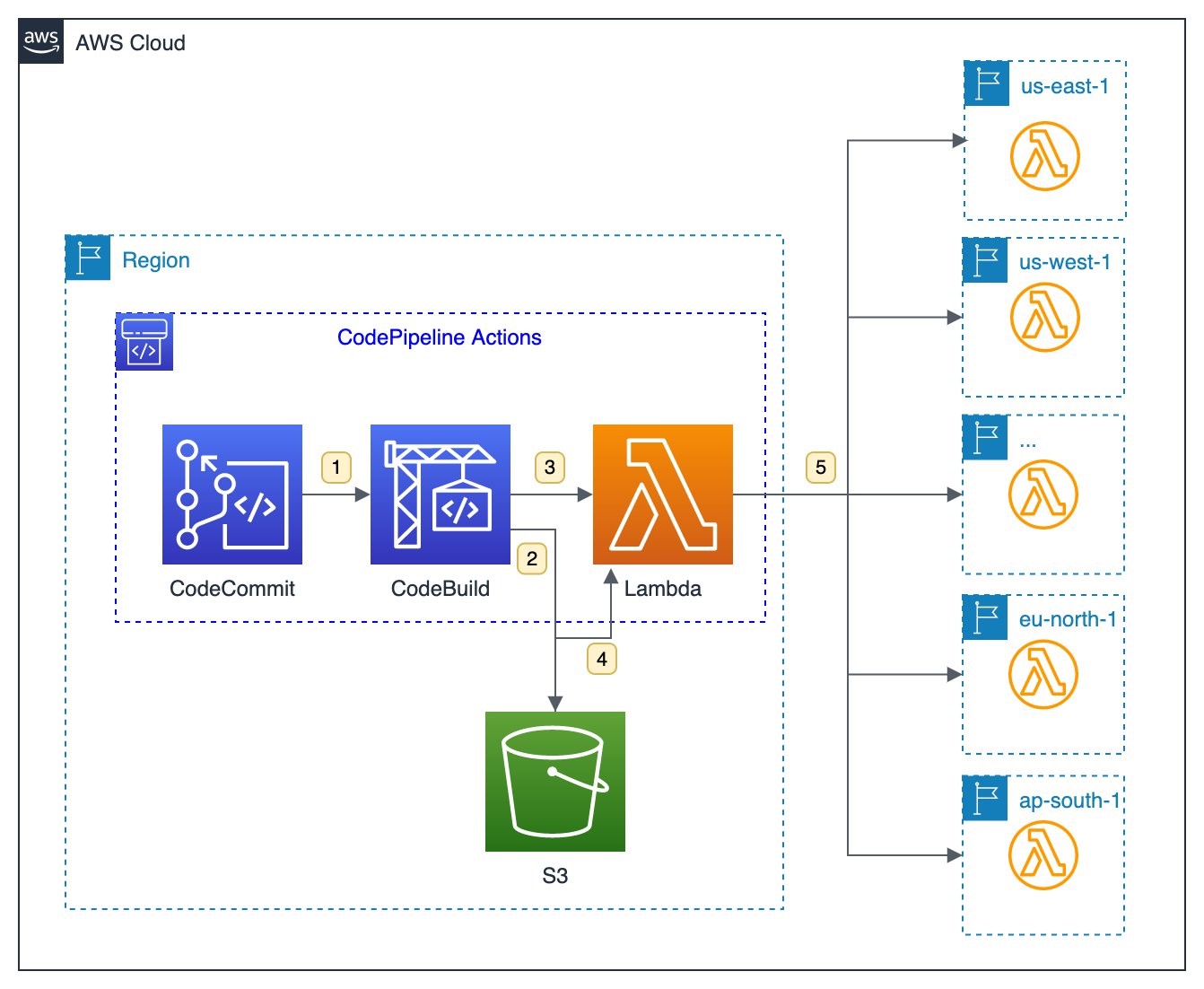
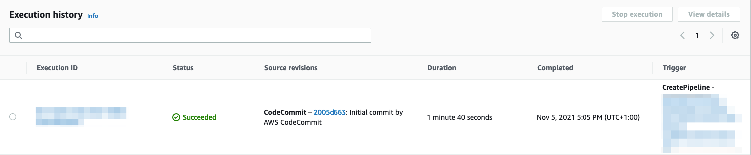


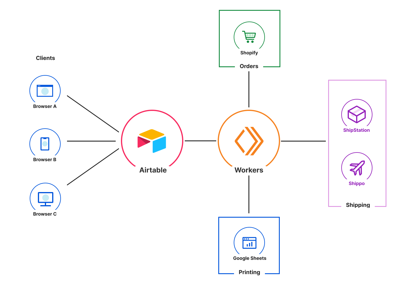


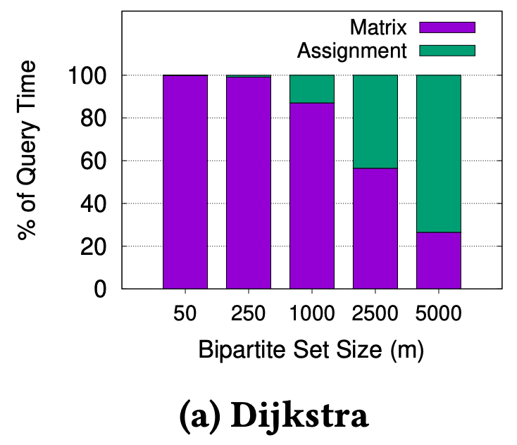
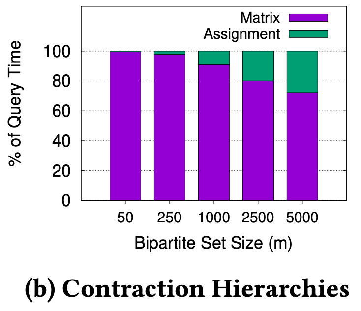

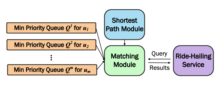
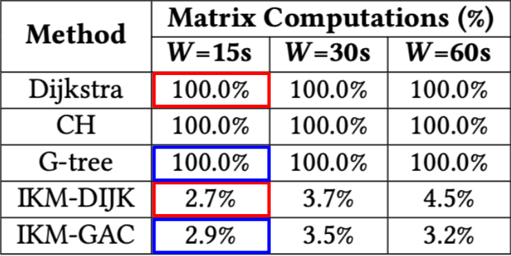
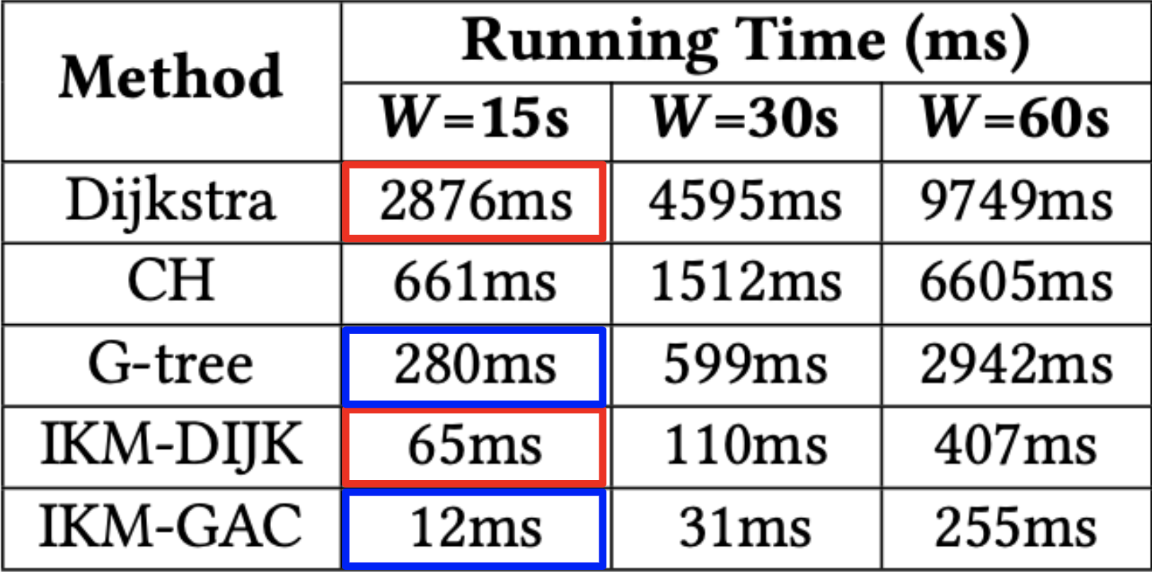
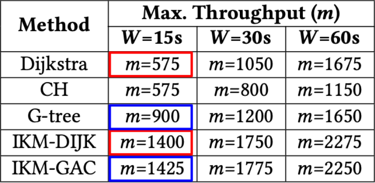
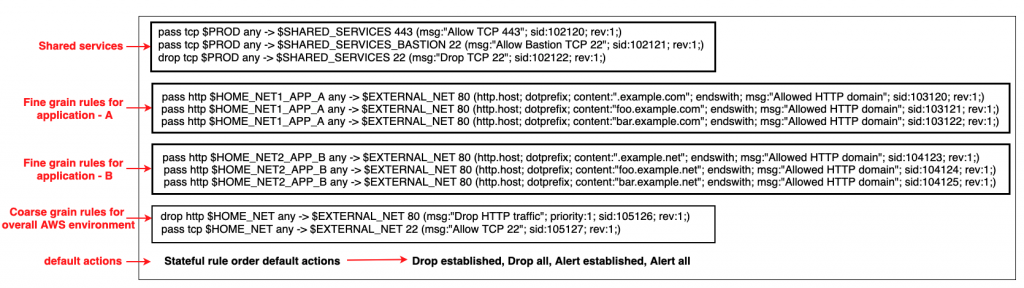
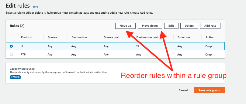
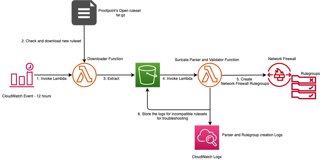
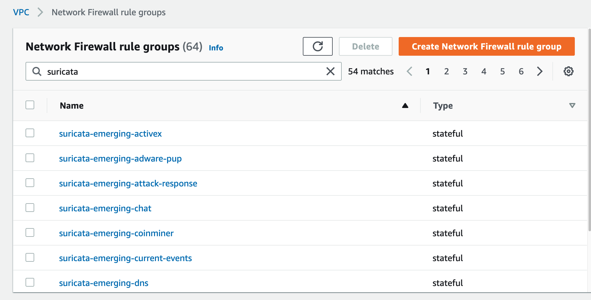
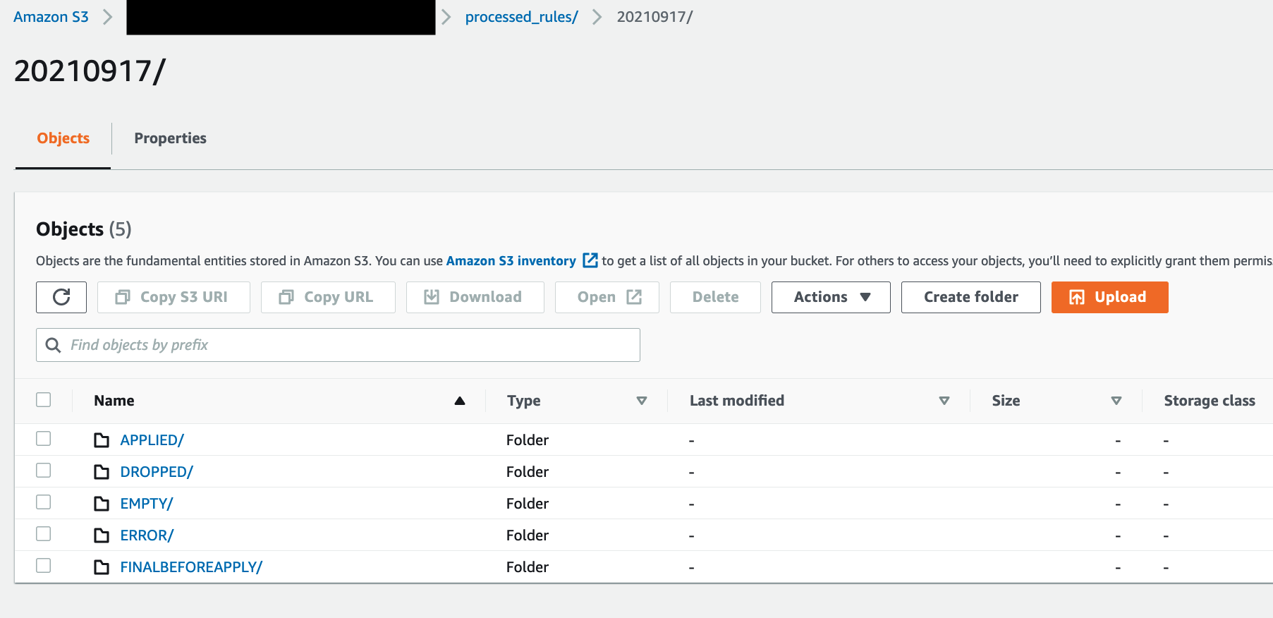
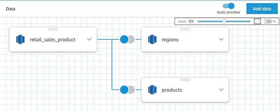
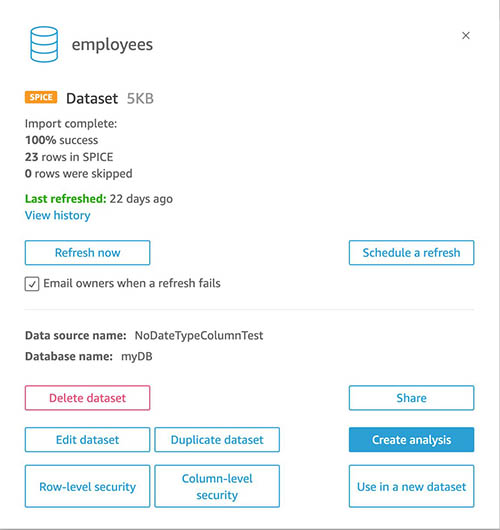
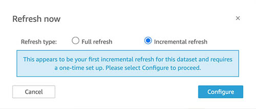

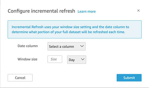
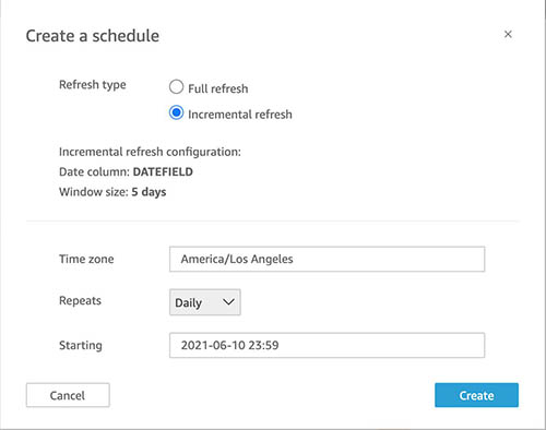


 Brooke White is a Software Development Engineer at AWS. She enables customers to get the most out of their data through her work on Amazon Redshift drivers. Prior to AWS, she built ETL pipelines and analytics APIs at a San Francisco Bay Area startup.