The development of AI and data science has transformed how we gain insights from data. In healthcare, AI tools are being used in the development of new treatments as researchers apply machine learning methods to datasets. However, applying AI in healthcare also brings risks, particularly when systems amplify existing biases in data or design.
The role of critical thinking skills in AI education
Kathy began her seminar by arguing that for many students who use AI tools in their coursework, questions remain about whether they are critically evaluating the tools’ outputs. Students may or may not check an AI-generated answer against primary sources to see if the answer is accurate. There is also growing concern that students’ use of AI tools lets them offload cognitive work rather than engage in deeper thinking. This presents a challenge for educators: how do we help students use AI productively while still supporting them to develop the critical judgement needed to evaluate its outputs?
Introducing Data Science, AI & You (DSAIY)
To tackle this challenge, Kathy and her colleagues have developed the Data Science, AI & You (DSAIY) programme (pronounced ‘Daisy’). DSAIY is a semester-long high school curriculum designed to introduce students to AI by actively engaging them in the machine learning process.
The programme introduces machine learning as the engine behind many AI tools, and introduces the concept of bias through real-world examples. Students use a variety of tools to collect and prepare data, train, test, and evaluate models. It culminates in an ‘AI-a-thon’ where young people work in cross-disciplinary teams alongside data scientists, clinicians, and their own teachers to gain real-world experience.
At the time of the seminar, 11 teachers had delivered the programme to over 800 students across a variety of settings in Rhode Island, USA. Teachers are heavily supported with four days of professional development and ongoing technical assistance throughout implementation. The students that took part had a wide variety of prior experience, including many with no prior background in computer science or statistics. Female participation is notably high; one teacher even remarked that the course saw more girls enrolled than any of his other computer science classes.
Hands-on with machine learning
In DSAIY, students experience the full machine learning pipeline from data collection and data preparation, to modeling and deployment. Using Python, they train and test simple machine learning models on authentic healthcare data. The aim of the programme is to move students from basic graphing to evaluating complex models, transitioning them from merely plotting data to deeply reasoning about it.
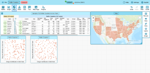
The programme makes use of CODAP (the Common Online Data Analysis Platform), a free, web-based tool developed by The Concord Consortium. CODAP provides an interactive, highly visual environment that lowers the barrier to entry. Students can visualise large datasets and click into individual data points, allowing them to see individual cases within a larger dataset.
CODAP, a tool for data visualisation and analysis
Understanding bias in healthcare systems
The curriculum uses real-world examples from healthcare to introduce concepts of bias and fairness. For example, students learn about pulse oximeters, which estimate blood oxygen levels. However, as these use red and infrared light, readings can vary depending on skin pigmentation, which can lead to inaccurate readings.
Students also collect their own blood oxygen data and plot it using CODAP to observe variability. They consider the accuracy of their measurements and grapple with the ethics of removing outliers from a dataset. This led to students asking critical questions about the makeup of their datasets, the context in which data are collected, and the implications of how data are used in healthcare.
Through the DSAIY programme, Kathy reported that students developed stronger data reasoning skills, gained a deeper awareness of inherent AI biases and risks, and built confidence in public speaking and collaborating with others. Students were also highly engaged and appreciated the focus on real-world healthcare applications and their social implications.
The importance of data literacy for AI literacy
Kathy concluded the seminar by arguing that AI literacy must start with data literacy. When students learn to examine, question, and reason about the data behind AI technologies, they develop the critical thinking skills needed to engage with outputs from real-world systems or everyday technologies like ChatGPT. This can then help them evaluate both the trustworthiness of these tools and their role in important decision-making processes.
You can watch the seminar here:
If you are interested in learning more about Kathy’s work, you can read about the DSAIY programme here or you can read the paper here. You can also learn about CODAP, the data visualisation tool featured in this seminar here.
Join our next seminar
In our current seminar series, we’re exploring how AI is taught across the curriculum. In our next seminar on Tuesday 14 July at 17:00–18:30 BST, we welcome Dan Verständig (Goethe University Frankfurt) who will explore the connection between Social explainable AI (Social XAI) and Critical Computational Literacy (CCL). To take part in the seminar, click the button below to register. We hope to see you there.
Gopan Sivasankaran is Regional Director, Middle East & Africa, at Rapid7
From AI adoption and cloud-first strategies to smart cities and critical infrastructure modernization, organizations across the United Arab Emirates are embracing innovation at an unprecedented rate. The country truly is setting the pace for digital transformation.
Against this backdrop of rapid innovation, today’s security teams are managing increasingly complex environments while defending against more sophisticated, AI-enabled threats. In this environment, business leaders still expect security to enable innovation, not slow it down. They’re pushed to reduce risk, improve visibility across expanding attack surfaces, and respond faster than ever before, with limited resources now table stakes.
This shift is changing what organizations expect from their cybersecurity partners, with customers no longer wanting disconnected tools or transactional relationships. They’re instead craving trusted advisors who can help simplify security operations, strengthen cyber resilience, and deliver measurable outcomes.
That’s why Rapid7 is excited to announce a new strategic, Middle East-spanning distribution partnership with Mindware.
A shared commitment to the region
The Middle East continues to establish itself as one of the world’s most ambitious digital economies. As organizations invest in cloud technologies, AI, and connected infrastructure, cybersecurity has become a critical foundation for sustainable growth.
This is precisely why Rapid7 has continued to invest in the Middle East: We recognize the region’s growing importance to the global cybersecurity landscape, and this new partnership with Mindware represents another important step in that journey.
This collaboration is about more than expanding our channel presence, it’s about investing in the partners helping organizations navigate an increasingly complex security landscape.
Mindware has built a strong reputation as one of the Middle East’s leading value-added distributors, combining deep regional expertise with technical enablement, professional services, and an extensive partner ecosystem. Together, we’re creating a framework that helps partners grow their cybersecurity practices while delivering greater value to customers.
Building stronger security operations
Security teams today face a common challenge: too many tools, too many alerts, and not enough time. Organizations are increasingly looking for platforms that bring exposure management, threat detection, and response together to improve visibility and reduce operational complexity.
Rapid7’s AI-powered cybersecurity operations platform helps organizations unify security operations, reduce risk, and respond to threats with greater speed and confidence. Combined with Mindware’s regional market knowledge, partner enablement capabilities, and technical expertise, this partnership will make it easier for organizations across the Middle East to access modern cybersecurity operations through trusted local partners.
For those partners, this creates new opportunities to expand managed services, strengthen technical capabilities, and help customers modernize their security operations while supporting long-term business growth.
Local expertise alongside global innovation
The most successful cybersecurity partnerships combine global innovation with local knowledge. Organizations want world-class technology, but they also expect partners who understand their business environment, regulatory landscape, and operational priorities.
By combining Rapid7’s cybersecurity innovation with Mindware’s established regional ecosystem, we’re helping partners fortify and deliver solutions capable of addressing today’s unprecedented security challenges and threats.
Together, we’ll invest in partner enablement and technical training programs designed to help build stronger security practices and create long-term customer success.
Looking ahead
Cyber resilience is no longer just a technology objective; it’s a business imperative. As organizations across the Gulf continue to accelerate digital transformation, security teams need solutions that reduce complexity, improve operational efficiency, and help them stay ahead of an evolving threat landscape.
Rapid7 and Mindware share a common belief that the future of cybersecurity is built through collaboration. By bringing together global cybersecurity innovation, regional expertise, and a shared commitment to partner success, we’re helping organizations across the Middle East strengthen cyber resilience while enabling partners to grow with confidence.
We’re excited about what’s ahead and look forward to working with our partners to build a stronger cybersecurity ecosystem across the region.
Ready to grow with Rapid7? Learn more about the Rapid7 PACT Partner Program and discover how we’re helping partners deliver stronger cybersecurity outcomes across the Middle East.
Северина Станкева: Поводът за този разговор е игра, която се появи миналата година като че ли отникъде и постигна невероятен успех и в лицето на публиката, и в това на критиката, толкова по-учудващ за дебютна игра на студио, за което също никой не беше чувал нищо – „Светлосянка: Експедиция 33“ (Clair Obscur: Expedition 33) на Sandfall Interactive. Когато ти я препоръчах, ти имаше поне две резерви към нея. Едната беше спрямо музиката, за която, съдейки от трейлъра, каза, че е „противна“ и „няма да я изтрая“, а другата – по отношение на стила битка, която определи като „наивна“. И за музиката, и за битките ще стане дума, но предлагам да започнем от като че ли реабилитиращото я в твоите очи художествено качество, заради което ми се струва, че в последна сметка я оцени толкова високо. Както се изрази по-късно, „Светлосянка“ е реквием на френската цивилизация, в което има нещо дълбоко антиутопично. Кое е собствено антиутопичното в нея? Това не е игра, която би била поставена в жанра (ако въобще е жанр, но това е друга тема) на антиутопията. Интерпретациите ѝ по-скоро се движат в трагическия ключ на семейната драма.
Миглена Николчина: Играта ни въвежда в един много красив, но разпадащ се свят, който някъде по средата се оказва, че не е истинският. Тази неистинност обаче е може би истината, тоест оказва се алегория на мъртвата вече Франция на живописта, операта, елегантността, цивилизоваността… Какво по-антиутопично от това? Що се отнася до оплакванията ми от музиката, те касаеха един конкретен момент; оплакванията ми от битките също засягат специфичен аспект, иначе веднага оцених хореографията им. Възможно е обаче да съм пренесла в тези си реакции смразяващия първоначален ефект на играта върху мен. Ще кажа и за него. Както предлагаш, ще се върнем към тези теми.
Като начало нека не се занимаваме много с онова, което най-вече занимаваше публиката по форумите – семейната драма. Тази семейна драма хората сериозно я разнищват, а на мен дори ми е забавна. Ако се погледне психоаналитично на нея, човек може и да се посмее. Под разни претексти родителите са готови да изтребят децата си, децата да изтребят родителите си, сестрите се бият на живот и смърт, накрая братът и сестрата също… И всичко това е, защото майката твърде много обича сина си; бащата – майката и дъщерята; сестрата – брат си… Сюжетът на играта систематично отстранява всички любовни или квазилюбовни претенденти, които не са част от тази инцестна въртележка. Във видеоигрите от самото им зараждане в центъра се поставят едипални битки с бащински властови фигури („босове“) и съвсем откровено с абектни репрезентации на майката – говорили сме за това, а и ти си го обсъждала подробно в изследването си за жените чудовища. В „Светлосянка“ обаче поразяват пищната многотия и оголването на фройдистко-еротичния аспект на конфликтите.
Но да се върна към антиутопията, тема, по която също вече сме говорили – ти и аз, аз и Еньо Стоянов… Говорили сме за специфичния тип руини, върху които се разгръщат едни или други дистопийни сюжети. С Еньо сме обсъждали как в „Ядрена зима“ (Fallout), особено в „Ню Вегас“ (New Vegas), руините са на загиналата американска средна класа. Това, което виждаме там, е провалът на проекта – на утопията – за средната класа. В „Метро“ (Metro) виждаме колосалните руини на комунистическия проект – там пък ядреният апокалипсис се разполага върху тези останки. В „Диско Елизиум“ (Disco Elysium) виждаме руините на специфично естонски исторически пластове, виждаме и такива, които се отнасят до краха на просветителския проект като цяло, има и слой, свързан с провала на комунизма, на прехода след него.
И ето че в „Светлосянка“ виждаме Париж. Париж е показан в три локации, които са в различна степен и форма на разруха. В единия играта започва и завършва, като този град присъства в три отделни времеви порядъка – естетизиран, но обхванат от обезпокоителни метаморфози в началото; халюцинаторно видоизменен в последното действие; най-сетне, тревожещо странен в единия от двата възможни финала. Това е част от Париж, „нарисувана“ и отцепена от цялото – музейна изрезка, в която най-важната сграда е операта.
Вторият Париж е напълно разрушен, отломъци от грамадни сгради висят във въздуха над купчина от архитектурни цепнатини и пламтящи пропасти. Има и трети – на разложението, разплут от просмукваща го неназована поквара. Всъщност има и един четвърти в „истинския“ финал на играта: в него Айфеловата кула е буквално фон на гробище.
За мен това визуално издевателство над някогашната световна столица на изкуството беше най-силното преживяване в играта, както и въобще нейната художническа и бих казала, изкуствоведска страна. Музиката отнесе най-много възторзи, тя също допринася за това, което виждам: един реквием. Но живописната страна на тази игра, в която всички персонажи са художници, за мен е най-сериозният носител на смисъла ѝ. Признавам, добра е музиката! Оплакването ми беше от момента, когато безкрайно тегаво се движиш из една равнина на фона на протяжна кахърна песен. Едвам пълзиш, а тя се върти и върти. И няма спасение! Има музика, която търпи повторение, дори да е видиотяващо, и има музика, чието повторение в един момент става непоносимо – може би тъкмо поради изобилната ѝ съдържателност.
Кадри от „Светлосянка“
Северина Станкева: Ефектът с повторението е търсен според мен. Набиващата се тема от началото ми беше дори симпатична, докато постепенно не се превърна в рококо кошмар без изход, някак още по-жесток заради лекотата си. Това се връзва и сюжетно. Освен това имам съмнението, че при теб ефектът е бил още по-силен, защото си прекарала доста повече време на съответните места, отколкото средностатистическия играч.
Миглена Николчина: Така е, аз съм много подробна, но не съм единствената. Във форумите предлагаха модове за тази локация, но аз започнах просто да изключвам звука. Що се отнася до битките, мисля, че беше грешка да играя на средно ниво, което по принцип винаги правя. То се оказа тежко – но оплакването ми не е от това, че е тежко, а от това, че тази тежест създава лудонаративен дисонанс. При много игри битките са гладко интегрирани или въобще играта е битките, там няма какво друго да очакваш. Но в „Светлосянка“ трудността на тези битки, времеемкостта им може да смажат сюжета, персонажите и най-вече ефекта от това, което може да се нарече онтологическа катастрофа: продънването на реалността в света на картината. Битките сами по себе си са красиви, противниците са живописни, смешно-страшни, за да го кажем с една естетическа категория на Хофман. Получава се разминаване обаче между ангажираността на играча с тях и залозите на другите аспекти на играта.
Северина Станкева: Съгласна съм, че има дисонанс между логиката на действията на играча и тази на разказа, но помоему едно от нещата, които тази игра съумява да направи изключително добре, е да съвместява такъв тип противоположности (точно както изобразителната техника, на която дължи името си), и то така, че моментите на дисонанс са някак инкорпорирани в цялото, без то да страда от това, напротив. С други думи, този разрив може да се разгледа като аспект на онтологическата катастрофа. Като голям фен на стила битка на „Секиро“ (Sekiro), търпението и дисциплината, които тя изисква, „Светлосянка“ много ми допадна в чисто действено отношение. Тяразширява арсенала от възможности на ритмичната битка, добавяйки походови елементи, които също – давам си сметка, че това е субективно предпочитание – ми се видяха освежаващи. Но отвъд личните предпочитания, несъвпадението между битка и разказ всъщност много добре ми се върза с контрастното построение на самия разказ, в който също хем има толкова наивни и детски елементи, хем е изключително мрачен и накъсван от постоянното врязване на трагедии. Темите на играта са смъртта и загубата и това как да им устоим, как да се справим с тях. Битките се случват на ниво, което е онтологически различно (по-художествено, по-наивно) от пласта на реалността (или това, което се приема за реалност в самия разказ). За това ще стане въпрос по-късно. Мисълта ми е, че при тях има двойна дистанция, която в началото не се разкрива като такава – игра в играта. Тоест аз хем съм съгласна, хем за мен лично дисонантното е много силно качество, не недостатък. Малко са игрите, които успяват да направят дисонансите да работят. Тази според мен го прави.
Миглена Николчина: Дисонанс или не, нека си призная, че на три пъти започвах играта, защото началото е толкова ужасяващо, че нямах сили да продължа. Внедряват те в този много красив, много парижки мизансцен на границата на XIX и XX век, сред елегантни хора, цветя, изискани жестове, изпълнени с нежност реплики… докато се стигне до момент, в който става ясно, че всяка година всички, които са достигнали до все по-ниска възраст, биват изтривани. Това е годината, в която изтриват достигналите 34 години, следват 33-годишните. Прекрасното момиче, преплело ръце с прекрасно момче, се разпилява като подети от вятъра листенца. Денят е меланхолно естетизиран празник сбогуване на оставащите с изтриваните. „Гомаж“ – аз я играх на френски тази игра.
Северина Станкева: То и на английски е оставено „гомаж“ (gommage – букв. „изтриване, заличаване“).
Миглена Николчина: Играх я на френски, защото е френска игра. Така. Девойката е една година по-голяма от него и я изтриват. И множеството нейни връстници се разнасят като облак. Непоносимо. За мен загубата, за която става дума в тази игра и която е нейният най-осезаем аспект, не е свързана с личната драма, а с цивилизационната. Играта е за гибелта на Париж, на Френското просвещение, на великото френско изкуство с неговите институции, на френската цивилизованост, на френската естетизация на любовта, общуването, живеенето. Дали това е замисъл, дали е преднамерено, или се е получило като страничен ефект от абсурдния сюжет, не мога кажа. От интервютата със създателите, които гледах, не може да се разбере. Подсмихват се и не казват.
Кадри от „Светлосянка“
Да започнем с първата загадка. Трагедията, която се е случила – пожар в дома на семейство художници, при който синът Версо загива, предизвиквайки лавина от фантастични последици, – е през 1905 г. Защо точно тази година? Какво да мислим за главоблъсканицата с надгробния камък на Версо, който се появява в единия от финалите с дата на смъртта му 33 декември 1905 г.? Връзката с цифрите в заглавието на играта не ми казва нищо, освен ако не си спомним Данте с неговото 3 х 3 = 9 – Беатриче е деветка… По-съществена ми се струва самата преднамереност, с която ни подхвърлят една несъществуваща дата тъкмо във финала, който се предполага да е връщане в реалността.
Във всеки случай 1905-та е важна, преломна година, с която всъщност започва XX век. Тогава излиза частната теория на относителността на Айнщайн. Тя изключително драматично се преживява от хората на изкуството – и във Франция, и извън нея. Относителността на времето се превръща в обсесия, която поражда всевъзможни експерименти – например с романната форма у Джойс, Томас Ман, Вирджиния Улф и пр. В играта виждаме заиграване с времето на композиционно ниво, то тече по различен начин в „света на картината“ и „света отвън“. И това е само един от аспектите.
Във форумите открих нещо, което до този момент не бях отчитала. През 1905 г. във Франция се прокарва закон, който разделя религията от държавата и се обявява свобода на вероизповеданията. Ако приемем сериозно такава връзка, може да забележим липсата на катедралата „Нотр Дам“. Да не би пък тя да е изгоряла? Айфеловата кула я има, макар и килната, но сред множеството руини не видях никъде останки от „Нотр Дам“… Така че ето още една загадка.
Какво друго се случва през 1905 г.? Троцки издава своята книга „1905“. Тя е за Първата руска революция, която се случва тогава. Не смятам, че създателите на играта са мислили за тази революция, но и тя, и книгата са знак за това какво предстои. През 1905 г. умира Жул Верн и излизат два негови романа – единият, докато е все още жив, който се казва „Завладяването на морето“, и другият – „Фарът на края на света“. Не знам дали са имали предвид Жул Верн, но и фар, и завладяване на морето има.
Това, което ще изтъкна е, че през 1905-та се състои първата изложба на фовизма. Течението съществува за кратко, но се смята за повратна точка в историята на живописта. С него се слага край на предишните иновативни течения, каквито са импресионизмът и постимпресионизмът (Внимание! Името на бащата на семейството художници в играта е Реноар.) и се влиза в ера на множество „изми“, сред които – като тежко визуално присъствие в тази игра – ще спомена, освен фовизма, и сюрреализма.
Накратко, част от трагедията се отнася според мен до едно драматично преобръщане в историята на изкуството. Играта пласт върху пласт наслагва сякаш с блажни бои тази история, ние се движим в нея – и в драмата на нейния край, който е край на Париж като световна столица на изкуството и цивилизацията.
(Следва продължение.)
В рубриката „Игромислие“ публикуваме разговори, в които се срещат, съпоставят и противопоставят различни гледни точки към многоизмерния, многожанров феномен на видеоигрите – не толкова като електронен спорт, колкото като нов синтез на изкуствата и като ново поле на общуване и социалност.
Снощи отидох на концерт на братятя Кавалера, които изсвириха целия Chaos AD.
Беше в “Маймунарника”, който май никога не съм виждал толкова пълен. От техническа гледна точка събитието беше трагично – звукът на подгряващата група беше по-добре, по време на концерта соло китарата беше тиха и се губеше, и токът на сцената спря три пъти. Не мисля, че съм присъствал на подобна издънка, и е направо невероятно за подобен концерт.
Въпреки това, си беше забавно. Публиката беше пълна с хора от всякакви възрасти, от възрастта на моите деца до почти дядовци и радва, че и младото поколение беше дошло да чуе малко класическа музика.
Започнаха с Refuse/Resist (започващо вероятно с най-известния запис на пулс ever) и завършиха с cover на същото парче 🙂 Макс изглежда все още има глас, въпреки напредналите годинки, бяха довели буквално едно дете (Игор Амадеус, синът на Макс) на бас, имаха приличен китарист, и Игор Кавалера беше там като основната причина да бъдат чути (и слава богу не му бяха объркали много звука на барабаните, за да се чуе наистина както трябва). Направиха едно страхотно изпълнение на Kaiowas, което май беше най-добре получилата се песен на концерта.
By Parth Jain, Rakesh Sukumar, Yingwu Zhao, Renzo Sanchez-Silva & Nathan Fisher A deep dive into the engineering challenges of building a real-time service dependency map at Netflix scale: from streaming architectures and distributed aggregation pipelines to time-travel queries and the methodology that made it work.
Introduction
In our first post, we introduced the problem: engineers at Netflix needed a unified, real-time view of service dependencies to troubleshoot faster, understand blast radius, and navigate our distributed architecture. We described our multi-source approach, combining eBPF network flows, IPC metrics, and distributed tracing into physically separate graph layers that can be queried independently or merged into a comprehensive view.
That post explained what we built and why. This post is about how, the engineering reality of building this system at Netflix scale.
Here’s the truth: the first version worked perfectly… in our local environment. Production was a different story. Kafka consumers fell behind. Instances ran out of memory. Some nodes received 100x the traffic of others. Garbage collection pauses consumed more CPU than actual business logic.
What you’ll learn in this post isn’t a success story, it’s a learning journey. We’ll walk through the architecture decisions that enabled scale, the production challenges that tested those decisions, the optimization methodology that guided us through, and the lessons that apply to any distributed system. Along the way, we’ll share the innovations that made it possible to process millions of flow records per second, reconstruct topology at any point in time, and provide sub-second query responses, all while maintaining near real-time freshness.
Architecture Deep-Dive: Building for Streaming and Scale
Streaming-First: Why Real-Time Matters
Traditional service topology systems use batch processing, aggregating data hourly or daily, then storing complete snapshots. This approach works at a modest scale but has a fundamental problem: by the time you see the data, it’s already old. During a production incident at 3am, an hour-old dependency map is archaeology, not observability.
Our key architectural decision was to build streaming-first. Instead of batch jobs that process historical data, we continuously ingest flow records from multi-region Kafka streams and IPC metrics as Server-Sent Events, process them through reactive pipelines with backpressure handling, and provide near real-time topology updates, typically within tens of minutes, compared to the hours-old or day-old data that batch processing approaches provide.
This wasn’t just about freshness, it was essential for our use cases. Live events can’t wait for the next hourly batch. Incident response needs current data. Change validation requires seeing immediate impact. The architecture had to support continuous updates while handling massive scale without falling behind.
How Backpressure Enables Real-Time Processing The streaming approach created new challenges, but also required solving a fundamental problem: how do you process millions of flow records per second in real-time without losing data when downstream systems slow down?
Traditional approaches fall short at our scale:
Unbounded queues: Simple but dangerous. Keep buffering until you run out of memory, then the instance crashes.
Drop-based flow control: Discard data when buffers fill. Fast, but now your topology is incomplete, you’ve lost connection information.
Batch processing: Process everything, but hours later. By then, the incident is over (or worse, still happening with stale data).
We needed something different: the ability to slow down gracefully under load without losing data. This is where reactive streams with backpressure became essential.
Here’s how it works: when Stage 3 can’t write to the graph database fast enough, it signals Stage 2 to slow down. Stage 2 signals Stage 1. Stage 1 signals the Kafka consumer to pause. The data waits in Kafka until downstream capacity returns.
When a downstream stage can’t keep up, it signals upstream to slow down — backpressure flows in the opposite direction of the data
Backpressure propagates naturally through the entire system. When any stage becomes overwhelmed from traffic spikes, GC pauses, or external slowdowns, the pipeline automatically slows to a sustainable rate. No data is lost in most cases, no instances crash, the system degrades gracefully.
This is what enables “real-time” at our scale. During normal operation, we process with minimal latency. During load spikes or temporary slowdowns, we slow down rather than fall over. The data still gets processed, just a few seconds or minutes later instead of immediately. For topology updates, this trade-off is acceptable: slightly delayed real-time updates are vastly better than hour-old batch data or incomplete topology from dropped records.
The cost of this approach is complexity. Reactive streams are harder to reason about compared to traditional synchronous blocking models (we’ll discuss this more in the challenges section). But at Netflix scale, backpressure isn’t optional, it’s the mechanism that keeps the system running reliably under production load.
Multi-Layer Architecture: Physical Separation for Independent Optimization
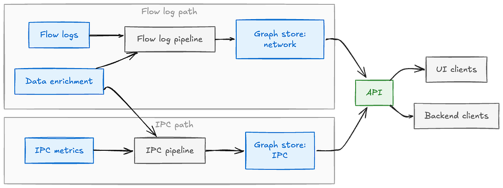
As we covered in our first post, our multi-source approach uses three physically separate topology layers with different storage optimized for each:
Network Layer: eBPF flow logs in graph database partition, comprehensive coverage but lacks application context
IPC Layer: Application metrics in a different graph database isolated from the one for Network Layer, rich endpoint details but only instrumented services
Tracing Layer: Distributed traces in columnar storage (Parquet), actual request paths but sampled.(We cover the tracing layer and its integration in our next post).
Flow logs and IPC metrics travel through two independently-optimized pipelines into separate graph stores, unified behind a single API
Physical storage isolation enables independent optimization, each layer has different throughput, query patterns, and evolution timelines. At query time, we execute parallel queries across relevant storage systems and merge results, providing unified views with sub-second latency while maintaining flexibility to evolve each layer independently.
The Three-Stage Distributed Aggregation Pipeline
The heart of the network layer ingestion is a three-stage distributed pipeline. This architecture solves a fundamental challenge with network flow logs: they only show individual network hops, not the true application-level connections we need to build a useful topology.
The Core Problem: Network Intermediaries
In cloud environments, traffic between applications rarely flows directly, it traverses intermediate network components like load balancers, NAT gateways, API gateways, and proxies. Network flow logs show individual hops: App A → Load Balancer and Load Balancer → App B appear as separate flows. But what engineers need is the logical dependency: App A → App B. Without resolving these intermediaries, our topology would be cluttered with infrastructure components rather than showing the service-to-service relationships that matter for troubleshooting.
The three-stage pipeline solves this:
The flow log pipeline in detail — three stages connected by SSE, with enrichment applied just before the final graph write
Multi-Region Kafka (4 regions)
  → Filter invalid flow logs
  → 5-minute time-window batching
  → Create initial aggregators per window
  → Distribute via consistent hashing
  → Stream to Stage 2 via SSE
Stage 1 consumes flow logs from multi-region Kafka, filters invalid records, batches them into 5-minute time windows, and creates initial aggregator objects. At this stage, we’re still working with raw network hops, identifying which flows involve intermediaries but not yet resolving them. Aggregators stream to Stage 2 for resolution.
Stage 1 Aggregators (via SSE streams)
  → Group flows by intermediary (load balancer, NAT gateway, proxy, etc.)
  → Identify pairs: (Source → Intermediary) + (Intermediary → Destination)
  → Resolve to direct edges: Source → Destination
  → Track which intermediaries were traversed
  → Aggregate metrics across both hops
  → Re-distribute via consistent hashing
  → Stream to Stage 3 via SSE
This is the key step. Stage 2 performs graph resolution:
Collect flows by intermediary: Group aggregators where an intermediary is either source or destination, creating maps of flows going TO intermediaries (Source → Intermediary) and FROM intermediaries (Intermediary → Destination)
Resolve direct edges: For each intermediary, join its incoming and outgoing flows to create direct application edges (App A → App B), combining metrics from both hops
Result: Clean application-level topology showing App A → App B instead of App A → Load Balancer → App B
This resolution happens at aggregation time, not query time, with resolved edges flowing to Stage 3.
Why can’t we do this in a single stage? The fundamental issue is data locality. To resolve App A → Load Balancer → App B into App A → App B, we need both flows on the same instance to perform the join. But in Stage 1, flows are scattered across instances based on Kafka’s partitioning. Stage 2’s critical function is to redistribute aggregators by intermediary identifier, all flows involving “Load Balancer X” route to the same instance for resolution. This is the classic map-reduce pattern: Stage 1 maps, Stage 2 shuffles and reduces by intermediary, Stage 3 performs final aggregation.
A concrete example of why a single stage isn’t enough — Stage 1 scatters flows by partition, Stage 2 reshuffles by intermediary to resolve direct edges, and Stage 3 persists the final result.
Stage 3: Final Aggregation and Enrichment (GraphEntity Ingestion Service)
Stage 2 Aggregators (via SSE streams)Flow
  → Final aggregation across time windows
  → Enrich with external data (query key-value stores)
  → Convert to graph entities
  → Persist to graph database (throttled writes)
Stage 3 performs final aggregation of resolved edges, enriches graph nodes with external data sources (application health, ownership, metadata), converts aggregators to concrete graph entities (nodes and edges with all properties populated), and persists them to the distributed graph database with controlled throttling to respect storage system limits.
Why Three Stages, Not Two?
We initially used two stages: aggregate in Stage 1, resolve and persist in Stage 2. This worked in testing but failed at production scale, Stage 2 became overwhelmed by data concentration.
The problem: intermediary resolution requires collecting ALL flows involving an intermediary on the same instance.As a result, the instances handling flow logs for popular applications and their intermediaries became ‘hot nodes’ due to significant data concentrationCompounding this, data enrichment (querying external stores for health and metadata) meant the busiest instances were also doing the most I/O.
The solution: split responsibilities into three stages. Stage 2 focuses purely on resolution and redistributes. Stage 3 handles enrichment and persistence. This graduated redistribution (distribute, resolve, distribute again), persist, spreads load across multiple instances and isolates compute-heavy resolution from I/O-heavy enrichment. Even when intermediaries see 100x typical traffic, no single instance becomes a bottleneck.
Why Server-Sent Events Instead of gRPC or Message Queues?
We initially used gRPC but it became a performance bottleneck, serialization overhead, connection pool management, and memory pressure for streaming responses consumed more CPU than business logic. Message queues added infrastructure complexity without benefit for our use case.
SSE proved ideal: lightweight HTTP-based protocol with minimal serialization, natural backpressure integration with reactive streams, and simpler connection model. The lesson: industry best practices like “use gRPC for service communication” don’t apply universally. For streaming large volumes of pre-aggregated data, lighter-weight alternatives may be more appropriate. Measure, don’t assume.
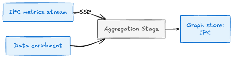
Why IPC Doesn’t Need Three Stages
The IPC pipeline mirrors the same pattern as the flow log pipeline, but needs only a single stage.
The IPC layer uses single-stage aggregation because: (1) IPC metrics are already at application level, no intermediaries to resolve, and (2) data is partitioned correctly from the start — each node receives all IPC metrics for its assigned applications via consistent hashing, eliminating the need for redistribution. This highlights a key principle: data partitioning strategy determines processing architecture. When data arrives with the right partitioning, you can aggregate directly; when it doesn’t (like network flows requiring intermediary resolution), you need shuffle/redistribution stages.
Dynamic Load Distribution: How Hashing Works with Auto-Scaling
How do we decide which instance receives which aggregator when our Auto Scaling Groups dynamically add or remove instances? Traditional approaches assume static clusters requiring explicit rebalancing, coordination services, or manual data movement when cluster size changes.
Our Approach: Dynamic Consistent Hashing
We use consistent hashing with dynamic instance discovery from our service registry. Each instance queries the registry to get the current list of healthy ASG instances, maintains them in sorted order (ensuring all instances have the same view), and uses this list for the hash function findOwnerInstance(aggregator.primaryKey). When ASG scales up or down, the hash function naturally redistributes aggregators based on the updated instance list, no explicit coordination needed.
The key insight: leverage existing infrastructure. Our service registry already tracks ASG membership for health checking. Using it as our source of truth gives us dynamic cluster membership for free. Consistent hashing provides stable partitioning (most aggregators stay on the same instance during membership changes), while the sorted list ensures consistency.
The Result
Load follows infrastructure automatically. During traffic spikes or live events, new instances immediately receive their share. During deployments, aggregators seamlessly shift to healthy instances. This pattern proved crucial for production stability, no manual intervention, no coordination protocol, just automatic rebalancing.
The V1 Journey: Major Challenges at Production Scale
Getting the initial version (V1) to production taught us that scale changes everything. What works in development breaks in production. Every assumption gets tested. And fixing one bottleneck reveals the next.
Challenge 1: Kafka Consumer Lag
The Problem: Our multi-region Kafka consumers started falling behind. Consumer lag grew from seconds to minutes, then hours. Flow logs were arriving faster than we could process them. If this continued, we’d never catch up, and our “real-time” topology would become increasingly stale.
Investigation: We instrumented Kafka consumer metrics heavily. Key findings:
Kafka had fewer partitions than optimal for our consumer group size
Each fetch operation retrieved relatively few records
Network socket buffers weren’t right-sized for our throughput
Cross-region read latency added overhead
Solutions Applied:
Increased Kafka partitions: More partitions enabled more parallel consumers in our consumer group, distributing load across more instances.
Tuned fetch parameters: Increased records per fetch operation, reducing the number of network round-trips. This trades off per-message latency (we fetch larger batches) for throughput (more records processed per second).
Increased socket receive buffer size: Ensured network buffers never limited fetch operations. At our scale, default buffer sizes were too small.
Results: Throughput improved significantly, and lag reduced to acceptable levels, typically under a minute even during peak traffic.
Lesson: At scale, you can’t optimize in isolation. Fixing Kafka lag revealed the next bottleneck: our instances themselves couldn’t keep up with the higher ingest rate. The pipeline moved faster, which exposed downstream capacity problems.
Challenge 2: Hot Nodes and Data Amplification
The Problem: This was the most severe production issue we faced. Some instances in our Auto Scaling Group were receiving 100x more traffic than others. Memory usage spiked. Garbage collection pauses became frequent and long. More CPU time was spent in GC than in business logic. Eventually, hot instances would go DOWN, triggering cascading failures as their load redistributed to other instances.
Root Cause Investigation: Flow logs for popular services dominate traffic volume. A service like our authentication layer or recommendation API is called by hundreds of other services, generating orders of magnitude more flow records than typical services.
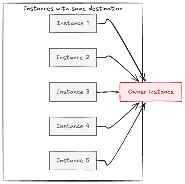
Our initial architecture used consistent hashing to determine which instance owned aggregation for each destination service. All flow logs for a given destination are routed to the same instance, the “owner” for that destination. This design seemed reasonable: group related data for efficient aggregation.
But popular destinations created hot nodes. One instance might own authentication services, another might own a rarely-used backend service. The load distribution was wildly uneven, some instances handled 100x the flow records of others.
Worse, data amplification occurred during redistribution. Consider a service called by 100 upstream services across 10 instances. All 10 instances receive flow logs for that destination (because they all have local clients calling it). When they route aggregators to the owner instance, that instance receives 10 separate aggregators it must merge. The data volume multiplied during shuffling.
When many instances route data for the same key to one owner, the volume multiplies right where it lands — the root cause of hot nodes.
We profiled extensively using async-profiler and heap dump analysis. The results were clear: hot instances spent most of their CPU on garbage collection, trying to manage the rapid allocation and deallocation of aggregator objects as flow logs poured in faster than they could be processed. Memory pressure led to GC thrashing, which consumed CPU, which slowed processing, which increased memory pressure, a vicious cycle.
Solution: The Three-Stage Pipeline’s Dual Benefits The three-stage pipeline we described earlier, designed primarily for proxy resolution, turned out to be exactly what we needed to solve the hot nodes problem as well. Here’s why:
Stage 1 performs initial aggregation locally before any distribution. Instead of sending every flow log to a remote instance immediately. Each instance performs online aggregation of raw flow logs into time-windowed aggregators (over 5-minute periods) directly in memory; this allows the raw flow to be discarded and garbage collected quickly, significantly reducing memory pressure, and ensures only the aggregation results are transferred across the network to downstream stages.
Stage 2 focuses on proxy resolution but also provides intermediate redistribution. Aggregators from Stage 1 distribute via consistent hashing to Stage 2 instances. Now we’re moving compressed aggregators, not individual flow logs. After resolution, Stage 2 redistributes resolved edges again to Stage 3, providing a second hashing operation that further spreads load.
Stage 3 receives resolved aggregators that have been compressed twice and distributed twice. Even for extremely popular services, load has been spread across enough distribution points that no single instance becomes overwhelmed.
The key insight: architectural decisions driven by one requirement (proxy resolution) often solve other problems (load distribution) as beneficial side effects. The three-stage pipeline with graduated redistribution achieves both goals, it resolves proxies to show clean application-level topology AND prevents hot nodes by spreading load across multiple distribution points.
Switching from gRPC to SSE As described earlier, this challenge also revealed that gRPC wasn’t the right protocol for inter-stage communication at our scale. We replaced gRPC with Server-Sent Events, dramatically reducing resource consumption on both sender and receiver sides.
Results:
CPU usage became evenly distributed across instances, no more hot nodes with 10x the load of others
Network bandwidth usage dropped significantly due to better aggregation and lighter-weight protocol
Memory pressure decreased as we reduced the object allocation rate
The system scaled gracefully with Auto Scaling Group changes
Lesson: Technology choices must match your specific use case. gRPC is excellent for request-response RPC patterns. For streaming large volumes of aggregated data in a pipeline, lighter-weight alternatives can be more appropriate. Let measurements guide the decision, not industry hype or existing team expertise.
Challenge 3: Memory and Garbage Collection
The Problem: Even after fixing hot nodes, we still saw high heap usage, frequent garbage collection pauses, and instances occasionally going DOWN. GC logs showed pauses consuming significant CPU time, in some cases, more than our business logic.
Root Cause: Multiple factors contributed: objects accumulating in heap while waiting for 5-minute aggregation windows to complete, unnecessary conversions between different object types as data flowed through stages, and immutability overhead, following Scala best practices, we used immutable data structures for aggregators, but every update created new objects, overwhelming the garbage collector at millions of records per second.
Investigation: Heap dumps and GC logs revealed flow log objects retained beyond their useful lifetime, unnecessary intermediate conversion objects, and constant creation/disposal of immutable aggregator versions. Minor GCs occurred every few seconds, major GCs took hundreds of milliseconds, the JVM spent more time on garbage collection than business logic.
Solutions Applied:
Faster processing: Process flow logs immediately, aggregate quickly, release references. Optimized Pekko stream stages to minimize object lifetime.
Eliminate unnecessary conversions: Route aggregators directly between stages instead of converting to intermediate types.
Mutable structures on hotpath: This was controversial, Scala best practices emphasize immutability. But at our scale, immutability created too many objects. We pragmatically chose mutable aggregators on the hotpath (immutability elsewhere), prioritizing performance over convention. Switching to mutable aggregators reduced heap allocation by over 50% and cut GC pause time significantly, though it required more careful code review.
Tuned time windows: Balanced data freshness against memory pressure.
Results:
Heap usage decreased substantially
GC pauses reduced to acceptable levels (tens of milliseconds instead of hundreds)
CPU freed up for business logic instead of garbage collection
Instance stability improved, no more instances going DOWN due to memory issues
Lesson: “Best practices” are starting points, not absolute rules. At unique scale, you may need to diverge from conventions. But do it deliberately, with measurement justifying the decision, and with awareness of the trade-offs. Don’t abandon immutability everywhere, just where performance data proves it’s necessary.
Challenge 4: Reactive Streams Complexity
The Problem: Our Pekko Streams pipelines would stall unexpectedly. Backpressure propagation didn’t work as expected. We struggled to debug why certain streams would stop processing without obvious errors. The reactive programming mental model, with its emphasis on async boundaries, backpressure, and demand-driven processing, proved harder to master than anticipated.
What We Learned: Reactive streams with backpressure are powerful tools for building systems that handle load spikes gracefully. When downstream consumers slow down (due to temporary load, GC pauses, or external system slowdowns), backpressure allows upstream producers to slow down rather than overflow buffers or drop data.
But this power comes with complexity:
Non-intuitive behavior: Traditional imperative code flows top-to-bottom. Reactive streams are demand-driven, downstream consumers pull from upstream producers. This inversion of control isn’t intuitive.
Async boundaries: The .async operator in Pekko Streams creates a boundary where processing moves to a different thread. This can improve parallelism but also introduces complexity around buffer sizing, demand signaling, and error propagation. We initially misunderstood when to use .async and ended up with over-parallelized streams that created more overhead than benefit.
Debugging difficulty: When a stream stalls, there’s no stack trace pointing to the problem. You must understand the internal mechanics, demand signals, buffer states, materializer state to diagnose issues.
Our Approach:
Deep learning investment: We invested significant time in understanding reactive streams concepts deeply. Reading documentation, experimenting with small examples, and building team expertise.
Simplified patterns: Where possible, we simplified our stream graphs. Complex branching and merging patterns are powerful but hard to debug. We preferred linear flows with clear stage boundaries.
Better monitoring: We added metrics at stream boundaries, tracking buffer sizes, element throughput, backpressure events. Visibility into stream internals helped diagnose issues.
Team education: We documented our learnings, shared patterns that worked, and built institutional knowledge about reactive streams.
Lesson: Powerful abstractions require investment. Don’t assume you understand a framework without validation. Build your mental model deliberately, test it with experiments, and be humble about your understanding. Reactive streams are worth mastering for systems that need to handle load gracefully, but expect a learning curve.
V2 Evolution: Continuous Refinement
V1 got us to production. The major architectural challenges like Kafka lag, hot nodes, memory pressure, were solved. But production at full scale revealed new optimization opportunities. V2 represents the continuous refinement that turns a working system into a production-ready system.
Challenge 5: Persistent Heap Pressure
The Problem: Despite V1 optimizations, we still observed higher-than-desired heap usage. GC metrics improved but weren’t optimal. Memory profiling showed room for improvement.
Root Cause: Deeper analysis revealed we were still doing unnecessary object conversions between stages. We’d convert aggregators to full graph entities (with all properties populated) before routing to the next stage, even though the next stage just needed the compressed aggregator state.
Solution: Architectural change to route aggregators directly through all stages, only converting to final graph entities at Stage 3 immediately before persistence. This eliminated two intermediate conversion steps and the associated object allocation.
Result: Heap usage dropped further, GC pauses became even less frequent, and memory headroom improved.
Challenge 6: Serialization Complexity
The Problem: Custom serialization logic for SSE messages caused occasional erratic errors that were hard to reproduce and debug. Different parts of the codebase used inconsistent serialization approaches.
Solution: Standardized on JSON encoding throughout the pipeline. While slightly less efficient than binary serialization, JSON’s human readability made debugging far easier, and the overhead was negligible compared to other operations. Consistency eliminated an entire class of bugs.
Result: Serialization-related errors disappeared. Debugging became easier because we could read SSE message contents directly.
Challenge 7: Stream Processing Inefficiencies
The Problem: Even after understanding reactive streams better, our Pekko configurations weren’t optimal. We had over-parallelized some stages and under-parallelized others. The .async boundaries weren’t placed optimally.
Solution: Through continued profiling and experimentation, we tuned parallelism parameters, adjusted buffer sizes, and refined async boundary placement. We added monitoring at stream boundaries to identify bottlenecks.
Result: Throughput improvements and more consistent processing latency.
Challenge 8: Uneven Graph Database Throughput
The Problem: Write distribution to our graph database wasn’t even. Some partitions received heavy write traffic while others sat idle. This caused throttling to kick in unevenly and limited overall write throughput.
Solution: Implemented batching of aggregators before writing to the graph database and improved distribution logic across partitions. Rather than writing each aggregator immediately, we batch them and write multiple entities in coordinated operations.
Result: More consistent write throughput and better utilization of database capacity.
Challenge 9: Data Enrichment at Aggregation Time
Beyond the core topology graph, we needed to enrich nodes with additional context. At Stage 3, before persisting graph entities, we integrate enrichment data from external sources, application health status, ownership information, and other metadata. Performing this enrichment at aggregation time rather than at query time avoids the performance overhead of post-query joins and ensures every topology node has full context when queried.
Pattern Recognition
Each V2 challenge followed the same pattern: production revealed an assumption, profiling identified the root cause, targeted fixes improved specific metrics. Measure, hypothesize, validate, iterate. This is how you build at scale, not by getting everything right upfront, but by continuous learning and improvement.
Time Travel: Continuous Topology Reconstruction
One of the most powerful capabilities we built enables querying historical topology: “What did the call graph look like when this incident happened?” This time-travel feature required solving an interesting architectural challenge, how to efficiently store and reconstruct topology across time.
The Problem
Engineers need to answer temporal questions: What did the topology look like during an incident? How have dependencies evolved? Traditional approaches, full snapshots or event sourcing — either have exponential storage costs or require slow log replay.
Our Approach: Time-Windowed Aggregators with Mutation Tracking
We combine two mechanisms:
1. Time-Windowed Aggregator Snapshots: Every aggregator stores startTs and endTs timestamps for its 5-minute window. These immutable aggregators persist in the graph database keyed by (entity_id, timestamp), providing checkpoint states every 5 minutes.
2. Property-Level Mutation Tracking: The graph database maintains mutation history at the property level, storing only changed properties with timestamps. This is much more efficient than full entity copies and provides sub-window precision beyond the 5-minute aggregation boundaries.
3. Query-Time Reconstruction: When querying historical topology, we query the mutation history API for the time range, retrieve all mutations, and reconstruct topology state by applying mutations in order.
This approach provides efficient storage (compressed aggregator states + sparse property mutations), fast retrieval (indexed mutation history, no log replay), and flexible analysis (arbitrary time ranges without pre-computing all possibilities).
Query-Time Re-Aggregation: We can further aggregate historical data at query time using the same aggregator classes from ingestion. This enables arbitrary groupby dimensions (availability tier, business domain, deployment cluster) that weren’t pre-computed, allowing exploratory analysis without exploding storage costs.
Lessons for Distributed Systems
While these challenges were specific to service topology, the lessons apply broadly to distributed systems at scale.
Scale Changes Everything
What works at 100 requests per second fails at 100,000 requests per second. The change isn’t linear, it’s qualitative. Approaches that are fine at modest scale hit fundamental walls at extreme scale.
Examples from our journey: immutable data structures create GC pressure at millions of allocations per second; single-stage aggregation fails catastrophically with power-law traffic distribution; standard gRPC becomes heavyweight for streaming aggregation at volume.
The lesson: be willing to break conventional wisdom when scale justifies it. But do it based on measurement, not speculation.
Optimize One Bottleneck at a Time
Distributed systems have cascading bottlenecks. Fix Kafka lag, and you discover hot node issues. Fix hot nodes, and you discover GC problems. Fix GC, and you discover serialization inefficiencies.
This isn’t failure, it’s the nature of complex systems. Each optimization raises throughput, which stresses the next weakest point. The approach: prioritize based on impact, fix the current bottleneck thoroughly with measurement confirming resolution, then move to the next one. Optimization at scale is continuous, not one-time.
Distribution Is Key to Scale
Single aggregation points are inevitable bottlenecks. Consistent hashing distributes load but doesn’t prevent concentration when data itself is unevenly distributed (power-law distributions like ours).
Our three-stage pipeline with graduated redistribution solved this. Load spreads across multiple distribution points at each stage. Even with highly skewed data, no single instance becomes overwhelmed. The general principle: use multi-stage processing with redistribution at each stage when dealing with skewed data at scale.
Current State and Impact
Service Topology operates in production today, processing flow logs, ipc metrics and traces from multiple regions and serving queries with sub-second latency. Teams across Netflix use it daily for incident investigation, blast radius analysis, dependency understanding, and production change management. The system has become essential infrastructure for maintaining reliability at scale.
Conclusion
Service Topology at Netflix represents a journey through building distributed systems at scale. We started with engineers struggling to understand dependencies across scattered tools. We built a multi-layer architecture using streaming aggregation, network intermediary resolution, and time-travel capabilities. And we learned that optimization at scale is continuous, measure, iterate, validate, repeat.
The challenges we faced, Kafka lag, hot nodes, memory pressure, required breaking conventional wisdom when data justified it. Each fix revealed the next bottleneck. But that iterative process, guided by constant measurement, is what makes systems work at extreme scale.
In our next post, we’ll explore the tracing layer integration, unified querying across heterogeneous storage, and how all three layers combine to provide comprehensive topology visibility.
Special thanks to the many engineers across Netflix who made this possible — the Observability team who built the broader system, the graph database platform team who provided the storage foundation, and the Platform Modernization Engineering, and Live teams who provided invaluable feedback and use cases throughout development.
A single cold start can push your Java Lambda function’s response time from milliseconds to seconds, enough to violate your p99 SLA, timeout a downstream service, and page your on-call. The Java Virtual Machine (JVM) performs best in long-running processes. Its Just-In-Time (JIT) compiler progressively optimizes code over thousands of invocations. Standard serverless execution environments recycle before the JVM reaches peak performance. This creates a tradeoff for latency-sensitive applications between cold-start penalties and runtime optimizations. For production services with p99 service level agreement (SLA) requirements, a single 14-second cold start spike can violate response time guarantees. It triggers downstream timeouts and degrades customer experience.
AWS Lambda Managed Instances changes this equation. As a capability of AWS Lambda, Managed Instances runs your functions on managed Amazon Elastic Compute Cloud (Amazon EC2) instances in your account and maintains JVM persistence across invocations. Connection pools, class hierarchies, and heap state persist across thousands of requests. This allows the JIT C2 compiler to complete optimizations like method inlining, escape analysis, and loop unrolling. The result: 18 to 30% better median latency and 3 to 30x better tail latency compared to Standard Lambda, as the benchmarks in this post demonstrate.
This post benchmarks four Java deployment modes across three workload types using 240,000 requests. The modes compared are Standard Lambda, AWS Lambda SnapStart, GraalVM Native Image, and Lambda Managed Instances. The workload types are CPU-bound, I/O + computation, and I/O-bound. This post presents benchmark results demonstrating Managed Instances delivering 30% better median latency and removing multi-second cold-start spikes on CPU-bound work after JIT warmup. It explains why these gains occur, maps each deployment mode to specific traffic patterns and cold-start tolerance requirements, and provides a decision framework for selecting the right approach for your workload.
Benchmarking setup
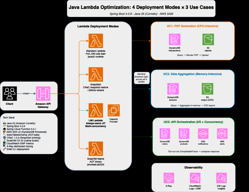
The benchmark runs all four deployment modes with identical Spring Boot 4.0.6 applications on Java 25 and AWS SDK v2. This configuration verifies fair comparison across modes. We tested three workloads: UC1 (PDF generation, CPU-bound), UC2 (data aggregation, I/O + computation), and UC3 (API orchestration, I/O-bound). The benchmark sends 240,000 requests using Artillery load testing at 33 RPS. Standard Lambda, SnapStart, and Native Lambda use 1024 MB (1 vCPU). Managed Instances uses c7i.xlarge instances with 2048 MB memory. Concurrency is tuned per workload (UC1=3, UC2=5, UC3=10) based on load testing to avoid thread contention. The benchmark measures p50, p99, and maximum latency across 10 runs of 2,000 requests each, with 5-minute cool-down between runs. The benchmark tracks JIT compilation metrics via Amazon CloudWatch Embedded Metrics Format. You can validate these results against Amazon API Gateway access logs, which confirm a <0.1% error rate. The GitHub repository contains complete source code, AWS Serverless Application Model (AWS SAM) templates, load scripts, and raw data. Performance claims in this post reference data from this benchmark methodology.
Figure 1 presents the architecture for all four deployment modes running in parallel against shared backend services.
To reproduce these benchmarks or deploy the sample applications, refer to the GitHub repository. The repository contains complete SAM templates, Artillery load configurations, deployment instructions, and cleanup commands. This post focuses on benchmark results and analysis. The benchmark used the following tools and services:
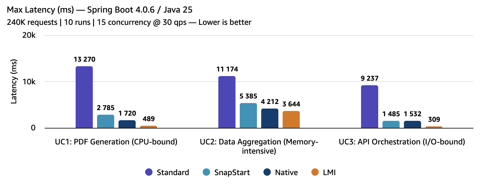
Managed Instances removes the extreme tail spikes characteristic of cold starts. Managed Instances delivers 27x faster maximum latency on CPU-bound workloads (UC1: 489 ms vs. 13,270 ms Standard). Mixed I/O + compute workloads see a 3x improvement (UC2: 3,644 ms vs. 11,174 ms Standard). I/O-bound workloads improve 30x (UC3: 309 ms vs. 9,237 ms Standard). We measured all results using the methodology described in Benchmarking setup.
The Standard Lambda 13-second maximum on UC1 represents a full cold start. That cold start includes JVM boot, Spring context initialization, Amazon DynamoDB client setup, and the first PDF render. SnapStart reduces this to under 3 seconds by restoring from a Firecracker microVM snapshot. However, the restore process plus re-initialization of resources that cannot be checkpointed (network connections, random number generators) still adds latency. GraalVM Native starts in under 2 seconds because the ahead-of-time (AOT) compiled binary skips JVM boot entirely. The Managed Instances maximum of 487 ms is not a cold start; it’s the slowest warm request across 20,000 invocations. For production SLAs, a 14-second cold start spike on Standard Lambda violates most requirements, while Managed Instances removes that spike entirely.
Observing median latency (p50)
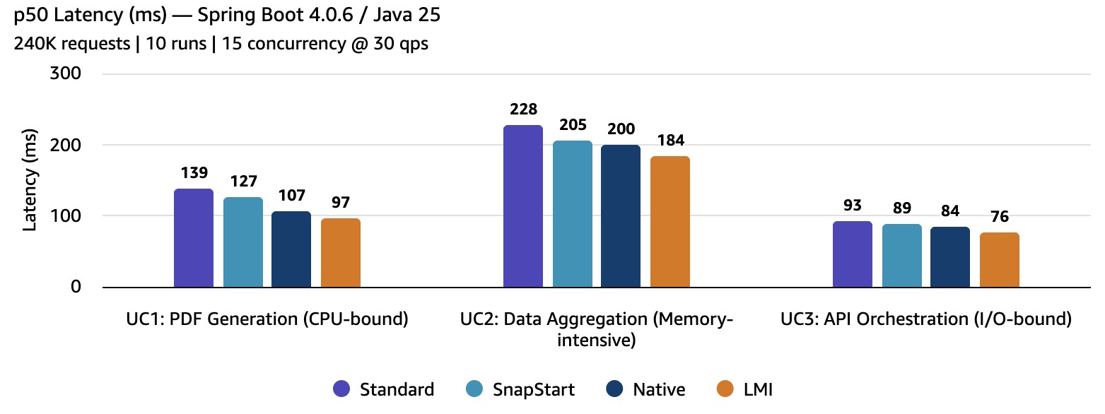
Lambda Managed Instances delivered the lowest median latency across all three workloads. Results demonstrate 30% faster median latency on CPU-bound workloads (UC1: 97 ms vs. 139 ms Standard). Mixed I/O + compute achieves a 19% improvement (UC2: 184 ms vs. 228 ms Standard). I/O-bound workloads improve 18% (UC3: 76 ms vs. 93 ms Standard).
The improvement scales with CPU intensity because the JIT C2 compiler on persistent Managed Instances optimizes hot code paths that short-lived serverless environments never reach. On CPU-bound workloads (UC1), the JIT compiler has more opportunity to optimize tight loops in PDF rendering. On I/O-bound workloads (UC3), network latency to Amazon DynamoDB, Amazon SQS, and Amazon SNS dominates the request duration, so JIT optimization provides smaller gains.
Observing tail latency (p99)
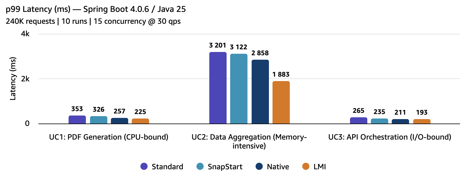
Managed Instances showed even larger improvements at the tail of the latency distribution. The p99 improves 36% on CPU-bound workloads (UC1: 225 ms vs. 353 ms Standard). Mixed I/O + compute achieves a 41% improvement (UC2: 1,883 ms vs. 3,201 ms Standard). I/O-bound workloads improve 27% (UC3: 193 ms vs. 265 ms Standard).
UC2 showed the largest p99 improvement (41%) because data aggregation combines DynamoDB queries, returning hundreds of records with in-memory statistical computation and Amazon S3 uploads. Standard Lambda environments that haven’t fully warmed their JIT produce significantly slower responses at the tail. The persistent JIT optimization (-Xms512m -Xmx1408m) with G1 garbage collection (GC) and explicit heap sizing on Managed Instances both contribute to tighter tail latency distribution. For services with SLAs on p99 response time, this reliability improvement matters more than median performance. For workloads with significant heap pressure, tuning -XX:MaxGCPauseMillis and monitoring GC logs can further tighten tail latency.
Why Lambda Managed Instances is faster: JIT compilation
The JVM’s Just-In-Time compiler works in tiers. The C1 compiler performs initial compilation quickly with basic optimizations. The C2 compiler profiles execution over hundreds of invocations and then applies aggressive optimizations: method inlining (eliminating function call overhead), escape analysis (allocating objects on the stack instead of the heap), loop unrolling (reducing branch overhead), and vectorization (processing multiple data elements in a single CPU instruction).
The following table presents JIT warmup progression using java.lang.management.
CompilationMXBean emitted through Amazon CloudWatch Embedded Metrics Format. We collected this data from a 1,500-request sustained load test on UC1 (PDF generation):
Phase
Invocation
Avg Latency
What’s Happening
First requests (application init)
1
~2,400ms
JVM boot, spring context creation, SDK client setup
Early requests (C1 compiled)
2-100
~145ms
C1 compiler active. App is functional, but not optimized
Steady state (C2 optimized)
1000+
~38ms
C2 optimizations completed
The first invocation includes one-time application start costs: class loading, Spring context initialization, and DynamoDB client construction. These costs are unrelated to JIT compilation and occur on any deployment mode.
Once C1 compilation stabilizes during early invocations, latency reaches approximately 145ms. This is the baseline compiled performance. Over the next several hundred invocations, the C2 compiler profiles hot code paths and applies optimizations. By invocation 1,000, latency drops to 38ms. This represents a 3.8x improvement from JIT optimization alone.
Standard Lambda environments typically recycle before C2 completes its optimization passes. On Managed Instances, concurrent requests share the same JVM. This accelerates JIT profiling: three concurrent requests generate three times the method invocation data for the C2 compiler to optimize. The C2 compiler profiles execution patterns across all concurrent requests. It identifies hot code paths faster and applies optimizations sooner than single-concurrency environments.
What this means: CPU-bound workloads see the largest gains (30% faster median latency on UC1) because the JIT compiler has more opportunity to optimize tight loops and method calls. I/O-bound workloads see smaller gains (18% faster on UC3) because network latency to DynamoDB, SQS, and SNS dominates request duration. The JIT compiler still optimizes your code, but the network time remains constant across all deployment modes.
Choosing the right mode
No single mode wins in every scenario. The right choice depends on your traffic pattern, cold-start tolerance, team expertise, and operational complexity budget.
Lambda Managed Instances is ideal for steady-state traffic patterns above 5 requests per second with low cold-start tolerance (p99 SLA under 500 ms). Best for workloads with predictable, sustained traffic that need low latency with zero cold starts. Managed Instances excels at CPU-bound workloads where JIT optimization compounds.
SnapStart works well for variable traffic patterns where cold-start reduction matters. Choose this as the default for Java Lambda functions. SnapStart reduces cold starts with minimal code changes (add CRaC priming). You have no additional infrastructure to manage. Works with the existing Lambda scaling model.
GraalVM Native Image works well for bursty traffic patterns with strict cold-start tolerance (sub-second cold starts required). Ideal if your team can invest in AOT compatibility (reflection configuration, build pipeline). This mode offers a smaller memory footprint. Requires testing for SDK compatibility.
Standard Lambda is the baseline for low-traffic or burst workloads where cold starts of 6-14 seconds are acceptable. Works well when invocation frequency is low enough that per-request billing is cheaper than fixed instance costs, or when operational simplicity is the top priority.
For example, if you run a Spring Boot API handling 100 requests per second with a 400 ms p99 SLA, Lambda Managed Instances reduces your p99 from 353 ms (cutting it close) to 225 ms (comfortable margin) and removes the multi-second cold start spikes that violate your SLA entirely.
Dimension
Standard
SnapStart
Native
Managed Instances
Cold start
6-14 s
2-7 s
800 ms – 2 s
None
Warm p50 (CPU-bound)
139 ms
127 ms
107 ms
97 ms
Tail latency
Worst
Better
Good
Fastest
Error rate
Low
Low
Higher (SDK compat)
Low
Operational complexity
Lowest
Low
High (build pipeline)
Medium (VPC, sizing)
Burst scaling
Fastest
Fastest
Fastest
Slower (capacity provider)
Migration effort
None
Low (add CRaC priming)
High (AOT compat, reflection configuration)
Medium (capacity provider, VPC, thread safety)
Memory efficiency
Good
Good
Lowest
(125-154 MB)
Fixed per instance
Lambda Managed Instances supports Graviton4 (arm64) instances, which offer approximately 20% better price-performance based on AWS published Graviton4 benchmarks. These benchmarks use x86_64 for consistency across all four modes (GraalVM native cross-compilation to arm64 adds complexity). The arm64 parallelization characteristics could shift the performance curves for longer-lived deployment modes like Managed Instances in ways worth exploring in a future post.
Cost considerations
Lambda Managed Instances uses instance-based pricing rather than per-invocation billing. For steady-state workloads above approximately 9 requests per second, the fixed instance cost is lower than equivalent Standard Lambda GB-second charges. You can use the official pricing calculator to compare Managed Instances and standard Lambda costs.
Try it with your runtime version
These benchmarks use Java 25 with Spring Boot 4.0.6. The GitHub repository also includes configurations for Java 21 with Spring Boot 3.x. The repository README walks you through deployment, load testing, and collecting your own metrics.
Conclusion
This post demonstrates how Lambda Managed Instances solves a fundamental Java-on-serverless mismatch. The JVM’s JIT compiler needs time to optimize hot code paths. Standard Lambda recycles environments before the JVM reaches peak optimization. Managed Instances keeps the JVM alive across invocations, allowing the C2 compiler to reach peak optimization. The benchmarks show the impact. In these benchmarks, Managed Instances delivered 18 to 30% faster p50 latency than Standard Lambda. Tail latency improved 27 to 41% at p99. Maximum response times dropped 3 to 30x on CPU-bound workloads. The 3.8x improvement from JIT optimization alone shows what’s possible when the runtime has time to complete its work.
For more information, refer to the Lambda Managed Instances documentation. The GitHub repository contains the complete benchmark code, SAM templates, and deployment instructions. Share your results in the comments and let the community know how Managed Instances performs on your workloads. To delete all benchmark resources and avoid ongoing charges, run the cleanup commands documented in the GitHub repository README.
ASRock Rack has developed an unlikely edge server based on NVIDIA’s industrial SoC, Thor. The Blackwell-era chip is being used to power the 2UXGI-THOR, a server aimed at the industrial and medical markets
On July 13, 2006, we launchedAmazon Simple Queue Service (Amazon SQS) as one of the first three services available to customers, alongside Amazon EC2 and Amazon S3. We had learned firsthand that distributed systems need a reliable way to pass messages between components without creating tight dependencies. If one service called another directly and that service was slow or unavailable, failures cascaded through the entire system. Message queuing solved this by letting services communicate asynchronously: a producer could drop a message into a queue and move on, while a consumer picked it up when ready. This approach kept individual service failures from affecting the rest of the system.
When Amazon SQS launched publicly in July 2006, it made this pattern available to every AWS customer. Twenty years later, that core function, decoupling producers from consumers, remains the reason customers use SQS. The scale, performance, and operational controls around it look very different now though.
Jeff Barr covered the first 15 years of SQS milestones in his 15th anniversary post, from the original 8 KB message limit in 2006 through FIFO queues, server-side encryption, and Lambda integration. Over the last five years, we have continued to scale SQS, added stronger security defaults, and introduced new capabilities that address increasingly complex workload patterns.
Key milestones between 2021 and 2026 High throughput mode for FIFO queues (2021): In May 2021, we launched general availability of high throughput mode for FIFO queues, supporting up to 3,000 transactions per second (TPS) per API action, a tenfold increase over the previous limit. We continued raising this ceiling over the following two years: to 6,000 TPS in October 2022, to 9,000 TPS in August 2023, and to 18,000 TPS in October 2023, before reaching 70,000 TPS per API action in select Regions by November 2023.
Server-side encryption with SSE-SQS (2021): In November 2021, we introduced server-side encryption with Amazon SQS-managed encryption keys (SSE-SQS), giving customers an encryption option that required no key management. In October 2022, we made SSE-SQS the default for all newly created queues, so customers no longer needed to explicitly enable it.
Dead-letter queue redrive enhancements (2021): We progressively expanded how customers recover unconsumed messages from dead-letter queues. In December 2021, we added DLQ redrive to source queue directly in the SQS console. In June 2023, we extended this capability to the AWS SDK and CLI through new APIs, including StartMessageMoveTask, CancelMessageMoveTask, and ListMessageMoveTasks. In November 2023, we added redrive support for FIFO queues.
Attribute-based access control, ABAC (2022): In November 2022, we introduced ABAC, giving customers the ability to configure access permissions based on queue tags rather than maintaining static policies as resources scaled.
JSON protocol support (2023): In November 2023, we added support for the JSON protocol in the AWS SDK, reducing end-to-end message processing latency by up to 23% for a 5 KB payload and lowering client-side CPU and memory usage.
Amazon EventBridge Pipes console integration (2023): We added the ability to connect a queue directly to EventBridge Pipes from the SQS console, routing messages to a broad range of AWS service targets without writing custom integration code.
Extended Client Library for Python (2024): We brought the Extended Client Library, previously available for Java, to Python developers, allowing messages up to 2 GB to be sent through SQS by storing the payload in Amazon S3 and passing a reference through the queue.
FIFO in-flight message limit increase (2024): We increased the in-flight message limit for FIFO queues from 20,000 to 120,000 messages, so consumers can process significantly more messages concurrently without being constrained by the previous ceiling.
Fair queues for multi-tenant workloads (2025): We introduced fair queues to mitigate the noisy neighbor problem in multi-tenant standard queues. By including a message group ID when sending messages, customers can prevent a single tenant from delaying message delivery for others, without any changes required on the consumer side.
1 MiB maximum message payload size (2025): We increased the maximum message payload from 256 KiB to 1 MiB for both standard and FIFO queues, helping customers send larger messages without offloading data to external storage. AWS Lambda event source mapping for SQS was updated in parallel to support the new payload size.
The constant underneath the change Despite two decades of feature additions, the fundamental use case for SQS has not shifted. Customers use it to decouple services, buffer bursts of traffic, and build systems that stay resilient when individual components fail. That same pattern now extends to AI workloads. Customers use SQS queues to buffer requests to large language models, manage inference throughput, and coordinate communication between autonomous AI agents operating as independent services. For an example of this architecture in practice, read Creating asynchronous AI agents with Amazon Bedrock.
Enterprise data architectures have become fundamentally distributed. Over the past decade, organizations have made deliberate investments across multiple platforms such as relational databases for transactional workloads, cloud data warehouses for analytics, object stores for unstructured data, and SaaS applications for domain-specific functions. Each was chosen to solve a specific problem, serve a specific team, or meet a specific performance requirement. The result is not accidental sprawl. It is a deeply heterogeneous data landscape shaped by intentional, workload-driven decisions. The challenge now is not consolidation, but interoperability: enabling these systems to function as a unified foundation for the next generation of AI-driven applications.
Agentic AI systems that autonomously reason, plan, and take action on behalf of users are moving rapidly from experimentation to enterprise production. These systems do not just retrieve information. They synthesize it, act on it, and learn from it. And unlike traditional analytics tools that can work with a well-scoped dataset, AI agents require something more demanding: unified, governed, and real-time access to all relevant enterprise data, regardless of where it lives.
This is the gap that matters most right now. Enterprises that have invested in building strong data capabilities across multiple providers are well-positioned, but only if those platforms can be accessed together, consistently, and with the governance controls that enterprise AI requires. Without a unified data foundation, AI agents operate with incomplete context, governance becomes inconsistent, and the promise of autonomous AI remains out of reach.
Solution approach
The following high-level architecture explains how you can onboard metadata catalogs and MCP servers to your context layer, which becomes the primary input for your AI agents.
Assuming your data products have a well-defined metadata catalog, you can take a unified-catalog-first approach, then build the context layer on top of it to let your AI agents discover all the context from one place. This helps bring in centralized governance and audit control, because every request gets routed through the centralized metadata catalog and context layer to simplify implementation of unified governance. In addition, this brings simplicity to enable business semantics, define attribute priorities, and define authoritative sources for the consumer use cases.
If any of the data sources does not have a well-defined metadata catalog, you can define Model Context Protocol (MCP) servers on them, and then directly onboard them to the context layer. For example, if you have semi-structured or unstructured datasets for which you do not have a well-defined metadata catalog, or you want to onboard third-party data sources through REST APIs, then you can add their respective MCP server to the context layer directly. The following architecture explains the extended flow for it.
In this series of posts, we demonstrate how you can unify the metadata catalog access across multiple providers, how you can enable AI agents to query the unified catalog, and how the context layer can be integrated to unify metadata from catalogs and MCP servers. We have divided the series into the following parts.
Part 1: Architecture approach with tradeoffs to unify a multi-cloud lakehouse architecture that can power Agentic AI (this post).
Part 2: Implementing an example solution to unify catalogs from multiple providers and deploy AI agents to query the unified data access layer.
Part 3: Integrate a context layer on top of the unified catalog for AI agents.
Part 4: Onboard additional data sources to the context layer through MCP servers and demonstrate the full solution.
This post focuses on explaining the architecture approach to build the open lakehouse architecture on AWS, unifying the metadata catalog across providers for the AI agents to access. In addition, it highlights the architecture trade-offs and best practices.
Use case
Every AI initiative launched on a fragmented data foundation is an initiative that will need to be rebuilt. Organizations that establish unified data access today are the ones that will scale Agentic AI with confidence tomorrow. Consider a large enterprise managing petabytes of data across a diverse set of environments:
On-premises: Network device telemetry, customer records, and operational databases.
Multiple cloud platforms: Marketing analytics, HR systems, and enterprise applications distributed across cloud providers.
Data platforms: Data science workloads, feature engineering pipelines, and finance and supply chain analytics running on specialized platforms.
SaaS applications: Salesforce, SAP, Zendesk, ITSM, and other business tools that each hold a critical piece of the enterprise data picture.
The business objective is to build a unified analytics and AI platform that can:
Query and analyze data across all environments without requiring full data migration.
Enforce consistent data governance and access control regardless of data location.
Power AI agents that can autonomously discover, query, and act on enterprise data.
Reduce total cost of ownership by eliminating redundant pipelines and storage.
This architecture directly addresses these needs by combining flexible data integration patterns, an open-table-format-based lakehouse architecture (with an example of Apache Iceberg), AI agent deployment to access unified metadata, and centralized governance.
Reference architecture
Before going deeper into a specific architecture, let’s revisit at a high level how the AWS open lakehouse architecture enables data ingestion and query or catalog federation to power analytics, machine learning development, and generative AI application development.
The following architecture diagram represents an end-to-end flow that includes:
Data ingestion to the data lake or data warehouse through Zero-ETL and batch or stream processing using AWS native services, or accessing data from Google Cloud Platform using AWS Interconnect – multicloud.
A centralized metadata catalog layer that includes data on AWS and metadata representation of non-AWS data sources using query or catalog federation.
A context layer that you can integrate to create a knowledge graph with ontology and business semantics that can enrich context for AI agents.
The consumption layer, which can include analytics, machine learning model development with Amazon SageMaker AI, and generative AI application development with Amazon Bedrock AgentCore, Amazon Quick, or other AWS and non-AWS AI applications.
Let’s look at an expanded version of this architecture that details the data ingestion and data consumption patterns to build a unified data access layer on AWS that spans multiple cloud and ISV providers.
Expanded technical architecture walkthrough
The following architecture demonstrates the comprehensive AWS approach for metadata catalog consolidation through flexible integration patterns, and it also highlights patterns for building a lakehouse on AWS. Built on the open standards of Apache Iceberg for storage and governance through AWS Lake Formation, it creates a unified data foundation that connects existing investments without requiring wholesale migration, and it makes enterprise data AI-ready from day one. This architecture delivers value at every layer: business teams query across platforms without data movement, IT teams manage governance through a single federated layer with the flexibility to federate or ingest per use case, and compliance teams enforce policies once across all sources with full lineage and audit coverage.
The following are the key components of the architecture.
Data access methods
This section provides options to access data that is not available in AWS Glue Data Catalog and not available on AWS.
AWS Glue Data Catalog implements the Iceberg REST Catalog API specification, which enables seamless federation with Databricks, Snowflake, or other Iceberg-compatible catalogs set up with Amazon Simple Storage Service (Amazon S3) as the storage layer.
With the growing adoption of Apache Iceberg, catalog federation will become a common standard in the future and simplify metadata unification.
2. Query federation (Reference point 1.1)
Direct cross-cloud querying over the public internet to Google BigQuery, Azure SQL, Salesforce, and other platforms.
Real-time access to external data sources without replication, and seamless access with AWS analytics services.
Provides flexibility, because the catalog federation capability of the Iceberg REST catalog is limited to Iceberg tables only.
2.1. Secured private connectivity to Google Cloud Platform using AWS Interconnect for multi-cloud (Reference points 3.1, 3.2)
The default query federation approach makes the connection and transfers data over the public internet, which has its own latency implications depending on the target platform and the data volume transferred over the internet. During re:Invent 2025, AWS announced the public preview of AWS Interconnect – multicloud, which recently became generally available.
AWS Interconnect – multicloud is a managed service that provides private, high-speed, and secure network connections between Amazon Web Services (AWS) and other cloud providers, starting with Google Cloud Platform (GCP), with Microsoft Azure and Oracle Cloud Infrastructure (OCI) coming later in 2026. You can enable the integration with three steps: 1) specify the target cloud service provider, 2) select the destination Region on the other side, and 3) pick the required bandwidth.
The following architecture represents AWS and GCP integration with AWS Interconnect – multicloud.
On the AWS side, you need an AWS Direct Connect gateway (a global construct that acts as a route reflector), which you can attach to your Amazon Virtual Private Cloud (Amazon VPC) through a virtual private gateway or AWS Transit Gateway, or AWS Cloud WAN. On the GCP side, you need a Google Cloud Router that you attach to your customer VPC. Interconnect – multicloud offers pre-cabled capacity pools at shared Interconnect points of presence (PoPs) in selected Regions, where both AWS and GCP routers are co-located and pre-wired.
Because Interconnect – multicloud primarily routes traffic within the VPC through a private network, to benefit from it you need to keep your query engine or jobs within a customer VPC.
2.2. High network bandwidth with on-premises systems (Reference point 4)
AWS Direct Connect for high-bandwidth, low-latency on-premises connectivity.
Data ingestion methods
This section focuses on ways you can use to onboard datasets (complete or subset) to a lakehouse on AWS.
1. Zero-ETL: Data movement to AWS with Zero-ETL ingestion (Reference points 5.1, 5.2)
AWS Zero-ETL capabilities for seamless data loading from AWS and non-AWS sources.
2. Extract, transform, load (ETL): Extract data from JDBC or SaaS sources and transform through a batch or stream pipeline (Reference points 3.1, 3.2)
Option to design batch and stream ingestion pipelines using AWS managed services with open source data processing engines such as Apache Spark and Apache Flink.
Hundreds of connectors available as part of AWS Glue to extract data from JDBC and SaaS sources, and the flexibility to design custom connectors that can run on serverless Glue clusters.
The following architecture expands the flow 1.1 to 1.2 ingestion method that integrates AWS services to onboard data to the Amazon S3 raw layer and then takes it through an ETL pipeline for data cleansing and transformations. It also includes steps to onboard unstructured data to Amazon S3 using Amazon Bedrock Data Automation, and taking the lakehouse data for machine learning development with Amazon SageMaker AI.
You can also use AWS Interconnect – multicloud to run Spark jobs (Spark with Amazon EMR on EKS or open source Spark on any compute within a customer VPC) to ingest and transform data from Google Cloud with private connectivity.
3. Accessing data from Google Cloud over a private network
Refer to the preceding data access methods (3.1 and 3.2).
4. Onboarding data from AWS Outposts (S3 on Outposts) (Reference points 9.1 to 9.5)
Option to onboard S3 on AWS Outposts data to regional Amazon S3 through AWS DataSync (reference 9.1 to 9.3), which might be a better fit to sync files as-is through a scheduled batch or an event-driven approach.
Flexibility to transform the S3 on Outposts data using an Amazon EMR clusters on Outposts job, and then directly write the transformed output to a regional Amazon S3 bucket in the formats you want (including open table formats such as Apache Hudi, Apache Iceberg, and Delta Lake).
Lakehouse foundation with Apache Iceberg
By standardizing on Apache Iceberg, you’re not choosing AWS over your other platforms. You’re choosing interoperability and future flexibility. Your data becomes truly portable across any Iceberg-compatible engine.
Open table format: Industry-standard format supported across AWS, Databricks, Snowflake, and other platforms, which eliminates vendor lock-in.
ACID transactions: Reliability with full transactional consistency.
Time travel and schema evolution: Built-in versioning and flexible schema management.
Performance optimization: Advanced features such as hidden partitioning, partition evolution, and metadata management.
Note that lakehouse storage is not limited to the Apache Iceberg format, and you have the flexibility to include other open table formats (for example, Apache Hudi and Delta Lake) or file formats (for example, Apache Parquet and Apache Avro).
Unified governance and access control
AWS governance capabilities transform the lakehouse from a storage layer into a fully governed data platform. This delivers security, compliance, and data quality out of the box, applied consistently across all data sources including federated catalogs. A unified catalog consolidates metadata from AWS and non-AWS sources with generative AI-powered business glossary generation, while automated ML-powered classification identifies sensitive data (for example, PII, PHI, and financial data) across structured and unstructured datasets. AWS Identity and Access Management (AWS IAM) and AWS Lake Formation enforce fine-grained access control at the row, column, cell, and tag level, applied consistently across Amazon Athena, Amazon Redshift Spectrum, Amazon EMR, and federated sources. End-to-end data lineage tracking provides visual data flow graphs, impact analysis, and compliance audit trails. When AI agents explore metadata from the unified catalog and submit a query to Amazon Athena for execution, the Lake Formation fine-grained access control filters data based on the user interacting with the AI agent.
For the foundation model integrated into your AI agents, you can use Amazon Bedrock Guardrails, which implements customized safeguards to block harmful content and minimize hallucinations. Amazon Bedrock AgentCore provides fine-grained policy control over agent actions with real-time enforcement and managed authentication for agents accessing AWS and third-party services.
A comprehensive audit and compliance stack spans Amazon CloudWatch, AWS CloudTrail, AWS IAM, AWS Key Management Service (AWS KMS), AWS Audit Manager, and AWS PrivateLink. This stack makes sure every agent invocation is traceable, every key is managed, and every configuration is automatically mapped to frameworks including ISO, SOC, GDPR, and HIPAA.
When an end user interacts with the AI chat assistant, the layers of security and governance should go through the following.
Layer 1: Who can access?
Enable Active Directory and single sign-on integration for user authentication, and a combination of AWS IAM roles for AWS API-level authorization.
Layer 2: What can they see?
Integrate an agent profile to define what datasets each agent can access, because not all agents should have access to all datasets.
Enable fine-grained access control on the metadata layer using AWS Lake Formation that can filter rows and columns.
Enable data masking as applicable while the query responses are served through the query engine.
Layer 3: What can the agent do?
Control agent actions by restricting them to read-only, and apply restrictions to INSERT, UPDATE, and DELETE if the agents are supposed to query only.
Apply a limit on the number of rows that can be returned from the query, and apply a query scan limit to reduce cost.
Layer 4: What does the agent reveal?
Enable output filtering to make sure no PII is included.
Apply Amazon Bedrock Guardrails on large language model (LLM) responses to make sure the model does not produce anything inappropriate.
In addition, enable audit logging of all queries to make sure future audit and compliance needs can be met.
AWS offers a complete analytics ecosystem that includes the following.
Amazon Athena: Serverless SQL queries with Iceberg v2 support, including provisioned capacity for consistent performance and workgroups for resource and cost management.
Amazon Redshift Spectrum: Federated queries across the data warehouse and Iceberg data lake.
Amazon Quick Sight: Enterprise visualization with governed access to all data.
AWS Glue and Amazon EMR: Distributed data processing capability for enterprise transformations.
AI-ready architecture (Reference points 8.1 to 8.4)
A consolidated lakehouse architecture helps you make data ready for AI agents that can access the data through readily available MCP servers or through the AWS SDK for Python (Boto3) for Amazon Athena or Amazon Redshift Spectrum. AI agents can integrate the AWS MCP Server to interact with AWS analytics services such as AWS Glue, Amazon Athena, and Amazon S3 Tables, a capability of Amazon S3, to query both data and metadata.
AI agents need context to understand how the catalog tables and their attributes are linked to each other, how users have queried them in the past, or what priorities are defined to understand which one is an authoritative source for a particular natural language question. To enable the AI agent with additional context, we can integrate the AWS Context service that was pre-announced recently at the AWS New York Summit 2026.
Governance integration: AI agents automatically inherit Lake Formation permissions, because the agent can submit the SQL query to be run through Amazon Athena or Amazon Redshift Spectrum. This makes sure they only access data that users are authorized to see. Amazon SageMaker Unified Studio data lineage tracks AI agent queries for full auditability.
The following diagram represents how the AI agent request flow looks.
This architecture delivers value across every layer of the organization. Business teams gain faster time-to-insight by querying data across all platforms without waiting for data movement, while eliminating duplicate storage and reducing transfer costs through federation. The Apache Iceberg open table format ensures data portability and freedom from vendor lock-in. For IT and data teams, a single governance layer across all sources, including federated catalogs, reduces operational complexity, while the flexibility to choose between federation and ingestion for each use case, combined with the elastic AWS infrastructure and the petabyte-scale metadata architecture of Iceberg, delivers both agility and scalability. Data governance and compliance teams benefit from a single point of policy enforcement across all data regardless of location, complete lineage and access logs for audit and compliance reporting, automated sensitive data classification, and policies that are defined once and enforced everywhere, including across federated sources.
Architecture tradeoffs and best practices
The following are a few key trade-offs you need to consider while designing the solution.
Data ingestion and access methods
Use catalog federation (Iceberg REST) when:
The source platform supports the Iceberg REST API (Databricks, Snowflake Polaris).
Data is already in Iceberg format with Amazon S3 backed storage.
You want bidirectional discovery (AWS tables visible in Databricks or Snowflake too).
Use query federation (Amazon SageMaker Lakehouse architecture or AWS Glue connectors) when:
The source is BigQuery, SQL Server, or another non-Iceberg platform.
Data must stay in the source cloud (sovereignty, contractual, or latency reasons).
Real-time access is required without replication lag.
Use ingestion (Zero-ETL, AWS Glue, or Amazon EMR) when:
Data is accessed frequently with a low-latency requirement by AI agents or high-concurrency analytics.
The business decides to build a data lake and warehouse on AWS.
You need full governance, time travel, and performance optimization.
Use AWS Interconnect – multicloud when:
You need real-time or near-real-time query federation to GCP data sources (BigQuery, AlloyDB, Cloud Spanner) and latency or security requirements prohibit public internet routing.
You have high-volume, recurring data transfers between AWS and GCP where public internet egress costs or bandwidth variability are unacceptable.
Your organization has compliance or regulatory requirements mandating that data never traverse the public internet (HIPAA, PCI-DSS, or financial services regulations).
You need bidirectional connectivity, such as GCP workloads calling AWS APIs, or AWS workloads calling GCP APIs, both over private paths.
Choosing between federation and ingestion based on use case
Dimension
Federation (Query in Place)
Ingestion (Move to AWS)
Data freshness
Real-time or near-real-time
Dependent on ingestion frequency
Query performance
Subject to source system latency and network
Subject to data volume and operation, avoids cross-cloud network latency
Cost
Lower storage cost. Higher per-query cost for cross-cloud egress
Integrating Amazon Bedrock AgentCore Gateway and Amazon Bedrock AgentCore Runtime based on use case
The following are key differences between AgentCore Gateway and AgentCore Runtime that are relevant for our use case.
Dimension
Amazon Bedrock AgentCore Gateway
Amazon Bedrock AgentCore Runtime
Timeout
5 minutes (hard limit)
15 min sync / 8 hours async
Statefulness
Stateless (per-request)
Stateful (session-based)
Best for
Lightweight API proxying
Long-running data processing
Your lakehouse queries
Will time out frequently
Handles multi-hour jobs
Because AgentCore Gateway has a 5-minute hard timeout limit, use AgentCore Runtime for data processing jobs.
AWS Glue ETL jobs can run for minutes to hours.
Amazon Redshift queries on large datasets routinely exceed 5 minutes.
Athena federated queries (especially cross-cloud through Interconnect) can be slow.
Iceberg table scans on multi-TB datasets take time.
You can use AgentCore Gateway if the scope is limited to Glue Data Catalog interactions to fetch metadata schema, because that won’t run for more than 5 minutes.
Design considerations for production implementation
In practice, there are multiple aspects to consider when deploying the solution for production. The following summarizes a few of the key issues you might encounter and approaches to address them.
Catalog federation: The metadata drift problem
One of the first surprises in production is metadata drift, the state where your federated catalog no longer reflects the actual schema of the source system, because the source system’s metadata changes are not reflected in the unified catalog. The agent continues to generate SQL against the stale schema, producing silent failures that are hard to trace.
The following are a few ways you can address the metadata drift issue.
Implement a catalog refresh schedule. Even a daily Glue crawler run against federated sources catches most drift before it causes agent failures.
Add schema validation as a pre-query step in your agent tool. Before running SQL, verify that the referenced columns exist in the current catalog metadata.
Instead of pulling metadata changes from the source in a scheduled manner, you can design an event-driven system, where the source system triggers a push event to run the schema change in the federated catalog.
Query federation: Latency is non-deterministic
Query federation works well for moderate data volumes, but latency becomes non-deterministic at scale. A query that returns in 3 seconds during testing can take more than 10 seconds in production when the source system is under load, the network path is congested, or the federated connector is cold-starting.
The following are a few approaches you can consider to improve the performance.
Set explicit query timeouts in your Athena execution context. Without them, a slow federated query will block your agent indefinitely.
Implement query result caching for frequently asked questions. Most business users ask the same questions repeatedly, and caching at the agent layer improves perceived performance.
For time-sensitive use cases, consider caching aggregated data in an AWS lakehouse on a schedule rather than querying live. This trades freshness for reliability.
AgentCore memory: Statefulness cost
AgentCore Memory enables stateful conversations, but in production, unbounded memory accumulation creates its own problems. An agent that remembers every conversation eventually starts surfacing stale context. For example, a user who asked about Q3 revenue six months ago gets that context injected into a Q1 query today.
The following are a few ways you can optimize cost and improve relevance.
Set explicit memory expiry (we use 30 days as shown in the implementation) and enforce it consistently.
Use session-scoped memory for transactional queries and long-term memory only for user preferences and recurring patterns.
Implement a memory review step in your LangGraph workflow. Before invoking the model, filter retrieved memories by recency and relevance score rather than injecting all of them.
LangGraph orchestration: When tool calls loop
The conditional routing of LangGraph is powerful, but in production we observed a failure mode where the agent enters a tool call loop. The model repeatedly calls the same tool with slightly different parameters, never reaching a satisfactory answer. This typically happens when the tool returns partial or ambiguous results and the model keeps trying to refine.
What we learned:
Add a maximum tool call counter in your LangGraph state. If the agent has called tools more than N times in a single session, force a graceful exit with a summary of what was found.
Return structured, unambiguous responses from your tools. Include row counts, column names, and explicit null indicators so the model can reason clearly about completeness.
Log every tool invocation with its input and output. This is the single most valuable debugging artifact when diagnosing agent misbehavior in production.
Handling hallucination risks in federated agent architectures
This is the most important section for teams moving from prototype to production. Hallucination in agentic AI systems that query real data is qualitatively different from hallucination in general-purpose LLMs, and it is more dangerous because the outputs look authoritative.
There are three distinct hallucination risk zones in a lakehouse AI agent:
SQL generation: The model generates SQL that is syntactically valid but semantically wrong. For example, when asked “What is our revenue growth this quarter?”, the model might generate a query that compares the wrong date ranges, uses the wrong aggregation function, or joins tables on incorrect keys, and then returns a confident, formatted answer with the wrong numbers.
Cross-source synthesis: When the agent queries multiple federated sources and synthesizes results, the risk compounds. The model may correctly retrieve customer counts from Amazon S3 and revenue figures from Snowflake, but incorrectly draw conclusions that aren’t supported by either dataset individually.
Memory-augmented reasoning: When long-term memory is active, the model may blend historical context with current query results in ways that are factually incorrect. For example, it might apply a business rule that was true six months ago but has since changed.
To improve, before any agent output informs a business decision, apply the following three-step validation framework:
Step 1: Source verification. Can you trace the answer back to a specific table, column, and row count? If the agent can’t show you the SQL and the row count, the answer is unverified.
Step 2: Reasonableness check. Does the answer fall within expected ranges? A sudden 10x spike in customer count is a signal to investigate.
Step 3: Cross-validation. For critical decisions, run the equivalent query directly in Athena or your BI tool and compare. Discrepancies reveal either a model reasoning error or a data quality issue. Resolve both before the answer is trusted.
These lessons don’t diminish the value of the architecture. They make it production-ready. The teams that move fastest with agentic AI are not the ones who skip these guardrails. They’re the ones who build them in from the start and spend less time firefighting in production.
Alternative to the unified catalog approach
In case you face technical and process challenges to unify catalogs across providers, you can let each data producer expose the metadata and data through MCP servers, as represented in the following diagram. In this approach, each producer takes the responsibility of maintaining the MCP servers and exposing them to the context layer. While this approach provides autonomy to data owners to operate independently and with flexibility, it also creates operational overhead to synchronize all metadata in a consistent way.
What’s next
In Part 2 of this series, we walk through the full implementation step by step, including hands-on scripts to:
Load example sales datasets into Databricks and marketing data to Snowflake as Iceberg tables, and federate them into AWS Glue Data Catalog through the Iceberg REST API.
Register Google BigQuery as a native federated data source in Amazon SageMaker, instead of a traditional AWS Lambda connector integration.
Create a customer master table as a native Iceberg table in Amazon S3.
Run a single SQL query in Amazon Athena that joins all four sources across two federation patterns, with no data movement.
Deploy an AI agent on Amazon Bedrock AgentCore that can autonomously query the same unified catalog using Amazon Athena and answer complex business questions in natural language queries. In addition, integrate AgentCore Memory to persist user context.
Conclusion
In this post, we summarized how you can unify data access across multiple cloud and ISV providers on AWS with the combination of catalog federation, query federation, and data movement to AWS. We then explained how AWS Glue Data Catalog and Lake Formation help provide unified catalog and access governance, and how AI agents hosted in Amazon Bedrock AgentCore can access it using MCP servers to explore the metadata context, convert user natural language queries to SQL, and use Amazon Athena to run the query across data sources to get the response to the end user. In addition, we provided an overview of different data ingestion methods to build a lakehouse architecture on AWS, including AWS Interconnect – multicloud and where it adds value.
We also provided architecture trade-offs and best practices to integrate the service capabilities. In the next post (Part 2), we will take a specific use case and provide a step-by-step implementation guide to unify the catalog and deploy the agent to Amazon Bedrock AgentCore.
When you process over 500 million transactions per month, every second of undetected anomaly means failed payments, lost revenue, and eroded merchant trust. Static monitoring thresholds that worked for thousands of merchants collapse at the scale of millions, and the cost of missed detection compounds exponentially.
In this post, we explore Razorpay’s anomaly detection and alerting platform (ADA) architecture using Amazon Managed Streaming for Apache Kafka (Amazon MSK) and other AWS services. According to Razorpay the system detects transaction anomalies in under 30 seconds, supports thousands of merchant-level alerts, and reduced monitoring costs by approximately 80 percent. The platform maintains 99.99 percent uptime for over 500 million transactions per month.
Founded in 2014, Razorpay has become one of India’s largest full-stack financial solutions companies, powering payments, banking, and business growth for over 10 million businesses. With offerings spanning payment gateway, RazorpayX for business banking, and Razorpay Capital for lending, the company processes over 500 million transactions per month across payments, payroll, banking, and cross-border services.
At this scale, Razorpay’s data platform processes more than 5 billion events daily. Every transaction, settlement, and disbursement generates events that must be monitored in real time for anomalies. These range from systemic degradations and latency regressions to card-testing fraud attacks and velocity abuse at the merchant level.
For a regulated payments platform, undetected anomalies carry consequences far beyond technical metrics. A missed fraud pattern can mean direct financial losses running into millions of rupees. It can also bring regulatory scrutiny from the Reserve Bank of India and irreversible damage to merchant confidence, the foundation of Razorpay’s business. Razorpay needed real-time anomaly detection, but the existing infrastructure couldn’t keep pace with the company’s growth.
The problem: When static thresholds can’t keep up with scale
As Razorpay scaled from thousands to millions of merchants, the existing monitoring infrastructure hit critical limitations across four dimensions.
Anomaly blind spots
Systemic degradations, latency regressions, and success-rate drops went undetected until customers complained. By the time a human operator noticed a 15 percent drop in payment success rates for a specific gateway-merchant combination, thousands of transactions had already failed.
Fraud at velocity
Card-testing activity, velocity abuse, and geo-anomalies at the merchant level required sub-minute detection. Unauthorized users could generate hundreds of micro-transactions in seconds. Traditional batch detection was too slow to prevent damage.
Static thresholds don’t scale
The existing tooling relied on static thresholds with no adaptive baselines. This created a painful dilemma: set thresholds too tight and drown in false alarms (alert fatigue), or set them too loose and miss real incidents.
High cardinality equals high cost
Monitoring thousands of merchants individually on the previous architecture cost approximately $500K per year: $250K in licensing fees plus $250K in infrastructure, with fundamental scalability limits. ThirdEye queried a 21-day lookback at query time, enforcing a 1–2 minute service level agreement (SLA) minimum. The system was not designed for thousands of concurrent merchant-level alerts, a limitation confirmed by the vendor.
Solution overview: ADA: Anomaly detection and alerting
Razorpay built ADA (Anomaly Detection and Alerting), a configurable, multi-tenant engine for real-time anomaly detection and fraud prevention. The platform’s design centers on three core principles that address the limitations of the previous architecture.
First, ADA is declarative: users express what to detect, not how. A single domain-specific language (AdaDSL) drives both batch and streaming execution, eliminating the need for engineers to write custom detection code for each new alert. Second, ADA is adaptive. Dynamic baselines incorporate calendar-aware patterns (day-of-week, time-of-day, holiday adjustments) and machine learning (ML)-compatible thresholds that replace brittle static rules. Third, ADA is inherently multi-tenant: Payments, Payroll, and Banking each operate with isolated detection logic while sharing underlying infrastructure. This design removes the need to maintain separate monitoring stacks per business unit.
Amazon MSK serves as the event backbone of ADA, ingesting transaction events, distributing detection rules, and connecting the components of the real-time pipeline.
Architecture: Amazon MSK as the streaming backbone
The ADA architecture positions Amazon MSK as the core integration layer connecting event producers to detection engines and alert consumers. Payment authorization, settlement, and disbursement events flow through Kafka topics managed by Amazon MSK. With Razorpay processing over 500 million transactions per month and 5 billion events daily, the ingestion layer must absorb high throughput with zero data loss.
High-throughput event ingestion
The architecture uses tenant-partitioned topics. Each business unit (Payments, Payroll, Banking) publishes to logically isolated topics while sharing physical infrastructure. This design supports independent consumer groups per tenant with predictable throughput guarantees.
Change Data Capture (CDC) events from Razorpay’s core transactional databases (Amazon Aurora MySQL-Compatible Edition) flow through Debezium and a Kafka Streams-based Harvester service into Amazon MSK. Application events from payment services also publish directly to Amazon MSK topics via native Kafka producers.
Why Amazon MSK as the backbone
Amazon MSK serves as the architectural backbone of ADA, fulfilling four critical functions that together support reliable, real-time anomaly detection at scale. At the ingestion layer, Amazon MSK absorbs the full stream of transaction events with three-replica durability. If downstream consumers experience an outage, they resume from their last committed offset without data loss. Beyond ingestion, Amazon MSK is the event distribution backbone of detection rules. AdaDSL definitions authored by domain experts are serialized and published to a dedicated Kafka snapshot topic, which Flink jobs consume as a broadcast stream.
This delivers hot-reloadable rule updates without pipeline restarts, a critical capability when detection logic must evolve daily. Amazon MSK further supports tenant isolation at the topic level. Payments, Payroll, and Banking events flow through isolated topic partitions that support independent scaling and consumer group management per business unit. Finally, Amazon MSK fully decouples event producers from detection consumers, meaning new detection logic can be deployed, scaled, or rolled back without touching production payment flows.
Real-time stream processing with Apache Flink
Apache Flink acts as the stateful stream processing engine between Amazon MSK and the detection/alerting layer. The Flink pipeline implements five key stages:
Kafka Source (tenant-partitioned topics) – Consumes events from Amazon MSK with exactly-once semantics using Flink’s Kafka connector.
Event-Time Assignment + Watermarking – Assigns event timestamps and generates watermarks with a late-arrival tolerance of 2× the window size.
KeyBy (tenant_id, entity_key) + Windowed Aggregation – Partitions the stream by tenant and merchant, then computes windowed aggregates (success rates, latencies, transaction volumes).
Async I/O – Baseline Fetch from ClickHouse. Non-blocking lookups against pre-computed baselines stored in ClickHouse, supporting 1,024 concurrent requests.
Rule Evaluation (threshold / ML / CEP) – Evaluates AdaDSL rules against the enriched stream. This includes Complex Event Processing (CEP) patterns for sequence detection (for example, five consecutive declines followed by a success, a signature of card-testing fraud).
The pipeline outputs to three sinks:
anomalies_fct to ClickHouse for anomaly persistence and historical analysis.
Alert Gateway to Slack/PagerDuty for immediate notification.
windows_fct for reconciliation against batch baselines.
AdaDSL: Declarative detection at scale
AdaDSL abstracts detection logic into human-readable declarations that platform engineers and domain experts can author without understanding the underlying execution mechanics. A single definition compiles to both a ClickHouse Materialized View selector and a Flink CEP pattern, supporting consistent detection semantics across batch and streaming modes.
AdaDSL updates are distributed via the Amazon MSK snapshot topic. When an engineer modifies a rule, it’s serialized to Kafka and consumed by Flink as a broadcast state update. The change propagates to all running pipeline instances without redeployment. This is an important architectural advantage: the detection logic evolves independently of the infrastructure.
Reliability and fault tolerance
The architecture delivers 99.99 percent availability through multiple layers of resilience:
Amazon MSK is deployed across three Availability Zones with replication.factor=3 and min.insync.replicas=2, paired with producer-side acks=all. No single broker failure causes data loss or ingestion interruption, because the durability guarantee depends on all three settings working together. Combined with configurable retention policies, Amazon MSK provides a meaningful replay window for consumer recovery.
Flink checkpointing to Amazon Simple Storage Service (Amazon S3) provides exactly-once processing semantics. If a Flink task fails, the job manager restores from the latest checkpoint and resumes processing from the corresponding Kafka offsets. No events are lost or duplicated.
Idempotent sinks: Dedupe keys (tenant:AdaDSL:version:entity:window_start) prevent reprocessed events from creating duplicate anomaly records or alerts.
Event-time watermarks: 2× window tolerance handles late-arriving events gracefully, supporting detection accuracy even under network delays.
Results and business impact
The migration from Pinot + ThirdEye to ADA on Amazon MSK and Apache Flink delivered measurable improvements. The platform achieved approximately 80 percent cost reduction compared to the previous architecture while maintaining a 99.99 percent uptime SLA. Anomaly detection latency in streaming mode is under 30 seconds, and the system processes over 5 billion events daily. It supports thousands of concurrent merchant-level alerts with full multi-tenant isolation across Payments, Payroll, and Banking.
Operational improvements
The ADA platform delivered significant operational improvements across detection accuracy, speed, and team autonomy:
Alert fatigue removed – Adaptive baselines with calendar-aware patterns (day-of-week, time-of-day, holiday adjustments) reduced false positives by over 90 percent compared to static thresholds.
Mean time to detection reduced from minutes to seconds – Sub-30-second streaming detection replaced batch detection cycles that previously required 1–2 minutes minimum.
Self-service detection – Domain experts in Payments, Payroll, and Banking teams author their own AdaDSL rules without requiring platform engineering involvement.
Unified platform – One system for anomaly detection, fraud detection, alert routing, and reconciliation across all business units.
Key learnings and best practices
Throughout the design and implementation of ADA, Razorpay identified several architectural principles that proved essential at scale:
1. Separate rule definition from execution
A declarative DSL lets domain experts define detection logic while the platform decides batch or streaming execution. This separation allowed Razorpay to scale the number of active detection rules from dozens to thousands without proportional engineering effort.
2. Use Amazon MSK as the unifying backbone
Kafka’s publish-subscribe model naturally decouples event producers from detection consumers. Beyond basic event transport, Amazon MSK serves as the distribution mechanism for rule updates (broadcast state), tenant isolation (topic partitioning), and fault tolerance (offset-based replay). Investing in the streaming backbone early benefited every subsequent design choice.
3. Combine Flink streaming with ClickHouse baselines
Flink excels at sub-minute, stateful detection. ClickHouse excels at deterministic baseline computation and historical context. Rather than forcing one engine to do both, the hybrid architecture plays to each engine’s strengths.
4. Design for multi-tenancy from day one
Shared infrastructure with tenant isolation (row-level security in ClickHouse, scoped topics in Amazon MSK, tenant-partitioned Flink pipelines) keeps operational costs low while serving multiple business units with independent SLAs.
5. Build for extensibility
A plugin-compatible architecture allows ML models (ETS/Prophet for forecasting), CEP patterns (Flink CEP for sequence detection), and custom root cause analysis (RCA) strategies to be added without platform-level changes. Razorpay’s roadmap includes large language model (LLM)-assisted RCA and autonomous AdaDSL generation.
Conclusion
Razorpay transformed its anomaly detection from static-threshold monitoring on Pinot + ThirdEye to an adaptive, real-time system on Amazon MSK and Apache Flink.
This reflects a pattern increasingly common among high-scale FinTech platforms: a reliable, high-throughput streaming layer is not an optimization. It’s a prerequisite for operating payment infrastructure at scale.
Amazon MSK forms the backbone that allows Razorpay to ingest 5 billion events daily and distribute detection rules in real time. It also isolates multiple business units on shared infrastructure and provides exactly-once processing guarantees for financial transaction monitoring. Apache Flink transforms those raw event streams into sub-30-second anomaly detection with CEP-based fraud pattern matching.
For platform engineers building real-time monitoring for financial services, the takeaway is clear. Invest in the streaming backbone early, design for declarative extensibility, and let managed services absorb the operational complexity of distributed stream processing.
If you’re building real-time monitoring for a high-throughput transactional system, start by evaluating your current architecture against the four limitations described in this post. These are anomaly blind spots, detection latency for fraud, static threshold scalability, and cost at high cardinality. From there, consider whether a declarative detection layer (separating rule definition from execution) could accelerate your team’s ability to ship new alerts without infrastructure changes. For a hands-on starting point, explore the Amazon MSK Labs workshop.
To learn more about Amazon MSK, visit the documentation.
Marketing teams running large-scale campaigns often send the same message across SMS, WhatsApp, and email regardless of how each customer engages or how many messages they’ve already received that week. This pattern wastes budget on channels customers ignores and pushes promotional content toward frustrated or message-fatigued customers. A MarketingSherpa study found that 45% of consumers who unsubscribe from email marketing cite messages being too frequent as the reason. Over-messaging therefore erodes the audience a brand has paid to acquire. This post shows how to build a campaign orchestrator on AWS End User Messaging and Amazon Bedrock. The orchestrator predicts the best channel for each customer, adapts content per channel, and holds back messages to fatigued or unhappy customers.
In this post, we describe the following capabilities for enterprise marketing teams:
Channel prediction that selects SMS, WhatsApp, or email for each customer based on engagement history
Content adaptation that takes a single campaign brief and produces channel-appropriate variants: a 160-character SMS, a longer WhatsApp template message, and an HTML email
Sentiment-aware suppression that holds back promotional messages when a customer’s stored sentiment score is negative
Frequency tracking across channels that lowers send rate when a customer shows disengagement signal
Natural-language campaign launch that turns a typed instruction such as “Send the Andaman package to Mumbai customers who haven’t booked in six months” into a segmented, channel-routed send
Amazon Bedrock model access granted for an Anthropic Claude model in your AWS Region
(Optional) An Amazon SageMaker AI endpoint for channel prediction. The orchestrator calls the endpoint when it’s configured and falls back to the customer’s stored preferred channel otherwise.
Solution overview
A marketer types a plain-language instruction into the campaign launcher. Amazon API Gateway forwards the instruction to an AWS Lambda function, which starts an AWS Step Functions state machine. The state machine walks the campaign through seven stages. Each stage moves the campaign closer to dispatching the right message on the right channel. The stages read and write customer state in Amazon DynamoDB and call Amazon Bedrock for language tasks. The final stage dispatches messages through AWS End User Messaging or Amazon Simple Email Service (Amazon SES).
When you turn on semantic segmentation, the state machine also queries an Amazon OpenSearch Serverless collection. The collection holds customer embeddings.
To deploy the sample in your account, refer to the GitHub repository.
Figure 1 shows the campaign orchestration system.
Message processing
When a marketer submits an instruction, the launcher Lambda function starts a Step Functions execution. The state machine then runs the stages in order. Each stage reads the output of the previous one, applies its own logic, and passes its result forward. The state machine retries transient failures within a stage, so a Bedrock throttle or a DynamoDB timeout doesn’t restart the whole campaign. A choice state redirects the workflow straight to the recording stage when no customers pass the safety check, so empty campaigns skip the content adaptation step. This decoupled design gives operators three things:
If one stage fails, the workflow retries that stage without rerunning earlier work
You can add new stages — for example, a translation step — without changing the others
The system scales with campaign volume
AI conversation engine
Amazon Bedrock does two distinct things in the orchestrator, and they happen at different stages. The parse stage runs first. It takes the marketer’s plain-language instruction and asks the model to return a small JSON object. The JSON has fields such as location, package, age range, and a short semantic query when the instruction implies a lifestyle or affinity. That JSON is what every downstream stage works against, so the parse output sets the shape of the campaign.The parse stage sends the following prompt to Anthropic Claude on Bedrock through the InvokeModel API:
You parse marketing campaign instructions into structured fields.

Instruction:
{instruction}

Return JSON with these fields:
- "sku" (string or null): product SKU or package name
- "location" (string or null): city or region
- "category" (string or null): one of "Electronics", "Travel", "Apparel", "Home"
- "min_age" (integer or null), "max_age" (integer or null)
- "min_purchases" (integer or null)
- "lookback_days" (integer or null)
- "has_cart_items" (bool or null)
- "semantic_query" (string or null): free-text lifestyle/affinity descriptor

Output ONLY the JSON object, no prose.
For the instruction “Send the Andaman package to budget-conscious families in Mumbai”, the model returns:
The adapt stage runs later, after segmentation and safety. It takes a single campaign brief and asks Bedrock to produce one variant per channel: a 160-character SMS, a longer WhatsApp template message, and an HTML email. The model never sees customer-level data at this point; the brief and the channel are the only inputs.The orchestrator stores one prompt per channel. The SMS prompt enforces a hard character limit; the WhatsApp prompt allows a longer message; the email prompt asks for structured HTML:
# SMS
Write a single SMS for the campaign brief below. Hard limit: 160 characters.
No emojis, no links unless the brief explicitly includes one. Plain text only.

# WhatsApp
Write a WhatsApp message for the campaign brief below. Up to 1024 characters.
Friendly tone, optional emoji where natural.

# Email
Write an HTML email body for the campaign brief below. Include a single <h1>,
two short paragraphs, and a call-to-action link placeholder {{CTA_URL}}.
No <html> or <body> wrappers.
Each prompt is formatted with the campaign brief and sent to Bedrock; the response becomes that channel’s variant for every approved customer in the segment.
The safety stage runs after the parse stage and before the adapt stage, and it is rule-based rather than model-based. It reads each customer’s stored sentiment score and rolling send count from DynamoDB, and drops customers below the sentiment threshold (default -0.3) or above the fatigue limit. The fatigue limit is a per-customer count of sends over a rolling window, for example five sends in the previous seven days. You set the fatigue window and the sentiment threshold as Step Functions input parameters. You populate the sentiment score upstream. For example, you can run a daily Amazon Comprehend Custom Classification job that scores recent support transcripts and writes the result back to the customer record.
The fatigue check reads the customer’s recent send timestamps from the rate-limits table and counts the entries inside the rolling window:
NEGATIVE_THRESHOLD     = Decimal("-0.3")     # configurable
MAX_MESSAGES_PER_WINDOW = 5
WINDOW_SECONDS         = 7 * 24 * 60 * 60     # 7 days

def _is_fatigued(customer_id):
    item = _rate_limits.get_item(Key={"limiter_key": f"customer:{customer_id}"}).get("Item")
    if not item:
        return False
    cutoff = int(time.time()) - WINDOW_SECONDS
    recent = [t for t in item.get("recent_sends", []) if int(t) >= cutoff]
    return len(recent) >= MAX_MESSAGES_PER_WINDOW
Each successful send writes its timestamp into the customer’s recent_sends list, so the next campaign sees an up-to-date fatigue count without a separate ETL step.
Orchestration
Each stage in the campaign workflow is a small AWS Lambda function. The state machine invokes them in sequence: parse the instruction, segment customers, predict channels, check safety, adapt content, deliver messages, and record results. The predict stage reads each customer’s per-channel engagement history from DynamoDB and picks the channel with the highest historical engagement rate. When you wire an Amazon SageMaker AI endpoint into the stack, the stage calls that endpoint instead and uses its score as the channel ranking signal.The state machine, not the functions, owns the control flow. New stages (for example, a translation step before adapt content) can be inserted without changing the existing handlers. The Step Functions definition lives in statemachine/campaign_orchestrator.asl.json. Refer to it in the GitHub repository for the exact state graph and retry policy.
Semantic search
Consider a marketer who types “Send the Andaman package to budget-conscious families interested in beach vacations.” A keyword filter against the customer table won’t match a profile tagged “economy package, kid-friendly, coastal”, because the words don’t overlap even though the meaning does. To bridge that gap, the seed script embeds each customer profile with Amazon Titan Text Embeddings v2 and writes the vector into an OpenSearch Serverless Vector search collection. The segment stage then embeds the marketer’s phrasing at query time and runs a k-nearest-neighbor search against the collection.
The orchestrator intersects those matches with the structured DynamoDB filter. The final segment respects both the hard constraints (location, age, recency) and the soft ones (lifestyle, affinity). OpenSearch Serverless scales the collection’s compute units to zero when idle, so this capability adds near-zero cost when no campaigns run.
Deployment
To deploy the sample in your AWS account, clone the GitHub repository and run the SAM-based deploy script:
git clone https://github.com/aws-samples/sample-ai-campaign-orchestrator.git
cd sample-ai-campaign-orchestrator
./scripts/deploy.sh --guided
The script prompts you for an AWS Region, a stack name, and the orchestrator parameters (your WhatsApp phone number ID and optional SES sender). It then runs sam build followed by sam deploy, and prints the API endpoint and stack outputs when the deployment finishes.
Test the solution
After the stack finishes deploying, seed the customer profiles table with one sample customer and run a campaign against it:
Then submit a campaign instruction to the API endpoint that the deploy script printed:
curl -X POST $ENDPOINT -H 'content-type: application/json' \
  -d '{"instruction": "Send the Andaman package to Mumbai customers"}'
From here you can:
Watch the campaign execution in the AWS Step Functions console.
Query the delivery tracking table in Amazon DynamoDB to see which customers the safety stage approved or suppressed, and which channel the orchestrator picked for each.
Check the recipient’s phone for the WhatsApp template message that the deliver stage sent.
Sample conversation
The recording in this section shows a marketer using the campaign launcher to send an Andaman travel promotion to a Mumbai segment. It opens with the marketer typing the natural-language instruction and the parse stage extracting structured filters. The segment stage then matches customers in DynamoDB. The safety stage suppresses a customer with a low sentiment score. The predict stage assigns a channel per remaining customer. The recording ends with the adapt stage producing one message variant per channel and the deliver stage dispatching them through AWS End User Messaging.
Clean up
To avoid incurring future charges, delete the resources you created. The sample includes a cleanup script in the GitHub repository. Run ./scripts/cleanup.sh to empty the deployment bucket and delete the stack. The stack deletion removes the AWS Step Functions state machine, AWS Lambda functions, Amazon DynamoDB tables, and (when configured) the Amazon OpenSearch Serverless collection.
Conclusion
You can combine AWS End User Messaging, Amazon Bedrock, and AWS Step Functions to build a campaign orchestrator. The orchestrator routes each message to the channel a customer is most likely to open. It also holds back sends to fatigued or unhappy customers.
The same pattern fits other business-initiated messaging workflows where per-recipient channel and content decisions matter. Examples include transactional banking notifications, appointment reminders, and logistics status updates. To deploy the sample in your account, refer to the GitHub repository. To learn more about AWS End User Messaging, refer to the service documentation.
If you’re applying this pattern, start with the safety check and frequency tracking. Those two stages reduce the risk of damaging customer relationships and produce the engagement data that channel prediction depends on. Once that data is in place, add the prediction and content adaptation stages. Use this implementation as a reference for production messaging on AWS.
In this post, we walk through Claw Boutique, an open-source reference architecture that connects a web storefront, WhatsApp, email, and Telegram into a single OpenClaw-driven ecommerce experience on AWS. Buyers interact through WhatsApp and a web store. The shop owner manages everything from Telegram, where an artificial intelligence (AI) agent processes restock, refund, and order commands.
The architecture separates concerns into three channels that share a common Store API and database.
Figure 1 – Claw Boutique architecture on AWS
Buyer channel (WhatsApp): Inbound WhatsApp messages arrive through AWS End User Messaging Social, which provides a managed WhatsApp Business API integration. Messages publish to an Amazon Simple Notification Service (Amazon SNS) topic, which triggers a Dispatcher AWS Lambda function. The dispatcher invokes a Strands Agent hosted on Amazon Bedrock AgentCore Runtime, running Amazon Nova Lite for real-time, tool-calling conversations. AgentCore Memory provides session continuity across messages. The agent can look up products, check order status, escalate issues, and send replies back through WhatsApp.
Seller channel (Telegram): The store owner receives stock alerts, review escalations, and order notifications on Telegram. An AI agent runs on Amazon EKS via the OpenClaw gateway. The owner replies with natural language commands such as “restock hoodies” or “apologize to the buyer,” and the agent runs the appropriate Store API calls.
All three channels converge on a single Store API Lambda function (Python/Flask) backed by Amazon Relational Database Service (Amazon RDS) for MySQL. Amazon Simple Email Service (Amazon SES) sends transactional email messages for order confirmations, shipping updates, and refund notices.
How it works: The order lifecycle
A single order touches the web storefront, WhatsApp, email, Telegram, and the admin dashboard. Here is the full flow.
1. Place an order
You visit the storefront, add items to the cart, and check out. The Store API creates the order in Amazon RDS and returns an order number.
Figure 2 – The Claw Boutique storefront
2. Order confirmation on WhatsApp and email
Two things happen right after checkout. The buyer receives a WhatsApp message with the order number, items, and total, followed by a feedback survey asking them to rate their experience from 1 to 5. At the same time, Amazon SES sends a confirmation email with the same order details.
Figure 3 – WhatsApp order confirmation and feedback survey
Figure 4 – Order confirmation email via Amazon SES
3. Stock alert on Telegram
Every purchase triggers a stock check. If any item is out of stock, running low (fewer than 5 units), or projected to sell out within 7 days, the seller gets a Telegram alert with current stock levels and sell-through rates. The seller can reply with a command such as “restock hoodies 20” and the AI agent runs it.
Figure 5 – Telegram stock alert with restock command
4. Negative feedback triggers an escalation
The buyer replies “1” to the WhatsApp survey. The Store API creates an escalation record and sends the seller a Telegram alert with the buyer’s name, phone number, rating, and review text.
Figure 6 – Telegram review escalation alert
5. Seller resolves the issue from Telegram
The seller replies “apologize” on Telegram. The AI agent looks up the unresolved escalation and takes four actions: sends a WhatsApp apology to the buyer, sends a refund confirmation email via Amazon SES, marks the order as “refunded” in the database, and resolves the escalation. If there are multiple open escalations, the agent lists them and asks which one to resolve.
6. Admin dashboard
The seller can also open the admin dashboard to view orders (now showing “refunded” status), escalation history, stock levels, and AI-generated business insights based on order patterns and buyer feedback.
Figure 7 – Admin dashboard with orders and insights
Ordering directly through WhatsApp
Buyers can also browse and order by texting the WhatsApp business number directly. The Strands Agent on AgentCore manages the full conversation: showing available products, checking order status, answering product questions, and escalating issues to the store owner.
Figure 8 – Ordering through WhatsApp via Amazon Bedrock AgentCore
Why two AI models?
Claw Boutique uses two AI models for different purposes, each chosen for the characteristics that matter most in its channel.
Amazon Nova Lite (via Amazon Bedrock AgentCore) for the buyer channel: Buyer-facing WhatsApp interactions need to be fast and cost-effective. Amazon Nova Lite provides sub-second responses with reliable tool calling at a fraction of the cost of larger models. AgentCore Runtime hosts the agent container, while AgentCore Memory manages conversation history per buyer phone number. The Strands Agents SDK handles tool definitions, orchestration, and model interaction with minimal boilerplate.
AI agent (via OpenClaw on Amazon EKS) for the seller channel: The seller channel involves more complex tasks: interpreting ambiguous commands, managing multi-step workflows (such as resolving escalations that span WhatsApp, email, and the database), and generating business insights. The model’s reasoning capabilities are well suited for these. OpenClaw provides the gateway, tool execution, and memory management layer.
This approach keeps buyer-facing latency low and costs predictable, while giving the seller access to deeper reasoning when managing the business.
Prerequisites
Before you deploy, make sure you have the following:
AWS Command Line Interface (AWS CLI) configured with credentials.
The entire stack deploys with AWS CDK. A single cdk deploy command provisions the Amazon Virtual Private Cloud (Amazon VPC), Amazon EKS cluster, Amazon RDS database, Lambda functions, Amazon API Gateway, Amazon CloudFront distribution, Amazon S3 bucket, Amazon SNS topic, and all AWS Identity and Access Management (IAM) roles and security groups. AWS CDK also runs database initialization (schema and seed data), Docker image build, Amazon Elastic Container Registry (Amazon ECR) push, and Amazon EKS deployment.
Configuration values (Telegram token, WhatsApp IDs, Amazon SES email) go into a CDK context file. Cold deploy takes about 25-30 minutes.
You can find the full source code and deployment instructions in the GitHub repository.
Cleaning up
To avoid ongoing charges, delete the resources created in this walkthrough when you’re done experimenting. Run the following command from the cdk/ directory:
cd cdk && npx cdk destroy
This removes the Amazon EKS cluster, Amazon RDS database, Lambda functions, and all other resources created by the stack. No context values are needed for destroy.
Conclusion
In this post, we showed how to build an ecommerce bot using OpenClaw and Amazon Bedrock AgentCore. By combining AWS End User Messaging Social for WhatsApp, Amazon Bedrock AgentCore Runtime for real-time buyer conversations, and Amazon EKS for a seller-side AI agent, you can create a system where buyers order through the channels they already use, and store owners manage their business from a single Telegram chat.
The project is open source and deploys with a single AWS CDK command. You can use it as a starting point and adapt it to your own product catalog, messaging channels, and business logic.
AWS Builder Center turned one year old last week. Launched on July 9, 2025, the platform has grown from a community hub with Wishlist voting, community profiles, and a toolbox into a full ecosystem with sandbox environments, workshops, Spaces, and a Builders’ Library. To mark the anniversary, Rick Suttles published a full feature timeline covering everything shipped over the past year: AWS Capabilities by Region (1,500+ services across 37 Regions), Spaces for community-created groups, workshops with category and complexity filters, badges and streaks, article series, view counts, saved items, student status, availability notifications, sign-in with GitHub and Amazon, and sandbox environments.
Jeff Barr published a retrospective summarizing Builder Center’s first year. Since launch, 5,548 authors have published 6,448 articles with more than 10.4 million page views combined. Builders have earned 99,226 badges since the badge system launched in March 2026. Community members have submitted 565 wishes, 10 of which have shipped with another 20 on the near-term roadmap.
The week’s headline addition is Sandbox Environments by Rick Suttles. Sandboxes give you a free, pre-provisioned AWS account to complete a workshop exercise. Each environment is active for 8 hours, after which the account and all its resources are automatically de-provisioned. You can have one active sandbox at a time and request one per week. No personal AWS account, credit card, or manual cleanup required.
Last week’s launches Here’s what else happened this week.
AWS Security Hub introduces Network Scanning – Security Hub introduced Network Scanning, a capability that identifies resources in your environment that are reachable from the public internet. Network Scanning probes your resources from the internet to detect actual reachability, complementing the existing network reachability findings in Security Hub that identify configurations that could make a resource reachable. It discovers public IP addresses, virtual machines, and load balancers across your AWS and Azure environments, identifies reachable ports, and determines what services are running behind them. Each reachable port generates a Security Hub finding with evidence of the port and service discovered. Security Hub Exposures then automatically correlates these findings with other findings and resource configurations to determine broader risk. Existing customers can enable Network Scanning in individual accounts and Regions, or across an organization through a configuration policy. For new customers, Network Scanning is on by default. It is included with Security Hub Essentials at no additional cost.
Security Hub also extends unified security management to Microsoft Azure – Security Hub now monitors Microsoft Azure resources, providing unified posture management, vulnerability management, and security response across both clouds. It automatically discovers Azure VMs, container images, Function Apps, and identities, and evaluates them for misconfigurations, internet exposure, and software vulnerabilities. AWS and Azure findings appear in the same prioritized view with the same formats and automation workflows.
Amazon SageMaker Studio integrates with Hugging Face for one-click model deployment and customization – You can now go from discovering a model on Hugging Face to working with it in SageMaker Studio in a single click. Select any supported model on Hugging Face and choose “Customize on SageMaker AI” or “Deploy on SageMaker AI” to land directly on the corresponding workflow page with the model pre-loaded. New customers receive a Studio environment created in seconds with pre-configured permissions for serverless model customization (including fine-tuning with custom reward functions for reinforcement learning), model evaluation, and deployment to SageMaker or Bedrock endpoints. Verified customers receive default GPU access to G5, G6, and G4dn instances without requesting quota increases, and quota utilization is visible directly inside the Studio environment.
Amazon EKS Auto Mode and Amazon ECS Managed Instances reduce GPU management fees by up to 60% – Beginning July 1, 2026, EKS Auto Mode and ECS Managed Instances reduce management fees for accelerated instance types: G-series fees are down 35%, and P-series and AWS Trainium fees are down 60%. The reductions apply automatically to existing clusters and require no action from customers. Both services include capabilities built for accelerated workloads. EKS Auto Mode provides automatic parallel image pulling on GPU instances with local NVMe storage and accelerator-aware node repair. ECS Managed Instances provides GPU metrics through Amazon CloudWatch Container Insights and automatic health monitoring for GPU hardware failures.
Amazon Aurora DSQL change data capture (CDC) is now generally available – Aurora DSQL CDC streams the results of insert, update, and delete operations as change events to Amazon Kinesis Data Streams. You can use it to synchronize data across microservices, trigger Lambda functions, or deliver changes to S3, Redshift, and OpenSearch Service through Amazon Data Firehose. CDC streaming is designed to have zero impact on database workload performance and requires no infrastructure to manage.
For a full list of AWS announcements, be sure to keep an eye on the What’s New with AWS page.
Other AWS news Here are some additional posts you may find useful:
Building secure AI agents at scale: Introducing Loom for AWS – Loom is an open-source enterprise platform for building agents with AWS Strands Agents and deploying them on Amazon Bedrock AgentCore Runtime. It provides a unified management UI and backend API with identity provider integration, scope-based authorization, multi-persona navigation, and full lifecycle management for agents, memory, MCP servers, and agent-to-agent integrations. Loom enforces automated resource tagging for cost attribution, implements RBAC and ABAC for multi-tenant security, uses paved-path blueprints for agent deployments, manages identity propagation through delegated actor chains, integrates with AWS Agent Registry for discovery and governance, and supports human-in-the-loop review before sensitive actions. The project is available in AWS Labs on GitHub.
Introducing Claude apps gateway for AWS – The Claude apps gateway is a self-hosted control plane that gives organizations centralized control over access, cost, and policy for Claude Code and Claude Desktop. It connects to any OIDC-compliant identity provider, enforces managed settings on every request, routes inference to Amazon Bedrock or Claude Platform on AWS, and supports per-user and per-group spend caps. The gateway runs as a stateless container in your private network, backed by a PostgreSQL database for short-lived sign-in state. No long-lived secrets are stored on developer machines. Deploy it through Amazon Bedrock to keep data within the AWS security boundary, or through Claude Platform on AWS for the native Claude platform experience.
Introducing OAuth support for AWS MCP Server – You can now connect agents to the AWS MCP Server using browser-based OAuth with the same credentials you use for the AWS Console or CLI. The new sign-in path supports IAM federation, AWS IAM Identity Center, and root or IAM users. AWS Sign-In issues short-lived access tokens and refresh tokens, with automatic token management so developers stay authenticated across restarts. For headless use cases, a non-interactive flow lets applications with existing AWS credentials obtain OAuth access tokens through the create-oauth2-token-with-iam API. New governance controls include OAuth-specific IAM condition keys, token introspection and revocation, dynamic client registration, and CloudTrail audit elements.
For a full list of AWS blog posts, be sure to keep an eye on the AWS Blogs page.
Upcoming AWS events Check your calendar and sign up for upcoming AWS events:
AWS Summits – Free in-person events for builders and innovators to learn, think big, and make new connections. Coming up: Taipei (July 15), Bogotá (July 30), Jakarta (August 6), Ciudad de México (August 12), Johannesburg (August 19), and Zurich (September 2).
Visit the AWS Builder Center to meet other builders, contribute solutions, and find resources that help you keep building.
Wishing everyone a restful and enjoyable summer. Whether you’re building, learning, or recharging, I hope you find time for all three. I’ll be heading to Scandinavia for a few weeks to trade the heat for some cooler weather and longer evenings. Come back next week for more news!
Today’s data-driven tools can make many aspects of our personal lives less time-consuming, because they present us with options and even make decisions for us. By relying on predictive text features, we write messages more quickly and outsource our word choices. By using music and film recommendations, we outsource our personal taste. And by using AI chatbots that produce confident answers to every single one of our questions, we outsource our thinking.
Of course, I use and enjoy all of these products. But because I grew up before data-driven tools existed, I also know the accidental delights of exploring a city without a smartphone map, the joy of thoughtfully choosing a gift for a friend, and the satisfaction of comparing insurance quotes and understanding their details. These non-AI-assisted acts exercise my critical thinking skills — something that is harder to do in a world where AI products promise so much convenience.
Critical thinking is even more vital now in the age of AI. The brand-new issue of Hello World — and our new podcast mini series — offers research, advice, and practical resources for teaching young people, and ourselves, to think critically.
In issue 30 we share articles from educators who have already been thinking deeply about the role of critical thinking in the age of AI. They discuss a range of questions such as: What do educators bring to the table when teaching with digital technologies? Why AI professional learning should build teachers’ critical thinking, not just their confidence in using tools Whose knowledge is shaping AI?
Our feature articles also include: • Managing cognitive load for deeper thinking • AI systems in assessment • Promoting human decision-making
From the team at the Computer Science Teachers Association (CSTA) in the USA we have an article about their newly rewritten CSTA K–12 Standards, a research-backed framework designed to prepare students for a future that seems to be arriving very fast on some days. As their article says:
“AI can generate answers instantly, but understanding and evaluating answers still requires human judgement. In a world moving at supersonic speed, CS education needs to find a new balance. Students must learn to think critically so they can direct AI rather than being directed by it.” – Amanda O’Mara, Smita Kolhatkar, and Tiffany Jones in Hello World issue 30
Download Hello World issue 30 for free
Developing critical thinking skills is important for young people, regardless of the discipline you teach. In the age of AI, computing education is uniquely situated to cultivate this mindset, encouraging students to engage more thoughtfully with the AI tools they use daily.
Also in issue 30: • Flatgames • Predictive classroom systems • A physics meets technology project
Let us know which articles you found most helpful for your teaching or which resources you tried out by sending us a message or tagging us on social media.
Thank you to Oracle for sponsoring this issue of Hello World.
Cisco has some unusual challenges when it comes to deploying security patches
across the company’s many devices running custom kernels. John Fastabend spoke
about his work preventing exploits with BPF at the 2026
Linux Storage,
Filesystem, Memory-Management, and BPF Summit.
The technique could substantially reduce the time necessary to respond to kernel
vulnerabilities, but it will not be fully effective unless more hooks are added
to the kernel.
Debian has announced the final normal update for Debian 12 (“bookworm”). Long-term-support updates will continue until 2028. As may be expected from a stable version, the update is mostly limited to security fixes. Still, it may be time for Debian users to look into upgrading to a more recent version. Conveniently, Debian 13 (“trixie”) also received an update this weekend, with many of the same security fixes.
The collective thoughts of the interwebz
Manage Consent
To provide the best experiences, we use technologies like cookies to store and/or access device information. Consenting to these technologies will allow us to process data such as browsing behavior or unique IDs on this site. Not consenting or withdrawing consent, may adversely affect certain features and functions.
Functional
Always active
The technical storage or access is strictly necessary for the legitimate purpose of enabling the use of a specific service explicitly requested by the subscriber or user, or for the sole purpose of carrying out the transmission of a communication over an electronic communications network.
Preferences
The technical storage or access is necessary for the legitimate purpose of storing preferences that are not requested by the subscriber or user.
Statistics
The technical storage or access that is used exclusively for statistical purposes.The technical storage or access that is used exclusively for anonymous statistical purposes. Without a subpoena, voluntary compliance on the part of your Internet Service Provider, or additional records from a third party, information stored or retrieved for this purpose alone cannot usually be used to identify you.
Marketing
The technical storage or access is required to create user profiles to send advertising, or to track the user on a website or across several websites for similar marketing purposes.