Tag Archives: Amazon Managed Streaming for Apache Kafka (Amazon MSK)

Introducing Protocol buffers (protobuf) schema support in Amazon Glue Schema Registry

Post Syndicated from Vikas Bajaj original https://aws.amazon.com/blogs/big-data/introducing-protocol-buffers-protobuf-schema-support-in-amazon-glue-schema-registry/

AWS Glue Schema Registry now supports Protocol buffers (protobuf) schemas in addition to JSON and Avro schemas. This allows application teams to use protobuf schemas to govern the evolution of streaming data and centrally control data quality from data streams to data lake. AWS Glue Schema Registry provides an open-source library that includes Apache-licensed serializers and deserializers for protobuf that integrate with Java applications developed for Apache Kafka, Amazon Managed Streaming for Apache Kafka (Amazon MSK), Amazon Kinesis Data Streams, and Kafka Streams. Similar to Avro and JSON schemas, Protocol buffers schemas also support compatibility modes, schema sourcing via metadata, auto-registration of schemas, and AWS Identity and Access Management (IAM) compatibility.

In this post, we focus on Protocol buffers schema support in AWS Glue Schema Registry and how to use Protocol buffers schemas in stream processing Java applications that integrate with Apache Kafka, Amazon Managed Streaming for Apache Kafka and Amazon Kinesis Data Streams

Introduction to Protocol buffers

Protocol buffers is a language and platform-neutral, extensible mechanism for serializing and deserializing structured data for use in communications protocols and data storage. A protobuf message format is defined in the .proto file. Protobuf is recommended over other data formats when you need language interoperability, faster serialization and deserialization, type safety, schema adherence between data producer and consumer applications, and reduced coding effort. With protobuf, you can use generated code from the schema using the protobuf compiler (protoc) to easily write and read your data to and from data streams using a variety of languages. You can also use build tools plugins such as Maven and Gradle to generate code from protobuf schemas as part of your CI/CD pipelines. ​We use the following schema for code examples in this post, which defines an employee with a gRPC service definition to find an employee by ID:

Employee.proto

syntax = "proto2";
package gsr.proto.post;

import "google/protobuf/wrappers.proto";
import "google/protobuf/duration.proto";
import "google/protobuf/timestamp.proto";
import "google/type/money.proto";

service EmployeeSearch {
    rpc FindEmployee(EmployeeSearchParams) returns (Employee);
}
message EmployeeSearchParams {
    required int32 id = 1;
}
message Employee {
    required int32 id = 1;
    required string name = 2;
    required string address = 3;
    required google.protobuf.Int32Value employee_age = 4;
    required google.protobuf.Timestamp start_date = 5;
    required google.protobuf.Duration total_time_span_in_company = 6;
    required google.protobuf.BoolValue is_certified = 7;
    required Team team = 8;
    required Project project = 9;
    required Role role = 10;
    required google.type.Money total_award_value = 11;
}
message Team {
    required string name = 1;
    required string location = 2;
}
message Project {
    required string name = 1;
    required string state = 2;
}
enum Role {
    MANAGER = 0;
    DEVELOPER = 1;
    ARCHITECT = 2;
}

AWS Glue Schema Registry supports both proto2 and proto3 syntax. The preceding protobuf schema using version 2 contains three message types: Employee, Team, and Project using scalar, composite, and enumeration data types. Each field in the message definitions has a unique number, which is used to identify fields in the message binary format, and should not be changed once your message type is in use. In a proto2 message, a field can be required, optional, or repeated; in proto3, the options are repeated and optional. The package declaration makes sure generated code is namespaced to avoid any collisions. In addition to scalar, composite, and enumeration types, AWS Glue Schema Registry also supports protobuf schemas with common types such as Money, PhoneNumber,Timestamp, Duration, and nullable types such as BoolValue and Int32Value. It also supports protobuf schemas with gRPC service definitions with compatibility rules, such as EmployeeSearch, in the preceding schema. To learn more about the Protocol buffers, refer to its documentation.

Supported Protocol buffers specification and features

AWS Glue Schema Registry supports all the features of Protocol buffers for versions 2 and 3 except for groups, extensions, and importing definitions. AWS Glue Schema Registry APIs and its open-source library supports the latest protobuf runtime version. The protobuf schema operations in AWS Glue Schema Registry are supported via the AWS Management Console, AWS Command Line Interface (AWS CLI), AWS Glue Schema Registry API, AWS SDK, and AWS CloudFormation.

How AWS Glue Schema Registry works

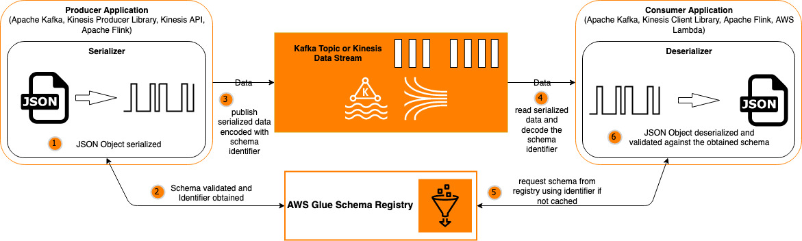
The following diagram illustrates a high-level view of how AWS Glue Schema Registry works. AWS Glue Schema Registry allows you to register and evolve JSON, Apache Avro, and Protocol buffers schemas with compatibility modes. You can register multiple versions of each schema as the business needs or stream processing application’s requirements evolve. The AWS Glue Schema Registry open-source library provides JSON, Avro, and protobuf serializers and deserializers that you configure in producer and consumer stream processing applications, as shown in the following diagram. The open-source library also supports optional compression and caching configuration to save on data transfers.

To accommodate various business use cases, AWS Glue Schema Registry supports multiple compatibility modes. For example, if a consumer application is updated to a new schema version but is still able to consume and process messages based on the previous version of the same schema, then the schema is backward-compatible. However, if a schema version has bumped up in the producer application and the consumer application is not updated yet but can still consume and process the old and new message, then the schema is configured as forward-compatible. For more information, refer to How the Schema Registry Works.

Create a Protocol buffers schema in AWS Glue Schema Registry

In this section, we create a protobuf schema in AWS Glue Schema Registry via the console and AWS CLI.

Create a schema via the console

Make sure you have the required AWS Glue Schema Registry IAM permissions.

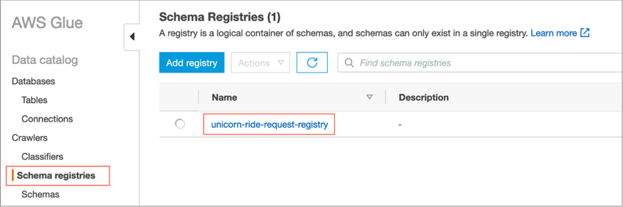
  1. On the AWS Glue console, choose Schema registries in the navigation pane.
  2. Click Add registry.
  3. For Registry name, enter employee-schema-registry.
  4. Click Add Registry.
  5. After the registry is created, click Add schema to register a new schema.
  6. For Schema name, enter Employee.proto.

The schema must be either Employee.proto or Employee if the protobuf schema doesn’t have the options option java_multiple_files = true; and option java_outer_classname = "<Outer class name>"; and if you decide to use protobuf schema generated code (POJOs) in your stream processing applications. We cover this with an example in a subsequent section of this post.­ For more information on protobuf options, refer to Options.

  1. For Registry, choose the registry employee-schema-registry.
  2. For Data format, choose Protocol buffers.
  3. For Compatibility mode, choose Backward.

You can choose other compatibility modes as per your use case.

  1. For First schema version, enter the preceding protobuf schema, then click Create schema and version.

After the schema is registered successfully, its status will be Available, as shown in the following screenshot.

Create a schema via the AWS CLI

Make sure you have IAM credentials with AWS Glue Schema Registry permissions.

  1. Run the following AWS CLI command to create a schema registry employee-schema-registry (for this post, we use the Region us-east-2):
    aws glue create-registry \
    --registry-name employee-schema-registry \
    --region us-east-2

The AWS CLI command returns the newly created schema registry ARN in response.

  1. Copy the RegistryArn value from the response to use in the following AWS CLI command.
  2. In the following command, use the preceding protobuf schema and schema name Employee.proto:
    aws glue create-schema --schema-name Employee.proto \
    --registry-id RegistryArn=<Schema Registry ARN that you copied from response of create registry CLI command> \
    --compatibility BACKWARD \
    --data-format PROTOBUF \
    --schema-definition file:///<project-directory>/Employee.proto \
    --region us-east-2

You can also use AWS CloudFormation to create schemas in AWS Glue Schema Registry.

Using a Protocol buffers schema with Amazon MSK and Kinesis Data Streams

Like Apache Avro’s SpecificRecord and GenericRecord, protobuf also supports working with POJOs to ensure type safety and DynamicMessage to create generic data producer and consumer applications. The following examples showcase the use of a protobuf schema registered in AWS Glue Schema Registry with Kafka and Kinesis Data Streams producer and consumer applications.

Use a protobuf schema with Amazon MSK

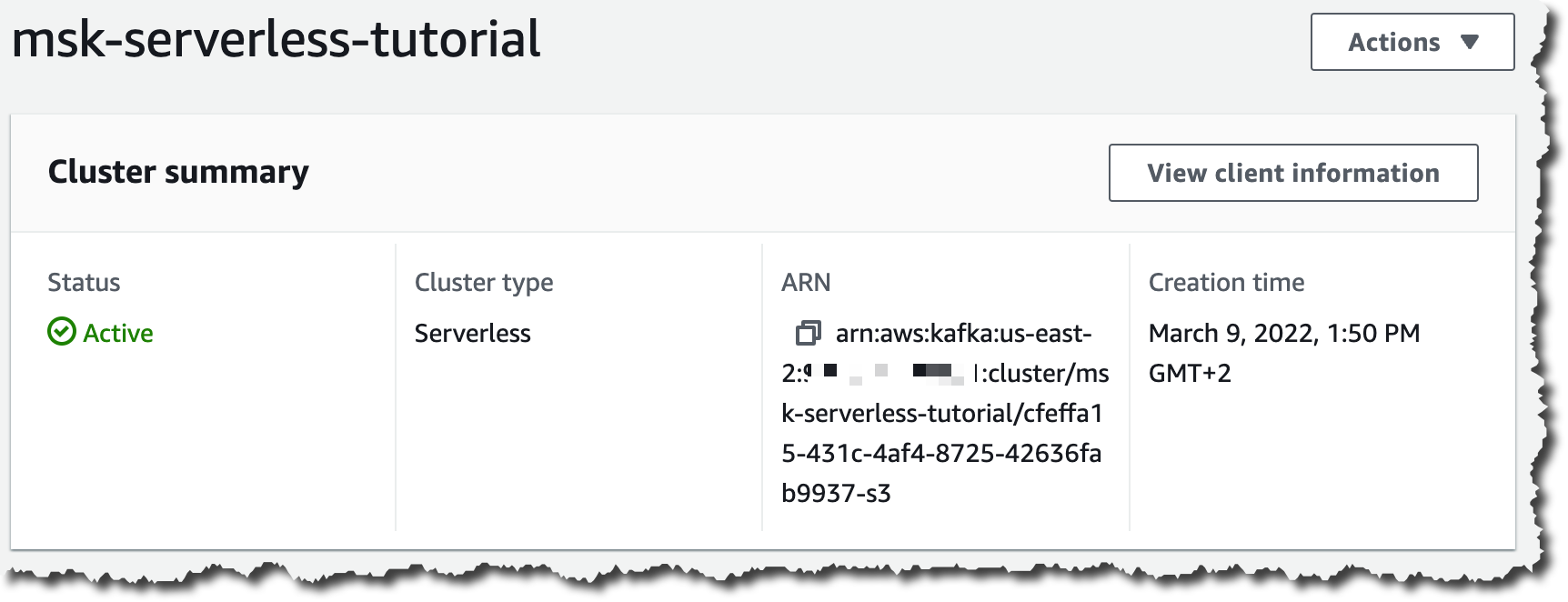
Create an Amazon MSK or Apache Kafka cluster with a topic called protobuf-demo-topic. If creating an Amazon MSK cluster, you can use the console. For instructions, refer to Getting Started Using Amazon MSK.

Use protobuf schema-generated POJOs

To use protobuf schema-generated POJOs, complete the following steps:

  1. Install the protobuf compiler (protoc) on your local machine from GitHub and add it in the PATH variable.
  2. Add the following plugin configuration to your application’s pom.xml file. We use the xolstice protobuf Maven plugin for this post to generate code from the protobuf schema.
    <plugin>
       <!-- https://www.xolstice.org/protobuf-maven-plugin/usage.html -->
       <groupId>org.xolstice.maven.plugins</groupId>
       <artifactId>protobuf-maven-plugin</artifactId>
       <version>0.6.1</version>
       <configuration>
           <protoSourceRoot>${basedir}/src/main/resources/proto</protoSourceRoot>
           <outputDirectory>${basedir}/src/main/java</outputDirectory>
           <clearOutputDirectory>false</clearOutputDirectory>
       </configuration>
       <executions>
           <execution>
               <goals>
                   <goal>compile</goal>
               </goals>
           </execution>
       </executions>
    </plugin>

  3. Add the following dependencies to your application’s pom.xml file:
    <!-- https://mvnrepository.com/artifact/com.google.protobuf/protobuf-java -->
    <dependency>
       <groupId>com.google.protobuf</groupId>
       <artifactId>protobuf-java</artifactId>
       <version>3.19.4</version>
    </dependency>
    
    <!-- https://mvnrepository.com/artifact/software.amazon.glue/schema-registry-serde -->
    <dependency>
       <groupId>software.amazon.glue</groupId>
       <artifactId>schema-registry-serde</artifactId>
       <version>1.1.9</version>
    </dependency>	

  4. Create a schema registry employee-schema-registry in AWS Glue Schema Registry and register the Employee.proto protobuf schema with it. Name your schema Employee.proto (or Employee).
  5. Run the following command to generate the code from Employee.proto. Make sure you have the schema file in the ${basedir}/src/main/resources/proto directory or change it as per your application directory structure in the application’s pom.xml <protoSourceRoot> tag value:
    mvn clean compile

Next, we configure the Kafka producer publishing protobuf messages to the Kafka topic on Amazon MSK.

  1. Configure the Kafka producer properties:
private Properties getProducerConfig() {
    Properties props = new Properties();
    props.put(ProducerConfig.BOOTSTRAP_SERVERS_CONFIG, this.bootstrapServers);
    props.put(ProducerConfig.KEY_SERIALIZER_CLASS_CONFIG, StringSerializer.class.getName());
    props.put(ProducerConfig.VALUE_SERIALIZER_CLASS_CONFIG, GlueSchemaRegistryKafkaSerializer.class.getName());
    props.put(AWSSchemaRegistryConstants.DATA_FORMAT, DataFormat.PROTOBUF.name());
    props.put(AWSSchemaRegistryConstants.AWS_REGION,"us-east-2");
    props.put(AWSSchemaRegistryConstants.REGISTRY_NAME, "employee-schema-registry");
    props.put(AWSSchemaRegistryConstants.SCHEMA_NAME, "Employee.proto");
    props.put(AWSSchemaRegistryConstants.PROTOBUF_MESSAGE_TYPE, ProtobufMessageType.POJO.getName());
    return props;
}

The VALUE_SERIALIZER_CLASS_CONFIG configuration specifies the AWS Glue Schema Registry serializer, which serializes the protobuf message.

  1. Use the schema-generated code (POJOs) to create a protobuf message:
    public EmployeeOuterClass.Employee createEmployeeRecord(int employeeId){
        EmployeeOuterClass.Employee employee =
                EmployeeOuterClass.Employee.newBuilder()
                        .setId(employeeId)
                        .setName("Dummy")
                        .setAddress("Melbourne, Australia")
                        .setEmployeeAge(Int32Value.newBuilder().setValue(32).build())
                        .setStartDate(Timestamp.newBuilder().setSeconds(235234532434L).build())
                        .setTotalTimeSpanInCompany(Duration.newBuilder().setSeconds(3453245345L).build())
                        .setIsCertified(BoolValue.newBuilder().setValue(true).build())
                        .setRole(EmployeeOuterClass.Role.ARCHITECT)
                        .setProject(EmployeeOuterClass.Project.newBuilder()
                                .setName("Protobuf Schema Demo")
                                .setState("GA").build())
                        .setTotalAwardValue(Money.newBuilder()
                                            .setCurrencyCode("USD")
                                            .setUnits(5)
                                            .setNanos(50000).build())
                        .setTeam(EmployeeOuterClass.Team.newBuilder()
                                .setName("Solutions Architects")
                                .setLocation("Australia").build()).build();
        return employee;
    }

  2. Publish the protobuf messages to the protobuf-demo-topic topic on Amazon MSK:
    public void startProducer() throws InterruptedException {
        String topic = "protobuf-demo-topic";
        KafkaProducer<String, EmployeeOuterClass.Employee> producer = new KafkaProducer<String, EmployeeOuterClass.Employee>(getProducerConfig());
        logger.info("Starting to send records...");
        int employeeId = 0;
        while(employeeId < 100)
        {
            EmployeeOuterClass.Employee person = createEmployeeRecord(employeeId);
            String key = "key-" + employeeId;
            ProducerRecord<String,  EmployeeOuterClass.Employee> record = new ProducerRecord<String,  EmployeeOuterClass.Employee>(topic, key, person);
            producer.send(record, new ProducerCallback());
            employeeId++;
        }
    }
    private class ProducerCallback implements Callback {
        @Override
        public void onCompletion(RecordMetadata recordMetaData, Exception e){
            if (e == null) {
                logger.info("Received new metadata. \n" +
                        "Topic:" + recordMetaData.topic() + "\n" +
                        "Partition: " + recordMetaData.partition() + "\n" +
                        "Offset: " + recordMetaData.offset() + "\n" +
                        "Timestamp: " + recordMetaData.timestamp());
            }
            else {
                logger.info("There's been an error from the Producer side");
                e.printStackTrace();
            }
        }
    }

  3. Start the Kafka producer:
    public static void main(String args[]) throws InterruptedException {
        ProducerProtobuf producer = new ProducerProtobuf();
        producer.startProducer();
    }

  4. In the Kafka consumer application’s pom.xml, add the same plugin and dependencies as the Kafka producer’s pom.xml.

Next, we configure the Kafka consumer consuming protobuf messages from the Kafka topic on Amazon MSK.

  1. Configure the Kafka consumer properties:
    private Properties getConsumerConfig() {
        Properties props = new Properties();
        props.put(ProducerConfig.BOOTSTRAP_SERVERS_CONFIG, this.bootstrapServers);
        props.put(ConsumerConfig.GROUP_ID_CONFIG, "protobuf-consumer");
        props.put(ConsumerConfig.AUTO_OFFSET_RESET_CONFIG,"earliest");
        props.put(ConsumerConfig.KEY_DESERIALIZER_CLASS_CONFIG, StringDeserializer.class.getName());
        props.put(ConsumerConfig.VALUE_DESERIALIZER_CLASS_CONFIG, GlueSchemaRegistryKafkaDeserializer.class.getName());
        props.put(AWSSchemaRegistryConstants.AWS_REGION,"us-east-2");
        props.put(AWSSchemaRegistryConstants.PROTOBUF_MESSAGE_TYPE, ProtobufMessageType.POJO.getName());
        return props;
    }

The VALUE_DESERIALIZER_CLASS_CONFIG config specifies the AWS Glue Schema Registry deserializer that deserializes the protobuf messages.

  1. Consume the protobuf message (as a POJO) from the protobuf-demo-topic topic on Amazon MSK:
    public void startConsumer() {
        logger.info("starting consumer...");
        String topic = "protobuf-demo-topic";
        KafkaConsumer<String, EmployeeOuterClass.Employee> consumer = new KafkaConsumer<String, EmployeeOuterClass.Employee>(getConsumerConfig());
        consumer.subscribe(Collections.singletonList(topic));
        while (true) {
            final ConsumerRecords<String, EmployeeOuterClass.Employee> records = consumer.poll(Duration.ofMillis(1000));
            for (final ConsumerRecord<String, EmployeeOuterClass.Employee> record : records) {
                final EmployeeOuterClass.Employee employee = record.value();
                logger.info("Employee Id: " + employee.getId() + " | Name: " + employee.getName() + " | Address: " + employee.getAddress() +
                        " | Age: " + employee.getEmployeeAge().getValue() + " | Startdate: " + employee.getStartDate().getSeconds() +
                        " | TotalTimeSpanInCompany: " + employee.getTotalTimeSpanInCompany() +
                        " | IsCertified: " + employee.getIsCertified().getValue() + " | Team: " + employee.getTeam().getName() +
                        " | Role: " + employee.getRole().name() + " | Project State: " + employee.getProject().getState() +
                        " | Project Name: " + employee.getProject().getName() + "| Award currency code: " + employee.getTotalAwardValue().getCurrencyCode() +
                        " | Award units : " + employee.getTotalAwardValue().getUnits() + " | Award nanos " + employee.getTotalAwardValue().getNanos());
            }
        }
    }

  2. Start the Kafka consumer:
    public static void main(String args[]){
        ConsumerProtobuf consumer = new ConsumerProtobuf();
        consumer.startConsumer();
    }

Use protobuf’s DynamicMessage

You can use DynamicMessage to create generic producer and consumer applications without generating the code from the protobuf schema. To use DynamicMessage, you first need to create a protobuf schema file descriptor.

  1. Generate a file descriptor from the protobuf schema using the following command:
    protoc --include_imports --proto_path=proto --descriptor_set_out=proto/Employeeproto.desc proto/Employee.proto

The option --descritor_set_out has the descriptor file name that this command generates. The protobuf schema Employee.proto is in the proto directory.

  1. Make sure you have created a schema registry and registered the preceding protobuf schema with it.

Now we configure the Kafka producer publishing DynamicMessage to the Kafka topic on Amazon MSK.

  1. Create the Kafka producer configuration. The PROTOBUF_MESSAGE_TYPE configuration is DYNAMIC_MESSAGE instead of POJO.
    private Properties getProducerConfig() {
       Properties props = new Properties();
       props.put(ProducerConfig.BOOTSTRAP_SERVERS_CONFIG, this.bootstrapServers);
       props.put(ProducerConfig.ACKS_CONFIG, "-1");
       props.put(ProducerConfig.CLIENT_ID_CONFIG,"protobuf-dynamicmessage-record-producer");
       props.put(ProducerConfig.KEY_SERIALIZER_CLASS_CONFIG, StringSerializer.class.getName());
       props.put(ProducerConfig.VALUE_SERIALIZER_CLASS_CONFIG,GlueSchemaRegistryKafkaSerializer.class.getName());
       props.put(AWSSchemaRegistryConstants.DATA_FORMAT, DataFormat.PROTOBUF.name());
       props.put(AWSSchemaRegistryConstants.AWS_REGION,"us-east-2");
       props.put(AWSSchemaRegistryConstants.REGISTRY_NAME, "employee-schema-registry");
       props.put(AWSSchemaRegistryConstants.SCHEMA_NAME, "Employee.proto");
       props.put(AWSSchemaRegistryConstants.PROTOBUF_MESSAGE_TYPE, ProtobufMessageType.DYNAMIC_MESSAGE.getName());
       return props;
        }

  2. Create protobuf dynamic messages and publish them to the Kafka topic on Amazon MSK:
    public void startProducer() throws Exception {
        Descriptor desc = getDescriptor();
        String topic = "protobuf-demo-topic";
        KafkaProducer<String, DynamicMessage> producer = new KafkaProducer<String, DynamicMessage>(getProducerConfig());
        logger.info("Starting to send records...");
        int i = 0;
        while (i < 100) {
            DynamicMessage dynMessage = DynamicMessage.newBuilder(desc)
                    .setField(desc.findFieldByName("id"), 1234)
                    .setField(desc.findFieldByName("name"), "Dummy Name")
                    .setField(desc.findFieldByName("address"), "Melbourne, Australia")
                    .setField(desc.findFieldByName("employee_age"), Int32Value.newBuilder().setValue(32).build())
                    .setField(desc.findFieldByName("start_date"), Timestamp.newBuilder().setSeconds(235234532434L).build())
                    .setField(desc.findFieldByName("total_time_span_in_company"), Duration.newBuilder().setSeconds(3453245345L).build())
                    .setField(desc.findFieldByName("is_certified"), BoolValue.newBuilder().setValue(true).build())
    		.setField(desc.findFieldByName("total_award_value"), Money.newBuilder().setCurrencyCode("USD")
    						.setUnits(1).setNanos(50000).build())
                    .setField(desc.findFieldByName("team"), createTeam(desc.findFieldByName("team").getMessageType()))
                    .setField(desc.findFieldByName("project"), createProject(desc.findFieldByName("project").getMessageType()))
                    .setField(desc.findFieldByName("role"), desc.findFieldByName("role").getEnumType().findValueByName("ARCHITECT"))
                    .build();
            String key = "key-" + i;
            ProducerRecord<String, DynamicMessage> record = new ProducerRecord<String, DynamicMessage>(topic, key, dynMessage);
            producer.send(record, new ProtobufProducer.ProducerCallback());
            Thread.sleep(1000);
            i++;
        }
    }
    private static DynamicMessage createTeam(Descriptor desc) {
        DynamicMessage dynMessage = DynamicMessage.newBuilder(desc)
                .setField(desc.findFieldByName("name"), "Solutions Architects")
                .setField(desc.findFieldByName("location"), "Australia")
                .build();
        return dynMessage;
    }
    
    private static DynamicMessage createProject(Descriptor desc) {
        DynamicMessage dynMessage = DynamicMessage.newBuilder(desc)
                .setField(desc.findFieldByName("name"), "Protobuf Schema Demo")
                .setField(desc.findFieldByName("state"), "GA")
                .build();
        return dynMessage;
    }
    
    private class ProducerCallback implements Callback {
        @Override
        public void onCompletion(RecordMetadata recordMetaData, Exception e) {
            if (e == null) {
                logger.info("Received new metadata. \n" +
                        "Topic:" + recordMetaData.topic() + "\n" +
                        "Partition: " + recordMetaData.partition() + "\n" +
                        "Offset: " + recordMetaData.offset() + "\n" +
                        "Timestamp: " + recordMetaData.timestamp());
            } else {
                logger.info("There's been an error from the Producer side");
                e.printStackTrace();
            }
        }
    }

  3. Create a descriptor using the Employeeproto.desc file that we generated from the Employee.proto schema file in the previous steps:
    private Descriptor getDescriptor() throws Exception {
        InputStream inStream = ProtobufProducer.class.getClassLoader().getResourceAsStream("proto/Employeeproto.desc");
        DescriptorProtos.FileDescriptorSet fileDescSet = DescriptorProtos.FileDescriptorSet.parseFrom(inStream);
        Map<String, DescriptorProtos.FileDescriptorProto> fileDescProtosMap = new HashMap<String, DescriptorProtos.FileDescriptorProto>();
        List<DescriptorProtos.FileDescriptorProto> fileDescProtos = fileDescSet.getFileList();
        for (DescriptorProtos.FileDescriptorProto fileDescProto : fileDescProtos) {
            fileDescProtosMap.put(fileDescProto.getName(), fileDescProto);
        }
        DescriptorProtos.FileDescriptorProto fileDescProto = fileDescProtosMap.get("Employee.proto");
        FileDescriptor[] dependencies = getProtoDependencies(fileDescProtosMap, fileDescProto);
        FileDescriptor fileDesc = FileDescriptor.buildFrom(fileDescProto, dependencies);
        Descriptor desc = fileDesc.findMessageTypeByName("Employee");
        return desc;
    }
    
    public static FileDescriptor[] getProtoDependencies(Map<String, FileDescriptorProto> fileDescProtos, 
    				  FileDescriptorProto fileDescProto) throws Exception {
    
        if (fileDescProto.getDependencyCount() == 0)
            return new FileDescriptor[0];
    
        ProtocolStringList dependencyList = fileDescProto.getDependencyList();
        String[] dependencyArray = dependencyList.toArray(new String[0]);
        int noOfDependencies = dependencyList.size();
    
        FileDescriptor[] dependencies = new FileDescriptor[noOfDependencies];
        for (int i = 0; i < noOfDependencies; i++) {
            FileDescriptorProto dependencyFileDescProto = fileDescProtos.get(dependencyArray[i]);
            FileDescriptor dependencyFileDesc = FileDescriptor.buildFrom(dependencyFileDescProto, 
    					     getProtoDependencies(fileDescProtos, dependencyFileDescProto));
            dependencies[i] = dependencyFileDesc;
        }
        return dependencies;
    }

  4. Start the Kafka producer:
    public static void main(String args[]) throws InterruptedException {
    	 ProducerProtobuf producer = new ProducerProtobuf();
             producer.startProducer();
    }

Now we configure the Kafka consumer consuming dynamic messages from the Kaka topic on Amazon MSK.

  1. Enter the following Kafka consumer configuration:
    private Properties getConsumerConfig() {
        Properties props = new Properties();
        props.put(ProducerConfig.BOOTSTRAP_SERVERS_CONFIG, this.bootstrapServers);
        props.put(ConsumerConfig.GROUP_ID_CONFIG, "protobuf-record-consumer");
        props.put(ConsumerConfig.AUTO_OFFSET_RESET_CONFIG,"earliest");
        props.put(ConsumerConfig.KEY_DESERIALIZER_CLASS_CONFIG, StringDeserializer.class.getName());
        props.put(ConsumerConfig.VALUE_DESERIALIZER_CLASS_CONFIG, GlueSchemaRegistryKafkaDeserializer.class.getName());
        props.put(AWSSchemaRegistryConstants.AWS_REGION,"us-east-2");
        props.put(AWSSchemaRegistryConstants.PROTOBUF_MESSAGE_TYPE, ProtobufMessageType.DYNAMIC_MESSAGE.getName());
        return props;
    }

  2. Consume protobuf dynamic messages from the Kafka topic protobuf-demo-topic. Because we’re using DYNAMIC_MESSAGE, the retrieved objects are of type DynamicMessage.
    public void startConsumer() {
        logger.info("starting consumer...");
        String topic = "protobuf-demo-topic";
        KafkaConsumer<String, DynamicMessage> consumer = new KafkaConsumer<String, DynamicMessage>(getConsumerConfig());
        consumer.subscribe(Collections.singletonList(topic));
        while (true) {
            final ConsumerRecords<String, DynamicMessage> records = consumer.poll(Duration.ofMillis(1000));
            for (final ConsumerRecord<String, DynamicMessage> record : records) {
                for (Descriptors.FieldDescriptor field : record.value().getAllFields().keySet()) {
                    logger.info(field.getName() + ": " + record.value().getField(field));
                }
            }
        }
    }

  3. Start the Kafka consumer:
    public static void main(String args[]){
            ConsumerProtobuf consumer = new ConsumerProtobuf();
            consumer.startConsumer();
         }

Use a protobuf schema with Kinesis Data Streams

You can use the protobuf schema-generated POJOs with the Kinesis Producer Library (KPL) and Kinesis Client Library (KCL).

  1. Install the protobuf compiler (protoc) on your local machine from GitHub and add it in the PATH variable.
  2. Add the following plugin configuration to your application’s pom.xml file. We’re using the xolstice protobuf Maven plugin for this post to generate code from the protobuf schema.
    <plugin>
       <!-- https://www.xolstice.org/protobuf-maven-plugin/usage.html -->
       <groupId>org.xolstice.maven.plugins</groupId>
       <artifactId>protobuf-maven-plugin</artifactId>
       <version>0.6.1</version>
       <configuration>
           <protoSourceRoot>${basedir}/src/main/resources/proto</protoSourceRoot>
           <outputDirectory>${basedir}/src/main/java</outputDirectory>
           <clearOutputDirectory>false</clearOutputDirectory>
       </configuration>
       <executions>
           <execution>
               <goals>
                   <goal>compile</goal>
               </goals>
           </execution>
       </executions>
    </plugin>

  3. Because the KPL and KCL latest versions have the AWS Glue Schema Registry open-source library (schema-registry-serde) and protobuf runtime (protobuf-java) included, you only need to add the following dependencies to your application’s pom.xml:
    <!-- https://mvnrepository.com/artifact/com.amazonaws/amazon-kinesis-producer -->
    <dependency>
        <groupId>com.amazonaws</groupId>
        <artifactId>amazon-kinesis-producer</artifactId>
        <version>0.14.11</version>
    	</dependency>
    	<!-- https://mvnrepository.com/artifact/software.amazon.kinesis/amazon-kinesis-client -->
    <dependency>
        <groupId>software.amazon.kinesis</groupId>
        <artifactId>amazon-kinesis-client</artifactId>
        <version>2.4.0version>
    </dependency>

  4. Create a schema registry employee-schema-registry and register the Employee.proto protobuf schema with it. Name your schema Employee.proto (or Employee).
  5. Run the following command to generate the code from Employee.proto. Make sure you have the schema file in the ${basedir}/src/main/resources/proto directory or change it as per your application directory structure in the application’s pom.xml <protoSourceRoot> tag value.
    mvn clean compile

The following Kinesis producer code with the KPL uses the Schema Registry open-source library to publish protobuf messages to Kinesis Data Streams.

  1. Start the Kinesis Data Streams producer:
    private static final String PROTO_SCHEMA_FILE = "proto/Employee.proto";
    private static final String SCHEMA_NAME = "Employee.proto";
    private static String REGION_NAME = "us-east-2";
    private static String REGISTRY_NAME = "employee-schema-registry";
    private static String STREAM_NAME = "employee_data_stream";
    private static int NUM_OF_RECORDS = 100;
    private static String REGISTRY_ENDPOINT = "https://glue.us-east-2.amazonaws.com";
    
    public static void main(String[] args) throws Exception {
         ProtobufKPLProducer producer = new ProtobufKPLProducer();
         producer.startProducer();
     }
    }

  2. Configure the Kinesis producer:
public void startProducer() throws Exception {
    logger.info("Starting KPL client with Glue Schema Registry Integration...");
    GlueSchemaRegistryConfiguration schemaRegistryConfig = new GlueSchemaRegistryConfiguration(REGION_NAME);
    schemaRegistryConfig.setCompressionType(AWSSchemaRegistryConstants.COMPRESSION.ZLIB);
    schemaRegistryConfig.setSchemaAutoRegistrationEnabled(false);
    schemaRegistryConfig.setCompatibilitySetting(Compatibility.BACKWARD);
    schemaRegistryConfig.setEndPoint(REGISTRY_ENDPOINT);
    schemaRegistryConfig.setProtobufMessageType(ProtobufMessageType.POJO);
    schemaRegistryConfig.setRegistryName(REGISTRY_NAME);
	
    //Setting Glue Schema Registry configuration in Kinesis Producer Configuration along with other configs
    KinesisProducerConfiguration config = new KinesisProducerConfiguration()
                                        .setRecordMaxBufferedTime(3000)
                                        .setMaxConnections(1)
                                        .setRequestTimeout(60000)
                                        .setRegion(REGION_NAME)
                                        .setRecordTtl(60000)
                                        .setGlueSchemaRegistryConfiguration(schemaRegistryConfig);

    FutureCallback<UserRecordResult> myCallback = new FutureCallback<UserRecordResult>() {
        @Override public void onFailure(Throwable t) {
              t.printStackTrace();
        };
        @Override public void onSuccess(UserRecordResult result) {
            logger.info("record sent successfully. Sequence Number: " + result.getSequenceNumber() + " | Shard Id : " + result.getShardId());
        };
    };
    
	//Creating schema definition object from the Employee.proto schema file.
    Schema gsrSchema = getSchemaDefinition();
    final KinesisProducer producer = new KinesisProducer(config);
    int employeeCount = 1;
    while(true) {
        //Creating and serializing schema generated POJO object (protobuf message)

        EmployeeOuterClass.Employee employee = createEmployeeRecord(employeeCount);
        byte[] serializedBytes = employee.toByteArray();
        ByteBuffer data = ByteBuffer.wrap(serializedBytes);
        Instant timestamp = Instant.now();

        //Publishing protobuf message to the Kinesis Data Stream
        ListenableFuture<UserRecordResult> f =
                    producer.addUserRecord(STREAM_NAME,
                                        Long.toString(timestamp.toEpochMilli()),
                                        new BigInteger(128, new Random()).toString(10),
                                        data,
                                        gsrSchema);
        Futures.addCallback(f, myCallback, MoreExecutors.directExecutor());
        employeeCount++;
        if(employeeCount > NUM_OF_RECORDS)
            break;
    }
    List<Future<UserRecordResult>> putFutures = new LinkedList<>();
    for (Future<UserRecordResult> future : putFutures) {
        UserRecordResult userRecordResult = future.get();
        logger.info(userRecordResult.getShardId() + userRecordResult.getSequenceNumber());
    }
}
  1. Create a protobuf message using schema-generated code (POJOs):
    public EmployeeOuterClass.Employee createEmployeeRecord(int count){
        EmployeeOuterClass.Employee employee =
                EmployeeOuterClass.Employee.newBuilder()
                .setId(count)
                .setName("Dummy")
                .setAddress("Melbourne, Australia")
                .setEmployeeAge(Int32Value.newBuilder().setValue(32).build())
                .setStartDate(Timestamp.newBuilder().setSeconds(235234532434L).build())
                .setTotalTimeSpanInCompany(Duration.newBuilder().setSeconds(3453245345L).build())
                .setIsCertified(BoolValue.newBuilder().setValue(true).build())
                .setRole(EmployeeOuterClass.Role.ARCHITECT)
                .setProject(EmployeeOuterClass.Project.newBuilder()
                            .setName("Protobuf Schema Demo")
                            .setState("GA").build())
                .setTotalAwardValue(Money.newBuilder()
                            .setCurrencyCode("USD")
                            .setUnits(5)
                            .setNanos(50000).build())
                .setTeam(EmployeeOuterClass.Team.newBuilder()
                            .setName("Solutions Architects")
                            .setLocation("Australia").build()).build();
        return employee;
    }

  2. Create the schema definition from Employee.proto:
    private Schema getSchemaDefinition() throws IOException {
        InputStream inputStream = ProtobufKPLProducer.class.getClassLoader().getResourceAsStream(PROTO_SCHEMA_FILE);
        StringBuilder resultStringBuilder = new StringBuilder();
        try (BufferedReader br = new BufferedReader(new InputStreamReader(inputStream))) {
            String line;
            while ((line = br.readLine()) != null) {
                resultStringBuilder.append(line).append("\n");
            }
        }
        String schemaDefinition = resultStringBuilder.toString();
        logger.info("Schema Definition " + schemaDefinition);
        Schema gsrSchema =
                new Schema(schemaDefinition, DataFormat.PROTOBUF.toString(), SCHEMA_NAME);
        return gsrSchema;
    }

The following is the Kinesis consumer code with the KCL using the Schema Registry open-source library to consume protobuf messages from the Kinesis Data Streams.

  1. Initialize the application:
    public void run(){
        logger.info("Starting KCL client with Glue Schema Registry Integration...");
        Region region = Region.of(ObjectUtils.firstNonNull(REGION_NAME, "us-east-2"));
        KinesisAsyncClient kinesisClient = KinesisClientUtil.createKinesisAsyncClient(KinesisAsyncClient.builder().region(region));
        DynamoDbAsyncClient dynamoClient = DynamoDbAsyncClient.builder().region(region).build();
        CloudWatchAsyncClient cloudWatchClient = CloudWatchAsyncClient.builder().region(region).build();
    
        EmployeeRecordProcessorFactory employeeRecordProcessorFactory = new EmployeeRecordProcessorFactory();
        ConfigsBuilder configsBuilder =
                new ConfigsBuilder(STREAM_NAME,
                        APPLICATION_NAME,
                        kinesisClient,
                        dynamoClient,
                        cloudWatchClient,
                        APPLICATION_NAME,
                        employeeRecordProcessorFactory);
    
        //Creating Glue Schema Registry configuration and Glue Schema Registry Deserializer object.
        GlueSchemaRegistryConfiguration gsrConfig = new GlueSchemaRegistryConfiguration(region.toString());
        gsrConfig.setEndPoint(REGISTRY_ENDPOINT);
        gsrConfig.setProtobufMessageType(ProtobufMessageType.POJO);
        GlueSchemaRegistryDeserializer glueSchemaRegistryDeserializer =
                new GlueSchemaRegistryDeserializerImpl(DefaultCredentialsProvider.builder().build(), gsrConfig);
        /*
         Setting Glue Schema Registry deserializer in the Retrieval Config for
         Kinesis Client Library to use it while deserializing the protobuf messages.
         */
        RetrievalConfig retrievalConfig = configsBuilder.retrievalConfig().retrievalSpecificConfig(new PollingConfig(STREAM_NAME, kinesisClient));
        retrievalConfig.glueSchemaRegistryDeserializer(glueSchemaRegistryDeserializer);
    
        Scheduler scheduler = new Scheduler(
                		configsBuilder.checkpointConfig(),
                		configsBuilder.coordinatorConfig(),
               		configsBuilder.leaseManagementConfig(),
                		configsBuilder.lifecycleConfig(),
                		configsBuilder.metricsConfig(),
                		configsBuilder.processorConfig(),
                		retrievalConfig);
    
        Thread schedulerThread = new Thread(scheduler);
        schedulerThread.setDaemon(true);
        schedulerThread.start();
    
        logger.info("Press enter to shutdown");
        BufferedReader reader = new BufferedReader(new InputStreamReader(System.in));
        try {
            reader.readLine();
            Future<Boolean> gracefulShutdownFuture = scheduler.startGracefulShutdown();
            logger.info("Waiting up to 20 seconds for shutdown to complete.");
            gracefulShutdownFuture.get(20, TimeUnit.SECONDS);
        } catch (Exception e) {
            logger.info("Interrupted while waiting for graceful shutdown. Continuing.");
        }
        logger.info("Completed, shutting down now.");
    }

  2. Consume protobuf messages from Kinesis Data Streams:
    public static class EmployeeRecordProcessorFactory implements ShardRecordProcessorFactory {
        @Override
        public ShardRecordProcessor shardRecordProcessor() {
            return new EmployeeRecordProcessor();
        }
    }
    public static class EmployeeRecordProcessor implements ShardRecordProcessor {
        private static final Logger logger = Logger.getLogger(EmployeeRecordProcessor.class.getSimpleName());
        public void initialize(InitializationInput initializationInput) {}
        public void processRecords(ProcessRecordsInput processRecordsInput) {
            try {
                logger.info("Processing " + processRecordsInput.records().size() + " record(s)");
                for (KinesisClientRecord r : processRecordsInput.records()) {
    			
                    //Deserializing protobuf message into schema generated POJO
                    EmployeeOuterClass.Employee employee = EmployeeOuterClass.Employee.parseFrom(r.data().array());
                    
                   logger.info("Processed record: " + employee);
                    logger.info("Employee Id: " + employee.getId() + " | Name: "  + employee.getName() + " | Address: " + employee.getAddress() +
                            " | Age: " + employee.getEmployeeAge().getValue() + " | Startdate: " + employee.getStartDate().getSeconds() +
                            " | TotalTimeSpanInCompany: " + employee.getTotalTimeSpanInCompany() +
                            " | IsCertified: " + employee.getIsCertified().getValue() + " | Team: " + employee.getTeam().getName() +
                            " | Role: " + employee.getRole().name() + " | Project State: " + employee.getProject().getState() +
                            " | Project Name: " + employee.getProject().getName() + " | Award currency code: " +    
                           employee.getTotalAwardValue().getCurrencyCode() + " | Award units : " + employee.getTotalAwardValue().getUnits() + 
    		      " | Award nanos " + employee.getTotalAwardValue().getNanos());
                }
            } catch (Exception e) {
                logger.info("Failed while processing records. Aborting" + e);
                Runtime.getRuntime().halt(1);
            }
        }
        public void leaseLost(LeaseLostInput leaseLostInput) {. . .}
        public void shardEnded(ShardEndedInput shardEndedInput) {. . .}
        public void shutdownRequested(ShutdownRequestedInput shutdownRequestedInput) {. . .}
    }

  3. Start the Kinesis Data Streams consumer:
    private static final Logger logger = Logger.getLogger(ProtobufKCLConsumer.class.getSimpleName());
    private static String REGION_NAME = "us-east-2";
    private static String STREAM_NAME = "employee_data_stream";
    private static final String APPLICATION_NAME =  "protobuf-demo-kinesis-kpl-consumer";
    private static String REGISTRY_ENDPOINT = "https://glue.us-east-2.amazonaws.com";
    
    public static void main(String[] args) throws ParseException {
        new ProtobufKCLConsumer().run();
    }
    

Enhance your protobuf schema

We covered examples of data producer and consumer applications integrating with Amazon MSK, Apache Kafka, and Kinesis Data Streams, and using a Protocol buffers schema registered with AWS Glue Schema Registry. You can further enhance these examples with schema evolution using the following rules, which are supported by AWS Glue Schema Registry. For example, the following protobuf schema shown is a backward-compatible updated version of Employee.proto. We have added another gRPC service definition CreateEmployee under EmployeeSearch and added an Optional field in the Employee message type. If you upgrade the consumer application with this version of the protobuf schema, the consumer application can still consume old and new protobuf messages.

Employee.proto (version-2)

syntax = "proto2";
package gsr.proto.post;

import "google/protobuf/wrappers.proto";
import "google/protobuf/duration.proto";
import "google/protobuf/timestamp.proto";
import "google/protobuf/empty.proto";
import "google/type/money.proto";

service EmployeeSearch {
    rpc FindEmployee(EmployeeSearchParams) returns (Employee);
    rpc CreateEmployee(EmployeeSearchParams) returns (google.protobuf.Empty);
}
message EmployeeSearchParams {
    required int32 id = 1;
}
message Employee {
    required int32 id = 1;
    required string name = 2;
    required string address = 3;
    required google.protobuf.Int32Value employee_age = 4;
    required google.protobuf.Timestamp start_date = 5;
    required google.protobuf.Duration total_time_span_in_company = 6;
    required google.protobuf.BoolValue is_certified = 7;
    required Team team = 8;
    required Project project = 9;
    required Role role = 10;
    required google.type.Money total_award_value = 11;
    optional string title = 12;
}
message Team {
    required string name = 1;
    required string location = 2;
}
message Project {
    required string name = 1;
    required string state = 2;
}
enum Role {
    MANAGER = 0;
    DEVELOPER = 1;
    ARCHITECT = 2;
}

Conclusion

In this post, we introduced Protocol buffers schema support in AWS Glue Schema Registry. AWS Glue Schema Registry now supports Apache Avro, JSON, and Protocol buffers schemas with different compatible modes. The examples in this post demonstrated how to use Protocol buffers schemas registered with AWS Glue Schema Registry in stream processing applications integrated with Apache Kafka, Amazon MSK, and Kinesis Data Streams. We used the schema-generated POJOs for type safety and protobuf’s DynamicMessage to create generic producer and consumer applications. The examples in this post contain the basic components of the stream processing pattern; you can adapt these examples to your use case needs.

To learn more, refer to the following resources:


About the Author

Vikas Bajaj is a Principal Solutions Architect at AWS. Vikas works with digital native customers and advises them on technology architecture and solutions to meet strategic business objectives.

Back up and restore Kafka topic data using Amazon MSK Connect

Post Syndicated from Rakshith Rao original https://aws.amazon.com/blogs/big-data/back-up-and-restore-kafka-topic-data-using-amazon-msk-connect/

You can use Apache Kafka to run your streaming workloads. Kafka provides resiliency to failures and protects your data out of the box by replicating data across the brokers of the cluster. This makes sure that the data in the cluster is durable. You can achieve your durability SLAs by changing the replication factor of the topic. However, streaming data stored in Kafka topics tends to be transient and typically has a retention time of days or weeks. You may want to back up the data stored in your Kafka topic long after its retention time expires for several reasons. For example, you might have compliance requirements that require you to store the data for several years. Or you may have curated synthetic data that needs to be repeatedly hydrated into Kafka topics before starting your workload’s integration tests. Or an upstream system that you don’t have control over produces bad data and you need to restore your topic to a previously well state.

Storing data indefinitely in Kafka topics is an option, but sometimes the use case calls for a separate copy. Tools such as MirrorMaker let you back up your data into another Kafka cluster. However, this requires another active Kafka cluster to be running as a backup, which increases compute costs and storage costs. A cost-effective and durable way of backing up the data of your Kafka cluster is to use an object storage service like Amazon Simple Storage Service (Amazon S3).

In this post, we walk through a solution that lets you back up your data for cold storage using Amazon MSK Connect. We restore the backed-up data to another Kafka topic and reset the consumer offsets based on your use case.

Overview of solution

Kafka Connect is a component of Apache Kafka that simplifies streaming data between Kafka topics and external systems like object stores, databases, and file systems. It uses sink connectors to stream data from Kafka topics to external systems, and source connectors to stream data from external systems to Kafka topics. You can use off-the-shelf connectors written by third parties or write your own connectors to meet your specific requirements.

MSK Connect is a feature of Amazon Managed Streaming for Apache Kafka (Amazon MSK) that lets you run fully managed Kafka Connect workloads. It works with MSK clusters and with compatible self-managed Kafka clusters. In this post, we use the Lenses AWS S3 Connector to back up the data stored in a topic in an Amazon MSK cluster to Amazon S3 and restore this data back to another topic. The following diagram shows our solution architecture.

To implement this solution, we complete the following steps:

  1. Back up the data using an MSK Connect sink connector to an S3 bucket.
  2. Restore the data using an MSK Connect source connector to a new Kafka topic.
  3. Reset consumer offsets based on different scenarios.

Prerequisites

Make sure to complete the following steps as prerequisites:

  1. Set up the required resources for Amazon MSK, Amazon S3, and AWS Identity and Access Management (IAM).
  2. Create two Kafka topics in the MSK cluster: source_topic and target_topic.
  3. Create an MSK Connect plugin using the Lenses AWS S3 Connector.
  4. Install the Kafka CLI by following Step 1 of Apache Kafka Quickstart.
  5. Install the kcat utility to send test messages to the Kafka topic.

Back up your topics

Depending on the use case, you may want to back up all the topics in your Kafka cluster or back up some specific topics. In this post, we cover how to back up a single topic, but you can extend the solution to back up multiple topics.

The format in which the data is stored in Amazon S3 is important. You may want to inspect the data that is stored in Amazon S3 to debug issues like the introduction of bad data. You can examine data stored as JSON or plain text by using text editors and looking in the time frames that are of interest to you. You can also examine large amounts of data stored in Amazon S3 as JSON or Parquet using AWS services like Amazon Athena. The Lenses AWS S3 Connector supports storing objects as JSON, Avro, Parquet, plaintext, or binary.

In this post, we send JSON data to the Kafka topic and store it in Amazon S3. Depending on the data type that meets your requirements, update the connect.s3.kcql statement and *.converter configuration. You can refer to the Lenses sink connector documentation for details of the formats supported and the related configurations. If the existing connectors don’t work for your use case, you can also write your own connector or extend existing connectors. You can partition the data stored in Amazon S3 based on fields of primitive types in the message header or payload. We use the date fields stored in the header to partition the data on Amazon S3.

Follow these steps to back up your topic:

  1. Create a new Amazon MSK sink connector by running the following command:
    aws kafkaconnect create-connector \
    --capacity "autoScaling={maxWorkerCount=2,mcuCount=1,minWorkerCount=1,scaleInPolicy={cpuUtilizationPercentage=10},scaleOutPolicy={cpuUtilizationPercentage=80}}" \
    --connector-configuration \
    "connector.class=io.lenses.streamreactor.connect.aws.s3.sink.S3SinkConnector, \
    key.converter.schemas.enable=false, \
    connect.s3.kcql=INSERT INTO <<S3 Bucket Name>>:my_workload SELECT * FROM source_topic PARTITIONBY _header.year\,_header.month\,_header.day\,_header.hour STOREAS \`JSON\` WITHPARTITIONER=KeysAndValues WITH_FLUSH_COUNT = 5, \
    aws.region=us-east-1, \
    tasks.max=2, \
    topics=source_topic, \
    schema.enable=false, \
    errors.log.enable=true, \
    value.converter=org.apache.kafka.connect.storage.StringConverter, \
    key.converter=org.apache.kafka.connect.storage.StringConverter " \
    --connector-name "backup-msk-to-s3-v1" \
    --kafka-cluster '{"apacheKafkaCluster": {"bootstrapServers": "<<MSK broker list>>","vpc": {"securityGroups": [ <<Security Group>> ],"subnets": [ <<Subnet List>> ]}}}' \
    --kafka-cluster-client-authentication "authenticationType=NONE" \
    --kafka-cluster-encryption-in-transit "encryptionType=PLAINTEXT" \
    --kafka-connect-version "2.7.1" \
    --plugins "customPlugin={customPluginArn=<< ARN of the MSK Connect Plugin >>,revision=1}" \
    --service-execution-role-arn " <<ARN of the IAM Role>> "

  2. Send data to the topic using kcat:
    ./kcat -b <<broker list>> -t source_topic -H "year=$(date +"%Y")" -H "month=$(date +"%m")" -H "day=$(date +"%d")" -H "hour=$(date +"%H")" -P
    {"message":"interesset eros vel elit salutatus"}
    {"message":"impetus deterruisset per aliquam luctus"}
    {"message":"ridens vocibus feugait vitae cras"}
    {"message":"interesset eros vel elit salutatus"}
    {"message":"impetus deterruisset per aliquam luctus"}
    {"message":"ridens vocibus feugait vitae cras"}

  3. Check the S3 bucket to make sure the data is being written.

MSK Connect publishes metrics to Amazon CloudWatch that you can use to monitor your backup process. Important metrics are SinkRecordReadRate and SinkRecordSendRate, which measure the average number of records read from Kafka and written to Amazon S3, respectively.

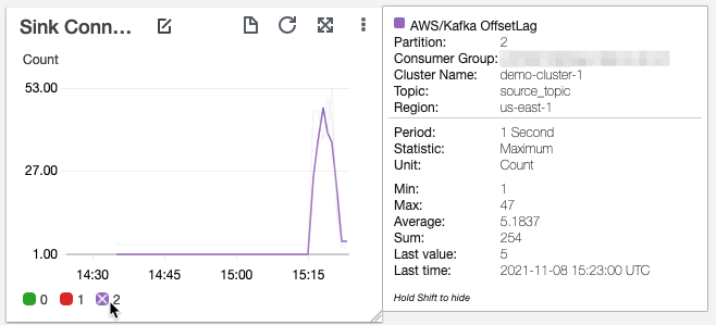
Also, make sure that the backup connector is keeping up with the rate at which the Kafka topic is receiving messages by monitoring the offset lag of the connector. If you’re using Amazon MSK, you can do this by turning on partition-level metrics on Amazon MSK and monitoring the OffsetLag metric of all the partitions for the backup connector’s consumer group. You should keep this as close to 0 as possible by adjusting the maximum number of MSK Connect worker instances. The command that we used in the previous step sets MSK Connect to automatically scale up to two workers. Adjust the --capacity setting to increase or decrease the maximum worker count of MSK Connect workers based on the OffsetLag metric.

Restore data to your topics

You can restore your backed-up data to a new topic with the same name in the same Kafka cluster, a different topic in the same Kafka cluster, or a different topic in a different Kafka cluster altogether. In this post, we walk through the scenario of restoring data that was backed up in Amazon S3 to a different topic, target_topic, in the same Kafka cluster. You can extend this to other scenarios by changing the topic and broker details in the connector configuration.

Follow these steps to restore the data:

  1. Create an Amazon MSK source connector by running the following command:
    aws kafkaconnect create-connector \
    --capacity "autoScaling={maxWorkerCount=2,mcuCount=1,minWorkerCount=1,scaleInPolicy={cpuUtilizationPercentage=10},scaleOutPolicy={cpuUtilizationPercentage=80}}"   \
    --connector-configuration \
        "connector.class=io.lenses.streamreactor.connect.aws.s3.source.S3SourceConnector, \
         key.converter.schemas.enable=false, \
         connect.s3.kcql=INSERT INTO target_topic SELECT * FROM <<S3 Bucket Name>>:my_workload PARTITIONBY _header.year\,_header.month\,_header.day\,_header.hour STOREAS \`JSON\` WITHPARTITIONER=KeysAndValues WITH_FLUSH_COUNT = 5 , \
         aws.region=us-east-1, \
         tasks.max=2, \
         topics=target_topic, \
         schema.enable=false, \
         errors.log.enable=true, \
         value.converter=org.apache.kafka.connect.storage.StringConverter, \
         key.converter=org.apache.kafka.connect.storage.StringConverter " \
    --connector-name "restore-s3-to-msk-v1" \
    --kafka-cluster '{"apacheKafkaCluster": {"bootstrapServers": "<<MSK broker list>>","vpc": {"securityGroups": [<<Security Group>>],"subnets": [ <<Subnet List>> ]}}}' \
    --kafka-cluster-client-authentication "authenticationType=NONE" \
    --kafka-cluster-encryption-in-transit "encryptionType=PLAINTEXT" \
    --kafka-connect-version "2.7.1" \
    --plugins "customPlugin={customPluginArn=<< ARN of the MSK Connect Plugin >>,revision=1}" \
    --service-execution-role-arn " <<ARN of the IAM Role>> "

The connector reads the data from the S3 bucket and replays it back to target_topic.

  1. Verify if the data is being written to the Kafka topic by running the following command:
    ./kafka-console-consumer.sh --bootstrap-server <<MSK broker list>> --topic target_topic --from-beginning

MSK Connect connectors run indefinitely, waiting for new data to be written to the source. However, while restoring, you have to stop the connector after all the data is copied to the topic. MSK Connect publishes the SourceRecordPollRate and SourceRecordWriteRate metrics to CloudWatch, which measure the average number of records polled from Amazon S3 and number of records written to the Kafka cluster, respectively. You can monitor these metrics to track the status of the restore process. When these metrics reach 0, the data from Amazon S3 is restored to the target_topic. You can get notified of the completion by setting up a CloudWatch alarm on these metrics. You can extend the automation to invoke an AWS Lambda function that deletes the connector when the restore is complete.

As with the backup process, you can speed up the restore process by scaling out the number of MSK Connect workers. Change the --capacity parameter to adjust the maximum and minimum workers to a number that meets the restore SLAs of your workload.

Reset consumer offsets

Depending on the requirements of restoring the data to a new Kafka topic, you may also need to reset the offsets of the consumer group before consuming or producing to them. Identifying the actual offset that you want to reset to depends on your specific business use case and involves manual work to identify this. You can use tools like Amazon S3 Select, Athena, or other custom tools to inspect the objects. The following screenshot demonstrates reading the records ending at offset 14 of partition 2 of topic source_topic using S3 Select.

After you identify the new start offsets for your consumer groups, you have to reset them on your Kafka cluster. You can do this using the CLI tools that come bundled with Kafka.

Existing consumer groups

If you want to use the same consumer group name after restoring the topic, you can do this by running the following command for each partition of the restored topic:

 ./kafka-consumer-groups.sh --bootstrap-server <<broker list>> --group <<consumer group>> --topic target_topic:<<partition>> --to-offset <<desired offset>> --reset-offsets --execute

Verify this by running the --describe option of the command:

./kafka-consumer-groups.sh --bootstrap-server <<broker list>> --group <<consumer group>>  --describe
TOPIC           PARTITION  CURRENT-OFFSET  LOG-END-OFFSET  LAG        ...
source_topic  0          211006          188417765       188206759  ...
source_topic  1          212847          192997707       192784860  ...
source_topic  2          211147          196410627       196199480  ...
target_topic  0          211006          188417765       188206759  ...
target_topic  1          212847          192997707       192784860  ...
target_topic  2          211147          196410627       196199480  ...

New consumer group

If you want your workload to create a new consumer group and seek to custom offsets, you can do this by invoking the seek method in your Kafka consumer for each partition. Alternatively, you can create the new consumer group by running the following code:

./kafka-console-consumer.sh --bootstrap-server <<broker list>> --topic target_topic --group <<consumer group>> --from-beginning --max-messages 1

Reset the offset to the desired offsets for each partition by running the following command:

./kafka-consumer-groups.sh --bootstrap-server <<broker list>> --group <<New consumer group>> --topic target_topic:<<partition>> --to-offset <<desired offset>> --reset-offsets --execute

Clean up

To avoid incurring ongoing charges, complete the following cleanup steps:

  1. Delete the MSK Connect connectors and plugin.
  2. Delete the MSK cluster.
  3. Delete the S3 buckets.
  4. Delete any CloudWatch resources you created.

Conclusion

In this post, we showed you how to back up and restore Kafka topic data using MSK Connect. You can extend this solution to multiple topics and other data formats based on your workload. Be sure to test various scenarios that your workloads may face and document the runbook for each of those scenarios.

For more information, see the following resources:


About the Author

Rakshith Rao is a Senior Solutions Architect at AWS. He works with AWS’s strategic customers to build and operate their key workloads on AWS.

Best practices for right-sizing your Apache Kafka clusters to optimize performance and cost

Post Syndicated from Steffen Hausmann original https://aws.amazon.com/blogs/big-data/best-practices-for-right-sizing-your-apache-kafka-clusters-to-optimize-performance-and-cost/

Apache Kafka is well known for its performance and tunability to optimize for various use cases. But sometimes it can be challenging to find the right infrastructure configuration that meets your specific performance requirements while minimizing the infrastructure cost.

This post explains how the underlying infrastructure affects Apache Kafka performance. We discuss strategies on how to size your clusters to meet your throughput, availability, and latency requirements. Along the way, we answer questions like “when does it make sense to scale up vs. scale out?” We end with guidance on how to continuously verify the size of your production clusters.

We use performance tests to illustrate and explain the effect and trade-off of different strategies to size your cluster. But as usual, it’s important to not just blindly trust benchmarks you happen to find on the internet. We therefore not only show how to reproduce the results, but also explain how to use a performance testing framework to run your own tests for your specific workload characteristics.

Sizing Apache Kafka clusters

The most common resource bottlenecks for clusters from an infrastructure perspective are network throughput, storage throughput, and network throughput between brokers and the storage backend for brokers using network attached storage such as Amazon Elastic Block Store (Amazon EBS).

The remainder of the post explains how the sustained throughput limit of a cluster not only depends on the storage and network throughput limits of the brokers, but also on the number of brokers and consumer groups as well as the replication factor r. We derive the following formula (referred to as Equation 1 throughout this post) for the theoretical sustained throughput limit tcluster given the infrastructure characteristics of a specific cluster:

max(tcluster) <= min{
  max(tstorage) * #brokers/r,
  max(tEBSnetwork) * #brokers/r,
  max(tEC2network) * #brokers/(#consumer groups + r-1)
}

For production clusters, it’s a best practice to target the actual throughput at 80% of its theoretical sustained throughput limit. Consider, for instance, a three-node cluster with m5.12xlarge brokers, a replication factor of 3, EBS volumes with a baseline throughput of 1000 MB/sec, and two consumer groups consuming from the tip of the topic. Taking all these parameters into account, the sustained throughput absorbed by the cluster should target 800 MB/sec.

However, this throughput calculation is merely providing an upper bound for workloads that are optimized for high throughput scenarios. Regardless of how you configure your topics and the clients reading from and writing into these topics, the cluster can’t absorb more throughput. For workloads with different characteristics, like latency-sensitive or compute-intensive workloads, the actual throughput that can be absorbed by a cluster while meeting these additional requirements is often smaller.

To find the right configuration for your workload, you need to work backward from your use case and determine the appropriate throughput, availability, durability, and latency requirements. Then, use Equation 1 to obtain the initial sizing of your cluster based on your throughput, durability, and storage requirements. Verify this initial cluster sizing by running performance tests and then fine-tune the cluster size, cluster configuration, and client configuration to meet your other requirements. Lastly, add additional capacity for production clusters so they can still ingest the expected throughput even if the cluster is running at reduced capacity, for instance, during maintenance, scaling, or loss of a broker. Depending on your workload, you may even consider adding enough spare capacity to withstanding an event affecting all brokers of an entire Availability Zone.

The remainder of the post dives deeper into the aspects of cluster sizing. The most important aspects are as follows:

  • There is often a choice between either scaling out or scaling up to increase the throughput and performance of a cluster. Small brokers give you smaller capacity increments and have a smaller blast radius in case they become unavailable. But having many small brokers increases the time it takes for operations that require a rolling update to brokers to complete, and increases the likelihood for failure.
  • All traffic that producers are sending into a cluster is persisted to disk. Therefore, the underlying throughput of the storage volume can become the bottleneck of the cluster. In this case, it makes sense to either increase the volume throughput if possible or to add more volumes to the cluster.
  • All data persisted on EBS volumes traverses the network. Amazon EBS-optimized instances come with dedicated capacity for Amazon EBS I/O, but the dedicated Amazon EBS network can still become the bottleneck of the cluster. In this case, it makes sense to scale up brokers, because larger brokers have higher Amazon EBS network throughput.
  • The more consumer groups that are reading from the cluster, the more data that egresses over the Amazon Elastic Compute Cloud (Amazon EC2) network of the brokers. Depending on the broker type and size, the Amazon EC2 network can become the bottleneck of the cluster. In that case, it makes sense to scale up brokers, because larger brokers have higher Amazon EC2 network throughput.
  • For p99 put latencies, there is a substantial performance impact of enabling in-cluster encryption. Scaling up the brokers of a cluster can substantially reduce the p99 put latency compared to smaller brokers.
  • When consumers fall behind or need to reprocess historic data, the requested data may no longer reside in memory, and brokers need to fetch data from the storage volume. This causes non-sequential I/O reads. When using EBS volumes, it also causes additional network traffic to the volume. Using larger brokers with more memory or enabling compression can mitigate this effect.
  • Using the burst capabilities of your cluster is a very powerful way to absorb sudden throughput spikes without scaling your cluster, which takes time to complete. Burst capacity also helps in response to operational events. For instance, when brokers are undergoing maintenance or partitions need to be rebalanced within the cluster, they can use the burst performance to complete the operation faster.
  • Monitor or alarm on important infrastructure-related cluster metrics such as BytesInPerSec, ReplicationBytesInPerSec, BytesOutPerSec, and ReplicationBytesOutPerSec to receive notification when the current cluster size is no longer optimal for the current cluster size.

The remainder of the post provides additional context and explains the reasoning behind these recommendations.

Understanding Apache Kafka performance bottlenecks

Before we start talking about performance bottlenecks from an infrastructure perspective, let’s revisit how data flows within a cluster.

For this post, we assume that producers and consumers are behaving well and according to best practices, unless explicitly stated differently. For example, we assume the producers are evenly balancing the load between brokers, brokers host the same number of partitions, there are enough partitions to ingest the throughput, consumers consume directly from the tip of the stream, and so on. The brokers are receiving the same load and are doing the same work. We therefore just focus on Broker 1 in the following diagram of a data flow within a cluster.

Data flow within a Kafka cluster

The producers send an aggregate throughput of tcluster into the cluster. As the traffic evenly spreads across brokers, Broker 1 receives an incoming throughput of tcluster/3. With a replication factor of 3, Broker 1 replicates the traffic it directly receives to the two other brokers (the blue lines). Likewise, Broker 1 receives replication traffic from two brokers (the red lines). Each consumer group consumes the traffic that is directly produced into Broker 1 (the green lines). All traffic that arrives in Broker 1 from producers and replication traffic from other brokers is eventually persisted to storage volumes attached to the broker.

Accordingly, the throughput of the storage volume and the broker network are both tightly coupled with the overall cluster throughput and warrant a closer look.

Storage backend throughput characteristics

Apache Kafka has been designed to utilize large sequential I/O operations when writing data to disk. Producers are only ever appending data to the tip of the log, causing sequential writes. Moreover, Apache Kafka is not synchronously flushing to disk. Instead, Apache Kafka is writing to the page cache, leaving it up to the operating system to flush pages to disk. This results in large sequential I/O operations, which optimizes disk throughput.

For many practical purposes, the broker can drive the full throughput of the volume and is not limited by IOPS. We assume that consumers are reading from the tip of the topic. This implies that performance of EBS volumes is throughput bound and not I/O bound, and reads are served from the page cache.

The ingress throughput of the storage backend depends on the data that producers are sending directly to the broker plus the replication traffic the broker is receiving from its peers. For an aggregated throughput produced into the cluster of tcluster and a replication factor of r, the throughput received by the broker storage is as follows:

tstorage = tcluster/#brokers + tcluster/#brokers * (r-1)
        = tcluster/#brokers * r

Therefore, the sustained throughput limit of the entire cluster is bound by the following:

max(tcluster) <= max(tstorage) * #brokers/r

AWS offers different options for block storage: instance storage and Amazon EBS. Instance storage is located on disks that are physically attached to the host computer, whereas Amazon EBS is network attached storage.

Instance families that come with instance storage achieve high IOPS and disk throughput. For instance, Amazon EC2 I3 instances include NVMe SSD-based instance storage optimized for low latency, very high random I/O performance, and high sequential read throughput. However, the volumes are tied to brokers. Their characteristics, in particular their size, only depend on the instance family, and the volume size can’t be adapted. Moreover, when a broker fails and needs to be replaced, the storage volume is lost. The replacement broker then needs to replicate the data from other brokers. This replication causes additional load on the cluster in addition to the reduced capacity from the broker loss.

In contrast, the characteristics of EBS volumes can be adapted while they’re in use. You can use these capabilities to automatically scale broker storage over time rather than provisioning storage for peak or adding additional brokers. Some EBS volume types, such as gp3, io2, and st1, also allow you to adapt the throughput and IOPS characteristics of existing volumes. Moreover, the lifecycle of EBS volumes is independent of the broker—if a broker fails and needs to be replaced, the EBS volume can be reattached to the replacement broker. This avoids most of the otherwise required replication traffic.

Using EBS volumes is therefore often a good choice for many common Apache Kafka workloads. They provide more flexibility and enable faster scaling and recovery operations.

Amazon EBS throughput characteristics

When using Amazon EBS as the storage backend, there are several volume types to choose from. The throughput characteristics of the different volume types range between 128 MB/sec and 4000 MB/sec (for more information, refer to Amazon EBS volume types). You can even choose to attach multiple volumes to a broker to increase the throughput beyond what can be delivered by a single volume.

However, Amazon EBS is network attached storage. All data a broker is writing to an EBS volume needs to traverse the network to the Amazon EBS backend. Newer generation instance families, like the M5 family, are Amazon EBS-optimized instances with dedicated capacity for Amazon EBS I/O. But there are limits on the throughput and the IOPS that depend on the size of the instance and not only on the volume size. The dedicated capacity for Amazon EBS provides a higher baseline throughput and IOPS for larger instances. The capacity ranges between 81 MB/sec and 2375 MB/sec. For more information, refer to Supported instance types.

When using Amazon EBS for storage, we can adapt the formula for the cluster sustained throughput limit to obtain a tighter upper bound:

max(tcluster) <= min{
  max(tstorage) * #brokers/r,
  max(tEBSnetwork) * #brokers/r
}

Amazon EC2 network throughput

So far, we have only considered network traffic to the EBS volume. But replication and the consumer groups also cause Amazon EC2 network traffic out of the broker. The traffic that producers are sending into a broker is replicated to r-1 brokers. Moreover, every consumer group reads the traffic that a broker ingests. Therefore, the overall outgoing network traffic is as follows:

tEC2network = tcluster/#brokers * #consumer groups + tcluster/#brokers * (r–1)
          = tcluster/#brokers * (#consumer groups + r-1)

Taking this traffic into account finally gives us a reasonable upper bound for the sustained throughput limit of the cluster, which we have already seen in Equation 1:

max(tcluster) <= min{
  max(tstorage) * #brokers/r,
  max(tEBSnetwork) * #brokers/r,
  max(tEC2network) * #brokers/(#consumer groups + r-1)
}

For production workloads, we recommend keeping the actual throughput of your workload below 80% of the theoretical sustained throughput limit as it’s determined by this formula. Furthermore, we assume that all data producers sent into the cluster are eventually read by at least one consumer group. When the number of consumers is larger or equal than 1, the Amazon EC2 network traffic out of a broker is always higher than the traffic into the broker. We can therefore ignore data traffic into brokers as a potential bottleneck.

With Equation 1, we can verify if a cluster with a given infrastructure can absorb the throughput required for our workload under ideal conditions. For more information about the Amazon EC2 network bandwidth of m5.8xlarge and larger instances, refer to Amazon EC2 Instance Types. You can also find the Amazon EBS bandwidth of m5.4xlarge instances on the same page. Smaller instances use credit-based systems for Amazon EC2 network bandwidth and the Amazon EBS bandwidth. For the Amazon EC2 network baseline bandwidth, refer to Network performance. For the Amazon EBS baseline bandwidth, refer to Supported instance types.

Right-size your cluster to optimize for performance and cost

So, what do we take from this? Most importantly, keep in mind that that these results only indicate the sustained throughput limit of a cluster under ideal conditions. These results can give you a general number for the expected sustained throughput limit of your clusters. But you must run your own experiments to verify these results for your specific workload and configuration.

However, we can draw a few conclusions from this throughput estimation: adding brokers increases the sustained cluster throughput. Similarly, decreasing the replication factor increases the sustained cluster throughput. Adding more than one consumer group may reduce the sustained cluster throughput if the Amazon EC2 network becomes the bottleneck.

Let’s run a couple of experiments to get empirical data on practical sustained cluster throughput that also accounts for producer put latencies. For these tests, we keep the throughput within the recommended 80% of the sustained throughput limit of clusters. When running your own tests, you may notice that clusters can even deliver higher throughput than what we show.

Measure Amazon MSK cluster throughput and put latencies

To create the infrastructure for the experiments, we use Amazon Managed Streaming for Apache Kafka (Amazon MSK). Amazon MSK provisions and manages highly available Apache Kafka clusters that are backed by Amazon EBS storage. The following discussion therefore also applies to clusters that have not been provisioned through Amazon MSK, if backed by EBS volumes.

The experiments are based on the kafka-producer-perf-test.sh and kafka-consumer-perf-test.sh tools that are included in the Apache Kafka distribution. The tests use six producers and two consumer groups with six consumers each that are concurrently reading and writing from the cluster. As mentioned before, we make sure that clients and brokers are behaving well and according to best practices: producers are evenly balancing the load between brokers, brokers host the same number of partitions, consumers consume directly from the tip of the stream, producers and consumers are over-provisioned so that they don’t become a bottleneck in the measurements, and so on.

We use clusters that have their brokers deployed to three Availability Zones. Moreover, replication is set to 3 and acks is set to all to achieve a high durability of the data that is persisted in the cluster. We also configured a batch.size of 256 kB or 512 kB and set linger.ms to 5 milliseconds, which reduces the overhead of ingesting small batches of records and therefore optimizes throughput. The number of partitions is adjusted to the broker size and cluster throughput.

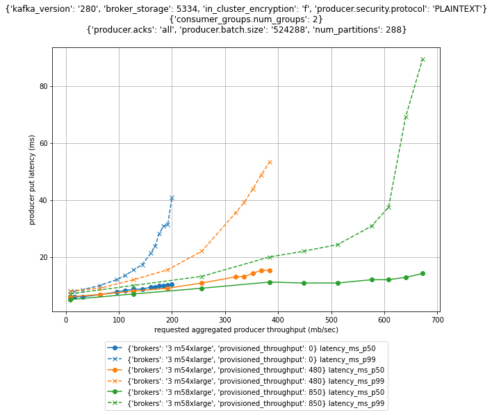
The configuration for brokers larger than m5.2xlarge has been adapted according to the guidance of the Amazon MSK Developer Guide. In particular when using provisioned throughput, it’s essential to optimize the cluster configuration accordingly.

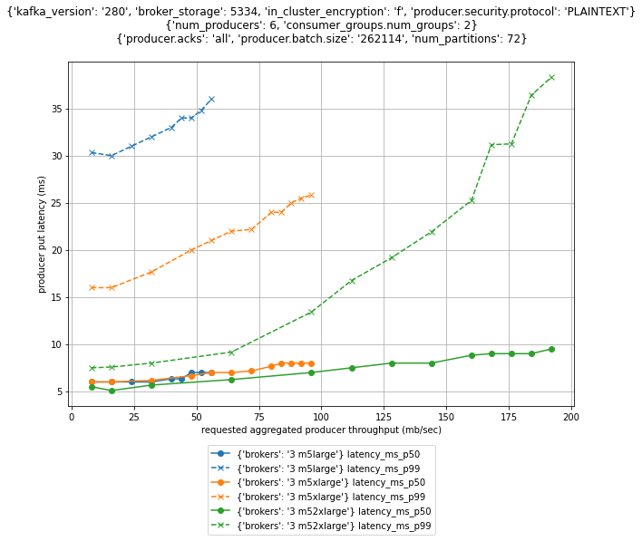
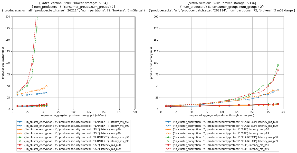
The following figure compares put latencies for three clusters with different broker sizes. For each cluster, the producers are running roughly a dozen individual performance tests with different throughput configurations. Initially, the producers produce a combined throughput of 16 MB/sec into the cluster and gradually increase the throughput with every individual test. Each individual test runs for 1 hour. For instances with burstable performance characteristics, credits are depleted before starting the actual performance measurement.

Comparing throughput and put latencies of different broker sizes

For brokers with more than 334 GB of storage, we can assume the EBS volume has a baseline throughput of 250 MB/sec. The Amazon EBS network baseline throughput is 81.25, 143.75, 287.5, and 593.75 MB/sec for the different broker sizes (for more information, see Supported instance types). The Amazon EC2 network baseline throughput is 96, 160, 320, and 640 MB/sec (for more information, see Network performance). Note that this only considers the sustained throughput; we discuss burst performance in a later section.

For a three-node cluster with replication 3 and two consumer groups, the recommended ingress throughput limits as per Equation 1 is as follows.

Broker size Recommended sustained throughput limit
m5.large 58 MB/sec
m5.xlarge 96 MB/sec
m5.2xlarge 192 MB/sec
m5.4xlarge 200 MB/sec

Even though the m5.4xlarge brokers have twice the number of vCPUs and memory compared to m5.2xlarge brokers, the cluster sustained throughput limit barely increases when scaling the brokers from m5.2xlarge to m5.4xlarge. That’s because with this configuration, the EBS volume used by brokers becomes a bottleneck. Remember that we’ve assumed a baseline throughput of 250 MB/sec for these volumes. For a three-node cluster and replication factor of 3, each broker needs to write the same traffic to the EBS volume as is sent to the cluster itself. And because the 80% of the baseline throughput of the EBS volume is 200 MB/sec, the recommended sustained throughput limit of the cluster with m5.4xlarge brokers is 200 MB/sec.

The next section describes how you can use provisioned throughput to increase the baseline throughput of EBS volumes and therefore increase the sustained throughput limit of the entire cluster.

Increase broker throughput with provisioned throughput

From the previous results, you can see that from a pure throughput perspective there is little benefit to increasing the broker size from m5.2xlarge to m5.4xlarge with the default cluster configuration. The baseline throughput of the EBS volume used by brokers limits their throughput. However, Amazon MSK recently launched the ability to provision storage throughput up to 1000 MB/sec. For self-managed clusters you can use gp3, io2, or st1 volume types to achieve a similar effect. Depending on the broker size, this can substantially increase the overall cluster throughput.

The following figure compares the cluster throughput and put latencies of different broker sizes and different provisioned throughput configurations.

Comparing max sustained throughput of different brokers with and without provisioned throughput

For a three-node cluster with replication 3 and two consumer groups, the recommended ingress throughput limits as per Equation 1 are as follows.

Broker size Provisioned throughput configuration Recommended sustained throughput limit
m5.4xlarge 200 MB/sec
m5.4xlarge 480 MB/sec 384 MB/sec
m5.8xlarge 850 MB/sec 680 MB/sec
m5.12xlarge 1000 MB/sec 800 MB/sec
m5.16xlarge 1000 MB/sec 800 MB/sec

The provisioned throughput configuration was carefully chosen for the given workload. With two consumer groups consuming from the cluster, it doesn’t make sense to increase the provisioned throughput of m4.4xlarge brokers beyond the 480 MB/sec. The Amazon EC2 network, not the EBS volume throughput, restricts the recommended sustained throughput limit of the cluster to 384 MB/sec. But for workloads with a different number of consumers, it can make sense to further increase or decrease the provisioned throughput configuration to match the baseline throughput of the Amazon EC2 network.

Scale out to increase cluster write throughput

Scaling out the cluster naturally increases the cluster throughput. But how does this affect performance and cost? Let’s compare the throughput of two different clusters: a three-node m5.4xlarge and a six-node m5.2xlarge cluster, as shown in the following figure. The storage size for the m5.4xlarge cluster has been adapted so that both clusters have the same total storage capacity and therefore the cost for these clusters is identical.

Comparing throughput of different cluster configurations

The six-node cluster has almost double the throughput of the three-node cluster and substantially lower p99 put latencies. Just looking at ingress throughput of the cluster, it can make sense to scale out rather than to scale up, if you need more that 200 MB/sec of throughput. The following table summarizes these recommendations.

Number of brokers Recommended sustained throughput limit
m5.large m5.2xlarge m5.4xlarge
3 58 MB/sec 192 MB/sec 200 MB/sec
6 115 MB/sec 384 MB/sec 400 MB/sec
9 173 MB/sec 576 MB/sec 600 MB/sec

In this case, we could have also used provisioned throughput to increase the throughput of the cluster. Compare, for instance, the sustained throughput limit of the six-node m5.2xlarge cluster in the preceding figure with that of the three-node m5.4xlarge cluster with provisioned throughput from the earlier example. The sustained throughput limit of both clusters is identical, which is caused by the same Amazon EC2 network bandwidth limit that usually grows proportional with the broker size.

Scale up to increase cluster read throughput

The more consumer groups are reading from the cluster, the more data egresses over the Amazon EC2 network of the brokers. Larger brokers have a higher network baseline throughput (up to 25 Gb/sec) and can therefore support more consumer groups reading from the cluster.

The following figure compares how latency and throughput changes for the different number of consumer groups for a three-node m5.2xlarge cluster.

Comparing the max sustained throughput of a cluster for different number of consumer groups

As demonstrated in this figure, increasing the number of consumer groups reading from a cluster decreases its sustained throughput limit. The more consumers that consumer groups are reading from the cluster, the more data that needs to egress from the brokers over the Amazon EC2 network. The following table summarizes these recommendations.

Consumer groups Recommended sustained throughput limit
m5.large m5.2xlarge m5.4xlarge
0 65 MB/sec 200 MB/sec 200 MB/sec
2 58 MB/sec 192 MB/sec 200 MB/sec
4 38 MB/sec 128 MB/sec 200 MB/sec
6 29 MB/sec 96 MB/sec 192 MB/sec

The broker size determines the Amazon EC2 network throughput, and there is no way to increase it other than scaling up. Accordingly, to scale the read throughput of the cluster, you either need to scale up brokers or increase the number of brokers.

Balance broker size and number of brokers

When sizing a cluster, you often have the choice to either scale out or scale up to increase the throughput and performance of a cluster. Assuming storage size is adjusted accordingly, the cost of those two options is often identical. So when should you scale out or scale up?

Using smaller brokers allows you to scale the capacity in smaller increments. Amazon MSK enforces that brokers are evenly balanced across all configured Availability Zones. You can therefore only add a number of brokers that are a multiple of the number of Availability Zones. For instance, if you add three brokers to a three-node m5.4xlarge cluster with provisioned throughput, you increase the recommended sustained cluster throughput limit by 100%, from 384 MB/sec to 768 MB/sec. However, if you add three brokers to a six-node m5.2xlarge cluster, you increase the recommended cluster throughput limit by 50%, from 384 MB/sec to 576 MB/sec.

Having too few very large brokers also increases the blast radius in case a single broker is down for maintenance or because of failure of the underlying infrastructure. For instance, for a three-node cluster, a single broker corresponds to 33% of the cluster capacity, whereas it’s only 17% for a six-node cluster. When provisioning clusters to best practices, you have added enough spare capacity to not impact your workload during these operations. But for larger brokers, you may need to add more spare capacity than required because of the larger capacity increments.

However, the more brokers are part of the cluster, the longer it takes for maintenance and update operations to complete. The service applies these changes sequentially to one broker at a time to minimize impact to the availability of the cluster. When provisioning clusters to best practices, you have added enough spare capacity to not impact your workload during these operations. But the time it takes to complete the operation is still something to consider because you need to wait for one operation to complete before you can run another one.

You need to find a balance that works for your workload. Small brokers are more flexible because they give you smaller capacity increments. But having too many small brokers increases the time it takes for maintenance operations to complete and increase the likelihood for failure. Clusters with fewer larger brokers complete update operations faster. But they come with larger capacity increments and a higher blast radius in case of broker failure.

Scale up for CPU intensive workloads

So far, we have we have focused on the network throughput of brokers. But there are other factors that determine the throughput and latency of the cluster. One of them is encryption. Apache Kafka has several layers where encryption can protect data in transit and at rest: encryption of the data stored on the storage volumes, encryption of traffic between brokers, and encryption of traffic between clients and brokers.

Amazon MSK always encrypts your data at rest. You can specify the AWS Key Management Service (AWS KMS) customer master key (CMK) that you want Amazon MSK to use to encrypt your data at rest. If you don’t specify a CMK, Amazon MSK creates an AWS managed CMK for you and uses it on your behalf. For data that is in-flight, you can choose to enable encryption of data between producers and brokers (in-transit encryption), between brokers (in-cluster encryption), or both.

Turning on in-cluster encryption forces the brokers to encrypt and decrypt individual messages. Therefore, sending messages over the network can no longer take advantage of the efficient zero copy operation. This results in additional CPU and memory bandwidth overhead.

The following figure shows the performance impact for these options for three-node clusters with m5.large and m5.2xlarge brokers.

Comparing put latencies for different encryption settings and broker sizes

For p99 put latencies, there is a substantial performance impact of enabling in-cluster encryption. As shown in the preceding graphs, scaling up brokers can mitigate the effect. The p99 put latency at 52 MB/sec throughput of an m5.large cluster with in-transit and in-cluster encryption is above 200 milliseconds (red and green dashed line in the left graph). Scaling the cluster to m5.2xlarge brokers brings down the p99 put latency at the same throughput to below 15 milliseconds (red and green dashed line in the right graph).

There are other factors that can increase CPU requirements. Compression as well as log compaction can also impact the load on clusters.

Scale up for a consumer not reading from the tip of the stream

We have designed the performance tests such that consumers are always reading from the tip of the topic. This effectively means that brokers can serve the reads from consumers directly from memory, not causing any read I/O to Amazon EBS. In contrast to all other sections of the post, we drop this assumption to understand how consumers that have fallen behind can impact cluster performance. The following diagram illustrates this design.

Illustration of cunsomers reading from page cache and storage

When a consumer falls behind or needs to recover from failure it reprocesses older messages. In that case, the pages holding the data may no longer reside in the page cache, and brokers need to fetch the data from the EBS volume. That causes additional network traffic to the volume and non-sequential I/O reads. This can substantially impact the throughput of the EBS volume.

In an extreme case, a backfill operation can reprocess the complete history of events. In that case, the operation not only causes additional I/O to the EBS volume, it also loads a lot of pages holding historic data into the page cache, effectively evicting pages that are holding more recent data. Consequently, consumers that are slightly behind the tip of the topic and would usually read directly from the page cache may now cause additional I/O to the EBS volume because the backfill operation has evicted the page they need to read from memory.

One option to mitigate these scenarios is to enable compression. By compressing the raw data, brokers can keep more data in the page cache before it’s evicted from memory. However, keep in mind that compression requires more CPU resources. If you can’t enable compression or if enabling compression can’t mitigate this scenario, you can also increase the size of the page cache by increasing the memory available to brokers by scaling up.

Use burst performance to accommodate traffic spikes

So far, we’ve been looking at the sustained throughput limit of clusters. That’s the throughput the cluster can sustain indefinitely. For streaming workloads, it’s important to understand baseline the throughput requirements and size accordingly. However, the Amazon EC2 network, Amazon EBS network, and Amazon EBS storage system are based on a credit system; they provide a certain baseline throughput and can burst to a higher throughput for a certain period based on the instance size. This directly translates to the throughput of MSK clusters. MSK clusters have a sustained throughput limit and can burst to a higher throughput for short periods.

The blue line in the following graph shows the aggregate throughput of a three-node m5.large cluster with two consumer groups. During the entire experiment, producers are trying to send data as quickly as possible into the cluster. So, although 80% of the sustained throughput limit of the cluster is around 58 MB/sec, the cluster can burst to a throughput well above 200 MB/sec for almost half an hour.

Throughput of a fully saturated cluster over time

Think of it this way: When configuring the underlying infrastructure of a cluster, you’re basically provisioning a cluster with a certain sustained throughput limit. Given the burst capabilities, the cluster can then instantaneously absorb much higher throughput for some time. For instance, if the average throughput of your workload is usually around 50 MB/sec, the three-node m5.large cluster in the preceding graph can ingress more than four times its usual throughput for roughly half an hour. And that’s without any changes required. This burst to a higher throughput is completely transparent and doesn’t require any scaling operation.

This is a very powerful way to absorb sudden throughput spikes without scaling your cluster, which takes time to complete. Moreover, the additional capacity also helps in response to operational events. For instance, when brokers are undergoing maintenance or partitions need to be rebalanced within the cluster, they can use burst performance to get brokers online and back in sync more quickly. The burst capacity is also very valuable to quickly recover from operational events that affect an entire Availability Zone and cause a lot of replication traffic in response to the event.

Monitoring and continuous optimization

So far, we have focused on the initial sizing of your cluster. But after you determine the correct initial cluster size, the sizing efforts shouldn’t stop. It’s important to keep reviewing your workload after it’s running in production to know if the broker size is still appropriate. Your initial assumptions may no longer hold in practice, or your design goals might have changed. After all, one of the great benefits of cloud computing is that you can adapt the underlying infrastructure through an API call.

As we have mentioned before, the throughput of your production clusters should target 80% of their sustained throughput limit. When the underlying infrastructure is starting to experience throttling because it has exceeded the throughput limit for too long, you need to scale up the cluster. Ideally, you would even scale the cluster before it reaches this point. By default, Amazon MSK exposes three metrics that indicate when this throttling is applied to the underlying infrastructure:

  • BurstBalance – Indicates the remaining balance of I/O burst credits for EBS volumes. If this metric starts to drop, consider increasing the size of the EBS volume to increase the volume baseline performance. If Amazon CloudWatch isn’t reporting this metric for your cluster, your volumes are larger than 5.3 TB and no longer subject to burst credits.
  • CPUCreditBalance – Only relevant for brokers of the T3 family and indicates the amount of available CPU credits. When this metric starts to drop, brokers are consuming CPU credits to burst beyond their CPU baseline performance. Consider changing the broker type to the M5 family.
  • TrafficShaping – A high-level metric indicating the number of packets dropped due to exceeding network allocations. Finer detail is available when the PER_BROKER monitoring level is configured for the cluster. Scale up brokers if this metric is elevated during your typical workloads.

In the previous example, we saw the cluster throughput drop substantially after network credits were depleted and traffic shaping was applied. Even if we didn’t know the maximum sustained throughput limit of the cluster, the TrafficShaping metric in the following graph clearly indicates that we need to scale up the brokers to avoid further throttling on the Amazon EC2 network layer.

Throttling of the broker network correlates with the cluster throughput drop

Amazon MSK exposes additional metrics that help you understand whether your cluster is over- or under-provisioned. As part of the sizing exercise, you have determined the sustained throughput limit of your cluster. You can monitor or even create alarms on the BytesInPerSec, ReplicationBytesInPerSec, BytesOutPerSec, and ReplicationBytesInPerSec metrics of the cluster to receive notification when the current cluster size is no longer optimal for the current workload characteristics. Likewise, you can monitor the CPUIdle metric and alarm when your cluster is under- or over-provisioned in terms of CPU utilization.

Those are only the most relevant metrics to monitor the size of your cluster from an infrastructure perspective. You should also monitor the health of the cluster and the entire workload. For further guidance on monitoring clusters, refer to Best Practices.

A framework for testing Apache Kafka performance

As mentioned before, you must run your own tests to verify if the performance of a cluster matches your specific workload characteristics. We have published a performance testing framework on GitHub that helps automate the scheduling and visualization of many tests. We have been using the same framework to generate the graphs that we have been discussing in this post.

The framework is based on the kafka-producer-perf-test.sh and kafka-consumer-perf-test.sh tools that are part of the Apache Kafka distribution. It builds automation and visualization around these tools.

For smaller brokers that are subject to bust capabilities, you can also configure the framework to first generate excess load over an extended period to deplete networking, storage, or storage network credits. After the credit depletion completes, the framework runs the actual performance test. This is important to measure the performance of clusters that can be sustained indefinitely rather than measuring peak performance, which can only be sustained for some time.

To run your own test, refer to the GitHub repository, where you can find the AWS Cloud Development Kit (AWS CDK) template and additional documentation on how to configure, run, and visualize the results of performance test.

Conclusion

We’ve discussed various factors that contribute to the performance of Apache Kafka from an infrastructure perspective. Although we’ve focused on Apache Kafka, we also learned about Amazon EC2 networking and Amazon EBS performance characteristics.

To find the right size for your clusters, work backward from your use case to determine the throughput, availability, durability, and latency requirements.

Start with an initial sizing of your cluster based on your throughput, storage, and durability requirements. Scale out or use provisioned throughput to increase the write throughput of the cluster. Scale up to increase the number of consumers that can consume from the cluster. Scale up to facilitate in-transit or in-cluster encryption and consumers that aren’t reading form the tip of the stream.

Verify this initial cluster sizing by running performance tests and then fine-tune the cluster size and configuration to match other requirements, such as latency. Add additional capacity for production clusters so that they can withstand the maintenance or loss of a broker. Depending on your workload, you may even consider withstanding an event affecting an entire Availability Zone. Finally, keep monitoring your cluster metrics and resize the cluster in case your initial assumptions no longer hold.


About the Author

Steffen Hausmann is a Principal Streaming Architect at AWS. He works with customers around the globe to design and build streaming architectures so that they can get value from analyzing their streaming data. He holds a doctorate degree in computer science from the University of Munich and in his free time, he tries to lure his daughters into tech with cute stickers he collects at conferences.
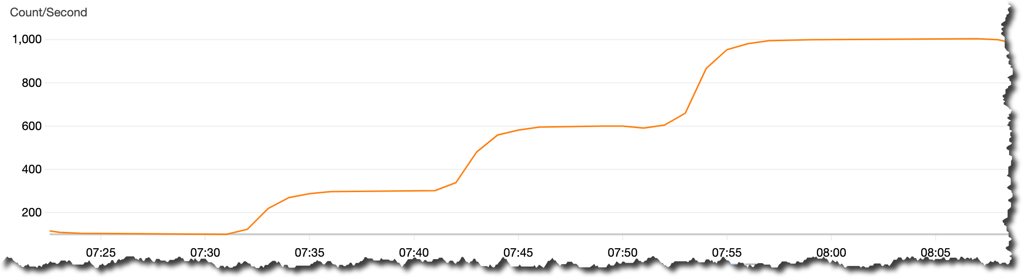
Mainframe offloading and modernization: Using mainframe data to build cloud native services with AWS

Post Syndicated from Malathi Pinnamaneni original https://aws.amazon.com/blogs/architecture/mainframe-offloading-and-modernization-using-mainframe-data-to-build-cloud-native-services-with-aws/

Many companies in the financial services and insurance industries rely on mainframes for their most business-critical applications and data. But mainframe workloads typically lack agility. This is one reason that organizations struggle to innovate, iterate, and pivot quickly to develop new applications or release new capabilities. Unlocking this mainframe data can be the first step in your modernization journey.

In this blog post, we will discuss some typical offloading patterns. Whether your goal is developing new applications using mainframe data or modernizing with the Strangler Fig Application pattern, you might want some guidance on how to begin.

Refactoring mainframe applications to the cloud

Refactoring mainframe applications to cloud-native services on AWS is a common industry pattern and a long-term goal for many companies to remain competitive. But this takes an investment of time, money, and organizational change management to realize the full benefits. We see customers start their modernization journey by offloading data from the mainframe to AWS to reduce risks and create new capabilities.

The mainframe data offloading patterns that we will discuss in this post use software services that facilitate data replication to Amazon Web Services (AWS):

  • File-based data synchronization
  • Change data capture
  • Event-sourced replication

Once data is liberated from the mainframe, you can develop new agile applications for deeper insights using analytics and machine learning (ML). You could create a microservices-based, or voice-based mobile application. For example, if a bank could access their historical mainframe data to analyze customer behavior, they could develop a new solution based on profiles to use for loan recommendations.

The patterns we illustrate can be used as a reference to begin your modernization efforts with reduced risk. The long-term goal is to rewrite the mainframe applications and modernize them workload by workload.

Solution overview: Mainframe offloading and modernization

This figure shows the flow of data being replicated from mainframe using integration services and consumed in AWS

Figure 1. Mainframe offloading and modernization conceptual flow

Mainframe modernization: Architecture reference patterns

File-based batch integration

Modernization scenarios often require replicating files to AWS, or synchronizing between on-premises and AWS. Use cases include:

  • Analyzing current and historical data to enhance business analytics
  • Providing data for further processing on downstream or upstream dependent systems. This is necessary for exchanging data between applications running on the mainframe and applications running on AWS
This diagram shows a file-based integration pattern on how data can be replicated to AWS for interactive data analytics

Figure 2. File-based batch ingestion pattern for interactive data analytics

File-based batch integration – Batch ingestion for interactive data analytics (Figure 2)

  1. Data ingestion. In this example, we show how data can be ingested to Amazon S3 using AWS Transfer Family Services or AWS DataSync. Mainframe data is typically encoded in extended binary-coded decimal interchange code (EBCDIC) format. Prescriptive guidance exists to convert EBCDIC to ASCII format.
  2. Data transformation. Before moving data to AWS data stores, transformation of the data may be necessary to use it for analytics. AWS analytics services like AWS Glue and AWS Lambda can be used to transform the data. For large volume processing, use Apache Spark on AWS Elastic Map Reduce (Amazon EMR), or a custom Spring Boot application running on Amazon EC2 to perform these transformations. This process can be orchestrated using AWS Step Functions or AWS Data Pipeline.
  3. Data store. Data is transformed into a consumable format that can be stored in Amazon S3.
  4. Data consumption. You can use AWS analytics services like Amazon Athena for interactive ad-hoc query access, Amazon QuickSight for analytics, and Amazon Redshift for complex reporting and aggregations.
This diagram shows a file-based integration pattern on how data can be replicated to AWS for further processing by downstream systems

Figure 3. File upload to operational data stores for further processing

File-based batch integration – File upload to operational data stores for further processing (Figure 3)

  1. Using AWS File Transfer Services, upload CSV files to Amazon S3.
  2. Once the files are uploaded, S3’s event notification can invoke AWS Lambda function to load to Amazon Aurora. For low latency data access requirements, you can use a scalable serverless import pattern with AWS Lambda and Amazon SQS to load into Amazon DynamoDB.
  3. Once the data is in data stores, it can be consumed for further processing.

Transactional replication-based integration (Figure 4)

Several modernization scenarios require continuous near-real-time replication of relational data to keep a copy of the data in the cloud. Change Data Capture (CDC) for near-real-time transactional replication works by capturing change log activity to drive changes in the target dataset. Use cases include:

  • Command Query Responsibility Segregation (CQRS) architectures that use AWS to service all read-only and retrieve functions
  • On-premises systems with tightly coupled applications that require a phased modernization
  • Real-time operational analytics
This diagram shows a transaction-based replication (CDC) integration pattern on how data can be replicated to AWS for building reporting and read-only functions

Figure 4. Transactional replication (CDC) pattern

  1. Partner CDC tools in the AWS Marketplace can be used to manage real-time data movement between the mainframe and AWS.
  2. You can use a fan-out pattern to read once from the mainframe to reduce processing requirements and replicate data to multiple data stores based on your requirements:
    • For low latency requirements, replicate to Amazon Kinesis Data Streams and use AWS Lambda to store in Amazon DynamoDB.
    • For critical business functionality with complex logic, use Amazon Aurora or Amazon Relational Database Service (RDS) as targets.
    • To build data lake or use as an intermediary for ETL processing, customers can replicate to S3 as target.
  3. Once the data is in AWS, customers can build agile microservices for read-only functions.

Message-oriented middleware (event sourcing) integration (Figure 5)

With message-oriented middleware (MOM) systems like IBM MQ on mainframe, several modernization scenarios require integrating with cloud-based streaming and messaging services. These act as a buffer to keep your data in sync. Use cases include:

  • Consume data from AWS data stores to enable new communication channels. Examples of new channels can be mobile or voice-based applications and can be innovations based on ML
  • Migrate the producer (senders) and consumer (receivers) applications communicating with on-premises MOM platforms to AWS with an end goal to retire on-premises MOM platform
This diagram shows an event-sourcing integration reference pattern for customers using middleware systems like IBM MQ on-premises with AWS services

Figure 5. Event-sourcing integration pattern

  1. Mainframe transactions from IBM MQ can be read using a connector or a bridge solution. They can then be published to Amazon MQ queues or Amazon Managed Streaming for Apache Kakfa (MSK) topics.
  2. Once the data is published to the queue or topic, consumers encoded in AWS Lambda functions or Amazon compute services can process, map, transform, or filter the messages. They can store the data in Amazon RDS, Amazon ElastiCache, S3, or DynamoDB.
  3. Now that the data resides in AWS, you can build new cloud-native applications and do the following:

Conclusion

Mainframe offloading and modernization using AWS services enables you to reduce cost, modernize your architectures, and integrate your mainframe and cloud-native technologies. You’ll be able to inform your business decisions with improved analytics, and create new opportunities for innovation and the development of modern applications.

More posts for Women’s History Month!

Other ways to participate

Create a low-latency source-to-data lake pipeline using Amazon MSK Connect, Apache Flink, and Apache Hudi

Post Syndicated from Ali Alemi original https://aws.amazon.com/blogs/big-data/create-a-low-latency-source-to-data-lake-pipeline-using-amazon-msk-connect-apache-flink-and-apache-hudi/

During the recent years, there has been a shift from monolithic to the microservices architecture. The microservices architecture makes applications easier to scale and quicker to develop, enabling innovation and accelerating time to market for new features. However, this approach causes data to live in different silos, which makes it difficult to perform analytics. To gain deeper and richer insights, you should bring all your data from different silos into one place.

AWS offers replication tools such as AWS Database Migration Service (AWS DMS) to replicate data changes from a variety of source databases to various destinations including Amazon Simple Storage Service (Amazon S3). But customers who need to sync the data in a data lake with updates and deletes on the source systems still face a few challenges:

  • It’s difficult to apply record-level updates or deletes when records are stored in open data format files (such as JSON, ORC, or Parquet) on Amazon S3.
  • In streaming use cases, where jobs need to write data with low latency, row-based formats such as JSON and Avro are best suited. However, scanning many small files with these formats degrades the read query performance.
  • In use cases where the schema of the source data changes frequently, maintaining the schema of the target datasets via custom code is difficult and error-prone.

Apache Hudi provides a good way to solve these challenges. Hudi builds indexes when it writes the records for the first time. Hudi uses these indexes to locate the files to which an update (or delete) belongs. This enables Hudi to perform fast upsert (or delete) operations by avoiding the need to scan the whole dataset. Hudi provides two table types, each optimized for certain scenarios:

  • Copy-On-Write (COW) – These tables are common for batch processing. In this type, data is stored in a columnar format (Parquet), and each update (or delete) creates a new version of files during the write.
  • Merge-On-Read (MOR) – Stores Data using a combination of columnar (for example Parquet) and row-based (for example Avro) file formats and is intended to expose near-real time data.

Hudi datasets stored in Amazon S3 provide native integration with other AWS services. For example, you can write Apache Hudi tables using AWS Glue (see Writing to Apache Hudi tables using AWS Glue Custom Connector) or Amazon EMR (see New features from Apache Hudi available in Amazon EMR). Those approaches require having a deep understanding of Hudi’s Spark APIs and programming skills to build and maintain data pipelines.

In this post, I show you a different way of working with streaming data with minimum coding. The steps in this post demonstrate how to build fully scalable pipelines using SQL language without prior knowledge of Flink or Hudi. You can query and explore your data in multiple data streams by writing familiar SELECT queries. You can join the data from multiple streams and materialize the result to a Hudi dataset on Amazon S3.

Solution overview

The following diagram provides an overall architecture of the solution described in this post. I describe the components and steps fully in the sections that follow.

You use an Amazon Aurora MySQL database as the source and a Debezium MySQL connector with the setup described in the MSK Connect lab as the change data capture (CDC) replicator. This lab walks you through the steps to set up the stack for replicating an Aurora database salesdb to an Amazon Managed Streaming for Apache Kafka (Amazon MSK) cluster, using Amazon MSK Connect with a MySql Debezium source Kafka connector.

In September 2021, AWS announced MSK Connect for running fully managed Kafka Connect clusters. With a few clicks, MSK Connect allows you to easily deploy, monitor, and scale connectors that move data in and out of Apache Kafka and MSK clusters from external systems such as databases, file systems, and search indexes. You can now use MSK Connect for building a full CDC pipeline from many database sources to your MSK cluster.

Amazon MSK is a fully managed service that makes it easy to build and run applications that use Apache Kafka to process streaming data. When you use Apache Kafka, you capture real-time data from sources such as database change events or website clickstreams. Then you build pipelines (using stream processing frameworks such as Apache Flink) to deliver them to destinations such as a persistent storage or Amazon S3.

Apache Flink is a popular framework for building stateful streaming and batch pipelines. Flink comes with different levels of abstractions to cover a broad range of use cases. See Flink Concepts for more information.

Flink also offers different deployment modes depending on which resource provider you choose (Hadoop YARN, Kubernetes, or standalone). See Deployment for more information.

In this post, you use the SQL Client tool as an interactive way of authoring Flink jobs in SQL syntax. sql-client.sh compiles and submits jobs to a long-running Flink cluster (session mode) on Amazon EMR. Depending on the script, sql-client.sh either shows the tabular formatted output of the job in real time, or returns a job ID for long-running jobs.

You implement the solution with the following high-level steps:

  1. Create an EMR cluster.
  2. Configure Flink with Kafka and Hudi table connectors.
  3. Develop your real-time extract, transform, and load (ETL) job.
  4. Deploy your pipeline to production.

Prerequisites

This post assumes you have a running MSK Connect stack in your environment with the following components:

  • Aurora MySQL hosting a database. In this post, you use the example database salesdb.
  • The Debezium MySQL connector running on MSK Connect, ending in Amazon MSK in your Amazon Virtual Private Cloud (Amazon VPC).
  • An MSK cluster running within in a VPC.

If you don’t have an MSK Connect stack, follow the instructions in the MSK Connect lab setup and verify that your source connector replicates data changes to the MSK topics.

You also need the ability to connect directly to the EMR leader node. Session Manager is a feature of AWS Systems Manager that provides you with an interactive one-click browser-based shell window. Session Manager also allows you to comply with corporate policies that require controlled access to managed nodes. See Setting up Session Manager to learn how to connect to your managed nodes in your account via this method.

If Session Manager is not an option, you can also use Amazon Elastic Compute Cloud (Amazon EC2) private key pairs, but you’ll need to launch the cluster in a public subnet and provide inbound SSH access. See Connect to the master node using SSH for more information.

Create an EMR cluster

The latest released version of Apache Hudi is 0.10.0, at the time of writing. Hudi release version 0.10.0 is compatible with Flink release version 1.13. You need Amazon EMR release version emr-6.4.0 and later, which comes with Flink release version 1.13. To launch a cluster with Flink installed using the AWS Command Line Interface (AWS CLI), complete the following steps:

  1. Create a file, configurations.json, with the following content:
    [
        {
          "Classification": "flink-conf",
          "Properties": {
            "taskmanager.numberOfTaskSlots":"4"
          }
        }
    ]

  2. Create an EMR cluster in a private subnet (recommended) or in a public subnet of the same VPC as where you host your MSK cluster. Enter a name for your cluster with the --name option, and specify the name of your EC2 key pair as well as the subnet ID with the --ec2-attributes option. See the following code:
    aws emr create-cluster --release-label emr-6.4.0 \
    --applications Name=Flink \
    --name FlinkHudiCluster \
    --configurations file://./configurations.json \
    --region us-east-1 \
    --log-uri s3://yourLogUri \
    --instance-type m5.xlarge \
    --instance-count 2 \
    --service-role EMR_DefaultRole \ 
    --ec2-attributes KeyName=YourKeyName,InstanceProfile=EMR_EC2_DefaultRole, SubnetId=A SubnetID of Amazon MSK VPC 

  3. Wait until the cluster state changes to Running.
  4. Retrieve the DNS name of the leader node using either the Amazon EMR console or the AWS CLI.
  5. Connect to the leader node via Session Manager or using SSH and an EC2 private key on Linux, Unix, and Mac OS X.
  6. When connecting using SSH, port 22 must be allowed by the leader node’s security group.
  7. Make sure the MSK cluster’s security group has an inbound rules that accepts traffic from the EMR cluster’s security groups.

Configure Flink with Kafka and Hudi table connectors

Flink table connectors allow you to connect to external systems when programming your stream operations using Table APIs. Source connectors provide access to streaming services including Kinesis or Apache Kafka as a data source. Sink connectors allow Flink to emit stream processing results to external systems or storage services like Amazon S3.

On your Amazon EMR leader node, download the following connectors and save them in the /lib/flink/lib directory:

  • Source connector – Download flink-connector-kafka_2.11-1.13.1.jar from the Apache repository. The Apache Kafka SQL connector allows Flink to read data from Kafka topics.
  • Sink connector – Amazon EMR release version emr-6.4.0 comes with Hudi release version 0.8.0. However, in this post you need Hudi Flink bundle connector release version 0.10.0, which is compatible with Flink release version 1.13. Download hudi-flink-bundle_2.11-0.10.0.jar from the Apache repository. It also contains multiple file system clients, including S3A for integrating with Amazon S3.

Develop your real-time ETL job

In this post, you use the Debezium source Kafka connector to stream data changes of a sample database, salesdb, to your MSK cluster. Your connector produces data changes in JSON. See Debezium Event Deserialization for more details. The Flink Kafka connector can deserialize events in JSON format by setting value.format with debezium-json in the table options. This configuration provides the full support for data updates and deletes, in addition to inserts.

You build a new job using Flink SQL APIs. These APIs allow you to work with the streaming data, similar to tables in relational databases. SQL queries specified in this method run continuously over the data events in the source stream. Because the Flink application consumes unbounded data from a stream, the output constantly changes. To send the output to another system, Flink emits update or delete events to the downstream sink operators. Therefore, when you work with CDC data or write SQL queries where the output rows need to update or delete, you must provide a sink connector that supports these actions. Otherwise, the Flink job ends with an error with the following message:

Target Table doesn't support consuming update or delete changes which is produced by {your query statement} …

Launch the Flink SQL client

Start a Flink YARN application on your EMR cluster with the configurations you previously specified in the configurations.json file:

cd /lib/flink && ./bin/yarn-session.sh --detached

After the command runs successfully, you’re ready to write your first job. Run the following command to launch sql-client:

./bin/sql-client.sh

Your terminal window looks like the following screenshot.

Set the job parameters

Run the following command to set the checkpointing interval for this session:

SET execution.checkpointing.interval = 1min;

Define your source tables

Conceptually, processing streams using SQL queries requires interpreting the events as logical records in a table. Therefore, the first step before reading or writing the data with SQL APIs is to create source and target tables. The table definition includes the connection settings and configuration along with a schema that defines the structure and the serialization format of the objects in the stream.

In this post, you create three source tables. Each corresponds to a topic in Amazon MSK. You also create a single target table that writes the output data records to a Hudi dataset stored on Amazon S3.

Replace BOOTSTRAP SERVERS ADDRESSES with your own Amazon MSK cluster information in the 'properties.bootstrap.servers' option and run the following commands in your sql-client terminal:

CREATE TABLE CustomerKafka (
      `event_time` TIMESTAMP(3) METADATA FROM 'value.source.timestamp' VIRTUAL,  -- from Debezium format
      `origin_table` STRING METADATA FROM 'value.source.table' VIRTUAL, -- from Debezium format
      `record_time` TIMESTAMP(3) METADATA FROM 'value.ingestion-timestamp' VIRTUAL,
      `CUST_ID` BIGINT,
      `NAME` STRING,
      `MKTSEGMENT` STRING,
       WATERMARK FOR event_time AS event_time
    ) WITH (
      'connector' = 'kafka',
      'topic' = 'salesdb.salesdb.CUSTOMER', -- created by debezium connector, corresponds to CUSTOMER table in Amazon Aurora database. 
      'properties.bootstrap.servers' = '<PLAINTEXT BOOTSTRAP SERVERS ADDRESSES>',
      'properties.group.id' = 'ConsumerGroup1',
      'scan.startup.mode' = 'earliest-offset',
      'value.format' = 'debezium-json'
    );

CREATE TABLE CustomerSiteKafka (
      `event_time` TIMESTAMP(3) METADATA FROM 'value.source.timestamp' VIRTUAL,  -- from Debezium format
      `origin_table` STRING METADATA FROM 'value.source.table' VIRTUAL, -- from Debezium format
      `record_time` TIMESTAMP(3) METADATA FROM 'value.ingestion-timestamp' VIRTUAL,
      `CUST_ID` BIGINT,
      `SITE_ID` BIGINT,
      `STATE` STRING,
      `CITY` STRING,
       WATERMARK FOR event_time AS event_time
    ) WITH (
      'connector' = 'kafka',
      'topic' = 'salesdb.salesdb.CUSTOMER_SITE',
      'properties.bootstrap.servers' = '< PLAINTEXT BOOTSTRAP SERVERS ADDRESSES>',
      'properties.group.id' = 'ConsumerGroup2',
      'scan.startup.mode' = 'earliest-offset',
      'value.format' = 'debezium-json'
    );

CREATE TABLE SalesOrderAllKafka (
      `event_time` TIMESTAMP(3) METADATA FROM 'value.source.timestamp' VIRTUAL,  -- from Debezium format
      `origin_table` STRING METADATA FROM 'value.source.table' VIRTUAL, -- from Debezium format
      `record_time` TIMESTAMP(3) METADATA FROM 'value.ingestion-timestamp' VIRTUAL,
      `ORDER_ID` BIGINT,
      `SITE_ID` BIGINT,
      `ORDER_DATE` BIGINT,
      `SHIP_MODE` STRING,
       WATERMARK FOR event_time AS event_time
    ) WITH (
      'connector' = 'kafka',
      'topic' = 'salesdb.salesdb.SALES_ORDER_ALL',
      'properties.bootstrap.servers' = '< PLAINTEXT BOOTSTRAP SERVERS ADDRESSES>',
      'properties.group.id' = 'ConsumerGroup3',
      'scan.startup.mode' = 'earliest-offset',
      'value.format' = 'debezium-json'
    );

By default, sql-client stores these tables in memory. They only live for the duration of the active session. Anytime your sql-client session expires, or you exit, you need to recreate your tables.

Define the sink table

The following command creates the target table. You specify 'hudi' as the connector in this table. The rest of the Hudi configurations are set in the with(…) section of the CREATE TABLE statement. See the full list of Flink SQL configs to learn more. Replace S3URI OF HUDI DATASET LOCATION with your Hudi dataset location in Amazon S3 and run the following code:

CREATE TABLE CustomerHudi (
      `order_count` BIGINT,
      `customer_id` BIGINT,
      `name` STRING,
      `mktsegment` STRING,
      `ts` TIMESTAMP(3),
      PRIMARY KEY (`customer_id`) NOT Enforced
    )
    PARTITIONED BY (`mktsegment`)
    WITH (
      'connector' = 'hudi',
      'write.tasks' = '4',
      'path' = '<S3URI OF HUDI DATASET LOCATION>',
      'table.type' = 'MERGE_ON_READ' --  MERGE_ON_READ table or, by default is COPY_ON_WRITE
    );

Verify the Flink job’s results from multiple topics

For select queries, sql-client submits the job to a Flink cluster, then displays the results on the screen in real time. Run the following select query to view your Amazon MSK data:

SELECT Count(O.order_id) AS order_count,
       C.cust_id,
       C.NAME,
       C.mktsegment
FROM   customerkafka C
       JOIN customersitekafka CS
         ON C.cust_id = CS.cust_id
       JOIN salesorderallkafka O
         ON O.site_id = CS.site_id
GROUP  BY C.cust_id,
          C.NAME,
          C.mktsegment; 

This query joins three streams and aggregates the count of customer orders, grouped by each customer record. After a few seconds, you should see the result in your terminal. Note how the terminal output changes as the Flink job consumes more events from the source streams.

Sink the result to a Hudi dataset

To have a complete pipeline, you need to send the result to a Hudi dataset on Amazon S3. To do that, add an insert into CustomerHudi statement in front of the select query:

INSERT INTO customerhudi
SELECT Count(O.order_id),
       C.cust_id,
       C.NAME,
       C.mktsegment,
       Proctime()
FROM   customerkafka C
       JOIN customersitekafka CS
         ON C.cust_id = CS.cust_id
       JOIN salesorderallkafka O
         ON O.site_id = CS.site_id
GROUP  BY C.cust_id,
          C.NAME,
          C.mktsegment;

This time, the sql-client disconnects from the cluster after submitting the job. The client terminal doesn’t have to wait for the results of the job as it sinks its results to a Hudi dataset. The job continues to run on your Flink cluster even after you stop the sql-client session.

Wait a few minutes until the job generates Hudi commit log files to Amazon S3. Then navigate to the location in Amazon S3 you specified for your CustomerHudi table, which contains a Hudi dataset partitioned by MKTSEGMENT column. Within each partition you also find Hudi commit log files. This is because you defined the table type as MERGE_ON_READ. In this mode with the default configurations, Hudi merges commit logs to larger Parquet files after five delta commit logs occur. Refer to Table & Query Types for more information. You can change this setup by changing the table type to COPY_ON_WRITE or specifying your custom compaction configurations.

Query the Hudi dataset

You may also use a Hudi Flink connector as a source connector to read from a Hudi dataset stored on Amazon S3. You do that by running a select statement against the CustomerHudi table, or create a new table with hudi specified for connector. The path must point to an existing Hudi dataset’s location on Amazon S3. Replace S3URI OF HUDI DATASET LOCATION with your location and run the following command to create a new table:

CREATE TABLE `CustomerHudiReadonly` (
      `_hoodie_commit_time` string,
      `_hoodie_commit_seqno` string,
      `_hoodie_record_key` string,
      `order_count` BIGINT,
      `customer_id` BIGINT,
      `name` STRING,
      `mktsegment` STRING,
      `ts` TIMESTAMP(3),
      PRIMARY KEY (`customer_id`) NOT Enforced
    )
    PARTITIONED BY (`mktsegment`)
    WITH (
      'connector' = 'hudi',
      'hoodie.datasource.query.type' = 'snapshot',
      'path' = '<S3URI OF HUDI DATASET LOCATION>',
     'table.type' = 'MERGE_ON_READ' --  MERGE_ON_READ table or, by default is COPY_ON_WRITE
    );

Note the additional column names prefixed with _hoodie_. These columns are added by Hudi during the write to maintain the metadata of each record. Also note the extra 'hoodie.datasource.query.type'  read configuration passed in the WITH portion of the table definition. This makes sure you read from the real-time view of your Hudi dataset. Run the following command:

Select * from CustomerHudiReadonly where customer_id <= 5;

The terminal displays the result within 30 seconds. Navigate to the Flink web interface, where you can observe a new Flink job started by the select query (See below for how to find the Flink web interface). It scans the committed files in the Hudi dataset and returns the result to the Flink SQL client.

Use a mysql CLI or your preferred IDE to connect to your salesdb database, which is hosted on Aurora MySQL. Run a few insert statements against the SALES_ORDER_ALL table:

insert into SALES_ORDER_ALL values (29001, 2, now(), 'STANDARD');
insert into SALES_ORDER_ALL values (29002, 2, now(), 'TWO-DAY');
insert into SALES_ORDER_ALL values (29003, 2, now(), 'STANDARD');
insert into SALES_ORDER_ALL values (29004, 2, now(), 'TWO-DAY');
insert into SALES_ORDER_ALL values (29005, 2, now(), 'STANDARD');

After a few seconds, a new commit log file appears in your Hudi dataset on Amazon S3. The Debezium for MySQL Kafka connector captures the changes and produces events to the MSK topic. The Flink application consumes the new events from the topic and updates the customer_count column accordingly. It then sends the changed records to the Hudi connector for merging with the Hudi dataset.

Hudi supports different write operation types. The default operation is upsert, where it initially inserts the records in the dataset. When a record with an existing key arrives in a process, it’s treated as an update. This operation is useful here where you expect to sync your dataset with the source database, and duplicate records are not expected.

Find the Flink web interface

The Flink web interface helps you view a Flink job’s configuration, graph, status, exception errors, resource utilization, and more. To access it, first you need to set up an SSH tunnel and activate a proxy in your browser, to connect to the YARN Resource Manager. After you connect to the Resource Manager, you choose the YARN application that’s hosting your Flink session. Choose the link under the Tracking UI column to navigate to the Flink web interface. For more information, see Finding the Flink web interface.

Deploy your pipeline to production

I recommend using Flink sql-client for quickly building data pipelines in an interactive way. It’s a good choice for experiments, development, or testing your data pipelines. For production environments, however, I recommend embedding your SQL scripts in a Flink Java application and running it on Amazon Kinesis Data Analytics. Kinesis Data Analytics is a fully managed service for running Flink applications; it has built-in auto scaling and fault tolerance features to provide your production applications the availability and scalability they need. A Flink Hudi application with the scripts from this this post is available on GitHub. I encourage you to visit this repo, and compare the differences between running in sql-client and Kinesis Data Analytics.

Clean up

To avoid incurring ongoing charges, complete the following cleanup steps:

  1. Stop the EMR cluster.
  2. Delete the AWS CloudFormation stack you created using the MSK Connect Lab setup.

Conclusion

Building a data lake is the first step to break down data silos and running analytics to gain insights from all your data. Syncing the data between the transactional databases and data files on a data lake isn’t trivial and involves significant effort. Before Hudi added support for Flink SQL APIs, Hudi customers had to have the necessary skills for writing Apache Spark code and running it on AWS Glue or Amazon EMR. In this post, I showed you a new way in which you can interactively explore your data in streaming services using SQL queries, and accelerate the development process for your data pipelines.

To learn more, visit Hudi on Amazon EMR documentation.


About the Author

Ali Alemi is a Streaming Specialist Solutions Architect at AWS. Ali advises AWS customers with architectural best practices and helps them design real-time analytics data systems which are reliable, secure, efficient, and cost-effective. He works backward from customer’s use cases and designs data solutions to solve their business problems. Prior to joining AWS, Ali supported several public sector customers and AWS consulting partners in their application modernization journey and migration to the Cloud.

Scaling DLT to 1M TPS on AWS: Optimizing a Regulated Liabilities Network

Post Syndicated from Erica Salinas original https://aws.amazon.com/blogs/architecture/scaling-dlt-to-1m-tps-on-aws-optimizing-a-regulated-liabilities-network/

SETL is an open source, distributed ledger technology (DLT) company that enables tokenisation, digital custody, and DLT for securities markets and payments. In mid-2021, they developed a blueprint for a Regulated Liabilities Network (RLN) that enables holding and managing a variety of tokenized value irrespective of its form. In a December 2021 collaboration with Amazon Web Services (AWS), SETL demonstrated that their RLN platform could support one million transactions per second. These findings were published in their whitepaper, The Regulated Liability Network: Whitepaper on scalability and performance.

This AWS-hosted architecture scaled each processing component and the complete transaction flow. It was built using Amazon Elastic Kubernetes Service (EKS), Amazon Elastic Cloud Compute (EC2), and Amazon Managed Streaming for Apache Kafka (MSK).

This post discusses the technical implementation of the simulated network. We show how scaling characteristics were achieved, while maintaining the business requirements of atomicity and finality. We also discuss how each RLN component was optimized for high performance.

Background: What is an RLN?

In The Regulated Internet of Value, Tony McLaughlin of Citi proposed a single network to record ownership of multiple token types, each which represents a liability of a regulated entity. The RLN would give commercial banks, e-money providers, and central banks, the ability to issue liabilities and immutably record all balances and owners. Because it is designed to maintain a globally sequenced set of state changes, an unambiguous ledger of token balances can be computed and updated. Transactions, which result in two or more ledger updates, are proposed to the network. They are authorized by all impacted network participants, ordered for distribution to participant ledgers, and then persisted by multiple participant ledgers. This process is completed with five processing components.

Figure 1. Core components and queues of RLN

Figure 1. Core components and queues of RLN

Given the existing performance limitations faced by many DLT platforms, a main concern with the network design was its ability to meet throughput requirements. SETL collaborated with AWS to define an architecture that integrated decoupled processing components, as shown in Figure 2. The target throughput was 1,000,000 TPS for each component through the simulated network.

Figure 2. Simulated RLN architecture in the AWS Cloud

Figure 2. Simulated RLN architecture in the AWS Cloud

A queue – process – queue architectural model

The basic architectural model applied was “queue – process – queue.” Each component consumed transactions from one or more Kafka topics, performed its requisite activities, and produced output to a second Kafka topic. Components of the message flow used Amazon EKS, Amazon EC2, and Amazon MSK.

Specific techniques were applied to achieve the scaling characteristics of components in the main message flow.

  • A distinct EKS-managed node group was used for each RLN component. Each node within the group had its own EC2 instance that housed at most two Kubernetes Pods. This technique decreased potential network throttling and enabled the monitoring of pod resource utilization using Amazon CloudWatch at the EC2 level. This aided in identifying bottlenecks, which can be challenging if large EC2 nodes house many Kubernetes Pods.
  • Each RLN queue component had its own dedicated Kafka cluster. By isolating the Kafka topics to their own cluster, we were able to scale and monitor the cluster individually. This decreased potential chokepoints.
  • A combination of eksctl, kubectl, and EC2 Auto Scaling groups was used to deploy and horizontally scale each RLN component. The tooling enabled rapid results by controlling pod configuration, automating deployments, and supporting multiple performance testing iterations.

Fine tuning RLN system components

The key metric tested was message throughput in transactions per second (TPS) consumed, processed, and produced for each component. An end-to-end test was performed, which measured throughput of the complete simulated network. Each RLN component was tuned to meet this metric as follows.

The Transaction Generator acted as the customer entering transactions into the system (see Figure 3.) The Kafka producer property buffer.memory was changed to 536870912 to simulate an increase in producer TPS for each component.

Figure 3. Simulated RLN Transaction Generator

Figure 3. Simulated RLN Transaction Generator

The Scheduler’s scaling technique was a dedicated Compute (one Pod/EC2 node) that listened to one Kafka partition in the Transaction Queue as seen in Figure 4. Additionally, turning on gzip compression (compression.type) on the producer resolved a network bottleneck for the downstream Kafka cluster.

Figure 4. Simulated RLN Scheduler

Figure 4. Simulated RLN Scheduler

The Approver’s scaling technique was like the Scheduler, however, the Proposal Queue had 10 topics as opposed to one. The approver is stateless, so it randomly selects a Kafka topic and partition to listen to. When scaling to 100 Kubernetes Pods, there would be roughly one Kafka partition per pod. As shown in Figure 5, each pod has its own EC2 instance. The Assembler’s scaling techniques were the same as for the Scheduler and Approver components.

Figure 5. Simulated RLN Approver

Figure 5. Simulated RLN Approver

The Sequencer, as designed, cannot scale horizontally due to the nature of the sequencing algorithm. However, without any special tuning of the Kafka consumer configuration or any significant increase in EC2 sizing, it was able to achieve one million TPS. Its architecture is shown in Figure 6.

Figure 6. Simulated RLN Sequencer

Figure 6. Simulated RLN Sequencer

The State Updater scaled with each Kubernetes Pod listening to an assigned Approved Proposal topic (one-to-one mapping) and receiving all sequenced hashes from the Hash Queue. Achieving 1 million TPS throughput required 10 nodes configured with c5.4xlarge, as seen in Figure 7.

Figure 7. Simulated RLN State Updater

Figure 7. Simulated RLN State Updater

Successful throughput testing

Test results demonstrate that each component can sustain over 1 million TPS. While horizontal scaling was applied, even a single instance achieved over 10,000 TPS. Individual component performance test results can be seen in Table 1.

Component Single Instance (TPS) # of Instances Multiple Instances (TPS)
Generator ~ 629,219 2 1,258,438
Scheduler ~11,019 100 1,101,928
Approver ~10,348 100 1,034,868
Assembler ~10,691 100 1,069,100
Sequencer ~1,052,845 1 N/A
State Updater ~100,256 10 1,002,569

Table 1. Test results per individual component

Network tests were performed with all components integrated to create a simulated RLN network. The tests were executed with transaction generation of ~1,000,000 TPS. Throughput was measured at the output of the final component’s (State Updater) instances (see Figure 8). It was also measured in aggregate at over 1.2 million TPS (see Figure 9).

Figure 8. Individual TPS for State Update component nodes

Figure 8. Individual TPS for State Update component nodes

Figure 9. Aggregate TPS for State Update component nodes

Figure 9. Aggregate TPS for State Update component nodes

While this study was designed to demonstrate capacity and throughput, the tests did replicate Kafka partitions across three Availability Zones in the selected AWS Region. Thus, testing demonstrated that the proposed architecture supports geographic resilience while meeting the throughput benchmark. Resiliency and security are areas of focus for testing in the next phases of architecting a production-ready version of RLN.

Looking forward

During the month of joint work between the SETL and AWS technical teams, we stood up and tuned basic RLN functionality. We successfully demonstrated the scalability of the environment to at least 1M TPS. By using Kafka queues and the horizontal and vertical scalability of AWS services, we addressed the primary concern of reaching production-level throughput.

The industry group collaborating on the RLN concept now has a solid technical foundation on which to build a production-ready RLN architecture. Future experimentation will include integration with financial institutions and technology partners that will provide the capabilities needed to build a successful RLN ecosystem.

Further explorations include enabling digital signing, verification at scale, and expanding the network to include financial institution environments integrated with their own RLN partitions.

Validate streaming data over Amazon MSK using schemas in cross-account AWS Glue Schema Registry

Post Syndicated from Vikas Bajaj original https://aws.amazon.com/blogs/big-data/validate-streaming-data-over-amazon-msk-using-schemas-in-cross-account-aws-glue-schema-registry/

Today’s businesses face an unprecedented growth in the volume of data. A growing portion of the data is generated in real time by IoT devices, websites, business applications, and various other sources. Businesses need to process and analyze this data as soon as it arrives to make business decisions in real time. Amazon Managed Streaming for Apache Kafka (Amazon MSK) is a fully managed service that enables building and running stream processing applications that use Apache Kafka to collect and process data in real time.

Stream processing applications using Apache Kafka don’t communicate with each other directly; they communicate via sending and receiving messages over Kafka topics. For stream processing applications to communicate efficiently and confidently, a message payload structure must be defined in terms of attributes and data types. This structure describes the schema applications use when sending and receiving messages. However, with a large number of producer and consumer applications, even a small change in schema (removing a field, adding a new field, or change in data type) may cause issues for downstream applications that are difficult to debug and fix.

Traditionally, teams have relied on change management processes (such as approvals and maintenance windows) or other informal mechanisms (documentation, emails, collaboration tools, and so on) to inform one another of data schema changes. However, these mechanisms don’t scale and are prone to mistakes. The AWS Glue Schema Registry allows you to centrally publish, discover, control, validate, and evolve schemas for stream processing applications. With the AWS Glue Schema Registry, you can manage and enforce schemas on data streaming applications using Apache Kafka, Amazon MSK, Amazon Kinesis Data Streams, Amazon Kinesis Data Analytics for Apache Flink, and AWS Lambda.

This post demonstrates how Apache Kafka stream processing applications validate messages using an Apache Avro schema stored in the AWS Glue Schema registry residing in a central AWS account. We use the AWS Glue Schema Registry SerDe library and Avro SpecificRecord to validate messages in stream processing applications while sending and receiving messages from a Kafka topic on an Amazon MSK cluster. Although we use an Avro schema for this post, the same approach and concept applies to JSON schemas as well.

Use case

Let’s assume a fictitious rideshare company that offers unicorn rides. To draw actionable insights, they need to process a stream of unicorn ride request messages. They expect rides to be very popular and want to make sure their solution can scale. They’re also building a central data lake where all their streaming and operation data is stored for analysis. They’re customer obsessed, so they expect to add new fun features to future rides, like choosing the hair color of your unicorn, and will need to reflect these attributes in the ride request messages. To avoid issues in downstream applications due to future schema changes, they need a mechanism to validate messages with a schema hosted in a central schema registry. Having schemas in a central schema registry makes it easier for the application teams to publish, validate, evolve, and maintain schemas in a single place.

Solution overview

The company uses Amazon MSK to capture and distribute the unicorn ride request messages at scale. They define an Avro schema for unicorn ride requests because it provides rich data structures, supports direct mapping to JSON, as well as a compact, fast, and binary data format. Because the schema was agreed in advance, they decided to use Avro SpecificRecord.SpecificRecord is an interface from the Avro library that allows the use of an Avro record as a POJO. This is done by generating a Java class (or classes) from the schema, by using avro-maven-plugin. They use AWS Identity and Access Management (IAM) cross-account roles to allow producer and consumer applications from the other AWS account to safely and securely access schemas in the central Schema Registry account.

The AWS Glue Schema Registry is in Account B, whereas the MSK cluster and Kafka producer and consumer applications are in Account A. We use the following two IAM roles to enable cross-account access to the AWS Glue Schema Registry. Apache Kafka clients in Account A assume a role in Account B using an identity-based policy because the AWS Glue Schema Registry doesn’t support resource-based policies.

  • Account A IAM role – Allows producer and consumer applications to assume an IAM role in Account B.
  • Account B IAM role – Trusts all IAM principals from Account A and allows them to perform read actions on the AWS Glue Schema Registry in Account B. In a real use case scenario, IAM principals that can assume cross-account roles should be scoped more specifically.

The following architecture diagram illustrates the solution:

The solution works as follows:

  1. A Kafka producer running in Account A assumes the cross-account Schema Registry IAM role in Account B by calling the AWS Security Token Service (AWS STS) assumeRole API.
  2. The Kafka producer retrieves the unicorn ride request Avro schema version ID from the AWS Glue Schema Registry for the schema that’s embedded in the unicorn ride request POJO. Fetching the schema version ID is internally managed by the AWS Glue Schema Registry SerDe’s serializer. The serializer has to be configured as part of the Kafka producer configuration.
  3. If the schema exists in the AWS Glue Schema Registry, the serializer decorates the data record with the schema version ID and then serializes it before delivering it to the Kafka topic on the MSK cluster.
  4. The Kafka consumer running in Account A assumes the cross-account Schema Registry IAM role in Account B by calling the AWS STS assumeRole API.
  5. The Kafka consumer starts polling the Kafka topic on the MSK cluster for data records.
  6. The Kafka consumer retrieves the unicorn ride request Avro schema from the AWS Glue Schema Registry, matching the schema version ID that’s encoded in the unicorn ride request data record. Fetching the schema is internally managed by the AWS Glue Schema Registry SerDe’s deserializer. The deserializer has to be configured as part of the Kafka consumer configuration. If the schema exists in the AWS Glue Schema Registry, the deserializer deserializes the data record into the unicorn ride request POJO for the consumer to process it.

The AWS Glue Schema Registry SerDe library also supports optional compression configuration to save on data transfers. For more information about the Schema Registry, see How the Schema Registry works.

Unicorn ride request Avro schema

The following schema (UnicornRideRequest.avsc) defines a record representing a unicorn ride request, which contains ride request attributes along with the customer attributes and system-recommended unicorn attributes:

{
    "type": "record",
    "name": "UnicornRideRequest",
    "namespace": "demo.glue.schema.registry.avro",
    "fields": [
      {"name": "request_id", "type": "int", "doc": "customer request id"},
      {"name": "pickup_address","type": "string","doc": "customer pickup address"},
      {"name": "destination_address","type": "string","doc": "customer destination address"},
      {"name": "ride_fare","type": "float","doc": "ride fare amount (USD)"},
      {"name": "ride_duration","type": "int","doc": "ride duration in minutes"},
      {"name": "preferred_unicorn_color","type": {"type": "enum","name": "UnicornPreferredColor","symbols": ["WHITE","BLACK","RED","BLUE","GREY"]}, "default": "WHITE"},
      {
        "name": "recommended_unicorn",
        "type": {
          "type": "record",
          "name": "RecommendedUnicorn",
          "fields": [
            {"name": "unicorn_id","type": "int", "doc": "recommended unicorn id"},
            {"name": "color","type": {"type": "enum","name": "unicorn_color","symbols": ["WHITE","RED","BLUE"]}},
            {"name": "stars_rating", "type": ["null", "int"], "default": null, "doc": "unicorn star ratings based on customers feedback"}
          ]
        }
      },
      {
        "name": "customer",
        "type": {
          "type": "record",
          "name": "Customer",
          "fields": [
            {"name": "customer_account_no","type": "int", "doc": "customer account number"},
            {"name": "first_name","type": "string"},
            {"name": "middle_name","type": ["null","string"], "default": null},
            {"name": "last_name","type": "string"},
            {"name": "email_addresses","type": ["null", {"type":"array", "items":"string"}]},
            {"name": "customer_address","type": "string","doc": "customer address"},
            {"name": "mode_of_payment","type": {"type": "enum","name": "ModeOfPayment","symbols": ["CARD","CASH"]}, "default": "CARD"},
            {"name": "customer_rating", "type": ["null", "int"], "default": null}
          ]
        }
      }
    ]
  }

Prerequisites

To use this solution, you must have two AWS accounts:

  • Account A – For the MSK cluster, Kafka producer and consumer Amazon Elastic Compute Cloud (Amazon EC2) instances, and AWS Cloud9 environment
  • Account B – For the Schema Registry and schema

For this solution, we use Region us-east-1, but you can change this as per your requirements.

Next, we create the resources in each account using AWS CloudFormation templates.

Create resources in Account B

We create the following resources in Account B:

  • A schema registry
  • An Avro schema
  • An IAM role with the AWSGlueSchemaRegistryReadonlyAccess managed policy and an instance profile, which allows all Account A IAM principals to assume it
  • The UnicornRideRequest.avsc Avro schema shown earlier, which is used as a schema definition in the CloudFormation template

Make sure you have the appropriate permissions to create these resources.

  1. Log in to Account B.
  2. Launch the following CloudFormation stack.
  3. For Stack name, enter SchemaRegistryStack.
  4. For Schema Registry name, enter unicorn-ride-request-registry.
  5. For Avro Schema name, enter unicorn-ride-request-schema-avro.
  6. For the Kafka client’s AWS account ID, enter your Account A ID.
  7. For ExternalId, enter a unique random ID (for example, demo10A), which should be provided by the Kafka clients in Account A while assuming the IAM role in this account.

For more information about cross-account security, see The confused deputy problem.

  1. When the stack is complete, on the Outputs tab of the stack, copy the value for CrossAccountGlueSchemaRegistryRoleArn.

The Kafka producer and consumer applications created in Account A assume this role to access the Schema Registry and schema in Account B.

  1. To verify the resources were created, on the AWS Glue console, choose Schema registries in the navigation bar, and locate unicorn-ride-request-registry.
  2. Choose the registry unicorn-ride-request-registry and verify that it contains unicorn-ride-request-schema-avro in the Schemas section.
  3. Choose the schema to see its content.

The IAM role created by the SchemaRegistryStack stack allows all Account A IAM principals to assume it and perform read actions on the AWS Glue Schema Registry. Let’s look at the trust relationships of the IAM role.

  1. On the SchemaRegistryStack stack Outputs tab, copy the value for CrossAccountGlueSchemaRegistryRoleName.
  2. On the IAM console, search for this role.
  3. Choose Trust relationships and look at its trusted entities to confirm that Account A is listed.
  4. In the Conditions section, confirm that sts:ExternalId has the same unique random ID provided during stack creation.

Create resources in Account A

We create the following resources in Account A:

  • A VPC
  • EC2 instances for the Kafka producer and consumer
  • An AWS Cloud9 environment
  • An MSK cluster

As a prerequisite, create an EC2 keypair and download it on your machine to be able to SSH into EC2 instances. Also create an MSK cluster configuration with default values. You need to have permissions to create the CloudFormation stack, EC2 instances, AWS Cloud9 environment, MSK cluster, MSK cluster configuration, and IAM role.

  1. Log in to Account A.
  2. Launch the following CloudFormation stack to launch the VPC, EC2 instances, and AWS Cloud9 environment.
  3. For Stack name, enter MSKClientStack.
  4. Provide the VPC and subnet CIDR ranges.
  5. For EC2 Keypair, choose an existing EC2 keypair.
  6. For the latest EC2 AMI ID, select the default option.
  7. For the cross-account IAM role ARN, use the value for CrossAccountGlueSchemaRegistryRoleArn (available on the Outputs tab of SchemaRegistryStack).
  8. Wait for the stack to create successfully.
  9. Launch the following CloudFormation stack to create the MSK cluster.
  10. For Stack name, enter MSKClusterStack.
  11. Use Amazon MSK version 2.7.1.
  12. For the MSK cluster configuration ARN, enter the MSK cluster configuration ARN. One that you created as part of the prerequisite.
  13. For the MSK cluster configuration revision number, enter 1 or change it according to your version.
  14. For the client CloudFormation stack name, enter MSKClientStack (the stack name that you created prior to this stack).

Configure the Kafka producer

To configure the Kafka producer accessing the Schema Registry in the central AWS account, complete the following steps:

  1. Log in to Account A.
  2. On the AWS Cloud9 console, choose the Cloud9EC2Bastion environment created by the MSKClientStack stack.
  3. On the File menu, choose Upload Local Files.
  4. Upload the EC2 keypair file that you used earlier while creating the stack.
  5. Open a new terminal and change the EC2 keypair permissions:
    chmod 0400 <keypair PEM file>

  6. SSH into the KafkaProducerInstance EC2 instance and set the Region as per your requirement:
    ssh -i <keypair PEM file> ec2-user@<KafkaProducerInstance Private IP address>
    aws configure set region <region>

  7. Set the environment variable MSK_CLUSTER_ARN pointing to the MSK cluster’s ARN:
    export MSK_CLUSTER_ARN=$(aws kafka list-clusters |  jq '.ClusterInfoList[] | select (.ClusterName == "MSKClusterStack") | {ClusterArn} | join (" ")' | tr -d \")

Change the .ClusterName value in the code if you used a different name for the MSK cluster CloudFormation stack. The cluster name is the same as the stack name.

  1. Set the environment variable BOOTSTRAP_BROKERS pointing to the bootstrap brokers:
    export BOOTSTRAP_BROKERS=$(aws kafka get-bootstrap-brokers --cluster-arn $MSK_CLUSTER_ARN | jq -r .BootstrapBrokerString)

  2. Verify the environment variables:
    echo $MSK_CLUSTER_ARN
    echo $BOOTSTRAP_BROKERS

  3. Create a Kafka topic called unicorn-ride-request-topic in your MSK cluster, which is used by the Kafka producer and consumer applications later:
    cd ~/kafka
    
    ./bin/kafka-topics.sh --bootstrap-server $BOOTSTRAP_BROKERS \
    --topic unicorn-ride-request-topic \
    --create --partitions 3 --replication-factor 2
    
    ./bin/kafka-topics.sh --bootstrap-server $BOOTSTRAP_BROKERS --list

The MSKClientStack stack copied the Kafka producer client JAR file called kafka-cross-account-gsr-producer.jar to the KafkaProducerInstance instance. It contains the Kafka producer client that sends messages to the Kafka topic unicorn-ride-request-topic on the MSK cluster and accesses the unicorn-ride-request-schema-avro Avro schema from the unicorn-ride-request-registry schema registry in Account B. The Kafka producer code, which we cover later in this post, is available on GitHub.

  1. Run the following commands and verify kafka-cross-account-gsr-producer.jar exists:
    cd ~
    ls -ls

  2. Run the following command to run the Kafka producer in the KafkaProducerInstance terminal:
    java -jar kafka-cross-account-gsr-producer.jar -bs $BOOTSTRAP_BROKERS \
    -rn <Account B IAM role arn that Kafka producer application needs to assume> \
    -topic unicorn-ride-request-topic \
    -reg us-east-1 \
    -nm 500 \
    -externalid <Account B IAM role external Id that you used while creating a CF stack in Account B>

The code has the following parameters:

  • -bs$BOOTSTRAP_BROKERS (the MSK cluster bootstrap brokers)
  • -rn – The CrossAccountGlueSchemaRegistryRoleArn value from the SchemaRegistryStack stack outputs in Account B
  • -topic – the Kafka topic unicorn-ride-request-topic
  • -regus-east-1 (change it according to your Region, it’s used for the AWS STS endpoint and Schema Registry)
  • -nm: 500 (the number of messages the producer application sends to the Kafka topic)
  • -externalId – The same external ID (for example, demo10A) that you used while creating the CloudFormation stack in Account B

The following screenshot shows the Kafka producer logs showing Schema Version Id received..., which means it has retrieved the Avro schema unicorn-ride-request-schema-avro from Account B and messages were sent to the Kafka topic on the MSK cluster in Account A.

Kafka producer code

The complete Kafka producer implementation is available on GitHub. In this section, we break down the code.

  • getProducerConfig() initializes the producer properties, as shown in the following code:
    • VALUE_SERIALIZER_CLASS_CONFIG – The GlueSchemaRegistryKafkaSerializer.class.getName() AWS serializer implementation that serializes data records (the implementation is available on GitHub)
    • REGISTRY_NAME – The Schema Registry from Account B
    • SCHEMA_NAME – The schema name from Account B
    • AVRO_RECORD_TYPEAvroRecordType.SPECIFIC_RECORD
private Properties getProducerConfig() {
        Properties props = new Properties();
        props.put(ProducerConfig.BOOTSTRAP_SERVERS_CONFIG, this.bootstrapServers);
        props.put(ProducerConfig.ACKS_CONFIG, "-1");
        props.put(ProducerConfig.CLIENT_ID_CONFIG,"msk-cross-account-gsr-producer");
        props.put(ProducerConfig.KEY_SERIALIZER_CLASS_CONFIG, StringSerializer.class.getName());
        props.put(ProducerConfig.VALUE_SERIALIZER_CLASS_CONFIG, GlueSchemaRegistryKafkaSerializer.class.getName());
        props.put(AWSSchemaRegistryConstants.DATA_FORMAT, DataFormat.AVRO.name());
        props.put(AWSSchemaRegistryConstants.AWS_REGION,regionName);
        props.put(AWSSchemaRegistryConstants.REGISTRY_NAME, "unicorn-ride-request-registry");
        props.put(AWSSchemaRegistryConstants.SCHEMA_NAME, "unicorn-ride-request-schema-avro");
        props.put(AWSSchemaRegistryConstants.AVRO_RECORD_TYPE, AvroRecordType.SPECIFIC_RECORD.getName());
        return props;
}
  • startProducer() assumes the role in Account B to be able to connect with the Schema Registry in Account B and sends messages to the Kafka topic on the MSK cluster:
public void startProducer() {
        assumeGlueSchemaRegistryRole();
        KafkaProducer<String, UnicornRideRequest> producer = 
		new KafkaProducer<String,UnicornRideRequest>(getProducerConfig());
        int numberOfMessages = Integer.valueOf(str_numOfMessages);
        logger.info("Starting to send records...");
        for(int i = 0;i < numberOfMessages;i ++)
        {
            UnicornRideRequest rideRequest = getRecord(i);
            String key = "key-" + i;
            ProducerRecord<String, UnicornRideRequest> record = 
		new ProducerRecord<String, UnicornRideRequest>(topic, key, rideRequest);
            producer.send(record, new ProducerCallback());
        }
 }
  • assumeGlueSchemaRegistryRole() as shown in the following code uses AWS STS to assume the cross-account Schema Registry IAM role in Account B. (For more information, see Temporary security credentials in IAM.) The response from stsClient.assumeRole(roleRequest) contains the temporary credentials, which include accessKeyId, secretAccessKey, and a sessionToken. It then sets the temporary credentials in the system properties. The AWS SDK for Java uses these credentials while accessing the Schema Registry (through the Schema Registry serializer). For more information, see Using Credentials.
    public void assumeGlueSchemaRegistryRole() {
            try {
    	   Region region = Region.of(regionName);
                if(!Region.regions().contains(region))
                     throw new RuntimeException("Region : " + regionName + " is invalid.");
                StsClient stsClient = StsClient.builder().region(region).build();
                AssumeRoleRequest roleRequest = AssumeRoleRequest.builder()
                        .roleArn(this.assumeRoleARN)
                        .roleSessionName("kafka-producer-cross-account-glue-schemaregistry-demo")
    	           .externalId(this.externalId)	
                        .build();
                AssumeRoleResponse roleResponse = stsClient.assumeRole(roleRequest);
                Credentials myCreds = roleResponse.credentials();
                System.setProperty("aws.accessKeyId", myCreds.accessKeyId());
                System.setProperty("aws.secretAccessKey", myCreds.secretAccessKey());
                System.setProperty("aws.sessionToken", myCreds.sessionToken());
                stsClient.close();
            } catch (StsException e) {
                logger.error(e.getMessage());
                System.exit(1);
            }
        }

  • createUnicornRideRequest() uses the Avro schema (unicorn ride request schema) generated classes to create a SpecificRecord. For this post, the unicorn ride request attributes values are hard-coded in this method. See the following code:
    public UnicornRideRequest getRecord(int requestId){
                /*
                 Initialise UnicornRideRequest object of
                 class that is generated from AVRO Schema
                 */
               UnicornRideRequest rideRequest = UnicornRideRequest.newBuilder()
                .setRequestId(requestId)
                .setPickupAddress("Melbourne, Victoria, Australia")
                .setDestinationAddress("Sydney, NSW, Aus")
                .setRideFare(1200.50F)
                .setRideDuration(120)
                .setPreferredUnicornColor(UnicornPreferredColor.WHITE)
                .setRecommendedUnicorn(RecommendedUnicorn.newBuilder()
                        .setUnicornId(requestId*2)
                        .setColor(unicorn_color.WHITE)
                        .setStarsRating(5).build())
                .setCustomer(Customer.newBuilder()
                        .setCustomerAccountNo(1001)
                        .setFirstName("Dummy")
                        .setLastName("User")
                        .setEmailAddresses(Arrays.asList("[email protected]"))
                        .setCustomerAddress("Flinders Street Station")
                        .setModeOfPayment(ModeOfPayment.CARD)
                        .setCustomerRating(5).build()).build();
                logger.info(rideRequest.toString());
                return rideRequest;
        }

Configure the Kafka consumer

The MSKClientStack stack created the KafkaConsumerInstance instance for the Kafka consumer application. You can view all the instances created by the stack on the Amazon EC2 console.

To configure the Kafka consumer accessing the Schema Registry in the central AWS account, complete the following steps:

  1. Open a new terminal in the Cloud9EC2Bastion AWS Cloud9 environment.
  2. SSH into the KafkaConsumerInstance EC2 instance and set the Region as per your requirement:
    ssh -i <keypair PEM file> ec2-user@<KafkaConsumerInstance Private IP address>
    aws configure set region <region>

  3. Set the environment variable MSK_CLUSTER_ARN pointing to the MSK cluster’s ARN:
    export MSK_CLUSTER_ARN=$(aws kafka list-clusters |  jq '.ClusterInfoList[] | select (.ClusterName == "MSKClusterStack") | {ClusterArn} | join (" ")' | tr -d \")

Change the .ClusterName value if you used a different name for the MSK cluster CloudFormation stack. The cluster name is the same as the stack name.

  1. Set the environment variable BOOTSTRAP_BROKERS pointing to the bootstrap brokers:
    export BOOTSTRAP_BROKERS=$(aws kafka get-bootstrap-brokers --cluster-arn $MSK_CLUSTER_ARN | jq -r .BootstrapBrokerString)

  2. Verify the environment variables:
    echo $MSK_CLUSTER_ARN
    echo $BOOTSTRAP_BROKERS

The MSKClientStack stack copied the Kafka consumer client JAR file called kafka-cross-account-gsr-consumer.jar to the KafkaConsumerInstance instance. It contains the Kafka consumer client that reads messages from the Kafka topic unicorn-ride-request-topic on the MSK cluster and accesses the unicorn-ride-request-schema-avro Avro schema from the unicorn-ride-request-registry registry in Account B. The Kafka consumer code, which we cover later in this post, is available on GitHub.

  1. Run the following commands and verify kafka-cross-account-gsr-consumer.jar exists:
    cd ~
    ls -ls

  2. Run the following command to run the Kafka consumer in the KafkaConsumerInstance terminal:
    java -jar kafka-cross-account-gsr-consumer.jar -bs $BOOTSTRAP_BROKERS \
    -rn <Account B IAM role arn that Kafka consumer application needs to assume> \
    -topic unicorn-ride-request-topic \
    -reg us-east-1 \
    -externalid <Account B IAM role external Id that you used while creating a CF stack in Account B>

The code has the following parameters:

  • -bs$BOOTSTRAP_BROKERS (the MSK cluster bootstrap brokers)
  • -rn – The CrossAccountGlueSchemaRegistryRoleArn value from the SchemaRegistryStack stack outputs in Account B
  • -topic – The Kafka topic unicorn-ride-request-topic
  • -regus-east-1 (change it according to your Region, it’s used for the AWS STS endpoint and Schema Registry)
  • -externalId – The same external ID (for example, demo10A) that you used while creating the CloudFormation stack in Account B

The following screenshot shows the Kafka consumer logs successfully reading messages from the Kafka topic on the MSK cluster in Account A and accessing the Avro schema unicorn-ride-request-schema-avro from the unicorn-ride-request-registry schema registry in Account B.

If you see the similar logs, it means both the Kafka consumer applications have been able to connect successfully with the centralized Schema Registry in Account B and are able to validate messages while sending and consuming messages from the MSK cluster in Account A.

Kafka consumer code

The complete Kafka consumer implementation is available on GitHub. In this section, we break down the code.

  • getConsumerConfig() initializes consumer properties, as shown in the following code:
    • VALUE_DESERIALIZER_CLASS_CONFIG – The GlueSchemaRegistryKafkaDeserializer.class.getName() AWS deserializer implementation that deserializes the SpecificRecord as per the encoded schema ID from the Schema Registry (the implementation is available on GitHub).
    • AVRO_RECORD_TYPEAvroRecordType.SPECIFIC_RECORD
private Properties getConsumerConfig() {
        Properties props = new Properties();
        props.put(ConsumerConfig.BOOTSTRAP_SERVERS_CONFIG, this.bootstrapServers);
        props.put(ConsumerConfig.GROUP_ID_CONFIG, "unicorn.riderequest.consumer");
        props.put(ConsumerConfig.AUTO_OFFSET_RESET_CONFIG,"earliest");
        props.put(ConsumerConfig.KEY_DESERIALIZER_CLASS_CONFIG, StringDeserializer.class.getName());
        props.put(ConsumerConfig.VALUE_DESERIALIZER_CLASS_CONFIG, GlueSchemaRegistryKafkaDeserializer.class.getName());
        props.put(AWSSchemaRegistryConstants.AWS_REGION, regionName);
        props.put(AWSSchemaRegistryConstants.AVRO_RECORD_TYPE, AvroRecordType.SPECIFIC_RECORD.getName());
        return props;
}
  • startConsumer() assumes the role in Account B to be able to connect with the Schema Registry in Account B and reads messages from the Kafka topic on the MSK cluster:
public void startConsumer() {
  logger.info("starting consumer...");
  assumeGlueSchemaRegistryRole();
  KafkaConsumer<String, UnicornRideRequest> consumer = new KafkaConsumer<String, UnicornRideRequest>(getConsumerConfig());
  consumer.subscribe(Collections.singletonList(topic));
  int count = 0;
  while (true) {
            final ConsumerRecords<String, UnicornRideRequest> records = consumer.poll(Duration.ofMillis(1000));
            for (final ConsumerRecord<String, UnicornRideRequest> record : records) {
                final UnicornRideRequest rideRequest = record.value();
                logger.info(String.valueOf(rideRequest.getRequestId()));
                logger.info(rideRequest.toString());
            }
        }
}
  • assumeGlueSchemaRegistryRole() as shown in the following code uses AWS STS to assume the cross-account Schema Registry IAM role in Account B. The response from stsClient.assumeRole(roleRequest) contains the temporary credentials, which include accessKeyId, secretAccessKey, and a sessionToken. It then sets the temporary credentials in the system properties. The SDK for Java uses these credentials while accessing the Schema Registry (through the Schema Registry serializer). For more information, see Using Credentials.
public void assumeGlueSchemaRegistryRole() {
        try {
	Region region = Region.of(regionName);
            if(!Region.regions().contains(region))
                 throw new RuntimeException("Region : " + regionName + " is invalid.");
            StsClient stsClient = StsClient.builder().region(region).build();
            AssumeRoleRequest roleRequest = AssumeRoleRequest.builder()
                    .roleArn(this.assumeRoleARN)
                    .roleSessionName("kafka-consumer-cross-account-glue-schemaregistry-demo")
                    .externalId(this.externalId)
                    .build();
            AssumeRoleResponse roleResponse = stsClient.assumeRole(roleRequest);
            Credentials myCreds = roleResponse.credentials();
            System.setProperty("aws.accessKeyId", myCreds.accessKeyId());
            System.setProperty("aws.secretAccessKey", myCreds.secretAccessKey());
            System.setProperty("aws.sessionToken", myCreds.sessionToken());
            stsClient.close();
        } catch (StsException e) {
            logger.error(e.getMessage());
            System.exit(1);
        }
    }

Compile and generate Avro schema classes

Like any other part of building and deploying your application, schema compilation and the process of generating Avro schema classes should be included in your CI/CD pipeline. There are multiple ways to generate Avro schema classes; we use avro-maven-plugin for this post. The CI/CD process can also use avro-tools to compile Avro schema to generate classes. The following code is an example of how you can use avro-tools:

java -jar /path/to/avro-tools-1.10.2.jar compile schema <schema file> <destination>

//compiling unicorn_ride_request.avsc
java -jar avro-tools-1.10.2.jar compile schema unicorn_ride_request.avsc .

Implementation overview

To recap, we start with defining and registering an Avro schema for the unicorn ride request message in the AWS Glue Schema Registry in Account B, the central data lake account. In Account A, we create an MSK cluster and Kafka producer and consumer EC2 instances with their respective application code (kafka-cross-account-gsr-consumer.jar and kafka-cross-account-gsr-producer.jar) and deployed in them using the CloudFormation stack.

When we run the producer application in Account A, the serializer (GlueSchemaRegistryKafkaSerializer) from the AWS Glue Schema Registry SerDe library provided as the configuration gets the unicorn ride request schema (UnicornRideRequest.avsc) from the central Schema Registry residing in Account B to serialize the unicorn ride request message. It uses the IAM role (temporary credentials) in Account B and Region, schema registry name (unicorn-ride-request-registry), and schema name (unicorn-ride-request-schema-avro) provided as the configuration to connect to the central Schema Registry. After the message is successfully serialized, the producer application sends it to the Kafka topic (unicorn-ride-request-topic) on the MSK cluster.

When we run the consumer application in Account A, the deserializer (GlueSchemaRegistryKafkaDeserializer) from the Schema Registry SerDe library provided as the configuration extracts the encoded schema ID from the message read from the Kafka topic (unicorn-ride-request-topic) and gets the schema for the same ID from the central Schema Registry in Account B. It then deserializes the message. It uses the IAM role (temporary credentials) in Account B and the Region provided as the configuration to connect to the central Schema Registry. The consumer application also configures Avro’s SPECIFIC_RECORD to inform the deserializer that the message is of a specific type (unicorn ride request). After the message is successfully deserialized, the consumer application processes it as per the requirements.

Clean up

The final step is to clean up. To avoid unnecessary charges, you should remove all the resources created by the CloudFormation stacks used for this post. The simplest way to do so is to delete the stacks. First delete the MSKClusterStack followed by MSKClientStack from Account A. Then delete the SchemaRegistryStack from Account B.

Conclusion

In this post, we demonstrated how to use AWS Glue Schema Registry with Amazon MSK and stream processing applications to validate messages using an Avro schema. We created a distributed architecture where the Schema Registry resides in a central AWS account (data lake account) and Kafka producer and consumer applications reside in a separate AWS account. We created an Avro schema in the schema registry in the central account to make it efficient for the application teams to maintain schemas in a single place. Because AWS Glue Schema Registry supports identity-based access policies, we used the cross-account IAM role to allow the Kafka producer and consumer applications running in a separate account to securely access the schema from the central account to validate messages. Because the Avro schema was agreed in advance, we used Avro SpecificRecord to ensure type safety at compile time and avoid runtime schema validation issues at the client side. The code used for this post is available on GitHub for reference.

To learn more about the services and resources in this solution, refer to AWS Glue Schema Registry, the Amazon MSK Developer Guide, the AWS Glue Schema Registry SerDe library, and IAM tutorial: Delegate access across AWS accounts using IAM roles.


About the Author

Vikas Bajaj is a Principal Solutions Architect at Amazon Web Service. Vikas works with digital native customers and advises them on technology architecture and modeling, and options and solutions to meet strategic business objectives. He makes sure designs and solutions are efficient, sustainable, and fit-for-purpose for current and future business needs. Apart from architecture and technology discussions, he enjoys watching and playing cricket.

Evolve JSON Schemas in Amazon MSK and Amazon Kinesis Data Streams with the AWS Glue Schema Registry

Post Syndicated from Aditya Challa original https://aws.amazon.com/blogs/big-data/evolve-json-schemas-in-amazon-msk-and-amazon-kinesis-data-streams-with-the-aws-glue-schema-registry/

Data is being produced, streamed, and consumed at an immense rate, and that rate is projected to grow exponentially in the future. In particular, JSON is the most widely used data format across streaming technologies and workloads. As applications, websites, and machines increasingly adopt data streaming technologies such as Apache Kafka and Amazon Kinesis Data Streams, which serve as a highly available transport layer that decouples the data producers from data consumers, it can become progressively more challenging for teams to coordinate and evolve JSON Schemas. Adding or removing a field or changing the data type on one or more existing fields could introduce data quality issues and downstream application failures without careful data handling. Teams rely on custom tools, complex code, tedious processes, or unreliable documentation to protect against these schema changes. This puts heavy dependency on human oversight, which can make the change management processes error-prone. A common solution is a schema registry that enables data producers and consumers to perform validation of schema changes in a coordinated fashion. This allows for risk-free evolution as business demands change over time.

The AWS Glue Schema Registry, a serverless feature of AWS Glue, now enables you to validate and reliably evolve streaming data against JSON Schemas. The Schema Registry is a free feature that can significantly improve data quality and developer productivity. With it, you can eliminate defensive coding and cross-team coordination, reduce downstream application failures, and use a registry that is integrated across multiple AWS services. Each schema can be versioned within the guardrails of a compatibility mode, providing developers the flexibility to reliably evolve JSON Schemas. Additionally, the Schema Registry can serialize data into a compressed format, which helps you save on data transfer and storage costs.

This post shows you how to use the Schema Registry for JSON Schemas and provides examples of how to use it with both Kinesis Data Streams and Apache Kafka or Amazon Managed Streaming for Apache Kafka (Amazon MSK).

Overview of the solution

In this post, we walk you through a solution to store, validate, and evolve a JSON Schema in the AWS Glue Schema Registry. The schema is used by Apache Kafka and Kinesis Data Streams applications while producing and consuming JSON objects. We also show you what happens when a new version of the schema is created with a new field.

The following diagram illustrates our solution workflow:

The steps to implement this solution are as follows:

  1. Create a new registry and register a schema using an AWS CloudFormation template.
  2. Create a new version of the schema using the AWS Glue console that is backward-compatible with the previous version.
  3. Build a producer application to do the following:
    1. Generate JSON objects that adhere to one of the schema versions.
    2. Serialize the JSON objects into an array of bytes.
    3. Obtain the corresponding schema version ID from the Schema Registry and encode the byte array with the same.
    4. Send the encoded byte array through a Kinesis data stream or Apache Kafka topic.
  4. Build a consumer application to do the following:
    1. Receive the encoded byte array through a Kinesis data stream or Apache Kafka topic.
    2. Decode the schema version ID and obtain the corresponding schema from the Schema Registry.
    3. Deserialize the array of bytes into the original JSON object.
    4. Consume the JSON object as needed.

Description of the schema used

For this post, we start with the following schema. The schema is of a weather report object that contains three main pieces of data: location, temperature, and timestamp. All three are required fields, but the schema does allow additional fields (indicated by the additionalProperties flag) such as windSpeed or precipitation if the producer wants to include them. The location field is an object with two string fields: city and state. Both are required fields and the schema doesn’t allow any additional fields within this object.

{
    "$id": "https://example.com/weather-report.schema.json",
    "$schema": "http://json-schema.org/draft-07/schema#",
    "title": "WeatherReport",
    "type": "object",
    "properties": {
        "location": {
            "type": "object",
            "properties": {
                "city": {
                    "type": "string",
                    "description": "Name of the city where the weather is being reported."
                },
                "state": {
                    "type": "string",
                    "description": "Name of the state where the weather is being reported."
                }
            },
            "additionalProperties": false,
            "required": [
                "city",
                "state"
            ]
        },
        "temperature": {
            "type": "integer",
            "description": "Temperature in Farenheit."
        },
        "timestamp": {
            "description": "Timestamp in epoch format at which the weather was noted.",
            "type": "integer"
        }
    },
    "additionalProperties": true,
    "required": [
        "location",
        "temperature",
        "timestamp"
    ]
}

Using the above schema, a valid JSON object would look like this:

{
    "location": {
        "city": "Phoenix",
        "state": "Arizona"
    },
    "temperature": 115,
    "windSpeed": 50,
    "timestamp": 1627335205
}

Deploy with AWS CloudFormation

For a quick start, you can deploy the provided CloudFormation stack. The CloudFormation template generates the following resources in your account:

  • Registry – A registry is a container of schemas. Registries allow you to organize your schemas, as well as manage access control for your applications. A registry has an Amazon Resource Name (ARN) to allow you to organize and set different access permissions to schema operations within the registry.
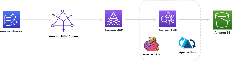
  • Schema – A schema defines the structure and format of a data record. A schema is a versioned specification for reliable data publication, consumption, or storage. Each schema can have multiple versions. Versioning is governed by a compatibility rule that is applied on a schema. Requests to register new schema versions are checked against this rule by the Schema Registry before they can succeed.

To manually create these resources without using AWS CloudFormation, refer to Creating a Registry and Creating a Schema.

Prerequisites

Make sure to complete the following steps as prerequisites:

  1. Create an AWS account. For this post, you configure the required AWS resources in the us-east-1 or us-west-2 Region. If you haven’t signed up, complete the following tasks:
    1. Create an account. For instructions, see Sign Up for AWS.
    2. Create an AWS Identity and Access Management (IAM) user. For instructions, see Creating an IAM User in your AWS account.
  2. Choose Launch Stack to launch the CloudFormation stack:

Review the newly registered schema

Let’s review the registry and the schema on the AWS Glue console.

  1. Sign in to the AWS Glue console and choose the appropriate Region.
  2. Under Data Catalog, choose Schema registries.
  3. Choose the GsrBlogRegistry schema registry.
  4. Choose the GsrBlogSchema schema.
  5. Choose Version 1.

We can see the JSON Schema version details and its definition. Note that the compatibility mode chosen is Backward compatibility. We see the purpose of that in the next section.

Evolve the schema by creating a new backward-compatible version

In this section, we take what is created so far and add a new schema version to demonstrate how we can evolve our schema while keeping the integrity intact.

To add a new schema version, complete the following steps, continuing from the previous section:

  1. On the Schema version details page, choose Register new version.
  2. Inside the properties object within the location object (after the state field), add a new country field as follows:
    "country": {
              "type": "string",
              "description": "Name of the country where the weather is being reported."
            }

Because the compatibility mode chosen for the schema is backward compatibility, it’s important that we don’t make this new field a required field. If we do that, the Schema Registry fail this new version.

  1. Choose Register version.

We now have a new version of the schema that allows the producers to include an optional country field within the location object if they choose to.

Use the AWS Glue Schema Registry

In this section, we walk through the steps to use the Schema Registry with Kinesis Data Streams or Apache Kafka.

Prerequisites

Make sure to complete the following steps as prerequisites:

  1. Configure your AWS credentials in your local machine.
  2. Install Maven on the local machine.
  3. Download the application code from the GitHub repo.
  4. Build the package:
    mvn clean package

Use the Schema Registry with Kinesis Data Streams

Run the Kinesis producer code to produce JSON messages that are associated with a schema ID assigned by the Schema Registry:

mvn exec:java -Dexec.mainClass="com.amazonaws.services.gsr.samples.json.kinesis.RunKinesisProducer" -Dexec.args="<<KINESIS_DATA_STREAM_NAME>>"

This command returns the following output:

Putting 1 record into <<KINESIS_DATA_STREAM_NAME>>
Sent message 0
Putting 1 record into <<KINESIS_DATA_STREAM_NAME>>
Sent message 1
Putting 1 record into <<KINESIS_DATA_STREAM_NAME>>
Sent message 2
Successfully produced 3 messages to a stream called <<KINESIS_DATA_STREAM_NAME>>

Run the Kinesis consumer code to receive JSON messages with the schema ID, obtain the schema from the Schema Registry, and validate:

mvn exec:java -Dexec.mainClass="com.amazonaws.services.gsr.samples.json.kinesis.RunKinesisConsumer" -Dexec.args="<<KINESIS_DATA_STREAM_NAME>>"

This command returns the following output with the JSON records received and decoded:

Number of Records received: 1
[JsonDataWithSchema(schema={"$schema":"http://json-schema.org/draft-07/schema#","additionalProperties":true,"title":"WeatherReport","type":"object","properties":{"temperature":{"description":"Temperature in Farenheit.","type":"integer"},"location":{"additionalProperties":false,"type":"object","properties":{"city":{"description":"Name of the city where the weather is being reported.","type":"string"},"state":{"description":"Name of the state where the weather is being reported.","type":"string"}},"required":["city","state"]},"timestamp":{"description":"Timestamp in epoch format at which the weather was noted.","type":"integer"}},"required":["location","temperature","timestamp"],"$id":"https://example.com/weather-report.schema.json"}, payload={"temperature":89,"location":{"city":"Orlando","state":"Florida"},"timestamp":1627335205})]

Use the Schema Registry with Apache Kafka

In the root of the downloaded GitHub repo folder, create a config file with the connection parameters for the Kafka cluster:

# Kafka
bootstrap.servers=localhost:9092

Run the Kafka producer code to produce JSON messages that are associated with a schema ID assigned by the Schema Registry:

mvn exec:java -Dexec.mainClass="com.amazonaws.services.gsr.samples.json.kafka.RunKafkaProducer" -Dexec.args="<<CONFIG_FILE_NAME>><< TOPIC_NAME>>"

This command returns the following output:

Sent message 0
Sent message 1
Sent message 2
Successfully produced 3 messages to a topic called <<TOPIC_NAME>>

Run the Kafka consumer code to consume JSON messages with the schema ID, obtain the schema from the Schema Registry, and validate:

mvn exec:java -Dexec.mainClass="com.amazonaws.services.gsr.samples.json.kafka.RunKafkaConsumer" -Dexec.args="<<CONFIG_FILE_NAME>> <<TOPIC_NAME>>"

This command returns the following output with the JSON records received and decoded:

Received message: key = message-0, value = JsonDataWithSchema(schema={"$schema":"http://json-schema.org/draft-07/schema#","additionalProperties":true,"title":"WeatherReport","type":"object","properties":{"temperature":{"description":"Temperature in Farenheit.","type":"integer"},"location":{"additionalProperties":false,"type":"object","properties":{"city":{"description":"Name of the city where the weather is being reported.","type":"string"},"state":{"description":"Name of the state where the weather is being reported.","type":"string"}},"required":["city","state"]},"timestamp":{"description":"Timestamp in epoch format at which the weather was noted.","type":"integer"}},"required":["location","temperature","timestamp"],"$id":"https://example.com/weather-report.schema.json"}, payload={"temperature":115,"location":{"city":"Phoenix","state":"Arizona"},"windSpeed":50,"timestamp":1627335205})

Clean up

Now to the final step, cleaning up the resources. Delete the CloudFormation stack to remove any resources you created as part of this walkthrough.

Schema Registry features

Let’s discuss the features the Schema Registry has to offer:

  • Schema discovery – When a producer registers a schema change, metadata can be applied as a key-value pair to provide searchable information for administrators or developers. This metadata can indicate the original source of the data (source=MSK_west), the team’s name to contact (owner=DataEngineering), or AWS tags (environment=Production). You could potentially encrypt a field in your data on the producing client and use metadata to specify to potential consumer clients which public key fingerprint to use for decryption.
  • Schema compatibility – The versioning of each schema is governed by a compatibility mode. If a new version of a schema is requested to be registered that breaks the specified compatibility mode, the request fails, and an exception is thrown. Compatibility checks enable developers building downstream applications to have a bounded set of scenarios to build applications against, which helps prepare for the changes without issue. Commonly used modes are FORWARD, BACKWARD, and FULL. For more information about mode definitions, see Schema Versioning and Compatibility.
  • Schema validation – Schema Registry serializers work to validate that the data produced is compatible with the assigned schema. If it isn’t, the data producer receives an exception from the serializer. This ensures that potentially breaking changes are found earlier in development cycles and can also help prevent unintentional schema changes due to human error.
  • Auto-registration of schemas – If configured to do so, the data producer can auto-register schema changes as they flow in the data stream. This is especially helpful for use cases where the source of the data is generated by a change data capture process (CDC) from the database.
  • IAM support – Due to integrated IAM support, only authorized producers can change certain schemas. Furthermore, only those consumers authorized to read the schema can do so. Schema changes are typically performed deliberately and with care, so it’s important to use IAM to control who performs these changes. Additionally, access control to schemas is important in situations where you might have sensitive information included in the schema definition itself. In the previous examples, IAM roles are inferred via the AWS SDK for Java, so they are inherited from the Amazon Elastic Compute Cloud (Amazon EC2) instance’s role that the application runs on, if using Amazon EC2. You can also apply IAM roles to any other AWS service that could contain this code, such as containers or AWS Lambda functions.

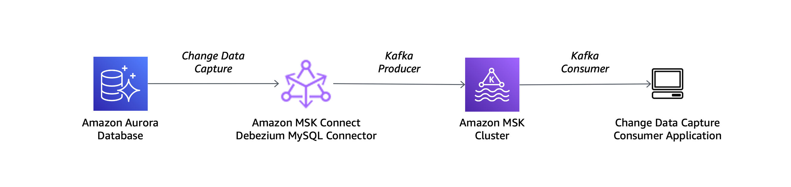
  • Secondary deserializer – If you have already registered schemas in another schema registry, there’s an option for specifying a secondary deserializer when performing schema lookups. This allows for migrations from other schema registries without having to start all over again. Any schema ID that is unknown to the Schema Registry is looked up in the registry tied to the secondary deserializer.
  • Compression – Using a schema registry can reduce data payload by no longer needing to send and receive schemas with each message. Schema Registry libraries also provide an option for zlib compression, which can reduce data requirements even further by compressing the payload of the message. This varies by use case, but compression can reduce the size of the message significantly.
  • Multiple data formats – The Schema Registry currently supports AVRO (v1.10.2) data format, JSON data format with JSON Schema format for the schema (specifications Draft-04, Draft-06, and Draft-07), and Java language support, with other data formats and languages to come.

Conclusion

In this post, we discussed the benefits of using the AWS Glue Schema Registry to register, validate, and evolve JSON Schemas for data streams as business needs change. We also provided examples of how to use the Schema Registry.

Learn more about Integrating with AWS Glue Schema Registry.


About the Author

Aditya Challa is a Senior Solutions Architect at Amazon Web Services. Aditya loves helping customers through their AWS journeys because he knows that journeys are always better when there’s company. He’s a big fan of travel, history, engineering marvels, and learning something new every day.

Introducing AWS Lambda batching controls for message broker services

Post Syndicated from Julian Wood original https://aws.amazon.com/blogs/compute/introducing-aws-lambda-batching-controls-for-message-broker-services/

This post is written by Mithun Mallick, Senior Specialist Solutions Architect.

AWS Lambda now supports configuring a maximum batch window for instance-based message broker services to fine tune when Lambda invocations occur. This feature gives you an additional control on batching behavior when processing data. It applies to Amazon Managed Streaming for Apache Kafka (Amazon MSK), self-hosted Apache Kafka, and Amazon MQ for Apache ActiveMQ and RabbitMQ.

Apache Kafka is an open source event streaming platform used to support workloads such as data pipelines and streaming analytics. It is conceptually similar to Amazon Kinesis. Amazon MSK is a fully managed, highly available service that simplifies the setup, scaling, and management of clusters running Kafka.

Amazon MQ is a managed, highly available message broker service for Apache ActiveMQ and RabbitMQ that makes it easier to set up and operate message brokers on AWS. Amazon MQ reduces your operational responsibilities by managing the provisioning, setup, and maintenance of message brokers for you.

Amazon MSK, self-hosted Apache Kafka and Amazon MQ for ActiveMQ and RabbitMQ are all available as event sources for AWS Lambda. You configure an event source mapping to use Lambda to process items from a stream or queue. This allows you to use these message broker services to store messages and asynchronously integrate them with downstream serverless workflows.

In this blog, I explain how message batching works. I show how to use the new maximum batching window control for the managed message broker services and self-managed Apache Kafka.

Understanding batching

For event source mappings, the Lambda service internally polls for new records or messages from the event source, and then synchronously invokes the target Lambda function. Lambda reads the messages in batches and provides these to your function as an event payload. Batching allows higher throughput message processing, up to 10,000 messages in a batch. The payload limit of a single invocation is 6 MB.

Previously, you could only use batch size to configure the maximum number of messages Lambda would poll for. Once a defined batch size is reached, the poller invokes the function with the entire set of messages. This feature is ideal when handling a low volume of messages or batches of data that take time to build up.

Batching window

The new Batch Window control allows you to set the maximum amount of time, in seconds, that Lambda spends gathering records before invoking the function. This brings similar batching functionality that AWS supports with Amazon SQS to Amazon MQ, Amazon MSK and self-managed Apache Kafka. The Lambda event source mapping batching functionality can be described as follows.

Batching controls with Lambda event source mapping

Batching controls with Lambda event source mapping

Using MaximumBatchingWindowInSeconds, you can set your function to wait up to 300 seconds for a batch to build before processing it. This allows you to create bigger batches if there are enough messages. You can manage the average number of records processed by the function with each invocation. This increases the efficiency of each invocation, and reduces the frequency.

Setting MaximumBatchingWindowInSeconds to 0 invokes the target Lambda function as soon as the Lambda event source receives a message from the broker.

Message broker batching behavior

For ActiveMQ, the Lambda event source mapping uses the Java Message Service (JMS) API to receive messages. For RabbitMQ, Lambda uses a RabbitMQ client library to get messages from the queue.

The Lambda event source mappings act as a consumer when polling the queue. The batching pattern for all instance-based message broker services is the same. As soon as a message is received, the batching window timer starts. If there are more messages, the consumer makes additional calls to the broker and adds them to a buffer. It keeps a count of the number of messages and the total size of the payload.

The batch is considered complete if the addition of a new message makes the batch size equal to or greater than 6 MB, or the batch window timeout is reached. If the batch size is greater than 6 MB, the last message is returned back to the broker.

Lambda then invokes the target Lambda function synchronously and passes on the batch of messages to the function. The Lambda event source continues to poll for more messages and as soon as it retrieves the next message, the batching window starts again. Polling and invocation of the target Lambda function occur in separate processes.

Kafka uses a distributed append log architecture to store messages. This works differently from ActiveMQ and RabbitMQ as messages are not removed from the broker once they have been consumed. Instead, consumers must maintain an offset to the last record or message that was consumed from the broker. Kafka provides several options in the consumer API to simplify the tracking of offsets.

Amazon MSK and Apache Kafka store data in multiple partitions to provide higher scalability. Lambda reads the messages sequentially for each partition and a batch may contain messages from different partitions.  Lambda then commits the offsets once the target Lambda function is invoked successfully.

Configuring the maximum batching window

To reduce Lambda function invocations for existing or new functions, set the MaximumBatchingWindowInSeconds value close to 300 seconds. A longer batching window can introduce additional latency. For latency-sensitive workloads set the MaximumBatchingWindowInSeconds value to an appropriate setting.

To configure Maximum Batching on a function in the AWS Management Console, navigate to the function in the Lambda console. Create a new Trigger, or edit an existing once. Along with the Batch size you can configure a Batch window. The Trigger Configuration page is similar across the broker services.

Max batching trigger window

Max batching trigger window

You can also use the AWS CLI to configure the --maximum-batching-window-in-seconds parameter.

For example, with Amazon MQ:

aws lambda create-event-source-mapping --function-name my-function \
--maximum-batching-window-in-seconds 300 --batch-size 100 --starting-position AT_TIMESTAMP \
--event-source-arn arn:aws:mq:us-east-1:123456789012:broker:ExampleMQBroker:b-24cacbb4-b295-49b7-8543-7ce7ce9dfb98

You can use AWS CloudFormation to configure the parameter. The following example configures the MaximumBatchingWindowInSeconds as part of the AWS::Lambda::EventSourceMapping resource for Amazon MQ:

  LambdaFunctionEventSourceMapping:
    Type: AWS::Lambda::EventSourceMapping
    Properties:
      BatchSize: 10
      MaximumBatchingWindowInSeconds: 300
      Enabled: true
      Queues:
        - "MyQueue"
      EventSourceArn: !GetAtt MyBroker.Arn
      FunctionName: !GetAtt LambdaFunction.Arn
      SourceAccessConfigurations:
        - Type: BASIC_AUTH
          URI: !Ref secretARNParameter

You can also use AWS Serverless Application Model (AWS SAM) to configure the parameter as part of the Lambda function event source.

MQReceiverFunction:
      Type: AWS::Serverless::Function 
      Properties:
        FunctionName: MQReceiverFunction
        CodeUri: src/
        Handler: app.lambda_handler
        Runtime: python3.9
        Events:
          MQEvent:
            Type: MQ
            Properties:
              Broker: !Ref brokerARNParameter
              BatchSize: 10
              MaximumBatchingWindowInSeconds: 300
              Queues:
                - "workshop.queueC"
              SourceAccessConfigurations:
                - Type: BASIC_AUTH
                  URI: !Ref secretARNParameter

Error handling

If your function times out or returns an error for any of the messages in a batch, Lambda retries the whole batch until processing succeeds or the messages expire.

When a function encounters an unrecoverable error, the event source mapping is paused and the consumer stops processing records. Any other consumers can continue processing, provided that they do not encounter the same error.  If your Lambda event records exceed the allowed size limit of 6 MB, they can go unprocessed.

For Amazon MQ, you can redeliver messages when there’s a function error. You can configure dead-letter queues (DLQs) for both Apache ActiveMQ, and RabbitMQ. For RabbitMQ, you can set a per-message TTL to move failed messages to a DLQ.

Since the same event may be received more than once, functions should be designed to be idempotent. This means that receiving the same event multiple times does not change the result beyond the first time the event was received.

Conclusion

Lambda supports a number of event sources including message broker services like Amazon MQ and Amazon MSK. This post explains how batching works with the event sources and how messages are sent to the Lambda function.

Previously, you could only control the batch size. The new Batch Window control allows you to set the maximum amount of time, in seconds, that Lambda spends gathering records before invoking the function. This can increase the overall throughput of message processing and reduces Lambda invocations, which may improve cost.

For more serverless learning resources, visit Serverless Land.

How Meshify Built an Insurance-focused IoT Solution on AWS

Post Syndicated from Grant Fisher original https://aws.amazon.com/blogs/architecture/how-meshify-built-an-insurance-focused-iot-solution-on-aws/

The ability to analyze your Internet of Things (IoT) data can help you prevent loss, improve safety, boost productivity, and even develop an entirely new business model. This data is even more valuable, with the ever-increasing number of connected devices. Companies use Amazon Web Services (AWS) IoT services to build innovative solutions, including secure edge device connectivity, ingestion, storage, and IoT data analytics.

This post describes Meshify’s IoT sensor solution, built on AWS, that helps businesses and organizations prevent property damage and avoid loss for the property-casualty insurance industry. The solution uses real-time data insights, which result in fewer claims, better customer experience, and innovative new insurance products.

Through low-power, long-range IoT sensors, and dedicated applications, Meshify can notify customers of potential problems like rapid temperature decreases that could result in freeze damage, or rising humidity levels that could lead to mold. These risks can then be averted, instead of leading to costly damage that can impact small businesses and the insurer’s bottom line.

Architecture building blocks

The three building blocks of this technical architecture are the edge portfolio, data ingestion, and data processing and analytics, shown in Figure 1.

Figure 1. Building blocks of Meshify’s technical architecture

Figure 1. Building blocks of Meshify’s technical architecture

I. Edge portfolio (EP)

Starting with the edge sensors, the Meshify edge portfolio covers two types of sensors:

  • LoRaWAN (Low power, long range WAN) sensor suite. This sensor provides the long connectivity range (> 1000 feet) and extended battery life (~ 5 years) needed for enterprise environments.
  • Cellular-based sensors. This sensor is a narrow band/LTE-M device that operates at LTE-M band 2/4/12 radio frequency and uses edge intelligence to conserve battery life.

II. Data ingestion (DI)

For the LoRaWAN solution, aggregated sensor data at the Meshify gateway is sent to AWS using AWS IoT Core and Meshify’s REST service endpoints. AWS IoT Core is a managed cloud platform that lets IoT devices easily and securely connect using multiple protocols like HTTP, MQTT, and WebSockets. It expands its protocol coverage through a new fully managed feature called AWS IoT Core for LoRaWAN. This gives Meshify the ability to connect LoRaWAN wireless devices with the AWS Cloud. AWS IoT Core for LoRaWAN delivers a LoRaWAN network server (LNS) that provides gateway management using the Configuration and Update Server (CUPS) and Firmware Updates Over-The-Air (FUOTA) capabilities.

III. Data processing and analytics (DPA)

Initial processing of the data is done at the ingestion layer, using Meshify REST API endpoints and the Rules Engine of AWS IoT Core. Meshify applies filtering logic to route relevant events to Amazon Managed Streaming for Apache Kafka (Amazon MSK). Amazon MSK is an AWS streaming data service that manages Apache Kafka infrastructure and operations, streamlining the process of running Apache Kafka applications on AWS.

Meshify’s applications then consume the events from Amazon MSK per the configured topic subscription. They enrich and correlate the events with the records with a managed service, Amazon Relational Database Service (RDS). These applications run as scalable containers on another managed service, Amazon Elastic Kubernetes Service (EKS), which runs container applications.

Bringing it all together – technical workflow

In Figure 2, we illustrate the technical workflow from the ingestion of field events to their processing, enrichment, and persistence. Finally, we use these events to power risk avoidance decision-making.

Figure 2. Technical workflow for Meshify IoT architecture

Figure 2. Technical workflow for Meshify IoT architecture

  1. After installation, Meshify-designed LoRa sensors transmit information to the cloud through Meshify’s gateways. LoRaWAN capabilities create connectivity between the sensors and the gateways. They establish a low power, wide area network protocol that securely transmits data over a long distance, through walls and floors of even the largest buildings.
  2. The Meshify Gateway is a redundant edge system, capable of sending sensor data from various sensors to the Meshify cloud environment. Once the LoRa sensor information is received by the Meshify Gateway, it converts the incoming radio frequency (RF) signals, which support faster transfer rate to Meshify’s cloud environment.
  3. Data from the Meshify Gateway and sensors is initially processed at Meshify’s AWS IoT Core and REST service endpoints. These destinations for IoT streaming data help with the initial intake and introduce field data to the Meshify cloud environment. The initial ingestion points can scale automatically based upon the volume of sensor data received. This enables rapid scaling and ease of implementation.
  4. After the data has entered the Meshify cloud environment, Meshify uses Amazon EKS and Amazon MSK to process the incoming data stream. Amazon MSK producer and consumer applications within the EKS systems enrich the data streams for the end users and systems to consume.
  5. Producer applications running on EKS send processed events to the Amazon MSK service. These events include storing and retrieval of raw data, enriched data, and system-level data.
  6. Consumer applications hosted on the EKS pods receive events per the subscribed Amazon MSK topic. Web, mobile, and analytic applications enrich and use these data streams to display data to end users, business teams, and systems operations.
  7. Processed events are persisted in Amazon RDS. The databases are used for reporting, machine learning, and other analytics and processing services.

Building a scalable IoT solution

Meshify first began work on the Meshify sensors and hosted platform in 2012. In the ensuing decade, Meshify has successfully created a platform to auto-scale upon demand with steady, predictable performance. This gave Meshify both the ability to use only the resources needed, and still have the capacity to handle unexpected voluminous data.

As the platform scaled, so did the volume of sensor data, operations and diagnostics data, and metadata from installations and deployments. Building an end-to-end data pipeline that integrates these different data sources and delivers co-related insights at low latency was time well spent.

Conclusion

In this post, we’ve shown how Meshify is using AWS services to power their suite of IoT sensors, software, and data platforms. Meshify’s most important architectural enhancements have involved the introduction of managed services, notably AWS IoT Core for LoRaWAN and Amazon MSK. These improvements have primarily focused on the data ingestion, data processing, and analytics stages.

Meshify continues to power the data revolution at the intersection of IoT and insurance at the edge, using AWS. Looking ahead, Meshify and HSB are excited at the prospect of scaling the relationship with AWS from cloud computing to the world of edge devices.

Learn more about how emerging startups and large enterprises are using AWS IoT services to build differentiated products.

Meshify is an IoT technology company and subsidiary of HSB, based in Austin, TX. Meshify builds pioneering sensor hardware, software, and data analytics solutions that protect businesses from property and equipment damage.

Offset lag metric for Amazon MSK as an event source for Lambda

Post Syndicated from Eric Johnson original https://aws.amazon.com/blogs/compute/offset-lag-metric-for-amazon-msk-as-an-event-source-for-lambda/

This post written by Adam Wagner, Principal Serverless Solutions Architect.

Last year, AWS announced support for Amazon Managed Streaming for Apache Kafka (MSK) and self-managed Apache Kafka clusters as event sources for AWS Lambda. Today, AWS adds a new OffsetLag metric to Lambda functions with MSK or self-managed Apache Kafka event sources.

Offset in Apache Kafka is an integer that marks the current position of a consumer. OffsetLag is the difference in offset between the last record written to the Kafka topic and the last record processed by Lambda. Kafka expresses this in the number of records, not a measure of time. This metric provides visibility into whether your Lambda function is keeping up with the records added to the topic it is processing.

This blog walks through using the OffsetLag metric along with other Lambda and MSK metrics to understand your streaming application and optimize your Lambda function.

Overview

In this example application, a producer writes messages to a topic on the MSK cluster that is an event source for a Lambda function. Each message contains a number and the Lambda function finds the factors of that number. It outputs the input number and results to an Amazon DynamoDB table.

Finding all the factors of a number is fast if the number is small but takes longer for larger numbers. This difference means the size of the number written to the MSK topic influences the Lambda function duration.

Example application architecture

Example application architecture

  1. A Kafka client writes messages to a topic in the MSK cluster.
  2. The Lambda event source polls the MSK topic on your behalf for new messages and triggers your Lambda function with batches of messages.
  3. The Lambda function factors the number in each message and then writes the results to DynamoDB.

In this application, several factors can contribute to offset lag. The first is the volume and size of messages. If more messages are coming in, the Lambda may take longer to process them. Other factors are the number of partitions in the topic, and the number of concurrent Lambda functions processing messages. A full explanation of how Lambda concurrency scales with the MSK event source is in the documentation.

If the average duration of your Lambda function increases, this also tends to increase the offset lag. This lag could be latency in a downstream service or due to the complexity of the incoming messages. Lastly, if your Lambda function errors, the MSK event source retries the identical records set until they succeed. This retry functionality also increases offset lag.

Measuring OffsetLag

To understand how the new OffsetLag metric works, you first need a working MSK topic as an event source for a Lambda function. Follow this blog post to set up an MSK instance.

To find the OffsetLag metric, go to the CloudWatch console, select All Metrics from the left-hand menu. Then select Lambda, followed by By Function Name to see a list of metrics by Lambda function. Scroll or use the search bar to find the metrics for this function and select OffsetLag.

OffsetLag metric example

OffsetLag metric example

To make it easier to look at multiple metrics at once, create a CloudWatch dashboard starting with the OffsetLag metric. Select Actions -> Add to Dashboard. Select the Create new button, provide the dashboard a name. Choose Create, keeping the rest of the options at the defaults.

Adding OffsetLag to dashboard

Adding OffsetLag to dashboard

After choosing Add to dashboard, the new dashboard appears. Choose the Add widget button to add the Lambda duration metric from the same function. Add another widget that combines both Lambda errors and invocations for the function. Finally, add a widget for the BytesInPerSec metric for the MSK topic. Find this metric under AWS/Kafka -> Broker ID, Cluster Name, Topic. Finally, click Save dashboard.

After a few minutes, you see a steady stream of invocations, as you would expect when consuming from a busy topic.

Data incoming to dashboard

Data incoming to dashboard

This example is a CloudWatch dashboard showing the Lambda OffsetLag, Duration, Errors, and Invocations, along with the BytesInPerSec for the MSK topic.

In this example, the OffSetLag metric is averaging about eight, indicating that the Lambda function is eight records behind the latest record in the topic. While this is acceptable, there is room for improvement.

The first thing to look for is Lambda function errors, which can drive up offset lag. The metrics show that there are no errors so the next step is to evaluate and optimize the code.

The Lambda handler function loops through the records and calls the process_msg function on each record:

def lambda_handler(event, context):
    for batch in event['records'].keys():
        for record in event['records'][batch]:
            try:
                process_msg(record)
            except:
                print("error processing record:", record)
    return()

The process_msg function handles base64 decoding, calls a factor function to factor the number, and writes the record to a DynamoDB table:

def process_msg(record):
    #messages are base64 encoded, so we decode it here
    msg_value = base64.b64decode(record['value']).decode()
    msg_dict = json.loads(msg_value)
    #using the number as the hash key in the dynamodb table
    msg_id = f"{msg_dict['number']}"
    if msg_dict['number'] <= MAX_NUMBER:
        factors = factor_number(msg_dict['number'])
        print(f"number: {msg_dict['number']} has factors: {factors}")
        item = {'msg_id': msg_id, 'msg':msg_value, 'factors':factors}
        resp = ddb_table.put_item(Item=item)
    else:
        print(f"ERROR: {msg_dict['number']} is >= limit of {MAX_NUMBER}")

The heavy computation takes place in the factor function:

def factor(number):
    factors = [1,number]
    for x in range(2, (int(1 + number / 2))):
        if (number % x) == 0:
            factors.append(x)
    return factors

The code loops through all numbers up to the factored number divided by two. The code is optimized by only looping up to the square root of the number.

def factor(number):
    factors = [1,number]
    for x in range(2, 1 + int(number**0.5)):
        if (number % x) == 0:
            factors.append(x)
            factors.append(number // x)
    return factors

There are further optimizations and libraries for factoring numbers but this provides a noticeable performance improvement in this example.

Data after optimization

Data after optimization

After deploying the code, refresh the metrics after a while to see the improvements:

The average Lambda duration has dropped to single-digit milliseconds and the OffsetLag is now averaging two.

If you see a noticeable change in the OffsetLag metric, there are several things to investigate. The input side of the system, increased messages per second, or a significant increase in the size of the message are a few options.

Conclusion

This post walks through implementing the OffsetLag metric to understand latency between the latest messages in the MSK topic and the records a Lambda function is processing. It also reviews other metrics that help understand the underlying cause of increases to the offset lag. For more information on this topic, refer to the documentation and other MSK Lambda metrics.

For more serverless learning resources, visit Serverless Land.

Introducing mutual TLS authentication for Amazon MSK as an event source

Post Syndicated from Julian Wood original https://aws.amazon.com/blogs/compute/introducing-mutual-tls-authentication-for-amazon-msk-as-an-event-source/

This post is written by Uma Ramadoss, Senior Specialist Solutions Architect, Integration.

Today, AWS Lambda is introducing mutual TLS (mTLS) authentication for Amazon Managed Streaming for Apache Kafka (Amazon MSK) and self-managed Kafka as an event source.

Many customers use Amazon MSK for streaming data from multiple producers. Multiple subscribers can then consume the streaming data and build data pipelines, analytics, and data integration. To learn more, read Using Amazon MSK as an event source for AWS Lambda.

You can activate any combination of authentication modes (mutual TLS, SASL SCRAM, or IAM access control) on new or existing clusters. This is useful if you are migrating to a new authentication mode or must run multiple authentication modes simultaneously. Lambda natively supports consuming messages from both self-managed Kafka and Amazon MSK through event source mapping.

By default, the TLS protocol only requires a server to authenticate itself to the client. The authentication of the client to the server is managed by the application layer. The TLS protocol also offers the ability for the server to request that the client send an X.509 certificate to prove its identity. This is called mutual TLS as both parties are authenticated via certificates with TLS.

Mutual TLS is a commonly used authentication mechanism for business-to-business (B2B) applications. It’s used in standards such as Open Banking, which enables secure open API integrations for financial institutions. It is one of the popular authentication mechanisms for customers using Kafka.

To use mutual TLS authentication for your Kafka-triggered Lambda functions, you provide a signed client certificate, the private key for the certificate, and an optional password if the private key is encrypted. This establishes a trust relationship between Lambda and Amazon MSK or self-managed Kafka. Lambda supports self-signed server certificates or server certificates signed by a private certificate authority (CA) for self-managed Kafka. Lambda trusts the Amazon MSK certificate by default as the certificates are signed by Amazon Trust Services CAs.

This blog post explains how to set up a Lambda function to process messages from an Amazon MSK cluster using mutual TLS authentication.

Overview

Using Amazon MSK as an event source operates in a similar way to using Amazon SQS or Amazon Kinesis. You create an event source mapping by attaching Amazon MSK as event source to your Lambda function.

The Lambda service internally polls for new records from the event source, reading the messages from one or more partitions in batches. It then synchronously invokes your Lambda function, sending each batch as an event payload. Lambda continues to process batches until there are no more messages in the topic.

The Lambda function’s event payload contains an array of records. Each array item contains details of the topic and Kafka partition identifier, together with a timestamp and base64 encoded message.

Kafka event payload

Kafka event payload

You store the signed client certificate, the private key for the certificate, and an optional password if the private key is encrypted in the AWS Secrets Manager as a secret. You provide the secret in the Lambda event source mapping.

The steps for using mutual TLS authentication for Amazon MSK as event source for Lambda are:

  1. Create a private certificate authority (CA) using AWS Certificate Manager (ACM) Private Certificate Authority (PCA).
  2. Create a client certificate and private key. Store them as secret in AWS Secrets Manager.
  3. Create an Amazon MSK cluster and a consuming Lambda function using the AWS Serverless Application Model (AWS SAM).
  4. Attach the event source mapping.

This blog walks through these steps in detail.

Prerequisites

1. Creating a private CA.

To use mutual TLS client authentication with Amazon MSK, create a root CA using AWS ACM Private Certificate Authority (PCA). We recommend using independent ACM PCAs for each MSK cluster when you use mutual TLS to control access. This ensures that TLS certificates signed by PCAs only authenticate with a single MSK cluster.

  1. From the AWS Certificate Manager console, choose Create a Private CA.
  2. In the Select CA type panel, select Root CA and choose Next.
  3. Select Root CA

    Select Root CA

  4. In the Configure CA subject name panel, provide your certificate details, and choose Next.
  5. Provide your certificate details

    Provide your certificate details

  6. From the Configure CA key algorithm panel, choose the key algorithm for your CA and choose Next.
  7. Configure CA key algorithm

    Configure CA key algorithm

  8. From the Configure revocation panel, choose any optional certificate revocation options you require and choose Next.
  9. Configure revocation

    Configure revocation

  10. Continue through the screens to add any tags required, allow ACM to renew certificates, review your options, and confirm pricing. Choose Confirm and create.
  11. Once the CA is created, choose Install CA certificate to activate your CA. Configure the validity of the certificate and the signature algorithm and choose Next.
  12. Configure certificate

    Configure certificate

  13. Review the certificate details and choose Confirm and install. Note down the Amazon Resource Name (ARN) of the private CA for the next section.
  14. Review certificate details

    Review certificate details

2. Creating a client certificate.

You generate a client certificate using the root certificate you previously created, which is used to authenticate the client with the Amazon MSK cluster using mutual TLS. You provide this client certificate and the private key as AWS Secrets Manager secrets to the AWS Lambda event source mapping.

  1. On your local machine, run the following command to create a private key and certificate signing request using OpenSSL. Enter your certificate details. This creates a private key file and a certificate signing request file in the current directory.
  2. openssl req -new -newkey rsa:2048 -days 365 -keyout key.pem -out client_cert.csr -nodes
    OpenSSL create a private key and certificate signing request

    OpenSSL create a private key and certificate signing request

  3. Use the AWS CLI to sign your certificate request with the private CA previously created. Replace Private-CA-ARN with the ARN of your private CA. The certificate validity value is set to 300, change this if necessary. Save the certificate ARN provided in the response.
  4. aws acm-pca issue-certificate --certificate-authority-arn Private-CA-ARN --csr fileb://client_cert.csr --signing-algorithm "SHA256WITHRSA" --validity Value=300,Type="DAYS"
  5. Retrieve the certificate that ACM signed for you. Replace the Private-CA-ARN and Certificate-ARN with the ARN you obtained from the previous commands. This creates a signed certificate file called client_cert.pem.
  6. aws acm-pca get-certificate --certificate-authority-arn Private-CA-ARN --certificate-arn Certificate-ARN | jq -r '.Certificate + "\n" + .CertificateChain' >> client_cert.pem
  7. Create a new file called secret.json with the following structure
  8. {
    "certificate":"",
    "privateKey":""
    }
    
  9. Copy the contents of the client_cert.pem in certificate and the content of key.pem in privatekey. Ensure that there are no extra spaces added. The file structure looks like this:
  10. Certificate file structure

    Certificate file structure

  11. Create the secret and save the ARN for the next section.
aws secretsmanager create-secret --name msk/mtls/lambda/clientcert --secret-string file://secret.json

3. Setting up an Amazon MSK cluster with AWS Lambda as a consumer.

Amazon MSK is a highly available service, so it must be configured to run in a minimum of two Availability Zones in your preferred Region. To comply with security best practice, the brokers are usually configured in private subnets in each Region.

You can use AWS CLI, AWS Management Console, AWS SDK and AWS CloudFormation to create the cluster and the Lambda functions. This blog uses AWS SAM to create the infrastructure and the associated code is available in the GitHub repository.

The AWS SAM template creates the following resources:

  1. Amazon Virtual Private Cloud (VPC).
  2. Amazon MSK cluster with mutual TLS authentication.
  3. Lambda function for consuming the records from the Amazon MSK cluster.
  4. IAM roles.
  5. Lambda function for testing the Amazon MSK integration by publishing messages to the topic.

The VPC has public and private subnets in two Availability Zones with the private subnets configured to use a NAT Gateway. You can also set up VPC endpoints with PrivateLink to allow the Amazon MSK cluster to communicate with Lambda. To learn more about different configurations, see this blog post.

The Lambda function requires permission to describe VPCs and security groups, and manage elastic network interfaces to access the Amazon MSK data stream. The Lambda function also needs two Kafka permissions: kafka:DescribeCluster and kafka:GetBootstrapBrokers. The policy template AWSLambdaMSKExecutionRole includes these permissions. The Lambda function also requires permission to get the secret value from AWS Secrets Manager for the secret you configure in the event source mapping.

  ConsumerLambdaFunctionRole:
    Type: AWS::IAM::Role
    Properties:
      AssumeRolePolicyDocument:
        Version: "2012-10-17"
        Statement:
          - Effect: Allow
            Principal:
              Service: lambda.amazonaws.com
            Action: sts:AssumeRole
      ManagedPolicyArns:
        - arn:aws:iam::aws:policy/service-role/AWSLambdaMSKExecutionRole
      Policies:
        - PolicyName: SecretAccess
          PolicyDocument:
            Version: "2012-10-17"
            Statement:
              - Effect: Allow
                Action: "SecretsManager:GetSecretValue"
                Resource: "*"

This release adds two new SourceAccessConfiguration types to the Lambda event source mapping:

1. CLIENT_CERTIFICATE_TLS_AUTH – (Amazon MSK, Self-managed Apache Kafka) The Secrets Manager ARN of your secret key containing the certificate chain (PEM), private key (PKCS#8 PEM), and private key password (optional) used for mutual TLS authentication of your Amazon MSK/Apache Kafka brokers. A private key password is required if the private key is encrypted.

2. SERVER_ROOT_CA_CERTIFICATE – This is only for self-managed Apache Kafka. This contains the Secrets Manager ARN of your secret containing the root CA certificate used by your Apache Kafka brokers in PEM format. This is not applicable for Amazon MSK as Amazon MSK brokers use public AWS Certificate Manager certificates which are trusted by AWS Lambda by default.

Deploying the resources:

To deploy the example application:

  1. Clone the GitHub repository
  2. git clone https://github.com/aws-samples/aws-lambda-msk-mtls-integration.git
  3. Navigate to the aws-lambda-msk-mtls-integration directory. Copy the client certificate file and the private key file to the producer lambda function code.
  4. cd aws-lambda-msk-mtls-integration
    cp ../client_cert.pem code/producer/client_cert.pem
    cp ../key.pem code/producer/client_key.pem
  5. Navigate to the code directory and build the application artifacts using the AWS SAM build command.
  6. cd code
    sam build
  7. Run sam deploy to deploy the infrastructure. Provide the Stack Name, AWS Region, ARN of the private CA created in section 1. Provide additional information as required in the sam deploy and deploy the stack.
  8. sam deploy -g
    Running sam deploy -g

    Running sam deploy -g

    The stack deployment takes about 30 minutes to complete. Once complete, note the output values.

  9. Create the event source mapping for the Lambda function. Replace the CONSUMER_FUNCTION_NAME and MSK_CLUSTER_ARN from the output of the stack created by the AWS SAM template. Replace SECRET_ARN with the ARN of the AWS Secrets Manager secret created previously.
  10. aws lambda create-event-source-mapping --function-name CONSUMER_FUNCTION_NAME --batch-size 10 --starting-position TRIM_HORIZON --topics exampleTopic --event-source-arn MSK_CLUSTER_ARN --source-access-configurations '[{"Type": "CLIENT_CERTIFICATE_TLS_AUTH","URI": "SECRET_ARN"}]'
  11. Navigate one directory level up and configure the producer function with the Amazon MSK broker details. Replace the PRODUCER_FUNCTION_NAME and MSK_CLUSTER_ARN from the output of the stack created by the AWS SAM template.
  12. cd ../
    ./setup_producer.sh MSK_CLUSTER_ARN PRODUCER_FUNCTION_NAME
  13. Verify that the event source mapping state is enabled before moving on to the next step. Replace UUID from the output of step 5.
  14. aws lambda get-event-source-mapping --uuid UUID
  15. Publish messages using the producer. Replace PRODUCER_FUNCTION_NAME from the output of the stack created by the AWS SAM template. The following command creates a Kafka topic called exampleTopic and publish 100 messages to the topic.
  16. ./produce.sh PRODUCER_FUNCTION_NAME exampleTopic 100
  17. Verify that the consumer Lambda function receives and processes the messages by checking in Amazon CloudWatch log groups. Navigate to the log group by searching for aws/lambda/{stackname}-MSKConsumerLambda in the search bar.
Consumer function log stream

Consumer function log stream

Conclusion

Lambda now supports mutual TLS authentication for Amazon MSK and self-managed Kafka as an event source. You now have the option to provide a client certificate to establish a trust relationship between Lambda and MSK or self-managed Kafka brokers. It supports configuration via the AWS Management Console, AWS CLI, AWS SDK, and AWS CloudFormation.

To learn more about how to use mutual TLS Authentication for your Kafka triggered AWS Lambda function, visit AWS Lambda with self-managed Apache Kafka and Using AWS Lambda with Amazon MSK.

Now Available: Updated guidance on the Data Analytics Lens for AWS Well-Architected Framework

Post Syndicated from Wallace Printz original https://aws.amazon.com/blogs/big-data/now-available-updated-guidance-on-the-data-analytics-lens-for-aws-well-architected-framework/

Nearly all businesses today require some form of data analytics processing, from auditing user access to generating sales reports. For all your analytics needs, the Data Analytics Lens for AWS Well-Architected Framework provides prescriptive guidance to help you assess your workloads and identify best practices aligned to the AWS Well-Architected Pillars: Operational Excellence, Security, Reliability, Performance Efficiency, and Cost Optimization. Today, we’re pleased to announce a completely revised and updated version of the Data Analytics Lens whitepaper.

Self-assess with Well-Architected design principles

The updated version of the Data Analytics Lens whitepaper has been revised to provide guidance to CxOs as well as all data personas. Within each of the five Well-Architected Pillars, we provide top-level design principles for CxOs to quickly identify areas for teams and fundamental rules that analytics workloads designers should follow. Each design principle is followed by a series of questions and best practices that architects and system designers can use to perform self-assessments. Additionally, the Data Analytics Lens includes suggestions that prescriptively explain steps to implement best practices useful for implementation teams.

For example, the Security Pillar design principle “Control data access” works with the best practice to build user identity solutions that uniquely identify people and systems. The associated suggestion for this best practice is to centralize workforce identities, which details how to use this principle and includes links to more documentation on the suggestion.

“Building Data Analytics platform or workloads is one of the complex architecture patterns. It involves multi-layered approach such as Data Ingestion, Data Landing, Transformation Layer, Analytical/Insight and Reporting. Choices of technology and service for each of these layers are wide. The AWS Well-Architected Analytics Lens helps us to design and validate with great confidence against each of the pillars. Now Cognizant Architects can perform assessments using the Data Analytics Lens to validate and help build secure, scalable and innovative data solutions for customers.”

– Supriyo Chakraborty, Principal Architect & Head of Data Engineering Guild, Cognizant Germany
– Somasundaram Janavikulam, Cloud Enterprise Architect & Well Architected Partner Program Lead, Cognizant

In addition to performing your own assessment, AWS can provide a guided experience through reviewing your workload with a Well-Architected Framework Review engagement. For customers building data analytics workloads with AWS Professional Services, our teams of Data Architects can perform assessments using the Data Analytics Lens during the project engagements. This provides you with an objective assessment of your workloads and guidance on future improvements. The integration is available now for customers of the AWS Data Lake launch offering, with additional Data Analytics offerings coming in 2022. Reach out to your AWS Account Team if you’d like to know more about these guided Reviews.

Updated architectural patterns and scenarios

In this version of the Data Analytics Lens, we have also revised the discussion of data analytics patterns and scenarios to keep up with the industry and modern data analytics practices. Each scenario includes sections on characteristics that help you plan when developing systems for that scenario, a reference architecture to visualize and explain how the components work together, and configuration notes to help you properly configure your solution.

This version covers the following topics:

  • Building a modern data architecture (formerly Lake House Architecture)
  • Organize around data domains by delivering data as a product using a data mesh
  • Efficiently and securely provide batch data processing
  • Use streaming ingest and stream processing for real-time workloads
  • Build operational analytics systems to improve business processes and performance
  • Provide data visualization securely and cost-effectively at scale

Changed from the first release, the machine learning and tenant analytics scenarios have been migrated to a separate Machine Learning Lens whitepaper and SaaS Lens whitepaper.

Conclusion

We expect this updated version will provide better guidance to validate your existing architectures, as well as provide recommendations for any gaps that identified.

For more information about building your own Well-Architected systems using the Data Analytics Lens, see the Data Analytics Lens whitepaper.

Special thanks to everyone across the AWS Solution Architecture and Data Analytics communities who contributed. These contributions encompassed diverse perspectives, expertise, and experiences in developing the new AWS Well-Architected Data Analytics Lens.


About the Authors

Wallace Printz is a Senior Solutions Architect based in Austin, Texas. He helps customers across Texas transform their businesses in the cloud. He has a background in semiconductors, R&D, and machine learning.

Indira Balakrishnan is a Senior Solutions Architect in the AWS Analytics Specialist SA Team. She is passionate about helping customers build cloud-based analytics solutions to solve their business problems using data-driven decisions. Outside of work, she volunteers at her kids’ activities and spends time with her family.

Query your Amazon MSK topics interactively using Amazon Kinesis Data Analytics Studio

Post Syndicated from Chinmayi Narasimhadevara original https://aws.amazon.com/blogs/big-data/query-your-amazon-msk-topics-interactively-using-amazon-kinesis-data-analytics-studio/

Amazon Kinesis Data Analytics Studio makes it easy to analyze streaming data in real time and build stream processing applications powered by Apache Flink using standard SQL, Python, and Scala. With a few clicks on the AWS Management Console, you can launch a serverless notebook to query data streams and get results in seconds. Kinesis Data Analytics reduces the complexity of building and managing Apache Flink applications. Apache Flink is an open-source framework and engine for processing data streams. It’s highly available and scalable, delivering high throughput and low latency for stream processing applications.

If you’re running Apache Flink workloads, you may experience the non-trivial challenge of developing your distributed stream processing applications without having true visibility into the steps your application performs for data processing. Kinesis Data Analytics Studio combines the ease of use of Apache Zeppelin notebooks with the power of the Apache Flink processing engine to provide advanced streaming analytics capabilities in a fully managed offering. This accelerates developing and running stream processing applications that continuously generate real-time insights.

In this post, we introduce you to Kinesis Data Analytics Studio and how to get started querying data interactively from an Amazon Managed Streaming for Kafka (Amazon MSK) cluster using SQL, Python, and Scala. We also demonstrate how to query data across different topics using Kinesis Data Analytics Studio. Kinesis Data Analytics Studio is also compatible with Amazon Kinesis Data Streams, Amazon Simple Storage Service (Amazon S3), and a variety of other data sources supported by Apache Flink.

Prerequisites

To get started, you must have the following prerequisites:

  • An MSK cluster
  • A data generator for populating data into the MSK cluster

To follow this guide and interact with your streaming data, you need a data stream with data flowing through.

Create and set up a Kafka cluster

You can create your Kafka cluster either using the Amazon MSK console or the following AWS Command Line Interface (AWS CLI) command. For console instructions, see Getting Started Using Amazon MSK and creating Studio notebook with MSK

You can either create topics and messages or use existing topics in the MSK cluster.

For this post, we have two topics in the MSK cluster, impressions and clicks, and they have the following fields in JSON format:

  • impressionsbid_id, campaign_id, country_code, creative_details, i_timestamp
  • clickscorrelation_id, tracker, c_timestamp

The correlation_id is the click correlation ID for a bid_id, so the field has common values across topics that we use for the join.

For the data in the MSK topic, we use the Amazon MSK Data Generator. Refer to the GitHub repo for setup and usage details. (We will be using the adtech.json sample for this blog)

The following are sample JSON records generated for the impressions topic:

{
   "country_code": "KN",
   "creative_details": "orchid",
   "i_timestamp": "Sat Jul 10 05:34:56 GMT 2021",
   "campaign_id": "1443403873",
   "bid_id": "0868262269"
}
{
   "country_code": "BO",
   "creative_details": "mint green",
   "i_timestamp": "Sat Jul 10 05:34:56 GMT 2021",
   "campaign_id": "1788762118",
   "bid_id": "1025543335"
}

The following are sample JSON records generated for the clicks topic:

{
   "c_timestamp": "Sat Jul 10 05:34:55 GMT 2021",
   "correlation_id": "0868262269",
   "tracker": "8q4rcfkbjnmicgo4rbw48xajokcm4xhcft7025ea1mt0htrfcvsgl1rusg8e8ez30p7orsmjx76vtrha2fi9qb3iaw8htd9uri9jauz64zdq8ldz7b0o8vzlkxs640hnwxgikpfvy5nno15c9etgrh79niku8hhtnxg94n03f2zci5ztv05jixu1r3p5yeehgm9kfd7szle9kikgo2xy5mlx09mmtlo9ndwqdznwjyj3yk02ufcwui1yvzveqfn"
}
{
   "c_timestamp": "Sat Jul 10 05:35:01 GMT 2021",
   "correlation_id": "0868262269",
   "tracker": "gfwq09yk0jwirg9mw60rrpu88h98tkd9xr645jsdoo7dwu24f8usha14uimtsfltvjmhl4i5rq24lz0aucqn6ji4da4xbo6db7lfezus7twhkw238dqw0pzdt98rn5lk8vf4tk6smkyyq38rhjaeh2ezsmlcg4v7im39u7knj10ofiint4fny0xcgqwta0uwq426oc21b1t8m446tmc6fyy7ops80xonzbzfc4a1xjd4x56x81uyg80dxyu2g7v"
}

Create a Kinesis Data Analytics Studio notebook

You can start interacting with your data stream by following these simple steps:

  1. On the Amazon MSK console, choose Process data in real time.
  2. Choose Apache Flink – Studio Notebook.
  3. Enter the name of your Kinesis Data Analytics Studio notebook and allow the notebook to create an AWS Identity and Access Management (IAM) role.

You can create a custom role for specific use cases on the IAM console.

  1. Choose an AWS Glue database to store the metadata around your sources and destinations, which the notebook uses.
  2. Choose Create Studio notebook.

We keep the default settings for the application and can scale up as needed.

  1. After you create the application, choose Start to start the Apache Flink application.
  2. When it’s complete (after a few minutes), choose Open in Apache Zeppelin.

To connect to an MSK cluster, you must specify the same VPC, subnets, and security groups for the Kinesis Data Analytics Studio notebook as were used to create the MSK cluster. If you chose Process data in real time during your setup, this is already set for you.

The Studio notebook is created with an IAM role for the notebook that grants the necessary access for the AWS Glue Data Catalog and tables.

Example applications

Apache Zeppelin supports the Apache Flink interpreter and allows for the use of Apache Flink directly within Zeppelin for interactive data analysis. Within the Flink interpreter, three languages are supported as of this writing: Scala, Python (PyFlink), and SQL. The notebook requires a specification to one of these languages at the top of each paragraph in order to interpret the language properly:

%flink          - Scala environment 
%flink.pyflink  - Python Environment
%flink.ipyflink - ipython Environment
%flink.ssql     - Streaming SQL Environment
%flink.bsql     - Batch SQL Environment 

There are several other predefined variables per interpreter, such as the senv variable in Scala for a StreamExecutionEnvironment, or st_env in Python for the same. You can review the full list of these entry point variables.

In this section, we show the same example code in all three languages to highlight the flexibility Zeppelin affords you for development.

SQL

We use the %flink.ssql(type=update) header to signify to the notebook that this paragraph will be interpreted as Flink SQL. We create two tables from the Kafka topics:

  • impressions – With bid_id, campaign_id, creative_details, country_code, and i_timestamp columns providing details of impressions in the system
  • clicks – With correlation_id, tracker, and c_timestamp providing details of the clicks for an impression.

The tables use the Kafka connector to read from a Kafka topic called impressions and clicks in the us-east-1 Region from the latest offset.

As soon as this statement runs within a Zeppelin notebook, AWS Glue Data Catalog tables are created according to the declaration specified in the create statement, and the tables are available immediately for queries from the MSK cluster.

You don’t need to complete this step if your AWS Glue Data Catalog already contains the tables.

%flink.ssql(type=update)
CREATE TABLE impressions (
bid_id VARCHAR,
creative_details VARCHAR(10),
campaign_id VARCHAR,
country_code VARCHAR(5),
i_timestamp VARCHAR,
serve_time as TO_TIMESTAMP (`i_timestamp`, 'EEE MMM dd HH:mm:ss z yyyy'),
 WATERMARK FOR serve_time AS serve_time -INTERVAL '5' SECOND
)
PARTITIONED BY (bid_id)
WITH (
'connector'= 'kafka',
'topic' = 'impressions',
'properties.bootstrap.servers' = '<bootstrap servers shown in the MSK client
info dialog>',
'format' = 'json',
'properties.group.id' = 'testGroup1',
'scan.startup.mode'= 'earliest-offset',
'json.timestamp-format.standard'= 'ISO-8601'
);

CREATE TABLE clicks (
correlation_id VARCHAR,
tracker VARCHAR(100),
c_timestamp VARCHAR,
click_time as TO_TIMESTAMP (`c_timestamp`, 'EEE MMM dd HH:mm:ss z yyyy'),
 WATERMARK FOR click_time AS click_time -INTERVAL '5' SECOND
)
PARTITIONED BY (correlation_id)
WITH (
'connector'= 'kafka',
'topic' = 'clicks',
'properties.bootstrap.servers' = '<bootstrap servers shown in the MSK client info dialog>',
'format' = 'json',
'properties.group.id' = 'testGroup1',
'scan.startup.mode'= 'earliest-offset',
'json.timestamp-format.standard'= 'ISO-8601'
);

The following screenshot is the AWS Glue Data Catalog view, which shows the tables that represent MSK topics.

In the preceding tables, WATERMARK FOR serve_time AS serve_time - INTERVAL '5' SECOND means that we can tolerate out-of-order delivery of events in the timeframe of 5 seconds and still produce correct results.

After you create the tables, run a query that calculates the number of impressions within a tumbling window of 60 seconds broken down by campaign_id and creative_details:

%flink.ssql(type=update)
SELECT 
 campaign_id, 
 creative_details, 
 TUMBLE_ROWTIME(serve_time, INTERVAL '60' SECOND) 
   AS window_end, COUNT(*) AS c
FROM impressions
GROUP BY 
  TUMBLE(serve_time, INTERVAL '60' SECOND), 
  campaign_id, 
  creative_details
ORDER BY window_end, c DESC;

The results from this query appear as soon as results are available.

Additionally, we want to see the clickthrough rate of the impressions:

SELECT 
  bid_id, 
  campaign_id,
  country_code, 
  creative_details, 
  CAST(serve_time AS TIMESTAMP) AS serveTime, 
  tracker,
  CAST(click_time AS TIMESTAMP) AS clickTime,
  CASE
     WHEN `click_time` IS NULL THEN FALSE
     WHEN `click_time` IS NOT NULL THEN TRUE
  END AS clicked
FROM  impressions 
LEFT OUTER JOIN clicks 
  ON bid_id = correlation_id AND
  click_time BETWEEN  serve_time AND 
  serve_time + INTERVAL '2' MINUTE ;

This query produces one row for each impression and matches it with a click (if any) that was observed within 2 minutes after serving the ad. This is essentially performing a join operation across the topics to get this information.

You can insert this data back into an existing Kafka topic using the following code:

INSERT INTO clickthroughrate 
SELECT 
  bid_id, 
  campaign_id,
  country_code, 
  creative_details, 
  CAST(serve_time AS TIMESTAMP WITHOUT TIME ZONE) AS serveTime, 
  tracker,
  CAST(click_time AS TIMESTAMP WITHOUT TIME ZONE) AS clickTime,
  CASE
     WHEN `click_time` IS NULL THEN FALSE
     WHEN `click_time` IS NOT NULL THEN TRUE
  END AS clicked
FROM  impressions 
LEFT OUTER JOIN clicks 
  ON bid_id = correlation_id AND
  click_time BETWEEN  serve_time AND 
  serve_time + INTERVAL '2' MINUTE ;

Create the corresponding table for the Kafka topic in the Data Catalog if it doesn’t exist already. After you run the preceding query, you can see data in your Amazon MSK topic (see the following sample below):

1095810839,1911670336,KH,"mint green","2021-06-15 01:08:00","ainhpsm6vxgs4gvyl52v13s173gntd7jyitlq328qmam37rpbs2tj1il049dlyb2vgwx89dbvwezl2vkcynqvlqfql7pxp8blg6807yxy1y54eedwff2nuhrbqhce36j00mbxdh72fpjmztymobq79y1g3xoyr6f09rgwqna1kbejkjw4nfddmm0d56g3mkd8obrrzo81z0ktu934a00b04e9q0h1krapotnon76rk0pmw6gr8c24wydp0b2yls","2021-06-15 01:08:07",true
0946058105,1913684520,GP,magenta,"2021-06-15 01:07:56","7mlkc1qm9ntazr7znfn9msew75xs9tf2af96ys8638l745t2hxwnmekaft735xdcuq4xtynpxr68orw5gmbrhr9zyevhawjwfbvzhlmziao3qs1grsb5rdzysvr5663qg2eqi5p7braruyb6rhyxkf4x3q5djo7e1jd5t91ybop0cxu4zqmwkq7x8l7c4y33kd4gwd4g0jmm1hy1df443gdq5tnj8m1qaymr0q9gatqt7jg61cznql0z6ix8pyr","2021-06-15 01:08:07",true
0920672086,0888784120,CK,silver,"2021-06-15 01:08:03","gqr76xyhu2dmtwpv9k3gxihvmn7rluqblh39gcrfyejt0w8jwwliq24okxkho1zuyxdw9mp4vzwi0nd4s5enhvm2d74eydtqnmf7fm4jsyuhauhh3d32esc8gzpbwkgs8yymlp22ih6kodrpjj2bayh4bjebcoeb42buzb43ii1e0zv19bxb8suwg17ut2mdhj4vmf8g9jl02p2tthe9w3rpv7w9w16d14bstiiviy4wcf86adfpz378a49f36q","2021-06-15 01:08:16",true

This is the CSV data from the preceding query, which shows the ClickThroughRate for the impressions. You can use this mechanism to store data back persistently into Kafka from Flink directly.

Scala

We use the %flink header to signify that this code block will be interpreted via the Scala Flink interpreter, and create a table identical to the one from the SQL example. However, in this example, we use the Scala interpreter’s built-in streaming table environment variable, stenv, to run a SQL DDL statement. If the table already exists in the AWS Glue Data Catalog, this statement issues an error stating that the table already exists.

%flink 
stenv.executeSql("""CREATE TABLE impressions (
  bid_id VARCHAR,
  creative_details VARCHAR(10),
  campaign_id VARCHAR,
  country_code VARCHAR(5),
  i_timestamp VARCHAR,
  serve_time as TO_TIMESTAMP (`i_timestamp`, 'EEE MMM dd HH:mm:ss z yyyy'),
  WATERMARK FOR serve_time AS serve_time -INTERVAL '5' SECOND
  )
  WITH (
  'connector'= 'kafka',
  'topic' = 'impressions',
  'properties.bootstrap.servers' = '< Bootstrap Servers shown in the MSK client info dialog >',
  'format' = 'json',
  'properties.group.id' = 'testGroup1',
  'scan.startup.mode'= 'earliest-offset',
  'json.timestamp-format.standard'= 'ISO-8601'
  )""")

stenv.executeSql("""
 CREATE TABLE clicks (
 correlation_id VARCHAR,
 tracker VARCHAR(100),
 c_timestamp VARCHAR,
 click_time as TO_TIMESTAMP (`c_timestamp`, 'EEE MMM dd HH:mm:ss z yyyy'),
 WATERMARK FOR click_time AS click_time -INTERVAL '5' SECOND
 )
 WITH (
 'connector'= 'kafka',
 'topic' = 'clicks',
 'properties.bootstrap.servers' = '< Bootstrap Servers shown in the MSK client info dialog >',
 'format' = 'json',
 'properties.group.id' = 'testGroup1',
 'scan.startup.mode'= 'earliest-offset',
 'json.timestamp-format.standard'= 'ISO-8601'
 )""")

Performing a tumbling window in the Scala table API first requires the definition of an in-memory reference to the table we created. We use the stenv variable to define this table using the from function and referencing the table name. After this is created, we can create a windowed aggregation over 1 minute of data, serve_time column. See the following code:

%flink
val inputTable: Table = stenv.from("impressions")
val tumblingWindowTable = inputTable.window(Tumble over 1.minute on $"serve_time" as $"oneMinuteWindow")
.groupBy( $"oneMinuteWindow", $"campaign_id",$"creative_details")
.select($"campaign_id", $"creative_details", $"oneMinuteWindow".rowtime as "window_end",$"creative_details".count as "c")

Use the ZeppelinContext to visualize the Scala table aggregation within the notebook:

%flink
z.show(tumblingWindowTable, streamType="update")

The following screenshot shows our results.

Additionally, we want to see the clickthrough rate of the impressions by joining with the clicks:

val left:Table = stenv.from("impressions").select("bid_id,campaign_id,country_code,creative_details,serve_time")
val right:Table = stenv.from("clicks").select("correlation_id,tracker,click_time")
val result:Table = left.leftOuterJoin(right).where($"bid_id" === $"correlation_id" && $"click_time" < ( $"serve_time" + 2.minutes) && $"click_time" > $"serve_time").select($"bid_id", $"campaign_id", $"country_code",$"creative_details",$"tracker",$"serve_time".cast(Types.SQL_TIMESTAMP) as "s_time", $"click_time".cast(Types.SQL_TIMESTAMP) as "c_time" , $"click_time".isNull.?("false","true") as "clicked" )

Use the ZeppelinContext to visualize the Scala table aggregation within the notebook.

z.show(result, streamType="update")

The following screenshot shows our results.

Python

We use the %flink.pyflink header to signify that this code block will be interpreted via the Python Flink interpreter, and create a table identical to the one from the SQL and Scala examples. In this example, we use the Python interpreter’s built-in streaming table environment variable, st_env, to run a SQL DDL statement. If the table already exists in the AWS Glue Data Catalog, this statement issues an error stating that the table already exists.

%flink.pyflink
st_env.execute_sql("""
 CREATE TABLE impressions (
 bid_id VARCHAR,
 creative_details VARCHAR(10),
 campaign_id VARCHAR,
 country_code VARCHAR(5),
 i_timestamp VARCHAR,
 serve_time as TO_TIMESTAMP (`i_timestamp`, 'EEE MMM dd HH:mm:ss z yyyy'),
 WATERMARK FOR serve_time AS serve_time -INTERVAL '5' SECOND
 )
 WITH (
 'connector'= 'kafka',
 'topic' = 'impressions',
 'properties.bootstrap.servers' = '< Bootstrap Servers shown in the MSK client info dialog >',
 'format' = 'json',
 'properties.group.id' = 'testGroup1',
 'scan.startup.mode'= 'earliest-offset',
 'json.timestamp-format.standard'= 'ISO-8601'
 )""")
 
st_env.execute_sql("""
 CREATE TABLE clicks (
 correlation_id VARCHAR,
 tracker VARCHAR(100),
 c_timestamp VARCHAR,
 click_time as TO_TIMESTAMP (`c_timestamp`, 'EEE MMM dd HH:mm:ss z yyyy'),
 WATERMARK FOR click_time AS click_time -INTERVAL '5' SECOND
 )
 WITH (
 'connector'= 'kafka',
 'topic' = 'clicks',
 'properties.bootstrap.servers' = '< Bootstrap Servers shown in the MSK client info dialog >',
 'format' = 'json',
 'properties.group.id' = 'testGroup1',
 'scan.startup.mode'= 'earliest-offset',
 'json.timestamp-format.standard'= 'ISO-8601'
 )""")

Performing a sliding (hopping) window in the Python table API first requires the definition of an in-memory reference to the table we created. We use the st_env variable to define this table using the from_path function and referencing the table name. After this is created, we can create a windowed aggregation over 1 minute of data, emitting results every 5 seconds according to the event_time column. See the following code:

%flink.pyflink

input_table = st_env.from_path("impressions")
tumbling_window_table =(input_table.window(Tumble.over("1.minute").on("serve_time").alias("one_minute_window"))
.group_by( "one_minute_window, campaign_id, creative_details")
.select("campaign_id, creative_details, one_minute_window.end as window_end, creative_details.count as c"))

Use the ZeppelinContext to visualize the Python table aggregation within the notebook:

%flink.pyflink

z.show(tumbling_window_table, stream_type="update")

The following screenshot shows our results.

Additionally, we want to see the clickthrough rate of the impressions by joining with the clicks:

impressions = st_env.from_path("impressions").select("bid_id,campaign_id,country_code,creative_details,serve_time")
clicks = st_env.from_path("clicks").select("correlation_id,tracker,click_time")
results = impressions.left_outer_join(clicks).where("bid_id == correlation_id && click_time < (serve_time + 2.minutes) && click_time > serve_time").select("bid_id, campaign_id, country_code, creative_details, tracker, serve_time.cast(STRING) as s_time, click_time.cast(STRING) as c_time, (click_time.isNull).?('false','true') as clicked")

Scaling

A Studio notebook consists of one or more tasks. You can split a Studio notebook task into several parallel instances to run, where each parallel instance processes a subset of the task’s data. The number of parallel instances of a task is called its parallelism, and adjusting that helps run your tasks more efficiently.

On creation, Studio notebooks are given four parallel Kinesis Processing Units (KPUs), which make up the application parallelism. To increase that parallelism, navigate to the Kinesis Data Analytics console, choose your application name, and choose the Configuration tab.

From this page, in the Scaling section, choose Edit and modify the Parallelism entry. We don’t recommend increasing the Parallelism Per KPU setting higher than 1 unless your application is I/O bound.

Choose Save changes to increase or decrease your application’s parallelism.

Clean up

You may want to clean up the demo environment when you are done, To do so, stop the Studio notebook and delete the resources created for the Data Generator and the Amazon MSK cluster ( if you created a new cluster).

Summary

Kinesis Data Analytics Studio makes developing stream processing applications using Apache Flink much faster, with rich visualizations, a scalable and user-friendly interface to develop pipelines, and the flexibility of language choice to make any streaming workload performant and powerful. You can run paragraphs from within the notebook or promote your Studio notebook to a Kinesis Data Analytics for Apache Flink application with a durable state, as shown in the SQL example in this post.

For more information, see the following resources:


About the Author

Chinmayi Narasimhadevara is a Solutions Architect focused on Big Data and Analytics at Amazon Web Services. Chinmayi has over 15 years of experience in information technology. She helps AWS customers build advanced, highly scalable and performant solutions

Introducing Amazon MSK Connect – Stream Data to and from Your Apache Kafka Clusters Using Managed Connectors

Post Syndicated from Danilo Poccia original https://aws.amazon.com/blogs/aws/introducing-amazon-msk-connect-stream-data-to-and-from-your-apache-kafka-clusters-using-managed-connectors/

Apache Kafka is an open-source platform for building real-time streaming data pipelines and applications. At re:Invent 2018, we announced Amazon Managed Streaming for Apache Kafka, a fully managed service that makes it easy to build and run applications that use Apache Kafka to process streaming data.

When you use Apache Kafka, you capture real-time data from sources such as IoT devices, database change events, and website clickstreams, and deliver it to destinations such as databases and persistent storage.

Kafka Connect is an open-source component of Apache Kafka that provides a framework for connecting with external systems such as databases, key-value stores, search indexes, and file systems. However, manually running Kafka Connect clusters requires you to plan and provision the required infrastructure, deal with cluster operations, and scale it in response to load changes.

Today, we’re announcing a new capability that makes it easier to manage Kafka Connect clusters. MSK Connect allows you to configure and deploy a connector using Kafka Connect with a just few clicks. MSK Connect provisions the required resources and sets up the cluster. It continuously monitors the health and delivery state of connectors, patches and manages the underlying hardware, and auto-scales connectors to match changes in throughput. As a result, you can focus your resources on building applications rather than managing infrastructure.

MSK Connect is fully compatible with Kafka Connect, which means you can migrate your existing connectors without code changes. You don’t need an MSK cluster to use MSK Connect. It supports Amazon MSK, Apache Kafka, and Apache Kafka compatible clusters as sources and sinks. These clusters can be self-managed or managed by AWS partners and 3rd parties as long as MSK Connect can privately connect to the clusters.

Using MSK Connect with Amazon Aurora and Debezium
To test MSK Connect, I want to use it to stream data change events from one of my databases. To do so, I use Debezium, an open-source distributed platform for change data capture built on top of Apache Kafka.

I use a MySQL-compatible Amazon Aurora database as the source and the Debezium MySQL connector with the setup described in this architectural diagram:

Architectural diagram.

To use my Aurora database with Debezium, I need to turn on binary logging in the DB cluster parameter group. I follow the steps in the How do I turn on binary logging for my Amazon Aurora MySQL cluster article.

Next, I have to create a custom plugin for MSK Connect. A custom plugin is a set of JAR files that contain the implementation of one or more connectors, transforms, or converters. Amazon MSK will install the plugin on the workers of the connect cluster where the connector is running.

From the Debezium website, I download the MySQL connector plugin for the latest stable release. Because MSK Connect accepts custom plugins in ZIP or JAR format, I convert the downloaded archive to ZIP format and keep the JARs files in the main directory:

$ tar xzf debezium-connector-mysql-1.6.1.Final-plugin.tar.gz
$ cd debezium-connector-mysql
$ zip -9 ../debezium-connector-mysql-1.6.1.zip *
$ cd ..

Then, I use the AWS Command Line Interface (CLI) to upload the custom plugin to an Amazon Simple Storage Service (Amazon S3) bucket in the same AWS Region I am using for MSK Connect:

$ aws s3 cp debezium-connector-mysql-1.6.1.zip s3://my-bucket/path/

On the Amazon MSK console there is a new MSK Connect section. I look at the connectors and choose Create connector. Then, I create a custom plugin and browse my S3 buckets to select the custom plugin ZIP file I uploaded before.

Console screenshot.

I enter a name and a description for the plugin and then choose Next.

Console screenshot.

Now that the configuration of the custom plugin is complete, I start the creation of the connector. I enter a name and a description for the connector.

Console screenshot.

I have the option to use a self-managed Apache Kafka cluster or one that is managed by MSK. I select one of my MSK cluster that is configured to use IAM authentication. The MSK cluster I select is in the same virtual private cloud (VPC) as my Aurora database. To connect, the MSK cluster and Aurora database use the default security group for the VPC. For simplicity, I use a cluster configuration with auto.create.topics.enable set to true.

Console screenshot.

In Connector configuration, I use the following settings:

connector.class=io.debezium.connector.mysql.MySqlConnector
tasks.max=1
database.hostname=<aurora-database-writer-instance-endpoint>
database.port=3306
database.user=my-database-user
database.password=my-secret-password
database.server.id=123456
database.server.name=ecommerce-server
database.include.list=ecommerce
database.history.kafka.topic=dbhistory.ecommerce
database.history.kafka.bootstrap.servers=<bootstrap servers>
database.history.consumer.security.protocol=SASL_SSL
database.history.consumer.sasl.mechanism=AWS_MSK_IAM
database.history.consumer.sasl.jaas.config=software.amazon.msk.auth.iam.IAMLoginModule required;
database.history.consumer.sasl.client.callback.handler.class=software.amazon.msk.auth.iam.IAMClientCallbackHandler
database.history.producer.security.protocol=SASL_SSL
database.history.producer.sasl.mechanism=AWS_MSK_IAM
database.history.producer.sasl.jaas.config=software.amazon.msk.auth.iam.IAMLoginModule required;
database.history.producer.sasl.client.callback.handler.class=software.amazon.msk.auth.iam.IAMClientCallbackHandler
include.schema.changes=true

Some of these settings are generic and should be specified for any connector. For example:

  • connector.class is the Java class of the connector.
  • tasks.max is the maximum number of tasks that should be created for this connector.

Other settings are specific to the Debezium MySQL connector:

  • The database.hostname contains the writer instance endpoint of my Aurora database.
  • The database.server.name is a logical name of the database server. It is used for the names of the Kafka topics created by Debezium.
  • The database.include.list contains the list of databases hosted by the specified server.
  • The database.history.kafka.topic is a Kafka topic used internally by Debezium to track database schema changes.
  • The database.history.kafka.bootstrap.servers contains the bootstrap servers of the MSK cluster.
  • The final eight lines (database.history.consumer.* and database.history.producer.*) enable IAM authentication to access the database history topic.

In Connector capacity, I can choose between autoscaled or provisioned capacity. For this setup, I choose Autoscaled and leave all other settings at their defaults.

Console screenshot.

With autoscaled capacity, I can configure these parameters:

  • MSK Connect Unit (MCU) count per worker – Each MCU provides 1 vCPU of compute and 4 GB of memory.
  • The minimum and maximum number of workers.
  • Autoscaling utilization thresholds – The upper and lower target utilization thresholds on MCU consumption in percentage to trigger auto scaling.

Console screenshot.

There is a summary of the minimum and maximum MCUs, memory, and network bandwidth for the connector.

Console screenshot.

For Worker configuration, you can use the default one provided by Amazon MSK or provide your own configuration. In my setup, I use the default one.

In Access permissions, I create a IAM role. In the trusted entities, I add kafkaconnect.amazonaws.com to allow MSK Connect to assume the role.

The role is used by MSK Connect to interact with the MSK cluster and other AWS services. For my setup, I add:

The Debezium connector needs access to the cluster configuration to find the replication factor to use to create the history topic. For this reason, I add to the permissions policy the kafka-cluster:DescribeClusterDynamicConfiguration action (equivalent Apache Kafka’s DESCRIBE_CONFIGS cluster ACL).

Depending on your configuration, you might need to add more permissions to the role (for example, in case the connector needs access to other AWS resources such as an S3 bucket). If that is the case, you should add permissions before creating the connector.

In Security, the settings for authentication and encryption in transit are taken from the MSK cluster.

Console screenshot.

In Logs, I choose to deliver logs to CloudWatch Logs to have more information on the execution of the connector. By using CloudWatch Logs, I can easily manage retention and interactively search and analyze my log data with CloudWatch Logs Insights. I enter the log group ARN (it’s the same log group I used before in the IAM role) and then choose Next.

Console screenshot.

I review the settings and then choose Create connector. After a few minutes, the connector is running.

Testing MSK Connect with Amazon Aurora and Debezium
Now let’s test the architecture I just set up. I start an Amazon Elastic Compute Cloud (Amazon EC2) instance to update the database and start a couple of Kafka consumers to see Debezium in action. To be able to connect to both the MSK cluster and the Aurora database, I use the same VPC and assign the default security group. I also add another security group that gives me SSH access to the instance.

I download a binary distribution of Apache Kafka and extract the archive in the home directory:

$ tar xvf kafka_2.13-2.7.1.tgz

To use IAM to authenticate with the MSK cluster, I follow the instructions in the Amazon MSK Developer Guide to configure clients for IAM access control. I download the latest stable release of the Amazon MSK Library for IAM:

$ wget https://github.com/aws/aws-msk-iam-auth/releases/download/1.1.0/aws-msk-iam-auth-1.1.0-all.jar

In the ~/kafka_2.13-2.7.1/config/ directory I create a client-config.properties file to configure a Kafka client to use IAM authentication:

# Sets up TLS for encryption and SASL for authN.
security.protocol = SASL_SSL

# Identifies the SASL mechanism to use.
sasl.mechanism = AWS_MSK_IAM

# Binds SASL client implementation.
sasl.jaas.config = software.amazon.msk.auth.iam.IAMLoginModule required;

# Encapsulates constructing a SigV4 signature based on extracted credentials.
# The SASL client bound by "sasl.jaas.config" invokes this class.
sasl.client.callback.handler.class = software.amazon.msk.auth.iam.IAMClientCallbackHandler

I add a few lines to my Bash profile to:

  • Add Kafka binaries to the PATH.
  • Add the MSK Library for IAM to the CLASSPATH.
  • Create the BOOTSTRAP_SERVERS environment variable to store the bootstrap servers of my MSK cluster.
$ cat >> ~./bash_profile
export PATH=~/kafka_2.13-2.7.1/bin:$PATH
export CLASSPATH=/home/ec2-user/aws-msk-iam-auth-1.1.0-all.jar
export BOOTSTRAP_SERVERS=<bootstrap servers>

Then, I open three terminal connections to the instance.

In the first terminal connection, I start a Kafka consumer for a topic with the same name as the database server (ecommerce-server). This topic is used by Debezium to stream schema changes (for example, when a new table is created).

$ cd ~/kafka_2.13-2.7.1/
$ kafka-console-consumer.sh --bootstrap-server $BOOTSTRAP_SERVERS \
                            --consumer.config config/client-config.properties \
                            --topic ecommerce-server --from-beginning

In the second terminal connection, I start another Kafka consumer for a topic with a name built by concatenating the database server (ecommerce-server), the database (ecommerce), and the table (orders). This topic is used by Debezium to stream data changes for the table (for example, when a new record is inserted).

$ cd ~/kafka_2.13-2.7.1/
$ kafka-console-consumer.sh --bootstrap-server $BOOTSTRAP_SERVERS \
                            --consumer.config config/client-config.properties \
                            --topic ecommerce-server.ecommerce.orders --from-beginning

In the third terminal connection, I install a MySQL client using the MariaDB package and connect to the Aurora database:

$ sudo yum install mariadb
$ mysql -h <aurora-database-writer-instance-endpoint> -u <database-user> -p

From this connection, I create the ecommerce database and a table for my orders:

CREATE DATABASE ecommerce;

USE ecommerce

CREATE TABLE orders (
       order_id VARCHAR(255),
       customer_id VARCHAR(255),
       item_description VARCHAR(255),
       price DECIMAL(6,2),
       order_date DATETIME DEFAULT CURRENT_TIMESTAMP
);

These database changes are captured by the Debezium connector managed by MSK Connect and are streamed to the MSK cluster. In the first terminal, consuming the topic with schema changes, I see the information on the creation of database and table:

Struct{source=Struct{version=1.6.1.Final,connector=mysql,name=ecommerce-server,ts_ms=1629202831473,db=ecommerce,server_id=1980402433,file=mysql-bin-changelog.000003,pos=9828,row=0},databaseName=ecommerce,ddl=CREATE DATABASE ecommerce,tableChanges=[]}
Struct{source=Struct{version=1.6.1.Final,connector=mysql,name=ecommerce-server,ts_ms=1629202878811,db=ecommerce,table=orders,server_id=1980402433,file=mysql-bin-changelog.000003,pos=10002,row=0},databaseName=ecommerce,ddl=CREATE TABLE orders ( order_id VARCHAR(255), customer_id VARCHAR(255), item_description VARCHAR(255), price DECIMAL(6,2), order_date DATETIME DEFAULT CURRENT_TIMESTAMP ),tableChanges=[Struct{type=CREATE,id="ecommerce"."orders",table=Struct{defaultCharsetName=latin1,primaryKeyColumnNames=[],columns=[Struct{name=order_id,jdbcType=12,typeName=VARCHAR,typeExpression=VARCHAR,charsetName=latin1,length=255,position=1,optional=true,autoIncremented=false,generated=false}, Struct{name=customer_id,jdbcType=12,typeName=VARCHAR,typeExpression=VARCHAR,charsetName=latin1,length=255,position=2,optional=true,autoIncremented=false,generated=false}, Struct{name=item_description,jdbcType=12,typeName=VARCHAR,typeExpression=VARCHAR,charsetName=latin1,length=255,position=3,optional=true,autoIncremented=false,generated=false}, Struct{name=price,jdbcType=3,typeName=DECIMAL,typeExpression=DECIMAL,length=6,scale=2,position=4,optional=true,autoIncremented=false,generated=false}, Struct{name=order_date,jdbcType=93,typeName=DATETIME,typeExpression=DATETIME,position=5,optional=true,autoIncremented=false,generated=false}]}}]}

Then, I go back to the database connection in the third terminal to insert a few records in the orders table:

INSERT INTO orders VALUES ("123456", "123", "A super noisy mechanical keyboard", "50.00", "2021-08-16 10:11:12");
INSERT INTO orders VALUES ("123457", "123", "An extremely wide monitor", "500.00", "2021-08-16 11:12:13");
INSERT INTO orders VALUES ("123458", "123", "A too sensible microphone", "150.00", "2021-08-16 12:13:14");

In the second terminal, I see the information on the records inserted into the orders table:

Struct{after=Struct{order_id=123456,customer_id=123,item_description=A super noisy mechanical keyboard,price=50.00,order_date=1629108672000},source=Struct{version=1.6.1.Final,connector=mysql,name=ecommerce-server,ts_ms=1629202993000,db=ecommerce,table=orders,server_id=1980402433,file=mysql-bin-changelog.000003,pos=10464,row=0},op=c,ts_ms=1629202993614}
Struct{after=Struct{order_id=123457,customer_id=123,item_description=An extremely wide monitor,price=500.00,order_date=1629112333000},source=Struct{version=1.6.1.Final,connector=mysql,name=ecommerce-server,ts_ms=1629202993000,db=ecommerce,table=orders,server_id=1980402433,file=mysql-bin-changelog.000003,pos=10793,row=0},op=c,ts_ms=1629202993621}
Struct{after=Struct{order_id=123458,customer_id=123,item_description=A too sensible microphone,price=150.00,order_date=1629115994000},source=Struct{version=1.6.1.Final,connector=mysql,name=ecommerce-server,ts_ms=1629202993000,db=ecommerce,table=orders,server_id=1980402433,file=mysql-bin-changelog.000003,pos=11114,row=0},op=c,ts_ms=1629202993630}

My change data capture architecture is up and running and the connector is fully managed by MSK Connect.

Availability and Pricing
MSK Connect is available in the following AWS Regions: Asia Pacific (Mumbai), Asia Pacific (Seoul), Asia Pacific (Singapore), Asia Pacific (Sydney), Asia Pacific (Tokyo), Canada (Central), EU (Frankfurt), EU (Ireland), EU (London), EU (Paris), EU (Stockholm), South America (Sao Paulo), US East (N. Virginia), US East (Ohio), US West (N. California), US West (Oregon). For more information, see the AWS Regional Services List.

With MSK Connect you pay for what you use. The resources used by your connectors can be scaled automatically based on your workload. For more information, see the Amazon MSK pricing page.

Simplify the management of your Apache Kafka connectors today with MSK Connect.

Danilo

Power your Kafka Streams application with Amazon MSK and AWS Fargate

Post Syndicated from Karen Grygoryan original https://aws.amazon.com/blogs/big-data/power-your-kafka-streams-application-with-amazon-msk-and-aws-fargate/

Today, companies of all sizes across all verticals design and build event-driven architectures centered around real-time streaming and stream processing. Amazon Managed Streaming for Apache Kafka (Amazon MSK) is a fully managed service that makes it easy for you to build and run applications that use Apache Kafka to process streaming and event data. Apache Kafka is an open-source platform for building real-time streaming data pipelines and applications. With Amazon MSK, you can continue to use native Apache Kafka APIs to build event-driven architectures, stream changes to and from databases, and power machine learning and analytics applications.

You can apply streaming in a wide range of industries and organizations, such as to capture and analyze data from IoT devices, track and monitor vehicles or shipments, monitor patients in medical facilities, or monitor financial transactions.

In this post, we walk through how to build a real-time stream processing application using Amazon MSK, AWS Fargate, and the Apache Kafka Streams API. The Kafka Streams API is a client library that simplifies development of stream applications. Behind the scenes, Kafka Streams library is really an abstraction over the standard Kafka Producer and Kafka Consumer API. When you build applications with the Kafka Streams library, your data streams are automatically made fault tolerant, and are transparently and elastically distributed over the instances of the applications. Kafka Streams applications are supported by Amazon MSK. Fargate is a serverless compute engine for containers that works with AWS container orchestration services like Amazon Elastic Container Service (Amazon ECS), which allows you to easily run, scale, and secure containerized applications.

We have chosen to run our Kafka Streams application on Fargate, because Fargate makes it easy for you to focus on building your applications. Fargate removes the need to provision and manage servers, lets you specify and pay for resources per application, and improves security through application isolation by design. Fargate allocates the right amount of compute, eliminating the need to choose instances and scale cluster capacity. You only pay for the resources required to run your containers, so there is no over-provisioning and paying for additional servers. Fargate runs each task or pod in its own kernel providing the tasks and pods their own isolated compute environment. This enables your application to have workload isolation and improved security by design.

Architecture overview

Our streaming application architecture consists of a stream producer, which connects to the Twitter Stream API, reads tweets, and publishes them to Amazon MSK. A Kafka Streams processor consumes these messages, performs window aggregation, pushes to topic result, and prints out to logs. Both apps are hosted on Fargate.

The stream producer application connects to the Twitter API (a stream of sample tweets), reads the stream of tweets, extracts only hashtags, and publishes them to the MSK topic. The following is a code snippet from the application:

   var configs = new AppConfig();
    var kafkaService = new KafkaService(configs.kafkaProducer());
    var twitterService = new TwitterService(kafkaService, configs.httpClient());
    if (null != BEARER_TOKEN) {
      twitterService.connectStream(BEARER_TOKEN);
    } else {
      LOG.error(
          "There was a problem getting you bearer token. Please make sure you set the BEARER_TOKEN environment variable");
    }

The MSK cluster is spread across three Availability Zones, with one broker per Availability Zone. We use the AWS-recommended (as of this writing) version of Apache Kafka 2.6.1. Apache Kafka topics have a replication factor and partitions of three, to take advantage of parallelism and resiliency.

The logic of our consumer streaming app is as follows; it counts the number of Twitter hashtags, with a minimum length of 1, that have been mentioned more than four times in a 20-second window:

private static final TimeWindows WINDOW_20_SEC = of(ofSeconds(20)).grace(ofMillis(0));
private static final int MIN_MENTIONED_IN_WINDOW = 4;
private static final int MIN_CHAR_LENGTH = 1;
…
var tweetStream =
    paragraphStream
        .filter(
            (k, v) -> v.length() > MIN_CHAR_LENGTH) // filter hashtags with length less 1 char
        .mapValues((ValueMapper<String, String>) String::toLowerCase) // lowercase hashtags
        .mapValues(String::trim) // remove leading and trailing spaces
        .selectKey((k, v) -> v) // select hashtag as a key
        .groupByKey()
        .windowedBy(WINDOW_20_SEC) // apply 20 seconds window aggregation
        .count(with(String(), Long())) // count hashtags, materialized in state store as String & Long
        .suppress(untilWindowCloses(unbounded())) // suppression will emit only the "final results", buffer unconstrained by size(not recommended for prod)
        .toStream()
        .map((k, v) -> new KeyValue<>(k.key(), v))
        .filter(
            (k, v) -> v > MIN_MENTIONED_IN_WINDOW); // filter hashtags mentioned less than 4 times

Prerequisites

Make sure to complete the following steps as prerequisites:

  1. Create an AWS account. For this post, you configure the required AWS resources in the us-east-1 or us-west-2 Region. If you haven’t signed up, complete the following tasks:
    1. Create an account. For instructions, see Sign Up for AWS.
    2. Create an AWS Identity and Access Management (IAM) user. For instructions, see Create an IAM User.
  2. Have a Bearer Token associated with your Twitter app. To create a developer account, see Get started with the Twitter developer platform.
  3. Install Docker on your local machine.

Solution overview

To implement this solution, we complete the following steps:

  1. Set up an MSK cluster and Amazon Elastic Container Registry (Amazon ECR).
  2. Build and upload application JAR files to Amazon ECR.
  3. Create an ECS cluster with a Fargate task and service definitions.
  4. Run our streaming application.

Set up an MSK cluster and Amazon ECR

Use the provided AWS CloudFormation template to create the VPC (with other required network components), security groups, MSK cluster with required Kafka topics (twitter_input and twitter_output), and two Amazon ECR repositories, one per each application.

Build and upload application JAR files to Amazon ECR

To build and upload the JAR files to Amazon ECR, complete the following steps:

  1. Download the application code from the GitHub repo.
  2. Build the applications by running the following command in the root of the project:
./gradlew clean build
  1. Create your Docker images (kafka-streams-msk and twitter-stream-producer):
docker-compose build
  1. Retrieve an authentication token and authenticate your Docker client to your registry. Use the following AWS Command Line Interface (AWS CLI) code:
aws ecr get-login-password --region <<region>> | docker login --username AWS --password-stdin <<account_id>>.dkr.ecr.<<region>>.amazonaws.com
  1. Tag and push your images to the Amazon ECR repository:
docker tag kafka-streams-msk:latest  <<account_id>>.dkr.ecr.<<region>>.amazonaws.com/kafka-streams-msk:latest 
docker tag twitter-stream-producer:latest  <<account_id>>.dkr.ecr.<<region>>.amazonaws.com/twitter-stream-producer:latest
  1. Run the following command to push images to your Amazon ECR repositories:
docker push <<account_id>>.dkr.ecr.<<region>>.amazonaws.com/kafka-streams-msk:latest 
docker push <<account_id>>.dkr.ecr.<<region>>.amazonaws.com/twitter-stream-producer:latest

Now you should see images in your Amazon ECR repository (see the following screenshot).

Create an ECS cluster with a Fargate task and service definitions

Use the provided CloudFormation template to create your ECS cluster, Fargate task, and service definitions. Make sure to have Twitter API Bearer Token ready.

Run the streaming application

When the CloudFormation stack is complete, it automatically deploys your applications. After approximately 10 minutes, all your apps should be up and running, aggregating, and producing results. You can see the result in Amazon CloudWatch logs or by navigating to the Logs tab of the Fargate task.

Improvements, considerations, and best practices

Consider the following when implementing this solution:

  • Fargate enables you to run and maintain a specified number of instances of a task definition simultaneously in a cluster. If any of your tasks should fail or stop for any reason, the Fargate scheduler launches another instance of your task definition to replace it in order to maintain the desired number of tasks in the service. Fargate is not recommended for workloads requiring privileged Docker permissions or workloads requiring more than 4v CPU or 30 Gb of memory (consider whether you can break up your workload into more, smaller containers that each use fewer resources).
  • Kafka Streams resiliency and availability is provided by state stores. These state stores can either be an in-memory hash map (as used in this post), or another convenient data structure (for example, a RocksDB database that is production recommended). The Kafka Streams application may embed more than one local state store that can be accessed via APIs to store and query data required for processing. In addition, Kafka Streams makes sure that the local state stores are robust to failures. For each state store, it maintains a replicated changelog Kafka topic in which it tracks any state updates. If your app restarts after a crash, it replays the changelog Kafka topic and recreates an in-memory state store.
  • The AWS Glue Schema Registry is out of scope for this post, but should be considered in order to centrally discover, validate, and control the evolution of streaming data using registered Apache Avro schemas. Some of the benefits that come with it are data policy enforcement, data discovery, controlled schema evolution, and fault-tolerant streaming (data) pipelines.
  • To improve availability, enable three (the maximum as of this writing) Availability Zone replications within a Region. Amazon MSK continuously monitors cluster health, and if a component fails, Amazon MSK automatically replaces it.
  • When you enable three Availability Zones your MSK cluster, you not only improve availability, but also improve cluster performance. You spread the load between a larger number of brokers, and can add more partitions per topic.
  • We highly encourage you to enable encryption at rest, TLS encryption in transit (client-to-broker, broker-to-broker), TLS based certificate authentication, and SASL/SCRAM authentication, which can be secured by AWS Secrets Manager.

Clean up

To clean up your resources, delete the CloudFormation stacks that you launched as part of this post. You can delete these resources via the AWS CloudFormation console or via the AWS Command Line Interface (AWS CLI).

Conclusion

In this post, we demonstrated how to build a scalable and resilient real-time stream processing application. We build the solution using the Kafka Streams API, Amazon MSK, and Fargate. We also discussed improvements, considerations, and best practices. You can use this architecture as a reference in your migrations or new workloads. Try it out and share your experience in the comments!


About the Author

Karen Grygoryan, Data Architect, AWS ProServe

Secure connectivity patterns to access Amazon MSK across AWS Regions

Post Syndicated from Sam Mokhtari original https://aws.amazon.com/blogs/big-data/secure-connectivity-patterns-to-access-amazon-msk-across-aws-regions/

AWS customers often segment their workloads across accounts and Amazon Virtual Private Cloud (Amazon VPC) to streamline access management while being able to expand their footprint. As a result, in some scenarios you, as an AWS customer, need to make an Amazon Managed Streaming for Apache Kafka (Amazon MSK) cluster accessible to Apache Kafka clients not only in the same Amazon VPC as the cluster but also in a remote Amazon VPC. A guest post by Goldman Sachs presented cross-account connectivity patterns to an MSK cluster using AWS PrivateLink. Inspired by the work of Goldman Sachs, this post demonstrates additional connectivity patterns that can support both cross-account and cross-Region connectivity to an MSK cluster. We also developed sample code that supports the automation of the creation of resources for the connectivity pattern based on AWS PrivateLink.

Overview

Amazon MSK makes it easy to run Apache Kafka clusters on AWS. It’s a fully managed streaming service that automatically configures, and maintains Apache Kafka clusters and Apache Zookeeper nodes for you. Amazon MSK lets you focus on building your streaming solutions and supports familiar Apache Kafka ecosystem tools (such as MirrorMaker, Kafka Connect, and Kafka streams) and helps avoid the challenges of managing the Apache Kafka infrastructure and operations.

If you have workloads segmented across several VPCs and AWS accounts, there may be scenarios in which you need to make Amazon MSK cluster accessible to Apache Kafka clients across VPCs.  To provide secure connection between resources across multiple VPCs, AWS provides several networking constructs. Let’s get familiar with these before discussing the different connectivity patterns:

  • Amazon VPC peering is the simplest networking construct that enables bidirectional connectivity between two VPCs. You can use this connection type to enable between VPCs across accounts and AWS Regions to communicate with each other using private IP addresses.
  • AWS Transit Gateway provides a highly available and scalable design for connecting VPCs. Unlike VPC peering that can go cross-Region, AWS Transit Gateway is a regional service, but you can use inter-Region peering between transit gateways to route traffic across Regions.

AWS PrivateLink is an AWS networking service that provides private access to a specific service instead of all resources within a VPC and without traversing the public internet. You can use this service to expose your own application in a VPC to other users or applications in another VPC via an AWS PrivateLink-powered service (referred to as an endpoint service). Other AWS principals can then create a connection from their VPC to your endpoint service using an interface VPC endpoint.

Amazon MSK networking

When you create an MSK cluster, either via the AWS Management Console or AWS Command Line Interface (AWS CLI), it’s deployed into a managed VPC with brokers in private subnets (one per Availability Zone) as shown in the following diagram. Amazon MSK also creates the Apache ZooKeeper nodes in the same private subnets.

The brokers in the cluster are made accessible to clients in the customer VPC through elastic network interfaces (ENIs) that appear in the customer account. The security groups on the ENIs dictate the source and type of ingress and egress traffic allowed on the brokers.

IP addresses from the customer VPC are attached to the ENIs, and all network traffic stays within the AWS network and is not accessible to the internet.

Connections between clients and an MSK cluster are always private.

This blog demonstrates four connectivity patterns to securely access an MSK cluster from a remote VPC. The following table lists these patterns and their key characteristics. Each pattern aligns with the networking constructs discussed earlier.

VPC Peering AWS Transit Gateway AWS PrivateLink with a single NLB


WS PrivateLink multiple NLB


Bandwidth Limited by instance network performance and flow limits. Up to 50 Gbps

10 Gbps per AZ


10 Gbps per AZ


Pricing Data transfer charge (free if data transfer is within AZs) Data transfer charge + hourly charge per attachment Data transfer charge + interface endpoint charge + Network load balancer charge Data transfer charge + interface endpoint charge + Network load balancer charge
Scalability Recommended for smaller number of VPCs No limit on number of VPCs No limit on number of VPCs No limit on number of VPCs

Let’s explore these connectivity options in more detail.

VPC peering

To access an MSK cluster from a remote VPC, the first option is to create a peering connection between the two VPCs.

Let’s say you use Account A to provision an MSK cluster in us-east-1 Region, as shown in the following diagram. Now, you have an Apache Kafka client in the customer VPC in Account B that needs to access this MSK cluster. To enable this connectivity, you just need to create a peering connection between the VPC in Account A and the VPC in Account B. You should also consider implementing fine-grained network access controls with security groups to make sure that only specific resources are accessible between the peered VPCs.

Because VPC peering works across Regions, you can extend this architecture to provide access to Apache Kafka clients in another Region. As shown in the following diagram, to provide access to Kafka clients in the VPC of Account C, you just need to create another peering connection between the VPC in Account C with the VPC in Account A. The same networking principles apply to make sure only specific resources are reachable. In the following diagram, a solid line indicates a direct connection from the Kafka client to MSK cluster, whereas a dotted line indicates a connection flowing via VPC peering.

VPC peering has the following benefits:*

  • Simplest connectivity option.
  • Low latency.
  • No bandwidth limits (it is just limited by instance network performance and flow limits).
  • Lower overall cost compared to other VPC-to-VPC connectivity options.

However, it has some drawbacks:

  • VPC peering doesn’t support transitive peering, which means that only directly peered VPCs can communicate with each other.
  • You can’t use this connectivity pattern when there are overlapping IPv4 or IPv6 CIDR blocks in the VPCs.
  • Managing access can become challenging as the number of peered VPCs grows.

You can use VPC peering when the number of VPCs to be peered is less than 10.

AWS Transit Gateway

AWS Transit Gateway can provide scalable connectivity to MSK clusters. The following diagram demonstrates how to use this service to provide connectivity to MSK cluster. Let’s again consider a VPC in Account A running an MSK cluster, and an Apache Kafka client in a remote VPC in Account B is looking to connect to this MSK cluster. You set up AWS Transit Gateway to connect these VPCs and use route tables on the transit gateway to control the routing.

To extend this architecture to support access from a VPC in another Region, you need to use another transit gateway because this service can’t span Regions. In other words, for the Apache Kafka client in Account C in us-west-2 to connect to the MSK cluster, you need to peer another transit gateway in us-west-2 with the transit gateway in us-east-1 and work with the route tables to manage access to the MSK cluster. If you need to connect another account in us-west-2, you don’t need an additional transit gateway. The Apache Kafka clients in the new account (Account D) simply require a connection to the existing transit gateway in us-west-2 and the appropriate route tables.

The hub and spoke model for AWS Transit Gateway simplifies management at scale because VPCs only need to connect to one transit gateway per Region to gain access to the MSK cluster in the attached VPCs. However, this setup has some drawbacks:

  • Unlike VPC peering in which you only pay for data transfer charges, Transit Gateway has an hourly charge per attachment in addition to the data transfer fee.
  • This connectivity pattern doesn’t support transitive routing.
  • Unlike VPC peering, Transit Gateway is an additional hop between VPCs which may cause more latency.
  • It has higher latency (an additional hop between VPCs) comparing to VPC Peering.
  • The maximum bandwidth (burst) per Availability Zone per VPC connection is 50 Gbps.

You can use AWS Transit Gateway when you need to provide scalable access to the MSK cluster.

AWS PrivateLink

To provide private, unidirectional access from an Apache Kafka client to an MSK cluster across VPCs, you can use AWS PrivateLink. This also eliminates the need to expose the entire VPC or subnet and prevents issues like having to deal with overlapping CIDR blocks between the VPC that hosts the MSK cluster ENIs and the remote Apache Kafka client VPC.

Let’s do a quick recap of the architecture as explained in blog post How Goldman Sachs builds cross-account connectivity to their Amazon MSK clusters with AWS PrivateLink.

Let’s assume Account A has a VPC with three private subnets and an MSK cluster with three broker nodes in a 3-AZ deployment. You have three ENIs, one for each broker node in each subnet representing the broker nodes, and each ENI gets a private IPv4 address from its subnet’s CIDR block, and an MSK broker DNS endpoint. To expose the MSK cluster in Account A to other accounts via AWS PrivateLink, you have to create a VPC endpoint service in Account A. The VPC endpoint service requires the entity, in this case the MSK cluster, to be fronted by a Network Load Balancer (NLB).

You can choose from two patterns using AWS PrivateLink to provide cross-account access to Amazon MSK: with a single NLB or multiple NLBs.

AWS PrivateLink connectivity pattern with a single NLB

The following diagram illustrates access to an MSK cluster via an AWS PrivateLink connectivity pattern with a single NLB.

In this pattern, you have a single dedicated internal NLB in Account A. The NLB has a separate listener for each MSK broker. Because this pattern has a single NLB endpoint, each of the listeners need to listen on unique port. In the preceding diagram, the ports are depicted as 8443, 8444, and 8445. Correspondingly, for each listener, you have a unique target group, each of which has a single registered target: the IP address of an MSK broker ENI. Because the ports are different from the advertised listeners defined in the MSK cluster for each of the broker nodes, the advertised listeners configuration for each of the broker nodes in the cluster should be updated. Additionally, one target group has all the broker ENI IPs as targets and a corresponding listener (on port 9094), which means a request coming to the NLB on port 9094 can be routed to any of the MSK brokers.

In Account B, you need to create a corresponding VPC endpoint for the VPC endpoint service in Account A. Apache Kafka clients in Account B can connect to the MSK cluster in Account B by directing their requests to the VPC endpoint. For Transport Layer Security (TLS) to work, you also need an Amazon Route 53 private hosted zone with the domain name kafka.<region of the amazon msk cluster>.amazonaws.com, with alias resource record sets for each of the broker endpoints pointing to the VPC endpoint in Account B.

In this pattern, for the Apache Kafka clients local to the VPC with the Amazon MSK broker ENIs in Account A to connect to the MSK cluster, you need to set up a Route 53 private hosted zone, similar to Account B, with alias resource record sets for each of the broker endpoints pointing to the NLB endpoint. This is because the ports in the advertised.listener configuration have been changed for the brokers and the default Amazon MSK broker endpoints won’t work.

To extend this connectivity pattern and provide access to Apache Kafka clients in a remote Region, you need to create a peering connection (which can be via VPC peering or AWS Transit Gateway) between the VPC in Account B and the VPC in the remote Region. The same networking principles apply to make sure only specific intended resources are reachable.

AWS PrivateLink connectivity pattern with multiple NLBs

In the second pattern, you don’t share one VPC endpoint service or NLB across multiple MSK brokers. Instead, you have an independent set for each broker. Each NLB has only one listener listening on the same port (9094) for requests to each Amazon MSK broker. Correspondingly, you have a separate VPC endpoint service for each NLB and each broker. Just like in the first pattern, in Account B, you need a Route53 hosted private zone to alias broker DNS endpoints to VPC endpoints—in this case, they’re aliased to their own specific VPC endpoint.

This pattern has the advantage of not having to modify the advertised listeners configuration in the MSK cluster. However, there is an additional cost of deploying more NLBs, one for each broker. Furthermore, in this pattern, Apache Kafka clients that are local to the VPC with the MSK broker ENIs in Account A can connect to the cluster as usual with no additional setup needed. The following diagram illustrates this setup.

To extend this connectivity pattern and provide access to Apache Kafka clients in a remote Region, you need to create a peering connection between the VPC in Account B and the VPC in the remote Region.

You can use the sample code provided on GitHub to set up the AWS PrivateLink connectivity pattern with multiple NLBs for an MSK cluster. The intent of the code is to automate the creation of multiple resources instead of wiring it manually.

These patterns have the following benefits:

  • They are scalable solutions and do not limit the number of consumer VPCs.
  • AWS PrivateLink allows for VPC CIDR ranges to overlap.
  • You don’t need path definitions or a route table (access only to the MSK cluster), therefore it’s easier to manage

 The drawbacks are as follows:

  • The VPC endpoint and service must be in the same Region.
  • The VPC endpoints support IPv4 traffic only.
  • The endpoints can’t be transferred from one VPC to another.

You can use either connectivity pattern when you need your solution to scale to a large number of Amazon VPCs that can consume each service. You can also use either pattern when the cluster and client VPCs have overlapping IP addresses and when you want to restrict access to only the MSK cluster instead of the VPC itself. The single NLB pattern adds relevant complexity to the architecture because you need to maintain an additional target group and listener that has all brokers registered as well as keep the advertised.listeners property up to date. You can offset that complexity with the multiple NLB pattern but at an additional cost for the increased number of NLBs.

Conclusion

In this post, we explored different secure connectivity patterns to access an MSK cluster from a remote VPC. We also discussed the advantages, challenges, and limitations of each connectivity pattern. You can use this post as guidance to help you identify an appropriate connectivity pattern to address your requirements for accessing an MSK cluster. You can also use a combination of connectivity patterns to address your use case.

References

To read more about the solutions that inspired this post, see How Goldman Sachs builds cross-account connectivity to their Amazon MSK clusters with AWS PrivateLink and the webinar Cross-Account Connectivity Options for Amazon MSK.


About the Authors

Dr. Sam Mokhtari is a Senior Solutions Architect in AWS. His main area of depth is data and analytics, and he has published more than 30 influential articles in this field. He is also a respected data and analytics advisor who led several large-scale implementation projects across different industries including energy, health, telecom, and transport.


Pooja Chikkala is a Solutions Architect in AWS. Big data and analytics is her area of interest. She has 13 years of experience leading large-scale engineering projects with expertise in designing and managing both on-premises and cloud-based infrastructures.


Rajeev Chakrabarti is a Principal Developer Advocate with the Amazon MSK team. He has worked for many years in the big data and data streaming space. Before joining the Amazon MSK team, he was a Streaming Specialist SA helping customers build streaming pipelines.


Imtiaz (Taz) Sayed is the WW Tech Leader for Analytics at AWS. He enjoys engaging with the community on all things data and analytics, and can be reached at IN.
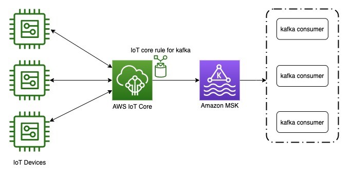


Field Notes: Deliver Messages Using an IoT Rule Action to Amazon Managed Streaming for Apache Kafka

Post Syndicated from Siddhesh Keluskar original https://aws.amazon.com/blogs/architecture/field-notes-deliver-messages-using-an-iot-rule-action-to-amazon-managed-streaming-for-apache-kafka/

With IoT devices scaling up rapidly, real-time data integration and data processing has become a major challenge. This is why customers often choose Message Queuing Telemetry Transport (MQTT) for message ingestion, and Apache Kafka to build a real-time streaming data pipeline. AWS IoT Core now supports a new IoT rule action to deliver messages from your devices directly to your Amazon MSK or self-managed Apache Kafka clusters for data analysis and visualization, without you having to write a single line of code.

In this post, you learn how to set up a real-time streaming data pipeline for IoT data using AWS IoT Core rule and Amazon Managed Streaming for Apache Kafka. The audience for this post is architects and developers creating solutions to ingest sensor data, and high-volume high-frequency streaming data, and process it using a Kafka cluster. Also, this blog describes the SASL_SSL (using user name and password) method to access your Kafka cluster.

Overview of solution

Figure 1 represents an IoT data ingestion pipeline where multiple IoT devices connect to AWS IoT Core. These devices can send messages to AWS IoT Core over MQTT or HTTPS protocol. AWS IoT Core rule for Kafka is configured to intercept messages from the desired topic and route them to the Apache Kafka cluster. These messages can then be received by multiple consumers connected to the Kafka cluster. In this post, we will use AWS Python SDK to represent IoT devices and publish messages.

Figure 1 - Architecture representing an IoT ingestion pipeline

Figure 1 – Architecture representing an IoT ingestion pipeline

Prerequisites

Walkthrough

I will show you how to stream AWS IoT data on an Amazon MSK cluster using AWS IoT Core rules and SASL_SSL SCRAM-SHA-512 mechanism of authentication. Following are the steps for this walkthrough:

  1. Create an Apache Kafka cluster using Amazon MSK.
  2. Configure an Apache Kafka cluster for SASL_SSL authentication.
  3. Set up a Kafka producer and consumer on AWS Cloud9 to test the setup.
  4. Configure an IoT Rule action to send a message to Kafka.

1. Create an Apache Kafka cluster using Amazon MSK

  • The first step is to create an Apache Kafka cluster. Open the service page for Amazon MSK by signing in to your AWS account.
  • Choose Create Cluster, and select Custom Create. AWS IoT Core supports SSL and SASL_SSL based authentication for Amazon MSK. We are using custom settings to configure these authentication methods.
Figure 2 - Screenshot showing how to create an MSK cluster.

Figure 2 – Screenshot showing how to create an MSK cluster.

  • Assign a cluster name, and select Apache Kafka (version of your choice), for this walkthrough, we are using 2.6.1.
  • Keep the configuration as Amazon MSK default configuration. Choose your Networking components: VPC, number of Availability Zones (a minimum of two is required for high availability), and subnets.
  • Choose SASL/SCRAM authentication (default selection is None).

Use the encryption settings as shown in the following screenshot:

Figure 3 - Screenshot showing Encryption Settings

Figure 3 – Screenshot showing Encryption Settings

  • Keep the monitoring settings as Basic Monitoring, and Choose Create Cluster.
  • It takes approximately 15–20 minutes for the cluster to be created.

2. Configure an Apache Kafka cluster for SASL_SSL authentication

  • When the Apache Kafka cluster is available, we must then configure authentication for producers and consumers.
  • Open AWS Secrets Manager, choose Store a new secret, and then choose Other type of secrets.
  • Enter user name and password as two keys, and assign the user name and password values of your choice.
Figure 5 - Screenshot showing how to store a new secret

Figure 4 – Screenshot showing how to store a new secret

  • Next, select Add new key link.
  • Note: Do not select DefaultEncryptionKey! A secret created with the default key cannot be used with an Amazon MSK cluster. Only a Customer managed key can be used as an encryption key for an Amazon MSK–compatible secret.
  • To add a new key, select Create key, select Symmetric key, and choose Next.
  • Type an Alias, and choose Next.
  • Select appropriate users as Key administrators, and choose Next.
  • Review the configuration, and select Finish.
Figure 6 - Select the newly-created Customer Managed Key as the encryption key

Figure 5 – Select the newly-created Customer Managed Key as the encryption key


Figure 7 - Specify the key value pais to be stored in this secret

Figure 6 – Specify the key value pair to be stored in this secret

  • Select the newly-created Customer Managed Key as the encryption key, and choose Next.
  • Provide a Secret name (Secret name must start with AmazonMSK_ for Amazon MSK cluster to recognize it), for example, AmazonMSK_SECRET_NAME.
  • Choose Next twice, and then choose Store.
Select the newly-created Customer Managed Key as the encryption key, and choose Next. Provide a Secret name (Secret name must start with AmazonMSK_ for Amazon MSK cluster to recognize it) (for example, AmazonMSK_SECRET_NAME). Choose Next twice, and then choose Store.

Figure 7 – Storing a new secret

  • Open the Amazon MSK service page, and select your Amazon MSK cluster. Choose Associate Secrets, and then select Choose secrets (this will only be available after the cluster is created and in Active Status).
  • Choose the secret we created in the previous step, and choose Associate secrets. Only the secret name starting with AmazonMSK_ will be visible.

3. Set up Kafka producer and consumer on AWS Cloud9 to test the setup

  • To test if the cluster and authentication is correctly setup, we use Kafka SDK on AWS Cloud9 IDE.
  • Choose Create environment, and follow the console to create a new AWS Cloud9 environment. You can use an existing AWS Cloud9 environment, in addition to an environment with Kafka consumer and producer already configured.
  • This blog requires Java 8 or earlier.
  • Verify your version of Java with the command: java -version. Next, add your AWS Cloud9 instance Security Group to inbound rules of your Kafka cluster.
  • Open the Amazon MSK page and select your cluster, then choose Security groups applied.
Figure 9 - Selecting Security Groups Applied

Figure 8 – Selecting Security Groups Applied

  • Next, choose Inbound rules, and then choose Edit inbound rules.
  • Choose Add rule, and add Custom TCP ports 2181 and 9096 with Security Group of your AWS Cloud9 instance.
Figure 10 - Screenshot showing rules applied

Figure 9 – Screenshot showing rules applied

  • The Security Group for your AWS Cloud9 can be found in the Environment details section of your AWS Cloud9 instance.
Figure 11 - Screenshot showing Edit Inbound Rules added

Figure 10 – Screenshot showing Edit Inbound Rules added

  • Use Port range values as per the client information section of your Bootstrap server and Zookeeper connection.
Figure 12 - Screesnhot showing where to access 'View client information'

Figure 11 – Screenshot showing where to access ‘View client information’


Figure 13 - Screesnhot showing client integration information

Figure 12 – Screenshot showing client integration information

Invoke the following commands on AWS Cloud9 console to download and extract Kafka CLI tools:

wget https://archive.apache.org/dist/kafka/2.2.1/kafka_2.12-2.2.1.tgz
tar -xzf kafka_2.12-2.2.1.tgz
cd kafka_2.12-2.2.1/
mkdir client && cd client 

Next, create a file users_jass.conf, and add the user name and password that you added in Secrets Manage:

sudo nano users_jaas.conf

Paste the following configuration and save. Verify the user name and passwords are the same as saved in Secrets Manager.

KafkaClient {
   org.apache.kafka.common.security.scram.ScramLoginModule required
   username="hello"
   password="world";
};

Invoke the following commands:

export KAFKA_OPTS=-Djava.security.auth.login.config=$PWD/users_jaas.conf

Create a new file with name client_sasl.properties.

sudo nano client_sasl.properties

Copy the following content to file:

security.protocol=SASL_SSL
sasl.mechanism=SCRAM-SHA-512
ssl.truststore.location=<path-to-keystore-file>/kafka.client.truststore.jks

<path-to-keystore-file> can be retrieved by running following command:

cd ~/environment/kafka_2.12-2.2.1/client
echo $PWD

Next, copy the cacerts file from your Java lib folder to client folder. The path of Java lib folder might be different based on your version of Java.

cd ~/environment/kafka_2.12-2.2.1/client
cp /usr/lib/jvm/java-11-amazon-corretto.x86_64/lib/security/cacerts kafka.client.truststore.jks  
Figure 14 - Screenshot showing client integration information

Figure 13 – Screenshot showing client integration information

Save the previous endpoints as BOOTSTRAP_SERVER and ZOOKEEPER_STRING.

export BOOTSTRAP_SERVER=b-2.iot-demo-cluster.slu5to.c13.kafka.us-east-1.amazonaws.com:9096,b-1.iot-demo-cluster.slu5to.c13.kafka.us-east-1.amazonaws.com:9096
export ZOOKEEPER_STRING=z-1.iot-demo-cluster.slu5to.c13.kafka.us-east-1.amazonaws.com:2181,z-3.iot-demo-cluster.slu5to.c13.kafka.us-east-1.amazonaws.com:2181,z-2.iot-demo-cluster.slu5to.c13.kafka.us-east-1.amazonaws.com:2181

Save the Topic name in an environment variable.

TOPIC="AWSKafkaTutorialTopic"

  • Next, create a new Topic using the Zookeeper String.
cd ~/environment/kafka_2.12-2.2.1
bin/kafka-topics.sh --create --zookeeper $ZOOKEEPER_STRING --replication-factor 2 --partitions 1 --topic $TOPIC 
  • Confirm that you receive the message: Created topic AWSKafkaTutorialTopic.
  • Start Kafka producer by running this command in your Kafka folder:
cd ~/environment/kafka_2.12-2.2.1

bin/kafka-console-producer.sh --broker-list $BOOTSTRAP_SERVER --topic $TOPIC --producer.config client/client_sasl.properties
  • Next, open a new Terminal by pressing the + button, and initiate the following commands to configure the environment variables:
export BOOTSTRAP_SERVER=b-2.iot-demo-cluster.slu5to.c13.kafka.us-east-1.amazonaws.com:9096,b-1.iot-demo-cluster.slu5to.c13.kafka.us-east-1.amazonaws.com:9096
TOPIC="AWSKafkaTutorialTopic"

cd ~/environment/kafka_2.12-2.2.1/client
export KAFKA_OPTS=-Djava.security.auth.login.config=$PWD/users_jaas.conf

cd ~/environment/kafka_2.12-2.2.1/
bin/kafka-console-consumer.sh --bootstrap-server $BOOTSTRAP_SERVER --topic $TOPIC --from-beginning --consumer.config client/client_sasl.properties --from-beginning
  • Now that you have a Kafka consumer and producer opened side-by-side, you can type in producer terminal and verify it from the consumer terminal.
Now that you have a Kafka consumer and producer opened side-by-side, you can type in producer terminal and verify it from the consumer terminal.

Figure 14 – Screenshot showing Kafka consumer and producer opened side-by-side

4. Configure an IoT Rule action to send a message to Kafka

  • Create an AWS Identity and Access Management (IAM) role with SecretsManager permissions to allow IoT rule to access Kafka KeyStore in AWS Secrets Manager.
  • Sign in to IAM, select Policies from the left-side panel, choose Create policy.
  • Select Choose a service, and search for AWS KMS.
  • In Actions, choose All AWS KMS actions. Select All resources in the Resources section, and choose Next.
  • Name the policy KMSfullAccess, and choose Create policy.
  • Select Roles from the left-side panel, choose Create Role, then select EC2 from Choose a use case, and choose Next:Permissions.
  • Assign the policy SecretsManagerReadWrite. Note: if you do not select EC2, SecretsManager Policy will be unavailable.
  • Search for and select SecretsManagerReadWrite and KMSfullAccess Policy.

Add tags, type Role name as kafkaSASLRole, and choose Create Role.

  • After the Role is created, search the newly-created Role name to view the Summary of the role.
  • Choose the Trust relationships tab, and choose Edit trust relationship.

Enter the following trust relationship:

{
  "Version": "2012-10-17",
  "Statement": [
    {
      "Effect": "Allow",
      "Principal": {
        "Service": "iot.amazonaws.com"
      },
      "Action": "sts:AssumeRole"
    }
  ]
}
  • Choose Update Trust Policy.
  • Next, create a new AWS IoT Core rule by signing in to the AWS IoT Core service. Choose Act from the left side-menu, and select Rules.
  • Choose Create. Insert details for Name, Description, and Rule query statement, and then choose Add action. The following query is used for this post:
  • SELECT * from ‘iot/topic’
  • Select Send a message to an Apache Kafka cluster. Next, choose Configure action.
Figure 15 - Screenshot to create a rule

Figure 15 – Screenshot to create a rule


Create a VPC destination (if you do not already have one).

Figure 16 – How to Create a VPC destination

  • Create a VPC destination (if you do not already have one).
  • Select the VPC ID of your Kafka cluster. Select a Security Group with access to Kafka cluster Security Group.
  • Choose security group settings of the EC2 instance we created, or the security group of Kafka cluster.
  • Choose Create Role, and then select Create Destination. It takes approximately 5–10 minutes for the Destination to be Enabled. After the status is Enabled, navigate back to the Rule creation page and select the VPC Destination.
  • Enter AWSKafkaTutorialTopic as Kafka topic (confirm there is no extra space after the topic name, or you will get an error). Do not update Key and Partition boxes.

    Figure 17 - Screenshot showing how to enter the AWSKafkaTutorialTopic

    Figure 17 – Screenshot showing how to enter the AWSKafkaTutorialTopic

  • Verify the Security Group of your VPC destination is added to the inbound list for your Kafka cluster.
Figure 18 - Showing Inbound list for Kafka Cluster

Figure 18 – Showing Security Group for Kafka Cluster


Figure -Screenshot showing Inbound Inbound rules

Figure 19 -Screenshot showing Inbound Inbound rules

The first two Custom TCP entries are for AWS Cloud9 security group. The last two entries are for VPC endpoint.

Set the Client properties as follows:

Bootstrap.server = The TLS bootstrap string for Kafka cluster

security.protocol = SASL_SSL

ssl.truststore = EMPTY for Amazon MSK, enter SecretBinary template for self-managed Kafka

ss.truststore.password = EMPTY for Amazon MSK, enter truststore password for self-managed Kafka

sasl.mechanism = SCRAM-SHA-512

  • Replace the secret name with your stored secret name starting with AmazonMSK_, replace the IAM role ARN with your IAM role ARN.
  • The secret and IAM role are created in previous steps of this post. Enter the following template in the sasl.scram.username field to retrieve username from Secrets Manager.
${get_secret('AmazonMSK_cluster_secret','SecretString','username','arn:aws:iam::318219976534:role/kafkaSASLRole')}

Perform a similar step for sasl.scram.password field:

${get_secret('AmazonMSK_cluster_secret','SecretString','password','arn:aws:iam::318219976534:role/kafkaSASLRole')}
  • Choose Add action.
  • Choose Create rule.

Testing the data pipeline

  • Open MQTT test client from AWS IoT Core page.
  • Publish the message to the MQTT topic that you configured while creating the rule.
  • Keep the consumer session active (created in earlier step). You will see data published on the MQTT topic being streamed to Kafka consumer.
Figure 20 - Screenshot showing testing the data pipeline

Figure 20 – Screenshot showing testing the data pipeline

Common troubleshooting checks

Confirm that your:

  1. AWS Cloud9 Security Group is added to Amazon MSK Security Group Inbound rule
  2. VPC endpoint Security Group is added to Amazon MSK Security Group Inbound rule
  3. Topic is created in the Kafka cluster
  4. IAM role has Secrets Manager and KMS permissions
  5. Environment variables are correctly configured in terminal
  6. Folder paths have been correctly followed

Cleaning up

To avoid incurring future changes, delete the following resources:

  • Amazon MSK cluster
  • AWS IoT Core rule
  • IAM role
  • Secrets Manager Secret
  • AWS Cloud9 instance

Conclusion

In this post, I showed you how to configure an IoT Rule Action to deliver messages to Apache Kafka cluster using AWS IoT Core and Amazon MSK. You can now build a real-time streaming data pipeline by securely delivering MQTT messages to a highly-scalable, durable, and reliable system using Apache Kafka.

Field Notes provides hands-on technical guidance from AWS Solutions Architects, consultants, and technical account managers, based on their experiences in the field solving real-world business problems for customers.


Amazon MSK Replicator and MirrorMaker2: Choosing the right replication strategy for Apache Kafka disaster recovery and migrations

Post Syndicated from Anusha Dharmalingam original https://aws.amazon.com/blogs/big-data/amazon-msk-replicator-and-mirrormaker2-choosing-the-right-replication-strategy-for-apache-kafka-disaster-recovery-and-migrations/

Customers need to replicate their Apache Kafka for a variety of reasons, such as compliance requirements, cluster migrations, and disaster recovery (DR) implementations. However, the right replication strategy can vary depending on the application context. In this post, we walk through the different considerations for using Amazon MSK Replicator over Apache Kafka’s MirrorMaker 2, and help you choose the right replication solution for your use case. We also discuss how to make applications using Amazon Managed Streaming for Apache Kafka (Amazon MSK) resilient to disasters using a multi-Region Kafka architecture using MSK Replicator.

Challenges with choosing DR strategies

Customers create business continuity plans and DR strategies to maximize resiliency for their applications, because downtime or data loss can result in losing revenue or halting operations. DR planning helps the business continue running in the event of a disaster impacting a subset of their application architecture. For customers using Kafka as a core streaming and messaging service in their applications, planning for DR for their Kafka infrastructure is an essential part of meeting goals for their application Recovery Time Objective (RTO) and Recovery Point Objective (RPO).

Amazon MSK is a fully managed service that makes it straightforward to build and run Kafka to process streaming data. Amazon MSK provides high availability by offering multi-AZ configurations to distribute brokers across multiple Availability Zones within an AWS Region. A single MSK cluster deployment provides message durability through intra-cluster data replication. Data replication with a replication factor of 3 and min-ISR value of 2 along with the producer setting acks=all provides the strongest availability guarantees, because it makes sure other brokers in the cluster acknowledge receiving the data before the leader broker responds to the producer. This design provides robust protection against single broker failure as well as single-AZ failure.

For enhanced resilience within a single Region, Amazon MSK also offers Express brokers, which significantly improve Kafka cluster reliability, throughput, recovery times. Express brokers include pay-as-you-go storage, automatic best-practice reliability configurations, no maintenance windows, and faster broker scaling and recovery times. This architecture reduces recovery time, minimizes the chance of errors with misconfigurations, and increases throughput, making your Kafka clusters more resilient across Availability Zones.

However, if an unlikely issue is impacting your applications or infrastructure across more than one Availability Zone, the architecture outlined in this post can help you prepare, respond, and recover from it.

For companies that can withstand a longer RTO but require a lower RPO on Amazon MSK, backing up data to Amazon Simple Storage Service (Amazon S3) is sufficient as a DR plan. This approach requires you to think through how to handle restarting the application after a DR failover. In this approach, you build a system to recover the data from Amazon S3 to Kafka topics (as described in Back up and restore Kafka topic data using Amazon MSK Connect). Depending on the volume of data being restored, it might take a long time to recover in this scenario. Additionally, you must consider how to handle consumer group offsets, and whether to allow applications to consume from the latest offset in the restored Kafka topics. Due to the high RTO, as well as the complexity and challenges associated with this approach, most streaming use cases rely on the availability of the MSK cluster itself for their business continuity plan. In these cases, setting up MSK clusters in multiple Regions and configuring data replication between clusters provides the required business resilience and continuity.

Choosing the right replication solution: MSK Replicator vs MirrorMaker 2

AWS recommends two primary solutions for cross-Region Kafka replication: MSK Replicator and MirrorMaker 2. Understanding when to use each solution is crucial for designing an effective DR strategy.

MSK Replicator: For most MSK cluster replications in the same account

MSK Replicator is a fully managed, serverless Kafka replication service that makes it straightforward to reliably replicate data across MSK clusters in different Regions or within the same Region. MSK Replicator is the recommended solution for application scenarios replicating data within the same AWS account. MSK Replicator has the following benefits:

  • Replication between MSK clusters – It supports replicating between MSK clusters in the same AWS account (including active-active or active-passive DR architectures for Amazon MSK)
  • No infrastructure management – It’s fully serverless with automatic scaling and straightforward setup through the AWS Management Console, AWS Command Line Interface (AWS CLI), or APIs
  • Built-in monitoring – It’s integrated with Amazon CloudWatch metrics and logging
  • Built-in high availability – As a managed service, it offers built-in fault tolerance across Availability Zones

MirrorMaker 2: For migrations and complex and hybrid scenarios

MirrorMaker 2 (MM2) remains the preferred solution for specific use cases that require more flexibility or involve non-Amazon MSK environments. MM2 is a utility bundled as part of Kafka that helps replicate data between Kafka clusters using the Kafka Connect framework.

We recommend MirrorMaker 2 for the following use cases:

  • Cross-account replication – Replicating data between MSK clusters in different AWS accounts
  • Migrations to Amazon MSK – Migrating from existing Kafka clusters on premises, in other clouds, or on self-managed Amazon Elastic Compute Cloud (Amazon EC2) deployments
  • Cross-cloud or hybrid cloud scenarios – Replicating between Kafka running on-premises or on different cloud providers and Amazon MSK for disaster recovery or data analytics use cases
  • Using mTLS or SASL/SCRAM authentication – When you need mutual TLS certificate-based or SASL/SCRAM authentication and can’t enable AWS Identity and Access Management (IAM) authentication in your MSK cluster (for replication from one MSK cluster to another in these scenarios, you can still use MSK Replicator by enabling IAM authentication in addition to existing authentication methods)
  • Custom replication policies – Advanced topic naming or transformation requirements

In the following sections, we discuss the architecture and deployment approaches for use cases where MSK Replicator and MirrorMaker 2 are the appropriate choices.

MSK Replicator solution overview

The following diagram illustrates the architecture for using MSK Replicator.

We create two MSK clusters – one in the primary Region, the other in the secondary Region as a standby cluster for disaster recovery. We deploy MSK Replicator in the secondary region to replicate topics, ACLs, data, and consumer group offsets from the primary cluster. In this solution, we showcase a single-direction replication for active-passive disaster recovery. This solution can also be extended for active-active disaster recovery scenarios. Our Kafka clients connect to the primary cluster and can be configured to connect to the secondary cluster in the event of a disaster recovery failover.

For details on implementation steps, refer to Introducing Amazon MSK Replicator – Fully Managed Replication across MSK Clusters in Same or Different AWS Regions. For details on disaster recovery scenarios, refer to Use replication to increase the resiliency of a Kafka streaming application across Regions. These resources provide the following benefits:

  • Full deployment steps – Step by step deployment process for MSK Replicator between regions
  • Comprehensive examples – Multiple deployment scenarios and configurations
  • Failover process – Key steps in executing a disaster recovery failover when using MSK Replicator

MirrorMaker2 solution overview

The following diagram illustrates the architecture for using MirrorMaker 2.

We create an MSK cluster in the primary Region, with the existing Kafka cluster on premises. This Kafka cluster is analogous to Kafka clusters running in other clouds, or in self-managed Kafka clusters on Amazon EC2. In this solution, we showcase a single-direction replication for cluster migration scenarios. Our Kafka clients interact with the on-premises Kafka cluster and can be migrated to run on AWS to interact with the MSK cluster.

Rather than manually configuring each component, we recommend using the automated deployment resources available in the following GitHub repository. For a step-by-step walkthrough of deploying MirrorMaker 2 on Amazon ECS with Fargate using auto scaling, refer to Amazon MSK Migration Workshop: Modernizing with Express Brokers. These resources provide the following benefits:

  • Infrastructure as code – Terraform for MSK clusters and supporting infrastructure
  • Containerized Kafka Connect – Docker images optimized for AWS
  • Amazon ECS with AWS Fargate deployment – Scalable, serverless container deployment using Amazon Elastic Container Service (Amazon ECS) with AWS Fargate
  • Auto scaling configuration – Automatic scaling based on workload demands
  • Comprehensive examples – Multiple deployment scenarios and configurations
  • Migration process – Key steps in executing a Kafka migration using MM2

Conclusion

Choosing the right replication solution depends on your specific requirements. We recommend using MSK Replicator when replicating from one MSK cluster to another and you want a fully managed solution for disaster recovery. MirrorMaker 2 is recommended for migrations to Amazon MSK, hybrid environments, or when you need complex custom replication policies.

For MSK Replicator deployments, refer to Introducing Amazon MSK Replicator – Fully Managed Replication across MSK Clusters in Same or Different AWS Regions and Use replication to increase the resiliency of a Kafka streaming application across Regions.

For MirrorMaker 2 deployments, refer to the GitHub repository and Amazon MSK Migration Workshop to implement production-ready solutions with automated deployment, monitoring, and scaling capabilities.

These approaches provide a customizable set of options for data redundancy and business continuity capabilities needed to meet regulatory compliance and disaster recovery requirements, while minimizing operational overhead through automation and best practices.


About the Author

Mazrim Mehrtens

Mazrim Mehrtens

Mazrim is a Sr. Specialist Solutions Architect for messaging and streaming workloads. Mazrim works with customers to build and support systems that process and analyze terabytes of streaming data in real time, run enterprise Machine Learning pipelines, and create systems to share data across teams seamlessly with varying data toolsets and software stacks.

Introducing Amazon Kinesis Data Analytics Studio – Quickly Interact with Streaming Data Using SQL, Python, or Scala

Post Syndicated from Danilo Poccia original https://aws.amazon.com/blogs/aws/introducing-amazon-kinesis-data-analytics-studio-quickly-interact-with-streaming-data-using-sql-python-or-scala/

The best way to get timely insights and react quickly to new information you receive from your business and your applications is to analyze streaming data. This is data that must usually be processed sequentially and incrementally on a record-by-record basis or over sliding time windows, and can be used for a variety of analytics including correlations, aggregations, filtering, and sampling.

To make it easier to analyze streaming data, today we are pleased to introduce Amazon Kinesis Data Analytics Studio.

Now, from the Amazon Kinesis console you can select a Kinesis data stream and with a single click start a Kinesis Data Analytics Studio notebook powered by Apache Zeppelin and Apache Flink to interactively analyze data in the stream. Similarly, you can select a cluster in the Amazon Managed Streaming for Apache Kafka console to start a notebook to analyze data in Apache Kafka streams. You can also start a notebook from the Kinesis Data Analytics Studio console and connect to custom sources.

Architectural diagram.

In the notebook, you can interact with streaming data and get results in seconds using SQL queries and Python or Scala programs. When you are satisfied with your results, with a few clicks you can promote your code to a production stream processing application that runs reliably at scale with no additional development effort.

For new projects, we recommend that you use the new Kinesis Data Analytics Studio over Kinesis Data Analytics for SQL Applications. Kinesis Data Analytics Studio combines ease of use with advanced analytical capabilities, which makes it possible to build sophisticated stream processing applications in minutes. Let’s see how that works in practice.

Using Kinesis Data Analytics Studio to Analyze Streaming Data
I want to get a better understanding of the data sent by some sensors to a Kinesis data stream.

To simulate the workload, I use this random_data_generator.py Python script. You don’t need to know Python to use Kinesis Data Analytics Studio. In fact, I am going to use SQL in the following steps. Also, you can avoid any coding and use the Amazon Kinesis Data Generator user interface (UI) to send test data to Kinesis Data Streams or Kinesis Data Firehose. I am using a Python script to have finer control over the data that is being sent.

import datetime
import json
import random
import boto3

STREAM_NAME = "my-input-stream"


def get_random_data():
    current_temperature = round(10 + random.random() * 170, 2)
    if current_temperature > 160:
        status = "ERROR"
    elif current_temperature > 140 or random.randrange(1, 100) > 80:
        status = random.choice(["WARNING","ERROR"])
    else:
        status = "OK"
    return {
        'sensor_id': random.randrange(1, 100),
        'current_temperature': current_temperature,
        'status': status,
        'event_time': datetime.datetime.now().isoformat()
    }


def send_data(stream_name, kinesis_client):
    while True:
        data = get_random_data()
        partition_key = str(data["sensor_id"])
        print(data)
        kinesis_client.put_record(
            StreamName=stream_name,
            Data=json.dumps(data),
            PartitionKey=partition_key)


if __name__ == '__main__':
    kinesis_client = boto3.client('kinesis')
    send_data(STREAM_NAME, kinesis_client)

This script sends random records to my Kinesis data stream using JSON syntax. For example:

{'sensor_id': 77, 'current_temperature': 93.11, 'status': 'OK', 'event_time': '2021-05-19T11:20:00.978328'}
{'sensor_id': 47, 'current_temperature': 168.32, 'status': 'ERROR', 'event_time': '2021-05-19T11:20:01.110236'}
{'sensor_id': 9, 'current_temperature': 140.93, 'status': 'WARNING', 'event_time': '2021-05-19T11:20:01.243881'}
{'sensor_id': 27, 'current_temperature': 130.41, 'status': 'OK', 'event_time': '2021-05-19T11:20:01.371191'}

From the Kinesis console, I select a Kinesis data stream (my-input-stream) and choose Process data in real time from the Process drop-down. In this way, the stream is configured as a source for the notebook.

Console screenshot.

Then, in the following dialog box, I create an Apache Flink – Studio notebook.

I enter a name (my-notebook) and a description for the notebook. The AWS Identity and Access Management (IAM) permissions to read from the Kinesis data stream I selected earlier (my-input-stream) are automatically attached to the IAM role assumed by the notebook.

Console screenshot.

I choose Create to open the AWS Glue console and create an empty database. Back in the Kinesis Data Analytics Studio console, I refresh the list and select the new database. It will define the metadata for my sources and destinations. From here, I can also review the default Studio notebook settings. Then, I choose Create Studio notebook.

Console screenshot.

Now that the notebook has been created, I choose Run.

Console screenshot.

When the notebook is running, I choose Open in Apache Zeppelin to get access to the notebook and write code in SQL, Python, or Scala to interact with my streaming data and get insights in real time.

In the notebook, I create a new note and call it Sensors. Then, I create a sensor_data table describing the format of the data in the stream:

%flink.ssql

CREATE TABLE sensor_data (
    sensor_id INTEGER,
    current_temperature DOUBLE,
    status VARCHAR(6),
    event_time TIMESTAMP(3),
    WATERMARK FOR event_time AS event_time - INTERVAL '5' SECOND
)
PARTITIONED BY (sensor_id)
WITH (
    'connector' = 'kinesis',
    'stream' = 'my-input-stream',
    'aws.region' = 'us-east-1',
    'scan.stream.initpos' = 'LATEST',
    'format' = 'json',
    'json.timestamp-format.standard' = 'ISO-8601'
)

The first line in the previous command tells to Apache Zeppelin to provide a stream SQL environment (%flink.ssql) for the Apache Flink interpreter. I can also interact with the streaming data using a batch SQL environment (%flink.bsql), or Python (%flink.pyflink) or Scala (%flink) code.

The first part of the CREATE TABLE statement is familiar to anyone who has used SQL with a database. A table is created to store the sensor data in the stream. The WATERMARK option is used to measure progress in the event time, as described in the Event Time and Watermarks section of the Apache Flink documentation.

The second part of the CREATE TABLE statement describes the connector used to receive data in the table (for example, kinesis or kafka), the name of the stream, the AWS Region, the overall data format of the stream (such as json or csv), and the syntax used for timestamps (in this case, ISO 8601). I can also choose the starting position to process the stream, I am using LATEST to read the most recent data first.

When the table is ready, I find it in the AWS Glue Data Catalog database I selected when I created the notebook:

Console screenshot.

Now I can run SQL queries on the sensor_data table and use sliding or tumbling windows to get a better understanding of what is happening with my sensors.

For an overview of the data in the stream, I start with a simple SELECT to get all the content of the sensor_data table:

%flink.ssql(type=update)

SELECT * FROM sensor_data;

This time the first line of the command has a parameter (type=update) so that the output of the SELECT, which is more than one row, is continuously updated when new data arrives.

On the terminal of my laptop, I start the random_data_generator.py script:

$ python3 random_data_generator.py

At first I see a table that contains the data as it comes. To get a better understanding, I select a bar graph view. Then, I group the results by status to see their average current_temperature, as shown here:

Notebook screenshot.

As expected by the way I am generating these results, I have different average temperatures depending on the status (OK, WARNING, or ERROR). The higher the temperature, the greater the probability that something is not working correctly with my sensors.

I can run the aggregated query explicitly using a SQL syntax. This time, I want the result computed on a sliding window of 1 minute with results updated every 10 seconds. To do so, I am using the HOP function in the GROUP BY section of the SELECT statement. To add the time to the output of the select, I use the HOP_ROWTIME function. For more information, see how group window aggregations work in the Apache Flink documentation.

%flink.ssql(type=update)

SELECT sensor_data.status,
       COUNT(*) AS num,
       AVG(sensor_data.current_temperature) AS avg_current_temperature,
       HOP_ROWTIME(event_time, INTERVAL '10' second, INTERVAL '1' minute) as hop_time
  FROM sensor_data
 GROUP BY HOP(event_time, INTERVAL '10' second, INTERVAL '1' minute), sensor_data.status;

This time, I look at the results in table format:

Notebook screenshot.

To send the result of the query to a destination stream, I create a table and connect the table to the stream. First, I need to give permissions to the notebook to write into the stream.

In the Kinesis Data Analytics Studio console, I select my-notebook. Then, in the Studio notebooks details section, I choose Edit IAM permissions. Here, I can configure the sources and destinations used by the notebook and the IAM role permissions are updated automatically.

Console screenshot.

In the Included destinations in IAM policy section, I choose the destination and select my-output-stream. I save changes and wait for the notebook to be updated. I am now ready to use the destination stream.

In the notebook, I create a sensor_state table connected to my-output-stream.

%flink.ssql

CREATE TABLE sensor_state (
    status VARCHAR(6),
    num INTEGER,
    avg_current_temperature DOUBLE,
    hop_time TIMESTAMP(3)
)
WITH (
'connector' = 'kinesis',
'stream' = 'my-output-stream',
'aws.region' = 'us-east-1',
'scan.stream.initpos' = 'LATEST',
'format' = 'json',
'json.timestamp-format.standard' = 'ISO-8601');

I now use this INSERT INTO statement to continuously insert the result of the select into the sensor_state table.

%flink.ssql(type=update)

INSERT INTO sensor_state
SELECT sensor_data.status,
    COUNT(*) AS num,
    AVG(sensor_data.current_temperature) AS avg_current_temperature,
    HOP_ROWTIME(event_time, INTERVAL '10' second, INTERVAL '1' minute) as hop_time
FROM sensor_data
GROUP BY HOP(event_time, INTERVAL '10' second, INTERVAL '1' minute), sensor_data.status;

The data is also sent to the destination Kinesis data stream (my-output-stream) so that it can be used by other applications. For example, the data in the destination stream can be used to update a real-time dashboard, or to monitor the behavior of my sensors after a software update.

I am satisfied with the result. I want to deploy this query and its output as a Kinesis Analytics application. To do so, I need to provide an S3 location to store the application executable.

In the configuration section of the console, I edit the Deploy as application configuration settings. There, I choose a destination bucket in the same region and save changes.

Console screenshot.

I wait for the notebook to be ready after the update. Then, I create a SensorsApp note in my notebook and copy the statements that I want to execute as part of the application. The tables have already been created, so I just copy the INSERT INTO statement above.

From the menu at the top right of my notebook, I choose Build SensorsApp and export to Amazon S3 and confirm the application name.

Notebook screenshot.

When the export is ready, I choose Deploy SensorsApp as Kinesis Analytics application in the same menu. After that, I fine-tune the configuration of the application. I set parallelism to 1 because I have only one shard in my input Kinesis data stream and not a lot of traffic. Then, I run the application, without having to write any code.

From the Kinesis Data Analytics applications console, I choose Open Apache Flink dashboard to get more information about the execution of my application.

Apache Flink console screenshot.

Availability and Pricing
You can use Amazon Kinesis Data Analytics Studio today in all AWS Regions where Kinesis Data Analytics is generally available. For more information, see the AWS Regional Services List.

In Kinesis Data Analytics Studio, we run the open-source versions of Apache Zeppelin and Apache Flink, and we contribute changes upstream. For example, we have contributed bug fixes for Apache Zeppelin, and we have contributed to AWS connectors for Apache Flink, such as those for Kinesis Data Streams and Kinesis Data Firehose. Also, we are working with the Apache Flink community to contribute availability improvements, including automatic classification of errors at runtime to understand whether errors are in user code or in application infrastructure.

With Kinesis Data Analytics Studio, you pay based on the average number of Kinesis Processing Units (KPU) per hour, including those used by your running notebooks. One KPU comprises 1 vCPU of compute, 4 GB of memory, and associated networking. You also pay for running application storage and durable application storage. For more information, see the Kinesis Data Analytics pricing page.

Start using Kinesis Data Analytics Studio today to get better insights from your streaming data.

Danilo