Post Syndicated from Bindhu Chinnadurai original https://aws.amazon.com/blogs/big-data/a-hybrid-approach-in-healthcare-data-warehousing-with-amazon-redshift/
Data warehouses play a vital role in healthcare decision-making and serve as a repository of historical data. A healthcare data warehouse can be a single source of truth for clinical quality control systems. Data warehouses are mostly built using the dimensional model approach, which has consistently met business needs.
Loading complex multi-point datasets into a dimensional model, identifying issues, and validating data integrity of the aggregated and merged data points are the biggest challenges that clinical quality management systems face. Additionally, scalability of the dimensional model is complex and poses a high risk of data integrity issues.
The data vault approach solves most of the problems associated with dimensional models, but it brings other challenges in clinical quality control applications and regulatory reports. Because data is closer to the source and stored in raw format, it has to be transformed before it can be used for reporting and other application purposes. This is one of the biggest hurdles with the data vault approach.
In this post, we discuss some of the main challenges enterprise data warehouses face when working with dimensional models and data vaults. We dive deep into a hybrid approach that aims to circumvent the issues posed by these two and also provide recommendations to take advantage of this approach for healthcare data warehouses using Amazon Redshift.
What is a dimensional data model?
Dimensional modeling is a strategy for storing data in a data warehouse using dimensions and facts. It optimizes the database for faster data retrieval. Dimensional models have a distinct structure and organize data to provide reports that increase performance.
In a dimensional model, a transaction record is divided either into facts (often numerical), additive transactional data, or dimensions (referential information that gives context to the facts). This categorization of data into facts and dimensions, as well as the entity-relationship framework of the dimensional model, presents complex business processes in a way that is easy for analysts to understand.
A dimensional model in data warehousing is designed for reading, summarizing, and analyzing numerical information such as patient vital stats, lab reading values, counts, and so on. Regardless of the division or use case it is related to, dimensional data models can be used to store data obtained from tracking various processes like patient encounters, provider practice metrics, aftercare surveys, and more.
The majority of healthcare clinical quality data warehouses are built on top of dimensional modeling techniques. The benefit of using dimensional data modeling is that, when data is stored in a data warehouse, it’s easier to persist and extract it.
Although it’s a competent data structure technique, there are challenges in scalability, source tracking, and troubleshooting with the dimensional modeling approach. Tracking and validating the source of aggregated and compute data points is important in clinical quality regulatory reporting systems. Any mistake in regulatory reports may result in a large penalty from regulatory and compliance agencies. These challenges exist because the data points are labeled using meaningless numeric surrogate keys, and any minor error can impair prediction accuracy, and consequently affect the quality of judgments. The ways to countervail these challenges are by refactoring and bridging the dimensions. But that adds data noise over time and reduces accuracy.
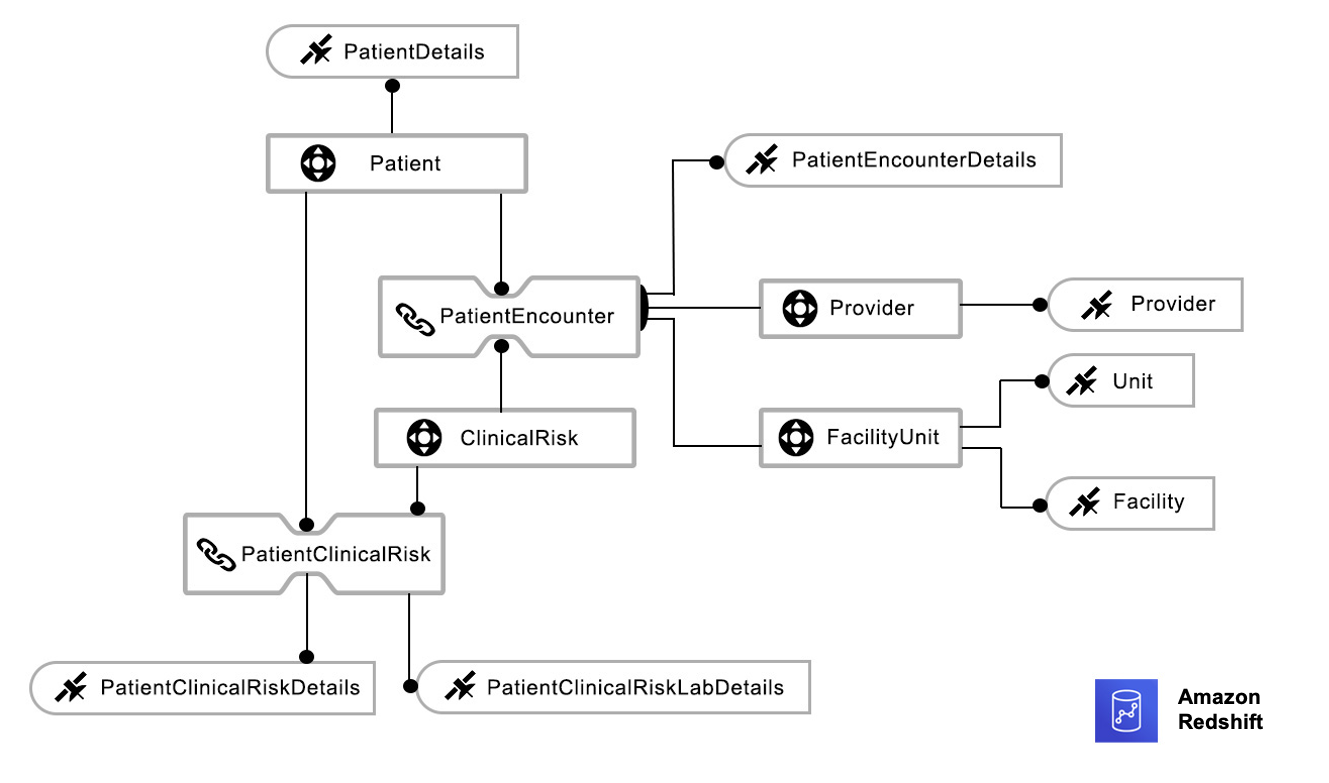
Let’s look at an example of a typical dimensional data warehouse architecture in healthcare, as shown in the following logical model.

The following diagram illustrates a sample dimensional model entity-relationship diagram.

This data model contains dimensions and fact tables. You can use the following query to retrieve basic provider and patient relationship data from the dimensional model:
Challenges of dimensional modeling
Dimensional modeling requires data preprocessing before generating a star schema, which involves a large amount of data processing. Any change to the dimension definition results in a lengthy and time-consuming reprocessing of the dimension data, which often results in data redundancy.
Another issue is that, when relying merely on dimensional modeling, analysts can’t assure the consistency and accuracy of data sources. Especially in healthcare, where lineage, compliance, history, and traceability are of prime importance because of the regulations in place.
A data vault seeks to provide an enterprise data warehouse while solving the shortcomings of dimensional modeling approaches. It is a data modeling methodology designed for large-scale data warehouse platforms.
What is a data vault?
The data vault approach is a method and architectural framework for providing a business with data analytics services to support business intelligence, data warehousing, analytics, and data science needs. The data vault is built around business keys (hubs) defined by the company; the keys obtained from the sources are not the same.
Amazon Redshift RA3 instances and Amazon Redshift Serverless are perfect choices for a data vault. And when combined with Amazon Redshift Spectrum, a data vault can deliver more value.
There are three layers to the data vault:
- Staging
- Data vault
- Business vault
Staging involves the creation of a replica of the original data, which is primarily used to aid the process of transporting data from various sources to the data warehouse. There are no restrictions on this layer, and it is typically not persistent. It is 1:1 with the source systems, generally in the same format as that of the sources.
The data vault is based on business keys (hubs), which are defined by the business. All in-scope data is loaded, and auditability is maintained. At the heart of all data warehousing is integration, and this layer contains integrated data from multiple sources built around the enterprise-wide business keys. Although data lakes resemble data vaults, a data vault provides more features of a data warehouse. However, it combines the functionalities of both.
The business vault stores the outcome of business rules, including deduplication, conforming results, and even computations. When results are calculated for two or more data marts, this helps eliminate redundant computation and associated inconsistencies.
Because business vaults still don’t satisfy reporting needs, enterprises create a data mart after the business vault to satisfy dashboarding needs.
Data marts are ephemeral views that can be implemented directly on top of the business and raw vaults. This makes it easy to adapt over time and eliminates the danger of inconsistent results. If views don’t give the required level of performance, the results can be stored in a table. This is the presentation layer and is designed to be requirements-driven and scope-specific subsets of the warehouse data. Although dimensional modeling is commonly used to deliver this layer, marts can also be flat files, .xml files, or in other forms.
The following diagram shows the typical data vault model used in clinical quality repositories.

When the dimensional model as shown earlier is converted into a data vault using the same structure, it can be represented as follows.
Advantages of a data vault
Although any data warehouse should be built within the context of an overarching company strategy, data vaults permit incremental delivery. You can start small and gradually add more sources over time, just like Kimball’s dimensional design technique.
With a data vault, you don’t have to redesign the structure when adding new sources, unlike dimensional modeling. Business rules can be easily changed because raw and business-generated data is kept independent of each other in a data vault.
A data vault isolates technical data reorganization from business rules, thereby facilitating the separation of these potentially tricky processes. Similarly, data cleaning can be maintained separately from data import.
A data vault accommodates changes over time. Unlike a pure dimensional design, a data vault separates raw and business-generated data and accepts changes from both sources.
Data vaults make it easy to maintain data lineage because it includes metadata identifying the source systems. In contrast to dimensional design, where data is cleansed before loading, data vault updates are always gradual, and results are never lost, providing an automatic audit trail.
When raw data is stored in a data vault, historical attributes that weren’t initially available can be added to the presentation area. Data marts can be implemented as views by adding a new column to an existing view.
In data vault 2.0, hash keys eliminate data load dependencies, which allows near-real-time data loading, as well as concurrent data loads of terabytes to petabytes. The process of mastering both entity-relationship modeling and dimensional design takes time and practice, but the process of automating a data vault is easier.
Challenges of a data vault
A data vault is not a one-size-fits-all solution for data warehouses, and it does have a few limitations.
To begin with, when directly feeding the data vault model into a report on one subject area, you need to combine multiple types of data. Due to the incapability of reporting technologies to perform such data processing, this integration can reduce report performance and increase the risk of errors. However, data vault models could improve report performance by incorporating dimensional models or adding additional reporting layers. And for data models that can be directly reported, a dimensional model can be developed.
Additionally, if the data is static or if it comes from a single source, it reduces the efficacy of data vaults. They often negate many benefits of data vaults, and require more business logic, which can be avoided.
The storage requirement for a data vault is also significantly higher. Three separate tables for the same subject area can effectively increase the number of tables by three, and when they are inserts only. If the data is basic, you can achieve the benefits listed here with a simpler dimensional model rather than deploying a data vault.
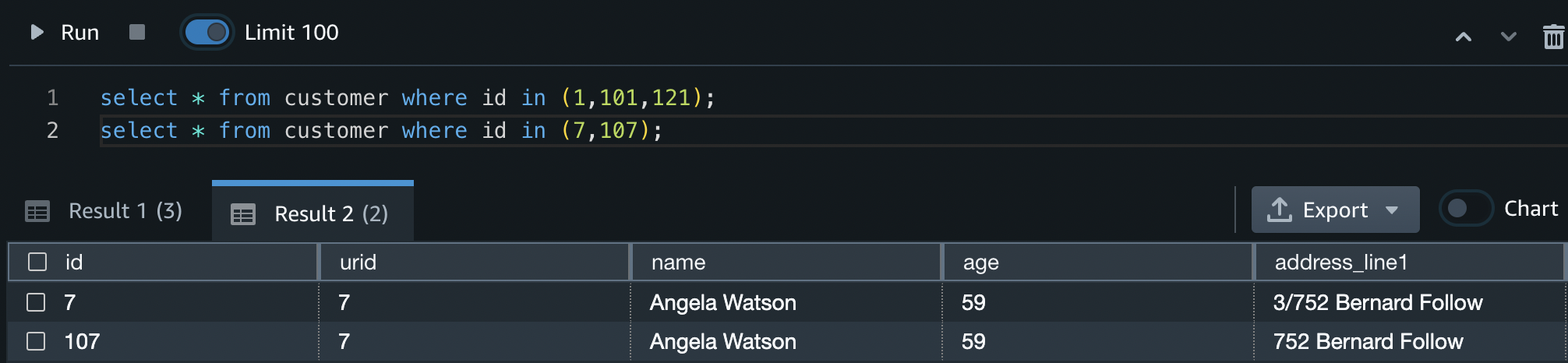
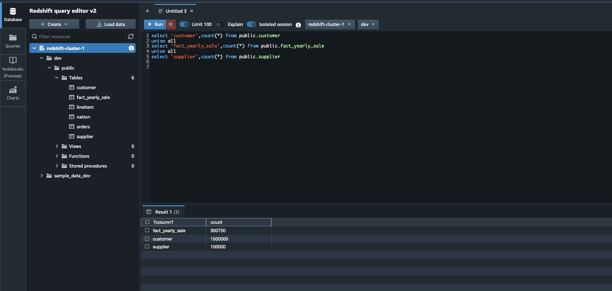
The following sample query retrieves provider and patient data from a data vault using the sample model we discussed in this section:
The query involves many joins, which increases the depth and time for the query run, as illustrated in the following chart.

This following table shows that the SQL depth and runtime is proportional, where depth is the number of joins. If the number of joins increase, then the runtime also increases and therefore the cost.
| SQL Depth | Runtime in Seconds | Cost per Query in Seconds |
| 14 | 80 | 40,000 |
| 12 | 60 | 30,000 |
| 5 | 30 | 15,000 |
| 3 | 25 | 12,500 |
The hybrid model addresses major issues raised by the data vault and dimensional model approaches that we’ve discussed in this post, while also allowing improvements in data collection, including IoT data streaming.
What is a hybrid model?
The hybrid model combines the data vault and a portion of the star schema to provide the advantages of both the data vault and dimensional model, and is mainly intended for logical enterprise data warehouses.
The hybrid approach is designed from the bottom up to be gradual and modular, and it can be used for big data, structured, and unstructured datasets. The primary data contains the business rules and enterprise-level data standards norms, as well as additional metadata needed to transform, validate, and enrich data for dimensional approaches. In this model, data processes from left to right provide data vault advantages, and data processes from right to left provide dimensional model advantages. Here, the data vault satellite tables serve as both satellite tables and dimensional tables.
After combining the dimensional and the data vault models, the hybrid model can be viewed as follows.

The following is an example entity-relation diagram of the hybrid model, which consists of a fact table from the dimensional model and all other entities from the data vault. The satellite entity from the data vault plays the dual role. When it’s connected to a data vault, it acts as a sat table, and when connected to a fact table, it acts as a dimension table. To serve this dual purpose, sat tables have two keys: a foreign key to connect with the data vault, and a primary key to connect with the fact table.
The following diagram illustrates the physical hybrid data model.

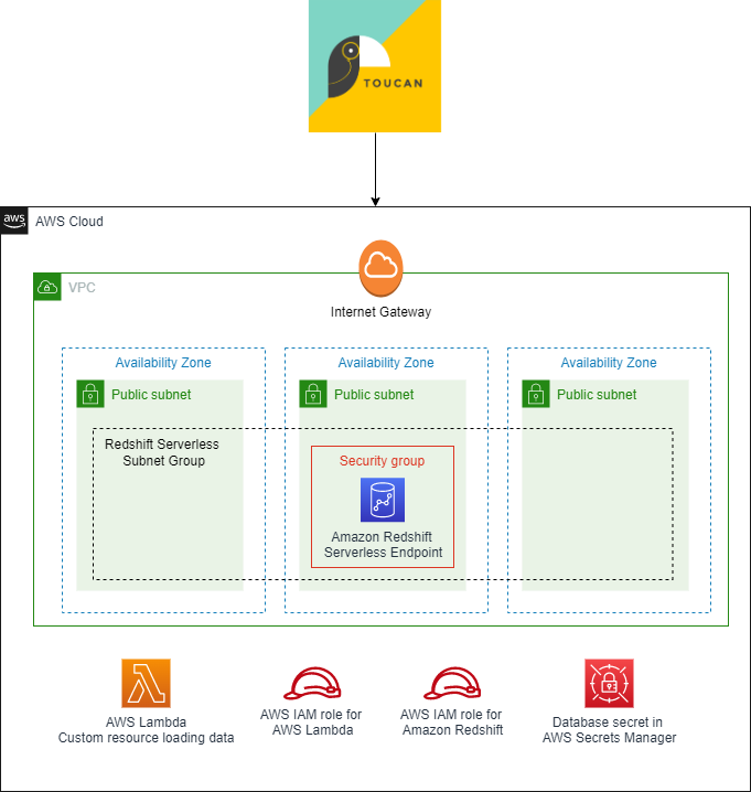
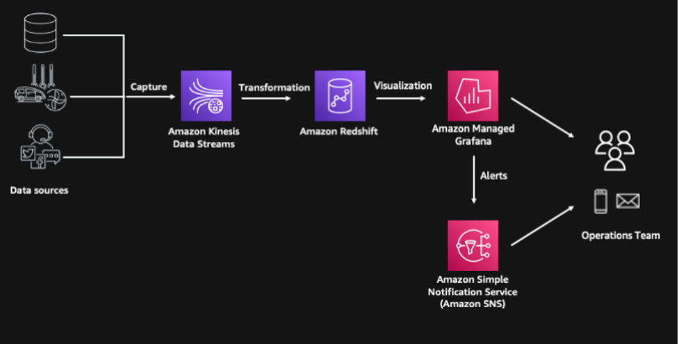
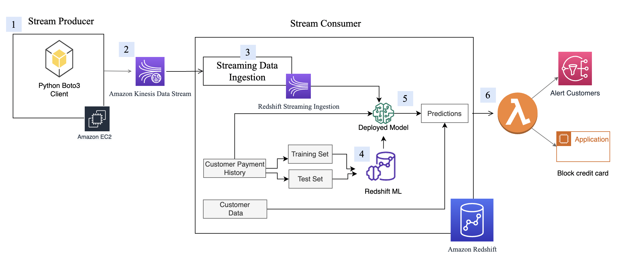
The following diagram illustrates a typical hybrid data warehouse architecture.

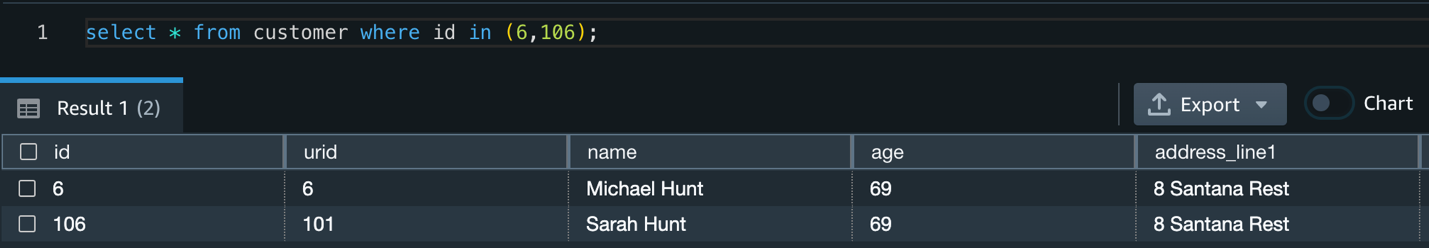
The following query retrieves provider and patient data from the hybrid model:
The number of joins is reduced from five to three by using the hybrid model.
Advantages of using the hybrid model
With this model, structural information is segregated from descriptive information to promote flexibility and avoid re-engineering in the event of a change. It maintains data integrity, allowing organizations to avoid hefty fines when data integrity is compromised.
The hybrid paradigm enables non-data professionals to interact with raw data by allowing users to update or create metadata and data enrichment rules. The hybrid approach simplifies the process of gathering and evaluating datasets for business applications. It enables concurrent data loading and eliminates the need for a corporate vault.
The hybrid model also benefits from the fact that there is no dependency between objects in the data storage. With hybrid data warehousing, scalability is multiplied.
You can build the hybrid model on AWS and take advantage of the benefits of Amazon Redshift, which is a fully managed, scalable cloud data warehouse that accelerates your time to insights with fast, simple, and secure analytics at scale. Amazon Redshift continuously adds features that make it faster, more elastic, and easier to use:
- Amazon Redshift data sharing enhances the hybrid model by eliminating the need for copying data across departments. It also simplifies the work of keeping the single source of truth, saving memory and limiting redundancy. It enables instant, granular, and fast data access across Amazon Redshift clusters without the need to copy or move it. Data sharing provides live access to data so that users always see the most up-to-date and consistent information as it’s updated in the data warehouse.
- Redshift Spectrum enables you to query open format data directly in the Amazon Simple Storage Service (Amazon S3) data lake without having to load the data or duplicate your infrastructure, and it integrates well with the data lake.
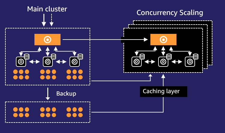
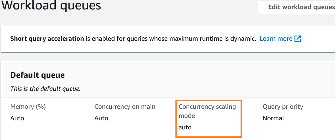
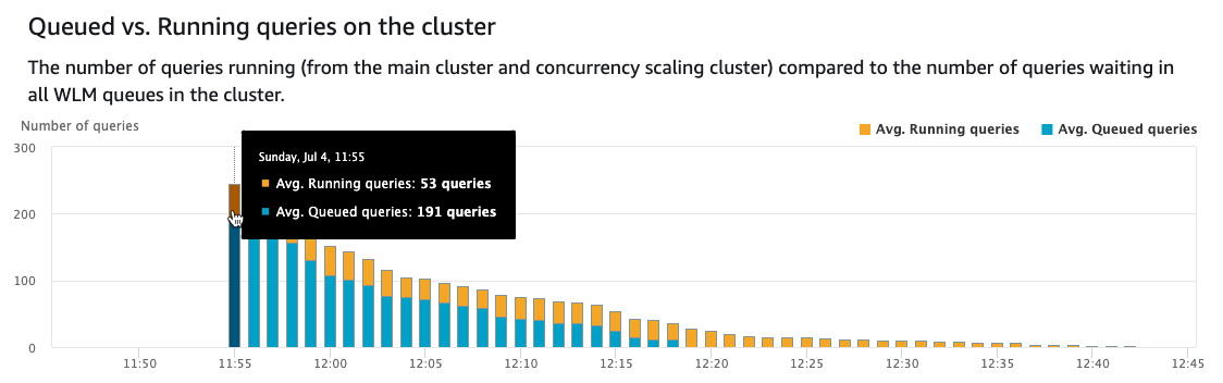
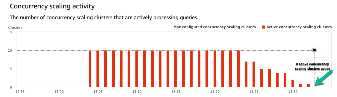
- With Amazon Redshift concurrency scaling, you can get consistently fast performance for thousands of concurrent queries and users. It instantly adds capacity to support additional users and removes it when the load subsides, with nothing to manage at your end.
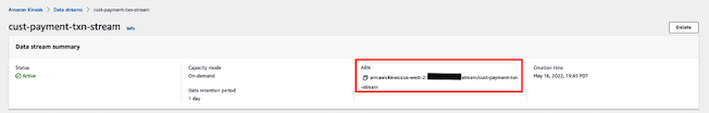
- To realize the benefits of using a hybrid model on AWS, you can get started today without needing to provision and manage data warehouse clusters using Redshift Serverless. All the related services that Amazon Redshift integrates with (such as Amazon Kinesis, AWS Lambda, Amazon QuickSight, Amazon SageMaker, Amazon EMR, AWS Lake Formation, and AWS Glue) are available to work with Redshift Serverless.
Conclusion
With the hybrid model, data can be transformed and loaded into a target data model efficiently and transparently. With this approach, data partners can research data networks more efficiently and promote comparative effectiveness. And with the several newly introduced features of Amazon Redshift, a lot of heavy lifting is done by AWS to handle your workload demands, and you only pay for what you use.
You can get started with the following steps:
- Create an Amazon Redshift RA3 instance for your primary clinical data repository and data marts.
- Build a data vault schema for the raw vault and create materialized views for the business vault.
- Enable Amazon Redshift data shares to share data between the producer cluster and consumer cluster.
- Load the structed and unstructured data into the producer cluster data vault for business use.
About the Authors
 Bindhu Chinnadurai is a Senior Partner Solutions Architect in AWS based out of London, United Kingdom. She has spent 18+ years working in everything for large scale enterprise environments. Currently she engages with AWS partner to help customers migrate their workloads to AWS with focus on scalability, resiliency, performance and sustainability. Her expertise is DevSecOps.
 Sarathi Balakrishnan was the Global Partner Solutions Architect, specializing in Data, Analytics and AI/ML at AWS. He worked closely with AWS partner globally to build solutions and platforms on AWS to accelerate customers’ business outcomes with state-of-the-art cloud technologies and achieve more in their cloud explorations. He helped with solution architecture, technical guidance, and best practices to build cloud-native solutions. He joined AWS with over 20 years of large enterprise experience in agriculture, insurance, health care and life science, marketing and advertisement industries to develop and implement data and AI strategies.


 Sandeep Bajwa is a Sr. Analytics Specialist based out of Northern Virginia, specialized in the design and implementation of analytics and data lake solutions.
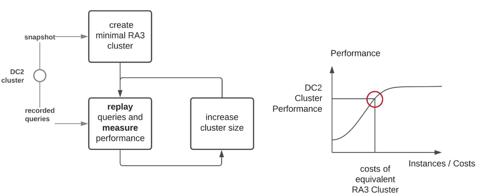


 Miguel Chin is a Data Engineering Manager at OLX Group, one of the world’s fastest-growing networks of trading platforms. He is responsible for managing a domain-oriented team of data engineers that helps shape the company’s data ecosystem by evangelizing cutting-edge data concepts like data mesh.
 David Greenshtein is a Specialist Solutions Architect for Analytics at AWS with a passion for ETL and automation. He works with AWS customers to design and build analytics solutions enabling business to make data-driven decisions. In his free time, he likes jogging and riding bikes with his son.


 Ramesh Ranganathan is a Senior Partner Solution Architect at AWS. He works with AWS customers and partners to provide guidance on enterprise cloud adoption, application modernization and cloud native development. He is passionate about technology and enjoys experimenting with AWS Serverless services.
 Kamen Sharlandjiev is an Analytics Specialist Solutions Architect and Amazon AppFlow expert. He’s on a mission to make life easier for customers who are facing complex data integration challenges. His secret weapon? Fully managed, low-code AWS services that can get the job done with minimal effort and no coding.
 Amit Shah is a cloud based modern data architecture expert and currently leading AWS Data Analytics practice in Atos. Based in Pune in India, he has 20+ years of experience in data strategy, architecture, design and development. He is on a mission to help organization become data-driven.


 David Zhang is an AWS Data Architect in Global Financial Services. He specializes in designing and implementing serverless analytics infrastructure, data management, ETL, and big data systems. He helps customers modernize their data platforms on AWS. David is also an active speaker and contributor to AWS conferences, technical content, and open-source initiatives. During his free time, he enjoys playing volleyball, tennis, and weightlifting. Feel free to connect with him on
  Manash Deb is a Software Development Manager in the AWS Directory Service team. With over 18 years of software dev experience, his passion is designing and delivering highly scalable, secure, zero-maintenance applications in the AWS identity and data analytics space. He loves mentoring and coaching others and to act as a catalyst and force multiplier, leading highly motivated engineering teams, and building large-scale distributed systems.
 Pavan Kumar Vadupu Lakshman Manikya is an AWS Solutions Architect who helps customers design robust, scalable solutions across multiple industries. With a background in enterprise architecture and software development, Pavan has contributed in creating solutions to handle API security, API management, microservices, and geospatial information system use cases for his customers. He is passionate about learning new technologies and solving, automating, and simplifying customer problems using these solutions.

 Manan Goel is a Product Go-To-Market Leader for AWS Analytics Services including Amazon Redshift at AWS. He has more than 25 years of experience and is well versed with databases, data warehousing, business intelligence, and analytics. Manan holds a MBA from Duke University and a BS in Electronics & Communications engineering.


 Paul Villena is an Analytics Solutions Architect in AWS with expertise in building modern data and analytics solutions to drive business value. He works with customers to help them harness the power of the cloud. His areas of interests are infrastructure-as-code, serverless technologies and coding in Python.


 Jon Roberts is a Sr. Analytics Specialist based out of Nashville, specializing in Amazon Redshift. He has over 27 years of experience working in relational databases. In his spare time, he runs.


 Jon Roberts is a Sr. Analytics Specialist based out of Nashville, specializing in Amazon Redshift. He has over 27 years of experience working in relational databases. In his spare time, he runs.
 Nelly Susanto is a Senior Database Migration Specialist of AWS Database Migration Accelerator. She has over 10 years of technical experience focusing on migrating and replicating databases along with data warehouse workloads. She is passionate about helping customers in their cloud journey.


 Ranjan Burman is an Analytics Specialist Solutions Architect at AWS. He specializes in Amazon Redshift and helps customers build scalable analytical solutions. He has more than 16 years of experience in different database and data warehousing technologies. He is passionate about automating and solving customer problems with cloud solutions.
 Saurav Das is part of the Amazon Redshift Product Management team. He has more than 16 years of experience in working with relational databases technologies and data protection. He has a deep interest in solving customer challenges centered around high availability and disaster recovery.