Post Syndicated from Raj Ramasubbu original https://aws.amazon.com/blogs/big-data/build-a-real-time-analytics-solution-with-apache-pinot-on-aws/
Online Analytical Processing (OLAP) is crucial in modern data-driven apps, acting as an abstraction layer connecting raw data to users for efficient analysis. It organizes data into user-friendly structures, aligning with shared business definitions, ensuring users can analyze data with ease despite changes. OLAP combines data from various data sources and aggregates and groups them as business terms and KPIs. In essence, it’s the foundation for user-centric data analysis in modern apps, because it’s the layer that translates technical assets into business-friendly terms that enable users to extract actionable insights from data.
Real-time OLAP
Traditionally, OLAP datastores were designed for batch processing to serve internal business reports. The scope of data analytics has grown, and more user personas are now seeking to extract insights themselves. These users often prefer to have direct access to the data and the ability to analyze it independently, without relying solely on scheduled updates or reports provided at fixed intervals. This has led to the emergence of real-time OLAP solutions, which are particularly relevant in the following use cases:
- User-facing analytics – Incorporating analytics into products or applications that consumers use to gain insights, sometimes referred to as data products.
- Business metrics – Providing KPIs, scorecards, and business-relevant benchmarks.
- Anomaly detection – Identifying outliers or unusual behavior patterns.
- Internal dashboards – Providing analytics that are relevant to stakeholders across the organization for internal use.
- Queries – Offering subsets of data to users based on their roles and security levels, allowing them to manipulate data according to their specific requirements.
Overview of Apache Pinot
Building these capabilities in real time means that real-time OLAP solutions have stricter SLAs and larger scalability requirements than traditional OLAP datastores. Accordingly, a purpose-built solution is needed to address these new requirements.
Apache Pinot is an open source real-time distributed OLAP datastore designed to meet these requirements, including low latency (tens of milliseconds), high concurrency (hundreds of thousands of queries per second), near real-time data freshness, and handling petabyte-scale data volumes. It ingests data from both streaming and batch sources and organizes it into logical tables distributed across multiple nodes in a Pinot cluster, ensuring scalability.
Pinot provides functionality similar to other modern big data frameworks, supporting SQL queries, upserts, complex joins, and various indexing options.
Pinot has been tested at very large scale in large enterprises, serving over 70 LinkedIn data products, handling over 120,000 Queries Per Second (QPS), ingesting over 1.5 million events per second, and analyzing over 10,000 business metrics across over 50,000 dimensions. A notable use case is the user-facing Uber Eats Restaurant Manager dashboard, serving over 500,000 users with instant insights into restaurant performance.
Pinot clusters are designed for high availability, horizontal scalability, and live configuration changes without impacting performance. To that end, Pinot is architected as a distributed datastore to enable all of the above requirements, and utilizes similar architectural constructs as Apache Kafka and Apache Hadoop in its design.
Solution overview
In this, we will provide a step-by-step guide showing you how you can build a real-time OLAP datastore on Amazon Web Services (AWS) using Apache Pinot on Amazon Elastic Compute Cloud (Amazon EC2) and do near real-time visualization using Tableau. You can use Apache Pinot for batch processing use cases as well but, in this post, we will focus on a near real-time analytics use case.
You can use Amazon Managed Service for Apache Flink service. The objective in the preceding figure is to ingest streaming data into Pinot, where it can perform.

The objective in the preceding figure is to ingest streaming data into Pinot, where it can perform aggregations, update current data models, and serve OLAP queries in real time to consuming users and applications, which in this case is a user-facing Tableau dashboard.
The data flow as follows:
- Data is ingested from a real-time source, such as clickstream data from a website. For the purposes of this post, we will use the Amazon Kinesis Data Generator to simulate the production of events.
- Events are captured in a streaming storage platform such as or Amazon Managed Streaming for Apache Kafka (MSK) for downstream consumption.
- The events are then ingested into the real-time server within Apache Pinot, which is used to process data coming from streaming sources, such as MSK and KDS. Apache Pinot consists of logical tables, which are partitioned into segments. Due to the time sensitive nature of streaming, events are directly written into memory as consuming segments, which can be thought of as parts of an active table that are continuously ingesting new data. Consuming segments are available for query processing immediately, thereby enabling low latency and high data freshness.
- After the segments reach a threshold in terms of time or number of rows, they are moved into Amazon Simple Storage Service (Amazon S3), which serves as deep storage for the Apache Pinot cluster. Deep storage is the permanent location for segment files. Segments used for batch processing are also stored there.
- In parallel, the Pinot controller tracks the metadata of the cluster and performs actions required to keep the cluster in an ideal state. Its primary function is to orchestrate cluster resources as well as manage connections between resources within the cluster and data sources outside of it. Under the hood, the controller uses Apache Helix to manage cluster state, failover, distribution, and scalability and Apache Zookeeper to handles distributed coordination functions such as leader election, locks, queue management, and state tracking.
- To enable the distributed aspect of the Pinot architecture, the broker accepts queries from the clients and forwards them to servers and collects the results and sends them back. The broker manages and optimizes the queries, distributes them across the servers, combines the results, and returns the result set. The broker sends the request to the right segments on the right servers, optimizes segment pruning, and splits the queries across servers appropriately. The results of each query are then merged and sent back to the requesting client.
- The results of the queries are updated in real time in the Tableau dashboard.
To ensure high availability, the solution deploys application load balancers for the brokers and servers. We can access the Apache Pinot UI using the controller load balancer and use it to run queries and monitor the Apache Pinot cluster
Let’s start to deploy this solution and perform near real-time visualizations using Apache Pinot and Tableau.
Prerequisites
Before you get started, make sure you have the following prerequisites:
- To deploy Apache Pinot
- An AWS account
- A basic understanding of Amazon S3, Amazon EC2, and Kinesis Data Streams
- An AWS Identity and Access Management (IAM) role with permissions to access AWS CloudShell and create a Data Streams instance, EC2 instances, and S3 buckets (see Adding and removing IAM identity permissions)
- Install Git to clone the code repository
- Install Node.js and npm to install packages
- To use Tableau for visualization
- Install Tableau Desktop to visualize data (for this post, 2023.3.0).
- Install Kinesis data generator (KDG) using AWS CloudFormation by following the instructions to stream sample web transactions into the Kinesis data stream. The KDG makes it easy to send data to a Kinesis data stream.
- Download the Apache Pinot drivers from here:
- Copy the drivers to the
C:\Program Files\Tableau\Driversfolder when using Tableau Desktop on Windows. For other operating systems, see the instructions. - Ensure all CloudFormation and AWS Cloud Development Kit (AWS CDK) templates are deployed in the same AWS Region for all resources throughout the following steps.
Deploy the Apache Pinot solution using the AWS CDK
The AWS CDK is an open source project that you can use to define your cloud infrastructure using familiar programming languages. It uses high-level constructs to represent AWS components to simplify the build process. In this post, we use TypeScript and Python to define the cloud infrastructure.
- First, bootstrap the AWS CDK. This sets up the resources required by the AWS CDK to deploy into the AWS account. This step is only required if you haven’t used the AWS CDK in the deployment account and Region. The format for the bootstrap command is
cdk bootstrap aws://<account-id>/<aws-region>.
In the following example, I’m running a bootstrap command for a fictitious AWS account with ID 123456789000 and us-east-1 N.Virginia Region:

- Next, clone the GitHub repository and install all the dependencies from
package.jsonby running the following commands from the root of the cloned repository. - Deploy the AWS CDK stack to create the AWS Cloud infrastructure by running the following command and enter y when prompted. Enter the IP address that you want to use to access the Apache Pinot controller and broker in /32 subnet mask format.
Deployment of the AWS CDK stack takes approximately 10–12 minutes. You should see a stack deployment message that will display the creation of AWS objects, followed by the deployment time, the Stack ARN, and the total time, similar to the following screenshot:

- Now, you can get the Apache Pinot controller Application Load Balancer (ALB) DNS name from the Copy the value for ControllerDNSUrl.
- Launch a browser session and paste the DNS name to see the Apache Pinot controller—it should look like the following screenshot, where you will see:
- Number of controllers, brokers, servers, minions, tenants, and tables
- List of tenants
- List of controllers
- List of brokers

Near real-time visualization using Tableau
Now that we have provisioned all AWS Cloud resources, we will stream some sample web transactions to a Kinesis data stream and visualize the data in near real time from Tableau Desktop.
You can follow these steps to open the Tableau workbook to visualize
- Download the Tableau workbook to your local machine and open the workbook from Tableau Desktop.
- Get the DNS name for Apache Pinot broker’s Application Load Balancer DNS name from the CloudFormation console. Choose Stacks, select the ApachePinotSolutionStack, and then choose Outputs and copy the value for BrokerDNSUrl.
- Choose Edit connection and enter the URL in the following format:
- Enter admin for both the username and password.
- Access the KDG tool by following the instructions. Use the record template that follows to send sample web transactions data to Kinesis Data streams called pinot-stream by choosing Send dataas shown in the following screenshot. Stop sending data after sending a handful of records by choosing Stop sending data to Kinesis.

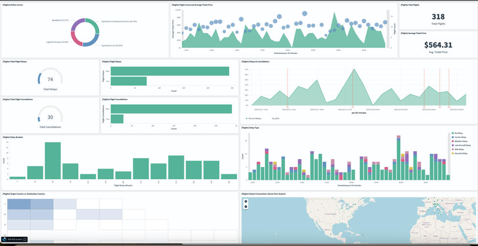
You should be able to see the web transactions data in Tableau Desktop as shown in the following screenshot.

Clean up
To clean up the AWS resources you created:
- Disable termination protection on the following EC2 instances by going to the Amazon EC2 console and choosing Instance from the navigation pane. Choose Actions, Instance Settings, and then Change termination protection and clear the Termination protection checkbox.
ApachePinotSolutionStack/bastionHostApachePinotSolutionStack/zookeeperNode1ApachePinotSolutionStack/zookeeperNode2ApachePinotSolutionStack/zookeeperNode3
- Run the following command from the cloned GitHub repo and enter
ywhen prompted.
Scaling the solution to production
The example in this post uses minimal resources to demonstrate functionality. Taking this to production requires a higher level of scalability. The solution provides autoscaling policies for independently scaling brokers and servers in and out, allowing the Apache Pinot custer to scale based on CPU requirements.
When autoscaling is initiated, the solution will invoke an AWS Lambda Function, to run the logic needed to add or remove brokers and servers in Apache Pinot.
In Apache Pinot, tables are tagged with an identifier that’s used for routing queries to the appropriate servers. When creating a table, you can specify a table name and optionally tag it. This is useful when you want to route queries to specific servers or build a multi-tenant Apache Pinot cluster. However, tagging adds additional considerations when removing brokers or servers. You need to make sure that neither have any active tables or tags associated with them. And when adding new components, rebalance the segments, so you can use the new brokers and servers.
Therefore, when scaling is needed in the solution, the autoscaling policy will invoke a Lambda function that either rebalances the segments of the tables when you add a new broker or server, or removes any tags associated with the broker or server you remove from the cluster.
Summary
Just like you would commonly use a distributed NoSQL datastore to serve a mobile application that requires low latency, high concurrency, high data freshness, high data volume, and high throughput, a distributed real-time OLAP datastore like Apache Pinot is purpose-built for achieving the same requirements for the analytics workload within your user-facing application. In this post, we walked you through how to deploy a scalable Apache Pinot-based near real-time user facing analytics solution on AWS. If you have any questions or suggestions, write to us in the comments section
About the authors
 Raj Ramasubbu is a Senior Analytics Specialist Solutions Architect focused on big data and analytics and AI/ML with Amazon Web Services. He helps customers architect and build highly scalable, performant, and secure cloud-based solutions on AWS. Raj provided technical expertise and leadership in building data engineering, big data analytics, business intelligence, and data science solutions for over 18 years prior to joining AWS. He helped customers in various industry verticals like healthcare, medical devices, life science, retail, asset management, car insurance, residential REIT, agriculture, title insurance, supply chain, document management, and real estate.
 Francisco Morillo is a Streaming Solutions Architect at AWS. Francisco works with AWS customers, helping them design real-time analytics architectures using AWS services, supporting Amazon Managed Streaming for Apache Kafka (Amazon MSK) and Amazon Managed Service for Apache Flink.
 Ismail Makhlouf is a Senior Specialist Solutions Architect for Data Analytics at AWS. Ismail focuses on architecting solutions for organizations across their end-to-end data analytics estate, including batch and real-time streaming, big data, data warehousing, and data lake workloads. He primarily partners with airlines, manufacturers, and retail organizations to support them to achieve their business objectives with well-architected data platforms.


 Jason Hines is a Senior Solutions Architect, at AWS, specializing in serving global customers in the Healthcare and Life Sciences industries. With over 25 years of experience, he has worked with numerous Fortune 100 companies across multiple verticals, bringing a wealth of knowledge and expertise to his role. Outside of work, Jason has a passion for an active lifestyle. He enjoys various outdoor activities such as hiking, scuba diving, and exploring nature. Maintaining a healthy work-life balance is essential to him.
 Ramesh H Singh is a Senior Product Manager Technical (External Services) at AWS in Seattle, Washington, currently with the Amazon DataZone team. He is passionate about building high-performance ML/AI and analytics products that enable enterprise customers to achieve their critical goals using cutting-edge technology. Connect with him on
  Leonardo Gomez is a Principal Analytics Specialist Solutions Architect at AWS. He has over a decade of experience in data management, helping customers around the globe address their business and technical needs. Connect with him on


 Sai Maddali is a Senior Manager Product Management at AWS who leads the product team for Amazon MSK. He is passionate about understanding customer needs, and using technology to deliver services that empowers customers to build innovative applications. Besides work, he enjoys traveling, cooking, and running.
 Nagarjuna Koduru is a Principal Engineer in AWS, currently working for AWS Managed Streaming For Kafka (MSK). He led the teams that built MSK Serverless and MSK Tiered storage products. He previously led the team in Amazon JustWalkOut (JWO) that is responsible for real time tracking of shopper locations in the store. He played pivotal role in scaling the stateful stream processing infrastructure to support larger store formats and reducing the overall cost of the system. He has keen interest in stream processing, messaging and distributed storage infrastructure.
 Masudur Rahaman Sayem is a Streaming Data Architect at AWS. He works with AWS customers globally to design and build data streaming architectures to solve real-world business problems. He specializes in optimizing solutions that use streaming data services and NoSQL. Sayem is very passionate about distributed computing.


 Shubham Purwar is a Cloud Engineer (ETL) at AWS Bengaluru specializing in AWS Glue and Athena. He is passionate about helping customers solve issues related to their ETL workload and implement scalable data processing and analytics pipelines on AWS. In his free time, Shubham loves to spend time with his family and travel around the world.
 Nitin Kumar is a Cloud Engineer (ETL) at AWS, specializing in AWS Glue. With a decade of experience, he excels in aiding customers with their big data workloads, focusing on data processing and analytics. He is committed to helping customers overcome ETL challenges and develop scalable data processing and analytics pipelines on AWS. In his free time, he likes to watch movies and spend time with his family.


 Under Authorized projects, you can pick the authorized projects allowed to use this environment profile to create an environment. By default, this is set to All projects.


 As a consumer, you’re now able to explore data and create reports, or you can aggregate data and create new assets to publish in Amazon DataZone, becoming a producer of a new data product to share with other users and departments.
 Carmen is a Solutions Architect at AWS, based in Milan (Italy). She is a Data Lover that enjoys helping companies in the adoption of Cloud technologies, especially with Data Analytics and Data Governance. Outside of work, she is a creative people who loves being in contact with nature and sometimes practicing adrenaline activities.


 Amit Ghodke is an Analytics Specialist Solutions Architect based out of Austin. He has worked with databases, data warehouses and analytical applications for the past 16 years. He loves to help customers implement analytical solutions at scale to derive maximum business value.
 Ritesh Kumar Sinha is an Analytics Specialist Solutions Architect based out of San Francisco. He has helped customers build scalable data warehousing and big data solutions for over 16 years. He loves to design and build efficient end-to-end solutions on AWS. In his spare time, he loves reading, walking, and doing yoga.


 Noritaka Sekiyama is a Principal Big Data Architect on the AWS Glue team and AWS Data Pipeline team. He is responsible for building software artifacts to help customers. In his spare time, he enjoys cycling with his road bike.
 Vaibhav Porwal is a Senior Software Development Engineer on the AWS Glue and AWS Data Pipeline team. He is working on solving problems in orchestration space by building low cost, repeatable, scalable workflow systems that enables customers to create their ETL pipelines seamlessly.
 Sriram Ramarathnam is a Software Development Manager on the AWS Glue and AWS Data Pipeline team. His team works on solving challenging distributed systems problems for data integration across AWS serverless and serverfull compute offerings.
 Matt Su is a Senior Product Manager on the AWS Glue team and AWS Data Pipeline team. He enjoys helping customers uncover insights and make better decisions using their data with AWS Analytics services. In his spare time, he enjoys skiing and gardening.


 Mackenzie Johnson is a Senior Manager at ActionIQ. She is an innovative marketing strategist who’s passionate about the convergence of complementary technologies and amplifying joint value. With extensive experience across digital transformation storytelling, she thrives on educating enterprise businesses about the impact of CX based on a data-driven approach.
 Phil Catterall is a Senior Product Manager at ActionIQ and leads product development on ActionIQ’s foundational data management, processing, and query federation capabilities. He’s passionate about designing and building scalable data products to empower business users in new ways.
 Sain Das is a Senior Product Manager on the Amazon Redshift team and leads Amazon Redshift GTM for partner programs including the Powered by Amazon Redshift and Redshift Ready programs.


 Ayush Agrawal is a Startups Solutions Architect from Gurugram, India with 11 years of experience in Cloud Computing. With a keen interest in AI, ML, and Cloud Security, Ayush is dedicated to helping startups navigate and solve complex architectural challenges. His passion for technology drives him to constantly explore new tools and innovations. When he’s not architecting solutions, you’ll find Ayush diving into the latest tech trends, always eager to push the boundaries of what’s possible.
 Fraser Sequeira is a Solutions Architect with AWS based in Mumbai, India. In his role at AWS, Fraser works closely with startups to design and build cloud-native solutions on AWS, with a focus on analytics and streaming workloads. With over 10 years of experience in cloud computing, Fraser has deep expertise in big data, real-time analytics, and building event-driven architecture on AWS.


 Çağrı Çakır is the Lead Software Engineer for the PostNL IoT platform, where he manages the architecture that processes billions of events each day. As an AWS Certified Solutions Architect Professional, he specializes in designing and implementing event-driven architectures and stream processing solutions at scale. He is passionate about harnessing the power of real-time data, and dedicated to optimizing operational efficiency and innovating scalable systems.
 Özge Kavalcı works as Senior Solution Engineer for the PostNL IoT platform and loves to build cutting-edge solutions that integrate with the IoT landscape. As an AWS Certified Solutions Architect, she specializes in designing and implementing highly scalable serverless architectures and real-time stream processing solutions that can handle unpredictable workloads. To unlock the full potential of real-time data, she is dedicated to shaping the future of IoT integration.
 Amit Singh works as a Senior Solutions Architect at AWS with enterprise customers on the value proposition of AWS, and participates in deep architectural discussions to make sure solutions are designed for successful deployment in the cloud. This includes building deep relationships with senior technical individuals to enable them to be cloud advocates. In his free time, he likes to spend time with his family and learn more about everything cloud.
 Lorenzo Nicora works as Senior Streaming Solutions Architect at AWS helping customers across EMEA. He has been building cloud-centered, data-intensive systems for several years, working in the finance industry both through consultancies and for fintech product companies. He has used open-source technologies extensively and contributed to several projects, including Apache Flink.
 Jatinder Singh is a Senior Technical Account Manager at AWS and finds satisfaction in aiding customers in their cloud migration and innovation endeavors. Beyond his professional life, he relishes spending moments with his family and indulging in hobbies such as reading, culinary pursuits, and playing chess.
 Hajer Bouafif is an Analytics Specialist Solutions Architect at Amazon Web Services. She focuses on Amazon OpenSearch Service and helps customers design and build well-architected analytics workloads in diverse industries. Hajer enjoys spending time outdoors and discovering new cultures.
 Puneetha Kumara is a Senior Technical Account Manager at AWS, with over 15 years of industry experience, including roles in cloud architecture, systems engineering, and container orchestration.
 Manpreet Kour is a Senior Technical Account Manager at AWS and is dedicated to ensuring customer satisfaction. Her approach involves a deep understanding of customer objectives, aligning them with software capabilities, and effectively driving customer success. Outside of her professional endeavors, she enjoys traveling and spending quality time with her family.


 Chiho Sugimoto is a Cloud Support Engineer on the AWS Big Data Support team. She is passionate about helping customers build data lakes using ETL workloads. She loves planetary science and enjoys studying the asteroid Ryugu on weekends.
 Fabrizio Napolitano is a Principal Specialist Solutions Architect or Data Analytics at AWS. He has worked in the analytics domain for the last 20 years, now focusing on helping Canadian public sector organizations innovate with data. Quite by surprise, he become a Hockey Dad after moving to Canada.
 Gal Heyne is a Technical Product Manager for AWS Data Processing services with a strong focus on AI/ML, data engineering, and BI. She is passionate about developing a deep understanding of customers’ business needs and collaborating with engineers to design easy-to-use data services products.


 Sotaro Hikita is a Solutions Architect. He supports customers in a wide range of industries, especially the financial industry, to build better solutions. He is particularly passionate about big data technologies and open source software.
 Noritaka Sekiyama is a Principal Big Data Architect on the AWS Glue team. He is responsible for building software artifacts to help customers. In his spare time, he enjoys cycling with his new road bike.
 Kyle Duong is a Senior Software Development Engineer on the AWS Glue and AWS Lake Formation team. He is passionate about building big data technologies and distributed systems.
 Kalaiselvi Kamaraj is a Senior Software Development Engineer with Amazon. She has worked on several projects within the Amazon Redshift query processing team and currently focusing on performance-related projects for Redshift data lakes.
 Sandeep Adwankar is a Senior Product Manager at AWS. Based in the California Bay Area, he works with customers around the globe to translate business and technical requirements into products that enable customers to improve how they manage, secure, and access data.


 Leonardo Gomez is a Principal Analytics Specialist at AWS, with over a decade of experience in data management. Specializing in data governance, he assists customers worldwide in maximizing their data’s potential while promoting data democratization. Connect with him on
  Priya Tiruthani is a Senior Technical Product Manager with Amazon DataZone at AWS. She focuses on improving data discovery and curation required for data analytics. She is passionate about building innovative products to simplify customers’ end-to-end data journey, especially around data governance and analytics. Outside of work, she enjoys being outdoors to hike, capture nature’s beauty, and recently play pickleball.
 Ron Kyker is a Principal Engineer with Amazon DataZone at AWS, where he helps drive innovation, solve complex problems, and set the bar for engineering excellence for his team. Outside of work, he enjoys board gaming with friends and family, movies, and wine tasting.
 Srinivasan Kuppusamy is a Senior Cloud Architect – Data at AWS ProServe, where he helps customers solve their business problems using the power of AWS Cloud technology. His areas of interests are data and analytics, data governance, and AI/ML.
 Francisco Morillo is a Streaming Solutions Architect at AWS, specializing in real-time analytics architectures. With over five years in the streaming data space, Francisco has worked as a data analyst for startups and as a big data engineer for consultancies, building streaming data pipelines. He has deep expertise in Amazon Managed Streaming for Apache Kafka (Amazon MSK) and Amazon Managed Service for Apache Flink. Francisco collaborates closely with AWS customers to build scalable streaming data solutions and advanced streaming data lakes, ensuring seamless data processing and real-time insights.
 Lorenzo Nicora works as Senior Streaming Solution Architect at AWS, helping customers across EMEA. He has been building cloud-centered, data-intensive systems for over 25 years, working in the finance industry both through consultancies and for FinTech product companies. He has leveraged open-source technologies extensively and contributed to several projects, including Apache Flink.


 Deepmala Agarwal works as an AWS Data Specialist Solutions Architect. She is passionate about helping customers build out scalable, distributed, and data-driven solutions on AWS. When not at work, Deepmala likes spending time with family, walking, listening to music, watching movies, and cooking!
 Utkarsh Mittal is a Senior Technical Product Manager for Amazon DataZone at AWS. He is passionate about building innovative products that simplify customers’ end-to-end analytics journeys. Outside of the tech world, Utkarsh loves to play music, with drums being his latest endeavor.