Tag Archives: Analytics

Automate replication of row-level security from AWS Lake Formation to Amazon QuickSight

Post Syndicated from Vetri Natarajan original https://aws.amazon.com/blogs/big-data/automate-replication-of-row-level-security-from-aws-lake-formation-to-amazon-quicksight/

Amazon QuickSight is cloud-powered, serverless, and embeddable business intelligence (BI) service that makes it straightforward to deliver insights to your organization. As a fully managed service, Amazon QuickSight lets you create and publish interactive dashboards that can then be accessed from different devices and embedded into your applications, portals, and websites.

When authors create datasets, build dashboards, and share with end-users, the users will see the same data as the author, unless row-level security (RLS) is enabled in the Amazon QuickSight dataset. Amazon QuickSight also provides options to pass a reader’s identity to a data source using trusted identity propagation and apply RLS at the source. To learn more, see Centrally manage permissions for tables and views accessed from Amazon QuickSight with trusted identity propagation and Simplify access management with Amazon Redshift and AWS Lake Formation for users in an External Identity Provider.

However, there are a few requirements when using trusted identity propagation with Amazon QuickSight:

  • The authentication method for Amazon QuickSight must be using AWS IAM Identity Center.
  • The dataset created using trusted identity propagation will be a direct query dataset in Amazon QuickSight. QuickSight SPICE can’t be used with trusted identity propagation. This is because when using SPICE, data is imported (replicated) and therefore the entitlements at the source can’t be used when readers access the dashboard.

This post outlines a solution to automatically replicate the entitlements for readers from the source (AWS Lake Formation) to Amazon QuickSight. This solution can be used even when the authentication method in Amazon QuickSight is not using IAM Identity Center and can work with both direct query and SPICE datasets in Amazon QuickSight. This lets you take advantage of auto scaling that comes with SPICE. Although we focus on using a Lake Formation table that exists in the same account, you can extend the solution for cross-account tables as well. When extracting data filter rules for the table in another account, the execution role must have necessary access to the tables in the other account.

Use case overview

For this post, let’s consider a large financial institution that has implemented Lake Formation as its central data lake and entitlement management system. The institution aims to streamline access control and maintain a single source of truth for data permissions across its entire data ecosystem. By using Lake Formation for entitlement management, the financial institution can maintain a robust, scalable, and compliant data access control system that serves as the foundation for its data-driven operations and analytics initiatives. This approach is particularly crucial for maintaining compliance with financial regulations and maintaining data security. The analytics team wants to build an Amazon QuickSight dashboard for data and business teams.
Solution overview

This solution uses APIs of AWS Lake Formation and Amazon QuickSight to extract, transform, and store AWS Lake Formation data filters in a format that can be used in QuickSight.

The solution has four key steps:

  1. Extract and transform the row-level security (data filters) and permissions to data filters for tables of interest from AWS Lake Formation.
  2. Create a rules dataset in Amazon QuickSight.

We use the following key services:

The following diagram illustrates the solution architecture.

Prerequisites

To implement this solution, you should have following services enabled in the same account

  1. AWS Lake Formation and
  2. Amazon QuickSight
  3. AWS Identity and Access Management (IAM) permissions: Make sure you have necessary IAM permissions to perform operation across all the services mentioned in the solution overview above
  4. AWS Lake Formation table with data filters with right permissions
  5. Amazon QuickSight principals (Users or Groups)

The below section shows how you can create Amazon QuickSight groups and AWS Lake formation tables and data filters

Create groups in QuickSight

Create two groups in Amazon QuickSight: QuickSight_Readers and QuickSight_Authors. For instructions, see Create a group with the QuickSight console.

You can then form the Amazon Resource Names (ARNs) of the groups as follows. These will be used when granting permission in AWS Lake Formation for data filters.

  • arn:aws:quicksight:<<identity-region>>:<<AWSAcocuntId>>:group/<<namespace>>/QuickSight_Readers
  • arn:aws:quicksight:<<identity-region>>:<<AWSAcocuntId>>:group/<<namespace>>/QuickSight_Authors

You can also get the ARN of the groups by executing the Amazon QuickSight CLI command list-groups. The following screenshot shows the output.

Create a table in AWS Lake Formation

The following section is for example purposes and not necessary for production use of this solution. Complete the following steps to create a table in AWS Lake Formation using sample data. In this post, the table is called saas_sales.

  1. Download the file Saas Sales.csv.
  2. Upload the file to an Amazon S3 location.
  3. Create a table in AWS Lake Formation.

Create row-level security (data filter) in AWS Lake Formation

In AWS Lake Formation, data filters are used to filter the data in a table for an individual or group. Complete the following steps to create a data filter:

  1. Create a data filter called QuickSightReaderFilter in the table saas_sales. For Row-level access, enter the expression segment = 'Enterprise'.
  2. Grant the Amazon QuickSight group access to this data filter. Use the reader group ARN from the first step for SAML Users and groups.
  3. Grant the QuickSight_Authors group full access to the table. Use the reader group ARN from the first step for SAML Users and groups.
  4. (Optional) You can create another table called second_table and create another data filter called SecondFilter and grant permission to the QuickSight_Readers group.

Now that you have set up the table, permissions, and data filters, you can extract the row-level access details for the QuickSight_Readers and QuickSight_Authors groups and the saas_sales table in AWS Lake Formation, and create the rules dataset in Amazon QuickSight for the saas_sales table.

Extract and transform data filters and permissions from AWS Lake Formation using a Lambda function

In AWS Lake Formation, data filters are created for each table. There can be many tables in AWS Lake Formation. However, for a team or a project, there are only a specific set of tables that the BI developer is interested in. Therefore, choose a list of tables to track and update the data filters for. In a batch process, for each table in AWS Lake Formation, extract the data filter definitions and write them into Amazon S3 using AWS Lake Formation and Amazon S3 APIs.

We use the following AWS Lake Formation APIs to extract the data filter details and permissions:

  • ListDataCellFilters – This API is used to list all the data filters in each table that is required for the project
  • ListPermissions – This API is used to retrieve the permissions for each of the data filters extracted using the ListDataCellFilters API

The Lambda function covers three parts of the solution:

  • Extract the data filters and permissions to data filters for tables of interest from AWS Lake Formation
  • Transform the data filters and permission into a format usable in Amazon QuickSight
  • Persist the transformed data

Complete the following steps to create an AWS Lambda function:

  1. On the Lambda console, create a function called Lake_Formation_QuickSight_RLS. Use Python 3.12 as the runtime and create a new role for execution.
  2. Configure Lambda function timeout to 2 minutes. This can vary depending on the number of tables to be parsed and the number of data filters to be transformed.
  3. Attach the following permissions to the Lambda execution role:
    {
    "Version": "2012-10-17",
    "Statement": [
    {
    "Sid": "VisualEditor0",
    "Effect": "Allow",
    "Action": [
    "lakeformation:ListDataCellsFilter",
    "lakeformation:ListPermissions"
    ],
    "Resource": "*"
    },
    {
    "Sid": "VisualEditor1",
    "Effect": "Allow",
    "Action": "s3:PutObject",
    "Resource": "arn:aws:s3:::<bucket_used_for_storage>/*"
    }
    ]
    }

  4. Set the following environment variables for the Lambda function:

    Name Value
    S3Bucket Value of the S3 bucket where the output files will be stored
    tablesToTrack List of tables to track as JSON converted to string
    Tmp /tmp

The Lambda function gets the list of tables and S3 bucket details from the environment variables. The list of tables is given as a JSON array converted to string. The JSON format is shown in the following code. The values for catalogId, DatabaseName, and Name can be fetched from the AWS Lake Formation console.

[
{
"CatalogId": "String",
"DatabaseName": "String",
"Name": "String"
}
]
  1. Add a folder named tmp.
  2. Download the zip file Lake_Formation_QuickSight_RLS.zip.
    Note: This is sample code for non-production usage. You should work with your security and legal teams to meet your organizational security, regulatory, and compliance requirements before deployment.
  3. For the Lambda function code, upload the downloaded .zip file to the Lambda function, on the Code tab.
  4. Provide necessary access to the execution role in AWS Lake Formation. Although the AWS Identity and Access Management (IAM) permissions are given to the Lambda execution role, explicit permission has to be given to the role in AWS Lake Formation for the Lambda function to get the details about the data filters. Therefore, you have to explicitly grant access to the execution role to limit the Lambda role to read-only admin. For more details, see Viewing data filters.

In the following sections, we explain what the Lambda function code does in more detail.

Extract data filters and permissions for data filters and tables in AWS Lake Formation

The main flow of the code takes the list of tables as input and extracts table and data filter permissions and data filter rules. The approach here is to get the permissions for the entire table and also for the data filters applied to the table. This way, both full access (table level) and partial access (data filter) can be extracted.

...
....
tablesToTrack= json.loads(os.environ["tablesToTrack"])
lf_client = boto3.client('lakeformation')
# For each table in the list get the data filter rules attached to the table.
for table in tablesToTrack:
df_response= lf_client.list_data_cells_filter(
Table= table
)
d_filters += df_response["DataCellsFilters"]

# Also, for each table in the list get the list of permissions at table level.
# This determines who has access to all rows in the table.
tresponse=lf_client.list_permissions(
Resource= {
"Table": table
}
)

d_permissions += tresponse["PrincipalResourcePermissions"]
transformDataFilterRules(d_filters)
# For each data filters fetched above, get the permissions.
# This determines the row level security for the tables.
for filter in d_filters:
p_response=lf_client.list_permissions(
Resource= {

"DataCellsFilter": {
"DatabaseName": filter ["DatabaseName"],
"Name": filter["Name"],
"TableCatalogId": filter["TableCatalogId"],
"TableName": filter["TableName"]
}

}
)
d_permissions += p_response["PrincipalResourcePermissions"]

transformFilterandTablePermissions(d_permissions)

Transform data filter definitions in to a format usable in Amazon QuickSight

The extracted permissions and filters are transformed to create a rules dataset in Amazon QuickSight. There are different ways to define data filters. The following figure illustrates some of the example transformations.

The function transformDataFilterRules in the following code can transform some of the OR and AND conditions into Amazon QuickSight acceptable format. The following are the details available in the transformed format:

  • Lake Formation catalog ID
  • Lake Formation database name
  • Lake Formation table name
  • Lake Formation data filter name
  • List of columns from all the tables provided in the input for which the data filter rules are defined

See the following code:

def transformDataFilterRules(rules):
global complete_transformed_filter_rules
transformed_filter_rules = []
filter_to_extract=[]
complete_transformed_filter_rules = []
col_headers=[]
col_headers.append("catalog")
col_headers.append("database")
col_headers.append("table")
col_headers.append("filter")

for rule in rules:
print(rule)
catalog=rule["TableCatalogId"]
database = rule["DatabaseName"]
table = rule["TableName"]
filter = rule["Name"]
row=[]
row.append(catalog)
row.append(database)
row.append(table)
row.append(filter)
logger.info(f"row==={row}")

f_conditions = re.split(' OR | or | and | AND ' , rule["RowFilter"]["FilterExpression"])

for f_condition in f_conditions:
logger.info(f"f_condition={f_condition}")
f_condition = f_condition.replace("(","")
f_condition = f_condition.replace(")","")
filter_rule_column= f_condition.split("=")
if len(filter_rule_column)>1:
filter_rule_column[0] = filter_rule_column[0].strip()
if not filter_rule_column[0].strip() in col_headers:
col_headers.append(filter_rule_column[0].strip())
i= col_headers.index(filter_rule_column[0].strip())
j= i- (len(row)-1)
if j>0:
for x in range(1, j):
row.append("")
logger.info(f"i={i} j={j} {filter_rule_column[1]}")
row.insert(i, filter_rule_column[1].replace("'",""))
print(row)
transformed_filter_rules.append(','.join(row))

row=[]
row.append(catalog)
row.append(database)
row.append(table)
row.append(filter)
max_columns = len(col_headers)
complete_transformed_filter_rules=[]
for rule in transformed_filter_rules:
r = rule.split(",")
to_fill = max_columns - len(r)
if to_fill>0:
for x in range(1, to_fill+1):
r.append("")
complete_transformed_filter_rules.append(','.join(r))

complete_transformed_filter_rules.insert(0,','.join(col_headers))

The following figure is an example of the transformed file. The file contains the columns for both tables. When creating a rules dataset for a specific table, the records are filtered for that table pulled into Amazon QuickSight.

The function transformFilterandTablePermissions in the following code snippet combines and transforms the table and data filter permissions into a flat structure that contains the following columns:

  • Amazon QuickSight group ARN
  • Lake Formation catalog ID
  • Lake Formation database name
  • Lake Formation table name
  • Lake Formation data filter name

See the following code:

def transformFilterandTablePermissions(permissions):
    global transformed_table_permissions,transformed_filter_permissions
    # Read and set table level access
    transformed_table_permissions = []
    transformed_filter_permissions = []
    transformed_filter_permissions.insert(0,"group,catalog,database,table,filter")
    transformed_table_permissions.insert(0,"group,catalog,database,table")
    
    for permission in permissions:
    group=""
    database=""
    table =""
    catalog=""
    
    p= permission["Permissions"]
    
    if "DESCRIBE" in p or "SELECT" in p:
    
    group = permission["Principal"]["DataLakePrincipalIdentifier"]
    if "Database" in permission["Resource"]:
    catalog=permission["Resource"]["Database"]["CatalogId"]
    database=permission["Resource"]["Database"]["Name"]
    table = "*"
    transformed_table_permissions.append(group + "," + catalog+ "," + database + "," + table)
    transformed_filter_permissions.append(group+"," +catalog + ","+ database + ","+ table)
    elif "TableWithColumns" in  permission["Resource"]  or "Table" in permission["Resource"]:
    if "TableWithColumns" in  permission["Resource"]:
    catalog=permission["Resource"]["TableWithColumns"]["CatalogId"]
    database = permission["Resource"]["TableWithColumns"]["DatabaseName"]
    table = permission["Resource"]["TableWithColumns"]["Name"]
    elif "Table" in  permission["Resource"]:
    catalog=permission["Resource"]["Table"]["CatalogId"]
    database = permission["Resource"]["Table"]["DatabaseName"]
    table = permission["Resource"]["Table"]["Name"]
    transformed_table_permissions.append( group + "," + catalog + "," + database + "," + table)
    transformed_filter_permissions.append(group+"," +catalog + ","+ database + ","+ table)
    elif "DataCellsFilter" in permission["Resource"]:
    catalog=permission["Resource"]["DataCellsFilter"]["TableCatalogId"]
    database = permission["Resource"]["DataCellsFilter"]["DatabaseName"]
    table = permission["Resource"]["DataCellsFilter"]["TableName"]
    filter = permission["Resource"]["DataCellsFilter"]["Name"]
    transformed_filter_permissions.append(group+"," +catalog + ","+ database + ","+ table+ ","+ filter)

The following figure is an example of the extracted data filter and table permissions. AWS Lake Formation can have data filters applied to any principal. However, we focus on the Amazon QuickSight principals:

  • The QuickSight_Authors ARN has full access to two tables. This is determined by transforming the table-level permissions in addition to the data filter permissions.
  • The QuickSight_Readers ARN has limited access based on filter conditions.

Store the transformed rules and permissions in two separate files in Amazon S3

The transformed rules and permissions are then persisted in a data store. In this solution, the transformed rules are written to an Amazon S3 location in CSV format. The name of the files created by the Lambda function are:

  • transformed_filter_permissions.csv
  • transformed_filter_rules.csv

See the following code:

with open("/tmp/transformed_table_permissions.csv", "w") as txt_file:
for line in transformed_table_permissions:
txt_file.write(line + "\n") # works with any number of elements in a line
txt_file.close()
s3 = boto3.resource('s3')
s3.meta.client.upload_file(Filename = "/tmp/transformed_table_permissions.csv", Bucket= os.environ['S3Bucket'], Key = "table-permissions/transformed_table_permissions.csv")

with open("/tmp/transformed_filter_permissions.csv", "w") as txt_file:
for line in transformed_filter_permissions:
txt_file.write(line + "\n") # works with any number of elements in a line
txt_file.close()

s3.meta.client.upload_file(Filename = "/tmp/transformed_filter_permissions.csv", Bucket= os.environ['S3Bucket'], Key = "filter-permissions/transformed_filter_permissions.csv")

with open("/tmp/transformed_filter_rules.csv", "w") as txt_file:
for line in complete_transformed_filter_rules:
txt_file.write(line + "\n") # works with any number of elements in a line
txt_file.close()

s3.meta.client.upload_file(Filename = "/tmp/transformed_filter_rules.csv", Bucket= os.environ['S3Bucket'], Key = "filter-rules/transformed_filter_rules.csv")

Create a rules dataset in Amazon QuickSight

In this section, we walk through the steps to create a rules dataset in Amazon QuickSight.

Create a table in Lake formation for the files

The first step is to create a table in AWS Lake Formation for the two files, transformed_filter_permissions.csv and transformed_filter_rules.csv.

Although you can directly use an Amazon S3 connector in Amazon QuickSight, creating a table and making the rules dataset using an Athena connector gives flexibility in writing custom SQL and using direct query. For the steps to bring an Amazon S3 location into AWS Lake Formation, see Creating tables.

For this post, the tables for the files are created in a separate database called quicksight_lf_transformation.

Grant permission for the tables to the QuickSight_Authors group

Grant permission in AWS Lake Formation for the two tables to the QuickSight_Authors group. This is essential for Amazon QuickSight authors to create a rules dataset in Amazon QuickSight. The following screenshot shows the permission details.

Create a rules dataset in Amazon QuickSight

Amazon QuickSight supports both user-level and group-level RLS. In this post, we use groups to enable RLS. To create the rules dataset, you first join the filter permissions table with the filter rules table on the columns catalog, database, table, and filter. Then you can filter the permissions to include the Amazon QuickSight principals, and include only the columns required for the dataset. The objective in this solution is to build a rules dataset for the saas_sales table.

Complete the following steps:

  1. On the Amazon QuickSight console, create a new Athena dataset.
  2. Specify the following:
    1. For Catalog, choose AWSDataCatalog.
    2. For Database, choose quicksight_lf_transformation.
    3. For Table, choose filter_permissions.
  3. Choose Edit/Preview data.
  4. Choose Add data.
  5. Choose Add source.
  6. Select Athena.
  7. Specify the following:
    1. For Catalog, choose AWSDataCatalog.
    2. For Database, choose quicksight_lf_transformation.
    3. For Table, choose filter_rules.

  8. Join the permissions table with the data filter rules table on the catalog, database, table and filter columns.
  9. Rename the column group as GroupArn. This needs to be done before filter is applied.
  10. Filter the data where column table equals saas_sales.
  11. Filter the data where column group is also filtered for values starting with arn:aws:quicksight (Amazon QuickSight principals).
  12. Exclude fields that are not part of the saas_sales table.
  13. Change Query mode to SPICE.
  14. Publish the dataset.

If your organization has a mapping of other principals to a Amazon QuickSight group or user, you can apply that mapping before joining the tables.

You can also write the following custom SQL to achieve the same result:

SELECT a."group" as GroupArn, segment FROM "QuickSight_lf_transformation"."filter_permissions" as a
left join
"QuickSight_lf_transformation"."filter_rules" as b
on
a.catalog = b.catalog and
a.database = b.database and
a."table" = b."table" and
a.filter = b.filter
where a."table" = 'saas_sales'
and a."group" like 'arn:aws:quicksight%'

  1. Name the dataset LakeFormationRLSDataSet and publish the dataset.

Test the row-level security

Now you’re ready to test the row-level security by publishing a dashboard as a user in the QuickSight_Authors group and then viewing the dashboard as a user in the QuickSight_Readers group.

Publish a dashboard as a QuickSight_Authors group user

As an author who belongs to the QuickSight_Authors group, the user will be able to see the saas_sales table in the Athena connector and all the data in the table. As shown in this section, all three segments are visible for the author when creating an analysis and viewing the published dashboard.

  1. Create a dataset by pulling data from the saas_sales table using the Athena connector.
  2. Attach LakeFormationRLSDataSet as the RLS dataset for the saas_sales dataset. For instructions, see Using row-level security with user-based rules to restrict access to a dataset.
  3. Create an analysis using the saas_sales dataset as an author who belongs to the QuickSight_Authors group.
  4. Publish the dashboard.
  5. Share the dashboard with the group QuickSight_Readers.

View the dashboard as a QuickSight_Readers group user

Complete the following steps to view the dashboard as a QuickSight_Readers group user:

  1. Log into Amazon QuickSight as a reader who belongs to the QuickSight_Readers group.

The user will be able to see only the segment Enterprise.

  1. Now, change the RLS in AWS Lake Formation, and set the segment to be SMB for the QuickSightReaderFilter.
  2. Run the Lambda function to export and transform the new data filter rules.
  3. Refresh the SPICE dataset LakeFormationRLSDataSet in Amazon QuickSight.
  4. When the refresh is complete, refresh the dashboard in the reader login.

Now the reader user will see SMB data.

Cleanup

Amazon QuickSight resources

  1. Delete the Amazon QuickSight dashboard and analysis created
  2. Delete the datasets saas_sales and LakeFormationRulesDataSet
  3. Delete the Athena data source
  4. Delete the QuickSight groups using the DeleteGroup API

AWS Lake Formation resources

  1. Delete the database quicksight_lf transformation created in AWS Lake Formation
  2. Revoke permission given to the Lambda execution role
  3. Delete the saas_sales table and data filters created
  4. If you have used Glue crawler to create the tables in AWS Lake Formation, remove the Glue crawler as well

Compute resources

  1. Delete the AWS Lambda function created
  2. Delete the AWS Lambda execution role associated with the lambda

Storage resources

  1. Empty the content of the Amazon S3 bucket created for this solution
  2. Delete the Amazon S3 bucket

Conclusion

This post explained how to replicate row-level security in AWS Lake Formation automatically in Amazon QuickSight. This makes sure that the SPICE dataset in QuickSight can use row-level access defined in Lake Formation.

This solution can also be extended for other data sources. The logic to programmatically extract the entitlements from the source and transform them into Amazon QuickSight format will vary by source. After the extract and transform are in place, it can scale to multiple teams in the organization. Although this post laid out a basic approach, the automation has to be either scheduled to run periodically or triggered based on events like data filters change or grant or revoke of AWS Lake Formation permissions to make sure that the entitlements remain in sync between AWS Lake Formation and Amazon QuickSight.

Try out this solution for your own use case, and share your feedback in the comments.


About the Authors

Vetri Natarajan is a Specialist Solutions Architect for Amazon QuickSight. Vetri has 15 years of experience implementing enterprise business intelligence (BI) solutions and greenfield data products. Vetri specializes in integration of BI solutions with business applications and enable data-driven decisions.

Ismael Murillo is a Solutions Architect for Amazon QuickSight. Before joining AWS, Ismael worked in Amazon Logistics (AMZL) with delivery station management, delivery service providers, and our customer actively in the field. Ismael focused on last mile delivery and delivery success. He designed and implemented many innovative solutions to help reduce cost, influence delivery success. He is also a United States Army Veteran, where he served for eleven years.

Amazon OpenSearch Service launches flow builder to empower rapid AI search innovation

Post Syndicated from Dylan Tong original https://aws.amazon.com/blogs/big-data/amazon-opensearch-service-launches-flow-builder-to-empower-rapid-ai-search-innovation/

You can now access the AI search flow builder on OpenSearch 2.19+ domains with Amazon OpenSearch Service and begin innovating AI search applications faster. Through a visual designer, you can configure custom AI search flows—a series of AI-driven data enrichments performed during ingestion and search. You can build and run these AI search flows on OpenSearch to power AI search applications on OpenSearch without you having to build and maintain custom middleware.

Applications are increasingly using AI and search to reinvent and improve user interactions, content discovery, and automation to uplift business outcomes. These innovations run AI search flows to uncover relevant information through semantic, cross-language, and content understanding; adapt information ranking to individual behaviors; and enable guided conversations to pinpoint answers. Nonetheless, search engines are limited in native AI-enhanced search support, so builders develop middleware to complement search engines to fill in functional gaps. This middleware consists of custom code that runs data flows to stitch data transformations, search queries, and AI enrichments in varying combinations tailored to use cases, datasets, and requirements.

With the new AI search flow builder for OpenSearch, you have a collaborative environment to design and run AI search flows on OpenSearch. You can find the visual designer within OpenSearch Dashboards under AI Search Flows, and get started quickly by launching preconfigured flow templates for popular use cases like semantic, multimodal or hybrid search, and retrieval augmented generation (RAG). Through configurations, you can create customize flows to enrich search and index processes through AI providers like Amazon Bedrock, Amazon SageMaker, Amazon Comprehend, OpenAI, DeepSeek, and Cohere. Flows can be programmatically exported, deployed, and scaled on any OpenSearch 2.19+ cluster through OpenSearch’s existing ingest, index, workflow and search APIs.

In the remainder of the post, we’ll walk through a couple of scenarios to demonstrate the flow builder. First, we’ll enable semantic search on your old keyword-based OpenSearch application without client-side code changes. Next, we’ll create a multi-modal RAG flow, to showcase how you can redefine image discovery within your applications.

AI search flow builder key concepts

Before we get started, let’s cover some key concepts. You can use the flow builder through APIs or a visual designer. The visual designer is recommended for helping you manage workflow projects. Each project contains at least one ingest or search flow. Flows are a pipeline of processor resources. Each processor applies a type of data transform such as encoding text into vector embeddings, or summarizing search results with a chatbot AI service.

Ingest flows are created to enrich data as it’s added to an index. They consist of:

  1. A data sample of the documents you want to index.
  2. A pipeline of processors that apply transforms on ingested documents.
  3. An index constructed from the processed documents.

Search flows are created to dynamically enrich search request and results. They consist of:

  1. A query interface based on the search API, defining how the flow is queried and ran.
  2. A pipeline of processors that transform the request context or search results.

Generally, the path from prototype to production starts with deploying your AI connectors, designing flows from a data sample, then exporting your flows from a development cluster to a preproduction environment for testing at-scale.

Scenario 1: Enable semantic search on an OpenSearch application without client-side code changes

In this scenario, we have a product catalog that was built on OpenSearch a decade ago. We aim to improve its search quality, and in turn, uplift purchases. The catalog has search quality issues, for instance, a search for “NBA,” doesn’t surface basketball merchandise. The application is also untouched for a decade, so we aim to avoid changes to client-side code to reduce risk and implementation effort.

A solution requires the following:

  • An ingest flow to generate text embeddings (vectors) from text in an existing index.
  • A search flow that encodes search terms into text embeddings, and dynamically rewrites keyword-type match queries into a k-NN (vector) query to run a semantic search on the encoded terms. The rewrite allows your application to transparently run semantic-type queries through keyword-type queries.

We will also evaluate a second-stage reranking flow, which uses a cross-encoder to rerank results as it can potentially boost search quality.

We’ll accomplish our task through the flow builder. We begin by navigating to AI Search Flows in the OpenSearch Dashboard, and selecting Semantic Search from the template catalog.

image of the flow template catalog.

This template requires us to select a text embedding model. We’ll use Amazon Bedrock Titan Text, which was deployed as a prerequisite. Once the template is configured, we enter the designer’s main interface. From the preview, we can see that the template consists of a preset ingestion and search flow.

image of the visual flow designer.

The ingest flow requires us to provide a data sample. Our product catalog is currently served by an index containing the Amazon product dataset, so we import a data sample from this index.

importing a data sample from an existing index.

The ingest flow includes a ML Inference Ingest Processor, which generates machine learning (ML) model outputs such as embeddings (vectors) as your data is ingested into OpenSearch. As previously configured, the processor is set to use Amazon Titan Text to generate text embeddings. We map the data field that holds our product descriptions to the model’s inputText field to enable embedding generation.

Configuring the ML Inference Ingest Processor to generate text embeddings.

We can now run our ingest flow, which builds a new index containing our data sample embeddings. We can inspect the index’s contents to confirm that the embeddings were successfully generated.

Inspect your new index and embeddings from the flow designer.

Once we have an index, we can configure our search flow. We’ll start with updating the query interface, which is preset to a basic match query. The placeholder my_text has to be replaced with the product descriptions. With this update, our search flow can now respond to queries from our legacy application.

Update the search flow’s query interface

The search flow includes an ML Inference Search Processor. As previously configured, it’s set to use Amazon Titan Text. Since it’s added under Transform query, it’s applied to query requests. In this case, it will transform search terms into text embeddings (a query vector). The designer lists the variables from the query interface, allowing us to map the search terms (query.match.text.query), to the model’s inputText field. Text embeddings will now be generated from the search terms whenever our index is queried.

Configure a ML Inference Search Processor to generate query vectors.

Next, we update the query rewrite configurations, which is preset to rewrite the match query into a k-NN query. We replace the placeholder my_embedding with the query field assigned to your embeddings. Note that we could rewrite this to another query type, including a hybrid query, which may improve search quality.

Configure a query rewrite.

Let’s compare our semantic and keyword solutions from the search comparison tool. Both solutions are able to find basketball merchandise when we search for “basketball.”

Keyword versus semantic search results on the term “basketball”.

But what happens if we search for “NBA?” Only our semantic search flow returns results because it detects the semantic similarities between “NBA” and “basketball.”

Keyword versus semantic search results on the term “NBA”.

We’ve managed improvements, but we might be able to do better. Let’s see if reranking our search results with a cross-encoder helps. We’ll add a ML Inference Search Processor under Transform response, so that the processor applies to search results, and select Cohere Rerank. From the designer, we see that Cohere Rerank requires a list of documents and the query context as input. Data transformations are needed to package the search results into a format that can be processed by Cohere Rerank. So, we apply JSONPath expressions to extract the query context, flatten data structures, and pack the product descriptions from our documents into a list.

configure a ML Inference Search Processor with a reranker and apply JSONPath expressions.

Let’s return to the search comparison tool to compare our flow variations. We don’t observe any meaningful difference in our previous search for “basketball” and “NBA.” However, improvements are observed when we search, “hot weather.” On the right, we see that the second and fifth search hit moved 32 and 62 spots up, and returned “sandals” that are well suited for “hot weather.”

Reranked search results for “hot weather” demonstrate search quality gains.

We’re ready to proceed to production, so we export our flows from our development cluster into our preproduction environment, use the workflow APIs to integrate our flows into automations, and scale our test processes through the bulk, ingest and search APIs.

Scenario 2: Use generative AI to redefine and elevate image search

In this scenario, we have photos of millions of fashion designs. We’re looking for a low-maintenance image search solution. We will use generative multimodal AI to modernize image search, eliminating the need for labor to maintain image tags and other metadata.

Our solution requires the following:

  • An ingest flow which uses a multimodal model like Amazon Titan Multimodal Embeddings G1 to generate image embeddings.
  • A search flow which generates text embeddings with a multimodal model, runs a k-NN query for text to image matching, and sends matching images to a generative model like Anthropic’s Claude Sonnet 3.7 that can operate on text and images.

We’ll start from the RAG with Vector Retrieval template. With this template, we can quickly configure a basic RAG flow. The template requires an embedding and large language model (LLM) that can process text and image content. We use Amazon Bedrock Titan Multimodal G1 and Anthropic’s Claude Sonnet 3.7, respectively.

From the designer’s preview panel, we can see similarities between this template and the semantic search template. Again, we seed the ingest flow with a data sample. Like the previous example, we use the Amazon product dataset except we replace the production descriptions with base64 encoded images because our models require base64 images, and this solution doesn’t require text. We map the base64 image data to the corresponding Amazon Titan G1 inputs to generate embeddings. We then run our ingest flow and confirm that our index contains base64 images and corresponding embeddings.

Ingest flow creates a new index containing base64 images and corresponding embeddings.

The initial steps for configuring this search flow are similar to the previous scenario: we update the query interface, map the query text fields to the model inputs for the ML Inference Search Processor, and revise the query rewrite settings. The main difference with this flow is the additional response processor set to use Anthropic’s Claude Sonnet 3.7 to process images.

We need to configure an LLM prompt that includes the query context and instructions for the LLM to play the role of a fashion advisor, and provide commentary about the image payload.

configure a LLM prompt to generate commentary for product images.

Next, we map the prompt and the base64 image data field to the model’s inputs accordingly.

Configure the ML Inference Search Processor to process search results with Anthropic Claude Sonnet 3.7.

Let’s test our multimodal RAG flow by searching for “sunset colored dresses.” We observe the following results.

This beautiful dress perfectly captures the essence of a sunset with its gorgeous ombre color gradient. Starting with a soft peachy pink at the top, it transitions into a vibrant orange in the middle, and finishes with a bright yellow at the hem – just like the colors of the sky as the sun dips below the horizon. The dress features a simple, casual silhouette with short cap sleeves and appears to have a comfortable, relaxed fit that would flatter many body types. The tie-dye effect gives it a bohemian, carefree vibe that’s perfect for summer outings, beach vacations, or casual evening events. I recommend this sunset-colored dress because it’s eye-catching, versatile, and embodies that magical sunset glow that can brighten any occasion. The colors would complement warm skin tones particularly well, and you could easily dress it up with gold accessories or keep it casual with simple sandals.
This vibrant tie-dye dress perfectly captures the essence of a sunset with its beautiful gradient of colors. The dress features bands of golden yellow, fiery orange, and rich pink that blend together seamlessly, reminiscent of the sky at dusk. The strapless design showcases the shoulders elegantly, while the gathered waist creates a flattering silhouette that flows into a comfortable, knee-length skirt. This dress would be an excellent choice for summer events, beach vacations, or casual outings. The sunset color palette is not only on-trend but also versatile enough to pair with neutral accessories. I recommend this piece for its eye-catching colors, comfortable fit, and the way it embodies the warm, relaxed feeling of watching a beautiful sunset.

Without any image metadata, OpenSearch finds images of sunset-colored dresses, and responds with accurate and colorful commentary.

Conclusion

The AI search flow builder is available in all AWS Regions that support OpenSearch 2.19+ on OpenSearch Service. To learn more, refer to Building AI search workflows in OpenSearch Dashboards, and the available tutorials on GitHub, which demonstrate how to integrate various AI models from Amazon Bedrock, SageMaker, and other AWS and third-party AI services.


About the authors

Dylan Tong is a Senior Product Manager at Amazon Web Services. He leads the product initiatives for AI and machine learning (ML) on OpenSearch including OpenSearch’s vector database capabilities. Dylan has decades of experience working directly with customers and creating products and solutions in the database, analytics and AI/ML domain. Dylan holds a BSc and MEng degree in Computer Science from Cornell University.

Tyler Ohlsen is a software engineer at Amazon Web Services focusing mostly on the OpenSearch Anomaly Detection and Flow Framework plugins.

Mingshi Liu is a Machine Learning Engineer at OpenSearch, primarily contributing to OpenSearch, ML Commons and Search Processors repo. Her work focuses on developing and integrating machine learning features for search technologies and other open-source projects.

Ka Ming Leung (Ming) is a Senior UX designer at OpenSearch, focusing on ML-powered search developer experiences as well as designing observability and cluster management features.

Unified scheduling for visual ETL flows and query books in Amazon SageMaker Unified Studio

Post Syndicated from Noritaka Sekiyama original https://aws.amazon.com/blogs/big-data/unified-scheduling-for-visual-etl-flows-and-query-books-in-amazon-sagemaker-unified-studio/

Data engineers and analysts often need to automate their data processing workflows and queries to maintain up-to-date data pipelines and reports. Amazon SageMaker Unified Studio provides a unified environment for data, analytics, machine learning (ML), and AI workloads. Amazon SageMaker Unified Studio provides powerful tools for visual extract, transform, and load (ETL) flows and query books. Until today, scheduling these workflows has required additional setup and infrastructure.

Today, we’re excited to introduce a new unified scheduling feature that simplifies this process. SageMaker Unified Studio allows you to create ETL flows using a visual interface and write SQL analytics queries using query books. This new unified scheduling feature allows you to schedule your visual ETL flows and query books directly from SageMaker Unified Studio within the same interface, eliminating the need for visiting other consoles or complex configurations. Using Amazon EventBridge Scheduler, this feature provides a seamless and easy-to-use scheduling experience.

In this post, we walk through how to schedule your visual ETL flows and query books with just a few clicks, explore the underlying architecture, and demonstrate how this feature can streamline your data workflow automation.

Feature overview

SageMaker Unified Studio unified scheduling is built on top of EventBridge Scheduler and Amazon SageMaker Training. When you configure a new schedule from SageMaker Unified Studio, a new EventBridge schedule is automatically created in your AWS account. The EventBridge schedule is configured with the SageMaker CreateTrainingJob API. The SageMaker Training job runs visual ETL flows or query books.

The following diagram illustrates how it works.

Prerequisites

To run the instruction, you must have the following prerequisites:

  • An AWS account
  • A SageMaker Unified Studio domain
  • A SageMaker Unified Studio project with a All capabilities profile. This profile includes Tooling blueprint in which Scheduling is enabled by default. If scheduling is disabled, you may need to update your project’s profile.

Schedule a visual ETL flow

Complete the following steps to configure a schedule on a visual ETL flow:

  1. On the SageMaker Unified Studio console, on the top menu, choose Build.
  2. Under DATA ANALYSIS & INTEGRATION, choose Visual ETL flows.
  3. For Select or create project to continue, select your project, and choose Continue.
  4. Choose your visual ETL flow. If you don’t have any visual ETL flows, refer to Author visual ETL flows on Amazon SageMaker Unified Studio to create a new visual ETL flow.
  5. Choose the Schedule icon.
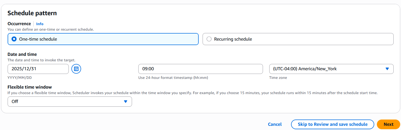
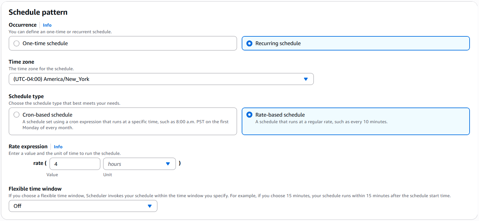
  6. For Schedule name, enter a unique name (for example, everyday).
  7. For Schedule Type, select Recurring.
  8. For Value, enter 1.
  9. For Unit, choose days.
  10. For Timezone, choose your time zone.
  11. Choose Create schedule.

You have successfully configured the schedule. Because Start date and time is not given, the visual ETL flow is triggered immediately and then it is triggered once a day after that.

Edit the schedule

You can view the configured schedules with the following steps:

  1. On the SageMaker Unified Studio console, navigate to Visual ETL flows for your project.
  2. Choose the Schedules tab.
  3. Choose Edit schedule under Actions.
  4. Edit with your preferences, then choose Save.

Pause or resume the schedule

If you want to pause the schedule, complete the following steps:

  1. Choose Pause schedule under Actions.

On the same Schedule tab, Status of the schedule will be updated to Paused.

  1. To resume the schedule, choose Activate schedule.

Delete the schedule

To delete the schedule, complete the following steps:

  1. Choose Delete schedule under Actions.
  2. Choose Delete schedule in the dialog.

On the same Schedule tab, you can verify that the deleted schedule disappears.

Schedule a query book flow

Complete the following steps to configure a schedule on a query book:

  1. On the SageMaker Unified Studio console, on the top menu, choose Build.
  2. Under DATA ANALYSIS & INTEGRATION, choose Query Editor.
  3. On the data explorer, under Lakehouse, choose AwsDataCatalog.
  4. Navigate to the table venue_event_agg. This table is created in the previous section.
  5. On the options menu (three dots), choose Query with Athena.
  6. On the Actions menu, choose Save to project.
  7. Choose Save changes.
  8. On the Actions menu, choose Create schedule.
  9. For Schedule Type, choose Recurring.
  10. For Value, enter 1.
  11. For Unit, choose days.
  12. For Timezone, choose your time zone.
  13. Choose Create schedule.

You have successfully configured the schedule. Because Start date and time was not set, the query book is triggered immediately and then it is triggered once a day after that. You can optionally configure start and end times if you want to limit your schedule to run in a specific date range.

To view the configured schedules, in the navigation pane, choose Scheduled queries.

You can view the list of scheduled queries and edit, pause, resume, or delete them, as shown in the previous section.

Clean up

To avoid incurring future charges, clean up the resources you created during this walkthrough:

  1. On the Schedule tab of Visual ETL flows, select the everyday schedule, and choose Delete schedule under Actions. The related EventBridge schedule is automatically deleted as well.
  2. On the SageMaker AI console, choose Training jobs under Training, and delete all the SageMaker training jobs that start with everyday-.
  3. (Optional) To delete the visual ETL flow, on the Flows tab of Visual ETL flows, select your visual ETL flow, and choose Delete flow under Actions.

Conclusion

The new unified scheduling experience in SageMaker Unified Studio simplifies workflow automation. With unified scheduling, you can seamlessly orchestrate your visual ETL flows and query books in one centralized location.

Whether you’re running daily data transformations, weekly analytical queries, or monthly reporting workflows, the unified scheduling experience provides a straightforward path to automation. This capability enables data teams to focus more on deriving insights from their data and less on managing infrastructure and scheduling configurations.

We encourage you to try out this new experience and share your feedback with us. For more information about SageMaker Unified Studio and its capabilities, visit our documentation or explore our other blog posts about visual ETL flows and query books.


About the Authors

Noritaka Sekiyama is a Principal Big Data Architect for AWS Analytics services with a strong focus on data engineering. He is responsible for building software artifacts to help customers. In his spare time, he enjoys cycling on his road bike.

Daniel Obi is a Frontend Engineer on the Amazon SageMaker Unified Studio team. He is dedicated to building intuitive and effective solutions that enhance user experience and technical functionality. Outside of his professional work, he enjoys watching and playing basketball.

Vasudevan Venkataramanan is a Senior Software Engineer on the Amazon SageMaker Unified Studio team. He is responsible for technical direction of scheduling and orchestration within SageMaker Unified Studio. Outside of his professional work, he enjoys spending time with his kid, and playing pickleball and cricket.

Yuhang Huang is a Software Development Manager on the Amazon SageMaker Unified Studio team. He leads the engineering team to design, build, and operate scheduling and orchestration capabilities in SageMaker Unified Studio. In his free time, he enjoys playing tennis.

Gal HeyneGal Heyne is a Senior Technical Product Manager for AWS Analytics services with a strong focus on AI/ML and data engineering. She is passionate about developing a deep understanding of customers’ business needs and collaborating with engineers to design simple-to-use data products.

How Flutter UKI optimizes data pipelines with AWS Managed Workflows for Apache Airflow

Post Syndicated from Monica Cujerean, Ionut Hedesiu original https://aws.amazon.com/blogs/big-data/how-flutter-uki-optimizes-data-pipelines-with-aws-managed-workflows-for-apache-airflow/

This post is co-written with Monica Cujerean and Ionut Hedesiu from Flutter UKI.

In this post, we share how Flutter UKI transitioned from a monolithic Amazon Elastic Compute Cloud (Amazon EC2)-based Airflow setup to a scalable and optimized Amazon Managed Workflows for Apache Airflow (Amazon MWAA) architecture using features like Kubernetes Pod Operator, continuous integration and delivery (CI/CD) integration, and performance optimization techniques.

About Flutter UKI

As a division of Flutter Entertainment, Flutter UKI stands at the forefront of the sports betting and gaming industry. Flutter UKI offers a diverse portfolio of entertainment options, encompassing sports wagering, casino games, bingo, and poker experiences. Flutter UKI’s digital presence is robust, operating through an array of renowned online brands. These include the iconic Paddy Power, Sky Betting and Gaming, and Tombola. While Flutter UKI has established a strong online foothold, it maintains a significant physical presence with a network of 576 Paddy Power betting shops strategically located across the United Kingdom and Ireland.

The Data team at Flutter UKI is integral to the company’s mission of using data to drive business success and innovation. Specializing in data, their teams are dedicated to ensuring the seamless integration, management, and accessibility of data across multiple facets of the organization. By developing robust data pipelines and maintaining high data quality standards, Flutter UKI empowers stakeholders with reliable insights, optimizes operational efficiencies, and enhances the user experience. Its commitment to data excellence underpins its efforts to remain at the forefront of the online gaming and entertainment industry, delivering value and strategic advantage to the business.

The journey from self managing Airflow on Amazon EC2 to operating Airflow workloads at scale using Amazon MWAA

Flutter UKI’s data orchestration story began in 2017 with a modest Apache Airflow deployment on EC2 instances. As the company’s digital footprint expanded, so did their data pipeline requirements, leading to an increasingly complex monolithic cluster that demanded constant attention and resource scaling. The operational overhead of managing these EC2 instances became a significant challenge for their engineering teams. In 2022, Flutter UKI reached a crossroads. They needed to choose between re-architecting their service on Amazon Elastic Kubernetes Service (Amazon EKS) or embracing Amazon Managed Workflows for Apache Airflow (MWAA).

Flutter UKI was looking to transform their data orchestration service from a resource-intensive, self-managed system to a more efficient, managed service that would allow them to focus on their core business objectives rather than infrastructure management. Through extensive proof-of-concept (POC) testing and close collaboration with AWS Enterprise Support, Flutter UKI gained confidence in the ability of Amazon MWAA to handle their sophisticated workloads at scale. Their choice of MWAA over a self-managed solution on Amazon EKS reflected Flutter UKI’s strategic focus on using managed services to reduce operational complexity and accelerate innovation.

The migration to Amazon MWAA followed a methodical approach. There was extensive testing of multiple POCs. During the POCs, the engineering team found MWAA to have a good ease of use, which helped them reduce the learning curve resulting in faster. Learning from each POC, they iterated on the final architecture by making data-driven decisions. Starting with a small subset of directed acyclic graphs (DAG), the Flutter UKI team expanded their deployment over time, gradually moving hundreds and eventually thousands of workflows to the managed service. This careful, phased transition allowed them to validate the performance and reliability of MWAA while minimizing operational risk.

High-level architecture design

During the service re-architecture, the data team strategically managed over 3,500 dynamically generated DAGs by implementing a sophisticated distribution approach across multiple Amazon MWAA environments to create a workload isolated environment. Another reason for having multiple environments was to make sure that no one MWAA environment doesn’t get overloaded by multiple DAGs. By placing DAG files across diverse Amazon Simple Storage Service (Amazon S3) locations and configuring unique DAG_FOLDER paths for each environment, the data team created an intelligent load balancing mechanism that allocates workflows based on complex criteria including environment type, task volume, and environment-specific DAG affinity. A round-robin distribution strategy was designed to minimize single environment load, ensuring scalable infrastructure with zero performance degradation. This approach allowed the team to optimize workflow orchestration, maintaining high performance while efficiently managing an extensive collection of dynamically generated DAGs across multiple MWAA environments. To provide more compute to individual tasks and to keep the MWAA efficient, Flutter UKI delegated the DAG execution to an external compute environment using Amazon Elastic Kubernetes Service (Amazon EKS). The resulting high-level architecture is shown in the following figure.

  1. Kubernetes Pod Operator (KPO) for tasks: Flutter UKI transitioned from using custom operators and many native Airflow operators to exclusively utilizing the Kubernetes Pod Operator (KPO). This decision simplified their architecture by eliminating unnecessary complexity, reducing maintenance overhead, and mitigating potential bugs. Additionally, this approach enabled them to allocate compute resources on a per-task basis, optimizing overall service performance. It also enabled the use of different container images for different tasks, thereby avoiding library dependency conflicts.
  2. Kubernetes Pod Operator wrapper (KPOw): Instead of using KPO directly, they developed a wrapper (KPOw) around it. This wrapper abstracts the underlying complexity and minimizes the impact of signature changes in Airflow, Amazon MWAA, Amazon EKS, or operator versions. By centralizing these changes, they only need to update the wrapper rather than thousands of individual DAGs. The wrapper also simplifies DAGs by hiding repetitive parameters, such as node affinity, pod resources, and EKS cluster configurations. Furthermore, it enforces company-specific naming conventions and allows for parameter validation at task execution time rather than during DagBag refresh. They also introduced profiles and image files, where profile files contain necessary KPO parameters, and the corresponding image files link to the repository for the task’s container image. This setup ensures consistency across tasks using the same profile and facilitates simultaneous updates across tasks.
  3. Monthly image updates in Kubernetes: Enforcing a policy of monthly image updates made sure that their code remained current, preventing security vulnerabilities and avoiding extensive code changes due to deprecated libraries.
  4. Continuous Airflow updates: Flutter UKI maintains a cutting-edge infrastructure by implementing new Airflow versions shortly after release, while following a carefully orchestrated deployment strategy. Their approach uses standard Amazon MWAA configurations and employs a systematic testing protocol. New versions are first deployed to development and test environments for thorough validation before reaching production systems. This methodical progression significantly reduces the risk of disruptions to business-critical workflows.

To achieve operational excellence, Flutter UKI has implemented a comprehensive monitoring framework centered on Amazon CloudWatch metrics. Their monitoring solution includes strategically configured alarms that provide early warning signals for potential issues. This proactive monitoring approach enables their teams to quickly identify and investigate anomalies in production workload executions, ensuring high availability and performance of their data pipelines. The combination of careful version management and robust monitoring exemplifies Flutter UKI’s commitment to operational excellence in their cloud infrastructure.

  1. CI/CD integration: By managing their code in GitLab, with mandatory code reviews and using Argo Events and Argo Workflows for image updates in AWS ECR, they streamlined their development processes.
  2. Performance Optimization: A significant portion of the DAGs are dynamically generated based on database metadata. This generation process runs outside Amazon MWAA, with its own CI/CD pipeline, and the resulting DAG files are stored in the S3 DAG. Placing code outside of tasks was avoided, including parameter evaluation. Parameters and secrets are stored in AWS Secrets Manager and retrieved at task runtime. Engineers aim to minimize or eliminate inter-service dependencies within MWAA.

DAGs are scheduled to distribute execution times as evenly as possible. Task code and common modules are hosted on Amazon S3 and retrieved at runtime. For larger codebases, Amazon Elastic File System (Amazon EFS) volumes are mounted to task pods are used.

Results

Today, Flutter UKI’s infrastructure comprises four Amazon MWAA clusters, each executing tasks on dedicated Amazon EKS node groups. They manage approximately 5,500 DAGs encompassing over 30,000 tasks, handling more than 60,000 DAG runs daily with a concurrency exceeding 450 tasks running simultaneously across clusters. They anticipate a 10% monthly increase in this workload in the short to medium term. During major events like Cheltenham and Grand National, where data load increases by 30%, their MWAA service has demonstrated stability and scalability, achieving a 100% success rate for critical processes in 2025, a significant improvement over previous years.

Conclusion

Flutter UKI’s journey with AWS Managed Workflows for Apache Airflow (Amazon MWAA) has resulted in a stable, scalable, and resilient production environment. The careful re-architecting of Flutter UKI’s service, combined with strategic decisions around task execution and infrastructure management, has not only simplified their operations, but also enhanced performance and reliability. Security and compliance benefits were also noticed, because MWAA provides managed security updates, built-in encryption, and integration with AWS security services. Perhaps most importantly, the shift to MWAA has allowed Flutter UKI’s engineering teams to redirect their efforts from infrastructure maintenance to business-critical tasks, focusing on DAG development and improving data pipeline efficiency, ultimately accelerating innovation in their core business operations.

If you’re looking to reduce operational overhead and migrate to a fully managed Airflow solution on AWS, consider using Amazon MWAA. Get in touch with your Technical Account Manager or your Solutions Architect to discuss a solution specific to your use-case. You can also reach out to AWS Support by creating a case if you’re facing an issues setting up the service.

Ready to see what Amazon MWAA is like? Visit the AWS Management Console for Amazon MWAA. For more information, see What Is Amazon Managed Workflows for Apache Airflow. Additionally, Using Amazon MWAA with Amazon EKS shows you how to integrate Amazon MWAA with Amazon EKS.


About the authors

Monica Cujerean is a Principal Data Engineer at Flutter UKI, focusing on service related initiatives that cover performance optimization, cost effectiveness, and new feature adoption on most AWS service in our stack: Amazon MWAA, Amazon Redshift, Amazon Aurora, and Amazon SageMaker.

Ionut Hedesiu is a Senior Data Architect at Flutter UKI, responsible for designing strategic solutions to cover complex and varied business needs. His main expertise is on Amazon MWAA, Kubernetes, Amazon Sagemaker, and ETL solutions.

Nidhi Agrawal is a Technical Account Manager at AWS and works with large enterprise customers to provide the technical guidance, best practices, and strategic support to customers, helping them optimize their environments in the AWS Cloud.

John Kellett is a Senior Customer Solutions Manager with 25 years of experience across private and public sectors. John helps drive end-to-end customer engagement through program management excellence. By understanding and representing customers’ strategic visions, John aligns to develop the people, organizational readiness, and technology competencies to meet the desired outcomes.

Sidhanth Muralidhar is a Principal Technical Account Manager at AWS. He works with large enterprise customers who run their workloads on AWS. He is passionate about working with customers and helping them architect workloads for cost, reliability, performance, and operational excellence at scale in their cloud journey. He has a keen interest in data analytics as well.

How BMW Group built a serverless terabyte-scale data transformation architecture with dbt and Amazon Athena

Post Syndicated from Philipp Karg original https://aws.amazon.com/blogs/big-data/how-bmw-group-built-a-serverless-terabyte-scale-data-transformation-architecture-with-dbt-and-amazon-athena/

Businesses increasingly require scalable, cost-efficient architectures to process and transform massive datasets. At the BMW Group, our Cloud Efficiency Analytics (CLEA) team has developed a FinOps solution to optimize costs across over 10,000 cloud accounts. While enabling organization-wide efficiency, the team also applied these principles to the data architecture, making sure that CLEA itself operates frugally. After evaluating various tools, we built a serverless data transformation pipeline using Amazon Athena and dbt.

This post explores our journey, from the initial challenges to our current architecture, and details the steps we took to achieve a highly efficient, serverless data transformation setup.

Challenges: Starting from a rigid and costly setup

In our early stages, we encountered several inefficiencies that made scaling difficult. We were managing complex schemas with wide tables that required significant effort in maintainability. Initially, we used Terraform to create tables and views in Athena, allowing us to manage our data infrastructure as code (IaC) and automate deployments through continuous integration and delivery (CI/CD) pipelines. However, this method slowed us down when changing data models or dealing with schema changes, therefore requiring high development efforts.

As our solution grew, we faced challenges with query performance and costs. Each query scanned large amounts of raw data, resulting in increased processing time and higher Athena costs. We used views to provide a clean abstraction layer, but this masked underlying complexity because seemingly simple queries against these views scanned large volumes of raw data, and our partitioning strategy wasn’t optimized for these access patterns. As our datasets grew, the lack of modularity in our data design increased complexity, making scalability and maintenance increasingly difficult. We needed a solution for pre-aggregating, computing, and storing query results of computationally intensive transformations. The absence of robust testing and lineage solutions made it challenging to identify the root causes of data inconsistencies when they occurred.

As part of our business intelligence (BI) solution, we used Amazon QuickSight to build our dashboards, providing visual insights into our cloud cost data. However, our initial data architecture led to challenges. We were building dashboards on top of large, wide datasets, with some hitting the QuickSight per-dataset SPICE limit of 1 TB. Additionally, during SPICE ingest, our largest datasets required 4–5 hours of processing time due to performing full scans each time, often scanning over a terabyte of data. This architecture wasn’t helping us be more agile and quick while scaling up. The long processing times and storage limitations hindered our ability to provide timely insights and expand our analytics capabilities.

To address these issues, we enhanced the data architecture with AWS Lambda, AWS Step Functions, AWS Glue, and dbt. This tool stack significantly enhanced our development agility, empowering us to quickly modify and introduce new data models. At the same time, we improved our overall data processing efficiency with incremental loads and better schema management.

Solution overview

Our current architecture consists of a serverless and modular pipeline coordinated by GitHub Actions workflows. We chose Athena as our primary query engine for several strategic reasons: it aligns perfectly with our team’s SQL expertise, excels at querying Parquet data directly in our data lake, and alleviates the need for dedicated compute resources. This makes Athena an ideal fit for CLEA’s architecture, where we process around 300 GB daily from a data lake of 15 TB, with our largest dataset containing 50 billion rows across up to 400 columns. The capability of Athena to efficiently query large-scale Parquet data, combined with its serverless nature, enables us to focus on writing efficient transformations rather than managing infrastructure.

The following diagram illustrates the solution architecture.

Using this architecture, we’ve streamlined our data transformation process using dbt. In dbt, a data model represents a single SQL transformation that creates either a table or a view—essentially a building block of our data transformation pipeline. Our implementation includes around 400 such models, 50 data sources, and around 100 data tests. This setup enables seamless updates—whether creating new models, updating schemas, or modifying views—triggered simply by creating a pull request in our source code repository, with the rest handled automatically.

Our workflow automation includes the following features:

  • Pull request – When we create a pull request, it’s deployed to our testing environment first. After passing validation and being approved or merged, it’s deployed to production using GitHub workflows. This setup enables seamless model creation, schema updates, or view changes—triggered just by creating a pull request, with the rest handled automatically.
  • Cron scheduler – For nightly runs or multiple daily runs to reduce data latency, we use scheduled GitHub workflows. This setup allows us to configure specific models with different update strategies based on data needs. We can set models to update incrementally (processing only new or changed data), as views (querying without materializing data), or as full loads (completely refreshing the data). This flexibility optimizes processing time and resource usage. We can target only specific folders—like source, prepared, or semantic layers—and run the dbt test afterward to validate model quality.
  • On demand – When adding new columns or changing business logic, we need to update historical data to maintain consistency. For this, we use a backfill process, which is a custom GitHub workflow created by our team. The workflow allows us to select specific models, include their upstream dependencies, and set parameters like start and end dates. This makes sure that changes are applied accurately across the entire historical dataset, maintaining data consistency and integrity.

Our pipeline is organized into three primary stages—Source, Prepared, and Semantic—each serving a specific purpose in our data transformation journey. The Source stage maintains raw data in its original form. The Prepared stage cleanses and standardizes this data, handling tasks like deduplication and data type conversions. The Semantic stage transforms this prepared data into business-ready models aligned with our analytical needs. An additional QuickSight step handles visualization requirements. To achieve low cost and high performance, we use dbt models and SQL code to manage all transformations and schema changes. By implementing incremental processing strategies, our models process only new or changed data rather than reprocessing the entire dataset with each run.

The Semantic stage (not to be confused with dbt’s semantic layer feature) introduces business logic, transforming data into aggregated datasets that are directly consumable by BMW’s Cloud Data Hub, internal CLEA dashboards, data APIs, or In-Console Cloud Assistant (ICCA) chatbot. The QuickSight step further optimizes data by selecting only necessary columns by using a column-level lineage solution and setting a dynamic date filter with a sliding window to ingest only relevant hot data into SPICE, avoiding unused data in dashboards or reports.

This approach aligns with BMW Group’s broader data strategy, which includes streamlining data access using AWS Lake Formation for fine-grained access control.

Overall, as a high-level structure, we’ve fully automated schema changes, data updates, and testing through GitHub pull requests and dbt commands. This approach enables controlled deployment with robust version control and change management. Continuous testing and monitoring workflows uphold data accuracy, reliability, and quality across transformations, supporting efficient, collaborative model iteration.

Key benefits of the dbt-Athena architecture

To design and manage dbt models effectively, we use a multi-layered approach combined with cost and performance optimizations. In this section, we discuss how our approach has yielded significant benefits in five key areas.

SQL-based, developer-friendly environment

Our team already had strong SQL skills, so dbt’s SQL-centric approach was a natural fit. Instead of learning a new language or framework, developers could immediately start writing transformations using familiar SQL syntax with dbt. This familiarity aligns well with the SQL interface of Athena and, combined with dbt’s added functionality, has increased our team’s productivity.

Behind the scenes, dbt automatically handles synchronization between Amazon Simple Storage Service (Amazon S3), the AWS Glue Data Catalog, and our models. When we need to change a model’s materialization type—for example, from a view to a table—it’s as simple as updating a configuration parameter rather than rewriting code. This flexibility has reduced our development time dramatically, allowed us to focus on building better data models rather than managing infrastructure.

Agility in modeling and deployment

Documentation is crucial for any data platform’s success. We use dbt’s built-in documentation capabilities by publishing them to GitHub Pages, which creates an accessible, searchable repository of our data models. This documentation includes table schemas, relationships between models, and usage examples, enabling team members to understand how models interconnect and how to use them effectively.

We use dbt’s built-in testing capabilities to implement comprehensive data quality checks. These include schema tests that verify column uniqueness, referential integrity, and null constraints, as well as custom SQL tests that validate business logic and data consistency. The testing framework runs automatically on every pull request, validating data transformations at each step of our pipeline. Additionally, dbt’s dependency graph provides a visual representation of how our models interconnect, helping us understand the upstream and downstream impacts of any changes before we implement them. When stakeholders need to modify models, they can submit changes through pull requests, which, after they’re approved and merged, automatically trigger the necessary data transformations through our CI/CD pipeline. This streamlined process enabled us to create new data products within days compared to weeks and reduced ongoing maintenance work by catching issues early in the development cycle.

Athena workgroup separation

We use Athena workgroups to isolate different query patterns based on their execution triggers and purposes. Each workgroup has its own configuration and metric reporting, allowing us to monitor and optimize separately. The dbt workgroup handles our scheduled nightly transformations and on-demand updates triggered by pull requests through our Source, Prepared, and Semantic stages. The dbt-test workgroup executes automated data quality checks during pull request validation and nightly builds. The QuickSight workgroup manages SPICE data ingestion queries, and the Ad-hoc workgroup supports interactive data exploration by our team.

Each workgroup can be configured with specific data usage quotas, enabling teams to implement granular governance policies. This separation provides several benefits: it enables clear cost allocation, provides isolated monitoring of query patterns across different use cases, and helps enforce data governance through custom workgroup settings. Amazon CloudWatch monitoring per workgroup helps us track usage patterns, identify query performance issues, and adjust configurations based on actual needs.

Using QuickSight SPICE

QuickSight SPICE (Super-fast, Parallel, In-memory Calculation Engine) provides powerful in-memory processing capabilities that we’ve optimized for our specific use cases. Rather than loading entire tables into SPICE, we create specialized views on top of our materialized semantic models. These views are carefully crafted to include only the necessary columns, relevant metadata joins, and appropriate time filtering to have only recent data available in dashboards.

We’ve implemented a hybrid refresh strategy for these SPICE datasets: daily incremental updates keep the data fresh, and weekly full refreshes maintain data consistency. This approach strikes a balance between data freshness and processing efficiency. The result is responsive dashboards that maintain high performance while keeping processing costs under control.

Scalability and cost-efficiency

The serverless architecture of Athena eliminates manual infrastructure management, automatically scaling based on query demand. Because costs are based solely on the amount of data scanned by queries, optimizing queries to scan as little data as possible directly reduces our costs. We use the distributed query execution capabilities of Athena through our dbt model structure, enabling parallel processing across data partitions. By implementing effective partitioning strategies and using Parquet file format, we minimize the amount of data scanned while maximizing query performance.

Our architecture offers flexibility in how we materialize data through views, full tables, and incremental tables. With dbt’s incremental models and partitioning strategy, we process only new or modified data instead of entire datasets. This approach has proven highly effective—we’ve observed significant reductions in data processing volume as well as data scanning, particularly in our QuickSight workgroup.

The effectiveness of these optimizations implemented at the end of 2023 is visible in the following diagram, showing costs by Athena workgroups.

The workgroups are illustrated as follows:

  • Green (QuickSight): Shows reduced data scanning post-optimization.
  • Light blue (Ad-hoc): Varies based on analysis needs.
  • Dark blue (dbt): Maintains consistent processing patterns
  • Orange (dbt-test): Shows regular, efficient test execution.

The increased dbt workload costs directly correlate with decreased QuickSight costs, reflecting our architectural shift from using complex views in QuickSight workgroups (which previously masked query complexity but led to repeated computations) to using dbt for materializing these transformations. Although this increased the dbt workload, the overall cost-efficiency improved significantly because materialized tables reduced redundant computations in QuickSight. This demonstrates how our optimization strategies successfully manage growing data volumes while achieving net cost reduction through efficient data materialization patterns.

Conclusion

Our data architecture uses dbt and Athena to provide a scalable, cost-efficient, and flexible framework for building and managing data transformation pipelines. Athena’s ability to query data directly in Amazon S3 alleviates the need to move or copy data into a separate data warehouse, and its serverless model and dbt’s incremental processing minimize both operational overhead and processing costs. Given our team’s strong SQL expertise, expressing these transformations in SQL through dbt and Athena was a natural choice, enabling rapid model development and deployment. With dbt’s automatic documentation and lineage, troubleshooting and identifying data issues is simplified, and the system’s modularity allows for quick adjustments to meet evolving business needs.

Starting with this architecture is quick and straightforward: all that is needed is the dbt-core and dbt-athena libraries, and Athena itself requires no setup, because it’s a fully serverless service with seamless integration with Amazon S3. This architecture is ideal for teams looking to rapidly prototype, test, and deploy data models, optimizing resource usage, accelerating deployment, and providing high-quality, accurate data processing.

For those interested in a managed solution from dbt, see From data lakes to insights: dbt adapter for Amazon Athena now supported in dbt Cloud.


About the Authors

Philipp Karg is a Lead FinOps Engineer at BMW Group and has a strong background in data engineering, AI, and FinOps. He focuses on driving cloud efficiency initiatives and fostering a cost-aware culture within the company to leverage the cloud sustainably.

Selman Ay is a Data Architect specializing in end-to-end data solutions, architecture, and AI on AWS. Outside of work, he enjoys playing tennis and engaging outdoor activities.

Cizer Pereira is a Senior DevOps Architect at AWS Professional Services. He works closely with AWS customers to accelerate their journey to the cloud. He has a deep passion for cloud-based and DevOps solutions, and in his free time, he also enjoys contributing to open source projects.

Access your existing data and resources through Amazon SageMaker Unified Studio, Part 1: AWS Glue Data Catalog and Amazon Redshift

Post Syndicated from Lakshmi Nair original https://aws.amazon.com/blogs/big-data/access-your-existing-data-and-resources-through-amazon-sagemaker-unified-studio-part-1-aws-glue-data-catalog-and-amazon-redshift/

Amazon SageMaker Unified Studio provides a unified environment for data, analytics, machine learning (ML), and AI workloads. Part of the next generation of Amazon SageMaker, SageMaker Unified Studio allows you to discover your data and put it to work using familiar AWS tools to complete end-to-end development workflows, including data analysis, data processing, model training, generative AI app development, and more, in a single governed environment. You can create or join projects to collaborate with your teams, share AI and analytics artifacts securely, and discover and use your data stored in different data sources through Amazon SageMaker Lakehouse.

This series of posts demonstrates how you can onboard and access existing AWS data sources using SageMaker Unified Studio. This post focuses on onboarding existing AWS Glue Data Catalog tables and database tables available in Amazon Redshift. Part 2 discusses using Amazon Simple Storage Service (Amazon S3), Amazon Relational Database Service (Amazon RDS), Amazon DynamoDB, and Amazon EMR.

Access your existing data and resources through Amazon SageMaker Unified Studio

This series primarily focuses on the UI experience. If you prefer script-based automation, refer to Bringing existing resources into Amazon SageMaker Unified Studio.

Access management with SageMaker Unified Studio

The SageMaker Unified Studio authorization model is a hierarchical access control list (ACL) based on the resource type such as a domain or a project. For example, at the domain level, a user might have a domain owner designation and at the project level, the user can be an owner or contributor. You can configure these profiles at AWS Identity and Access Management (IAM) user, single sign-on (SSO) user, and SSO group level.

Each project has a project role. When the user interacts with resources within SageMaker Unified Studio, it generates IAM session credentials based on the user’s effective profile in the specific project context, and then users can use tools such as Amazon Athena or Amazon Redshift to query the relevant data. The project owner can add or remove project members for their project, create publishing agreements with a domain, and publish assets to a domain.

SageMaker Unified Studio can be accessed by IAM users or SSO authenticated users, and IAM roles can interact with the SageMaker Unified Studio through its APIs.

Solution overview

AWS Lake Formation enables you to define fine-grained access control on the Data Catalog, where you can configure access at database, table, row, or column level or define permissions with tags. When setting up Lake Formation, you can configure it with hybrid access mode, where you get flexibility to selectively enable Lake Formation permissions for specific databases and tables, and continue using IAM permissions for others. SageMaker Unified Studio supports Lake Formation hybrid mode.

When you create a project in SageMaker Unified Studio, an AWS Glue database is added by default as part of the project. Assets published into that database don’t need any additional permissions, but if you want to publish or subscribe assets from an existing AWS Glue database, then you need to provide explicit permissions to SageMaker Unified Studio to be able to access the database and tables. For more details, see Configure Lake Formation permissions for Amazon SageMaker Unified Studio.

Let’s understand how we can access existing datasets through SageMaker Unified Studio.

Prerequisites

To run the instruction, you must complete the following prerequisites:

  • An AWS account
  • A SageMaker Unified Studio domain
  • A SageMaker Unified Studio project with All capabilities project profile

In the SageMaker Unified Studio, select the project and navigate to the Project overview page. Copy the Project role ARN as highlighted in the screenshot. This project role will be used further in the post to provide permissions on existing datasets and resources.

Use existing AWS Glue tables

This section has following prerequisites:

One extra prerequisite step is to revoke IAMAllowedPrincipals group permission on both database and table to enforce Lake Formation permission for access. For detailed instruction see Revoking permission using the Lake Formation console.

To access existing Data Catalog tables in SageMaker Unified Studio, complete the following steps:

  1. On the Lake Formation console using the data lake administrator, choose Data lake locations in the navigation pane and choose Register location.
  2. Enter the S3 prefix for Amazon S3 path.
  3. For IAM role, choose your Lake Formation data access IAM role, which is not a service linked role.
  4. Select Lake Formation for Permission mode and choose Register location.

  1. On the Lake Formation console, under Data Catalog in the navigation pane, choose Databases.
  2. Select the existing Data Catalog database.
  3. From the Actions menu, choose Grant to grant permissions to the project role.

  1. For IAM users and roles, choose the project role.
  2. Select Named Data Catalog resources, and for Catalogs, choose the default catalog.
  3. For Databases, choose your existing Data Catalog database.

  1. For Database permissions, select Describe and choose Grant.

The next step is to grant the permission on the tables to the project role.

  1. On the Lake Formation console, under Data Catalog in the navigation pane, choose Databases.
  2. Select the existing Data Catalog database.
  3. From the Actions menu, choose Grant to grant permissions to the project role.
  4. For IAM users and roles, choose the project role.
  5. Select Named Data Catalog resources, and for Catalogs, choose the default catalog.
  6. For Databases, choose your Data Catalog database.
  7. For Tables, select the tables that you need to provide permission to the project role.

  1. For Table permissions, select Select and Describe.
  2. For Grantable permissions, select Select and Describe.
  3. Choose Grant.

You should revoke any existing permissions of IAMAllowedPrincipals on the databases and tables within Lake Formation.

Now let’s verify that we can access the existing AWS Glue table from the SageMaker Unified Studio Query Editor.

  1. In SageMaker Unified Studio, navigate to your project.
  2. On the project page, under Lakehouse, choose Data.
  3. Next to the Data Catalog table, choose the options menu (three dots), and choose Query with Athena.

SageMaker Unified Studio provides a unified JupyterLab experience across different languages, including SQL, PySpark, and Scala Spark. It also supports unified access across different compute runtimes such as Amazon Redshift and Athena for SQL, Amazon EMR Serverless, Amazon EMR on EC2, and AWS Glue for Spark. To access the data through the unified JupyterLab experience, complete the following steps:

  1. On the SageMaker Unified Studio project page, on the top menu, choose Build, and under IDE & APPLICATIONS, choose
  2. Wait for the space to be ready.
  3. Choose the plus sign and for Notebook, choose Python 3.
  4. In the notebook, switch the connection type to PySpark, choose spark.fineGrained, and query the existing Data Catalog table:
from pyspark.sql import SparkSession
spark = SparkSession.builder.getOrCreate()
df_sql = spark.sql("""
select * from retaildb.salesorders
""" )

df_sql.show()

Use existing Redshift clusters

This section has following prerequisites:

  • A Redshift cluster

To bring in existing Redshift clusters, follow these steps:

  1. To use your provisioned Redshift cluster or a Redshift Serverless workgroup, add either of the following tags (key/value) to the resource:
    1. Add AmazonDataZoneProject: <projectID> if you want to allow only a specific SageMaker Unified Studio project to access the Amazon Redshift resource. Replace <projectID> with the ID of the project created in SageMaker Unified Studio.
    2. Add for-use-with-all-datazone-projects: true if you want to allow all SageMaker Unified Studio projects to access the Amazon Redshift resource.

  1. To add the compute connection in SageMaker Unified Studio, you can authenticate the cluster using either the user name and password of the database, IAM credentials, or AWS Secrets Manager. To provide the authentication using Secrets Manager, add either of the following tags. This will enable the existing secret to appear on the dropdown menu, while defining the connection in SageMaker Unified Studio.
    1. AmazonDataZoneProject: <projectID>
    2. for-use-with-all-datazone-projects: true

In the following screenshot, you can see the tag configuration section within Secrets Manager settings for Redshift Serverless compute. To understand how to create a secret for a database in a Redshift cluster using Secrets Manager, refer to Managing Amazon Redshift admin passwords using AWS Secrets Manager.

  1. After the tags are applied, log in to SageMaker Unified Studio and choose the project.
  2. Go to the Compute section of your project, and on the Data warehouse tab, choose Add compute.
  3. Select Connect to existing compute resources.
  4. Choose the compute type: Amazon Redshift Provisioned cluster or Amazon Redshift Serverless.
  5. Configure the parameters by selecting the existing compute and authentication and choose Add compute.

The detailed walkthrough process is illustrated in the following screenshot.

Use Redshift tables with existing compute

This section has following prerequisites:

  • A Redshift table

In this section, we illustrate steps to create a federated connection for an existing Amazon Redshift data source. You can register an existing Redshift provisioned cluster as well as Redshift Serverless with the Data Catalog using SageMaker Unified Studio. This creates a federated multi-level catalog and provides the ability to centrally manage permissions to the data with fine-grained access control using Lake Formation. By mounting Amazon Redshift data in the Data Catalog, you can query it using your preferred tools such as Athena or AWS Glue extract, transform, and load (ETL) without having to copy or move the data.

Create an Amazon Redshift managed VPC endpoint for Amazon Redshift

Amazon Redshift managed virtual private cloud (VPC) endpoints use AWS PrivateLink to allow one VPC to privately access resources in another VPC as if they were local to the same VPC. With an Amazon Redshift managed VPC endpoint, you can connect to your private Redshift cluster with the RA3 instance type or Redshift Serverless within your VPC.

In this section, we explain how to create an Amazon Redshift managed VPC endpoint for both Redshift Serverless and an Amazon Redshift provisioned cluster in a single account. The managed VPC endpoint needs to be created only if your Redshift provisioned or Redshift Serverless cluster is in a different VPC than the SageMaker Unified Studio domain VPC.

If the SageMaker Unified Studio domain account is in a different account, allow the additional AWS accounts to create cluster endpoints. For steps to authorize your Amazon Redshift provisioned or Redshift Serverless cluster to deploy endpoints in additional accounts and grant access to the cross-account VPC, refer to Granting access to a VPC.

Redshift Serverless

For Redshift Serverless, follow these instructions.

The common practice is to allow port 5439 (Amazon Redshift connectivity port) to the security group or CIDR range in which your consumption workloads run.

  1. In the security group associated with the Redshift cluster, add an inbound rule with Type as Redshift, Protocol as TCP, Port range as 5439 (Amazon Redshift connectivity port), and Source as the CIDR range in which your consumption workloads run.

  1. On the Amazon Redshift console of the workgroup, go to Redshift-managed VPC endpoints.
  2. Choose Create endpoint.
  3. In the Endpoint settings section, choose the VPC, associated private subnet, and security group created for the SageMaker Unified Studio domain account to deploy the endpoint against.

The following screenshot shows the Amazon Redshift managed VPC endpoint created for Redshift Serverless.

Redshift provisioned

For Amazon Redshift provisioned, follow these instructions:

  1. To implement an Amazon Redshift managed VPC endpoint for a provisioned cluster, you need to enable cluster relocation and create subnet groups. In the cluster subnet group, choose the VPC and subnets of the SageMaker Unified Studio domain account.
  2. On the Amazon Redshift console, choose Configurations in the navigation pane.
  3. Provide the endpoint details, then choose Create endpoint.

Create a federated connection for Amazon Redshift

Complete the following steps to create a federated catalog in the Data Catalog to query the data using various preferred analytics tools such as Athena, visual ETL in SageMaker Unified Studio, Amazon EMR, and more:

  1. On the SageMaker Unified Studio console, choose your project.
  2. Choose Data in the navigation pane.
  3. In the data explorer, choose the plus sign to add a data source.
  4. Under Add a data source, choose Add connection, then choose Amazon Redshift.
  5. Enter the following parameters in the connection details, and choose Add data.
    1. Name: Enter the connection name.
    2. Host: Enter the Amazon Redshift managed VPC endpoint.
    3. Port: Enter the port number (Amazon Redshift uses 5439 as the default port).
    4. Database: Enter the database name.
    5. Authentication: Choose either the database user name and password credentials or Secrets Manager.

After the connection is established, you will see that the federated catalog is created, as shown in the following screenshot. This catalog uses the AWS Glue connection to connect to Amazon Redshift. The databases, tables, and views are automatically cataloged in the Data Catalog and registered with Lake Formation.

With Athena, data analysts can run federated SQL queries to scan data from multiple data sources in-place without creating complex data pipelines or data replication.

Use existing Data Catalog tables and Amazon Redshift assets in the SageMaker Unified Studio business data catalog

You can use the SageMaker Unified Studio business data catalog to catalog the data across your organization with business context. To use Amazon SageMaker Catalog, you must bring your existing data assets into the inventory of your project. Follow the instructions in this section to bring your existing Data Catalogs and Amazon Redshift assets into the project inventory.

Add an existing Data Catalog to the project inventory

To enrich the asset with business context and share your assets outside your own project, you must first bring the metadata to SageMaker Catalog. To import the metadata of the assets into the project’s inventory, you need to create a data source in the project catalog.

  1. In SageMaker Unified Studio, navigate to the Project catalog page within the project.
  2. Choose Data sources.
  3. Choose CREATE DATA SOURCE.
  4. For Name, provide the name of the data source.
  5. Choose AWS Glue (Lakehouse) for Data source type.
  6. For Data selection, choose the Database name and choose Next.
  7. Keep the rest as default and choose CREATE.
  8. Choose RUN to import the metadata.

After the data source successfully completes its run, metadata of all the data assets gets added to the project’s inventory.

Add existing Redshift tables and views to the project inventory

Create a data source to bring in the existing Redshift tables and views to add to the project’s inventory:

  1. In SageMaker Unified Studio, navigate to the Project catalog within the project.
  2. Choose Data sources.
  3. Choose CREATE DATA SOURCE.
  4. For Name, provide the name of the data source.
  5. Choose Amazon Redshift for Data source type.
  6. For Connection, choose the name of the Redshift connection.
  7. For Database name, choose dev and for Schema, enter public.
  8. Keep the rest as default and choose CREATE.
  9. Choose RUN to import the metadata.

After the data source successfully completes its run, metadata of all the data assets gets added to the project’s inventory.

Conclusion

This post explained how you can access existing data and resources available in the Data Catalog and Amazon Redshift using SageMaker Unified Studio. SageMaker Unified Studio provides an integrated environment for analytics and AI. Being able to access existing datasets available in your AWS account helps reduce operational overhead because users of your organization can access a common interface, collaborate, and share datasets. It also brings in efficiency for administrators because they can manage permissions for domains and projects in a common place.

In the next post, we will demonstrate how you can onboard and access other existing data sources such as Amazon S3, Amazon RDS, DynamoDB, and Amazon EMR.


About the Authors

Lakshmi Nair is a Senior Analytics Specialist Solutions Architect at AWS. She specializes in designing advanced analytics systems across industries. She focuses on crafting cloud-based data platforms, enabling real-time streaming, big data processing, and robust data governance. She can be reached via LinkedIn.

Noritaka Sekiyama is a Principal Big Data Architect on the AWS Glue team. He is also the author of the book Serverless ETL and Analytics with AWS Glue. He is responsible for building software artifacts to help customers. In his spare time, he enjoys cycling with his road bike.

Sakti Mishra is a Principal Data and AI Solutions Architect at AWS, where he helps customers modernize their data architecture and define end-to end-data strategies, including data security, accessibility, governance, and more. He is also the author of Simplify Big Data Analytics with Amazon EMR and AWS Certified Data Engineer Study Guide. Outside of work, Sakti enjoys learning new technologies, watching movies, and visiting places with family. He can be reached via LinkedIn.

Daiyan Alamgir is a Principal Frontend Engineer on the Amazon SageMaker Unified Studio team based in New York.

Vipin Mohan is a Principal Product Manager at AWS, leading the launch of generative AI capabilities in Amazon SageMaker Unified Studio. He is committed to shaping impactful products by working backward from customer insights, championing user-focused solutions, and delivering scalable results.

Chanu Damarla is a Principal Product Manager on the Amazon SageMaker Unified Studio team. He works with customers around the globe to translate business and technical requirements into products that delight customers and enable them to be more productive with their data, analytics, and AI.

Melting the ice — How Natural Intelligence simplified a data lake migration to Apache Iceberg

Post Syndicated from Yonatan Dolan original https://aws.amazon.com/blogs/big-data/melting-the-ice-how-natural-intelligence-simplified-a-data-lake-migration-to-apache-iceberg/

This post is co-written with Haya Axelrod Stern, Zion Rubin and Michal Urbanowicz from Natural Intelligence.

Many organizations turn to data lakes for the flexibility and scale needed to manage large volumes of structured and unstructured data. However, migrating an existing data lake to a new table format such as Apache Iceberg can bring significant technical and organizational challenges

Natural Intelligence (NI) is a world leader in multi-category marketplaces. NI’s leading brands, Top10.com and BestMoney.com, help millions of people worldwide to make informed decisions every day. Recently, NI embarked on a journey to transition their legacy data lake from Apache Hive to Apache Iceberg.

In this blog post, NI shares their journey, the innovative solutions developed, and the key takeaways that can guide other organizations considering a similar path.

This article details NI’s practical approach to this complex migration, focusing less on Apache Iceberg’s technical specifications, but rather on the real-world challenges and solutions encountered during the transition to Apache Iceberg, a challenge that many organizations are grappling with.

Why Apache Iceberg?

The architecture at NI followed the commonly used medallion architecture, comprised of a bronze-silver-gold layered framework, shown in the figure that follows:

  • Bronze layer: Unprocessed data from various sources, stored in its raw format in Amazon Simple Storage Service (Amazon S3), ingested through Apache Kafka brokers.
  • Silver layer: Contains cleaned and enriched data, processed using Apache Flink.
  • Gold layer: Holds analytics-ready datasets designed for business intelligence (BI) and reporting, produced using Apache Spark pipelines, and consumed by services such as Snowflake, Amazon Athena, Tableau, and Apache Druid. The data is stored in Apache Parquet format with AWS Glue Catalog providing metadata management.

BDB4681-Arch1

While this architecture supported NI analytical needs, it lacked the flexibility required for a truly open and adaptable data platform. The gold layer was coupled only with query engines that supported Hive and AWS Glue Data Catalog. It was possible to use Amazon Athena however Snowflake required maintaining another catalog in order to query those external tables. This issue made it difficult to evaluate or adopt alternative tools and engines without costly data duplication, query rewrite data catalog synchronization. As business scaled, NI needed a data platform that could seamlessly support multiple query engines simultaneously with a single data catalog and avoiding any vendor lock-in.

The power of Apache Iceberg

Apache Iceberg emerged as the perfect solution—a flexible, open table format that aligns with NI’s approach of Data Lake First. Iceberg offers several critical advantages such as ACID transactions, schema evolution, time travel, performance improvements and more. But the key strategic benefits lay in the ability to support multiple query engines simultaneously. It also has the following advantages:

  • Decoupling of storage and compute: The open table format enables you to separate the storage layer from the query engine, allowing an easy swap and support for multiple engines concurrently without data duplication.
  • Vendor independence: As an open table format, Apache Iceberg prevents vendor lock-in, giving you the flexibility to adapt to changing analytics needs.
  • Vendor adoption: Apache Iceberg is widely supported by major platforms and tools, providing seamless integration and long-term ecosystem compatibility.

By transitioning to Iceberg, NI was able to embrace a truly open data platform, providing long-term flexibility, scalability, and interoperability while maintaining a unified source of truth for all analytics and reporting needs.

Challenges faced

Migrating a live production data lake to Iceberg was challenging because of operational complexities and legacy constraints. The data service at NI runs hundreds of Spark and machine learning pipelines, manages thousands of tables, and supports over 400 dashboards—all operating 24/7. Any migration would need to be done without production interruptions; and coordinating such a migration while operations continue seamlessly was daunting.

NI needed to accommodate diverse users with varying requirements and timelines from data engineers to data analysts all the way to data scientists and BI teams.

Adding to the challenge were legacy constraints. Some of the existing tools didn’t fully support Iceberg, so there was a need to maintain Hive-backed tables for compatibility. As NI realized that not all consumers could adopt Iceberg immediately. A plan was required to allow for incremental transitions without downtime or disruption to ongoing operations.

Key pillars for migration

To help ensure a smooth and successful transition, six critical pillars were defined:

  • Support ongoing operations: Maintain uninterrupted compatibility with existing systems and workflows during the migration process.
  • User transparency: Minimize disruption for users by preserving existing table names and access patterns.
  • Gradual consumer migration: Allow consumers to adopt Iceberg at their own pace, avoiding a forced, simultaneous switchover.
  • ETL flexibility: Migrate ETL pipelines to Iceberg without imposing constraints on development or deployment.
  • Cost effectiveness: Minimize storage and compute duplication and overhead during the migration period.
  • Minimize maintenance: Reduce the operational burden of managing dual table formats (Hive and Iceberg) during the transition.

Evaluating traditional migration approaches

Apache Iceberg supports two main approaches for migration: In-place and rewrite-based migration.

In-place migration

How it works: Converts an existing dataset into an Iceberg table without duplicating data by creating Iceberg metadata on top of the existing files while preserving their layout and format.

Advantages:

  • Cost-effective in terms of storage (no data duplication)
  • Simplified implementation
  • Maintains existing table names and locations
  • No data movement and minimal compute requirements, translating into lower cost

Disadvantages:

  • Downtime required: All write operations must be paused during conversion, which was unacceptable in NI cases because data and analytics are considered mission critical and run 24/7
  • No gradual adoption: All consumers must switch to Iceberg simultaneously, increasing the risk of disruption
  • Limited validation: No opportunity to validate data before cutover; rollback requires restoring from backups
  • Technical constraints: Schema evolution during migration can be challenging; data type incompatibilities can halt the entire process

Rewrite-based migration

How it works: Rewrite-based migration in Apache Iceberg involves creating a new Iceberg table by rewriting and reorganizing existing dataset files into Iceberg’s optimized format and structure for improved performance and data management.

Advantages:

  • Zero downtime during migration
  • Supports gradual consumer migration
  • Enables thorough validation
  • Simple rollback mechanism

Disadvantages:

  • Resource overhead: Double storage and compute costs during migration
  • Maintenance complexity: Managing two parallel data pipelines increases operational burden
  • Consistency challenges: Maintaining perfect consistency between the two systems is challenging
  • Performance impact: Increased latency because of dual writes; potential pipeline slowdowns

Why neither option alone was good enough

NI decided that neither option could meet all critical requirements:

  • In-place migration fell short because of unacceptable downtime and lack of support for gradual migration.
  • Rewrite-based migration fell short because of prohibitive cost overhead and complex operational management.

This analysis led NI to develop a hybrid approach that combines the advantages of both methods while mitigating and minimizing limitations.

The hybrid solution

The hybrid migration strategy was designed around five foundational elements, using AWS analytical services for orchestration, processing, and state management.

  1. Hive-to-Iceberg CDC: Automatically synchronize Hive tables with Iceberg using a custom change data capture (CDC) process to support existing consumers. Unlike traditional CDC focusing on row-level changes, the process was done at the partition-level to preserve Hive’s behavior of updating tables by overwriting partitions. This helps ensure that data consistency is maintained between Hive and Iceberg without logic changes at the migration phase, making sure that the same data exists on both tables.
  2. Continuous schema synchronization: Schema evolution during the migration introduced maintenance challenges. Automated schema sync processes compared Hive and Iceberg schemas, reconciling differences while maintaining type compatibility.
  3. Iceberg-to-Hive reverse CDC: To enable the data team to transition extract, transform, and load (ETL) jobs to write directly to Iceberg while maintaining compatibility with existing Hive-based processes not yet migrated, a reverse CDC from Iceberg to Hive was implemented. This allowed ETLs to write to Iceberg while maintaining Hive tables for downstream processes that had not yet migrated and still relied on them during the migration period.
  4. Alias management in Snowflake: Snowflake aliases made sure that Iceberg tables retained their original names, making the transition transparent to users. This approach minimized reconfiguration efforts across dependent teams and workflows.
  5. Table replacement: Swap production tables while retaining original names, completing the migration.

Technical deep dive

The migration to from Hive to Iceberg was constructed of several steps:

1. Hive-to-Iceberg CDC pipeline

Objective: Keep Hive and Iceberg tables synchronized without duplicating effort.

The preceding figure demonstrates how every partition written to the Hive table is automatically and transparently copied to the Iceberg table using a CDC process. This process makes sure that both tables are synchronized, enabling a seamless and incremental migration without disrupting downstream systems. NI chose partition-level synchronization because the legacy Hive ETL jobs already wrote updates by overwriting entire partitions and updating the partition location. Adopting that same approach in the CDC pipeline helped ensure that it remained consistent with how data was originally managed, making the migration smoother and avoiding the need to rework row-level logic.

Implementation:

  • To keep Hive and Iceberg tables synchronized without duplicating effort, a streamlined pipeline was implemented. Whenever partitions in Hive tables are updated, the AWS Glue Catalog emits events such as UpdatePartition. Amazon EventBridge captured these events, filtered them for the relevant databases and tables according to the event bridge rule, and triggered an AWS Lambda This function parsed the event metadata and sent the partition updates to an Apache Kafka topic.
  • A Spark job running on Amazon EMR consumed the messages from Kafka, which contained the updated partition details from the Data Catalog events. Using that event metadata, the Spark job queried the relevant Hive table, and wrote it to Iceberg table in Amazon S3 using the Spark Iceberg overwritePartitions API, as shown in the following example:
{
   "id":"10397e54-c049-fc7b-76c8-59e148c7cbfc",
   "detail-type":"Glue Data Catalog Table State Change",
   "source":"aws.glue",
   "time":"2024-10-27T17:16:21Z",
   "region":"us-east-1",
   "detail":{
      "databaseName":"dlk_visitor_funnel_dwh_production",
      "changedPartitions":[
         "2024-10-27"
      ],
      "typeOfChange":"UpdatePartition",
      "tableName":"fact_events"
   }
}
  • By targeting only modified partitions, the pipeline (shown in the following figure) significantly reduced the need for costly full-table rewrites. Iceberg’s robust metadata layers, including snapshots and manifest files, were seamlessly updated to capture these changes, providing efficient and accurate synchronization between Hive and Iceberg tables.

2. Iceberg-to-Hive reverse CDC pipeline

Objective: Support Hive consumers while allowing ETL pipelines to transition to Iceberg.

BDB4681-arch4

The preceding figure shows the reverse process, where every partition written to the Iceberg table is automatically and transparently copied to the Hive table using a CDC mechanism. This process helps ensure synchronization between the two systems, enabling seamless data updates for legacy systems that still rely on Hive while transitioning to Iceberg.

Implementation:

Synchronizing data from Iceberg tables back to Hive tables presented a different challenge. Unlike Hive tables, Data Catalog doesn’t track partition updates for Iceberg tables because partitions in Iceberg are managed internally and not within the catalog. This meant NI couldn’t rely on Glue Catalog events to detect partition changes.

To address this, NI implemented a solution similar to the previous flow but adapted to Iceberg’s architecture. Apache Spark was used to query Iceberg’s metadata tables—specifically the snapshots and entries tables—to identify the partitions modified since the last synchronization. The query used was:

SELECT e.data_file.partition, MAX(s.committed_at) AS last_modified_time 
FROM $target_table.snapshots JOIN $target_table.entries e ON s.snapshot_id = e.snapshot_id 
WHERE s.committed_at &amp;gt; '$last_sync_time' 
GROUP BY e.data_file.partition;

This query returned only the partitions that had been updated since the last synchronization, enabling it to focus exclusively on the changed data. Using this information, similar to the earlier process, a Spark job retrieved the updated partitions from Iceberg and wrote them back to the corresponding Hive table, providing seamless synchronization between both tables.

3. Continuous schema synchronization

Objective: Automate schema updates to maintain consistency across Hive and Iceberg.

BDB4681-arch5

The preceding figure shows how the automatic schema sync process helps ensure consistency between Hive and Iceberg tables schemas by automatically synchronizing schema changes. In this example adding the Channel column, minimizing manual work and double maintenance during the extended migration period.

 Implementation:

To handle schema changes between Hive and Iceberg, a process was implemented to detect and reconcile differences automatically. When a schema change happens in a Hive table, Data Catalog emits an UpdateTable event. This event triggers a Lambda function (routed through EventBridge), which retrieves the updated schema from Data Catalog for the Hive table and compares it to the Iceberg schema. It’s important to call out that in NI’s setup, schema changes originate from Hive because the Iceberg table is hidden behind aliases across the system. Because Iceberg is primarily used for Snowflake, a one-way sync from Hive to Iceberg is sufficient. As a result, there is no mechanism to detect or handle schema changes made directly in Iceberg, because they aren’t needed in the current workflow.

During the schema reconciliation (shown in the following figure), data types are normalized to help ensure compatibility—for example, converting Hive’s VARCHAR to Iceberg’s STRING. Any new fields or type changes are validated and applied to the Iceberg schema using a Spark job running on Amazon EMR. Amazon DynamoDB stores schema synchronization checkpoints which allow tracking changes over time and maintain consistency between the Hive and Iceberg schemas.

BDB4681-arch6

By automating this schema synchronization, maintenance overhead was significantly reduced and freed developers from manually keeping schemas in sync, making the long migration period significantly more manageable.

The preceding figure depicts an automated workflow to maintain schema consistency between Hive and Iceberg tables. AWS Glue captures table state change events from Hive, which trigger an EventBridge event. The event invokes a Lambda function that fetches metadata from DynamoDB and compares schemas fetched from AWS Glue for both Hive and Iceberg tables. If a mismatch is detected, the schema in Iceberg is updated to help ensure alignment, minimizing manual intervention and supporting smooth operation during the migration.

4. Alias management in Snowflake

Objective: Enable Snowflake consumers to adopt Iceberg without changing query references.

The preceding figure shows how Snowflake aliases enable seamless migration by mapping queries like SELECT platform, COUNT(clickouts) FROM funnel.clickouts to Iceberg tables in the Glue Catalog. Even with suffixes added during the Iceberg migration, existing queries and workflows remain unchanged, minimizing disruption for BI tools and analysts.

Implementation:

To help ensure a seamless experience for BI tools and analysts during the migration, Snowflake aliases were used to map external tables to the Iceberg metadata stored in Data Catalog. By assigning aliases that matched the original Hive table names, existing queries and reports were preserved without interruption. For example, an external table was created in Snowflake and aliased it to the original table name, as shown in the following query:

CREATE OR REPLACE ICEBERG TABLE dlk_visitor_funnel_dwh_production.aggregated_cost 
EXTERNAL_VOLUME = 's3_dlk_visitor_funnel_dwh_production_iceberg_migration' 
CATALOG = 'glue_dlk_visitor_funnel_dwh_production_iceberg_migration' 
CATALOG_TABLE_NAME = 'aggregated_cost'; 
ALTER ICEBERG TABLE dlk_visitor_funnel_dwh_production.aggregated_cost REFRESH;

When migration was completed, a simple change back to the alias was done to point to the new location or schema, making the transition seamless and minimizing any disruption to user workflows.

5. Table replacement

Objective: When all ETLs and related data workflows were successfully transitioned to use Apache Iceberg’s capabilities, and everything was functioning correctly with the synchronization flow, it was time to move on to the final phase of the migration. The primary objective was to maintain the original table names, avoiding the use of any prefixes like those employed in the earlier, intermediate migration steps. This helped ensure that the configuration remained tidy and free from unnecessary naming complications.

The preceding figure shows the table replacement to complete the migration, where Hive on Amazon EMR was used to register Parquet files as Iceberg tables while preserving original table names and avoiding data duplication, helping to ensure a seamless and tidy migration.

Implementation:

One of the challenges was that renaming tables isn’t possible within AWS Glue, which prevents the use of a straightforward renaming approach for the existing synchronization flow tables. In addition, AWS Glue doesn’t support the Migrate procedure, which creates Iceberg metadata on top of the existing data file while preserving the original table name. The strategy to overcome this limitation was to use a Hive metastore on an Amazon EMR cluster. By using Hive on Amazon EMR, NI was able to create the final tables with their original names because it operates in a separate metastore environment, giving the flexibility to define any required schema and table names without interference.

The add_files procedure was used to methodically register all the existing Parquet files, thus constructing all necessary metadata within Hive. This was a crucial step, because it helped ensure that all data files were appropriately cataloged and linked within the metastore.

The preceding figure shows the transition of a production table to Iceberg by using the add_files procedure to register existing Parquet files and create Iceberg metadata. This helped ensure a smooth migration while preserving the original data and avoiding duplication.

This setup allowed the use of existing Parquet files without duplicating data, thus saving resources. Although the sync flow used separate buckets for the final architecture, NI chose to maintain the original buckets and cleaned the intermediate files. This resulted in a different folder structure on Amazon S3. The historical data had subfolders for each partition under the root table directory, while the new Iceberg data organizes subfolders within a data folder. This difference was acceptable to avoid data duplication and preserve the original Amazon S3 buckets.

Technical recap

The AWS Glue Data Catalog served as the primary source of truth for schema and table updates, with Amazon EventBridge capturing Data Catalog events to trigger synchronization workflows. AWS Lambda parsed event metadata and managed schema synchronization, while Apache Kafka buffered events for real-time processing. Apache Spark on Amazon EMR handled data transformations and incremental updates, and Amazon DynamoDB maintained state, including synchronization checkpoints and table mappings. Finally, Snowflake seamlessly consumed Iceberg tables via aliases without disrupting existing workflows.

Migration outcome

The migration was completed with zero downtime; continuous operations were maintained throughout the migration, supporting hundreds of pipelines and dashboards without interruption. The migration was done with a cost optimized mindset with incremental updates and partition-level synchronization that minimized the usage of compute and storage resources. Lastly, NI Established a modern, vendor-neutral platform that enables scaling their evolving analytics and machine learning needs. It enables seamless integration with multiple compute and query engines, supporting flexibility and further innovation.

Conclusion

Natural intelligence migration to Apache Iceberg was a pivotal step in modernizing the company’s data infrastructure. By adopting a hybrid strategy and using the power of event-driven architectures, NI helped ensure a seamless transition that balanced innovation with operational stability. The journey underscored the importance of careful planning, understanding the data ecosystem, and focusing on an organization-first approach.

Above all, business was kept in focus and continuity prioritized the user experience. By doing so, NI unlocked the flexibility and scalability of their data lake while minimizing disruption, allowing teams to use cutting-edge analytics capabilities, positioning the company at the forefront of modern data management and readiness for the future.

If you’re considering an Apache Iceberg migration or facing similar data infrastructure challenges, we encourage you to explore the possibilities. Embrace open formats, use automation, and design with your organization’s unique needs in mind. The journey might be complex, but the rewards in scalability, flexibility, and innovation are well worth the effort. You can use the AWS prescriptive guide to help learn more about how to best use Apache Iceberg for your organization


About the Authors

Yonatan DolanYonatan Dolan is a Principal Analytics Specialist at Amazon Web Services. Yonatan is an Apache Iceberg evangelist.

Haya Stern is a Senior Director of Data at Natural Intelligence. She leads the development of NI’s large-scale data platform, with a focus on enabling analytics, streamlining data workflows, and improving dev efficiency. In the past year, she led the successful migration from the previous data architecture to a modern lake house based on Apache Iceberg and Snowflake.

Zion Rubin is a Data Architect at Natural Intelligence with ten years of experience architecting large‑scale big‑data platforms, now focused on developing intelligent agent systems that turn complex data into real‑time business insight.

Michał Urbanowicz is a Cloud Data Engineer at Natural Intelligence with expertise in migrating data warehouses and implementing robust retention, cleanup, and monitoring processes to ensure scalability and reliability. He also develops automations that streamline and support campaign management operations in cloud-based environments.

Amazon SageMaker Lakehouse now supports attribute-based access control

Post Syndicated from Sandeep Adwankar original https://aws.amazon.com/blogs/big-data/amazon-sagemaker-lakehouse-now-supports-attribute-based-access-control/

Amazon SageMaker Lakehouse now supports attribute-based access control (ABAC) with AWS Lake Formation, using AWS Identity and Access Management (IAM) principals and session tags to simplify data access, grant creation, and maintenance. With ABAC, you can manage business attributes associated with user identities and enable organizations to create dynamic access control policies that adapt to the specific context.

SageMaker Lakehouse is a unified, open, and secure data lakehouse that now supports ABAC to provide unified access to general purpose Amazon S3 buckets, Amazon S3 Tables, Amazon Redshift data warehouses, and data sources such as Amazon DynamoDB or PostgreSQL. You can then query, analyze, and join the data using Redshift, Amazon AthenaAmazon EMR, and AWS Glue. You can secure and centrally manage your data in the lakehouse by defining fine-grained permissions with Lake Formation that are consistently applied across all analytics and machine learning(ML) tools and engines. In addition to its support for role-based and tag-based access control, Lake Formation extends support to attribute-based access to simplify data access management for SageMaker Lakehouse, with the following benefits:

  • Flexibility – ABAC policies are flexible and can be updated to meet changing business needs. Instead of creating new rigid roles, ABAC systems allow access rules to be modified by simply changing user or resource attributes.
  • Efficiency – Managing a smaller number of roles and policies is more straightforward than managing a large number of roles, reducing administrative overhead.
  • Scalability – ABAC systems are more scalable for larger enterprises because they can handle a large number of users and resources without requiring a large number of roles.

Attribute-based access control overview

Previously, within SageMaker Lakehouse, Lake Formation granted access to resources based on the identity of a requesting user. Our customers were requesting the capability to express the full complexity required for access control rules in organizations. ABAC allows for more flexible and nuanced access policies that can better reflect real-world needs. Organizations can now grant permissions on a resource based on user attribute and is context-driven. This allows administrators to grant permissions on a resource with conditions that specify user attribute keys and values. IAM principals with matching IAM or session tag key-value pairs will gain access to the resource.

Instead of creating a separate role for each team member’s access to a specific project, you can set up ABAC policies to grant access based on attributes like membership and user role, reducing the number of roles required. For instance, without ABAC, a company with an account manager role that covers five different geographical territories needs to create five different IAM roles and grant data access for only the specific territory for which the IAM role is meant. With ABAC, they can simply add those territory attributes as keys/values to the principal tag and provide data access grants based on those attributes. If the value of the attribute for a user changes, access to the dataset will automatically be invalidated.

With ABAC, you can use attributes such as department or country and use IAM or sessions tags to determine access to data, making it more straightforward to create and maintain data access grants. Administrators can define fine-grained access permissions with ABAC to limit access to databases, tables, rows, columns, or table cells.

In this post, we demonstrate how to get started with ABAC in SageMaker Lakehouse and use with various analytics services.

Solution overview

To illustrate the solution, we are going to consider a fictional company called Example Retail Corp. Example Retail’s leadership is interested in analyzing sales data in Amazon S3 to determine in-demand products, understand customer behavior, and identify trends, for better decision-making and increased profitability. The sales department sets up a team for sales analysis with the following data access requirements:

  • All data analysts in the Sales department in the US get access to only sales-specific data in only US regions
  • All BI analysts in the Sales department have full access to data in only US regions
  • All scientists in the Sales department get access to only sales-specific data across all regions
  • Anyone outside of Sales department have no access to sales data

For this post, we consider the database salesdb, which contains the store_sales table that has store sales details. The table store_sales has the following schema.

To demonstrate the product sales analysis use case, we will consider the following personas from the Example Retail Corp:

  • Ava is a data administrator in Example Retail Corp who is responsible for supporting team members with specific data permission policies
  • Alice is a data analyst who should be able to access sales specific US store data to perform product sales analysis
  • Bob is a BI analyst who should be able to access all data from US store sales to generate reports
  • Charlie is a data scientist who should be able to access sales specific across all regions to explore and find patterns for trend analysis

Ava decides to use SageMaker Lakehouse to unify data across various data sources while setting up fine-grained access control using ABAC. Alice is excited about this decision as she can now build daily reports using her expertise with Athena. Bob now knows that he can quickly build Amazon QuickSight dashboards with queries that are optimized using Redshift’s cost-based optimizer. Charlie, being an open source Apache Spark contributor, is excited that he can build Spark based processing with Amazon EMR to build ML forecasting models.

Ava defines the user attributes as static IAM tags that could also include attributes stored in the identity provider (IdP) or as session tags dynamically to represent the user metadata. These tags are assigned to IAM users or roles and can be used to define or restrict access to specific resources or data. For more details, refer to Tags for AWS Identity and Access Management resources and Pass session tags in AWS STS.

For this post, Ava assigns users with static IAM tags to represent the user attributes, including their department membership, Region assignment, and current role relationship. The following table summarizes the tags that represent user attributes and user assignment.

User Persona Attributes Access
Alice Data Analyst Department=sales
Region=US
Role=Analyst
Sales specific data in US and no access to customer data
Bob BI Analyst Department=sales
Region=US
Role=BIAnalyst
All data in US
Charlie Data Scientist Department=sales
Region=ALL
Role=Scientist
Sales specific data in All regions and no access to customer data

Ava then defines access control policies in Lake Formation that grant or restrict access to certain resources based on predefined criteria (user attributes defined using IAM tags) being satisfied. This allows for flexible and context-aware security policies where access privileges can be adjusted dynamically by modifying the user attribute assignment without changing the policy rules. The following table summarizes the policies in the Sales department.

Access User Attributes Policy
All analysts (including Alice) in US get access to sales specific data in US regions Department=sales
Region=US
Role=Analyst
Table: store_sales (store_id, transaction_date, product_name, country, sales_price, quantity columns)
Row filter: country='US'
All BI analysts (including Bob) in US get access to all data in US regions Department=sales
Region=US
Role=BIAnalyst
Table: store_sales (all columns)
Row filter: country='US'
All scientists (including Charlie) get access to sales-specific data from all regions Department=sales
Region=ALL
Role=Scientist
Table: store_sales (all rows)
Column filter: store_id, transaction_date, product_name, country, sales_price,quantity

The following diagram illustrates the solution architecture.

Implementing this solution consists of the following high-level steps. For Example Retail, Ava as a data Administrator performs these steps:

  1. Define the user attributes and assign them to the principal.
  2. Grant permission on the resources (database and table) to the principal based on user attributes.
  3. Verify the permissions by querying the data using various analytics services.

Prerequisites

To follow the steps in this post, you must complete the following prerequisites:

  1. AWS account with access to the following AWS services:
    • Amazon S3
    • AWS Lake Formation and AWS Glue Data Catalog
    • Amazon Redshift
    • Amazon Athena
    • Amazon EMR
    • AWS Identity and Access Management (IAM)
  1. Set up an admin user for Ava. For instructions, see Create a user with administrative access.
  2. Setup S3 bucket for uploading script.
  3. Set up a data lake admin. For instructions, see Create a data lake administrator.
  4. Create IAM user named Alice and attach permissions for Athena access. For instructions, refer to Data analyst permissions.
  5. Create IAM user Bob and attach permissions for Redshift access.
  6. Create IAM user Charlie and attach permissions for EMR Serverless access.
  7. Create job runtime role: scientist_role and that will be used by Charlie. For instruction refer to: Job runtime roles for Amazon EMR Serverless
  8. Setup EMR Serverless application with Lake Formation enabled. For instruction refer to: Using EMR Serverless with AWS Lake Formation for fine-grained access control
  9. Have an existing AWS Glue database or table and Amazon Simple Storage Service (Amazon) S3 bucket that holds the table data. For this post, we use salesdb as our database, store_sales as our table, and data is stored in an S3 bucket.

Define attributes for the IAM principals Alice, Bob, Charlie

Ava completes the following steps to define the attributes for the IAM principal:

  1. Log in as an admin user and navigate to the IAM console.
  2. Choose Users under Access management in the navigation pane and search for the user Alice.
  3. Choose the user and choose the Tags tab.
  4. Choose Add new tag and provide the following key pairs:
    • Key: Department and value: sales
    • Key: Region and value: US
    • Key: Role and value: Analyst
  5. Choose Save changes.
  6. Repeat the process for the user Bob and provide the following key pairs:
    • Key: Department and value: sales
    • Key: Region and value: US
    • Key: Role and value: BIAnalyst
  7. Repeat the process for the user Charlie and IAM role scientist_role and provide the following key pairs:
    • Key: Department and value: sales
    • Key: Region and value: ALL
    • Key: Role and value: Scientist

Grant permissions to Alice, Bob, Charlie using ABAC

Ava now grants database and table permissions to users with ABAC.

Grant database permissions

Complete the following steps:

  1. Ava logs in as data lake admin and navigate to the Lake Formation console.
  2. In the navigation pane, under Permissions, choose Data lake permissions.
  3. Choose Grant.
  4. On the Grant permissions page, choose Principals by attribute.
  5. Specify the following attributes:
    • Key: Department  and value: sales
    • Key: Role and value: Analyst,Scientist
  6. Review the resulting policy expression.
  7. For Permission scope, select This account.
  8. Next, choose the catalog resources to grant access:
    • For Catalogs, enter the account ID.
    • For Databases, enter salesdb.
  9. For Database permissions, select Describe.
  10. Choose Grant.

Ava now verifies the database permission by navigating to the Databases tab under the Data Catalog and searching for salesdb. Select salesdb and choose View under Actions.

Grant table permissions to Alice

Complete the following steps to create a data filter to view sales specific columns in store_sales records whose country=US:

  1. On the Lake Formation console, choose Data filters under Data Catalog in the navigation pane.
  2. Choose Create new filter.
  3. Provide the data filter name as us_sales_salesonlydata.
  4. For Target catalog, enter the account ID.
  5. For Target database, choose salesdb.
  6. For Target table, choose store_sales.
  7. For column-level access, choose Include columns: store_id, item_code, transaction_date, product_name, country, sales_price, and quantity.
  8. For Row-level access, choose Filter rows and enter the row filter country='US'.
  9. Choose Create data filter.
  1. On the Grant permissions page, choose Principals by attribute.
  2. Specify the attributes:
    • Key: Department and value: sales
    • Key: Role as value: Analyst
    • Key: Region and value: US
  3. Review the resulting policy expression.
  4. For Permission scope, select This account.
  5. Choose the catalog resources to grant access:
    • Catalogs: Account ID
    • Databases: salesdb
    • Table: store_sales
    • Data filters: us_sales
  6. For Data filter permissions, select Select.
  7. Choose Grant.

Grant table permissions to Bob

Complete the following steps to create a data filter to view only store_sales records whose country=US:

  1. On the Lake Formation console, choose Data filters under Data Catalog in the navigation pane.
  2. Choose Create new filter.
  3. Provide the data filter name as us_sales.
  4. For Target catalog, enter the account ID.
  5. For Target database, choose salesdb.
  6. For Target table, choose store_sales.
  7. Leave Column-level access as Access to all columns.
  8. For Row-level access, enter the row filter country='US'.
  9. Choose Create data filter.

Complete the following steps to grant table permissions to Bob:

  1. On the Grant permissions page, choose Principals by attribute.
  2. Specify the attributes:
    • Key: Department and value: sales
    • Key: Role as value: BIAnalyst
    • Key: Region and value: US
  3. Review the resulting policy expression.
  4. For Permission scope, select This account.
  5. Choose the catalog resources to grant access:
    • Catalogs: Account ID
    • Databases: salesdb
    • Table: store_sales
  6. For Data filter permissions, select Select.
  7. Choose Grant.

Grant table permissions to Charlie

Complete the following steps to grant table permissions to Charlie:

  1. On the Grant permissions page, choose Principals by attribute.
  2. Specify the attributes:
    1. Key: Department and value: sales
    2. Key: Role as value: Scientist
    3. Key: Region and value: ALL
  3. Review the resulting policy expression.
  4. For Permission scope, select This account
  5. Choose the catalog resources to grant access:
    1. Catalogs: Account ID
    2. Databases: salesdb
    3. Table: store_sales
  6. For Table permissions, select Select.
  7. For Data permissions, specify the following columns: store_id, transaction_date, product_name, country, sales_price, and quantity.
  8. Choose Grant.

Alice now verifies the table permission by navigating to the Tables tab under the Data Catalog and searching for store_sales. Select store_sales and choose View under Actions. The following screenshots show the details for both sets of permissions.

Data Analyst uses Athena for building daily sales reports

Alice, the data analyst logs in to the Athena console and run the following query:

select * from "salesdb"."store_sales" limit 5

Alice has the user attributes as Department=sales, Role=Analyst, Region=US, and this attribute combination allows her access to US sales data to specific sales only column, without access to customer data as shown in the following screenshot.

BI Analyst uses Redshift for building sales dashboards

Bob, the BI Analyst, logs in to the Redshift console and run the following query:

select * from "salesdb"."store_sales" limit 10

Bob has the user attributes Department=sales, Role=BIAnalyst, Region=US, and this attribute combination allows him access to all columns including customer data for US sales data.

Data Scientist uses Amazon EMR to process sales data

Finally, Charlie logs in to the EMR console and submit the EMR job with runtime role as scientist_role. Charlie uses  the script sales_analysis.py that is uploaded to s3 bucket created for the script. He chooses the EMR Serverless application created with Lake Formation enabled.

Charlie submits batch job runs by choosing the following values:

  • Name: sales_analysis_Charlie
  • Runtime_role: scientist_role
  • Script location: <s3_script_path>/sales_analysis.py
  • For spark properties, provide key as spark.emr-serverless.lakeformation.enabled and value as true.
  • Additional configurations: Under Metastore configuration select Use AWS Glue Data Catalog as metastore. Charlie keeps rest of the configuration as default.

Once the job run is completed, Charlie can view the output by selecting stdout under Driver log files.

Charlie uses scientist_role as job runtime role with the attributes Department=sales, Role=Scientist, Region=ALL, and this attribute combination allows him access to select columns of all sales data.

Clean up

Complete the following steps to delete the resources you created to avoid unexpected costs:

  1. Delete the IAM users created.
  2. Delete the AWS Glue database and table resources created for the post, if any.
  3. Delete the Athena, Redshift and EMR resources created for the post.

Conclusion

In this post, we showcased how you can use SageMaker Lakehouse attribute-based access control, using IAM principals and session tags to simplify data access, grant creation, and maintenance. With attribute-based access control, you can manage permissions using dynamic business attributes associated with user identities and secure your data in the lakehouse by defining fine-grained permissions in the Lake Formation that are enforced across analytics and ML tools and engines.

For more information, refer to documentation. We encourage you to try out the SageMaker Lakehouse with ABAC and share your feedback with us.


About the authors

Sandeep Adwankar is a Senior Product Manager at AWS. Based in the California Bay Area, he works with customers around the globe to translate business and technical requirements into products that enable customers to improve how they manage, secure, and access data.

Srividya Parthasarathy is a Senior Big Data Architect on the AWS Lake Formation team. She enjoys building data mesh solutions and sharing them with the community.

Accelerate data pipeline creation with the new visual interface in Amazon OpenSearch Ingestion

Post Syndicated from Samuel Selvan original https://aws.amazon.com/blogs/big-data/accelerate-data-pipeline-creation-with-the-new-visual-interface-in-amazon-opensearch-ingestion/

Amazon OpenSearch Ingestion is a fully managed serverless pipeline that allows you to ingest, filter, transform, enrich, and route data to an Amazon OpenSearch Service domain or Amazon OpenSearch Serverless collection. OpenSearch Ingestion is capable of ingesting data from a wide variety of sources and has a rich ecosystem of built-in processors to take care of your most complex data transformation needs.

Today, we’re launching a new visual interface for OpenSearch Ingestion that makes it simple to create and manage your data pipelines from the AWS Management Console. With this new feature, you can build pipelines in minutes without writing complex configurations manually.

The new visual interface brings three key improvements to help streamline your workflow:

  • A guided visual workflow that walks you through pipeline creation
  • Automatic permission setup that eliminates manual AWS Identity and Access Management (IAM) policy management
  • Real-time validation checks that help catch issues early

These enhancements make it straightforward to ingest, transform, enrich, and route your data, whether you’re setting up your first pipeline or architecting sophisticated data workflows with multiple transformations and sinks.

In this post, we walk through how these new features work and how you can use them to accelerate your data ingestion projects.

Automatic discovery

Before the visual interface, creating an OpenSearch Ingestion pipeline started with selecting a blueprint that provided a template with placeholders for sources and sinks. You would then need to manually modify this template to match your specific requirements.

The new visual interface improves this process by automatically discovering your sources and sinks as you build. Instead of modifying template code, you can simply select from available resources on the dropdown menus and watch your pipeline configuration build in real time.

This automatic discovery feature eliminates the need to switch between different service consoles to find your source and sink details. Previously, you had to navigate to services like Amazon Simple Storage Service (Amazon S3) or Amazon DynamoDB to copy resource details and Amazon Resource Name (ARN) values, then switch back to enter them into your template. This keeps you focused on your pipeline design, streamlining the entire creation process.

Automated IAM role management

With automatic permission creation, you no longer need to manually create IAM policies for your pipelines and the components involved. With the new UI, you can now create a unified IAM role automatically, granting the necessary permissions for all the components in your pipeline. This significantly reduces the complexity of security management and minimizes the risk of permission-related errors. You can also still use your existing roles if you have them defined already.

Real-time validation

The new interface introduces real-time validation capabilities that go far beyond basic syntax checking. Whereas previous versions only validated keyword syntax, the new interface executes your processor chain in real time, catching both configuration and runtime errors as you build. As you construct your pipeline, the interface continuously validates your entire configuration, helping you identify and resolve potential issues like processor misconfigurations, data type mismatches, or transformation errors before deployment. This proactive, execution-based validation approach helps make sure your pipelines work as intended from the start, alleviating the need to wait until runtime to discover processing chain issues.

Now that we’ve covered the key features, let’s walk through the process of creating a pipeline using the new interface.

Create a pipeline in OpenSearch Ingestion

Getting started with the visual interface is straightforward — you can choose a blueprint as your pipeline foundation or start with a clean slate from a blank template. The interface then guides you through each step, using intelligent resource discovery and automatic population features to simplify the entire creation process. For this post, we use the “Zero-ETL with DynamoDB” blueprint.

The visual interface streamlines source configuration by presenting your DynamoDB tables on an easy-to-navigate dropdown menu. After you select a table, the interface handles all the technical details, including automatically retrieving and configuring the ARN. This same functionality extends to Amazon S3 export configuration, where you can choose Browse S3 to select your bucket and folders directly within the pipeline creation workflow.

After your source is configured, you can enhance your pipeline with processors to transform your data. The processor configuration panel starts with a search field where you can find and select the processor you need. You can choose Add to include processors also then arrange them in the desired order. This flexibility allows you to build complex data transformation workflows by combining different processors in the sequence you need.

If there are any issues, such as missing required fields, the interface displays clear error messages, allowing you to address problems before moving forward. This validation at each step makes sure your pipeline is properly configured before deployment.

The following screen capture shows an example of the visual interface.

The interface’s real-time validation capabilities extend to processor configuration, helping you identify and resolve potential issues before they impact your pipeline. Each processor’s configuration is validated as you build your pipeline, with clear error messages guiding you toward proper setup. This proactive validation approach makes sure your data transformation logic is sound before moving to the next stage of pipeline creation.

The sink configuration panel offers flexibility in choosing your OpenSearch destination. You can select between a managed cluster or serverless option, depending on your specific needs. For added convenience, we’ve integrated the ability to create a new OpenSearch domain directly from this interface, streamlining the end-to-end pipeline setup process.

The sink configuration provides options for both dynamic and custom mapping. Dynamic mapping automatically handles data type detection and mapping creation, whereas custom mapping gives you precise control over your data structure. To maintain data reliability, you can enable a dead-letter queue (DLQ)—a holding area for messages that couldn’t be processed successfully—to capture and manage any failed events.

As you make choices in the visual interface, the corresponding YAML/JSON configuration updates in real time. This immediate feedback helps you understand how your selections translate into technical configurations, from index naming to mapping options and advanced settings like flush timeout and document versioning.

Security configuration is now seamless with automated IAM role management. The interface intelligently handles the creation and management of permissions across all pipeline components. You can either create a new service role or use an existing one, and the interface automatically generates a unified IAM role that provides the precise permissions needed across pipeline components—from your source to Amazon S3 components needed for the DLQ and OpenSearch/Amazon S3 sinks. This automation not only saves time but also reduces the risk of permission-related errors that could occur when managing access controls across multiple resources. The following screen capture shows an example.

By consolidating resource selection into a single interface, we’ve eliminated the need to navigate between multiple AWS services. This saves time and reduces the potential for errors that could occur when manually copying resource identifiers. Once a pipeline is created using the visual interface, you can also edit a pipeline using the same visual interface to quickly alter pipeline configuration.

Conclusion

The new visual interface for OpenSearch Ingestion introduces guided visual workflows that simplify pipeline creation, automatic discovery of resources, automated IAM role management, real-time validation, and dynamic configuration previews. These enhancements collectively streamline the pipeline creation process, reduce the potential for errors, and provide a more intuitive experience for users of all skill levels.

Ready to get started? Visit the OpenSearch Service console today and begin building your first visual pipeline. With this new interface, you can transform your data ingestion workflows and unlock new insights from your data more quickly and efficiently than ever before.


About the authors

Sam Selvan is a Principal Specialist Solution Architect with Amazon OpenSearch Service.

Jagadish Kumar (Jag) is a Senior Specialist Solutions Architect at AWS focused on Amazon OpenSearch Service. He is deeply passionate about Data Architecture and helps customers build analytics solutions at scale on AWS.

Accelerate your analytics with Amazon S3 Tables and Amazon SageMaker Lakehouse

Post Syndicated from Sandeep Adwankar original https://aws.amazon.com/blogs/big-data/accelerate-your-analytics-with-amazon-s3-tables-and-amazon-sagemaker-lakehouse/

Amazon SageMaker Lakehouse is a unified, open, and secure data lakehouse that now seamlessly integrates with Amazon S3 Tables, the first cloud object store with built-in Apache Iceberg support. With this integration, SageMaker Lakehouse provides unified access to S3 Tables, general purpose Amazon S3 buckets, Amazon Redshift data warehouses, and data sources such as Amazon DynamoDB or PostgreSQL. You can then query, analyze, and join the data using Redshift, Amazon Athena, Amazon EMR, and AWS Glue. In addition to your familiar AWS services, you can access and query your data in-place with your choice of Iceberg-compatible tools and engines, providing you the flexibility to use SQL or Spark-based tools and collaborate on this data the way you like. You can secure and centrally manage your data in the lakehouse by defining fine-grained permissions with AWS Lake Formation that are consistently applied across all analytics and machine learning(ML) tools and engines.

Organizations are becoming increasingly data driven, and as data becomes a differentiator in business, organizations need faster access to all their data in all locations, using preferred engines to support rapidly expanding analytics and AI/ML use cases. Let’s take an example of a retail company that started by storing their customer sales and churn data in their data warehouse for business intelligence reports. With massive growth in business, they need to manage a variety of data sources as well as exponential growth in data volume. The company builds a data lake using Apache Iceberg to store new data such as customer reviews and social media interactions.

This enables them to cater to their end customers with new personalized marketing campaigns and understand its impact on sales and churn. However, data distributed across data lakes and warehouses limits their ability to move quickly, as it may require them to set up specialized connectors, manage multiple access policies, and often resort to copying data, that can increase cost in both managing the separate datasets as well as redundant data stored. SageMaker Lakehouse addresses these challenges by providing secure and centralized management of data in data lakes, data warehouses, and data sources such as MySQL, and SQL Server by defining fine-grained permissions that are consistently applied across data in all analytics engines.

In this post, we guide you how to use various analytics services using the integration of SageMaker Lakehouse with S3 Tables. We begin by enabling integration of S3 Tables with AWS analytics services. We create S3 Tables and Redshift tables and populate them with data. We then set up SageMaker Unified Studio by creating a company specific domain, new project with users, and fine-grained permissions. This lets us unify data lakes and data warehouses and use them with analytics services such as Athena, Redshift, Glue, and EMR.

Solution overview

To illustrate the solution, we are going to consider a fictional company called Example Retail Corp. Example Retail’s leadership is interested in understanding customer and business insights across thousands of customer touchpoints for millions of their customers that will help them build sales, marketing, and investment plans. Leadership wants to conduct an analysis across all their data to identify at-risk customers, understand impact of personalized marketing campaigns on customer churn, and develop targeted retention and sales strategies.

Alice is a data administrator in Example Retail Corp who has embarked on an initiative to consolidate customer information from multiple touchpoints, including social media, sales, and support requests. She decides to use S3 Tables with Iceberg transactional capability to achieve scalability as updates are streamed across billions of customer interactions, while providing same durability, availability, and performance characteristics that S3 is known for. Alice already has built a large warehouse with Redshift, which contains historical and current data about sales, customers prospects, and churn information.

Alice supports an extended team of developers, engineers, and data scientists who require access to the data environment to develop business insights, dashboards, ML models, and knowledge bases. This team includes:

Bob, a data analyst who needs to access to S3 Tables and warehouse data to automate building customer interactions growth and churn across various customer touchpoints for daily reports sent to leadership.

Charlie, a Business Intelligence analyst who is tasked to build interactive dashboards for funnel of customer prospects and their conversions across multiple touchpoints and make those available to thousands of Sales team members.

Doug, a data engineer responsible for building ML forecasting models for sales growth using the pipeline and/or customer conversion across multiple touchpoints and make those available to finance and planning teams.

Alice decides to use SageMaker Lakehouse to unify data across S3 Tables and Redshift data warehouse. Bob is excited about this decision as he can now build daily reports using his expertise with Athena. Charlie now knows that he can quickly build Amazon QuickSight dashboards with queries that are optimized using Redshift’s cost-based optimizer. Doug, being an open source Apache Spark contributor, is excited that he can build Spark based processing with AWS Glue or Amazon EMR to build ML forecasting models.

The following diagram illustrates the solution architecture.

Implementing this solution consists of the following high-level steps. For Example Retail, Alice as a data Administrator performs these steps:

  1. Create a table bucket. S3 Tables stores Apache Iceberg tables as S3 resources, and customer details are managed in S3 Tables. You can then enable integration with AWS analytics services, which automatically sets up the SageMaker Lakehouse integration so that the tables bucket is shown as a child catalog under the federated s3tablescatalog in the AWS Glue Data Catalog and is registered with AWS Lake Formation for access control. Next, you create a table namespace or database which is a logical construct that you group tables under and create a table using Athena SQL CREATE TABLE statement.
  2. Publish your data warehouse to Glue Data Catalog. Churn data is managed in a Redshift data warehouse, which is published to the Data Catalog as a federated catalog and is available in SageMaker Lakehouse.
  3. Create a SageMaker Unified Studio project. SageMaker Unified Studio integrates with SageMaker Lakehouse and simplifies analytics and AI with a unified experience. Start by creating a domain and adding all users (Bob, Charlie, Doug). Then create a project in the domain, choosing project profile that provisions various resources and the project AWS Identity and Access Management (IAM) role that manages resource access. Alice adds Bob, Charlie, and Doug to the project as members.
  4. Onboard S3 Tables and Redshift tables to SageMaker Unified Studio. To onboard the S3 Tables to the project, in Lake Formation, you grant permission on the resource to the SageMaker Unified Studio project role. This enables the catalog to be discoverable within the lakehouse data explorer for users (Bob, Charlie, and Doug) to start querying tables .SageMaker Lakehouse resources can now be accessed from computes like Athena, Redshift, and Apache Spark based computes like Glue to derive churn analysis insights, with Lake Formation managing the data permissions.

Prerequisites

To follow the steps in this post, you must complete the following prerequisites:

Alice completes the following steps to create the S3 Table bucket for the new data she plans to add/import into an S3 Table.

  1. AWS account with access to the following AWS services:
    • Amazon S3 including S3 Tables
    • Amazon Redshift
    • AWS Identity and Access Management (IAM)
    • Amazon SageMaker Unified Studio
    • AWS Lake Formation and AWS Glue Data Catalog
    • AWS Glue
  2. Create a user with administrative access.
  3. Have access to an IAM role that is a Lake Formation data lake administrator. For instructions, refer to Create a data lake administrator.
  4. Enable AWS IAM Identity Center in the same AWS Region where you want to create your SageMaker Unified Studio domain. Set up your identity provider (IdP) and synchronize identities and groups with AWS IAM Identity Center. For more information, refer to IAM Identity Center Identity source tutorials.
  5. Create a read-only administrator role to discover the Amazon Redshift federated catalogs in the Data Catalog. For instructions, refer to Prerequisites for managing Amazon Redshift namespaces in the AWS Glue Data Catalog.
  6. Create an IAM role named DataTransferRole. For instructions, refer to Prerequisites for managing Amazon Redshift namespaces in the AWS Glue Data Catalog.
  7. Create an Amazon Redshift Serverless namespace called churnwg. For more information, see Get started with Amazon Redshift Serverless data warehouses.

Create a table bucket and enable integration with analytics services

Alice completes the following steps to create the S3 Table bucket for the new data she plans to add/import into an S3 Tables.

Follow the below steps to create a table bucket to enable integration with SageMaker Lakehouse:

  1. Sign in to the S3 console as user created in prerequisite step 2.
  2. Choose Table buckets in the navigation pane and choose Enable integration.
  3. Choose Table buckets in the navigation pane and choose Create table bucket.
  4. For Table bucket name, enter a name such as blog-customer-bucket.
  5. Choose Create table bucket.
  6. Choose Create table with Athena.
  7. Select Create a namespace and provide a namespace (for example, customernamespace).
  8. Choose Create namespace.
  9. Choose Create table with Athena.
  10. On the Athena console, run the following SQL script to create a table:
    CREATE TABLE customer (
      `c_salutation` string, 
      `c_preferred_cust_flag` string, 
      `c_first_sales_date_sk` int, 
      `c_customer_sk` int, 
      `c_login` string, 
      `c_current_cdemo_sk` int, 
      `c_first_name` string, 
      `c_current_hdemo_sk` int, 
      `c_current_addr_sk` int, 
      `c_last_name` string, 
      `c_customer_id` string, 
      `c_last_review_date_sk` int, 
      `c_birth_month` int, 
      `c_birth_country` string, 
      `c_birth_year` int, 
      `c_birth_day` int, 
      `c_first_shipto_date_sk` int, 
      `c_email_address` string)
      TBLPROPERTIES ('table_type' = 'iceberg')
      
    
    INSERT INTO customer VALUES
    ('Dr.','N',2452077,13251813,'Y',1381546,'Joyce',2645,2255449,'Deaton','AAAAAAAAFOEDKMAA',2452543,1,'GREECE',1987,29,2250667,'[email protected]'),
    ('Dr.','N',2450637,12755125,'Y',1581546,'Daniel',9745,4922716,'Dow','AAAAAAAAFLAKCMAA',2432545,1,'INDIA',1952,3,2450667,'[email protected]'),
    ('Dr.','N',2452342,26009249,'Y',1581536,'Marie',8734,1331639,'Lange','AAAAAAAABKONMIBA',2455549,1,'CANADA',1934,5,2472372,'[email protected]'),
    ('Dr.','N',2452342,3270685,'Y',1827661,'Wesley',1548,11108235,'Harris','AAAAAAAANBIOBDAA',2452548,1,'ROME',1986,13,2450667,'[email protected]'),
    ('Dr.','N',2452342,29033279,'Y',1581536,'Alexandar',8262,8059919,'Salyer','AAAAAAAAPDDALLBA',2952543,1,'SWISS',1980,6,2650667,'[email protected]'),
    ('Miss','N',2452342,6520539,'Y',3581536,'Jerry',1874,36370,'Tracy','AAAAAAAALNOHDGAA',2452385,1,'ITALY',1957,8,2450667,'[email protected]')

This is just an example of adding a few rows to the table, but generally for production use cases, customers use engines such as Spark to add data to the table.

S3 Tables customer is now created, populated with data and integrated with SageMaker Lakehouse.

Set up Redshift tables and publish to the Data Catalog

Alice completes the following steps to connect the data in Redshift to be published into the data catalog. We’ll also demonstrate how the Redshift table is created and populated, but in Alice’s case Redshift table already exists with all the historic data on sales revenue.

  1. Sign in to the Redshift endpoint churnwg as an admin user.
  2. Run the following script to create a table under the dev database under the public schema:
    CREATE TABLE customer_churn (
    customer_id BIGINT,
    tenure INT,
    monthly_charges DECIMAL(5,1),
    total_charges DECIMAL(5,1),
    contract_type VARCHAR(100),
    payment_method VARCHAR(100),
    internet_service VARCHAR(100),
    has_phone_service BOOLEAN,
    is_churned BOOLEAN
    );
    
    INSERT INTO customer_churn VALUES
    (10251783, 12, 70.5, 850.0, 'Month-to-Month', 'Credit Card', 'Fiber Optic', true, true),
    (13251813, 36, 55.0, 1980.0, 'One Year', 'Bank Transfer', 'DSL', true, false),
    (12755125, 6, 90.0, 540.0, 'Month-to-Month', 'Mailed Check', 'Fiber Optic', false, true),
    (26009249, 12, 70.5, 850.0, 'One Year', 'Credit Card', 'DSL', true, false),
    (3270685, 36, 55.0, 1980.0, 'One Year', 'Bank Transfer', 'DSL', true, false),
    (29033279, 6, 90.0, 540.0, 'Month-to-Month', 'Mailed Check', 'Fiber Optic', false, true),
    (6520539, 24, 60.0, 1440.0, 'Two Year', 'Electronic Check', 'DSL', true, false);

    This is just an example of adding a few rows to the table, but generally for production use cases, customers use several ways to add data to the table as documented in Loading data in Amazon Redshift.

  3. On the Redshift Serverless console, navigate to the namespace.
  4. On the Action dropdown menu, choose Register with AWS Glue Data Catalog to integrate with SageMaker Lakehouse.
  5. Choose Register.
  6. Sign in to the Lake Formation console as the data lake administrator.
  7. Under Data Catalog in the navigation pane, choose Catalogs and Pending catalog invitations.
  8. Select the pending invitation and choose Approve and create catalog.
  9. Provide a name for the catalog (for example, churn_lakehouse).
  10. Under Access from engines, select Access this catalog from Iceberg-compatible engines and choose DataTransferRole for the IAM role.
  11. Choose Next.
  12. Choose Add permissions.
  13. Under Principals, choose the datalakeadmin role for IAM users and roles, Super user for Catalog permissions, and choose Add.
  14. Choose Create catalog.

Redshift Table customer_churn is now created, populated with data and integrated with SageMaker Lakehouse.

Create a SageMaker Unified Studio domain and project

Alice now sets up SageMaker Unified Studio domain and projects so that she can bring users (Bob, Charlie and Doug) together in the new project.

Complete the following steps to create a SageMaker domain and project using SageMaker Unified Studio:

  1. On the SageMaker Unified Studio console, create a SageMaker Unified Studio domain and project using the All Capabilities profile template. For more details, refer to Setting up Amazon SageMaker Unified Studio. For this post, we create a project named churn_analysis.
  2. Setup AWS Identity center with users Bob, Charlie and Doug, Add them to domain and project.
  3. From SageMaker Unified Studio, navigate to the project overview and on the Project details tab, note the project role Amazon Resource Name (ARN).
  4. Sign in to the IAM console as an admin user.
  5. In the navigation pane, choose Roles.
  6. Search for the project role and add AmazonS3TablesReadOnlyAccess by choosing Add permissions.

SageMaker Unified Studio is now setup with domain, project and users.

Onboard S3 Tables and Redshift tables to the SageMaker Unified Studio project

Alice now configures SageMaker Unified Studio project role for fine-grained access control to determine who on her team gets to access what data sets.

Grant the project role full table access on customer dataset. For that, complete the following steps:

  1. Sign in to the Lake Formation console as the data lake administrator.
  2. In the navigation pane, choose Data lake permissions, then choose Grant.
  3. In the Principals section, for IAM users and roles, choose the project role ARN noted earlier.
  4. In the LF-Tags or catalog resources section, select Named Data Catalog resources:
    • Choose <account_id>:s3tablescatalog/blog-customer-bucket for Catalogs.
    • Choose customernamespace for Databases.
    • Choose customer for Tables.
  5. In the Table permissions section, select Select and Describe for permissions.
  6. Choose Grant.

Now grant the project role access to subset of columns  from customer_churn dataset.

  1. In the navigation pane, choose Data lake permissions, then choose Grant.
  2. In the Principals section, for IAM users and roles, choose the project role ARN noted earlier.
  3. In the LF-Tags or catalog resources section, select Named Data Catalog resources:
    • Choose <account_id>:churn_lakehouse/dev for Catalogs.
    • Choose public for Databases.
    • Choose customer_churn for Tables.
  4. In the Table Permissions section, select Select.
  5. In the Data Permissions section, select Column-based access.
  6. For Choose permission filter, select Include columns and choose customer_id, internet_service, and is_churned.
  7. Choose Grant.

All users in the project churn_analysis in SageMaker Unified Studio are now setup. They have access to all columns in the table and fine-grained access permissions for Redshift table where they have access to only three columns.

Verify data access in SageMaker Unified Studio

Alice can now do a final verification if the data is all available to ensure that each of her team members are set up to access the datasets.

Now you can verify data access for different users in SageMaker Unified Studio.

  1. Sign in to SageMaker Unified Studio as Bob and choose the churn_analysis
  2. Navigate to the Data explorer to view s3tablescatalog and churn_lakehouse under Lakehouse.

Data Analyst uses Athena for analyzing customer churn

Bob, the data analyst can now logs into to the SageMaker Unified Studio, chooses the churn_analysis project and navigates to the Build options and choose Query Editor under Data Analysis & Integration.

Bob chooses the connection as Athena (Lakehouse), the catalog as s3tablescatalog/blog-customer-bucket, and the database as customernamespace. And runs the following SQL to analyze the data for customer churn:

select * from "churn_lakehouse/dev"."public"."customer_churn" a, 
"s3tablescatalog/blog-customer-bucket"."customernamespace"."customer" b
where a.customer_id=b.c_customer_sk limit 10;

Bob can now join the data across S3 Tables and Redshift in Athena and now can proceed to build full SQL analytics capability to automate building customer growth and churn leadership daily reports.

BI Analyst uses Redshift engine for analyzing customer data

Charlie, the BI Analyst can now logs into the SageMaker Unified Studio and chooses the churn_analysis project. He navigates to the Build options and choose Query Editor under Data Analysis & Integration. He chooses the connection as Redshift (Lakehouse), Databases as dev, Schemas as public.

He then runs the follow SQL to perform his specific analysis.

select * from "dev@churn_lakehouse"."public"."customer_churn" a, 
"blog-customer-bucket@s3tablescatalog"."customernamespace"."customer" b
where a.customer_id=b.c_customer_sk limit 10;

Charlie can now further update the SQL query and use it to power QuickSight dashboards that can be shared with Sales team members.

Data engineer uses AWS Glue Spark engine to process customer data

Finally, Doug logs in to SageMaker Unified Studio as Doug and chooses the churn_analysis project to perform his analysis. He navigates to the Build options and choose JupyterLab under IDE & Applications. He downloads the churn_analysis.ipynb notebook and upload it into the explorer. He then runs the cells by selecting compute as project.spark.compatibility.

He runs the following SQL to analyze the data for customer churn:

Doug, now can use Spark SQL and start processing data from both S3 tables and Redshift tables and start  building forecasting models for customer growth and churn

Cleaning up

If you implemented the example and want to remove the resources, complete the following steps:

  1. Clean up S3 Tables resources:
    1. Delete the table.
    2. Delete the namespace in the table bucket.
    3. Delete the table bucket.
  2. Clean up the Redshift data resources:
    1. On the Lake Formation console, choose Catalogs in the navigation pane.
    2. Delete the churn_lakehouse catalog.
  3. Delete SageMaker project, IAM roles, Glue resources, Athena workgroup, S3 buckets created for domain.
  4. Delete SageMaker domain and VPC created for the setup.

Conclusion

In this post, we showed how you can use SageMaker Lakehouse to unify data across S3 Tables and Redshift data warehouses, which can help you build powerful analytics and AI/ML applications on a single copy of data. SageMaker Lakehouse gives you the flexibility to access and query your data in-place with Iceberg-compatible tools and engines. You can secure your data in the lakehouse by defining fine-grained permissions that are enforced across analytics and ML tools and engines.

For more information, refer to Tutorial: Getting started with S3 Tables, S3 Tables integration, and Connecting to the Data Catalog using AWS Glue Iceberg REST endpoint. We encourage you to try out the S3 Tables integration with SageMaker Lakehouse integration and share your feedback with us.


About the authors

Sandeep Adwankar is a Senior Technical Product Manager at AWS. Based in the California Bay Area, he works with customers around the globe to translate business and technical requirements into products that enable customers to improve how they manage, secure, and access data.

Srividya Parthasarathy is a Senior Big Data Architect on the AWS Lake Formation team. She works with the product team and customers to build robust features and solutions for their analytical data platform. She enjoys building data mesh solutions and sharing them with the community.

Aditya Kalyanakrishnan is a Senior Product Manager on the Amazon S3 team at AWS. He enjoys learning from customers about how they use Amazon S3 and helping them scale performance. Adi’s based in Seattle, and in his spare time enjoys hiking and occasionally brewing beer.

Integrate ThoughtSpot with Amazon Redshift using AWS IAM Identity Center

Post Syndicated from Maneesh Sharma original https://aws.amazon.com/blogs/big-data/integrate-thoughtspot-with-amazon-redshift-using-aws-iam-identity-center/

Amazon Redshift is a fast, scalable, and fully managed cloud data warehouse that allows you to process and run your complex SQL analytics workloads on structured and semi-structured data. Tens of thousands of customers use Amazon Redshift to process large amounts of data, modernize their data analytics workloads, and provide insights for their business users.

The combination of Amazon Redshift and ThoughtSpot’s AI-powered analytics service enables organizations to transform their raw data into actionable insights with unprecedented speed and efficiency. Through this collaboration, Amazon Redshift now supports AWS IAM Identity Center integration with ThoughtSpot, enabling seamless and secure data access with streamlined authentication and authorization workflows. This single sign-on (SSO) integration is available across ThoughtSpot’s cloud landscape and can be used for both embedded and standalone analytics implementations.

Prior to the IAM Identity Center integration, ThoughtSpot users didn’t have native connectivity to integrate Amazon Redshift with their identity providers (IdPs), which can provide unified governance and identity propagation across multiple AWS services like AWS Lake Formation and Amazon Simple Storage Service (Amazon S3).

Now, ThoughtSpot users can natively connect to Amazon Redshift using the IAM Identity Center integration, which streamlines data analytics access management while maintaining robust security. By configuring Amazon Redshift as an AWS managed application, organizations benefit from SSO capabilities with trusted identity propagation and a trusted token issuer (TTI). The IAM Identity Center integration with Amazon Redshift provides centralized user management, automatically synchronizing access permissions with organizational changes—whether employees join, transition roles, or leave the organization. The solution uses Amazon Redshift role-based access control features that align with IdP groups synced in IAM Identity Center. Organizations can further enhance their security posture by using Lake Formation to define granular access control permissions on catalog resources for IdP identities. From a compliance and security standpoint, the integration offers comprehensive audit trails by logging end-user identities both in Amazon Redshift and AWS CloudTrail, providing visibility into data access patterns and user activities.

Dime Dimovski, a Data Warehousing Architect at Merck, shares:

“The recent integration of Amazon Redshift with our identity access management center will significantly enhance our data access management because we can propagate user identities across various tools. By using OAuth authentication from ThoughtSpot to Amazon Redshift, we will benefit from a seamless single sign-on experience—giving us granular access controls as well as the security and efficiency we need.”

In this post, we walk you through the process of setting up ThoughtSpot integration with Amazon Redshift using IAM Identity Center authentication. The solution provides a secure, streamlined analytics environment that empowers your team to focus on what matters most: discovering and sharing valuable business insights.

Solution overview

The following diagram illustrates the architecture of the ThoughtSpot SSO integration with Amazon Redshift, IAM Identity Center, and your IdP.

The solution includes the following steps:

  1. The user configures ThoughtSpot to access Amazon Redshift using IAM Identity Center.
  2. When a user attempts to sign in, ThoughtSpot initiates a browser-based OAuth flow and redirects the user to their preferred IdP (such as Okta or Microsoft EntraID) sign-in page to enter their credentials.
  3. Following successful authentication, IdP issues authentication tokens (ID and access token) to ThoughtSpot.
  4. The Amazon Redshift driver then makes a call to the Amazon Redshift enabled AWS Identity Center application and forwards the access token.
  5. Amazon Redshift passes the token to IAM Identity Center for validation.
  6. IAM Identity Center first validates the token using the OpenID Connect (OIDC) discovery connection to the TTI and returns an IAM Identity Center generated access token for the same user. The TTI enables you to use trusted identity propagation with applications that authenticate outside of AWS. In the preceding figure, the IdP authorization server is the TTI.
  7. Amazon Redshift uses IAM Identity Center APIs to obtain the user and group membership information from AWS Identity Center.
  8. The ThoughtSpot user can now connect with Amazon Redshift and access data based on the user and group membership returned from IAM Identity Center.

In this post, you will use the following steps to build the solution:

  1. Set up an OIDC application.
  2. Set up a TTI in IAM Identity Center.
  3. Set up client connections and TTIs in Amazon Redshift.
  4. Federate to Amazon Redshift from ThoughtSpot using IAM Identity Center.

Prerequisites

Before you begin implementing the solution, you must have the following in place:

Set up an OIDC application

In this section, we’ll show you the step-by-step process to set up an OIDC application using both Okta and EntraID as the identity providers.

Set up an Okta OIDC application

Complete the following steps to set up an Okta OIDC application:

  1. Sign in to your Okta organization as a user with administrative privileges.
  2. On the admin console, under Applications in the navigation pane, choose Applications.
  3. Choose Create App Integration.
  4. Select OIDC – OpenID Connect for Sign-in method and Web Application for Application type.
  5. Choose Next.
  6. On the General tab, provide the following information:
    1. For App integration name, enter a name for your app integration. For example, ThoughtSpot_Redshift_App.
    2. For Grant type, select Authorization Code and Refresh Token.
    3. For Sign-in redirect URIs, choose Add URI and along with the default URI, add the URI https://<your_okta_instance_name>/callosum/v1/connection/generateTokens. The sign-in redirect URI is where Okta sends the authentication response and ID token for the sign-in request. The URIs must be absolute URIs.
    4. For Sign-out redirect URIs, keep the default value as http://localhost:8080.
    5. Skip the Trusted Origins section and for Assignments, select Skip group assignment for now.
    6. Choose Save.
  7. Choose the Assignments tab and then choose Assign to Groups. In this example, we’re assigning awssso-finance and awssso-sales.
  8. Choose Done.

Set up an EntraID OIDC application

To create your EntraID application, follow these steps:

  1. Sign in to the Microsoft Entra admin center as Cloud Application Administrator (or higher level of access).
  2. Browse to App registrations under Manage, and choose New registration.
  3. Enter a name for the application. For example, ThoughtSpot-OIDC-App.
  4. Select a supported account type, which determines who can use the application. For this example, select the first option in the list.
  5. Under Redirect URI, choose Web for the type of application you want to create. Enter the URI where the access token is sent to. Your redirect URL will be in the format https://<your_instance_name>/callosum/v1/connection/generateTokens.
  6. Choose Register.
  7. In the navigation pane, choose Certificates & secrets.
  8. Choose New client secret.
  9. Enter a description and select an expiration for the secret or specify a custom lifetime. For this example, keep the Microsoft recommended default expiration value of 6 months.
  10. Choose Add.
  11. Copy the secret value.

The secret value will only be presented one time; after that you can’t read it. Make sure to copy it now. If you fail to save it, you must generate a new client secret.

  1. In the navigation pane, under Manage, choose Expose an API.

If you’re setting up for the first time, you can see Add to the right of the application ID URI.

  1. Choose Save.
  2. After the application ID URI is set up, choose Add a scope.
  3. For Scope name, enter a name. For example, redshift_login.
  4. For Admin consent display name, enter a display name. For example, redshift_login.
  5. For Admin consent description, enter a description of the scope.
  6. Choose Add scope.
  7. In the navigation pane, choose API permissions.
  8. Choose Add a permission and choose Microsoft Graph.
  9. Choose Delegated Permission.
  10. Under OpenId permissions, choose email, offlines_access, openid, and profile, and choose Add permissions.

Set up a TTI in IAM Identity Center

Assuming you have completed the prerequisites, you will establish your IdP as a TTI in your delegated administration account. To create a TTI, refer to How to add a trusted token issuer to the IAM Identity Center console. In this post, we walk through the steps to set up a TTI for both Okta and EntraID.

Set up a TTI for Okta

To get the issuer URL from Okta, complete the following steps:

  1. Sign in as an admin to Okta and navigate to Security and then to API.
  2. Choose Default on the Authorization Servers tab and copy the Issuer
    url.
  3. In the Map attributes section, choose which IdP attributes correspond to Identity Center attributes. For example, in the following screenshot, we mapped Okta’s Subject attribute to the Email attribute in IAM Identity Center.
  4. Choose Create trusted token issuer.

Set up a TTI for EntraID

Complete the following steps to set up a TTI for EntraID:

  1. To find out which token your application is using, under Manage, choose Manifest.
  2. Locate the accessTokenAcceptedVersion parameter: null or 1 indicate v1.0 tokens, and 2 indicates v2.0 tokens.

Next, you need to find the tenant ID value from EntraID.

  1. Go to the EntraID application, choose Overview, and a new page will appear containing the Essentials
  2. You can find the tenant ID value as shown in the following screenshot. If you’re using the v1.0 token, the issuer URL will be https://sts.windows.net/<Directory (tenant) ID>/. If you’re using the v2.0 token, the issuer URL will be https://login.microsoftonline.com/<Directory (tenantid) ID>/v2.0.
  3. For Map attributes, the following example uses Other, where we’re specifying the user principal name (upn) as the IdP attribute to map with Email from the IAM identity Center attribute.
  4. Choose Create trusted token issuer.

Set up client connections and TTIs in Amazon Redshift

In this step, you configure the Amazon Redshift applications that exchange externally generated tokens to use the TTI you created in the previous step. Also, the audience claim (or aud claim) from your IdP must be specified. You need to collect the audience value from the respective IdP.

Acquire the audience value from Okta

To acquire the audience value from Okta, complete the following steps:

  1. Sign in as an admin to Okta and navigate to Security and then to API.
  2. Choose Default on the Authorization Servers tab and copy the Audience value.

Acquire the audience value from EntraID

Similarly, to get the audience value EntraID, complete the following steps:

  1. Go to the EntraID application, choose Overview, and a new page will appear containing the Essentials
  2. You can find the audience value (Application ID URI) as shown in the following screenshot.

Configure the application

After you collect the audience value from the respective IdP, you need to configure the Amazon Redshift application in the member account where the Amazon Redshift cluster or serverless instance exists.

  1. Choose IAM Identity Center connection in the navigation pane on the Amazon Redshift console.
  2. Choose the Amazon Redshift application that you created as part of the prerequisites.
  3. Choose the Client connections tab and choose Edit.
  4. Choose Yes under Configure client connections that use third-party IdPs.
  5. Select the check box for Trusted token issuer that you created in the previous section.
  6. For Aud claim, enter the audience claim value under Configure selected trusted token issuers.
  7. Choose Save.

Your IAM Identity Center, Amazon Redshift, and IdP configuration is complete. Next, you need to configure ThoughtSpot.

Federate to Amazon Redshift from ThoughtSpot using IAM Identity Center

Complete the following steps in ThoughtSpot to federate with Amazon Redshift using IAM Identity Center authentication:

  1. Sign in to ThoughtSpot cloud.
  2. Choose Data in the top navigation bar.
  3. Open the Connections tab in the navigation pane, and select the Redshift

Alternatively, you can choose Create new in the navigation pane, choose Connection, and select the Redshift tile.

  1. Create a name for your connection and a description (optional), then choose Continue.
  2. Under Authentication Type, choose AWS IDC OAuth and enter following details:
    1. For Host, enter the Redshift endpoint. For example, test-cluster.ab6yejheyhgf.us-east-1.redshift.amazonaws.com.
    2. For Port, enter 5439.
    3. For OAuth Client ID, enter the client ID from the IdP OIDC application.
    4. For OAuth Client Secret, enter the client secret from the IdP OIDC application.
    5. For Scope, enter the scope from the IdP application:
      • For Okta, use openid offline_access openid profile. You can use the Okta scope values shared earlier as is on ThoughtSpot. You can modify the scope according to your requirements.
      • For EntraID, use the API scope and API permissions. For example, api://1230a234-b456-7890-99c9-a12345bcc123/redshift_login offline_access.
    6. For API scope value, go to the OIDC application, and under Manage, choose Expose an API to acquire the value.
    7. For API permissions, go to the OIDC application, and under Manage, choose API permissions to acquire the permissions.
    8. For Auth Url, enter the authorization endpoint URI:
      • For Okta use https:// <okta-hostname>/oauth2/default/v1/authorize. For example, https://prod-1234567.okta.com/oauth2/default/v1/authorize.
      • For EntraID, use https://login.microsoftonline.com/<Directory (tenantid) ID>/oauth2/v2.0/authorize. For example, https://login.microsoftonline.com/e12a1ab3-1234-12ab-12b3-1a5012221d12/oauth2/v2.0/authorize.
    9. For Access token Url, enter the token endpoint URI:
      • For Okta, use https://<okta-hostname>/oauth2/default/v1/token. For example, https://prod-1234567.okta.com/oauth2/default/v1/token.
      • For EntraID, use https://login.microsoftonline.com/<Directory (tenantid) ID>/oauth2/v2.0/token. For example, https://login.microsoftonline.com/e12a1ab3-1234-12ab-12b3-1a5012221d12/oauth2/v2.0/token.
    10. For AWS Identity Namespace, enter the namespace configured in your Amazon Redshift IAM Identity Center application. The default value is AWSIDC unless previously customized. For this example, we use awsidc.
    11. For Database, enter the database name you want to connect. For example, dev.
  3. Choose Continue.
  4. Enter your IdP user credentials in the browser pop-up window.

The following screenshot illustrates the ThoughtSpot integration with Amazon Redshift using Okta as the IdP.

The following screenshot shows the ThoughtSpot integration with Amazon Redshift using EntraID as the IdP.

Upon a successful authentication, you will be redirected back to ThoughtSpot and logged in as an IAM Identity Center authenticated user.

Congratulations! You’ve logged in through IAM Identity Center and Amazon Redshift, and you’re ready to dive into your data analysis with ThoughtSpot.

Clean up

Complete the following steps to clean up your resources:

  1. Delete the IdP applications that you created to integrate with IAM Identity Center.
  2. Delete the IAM Identity Center configuration.
  3. Delete the Amazon Redshift application and the Amazon Redshift provisioned cluster or serverless instance that you created for testing.
  4. Delete the IAM role and IAM policy that you created for IAM Identity Center and Amazon Redshift integration.
  5. Delete the permission set from IAM Identity Center that you created for Amazon Redshift Query Editor V2 in the management account.
  6. Delete the ThoughtSpot connection to integrate with Amazon Redshift using AWS IDC OAuth.

Conclusion

In this post, we explored how to integrate ThoughtSpot with Amazon Redshift using IAM Identity Center. The process consisted of registering an OIDC application, setting up an IAM Identity Center TTI, and finally configuring ThoughtSpot for IAM Identity Center authentication. This setup creates a robust and secure analytics environment that streamlines data access for business users.

For additional guidance and detailed documentation, refer to the following key resources:


About the authors

Maneesh Sharma is a Senior Database Engineer at AWS with more than a decade of experience designing and implementing large-scale data warehouse and analytics solutions. He collaborates with various Amazon Redshift Partners and customers to drive better integration.

BP Yau is a Sr Partner Solutions Architect at AWS. His role is to help customers architect big data solutions to process data at scale. Before AWS, he helped Amazon.com Supply Chain Optimization Technologies migrate its Oracle data warehouse to Amazon Redshift and build its next generation big data analytics platform using AWS technologies.

Ali Alladin is the Senior Director of Product Management and Partner Solutions at ThoughtSpot. In this role, Ali oversees Cloud Engineering and Operations, ensuring seamless integration and optimal performance of ThoughtSpot’s cloud-based services. Additionally, Ali spearheads the development of AI-powered solutions in augmented and embedded analytics, collaborating closely with technology partners to drive innovation and deliver cutting-edge analytics capabilities. With a robust background in product management and a keen understanding of AI technologies, Ali is dedicated to pushing the boundaries of what’s possible in the analytics space, helping organizations harness the full potential of their data.

Debu Panda is a Senior Manager, Product Management at AWS. He is an industry leader in analytics, application platform, and database technologies, and has more than 25 years of experience in the IT world.

Streamline data discovery with precise technical identifier search in Amazon SageMaker Unified Studio

Post Syndicated from Ramesh H Singh original https://aws.amazon.com/blogs/big-data/streamline-data-discovery-with-precise-technical-identifier-search-in-amazon-sagemaker-unified-studio/

We’re excited to introduce a new enhancement to the search experience in Amazon SageMaker Catalog, part of the next generation of Amazon SageMaker—exact match search using technical identifiers. With this capability, you can now perform highly targeted searches for assets such as column names, table names, database names, and Amazon Redshift schema names by enclosing search terms in a qualifier such as double quotes (" "). This yields results with exact precision, dramatically improving the speed and accuracy of data discovery.

In this post, we demonstrate how to streamline data discovery with precise technical identifier search in Amazon SageMaker Unified Studio.

Solving real-world discovery challenges

In large, enterprise-scale environments, discovering the right dataset often hinges on pinpointing specific technical identifiers. Users frequently search for exact terms like "customer_id" or "sales_summary_2023" – but conventional keyword and semantic searches often return related results, instead of the exact match.

With the new qualified search capability, entering "customer_id" will surface only those assets whose technical name matches exactly—eliminating noise, saving time, and improving confidence in discovery. Whether you’re a data analyst seeking a specific metric or a data steward validating metadata compliance, this update delivers a more precise, governed, and intuitive search experience.

Built for complex, high-scale catalogs

This feature builds on existing keyword and semantic search capabilities in SageMaker Unified Studio and adds an important layer of control for customers managing complex data catalogs with intricate naming conventions. By reducing time spent filtering partial matches and improving the relevance of results, this enhancement streamlines workflows and helps maintain metadata quality across domains.

One such customer is NatWest, a global banking leader operating across thousands of assets:

“In our complex data ecosystem, discovering the right assets quickly is paramount. In a data-driven banking environment, the new exact and partial match search capabilities in SageMaker Unified Studio have been transformative. By enabling precise discovery of critical attributes like loan IDs and party IDs across thousands of data assets, we’ve dramatically accelerated insight generation while strengthening our metadata governance. This feature cuts through complexity, reduces search time, minimizes errors, and fosters unprecedented collaboration across our data engineering, analytics, and business teams.”

— Manish Mittal, Data Marketplace Engineering Lead, NatWest

Key benefits

With this new capability, SageMaker Catalog users can:

  • Quickly locate precise data assets – Search using known technical names—like "customer_id" or "revenue_code" – to immediately surface the right datasets without sifting through irrelevant results.
  • Reduce false positives and ambiguous matches – Alleviate confusion caused by keyword or semantic searches that return loosely matched results, improving trust in the search experience.
  • Accelerate productivity across data roles – Analysts, stewards, and engineers can find what they need faster—reducing delays in reporting, validation, and development cycles.
  • Strengthen governance and compliance – Surface and validate critical naming conventions and metadata standards (for example, columns prefixed with "pii_" or "audit_" will return all column names starting with pii or audit) to support policy enforcement and audit readiness.

Example use cases

This feature can help the following roles in different use cases:

  • Data analysts – A business analyst preparing a margin analysis report searches for "profit_margin" to locate the exact field across multiple sales datasets. This reduces time-to-insight and makes sure the right metric is used in reporting.
  • Data stewards – A governance lead searches for terms like "audit_log" or "classified_pii" to confirm that all required classifications and logging conventions are in place. This helps enforce data handling policies and validate catalog health.
  • Data engineers – A platform engineer performs a search for "temp_" or "backup_" to identify and clean up unused or legacy assets created during extract, transform, and load (ETL) workflows. This supports data hygiene and infrastructure cost optimization.

Solution demo

To demonstrate the exact match filter solution, we have ingested an individual asset loaded from the TPC-DS tables and also created data product bundling of assets.

The following screenshot shows an example of the data product.

The following screenshot shows an example of the individual assets.

Next, the data analyst wants to search all assets that have customer login details. The customer login is stored as the "c_login" field in the assets.

With the technical identifier feature, the data analyst directly searches the catalog with the identifier "c_login" to get the required results, as shown in the following screenshot.

The data analyst can verify that the login information is present in the returned result.

Conclusion

The addition of precise technical identifier search in SageMaker Unified Studio reinforces a step toward enhancing data discovery and usability in complex data ecosystems. By providing search capabilities based on technical identifiers, this feature addresses the needs of diverse stakeholders, enabling them to efficiently locate the assets they require.

As data continues to grow in scale and complexity, SageMaker Unified Studio remains committed to delivering features that simplify data management, improve productivity, and enable organizations to unlock actionable insights. Start using this enhanced search capability today and experience the difference it brings to your data discovery journey.

Refer to the product documentation to learn more about how to set up metadata rules for subscription and publishing workflows.


About the Authors

Ramesh H Singh is a Senior Product Manager Technical (External Services) at AWS in Seattle, Washington, currently with the Amazon SageMaker team. He is passionate about building high-performance ML/AI and analytics products that enable enterprise customers to achieve their critical goals using cutting-edge technology. Connect with him on LinkedIn.

Pradeep Misra PicPradeep Misra is a Principal Analytics Solutions Architect at AWS. He works across Amazon to architect and design modern distributed analytics and AI/ML platform solutions. He is passionate about solving customer challenges using data, analytics, and AI/ML. Outside of work, Pradeep likes exploring new places, trying new cuisines, and playing board games with his family. He also likes doing science experiments, building LEGOs and watching anime with his daughters.

Rajat Mathur is a Software Development Manager at AWS, leading the Amazon DataZone and SageMaker Unified Studio engineering teams. His team designs, builds, and operates services which make it faster and easier for customers to catalog, discover, share, and govern data. With deep expertise in building distributed data systems at scale, Rajat plays a key role in advancing AWS’s data analytics and AI/ML capabilities.

Jie Lan is a Software Engineer at AWS based in New York, where he works on the Amazon SageMaker team. He is passionate about developing cutting-edge solutions in the big data and AI space, helping customers leverage cloud technology to solve complex problems.

Process millions of observability events with Apache Flink and write directly to Prometheus

Post Syndicated from Lorenzo Nicora original https://aws.amazon.com/blogs/big-data/process-millions-of-observability-events-with-apache-flink-and-write-directly-to-prometheus/

AWS recently announced support for a new Apache Flink connector for Prometheus. The new connector, contributed by AWS to the Flink open source project, adds Prometheus and Amazon Managed Service for Prometheus as a new destination for Flink.

In this post, we explain how the new connector works. We also show how you can manage your Prometheus metrics data cardinality by preprocessing raw data with Flink to build real-time observability with Amazon Managed Service for Prometheus and Amazon Managed Grafana.

Amazon Managed Service for Prometheus is a secure, serverless, scaleable, Prometheus-compatible monitoring service. You can use the same open source Prometheus data model and query language that you use today to monitor the performance of your workloads without having to manage the underlying infrastructure. Flink connectors are software components that move data into and out of an Amazon Managed Service for Apache Flink application. You can use the new connector to send processed data to an Amazon Managed Service for Prometheus destination starting with Flink version 1.19. With Amazon Managed Service for Apache Flink, you can transform and analyze data in real time. There are no servers and clusters to manage, and there is no compute and storage infrastructure to set up.

Observability beyond compute

In an increasingly connected world, the boundary of systems extends beyond compute assets, IT infrastructure, and applications. Distributed assets such as Internet of Things (IoT) devices, connected cars, and end-user media streaming devices are an integral part of business operations in many sectors. The ability to observe every asset of your business is key to detecting potential issues early, improving the experience of your customers, and protecting the profitability of the business.

Metrics and time series

It is helpful to think of observability as three pillars: metrics, logs, and traces. The most relevant pillar for distributed devices, like IoT, is metrics. This is because metrics can capture measurements from sensors or counting of specific events emitted by the device.

Metrics are series of samples of a given measurement at specific times. For example, in the case of a connected vehicle, they can be the readings from the electric motor RPM sensor. Metrics are normally represented as time series, or sequences of discrete data points in chronological order. Metrics’ time series are normally associated with dimensions, also called labels or tags, to help with classifying and analyzing the data. In the case of a connected vehicle, labels might be something like the following:

  • Metric name – For example, “Electric Motor RPM”
  • Vehicle ID – A unique identifier of the vehicle, like the Vehicle Identification Number (VIN)

Prometheus as a specialized time series database

Prometheus is a popular solution for storing and analyzing metrics. Prometheus defines a standard interface for storing and querying time series. Commonly used in combination with visualization tools like Grafana, Prometheus is optimized for real-time dashboards and real-time alerting.

Often considered mainly for observing compute resources, like containers or applications, Prometheus is actually a specialized time series database that can effectively be used to observe different types of distributed assets, including IoT devices.

Amazon Managed Service for Prometheus is a serverless, Prometheus-compatible monitoring service. See What is Amazon Managed Service for Prometheus? to learn more about Amazon Managed Service for Prometheus.

Effectively processing observability events, at scale

Handling observability data at scale becomes more challenging, due to the number of assets and unique metrics, especially when observing massively distributed devices, for the following reasons:

  • High cardinality – Each device emits multiple metrics or types of events, each to be tracked independently.
  • High frequency – Devices might emit events very frequently, multiple times per second. This might result in a large volume of raw data. This aspect in particular represents the main difference from observing compute resources, which are usually scraped at longer intervals.
  • Events arrive at irregular intervals and out of order – Unlike compute assets that are usually scraped at regular intervals, we often see delays of transmission or temporarily disconnected devices, which cause events to arrive at irregular intervals. Concurrent events from different devices might follow different paths and arrive at different times.
  • Lack of contextual information – Devices often transmit over channels with limited bandwidth, such as GPRS or Bluetooth. To optimize communication, events seldom contain contextual information, such as device model or user detail. However, this information is required for an effective observability.
  • Derive metrics from events – Devices often emit specific events when specific facts happen. For example, when the vehicle ignition is turned on or off, or when a warning is emitted by the onboard computer. These are not direct metrics. However, counting and measuring the rates of these events are valuable metrics that can be inferred from these events.

Effectively extracting value from raw events requires processing. Processing might happen on read, when you query the data, or upfront, before storing.

Storing and analyzing raw events

The common approach with observability events, and with metrics in particular, is “storing first.” You can simply write the raw metrics into Prometheus. Processing, such as grouping, aggregating, and calculating derived metrics, happens “on query,” when data is extracted from Prometheus.

This approach might become particularly inefficient when you’re building real-time dashboards or alerting, and your data has very high cardinality or high frequency. As a time series database is continuously queried, a large volume of data is repeatedly extracted from the storage and processed. The following diagram illustrates this workflow.

Process on query

Preprocessing raw observability events

Preprocessing raw events before storing shifts the work left, as illustrated in the following diagram. This increases the efficiency of real-time dashboards and alerts, allowing the solution to scale.

Pre-process

Apache Flink for preprocessing observability events

Preprocessing raw observability events requires a processing engine that allows you to do the following:

  • Enrich events efficiently, looking up reference data and adding new dimensions to the raw events. For example, adding the vehicle model based on the vehicle ID. Enrichment allows adding new dimensions to the time series, enabling analysis otherwise impossible.
  • Aggregate raw events over time windows, to reduce frequency. For example, if a vehicle emits an engine temperature measurement every second, you can emit a single sample with the average over 5 seconds. Prometheus can efficiently aggregate frequent samples on read. However, ingesting data with a frequency much higher than what is useful for dashboarding and real-time alerting is not an efficient use of Prometheus ingestion throughout and storage.
  • Aggregate raw events over dimensions, to reduce cardinality. For example, aggregating some measurement per vehicle model.
  • Calculate derived metrics applying arbitrary logic. For example, counting the number of warning events emitted by each vehicle. This also enables analysis otherwise impossible using only Prometheus and Grafana.
  • Support event-time semantics, to aggregate over time events from different sources.

Such a preprocessing engine must also be able to scale and process the large volume of input raw events, and to process data with low latency—normally subsecond or single-digit seconds—to enable real-time dashboards and altering. To address these requirements, we see many customers using Flink.

Apache Flink meets the aforementioned requirements. Flink is a framework and distributed stream processing engine, designed to perform computations at in-memory speed and at scale. Amazon Managed Service for Apache Flink offers a fully managed, serverless experience, allowing you to run your Flink applications without managing infrastructure or clusters.

Amazon Managed Service for Apache Flink can process the ingested raw events. The resulting metrics, with lower cardinality and frequency, and additional dimensions, can be written to Prometheus for a more effective visualization and analysis. The following diagram illustrates this workflow.

Amazon Managed Service for Apache Flink, Amazon Managed Prometheus and Grafana

Integrating Apache Flink and Prometheus

The new Flink Prometheus connector allows Flink applications to seamlessly write preprocessed time series data to Prometheus. No intermediate component is needed, and there is no requirement to implement a custom integration. The connector is designed to scale, using the ability of Flink to scale horizontally, and optimizing the writes to a Prometheus backend using a Remote-Write interface.

Example use case

AnyCompany is a car rental company managing a fleet of hundreds of thousands hybrid connected vehicles, in multiple regions. Each vehicle continuously transmits measurements from several sensors. Each sensor emits a sample every second or more frequently. Vehicles also communicate warning events when something wrong is detected by the onboard computer. The following diagram illustrates the workflow.

Example use case: connected cars

AnyCompany is planning to use Amazon Managed Service for Prometheus and Amazon Managed Grafana to visualize vehicle metrics and set up custom alerts.

However, building a real-time dashboard based on raw data, as transmitted by the vehicles, might be complicated and inefficient. Each vehicle might have hundreds of sensors, each of them resulting in a separate time series to display. Additionally, AnyCompany wants to monitor the behavior of different vehicle models. Unfortunately, the events transmitted by the vehicles only contain the VIN. The model can be inferred by looking up (joining) some reference data.

To overcome these challenges, AnyCompany has built a preprocessing stage based on Amazon Managed Service for Apache Flink. This stage has the following capabilities:

  • Enrich the raw data by adding the vehicle model, and looking up reference data based on the vehicle identification.
  • Reduce the cardinality, aggregating the results per vehicle model, available after the enrichment step.
  • Reduce the frequency of the raw metrics to reduce write bandwidth, aggregating over time windows of a few seconds.
  • Calculate derived metrics based on multiple raw metrics. For example, determine whether a vehicle is in motion when either the internal combustion engine or the electrical motor are rotating.

The result of preprocessing are more actionable metrics. A dashboard built on these metrics can, for example, help determine whether the last software update released over-the-air to all vehicles of a specific model in specific regions, is causing issues.

Using the Flink Prometheus connector, the preprocessor application can write directly to Amazon Managed Service for Prometheus, without intermediate components.

Nothing prevents you from choosing to write raw metrics with full cardinality and frequency to Prometheus, allowing you to drill down to the single vehicle. The Flink Prometheus connector is designed to scale by batching and parallelizing writes.

Solution overview

The following GitHub repository contains a fictional end-to-end example covering this use case. The following diagram illustrates the architecture of this example.

Example architecture

The workflow consists of the following steps:

  1. Vehicles, radio transmission, and ingestion of IoT events have been abstracted away, and replaced by a data generator that produces raw events for a hundred thousand fictional vehicles. For simplicity, the data generator is itself an Amazon Managed Service for Apache Flink application.
  2. Raw vehicle events are sent to a stream storage service. In this example, we use Amazon Managed Streaming for Apache Kafka (Amazon MSK).
  3. The core of the system is the preprocessor application, running in Amazon Managed Service for Apache Flink. We will dive deeper into the details of the processor in the following sections.
  4. Processed metrics are directly written to the Prometheus backend, in Amazon Managed Service for Prometheus.
  5. Metrics are used to generate real-time dashboards on Amazon Managed Grafana.

The following screenshot shows a sample dashboard.

Grafana dashboard

Raw vehicle events

Each vehicle transmits three metrics almost every second:

  • Internal combustion (IC) engine RPM
  • Electric motor RPM
  • Number of reported warnings

The raw events are identified by the vehicle ID and the region where the vehicle is located.

Preprocessor application

The following diagram illustrates the logical flow of the preprocessing application running in Amazon Managed Service for Apache Flink.

Flink application logical data flow

The workflow consists of the following steps:

  1. Raw events are ingested from Amazon MSK from Flink Kafka source.
  2. An enrichment operator adds the vehicle model, which is not contained in the raw events. This additional dimension is then used to aggregate the raw events. The resulting metrics have only two dimensions: vehicle model and region.
  3. Raw events are then aggregated over time windows (5 seconds) to reduce frequency. In this example, the aggregation logic also generates a derived metric: the number of vehicles in motion. A new metric can be derived from raw metrics with arbitrary logic. For the sake of the example, a vehicle is considered “in motion” if either the IC engine or electric motor RPM metric are not zero.
  4. The processed metrics are mapped into the input data structure of the Flink Prometheus connector, which maps directly to the time series records expected by the Prometheus Remote-Write interface. Refer to the connector documentation for more details.
  5. Finally, the metrics are sent to Prometheus using the Flink Prometheus connector. Write authentication, required by Amazon Managed Service for Prometheus, is seamlessly enabled using the Amazon Managed Service for Prometheus request signer provided with the connector. Credentials are automatically derived from the AWS Identity and Access Management (IAM) role of the Amazon Managed Service for Apache Flink application. No additional secret or credential is required.

In the GitHub repository, you can find the step-by-step instructions to set up the working example and create the Grafana dashboard.

Flink Prometheus connector key features

The Flink Prometheus connector allows Flink applications to write processed metrics to Prometheus, using the Remote-Write interface.

The connector is designed to scale write throughput by:

  • Parallelizing writes, using the Flink parallelism capability
  • Batching multiple samples in a single write request to the Prometheus endpoint

Error handling complies with Prometheus Remote-Write 1.0 specifications. The specifications are particularly strict about malformed or out-of-order data rejected by Prometheus.

When a malformed or out-of-order write is rejected, the connector discards the offending write request and continues, preferring data freshness over completeness. However, the connector makes data loss observable, emitting WARN log entries and exposing metrics that measure the volume of discarded data. In Amazon Managed Service for Apache Flink, these connector metrics can be automatically exported to Amazon CloudWatch.

Responsibilities of the user

The connector is optimized for efficiency, write throughput, and latency. Validation of incoming data would be particularly expensive in terms of CPU utilization. Additionally, different Prometheus backend implementations enforce constraints differently. For these reasons, the connector doesn’t validate incoming data before writing to Prometheus.

The user is responsible of making sure that the data sent to the Flink Prometheus connector follows the constraints enforced by the particular Prometheus implementations they are using.

Ordering

Ordering is particularly relevant. Prometheus expects that samples belonging to the same time series—samples with the same metric name and labels—are written in time order. The connector makes sure ordering is not lost when data is partitioned to parallelize writes.

However, the user is responsible for retaining the ordering upstream in the pipeline. To achieve this, the user must carefully design data partitioning within the Flink application and the stream storage. Only partitioning by key must be used, and partitioning keys must compound the metric name and all labels that will be used in Prometheus.

Conclusion

Prometheus is a specialized time series database, designed for building real-time dashboards and altering. Amazon Managed Service for Prometheus is a fully managed, serverless backend compatible with the Prometheus open source standard. Amazon Managed Grafana allows you to build real-time dashboards, seamlessly interfacing with Amazon Managed Service for Prometheus.

You can use Prometheus for observability use cases beyond compute resource, to observe IoT devices, connected cars, media streaming devices, and other highly distributed assets providing telemetry data.

Directly visualizing and analyzing high-cardinality and high-frequency data can be inefficient. Preprocessing raw observability events with Amazon Managed Service for Apache Flink shifts the work left, greatly simplifying the dashboards or alerting you can build on top of Amazon Managed Service for Prometheus.

For more information about running Flink, Prometheus, and Grafana on AWS, see the resources of these services:

For more information about the Flink Prometheus integration, see the Apache Flink documentation.


About the authors

Lorenzo NicoraLorenzo Nicora works as Senior Streaming Solution Architect at AWS, helping customers across EMEA. He has been building cloud-centered, data-intensive systems for over 25 years, working across industries both through consultancies and product companies. He has used open-source technologies extensively and contributed to several projects, including Apache Flink, and is the maintainer of the Flink Prometheus connector.

Francisco MorilloFrancisco Morillo is a Senior Streaming Solutions Architect at AWS. Francisco works with AWS customers, helping them design real-time analytics architectures using AWS services, supporting Amazon MSK and Amazon Managed Service for Apache Flink. He is also a main contributor to the Flink Prometheus connector.

Manage concurrent write conflicts in Apache Iceberg on the AWS Glue Data Catalog

Post Syndicated from Sotaro Hikita original https://aws.amazon.com/blogs/big-data/manage-concurrent-write-conflicts-in-apache-iceberg-on-the-aws-glue-data-catalog/

In modern data architectures, Apache Iceberg has emerged as a popular table format for data lakes, offering key features including ACID transactions and concurrent write support. Although these capabilities are powerful, implementing them effectively in production environments presents unique challenges that require careful consideration.

Consider a common scenario: A streaming pipeline continuously writes data to an Iceberg table while scheduled maintenance jobs perform compaction operations. Although Iceberg provides built-in mechanisms to handle concurrent writes, certain conflict scenarios—such as between streaming updates and compaction operations—can lead to transaction failures that require specific handling patterns.

This post demonstrates how to implement reliable concurrent write handling mechanisms in Iceberg tables. We will explore Iceberg’s concurrency model, examine common conflict scenarios, and provide practical implementation patterns of both automatic retry mechanisms and situations requiring custom conflict resolution logic for building resilient data pipelines. We will also cover the pattern with automatic compaction through AWS Glue Data Catalog table optimization.

Common conflict scenarios

The most frequent data conflicts occur in several specific operational scenarios that many organizations encounter in their data pipelines, which we discuss in this section.

Concurrent UPDATE/DELETE on overlapping partitions

When multiple processes attempt to modify the same partition simultaneously, data conflicts can arise. For example, imagine a data quality process updating customer records with corrected addresses while another process is deleting outdated customer records. Both operations target the same partition based on customer_id, leading to potential conflicts because they’re modifying an overlapping dataset. These conflicts are particularly common in large-scale data cleanup operations.

Compaction vs. streaming writes

A classic conflict scenario occurs during table maintenance operations. Consider a streaming pipeline ingesting real-time event data while a scheduled compaction job runs to optimize file sizes. The streaming process might be writing new records to a partition while the compaction job is attempting to combine existing files in the same partition. This scenario is especially common with Data Catalog table optimization, where automatic compaction can run concurrently with continuous data ingestion.

Concurrent MERGE operations

MERGE operations are particularly susceptible to conflicts because they involve both reading and writing data. For instance, an hourly job might be merging customer profile updates from a source system while a separate job is merging preference updates from another system. If both jobs attempt to modify the same customer records, they can conflict because each operation bases its changes on a different view of the current data state.

General concurrent table updates

When multiple transactions occur simultaneously, some transactions might fail to commit to the catalog due to interference from other transactions. Iceberg has mechanisms to handle this scenario, so it can adapt to concurrent transactions in many cases. However, commits can still fail if the latest metadata is updated after the base metadata version is established. This scenario applies to any type of updates on an Iceberg table.

Iceberg’s concurrency model and conflict type

Before diving into specific implementation patterns, it’s essential to understand how Iceberg manages concurrent writes through its table architecture and transaction model. Iceberg uses a layered architecture to manage table state and data:

  • Catalog layer – Maintains a pointer to the current table metadata file, serving as the single source of truth for table state. The Data Catalog provides the functionality as the Iceberg catalog.
  • Metadata layer – Contains metadata files that track table history, schema evolution, and snapshot information. These files are stored on Amazon Simple Storage Service (Amazon S3).
  • Data layer – Stores the actual data files and delete files (for Merge-on-Read operations). These files are also stored on Amazon S3.

The following diagram illustrates this architecture.

This architecture is fundamental to Iceberg’s optimistic concurrency control, where multiple writers can proceed with their operations simultaneously, and conflicts are detected at commit time.

Write transaction flow

A typical write transaction in Iceberg follows these key steps:

  1. Read current state. In many operations (like OVERWRITE, MERGE, and DELETE), the query engine needs to know which files or rows are relevant, so it reads the current table snapshot. This is optional for operations like INSERT.
  2. Determine the changes in transaction, and write new data files.
  3. Load the table’s latest metadata, and determine which metadata version is used as the base for the update.
  4. Check if the change prepared in Step 2 is compatible with the latest table data in Step 3. If the check failed, the transaction must stop.
  5. Generate new metadata files.
  6. Commit the metadata files to the catalog. If the commit failed, retry from Step 3. The number of retries depends on the configuration.

The following diagram illustrates this workflow.

Iceberg write transaction flow

Conflicts can occur at two critical points:

  • Data update conflicts – During validation when checking for data conflicts (Step 4)
  • Catalog commit conflicts – During the commit when attempting to update the catalog pointer (Step 6)

When working with Iceberg tables, understanding the types of conflicts that can occur and how they’re handled is crucial for building reliable data pipelines. Let’s examine the two primary types of conflicts and their characteristics.

Catalog commit conflicts

Catalog commit conflicts occur when multiple writers attempt to update the table metadata simultaneously. When a commit conflict occurs, Iceberg will automatically retry the operation based on the table’s write properties. The retry process only repeats the metadata commit, not the entire transaction, making it both safe and efficient. When the retries fail, the transaction fails with CommitFailedException.

In the following diagram, two transactions run concurrently. Transaction 1 successfully updates the table’s latest snapshot in the Iceberg catalog from 0 to 1. Meanwhile, transaction 2 attempts to update from Snapshot 0 to 1, but when it tries to commit the changes to the catalog, it finds that the latest snapshot has already been changed to 1 by transaction 1. As a result, transaction 2 needs to retry from Step 3.

Catalog commit conflicts1

These conflicts are typically transient and can be automatically resolved through retries. You can optionally configure write properties controlling commit retry behavior. For more detailed configuration, refer to Write properties in the Iceberg documentation.

The metadata used when reading the current state (Step 1) and the snapshot used as base metadata for updates (Step 3) can be different. Even if another transaction updates the latest snapshot between Steps 1 and 3, the current transaction can still commit changes to the catalog as long as it passes the data conflict check (Step 4). This means that even when computing changes and writing data files (Step 1 to 2) take a long time, and other transactions make changes during this period, the transaction can still attempt to commit to the catalog. This demonstrates Iceberg’s intelligent concurrency control mechanism.

The following diagram illustrates this workflow.

Catalog commit conflicts2

Data update conflicts

Data update conflicts are more complex and occur when concurrent transactions attempt to modify overlapping data. During a write transaction, the query engine checks consistency between the snapshot being written and the latest snapshot according to transaction isolation rules. When incompatibility is detected, the transaction fails with a ValidationException.

In the following diagram, two transactions run concurrently on an employee table containing id, name, and salary columns. Transaction 1 attempts to update a record based on Snapshot 0 and successfully commits this change, making the latest snapshot version 1. Meanwhile, transaction 2 also attempts to update the same record based on Snapshot 0. When transaction 2 initially scanned the data, the latest snapshot was 0, but it has since been updated to 1 by transaction 1. During the data conflict check, transaction 2 discovers that its changes conflict with Snapshot 1, resulting in the transaction failing.

data conflict

These conflicts can’t be automatically retried by Iceberg’s library because when data conflicts occur, the table’s state has changed, making it uncertain whether retrying the transaction would maintain overall data consistency. You need to handle this type of conflict based on your specific use case and requirements.

The following table summarizes how different write patterns have varying likelihood of conflicts.

Write Pattern Catalog Commit Conflict (Automatically retryable) Data Conflict (Non-retryable)
INSERT (AppendFiles) Yes Never
UPDATE/DELETE with Copy-on-Write or Merge-on-Read (OverwriteFiles) Yes Yes
Compaction (RewriteFiles) Yes Yes

Iceberg table’s isolation levels

Iceberg tables support two isolation levels: Serializable and Snapshot isolation. Both provide a read consistent view of the table and ensure readers see only committed data. Serializable isolation guarantees that concurrent operations run as if they were performed in some sequential order. Snapshot isolation provides weaker guarantees but offers better performance in environments with many concurrent writers. Under snapshot isolation, data conflict checks can pass even when concurrent transactions add new files with records that potentially match its conditions.

By default, Iceberg tables use serializable isolation. You can configure isolation levels for specific operations using table properties:

tbl_properties = {
    'write.delete.isolation-level' = 'serializable',
    'write.update.isolation-level' = 'serializable',
    'write.merge.isolation-level' = 'serializable'
}

You must choose the appropriate isolation level based on your use case. Note that for conflicts between streaming ingestion and compaction operations, which is one of the most common scenarios, snapshot isolation does not provide any additional benefits to the default serializable isolation. For more detailed configuration, see IsolationLevel.

Implementation patterns

Implementing robust concurrent write handling in Iceberg requires different strategies depending on the conflict type and use case. In this section, we share proven patterns for handling common scenarios.

Manage catalog commit conflicts

Catalog commit conflicts are relatively straightforward to handle through table properties. The following configurations serve as initial baseline settings that you can adjust based on your specific workload patterns and requirements.

For frequent concurrent writes (for example, streaming ingestion):

tbl_properties = {
    'commit.retry.num-retries': '10',
    'commit.retry.min-wait-ms': '100',
    'commit.retry.max-wait-ms': '10000',
    'commit.retry.total-timeout-ms': '1800000'
}

For maintenance operations (for example, compaction):

tbl_properties = {
    'commit.retry.num-retries': '4',
    'commit.retry.min-wait-ms': '1000',
    'commit.retry.max-wait-ms': '60000',
    'commit.retry.total-timeout-ms': '1800000'
}

Manage data update conflicts

For data update conflicts, which can’t be automatically retried, you need to implement a custom retry mechanism with proper error handling. A common scenario is when stream UPSERT ingestion conflicts with concurrent compaction operations. In such cases, the stream ingestion job should typically implement retries to handle incoming data. Without proper error handling, the job will fail with a ValidationException.

We show two example scripts demonstrating a practical implementation of error handling for data conflicts in Iceberg streaming jobs. The code specifically catches ValidationException through Py4JJavaError handling, which is essential for proper Java-Python interaction. It includes exponential backoff and jitter strategy by adding a random delay of 0–25% to each retry interval. For example, if the base exponential backoff time is 4 seconds, the actual retry delay will be between 4–5 seconds, helping prevent immediate retry storms while maintaining reasonable latency.

In this example, we create a scenario with frequent MERGE operations on the same records by using 'value' as a unique identifier and artificially limiting its range. By applying a modulo operation (value % 20), we constrain all values to fall within 0–19, which means multiple updates will target the same records. For instance, if the original stream contains values 0, 20, 40, and 60, they will all be mapped to 0, resulting in multiple MERGE operations targeting the same record. We then use groupBy and max aggregation to simulate a typical UPSERT pattern where we keep the latest record for each value. The transformed data is stored in a temporary view that serves as the source table in the MERGE statement, allowing us to perform UPDATE operations using 'value' as the matching condition. This setup helps demonstrate how our retry mechanism handles ValidationExceptions that occur when concurrent transactions attempt to modify the same records.

The first example uses Spark Structured Streaming using a rate source with a 20-second trigger interval to demonstrate the retry mechanism’s behavior when concurrent operations cause data conflicts. Replace <database_name> with your database name, <table_name> with your table name, amzn-s3-demo-bucket with your S3 bucket name.

import time
import random
from pyspark.sql import SparkSession
from py4j.protocol import Py4JJavaError
from pyspark.sql.functions import max as max_

CATALOG = "glue_catalog"
DATABASE = "<database_name>"
TABLE = "<table_name>"
BUCKET = "amzn-s3-demo-bucket"

spark = SparkSession.builder \
    .appName("IcebergUpsertExample") \
    .config(f"spark.sql.catalog.{CATALOG}", "org.apache.iceberg.spark.SparkCatalog") \
    .config("spark.sql.extensions","org.apache.iceberg.spark.extensions.IcebergSparkSessionExtensions") \
    .config(f"spark.sql.catalog.{CATALOG}.io-impl","org.apache.iceberg.aws.s3.S3FileIO") \
    .config("spark.sql.defaultCatalog", CATALOG) \
    .config(f"spark.sql.catalog.{CATALOG}.type", "glue") \
    .getOrCreate()
    
spark.sql(f"""
    CREATE TABLE IF NOT EXISTS {DATABASE}.{TABLE} (
        timestamp TIMESTAMP,
        value LONG
    )
    USING iceberg
    LOCATION 's3://{BUCKET}/warehouse'
""")

def backoff(attempt):
    """Exponential backoff with jitter"""
    exp_backoff = min(2 ** attempt, 60)
    jitter = random.uniform(0, 0.25 * exp_backoff)
    return exp_backoff + jitter

def is_validation_exception(java_exception):
    """Check if exception is ValidationException"""
    cause = java_exception
    while cause is not None:
        if "org.apache.iceberg.exceptions.ValidationException" in str(cause.getClass().getName()):
            return True
        cause = cause.getCause()
    return False

def upsert_with_retry(microBatchDF, batchId):
    max_retries = 5
    attempt = 0
    
    # Use a narrower key range to intentionally increase updates for the same value in MERGE
    transformedDF = microBatchDF \
        .selectExpr("timestamp", "value % 20 AS value") \
        .groupBy("value") \
        .agg(max_("timestamp").alias("timestamp"))
        
    view_name = f"incoming_data_{batchId}"
    transformedDF.createOrReplaceGlobalTempView(view_name)
    
    while attempt < max_retries:
        try:
            spark.sql(f"""
                MERGE INTO {DATABASE}.{TABLE} AS t
                USING global_temp.{view_name} AS i
                ON t.value = i.value
                WHEN MATCHED THEN
                  UPDATE SET
                    t.timestamp = i.timestamp,
                    t.value     = i.value
                WHEN NOT MATCHED THEN
                  INSERT (timestamp, value)
                  VALUES (i.timestamp, i.value)
            """)
            
            print(f"[SUCCESS] Batch {batchId} processed successfully")
            return
            
        except Py4JJavaError as e:
            if is_validation_exception(e.java_exception):
                attempt += 1
                if attempt < max_retries:
                    delay = backoff(attempt)
                    print(f"[RETRY] Batch {batchId} failed with ValidationException. "
                          f"Retrying in {delay} seconds. Attempt {attempt}/{max_retries}")
                    time.sleep(delay)
                else:
                    print(f"[FAILED] Batch {batchId} failed after {max_retries} attempts")
                    raise

# Sample streaming query setup
df = spark.readStream \
    .format("rate") \
    .option("rowsPerSecond", 10) \
    .load()

# Start streaming query
query = df.writeStream \
    .trigger(processingTime="20 seconds") \
    .option("checkpointLocation", f"s3://{BUCKET}/checkpointLocation") \
    .foreachBatch(upsert_with_retry) \
    .start()

query.awaitTermination()

The second example uses GlueContext.forEachBatch available on AWS Glue Streaming jobs. The implementation pattern for the retry mechanism remains the same, but the main differences are the initial setup using GlueContext and how to create a streaming DataFrame. Although our example uses spark.readStream with a rate source for demonstration, in actual AWS Glue Streaming jobs, you would typically create your streaming DataFrame using glueContext.create_data_frame.from_catalog to read from sources like Amazon Kinesis or Kafka. For more details, see AWS Glue Streaming connections. Replace <database_name> with your database name, <table_name> with your table name, amzn-s3-demo-bucket with your S3 bucket name.

import time
import random
from py4j.protocol import Py4JJavaError
from pyspark.context import SparkContext
from awsglue.context import GlueContext
from pyspark.sql import SparkSession
from pyspark.sql.functions import max as max_

CATALOG = "glue_catalog"
DATABASE = "<database_name>"
TABLE = "<table_name>"
BUCKET = "amzn-s3-demo-bucket"

spark = SparkSession.builder \
    .appName("IcebergUpsertExample") \
    .config(f"spark.sql.catalog.{CATALOG}", "org.apache.iceberg.spark.SparkCatalog") \
    .config("spark.sql.extensions","org.apache.iceberg.spark.extensions.IcebergSparkSessionExtensions") \
    .config(f"spark.sql.catalog.{CATALOG}.io-impl","org.apache.iceberg.aws.s3.S3FileIO") \
    .config("spark.sql.defaultCatalog", CATALOG) \
    .config(f"spark.sql.catalog.{CATALOG}.type", "glue") \
    .getOrCreate()

sc = spark.sparkContext
glueContext = GlueContext(sc)

spark.sql(f"""
    CREATE TABLE IF NOT EXISTS {DATABASE}.{TABLE} (
        timestamp TIMESTAMP,
        value LONG
    )
    USING iceberg
    LOCATION 's3://{BUCKET}/warehouse'
""")

def backoff(attempt):
    exp_backoff = min(2 ** attempt, 60)
    jitter = random.uniform(0, 0.25 * exp_backoff)
    return exp_backoff + jitter

def is_validation_exception(java_exception):
    cause = java_exception
    while cause is not None:
        if "org.apache.iceberg.exceptions.ValidationException" in str(cause.getClass().getName()):
            return True
        cause = cause.getCause()
    return False

def upsert_with_retry(batch_df, batchId):
    max_retries = 5
    attempt = 0
    transformedDF = batch_df.selectExpr("timestamp", "value % 20 AS value") \
                           .groupBy("value") \
                           .agg(max_("timestamp").alias("timestamp"))
                           
    view_name = f"incoming_data_{batchId}"
    transformedDF.createOrReplaceGlobalTempView(view_name)
    
    while attempt < max_retries:
        try:
            spark.sql(f"""
                MERGE INTO {DATABASE}.{TABLE} AS t
                USING global_temp.{view_name} AS i
                ON t.value = i.value
                WHEN MATCHED THEN
                  UPDATE SET
                    t.timestamp = i.timestamp,
                    t.value     = i.value
                WHEN NOT MATCHED THEN
                  INSERT (timestamp, value)
                  VALUES (i.timestamp, i.value)
            """)
            print(f"[SUCCESS] Batch {batchId} processed successfully")
            return
        except Py4JJavaError as e:
            if is_validation_exception(e.java_exception):
                attempt += 1
                if attempt < max_retries:
                    delay = backoff(attempt)
                    print(f"[RETRY] Batch {batchId} failed with ValidationException. "
                          f"Retrying in {delay} seconds. Attempt {attempt}/{max_retries}")
                    time.sleep(delay)
                else:
                    print(f"[FAILED] Batch {batchId} failed after {max_retries} attempts")
                    raise

# Sample streaming query setup
streaming_df = spark.readStream \
    .format("rate") \
    .option("rowsPerSecond", 10) \
    .load()

# In actual Glue Streaming jobs, you would typically create a streaming DataFrame like this:
"""
streaming_df = glueContext.create_data_frame.from_catalog(
    database = "database",
    table_name = "table_name",
    transformation_ctx = "streaming_df",
    additional_options = {
        "startingPosition": "TRIM_HORIZON",
        "inferSchema": "false"
    }
)
"""

glueContext.forEachBatch(
    frame=streaming_df,
    batch_function=upsert_with_retry,
    options={
        "windowSize": "20 seconds",
        "checkpointLocation": f"s3://{BUCKET}/checkpointLocation"
    }
)

Minimize conflict possibility by scoping your operations

When performing maintenance operations like compaction or updates, it’s recommended to narrow down the scope to minimize overlap with other operations. For example, consider a table partitioned by date where a streaming job continuously upserts data for the latest date. The following is the example script to run the rewrite_data_files procedure to compact the entire table:

# Example of broad scope compaction
spark.sql("""
   CALL catalog_name.system.rewrite_data_files(
       table => 'db.table_name'
   )
""")

By narrowing the compaction scope with a date partition filter in the where clause, you can avoid conflicts between streaming ingestion and compaction operations. The streaming job can continue to work with the latest partition while compaction processes historical data.

# Narrow down the scope by partition
spark.sql("""
    CALL catalog_name.system.rewrite_data_files(
        table => 'db.table_name',
        where => 'date_partition < current_date'
    )
""")

Conclusion

Successfully managing concurrent writes in Iceberg requires understanding both the table architecture and various conflict scenarios. In this post, we explored how to implement reliable conflict handling mechanisms in production environments.

The most critical concept to remember is the distinction between catalog commit conflicts and data conflicts. Although catalog commit conflicts can be handled through automatic retries and table properties configuration, data conflicts require careful implementation of custom handling logic. This becomes particularly important when implementing maintenance operations like compaction, where using the where clause in rewrite_data_files can significantly minimize conflict potential by reducing the scope of operations.

For streaming pipelines, the key to success lies in implementing proper error handling that can differentiate between conflict types and respond appropriately. This includes configuring suitable retry settings through table properties and implementing backoff strategies that align with your workload characteristics. When combined with well-timed maintenance operations, these patterns help build resilient data pipelines that can handle concurrent writes reliably.

By applying these patterns and understanding the underlying mechanisms of Iceberg’s concurrency model, you can build robust data pipelines that effectively handle concurrent write scenarios while maintaining data consistency and reliability.


About the Authors

Sotaro Hikita is an Analytics Solutions Architect. He supports customers across a wide range of industries in building and operating analytics platforms more effectively. He is particularly passionate about big data technologies and open source software.

Noritaka Sekiyama is a Principal Big Data Architect on the AWS Glue team. He works based in Tokyo, Japan. He is responsible for building software artifacts to help customers. In his spare time, he enjoys cycling with his road bike.

Accelerate operational analytics with Amazon Q Developer in Amazon OpenSearch Service

Post Syndicated from Esra Kayabali original https://aws.amazon.com/blogs/aws/accelerate-operational-analytics-with-amazon-q-developer-in-amazon-opensearch-service/

Today, I’m happy to announce Amazon Q Developer support for Amazon OpenSearch Service, providing AI-assisted capabilities to help you investigate and visualize operational data. Amazon Q Developer enhances the OpenSearch Service experience by reducing the learning curve for query languages, visualization tools, and alerting features. The new capabilities complement existing dashboards and visualizations by enabling natural language exploration and pattern detection. After incidents, you can rapidly create additional visualizations to strengthen your monitoring infrastructure. This enhanced workflow accelerates incident resolution and optimizes engineering resource usage, helping you focus more time on innovation rather than troubleshooting.

Amazon Q Developer in Amazon OpenSearch Service improves operational analytics by integrating natural language exploration and generative AI capabilities directly into OpenSearch workflows. During incident response, you can now quickly gain context on alerts and log data, leading to faster analysis and resolution times. When alert monitors trigger, Amazon Q Developer provides summaries and insights directly in the alerts interface, helping you understand the situation quickly without waiting for specialists or consulting documentation. From there, you can use Amazon Q Developer to explore the underlying data, build visualizations using natural language, and identify patterns to determine root causes. For example, you can create visualizations that break down errors by dimensions such as Region, data center, or endpoint. Additionally, Amazon Q Developer assists with dashboard configuration and recommends anomaly detectors for proactive alerting, improving both initial monitoring setup and troubleshooting efficiency.

Get started with Amazon Q Developer in OpenSearch Service
To get started, I go to my OpenSearch user interface and sign in. From the home page, I choose a workspace to test Amazon Q Developer in OpenSearch Service. For this demonstration, I use a preconfigured environment with the sample logs dataset available on the user interface.

This feature is on by default through the Amazon Q Developer Free tier, which is also on by default. You can disable the feature by unselecting the Enable natural language query generation checkbox under the Artificial Intelligence (AI) and Machine Learning (ML) section during domain creation or by editing the cluster configuration in console.

In OpenSearch Dashboards, I navigate to Discover from the left navigation pane. To use natural language to explore the data, I switch to PPL language in order to show the prompt box.

I choose the Amazon Q icon in the main navigation bar to open the Amazon Q panel. You can use this panel to create recommended anomaly detectors to drive alerting and use natural language to generate visualization.

I enter the following prompt in the Ask a natural language question text box:

Show me a breakdown of HTTP response codes for the last 24 hours

When results appear, Amazon Q automatically generates a summary of these results. You can control the summary display using the Show result summarization option under the Amazon Q panel to hide or show the summary. You can use the thumbs up or thumbs down buttons to provide feedback, and you can copy the summary to your clipboard using the copy button.

Other capabilities of Amazon Q Developer in OpenSearch Service are generating visualizations directly from natural language descriptions, providing conversational assistance for OpenSearch related queries, providing AI-generated summaries and insights for your OpenSearch alerts, and analyzing your data, and suggesting appropriate anomaly detectors.

Let’s look into how to generate visualizations directly from natural language descriptions. I choose Generate visualization from Amazon Q panel. I enter Create a bar chart showing the number of requests by HTTP status code in the input field and choose generate.

To refine the visualization, you can choose Edit visual and add style instructions such as Show me a pie chart or Use a light gray background with a white grid.

Now available
You can now use Amazon Q Developer in OpenSearch Service to reduce mean time to resolution, enable more self-service troubleshooting, and help teams extract greater value from your observability data.

The service is available today in US East (N. Virginia), US West (Oregon), Asia Pacific (Mumbai), Asia Pacific (Sydney), Asia Pacific (Tokyo), Canada (Central), Europe (Frankfurt), Europe (London), Europe (Paris), and South America (São Paulo) AWS Regions.

To learn more, visit the Amazon Q Developer documentation and start using Amazon Q Developer in your OpenSearch Service domain today.

— Esra


How is the News Blog doing? Take this 1 minute survey!

(This survey is hosted by an external company. AWS handles your information as described in the AWS Privacy Notice. AWS will own the data gathered via this survey and will not share the information collected with survey respondents.)

Enhance governance with metadata enforcement rules in Amazon SageMaker

Post Syndicated from Pradeep Misra original https://aws.amazon.com/blogs/big-data/enhance-governance-with-metadata-enforcement-rules-in-amazon-sagemaker/

The next generation of SageMaker brings together widely adopted AWS machine learning and analytics capabilities, delivering an integrated experience with unified access to all data. Amazon SageMaker Lakehouse supports unified data access, and Amazon SageMaker Catalog, built on Amazon DataZone, offers catalog and governance features to meet enterprise security needs. Amazon SageMaker Catalog now supports metadata rules allowing organizations to enforce metadata standards across data publishing and subscription workflows.

A rule is a formal agreement that enforces specific metadata requirements across user workflows (e.g., publishing assets to the catalog, requesting data access) within the Amazon SageMaker Unified Studio portal. For instance, a metadata enforcement rule can specify the required information for creating a subscription request or publishing a data asset or a data product to the catalog, ensuring alignment with organizational standards. Metadata rules also enable the creation of custom approval workflows for subscriptions to assets, using collected metadata to facilitate access decisions or auto-fulfillment—outside of SageMaker.

By standardizing metadata practices, Amazon SageMaker Catalog enables customers to meet compliance requirements, enhance audit readiness, and streamline access workflows for greater efficiency and control. One such customer is Amazon Shipping Tech, which uses SageMaker Catalog for cataloging, discovery, sharing, and governance across their data ecosystem:

“We’re building an Analytics Ecosystem to drive discovery across the organization—but without consistent metadata, even our most valuable data can go unused. This feature empowers more teams to actively contribute to metadata curation with the right governance in place. It allows us to set clear standards for data producers while streamlining the collection of required subscription details—no extra templates needed. By enforcing standard metadata attributes, we improve discoverability, add context to each request, and strengthen support for analytics and GenAI solutions.”

— Saurabh Pandey, Principal Data Engineer at Amazon Shipping Tech

Sample use-cases

Metadata rules could help in the following use cases:

  • A producer at an automobile company is preparing to publish a new dataset into the organization’s data catalog. The domain owner for the automotive domain requires that the producer include metadata fields such as Model Year, Region, and Compliance Status. Before the dataset can be published, automated checks make sure that these fields are correctly filled out according to the predefined standards.
  • A consumer is requesting access to data assets in SageMaker. To meet organization standards and support audit and reporting needs, they must complete the subscription request, fill out a detailed form that includes the project purpose, and attach an email link with pre-approval and compliance training evidence to request subscription for financial data product. The data owner reviews the request, checking that all required metadata are provided before granting access.

Key benefits

Key benefits of new metadata enforcement rules include:

  • Enhanced control for domain (unit) owners – Admins can enforce additional metadata fields on subscription and publishing workflows, which must be adhered to by data users. This process supports thorough reviews and enforces organizational compliance.
  • Custom workflow support – You can create custom workflows for fulfilling subscriptions on non-managed assets by capturing essential metadata from data consumers. This metadata is used to configure access or support specific business requirements.

In this post, we guide you through two workflows: setting up metadata enforcement rules for a specific domain and publishing an asset or data product in a catalog, and setting up metadata enforcement rules for a specific domain and subscribing to an asset or data product that is owned by a project within that domain.

Solution Overview: Metadata Enforcement for Publishing

In this solution, we’ll walk through two workflows: setting up metadata enforcement for publishing, and setting up metadata enforcement for subscription.

Prerequisites

To follow this post, you should have a SageMaker Unified Studio domain set up with a domain owner or domain unit owner privileges. For instructions, refer to the following Getting started guide.

Set up metadata enforcement for publishing

In this section, we show you how to set up metadata rules for a specific domain as a domain admin. We also explain what happens when you publish an asset or data product in a catalog with these rules applied.

Create a domain unit for the marketing team

As a domain admin, complete the following steps:

  1. On the SageMaker Unified Studio console, choose the Govern dropdown menu and choose Domain units.
  2. Choose CREATE DOMAIN UNIT.
  3. Provide details shown in the following screenshot and choose CREATE DOMAIN UNIT.

You can see the domain unit as shown in the following screenshot.

Enable a metadata form creation policy in the Marketing domain unit

Complete the following steps:

  1. Navigate to the AUTHORIZATION POLICIES tab in the Marketing domain unit and choose Metadata form creation policy.
  2. Choose ADD POLICY GRANT.
  3. Select All projects in a domain unit and add a policy grant.
  4. You can also select specific projects that can create metadata forms.
  5. Choose ADD POLICY GRANT.

You can see the policy now created for the Marketing domain unit.

Create a metadata form to be enforced for assets before publishing

To create a metadata form, complete the following steps:

  1. In the publish-1 project, choose Metadata entities under Project catalog in the navigation pane.
  2. On the Metadata forms tab, choose CREATE METADATA FORM.
  3. Provide a display name, technical name, and description.
  4. Choose CREATE METADATA FORM.
  5. After you create the form, you can choose CREATE FIELD to enforce fields that should be there in all published assets.
  6. Provide details as shown in the following screenshot.
  7. Select Searchable, Required, and Publishing because these fields are required before publishing.
  8. Choose CREATE FIELD.
  9. Add another field as shown in the following screenshot.

Both fields created with the Publishing action will require values before publishing to the catalog.

Create rules for asset publishing

Complete the following steps:

  1. In the publish-1 project, under Domain Management in the navigation pane, choose Domain units.
  2. Choose the Marketing domain unit.
  3. On the Rules tab, choose ADD.
  4. Create the rule configuration with details in the following screenshot and add the metadata form created in the previous step.
  5. You can select the scope of enforcement by asset type and projects.
  6. Choose ADD RULE to create the rule.

The publishing enforcement rule publish_rules is now created.

Create a project in the Marketing domain unit

Create a project named publish-1 in the Marketing domain unit. To learn how to create a project, refer to Create a project.

Create an asset in the project

Rules work on assets managed by the SageMaker Catalog or on custom assets. To create an asset, complete the following steps:

  1. In the publish-1 project, choose Assets under Project catalog in the navigation pane.
  2. On the Create dropdown menu, choose Create asset.
  3. Provide an asset name and description, then choose Next.

For this solution, you will create an Amazon Simple Storage Service (Amazon S3) object collection.

  1. For Asset type, choose S3 object collection.
  2. For S3 location ARN¸ enter the Amazon Resource Name (ARN) of the S3 object.
  3. Choose Next.
  4. Choose CREATE.

The asset marketing_campaign_asset is now created. This is still an inventory asset and not published to the catalog.

Publish rules enforcement

Asset details now show that the required values are missing for the mandatory form Publish_form.

You can try to publish without the required fields and the system will throw an error to enforce publishing metadata rules, as shown in the following screenshot.

To fix the issue, edit the value for the metadata form to provide the required info.

Provide details for the fields and choose SAVE.

Choose PUBLISH ASSET now and the asset will be published to the catalog.

You can see the asset is published with the required fields enforced with rules.

Set up metadata enforcement for subscription requests

In this section, we show you how to set up metadata rules for a specific domain as a domain admin. We also explain what happens when you subscribe to an asset or data product with these rules applied.

Create rules for asset subscription

Complete the following steps:

  1. Navigate to the project used in the previous section and choose Metadata entities under Project catalog in the navigation pane.
  2. On the Metadata forms tab, choose CREATE METADATA FORM to create a new form.
  3. Provide a form name and description, then choose CREATE METADATA FORM.
  4. Add fields to the form by choosing CREATE FIELD and turning on Enabled.
  5. Add a field for subscribers to explain the use case when requesting access.

Create rules for asset subscription

Complete the following steps:

  1. On the project page, choose Domain units under Domain Management in the navigation pane.
  2. Choose the Marketing domain unit.

We already have a publishing rule.

  1. On the Rules tab, choose ADD to add a new rule.
  2. Provide details for the new rule.
  3. Specify the action as Subscription request.
  4. Add the metadata form created in the previous steps (Subscribe_form).
  5. Choose the scope and projects for enforcement as shown in the following screenshot.
  6. Choose ADD RULE.

You will see the subscription enforcement rule is now created.

Subscribe the asset

Complete the following steps to subscribe the asset:

  1. On the project page, navigate to the marketing asset.
  2. Choose SUBSCRIBE.

The subscribe form is now attached in the request for the user to provide information.

After a data consumer submits a subscription request, the data producer receives it along with the provided metadata—such as Use Case. This allows producers to review the request before granting access.

Clean up

To avoid incurring additional charges, delete the Amazon SageMaker domain. Refer to Delete domains for the process.

Conclusion

In this post, we discussed metadata rules and how to implement them for both publishing and subscribing to assets across different domains, demonstrating effective metadata governance practices.

The new metadata enforcement rule in Amazon SageMaker strengthens data governance by enabling domain unit owners to establish clear metadata requirements for data users, streamlining catalog health and enhancing data governance process for access request. This feature enables organizations to align with organization’s metadata standards, implement custom workflows, and provide a consistent, governed data workflow experience.

The feature is supported in AWS Commercial Regions where Amazon SageMaker is currently available. To get started with metadata rules—

  • Read the user guide for creating rules in the publishing workflow
  • Read the user guide for creating rules in subscription requests


About the Authors

Pradeep Misra PicPradeep Misra is a Principal Analytics Solutions Architect at AWS. He works across Amazon to architect and design modern distributed analytics and AI/ML platform solutions. He is passionate about solving customer challenges using data, analytics, and AI/ML. Outside of work, Pradeep likes exploring new places, trying new cuisines, and playing board games with his family. He also likes doing science experiments, building LEGOs and watching anime with his daughters.

Ramesh H Singh is a Senior Product Manager Technical (External Services) at AWS in Seattle, Washington, currently with the Amazon SageMaker team. He is passionate about building high-performance ML/AI and analytics products that enable enterprise customers to achieve their critical goals using cutting-edge technology. Connect with him on LinkedIn.

Sandhya Edupuganti is a Senior Engineering Leader spearheading Amazon DataZone (aka) SageMaker Catalog. She is based in Seattle Metro area and has been with Amazon for over 17 years leading strategic initiatives in Amazon Advertising, Amazon-Retail, Latam-Expansion and AWS Analytics.

Connect, share, and query where your data sits using Amazon SageMaker Unified Studio

Post Syndicated from Lakshmi Nair original https://aws.amazon.com/blogs/big-data/connect-share-and-query-where-your-data-sits-using-amazon-sagemaker-unified-studio/

The ability for organizations to quickly analyze data across multiple sources is crucial for maintaining a competitive advantage. Imagine a scenario where the retail analytics team is trying to answer a simple question: Among customers who purchased summer jackets last season, which customers are likely to be interested in the new spring collection?

While the question is straightforward, getting the answer requires piecing together data across multiple data sources such as customer profiles stored in Amazon Simple Storage Service (Amazon S3) from customer relationship management (CRM) systems, historical purchase transactions in an Amazon Redshift data warehouse, and current product catalog information in Amazon DynamoDB. Traditionally, answering this question would involve multiple data exports, complex extract, transform, and load (ETL) processes, and careful data synchronization across systems.

In this blog post, we will demonstrate how business units can use Amazon SageMaker Unified Studio to discover, subscribe to, and analyze these distributed data assets. Through this unified query capability, you can create comprehensive insights into customer transaction patterns and purchase behavior for active products without the traditional barriers of data silos or the need to copy data between systems.

SageMaker Unified Studio provides a unified experience for using data, analytics, and AI capabilities. You can use familiar AWS services for model development, generative AI, data processing, and analytics—all within a single, governed environment. To strike a fine balance of democratizing data and AI access while maintaining strict compliance and regulatory standards, Amazon SageMaker Data and AI Governance is built into SageMaker Unified Studio. With Amazon SageMaker Catalog, teams can collaborate through projects, discover, and access approved data and models using semantic search with generative AI-created metadata, or you can use natural language to ask Amazon Q to find your data. Within SageMaker Unified Studio, organizations can implement a single, centralized permission model with fine-grained access controls, facilitating seamless data and AI asset sharing through streamlined publishing and subscription workflows. Teams can also query the data directly from sources such as Amazon S3 and Amazon Redshift, through Amazon SageMaker Lakehouse.

SageMaker Lakehouse streamlines connecting to, cataloging, and managing permissions on data from multiple sources. Built on AWS Glue Data Catalog and AWS Lake Formation, it organizes data through catalogs that can be accessed through an open, Apache Iceberg REST API to help ensure secure access to data with consistent, fine-grained access controls. SageMaker Lakehouse organizes data access through two types of catalogs: federated catalogs and managed catalogs (shown in the following figure). A catalog is a logical container that organizes objects from a data store, such as schemas, tables, views, or materialized views such as from Amazon Redshift. You can also create nested catalogs to mirror the hierarchical structure of your data sources within SageMaker Lakehouse.

  • Federated catalogs: Through SageMaker Unified Studio, you can create connections to external data sources such as Amazon DynamoDB. See Data connections in Amazon SageMaker Lakehouse for all the supported external data sources. These connections are stored in the AWS Glue Data Catalog (Data Catalog) and registered with Lake Formation, allowing you to create a federated catalog for each available data source.
  • Managed catalogs: A managed catalog refers to the data that resides on Amazon S3 or Redshift Managed Storage (RMS).

The existing Data Catalog becomes the Default catalog (identified by the AWS account number) and is readily available in SageMaker Lakehouse.

If the business units don’t have a data warehouse but need the benefits of one—such as a query result cache and query rewrite optimizations—then, they can create an RMS managed catalog in SageMaker Unified Studio. This is a SageMaker Lakehouse managed catalog backed by RMS storage. The table metadata is managed by Data Catalog. When you create an RMS managed catalog, it deploys an Amazon Redshift managed serverless workgroup. Users can write data to managed RMS tables using Iceberg APIs, Amazon Redshift, or Zero-ETL ingestion from supported data sources.

Functional working model

In SageMaker Unified Studio, the infrastructure team will enable the blueprints and configure the project profiles for tools and technologies to the respective business units to build and monitor their pipelines. They will also onboard the teams to SageMaker Unified Studio, enabling them to build the data products in a single integrated, governed environment. To enforce standardization within the organization, the central governance team can also create hierarchical representations of business units through domain units and dictate certain actions that these teams can perform under a domain unit. Global policies such as data dictionaries (business glossaries), data classification tags, and additional information with metadata forms can be created by the governance team to ensure standardization and consistency within the organization.

Individual business units will use these project profiles based on their needs to process the data using the authorized tool of their choice and create data products. Business units can enjoy the full flexibility to process and consume the data without worrying about the maintenance of the underlying infrastructure. Depending on the nature of the workloads, business units can choose a storage solution that best fits their use case. You can use SageMaker Lakehouse to unify the data across different data sources.

To share the data outside the business unit, the teams will publish the metadata of their data to a SageMaker catalog and make it discoverable and accessible to other business units. Amazon SageMaker Catalog serves as a central repository hub to store both technical and business catalog information of the data product. To establish trust between the data producers and data consumers, SageMaker Catalog also integrates the data quality metrics and data lineage events to track and drive transparency in data pipelines. While sharing the data, data producers of these business units can apply fine grained access control permissions at row and column level to these assets during subscription approval workflows. SageMaker Unified Studio automatically grants subscription access to the subscribed data assets after the subscription request is approved by the data producer. As shown in the following figure, the data sharing capability highlights that the data remains at its origin with the data producer, while consumers from other business units can consume and analyze it using their own compute resources. This approach eliminates any data duplication or data movement.

Solution overview

In this post, we explore two scenarios for sharing data between different teams (retail, marketing, and data analysts). The solution in this post gives you the implementation for a single account use case.

Scenario 1

The retail team needs to create a comprehensive view of customer behavior to optimize their spring collection launch. Their data landscape is diverse:

  • Customer profiles stored in Amazon S3 (default Data Catalog)
  • Historical purchase transactions stored in RMS (SageMaker Lakehouse managed RMS catalog)
  • Inventory information of the product in DynamoDB. (federated catalog)

The team needs to share this unified view with their regional data analysts while maintaining strict data governance protocols. Data analysts discover the data and subscribe to the data. We will also walk through the publishing and subscription workflow as part of the data sharing process. To get a unified view of the customer sales transactions for active products, the data analysts will use Amazon Athena.

Here are the high level steps of the solution implementation as shown in the preceding diagram:

  1. In this post, we take an example of two teams who participate in the collaboration. The retail team has created a project retailsales-sql-project and the data analysts team has created a project dataanalyst-sql-project within SageMaker Unified Studio.
  2. The retail team creates and stores their data in various sources:
    1. customer data in Amazon S3 (contains customer data)
    2. inventory data in a DynamoDB table (contains product catalog information)
    3. store_sales_lakehouse in SageMaker Lakehouse managed RMS (contains purchase history)
  3. The retail team publishes the assets to the project catalog to make them discoverable to other domain members within the organization.
  4. The data analysts team discovers the data and subscribes to the data assets.
  5. An incoming request is sent to the retail team, who then approves the subscription request. After the subscription is approved, data analysts use Athena to create a unified query from all the subscribed data assets to get insights into the data.

In this scenario, we will review how SageMaker Catalog manages the subscription grants to Data Catalog assets (both federated and managed).

For this scenario, we assume that the retail team doesn’t have their own data warehouse and they want to create and manage Amazon Redshift tables using Data Catalog.

Scenario 2

The marketing team needs access to transaction data for campaign optimization. They have campaign performance data stored in an Amazon Redshift data warehouse. However, to have improved campaign ROI and better resource allocation, they need data from the retail team to understand actual customer purchase behavior. To improve the campaign ROI, they need answers to crucial questions such as:

  • What is the true conversion rate across different customer segments?
  • Which customers should be targeted for upcoming promotions?
  • How do seasonal buying patterns affect campaign success?

Here the retail team shares the purchase history data store_sales to the marketing team. In this scenario, shown in the preceding figure, we assume that the retail team has their own data warehouse and uses Amazon Redshift to store the purchase history data.

The high level steps of the solution implementation for this scenario are:

  1. The marketing team has created the project marketing-sql-project within SageMaker Unified Studio.
  2. The retail team has store_sales in Amazon Redshift data warehouse (contains purchase history)
  3. The retail team has published the assets to the project catalog
  4. The marketing team discovers the data and subscribes to the data assets.
  5. An incoming request is sent to the retail team, who then approves the subscription request. After the subscription is approved, the marketing team uses Amazon Redshift to consume the purchase history and identify high-value customer segments.

In this scenario, we will review the process of how SageMaker Catalog grants access to managed Amazon Redshift assets.

Prerequisites

To follow the step by step guide, you must complete the following prerequisites:

Note that the default SQL analytics project profile provides you with a RedshiftServerless blueprint. However, in this post, we want to showcase the data sharing capabilities of different types of SageMaker Lakehouse catalogs (managed and federated).

For the simplicity, we chose the SQL analytics project profile. However, you can also test this by using the Custom project profile by selecting specific blueprints such as LakehouseCatalog and LakeHouseDatabase for scenarios where the business unit doesn’t have their own data warehouse.

Solution walkthrough (Scenario 1)

The first step focuses on preparing the data for each data source for unified access.

Data preparation

In this section, you will create the following data sets:

  • customer data in Amazon S3 (default Data Catalog)
  • inventory data in a DynamoDB table (federated catalog)
  • store_sales_lakehouse in SageMaker Lakehouse managed RMS (managed catalog)
  1. Sign in to SageMaker Unified Studio as a member of the retail team and select the project retailsales-sql-project.
  2. On the top menu, choose Build, and under DATA ANALYSIS & INTEGRATION, select Query Editor.

  1. Select the following options:
    1. Under CONNECTIONS, select Athena (Lakehouse).
    2. Under CATALOGS, select AwsDataCatalog.
    3. Under DATABASES, select glue_db_<environmentid> or the customer glue database name you provided during project creation.
    4. After the options are selected, choose Choose.

When users select a project profile within SageMaker Unified Studio, the system automatically triggers the relevant AWS CloudFormation stack (DataZone-Env-<environmentid>) and deploys the necessary infrastructure resources in the form of environments. Environments are the actual data infrastructure behind a project.

  1. Run the following SQL:
CREATE TABLE customer AS
SELECT 13251813 cust_id,'Joyce Deaton'   cust_name,'Greece'   cust_country, '[email protected]'   cust_email
UNION
SELECT 1581546  ,'Daniel Dow'  ,'India'  , '[email protected]'  
UNION
SELECT 1581536  ,'Marie Lange'  ,'Canada'  , '[email protected]'  
UNION
SELECT 1827661  ,'Wesley Harris'  ,'Rome'  , '[email protected]'  
UNION
SELECT 1581536  ,'Alexander Salyer'  ,'Germany'  , '[email protected]'  
UNION
SELECT 3581536  ,'Jerry Tracy'  ,'Swiss'  , '[email protected]' 
  1. After the SQL is executed, you will find that the customer table has been created in the Lakehouse section under Lakehouse/AwsDataCatalog/glue_db_<environmentid>.

  1. The product catalog is stored in DynamoDB. You can create a new table named inventory in DynamoDB with partition key prod_id through AWS CloudShell with the following command:
aws dynamodb create-table \
    --table-name inventory\
    --attribute-definitions \
AttributeName=prod_id,AttributeType=N \
    --key-schema \
AttributeName=prod_id,KeyType=HASH \
    --provisioned-throughput \
ReadCapacityUnits=5,WriteCapacityUnits=5 \
    --table-class STANDARD
  1. Populate the DynamoDB table using the following commands:
aws dynamodb put-item --table-name inventory --item '{"prod_id": {"N": "1"}, "prod_name": {"S": "Widget A"},"active": {"S": "Y"}}' 

aws dynamodb put-item --table-name inventory --item '{"prod_id": {"N": "2"}, "prod_name": {"S": "Gadget B"},"active": {"S": "Y"}}'

aws dynamodb put-item --table-name inventory --item '{"prod_id": {"N": "3"}, "prod_name": {"S": "Item C"},"active": {"S": "N"}}' 
  1. To use the DynamoDB table in SageMaker Unified Studio, you need to configure a resource-based policy that allows the appropriate actions for the project role.
    1. To create the resource-based policy, navigate to the DynamoDB console and choose Tables from the navigation pane.
    2. Select the Permissions table and choose Create table policy.

  1. The following is an example policy that allows connecting to DynamoDB tables as a federated source. Replace the <aws_region> with the Region you are working on, <aws_account_id> with the AWS Account ID where DynamoDB is deployed, <dynamodb_table> with the DynamoDB table (in this case inventory) that you intend to query from Amazon SageMaker Unified Studio and <datazone_usr_role_xxxxxxxxxxxxxx_yyyyyyyyyyyyyy> with the Project role Amazon Resource Name (ARN) in SageMaker Unified Studio portal. You can get the project role ARN by navigating to the project in SageMaker Unified Studio and then to Project overview.

{
    "Version": "2012-10-17",
    "Statement": [
        {
            "Effect": "Allow",
            "Principal": "*",
            "Action": [
                "dynamodb:Query",
                "dynamodb:Scan",
                "dynamodb:DescribeTable",
                "dynamodb:PartiQLSelect",
                "dynamodb:BatchWriteItem"
            ],
            "Resource": "arn:aws:dynamodb:<aws_region>:<aws_accountid>:table/<dynamodb_table>",
            "Condition": {
                "ArnEquals": {
                    "aws:PrincipalArn": "arn:aws:iam::<aws_accountid>:role/<datazone_usr_role_xxxxxxxxxxxxxx_yyyyyyyyyyyyyy>"
                }
            }
        }
    ]
}

After the policies are incorporated on the DynamoDB table, create an SageMaker Lakehouse connection within SageMaker Unified Studio. As shown in the example, dynamodb-connection-catalogs is created.

  1. After the connection is successfully established, you will see the DynamoDB table inventory under Lakehouse.

The next step is to create a managed catalog for RMS objects using SageMaker Lakehouse.

  1. Choose Data in the navigation pane.
  2. In the data explorer, choose the plus icon to add a data source.
  3. Select Create Lakehouse catalog.
  4. Choose Next.

  1. Enter the name of the catalog. The catalog name provided in the example is redshift-lakehouse-connection-catalogs. Choose Add data.

  1. After the connection is created, you will see the catalog under Lakehouse.

  1. This creates a managed Amazon Redshift Serverless workgroup in your AWS account. You will see a new database dev@<redshift-catalog-name> in the managed Amazon Redshift Serverless workgroup.
    1. On the top menu, choose Build, and under DATA ANALYSIS & INTEGRATION, select Query Editor.
    2. Select Redshift (Lakehouse) from CONNECTIONSdev@<redshift-catalog-name> from DATABASES and public from SCHEMAS

  1. Run the following SQL in order. The SQL creates the store_sales_lakehouse table in the dev database in the public schema. The retail team inserts data into the store_sales_lakehouse table.
CREATE TABLE public.store_sales_lakehouse (
    sale_id INTEGER IDENTITY(1,1) PRIMARY KEY,
    cust_id INTEGER NOT NULL,
    sale_date DATE NOT NULL,
    sale_amount DECIMAL(10, 2) NOT NULL,
    prod_id INTEGER  NOT NULL,
    last_purchase_date DATE
);
INSERT INTO public.store_sales_lakehouse (cust_id, sale_date, sale_amount, prod_id, last_purchase_date)
VALUES
(13251813, '2023-01-15', 150.00, 1, '2023-01-15'),
(29033279, '2023-01-20', 200.00, 4, '2023-01-20'),
(12755125, '2023-02-01', 75.50, 3, '2023-02-01'),
(26009249, '2023-02-10', 300.00, 2, '2023-02-10'),
(3270685, '2023-02-15', 125.00, 2, '2023-02-15'),
(6520539, '2023-03-01', 100.00, 2, '2023-03-01'),
(10251183, '2023-03-10', 250.00, 1, '2023-03-10'),
(10251283, '2023-03-15', 180.00, 1, '2023-03-15'),
(10251383, '2023-04-01', 90.00, 2, '2023-04-01'),
(10251483, '2023-04-10', 220.00, 3, '2023-04-10'),
(10251583, '2023-04-15', 175.00, 3, '2023-04-15'),
(10251683, '2023-05-01', 130.00, 1, '2023-05-01'),
(10251783, '2023-05-10', 280.00, 1, '2023-05-10'),
(10251883, '2023-05-15', 195.00, 4, '2023-05-15'),
(10251983, '2023-06-01', 110.00, 2, '2023-06-01'),
(10251083, '2023-06-10', 270.00, 1, '2023-06-10'),
(10252783, '2023-06-15', 185.00, 2, '2023-06-15'),
(10253783, '2023-07-01', 95.00, 3, '2023-07-01'),
(10254783, '2023-07-10', 240.00, 1, '2023-07-10'),
(10255783, '2023-07-15', 160.00, 3, '2023-07-15');
  1. On successful creation of the table, you should now be able to query the data. Select the table store_sales_lakehouse and select Query with Redshift.

Import assets to the project catalog from various data sources

To share your assets outside your own project to other business units, you must first bring your metadata to SageMaker Catalog. To import the assets into the project’s inventory, you need to create a data source in the project catalog. In this section, we show you how to import the technical metadata from AWS Glue data catalogs. Here, you will import data assets from various sources that you have created as part of your data preparation.

  1. Sign in to SageMaker Unified Studio as a member of the retail team. Select the project retailsales-sql-project, under Project catalog. Choose Data sources and import the assets by choosing Run.

  1. To import the federated catalog, create a new data source and choose Run. This will import the metadata of the inventory data from DynamoDB table.

  1. After successful run of all the data sources, choose Assets under Project catalog in the navigation plane. You will find all the assets in the Inventory of Project catalog.

Publish the assets

To make the assets discoverable to the data analysts team, the retail team must publish their assets.

  1. In the project retailsales-sql-project, choose Project catalog and select Assets.
  2. Select each asset in the INVENTORY tab, enrich the asset with the automated metadata generation and PUBLISH ASSET.

Discover the assets

SageMaker Catalog within SageMaker Unified Studio enables efficient data asset discovery and access management. The data analysts team signs in to SageMaker Unified Studio and selects the project dataanalyst-sql-project. The data analysts team then locates the desired assets in SageMaker Catalog and initiates the subscription request.

In this section, members of dataanalyst-sql-project browse the catalog and find the assets. There are multiple ways to find the desired assets.

  • Sign in to SageMaker Unified Studio as a member of the data analysts team. Choose Discover in the top navigation bar and select Catalog. Find the desired asset by browsing or entering the name of the asset into the search bar.
  • Search for the asset through a conversational interface using Amazon Q.
  • Use the faceted filter search by selecting the desired project in the BROWSE CATALOG.

The data analysts team selects the project retailsales-sql-project.

Subscribe to the assets

The data analysts team submits a subscription request with an appropriate justification for each of these assets.

  1. For each asset, choose SUBSCRIBE.
  2. Select dataanalyst-sql-project in Project.
  3. Provide the Reason for request as “need this data for analysis”.

Note that during the subscription process, the requester sees a message that the asset access control and fulfillment will be Managed. This means that SageMaker Unified Studio automatically manages subscription access grants and permissions for these assets.

Subscription approval workflow

To approve the subscription request, you must be a member of the retail team and select the project that has published the asset.

  1. Sign in to SageMaker Unified Studio as a member of the retail team and select the project retailsales-sql-project.
  2. In the navigation pane, choose Project catalog and then select Subscription requests.
  3. In INCOMING REQUESTS, choose the REQUESTED tab and select View request for each asset to see detailed information of the subscription request.

  • REQUEST DETAILS provides information about the subscribing project, the requestor, and the justification to access the asset.
  • RESPONSE DETAILS provides an option to approve the subscription with full access to the data (Full access) or restricted access to the data (Approve with row or column filters). With restricted access to data, the subscription approval workflow process offers granular access control for sensitive data through row-level filtering and column-level filtering. Using row filters, approvers can restrict access to specific records based on defined criteria. Using column filters, approvers can control access to specific columns within the data sets. This allows excluding sensitive fields while sharing the relevant data. Approvers can implement these filters during the approval process, helping to ensure that the data access aligns with the organization’s security requirements and compliance policies. For this post, select Full access in the RESPONSE DETAILS
  • (Optional) Decision comment is where you can add a comment about accepting or rejecting the subscription request.
  • Choose APPROVE.

  1. Repeat the subscription approval workflow process for all the requested assets.
  2. After all the subscription requests are approved, choose the APPROVED tab to view all the approved assets.

Subscription fulfillment methods

After subscription approval, a fulfillment process manages access to the assets. SageMaker Unified Studio provides fulfillment methods for managed assets and unmanaged assets.

  • Managed assets: SageMaker Unified Studio automatically manages the fulfillment and permissions for assets such as AWS Glue tables and Amazon Redshift tables and views.
  • Unmanaged assets: For unmanaged assets, permissions are handled externally. SageMaker Unified Studio publishes standard events for actions such as approvals through Amazon EventBridge, enabling integration with other AWS services or third-party solutions for custom integrations.

In this scenario 1, because the assets are Data Catalogs, SageMaker Unified Studio grants and manages access to these managed assets on your behalf through Lake Formation. See the SageMaker Unified Studio subscription workflow for updates on sharing options.

Analyze the data

The data analysts team uses the subscribed data assets from varied sources to get unified insights.

  1. As a data analyst, sign in to SageMaker Unified Studio and select the project dataanalyst-sql-project. In the navigation pane, choose Project catalog and select Assets.
  2. Choose the SUBSCRIBED tab to find all the subscribed assets from the retailsales-sql-project.
  3. The status under each asset is Asset accessible. This indicates that the subscription grants are fulfilled and the data analysts team can now consume the assets with the compute of their choice.

Query using Athena (subscription grants fulfilled using Lake Formation)

As a member of the data analysts team, create a unified view to get purchase history with customer information for active products.

  1. In the dataanalyst-sql-project project, go to Build and select Query Editor.
  2. Use the following sample query to get the required information. Replace glue_db_<environmentid> with your subscribed glue database.
select * from "redshift-lakehouse-connection-catalogs/dev"."public"."store_sales_lakehouse" sales 
 left  join "awsdatacatalog"."glue_db_<environmentid>"."customer" customer
 on sales.cust_id=customer.cust_id
 inner  join "dynamodb-connection-catalogs"."default"."inventory" inventory
 on sales.prod_id = inventory.prod_id
 where inventory.active ='Y'

Solution walk-through (Scenario 2)

In this scenario, we assume that the retail team stores the purchase history data in their Amazon Redshift data warehouse. Because you’re using the default SQL analytics project profile to create the project, you will use a Redshift Serverless compute (project.redshift). The purchase history data is shared with the marketing team for enhanced campaign performance.

  1. Sign in to SageMaker Unified Studio as a member of the retail team and select the project retailsales-sql-project.
  2. On the top menu, choose Build, and under DATA ANALYSIS & INTEGRATION, select Query Editor
  3. Select the following options:
    • Under CONNECTIONS, select Redshift(Lakehouse).
    • Under CATALOGS, select dev.
    • Under DATABASES, select public.
  4. Run the following SQL:
CREATE TABLE public.store_sales (
sale_id INTEGER IDENTITY(1,1) PRIMARY KEY,
cust_id INTEGER NOT NULL,
sale_date DATE NOT NULL,
sale_amount DECIMAL(10, 2) NOT NULL,
prod_id INTEGER  NOT NULL,
last_purchase_date DATE
);
INSERT INTO public.store_sales (cust_id, sale_date, sale_amount, prod_id, last_purchase_date)
VALUES
(13251813, '2023-01-15', 150.00, 1, '2023-01-15'),
(29033279, '2023-01-20', 200.00, 4, '2023-01-20'),
(12755125, '2023-02-01', 75.50, 3, '2023-02-01'),
(26009249, '2023-02-10', 300.00, 2, '2023-02-10'),
(3270685, '2023-02-15', 125.00, 2, '2023-02-15'),
(6520539, '2023-03-01', 100.00, 2, '2023-03-01'),
(10251183, '2023-03-10', 250.00, 1, '2023-03-10'),
(10251283, '2023-03-15', 180.00, 1, '2023-03-15'),
(10251383, '2023-04-01', 90.00, 2, '2023-04-01'),
(10251483, '2023-04-10', 220.00, 3, '2023-04-10'),
(10251583, '2023-04-15', 175.00, 3, '2023-04-15'),
(10251683, '2023-05-01', 130.00, 1, '2023-05-01'),
(10251783, '2023-05-10', 280.00, 1, '2023-05-10'),
(10251883, '2023-05-15', 195.00, 4, '2023-05-15'),
(10251983, '2023-06-01', 110.00, 2, '2023-06-01'),
(10251083, '2023-06-10', 270.00, 1, '2023-06-10'),
(10252783, '2023-06-15', 185.00, 2, '2023-06-15'),
(10253783, '2023-07-01', 95.00, 3, '2023-07-01'),
(10254783, '2023-07-10', 240.00, 1, '2023-07-10'),
(10255783, '2023-07-15', 160.00, 3, '2023-07-15');

5. On successful execution of the query, you will see store_sales under Redshift in the navigation pane.

Import the asset to the project catalog inventory

To share your assets outside your own project to other marketing business units, you must first share your metadata to SageMaker Catalog. To import the assets into the project’s inventory, you need to run the data source in the project catalog.

In the project retailsales-sql-project, under Project catalog, select Data sources and import the asset store-sales. Select the highlighted data source and choose Run as shown in the screenshot.

Publish the asset

To make the assets discoverable to the marketing team, the retail team must publish their asset.

  1. Go to the navigation pane and choose Project catalog, and then select Assets.
  2. Select store-sales in the INVENTORY tab, enrich the asset with the automated metadata generation and PUBLISH ASSET as illustrated in the screenshot.

Discover and subscribe the asset

The marketing team discovers and subscribes to the store-sales asset.

  1. Sign in to SageMaker Unified Studio as a member of the marketing team and select marketing-sql-project.
  2. Navigate to the Discover menu in the top navigation bar and choose Catalog. Find the desired asset by browsing or entering the name of the asset into the search bar.
  3. Select the asset and choose SUBSCRIBE.
  4. Enter a justification in Reason for request and choose REQUEST.

Subscription approval workflow

The retail team gets an incoming request in their project to approve the subscription request.

  1. Sign in to the SageMaker Unified Studio and select the project retailsales-sql-project as a member of the retail team. Under Project catalog, select Subscription requests.
  2. In the INCOMING REQUESTS, under the REQUESTED tab, select View request for store-sales.

  1. You will see detailed information for the subscription request.
  2. Select Full access in the RESPONSE DETAILS and choose APPROVE.

Analyze the data

Sign in to SageMaker Unified Studio as a member of the marketing team and select marketing-sql-project.

  1. In the Project catalog, select Assets and choose the SUBSCRIBED tab to find all the subscribed assets from the retailsales-sql-project.
  2. Notice the status under the asset marked as Asset accessible. This indicates that the subscription grants are fulfilled and the marketing team can now consume the asset with the compute of their choice.

Query using Amazon Redshift (subscription grants fulfilled using native Amazon Redshift data sharing)

To query the shared data with Amazon Redshift compute, select Build and then Query Editor. Select the following options

  1. Under CONNECTIONS, select Redshift(Lakehouse).
  2. Under CATALOGS, select dev.
  3. Under DATABASES, select project.
select * from "dev"."project"."store_sales" sales  

When a subscription to an Amazon Redshift table or view is approved, SageMaker Unified Studio automatically adds the subscribed asset to the consumer’s Amazon Redshift Serverless workgroup for the project. Notice the subscribed asset is shared under the folder project. In the Redshift navigation pane, you can also see the datashare created between the source and the target cluster. In this case, because the data is shared in the same account but between different clusters, SageMaker Unified Studio creates a view in the target database and permissions are granted on the view. See Grant access to managed Amazon Redshift assets in Amazon SageMaker Unified Studio for information about data sharing options within Amazon Redshift.

Clean up

Make sure you remove the SageMaker Unified Studio resources to avoid any unexpected costs. Start by deleting the connections, catalogs, underlying data sources, projects, databases, and domain that you created for this post. For additional details, see the Amazon SageMaker Unified Studio Administrator Guide.

Conclusion

In this post, we explored two distinct approaches to data sharing and analytics.

Business units without an existing data warehouse can use a SageMaker Lakehouse managed RMS catalog. In the first scenario, we showcased subscription fulfillment of AWS Glue Data Catalogs using AWS Lake Formation for federated and managed catalogs. The data analysts team was able to connect and subscribe to the data shared by the retail team that resided in Amazon S3, Amazon Redshift, and other data sources such as DynamoDB through SageMaker Lakehouse.

In the second scenario, we demonstrated the native data-sharing capabilities of Amazon Redshift. In this scenario, we assume that the retail team has sales transactions stored in an Amazon Redshift data warehouse. Using the data sharing feature of Amazon Redshift, the asset was shared to the marketing team using Amazon SageMaker Unified Studio.

Both approaches enable unified querying across varied data sources with teams able to efficiently discover, publish, and subscribe to data assets while maintaining strict access controls through Amazon SageMaker Data and AI Governance. Subscription fulfillment is automated, reducing the administrative overhead. Using the query-in-place approach eliminates data redundancy and maintains data consistency while allowing unified analysis across data sources through a single integrated experience.

To learn more, see the Amazon SageMaker Unified Studio Administrator Guide and the following resources:


About the authors

Lakshmi Nair is a Senior Analytics Specialist Solutions Architect at AWS. She specializes in designing advanced analytics systems across industries. She focuses on crafting cloud-based data platforms, enabling real-time streaming, big data processing, and robust data governance. She can be reached through LinkedIn

Ramkumar Nottath is a Principal Solutions Architect at AWS focusing on Analytics services. He enjoys working with various customers to help them build scalable, reliable big data and analytics solutions. His interests extend to various technologies such as analytics, data warehousing, streaming, data governance, and machine learning. He loves spending time with his family and friends. 

Implement Amazon EMR HBase Graceful Scaling

Post Syndicated from Yu-Ting Su original https://aws.amazon.com/blogs/big-data/implement-amazon-emr-hbase-graceful-scaling/

Apache HBase is a massively scalable, distributed big data store in the Apache Hadoop ecosystem. We can use Amazon EMR with HBase on top of Amazon Simple Storage Service (Amazon S3) for random, strictly consistent real-time access for tables with Apache Kylin. It ingests data through spark jobs and queries the HTables through Apache Kylin cubes. The HBase cluster uses HBase write-ahead logs (WAL) instead of Amazon EMR WAL.

A time goes by, companies may want to scale in long-running Amazon EMR HBase clusters because of issues such as Amazon Elastic Compute Cloud (Amazon EC2) scheduling events and budget concerns. Another issue is that companies may use Spot Instances and auto scaling for task nodes for short-term parallel computation power, like MapReduce tasks and spark executors. Amazon EMR also runs HBase region servers on task nodes for Amazon EMR on S3 clusters. Spot interruptions will lead to an unexpected shutdown on HBase region servers. For an Amazon EMR HBase cluster without enabling write-ahead logs (WAL) for Amazon EMR feature, an unexpected shutdown on HBase region servers will cause WAL splits with server recovery process, and it will bring extra load to the cluster and sometimes makes HTables inconsistent.

For these reasons, administrators look for a way to scale-in Amazon EMR HBase cluster gracefully and stop all HBase region servers on the task nodes.

This post demonstrates how to gracefully decommission target region servers programmatically. The scripts do the following tasks. The script also tests successfully in Amazon EMR 7.3.0, Amazon EMR 6.15.0, and 5.36.2.

  • Automatically move the HRegions through a script
  • Raise the decommission priority
  • Decommission HBase region servers gracefully
  • Prevent Amazon EMR provisioning region servers on task nodes by Amazon EMR software configurations
  • Prevent Amazon EMR provisioning region servers on task nodes by Amazon EMR steps

Overview of solution

For graceful scaling in, the script uses HBase built-in graceful_stop.sh to move regions to other region servers to avoid WAL splits when decommissioning nodes. The script uses HDFS CLI and web interface to make sure there are no missing and corrupted HDFS block during the scaling events. To prevent Amazon EMR provisions HBase region servers on task nodes, administrators need to specify software configurations per instance groups when launching a cluster. For existing clusters, administrators can either use a step to terminate HBase region servers on task nodes, or reconfigure the task instance group’s HBase storagerootdir.

Solution

For a running Amazon EMR cluster, administrators can use AWS Command Line Interface (AWS CLI) to issue a modify-instance-groups with EC2InstanceIdsToTerminate to terminate specified instances immediately. But terminating an instance in this way can cause a data loss and unpredictable cluster behavior when HDFS blocks have not enough copies or there are ongoing tasks on those decommissioned nodes. To avoid these risks, administrators can send a modify-instance-groups with a new instance request count without a specific instance ID that administrators want to terminate. This command triggers a graceful decommission process on the Amazon EMR side. However, Amazon EMR only supports graceful decommission for YARN and HDFS. Amazon EMR doesn’t support graceful decommission for HBase.

Hence, administrators can try method 1, as described later in this post, to raise the decommission priority of the decommission targets as the first step. In case tweaking the decommissions priority didn’t work, move forward to the second approach, method 2. Method 2 is to stop the resizing request, and move the HRegions manually before terminating the target core nodes. Note that Amazon EMR is a managed service. Amazon EMR service will terminate the EC2 instance after anyone stops it or detach its Amazon Elastic Block Store (Amazon EBS) volumes. Therefore, don’t try to detach EBS volumes on the decommission targets and attach them to new nodes.

Method 1: Decommission HBase region servers through resizing

To decommission Hadoop nodes, administrators can add decommission targets to HDFS’s and YARN’s exclude list, which were dfs.hosts.exclude and yarn.nodes.exclude.xml. However, Amazon EMR disallows manual update to these files. The reason is that the Amazon EMR service daemon, master instance controller, is the only valid process to update these two files on master nodes. Manual updates to these two files will be reset.

Thus, one of the most accessible ways to raise a core node’s decommission priority according to Amazon EMR is having less instance controller heartbeat.

As the first step, pass move_regions to the following script on Amazon S3, blog_HBase_graceful_decommission.sh, as an Amazon EMR step to move HRegions to other region servers and shutdown processes of region server and instance controller. Please also provide targetRS and S3Path to blog_HBase_graceful_decommission.sh. targetRS represents to the private DNS of the decommission target region server. S3Path represents the location of the region migration script.

This step needs to be run in off-peak hours. After all HRegions on the target region server are moved to other nodes, splitting WAL activities after stopping the HBase region server will generate a very low workload to the cluster because it serves 0 regions.

For more information , refer to blog_HBase_graceful_decommission.sh.

Taking a closer look at the move_regions option in blog_HBase_graceful_decommission.sh, this script disables the region balancer and moves the regions to other region servers. The script retrieves Secure Shell (SSH) credentials from AWS Secrets Manager to access worker nodes.

In addition, the script included some AWS CLI operations. Please make sure the instance profile, EMR_EC2_DefaultRole, can operate the following APIs and have SecretsManagaerReadWrite permission.

Amazon EMR APIs:

  • describe-cluster
  • list-instances
  • modify-instance-groups

Amazon S3 APIs:

  • cp

Secrets Manager APIs:

  • get-secret-value

In Amazon EMR 5.x, HBase on Amazon S3 will make the master node also work as a region server hosting hbase:meta regions. This script will get stuck when trying to move non-hbase:meta HRegions to the master. To automate the script, the parameter, maxthreads, is increased to move regions through multiple threads. By moving regions in a while loop, one of the threads got a runtime error because it tries to move non-hbase:meta HRegions to the master node. Other threads can keep on moving HRegions to other region servers. After the only stuck thread timed out after 300 seconds, it moves forward to the next run. After six retries, manual actions will be required, such as using a move action through the HBase shell for the remaining regions’ movement or resubmitting the step.

The following is the syntax to use the script to invoke the move_regions function through blog_HBase_graceful_decommission.sh as an Amazon EMR step:

Step type: Custom JAR
Name: Move HRegions
JAR location :s3://<region>.elasticmapreduce/libs/script-runner/script-runner.jar
Main class :None
Arguments :s3://yourbucket/your/step/location/blog_HBase_graceful_decommission.sh move_regions <your-secret-id> <targetRS: target_region_server_private_DNS> <S3Path: S3 location>
Action on failure:Continue

Here’s an Amazon EMR step example to move regions:

Step type: Custom JAR
Name: Move HRegions
JAR location :s3://us-west-2.elasticmapreduce/libs/script-runner/script-runner.jar
Main class :None
Arguments :s3://yourbucket/your/step/location/blog_HBase_graceful_decommission.sh move_regions your-secret-id ip-172-0-0-1.us-west-2.compute.internal s3://yourbucket/yourpath/
Action on failure:Continue

In the HBase web UI, the target region server will serve 0 regions after the evacuation, as shown in the following screenshot.

After that, the stop_RS_IC function in the script stopped the HBase region server and instance controller process on the decommission target after making sure that there is no running YARN container on that node.

Note that the script is for Amazon EMR 5.30.0 and later release versions. For Amazon EMR 4.x-5.29.0 release versions, stop_RS_IC in the script needs to be updated by referring to How do I restart a service in Amazon EMR? In the AWS Knowledge Center. Also, in Amazon EMR versions earlier than 5.30.0, Amazon EMR uses a service nanny to watch the status of other processes. If a service nanny automatically restarts the instance controller, please stop the service nanny using the stop_RS_IC function before stopping the instance controller on that node. Here’s an example:

if [ "\$runningContainers" -eq 0 ]; then
        echo "0 container is running on \${targetRS}" | tee -a /tmp/graceful_stop.log;
        echo "Shutdown IC" | tee -a /tmp/graceful_stop.log;
        sudo /etc/init.d/service-nanny stop | tee -a /tmp/graceful_stop.log;
        sudo /etc/init.d/instance-controller stop | tee -a /tmp/graceful_stop.log;
        sudo /etc/init.d/instance-controller status | tee -a /tmp/graceful_stop.log;
else
        echo "Still have \${runningContainers} containers running on \${targetRS}" | tee -a /tmp/graceful_stop.log;
     	echo "Not to shutdown IC" | tee -a /tmp/graceful_stop.log;
fi

After the step is successfully completed, scale in and define (current core node amount is −1) as the desired target node amount using the Amazon EMR console. Amazon EMR might pick up the target core node to decommission it because the instance controller isn’t running on that node. There can be a few minutes of delay for Amazon EMR to detect the heartbeat loss of that target node through polling the instance controller. Thus, make sure the workload is very low and there will be no container to the target node for a while.

Stopping the instance controller merely increases the decommissioning priority. But method 1 doesn’t guarantee that the target core node will be picked up as the decommissioning target by Amazon EMR. If Amazon EMR doesn’t pick up the decommission target as the decommissioning victim after using method 1, administrators can stop the resize activity using the AWS Management Console. Then, proceed to method 2.

Method 2: Manually decommission the target core nodes

Administrators can terminate the node using the EC2InstanceIdsToTerminate option in the modify-instance-groups API. But this action will directly terminate the EC2 instance and will risk losing HDFS blocks. To mitigate the risk of having a data loss, administrators can use the following steps in off-peak hours with zero or very few running jobs.

First, run the move_hregions function through blog_HBase_graceful_decommission.sh as an Amazon EMR step in method 1. The function moves HRegions to other region servers and stopped the HBase region server as well as the instance controller process.

Then, run the terminate_ec2 function in blog_HBase_graceful_decommission.sh as an Amazon EMR step. To run this function successfully, please provide the target instance group ID and target instance ID to the script. This function merely terminates one node at a time by specifying the EC2InstanceIdsToTerminate option in the modify-instance-groups API. This makes sure that the core nodes are not terminated back-to-back and lowered the risks of missing HDFS blocks. It inspects HDFS and makes sure all HDFS blocks had at least two copies. If an HDFS block have only one copy, the script will exit with an error message similar to, “Some HDFS blocks have only 1 copy. Please increase HDFS replication factor through the following command for existing HDFS blocks.”

$ hdfs dfs -setrep -R -w 2 <the-file-or-directory-you-want-to-modify>

To make sure all upcoming HDFS blocks have at least two copies, reconfigure the core instance group with the following software configuration:

[{
    "classification": "hdfs-site",
    "properties": {
        "dfs.replication": "2"
    },
    "configurations": []
}]

In addition, the terminateEC2 function compares the metadata of the replicating blocks before and after terminating the core node using hdfs dfsadmin -report. This makes sure no under-replicating, corrupted, or missing HDFS block increased.

The terminateEC2 function tracked decommission status. The script will complete after the decommission completes. It can take some time to recover HDFS blocks. The elapsed time depends on several factors such as the total number of blocks, I/O, bandwidth, HDFS handler amount, and name node resources. If there are many HDFS blocks to be recovered, it may take a few hours to complete. Before running the script, please make sure that the instance profile, EMR_EC2_DefaultRole, have permission of elasticmapreduce:ModifyInstanceGroups.

The following is the syntax to use the script to invoke the terminate_ec2 function through blog_HBase_graceful_decommission.sh as an Amazon EMR step:

Step type: Custom JAR
Name: Terminate EC2
JAR location :s3://<region>.elasticmapreduce/libs/script-runner/script-runner.jar
Main class :None
Arguments :s3://yourbucket/your/step/location/blog_HBase_graceful_decommission.sh terminate_ec2 <your-secret-id> <instance_groupID> <target_EC2_Instance_ID>
Action on failure:Continue

Here’s an Amazon EMR step example to move regions:

Step type: Custom JAR
Name: Terminate EC2
JAR location :s3://us-west-2.elasticmapreduce/libs/script-runner/script-runner.jar
Main class :None
Arguments :s3://yourbucket/your/step/location/blog_HBase_graceful_decommission.sh terminate_ec2 your-secret-id ig-ABCDEFGH12345 i-1234567890abcdef
Action on failure:Continue

While invoking terminate_ec2, the script checks HDFS Name Node Web UI for the decommission target to understand how many blocks need to be recovered on other nodes after submitting the decommission request. Here are the steps:

  1. On the Amazon EMR console, version 6.x, find HDFS NameNode web UI. For example, enter http://<master-node-public-DNS>:9870
  2. On the top menu bar, choose Datanodes
  3. In the In operation section, check the on-service data nodes and the total number of data blocks on the nodes, as shown in the following screenshot.
  4. To view the HDFS decommissioning progress, go to Overview, as shown in the following screenshot.

On the Datanodes page, the decommission target node will not have a green checkmark, and the node will be in the Decommissioning section, as shown in the following screenshot.

The step’s STDOUT also reveals the decommission status:

Hostname: ip-172-31-4-197.us-west-2.compute.internal
Decommission Status : Decommission in progress

The decommission target will transit from Decommissioning to Decommissioned in the HDFS NameNode web UI, as shown in the following screenshot.

The decommissioned target will appear in the Dead datanodes section in the step’s STDOUT after the process is completed:

Dead datanodes (1):
Name: 172.31.4.197:50010 (ip-172-31-4-197.us-west-2.compute.internal)
Hostname: ip-172-31-4-197.us-west-2.compute.internal
Decommission Status : Decommissioned
Configured Capacity: 62245027840 (57.97 GB)
DFS Used: 394412032 (376.14 MB)
Non DFS Used: 0 (0 B)
DFS Remaining: 61179640063 (56.98 GB)
DFS Used%: 0.63%
DFS Remaining%: 98.29%
Configured Cache Capacity: 0 (0 B)
Cache Used: 0 (0 B)
Cache Remaining: 0 (0 B)
Cache Used%: 100.00%
Cache Remaining%: 0.00%
Xceivers: 0
Last contact: Tue Jan 14 06:09:17 UTC 2025

After the target node is decommissioned, the hdfs dfsadmin report will be displayed in the last section in the step’s STDOUT . There should be no difference between rep_blocks_${beforeDate} and rep_blocks_${afterDate} as described in the script. It means no additional amount of under-replicated, missing, or corrupt blocks after the decommission. In HBase web UI, the decommissioned region server will be moved to dead region servers. The dead region server records will be reset after restarting HMaster during routine maintenance.

After the Amazon EMR step is completed without errors, please repeat the preceding steps to decommission the next target core node because administrators may have more than one core nodes to decommission.

After administrators complete all decommission tasks, administrators can manually enable the HBase balancer through the HBase shell again:

$ echo "balance_switch true" | sudo -u hbase hbase shell
## To make sure balance_switch is enabled, submit the same command again. The output should say it’s already in “true” status.
$ echo "balance_switch true" | sudo -u hbase hbase shell

Prevent Amazon EMR from provisioning HBase region servers on task nodes

For new clusters, configure HBase settings for master and core groups only and keep the HBase settings empty when launching an Amazon EMR HBase on an S3 cluster. This prevents provisioning HBase region servers on task nodes.

For example, define configurations for applications other than HBase settings in the software configuration textbox in the Software settings section on the Amazon EMR console, as shown in the following screenshot.

Image 007

Then, configure HBase settings in Node configuration – optional for each instance group in the Cluster configuration – required section, as shown in the following screenshot.

Image 008

For master and core instance groups, HBase configurations will be like the following screenshot.

Image 009

Here’s a json formatted example:

[
    {
        "Classification": "hbase",
        "Properties": {
            "hbase.emr.storageMode": "s3"
         }
    },
    {
        "Classification": "hbase-site",
        "Properties": {
            "hbase.rootdir": "s3://my/HBase/on/S3/RootDir/"
        }
    }
]

For task instance groups, there will be no HBase configuration, as shown in the following screenshot.

Image 010

Here’s a json formatted example:

[]

Here’s an example in AWS CLI:

$ aws emr create-cluster \
--applications Name=Hadoop Name=HBase Name=ZooKeeper \
... (skip) \
--instance-groups '[ {"InstanceCount":1,"EbsConfiguration":{"EbsBlockDeviceConfigs":[{"VolumeSpecification":{"SizeInGB":32,"VolumeType":"gp2"},"VolumesPerInstance":2}]},"InstanceGroupType":"MASTER","InstanceType":"m5.xlarge","Configurations":[{"Classification":"hbase","Properties":{"hbase.emr.storageMode":"s3"}},{"Classification":"hbase-site","Properties":{"hbase.rootdir":"s3://my/HBase/on/S3/RootDir/"}}],"Name":"Master - 1"},\
{"InstanceCount":1,"EbsConfiguration":{"EbsBlockDeviceConfigs":[{"VolumeSpecification":{"SizeInGB":32,"VolumeType":"gp2"},"VolumesPerInstance":2}]},"InstanceGroupType":"TASK","InstanceType":"m5.xlarge","Name":"Task - 3"},\
{"InstanceCount":2,"EbsConfiguration":{"EbsBlockDeviceConfigs":[{"VolumeSpecification":{"SizeInGB":64,"VolumeType":"gp2"},"VolumesPerInstance":1}],"EbsOptimized":true},"InstanceGroupType":"CORE","InstanceType":"m5.2xlarge","Configurations":[{"Classification":"hbase","Properties":{"hbase.emr.storageMode":"s3"}},{"Classification":"hbase-site","Properties":{"hbase.rootdir":"s3://my/HBase/on/S3/RootDir/"}}],"Name":"Core - 2"}]' --configurations '[{"Classification":"hdfs-site","Properties":{"dfs.replication":"2"}}]' \
--auto-scaling-role Amazon EMR_AutoScaling_DefaultRole \
... (skip) \
--scale-down-behavior TERMINATE_AT_TASK_COMPLETION --region us-west-2

Stop decommission the HBase region servers on task nodes

For an existing Amazon EMR HBase on an S3 cluster, pass stop_and_check_task_rs to blog_HBase_graceful_decommission.sh as an Amazon EMR step to stop HBase region servers on nodes in a task instance group. The script requirs a task instance group ID and an S3 location to place sharing scripts for task nodes.

The following is the syntax to pass stop_and_check_task_rs to blog_HBase_graceful_decommission.sh as an Amazon EMR step:

Step type: Custom JAR
Name: Stop Hbase Region servers on Task Nodes
JAR location: s3://<region>.elasticmapreduce/libs/script-runner/script-runner.jar
Arguments: s3://yourbucket/your/step/location/blog_HBase_graceful_decommission.sh stop_and_check_task_rs <your-secret-id> <instance_groupID> <S3Path: S3 location>
Action on failure:Continue

Here’s an Amazon EMR step example to stop HBase regions on nodes in a task group:

Step type: Custom JAR
Name: Stop Hbase Region servers on Task Nodes
JAR location :s3://us-west-2.elasticmapreduce/libs/script-runner/script-runner.jar
Main class :None
Arguments :s3://yourbucket/your/step/location/ blog_HBase_graceful_decommission.sh your-secret-id stop_and_check_task_rs ig-ABCDEFGH12345 s3://yourbucket/yourpath/
Action on failure:Continue

This step above not only stops HBase region servers on existing task nodes. To avoid provisioning HBase region servers on new task nodes, the script also reconfigures and scales in the task group. Here are the steps:

  1. Using the move_regions function, in blog_HBase_graceful_decommission.sh, move HRegions on the task group to other nodes and stop region servers on those task nodes.

After making sure that the HBase region servers are stopped at these task nodes, the script reconfigures the task instance group. The reconfiguration details are to let HBase rootdir point to a non-existing location. These settings only apply to the task group. Here’s an example:

[
    {
        "Classification": "hbase-site",
        "Properties": {
            "hbase.rootdir": "hdfs://non/existing/location"
        }
    },
    {
        "Classification": "hbase",
        "Properties": {
            "hbase.emr.storageMode": "hdfs"
        }
    }
]

When the task group’s state returns to RUNNING, the script scales in these task nodes to 0. New task nodes in the upcoming scaling out events will not run HBase region servers.

Conclusion

These scaling steps demonstrate how to handle Amazon EMR HBase scaling gracefully. The functions in the script can help administrators to resolve problems when companies want to gracefully scale the Amazon EMR HBase on S3 clusters without Amazon EMR WAL.

If you have a similar request to scale in an Amazon EMR HBase on an S3 cluster gracefully because the cluster doesn’t enable Amazon EMR WAL, you can refer to this post. Please test the steps in the testing environment for verifications first. After you confirm the steps can meet your production requirements, you can proceed and apply the steps to production environment.


About the Authors

Image 011Yu-Ting Su is a Sr. Hadoop Systems Engineer at Amazon Web Services (AWS). Her expertise is in Amazon EMR and Amazon OpenSearch Service. She’s passionate about distributing computation and helping people to bring their ideas to life.

Image 012Hsing-Han Wang is a Cloud Support Engineer at Amazon Web Services (AWS). He focuses on Amazon EMR and AWS Lambda. Outside of work, he enjoys hiking and jogging, and he is also an Eorzean.

Image 013Cheng Wang is a Technical Account Manager at AWS who has over 10 years of industry experience, focusing on enterprise service support, data analysis, and business intelligence solutions.

Chris Li is an Enterprise Support manager at AWS. He leads a team of Technical Account Managers to solve complex customer problems and implement well-structured solutions.

Cloudflare enables native monitoring and forensics with Log Explorer and custom dashboards

Post Syndicated from Jen Sells original https://blog.cloudflare.com/monitoring-and-forensics/

In 2024, we announced Log Explorer, giving customers the ability to store and query their HTTP and security event logs natively within the Cloudflare network. Today, we are excited to announce that Log Explorer now supports logs from our Zero Trust product suite. In addition, customers can create custom dashboards to monitor suspicious or unusual activity.

Every day, Cloudflare detects and protects customers against billions of threats, including DDoS attacks, bots, web application exploits, and more. SOC analysts, who are charged with keeping their companies safe from the growing spectre of Internet threats, may want to investigate these threats to gain additional insights on attacker behavior and protect against future attacks. Log Explorer, by collecting logs from various Cloudflare products, provides a single starting point for investigations. As a result, analysts can avoid forwarding logs to other tools, maximizing productivity and minimizing costs. Further, analysts can monitor signals specific to their organizations using custom dashboards.

Zero Trust dataset support in Log Explorer

Log Explorer stores your Cloudflare logs for a 30-day retention period so that you can analyze them natively and in a single interface, within the Cloudflare Dashboard. Cloudflare log data is diverse, reflecting the breadth of capabilities available.  For example, HTTP requests contain information about the client such as their IP address, request method, autonomous system (ASN), request paths, and TLS versions used. Additionally, Cloudflare’s Application Security WAF Detections enrich these HTTP request logs with additional context, such as the WAF attack score, to identify threats.

Today we are announcing that seven additional Cloudflare product datasets are now available in Log Explorer. These seven datasets are the logs generated from our Zero Trust product suite, and include logs from Access, Gateway DNS, Gateway HTTP, Gateway Network, CASB, Zero 

Trust Network Session, and Device Posture Results. Read on for examples of how to use these logs to identify common threats.

Investigating unauthorized access

By reviewing Access logs and HTTP request logs, we can reveal attempts to access resources or systems without proper permissions, including brute force password attacks, indicating potential security breaches or malicious activity.

Below, we filter Access Logs on the Allowed field, to see activity related to unauthorized access.


By then reviewing the HTTP logs for the requests identified in the previous query, we can assess if bot networks are the source of unauthorized activity.


With this information, you can craft targeted Custom Rules to block the offending traffic. 

Detecting malware

Cloudflare’s Web Gateway can track which websites users are accessing, allowing administrators to identify and block access to malicious or inappropriate sites. These logs can be used to detect if a user’s machine or account is compromised by malware attacks. When reviewing logs, this may become apparent when we look for records that show a rapid succession of attempts to browse known malicious sites, such as hostnames that have long strings of seemingly random characters that hide their true destination. In this example, we can query logs looking for requests to a spoofed YouTube URL.


Monitoring what matters using custom dashboards

Security monitoring is not one size fits all. For instance, companies in the retail or financial industries worry about fraud, while every company is concerned about data exfiltration, of information like trade secrets. And any form of personally identifiable information (PII) is a target for data breaches or ransomware attacks.

While log exploration helps you react to threats, our new custom dashboards allow you to define the specific metrics you need in order to monitor threats you are concerned about. 

Getting started is easy, with the ability to create a chart using natural language. A natural language interface is integrated into the chart create/edit experience, enabling you to describe in your own words the chart you want to create. Similar to the AI Assistant we announced during Security Week 2024, the prompt translates your language to the appropriate chart configuration, which can then be added to a new or existing custom dashboard.

  • Use a prompt: Enter a query like “Compare status code ranges over time”. The AI model decides the most appropriate visualization and constructs your chart configuration.

  • Customize your chart: Select the chart elements manually, including the chart type, title, dataset to query, metrics, and filters. This option gives you full control over your chart’s structure. 

Video shows entering a natural language description of desired metric “compare status code ranges over time”, preview chart shown is a time series grouped by error code ranges, selects “add chart” to save to dashboard.

For more help getting started, we have some pre-built templates that you can use for monitoring specific uses. Available templates currently include: 

  • Bot monitoring: Identify automated traffic accessing your website

  • API Security: Monitor the data transfer and exceptions of API endpoints within your application

  • API Performance: See timing data for API endpoints in your application, along with error rates

  • Account Takeover: View login attempts, usage of leaked credentials, and identify account takeover attacks

  • Performance Monitoring: Identify slow hosts and paths on your origin server, and view time to first byte (TTFB) metrics over time

Templates provide a good starting point, and once you create your dashboard, you can add or remove individual charts using the same natural language chart creator. 

Video shows editing chart from an existing dashboard and moving individual charts via drag and drop.

Example use cases

Custom dashboards can be used to monitor for suspicious activity, or to keep an eye on performance and errors for your domains. Let’s explore some examples of suspicious activity that we can monitor using custom dashboards.

Take, for example, our use case from above: investigating unauthorized access. With custom dashboards, you can create a dashboard using the Account takeover template to monitor for suspicious login activity related to your domain.


As another example, spikes in requests or errors are common indicators that something is wrong, and they can sometimes be signals of suspicious activity. With the Performance Monitoring template, you can view origin response time and time to first byte metrics as well as monitor for common errors. For example, in this chart, the spikes in 404 errors could be an indication of an unauthorized scan of your endpoints.


Seamlessly integrated into the Cloudflare platform

When using custom dashboards, if you observe a traffic pattern or spike in errors that you would like to further investigate, you can click the button to “View in Security Analytics” in order to drill down further into the data and craft custom WAF rules to mitigate the threat.  


These tools, seamlessly integrated into the Cloudflare platform, will enable users to discover, investigate, and mitigate threats all in one place, reducing time to resolution and overall cost of ownership by eliminating the need to forward logs to third party security analysis tools. And because it is a native part of Cloudflare, you can immediately use the data from your investigation to craft targeted rules that will block these threats. 

What’s next

Stay tuned as we continue to develop more capabilities in the areas of observability and forensics, with additional features including: 

  • Custom alerts: create alerts based on specific metrics or anomalies

  • Scheduled query detections: craft log queries and run them on a schedule to detect malicious activity

  • More integration: further streamlining the journey between detect, investigate, and mitigate across the full Cloudflare platform.

How to get it

Current Log Explorer beta users get immediate access to the new custom dashboards feature. Pricing will be made available to everyone during Q2 2025. Between now and then, these features continue to be available at no cost.

Let us know if you are interested in joining our Beta program by completing this form, and a member of our team will contact you.

Watch on Cloudflare TV

Upgraded Turnstile Analytics enable deeper insights, faster investigations, and improved security

Post Syndicated from Sally Lee original https://blog.cloudflare.com/upgraded-turnstile-analytics-enable-deeper-insights-faster-investigations/

Attackers are increasingly using more sophisticated methods to not just brute force their way into your sites but also simulate real user behavior for targeted harmful activity like account takeovers, credential stuffing, fake account creation, content scraping, and fraudulent transactions. They are no longer trying to simply take your website down or gain access to it, but rather cause actual business harm. There is also the increasing complexity added by attackers rotating IP addresses, routing through proxies, and using VPNs. In this evolving security landscape, meaningful analytics matter. Many traditional CAPTCHA solutions provide simplistic pass or fail trends on challenges without insights into traffic patterns or behavior. Cloudflare Turnstile aims to equip you with more than just basic trends, so you can make informed decisions and stay ahead of the attackers. 

We are excited to introduce a major upgrade to Turnstile Analytics. With these upgraded analytics, you can identify harder-to-detect bots faster, and fine-tune your bot security posture with less manual log analysis than before. Turnstile, our privacy-first CAPTCHA alternative, has been helping you protect your applications from automated abuse while ensuring a seamless experience for legitimate users. Now, using enhanced analytics, you can gain deeper insights into your visitor traffic, challenge effectiveness, and potential security threats. 

Previously, Turnstile users had limited visibility into what types of bots were being blocked, what specific characteristics were exhibited by bots that were attacking your website, and what identifiable behavior they had. Customers had to manually sift through limited analytics, correlate Siteverify API responses, and cross-reference multiple sources to identify trends. The previous Turnstile analytics dashboard made it difficult to get a bird’s eye view of Turnstile efficacy, identify any patterns of abuse, and drill down on the specifics of an attack to create additional rules and safeguards. 

The new Turnstile Analytics surfaces all of this information in one place, making it easier than before to assess your visitor traffic patterns through Turnstile and take immediate action against suspicious activity.

What’s new with Turnstile Analytics?

The main motivation behind this release is to provide actionable insights that further strengthen the layers of protection and to give customers the ability to dissect visitor traffic by the most relevant attributes, so that identifying bot behavior patterns becomes easier. New features of Turnstile Analytics include: 

Top statistics 

When you click into widget analytics under Turnstile in the Cloudflare Dashboard, you now have enhanced visibility of TopN statistics, and granular views of your traffic. The new TopN section is where you can view the top statistics of attributes such as hostname, autonomous system (ASN), user agent, browser, source IP address, country, and OS. This allows customers to analyze traffic at a more granular level and detect potential anomalies or patterns. You can analyze which browsers, user agents, ASNs, and locations generated the most failed challenges, making it easier to detect bot behavior patterns and anomalies in your visitor traffic. Suspicious IP addresses that have a high challenge failure rate can be proactively mitigated through additional security measures. For instance, if you have WAF custom rules in place based on suspicious IP addresses, you can in turn adjust your WAF custom rules based on the trends you see in Turnstile, strengthening your other layers of security even further.


TopN section of Turnstile Analytics

Challenge outcomes

When a visitor encounters Turnstile, it issues a challenge to assess whether the visitor is a human or a bot, based on various signals. The Challenge outcomes section helps you evaluate what portion of your traffic is likely human or likely bots.

The ability to easily monitor the effectiveness of Turnstile by looking at trends of Likely Human and Likely Bot metrics is important for peace of mind, knowing that the bots are being blocked and Turnstile is protecting your sites. But it’s also important to track changes in bot activity over time by monitoring challenge success and failure trends and across different attributes. You can detect anomalies in your traffic pattern and solve rates. For example, a sudden drop in solve rate overlaid with a surge in challenge attempts may indicate an attack. It is crucial to monitor bot behaviors and attacks that may be specific to your industry or to your business through Turnstile Analytics and correlate them with your internal security logs to keep your security rules up to date, to easily investigate any attacks, and to find areas of vulnerability. 


Challenge outcomes section of Turnstile Analytics

Solve rates

When the visitor successfully solves the challenge, the Solve rates section shows how the visitors have solved the challenge. Solve rates can be broken down into interactive solves, non-interactive solves, and pre-clearance solves. If you are using the managed mode, for example, you can see how many of your visitors required interaction with the widget and were prompted to check the box for Turnstile to verify that they are human. 
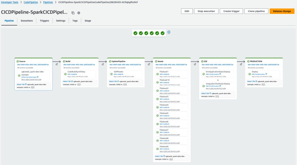

Solve rates section of Turnstile Analytics

Token validations

After a visitor successfully completes a Turnstile challenge, a token is generated that must be validated via the Siteverify API. The API response provides the ultimate outcome of our bot determination. Only rendering the widget on the client side without calling the Siteverify API for token validation is an incomplete implementation of Turnstile, and your site will not be protected. The Turnstile token that is returned from the challenge stage must be validated via the Siteverify API as we check if the token is valid, whether it has been redeemed already (a single token can only be redeemed once), and whether it has expired. 


Token validation section of Turnstile Analytics

Let’s walk through a real world example

Common use cases of Turnstile include protecting login and sign up pages from credential stuffing, account takeover, and fraudulent account creation attacks. Let’s walk through how you can best set up Turnstile on your login pages and interpret your traffic with the new Turnstile analytics. 

You can set up two separate widgets for your login and sign up page, or you can set up one widget and use the ‘action‘ field to distinguish traffic between these pages. The ‘cData’ field can be used to pass along custom data to keep track of each individual attempt. This field is useful to track any pertinent information from your business logic such as account ID, session ID, etc. In this case, let’s assume we are passing along a session ID along with the login attempt. This is helpful if you are trying to protect and monitor against account takeover attacks or credential stuffing attacks. cData is a custom data field that is not stored in Cloudflare systems at any time. 
Rendering the Turnstile widget

To place the Turnstile widget on your login page: 

<script src="https://challenges.cloudflare.com/turnstile/v0/api.js" async defer></script>
<form action="/login" method="POST">
  <div class="cf-turnstile" data-sitekey="your-site-key" data-action="login" data-cdata=”session123”></div>
  <input type="submit" value="Log in">
</form>

To place the Turnstile widget on your signup page: 

<form action="/signup" method="POST">
  <div class="cf-turnstile" data-sitekey="your-site-key" data-action="signup"></div>
  <input type="submit" value="Sign up">
</form>

Validating the Turnstile token with the Siteverify API 

At this point, you have placed the Turnstile widget in your login page. When a visitor visits this page, a Turnstile challenge will be issued and when the visitor completes the challenge, you will receive a Turnstile token that contains the outcome of the challenge. This must be validated via the Siteverify API like below: 

// This is the demo secret key. 
// In production, we recommend you store your secret key(s) safely.
const SECRET_KEY = "1x0000000000000000000000000000000AA";

async function handlePost(request) {
  const body = await request.formData();
  // Turnstile injects a token in "cf-turnstile-response".
  const token = body.get("cf-turnstile-response");
  const ip = request.headers.get("CF-Connecting-IP");

  // Validate the token by calling the
  // "/Siteverify" API endpoint.
  let formData = new FormData();
  formData.append("secret", SECRET_KEY);
  formData.append("response", token);
  formData.append("remoteip", ip);

  const url = "https://challenges.cloudflare.com/turnstile/v0/siteverify";
  const result = await fetch(url, {
    body: formData,
    method: "POST",
  });

  const outcome = await result.json();
  if (outcome.success) {
    // happy path: let the visitor continue with login/signup
  } else {
    // option 1: custom error page directing the visitor to reach out to support
    // option 2: same as happy path but flag as potential bot
  }
}

As you can see in the code example above, you can control the visitor experience based on the Siteverify outcome. In the case where Siteverify API said the token is valid, it’s straightforward — let the visitor continue to log in and sign up. This can be monitored by the Valid tokens metric in the Token validation section in the new Turnstile Analytics. 


Example Invalid Token Siteverify Outcome: 

{
  "success": false,
  "challenge_ts": "2025-02-28T15:14:30.096Z",
  "hostname": "mybusiness.com",
  "error-codes": [],
  "action": "login",
  "cdata": "account123",
  "metadata":{
    "ephemeral_id": "x:9f78e0ed210960d7693b167e"
  }
}

If Siteverify returns "success": false, this means that the token was invalid and Turnstile determined the visitor to be a bot. In this case, you have control over what you want the experience to be, such as redirecting the user to a custom error page where they can reach out to support.  

You can also flag that session (in this case, “session123”) as suspicious and require the account owner to take action. You can implement the UI so that it seems like the bot was successful in logging in to an account, but block any important actions, such as account changes or purchases. Likewise, you can alert the account owner that there has been a suspicious login attempt. 

Turnstile is a building block to help you build out your security defenses, and you can design your logic to fit your priorities across UI, UX, and security. 

Interpreting login page analytics

The very first thing to monitor is the Top Statistics section to look out for any anomalous traffic characteristics in the “countries”, “source ASN”, and “source user agents” metrics. By seeing the traffic distribution, you can have a better understanding of your visitors and potentially spot any anomalies. At this point, you can also take a look at “Source browsers”, “Source OS”, and “Countries” to see if that aligns with your visitor demographics. If you have a list of suspicious IP addresses that you maintain, you can cross-reference them to see their success and failure rates. 


Example TopN Section 

Let’s say you suspect there has been a credential stuffing attack where bots were brute forcing their way into accounts. Below is mock data of what your analytics may look like where the time window is zoomed into the time of the attack. 


Example Challenge outcomes section 

You can see that time period where the number of challenges unsolved started spiking and the “likely bot” metric shot up. This shows an increase in bot traffic, indicating an attack. However, you can also see that Turnstile was able to catch these bots as they were unable to solve or even complete the challenge. 

Let’s look at another example. 


Example Token validation section 

In this case, of the 11.13M tokens issued in the timeframe, 0.01% of them were invalid. This means that 0.01% of the traffic is considered to be non-legitimate visitors, despite the fact that they received the Turnstile tokens.  This is why it is crucial to always validate your tokens through the Siteverify API. What becomes more interesting is if the login credentials these suspicious visitors provided were correct credentials, which could indicate that this is a potential account takeover attack or the accounts in question have been compromised. If the login credentials were incorrect, but the attempts were in a burst, that could indicate credential stuffing attack. By correlating Turnstile analytics with your internal application data such as whether the login attempt had a correct or incorrect password, you can further identify the nature and behavior of the attacker and build out the defenses or mitigate accordingly. 

This was an example showing how Turnstile can protect and provide insights on just your login page. Imagine how this could be expanded to other use cases such as your sign-up pages, submit form pages, contact pages, checkout pages, and more. 

Looking ahead

We are not planning on stopping here with Turnstile Analytics. Next on our roadmap is to expand Turnstile Analytics to give you more insights around client side and server side errors, so that you can further break down the traffic beyond just the challenge outcomes. We will also be incorporating Ephemeral IDs into the analytics, so that you can filter by Ephemeral ID, see top Ephemeral IDs, and the frequency of their solve attempts. 

We have many more exciting things in store for Turnstile for 2025! There is no prerequisite with Turnstile, and our free tier is unlimited in volume, so there is no barrier to get started today. Let’s help make the Internet a more secure, better place, together!