Post Syndicated from Faris Haddad original https://aws.amazon.com/blogs/big-data/the-art-and-science-of-data-product-portfolio-management/

This post is the first in a series dedicated to the art and science of practical data mesh implementation (for an overview of data mesh, read the original whitepaper The data mesh shift). The series attempts to bridge the gap between the tenets of data mesh and its real-life implementation by deep-diving into the functional and non-functional capabilities essential to a working operating model, laying out the decisions that need to be made for each capability, and describing the key business and technical processes required to implement them. Taken together, the posts in this series lay out some possible operating models for data mesh within an organization.

Kudzu

Kudzu—or kuzu (クズ)—is native to Japan and southeast China. First introduced to the southeastern United States in 1876 as a promising solution for erosion control, it now represents a cautionary tale about unintended consequences, as Kudzu’s speed of growth outcompetes everything from native grasses to tree systems by growing over and shading them from the sunlight they need to photosynthesize—eventually leading to species extinction and loss of biodiversity. The story of Kudzu offers a powerful analogy to the dangers and consequences of implementing data mesh architectures without fully understanding or appreciating how they are intended to be used. When the “Kudzu” of unmanaged pseudo-data products (methods of sharing data that masquerade as data products while failing to fulfill the myriad obligations associated with them) has overwhelmed the local ecosystem of true data products, eradication is costly and prone to failure, and can represent significant wasted effort and resources, as well as lost time.

Desert

While Kudzu was taking over the south in the 1930s, desertification caused by extensive deforestation was overwhelming the Midwest, with large tracts of land becoming barren and residents forced to leave and find other places to make a living. In the same way, overly restrictive data governance practices that either prevent data products from taking root at all, or pare them back too aggressively (deforestation), can over time create “data deserts” that drive both the producers and consumers of data within an organization to look elsewhere for their data needs. At the same time, unstructured approaches to data mesh management that don’t have a vision for what types of products should exist and how to ensure they are developed are at high risk of creating the same effect through simple neglect. This is due to a  common misconception about data mesh as a data strategy, which is that it is effectively self-organizing—meaning that once presented with the opportunity, data owners within the organization will spring to the responsibilities and obligations associated with publishing high-quality data products. In reality, the work of a data producer is often thankless, and without clear incentive strategies, organizations may end up with data deserts that create more data governance issues as producers and consumers go elsewhere to seek out the data they need to perform work.

Bonsai

Bonsai (盆栽) is an art form originating from an ancient Chinese tradition called penjing (盆景), and later shaped by the minimalist teachings of Zen Buddhism into the practice we know and recognize today. The patient practice of Bonsai offers useful analogies to the concepts and processes required to avoid the chaos of Kudzu as well as the specter of organizational data deserts. Bonsai artists carefully observe the naturally occurring buds that are produced by the tree and encourage those that add to the overall aesthetics of the tree, while pruning those that don’t work well with their neighbors. The same ideas apply equally well to data products within a data mesh—by encouraging the growth and adoption of those data products that add value to our data mesh, and continuously pruning those that do not, we maximize the value and sustainability of our data mesh implementations. In a similar vein, Bonsai artists must balance their vision for the shape of the tree with a respect for the natural characteristics and innate structure of the species they have chosen to work with—to ignore the biology of the tree would be disastrous to the longevity of the tree, as well as to the quality of the art itself. In the same way, organizations seeking to implement successful data mesh strategies must respect the nature and structure (legal, political, commercial, technology) of their organizations in their implementation.

Of the key capabilities proposed for the implementation of a sustainable data mesh operating model, the one that is most relevant to the problems we’ve described—and explore later in this post—is data product portfolio management.

Overview of data product portfolio management

Data mesh architectures are, by their nature, ideal for implementation within federated organizations, with decentralized ownership of data and clear legal, regulatory, or commercial boundaries between entities or lines of business. The same organizational characteristics that make data mesh architectures valuable, however, also put them at risk of turning into one of the twin nightmares of Kudzu or data deserts.

To define the shape and nature of an organizational data mesh, a number of key questions need to be answered, including but not limited to:

• What are the key data domains within the organization? What are the key data products within these domains needed to solve current business problems? How do we iterate on this discovery process to add value while we are mapping our domains?
• Who are the consumers in our organization, and what logical, regulatory, physical, or commercial boundaries might separate them from producers and their data products?
• How do we encourage the development and maintenance of key data products in a decentralized organization?
• How do we monitor data products against their SLAs, and ensure alerting and escalation on failure so that the organization is protected from bad data?
• How do we enable those we see as being autonomous producers and consumers with the right skills, the right tools, and the right mindset to actually want to (and be able to) take more ownership of independently publishing data as a product and consuming it responsibly?
• What is the lifecycle of a data product? When do new data products get created, and who is allowed to create them? When are data products deprecated, and who is accountable for the consequences to their consumers?
• How do we define “risk” and “value” in the context of data products, and how can we measure this? Whose responsibility is it to justify the existence of a given data product?

To answer questions such as these and plan accordingly, organizations must implement data product portfolio management (DPPM). DPPM does not exist in a vacuum—by its nature, DPPM is closely related to and interdependent with enterprise architecture practices like business capability management and project portfolio management. DPPM itself may therefore also be considered, in part, an enterprise architecture practice.

As an enterprise architecture practice, DPPM is responsible for its implementation, which should reside within a function whose remit is appropriately global and cross-functional. This may be within the CDO office for those organizations that have a CDO or equivalent central data function, or the enterprise architecture team in organizations that do not.

Goals of DPPM

The goals of DPPM can be summarized as follows:

• Protect value – DPPM protects the value of the organizational data strategy by developing, implementing, and enforcing frameworks to measure the contribution of data products to organizational goals in objective terms. Examples may include associated revenue, savings, or reductions in operational losses. Earlier in their lifecycle, data products may be measured by alternative metrics, including adoption (number of consumers) and level of activity (releases, interaction with consumers, and so on). In the pursuit of this goal, the DPPM capability is accountable for engaging with the business to continuously priorities where data as a product can add value and align delivery priority accordingly. Strategies for measuring value and prioritizing data products are explored later in this post.
• Manage risk – All data products introduce risk to the organization—risk of wasted money and effort through non-adoption, risk of operational loss associated with improper use, and risk of failure on the part of the data product to meet requirements on availability, completeness, or quality. These risks are exacerbated in the case of proliferation of low-quality or unsupervised data products. DPPM seeks to understand and measure these risks on an individual and aggregated basis. This is a particularly challenging goal because what constitutes risk associated with the existence of a particular data product is determined largely by its consumers and is likely to change over time (though like entropy, is only ever likely to increase).
• Guide evolution – The final goal of DPPM is to guide the evolution of the data product landscape to meet overarching organizational data goals, such as mutually exclusive or collectively exhaustive domains and data products, the identification and enablement of single-threaded ownership of product definitions, or the agile inclusion of new sources of data and creation of products to serve tactical or strategic business goals. Some principles for the management of data mesh evolution, and the evaluation of data products against organizational goals, are explored later in this post.

Challenges of DPPM

In this section, we explore some of the challenges of DPPM, and the pragmatic ways some of these challenges could be addressed.

Infancy

Data mesh as a concept is still relatively new. As such, there is little standardization associated with practical operating models for building and managing data mesh architectures, and no access to fully fledged out-of-the-box reference operating models, frameworks, or tools to support the practice of DPPM.

Some elements of DPPM are supported in disparate tools (for example, some data catalogs include basic community features that contribute to measuring value), but not in a holistic way. Over time, standardization of the processes associated with DPPM will likely occur as a side-effect of commoditization, driven by the popularity and adoption of new services that take on and automate more of the undifferentiated heavy lifting associated with mesh supervision. In the meantime, however, organizations adopting data mesh architectures are left largely to their own devices around how to operate them effectively.

Resistance

The purest expression of democracy is anarchy, and the more federated an organization is (itself a supporting factor in choosing data mesh architectures), the more resistance may be observed to any forms of centralized governance. This is a challenge for DPPM, because in some way it must come together in one place. Just as the Bonsai artist knows the vision for the entire tree, there must be a cohesive vision for and ability to guide the evolution of a data mesh, no matter how broadly federated and autonomous individual domains or data products might be.

Balancing this with the need to respect the natural shape (and culture) of an organization, however, requires organizations that implement DPPM to think about how to do so in a way that doesn’t conflict with the reality of the organization. This might mean, for example, that DPPM may need to happen at several layers—at minimum within data domains, possibly within lines of business, and then at an enterprise level through appropriate data committees, guilds, or other structures that bring stakeholders together. All of this complicates the processes and collaboration needed to perform DPPM effectively.

Maturity

Data mesh architectures, and therefore DPPM, presume relatively high levels of data maturity within an organization—a clear data strategy, understanding of data ownership and stewardship, principles and policies that govern the use of data, and a moderate-to-high level of education and training around data within the organization. A lack of data maturity within the organization, or a weak or immature enterprise architecture function, will face significant hurdles in the implementation of any data mesh architecture, let alone a strong and useful DPPM practice.

In reality, however, data maturity is not uniform across organizations. Even in seemingly low-maturity organizations, there are often teams who are more mature and have a higher appetite to engage. By leaning into these teams and showing value through them first, then using them as evangelists, organizations can gain maturity while benefitting earlier from the advantages of data mesh strategies.

The following sections explore the implementation of DPPM along the lines of people, process, and technology, as well as describing the key characteristics of data products—scope, value, risk, uniqueness, and fitness—and how they relate to data mesh practices.

People

To implement DPPM effectively, a wide variety of stakeholders in the organization may need to be involved in one capacity or another. The following table suggests some key roles, but it’s up to an individual organization to determine how and if these map to their own roles and functions.

Function	RACI	Role	Responsibility
Senior Leadership	A	Chief Data Officer	Ultimately accountable for organizational data strategy and implementation. Approves changes to DPPM principles and operating model. Acts as chair of, and appoints members to, the data council.
.	R	Data Council**	Stakeholder body representing organizational governance around data strategy. Acts as steering body for the governance of DPPM as a practice (KPI monitoring, maturity assessments, auditing, and so on). Approves changes to guidelines and methodologies. Approves changes to data product portfolio (discussed later in this post). Approves and governs centrally funded and prioritized data product development activities.
Enterprise Architecture	AR	Head of Enterprise Architecture	Responsible for development and enforcement of data strategy. Accountable and responsible for the design and implementation of DPPM as an organizational capability.
.	R	Domain Architect	Responsible for the implementing screening, data product analysis, periodic evaluation, and optimal portfolio selection practices. Responsible for the development of methodologies and their selection criteria.
Legal & Compliance	C	Legal & Compliance Officer	Consults on permissibility of data products with reference to local regulation. Consults on permissibility of data sharing with reference to local regulation or commercial agreements.
.	C	Data Privacy Officer	Consults on permissibility of data use with reference to local data privacy law. Consults on permissibility of cross-entity or border data sharing with reference to data privacy law.
Information Security	RC	Information Security Officer	Consults on maturity assessments (discussed later in this post) for information security-relevant data product capabilities. Approves changes to data product technology architecture. Approves changes to IAM procedures relating to data products.
Business Functions	A	Data Domain Owner	Ultimately accountable for the appropriate use of domain data, as well as its quality and availability. Accountable for domain data products. Approves changes to the domain data model and domain data product portfolio.
c	R	Data Domain Steward	Responsible for implementing data domain responsibilities, including operational (day-to-day) governance of domain data products. Approves use of domain data in new data products, and performs regular (such as yearly) attestation of data products using domain data.
.	A	Data Owner	Ultimately accountable for the appropriate use of owned data (for example, CRM data), as well as its quality and availability.
.	R	Data Steward	Responsible for implementing data responsibilities. Approves use of owned data in new data products, and performs regular (such as yearly) attestation of data products using owned data.
.	AR	Data Product Owner	Accountable and responsible for the design, development, and delivery of data products against their stated SLOs. Contributes to data product analysis and portfolio adjustment practices for own data products.

** The data council typically consists of permanent representatives from each function (data domain owners), enterprise architecture, and the chief data officer or equivalent.

Process

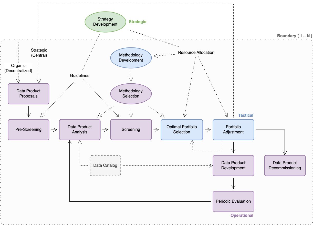
The following diagram illustrates the strategic, tactical, and operational practices associated with DPPM. Some considerations for the implementation of these practices is explored in more detail in this post, though their specific interpretation and implementation is dependent on the individual organization.

Boundaries

When reading this section, it’s important to bear in mind the impact of boundaries—although strategy development may be established as a global practice, other practices within DPPM must respect relevant organizational boundaries (which may be physical, geographical, operational, legal, commercial, or regulatory in nature). In some cases, the existence of boundaries may require some or all tactical and operational practices to be duplicated within each associated boundary. For example, an insurance company with a property and casualty legal entity in North America and a life entity in Germany may need to implement DPPM separately within each entity.

Strategy development

This practice deals with answering questions associated with the overall data mesh strategy, including the following:

• The overall scope (data domains, participating entities, and so on) of the data mesh
• The degree of freedom of participating entities in their definition and implementation of the data mesh (for example, a mesh of meshes vs. a single mesh)
• The distribution of responsibilities for activities and capabilities associated with the data mesh (degree of democratization)
• The definition and documentation of key performance indicators (KPIs) against which the data mesh should be governed (such as risk and value)
• The governance operating model (including this practice)

Key deliverables include the following:

• Organizational guidelines for operational processes around pre-screening and screening of data products
• Well-defined KPIs that guide methodology development and selection for practices like data product analysis, screening, and optimal portfolio selection
• Allocation of organizational resources (people, budget, time) to the implementation of tactical processes around methodology development, optimal portfolio selection, and portfolio adjustment

Key considerations

In this section, we discuss some key considerations for strategy development.

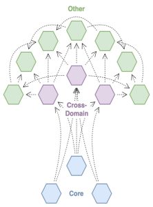
Data mesh structure

This diagram illustrates the analogous relationship between data products in a data mesh, and the structure of the mesh itself.

The following considerations relate to screening, data product analysis, and optimal portfolio selection.

• Trunk (core data products) – Core data products are those that are central to the organization’s ability to function, and from which the majority of other data products are derived. These may be data products consumed in the implementation of key business activities, or associated with critical processes such as regulatory reporting and risk management. Organizational governance for these data products typically favors availability and data accuracy over agility.

• Branch (cross-domain data products) – Cross-domain data products represent the most common cross-domain use cases for data (for example, joining customer data with product data). These data products may be widely used across business functions to support reporting and analytics, and—to a lesser extent—operational processes. Because these data products may consume a variety of sources, organizational governance may favor a balanced view on agility vs. reliability, accepting some degree of risk in return for being able to adapt to changes in data sources. Data product versioning can offer mitigation of risks associated with change.
• Leaf (everything else) – These are the myriad data products that may arise within a data mesh, either as permanent additions to support individual teams and use cases or as temporary data products to fill data gaps or support time-limited initiatives. Because the number of these data products may be high and risks are typically limited to a single process or a small part of the organization, organizational governance typically favors a light touch and may prefer to govern through guidelines and best practices, rather than through active participation in the data product lifecycle.

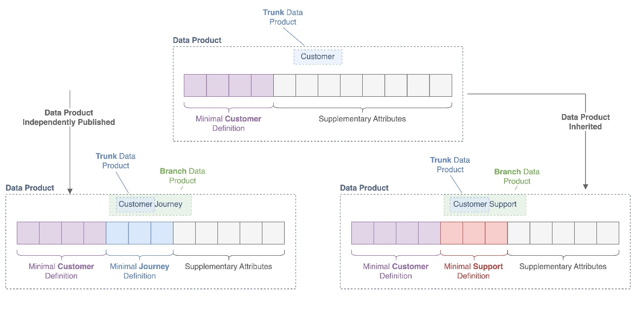
Data products vs. data definitions

The following figure illustrates how data definitions are defined and inherited throughout the lineage of data products.

In a data mesh architecture, data products may inherit data from each other (one data product consumes another in its data pipeline) or independently publish data within (or related to) the same domain. For example, a customer data product may be inherited by a customer support data product, while another the customer journey data product may directly publish customer-relevant data from independent sources. When no standards are applied to how domain data attributes are used and published, data products even within the same data domain may lose interoperability because it becomes difficult or impossible to join them together for reporting or analytics purposes.

To prevent this, it can be useful to distinguish between data products and data definitions. Typically, organizations will select a single-threaded owner (often a data owner or steward, or a domain data owner or steward) who is responsible for defining minimal data definitions for common and reusable data entities within data domains. For example, a data owner responsible for the sales and marketing data domain may identify a customer data product as a reusable data entity within the domain and publish a minimal data definition that all producers of customer-relevant data must incorporate within their data products, to ensure that all data products associated with customer data are interoperable.

DPPM can assist in the identification and production of data definitions as part of its data product analysis activities, as well as enforce their incorporation as part of oversight of data product development.

Service management thinking

These considerations relate to data product analysis, periodic evaluation, and methodology selection.

Data products are services provided to the organization or externally to customers and partners. As such, it may make sense to adapt a service management framework like ITIL, in combination with the ITIL Maturity Model, for use in evaluating the fitness of data products for their scope and audience, as well as in describing the roles, processes, and acceptable technologies that should form the operating model for any data product.

At the operational level, the stakeholders required to implement each practice may change depending on the scope of the data product. For example, the release management practice for a core data product may require involvement of the data council, whereas the same practice for a team data product may only involve the team or functional head. To avoid creating decision-making bottlenecks, organizations should aim to minimize the number of stakeholders in each case and focus on single-threaded owners wherever possible.

The following table proposes a subset of capabilities and how they might be applied to data products of different scopes. Suggested target maturity levels, between 1 and 5, are included for each scope. (1= Initial, 5= Optimizing)

Target Maturity	Data Product Scope.
	4 – 5	3 – 4	2 – 3	2
Capability	Core	Cross-Domain	Function / Team	Personal
Information Security Management	X	X	X	X
Knowledge Management	X	X	X	.
Release Management	X	X	X	.
Service-Level Management	X	X	X	.
Measurement and Reporting	X	X	.	.
Availability Management	X	X	.	.
Capacity and Performance Management	X	X	.	.
Incident Management	X	X	.	.
Monitoring and Event Management	X	X	.	.
Service Validation and Testing	X	X	.	.

Methodology development

This practice deals with the development of concrete, objective frameworks, metrics, and processes for the measurement of data product value and risk. Because the driving factors behind risk and value are not necessarily the same between products, it may be necessary to develop several methodologies or variants thereof.

Key deliverables include the following:

• Well-defined frameworks for measuring risk and value of data products, as well as for determining the optimal portfolio of data products
• Operationally feasible, measurable metrics associated with value and risk

Key considerations

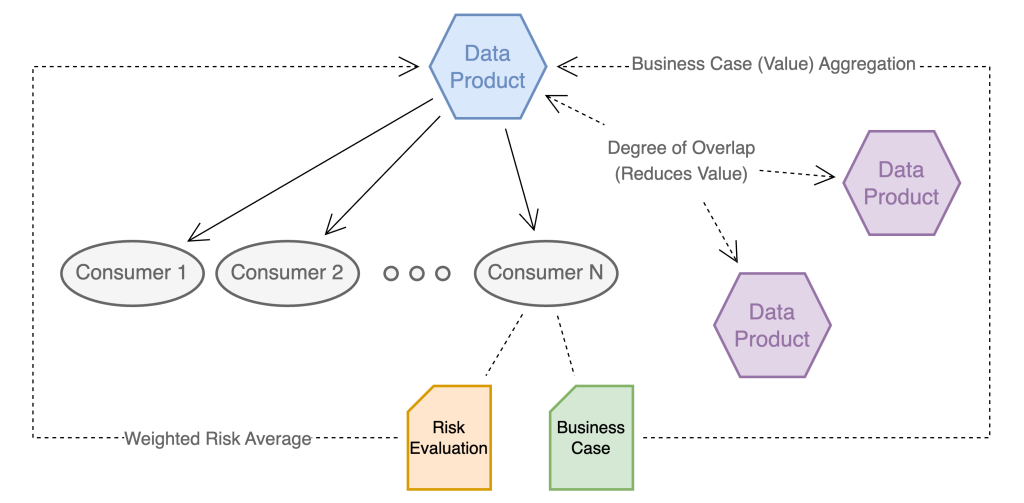
A key consideration for assessing data products is that of consumer value or risk vs. uniqueness. The following diagram illustrates how value and risk of a data product are driven by its consumers.

Data products don’t inherently present risk or add value, but rather indirectly pose—in an aggregated fashion—the risk and value created by their consumers.

In a consumer-centric value and risk model, governance of consumers ensures that all data use meets the following requirements:

• Is associated with a business case justifying the use of data (for example, new business, cost reduction through business process automation, and so on)
• Is regularly evaluated with reference to the risk associated with the use case (for example, regulatory reporting

The value and risk associated with the linked data products are then calculated as an aggregation. Where organizations already track use cases associated with data, either as part of data privacy governance or as a by-product of the access approval process, these existing systems and databases can be reused or extended.

Conversely, where data products overlap with each other, their value to the organization is reduced accordingly, because redundancies between data products represent an inefficient use of resources and increase organizational complexity associated with data quality management.

To ensure that the model is operationally feasible (see the key deliverables of methodology development), it may be sufficient to consider simple aggregations, rather than attempting to calculate value and risk attribution at a product or use case level.

Optimal portfolio selection

This practice deals with the determination of which combination of data products (existing, new, or potential) would best meet the organization’s current and known future needs. This practice takes input from data product analysis and data product proposals, as well as other enterprise architecture practices (for example, business architecture), and considers trade-offs between data-debt and time-to-value, as well as other considerations such as redundancy between data products to determine the optimal mix of permanent and temporary data products at any given point in time.

Because the number of data products in an organization may become significant over time, it may be useful to apply heuristics to the problem of optimal portfolio selection. For example, it may be sufficient to consider core and cross-domain data products (trunk and branches) during quarterly portfolio reviews, with other data products (leaves) audited on a yearly basis.

Key deliverables include the following:

• A target state definition for the data mesh, including all relevant data products
• An indication of organizational priorities for use by the portfolio adjustment practice

Key considerations

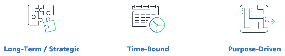
The following are key considerations regarding the data product half-life:

• Long-term or strategic data products – These data products fill a long-term organizational need, are often associated with key source systems in various domains, and anchor the overall data strategy. Over time, as an organization’s data mesh matures, long-term data products should form the bulk of the mesh.
• Time-bound data products – These data products fill a gap in data strategy and allow the organization to move on data opportunities until core data products can be updated. An example of this might be data products created and used in the context of mergers and acquisitions transactions and post-acquisition, to provide consistent data for reporting and business intelligence until mid-term and long-term application consolidation has taken place. Time-bound data products are considered as data-debt and should be managed accordingly.
• Purpose-driven data products – These data products serve a narrow, finite purpose. Purpose-driven data products may or may not be time-bound, but are characterized primarily by a strict set of consumers known in advance. Examples of this might include:
  • Data products developed to support system-of-record harmonization between lines of business (for example, deduplication of customer records between insurance lines of business using separate CRM systems
  • Data products created explicitly for the monitoring of other data products (data quality, update frequency, and so on)

Portfolio adjustment

This practice implements the feasibility analysis, planning and project management, as well as communication and organizational change management activities associated with changes to the optimal portfolio. As part of this practice, a gap analysis is conducted between the current and target data product portfolio, and a set of required actions and estimated time and effort prepared for review by the organization. During such a period, data products may be marked for development (new data products to fill a need), changes, consolidation (merging two or more data products into a single data product), or deprecation. Several iterations of optimal portfolio selection and portfolio adjustment may be required to find an appropriate balance between optimality and feasibility of implementation.

Key deliverables include the following:

• A gap analysis between the current and target data product portfolio, as well as proposed remediation activities
• High-level project plans and effort or budget assessments associated with required changes, for approval by relevant stakeholders (such as the data council)

Data product proposals

This practice organizes the collection and prioritization of requests for new, or changes to existing, data products within the organization. Its implementation may be adapted from or managed by existing demand management processes within the organization.

Key deliverables include a registry of demand against new or existing data products, including metadata on source systems, attributes, known use cases, proposed data product owners, and suggested organizational priority.

Methodology selection

This practice is associated with the identification and application of the most appropriate methodologies (such as value and risk) during data product analysis, screening, and optimal portfolio selection. The selection of an appropriate methodology for the type, maturity, and scope of a data product (or an entire portfolio) is a key element in avoiding either a “Kudzu” mesh or a “data desert.”

Key deliverables include reusable selection criteria for mapping methodologies to data products during data product analysis, screening, and optimal portfolio selection.

Pre-screening

This optional practice is primarily a mechanism to avoid unnecessary time and effort in the comparatively expensive practice of data product analysis by offering simple self-service applications of guidelines to the evaluation of data products. An example might include the automated approval of data products that fall under the classification of personal data products, requiring only attestation on the part of the requester that they will uphold the relevant portions of the guideline that governs such data products.

Key deliverables include tools and checklists for the self-service evaluation of data products against guidelines and automated registration of approved data products.

Data product analysis

This practice incorporates guidelines, methodologies, as well as (where available) metadata relating to data products (performance against SLOs, service management metrics, degree of overlap with other data products) to establish an understanding of the value and risk associated with individual data products, as well as gaps between current and target capability maturities, and compliance with published product definitions and standards.

Key deliverables include a summary of findings for a particular data product, including scores for relevant value, risk, and maturity metrics, as well as operational gaps requiring remediation and recommendations on next steps (repair, enhance, decommission, and so on).

Screening

This optional practice is a mechanism to reduce complexity in optimal portfolio selection by ensuring the early removal of data products from consideration that fail to meet value or risk targets, or have been identified as redundant to other data products already available in the organization.

Key deliverables include a list of data products that should be slated for removal (direct-to-decommissioning).

Data product development

This practice is not performed directly under DPPM, but is managed in part by the portfolio adjustment practice, and may be governed by standards that are developed as part of DPPM. In the context of DPPM, this practice is primarily associated with ensuring that data products are developed according to the specifications agreed as part of portfolio adjustment.

Key deliverables include project management and software or service development deliverables and artefacts.

Data product decommissioning

This practice manages the decommissioning of data products and the migration of affected consumers to new or other data products where relevant. Unmanaged decommissioning of data products, especially those with many downstream consumers, can threaten the stability of the entire data mesh, as well as have significant consequences to business functions.

Key deliverables include a decommissioning plan, including stakeholder assessment and sign-off, timelines, migration plans for affected consumers, and back-out strategies.

Periodic evaluation

This practice manages the calendar and implementation of periodic reviews of the data mesh, both in its entirety as well as at the data product level, and is primarily an exercise in project management.

Key deliverables include the following:

• yearly review calendar, published and made available to all data product owners and affected stakeholders
• Project management deliverables and artefacts, including evidence of evaluations having been performed against each data product

Technology

Although most practices within DPPM don’t rely heavily on technology and automation, some key supporting applications and services are required to implement DPPM effectively:

• Data catalog – Core to the delivery of DPPM is the organizational data catalog. Beyond providing transparency into what data products exist within an organization, a data catalog can provide key insights into data lineage between data products (key to the implementation of portfolio adjustment) and adoption of data products by the organization. The data catalog can also be used to capture and make available both the documented as well as the realized SLO for any given data product, and—through the use of a business glossary—assist in the identification of redundancy between data products.
• Service management – Service management solutions (such as ServiceNOW) used in the context of data product management offer important insights into the fitness of data products by capturing and tracking incidents, problems, requests, and other metrics against data products.
• Demand management – A demand management solution supports self-service implementation and automation of data product proposal and pre-screening activities, as well as prioritization activities associated with selection and development of data products.

Conclusion

Although this post focused on implementing DPPM in the context of a data mesh, this capability—like data product thinking—is not exclusive to data mesh architectures. The practices outlined here can be practiced at any scale to ensure that the production and use of data within the organization is always in line with its current and future needs, that governance is implemented in a consistent way, and that the organization can have Bonsai, not Kudzu.

For more information about data mesh and data management, refer to the following:

• How to unlock the full value of data? Manage it like a product
• The data mesh shift

In upcoming posts, we will cover other aspects of data mesh operating models, including data mesh supervision and service management models for data product owners.

---

About the Authors

Maximilian Mayrhofer is a Principal Solutions Architect working in the AWS Financial Services EMEA Go-to-Market team. He has over 12 years experience in digital transformation within private banking and asset management. In his free time, he is an avid reader of science fiction and enjoys bouldering.

Faris Haddad is the Data & Insights Lead in the AABG Strategic Pursuits team. He helps enterprises successfully become data-driven.