Tag Archives: AWS Glue

Optimize your modern data architecture for sustainability: Part 1 – data ingestion and data lake

2022-11-04 Sam Mokhtari

Post Syndicated from Sam Mokhtari original https://aws.amazon.com/blogs/architecture/optimize-your-modern-data-architecture-for-sustainability-part-1-data-ingestion-and-data-lake/

The modern data architecture on AWS focuses on integrating a data lake and purpose-built data services to efficiently build analytics workloads, which provide speed and agility at scale. Using the right service for the right purpose not only provides performance gains, but facilitates the right utilization of resources. Review Modern Data Analytics Reference Architecture on AWS, see Figure 1.

In this series of two blog posts, we will cover guidance from the Sustainability Pillar of the AWS Well-Architected Framework on optimizing your modern data architecture for sustainability. Sustainability in the cloud is an ongoing effort focused primarily on energy reduction and efficiency across all components of a workload. This will achieve the maximum benefit from the resources provisioned and minimize the total resources required.

Modern data architecture includes five pillars or capabilities: 1) data ingestion, 2) data lake, 3) unified data governance, 4) data movement, and 5) purpose-built analytics. In the first part of this blog series, we will focus on the data ingestion and data lake pillars of modern data architecture. We’ll discuss tips and best practices that can help you minimize resources and improve utilization.

Figure 1. Modern Data Analytics Reference Architecture on AWS

1. Data ingestion

The data ingestion process in modern data architecture can be broadly divided into two main categories: batch, and real-time ingestion modes.

To improve the data ingestion process, see the following best practices:

Avoid unnecessary data ingestion

Work backwards from your business needs and establish the right datasets you’ll need. Evaluate if you can avoid ingesting data from source systems by using existing publicly available datasets in AWS Data Exchange or Open Data on AWS. Using these cleaned and curated datasets will help you to avoid duplicating the compute and storage resources needed to ingest this data.

Reduce the size of data before ingestion

When you design your data ingestion pipelines, use strategies such as compression, filtering, and aggregation to reduce the size of ingested data. This will permit smaller data sizes to be transferred over network and stored in the data lake.

To extract and ingest data from data sources such as databases, use change data capture (CDC) or date range strategies instead of full-extract ingestion. Use AWS Database Migration Service (DMS) transformation rules to selectively include and exclude the tables (from schema) and columns (from wide tables, for example) for ingestion.

Consider event-driven serverless data ingestion

Adopt an event-driven serverless architecture for your data ingestion so it only provisions resources when work needs to be done. For example, when you use AWS Glue jobs and AWS Step Functions for data ingestion and pre-processing, you pass the responsibility and work of infrastructure optimization to AWS.

2. Data lake

Amazon Simple Storage Service (S3) is an object storage service which customers use to store any type of data for different use cases as a foundation for a data lake. To optimize data lakes on Amazon S3, follow these best practices:

Understand data characteristics

Understand the characteristics, requirements, and access patterns of your workload data in order to optimally choose the right storage tier. You can classify your data into categories shown in Figure 2, based on their key characteristics.

Figure 2. Data Characteristics

Adopt sustainable storage options

Based on your workload data characteristics, use the appropriate storage tier to reduce the environmental impact of your workload, as shown in Figure 3.

Figure 3. Storage tiering on Amazon S3

Implement data lifecycle policies aligned with your sustainability goals

Based on your data classification information, you can move data to more energy-efficient storage or safely delete it. Manage the lifecycle of all your data automatically using Amazon S3 Lifecycle policies.

Amazon S3 Storage Lens delivers visibility into storage usage, activity trends, and even makes recommendations for improvements. This information can be used to lower the environmental impact of storing information on S3.

Select efficient file formats and compression algorithms

Use efficient file formats such as Parquet, where a columnar format provides opportunities for flexible compression options and encoding schemes. Parquet also enables more efficient aggregation queries, as you can skip over the non-relevant data. Using an efficient way of storage and accessing data is translated into higher performance with fewer resources.

Compress your data to reduce the storage size. Remember, you will need to trade off compression level (storage saved on disk) against the compute effort required to compress and decompress. Choosing the right compression algorithm can be beneficial as well. For instance, ZStandard (zstd) provides a better compression ratio compared with LZ4 or GZip.

Use data partitioning and bucketing

Partitioning and bucketing divides your data and keeps related data together. This can help reduce the amount of data scanned per query, which means less compute resources needed to service the workload.

Track and assess the improvement for environmental sustainability

The best way for customers to evaluate success in optimizing their workloads for sustainability is to use proxy measures and unit of work KPIs. For storage, this is GB per transaction, and for compute, it would be vCPU minutes per transaction. To use proxy measures to optimize workloads for energy efficiency, read Sustainability Well-Architected Lab on Turning the Cost and Usage Report into Efficiency Reports.

In Table 1, we have listed certain metrics to use as a proxy metric to measure specific improvements. These fall under each pillar of modern data architecture covered in this post. This is not an exhaustive list, you could use numerous other metrics to spot inefficiencies. Remember, just tracking one metric may not explain the impact on sustainability. Use an analytical exercise of combining the metric with data, type of attributes, type of workload, and other characteristics.

Pillar	Metrics
Data ingestion	DMS Replication Instance and Task Metrics – CPUAllocated, CPUUtilization, WriteThroughput, ReadThroughput CloudWatch Metrics – Amazon Kinesis – ReadProvisionedThroughputExceeded, WriteProvisionedThroughputExceeded CloudWatch Metrics – Amazon MSK – BurstBalance, CpuIdle, CpuIoWait, KafkaAppLogsDiskUsed, KafkaDataLogsDiskUsed
Data lake	CloudWatch Metrics for Amazon S3 – BucketSizeBytes

Table 1. Metrics for the Modern data architecture pillars

Conclusion

In this post, we have provided guidance and best practices to help reduce the environmental impact of the data ingestion and data lake pillars of modern data architecture.

In the next post, we will cover best practices for sustainability for the unified governance, data movement, and purpose-built analytics and insights pillars.

Further reading:

To learn more, check out the Sustainability Pillar of the AWS Well-Architected Framework and other blog posts on architecting for sustainability.
For more architecture content, refer to AWS Architecture Center for reference architecture diagrams, vetted architecture solutions, Well-Architected best practices, patterns, icons, and more.

Doing data preparation using on-premises PostgreSQL databases with AWS Glue DataBrew

2022-10-21 John Espenhahn

Post Syndicated from John Espenhahn original https://aws.amazon.com/blogs/big-data/doing-data-preparation-using-on-premises-postgresql-databases-with-aws-glue-databrew/

Today, with AWS Glue DataBrew, data analysts and data scientists can easily access and visually explore any amount of data across their organization directly from their Amazon Simple Storage Service (Amazon S3) data lake, Amazon Redshift data warehouse, and Amazon Aurora and Amazon Relational Database Service (Amazon RDS) databases. Customers can choose from over 250 built-in functions to combine, pivot, and transpose the data without writing code.

Now, with added support for JDBC-accessible databases, DataBrew also supports additional data stores including PostgreSQL, MySQL, Oracle, and Microsoft SQL Server. In this blog post, we will be using DataBrew to clean data from an on-premise database, and storing the cleaned data in an Amazon S3 data lake.

Solution Overview

I will be configuring an existing subnet in an Amazon VPC for use with DataBrew. Then configuring DataBrew to securely connect to an existing on-premise database and executing a data preparation job.

Components

You should have an AWS account with a Virtual Private Cloud (Amazon VPC). DataBrew will connect to your database from this VPC.
You should have a subnet within your Amazon VPC. In this blog, this subnet will be configured for use with DataBrew.
You should have an on-premise database with data to be cleaned with DataBrew.
I assume you have a VPN connection between your Amazon VPC and on premise network to enable secure connections between them. I’ve implemented a VPN tunnel using AWS Site-to-Site VPN. You may choose to Simulate Site-to-Site VPN Customer Gateways Using strongSwan.
This guide will walk through creation of a DataBrew dataset, project, and job.
DataBrew requires access to Amazon S3 and AWS Glue. This guide will walk through creating VPC endpoints to enable private connections between your VPC and these AWS services for DataBrew to use.
To establish network connectivity, DataBrew will provision an Amazon VPC elastic network interface in the VPC you specify. This blog will cover securing this network interface with a security group.

Prerequisites

To complete this blog, you should have the following prerequisites:

An AWS account
A Virtual Private Cloud (Amazon VPC) and subnet
An on-premise network and database
A VPN connection between your Amazon VPC and on premise network

Additionally, you will need to have enabled access to your on-premise network from the subnet in the Amazon VPC. If you haven’t enabled it already, you can Simulate Site-to-Site VPN Customer Gateways Using strongSwan, or you can enable access by completing the AWS Site-to-Site VPN getting started guide.

If you are unsure if you have enabled access from your VPC subnet to your on-premise database, you can test access by running the AWS Systems Manager automation AWSSupport-SetupIPMonitoringFromVPC. From the User Guide, choose Run this Automation. In the Systems Manager console, under Input Parameters, you will need to enter the Amazon VPC subnet ID for SubnetId and the IP address of your on-premise host for TargetIPs. Then choose Execute. Once the automation completes, locate the Outputs section and open the URL linked under createCloudWatchDashboard.Output. From that dashboard, confirm from the Ping log group that pings are successful. If they are not, you will need to investigate. A useful resource for this is How do I troubleshoot instance connection timeout errors in Amazon VPC.

Step 1: Configure the Amazon VPC

Ensure your Amazon VPC has DNS Support and DNS Hostnames enabled. You can verify this by selecting your VPC in the Amazon VPC console and checking the details for DNS hostnames and DNS resolution. If they are disabled, they can be enabled by choosing Actions then the corresponding Edit option.

On-premise or hybrid DNS are also supported, but requires additional setup. See Other Considerations at the end of this post for more.

Step 2: Configure the Amazon VPC Subnet

Your subnet must have access to Amazon S3 and AWS Glue services. I will add VPC endpoints for Amazon S3 and AWS Glue services to keep my traffic within the AWS network.

To add the VPC endpoint for Amazon S3, open the Amazon VPC console at https://console.aws.amazon.com/vpc/.
In the navigation pane, choose Endpoints, Create Endpoint.
Filter by “s3”.
Choose the service where the Type column indicates Gateway.
Select the route tables associated with the subnet to be used with DataBrew.
Choose Create endpoint.
To add the VPC endpoint for AWS Glue, again choose Create Endpoint.
Filter by “glue”.
Choose the service where the Type column indicates Interface.
Select the route tables associated with the subnet to be used with DataBrew.
Choose Create endpoint.

Step 3 : Configure Network ACL

By default Network ACLs allow all inbound and outbound traffic. If you have customized your network ACL, ensure inbound return traffic from and outbound traffic to your on-premise network, Amazon S3, and AWS Glue are allowed.

From the Amazon VPC console, choose Subnets.
Choose the subnet you are using with DataBrew.
From the Details tab, choose the Network ACL link.
Validate your inbound and outbound rules, updating your rules to allow the required traffic if needed. The screenshot below shows the default rules I am using.

Step 4: Configure the VPC security group

To provide connectivity to your VPC, DataBrew will create an Elastic Network Interface (ENI) in the VPC subnet you specify. DataBrew attaches the security group you specify to the ENI to limit network access. This security group must have a self-referential rule to allow all inbound TCP traffic from itself. This will block access from unspecified sources. I will be using the default security group, which has the following configuration.

Your security group must allow outbound traffic to itself, Amazon S3, AWS Glue, and your on-premise network. I’ll be using the default security group, which allows all outbound traffic.

Optionally, you may wish to explicitly restrict outbound traffic to only your on-premise network, Amazon S3, and AWS Glue. To do so, remove the All TPC outbound rule. Ensure your security group has a self-referential rule to allow all outbound TCP traffic to itself. Allow traffic to your on-premise network by specifying the CIDR block associated with your network. In my case, it is 10.196.0.0/16. Allow traffic to Amazon S3 with the AWS-managed S3 prefix list, which includes the set of CIDR blocks for Amazon S3. Allow traffic to the AWS Glue VPC endpoint by associating the same security group with the AWS Glue VPC endpoint created above from the Amazon VPC console.

An example of what these scoped-down outbound rules may look like:

Ensure your on-premise network security rules allow traffic from your Amazon VPC subnet’s CIDR block.

Step 5 : Create database credentials

Following best practices, I will be creating a database user with scoped down permissions for use with DataBrew.

Connect to your database. In my case with psql -h 10.196.0.20

Create a user, which I’ll call postgresql, with readonly access to the table that will be used with DataBrew. My table is called demo in database postgres. I’ll do this by executing the following queries:

CREATE USER postgresql WITH PASSWORD ‘****’;
GRANT CONNECT ON DATABASE postgres TO postgresql;
GRANT USAGE ON SCHEMA public TO postgresql;
REVOKE CREATE ON SCHEMA public FROM postgresql;
GRANT SELECT ON demo TO postgresql;

Step 6 : Create DataBrew project

From the AWS DataBrew console, choose Create project.
Enter a Project name.
Under Select a dataset choose New dataset.
Enter a Dataset name.
Under Connect to new dataset choose JDBC.
Choose Add JDBC connection.
Enter a Connection name, I use my-connection.
Choose Enter JDBC details.
Choose Database type, in my case PostgreSQL.
For Host/endpoint, enter your host’s private IP address.
Enter your Database name, Database user, and Database password.
Choose your VPC, and the Subnet and Security Group you configured above.
Review “Additional configurations”, where you can optionally configure the following:
1. If you are using a recent database version, such as MySQL 8, you may need to provide a custom JDBC driver. For more information, see the Developer Guide.
2. DataBrew can be set to fail the connection to your database if it is unable to connect over SSL. Additionally, DataBrew provides default certificates for establishing SSL connections. If you obtained a certificate from a third-party issuer, or the default certificates provided by DataBrew do not meet your requirements, you can provide your own. DataBrew handles only X.509 certificates. The certificate must be DER-encoded and supplied in base64 encoding PEM format.
Choose Create connection at the bottom of the modal.
Choose the newly created connection by clicking on its name.
Enter the name of the table within your database you want to bring into DataBrew.
Under the Permissions header, choose Create new IAM role from the dropdown and enter a role suffix.
Choose Create project, this will open the project view. After one to two minutes you will be able to work with your data. If the connection fails, see How do I troubleshoot instance connection timeout errors in Amazon VPC.
Start by applying some simple transforms, I’m dropping some columns that are not needed in my data lake. To do so, from the action bar I choose COLUMN, then Delete.
This opens the side-bar where I choose the column to delete, and choose Apply.

Step 7 : Create DataBrew job

Once I’ve got a few transforms added to my project’s recipe, I will run a job to execute the recipe against my full dataset, and store the result in my Amazon S3 bucket.

Choose Create job from the top of the project grid view.
On the job page, provide a Job name and S3 output location.
Under the header Permissions, choose Create new IAM role. This will create a new scoped down IAM role with the permissions required to execute your job.
Finally, choose Create and run job. Once the job completes, you can view the output in Amazon S3.

Cleanup

From the DataBrew console, delete your Job, Project, Recipe, and Dataset.

If you executed the Systems Manager automation to test access, under the Systems Manager console, choose CloudWatch Dashboard. Select the dashboard created by the automation. Choose Terminate test. Then choose Execute.

Other considerations

AWS Glue DataBrew’s networking requirements are similar to that of AWS Glue ETL jobs. Below summarizes some of those advanced networking conditions. For more details on AWS Glue ETL, see How to access and analyze on-premises data stores using AWS Glue by Rajeev Meharwal.

DNS

If you are using AWS VPC provided DNS, ensure you have enabled DnsHostnames and DnsSupport for your VPC. For more information, see DNS support in your VPC.

If you have configured a custom DNS server with your AWS VPC, you must implement forward and reverse lookups for Amazon EC2 private DNS hostnames. For more information, see Amazon DNS server. Alternatively, setup hybrid DNS resolution to resolve both on-premise DNS servers and the VPC provided DNS. For implementation details, see the following AWS Security Blog posts:

Joining or unioning multiple databases

If you are joining a database dataset into your project, the database must be accessible from the project dataset’s subnet.

For example, if you have completed the setup above using Private Subnet 1, and you have another Amazon RDS database in Private Subnet 2 in the same VPC, as shown below. You will want a local route for the route table associated with Subnet 1. You will also need to ensure the security group attached to your Amazon RDS database allows inbound traffic from your DataBrew security group.

If your Amazon RDS database is in a different AWS VPC than you are using with DataBrew, you will need to setup VPC peering.

About the Authors

John Espenhahn is a Software Engineer working on AWS Glue DataBrew service. He has also worked on Amazon Kendra user experience as a part of Database, Analytics & AI AWS consoles. He is passionate about technology and building in the analytics space.

Nitya Sheth is a Software Engineer working on AWS Glue DataBrew service. He has also worked on AWS Synthetics service as well as on user experience implementations for Database, Analytics & AI AWS consoles. In his free time, he divides his time between exploring new hiking places and new books.

Simplify semi-structured nested JSON data analysis with AWS Glue DataBrew and Amazon QuickSight

2022-10-20 Sriharsh Adari

Post Syndicated from Sriharsh Adari original https://aws.amazon.com/blogs/big-data/simplify-semi-structured-nested-json-data-analysis-with-aws-glue-databrew-and-amazon-quicksight/

As the industry grows with more data volume, big data analytics is becoming a common requirement in data analytics and machine learning (ML) use cases. Data comes from many different sources in structured, semi-structured, and unstructured formats. For semi-structured data, one of the most common lightweight file formats is JSON. However, due to the complex nature of data, JSON often includes nested key-value structures. Analysts may want a simpler graphical user interface to conduct data analysis and profiling.

To support these requirements, AWS Glue DataBrew offers an easy visual data preparation tool with over 350 pre-built transformations. You can use DataBrew to analyze complex nested JSON files that would otherwise require days or weeks writing hand-coded transformations. You can then use Amazon QuickSight for data analysis and visualization.

In this post, we demonstrate how to configure DataBrew to work with nested JSON objects and use QuickSight for data visualization.

Solution overview

To implement our solution, we create a DataBrew project and DataBrew job for unnesting data. We profile the unested data in DataBrew and analyze data in QuickSight. The following diagram illustrates the architecture of this solution.

Prerequisites

Before you get started, make sure you have the following prerequisites:

An AWS account
A basic understanding of Amazon Simple Storage Service (Amazon S3)
A basic understanding of QuickSight to create dashboards
Permissions to create the DataBrew dataset, project, and jobs; S3 buckets; and QuickSight dashboards
An AWS Identity and Access Management (IAM) role that DataBrew can use or permission to create a new IAM role (see Adding and removing IAM identity permissions for more information)

Prepare the data

To illustrate the DataBrew functionality to support data analysis for nested JSON files, we use a publicly available sample customer order details nested JSON dataset.

Complete the following steps to prepare your data:

Sign in to the AWS Management Console.
Browse to the publicly available datasets on the Amazon S3 console.
Select the first dataset (customer_1.json) and choose Download to save the files on your local machine.
Repeat this step to download all three JSON files.

You can view the sample data from your local machine using any text editor, as shown in the following screenshot.
Create input and output S3 buckets with subfolders nestedjson and outputjson to capture data.
Choose Upload and upload the three JSON files to the nestedjson folder.

Create a DataBrew project

To create your Amazon S3 connection, complete the following steps:

On the DataBrew console, choose Projects in the navigation pane.
Choose Create project.
For Project name, enter Glue-DataBew-NestedJSON-Blog.
Select New dataset.
For Dataset name, enter Glue-DataBew-NestedJSON-Dataset.
For Enter your source from S3, enter the path to the nestedjson folder.
Choose Select the entire folder to select all the files.
Under Additional configurations, select JSON as the file type, then select JSON document.
In the Permissions section, choose Choose existing IAM role if you have one available, or choose Create new IAM role.
Choose Create project.
Skip the preview steps and wait for the project to be ready.
As shown in the following screenshot, the three JSON files were uploaded to the S3 bucket, so three rows of customer order details are loaded.
The orders column contains nested files. We can use DataBrew to unnest or nest transform to flatten the columns and rows.
Choose the menu icon (three dots) and choose Nest-unnest.
Depending on the nesting, either choose Unnest to columns or Unnest to rows. In this blog post, we choose Unnest to columns to flatten example JSON file.

Repeat this step until you get a flattened json for all the nested json data and this will create the AWS Glue Databrew recipe as shown below.
Choose Apply.

DataBrew automatically creates the required recipe steps with updated column values.
Choose Create job.
For Job name, enter Glue-DataBew-NestedJSON-job.
For S3 location, enter the path to the outputjson folder.
In the Permissions section, for Role name, choose the role you created earlier.
Choose Create and run job.

On the Jobs page, you can choose the job to view its run history, details, and data lineage.

Profile the metadata with DataBrew

After you have a flattened file in the S3 output bucket, you can use DataBrew to carry out the data analysis and profiling for the flattened file. Complete the following steps:

On the Datasets page, choose Connect new datasets.
Provide your dataset details and choose Create dataset.
Choose the newly added data source, then choose the Data profile overview tab.
Enter the name of the job and the S3 path to save the output.
Choose Create and run job.

The job takes around two minutes to complete and display all the updated information. You can explore the data further on the Data profile overview and Column statistics tabs.

Visualize the data in QuickSight

After you have the output file generated by DataBrew in the S3 output bucket, you can use QuickSight to query the JSON data. QuickSight is a scalable, serverless, embeddable, ML-powered business intelligence (BI) service built for the cloud. QuickSight lets you easily create and publish interactive BI dashboards that include ML-powered insights. QuickSight dashboards can be accessed from any device, and seamlessly embedded into your applications, portals, and websites.

Launch QuickSight

On the console, enter quicksight into the search bar and choose QuickSight.

You’re presented with the QuickSight welcome page. If you haven’t signed up for QuickSight, you may have to complete the signup wizard. For more information, refer to Signing up for an Amazon QuickSight subscription.

After you have signed up, QuickSight presents a “Welcome wizard.” You can view the short tutorial, or you can close it.

Grant Amazon S3 access

To grant Amazon S3 access, complete the following steps:

On the QuickSight console, choose your user name, choose Manage QuickSight, then choose Security & permissions.
Choose Add or remove.
Locate Amazon S3 in the list. Choose one of the following:
1. If the check box is clear, select Amazon S3.
2. If the check box is already selected, choose Details, then choose Select S3 buckets.
Choose the buckets that you want to access from QuickSight, then choose Select.
Choose Update.
If you changed your Region during the first step of this process, change it back to the Region that you want to use.

Create a dataset

Now that you have QuickSight up and running, you can create your dataset. Complete the following steps:

On the QuickSight console, choose Datasets in the navigation pane.
Choose New dataset.

QuickSight supports several data sources. For a complete list, refer to Supported data sources.
For your data source, choose S3.

The S3 import requires a data source name and a manifest file.
On your machine, use a text editor to create a manifest file called BlogGlueDataBrew.manifest using the following structure (provide the name of the your output bucket):
```
{
    "fileLocations": [
        {
            "URIPrefixes": [
            "https://s3.amazonaws.com/ s3://<output bucket>/outputjson/"
            ]
        }
    ],
    "globalUploadSettings": {
        "format": "CSV",
        "delimiter": ","
    }
}
```
The manifest file points to the folder that you created earlier as part of your DataBrew project. For more information, refer to Supported formats for Amazon S3 manifest files.
Select Upload and navigate to the manifest file to upload it.
Choose Connect to upload data into SPICE, which is an in-memory database built into QuickSight to achieve fast performance.
Choose Visualize.

You can now create visuals by adding different fields.

To learn more about authoring dashboards in QuickSight, check out the QuickSight Author Workshop.

Clean up

Complete the following steps to avoid incurring future charges:

On the DataBrew console, choose Projects in the navigation pane.
Select the project you created and on the Actions menu, choose Delete.
Choose Jobs in the navigation pane.
Select the job you created and on the Actions menu, choose Delete.
Choose Recipes in the navigation pane.
Select the recipe you created and on the Actions menu, choose Delete.
On the QuickSight dashboard, choose your user name on the application bar, then choose Manage QuickSight.
Choose Account settings, then choose Delete account.
Choose Delete account.
Enter confirm and choose Delete account.

Conclusion

This post walked you through the steps to configure DataBrew to work with nested JSON objects and use QuickSight for data visualization. We used Glue DataBrew to unnest our JSON file and profile the data, and then used QuickSight to create dashboards and visualizations for further analysis.

You can use this solution for your own use cases when you need to unnest complex semi-structured JSON files without writing code. If you have comments or feedback, please leave them in the comments section.

About the authors

Sriharsh Adari is a Senior Solutions Architect at Amazon Web Services (AWS), where he helps customers work backwards from business outcomes to develop innovative solutions on AWS. Over the years, he has helped multiple customers on data platform transformations across industry verticals. His core area of expertise include Technology Strategy, Data Analytics, and Data Science. In his spare time, he enjoys playing sports, binge-watching TV shows, and playing Tabla.

Rahul Sonawane is a Principal Analytics Solutions Architect at AWS with AI/ML and Analytics as his area of specialty.

Amogh Gaikwad is a Solutions Developer at Amazon Web Services. He helps global customers build and deploy AI/ML solutions. His work is mainly focused on computer vision, and NLP uses-cases and helping customers optimize their AI/ML workloads for sustainability. Amogh has received his master’s in Computer Science specializing in Machine Learning.

Get started with Apache Hudi using AWS Glue by implementing key design concepts – Part 1

2022-10-17 Amit Maindola

Post Syndicated from Amit Maindola original https://aws.amazon.com/blogs/big-data/part-1-get-started-with-apache-hudi-using-aws-glue-by-implementing-key-design-concepts/

Many organizations build data lakes on Amazon Simple Storage Service (Amazon S3) using a modern architecture for a scalable and cost-effective solution. Open-source storage formats like Parquet and Avro are commonly used, and data is stored in these formats as immutable files. As the data lake is expanded to additional use cases, there are still some use cases that are very difficult with data lakes, such as CDC (change data capture), time travel (querying point-in-time data), privacy regulation requiring deletion of data, concurrent writes, and consistency regarding handling small file problems.

Apache Hudi is an open-source transactional data lake framework that greatly simplifies incremental data processing and streaming data ingestion. However, organizations new to data lakes may struggle to adopt Apache Hudi due to unfamiliarity with the technology and lack of internal expertise.

In this post, we show how to get started with Apache Hudi, focusing on the Hudi CoW (Copy on Write) table type on AWS using AWS Glue, and implementing key design concepts for different use cases. We expect readers to have a basic understanding of data lakes, AWS Glue, and Amazon S3. We walk you through common batch data ingestion use cases with actual test results using a TPC-DS dataset to show how the design decisions can influence the outcome.

Apache Hudi key concepts

Before diving deep into the design concepts, let’s review the key concepts of Apache Hudi, which is important to understand before you make design decisions.

Hudi table and query types

Hudi supports two table types: Copy on Write (CoW) and Merge on Read (MoR). You have to choose the table type in advance, which influences the performance of read and write operations.

The difference in performance depends on the volume of data, operations, file size, and other factors. For more information, refer to Table & Query Types.

When you use the CoW table type, committed data is implicitly compacted, meaning it’s updated to columnar file format during write operation. With the MoR table type, data isn’t compacted with every commit. As a result, for the MoR table type, compacted data lives in columnar storage (Parquet) and deltas are stored in a log (Avro) raw format until compaction merges changes the data to columnar file format. Hudi supports snapshot, incremental, and read-optimized queries for Hudi tables, and the output of the result depends on the query type.

Indexing

Indexing is another key concept for the design. Hudi provides efficient upserts and deletes with fast indexing for both CoW and MoR tables. For CoW tables, indexing enables fast upsert and delete operations by avoiding the need to join against the entire dataset to determine which files to rewrite. For MoR, this design allows Hudi to bound the amount of records any given base file needs to be merged against. Specifically, a given base file needs to be merged only against updates for records that are part of that base file. In contrast, designs without an indexing component could end up having to merge all the base files against all incoming update and delete records.

Solution overview

The following diagram describes the high-level architecture for our solution. We ingest the TPC-DS (store_sales) dataset from the source S3 bucket in CSV format and write it to the target S3 bucket using AWS Glue in Hudi format. We can query the Hudi tables on Amazon S3 using Amazon Athena and AWS Glue Studio Notebooks.

The following diagram illustrates the relationships between our tables.

For our post, we use the following tables from the TPC-DS dataset: one fact table, store_sales, and the dimension tables store, item, and date_dim. The following table summarizes the table row counts.

Table	Approximate Row Counts
store_sales	2.8 billion
store	1,000
item	300,000
date_dim	73,000

Set up the environment

After you sign in to your test AWS account, launch the provided AWS CloudFormation template by choosing Launch Stack:

This template configures the following resources:

AWS Glue jobs hudi_bulk_insert, hudi_upsert_cow, and hudi_bulk_insert_dim. We use these jobs for the use cases covered in this post.
An S3 bucket to store the output of the AWS Glue job runs.
AWS Identity and Access Management (IAM) roles and policies with appropriate permissions.

Before you run the AWS Glue jobs, you need to subscribe to the AWS Glue Apache Hudi Connector (latest version: 0.10.1). The connector is available on AWS Marketplace. Follow the connector installation and activation process from the AWS Marketplace link, or refer to Process Apache Hudi, Delta Lake, Apache Iceberg datasets at scale, part 1: AWS Glue Studio Notebook to set it up.

After you create the Hudi connection, add the connector name to all the AWS Glue scripts under Advanced properties.

Bulk insert job

To run the bulk insert job, choose the job hudi_bulk_insert on the AWS Glue console.

The job parameters as shown in the following screenshot are added as part of the CloudFormation stack setup. You can use different values to create CoW partitioned tables with different bulk insert options.

The parameters are as follows:

HUDI_DB_NAME – The database in the AWS Glue Data Catalog where the catalog table is created.
HUDI_INIT_SORT_OPTION – The options for bulk_insert include GLOBAL_SORT, which is the default. Other options include NONE and PARTITION_SORT.
HUDI_TABLE_NAME – The table name prefix that you want to use to identify the table created. In the code, we append the sort option to the name you specify in this parameter.
OUTPUT_BUCKET – The S3 bucket created through the CloudFormation stack where the Hudi table datasets are written. The bucket name format is <account number><bucket name>. The bucket name is the one given while creating the CloudFormation stack.
CATEGORY_ID – The default for this parameter is ALL, which processes categories of test data in a single AWS Glue job. To test the parallel on the same table, change the parameter value to one of categories from 3, 5, or 8 for the dataset that we use for each parallel AWS Glue job.

Upsert job for the CoW table

To run the upsert job, choose the job hudi_upsert_cow on the AWS Glue console.

The following job parameters are added as part of the CloudFormation stack setup. You can run upsert and delete operations on CoW partitioned tables with different bulk insert options based on the values provided for these parameters.

OUTPUT-BUCKET – The same value as the previous job parameter.
HUDI_TABLE_NAME – The name of the table created in your AWS Glue Data Catalog.
HUDI_DB_NAME – The same value as the previous job parameter. The default value is Default.

Bulk insert job for the Dimension tables

To test the queries on the CoW tables, the fact table that is created using the bulk insert operation needs supplemental dimensional tables. This AWS Glue job has to be run before you can test the TPC queries provided later in this post. To run this job, choose hudi_bulk_insert_dim on the AWS Glue console and use the parameters shown in the following screenshot.

The parameters are as follows:

OUTPUT-BUCKET – The same value as the previous job parameter.
HUDI_INIT_SORT_OPTION – The options for bulk_insert include GLOBAL_SORT, which is the default. Other available options are NONE and PARTITION_SORT.
HUDI_DB_NAME – The Hudi database name. Default is the default value.

Hudi design considerations

In this section, we walk you through a few use cases to demonstrate the difference in the outcome for different settings and operations.

Data migration use case

In Apache Hudi, you ingest the data into CoW or MoR tables types using either insert, upsert, or bulk insert operations. Data migration initiatives often involve one-time initial loads into the target datastore, and we recommend using the bulk insert operation for initial loads.

The bulk insert option provides the same semantics as insert, while implementing a sort-based data writing algorithm, which can scale very well for several hundred TBs of initial load. However, this just does a best-effort job at sizing files vs. guaranteeing file sizes like inserts and upserts do. Also, the primary keys aren’t sorted during the insert, therefore it’s not advised to use insert during the initial data load. By default, a Bloom index is created for the table, which enables faster lookups for upsert and delete operations.

Bulk insert has the following three sort options, which have different outcomes.

GLOAL_SORT – Sorts the record key for the entire dataset before writing.
PARTITION_SORT – Applies only to partitioned tables. In this option, the record key is sorted within each partition, and the insert time is faster than the default sort.
NONE – Doesn’t sort data before writing.

For testing the bulk insert with the three sort options, we use the following AWS Glue job configuration, which is part of the script hudi_bulk_insert:

AWS Glue version: 3.0
AWS Glue worker type: G1.X
Number of AWS Glue workers: 200
Input file: TPC-DS/2.13/1TB/store_sales
Input file format: CSV (TPC-DS)
Number of input files: 1,431
Number of rows in the input dataset: Approximately 2.8 billion

The following charts illustrate the behavior of the bulk insert operations with GLOBAL_SORT, PARTITION_SORT, and NONE as sort options for a CoW table. The statistics in the charts are created by using an average of 10 bulk insert operation runs for each sort option.

Because bulk insert does a best-effort job to pack the data in files, you see a different number of files created with different sort options.

We can observe the following:

Bulk insert with GLOBAL_SORT has the least number of files, because Hudi tried to create the optimal sized files. However, it takes the most time.
Bulk insert with NONE as the sort option has the fastest write time, but resulted in a greater number of files.
Bulk insert with PARTITION_SORT also has a faster write time compared to GLOBAL SORT, but also results in a greater number of files.

Based on these results, although GLOBAL_SORT takes more time to ingest the data, it creates a smaller number of files, which has better upsert and read performance.

The following diagrams illustrate the Spark run plans for the bulk_insert operation using various sort options.

The first shows the Spark run plan for bulk_insert when the sort option is PARTITION_SORT.

The next is the Spark run plan for bulk_insert when the sort option is NONE.

The last is the Spark run plan for bulk_insert when the sort option is GLOBAL_SORT.

The Spark run plan for bulk_insert with GLOBAL_SORT involves shuffling of data to create optimal sized files. For the other two sort options, data shuffling isn’t involved. As a result, bulk_insert with GLOBAL_SORT takes more time compared to the other sort options.

To test the bulk insert with various bulk insert sort data options on a partitioned table, modify the Hudi AWS Glue job (hudi_bulk_insert) parameter --HUDI_INIT_SORT_OPTION.

We change the parameter --HUDI_INIT_SORT_OPTION to PARTITION_SORT or NONE to test the bulk insert with different data sort options. You need to run the job hudi_bulk_insert_dim, which loads the rest of the tables needed to test the SQL queries.

Now, look at the query performance difference between these three options. For query runtime, we ran two TPC-DS queries (q52.sql and q53.sql, as shown in the following query snippets) using interactive session with AWS Glue Studio Notebook with the following notebook configuration to compare the results.

AWS Glue version: 3.0
AWS Glue worker type: G1.X
Number of AWS Glue workers: 50

Before executing the following queries, replace the table names in the queries with the tables you generate in your account.
q52

SELECT
  dt.d_year,
  item.i_brand_id brand_id,
  item.i_brand brand,
  sum(ss_ext_sales_price) ext_price
FROM date_dim dt, store_sales, item
WHERE dt.d_date_sk = store_sales.ss_sold_date_sk
  AND store_sales.ss_item_sk = item.i_item_sk
  AND item.i_manager_id = 1
  AND dt.d_moy = 11
  AND dt.d_year = 2000
GROUP BY dt.d_year, item.i_brand, item.i_brand_id
ORDER BY dt.d_year, ext_price DESC, brand_id
LIMIT 100

SELECT *
FROM
  (SELECT
    i_manufact_id,
    sum(ss_sales_price) sum_sales,
    avg(sum(ss_sales_price))
    OVER (PARTITION BY i_manufact_id) avg_quarterly_sales
  FROM item, store_sales, date_dim, store
  WHERE ss_item_sk = i_item_sk AND
    ss_sold_date_sk = d_date_sk AND
    ss_store_sk = s_store_sk AND
    d_month_seq IN (1200, 1200 + 1, 1200 + 2, 1200 + 3, 1200 + 4, 1200 + 5, 1200 + 6,
                          1200 + 7, 1200 + 8, 1200 + 9, 1200 + 10, 1200 + 11) AND
    ((i_category IN ('Books', 'Children', 'Electronics') AND

As you can see in the following chart, the performance of the GLOBAL_SORT table outperforms NONE and PARTITION_SORT due to a smaller number of files created in the bulk insert operation.

Ongoing replication use case

For ongoing replication, updates and deletes usually come from transactional databases. As you saw in the previous section, the bulk operation with GLOBAL_SORT took the most time and the operation with NONE took the least time. When you anticipate a higher volume of updates and deletes on an ongoing basis, the sort option is critical for your write performance.

To illustrate the ongoing replication using Apache Hudi upsert and delete operations, we tested using the following configuration:

AWS Glue version: 3.0
AWS Glue worker type: G1.X
Number of AWS Glue workers: 100

To test the upsert and delete operations, we use the store_sales CoW table, which was created using the bulk insert operation in the previous section with all three sort options. We make the following changes:

Insert data into a new partition (month 1 and year 2004) using the existing data from month 1 of year 2002 with a new primary key; total of 32,164,890 records
Update the ss_list_price column by $1 for the existing partition (month 1 and year 2003); total of 5,997,571 records
Delete month 5 data for year 2001; total of 26,997,957 records

The following chart illustrates the runtimes for the upsert operation for the CoW table with different sort options used during the bulk insert.

As you can see from the test run, the runtime of the upsert is higher for NONE and PARTITION_SORT CoW tables. The Bloom index, which is created by default during the bulk insert operation, enables faster lookup for upsert and delete operations.

To test the upsert and delete operations on a CoW table for tables with different data sort options, modify the AWS Glue job (hudi_upsert_cow) parameter HUDI_TABLE_NAME to the desired table, as shown in the following screenshot.

For workloads where updates are performed on the most recent partitions, a Bloom index works fine. For workloads where the update volume is less but the updates are spread across partitions, a simple index is more efficient. You can specify the index type while creating the Hudi table by using the parameter hoodie.index.type. Both the Bloom index and simple index enforce uniqueness of table keys within a partition. If you need uniqueness of keys for the entire table, you must create a global Bloom index or global simple index based on the update workloads.

Multi-tenant partitioned design use case

In this section, we cover Hudi optimistic concurrency using a multi-tenant table design, where each tenant data is stored in a separate table partition. In a real-world scenario, you may encounter a business need to process different tenant data simultaneously, such as a strict SLA to make the data available for downstream consumption as quickly as possible. Without Hudi optimistic concurrency, you can’t have concurrent writes to the same Hudi table. In such a scenario, you can speed up the data writes using Hudi optimistic concurrency when each job operates on a different table dataset. In our multi-tenant table design using Hudi optimistic concurrency, you can run concurrent jobs, where each job writes data to a separate table partition.

For AWS Glue, you can implement Hudi optimistic concurrency using an Amazon DynamoDB lock provider, which was introduced with Apache Hudi 0.10.0. The initial bulk insert script has all the configurations needed to allow multiple writes. The role being used for AWS Glue needs to have DynamoDB permissions added to make it work. For more information about concurrency control and alternatives for lock providers, refer to Concurrency Control.

To simulate concurrent writes, we presume your tenant is based on the category field from the TPC DC test dataset and accordingly partitioned based on the category id field (i_category_id). Let’s modify the script hudi_bulk_insert to run an initial load for different categories. You need to configure your AWS Glue job to run concurrently based on the Maximum concurrency parameter, located under the advanced properties. We describe the Hudi configuration parameters that are needed in the appendix at the end of this post.

The TPC-DS dataset includes data from years 1998–2003. We use i_catagory_id as the tenant ID. The following screenshot shows the distribution of data for multiple tenants (i_category_id). In our testing, we load the data for i_category_id values 3, 5, and 8.

The AWS Glue job hudi_bulk_insert is designed to insert data into specific partitions based on the parameter CATEGORY_ID. If bulk insert job for dimension tables is not run before you need to run the job hudi_bulk_insert_dim, which loads the rest of the tables needed to test the SQL queries.

Now we run three concurrent jobs, each with respective values 3, 5, and 8 to simulate concurrent writes for multiple tenants. The following screenshot illustrates the AWS Glue job parameter to modify for CATEGORY_ID.

We used the following AWS Glue job configuration for each of the three parallel AWS Glue jobs:

AWS Glue version: 3.0
AWS Glue worker type: G1.X
Number of AWS Glue workers: 100
Input file: TPC-DS/2.13/1TB/store_sales
Input file format: CSV (TPC-DS)

The following screenshot shows all three concurrent jobs started around the same time for three categories, which loaded 867 million rows (50.1 GB of data) into the store_sales table. We used the GLOBAL_SORT option for all three concurrent AWS Glue jobs.

The following screenshot shows the data from the Hudi table where all three concurrent writers inserted data into different partitions, which is illustrated by different colors. All the AWS Glue jobs were run in US Central Time zone (UTC -5). The _hoodie_commit_time is in UTC.

The first two results highlighted in blue corresponds to the AWS Glue job CATEGORY_ID = 3, which had the start time of 09/27/2022 21:23:39 US CST (09/28/2022 02:23:39 UTC).

The next two results highlighted in green correspond to the AWS Glue job CATEGORY_ID = 8, which had the start time of 09/27/2022 21:23:50 US CST (09/28/2022 02:23:50 UTC).

The last two results highlighted in green correspond to the AWS Glue job CATEGORY_ID = 5, which had the start time of 09/27/2022 21:23:44 US CST (09/28/2022 02:23:44 UTC).

The sample data from the Hudi table has _hoodie_commit_time values corresponding to the AWS Glue job run times.

As you can see, we were able to load data into multiple partitions of the same Hudi table concurrently using Hudi optimistic concurrency.

Key findings

As the results show, bulk_insert with GLOBAL_SORT scales well for loading TBs of data in the initial load process. This option is recommended for use cases that require frequent changes after a large migration. Also, when query performance is critical in your use case, we recommend the GLOBAL_SORT option because of the smaller number of files being created with this option.

PARTITION_SORT has better performance for data load compared to GLOBAL_SORT, but it generates a significantly larger number of files, which negatively impacts query performance. You can use this option when the query involves a lot of joins between partitioned tables on record key columns.

The NONE option doesn’t sort the data, but it’s useful when you need the fastest initial load time and requires minimal updates, with the added capability of supporting record changes.

Clean up

When you’re done with this exercise, complete the following steps to delete your resources and stop incurring costs:

On the Amazon S3 console, empty the buckets created by the CloudFormation stack.
On the CloudFormation console, select your stack and choose Delete.

This cleans up all the resources created by the stack.

Conclusion

In this post, we covered some of the Hudi concepts that are important for design decisions. We used AWS Glue and the TPC-DS dataset to collect the results of different use cases for comparison. You can learn from the use cases covered in this post to make the key design decisions, particularly when you’re at the early stage of Apache Hudi adoption. You can go through the steps in this post to start a proof of concept using AWS Glue and Apache Hudi.

References

Appendix

The following table summarizes the Hudi configuration parameters that are needed.

Configuration	Value	Description	Required
hoodie.write. concurrency.mode	`optimistic_concurrency_control`	Property to turn on optimistic concurrency control.	Yes
hoodie.cleaner. policy.failed.writes	`LAZY`	Property to turn on optimistic concurrency control.	Yes
hoodie.write. lock.provider	`org.apache. hudi.client. transaction.lock. DynamoDBBasedLockProvider`	Lock provider implementation to use.	Yes
hoodie.write. lock.dynamodb.table	`<String>`	The DynamoDB table name to use for acquiring locks. If the table doesn’t exist, it will be created. You can use the same table across all your Hudi jobs operating on the same or different tables.	Yes
hoodie.write. lock.dynamodb.partition_key	`<String>`	The string value to be used for the locks table partition key attribute. It must be a string that uniquely identifies a Hudi table, such as the Hudi table name.	Yes: ‘tablename’
hoodie.write. lock.dynamodb.region	`<String>`	The AWS Region in which the DynamoDB locks table exists, or must be created.	Yes: Default: us-east-1
hoodie.write. lock.dynamodb.billing_mode	`<String>`	The DynamoDB billing mode to be used for the locks table while creating. If the table already exists, then this doesn’t have an effect.	Yes: Default PAY_PER_REQUEST
hoodie.write. lock.dynamodb.endpoint_url	`<String>`	The DynamoDB URL for the Region where you’re creating the table.	Yes: dynamodb.us-east-1.amazonaws.com
hoodie.write. lock.dynamodb.read_capacity	`<Integer>`	The DynamoDB read capacity to be used for the locks table while creating. If the table already exists, then this doesn’t have an effect.	No: Default 20
hoodie.write. lock.dynamodb. write_capacity	`<Integer>`	The DynamoDB write capacity to be used for the locks table while creating. If the table already exists, then this doesn’t have an effect.	No: Default 10

About the Authors

Amit Maindola is a Data Architect focused on big data and analytics at Amazon Web Services. He helps customers in their digital transformation journey and enables them to build highly scalable, robust, and secure cloud-based analytical solutions on AWS to gain timely insights and make critical business decisions.

Srinivas Kandi is a Data Architect with focus on data lake and analytics at Amazon Web Services. He helps customers to deploy data analytics solutions in AWS to enable them with prescriptive and predictive analytics.

Mitesh Patel is a Principal Solutions Architect at AWS. His main area of depth is application and data modernization. He helps customers to build scalable, secure and cost effective solutions in AWS.

Build incremental crawls of data lakes with existing Glue catalog tables

2022-10-14 Leonardo Gomez

Post Syndicated from Leonardo Gomez original https://aws.amazon.com/blogs/big-data/build-incremental-crawls-of-data-lakes-with-existing-glue-catalog-tables/

AWS Glue includes crawlers, a capability that make discovering datasets simpler by scanning data in Amazon Simple Storage Service (Amazon S3) and relational databases, extracting their schema, and automatically populating the AWS Glue Data Catalog, which keeps the metadata current. This reduces the time to insight by making newly ingested data quickly available for analysis with your preferred analytics and machine learning (ML) tools.

Previously, you could reduce crawler cost by using Amazon S3 Event Notifications to incrementally crawl changes on Data Catalog tables created by crawler. Today, we’re extending this support to crawling and updating Data Catalog tables that are created by non-crawler methods, such as using data pipelines. This crawler feature can be useful for several use cases, such as following:

You currently have a data pipeline to create AWS Glue Data Catalog tables and want to offload detection of partition information from the data pipeline to a scheduled crawler
You have an S3 bucket with event notifications enabled and want to continuously catalog new changes and prevent creation of new tables in case of ill-formatted files that break the partition detection
You have manually created Data Catalog tables and want to run incremental crawls on new file additions instead of running full crawls due to long crawl times

To accomplish incremental crawling, you can configure Amazon S3 Event Notifications to be sent to an Amazon Simple Queue Service (Amazon SQS) queue. You can then use the SQS queue as a source to identify changes and can schedule or run an AWS Glue crawler with Data Catalog tables as a target. With each run of the crawler, the SQS queue is inspected for new events. If no new events are found, the crawler stops. If events are found in the queue, the crawler inspects their respective folders, processes through built-in classifiers (for CSV, JSON, AVRO, XML, and so on), and determines the changes. The crawler then updates the Data Catalog with new information, such as newly added or deleted partitions or columns. This feature reduces the cost and time to crawl large and frequently changing Amazon S3 data.

This post shows how to create an AWS Glue crawler that supports Amazon S3 event notification on existing Data Catalog tables using the new crawler UI and an AWS CloudFormation template.

Overview of solution

To demonstrate how the new AWS Glue crawler performs incremental updates, we use the Toronto parking tickets dataset—specifically data about parking tickets issued in the city of Toronto between 2019–2020. The goal is to create a manual dataset as well as its associated metadata tables in AWS Glue, followed by an event-based crawler that detects and implements changes to the manually created datasets and catalogs.

As mentioned before, instead of crawling all the subfolders on Amazon S3, we use an Amazon S3 event-based approach. This helps improve the crawl time by using Amazon S3 events to identify the changes between two crawls by listing all the files from the subfolder that triggered the event instead of listing the full Amazon S3 target. To accomplish this, we create an S3 bucket, an event-based crawler, an Amazon Simple Storage Service (Amazon SNS) topic, and an SQS queue. The following diagram illustrates our solution architecture.

Prerequisites

For this walkthrough, you should have the following prerequisites:

An AWS account
An AWS Identity and Access Management (IAM) user with access to the following services:
- AWS CloudFormation
- AWS Glue
- Amazon SNS
- Amazon SQS
- Amazon S3

If the AWS account you use to follow this post uses Lake Formation to manage permissions on the AWS Glue Data Catalog, make sure that you log in as a user with access to create databases and tables. For more information, refer to Implicit Lake Formation permissions.

Launch your CloudFormation stack

To create your resources for this use case, complete the following steps:

Launch your CloudFormation stack in us-east-1:
For Stack name, enter a name for your stack .
For paramBucketName, enter a name for your S3 bucket (with your account number).
Choose Next.
Select I acknowledge that AWS CloudFormation might create IAM resources with custom names.
Choose Create stack.

Wait for the stack formation to finish provisioning the requisite resources. When you see the CREATE_COMPLETE status, you can proceed to the next steps.

Additionally, note down the ARN of the SQS queue to use at a later point.

Query your Data Catalog

Next, we use Amazon Athena to confirm that the manual tables have been created in the Data Catalog, as part of the CloudFormation template.

On the Athena console, choose Launch query editor.
For Data source, choose AwsDataCatalog.
For Database, choose torontoparking.

The tickets table should appear in the Tables section.

Now you can query the table to see its contents.
You can write your own query, or choose Preview Table on the options menu.

This writes a simple SQL query to show us the first 10 rows.
Choose Run to run the query.

As we can see in the query results, the database and table for 2019 parking ticket data have been created and partitioned.

Create the Amazon S3 event crawler

The next step is to create the crawler that detects and crawls only on incrementally updated tables.

On the AWS Glue console, choose Crawlers in the navigation pane.
Choose Create crawler.
For Name, enter a name.
Choose Next.

Now we need to select the data source for the crawler.
Select Yes to indicate that our data is already mapped to our AWS Glue Data Catalog.
Choose Add tables.
For Database, choose torontoparking and for Tables, choose tickets.
Select Crawl based on events.
For Include SQS ARN, enter the ARN you saved from the CloudFormation stack outputs.
Choose Confirm.

You should now see the table populated under Glue tables, with the parameter set as Recrawl by event.
Choose Next.
For Existing IAM role, choose the IAM role created by the CloudFormation template (GlueCrawlerTableRole).
Choose Next.
For Frequency, choose On demand.

You also have the option of choosing a schedule on which the crawler will run regularly.
Choose Next.
Review the configurations and choose Create crawler.

Now that the crawler has been created, we add the 2020 ticketing data to our S3 bucket so that we can test our new crawler. For this step, we use the AWS Command Line Interface (AWS CLI)

To add this data, use the following command:

aws s3 cp s3://aws-bigdata-blog/artifacts/gluenewcrawlerui2/source/year=2020/Parking_Tags_Data_2020.000.csv s3://glue-table-crawler-blog-<YOURACCOUNTNUMBER>/year=2020/Parking_Tags_Data_2020.000.csv

After successful completion of this command, your S3 bucket should contain the 2020 ticketing data and your crawler is ready to run. The terminal should return the following:

copy: s3://aws-bigdata-blog/artifacts/gluenewcrawlerui2/source/year=2020/Parking_Tags_Data_2020.000.csv to s3://glue-table-crawler-blog-<YOURACCOUNTNUMBER>/year=2020/Parking_Tags_Data_2020.000.csvRun the crawler and verify the updates

Run the crawler and verify the updates

Now that the new folder has been created, we run the crawler to detect the changes in the table and partitions.

Navigate to your crawler on the AWS Glue console and choose Run crawler.

After running the crawler, you should see that it added the 2020 data to the tickets table.
On the Athena console, we can ensure that the Data Catalog has been updated by adding a where year = 2020 filter to the query.

AWS CLI option

You can also create the crawler using the AWS CLI. For more information, refer to create-crawler.

Clean up

To avoid incurring future charges, and to clean up unused roles and policies, delete the resources you created: the CloudFormation stack, S3 bucket, AWS Glue crawler, AWS Glue database, and AWS Glue table.

Conclusion

You can use AWS Glue crawlers to discover datasets, extract schema information, and populate the AWS Glue Data Catalog. In this post, we provided a CloudFormation template to set up AWS Glue crawlers to use Amazon S3 event notifications on existing Data Catalog tables, which reduces the time and cost needed to incrementally process table data updates in the Data Catalog.

With this feature, incremental crawling can now be offloaded from data pipelines to the scheduled AWS Glue crawler, reducing cost. This alleviates the need for full crawls, thereby reducing crawl times and Data Processing Units (DPUs) required to run the crawler. This is especially useful for customers that have S3 buckets with event notifications enabled and want to continuously catalog new changes.

To learn more about this feature, refer to Accelerating crawls using Amazon S3 event notifications.

Special thanks to everyone who contributed to this crawler feature launch: Theo Xu, Jessica Cheng, Arvin Mohanty, and Joseph Barlan.

About the authors

Leonardo Gómez is a Senior Analytics Specialist Solutions Architect at AWS. Based in Toronto, Canada, he has over a decade of experience in data management, helping customers around the globe address their business and technical needs.

Aayzed Tanweer is a Solutions Architect working with startup customers in the FinTech space, with a special focus on analytics services. Originally hailing from Toronto, he recently moved to New York City, where he enjoys eating his way through the city and exploring its many peculiar nooks and crannies.

Sandeep Adwankar is a Senior Technical Product Manager at AWS. Based in the California Bay Area, he works with customers around the globe to translate business and technical requirements into products that enable customers to improve how they manage, secure, and access data.

Code versioning using AWS Glue Studio and GitHub

2022-10-14 Leonardo Gomez

Post Syndicated from Leonardo Gomez original https://aws.amazon.com/blogs/big-data/code-versioning-using-aws-glue-studio-and-github/

AWS Glue now offers integration with Git, an open-source version control system widely used across the developer community. Thanks to this integration, you can incorporate your existing DevOps practices on AWS Glue jobs. AWS Glue is a serverless data integration service that helps you create jobs based on Apache Spark or Python to perform extract, transform, and load (ETL) tasks on datasets of almost any size.

Git integration in AWS Glue works for all AWS Glue job types, both visual and code-based. It offers built-in integration with both GitHub and AWS CodeCommit, and makes it easier to use automation tools like Jenkins and AWS CodeDeploy to deploy AWS Glue jobs. AWS Glue Studio’s visual editor now also supports parameterizing data sources and targets for transparent deployments between environments.

Overview of solution

To demonstrate how to integrate AWS Glue Studio with a code hosting platform for version control and collaboration, we use the Toronto parking tickets dataset, specifically the data about parking tickets issued in the city of Toronto in 2019. The goal is to create a job to filter parking tickets based on a specific category and push the code to a GitHub repo for version control. After the job is uploaded on the repository, we make some changes to the code and pull the changes back to the AWS Glue job.

Prerequisites

For this walkthrough, you should have the following prerequisites:

An AWS account
A GitHub account
An AWS Identity and Access Management (IAM) user with access to the following services:
- AWS CloudFormation
- AWS Glue
- Amazon Simple Storage Service (Amazon S3)

If the AWS account you use to follow this post uses AWS Lake Formation to manage permissions on the AWS Glue Data Catalog, make sure that you log in as a user with access to create databases and tables. For more information, refer to Implicit Lake Formation permissions.

Launch your CloudFormation stack

To create your resources for this use case, complete the following steps:

Launch your CloudFormation stack in us-east-1:
Under Parameters, for paramBucketName, enter a name for your S3 bucket (include your account number).
Select I acknowledge that AWS CloudFormation might create IAM resources with custom names.
Choose Create stack.
Wait until the creation of the stack is complete, as shown on the AWS CloudFormation console.

Launching this stack creates AWS resources. You need the following resources from the Outputs tab for the next steps:

CFNGlueRole – The IAM role to run AWS Glue jobs
S3Bucket – The name of the S3 bucket to store solution-related files
CFNDatabaseBlog – The AWS Glue database to store the table related to this post
CFNTableTickets – The AWS Glue table to use as part of the sample job

Configure the GitHub repository

We use GitHub as the source control system for this post. In order to use it, you need a GitHub account. After the account is created, you need to create following components:

GitHub repository – Create a repository and name it glue-ver-log. For instructions, refer to Create a repo.
Branch – Create a branch and name it develop. For instructions, refer to Managing branches.
Personal access token – For instructions, refer to Creating a personal access token. Make sure to keep the personal access token handy because you use it in later steps.

Create an AWS Glue Studio job

Now that the infrastructure is set up, let’s author an AWS Glue job in our account. Complete the following steps:

On the AWS Glue console, choose Jobs in the navigation pane.
Select Visual job with blank canvas and choose Create.
Enter a name for the job using the title editor. For example, aws-glue-git-demo-job.
On the Visual tab, choose Source and then choose AWS Glue Data Catalog
For Database, choose torontoparking and for Table, choose tickets.
Choose Transform and then Filter.
Add a filter by infraction_description and set the value to PARK ON PRIVATE PROPERTY.
Choose Target and then choose Amazon S3.
For Format, choose Parquet.
For S3 Target Location, enter s3://glue-version-blog-YOUR ACOUNT NUMBER/output/.
For Data Catalog update options, select Do not update the Data Catalog.
Go to the Script tab to verify that a script has been generated.
Go to the Job Details tab to make sure that the role GlueBlogRole is selected and leave everything else with the default values.

Because the catalog table names in the production and development environment may be different, AWS Glue Studio now allows you to parameterize visual jobs. To do so, perform the following steps:
On the Job details tab, scroll to the Job parameters section under Advanced properties.
Create the --source.database.name parameter and set the value to torontoparking.
Create the --souce.table.name parameter and set the value to tickets.
Go to the Visual tab and choose the AWS Glue Data Catalog node.Notice that under each of the database and table selection options is a new expandable section called Use runtime parameters.
The run time parameters are auto populated with the parameters previously created. Clicking on the Apply button will apply the default values for these parameters.
Go to the Script tab to review the script.AWS Glue Studio code generation automatically picks up the parameters to resolve and then makes the appropriate references in the script so that the parameters can be used.
Now the job is ready to be pushed into the develop branch of our version control system.
On the Version Control tab, for Version control system, choose Github.
For Personal access token, enter your GitHub token.
For Repository owner, enter the owner of your GitHub account.
In the Repository configuration section, for Repository, choose glue-ver-blog.
For Branch, choose develop.
For Folder, leave it blank.
Choose Save to save the job.

Push to the repository

Now the job can be pushed to the remote repository.

On the Actions menu, choose Push to repository.
Choose Confirm to confirm the operation.

After the operation succeeds, the page reloads to reflect the latest information from the version control system. A notification shows the latest available commit and links you to the commit on GitHub.
Choose the commit link to go to the repository on GitHub.

You have successfully created your first commit to GitHub from AWS Glue Studio!

Pull from the repository

Now that we have committed the AWS Glue job to GitHub, it’s time to see how we can pull changes using AWS Glue Studio. For this demo, we make a small modification in our example job using the GitHub UI and then pull the changes using AWS Glue Studio.

On GitHub, choose the develop branch.
Choose the aws-glue-git-demo-job folder.
Choose the aws-glue-git-demo-job.json file.
Choose the edit icon.
Set the MaxRetries parameter to 1.
Choose Commit changes.
Return to the AWS Glue console and on the Actions menu, choose Pull from repository.
Choose Confirm.

Notice that the commit ID has changed.

On the Job details tab, you can see that the value for Number of retries is 1.

Clean up

To avoid incurring future charges, and to clean up unused roles and policies, delete the resources you created: the datasets, CloudFormation stack, S3 bucket, AWS Glue job, AWS Glue database, and AWS Glue table.

Conclusion

This post showed how to integrate AWS Glue with GitHub, but this is only the beginning—now you can use the most popular functionalities offered by Git.

To learn more and get started using the AWS Glue Studio Git integration, refer to Configuring Git integration in AWS Glue.

About the authors

Daiyan Alamgir is a Principal Frontend Engineer on AWS Glue based in New York. He leads the AWS Glue UI team and is focused on building interactive web-based applications for data analysts and engineers to address their data integration use cases.

Land data from databases to a data lake at scale using AWS Glue blueprints

2022-10-11 Moustafa Mahmoud

Post Syndicated from Moustafa Mahmoud original https://aws.amazon.com/blogs/big-data/land-data-from-databases-to-a-data-lake-at-scale-using-aws-glue-blueprints/

To build a data lake on AWS, a common data ingestion pattern is to use AWS Glue jobs to perform extract, transform, and load (ETL) data from relational databases to Amazon Simple Storage Service (Amazon S3). A project often involves extracting hundreds of tables from source databases to the data lake raw layer. And for each source table, it’s recommended to have a separate AWS Glue job to simplify operations, state management, and error handling. This approach works perfectly with a small number of tables. However, with hundreds of tables, this results in hundreds of ETL jobs, and managing AWS Glue jobs at this scale may pose an operational challenge if you’re not yet ready to deploy using a CI/CD pipeline. Instead, we tackle this issue by decoupling the following:

ETL job logic – We use an AWS Glue blueprint, which allows you to reuse one blueprint for all jobs with the same logic
Job definition – We use a JSON file, so you can define jobs programmatically without learning a new language
Job deployment – With AWS Step Functions, you can copy workflows to manage different data processing use cases on AWS Glue

In this post, you will learn how to handle data lake landing jobs deployment in a standardized way—by maintaining a JSON file with table names and a few parameters (for example, a workflow catalog). AWS Glue workflows are created and updated after manually running the resources deployment flow in Step Functions. You can further customize the AWS Glue blueprints to make your own multi-step data pipelines to move data to downstream layers and purpose-built analytics services (example use cases include partitioning or importing to an Amazon DynamoDB table).

Overview of solution

The following diagram illustrates the solution architecture, which contains two major areas:

Resource deployment (components 1–2) – An AWS Step Functions workflow is run manually on demand to update or deploy the required AWS Glue resources. These AWS Glue resources will be used for landing data into the data lake
ETL job runs (components 3–6) – The AWS Glue workflows (one per source table) run on the defined schedule, and extract and land data to the data lake raw layer

The solution workflow contains the following steps:

An S3 bucket stores an AWS Glue blueprint (ZIP) and the workflow catalog (JSON file).
A Step Functions workflow orchestrates the AWS Glue resources creation.
We use Amazon Aurora as the data source with our sample data, but any PostgreSQL database works with the provided script, or other JDBC sources with customization.
AWS Secrets Manager stores the secrets of the source databases.
On the predefined schedule, AWS Glue triggers relevant AWS Glue jobs to perform ETL.
Extracted data is loaded into an S3 bucket that serves as the data lake raw layer.

Prerequisites

To follow along with this post, complete the following prerequisite steps.

If you want to use a new database with sample data, you need two private subnets, with a Secrets Manager VPC endpoint associated to the subnets and security groups, and an Amazon S3 VPC endpoint associated to the corresponding route tables.

If you want to use your existing database either in AWS or on premises as a data source, you need network connectivity (a subnet and security group) for the AWS Glue jobs that can access the source database, Amazon S3, and Secrets Manager.

Provision resources with AWS CloudFormation

In this step, we provision our solution resources with AWS CloudFormation.

Database with sample data (optional)

This CloudFormation stack works only in AWS Regions where Amazon Aurora Serverless v1 is supported. Complete the following steps to create a database with sample data:

Choose Launch Stack.
On the Create stack page, choose Next.
For Stack name, enter demo-database.
For DBSecurityGroup, choose select the security group for the database (for example, default).
For DBSubnet, choose two or more private subnets to host the database.
For ETLAZ, choose the Availability Zone for ETL jobs. It must match with ETLSubnet.
For ETLSubnet, choose the subnet for the jobs. This must match with ETLAZ.

To find the subnet and corresponding Availability Zone, go to the Amazon Virtual Private Cloud (Amazon VPC) console and look at the columns Subnet ID and Availability Zone.

Choose Next.
On the Configure stack options page, skip the inputs and choose Next.
On the Review page, choose Create stack.
When the stack is complete, go to the Outputs tab and note the value for SecretsARN.

This CloudFormation stack creates the following resources:

An Amazon Aurora PostgreSQL-Compatible Edition (Serverless v1, engine version 11.13) database
A Secrets Manager secret (DemoDBSecret) storing the connection details to the source database
An AWS Glue network connection (rds_vpc) that can communicate with the source database and Amazon S3

Now you can populate the database with sample data. The data is generated by referencing to the sample HR schema.

Open the Amazon RDS Query Editor.
In the Connect to database section, provide the following information:
- For Database instance, enter demo-<123456789012>.
- For Database username, connect with a Secrets Manager ARN.
- For Secrets Manager ARN, enter the ARN from the outputs of the CloudFormation stack.
- For Database name, enter hr.
Choose Connect to database.
Enter the contents of the SQL file into the editor, then choose Run.

Main stack (required)

This CloudFormation stack works in all AWS Regions.

Choose Launch Stack.
On the Create stack page, choose Next.
For Stack name, enter data-lake-landing.
For BlueprintName, enter a name for your blueprint (default: data-lake-landing).
For S3BucketNamePrefix, enter a prefix (default: data-lake-raw-layer).
Choose Next.
On the Configure stack options page, skip the inputs and choose Next.
On the Review page, select I acknowledge that AWS CloudFormation might create IAM resources with custom names.
Choose Create stack.
When the stack is complete, go to the Outputs tab and note the names of the S3 bucket (for example, data-lake-raw-layer-123456789012-region) and Step Functions workflow (for example, data-lake-landing).

The CloudFormation stack creates the following resources:

An S3 bucket as the data lake raw layer
A Step Functions workflow (see the definition on the GitHub repo)
AWS Identity and Access Management (IAM) roles and policies for the Step Functions workflow to provision AWS Glue resources and AWS Glue job executions.

The GlueExecutionRole is limited to the DemoDBSecret in Secrets Manager. If you need to connect to other databases which has a different endpoint/address or credentials, don’t forget to create new secrets and grant additional permissions to the IAM role or secrets so your AWS Glue jobs can authenticate with the source databases.

Prepare database connections

If you want to use this solution to perform ETL against your existing databases, follow this section. Otherwise, if you have deployed the CloudFormation stack for the database with sample data, jump to the section “Edit the workflow catalog”.

You need to have a running PostgreSQL database ready. To connect to other database engines, you need to customize this solution, particularly the jdbcUrl in the supplied PySpark script.

Create the database secret

To create your Secrets Manager secret, complete the following steps:

On the Secrets Manager console, choose Store a new secret.
For Secret type, choose Credentials for Amazon RDS database or Credentials for other database.
For Credentials, enter the user name and password to your database.
For Encryption key, keep the default AWS Key Management Service (AWS KMS) managed key aws/secretsmanager.
For Database, choose the database instance, or manually input the engine, server address, database name, and port.
Choose Next.
For Secret name, enter a name for your secret (for example, rds-secrets).
Choose Next.
Skip the Configure rotation – optional page and choose Next.
Review the summary and choose Store.

Create the AWS Glue connection

To create your AWS Glue connection, complete the following steps:

On the AWS Glue Studio console, choose Connectors.
Under Connections, choose Create connection.
For Name, enter a name (for example, rds-vpc).
For Connection type, choose Network.
For the VPC, subnet, and security groups (prepared in the prerequisite steps), enter where the ETL jobs run and are able to connect to the source database, Amazon S3, and Secrets Manager.
Choose Create connection.

You’re now ready to configure the rest of the solution.

Edit the workflow catalog

To download the workflow catalog, complete the following steps:

Download and edit the sample file.
If you are using the provided sample database, you must change the values of GlueExecutionRole and DestinationBucketName. If you are using your own databases, you must change all vaules except WorkflowName, JobScheduleType, and ScheduleCronPattern.

{
  "WorkflowList": [
    {
      "WorkflowName": "rds_to_s3_public_regions",
      "GlueExecutionRole": "arn:aws:iam::123456789012:role/AWSGlueServiceRole-data-lake-landing",
      "NetworkConnectionName": "rds-vpc",
      "SecretName": "DemoDBSecret",
      "SourceTable": "public.regions",
      "DestinationBucketName": "data-lake-raw-layer-123456789012-eu-west-1",
      "TransactionTimestampColumnName": "updated_at",
      "JobScheduleType": "Cron",
      "ScheduleCronPattern": "10 21 * * ? *"
    }
  ]
}

Rename the file your_blueprint_name.json and upload it to your S3 bucket (for example, s3://data-lake-raw-layer-123456789012-eu-west-1/data-lake-landing.json).

The example workflow has the JobScheduleType set to Cron. See Time-based schedules for jobs and crawlers for examples setting cron patterns. Alternatively set JobScheduleType to OnDemand.

See blueprint.cfg for the full list of parameters.

The provided workflow catalog JSON file contains job definitions of seven tables: public.regions, public.countries, public.locations, public.departments, public.jobs, public.employees, and public.job_history.

Review the PySpark script (optional)

The sample script performs the following:

Read the updated records from the source table:

jdbc_df = (spark.read.format("jdbc")
           .option("url", jdbcUrl)
           .option("user", secret["username"])
           .option("password", secret["password"])
           .option("query", sql_query)
           .load()
)

Add the date and timestamp columns:

df_withdate = jdbc_df.withColumn("ingestion_timestamp", lit(current_timestamp()))

Write the DataFrame to Amazon S3 as Parquet files.

Prepare the AWS Glue blueprint

Prepare your AWS Glue blueprint with the following steps:

Download the sample file and unzip it in your local computer.
Make any necessary changes to the PySpark script to include your own logic, and compress the three files (blueprint.cfg, jdbc_to_s3.py, layout.py; exclude any folders) as your_blueprint_name.zip (for example, data-lake-landing.zip):

zip data-lake-landing.zip blueprint.cfg jdbc_to_s3.py layout.py

Upload to the S3 bucket (for example, s3://data-lake-raw-layer-123456789012-region/data-lake-landing.zip).

Now you should have two files uploaded to your S3 bucket.

Run the Step Functions workflow to deploy AWS Glue resources

To run the Step Functions workflow, complete the following steps:

On the Step Functions console, select your state machine (data-lake-landing) and choose View details.
Choose Start execution.
Keep the default values in the pop-up.
Choose Start execution.
Wait until the Success step at the bottom turns green.

It’s normal to have some intermediate steps with the status “Caught error.”

When the workflow catalog contains a large number of ETL job entries, you can expect some delays. In our test environment, creating 100 jobs from a clean state can take around 22 minutes; the second run (deleting existing AWS Glue resources and creating 100 jobs) can take around 27 minutes.

Verify the workflow in AWS Glue

To check the workflow, complete the following steps:

On the AWS Glue console, choose Workflows.
Verify that all AWS Glue workflows defined in workflow_config.json are listed.
Select one of the workflows, and on the Action menu, choose Run.
Wait for about 3 minutes (or longer if not using the provided database with sample data), and verify on the Amazon S3 console that new Parquet files are created in your data lake (for example, s3://data-lake-raw-layer-123456789012-region/database/table/ingestion_date=yyyy-mm-dd/).

Step Functions workflow overview

This section describes the major steps in the Step Functions workflow.

Register the AWS Glue blueprint

A blueprint allows you to parameterize a workflow (defining jobs and crawlers), and subsequently generate multiple AWS Glue workflows reusing the same code logic to handle similar data ETL activities. The following diagram illustrates the AWS Glue blueprint registration part of the Step Functions workflow.

The step Glue: CreateBlueprint takes the ZIP archive in Amazon S3 (sample) and registers it for later use.

To understand how to develop a blueprint, see Developing blueprints in AWS Glue.

Parse the workflow catalog and clean up resources

The step S3: ParseGlueWorkflowsConfig triggers the following Map state, and runs a set of steps for each element of an input array.

We set the maximum concurrency to five parallel iterations to lower the chance of exceeding the maximum allowed API request rate (per account per Region). For each ETL job definition, the Step Functions workflow cleans up relevant AWS Glue resources (if they exist), including the workflow, job, and trigger.

For more information on the Map state, refer to Map.

Run the AWS Glue blueprint

Within the Map state, the step Glue: CreateWorkflowFromBlueprint starts an asynchronous process to create the AWS Glue workflow (for each job definition), and the jobs and triggers that the workflow encapsulates.

In this solution, all AWS Glue workflows share the same logic, beginning with a trigger to handle the schedule, followed by a job to run the ETL logic.

As indicated by the step CreateWorkflowFailed, any AWS Glue blueprint creation failure stops the whole Step Functions workflow and marks it with a failed status. Note that no rollback will happen. Fix the errors and rerun the Step Functions workflow. This will not result in duplicated AWS Glue resources and existing ones will be cleaned up in the process.

Limitations

Note the following limitations of this solution:

Each run of the Step Functions workflow deletes all relevant AWS Glue jobs defined in the workflow catalog, and creates new jobs with a different (random) suffix. As a result, you will lose the job run history in AWS Glue. The underlying metrics and logs are retained in Amazon CloudWatch.

Clean up

To avoid incurring future charges, perform the following steps:

Disable the schedules of the deployed AWS Glue jobs:
1. Open the workload configuration file in your S3 bucket (s3://data-lake-raw-layer-123456789012-eu-west-1/data-lake-landing.json) and replace the value of JobScheduleType to OnDemand for all workflow definitions.
2. Run the Step Functions workflow (data-lake-landing).
3. Observe that all AWS Glue triggers ending with _starting_trigger have the trigger type On-demand instead of Schedule.
Empty the S3 bucket and delete the CloudFormation stack.
Delete the deployed AWS Glue resources:
1. All AWS Glue triggers ending with _starting_trigger.
2. All AWS Glue jobs starting with the WorkflowName defined in the workflow catalog.
3. All AWS Glue workflows with the WorkflowName defined in the workflow catalog.
4. AWS Glue blueprints.

Conclusion

AWS Glue blueprints allow data engineers to build and maintain AWS Glue jobs landing data from RDBMS to your data lake at scale.By adopting this standardized and reusable approach, instead of maintaining hundreds of AWS Glue jobs, you now keep track the workflow catalog. When you have new tables to land to your data lake, simply add the entries to your workflow catalog and rerun the Step Functions workflow to deploy resources.

We highly encourage you to customize the blueprints for your multi-step data pipeline (for example, detect and mask sensitive data) and make them available to your organization and the AWS Glue community. To get started, see the Performing complex ETL activities using blueprints and workflows in AWS Glue and the sample blueprints on GitHub. If you have any questions, please leave a comment.

About the Authors

Moustafa Mahmoud is a Solutions Architect of AWS Data Lab with a passion for data integration, data analysis, machine learning, and BI. Moustafa helps customers convert their ideas to a production-ready data product on AWS. He has over 10 years of experience as a data engineer, machine learning practitioner, and software developer. In his spare time, Moustafa loves exploring nature, reading, and spending time with friends and family.

Corvus Lee is a Solutions Architect of AWS Data Lab. He enjoys all kinds of data-related discussions, and helps customers build MVPs using AWS Databases, Analytics, and Machine Learning services.

Ingest streaming data to Apache Hudi tables using AWS Glue and Apache Hudi DeltaStreamer

2022-10-06 Vishal Pathak

Post Syndicated from Vishal Pathak original https://aws.amazon.com/blogs/big-data/ingest-streaming-data-to-apache-hudi-tables-using-aws-glue-and-apache-hudi-deltastreamer/

In today’s world with technology modernization, the need for near-real-time streaming use cases has increased exponentially. Many customers are continuously consuming data from different sources, including databases, applications, IoT devices, and sensors. Organizations may need to ingest that streaming data into data lakes built on Amazon Simple Storage Service (Amazon S3). You may also need to achieve analytics and machine learning (ML) use cases in near-real time. To ensure consistent results in those near-real-time streaming use cases, incremental data ingestion and atomicity, consistency, isolation, and durability (ACID) properties on data lakes have been a common ask.

To address such use cases, one approach is to use Apache Hudi and its DeltaStreamer utility. Apache Hudi is an open-source data management framework designed for data lakes. It simplifies incremental data processing by enabling ACID transactions and record-level inserts, updates, and deletes of streaming ingestion on data lakes built on top of Amazon S3. Hudi is integrated with well-known open-source big data analytics frameworks, such as Apache Spark, Apache Hive, Presto, and Trino, as well as with various AWS analytics services like AWS Glue, Amazon EMR, Amazon Athena, and Amazon Redshift. The DeltaStreamer utility provides an easy way to ingest streaming data from sources like Apache Kafka into your data lake.

This post describes how to run the DeltaStreamer utility on AWS Glue to read streaming data from Amazon Managed Streaming for Apache Kafka (Amazon MSK) and ingest the data into S3 data lakes. AWS Glue is a serverless data integration service that makes it easy to discover, prepare, and combine data for analytics, ML, and application development. With AWS Glue, you can create Spark, Spark Streaming, and Python shell jobs to extract, transform, and load (ETL) data. You can create AWS Glue Spark streaming ETL jobs using either Scala or PySpark that run continuously, consuming data from Amazon MSK, Apache Kafka, and Amazon Kinesis Data Streams and writing it to your target.

Solution overview

To demonstrate the DeltaStreamer utility, we use fictional product data that represents product inventory including product name, category, quantity, and last updated timestamp. Let’s assume we stream the data from data sources to an MSK topic. Now we want to ingest this data coming from the MSK topic into Amazon S3 so that we can run Athena queries to analyze business trends in near-real time.

The following diagram provides the overall architecture of the solution described in this post.

To simulate application traffic, we use Amazon Elastic Compute Cloud (Amazon EC2) to send sample data to an MSK topic. Amazon MSK is a fully managed service that makes it easy to build and run applications that use Apache Kakfa to process streaming data. To consume the streaming data from Amazon MSK, we set up an AWS Glue streaming ETL job that uses the Apache Hudi Connector 0.10.1 for AWS Glue 3.0, with the DeltaStreamer utility to write the ingested data to Amazon S3. The Apache Hudi Connector 0.9.0 for AWS Glue 3.0 also supports the DeltaStreamer utility.

As the data is being ingested, the AWS Glue streaming job writes the data into the Amazon S3 base path. The data in Amazon S3 is cataloged using the AWS Glue Data Catalog. We then use Athena, which is an interactive query service, to query and analyze the data using standard SQL.

Prerequisites

We use an AWS CloudFormation template to provision some resources for our solution. The template requires you to select an EC2 key pair. This key is configured on an EC2 instance that lives in the public subnet. We use this EC2 instance to ingest data to the MSK cluster running in a private subnet. Make sure you have a key in the AWS Region where you deploy the template. If you don’t have one, you can create a new key pair.

Create the Apache Hudi connection

To add the Apache Hudi Connector for AWS Glue, complete the following steps:

On the AWS Glue Studio console, choose Connectors.
Choose Go to AWS Marketplace.
Search for and choose Apache Hudi Connector for AWS Glue.
Choose Continue to Subscribe.
Review the terms and conditions, then choose Accept Terms.

After you accept the terms, it takes some time to process the request.
When the subscription is complete, you see the Effective date populated next to the product.
Choose Continue to Configuration.
For Fulfillment option, choose Glue 3.0.
For Software version, choose 0.10.1.
Choose Continue to Launch.
Choose Usage instructions, and then choose Activate the Glue connector from AWS Glue Studio.

You’re redirected to AWS Glue Studio.
For Name, enter Hudi-Glue-Connector.
Choose Create connection and activate connector.

A message appears that the connection was successfully created. Verify that the connection is visible on the AWS Glue Studio console.

Launch the CloudFormation stack

For this post, we provide a CloudFormation template to create the following resources:

VPC, subnets, security groups, and VPC endpoints
AWS Identity and Access Management (IAM) roles and policies with required permissions
An EC2 instance running in a public subnet within the VPC with Kafka 2.12 installed and with the source data initial load and source data incremental load JSON files
An Amazon MSK server running in a private subnet within the VPC
An AWS Glue Streaming DeltaStreamer job to consume the incoming data from the Kafka topic and write it to Amazon S3
Two S3 buckets: one of the buckets stores code and config files, and other is the target for the AWS Glue streaming DeltaStreamer job

To create the resources, complete the following steps:

Choose Launch Stack:
For Stack name, enter hudi-deltastreamer-glue-blog.
For ClientIPCIDR, enter the IP address of your client that you use to connect to the EC2 instance.
For HudiConnectionName, enter the AWS Glue connection you created earlier (Hudi-Glue-Connector).
For KeyName, choose the name of the EC2 key pair that you created as a prerequisite.
For VpcCIDR, leave as is.
Choose Next.
Choose Next.
On the Review page, select I acknowledge that AWS CloudFormation might create IAM resources with custom names.
Choose Create stack.

After the CloudFormation template is complete and the resources are created, the Outputs tab shows the following information:

HudiDeltastreamerGlueJob – The AWS Glue streaming job name
MSKCluster – The MSK cluster ARN
PublicIPOfEC2InstanceForTunnel – The public IP of the EC2 instance for tunnel
TargetS3Bucket – The S3 bucket name

Create a topic in the MSK cluster

Next, SSH to Amazon EC2 using the key pair you created and run the following commands:

SSH to the EC2 instance as ec2-user:
```
ssh -i <KeyName> ec2-user@<PublicIPOfEC2InstanceForTunnel>
```
You can get the KeyName value on the Parameters tab and the public IP of the EC2 instance for tunnel on the Outputs tab of the CloudFormation stack.
For the next command, retrieve the bootstrap server endpoint of the MSK cluster by navigating to msk-source-cluster on the Amazon MSK console and choosing View client information.

Run the following command to create the topic in the MSK cluster hudi-deltastream-demo:

./kafka_2.12-2.6.2/bin/kafka-topics.sh --create \
--topic hudi-deltastream-demo \
--bootstrap-server "<replace text with value under private endpoint on MSK>" \
--partitions 1 \
--replication-factor 2 \
--command-config ./config_file.txt

Ingest the initial data from the deltastreamer_initial_load.json file into the Kafka topic:

./kafka_2.12-2.6.2/bin/kafka-console-producer.sh \
--broker-list "<replace text with value under private endpoint on MSK>" \
--topic hudi-deltastream-demo \
--producer.config ./config_file.txt < deltastreamer_initial_load.json

The following is the schema of a record ingested into the Kafka topic:

{
  "type":"record",
  "name":"products",
  "fields":[{
     "name": "id",
     "type": "int"
  }, {
     "name": "category",
     "type": "string"
  }, {
     "name": "ts",
     "type": "string"
  },{
     "name": "name",
     "type": "string"
  },{
     "name": "quantity",
     "type": "int"
  }
]}

The schema uses the following parameters:

id – The product ID
category – The product category
ts – The timestamp when the record was inserted or last updated
name – The product name
quantity – The available quantity of the product in the inventory

The following code gives an example of a record:

{
    "id": 1, 
    "category": "Apparel", 
    "ts": "2022-01-02 10:29:00", 
    "name": "ABC shirt", 
    "quantity": 4
}

Start the AWS Glue streaming job

To start the AWS Glue streaming job, complete the following steps:

On the AWS Glue Studio console, find the job with the value for HudiDeltastreamerGlueJob.
Choose the job to review the script and job details.
On the Job details tab, replace the value of the --KAFKA_BOOTSTRAP_SERVERS key with the Amazon MSK bootstrap server’s private endpoint.
Choose Save to save the job settings.
Choose Run to start the job.

When the AWS Glue streaming job runs, the records from the MSK topic are consumed and written to the target S3 bucket created by AWS CloudFormation. To find the bucket name, check the stack’s Outputs tab for the TargetS3Bucket key value.

The data in Amazon S3 is stored in Parquet file format. In this example, the data written to Amazon S3 isn’t partitioned, but you can enable partitioning by specifying hoodie.datasource.write.partitionpath.field=<column_name> as the partition field and setting hoodie.datasource.write.hive_style_partitioning to True in the Hudi configuration property in the AWS Glue job script.

In this post, we write the data to a non-partitioned table, so we set the following two Hudi configurations:

hoodie.datasource.hive_sync.partition_extractor_class is set to org.apache.hudi.hive.NonPartitionedExtractor
hoodie.datasource.write.keygenerator.class is set to org.apache.hudi.keygen.NonpartitionedKeyGenerator

DeltaStreamer options and configuration

DeltaStreamer has multiple options available; the following are the options set in the AWS Glue streaming job used in this post:

continuous – DeltaStreamer runs in continuous mode running source-fetch.
enable-hive-sync – Enables table sync to the Apache Hive Metastore.
schemaprovider-class – Defines the class for the schema provider to attach schemas to the input and target table data.
source-class – Defines the source class to read data and has many built-in options.
source-ordering-field – The field used to break ties between records with the same key in input data. Defaults to ts (the Unix timestamp of record).
target-base-path – Defines the path for the target Hudi table.
table-type – Indicates the Hudi storage type to use. In this post, it’s set to COPY_ON_WRITE.

The following are some of the important DeltaStreamer configuration properties set in the AWS Glue streaming job:

# Schema provider props (change to absolute path based on your installation)
hoodie.deltastreamer.schemaprovider.source.schema.file=s3://" + args("CONFIG_BUCKET") + "/artifacts/hudi-deltastreamer-glue/config/schema.avsc
hoodie.deltastreamer.schemaprovider.target.schema.file=s3://" + args("CONFIG_BUCKET") + "/artifacts/hudi-deltastreamer-glue/config/schema.avsc

# Kafka Source
hoodie.deltastreamer.source.kafka.topic=hudi-deltastream-demo

#Kafka props
bootstrap.servers=args("KAFKA_BOOTSTRAP_SERVERS")
auto.offset.reset=earliest
security.protocol=SSL

The configuration contains the following details:

hoodie.deltastreamer.schemaprovider.source.schema.file – The schema of the source record
hoodie.deltastreamer.schemaprovider.target.schema.file – The schema for the target record.
hoodie.deltastreamer.source.kafka.topic – The source MSK topic name
bootstap.servers – The Amazon MSK bootstrap server’s private endpoint
auto.offset.reset – The consumer’s behavior when there is no committed position or when an offset is out of range

Hudi configuration

The following are some of the important Hudi configuration options, which enable us to achieve in-place updates for the generated schema:

hoodie.datasource.write.recordkey.field – The record key field. This is the unique identifier of a record in Hudi.
hoodie.datasource.write.precombine.field – When two records have the same record key value, Apache Hudi picks the one with the largest value for the pre-combined field.
hoodie.datasource.write.operation – The operation on the Hudi dataset. Possible values include UPSERT, INSERT, and BULK_INSERT.

AWS Glue Data Catalog table

The AWS Glue job creates a Hudi table in the Data Catalog mapped to the Hudi dataset on Amazon S3. Because the hoodie.datasource.hive_sync.table configuration parameter is set to product_table, the table is visible under the default database in the Data Catalog.

The following screenshot shows the Hudi table column names in the Data Catalog.

Query the data using Athena

With the Hudi datasets available in Amazon S3, you can query the data using Athena. Let’s use the following query:

SELECT * FROM "default"."product_table";

The following screenshot shows the query output. The table product_table has four records from the initial ingestion: two records for the category Apparel, one for Cosmetics, and one for Footwear.

Load incremental data into the Kafka topic

Now suppose that the store sold some quantity of apparel and footwear and added a new product to its inventory, as shown in the following code. The store sold two items of product ID 1 (Apparel) and one item of product ID 3 (Footwear). The store also added the Cosmetics category, with product ID 5.

{"id": 1, "category": "Apparel", "ts": "2022-01-02 10:45:00", "name": "ABC shirt", "quantity": 2}
{"id": 3, "category": "Footwear", "ts": "2022-01-02 10:50:00", "name": "DEF shoes", "quantity": 5}
{"id": 5, "category": "Cosmetics", "ts": "2022-01-02 10:55:00", "name": "JKL Lip gloss", "quantity": 7}

Let’s ingest the incremental data from the deltastreamer_incr_load.json file to the Kafka topic and query the data from Athena:

./kafka_2.12-2.6.2/bin/kafka-console-producer.sh \
--broker-list "<replace text with value under private endpoint on MSK>" \
--topic hudi-deltastream-demo \
--producer.config ./config_file.txt < deltastreamer_incr_load.json

Within a few seconds, you should see a new Parquet file created in the target S3 bucket under the product_table prefix. The following is the screenshot from Athena after the incremental data ingestion showing the latest updates.

Additional considerations

There are some hard-coded Hudi options in the AWS Glue Streaming job scripts. These options are set for the sample table that we created for this post, so update the options based on your workload.

Clean up

To avoid any incurring future charges, delete the CloudFormation stack, which deletes all the underlying resources created by this post, except for the product_table table created in the default database. Manually delete the product_table table under the default database from the Data Catalog.

Conclusion

In this post, we illustrated how you can add the Apache Hudi Connector for AWS Glue and perform streaming ingestion into an S3 data lake using Apache Hudi DeltaStreamer with AWS Glue. You can use the Apache Hudi Connector for AWS Glue to create a serverless streaming pipeline using AWS Glue streaming jobs with the DeltaStreamer utility to ingest data from Kafka. We demonstrated this by reading the latest updated data using Athena in near-real time.

As always, AWS welcomes feedback. If you have any comments or questions on this post, please share them in the comments.

About the authors

Vishal Pathak is a Data Lab Solutions Architect at AWS. Vishal works with customers on their use cases, architects solutions to solve their business problems, and helps them build scalable prototypes. Prior to his journey in AWS, Vishal helped customers implement business intelligence, data warehouse, and data lake projects in the US and Australia.

Noritaka Sekiyama is a Principal Big Data Architect on the AWS Glue team. He enjoys learning different use cases from customers and sharing knowledge about big data technologies with the wider community.

Anand Prakash is a Senior Solutions Architect at AWS Data Lab. Anand focuses on helping customers design and build AI/ML, data analytics, and database solutions to accelerate their path to production.

Build, Test and Deploy ETL solutions using AWS Glue and AWS CDK based CI/CD pipelines

2022-10-03 Puneet Babbar

Post Syndicated from Puneet Babbar original https://aws.amazon.com/blogs/big-data/build-test-and-deploy-etl-solutions-using-aws-glue-and-aws-cdk-based-ci-cd-pipelines/

AWS Glue is a serverless data integration service that makes it easy to discover, prepare, and combine data for analytics, machine learning (ML), and application development. It’s serverless, so there’s no infrastructure to set up or manage.

This post provides a step-by-step guide to build a continuous integration and continuous delivery (CI/CD) pipeline using AWS CodeCommit, AWS CodeBuild, and AWS CodePipeline to define, test, provision, and manage changes of AWS Glue based data pipelines using the AWS Cloud Development Kit (AWS CDK).

The AWS CDK is an open-source software development framework for defining cloud infrastructure as code using familiar programming languages and provisioning it through AWS CloudFormation. It provides you with high-level components called constructs that preconfigure cloud resources with proven defaults, cutting down boilerplate code and allowing for faster development in a safe, repeatable manner.

Solution overview

The solution constructs a CI/CD pipeline with multiple stages. The CI/CD pipeline constructs a data pipeline using COVID-19 Harmonized Data managed by Talend / Stitch. The data pipeline crawls the datasets provided by neherlab from the public Amazon Simple Storage Service (Amazon S3) bucket, exposes the public datasets in the AWS Glue Data Catalog so they’re available for SQL queries using Amazon Athena, performs ETL (extract, transform, and load) transformations to denormalize the datasets to a table, and makes the denormalized table available in the Data Catalog.

The solution is designed as follows:

A data engineer deploys the initial solution. The solution creates two stacks:
- cdk-covid19-glue-stack-pipeline – This stack creates the CI/CD infrastructure as shown in the architectural diagram (labeled Tool Chain).
- cdk-covid19-glue-stack – The cdk-covid19-glue-stack-pipeline stack deploys the cdk-covid19-glue-stack stack to create the AWS Glue based data pipeline as shown in the diagram (labeled ETL).
The data engineer makes changes on cdk-covid19-glue-stack (when a change in the ETL application is required).
The data engineer pushes the change to a CodeCommit repository (generated in the cdk-covid19-glue-stack-pipeline stack).
The pipeline is automatically triggered by the push, and deploys and updates all the resources in the cdk-covid19-glue-stack stack.

At the time of publishing of this post, the AWS CDK has two versions of the AWS Glue module: @aws-cdk/aws-glue and @aws-cdk/aws-glue-alpha, containing L1 constructs and L2 constructs, respectively. At this time, the @aws-cdk/aws-glue-alpha module is still in an experimental stage. We use the stable @aws-cdk/aws-glue module for the purpose of this post.

The following diagram shows all the components in the solution.

Figure 1 – Architecture diagram

The data pipeline consists of an AWS Glue workflow, triggers, jobs, and crawlers. The AWS Glue job uses an AWS Identity and Access Management (IAM) role with appropriate permissions to read and write data to an S3 bucket. AWS Glue crawlers crawl the data available in the S3 bucket, update the AWS Glue Data Catalog with the metadata, and create tables. You can run SQL queries on these tables using Athena. For ease of identification, we followed the naming convention for triggers to start with t_*, crawlers with c_*, and jobs with j_*. A CI/CD pipeline based on CodeCommit, CodeBuild, and CodePipeline builds, tests and deploys the solution. The complete infrastructure is created using the AWS CDK.

The following table lists the tables created by this solution that you can query using Athena.

Table Name	Description	Dataset Location	Access	Location
`neherlab_case_counts`	Total number of cases	s3://covid19-harmonized-dataset/covid19tos3/neherlab_case_counts/	Read	Public
`neherlab_country_codes`	Country code	s3://covid19-harmonized-dataset/covid19tos3/neherlab_country_codes/	Read	Public
`neherlab_icu_capacity`	Intensive Care Unit (ICU) capacity	s3://covid19-harmonized-dataset/covid19tos3/neherlab_icu_capacity/	Read	Public
`neherlab_population`	Population	s3://covid19-harmonized-dataset/covid19tos3/neherlab_population/	Read	Public
`neherla_denormalized`	Denormalized table that combines all the preceding tables into one table	s3://<your-S3-bucket-name>/neherlab_denormalized	Read/Write	Reader’s AWS account

Anatomy of the AWS CDK application

In this section, we visit key concepts and anatomy of the AWS CDK application, review the important sections of the code, and discuss how the AWS CDK reduces complexity of the solution as compared to AWS CloudFormation.

An AWS CDK app defines one or more stacks. Stacks (equivalent to CloudFormation stacks) contain constructs, each of which defines one or more concrete AWS resources. Each stack in the AWS CDK app is associated with an environment. An environment is the target AWS account ID and Region into which the stack is intended to be deployed.

In the AWS CDK, the top-most object is the AWS CDK app, which contains multiple stacks vs. the top-level stack in AWS CloudFormation. Given this difference, you can define all the stacks required for the application in the AWS CDK app. In AWS Glue based ETL projects, developers need to define multiple data pipelines by subject area or business logic. In AWS CloudFormation, we can achieve this by writing multiple CloudFormation stacks and often deploy them independently. In some cases, developers write nested stacks, which over time becomes very large and complicated to maintain. In the AWS CDK, all stacks are deployed from the AWS CDK app, increasing modularity of the code and allowing developers to identify all the data pipelines associated with an application easily.

Our AWS CDK application consists of four main files:

app.py – This is the AWS CDK app and the entry point for the AWS CDK application
pipeline.py – The pipeline.py stack, invoked by app.py, creates the CI/CD pipeline
etl/infrastructure.py – The etl/infrastructure.py stack, invoked by pipeline.py, creates the AWS Glue based data pipeline
default-config.yaml – The configuration file contains the AWS account ID and Region.

The AWS CDK application reads the configuration from the default-config.yaml file, sets the environment information (AWS account ID and Region), and invokes the PipelineCDKStack class in pipeline.py. Let’s break down the preceding line and discuss the benefits of this design.

For every application, we want to deploy in pre-production environments and a production environment. The application in all the environments will have different configurations, such as the size of the deployed resources. In the AWS CDK, every stack has a property called env, which defines the stack’s target environment. This property receives the AWS account ID and Region for the given stack.

Lines 26–34 in app.py show the aforementioned details:

# Initiating the CodePipeline stack
PipelineCDKStack(
app,
"PipelineCDKStack",
config=config,
env=env,
stack_name=config["codepipeline"]["pipelineStackName"]
)

The env=env line sets the target AWS account ID and Region for PipelieCDKStack. This design allows an AWS CDK app to be deployed in multiple environments at once and increases the parity of the application in all environment. For our example, if we want to deploy PipelineCDKStack in multiple environments, such as development, test, and production, we simply call the PipelineCDKStack stack after populating the env variable appropriately with the target AWS account ID and Region. This was more difficult in AWS CloudFormation, where developers usually needed to deploy the stack for each environment individually. The AWS CDK also provides features to pass the stage at the command line. We look into this option and usage in the later section.

Coming back to the AWS CDK application, the PipelineCDKStack class in pipeline.py uses the aws_cdk.pipeline construct library to create continuous delivery of AWS CDK applications. The AWS CDK provides multiple opinionated construct libraries like aws_cdk.pipeline to reduce boilerplate code from an application. The pipeline.py file creates the CodeCommit repository, populates the repository with the sample code, and creates a pipeline with the necessary AWS CDK stages for CodePipeline to run the CdkGlueBlogStack class from the etl/infrastructure.py file.

Line 99 in pipeline.py invokes the CdkGlueBlogStack class.

The CdkGlueBlogStack class in etl/infrastructure.py creates the crawlers, jobs, database, triggers, and workflow to provision the AWS Glue based data pipeline.

Refer to line 539 for creating a crawler using the CfnCrawler construct, line 564 for creating jobs using the CfnJob construct, and line 168 for creating the workflow using the CfnWorkflow construct. We use the CfnTrigger construct to stitch together multiple triggers to create the workflow. The AWS CDK L1 constructs expose all the available AWS CloudFormation resources and entities using methods from popular programing languages. This allows developers to use popular programing languages to provision resources instead of working with JSON or YAML files in AWS CloudFormation.

Refer to etl/infrastructure.py for additional details.

Walkthrough of the CI/CD pipeline

In this section, we walk through the various stages of the CI/CD pipeline. Refer to CDK Pipelines: Continuous delivery for AWS CDK applications for additional information.

Source – This stage fetches the source of the AWS CDK app from the CodeCommit repo and triggers the pipeline every time a new commit is made.
Build – This stage compiles the code (if necessary), runs the tests, and performs a cdk synth. The output of the step is a cloud assembly, which is used to perform all the actions in the rest of the pipeline. The pytest is run using the amazon/aws-glue-libs:glue_libs_3.0.0_image_01 Docker image. This image comes with all the required libraries to run tests for AWS Glue version 3.0 jobs using a Docker container. Refer to Develop and test AWS Glue version 3.0 jobs locally using a Docker container for additional information.
UpdatePipeline – This stage modifies the pipeline if necessary. For example, if the code is updated to add a new deployment stage to the pipeline or add a new asset to your application, the pipeline is automatically updated to reflect the changes.
Assets – This stage prepares and publishes all AWS CDK assets of the app to Amazon S3 and all Docker images to Amazon Elastic Container Registry (Amazon ECR). When the AWS CDK deploys an app that references assets (either directly by the app code or through a library), the AWS CDK CLI first prepares and publishes the assets to Amazon S3 using a CodeBuild job. This AWS Glue solution creates four assets.
CDKGlueStage – This stage deploys the assets to the AWS account. In this case, the pipeline deploys the AWS CDK template etl/infrastructure.py to create all the AWS Glue artifacts.

Code

The code can be found at AWS Samples on GitHub.

Prerequisites

This post assumes you have the following:

An AWS account
The AWS Command Line Interface (AWS CLI) installed
The GIT Command Line Interface (GIT CLI) installed
The AWS CDK Toolkit (cdk command) installed
Python 3 installed
Permissions to create AWS resources

Deploy the solution

To deploy the solution, complete the following steps:

Download the source code from the AWS Samples GitHub repository to the client machine:

$ git clone [email protected]:aws-samples/aws-glue-cdk-cicd.git

Create the virtual environment:

$ cd aws-glue-cdk-cicd 
$ python3 -m venv .venv

This step creates a Python virtual environment specific to the project on the client machine. We use a virtual environment in order to isolate the Python environment for this project and not install software globally.

Activate the virtual environment according to your OS:
- On MacOS and Linux, use the following code:

$ source .venv/bin/activate

- On a Windows platform, use the following code:

% .venv\Scripts\activate.bat

After this step, the subsequent steps run within the bounds of the virtual environment on the client machine and interact with the AWS account as needed.

Install the required dependencies described in requirements.txt to the virtual environment:

$ pip install -r requirements.txt

Bootstrap the AWS CDK app:

cdk bootstrap

This step populates a given environment (AWS account ID and Region) with resources required by the AWS CDK to perform deployments into the environment. Refer to Bootstrapping for additional information. At this step, you can see the CloudFormation stack CDKToolkit on the AWS CloudFormation console.

Synthesize the CloudFormation template for the specified stacks:

$ cdk synth # optional if not default (-c stage=default)

You can verify the CloudFormation templates to identify the resources to be deployed in the next step.

Deploy the AWS resources (CI/CD pipeline and AWS Glue based data pipeline):

$ cdk deploy # optional if not default (-c stage=default)

At this step, you can see CloudFormation stacks cdk-covid19-glue-stack-pipeline and cdk-covid19-glue-stack on the AWS CloudFormation console. The cdk-covid19-glue-stack-pipeline stack gets deployed first, which in turn deploys cdk-covid19-glue-stack to create the AWS Glue pipeline.

Verify the solution

When all the previous steps are complete, you can check for the created artifacts.

CloudFormation stacks

You can confirm the existence of the stacks on the AWS CloudFormation console. As shown in the following screenshot, the CloudFormation stacks have been created and deployed by cdk bootstrap and cdk deploy.

Figure 2 – AWS CloudFormation stacks

CodePipeline pipeline

On the CodePipeline console, check for the cdk-covid19-glue pipeline.

Figure 3 – AWS CodePipeline summary view

You can open the pipeline for a detailed view.

Figure 4 – AWS CodePipeline detailed view

AWS Glue workflow

To validate the AWS Glue workflow and its components, complete the following steps:

On the AWS Glue console, choose Workflows in the navigation pane.
Confirm the presence of the Covid_19 workflow.

Figure 5 – AWS Glue Workflow summary view

You can select the workflow for a detailed view.

Figure 6 – AWS Glue Workflow detailed view

Choose Triggers in the navigation pane and check for the presence of seven t-* triggers.

Figure 7 – AWS Glue Triggers

Choose Jobs in the navigation pane and check for the presence of three j_* jobs.

Figure 8 – AWS Glue Jobs

The jobs perform the following tasks:

- etlScripts/j_emit_start_event.py – A Python job that starts the workflow and creates the event
- etlScripts/j_neherlab_denorm.py – A Spark ETL job to transform the data and create a denormalized view by combining all the base data together in Parquet format
- etlScripts/j_emit_ended_event.py – A Python job that ends the workflow and creates the specific event

Choose Crawlers in the navigation pane and check for the presence of five neherlab-* crawlers.

Figure 9 – AWS Glue Crawlers

Execute the solution

The solution creates a scheduled AWS Glue workflow which runs at 10:00 AM UTC on day 1 of every month. A scheduled workflow can also be triggered on-demand. For the purpose of this post, we will execute the workflow on-demand using the following command from the AWS CLI. If the workflow is successfully started, the command returns the run ID. For instructions on how to run and monitor a workflow in Amazon Glue, refer to Running and monitoring a workflow in Amazon Glue.

aws glue start-workflow-run --name Covid_19

You can verify the status of a workflow run by execution the following command from the AWS CLI. Please use the run ID returned from the above command. A successfully executed Covid_19 workflow should return a value of 7 for SucceededActions and 0 for FailedActions.

aws glue get-workflow-run --name Covid_19 --run-id <run_ID>

A sample output of the above command is provided below.

{
"Run": {
"Name": "Covid_19",
"WorkflowRunId": "wr_c8855e82ab42b2455b0e00cf3f12c81f957447abd55a573c087e717f54a4e8be",
"WorkflowRunProperties": {},
"StartedOn": "2022-09-20T22:13:40.500000-04:00",
"CompletedOn": "2022-09-20T22:21:39.545000-04:00",
"Status": "COMPLETED",
"Statistics": {
"TotalActions": 7,
"TimeoutActions": 0,
"FailedActions": 0,
"StoppedActions": 0,
"SucceededActions": 7,
"RunningActions": 0
}
}
}

(Optional) To verify the status of the workflow run using AWS Glue console, choose Workflows in the navigation pane, select the Covid_19 workflow, click on the History tab, select the latest row and click on View run details. A successfully completed workflow is marked in green check marks. Please refer to the Legend section in the below screenshot for additional statuses.

Figure 10 – AWS Glue Workflow successful run

Check the output

When the workflow is complete, navigate to the Athena console to check the successful creation and population of neherlab_denormalized table. You can run SQL queries against all 5 tables to check the data. A sample SQL query is provided below.

SELECT "country", "location", "date", "cases", "deaths", "ecdc-countries",
        "acute_care", "acute_care_per_100K", "critical_care", "critical_care_per_100K" 
FROM "AwsDataCatalog"."covid19db"."neherlab_denormalized"
limit 10;

Figure 10 – Amazon Athena

Clean up

To clean up the resources created in this post, delete the AWS CloudFormation stacks in the following order:

cdk-covid19-glue-stack
cdk-covid19-glue-stack-pipeline
CDKToolkit

Then delete all associated S3 buckets:

cdk-covid19-glue-stack-p-pipelineartifactsbucketa-*
cdk-*-assets-<AWS_ACCOUNT_ID>-<AWS_REGION>
covid19-glue-config-<AWS_ACCOUNT_ID>-<AWS_REGION>
neherlab-denormalized-dataset-<AWS_ACCOUNT_ID>-<AWS_REGION>

Conclusion

In this post, we demonstrated a step-by-step guide to define, test, provision, and manage changes to an AWS Glue based ETL solution using the AWS CDK. We used an AWS Glue example, which has all the components to build a complex ETL solution, and demonstrated how to integrate individual AWS Glue components into a frictionless CI/CD pipeline. We encourage you to use this post and associated code as the starting point to build your own CI/CD pipelines for AWS Glue based ETL solutions.

About the authors

Puneet Babbar is a Data Architect at AWS, specialized in big data and AI/ML. He is passionate about building products, in particular products that help customers get more out of their data. During his spare time, he loves to spend time with his family and engage in outdoor activities including hiking, running, and skating. Connect with him on LinkedIn.

Suvojit Dasgupta is a Sr. Lakehouse Architect at Amazon Web Services. He works with customers to design and build data solutions on AWS.

Justin Kuskowski is a Principal DevOps Consultant at Amazon Web Services. He works directly with AWS customers to provide guidance and technical assistance around improving their value stream, which ultimately reduces product time to market and leads to a better customer experience. Outside of work, Justin enjoys traveling the country to watch his two kids play soccer and spending time with his family and friends wake surfing on the lakes in Michigan.

Automate ETL jobs between Amazon RDS for SQL Server and Azure Managed SQL using AWS Glue Studio

2022-09-26 Daniel Maldonado

Post Syndicated from Daniel Maldonado original https://aws.amazon.com/blogs/big-data/automate-etl-jobs-between-amazon-rds-for-sql-server-and-azure-managed-sql-using-aws-glue-studio/

Nowadays many customers are following a multi-cloud strategy. They might choose to use various cloud-managed services, such as Amazon Relational Database Service (Amazon RDS) for SQL Server and Azure SQL Managed Instances, to perform data analytics tasks, but still use traditional extract, transform, and load (ETL) tools to integrate and process the data. However, traditional ETL tools may require you to develop custom scripts, which makes ETL automation difficult.

In this post, I show you how to automate ETL jobs between Amazon RDS for SQL Server and Azure SQL Managed Instances using AWS Glue Studio, which is part of AWS Glue, a fully managed serverless integration service. AWS Glue Studio has a graphical interface that makes it easy to create, run, and monitor ETL jobs, and you can create a schedule to run your jobs at specific times.

Solution overview

To move data from one database to another, there are different services available either on-premise or in the cloud, varied by bandwidth limits, ongoing changes (CDC), schema and table modifications, and other features. Beyond that, we need to apply advanced data transformations, monitor, and automate the ETL jobs. This is where AWS Glue Studio can help us facilitate these activities.

As shown in the following diagram, we use AWS Glue Studio as the middleware to pull data from the source database (in this case an Azure SQL Managed Instance), then create and automate the ETL job using one of the pre-built transformations in AWS Glue Studio. Finally, we load the data to the target database (in this case an RDS for SQL Server instance).

The solution workflow consists of the following steps:

Create connections for the source and target databases.
Create and run AWS Glue crawlers.
Create and run an ETL job that transforms the data and loads it from source to target.
Schedule the ETL job to run automatically.
Monitor the ETL job.

Prerequisites

Complete the following prerequisite steps:

Install SQL Server Management Studio (SSMS) or an equivalent client tool.
Set up a VPN connection between Amazon Virtual Private Cloud (Amazon VPC) and the Azure private subnet.
Create a security group for AWS Glue ENI in your VPC.
Create an AWS Identity and Access Management (IAM) role for AWS Glue. For instructions, refer to Setting up IAM permissions for AWS Glue.
Open the appropriate firewall ports in the Azure private subnet.
Create a source database table (Azure SQL Managed Instance). You can deploy the Azure database instance using the following QuickStart. For testing purposes, I import the public AdventureWorks sample database and use the dbo.Employee table. See the following code:
```
#Query table
SELECT * FROM [AdventureWorksLT2019].[dbo].[Employee]
```
Create the target database table (Amazon RDS for SQL Server). To deploy the RDS instance, refer to Create and Connect to a Microsoft SQL Server Database with Amazon RDS. You can create an empty database and table with the following statements. This is the table where the data coming from Azure will be stored.

#Create database
CREATE DATABASE AdventureWorksonRDS;
#Create table
CREATE TABLE Employee
(EmpID INT NOT NULL,
EmpName VARCHAR(50) NOT NULL,
Designation VARCHAR(50) NULL,
Department VARCHAR(50) NULL,
JoiningDate DATETIME NULL,
CONSTRAINT [PK_Employee] PRIMARY KEY CLUSTERED (EmpID)

#Query table
SELECT * FROM [AdventureWorksonRDS].[dbo].[Employee]

Create connections

The first step is to populate our AWS Glue Data Catalog with the schema information coming from our source and target data sources.

To do that, we first create connections. A connection is a Data Catalog object that stores connection information for a particular data store. Connections store login credentials, URI strings, VPC information, and more. Creating connections in the Data Catalog saves the effort of having to specify the connection details every time you create a crawler or job.

Create a connection for Azure SQL Managed Instance

To create the connection to our source database, complete the following steps:

On the AWS Glue console, choose AWS Glue Studio.
In the navigation pane of the AWS Glue Studio console, choose Connectors.
Choose Create connection.
For Name, enter AzureSQLManaged.
For Connection type, choose JDBC.
For JDBC URL, use the SQL Server syntax jdbc:protocol://host:port;database=db_name.

You can find the host and database name on the Azure SQL Managed Instance service console, on the Overview page.For this specific example, we use the following information for our Azure SQL Instance:

- Protocol – sqlserver
- Host – adi-qa-sql-managed-instance-test.public.xxxxxxxxxxxx.database.windows.net
- Port – 3342
- Database name – AdventureWorksLT2019

Enter your user name and password.
Choose Create connection.

Create a connection for Amazon RDS for SQL Server

To create a connection for our target data source, complete the following steps:

On the AWS Glue Studio console, choose Connectors in the navigation pane.
Choose Create connection.
For Name, enter AWSRDSforSQL.
For Connection type, choose Amazon RDS.
For Database engine, choose Microsoft SQL Server.
For Database instances, choose your RDS DB instance.
For Database name, enter AdventureWorksonRDS.
Enter your user name and password.
Choose Create connection.

You can now see the two connections created in the Connections section.

Create and run AWS Glue crawlers

You can use a crawler to populate the AWS Glue Data Catalog with tables. This is the most common method used by most AWS Glue users. A crawler can crawl multiple data stores in a single run. Upon completion, it updates the Data Catalog with the tables it found. The ETL jobs that you define in AWS Glue use these Data Catalog tables as sources and targets.

Create a crawler for Azure SQL Managed Instance

To create a crawler for our source database, complete the following steps:

On the AWS Glue console, choose Crawlers in the navigation pane.
Choose Create crawler.
If the data hasn’t been mapped into an AWS Glue table, select Not yet and choose Add a data source.
For Data source¸ choose JDBC.
For Connection, choose AzureSQLManaged.
For Include path, specify the path of the database including the schema: AdventureWorksLT2019/dbo/%.
Choose Add a JDBC data source.
Choose Next.
Choose the IAM role created as part of the prerequisites and choose Next.
Choose Add database to create the target database in the AWS Glue Data Catalog.
For Name, enter azuresqlmanaged_db.
Choose Create database.
For Target database, choose azuresqlmanaged_db.
Choose Next.
Review if everything looks correct and choose Create crawler.

Create a crawler for Amazon RDS for SQL Server

Repeat the crawler creation steps to create the crawler for the target RDS for SQL Server database, using the following information:

Crawler name – AmazonRDSSQL_Crawler
Data source – JDBC
Connection – AWSRDSforSQL
Include path – AdventureWorksonRDS/dbo/%
IAM role – AWSGlueServiceRoleDefault
Database name – amazonrdssql_db

Run the crawlers

Now it’s time to run the crawlers.

On the AWS Glue console, choose Crawlers in the navigation pane.
Select the crawlers you created and choose Run.
When the crawler is complete, choose Databases in the navigation pane. Here you can find the databases discovered by the crawler.
Choose Tables in the navigation pane and explore the tables discovered by the crawler that correctly identified the data type as SQL Server.
Choose the table adventureworkslt2019_dbo_employee and review the schema created for the data source.

Create and run an ETL job

Now that we have crawled our source and target databases, and we have the data in the AWS Glue Data Catalog, we can create an ETL job to load and transform this data.

On the AWS Glue Studio console, choose Jobs in the navigation pane.
Select Visual with a blank canvas to use a visual interface to create our ETL jobs.
Choose Create.
On the Source menu, choose AWS Glue Data Catalog.
On the Data source properties tab, specify the database and table (for this post, azuresqlmanaged_db and adventureworkslt2019_dbo_employee).
On the Transform menu, choose Apply mapping to map the source fields to the target database.
On the Transform tab, you can see the data fields to be loaded, and you even can drop some of them if needed.
On the Target menu, choose AWS Glue Data Catalog.
On the Data target properties tab, choose the database and table where you want to load the transformed data (for this post, amazonrdssql_db and adventureworksrds_dbo_employee).
On the Job details tab, for Name, enter ETL_Azure_to_AWS.
For IAM Role, choose the appropriate role.
Choose Save.
Choose Run to run the job.

If the ETL job ran successfully, it should map the data from the source database (Azure SQL) to the target database (Amazon RDS for SQL). To confirm it, you can connect to the target database using SQL Server Management Studio (SSMS), and query the empty database/table AdventureWorksonRDS/dbo.Employee. It should have the data coming from the Azure SQL Managed Instance.

#Query table
SELECT * FROM [AdventureWorksonRDS].[dbo].[Employee]

Schedule your ETL job

In AWS Glue Studio, you can create a schedule to have your jobs run at specific times. This will reimport the full dataset and reference the use of bookmarks to do incremental loads. You can schedule your ETL jobs on an hourly, daily, weekly, monthly, or custom basis, depending on your needs. To schedule a job, complete the following steps:

On the AWS Glue Studio, navigate to the job you created.
On the Schedules tab, choose Create schedule.
For Name, enter a name (for example, dbo_employee_daily_load).
Choose your preferred frequency, start hour, and minute of the hour. For this post, we schedule it daily at 3:00 UTC.
For Description, enter an optional description.
Choose Create schedule.

Confirm on the Schedules tab that the schedule was created and activated successfully.

You have now automated your ETL job to run at your desired frequency.

Monitor your ETL job

The job monitoring dashboard provides an overall summary of the job runs, with totals for the jobs with a status of Running, Canceled, Success, or Failed.

The Runs tab shows the jobs for the specified date range and filters. You can filter the jobs on additional criteria, such as status, worker type, job type, and job name.

Conclusion

In this post, I went through the steps to automate ETL jobs using AWS Glue Studio, which is a user-friendly graphical interface to perform data integration tasks such as discovering and extracting data from various sources; enriching, cleaning, normalizing, and combining data; and loading and organizing data in databases, data warehouses, and data lakes. You can easily find and access this data using the AWS Glue Data Catalog. Data engineers and ETL developers can visually create, run, and monitor ETL workflows with a few clicks in AWS Glue Studio.

About the author

Daniel Maldonado is an AWS Solutions Architect, specializing in Microsoft workloads and big data technologies, and focused on helping customers migrate their applications and data to AWS. Daniel has over 13 years of experience working with information technologies and enjoys helping clients reap the benefits of running their workloads in the cloud.

Upgrade Amazon EMR Hive Metastore from 5.X to 6.X

2022-09-23 Jianwei Li

Post Syndicated from Jianwei Li original https://aws.amazon.com/blogs/big-data/upgrade-amazon-emr-hive-metastore-from-5-x-to-6-x/

If you are currently running Amazon EMR 5.X clusters, consider moving to Amazon EMR 6.X as it includes new features that helps you improve performance and optimize on cost. For instance, Apache Hive is two times faster with LLAP on Amazon EMR 6.X, and Spark 3 reduces costs by 40%. Additionally, Amazon EMR 6.x releases include Trino, a fast distributed SQL engine and Iceberg, high-performance open data format for petabyte scale tables.

To upgrade Amazon EMR clusters from 5.X to 6.X release, a Hive Metastore upgrade is the first step before applications such as Hive and Spark can be migrated. This post provides guidance on how to upgrade Amazon EMR Hive Metastore from 5.X to 6.X as well as migration of Hive Metastore to the AWS Glue Data Catalog. As Hive 3 Metastore is compatible with Hive 2 applications, you can continue to use Amazon EMR 5.X with the upgraded Hive Metastore.

Solution overview

In the following section, we provide steps to upgrade the Hive Metastore schema using MySQL as the backend.. For any other backends (such as MariaDB, Oracle, or SQL Server), update the commands accordingly.

There are two options to upgrade the Amazon EMR Hive Metastore:

Upgrade the Hive Metastore schema from 2.X to 3.X by using the Hive Schema Tool
Migrate the Hive Metastore to the AWS Glue Data Catalog

We walk through the steps for both options.

Pre-upgrade prerequisites

Before upgrading the Hive Metastore, you must complete the following prerequisites steps:

Verify the Hive Metastore database is running and accessible.
You should be able to run Hive DDL and DML queries successfully. Any errors or issues must be fixed before proceeding with upgrade process. Use the following sample queries to test the database:
```
create table testtable1 (id int, name string);)
insert into testtable1 values (1001, "user1");
select * from testtable1;
```

To get the Metastore schema version in the current EMR 5.X cluster, run the following command in the primary node:

sudo hive —service schematool -dbType mysql -info

The following code shows our sample output:

$ sudo hive --service schematool -dbType mysql -info
Metastore connection URL: jdbc:mysql://xxxxxxx.us-east-1.rds.amazonaws.com:3306/hive?createDatabaseIfNotExist=true
Metastore Connection Driver : org.mariadb.jdbc.Driver
Metastore connection User: admin
Hive distribution version: 2.3.0
Metastore schema version:  2.3.0

Stop the Metastore service and restrict access to the Metastore MySQL database.
It’s very important that no one else accesses or modifies the contents of the Metastore database while you’re performing the schema upgrade.To stop the Metastore, use the following commands:
```
$ sudo stop hive-server2
$ sudo stop hive-hcatalog-server
```
For Amazon EMR release 5.30 and 6.0 onwards (Amazon Linux 2 is the operating system for the Amazon EMR 5.30+ and 6.x release series), use the following commands:
```
$ sudo systemctl stop hive-server2.service
$ sudo systemctl stop hive-hcatalog-server.service
```
You can also note the total number of databases and tables present in the Hive Metastore before the upgrade, and verify the number of databases and tables after the upgrade.
To get the total number of tables and databases before the upgrade, run the following commands after connecting to the external Metastore database (assuming the Hive Metadata DB name is hive):
```
$mysql -u <username> -h <mysqlhost> --password;
$use hive;
$select count(*) from DBS;
$select count(*) from TBLS;
```
Take a backup or snapshot of the Hive database.
This allows you to revert any changes made during the upgrade process if something goes wrong. If you’re using Amazon Relational Database Service (Amazon RDS), refer to Backing up and restoring an Amazon RDS instance for instructions.
Take note of the Hive table storage location if data is stored in HDFS.

If all the table data is on Amazon Simple Storage Service (Amazon S3), then no action is needed. If HDFS is used as the storage layer for Hive databases and tables, then take a note of them. You will need to copy the files on HDFS to a similar path on the new cluster, and then verify or update the location attribute for databases and tables on the new cluster accordingly.

Upgrade the Amazon EMR Hive Metastore schema with the Hive Schema Tool

In this approach, you use the persistent Hive Metastore on a remote database (Amazon RDS for MySQL or Amazon Aurora MySQL-Compatible Edition). The following diagram shows the upgrade procedure.

EMR Hive Metastore Upgrade

To upgrade the Amazon EMR Hive Metastore from 5.X (Hive version 2.X) to 6.X (Hive version 3.X), we can use the Hive Schema Tool. The Hive Schema Tool is an offline tool for Metastore schema manipulation. You can use it to initialize, upgrade, and validate the Metastore schema. Run the following command to show the available options for the Hive Schema Tool:

sudo hive --service schematool -help

Be sure to complete the prerequisites mentioned earlier, including taking a backup or snapshot, before proceeding with the next steps.

Note down the details of the existing Hive external Metastore to be upgraded.
This includes the RDS for MySQL endpoint host name, database name (for this post, hive), user name, and password. You can do this through one of the following options:

Get the Hive Metastore DB information from the Hive configuration file – Log in to the EMR 5.X primary node, open the file /etc/hive/conf/hive-site.xml, and note the four properties:

<property>
	  <name>javax.jdo.option.ConnectionURL</name>
	  <value>jdbc:mysql://{hostname}:3306/{dbname}?createDatabaseIfNotExist=true</value>
	  <description>username to use against metastore database</description>
	</property>
	<property>
	  <name>javax.jdo.option.ConnectionDriverName</name>
	  <value>org.mariadb.jdbc.Driver</value>
	  <description>username to use against metastore database</description>
	</property>
	<property>
	  <name>javax.jdo.option.ConnectionUserName</name>
	  <value>{username}</value>
	  <description>username to use against metastore database</description>
	</property>
	<property>
	  <name>javax.jdo.option.ConnectionPassword</name>
	  <value>{password}</value>
	  <description>password to use against metastore database</description>
	</property>

Get the Hive Metastore DB information from the Amazon EMR console – Navigate to the EMR 5.X cluster, choose the Configurations tab, and note down the Metastore DB information.

Create a new EMR 6.X cluster.
To use the Hive Schema Tool, we need to create an EMR 6.X cluster. You can create a new EMR 6.X cluster via the Hive console or the AWS Command Line Interface (AWS CLI), without specifying external hive Metastore details. This lets the EMR 6.X cluster launch successfully using the default Hive Metastore. For more information about EMR cluster management, refer to Plan and configure clusters.
After your new EMR 6.X cluster is launched successfully and is in the waiting state, SSH to the EMR 6.X primary node and take a backup of /etc/hive/conf/hive-site.xml:
```
sudo cp /etc/hive/conf/hive-site.xml /etc/hive/conf/hive-site.xml.bak
```
Stop Hive services:
```
sudo systemctl stop hive-hcatalog-server.service
sudo systemctl stop hive-server2.service
```
Now you update the Hive configuration and point it to the old hive Metastore database.

Modify /etc/hive/conf/hive-site.xml and update the properties with the values you collected earlier:

<property>
  <name>javax.jdo.option.ConnectionURL</name>
  <value>jdbc:mysql://{hostname}:3306/{dbname}?createDatabaseIfNotExist=true</value>
  <description>username to use against metastore database</description>
</property>
<property>
  <name>javax.jdo.option.ConnectionDriverName</name>
  <value>org.mariadb.jdbc.Driver</value>
  <description>username to use against metastore database</description>
</property>
<property>
  <name>javax.jdo.option.ConnectionUserName</name>
  <value>{username}</value>
  <description>username to use against metastore database</description>
</property>
<property>
  <name>javax.jdo.option.ConnectionPassword</name>
  <value>{password}</value>
  <description>password to use against metastore database</description>
</property>

On the same or new SSH session, run the Hive Schema Tool to check that the Metastore is pointing to the old Metastore database:
```
sudo hive --service schemaTool -dbType mysql -info
```
The output should look as follows (old-hostname, old-dbname, and old-username are the values you changed):
```
Metastore connection URL:     jdbc:mysql://{old-hostname}:3306/{old-dbname}?createDatabaseIfNotExist=true
Metastore Connection Driver :     org.mariadb.jdbc.Driver
Metastore connection User:     {old-username}
Hive distribution version:     3.1.0
Metastore schema version:      2.3.0
schemaTool completed
```
You can upgrade the Hive Metastore by passing the -upgradeSchema option to the Hive Schema Tool. The tool figures out the SQL scripts required to initialize or upgrade the schema and then runs those scripts against the backend database.

Run the upgradeSchema command with -dryRun, which only lists the SQL scripts needed during the actual run:

sudo hive --service schematool -dbType mysql -upgradeSchema -dryRun

The output should look like the following code. It shows the Metastore upgrade path from the old version to the new version. You can find the upgrade order on the GitHub repo. In case of failure during the upgrade process, these scripts can be run manually in the same order.

Metastore connection URL:     jdbc:mysql://{old-hostname}:3306/{old-dbname}?createDatabaseIfNotExist=true
Metastore Connection Driver :     org.mariadb.jdbc.Driver
Metastore connection User:     {old-username}
Hive distribution version:     3.1.0
Metastore schema version:      2.3.0
schemaTool completed

To upgrade the Hive Metastore schema, run the Hive Schema Tool with -upgradeSchema:
```
sudo hive --service schematool -dbType mysql -upgradeSchema
```
The output should look like the following code:
```
Starting upgrade metastore schema from version 2.3.0 to 3.1.0
Upgrade script upgrade-2.3.0-to-3.0.0.mysql.sql
...
Completed upgrade-2.3.0-to-3.0.0.mysql.sql
Upgrade script upgrade-3.0.0-to-3.1.0.mysql.sql
...
Completed upgrade-3.0.0-to-3.1.0.mysql.sql
schemaTool completed
```
In case of any issues or failures, you can run the preceding command with verbose. This prints all the queries getting run in order and their output.
```
sudo hive --service schemaTool -verbose -dbType mysql -upgradeSchema
```
If you encounter any failures during this process and you want to upgrade your Hive Metastore by running the SQL yourself, refer to Upgrading Hive Metastore.

If HDFS was used as storage for the Hive warehouse or any Hive DB location, you need to update the NameNode alias or URI with the new cluster’s HDFS alias.

Use the following commands to update the HDFS NameNode alias (replace <new-loc> <old-loc> with the HDFS root location of the new and old clusters, respectively):

hive —service metatool -updateLocation <new-loc> <old-loc>

You can run the following command on any EMR cluster node to get the HDFS NameNode alias:

hdfs getconf -confKey dfs.namenode.rpc-address

At first you can run with the dryRun option, which displays all the changes but aren’t persisted. For example:

[hadoop@ip-172-31-87-188 ~]$ hive --service metatool -updateLocation hdfs://ip-172-31-50-80.ec2.internal:8020 hdfs://ip-172-31-87-188.ec2.internal:8020 -dryRun
Initializing HiveMetaTool..
Looking for LOCATION_URI field in DBS table to update..
Dry Run of updateLocation on table DBS..
old location: hdfs://ip-172-31-87-188.ec2.internal:8020/user/hive/warehouse/testdb.db new location: hdfs://ip-172-31-50-80.ec2.internal:8020/user/hive/warehouse/testdb.db
old location: hdfs://ip-172-31-87-188.ec2.internal:8020/user/hive/warehouse/testdb_2.db new location: hdfs://ip-172-31-50-80.ec2.internal:8020/user/hive/warehouse/testdb_2.db
old location: hdfs://ip-172-31-87-188.ec2.internal:8020/user/hive/warehouse new location: hdfs://ip-172-31-50-80.ec2.internal:8020/user/hive/warehouse
Found 3 records in DBS table to update
Looking for LOCATION field in SDS table to update..
Dry Run of updateLocation on table SDS..
old location: hdfs://ip-172-31-87-188.ec2.internal:8020/user/hive/warehouse/testtable1 new location: hdfs://ip-172-31-50-80.ec2.internal:8020/user/hive/warehouse/testtable1
Found 1 records in SDS table to update

However, if the new location needs to be changed to a different HDFS or S3 path, then use the following approach.

First connect to the remote Hive Metastore database and run the following query to pull all the tables for a specific database and list the locations. Replace HiveMetastore_DB with the database name used for the Hive Metastore in the external database (for this post, hive) and the Hive database name (default):

mysql> SELECT d.NAME as DB_NAME, t.TBL_NAME, t.TBL_TYPE, s.LOCATION FROM <HiveMetastore_DB>.TBLS t 
JOIN <HiveMetastore_DB>.DBS d ON t.DB_ID = d.DB_ID JOIN <HiveMetastore_DB>.SDS s 
ON t.SD_ID = s.SD_ID AND d.NAME='default';

Identify the table for which location needs to be updated. Then run the Alter table command to update the table locations. You can prepare a script or chain of Alter table commands to update the locations for multiple tables.

ALTER TABLE <table_name> SET LOCATION "<new_location>";

Start and check the status of Hive Metastore and HiveServer2:

sudo systemctl start hive-hcatalog-server.service
sudo systemctl start hive-server2.service
sudo systemctl status hive-hcatalog-server.service
sudo systemctl status hive-server2.service

Post-upgrade validation

Perform the following post-upgrade steps:

Confirm the Hive Metastore schema is upgraded to the new version:

sudo hive --service schemaTool -dbType mysql -validate

The output should look like the following code:

Starting metastore validation

Validating schema version
Succeeded in schema version validation.
[SUCCESS]
Validating sequence number for SEQUENCE_TABLE
Succeeded in sequence number validation for SEQUENCE_TABLE.
[SUCCESS]
Validating metastore schema tables
Succeeded in schema table validation.
[SUCCESS]
Validating DFS locations
Succeeded in DFS location validation.
[SUCCESS]
Validating columns for incorrect NULL values.
Succeeded in column validation for incorrect NULL values.
[SUCCESS]
Done with metastore validation: [SUCCESS]
schemaTool completed

Run the following Hive Schema Tool command to query the Hive schema version and verify that it’s upgraded:

$ sudo hive --service schemaTool -dbType mysql -info
Metastore connection URL:        jdbc:mysql://<host>:3306/<hivemetastore-dbname>?createDatabaseIfNotExist=true
Metastore Connection Driver :    org.mariadb.jdbc.Driver
Metastore connection User:       <username>
Hive distribution version:       3.1.0
Metastore schema version:        3.1.0

Run some DML queries against old tables and ensure they are running successfully.
Verify the table and database counts using the same commands mentioned in the prerequisites section, and compare the counts.

The Hive Metastore schema migration process is complete, and you can start working on your new EMR cluster. If for some reason you want to relaunch the EMR cluster, then you just need to provide the Hive Metastore remote database that we upgraded in the previous steps using the options on the Amazon EMR Configurations tab.

Migrate the Amazon EMR Hive Metastore to the AWS Glue Data Catalog

The AWS Glue Data Catalog is flexible and reliable, and can reduce your operation cost. Moreover, the Data Catalog supports different versions of EMR clusters. Therefore, when you migrate your Amazon EMR 5.X Hive Metastore to the Data Catalog, you can use the same Data Catalog with any new EMR 5.8+ cluster, including Amazon EMR 6.x. There are some factors you should consider when using this approach; refer to Considerations when using AWS Glue Data Catalog for more information. The following diagram shows the upgrade procedure.
EMR Hive Metastore Migrate to Glue Data Catalog
To migrate your Hive Metastore to the Data Catalog, you can use the Hive Metastore migration script from GitHub. The following are the major steps for a direct migration.

Make sure all the table data is stored in Amazon S3 and not HDFS. Otherwise, tables migrated to the Data Catalog will have the table location pointing to HDFS, and you can’t query the table. You can check your table data location by connecting to the MySQL database and running the following SQL:

select SD_ID, LOCATION from SDS where LOCATION like 'hdfs%';

Make sure to complete the prerequisite steps mentioned earlier before proceeding with the migration. Ensure the EMR 5.X cluster is in a waiting state and all the components’ status are in service.

Note down the details of the existing EMR 5.X cluster Hive Metastore database to be upgraded.
As mentioned before, this includes the endpoint host name, database name, user name, and password. You can do this through one of the following options:
- Get the Hive Metastore DB information from the Hive configuration file – Log in to the Amazon EMR 5.X primary node, open the file /etc/hive/conf/hive-site.xml, and note the four properties:
```
<property>
  <name>javax.jdo.option.ConnectionURL</name>
  <value>jdbc:mysql://{hostname}:3306/{dbname}?createDatabaseIfNotExist=true</value>
  <description>username to use against metastore database</description>
</property>
<property>
  <name>javax.jdo.option.ConnectionUserName</name>
  <value>{username}</value>
  <description>username to use against metastore database</description>
</property>
<property>
  <name>javax.jdo.option.ConnectionPassword</name>
  <value>{password}</value>
  <description>password to use against metastore database</description>
</property>
```
- Get the Hive Metastore DB information from the Amazon EMR console – Navigate to the Amazon EMR 5.X cluster, choose the Configurations tab, and note down the Metastore DB information.
On the AWS Glue console, create a connection to the Hive Metastore as a JDBC data source.
Use the connection JDBC URL, user name, and password you gathered in the previous step. Specify the VPC, subnet, and security group associated with your Hive Metastore. You can find these on the Amazon EMR console if the Hive Metastore is on the EMR primary node, or on the Amazon RDS console if the Metastore is an RDS instance.
Download two extract, transform, and load (ETL) job scripts from GitHub and upload them to an S3 bucket:
```
wget https://raw.githubusercontent.com/aws-samples/aws-glue-samples/master/utilities/Hive_metastore_migration/src/hive_metastore_migration.py
wget https://raw.githubusercontent.com/aws-samples/aws-glue-samples/master/utilities/Hive_metastore_migration/src/import_into_datacatalog.py
```
If you configured AWS Glue to access Amazon S3 from a VPC endpoint, you must upload the script to a bucket in the same AWS Region where your job runs.

Now you must create a job on the AWS Glue console to extract metadata from your Hive Metastore to migrate it to the Data Catalog.
On the AWS Glue console, choose Jobs in the navigation pane.
Choose Create job.
Select Spark script editor.
For Options¸ select Upload and edit an existing script.
Choose Choose file and upload the import_into_datacatalog.py script you downloaded earlier.
Choose Create.
On the Job details tab, enter a job name (for example, Import-Hive-Metastore-To-Glue).
For IAM Role, choose a role.
For Type, choose Spark.
For Glue version¸ choose Glue 3.0.
For Language, choose Python 3.
For Worker type, choose G1.X.
For Requested number of workers, enter 2.
In the Advanced properties section, for Script filename, enter import_into_datacatalog.py.
For Script path, enter the S3 path you used earlier (just the parent folder).
Under Connections, choose the connection you created earlier.
For Python library path, enter the S3 path you used earlier for the file hive_metastore_migration.py.
Under Job parameters, enter the following key-pair values:
- --mode: from-jdbc
- --connection-name: EMR-Hive-Metastore
- --region: us-west-2
Choose Save to save the job.
Run the job on demand on the AWS Glue console.

If the job runs successfully, Run status should show as Succeeded. When the job is finished, the metadata from the Hive Metastore is visible on the AWS Glue console. Check the databases and tables listed to verify that they were migrated correctly.

Known issues

In some cases where the Hive Metastore schema version is on a very old release or if some required metadata tables are missing, the upgrade process may fail. In this case, you can use the following steps to identify and fix the issue. Run the schemaTool upgradeSchema command with verbose as follows:

sudo hive --service schemaTool -verbose -dbType mysql -upgradeSchema

This prints all the queries being run in order and their output:

jdbc:mysql://metastore.xxxx.us-west-1> CREATE INDEX PCS_STATS_IDX ON PAR T_COL_STATS (DB_NAME,TABLE_NAME,COLUMN_NAME,PARTITION_NAME) USING BTREE
Error: (conn=6831922) Duplicate key name 'PCS_STATS_IDX' (state=42000,code=1061)
Closing: 0: jdbc:mysql://metastore.xxxx.us-west-1.rds.amazonaws.com:3306/hive?createDatabaseIfNotExist=true
org.apache.hadoop.hive.metastore.HiveMetaException: Schema initialization FAILED! Metastore state would be inconsistent !!
Underlying cause: java.io.IOException : Schema script failed, errorcode 2

Note down the query and the error message, then take the required steps to address the issue. For example, depending on the error message, you may have to create the missing table or alter an existing table. Then you can either rerun the schemaTool upgradeSchema command, or you can manually run the remaining queries required for upgrade. You can get the complete script that schemaTool runs from the following path on the primary node /usr/lib/hive/scripts/metastore/upgrade/mysql/ or from GitHub.

Clean up

Running additional EMR clusters to perform the upgrade activity in your AWS account may incur additional charges. When you complete the Hive Metastore upgrade successfully, we recommend deleting the additional EMR clusters to save cost.

Conclusion

To upgrade Amazon EMR from 5.X to 6.X and take advantage of some features from Hive 3.X or Spark SQL 3.X, you have to upgrade the Hive Metastore first. If you’re using the AWS Glue Data Catalog as your Hive Metastore, you don’t need to do anything because the Data Catalog supports both Amazon EMR versions. If you’re using a MySQL database as the external Hive Metastore, you can upgrade by following the steps outlined in this post, or you can migrate your Hive Metastore to the Data Catalog.

There are some functional differences between the different versions of Hive, Spark, and Flink. If you have some applications running on Amazon EMR 5.X, make sure test your applications in Amazon EMR 6.X and validate the function compatibility. We will cover application upgrades for Amazon EMR components in a future post.

About the authors

Jianwei Li is Senior Analytics Specialist TAM. He provides consultant service for AWS enterprise support customers to design and build modern data platform. He has more than 10 years experience in big data and analytics domain. In his spare time, he like running and hiking.

Narayanan Venkateswaran is an Engineer in the AWS EMR group. He works on developing Hive in EMR. He has over 17 years of work experience in the industry across several companies including Sun Microsystems, Microsoft, Amazon and Oracle. Narayanan also holds a PhD in databases with focus on horizontal scalability in relational stores.

Partha Sarathi is an Analytics Specialist TAM – at AWS based in Sydney, Australia. He brings 15+ years of technology expertise and helps Enterprise customers optimize Analytics workloads. He has extensively worked on both on-premise and cloud Bigdata workloads along with various ETL platform in his previous roles. He also actively works on conducting proactive operational reviews around the Analytics services like Amazon EMR, Redshift, and OpenSearch.

Krish is an Enterprise Support Manager responsible for leading a team of specialists in EMEA focused on BigData & Analytics, Databases, Networking and Security. He is also an expert in helping enterprise customers modernize their data platforms and inspire them to implement operational best practices. In his spare time, he enjoys spending time with his family, travelling, and video games.

Enable self-service visual data integration and analysis for fund performance using AWS Glue Studio and Amazon QuickSight

2022-09-22 Rajeshkumar Karuppaswamy

Post Syndicated from Rajeshkumar Karuppaswamy original https://aws.amazon.com/blogs/big-data/enable-self-service-visual-data-integration-and-analysis-for-fund-performance-using-aws-glue-studio-and-amazon-quicksight/

IMM (Institutional Money Market) is a mutual fund that invests in highly liquid instruments, cash, and cash equivalents. IMM funds are large financial intermediaries that are crucial to financial stability in the US. Due to its criticality, IMM funds are highly regulated under the security laws, notably Rule 2a-7, Which states that during market stress, fund managers can impose a liquidity fee up to 2% or redemption gates (a delay in processing redemption) if the fund’s weekly liquid assets drop below 30% of its total assets. The liquidity fees and gates allow money market funds to stop heavy redemption in times of market volatility.

Traditional banks use legacy systems and rely on monolithic architectures. Typically, data and business logic is tightly coupled on the same mainframe machines. It’s hard for analysts and fund managers to perform self-service and gather real-time analytics from these legacy systems. They work on the previous nightly report and struggle to keep up with market fluctuations. The slightest modification to the reports on these legacy systems involves vast costs, time, and significant dependency on the software development team. Due to these limitations, analysts and fund managers can’t respond effectively to market trends and face a tremendous challenge in adhering to the regulatory requirements of monitoring the market volatility.

Over the last few years, many banks have adopted the cloud. Banks have migrated their legacy workloads to reduce cost, improve their competitive advantage, and address competition from FinTech and startups. As part of the cloud strategy, many mainframe applications got re-platformed or re-architected to a more efficient database platform. However, many opportunities exist in modernizing the application. One such option is to enable self-service to run real-time analytics. AWS offers various services that help such use cases. In this post, we demonstrate how to analyze fund performance visually using AWS Glue Studio and QuickSight in a self-service fashion.

The aim of the post is to assist operations analysts and fund managers to self-service their data analysis needs without previous coding experience. This post demonstrates how AWS Glue Studio reduces the software development team’s dependency and helps analysts and fund managers perform near-real-time analytics. This post also illustrates how to build visualizations and quickly get business insights using Amazon QuickSight.

Solution overview

Most banks record their daily trading transactions activity in relational database systems. A relational database keeps the ledger of daily transactions that involves many buys and sells of IMM funds. We use the mock trades data and a simulated Morningstar data feed to demonstrate our use case.

The following sample Amazon Relational Database Service (Amazon RDS) instance records daily IMM trades, and Morningstar market data gets stored in Amazon Simple Storage Service (Amazon S3). With AWS Glue Studio, analysts and fund managers can analyze the IMM trades in near-real time and compare them with market observations from Morningstar. They can then review the data in Amazon Athena, and use QuickSight to visualize and further analyze the trade patterns and market trends.

This near-real time and self-service enables fund managers quickly respond to the market volatility and apply fees or gates on IMM funds to comply with Rule 2a-7 regulatory requirements.

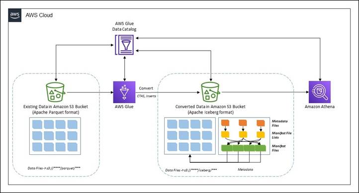
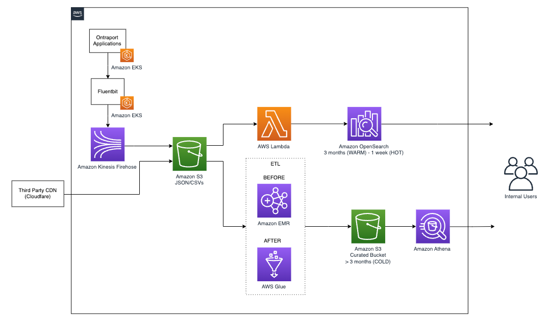
The following diagram illustrates the solution architecture.

Provision resources with AWS CloudFormation

To create your resources for this use case, we deploy an AWS CloudFormation template. Complete the following steps:

Choose Launch Stack (in us-east-1):
Choose Next three times to reach the Review step.
Select I acknowledge that AWS CloudFormation might create IAM resources.
Choose Create stack.

Create an AWS Glue connection

You create an AWS Glue connection to access the MySQL database created by the CloudFormation template. An AWS Glue crawler uses the connection in the next step.

On the AWS Glue console, under Databases in the navigation pane, choose Connections.
Choose Add connection.
For Connection name, enter Trade-Analysis.
For Connection type¸ choose JDBC.
Choose Next.
For JDBC URL, enter your URL.
To connect to an Amazon RDS for MySQL data store with a DBDEV database, use the following code:
```
jdbc: mysql://xxx-cluster.cluster-xxx.us-east-1.rds.amazonaws.com:3306/DBDEV
```
For more details, see AWS Glue connection properties. Refer to the CloudFormation fund-analysis stack Outputs tab to get the Amazon RDS ARN.

The next step requires you to first retrieve your MySQL database user name and password via AWS Secrets Manager.
On the Secrets Manager console, choose Secrets in the navigation pane.
Choose the secret rds-secret-fund-analysis.
Choose Retrieve secret value to get the user name and password.
Return to the connection configuration and enter the user name and password.
For VPC, choose the VPC ending with fund-analysis.
For Subnet and Security groups, choose the values ending with fund-analysis.
Choose Next and Finish to complete the connection setup.
Select the connection you created and choose Test Connection.
For IAM role, choose the role AWSGlueServiceRole-Studio.

For more details about using AWS Identity and Access Management (IAM), refer to Setting up for AWS Glue Studio.

Create and run AWS Glue crawlers

In this step, you create two crawlers. The crawlers connect to a data store, determine the schema for your data, and then create metadata tables in your AWS Glue Data Catalog.

Crawl MySQL data stores

The first crawler creates metadata for the MySQL data stores. Complete the following steps:

On the AWS Glue console, choose Crawlers in the navigation pane.
Choose Add crawler.
For Crawler name, enter Trades Crawlers.
Choose Next.
For Crawler source type, choose Data stores.
For Repeat crawls of S3 data stores, choose Crawl all folders.
Choose Next.
For Choose a data store, choose JDBC.
For Connection, choose Trade-Analysis.
For Include path, enter the MySQL database name (DBDEV).
Choose Next.
For Add another data store, choose No.
Choose Next.
For the IAM role to access the data stores, choose the role AWSGlueServiceRole-Studio.
For Frequency, choose Run on demand.
Choose Add database.
For Database name, enter trade_analysis_db.
Choose Create.
Choose Next.
Review all the steps and choose Finish to create your crawler.
Select the Trades Crawlers crawler and choose Run crawler to get the metadata.

Crawl Amazon S3 data stores

Now you configure a crawler to create metadata for the Amazon S3 data stores.

On the AWS Glue console, choose Crawlers in the navigation pane.
Choose Add crawler.
For Crawler name, enter Ratings.
Choose Next.
For Crawler source type, choose Data stores.
For Repeat crawls of S3 data stores, choose Crawl all folders.
Choose Next.
For Choose a data store, choose S3.
For Connection, choose Trade-Analysis.
For Include path, enter s3://aws-bigdata-blog/artifacts/analyze_fund_performance_using_glue/Morningstar.csv.
Choose Next.
For Add another data store, choose No.
Choose Next.
For the IAM role to access the data stores, choose the role AWSGlueServiceRole-Studio.
For Frequency, choose Run on demand.
Choose Add database.
For Database name, enter trade_analysis_db.
Review all the steps and choose Finish to create your crawler.
Select the Ratings crawler and choose Run crawler to get the metadata.

Review crawler output

To review the output of your two crawlers, navigate to the Databases page on the AWS Glue console.

You can review the database trade_analysis_db created in previous steps and the contents of the metadata tables.

Create a job using AWS Glue Studio

A job is the AWS Glue component that allows the implementation of business logic to transform data as part of the extract, transform, and load (ETL) process. For more information, see Adding jobs in AWS Glue.

To create an AWS Glue job using AWS Glue Studio, complete the following steps:

On the AWS Glue console, in the navigation pane, choose AWS Glue Studio.
Choose Create and manage jobs.
Choose View jobs.
AWS Glue Studio supports different sources. For this post, you use two AWS Glue tables as data sources and one S3 bucket as the destination.
In the Create job section, select Visual with a blank canvas.
Choose Create.

This takes you to the visual editor to create an AWS Glue job.
Change the job name from Untitled Job to Trade-Analysis-Job.

You now have an AWS Glue job ready to filter, join, and aggregate data from two different sources.

Add two data sources

For this post, you use two AWS Glue tables as data sources: Trades and Ratings, which you created earlier.

On the AWS Glue Studio console, on the Source menu, choose MySQL.
On the Node properties tab, for Name, enter Trades.
For Node type, choose MySQL.
On the Data Source properties – MySQL tab, for Database, choose trade_analysis_db.
For Table, choose dbdev_mft_actvitity.
Before adding the second data source to the analysis job, be sure that the node you just created isn’t selected.
On the Source menu, choose Amazon S3.
On the Node properties tab, for Name, enter Ratings.
For Node type, choose Amazon S3.
On the Data Source properties – S3 tab, for Database, choose trade_analysis_db.
For Table, choose morning_star_csv.
You now have two AWS Glue tables as the data sources for the AWS Glue job.The Data preview tab helps you sample your data without having to save or run the job. The preview runs each transform in your job so you can test and debug your transformations.
Choose the Ratings node and on the Data preview tab, choose Start data preview session.
Choose the AWSGlueServiceRole-Studio IAM role and choose Confirm to sample the data.

Data previews are available for each source, target, and transform node in the visual editor, so you can verify the results step by step for other nodes.

Join two tables

A transform is the AWS Glue Studio component were the data is modified. You have the option of using different transforms that are part of this service or custom code. To add transforms, complete the following steps:

On the Transform menu, choose Join.
On the Node properties tab, for Name, enter trades and ratings join.
For Node type, choose Join.
For Node parents, choose the Trades and Ratings data sources.
On the Transform tab, for Join type, choose Outer join.
Choose the common column between the tables to establish the connection.
For Join conditions, choose symbol from the Trades table and mor_rating_fund_symbol from the Ratings table.

Add a target

Before adding the target to store the result, be sure that the node you just created isn’t selected. To add the target, complete the following steps:

On the Target menu, choose Amazon S3.
On the Node properties tab, for Name, enter trades ratings merged.
For Node type, choose Amazon S3 for writing outputs.
For Node parents, choose trades and ratings join.
On the Data target properties – S3 tab, for Format, choose Parquet.
For Compression type, choose None.
For S3 target location, enter s3://glue-studio-blog- {Your Account ID as a 12-digit number}/.
For Data catalog update options, select Create a table in the Data Catalog and on subsequent runs, update the schema and add new partitions.
For Database, choose trade-analysis-db.
For Table name, enter tradesratingsmerged.

Configure the job

When the logic behind the job is complete, you must set the parameters for the job run. In this section, you configure the job by selecting components such as the IAM role and the AWS Glue version you use to run the job.

Choose the Job details tab.
For Job bookmark, choose Disable.
For Number of retries, optionally enter 0.
Choose Save.
When the job is saved, choose Run.

Monitor the job

AWS Glue Studio offers a job monitoring dashboard that provides comprehensive information about your jobs. You can get job statistics and see detailed information about the job and the job status when running.

In the AWS Glue Studio navigation pane, choose Monitoring.
Change the date range to 1 hour using the Date range selector to get the recently submitted job.
The Job runs summary section displays the current state of the job run. The status of the job could be Running, Canceled, Success, or Failed.The Job run success rate section provides the estimated DPU usage for jobs, and gives you a summary of the performance of the job. Job type breakdown and Worker type breakdown contain additional information about the job.
For get more details about the job run, choose View run details.

Review the results using Athena

To view the data in Athena, complete the following steps:

Navigate to the Athena console, where you can see the database and tables created by your crawlers.

If you haven’t used Athena in this account before, a message appears instructing you to set a query result location.
Choose Settings, Manage, Browse S3, and select any bucket that you created.
Choose Save and return to the editor to continue.
In the Data section, expand Tables to see the tables you created with the AWS Glue crawlers.
Choose the options menu (three dots) next to one of the tables and choose Preview Table.

The following screenshot shows an example of the data.

Create a QuickSight dashboard and visualizations

To set up QuickSight for the first time, sign up for a QuickSight subscription and allow connections to Athena.

To create a dashboard in QuickSight based on the AWS Glue Data Catalog tables you created, complete the following steps:

On the QuickSight console, choose Datasets in the navigation pane.
Choose New dataset.
Create a new QuickSight dataset called Fund-Analysis with Athena as the data source.
In the Choose your table section, choose AwsDataCatlog for Catalog and choose trade_analysis_db for Database.
For Tables, select the tradesratingmerged table to visualize.
Choose Select.
Import the data into SPICE.
SPICE is an in-memory engine that QuickSight uses to perform advanced calculations and improve performance. Importing the data into SPICE can save time and money. When using SPICE, you can refresh your datasets both fully or incrementally. As of this writing, you can schedule incremental refreshes up to every 15 minutes. For more information, refer to Refreshing SPICE data. For near-real-time analysis, select Directly query your data instead.
Choose Visualize.

After you create the dataset, you can view it and edit its properties. For this post, leave the properties unchanged.
To analyze the market performance from the Morningstar file, choose the clustered bar combo chart under Visual types.
Drag Fund_Symbol from Fields list to X-axis.
Drag Ratings to Y-axis and Lines.
Choose the default title choose Edit title to change the title to “Market Analysis.”
The following QuickSight dashboard was created using a custom theme, which is why the colors may appear different than yours.
To display the Morningstar details in tabular form, add a visual to create additional graphs.
Choose the table visual under Visual types.
Drag Fund Symbol and Fund Names to Group by.
Drag Ratings, Historical Earnings, and LT Earnings to Value.

In QuickSight, up until this point, you analyzed the market performance reported by Morningstar. Let’s analyze the near-real-time daily trade activities.
Add a visual to create additional graphs.
Choose the clustered bar combo chart under Visual types.
Drag Fund_Symbol from Fields list to X-axis and Trade Amount to Y-axis.
Choose the default title choose Edit title to change the title to “Daily Transactions.”
To display the daily trades in tabular form, add a visual to create additional graphs.
Drag Trade Date, Customer Name, Fund Name, Fund Symbol, and Buy/Sell to Group by.
Drag Trade Amount to Value.

The following screenshot shows a complete dashboard. This compares the market observation reported in the street against the daily trades happening in the bank.

In the Market Analysis section of the dashboard, GMFXXD funds were performing well based on the previous night’s feed from Morningstar. However, the Daily Transactions section of the dashboard shows that customers were selling their positions from the funds. Relying only on the previous nightly batch report will mislead the fund managers or operation analyst to act.

Near-real-time analytics using AWS Glue Studio and QuickSight can enable fund managers and analysts to self-serve and impose fees or gates on those IMM funds.

Clean up

To avoid incurring future charges and to clean up unused roles and policies, delete the resources you created: the CloudFormation stack, S3 bucket, and AWS Glue job.

Conclusion

In this post, you learned how to use AWS Glue Studio to analyze data from different sources with no previous coding experience and how to build visualizations and get business insights using QuickSight. You can use AWS Glue Studio and QuickSight to speed up the analytics process and allow different personas to transform data with no development experience.

For more information about AWS Glue Studio, see the AWS Glue Studio User Guide. For information about QuickSight, refer to the Amazon QuickSight User Guide.

About the authors

Rajeshkumar Karuppaswamy is a Customer Solutions Manager at AWS. In this role, Rajeshkumar works with AWS Customers to drive Cloud strategy, provides thought leadership to accelerate businesses achieve speed, agility, and drive innovation. His areas of interests are AI & ML, analytics, and data engineering.

Richa Kaul is a Senior Leader in Customer Solutions serving Financial Services customers. She is based out of New York. She has extensive experience in large scale cloud transformation, employee excellence, and next generation digital solutions. She and her team focus on optimizing value of cloud by building performant, resilient and agile solutions. Richa enjoys multi sports like triathlons, music, and learning about new technologies.

Noritaka Sekiyama is a Principal Big Data Architect on the AWS Glue team. He is responsible for building software artifacts to help customers. This summer, he enjoyed goldfish scooping with his children.

Detect and process sensitive data using AWS Glue Studio

2022-09-20 Leonardo Gomez

Post Syndicated from Leonardo Gomez original https://aws.amazon.com/blogs/big-data/detect-and-process-sensitive-data-using-aws-glue-studio/

Data lakes offer the possibility of sharing diverse types of data with different teams and roles to cover numerous use cases. This is very important in order to implement a data democratization strategy and incentivize the collaboration between lines of business. When a data lake is being designed, one of the most important aspects to consider is data privacy. Without it, sensitive information could be accessed by the wrong team, which may affect the reliability of a data platform. However, identifying sensitive data inside a data lake could represent a challenge due to the diversity of the data and also its volume.

Earlier this year, AWS Glue announced the new sensitive data detection and processing feature to help you identify and protect sensitive information in a straightforward way using AWS Glue Studio. This feature uses pattern matching and machine learning to automatically recognize personally identifiable information (PII) and other sensitive data at the column or cell level as part of AWS Glue jobs.

Sensitive data detection in AWS Glue identifies a variety of sensitive data like phone and credit card numbers, and also offers the option to create custom identification patterns or entities to cover your specific use cases. Additionally, it helps you take action, such as creating a new column that contains any sensitive data detected as part of a row or redacting the sensitive information before writing records into a data lake.

This post shows how to create an AWS Glue job that identifies sensitive data at the row level. We also show how create a custom identification pattern to identify case-specific entities.

Overview of solution

To demonstrate how to create an AWS Glue job to identify sensitive data, we use a test dataset with customer comments that contain private data like Social Security number (SSN), phone number, and bank account number. The goal is to create a job that automatically identifies the sensitive data and triggers an action to redact it.

Prerequisites

For this walkthrough, you should have the following prerequisites:

An AWS account
An AWS Identity and Access Management (IAM) user with access to the following services:
- Amazon Athena
- AWS CloudFormation
- AWS Glue
- Amazon Simple Storage Service (Amazon S3)

Launch your CloudFormation stack

To create your resources for this use case, complete the following steps:

Launch your CloudFormation stack in us-east-1:
Under Parameters, enter a name for your S3 bucket (include your account number).
Select I acknowledge that AWS CloudFormation might create IAM resources with custom names.
Choose Create stack.
Wait until the creation of the stack is complete, as shown on the AWS CloudFormation console.

Launching this stack creates AWS resources. You need the following resources from the Outputs tab for the next steps:

GlueSenRole – The IAM role to run AWS Glue jobs
BucketName – The name of the S3 bucket to store solution-related files
GlueDatabase – The AWS Glue database to store the table related to this post

Create and run an AWS Glue job

Let’s first create the dataset that is going to be used as the source of the AWS Glue job:

Open AWS CloudShell.
Run the following command:
```
aws s3 cp s3://aws-bigdata-blog/artifacts/gluesendata/sourcedata/customer_comments.csv s3://glue-sendata-blog-<YOUR ACCOUNT NUMBER>/customer_comments/customer_comments.csv
```
This action copies the dataset that is going to be used as the input for the AWS Glue job covered in this post.

Now, let’s create the AWS Glue job.

On the AWS Glue Studio console, choose Jobs in the navigation pane.
Select Visual with blank canvas.
Choose the Job Details tab to configure the job.
For Name, enter GlueSenJob.
For IAM Role, choose the role GlueSenDataBlogRole.
For Glue version, choose Glue 3.0.
For Job bookmark, choose Disable.
Choose Save.
After the job is saved, choose the Visual tab and on the Source menu, choose Amazon S3.
On the Data source properties -S3 tab, for S3 source type, select S3 location.
Add the S3 location of the file that you copied previously using CloudShell.
Choose Infer schema.

This last action infers the schema and file type of the of the source for this post, as you can see in the following screenshot.

Now, let’s see what the data looks like.

On the Data preview tab, choose Start data preview session.
For IAM role, choose the role GlueSeDataBlogRole.
Choose Confirm.

This last step may take a couple of minutes to run.

When you review the data, you can see that sensitive data like phone numbers, email addresses, and SSNs are part of the customer comments.

Now let’s identify the sensitive data in the comments dataset and mask it.

On the Transform menu, choose Detect PII.

The AWS Glue sensitive data identification feature allows you to find sensitive data at the row and column level, which covers a diverse number of use cases. For this post, because we scan comments made by customers, we use the row-level scan.

On the Transform tab, select Find sensitive data in each row.
For Types of sensitive information to detect, select Select specific patterns.

Now we need to select the entities or patterns that are going to be identified by the job.

For Selected patterns, choose Browse.
Select the following patterns:
1. Credit Card
2. Email Address
3. IP Address
4. Mac Address
5. Person’s Name
6. Social Security Number (SSN)
7. US Passport
8. US Phone
9. US/Canada bank account
Choose Confirm.

After the sensitive data is identified, AWS Glue offers two options:

Enrich data with detection results – Adds a new column to the dataset with the list of the entities or patterns that were identified in that specific row.
Redact detected text – Replaces the sensitive data with a custom string. For this post, we use the redaction option.

For Actions, select Redact detected text.
For Replacement text, enter ####.

Let’s see how the dataset looks now.

Check the result data on the Data preview tab.

As you can see, the majority of the sensitive data was redacted, but there is a number on row 11 that isn’t masked. This is because it’s a Canadian permanent resident number, and this pattern isn’t part of the ones that the sensitive data identification feature offers. However, we can add a custom pattern to identify this number.

On the Transform tab, for Selected patterns, choose Create new.

This action opens the Create detection pattern window, where we create the custom pattern to identify the Canadian permanent resident number.

For Pattern name, enter Can_PR_Number.
For Expression, enter the regular expression [P]+[D]+[0]\d\d\d\d\d\d
Choose Validate.
Wait until you get the validation message, then choose Create pattern.

Now you can see the new pattern listed under Custom patterns.

On the AWS Glue Studio Console, for Selected patterns, choose Browse.

Now you can see Can_PR_Number as part of the pattern list.

Select Can_PR_Number and choose Confirm.

On the Data preview tab, you can see that the Canadian permanent resident number has been redacted.

Let’s add a destination for the dataset with redacted information.

On the Target menu, choose Amazon S3.
On the Data target properties -S3 tab, for Format, choose Parquet.
For S3 Target Location, enter s3://glue-sendata-blog-<YOUR ACCOUNT ID>/output/redacted_comments/.
For Data Catalog update options, select Create a table in the Data Catalog and on subsequent runs, update the schema and add new partitions.
For Database, choose gluesenblog.
For Table name, enter custcomredacted.
Choose Save, then choose Run.

You can view the job run details on the Runs tab.

Wait until the job is complete.

Query the dataset

Now let’s see what the final dataset looks like. To do so, we query the data with Athena. As part of this post, we assume that a query result location for Athena is already configured; if not, refer to Working with query results, recent queries, and output files.

On the Athena console, open the query editor.
For Database, choose the gluesenblog database.

Run the following query:

SELECT * FROM "gluesenblog"."custcomredacted" limit 15;

Verify the results; you can observe that all the sensitive data is redacted.

Clean up

To avoid incurring future charges, and to clean up unused roles and policies, delete the resources you created: Datasets, CloudFormation stack, S3 bucket, AWS Glue job, AWS Glue database, and AWS Glue table.

Conclusion

AWS Glue sensitive data detection offers an easy way to identify and process private data, without coding. This feature allows you to detect and redact sensitive data when it’s ingested into a data lake, enforcing data privacy before the data is available to data consumers. AWS Glue sensitive data detection is generally available in all Regions that support AWS Glue.

To learn more and get started using AWS Glue sensitive data detection, refer to Detect and process sensitive data.

About the author

Identify source schema changes using AWS Glue

2022-09-14 Narendra Gupta

Post Syndicated from Narendra Gupta original https://aws.amazon.com/blogs/big-data/identify-source-schema-changes-using-aws-glue/

In today’s world, organizations are collecting an unprecedented amount of data from all kinds of different data sources, such as transactional data stores, clickstreams, log data, IoT data, and more. This data is often in different formats, such as structured data or unstructured data, and is usually referred to as the three Vs of big data (volume, velocity, and variety). To extract information from the data, it’s usually stored in a data lake built on Amazon Simple Storage Service (S3). The data lake provides an important characteristic called schema on read, which allows you to bring data in the data lake without worrying about the schema or changes in the schema on the data source. This enables faster ingestion of data or building data pipelines.

However, you may be reading and consuming this data for other use cases, such as pointing to applications, building business intelligence (BI) dashboards in services like Amazon QuickSight, or doing data discovery using a serverless query engine like Amazon Athena. Additionally, you may have built an extract, transform, and load (ETL) data pipeline to populate your data store like a relational database, non-relational database, or data warehouse for further operational and analytical needs. In these cases, you need to define the schema upfront or even keep an account of the changes in the schema, such as adding new columns, deleting existing columns, changing the data type of existing columns, or renaming existing columns, to avoid any failures in your application or issues with your dashboard or reporting.

In many use cases, we have found that the data teams responsible for building the data pipeline don’t have any control of the source schema, and they need to build a solution to identify changes in the source schema in order to be able to build the process or automation around it. This might include sending notifications of changes to the teams dependent on the source schema, building an auditing solution to log all the schema changes, or building an automation or change request process to propagate the change in the source schema to downstream applications such as an ETL tool or BI dashboard. Sometimes, to control the number of schema versions, you may want to delete the older version of the schema when there are no changes detected between it and the newer schema.

For example, assume you’re receiving claim files from different external partners in the form of flat files, and you’ve built a solution to process claims based on these files. However, because these files were sent by external partners, you don’t have much control over the schema and data format. For example, columns such as customer_id and claim_id were changed to customerid and claimid by one partner, and another partner added new columns such as customer_age and earning and kept the rest of the columns the same. You need to identify such changes in advance so you can edit the ETL job to accommodate the changes, such as changing the column name or adding the new columns to process the claims.

In this solution, we showcase a mechanism that simplifies the capture of the schema changes in your data source using an AWS Glue crawler.

Solution overview

An AWS Glue data crawler is built to sync metadata based on existing data. After we identify the changes, we use Amazon CloudWatch to log the changes and Amazon Simple Notification Service (Amazon SNS) to notify the changes to the application team over email. You can expand this solution to solve for other use cases such as building an automation to propagate the changes to downstream applications or pipelines, which is out of scope for this post, to avoid any failures in downstream applications because of schema changes. We also show a way to delete older versions of the schema if there are no changes between the compared schema versions.

If you want to capture the change in an event-driven manner, you can do so by using Amazon EventBridge. However, if you want to capture the schema changes on multiple tables at the same time, based on a specific schedule, you can use the solution in this post.

In our scenario, we have two files, each with different schemas, simulating data that has undergone a schema change. We use an AWS Glue crawler to extract the metadata from data in an S3 bucket. Then we use an AWS Glue ETL job to extract the changes in the schema to the AWS Glue Data Catalog.

AWS Glue provides a serverless environment to extract, transform, and load a large number of datasets from several sources for analytic purposes. The Data Catalog is a feature within AWS Glue that lets you create a centralized data catalog of metadata by storing and annotating data from different data stores. Examples include object stores like Amazon S3, relational databases like Amazon Aurora PostgreSQL-Compatible Edition, and data warehouses like Amazon Redshift. You can then use that metadata to query and transform the underlying data. You use a crawler to populate the Data Catalog with tables. It can automatically discover new data, extract schema definitions, detect schema changes, and version tables. It can also detect Hive-style partitions on Amazon S3 (for example year=YYYY, month=MM, day=DD).

Amazon S3 serves as the storage for our data lake. Amazon S3 is an object storage service that offers industry-leading scalability, data availability, security, and performance.

The following diagram illustrates the architecture for this solution.

The workflow includes the following steps:

Copy the first data file to the data folder of the S3 bucket and run the AWS Glue crawler to create a new table in the Data Catalog.
Move the existing file from the data folder to the archived folder.
Copy the second data file with the updated schema to the data folder, then rerun the crawler to create new version of table schema.
Run the AWS Glue ETL job to check if there is a new version of the table schema.
The AWS Glue job lists the changes in the schema with the previous version of the schema in CloudWatch Logs. If there are no changes in the schema and the flag to delete older versions is set to true, the job also deletes the older schema versions.
The AWS Glue job notifies all changes in the schema to the application team over email using Amazon SNS.

To build the solution, complete the following steps:

Create an S3 bucket with the data and archived folders to store the new and processed data files.
Create an AWS Glue database and an AWS Glue crawler that crawls the data file in the data folder to create an AWS Glue table in the database.
Create an SNS topic and add an email subscription.
Create an AWS Glue ETL job to compare the two versions of the table schema, list the changes in the schema with the older version of schema, and delete older versions of schema if the flag to delete older versions is set to true. The job also publishes an event in Amazon SNS to notify the changes in the schema to the data teams.

For the purpose of this post, we manually perform the steps to move the data files from the data folder to the archive folder, triggering the crawler and ETL job. Depending on your application needs, you can automate and orchestrate this process through AWS Glue workflows.

Let’s set up the infrastructure required to go through the solution to compare an AWS Glue table version to a version updated with recent schema changes.

Create an S3 bucket and folders

To create an S3 bucket with the data and archived folders to store the new and processed data files, complete the following steps:

On the Amazon S3 console, choose Buckets in the navigation pane.
Choose Create bucket.
For Bucket name, enter a DNS-compliant unique name (for example, aws-blog-sscp-ng-202202).
For Region, choose the Region where you want the bucket to reside.
Keep all other settings as default and choose Create bucket.
On the Buckets page, choose the newly created bucket.
Choose Create folder.
For Folder name, enter data.
Leave server-side encryption at its default (disabled).
Choose Create folder.
Repeat these steps to create the archived folder in the same bucket.

Create an AWS Glue database and crawler

Now we create an AWS Glue database and crawler that crawls the data file in the data bucket to create an AWS Glue table in the new database.

On the AWS Glue console, choose Databases in the navigation pane.
Choose Add database.
Enter a name (for example, sscp-database) and description.
Choose Create.
Choose Crawlers in the navigation pane.
Choose Add crawler.
For Crawler name, enter a name (glue-crawler-sscp-sales-data).
Choose Next.
For the crawler source type¸ choose Data stores.
To repeat crawls of the data stores, choose Crawl all folders.
Choose Next.
For Choose a data store, choose S3.
For Include path, choose the S3 bucket and folder you created (s3://aws-blog-sscp-ng-202202/data).
Choose Next.
On the Add another data store page, choose No, then choose Next.
Choose Create an IAM role and enter a name for the role (for example, sscp-blog).
Choose Next.
Choose Run on Demand, then choose Next.
For Database, choose your AWS Glue database (sscp-database).
For Prefix added to tables, enter a prefix (for example, sscp_sales_).
Expand the Configuration options section and choose Update the table definition in the data catalog.
Leave all other settings as default and choose Next.
Choose Finish to create the crawler.

Create an SNS topic

To create an SNS topic and add an email subscription, complete the following steps:

On the Amazon SNS console, choose Topics in the navigation pane.
Choose Create topic.
For Type, choose Standard.
Enter a name for the topic (for example, NotifySchemaChanges).
Leave all other settings as default and choose Create topic.
In the navigation pane, choose Subscriptions.
Choose Create subscription.
For Topic ARN, choose the ARN of the created SNS topic.
For Protocol, choose Email.
For Endpoint, enter the email address to receive notifications.
Leave all other defaults and choose Create subscription.You should receive an email to confirm the subscription.
Choose the link in the email to confirm.
Add the following permission policy to the AWS Glue service role created earlier as part of the crawler creation (AWSGlueServiceRole-sscp-blog) to allow publishing to the SNS topic. Make sure to change <$SNSTopicARN> in the policy with the actual ARN of the SNS topic.

{
    "Version": "2012-10-17",
    "Statement": [
        {
            "Sid": "AllowEventPublishing",
            "Effect": "Allow",
            "Action": "sns:Publish",
            "Resource": "<$SNSTopicARN>"
        }
    ]
}

Create an AWS Glue ETL job

Now you create an AWS Glue ETL job to compare two schema versions of a table and list the changes in schemas. If there are no changes in the schema and the flag to delete older versions is set to true, the job also deletes any older versions. If there are changes in schema, the job lists changes in the CloudWatch logs and publishes an event in Amazon SNS to notify changes to the data team.

On the AWS Glue console, choose AWS Glue Studio.
Choose Create and manage jobs.
Choose the Python Shell script editor.
Choose Create to create a Python Shell job.

Enter the following code in the script editor field:

import boto3
import pandas as pd

# Input Paramaters:  
# catalog_id - Your AWS Glue Catalg Id - it is same as your AWS account ID
# db_name - name of your AWS Glue Database in your Glue Data catalog_id
# table_name - name of the table in your AWS Glue Database that you would like to check of change in schema
# topic_arn - ARN of the SNS topic to publish the changes in table schema
# versions_to_compare - Two versions that customer would want to compare. 0 is the lastes version and 1 in the version prior to the latest version
# delete_old_versions - If True and there are no changes in the versions compared, job would delete all old versions except for the latest "number_of_versions_to_retain" versions 
# number_of_versions_to_retain - if delete_old_versions is True and there are no changes in the versions compared, the job would delete all old versions except for the latest "number_of_versions_to_retain" versions

catalog_id = '<$catalog_id>'
db_name='<$db_name>'
table_name='<$table_name>'
topic_arn='<$sns_topic_ARN>'
versions_to_compare=[0,1]
delete_old_versions = False
number_of_versions_to_retain = 2

columns_modified = []

# Function to compare the name and type of columns in new column list with old column list to 
# find any newly added column and the columns with changed data type
def findAddedUpdated(new_cols_df, old_cols_df, old_col_name_list):
    for index, row in new_cols_df.iterrows():
        new_col_name = new_cols_df.iloc[index]['Name']
        new_col_type = new_cols_df.iloc[index]['Type']

        # Check if a column with same name exist in old table but the data type has chaged
        if new_col_name in old_col_name_list:
            old_col_idx = old_cols_df.index[old_cols_df['Name']==new_col_name][0]
            old_col_type = old_cols_df.iloc[old_col_idx]['Type']

            if old_col_type != new_col_type:
                columns_modified.append(f"Data type changed for '{new_col_name}' from '{old_col_type}' to '{new_col_type}'")
        # If a column is only in new column list, it a newly added column
        else:
            columns_modified.append(f"Added new column '{new_col_name}' with data type as '{new_col_type}'")

# Function to iterate through the list of old columns and check if any column doesn't exist in new columns list to find out dropped columns
def findDropped(old_cols_df, new_col_name_list):
    for index, row in old_cols_df.iterrows():
        old_col_name = old_cols_df.iloc[index]['Name']
        old_col_type = old_cols_df.iloc[index]['Type']

        #check if column doesn't exist in new column list  
        if old_col_name not in new_col_name_list:
            columns_modified.append(f"Dropped old column '{old_col_name}' with data type as '{old_col_type}'")

# Function to publish changes in schema to a SNS topic that can be subscribed to receive email notifications when changes are detected
def notifyChanges(message_to_send):
    sns = boto3.client('sns')
    # Publish a simple message to the specified SNS topic
    response = sns.publish(
        TopicArn=topic_arn,   
        Message=message_to_send,  
        Subject="DWH Notification: Changes in table schema"
    )
    
# Function to convert version_id to int to use for sorting the versions
def version_id(json):
    try:
        return int(json['VersionId'])
    except KeyError:
        return 0

# Function to delete the table versions
def delele_versions(glue_client, versions_list, number_of_versions_to_retain):
    print("deleting old versions...")
    if len(versions_list) > number_of_versions_to_retain:
        version_id_list = []
        for table_version in versions_list:
            version_id_list.append(int(table_version['VersionId']))
        # Sort the versions in descending order
        version_id_list.sort(reverse=True)
        versions_str_list = [str(x) for x in version_id_list]
        versions_to_delete = versions_str_list[number_of_versions_to_retain:]
        
        del_response = glue_client.batch_delete_table_version(
            DatabaseName=db_name,
            TableName=table_name,
            VersionIds=versions_to_delete
        )
        return del_response

# Calling glue API to get the list of table versions. The solution assums that number of version in the table are less than 100. If you have more than 100 versions, you should use pagination and loop through each page.  
glue = boto3.client('glue')
response = glue.get_table_versions(
    CatalogId=catalog_id,
    DatabaseName=db_name,
    TableName=table_name,
    MaxResults=100
)
table_versions = response['TableVersions']
table_versions.sort(key=version_id, reverse=True)

version_count = len(table_versions)
print(version_count)

# checking if the version of table to compare exists. You would need pass the numbers of versions to compare to the job. 
if version_count > max(versions_to_compare):

    new_columns = table_versions[versions_to_compare[0]]['Table']['StorageDescriptor']['Columns']
    new_cols_df = pd.DataFrame(new_columns)

    old_columns = table_versions[versions_to_compare[1]]['Table']['StorageDescriptor']['Columns']
    old_cols_df = pd.DataFrame(old_columns)

    new_col_name_list =  new_cols_df['Name'].tolist()
    old_col_name_list =  old_cols_df['Name'].tolist()
    findAddedUpdated(new_cols_df, old_cols_df, old_col_name_list)
    findDropped(old_cols_df, new_col_name_list)
    if len(columns_modified) > 0: 
        email_msg = f"Following changes are identified in '{table_name}' table of '{db_name}' database of your Datawarehouse. Please review.\n\n"
        print("Job completed! -- below is list of changes.")
        for column_modified in columns_modified:
            email_msg += f"\t{column_modified}\n"

        print(email_msg)
        notifyChanges(email_msg)
    else:
        if delete_old_versions:
            delele_versions(glue, table_versions,number_of_versions_to_retain)
        print("Job completed! -- There are no changes in table schema.")
else:
    print("Job completed! -- Selected table doesn't have the number of versions selected to compare. Please verify the list passed in 'versions_to_compare'")

Enter a name for the job (for example, find-change-job-sscp).
For IAM Role, choose the AWS Glue service role (AWSGlueServiceRole-sscp-blog).
Leave all other defaults and choose Save.

Test the solution

We’ve configured the infrastructure to run the solution. Let’s now see it in action. First we upload the first data file and run our crawler to create a new table in the Data Catalog.

Create a CSV file called salesdata01.csv with the following contents:

ordertime,region,rep,item,units,unitcost
2022-01-06,US-West,Jones,Pencil,95,1.99
2022-01-06,US-Central,Kivell,Binder,50,19.99
2022-01-07,US-Central,Jardine,Pencil,36,4.99
2022-01-07,US-Central,Gill,Pen,27,19.99
2022-01-08,US-East,Sorvino,Pencil,56,2.99
2022-01-08,US-West,Jones,Binder,60,4.99
2022-01-09,US-Central,Andrews,Pencil,75,1.99
2022-01-10,US-Central,Jardine,Pencil,90,4.99
2022-01-11,US-East,Thompson,Pencil,32,1.99
2022-01-20,US-West,Jones,Binder,60,8.99

On the Amazon S3 console, navigate to the data folder and upload the CSV file.
On the AWS Glue console, choose Crawlers in the navigation pane.
Select your crawler and choose Run crawler.The crawler takes a few minutes to complete. It adds a table (sscp_sales_data) in the AWS Glue database (sscp-database).
Verify the created table by choosing Tables in the navigation pane.Now we move the existing file in the data folder to the archived folder.
On the Amazon S3 console, navigate to the data folder.
Select the file you uploaded (salesdata01.csv) and on the Actions menu, choose Move.
Move the file to the archived folder.Now we copy the second data file with the updated schema to the data folder and rerun the crawler.

Create a CSV file called salesdata02.csv with the following code. It contains the following changes from the previous version:

The data in the region column is changed from region names to some codes (for example, the data type is changed from string to BIGINT).
The rep column is dropped.

The new column total is added.

ordertime,region,item,units,unitcost,total
2022-02-01,01,Pencil,35,4.99,174.65
2022-02-01,03,Desk,2,125,250
2022-02-02,01,Pen Set,16,15.99,255.84
2022-02-02,03,Binder,28,8.99,251.72
2022-02-03,01,Pen,64,8.99,575.36
2022-02-03,01,Pen,15,19.99,299.85
2022-02-06,03,Pen Set,96,4.99,479.04
2022-02-10,03,Pencil,67,1.29,86.43
2022-02-11,01,Pen Set,74,15.99,183.26
2022-02-11,03,Binder,46,8.99,413.54

On the Amazon S3 bucket, upload the file to the data folder.
On the AWS Glue console, choose Crawlers in the navigation pane.
Select your crawler and choose Run crawler.The crawler takes approximately 2 minutes to complete. It updates the schema of the previously created table (sscp_sales_data).
Verify the new version of the table is created on the Tables page.Now we run the AWS Glue ETL job to check if there is a new version of the table schema and list the changes in the schema with the previous version of the schema in CloudWatch Logs.
On the AWS Glue console, choose Jobs in the navigation pane.
Select your job (find-change-job-sscp) and on the Actions menu, choose Edit script.
Change the following input parameters for the job in the script to match with your configuration:
Choose Save.
Close the script editor.
Select the job again and on the Actions menu, choose Run job.
Leave all default parameters and choose Run job.
To monitor the job status, choose the job and review the History tab.
When the job is complete, choose the Output link to open the CloudWatch logs for the job.

The log should show the changes identified by the AWS Glue job.

You should also receive an email with details on the changes in the schema. The following is an example of an email received.

We can now review the changes identified by the AWS Glue ETL job and make changes in the downstream data store accordingly before running the job to propagate the data from the S3 bucket to downstream applications. For example, if you have an Amazon Redshift table, after the job lists all the schema changes, you need to connect to the Amazon Redshift database and make these schema changes. Follow the change request process set by your organization before making schema changes in your production system.

The following table has a list of mappings for Apache Hive and Amazon Redshift data types. You can find similar mappings for other data stores and update your downstream data store.

The provided Python code takes care of the logic to compare the schema changes. The script takes in the parameters of the AWS Glue Data Catalog ID, AWS Glue database name, and AWS Glue table name.

Hive Data Types	Description	Amazon Redshift Data Types	Description
TINYINT	1 byte integer	.	.
SMALLINT	Signed two-byte integer	SMALLINT	Signed two-byte integer
INT	Signed four-byte integer	INT	Signed four-byte integer
BIGINT	Signed eight-byte integer	BIGINT	Signed eight-byte integer
DECIMAL	.	.	.
DOUBLE	.	.	.
STRING	.	VARCHAR, CHAR	.
VARCHAR	1 to 65355, available starting with Hive 0.12.0	VARCHAR	.
CHAR	255 length, available starting with Hive 0.13.0	CHAR	.
DATE	year/month/day	DATE	year/month/day
TIMESTAMP	No timezone	TIME	Time without time zone
.	.	TIMETZ	Time with time zone
ARRAY/STRUCTS	.	SUPER	.
BOOLEAN	.	BOOLEAN	.
BINARY	.	VARBYTE	Variable-length binary value

Clean up

When you’re done exploring the solution, clean up the resources you created as part of this walkthrough:

AWS Glue ETL job (find-change-job-sscp)
AWS Glue crawler (glue-crawler-sscp-sales-data)
AWS Glue table (sscp_sales_data)
AWS Glue database (sscp-database)
IAM role for the crawler and ETL job (AWSGlueServiceRole-sscp-blog)
S3 bucket (aws-blog-sscp-ng-202202) with all the files in the data and archived folders
SNS topic and subscription (NotifySchemaChanges)

Conclusion

In this post, we showed you how to use AWS services together to detect schema changes in your source data, which you can then use to change your downstream data stores and run ETL jobs to avoid any failures in your data pipeline. We used AWS Glue to understand and catalog the source data schema, AWS Glue APIs to identify schema changes, and Amazon SNS to notify the team about the changes. We also showed you how to delete the older versions of your source data schema using AWS Glue APIs. We used Amazon S3 as our data lake storage tier.

Here you can learn more about AWS Glue.

About the authors

Narendra Gupta is a Specialist Solutions Architect at AWS, helping customers on their cloud journey with a focus on AWS analytics services. Outside of work, Narendra enjoys learning new technologies, watching movies, and visiting new places.

Navnit Shukla is AWS Specialist Solutions Architect in Analytics. He is passionate about helping customers uncover insights from their data. He has been building solutions to help organizations make data-driven decisions.

Create single output files for recipe jobs using AWS Glue DataBrew

2022-09-07 Dhiraj Thakur

Post Syndicated from Dhiraj Thakur original https://aws.amazon.com/blogs/big-data/create-single-output-files-for-recipe-jobs-using-aws-glue-databrew/

AWS Glue DataBrew offers over 350 pre-built transformations to automate data preparation tasks (such as filtering anomalies, standardizing formats, and correcting invalid values) that would otherwise require days or weeks writing hand-coded transformations.

You can now choose single or multiple output files instead of autogenerated files for your DataBrew recipe jobs. You can generate a single output file when the output is small or downstream systems need to consume it more easily, such as visualization tools. Alternatively, you can specify your desired number of output files when configuring a recipe job. This gives you the flexibility to manage recipe job output for visualization, data analysis, and reporting, while helping prevent you from generating too many files. In some cases, you may also want to customize the output file partitions for efficient storage and transfer.

In this post, we walk you through how to connect and transform data from an Amazon Simple Storage Service (Amazon S3) data lake and configure the output as a single file via the DataBrew console.

Solution overview

The following diagram illustrates our solution architecture.

DataBrew queries sales order data from the S3 data lake and performs data transformation. Then the DataBrew job writes the final output back to the data lake in a single file.

To implement the solution, you complete the following high-level steps:

Create a dataset.
Create a DataBrew project using the dataset.
Build a transformation recipe.
Create and run a DataBrew recipe job on the full data.

Prerequisites

To complete this solution, you should have an AWS account and the appropriate permissions to create the resources required as part of the solution.

You also need a dataset in Amazon S3. For our use case, we use a mock dataset. You can download the data files from GitHub. On the Amazon S3 console, upload all three CSV files to an S3 bucket.

Create a dataset

To create your dataset in DataBrew, complete the following steps:

On the Datasets page of the DataBrew console, choose Connect new dataset.
For Dataset name, enter a name (for example, order).
Enter the S3 bucket path where you uploaded the data files as part of the prerequisite steps.
Choose Select the entire folder.
For File type¸ select CSV and choose Comma (,) for CSV delimiter.
For Column header values, select Treat first row as header.
Choose Create dataset.

Create a DataBrew project using the dataset

To create your DataBrew project, complete the following steps:

On the DataBrew console, on the Projects page, choose Create project.
For Project Name, enter valid-order.
For Attached recipe, choose Create new recipe.
The recipe name is populated automatically (valid-order-recipe).
For Select a dataset, select My datasets.
Select the order dataset.
For Role name, choose the AWS Identity and Access Management (IAM) role to be used with DataBrew.
Choose Create project.

You can see a success message along with our Amazon S3 order table with 500 rows.

After the project is opened, a DataBrew interactive session is created. DataBrew retrieves sample data based on your sampling configuration selection.

Build a transformation recipe

In a DataBrew interactive session, you can cleanse and normalize your data using over 350 pre-built transformations. In this post, we use DataBrew to perform a few transforms and filter only valid orders with order amounts greater than $0.

To do this, you perform the following steps:

Choose Column and choose Delete.
For Source columns, choose the columns order_id, timestamp, and transaction_date.
Choose Apply.
We filter the rows based on an amount value greater than $0 and add the condition as a recipe step.
To create a custom sort based on state, choose SORT and choose Ascending.
For Source, choose the column state_name.
Select Sort by custom values.
Enter a list of state names separated by commas.
Choose Apply.

The following screenshot shows the full recipe that we applied to our dataset.

Create and run a DataBrew recipe job on the full data

Now that we have built the recipe, we can create and run a DataBrew recipe job.

On the project details page, choose Create job.
For Job name, enter valid-order.
For Output to, choose Amazon S3.
Enter the S3 path to store the output file.
Choose Settings.

For File output options, you have multiple options:

- Autogenerate files – This is the default file output setting, which generates multiple files and usually results in the fastest job runtime
- Single file output – This option generates a single output file
- Multiple file output – With this option, you specify the maximum number of files you want to split your data into

For this post, select Single file output.
Choose Save.
For Role name, choose the IAM role to be used with DataBrew.
Choose Create and run job.
Navigate to the Jobs page and wait for the product-wise-sales-job job to complete.
Navigate to output S3 bucket to confirm that a single output file is stored there.

Clean up

To avoid incurring future charges, delete all the resources created during this walkthrough:

Delete the recipe job valid-order.
Empty the job output stored in your S3 bucket and delete the bucket.
Delete the IAM roles created as part of your projects and jobs.
Delete the project valid-order and its associated recipe valid-order-recipe.
Delete the DataBrew datasets.

Conclusion

In this post, we showed how to connect and transform data from an S3 data lake and create a DataBrew dataset. We also demonstrated how we can bring data from our data lake into DataBrew, seamlessly apply transformations, and write the prepared data back to the data lake in a single output file.

To learn more, refer to Creating and working with AWS Glue DataBrew recipe jobs.

About the Author

Dhiraj Thakur is a Solutions Architect with Amazon Web Services. He works with AWS customers and partners to provide guidance on enterprise cloud adoption, migration, and strategy. He is passionate about technology and enjoys building and experimenting in the analytics and AI/ML space.

Let’s Architect! Modern data architectures

2022-09-07 Luca Mezzalira

Post Syndicated from Luca Mezzalira original https://aws.amazon.com/blogs/architecture/lets-architect-modern-data-architectures/

With the rapid growth in data coming from data platforms and applications, and the continuous improvements in state-of-the-art machine learning algorithms, data are becoming key assets for companies.

Modern data architectures include data mesh—a recent style that represents a paradigm shift, in which data is treated as a product and data architectures are designed around business domains. This type of approach supports the idea of distributed data, where each business domain focuses on the quality of the data it produces and exposes to the consumers.

In this edition of Let’s Architect!, we focus on data mesh and how it is designed on AWS, plus other approaches to adopt modern architectural patterns.

Design a data mesh architecture using AWS Lake Formation and AWS Glue

Domain Driven Design (DDD) is a software design approach where a solution is divided into domains aligned with business capabilities, software, and organizational boundaries. Unlike software architectures, most data architectures are often designed around technologies rather than business domains.

In this blog, you can learn about data mesh, an architectural pattern that applies the principles of DDD to data architectures. Data are organized into domains and considered the product that each team owns and offers for consumption.

A data mesh design organizes around data domains. Each domain owns multiple data products with their own data and technology stacks

Building Data Mesh Architectures on AWS

In this video, discover how to use the data mesh approach in AWS. Specifically, how to implement certain design patterns for building a data mesh architecture with AWS services in the cloud.

This is a pragmatic presentation to get a quick understanding of data mesh fundamentals, the benefits/challenges, and the AWS services that you can use to build it. This video provides additional context to the aforementioned blog post and includes several examples on the benefits of modern data architectures.

This diagram demonstrates the pattern for sharing data catalogs between producer domains and consumer domains

Build a modern data architecture on AWS with Amazon AppFlow, AWS Lake Formation, and Amazon Redshift

In this blog, you can learn how to build a modern data strategy using AWS managed services to ingest data from sources like Salesforce. Also discussed is how to automatically create metadata catalogs and share data seamlessly between the data lake and data warehouse, plus creating alerts in the event of an orchestrated data workflow failure.

The second part of the post explains how a data warehouse can be built by using an agile data modeling pattern, as well as how ELT jobs were quickly developed, orchestrated, and configured to perform automated data quality testing.

A data platform architecture and the subcomponents used to build it

AWS Lake Formation Workshop

With a modern data architecture on AWS, architects and engineers can rapidly build scalable data lakes; use a broad and deep collection of purpose-built data services; and ensure compliance via unified data access, security, and governance. As data mesh is a modern architectural pattern, you can build it using a service like AWS Lake Formation.

Familiarize yourself with new technologies and services by not only learning how they work, but also to building prototypes and projects to gain hands-on experience. This workshop allows builders to become familiar with the features of AWS Lake Formation and its integrations with other AWS services.

A data catalog is a key component in a data mesh architecture. AWS Glue crawlers interact with data stores and other elements to populate the data catalog

See you next time!

Thanks for joining our discussion on data mesh! See you in a couple of weeks when we talk more about architectures and the challenges that we face every day while working with distributed systems.

Looking for more architecture content?

AWS Architecture Center provides reference architecture diagrams, vetted architecture solutions, Well-Architected best practices, patterns, icons, and more!

Crawl Delta Lake tables using AWS Glue crawlers

2022-09-07 Kyle Duong

Post Syndicated from Kyle Duong original https://aws.amazon.com/blogs/big-data/crawl-delta-lake-tables-using-aws-glue-crawlers/

In recent evolution in data lake technologies, it became popular to bring ACID (atomicity, consistency, isolation, and durability) transactions on Amazon Simple Storage Service (Amazon S3). You can achieve that by introducing open-source data lake formats such as Apache Hudi, Apache Iceberg, and Delta Lake. Delta Lake is one of the common open-source data lake formats.

Delta Lake is available with multiple AWS services, such as AWS Glue Spark jobs, Amazon EMR, Amazon Athena, and Amazon Redshift Spectrum. To utilize Delta Lake from Glue Spark jobs, follow this blog series. To utilize Delta Lake from Athena and Redshift Spectrum, you need to have specific table definitions on the AWS Glue Data Catalog, and there is an extra step to make it queryable from Athena and Redshift Spectrum.

One of the key capabilities of Delta Lake and other data lake formats is reading consistent snapshot using ACID transactions. Even when there are many concurrent writes, you can guarantee consistent version of the tables at the specific point in time without retrieving intermediate or incomplete state. It is highly demanded capability especially in complex data pipelines.

AWS Glue crawlers are designed to populate table definitions on the Data Catalog based on data dynamically. This year, AWS Glue crawlers started supporting Delta Lake. It simplifies those use cases by creating table definitions of Delta tables dynamically, populating the metadata from the Delta Lake transaction logs, and creating the manifest files in Amazon S3 for Athena and Redshift Spectrum to consume. With Delta lake crawler, you can easily read consistent snapshot from Athena and Redshift Spectrum. AWS Glue crawler integration with Delta Lake also supports AWS Lake Formation access control. You can grant Lake Formation permissions on the Delta tables created by the crawler to AWS principals that then query through Athena and Redshift Spectrum to access data in Delta tables.

This post demonstrates how AWS Glue crawlers work with Delta tables, and describes typical use cases to query Delta tables.

How AWS Glue Crawler works with Delta Lake

Delta Lake provides an abstraction known as a Delta table that encapsulates all metadata, data files, and partitions under a transaction log. Delta Lake stores the metadata and schema within the distributed file system rather than in a central data catalog.

To access data using the Delta Lake protocol, Redshift Spectrum and Athena need a manifest file that lists all files that are associated to a particular Delta table, along with the table metadata populated in the AWS Glue Data Catalog. Traditionally, this manifest file creation required running a GENERATE symlink_format_manifest query on Apache Spark.

The AWS Glue crawler populates the metadata from the Delta Lake transaction log into the Data Catalog, and creates the manifest files in Amazon S3 for different query engines to consume. To simplify access to Delta tables, the crawler provides an option to select a Delta Lake data store, which encapsulates all parameters that are required for crawling. For each Delta Lake data store, the crawler scans the Delta table’s transaction log to detect metadata. It populates the _symlink_manifest folder with the manifest files that are partitioned by the partition keys, based on configuration parameters that you choose.

Crawl Delta Lake tables using AWS Glue Crawler

In this tutorial, let’s go through how to crawl delta tables using AWS Glue Crawler.

Prerequisites

Complete the following prerequisite steps for this tutorial:

Install and configure the AWS Command Line Interface (AWS CLI).
Create your S3 bucket if you don’t have one.
Create an AWS Identity and Access Management (IAM) role for your AWS Glue crawler if you don’t have one. For instructions, refer to Create an IAM role for AWS Glue.
Run the following command to copy the sample Delta table into your S3 bucket (replace your_s3_bucket with your S3 bucket name):

$ aws s3 sync s3://aws-bigdata-blog/artifacts/delta-lake-crawler/sample_delta_table/ s3://your_s3_bucket/data/sample_delta_table/

Create a Delta Lake crawler

You can create a Delta Lake crawler via the AWS Glue console, the AWS Glue SDK, or the AWS CLI. In the SDK, specify a DeltaTarget with the following configurations:

DeltaTables – A list of Amazon S3 DeltaPath values where the Delta tables are located. (Note that each path must be the parent of a _delta_log folder).
WriteManifest – A Boolean value indicating whether or not the crawler should write the manifest files for each DeltaPath.
ConnectionName – An optional connection name stored in the Data Catalog that the crawler should use to access Delta tables backed by a VPC.

To create your crawler on the AWS Glue console, complete the following steps:

On the AWS Glue console, choose Crawlers in the navigation pane.
Choose Create crawler.
For Name, enter delta-lake-crawler, and choose Next.
For Data source configuration, chooseNot yet.
For Data source, choose Add a data source.
For Data source, select Delta Lake.
For Include delta lake table paths, enter s3://your_s3_bucket/data/sample_delta_table/.
Select Enable write manifest, then choose Add a Delta Lake data source. Choose Next.
For IAM role, under Existing IAM role, choose your IAM role, then choose Next.
For Target database, choose Add database, then Create a database page is shown up.
For Name, enter delta_lake, then choose Create database. Then come back to the previous page. For Target database, click the reload button, and select delta_lake database.
For Frequency under Crawler schedule, choose On demand, then choose Next.
Review your configuration, and choose Create crawler. You can trigger the crawler to run manually via the AWS Glue console, or through the SDK or AWS CLI using the StartCrawl API. You could also schedule a trigger via the AWS Glue console. For this post, we run the crawler via the AWS Glue console.
Select delta-lake-crawler, and choose Run.
Wait for the crawler to complete.

After the crawler runs, it writes a single manifest table in the Data Catalog for each DeltaPath under its configuration that has a valid Delta table. The manifest table uses the format SymlinkTextInputFormat and the manifest location s3://your_s3_bucket/data/sample_delta_table/_symlink_format_manifest/.

You can see the Delta table definition on the AWS Glue console. The table location points to the preceding manifest location.

The table definition also includes an AdditionalLocations field, which is an array that points to the location s3://your_s3_bucket/data/sample_delta_table/. You can access this additional field through the following AWS CLI command:

$ aws glue get-table --database delta_lake --name sample_delta_table
{
    "Table": {
        "Name": "sample_delta_table",
        "DatabaseName": "delta_lake",
        "Owner": "owner",
        "CreateTime": "2022-07-07T17:49:43+09:00",
        "UpdateTime": "2022-07-07T20:33:09+09:00",
        "LastAccessTime": "2022-07-07T17:49:43+09:00",
        "Retention": 0,
        "StorageDescriptor": {
            "Columns": [
                {
                    "Name": "product_id",
                    "Type": "string"
                },
                {
                    "Name": "product_name",
                    "Type": "string"
                },
                {
                    "Name": "price",
                    "Type": "bigint"
                },
                {
                    "Name": "currency",
                    "Type": "string"
                },
                {
                    "Name": "category",
                    "Type": "string"
                },
                {
                    "Name": "updated_at",
                    "Type": "double"
                }
            ],
            "Location": "s3://your_s3_bucket/data/sample_delta_table/_symlink_format_manifest/",
            "AdditionalLocations": [
                "s3://your_s3_bucket/data/sample_delta_table/"
            ],
            "InputFormat": "org.apache.hadoop.hive.ql.io.SymlinkTextInputFormat",
            "OutputFormat": "org.apache.hadoop.hive.ql.io.HiveIgnoreKeyTextOutputFormat",
            "Compressed": false,
            "NumberOfBuckets": -1,
            "SerdeInfo": {
                "SerializationLibrary": "org.apache.hadoop.hive.ql.io.parquet.serde.ParquetHiveSerDe",
                "Parameters": {}
            },
            "BucketColumns": [],
            "SortColumns": [],
            "Parameters": {
                "CrawlerSchemaDeserializerVersion": "1.0",
                "CrawlerSchemaSerializerVersion": "1.0",
                "UPDATED_BY_CRAWLER": "delta-lake-crawler",
                "classification": "parquet"
            },
            "StoredAsSubDirectories": false
        },
        "PartitionKeys": [],
        "TableType": "EXTERNAL_TABLE",
        "Parameters": {
            "CrawlerSchemaDeserializerVersion": "1.0",
            "CrawlerSchemaSerializerVersion": "1.0",
            "UPDATED_BY_CRAWLER": "delta-lake-crawler",
            "classification": "parquet",
            "last_modified_by": "hadoop",
            "last_modified_time": "1657193589",
            "transient_lastDdlTime": "1657193589"
        },
        "CreatedBy": "arn:aws:sts::123456789101:assumed-role/AWSGlueServiceRole-Default/AWS-Crawler",
        "IsRegisteredWithLakeFormation": false,
        "CatalogId": "123456789101",
        "IsRowFilteringEnabled": false,
        "VersionId": "1",
        "DatabaseId": "7cb01f36ebbc460eb2d4dcce2c91ed2b"
    }
}

Query Delta tables

After you create the manifest table, AWS query engines such as Athena and Redshift Spectrum are able to query against the files by reading the manifest file locations to filter which data files to query in the Delta table.

Query from Athena

Athena users need to point their catalog to the AWS Glue Data Catalog. Open the Athena console in the same Region as where your table is registered in the Data Catalog, and confirm that the data source is set to AwsDataCatalog.

Now you’re ready to run queries on Athena. To access your Delta table, run the following query:

SELECT * FROM "delta_lake"."sample_delta_table" limit 10;

The following screenshot shows our output.

Query from Redshift Spectrum

Redshift Spectrum requires an external schema pointing to the database in which the Delta table was created.

To query with Redshift Spectrum, complete the following steps:

Create an IAM role for an Amazon Redshift cluster with the following configuration:
1. For permissions, use arn:aws:iam::aws:policy/AmazonS3ReadOnlyAccess, or your custom policy for reading your S3 bucket.
2. Use the following trust relationship:
```
{
    "Version": "2012-10-17",
    "Statement": [
        {
            "Effect": "Allow",
            "Principal": {
                "Service": "redshift.amazonaws.com"
            },
            "Action": "sts:AssumeRole"
        }
    ]
}
```
To lean more, visit IAM policies for Amazon Redshift Spectrum.
Launch a new Redshift cluster with the following configuration:
1. Choose dc2.large, 1 node.
2. Configure the IAM role you created in step 1.
Connect with the Amazon Redshift query editor v2.For instructions, see Querying a database using the query editor v2.

Create an external schema for the delta_lake database to use in Redshift Spectrum (replace <your IAM role ARN> with your IAM role ARN):

create external schema spectrum from data catalog 
database 'delta_lake' 
iam_role '<your IAM role ARN>'
create external database if not exists;

Run the following SQL against spectrum.sample_delta_table:

SELECT * FROM "dev"."spectrum"."sample_delta_table" LIMIT 10

The following screenshot shows our output.

Limitations of Delta crawlers and manifest tables

When the data or schema in a Delta table is updated, the manifest tables in the AWS Glue Data Catalog may become out of sync. It means that you can still query the manifest table and get the consistent result, but the result of the table is at the previous point of time. To get the latest result, you must update the manifest tables using the crawler or manually update the manifest table through the AWS Glue SDK or AWS CLI. When you want to keep the manifest table up-to-date, you can run Delta Lake crawlers on a schedule (for example, once an hour).

When the Delta table data is updated, the manifest files under the _symlink_manifest folder of your Delta tables may also become out of sync, in which case you need to rerun a crawler with writeManifest enabled.

Use of Delta tables in EMR and Glue Spark

The delta lake crawler is designed for use in Athena, Redshift Spectrum, and other engines compatible with parquet-based manifest tables. For EMR Spark or Glue Spark jobs, you do not need to create a manifest table by running the delta lake crawler, instead, you can read from and write to delta table directly using Delta Lake library. You can follow this blog series to understand how to process Delta tables on Glue Spark jobs.

Secure Delta tables using Lake Formation permissions

Manifest tables created by the Delta Lake crawler support Lake Formation access control, including cell-level security. It allows Data Lake administrators to filter specific rows and columns for certain users of their manifest tables. Through the use of CreateDataCellFilter and GrantPermissions APIs, you can grant row and column filters to the Delta manifest table. You can query the Delta manifest table from Athena and Redshift Spectrum with the use of these filters configured on the Delta manifest tables.

To learn more about Lake Formation cell-level security, refer to the following blog posts:

Clean up

Now to the final step, cleaning up the resources:

Delete the Amazon Redshift cluster.
Delete your data under your S3 path: s3://your_s3_bucket/data/sample_delta_table/.
Delete the AWS Glue crawler delta-lake-crawler.
Delete the AWS Glue database delta_lake.

Conclusion

This post demonstrated how to crawl Delta tables using an AWS Glue crawler, and how to query against the crawled tables from Athena and Redshift Spectrum. With AWS Glue crawlers, the manifest files are automatically created, so you can easily integrate Delta tables with Athena and Redshift Spectrum without manual effort in maintaining manifest files. It also enables you to manage cell-level security on the Delta tables using Lake Formation permissions.

Let’s start using Glue crawlers for your own Delta tables. If you have comments or feedback, please feel free to leave them in the comments.

About the authors

Kyle Duong is a Software Development Engineer on the AWS Glue and AWS Lake Formation team. He is passionate about building big data technologies and distributed systems. In his free time, he enjoys cycling or playing basketball.

Interactively develop your AWS Glue streaming ETL jobs using AWS Glue Studio notebooks

2022-09-01 Arun A K

Post Syndicated from Arun A K original https://aws.amazon.com/blogs/big-data/interactively-develop-your-aws-glue-streaming-etl-jobs-using-aws-glue-studio-notebooks/

Enterprise customers are modernizing their data warehouses and data lakes to provide real-time insights, because having the right insights at the right time is crucial for good business outcomes. To enable near-real-time decision-making, data pipelines need to process real-time or near-real-time data. This data is sourced from IoT devices, change data capture (CDC) services like AWS Data Migration Service (AWS DMS), and streaming services such as Amazon Kinesis, Apache Kafka, and others. These data pipelines need to be robust, able to scale, and able to process large data volumes in near-real time. AWS Glue streaming extract, transform, and load (ETL) jobs process data from data streams, including Kinesis and Apache Kafka, apply complex transformations in-flight, and load it into a target data stores for analytics and machine learning (ML).

Hundreds of customers are using AWS Glue streaming ETL for their near-real-time data processing requirements. These customers required an interactive capability to process streaming jobs. Previously, when developing and running a streaming job, you had to wait for the results to be available in the job logs or persisted into a target data warehouse or data lake to be able to view the results. With this approach, debugging and adjusting code is difficult, resulting in a longer development timeline.

Today, we are launching a new AWS Glue streaming ETL feature to interactively develop streaming ETL jobs in AWS Glue Studio notebooks and interactive sessions.

In this post, we provide a use case and step-by-step instructions to develop and debug your AWS Glue streaming ETL job using a notebook.

Solution overview

To demonstrate the streaming interactive sessions capability, we develop, test, and deploy an AWS Glue streaming ETL job to process Apache Webserver logs. The following high-level diagram represents the flow of events in our job.
BDB-2464 High Level Application Architecture
Apache Webserver logs are streamed to Amazon Kinesis Data Streams. An AWS Glue streaming ETL job consumes the data in near-real time and runs an aggregation that computes how many times a webpage has been unavailable (status code 500 and above) due to an internal error. The aggregate information is then published to a downstream Amazon DynamoDB table. As part of this post, we develop this job using AWS Glue Studio notebooks.

You can either work with the instructions provided in the notebook, which you download when instructed later in this post, or follow along with this post to author your first streaming interactive session job.

Prerequisites

To get started, click the Launch Stack button below, to run an AWS CloudFormation template on your AWS environment.

The template provisions a Kinesis data stream, DynamoDB table, AWS Glue job to generate simulated log data, and the necessary AWS Identity and Access Management (IAM) role and polices. After you deploy your resources, you can review the Resources tab on the AWS CloudFormation console for detailed information.

Set up the AWS Glue streaming interactive session job

To set up your AWS Glue streaming job, complete the following steps:

Download the notebook file and save it to a local directory on your computer.
On the AWS Glue console, choose Jobs in the navigation pane.
Choose Create job.
Select Jupyter Notebook.
Under Options, select Upload and edit an existing notebook.
Choose Choose file and browse to the notebook file you downloaded.
Choose Create.

For Job name¸ enter a name for the job.
For IAM Role, use the role glue-iss-role-0v8glq, which is provisioned as part of the CloudFormation template.
Choose Start notebook job.

You can see that the notebook is loaded into the UI. There are markdown cells with instructions as well as code blocks that you can run sequentially. You can either run the instructions on the notebook or follow along with this post to continue with the job development.

Run notebook cells

Let’s run the code block that has the magics. The notebook has notes on what each magic does.

Run the first cell.

After running the cell, you can see in the output section that the defaults have been reconfigured.

In the context of streaming interactive sessions, an important configuration is job type, which is set to streaming. Additionally, to minimize costs, the number of workers is set to 2 (default 5), which is sufficient for our use case that deals with a low-volume simulated dataset.

Our next step is to initialize an AWS Glue streaming session.

Run the next code cell.

After we run this cell, we can see that a session has been initialized and a session ID is created.

A Kinesis data stream and AWS Glue data generator job that feeds into this stream have already been provisioned and triggered by the CloudFormation template. With the next cell, we consume this data as an Apache Spark DataFrame.

Run the next cell.

Because there are no print statements, the cells don’t show any output. You can proceed to run the following cells.

Explore the data stream

To help enhance the interactive experience in AWS Glue interactive sessions, GlueContext provides the method getSampleStreamingDynamicFrame. It provides a snapshot of the stream in a static DynamicFrame. It takes three arguments:

The Spark streaming DataFrame
An options map
A writeStreamFunction to apply a function to every sampled record

Available options are as follows:

windowSize – Also known as the micro-batch duration, this parameter determines how long a streaming query will wait after the previous batch was triggered.
pollingTimeInMs – This is the total length of time the method will run. It starts at least one micro-batch to obtain sample records from the input stream. The time unit is milliseconds, and the value should be greater than the windowSize.
recordPollingLimit – This is defaulted to 100, and helps you set an upper bound on the number of records that is retrieved from the stream.

Run the next code cell and explore the output.

We see that the sample consists of 100 records (the default record limit), and we have successfully displayed the first 10 records from the sample.

Work with the data

Now that we know what our data looks like, we can write the logic to clean and format it for our analytics.

Run the code cell containing the reformat function.

Note that Python UDFs aren’t the recommended way to handle data transformations in a Spark application. We use reformat() to exemplify troubleshooting. When working with a real-world production application, we recommend using native APIs wherever possible.

We see that the code cell failed to run. The failure was on purpose. We deliberately created a division by zero exception in our parser.

Failure and recovery

In case of a regular AWS Glue job, for any error, the whole application exits, and you have to make code changes and resubmit the application. However, in case of interactive sessions, the coding context and definitions are fully preserved and the session is still operational. There is no need to bootstrap a new cluster and rerun all the preceding transformation. This allows you to focus on quickly iterating your batch function implementation to obtain the desired outcome. You can fix the defects and run them in a matter of seconds.

To test this out, go back to the code and comment or delete the erroneous line error_line=1/0 and rerun the cell.

Implement business logic

Now that we have successfully tested our parsing logic on the sample stream, let’s implement the actual business logic. The logics are implemented in the processBatch method within the next code cell. In this method, we do the following:

Pass the streaming DataFrame in micro-batches
Parse the input stream
Filter messages with status code >=500
Over a 1-minute interval, get the count of failures per webpage
Persist the preceding metric to a DynamoDB table (glue-iss-ddbtbl-0v8glq)

Run the next code cell to trigger the stream processing.

Wait a few minutes for the cell to complete.
On the DynamoDB console, navigate to the Items page and select the glue-iss-ddbtbl-0v8glq table.

The page displays the aggregated results that have been written by our interactive session job.

Deploy the streaming job

So far, we have been developing and testing our application using the streaming interactive sessions. Now that we’re confident of the job, let’s convert this into an AWS Glue job. We have seen that the majority of code cells are doing exploratory analysis and sampling, and aren’t required to be a part of the main job.

A commented code cell that represents the whole application is provided to you. You can uncomment the cell and delete all other cells. Another option would be to not use the commented cell, but delete just the two cells from the notebook that do the sampling or debugging and print statements.

To delete a cell, choose the cell and then choose the delete icon.

Now that you have the final application code ready, save and deploy the AWS Glue job by choosing Save.

A banner message appears when the job is updated.

Explore the AWS Glue job

After you save the notebook, you should be able to access the job like any regular AWS Glue job on the Jobs page of the AWS Glue console.

Additionally, you can look at the Job details tab to confirm the initial configurations, such as number of workers, have taken effect after deploying the job.

Run the AWS Glue job

If needed, you can choose Run to run the job as an AWS Glue streaming job.

To track progress, you can access the run details on the Runs tab.

Clean up

To avoid incurring additional charges to your account, stop the streaming job that you started as part of the instructions. Also, on the AWS CloudFormation console, select the stack that you provisioned and delete it.

Conclusion

In this post, we demonstrated how to do the following:

Author a job using notebooks
Preview incoming data streams
Code and fix issues without having to publish AWS Glue jobs
Review the end-to-end working code, remove any debugging, and print statements or cells from the notebook
Publish the code as an AWS Glue job

We did all of this via a notebook interface.

With these improvements in the overall development timelines of AWS Glue jobs, it’s easier to author jobs using the streaming interactive sessions. We encourage you to use the prescribed use case, CloudFormation stack, and notebook to jumpstart your individual use cases to adopt AWS Glue streaming workloads.

The goal of this post was to give you hands-on experience working with AWS Glue streaming and interactive sessions. When onboarding a productionized workload onto your AWS environment, based on the data sensitivity and security requirements, ensure you implement and enforce tighter security controls.

About the authors

Arun A K is a Big Data Solutions Architect with AWS. He works with customers to provide architectural guidance for running analytics solutions on the cloud. In his free time, Arun loves to enjoy quality time with his family.

Linan Zheng is a Software Development Engineer at AWS Glue Streaming Team, helping building the serverless data platform. His works involve large scale optimization engine for transactional data formats and streaming interactive sessions.

Roman Gavrilov is an Engineering Manager at AWS Glue. He has over a decade of experience building scalable Big Data and Event-Driven solutions. His team works on Glue Streaming ETL to allow near real time data preparation and enrichment for machine learning and analytics.

Shiv Narayanan is a Senior Technical Product Manager on the AWS Glue team. He works with AWS customers across the globe to strategize, build, develop, and deploy modern data platforms.

Tracking email engagement with AWS Analytics services

2022-08-31 Justin Morris

Post Syndicated from Justin Morris original https://aws.amazon.com/blogs/messaging-and-targeting/tracking-email-engagement-with-aws-analytics-services/

Email at scale is one of the most valuable forms of reaching and engaging with customers, but creating the most engaging email content means frequent tracking, monitoring, and analyzing bounces, complaints, opens, and clicks. Managing your reputation as a sender and understanding user engagement have never been more important and play a crucial role in email deliverability and inbox placement.

Amazon Simple Email Service (Amazon SES) is a cost-effective, flexible, and scalable email service that enables customers to send mail from within any application. You can configure Amazon SES quickly to support several email use cases, including transactional, marketing, or mass email communications. An additional benefit of using Amazon SES is event publishing which enables you to track your email sending, feedback, and user engagement at a granular level. AWS also offers analytics tools like Amazon Athena and Amazon QuickSight, which can be connected to SES for even deeper insights capabilities.

In this post, we will walk you through how to create an end-to-end solution for event analysis and how to build custom dashboards to analyze SES utilization, user engagement, and sender reputation.

Prerequisites

The solution presented in this blog requires the following prerequisites to be satisfied before continuing:
An AWS Account that provides access to AWS services.
An AWS Identity and Access Management (IAM) user with the permissions to create an IAM role and policies, and create stacks in AWS CloudFormation.
An Amazon Simple Email Service (Amazon SES) verified identity. You can create and verify a sending identity by following the steps described in the documentation.
Your Amazon SES account is out of the sandbox.
Use a region where AWS Glue DataBrew is available.

Solution Overview

The Figure below describes the architecture diagram for the proposed solution.

Amazon SES publishes email sending events to Amazon Kinesis Data Firehose using a default configuration set.
Amazon Kinesis Data Firehose Delivery Stream stores event data in an Amazon Simple Storage Service (Amazon S3) bucket, known as the Destination bucket.
AWS Glue DataBrew processes and transforms event data in the Destination bucket. It applies the transformations defined in a recipe to the source dataset and stores the output using a different prefix (‘/partitioned’) within the same bucket. Output objects are stored in the Apache Parquet format and partitioned.
An AWS Lambda function copies the resulting output objects to the Aggregation bucket. The Lambda function is invoked asynchronously via Amazon S3 event notifications when objects are created in the Destination bucket.
An AWS Glue crawler runs periodically over the event data stored in the Aggregation bucket to determine its schema and update the table partitions in the AWS Glue Data Catalog.
Amazon Athena queries the event data table registered in the AWS Glue Data Catalog using standard SQL.
Amazon QuickSight dashboards allow visualizing event data in an interactive way via its integration with Amazon Athena data sources.

Figure 1. Serverless architecture for processing Amazon SES Email Sending Events at scale

Solution Deployment

After all the prerequisites listed above are met, the sequence of steps required to deploy the solution is summarized as follows:

Deploy the CloudFormation template in your desired AWS Region.
Configure your Amazon SES verified identity.
Send emails via the Amazon SES API or the Amazon SES Simple Mail Transfer Protocol (SMTP) interface.
Configure AWS Glue DataBrew to transform the source dataset as required.
Create an Amazon QuickSight dashboard to visualize email sending events.

Step 1: Deploy the CloudFormation template in your desired AWS Region

The serverless pipeline described in this post is available as a CloudFormation template at this link.

To deploy the template using the CloudFormation console:

Browse to this URL – make sure to switch to desired AWS Region using the navigation bar.
In the Stack name section, enter a name for the Stack.
Choose Create Stack.

This template will deploy the required resources to implement the serverless pipeline. The deployment takes less than 5 minutes to complete.

Step 2: Configure your Amazon SES verified identity

Amazon SES leverages configuration sets to define groups of rules that you can apply to your verified identities. In this case, the CloudFormation template deployed in the previous step defines a configuration set that uses an event destination based on Amazon Kinesis Data Firehose. In this step you are going to configure your verified identity to use the configuration set “SESConfigurationSet” by default.

Open the Amazon SES console.

In the navigation pane, under Configuration, choose Verified identities.
In the Identity column, select the verified identity that you want to edit.
On the identity’s detail page, select the Configuration set tab and then choose Edit.
In the Default configuration set page, check the Assign a default configuration set box.
For the Default configuration set dropdown, choose SESConfigurationSet.

Step 3: Send emails via the Amazon SES API or the Amazon SES Simple Mail Transfer Protocol (SMTP) interface

To test the pipeline, you can start sending emails using the Amazon SES API or the SMTP interface. During Step 2 you have associated the SESConfigurationSet as the default configuration set for the verified identity. As a result, all the emails you are going to send from the verified identity will generate email sending events that will flow through the Amazon Kinesis Data Firehose Delivery Stream and persisted in the Amazon S3 Destination bucket under the ‘/raw’ prefix.

As an alternative to the Amazon SES API or the SMTP interface, it is possible to quickly send test emails using the Amazon SES mailbox simulator:

Open the Amazon SES console.
In the navigation pane, under Configuration, choose Verified identities.
In the Identity column, select the verified identity that you want to send a test email from.
Choose Send Test Email.
On the Send test email page, for From-address enter the desired value, for example sender.
For Scenario, choose the email sending scenario that you want to simulate, for example Success Delivery.
For Subject, enter the desired email subject.
For Body, type an optional body text.
For Configuration set, you can leave the field empty if you have associated a default configuration set to this identify in Step 2. Choose the SESConfigurationSet otherwise.
Choose Send test email to send the email.

Figure 2. Sending a test email using the Amazon SES mailbox simulator

The Amazon Kinesis Data Firehose Delivery Stream has been configured to buffer data for up to 5 MiB or 60 seconds before delivering it to the Amazon S3 Destination bucket. To verify that the delivery is working as expected, wait for 60 seconds and then:

Open the Amazon S3 console.
In the navigation pane, choose Buckets.
Choose the bucket named <ACCOUNT-ID>-<REGION>-ses-events-destination (replace <ACCOUNT-ID> and <REGION> based on your actual environment).
Navigate to the ‘/raw‘ prefix and verify it contains some compressed objects (the number of objects depends on the volume of email sending events triggered).

As part of this blog post, we are providing you with sample email sending events that will be used to populate the Amazon QuickSight dashboard in Step 5. You can use AWS CloudShell in your own AWS account to run the command below and synchronize the sample events to your Amazon S3 bucket:

aws s3 sync s3://ses-blog-assets/sample-ses-email-events/ s3://<ACCOUNT-ID>-<REGION>-ses-events-destination/

Remember to replace <ACCOUNT-ID> and <REGION> based on your actual environment.

Step 4: Configure AWS Glue DataBrew to transform the source dataset as required

In this step we will go over the configuration of DataBrew, a visual data preparation tool, to clean and prepare the data for analysis in QuickSight. The CloudFormation template you deployed in previous steps already created a DataBrew dataset for you. In this step, you will import a DataBrew recipe that contains the transformations necessary to analyze the SES email sending events, and then create a DataBrew job to process the data.

Upload a DataBrew recipe
To upload a recipe, you should follow the steps below:
1. Download this JSON file that contains the recipe.
2. Navigate to the DataBrew console, on the left panel choose Recipes.
3. In the Recipes console, on the top left choose Upload recipe.
4. For Recipe name provide the following ses-clean-recipe.
5. For Upload recipe choose Upload and select the file you downloaded in Step 1.
6. Choose Create and publish recipe.
Create and Schedule a DataBrew job
Create a job to apply the recipe you created above on the dataset and configure it to output a parquet file. To do that, complete the following steps:
1. In the DataBrew console, at top right of the project editor, choose the Create job button.
2. For Job name, enter ses-event-transformed.
3. In the Job Input section, for Choose dataset choose the dataset named SESDataBrewDataset. Select the recipe imported in the previous step.
4. For output choose Amazon S3.
5. For File type, choose PARQUET and compression as GZIP.
6. For S3 location provide the following S3 Bucket that has been created for you by the CloudFormation template: ‘s3://<ACCOUNT-ID>-<REGION>-ses-events-destination/partitioned/‘ (replace <ACCOUNT-ID> and <REGION> based on your environment).
7. Choose Settings. For File output storage choose Replace output files for each job run. For Custom partition by column values choose Enabled, and on Columns to partition by add the following: year, month, day, hour (in this order). Choose Save.
8. Expand the Associated schedules section, choose Create new schedule and create a schedule that runs every hour and every day. Choose Add.
9. Under Permissions, for Role name, choose an existing role or create a new one.
10. Choose Create and run job.
11. Navigate to the Jobs page and wait for the ses-event-transformed job to complete.
12. Choose the Destination link to navigate to Amazon S3 to access the job output.

You have now created a DataBrew job that would transform your dataset based on the recipe you created above.

The SESDataBrewDataset dataset has been created to fetch only the email sending events generated in the past 1 hour to allow for a more efficient differential processing. At the end of each job execution, a Lambda function copies the latest transformed data to the Aggregation bucket named <ACCOUNT-ID>-<REGION>-ses-events-destination-aggregated. Every hour, an AWS Glue crawler scans the Aggregation bucket to update the Glue Catalog accordingly. Before moving to the next Step, either wait for the next scheduled crawler run or browse to the AWS Glue console and run the crawler called SESEventDataCrawler manually.

Step 5: Create an Amazon QuickSight dashboard to visualize email sending events

Now that your cleaned dataset is ready, you are ready to deploy your dashboard. For this blog post we are providing you with a sample QuickSight dashboard. Follow the steps below to deploy it as is. However, if you would like to have a custom dashboard with your own metrics and KPIs and want to use your BI tool of choice, you can leverage the output of the DataBrew job that is stored in S3 to build your own analysis and deploy it in a dashboard.

To deploy the sample dashboard, you first need to create a QuickSight data source, a QuickSight dataset and then a QuickSight dashboard. These resources are going to be deployed using the AWS CLI. You can use AWS CloudShell in your own AWS account to run the commands below. Remember to replace <ACCOUNT-ID> and <REGION> in the following commands based on your actual environment.

Create a QuickSight data source
1. 1. Download this JSON file which contains the data source definition.
  2. Open the file and change the following:
    1. Principal: the QuickSight users authorized to use the dataset. You can use the procedure described in the documentation to retrieve the QuickSight Principal ARN.
  3. Apply the command below to create the data source.
aws quicksight create-data-source --aws-account-id <ACCOUNT-ID> --cli-input-json file://create-data-source.json --region <REGION>
1. Record the data source ARN.
Create a QuickSight dataset
1. 1. Download this JSON file which contains the dataset definition.
  2. Open the file and change the following:
    1. DataSourceArn: data source ARN from Step a.
    2. ImportMode: if you use QuickSight Enterprise, you can use SPICE. Otherwise, use DIRECT_QUERY.
    3. Principal: the list of QuickSight users ARNs authorized to use the dataset.
  3. Apply the command below to create the data source
aws quicksight create-data-set --aws-account-id <ACCOUNT-ID> --cli-input-json file://create-dataset.json --region <REGION>
1. Record the dataset ARN
Create the Quicksight Dashboard
1. 1. Download this JSON file which contains the dataset definition.
  2. Open the file and change the following:
    1. Principal: the list of QuickSight users ARNs authorized to view the dashboard.
    2. DataSetArn: Dataset ARN from Step b.
  3. Apply the command below to create the data source.
aws quicksight create-dashboard --aws-account-id <ACCOUNT-ID> --cli-input-json file://create-dashboard.json --region <REGION>

After completing the three steps above, you will see a dashboard like the one below populated with your own data.

Figure 3. The sample QuickSight dashboard visualizing SES Email Sending Events

Cleaning up

You should have now successfully produced a first analysis of your Amazon SES email sending events. To avoid incurring any extra charges, remember to delete any resources created manually following the instructions in this blog post and delete the CloudFormation stack that you deployed.

Conclusion

In this blog post we showed you how you can collect your SES email sending events through Firehose, prepare them with DataBrew and visualize them with QuickSight. This solution provides you with a starting point that you can customize at your will to meet your organization requirements. This solution is set to run on a scheduled basis, every hour, making it easier for you to leverage incremental data processing.

You can also augment your event data with your business data by joining them through DataBrew. Finally, you can also leverage Amazon AppFlow (a SaaS integration service) with DataBrew to easily integrate data from third party solutions that you are already using.

About the Authors

Luca Iannario is a Sr. Solutions Architect at AWS within the Public Sector team in EMEA. He works with customers of all sizes across Government, Education, Healthcare and NPO verticals, helps them deploying AWS Services securely at scale and facilitates their cloud adoption journey. His goal is to build better societies by bringing the benefits of the cloud to all citizens. In his spare time, Luca enjoys traveling and watching movies.

Lotfi Mouhib

Lotfi Mouhib is a Senior Solutions Architect working for the Public Sector team with Amazon Web Services. He helps public sector customers across EMEA realize their ideas, build new services, and innovate for citizens. In his spare time, Lotfi enjoys cycling and running

Justin Morris

Justin Morris is a Email Deliverability Manager for the Simple Email Service team. With over 10 years of experience in the IT industry, he has developed a natural talent for diagnosing and resolving customer issues and continuously looks for growth opportunities to learn new technologies and services.

Set up and monitor AWS Glue crawlers using the enhanced AWS Glue UI and crawler history

2022-08-26 Leonardo Gomez

Post Syndicated from Leonardo Gomez original https://aws.amazon.com/blogs/big-data/set-up-and-monitor-aws-glue-crawlers-using-the-enhanced-aws-glue-ui-and-crawler-history/

A data lake is a centralized, curated, and secured repository that stores all your data, both in its original form and prepared for analysis. Setting up and managing data lakes today involves a lot of manual, complicated, and time-consuming tasks. AWS Glue and AWS Lake Formation make it easy to build, secure, and manage data lakes. As data from existing data stores is moved in the data lake, there is a need to catalog the data to prepare it for analytics from services such as Amazon Athena.

AWS Glue crawlers are a popular way to populate the AWS Glue Catalog. AWS Glue crawlers are a key component that allow you to connect to data sources or targets, use different classifiers to determine the logical schema for the data, and create metadata in the Data Catalog. You can run crawlers on a schedule, on demand, or triggered based on an Amazon Simple Storage Service (Amazon S3) event to ensure that the Data Catalog is up to date. Using S3 event notifications can reduce the cost and time a crawler needs to update large and frequently changing tables.

The AWS Glue crawlers UI has been redesigned to offer a better user experience, and new functionalities have been added. This new UI provides easier setup of crawlers across multiple sources, including Amazon S3, Amazon DynamoDB, Amazon Redshift, Amazon Aurora, Amazon DocumentDB (with MongoDB compatibility), Delta Lake, MariaDB, Microsoft SQL Server, MySQL, Oracle, PostgreSQL, and MongoDB. A new AWS Glue crawler history feature has also been launched, which provides a convenient way to view crawler runs, their schedules, data sources, and tags. For each crawl, the crawler history offers a summary of data modifications such as changes in the database schema or Amazon S3 partition changes. Crawler history also provides DPU hours that can reduce the time to analyze and debug crawler operations and costs.

This post shows how to create an AWS Glue crawler that supports S3 event notification using the new UI. We also show how to navigate through the new crawler history section and get valuable insights.

Overview of solution

To demonstrate how to create an AWS Glue crawler using the new UI, we use the Toronto parking tickets dataset, specifically the data about parking tickets issued in the city of Toronto between 2017–2018. The goal is to create a crawler based on S3 events, run it, and explore the information showed in the UI about the run of this crawler.

As mentioned before, instead of crawling all the subfolders on Amazon S3, we use an S3 event-based approach. This helps improve the crawl time by using S3 events to identify the changes between two crawls by listing all the files from the subfolder that triggered the event instead of listing the full Amazon S3 target. For this post, we create an S3 event, Amazon Simple Storage Service (Amazon SNS) topic, and Amazon Simple Queue Service (Amazon SQS ) queue.

The following diagram illustrates our solution architecture.

Prerequisites

For this walkthrough, you should have the following prerequisites:

An AWS account
An AWS Identity and Access Management (IAM) user with access to the following services:
- Amazon S3
- AWS Glue
- Amazon SNS
- Amazon SQS
- AWS CloudFormation

Launch your CloudFormation stack

To create your resources for this use case, complete the following steps:

Launch your CloudFormation stack in us-east-1:
Under Parameters, enter a name for your S3 bucket (include your account number).
Select I acknowledge that AWS CloudFormation might create IAM resources with custom names.
Choose Create stack.
Wait until the creation of the stack is complete, as shown on the AWS CloudFormation console.
On the stack’s Outputs tab, take note of the SQS queue ARN—we use it during the crawler creation process.

Launching this stack creates AWS resources. You need the following resources from the Outputs tab for the next steps:

GlueCrawlerRole – The IAM role to run AWS Glue jobs
BucketName – The name of the S3 bucket to store solution-related files
GlueSNSTopic – The SNS topic, which we use as the target for the S3 event
SQSArn – The SQS queue ARN; this queue is going to be consumed by the AWS Glue crawler

Create an AWS Glue crawler

Let’s first create the dataset that is going to be used as the source of the AWS Glue crawler:

Open AWS CloudShell.
Run the following command:
```
aws s3 cp s3://aws-bigdata-blog/artifacts/gluenewcrawlerui/sourcedata/year=2017/Parking_Tags_Data_2017_2.csv s3://glue-crawler-blog-<YOUR ACCOUNT NUMBER>/torontotickets/year=2017/Parking_Tags_Data_2017_2.csv
```
This action triggers an S3 event that sends a message to the SNS topic that you created using the CloudFormation template. This message is consumed by an SQS queue that will be input for the AWS Glue crawler.

Now, let’s create the AWS Glue crawler.
On the AWS Glue console, choose Crawlers in the navigation pane.
Choose Create crawler.
For Name, enter a name (for example, BlogPostCrawler).
Choose Next.
For Is your data already mapped to Glue tables, select Not yet.
In the Data sources section, choose Add data source.

For this post, you use an S3 dataset as a source.
For Data source, choose S3.
For Location of S3 data, select In this account.
For S3 path, enter the path to the S3 bucket you created with the CloudFormation template (s3://glue-crawler-blog-YOUR ACCOUNT NUMBER/torontotickets/).
For Subsequent crawler runs, select Crawl based on events.
Enter the SQS queue ARN you created earlier.
Choose Add a S3 data source.
Choose Next.
For Existing IAM role¸ choose the role you created (GlueCrawlerBlogRole).
Choose Next.

Now let’s create an AWS Glue database.
Under Target database, choose Add database.
For Name, enter blogdb.
For Location, choose the S3 bucket created by the CloudFormation template.
Choose Create database.
On the Set output and scheduling page, for Target database, choose the database you just created (blogdb).
For Table name prefix, enter blog.
For Maximum table threshold, you can optionally set a limit for the number of tables that this crawler can scan. For this post, we leave this option blank.
For Frequency, choose On demand.
Choose Next.
Review the configuration and choose Create crawler.

Run the AWS Glue crawler

To run the crawler, navigate to the crawler on the AWS Glue console.

Choose Run crawler.

On the Crawler runs tab, you can see the current run of the crawler.

Explore the crawler run history data

When the crawler is complete, you can see the following details:

Duration – The exact duration time of the crawler run
DPU hours – The number of DPU hours spent during the crawler run; this is very useful to calculate costs
Table changes – The changes applied to the table, like new columns or partitions

Choose Table changes to see the crawler run summary.

You can see the table blogtorontotickets was created, and also a 2017 partition.

Let’s add more data to the S3 bucket to see how the crawler processes this change.

Open CloudShell.

Run the following command:

aws s3 cp s3://aws-bigdata-blog/artifacts/gluenewcrawlerui/sourcedata/year=2018/Parking_Tags_Data_2018_1.csv s3://glue-crawler-blog-<YOUR ACCOUNT NUMBER>/torontotickets/year=2018/Parking_Tags_Data_2018_1.csv

Choose Run crawler to run the crawler one more time.

You can see the second run of the crawler listed.

Note that the DPU hours were reduced by more than half; this is because only one partition was scanned and added. Having an event-based crawler helps reduce runtime and cost.

You can choose the Table changes information of the second run to see more details.

Note under Partitions added, the 2018 partition was created.

Additional notes

Keep in mind the following considerations:

Crawler history is supported for crawls that have occurred since the launch date of the crawler history feature, and only retains up to 12 months of crawls. Older crawls will not be returned.
To set up a crawler using AWS CloudFormation, you can use following template.
You can get all the crawls of a specified crawler by using list-crawls APIs.
You can update existing crawlers with a single Amazon S3 target to use this new feature. You can do this either via the AWS Glue console or by calling the update_crawler API.

Clean up

Conclusion

You can use AWS Glue crawlers to discover datasets, extract schema information, and populate the AWS Glue Data Catalog. AWS Glue crawlers now provide an easier-to-use UI workflow to set up crawlers and also provide metrics associated with past crawlers run to simplify monitoring and auditing. In this post, we provided a CloudFormation template to set up AWS Glue crawlers to use S3 event notifications, which reduces the time and cost needed to incrementally process table data updates in the AWS Glue Data Catalog. We also showed you how to monitor and understand the cost of crawlers.

Special thanks to everyone who contributed to the crawler history launch: Theo Xu, Jessica Cheng and Joseph Barlan.

Happy crawling!

About the authors

Leonardo Gómez is a Senior Analytics Specialist Solutions Architect at AWS. Based in Toronto, Canada, He has over a decade of experience in data management, helping customers around the globe address their business and technical needs. Connect with him on LinkedIn.